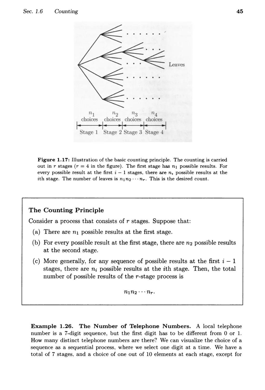
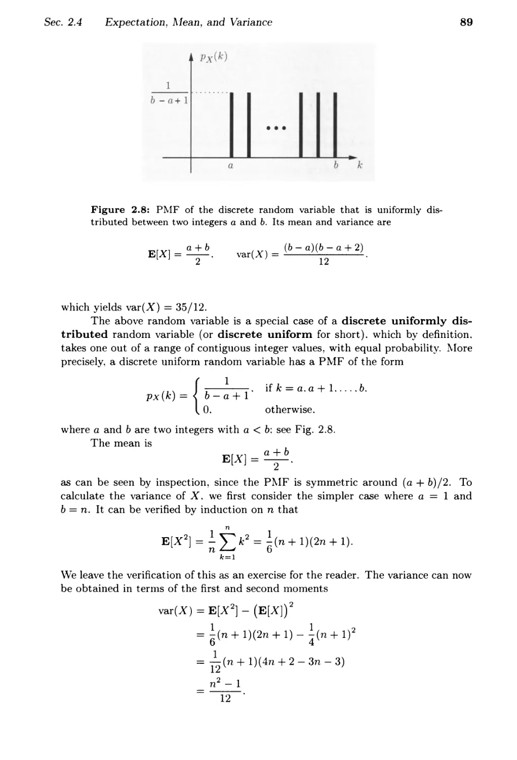
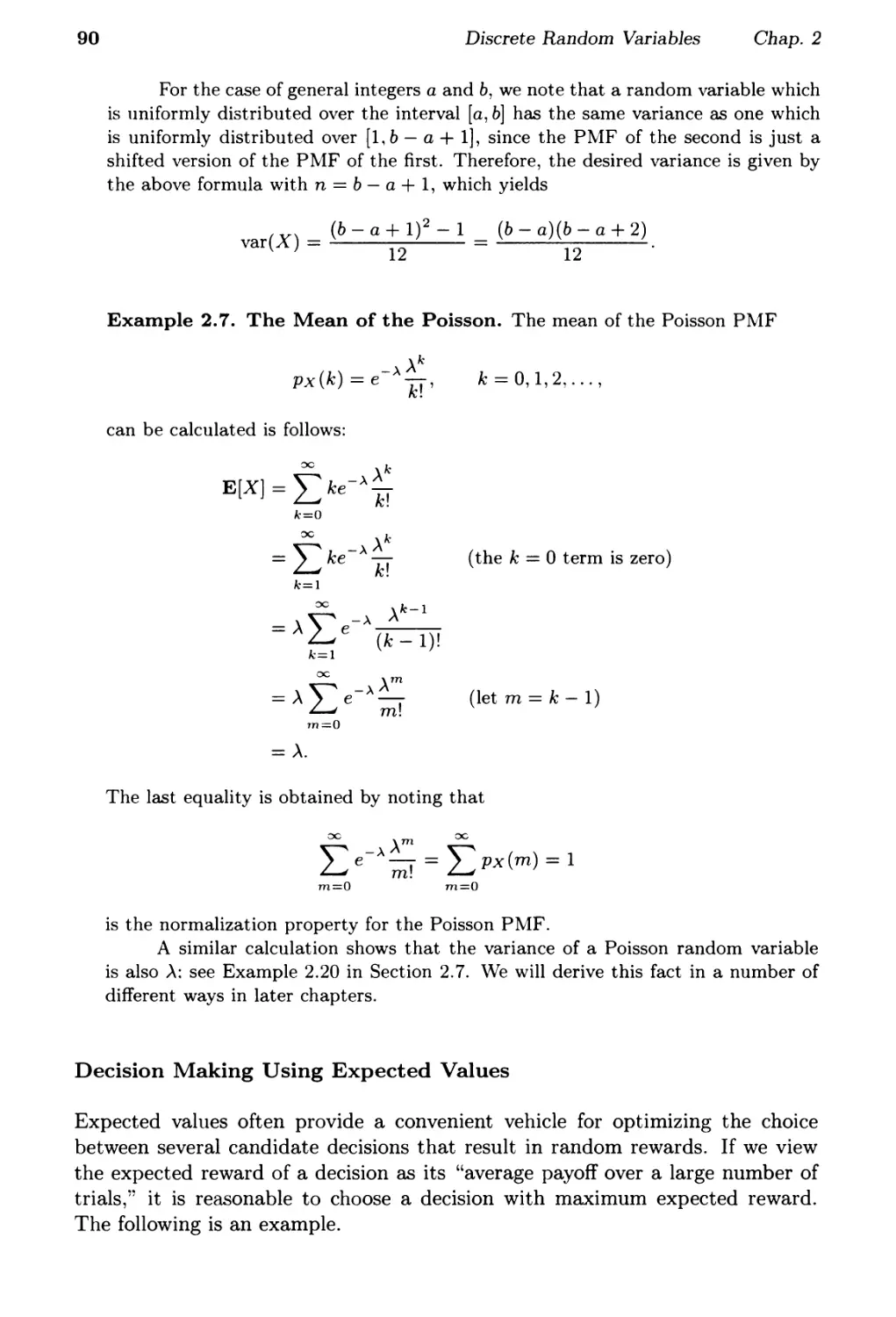
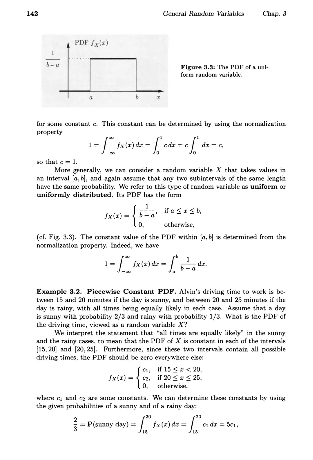
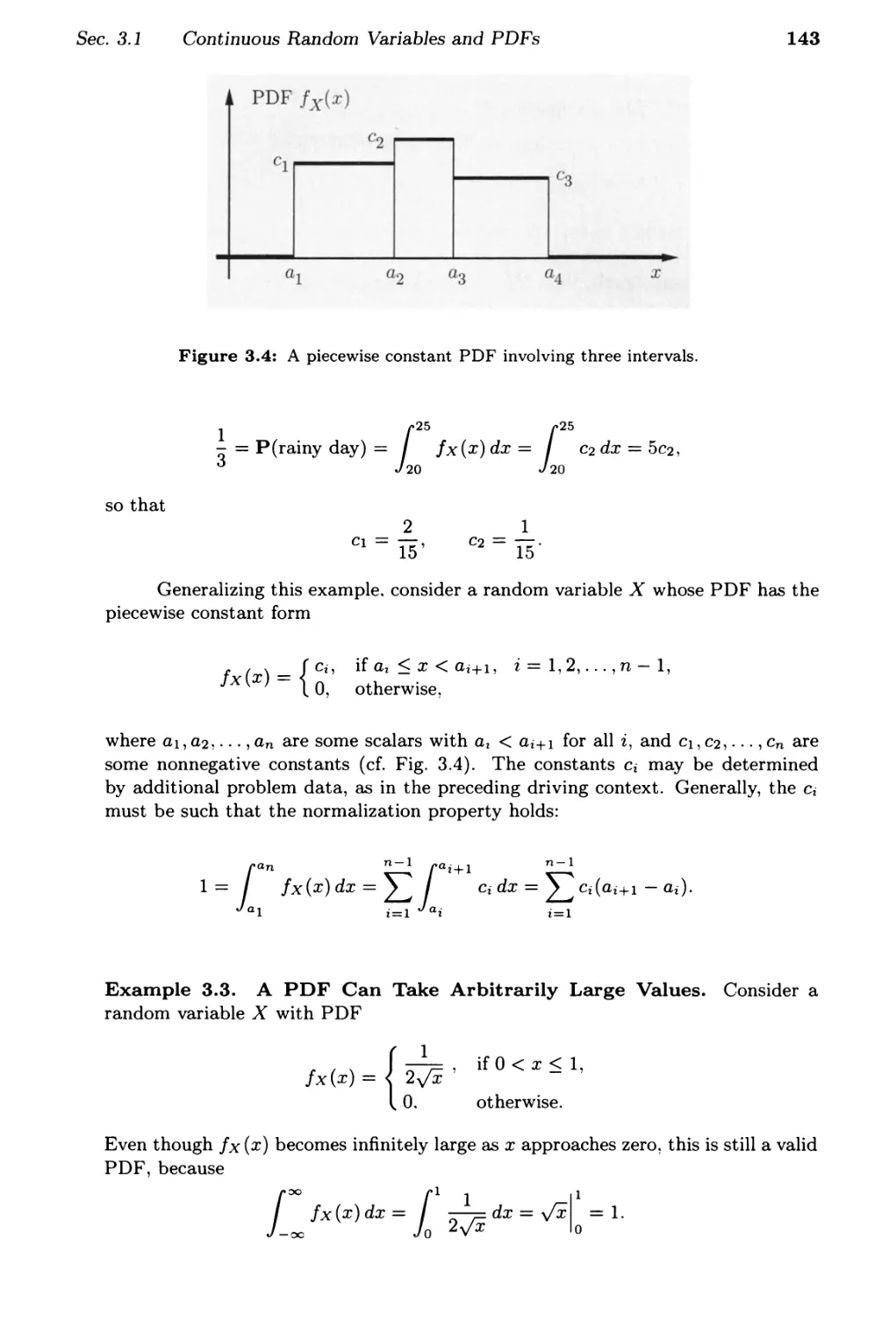
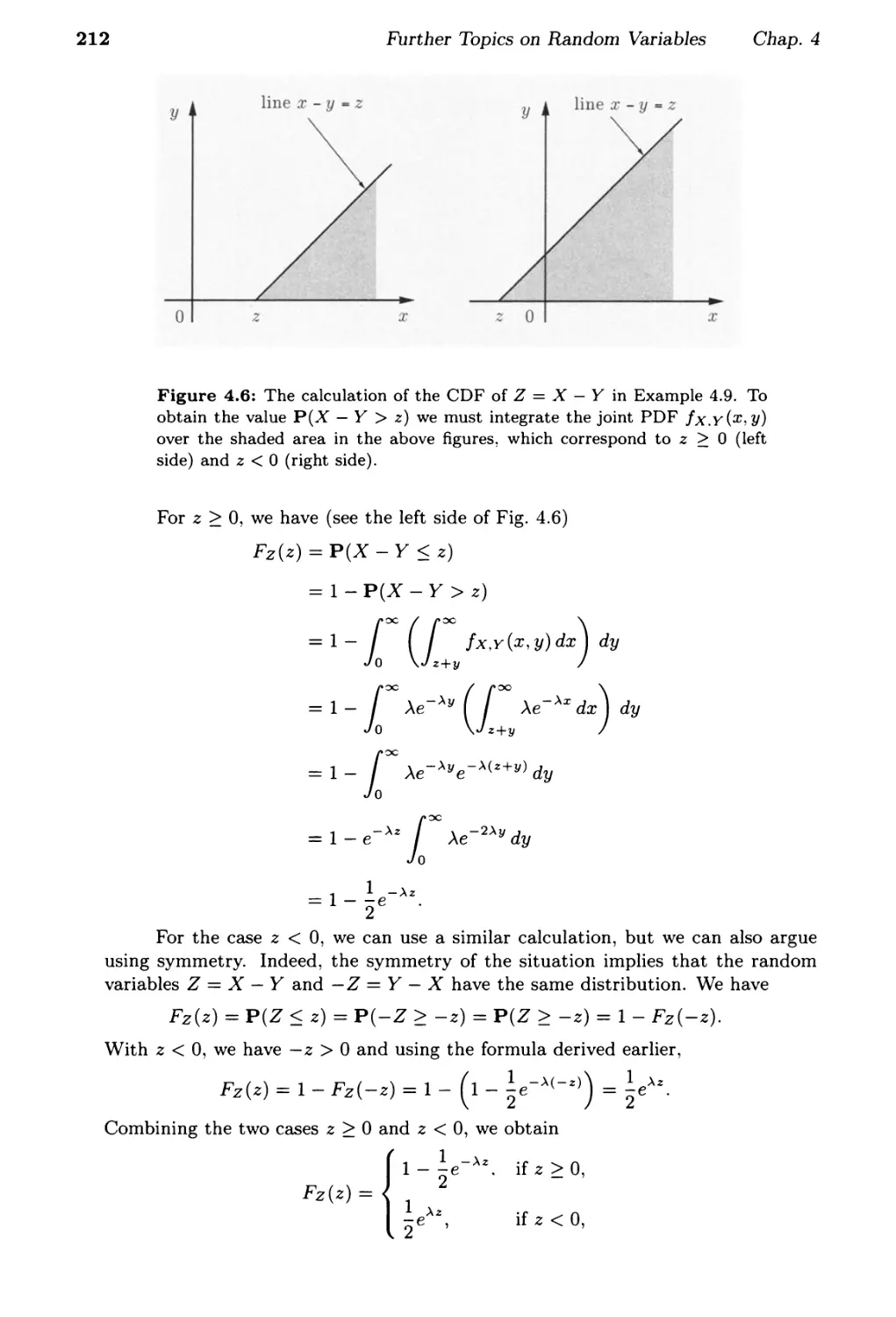
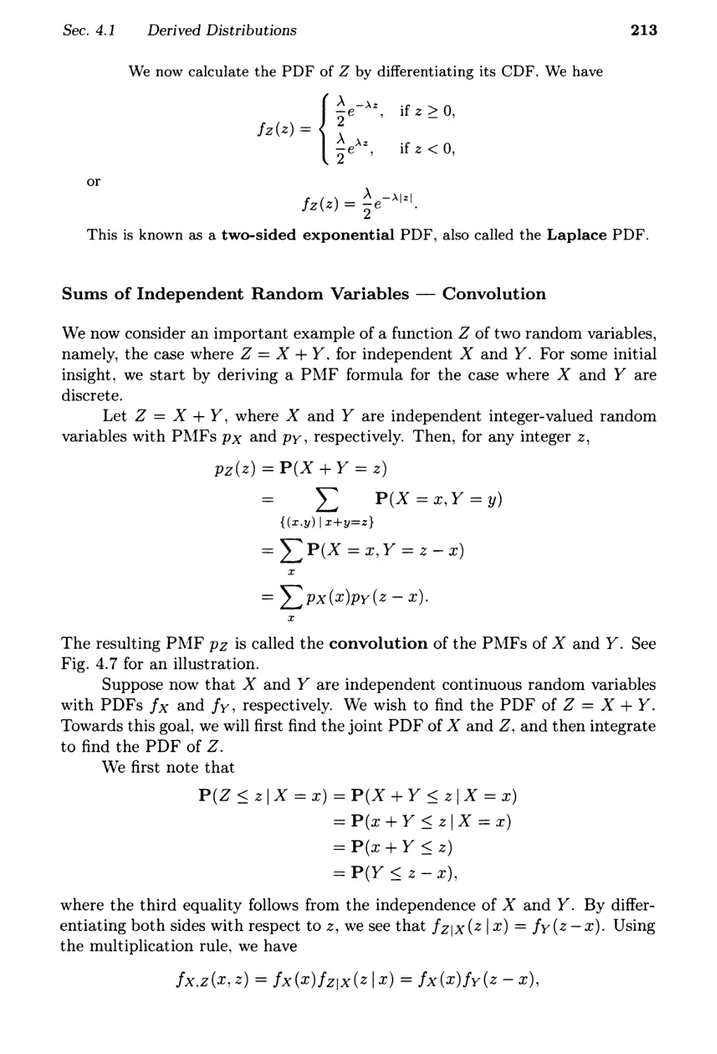
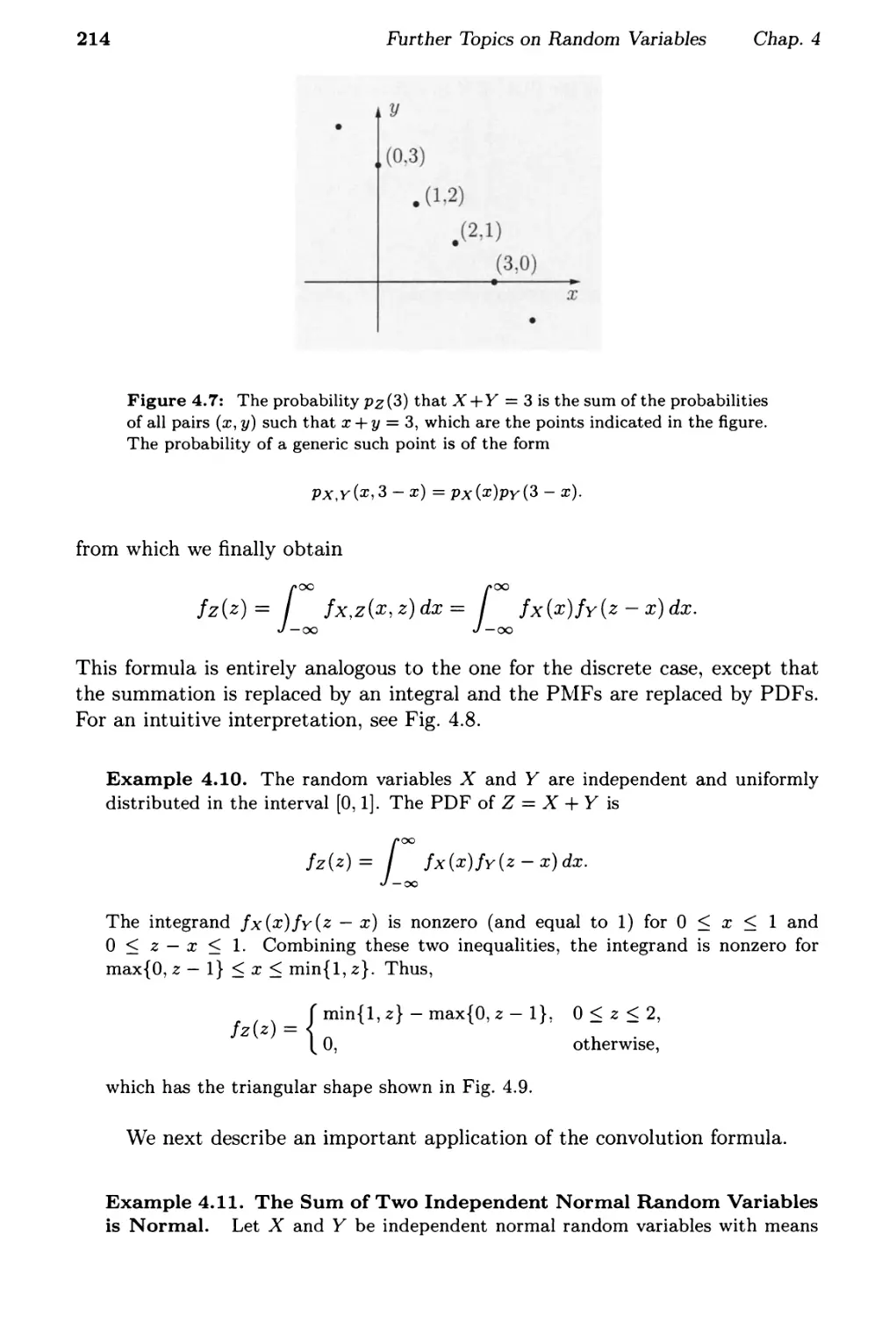
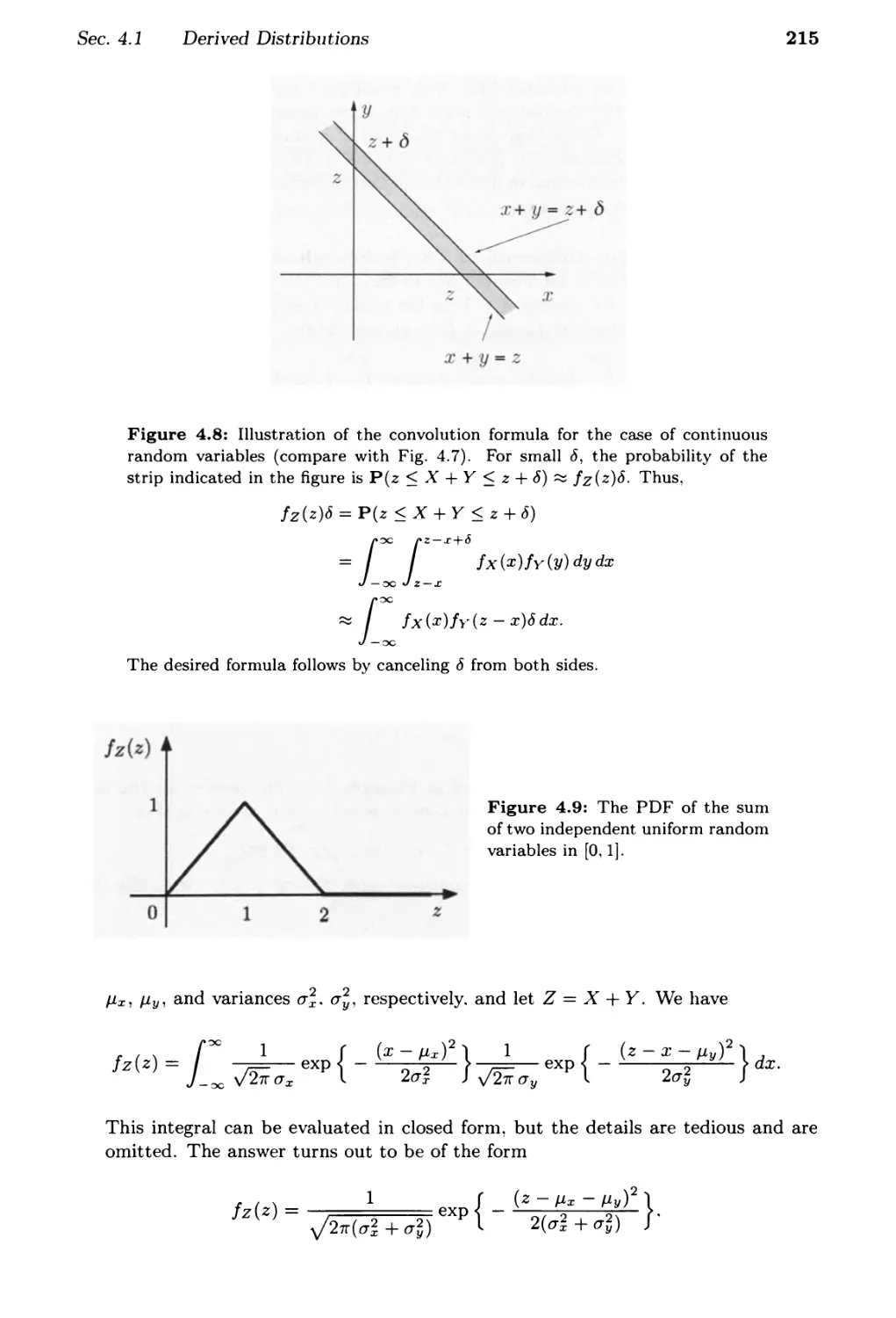
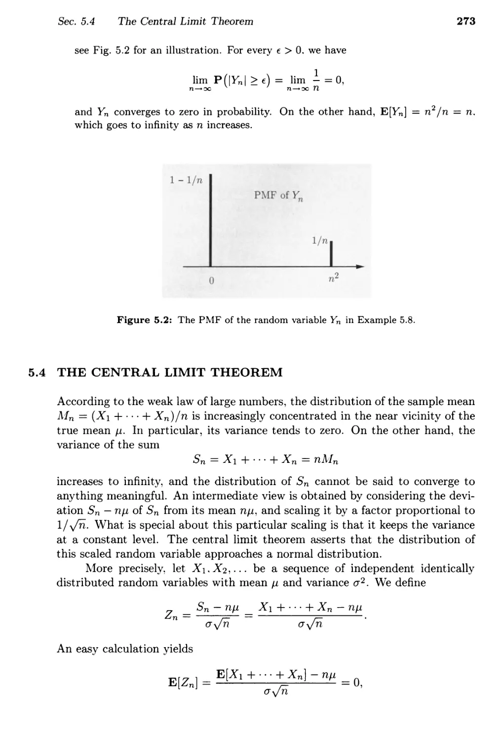
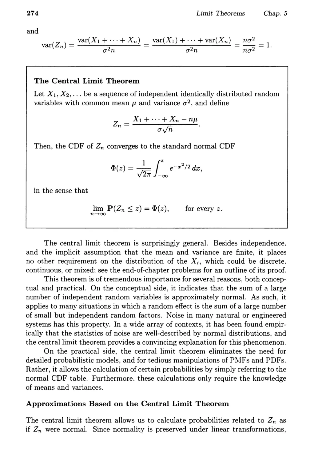
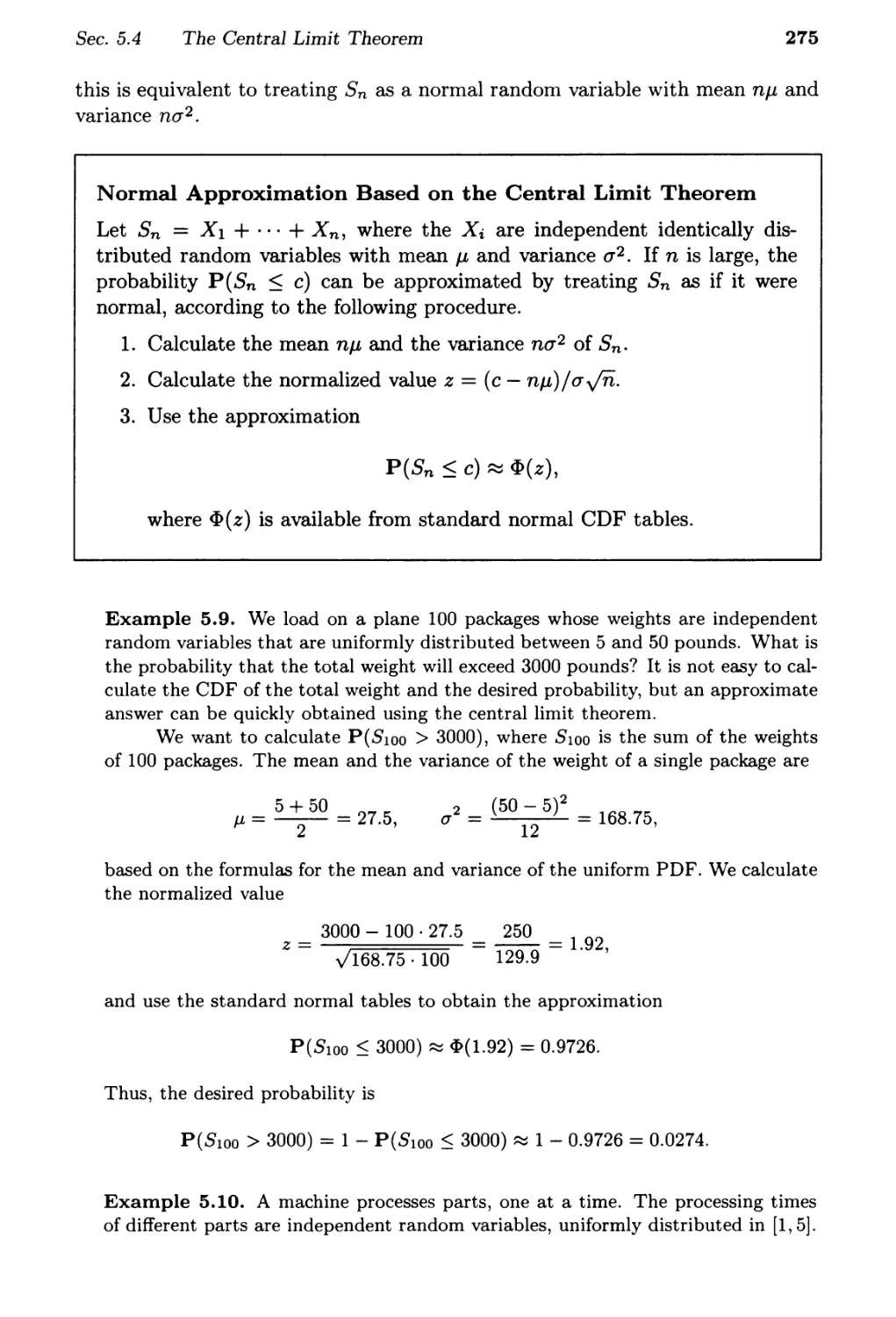
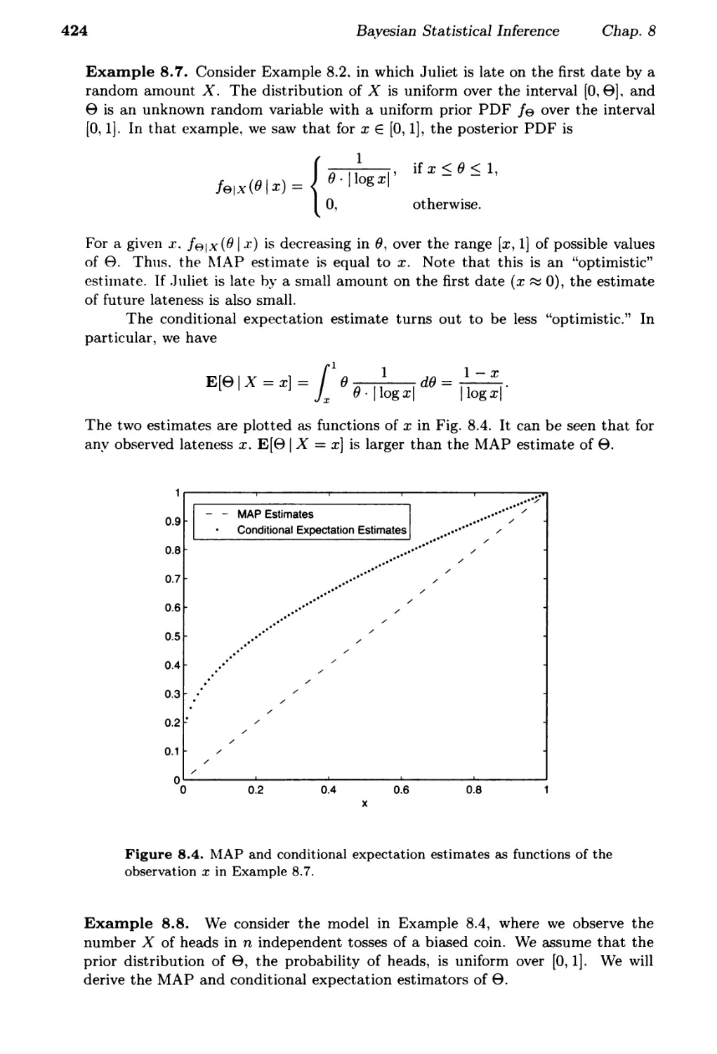
/


Author: Bertsekas D.P. Tsitsiklis J.N.
Tags: mathematics probability theory
ISBN: 978-1-886529-23-6
Year: 2008


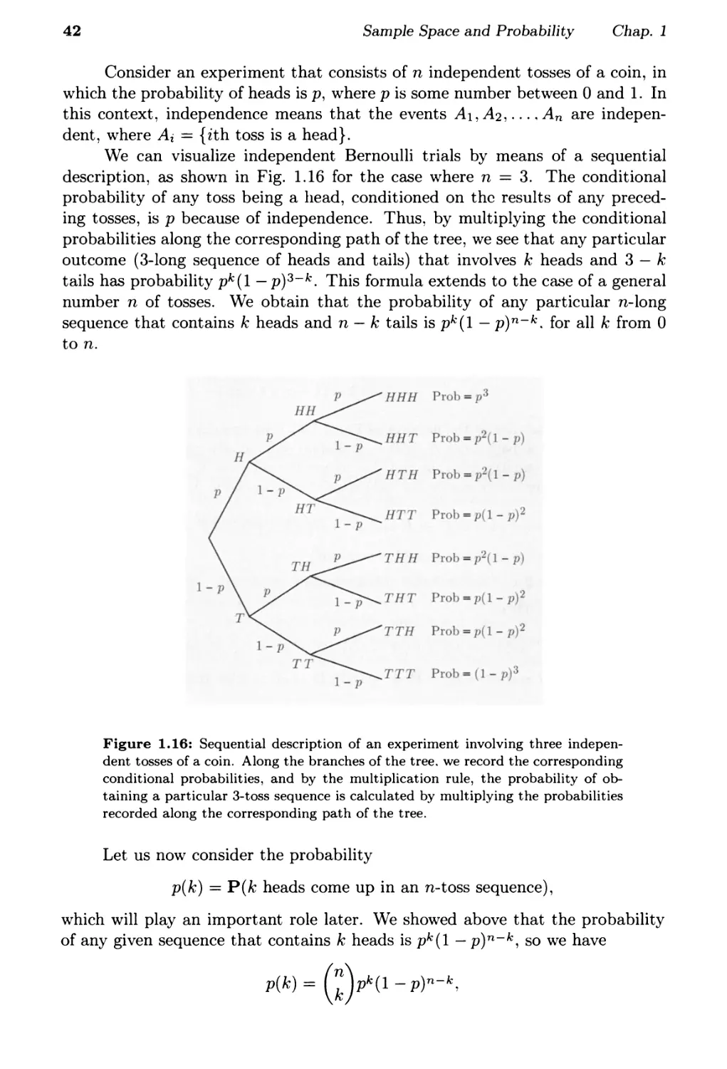
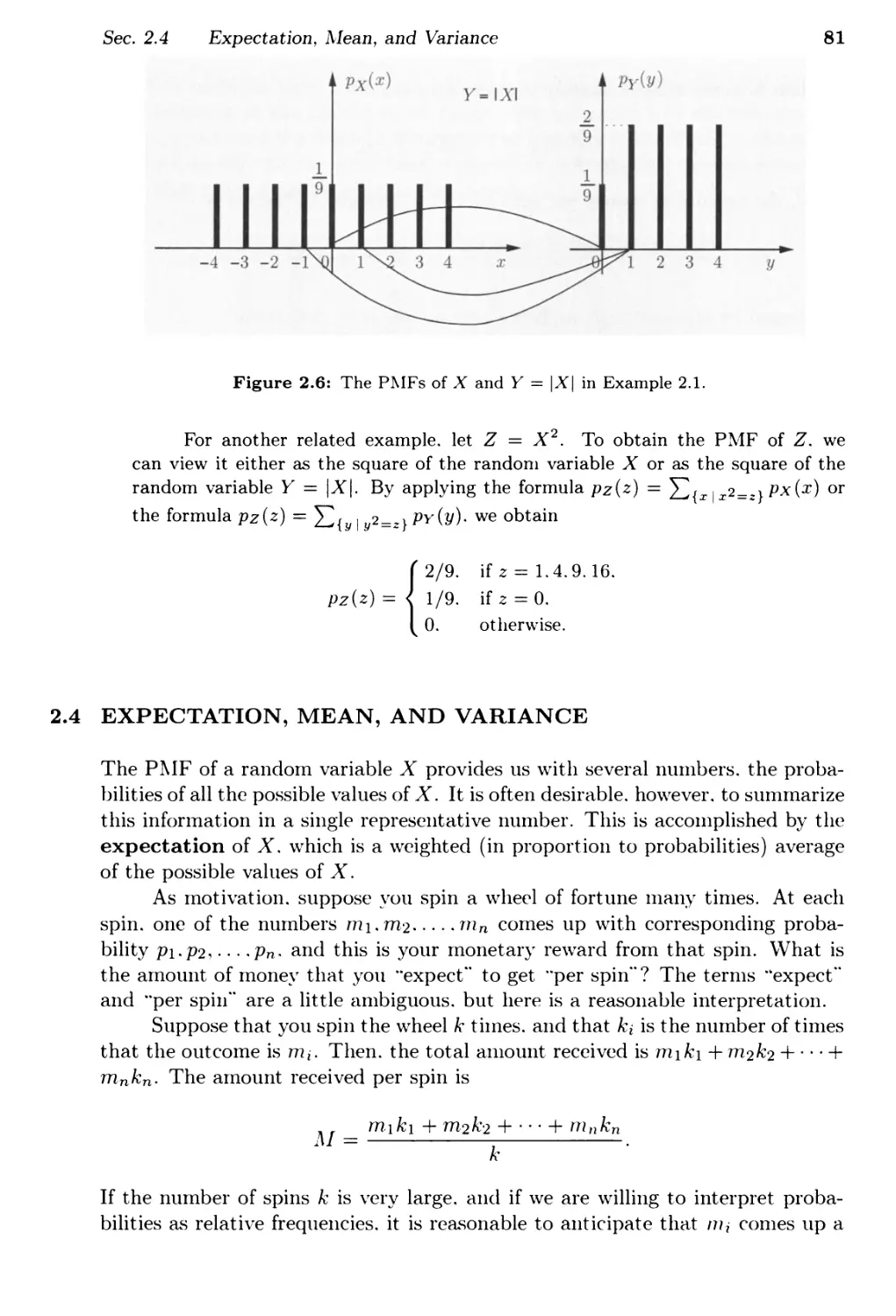
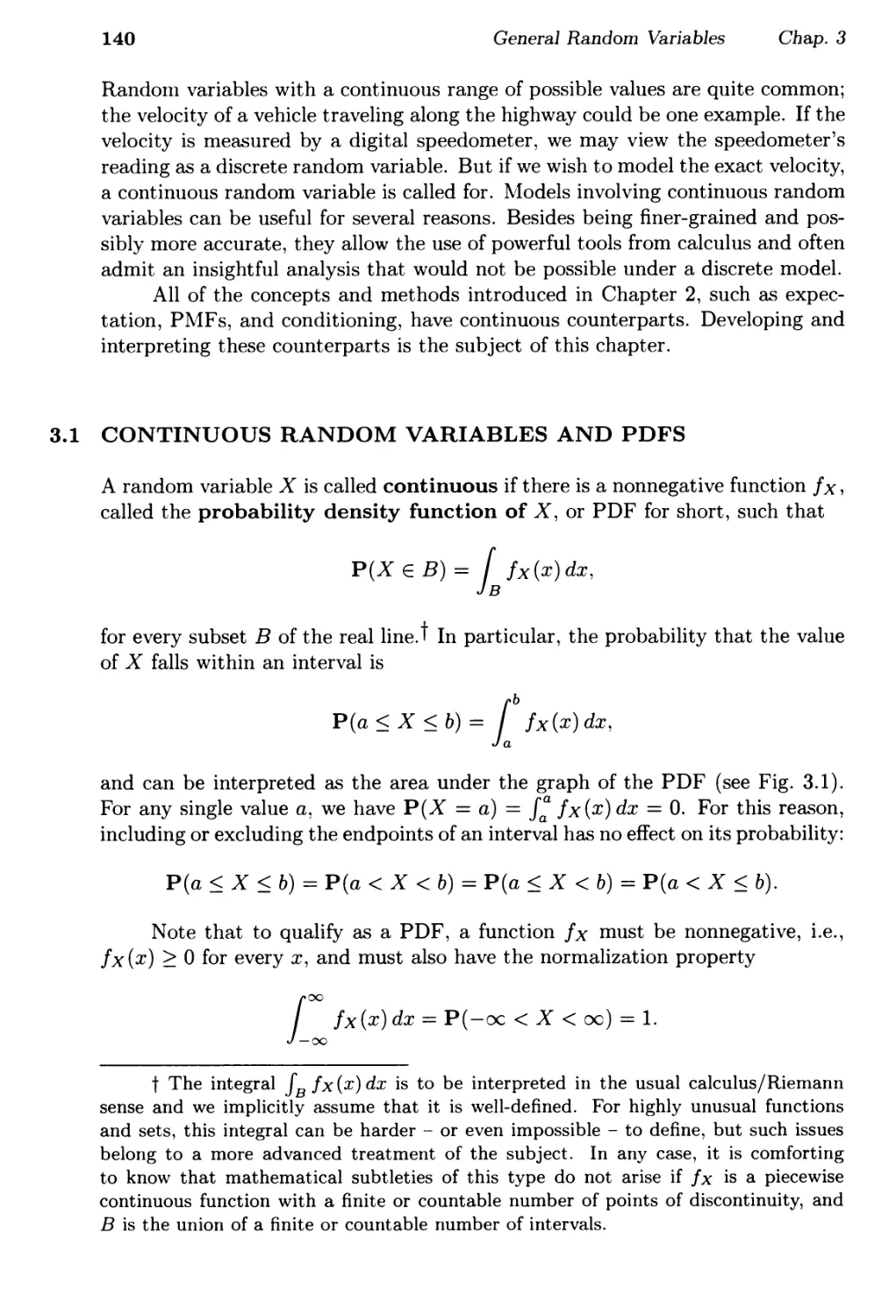
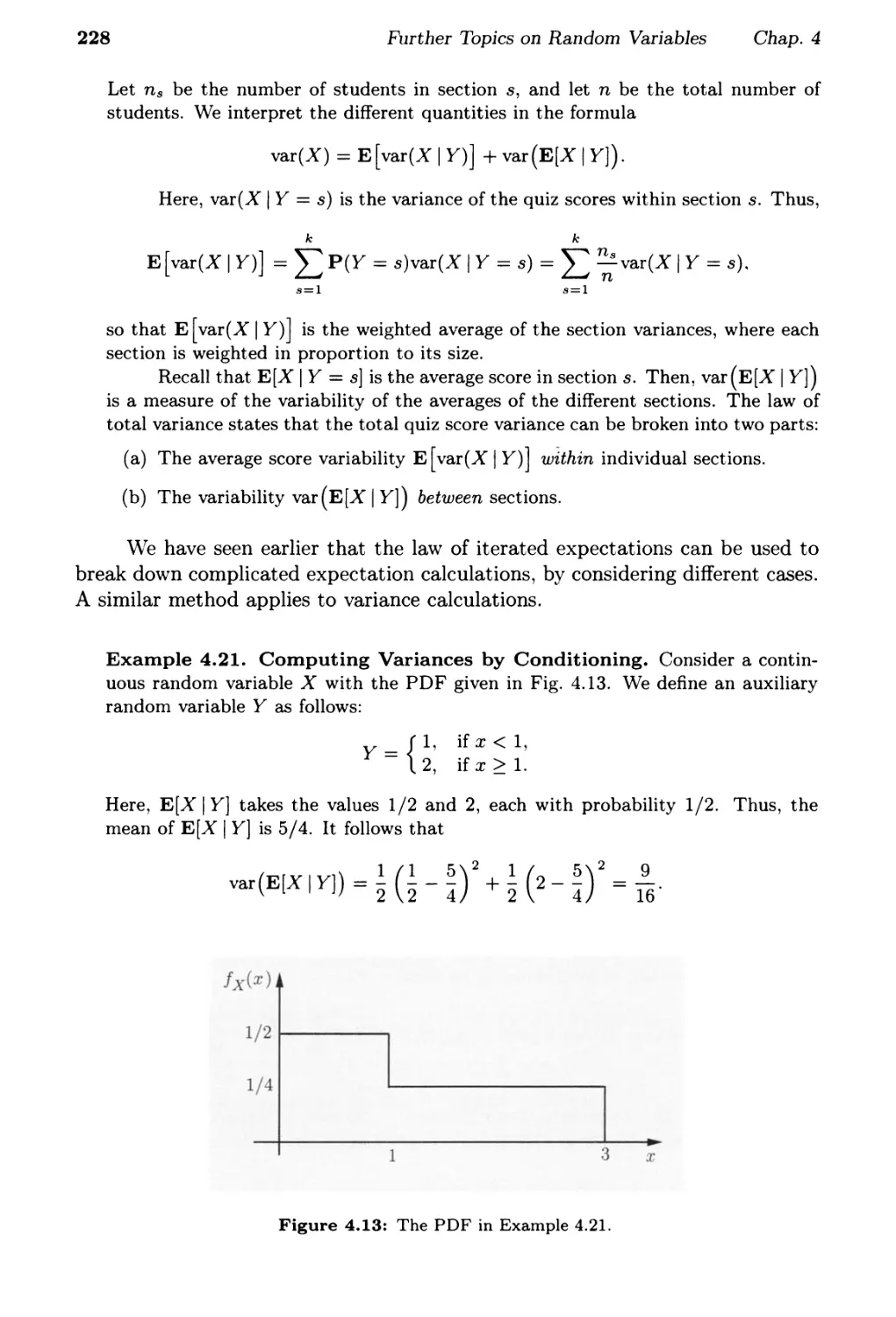
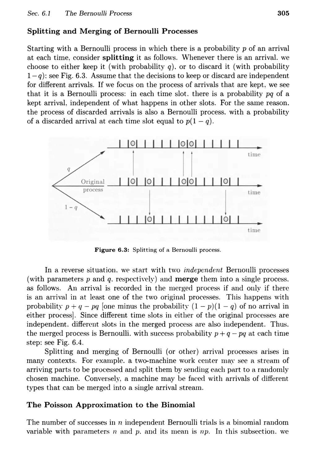
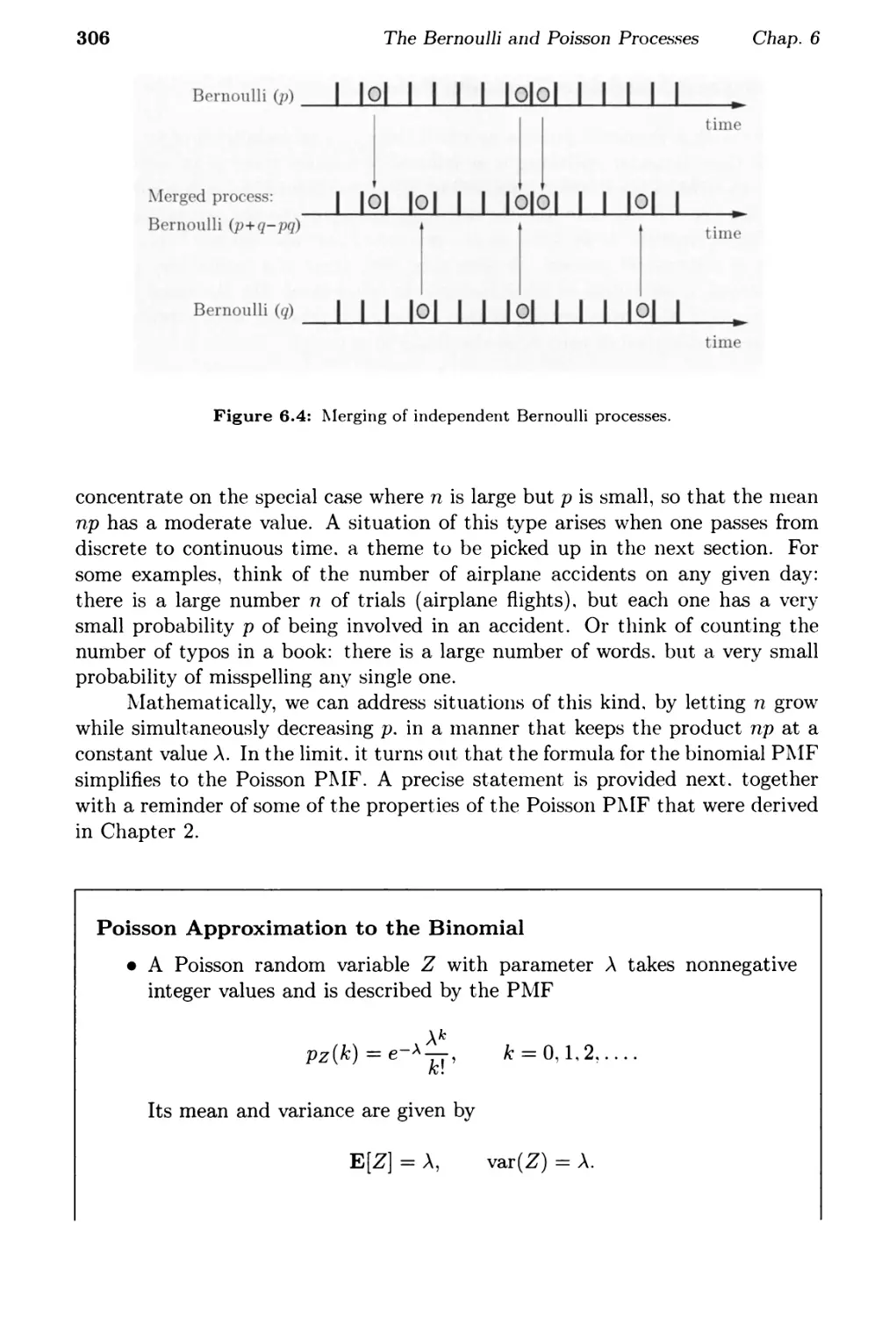
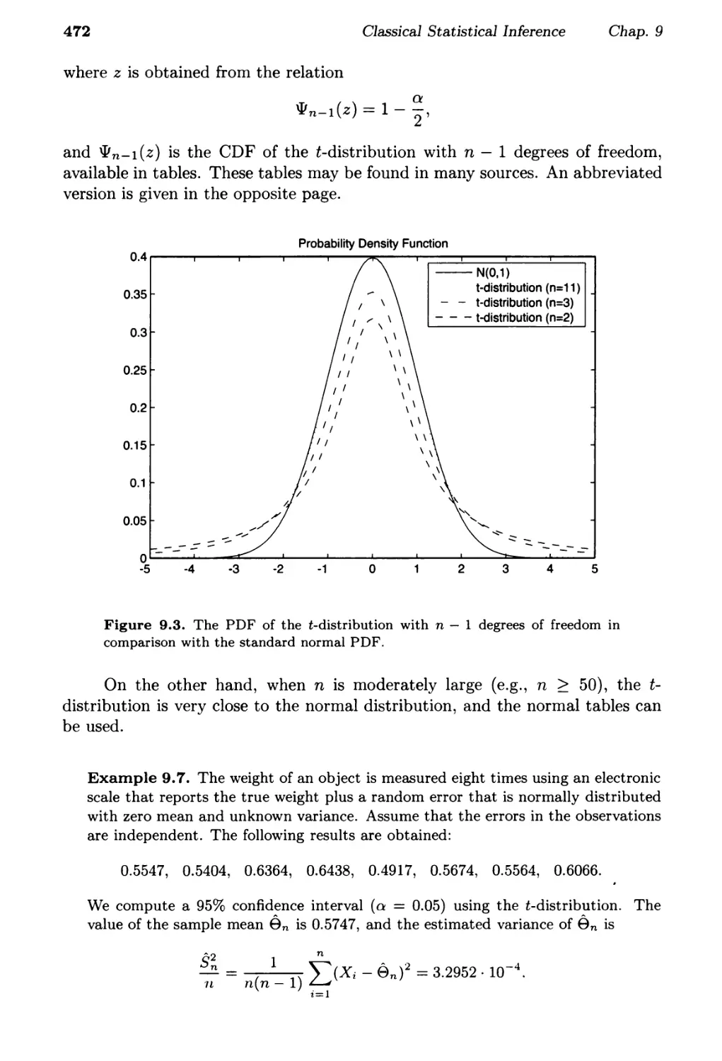
Text
Introduction to Probability
SECOND EDITION
DiITlitri P. Bertsekas and John N. Tsitsiklis
Massachusetts Institute of Technology
WWW site for book information and orders
http://www.athenasc.com
Athena Scientific, BelITlont, Massachusetts
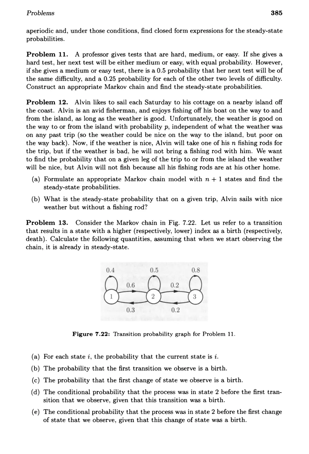
Athena Scientific
Post Office Box 805
Nashua, NH 03061-0805
U.S.A.
Email: info@athenasc.com
WWW: http://www.athenasc.com
Cover Design: Ann Gallager
@ 2002, 2008 Dimitri P. Bertsekas and John N. Tsitsiklis
All rights reserved. No part of this book may be reproduced in any form by any
electronic or mechanical means (including photocopying, recording, or informa-
tion storage and retrieval) without permission in writing from the publisher.
Publisher's Cataloging-in-Publication Data
Bertsekas, Dimitri P., Tsitsiklis, John N.
Introduction to Probability
Incl udes bi bliographical references and index
1. Probabilities. 2. Stochastic Processes. I. Title.
QA273.B4752008 519.2 - 21
Library of Congress Control Number: 2002092167
ISBN 978-1-886529-23-6
To the memory of
Pantelis Bertsekas and Nikos Tsitsiklis
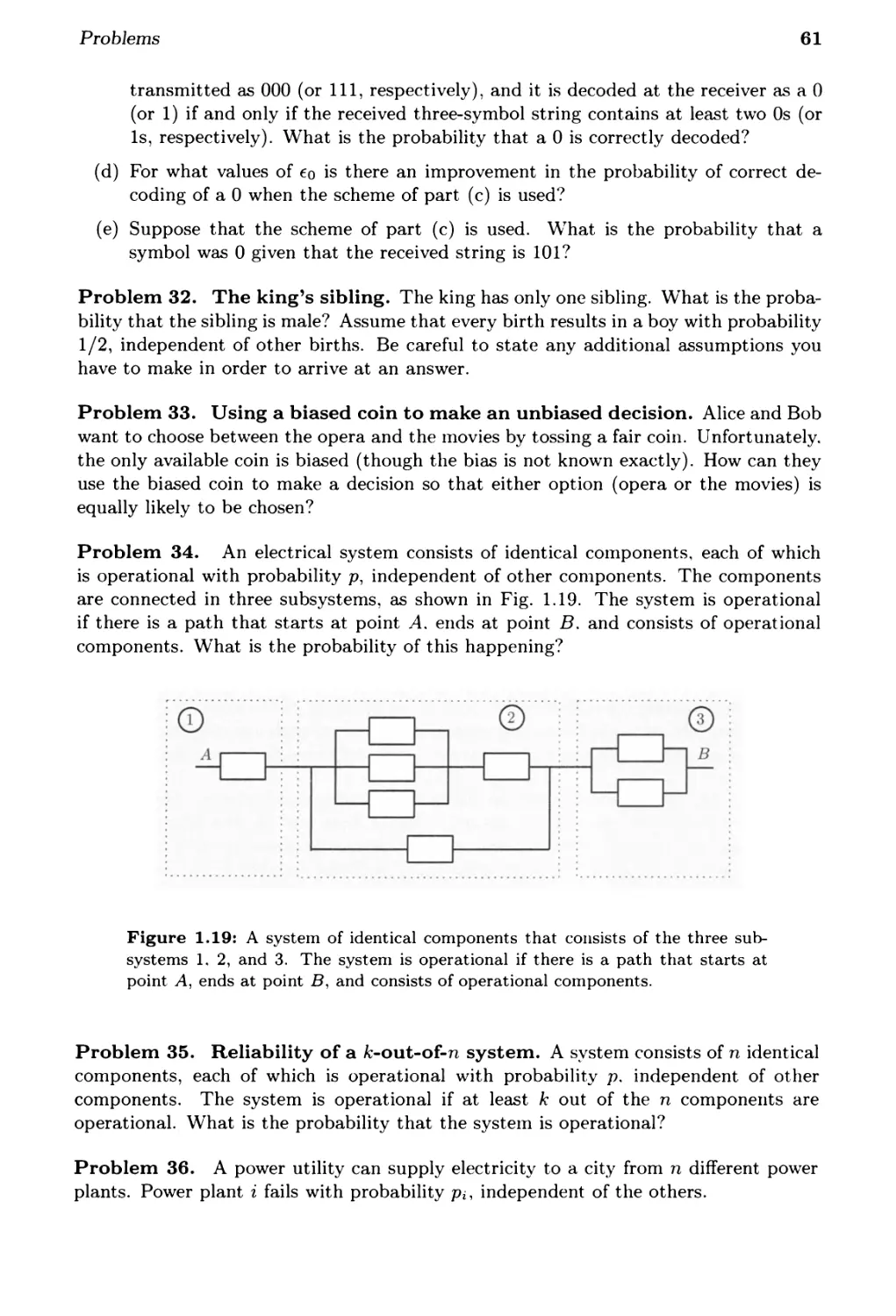
Preface
Probability is common sense reduced to calculation
Laplace
This book is an outgrowth of our involvement in teaching an introductory prob-
ability course ("Probabilistic Systems Analysis") at the 1/Iassachusetts Institute
of Technology.
The course is attended by a large number of students with diverse back-
grounds, and a broad range of interests. They span the entire spectrum from
freshmen to beginning graduate students, and from the engineering school to the
school of management. Accordingly, we have tried to strike a balance between
simplicity in exposition and sophistication in analytical reasoning. Our key aim
has been to develop the ability to construct and analyze probabilistic models in
a manner that combines intuitive understanding and mathematical precision.
In this spirit, some of the more mathematically rigorous analysis has been
just sketched or intuitively explained in the text. so that complex proofs do not
stand in the way of an otherwise simple exposition. At the same time, some of
this analysis is developed (at the level of advanced calculus) in theoretical prob-
lems, that are included at the end of the corresponding chapter. Furthermore,
some of the subtler mathematical issues are hinted at in footnotes addressed to
the more attentive reader.
The book covers the fundamentals of probability theory (probabilistic mod-
els, discrete and continuous random variables, multiple random variables, and
limit theorems), which are typically part of a first course on the subject. It
also contains, in Chapters 4-6 a number of more advanced topics, from which an
instructor can choose to match the goals of a particular course. In particular, in
Chapter 4, we develop transforms, a more advanced view of conditioning, sums
of random variables, least squares estimation, and the bivariate normal distribu-
v
vi
Preface
tion. Furthermore, in Chapters 5 and 6, we provide a fairly detailed introduction
to Bernoulli, Poisson, and larkov processes.
Our !vI. I. T. course covers all seven chapters in a single semester, with the ex-
ception of the material on the bivariate normal (Section 4.7), and on continuous-
time Iarkov chains (Section 6.5). However, in an alternative course, the material
on stochastic processes could be omitted, thereby allowing additional emphasis
on foundational material, or coverage of other topics of the instructor's choice.
Our most notable omission in coverage is an introduction to statistics.
While we develop all the basic elements of Bayesian statistics, in the form of
Bayes' rule for discrete and continuous models, and least squares estimation, we
do not enter the subjects of parameter estimation, or non-Bayesian hypothesis
testing.
The problems that supplement the main text are divided in three categories:
(a) Theoretical problems: The theoretical problems (marked by *) constitute
an important component of the text, and ensure that the mathematically
oriented reader will find here a smooth development without major gaps.
Their solutions are given in the text, but an ambitious reader may be able
to solve many of them, especially in earlier chapters, before looking at the
solutions.
(b) Problems in the text: Besides theoretical problems, the text contains several
problems, of various levels of difficulty. These are representative of the
problems that are usually covered in recitation and tutorial sessions at
M.LT., and are a primary mechanism through which many of our students
learn the material. Our hope is that students elsewhere will attempt to
solve these problems, and then refer to their solutions to calibrate and
enhance their understanding of the material. The solutions are posted on
the book's www site
http://www.athenasc.com/probbook.html
(c) Supplementary problems: There is a large (and growing) collection of ad-
ditional problems, which is not included in the book, but is made available
at the book's www site. Many of these problems have been assigned as
homework or exam problems at M.LT., and we expect that instructors
elsewhere will use them for a similar purpose. While the statements of
these additional problems are publicly accessible, the solutions are made
available from the authors only to course instructors.
We would like to acknowledge our debt to several people who contributed
in various ways to the book. Our writing project began when we assumed re-
sponsibility for a popular probability class at M.L T. that our colleague Al Drake
had taught for several decades. We were thus fortunate to start with an organi-
zation of the subject that had stood the test of time, a lively presentation of the
various topics in Al's classic text book, and a rich set of material that had been
used in recitation sessions and for homework. We are thus indebted to Al Drake
Preface
vii
for providing a very favorable set of initial conditions.
We are thankful to the several colleagues who have either taught from the
draft of the book at various universities or have read it, and have provided us
with valuable feedback. In particular, we thank Ibrahim Abou Faycal, Gustavo
de Veciana. Eugene Feinberg, Bob Gray, Muriel Medard, Jason Papastavrou,
Ilya Pollak, David Tse, and Terry Wagner.
The teaching assistants for the M.LT. class have been very helpful. They
pointed out corrections to various drafts, they developed problems and solutions
suitable for the class, and through their direct interaction with the student body,
they provided a robust mechanism for calibrating the level of the material.
Reaching thousands of bright students at M.LT. at an early stage in their
studies was a great source of satisfaction for us. We thank them for their valu-
able feedback and for being patient while they were taught from a textbook-in-
progress.
Last but not least, we are grateful to our families for their support through-
out the course of this long project.
Dimitri P. Bertsekas, dimitrib@mit.edu
John N. Tsitsiklis, jnt@mit.edu
Cambridge, Mass., May 2002
viii
Preface
Preface to the Second Edition
This is a substantial revision of the 1st edition, involving a reorganization of old
material and the addition of new material. The length of the book has increased
by about 25 percent. The main changes are the following:
(a) Two new chapters on statistical inference have been added. one on Bayesian
and one on classical methods. Our philosophy has been to focus on the
main concepts and to facilitate understanding of the main methodologies
through some key examples.
(b) Chapters 3 and 4 have been revised, in part to accommodate the new
material of the inference chapters and in part to streamline the presenta-
tion. Section 4.7 of the 1st edition (bivariate normal distribution) has been
omitted from the new edition, but is available at the book's website.
(c) A number of new examples and end-of-chapter problems have been added.
The main objective of the new edition is to provide flexibility to instructors
in their choice of material, and in particular to give them the option of including
an introduction to statistical inference. Note that Chapters 6-7, and Chapters 8-
9 are mutually independent, thus allowing for different paths through the book.
Furthermore, Chapter 4 is not needed for Chapters 5-7, and only Sections 4.2-4.3
from Chapter 4 are needed for Chapters 8 and 9. Thus, some possible course
offerings based on this book are:
(a) Probability and introduction to statistical inference: Chapters 1-3, Sections
4.2-4.3, Chapter 5, Chapters 8-9.
(b) Probability and introduction to stochastic processes: Chapters 1-3 and 5-7,
with possibly a few sections from Chapter 4.
We would like to express our thanks to various colleagues who have con-
tributed valuable comments on the material in the 1st edition and/or the or-
ganization of the material in the new chapters. Ed Coffman, Munther Dahleh,
Vivek Goyal, Anant Sahai, David Tse, George Verghese, Alan Willsky, and John
Wyatt have been very helpful in this regard. Finally, we thank Mengdi Wang
for her help with figures and problems for the new chapters.
Dimitri P. Bertsekas, dimitrib@mit.edu
John N. Tsitsiklis, jnt@mit.edu
Cambridge, Mass., June 2008
Contents
1. Sample Space and Probability ..... ....
1.1. Sets . . . . . . . . . . . . . . . . . . . . .
1.2. Probabilistic rvIodels. . . . . . . . . . . . . . . . .
1.3. Conditional Probability . . . . . . . . . . .
1.4. Total Probability Theorem and Bayes' Rule . . . . . . . .
1.5. Independence. . . . . . . . .. ........
1.6. Counting ........... ..........
1.7. Summary and Discussion . . . . . .. .....
Problems. . . . . . . . .. ..............
. p. 1
. . p. 3
. p. 6
p. 18
p. 28
p. 34
p. 44
p. 51
p. 53
2. Discrete Random Variables . . .. ...... p. 71
2.1. Basic Concepts . . . . . . . . . . . . .. ....... p. 72
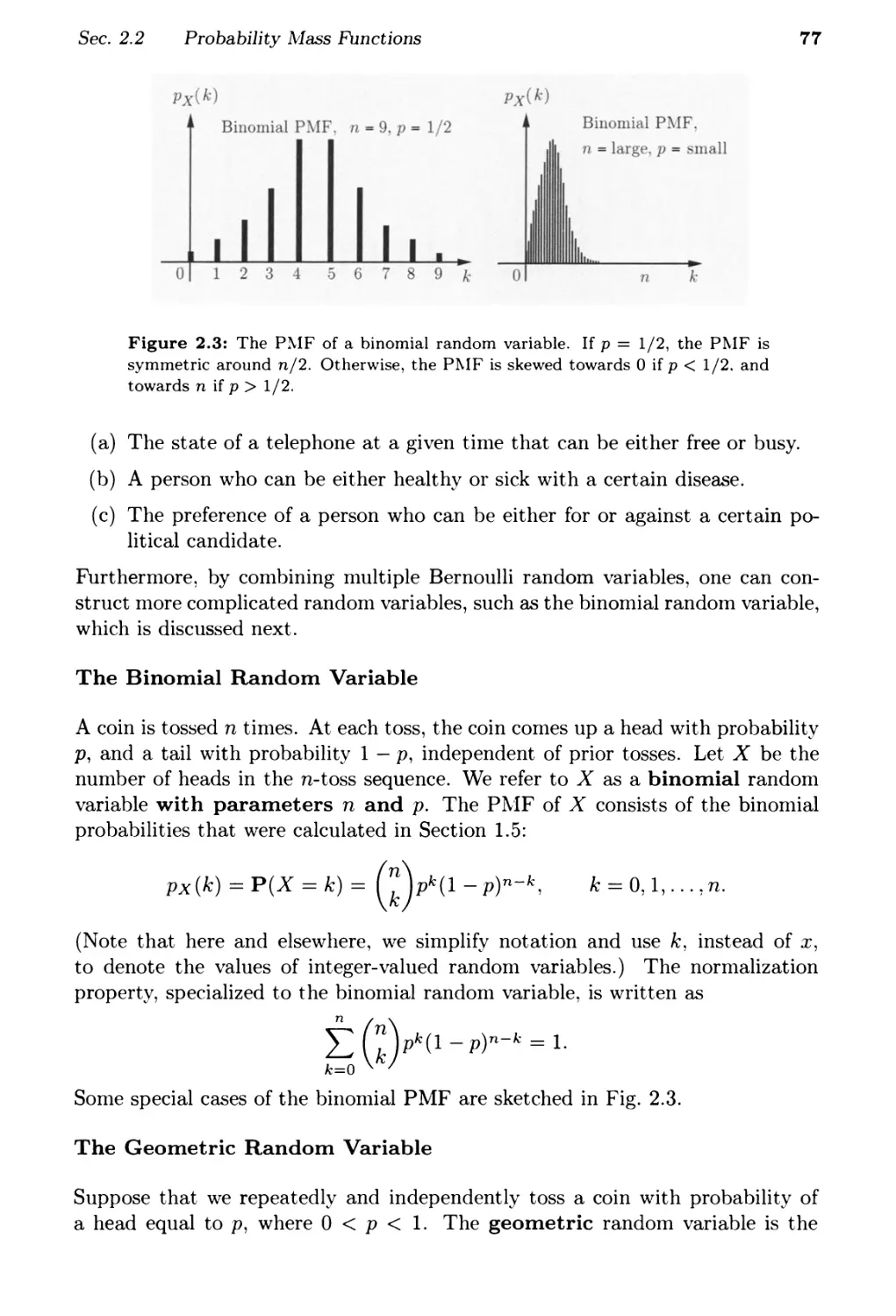
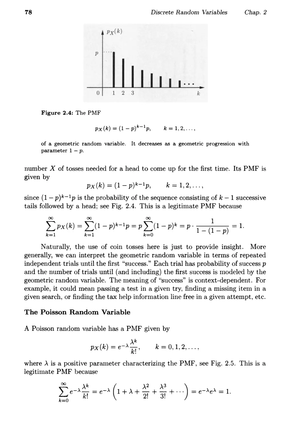
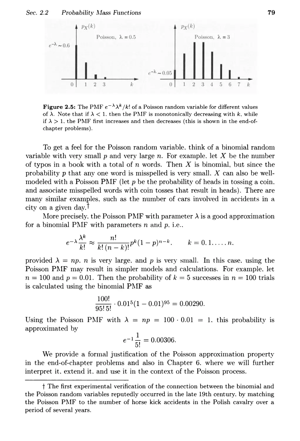
2.2. Probability rvlass Functions . . . . . . . . . . . . . . . p. 74
2.3. Functions of Random Variables . . . . . . . . . . . . . . . . p. 80
2.4. Expectation, lean, and Variance . . . . . . . . . . . p. 81
2.5. Joint PrvlFs of Iultiple Random Variables . . . . . . . p. 92
2.6. Conditioning . . . . . .. ............. p. 97
2.7. Independence. . . . . . . . . . . . . . . . . . . . p. 109
2.8. Summary and Discussion . . . . . . . . . . . . p. 115
Problems. . . . . . . . . . .. ............ p. 119
3. General Random Variables ............ p. 139
3.1. Continuous Random Variables and PDFs ........... p. 140
3.2. Cumulative Distribution Functions . . . . . . . . . . . . . . p. 148
3.3. Normal Random Variables . . . . . . . . . . . . . . . . . . p. 153
3.4. Joint PDFs of rvlultiple Random Variables . . . . . p. 158
3.5. Conditioning .................... . p. 164
3.6. The Continuous Bayes' Rule . . . . . . . . .. . p. 178
ix
x
3.7. Summary and Discussion ....
Problems. . . . . . . . . . . . . .
4. Further Topics on Random Variables
4.1. Derived Distributions . . . . . . . . .. .....
4.2. Covariance and Correlation ....... . . .
4.3. Conditional Expectation and Variance Revisited . . .
4.4. Transforms ................ . . .
4.5. Sum of a Random Number of Independent Random Variables
4.6. Summary and Discussion ...... . . .
Problems. . . . . . . . . . . . . . . . .
5. Limit Theorems .
. . . . . . . . . . .
. .
5.1. Markov and Chebyshev Inequalities
5.2. The Weak Law of Large Numbers .
5.3. Convergence in Probability. . . .
5.4. The Central Limit Theorem . . .
5.5. The Strong Law of Large Numbers
5.6. Summary and Discussion . . . .
Problems. . . . . . . . . . . .
6. The Bernoulli and Poisson Processes. . .
6.1. The Bernoulli Process . . . . . .
6.2. The Poisson Process ........
6.3. Summary and Discussion ....
Problems. . . . . . . .. ...
. . . . . .
Contents
. p. 182
. p. 184
p. 201
p. 202
p.217
p. 222
p. 229
p. 240
p. 244
p. 246
p. 263
p. 265
p. 269
p. 271
p. 273
p. 280
p. 282
p. 284
p. 295
. p. 297
. p. 309
. p. 324
. p. 326
7. Markov Chains . . . . . . . . . . .. ...... p. 339
7.1. Discrete-Time Markov Chains . . . . . . . . . . p. 340
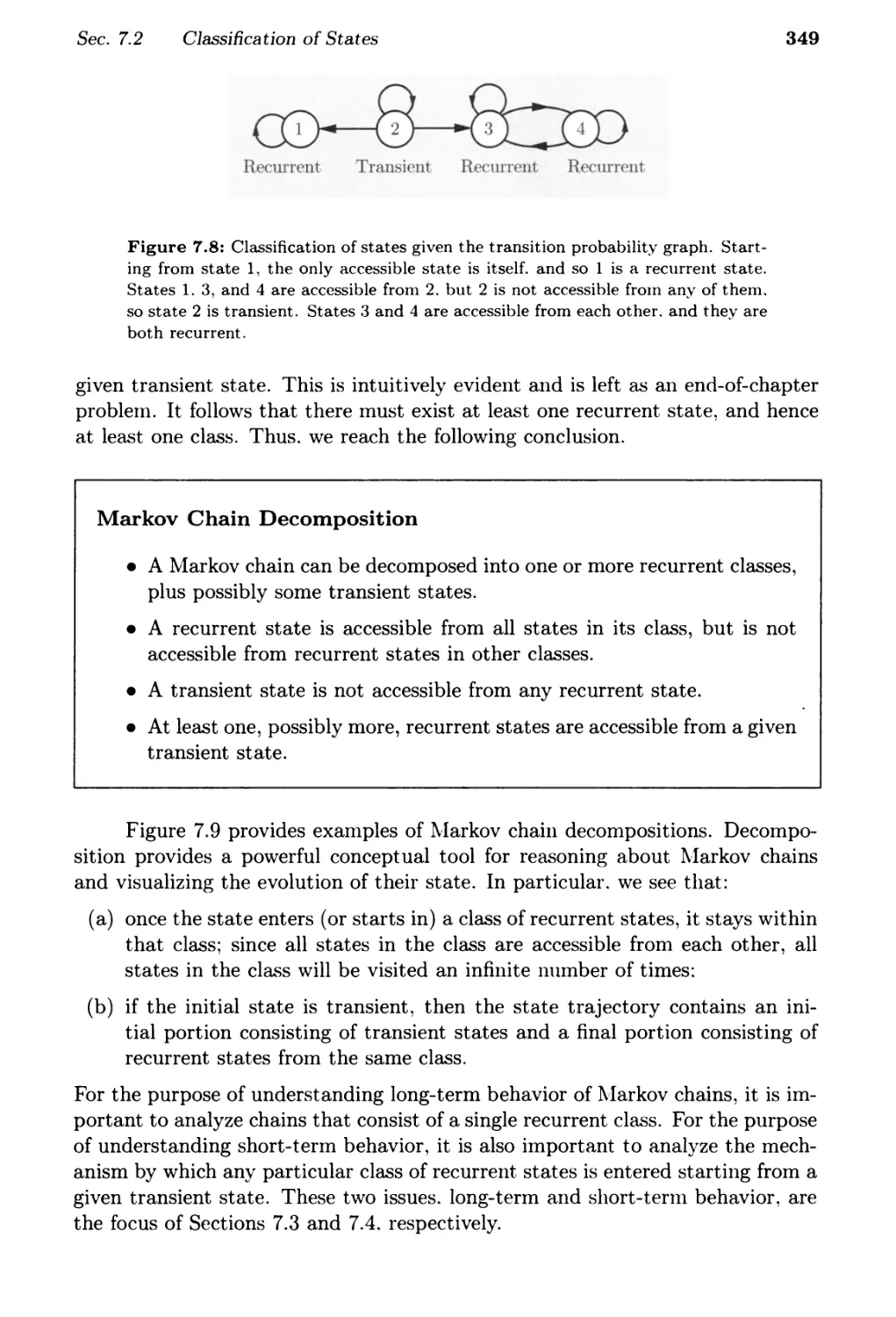
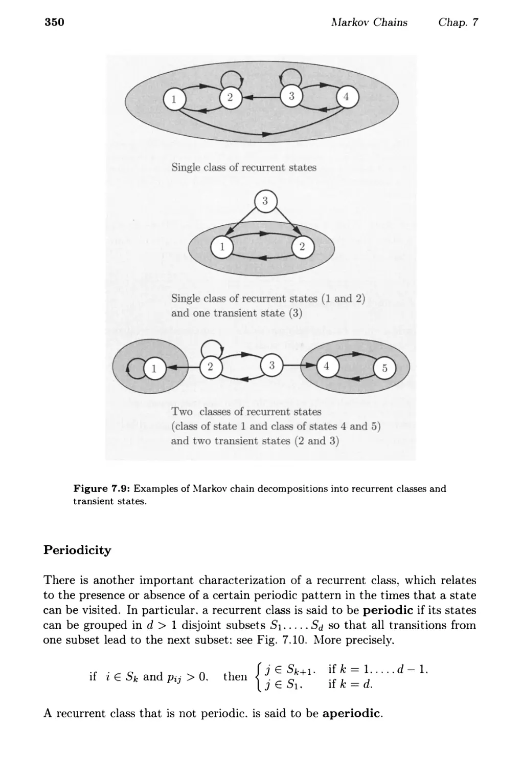
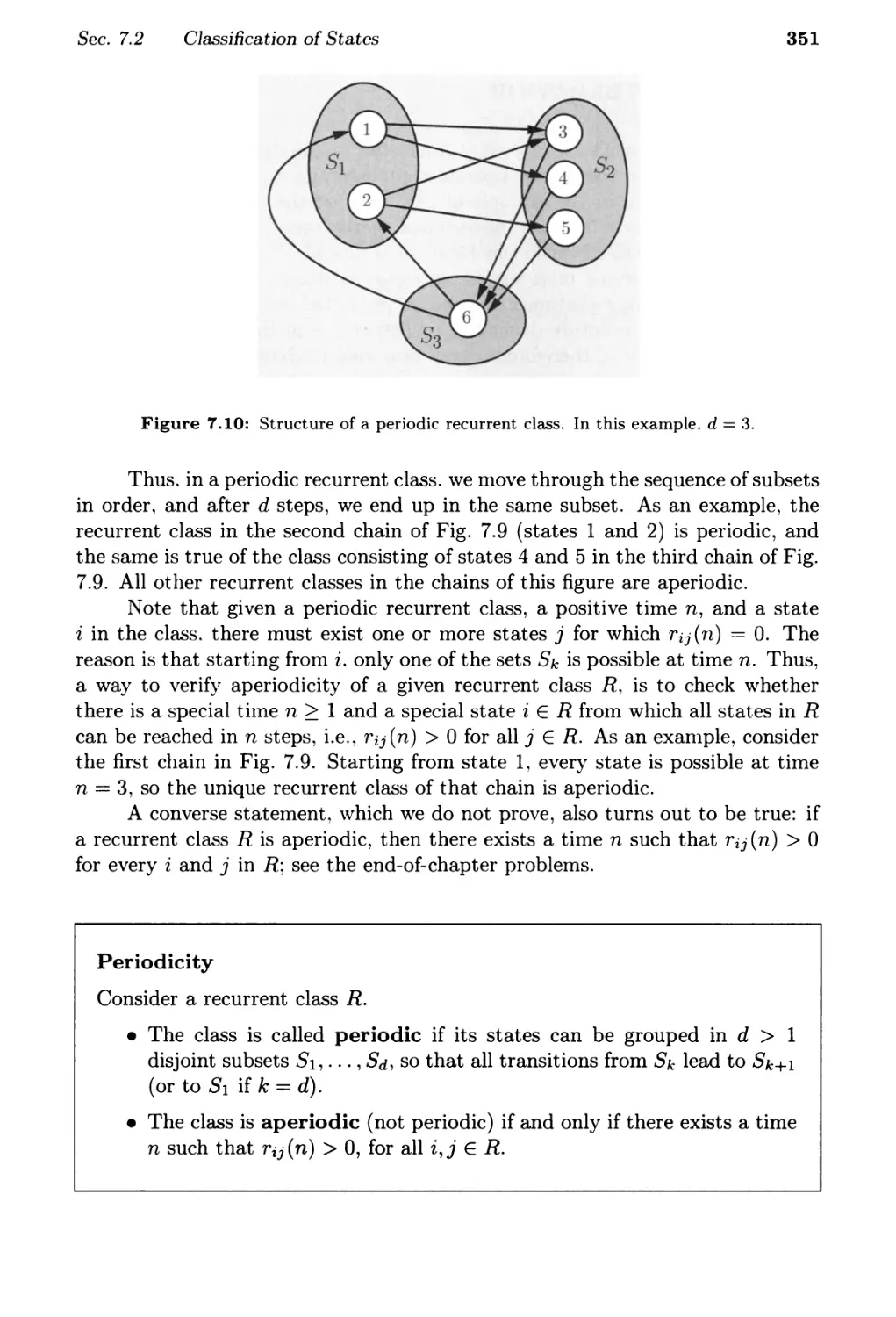
7.2. Classification of States. . . . .. ............ p. 346
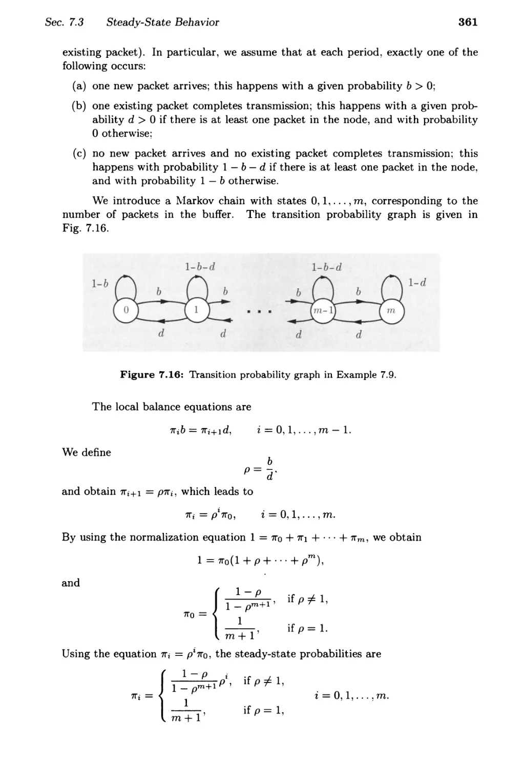
7.3. Steady-State Behavior . . . . .. ......... . p. 352
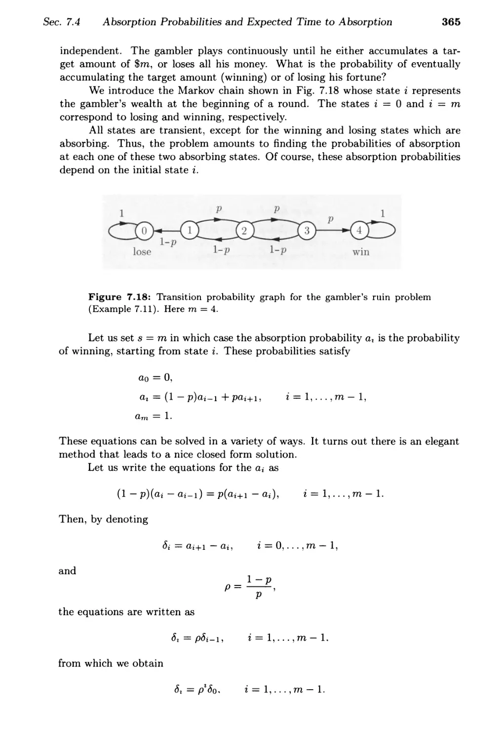
7.4. Absorption Probabilities and Expected Time to Absorption ... p. 362
7.5. Continuous-Time Markov Chains . . . . . . . . . . .. . p. 369
7.6. Summary and Discussion . . . . . . . . . . . . p. 378
Pro blems. . . . . . . . . . . . . .. . p. 380
8. Bayesian Statistical Inference . . . . . . . . . . . . . .
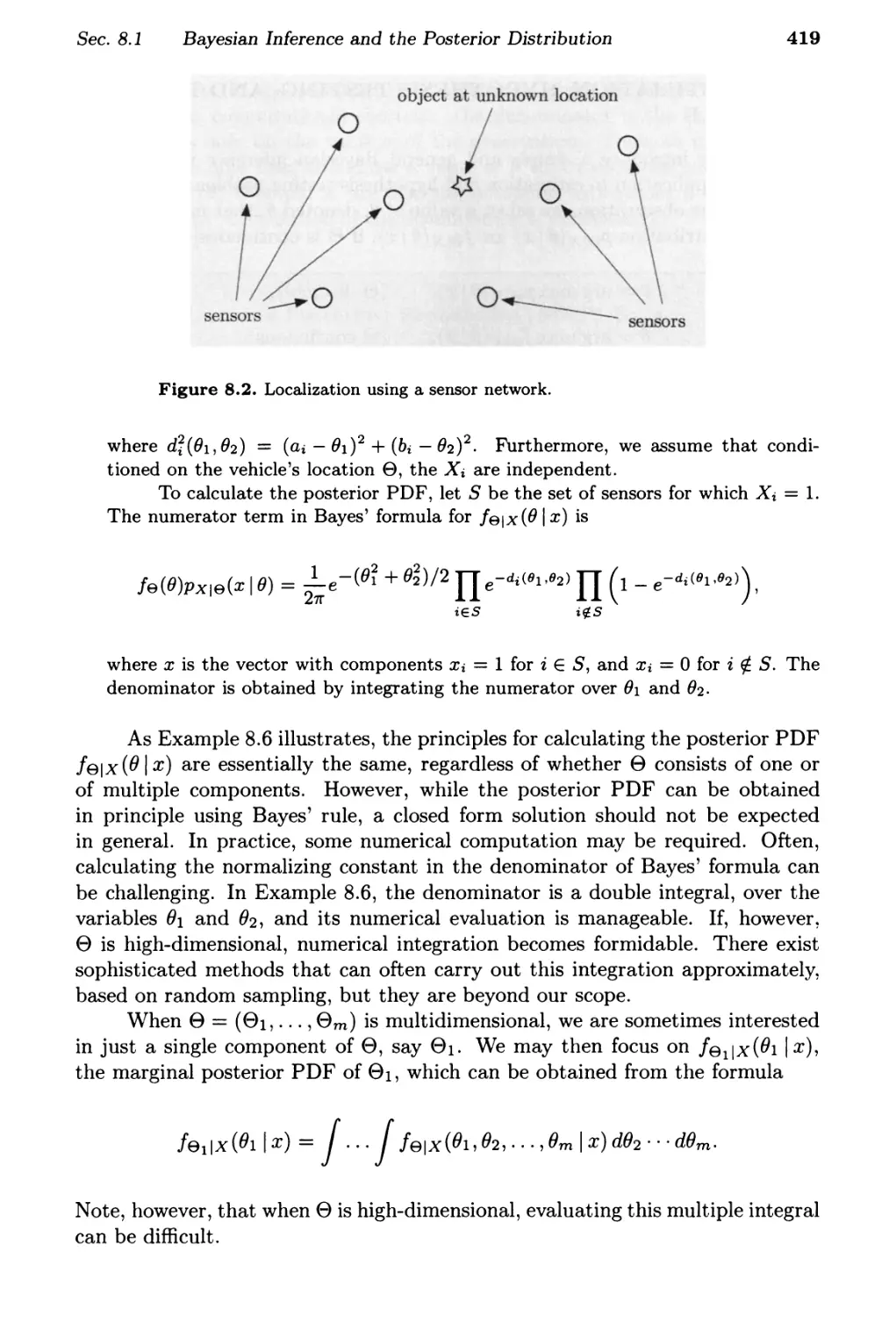
8.1. Bayesian Inference and the Posterior Distribution ......
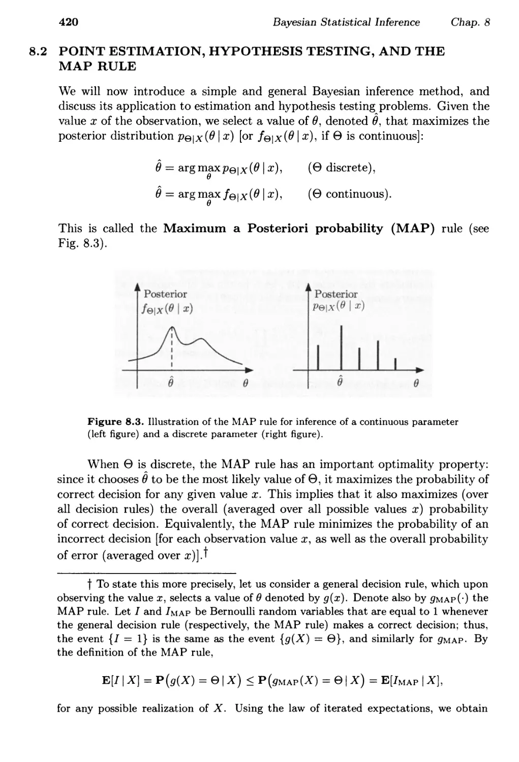
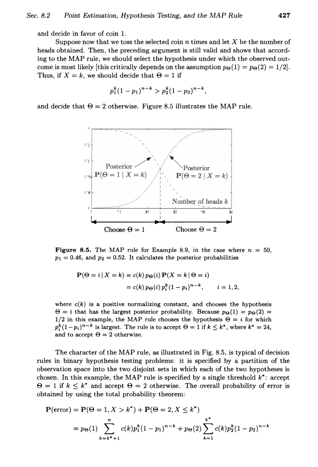
8.2. Point Estimation, Hypothesis Testing, and the MAP Rule . . .
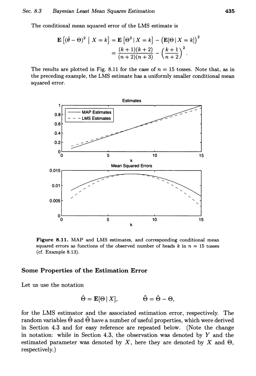
8.3. Bayesian Least Mean Squares Estimation .........
8.4. Bayesian Linear Least Mean Squares Estimation . . . .
p. 407
. p. 412
. p. 420
p. 430
p. 437
Contents
8.5. Summary and Discussion ......
Pro b 1 ems. . . . . . . . . . . .
9. Classical Statistical Inference . .
9.1. Classical Parameter Estimation . . . .
9.2. Linear Regression . . . . . . . . . .
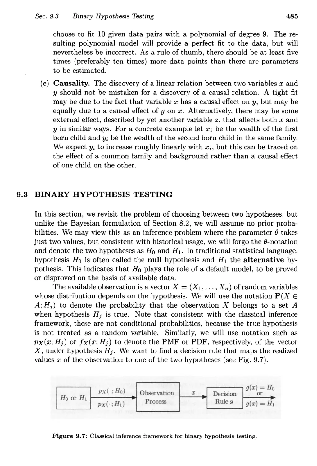
9.3. Binary Hypothesis Testing . . . .
9.4. Significance Testing . . . . . . . . .
9.5. Summary and Discussion ......
Problems. . . . . . . . . . . . . .
Index . . .
xi
. p. 444
. p. 446
. . . . . . . . . p. 459
. . p. 462
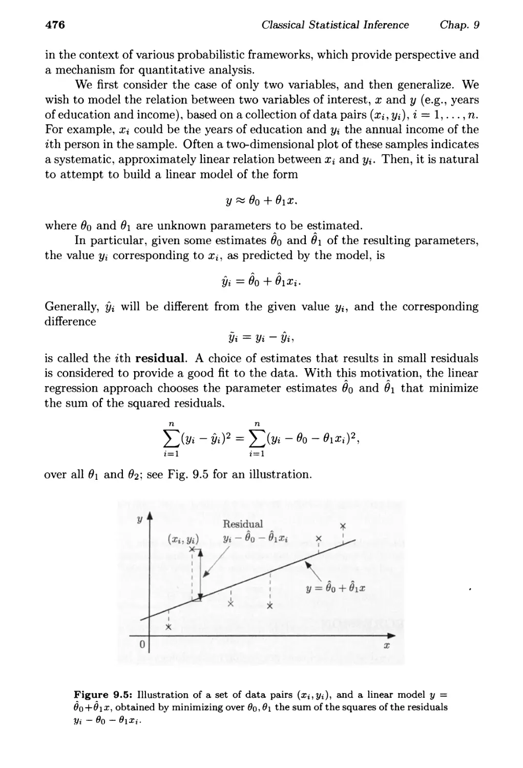
. . . . . . . . p. 477
. . . . . p. 486
p. 496
. . . . . . . . . . . . p. 505
. . . . . . p. 507
.................... .
p. 521
1
Sample Space and
Probability
Contents
1.1. Sets . . . . . . . . . . . . . . . . . . . . . .
1.2. Probabilistic l'vlodels. . . . . . . . . . . . . . . . . . .
1.3. Conditional Probability . . . . . . . . . . . . .
1.4. Total Probability Theorem and Bayes' Rule . . . . . . . .
1.5. Independence. . . . . . . . .. ......
1.6. Counting .......... .......
1.7. Summary and Discussion ......
Problems. . . . . . . . . . . . . . . .
. p. 3
. p. 6
p. 18
p. 28
p.34
p.44
p. 51
p. 53
1
2
Sample Space and Probability
Chap. 1
"Probability" is a very useful concept, but can be interpreted in a number of
ways. As an illustration, consider the following.
A patient is admitted to the hospital and a potentially life-saving drug is
administered. The following dialog takes place between the nurse and a
concerned relative.
RELATIVE: Nurse, what is the probability that the drug will work?
NURSE: I hope it works, we'll know tomorrow.
RELATIVE: Yes, but what is the probability that it will?
NURSE: Each case is different, we have to wait.
RELATIVE: But let's see, out of a hundred patients that are treated under
similar conditions, how many times would you expect it to work?
NURSE (somewhat annoyed): I told you, every person is different, for some
it works, for some it doesn't.
RELATIVE (insisting): Then tell me, if you had to bet whether it will work
or not, which side of the bet would you take?
NURSE (cheering up for a moment): I'd bet it will work.
RELATIVE (somewhat relieved): OK, now, would you be willing to lose two
dollars if it doesn't work, and gain one dollar if it does?
NURSE (exasperated): What a sick thought! You are wasting my time!
In this conversation, the relative attempts to use the concept of probability
to discuss an uncertain situation. The nurse's initial response indicates that the
meaning of "probability" is not uniformly shared or understood, and the relative
tries to make it more concrete. The first approach is to define probability in
terms of frequency of occurrence, as a percentage of successes in a moderately
large number of similar situations. Such an interpretation is often natural. For
example, when we say that a perfectly manufactured coin lands on heads "with
probability 50%," we typically mean "roughly half of the time." But the nurse
may not be entirely wrong in refusing to discuss in such terms. What if this
was an experimental drug that was administered for the very first time in this
hospital or in the nurse's experience?
While there are many situations involving uncertainty in which the fre-
quency interpretation is appropriate, there are other situations in which it is
not. Consider. for example, a scholar who asserts that the Iliad and the Odyssey
were composed by the same person, with probability 90%. Such an assertion
conveys some information, but not in terms of frequencies, since the subject is
a one-time event. Rather, it is an expression of the scholar's subjective be-
lief. One might think that subjective beliefs are not interesting, at least from a
mathematical or scientific point of view. On the other hand, people often have
to make choices in the presence of uncertainty, and a systematic way of making
use of their beliefs is a prerequisite for successful, or at least consistent, decision
making.
Sec. 1.1
Sets
3
In fact, the choices and actions of a rational person can reveal a lot about
the inner-held subjective probabilities, even if the person does not make conscious
use of probabilistic reasoning. Indeed, the last part of the earlier dialog was an
attempt to infer the nurse's beliefs in an indirect manner. Since the nurse was
willing to accept a one-for-one bet that the drug would work, we may infer
that the probability of success was judged to be at least 50%. Had the nurse
accepted the last proposed bet (two-for-one), this would have indicated a success
probability of at least 2/3.
Rather than dwelling further on philosophical issues about the appropriate-
ness of probabilistic reasoning, we will simply take it as a given that the theory
of probability is useful in a broad variety of contexts, including some where the
assumed probabilities only reflect subjective beliefs. There is a large body of
successful applications in science, engineering, medicine, management, etc., and
on the basis of this empirical evidence, probability theory is an extremely useful
tool.
Our main objective in this book is to develop the art of describing un-
certainty in terms of probabilistic models, as well as the skill of probabilistic
reasoning. The first step, which is the subject of this chapter, is to describe
the generic structure of such models and their basic properties. The models we
consider assign probabilities to collections (sets) of possible outcomes. For this
reason, we must begin with a short review of set theory.
1.1 SETS
Probability makes extensive use of set operations, so let us introduce at the
outset the relevant notation and terminology.
A set is a collection of objects, which are the elements of the set. If S is
a set and x is an element of S, we write xES. If x is not an element of S, we
write x tt. S. A set can have no elements, in which case it is called the empty
set, denoted by 0.
Sets can be specified in a variety of ways. If S contains a finite number of
elements, say Xl, X2, . . . , X n , we write it as a list of the elements, in braces:
S = {Xl, X2, . . . , X n }.
For example, the set of possible outcomes of a die roll is {I, 2, 3, 4, 5, 6}, and the
set of possible outcomes of a coin toss is {H, T}, where H stands for "heads"
and T stands for "tails."
If S contains infinitely many elements Xl, X2, . . ., which can be enumerated
in a list (so that there are as many elements as there are positive integers) we
wri te
S = {Xl, X2, . . .},
and we say that S is countably infinite. For example, the set of even integers
can be written as {O, 2, -2,4, -4, . . .}, and is countably infinite.
4
Sample Space and Probability
Chap. 1
Alternatively, we can consider the set of all x that have a certain property
P, and denote it by
{x I x satisfies P}.
(The symbol "I" is to be read as "such that.") For example, the set of even
integers can be written as {k I k/2 is integer}. Similarly, the set of all scalars x
in the interval [0, 1] can be written as {x I 0 < x < I}. Note that the elements x
of the latter set take a continuous range of values, and cannot be written down
in a list (a proof is sketched in the end-of-chapter problems); such a set is said
to be uncountable.
If every element of a set S is also an element of a set T, we say that S
is a subset of T, and we write SeT or T =:) S. If SeT and T c S, the
two sets are equal, and we write S = T. It is also expedient to introduce a
universal set, denoted by 0, which contains all objects that could conceivably
be of interest in a particular context. Having specified the context in terms of a
universal set 0, we only consider sets S that are subsets of O.
Set Operations
The complement of a set S, with respect to the universe 0, is the set {x E
o I x tt. S} of all elements of 0 that do not belong to S, and is denoted by Se.
Note that Oe = 0.
The union of two sets Sand T is the set of all elements that belong to S
or T (or both), and is denoted by S U T. The intersection of two sets Sand T
is the set of all elements that belong to both Sand T, and is denoted by S n T.
Thus,
S U T = {x I xES or x E T},
and
S n T = {x I xES and x E T}.
In some cases, we will have to consider the union or the intersection of several,
even infinitely many sets, defined in the obvious way. For example, if for every
positive integer n, we are given a set Sn, then
00
U Sn = Sl U S2 U... = {x I x E Sn for some n},
n=l
and
00
n Sn = SIn S2 n . . . = {x I x E Sn for all n}.
n=l
Two sets are said to be disjoint if their intersection is empty. More generally,
several sets are said to be disjoint if no two of them have a common element. A
collection of sets is said to be a partition of a set S if the sets in the collection
are disjoint and their union is S.
Sec. 1.1
Sets
5
If x and yare two objects. we use (x y) to denote the ordered pair of x
and y. The set of scalars (real numbers) is denoted by R: the set of pairs (or
triplets) of scalars, i.e.. the two-dimensional plane (or three-dimensional space,
respectively) is denoted by R2 (or R3. respectively).
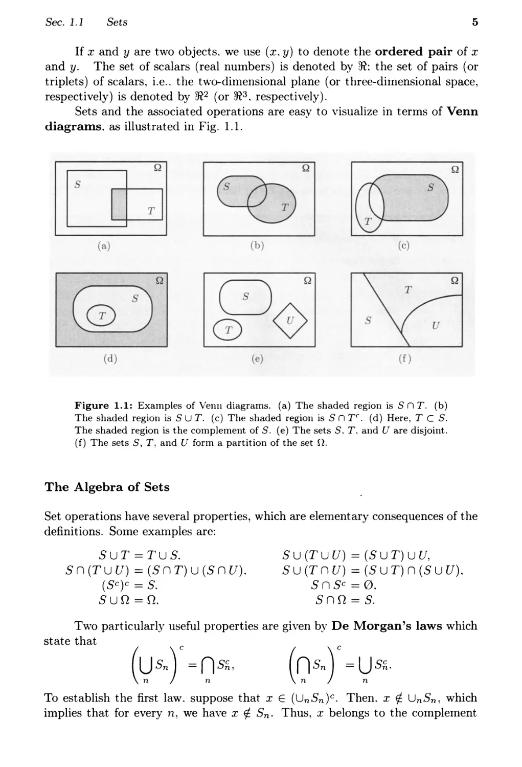
Sets and the associated operations are easy to visualize in terms of Venn
diagrams. as illustrated in Fig. 1.1.
Figure 1.1: Examples of Venn diagrams. (a) The shaded region is S n T. (b)
The shaded region is S u T. (c) The shaded region is S n T C . (d) Here, T C S.
The shaded region is the complement of S. (e) The sets S. T. and U are disjoint.
(f) The sets S, T, and U form a partition of the set O.
The Algebra of Sets
Set operations have several properties, which are elementary consequences of the
definitions. Some exalnples are:
S u T = T u S.
S n (T U U) = (S n T) U (S n U).
(Se)e = S.
SuO = O.
S U (T U U) = (S U T) U U,
S U (T n U) = (S U T) n (S U U).
S n Se = 0.
S n 0 = S.
Two particularly useful properties are given by De Morgan's laws which
state that
(ysn)C =0S ,
(0 Sn ) C = ys .
To establish the first law. suppose that x E (UnSn)e. Then. x tJ. UnS n , which
implies that for every n, we have x tJ. Sn. Thus, x belongs to the complement
6
Sample Space and Probability
Chap. 1
of every Sn. and x E nnSh. This shows that (UnSn)c C nnS , The converse
inclusion is established by reversing the above argument, and the first law follows.
The argument for the second law is similar.
1.2 PROBABILISTIC MODELS
A probabilistic model is a mathematical description of an uncertain situation.
It must be in accordance with a fundamental framework that we discuss in this
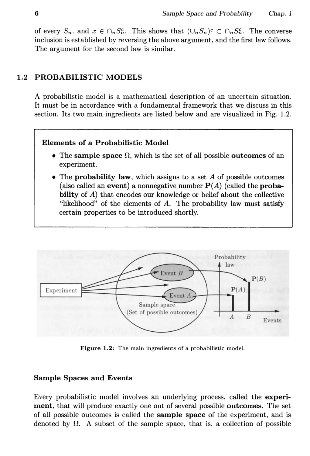
section. Its two main ingredients are listed below and are visualized in Fig. 1.2.
Elements of a Probabilistic Model
. The sample space 0, which is the set of all possible outcomes of an
experiment.
. The probability law, which assigns to a set A of possible outcomes
(also called an event) a nonnegative number P(A) (called the proba-
bility of A) that encodes our knowledge or belief about the collective
"likelihood" of the elements of A. The probability law must satisfy
certain properties to be introduced shortly.
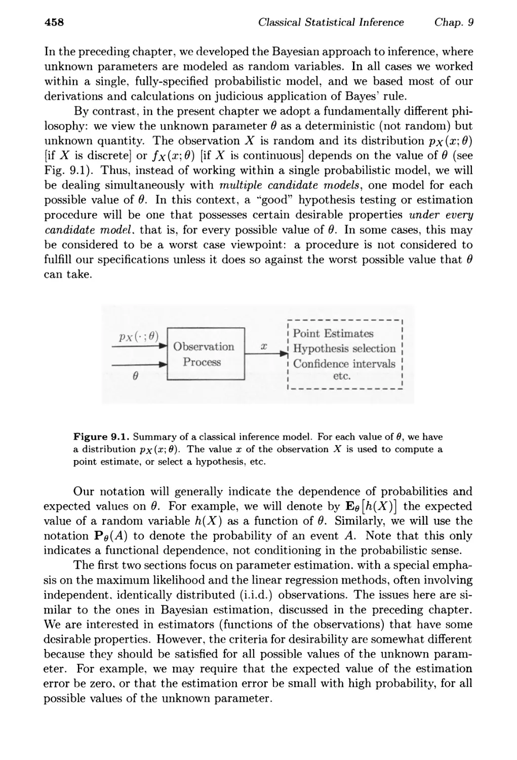
Figure 1.2: The main ingredients of a probabilistic model.
Sample Spaces and Events
Every probabilistic model involves an underlying process, called the experi-
ment, that will produce exactly one out of several possible outcomes. The set
of all possible outcomes is called the sample space of the experiment, and is
denoted by O. A subset of the sample space, that is, a collection of possible
Sec. 1.2
Probabilistic Models
7
outcomes, is called an event.t There is no restriction on what constitutes an
experiment. For example, it could be a single toss of a coin, or three tosses,
or an infinite sequence of tosses. However, it is important to note that in our
formulation of a probabilistic model. there is only one experiment. So, three
tosses of a coin constitute a single experiment. rather than three experiments.
The sample space of an experiment may consist of a finite or an infinite
number of possible outcomes. Finite sample spaces are conceptually and math-
ematically simpler. Still, sample spaces with an infinite number of elements are
quite common. As an example, consider throwing a dart on a square target and
viewing the point of impact as the outcome.
Choosing an Appropriate Sample Space
Regardless of their number. different elements of the sample space should be
distinct and mutually exclusive, so that when the experiment is carried out
there is a unique outcome. For example, the sample space associated with the
roll of a die cannot contain "1 or 3" as a possible outcome and also "1 or 4"
as another possible outcome. If it did, we would not be able to assign a unique
outcome when the roll is a 1.
A given physical situation may be modeled in several different ways, de-
pending on the kind of questions that we are interested in. Generally, the sample
space chosen for a probabilistic model must be collectively exhaustive, in the
sense that no matter what happens in the experiment, we always obtain an out-
come that has been included in the sample space. In addition, the sample space
should have enough detail to distinguish between all outcomes of interest to the
modeler, while avoiding irrelevant details.
Example 1.1. Consider two alternative games, both involving ten successive coin
tosses:
Game 1: We receive $1 each time a head comes up.
Game 2: We receive $1 for every coin toss. up to and including the first time
a head comes up. Then. we receive $2 for every coin toss. up to the second
time a head comes up. 1vlore generally, the dollar amount per toss is doubled
each time a head comes up.
t Any collection of possible outcomes, including the entire sample space f2 and
its complement, the empty set 0, may qualify as an event. Strictly speaking, however,
SOfie sets have to be excluded. In particular, when dealing with probabilistic models
involving an uncountably infinite sample space. there are certain unusual subset for
which one cannot associate meaningful probabilities. This is an intricate technical issue,
involving the mathematics of measure theory. Fortunately, such pathological subsets
do not arise in the problems considered in this text or in practice. and the issue can be
safely ignored.
8
Sample Space and Probability
Chap. 1
In game 1. it is only the total number of heads in the ten-toss sequence that mat-
ters. while in game 2, the order of heads and tails is also important. Thus, in
a probabilistic model for game 1. we can work with a sample space consisting of
eleven possible outcomes. namely, O. 1, . . . ,10. In game 2, a finer grain description
of the experiment is called for. and it is more appropriate to let the sample space
consist of every possible ten-long sequence of heads and tails.
Sequential Models
!\Iany experiments have an inherently sequential character; for example, tossing
a coin three times. observing the value of a stock on five successive days, or
receiving eight successive digits at a con1munication receiver. It is then often
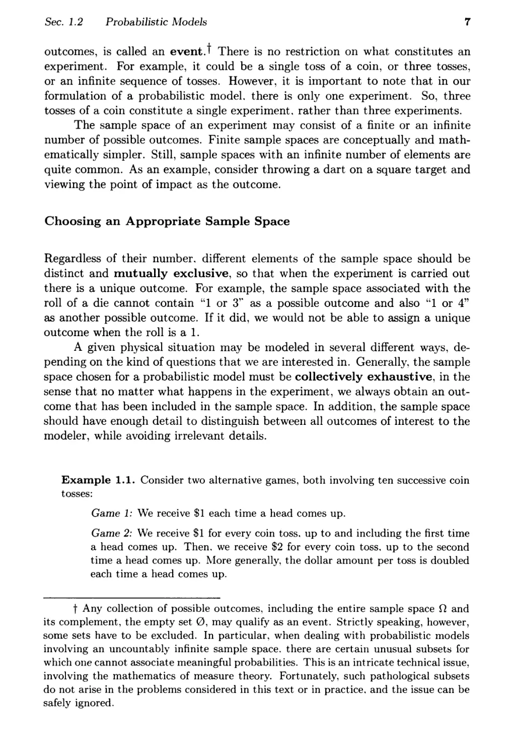
useful to describe the experiment and the associated sample space by means of
a tree-based sequential description, as in Fig. 1.3.
Figure 1.3: Two equivalent descriptions of the sample space of an experiment
involving two rolls of a 4-sided die. The possible outcomes are all the ordered pairs
of the form (i. j). where i is the result of the first roll, and j is the result of the
second. These outcomes can be arranged in a 2-dimensional grid as in the figure
on the left, or they can be described by the tree on the right. which reflects the
sequential character of the experiment. Here, each possible outcome corresponds
to a leaf of the tree and is associated with the unique path from the root to
that leaf. The shaded area on the left is the event {(1,4), (2,4), (3,4), (4,4)}
that the result of the second roll is 4. That same event can be described by the
set of leaves highlighted on the right. Note also that every node of the tree can
be identified with an event, namely. the set of all leaves downstream from that
node. For example, the node labeled by a 1 can be identified with the event
{(1.1), (1,2). (1,3), (1, 4)} that the result of the first roll is 1.
Probability Laws
Suppose we have settled on the sample space n associated with an experiment.
To complete the probabilistic model we must now introduce a probability law.
Sec. 1.2
Probabilistic !\1odels
9
Intuitively, this specifies the "likelihood" of any outcome, or of any set of possible
outcomes (an event. as we have called it earlier). 110re precisely. the probability
law assigns to every event A. a number P(A), called the probability of A.
satisfying the following axioms.
Probability Axioms
1. (Nonnegativity) P(A) > 0, for every event A.
2. (Additivity) If A and B are two disjoint events, then the probability
of their union satisfies
P(A U B) = P(A) + P(B).
More generally, if the sample space has an infinite number of elements
and AI, A2, . . . is a sequence of disjoint events, then the probability of
their union satisfies
P(A I U A2 U . . .) = P(A 1 ) + P(A 2 ) + . . . .
3. (Normalization) The probability of the entire sample space 0 IS
equal to 1, that is, P(O) = 1.
In order to visualize a probability law. consider a unit of mass which is
"spread" over the sample space. Then, P(A) is simply the total mass that was
assigned collectively to the elements of A. In terms of this analogy, the additivity
axiom becomes quite intuitive: the total mass in a sequence of disjoint events is
the sum of their individual masses.
A more concrete interpretation of probabilities is in terms of relative fre-
quencies: a statement such as P(A) = 2/3 often represents a belief that event A
will occur in about two thirds out of a large number of repetitions of the exper-
iment. Such an interpretation, though not always appropriate, can sometimes
facilitate our intuitive understanding. It will be revisited in Chapter 5, in our
study of limit theorems.
There are many natural properties of a probability law. which have not been
included in the above axioms for the simple reason that they can be derived
from them. For example, note that the normalization and additivity axioms
imply that
1 = P(O) = P(O U 0) = P(O) + P(0) = 1 + P(0).
and this shows that the probability of the empty event is 0:
P(0) = o.
10
Sample Space and Probability
Chap. 1
As another example, consider three disjoint events AI, A 2 , and A3. We can use
the additivity axiom for two disjoint events repeatedly, to obtain
P(A I U A 2 U A 3 ) = P(AI U (A 2 U A 3 ))
= P(A l ) + P(A 2 U A 3 )
= P(A 1 ) + P(A2) + P(A3).
Proceeding similarly, we obtain that the probability of the union of finitely many
disjoint events is always equal to the sum of the probabilities of these events.
Iore such properties will be considered shortly.
Discrete Models
Here is an illustration of how to construct a probability law starting from some
common sense assumptions about a model.
Example 1.2. Consider an experiment involving a single coin toss. There are two
possible outcomes, heads (H) and tails (T). The sample space is f2 = {H, T}, and
the events are
{H. T}, {H}, {T}, 0.
If the coin is fair, i.e., if we believe that heads and tails are "equally likely," we
should assign equal probabilities to the two possible outcomes and specify that
P( {H}) = P( {T}) = 0.5. The additivity axiom implies that
P({H,T}) =P({H}) +P({T}) = 1,
which is consistent with the normalization axiom. Thus, the probability law is given
by
P ( { H, T}) = 1,
p( {H}) = 0.5.
p( {T}) = 0.5,
P(0) = 0,
and satisfies all three axioms.
Consider another experiment involving three coin tosses. The outcome will
now be a 3-10ng string of heads or tails. The sample space is
f2 = {HHH, HHT, HTH, HTT, THH, THT, TTH, TTT}.
We assume that each possible outcome has the same probability of 1/8. Let us
construct a probability law that satisfies the three axioms. Consider, as an example.
the event
A = {exactly 2 heads occur} = {H HT, HT H, T H H}.
Using additivity, the probability of A is the sum of the probabilities of its elements:
P({HHT, HTH. THH}) = P({HHT}) +P({HTH}) +P({THH})
111
=-+-+-
888
3
8
Sec. 1.2
Probabilistic A10dels
11
Similarly the probability of any event is equal to 1/8 times the number of possible
outcomes contained in the event. This defines a probability law that satisfies the
three axioms.
By using the additivity axiom and by generalizing the reasoning in the
preceding example, we reach the following conclusion.
Discrete Probability Law
If the sample space consists of a finite number of possible outcomes, then the
probability law is specified by the probabilities of the events that consist of
a single element. In particular, the probability of any event {Sl, S2, . . . , Sn}
is the sum of the probabilities of its elements:
P ( { Sl , S2, . . . , Sn}) = P (Sl) + P (S2) + . . . + P (Sn).
Note that we are using here the simpler notation P(Si) to denote the prob-
ability of the event {Si}, instead of the more precise P ( {Si} ). This convention
will be used throughout the remainder of the book.
In the special case where the probabilities P(Sl),' . . , P(sn) are all the same
(by necessity equal to l/n, in view of the normalization axiom), we obtain the
following.
Discrete Uniform Probability Law
If the sample space consists of n possible outcomes which are equally likely
(i.e., all single-element events have the same probability), then the proba-
bility of any event A is given by
P(A) = number of elements of A .
n
Let us provide a few more examples of sample spaces and probability laws.
Example 1.3. Consider the experiment of rolling a pair of 4-sided dice (cf. Fig.
1.4). We assume the dice are fair, and we interpret this assumption to mean that
each of the sixteen possible outcomes [pairs (i, j), with i. j = 1,2.3,4] has the same
probability of 1/16. To calculate the probability of an event, we must count the
number of elements of the event and divide by 16 (the total number of possible
12
Sample Space and Probability
Chap. 1
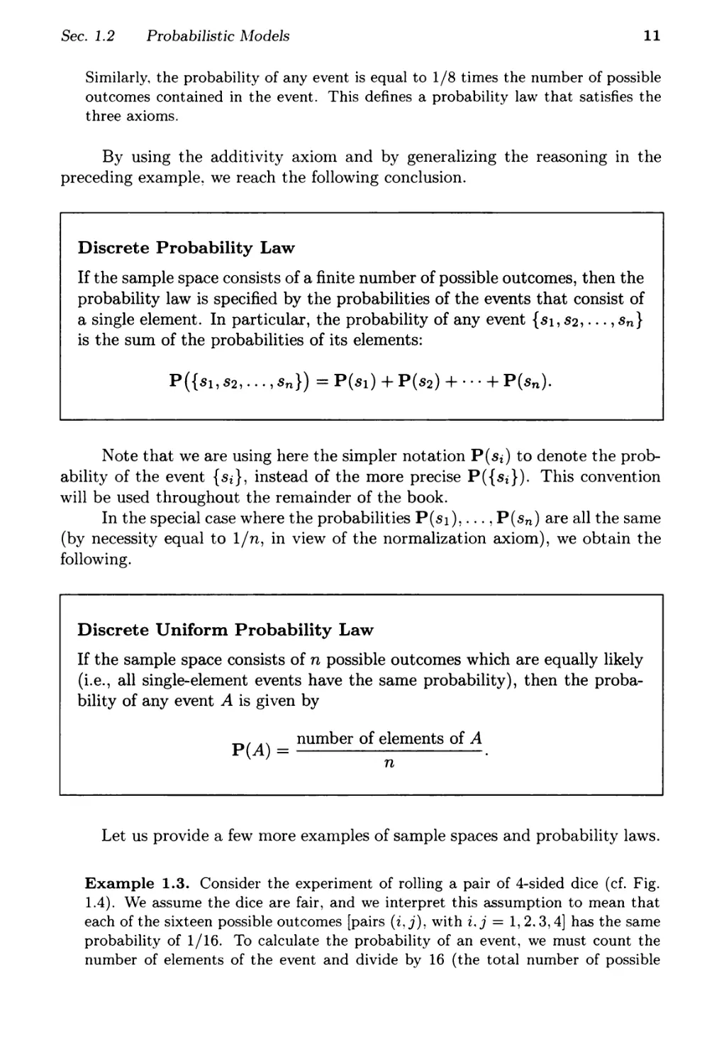
outcomes). Here are some event probabilities calculated in this way:
p( {the sum of the rolls is even}) = 8/16 = 1/2,
P ({ the sum of the rolls is odd}) = 8/16 = 1/2,
P ( {the first roll is equal to the second}) = 4/16 = 1/4,
P ({ the first roll is larger than the second}) = 6/16 = 3/8,
P ( {at least one roll is equal to 4}) = 7/16.
Figure 1.4: Various events in the experiment of rolling a pair of 4-sided dice,
and their probabilities, calculated according to the discrete uniform law.
Continuous Models
Probabilistic models with continuous sample spaces differ from their discrete
counterparts in that the probabilities of the single-element events may not be
sufficient to characterize the probability law. This is illustrated in the following
examples, which also indicate how to generalize the uniform probability law to
the case of a continuous sample space.
Example 1.4. A wheel of fortune is continuously calibrated from 0 to 1, so the
possible outcomes of an experiment consisting of a single spin are the numbers in
the interval n = [0, 1]. Assuming a fair wheel, it is appropriate to consider all
outcomes equally likely, but what is the probability of the event consisting of a
single element? It cannot be positive, because then, using the additivity axiom, it
would follow that events with a sufficiently large number of elements would have
Sec. 1.2
Probabilistic Models
13
probability larger than 1. Therefore, the probability of any event that consists of a
single element must be O.
In this example, it makes sense to assign probability b - a to any subinter-
val [a, b] of [0, 1], and to calculate the probability of a more complicated set by
evaluating its "length." t This assignment satisfies the three probability axioms and
qualifies as a legitimate probability law.
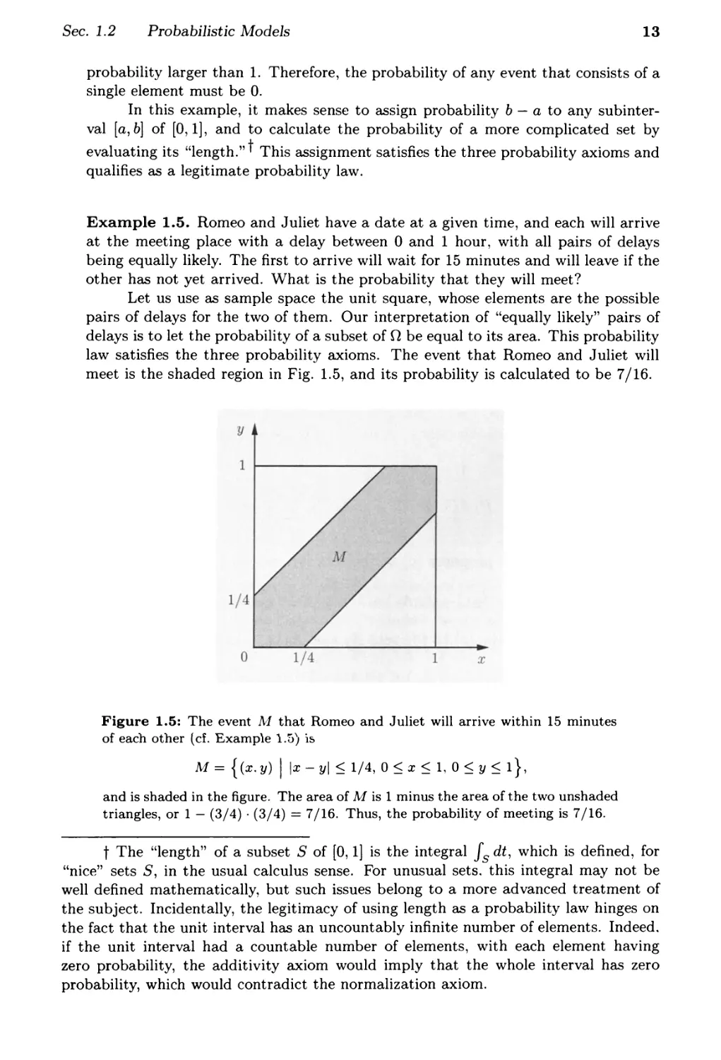
Example 1.5. Romeo and Juliet have a date at a given time, and each will arrive
at the meeting place with a delay between 0 and 1 hour, with all pairs of delays
being equally likely. The first to arrive will wait for 15 minutes and will leave if the
other has not yet arrived. What is the probability that they will meet?
Let us use as sample space the unit square, whose elements are the possible
pairs of delays for the two of them. Our interpretation of "equally likely" pairs of
delays is to let the probability of a subset of n be equal to its area. This probability
law satisfies the three probability axioms. The event that Romeo and Juliet will
meet is the shaded region in Fig. 1.5, and its probability is calculated to be 7/16.
Figure 1.5: The event !'vI that Romeo and Juliet will arrive within 15 minutes
of each other (cf. Example 1.5) i5
M = { (x. y) Ilx - yl 1/4, 0 x 1, 0 y I},
and is shaded in the figure. The area of M is 1 minus the area of the two unshaded
triangles, or 1 - (3/4) . (3/4) = 7/16. Thus, the probability of meeting is 7/16.
t The "length" of a subset S of [0, 1] is the integral Is dt, which is defined, for
"nice" sets S, in the usual calculus sense. For unusual sets. this integral may not be
well defined mathematically, but such issues belong to a more advanced treatment of
the subject. Incidentally, the legitimacy of using length as a probability law hinges on
the fact that the unit interval has an uncountably infinite number of elements. Indeed.
if the unit interval had a countable number of elements, with each element having
zero probability, the additivity axiom would imply that the whole interval has zero
probability, which would contradict the normalization axiom.
14
Sanlple Space and Probability
Chap. 1
Properties of Probability Laws
Probability laws have a number of properties, which can be deduced from the
axioms. Some of them are summarized below.
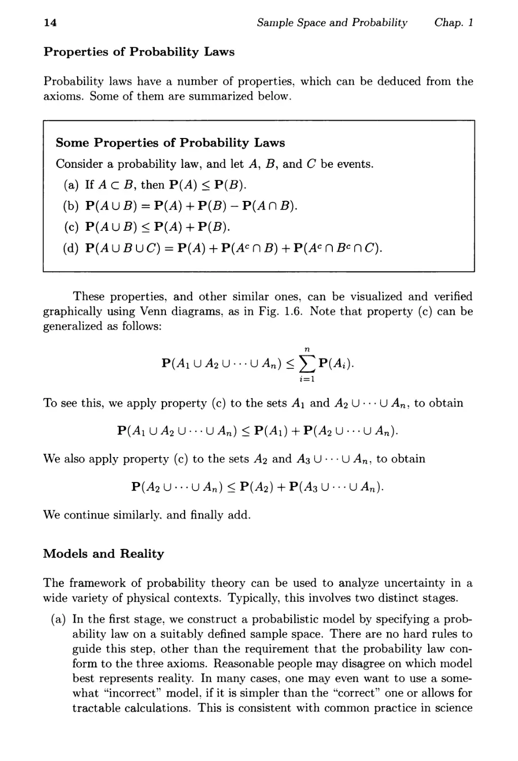
Some Properties of Probability Laws
Consider a probability law, and let A, B, and C be events.
(a) If A c B, then P(A) < P(B).
(b) P(A U B) = P(A) + P(B) - P(A n B).
(c) P(A U B) < P(A) + P(B).
(d) P(A U B U C) = P(A) + p(Ae n B) + p(Ae n Be n C).
These properties, and other similar ones, can be visualized and verified
graphically using Venn diagrams, as in Fig. 1.6. Note that property (c) can be
generalized as follows:
n
P(A 1 U A2 U . . . U An) < L P(Ai).
i=1
To see this, we apply property (c) to the sets Al and A 2 U . . . U An, to obtain
P(A I U A 2 U... U An) < P(A I ) + P(A 2 U... U An).
We also apply property (c) to the sets A2 and A3 U . . . U An, to obtain
P(A2 U... U An) < P(A2) + P(A3 U ... U An).
We continue similarly. and finally add.
Models and Reality
The framework of probability theory can be used to analyze uncertainty in a
wide variety of physical contexts. Typically, this involves two distinct stages.
(a) In the first stage, we construct a probabilistic model by specifying a prob-
ability law on a suitably defined sample space. There are no hard rules to
guide this step, other than the requirement that the probability law con-
form to the three axioms. Reasonable people may disagree on which model
best represents reality. In many cases, one may even want to use a some-
what "incorrect" model, if it is simpler than the "correct" one or allows for
tractable calculations. This is consistent with common practice in science
Sec. 1.2
Probabilistic Models
15
and engineering, where the choice of a model often involves a tradeoff be-
tween accuracy, simplicity, and tractability. Sometimes, a model is chosen
on the basis of historical data or past outcomes of similar experiments.
using statistical inference methods, which will be discussed in Chapters 8
and 9.
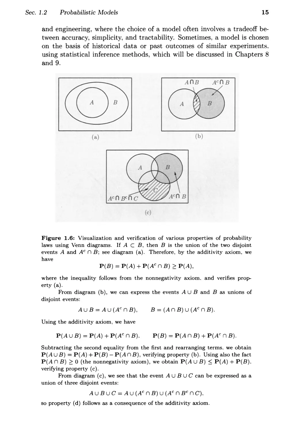
Figure 1.6: Visualization and verification of various properties of probability
laws using Venn diagrams. If A C B, then B is the union of the two disjoint
events A and AC n B; see diagram (a). Therefore, by the additivity axiom, we
have
P(B) = P(A) + P(A C n B) P(A),
where the inequality follows from the nonnegativity axiom. and verifies prop-
erty (a).
From diagram (b), we can express the events A u Band B as unions of
disjoint events:
Au B = Au (A C n B),
B = (A n B) u (A C n B).
Using the additivity axiom, we have
P(A u B) = P(A) + P(A C n B).
P(B) = P(A n B) + P(A C n B).
Subtracting the second equality from the first and rearranging terms. we obtain
P(A U B) = P(A) + P(B) - P(A n B), verifying property (b). Using also the fact
P(A n B) 0 (the nonnegativity axiom), \\re obtain P(A U B) P(A) + P(B).
verifying property (c).
From diagram (c), we see that the event A U B u C can be expressed as a
union of three disjoint events:
Au B u C = Au (A C n B) u (A C n B C n C).
so property (d) follows as a consequence of the additivity axiom.
16
Sample Space and Probability
Chap. 1
(b) In the second stage. we work within a fully specified probabilistic model and
derive the probabilities of certain events, or deduce some interesting prop-
erties. While the first stage entails the often open-ended task of connecting
the real world with mathematics, the second one is tightly regulated by the
rules of ordinary logic and the axioms of probability. Difficulties may arise
in the latter if some required calculations are complex, or if a probability
law is specified in an indirect fashion. Even so, there is no room for ambi-
guity: all conceivable questions have precise answers and it is only a matter
of developing the skill to arrive at them.
Probability theory is full of "paradoxes" in which different calculation
methods seem to give different answers to the same question. Invariably though,
these apparent inconsistencies turn out to reflect poorly specified or ambiguous
probabilistic models. An example, Bertrand's paradox, is shown in Fig. 1.7.
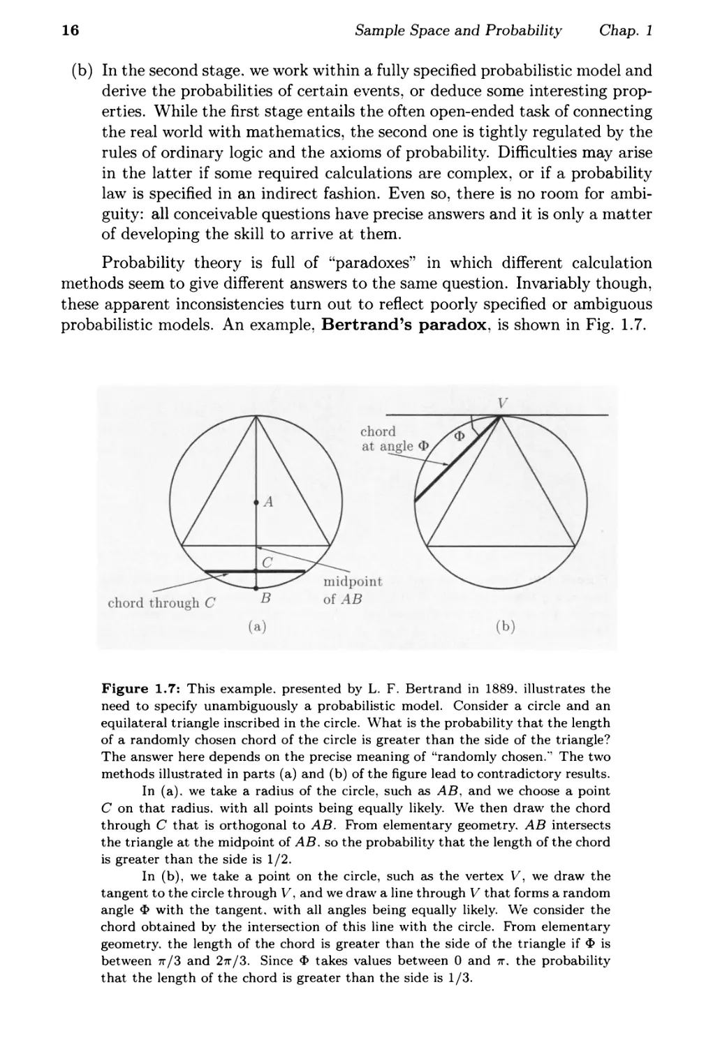
Figure 1.7: This example. presented by L. F. Bertrand in 1889. illustrates the
need to specify unambiguously a probabilistic model. Consider a circle and an
equilateral triangle inscribed in the circle. What is the probability that the length
of a randomly chosen chord of the circle is greater than the side of the triangle?
The answer here depends on the precise meaning of "randomly chosen." The two
methods illustrated in parts (a) and (b) of the figure lead to contradictory results.
In (a). we take a radius of the circle, such as AB, and we choose a point
C on that radius. with all points being equally likely. We then draw the chord
through C that is orthogonal to AB. From elementary geometry. AB intersects
the triangle at the midpoint of AB. so the probability that the length of the chord
is greater than the side is 1/2.
In (b), we take a point on the circle, such as the vertex V, we draw the
tangent to the circle through V, and we drav.' a line through V that forms a random
angle <I> with the tangent. with all angles being equally likely. We consider the
chord obtained by the intersection of this line with the circle. From elementary
geometry. the length of the chord is greater than the side of the triangle if <I> is
between 7r /3 and 27r /3. Since <I> takes values between 0 and 7r. the probability
that the length of the chord is greater than the side is 1/3.
Sec. 1.2
Probabilistic J\;Iodels
17
A Brief History of Probability
. B.C.E. Games of chance were popular in ancient Greece and Rome, but
no scientific development of the subject took place, possibly because the
number system used by the Greeks did not facilitate algebraic calculations.
The development of probability based on sound scientific analysis had to
await the development of the modern arithmetic system by the Hindus and
the Arabs in the second half of the first millennium, as well as the flood of
scientific ideas generated by the Renaissance.
. 16th century. Girolamo Cardano, a colorful and controversial Italian
mathematician, publishes the first book describing correct methods for cal-
culating probabilities in games of chance involving dice and cards.
. 17th century. A correspondence between Fermat and Pascal touches upon
several interesting probability questions and motivates further study in the
field.
. 18th century. Jacob Bernoulli studies repeated coin tossing and introduces
the first law of large numbers, which lays a foundation for linking theoreti-
cal probability concepts and empirical fact. Several mathematicians. such as
Daniel Bernoulli, Leibnitz, Bayes, and Lagrange, make important contribu-
tions to probability theory and its use in analyzing real-world phenomena.
De Moivre introduces the normal distribution and proves the first form of
the central limit theorem.
. 19th century. Laplace publishes an influential book that establishes the
importance of probability as a quantitative field and contains many original
contributions, including a more general version of the central limit theo-
rem. Legendre and Gauss apply probability to astronomical predictions,
using the method of least squares, thus pointing the way to a vast range of
applications. Poisson publishes an influential book with many original con-
tributions, including the Poisson distribution. Chebyshev, and his students
Markov and Lyapunov, study limit theorems and raise the standards of
mathematical rigor in the field. Throughout this period, probability theory
is largely viewed as a natural science, its primary goal being the explanation
of physical phenomena. Consistently with this goal, probabilities are mainly
interpreted as limits of relative frequencies in the context of repeatable ex-
periments.
. 20th century. Relative frequency is abandoned as the conceptual foun-
dation of probability theory in favor of a now universally used axiomatic
system, introduced by Kolmogorov. Similar to other branches of mathe-
matics, the development of probability theory from the axioms relies only
on logical correctness, regardless of its relevance to physical phenomena.
Nonetheless, probability theory is used pervasively in science and engineer-
ing because of its ability to describe and interpret most types of uncertain
phenomena in the real world.
18
Sample Space and Probability
Chap. 1
1.3 CONDITIONAL PROBABILITY
Conditional probability provides us with a way to reason about the outcome
of an experiment, based on partial information. Here are some examples of
situations we have in mind:
(a) In an experiment involving two successive rolls of a die you are told that
the sum of the two rolls is 9. How likely is it that the first roll was a 6?
(b) In a word guessing game, the first letter of the word is a "t". What is the
likelihood that the second letter is an "h"?
(c) How likely is it that a person has a certain disease given that a medical
test was negative?
(d) A spot shows up on a radar screen. How likely is it to correspond to an
aircraft?
In more precise terlns, given an experiment, a corresponding sample space,
and a probability law, suppose that we know that the outcome is within some
given event B. We wish to quantify the likelihood that the outcome also belongs
to some other given event A. We thus seek to construct a new probability law
that takes into account the available knowledge: a probability law that for any
event A. specifies the conditional probability of A given B. denoted by
P(A I B).
We would like the conditional probabilities P(A I B) of different events A
to constitute a legitimate probability law, which satisfies the probability axioms.
The conditional probabilities should also be consistent with our intuition in im-
portant special cases, e.g. when all possible outconles of the experiment are
equally likely. For example. suppose that all six possible outcomes of a fair die
roll are equally likely. If we are told that the outcome is even, we are left with
only three possible outcomes. namely, 2. 4, and 6. These three outcomes were
equally likely to start with, and so they should remain equally likely given the
additional knowledge that the outcome was even. Thus, it is reasonable to let
P(the outcome is 61 the outcome is even) = !.
3
This argument suggests that an appropriate definition of conditional probability
when all outcomes are equally likely, is given by
P(A I B) = number of elements of An B .
number of elements of B
Generalizing the argument, we introduce the following definition of condi-
tional probability:
P(AIB) = p(AnB)
P(B) ,
Sec. 1.3
Conditional Probability
19
where we assume that P(B) > 0; the conditional probability is undefined if the
conditioning event has zero probability. In words, out of the total probability of
the elements of B, P(A I B) is the fraction that is assigned to possible outcomes
that also belong to A.
Conditional Probabilities Specify a Probability Law
For a fixed event B, it can be verified that the conditional probabilities P(A I B)
form a legitimate probability law that satisfies the three axioms. Indeed, non-
negativity is clear. Furthermore,
P(S1I B ) = P(S1nB) = P(B) =
P(B) P(B) 1,
and the normalization axiom is also satisfied. To verify the additivity axiom, we
write for any two disjoint events Al and A 2 ,
P ( A uA I B ) = P((AIUA 2 )nB)
1 2 P(B)
P((A 1 n B) U (A 2 n B))
P(B)
P(A I n B) + P(A2 n B)
P(B)
P(A 1 n B) P(A2 n B)
= P(B) + P(B)
= P(A 1 I B) + P(A21 B),
where for the third equality, we used the fact that Al n Band A2 n Bare
disjoint sets, and the additivity axiom for the (unconditional) probability law.
The argument for a countable collection of disjoint sets is similar.
Since conditional probabilities constitute a legitimate probability law, all
general properties of probability laws remain valid. For example, a fact such as
P(A U C) < P(A) + P(C) translates to the new fact
P(A U C I B) < P(A I B) + P(C I B).
Let us also note that since we have P(B I B) = P(B)jP(B) = 1, all of the con-
ditional probability is concentrated on B. Thus, we might as well discard all
possible outcomes outside B and treat the conditional probabilities as a proba-
bility law defined on the new universe B.
Let us summarize the conclusions reached so far.
20
Sample Space and Probability
Chap. 1
Properties of Conditional Probability
. The conditional probability of an event A, gIven an event B with
P(B) > 0, is defined by
P(AIB) = P(AnB)
P(B) ,
and specifies a new (conditional) probability law on the same sample
space 0. In particular, all properties of probability laws remain valid
for conditional probability laws.
. Conditional probabilities can also be viewed as a probability law on a
new universe B, because all of the conditional probability is concen-
trated on B.
. If the possible outcomes are finitely many and equally likely, then
P(A I B) = number of elements of An B .
number of elements of B
Example 1.6. We toss a fair coin three successive times. We wish to find the
conditional probability P(A I B) when A and B are the events
A = {more heads than tails come up},
B = {1st toss is a head}.
The sample space consists of eight sequences.
n = {HHH. HHT. HTH, HTT, THH, THT. TTH, TTT}.
which we assume to be equally likely. The event B consists of the four elements
HHH, HHT. HTH. HTT. so its probability is
P(B) = i.
8
The event .4 n B consists of the three elements H H H. H HT. HT H, so its proba-
bility is
3
p(AnB)=S'
Thus, the conditional probability P(A I B) is
P(A I B) = P(A n B) = 3/8 = .
P(B) 4/8 4
Because all possible outcomes are equally likely here, we can also compute P(A I B)
using a shortcut. We can bypass the calculation of P(B) and p(AnB), and simply
Sec. 1.3
Conditional Probability
21
divide the number of elements shared by A and B (which is 3) with the number of
elements of B (which is 4), to obtain the same result 3/4.
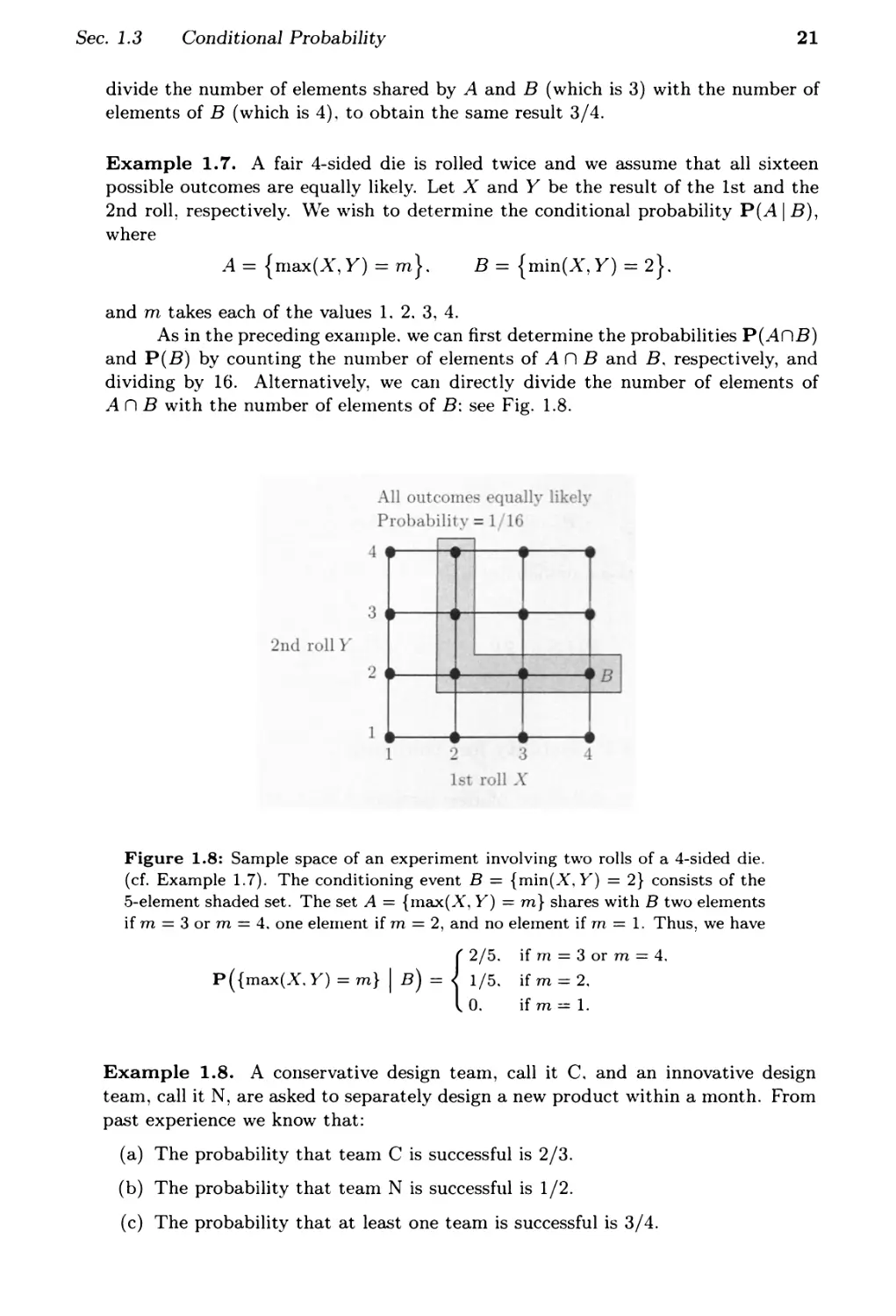
Example 1.7. A fair 4-sided die is rolled twice and we assume that all sixteen
possible outcomes are equally likely. Let X and Y be the result of the 1st and the
2nd roll respectively. We wish to determine the conditional probability P(A I B),
where
.4 = {rnax(X, Y) = m}.
B = {min(X, Y) = 2}.
and m takes each of the values 1. 2. 3, 4.
As in the preceding exalnple. we can first determine the probabilities p(AnB)
and P(B) by counting the nUlnber of elernents of A n Band B. respectively, and
dividing by 16. Alternatively, we can directly divide the number of elements of
A n B with the number of elernents of B: see Fig. 1.8.
Figure 1.8: Sample space of an experiment involving two rolls of a 4-sided die.
(cf. Example 1.7). The conditioning event B = {min(X, Y) = 2} consists of the
5-element shaded set. The set A = {rnax(X, Y) == m} shares with B two elements
if m = 3 or m = 4. one elernent if m = 2, and no element if Tn = 1. Thus, we have
{ 2/5. if m = 3 or m = 4.
p( {max(X. Y) = m} I B) = 1/5. if m = 2.
O. if m == 1.
Example 1.8. A conservative design team, call it C. and an innovative design
team, call it N, are asked to separately design a new product within a month. From
past experience we know that:
(a) The probability that team C is successful is 2/3.
(b) The probability that team N is successful is 1/2.
(c) The probability that at least one team is successful is 3/4.
22
Sample Space and Probability
Chap. 1
Assuming that exactly one successful design is produced, what is the probability
that it was designed by team N?
There are four possible outcomes here, corresponding to the four combinations
of success and failure of the two teams:
S S: both succeed,
SF: C succeeds, N fails,
F F: both fail,
F S: C fails, N succeeds.
We were given that the probabilities of these outcomes satisfy
P(SS) + P(SF) = ,
1
P(SS) + P(FS) = 2'
P(SS) + P(SF) + P(FS) = .
From these relations, together with the normalization equation
P(SS) + P(SF) + P(FS) + P(FF) = 1,
we can obtain the probabilities of individual outcomes:
5
P(SS) = 12 '
P(SF) = ,
1
P(FS) = -,
12
P(FF) = .
The desired conditional probability is
1
P(FS I {SF, FS}) = 1 12 1
4 + 12
1
4
Using Conditional Probability for Modeling
When constructing probabilistic models for experiments that have a sequential
character, it is often natural and convenient to first specify conditional prob-
abilities and then use them to determine unconditional probabilities. The rule
p(AnB) = P(B)P(A I B), which is a restatement of the definition of conditional
probability, is often helpful in this process.
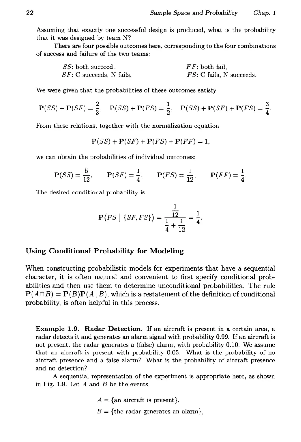
Example 1.9. Radar Detection. If an aircraft is present in a certain area, a
radar detects it and generates an alarm signal with probability 0.99. If an aircraft is
not present. the radar generates a (false) alarm, with probability 0.10. We assume
that an aircraft is present with probability 0.05. What is the probability of no
aircraft presence and a false alarm? What is the probability of aircraft presence
and no detection?
A sequential representation of the experiment is appropriate here, as shown
in Fig. 1.9. Let A and B be the events
A = {an aircraft is present},
B = {the radar generates an alarm},
Sec. 1.3
Conditional Probability
23
and consider also their complements
A C = {an aircraft is not present}.
B C = {the radar does not generate an alarm}.
The given probabilities are recorded along the corresponding branches of the tree de-
scribing the sample space, as shown in Fig. 1.9. Each possible outcome corresponds
to a leaf of the tree, and its probability is equal to the product of the probabilities
associated with the branches in a path from the root to the corresponding leaf. The
desired probabilities are
P(not present, false alarm) = P(A C n B) = P(AC)P(B lAC) = 0.95 . 0.10 = 0.095,
P (present , no detection) = P(A n B C ) = P(A)P(B C I A) = 0.05 . 0.01 = 0.0005.
Figure 1.9: Sequential description of the experiment for the radar detection
problem in Example 1.9.
Extending the preceding example, we have a general rule for calculating
various probabilities in conjunction with a tree-based sequential description of
an experiment. In particular:
(a) We set up the tree so that an event of interest is associated with a leaf.
We view the occurrence of the event as a sequence of steps, namely, the
traversals of the branches along the path fronl the root to the leaf.
(b) We record the conditional probabilities associated with the branches of the
tree.
(c) We obtain the probability of a leaf by multiplying the probabilities recorded
along the corresponding path of the tree.
24
Sample Space and Probability
Chap. 1
In mathematical terms, we are dealing with an event A which occurs if and
only if each one of several events AI, . . . , An has occurred, i.e., A = Al n A 2 n
. . . n An. The occurrence of A is viewed as an occurrence of A I, followed by the
occurrence of A 2 , then of A3, etc., and it is visualized as a path with n branches,
corresponding to the events AI, . . . , An. The probability of A is given by the
following rule (see also Fig. 1.10).
Multiplication Rule
Assuming that all of the conditioning events have positive probability, we
have
P( n l Ai) = P(A 1 )P(A21 A1)P(A 3 1 Al n A 2 )... P(An I n ll Ai).
The multiplication rule can be verified by writing
P(A I n A 2 )
P( nf=l Ai) = P(A 1 ) . P(AI)
P(A 1 n A 2 n A 3 )
P(A 1 n A 2 )
P( ni=l Ai)
P ( n -IA. ) '
z=l z
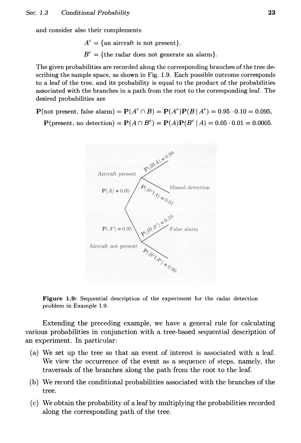
Figure 1.10: Visualization of the multiplication rule. The intersection event
A = Al n A2 n . . . n An is associated with a particular path on a tree that
describes the experiment. We associate the branches of this path with the events
AI. . . . . An. and we record next to the branches the corresponding conditional
probabilities.
The final node of the path corresponds to the intersection event A, and
its probability is obtained by multiplying the conditional probabilities recorded
along the branches of the path
P(AI n A2 n... n An) = P(AI)P(A21 AI)'" P(An I Al n A2 n... nAn-I).
Note that any intermediate node along the path also corresponds to some inter-
section event and its probability is obtained by multiplying the corresponding
conditional probabilities up to that node. For example, the event Al n A2 n A3
corresponds to the node shown in the figure. and its probability is
P(A I n A2 n A3) = P(AI )P(A21 Al )P(A31 Al n A2).
Sec. 1.3
Conditional Probability
25
and by using the definition of conditional probability to rewrite the right-hand
side above as
P(A 1 )P(A 2 1 AI)P(A31 Al n A 2 )... P(An I n ==-11 Ai).
For the case of just two events, Al and A 2 , the multiplication rule is simply the
definition of conditional probability.
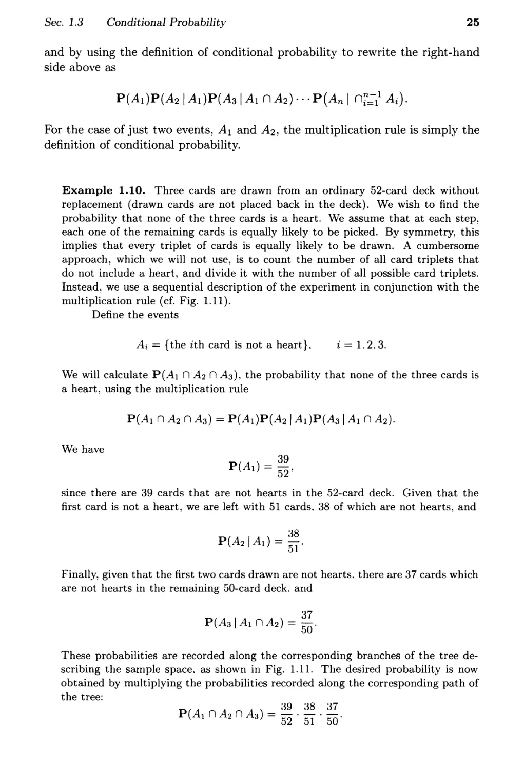
Example 1.10. Three cards are drawn from an ordinary 52-card deck without
replacement (drawn cards are not placed back in the deck). We wish to find the
probability that none of the three cards is a heart. We assume that at each step,
each one of the remaining cards is equally likely to be picked. By symmetry, this
implies that every triplet of cards is equally likely to be drawn. A cumbersome
approach, which we will not use, is to count the number of all card triplets that
do not include a heart, and divide it with the number of all possible card triplets.
Instead, we use a sequential description of the experiment in conjunction with the
multiplication rule (cf. Fig. 1.11).
Define the events
Ai = {the ith card is not a heart}.
i = 1. 2.3.
We will calculate P(A 1 n A 2 n A 3 ), the probability that none of the three cards is
a heart, using the multiplication rule
P(A 1 n A2 n A 3 ) = P(A 1 )P(A 2 1 A I )P(A 3 / Al n A 2 ).
We have
39
P(A I ) = 52 '
since there are 39 cards that are not hearts in the 52-card deck. Given that the
first card is not a heart, we are left with 51 cards. 38 of which are not hearts, and
38
P(A 2 1 AI) = -.
51
Finally, given that the first two cards drawn are not hearts. there are 37 cards which
are not hearts in the remaining 50-card deck. and
37
P(A 3 1 Al n A 2 ) = 50 '
These probabilities are recorded along the corresponding branches of the tree de-
scribing the sample space. as shown in Fig. 1.11. The desired probability is now
obtained by multiplying the probabilities recorded along the corresponding path of
the tree:
39 38 37
P(A I n A 2 n A 3 ) = - . - . -.
52 51 50
26
Sample Space and Probability
Chap. 1
Figure 1.11: Sequential description
of the experiment in the 3-card se-
lection problem of Example 1.10.
Note that once the probabilities are recorded along the tree, the probability
of several other events can be similarly calculated. For example,
P (1st is not a heart and 2nd is a heart) = 39 2 . 13 ,
5 51
. 39 38 13
P(lst and 2nd are not hearts, and 3rd IS a heart) = 52 . 51 . 50 '
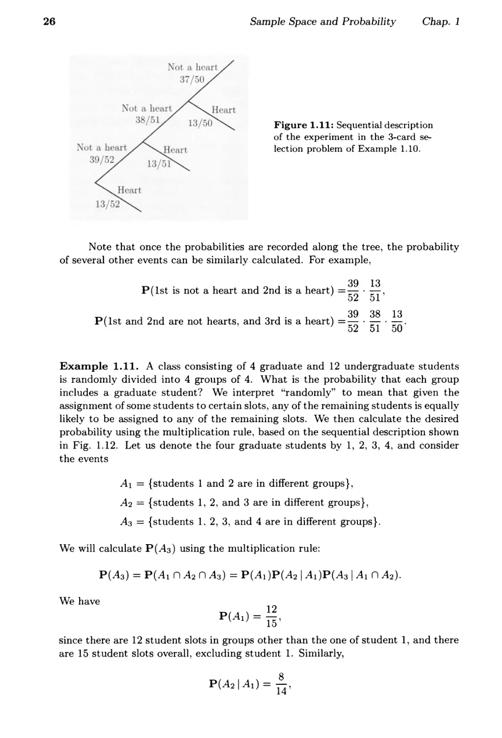
Example 1.11. A class consisting of 4 graduate and 12 undergraduate students
is randomly divided into 4 groups of 4. What is the probability that each group
includes a graduate student? We interpret "randomly" to mean that given the
assignment of some students to certain slots, any of the remaining students is equally
likely to be assigned to any of the remaining slots. We then calculate the desired
probability using the multiplication rule, based on the sequential description shown
in Fig. 1.12. Let us denote the four graduate students by 1, 2, 3, 4, and consider
the events
Al = {students 1 and 2 are in different groups},
A2 = {students 1, 2, and 3 are in different groups},
A3 = {students 1. 2, 3, and 4 are in different groups}.
We will calculate P(A 3 ) using the multiplication rule:
P(A 3 ) = P(A I n A 2 n A 3 ) = P(A I )P(A 2 1 Al )P(A 3 1 Al n A 2 ).
We have
P ( A ) = 12
1 15 '
since there are 12 student slots in groups other than the one of student 1, and there
are 15 student slots overall, excluding student 1. Similarly,
8
P(A2 I AI) = 14 '
Sec. 1.3
Conditional Probability
27
Figure 1.12: Sequential descrip-
tion of the experiment in the stu-
dent problem of Example 1.11.
since there are 8 student slots in groups other than those of students 1 and 2, and
there are 14 student slots, excluding students 1 and 2. Also,
4
P(A31 Al n A2) = 13 '
since there are 4 student slots in groups other than those of students 1. 2. and 3,
and there are 13 student slots, excluding students 1, 2, and 3. Thus, the desired
probability is
12 8 4
-.-.-
15 14 13 '
and is obtained by multiplying the conditional probabilities along the corresponding
path of the tree in Fig. 1.12.
Example 1.12. The Monty Hall Problem. This is a much discussed puzzle,
based on an old American game show . You are told that a prize is equally likely to
be found behind anyone of three closed doors in front of you. You point to one of
the doors. A friend opens for you one of the remaining two doors, after making sure
that the prize is not behind it. At this point, you can stick to your initial choice,
or switch to the other unopened door. You win the prize if it lies behind your final
choice of a door. Consider the following strategies:
(a) Stick to your initial choice.
(b) Switch to the other unopened door.
(c) You first point to door 1. If door 2 is opened, you do not switch. If door 3 is
opened, you switch.
Which is the best strategy? To answer the question, let us calculate the probability
of winning under each of the three strategies.
Under the strategy of no switching, your initial choice will determine whether
you win or not, and the probability of winning is 1/3. This is because the prize is
equally likely to be behind each door.
Under the strategy of switching, if the prize is behind the initially chosen
door (probability 1/3). you do not win. If it is not (probability 2/3), and given that
28
Sample Space and Probability
Chap. 1
another door without a prize has been opened for you, you will get to the winning
door once you switch. Thus. the probability of winning is now 2/3, so (b) is a better
strategy than ( a).
Consider now strategy (c). Under this strategy, there is insufficient informa-
tion for determining the probability of winning. The answer depends on the way
that your friend chooses which door to open. Let us consider two possibilities.
Suppose that if the prize is behind door 1, your friend always chooses to open
door 2. (If the prize is behind door 2 or 3, your friend has no choice.) If the prize
is behind door 1. your friend opens door 2, you do not switch, and you win. If the
prize is behind door 2, your friend opens door 3, you switch. and you win. If the
prize is behind door 3. your friend opens door 2. you do not switch, and you lose.
Thus, the probability of winning is 2/3. so strategy (c) in this case is as good as
strategy (b).
Suppose now that if the prize is behind door 1. your friend is equally likely to
open either door 2 or 3. If the prize is behind door 1 (probability 1/3). and if your
friend opens door 2 (probability 1/2), you do not switch and you win (probability
1/6). But if your friend opens door 3, you switch and you lose. If the prize is behind
door 2, your friend opens door 3. you switch, and you win (probability 1/3). If the
prize is behind door 3, your friend opens door 2, you do not switch and you lose.
Thus. the probability of winning is 1/6 + 1/3 = 1/2, so strategy (c) in this case is
inferior to strategy (b).
1.4 TOTAL PROBABILITY THEOREM AND BAYES' RULE
In this section, we explore some applications of conditional probability. We start
with the following theorem. which is often useful for computing the probabilities
of various events. using a "divide-and-conquer" approach.
Total Probability Theorem
Let AI, . . . , An be disjoint events that form a partition of the sample space
(each possible outcome is included in exactly one of the events AI, . . . , An)
and assume that P(A i ) > 0, for all i. Then, for any event B, we have
P(B) = P(AI n B) + . . . + P(An n B)
= P(AI)P(B I AI) + ... + P(An)P(B I An).
The theorem is visualized and proved in Fig. 1.13. Intuitively, we are par-
titioning the sample space into a number of scenarios (events) Ai. Then, the
probability that B occurs is a weighted average of its conditional probability
under each scenario, where each scenario is weighted according to its (uncondi-
tional) probability. One of the uses of the theorem is to compute the probability
of various events B for which the conditional probabilities P(B I Ai) are known or
Sec. 1.4
Total Probability Theorem and Bayes' Rule
29
easy to derive. The key is to choose appropriately the partition AI. . . . . An. and
this choice is often suggested by the problem structure. Here are some exalnples.
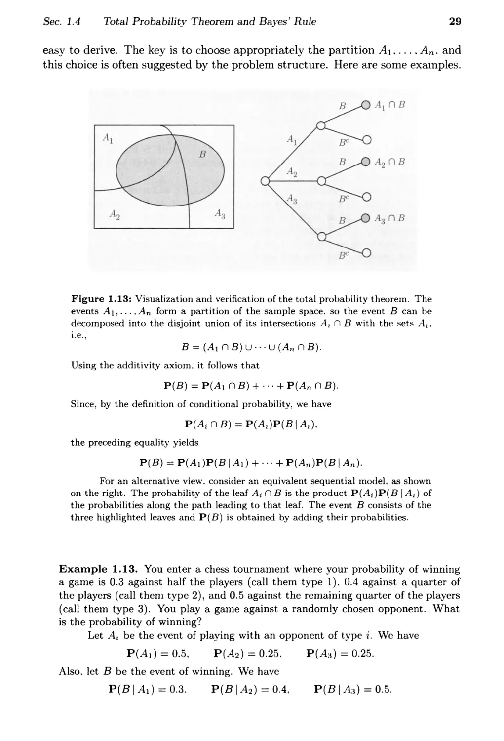
Figure 1.13: Visualization and verification of the total probability theorem. The
events AI, . . . . An form a partition of the sample space. so the event B can be
decomposed into the disjoint union of its intersections Az n B with the sets At.
I.e.,
B == (AI n B) u .. . U (An n B).
Using the additivity axiom. it follows that
P(B) == P(AI n B) + .. . + P(An n B).
Since, by the definition of conditional probability, we have
P(A i n B) == P(At)P(B I Az).
the preceding equality yields
P(B) == P(AI )P(B I AI) + . . . + P(An )P(B I An).
For an alternative view. consider an equivalent sequential model. as shown
on the right. The probability of the leaf Ai n B is the product P(AdP(B I At) of
the probabilities along the path leading to that leaf. The event B consists of the
three highlighted leaves and P( B) is obtained by adding their probabilities.
Example 1.13. You enter a chess tournament where your probability of winning
a game is 0.3 against half the players (call them type 1). 0.4 against a quarter of
the players (call them type 2), and 0.5 against the remaining quarter of the players
(call them type 3). You playa game against a randomly chosen opponent. What
is the probability of winning?
Let At be the event of playing with an opponent of type i. We have
P(A I ) = 0.5,
P(A2) = 0.25.
P(A 3 ) = 0.25.
Also. let B be the event of winning. We have
P(B I AI) = 0.3.
P(B I A2) = 0.4,
P(B I A 3 ) = 0.5.
30
Sample Space and Probability
Chap. 1
Thus, by the total probability theorem, the probability of winning is
P(B) = P(Al)P(B I AI) + P(A2)P(B I A2) + P(A3)P(B I A3)
= 0.5 . 0.3 + 0.25 . 0.4 + 0.25 . 0.5
= 0.375.
Example 1.14. You roll a fair four-sided die. If the result is 1 or 2, you roll once
more but otherwise, you stop. What is the probability that the sum total of your
rolls is at least 4?
Let Ai be the event that the result of first roll is i, and note that P(A 1 ) = 1/4
for each i. Let B be the event that the sum total is at least 4. Given the event AI.
the sum total will be at least 4 if the second roll results in 3 or 4, which happens
with probability 1/2. Similarly, given the event A2, the sum total will be at least
4 if the second roll results in 2, 3, or 4, which happens with probability 3/4. Also,
given the event A3, you stop and the sum total remains below 4. Therefore,
1
P(BIAl) = 2'
3
P(BIA2) = 4'
P(B I A 3 ) = 0,
P(B I A4) = 1.
By the total probability theorem.
11 131 1 9
P(B) = - . - + - . - + - .0+ - .1= -.
4 2 4 4 4 4 16
The total probability theorem can be applied repeatedly to calculate proba-
bilities in experiments that have a sequential character, as shown in the following
example.
Example 1.15. Alice is taking a probability class and at the end of each week
she can be either up-to-date or she may have fallen behind. If she is up-to-date in
a given week, the probability that she will be up-to-date (or behind) in the next
week is 0.8 (or 0.2, respectively). If she is behind in a given week, the probability
that she will be up-to-date (or behind) in the next week is 0.4 (or 0.6, respectively).
Alice is (by default) up-to-date when she starts the class. What is the probability
that she is up-to-date after three weeks?
Let U i and B i be the events that Alice is up-to-date or behind, respectively,
after i weeks. According to the total probability theorem, the desired probability
P(U 3 ) is given by
P(U3) = P(U2)P(U31 U2) + P(B2)P(U 3 1 B 2 ) = P(U 2 ) .0.8 + P(B 2 ) .0.4.
The probabilities P (U2) and P (B2) can also be calculated using the total probability
theorem:
P(U2) = P(U 1 )P(U21 U 1 ) + P(B 1 )P(U21 B 1 ) = P(U 1 ) .0.8 + P(Bl) .0.4,
P(B 2 ) = P(U 1 )P(B 2 1 U l ) + P(B l )P(B21 B l ) = P(U l ) .0.2 + P(B l ) .0.6.
Sec. 1.4
Total Probability Theorem and Bayes' Rule
31
Finally, since Alice starts her class up-to-date, we have
P(U 1 ) = 0.8,
P(B 1 ) = 0.2.
We can now combine the preceding three equations to obtain
P( U 2 ) = 0.8 . 0.8 + 0.2 .0.4 = 0.72,
P(B2) = 0.8 . 0.2 + 0.2 . 0.6 = 0.28,
and by using the above probabilities in the formula for P(U 3 ):
P(U 3 ) = 0.72 . 0.8 + 0.28.0.4 = 0.688.
Note that we could have calculated the desired probability P(U3) by con-
structing a tree description of the experiment, then calculating the probability of
every element of U 3 using the lTIultiplication rule on the tree, and adding. However.
there are cases where the calculation based on the total probability theorem is more
convenient. For example. suppose we are interested in the probability P(U20) that
Alice is up-to-date after 20 weeks. Calculating this probability using the multipli-
cation rule is very cumbersome. because the tree representing the experiment is 20
stages deep and has 2 20 leaves. On the other hand, with a computer, a sequential
calculation using the total probability formulas
P(U 1 + 1 ) = P(U i ) .0.8 + P(B i ) .0.4.
P(Bi+l) = P(U i ) .0.2 + P(B i ) .0.6.
and the initial conditions P(U 1 ) = 0.8. P(B 1 ) = 0.2. is very simple.
Inference and Bayes' Rule
The total probability theorem is often used in conjunction with the following
celebrated theorem, which relates conditional probabilities of the form P(A I B)
with conditional probabilities of the form P(B I A), in which the order of the
conditioning is reversed.
Bayes' Rule
Let AI, A 2 , . . . , An be disjoint events that form a partition of the sample
space, and assume that P(A i ) > 0, for all i. Then, for any event B such
that P(B) > 0, we have
P(A-I B) = P(Ai)P(B I Ai)
Z P(B)
P(Ai)P(B I Ai)
- P(A 1 )P(B I AI) + . . . + P(An)P(B I An)'
32
Sample Space and Probability
Chap. 1
Figure 1.14: An example of the inference context that is implicit in Bayes'
rule. We observe a shade in a person's X-ray (this is event B, the '"effect") and
we want to estimate the likelihood of three mutually exclusive and collectively
exhaustive potential causes: cause 1 (event AI) is that there is a malignant tumor,
cause 2 (event A2) is that there is a nonmalignant tumor, and cause 3 (event
A 3 ) corresponds to reasons other than a tumor. We assume that we know the
probabilities P(A i ) and P(B I A l ), i = 1. 2. 3. Given that we see a shade (event
B occurs). Bayes' rule gives the posterior probabilities of the various causes as
P ( A. I B ) - P(Al)P(B I Ad
1 - P(A1)P(B I AI) + P(A2)P(B I A2) + P(A 3 )P(B I A3) ' i = 1. 2,3.
For an alternative view, consider an equivalent sequential model, as shown
on the right. The probability P(A 1 I B) of a malignant tumor is the probability
of the first highlighted leaf. which is P(AI n B), divided by the total probability
of the highlighted leaves. which is P(B).
To verify Bayes' rule. note that by the definition of conditional probability,
we have
P(A i n B) = P(Ai)P(B I Ai) = P(Ai I B)P(B).
This yields the first equality. The second equality follows from the first by using
the total probability theorem to rewrite P(B).
Bayes' rule is often used for inference. There are a number of "causes"
that may result in a certain "effect." We observe the effect, and we wish to infer
the cause. The events AI, . . . . An are associated with the causes and the event B
represents the effect. The probability P(B I Ai) that the effect will be observed
when the cause Ai is present amounts to a probabilistic model of the cause-effect
relation (cf. Fig. 1.14). Given that the effect B has been observed, we wish to
evaluate the probability P(A i I B) that the cause Ai is present. We refer to
P(A i I B) as the posterior probability of event Ai given the information, to
be distinguished from P(Ai), which we call the prior probability.
Sec. 1.4
Total Probability Theorem and Bayes' Rule
33
Example 1.16. Let us return to the radar detection problem of Example 1.9 and
Fig. 1.9. Let
A = {an aircraft is present},
B = {the radar generates an alarm}.
We are given that
P(A) = 0.05,
P(B I A) = 0.99,
P(B lAC) = 0.1.
Applying Bayes' rule, with Al = A and A2 = A C , we obtain
P(aircraft present I alarm) = P(A I B)
P(A)P(B I A)
P(B)
P(A)P(B I A)
P(A)P(B I A) + P(Ac)P(B lAc)
0.05 . 0.99
0.05 . 0.99 + 0.95 . 0.1
0.3426.
Example 1.17. Let us return to the chess problem of Example 1.13. Here. At is
the event of getting an opponent of type i and
P(AI) = 0.5,
P(A2) = 0.25.
P(A 3 ) = 0.25.
Also, B is the event of winning, and
P(B I AI) = 0.3.
P(B I A 2 ) = 0.4,
P(B I A 3 ) = 0.5.
Suppose that you win. What is the probability P(A I I B) that you had an opponent
of type I?
U sing Bayes' rule, we have
P(AI)P(B I AI)
P(A11 B) = P(AI)P(B I AI) + P(A2)P(B I A 2 ) + P(A 3 )P(B I A 3 )
0.5 . 0.3
0.5 . 0.3 + 0.25 . 0.4 + 0.25 . 0.5
= 0.4.
Example 1.18. The False-Positive Puzzle. A test for a certain rare disease is
assumed to be correct 95% of the time: if a person has the disease, the test results
are positive with probability 0.95, and if the person does not have the disease,
the test results are negative with probability 0.95. A random person drawn from
34
Sample Space and Probability
Chap. 1
a certain population has probability 0.001 of having the disease. Given that the
person just tested positive, what is the probability of having the disease?
If A is the event that the person has the disease, and B is the event that the
test results are positive, the desired probability. P( A I B), is
P( 4)P(B I A)
P(A I B) = P(A)P(B I A) + P(Ac)P(B lAc)
0.001 . 0.95
0.001 .0.95 + 0.999 . 0.05
= 0.0187.
Note that even though the test was assumed to be fairly accurate, a person who has
tested positive is still very unlikely (less than 2%) to have the disease. According
to The Economist (February 20th. 1999). 80% of those questioned at a leading
American hospital substantially missed the correct answer to a question of this
type; ITIOst 9f them thought that the probability that the person has the disease
is 0.95!
1.5 INDEPENDENCE
We have introduced the conditional probability P(A I B) to capture the partial
information that event B provides about event A. An interesting and important
special case arises when the occurrence of B provides no such information and
does not alter the probability that A has occurred, i.e.,
P(A I B) = P(A).
When the above equality holds. we say that A is independent of B. Note that
by the definition P(A I B) = P(A n B)jP(B), this is equivalent to
P(A n B) = P(A)P(B).
We adopt this latter relation as the definition of independence because it can be
used even when P(B) = 0, in which case P(A I B) is undefined. The symmetry
of this relation also implies that independence is a symmetric property; that is,
if A is independent of B, then B is independent of A, and we can unambiguously
say that A and B are independent events.
Independence is often easy to grasp intuitively. For example, if the occur-
rence of two events is governed by distinct and noninteracting physical processes,
such events will turn out to be independent. On the other hand, independence
is not easily visualized in ternlS of the sample space. A common first thought
is that two events are independent if they are disjoint, but in fact the oppo-
site is true: two disjoint events A and B with P(A) > 0 and P(B) > 0 are
never independent, since their intersection An B is empty and has probability O.
Sec. 1.5
Independence
35
For example, an event A and its complement Ac are not independent [unless
P(A) = 0 or P(A) = 1], since knowledge that A has occurred provides precise
information about whether Ac has occurred.
Example 1.19. Consider an experiment involving two successive rolls of a 4-sided
die in which all 16 possible outcomes are equally likely and have probability 1/16.
( a) Are the events
Ai = {1st roll results in i},
B j = {2nd roll results in j},
independent? We have
P(A i n B j ) = P (the outcome of the two rolls is (i, j)) = 1 '
P Ai = number of elements of At
( ) total number of possible outcomes
P B.) = number of elements of BJ
(J total number of possible outcomes
4
16'
4
16'
We observe that P(A i n BJ) = P(Ai)P(Bj), and the independence of At and
Bj is verified. Thus, our choice of the discrete uniform probability law implies
the independence of the two rolls.
(b) Are the events
A = {1st roll is a I},
B = {sum of the two rolls is a 5},
independent? The answer here is not quite obvious. We have
P(A n B) = p( the result of the two rolls is (1,4)) = 1 '
and also
P(A) = number of elements of A 4
total number of possible outcomes 16
The event B consists of the outcomes (1,4), (2,3), (3,2), and (4,1). and
P(B) = number of elements of B 4
total number of possible outcomes 16'
Thus, we see that P(A n B)
independent.
( c) Are the events
P(A)P(B), and the events A and Bare
A = {maximum of the two rolls is 2}, B = {minimum of the two rolls is 2},
36
Sample Space and Probability
Chap. 1
independent? Intuitively. the answer is "no" because the rninimum of the
two rolls conveys some information about the maximum. For example, if the
minimum is 2, the maximum cannot be 1. More precisely, to verify that A
and B are not independent, we calculate
P( A n B) = P (the result of the two rolls is (2,2») = 11 6 ,
and also
P(A) = number of elements of A 3
total number of possible outcomes 16'
P(B) = number of elements of B 5
total number of possible outcomes 16
We have P(A)P(B) = 15/(16)2, so that P(A n B) =I P(A)P(B). and A and
B are not independent.
We finally note that, as mentioned earlier, if A and B are independent, the
occurrence of B does not provide any new information on the probability of A
occurring. It is then intuitive that the non-occurrence of B should also provide
no information on the probability of A. Indeed. it can be verified that if A and
B are independent, the sallIe holds true for A and Be (see the end-of-chapter
problems) .
Conditional Independence
We noted earlier that the conditional probabilities of events, conditioned on
a particular event. form a legitimate probability law. We can thus talk about
independence of various events with respect to this conditional law . In particular,
given an event C. the events A and B are called conditionally independent
if
P(A n B I C) = P(A I C)P(B I C).
To derive an alternative characterization of conditional independence, we use the
definition of the conditional probability and the multiplication rule, to write
P(A BIG) = p(AnBnG)
n P(C)
P(C)P(B I C)P(A I B n C)
P(C)
= P(B I C)P(A I B n C).
We now compare the preceding two expressions. and after eliminating the com-
mon factor P(B I C), assumed nonzero. we see that conditional independence is
the same as the condition
P(A I B n C) = P(A I C).
Sec. 1.5
Independence
37
In words, this relation states that if C is known to have occurred, the additional
knowledge that B also occurred does not change the probability of A.
Interestingly, independence of two events A and B with respect to the
unconditional probability law. does not imply conditional independence, and
vice versa, as illustrated by the next two examples.
Example 1.20. Consider two independent fair coin tosses, in which all four possible
outcomes are equally likely. Let
HI = {1st toss is a head},
H2 = {2nd toss is a head},
D = {the two tosses have different results}.
The events HI and H 2 are (unconditionally) independent. But
1
P(H 1 I D) = 2'
1
P(H2ID)=2'
P(HI n H21 D) = 0,
so that P(H 1 n H21 D) P(HI I D)P(H 2 1 D), and HI, H2 are not conditionally
independent.
This example can be generalized. For any probabilistic model, let A and B be
independent events, and let C be an event such that P(C) > 0, P(A I C) > 0, and
P(B I C) > 0, while A n B n C is empty. Then, A and B cannot be conditionally
independent (given C) since P(A n B I C) = 0 while P(A I C) P(B I C) > o.
Example 1.21. There are two coins, a blue and a red one. We choose one of
the two at random, each being chosen with probability 1/2, and proceed with two
independent tosses. The coins are biased: with the blue coin, the probability of
heads in any given toss is 0.99, whereas for the red coin it is 0.01.
Let B be the event that the blue coin was selected. Let also Hi be the event
that the ith toss resulted in heads. Given the choice of a coin, the events HI and
H2 are independent. because of our assumption of independent tosses. Thus,
P(H 1 n H2 I B) = P(HI I B)P(H2 I B) = 0.99 . 0.99.
On the other hand, the events HI and H2 are not independent. Intuitively, if we
are told that the first toss resulted in heads, this leads us to suspect that the blue
coin was selected, in which case, we expect the second toss to also result in heads.
Mathematically, we use the total probability theorem to obtain
P(H 1 ) = P(B)P(H 1 I B) + P(BC)P(H 1 I B C ) = _ 2 1 .0.99 + ! .0.01 = !,
2 2
as should be expected from symmetry considerations. Similarly, we have P(H2) =
1/2. Now notice that
P(H 1 n H2) = P(B)P(HI n H21 B) + P(BC)P(H 1 n H21 B C )
1 1 1
= - . 0.99 . 0.99 + - . 0.01 . 0.01 -.
222
38
Sample Space and Probability
Chap. 1
Thus, P(H 1 n H 2 ) P(H 1 )P(H 2 ), and the events HI and H2 are dependent, even
though they are conditionally independent given B.
We now summarize.
Independence
. Two events A and B are said to be independent if
P(A n B) = P(A)P(B).
If in addition, P(B) > 0, independence is equivalent to the condition
P(A I B) = P(A).
. If A and B are independent, so are A and Be.
. Two events A and B are said to be conditionally independent,
given another event C with P(C) > 0, if
P(A n B I C) = P(A I C)P(B I C).
If in addition, P(B n C) > 0, conditional independence is equivalent
to the condition
P(A I B n C) = P(A I C).
. Independence does not imply conditional independence, and vice versa.
Independence of a Collection of Events
The definition of independence can be extended to multiple events.
Definition of Independence of Several Events
We say that the events AI, A 2 , . . . , An are independent if
P ( n Ai ) = II P(A i ),
ieS ieS
for every subset S of {I, 2, . . . , n}.
Sec. 1.5
Independence
39
For the case of three events, AI, A 2 , and A3, independence amounts to
satisfying the four conditions
P(A1 n A2) = P(A 1 ) P(A 2 ),
P(A 1 n A3) = P(A 1 ) P(A3),
P(A 2 n A3) = P(A2) P(A3),
P(A 1 n A2 n A3) = P(A 1 ) P(A 2 ) P(A 3 ).
The first three conditions simply assert that any two events are independent,
a property known as pairwise independence. But the fourth condition is
also important and does not follow from the first three. Conversely, the fourth
condition does not imply the first three see the two examples that follow.
Example 1.22. Pairwise Independence does not Imply Independence.
Consider two independent fair coin tosses, and the following events:
HI = {1st toss is a head},
H2 = {2nd toss is a head},
D = {the two tosses have different results}.
The events HI and H2 are independent, by definition. To see that HI and Dare
independent, we note that
P(D I H ) = P(H 1 n D) = 1/4 = = P(D).
I P(H 1 ) 1/2 2
Similarly, H 2 and D are independent. On the other hand, we have
111
P(H 1 n H2 n D) = 0 2 . 2 . 2 = P(H 1 )P(H2)P(D),
and these three events are not independent.
Example 1.23. The Equality P(A 1 n A 2 n A 3 ) = P(A 1 ) P(A 2 ) P(A3) is not
Enough for Independence. Consider two independent rolls of a fair six-sided
die, and the following events:
A = {1st roll is 1, 2, or 3},
B = {1st roll is 3,4, or 5},
C = {the sum of the two rolls is 9}.
We have
1 1 1
P(A n B) = (3 2 . 2 = P(A)P(B),
114
p(AnC) = - -. - = P(A)P(C)
36 2 36 '
1 1 4
P(B n C) = - - . _ 3 = P(B)P(C).
12 2 6
40
Sample Space and Probability
Chap. 1
Thus the three events A, B. and C are not independent. and indeed no two of these
events are independent. On the other hand, we have
P(A n B n C) = 3 1 6 = . . 3 = P(A)P(B)P(C).
The intuition behind the independence of a collection of events is anal-
ogous to the case of two events. Independence means that the occurrence or
non-occurrence of any number of the events from that collection carries no
information on the remaining events or their complements. For example, if the
events AI, A2, A3. A4 are independent, one obtains relations such as
P(A 1 U A21 A3 n A 4 ) = P(A 1 U A2)
or
P(A 1 U A 2 1 A3 n A 4 ) = P(A 1 U A 2 );
see the end-of-chapter problems.
Reliability
In probabilistic models of complex systems involving several components, it is
often convenient to assume that the behaviors of the components are uncoupled
(independent). This typically simplifies the calculations and the analysis, as
illustrated in the following example.
Example 1.24. Network Connectivity. A computer network connects two
nodes A and B through intermediate nodes C, D, E, F, as shown in Fig. 1.15 ( a).
For every pair of directly connected nodes. say i and j, there is a given probability
Pij that the link from i to j is up. We assume that link failures are independent
of each other. What is the probability that there is a path connecting A and B in
which all links are up?
Figure 1.15: (a) Network for Example 1.24. The number next to each link
indicates the probability that the link is up. (b) Series and parallel connections
of three components in a reliability problem.
Sec. 1.5
Independence
41
This is a typical problem of assessing the reliability of a system consisting of
components that can fail independently. Such a system can often be divided into
subsystems, where each subsystem consists in turn of several components that are
connected either in series or in parallel; see Fig. 1.15(b).
Let a subsystem consist of con1ponents 1, 2, . . . ,m, and let Pi be the prob-
ability that component i is up ("succeeds"). Then, a series subsystem succeeds
if all of its components are up, so its probability of success is the product of the
probabilities of success of the corresponding components, i.e..
P(series subsystem succeeds) = PIP2 . . . Pm.
A parallel subsystem succeeds if anyone of its components succeeds, so its prob-
ability of failure is the product of the probabilities of failure of the corresponding
components, i.e.,
P(parallel subsystem succeeds) = 1 - P(parallel subsystem fails)
= 1 - (1 - PI) (1 - P2) . . . (1 - Pm).
Returning now to the network of Fig. 1.15(a), we can calculate the probabil-
ity of success (a path from A to B is available) sequentially, using the preceding
formulas, and starting from the end. Let us use the notation X ---+ Y to denote the
event that there is a (possibly indirect) connection from node X to node Y. Then.
P(C ---+ B) = 1 - (1 - P(C ---+ E and E ---+ B)) (1 - P(C ---+ F and F ---+ B))
= 1 - (1 - pCEPEB)(l - PCFPFB)
= 1 - (1 - 0.8 . 0.9)(1 - 0.95 . 0.85)
= 0.946,
P(A ---+ C and C ---+ B) = P(A ---+ C)P(C ---+ B) = 0.9.0.946 = 0.851.
P(A ---+ D and D ---+ B) = P(A ---+ D)P(D ---+ B) = 0.75.0.95 = 0.712,
and finally we obtain the desired probability
P (A ---+ B) = 1 - (1 - P (A ---+ C and C ---+ B)) (1 - P (A ---+ D and D ---+ B))
= 1 - (1 - 0.851)(1 - 0.712)
= 0.957.
Independent Trials and the Binomial Probabilities
If an experiment involves a sequence of independent but identical stages, we say
that we have a sequence of independent trials. In the special case where there
are only two possible results at each stage, we say that we have a sequence of
independent Bernoulli trials. The two possible results can be anything, e.g.,
"it rains" or "it doesn't rain," but we will often think in terms of coin tosses and
refer to the two results as '"heads" (H) and "tails" (T).
42
Sample Space and Probability
Chap. 1
Consider an experiment that consists of n independent tosses of a coin, in
which the probability of heads is p, where p is some number between 0 and 1. In
this context, independence means that the events AI, A 2 , . . . . An are indepen-
dent, where Ai = {ith toss is a head}.
We can visualize independent Bernoulli trials by means of a sequential
description, as shown in Fig. 1.16 for the case where n = 3. The conditional
probability of any toss being a head, conditioned on the results of any preced-
ing tosses, is p because of independence. Thus, by multiplying the conditional
probabilities along the corresponding path of the tree, we see that any particular
outcome (3-long sequence of heads and tails) that involves k heads and 3 - k
tails has probability pk (1 - p )3-k. This formula extends to the case of a general
number n of tosses. We obtain that the probability of any particular n-long
sequence that contains k heads and n - k tails is pk(1 - p)n-k. for all k from 0
to n.
Figure 1.16: Sequential description of an experiment involving three indepen-
dent tosses of a coin. Along the branches of the tree. we record the corresponding
conditional probabilities, and by the multiplication rule, the probability of ob-
taining a particular 3-toss sequence is calculated by multiplying the probabilities
recorded along the corresponding path of the tree.
Let us now consider the probability
p(k) = P(k heads come up in an n-toss sequence),
which will play an important role later. We showed above that the probability
of any given sequence that contains k heads is pk(l - p)n-k, so we have
p(k) = ( )pk(l - p)n-k,
Sec. 1.5
Independence
43
where we use the notation
( ) = number of distinct n-toss sequences that contain k heads.
The numbers ( ) (read as "n choose k") are known as the binomial coeffi-
cients, while the probabilities p(k) are known as the binomial probabilities.
Using a counting argument, to be given in Section 1.6, we can show that
( n ) n!
k - k!(n-k)!'
k = 0, 1, . . . , n,
where for any positive integer i we have
i! = 1 . 2 . . . (i - 1) . i,
and, by convention, O! = 1. An alternative verification is sketched in the end-of-
chapter problems. Note that the binomial probabilities p(k) must add to 1, thus
showing the binomial formula
t ( )pk(l - p)n-k = 1.
k=O
Example 1.25. Grade of Service. An internet service provider has installed c
modems to serve the needs of a population of n dialup customers. It is estimated
that at a given time, each customer will need a connection with probability p,
independent of the others. What is the probability that there are more customers
needing a connection than there are modems?
Here we are interested in the probability that more than c customers simul-
taneously need a connection. It is equal to
n
L p(k),
k=c+l
where
p(k) = ( )pk(l_ p)n-k
are the binomial probabilities. For instance, if n = 100, p = 0.1, and c = 15, the
probability of interest turns out to be 0.0399.
This example is typical of problems of sizing a facility to serve the needs
of a homogeneous population, consisting of independently acting customers. The
problem is to select the facility size to guarantee a certain probability (sometimes
called grade of service) that no user is left unserved.
44
Sample Space and Probability
Chap. 1
1.6 COUNTING
The calculation of probabilities often involves counting the number of outcomes
in various events. We have already seen two contexts where such counting arises.
(a) When the sample space [2 has a finite number of equally likely outcomes,
so that the discrete uniform probability law applies. Then, the probability
of any event A is given by
P(A) = number of elements of A
number of elements of [2 ,
and involves counting the elements of A and of [2.
(b) When we want to calculate the probability of an event A with a finite
number of equally likely outcomes, each of which has an already known
probability p. Then the probability of A is given by
P(A) = p . (number of elements of A),
and involves counting the number of elements of A. An example of this type
is the calculation of the probability of k heads in n coin tosses (the binomial
probabilities). We saw in the preceding section that the probability of each
distinct sequence involving k heads is easily obtained, but the calculation
of the number of all such sequences, to be presented shortly, requires some
thought.
While counting is in principle straightforward, it is frequently challenging;
the art of counting constitutes a large portion of the field of combinatorics. In
this section, we present the basic principle of counting and apply it to a number
of situations that are often encountered in probabilistic models.
The Counting Principle
The counting principle is based on a divide-and-conquer approach, whereby the
counting is broken down into stages through the use of a tree. For example,
consider an experiment that consists of two consecutive stages. The possible
results at the first stage are aI, a2, . . . , am; the possible results at the second
stage are bl, b2, . . . , b n . Then the possible results of the two-stage experiment
are all possible ordered pairs (ai, bj), i = 1, . . . , m, j = 1, . . . , n. Note that the
number of such ordered pairs is equal to mn. This observation can be generalized
as follows (see also Fig. 1.17).
Sec. 1.6
Counting
45
Figure 1.17: Illustration of the basic counting principle. The counting is carried
out in r stages (r = 4 in the figure). The first stage has n 1 possible results. For
every possible result at the first i-I stages, there are nt possible results at the
ith stage. The number of leaves is nl n2 . . . n r . This is the desired count.
The Counting Principle
Consider a process that consists of r stages. Suppose that:
(a) There are n1 possible results at the first stage.
(b) For every possible result at the first stage, there are n2 possible results
at the second stage.
(c) More generally, for any sequence of possible results at the first i-I
stages, there are ni possible results at the ith stage. Then, the total
number of possible results of the r-stage process is
n1 n2 . . . n r .
Example 1.26. The Number of Telephone Numbers. A local telephone
number is a 7-digit sequence, but the first digit has to be different from 0 or 1.
How many distinct telephone numbers are there? We can visualize the choice of a
sequence as a sequential process, where we select one digit at a time. We have a
total of 7 stages, and a choice of one out of 10 elements at each stage, except for
46
Sample Space and Probability
Chap. 1
the first stage where we only have 8 choices. Therefore, the answer is
8 . 10 . 10. . . 10 = 8 . 10 6 .
.......
"V'
6 times
Example 1.27. The Number of Subsets of an n-Element Set. Consider
an n-element set {Sl, S2, . . . , Sn}. How many subsets does it have (including itself
and the empty set)? We can visualize the choice of a subset as a sequential process
where we examine one element at a time and decide whether to include it in the set
or not. We have a total of n stages, and a binary choice at each stage. Therefore
the number of subsets is
2 . 2 . . . 2 = 2 n .
n times
It should be noted that the Counting Principle remains valid even if each
first-stage result leads to a different set of potential second-stage results, etc. The
only requirement is that the number of possible second-stage results is constant,
regardless of the first-stage result.
In what follows, we will focus primarily on two types of counting arguments
that involve the selection of k objects out of a collection of n objects. If the order
of selection matters, the selection is called a permutation, and otherwise, it is
called a combination. We will then discuss a more general type of counting,
involving a partition of a collection of n objects into multiple subsets.
k-permutations
We start with n distinct objects, and let k be some positive integer, with k < n.
We wish to count the number of different ways that we can pick k out of these
n objects and arrange them in a sequence, i.e., the number of distinct k-object
sequences. We can choose any of the n objects to be the first one. Having chosen
the first, there are only n - 1 possible choices for the second; given the choice of
the first two, there only remain n - 2 available objects for the third stage, etc.
When we are ready to select the last (the kth) object, we have already chosen
k - 1 objects, which leaves us with n - (k - 1) choices for the last one. By the
Counting Principle, the number of possible sequences, called k-permutations,
IS
n( n _ 1) . . . (n _ k + 1) = n( n - 1) . . . (n - k + 1) (n - k) . · . 2 . 1
(n - k) . . .2. 1
n!
(n-k)!'
In the special case where k = n, the number of possible sequences, simply called
permutations, is
n( n - 1) (n - 2) . . .2 . 1 = n!.
(Let k = n in the formula for the number of k-permutations, and recall the
convention O! = 1.)
Sec. 1.6
Counting
47
Example 1.28. Let us count the number of words that consist of four distinct
letters. This is the problem of counting the number of 4-permutations of the 26
letters in the alphabet. The desired number is
n! 26!
(n _ k)! = 22! = 26 . 25 . 24 . 23 = 358, 800.
The count for permutations can be combined with the Counting Principle
to solve more complicated counting problems.
Example 1.29. You have nl classical music CDs, n2 rock music CDs, and n3
country music CDs. In how many different ways can you arrange them so that the
CDs of the same type are contiguous?
We break down the problem in two stages where we first select the order of
the CD types, and then the order of the CDs of each type. There are 3! ordered se-
quences of the types of CDs (such as classical/rock/country, rock/country/classical,
etc.), and there are nl! (or n2!. or n3!) permutations of the classical (or rock. or
country, respectively) CDs. Thus for each of the 3! CD type sequences, there are
nt! n2! n3! arrangements of CDs. and the desired total number is 3! n I! n2! n3!.
Suppose now that you offer to give k i out of the n1. CDs of each type i to a
friend, where k i < ni, i = 1.2.3. What is the number of all possible arrangements
of the CDs that you are left with? The solution is similar, except that the number of
(ni - k i )-permutations of CDs of type i replaces ni! in the estimate, so the number
of possible arrangements is
, , ,
3! . nl. . n2. . n3. .
kt! k 2 ! k3!
Combinations
There are n people and we are interested in forming a committee of k. How
many different committees are possible? :NIore abstractly, this is the same as the
problem of counting the number of k-element subsets of a given n-element set.
Notice that forming a combination is different than forming a k-permutation.
because in a combination there is no ordering of the selected elements.
For example, whereas the 2-permutations of the letters A, B, C, and Dare
AB.BA,AC CA,AD,DA,BC.CB,BD.DB,CD,DC,
the combinations of two out of these four letters are
AB, AC, AD, BC,BD. CD.
In the preceding example, the combinations are obtained from the per-
mutations by grouping together "duplicates"; for example, AB and BA are not
48
Sample Space and Probability
Chap. 1
viewed as distinct, and are both associated with the combination AB. This rea-
soning can be generalized: each combination is associated with k! "duplicate"
k-permutations, so the number n!/(n - k)! of k-permutations is equal to the
number of combinations times k!. Hence, the number of possible combinations,
is equal to
n!
k!(n-k)!'
Let us now relate the above expression to the binomial coefficient, which
was denoted by ( ) and was defined in the preceding section as the number of
n-toss sequences with k heads. We note that specifying an n-toss sequence with
k heads is the same as selecting k elements (those that correspond to heads) out
of the n-element set of tosses, i.e., a combination of k out of n objects. Hence,
the binomial coefficient is also given by the same formula and we have
( )
n!
k!(n-k)!'
Example 1.30. The number of combinations of two out of the four letters A, B.
C, and D is found by letting n = 4 and k = 2. It is
( 4 ) _ _ 6
2 - 2! 2! - ,
consistent with the listing given earlier.
It is worth observing that counting arguments sometimes lead to formulas
that are rather difficult to derive algebraically. One example is the binomial
formula
t ( )pk(l - p)n-k = L
k=O
discussed in Section 1.5. In the special case where p = 1/2, this formula becomes
t ( ) = 2 11 ,
k=O
and admits the following simple interpretation. Since ( ) is the number of k-
element subsets of a given n-element subset. the sum over k of ( ) counts the
number of subsets of all possible cardinalities. It is therefore equal to the number
of all subsets of an n-element set. which is 2 n .
Example 1.31. We have a group of n persons. Consider clubs that consist of a
special person from the group (the club leader) and a number (possibly zero) of
Sec. 1.6
Counting
49
additional club members. Let us count the number of possible clubs of this type in
two different ways, thereby obtaining an algebraic identity.
There are n choices for club leader. Once the leader is chosen, we are left
with a set of n - 1 available persons, and we are free to choose any of the 2 n - 1
subsets. Thus the number of possible clubs is n2n-l.
Alternatively, for fixed k, we can form a k-person club by first selecting k out
of the n available persons [there are ( ) choices]. We can then select one of the
members to be the leader (there are k choices). By adding over all possible club
sizes k, we obtain the number of possible clubs as L =l k( ), thereby showing the
identi ty
tk ( ) =n2n-l.
k=l
Partitions
Recall that a combination is a choice of k elements out of an n-element set
without regard to order. Thus, a combination can be viewed as a partition of
the set in two: one part contains k elements and the other contains the remaining
n - k. We now generalize by considering partitions into more than two subsets.
We are given an n-element set and nonnegative integers nl, n2, . . . . nr-
whose sum is equal to n. We consider partitions of the set into r disjoint subsets.
with the ith subset containing exactly ni elements. Let us count in how many
ways this can be done.
We form the subsets one at a time. We have (nn 1 ) ways of forming the
first subset. Having formed the first subset, we are left with n - nl elements.
We need to choose n2 of them in order to form the second subset, and we have
(n ;l) choices, etc. Using the Counting Principle for this r-stage process, the
total number of choices is
( n ) ( n - n l ) ( n - nl - n 2 ) ... ( n - nl - ... - nr-l ) ,
n 1 n2 n3 n r
which is equal to
n!
nl!(n-nl)!
(n-nl)!
n2! (n - nl - n2)!
(n - nl - ... - nr-l)!
(n - n 1 - . . . - n r - 1 - n r )! n r ! .
We note that several terms cancel and we are left with
n!
n 1 ! n2! . . . n r ! .
This is called the multinomial coefficient and is usually denoted by
( n 1. n2 . . , nJ .
50
Sample Space and Probability
Chap. 1
Example 1.32. Anagrams. How many different words (letter sequences) can be
obtained by rearranging the letters in the word TATTOO? There are six positions
to be filled by the available letters. Each rearrangement corresponds to a partition
of the set of the six positions into a group of size 3 (the positions that get the letter
T), a group of size 1 (the position that gets the letter A), and a group of size 2 (the
positions that get the letter 0). Thus, the desired number is
6! 1.2.3.4.5.6
= = 60.
I! 2! 3! 1 . 1 . 2 . 1 . 2 . 3
It is instructive to derive this answer using an alternative argument. (This
argument can also be used to rederive the multinomial coefficient formula: see
the end-of-chapter problems.) Let us write TATTOO in the form T 1 AT 2 T 3 0102
pretending for a moment that we are dealing with 6 distinguishable objects. These
6 objects can be rearranged in 6! different ways. However, any of the 3! possible
permutations of Tl, T2, and T3, as well as any of the 2! possible permutations of
0 1 and 02, lead to the same word. Thus, when the subscripts are removed, there
are only 6!j(3! 2!) different words.
Example 1.33. A class consisting of 4 graduate and 12 undergraduate students
is randomly divided into four groups of 4. What is the probability that each group
includes a graduate student? This is the same as Example 1.11 in Section 1.3, but
we will now obtain the answer using a counting argument.
We first determine the nature of the sample space. A typical outcome is a
particular way of partitioning the 16 students into four groups of 4. We take the
term "randomly" to mean that every possible partition is equally likely, so that the
probability question can be reduced to one of counting.
According to our earlier discussion, there are
( 16 ) 16!
4, 4, 4, 4 - 4! 4! 4! 4!
different partitions, and this is the size of the sample space.
Let us now focus on the event that each group contains a graduate student.
Generating an outcome with this property can be accomplished in two stages:
(a) Take the four graduate students and distribute them to the four groups; there
are four choices for the group of the first graduate student, three choices for
the second, two for the third. Thus, there is a total of 4! choices for this stage.
(b) Take the remaining 12 undergraduate students and distribute them to the
four groups (3 students in each). This can be done in
( 3, ; , 3 )
12!
3! 3! 3! 3!
different ways.
By the Counting Principle, the event of interest can occur in
4! 12!
3! 3! 3! 3!
Sec. 1.7
Summary and Discussion
51
different ways. The probability of this event is
4! 12!
3! 3! 3! 3!
16!
4! 4! 4! 4!
After some cancellations, we find that this is equal to
12 . 8 . 4
15 . 14 . 13 '
consistent with the answer obtained in Example 1.11.
Here is a summary of all the counting results we have developed.
Summary of Counting Results
. Permutations of n objects: n!.
. k-permutations of n objects: n!/(n - k)!.
· Combinations of k out of n objects: ( ) = k! (nn k)!"
. Partitions of n objects into r groups, with the ith group having ni
objects:
( n ) n!
n 1 , n2, . . . , n r - n 1 ! n2! . . . n r ! .
SUMMARY AND DISCUSSION
A probability problem can usually be broken down into a few basic steps:
(a) The description of the sample space, that is, the set of possible outcomes
of a given experiment.
(b) The (possibly indirect) specification of the probability law (the probability
of each event).
(c) The calculation of probabilities and conditional probabilities of various
events of interest.
The probabilities of events must satisfy the nonnegativity, additivity, and nor-
malization axioms. In the important special case where the set of possible out-
comes is finite, one can just specify the probability of each outcome and obtain
52
Sample Space and Probability
Chap. 1
the probability of any event by adding the probabilities of the elements of the
event.
Given a probability law, we are often interested in conditional probabilities,
which allow us to reason based on partial information about the outcome of
the experiment. We can view conditional probabilities as probability laws of a
special type, under which only outcomes contained in the conditioning event can
have positive conditional probability. Conditional probabilities can be derived
from the (unconditional) probability law using the definition P(A I B) = P(A n
B)jP(B). However, the reverse process is often convenient, that is, first specify
some conditional probabilities that are natural for the real situation that we wish
to model, and then use them to derive the (unconditional) probability law.
We have illustrated through examples three methods for calculating prob-
abilities:
(a) The counting method. This method applies to the case where the num-
ber of possible outcomes is finite, and all outcomes are equally likely. To
calculate the probability of an event, we count the number of elements of
the event and divide by the number of elements of the sample space.
(b) The sequential method. This method applies when the experiment has a
sequential character, and suitable conditional probabilities are specified or
calculated along the branches of the corresponding tree (perhaps using the
counting method). The probabilities of various events are then obtained
by multiplying conditional probabilities along the corresponding paths of
the tree, using the multiplication rule.
(c) The divide-and-conquer method. Here, the probabilities P(B) of vari-
ous events B are obtained from conditional probabilities P(B I Ai), where
the Ai are suitable events that form a partition of the sample space and
have known probabilities P(Ai). The probabilities P(B) are then obtained
by using the total probability theorem.
Finally, we have focused on a few side topics that reinforce our main themes.
We have discussed the use of Bayes' rule in inference, which is an important
application context. We have also discussed some basic principles of counting
and combinatorics, which are helpful in applying the counting method.
Problems
53
PROBLEMS
SECTION 1.1. Sets
Problem 1. Consider rolling a six-sided die. Let A be the set of outcomes where the
roll is an even number. Let B be the set of outcomes where the roll is greater than 3.
Calculate and compare the sets on both sides of De l'dorgan's laws
(AUB)'=AcnB C .
(A n B) C = A C U B C .
Problem 2. Let A and B be two sets.
(a) Show that
A C = (A e n B) U (A C n B C ),
B C = (A n B C ) U (A C n B C ).
(b) Show that
(A n B)C = (A C n B) U (A C n Be) U (A n B C ).
(c) Consider rolling a fair six-sided die. Let A be the set of outcomes where the roll
is an odd number. Let B be the set of outcomes where the roll is less than 4.
Calculate the sets on both sides of the equality in part (b), and verify that the
equality holds.
Problem 3. * Prove the identity
Au (n =l Bn) = n =l(A U Bn).
Solution. If x belongs to the set on the left, there are two possibilities. Either x E A,
in which case x belongs to all of the sets A U B 11 . and therefore belongs to the set on
the right. Alternatively. x belongs to all of the sets Bn in which case. it belongs to all
of the sets A U Bn. and therefore again belongs to the set on the right.
Conversely. if x belongs to the set on the right. then it belongs to A U Bn for all
n. If x belongs to A. then it belongs to the set on the left. Otherwise. x must belong
to every set Bn and again belongs to the set on the left.
Problem 4. * Cantor's diagonalization argument. Show that the unit interval
[0, 1] is uncountable. i.e., its elements cannot be arranged in a sequence.
Solution. Any number x in [0. 1] can be represented in terms of its decimal expansion.
e.g., 1/3 = 0.3333.... Note that most numbers have a unique decimal expansion,
but there are a few exceptions. For example, 1/2 can be represented as 0.5000. . . or
as 0.49999. ". It can be shown that this is the only kind of exception, i.e.. decimal
expansions that end with an infinite string of zeroes or an infinite string of nines.
54
Sample Space and Probability
Chap. 1
Suppose, to obtain a contradiction, that the elements of [0, 1] can be arranged
in a sequence Xl, X2, X3, . . ., so that every element of [0, 1] appears in the sequence.
Consider the decimal expansion of X n :
123
X n = O.anana n . . . ,
where each digit a belongs to {O, 1, . . . ,9}. Consider now a number y constructed as
follows. The nth digit of y can be 1 or 2, and is chosen so that it is different from the
nth digit of Xn. Note that y has a unique decimal expansion since it does not end with
an infinite sequence of zeroes or nines. The number y differs from each X n , since it has
a different nth digit. Therefore, the sequence Xl, X2, . . . does not exhaust the elements
of [0, 1], contrary to what was assumed. The contradiction establishes that the set [0, 1]
is uncountable.
SECTION 1.2. Probabilistic Models
Problem 5. Out of the students in a class, 60% are geniuses, 70% love chocolate,
and 40% fall into both categories. Determine the probability that a randomly selected
student is neither a genius nor a chocolate lover.
Problem 6. A six-sided die is loaded in a way that each even face is twice as likely
as each odd face. All even faces are equally likely, as are all odd faces. Construct a
probabilistic model for a single roll of this die and find the probability that the outcome
is less than 4.
Problem 7. A four-sided die is rolled repeatedly, until the first time (if ever) that an
even number is obtained. What is the sample space for this experiment?
Problem 8. You enter a special kind of chess tournament, in which you play one game
with each of three opponents, but you get to choose the order in which you play your
opponents, knowing the probability of a win against each. You win the tournament if
you win two games in a row, and you want to maximize the probability of winning.
Show that it is optimal to play the weakest opponent second, and that the order of
playing the other two opponents does not matter.
Problem 9. A partition of the sample space n is a collection of disjoint events
Sl,..., Sn such that n = U lSi'
(a) Show that for any event A, we have
n
P(A) = L P(A n Si)'
i=l
(b) Use part (a) to show that for any events A, B, and C, we have
P(A) = P(A n B) + P(A n C) + P(A n B C n CC) - P(A n B n C).
Problem 10. Show the formula
p( (A n B C ) u (A C n B)) = P(A) + P(B) - 2P(A n B),
Problems
55
which gives the probability that exactly one of the events A and B will occur. [Compare
with the formula P(A U B) = P(A) + P(B) - P(A n B), which gives the probability
that at least one of the events A and B will occur.]
Problem 11. * Bonferroni's inequality.
(a) Prove that for any two events A and B, we have
P(A n B) > P(A) + P(B) - 1.
(b) Generalize to the case of n events AI, A2, . . . , An, by showing that
P(A 1 n A2 n... n An) > P(A 1 ) + P(A 2 ) +... + P(An) - (n - 1).
Solution. We have P(A U B) = P(A) + P(B) - P(A n B) and P(A U B) < 1. which
implies part (a). For part (b), we use De 10rgan's law to obtain
1 - P(A 1 n . . . n An) = P ((AI n .. . n An )C)
=P(A U...UA )
< P(A ) + . . . + P(A )
= (1 - P ( AI)) + . . . + (1 - P ( An) )
= n - P (A 1) - . . . - P (An).
Problem 12. * The inclusion-exclusion formula. Show the following generaliza-
tions of the formula
P(A U B) = P(A) + P(B) - P(A n B).
(a) Let A, B, and C be events. Then,
P(AUBUC) = P(A)+P(B)+P(C)-p(AnB)-p(BnC)-p(AnC)+p(AnBnC).
(b) Let Al,A2,...,An be events. Let 8 1 = {ill < i < n}, 82 = {(il,i2) 11 < i 1 <
i2 < n}, and more generally, let 8m be the set of all m-tuples (i 1 ,..., i m ) of
indices that satisfy 1 < il < i2 < . . . < i m < n. Then.
P (Uk=I A k) = L P(A l ) - L P(A il n A i2 )
iESI (q ,i2) ES 2
+
L
P(A il n A i2 n A i3 ) - ... + (_l)n-lp (n k =I A k).
(q .l2. i 3) ES 3
Solution. (a) We use the formulas P(X U Y) = P(X) + P(Y) - P(X n Y) and
(AUB)nC=(AnC)U(BnC). We have
P(A U B U C) = P(A U B) + P(C) - P((A U B) n C)
= P(A U B) + P(C) - P((A n C) U (B n C))
= P(A U B) + P(C) - P(A n C) - P(B n C) + P(A n B n C)
= P(A) + P(B) - P(A n B) + P(C) - P(A n C) - P(B n C)
+ P(A n B n C)
= P(A) + P(B) + P(C) - P(A n B) - P(B n C) - P(A n C)
+ P(A n B n C).
56
Sample Space and Probability
Chap. 1
(b) Use induction and verify the main induction step by emulating the derivation of
part (a). For a different approach, see the problems at the end of Chapter 2.
Problem 13. * Continuity property of probabilities.
(a) Let AI, A2, . . . be an infinite sequence of events, which is "monotonically increas-
ing," meaning that An C An+l for every n. Let A = U =IAn' Show that
P(A) = lim n _ oc P(An). Hint: Express the event A as a union of countably
many disjoint sets.
(b) Suppose now that the events are "monotonically decreasing," i.e., A n + I C An
for every n. Let A = n =IAn' Show that P(A) = lim n -+ co P(An). Hint: Apply
the result of part (a) to the complements of the events.
(c) Consider a probabilistic model whose sample space is the real line. Show that
p([O, (0)) = lim P([O,n]),
n-oo
and
lim P ([n, (0)) = O.
n-+co
Solution. (a) Let BI = Al and, for n > 2, Bn = An n A -I' The events Bn are
disjoint, and we have Uk=IBk = An' and Uk=lBk = A. We apply the additivity axiom
to obtain
oc
n
P(A) = P(Bk) = lim P(Bk) = lim P(Uk=IBk) = lim P(An).
n-oc n-+co n-oc
k=1 k=1
(b) Let C n = A and C = A C . Since An+1 C An, we obtain C n C C n + l , and the events
C n are increasing. Furthermore, C = A C = (n =IAn)C = U =IA = U =ICn' Using
the result from part (a) for the sequence C n , we obtain
1- P(A) = P(A C ) = P(C) = lim P(C n ) = lim (1- P(An)),
n-oo n-oo
from which we conclude that P(A) = limn_oo P(An).
(c) For the first equality, use the result froIn part (a) with An = [0, n] and A = [0,00).
For the second, use the result from part (b) with An = [n, (0) and A = n IAn = 0.
SECTION 1.3. Conditional Probability
Problem 14. We roll two fair 6-sided dice. Each one of the 36 possible outcomes is
assumed to be equally likely.
(a) Find the probability that doubles are rolled.
(b) Given that the roll results in a sum of 4 or less, find the conditional probability
that doubles are rolled.
(c) Find the probability that at least one die roll is a 6.
(d) Given that the two dice land on different numbers, find the conditional probability
that at least one die roll is a 6.
Problem 15. A coin is tossed twice. Alice claims that the event of two heads is at
least as likely if we know that the first toss is a head than if we know that at least one
Problems
57
of the tosses is a head. Is she right? Does it make a difference if the coin is fair or
unfair? How can we generalize Alice's reasoning?
Problem 16. We are given three coins: one has heads in both faces, the second has
tails in both faces, and the third has a head in one face and a tail in the other. We
choose a coin at random, toss it, and the result is heads. What is the probability that
the opposite face is tails?
Problem 17. A batch of one hundred items is inspected by testing four randomly
selected items. If one of the four is defective, the batch is rejected. What is the
probability that the batch is accepted if it contains five defectives?
Problem 18. Let A and B be events. Show that P(A n B I B) = P(A I B), assuming
that P(B) > O.
SECTION 1.4. Total Probability Theorem and Bayes' Rule
Problem 19. Alice searches for her term paper in her filing cabinet. which has several
drawers. She knows that she left her term paper in drawer j with probability Pj > O.
The drawers are so messy that even if she correctly guesses that the term paper is in
drawer i. the probability that she finds it is only die Alice searches in a particular
drawer. say drawer i. but the search is unsuccessful. Conditioned on this event, show
that the probability that her paper is in drawer j, is given by
P j I . f J . -I- ,; . Pi ( 1 - d i ) f
-;- (, i j = i.
1 - Pl d i . 1 - Pi d i ·
Problem 20. How an inferior player with a superior strategy can gain an
advantage. Boris is about to play a two-game chess match with an opponent, and
wants to find the strategy that maximizes his winning chances. Each game ends with
either a win by one of the players, or a draw. If the score is tied at the end of the two
games, the match goes into sudden-death mode, and the players continue to play until
the first time one of them wins a game (and the match). Boris has two playing styles.
timid and bold, and he can choose one of the two at will in each game. no matter what
style he chose in previous games. With timid play. he draws with probability Pd > 0,
and he loses with probability 1 - Pd. With bold play. he wins with probability pw, and
he loses with probability 1 - pw. Boris will always play bold during sudden death, but
may switch style between games 1 and 2.
(a) Find the probability that Boris wins the match for each of the following strategies:
(i) Play bold in both games 1 and 2.
(ii) Play timid in both games 1 and 2.
(iii) Play timid whenever he is ahead in the score. and play bold otherwise.
(b) Assume that Pw < 1/2, so Boris is the worse player, regardless of the playing
style he adopts. Show that with the strategy in (iii) above. and depending on
the values of pw and Pd. Boris may have a better than a 50-50 chance to win the
match. How do you explain this advantage?
Problem 21. Two players take turns removing a ball from a jar that initially contains
m white and n black balls. The first player to remove a white ball wins. Develop a
58
Sample Space and Probability
Chap. 1
recursive formula that allows the convenient computation of the probability that the
starting player wins.
Problem 22. Each of k jars contains m white and n black balls. A ball is randomly
chosen from jar 1 and transferred to jar 2, then a ball is randomly chosen from jar 2
and transferred to jar 3, etc. Finally, a ball is randomly chosen from jar k. Show that
the probability that the last ball is white is the same as the probability that the first
ball is white, i.e., it is m/(m + n).
Problem 23. We have two jars, each initially containing an equal number of balls.
We perform four successive ball exchanges. In each exchange, we pick simultaneously
and at random a ball from each jar and move it to the other jar. What is the probability
that at the end of the four exchanges all the balls will be in the jar where they started?
Problem 24. The prisoner's dilemma. The release of two out of three prisoners
has been announced. but their identity is kept secret. One of the prisoners considers
asking a friendly guard to tell him who is the prisoner other than himself that will be
released, but hesitates based on the following rationale: at the prisoner's present state
of knowledge, the probability of being released is 2/3, but after he knows the answer,
the probability of being released will become 1/2, since there will be two prisoners
(including himself) whose fate is unknown and exactly one of the two will be released.
What is wrong with this line of reasoning?
Problem 25. A two-envelopes puzzle. You are handed two envelopes. and you
know that each contains a positive integer dollar amount and that the two amounts are
different. The values of these two amounts are modeled as constants that are unknown.
Without knowing what the amounts are, you select at random one of the two envelopes,
and after looking at the amount inside, you may switch envelopes if you wish. A friend
claims that the following strategy will increase above 1/2 your probability of ending
up with the envelope with the larger amount: toss a coin repeatedly. let X be equal to
1/2 plus the number of tosses required to obtain heads for the first time, and switch
if the amount in the envelope you selected is less than the value of X. Is your friend
correct?
Problem 26. The paradox of induction. Consider a statement whose truth is
unknown. If we see many examples that are compatible with it, we are tempted to
view the statement as more probable. Such reasoning is often referred to as induc-
tive inference (in a philosophical, rather than mathematical sense). Consider now the
statement that "all cows are white." An equivalent statement is that "everything that
is not white is not a cow." We then observe several black crows. Our observations are
clearly compatible with the statement. but do they make the hypothesis "all cows are
white" more likely?
To analyze such a situation, we consider a probabilistic model. Let us assume
that there are two possible states of the world, which we model as complementary
events:
A : all cows are white,
A C : 50% of all cows are white.
Let p be the prior probability P (A) that all cows are white. We make an observation
of a cow or a crow, with probability q and 1 - q, respectively, independent of whether
Problems
59
event A occurs or not. Assume that 0 < p < 1,0 < q < 1, and that all crows are black.
(a) Given the event B = {a black crow was observed}, what is P(A I B)?
(b) Given the event C = {a white cow was observed}, what is P(A I C)?
Problem 27. Alice and Bob have 2n + 1 coins, each coin with probability of heads
equal to 1/2. Bob tosses n+ 1 coins, while Alice tosses the remaining n coins. Assuming
independent coin tosses, show that the probability that after all coins have been tossed,
Bob will have gotten more heads than Alice is 1/2.
Problem 28. * Conditional version of the total probability theorem. Let
C 1 , . . . ,C n be disjoint events that form a partition of the state space. Let also A and
B be events such that P(B n C i ) > 0 for all i. Show that
n
P(A I B) = L P(C i I B)P(A I B n C 1 ).
i=l
Solution. We have
n
p(AnB)= LP((AnB)nCi)'
i=l
and by using the multiplication rule,
P(( (A n B) n Ci) = P(B)P(C i I B)P(A I B n C i ).
Combining these two equations, dividing by P(B), and using the formula P(A I B) =
P(A n B)/P(B), we obtain the desired result.
Problem 29. * Let A and B be events with P(A) > 0 and P(B) > O. We say that
an event B suggests an event A if P (A I B) > P (A), and does not suggest event A if
P(A I B) < P(A).
( a) Show that B suggests A if and only if A suggests B.
(b) Assume that P (B C ) > O. Show that B suggests A if and only if B C does not
suggest A.
( c) We know that a treasure is located in one of two places, with probabilities {3 and
1 - {3, respectively, where 0 < (3 < 1. We search the first place and if the treasure
is there, we find it with probability p > O. Show that the event of not finding the
treasure in the first place suggests that the treasure is in the second place.
Solution. (a) We have P(A I B) = P(A n B)/P(B), so B suggests A if and only if
P(A n B) > P(A)P(B), which is equivalent to A suggesting B, by symmetry.
(b) Since P(B) + P(B C ) = 1, we have
P(B)P(A) + P(BC)P(A) = P(A) = P(B)P(A I B) + P(BC)P(A I B C ),
which implies that
P(B C ) (P(A) - P(A I B C )) = P(B) (P(A I B) - P(A)).
60
Sample Space and Probability
Chap. 1
Thus, P(A I B) > P(A) (B suggests A) if and only if P(A) > P(A I B C ) (B C does not
suggest A).
( c) Let A and B be the events
A = {the treasure is in the second place},
B = {we don't find the treasure in the first place}.
Using the total probability theorem, we have
P(B) = P(AC)P(B lAC) + P(A)P(B I A) = 13(1 - p) + (1 - ,8),
so
P(A I B) - P(A n B) _ 1 - 13
- P(B) - 13(1 - p) + (1 - 13)
1 -: > 1 - (J = P(A).
1- p
It follows that event B suggests event A.
SECTION 1.5. Independence
Problem 30. A hunter has two hunting dogs. One day, on the trail of some animal,
the hunter comes to a place where the road diverges into two paths. He knows that
each dog. independent of the other. will choose the correct path with probability p.
The hunter decides to let each dog choose a path, and if they agree, take that one, and
if they disagree, to randomly pick a path. Is his strategy better than just letting one
of the two dogs decide on a path?
Problem 31. Communication through a noisy channel. A source transmits a
message (a string of symbols) through a noisy communication channel. Each symbol is
o or 1 with probability p and 1 - p, respectively, and is received incorrectly with prob-
ability fO and f1, respectively (see Fig. 1.18). Errors in different symbol transmissions
are independent.
Figure 1.18: Error probabilities in a binary communication channel.
(a) What is the probability that the kth symbol is received correctly?
(b) What is the probability that the string of symbols 1011 is received correctly?
(c) In an effort to improve reliability, each symbol is transmitted three times and
the received string is decoded by majority rule. In other words, a 0 (or 1) is
Problems
61
transmitted as 000 (or 111, respectively), and it is decoded at the receiver as a 0
(or 1) if and only if the received three-symbol string contains at least two Os (or
Is, respectively). What is the probability that a 0 is correctly decoded?
(d) For what values of fa is there an improvement in the probability of correct de-
coding of a 0 when the scheme of part (c) is used?
(e) Suppose that the scheme of part (c) is used. \\That is the probability that a
symbol was 0 given that the received string is 101?
Problem 32. The king's sibling. The king has only one sibling. What is the proba-
bility that the sibling is male? Assume that every birth results in a boy with probability
1/2, independent of other births. Be careful to state any additional assumptions you
have to make in order to arrive at an answer.
Problem 33. Using a biased coin to make an unbiased decision. Alice and Bob
want to choose between the opera and the lllovies by tossing a fair coin. Unfortunately.
the only available coin is biased (though the bias is not known exactly). How can they
use the biased coin to make a decision so that either option (opera or the movies) is
equally likely to be chosen?
Problem 34. An electrical system consists of identical cOlllponents, each of which
is operational with probability p, independent of other con1ponents. The components
are connected in three subsystems, as shown in Fig. 1.19. The system is operational
if there is a path that starts at point A. ends at point B. and consists of operational
components. What is the probability of this happening?
Figure 1.19: A system of identical components that consists of the three sub-
systems 1. 2, and 3. The systenl is operational if there is a path that starts at
point A, ends at point B, and consists of operational components.
Problem 35. Reliability of a k-out-of-n system. A system consists of n identical
components, each of which is operational with probability p. independent of other
components. The system is operational if at least k out of the n components are
operational. What is the probability that the systelll is operational?
Problem 36. A power utility can supply electricity to a city from n different power
plants. Power plant i fails with probability Pi, independent of the others.
62
Sample Space and Probability
Chap. 1
(a) Suppose that anyone plant can produce enough electricity to supply the entire
city. What is the probability that the city will experience a black-out?
(b) Suppose that two power plants are necessary to keep the city from a black-out.
Find the probability that the city will experience a black-out.
Problem 37. A cellular phone system services a population of ni "voice users" (those
who occasionally need a voice connection) and n2 "data users" (those who occasionally
need a data connection). We estimate that at a given time, each user will need to be
connected to the system with probability PI (for voice users) or P2 (for data users),
independent of other users. The data rate for a voice user is rl bits/sec and for a data
user is r2 bits/sec. The cellular system has a total capacity of c bits/sec. What is the
probability that more users want to use the system than the system can accommodate?
Problem 38. The problem of points. Telis and Wendy playa round of golf (18
holes) for a $10 stake, and their probabilities of winning on anyone hole are P and
1 - p, respectively, independent of their results in other holes. At the end of 10 holes,
with the score 4 to 6 in favor of Wendy Telis receives an urgent call and has to report
back to work. They decide to split the stake in proportion to their probabilities of
winning had they completed the round, as follows. If PT and pw are the conditional
probabilities that Telis and Wendy, respectively, are ahead in the score after 18 holes
given the 4-6 score after 10 holes, then Telis should get a fraction PT / (PT + pw) of the
stake, and Wendy should get the remaining pw /(PT + pw). How much money should
Telis get? Note: This is an example of the, so-called, problem of points, which played
an important historical role in the development of probability theory. The problem
was posed by Chevalier de Mere in the 17th century to Pascal, who introduced the
idea that the stake of an interrupted game should be divided in proportion to the
players' conditional probabilities of winning given the state of the game at the time of
interruption. Pascal worked out some special cases and through a correspondence with
Fermat, stimulated much thinking and several probability-related investigations.
Problem 39. A particular class has had a history of low attendance. The annoyed
professor decides that she will not lecture unless at least k of the n students enrolled
in the class are present. Each student will independently show up with probability
pg if the weather is good, and with probability Pb if the weather is bad. Given the
probability of bad weather on a given day, obtain an expression for the probability that
the professor will teach her class on that day.
Problem 40. Consider a coin that comes up heads with probability P and tails with
probability 1 - p. Let qn be the probability that after n independent tosses, there have
been an even number of heads. Derive a recursion that relates qn to qn-l, and solve
this recursion to establish the formula
qn = (1 + (1 - 2p) n) /2.
Problem 41. Consider a game show with an infinite pool of contestants, where
at each round i, contestant i obtains a number by spinning a continuously calibrated
wheel. The contestant with the smallest number thus far survives. Successive wheel
spins are independent and we assume that there are no ties. Let N be the round at
which contestant 1 is eliminated. For any positive integer n, find P(N = n).
Problems
63
Problem 42. * Gambler's ruin. A gambler makes a sequence of independent bets.
In each bet, he wins $1 with probability p, and loses $1 with probability 1 - p. Initially,
the gambler has $k, and plays until he either accumulates $n or has no money left.
What is the probability that the gambler will end up with $n?
Solution. Let us denote by A the event that he ends up with $n, and by F the event
that he wins the first bet. Denote also by Wk the probability of event A if he starts
with $k. We apply the total probability theorem to obtain
Wk = P(A I F)P(F) + P(A I FC)P(F C ) = pP(A I F) + qP(A I F C ).
o < k < n,
where q = 1 - p. By the independence of past and future bets, having won the first bet
is the same as if he were just starting now but with $(k+l), so that P(A I F) = Wk+l
and similarly P(A I F C ) = Wk-l. Thus, we have Wk = PWk+1 + qWk-l, \\rhich can be
written as
Wk+l - Wk = r(wk - Wk-l),
o < k < n,
where r = q/p. We will solve for Wk in terms of p and q using iteration, and the
boundary values Wo = 0 and W n = 1.
We have Wk+l - Wk = rk(wl - wo), and since Wo = 0,
k k-l k k
Wk+l = Wk + r WI = Wk-l + r WI + r WI = 'U'l + rWI +... + r WI.
The sum in the right-hand side can be calculated separately for the two cases where
r = 1 (or p = q) and r:l1 (or P:l q). We have
{ I - r k
WI.
Wk = 1 - r '
kWI.
if p :I q.
if p = q.
Since W n = 1, we can solve for WI and therefore for Wk:
1-r if p :I q,
1 - r n '
WI=
1 if p = q,
n
so that
1 - r k if p :I q,
1 - r n .
Wk =
k if p = q.
,
n
Problem 43. * Let A and B be independent events. Use the definition of indepen-
dence to prove the following:
( a) The events A and B C are independent.
(b) The events A C and B C are independent.
Solution. ( a) The event A is the union of the disjoint events A n B C and A n B . Using
the additivity axiom and the independence of A and B, we obtain
P(A) = P(A n B) + P(A n B C ) = P(A)P(B) + P(A n B C ).
64
Sample Space and Probability
Chap. 1
It follows that
P(A n B C ) = P(A)(l - P(B)) = P(A)P(B C ).
so A and B C are independent.
(b) Apply the result of part (a) twice: first on A and B. then on B C and A.
Problem 44. * Let A. B. and G be independent events, with P( G) > O. Prove that
A and B are conditionally independent given G.
Solution. We have
P(A BIG) = P(AnBnG)
n P(G)
P(A)P(B)P(G)
P(G)
=P(A)P(B)
= P(A I G)P(B I G),
so A and B are conditionally independent given G. In the preceding calculation, the
first equality uses the definition of conditional probabilities; the second uses the as-
sumed independence; the fourth uses the independence of A from G, and of B from G.
Problem 45. * Assume that the events AI, A 2 , A3, A4 are independent and that
P(A 3 n A 4 ) > O. Show that
P(A 1 U A 2 I A3 n A 4 ) = P(A 1 U A 2 ).
Solution. We have
P ( A I A A ) = P(A 1 n A3 n A 4 ) = P(A 1 )P(A 3 )P(A 4 ) = P ( A )
I 3 n 4 P(A 3 n A 4 ) P(A 3 )P(A 4 ) I .
We similarly obtain P(A 2 1 A3 n A 4 ) = P(A 2 ) and P(A 1 n A21 A3 n A 4 ) = P(A 1 n A 2 ),
and finally,
P(A 1 U A 2 I A3 n A 4 ) = P(A 1 I A3 n A 4 ) + P(A 2 1 A3 n A 4 ) - P(A 1 n A21 A3 n A 4 )
= P(A 1 ) + P(A 2 ) - P(A 1 n A 2 )
= P(AI U A 2 ).
Problem 46. * Laplace's rule of succession. Consider m + 1 boxes with the kth
box containing k red balls and m - k white balls, where k ranges from 0 to m. We
choose a box at random (all boxes are equally likely) and then choose a ball at random
from that box, n successive times (the ball drawn is replaced each time, and a new ball
is selected independently). Suppose a red ball was drawn each of the n times. What
is the probability that if we draw a ball one more time it will be red? Estimate this
probability for large m.
Solution. We want to find the conditional probability P(E I Rn), where E is the event
of a red ball drawn at time n + 1. and Rn is the event of a red ball drawn each of the n
preceding times. Intuitively, the consistent draw of a red ball indicates that a box with
Problems
65
a high percentage of red balls was chosen, so we expect that P(E I Rn) is closer to 1
than to O. In fact, Laplace used this example to calculate the probability that the sun
will rise tomorrow given that it has risen for the preceding 5,000 years. (It is not clear
how serious Laplace was about this calculation, but the story is part of the folklore of
probability theory.)
We have
P ( E I R ) = p(EnR n )
n P(Rn)'
and by using the total probability theorem, we obtain
m ( k ) n 1 m ( k ) n
P(Rn) = L P(kth box chosen) m = m + 1 L m
k=O k=O
1 111 ( k ) n+l
P(E n Rn) = P(Rn+l) = ,,-
m+ 1 m
k=O
For large m, we can view P(Rn) as a piecewise constant approximation to an integral:
1 m ( k ) 11, 1 1 m 1
P Rn = - xndx =
( ) m + 1 L m (m + l)m n (m + l)m Tl
k=O 0
mn+l 1
n+l n+1
Similarly,
1
P(EnRn)=P(Rn+l) n+2 '
so that
P (E I Rn) n + 1 .
n+2
Thus, for large m, drawing a red ball one more time is almost certain when n is large.
Problem 47. * Binomial coefficient formula and the Pascal triangle.
(a) Use the definition of ( ) as the number of distinct n-toss sequences with k
heads, to derive the recursion suggested by the so called Pascal triangle, given in
Fig. 1.20.
(b) Use the recursion derived in part (a) and induction, to establish the formula
( n ) n!
k - k! (n - k)!'
Solution. (a) Note that n-toss sequences that contain k heads (for 0 < k < n) can be
obtained in two ways:
(1) By starting with an (n - 1 )-toss sequence that contains k heads and adding a tail
at the end. There are (n 1) different sequences of this type.
(2) By starting with an (n - 1 )-toss sequence that contains k - 1 heads and adding
a head at the end. There are ( = ) different sequences of this type.
66
Sample Space and Probability
Chap. 1
Figure 1.20: Sequential calculation method of the binomial coefficients using the
Pascal triangle. Each term ( ) in the triangular array on the left is computed
and placed in the triangular array on the right by adding its two neighbors in the
row above it (except for the boundary terms with k = 0 or k = n, which are equal
to 1).
Thus,
if k = 0, n.
This is the formula corresponding to the Pascal triangle calculation, given in Fig. 1.20.
( ) { = )+(n k 1}
if k = 1, 2, . . . , n - 1.
(b) We now use the recursion from part (a), to demonstrate the formula
( n ) n!
k - k! (n - k)!'
by induction on n. Indeed, we have from the definition ( ) = ( ) = 1, so for n = 1 the
above formula is seen to hold as long as we use the convention O! = 1. If the formula
holds for each index up to n - 1, we have for k = 1,2, . . . ,n - 1,
( ) ( =n + (n k 1)
(n-1)! (n-1)!
+
(k - I)! (n - 1 - k + I)! k! (n - 1 - k)!
k n! n - k n!
= -. +
n k! (n - k)! n k! (n - k)!
n!
k!(n-k)!'
and the induction is complete.
Problem 48. * The Borel-Cantelli lemma. Consider an infinite sequence of trials.
The probability of success at the ith trial is some positive number Pi. Let N be the
Problems
67
event that there is no success, and let I be the event that there is an infinite number
of successes.
(a) Assume that the trials are independent and that 2:::1 Pl = 00. Show that
P(N) = 0 and P(I) = 1.
(b) Assume that 2::1 Pl < 00. Show that P(I) = O.
Solution. (a) The event N is a subset of the event that there were no successes in the
first n trials, so that
n
P(N) < IT (1 - Pi)'
i=1
Taking logarithms,
n
n
10gP(N) < L 1o g(1-Pl) < L(-pd.
i=1
i=1
Taking the limit as n tends to infinity, we obtain log P(N) = -00. or P(N) = O.
Let now Ln be the event that there is a finite number of successes and that the
last success occurs at the nth trial. We use the already established result P(N) = 0,
and apply it to the sequence of trials after trial n, to obtain P(Ln) = O. The event I C
(finite number of successes) is the union of the disjoint events Ln, n > 1. and N, so
that
oc
P(I C ) = P(N) + L P(Ln) = 0,
n=1
and P(I) = 1.
(b) Let Si be the event that the ith trial is a success. Fix some number n and for every
i > n, let F i be the event that the first success after time n occurs at time i. Note
that F i C Si. Finally, let An be the event that there is at least one success after time
n. Note that I C An, because an infinite number of successes implies that there are
successes subsequent to time n. Furthermore, the event An is the union of the disjoint
events Fi, i > n. Therefore,
P(I) < P(An) = P C=Ql Fi)
oc
oc
oc
L P(F i ) < L P(Si) = L Pi.
i=n+ 1
i=n+ 1
l=n+ 1
We take the limit of both sides as n 00. Because of the assumption 2::1 Pl < 00,
the right-hand side converges to zero. This implies that P(I) = O.
SECTION 1.6. Counting
Problem 49. De Mere's puzzle. A six-sided die is rolled three times independently.
Which is more likely: a sum of 11 or a sum of 12? (This question was posed by the
French nobleman de Mere to his friend Pascal in the 17th century.)
Problem 50. The birthday problem. Consider n people who are attending a
party. We assume that every person has an equal probability of being born on any day
68
Sample Space and Probability
Chap. 1
during the year. independent of everyone else, and ignore the additional complication
presented by leap years (i.e., assume that nobody is born on February 29). What is
the probability that each person has a distinct birthday?
Problem 51. An urn contains m red and n white balls.
(a) We draw two balls randomly and simultaneously. Describe the sample space and
calculate the probability that the selected balls are of different color, by using
two approaches: a counting approach based on the discrete uniform law, and a
sequential approach based on the multiplication rule.
(b) We roll a fair 3-sided die whose faces are labeled 1,2,3, and if k comes up. we
remove k balls from the urn at random and put theIn aside. Describe the sample
space and calculate the probability that all of the balls drawn are red. using a
divide-and-conquer approach and the total probability theoren1.
Problem 52. We deal from a well-shuffled 52-card deck. Calculate the probability
that the 13th card is the first king to be dealt.
Problem 53. Ninety students, including Joe and Jane, are to be split into three
classes of equal size, and this is to be done at random. What is the probability that
Joe and Jane end up in the same class?
Problem 54. Twenty distinct cars park in the same parking lot every day. Ten of
these cars are US-made. while the other ten are foreign-made. The parking lot has
exactly twenty spaces. all in a row. so the cars park side by side. However. the drivers
have varying schedules. so the position any car might take on a certain day is random.
(a) In how many different ways can the cars line up?
(b) What is the probability that on a given day, the cars will park in such a way
that they alternate (no two US-made are adjacent and no two foreign-made are
adj acent ) ?
Problem 55. Eight rooks are placed in distinct squares of an 8 x 8 chessboard, with
all possible placements being equally likely. Find the probability that all the rooks are
safe from one another, i.e.. that there is no row or column with more than one rook.
Problem 56. An academic department offers 8 lower level courses: {L I , L 2 , . . . . L 8 }
and 10 higher level courses: {HI. H 2 ..... H IO }. A valid curriculum consists of 4 lower
level courses. and 3 higher level courses.
(a) How many different curricula are possible?
(b) Suppose that {HI.. . . , H5} have L 1 as a prerequisite, and {H6, . . . H IO } have L2
and L3 as prerequisites. i.e.. any curricula which involve, say, one of {HI, . . . , H 5}
must also include L I . How n1any different curricula are there?
Problem 57. How many 6-word sentences can be nlade using each of the 26 letters
of the alphabet exactly once? A word is defined as a nonempty (possibly jibberish)
sequence of letters.
Problems
69
Problem 58. We draw the top 7 cards from a well-shuffled standard 52-card deck.
Find the probability that:
(a) The 7 cards include exactly 3 aces.
(b) The 7 cards include exactly 2 kings.
(c) The probability that the 7 cards include exactly 3 aces. or exactly 2 kings, or
both.
Problem 59. A parking lot contains 100 cars, k of which happen to be lemons. We
select m of these cars at random and take them for a test drive. Find the probability
that n of the cars tested turn out to be lemons.
Problem 60. A well-shuffled 52-card deck is dealt to 4 players. Find the probability
that each of the players gets an ace.
Problem 61. * Hypergeometric probabilities. An urn contains n balls, out of
which m are red. We select k of the balls at random. without replacement (i.e., selected
balls are not put back into the urn before the next selection). What is the probability
that i of the selected balls are red?
Solution. The sample space consists of the ( ) different ways that we can select k out
of the available balls. For the event of interest to occur. we have to select i out of the
m red balls, which can be done in (7) ways, and also select k - i out of the n - m balls
that are not red, which can be done in (n k -=-7) ways. Therefore, the desired probability
IS
(7)(: 7)
( )
for i > 0 satisfying i < m, i < k, and k - i < n - m. For all other i, the probability is
zero.
Problem 62. * Correcting the number of permutations for indistinguishable
objects. When permuting n objects, some of which are indistinguishable, different
permutations may lead to indistinguishable object sequences, so the number of distin-
guishable object sequences is less than n!. For example, there are six permutations of
the letters A, B, and C:
ABC. ACB, BAC, BCA, CAB, CBA,
but only three distinguishable sequences that can be formed using the letters A, D,
and D:
ADD, DAD. DDA.
(a) Suppose that k out of the n objects are indistinguishable. Show that the number
of distinguishable object sequences is n! / k!.
(b) Suppose that we have r types of indistinguishable objects, and for each i, k i
objects of type i. Show that the number of distinguishable object sequences is
n!
k 1 ! k2! . . . k r ! .
70
Sample Space and Probability
Chap. 1
Solution. (a) Each one of the n! permutations corresponds to k! duplicates which are
obtained by permuting the k indistinguishable objects. Thus, the n! permutations can
be grouped into n! / k! groups of k! indistinguishable permutations that result in the
same object sequence. Therefore, the number of distinguishable object sequences is
n! / k!. For example, the three letters A, D, and D give the 3! = 6 permutations
ADD, ADD, DAD, DDA, DAD, DDA,
obtained by replacing Band C by D in the permutations of A, B, and C given earlier.
However, these 6 permutations can be divided into the n! / k! = 3! /2! = 3 groups
{ADD, ADD}, {DAD, DAD}, {DDA, DDA},
each having k! = 2! = 2 indistinguishable permutations.
(b) One solution is to extend the argument in (a) above: for each object type i, there are
k i ! indistinguishable permutations of the k i objects. Hence, each permutation belongs
to a group of kd k2! . . . k r ! indistinguishable permutations, all of which yield the same
object sequence.
An alternative argument goes as follows. Choosing a distinguishable object se-
quence is the same as starting with n slots and for each i, choosing the k i slots to be
occupied by objects of type i. This is the same as partitioning the set {I,.. . ,n} into
groups of size k 1 , . . . , k r , and the number of such partitions is given by the multinomial
coefficient.
2
Discrete Random Variables
Contents
2.1. Basic Concepts . . . . . . .. .... . . . p. 72
2.2. Probability Mass Functions . . . . . . . . . p. 74
2.3. Functions of Random Variables . . . . . . . . . . . . . . p. 80
2.4. Expectation, Mean, and Variance . . . . . . . . . p. 81
2.5. Joint PMFs of Multiple Random Variables . . . . . . . p. 92
2.6. Conditioning . . . . . . . . . . . . . . . . . . . . . . p. 97
2.7. Independence. . . . . . . . . . . . . . . . . . . . . . p. 109
2.8. Summary and Discussion ........... . p. 115
Problems. . . . . . . . . . . . .. ........ p. 119
71
72
Discrete Random Variables
Chap. 2
2.1 BASIC CONCEPTS
In many probabilistic n10dels. the outcomes are numerical, e.g. when they corre-
spond to instru1l1ent readings or stock prices. In other experiments. the outcomes
are not nUlnerical. but they 111ay be associated with some numerical values of
interest. For exan1ple. if the experiment is the selection of students from a given
population. we may wish to consider their grade point average. When dealing
with such numerical values. it is often useful to assign probabilities to them.
This is done through the notion of a random variable, the focus of the present
chapter.
Given an experiUlent and the corresponding set of possible outcornes (the
sa1l1ple space), a random variable associates a particular number with each out-
come: see Fig. 2.1. We refer to this number as the numerical value or simply
the value of the rando1l1 variable. l\Iathelnatically, a random variable is a
real-valued function of the experimental outcome.
Figure 2.1: (a) Visualization of a random variable. It is a function that assigns
a numerical value to each possible outconle of the experiment. (b) An example
of a random variable. The experiment consists of two rolls of a 4-sided die, and
the random variable is the maximum of the two rolls. If the outcome of the
experiment is (4. 2). the value of this randonl variable is 4.
Here are SOllIe examples of random variables:
(a) In an experilnent involving a sequence of 5 tosses of a coin. the number of
heads in the sequence is a random variable. However, the 5-long sequence
Sec. 2.1
Basic Concepts
73
of heads and tails is not considered a random variable because it does not
have an explicit numerical value.
(b) In an experinlent involving two rolls of a die. the following are exalnples of
randon1 variables:
(i) The sum of the two rolls.
(ii) The number of sixes in the two rolls.
(iii) The second roll raised to the fifth power.
(c) In an experiment involving the transmission of a lnessage, the time needed
to transmit the message. the number of symbols received in error. and the
delay with \\rhich the message is received are all random variables.
There are several basic concepts associated \vith random variables. which
are sun1lnarized below. These concepts \vill bc discussed in detail in the present
chapter.
Main Concepts Related to Random Variables
Starting with a probabilistic model of an experiment:
. A random variable is a real-valued function of the outcome of the
experiment.
. A function of a random variable defines another random variable.
. We can associate with each random variable certain ' averages" of in-
terest, such as the mean and the variance.
. A random variable can be conditioned on an event or on another
random variable.
. There is a notion of independence of a random variable from an
event or from another random variable.
A random variable is called discrete if its range (the set of values that it
can take) is either finite or countably infinite. For example. the random variables
mentioned in (a) and (b) above can take at lnost a finite number of numerical
values, and are therefore discrete.
A random variable that can take an uncountably infinite number of values
is not discrete. For an example. consider the experiment of choosing a point
a from the interval [-1. 1]. The random variable that associates the numerical
value a 2 to the outcome a is not discrete. On the other hand. the random variable
that associates with a the numerical value
{ I. if a > O.
sgn(a) = O. ifa=O
-1. if a < O.
74
Discrete Random Variables
Chap. 2
is discrete.
In this chapter. we focus exclusively 011 discrete random variables, even
though \ve will typically 0111it the qualifier "discrete:'
Concepts Related to Discrete Random Variables
Starting with a probabilistic model of an experiment:
. A discrete random variable is a real-valued function of the outcome
of the experiment that can take a finite or countably infinite number
of values.
. A discrete random variable has an associated probability mass func-
tion (PMF), which gives the probability of each numerical value that
the random variable can take.
. A function of a discrete random variable defines another discrete
random variable, whose P:NIF can be obtained from the P11F of the
original random variable.
We will discuss each of the above concepts and the associated methodology
in the following sections. In addition. we will provide examples of some important
and frequently encountered randolll variables. In Chapter 3, we will discuss
general (not necessarily discrete) random variables.
Even though this chapter may appear to be covering a lot of new ground,
this is not really the case. The general line of development is to simply take
the concepts from Chapter 1 (probabilities, conditioning, independence, etc.)
and apply them to randolll variables rather than events, together with some
convenient new notation. The only genuinely new concepts relate to means and
varIances.
2.2 PROBABILITY MASS FUNCTIONS
The 1110st important way to characterize a random variable is through the prob-
abilities of the values that it can take. For a discrete random variable X, these
are captured by the probability mass function (PNIF for short) of X, denoted
Px. In particular. if x is any possible value of X. the probability mass of x.
denoted P.x(x). is the probability of thc event {X = x} consisting of all outcomes
that give rise to a value of X equal to x:
P.Y ( T) = P ( {X = .r } ) .
For exalnple. let the experilnent consist of two independent tosses of a fair coin,
and let X be the nU111ber of heads obtained. Then the Pl\IF of X is
Sec. 2.2
Probability Mass Functions
75
{ 1/4,
px(x) = 1/2,
0,
if x = 0 or x = 2,
if x = 1,
otherwise.
In what follows, we will often omit the braces from the event/set notation
when no ambiguity can arise. In particular, we will usually write P(X = x) in
place of the more correct notation p({X = x}), and we will write P(X E S)
for the probability that X takes a value within a set S. We will also adhere
to the following convention throughout: we will use upper case characters
to denote random variables, and lower case characters to denote real
numbers such as the numerical values of a random variable.
Note that
Lpx(x) = 1,
x
where in the summation above, x ranges over all the possible numerical values of
X. This follows from the additivity and normalization axioms: as x ranges over
all possible values of X, the events {X = x} are disjoint and form a partition of
the sample space. By a similar argument, for any set S of possible values of X,
we have
P(X E S) = Lpx(x).
xES
For example, if X is the number of heads obtained in two independent tosses of
a fair coin, as above, the probability of at least one head is
2 1 1 3
P(X > 0) = LPx(x) = "2 + 4 = 4'
x=l
Calculating the PMF of X is conceptually straightforward, and is illus-
trated in Fig. 2.2.
Calculation of the PMF of a Random Variable X
For each possible value x of X:
1. Collect all the possible outcomes that give rise to the event {X = x}.
2. Add their probabilities to obtain px(x).
The Bernoulli Random Variable
Consider the toss of a coin, which comes up a head with probability p, and a tail
with probability 1 - p. The Bernoulli random variable takes the two values 1
76
Discrete Random Variables
Chap. 2
Figure 2.2: (a) Illustration of the method to calculate the PMF of a random
variable X. For each possible value x, we collect all the outcomes that give rise
to X == x and add their probabilities to obtain p X (x). (b) Calculation of the
Pl\IF p x of the random variable X == maximum roll in two independent rolls
of a fair 4-sided die. There are four possible values x, namely. 1, 2. 3, 4. To
calculate px (x) for a given x, we add the probabilities of the outcomes that give
rise to x. For example. there are three outcon1es that give rise to x == 2, namely.
(1. 2). (2.2). (2. 1). Each of these outcomes has probability 1/16. so px (2) == 3/16,
as indicated in the figure.
and 0, depending on whether the outcome is a head or a tail:
x = { I.
O.
if a head,
if a tail.
Its P!vIF is
px(k) = { f'- p,
if k = 1.
if k = O.
For all its simplicity. the Bernoulli random variable is very important. In
practice. it is used to model generic probabilistic situations with just two out-
comes, such as:
Sec. 2.2
Probability lvlass Functions
77
Figure 2.3: The P IF of a binomial random variable. If p = 1/2, the P IF is
symmetric around n/2. Otherwise, the P1IF is skewed towards 0 if p < 1/2. and
towards n if p > 1/2.
(a) The state of a telephone at a given time that can be either free or busy.
(b) A person who can be either healthy or sick with a certain disease.
(c) The preference of a person who can be either for or against a certain po-
litical candidate.
Furthermore, by combining multiple Bernoulli random variables, one can con-
struct more complicated random variables, such as the binomial random variable,
which is discussed next.
The Binomial Random Variable
A coin is tossed n times. At each toss, the coin comes up a head with probability
p, and a tail with probability 1 - p, independent of prior tosses. Let X be the
number of heads in the n-toss sequence. We refer to X as a binomial random
variable with parameters nand p. The Pl\IF of X consists of the binomial
probabilities that were calculated in Section 1.5:
px(k) = P(X = k) = ( )pk(l - p)n-k,
k = 0, 1, . . . , n.
(Note that here and elsewhere, we simplify notation and use k, instead of x,
to denote the values of integer-valued random variables.) The normalization
property, specialized to the binomial random variable, is written as
t ( )pk(l - p)n-k = 1.
k=O
Some special cases of the binomial PMF are sketched in Fig. 2.3.
The Geometric Random Variable
Suppose that we repeatedly and independently toss a coin with probability of
a head equal to p, where 0 < p < 1. The geometric random variable is the
78
Discrete Random Variables
Chap. 2
Figure 2.4: The PMF
px(k) = (1 _ p)k-lp,
k = 1,2, . . . ,
of a geometric random variable. It decreases as a geometric progression with
parameter 1 - p.
number X of tosses needed for a head to come up for the first time. Its PMF is
given by
px(k) = (1- p)k-lp,
k = 1, 2, . . . ,
since (1 - p)k-lp is the probability of the sequence consisting of k - 1 successive
tails followed by a head; see Fig. 2.4. This is a legitimate PMF because
00 00 00 1
"'" px(k) = ""'(1 - p)k-lp = P ""'(1 - p)k = p' = 1.
1- (1- p)
k=l k=l k=O
Naturally, the use of coin tosses here is just to provide insight. More
generally, we can interpret the geometric random variable in terms of repeated
independent trials until the first "success." Each trial has probability of success p
and the number of trials until (and including) the first success is modeled by the
geometric random variable. The meaning of "success" is context-dependent. For
example, it could mean passing a test in a given try, finding a missing item in a
given search, or finding the tax help information line free in a given attempt, etc.
The Poisson Random Variable
A Poisson random variable has a PNIF given by
A k
px(k) = e-Ak!'
k = 0,1,2, . . . ,
where A is a positive parameter characterizing the PMF, see Fig. 2.5. This is a
legitimate PMF because
00 A k ( A2 A 3 )
"'" e- A - = e- A 1 + A + - + - + . .. = e-Ae A = 1.
k! 2! 3!
k=O
Sec. 2.2
Probability 1\1ass Functions
79
Figure 2.5: The P 1F e-)., >-..k / k! of a Poisson random variable for different values
of >-... Note that if >-.. < 1. then the P IF is n1onotonically decreasing with k, while
if >-.. > 1. the PrviF first increases and then decreases (this is shown in the end-of-
chapter problems).
To get a feel for the Poisson random variable. think of a binomial random
variable with very small p and very large n. For exan1ple. let X be the number
of typos in a book with a total of n words. Then X is binomial, but since the
probability p that anyone word is misspelled is very small. X can also be well-
modeled with a Poisson P1IF (let p be the probability of heads in tossing a coin.
and associate misspelled words with coin tosses that result in heads). There are
many similar examl?les, such as the number of cars involved in accidents in a
ci ty on a given day. r
l\lore precisely. the Poisson P1 / IF with parameter A is a good approximation
for a binomial P1IF with parameters nand p. i.e..
A k
e- A -
k!
n'
k! (n k)! pk (1 - p) 11 - k .
k = 0.1.. ...n.
provided A = np. n is very large. and p is very sInall. In this case. using the
Poisson P1IF may result in simpler models and calculations. For example. let
n = 100 and p = 0.01. Then the probability of k = 5 successes in n = 100 trials
is calculated using the binomial Pl\'1F as
100!. 5 ( _ ) 95 _
, , 0.01 1 0.01 - 0.00290.
95.5.
Using the Poisson P!vIF with A = np = 100. 0.01 = 1. this probability IS
approximated by
-1 1 - 3
e 5! - 0.00 06.
We provide a forInal justification of the Poisson approxiInation property
in the end-of-chapter problems and also in Chapter 6. where we will further
interpret it. extend it. and use it in the context of the Poisson process.
t The first experimental verification of the connection between the binomial and
the Poisson random variables reputedly occurred in the late 19th century. by matching
the Poisson P /IF to the number of horse kick accidents in the Polish cavalry over a
period of several years.
80
Discrete Random Variables
Chap. 2
2.3 FUNCTIONS OF RANDOM VARIABLES
Given a random variable X, one may generate other random variables by ap-
plying various transformations on X. As an example, let the random variable
X be today's temperature in degrees Celsius, and consider the transformation
Y = 1.8X + 32. which gives the temperature in degrees Fahrenheit. In this
example Y is a linear function of X, of the form
Y = g(X) = aX + b,
where a and b are scalars. We may also consider nonlinear functions of the
general form
Y = g(X).
For example. if we wish to display temperatures on a logarithmic scale, we would
want to use the function g( X) = log X.
If Y = g(X) is a function of a random variable X, then Y is also a random
variable, since it provides a numerical value for each possible outcome. This is
because every outcome in the sample space defines a numerical value x for X
and hence also the numerical value y = g(x) for Y. If X is discrete with PNIF
Px. then Y is also discrete and its P!vIF py can be calculated using the PNIF
of X. In particular, to obtain Py (y) for any y, we add the probabilities of all
values of x such that g(x) = y:
py(y) = L px(x).
{x I g(x)=y}
Example 2.1. Let Y == IX I and let us apply the preceding fOfmula fOf the PtvlF
py to the case whefe
( ) { I /9. if x is an integer in the range [-4, 4]
px x ==
. O. otherwise:
see Fig. 2.6 for an illustration. The possible values of Yare y = 0.1,2,3.4. To
compute py(y) for some given value y from this range. we must add px(x) over
all values x such that Ixl == y. In particular. there is only one value of X that
corresponds to y = O. namely x == O. Thus.
1
Py (0) = px (0) == -.
9
Also. there are two values of X that correspond to each y = 1.2,3.4. so for example,
2
Py ( 1) = p x ( -1) + P x ( 1) = -.
9
Thus, the Pl\IF of Y is
{ 2/9.
py(y) = 1/9.
O.
ify = 1.2,3,4,
if y = O.
otherwise.
Sec. 2.4
Expectation, }VIean, and Variance
81
Figure 2.6: The Pl\IFs of X and Y == IX I in Example 2.1.
For another related example. let Z = X 2 . To obtain the PMF of Z. we
can view it either as the square of the randonl variable X or as the square of the
random variable Y = IXI. By applying the formula pz(z) = L{xlx 2 =z}px(x) or
the formula pz(z) = L{y I y2=z} py(y). we obtain
{ 2/9. if z = 1.4.9. 16.
pz(z) == 1/9. if z == O.
O. otherwise.
2.4 EXPECTATION, MEAN, AND VARIANCE
The Pl\IF of a random variable X provides us with several nurnbers. the proba-
bilities of all thc possible values of X. It is often desirable. however. to sUll1marize
this inforlnation in a single represcntative nUll1ber. This is accolllplished by the
expectation of X. which is a wcighted (in proportion to probabilities) average
of the possible values of X.
As motivation. suppose you spin a wheel of fortune Inany tinles. At each
spin. one of the numbers mI. m2. . . . . rn n comes up with corresponding proba-
bility Pl. P2, . . . . Pn. and this is your monetary re\vard from that spin. \Vhat is
the amount of money that you "expect" to get "per spin"? The tern1S "expect'.
and "per spin" are a little alllbiguous. but here is a reasonable interpretation.
Suppose that you spin the wheel k tilnes. and that k i is the number of tin1es
that the outcolne is mi. Then. the total al1l0unt reccived is m1k 1 + m2k2 +. . . +
mnk n . The amount received per spin is
\ 1 = m'lk 1 + m2 k 2 +... + rrznk n
1 k .
If the number of spins k is very large. and if \ve are willing to interpret proba-
bilities &" relative frequencies. it is rea.."onable to anticipate that 171i COllles up a
82
Discrete Random Variables
Chap. 2
fraction of times that is roughly equal to Pi:
k i
- Pi,
k
i = 1, . . . , n.
Thus, the amount of money per spin that you "expect" to receive is
m1k 1 + m2k2 + . . . + mnk n
M = k mlPl + m2P2 + ... + mnPn.
Motivated by this example, we introduce the following definition.t
Expectation
We define the expected value (also called the expectation or the mean)
of a random variable X, with PMF P x, by
E[X] = L xpx(x).
x
Example 2.2. Consider two independent coin tosses, each with a 3/4 probability
of a head, and let X be the number of heads obtained. This is a binomial random
variable with parameters n = 2 and p = 3/4. Its PMF is
{ (1/4)2 ,
px(k) = 2. (1/4) . (3/4),
(3/4)2 ,
if k = 0,
if k = 1,
if k = 2,
so the mean is
( 1 ) 2 ( 1 3 ) ( 3 ) 2 24 3
E[X] = o. 4 + 1. 2. 4 . 4 + 2. 4 = 16 = 2'
t When dealing with random variables that take a countably infinite number
of values, one has to deal with the possibility that the infinite sum Lx xpx (x) is
not well-defined. More concretely, we will say that the expectation is well-defined if
Lx Ixlpx(x) < 00. In this case, it is known that the infinite sum Lx xpx(x) converges
to a finite value that is independent of the order in which the various terms are summed.
For an example where the expectation is not well-defined, consider a random
variable X that takes the value 2 k with probability 2- k , for k = 1,2,.... For a more
subtle example, consider a random variable X that takes the values 2 k and _2 k with
probability 2- k , for k = 2, 3 . ... The expectation is again undefined, even though the
PMF is symmetric around zero and one might be tempted to say that E[X] is zero.
Throughout this book, in the absence of an indication to the contrary, we implic-
itly assume that the expected value of the random variables of interest is well-defined.
Sec. 2.4
Expectation, Mean, and Variance
83
It is useful to view the mean of X as a "representative" value of X, which
lies somewhere in the middle of its range. We can make this statement more
precise, by viewing the mean as the center of gravity of the PMF, in the sense
explained in Fig. 2.7. In particular, if the PMF is symmetric around a certain
point, that point must be equal to the mean.
Figure 2.7: Interpretation of the mean as a center of gravity. Given a bar with
a weight px(x) placed at each point x with px(x) > 0, the center of gravity c is
the point at which the sum of the torques from the weights to its left is equal to
the sum of the torques from the weights to its right:
L(x - c)px(x) = O.
x
Thus, c = Lx xpx(x), i.e., the center of gravity is equal to the mean E[X].
Variance, Moments, and the Expected Value Rule
Besides the mean, there are several other quantities that we can associate with
a random variable and its PMF. For example, we define the 2nd moment
of the random variable X as the expected value of the random variable X2.
More generally, we define the nth moment as E[Xn], the expected value of the
random variable Xn. With this terminology, the 1st moment of X is just the
mean.
The most important quantity associated with a random variable X, other
than the mean, is its variance, which is denoted by var(X) and is defined as
the expected value of the random variable (X - E[X]) 2, i.e.,
var(X) = E [(X - E[X])2] .
Since (X - E[X]) 2 can only take nonnegative values, the varIance is always
nonnegative.
The variance provides a measure of dispersion of X around its mean. An-
other measure of dispersion is the standard deviation of X, which is defined
as the square root of the variance and is denot ed by a x:
ax = v var(X).
84
Discrete Random Variables
Chap. 2
The standard deviation is often easier to interpret because it has the same units
as X. For example, if X measures length in meters, the units of variance are
square meters, while the units of the standard deviation are meters.
One way to calculate var(X), is to use the definition of expected value,
after calculating the P IF of the random variable (X - E[ X]) 2. This latter
random variable is a function of X, and its Pl\iF can be obtained in the manner
discussed in the preceding section.
Example 2.3. Consider the random variable X of Example 2.1. which has the
PMF
( ) { 1/9. if x is an integer in the range [-4.4].
px x =
0, otherwise.
The mean E[X] is equal to O. This can be seen from the symmetry of the Pl\IF of
X around 0, and can also be verified from the definition:
4
E[X] = LXPx(x) = L x = o.
x x=--1
Let Z = (X - E[X])2 = X 2 . As in Example 2.1, we have
{ 2/9,
pz(z) = 1/9.
0,
if z = 1,4.9.16,
if z = 0,
otherwise.
The variance of X is then obtained by
L 1 2 2 2 2 60
var(X) = E[Z] = zpz(z) = o. - + 1 . - + 4. - + 9 . - + 16. - = -.
9 9 9 9 9 9
z
It turns out that there is an easier method to calculate var(X). which uses
the PMF of X but does not require the PMF of (X -E[X])2. This method
is based on the following rule.
Expected Value Rule for Functions of Random Variables
Let X be a random variable with P 1F px, and let g(X) be a function of
X. Then, the expected value of the random variable g(X) is given by
E[g(X)] = Lg(x)px(x).
x
To verify this rule, we let Y = g(X) and use the formula
py(y) = L px(x)
{xlg(x)=y}
Sec. 2.4
Expectation, !\lean, and Variance
85
derived in the preceding section. We have
E[g(X)] = E[Y]
= L ypy(y)
y
= LY L px(x)
y {x I g(x)=y}
= L L YPx(x)
y {xlg(x)=y}
= L L g(x)px(x)
y {xlg(x)=y}
= Lg(x)px(x).
x
Using the expected value rule, we can write the variance of X as
var(X) = E [(X - E[X])2] = L(x - E[X])2 pX (X)'
x
Similarly, the nth moment is given by
E[xn] = L xnpx(x),
x
and there is no need to calculate the P 'iF of X n .
Example 2.3 (continued). For the randon1 variable X with PrvlF
( ) { I /9. if x is an integer in the range [-4.4].
px x =
O. otherwise,
we have
var(X) = E [(X - E[xJ) 2]
= L(x - E[X])2 px (x)
x
4
= L x 2
x=-4
(since E[X] = 0)
1
= -(16 + 9 + 4 + 1 + 0 + 1 + 4 + 9 + 16)
9
60
9'
which is consistent \vith the result obtained earlier.
86
Discrete Random Variables
Chap. 2
As we have already noted, the variance is always nonnegative, but could it
be zero? Since every term in the formula Lx(X - E[X])2 pX (x) for the variance
is nonnegative, the sum is zero if and only if (x - E[X])2pX(x) = 0 for every x.
This condition implies that for any x with px(x) > 0, we must have x = E[X]
and the random variable X is not really "random": its value is equal to the mean
E[X]. with probability 1.
Variance
The variance var(X) of a random variable X is defined by
var(X) = E [(X - E[X])2] ,
and can be calculated as
var(X) = L(x - E[X])2 pX (x).
x
It is always nonnegative. Its square root is denoted by ax and is called the
standard deviation.
Properties of Mean and Variance
\Ve will now use the expected value rule in order to derive some important
properties of the mean and the variance. We start with a random variable X
and define a new random variable Y, of the form
Y = aX + b.
where a and b are given scalars. Let us derive the mean and the variance of the
linear function Y. We have
E[Y] = L(ax + b)px(x) = a L xpx(x) + b LPx(x) = aE[X] + b.
x
x
x
Furthermore.
var(Y) = L(ax + b - E[aX + b])2 pX (X)
x
= L(ax + b - aE[X] - b)2 pX (x)
x
= a 2 L(x - E[X]) 2pX (x)
x
= a 2 var(X).
Sec. 2.4
Expectation, !vIean, and Variance
87
Mean and Variance of a Linear Function of a Random Variable
Let X be a random variable and let
Y = aX + b.
where a and b are given scalars. Then,
E[Y] = aE[X] + b,
var(Y) = a 2 var(X).
Let us also give a convenient alternative formula for the varIance of a
random variable X.
Variance in Terms of Moments Expression
2
var(X) = E[X2] - (E[X]) .
This expression is verified as follows:
var(X) = 2)x - E[X])2 pX (x)
x
= L (x2 - 2xE[X] + (E[X])2)PX(.r)
J'
= Lx 2 px(x) - 2E[X] LXPx(x) + (E[X]) 2 LPX(X)
x
x
x
= E[X2] - 2(E[X])2 + (E[X])2
= E[X2] - (E[X])2.
We finally illustrate by exanlple a conU11on pitfall: unless g(X) is a linear
function, it is not generally true that E[g(X)] is equal to g(E[X]).
Example 2.4. Average Speed Versus Average Time. If the weather is good
(which happens with probability 0.6). Alice walks the 2 miles to class at a speed
of V = 5 miles per hour, and otherwise rides her motorcycle at a speed of V = 30
miles per hour. What is the mean of the time T to get to class?
A correct way to solve the problem is to first derive the Pl\'lF of T.
( ) { 0.6. if t = 2/5 hours.
PT t =
0.4. if t = 2/30 hours.
and then calculate its mean by
2 2 4
E[T] = 0.6 . - + 0.4 . - = - hours.
5 30 15
88
Discrete Random Variables
Chap. 2
However, it is wrong to calculate the mean of the speed V,
E[V] = 0.6 .5 + 0.4 . 30 = 15 miles per hour,
and then claim that the mean of the time T is
2 2
E[V] = 15 hours.
To summarize, in this example we have
2
T= V '
and E[T] = E [ ] # E ]'
Mean and Variance of Some Common Random Variables
We will now derive formulas for the mean and the variance of a few important
random variables. These formulas will be used repeatedly in a variety of contexts
throughout the text.
Example 2.5. Mean and Variance of the Bernoulli. Consider the experi-
ment of tossing a coin, which comes up a head with probability p and a tail with
probability 1 - p. and the Bernoulli random variable X with PMF
PX(k)= { P,
1 - p.
if k = 1.
if k = O.
The mean. second moment. and variance of X are given by the following calcula-
tions:
E[X] = 1.p+0. (1- p) =p.
E[X 2 ] = 1 2 'p+O. (l-p) =p,
2 ( ) 2 2
var(X) = E[X ] - E[X] = p - p = p(l - p).
Example 2.6. Discrete Uniform Random Variable. What is the mean and
variance associated with a roll of a fair six-sided die? If we view the result of the
roll as a random variable X, its PMF is
x(k) = { 1/6, if k = .2,3,4,5,6,
p 0, otherwIse.
Since the PrvlF is symmetric around 3.5. we conclude that E[X] = 3.5. Regarding
the variance, we have
var(X) = E[X 2 ] _ (E[X]) 2
1
= 6(1 2 + 2 2 + 3 2 + 4 2 + 52 + 6 2 ) _ (3.5)2,
Sec. 2.4
Expectation, Alean, and Variance
89
Figure 2.8: Pl'vfF of the discrete random variable that is uniformly dis-
tributed between two integers a and b. Its mean and variance are
E[X] = a + b .
2
( ) (b-a)(b-a+2)
varX = .
12
which yields var(X) = 35/12.
The above random variable is a special case of a discrete uniformly dis-
tributed random variable (or discrete uniform for short). which by definition.
takes one out of a range of contiguous integer values, with equal probability. Iore
precisely, a discrete uniform random variable has a PrvIF of the form
PX(k)= { b- +l '
o.
if k = a. a + 1. . . . . b.
otherwise.
where a and b are two integers with a < b: see Fig. 2.8.
The mean is
E[X] = a;b .
as can be seen by inspection, since the P IF is symmetric around (a + b) /2. To
calculate the variance of X. we first consider the simpler case where a = 1 and
b = n. It can be verified by induction on n that
n
2 1 L 2 1
E [X ] == - k == - (n + 1) (2n + 1).
n 6
k=l
We leave the verification of this as an exercise for the reader. The variance can now
be obtained in tern1S of the first and second lTIOments
var(X) = E[X 2 ] _ (E[X]) 2
= ! (n + 1) (2n + 1) - ! (n + 1) 2
6 4
1
= 12 (n+1)(4n+2-3n-3)
n 2 - 1
12
90
Discrete Random Variables
Chap. 2
For the case of general integers a and b, we note that a random variable which
is uniformly distributed over the interval [a, b] has the same variance as one which
is uniformly distributed over [1 b - a + 1], since the PMF of the second is just a
shifted version of the PMF of the first. Therefore, the desired variance is given by
the above formula with n = b - a + 1, which yields
(X) (b - a + 1)2 - 1
var =
12
(b - a)(b - a + 2)
12
Example 2.7. The Mean of the Poisson. The mean of the Poisson PMF
(k) _AAk
px =e k!'
k=0,1,2,...,
can be calculated is follows:
C)C ,k
E[X] = L ke->'TI
k=O
00 k
- - ke - A A k! ( h k 0 . )
t e = term IS zero
k=I
C)C A k - 1
=>'Le->' (k_l)!
k=I
oc m
= A e - A (let m = k - 1)
m!
1n=O
- ,
- .1\.
The last equality is obtained by noting that
OC Am oc
L e- A , = LPx(m) = 1
m.
m=O m=O
is the normalization property for the Poisson PMF.
A similar calculation shows that the variance of a Poisson random variable
is also A: see Example 2.20 in Section 2.7. We will derive this fact in a number of
different ways in later chapters.
Decision Making Using Expected Values
Expected values often provide a convenient vehicle for optimizing the choice
between several candidate decisions that result in random rewards. If we view
the expected reward of a decision as its "average payoff over a large number of
trials," it is reasonable to choose a decision with maximum expected reward.
The following is an example.
Sec. 2.4
Expectation, Mean, and Variance
91
Example 2.8. The Quiz Problem. This example, when generalized appro-
priately, is a prototypical formulation of the problem of optimal sequencing of a
collection of tasks with uncertain rewards.
Consider a quiz game where a person is given two questions and must decide
which one to answer first. Question 1 will be answered correctly with probability
0.8, and the person will then receive as prize $100, while question 2 will be answered
correctly with probability 0.5, and the person will then receive as prize $200. If the
first question attempted is answered incorrectly, the quiz terminates, i.e., the person
is not allowed to attempt the second question. If the first question is answered
correctly, the person is allowed to attempt the second question. Which question
should be answered first to maximize the expected value of the total prize money
recei ved?
The answer is not obvious because there is a tradeoff: attempting first the
more valuable but also more difficult question 2 carries the risk of never getting a
chance to attempt the easier question 1. Let us view the total prize money received
as a random variable X, and calculate the expected value E[X] under the two
possible question orders (cf. Fig. 2.9):
Figure 2.9: Sequential description of the sample space of the quiz problem
for the two cases where we answer question 1 or question 2 first.
(a) Answer question 1 first: Then the P 1F of X is (cf. the left side of Fig. 2.9)
px (0) = 0.2,
px (100) = 0.8 . 0.5,
px (300) = 0.8 . 0.5,
and we have
E[X] = 0.8 . 0.5 . 100 + 0.8 . 0.5 . 300 = $160.
(b) Answer question 2 first: Then the PMF of X is (cf. the right side of Fig. 2.9)
px (0) = 0.5,
px (200) = 0.5 . 0.2.
px (300) = 0.5 . 0.8,
and we have
E[X] = 0.5 . 0.2 . 200 + 0.5 . 0.8 . 300 = $140.
92
Discrete Random Variables
Chap. 2
Thus, it is preferable to atternpt the easier question 1 first.
Let us now generalize the analysis. Denote by PI and P2 the probabilities
of correctly answering questions 1 and 2, respectively, and by VI and V2 the corre-
sponding prizes. If question 1 is answered first, we have
E[X] = PI (1 - P2)VI + PIP2( VI + V2) = PI VI + PIP2 V 2,
while if question 2 is answered first, we have
E[X] == P2(1 - PI)V2 + P2PI(V2 + VI) == P2 V 2 + p2PIVI.
It is thus optimal to answer question 1 first if and only if
PI VI + PIP2 V 2 > P2 V 2 + P2PI VI.
or equivalently if
PI VI > P2 V2 .
1 - PI - 1 - P2
Therefore, it is optimal to order the questions in decreasing value of the expression
pv / (1 - p). which provides a convenient index of quality for a question with prob-
ability of correct answer P and value v. Interestingly, this rule generalizes to the
case of more than two questions (see the end-of-chapter problems).
2.5 JOINT PMFS OF MULTIPLE RANDOM VARIABLES
Probabilistic models often involve several random variables. For example, in
a medical diagnosis context, the results of several tests may be significant, or
in a networking context. the workloads of several routers may be of interest.
All of these random variables are associated with the same experiment, sample
space, and probability law, and their values may relate in interesting ways. This
motivates us to consider probabilities of events involving simultaneously several
randolll variables. In this section, we will extend the concepts of PMF and
expectation developed so far to multiple randorrl variables. Later on, we will
also develop notions of conditioning and independence that closely parallel the
ideas discussed in Chapter 1.
Consider two discrete random variables X and Y associated with the same
experiment. The probabilities of the values that X and Y can take are captured
by the joint PMF of X and Y, denoted p x, y. In particular. if (x, y) is a pair
of possible values of X and Y, the probability mass of (x. y) is the probability
of the event {X = x. Y = y}:
px.y(x. y) = P(X = x. Y = y).
Here and elsewhere. we use the abbreviated notation P(X = x, Y = y) instead
of the lllore precise notations P( {X = x} n {Y = y}) or P(X = x and Y = y).
Sec. 2.5
Joint PMFs of lvIultiple Random Variables
93
The joint PMF determines the probability of any event that can be specified
in terms of the random variables X and Y. For example if A is the set of all
pairs (x, y) that have a certain property, then
P((X. Y) E A) = L PX,y(x,y).
(x.y)EA
In fact, we can calculate the P11Fs of X and Y by using the formulas
pX(x) = LPX,y(x,y),
y
py(y) = LPX,y(x,y).
x
The formula for P x (x) can be verified using the calculation
pX(X) = P(X = x)
= L P(X = x. Y = y)
y
= LPx.y(x,y),
y
where the second equality follows by noting that the event {X = x} is the union
of the disjoint events {X = x. Y = y} as y ranges over all the different values of
Y. The formula for py (y) is verified similarly. We sometin1es refer to P x and
py as the marginal P1IFs, to distinguish them from the joint P1IF.
We can calculate the marginal P11Fs from the joint P1IF by using the
tabular method. Here. the joint PIvIF of X and Y is arranged in a two-
dimensional table, and the marginal PMF of X or Y at a given value is obtained
by adding the table entries along a corresponding column or row respectively.
This method is illustrated by the following example and Fig. 2.10.
Example 2.9. Consider two random variables. X and Y, described by the joint
PMF shown in Fig. 2.10. The marginal Pl\IFs are calculated by adding the table
entries along the columns (for the marginal Pl\;IF of X) and along the rows (for the
marginal PMF of Y), as indicated.
Functions of Multiple Random Variables
When there are multiple random variables of interest, it is possible to generate
new random variables by considering functions involving several of these randolll
variables. In particular, a function Z = g(X. Y) of the random variables X and
Y defines another randorll variable. Its P 1F can be calculated from the joint
PMF Px.y according to
pz(z) = L px.y(x, y).
{(x.y) I g(x.y)=z}
94
Discrete Random Variables
Chap. 2
Figure 2.10: Illustration of the tabular method for calculating the marginal
PMFs from the joint PMF in Example 2.9. The joint PMF is represented by the
table, where the number in each square (x, y) gives the value of PX,y(x, y). To
calculate the marginal PIvIF P X (x) for a given value of x, we add the numbers in
the column corresponding to x. For example px (2) = 6/20. Similarly, to calculate
the marginal P:rvIF py(y) for a given value of y, we add the numbers in the row
corresponding to y. For example py (2) = 7/20.
Furthermore. the expected value rule for functions naturally extends and takes
the form
E[g(X,Y)] = LLg(x,y)PX,y(x,y).
x y
The verification of this is very similar to the earlier case of a function of a single
random variable. In the special case where 9 is linear and of the form aX +bY +c,
where a, b, and c are given scalars, we have
E[aX + bY + c] = aE[X] + bE[Y] + c.
Example 2.9 (continued). Consider again the random variables X and Y whose
joint PMF is given in Fig. 2.10, and a new random variable Z defined by
Z = X + 2Y.
The PMF of Z can be calculated using the formula
pz(z) = L PX,y(x, y),
{(x,y) I x+2y=z}
Sec. 2.5
Joint PMFs of Multiple Random Variables
95
and we have, using the PMF given in Fig. 2.10,
1 1 224
pz(3) = 20 ' pz(4) = 20 ' pz(5) = 20 ' pz(6) = 20 ' pz(7) = 20 '
33211
P z (8) = 20 ' P z (9) = 20 ' P z ( 10) = 20 ' P z ( 11) = 20 ' P z ( 12) = 20 '
The expected value of Z can be obtained from its PMF:
E[Z] = L zpz(z)
1 1 224
=3.-+4.-+5.-+6.-+7.-
20 20 20 20 20
33211
+ 8. - + 9. - + 10. - + 11 . - + 12. -
20 20 20 20 20
= 7.55.
Alternatively, we can obtain E[ Z] using the formula
E[Z] = E[X] + 2E[Y].
From the marginal PMFs, given in Fig. 2.10, we have
3 6 8 3 51
E [ X] = 1 . - + 2 . - + 3 . - + 4 . - = -
20 20 20 20 20'
3 7 7 3 50
E [ Y] = 1 . - + 2 . - + 3 . - + 4 . - = -
20 20 20 20 20'
so
E [ Z] = 51 2. 50 = 7.55.
20 + 20
More than Two Random Variables
The joint PMF of three random variables X, Y, and Z is defined in analogy with
the above as
PX,y.z(x y, z) = P(X = x, Y = y, Z = z).
for all possible triplets of numerical values (x, y, z). Corresponding marginal
PMFs are analogously obtained by equations such as
PX,y(x, y) = LPx.y,z(x, Y, z),
z
and
px(x) = L LPX,y.z(x, y, z).
y z
96
Discrete Random Variables
Chap. 2
The expected value rule for functions is given by
E[g(X, Y. Z)] = L L L g(x, y, z)pX,y,z(x, y, z),
x y z
and if 9 is linear and has the form aX + bY + cZ + d, then
E[aX + bY + cZ + d] = aE[X] + bE[Y] + cE[Z] + d.
Furthermore, there are obvious generalizations of the above to more than three
random variables. For example, for any random variables Xl, X2,..., X n and
any scalars aI, a2. . . . , an, we have
E[alX I + a2 X 2 + ... + anXn] = aIE[XI] + a2E[X2] + ... + anE[X n ].
Example 2.10. Mean of the Binomial. Your probability class has 300 students
and each student has probability 1/3 of getting an A, independent of any other
student. What is the mean of X. the number of students that get an A? Let
Xl = { I. if the i h student gets an A,
O. otherWIse.
Thus Xl. X2..... X n are Bernoulli random variables with common mean p = 1/3.
Their sum
X=Xl+X2+",+X n
is the number of students that get an A. Since X is the number of "successes" in n
independent trials, it is a binomial random variable with parameters nand p.
Using the linearity of X as a function of the Xi, we have
300 300
E[X] = L E[X i ] = L = 300 . = 100.
1=1 i=l
If we repeat this calculation for a general number of students n and probability of
A equal to p, we obtain
11
n
E[X] = LE[X l ] = LP = np.
i=l l=l
Example 2.11. The Hat Problem. Suppose that n people throw their hats in
a box and then each picks one hat at random. (Each hat can be picked by only
one person, and each assignment of hats to persons is equally likely.) What is the
expected value of X, the number of people that get back their own hat?
For the ith person. we introduce a random variable Xi that takes the value
1 if the person selects his/her own hat. and takes the value 0 otherwise. Since
P(X i = 1) = l/n and P(X i = 0) = 1 - l/n, the mean of Xi is
1 ( 1 ) 1
E[X i ]=1.-+0. 1-- =-.
n n n
Sec. 2.6
Condi tioning
97
We no\v have
x = Xl + X2 +... + Xn.
so that
1
E[X] = E[XI] + E[X 2 ] + ... + E[X n ] = n . - = 1.
n
Summary of Facts About Joint PMFs
Let X and Y be random variables associated with the same experiment.
. The joint PMF p x. y of X and Y is defined by
PX,Y(X, y) = P(X = x, Y = y).
. The marginal PMFs of X and Y can be obtained from the joint
PlVIF, using the formulas
px(x) = LPx,y(x y),
y
py(y) = Lpx,y(x y).
x
. A function g(X, Y) of X and Y defines another random variable, and
E[g(X, Y)] = LLg(x,y)PX,y(x,y).
x y
If 9 is linear, of the form aX + bY + c, we have
E[aX + bY + c] = aE[X] + bE[Y] + c.
. The above have natural extensions to the case where more than two
random variables are involved.
2.6 CONDITIONING
Similar to our discussion in Chapter 1. conditional probabilities can be used to
capture the information conveyed by various events about the different possible
values of a random variable. We are thus motivated to introduce conditional
PMFs, given the occurrence of a certain event or given the value of another ran-
dom variable. In this section, we develop this idea and we discuss the properties
of conditional P IFs. In reality though, there is not much that is new, only an
elaboration of concepts that are familiar from Chapter 1. together with some
new notation.
98
Discrete Random Variables
Chap. 2
Conditioning a Random Variable on an Event
The conditional PMF of a random variable X, conditioned on a particular
event A with P(A) > 0, is defined by
P({X=x}nA)
PXIA(X) = P(X = x I A) = P(A) .
Note that the events {X = x} n A are disjoint for different values of x, their
union is A, and, therefore,
P(A) = LP({X = x} n A).
x
Combining the above two formulas, we see that
LPXIA(X) = 1,
x
so PXIA is a legitimate PrviF.
The conditional PMF is calculated similar to its unconditional counterpart:
to obtain PXIA(X), we add the probabilities of the outcomes that give rise to
X = x and belong to the conditioning event A, and then normalize by dividing
with P(A).
Example 2.12. Let X be the roll of a fair six-sided die and let A be the event that
the roll is an even number. Then, by applying the preceding formula, we obtain
PXIA (k) = P(X = k I roll is even)
P(X = k and X is even)
P(roll is even)
= { 1/3, if k = 2,4,6,
0, otherwise.
Example 2.13. A student will take a certain test repeatedly, up to a maximum
of n times, each time with a probability P of passing, independent of the number
of previous attempts. What is the PMF of the number of attempts, given that the
student passes the test?
Let A be the event that the student passes the test (with at most n attempts).
We introduce the random variable X, which is the number of attempts that would
be needed if an unlimited number of attempts were allowed. Then, X is a geometric
random variable with parameter p, and A = {X < n}. We have
n
P(A) == L(l - p)m-lp,
rn=l
Sec. 2.6
Conditioning
99
Figure 2.11: Visualization and calculation of the conditional Pt-vIF PXiA (k) in
Example 2.13. We start with the Pt-vIF of X, we set to zero the P IF values for all
k that do not belong to the conditioning event A. and we normalize the remaining
values by dividing with P(A).
and
(1 _ p)k-lp
if k == 1. . . . . n.
n
PXIA(k) =
2:(1 - prn-lp
m=l
o.
other\\'ise.
as illustrated in Fig. 2.11.
Figure 2.12 provides a more abstract visualization of the construction of
the conditional P1'IF.
Figure 2.12: Visualization and calculation of the conditional P!vIF P X I A (x). For
each x, we add the probabilities of the outcomes in the intersection {X == x} n A,
and normalize by dividing with P(A).
Conditioning one Random Variable on Another
Let X and Y be two random variables associated with the same experiment. If
we know that the value of Y is some particular y [with py(y) > 0], this provides
partial knowledge about the value of X. This knowledge is captured by the
100
Discrete Random Variables
Chap. 2
conditional PMF PXIY of X given Y, which is defined by specializing the
definition of PXIA to events A of the form {Y = y}:
PXIY(x I y) = P(X = x I Y = y).
Using the definition of conditional probabilities we have
( I ) - P(X = x. Y = y) _ px.y(x. y)
P.xIY x Y - P(Y ) - ( ) '
= y PY Y
Let us fix some y with py(y) > O. and consider PJxIY(x I y) as a function
of x. This function is a valid P1IF for X: it assigns nonnegative values to each
possible x. and these values add to 1. Furtheru10re. this function of x has the
same shape as px.y(.r. y) except that it is divided by py(y). which enforces the
norn1alization property
2:PXIY(x I y) = 1.
.r
Figure 2.13 provides a visualization of the conditional P IF.
Figure 2.13: Visualization of the conditional Pt\IF p X I Y (x I y). For each y, we
view the joint PJ\IF along the slice Y = y and renormalize so that
2:PXiy(xly) = 1.
.c
Sec. 2.6
Conditioning
101
The conditional P1IF is often convenient for the calculation of the joint
P1'fF, using a sequential approach and the formula
PX,y(X, y) = Py(y)pXIY(x I y),
or its counterpart
Px.y(X, y) = PX(x)PYlx(Y I x).
This method is entirely similar to the use of the multiplication rule from Chap-
ter 1. The following example provides an illustration.
Example 2.14. Professor tvIay B. Right often has her facts wrong, and answers
each of her students' questions incorrectly with probability 1/4, independent of
other questions. In each lecture, tvIay is asked 0, 1, or 2 questions with equal
probability 1/3. Let X and Y be the number of questions May is asked and the
number of questions she answers wrong in a given lecture, respectively. To construct
the joint PMF px.y(x, y), we need to calculate the probability P(X = x, Y = y)
for all combinations of values of x and y. This can be done by using a sequential
description of the experiment and the multiplication rule, as shown in Fig. 2.14.
For example. for the case where one question is asked and is answered wrong, we
have
1 1 1
px.y(l, 1) = px(x)PYlx(y I x) = :3 . 4 = 12 '
The joint P1JF can be represented by a two-dimensional table, as shown in Fig.
2.14. It can be used to calculate the probability of any event of interest. For
instance, we have
P(at least one wrong answer) = px.y(l, 1) + px.y(2, 1) + px.y(2, 2)
461
= 48 + 48 + 48 '
. The conditional PMF can also be used to calculate the marginal P IFs. In
particular. we have by using the definitions,
pX(X) = LPX,y(x, y) = LPY(Y)PXIY(x I y).
y y
This formula provides a divide-and-conquer method for calculating marginal
PMFs. It is in essence identical to the total probability theorem given in Chap-
ter 1, but cast in different notation. The following example provides an illustra-
tion.
Example 2.15. Consider a transmitter that is sending messages over a computer
network. Let us define the following two random variables:
X : the travel time of a given message, Y: the length of the given message.
We know the P 1F of the travel time of a message that has a given length, and we
know the PMF of the message length. We want to find the (unconditional) PMF
of the travel time of a message.
102
Discrete Random Variables
Chap. 2
Figure 2.14: Calculation of the joint PMF PX,y(x, y) in Example 2.14.
We assume that the length of a message can take two possible values: Y = 10 2
bytes with probability 5/6, and Y = 10 4 bytes with probability 1/6, so that
Y ( ) = { 5/6, ify = 10 2 ,
P Y 1/6, if y = 10 4 .
We assume that the travel time X of the message depends on its length Y and the
congestion in the network at the time of transmission. In particular, the travel time
is 10- 4 y seconds with probability 1/2, 10- 3 y seconds with probability 1/3, and
10- 2 y seconds with probability 1/6. Thus, we have
{ 1/2, if x = 10- 2 ,
PXIY (x 110 2 ) = 1/3, f x = 10- 1 ,
1/6, If x = 1,
{ 1/2, if x = 1,
PXIY (x 1104) = 1/3, if x = 10,
1/6, if x = 100.
To find the PMF of X, we use the total probability formula
pX(x) = LPY(Y)PXIY(x I y).
y
We obtain
px(1O- 2 ) = . ,
( 0 -1 ) 5 1
PX 1 = 6 . 3'
5 1 1 1
px(l) = - . - + - . -
6 6 6 2'
1 1
px(10) = 6 . 3'
1 1
P x ( 100) = 6 . 6'
Sec. 2.6
Conditioning
103
We finally note that one can define conditional P 1Fs involving more than
two random variables, such as PX.Ylz(x, Y I z) or PXIY.z(x I y, z). The concepts
and methods described above generalize ea.."ily.
Summary of Facts About Conditional PMFs
Let X and Y be random variables associated with the same experiment.
. Conditional PMFs are similar to ordinary PMFs, but pertain to a
universe where the conditioning event is known to have occurred.
. The conditional PMF of X given an event A with P(A) > 0, is defined
by
PXIA(X) = P(X = x I A)
and satisfies
LPXIA(X) = 1.
x
. If AI, . . . , An are disjoint events that form a partition of the sample
space, \vith P(A i ) > 0 for all i, then
n
px(x) = L P(Ai)PxIA i (x).
i=I
(This is a special case of the total probability theorem.) Furthermore,
for any event B, with P(A i n B) > 0 for all i, we have
n
pXIB(X) = L P(Ai I B)PxIAinB(X).
i=I
. The conditional PMF of X given Y = Y is related to the joint PMF
by
PX,y(X, y) = PY(Y)PXIY(x I y).
. The conditional PMF of X given Y can be used to calculate the
marginal PMF of X through the formula
pX(X) = LPY(Y)PXIY(x I y).
y
. There are natural extensions of the above involving more than two
random variables.
104
Discrete Random Variables
Chap. 2
Conditional Expectation
A conditional P1IF can be thought of as an ordinary P1IF over a new universe
deterlnined by the conditioning event. In the same spirit. a conditional expec-
tation is the same as an ordinary expectation, except that it refers to the ne\v
universe. and all probabilities and P IFs are replaced by their conditional coun-
terparts. (Conditional variances can also be treated similarly.) We list the main
definitions and relevant facts below.
Summary of Facts About Conditional Expectations
Let X and Y be random variables associated with the same experiment.
. The conditional expectation of X given an event A with P(A) > 0, is
defined by
E[XIA] = LXPXIA(X),
x
For a function g(X), we have
E[g(X) I A] = Lg(X)pxIA(X),
x
. The conditional expectation of X given a value y of Y is defined by
E[X I Y = y] = L xPXIY(x I y).
x
. If AI,. . . , An be disjoint events that form a partition of the sample
space, with P(A i ) > 0 for all i, then
n
E[X] = L P(Ai)E[X I Ai].
i=l
Furthermore, for any event B with P(Ai n B) > 0 for all i, we have
n
E[X I B] = L P(A i I B)E[X I Ai n B].
i=I
. We have
E[X] = LPy(y)E[X I Y = y].
y
The last three equalities above apply in different situations. but are essen-
tially equivalent. and will be referred to collectively as the total expectation
Sec. 2.6
Conditioning
105
theorem. They all follow from the total probability theorem. and express the
fact that "the unconditional average can be obtained by averaging the condi-
tional averages." They can be used to calculate the unconditional expectation
E[X] from the conditional P IF or expectation, using a divide-and-conquer ap-
proach. To verify the first of the three equalities. we write
n
px(x) = L P(Ai)PxIAl (x I Ai).
i=l
we multiply both sides by x. and we sum over x:
E[X] = LXPx(x)
x
n
= Lx L P(Ai)PxIAl (x I Ai)
x i=1
n
= L P(A i ) LX PxlAl (.T I Ai)
i=1 .'1'
n
= L P(Ai)E[X I Ad.
i=1
The remaining two equalities are verified silnilarly.
Example 2.16. Iessages transmitted by a computer in Boston through a data
network are destined for New York with probability 0.5, for Chicago with probability
0.3, and for San Francisco with probability 0.2. The transit time X of a message
is random. Its mean is 0.05 seconds if it is destined for New York, 0.1 seconds if it
is destined for Chicago, and 0.3 seconds if it is destined for San Francisco. Then.
E[X] is easily calculated using the total expectation theorem as
E[X] = 0.5 . 0.05 + 0.3 . 0.1 + 0.2 . 0.3 = 0.115 seconds.
Example 2.17. Mean and Variance of the Geometric. You write a software
program over and over, and each time there is probability p that it works correctly.
independent of previous attempts. What is the mean and variance of X. the number
of tries until the program works correctly?
We recognize X as a geometric random variable with P IF
px(k) = (1 _ p)k-lp,
k=1,2,....
The mean and variance of X are given by
00
00
E[X] = L k(l - p)k-lp,
k=l
var(X) = L(k - E[X])2(1 _ p)k-lp,
k=l
106
Discrete Random Variables
Chap. 2
but evaluating these infinite sums is somewhat tedious. As an alternative, we will
apply the total expectation theorem, with Al = {X = I} = {first try is a success},
A 2 = {X > I} = {first try is a failure}, and end up with a much simpler calcula-
tion.
If the first try is successful, we have X = 1, and
E[XIX = 1] = 1.
If the first try fails (X > 1). we have wasted one try, and we are back where we
started. So, the expected number of remaining tries is E[X], and
E[X I X > 1] = 1 + E[X].
Thus.
E[X] = P(X = l)E[X I X = 1] + P(X > l)E[X I X > 1]
= p + (1 - p)(l + E[X]),
from which we obtain
E[X] = .
p
With similar reasoning, we also have
E[X 2 1 X = 1] = 1,
E[X 2 1 X > 1] = E[(l + X)2] = 1 + 2E[X] + E[X 2 ],
so that
E[X 2 ] = p' 1 + (1 - p)(l + 2E[X] + E[X 2 ]),
from which we obtain
E[X 2 ] = 1 + 2(1 - p)E[X] ,
p
and, using the formula E[X] = lip derived above,
E[X 2 ] = - .
p2 P
We conclude that
2 ( ) 2 2 1 1 1 - p
var(X) = E[X ] - E[X] = - - - - - = .
p2 P p2 p2
Example 2.18. The Two-Envelopes Paradox. This is a much discussed puzzle
that involves a subtle mathematical point regarding conditional expectations.
You are handed two envelopes. and you are told that one of them contains
m times as much money as the other, where m is an integer with m > 1. You
open one of the envelopes and look at the amount inside. You may now keep this
amount, or you may switch envelopes and keep the amount in the other envelope.
What is the best strategy?
Sec. 2.6
Conditioning
107
Here is a line of reasoning that argues in favor of switching. Let A be the
envelope you open and B be the envelope that you may switch to. Let also x and
y be the amounts in A and B, respectively. Then, as the argument goes, either
y = x/m or y = mx, with equal probability 1/2, so given x, the expected value of
y IS
1 xlI ( 1 ) 1 + m 2
2 . m + 2 . mx = 2 m + m x = 2m x > x,
since 1 + m 2 > 2m for m > 1. Therefore, you should always switch to envelope B!
But then, since you should switch regardless of the amount found in A, you might
as well open B to begin with; but once you do, you should switch again, etc.
There are two assumptions, both flawed to some extent, that underlie this
paradoxical line of reasoning.
(a) You have no a priori knowledge about the amounts in the envelopes, so given
x, the only thing you know about y is that it is either l/m or m times x, and
there is no reason to assume that one is more likely than the other.
(b) Given two random variables X and Y, representing monetary amounts, if
E[Y I X = x] > x,
for all possible values x of X, then the strategy that always switches to Y
yields a higher expected monetary gain.
Let us scrutinize these assumptions.
Assumption (a) is flawed because it relies on an incompletely specified prob-
abilistic model. Indeed, in any correct model, all events, including the possible
values of X and Y, must have well-defined probabilities. With such probabilistic
knowledge about X and Y, the value of X may reveal a great deal of information
about Y. For example, assume the following probabilistic model: someone chooses
an integer dollar amount Z from a known range [&, z] according to some distribu-
tion, places this amount in a randomly chosen envelope, and places m times this
amount in the other envelope. You then choose to open one of the two envelopes
(with equal probability), and look at the enclosed amount X. If X turns out to
be larger than the upper range limit z, you know that X is the larger of the two
amounts, and hence you should not switch. On the other hand, for some other
values of X, such as the lower range limit &, you should switch envelopes. Thus, in
this model, the choice to switch or not should depend on the value of X. Roughly
speaking, if you have an idea about the range and likelihood of the values of X, you
can judge whether the amount X found in A is relatively small or relatively large,
and accordingly switch or not switch envelopes.
Mathematically, in a correct probabilistic model, we must have a joint PMF
for the random variables X and Y, the amounts in envelopes A and B, respectively.
This joint PMF is specified by introducing a PMF p z for the random variable Z,
the minimum of the amounts in the two envelopes. Then, for all z,
1
PX,Y (mz, z) = PX,y(z, mz) = 2 pz (z),
and
PX,y(x, y) = 0,
108
Discrete Random Variables
Chap. 2
for every (x, y) that is not of the form (mz, z) or (z, mz). With this specification
of px.y(x, y), and given that X = x, one can use the rule
switch if and only if E(Y I X = x] > x.
According to this decision rule, one mayor may not switch envelopes, depending
on the value of X, as indicated earlier.
Is it true that, with the above described probabilistic model and decision
rule, you should be switching for some values x but not for others? Ordinarily yes,
as illustrated from the earlier example where Z takes values in a bounded range.
However, here is a devilish example where because of a subtle mathematical quirk,
you will always switch!
A fair coin is tossed until it comes up heads. Let N be the number of tosses.
Then, m N dollars are placed in one envelope and m N -1 dollars are placed in the
other. Let X be the amount in the envelope you open (envelope A), and let Y be
the amount in the other envelope (envelope B).
Now, if A contains $1, clearly B contains $m, so you should switch envelopes.
If. on the other hand, A contains m n dollars, where n > 0, then B contains either
m n - 1 or mn+l dollars. Since N has a geometric PMF, we have
P(Y = m n + 1 lX = m n )
P(Y = m n - 1 1 X = m n )
P(Y = mn+l, X = m n )
P(Y = mn-l, X = m n )
P(N=n+1)
P(N = n)
1
2
Thus
P(Y = m n - 1 /X = m n ) = ,
3
P(Y = mn+ll X = m n ) = ,
and
( . I n ] 2 n-l 1 n+l 2 + m 2 n
E amount In B X = m = 3 . m + 3 . m = 3m . m .
We have (2 + m 2 )/3m > 1 if and only if m 2 - 3m + 2 > 0 or (m - l)(m - 2) > O.
Thus if m > 2, then
E(amount in B I X = m n ] > m n ,
and to maximize the expected monetary gain you should always switch to B!
What is happening in this example is that you switch for all values of x
because
E(Y I X = x] > x,
for all x.
A naive application of the total expectation theorem might seem to indicate that
E(Y] > E[X]. However, this cannot be true, since X and Y have identical PMFs.
Instead, we have
E(Y] = E(X] = 00,
which is not necessarily inconsistent with the relation E(Y I X = x] > x for all x.
The conclusion is that the decision rule that switches if and only if E(Y I X =
x] > x does not improve the expected monetary gain in the case where E(Y]
E(X] = 00, and the apparent paradox is resolved.
Sec. 2. 7
Independence
2.7 INDEPENDENCE
109
We now discuss concepts of independence related to random variables. These
are analogous to the concepts of independence between events (cf. Chapter 1).
They are developed by simply introducing suitable events involving the possible
values of various random variables, and by considering the independence of these
events.
Independence of a Random Variable from an Event
The independence of a random variable from an event is similar to the indepen-
dence of two events. The idea is that knowing the occurrence of the conditioning
event provides no new information on the value of the random variable. More
formally, we say that the random variable X is independent of the event A
if
P(X = x and A) = P(X = x)P(A) = px(x)P(A),
for all x,
which is the same as requiring that the two events {X = x} and A be indepen-
dent, for any choice x. From the definition of the conditional P11F, we have
P(X = x and A) = PXIA(X)P(A).
so that as long as P(A) > 0, independence is the same as the condition
PXIA(X) = px(x),
for all x.
Example 2.19. Consider two independent tosses of a fair coin. Let X be the
number of heads and let A be the event that the number of heads is even. The
(unconditional) PMF of X is
{ 1/4.
px (x) = 1/2,
1/4,
if x = O.
if x = 1,
if x = 2.
and P(A) = 1/2. The conditional PNIF is obtained from the definition PXIA(X) =
p(X = x and A)/P(A):
{ 1/2,
PXIA (x) = 0,
1/2,
if x = 0,
if x = 1,
if x = 2.
Clearly, X and A are not independent, since the PMFs PX and PXIA are different.
For an example of a random variable that is independent of A, consider the random
variable that takes the value 0 if the first toss is a head. and the value 1 if the first
toss is a tail. This is intuitively clear and can also be verified by using the definition
of independence.
110
Discrete Random Variables
Chap. 2
Independence of Random Variables
The notion of independence of two random variables is similar to the indepen-
dence of a random variable from an event. We say that two random variables
X and Yare independent if
PX,y(X, y) = px(x) py(y),
for all x, y.
This is the same as requiring that the two events {X = x} and {Y = y} be in-
dependent for every x and y. Finally, the formula PX,y(x, y) = PXIY(x I y)py(y)
shows that independence is equivalent to the condition
PXIY(x I y) = px(x).
for all y with py(y) > 0 and all x.
Intuitively, independence means that the value of Y provides no information on
the value of X.
There is a similar notion of conditional independence of two random vari-
ables, given an event A with P(A) > o. The conditioning event A defines a new
universe and all probabilities (or PMFs) have to be replaced by their conditional
counterparts. For example, X and Yare said to be conditionally indepen-
dent, given a positive probability event A, if
P(X = x, Y = y I A) = P(X = x I A)P(Y = y I A),
for all x and y,
or, in this chapter's notation,
PX,YIA(X, y) = PXIA(X)PYIA(Y)'
for all x and y.
Once more, this is equivalent to
PXIY,A(X I y) = PXIA(X)
for all x and y such that PYIA(Y) > O.
As in the case of events (Section 1.5), conditional independence may not imply
unconditional independence and vice versa. This is illustrated by the example
in Fig. 2.15.
If X and Yare independent random variables, then
E[XY] = E[X] E[Y],
as shown by the following calculation:
E[XY] = LLxyPx,y(x,y)
x y
= LLxyPx(x)PY(Y)
x y
(by independence)
= LXPx(x) LYPY(Y)
x y
= E[X] E[Y].
Sec. 2.7
Independence
111
Figure 2.15: Example illustrating that conditional independence may not imply
unconditional independence. For the P!vIF shown, the random variables X and
Yare not independent. For example. we have
PXly(111) = P(X = 11 Y = 1) = O:/; P(X = 1) = px(I).
On the other hand, conditional on the event A = {X :::; 2. Y 2:: 3} (the shaded
set in the figure), the random variables X and Y can be seen to be independent.
In particular, we have
PXIY.A(xly) = g :
if x = 1,
if x = 2,
for both values y = 3 and y = 4.
A very similar calculation also shows that if X and Yare independent, then
E[g(X)h(Y)] = E[g(X)]E[h(Y)].
for any functions g and h. In fact, this follows immediately once we realize that
if X and Yare independent, then the same is true for g(X) and h(Y). This is
intuitively clear and its formal verification is left as an end-of-chapter problem.
Consider now the sum X + Y of two independent random variables X and
Y, and let us calculate its variance. Since the variance of a random variable is
unchanged when the random variable is shifted by a constant, it is convenient to
work with the zero-mean random variables X = X - E[X] and Y = Y - E[Y].
We have
- -
var(X + Y) = var(X + Y)
- - 2
=E[(X+Y) ]
= E[X2 + 2X Y + Y2]
= E[X2] + 2E[X Y] + E[Y2]
= E[X2] + E[Y2]
- -
= var(X) + var(Y)
= var(X) + var(Y).
112
Discrete Random Variables
Chap. 2
\Ve have used above the property E[X Y] = O. which is justified as follows. The
random variables X = X - E[X] and Y = Y - E[Y] are independent (because
they are functions of the independent random variables X and Y). and since
they also have zerO-lnean. we obtain
E[X Y] = E[X] E[Y] = o.
In conclusion. the variance of the sum of two independent random variables
is equal to the sum of their variances. For an interesting comparison, note that
the mean of the sum of two random variables is always equal to the sum of their
n1eans. even if they are not independent.
Summary of Facts About Independent Random Variables
Let A be an event, with P(A) > 0, and let X and Y be random variables
associated with the same experiment.
. X is independent of the event A if
pXIA(X) = px(x),
for all x,
that is, if for all x, the events {X = x} and A are independent.
. X and Yare independent if for all pairs (x, y), the events {X = x}
and {Y = y} are independent, or equivalently
PX,y(x, y) = px(x)py(y),
for all x, y.
. If X and Yare independent random variables, then
E[XY] = E[X] E[Y].
Furthermore, for any functions g and h, the random variables g(X)
and h(Y) are independent, and we have
E[g(X)h(Y)] = E[g(X)] E[h(Y)].
. If X and Yare independent, then
var(X + Y) = var(X) + var(Y).
Independence of Several Random Variables
The preceding discussion extends naturally to the case of more than two random
variables. For exalnple. three ralldoln variables X. Y. and Z are said to be
Sec. 2.7
Independence
113
independent if
Px.y.z(x. y. z) = px (x )py (y )pz(z).
for all x. y. z.
If X, Y. and Z are independent random variables. then any three randolll
variables of the form j(X). g(Y). and h(Z), are also independent. Similarly. any
two random variables of the form g(X, Y) and h(Z) are independent. On the
other hand. two random variables of the form g(X, Y) and h(Y, Z) are usually
not independent because they are both affected by Y. Properties such as the
above are intuitively clear if we interpret independence in terms of noninter-
acting (sub) experiments. They can be formally verified but this is sometimes
tedious. Fortunately, there is general agreement between intuition and what is
mathematically correct. This is basically a testament that our definitions of
independence adequately reflect the intended interpretation.
Variance of the Sum of Independent Random Variables
Sums of independent random variables are especially important in a variety of
contexts. For example. they arise in statistical applications where \ve "average"
a number of independent measurements, with the aim of minimizing the effects
of measurement errors. They also arise when dealing with the cumulative effect
of several independent sources of randomness. We provide some illustrations in
the examples that follow and we will also return to this theme in later chapters.
In the examples below, we will make use of the following key property. If
Xl, X 2. . . . . X n are independent random variables, then
var(X l + X2 +... + X n ) = var(X l ) + var(X 2 ) +... + var(X n ).
This can be verified by repeated use of the formula var(X +Y) = var(X)+var(Y)
for two independent random variables X and Y.
Example 2.20. Variance of the Binomial and the Poisson. We consider n
independent coin tosses. with each toss having probability p of coming up a head.
For each i, we let Xl be the Bernoulli random variable which is equal to 1 if the
ith toss comes up a head, and is 0 otherwise. Then. X = Xl + X 2 + . . . + X n
is a binomial randon1 variable. Its mean is E[X] = np. as derived in Example
2.10. By the independence of the coin tosses. the random variables X I, . . . . X n are
independent, and
n
var(X) = L var(X l ) = np(l - p).
i=l
As we discussed in Section 2.2. a Poisson random variable Y with parameter
A can be viewed as the "limit'. of the binomial as n ----+ oc. p ----+ O. while np = A.
Thus. taking the limit of the mean and the variance of the binomial. we informally
obtain the mean and variance of the Poisson: E[Y] = var(Y) = A. We have indeed
114
Discrete Random Variables
Chap. 2
verified the formula E[Y] = ,.\ in Example 2.7. To verify the formula var(Y) = "\.
we write
00 k
E[y2] = Lk2e-A !
k=l
00 e-,X,.\k-l
= ,\ L k (k - I)!
k=l
00 -'x,.\ffi
="\L(m+1) e ,
m.
m=O
= "\(E[Y] + 1)
= ,.\(,.\ + 1),
from which
var(Y) = E[y 2 ] _ (E[y])2 = ,.\(,.\ + 1) _,.\2 = "\.
The formulas for the mean and variance of a weighted sum of random
variables form the basis for many statistical procedures that estimate the mean
of a random variable by averaging many independent samples. A typical case is
illustrated in the following example.
Example 2.21. Mean and Variance of the Sample Mean. We wish to
estimate the approval rating of a president, to be called B. To this end, we ask n
persons drawn at random from the voter population, and we let Xi be a random
variable that encodes the response of the ith person:
Xl = { I,
0,
if the ith person approves B's performance,
if the ith person disapproves B's performance.
We model Xl, X 2, . . . , X n as independent Bernoulli random variables with common
mean p and variance p( 1 - p). N at urally, we view p as the true approval rating of
B. We "average" the responses and compute the sample mean Sn, defined as
Sn = Xl + X 2 +... + X n .
n
Thus, the random variable Sn is the approval rating of B within our n-person
sample.
We have, using the linearity of Sn as a function of the Xi,
n n
E[Sn] = L E[Xi] = LP=P'
i=l i=l
and making use of the independence of Xl, . . . , X n,
n
L 1 p(l - p)
var(Sn) = 2"var(X i ) = .
n n
i=l
Sec. 2.8
Summary and Discussion
115
The sample mean Sn can be viewed as a "good" estimate of the approval rating.
This is because it has the correct expected value, which is the approval rating p, and
its accuracy, as reflected by its variance, improves as the sample size n increases.
Note that even if the random variables Xi are not Bernoulli, the same calcu-
lation yields
var(Sn) = var(X) ,
n
as long as the Xi are independent, with common mean E[X] and variance var(X).
Thus, again, the sample mean becomes a good estimate (in terms of variance) of the
true mean E[X], as the sample size n increases. We will revisit the properties of the
sample mean and discuss them in much greater detail in Chapter 5, in connection
with the laws of large numbers.
Example 2.22. Estimating Probabilities by Simulation. In many practical
situations, the analytical calculation of the probability of some event of interest is
very difficult. However, if we have a physical or computer model that can generate
outcomes of a given experiment in accordance with their true probabilities, we
can use simulation to calculate with high accuracy the probability of any given
event A. In particular, we independently generate with our model n outcomes,
we record the number m of outcomes that belong to the event A of interest, and
we approximate P(A) by min. For example, to calculate the probability p =
P(Heads) of a coin, we toss the coin n times, and we approximate p with the ratio
(number of heads recorded) In.
To see how accurate this process is, consider n independent Bernoulli random
variables Xl,"" X n , each with PMF
{ P(A),
pX i (k) = 1 _ P(A),
if k = 1,
if k = O.
In a simulation context, Xi corresponds to the ith outcome, and takes the value 1
if the ith outcome belongs to the event A. The value of the random variable
X = Xl + X 2 + . . . + X n
n
is the estimate of P(A) provided by the simulation. According to Example 2.21, X
has mean P(A) and variance P(A) (1 - P(A)) In, so that for large n, it provides an
accurate estimate of P (A).
2.8 SUMMARY AND DISCUSSION
Random variables provide the natural tools for dealing with probabilistic models
in which the outcome determines certain numerical values of interest. In this
chapter, we focused on discrete random variables, and developed a conceptual
framework and some relevant tools.
In particular, we introduced concepts such as the PMF, the mean, and the
variance, which describe in various degrees of detail the probabilistic character
116
Discrete Random Variables
Chap. 2
of a discrete random variable. \Ve showed how to use the Pl\IF of a random
variable X to calculate the mean and the variance of a related random variable
Y = g(X) without calculating the P1IF of Y. In the special case where 9 is
a linear function. Y = aX + b. the means and the variances of X and Yare
related by
E[Y] = aE[X] + b
var(Y) = a 2 var(X).
\Ve also discussed several special random variables, and derived their P1IF.
mean, and variance. as sUlnmarized in the table that follows.
Summary of Results for Special Random Variables
Discrete Uniform over [a, b]:
PX(k)= { b- +l '
0,
if k = a, a + 1, . . . , b,
otherwise,
E[X] = a; b ,
(X) - (b-a)(b-a+2)
var - 12 .
Bernoulli with Parameter p: (Describes the success or failure in a single
trial. )
px(k) = { p,_ f k 1,
1 p. If k - 0,
E[X] = p, var(X) = p(l - p).
Binomial with Parameters p and n: (Describes the number of successes
in n independent Bernoulli trials.)
px(k) = ( )pk(l - p)n-k, k = 0,1,. .. , n,
E[X] = np, var(X) = np(l - p).
Geometric with Parameter p: (Describes the number of trials until the
first success, in a sequence of independent Bernoulli trials.)
px(k) = (1 - p)k-lp
k = 1, 2, . . . ,
1
E[X] = -.
p
I-p
var(X) = 2 '
P
Sec. 2.8
Summary and Discussion
117
Poisson with Parameter A: (Approximates the binomial PMF when n
is large, P is small, and A = np.)
A k
px(k) = e- A k! '
k = 0, 1, . . . ,
E[X] = A,
var(X) = A.
We also considered multiple random variables, and introduced joint prvlFs,
conditional P IFs, and associated expected values. Conditional PMFs are often
the starting point in probabilistic Illodels and can be used to calculate other
quantities of interest, such as marginal or joint P1IFs and expectations, through
a sequential or a divide-and-conquer approach. In particular. given the condi-
tional P11F PXIY(x I y):
(a) The joint P1IF can be calculated by
PX,y(x. y) = PY(Y)PXly(.T I y).
This can be extended to the case of three or more random variables. as in
PX,Y,Z(x. y. z) = pz(z )PYlz(Y I z )PXIY.z(x I y. z).
and is analogous to the sequential tree-based calculation 111ethod using the
multiplication rule. discussed in Chapter 1.
(b) The marginal P11F can be calculated by
pX(x) = LPY(Y)P)(IY(x I y).
y
which generalizes the divide-and-conquer calculation n1ethod we discussed
in Chapter 1.
(c) The divide-and-conquer calculation Inethod in (b) above can be extended
to compute expected values using the total expectation theorem:
E[X] = LPy(y)E[X I Y = y].
y
We introduced the notion of independence of randolll variables, in analogy
with the notion of independence of events. Among other topics. we focused on
random variables X obtained by adding several independent randolll variables
Xl,... .X n :
X = Xl + . . . + Xn.
118
Discrete Random Variables
Chap. 2
We argued that the mean and the variance of the sum are equal to the sum of
the means and the sum of the variances, respectively:
E[X] = E[X1] + ... + E[X n ],
var(X) = var(X1) + . . . + var(X n ).
The formula for the mean does not require independence of the Xi, but the
formula for the variance does.
The concepts and methods of this chapter extend appropriately to general
random variables (see the next chapter), and are fundamental for our subject.
Problems
119
PROBLEMS
SECTION 2.2. Probability Mass Functions
Problem 1. The MIT soccer team has 2 games scheduled for one weekend. It has
a 0.4 probability of not losing the first game. and a 0.7 probability of not losing the
second game, independent of the first. If it does not lose a particular game, the team
is equally likely to win or tie. independent of what happens in the other game. The
IIT team will receive 2 points for a win, 1 for a tie. and 0 for a loss. Find the PMF
of the number of points that the team earns over the \veekend.
Problem 2. You go to a party with 500 guests. What is the probability that
exactly one other guest has the same birthday as you? Calculate this exactly and
also approximately by using the Poisson P IF. (For simplicity. exclude birthdays on
February 29.)
Problem 3. Fischer and Spassky playa chess match in which the first player to win
a game wins the match. After 10 successive draws. the match is declared drawn. Each
game is won by Fischer with probability 0.4. is won by Spassky with probability 0.3.
and is a draw with probability 0.3. independent of previous games.
(a) What is the probability that Fischer wins the match?
(b) What is the P IF of the duration of the Inatch?
Problem 4. An internet service provider uses 50 modelns to serve the needs of 1000
customers. It is estimated that at a given time. each customer will need a connection
with probability 0.01, independent of the other custon1ers.
(a) What is the P /IF of the number of modems in use at the given time?
(b) Repeat part (a) by approximating the PrvlF of the number of customers that
need a connection with a Poisson PrvfF.
( c) \Vhat is the probability that there are more custon1ers needing a connection than
there are modems? Provide an exact. as well as an approxinlate formula based
on the Poisson approximation of part (b).
Problem 5. A packet communication system consists of a buffer that stores packets
from some source, and a communication line that retrieves packets from the buffer and
transmits them to a receiver. The system operates in time-slot pairs. In the first slot,
the system stores a number of packets that are generated by the source according to
a Poisson PMF with parameter A; however, the maximum number of packets that can
be stored is a given integer b. and packets arriving to a full buffer are discarded. In the
second slot, the system transmits either all the stored packets or c packets (whichever
is less). Here, c is a given integer with 0 < c < b.
120
Discrete Random Variables
Chap. 2
(a) Assuming that at the beginning of the first slot the buffer is empty, find the PMF
of the number of packets stored at the end of the first slot and at the end of the
second slot.
(b) What is the probability that some packets get discarded during the first slot?
Problem 6. The Celtics and the Lakers are set to playa playoff series of n basketball
games, where n is odd. The Celtics have a probability p of winning anyone game,
independent of other games.
(a) Find the values of p for which n = 5 is better for the Celtics than n = 3.
(b) Generalize part (a), i.e., for any k > 0, find the values for p for which n = 2k + 1
is better for the Celtics than n = 2k - 1.
Problem 7. You just rented a large house and the realtor gave you 5 keys, one for
each of the 5 doors of the house. Unfortunately, all keys look identical. so to open the
front door, you try them at random.
(a) Find the PMF of the number of trials you will need to open the door, under the
following alternative assumptions: (1) after an unsuccessful trial. you mark the
corresponding key. so that you never try it again. and (2) at each trial you are
equally likely to choose any key.
(b) Repeat part (a) for the case where the realtor gave you an extra duplicate key
for each of the 5 doors.
Problem 8. Recursive computation of the binomial PMF. Let X be a binomial
random variable with parameters nand p. Show that its PMF can be computed by
starting with px(O) = (1- p)n. and then using the recursive formula
p n - k
px (k + 1) = 1 _ p . k + 1 . px (k),
k = 0, 1. . . . , n - 1.
Problem 9. Form of the binomial PMF. Consider a binomial random variable
X with parameters nand p. Let k* be the largest integer that is less than or equal
to (n + l)p. Show that the PNIF px(k) is monotonically nondecreasing with k in the
range from 0 to k*. and is monotonically decreasing with k for k > k*.
Problem 10. Form of the Poisson PMF. Let X be a Poisson random variable
with parameter A. Show that the P 1F px (k) increases monotonically with k up to
the point where k reaches the largest integer not exceeding A, and after that point
decreases monotonically with k.
Problem 11.* The matchbox problem - inspired by Banach's smoking
habits. A smoker mathematician carries one matchbox in his right pocket and one in
his left pocket. Each time he wants to light a cigarette, he selects a matchbox from
either pocket with probability p = 1/2, independent of earlier selections. The two
matchboxes have initially n matches each. What is the PMF of the number of remain-
ing matches at the moment when the mathematician reaches for a match and discovers
that the corresponding matchbox is empty? How can we generalize to the case where
the probabilities of a left and a right pocket selection are p and 1 - p, respectively?
Problems
121
Solution. Let X be the number of matches that remain when a matchbox is found
empty. For k = 0, 1, . . . n, let Lk (or Rk) be the event that an empty box is first
discovered in the left (respectively. right) pocket while the number of matches in the
right (respectively, left) pocket is k at that time. The PMF of X is
px(k) = P(Lk) + P(R k ).
k = 0, 1, . . . , n.
Viewing a left and a right pocket selection as a "success" and a "failure," respectively,
P(L k ) is the probability that there are n successes in the first 2n - k trials, and trial
2n - k + 1 is a success. or
P(Lk) = en: k) Gf n - k .
k = 0, 1, . . . , n.
By symmetry. P(L k ) = P(R k ). so
( 2n k ) ( 1 ) 2n-k
px(k) = P(L k ) + P(R k ) = n 2 .
k = O. 1, . . . . n.
In the more general case, where the probabilities of a left and a right pocket
selection are p and 1 - p, using a similar reasoning. we obtain
P(L k ) = Pen: k)pn(1_ pr- k ,
k = 0.1,. . . . n.
and
peRk) = (1 - p) en: k)pn-k(1 - pr,
k = 0, 1,...,n.
which yields
px(k) = P(L k ) + P(Rk)
= en: k) (pn+l(l_ pr- k + pn-k(1 - pr+ 1 ).
k = O. 1,....n.
Problem 12. * Justification of the Poisson approximation property. Con-
sider the PMF of a binomial random variable with parameters nand p. Show that
asymptotically, as
n ---+- 00,
p---+-O.
while np is fixed at a given value '\, this PMF approaches the P IF of a Poisson random
variable with parameter '\.
Solution. Using the equation ,\ = np, write the binomial Pl\IF as
,
px(k) = (n :k)! k! pk(1 - p)"-k
= n(n - 1) . . . (n - k + 1) . ,\k . ( 1 _ ,\ ) n-k
n k k! n
122
Discrete Random Variables
Chap. 2
Fix k and let n 00. We have, for j = 1,... .k,
n-k+j 1
.
n
,\ -k
( 1 --- n ) -d.
( 1 - r
-,X
e
Thus, for each fixed k, as n 00 we obtain
(k) _,X,\k
px e IJ'
SECTION 2.3. Functions of Random Variables
Problem 13. A family has 5 natural children and has adopted 2 girls. Each natural
child has equal probability of being a girl or a boy, independent of the other children.
Find the Pl\IF of the number of girls out of the 7 children.
Problem 14. Let X be a random variable that takes values from 0 to 9 with equal
probability 1/10.
(a) Find the PMF of the random variable Y = X mod(3).
(b) Find the PMF of the random variable Y = 5 mod(X + 1).
Problem 15. Let K be a random variable that takes, with equal probability 1/(2n+1),
the integer values in the interval [-n, n]. Find the PMF of the random variable Y =
InX. where X = a lKI . and a is a positive number.
SECTION 2.4. Expectation, Mean, and Variance
Problem 16. Let X be a random variable with PMF
( ) { x2/a.
px x =
0,
if x = -3, -2, -1,0, 1,2,3,
otherwise.
(a) Find a and E[X].
(b) What is the PMF of the random variable Z == (X - E[xJ) 2 ?
( c) Using the result from part (b), find the variance of X.
(d) Find the variance of X using the formula var(X) = Lx (x - E[X])2 pX (x).
Problem 17. A city's temperature is modeled as a random variable with mean and
standard deviation both equal to 10 degrees Celsius. A day is described as "normal" if
the temperature during that day ranges within one standard deviation from the mean.
What would be the temperature range for a normal day if temperature were expressed
in degrees Fahrenheit?
Problem 18. Let a and b be positive integers with a < b, and let X be a random
variable that takes as values, with equal probability, the powers of 2 in the interval
[2 a , 2 b ]. Find the expected value and the variance of X.
Problems
123
Problem 19. A prize is randomly placed in one of ten boxes, numbered from 1 to 10.
You search for the prize by asking yes-no questions. Find the expected number of
questions until you are sure about the location of the prize, under each of the following
strategies.
(a) An enumeration strategy: you ask questions of the form "is it in box k?" .
(b) A bisection strategy: you eliminate as close to half of the remaining boxes as
possible by asking questions of the form "is it in a box numbered less than or
equal to k?" .
Solution. We will find the expected gain for each strategy, by computing the expected
number of questions until we find the prize.
(a) With this strategy, the probability 1/10 of finding the location of the prize with i
questions, where i = 1, . . . , 10, is 1/10. Therefore, the expected number of questions is
10
1 L i = 1 . 55 = 5.5.
i=1
(b) It can be checked that for 4 of the 10 possible box numbers, exactly 4 questions
will be needed, whereas for 6 of the 10 numbers, 3 questions will be needed. Therefore,
with this strategy, the expected number of questions is
4 6
- . 4 + - . 3 = 3.4.
10 10
Problem 20. As an advertising campaign, a chocolate factory places golden tickets
in some of its candy bars, with the promise that a golden ticket is worth a trip through
the chocolate factory, and all the chocolate you can eat for life. If the probability of
finding a golden ticket is p, find the mean and the variance of the number of candy
bars you need to eat to find a ticket.
Problem 21. St. Petersburg paradox. You toss independently a fair coin and you
count the number of tosses until the first tail appears. If this number is n, you receive
2 n dollars. What is the expected amount that you will receive? How much would you
be willing to pay to play this game?
Problem 22. Two coins are simultaneously tossed until one of them comes up a head
and the other a tail. The first coin comes up a head with probability p and the second
with probability q. All tosses are assumed independent.
(a) Find the PMF, the expected value, and the variance of the number of tosses.
(b) What is the probability that the last toss of the first coin is a head?
Problem 23.
(a) A fair coin is tossed repeatedly and independently until two consecutive heads
or two consecutive tails appear. Find the PMF, the expected value, and the
variance of the number of tosses.
124
Discrete Random Variables
Chap. 2
(b) Assume now that the coin is tossed until we obtain a tail that is immediately
preceded by a head. Find the PlVIF and the expected value of the number of
tosses.
SECTION 2.5. Joint PMFs of Multiple Random Variables
Problem 24. A stock market trader buys 100 shares of stock A and 200 shares of
stock B. Let X and Y be the price changes of A and B. respectively. over a certain time
period. and assume that the joint PMF of X and Y is uniform over the set of integers
x and y satisfying
-2 < x < 4,
-l < y-x < l.
(a) Find the marginal PMFs and the means of X and Y.
(b) Find the mean of the trader's profit.
Problem 25. A class of n students takes a test consisting of m questions. Suppose
that student i submitted answers to the first m l questions.
(a) The grader randomly picks one answer, call it (1, J), where 1 is the student ID
number (taking values 1,..., n) and J is the question number (taking values
1. . . . , m). Assume that all answers are equally likely to be picked. Calculate the
joint and the marginal PlVIFs of 1 and J.
(b) Assume that an answer to question j. if submitted by student i, is correct with
probability Plj. Each answer gets a points if it is correct and gets b points
otherwise. Calculate the expected value of the score of student i.
Problem 26. PMF of the minimum of several random variables. On a
given day. your golf score takes values from the range 101 to 110. with probability 0.1,
independent of other days. Determined to improve your score, you decide to play on
three different days and declare as your score the minimum X of the scores Xl, X 2,
and X 3 on the different days.
( a) Calculate the PlVIF of X.
(b) By how much has your expected score improved as a result of playing on three
days?
Problem 27. * The multinomial distribution. A die with T faces, numbered
1, . . . . T. is rolled a fixed number of times n. The probability that the ith face comes up
on anyone roll is denoted PI' and the results of different rolls are assumed independent.
Let Xl be the number of times that the ith face comes up.
(a) Find the joint PMF PXl.....xr(k 1 ,..., k r ).
(b) Find the expected value and variance of Xi.
(c) Find E[XlX J ] for i -I j.
Solution. (a) The probability of a sequence of rolls where, for i = 1, . . . ,T, face i comes
up k i times is p l . . . p r. Every such sequence determines a partition of the set of n
rolls into T subsets with the ith subset having cardinality k i (this is the set of rolls
Problems
125
for which the ith face came up). The number of such partitions is the multinomial
coefficient (cf. Section 1.6)
( k 1 , . . 'kJ -
n!
kd . .. k r ! .
Thus, if k l + . . . + k r = n,
PXI,...,Xr(kl,...,k r ) =
( n ) kl k r
P .. . P
k l , . . . , k r I r ,
and otherwise, PxI.....X r (k l , . . . , k r ) = O.
(b) The random variable Xl is binomial with parameters n and Pl' Therefore, E[X i ] =
npi, and var(X i ) = npi(l - Pi).
(c) Suppose that i "I j, and let Yi,k (or Yj,k) be the Bernoulli random variable that
takes the value 1 if face i (respectively, j) comes up on the kth roll. and the value 0
otherwise. Note that Yi,k ,k = 0, and that for I "I k. .k and .l are independent, so
that E[Yi.k Yj,L] = PiPj. Therefore,
E[XlX j ] = E [(Yi.l + .. . + ,n)( .l + .. . + .n)]
= n(n - l)E[Yi,1 Yj,2]
= n(n - l)PiPj.
Problem 28. * The quiz problem. Consider a quiz contest where a person is given
a list of n questions and can answer these questions in any order he or she chooses.
Question i will be answered correctly with probability Pi. and the person will then
receive a reward Vi. At the first incorrect answer, the quiz terminates and the person
is allowed to keep his or her previous rewards. The problem is to choose the ordering
of questions so as to maximize the expected value of the total reward obtained. Show
that it is optimal to answer questions in a nonincreasing order of Pi v i/(l - Pi).
Solution. We will use a so-called interchange argument, which is often useful in
sequencing problems. Let i and j be the kth and (k + 1 )st questions in an optimally
ordered list
L = (il,'" ,ik-l,i,j,ik+2,... ,in).
Consider the list
L' = (il,...,ik-l,j,i.ik+2,...,in)
obtained from L by interchanging the order of questions i and j. We compute the
expected values of the rewards of Land L', and note that since L is optimally ordered,
we have
E[reward of L] > E[reward of L'].
Define the weight of question i to be
( . ) Pi Vi
W 'I, = .
1 - Pi
126
Discrete Random Variables
Chap. 2
We will show that any permutation of the questions in a nonincreasing order of weights
maximizes the expected reward.
If L = (iI, . . . ,in) is a permutation of the questions, define L(k) to be the permu-
tation obtained from L by interchanging questions ik and ik+l. Let us first compute
the difference between the expected reward of L and that of L(k). We have
E[reward of L] = Pi 1 ViI + PilPi2 V 12 + . . . + Pil . . . Pin Vi n ,
and
E [reward of L (k)] = Pi 1 ViI + Pi 1 Pi2 Vi2 + . . . + Pi 1 . . . Pl k - 1 Vi k _ 1
+ Pi 1 . . . Pik-lPik+l Vik+l + Pi 1 . . . P1k-lPik+lP1k V 1k
+ Pi 1 ... Pik+2Vik+2 +... + Pi 1 ... Pin Vi n .
Therefore,
E[reward of L(k)] - E[reward of L] = Pi 1 ... Pik-l (Pik+l Vik+l + Pik+lPikVik
- Pik V 1k - PikPik+l Vik+l)
= Pi 1 ... Pik-l (1 - Pik)(l - Pik+l)(w(ik+l) - W(ik))'
Now, let us go back to our problem. Consider any permutation L of the questions.
If W(ik) < W(ik+l) for some k, it follows from the above equation that the permutation
L(k) has an expected reward larger than that of L. So, an optimal permutation of the
questions must be in a nonincreasing order of weights.
Let us finally show that any two such permutations have equal expected rewards.
Assume that L is such a permutation and say that W(ik) = W(ik+l) for some k. We
know that interchanging ik and ik+l preserves the expected reward. So, the expected
reward of any permutation L' in a non-increasing order of weights is equal to that of
L, because L' can be obtained from L by repeatedly interchanging adjacent questions
having equal weights.
Problem 29. * The inclusion-exclusion formula. Let AI, A2, . . . ,An be events.
Let 8 1 = {i 11 < i < n}, 82 = {(iI, i2) 11 < il < i2 < n}, and more generally, let 8m
be the set of all m-tuples (il,"', i m ) of indices that satisfy 1 < il < i2 < ... < i m < n.
Show that
P (Uk=lA k ) = 2: P(A i ) - 2: P(A il n A i2 )
lESl (il,i2) ES 2
+
2:
P(A il n A i2 n A i3 ) - ... + (_l)n-lp (n k =I A k)'
(11,i2,i3) ES 3
Hint: Let Xi be a binary random variable which is equal to 1 when Ai occurs, and
equal to 0 otherwise. Relate the event of interest to the random variable (1 - Xl) (1 -
X 2 ) . . . (1 - X n ).
Solution. Let us express the event B = Uk=lA k in terms of the random variables
XI, . . . , X n. The event B C occurs when all of the random variables XI, . . . , X n are zero,
which happens when the random variable Y = (1-X 1 )(1-X 2 )... (l-X n ) is equal to 1.
Problems
127
Note that Y can only take values in the set {O, I}, so that P(B C ) = P(Y = 1) = E[Y].
Therefore,
P(B) = 1 - E[(l - X I )(l - X 2 )... (1 - X n )]
=E[XI+...+Xn]-E [ 2: Xi 1X 1 2 ] +...+(_l)n-IE[XI",Xn].
(q,i2) ES 2
We note that
E[X i ] = P(Ad,
E[X il X i2 X i3 ] = P( Ail n A 12 n A i3 ),
E[X il X 12 ] = P(A il n A i2 ),
E[X I X2'" X n ] = p(nk=IA k ),
etc., from which the desired formula follows.
Problem 30. * Alvin's database of friends contains n entries, but due to a software
glitch, the addresses correspond to the names in a totally random fashion. Alvin writes
a holiday card to each of his friends and sends it to the (software-corrupted) address.
What is the probability that at least one of his friends will get the correct card? Hint:
Use the inclusion-exclusion formula.
Solution. Let Ak be the event that the kth card is sent to the correct address. We
have for any k, j, i,
1 1
P(Ak nAJ nA i ) = -.
n n-1
P (A k ) = = (n - I)! ,
n n!
1 1
P(Ak n Aj) = P(Ak)P(AJ I Ak) = - .
n n-1
(n - 3)!
n!
(n - 2)!
n!
1
n-2
etc., and
p(n k =l A k) = .
n.
Applying the inclusion-exclusion formula,
P (Uk=IA k ) = 2: P(A i ) - 2: P(A il n A i2 )
iESI (il,i2) ES 2
+
2:
P(A il n A i2 n A i3 ) - ... + (_l)n-Ip (nk=IA k ) ,
(il,i2,i3) ES 3
we obtain the desired probability
P(Uk=IA k ) = ( n ) (n - I)! _ ( n ) (n - 2)! + ( n ) (n - 3)! _... + (_l)n-l
1 n! 2 n! 3 n! n!
= 1 - + - ... + (_l)n-l .
2! 3! n!
When n is large, this probability can be approximated by 1 - e- l .
128
Discrete Random Variables
Chap. 2
SECTION 2.6. Conditioning
Problem 31. Consider four independent rolls of a 6-sided die. Let X be the number
of Is and let Y be the number of 2s obtained. What is the joint Pl\1F of X and Y?
Problem 32. D. Bernoulli's problem of joint lives. Consider 2m persons
forming m couples who live together at a given time. Suppose that at some later time,
the probability of each person being alive is p, independent of other persons. At that
later time. let A be the number of persons that are alive and let S be the number of
couples in which both partners are alive. For any survivor number a, find E[S I A = a].
Problem 33. * A coin that has probability of heads equal to p is tossed successively
and independently until a head comes twice in a row or a tail comes twice in a row.
Find the expected value of the number of tosses.
Solution. One possibility here is to calculate the PMF of X. the number of tosses
until the game is over, and use it to compute E[X]. However, with an unfair coin, this
turns out to be cumbersome. so we argue by using the total expectation theorem and
a suitable partition of the sample space. Let Hk (or Tk) be the event that a head (or a
tail, respectively) comes at the kth toss. and let p (respectively, q) be the probability
of H k (respectively. T k ). Since HI and T I form a partition of the sample space, and
P(H I ) = p and P(T I ) = q, we have
E[X] = pE[X I HI] + qE[X I TI].
Using again the total expectation theorem, we have
E[X I HI] = pE[X I HI n H 2 ] + qE[X I HI n T2] = 2p + q(l + E[X I TI]),
where we have used the fact
E[X I HI n H 2 ] = 2
(since the game ends after two successive heads), and
E[X I HI n T 2 ] = 1 + E[X I TI]
(since if the game is not over. only the last toss matters in determining the number of
additional tosses up to termination). Similarly, we obtain
E[X I TI] = 2q + p(l + E[X I HI])'
Combining the above two relations. collecting terms, and using the fact p + q = 1, we
obtain after some calculation
E[X I TI] = 2 + p2 ,
1- pq
and similarly
E[X I HI] = 2 + q2 .
1- pq
Problems
129
Thus,
E[X] = p. 2 + l + q . 2 + p2 ,
1-pq 1-pq
and finally, using the fact p + q = 1,
E[X] = 2 + pq .
1- pq
In the case of a fair coin (p = q = 1/2), we obtain E[X] = 3. It can also be verified
that 2 < E[X] < 3 for all values of p.
Problem 34. * A spider and a fly move along a straight line. At each second, the fly
moves a unit step to the right or to the left with equal probability p, and stays where
it is with probability 1 - 2p. The spider always takes a unit step in the direction of the
fly. The spider and the fly start D units apart, where D is a random variable taking
positive integer values with a given PMF. If the spider lands on top of the fly, it's the
end. What is the expected value of the time it takes for this to happen?
Solution. Let T be the time at which the spider lands on top of the fly. We define
Ad: the event that initially the spider and the fly are d units apart.
Bd: the event that after one second the spider and the fly are d units apart.
Our approach will be to first apply the (conditional version of the) total expectation
theorem to compute E[T I Ad, then use the result to compute E[T I A 2 ]. and similarly
compute sequentially E[T I Ad] for all relevant values of d. We will then apply the
(unconditional version of the) total expectation theorem to compute E[T].
We have
Ad = (Ad n Bd) U (Ad n B d - I ) U (Ad n Bd-2),
if d > 1.
This is because if the spider and the fly are at a distance d > 1 apart, then one second
later their distance will be d (if the fly moves away from the spider) or d - 1 (if the fly
does not move) or d - 2 (if the fly moves towards the spider). We also have, for the
case where the spider and the fly start one unit apart,
Al = (AI n B 1 ) U (AI n Bo).
U sing the total expectation theorem. we obtain
E[T I Ad] = P(Bd I Ad)E[T I Ad n Bd]
+ P(Bd-l I Ad)E[T I Ad n Bd-I]
+ P(Bd-21 Ad)E[T I Ad n B d - 2 ],
if d > 1,
and
E[T I Ad = P(B 1 I A 1 )E[T I Al n Bd + P(Bo I A 1 )E[T I Al n Bo], if d = 1.
I t can be seen based on the problem data that
P(BI I AI) = 2p,
P(Bo I AI) = 1 - 2p,
130
Discrete Random Variables
Chap. 2
E[T I Al n Bd = 1 + E[T I AI],
E[T I Al n Bo] = 1,
so by applying the formula for the case d = 1, we obtain
E[T I Ad = 2p(1 + E[T I Ad) + (1 - 2p),
or
1
E[T I Ad = 1 _ 2p '
By applying the formula with d = 2, we obtain
E[T I A 2 ] = pE[T I A 2 n B2] + (1 - 2p)E[T I A 2 n Bd + pE[T I A 2 n Bo].
We have
E[TI A 2 n Bo] = 1,
E[T I A 2 n Bd = 1 + E[T I Ad,
E[T I A 2 n B 2 ] = 1 + E[T I A 2 ],
so by substituting these relations in the expression for E[T I A 2 ], we obtain
E[T I A 2 ] = p(l + E[T I A 2 ]) + (1 - 2p)(1 + E[T I Ad) + p
=P(1+E[TIA2])+(1-2 P ) ( 1+ 1 ) +P.
1- 2p
This equation yields after some calculation
2
E[TI A 2 ] = -.
1-p
Generalizing. we obtain for d > 2,
E[T I Ad] = p(l + E[T I Ad]) + (1 - 2p) (1 + E[T I Ad-d) + p(l + E[T I A d - 2 ]).
Thus, E[T I Ad] can be generated recursively for any initial distance d, using as initial
conditions the values of E[T I Ai] and E[T I A 2 ] obtained earlier.
Finally, the expected value of T can be obtained using the given PMF for the
initial distance D and the total expectation theorem:
E[T] = 2:PD(d)E[TIA d ].
d
Problem 35. * Verify the expected value rule
E[g(X,Y)] = 2:2:g(x,y)PX,y(x,y),
x y
using the expected value rule for a function of a single random variable. Then, use the
rule for the special case of a linear function, to verify the formula
E[aX + bY] = aE[X] + bE[Y],
Problems
131
where a and b are given scalars.
Solution. We use the total expectation theorem to reduce the problem to the case of
a single random variable. In particular, we have
E[g(X, Y)] = LPy(y)E[g(X, Y) I Y = y]
y
= LPy(y)E[g(X,y)IY=y]
y
= LPY(Y) Lg(x,y)PXly(xIY)
y x
= LLg(x,y)PX,y(x,y),
x y
as desired. Note that the third equality above used the expected value rule for the
function 9 (X, y) of a single random variable X.
For the linear special case, the expected value rule gives
E[aX + bY] = L L(ax + by)px,Y(x, y)
x y
= a LX LPX,y(x,y) + b LY LPX,y(x,y)
x
y
y
x
= a L xpx(x) + b L ypy(y)
x
y
= aE[X] + bE[Y].
Problem 36. * The multiplication rule for conditional PMFs. Let X, Y, and
Z be random variables.
( a) Show that
PX,y,z(x, y, z) = PX (x)PYIX (y I x)PzIX,Y(z I x, y).
(b) How can we interpret this formula as a special case of the multiplication rule
given in Section 1.3?
(c) Generalize to the case of more than three random variables.
Solution. (a) We have
PX,Y,Z(x, y, z) = P(X = x, Y = y, Z = z)
= P(X = x)P(Y = y, Z = z I X = x)
= P(X = x)P(Y = y I X = x)P(Z = z I X = X, Y = y)
= P x (x) PY I x (y I x) P Z I x, Y (z I x, y).
(b) The formula can be written as
P(X = x, Y = y, Z = z) = P(X = x)P(Y = y I X = x)P(Z = z I X = x, Y = y),
132
Discrete Random Variables
Chap. 2
which is a special case of the multiplication rule.
(c) The generalization is
PXI.....Xn(XI,... ,Xn)
= PXI (XI) PX 2I X I (x21 Xl)'" PXnIXI.....Xn-1 (Xn I Xl,... ,Xn-l)'
Problem 37. * Splitting a Poisson random variable. A transmitter sends out
either a 1 with probability p or a 0 with probability 1 - p. independent of earlier
transmissions. If the number of transmissions within a given time interval has a Poisson
P IF with parameter A, show that the number of Is transmitted in that same time
interval has a Poisson PrvlF with pararneter pA.
Solution. Let X and Y be the numbers of Is and Os transmitted. respectively. Let
Z = X + Y be the total number of symbols translnitted. We have
P(X = n Y = m) = P(X = n. Y = m I Z = n + m)P(Z = n + m)
= ( n + m ) pn (1 _ p)17l . e->'A n+17l
n (n + m)!
e-'\p(Ap)n e-,\(l-p) (A(l _ p))rn
n! m!
Thus.
oc
P(X = n) = L P(X = n, Y = m)
rn=O
_ e-'\P(Ap)Tl -'\(l-p) (A(l _ p))m
- n! e m!
rn=O
-'\P ( \ ) n
_ e /\ p -'\(l-p) '\(l-p)
- ,e e
n.
e -,\p (Ap) n
n!
so that X is Poisson with paranleter Ap.
SECTION 2.7. Independence
Problem 38. Alice passes through four traffic lights on her way to work, and each
light is equally likely to be green or red. independent of the others.
(a) What is the P 1F, the mean, and the variance of the number of red lights that
Alice encounters?
(b) Suppose that each red light delays Alice by exactly two minutes. What is the
variance of Alice's commuting tinle?
Problem 39. Each morning, Hungry Harry eats some eggs. On any given morning.
the number of eggs he eats is equally likely to be 1. 2, 3. 4, 5, or 6, independent of
Problems
133
what he has done in the past. Let X be the number of eggs that Harry eats in 10 days.
Find the mean and variance of X.
Problem 40. A particular professor is known for his arbitrary grading policies. Each
paper receives a grade from the set {A, A-, B+. B, B-, C+}, with equal probability,
independent of other papers. How many papers do you expect to hand in before you
receive each possible grade at least once?
Problem 41. You drive to work 5 days a week for a full year (50 weeks), and with
probability p = 0.02 you get a traffic ticket on any given day, independent of other
days. Let X be the total number of tickets you get in the year.
(a) What is the probability that the number of tickets you get is exactly equal to the
expected value of X?
(b) Calculate approximately the probability in (a) using a Poisson approximation.
(c) Anyone of the tickets is $10 or $20 or $50 with respective probabilities 0.5, 0.3,
and 0.2, and independent of other tickets. Find the mean and the variance of the
amount of money you pay in traffic tickets during the year.
(d) Suppose you don't know the probability p of getting a ticket. but you got 5 tickets
during the year, and you estimate p by the sample mean
p = 2 0 = 0.02.
What is the range of possible values of p assuming that the difference between
p and the sample mean p is within 5 times the standard deviation of the sample
mean?
Problem 42. Computational problem. Here is a probabilistic method for com-
puting the area of a given subset S of the unit square. The method uses a sequence of
independent random selections of points in the unit square [0, 1] x [0, 1], according to a
uniform probability law. If the ith point belongs to the subset S the value of a random
variable Xi is set to 1, and otherwise it is set to O. Let Xl, X2,... be the sequence of
random variables thus defined, and for any n, let
Sn = Xl + X2 +... + X n .
n
(a) Show that E[Sn] is equal to the area of the subset S. and that var(Sn) diminishes
to 0 as n increases.
(b) Show that to calculate Sn. it is sufficient to know Sn-l and X n , so the past
values of X k, k = 1, . . . , n - 1, do not need to be remembered. Give a formula.
(c) Write a computer program to generate Sn for n = 1, 2, . . . , 10000, using the
computer's random number generator, for the case where the subset S is the
circle inscribed within the unit square. How can you use your program to measure
experimentally the value of 7r?
(d) Use a similar computer program to calculate approximately the area of the set
of all (x. y) that lie within the unit square and satisfy 0 < cos 7rX + sin 7rY < 1.
134
Discrete Random Variables
Chap. 2
Problem 43. * Suppose that X and Yare independent, identically distributed, geo-
metric random variables with parameter p. Show that
P(X = i I X + Y = n) = 1 ,
n-1
i=1,...,n-1.
Solution. Consider repeatedly and independently tossing a coin with probability of
heads p. We can interpret P(X = i I X + Y = n) as the probability that we obtained
a head for the first time on the ith toss given that we obtained a head for the second
time on the nth toss. We can then argue, intuitively, that given that the second head
occurred on the nth toss, the first head is equally likely to have come up at any toss
between 1 and n - 1. To establish this precisely, note that we have
P(X - . , X Y _ ) _ P(X = i, X + Y = n) _ P(X = i)P(Y = n - i)
- + -n - - .
P(X + Y = n) P(X + Y = n)
Also
P(X = i) = p(l _ p)i-l,
for i > 1,
and
P(Y = n - i) = p(l _ p)n-i-l,
for n - i > 1.
It follows that
{ 2 ( 1 _ ) n-2
P(X = i)P(Y = n - i) = P P ,
0,
if i = 1, . . . , n - 1,
otherwise.
Therefore, for any i and j in the range [1, n - 1], we have
P(X = i I X + Y = n) = P(X = j I X + Y = n).
Hence
P(X = i I X + Y = n) = 1 ,
n-1
i=1,...,n-1.
Problem 44. * Let X and Y be two random variables with given joint PMF, and
let 9 and h be two functions of X and Y, respectively. Show that if X and Yare
independent, then the same is true for the random variables g(X) and h(Y).
Solution. Let U = g(X) and V = h(Y). Then, we have
pu,v(u,V) = L PX,y(x,y)
{(x,y) I g(x)=u, h(y)=v}
L px(x)Py(y)
{(x,y) I g(x)=u, h(y)=v}
L px(x) L PY(Y)
{x I g(x)=u} {x I h(y)=v}
= pu(u)pv(v),
so U and V are independent.
Problems
135
Problem 45. * Variability extremes. Let Xl, . . . ,X n be independent random vari-
ables and let X = Xl + . . . + X n be their sum.
(a) Suppose that each Xt is Bernoulli with parameter Pi, and that PI, . . . ,pn are
chosen so that the mean of X is a given J.l > O. Show that the variance of X is
maximized if the Pi are chosen to be all equal to J.l/n.
(b) Suppose that each Xi is geometric with parameter pi, and that PI,. . . ,pn are
chosen so that the mean of X is a given J.l > O. Show that the variance of X
is minimized if the Pi are chosen to be all equal to n/ J.l. [Note the strikingly
different character of the results of parts (a) and (b).]
Solution. (a) We have
n
n
n
var(X) = L var(X i ) = LPi(l - Pi) = J.l- LP;'
t=l
t=l
i=l
Thus maximizing the variance is equivalent to minimizing E l p;. It can be seen
(using the constraint E7=1 Pi = J.l) that
1l
n
n
LP; == L(J.l/n)2 + L(Pi - J.l/n)2,
i=l
i=l
t=l
so E l p; is minimized when Pt = J.l/n for all i.
(b) We have
n n
JL = L E[X;] = L ;; ,
t=l t=l
and
n n
var(X) = L var(X,) = L 1 ;t .
1=1 t=l
Introducing the change of variables Yt = l/pi = E[X i ]. we see that the constraint
becomes
n
L Yi = J.l,
i=l
and that we must minimize
n
n
L Yi (Yi - 1) = L Y; - J.l,
i=l
i=l
subject to that constraint. This is the same problem as the one of part (a), so the
method of proof given there applies.
Problem 46. * Entropy and uncertainty. Consider a random variable X that can
take n values. Xl...., x n , with corresponding probabilities PI,... ,Pn. The entropy of
X is defined to be
n
H(X) = - L Pi log Pt.
i=l
136
Discrete Random Variables
Chap. 2
(All logarithms in this problem are with respect to base two.) The entropy H(X)
provides a measure of the uncertainty about the value of X. To get a sense of this note
that H(X) > 0 and that H(X) is very close to 0 when X is "nearly deterministic;'
i.e., takes one of its possible values with probability very close to 1 (since we have
plogp 0 if either p 0 or p 1).
The notion of entropy is fundamental in information theory, which originated
with C. Shannon's famous work and is described in many specialized textbooks. For
example. it can be shown that H(X) is a lower bound to the average number of yes-no
questions (such as "is X = Xl?" or "is X < xs?") that must be asked in order to deter-
mine the value of X. Furthermore, if k is the average number of questions required to
determine the value of a string of independent identically distributed random variables
Xl, X 2 ,.... Xn. then. with a suitable strategy. kin can be made as close to H(X) as
desired, when n is large.
(a) Show that if ql. . . . . qn are nonnegative numbers such that L:: I qi = 1, then
n
H(X) < - LPi logqi,
i=l
with equality if and only if Pi = qi for all i. As a special case, show that
H(X) < log n, with equality if and only if Pt = 1/n for all i. Hint: Use the
inequality In Q < Q - 1, for Q > O. which holds with equality if and only if Q = 1;
here In Q stands for the natural logarithm.
(b) Let X and Y be random variables taking a finite number of values, and having
joint PMF px.y(x,y). Define
"" "" ( px.y (x. y) )
I(X,Y) = px.y(x,y)log px(x)py(y) .
x y
Show that I(X, Y) > 0, and that I(X. Y) = 0 if and only if X and Yare
independent.
(c) Show that
I(X. Y) = H(X) + H(Y) - H(X, Y),
where
H(X. Y) = - L LPx.y(x. y) logpx.y(x. y),
x y
x
H(Y) = - LPY(Y) logpy(y).
y
H(X) = - LPx(x) logpx(x).
(d) Show that
I(X. Y) = H(X) - H(X I Y),
where
H(X I Y) = - LPY(Y) LPX'Y(x I y) 10gPxlY(x I y).
y x
[Note that H(X I Y) may be viewed as the conditional entropy of X given Y, that
is. the entropy of the conditional distribution of X. given that Y = y, averaged
Problems
137
over all possible values y. Thus. the quantity I(X, Y) = H(X) - H(X I Y) is the
reduction in the entropy (uncertainty) on X, when Y becomes known. It can be
therefore interpreted as the information about X that is conveyed by Y. and is
called the mutual information of X and Y.]
Solution. (a) We will use the inequality In 0 < 0-1. (To see why this inequality is true.
write In 0 = 11° (3-1 d(3 < 11° d{3 = 0 - 1 for 0 > 1. and write In 0 == - I (3-1 d(3 <
- I dB = 0 - 1 for 0 < 0 < 1.)
We have
- tPdnPi + tp,ln q , = tp, In ( :: ) < t pi ( :: - 1) = 0,
with equality if and only if Pt = qt for all i. Since In p = log pin 2. we obtain the desired
relation H(X) < - L:l Pi log ql' The inequality H(X) < log n is obtained by setting
qi = l/n for all i.
(b) The nurnbers px(x)py(y) satisfy Lx L y px(x)py(y) = 1. so by part (a), we have
L L px.y (x. y) log(px.y (x, y)) > L L px.y (x. y) log(px (x)py (y)),
x y
x y
with equality if and only if
px.y(x, y) = px(x)py(y),
for all x and y,
which is equivalent to X and Y being independent.
(c) We have
I(X, Y) = L LPX,y(x, y) logpx.y(x. y) - L L px.y(x, y) log(px (x)py(y)),
x y
x y
and
L LPx.y(x. y) logpx,y(x. y) = -H(X, Y).
x y
- L LPx.y(x, y) log(px(x)py(y)) = - L LPx.y(x, y) logpx(x)
x y
x y
- L LPx.y(x. y) logpy(y)
x y
= - LPx(x) logpx(x) - LPY(Y) logpy(y)
x
y
= H(X) + H(Y).
Combining the above three relations, we obtain I(X, Y) = H(X) + H(Y) - H(X. Y).
138
Discrete Random Variables
(d) From the calculation in part (c), we have
I(X, Y) = L L PX,y(x, y) 10gpx,Y(x, y) - LPx(x) logpx(x)
x y
x
- LLPX,y(x,y)logpy(y)
x y
'"" '"" ( PX,y (x, y) )
= H(X) +
PX,y(x,y)log py(y)
x y
= H(X) + L LPY(Y)PX'Y(x I y) 10gPxlY(x I y)
x y
= H(X) - H(X I Y).
Chap. 2
3
General Random Variables
Contents
3.1. Continuous Random Variables and PDFs . . . . . . . p. 140
3.2. Cumulative Distribution Functions . . . . . . . .. . p. 148
3.3. Normal Random Variables . . . . . . . . . . . . . . . . p. 153
3.4. Joint PDFs of Multiple Random Variables . . . . . . . . . p. 158
3.5. Conditioning ....... ... . . . p. 164
3.6. The Continuous Bayes' Rule . . . . . . . . . . .. . p. 178
3.7. Summary and Discussion . . . . .. ...... p. 182
Problems. . . . . . . .. .......... . p. 184
139
140
General Random Variables
Chap. 3
RandoIn variables with a continuous range of possible values are quite common;
the velocity of a vehicle traveling along the highway could be one example. If the
velocity is measured by a digital speedometer, we may view the speedometer's
reading as a discrete random variable. But if we wish to model the exact velocity,
a continuous random variable is called for. :Lvlodels involving continuous random
variables can be useful for several reasons. Besides being finer-grained and pos-
sibly more accurate, they allow the use of powerful tools from calculus and often
admit an insightful analysis that would not be possible under a discrete model.
All of the concepts and methods introduced in Chapter 2, such as expec-
tation, PMFs, and conditioning, have continuous counterparts. Developing and
interpreting these counterparts is the subject of this chapter.
3.1 CONTINUOUS RANDOM VARIABLES AND PDFS
A random variable X is called continuous if there is a nonnegative function Ix,
called the probability density function of X, or PDF for short, such that
P(X E B) = L !x(x) dx,
for every subset B of the real line. t In particular, the probability that the value
of X falls within an interval is
P(a < X < b) = l b !x(x) dx,
and can be interpreted as the area under the graph of the PDF (see Fig. 3.1).
For any single value a, we have P(X = a) = fa a Ix (x) dx = O. For this reason,
including or excluding the endpoints of an interval has no effect on its probability:
P(a < X < b) = P(a < X < b) = P(a < X < b) = P(a < X < b).
Note that to qualify as a PDF, a function Ix must be nonnegative, l.e.,
Ix (x) > 0 for every x, and must also have the normalization property
I: !x(x)dx = P(-oc < X < 00) = 1.
t The integral fBfx(x)dx is to be interpreted in the usual calculus/Riemann
sense and we implicitly assume that it is \vell-defined. For highly unusual functions
and sets, this integral can be harder - or even impossible - to define, but such issues
belong to a more advanced treatment of the subject. In any case, it is comforting
to know that mathematical subtleties of this type do not arise if f x is a piecewise
continuous function with a finite or countable number of points of discontinuity, and
B is the union of a finite or countable number of intervals.
Sec. 3.1
Continuous Random Variables and PDFs
141
Figure 3.1: Illustration of a PDF. The probability that X takes a value in an
interval [a, b] is J: f x (x) dx. which is the shaded area in the figure.
Graphically, this means that the entire area under the graph of the PDF must
be equal to 1.
To interpret the PDF, note that for an interval [x. x + 6'] with very small
length 6', we have
l X+
P([x,x+8])= x fx(t)dt fx(x).8,
so we can view f x (x) as the "probability mass per unit length" near x (cf.
Fig. 3.2). It is important to realize that even though a PDF is used to calculate
event probabilities, fx (x) is not the probability of any particular event. In
particular, it is not restricted to be less than or equal to one.
Figure 3.2: Interpretation of the
PDF f x (x) as "probability mass per
unit length" around x. If 8 is very
small, the probability that X takes
a value in the interval [x, x + 8] is
the shaded area in the figure, which
is approximately equal to f x (x) . 8.
Example 3.1. Continuous Uniform Random Variable. A gambler spins a
wheel of fortune, continuously calibrated between 0 and 1. and observes the resulting
number. Assuming that any two subintervals of [0,1] of the same length have the
same probability, this experiment can be modeled in terms of a random variable X
with PDF
ix(x) = { ',
if 0 < x < 1,
otherwise,
142
General Random Variables
Chap. 3
Figure 3.3: The PDF of a uni-
form random variable.
for some constant c. This constant can be determined by using the normalization
property
1 = ] 00 fx(x)dx= tcdx=c t dx=c,
- Jo J o
so that c = 1.
More generally, we can consider a random variable X that takes values in
an interval [a, b], and again assume that any two subintervals of the same length
have the same probability. We refer to this type of random variable as uniform or
uniformly distributed. Its PDF has the form
!x(x) = { b 1 a'
0,
if a < x < b,
otherwise,
(cf. Fig. 3.3). The constant value of the PDF within [a, b] is determined from the
normalization property. Indeed, we have
] j b 1
1= _oofx(x)dx= a b_ a dx .
Example 3.2. Piecewise Constant PDF. Alvin's driving time to work is be-
tween 15 and 20 minutes if the day is sunny, and between 20 and 25 minutes if the
day is rainy, with all times being equally likely in each case. Assume that a day
is sunny with probability 2/3 and rainy with probability 1/3. What is the PDF of
the driving time, viewed as a random variable X?
We interpret the statement that "all times are equally likely" in the sunny
and the rainy cases, to mean that the PDF of X is constant in each of the intervals
[15, 20] and [20, 25]. Furthermore, since these two intervals contain all possible
driving times, the PDF should be zero everywhere else:
{ C1,
!x (x) = C2,
0,
if 15 < x < 20,
if 20 < x < 25,
otherwise,
where C1 and C2 are some constants. We can determine these constants by using
the given probabilities of a sunny and of a rainy day:
2 j 20 j 20
3 = P(sunny day) = /x(x)dx= c 1 dx=5 C 1,
15 15
Sec. 3.1
Continuous Random Variables and PDFs
143
Figure 3.4: A piecewise constant PDF involving three intervals.
1 1 25 1 25
3 = P(rainy day) = /x(x) dx = C2 dx = 5C2,
20 20
so that
2
Cl = 15 '
1
C2 =-.
15
Generalizing this example. consider a random variable X whose PDF has the
piecewise constant form
f x ( x) = { Ci,
0,
ifat < x<ai+l, i=1,2,...,n-1,
otherwise
where al, a2 . . . ,an are some scalars with at < ai+ 1 for all i, and Cl, C2, . . . ,C n are
some nonnegative constants (cf. Fig. 3.4). The constants Ci may be determined
by additional problem data, as in the preceding driving context. Generally, the Ci
must be such that the normalization property holds:
f an n-l f ai + l n-l
1 = /x(x) dx = L Ci dx = L Ci(ai+l - ad.
al i=l ai i=l
Example 3.3. A PDF Can Take Arbitrarily Large Values. Consider a
random variable X with PDF
fx(x) = { 2 '
O.
if 0 < x < 1,
otherwise.
Even though f x (x) becomes infinitely large as x approaches zero, this is still a valid
PDF, because
j XJ (l 1 1 1
-00 !x(x) dx = Jo 2..jX dx = ..jX 0 = 1.
144
General Random Variables
Chap. 3
Summary of PDF Properties
Let X be a continuous random variable with PDF fx.
. /x(x) > 0 for all x.
· i: fx(x) dx = 1.
. If 6 is very small, then p([x, x + 6]) fx(x) .6.
. For any subset B of the real line,
P(X E B) = l fx(x) dx.
Expectation
The expected value or expectation or mean of a continuous random variable
X is defined by t
E[X] = i: xfx(x) dx.
This is similar to the discrete case except that the P!vIF is replaced by the PDF
and summation is replaced by integration. As in Chapter 2. E[X] can be inter-
preted as the "'center of gravity" of the PDF and, also. as the anticipated average
value of X in a large nun1ber of independent repetitions of the experiment. Its
mathematical properties are similar to the discrete case - after all, an integral
is just a lin1iting forln of a sum.
If X is a continuous random variable with given PDF. any real-valued
function Y = g(X) of X is also a random variable. Note that Y can be a
continuous randolll variable: for example, consider the trivial case where Y =
g(X) = X. But Y can also turn out to be discrete. For example. suppose that
t One has to deal with the possibility that the integral J oo xfx(x) dx is infi-
nite or undefined. Iore concretely. we will say that the expectation is well-defined if
J x Ixlfx (x) dx < ac. In that case, it is known that the integral J x xfx (x) dx takes
a finite and unambiguous value.
For an example where the expectation is not well-defined. consider a random
variable X with PDF fx (x) = c/(l + x 2 ), where c is a constant chosen to enforce the
normalization condition. The expression Ixlfx (x) can be approximated by c/lxl when
Ixl is large. Using the fact Jl x (l/x)dx = x. one can show that J x Ixlfx(x)dx = x.
Thus. E[X] is left undefined. despite the symmetry of the PDF around zero.
Throughout this book. in the absence of an indication to the contrary, we implic-
itly assume that the expected value of any random variable of interest is well-defined.
Sec. 3.1
Continuous Random Variables and PDFs
145
g(x) = 1 for x > O. and g(x) = O. otherwise. Then Y = g(X) is a discrete
random variable taking values in the finite set {O. I}. In either case. the mean
of g(X) satisfies the expected value rule
E[g(X)] = I: g(x)fx(x) dx,
in complete analogy with the discrete case; see the end-of-chapter problems.
The nth moment of a continuous random variable X is defined as E[Xn].
the expected value of the random variable Xn. The variance. denoted by
var(X). is defined as the expected value of the random variable (X - E[X])2.
We now summarize this discussion and list a number of additional facts
that are practically identical to their discrete counterparts.
Expectation of a Continuous Random Variable and its Properties
Let X be a continuous random variable with PDF f.x.
. The expectation of X is defined by
E[X] = I: xfx(x) dx.
. The expected value rule for a function g(X) has the form
E[g(X)] = I: g(x)fx(x) dx.
. The variance of X is defined by
var(X) = E[(X - E[X]) 2] = I: (x - E[X]) 2 fx(x) dx.
. We have
o < var(X) = E[X2] - (E[X])2.
. If Y = aX + b, where a and b are given scalars, then
E[Y] = aE[X] + b,
var(Y) = a 2 var(X).
Example 3.4. Mean and Variance of the Uniform Random Variable.
Consider a uniform PDF over an interval [a. b]. as in Example 3.1. \Ve have
J x {O
E[X] = _= xfx(x)dx = Ja x. b 1 a dx
146
General Random Variables
Chap. 3
= . !X 2 1 b
b-a 2 a
1 b 2 - a 2
-.
b - a 2
a+b
2 '
as one expects based on the symmetry of the PDF around (a + b)/2.
To obtain the variance, we first calculate the second moment. We have
I b 2 1 I b
2 X 2
E[X ] = a b - a dx = b _ a a X dx
1 1 3 1 b b 3 - a 3
= b - a . 3 X a = 3(b - a)
a 2 + ab + b 2
3
Thus, the variance is obtained as
var(X) = E[X 2 ] _ (E[XJ) 2 = a 2 + ;b + b 2
(a + b )2
4
(b - a)2
12
after some calculation.
Exponential Random Variable
An exponential random variable has a PDF of the form
fx(x) = { 'xe-AX,
0,
if x > 0,
otherwise,
where ,X is a positive parameter characterizing the PDF (see Fig. 3.5). This is a
legitimate PDF because
/ 00 fx(x) dx = [00 Ae- AX dx = _e-Axl oo = 1.
-00 Jo 0
Note that the probability that X exceeds a certain value decreases exponentially.
Indeed, for any a > 0, we have
P(X > a) = 1 00 Ae- AX dx = -e-Axl = e- Aa .
An exponential random variable can, for example, be a good model for
the amount of time until an incident of interest takes place, such as a message
Sec. 3.1
Continuous Random Variables and PDFs
147
Figure 3.5: The PDF Ae- AX of an exponential random variable.
arriving at a computer, some equipment breaking down, a light bulb burning
out, an accident occurring, etc. We will see that it is closely connected to the
geometric random variable, which also relates to the (discrete) time that will
elapse until an incident of interest takes place. The exponential random variable
will also playa major role in our study of stochastic processes in Chapter 6, but
for the time being we will simply view it as a special random variable that is
fair ly tractable analytically.
The mean and the variance can be calculated to be
1
E[X] = A '
1
var(X) = A 2 '
These formulas can be verified by straightforward calculation, as we now show.
We have, using integration by parts,
E[X] = 1 00 XAe->'x dx
= (-xe- Ax ) I: + 1 00 e->'x dx
=0-
e- AX 00
A
o
1
A'
Using again integration by parts, the second moment is
E[X2] = 1 00 x 2 Ae->'x dx
= (-x 2 e- Ax ) I: + 1 00 2xe->'x dx
2
= 0 + A E[X]
2
A 2 .
148
General Random Variables
Chap. 3
Finally, using the formula var(X) = E[X2] - (E[X]) 2. we obtain
2 1 1
var(X) = A 2 - A 2 = A 2 '
Example 3.5. The time until a small meteorite first lands anywhere in the Sahara
desert is lTIodeled as an exponential random variable with a mean of 10 days. The
time is currently midnight. What is the probability that a meteorite first lands
some time between 6 a.m. and 6 p.m. of the first day?
Let X be the time elapsed until the event of interest, measured in days.
Then, X is exponential, with mean 1/)", == 10, which yields)... = 1/10. The desired
probability is
P(1/4 < X < 3/4) = P(X > 1/4) - P(X > 3/4) = e- 1 / 40 - e- 3 / 40 = 0.0476.
where we have used the formula P(X > a) = P(X > a) = e-,\a.
3.2 CUMULATIVE DISTRIBUTION FUNCTIONS
We have been dealing with discrete and continuous random variables in a some-
what different manner. using PMFs and PDFs, respectively. It would be desir-
able to describe all kinds of random variables with a single mathematical concept.
This is accomplished with the cumulative distribution function, or CDF for
short. The CDF of a random variable X is denoted by Fx and provides the
probability P(X < x). In particular, for every x we have
LPx(k),
k x
if X is discrete,
Fx(x) = P(X < x) =
[XX) !x(t) dt,
if X is continuous.
Loosely speaking, the CDF Fx (x) ' accumulates" probability "up to" the value x.
Any random variable associated with a given probability model has a CDF,
regardless of whether it is discrete or continuous. This is because {X < x} is
always an event and therefore has a well-defined probability. In what follows, any
unambiguous specification of the probabilities of all events of the form {X < x},
be it through a PlVIF, PDF, or CDF. will be referred to as the probability law
of the random variable X.
Figures 3.6 and 3.7 illustrate the CDFs of various discrete and continuous
random variables. From these figures, as well as from the definition, sonle general
properties of the CDF can be observed.
Sec. 3.2
Cumulative Distribution Functions
149
Figure 3.6: CDFs of some discrete random variables. The CDF is related to the
PJ\IF through the formula
Fx(x) = P(X x) = LPx(k)
k$..r
and has a staircase form. with jumps occurring at the values of positive probability
mass. Note that at the points where a jump occurs. the value of Fx is the larger
of the two corresponding values (i.e.. Fx is continuous froln the right).
Figure 3.7: CDFs of sOlne continuous randorn variables. The CDF is related to
the PDF through the formula
Fx(x) = P(X x) = [Xx fx(t)dt.
Thus. the PDF f x can be obtained frorn the CDF by differentiation:
dFx
fx(x) = -(x).
dx
For a continuous randon1 variable, the CDF has no jumps, i.e.. it is continuous.
150
General Random Variables
Chap. 3
Properties of a CDF
The CDF Fx of a random variable X is defined by
Fx(x) = P(X < x),
for all x,
and has the following properties.
. Fx is monotonically nondecreasing:
if x < y, then Fx(x) < Fx(y).
. Fx (x) tends to 0 as x ---+ -00, and to 1 as x ---+ 00.
. If X is discrete, then F x (x) is a piecewise constant function of x.
. If X is continuous, then Fx(x) is a continuous function of x.
. If X is discrete and takes integer values, the PMF and the CDF can
be obtained from each other by summing or differencing:
k
Fx(k) = L px(i),
i=-oo
px(k) = P(X < k) - P(X < k - 1) = Fx(k) - Fx(k - 1),
for all integers k.
. If X is continuous, the PDF and the CDF can be obtained from each
other by integration or differentiation:
Fx(x) = [Xoo fx(t) dt,
dFx
/x(x) = dx (x).
(The second equality is valid for those x at which the PDF is contin-
uous. )
Sometimes, in order to calculate the P11F or PDF of a discrete or contin-
uous random variable. respectively. it is more convenient to first calculate the
CDF. The systematic use of this approach for functions of continuous random
variables will be discussed in Section 4.1. The following is a discrete example.
Example 3.6. The Maximum of Several Random Variables. You are al-
lowed to take a certain test three times. and your final score will be the maximum
Sec. 3.2
Cumulative Distribution Functions
151
of the test scores. Thus,
x = max{ Xl, X 2 , X 3 },
where Xl, X 2 . X 3 are the three test scores and X is the final score. Assume that
your score in each test takes one of the values from 1 to 10 with equal probability
1/10, independently of the scores in other tests. What is the P 1F px of the final
score?
We calculate the PMF indirectly. We first compute the CDF Fx and then
obtain the P IF as
px(k) = Fx(k) - Fx(k - 1),
k=1,...,10.
We have
Fx(k) = P(X < k)
= P(X I < k, X 2 < k, X 3 < k)
= P(X I < k) P(X 2 < k) P(X 3 < k)
= C ) 3,
where the third equality follows from the independence of the events {Xl < k},
{X 2 < k}, {X 3 < k}. Thus, the PMF is given by
( k ) 3 ( k-1 ) 3
px (k) = 10 - 10 .
k = 1.. .. . 10.
The preceding line of argument can be generalized to any number of random
variables Xl..... Xn. In particular, if the events {Xl < x}...., {X n < x} are
independent for every x, then the CDF of X = max{X I ,. . . . Xn} is
Fx ( x) = F x I (x) . . . F x n (x).
From this formula, we can obtain p x (x) by differencing (if X is discrete), or f x (x)
by differentiation (if X is continuous).
The Geometric and Exponential CDFs
Because the CDF is defined for any type of random variable, it provides a conve-
nient means for exploring the relations between continuous and discrete random
variables. A particularly interesting case in point is the relation between geo-
metric and exponential random variables.
Let X be a geometric random variable with parameter p; that is, X is the
number of trials until the first success in a sequence of independent Bernoulli
trials, where the probability of success at each trial is p. Thus, for k = 1,2, . . .,
we have P(X = k) = p(l - p)k-l and the CDF is given by
n ( )
1- 1-pn
Fgeo(n) = LP(l - p)k-l = P 1 _ (1 _ p) = 1 - (1 - p)n,
k=l
for n = 1, 2, . . ..
152
General Random Variables
Chap. 3
Suppose now that X is an exponential random variable with parameter
A > O. Its CDF is given by
Fexp(x) = P(X < x) = 0,
for x < 0,
and
Fexp(X) = l x Ae-).,tdt = -e-).,t I: = 1 - e-).,x,
for x > O.
Figure 3.8: Relation of the geometric and the exponential CDFs. We have
F exp (n<5) == Fgeo(n), n == 1. 2, . . . ,
where <5 is chosen so that e->'o == 1- p. As <5 approaches 0, the exponential random
variable can be interpreted as a "limit" of the geometric.
To compare the two CDFs above, let us define 6 = - ln( 1 - p) / A, so that
e- A8 = 1 - p.
Then, we see that the values of the exponential and the geometric CDFs are
equal whenever x = n6, with n = 1.2. . . ., i.e.,
F exp (n6) = Fgeo(n),
n = 1, 2. . . . .
and are close to each other for other values of x (see Fig. 3.8). Suppose now
that we toss very quickly (every 6 seconds, where 6 « 1) a biased coin with
a very small probability of heads (equal to p = 1 - e- A8 ). Then, the first
time to obtain a head (a geometric random variable with parameter p) is a close
approximation to an exponential random variable with parameter A, in the sense
that the corresponding CDFs are very close to each other, as shown in Fig. 3.8.
This relation between the geometric and the exponential random variables will
play an important role when we study the Bernoulli and Poisson processes in
Chapter 6.
Sec. 3.3
Normal Random Variables
153
3.3 NORMAL RANDOM VARIABLES
A continuous random variable X is said to be normal or Gaussian if it has a
PDF of the form (see Fig. 3.9)
1 2 2
fx(x) = e-(x-Jl) /20'
a '
where J-l and a are two scalar parameters characterizing the PDF. with a assumed
positive. It can be verified that the normalization property
1 1 00 2 2
e-(x-Jl) /20' dx = 1
a -00
holds (see the end-of-chapter problems).
Figure 3.9: A normal PDF and CDF. with J.L = 1 and (72 = 1. We observe that
the PDF is symmetric around its mean J.L, and has a characteristic bell shape.
As x gets further froln J1. the term e-(x-J.L)2/ 2 <7 2 decreases very rapidly. In this
figure, the PDF is very close to zero outside the interval [-1. 3].
The mean and the variance can be calculated to be
E[X] = J-l. var(X) = a 2 .
To see this, note that the PDF is symmetric around J-l. so the mean can only be
J-l. Furthermore, the variance is given by
1 I x 2 2
var( X) = (x - J-l )2e- (x-Jl) /20' dx.
a -X)
U sing the change of variables y = (x - J-l) / a and integration by parts, we have
a 2 I x
var(X) = - y 2 e- y2 / 2 dy
-x
a 2 ( 2 ) x a 2 1 00 2
= - -ye-Y /2 + - e- Y /2dy
-x -x
= £ l oe e- y2 / 2 dy
-x
= a 2 .
154
General Random Variables
Chap. 3
The last equality above is obtained by using the fact
1 J oo
- e- y2 / 2 dy = 1,
-00
which is just the normalization property of the normal PDF for the case where
J-l = 0 and a = 1.
A normal random variable has several special properties. The following
one is particularly important and will be justified in Section 4.1.
Normality is Preserved by Linear Transformations
If X is a normal random variable with mean J-l and variance a 2 , and if a :I 0,
b are scalars, then the random variable
Y = aX + b
is also normal, with mean and variance
E[Y] = aJ-l + b,
var(Y) = a 2 a 2 .
The Standard Normal Random Variable
A normal random variable Y with zero mean and unit variance is said to be a
standard normal. Its CDF is denoted by <1>:
1 J y 2
<I>(y) = P(Y < y) = P(Y < y) = fie e- t /2 dt.
y 27r -00
It is recorded in a table (given in the next page). and is a very useful tool
for calculating various probabilities involving normal random variables; see also
Fig. 3.10.
Note that the table only provides the values of <I>(y) for y > 0, because the
omitted values can be found using the symmetry of the PDF. For example, if Y
is a standard normal random variable, we have
<1>( -0.5) = P(Y < -0.5) = P(Y > 0.5) = 1 - P(Y < 0.5)
= 1 - <1>(0.5) = 1 - .6915 = 0.3085.
More generally, we have
<1>( -y) = 1 - <I>(y),
for all y.
Sec. 3.3
Normal Random Variables
155
.00 .01 .02 .03 .04 .05 .06 .07 .08 .09
0.0 .5000 .5040 .5080 .5120 .5160 .5199 .5239 .5279 .5319 .5359
0.1 .5398 .5438 .5478 .5517 .5557 .5596 .5636 .5675 .5714 .5753
0.2 .5793 .5832 .5871 .5910 .5948 .5987 .6026 .6064 .6103 .6141
0.3 .6179 .6217 .6255 .6293 .6331 .6368 .6406 .6443 .6480 .6517
0.4 .6554 .6591 .6628 .6664 .6700 .6736 .6772 .6808 .6844 .6879
0.5 .6915 .6950 .6985 .7019 .7054 .7088 .7123 .7157 .7190 .7224
0.6 .7257 .7291 .7324 .7357 .7389 .7422 .7454 .7486 .7517 .7549
0.7 .7580 .7611 .7642 .7673 .7704 .7734 .7764 .7794 .7823 .7852
0.8 .7881 .7910 .7939 .7967 .7995 .8023 .8051 .8078 .8106 .8133
0.9 .8159 .8186 .8212 .8238 .8264 .8289 .8315 .8340 .8365 .8389
1.0 .8413 .8438 .8461 .8485 .8508 .8531 .8554 .8577 .8599 .8621
1.1 .8643 .8665 .8686 .8708 .8729 .8749 .8770 .8790 .8810 .8830
1.2 .8849 .8869 .8888 .8907 .8925 .8944 .8962 .8980 .8997 .9015
1.3 .9032 .9049 .9066 .9082 .9099 .9115 .9131 .9147 .9162 .9177
1.4 .9192 .9207 .9222 .9236 .9251 .9265 .9279 .9292 .9306 .9319
1.5 .9332 .9345 .9357 .9370 .9382 .9394 .9406 .9418 .9429 .9441
1.6 .9452 .9463 .9474 .9484 .9495 .9505 .9515 .9525 .9535 .9545
1.7 .9554 .9564 .9573 .9582 .9591 .9599 .9608 .9616 .9625 .9633
1.8 .9641 .9649 .9656 .9664 .9671 .9678 .9686 .9693 .9699 .9706
1.9 .9713 .9719 .9726 .9732 .9738 .9744 .9750 .9756 .9761 .9767
2.0 .9772 .9778 .9783 .9788 .9793 .9798 .9803 .9808 .9812 .9817
2.1 .9821 .9826 .9830 .9834 .9838 .9842 .9846 .9850 .9854 .9857
2.2 .9861 .9864 .9868 .9871 .9875 .9878 .9881 .9884 .9887 .9890
2.3 .9893 .9896 .9898 .9901 .9904 .9906 .9909 .9911 .9913 .9916
2.4 .9918 .9920 .9922 .9925 .9927 .9929 .9931 .9932 .9934 .9936
2.5 .9938 .9940 .9941 .9943 .9945 .9946 .9948 .9949 .9951 .9952
2.6 .9953 .9955 .9956 .9957 .9959 .9960 .9961 .9962 .9963 .9964
2.7 .9965 .9966 .9967 .9968 .9969 .9970 .9971 .9972 .9973 .9974
2.8 .9974 .9975 .9976 .9977 .9977 .9978 .9979 .9979 .9980 .9981
2.9 .9981 .9982 .9982 .9983 .9984 .9984 .9985 .9985 .9986 .9986
3.0 .9987 .9987 .9987 .9988 .9988 .9989 .9989 .9989 .9990 .9990
3.1 .9990 .9991 .9991 .9991 .9992 .9992 .9992 .9992 .9993 .9993
3.2 .9993 .9993 .9994 .9994 .9994 .9994 .9994 .9995 .9995 .9995
3.3 .9995 .9995 .9995 .9996 .9996 .9996 .9996 .9996 .9996 .9997
3.4 .9997 .9997 .9997 .9997 .9997 .9997 .9997 .9997 .9997 .9998
The standard normal table. The entries in this table provide the numerical values
of cp(y) = P(Y < y), where Y is a standard normal random variable, for y between 0
and 3.49. For example, to find cp( 1. 71), we look at the row corresponding to 1. 7 and
the column corresponding to 0.01. so that cp(1.71) = .9564. When y is negative. the
value of cp(y) can be found using the formula cp(y) = 1 - cp( -y).
156
General Random Variables
Chap. 3
Let X be a normal random variable with mean J-l and variance a 2 . We
"standardize" X by defining a new random variable Y given by
X - J-l
Y = .
a
Since Y is a linear function of X, it is normal. Furthermore,
E[Y] = E[X] - J-l = 0,
a
var(Y) = var X) = 1.
a
Thus, Y is a standard normal random variable. This fact allows us to calculate
the probability of any event defined in terms of X: we redefine the event in terms
of Y, and then use the standard normal table.
Figure 3.10: The PDF
1 2 / 2
fy(y) = -e- Y
V21r
of the standard normal random variable. The corresponding CDF, which is de-
noted by <I>, is recorded in a table.
Example 3.7. Using the Normal Table. The annual snowfall at a particular
geographic location is modeled as a normal random variable with a mean of J-L = 60
inches and a standard deviation of a = 20. What is the probability that this year's
snowfall will be at least 80 inches?
Let X be the snow accumulation, viewed as a normal random variable, and
let
y _ X - J-L _ X - 60
- a - 20 '
be the corresponding standard normal random variable. We have
P ( X > 80 ) = P ( X - 60 > 80 - 60 ) = P ( y > 80 - 60 ) = P ( Y > 1 ) = 1-cp ( 1 )
- 20 - 20 - 20 - ,
where cp is the CDF of the standard normal. We read the value cp(l) from the table:
cp( 1) = 0.8413,
Sec. 3.3
Normal Random Variables
157
so that
P(X > 80) = 1 - cp(l) = 0.1587.
Generalizing the approach in the preceding example, we have the following
procedure.
CDF Calculation for a Normal Random Variable
For a normal random variable X with mean J.l and variance a 2 , we use a
two-step procedure.
(a) "Standardize" X, i.e., subtract J.l and divide by a to obtain a standard
normal random variable Y.
(b) Read the CDF value from the standard normal table:
P(X < x) = P ( X ; /l < x: /l ) = P (y < x : /l ) = <p ( x : /l ) .
Normal randonl variables are often used in signal processing and communi-
cations engineering to model noise and unpredictable distortions of signals. The
following is a typical example.
Example 3.8. Signal Detection. A binary message is transmitted as a signal
S, which is either -lor +1. The communication channel corrupts the transmission
with additive normal noise with mean J.L = 0 and variance a 2 . The receiver concludes
that the signal -1 (or + 1) was translnitted if the value received is < 0 (or > 0,
respectively); see Fig. 3.11. What is the probability of error?
An error occurs whenever -1 is transmitted and the noise N is at least 1 so
that S + N = -1 + N > 0, or whenever + 1 is transmitted and the noise N is smaller
than -1 so that s + N = 1 + N < O. In the former case. the probability of error is
P(N > 1) = 1 - P(N < 1) = 1 _ P ( N; J.t < 1: J.t )
= 1 - C : J.t ) = 1 - C ) .
In the latter case. the probability of error is the same, by symmetry. The value
of CP(l/a) can be obtained from the normal table. For a = 1, we have CP(l/a) =
cp(l) = 0.8413, and the probability of error is 0.1587.
Normal random variables play an important role in a broad range of proba-
bilistic models. The main reason is that. generally speaking, they model well the
additive effect of many independent factors in a variety of engineering, physical.
and statistical contexts. lathematically. the key fact is that the sum of a large
158
General Random Variables
Chap. 3
Figure 3.11: The signal detection scheme of Example 3.8. The area of the
shaded region gives the probability of error in the two cases where -1 and + 1
is transmitted.
number of independent and identically distributed (not necessarily normal) ran-
dom variables has an approximately normal CDF, regardless of the CDF of the
individual random variables. This property is captured in the celebrated central
limit theorem, which will be discussed in Chapter 5.
3.4 JOINT PDFS OF MULTIPLE RANDOM VARIABLES
We will now extend the notion of a PDF to the case of multiple random variables.
In complete analogy with discrete random variables, we introduce joint, marginal,
and later on, conditional PDFs. Their intuitive interpretation as well as their
main properties parallel the discrete case.
We say that two continuous random variables associated with the same
experiment are jointly continuous and can be described in terms of a joint
PDF fx.Y if fx.Y is a nonnegative function that satisfies
P((X, Y) E B) = J J fx,Y(x,y)dxdy,
(x,Y)EB
for every subset B of the two-dimensional plane. The notation above means
that the integration is carried over the set B. In the particular case where B is
a rectangle of the form B = {(x, y) I a < x < b, c < y < d}, we have
P(a < X < b, C < Y < d) = l d l b !x'y(x,y)dxdy.
Sec. 3.4
Joint PDFs of Multiple Random Variables
159
Furthermore, by letting B be the entire two-dimensional plane, we obtain the
normalization property
i: i: !x'y(x,y)dxdy = 1.
To interpret the joint PDF, we let <5 be a small positive number and consider
the probability of a small rectangle. We have
j C+6 ra+6
P(a < X < a +8, c < Y < c+ 8) = c Ja !x.y(x, y) dx dy !x.y(a, c). 8 2 ,
so we can view !x,y(a, c) as the "probability per unit area" in the vicinity of
(a. c).
The joint PDF contains all relevant probabilistic information on the random
variables X, Y, and their dependencies. It allows us to calculate the probability
of any event that can be defined in terms of these two random variables. As
a special case, it can be used to calculate the probability of an event involving
only one of them. For example, let A be a subset of the real line and consider
the event {X E A}. We have
P(X E A) = p(X E A and Y E (-00, x)) = J 1 "" !x,y(x, y) dydx.
A -()C
Comparing with the formula
P(X E A) = l !x(x) dx,
we see that the marginal PDF !x of X is given by
!x(x) = i: !x.y(x, y) dy.
Similarly,
Jy(y) = i: !x'y(x, y) dx.
Example 3.9. Two-Dimensional Uniform PDF. Romeo and Juliet have a
date at a given time, and each will arrive at the meeting place with a delay between
o and 1 hour (recall the example given in Section 1.2). Let X and Y denote the
delays of Romeo and Juliet, respectively. Assuming that no pairs (x, y) in the unit
square are more likely than others, a natural model involves a joint POF of the
form
{ c. if 0 < x < 1 and 0 < Y < 1,
fx.y(x,y) = 0, otherwise,
160
General Random Variables
Chap. 3
where c is a constant. For this PDF to satisfy the normalization property
j J OC fx,Y(x,y)dxdy = 1 1 1 1 cdxdy = 1,
- -x 0 0
we must have
c = 1.
This is an example of a uniform joint PDF. fvlore generally, let us fix some
subset S of the two-dimensional plane. The corresponding uniform joint PDF on S
is defined to be
{ if (x, y) E S,
fx,y(x, y) = area 1 0f S '
O. otherwise.
For any set A c S. the probability that (X, Y) lies in A is
( ) J J 1 J J area of A
P (X.Y)EA = fx.y(x.y)dxdy= fS dxdy= fS '
area 0 area 0
(x.y)EA (x,y)EA
Example 3.10. We are told that the joint PDF of the random variables X and
Y is a constant c on the set S shown in Fig. 3.12 and is zero outside. We wish to
determine the value of c and the marginal PDFs of X and Y.
The area of the set S is equal to 4 and, therefore, fx.y(x,y) = c = 1/4, for
(x, y) E S. To find the marginal PDF fx (x) for some particular x, we integrate
(with respect to y) the joint PDF over the vertical line corresponding to that x.
The resulting PDF is shown in the figure. We can compute fy similarly.
Figure 3.12: The joint PDF in Example 3.10 and the resulting marginal PDFs.
Sec. 3.4
Joint PDFs of A1ultiple Random Variables
161
Example 3.11. Buffon's Needle. t This is a famous example, which marks the
origin of the subject of geometric probability. that is, the analysis of the geometric
configuration of randomly placed objects.
A surface is ruled with parallel lines, which are at distance d from each other
(see Fig. 3.13). Suppose that we throw a needle of length l on the surface at random.
What is the probability that the needle will intersect one of the lines?
Figure 3.13: Buffon's needle. The
length of the line segment between the
midpoint of the needle and the point
of intersection of the axis of the needle
with the closest parallel line is x/sin ().
The needle will intersect the closest par-
allelline if and only if this length is less
than l/2.
We assume here that l < d so that the needle cannot intersect two lines
simultaneously. Let X be the vertical distance from the midpoint of the needle to
the nearest of the parallel lines. and let 8 be the acute angle formed by the axis
of the needle and the parallel lines (see Fig. 3.13). We model the pair of random
variables (X. 8) with a uniform joint PDF over the rectangular set {(x, 0) 10 < x <
d/2. 0 < 0 < 7r/2}, so that
f ( 0) _ { 4/(7rd).
X.8 x, - 0,
if x E [0, d/2] and 0 E [0.11'/2],
otherwise.
As can be seen from Fig. 3.13, the needle will intersect one of the lines if and
only if
X < sin 8
-2 '
so the probability of intersection is
p(x < (l/2) sin 8) = J J fx.e(x,O)dxdO
x (l/2) sin 9
t This problem was posed and solved in 1777 by the French naturalist Buffon.
A number of variants of the problem have been investigated, including the case where
the surface is ruled with two sets of perpendicular lines (Laplace, 1812); see the end-
of-chapter problems. The problem has long fascinated scientists, and has been used
as a basis for experimental evaluations of 11' (among others, it has been reported that
a captain named Fox measured 11' experimentally using needles, while recovering from
wounds suffered in the American Civil War). The internet contains several graphical
simulation programs for computing 1r using Buffon's ideas.
162
General Random Variables
Chap. 3
4 1 7r /2 1 (1/2) sin 9
= -- d dxdO
7r 0 0
4 1 7r / 2 l
= -- d - sin 0 dO
7r 0 2
2l 1 7r /2
= --(-cosO)
7rd 0
21
7rd'
The probability of intersection can be empirically estimated, by repeating the ex-
periment a large number of times. Since it is equal to 2l /7rd, this provides us with
a method for the experimental evaluation of 7r.
Joint CDFs
If X and Yare two random variables associated with the same experiment, we
define their joint CDF by
Fx,y(x, y) = P(X < x, Y < y).
As in the case of a single random variable, the advantage of working with the
CDF is that it applies equally well to discrete and continuous random variables.
In particular, if X and Yare described by a joint PDF f x, y, then
Fx.Y(x,y) = P(X < x. Y < y) = [Xoo[ fx.y(s.t)dtds.
Conversely, the PDF can be recovered from the CDF by differentiating:
8 2 Fx y
fx,Y(x, y) = 8x8 (x, y).
Example 3.12. Let X and Y be described by a uniform PDF on the unit square.
The joint CDF is given by
Fx.y(x, y) = P(X < x, Y < y) = xy,
for 0 < x, Y < 1.
We then verify that
8 2 Fx,y 82(xy)
8x8y (x, y) = 8x8y (x, y) = 1 = fx.y (x, y),
for all (x, y) in the unit square.
Sec. 3.4
Joint PDFs of A1ultiple Random Variables
163
Expectation
If X and Yare jointly continuous random variables and 9 is some function, then
Z = g(X, Y) is also a random variable. We will see in Section 4.1 methods for
computing the PDF of Z, if it has one. For now, let us note that the expected
value rule is still applicable and
E[g(X, Y)] = I: I: g(x, y)fx,y(x, y) dxdy.
As an important special case, for any scalars a, b, and c, we have
E[aX + bY + c] = aE[X] + bE[Y] + c.
More than Two Random Variables
The joint PDF of three random variables X, Y, and Z is defined in analogy with
the case of two random variables. For example, we have
p((X,Y,Z) E B) = ! ! !fx,y,z(x,y,Z)dXdYdZ,
(x,y,z)EB
for any set B. We also have relations such as
fx,Y(x, y) = I: fx,y,z(x, y, z) dz,
and
fx(x) = I: I: fx,y.z(x, y, z) dydz.
The expected value rule takes the form
E[g(X, Y, Z)] = I: I: I: g(x, y, z)fx.y,z(x, y, z) dxdydz,
and if 9 is linear, of the form aX + bY + cZ, then
E[aX + bY + cZ] = aE[X] + bE[Y] + cE[Z].
Furthermore, there are obvious generalizations of the above to the case of more
than three random variables. For example, for any random variables Xl, X2,...,
X n and any scalars aI, a2. . . . , an, we have
E[alX l + a2X2 + ... + anXn] = alE[XI] + a2 E [X2] + ... + anE[X n ].
164
General Random Variables
Chap. 3
Summary of Facts about Joint PDFs
Let X and Y be jointly continuous random variables with joint PDF f x, y.
. The joint PDF is used to calculate probabilities:
p((X, Y) E B) = J J fx,y(x, y) dxdy.
(x,y)EB
. The marginal PDFs of X and Y can be obtained from the joint PDF,
using the formulas
fx(x) = 1: fx.y(x, y) dy,
jy(y) = 1: fx.y(x,y)dx.
. The joint CDF is defined by Fx,y(x, y) = P(X < x, Y < y), and
determines the joint PDF through the formula
8 2 Fx y
fx.y(x,y) = 8 8' (x,y),
, x y
for every (x, y) at which the joint PD F is continuous.
. A function g(X, Y) of X and Y defines a new random variable, and
E[g(X,Y)] = 1:1: g(x,y)fX,y(x,y)dxdy.
If 9 is linear, of the form aX + bY + c, we have
E[aX + bY + c] = aE[X] + bE[Y] + c.
. The above have natural extensions to the case where more than two
random variables are involved.
3.5 CONDITIONING
Similar to the case of discrete random variables. we can condition a random
variable on an event or on another random variable, and define the concepts
of conditional PDF and conditional expectation. The various definitions and
formulas parallel the ones for the discrete case, and their interpretation is similar,
except for some subtleties that arise \vhen we condition on an event of the form
{Y = y}, which has zero probability.
Sec. 3.5
Conditioning
165
Conditioning a Random Variable on an Event
The conditional PDF of a continuous random variable X, given an event A
with P(A) > 0, is defined as a nonnegative function fXIA that satisfies
P(X E B I A) = l fXIA(X) dx,
for any subset B of the real line. In particular, by letting B be the entire real
line, we obtain the normalization property
1: fXIA(X) dx = L
so that f x I A is a legitimate PDF.
In the important special case where we condition on an event of the form
{X E A}, with P(X E A) > 0, the definition of conditional probabilities yields
P ( X B I X A ) = P(X E B, X E A)
E E P(X E A)
r fx(x)dx
J AnB
P(X E A)
By comparing with the earlier formula, we conclude that
{ fx(x)
fXI{XEA}(X) = P(X E A) ·
0,
if x E A
otherwise.
As in the discrete case, the conditional PDF is zero outside the conditioning set.
Within the conditioning set, the conditional PDF has exactly the same shape as
the unconditional one, except that it is scaled by the constant factor 1 /P (X E A),
so that fXI{XEA} integrates to 1; see Fig. 3.14. Thus, the conditional PDF is
similar to an ordinary PDF, except that it refers to a new universe in which the
event {X E A} is known to have occurred.
Example 3.13. The Exponential Random Variable is Memoryless. The
time T until a new light bulb burns out is an exponential random variable with
parameter A. Ariadne turns the light on, leaves the room, and when she returns, t
time units later. finds that the light bulb is still on. which corresponds to the event
A = {T > t}. Let X be the additional time until the light bulb burns out. What
is the conditional CDF of X. given the event A?
We have, for x > O.
P(X > x I A) = P(T > t + x IT> t) = P(T > ; ; T > t)
P(T> t + x) e-'\(t+x) -,\x
=e
P(T> t) e-,\t
166
General Random Variables
Chap. 3
Figure 3.14: The unconditional PDF Ix and the conditional PDF IXI{XEA},
where A is the interval [a, b]. Note that within the conditioning event A, IXI{XEA}
retains the same shape as Ix, except that it is scaled along the vertical axis.
where we have used the expression for the CDF of an exponential random variable
deri ved in Sect ion 3.2.
Thus, the conditional CDF of X is exponential with parameter A regardless
of the time t that elapsed between the lighting of the bulb and Ariadne's arrival.
This is known as the memorylessness property of the exponential. Generally, if we
model the time to complete a certain operation by an exponential random variable
X, this property implies that as long as the operation has not been completed, the
remaining time up to completion has the same exponential CDF, no matter when
the operation started.
When multiple random variables are involved, there is a similar notion
of a joint conditional PDF. Suppose, for example, that X and Yare jointly
continuous random variables, with joint PDF fx,y. If we condition on a positive
probability event of the form C = {(X, Y) E A}, we have
{ fx,y(x, y)
fx,Ylc(x, y) = P(C)'
0,
if (x, y) E A,
otherwise.
In this case, the conditional PDF of X, given this event, can be obtained from
the formula
fXIc{x) = I: fx.YIc{X' y) dy.
These two formulas provide one possible method for obtaining the conditional
PDF of a random variable X when the conditioning event is not of the form
{X E A}, but is instead defined in terms of multiple random variables.
We finally note that there is a version of the total probability theorem,
which involves conditional PDFs: if the events AI,. . . , An form a partition of
Sec. 3.5
Conditioning
167
the sample space, then
n
fx(x) = L P(Ai)fxIAi (x).
i=1
To justify this statement, we use the total probability theorem from Chapter 1,
and obtain
11
P(X < x) = L P(Ai)P(X < x I Ai).
i=l
This formula can be rewritten as
lX oc Jx(t)dt = tP(Ai) LXx JXIA,(t)dt.
We then take the derivative of both sides, with respect to x, and obtain the
desired result.
Conditional PDF Given an Event
. The conditional PDF fXIA of a continuous random variable X, given
an event A with P(A) > 0, satisfies
P(X E B I A) = l JXIA(X) dx.
. If A is a subset of the real line with P(X E A) > 0, then
{ fx(x) 'f E A
fXI{XEA}(X) = P(X E A)' I X ,
0, otherwise.
. Let AI, A 2 , . . . , An be disjoint events that form a partition of the sam-
ple space, and assume that P(A i ) > 0 for all i. Then,
n
fx(x) = LP(Ai)fxIAi(X)
i=l
(a version of the total probability theorem).
The following example illustrates a divide-and-conquer approach that uses
the total probability theorem to calculate a PDF.
168
General Random Variables
Chap. 3
Example 3.14. The metro train arrives at the station near your home every
quarter hour starting at 6:00 a.m. You walk into the station every morning between
7: 10 and 7:30 a.m., and your arrival time is a uniform random variable over this
interval. What is the PDF of the time you have to wait for the first train to arrive?
Figure 3.15: The PDFs fx. fYIA' fYIB, and fy in Example 3.14.
The time of your arrival, denoted by X, is a uniform random variable over
the interval from 7:10 to 7:30; see Fig. 3.15(a). Let Y be the waiting time. We
calculate the PDF fy using a divide-and-conquer strategy. Let A and B be the
events
A = {7:10 < X < 7:15} = {you board the 7:15 train},
B = {7:15 < X < 7:30} = {you board the 7:30 train}.
Conditioned on the event A. your arrival time is uniform over the interval from 7:10
to 7: 15. In this case, the waiting time Y is also uniform and takes values between
o and 5 minutes; see Fig. 3.15(b). Similarly, conditioned on B, Y is uniform and
takes values between 0 and 15 minutes: see Fig. 3.15(c). The PDF of Y is obtained
using the total probability theorem,
fy(y) = P(A)fYIA(Y) + P(B)fYIB(Y)'
and is shown in Fig. 3.15(d). We have
1 1 3 1 1
fy (y) = 4 . 5 + 4 . 15 = 10 '
1 3 1 1
fy(y) = 4 .0+ 4 . 15 = 20 '
for 0 < Y < 5,
for 5 < y < 15.
Sec. 3.5
Conditioning
169
Conditioning one Random Variable on Another
Let X and Y be continuous random variables with joint PDF fx.Y. For any y
with fy(y) > O. the conditional PDF of X given that Y = y, is defined by
fx,y(x, y)
!xlY(x I y) = Jy(y) .
This definition is analogous to the formula PXIY(x I y) = px.y(x, y)/py(y) for
the discrete case.
When thinking about the conditional PDF. it is best to view y as a fixed
number and consider f x I y (x I y) as a function of the single variable x. Viewed as
a function of x, fXIY(x I y) has the sanle shape as the joint PDF fx.y(x, y), be-
cause the denominator fy(y) does not depend on x see Fig. 3.16. Furthermore.
the formula
Jy(y) = I: !x.y(x. y) dx
implies the normalization property
I: !XIY(x I y) dx = L
so for any fixed y, fXIY(x I y) is a legitin1ate PDF.
Figure 3.16: Visualization of the conditional PDF f XIY (x I y). Let X and Y
have a joint PDF which is uniform on the set S. For each fixed y, we consider the
joint PDF along the slice Y = y and normalize it so that it integrates to 1.
Example 3.15. Circular Uniform PDF. Ben throws a dart at a circular target
of radius r (see Fig. 3.17). We assume that he always hits the target, and that
all points of impact (x. y) are equally likely. so that the joint PDF of the random
170
General Random Variables
Chap. 3
Figure 3.17: Circular target for
Example 3.15.
variables X and Y is uniform. Following Example 3.9, and since the area of the
circle is 7rr 2 , we have
{ if (x, y) is in the circle,
!x,Y (x, y) = area of t1he circle '
0, otherwise,
= { 7r 2 ' if x 2 + y2 < r 2 ,
0, otherwise.
To calculate the conditional PD F f x I Y (x I y), let us first find the marginal
PDF fy (y). For Iyl > r, it is zero. For Iyl < r, it is given by
Jy(y) = 1: !x,y(x,y)dx
1 1
=- dx
7rr 2
x2+y2 r2
j y r 2 _ Y2
1
=- dx
7rr 2
_ y r 2 _y2
= y' r2 _ y2,
7rr 2
if Iyl < r.
Note that the marginal PD F fy is not uniform.
The conditional PDF is
f ( I ) - fx,y(x,y)
XIY x Y - fy(y)
1
7rr 2
y' r2 _ y2
7rr 2
1
2 y' r2 _ y2 '
. f 2 2 < 2
1 X +y _ r .
Thus, for a fixed value of y, the conditional PDF fXIY is uniform.
Sec. 3.5
Conditioning
171
To interpret the conditional PDF, let us fix some small positive numbers
8 1 and 82, and condition on the event B = {y < Y < y + 8 2 }. We have
P ( x < X < x 8 I < Y < 8 ) = P(x X x + 8 1 and y Y y + (2)
- - + 1 Y - - y + 2 P ( < Y < + 8 )
y_ _y 2
""-J fx,y(x, y)8 1 8 2
""-J fy (y)82
= fXIY(x I y)8 1 .
In words, fXIY(x I y)8 1 provides us with the probability that X belongs to a
small interval [x, x + 8 1 ], given that Y belongs to a small interval [y, y + 8 2 ],
Since fXIY(x I y)8 1 does not depend on 8 2 , we can think of the limiting case
where 8 2 decreases to zero and write
P(x < X < x + 8 1 1 Y = y) fXIY(x I y)8 1 ,
(8 1 small),
and, more generally,
P(X E A I Y = y) = i !xlY(x I y) dx.
Conditional probabilities, given the zero probability event {Y = y}, were left
undefined in Chapter 1. But the above formula provides a natural way of defining
such conditional probabilities in the present context. In addition, it allows us to
view the conditional PDF fXIY(x I y) (as a function of x) as a description of the
probability law of X, given that the event {Y = y} has occurred.
As in the discrete case, the conditional PDF fXIY' together with the
marginal PDF fy are sometimes used to calculate the joint PDF. Furthermore,
this approach can also be used for modeling: instead of directly specifying f x, Y ,
it is often natural to provide a probability law for Y, in terms of a PDF fy,
and then provide a conditional PDF fXIY(x I y) for X, given any possible value
y of Y.
Example 3.16. The speed of a typical vehicle that drives past a police radar is
modeled as an exponentially distributed random variable X with mean 50 miles per
hour. The police radar's measurement Y of the vehicle's speed has an error which
is modeled as a normal random variable with zero mean and standard deviation
equal to one tenth of the vehicle's speed. What is the joint PDF of X and Y?
We have Ix (x) = (1/50)e- x / 5o , for x > O. Also, conditioned on X = x, the
measurement Y has a normal PDF with mean x and variance x 2 /100. Therefore,
1 ( I x ) = 1 e-(y-x)2/(2x 2 /100).
YIX y v'27r (x/10)
Thus, for all x > 0 and all y,
f ( ) - f ( )I ( I ) - 1 -x/50 10 -50(y-x)2/ x 2
X,Y x,y - x x YIX Y x - 50 e v'27rx e .
172
General Random Variables
Chap. 3
Conditional PDF Given a Random Variable
Let X and Y be jointly continuous random variables with joint PDF fx,Y.
. The joint, marginal, and conditional PDFs are related to each other
by the formulas
fx,y(x, y) = fy(y)fxIY(x I y),
fx(x) = i: jy(Y)fxw(x j y) dy.
The conditional PDF fXIY(x I y) is defined only for those y for which
fy (y) > o.
. We have
P(X E AjY = y) = ifxw(x1Y)dX.
For the case of more than two random variables, there are natural exten-
sions to the above. For example, we can define conditional PDFs by formulas
such as
fx,y.z(x, y, z)
fX,Ylz(x. Y I z) = fz(z) .
fx,y.z(x, y z)
fxw,z(xly,z) = f ( ) ·
y,Z y, Z
if f z (z) > 0,
if fy,z(y,z) > O.
There is also an analog of the multiplication rule,
fx,y.z(x. y. z) = fXIY,z(x I y. z)fYlz(y I z)fz(z),
and of other formulas developed in this section.
Conditional Expectation
For a continuous random variable X, we define its conditional expectation
E[X I A] given an event A, similar to the unconditional case, except that we now
need to use the conditional PDF fXIA' The conditional expectation E[X I Y = y]
is defined similarly, in terms of the conditional PDF fXIY' Various familiar
properties of expectations carryover to the present context and are summarized
below. We note that all formulas are analogous to corresponding formulas for
the case of discrete random variables. except that sums are replaced by integrals,
and PMFs are replaced by PDFs.
Sec. 3.5
Condi tioning
173
Summary of Facts About Conditional Expectations
Let X snd Y be jointly continuous random variables, and let A be an event
with P(A) > O.
. Definitions: The conditional expectation of X given the event A is
defined by
E[XIA] = i: X!XIA(X)dx.
The conditional expectation of X given that Y = y is defined by
E[X I Y = y] = i: x!XIY(x I y) dx.
. The expected value rule: For a function g(X), we have
E[g(X) I A] = i: g(X)!XIA(X) dx,
and
E[g(X) I Y = y] = i: g(x)!xlY(x I y) dx.
. Total expectation theorem: Let AI, A2, . . . , An be disjoint events
that form a partition of the sample space, and assume that P(A i ) > 0
for all i. Then,
n
E[X] = L P(Ai)E[X I Ai].
i=l
Similarly,
E[X] = i: E[X I Y = y]Jy(y) dy.
. There are natural analogs for the case of functions of several random
variables. For example,
E[g(X, Y) I Y = y] = J g(x, y)!XIY(x I y) dx,
and
E[g(X, Y)] = J E[g(X, Y) I Y = y]Jy(y) dy.
The expected value rule is established in the same manner as for the case of
unconditional expectations. To justify the first version of the total expectation
174
General Random Variables
Chap. 3
theorem, we start with the total probability theorem
n
!x(x) = L P(Ai)!XIA i (x),
i=l
multiply both sides by x, and then integrate from -00 to 00.
To justify the second version of the total expectation theorem, we observe
that
i: E[XIY = y]Jy(y)dy = i: [I: XfxlY(xIY)dX] Jy(y)dy
= i: i: xfxlY(x I y)Jy(y) dxdy
= i:i: xfX,y(x,y)dxdy
= i: x [I: fx,Y(x,y)d Y ] dx
= i: xfx(x) dx
= E[X].
The total expectation theorem can often facilitate the calculation of the
mean, variance, and other moments of a random variable, using a divide-and-
conquer approach.
Example 3.17. Mean and Variance of a Piecewise Constant PDF. Suppose
that the random variable X has the piecewise constant PDF
{ 1/3,
fx (x) = 2/3,
0,
if 0 < x < 1,
if 1 < x < 2,
otherwise,
(see Fig. 3.18). Consider the events
Al = {X lies in the first interval [0, 1] },
A 2 = {X lies in the second interval (1, 2] } .
We have from the given PDF,
(I 1
P(AI) = 10 Ix (x) dx = 3'
1 2 2
P(A 2 ) = 1 Ix (x) dx = 3'
Furthermore, the conditional mean and second moment of X, conditioned on Al
and A2, are easily calculated since the corresponding conditional PDFs fXIAI and
Sec. 3.5
Conditioning
175
Figure 3.18: Piecewise constant
PDF for Example 3.17.
f X IA2 are uniform. We recall from Example 3.4 that the mean of a uniform random
variable over an interval [a, b] is (a + b) /2 and its second moment is (a 2 + ab + b 2 ) /3.
Thus,
1
E[X I AI] = 2'
E[X2IAl]= '
3
E[XIA 2 ] = 2'
E [ x 2 I A 2 ] -
- 3'
We now use the total expectation theorem to obtain
1 1 2 3 7
E[X] = P(AI)E[X I AI] + P(A 2 )E[X I A 2 ] = 3 . 2 + 3 . 2 = 6'
2 2 2 1 1 2 7 15
E[X ] = P(AI)E[X I Ad + P(A 2 )E[X I A 2 ] = 3 . 3 + 3 . 3 = g'
The variance is given by
var(X) = E[X 2 ] _ ( E[X] ) 2 = 15 _ 49 = .!..!..
9 36 36
Note that this approach to the mean and variance calculation is easily generalized
to piecewise constant PDFs with more than two pieces.
Independence
In full analogy with the discrete case, we say that two continuous random vari-
ables X and Yare independent if their joint PDF is the product of the marginal
PDFs:
fx,y(x, y) = fx(x)fy(y),
for all x, y.
Comparing with the formula fx,y(x, y) = fXIY(x I y)fy(y), we see that inde-
pendence is the same as the condition
fXIY(x I y) = fx(x),
for all y with fy(y) > 0 and all x,
176
General Random Variables
Chap. 3
or, symmetrically,
fYlx(Y I x) = fy(y).
for all x with fx(x) > 0 and all y.
There is a natural generalization to the case of more than two random vari-
ables. For example, we say that the three random variables X, Y, and Z are
independent if
fx.y.z(x. y. z) = fx(x)fy(y)fz(z).
for all x, y, z.
Example 3.18. Independent Normal Random Variables. Let X and Y
be independent normal random variables with means J-lx, J-ly. and variances 0';, O' ,
respectively. Their joint PDF is of the form
1 { (x - J-lx)2
f x. y (x. y) = f x (x) fy (y) = 2 exp - 2 2
O'xO'y O'x
(y - J-ly)2 }
20'2 .
y
This joint PDF has the shape of a bell centered at (J-lx. J-ly). and whose width in
the x and y directions is proportional to 0' x and 0' y. respectively. We can get some
additional insight into the form of this PDF by considering its contours, i.e., sets
of points at which the PDF takes a constant value. These contours are described
by an equation of the form
(x - J-lx )2 + (y - J-ly)2 = constant.
O'i O'
and are ellipses whose two axes are horizontal and vertical (see Fig. 3.19). In the
special case where 0' x = 0' y. the contours are circles.
Figure 3.19: Contours of the joint PDF of two independent normal random
variables X and Y with means J1x. J1y. and variances a , a , respectively.
Sec. 3.5
Conditioning
177
If X and Yare independent, then any two events of the form {X E A} and
{Y E B} are independent. Indeed,
P(X E A and Y E B) = 1 1 fx.y(x, y) dydx
xEA yEB
= 1 1 fx(x)fy(y) dydx
xEA yEB
= 1 fx(x) dx l fy(y) dy
xEA yEB
= P(X E A) P(Y E B).
In particular, independence implies that
Fx,y(x. y) = P(X < x, Y < y) = P(X < x) P(Y < y) = Fx(x)Fy(y).
The converse of these statements is also true: see the end-of-chapter problems.
The property
Fx.Y(x. y) = Fx(x)Fy(y).
for all x. y.
can be used to provide a general definition of independence between two random
variables. e.g., if X is discrete and Y is continuous.
An argument similar to the discrete case shows that if X and Yare inde-
pendent, then
E[g(X)h(Y)] = E[g(X)] E[h(Y)].
for any two functions 9 and h. Finally. the variance of the sum of independent
random variables is equal to the sum of their variances.
Independence of Continuous Random Variables
Let X and Y be jointly continuous random variables.
. X and Yare independent if
/x,y(x, y) = /x(x)fy(y),
for all x, y.
. If X and Yare independent, then
E[XY] = E[X] E[Y].
178
General Random Variables
Chap. 3
Furthermore, for any functions 9 and h, the random variables g(X)
and h(Y) are independent, and we have
E [g(X)h(Y)] = E [g(X)] E [h(Y)].
. If X and Y are independent then
var(X + Y) = var(X) + var(Y).
3.6 THE CONTINUOUS BAYES' RULE
In many situations, we represent an unobserved phenomenon by a random vari-
able X with PDF fx and we make a noisy measurement Y, which is modeled
in terms of a conditional PDF fYlx' Once the value of Y is measured. what
information does it provide on the unknown value of X? This setting is similar
to the one of Section 1.4, where we introduced Bayes' rule and used it to solve
inference problems; see Fig. 3.20. The only difference is that we are now dealing
with continuous random variables.
Figure 3.20: Schematic description of the inference probleln. We have an
unobserved random variable X with known PDF, and we obtain a measurement
Y according to a conditional PDF fYlx' Given an observed value y of Y, the
inference problem is to evaluate the conditional PDF fXIY(x I y).
Note that whatever information is provided by the event {Y = y} is cap-
tured by the conditional PDF fXIY(x I y). It thus suffices to evaluate this PDF.
From the formulas fxfYlx = fx.Y = fy fXIY' it follows that
f ( I ) - fx(x)fYlx(Y I x)
XIY x Y - fy(y) .
Based on the normalization property J oo fXIY(x I y) dx = 1, an equivalent ex-
preSSIon IS
f ( I ) - fx(x)fYlx(Y I x)
XIY x Y - 00 .
lex; fx(t)fYlx(Y It) dt
Sec. 3.6
The Continuous Bayes' Rule
179
Example 3.19. A light bulb produced by the General Illumination Company is
known to have an exponentially distributed lifetime Y. However, the company has
been experiencing quality control problems. On any given day, the parameter ,X of
the PDF of Y is actually a random variable, uniformly distributed in the interval
[1. 3/2]. We test a light bulb and record its lifetime. What can we say about the
underlying parameter ,X?
We model the parameter ,X in terms of a uniform random variable A with
PDF
ft..().) = 2, for 1 < ). < .
The available information about A is captured by the conditional PDF fAIY('x I y),
which using the continuous Bayes' rule, is given by
f ( ' I ) - fA(,X)fYIA(yl'x)
AIY /\ y _ 1 00
-00 it... (t)jyIA (y I t) dt
2'xe-'\Y
3/2 '
1 2te -ty dt
3
for 1 < ,X < -.
- - 2
Inference about a Discrete Random Variable
In some cases, the unobserved phenomenon is inherently discrete. For some
examples, consider a binary signal which is observed in the presence of normally
distributed noise, or a medical diagnosis that is made on the basis of continuous
measurements such as temperature and blood counts. In such cases, a somewhat
different version of Bayes' rule applies.
We first consider the case where the unobserved phenomenon is described in
terms of an event A whose occurrence is unknown. Let P(A) be the probability of
event A. Let Y be a continuous random variable, and assume that the conditional
PDFs fYIA(Y) and fYIAc(y) are known. We are interested in the conditional
probability P(A I Y = y) of the event A, given the value Y of Y.
Instead of working with the conditioning event {Y = y}, which has zero
probability, let us instead condition on the event {y < Y < y + 8}, where 8 is
a small positive number, and then take the limit as 8 tends to zero. We have,
using Bayes' rule, and assuming that fy(y) > 0,
P(A I Y = y) P(A I y < Y < y + 8)
P(A)P(y Y y + 81 A)
P(y < Y < y + 8)
P(A)fYIA(y)8
fy(y)8
P(A)fYIA(Y)
fy(y)
The denominator can be evaluated using the following version of the total prob-
ability theorem:
fy(y) = P(A)fYIA(Y) + P(Ac)fYIAC(Y),
180
General Random Variables
Chap. 3
so that
P(A I Y = y) = P(A)fYIA(Y) .
P(A)fYIA(Y) + P(Ac)fYIAc(Y)
In a variant of this formula, we consider an event A of the form {N = n},
where N is a discrete random variable that represents the different discrete
possibilities for the unobserved phenomenon of interest. Let PN be the PrviF
of N. Let also Y be a continuous random variable which, for any given value n
of N, is described by a conditional PDF fYIN(Y I n). The above formula becomes
P(N = n I Y = y) = PN(n):: ;/y I n) .
The denominator can be evaluated using the following version of the total prob-
ability theorem:
fy(y) = LPN(i)fYIN(Y I i).
'l
so that
P(N = n I Y = y) = PN(n)fYiN(Y I n) .
LPN(i)fYIN(Y I i)
'l
Example 3.20. Signal Detection. A binary signal S is transmitted, and we are
given that P(S = 1) = p and P(S = -1) = 1- p. The received signal is Y = N + S.
where N is normal noise, with zero mean and unit variance, independent of S. What
is the probability that S = 1, as a function of the observed value y of Y?
Conditioned on S = s, the random variable Y has a normal distribution with
mean s and unit variance. Applying the formulas given above, we obtain
P(S = 11 Y = y) = ps(l)fyIS(Y 11) =
fy(y)
P -(y-l)2/2
-e
J2ir
p -(y-l)2/2 1 - P -(y+l)2/2'
-e + e
J2ir J2ir
which simplifies to
pe Y
P(S = 11 Y = y) =
pe Y + (1 - p)e- Y .
Note that the probability P(S = 11 Y = y) goes to zero as y decreases to -00,
goes to 1 as y increases to (X) , and is monotonically increasing in between, which is
consistent with intuition.
Sec. 3.6
The Continuous Bayes' Rule
181
Inference Based on Discrete Observations
We finally note that our earlier forlnula expressing P(A I Y = y) in terms of
fYIA (y) can be turned around to yield
f ( ) - fy(y)P(AIY=y)
YIA Y - P(A) .
Based on the normalization property J oc fYIA(Y) dy = 1. an equivalent expres-
SIon IS
f ( ) - fy (y) P (A I Y = y)
YIA Y - J oc .
-00 Jy(t) P(A I Y = t) dt
This formula can be used to make an inference about a random variable Y when
an event A is observed. There is a similar formula for the case where the event
A is of the form {N = n}, where N is an observed discrete random variable that
depends on Y in a manner described by a conditional P!\IF PNly(n I y).
Bayes' Rule for Continuous Random Variables
Let Y be a continuous random variable.
. If X is a continuous random variable, we have
fy(y)fXIY(x I y) = fx(x)fYlx(Y I x),
and
f ( I ) - fx(x)fYlx(Y I x) _ fx(x)fYlx(Y I x)
XIY x Y - - 00 .
Jy(y) [00 fx(t)Jy[x(Y I t) dt
. If N is a discrete random variable, we have
fy(y) P(N = n I Y = y) = PN(n)fYIN(Y In),
resulting in the formulas
P(N = n I Y = y) = PN(n)JyIN(Y In) = PN(n)fYIN(Y In) ,
fy(y) LPN(i)fYIN(y I i)
i
182
General Random Variables
Chap. 3
and
f ( I ) - fy(y) P(N = n I Y = y) _ fy(y) P(N = n I Y = y)
YIN Y n - - 00 .
PN(n) 100 Jy(t) P(N = n I Y = t) dt
. There are similar formulas for P(A I Y = y) and fYIA(Y)'
3.7 SUMMARY AND DISCUSSION
Continuous random variables are characterized by PDFs, which are used to cal-
culate event probabilities. This is similar to the use of P:NIFs for the discrete case,
except that now we need to integrate instead of summing. Joint PDFs are similar
to joint P1IFs and are used to determine the probability of events that are de-
fined in terms of multiple random variables. Furthermore, conditional PDFs are
similar to conditional PivIFs and are used to calculate conditional probabilities,
given the value of the conditioning random variable. An important application is
in problems of inference, using various forms of Bayes' rule that were developed
in this chapter.
There are several special continuous random variables which frequently
arise in probabilistic models. We introduced some of them, and derived their
mean and variance. A summary is provided in the table that follows.
Summary of Results for Special Random Variables
Continuous Uniform Over [a, b]:
fx(x) = { b a '
0,
if a < x < b,
otherwise,
E[X] = a; b ,
( b - a ) 2
var(X) = 12 .
Exponential with Parameter A:
fx(x) = { Ae-'\x,
0,
if x > 0,
otherwise,
Fx(x) = { I - e-'\x,
0,
if x > 0,
otherwise,
1
E[X] = A '
1
var(X) = A 2 .
Sec. 3.7
Summary and Discussion
183
Normal with Parameters J-l and a 2 > 0:
1 2 2
!x(x) = e-(x-J.L) /20'
a
E[X] = J-l,
var(X) = a 2 .
We have also introduced CDFs which can be used to characterize general
random variables that are neither discrete nor continuous. CDFs are related to
PMFs and PDFs, but are more general. For a discrete random variable, we can
obtain the P IF by differencing the CDF; for a continuous random variable, we
can obtain the PDF by differentiating the CDF.
184
General Random Variables
Chap. 3
PROBLEMS
SECTION 3.1. Continuous Random Variables and PDFs
Problem 1. Let X be uniformly distributed in the unit interval [0, 1]. Consider the
random variable Y = g(X), where
g(x) = { :
ifx < 1/3,
if x> 1/3.
Find the expected value of Y by first deriving its PMF. Verify the result using the
expected value rule.
Problem 2. Laplace random variable. Let X have the PDF
I ( ) - .x -Alxl
x x - 2 e ,
where .x is a positive scalar. Verify that Ix satisfies the normalization condition, and
evaluate the mean and variance of X.
Problem 3. * Show that the expected value of a discrete or continuous random vari-
able X satisfies
E[X] = l x P(X > x) dx - l x P(X < -x) dx.
Solution. Suppose that X is continuous. We then have
l X P(X > x)dx = l x (l X fX(Y)d Y ) dx
= 1°C (l Y fx (y) dX) dy
= 1°C fx(y) (l Y dX) dy
= l x yfx(y) dy,
where for the second equality we have reversed the order of integration by writing the
set {(x.y) 10 < x < 00. x < y < oo} as {(x.y) 10 < x < y, 0 < y < oo}. Similarly. we
can show that
(X P(X < -x) dx = _ f o yfx(y) dy.
Jo -x
Problems
185
Combining the two relations above, we obtain the desired result.
If X is discrete, we have
P(X > x) = 1= LPX(Y)
o y>x
= L (l Y PX(Y)dX)
y>O 0
= Lpx(y)(l Y dX)
y>o 0
= LPX(Y)Y'
y>o
and the rest of the argument is similar to the continuous case.
Problem 4. * Establish the validity of the expected value rule
E[g(X)] = f: g(x)fx(x)dx,
where X is a continuous random variable with PDF f x.
Solution. Let us express the function 9 as the difference of two nonnegative functions,
g(x) = g+(x) - g- (x).
where g+ (x) = max{g(x). O}. and g- (x) = maxi -g(x). O}. In particular. for any t > 0,
we have g(x) > t if and only if g+(x) > t.
We will use the result
E[g(X)] = 1= p(g(X) > t) dt -1= p(g(X) < -t) dt
from the preceding problem. The first term in the right-hand side is equal to
1 00 ;; fx(X)dXdt= j oo ;; fx(x)dtdx = j OO g+(x)fx(x)dx.
o {x I g(x»t} -00 {t I O t<g(x)} -00
By a symmetrical argument, the second term in the right-hand side is given by
1°C p(g(X) < -t) dt = f: g-(x)fx(x) dx.
Combining the above equalities, we obtain
E[g(X)] = f: g+(x)fx(x) dx - f: g-(x)fx(x) dx = f: g(x)fx(x) dx.
186
General Random Variables
Chap. 3
SECTION 3.2. Cumulative Distribution Functions
Problem 5. Consider a triangle and a point chosen within the triangle according to
the uniform probability law. Let X be the distance from the point to the base of the
triangle. Given the height of the triangle, find the CDF and the PDF of X.
Problem 6. Calamity Jane goes to the bank to make a withdrawal, and is equally
likely to find 0 or 1 customers ahead of her. The service time of the customer ahead,
if present, is exponentially distributed with parameter A. What is the CDF of Jane's
waiting time?
Problem 7. Alvin throws darts at a circular target of radius r and is equally likely
to hit any point in the target. Let X be the distance of Alvin's hit from the center.
(a) Find the PDF, the mean. and the variance of X.
(b) The target has an inner circle of radius t. If X < t, Alvin gets a score of S = 1/ X.
Otherwise his score is S = O. Find the CDF of S. Is S a continuous random
variable?
Problem 8. Consider two continuous random variables Y and Z, and a random
variable X that is equal to Y with probability p and to Z with probability 1 - p.
(a) Show that the PDF of X is given by
fx (x) = pfy (x) + (1 - p)fz(x).
(b) Calculate the CDF of the two-sided exponential random variable that has PDF
given by
_ { pAe AX ,
fx (x) - (1 _ p)Ae-AX.
if x < 0,
if x > 0,
where A > 0 and 0 < p < 1.
Problem 9. * Mixed random variables. Probabilistic models sometimes involve
random variables that can be viewed as a mixture of a discrete random variable Y and
a continuous random variable Z. By this we mean that the value of X is obtained
according to the probability law of Y with a given probability p. and according to the
probability law of Z with the complementary probability 1 - p. Then, X is called a
mixed random variable and its CDF is given. using the total probability theorem, by
Fx(x) = P(X < x)
= pP(Y < x) + (1 - p)P(Z < x)
= pFy(x) + (1 - p)Fz(x).
Its expected value is defined in a way that conforms to the total expectation theorem:
E[X] = pE[Y] + (1 - p)E[Z].
The taxi stand and the bus stop near AI's home are in the same location. Al goes
there at a given time and if a taxi is waiting (this happens with probability 2/3) he
Problems
187
boards it. Otherwise he waits for a taxi or a bus to come, whichever comes first. The
next taxi will arrive in a time that is uniformly distributed between 0 and 10 minutes,
while the next bus will arrive in exactly 5 minutes. Find the CDF and the expected
value of AI's waiting time.
Solution. Let A be the event that Al will find a taxi waiting or will be picked up by
the bus after 5 minutes. Note that the probability of boarding the next bus, given that
Al has to wait, is
Pea taxi will take more than 5 minutes to arrive) = .
AI's waiting time, call it X, is a mixed random variable. With probability
2 1 1 5
P(A) = - + - . - = -
3 3 2 6'
it is equal to its discrete component Y (corresponding to either finding a taxi waiting,
or boarding the bus), which has PMF
py(y) =
2
3P (A) ,
1
6P(A) ,
if y = 0,
if Y = 5,
12
15'
3
15 '
if Y = 5.
if Y = 0,
[This equation follows from the calculation
( 0 ) = P ( Y = 0 I A ) = P(Y = 0, A) 2
Py P(A) - 3P(A)'
The calculation for py(5) is similar.] With the complementary probability 1 - P(A),
the waiting time is equal to its continuous component Z (corresponding to boarding a
taxi after having to wait for some time less than 5 minutes), which has PDF
fz(z) = { 1/5, if 0 < < 5,
0, otherwIse.
The CDF is given by Fx(x) = P(A)Fy(x) + (1 - P(A))Fz(x), from which
0,
if x < 0,
Fx(x) =
5 12 1 x
6 . 15 + 6 . 5 ' if 0 < x < 5,
1,
if 5 < x.
The expected value of the waiting time is
5 3 1 5 15
E[X] = P(A)E[Y] + ( 1 - P (A) ) E[Z] = - . - . 5 + - . - = -.
6 15 6 2 12
188
General Random Variables
Chap. 3
Problem 10. * Simulating a continuous random variable. A computer has a
subroutine that can generate values of a random variable U that is uniformly distributed
in the interval [0, 1]. Such a subroutine can be used to generate values of a continuous
random variable with given CDF F(x) as follows. If U takes a value u, we let the value
of X be a number x that satisfies F(x) = u. For simplicity, we assume that the given
CDF is strictly increasing over the range S of values of interest. where S = {x I 0 <
F( x) < I}. This condition guarantees that for any u E (0. 1). there is a unique x that
satisfies F(x) = u.
(a) Show that the CDF of the random variable X thus generated is indeed equal to
the given CDF.
(b) Describe how this procedure can be used to simulate an exponential random
variable with parameter A.
(c) How can this procedure be generalized to simulate a discrete integer-valued ran-
dom variable?
Solution. (a) By definition, the random variables X and U satisfy the relation F(X) =
U. Since F is strictly increasing, we have for every x,
X < x
if and only if
F(X) < F(x).
Therefore,
P(X < x) = P(F(X) < F(x)) = p(U < F(x)) = F(x),
where the last equality follows because U is uniform. Thus, X has the desired CDF.
(b) The exponential CDF has the form F(x) = 1 - e- AX for x > O. Thus, to generate
values of X we should generate values u E (0. 1) of a uniformly distributed random
variable U and set X to the value for which 1 - e- AX = u, or x = -In(l - u)/ A.
(c) Let again F be the desired CDF. To any u E (0.1), there corresponds a unique
integer Xu such that F(x u - 1) < u < F(x u ). This correspondence defines a random
variable X as a function of the random variable U. We then have. for every integer k
P(X = k) = P(F(k - 1) < U < F(k)) = F(k) - F(k - 1).
Therefore, the CDF of X is equal to F, as desired.
SECTION 3.3. Normal Random Variables
Problem 11. Let X and Y be normal random variables with means 0 and 1, respec-
tively, and variances 1 and 4, respectively.
(a) Find P(X < 1.5) and P(X < -1).
(b) Find the PDF of (Y - 1)/2.
(c) Find P( -1 < Y < 1).
Problem 12. Let X be a normal random variable with zero mean and standard
deviation u. Use the normal tables to compute the probabilities of the events {X > ku}
and {IXI < ku} for k = 1,2,3.
Problems
189
Problem 13. A city's temperature is modeled as a normal random variable with mean
and standard deviation both equal to 10 degrees Celsius. What is the probability that
the temperature at a randomly chosen time will be less than or equal to 59 degrees
Fahrenhei t?
Problem 14. * Show that the normal PDF satisfies the normalization property. Hint:
2
The integral J oe e- x /2 dx is equal to the square root of
J OC j oo 2 2
-x /2 -y /2 d d
e e x y.
-oe -00
and the latter integral can be evaluated by transforming to polar coordinates.
Solution. We note that
(j OC 11" e _x2 /2 dX ) 2 = 2 J OO e _x2 /2 dx j "" e _y2 /2 dy
-oe V2ii -oo-oe
1 j oo J OO 2 2
= 211" -oc -oc e -(x +y )/2 dx dy
1 1 27r 1 00 2
= - e- r /2rdrdO
27r 0 0
l oe
r 2 2
= 0 e - / r dr
= 1 00 e- U du
-u 1 00
= -e
o
= 1,
where for the third equality, we use a transformation into polar coordinates, and for
the fifth equality, we use the change of variables u = r 2 /2. Thus, we have
J OO -x2/2 d _ 1
e x - ,
- 00 V2ii
because the integral is positive. Using the change of variables u = (x - J-L)/a, it follows
that
j oe j oe 1 2 2 J OC 1 2
!x(x) dx = e-(x- Il ) /2(7 dx = _e- u /2 du = 1.
-oe -oc V2ii a -00 V2ii
SECTION 3.4. Joint PDFs of Multiple Random Variables
Problem 15. A point is chosen at random (according to a uniform PDF) within a
semicircle of the form {(x, y) I x 2 + y2 < r 2 , y > O}, for some given r > O.
(a) Find the joint PDF of the coordinates X and Y of the chosen point.
190
General Random Variables
Chap. 3
(b) Find the marginal PDF of Y and use it to find E[Y].
(c) Check your answer in (b) by computing E[Y] directly without using the marginal
PDF of Y.
Problem 16. Consider the following variant of Buffon's needle problem (Example
3.11), which was investigated by Laplace. A needle of length l is dropped on a plane
surface that is partitioned in rectangles by horizontal lines that are a apart and vertical
lines that are b apart. Suppose that the needle's length l satisfies l < a and l < b. What
is the expected number of rectangle sides crossed by the needle? What is the probability
that the needle will cross at least one side of some rectangle?
Problem 17. * Estimating an expected value by simulation using samples of
another random variable. Let Y 1 .. . . ,Y n be independent random variables drawn
from a common and known PDF fy. Let S be the set of all possible values of Yi,
S = {y I fy(y) > O}. Let X be a random variable with known PDF fx, such that
fx (y) = 0, for all y S. Consider the random variable
n
Z = .!. Yi f x (Yi) .
n fy( )
t=l
Show that
E[Z] = E[X].
Solution. We have
[ fx(Yi) ] r fx(y) r
E Yi Jy(Yi) = JsY Jy(y) Jy(y)dy = JsY!x(y)d Y = E[Xj.
Thus,
E[Z] =.! E [ Yi fx(Yi) ] =.! E[X] = E[X].
n fy (Yi) n
t=l i=l
SECTION 3.5. Conditioning
Problem 18. Let X be a random variable with PDF
fx (x) = { x/4,
0,
if 1 < x < 3,
otherwise,
and let A be the event {X > 2}.
(a) Find E[X], P(A), fXIA(X), and E[X I A].
(b) Let Y = X 2 . Find E[Y] and var(Y).
Problem 19. The random variable X has the PDF
f x ( x) = { ex - 2 , if 1 < < 2,
0, otherwIse.
Problems
191
(a) Determine the value of c.
(b) Let A be the event {X > 1.5}. Calculate P(A) and the conditional PDF of X
given that A has occurred.
( c) Let Y = X 2 . Calculate the conditional expectation and the conditional variance
of Y given A.
Problem 20. An absent-minded professor schedules two student appointments for the
same time. The appointment durations are independent and exponentially distributed
with mean thirty minutes. The first student arrives on time, but the second student
arrives five minutes late. What is the expected value of the time between the arrival
of the first student and the departure of the second student?
Problem 21. We start with a stick of length f. We break it at a point which is chosen
according to a uniform distribution and keep the piece, of length Y, that contains the
left end of the stick. We then repeat the same process on the piece that we were left
with, and let X be the length of the remaining piece after breaking for the second time.
(a) Find the joint PDF of Y and X.
(b) Find the marginal PD F of X.
(c) Use the PDF of X to evaluate E[X].
(d) Evaluate E[X], by exploiting the relation X = Y . (XjY).
Problem 22. We have a stick of unit length, and we consider breaking it in three
pieces using one of the following three methods.
(i) We choose randomly and independently two points on the stick using a uniform
PD F, and we break the stick at these two points.
(ii) We break the stick at a random point chosen by using a uniform PDF, and then
we break the piece that contains the right end of the stick. at a random point
chosen by using a uniform PDF.
(iii) We break the stick at a random point chosen by using a uniform PDF, and then
we break the larger of the two pieces at a random point chosen by using a uniform
PDF.
For each of the methods (i), (ii), and (iii), what is the probability that the three pieces
we are left with can form a triangle?
Problem 23. Let the random variables X and Y have a joint PDF which is uniform
over the triangle with vertices at (0,0), (0,1), and (1.0).
(a) Find the joint PDF of X and Y.
(b) Find the marginal PDF of Y.
(c) Find the conditional PDF of X given Y.
(d) Find E[X I Y = y], and use the total expectation theorem to find E[X] in terms
of E[Y].
(e) Use the symmetry of the problem to find the value of E[X].
192
General Random Variables
Chap. 3
Problem 24. Let X and Y be two random variables that are uniformly distributed
over the triangle formed by the points (0,0), (1.0), and (0, 2) (this is an asymmetric
version of the PDF in the previous problem). Calculate E[X] and E[Y] by following
the same steps as in the previous problem.
Problem 25. The coordinates X and Y of a point are independent zero mean normal
random variables with common variance a 2 . Given that the point is at a distance of
at least c from the origin. find the conditional joint PDF of X and Y.
Problem 26. * Let Xl, . . . . X n be independent random variables. Show that
var ( TI n X ) n ( ( ) )
l=l l var Xl
TI =l E[X;] = g E[Xn + 1 - 1.
Solution. We have
var(IT x,) = E[IT x;J - IT (E[XiJ) 2
l=l i=l 1=1
11 n
= II E[X;] - II (E[X l ])2
i=l
l=l
n n
= II (var(X,) + (E[X,J)2) - II (E[X;](
z=l i=l
The desired result follows by dividing both sides by
n
II (E[X i ]) 2.
l=l
Problem 27.* Conditioning multiple random variables on events. Let X
and Y be continuous random variables with joint PDF ! x. y, let A be a subset of the
two-dimensional plane, and let C = {(X, Y) E A}. Assume that P(C) > 0, and define
{ !x.y(x,y)
!x.YIC(x, y) = P(C) ,
0,
if (x,y) E A,
otherwise.
(a) Show that !x.YIC is a legitimate joint PDF.
(b) Consider a partition of the two-dimensional plane into disjoint subsets Ai, i =
1,...,n, let C i = {(X.Y) E Ai}, and assume that P(C i ) > 0 for all i. Derive
the following version of the total probability theorem
n
!x,y(x, y) = L P(Ci)!x,YIC i (x, y).
i=l
Problems
193
Problem 28. * Consider the following two-sided exponential PDF
{ p>..e - AX ,
fx (x) = (1 _ p)Ae AX ,
if x > 0,
if x < 0,
where >.. and p are scalars with >.. > 0 and p E [0, 1]. Find the mean and the variance
of X in two ways:
(a) By straightforward calculation of the associated expected values.
(b) By using a divide-and-conquer strategy, and the mean and variance of the (one-
sided) exponential random variable.
Solution. (a)
E[X] = 1: xfx(x) dx
= f o x(I - p)Ae AX dx + 1 00 xpAe-AX dx
-00 0
=_ l-p + p
>.. >..
2p - 1
>..
E[X 2 ] = 1: x 2 fx(x)dx
= f o x2(1 - p)Ae AX dx + 1 °c x2p>"e-AX dx
-oc 0
2 (1 - p) 2p
= >..2 + >..2
2
>..2 '
and
2 ( 2p - 1 ) 2
var(X) = >..2 - >.. .
(b) Let A be the event {X > O}, and note that P(A) = p. Conditioned on A, the
random variable X has a (one-sided) exponential distribution with parameter >... Also,
conditioned on A c. the random variable - X has the same one-sided exponential dis-
tribution. Thus,
1
E[X I A] = >.. '
E[X lAC] = - '
and
E[X 2 I A] = E[X 2 lAC] = :2 '
It follows that
E[X] = P(A)E[X I A] + P(AC)E[X lAC]
p 1- p
>.. >..
2p -1
>..
194
General Random Variables
Chap. 3
E[X 2 ] = P(A)E[X 2 1 A] + P(A C )E[X 2 1 A C ]
2p 2(1 - p)
= ,A2 + ,A2
2
,A2'
and
2 ( 2p - 1 ) 2
var(X) = ,A2 - ,A
Problem 29.* Let X, Y. and Z be three random variables with joint PDF fx,y,z.
Show the multiplication rule:
fx.y,z(X, Y, z) = fXIY,z(x I y, z)fYlz(Y I z)fz(z).
Solution. We have, using the definition of conditional density,
fx,y,z(X, y, z)
f x I Y, Z (x I Y, z) = f ( ) ,
Y, Z Y, z
and
fy,z(y, z) = fYlz(y I z)fz(z).
Combining these two relations, we obtain the multiplication rule.
Problem 30.* The Beta PDF. The beta PDF with parameters a > 0 and {3 > 0
has the form
{ 1 x o - 1 (1 _ x)!3- 1
fx(x) = B(a,{3) ,
0,
if 0 < x < 1,
otherwise.
The normalizing constant is
B(o, (3) = 1 1 x"-1(1 - X)B-1 dx,
and is known as the Beta function.
(a) Show that for any m > 0, the mth moment of X is given by
E[X 1rt ] = B(a + m, (3) .
B(a,{3)
(b) Assume that a and (3 are integer. Show that
B ( (3) = (a - I)! ({3 - I)!
a, (a+{3-1)!'
so that
m a(a+1)...(a+m-1)
E[X ] = .
(a + (3) (a + (3 + 1) . . . (a + (3 + m - 1)
Problems
195
(Recall here the convention that O! = 1.)
Solution. (a) We have
E[X m ] = 1 1 1 xmxO-l(1 _ x)i3- 1 dx = B(o + m, (3) .
B(o, ) 0 B(o. )
(b) In the special case where 0 = 1 or = 1, we can carry out the straightforward
integration in the definition of B(o, ), and verify the result. We will now deal with
the general case. Let Y, Yl, . . . , Yo:+,B be independent random variables, uniformly dis-
tributed over the interval [0, 1], and let A be the event
A = {Y 1 < ... < Yo: < Y < Yo:+ 1 < ... < Yo:+,B}.
Then,
1
P(A) = (o+ + I)! '
because all ways of ordering these 0 + + 1 random variables are equally likely.
Consider the following two events:
B = { max {Y 1 , .. . , Yo:} < Y},
C = {Y < min{Yo:+ 1 ,..., Yo:+,B}}.
We have, using the total probability theorem,
p(BnC)= 11p(Bnc1Y=Y)jy(Y)dY
= 1 1 p( max{Y 1 ,..., Yo} < y < min{Y o + 1 ,..., Y o + i3 }) dy
= 1 1 p( maX{Yl,..., Yo} < y) p(y < min{Y o + 1 ,..., Y o +i3}) dy
= 1 1 yO(1 - y)i3 dy.
We also have
1
P(A I B n C) = o! {3! '
because given the events Band C, all o! possible orderings of Y 1 , . . . , Yo: are equally
likely, and all {3! possible orderings of Yo: + 1 , . . . , Yo:+,B are equally likely.
By writing the equation
P(A) = P(B n C) P(A I B n C)
in terms of the preceding relations, we finally obtain
(0 +; + I)! = 0,1(3! 1 1 yO (1 - y)i3 dy,
196
General Random Variables
Chap. 3
or
1 1 Q {3 a! {3!
y ( 1 - y) dy = ( (3 )' .
o a+ +1.
This equation can be written as
a! 8!
B( a + 1. (3 + 1) = ( (3 )' '
a+ +1.
for all integer a > 0, (3 > O.
Problem 31. * Estimating an expected value by simulation. Let Ix (x) be a
PD F such that for some nonnegative scalars a, b, and c, we have f x (x) = 0 for all x
outside the interval [a, b]. and xfx (x) < c for all x. Let , i = 1, .. . ,n, be independent
random variables with values generated as follows: a point (Vi, W 1 ) is chosen at random
(according to a uniform PDF) within the rectangle whose corners are (a, 0), (b, 0). (a, c),
and (b, c), and if W l < Vifx ( ). the value of Yi is set to 1, and otherwise it is set to O.
Consider the random variable
Z = Y 1 + . . . + Y n .
n
Show that
E[Z] = E[X]
c(b - a)
and
1
var(Z) < 4n '
In particular, we have var(Z) 0 as n 00.
Solution. We have
P(Yi = 1) = p(W 1 < Vifx(Vi))
_ j b 1 V!X(V) 1
- a 0 c( b - a) dw dv
l b vfx(v) dv
c( b - a)
E[X]
c(b - a)'
The random variable Z has mean P(Yi = 1) and variance
P( = 1)(1 - P(Yi = 1))
var(Z) = .
n
Since 0 < (1 - 2p)2 = 1 - 4p(1 - p), we have p(l - p) < 1/4 for any p in [0,1], so it
follows that var(Z) < 1/(4n).
Problem 32.* Let X and Y be continuous random variables with joint PDF fx,y.
Suppose that for any subsets A and B of the real line, the events {X E A} and {Y E B}
are independent. Show that the random variables X and Yare independent.
Problems
197
Solution. For any two real numbers x and y, using the independence of the events
{X < x} and {Y < y}, we have
Fx.y(x, y) = P(X < x. Y < y) = P(X < x) P(Y < y) = Fx(x)Fy(y).
Taking derivatives of both sides, we obtain
a 2 Fx y aFx aFy
fx,y(x,y) = axa (x.y) = ax (x) ay (y) = fx(x)fy(y),
which establishes that X and Yare independent.
Problem 33. * The sum of a random number of random variables. You visit
a random number N of stores and in the ith store, you spend a random amount of
money Xi. Let
T=X 1 +X 2 +",+XN
be the total amount of money that you spend. We assume that N is a positive integer
random variable with a given PMF, and that the Xl are random variables with the
same mean E[X] and variance var(X). Furthermore, we assume that N and all the Xi
are independent. Show that
E[T] = E[X] E[N],
and
var(T) = var(X) E[N] + (E[X])2 var (N).
Solution. We have for all i.
E[T IN = i] = iE[X],
since conditional on N = i, you will visit exactly i stores, and you will spend an
expected amount of money E[X] in each.
We now apply the total expectation theorem. We have
00
E[T] = L P(N = i) E[T IN = i]
i=l
00
= L P(N = i)iE[X]
i=l
00
= E[X] L iP(N = i)
1=1
= E[X] E[N].
198
General Random Variables
Chap. 3
Similarly, using also the independence of the Xi, which implies that E[XiX j ] = (E[X])2
if i =I j, the second moment of T is calculated as
00
E[T 2 ] = L P(N = i) E[T21 N = i]
1=1
00
= L P (N=i)E[(X I +"'+XN)2IN=i]
i=1
00
= L P(N = i) (iE[X 2 ] + i(i - 1) (E[X)) 2)
1=1
00 00
= E[X 2 ] L iP(N = i) + (E[X])2 L i(i - l)P(N = i)
i=1
1=1
= E[X 2 ] E[N] + (E[X]) 2 (E[N 2 ] - E[N))
= var(X) E[N] + (E[X]) 2E[N 2 ].
The variance is then obtained by
var(T) = E[T 2 ] _ (E[T]) 2
= var(X) E[N] + (E[X])2 E [N 2 ] - (E[X)) 2 (E[N])2
= var(X) E[N] + (E[X)) 2 (E[N 2 ] _ (E[N]) 2),
so finally
var(T) = var(X) E[N] + (E[X]) 2 var(N).
Note: The formulas for E[T] and var(T) will also be obtained in Chapter 4, using a
more abstract approach.
SECTION 3.6. The Continuous Bayes' Rule
Problem 34. A defective coin minting machine produces coins whose probability of
heads is a random variable P with PDF
f p ( ) = { peP, p E [0, ],
p 0, otherwIse.
A coin produced by this machine is selected and tossed repeatedly, with successive
tosses assumed independent.
(a) Find the probability that a coin toss results in heads.
(b) Given that a coin toss resulted in heads, find the conditional PDF of P.
(c) Given that the first coin toss resulted in heads, find the conditional probability
of heads on the next toss.
Problem 35. * Let X and Y be independent continuous random variables with PDFs
f x and fy, respectively, and let Z = X + Y.
Problems
199
(a) Show that fZlx (z I x) = fy (z - x). Hint: Write an expression for the conditional
CD F of Z given X, and differentiate.
(b) Assume that X and Yare exponentially distributed with parameter A. Find the
conditional PDF of X, given that Z = z.
(c) Assume that X and Yare normal random variables with mean zero and variances
a; and a , respectively. Find the conditional PDF of X, given that Z = z.
Solution. (a) We have
P(Z < z I X = x) = P(X + Y < z I X = x)
= P(x + Y < z I X = x)
= P(x + Y < z)
= P(Y < z - x),
where the third equality follows from the independence of X and Y. By differentiating
both sides with respect to z, the result follows.
(b) We have, for 0 < x < z,
f ( I ) - fZlx(z I x)fx(x)
XIZ x z - fz(z)
fy (z - x)fx (x)
fz(z)
Ae-A(z-x) Ae- AX
fz(z)
A 2 e - AZ
fz(z) .
Since this is the same for all x, it follows that the conditional distribution of X IS
uniform on the interval [0, z], with PDF fXlz(x I z) = l/z.
(c) We have
f ( I ) - fy (z - x) f x (x)
XIZ x z - fz(z)
1
fz(z)
1 _(z-x)2/2(72 1 -x2/2(72
eYe x
ay ax
We focus on the terms in the exponent. By completing the square, we find that the
negative of the exponent is of the form
(z - X)2 x 2 a; + a ( za; ) 2 z2 ( a; )
+-- x- +- 1-
2a 2a - 2a a a + a 2a a + a .
Thus, the conditional PDF of X is of the form
{ a; + a ( za; ) 2 }
f x I z (x I z) = c( z) . exp - 2 2 2 X - 2 2 '
axa y ax + a y
where c(z) does not depend on x and plays the role of a normalizing constant. We
recognize this as a normal distribution with mean
a 2
E[X I Z = z] = 2 x 2 z,
ax + a y
and variance
a 2 a 2
var(X I Z = z) = 2 x Y 2 '
ax + a y
4
Further Topics
on Random Variables
Contents
4.1. Derived Distributions . . . . . . . . . . .. .... p. 202
4.2. Covariance and Correlation ............... p. 217
4.3. Conditional Expectation and Variance Revisited . . . . . . p. 222
4.4. Transforms ................... . p. 229
4.5. Sum of a Random Kumber of Independent Random Variables p. 240
4.6. Summary and Discussion . .. ..... p. 244
Pro b lems. . . . . . . . . . . . . . . . . . . . . . . . p. 246
201
202
Further Topics on Randon] Variables
Chap. 4
In this chapter. we develop a nUlnber of more advanced topics. We introduce
nlethods that are useful in:
(a) deriving the distribution of a function of one or multiple random variables;
(b) dealing with the sunl of independent random variables. including the case
where the nUlnber of random variables is itself randol1l;
(c) quantifying the degree of dependence between two randoln variables.
With these goals in nlind. we introduce a number of tools. including transforms
and convolutions. and we refine our understanding of the concept of conditional
expectation.
The Illaterial in this chapter is not needed for Chapters 5-7. with the ex-
ception of the solutions of a few problems. and Inay be viewed as optional in
a first reading of the book. On the other hand. the concepts and methods dis-
cussed here constitute essential background for a more advanced treatment of
probability and stochastic processes. and provide po\verful tools in several disci-
plines that rely on probabilistic models. Furthermore, the concepts introduced
in Sections 4.2 and 4.3 \viU be required in our study of inference and statistics,
in Chapters 8 and 9.
4.1 DERIVED DISTRIBUTIONS
In this section, \\te consider functions Y = g(X) of a continuous random variable
X. We discuss techniques whereby, given the PDF of X, we calculate the PDF
of Y (also called a derived distribution). The principal method for doing so is
the following two-step approach.
Calculation of the PDF of a Function Y = g(X) of a Continuous
Random Variable X
1. Calculate the CDF Fy of Y using the formula
Fy(y) = p(g(X) < y) = [ fx(x) dx.
J{x I g(x):=;y}
2. Differentiate to obtain the PDF of Y:
dFy
Jy(y) = dy (y).
Example 4.1. Let X be uniform on [0. 1]. and let Y = ..JX. We note that for
every y E [0,1]. we have
Fy(y) = P(Y < y) = P(..JX < y) = P(X < y2) = y2.
Sec. 4.1
Derived Distributions
203
We then differentiate and obtain
dFy d(y2)
fy(y) = -(y) = = 2y,
dy dy
O < y < 1.
Outside the range [0, 1], the CDF Fy (y) is constant, with Fy (y) = 0 for y < 0, and
Fy (y) = 1 for y > 1. By differentiating, we see that fy (y) = 0 for y outside [0, 1].
Example 4.2. John Slow is driving from Boston to the New York area, a distance
of 180 miles at a constant speed, whose value is uniformly distributed between 30
and 60 miles per hour. What is the PDF of the duration of the trip?
Let X be the speed and let Y = g(X) be the trip duration:
g(X) = 180 .
X
To find the CDF of Y, we must calculate
P(Y < y) = P C O < y) = P c: o < X ) .
We use the given uniform PDF of X, which is
fx(x) = { 1/30,
0,
if 30 < x < 60,
otherwise,
and the corresponding CD F , which is
{ 0, if x < 30,
Fx(x) = (x - 30)/30, if 30 < x < 60,
1 , if 60 < x.
Thus,
Fy(y) = P c: o < X)
= 1 - Fx C:O )
0,
if y < 180/60,
180 _ 30
1 - Y 30 if 180/60 < Y < 180/30,
1,
if 180/30 < y,
if y < 3,
if 3 < Y < 6,
if 6 < y,
{ 0,
= 2 - (6/y),
1,
204
Further Topics on Random Variables
Chap. 4
(see Fig. 4.1). Differentiating this expression. we obtain the PDF of Y:
{ O. if y < 3.
fy(y)= 6/y2. if3<y<6,
O. if 6 < y.
Example 4.3. Let Y = g(X) = X 2 . where X is a random variable with known
PDF. For any y > 0, we have
Fy(y) = P(Y < y)
= P(X 2 < y)
= P( - < X < )
= Fx( ) - Fx( - ),
and therefore. by differentiating and using the chain rule,
1 1
jy(y) = 2.jY fx( ) + 2.jY fx(- ),
y > O.
Figure 4.1: The calculation of the PDF of Y = 180/ X in Example 4.20. The
arrows indicate the flow of the calculation.
Sec. 4.1
Derived Distributions
205
The Linear Case
We now focus on the important special case where Y is a linear function of X;
see Fig. 4.2 for a graphical interpretation.
Figure 4.2: The PDF of aX + b in terms of the PDF of X. In this figure, a = 2
and b = 5. As a first step, we obtain the PDF of aX . The range of Y is wider than
the range of X, by a factor of a. Thus, the PDF f x must be stretched (scaled
horizontally) by this factor. But in order to keep the total area under the PDF
equal to 1, we need to scale down the PDF (vertically) by the same factor a. The
random variable aX + b is the same as aX except that its values are shifted by
b. Accordingly, we take the PDF of aX and shift it (horizontally) by b. The end
result of these operations is the PDF of Y = aX + b and is given mathematically
by
1 ( y - b )
fy(y) = fx .
If a were negative, the procedure would be the same except that the PDF
of X would first need to be reflected around the vertical axis ("flipped") yielding
f - x. Then a horizontal and vertical scaling (by a factor of I a I and 1/ I a I. respec-
tively) yields the PDF of -lalX = aX. Finally, a horizontal shift of b would again
yield the PDF of aX + b.
The PDF of a Linear Function of a Random Variable
Let X be a continuous random variable with PDF Ix, and let
Y = aX + b,
where a and b are scalars, with a # O. Then,
1 ( y a b ) .
Jy(y) = Ix
206
Further Topics on Random Variables
Chap. 4
To verify this formula, we first calculate the CDF of Y and then differenti-
ate. We only show the steps for the case where a > 0; the case a < 0 is similar.
We have
Fy(y) = P(Y < y)
= P(aX + b < y)
=p(X <Y:b )
= Fx ( Y : b ) .
We now differentiate this equality and use the chain rule, to obtain
Jy(y) = dFy (y) = ! Ix ( y - b ) .
dy a a
Example 4.4. A Linear Function of an Exponential Random Variable.
Suppose that X is an exponential random variable with PDF
fx(x) = { ,\e- AX , ifx > ,
0, otherwise,
where ,\ is a positive parameter. Let Y = aX + b. Then,
{ e-A(Y-b)/a, if (y - b)ja > 0,
fy(y) = lal
0, otherwise.
Note that if b = 0 and a > 0, then Y is an exponential random variable with
parameter '\j a. In general, however, Y need not be exponential. For example, if
a < 0 and b = 0, then the range of Y is the negative real axis.
Example 4.5. A Linear Function of a Normal Random Variable is Nor-
mal. Suppose that X is a normal random variable with mean J.L and variance a 2 ,
and let Y = aX + b, where a and b are scalars, with a # o. We have
!x(x) = e-{x- p )2/2a 2 .
27ra
Therefore,
1 ( y - b )
fy(y) = fx
= 1 exp { _ ( _ J.L ) 2 / 20- 2 }
lal a a
1 { (Y-b-aJ.L)2 }
= lala exp - 2a 2 0'2 .
We recognize this as a normal PDF with mean aJ.L + b and variance a 2 a 2 . In
particular, Y is a normal random variable.
Sec. 4.1
Derived Distributions
207
The Monotonic Case
The calculation and the formula for the linear case can be generalized to the
case where 9 is a monotonic function. Let X be a continuous random variable
and suppose that its range is contained in a certain interval I, in the sense that
!x(x) = 0 for x tt I. We consider the random variable Y = g(X) and assume
that 9 is strictly monotonic over the interval I. so that either
(a) g(x) < g(X') for all x. x' E I satisfying x < x' (lTIonotonically increasing
case). or
(b) g(x) > g(X') for all x, x' E I satisfying x < x' (monotonically decreasing
case) .
Furtherrllore. we assume that the function 9 is differentiable. Its derivative
will necessarily be nonnegative in the increasing case and nonpositive in the
decreasing case.
An important fact is that a strictly monotonic function can be "inverted"
in the sense that there is some function h, called the inverse of g. such that for
all x E I, we have
y = g(x)
if and only if
x = h(y).
For example, the inverse of the function g(x) = 180/x considered in Example 4.2
is h(y) = 180/y, because we have y = 180/x if and only if x = 180/y. Other
such examples of pairs of inverse functions include
g(x)=ax+b.
h(y) = Y - b .
a
where a and b are scalars with a =1= O. and
g(x) = e ax ,
h(y)= ln y .
a
w here a is a nonzero scalar.
For strictly monotonic functions g, the follo\ving is a convenient analytical
formula for the PDF of the function Y = g(X).
PDF Formula for a Strictly Monotonic Function of a Continuous
Random Variable
Suppose that 9 is strictly monotonic and that for some function h and all x
in the range of X we have
y =g(x)
if and only if
x = h(y).
208
Further Topics on Random Variables
Chap. 4
Assume that h is differentiable. Then, the PDF of Y in the region where
fy(y) > 0 is given by
dh
Jy(y) = Ix (h(y)) dy (y) .
For a verification of the above formula, assume first that 9 is monotonically
increasing. Then. we have
Fy(y) = P(g(X) < y) = P(X < h(y)) = Fx(h(y)),
where the second equality can be justified using the monotonically increasing
property of 9 (see Fig. 4.3). By differentiating this relation, using also the chain
rule, we obtain
dFy dh
Jy(y) = dy (y) = Ix (h(y)) dy (y).
Because 9 is monotonically increasing. h is also monotonically increasing, so its
derivative is nonnegative:
dh dh
dy (y) = dy (y) .
This justifies the PDF formula for a monotonically increasing function g. The
justification for the case of monotonically decreasing function is similar: we
differentiate instead the relation
Fy(y) = P(g(X) < y) = P(X > h(y)) = 1- Fx(h(y)).
and use the chain rule.
Figure 4.3: Calculating the probability P (g(X) y). When 9 is monotonically
increasing (left figure). the event {g(X) y} is the same as the event {X h(y)}.
When 9 is monotonically decreasing (right figure), the event {g(X) y} is the
same as the event {X 2:: h(y)}.
Sec. 4.1
Derived Distributions
209
Example 4.2 (continued). To check the PDF formula, let us apply it to the
problem of Example 4.2. In the region of interest, x E [30, 60] we have h(y) =
180/y, and
1
f x (h(y)) = 30 '
dh ( ) = 180
d y 2 .
Y Y
Thus, in the region of interest y E [3, 6], the PDF formula yields
dh 1 180 6
Jy(y) = !x (h(y)) dy (y) = 30 . ]j2 = y2 '
consistent with the expression obtained earlier.
Example 4.6. Let Y = g(X) = X 2 , where X is a continuous uniform random
variable on the interval (0, 1]. Within this interval 9 is strictly monotonic, and its
inverse is h(y) = yY. Thus, for any y E (0.1], we have
fx(yY) = 1.
dh (y)
dy
1
2yY'
and
{ - ifYE(O.l].
!y(y) = 2 '
0, otherwise.
We finally note that if we interpret PDFs in terms of probabilities of small
intervals, the content of our formulas becomes pretty intuitive see Fig. 4.4.
Functions of Two Random Variables
The two-step procedure that first calculates the CDF and then differentiates to
obtain the PDF also applies to functions of more than one random variable.
Example 4.7. Two archers shoot at a target. The distance of each shot from the
center of the target is uniformly distributed from 0 to 1, independent of the other
shot. What is the PDF of the distance of the losing shot from the center?
Let X and Y be the distances from the center of the first and second shots.
respectively. Let also Z be the distance of the losing shot:
Z = max{X, Y}.
We know that X and Yare uniformly distributed over [0. 1], so that for all z E [0. 1].
we have
P(X < z) = P(Y < z) = z.
210
Further Topics on Random Variables
Chap. 4
Figure 4.4: Illustration of the PDF formula for a monotonically increasing func-
tion g. Consider an interval [x, x + (h], where (h is a small number. Under
the mapping g. the image of this interval is another interval [y, y + 82]. Since
(dg/dx)(x) is the slope of g, we have
82 dg (x)
81 dx '
or in terms of the inverse function,
dh (y),
82 dy
We now note that the event {x X x + 81} is the same as the event {y y
y + 82}' Thus,
fy(y)82 P(y Y y + 82)
= P(x X x + 8 1 )
fx(x)8 1 .
We move 81 to the left-hand side and use our earlier formula for the ratio 82/81,
to obtain
fy(y) dg (x) = fx(x).
dx
Alternatively, if we move 82 to the right-hand side and use the formula for 81/82,
we obtain
dh
Iy(y) = Ix (h(Y») dy (y).
Thus, using the independence of X and Y, we have for all z E [0, 1],
Fz(z) = p(max{X, Y} < z)
= P(X < z, Y < z)
= P(X < z) P(Y < z)
2
= Z .
Sec. 4.1
Derived Distributions
211
Figure 4.5: The calculation of the CDF of Z = Y / X in Example 4.8. The value
P(Y / X z) is equal to the shaded subarea of the unit square. The figure on the
left deals with the case where 0 z 1 and the figure on the right refers to the
case where z > 1.
Differentiating, we obtain
fz(z) = { 2z,
0,
if 0 < z < 1,
otherwise.
Example 4.8. Let X and Y be independent random variables that are uniformly
distributed on the interval [0, 1]. What is the PDF of the random variable Z =
Y/X?
We will find the PDF of Z by first finding its CDF and then differentiating.
We consider separately the cases 0 < z < 1 and z > 1. As shown in Fig. 4.5, we
have
{ z/2,
Fz(z) = P ( < z) = 1- 1j(2z),
0,
if 0 < z < 1,
if z > 1,
otherwise.
By differentiating, we obtain
{ 1/2,
fz (z) = 1/ (2z 2 ),
0,
if 0 < z < 1,
if z > 1,
otherwise.
Example 4.9. Romeo and Juliet have a date at a given time, and each, indepen-
dently, will be late by an amount of time that is exponentially distributed with
parameter A. What is the PDF of the difference between their times of arrival?
Let us denote by X and Y the amounts by which Romeo and Juliet are late,
respectively. We want to find the PDF of Z = X - Y, assuming that X and Yare
independent and exponentially distributed with parameter A. We will first calculate
the CDF Fz(z) by considering separately the cases z > 0 and z < 0 (see Fig. 4.6).
212
Further Topics on Random Variables
Chap. 4
Figure 4.6: The calculation of the CDF of Z = X - Y in Example 4.9. To
obtain the value P(X - Y > z) we must integrate the joint PDF fx.Y(x, y)
over the shaded area in the above figures which correspond to z 0 (left
side) and z < 0 (right side).
For z > 0, we have (see the left side of Fig. 4.6)
Fz(z)=P(X-Y < z)
= 1 - P(X - Y > z)
= 1 -l (l y fx.y(x, y) dX) dy
= 1 -1°C Ae-'xy (l y Ae-'xx dX) dy
= 1 -l Ae-'xye-'x(z+y) dy
= 1 - e-'xz 1°C Ae- 2 ,Xy dy
= 1 - !e-.xz
2 .
For the case z < 0, we can use a similar calculation, but we can also argue
using symmetry. Indeed, the symmetry of the situation implies that the random
variables Z = X - Y and -Z = Y - X have the same distribution. We have
Fz(z) = P(Z < z) = P(-Z > -z) = P(Z > -z) = 1- Fz(-z).
With z < 0, we have - z > 0 and using the formula derived earlier,
( ) ( ) ( 1 - .x<-Z) ) l.xz
Fz z = 1 - Fz -z = 1 - 1 - 2 e = 2e .
Combining the two cases z > 0 and z < 0, we obtain
1 1 -.xz . f > 0
- 2e . 1 Z _ ,
Fz(z) =
1 .xz
2 e ,
if z < 0,
Sec. 4.1
Derived Distributions
213
We now calculate the PDF of Z by differentiating its CDF. We have
fz(z) =
e -AZ , if z > 0,
A -Xz f
2 e, i z < 0,
or
fz(z) = A e--Xlzi.
2
This is known as a two-sided exponential PDF, also called the Laplace PDF.
Sums of Independent Random Variables - Convolution
We now consider an important example of a function Z of two random variables,
namely, the case where Z = X + Y. for independent X and Y. For some initial
insight, we start by deriving a PMF formula for the case where X and Yare
discrete.
Let Z = X + Y, where X and Yare independent integer-valued random
variables with P11Fs p x and py, respectively. Then, for any integer z,
PZ(z) = P(X + Y = z)
L P(X = x, Y = y)
{(x.y) I x+y=z}
=LP(X=x,Y=z-x)
x
= LPx(x)PY(z - x).
x
The resulting PMF PZ is called the convolution of the PMFs of X and Y. See
Fig. 4.7 for an illustration.
Suppose now that X and Yare independent continuous random variables
with PDFs fx and fy, respectively. We wish to find the PDF of Z = X + Y.
Towards this goal, we will first find the joint PDF of X and Z, and then integrate
to find the PDF of Z.
We first note that
P(Z < z I X = x) = P(X + Y < z I X = x)
= P(x + Y < z I X = x)
= P(x + Y < z)
=P(Y < z-x),
where the third equality follows from the independence of X and Y. By differ-
entiating both sides with respect to z, we see that fZlx(z I x) = fy(z -x). Using
the multiplication rule, we have
fx,z(x, z) = fx(x)fzlx(z I x) = fx(x)fy(z - x),
214
Further Topics on Random Variables
Chap. 4
Figure 4.7: The probability pz(3) that X +Y = 3 is the sum of the probabilities
of all pairs (x, y) such that x + y = 3, which are the points indicated in the figure.
The probability of a generic such point is of the form
px,y(x,3 - x) = px(x)py(3 - x).
from which we finally obtain
fz(z) = I: fx,z(x, z) dx = I: fx(x)jy(z - x) dx.
This formula is entirely analogous to the one for the discrete case, except that
the summation is replaced by an integral and the P1;IFs are replaced by PDFs.
For an intuitive interpretation, see Fig. 4.8.
Example 4.10. The random variables X and Yare independent and uniformly
distributed in the interval [0,1]. The PDF of Z = X + Y is
fz(z) = I: !x(x)Jy(z - x) dx.
The integrand f x (x) fy (z - x) is nonzero (and equal to 1) for 0 < x < 1 and
o < z - x < 1. Combining these two inequalities, the integrand is nonzero for
max{O, z - I} < x < min{l, z}. Thus,
{ min{l, z} - max{O, z - I},
fz(z) =
0,
o < z < 2,
otherwise,
which has the triangular shape shown in Fig. 4.9.
We next describe an important application of the convolution formula.
Example 4.11. The Sum of Two Independent Normal Random Variables
is Normal. Let X and Y be independent normal random variables with means
Sec. 4.1
Derived Distributions
215
Figure 4.8: Illustration of the convolution formula for the case of continuous
random variables (compare with Fig. 4.7). For small 8, the probability of the
strip indicated in the figure is P(z
X + y
z + 8)
fz(z)8. Thus,
fz(z)8 = P(z
X + y
z + 8)
= I: l
I+O fx(x)fy(y) dydx
:::::; I: fx(x)fy(z - x)8dx.
The desired formula follows by canceling 8 from both sides.
Figure 4.9: The PDF of the sum
of two independent uniform random
variables in [0, 1].
J-lx, J-ly, and variances a;. a
, respectively. and let Z = X + Y. We have
j X) 1 { (X-I-Lx)2 } 1 { (Z_X_I-Ly)2 }
f z (z) =
exp - 2 2
exp - 2 2 dx.
-X) 27r ax aT 27r a y a y
This integral can be evaluated in closed forn1, but the details are tedious and are
omitted. The answer turns out to be of the form
f ( ) - 1 { (z - I-Lx - J-ly)2 }
Z Z - exp - 2 2 .
J 27r(a
+ a
) 2(a x + a y )
216
Further Topics on Random Variables
Chap. 4
which we recognize as a normal PDF with mean Jlx + Jly and variance a; + a
.
We therefore reach the conclusion that the sum of two independent normal random
variables is normal. Given that scalar multiples of normal random variables are
also normal (cf. Example 4.5), it follows that aX + bY is also normal, for any
nonzero a and b. An alternative derivation of this important fact will be provided
in Section 4.4, using transforms.
Example 4.12. The Difference of Two Independent Random Variables.
The convolution formula can also be used to find the PDF of X - Y, when X and
Yare independent, by viewing X - Y as the sum of X and - Y. We observe that
the PDF of -Y is given by f-y(y) = fy(-y), and obtain
fx -y(z) = I: fx(x)f-y(z - x) dx = I: fx(x)fy(x - z) dx.
As an illustration, consider the case where X and Yare independent expo-
nential random variables with parameter ..\, as in Example 4.9. Fix some z > 0 and
note that fy (x - z) is nonzero only when x > z. Thus,
fx-y(z) = I: fx(x)Jy(x - z)dx
= JOC '\e-'xX '\e-'x(X-Z) dx
\ 2 ,xz J ex) -2'xx d
= /\ e e x
z
_ \ 2 ,xz
-2'xz
- /\ e 2..\ e
A -,Xz
= -e
2
in agreement with the result obtained in Example 4.9. The answer for the case
z < 0 is obtained with a similar calculation or, alternatively. by noting that
fx-y(z) = fy-x(z) = f-(x-y)(z) = fx-y(-z),
where the first equality holds by symmetry, since X and Yare identically dis-
tributed.
When applying the convolution formula, often the most delicate step was
to determine the correct limits for the integration. This is often tedious and
error prone. but can be bypassed using a graphical method described next.
Graphical Calculation of Convolutions
We use a dummy variable t as the argument of the different functions involved
in this discussion; see also Fig. 4.10. Consider two PDFs fx(t) and fy(t). For
a fixed value of z, the graphical evaluation of the convolution
fz(z) = I: fx(t)Jy(z - t) dt
Sec. 4.2
Covariance and Correlation
217
consists of the following steps:
(a) We plot fy(z - t) as a function of t. This plot has the same shape as the
plot of fy (t) except that it is first "flipped" and then shifted by an amount
z. If z > O. this is a shift to the right, if z < O. this is a shift to the left.
(b) We place the plots of f x (t) and fy (z - t) on top of each other, and form
their product.
(c) We calculate the value of f z (z) by calculating the integral of the product
of these two plots.
By varying the amount z by which we are shifting. we obtain fz(z) for any z.
Figure 4.10: Illustration of the convolution calculation. For the value of z under
consideration. f z (z) is equal to the integral of the function shown in the last plot.
4.2 COVARIANCE AND CORRELATION
In this section. we introduce a quantitative measure of the strength and direction
of the relationship between two random variables. It plays an ilnportant role in
many contexts. and it \vill be used in the estin1ation Inethodology to be developed
in Chapters 8 and 9.
218
Further Topics on Random Variables
Chap. 4
The covariance of two random variables X and Y, denoted by cov(X. Y).
is defined by
cov(X, Y) = E [(X - E[X]) (Y - E[Y]) ] .
When cov(X. Y) = O. we say that X and Yare uncorrelated. Roughly speak-
ing. a positive or negative covariance indicates that the values of X - E[X] and
Y - E[Y] obtained in a single experiment "tend" to have the same or the oppo-
site sign, respectively (see Fig. 4.11). Thus the sign of the covariance provides
an important qualitative indicator of the relationship between X and Y.
Figure 4.11: Exarnples of positively and negatively correlated random variables.
Here. X and Yare uniforully distributed over the ellipses shown in the figure. In
case (a) the covariance cov(X. Y) is positive, while in case (b) it is negative.
An alternative formula for the covariance is
cov(X, Y) = E[XY] - E[X] E[Y],
as can be verified by a simple calculation. We record a few properties of covari-
ances that are easily derived from the definition: for any random variables X.
Y, and Z, and any scalars a and b, we have
cov(X. X) = var(X).
cov(X. aY + b) = a . cov(X. Y)
cov(X. Y + Z) = cov(X. Y) + cov(X
Z).
Note that if X and Yare independent, we have E[XY] = E[X] E[Y]
which
implies that cov(X. Y) = O. Thus, if X and Yare independent, they are also
uncorrelated. However, the converse is generally not true, as illustrated by the
following example.
Example 4.13. The pair of random variables (X. Y) takes the values (1,0), (0,1).
(-1,0). and (0. -1). each with probability 1/4 (see Fig. 4.12). Thus, the marginal
Sec. 4.2
Covariance and Correlation
219
PMFs of X and Yare symmetric around 0, and E[X] = E[Y] = O. Furthermore,
for all possible value pairs (x, y), either x or y is equal to 0, which implies that
XY = 0 and E[XY] = O. Therefore,
cov(X, Y) = E[XY] - E[X] E[Y] = 0,
and X and Yare uncorrelated. However, X and Yare not independent since, for
example, a nonzero value of X fixes the value of Y to zero.
This example can be generalized. In particular, assume that X and Y satisfy
E[X I Y = y] = E[X],
for all y.
Then, assuming X and Yare discrete, the total expectation theorem implies that
E[XY] = 2: ypy(y)E[X I Y = y] = E[X] 2: ypy(y) = E[X] E[Y],
y
y
so X and Yare uncorrelated. The argument for the continuous case is similar.
Figure 4.12: Joint PMF of X and Y
for Example 4.13. Each of the four
points shown has probability 1/4. Here
X and Yare uncorrelated but not in-
dependent.
The correlation coefficient p(X, Y) of two random variables X and Y
that have nonzero variances is defined as
p(X, Y) = cov(X, Y) .
, v var(X)var(Y)
(The simpler notation p will also be used when X and Yare clear from the
context.) It may be viewed as a normalized version of the covariance cov(X, Y),
and in fact, it can be shown that p ranges from -1 to 1 (see the end-of-chapter
problems) .
If p > 0 (or p < 0), then the values of X - E[X] and Y - E[Y] "tend"
to have the same (or opposite
respectively) sign. The size of Ipl provides a
normalized measure of the extent to which this is true. In fact, always assuming
that X and Y have positive variances, it can be shown that p = 1 (or p = -1)
if and only if there exists a positive (or negative, respectively) constant c such
that
Y - E[Y] = c(X - E[X])
220
Further Topics on Random Variables
Chap. 4
(see the end-of-chapter problems). The following example illustrates in part this
property.
Example 4.14. Consider n independent tosses of a coin with probability of a head
equal to p. Let X and Y be the numbers of heads and of tails, respectively, and let
us look at the correlation coefficient of X and Y. Here, we have X + Y = n, and
also E[X] + E[Y] = n. Thus,
X - E[X] = -(Y - E[Y]).
We will calculate the correlation coefficient of X and Y, and verify that it is indeed
equal to -1.
We have
cov(X, Y) = E[ (X - E[XJ) (Y - E[YJ)]
= -E [(X - E[XJ)2]
= -var(X).
Hence, the correlation coefficient is
p(X, Y) = cov(X, Y)
y' var(X)var(Y)
-var(X) = -1.
y' var(X)var(X)
Variance of the Sum of Random Variables
The covariance can be used to obtain a formula for the variance of the sum
of several (not necessarily independent) random variables. In particular, if
Xl, X2, . . . , X n are random variables with finite variance, we have
var(X I + X2) = var(X I ) + var(X2) + 2cov(X 1 , X2),
and, more generally,
var ( f= _ n l Xi ) = t var(Xi) + L COV(Xi, Xj).
i=l {(i,j) I i#j}
This can be seen from the following calculation, where for brevity, we denote
Xi = Xi - E[Xi]:
var (t Xi ) = E [ (t Xi ) 2]
Sec. 4.2
Covariance and Correlation
221
= E [tt,XiXj]
n n
= LLE[X\Xj]
i=l j=l
n
= LE [X/] + L E[XiXj]
i=l {{i,j) I i;Cj}
n
= L var(X i ) + L cov(X i , Xj).
i=l {(i,j) I i;cj}
The following example illustrates the use of this formula.
Example 4.15. Consider the hat problem discussed in Section 2.5, where n people
throw their hats in a box and then pick a hat at random. Let us find the variance
of X, the number of people who pick their own hat. We have
X = Xl + . . . + X n ,
where X
is the random variable that takes the value 1 if the ith person selects
his/her own hat, and takes the value 0 otherwise. Noting that Xi is Bernoulli with
parameter p = P(X i = 1) = l/n, we obtain
1
E[X i ] = -,
n
var(Xd =
(1 -
) .
For i =F j, we have
cov(X i , X j ) = E[XiX j ] - E[X i ] E[X]]
1 1
= P(X i = 1 and X j = 1) - - . -
n n
1
= P(X i = l)P(X j = 11 Xi = 1) - "2
n
1 1 1
n n - 1 n 2
1
- n 2 (n-1)'
Therefore,
var(X) = var (
Xi)
n
= Lvar(X
) + L cov(Xi,X j )
i=l {(i,j) I i
j}
= n . .!. ( 1 - .!. ) + n(n - 1) . 1
n n n 2 (n - 1)
=1.
222
Further Topics on Random Variables
Chap. 4
Covariance and Correlation
. The covariance of X and Y is given by
cov(X, Y) = E[ (X - E[X]) (Y - E[Y])] = E[XY] - E[X] E[Y].
. If cov(X, Y) = 0, we say that X and Yare uncorrelated.
. If X and Yare independent, they are uncorrelated. The converse is
not always true.
. We have
var(X + Y) = var(X) + var(Y) + 2cov(X, Y).
. The correlation coefficient p(X, Y) of two random variables X and
Y with positive variances is defined by
p(X, Y) = cov(X, Y) ,
V var(X)var(Y) ,
and satisfies
-1 < p(X, Y) < 1.
4.3 CONDITIONAL EXPECTATION AND VARIANCE REVISITED
In this section, we revisit the conditional expectation of a random variable X
given another random variable Y, and view it as a random variable determined
by Y. We derive a reformulation of the total expectation theorem. called the law
of iterated expectations. We also obtain a new formula, the law of total
variance, that relates conditional and unconditional variances.
We introduce a random variable, denoted by E[X I Y], that takes the value
E[X I Y = y] when Y takes the value y. Since E[X I Y = y] is a function of y,
E[X I Y] is a function of Y
and its distribution is determined by the distribution
of Y. The properties of E [X I Y] will be important in this section but also later,
particularly in the context of estimation and statistical inference, in Chapters 8
and 9.
Example 4.16. We are given a biased coin and we are told that because of
manufacturing defects, the probability of heads. denoted by Y, is itself random,
with a known distribution over the interval [0. 1]. We toss the coin a fixed number
n of times, and we let X be the number of heads obtained. Then. for any y E [0, 1],
we have E[X I Y = y] = ny. so E[X I Y] is the random variable nY.
Sec. 4.3
Conditional Expectation and Variance Revisited
223
Since E[X I Y] is a random variable, it has an expectation E [E[X I Y]] of
its own, which can be calculated using the expected value rule:
E[E[X I YJ] =
L E[X I Y = y]py(y),
y
Y discrete,
i: E[X I Y = y]Jy(y) dy,
Y continuous.
Both expressions in the right-hand side are familiar fron1 Chapters 2 and 3, re-
spectively. By the corresponding versions of the total expectation theorem. they
are equal to E[X]. This brings us to the following conclusion. which is actually
valid for every type of random variable Y (discrete. continuous. or rnixed), as
long as X has a well-defined and finite expectation E[X].
Law of Iterated Expectations:
E[E[X I YJ] = E[X].
The following examples illustrate ho\\
the law of iterated expectations fa-
cilitates the calculation of expected values when the problem data include con-
ditional probabilities.
Example 4.16 (continued). Suppose that Y. the probability of heads for our
coin is uniformly distributed over the interval [0.1]. Since E[X I Y] == nY and
E[Y] = 1/2. by the law of iterated expectations, we have
E[X] = E[E[X I YJ] = E[nY] = nE[Y] = ; .
Example 4.17. We start with a stick of length £. \Ve break it at a point which
is chosen randomly and uniformly over its length. and keep the piece that contains
the left end of the stick. We then repeat the same process on the piece that we
were left with. What is the expected length of the piece that we are left with after
breaking twice?
Let Y be t he length of the piece after we break for the first time. Let X be
the length after we break for the second time. We have E[X I Y] = Y/2. since the
breakpoint is chosen uniformly over a piece of length Y. For a similar reason. we
also have E[Y] == £/2. Thus.
E[X] = E[E[X I YJ] = E [
] = E
] =
.
Example 4.18. Averaging Quiz Scores by Section. A class has n students
and the quiz score of student i is Xi. The average quiz score is
n
m =
LXi.
1=1
224
Further Topics on Random Variables
Chap. 4
The students are divided into k disjoint subsets AI,... . Ak, and are accordingly
assigned to different sections. We use ns to denote the number of students in
section s. The average score in section s is
ms =
L X,.
ns
iEAs
The average score over the whole class can be computed by taking the average score
ms of each section, and then forming a weighted average; the weight given to section
s is proportional to the number of students in that section, and is ns/n. We verify
that this gives the correct result:
k k
L ns ms = L ns .
L x,
n n ns
s=1 s=1 iEAs
k
=
L L X,
s=1 iEAs
n
=
LXi.
1=1
= m.
How is this related to conditional expectations? Consider an experiment in
which a student is selected at random, each student having probability l/n of being
selected. Consider the following two random variables:
x = quiz score of a student,
Y = section of a student, (Y E {I,..., k}).
We then have
E[X] = m.
Conditioning on Y = s is the same as assuming that the selected student is
in section s. Conditional on that event, every student in that section has the same
probability 1/ ns of being chosen. Therefore.
E[X I Y = s] =
L Xi = ms.
ns
iEAs
A randomly selected student belongs to section s with probability ns/n, Le., P(Y =
s) = ns/n. Hence,
k k
m = E[X] = E[E[X I YJ] = LE[X I Y = s]P(Y = s) = L :: ms.
s=1 s=1
Thus, averaging by section can be viewed as a special case of the law of iterated
expectations.
Sec. 4.3
Conditional Expectation and Variance Revisited
225
Example 4.19. Forecast Revisions. Let Y be the sales of a company in the
first semester of the coming year, and let X be the sales over the entire year. The
company has constructed a statistical model of sales, and so the joint distribution
of X and Y is assumed to be known. In the beginning of the year, the expected
value E[X] serves as a forecast of the actual sales X. In the middle of the year.
the first semester sales have been realized and the value of the random variable Y
is now known. This places us in a new "universe," where everything is conditioned
on the realized value of Y. Based on the knowledge of Y, the company constructs
a revised forecast of yearly sales, which is E [X I Y].
We view E[X I Y] - E[X] as the forecast revision, in light of the mid-year
information. The law of iterated expectations implies that
E[E[X I Y] - E[XJ] = E[E[X I YJ] - E[X] = E[X] - E[X] = O.
This indicates that while the actual revision will usually be nonzero, in the beginning
of the year we expect the revision to be zero. on the average. This is quite intuitive.
Indeed. if the expected revision were positive. the original forecast should have been
higher in the first place.
We finally note an important property: for any function g, we have
E[Xg(Y) I Y] = g(Y) E[X I Y].
This is because given the value of Y, g(Y) is a constant and can be pulled outside
the expectation; see also Problem 25.
The Conditional Expectation as an Estimator
If we view Y as an observation that provides information about X, it is natural
to view the conditional expectation, denoted
X=E[XIY].
as an estimator of X given Y. The estimation error
- ...
X=X-X
,
is a random variable satisfying
E[X I Y] = E[X - X I Y] = E[X I Y] - E[X I Y] = X - X = o.
Thus, the random variable E[X I Y] is identically zero: E[X I Y = y] = 0 for all
values of y. By using the law of iterated expectations, we also have
E[X] = E[E[X I YJ] = o.
This property is reassuring, as it indicates that the estimation error does not
have a systematic upward or downward bias.
226
Further Topics on Random Variables
Chap. 4
\Ve will now show that X has anot
er interesting property: it is uncor-
related with the estimation error X. Indeed. using the law of iterated
expectations, we have
E[XX] = E[E[XX I YJ] = E[XE[X I YJ] == 0,
where the last two equalities follow from the fact that X is cOlnpletely determined
by Y. so that
E[XX I Y] = XE[X I Y] = O.
It follows that
cov(X. X) = E[XX] - E[X] E[X] = 0 - E[X] .0= O
... -
and X and X are uncorrelated.
An important consequence of the fact cov(
, X)... = 0 is that by considering
the variance of both sides in the equation X = X + X, we obtain
var(X) = var(X) + var(X).
This relation can be written in the form of a useful law. as we now discuss.
The Conditional Variance
We introduce the random variable
var(XIY)=E[(X-E[Xly])21 Y] =E[X2IY].
This is the function of Y whose value is the conditional variance of X when Y
takes the value y:
var(X I Y = y) = E[ X2 1 Y = yJ.
Using the fact E[X] = 0 and the law of iterated expectations, we can write the
variance of the estin1ation error as
var(X) = E[X2] = E[E[ X2 1 YJ] = E[var(X I Y)].
- ...
and rewrite the equation var(X) = var(X) + var(X) as follows.
Law of Total Variance:
var(X) = E[var(X I Y)] + var(E[X I Y]).
The law of total variance is helpful in calculating variances of random
variables by using conditioning. as illustrated by the following examples.
Sec. 4.3
Conditional Expectation and Variance Revisited
227
Example 4.16 (continued). We consider n independent tosses of a biased coin
whose probability of heads, Y, is uniformly distributed over the interval [0, 1]. With
X being the number of heads obtained, we have E[X I Y] = nY and var(X I Y) =
nY(l - Y). Thus,
E[var(X I Y)] =E[nY(l - Y)] = n(E[Y] - E[y 2 ])
( 2 ) ( 1 1 1 ) n
= n E[Y] - var(Y) - (E[YD = n - - - - - =-.
2 12 4 6
Furthermore,
n 2
var(E[X I Y]) = var(nY) = 12 '
Therefore, by the law of total variance, we have
n n 2
var(X) = E [var(X I Y)] + var(E[X I Y]) = 6 + 12 '
Example 4.17 (continued). Consider again the problem where we break twice a
stick of length £ at randomly chosen points. Here Y is the length of the piece left
after the first break and X is the length after the second break. We calculated the
mean of X as £/4. We will now use the law of total variance to calculate var(X).
Since X is uniformly distributed between 0 and Y, we have
y 2
var(X I Y) = -.
12
Thus, since Y is uniformly distributed between 0 and £, we have
1 1 '- 1 2 1 1 3 1 l £2
E [ var(X I Y) ] = - -y dy = - . -y =-
12 0 £ 12 3£ 0 36 .
We also have E[X I Y] = Y/2, so
1 1 £2 £2
var(E[X I Y]) = var(Y/2) = 4 var (Y) = 4 . 12 = 48 '
U sing now the law of total variance, we obtain
£2 £2 7£2
var(X) = E[var(X I Y)] + var(E[X I YJ) = 36 + 48 = 144 '
Example 4.20. Averaging Quiz Scores by Section - Variance. The setting
is the same as in Example 4.18 and we consider again the random variables
X = quiz score of a student,
Y = section of a student, (Y E {I,..., k}).
228
Further Topics on Random Variables
Chap. 4
Let ns be the number of students in section s, and let n be the total number of
students. We interpret the different quantities in the formula
var(X) = E[var(X I Y)] + var(E[X I y]).
Here, var(X I Y = s) is the variance of the quiz scores within section s. Thus,
k k
E[var(X I Y)] = L P(Y = s)var(X I Y = s) = L :: var(X I Y = s).
8=1 8=1
so that E [var(X I Y)] is the weighted average of the section variances, where each
section is weighted in proportion to its size.
Recall that E[X I Y = s] is the average score in section s. Then, var(E[X I Y])
is a measure of the variability of the averages of the different sections. The law of
total variance states that the total quiz score variance can be broken into two parts:
(a) The average score variability E [var(X I Y)] w
thin individual sections.
(b) The variability var(E[X I Y]) between sections.
We have seen earlier that the law of iterated expectations can be used to
break down complicated expectation calculations, by considering different cases.
A similar method applies to variance calculations.
Example 4.21. Computing Variances by Conditioning. Consider a contin-
uous random variable X with the PDF given in Fig. 4.13. We define an auxiliary
random variable Y as follows:
Y = { I,
2,
if x < 1,
if x > 1.
Here, E[X I Y] takes the values 1/2 and 2, each with probability 1/2. Thus, the
mean of E[X I Y] is 5/4. It follows that
1 ( 1 5 ) 2 1 ( 5 ) 2 9
var ( E[X I Y] ) = - - - - + - 2 - - =-.
2 2 4 2 4 16
Figure 4.13: The PDF in Example 4.21.
Sec. 4.4
Transforms
229
Conditioned on Y = 1 or Y = 2. X is uniformly distributed on an interval of
length 1 or 2, respectively. Therefore,
1
var (X I Y = 1) = 12
4
var(X I Y = 2) = 12 '
and
1 1 145
E [ var(X I Y) ] = - . - + - . - = -.
2 12 2 12 24
Putting everything together. we obtain
5 9 37
var(X) = E [ var(X I Y) ] + var ( E[X I V] ) = - + - = -.
24 16 48
We summarize the Illain points in this section.
Properties of the Conditional Expectation and Variance
. E[X I Y = y] is a number whose value depends on y.
. E[X I Y] is a function of the random variable Y, hence a random vari-
able. Its value is E[X I Y = y] whenever the value of Y is y.
. E[E[X I YJ] = E[X] (law of iterated expectations).
. E[X I Y = y] may be viewed as an estimate of X given Y = y. The
corresponding error E[X I Y] - X is a zero mean random variable that
is uncorrelated with E[X I Y].
. var(X I Y) is a random variable whose value is var(X I Y = y) whenever
the value of Y is y.
. var(X) = E[var(X I Y)] + var(E[X I Y]) (law of total variance).
4.4 TRANSFORMS
In this section. we introduce the transform associated with a random variable.
The transform provides us with an alternative representation of a probability
law. It is not particularly intuitive, but it is often convenient for certain types
of nlathematical manipulations.
The transform associated with a random variable X (also referred to as
the associated moment generating function) is a function !vI x ( s) of a scalar
parameter s, defined by
Alx(s) = E[e sX ].
230
Further Topics on Random Variables
Chap. 4
The simpler notation M(s) can also be used whenever the underlying random
variable X is clear from the context. In more detail, when X is a discrete random
variable, the corresponding transform is given by
M(s) = L eSxpx(x),
x
while in the continuous case it is given by t
M(s) = I: e SX !x(x) dx.
Let us now provide some examples of transforms.
Example 4.22. Let
{ 1/2,
px (x) = 1/6,
1/3,
if x = 2,
if x = 3,
if x = 5.
The corresponding transform is
M(s) = E[sSX] =
e2S +
e3S +
e5S.
263
Example 4.23. The Transform Associated with a Poisson Random Vari-
able. Let X be a Poisson random variable with parameter ,\:
,\Xe-A
px (x) = "
x.
x = 0, 1, 2, . . .
The corresponding transform is
00 x -A
M(s)=Le.x >.e, .
x.
x=o
t The reader who is familiar with Laplace transforms may recognize that the
transform associated with a continuous random variable is essentially the same as the
Laplace transform of its PDF, the only difference being that Laplace transforms usually
involve e- sx rather than e Sx . For the discrete case, a variable z is sometimes used in
place of e S and the resulting transform
M(z) = L ZXpx(x)
x
is known as the z-transform. However, we will not be using z-transforms in this book.
Sec. 4.4
Transforms
231
We let a = e S A and obtain
x :r
i\ I ( ) -A
a -A a a-A A ( e 8 - 1 )
j
S = e
--, = e e = e = e .
x.
x=o
Example 4.24. The Transform Associated with an Exponential Random
Variable. Let X be an exponential randonl variable with parameter A:
f x ( x) = Ae - A.r ,
x > 0.
Then,
1\l(s) = A 1"" eST e ->O.r dx
= A 1"" e("->O).r dx
e(S-A):r x
=A
S-A
o
(if S < A)
A
A - s'
The above calculation and the formula for Al (s) is correct only if the integrand
e(S-A)X decays as :r increases. which is the case if and only if s < A: otherwise, the
integral is infinite.
It is important to realize that the transforrn is not a number but rather a
function of a parameter s. Thus. we are dealing with a transforluation that starts
with a function, e.g., a PDF, and results in a new function. Strictly speaking,
AI(s) is only defined for those values of s for which E[e sX ] is finite. as noted in
the preceding example.
Example 4.25. The Transform Associated with a Linear Function of
a Random Variable. Let Mx(s) be the transform associated with a random
variable X. Consider a new random variable Y = aX + b. We then have
AIY(8) = E[es(aX+b)] = eSbE[esaX] = e sb AIx(sa).
For example, if X is exponential with parameter A = L so that Al x (8) = 1/( 1 - s),
and if Y = 2X + 3. then
( ) 38 1
Al y 8 = e
1 - 28
Example 4.26. The Transform Associated with a Normal Random Vari-
able. Let X be a normal random variable with mean J.-l and variance 0'2. To calcu-
late the corresponding transform, we first consider the special case of the standard
232
Further Topics on Random Variables
Chap. 4
normal random variable Y, where J.-l = 0 and 0'2 = 1, and then use the formula
derived in the preceding example. The PDF of the standard normal is
1 2 / 2
Jy(y) =
e-Y ,
and the associated transform is
My(s) = j oe
e-y2/2 e SY dy
-oo
=
J OO e-(y2/2)+SYdy
-00
= es2 /2
J OO e _(y2 /2)+sy_(s2 /2) dy
-00
2 1 J OO 2
= e S /2_ e-(Y-s) /2 dy
-00
S2 / 2
=e ,
where the last equality follows by using the normalization property of a normal
PDF with mean s and unit variance.
A general normal random variable with mean J.-l and variance 0'2 is obtained
from the standard normal via the linear transformation
x = O'Y + J.L.
2
The transform associated with the standard normal is Aly (s) = e S /2, as verified
above. By applying the formula of Example 4.25, we obtain
S" ( 0'2s2 / 2 ) +1I8
Mx(s) = e r fy[y(so') = e r .
From Transforms to Moments
The reason behind the alternative name "moment generating function" is that
the moments of a random variable are easily computed once a formula for the
associated transform is available. To see this, let us consider a continuous random
variable X, and let us take the derivative of both sides of the definition
M(s) = 1: e SX fx(x) dx,
with respect to s. We obtain
d d J OC
-M(s) = - e SX fx(x) dx
ds ds -00
j oo d
= -eSXfx(x)dx
-00 ds
= 1: xe SX fx(x) dx.
Sec. 4.4
TransForms
233
This equality holds for all values of s. t By considering the special case where
s = 0, we obtain
:S M(S) 8=0 = I: x!x(x)dx = E[X].
rviore generally, if we differentiate n times the function 1\1 (s) \vith respect to s,
a similar calculation yields
:snn M(s) 8=0 = I: x n !x(x) dx = E[xn].
Example 4.27. We saw earlier (Example 4.22) that the PJvIF
{ 1/2, if x = 2.
px(x) = 1/6, if x = 3,
1/3, if x = 5.
is associated with the transform
i\ / ( ) 1 28 1 3.., 1 58
.H S = -e + -e + -e .
263
Thus,
E[X] = :s 1l1(S)ls=0
1 28 1 38 1 58 1
= - . 2e + - . 3e + - . 5e
2 6 3 8=0
111
=2. 2 +6. 3 +3. 5
19
6
Also,
d 2 I
E[X 2 ] = ds2 M(s) s=o
1 28 1 38 1 58 1
= - . 4e + - . ge + - . 25e
2 6 3 8=0
111
= 2 . 4 + 6 . 9 + 3 . 25
71
6
t This derivation involves an interchange of differentiation and integration. The
interchange turns out to be justified for all of the applications to be considered in
this book. Furthermore, the derivation remains valid for general random variables,
including discrete ones. In fact, it could be carried out more abstractly, in the form
M(S) =
E[eSX] = E [
eSX] = E[Xe sx ],
leading to the same conclusion.
234
Further Topics on Random Variables
Chap. 4
For an exponential randOlll variable with PDF
f x (x) = ..\e -AX.
x > O.
we found earlier (Example 4.24) that
..\
fy/ ( s) = ..\ .
-s
Thus.
d ..\
ds A/(s) = (..\ _ S)2 '
By setting s = O. we obtain
d 2 2..\
ds 2 Al(s) = (..\ _ S)3 '
1
E[X] = ..\ '
2 2
E[X ] = ..\2 '
which agrees with the formulas derived in Chapter 3.
\Ve close by noting two lllore useful and generic properties of transforms.
For any random variable X. we have
Alx(O) = E[e OX ] = E[I] = 1
and if X takes only nonnegative integer values, then
liB1 1\I x (s) = P(X = 0)
s----. - x
(see the end-of-chapter problems).
Inversion of Transforms
A very important property of the transform AI x (s) is that it can be inverted,
i.e.. it can be used to deterB1ine the probability law of the random variable X.
Some appropriate mathematical conditions are required, which are satisfied in
all of our examples that nlake use of the inversion property. The following is a
more precise statement. Its proof is beyond our scope.
Inversion Property
The transform Mx (s) associated with a random variable X uniquely deter-
mines the CDF of X, assuming that Afx(s) is finite for all s in some interval
[-a, a], where a is a positive number.
There exist explicit forn1ulas that allow us to recover the P!\IF or PDF of a
randon1 variable starting from the associated transform, but they are quite diffi-
cult to use. In practice, transforms are usually inverted by "pattern matching,"
Sec. 4.4
TransForms
235
based on tables of known distribution-transform pairs. We will see a number of
such examples shortly.
Example 4.28. We are told that the transform associated with a random variable
X is
M( ) 1 -s 1 1 4s 1 5s
S = -e + - + -e + -e .
4 2 8 8
Since M (s) is a sum of terms of the form e Sx , we can compare with the general
formula
M(s) = L eSXpx(x),
x
and infer that X is a discrete random variable. The different values that X can
take can be read from the corresponding exponents, and are -1, 0, 4, and 5. The
probability of each value x is given by the coefficient multiplying the corresponding
e Sx term. In our case,
1
P(X = -1) = -,
4
1
P(X = 0) = -,
2
1
P(X = 4) = 8'
1
P(X = 5) = -.
8
Generalizing from the last example, the distribution of a finite-valued dis-
crete random variable can be always found by inspection of the corresponding
transform. The same procedure also works for discrete random variables with
an infinite range, as in the example that follows.
Example 4.29. The Transform Associated with a Geometric Random
Variable. We are told that the transform associated with a random variable X is
of the form
peS
M(s) = 1 (1 ) '
- - p e S
where p is a constant in the range 0 < p < 1. We wish to find the distribution of
X. We recall the formula for the geometric series:
1 2
=l+a+a +"',
I-a
which is valid whenever lal < 1. We use this formula with a = (1 - p)e S , and for s
sufficiently close to zero so that (1 - P )e S < 1. We obtain
M ( s) = pes (1 + (1 - p) e S + (1 - p) 2 e 2s + (1 _ p) 3 e 38 + .. . ).
As in the previous example, we infer that this is a discrete random variable that
takes positive integer values. The probability P(X = k) is found by reading the
coefficient of the term e ks . In particular, P (X = 1) = p, P (X = 2) = p( 1 - p), and
P(X = k) = p(l _ p)k-l,
k = 1, 2, .. .
We recognize this as the geometric distribution with parameter p.
236
Further Topics on Random Variables
Chap. 4
Note that
d M _ pes (1 - p)pe 2s
ds (s) - 1 - (1 - p)e s + (1 - (1 - p)e s )2 '
For s = 0, the right-hand side is equal to l/p, which agrees with the formula for
E[X] derived in Chapter 2.
Example 4.30. The Transform Associated with a Mixture of Two Dis-
tributions. The neighborhood bank has three tellers, two of them fast, one slow.
The time to assist a customer is exponentially distributed with parameter A = 6 at
the fast tellers, and A = 4 at the slow teller. Jane enters the bank and chooses a
teller at random, each one with probability 1/3. Find the PDF of the time it takes
to assist Jane and the associated transform.
We have
! ( ) 2 6 -6x 1 4 -4x
xX=3. e +3. e ,
x > 0.
Then,
M(s) = loc e Sx G6e- 6X +
4e-4X) dx
2 1 00 sX 6 -6x d 1 1 00 sX 4 -4x d
=- e e x+- e e x
3 0 3 0
2 6 1 4
= 3 . 6 - s + 3 . 4 _ s (for s < 4).
More generally, let Xl,..., X n be continuous random variables with PDFs
! x I ' . . . , ! x n' The value y of a random variable Y is generated as follows: an index
i is chosen with a corresponding probability pi, and y is taken to be equal to the
value of Xi. Then,
!y(y) = PI!XI (y) + ... + Pn!xn (y),
and
My(s) = PIMxI (s) .+ ... + PnMxn (s).
The steps in this problem can be reversed. For example, we may be given
that the transform associated with a random variable Y is of the form
1 1 3 1
-. - + -'-.
2 2-s 4 1-s
We can then rewrite it as
1 2 3 1
-.-+-.-
4 2-s 4 1-s'
and recognize that Y is the mixture of two exponential random variables with
parameters 2 and 1, which are selected with probabilities 1/4 and 3/4, respectively.
Sec. 4.4
TransForms
237
Sums of Independent Random Variables
Transform methods are particularly convenient when dealing with a sum of ran-
dom variables. The reason is that addition of independent random variables
corresponds to multiplication of transforms, as we will proceed to show. This
provides an often convenient alternative to the convolution formula.
Let X and Y be independent random variables, and let Z = X + Y. The
transform associated with Z is, by definition,
Mz(s) = E[e sZ ] = E[es(x+y)] = E[e sX e sY ].
Since X and Yare independent, e Sx and e SY are independent random variables,
for any fixed value of s. Hence, the expectation of their product is the product
of the expectations, and
Mz(s) = E[esX]E[e sY ] = Mx(s)My(s).
By the same argument, if Xl,..., X n is a collection of independent random
variables, and
Z=Xl+...+X n ,
then
Mz(s) = M XI (s)... MXn(s).
Example 4.31. The Transform Associated with the Binomial. Let X I, . . . , X n
be independent Bernoulli random variables with a common parameter p. Then,
M Xi (s) = (1 - p) e Os + pe I S = 1 - p + pes,
for all i.
The random variable Z = XI + . . . + X n is binomial with parameters nand p. The
corresponding transform is given by
M z (s) = (1 _ p + peS) n.
Example 4.32. The Sum of Independent Poisson Random Variables is
Poisson. Let X and Y be independent Poisson random variables with means A
and J.L, respectively, and let Z = X + Y. Then,
M ( ) - >.(es_l)
X S - e ,
My(s) = eJ.L(eS-l),
and
M ( ) - M ( )M ( ) - >.(es-l) J.L(eS-l) _ (>'+J.L)(es-l)
zs- xS ys-e e -e .
Thus, the transform associated with Z is the same as the transform associated
with a Poisson random variable with mean A + J.L. By the uniqueness property of
transforms, Z is Poisson with mean A + J.L.
238
Further Topics on Random Variables
Chap. 4
Example 4.33. The Sum of Independent Normal Random Variables is
Normal. Let X and Y be independent normal random variables with means J.Lx,
J.Ly, and variances a;, o'
, respectively, and let Z = X + Y. Then,
{ 0'2 S2 }
1Ylx(s)=exp T+J.LxS ,
{ 0'2 S2 }
My(s) = exp + + J.Lys ,
and
{ (0'2 + O' 2 )s2 }
Mw(s)=exp x 2 y +(J.Lx+J.Ly)s.
We observe that the transform associated with Z is the same as the transform
associated with a normal random variable with mean J.Lx + J.Ly and variance a; + o'
.
By the uniqueness property of transforms, Z is normal with these parameters, thus
providing an alternative to the derivation described in Section 4.1, based on the
convolution formula.
Summary of Transforms and their Properties
. The transform associated with a random variable X is given by
L esxpx(x),
x
Mx(s) = E[e sX ] = < 00
[00 e SX fx(x) dx,
X discrete,
X continuous.
. The distribution of a random variable is completely determined by the
corresponding transform.
. Moment generating properties:
Mx(O) = 1,
d
ds Mx(s) = E[X],
s=o
d n
ds n Mx(s) 8=0 = E[X n ].
. If Y = aX + b, then My(s) = esbMx(as).
. If X and Yare independent, then Mx+y(s) = Mx(s)My(s).
We have obtained formulas for the transforms associated with a few com-
mon random variables. We can derive such formulas with a moderate amount
of algebra for many other distributions (see the end-of-chapter problems for the
case of the uniform distribution). We summarize the most useful ones in the
tables that follow.
Sec. 4.4
Transforms
239
Transforms for Common Discrete Random Variables
Bernoulli(p) (k = 0, 1)
(k) { p, if k = 1
PX . = .
1 - p, If k = 0,
Binomial(n,p) (k = 0.1,..., n)
Px(k) = (
)pk(l - p)n-k,
Geometric(p) (k = 1, 2
. . .)
px(k) = p(1 - p)k-l,
Poisson(A) (k = 0.1, . . .)
e-AA k
px(k) = k!
Uniform(a, b) (k = a, a + 1,..., b)
( k ) _ 1
px - b - a + 1 '
A1x(s) = 1 - p + pes.
A{ x ( s) = (1 - p + pes) n .
peS
Mx(s) = ( ) "
1 - 1 - p e S
A1 x ( s) = e A ( e S - 1 ) .
esa(es(b-a+l) -1)
1\/x (s) = .
(b - a + 1) (e s - 1)
Transforms for Common Continuous Random Variables
Uniform(a, b) (a < x < b)
1
!x(x)= b_a '
Exponential(A) (x > 0)
!x(x) = Ae- AX ,
Normal(J-l,a 2 ) (-00 < x < (0)
1 2 2
!x(x) = e-(x-Jl) /20' .
a '
esb - e sa
Mx(s) = s(b - a) .
A
A1x(s) = ,
A-S
(s < A).
!vI x (s) = e(0'2 s2 /2)+JlS .
240
Further Topics on Random Variables
Chap. 4
Transforms Associated with Joint Distributions
If two random variables X and Yare described by some joint distribution (e.g., a
joint PDF), then each one is associated with a transform J\1 x (s) or lvly(s). These
are the transforms of the marginal distributions and do not convey information on
the dependence bet\veen the two random variables. Such information is contained
in a multivariate transform, which we now define.
Consider n random variables Xl,..., X n related to the same experiment.
Let s 1. . . . . Sn be scalar free parameters. The associated multivariate trans-
form is a function of these n parameters and is defined by
J\fX1....,x n (Sl..... Sn) = E[e S1X1 +...+snXn].
The inversion property of transforms discussed earlier extends to the multivari-
ate case. In particular. if Y l . . . . . Y n is another set of random variables and if
Al x1 ..... xn (Sl..... Sn) = Alyl.....yn (Sl,.... Sn) for all (Sl..... sn) belonging to
some n-dimensional cube with positive volume. then the joint distribution of
Xl, . . . . X n is the same a8 the joint distribution of Yl, . . . , Y n .
4.5 SUM OF A RANDOM NUMBER OF INDEPENDENT RANDOM
VARIABLES
In our discussion so far of sums of random variables, we have always assumed
that the number of variables in the sum is known and fixed. In this section. we
will consider the case where the number of random variables being added is itself
random. In particular. we consider the sum
Y=X1+",+XN,
where N is a random variable that takes nonnegative integer values, and Xl, X 2 . . . .
are identically distributed random variables. (If N = 0, we let Y = 0.) We as-
sume that N. Xl. X2,... are independent, meaning that any finite subcollection
of these random variables are independent.
Let us denote by E[X] and var(X) the common mean and variance, re-
spectively. of the Xi. We wish to derive formulas for the mean, variance, and
the transform of Y. The method that we follow is to first condition on the event
{N = n}, which brings us to the more familiar case of a fixed number of random
variables.
Fix a nonnegative integer n. The random variable Xl + . . . + X n is inde-
pendent of N and, therefore, independent of {N = n}. Hence,
E[Y I N = n] = E[X 1 +... + XN IN = n]
= E[X I + . . . + X n IN = n]
= E[X I + . . . + Xn]
= nE[X].
Sec. 4.5
Sum of a Random Number of Independent Random Variables
241
This is true for every nonnegative integer n, so
E[Y I N] = NE[X].
Using the law of iterated expectations, we obtain
E[Y] = E[E[Y I NJ] = E[N E[XJ] = E[N] E[X].
Similarly,
var(Y I N = n) = var(X 1 + . . . + XN IN = n)
= var(X l + . . . + X n )
= n var(X).
Since this is true for every nonnegative integer n, the random variable var(Y I N)
is equal to Nvar(X). We now use the law of total variance to obtain
var(Y) = E[var(Y IN)] + var(E[Y IN])
= E[Nvar(X)] + var(N E[X])
= E[N]var(X) + (E[X])2 var (N).
The calculation of the transform proceeds along similar lines. The trans-
form associated with Y, conditional on N = n, is E[e sY IN = n]. However, condi-
tioned on N = n, Y is the sum of the independent random variables Xl, . . . , X n ,
and
E[e sY IN = n]= E[e SX1 ... eSXN IN = n]
= E [ e Sx 1 . . . e Sx n ]
= E[eSX1] . . . E[e sXn ]
= (Mx(s))n.
where ]}lx(s) is the transform associated with Xi, for each i. Using the law of
iterated expectations, the (unconditional) transform associated with Y is
ex)
My(s) = E[e sY ] = E[E[e sY I NJ] = E[(Mx(s)tJ = L (MX(S)rPN(n).
n=O
Using the observation
(A/x (s)) n = e1og(Mx (s))n = en log A/x (s),
we have
00
AIy(s) = LenIOgA/x(s)PN(n).
n=O
242
Further Topics on Random Variables
Chap. 4
Comparing with the formula
x
AIN(s) = E[e sN ] = L esnpN(n).
n=O
we see that Afy (s) = AI N ( log AI x (s) ). Le.
Afy (s) is obtained from the formula
for AfN(S). with s replaced by log Afx(s) or, equivalently, with e S replaced by
Alx(s).
Let us summarize the properties derived so far.
Properties of the Sum of a Random Number of Independent Ran-
dom Variables
Let Xl, X2, . . . be identically distributed random variables with mean E[X]
and variance var(X). Let N be a random variable that takes nonnegative in-
teger values. We assume that all of these random variables are independent,
and we consider the sum
Y=X 1 +",+XN.
Then:
. E[Y] = E[N] E[X].
. var(Y) = E[N] var(X) + (E[X])2 var (N).
. We have
!v!y(s) = AIN(logMx(s)).
Equivalently, the transform !v!y (s) is found by starting with the trans-
form !v! N (s) and replacing each occurrence of e S with !vI x (s).
Example 4.34. A remote village has three gas stations. Each gas station is open
on any given day with probability 1/2. independent of the others. The amount of
gas available in each gas station is unknown and is uniformly distributed between 0
and 1000 gallons. We wish to characterize the probability law of the total amount
of gas available at the gas stations that are open.
The number N of open gas stations is a binomial random variable with p =
1/2 and the corresponding transform is
A1 N ( s) = (1 - p + pe S ) 3 =
(1 + e S ) 3 .
8
The transform 1Y1x(s) associated with the amount of gas available in an open gas
station is
elOOOs _ 1
A/x (s) = 1000s .
Sec. 4.5
Sum of a Random Number of Independent Random Variables
243
The transform associated with the total amount Y available is the same as M N (s),
except that each occurrence of e S is replaced with M x (s), Le.,
1 ( ( elOOOs _ 1 ) ) 3
My(s) = 8 1 + 1000s .
Example 4.35. Sum of a Geometric Number of Independent Exponen-
tial Random Variables. Jane visits a number of bookstores, looking for Great
Expectations. Any given bookstore carries the book with probability p, indepen-
dent of the others. In a typical bookstore visited, Jane spends a random amount
of time, exponentially distributed with parameter A, until she either finds the book
or she determines that the bookstore does not carry it. We assume that Jane will
keep visiting bookstores until she buys the book and that the time spent in each is
independent of everything else. We wish to find the mean, variance, and PDF of
the total time spent in bookstores.
The total number N of bookstores visited is geometrically distributed with pa-
rameter p. Hence, the total time Y spent in bookstores is the sum of a geometrically
distributed number N of independent exponential random variables Xl, X 2 ,. ... We
have
E[Y] = E[N] E[X] =
.
.
Using the formulas for the variance of geometric and exponential random variables,
we also obtain
( ) 2 1 1 1 1 - p 1
var(Y) = E[N] var(X) + E[X] var(N) = p . -X 2 + -X 2 ' p2 = A2p2 '
In order to find the transform My(s), let us recall that
A
Mx(s) = A '
-s
peS
M N (s) = 1 _ (1 _ p )e s .
Then, My(s) is found by starting with MN(S) and replacing each occurrence of e S
with Mx(s). This yields
My(s) = pMx(s)
1 - (1 - p)Mx(s)
PA
-X-s
A '
1 - (1 - p)
-X-s
which simplifies to
PA
My(s) = A .
p - s
We recognize this as the transform associated with an exponentially distributed
random variable with parameter PA, and therefore,
fy(y) = pAe-P).Y,
y > o.
244
Further Topics on Random Variables
Chap. 4
This result can be surprising because the sum of a fixed number n of indepen-
dent exponential random variables is not exponentially distributed. For example,
if n = 2, the transform associated with the SUIH is (AI (A - s)) 2, which does not
correspond to an exponential distribution.
Example 4.36. Sum of a Geometric Number of Independent Geometric
Random Variables. This example is a discrete counterpart of the preceding one.
We let N be geometrically distributed with parameter p. We also let each random
variable Xi be geometrically distributed with parameter q. We assume that all of
these random variables are independent. Let Y = Xl + . . . + X N. We have
peS
MN(S) = 1 - (1 - p)e s '
qe S
Mx(s ) =
1 - (1 - q)e s
To determine My(s), we start with the formula for MN(S) and replace each occur-
rence of e S with M x ( s ). This yields
pMx(s)
Jvly (s) = 1 _ (1 - p)Mx (s) ,
and, after some algebra,
s
My(s) = pqe .
1 - (1 - pq) e S
We conclude that Y is geometrically distributed, with parameter pq.
4.6 SUMMARY AND DISCUSSION
In this chapter
we have studied a number of advanced topics. We discuss here
some of the highlights.
In Section 4.1, we addressed the problem of calculating the PDF of a func-
tion g(X) of a continuous random variable X. The concept of a CDF is very
useful here. In particular, the PDF of g(X) is typically obtained by calculat-
ing and differentiating the corresponding CDF. In some cases
such as when the
function g is strictly monotonic, the calculation is facilitated through the use of
special formulas. We also considered some examples involving a function g(X, Y)
of two continuous random variables. In particular, we derived the convolution
formula for the probability law of the sum of two independent random variables.
In Section 4.2, we introduced covariance and correlation, both of which
are important qualitative indicators of the relationship between two random
variables. The covariance and its scaled version, the correlation coefficient, are
involved in determining the variance of the sum of dependent random variables.
They also play an important role in the linear least mean squares estimation
methodology of Section 8.4.
Sec. 4.6
Summary and Discussion
245
In Section 4.3, we reconsidered the subject of conditioning, with the aim
of developing tools for computing expected values and variances. We took a
closer look at the conditional expectation and indicated that it can be viewed
as a random variable, with an expectation and variance of its own. We derived
some related properties, including the law of iterated expectations, and the law
of total variance.
In Section 4.4, we introduced the transform associated with a random vari-
able, and saw how such a transform can be computed. Conversely, we indicated
that given a transform, the distribution of an associated random variable is
uniquely determined. It can be found, for example, using tables of commonly
occurring transforms. We have found transforms useful for a variety of purposes,
such as the following.
(a) Knowledge of the transform associated with a random variable provides a
shortcut for calculating the moments of the random variable.
(b) The transform associated with the sum of two independent random vari-
ables is equal to the product of the transforms associated with each one of
them. This property was used to show that the sum of two independent
normal (respectively, Poisson) random variables is normal (respectively,
Poisson).
(c) Transforms can be used to characterize the distribution of the sum of a
random number of random variables (Section 4.5), something which is often
impossible by other means.
Finally, in Section 4.5, we derived formulas for the mean, the variance, and
the transform of the sum of a random number of randolll variables, by combining
the methodology of Sections 4.3 and 4.4.
246
Further Topics on Random Variables
Chap. 4
PROBLEMS
SECTION 4.1. Derived Distributions
Problem 1. If X is a random variable that is uniformly distributed between -1 and
1. find the PDF of JiXT and the PDF of -In IXI.
Problem 2. Find the PDF of eX in terms of the PDF of X. Specialize the answer
to the case where X is uniformly distributed between 0 and 1.
Problem 3. Find the PDFs of IX1 1 / 3 and IX1 1 / 4 in terms of the PDF of X.
Problem 4. The metro train arrives at the station near your home every quarter
hour starting at 6:00 a.m. You walk into the station every morning between 7:10 and
7:30 a.m., with the time in this interval being a random variable with given PDF (cf.
Example 3.14, in Chapter 3). Let X be the elapsed time, in minutes, between 7:10 and
the time of your arrival. Let Y be the time that you have to wait until you board a
train. Calculate the CDF of Y in terms of the CDF of X and differentiate to obtain a
formula for the PDF of Y.
Problem 5. Let X and Y be independent random variables, uniformly distributed
in the interval [0,1]. Find the CDF and the PDF of IX - YI.
Problem 6. Let X and Y be the Cartesian coordinates of a randomly chosen point
(according to a uniform PDF) in the triangle with vertices at (0,1), (0, -1), and (1,0).
Find the CDF and the PDF of IX - YI.
Problem 7. Two points are chosen randomly and independently from the interval
[0. 1] according to a uniform distribution. Show that the expected distance between
the two points is 1/3.
Problem 8. Find the PDF of Z = X + Y, when X and Yare independent exponential
random variables with common parameter A.
Problem 9. Consider the same problem as in Example 4.9, but assume that the
random variables X and Yare independent and exponentially distributed with different
parameters A and j.L, respectively. Find the PDF of X - Y.
Problem 10. Let X and Y be independent random variables with PMFs
1/2, ify = 0,
( ) 1/3, if Y = 1,
py Y =
1/6, ify = 2,
0, otherwise.
( ) { 1/3,
PX x =
0,
if x = 1, 2, 3,
otherwise,
Find the PMF of Z = X + Y, using the convolution formula.
Problems
247
Problem 11. Use the convolution formula to establish that the sum of two indepen-
dent Poisson random variables with parameters A and J.L. respectively, is Poisson with
parameter A + J.L.
Problem 12. The random variables X, Y. and Z are independent and uniformly
distributed between zero and one. Find the PDF of X + Y + Z.
Problem 13. Consider a PDF that is positive only within an interval [a, b] and is
symmetric around the mean (a + b)/2. Let X and Y be independent random variables
that both have this PDF. Suppose that you have calculated the PDF of X + Y. How
can you easily obtain the PDF of X - Y?
Problem 14. Competing exponentials. The lifetimes of two light bulbs are
modeled as independent and exponential random variables X and Y, with parameters
A and J.L, respectively. The time at which a light bulb first burns out is
Z == min{X. Y}.
Show that Z is an exponential random variable with parameter A + J.L.
Problem 15. * Cauchy random variable.
(a) Let X be a random variable that is uniformly distributed between -1/2 and 1/2.
Show that the PDF of Y == tan( 7r X) is
1
fy (y) = 7r(1 + y2) ,
-x < y < 00.
(Y is called a Cauchy random variable.)
(b) Let Y be a Cauchy random variable. Find the PDF of the random variable X,
which is equal to the angle between -7r /2 and 7r /2 whose tangent is Y.
Solution. (a) We first note that Y is a continuous, strictly monotonically increasing
function of X. which takes values between -00 and x. as X ranges over the interval
[-1/2,1/2]. Therefore, we have for all scalars y.
Fy(y) = P(Y < y) = P(tan(7!X) < y) = p(7rX < tan- 1 y) =
tan- 1 y +
,
where the last equality follows using the CDF of X. which is uniformly distributed in the
interval [-1/2,1/2]. Therefore, by differentiation, using the formula d/dy(tan- 1 y) ==
1/(1 + y2). we have for all y.
1
fy (y) = 7r(1 + y2) .
(b) We first compute the CDF of X and then differentiate to obtain its PDF. We have
for -7r /2 < x < 7r /2.
P(X < x) = P(tan- 1 Y < x)
= P(Y < tan x)
248
Further Topics on Random Variables
Chap. 4
1 j tan x 1
= - dy
1f _ 00 1 + y2
1 -1 I tan x
= - tan y
1f -oc
=
(x+ ; ).
For x < -1f/2, we have P(X < x) = 0, and for 1f/2 < x, we have P(X < x) = 1.
Taking the derivative of the CDF P(X < x), we find that X is uniformly distributed
on the interval [-1f /2, 1f /2].
Note: An interesting property of the Cauchy random variable is that it satisfies
1 00 j o
Y dy = - Y dy = 00
o 1f (1 + y2) _ 00 1f (1 + y2) ,
as can be easily verified. As a result. the Cauchy random variable does not have a well-
defined expected value, despite the symmetry of its PDF around 0; see the footnote in
Section 3.1 on the definition of the expected value of a continuous random variable.
Problem 16. * The polar coordinates of two independent normal random
variables. Let X and Y be independent standard normal random variables. The pair
(X, Y) can be described in polar coordinates in terms of random variables R > 0 and
e E [0,21f], so that
X = Rcos8,
Y = Rsin8.
(a) Show that 8 is uniformly distributed in [0,21f], that R has the PDF
r 2 / 2
fR(r) = re- ,
r > 0,
and that Rand 8 are independent. (The random variable R is said to have a
Rayleigh distribution.)
(b) Show that R 2 has an exponential distribution with parameter 1/2.
Note: Using the results in this problem, we see that samples of a normal random vari-
able can be generated using samples of independent uniform and exponential random
variables.
Solution. (a) The joint PDF of X and Y is
1 (x 2 + 2)/2
fx.y (x. y) = fx (x)fy(y) = 21f e- Y .
We first find the joint CDF of Rand 8. Fix some r > 0 and some B E [0. 21f]. and
let A be the set of points (x, y) whose polar coordinates (r,O) satisfy 0 < r < rand
o < B < B; note that the set A is a sector of a circle of radius T. with angle B. We have
FR.e(r, B) = P(R < T, 8 < B) = p( (X, Y) E A)
=
j j e-<x2+y2)/2 dxdy =
r r e- r2 / 2 rdfdO,
21f 21f Jo Jo
(x.y)EA
Problems
249
where the last equality is obtained by transforming to polar coordinates. We then
differentiate, to find that
_ a 2 FR.8 _ r -r 2 /2
f R. 8 ( r. 0) - ar ao ( r. 0) - 21T e .
r > 0, 0 E [0, 21T].
Th us,
1 2
2
f R(r) = 0 f R.e(r, B) dB = r e- r /2,
r > O.
Furthermore,
f ( 0 1 ) = fRle(r,O) =
J8IR r fR(r) 21T'
Since the conditional PDF fel R of 8 is unaffected by the value of the conditioning
variable R. it follows that it is also equal to the unconditional PDF fe. In particular,
fR,e(r.O) == fR(r)fe(O), so that Rand 8 are independent.
(b) Let t > O. We have
OE[0,21T].
J x 2 I x
P(R 2 > t) = P(R > Vi) = re- r /2 dr = e- u du = e- t / 2 .
Vi t /2
where we have used the change of variables u = r 2 /2. By differentiating, we obtain
f (t) -! -t/2
R2 - 2 e ,
t > O.
SECTION 4.2. Covariance and Correlation
Problem 17. Suppose that X and Yare random variables with the same variance.
Show that X - Y and X + Yare uncorrelated.
Problem 18. Consider four random variables. \iF. X. Y, Z. with
E[W] = E[X] = E[Y] = E[Z] = 0,
var(W) = var(X) = var(Y) = var(Z) = 1.
and assume that W. X, Y. Z are pairwise uncorrelated. Find the correlation coefficients
p(R. S) and p(R. T). where R = W + X, S = X + Y. and T = Y + Z.
Problem 19. Suppose that a random variable X satisfies
E[X] = O. E[X 2 ] == 1, E[X 3 ] = O. E[X 4 ] = 3.
and let
2
Y = a + bX + eX .
Find the correlation coefficient p(X. Y).
250
Further Topics on Random Variables
Chap. 4
Problem 20. * Schwarz inequality. Show that for any random variables X and Y.
we have
(E[XY]) 2 < E[X 2 ] E[y 2 ].
Solution. We may assume that E[y 2 ] :I O
otherwise, we have Y = 0 with probability
1. and hence E[XY] = O. so the inequality holds. We have
0< E [( X _ E [XY] y ) 2 ]
- E [Y2]
= E [ X 2 _ 2 E [XY] XY + (E[XYJ) 2 y 2 ]
E[Y2] (E[Y2]) 2
= E[X 2 ] _ 2 E [XY] E[XY] + (E[XYJ)2 E[y 2 ]
E[Y2] (E[Y2]) 2
2 (E[XY]) 2
= E[X ] - E[Y2] ,
Le., (E[XY]) 2 < E[X 2 ] E[y 2 ].
Problem 21. * Correlation coefficient. Consider the correlation coefficient
p(X. Y) = cov(X. Y)
v var(X)var(Y)
of two random variables X and Y that have positive variances. Show that:
(a) Ip(X, Y)I < 1. Hint: Use the Schwarz inequality from the preceding problem.
(b) If Y - E[Y] is a positive (or negative) multiple of X - E[X], then p(X, Y) = 1
[or p(X. Y) = -1, respectively].
(c) If p(X, Y) = 1 [or p(X, Y) = -1]. then, with probability 1. Y - E[Y] is a positive
(or negative. respectively) multiple of X - E[X].
Solution. (a) Let X = X - E[X] and Y = Y - E[Y]. Using the Schwarz inequality,
we get
2 (E[XY]) 2
(p(X, Y)) = E[X2] E[Y2] < 1,
and hence Ip(X, Y)I < 1.
(b) If Y = aX, then
p(X, Y) = E[X aX]
V E[X2] E[(aX)2]
a
lal'
Problems
251
(c) If (p(X, Y)) 2 = 1, the calculation in the solution of Problem 20 yields
[( - - ) 2 ] ( E [ Xy ]) 2
E X _ E[
Y] y = E[X 2 ] - _
E[Y2] E[Y2]
= E[X 2 ] (1 _ (p(X, Y)) 2)
_ 0
- .
Thus, with probability 1, the random variable
- E[XY]-
X- _ Y
E[Y2]
is equal to zero. It follows that, with probability 1,
- E[XY] -
X= _ Y=
E[y2]
E[X2] ( X Y ) Y
E[Y2] p, ,
i.e., the sign of the constant ratio of X and Y is determined by the sign of p( X, Y).
SECTION 4.3. Conditional Expectation and Variance Revisited
Problem 22. Consider a gambler who at each gamble either wins or loses his bet with
probabilities p and 1 - p, independent of earlier gambles. When p > 1/2, a popular
gambling system, known as the Kelly strategy, is to always bet the fraction 2p - 1 of
the current fortune. Compute the expected fortune after n gambles, starting with x
units and employing the Kelly strategy.
Problem 23. Pat and Nat are dating, and all of their dates are scheduled to start at
9 p.m. Nat always arrives promptly at 9 p.m. Pat is highly disorganized and arrives at
a time that is uniformly distributed between 8 p.m. and 10 p.m. Let X be the time in
hours between 8 p.m. and the time when Pat arrives. If Pat arrives before 9 p.m., their
date will last exactly 3 hours. If Pat arrives after 9 p.m., their date will last for a time
that is uniformly distributed between 0 and 3 - X hours. The date starts at the time
they meet. N at gets irritated when Pat is late and will end the relationship after the
second date on which Pat is late by more than 45 minutes. All dates are independent
of any other dates.
(a) What is the expected number of hours Nat waits for Pat to arrive?
(b) What is the expected duration of any particular date?
(c) What is the expected number of dates they will have before breaking up?
Problem 24. A retired professor comes to the office at a time which is uniformly
distributed between 9 a.m. and 1 p.m., performs a single task, and leaves when the task
is completed. The duration of the task is exponentially distributed with parameter
A(Y) = 1/(5 - y), where y is the length of the time interval between 9 a.m. and the
time of his arrival.
252
Further Topics on Random Variables
Chap. 4
(a) What is the expected amount of time that the professor devotes to the task?
(b) What is the expected time at which the task is completed?
(c) The professor has a Ph.D. student who on a given day comes to see him at a
time that is uniformly distributed between 9 a.m. and 5 p.m. If the student does
not find the professor, he leaves and does not return. If he finds the professor, he
spends an amount of time that is uniformly distributed between 0 and 1 hour.
The professor will spend the same total amount of time on his task regardless of
whether he is interrupted by the student. What is the expected amount of time
that the professor will spend with the student and what is the expected time at
which he will leave his office?
Problem 25. * Show that for a discrete or continuous random variable X, and any
function g(Y) of another random variable Y, we have E[Xg(Y) I Y] = g(Y) E[X I Y].
Solution. Assume that X is continuous. From a version of the expected value rule for
conditional expectations given in Chapter 3, we have
E[Xg(Y) I Y = y] = I: xg(y)fxlY(x I y) dx
= g(y) I: xfxlY(x I y) dx
=g(y)E[XIY=y].
This shows that the realized values E[Xg(Y) I Y = y] and g(y)E[X I Y = y] of the
random variables E[Xg(Y) I Y] and g(Y)E[X I Y] are always equal. Hence these two
random variables are equal. The proof is similar if X is discrete.
Problem 26. * Let X and Y be independent random variables. Use the law of total
variance to show that
var(XY) = (E[X]) 2 var(Y) + (E[Y]) 2 var(X) + var(X)var(Y).
Solution. Let Z = XY. The law of total variance yields
var(Z) = var(E[Z I X]) + E [var(Z I X)].
We have
E[Z I X] = E[XY I X] = XE[Y],
so that
var(E[Z I X]) = var(XE[Y]) = (E[y])2 var (X).
Furthermore,
var(Z I X) = var(XY I X) = X 2 var(Y I X) = X 2 var(Y),
so that
E [var(Z I X)] = E[X 2 ]var(Y) = (E[X]) 2 var(Y) + var(X)var(Y).
Problems
253
Combining the preceding relations, we obtain
var(XY) = (E[X]) 2 var(Y) + (E[Y]) 2 var(X) + var(X)var(Y).
Problem 27. * We toss n times a biased coin whose probability of heads, denoted by
q, is the value of a random variable Q with given mean J.-L and positive variance a 2 . Let
Xt be a Bernoulli random variable that models the outcome of the ith toss (Le., Xi = 1
if the ith toss is a head). We assume that Xl, . . . ,X n are conditionally independent,
given Q = q. Let X be the number of heads obtained in the n tosses.
(a) Use the law of iterated expectations to find E[Xt] and E[X].
(b) Find cov(X i , X j ). Are Xl, . . . , X n independent?
(c) Use the law of total variance to find var(X). Verify your answer using the co-
variance result of part (b).
Solution. (a) We have, from the law of iterated expectations and the fact E[X i I Q] = Q,
E[X i ] = E [E[X t I QJ] = E[Q] = J.-L.
Since X = Xl + . . . + X n , it follows that
E[X] = E[X 1] + . . . + E[X n ] = nJ.-L.
(b) We have, for i ¥ j, using the conditional independence assumption,
E[XtXJ I Q] = E[X i I Q] E[X j I Q] = Q2,
and
E[XtXj] = E [E[XiX j I QJ] = E[Q2].
Thus,
cov(X i , Xj) = E[XtXJ] - E[X i ] E[X j ] = E[Q2] - J.-L2 = a 2 .
Since cov(X i , X j ) > 0, Xl, . . . ,X n are not independent.
Also, for i = j, using the observation that xl = X t ,
var(X i ) = E[X;] - (E[X i ]) 2
= E[X i ] - (E[X i ]) 2
2
=J..L-J..L.
254
Further Topics on Random Variables
Chap. 4
(c) Using the law of total variance, and the conditional independence of Xl, . . . , X n,
we have
var(X) = E[var(X I Q)] + var(E[X I Q])
= E[var(X l +... + X n I Q)] + var(E[X l +... + X n I Q])
= E[nQ(l - Q)] + var(nQ)
= nE[Q - Q2] + n 2 var(Q)
( 2 2 ) 2 2
=nJ.-L-J.-L -a +na
= n(J.-L - J.-L2) + n(n - 1)a 2 .
To verify the result using the covariance formulas of part (b), we write
var(X) = var(X l + . . . + X n )
n
=Lvar(X i )+ L COV(Xi,X j )
i=l {(i,j) I i#j}
= n var( Xl) + n (n - 1 )cov ( Xl , X 2 )
= n(J.-L - J.-L2) + n(n - 1)a 2 .
Problem 28. * The Bivariate Normal PDF. The (zero mean) bivariate normal
PDF is of the form
f x, y ( x, y) = ce - q (x, y) ,
where the exponent term q(x, y) is a quadratic function of x and y,
q(x, y) =
x 2 xy y2
- - 2 p - + -
2 2
ax axa y a y
2(1 - p2)
a x and a yare positive constants, p is a constant that satisfies -1 < p < 1, and c is a
normalizing constant.
(a) By completing the square, rewrite q(x, y) in the form (ax - {3y)2 + ,y2, for some
constants a, (3, and ,.
(b) Show that X and Yare zero mean normal random variables with variance a;
and a
, respectively.
(c) Find the normalizing constant c.
(d) Show that the conditional PDF of X given that Y = y is normal, and identify
its conditional mean and variance.
(e) Show that the correlation coefficient of X and Y is equal to p.
(f) Show that X and Yare independent if and only if they are uncorrelated.
(g) Show that the estimation error E[X I Y] - X is normal with mean zero and
variance (1 - p2 )a;, and is independent from Y.
Problems
255
Solution. (a) We can rewrite q(x, y) in the form
q ( x, y) = ql ( x, y) + q2 (y ) ,
where
1 ( X Y ) 2
ql(X,y) = 2(1- p2) ax - P ay .
and
y2
q2(y) = _ 2 2'
a y
(b) We have
fy(y) = c 1: e- Q1 (X'Y)e- n (y) dx = ce-n(y) 1: e- Q1 (X'Y) dx.
U sing the change of variables
x/ax - py/a y
u=
V I - p2 '
we obtain
1: e-Ql(X'Y)dx=ax V l-p21: e- u2/2 du=ax V l-p2V21i.
Thus,
fy(y) = ca x V I - p2 V21ie-y2/2CT
.
We recognize this as a normal PDF with mean zero and variance a
. The result for
the random variable X follows by symmetry.
(c) The normalizing constant for the PDF of Y must be equal to 1/( V21i a y ). It follows
that
ca X V I - p2 V21i =
'
27r a y
which implies that
1
c=
27ra x a y v 1 - p2
(d) Since
f x, y (x, y) = 1 e - q 1 (x. y) e - q2 (y)
27ra x a y V I - p2 '
and
fy (y) = 1 e - q2 (y) ,
V21i a y
we obtain
f ( I ) - fx,y(x, y) _ 1 { (x - pa x y/a y )2 }
XIY x Y - - exp -
fy(y) V21ia x V 1-p2 2a
(1-p2)'
256
Further Topics on Random Variables
Chap. 4
For any fixed y, we recognize this as a normal PDF with mean (pax/ay)y, and variance
a;(l - p2). In particular, E[X I Y = y] = (pax/ay)y. and E[X I Y] = (pax/ay)Y.
(e) Using the expected value rule and the law of iterated expectations, we have
E[XY] = E [E[XY I YJ]
= E[YE[X I YJ]
= E[Y(pax/ay)Y]
= p ax E[y 2 ]
a y
= paxa y .
Thus, the correlation coefficient p(X. Y) is equal to
p(X, Y) = cov(X. Y) = E[XY] = p.
axa y axa y
(f) If X and Yare uncorrelated, then p = 0, and the joint PD F satisfies f x. y (x, y) =
fx (x)fy (y), so that X and Yare independent. Conversely, if X and Yare independent,
then they are automatically uncorrelated.
(g) From part (d). we know that conditioned on Y = y, X is normal with mean
E[X I Y = y] and variance (1- p2)a;. Therefore, conditioned on Y = y, the estimation
error X = E[X I Y = y] - X is normal with mean zero and variance (1 - p2)a;, Le..
1 -2 }
ixlY(x I y) = J27r(1 _ p2)a; exp { - 2(1 _x p2)a; .
ince the conditional PDF of X does not depend on the value y of Y. it follows that
X i
independent of Y, and the above conditional PDF is also the unconditional PDF
of X.
SECTION 4.4. Transforms
Problem 29. Let X be a random variable that takes the values 1. 2, and 3, with the
following probabilities:
1
P(X = 1) = 2'
1
P(X=2)=4'
1
P(X = 3) = -.
4
Find the transform associated with X and use it to obtain the first three moments,
E[X]. E[X 2 ], E[X 3 ].
Problem 30. Calculate E[X 3 ] and E[X 4 ] for a standard normal random variable X.
Problem 31. Find the third, fourth, and fifth moments of an exponential random
variable with parameter A.
Problems
257
Problem 32. A nonnegative integer-valued random variable X has one of the follow-
ing two expressions as its transform:
1. lYf ( s) = e 2 ( e e S - 1 - 1) .
S
2. M(s) = e 2 (ee -1).
(a) Explain why one of the two cannot possibly be the transform.
(b) Use the true transform to find P(X = 0).
Problem 33. Find the PDF of the continuous random variable X associated with
the transform
1 2 2 3
M(s) = - . - + - . -.
3 2-s 3 3-s
Problem 34. A soccer team has three designated players who take turns striking
penalty shots. The ith player has probability of success PI' independent of the successes
of the other players. Let X be the number of successful penalty shots after each player
has had one turn. Use convolution to calculate the P
IF of X. Confirm your answer
by first calculating the transform associated with X and then obtaining the Pi\1F from
the transform.
Problem 35. Let X be a random variable that takes nonnegative integer values, and
is associated with a transform of the form
3 + 4e 2s + 2e 3s
Al x ( s) = c . ,
3 - e S
where c is some scalar. Find E[X], Px(l), and E[X I X i= 0].
Problem 36. Let X. Y, and Z be independent random variables
where X is Bernoulli
with parameter 1/3, Y is exponential with parameter 2, and Z is Poisson with param-
eter 3.
(a) Consider the new random variable U = XY + (1 - X)Z. Find the transform
associated with U.
(b) Find the transform associated with 2Z + 3.
(c) Find the transform associated with Y + Z.
Problem 37. A pizza parlor serves n different types of pizza, and is visited by a
number K of customers in a given period of time, where K is a nonnegative integer
random variable with a known associated transform MK(S) = E[e 8K ]. Each customer
orders a single pizza. with all types of pizza being equally likely, independent of the
number of other customers and the types of pizza they order. Give a formula, in terms
of Al K ('). for the expected number of different types of pizzas ordered.
Problem 38. * Let X be a discrete random variable taking nonnegative integer values.
Let M (s) be the transform associated with X.
(a) Show that
P(X = 0) = lim M(s).
8--00
258
Further Topics on Random Variables
Chap. 4
(b) Use part (a) to verify that if X is a binomial random variable with parameters
nand p, we have P(X = 0) = (1 - p)n. Furthermore, if X is a Poisson random
variable with parameter A. we have P(X = 0) = e->'.
(c) Suppose that X is instead known to take only integer values that are greater
than or equal to a given integer k. How can we calculate P(X = k) using the
transform associated with X?
Solution. (a) We have
<x:
Al(8) = LP(X = k)e ks .
k=O
As 8
-oc, all the terms e ks with k > 0 tend to 0, so we obtain lirIls_-:x; A1(8) =
P(X = 0).
(b) In the case of the binomial, \ve have from the transform tables
Al(8) = (1 - p + peS)n,
so that lims_-<x: A1(8) = (1 - p)n. In the case of the Poisson, we have
Al(8) = e>.(eS-l),
so that lim s -+- oo Al(8) = e->'.
(c) The random variable Y = X - k takes only nonnegative integer values and the
associat
d transform is AlY(8) = e- Sk Al(8) (cf. Example 4.25). Since P(Y = 0) =
P(X = k), we have from part (a),
P(X = k) = lim e- sk Al(8).
S-+ - <x:
Problem 39. * Transforms associated with uniform random variables.
(a) Find the transform associated with an integer-valued random variable X that is
uniformly distributed in the range {a, a + 1, . . . , b}.
(b) Find the transform associated with a continuous random variable X that is uni-
formly distributed in the range [a, b].
Solution. (a) The PMF of X is
PX(k)= { b-
+l '
O.
if k = a, a + 1. . . . , b,
otherwise.
The transform is
x
A1(8) = L eskp(X = k)
k=-oo
Problems
259
b
L 1 sk
- e
b-a+1
k=a
sa b-a
_ e '""" e sk
b-a+1L..,;
k=O
e sa e s (b-a+l) - 1
b - a + 1 e S - 1
(b) We have
sX J b eSx eSb - e sa
M(s) = E[e ] = a b _ a dx = s(b - a) .
Problem 40. * Suppose that the transform associated with a discrete random variable
X has the form
A(e S )
M(s) = B(e s ) '
where A(t) and B(t) are polynomials of the generic variable t. Assume that A(t) and
B ( t) have no common roots and that the degree of A ( t) is smaller than the degree of
B(t). Assume also that B(t) has distinct, real, and nonzero roots that have absolute
value greater than 1. Then it can be seen that M (s) can be written in the form
al am
M(s) = + . . . + ,
1-rle s 1-r m e s
where l/rl, . . . , l/rm are the roots of B(t) and the ai are constants that are equal to
limes_..l.. (1 - rieS)M(s), i = 1,. . . , m.
r.
1.
(a) Show that the PMF of X has the form
P(X = k) =
m
Lair:, ifk=O,l,...,
i=1
0, otherwise.
Note: For large k, the PMF of X can be approximated by a-r
, where 1, is the
1. 1.
index corresponding to the largest Iri I (assuming 1, is unique).
(b) Extend the result of part (a) to the case where M(s) = ebs A(e S )/ B(e S ) and b is
an integer.
Solution. (a) We have for all s such that Iriles < 1
1 I s 2 2s
= + rie + ri e +.. . .
1 - ries
Therefore,
M(s) = ta i + ( tairi ) eS + ( t air; ) e2s +"',
1.=1 1.=1 1.=1
260
Further Topics on Random Variables
Chap. 4
and by inverting this transform, we see that
m
P(X = k) = LaiT
1.=1
for k > 0, and P(X = k) = 0 for k < O. Note that if the coefficients at are nonnegative,
this PMF is a mixture of geometric PMFs.
(b) In this case, AI (s) corresponds to the translation by b of a random variable whose
transform is A(e S )/ B(e S ) (cf. Example 4.25), so we have
P(X = k) =
m
'"'" (k-b)
atTi ,
t=l
if k = b, b + 1, .. .,
0,
otherwise.
SECTION 4.4. Sum of a Random Number of Independent Random
Variables
Problem 41. At a certain time, the number of people that enter an elevator is a
Poisson random variable with parameter A. The weight of each person is independent
of every other person's weight, and is uniformly distributed between 100 and 200 Ibs.
Let Xi be the fraction of 100 by which the ith person exceeds 100 Ibs, e.g., if the 7 th
person weighs 175 Ibs., then X 7 = 0.75. Let Y be the sum of the Xi.
( a) Find the transform associated with Y.
(b) Use the transform to compute the expected value of Y.
(c) Verify your answer to part (b) by using the law of iterated expectations.
Problem 42. Construct an example to show that the sum of a random number of
independent normal random variables is not normal (even though a fixed sum is).
Problem 43. A motorist goes through 4 lights, each of which is found to be red with
probability 1/2. The waiting times at each light are modeled as independent normal
random variables with mean 1 minute and standard deviation 1/2 minute. Let X be
the total waiting time at the red lights.
(a) Use the total probability theorem to find the PDF and the transform associated
with X, and the probability that X exceeds 4 minutes. Is X normal?
(b) Find the transform associated with X by viewing X as a sum of a random number
of random variables.
Problem 44. Consider the calculation of the mean and variance of a sum
Y = Xl +... + XN,
where N is itself a sum of integer-valued random variables, Le.,
N = K 1 +... + KJv!.
Problems
261
Here N, M, K I, K 2, . . .. X I, X 2, . . . are independent random variables, N, M, K I, K 2, . . .
are integer-valued and nonnegative, K I, K 2, . . . are identically distributed with common
mean and variance denoted E[K] and var(K), and Xl, X 2 , . . . are identically distributed
with common mean and variance denoted E[X] and var(X).
(a) Derive formulas for E[N] and var(N) in terms of E[A-f], var(Af), E[K], var(K).
(b) Derive formulas for E[Y] and var(Y) in terms of E[1\1], var(M), E[K], var(K),
E[X]. var(X).
(c) A crate contains !v! cartons, where M is geometrically distributed with parame-
ter p. The ith carton contains K i widgets, where K i is Poisson-distributed with
parameter J.L. The weight of each widget is exponentially distributed with pa-
rameter A. All these random variables are independent. Find the expected value
and variance of the total weight of a crate.
Problem 45. * Use transforms to show that the sum of a Poisson-distributed number
of independent. identically distributed Bernoulli random variables is Poisson.
Solution. Let N be a Poisson-distributed random variable with parameter A. Let Xi,
i = 1, . . . , N, be independent Bernoulli random variables with parameter p, and let
L = Xl + . . . + X N
be the corresponding sum. The transform associated with L is found by starting with
the transform associated with N, which is
M ( ) - A(es-l)
N S - e ,
and replacing each occurrence of e S by the transform associated with Xi, which is
Mx(s)=l-p+pe s .
We obtain
ML(S) = eA(I-p+peS-I) = eAP(eS-I).
This is the transform associated with a Poisson random variable with parameter Ap.
5
Limit Theorems
Contents
5.1. Markov and Chebyshev Inequalities .
5.2. The Weak Law of Large Numbers .
5.3. Convergence in Probability . . . . . . .
5.4. The Central Limit Theorem . . . . . . .
5.5. The Strong Law of Large Numbers . . . . . .
5.6. Summary and Discussion ..... ...
Problems. . . . . . . . . . . .. ...
. . . . . . . p. 265
. p. 269
. . p. 271
. p. 273
. p. 280
. . . . . . p. 282
. p. 284
263
264
Limit Theorems
Chap. 5
In this chapter, we discuss some fundamental issues related to the asymptotic
behavior of sequences of random variables. Our principal context involves a
sequence X I, X 2, . . . of independent identically distributed random variables with
mean J-l and variance a 2 . Let
Sn = Xl + . . . + X n
be the sum of the first n of them. Limit theorems are mostly concerned with the
properties of Sn and related random variables as n becomes very large.
Because of independence, we have
var(Sn) = var(X l ) + ... + var(Xn) = na 2 .
Thus, the distribution of Sn spreads out as n increases, and cannot have a
meaningful limit. The situation is different if we consider the sample mean
Xl + . . . + X n Sn
]\,/n =
n n
A quick calculation yields
E[Afn] = J-l,
a 2
var(lvln) = -.
n
In particular, the variance of M n decreases to zero as n increases, and the bulk
of the distribution of M n must be very close to the mean J-l. This phenomenon
is the subject of certain laws of large numbers, which generally assert that the
sample mean A1n (a random variable) converges to the true mean J-l (a num-
ber), in a precise sense. These laws provide a mathematical basis for the loose
interpretation of an expectation E[X] = J-l as the average of a large number of
independent samples drawn from the distribution of X.
We will also consider a quantity which is intermediate between Sn and M n .
We first subtract nJ-l from Sn, to obtain the zero-mean random variable Sn - nJ-l
and then divide by aJTi, to form the random variable
Z - Sn - nJ-l
n - aJTi .
It can be seen that
E[Zn] = 0,
var(Zn) = 1.
Since the mean and the variance of Zn remain unchanged as n increases, its
distribution neither spreads, nor shrinks to a point. The central limit theorem
is concerned with the asymptotic shape of the distribution of Zn and asserts that
it becomes the standard normal distribution.
Sec. 5.1
Alarkov and Chebyshev Inequalities
265
Limit theorems are useful for several reasons:
(a) Conceptually. they provide an interpretation of expectations (as well as
probabilities) in terms of a long sequence of identical independent experi-
ments.
(b) They allow for an approximate analysis of the properties of random vari-
ables such as Sn. This is to be contrasted with an exact analysis which
would require a formula for the P1IF or PDF of Sn. a complicated and
tedious task when n is large.
(c) They play a major role in inference and statistics, in the presence of large
data sets.
5.1 MARKOV AND CHEBYSHEV INEQUALITIES
In this section. we derive some important inequalities. These inequalities use
the mean and possibly the variance of a random variable to draw conclusions
on the probabilities of certain events. They are primarily useful in situations
where exact values or bounds for the mean and variance of a random variable X
are easily computable. but the distribution of X is either unavailable or hard to
calculate.
We first present the Markov inequality. Loosely speaking. it asserts that
if a nonnegative random variable has a smalllnean. then the probability that it
takes a large value must also be small.
Markov Inequality
If a random variable X can only take nonnegative values, then
P(X > a) < E[X] ,
a
for all a > O.
To justify the
Iarkov inequality, let us fix a positive number a and consider
the random variable Y a defined by
Y a = { 0,
a,
if X < a,
if X > a.
It is seen that the relat ion
Y a < X
always holds and therefore.
E[Y a ] < E[X].
266
Limit Theorems
Chap. 5
Figure 5.1: Illustration of the derivation of the tvIarkov inequality. Part (a) of
the figure shows the PDF of a nonnegative random variable X. Part (b) shows
the Pl\IF of a related random variable Ya. which is constructed as follows. All of
the probability mass in the PDF of X that lies between 0 and a is assigned to 0,
and all of the mass that lies above a is assigned to a. Since mass is shifted to the
left. the expectation can only decrease and, therefore.
E[..\'"]
E[Y a ] = aP(Y a = a) = aP(X
a).
On the other hand,
E[Y a ] = aP(Y a = a) = aP(X > a),
from which \ve obtain
aP(X > a) < E[X];
see Fig. 5.1 for an illustration.
Example 5.1. Let X be uniformly distributed in the interval [0.4] and note that
E[X] = 2. Then. the
Iarkov inequality asserts that
P ( X > 2 ) <
= 1.
- -2
P ( X > 3 ) <
= 0.67.
- -3
P ( X > 4 ) <
= 0.5.
- -4
By comparing with the exact probabilities
P(X > 2) = 0.5.
P(X > 3) = 0.25.
P(X > 4) = 0,
we see that the bounds provided by the l\ilarkov inequality can be quite loose.
Sec. 5.1
Markov and Chebyshev Inequalities
267
We continue with the Chebyshev inequality. Loosely speaking, it asserts
that if a random variable has small variance, then the probability that it takes a
value far from its mean is also small. Note that the Chebyshev inequality does
not require the random variable to be nonnegative.
Chebyshev Inequality
If X is a random variable with mean J..L and variance (J'2, then
(J'2
p(IX - J..LI > c) < 2'
c
for all c > o.
To justify the Chebyshev inequality, we consider the nonnegative random
variable (X - J-l)2 and apply the Markov inequality with a = c 2 . We obtain
p((X _ /1)2 > c 2 ) < E[(X
/1)2] = a: .
c c
We complete the derivation by observing that the event (X - J-l)2 > c 2 is identical
to the event I X - J-li > c, so that
a 2
p(IX - J-li > c) = p((X - J-l)2 > c 2 ) < 2'
c
For a similar derivation that bypasses the !VIarkov inequality, assume for
simplicity that X is a continuous random variable, introduce the function
g(X)= { O;
c,
if Ix - J-li < c,
if Ix - J-li > c,
note that (x - J-l)2 > g(x) for all x, and write
a 2 = i: (x - /1)2 !x(x) dx > i: g(x) !x(x) dx = c 2 p(IX - /11 > c),
which is the Chebyshev inequality.
An alternative form of the Chebyshev inequality is obtained by letting
c = ka, where k is positive, which yields
a 2 1
P(IX - J-li > ka) < k 2 a 2 = k 2 '
Thus, the probability that a random variable takes a value more than k standard
deviations away from its mean is at most l/k 2 .
268
Limit Theorems
Chap. 5
The Chebyshev inequality tends to be more powerful than the Markov
inequality (the bounds that it provides are more accurate), because it also uses
information on the variance of X. Still, the mean and the variance of a random
variable are only a rough summary of its properties, and we cannot expect the
bounds to be close approximations of the exact probabilities.
Example 5.2. As in Example 5.1, let X be uniformly distributed in [0,4]. Let us
use the Chebyshev inequality to bound the probability that IX - 21 > 1. We have
a 2 = 16/12 = 4/3, and
p(IX - 21 > 1) <
,
which is uninformative.
For another example, let X be exponentially distributed with parameter A =
1
so that E[X] = var(X) = 1. For c > 1, using the Chebyshev inequality, we
obtain
1
P(X > c)=P(X-l > c-l) < p(IX- 1 1 > c-l) < (c-l)2 '
This is again conservative compared to the exact answer P(X > c) = e- c .
Example 5.3. Upper Bounds in the Chebyshev Inequality. When X is
known to take values in a range [a, b], we claim that a 2 < (b - a)2/4. Thus, if
a 2 is unknown, we may use the bound (b - a)2/4 in place of a 2 in the Chebyshev
inequality, and obtain
P (IX - /-LI > c) < (b
C:)2 ,
for all c > o.
To verify our claim, note that for any constant " we have
E [(X - ,)2] = E[X 2 ] _ 2E[X], +,2,
and the above quadratic is minimized when, = E[X]. It follows that
Q'2=E[(X-E[XJ)2] < E[(X-I')2],
for all ,.
By letting, = (a + b) /2, we obtain
Q'2 < E[(X_ a;b )2] =E[(X_a)(X_b)]+ (b
a)2 < (b
a)2 ,
where the equality above is verified by straightforward calculation, and the last
inequality follows from the fact
(x - a) (x - b) < 0
for all x in the range [a, b].
The bound a 2 < (b - a)2/4 may be quite conservative, but in the absence of
further information about X, it cannot be improved. It is satisfied with equality
when X is the random variable that takes the two extreme values a and b with
equal probability 1/2.
Sec. 5.2
The Weak Law of Large Numbers
269
5.2 THE WEAK LAW OF LARGE NUMBERS
The weak law of large numbers asserts that the sample mean of a large number
of independent identically distributed random variables is very close to the true
mean, with high probability.
As in the introduction to this chapter, we consider a sequence Xl, X 2, . . . of
independent identically distributed random variables with mean J-l and variance
a 2 , and define the sample mean by
Xl+",+X n
A1n = .
n
We have
E[M n ] = E[XI] + .. . + E[X n ] = nIL = IL,
n n
and, using independence,
( i\ If ) _ var ( X 1 + . . . + X n )
var 1V1n - 2
n
var ( Xl) + . . . + var ( X n )
n 2
na 2 a 2
n 2 n
We apply the Chebyshev inequality and obtain
a 2
P(IM n - J-li > E) < 2'
nE
for any E > O.
We observe that for any fixed E > 0, the right-hand side of this inequality goes to
zero as n increases. As a consequence, we obtain the weak law of large numbers,
which is stated below. It turns out that this law remains true even if the Xi
have infinite variance, but a much more elaborate argument is needed, which we
omit. The only assumption needed is that E[X i ] is well-defined.
The Weak Law of Large Numbers
Let Xl, X2, . . . be independent identically distributed random variables with
mean J..L. For every € > 0, we have
P(IMn-lLl > f)=P( Xl+.
.+Xn _1L > f)
O,
as n -+ 00.
The weak law of large numbers states that for large n, the bulk of the
distribution of M n is concentrated near J-l. That is, if we consider a positive
length interval [J-l - E, J-l + E] around J-l, then there is high probability that Jv/ n
will fall in that interval; as n -+ 00, this probability converges to 1. Of course, if
E is very snlall, we may have to wait longer (i. e., need a larger value of n) before
we can assert that M n is highly likely to fall in that interval.
270
Limit Theorems
Chap. 5
Example 5.4. Probabilities and Frequencies. Consider an event A defined in
the context of some probabilistic experiment. Let p = P(A) be the probability of
this event. We consider n independent repetitions of the experiment, and let M n
be the fraction of time that event A occurs; in this context, M n is often called the
empirical frequency of A. Note that
X 1 +",+X n
M n = ,
n
where Xi is 1 whenever A occurs, and 0 otherwise; in particular, E[X i ] = p. The
weak law applies and shows that when n is large, the empirical frequency is most
likely to be within € of p. Loosely speaking, this allows us to conclude that em-
pirical frequencies are faithful estimates of p. Alternatively, this is a step towards
interpreting the probability p as the frequency of occurrence of A.
Example 5.5. Polling. Let p be the fraction of voters who support a particular
candidate for office. We interview n "randomly selected" voters and record Mn,
the fraction of them that support the candidate. We view M n as our estimate of p
and would like to investigate its properties.
We interpret "randomly selected" to mean that the n voters are chosen inde-
pendently and uniformly from the given population. Thus, the reply of each person
interviewed can be viewed as an independent Bernoulli random variable Xt with
success probability p and variance a 2 = p(l - p). The Chebyshev inequality yields
p(IM n _ pi > €) < p(l
p) .
n€
The true value of the parameter p is assumed to be unknown. On the other hand,
it may be verified that p(l - p) < 1/4 (cf. Example 5.3), which yields
1
P(IM n -pi > €) < _ 4 2'
n€
For example, if € = 0.1 and n = 100, we obtain
1
p(IMlOo - pi > 0.1) < 4.100. (0.1)2 = 0.25.
In words, with a sample size of n = 100, the probability that our estimate is
incorrect by more than 0.1 is no larger than 0.25.
Suppose now that we impose some tight specifications on our poll. We would
like to have high confidence (probability at least 95%) that our estimate will be
very accurate (within .01 of p). How many voters should be sampled?
The only guarantee that we have at this point is the inequality
1
P (lMn - pi > 0.01) < 4n(0.01 )2 .
We will be sure to satisfy the above specifications if we choose n large enough so
that
1
4n(0.01)2 < 1 - 0.95 = 0.05,
which yields n > 50,000. This choice of n satisfies our specifications, but turns
out to be fairly conservative, because it is based on the rather loose Chebyshev
inequality. A refinement will be considered in Section 5.4.
Sec. 5.3
Convergence in Probability
271
5.3 CONVERGENCE IN PROBABILITY
We can interpret the weak law of large nunlbers as stating that ooAl n converges to
J-l." However. since 1\1 1 , AI2. . . . is a sequence of randonl variables. not a sequence
of numbers. the meaning of convergence has to be made precise. A particular
definition is provided below. To facilitate the comparison with the ordinary
notion of convergence. we also include t he definition of the latter.
Convergence of a Deterministic Sequence
Let aI, a2, . .. be a sequence of real numbers, and let a be another real
number. We say that the sequence an converges to a, or lim n - oo an = a, if
for every E > 0 there exists some no such that
Ian - al < E,
for all n > no.
Intuitively. if limn_x an = a. then for any given accuracy level E. an nlust
be within E of a. when n is large enough.
Convergence in Probability
Let Y 1 , Y2, . .. be a sequence of random variables (not necessarily indepen-
dent), and let a be a real number. We say that the sequence Y n converges
to a in probability, if for every E > 0, we have
lim p(IY n - al > E) = O.
n-oo
Given this definition. the weak law of large numbers sirnply states that the
sample mean converges in probability to the true mean J-l. l\Iore generally, the
Chebyshev inequality irnplies that if all
t have the sanIC mean J-l. and var(Y n )
converges to 0, then Y n converges to J-l in probability.
If the random variables Y 1 . Y2
. .. have a P1IF or a PDF and converge
in probability to a. then according to the above definition. ooalnlost all" of the
P
1F or PDF of Y n is concentrated within E of a for large values of n. It is also
instructive to rephrase the above definition as follows: for every E > O. and for
every 8 > O. there exists sonle no such that
P(IY n - al > E) < 8.
for all n > no.
If we refer to f as the accuracy level. and 8 as the confidence level. the definition
takes the following intuitive form: for any given level of accuracy and confidence.
272
Limit Theorems
Chap. 5
Y n will be equal to a, within these levels of accuracy and confidence, provided
that n is large enough.
Example 5.6. Consider a sequence of independent random variables X n that are
uniformly distributed in the interval [0. 1], and let
Y n = min { Xl, . . . . X n } .
The sequence of values of Y n cannot increase as n increases, and it will occasionally
decrease (whenever a value of X n that is smaller than the preceding values is ob-
tained). Thus, we intuitively expect that Y n converges to zero. Indeed, for f. > O.
we have using the independence of the X n,
p(IY n - 01 > f.) = P(X 1 > f.,.... X n > f.)
= P(X 1 > f.) . . . P(X n > f.)
= (1 - f.)n.
In particular.
lim p(IY n - 01 > f.) = lim (1 - f.)n = O.
n-x n-oc
Since this is true for every f. > O. we conclude that Y n converges to zero, in proba-
bility.
Example 5.7. Let Y be an exponentially distributed random variable with pa-
rameter A = 1. For any positive integer n, let Y n = Y In. (Note that these random
variables are dependent.) We wish to investigate whether the sequence Y n converges
to zero.
For f. > O. we have
p(IY n -01 > f.) = P(Y n > f.) = P(Y > nf.) = e-n
.
In particular,
lim p(IY n - 01 > f.) = lim e-n
= O.
n-x n-x
Since this is the case for every f. > O. Y n converges to zero, in probability.
One might be tempted to believe that if a sequence Y n converges to a
number a, then E[Y n ] must also converge to a. The following example shows
that this need not be the case, and illustrates some of the limitations of the
notion of convergence in probability.
Example 5.8. Consider a sequence of discrete random variables Y n with the
following distribution:
P(Y n = y) =
1
1 - -. for y = 0,
n
1
for y = n 2 ,
n
0, elsewhere:
Sec. 5.4
The Central Limit Theorem
273
see Fig. 5.2 for an illustration. For every f. > O. we have
Hrn P(lYnl > f) = Hrn 2. = 0,
n-x n-x n
and Y n converges to zero in probability. On the other hand, E[Y n ] = n 2 In = n.
which goes to infinity as n increases.
Figure 5.2: The PMF of the random variable Y n in Example 5.8.
5.4 THE CENTRAL LIMIT THEOREM
According to the weak law of large numbers, the distribution of the sample mean
Aln = (Xl + . . . + Xn)/n is increasingly concentrated in the near vicinity of the
true mean J-l. In particular, its variance tends to zero. On the other hand, the
variance of the sum
Sn = Xl + . . . + X n = nlvln
increases to infinity, and the distribution of Sn cannot be said to converge to
anything meaningful. An intermediate view is obtained by considering the devi-
ation Sn - nJ-l of Sn from its mean nJ-l, and scaling it by a factor proportional to
1/ Vii. What is special about this particular scaling is that it keeps the variance
at a constant level. The central limit theorem asserts that the distribution of
this scaled random variable approaches a normal distribution.
More precisely, let Xl. X 2, . .. be a sequence of independent identically
distributed random variables with mean J-l and variance a 2 . We define
Zn = Sn - nJ-l
aJTi
Xl + ... + X n - nJ-l
a Vii
An easy calculation yields
E[Zn] = E[X 1 + . . . + Xn] - n/-l = 0,
a Vii
274
Limit Theorems
Chap. 5
and
(Z ) _ var(X 1 + ... + X n ) _ var(X 1 ) + ... + var(Xn) _ na 2 _
var n - - - - - 1.
a 2 n a 2 n na 2
The Central Limit Theorem
Let Xl, X2,... be a sequence of independent identically distributed random
variables with common mean J-l and variance a 2 , and define
Xl + . . · + X n - nJl
Zn = .;n .
a n
Then, the CDF of Zn converges to the standard normal CDF
1 f z
tP(z)=- e- x2 / 2 dx,
-00
in the sense that
lim P(Zn < z) = tP(z),
n-+oo
for every z.
The central limit theorem is surprisingly general. Besides independence.
and the implicit assumption that the mean and variance are finite, it places
no other requirement on the distribution of the Xi, which could be discrete.
continuous, or mixed
see the end-of-chapter problenls for an outline of its proof.
This theorem is of tremendous importance for several reasons, both concep-
tual and practical. On the conceptual side, it indicates that the sum of a large
number of independent random variables is approximately normal. As such, it
applies to many situations in which a random effect is the sum of a large number
of small but independent random factors. Noise in many natural or engineered
systems has this property. In a wide array of contexts, it has been found empir-
ically that the statistics of noise are well-described by normal distributions, and
the central limit theorem provides a convincing explanation for this phenomenon.
On the practical side, the central limit theorem eliminates the need for
detailed probabilistic models, and for tedious manipulations of PJ\'1Fs and PDFs.
Rather, it allows the calculation of certain probabilities by simply referring to the
normal CDF table. Furthermore. these calculations only require the knowledge
of means and variances.
Approximations Based on the Central Limit Theorem
The central limit theorem allows us to calculate probabilities related to Zn as
if Zn were normal. Since normality is preserved under linear transformations,
Sec. 5.4
The Central Limit Theorem
275
this is equivalent to treating Sn as a normal random variable with mean nJ..L and
variance na 2 .
Normal Approximation Based on the Central Limit Theorem
Let Sn = Xl + . . . + X n , where the Xi are independent identically dis-
tributed random variables with mean J.l and variance a 2 . If n is large, the
probability P(Sn < c) can be approximated by treating Sn as if it were
normal, according to the following procedure.
1. Calculate the mean nJ.L and the variance na 2 of Sn.
2. Calculate the normalized value z = (c - nJ.L)/aJTi.
3. Use the approximation
P(Sn < c)
tP(z),
where tP(z) is available from standard normal CDF tables.
Example 5.9. We load on a plane 100 packages whose weights are independent
random variables that are uniformly distributed between 5 and 50 pounds. What is
the probability that the total weight will exceed 3000 pounds? It is not easy to cal-
culate the CDF of the total weight and the desired probability, but an approximate
answer can be quickly obtained using the central limit theorem.
We want to calculate P(8 100 > 3000), where 8 1 00 is the sum of the weights
of 100 packages. The mean and the variance of the weight of a single package are
5+ 50
J.-t = = 27.5,
2
(72 = (50 - 5)2 = 168.75
12 '
based on the formulas for the mean and variance of the uniform PDF. We calculate
the normalized value
z=
3000 - 100 . 27.5
y' 168.75. 100
250
- 129.9 = 1.92,
and use the standard normal tables to obtain the approximation
P(8 1 00 < 3000)
cp(1.92) = 0.9726.
Thus, the desired probability is
P(8 1 00 > 3000) = 1 - P(8 100 < 3000)
1 - 0.9726 = 0.0274.
Example 5.10. A machine processes parts, one at a time. The processing times
of different parts are independent random variables, uniformly distributed in [1, 5].
276
Limit Theorems
Chap. 5
We wish to approximate the probability that the number of parts processed within
320 time units, denoted by N 320 , is at least 100.
There is no obvious way of expressing the random variable N 32 0 as a sum
of independent random variables, but we can proceed differently. Let Xi be the
processing time of the ith part, and let 8 1 0 0 = Xl +.. .+X 100 be the total processing
time of the first 100 parts. The event {N 3 20 > 100} is the same as the event
{8 1 00 < 320}, and we can now use a normal approximation to the distribution of
8 100 . Note that J.-t = E[X t ] = 3 and (72 = var(X i ) = 16/12 = 4/3. We calculate the
normalized value
320 - nJ.-t
z=
(7
_ 320 - 300 = 1.73,
J 10a . 4/3
and use the approximation
P(8 1 00 < 320)
cp(1.73) = 0.9582.
If the variance of the Xi is unknown, but an upper bound is available,
the normal approximation can be used to obtain bounds on the probabilities of
interest.
Example 5.11. Polling. Let us revisit the polling problem in Example 5.5.
We poll n voters and record the fraction M n of those polled who are in favor of a
particular candidate. If p is the fraction of the entire voter population that supports
this candidate, then
X 1 +",+X n
M n =
n
where the Xi are independent Bernoulli random variables with parameter p. In
particular, M n has mean p and variance p( 1 - p) / n. By the normal approximation.
Xl + . . . + X n is approximately normal, and therefore AI n is also approximately
normal.
We are interested in the probability P(INf n - pi > E) that the polling error is
larger than some desired accuracy E. Because of the symmetry of the normal PDF
around the mean, we have
P(IAln - pi > E)
2P(Nf n - p > E).
The variance p(l- p)/n of M n - p depends on p and is therefore unknown. We note
that the probability of a large deviation from the mean increases with the variance.
Thus, we can obtain an upper bound on P(M n - p > E) by assuming that M n - p
has the largest possible variance, namely, 1/ (4n) which corresponds to p = 1/2. To
calculate this upper bound, we evaluate the standardized value
E
z=
1/(2
) ,
and use the normal approximation
P(M n - p > E) < 1 - cp(z) = 1 - <J?(2EJn).
Sec. 5.4
The Central Limit Theorem
277
For instance, consider the case where n = 100 and f. = 0.1. Assuming the
worst-case variance, and treating M n as if it were normal, we obtain
P(IM1oo - pi > 0.1)
2P(1\4 n - p > 0.1)
< 2 - 2CP(2. 0.1 . V100 ) = 2 - 2cp(2) = 2 - 2.0.977 = 0.046.
This is much smaller (and more accurate) than the estimate of 0.25 that was ob-
tained in Example 5.5 using the Chebyshev inequality.
We now consider a reverse problem. How large a sample size n is needed
if we wish our estimate M n to be within 0.01 of p with probability at least 0.95?
Assuming again the worst possible variance, we are led to the condition
2 - 2cp (2 . 0.01 . vn) < 0.05,
or
cp (2 . 0.01 . vn) > 0.975.
From the normal tables, we see that cp(1.96) = 0.975, which leads to
2 . 0.01 . vn > 1.96,
or
n > (1.96)2 = 9604.
- 4. (0.01)2
This is significantly better than the sample size of 50,000 that we found using
Chebyshev's inequality.
The normal approxin1ation is increasingly accurate as n tends to infinity,
but in practice we are generally faced with specific and finite values of n. It
would be useful to know how large n should be before the approximation can
be trusted, but there are no simple and general guidelines. Much depends on
whether the distribution of the Xi is close to normal and, in particular, whether
it is symmetric. For example, if the Xi are uniform, then S8 is already very close
to normal. But if the Xi are, say, exponential. a significantly larger n will be
needed before the distribution of Sn is close to a normal one. Furthermore, the
normal approximation to P(Sn < c) tends to be more faithful when c is in the
vicinity of the mean of Sn.
De Moivre-Laplace Approximation to the Binomial
A binomial random variable Sn with parameters nand p can be viewed as the
sum of n independent Bernoulli random variables Xl,.... X n , with common
parameter p:
Sn=XI+"'+X n ,
Recall that
J-l = E[Xi] = p
a = v var(X i ) = Vp (l - p),
278
Limit Theorems
Chap. 5
Figure 5.3: The central limit approximation treats a binomial random variable
Sn as if it were normal with mean np and variance np( 1 - p). This figure shows
a binomial PMF together with the approximating normal PDF. (a) A first ap-
proximation of a binomial probability P(k
Sn
l) is obtained by integrating
the area under the normal PDF from k to l, which is the shaded area in the
figure. With this approach, if we have k = l. the probability P(Sn = k) will be
approximated by zero. (b) A possible remedy is to use the normal probability
between k -
and k +
to approximate P(Sn = k). By extending this idea,
P(k
S11
l) can be approximated by using the area under the normal PDF
from k -
to l +
, which corresponds to the shaded area.
We will now use the approximation suggested by the central limit theorem to
provide an approximation for the probability of the event {k < Sn < l}, where
k and l are given integers. We express the event of interest in terms of a stan-
dardized random variable, using the equivalence
k < Sn < l
{::::::::}
k - np Sn - np l - np
< <
J np(1 - p) J np(1 - p) J np(l - p)
By the central limit theorem, (Sn - np)j J np(1 - p) has approximately a stan-
dard normal distribution, and we obtain
P(k < Sn < l) = P ( k - np < Sn - np < l - np )
- - J np(l - p) - J np(l - p) - J np(l - p)
( l - n p ) ( k - np )
<P Jnp(l _ p) - <P Jnp(l _ p) .
An approximation of this forn1 is equivalent to treating Sn as a normal
random variable with mean np and variance np(1 - p). Figure 5.3 provides an
illustration and indicates that a more accurate approximation may be possible if
we replace k and l by k -
and l +
, respectively. The corresponding formula
is given below.
Sec. 5.4
The Central Limit Theorem
279
De Moivre-Laplace Approximation to the Binomial
If Sn is a binomial random variable with parameters nand p, n is large, and
k, I are nonnegative integers, then
( I + 1 - np ) ( k - 1 - np )
P(k < Sn < I)
<P 2 - <p 2 .
- - V n p(1 - p) v np(l - p)
When p is close to 1/2, in which case the PlvIF of the Xi is symmetric, the
above formula yields a very good approximation for n as low as 40 or 50. When
p is near 1 or near O. the quality of the approximation drops. and a larger value
of n is needed to maintain the same accuracy.
Example 5.12. Let Sn be a binomial random variable with paralneters n = 36
and p = 0.5. An exact calculation yields
P(Sn < 21) = ?
Ck 6 ) (0.5)36 = 0.8785.
The central limit theorem approximation. without the above discussed refinement.
yields
P(Sn < 21)
cp ( 21 - np ) = cp ( 21 - 18 ) = <1>(1) = 0.8413.
v np(l - p) 3
U sing the proposed refinement, we have
P(Sn < 21)
cp ( 21.5 - np ) = <1> ( 21.5 - 18 ) = cp(1.17) = 0.879,
v np(l - p) 3
which is much closer to the exact value.
The de
Ioivre-Laplace formula also allows us to approximate the probability
of a single value. For example.
P( Sn = 19) ::::: <I> C 9.5 3- 18 ) - <I> C 8 .\- 18 ) = 0.6915 - 05675 = 0.124.
This is very close to the exact value which is
G
) (0.5)36 = 0.1251.
280
Limit Theorems
Chap. 5
5.5 THE STRONG LAW OF LARGE NUMBERS
The strong law of large numbers is similar to the weak law in that it also deals
with the convergence of the sample mean to the true mean. It is different,
however, because it refers to another type of convergence.
The following is a general statement of the strong law of large numbers.
A proof of the strong law, under the mildly restrictive assumption that the Xi
have finite fourth moments is developed in the end-of-chapter problems.
The Strong Law of Large Numbers
Let Xl, X2,. .. be a sequence of independent identically distributed random
variables with mean J-l. Then, the sequence of sample means M n = (Xl +
. .. + Xn)/n converges to Jl, with probability 1, in the sense that
p ( Hrn Xl + · .. + X n = J1. ) = 1.
n-+oo n
In order to interpret the strong law of large numbers. we need to go back to
our original description of probabilistic models in terln
of sample spaces. The
contemplated experiment is infinitely long and generates a sequence of values,
one value for each one of the random variables in the sequence X I . X 2. . . .. Thus,
it is best to think of the sample space as a set of infinite sequences (Xl, X2. . . .)
of real numbers: any such sequence is a possible outcome of the experilllent.
Let us now consider the set A consisting of those sequences (x 1 , X2
. . .) whose
long-term average is J-l. i.e..
(Xl, X2. . . .) E A
<==>
. Xl + . . . + X n
hm = J-l.
n-+oc n
The strong law of large numbers states that all of the probability is concentrated
on this particular subset of the sample space. Equivalently, the collection of
outcomes that do not belong to A (infinite sequences whose long-term average
is not J-l) has probability zero.
The difference between the weak and the strong law is subtle and deserves
close scrutiny. The weak law states that the probability P(IA1n - J-li > f) of a
significant deviation of A1n from J-l goes to zero as n
oc. Still, for any finite
n, this probability can be positive and it is conceivable that once in a while,
even if infrequently
A1n deviates significantly from J1. The weak law provides
no conclusive inforlllation on the number of such deviations. but the strong law
does. According to the strong law. and with probability 1. Aln converges to J-l.
This implies that for any given f > 0, the probability that the difference lAIn - J-li
will exceed f an infinite nUlllber of times is equal to zero.
Sec. 5.5
The Strong Law of Large Numbers
281
Example 5.13. Probabilities and Frequencies. As in Example 5.4, consider an
event A defined in terms of some probabilistic experiment. We consider a sequence
of independent repetitions of the same experiment. and let Al n be the fraction of
the first n repetitions in which A occurs. The strong law of large numbers asserts
that Aln converges to P(A), with probability 1. In contrast, the weak law of large
numbers asserts that A1n converges to P(A) in probability (cf. Example 5.4).
We have often talked intuitively about the probability of an event A as the
frequency with which it occurs in an infinitely long sequence of independent trials.
The strong law backs this intuition and establishes that the long-term frequency of
occurrence of A is indeed equal to P(A), with essential certainty (the probability
of this happening is 1).
Convergence with Probability 1
The convergence concept behind the strong law is different than the notion em-
ployed in the weak law. We provide here a definition and some discussion of this
new convergence concept.
Convergence with Probability 1
Let Y 1 , Y2, . .. be a sequence of random variables (not necessarily indepen-
dent). Let c be a real number. We say that Y n converges to c with prob-
ability 1 (or almost surely) if
P ( lim Y n = C ) = 1.
n
oo
Similar to our earlier discussion. a proper interpretation of this type of
convergence involves a sample space consisting of infinite sequences: all of the
probability is concentrated on those sequences that converge to c. This does not
mean that other sequences are impossible, only that they are extremely unlikely,
in the sense that their total probability is zero.
Example 5.14. Let Xl. X 2 .. .. be a sequence of independent random variables
that are uniformly distributed in [0, 1], and let Y n = min {X 1, . . . . X n}. We wish to
show that Y n converges to O. with probability 1.
In any execution of the experiment, the sequence Y n is nonincreasing. Le.,
Y n + 1 < Y n for all n. Since this sequence is bounded below by zero. it must have a
limit. which we denote by Y. Let us fix some € > O. \Ve have Y > € if and only if
Xl > € for all i, which implies that
P(Y > €) = P(X 1 > €.....X n > €) = (1- €)n.
282
Limit Theorems
Chap. 5
Since this is true for all n
we must have
P(Y > €) < lim (1 - €)n = O.
n --+ oc
This shows that P(Y > €) = 0, for any positive €. We conclude that P(Y > 0) = 0,
which implies that P(Y = 0) = 1. Since Y is the limit of Y n , we see that Y n
converges to zero with probability 1.
Convergence with probability 1 implies convergence in probability (see the
end-of-chapter problems), but the converse is not necessarily true. Our last
example illustrates the difference between convergence in probability and con-
vergence with probability 1.
Example 5.15. Consider a discrete-time arrival process. The set of times is
partitioned into consecutive intervals of the form I k = {2 k , 2 k + 1, . . . , 2k+ 1 - I}.
Note that the length of Ik is 2 k , which increases with k. During each interval Ik,
there is exactly one arrival, and all times within an interval are equally likely. The
arrival times within different intervals are assumed to be independent. Let us define
Y n = 1 if there is an arrival at time n, and Y n = 0 if there is no arrival.
We have P(Y n =1= 0) = 1/2k, if n Elk. Note that as n increases, it belongs to
intervals I k with increasingly large indices k. Consequently,
!im P(Y" i= 0) = !im
= 0,
n--+oc k--+oo 2
and we conclude that Y n converges to 0 in probability. However, when we carry out
the experiment, the total number of arrivals is infinite (one arrival during each
interval I k). Therefore, Y n is unity for infinitely many values of n, the event
{lim n --+ x Y n = O} has zero probability, and we do not have convergence with prob-
ability 1.
Intuitively. the following is happening. At any given time, there is only a
small. and diminishing with n. probability of a substantial deviation from 0, which
implies convergence in probability. On the other hand. given enough time, a sub-
stantial deviation from 0 is certain to occur and for this reason, we do not have
convergence with probability 1.
5.6 SUMMARY AND DISCUSSION
In this chapter. we explored some fundamental aspects of probability theory that
have major conceptual and practical implications. On the conceptual side, they
put on a firm ground the interpretation of probability as relative frequency in
a large number of independent trials. On the practical side, they allow the ap-
proximate calculation of probabilities in models that involve sums of independent
random variables and that would be too hard to compute with other means. We
will see a wealth of applications in the chapter on statistical inference.
Sec. 5.6
Summary and Discussion
283
We discussed three major laws that take the form of limit theorems.
(a) The first one, the weak law of large numbers, indicates that the sample
mean is very likely to be close to the true mean, as the sample size in-
creases. It is based on the Chebyshev inequality, which is of independent
interest and is representative of a large collection of useful inequalities that
permeate probability theory.
(b) The second one, the central limit theorem, is one of the most remarkable
results of probability theory, and asserts that the sum of a large number
of independent random variables is approximately normal. The central
limit theorem finds many applications: it is one of the principal tools of
statistical analysis and also justifies the use of normal random variables in
modeling a wide array of situations.
(c) The third one, the strong law of large numbers, makes a more emphatic
connection of probabilities and relative frequencies, and is often an impor-
tant tool in theoretical studies.
While developing the various limit theorems, we introduced a number of
convergence concepts (convergence in probability and convergence with proba-
bility 1), which provide a precise language for discussing convergence in proba-
bilistic models. The limit theorems and the convergence concepts discussed in
this chapter underlie several more advanced topics in the study of probabilistic
models and stochastic processes.
284
Limit Theorems
Chap. 5
PROBLEMS
SECTION 5.1. Some Useful Inequalities
Problem 1. A statistician wants to estimate the mean height h (in meters) of a
population, based on n independent samples X I, . . . , X n, chosen uniformly from the
entire population. He uses the sample mean M n = (Xl + ... + Xn)/n as the estimate
of h, and a rough guess of 1.0 meters for the standard deviation of the samples Xl'
(a) How large should n be so that the standard deviation of M n is at most 1 cen-
timeter?
(b) How large should n be so that Chebyshev's inequality guarantees that the esti-
mate is within 5 centimeters from h, with probability at least 0.99?
( c) The statistician realizes that all persons in the population have heights between
1.4 and 2.0 meters, and revises the standard deviation figure that he uses based
on the bound of Example 5.3. How should the values of n obtained in parts (a)
and (b) be revised?
Problem 2. * The Chernoff bound. The Chernoff bound is a powerful tool that
relies on the transform associated with a random variable, and provides bounds on the
probabilities of certain tail events.
( a) Show that the inequality
P(X > a) < e- sa A1(s)
holds for every a and every s > 0, where M(s) = E[e SX ] is the transform associ-
ated with the random variable X, assumed to be finite in a small open interval
containing s = O.
(b) Show that the inequality
P(X < a) < e- sa M(s)
holds for every a and every s < O.
(c) Show that the inequality
P(X > a) < e-ct>(a)
holds for every a, where
cP(a) = max (sa - In Af(s)).
s
O
(d) Show that if a > E[X], then cP(a) > O.
Problems
285
(e) Apply the result of part (c) to obtain a bound for P(X > a), for the case where
X is a standard normal random variable and a > O.
(f) Let Xl, X2, . .. be independent random variables with the same distribution as
X. Show that for any a > E[X], we have
p (
t Xi > a) < e-n
(a),
so that the probability that the sample mean exceeds the mean by a certain
amount decreases exponentially with n.
Solution. (a) Given some a and s > 0, consider the random variable Y a defined by
Y a = { O
a
e ,
if X < a,
if X > a.
It is seen that the relation
Y a < e Sx
always holds and therefore,
E[Y a ] < E[e Sx ] = M(s).
On the other hand,
E[Y a ] = esaP(Y a = e sa ) = esap(X > a),
from which we obtain
P(X > a) < e- sa Jvf(s).
(b) The argument is similar to the one for part (a). We define Y a by
{ esa,
Y a =
0,
if X < a,
if X > a.
Since s < 0, the relation
Y a < e Sx
always holds and therefore,
E[Y a ] < E[e Sx ] = M(s).
On the other hand,
E[Y a ] = esaP(Y a = e sa ) = esap(X < a).
from which we obtain
P(X < a) < e- sa M(s).
286
Limit Theorems
Chap. 5
(c) Since the inequality from part (a) is valid for every s > 0, we obtain
p (X > a) < min (e - sa 1\,[ ( S ) )
s
o
. - ( sa-In 1\1(s) )
= mln e
s
o
_ - maxs>O ( sa-In 1\1(s) )
-e -
= e-<t>(a).
(d) For s = 0, we have
sa -lnM(s) = 0 -In 1 = 0,
where we have used the generic property M(O) = 1 of transforms. Furthermore,
d l Id I
- d (sa - In M (s) ) = a - M ( ) . - d M ( s) = a-I . E [X] > o.
s s=O S S s=o
Since the function sa -In M (s) is zero and has a positive derivative at s = 0, it must be
positive when s is positive and small. It follows that the maximum cP( a) of the function
sa - In M(s) over all s > 0 is also positive.
( e) For a standard normal random variable X, we have M (s) = e s2 /2. Therefore,
sa - In M(s) = sa - s2/2. To maximize this expression over all s > 0, we form the
derivative, which is a - s, and set it to zero, resulting in s = a. Thus, cP(a) = a 2 /2,
which leads to the bound
P(X > a) < e- a2 / 2 .
Note: In the case where a < E[X], the maximizing value of s turns out to be s = 0,
resulting in cP( a) = 0 and in the uninteresting bound
P(X > a) < 1.
(f) Let Y = Xl + . . . + Xn. Using the result of part (c), we have
P (
il: Xi > a) = P(Y > na) < e-<I>y(na) ,
where
cPy ( na) = max (nsa - In My ( s ) ) ,
s
o
and
My(s) = (M(s))n
is the transform associated with Y. We have In My(s) = n In M(s), from which we
obtain
cPy (na) = n . max (sa - In M(s)) = ncP(a),
s
O
Problems
287
and
p (
t Xi > a) < e-n
(a).
Note that when a > E[X], part (d) asserts that cP(a) > 0, so the probability of interest
decreases exponentially with n.
Problem 3. * Jensen inequality. A twice differentiable real-valued function J of a
single variable is called convex if its second derivative (d 2 J /dx 2 )(x) is nonnegative for
all x in its domain of definition.
(a) Show that the functions f(x) = e ax , J(x) = -In x, and J(x) = x 4 are all convex.
(b) Show that if J is twice differentiable and convex, then the first order Taylor
approximation of J is an underestimate of the function. that is,
f(a) + (x - a) :
(a) < f(x),
for every a and x.
(c) Show that if J has the property in part (b), and if X is a random variable, then
J(E[X]) < E[f(X)].
Solution. (a) We have
d 2 ax 2 ax 0
dx 2 e = a e > ,
d 2 1
d 2 (-lnx) = 2 > 0,
x x
d 2 4 2
dx 2 X = 4 . 3 . x > 0.
(b) Since the second derivative of f is nonnegative, its first derivative nlust be nonde-
creasing. Using the fundamental theorem of calculus, we obtain
f(x) = f(a) + IX : (t) dt > f(a) + IX : (a) dt = f(a) + (x - a) :
(a).
(c) Since the inequality from part (b) is assumed valid for every possible value x of the
random variable X, we obtain
f(a) + (X - a) :
(a) < f(X).
We now choose a = E[X] and take expectations, to obtain
f(E[XJ) + (E[X] - E[XJ) :
(E[XJ) < E[f(X)],
or
J (E[X]) < E [J(X)].
288
Limit Theorems
Chap. 5
SECTION 5.2. The Weak Law of Large Numbers
Problem 4. In order to estimate I. the true fraction of smokers in a large population,
Alvin selects n people at random. His estimator M n is obtained by dividing Sn. the
number of smokers in his sample. by n, i.e., A1n = Sn/n. Alvin chooses the sample
size n to be the smallest possible number for which the Chebyshev inequality yields a
guarantee that
P(I
ln - II > f) < 8,
where f and 8 are some prespecified tolerances. Determine how the value of n recom-
mended by the Chebyshev inequality changes in the following cases.
(a) The value of f is reduced to half its original value.
(b) The probability 8 is reduced to half its original value.
SECTION 5.3. Convergence in Probability
Problem 5. Let XI. X2, . .. be independent random variables that are uniformly
distributed over [-1. 1]. Sho\v that the sequence Y I , Y 2 . . . . converges in probability to
some limit, and identify the limit, for each of the following cases:
(a) Y n = Xn/n.
(b) Y n = (xn)n.
(c) Y n = Xl' X 2 ... Xn.
(d) Y n = max{X 1 ,..., X n }.
Problem 6. * Consider two sequences of random variables XI. X 2, . . . and Y 1 , Y 2 , . . .,
which converge in probability to some constants. Let e be another constant. Show that
eXn. X n + Y n . max{O, X n }. IX n I. and X n Y n all converge in probability to corresponding
limits.
Solution. Let x and y be the limits of X n and Y n , respectively. Fix some f > 0 and a
constant e. If e = 0, then eX n equals zero for all n, and convergence trivially holds. If
e =1= 0, we observe that P(leX n - ex I > f) = p(IX n - xl > f/lel). which converges to
zero. thus establishing convergence in probability of eX n.
We will now show that P(IX n + Y n - X - yl > f) converges to zero, for any f > O.
To bound this probability. we note that for IX n + Y n - X - yl to be as large as f, we
need either IX n - xl or /Y n - xl (or both) to be at least f/2. Therefore, in terms of
events. we have
{IXn+Yn-x-yl > f} C {IXn-xl > f/2}U{IY n -YI > f/2}.
This implies that
p(IX n + Y n - X - yl > f) < p(IX n - xl > f/2) + p(IY n - yl > f/2),
and
lim p(IX n + Y n -x-yl > f) < lim p(IX n -xl > f/2) + lim p(IY n -yl > f/2) = 0,
n-::X) n-::X) n-oc
Problems
289
where the last equality follows since X n and Y n converge, in probability, to x and y,
respectively.
By a similar argument, it is seen that the event {I max{O, Xn} - max{O, x}1 > E }
is contained in the event {IX n - xl > E}. Since limn_
P (IX n - xl > E) = 0, this
implies that
lim p(1 max{O. Xn} - max{O,x}1 > E) = O.
n-
Hence max{O, Xn} converges to max{O, x} in probability.
We have IXnl = max{O, Xn}+max{O, -X n }. Since max{O, Xn} and max{O, -Xn}
converge, as shown earlier, it follows that their sum, IX n I, converges to max{O, x} +
max{O. -x} = Ixl in probability.
Finally, we have
P(IXnY n - xyl > 10) = p(I(Xn - x)(Y n - y) + xY n + yX n - 2xyl > 10)
< P(I(Xn - x)(Y" - y)1 > 10/2) + p(lxY n + yX n - 2xyl > 10/2).
Since xY n and yX n both converge to xy in probability. the last probability in the above
expression converges to O. It will thus suffice to show that
}
P(I(Xn - x)(Y n - y)1 > 10/2) = O.
To bound this probability. we note that for I(X n - x)(Y n - y)1 to be as large as E/2, we
need either IX n - xl or /Y n - xl (or both) to be at least #. The rest of the proof
is similar to the earlier proof that X n + Y n converges in probability.
Problem 7. * A sequence X n of random variables is said to converge to a number c
in the mean square, if
lim E[(X n - C)2] = O.
n-(X)
(a) Show that convergence in the mean square implies convergence in probability.
(b) Give an example that shows that convergence in probability does not imply con-
vergence in the mean square.
Solution. (a) Suppose that X n converges to c in the mean square. Using the l\1arkov
inequality, we have
( ) ( 2 2 ) E [(X n - C)2]
P IX n - cl > E = P IX n - cl > E < 2 .
E
Taking the limit as n
x. we obtain
lim p(IX n - cl > E) = O.
n-x
which establishes convergence in probability.
(b) In Example 5.8, we have convergence in probability to 0 but E[Y;] = n 3 , which
diverges to infinity.
290
Limit Theorems
Chap. 5
SECTION 5.4. The Central Limit Theorem
Problem 8. Before starting to play the roulette in a casino, you want to look for
biases that you can exploit. You therefore watch 100 rounds that result in a number
between 1 and 36. and count the number of rounds for which the result is odd. If the
count exceeds 55, you decide that the roulette is not fair. Assuming that the roulette is
fair, find an approximation for the probability that you will make the wrong decision.
Problem 9. During each day. the probability that your computer's operating system
crashes at least once is 5%, independent of every other day. You are interested in the
probability of at least 45 crash-free days out of the next 50 days.
(a) Find the probability of interest by using the normal approximation to the bino-
filial.
(b) Repeat part (a), this time using the Poisson approximation to the binomial.
Problem 10. A factory produces X n gadgets on day n. where the X n are independent
and identically distributed randonl variables, with mean 5 and variance 9.
(a) Find an approxinlation to the probability that the total number of gadgets pro-
duced in 100 days is less than 440.
(b) Find (approximately) the largest value of n such that
P(X 1 +... + X n > 200 + 5n) < 0.05.
(c) Let N be the first day on which the total number of gadgets produced exceeds
1000. Calculate an approximation to the probability that N > 220.
Problem 11. Let Xl. Y 1 , X 2. Y 2 . . .. be independent random variables, uniformly
distributed in the unit interval [0. 1]
and let
(Xl + . . . + X 16) - (Y 1 + . . . + Y 16 )
W = 16 .
Find a numerical approximation to the quantity
P(IH/ - E[W]I < 0.001).
Problem 12. * Proof of the central limit theorem. Let Xl, X 2, . . . be a sequence
of independent identically distributed zero-mean random variables with common vari-
ance a 2 , and associated transfonn Afx(s). We assume that Mx(s) is finite when
-d < s < d, where d is some positive number. Let
Xl + . . . + X n
ZlI =
ayln
(a) Show that the transform associated with Zn satisfies
MZn(s) = (Mx ( aJn )) n
Problems
291
(b) Suppose that the transform M x (s) has a second order Taylor series expansion
around 8 = 0, of the form
lvIx (8) = a + b8 + cs 2 + 0(8 2 ),
where 0(8 2 ) is a function that satisfies lims_o 0(8 2 )/8 2 = O. Find a, b, and c in
terms of a 2 .
( c) Combine the results of parts (a) and (b) to show that the transform Iv/ Zn (8)
converges to the transform associated with a standard normal random variable,
that is,
s2/2
lim MZ n (8) = e ,
n-oo
for all s.
Note: The central limit theorem follows from the result of part (c), together with the
fact (whose proof lies beyond the scope of this text) that if the transforms M Zn (8)
converge to the transform MZ(8) of a random variable Z whose CDF is continuous,
then the CDFs FZ n converge to the CDF of Z. In our case, this implies that the CDF
of Zn converges to the CDF of a standard normal.
Solution. (a) We have, using the independence of the Xi,
MZn(s) = E[e SZn ]
= E [ex p { a
t X, } ]
n
= II E [eSXi/(uy'n)]
i=l
= ( Mx ( a
) ) n .
(b) Using the moment generating properties of the transform, we have
a = Mx (0) = 1,
b = d d MX(8) 1 = E[X] = 0,
8 s=o
and
=
. d 2 M ( ) I = E[X 2 ] a 2
c 2 d 2 XS 2 2
s 8=0
(c) We combine the results of parts (a) and (b). We have
( ( 8 ) ) n ( b8 CS 2 ( 82 ) ) n
MZn(s) = Mx aVii = a+ aVii + a 2 n +0 a 2 n '
and using the formulas for a, b, and c from part (b), it follows that
Mzn(s) = (1+ ;: +0 ( :22 n ))n.
292
Limit Theorems
Chap. 5
We now take the limit as n
00, and use the identity
lim ( l+
) n=ec,
n-oo n
to obtain
8 2 /2
lim A1z n (8) = e .
n-x
SECTION 5.5. The Strong Law of Large Numbers
Problem 13. * Consider two sequences of random variables Xl, X 2, . . . and Y 1 , Y 2 , . . ..
Suppose that X n converges to a and Y n converges to b, with probability 1. Show that
X n + Y n converges to a+b, with probability 1. Also, assuming that the random variables
Y n cannot be equal to zero, show that Xn/Y n converges to a/b, with probability 1.
Solution. Let A (respectively, B) be the event that the sequence of values of the
random variables X n (respectively, Y n ) does not converge to a (respectively, b). Let C
be the event that the sequence of values of X n + Y n does not converge to a + band
notice that C c Au B.
Since X nand Y n converge to a and b, respectively, with probability 1
we have
P(A) = 0 and P(B) = O. Hence,
P(C) < P(A u B) < P(A) + P(B) = O.
Therefore. P(CC) = 1, or equivalently, X n + Y n converges to a + b with probability 1.
For the convergence of X n / Y n , the argument is similar.
Problem 14. * Let Xl- X 2, . .. be a sequence of independent identically distributed
random variables. Let Y I , Y 2 , . .. be another sequence of independent identically dis-
tributed random variables. We assume that the Xl and
have finite mean, and that
Yl + . . . + Y n cannot be equal to zero. Does the sequence
X1+",+X n
Zn =
Y I + . . . + Y n
converge with probability 1, and if so, what is the limit?
Solution. We have
Zn = (Xl + ... + Xn)/n .
(Y 1 + . . . + Yn)/n
By the strong law of large numbers, the numerator and denominator converge with
probability 1 to E[X] and E[Y]. respectively. It follows that Zn converges to E[X]/E[Y],
with probability 1 (cf. the preceding problem).
Problem 15. * Suppose that a sequence Y 1 , Y 2 , . . . of random variables converges to
a real number c, with probability 1. Show that the sequence also converges to c in
probability.
Solution. Let C be the event that the sequence of values of the random variables Y n
converges to c. By assumption, we have P(C) = 1. Fix some E > 0, and let Ak be
the event that I Y n - cl < E for every n > k. If the sequence of values of the random
variables Y n converges to c, then there must exist some k such that for every n > k,
Problems
293
this sequence of values is within less than E from c. Therefore, every element of C
belongs to Ak for some k, or
00
C c U Ak.
k=1
Note also that the sequence of events Ak is monotonically increasing, in the sense
that Ak C Ak+l for all k. Finally, note that the event Ak is a subset of the event
{I Y k - cl < E}. Therefore,
lim P(IYk - cl < E) > lim P(A k ) = P(U
=IAk) > P(C) = 1,
k-oo k-oo
where the first equality uses the continuity property of probabilities (Problem 13 in
Chapter 1). It follows that
lim p(IY k - cl > E) = 0,
k-oo
which establishes convergence in probability.
Problem 16. * Consider a sequence Y n of nonnegative random variables and suppose
that
E [
Yn] < 00.
Show that Y n converges to 0, with probability 1.
Note: This result provides a commonly used method for establishing convergence with
probability 1. To evaluate the expectation of 2:::=1 Y n , one typically uses the formula
E [
Yn] =
E[Yn].
The fact that the expectation and the infinite summation can be interchanged, for
the case of nonnegative random variables, is known as the monotone convergence
theorem. a fundamental result of probability theory, whose proof lies beyond the scope
of this text.
Solution. We note that the infinite sum 2:::=1 Y n must be finite, with probability
1. Indeed. if it had a positive probability of being infinite, then its expectation would
also be infinite. But if the sum of the values of the random variables Y n is finite, the
sequence of these values must converge to zero. Since the probability of this event is
equal to 1, it follows that the sequence Y n converges to zero, with probability 1.
Problem 17. * Consider a sequence of Bernoulli random variables X n, and let pn =
P(X n = 1) be the probability of success in the nth trial. Assuming that 2:::=1 Pn < 00,
show that the number of successes is finite, with probability 1. [Compare with Problem
48(b) in Chapter 1.]
Solution. Using the monotone convergence theorem (see above note), we have
E [
Xn] =
E[Xn] =
pn < 00.
294
Limit Theorems
Chap. 5
This implies that
00
L:X n < 00,
n=l
with probability 1. We then note that the event { 2:::1 X n < oo} is the same as the
event that there is a finite number of successes.
Problem 18.* The strong law of large numbers. Let Xl, X 2 ,... be a sequence
of independent identically distributed random variables and assume that E[Xt] < 00.
Prove the strong law of large numbers.
Solution. We note that the assumption E[Xt] < 00 implies that the expected value of
the Xi is finite. Indeed, using the inequality Ixl < 1 + x 4 , we have
E [IXi I] < 1 + E[Xt] < 00.
Let us assume first that E[X i ] = O. We will show that
E [
(Xl + .
+ Xn)4 ] < 00.
We have
E [ (Xl + .
+ Xn)4 ] =
4 i?
i
i
i
E[X il X i2 X'3 Xi 4]'
Let us consider the various terms in this sum. If one of the indices is different from
all of the other indices, the corresponding term is equal to zero. For example, if il IS
different from i2, i3, or i 4 , the assumption E[X i ] = 0 yields
E[X ii Xi2Xi3Xi4] = E[Xil]E[Xi2Xi3Xi4] = O.
Therefore, the nonzero terms in the above sum are either of the form E[Xt] (there are
n such terms), or of the form E[Xl XJ], with i =F j. Let us count how many terms
there are of this form. Such terms are obtained in three different ways: by setting
il = i 2 =F i3 = i 4 , or by setting il = i3 =F i 2 = i 4 , or by setting il = i4 =F i 2 = i3. For
each one of these three ways, we have n choices for the first pair of indices, and n - 1
choices for the second pair. We conclude that there are 3n( n - 1) terms of this type.
Thus,
E[(X I +... + Xn)4] = nE[Xt] + 3n(n - l)E[XfX
].
Using the inequality xy < (x 2 + y2)/2, we obtain E[X? Xi] < E[Xt], and
E [(Xl + . . . + Xn)4] < (n + 3n(n - 1) )E[Xt] < 3n 2 E[Xt].
It follows that
E [
(Xl + .
+ Xn)4 ] =
4 E[(XI +... + Xn)4] <
2 E[X:] < 00,
where the last step uses the well known property 2::=1 n- 2 < 00. This implies that
(Xl +.. .+X n )4 /n 4 converges to zero with probability 1 (cf. Problem 16), and therefore,
(Xl + . . . + Xn)/n also converges to zero with probability 1, which is the strong law of
large numbers.
For the more general case where the mean of the random variables Xi is nonzero,
the preceding argument establishes that (Xl + . . . + X n - nE[ Xl,]) / n converges to zero,
which is the same as (Xl + . . . + Xn)/n converging to E[X l ], with probability 1.
6
The Bernoulli and Poisson Processes
Contents
6.1. The Bernoulli Process . . . . . . . . . . . . . . . . . . p. 297
6.2. The Poisson Process . . . . . . . .. ..... p. 309
6.3. Sunllnary and Discussion ................ p. 324
Problelns. . . . . . . . . . . . . .. ... .. p. 326
295
296
The Bernoulli and Poisson Processes
Chap. 6
A stochastic process is a mathematical model of a probabilistic experiment that
evolves in tinle and generates a sequence of numerical values. For example. a
stochastic process can be used to rnodel:
(a) the sequence of daily prices of a stock;
(b) the sequence of scores in a foot ball game
(c) the sequence of failure times of a machine:
(d) the sequence of hourly traffic loads at a node of a comnlunication network;
(e) the sequence of radar me&,;urements of the position of an airplane.
Each nun1erical value in thc sequence is modeled by a random variable, so a
stocha.stic process is sinlply a (finite or infinite) sequence of random variables
and does not represent a major conceptual departure from our basic framework.
We are still dealing with a single basic experiment that involves outcomes gov-
erned by a probability law. and random variables that inherit their probabilistic
properties from that law.t
However. stochastic processes involve son1e change in emphasis over our
earlicr Inodels. In particular:
(a) V\ie tend to focus on the dependencies in the sequence of values generated
by the process. For exanlple. how do future prices of a stock depend on
past values?
(b) We are often interested in long-term averages involving the entire se-
quence of generated values. For example. what is the fraction of time that
a machine is idle?
(c) 'Ve sometimes wish to characterize the likelihood or frequency of certain
boundary events. For example, what is the probability that within a
given hour all circuits of son1e telephone systenI become simultaneously
busy: or what is the frequency with which some buffer in a computer net-
work overflows with data?
There is a ,vide variety of stochastic processes. but in this book we will
only discuss two major categories.
(i) A rrival- Type Processes: Here. we are interested in occurrences that have
the character of an .'arrival." such as message receptions at a receiver, job
completions in a manufacturing cell. customer purchases at a store, etc.
We will focus on models in which the interarrival times (the times between
successive arrivals) are independent random variables. In Section 6.1, we
consider the case where arrivals occur in discrete time and the interarrival
t Let us empha..')ize that all of the random variables arising in a stochastic process
refer to a single and common experiment, and are therefore defined on a common sample
space. The corresponding probability law can be specified explicitly or implicitly (in
terms of its properties), provided that it determines unambiguously the joint CDF of
any subset of the random variables involved.
Sec. 6.1
The Bernoulli Process
297
times are geometrically distributed - this is the Bernoulli process. In Sec-
tion 6.2, we consider the case where arrivals occur in continuous time and
the interarrival times are exponentially distributed - this is the Poisson
process.
(ii) Markov Processes: Here, we are looking at experiments that evolve in time
and in which the future evolution exhibits a probabilistic dependence on
the past. As an example, the future daily prices of a stock are typically
dependent on past prices. However. in a lVIarkov process, we assume a very
special type of dependence: the next value depends on past values only
through the current value. There is a rich methodology that applies to
such processes, and is the subject of Chapter 7.
6.1 THE BERNOULLI PROCESS
The Bernoulli process can be visualized as a sequence of independent coin tosses,
where the probability of heads in each toss is a fixed number p in the range
o < p < 1. In general, the Bernoulli process consists of a sequence of Bernoulli
trials. Each trial produces a 1 (a success) with probability p, and a 0 (a failure)
with probability 1 - p, independent of what happens in other trials.
Of course, coin tossing is just a paradigm for a broad range of contexts
involving a sequence of independent binary outcomes. For example, a Bernoulli
process is often used to model systems involving arrivals of customers or jobs at
service centers. Here, time is discretized into periods, and a "success" at the kth
trial is associated with the arrival of at least one customer at the service center
during the kth period. We will often use the term .'arrival" in place of '.success"
when this is justified by the context.
In a more formal description, we define the Bernoulli process as a sequence
Xl, X 2 ,... of independent Bernoulli random variables Xi with
P(Xi = 1) = P(success at the ith trial) = p,
P(X i = 0) = P(failure at the ith trial) = 1 - p,
for each i. t
Given an arrival process, one is often interested in random variables such
as the number of arrivals within a certain time period. or the time until the first
arrival. For the case of a Bernoulli process, some answers are already available
from earlier chapters. Here is a summary of the main facts.
t Generalizing from the case of a finite number of random variables, the inde-
pendence of an infinite sequence of random variables Xi is defined by the requirement
that the random variables Xl..... X n be independent for any finite n. Intuitively,
knowing the values of any finite subset of the random variables does not provide any
new probabilistic information on the remaining random variables, and the conditional
distribution of the latter is the same as the unconditional one.
298
The Bernoulli and Poisson Processes
Chap. 6
Some Random Variables Associated with the Bernoulli Process
and their Properties
. The binomial with parameters p and n. This is the number S of
successes in n independent trials. Its PMF, mean, and variance are
ps(k) = (
)pk(l - p)n-k,
k = O,I,...,n,
E[S] = np,
var(S) = np(1 - p).
. The geometric with parameter p. This is the number T of trials
up to (and including) the first success. Its PNIF, mean, and variance
are
PT(t) = (1- p)t-l p , t = 1,2,...,
1 I-p
E[T] = -, var(T) = 2 '
P P
Independence and Memorylessness
The independence assuulption underlying the Bernoulli process has important
implications. including a memorylessness property (whatever has happened in
past trials provides no inforulation on the outcomes of future trials). An appre-
ciation and intuitive understanding of such properties is very useful, and allows
the quick solution of lllany problems that would be difficult with a more formal
approach. In this subsection. we aim at developing the necessary intuition.
Let us start by considering random variables that are defined in terms of
what happened in a certain set of trials. For example. the random variable
Z = (Xl + X 3 )X 6 X 7 is defined in terulS of the first, third. sixth, and seventh
trial. If we have two random variables of this type and if the two sets of trials
that define therll have no rOlIlI110n eleUIent. then these randorIl variables are
independent. This is a generalization of a fact first seen in Chapter 2: if two
random variables U and V are independent, then any two functions of them,
g(U) and h(V). are also independent.
Example 6.1.
(a) Let U be the number of successes in trials 1 to 5. Let V be the number of
successes in trials 6 to 10. Then. [] and V are independent. This is because
U = Xl +... +X 5 . V == X(j +... +X IO . and the two collections {Xl..... X 5 }.
{X 6 ..... X IO } have no common elements.
(b) Let U (respectively. V) be the first odd (respectively, even) time i in which we
have a success. Then. U is determined by the odd-time sequence Xl. x 3 , . . .,
Sec. 6.1
The Bernoulli Process
299
whereas V is determined by the even-time sequence X 2 . X4, . ... Since these
two sequences have no common elements, U and V are independent.
Suppose now that a Bernoulli process has been running for n time steps,
and that we have observed the values of Xl, X 2 , . . . , Xn. We notice that the
sequence of future trials X n + 1 , X n + 2 , . .. are independent Bernoulli trials and
therefore form a Bernoulli process. In addition, these future trials are indepen-
dent from the past ones. We conclude that starting from any given point in
time, the future is also modeled by a Bernoulli process, which is independent of
the past. We refer to this loosely as the fresh-start property of the Bernoulli
process.
Let us now recall that the time T until the first success is a geometric
random variable. Suppose that we have been watching the process for n time
steps and no success has been recorded. What can we say about the number T-n
of remaining trials until the first success? Since the future of the process (after
time n) is independent of the past and constitutes a fresh-starting Bernoulli
process, the number of future trials until the first success is described by the
same geometric PMF. Mathematically, we have
P(T - n = tiT> n) = (1 - p)t-l p = P(T = t),
t = 1,2, . . ..
We refer to this as the memorylessness property. It can also be derived al-
gebraically, using the definition of conditional probabilities, but the argument
given here is certainly more intuitive.
Independence Properties of the Bernoulli Process
. For any given time n, the sequence of random variables X n + 1 , X n +2,. . .
(the future of the process) is also a Bernoulli process, and is indepen-
dent from Xl, . . . , X n (the past of the process).
. Let n be a given time and let T be the time of the first success after
time n. Then, T - n has a geometric distribution with parameter p,
and is independent of the random variables Xl, . . . , X n.
Example 6.2. A computer executes two types of tasks, priority and nonpriority,
and operates in discrete time units (slots). A priority task arrives with probability
p at the beginning of each slot, independent of other slots, and requires one full slot
to complete. A nonpriority task is always available and is executed at a given slot
if no priority task is available. In this context, it may be important to know the
probabilistic properties of the time intervals available for non priority tasks.
With this in mind, let us call a slot busy if within this slot, the computer
executes a priority task, and otherwise let us call it idle. We call a string of idle
(or busy) slots, flanked by busy (or idle, respectively) slots. an idle period (or busy
300
The Bernoulli and Poisson Processes
Chap. 6
period, respectively). Let us derive the PMF, mean, and variance of the following
random variables (cf. Fig. 6.1):
( a) T = the time index of the first idle slot;
(b) B = the length (number of slots) of the first busy period;
( c) I = the length of the first idle period.
(d) Z = the number of slots after the first slot of the first busy period up to and
including the first subsequent idle slot.
Figure 6.1: Illustration of random variables, and busy and idle periods in
Example 6.2. In the top diagram, T = 4, B = 3, I = 2, and Z = 3. In the
bottom diagram, T = 1, I = 5, B = 4, and Z = 4.
We recognize T as a geometrically distributed random variable with param-
eter 1 - p. Its PMF is
PT(k) = pk-l (1 - p).
k=1,2,....
I ts mean and variance are
E[T] = _ 1 1 ,
-p
p
var(T) = ( )2 .
1-p
Let us now consider the first busy period. It starts with the first busy slot,
call it slot L. (In the top diagram in Fig. 6.1, L = 1; in the bottom diagram, L = 6.)
The number Z of subsequent slots until (and including) the first subsequent idle
slot has the same distribution as T, because the Bernoulli process starts fresh at
time L + 1. We then notice that Z = B and conclude that B has the same PMF
as T.
If we reverse the roles of idle and busy slots, and interchange p with 1 - p, we
see that the length I of the first idle period has the same PMF as the time index
Sec. 6.1
The Bernoulli Process
301
of the first busy slot, so that
k 1 1 1-p
PI ( k) = (1 - p) - p, k = 1, 2, .. . , E [I] = -, var (I) =
.
p p
We finally note that the argument given here also works for the second, third,
etc., busy (or idle) period. Thus, the PMFs calculated above apply to the ith busy
and idle period, for any i.
If we start watching a Bernoulli process at a certain time n, what we see
is indistinguishable from a Bernoulli process that has just started. It turns out
that the same is true if we start watching the process at some random time N,
as long as N is determined only by the past history of the process and does
not convey any information on the future. Indeed, such a property was used in
Example 6.2, when we stated that the process starts fresh at time L + 1. For
another example, consider a roulette wheel with each occurrence of red viewed
as a success. The sequence generated starting at some fixed spin (say, the 25th
spin) is probabilistically indistinguishable from the sequence generated starting
immediately after red occurs in five consecutive spins. In either case, the process
starts fresh (although one can certainly find gamblers with alternative theories).
The next example makes a similar argument, but more formally.
Example 6.3. Fresh-Start at a Random Time. Let N be the first time that
we have a success immediately following a previous success. (That is, N is the first
i for which X i - 1 = Xi = 1.) What is the probability P(XN+1 = XN+2 = 0) that
there are no successes in the two trials that follow?
Intuitively, once the condition X N -1 = X N = 1 is satisfied, and from then
on, the future of the process consists of independent Bernoulli trials. Therefore, the
probability of an event that refers to the future of the process is the same as in a
fresh-starting Bernoulli process, so that P(XN+1 = XN+2 = 0) = (1 _ p)2.
To provide a rigorous justification of the above argument, we note that the
time N is a random variable, and by conditioning on the possible values of N, we
have
00
P(XN+1 = X N + 2 = 0) = L P(N = n)P(XN+1 = XN+2 = 0 IN = n)
n=l
(X)
= L P(N = n)P(Xn+1 = Xn+2 = 0 IN = n).
n=l
Because of the way that N was defined, the event {N = n} occurs if and only if
the values of Xl, . . . ,X n satisfy a certain condition. But these random variables
are independent of Xn+1 and X n +2. Therefore,
P(X n + 1 = Xn+2 = 0 IN = n) = P(X n +1 = Xn+2 = 0) = (1 _ p)2,
which leads to
(X)
P(XN+1 = XN+2 = 0) = L P(N = n)(l - p)2 = (1 _ p)2.
n=l
302
The Bernoulli and Poisson Processes
Chap. 6
Interarrival Times
An important random variable associated with the Bernoulli process is the time
of the kth success (or arrival), which we denote by Yk. A related random variable
is the kth interarfival time. denoted by Tk. It is defined by
T1 = Y l .
Tk = Yk - Y k - I ,
k = 2, 3, . . . .
and represents the number of trials following the (k - 1 )st success until the next
success. See Fig. 6.2 for an illustration, and also note that
Yk = TI + T2 + . . . + Tk.
Figure 6.2: Illustration of interarrival times, where a 1 represents an arrival. In
this example, Tl == 3, T2 == 5, T3 == 2, T4 == 1. Furthermore, Yl == 3, Y2 == 8,
Y3 == 10, Y4 == 11.
We have already seen that the time Tl until the first success is a geometric
random variable with parameter p. Having had a success at time T I , the future is
a new Bernoulli process, similar to the original: the number of trials T 2 until the
next success has the same geometric PMF. Furthermore, past trials (up to and
including time T I ) are independent of future trials (from time Tl + 1 onward).
Since T2 is determined exclusively by what happens in these future trials, we
see that T2 is independent of TI' Continuing similarly, we conclude that the
random variables TI. T2. T3. . . . are independent and all have the same geometric
distribution.
This important observation leads to an alternative
but equivalent way of
describing the Bernoulli process, which is sometimes more convenient.
Alternative Description of the Bernoulli Process
1. Start with a sequence of independent geometric random variables T 1 ,
T2, . . ., with common parameter p, and let these stand for the interar-
rival times.
2. Record a success (or arrival) at times T I , T1 + T2, T1 + T2 + T3, etc.
Sec. 6.1
The Bernoulli Process
303
Example 6.4. It has been observed that after a rainy day. the number of days
until it rains again is geometrically distributed with parameter p. independent of
the past. Find the probability that it rains on both the 5th and the 8th day of the
month.
If we attempt to approach this problem by manipulating the geon1etric Pl'vIFs
in the problem statement. the solution is quite tedious. However, if we view rainy
days as "arrivals," we notice that the description of the weather conforn1s to the al-
ternative description of the Bernoulli process given above. Therefore, any given day
is rainy with probability p. independent of other days. In particular. the probability
that days 5 and 8 are rainy is equal to p2.
The kth Arrival Time
The time Yk of the kth success (or arrival) is equal to the SUln Yk = Tl + T2 +
. . . + Tk of k independent identically distributed geometric random variables.
This allows us to derive formulas for the mean. variance. and P
IF of Yk. which
are given in the table that follows.
Properties of the kth Arrival Time
. The kth arrival time is equal to the sum of the first k interarrival times
Yk = T1 + T2 + . . . + Tk,
and the latter are independent geometric random variables with com-
nlon parameter p.
. The mean and variance of Y k are given by
k
E[Yk] = E[T1] +... + E[Tk] = -,
P
k(l - p)
var(Y k ) = var(T1) + . . . + var(Tk) = 2 .
P
. The PMF of Yk is given by
( t - 1 )
PYk(t) = k _ 1 p k (l- p)t-k,
t = k, k + 1, . . . ,
and is known as the Pascal PMF of order k.
To verify the formula for the PMF of Y k , we first note that Yk cannot be
smaller than k. For t > k. we observe that the event {Yk = t} (the kth success
304
The Bernoulli and Poisson Processes
Chap. 6
comes at time t) will occur if and only if both of the following two events A and
B occur:
(a) event A: trial t is a success:
(b) event B: exactly k - 1 successes occur in the first t - 1 trials.
The probabilities of these two events are
P(A) = P,
and
( t-l )
P(B) = pk-l (1 - p)t-k.
k-l
respectively. In addition. these two events are independent (whether trial t is a
success or not is independent of what happened in the first t -1 trials). Therefore,
( t - 1 )
PYk(t) = P(Yk = t) = P(A n B) = P(A)P(B) = k _ 1 pk(1 - p)t-k.
as claimed.
Example 6.5. In each minute of basketball play, Alicia commits a single foul with
probability p and no foul with probability 1 - p. The number of fouls in different
minutes are assumed to be independent. Alicia will foul out of the game once she
commits her sixth foul. and will play 30 minutes if she does not foul out. What is
the PMF of Alicia's playing time?
We model fouls as a Bernoulli process with parameter p. Alicia's playing time
Z is equal to Y6. the time until the sixth foul, except if Y 6 is larger than 30, in which
case. her playing time is 30; that is, Z = min {Y6, 30}. The random variable Y 6 has
a Pascal PrvIF of order 6, which is given by
( t - 1 ) 6 t-6
PY6 (t) = 5 p ( 1 - p) ·
t = 6,7, . . .
To determine the Pl\1F pz (z) of Z, we first consider the case where z is between 6
and 29. For z in this range, we have
pz(z) = P(Z = z) = P(YB = z) = (z 5 l)pB(l _ p)Z-B,
z = 6, 7, . . . , 29.
The probability that Z = 30 is then determined from
29
pz(30) = 1 - LPZ(z).
z=6
Sec. 6.1
The Bernoulli Process
305
Splitting and Merging of Bernoulli Processes
Starting with a Bernoulli process in which there is a probability p of an arrival
at each time, consider splitting it as follows. Whenever there is an arrival. we
choose to either keep it (with probability q). or to discard it (with probability
1 - q)
see Fig. 6.3. Assume that the decisions to keep or discard are independent
for different arrivals. If we focus on the process of arrivals that are kept, we see
that it is a Bernoulli process: in each time slot. there is a probability pq of a
kept arrival, independent of what happens in other slots. For the same reason.
the process of discarded arrivals is also a Bernoulli process. with a probability
of a discarded arrival at each time slot equal to p(1 - q).
Figure 6.3: Splitting of a Bernoulli process.
In a reverse situation. we start "lith t\VO independent Bernoulli processes
(with parameters p and q. respectively) and merge them into a single process.
as follows. An arrival is recorded in the 111erged process if and only if there
is an arrival in at least one of the two original processes. This happens with
probabilit;\. p + q - pq [one minus the probability (1 - p)(l - q) of no arrival in
either process]. Since different time slots in either of the original processes are
independent. different slots in the merged process are also independent. Thus.
the rnerged process is Bernoulli. with success probability p + q - pq at each tin1e
step: see Fig. 6.4.
S pH t t ing and merging of Bernoulli (or ot her) arrival processes arises in
many contexts. For exaulple. a two-machine work center 11lay see a strearn of
arriving parts to be processed and split them by sending each part to a randolnly
chosen machine. Conversely, a machine may be faced with arrivals of different
types that can be merged into a single arrival strealn.
The Poisson Approximation to the Binomial
The number of successes in n independent Bernoulli trials is a binomial random
variable with parameters nand p. and its rnean is np. In this subsection. \ve
306
The Bernoulli and Poisson Processes
Chap. 6
Figure 6.4: !\Ierging of independent Bernoulli processes.
concentrate on the special ca.,;e where n is large but p is small, so that the Inean
np has a moderate value. A situation of this type arises when one passes from
discrete to continuous time. a theme to be picked up in the next section. For
some examples, think of the number of airplane accidents on any given day:
there is a large number n of trials (airplane flights)
but each one has a very
small probability p of being involved in an accident. Or think of counting the
number of typos in a book: there is a large number of words. but a very snlall
probability of misspelling any single one.
Iathematically, we can address situations of this kind. by letting n grow
while simultaneously decreasing p. in a 111anner that keeps the product np at a
constant value A. In the limit. it turns out that the formula for the binomial P11F
simplifies to the Poisson P1IF. A precise state111ent is provided next. together
with a reminder of SOIne of the properties of the Poisson P1IF that were derived
in Chapter 2.
Poisson Approximation to the Binomial
. A Poisson random variable Z with parameter A takes nonnegative
integer values and is described by the PMF
A k
pz(k) = e-Ak!'
k = 0, 1
2, . . . .
Its mean and variance are given by
E[Z] = A,
var(Z) = A.
Sec. 6.1
The Bernoulli Process
307
. For any fixed nonnegative integer k, the binomial probability
n!
ps(k) = (n _ k)! k! . pk(l - p)n-k
converges to pz(k), when we take the limit as n -+ 00 and p = Aln,
while keeping A constant.
. In general, the Poisson PMF is a good approximation to the binomial
as long as A = np, n is very large, and p is very small.
To verify the validity of the Poisson approximation, we let p = A/n and
note that
n!
ps(k) = (n _ k)! k! . pk(l - p)n-k
= n(n-l)...(n-k+l) . A k . ( 1- A ) n-k
k! n k n
= n . (n-l) ... (n-k+l) . A k . ( 1- A ) n-k.
n n n k! n
Let us focus on a fixed k and let n -+ 00. Each one of the ratios (n - 1)/n,
(n - 2)/n,..., (n - k + 1)/n converges to 1. Furthermore,t
( A ) -k
1- -
n
-+ 1,
(1-
) n
-+ e- A .
We conclude that for each fixed k, and as n -+ 00, we have
A k
ps(k) -+ e-Ak"!'
Example 6.6. As a rule of thumb, the Poisson/binomial approximation
_AA k
e -
k!
,
n. k ( ) n-k
(n-k)!k! 'P 1-p ,
k = 0, 1, . . . , n,
is valid to several decimal places if n > 100, P < 0.01, and A = np. To check this,
consider the following.
Gary Kasparov, a world chess champion, plays against 100 amateurs in a large
simultaneous exhibition. It has been estimated from past experience that Kasparov
t We are using here, the well known formula lim x _ oc (l -
)x = e- 1 . Letting
x = n/ A, we have limn_X) (1 -
)n j A = e- 1 , and lim n _ oc (1 _
)n = e- A .
308
The Bernoulli and Poisson Processes
Chap. 6
wins in such exhibitions 99% of his games on the average (in precise probabilistic
terms, we assume that he wins each game with probability 0.99, independent of
other games). What are the probabilities that he will win 100 games, 98 games, 95
games, and 90 games?
We model the number of games X that Kasparov does not win as a binomial
random variable with parameters n = 100 and p = 0.01. Thus the probabilities
that he will win 100 games, 98, 95 games, and 90 games are
px(O) = (1 - 0.01)100 = 0.366,
100! 2 98
px(2) = _ 8 ' 2 ' .0.01 (1 - 0.01) = 0.185,
9 . .
100! 5 95
px(5) = _ 5 ' 5 ' .0.01 (1 - 0.01) = 0.00290,
9 . .
( 10 ) = 100! .0.01 10 ( 1 _ 0.01 ) 90 = 7.006 . 10- 8
px 90! 10! '
respectively. Now let us check the corresponding Poisson approximations with A =
100 . 0.01 = 1. They are:
pz(O) = e -I
! = 0.368,
pz(2) = e -I
= 0.184,
2.
pz(5) = e- I
! = 0.00306,
pz(lO) = e-I
= 1.001 . 10- 8 .
10.
By comparing the binomial PMF values px(k) with their Poisson approximations
pz(k), we see that there is close agreement.
Suppose now that Kasparov plays simultaneously against just 5 opponents.
who are, however. stronger so that his probability of a win per game is 0.9. Here
are the binomial probabilities px (k) for n = 5 and p = 0.1, and the corresponding
Poisson approximations pz(k) for A = np = 0.5:
k 0 1 2 3 4 5
px(k) 0.590 0.328 0.0729 0.0081 0.00045 0.00001
pz(k) 0.605 0.303 0.0758 0.0126 0.0016 0.00016
We see that the approximation, while not poor. is considerably less accurate than
in the case where n = 100 and p = 0.01.
Example 6.7. A packet consisting of a string of n symbols is transmitted over
a noisy channel. Each symbol has probability p = 0.0001 of being transmitted in
Sec. 6.2
The Poisson Process
309
error, independent of errors in the other symbols. How small should n be in order
for the probability of incorrect translnission (at least one sYlnbol in error) to be less
than 0.001?
Each symbol transmission is viewed as an independent Bernoulli trial. Thus,
the probability of a positive number S of errors in the packet is
1 - P(S = 0) = 1 - (1 _ p)n.
For this probability to be less than 0.001. we must have 1 - (1 - O.OOOl)n < 0.001
or
n < In 0.999 = 10.0045.
In 0.9999
We can also use the Poisson approximation for P(S = 0), which is e->" with A =
np = 0.0001 . n, and obtain the condition 1 - e-O.OOOl.n < 0.001. which leads to
n -In 0.999 = 10.005.
< 0.0001
Givell that n must be integer, both methods lead to the same conclusion that n
can be at most 10.
6.2 THE POISSON PROCESS
The Poisson process is a continuous-time analog of the Bernoulli process and
applies to situations where there is no natural way of dividing tirne into discrete
periods.
To see the need for a continuous-time version of the Bernoulli process. let
us consider a possible model of traffic accidents within a city. \Ve can start by
discretizing time into one-Ininute periods and record a "success" during every
minute in which there is at least one traffic accident. Assuming the traffic in-
tensity to be constant over time, the probability of an accident should be the
same during each period. Under the additional (and quite plausible) assumption
that different time periods are independent. the sequence of successes becomes a
Bernoulli process. Note that in real life. two or lllore accidents during the sanle
one-minute interval are certainly possible, but the Bernoulli process model does
not keep track of the exact nun1ber of accidents. In particular. it does not allo\\r
us to calculate the expected number of accidents \\rithin a given period.
One way around this difficulty is to choose the length of a time period to be
very smalL so that the probability of two or more accidents becomes negligible.
But how small should it be? A second? A rllillisecond? Instead of n1aking an
arbitrary choice, it is preferable to consider a limiting situation where the length
of the time period becomes zero. and work with a continuous-time model.
We consider an arrival process that evolves in continuous time. in the sense
that any real number t is a possible arrival tirne. We define
P(k. r) = P(there are exactly k arrivals during an interval of length r),
310
The Bernoulli and Poisson Processes
Chap. 6
and assume that this probability is the same for all intervals of the same length i.
We also introduce a positive parameter A, called the arrival rate or intensity
of the process, for reasons that will soon become apparent.
Definition of the Poisson Process
An arrival process is called a Poisson process with rate A if it has the fol-
lowing properties:
(a) (Time-homogeneity) The probability P(k, i) of k arrivals is the
same for all intervals of the same length i.
(b) (Independence) The number of arrivals during a particular interval
is independent of the history of arrivals outside this interval.
(c) (Small interval probabilities) The probabilities P(k, i) satisfy
P(O, i) = 1 - Ai + O(i),
P(I, i) = Ai + 01(i),
P(k, i) = Ok (i), for k = 2,3,.. .
Here, o( i) and Ok ( i) are functions of i that satisfy
. O ( i )
hm - = 0,
r-+O T
lim Ok (i) = O.
r-+O i
The first property states that arrivals are '"equally likely" at all times. The
arrivals during any time interval of length i are statistically the same, i.e., they
obey the same probability law. This is a counterpart to the assumption that the
success probability p in a Bernoulli process is the same for all trials.
To interpret the second property, consider a particular interval [i, if], of
length if - t. The unconditional probability of k arrivals during that interval
is P(k, if - i). Suppose now that we are given complete or partial information
on the arrivals outside this interval. Property (b) states that this information
is irrelevant: the conditional probability of k arrivals during [i, if] remains equal
to the unconditional probability P(k, if - i). This property is analogous to the
independence of trials in a Bernoulli process.
The third property is critical. The o( i) and Ok (i) terms are meant to be
negligible in comparison to i, when the interval length i is very small. They can
be thought of as the 0(i 2 ) terms in a Taylor series expansion of P(k, i). Thus,
for small T, the probability of a single arrival is roughly Ai, plus a negligible
term. Similarly, for small i, the probability of zero arrivals is roughly 1 - Ai.
Finally, the probability of two or more arrivals is negligible in comparison to
P( 1, i), as i becomes smaller.
Sec. 6.2
The Poisson Process
311
N umber of Arrivals in an Interval
We will now derive some probability distributions associated with the arrivals
in a Poisson process. We first use the connection with the Bernoulli process to
obtain the PMF of the number of arrivals in a given time interval.
Let us consider a fixed time interval of length T, and partition it into T / 6
periods of length 6. where 6 is a very small nUlnber: see Fig. 6.5. The probability
of more than two arrivals during any period can be neglected. because of property
(c) and the preceding discussion. Different periods are independent, by property
(b). Furthermore, each period has one arrival with probability approximately
equal to A6, or zero arrivals with probability approximately equal to 1 - A6.
Therefore, the process being studied can be approxin1ated by a Bernoulli process,
with the approximation becoming Inore and more accurate as 6 becomes smaller.
Figure 6.5: Bernoulli approximation of the Poisson process over an interval of
length T.
The probability P(k, T) of k arrivals in time T is approximately the same as
the (binomial) probability of k successes in n = T / 6 independent Bernoulli trials
with success probability p = A6 at each trial. While keeping the length T of the
interval fixed, we let the period length 6 decrease to zero. We then note that the
number n of periods goes to infinity, while the product np remains constant and
equal to AT. Under these circumstances. we saw in the previous section that the
binomial PMF converges to a Poisson P11F with parameter AT. We are then led
to the important conclusion that
(AT )k
P ( k , T ) = e- AT , k = 0 , 1 , . . . .
k!
Note that a Taylor series expansion of e- AT yields
P(O, T) = e- AT = 1 - AT + O(T),
P(I,T) = ATe-AT = AT - A 2 T 2 + 0(T 3 ) = AT + 01(T),
consistent with property (c).
312
The Bernoulli and Poisson Processes
Chap. 6
Using our earlier formulas for the mean and variance of the Poisson P1/IF.
we obtain
E[N r ] = AT.
var(N r ) = AT.
where N r denotes the number of arrivals during a time interval of length T.
These formulas are hardly surprising. since we are dealing with the limit of a
binomial PI\IF with parameters n = TjtJ, P = AtJ. mean np = AT, and variance
np(1 - p)
np = AT.
Let us now derive the probability law for the time T of the first arrival,
assuming that the process starts at time zero. Note that we have T > t if and
only if there are no arrivals during the interval [0. t]. Therefore.
FT(t) = P(T < t) = 1- P(T > t) = 1- P(O,t) = 1- e- At .
t > O.
\\Te then differentiate the CDF FT(t) of T, and obtain the PDF formula
fT(t) = Ae- At .
t > O.
which shows that the time until the first arrival is exponentially distributed with
parameter A. We sumnlarize this discussion in the table that follows. See also
Fig. 6.6.
Random Variables Associated with the Poisson Process and their
Properties
. The Poisson with parameter AT. This is the number N r of arrivals
in a Poisson process with rate A, over an interval of length T. Its PMF,
mean, and variance are
_ _ _Ar(AT)k
PN-r(k)-P(k,T)-e k! ' k=O,l,...,
E[N r ] = AT,
var(N r ) = AT.
. The exponential with parameter A. This is the time T until the
first arrival. Its PDF, mean, and variance are
fT(t) = Ae- At , t > 0,
1
E[T] = ,.\ '
1
var(T) = ,.\2 '
Example 6.8. You get em ail according to a Poisson process at a rate of A = 0.2
messages per hour. You check your elnail every hour. What is the probability of
finding 0 and 1 new messages?
Sec. 6.2
The Poisson Process
313
Poisson Bernoulli
Times of Arrival Continuous Discrete
PMF of # of Arrivals Poisson Binomial
Interarrival Time CDF Exponential Geometric
Arrival Rate A/unit time p / trial
Figure 6.6: View of the Bernoulli process as the discrete-time version of the
Poisson process. We discretize time in small intervals 8 and associate each interval
with a Bernoulli trial whose parameter is p = -X8. The table summarizes some of
the basic correspondences.
These probabilities can be found using the Poisson PMF e-AT(AT)k/kL with
T = 1, and k = 0 or k = 1:
P(O.l) = e- O . 2 = 0.819,
P(l, 1) = 0.2 . e- 0 . 2 = 0.164.
Suppose that you have not checked your email for a whole day. What is the
probability of finding no new messages? We use again the Poisson P
IF and obtain
P(0,24) = e -0.2.24 = 0.0083.
Alternatively, we can argue that the event of no messages in a 24- hour period is the
intersection of the events of no messages during each of 24 hours. The latter events
are independent and the probability of each is P(O. 1) = e- 0 . 2 , so
P(O, 24) = (P(O, 1)) 24 = (e -0.2) 24 = 0.0083,
which is consistent with the preceding calculation method.
Example 6.9. The Sum of Independent Poisson Random Variables is
Poisson. Arrivals of customers at the local supermarket are modeled by a Poisson
process with a rate of A = 10 customers per minute. Let Al be the number of
314
The Bernoulli and Poisson Processes
Chap. 6
customers arriving between 9:00 and 9: 10. Also. let N be the number of customers
arriving between 9:30 and 9:35. What is the distribution of Al + N?
We notice that 1\1 is Poisson with parameter J..l = 10.10 == 100 and N is Poisson
with parameter l/ = 10.5 = 50. Furthermore. Al and N are independent. As shown
in Section 4.4, using transforms, M + N is Poisson with parameter J..l + l/ = 150 (see
also Probem 11 in Chapter 4). We will now proceed to derive the same result in a
more direct and intuitive rnanner.
Let N be the number of customers that arrive between 9: 10 and 9:15. Note
t
at N has the same distribution as N (Poisson with parameter 50). Furthermore,
N is also independent of AI. Thus. the distribution of Al + N is the same as the
- -
distribution of Al + N. But !vI + N is the number of arrivals during an interval of
length 15. and has therefore a Poisson distribution with parameter 10 . 15 = 150.
This example makes a point that is valid in general. The probability of k
arrivals during a set of tirnes of total length T is always given by P(k. T), even if
that set is not an interval. (In this example. ""C dealt with the set [9:00.9: 10]U
[9:30.9:35]. of total length 15.)
Independence and Memorylessness
The Poisson process has several properties that parallel those of the Bernoulli
process, including the independence of nonoverlapping time sets, and the mem-
orylessness of the interarrival tinle distribution. Given that the Poisson process
can be viewed as a limiting ca..<;e of a Bernoulli process. the fact that it inherits
the qualitative properties of the latter should be hardly surprising.
Independence Properties of the Poisson Process
. For any given time t > 0, the history of the process after time t is also
a Poisson process, and is independent from the history of the process
until time t.
. Let t be a given time and let T be the time of the first arrival after
time t. Then, T - t has an exponential distribution with parameter A,
and is independent of the history of the process until time t.
The first property in the above table is establ
shed by observing that the
portion of the process that starts at time t satisfies the properties required by
the definition of the Poisson process. The independence of the future from the
past is a direct consequence of the independence assumption in the definition
of the Poisson process. Finally, the fact that T - t has the same exponential
distribution can be verified by noting that
P ( T - t > s) = P (0 arrivals during [t, t + s]) = P (0, s) = e - AS .
This is the memorylessness property, which is analogous to the one for the
Bernoulli process. The following examples make use of this property.
Sec. 6.2
The Poisson Process
315
Example 6.10. You and your partner go to a tennis court, and have to wait until
the players occupying the court finish playing. Assume (somewhat unrealistically)
that their playing time has an exponential PDF. Then, the PDF of your waiting
time (equivalently, their remaining playing time) also has the same exponential
PDF, regardless of when they started playing.
Example 6.11. When you enter the bank
you find that all three tellers are busy
serving other customers, and there are no other customers in queue. Assume that
the service times for you and for each of the customers being served are independent
identically distributed exponential random variables. What is the probability that
you will be the last to leave?
The answer is 1/3. To see this, focus at the moment when you start service
with one of the tellers. Then, the remaining time of each of the other two customers
being served, as well as your own remaining time, have the same PDF. Therefore,
you and the other two customers have equal probability 1/3 of being the last to
leave.
Interarrival Times
An important random variable associated with a Poisson process that starts at
time 0, is the time of the kth arrival, which we denote by Yk. A related random
variable is the kth interarrival time, denoted by Tk. It is defined by
Tl = Y 1 ,
Tk = Yk - Yk-l,
k=2,3,...
and represents the amount of time between the (k - l)st and the kth arrival.
Note that
Yk = T 1 + T2 + . . . + Tk'
We have already seen that the time T1 until the first arrival is an exponen-
tial random variable with parameter A. Starting from the time Tl of the first
arrival, the future is a fresh-starting Poisson process. t Thus, the time until the
next arrival has the same exponential PDF. Furthermore, the past of the process
(up to time Tl) is independent of the future (after time T 1 ). Since T2 is deter-
mined exclusively by what happens in the future, we see that T 2 is independent
of T I . Continuing similarly, we conclude that the random variables Tl, T2, T3, . . .
are independent and all have the same exponential distribution.
This important observation leads to an alternative, but equivalent, way of
describing the Poisson process.
t This statement is a bit stronger than the fact, discussed earlier, that starting
from any given deterministic time t the process starts fresh, but is quite intuitive. It
can be formally justified using an argument analogous to the one in Example 6.3, by
conditioning on all possible values of the random variable TI'
316
The Bernoulli and Poisson Processes
Chap. 6
Alternative Description of the Poisson Process
1. Start with a sequence of independent exponential randonl variables
T l , T2,. . ., with common parameter A, and let these represent the in-
terarrival times.
2. Record an arrival at tiInes Tl, Tl + T2, Tl + T2 + T3
etc.
The kth Arrival Time
The tirne Y k . of thp kth arrival is equal to the sum Yk = TI + T 2 + . . . + Tk of
k independent identically distributed exponential randonl variables. This allows
us to deriye forlllulas for the nleau. variance. and PDF of Y k .. which are given in
the table that follo,vs.
Properties of the kth Arrival Time
. The kth arrival time is equal to the sum of the first k interarrival times
Yk = Tl + T2 + . . . + Tk,
and the latter are independent exponential random variables with com-
mon parameter A.
. The mean and variance of Yk are given by
k
E[Yk] = E[TI] + . . . + E[Tk] = A '
k
var(Yk) = var(Tl) + . . . + var(Tk) = A 2 .
. The PDF of Yk is given by
Akyk-l e-)..Y
/Yk(Y) = (k - I)! '
y > 0,
and is known as the Erlang PDF of order k.
To evaluate the PDF fY k of Yk. we argue that for a small fJ, the product
fJ . fY k (y) approxiInates the probability that the kth arrival occurs between times
Sec. 6.2
The Poisson Process
317
y and y + b'. t When b' is very sn1alL the probability of more than one arrival
during the interval [yo y + b'] is negligible. Thus, the kth arrival occurs between
y and y + b' if and only if the following t\VO events A and B occur:
(a) event A: there is an arrival during the interval [y, y + 8]
(b) event B: there are exactly k - 1 arrivals before time y.
The probabilities of these two events are
P(A)
Ab',
and
Ak-Iyk-1e- AY
P(B) = P(k - l.y) = (k _ I)!
Since A and B are independent, we have
Ak-lyk-le- AY
o/Yk(y)
P(Y < Yk < y+o)
p(AnB)=p(A)P(B)
M (k-l)! '
from which we obtain
Akyk-1e- AY
/Yk(Y) = (k - I)! '
y > o.
Example 6.12. You call the IRS hotline and you are told that you are the 56th
person in line, excluding the person currently being served. Callers depart according
to a Poisson process with a rate of A = 2 per Ininute. How long will you have to
wait on the average until your service starts, and what is the probability you will
have to wait for more than 30 minutes?
By the ITlenlorylessness property, the remaining service time of the person
currently being served is exponentially distributed with parameter 2. The service
times of the 55 persons ahead of you are also exponential v.rith the same parameter,
t For an alternative derivation that does not rely on approximation arguments,
note that for a given y > 0, the event {Y k < y} is the same as the event
{ number of arrivals in the interval [0, y] is at least k }.
Thus, the CDF of Yk is given by
x k-l k-l \
(A )n -AY
FYk(y) = p(Y k < y) = LP(n.y) = 1- LP(n.y) = 1- L y
.
n.
n=k n=O n=O
The PDF of Y k can be obtained by differentiating the above expression, which by
straightforward calculation yields the Erlang PDF formula
d Akyk-1e- AY
fY k (y) = dy FY k (y) = (k - I)! .
318
The Bernoulli and Poisson Processes
Chap. 6
and all of these random variables are independent. Thus, your waiting time in
minutes, call it Y, is Erlang of order 56, and
E[Y] = 5: = 28.
The probability that you have to wait for more than 30 minutes is given by the
formula
l ex) A56 55 -)..y
P(Y > 30) = Y
dYe
30 55.
Computing this probability is quite tedious. On the other hand, since Y is the sum
of a large number of independent identically distributed random variables, we can
use an approximation based on the central limit theorem and the normal tables.
Splitting and Merging of Poisson Processes
Similar to the case of a Bernoulli process, we can start with a Poisson process
with rate A and split it. as follows: each arrival is kept with probability p and
discarded with probability 1 - p, independent of what happens to other arrivals.
In the Bernoulli case, we saw that the result of the splitting was also a Bernoulli
process. In the present context, the result of the splitting turns out to be a
Poisson process with rate Ap.
Alternatively, we can start with two independent Poisson processes, with
rates Al and A2, and merge them by recording an arrival whenever an arrival
occurs in either process. It turns out that the merged process is also Poisson
with rate Al + A2. Furthermore, any particular arrival of the merged process has
probability A1/(A1 + A2) of originating from the first process, and probability
A2/(Al + A2) of originating from the second, independent of all other arrivals
and their origins.
We discuss these properties in the context of some examples, and at the
same time provide the arguments that establish their validity.
Example 6.13. Splitting of Poisson Processes. A packet that arrives at a
node of a data network is either a local packet that is destined for that node (this
happens with probability p), or else it is a transit packet that must be relayed to
another node (this happens with probability 1 - p). Packets arrive according to a
Poisson process with rate A, and each one is a local or transit packet independent of
other packets and of the arrival times. As stated above, the process of local packet
arrivals is Poisson with rate Ap. Let us see why.
We verify that the process of local packet arrivals satisfies the defining prop-
erties of a Poisson process. Since A and p are constant (do not change with time),
the first property (time-homogeneity) clearly holds. Furthermore, there is no de-
pendence between what happens in disjoint time intervals, verifying the second
property. Finally, if we focus on a small interval of length 8, the probability of a
local arrival is approximately the probability that there is a packet arrival, and that
this turns out to be a local one, i.e., A8.p. In addition, the probability of two or more
local arrivals is negligible in comparison to 8, and this verifies the third property.
Sec. 6.2
The Poisson Process
319
We conclude that local packet arrivals form a Poisson process and, in particular
the number of such arrivals during an interval of length T has a Poisson P
'lF with
parameter pAT. By a symnletrical argument, the process of transit packet arrivals
is also Poisson, with rate A(l - p). A somewhat surprising fact in this context is
that the two Poisson processes obtained by splitting an original Poisson process are
independent: see the end-of-chapter problems.
Example 6.14. Merging of Poisson Processes. People with letters to mail
arrive at the post office according to a Poisson process with rate AI, while people
with packages to mail arrive according to an independent Poisson process with rate
A2. As stated earlier the merged process, which includes arrivals of both types, is
Poisson with rate Al + A2. Let us see why.
First, it should be clear that the merged process satisfies the time-homogeneity
property. Furthermore. since different intervals in each of the two arrival processes
are independent, the same property holds for the merged process. Let us now focus
on a small interval of length 8. Ignoring terms that are negligible compared to 8,
we have
P(O arrivals in the merged process)
(1 - A I 8)(1 - A 2 8)
1 - (AI + A2)8,
P(l arrival in the merged process)
A 1 8(1 - A 2 8) + (1 - A 1 8)A 2 8
(AI + A2)8,
and the third property has been verified.
Given that an arrival has just been recorded, what is the probability that it
is an arrival of a person with a letter to mail? We focus again on a small interval
of length 8 around the current time, and we seek the probability
P(l arrival of person with a letter 11 arrival).
Using the definition of conditional probabilities, and ignoring the negligible proba-
bility of more than one arrival, this is
P(l arrival of person with a letter)
,....",
,....",
P (1 arrival)
A 1 8
(AI + A2)8
Al
Al + A2 .
Generalizing this calculation, we let Lk be the event that the kth arrival corresponds
to an arrival of a person with a letter to mail, and we have
Al
P(Lk) = A A
1 + 2
Furthermore, since distinct arrivals happen at different times, and since, for Poisson
processes, events at different times are independent, it follows that the random
variables Ll, L2, . . . are independent.
Example 6.15. Competing Exponentials. Two light bulbs have independent
and exponentially distributed lifetimes Ta and Tb, with parameters Aa and Ab,
respectively. What is the distribution of Z = min{Ta, T b }, the first tilDe when a
bulb burns out?
320
The Bernoulli and Poisson Processes
Chap. 6
For all z > 0, we have,
Fz(z) = P(min{T a , T b } < z)
= 1 - P(min{Ta, T b } > z)
= 1 - P(Ta > z, Tb > z)
= 1 - P(Ta > z)P(T b > z)
1 -AaZ - A b z
= -e e
= 1 - e-CAa+Ab)z.
This is recognized as the exponential CDF with parameter Aa + Ab. Thus, the mini-
mum of two independent exponentials with parameters Aa and Ab is an exponential
with parameter Aa + Ab.
For a more intuitive explanation of this fact, let us think of Ta and Tb as
the times of the first arrivals in two independent Poisson processes with rates Aa
and Ab, respectively. If we merge these two processes, the first arrival time will be
min{Ta, Tb}. But we already know that the merged process is Poisson with rate
Aa + Ab, and it follows that the first arrival time, min {Ta, T b }, is exponential with
parameter Aa + Ab.
The preceding discussion can be generalized to the case of more than two
processes. Thus, the total arrival process obtained by merging the arrivals of
n independent Poisson processes with arrival rates AI,..., An is Poisson with
arrival rate equal to the sum Al + . . . + An.
Example 6.16. More on Competing Exponentials. Three light bulbs have
independent exponentially distributed lifetimes with a common parameter A. What
is the expected value of the time until the last bulb burns out?
We think of the times when each bulb burns out as the first arrival times
in independent Poisson processes. In the beginning, we have three bulbs, and the
merged process has rate 3A. Thus, the time Tl of the first burnout is exponential
with parameter 3A, and mean 1/3A. Once a bulb burns out, and because of the
memorylessness property of the exponential distribution, the remaining lifetimes
of the other two light bulbs are again independent exponential random variables
with parameter A. We thus have two Poisson processes running in parallel, and
the remaining time T 2 until the first arrival in one of these two processes is now
exponential with parameter 2A and mean 1/2A. Finally, once a second bulb burns
out, we are left with a single one. Using memorylessness once more, the remaining
time T3 until the last bulb burns out is exponential with parameter A and mean
1/ A. Thus, the expected value of the total time is
1 1 1
E[TI + T 2 + T 3 ] = 3A + 2A + A '
Note that the random variables Tl, T 2 , T3 are independent, because of memory less-
ness. This allows us to also compute the variance of the total time:
1 1 1
var(Tl + T 2 + T 3 ) = var(Tl) + var(T 2 ) + var(T 3 ) = 9A 2 + 4A 2 + A 2 '
Sec. 6.2
The Poisson Process
321
Bernoulli and Poisson Processes, and Sums of Random Variables
The insights obtained from splitting and merging of Bernoulli and Poisson pro-
cesses can be used to provide simple explanations of some interesting properties
involving sums of a random number of independent randon1 variables. Alter-
native proofs, based for exalnple on n1anipulating P!\1Fs/PDFs, solving derived
distribution problelns, or using transfornls. tend to be unintuitive. We collect
these properties in the following t able.
Properties of Sums of a Random Number of Random Variables
Let N, Xl, X2,... be independent random variables, where N takes nonneg-
ative integer values. Let Y = Xl + . . . + XN for positive values of N, and
let Y = 0 when N = O.
. If Xi is Bernoulli with parameter p, and N is binomial with parameters
m and q, then Y is binomial with parameters m and pq.
. If Xi is Bernoulli with parameter p, and N is Poisson with parameter
A, then Y is Poisson with parameter Ap.
. If Xi is geometric with parameter p, and N is geometric with param-
eter q, then Y is geometric with parameter pq.
. If Xi is exponential with parameter A, and N is geometric with pa-
rameter q, then Y is exponential with parameter Aq.
The first two properties are shown in Problem 22, the third property is
shown in Problem 6. and the last property is shown in Problem 23. The last
three properties were also shown in Chapter 4. by using transforms (see Section
4.4 and the last end-of-chapter problem of Chapter 4). One more related property
is shown in Problem 24. namely that if Nt denotes the number of arrivals of a
Poisson process with parameter A within an interval of length t, and T is an
interval with length that is exponentially distributed with parameter 1/ and is
independent of the Poisson process. then NT + 1 is geometrically distributed
with parameter I//(A + v).
Let us also note a related and quite deep fact. namely that the sum of
a large number of (not necessarily Poisson) independent arrival processes, can
be approximated by a Poisson process with arrival rate equal to the sum of
the individual arrival rates. The component processes must have a small rate
relative to the total (so that none of them imposes its probabilistic character on
the total arrival process) and they must also satisfy some technical mathematical
assumptions. Further discussion of this fact is beyond our scope, but we note
that it is in large measure responsible for the abundance of Poisson-like processes
in practice. For example. the telephone traffic originating in a city consists of
322
The Bernoulli and Poisson Processes
Chap. 6
many component processes, each of which characterizes the phone calls placed by
individual residents. The component processes need not be Poisson
some people
for example tend to make calls in batches, and (usually) while in the process of
talking, cannot initiate or receive a second call. However, the total telephone
traffic is well-modeled by a Poisson process. For the same reasons, the process
of auto accidents in a city, customer arrivals at a store, particle emissions from
radioactive material, etc., tend to have the character of the Poisson process.
The Random Incidence Paradox
The arrivals of a Poisson process partition the time axis into a sequence of
interarrival intervals; each interarrival interval starts with an arrival and ends at
the time of the next arrival. We have seen that the lengths of these interarrival
intervals are independent exponential random variables with parameter A, where
A is the rate of the process. :NIore precisely, for every k, the length of the kth
interarrival interval has this exponential distribution. In this subsection, we look
at these interarrival intervals from a different perspective.
Let us fix a tirne instant t* and consider the lcngth L of the interarrival
interval that contains t*. For a concrete context, think of a person who shows
up at the bus station at some arbitrary time t* and records the time from the
previous bus arrival until the next bus arrival. The arrival of this person is often
referred to as a "random incidence," but the reader should be aware that the
term is misleading: t* is just a particular time instance, not a random variable.
We assume that t* is much larger than the starting time of the Poisson
process so that we can be fairly certain that there has been an arrival prior to
time t*. To avoid the issue of how large t* should be, we assume that the Poisson
process has been running forever, so that we can be certain that there has been
a prior arrival, and that L is well-defined. One might superficially argue that L
is the length of a "typical" interarrival interval, and is exponentially distributed,
but this turns out to be false. Instead, we will establish that L has an Erlang
PDF of order two.
This is known as the random incidence phenomenon or paradox, and it can
be explained with the help of Fig. 6.7. Let [U, V] be the interarrival interval that
contains t*, so that L = V - U. In particular
U is the time of the first arrival
prior to t* and V is the time of the first arrival after t*. We split L into two
parts,
L = (t* - U) + (V - t*).
where t* - U is the elapsed time since the last arrival, and V - t* is the remaining
time until the next arrival. Note that t* - U is determined by the past history of
the process (before t*), while V - t* is determined by the future of the process
(after time t*). By the independence properties of the Poisson process, the
random variables t* - U and V - t* are independent. By the memorylessness
property, the Poisson process starts fresh at time t*, and therefore V - t* is
exponential with parameter A. The random variable t* - U is also exponential
Sec. 6.2
The Poisson Process
323
with parameter A. The easiest way to see this is to realize that if we run a
Poisson process backwards in time it remains Poisson; this is because the defining
properties of a Poisson process make no reference to whether time moves forward
or backward. A more formal argument is obtained by noting that
P(t* - U > x) = P (no arrivals during [t* - x, t*]) = P(O, x) = e- AX ,
x > 0.
We have therefore established that L is the sum of two independent exponential
random variables with parameter A, Le., Erlang of order two, with mean 2/ A.
Figure 6.7: Illustration of the random incidence phenomenon. For a fixed time
instant t*, the corresponding interarrival interval [U, V] consists of the elapsed
time t* - U and the remaining time V - t*. These two times are independent
and are exponentially distributed with parameter A, so the PDF of their sum is
Erlang of order two.
Random incidence phenomena are often the source of misconceptions and
errors, but these can be avoided with careful probabilistic modeling. The key
issue is that an observer who arrives at an arbitrary time is more likely to fall in
a large rather than a small interarrival interval. As a consequence the expected
length seen by the observer is higher, 2/ A compared with the 1/ A mean of the
exponential PDF. A similar situation arises in the example that follows.
Example 6.17. Random Incidence in a Non-Poisson Arrival Process.
Buses arrive at a station deterministically, on the hour, and five minutes after the
hour. Thus, the interarrival times alternate between 5 and 55 minutes. The average
interarrival time is 30 minutes. A person shows up at the bus station at a "random"
time. We interpret "random" to mean a time that is uniformly distributed within
a particular hour. Such a person falls into an interarrival interval of length 5 with
probability 1/12, and an interarrival interval of length 55 with probability 11/12.
The expected length of the chosen interarrival interval is
1 11
5. 12 + 55. 12 = 50.83,
which is considerably larger than 30, the average interarrival time.
324
The Bernoulli and Poisson Processes
Chap. 6
As the preceding example indicates. random incidence is a subtle phe-
nomenon that introduces a bias in favor of larger interarrival intervals, and can
manifest itself in contexts other than the Poisson process. In general, whenever
different calculations give contradictory results, the reason is that they refer to
different probabilistic mechanisms. For instance. considering a fixed nonran-
dom k and the associated randorll value of the kth interarrival interval is a
different experiment fron1 fixing a tilne t and considering the random K such
that the Kth interarrival interval contains t.
For a last example with the same flavor, consider a survey of the utilization
of town buses. One approach is to select a few buses at randon1 and calculate
the average number of riders in the selected buses. An alternative approach is to
select a few bus riders at random, look at the buses that they rode and calculate
the average number of riders in the latter set of buses. The estimates produced
by the two methods have very different statistics, with the second method being
biased upwards. The reason is that with the second method, it is llluch more
likely to select a bus with a large number of riders than a bus that is near-empty.
6.3 SUMMARY AND DISCUSSION
In this chapter. \ve introduced and analyzed two memory less arrival processes.
The Bernoulli process evolves in discrete time, and during each discrete time
step. there is a constant probability p of an arrival. The Poisson process evolves
in continuous time, and during each small interval of length <5 > 0, there is a
probability of an arrival approxin1ately equal to "\8. In both cases, the numbers of
arrivals in disjoint time intervals are assumed independent. The Poisson process
can be viewed as a limiting case of the Bernoulli process, in which the duration
of each discrete time slot is taken to be a very Slllall number <5. This fact can be
used to draw parallels between the major properties of the two processes, and
to transfer insights gained from one process to the other.
Using the memorylessness property of the Bernoulli and Poisson processes,
we derived the following.
(a) The Pl\IF of the number of arrivals during a time interval of given length
is binomial and Poisson. respectively.
(b) The distribution of the tilne between successive arrivals is geometric and
exponential, respectively.
(c) The distribution of the tilne until the kth arrival, is Pascal of order k and
Erlang of order k, respectively.
Furthermore
we saw that one can start with two independent Bernoulli
(respectively, Poisson) processes and "merge" them to form a new Bernoulli (re-
spectively. Poisson) process. Conversely. if one '.accepts" each arrival by tossing
a coin with success probability p ('"splitting"), the process of accepted arrivals
is a Bernoulli or Poisson process whose arrival rate is p times the original rate.
Sec. 6.3
Summary and Discussion
325
We finally considered the "random incidence" phenomenon where an ex-
ternal observer arrives at some given tirne and measures the interarrival interval
within which he arrives. The probabilistic properties of the measured interval
are not "typical" because the arriving observer is more likely to fall in a larger
interarrival interval. This phenomenon indicates that when talking about a "typ_
ical" interval, one must carefully describe the mechanism by which it is selected.
Different mechanislns will in general result in different probabilistic properties.
326
The Bernoulli and Poisson Processes
Chap. 6
PROBLEMS
SECTION 7.1. The Bernoulli Process
Problem 1. Each of n packages is loaded independently onto either a red truck (with
probability p) or onto a green truck (with probability 1- p). Let R be the total number
of items selected for the red truck and let G be the total number of items selected for
the green truck.
(a) Determine the PMF, expected value, and variance of the random variable R.
(b) Evaluate the probability that the first item to be loaded ends up being the only
one on its truck.
(c) Evaluate the probability that at least one truck ends up with a total of exactly
one package.
(d) Evaluate the expected value and the variance of the difference R - G.
(e) Assume that n > 2. Given that both of the first two packages to be loaded go
onto the red truck, find the conditional expectation, variance, and PMF of the
random variable R.
Problem 2. Dave fails quizzes with probability 1/4, independent of other quizzes.
( a) What is the probability that Dave fails exactly two of the next six quizzes?
(b) What is the expected number of quizzes that Dave will pass before he has failed
three times?
(c) What is the probability that the second and third time Dave fails a quiz will
occur when he takes his eighth and ninth quizzes, respectively?
(d) What is the probability that Dave fails two quizzes in a row before he passes two
quizzes in a row?
Problem 3. A computer system carries out tasks submitted by two users. Time
is divided into slots. A slot can be idle, with probability PI = 1/6, and busy with
probability PB = 5/6. During a busy slot, there is probability PIIB = 2/5 (respectively,
P21B = 3/5) that a task from user 1 (respectively, 2) is executed. We assume that
events related to different slots are independent.
(a) Find the probability that a task from user 1 is executed for the first time during
the 4th slot.
(b) Given that exactly 5 out of the first 10 slots were idle, find the probability that
the 6th idle slot is slot 12.
(c) Find the expected number of slots up to and including the 5th task from user 1.
Problems
327
(d) Find the expected number of busy slots up to and including the 5th task from
user 1.
(e) Find the PMF, mean, and variance of the number of tasks from user 2 until the
time of the 5th task from user 1.
Problem 4. * Consider a Bernoulli process with probability of success in each trial
equal to p.
(a) Relate the number of failures before the rth success (sometimes called a negative
binomial random variable) to a Pascal random variable and derive its PMF.
(b) Find the expected value and variance of the number of failures before the rth
success.
(c) Obtain an expression for the probability that the ith failure occurs before the
rth success.
Solution. (a) Let Y be the number of trials until the rth success. which is a Pascal
random variable of order r. Let X be the number of failures before the rth success, so
that X = Y - r. Therefore, px (k) = Py (k + r), and
px(k) = e
r
l)pr(1_ p)k,
k=O,l,....
(b) Using the notation of part (a), we have
E[X] = E[Y] - r = :. _ r = (1 - p)r .
p p
Furthermore.
(1 - p)r
var(X) = var(Y) = 2 .
P
(c) Let again X be the number of failures before the rth success. The ith failure occurs
before the rth success if and only if X > i. Therefore, the desired probability is equal
to
PX(k) =
e
r
l)pr(1_ p)k,
i = 1, 2, .. ..
An alternative formula is derived as follows. Consider the first r + i-I trials. The
number of failures in these trials is at least i if and only if the number of successes is
less than r. But this is equivalent to the ith failure occurring before the rth success.
Hence. the desired probability is the probability that the number of successes in r+i-1
trials is less than r. which is
r-l ( )
L r +
- 1 pk(l _ p(+.-l-k.
k=O
i = 1,2,....
Problem 5. * Random incidence in the Bernoulli process. Your cousin has
been playing the same video game from time immemorial. Assume that he wins each
328
The Bernoulli and Poisson Processes
Chap. 6
game with probability p. independent of the outcomes of other games. At midnight,
you enter his room and witness his losing the current game. What is the PMF of the
number of lost ganles between his most recent win and his first future win?
Solution. Let t be the numher of the game when you enter the room. Let IvI be the
numher of the most recent past game that he won, and let N be the number of the first
game to be won in the future. The random variable X = N - t is geometrically dis-
tributed with parameter p. By symmetry and independence of the games, the random
variahle Y = t - !'vI is also geometrically distributed with parameter p. The games he
lost hetween his most recent win and his first future win are all the games between M
and N. Their number L is given by
L = N - Al - 1 = X + Y - 1.
Thus. L + 1 has a Pascal PtvlF of order two, and
P(L + 1 = k) = e
1)p2(1_ p)k-2 = (k - l)l(l- p)k-2,
k=2,3,....
Hence.
P L (i) = P (L + 1 = i + 1) = i p2 (1 - p r -1 .
i = 1, 2. .. ..
Problem 6. * Sum of a geometric number of independent geometric random
variables. Let Y = Xl + . . . + XN. where the random variables Xl are geometric with
parameter p. and N is geometric with parameter q. Assume that the random variables
N, Xl. X2.. .. are independent. Show. without using transforms, that Y is geometric
with parameter pq. Hint: Interpret the various random variables in terms of a split
Bernoulli process.
Solution. We derived this result in Chapter 4. using transforms. but we develop a
more intuitive derivation here. We interpret the random variables Xi and N as follows.
We view the times Xl. Xl + X 2 , etc. as the arrival times in a Bernoulli process with
parameter p. Each arrival is rejected with probability 1 - q and is accepted with
probability q. \\7e interpret N as the nun1ber of arrivals until the first acceptance. The
process of accepted arrivals is obtained by splitting a Bernoulli process and is therefore
itself Bernoulli with parameter pq. The random variable Y = Xl + . . . + X N is the
time of the first accepted arrival and is therefore geometric. with parameter pq.
Problem 7. * The bits in a uniform random variable form a Bernoulli pro-
cess. Let Xl, X 2. . . . be a sequence of binary random variables taking values in the set
{O, I}. Let Y be a continuous random variable that takes values in the set [0, 1]. We
relate X and Y by assuming that Y is the real number whose binary representation is
0.X 1 X 2 X 3 . ... 110re concretely. we have
x
Y = L2- k X k .
k=l
(a) Suppose that the Xi form a Bernoulli process with parameter p = 1/2. Show
that Y is uniformly distributed. Hint: Consider the probability of the event
(i - 1) /2 k < Y < i /2k. where i and k are positive integers.
Problems
329
(b) Suppose that Y is uniformly distributed. Show that the Xi form a Bernoulli
process with parameter p = 1/2.
Solution. (a) We have
1
p(Y E [0,1/2]) = P(X 1 = 0) = 2 = p(Y E [1/2.1]).
Furthermore,
1
p(Y E [0.1/4]) = P(X 1 = O. X 2 = 0) = 4'
Arguing similarly, we consider an interval of the form [(i - 1)/2 k . i/2 k ], where i and k
are positive integers and i < 2 k . For Y to fall in the interior of this interval, we need
Xl, . . . , X k to take on a particular sequence of values (namely, the digits in the binary
expansion of i-I). Hence,
P ((i -1)/2 k < Y < i/2k) = 21k o
Note also that for any y E [0.1], we have P(Y = y) = 0, because the event {Y = y} can
only occur if infinitely many XiS take on particular values, a zero probability event.
Therefore, the CDF of Y is continuous and satisfies
P(Y < i/2k) = i/2 k .
Since every number y in [0, 1] can be closely approximated by a number of the form
i/2 k . we have P(Y < y) = y. for every y E [0,1], which establishes that Y is uniform.
(b) As in part (a). we observe that every possible zero-one pattern for Xl,"" Xk
is associated to one particular interval of the form [( i-I) /2 k . i /2k] for Y. These
intervals have equal length, and therefore have the same probability 1/2k. since Y
is uniform. This particular joint PMF for X I, . . . . X k, corresponds to independent
Bernoulli random variables with parameter p = 1/2.
SECTION 7.2. The Poisson Process
Problem 8. During rush hour. from 8 a.m. to 9 a.m., traffic accidents occur according
to a Poisson process with a rate of 5 accidents per hour. Between 9 a.m. and 11 a.m.,
they occur as an independent Poisson process with a rate of 3 accidents per hour. What
is the PMF of the total number of accidents bet\\J"een 8 a.m. and 11 a.m.?
Problem 9. An athletic facility has 5 tennis courts. Pairs of players arrive at the
courts and use a court for an exponentially distributed time with mean 40 minutes.
Suppose a pair of players arrives and finds all courts busy and k other pairs waiting in
queue. What is the expected waiting time to get a court?
Problem 10. A fisherman catches fish according to a Poisson process with rate
A = 0.6 per hour. The fisherman will keep fishing for two hours. If he has caught at
least one fish, he quits. Otherwise, he continues until he catches at least one fish.
330
The Bernoulli and Poisson Processes
Chap. 6
(a) Find the probability that he stays for more than two hours.
(b) Find the probability that the total time he spends fishing is between two and five
hours.
(c) Find the probability that he catches at least two fish.
(d) Find the expected number of fish that he catches.
(e) Find the expected total fishing time, given that he has been fishing for four hours.
Problem 11. Customers depart from a bookstore according to a Poisson process
with rate A per hour. Each customer buys a book with probability p, independent of
everything else.
(a) Find the distribution of the tinle until the first sale of a book.
(b) Find the probability that no books are sold during a particular hour.
( c) Find the expected number of customers who buy a book during a particular hour.
Problem 12. A pizza parlor serves n different types of pizza, and is visited by
a number K of customers in a given period of time, where K is a Poisson random
variable with mean A. Each customer orders a single pizza, with all types of pizza
being equally likely, independent of the number of other customers and the types of
pizza they order. Find the expected number of different types of pizzas ordered.
Problem 13. Transmitters A and B independently send messages to a single receiver
in a Poisson manner, with rates of AA and AB, respectively. All messages are so brief
that we may assume that they occupy single points in time. The number of words in
a message, regardless of the source that is transmitting it, is a random variable with
PMF
pw ( w) =
2/6,
3/6,
1/6,
0,
if w = 1,
if w = 2,
if w = 3,
otherwise,
and is independent of everything else.
(a) What is the probability that during an interval of duration t, a total of exactly
nine messages will be received?
(b) Let N be the total number of words received during an interval of duration t.
Determine the expected value of N.
(c) Determine the PDF of the time from t = 0 until the receiver has received exactly
eight three-word messages from transmitter A.
( d) What is the probability that exactly eight of the next twelve messages received
will be from transmitter A?
Problem 14. Beginning at time t = O. we start using bulbs. one at a time, to
illuminate a room. Bulbs are replaced immediately upon failure. Each new bulb is
selected independently by an equally likely choice between a type-A bulb and a type-B
bulb. The lifetime, X, of any particular bulb of a particular type is a random variable,
Problems
331
independent of everything else, with the following PDF:
{ e-x if x > 0
for type-A Bulbs: Ix (x) = ' h - .'
0, ot erWlse;
{ 3 - 3x
for type-B Bulbs: Ix (x) = e ,
0,
if x > 0,
otherwise.
(a) Find the expected time until the first failure.
(b) Find the probability that there are no bulb failures before time t.
(c) Given that there are no failures until time t, determine the conditional probability
that the first bulb used is a type-A bulb.
(d) Find the variance of the time until the first bulb failure.
(e) Find the probability that the 12th bulb failure is also the 4th type-A bulb failure.
(f) Up to and including the 12th bulb failure, what is the probability that a total of
exactly 4 type-A bulbs have failed?
(g) Determine either the PDF or the transform associated with the time until the
12th bulb failure.
(h) Determine the probability that the total period of illumination provided by the
first two type-B bulbs is longer than that provided by the first type-A bulb.
(i) Suppose the process terminates as soon as a total of exactly 12 bulb failures
have occurred. Determine the expected value and variance of the total period of
illumination provided by type-B bulbs while the process is in operation.
(j) Given that there are no failures until time t, find the expected value of the time
until the first failure.
Problem 15. A service station handles jobs of two types, A and B. (Multiple jobs can
be processed simultaneously.) Arrivals of the two job types are independent Poisson
processes with parameters AA = 3 and AB = 4 per minute, respectively. Type A jobs
stay in the service station for exactly one minute. Each type B job stays in the service
station for a random but integer amount of time which is geometrically distributed,
with mean equal to 2, and independent of everything else. The service station started
operating at some time in the remote past.
(a) What is the mean, variance, and PMF of the total number of jobs that arrive
within a given three-minute interval?
(b) We are told that during a 10-minute interval, exactly 10 new jobs arrived. What
is the probability that exactly 3 of them are of type A?
(c) At time 0, no job is present in the service station. What is the PMF of the number
of type B jobs that arrive in the future, but before the first type A arrival?
(d) At time t = 0, there were exactly two type A jobs in the service station. What
is the PDF of the time of the last (before time 0) type A arrival?
( e) At time 1, there was exactly one type B job in the service station. Find the
distribution of the time until this type B job departs.
332
The Bernoulli and Poisson Processes
Chap. 6
Problem 16. Each morning, as you pull out of your driveway. you would like to make
a U-turn rather than drive around the block. Unfortunately, U-turns are illegal in your
neighborhood, and police cars drive by according to a Poisson process with rate A. You
decide to make a V-turn once you see that the road has been clear of police cars for T
time units. Let N be the number of police cars you see before you make the U-turn.
(a) Find E[N].
(b) Find the conditional expectation of the time elapsed between police cars n - 1
and n, given that N > n.
(c) Find the expected time that you wait until you make the V-turn. Hint: Condition
on N.
Problem 17. A wombat in the San Diego zoo spends the day walking from a burrow
to a food tray, eating, walking back to the burrow, resting, and repeating the cycle.
The amount of time to walk fron1 the burrow to the tray (and also from the tray to the
burrow) is 20 secs. The amounts of time spent at the tray and resting are exponentially
distributed with mean 30 secs. The wombat, with probability 1/3, will momentarily
stand still (for a negligibly small time) during a walk to or from the tray
with all times
being equally likely (and independent of what happened in the past). A photographer
arrives at a random time and will take a picture at the first time the wombat will stand
still. What is the expected value of the length of time the photographer has to wait to
snap the wombat's picture?
Problem 18. * Consider a Poisson process. Given that a single arrival occurred in a
given interval [0, t], show that the PDF of the arrival time is uniform over [0, t].
Solution. Consider an interval [a, b] C [0. t] of length 1 == b - a. Let T be the time of
the first arrival, and let A be the event that a single arrival occurred during [0, t]. We
have
P(T E [a, b] and A)
P(TE[a.b]IA) = P(A) .
The numerator is equal to the probability P( 1, l) that the Poisson process has exactly
one arrival during the length 1 interval [a, b], times the probability P(O, t - l) that the
process has zero arrivals during the set [0, a) U (b, t]. of total length t - l. Hence
P ( T [ a. b ] I A ) = P(l.l)P(O, t -l) = (Al)e-A1e-A(t-l)
E P(l, t) (At)e- At
1
t '
which establishes that T is uniformly distributed.
Problem 19. *
(a) Let Xl and X2 be independent and exponentially distributed. with parameters
Al and A2, respectively. Find the expected value of max{X 1 . X 2 }.
(b) Let Y be exponentially distributed with parameter AI. Let Z be Erlang of order
2 with parameter A2. Assume that },. and Z are independent. Find the expected
value of max{Y, Z}.
Solution. A direct but tedious approach would be to find the PDF of the random
variable of interest and then evaluate an integral to find its expectation. A much
Problems
333
simpler solution is obtained by interpreting the random variables of interest in terms
of underlying Poisson processes.
(a) Consider two independent Poisson processes with rates Al and A2, respectively. We
interpret Xl as the first arrival time in the first process, and X 2 as the first arrival
time in the second process. Let T = min {X I, X 2} be the first time when one of the
processes registers an arrival. Let S = max{X I , X 2 } - T be the additional time until
both have registered an arrival. Since the merged process is Poisson with rate Al + A2,
we have
1
E [T] = A A '
I + 2
Concerning S. there are two cases to consider.
(i) The first arrival comes from the first process; this happens with probability
AI/(AI + A2)' We then have to wait for an arrival from the second process,
which takes II A2 time on the average.
(ii) The first arrival comes from the second process; this happens with probability
A2/(AI + A2). We then have to wait for an arrival from the first process, which
takes 1 I A I time on the average. Putting everything together, we obtain
E[ max{X I ,X 2 }]
1 Al 1 A2
= + .-+
Al + A2 Al + A2 A2 Al + A2
1 (1 Al A2 )
- +-+-
- Al + A2 A2 Al .
1
Al
(b) Consider two independent Poisson processes with rates Al and A2, respectively.
We interpret Y as the first arrival time in the first process, and Z as the second
arrival time in the second process. Let T be the first time when one of the processes
registers an arrival. Since the merged process is Poisson with rate Al + A2, we have
E [T] = 1 I (A I + A2)' There are two cases to consider.
(i) The arrival at time T comes from the first process; this happens with probability
AI/(AI + A2). In this case, we have to wait an additional time until the second
process registers two arrivals. This additional time is Erlang of order 2, with
parameter A2, and its expected value is 21 A2.
(ii) The arrival at time T comes from the second process; this happens with prob-
ability A2/(AI + A2). In this case, the additional time S we have to wait is the
time until each of the two processes registers an arrival. This is the maximum
of two independent exponential random variables and, according to the result of
part (a), we have
1 ( AI A2 )
E[S] = Al + A2 1 + A2 + Al .
Putting everything together, we have
[ ] 1 Al 2 A2
E max{Y, Z} = A A + A A ' "\ + A A ' E[S].
I + 2 I + 2 /\2 I + 2
where E[S] is given by the previous formula.
334
The Bernoulli and Poisson Processes
Chap. 6
Problem 20. * Let Yk be the time of the kth arrival in a Poisson process with rate
A. Show that for all Y > 0,
x
LfYk(Y) = A.
k=l
Solution. We have
OC oc A k k-l _>.y
Lhk(y)=L rk-
)!
k=l k=l
Ak-Iyk-Ie->'Y
= A
(k - I)!
k=l
= A
Amyme->'Y
m!
m=O
(let m = k - 1)
= A.
The last equality holds because the A myme->'Y 1m! terms are the values of a Poisson
PMF with parameter AY and must therefore sum to 1.
For a more intuitive derivation, let 8 be a small positive number and consider the
following events:
A k : the kth arrival occurs between Y and y+8; the probability of this event is P(Ak)
fYk (y)8;
A: an arrival occurs between y and y + 8; the probability of this event is P(A)
fy(y)8.
Suppose that 8 is taken small enough so that the possibility of two or more arrivals
during an interval of length 8 can be ignored. With this approximation, the events
AI, A2, . .. become disjoint, and their union is A. Therefore,
OC
OC
LfYk(Y)' 8
LP(Ak)
k=l k=l
P(A)
A8,
and the desired result follows by canceling 8 from both sides.
Problem 21. * Consider an experiment involving two independent Poisson processes
with rates Al and A2. Let Xl (k) and X 2 (k) be the times of the kth arrival in the 1st
and the 2nd process, respectively. Show that
( + 1 ) ( AI ) k ( A2 ) n+m-I-k .
P(Xi(n) < X2(m)) = n }
; i n ; - Ai + A2 Ai + A2
Solution. Consider the merged Poisson process, which has rate Al + A2. Each time
there is an arrival in the merged process, this arrival comes from the first process
Problems
335
("success") with probability Al / (AI + A2), and from the second process ("failure") with
probability A2/(AI + A2)' Consider the situation after n + m - 1 arrivals. The number
of arrivals from the first process is at least n if and only if the number of arrivals from
the second process is less than m, which happens if and only if the nth success occurs
before the mth failure. Thus, the event {XI(n) < X2(m)} is the same as the event of
having at least n successes in the first n + m - 1 trials. Therefore, using the binon1ial
PMF for the number of successes in a given number of trials, we have
( + 1 ) ( AI ) k ( A2 ) n+m-I-k .
P(XI(n) < X2(m)) = n
'; l n ; - .xl +.x2 .xl + .x2
Problem 22. * Sum of a random number of independent Bernoulli random
variables. Let N, Xl, X 2 . . .. be independent random variables, where N takes non-
negative integer values, and Xl, X 2 ,... are Bernoulli with parameter p. Let Y =
Xl + . . . + XN for positive values of N and let Y = 0 when N = O.
( a) Show that if N is binomial with parameters m and q, then Y is binomial with
parameters m and pq.
(b) Show that if N is Poisson with parameter A, then Y is Poisson with parameter
Ap.
Solution. (a) Consider splitting the Bernoulli process Xl, X 2 , . . . by keeping successes
with probability q and discarding them with probability 1 - q. Then Y represents the
number of successes in the split process during the first m trials. Since the split process
is Bernoulli with parameter pq, it follows that Y is binomial with parameters m and
pq.
(b) Consider splitting a Poisson process with parameter A by keeping arrivals with
probability q and discarding them with probability 1 - q. Then Y represents the
number of arrivals in the split process during a unit interval. Since the split process is
Poisson with parameter AP, it follows that Y is Poisson with parameter Ap.
Problem 23. * Sum of a geometric number of independent exponential ran-
dom variables. Let Y = Xl +. . . + XN, where the random variables Xi are exponen-
tial with parameter A, and N is geometric with parameter p. Assume that the random
variables N, Xl, X2, . .. are independent. Show, without using transforms, that Y is
exponential with parameter Ap. Hint: Interpret the various random variables in terms
of a split Poisson process.
Solution. We derived this result in Chapter 4, using transforms, but we develop a
more intuitive derivation here. We interpret the random variables Xl and N as follows.
We view the times Xl, Xl + X 2 , etc. as the arrival times in a Poisson process with
parameter A. Each arrival is rejected with probability 1 - p and is accepted with
probability p. We interpret N as the number of arrivals until the first acceptance. The
process of accepted arrivals is obtained by splitting a Poisson process and is therefore
itself Poisson with parameter Ap. Note that Y = X I + . . . + X N is the time of the first
accepted arrival and is therefore exponential with parameter Ap.
Problem 24. * The number of Poisson arrivals during an exponentially dis-
tributed interval. Consider a Poisson process with parameter A, and an independent
336
The Bernoulli and Poisson Processes
Chap. 6
random variable T, which is exponential with parameter lI. Find the PMF of the
number of Poisson arrivals during the time interval [0, T].
Solution. Let us view T as the first arrival time in a new, independent, Poisson process
with parameter lI, and merge this process with the original Poisson process. Each
arrival in the merged process comes from the original Poisson process with probability
A/ (A + lI), independent of other arrivals. If we view each arrival in the merged process
as a trial, and an arrival from the new process as a success, we note that the number
K of trials/arrivals until the first success has a geometric PMF, of the form
( II ) ( A ) k-l
PK(k)= A+lI A+lI '
k=1,2,....
Now the number L of arrivals from the original Poisson process until the first "success"
is equal to K - 1 and its PMF is
pL(l)=PK(l+l)= C:J c
v y,
[=0,1,....
Problem 25. * An infinite server queue. We consider a queueing system with an
infinite number of servers, in which customers arrive according to a Poisson process with
rate A. The ith customer stays in the system for a random amount of time, denoted by
Xt. We assume that the random variables Xi are independent identically distributed,
and also independent from the arrival process. We also assume, for simplicity, that the
Xi take integer values in the range 1, 2, . . . . n, with given probabilities. Find the PMF
of Nt, the number of customers in the system at time t.
Solution. Let us refer to those customers i whose service time Xi is equal to k as
"type-k" customers. We view the overall arrival process as the merging of n Poisson
subprocesses; the kth subprocess corresponds to arrivals of type-k customers, is inde-
pendent of the other arrival subprocesses, and has rate APk, where Pk = P(X i = k).
Let Nt be the number of type-k customers in the system at time t. Thus,
n
Nt =
N t k ,
k=l
and the random variables N t k are independent.
We now determine the PMF of N t k . A type-k customer is in the system at time t
if and only if that customer arrived between times t - k and t. Thus, N t k has a Poisson
PMF with mean Akpk. Since the sum of independent Poisson random variables is
Poisson, it follows that Nt has a Poisson PMF with parameter
n
E[N t ] = A
kPk = AE[X i ].
k=l
Problem 26. * Independence of Poisson processes obtained by splitting.
Consider a Poisson process whose arrivals are split, with each arrival assigned to one
of two subprocesses by tossing an independent coin with success probability p. In
Problems
337
Example 6.13, it was established that each of the subprocesses is a Poisson process.
Show that the two subprocesses are independent.
Solution. Let us start with two independent Poisson processes PI and P2, with rates p>..
and (1 - p)>.., respecti:vely. We merge the two processes and obtain a Poisson process
P with rate >... We now split the process P into two new subprocesses Pf and P
,
according to the following rule: an arrival is assigned to subprocess Pf (respectively.
P
) if and only if that arrival corresponds to an arrival from subprocess PI (respectively,
P2)' Clearly, the two new subprocesses P
and P
are independent, since they are
identical to the original subprocesses PI and P 2 . However, Pf and P
were generated
by a splitting mechanism that looks different than the one in the problem statement.
We will now verify that the new splitting mechanism considered here is statistically
identical to the one in the problem statement. It will then follow that the subprocesses
constructed in the problem statement have the same statistical properties as Pf and
P
, and are also independent.
So, let us consider the above described splitting mechanism. Given that P had
an arrival at time t, this was due to either an arrival in PI (with probability p). or to
an arrival in P 2 (probability 1 - p). Therefore, the arrival to P is assigned to Pf or
P
with probabilities p and 1 - p, respectively, exactly as in the splitting procedure
described in the problem statelnent. Consider now the kth arrival in P and let Lk
be the event that this arrival originated from subprocess PI; this is the same as the
event that the kth arrival is assigned to subprocess Pf. As explained in the context
of Example 6.14, the events Lk are independent. Thus, the assignments of arrivals to
the subprocesses Pf and P
are independent for different arrivals, which is the other
requirement of the splitting mechanism described in the problem statement.
Problem 27.* Random incidence in an Erlang arrival process. Consider an
arrival process in which the interarrival times are independent Erlang random variables
of order 2, with mean 2/>". Assume that the arrival process has been ongoing for a very
long time. An external observer arrives at a given time t. Find the PDF of the length
of the interarrival interval that contains t.
Solution. We view the Erlang arrival process in the problem statement as part of a
Poisson process with rate >... In particular, the Erlang arrival process registers an arrival
once every two arrivals of the Poisson process. For concreteness, let us say that the
Erlang process arrivals correspond to even-numbered arrivals in the Poisson process.
Let Yk be the time of the kth arrival in the Poisson process.
Let K be such that Y K < t < YK+I. By the discussion of random incidence
in Poisson processes in the text, we have that Y K + 1 - Y K is Erlang of order 2. The
interarrival interval for the Erlang process considered in this problem is of the form
[YK, YK+2] or [YK-I, YK+l], depending on whether K is even or odd, respectively. In
the first case, the interarrival interval in the Erlang process is of the form (Y K + 1 -
YK) + (YK+2 - YK+I). We claim that YK+2 - YK+I is exponential with parameter >..
and independent of Y K + 1 - Y K. Indeed, an observer who arrives at time t and notices
that K is even, must first wait until the time YK+I of the next Poisson arrival. At
that time, the Poisson process starts afresh, and the time YK+2 - Y K + I until the next
Poisson arrival is independent of the past (hence, independent of Y K + 1 - Y K) and
has an exponential distribution with parameter >.., as claimed. This establishes that,
conditioned on K being even, the inter arrival interval length Y K +2 - Y K of the Erlang
process is Erlang of order 3 (since it is the sum of an exponential random variable
338
The Bernoulli and Poisson Processes
Chap. 6
and a random variable which is Erlang of order 2). By a symmetrical argument
if
we condition on K being odd, the conditional PDF of the interarrival interval length
Y K + 1 - Y K - 1 of the Erlang process is again the same. Since the conditional PDF of
the length of the interarrival interval that contains t is Erlang of order 3, for every
conditioning event, it follows that the unconditional PDF is also Erlang of order 3.
7
Markov Chains
Contents
7.1. Discrete-Time I\:farkov Chains .... . . . . . . p. 340
7.2. Classification of States. . . . . . . . . . . . . . . . . . p. 346
7.3. Steady-State Behavior . . . . . . . . . . . . . . p. 352
7.4. Absorption Probabilities and Expected Time to Absorption . p. 362
7.5. Continuous-Time Markov Chains . . . . . . . . . . . . . p. 369
7.6. Summary and Discussion . . . . . . . . . . . . . . p. 378
Problems. . . . . . . . . . . . . . . . . . . . p. 380
339
340
Alarkov Chains
Chap. 7
The Bernoulli and Poisson processes studied in the preceding chapter are Inemo-
ryless, in the sense that the future does not depend OIl the past: the occurrences
of new "successes" or "arrivals" do not depend on the past history of the process.
In this chapter. we consider processes where the future depends on and can be
predicted to some extent by what has happened in the past.
We emphasize models where the effect of the past on the future is sum-
marized by a state. which changes over tilne according to given probabilities.
We restrict ourselves to models in which the state can only take a finite number
values and can change according to probabilities that do not depend on the time
of the change. We want to analyze the probabilistic properties of the sequence
of state values.
The range of applications of the type of nlodels described in this chapter
is truly vast. It includes just about any dynamical system whose evolution over
time involves uncertainty, provided the state of the system is suitably defined.
Such systems arise in a broad variety of fields, such as. for example. con11nu-
nications
automatic control, signal processing. Illanufacturing, economics. and
operations research.
7.1 DISCRETE-TIME MARKOV CHAINS
We will first consider discrete-time Markov chains, in which the state changes
at certain discrete time instants, indexed by an integer variable n. At each time
step n, the state of the chain is denoted by Xn. and belongs to a finite set S of
possible states, called the state space. Without loss of generality, and unless
there is a statement to the contrary. we will assume that S = {I, . . . . m }, for some
positive integer m. The
larkov chain is described in terms of its transition
probabilities Pij: whenever the state happens to be i, there is probability Pij
that the next state is equal to j.
Iathematically.
Pij = P(X n + l = j I X n = i).
i. j E S.
The key assumption underlying
1arkov chains is that the transition probabilities
Pij apply whenever state i is visited, no n1atter what happened in the past, and
no matter how state i was reached. 1Iathematically, we assume the Markov
property, which requires that
P(X n + l = j I X n = i. X n - I = in-I..... Xo = io) = P(X n + l = j I X n = i)
= Pij.
for all times n, all states i.j E S. and all possible sequences io...., in-l of earlier
states. Thus. the probability law of the next state Xn+l depends on the past
only through the value of the present state Xn.
The transition probabilities Pij must be of course nonnegative, and sum to
one:
m
LPij = 1,
j=l
for all i.
Sec. 7.1
Discrete- Time Markov Chains
341
We will generally allow the probabilities Pii to be positive, in which case it is
possible for the next state to be the same as the current one. Even though the
state does not change, we still view this as a state transition of a special type (a
"self- transition" ).
Specification of Markov Models
. A Markov chain model is specified by identifying:
(a) the set of states S = {I, . . . , m},
(b) the set of possible transitions, namely, those pairs (i, j) for which
Pij > 0, and,
(c) the numerical values of those Pij that are positive.
. The Markov chain specified by this model is a sequence of random
variables Xo, Xl, X 2 ,.. ., that take values in S, and which satisfy
P(X n + 1 = j I X n == i, X n - 1 = in-I"", Xo = io) = Pij,
for all times n, all states i,j E 5, and all possible sequences io,..., in-l
of earlier states.
All of the elements of a Markov chain model can be encoded in a transition
probability matrix, which is simply a two-dimensional array whose element
at the ith row and jth column is Pij:
PIl P12 plm
P2I P22 P2m
Pml pm2 Pmm
It is also helpful to layout the model in the so-called transition probability
graph, whose nodes are the states and whose arcs are the possible transitions.
By recording the numerical values of Pij near the corresponding arcs, one can
visualize the entire model in a way that can make some of its major properties
readily apparent.
Example 7.1. Alice is taking a probability class and in each week, she can be
either up-to-date or she may have fallen behind. If she is up-to-date in a given
week, the probability that she will be up-to-date (or behind) in the next week is
0.8 (or 0.2, respectively). If she is behind in the given week, the probability that
she will be up-to-date (or behind) in the next week is 0.6 (or 0.4, respectively). We
assume that these probabilities do not depend on whether she was up-to-date or
behind in previous weeks, so the problem has the typical Markov chain character
(the future depends on the past only through the present).
342
Markov Chains
Chap. 7
Let us introduce states 1 and 2, and identify them with being up-to-date and
behind, respectively. Then, the transition probabilities are
Pll = 0.8.
P12 = 0.2,
P21 = 0.6,
P22 = 0.4,
and the transition probability matrix is
[ 0.8 0.2 ]
0.6 0.4 .
The transition probability graph is shown in Fig. 7.1.
Figure 7.1: The transition probability graph in Example 7.1.
Example 7.2. Spiders and Fly. A fly moves along a straight line in unit
increments. At each time period, it moves one unit to the left with probability
0.3, one unit to the right with probability 0.3, and stays in place with probability
0.4, independent of the past history of movements. Two spiders are lurking at
positions 1 and m: if the fly lands there, it is captured by a spider, and the process
terminates. We want to construct a Markov chain model, assuming that the fly
starts in a position between 1 and m.
Let us introduce states 1, 2, . . . , m, and identify them with the corresponding
positions of the fly. The nonzero transition probabilities are
Pll = 1,
Pmm = 1,
. _ { 0.3, if j = i-lor j = i + 1,
PlJ - 0 4 . f ' - .
., 1 J - 'l,
The transition probability graph and matrix are shown in Fig. 7.2.
for i = 2, . . . , m - 1.
Figure 7.2: The transition probability graph and the transition probability ma-
trix in Example 7.2, for the case where m = 4.
Sec. 7.1
Discrete- Time Markov Chains
343
Example 7.3. Machine Failure, Repair, and Replacement. A machine can
be either working or broken down on a given day. If it is working, it will break
down in the next day with probability b, and will continue working with probability
1 - b. If it breaks down on a given day, it will be repaired and be working in the
next day with probability r, and will continue to be broken down with probability
1- r.
We model the machine by a Markov chain with the following two states:
State 1: Machine is working,
State 2: Machine is broken down.
The transition probability graph of the chain is given in Fig. 7.3. The transition
probability matrix is
[l r b l
r]'
Figure 7.3: Transition probability graph for Example 7.3.
The situation considered here evidently has the
1arkov property: the state of
the machine at the next day depends explicitly only on its state at the present day.
However, it is possible to use a Markov chain model even if there is a dependence
on the states at several past days. The general idea is to introduce some additional
states which encode relevant information from preceding periods, as in the variation
that we consider next.
Suppose that whenever the machine remains broken for a given number of
f days, despite the repair efforts, it is replaced by a new working machine. To
model this as a Markov chain, we replace the single state 2, corresponding to a
broken down machine, with several states that indicate the number of days that
the machine is broken. These states are
State (2, i): The machine has been broken for i days, i = 1,2, . . . ,f.
The transition probability graph is given in Fig. 7.4 for the case where f = 4.
The second half of the preceding example illustrates that in order to con-
struct a Markov model, there is often a need to introduce new states that capture
the dependence of the future on the model's past history. We note that there
is some freedom in selecting these additional states, but their number should be
generally kept small, for reasons of analytical or computational tractability.
The Probability of a Path
Given a Markov chain model, we can compute the probability of any particular
sequence of future states. This is analogous to the use of the multiplication rule
344
Markov Chains
Chap. 7
Figure 7.4: Transition probability graph for the second part of Example 7.3. A
machine that has remained broken for l = 4 days is replaced by anew, working
machine.
in sequential (tree) probability models. In particular, we have
P(Xo = io, Xl = iI,..., X n = in) = P(Xo = iO)PioiIPili2'" Pin-l in'
To verify this property, note that
P(Xo = io, Xl = iI, . . . , X n = in)
= P(X n = in I Xo = io,..., X n - I = in-I)P(XO = io,..., Xn-l = in-I)
= Pin-l inP(XO = io, . . . , X n - I = in-I),
where the last equality made use of the Markov property. We then apply the
same argument to the term P(Xo = io,..., Xn-I = in-I) and continue similarly,
until we eventually obtain the desired expression. If the initial state Xo is given
and is known to be equal to some io, a similar argument yields
P(X I = iI,...
X n = in I Xo = io) = PioilPili2 ... Pin-l in'
Graphically, a state sequence can be identified with a sequence of arcs in the
transition probability graph, and the probability of such a path (given the ini-
tial state) is given by the product of the probabilities associated with the arcs
traversed by the path.
Example 7.4. For the spider and fly example (Example 7.2), we have
P(X 1 = 2. X 2 = 2, X 3 = 3, X 4 = 41 Xo = 2) = P22P22P23P34 = (0.4)2 (0.3)2.
We also have
P(X o = 2, Xl = 2. X 2 = 2, X 3 = 3, X4 = 4) = P(X o = 2)P22P22P23P34
= P(X o = 2)(0.4)2(0.3)2.
Note that in order to calculate a probability of this form, in which there is no
conditioning on a fixed initial state. we need to specify a probability law for the
initial state Xo.
Sec. 7.1
Discrete- Time Markov Chains
345
n-Step Transition Probabilities
1any Markov chain problems require the calculation of the probability law of
the state at some future time, conditioned on the current state. This probability
law is captured by the n-step transition probabilities, defined by
rij(n) = P(X n = j I Xo = i).
In words, rij (n) is the probability that the state after n time periods will be j,
given that the current state is i. It can be calculated using the following basic
recursion, known as the Chapman-Kolmogorov equation.
Chapman-Kolmogorov Equation for the n-Step Transition
Probabilities
The n-step transition probabilities can be generated by the recursive formula
m
rij(n) = L rik(n - l)Pkj,
k=l
for n > 1, and all i, j,
starting with
rij (1) = Pij.
To verify the formula, we apply the total probability theorem as follows:
m
P(X n = j I Xo = i) = L P(Xn-l = k I Xo = i) P(X n = j I Xn-l = k, Xo = i)
k=l
m
= L rik(n - I)Pkj;
k=l
see Fig. 7.5 for an illustration. We have used here the 11arkov property: once
we condition on Xn-l = k, the conditioning on Xo = i does not affect the
probability Pkj of reaching j at the next step.
We can view rij(n) as the element at the ith row and jth column of a two-
dimensional array, called the n-step transition probability matrix. t Fig-
ures 7.6 and 7.7 give the n-step transition probabilities rij (n) for the cases of
t Those readers familiar with matrix multiplication, may recognize that the
Chapman-Kolmogorov equation can be expressed as follows: the matrix of n-step tran-
sition probabilities TZJ (n) is obtained by multiplying the matrix of (n - 1 )-step tran-
sition probabilities T ik (n - 1), with the one-step transition probability matrix. Thus,
the n-step transition probability matrix is the nth power of the transition probability
matrix.
346
Markov Chains
Chap. 7
Figure 7.5: Derivation of the Chapman-Kolmogorov equation. The probability
of being at state j at time n is the sum of the probabilities Tik(n - l)pkj of the
different ways of reaching j.
Examples 7.1 and 7.2, respectively. There are some interesting observations
about the limiting behavior ofrij(n) in these two examples. In Fig. 7.6, we see
that each rij (n) converges to a limit, as n
00, and this limit does not depend
on the initial state i. Thus, each state has a positive "steady-state" probabil-
ity of being occupied at times far into the future. Furthermore, the probability
rij (n) depends on the initial state i when n is small, but over time this depen-
dence diminishes. Many (but by no means all) probabilistic models that evolve
over time have such a character: after a sufficiently long time, the effect of their
initial condition becomes negligible.
In Fig. 7.7, we see a qualitatively different behavior: rij(n) again converges,
but the limit depends on the initial state, and can be zero for selected states.
Here, we have two states that are "absorbing," in the sense that they are infinitely
repeated, once reached. These are the states 1 and 4 that correspond to the
capture of the fly by one of the two spiders. Given enough time, it is certain that
some absorbing state will be reached. Accordingly, the probability of being at the
non-absorbing states 2 and 3 diminishes to zero as time increases. Furthermore,
the probability that a particular absorbing state will be reached depends on how
"close" we start to that state.
These examples illustrate that there is a variety of types of states and
asymptotic occupancy behavior in Markov chains. We are thus motivated to
classify and analyze the various possibilities, and this is the subject of the next
three sections.
7.2 CLASSIFICATION OF STATES
In the preceding section, we saw some examples indicating that the various states
of a Markov chain can have qualitatively different characteristics. In particular,
Sec. 7.2
Classification of States
347
Figure 7.6: n-step transition probabilities for the "up-to-date/behind" Exam-
ple 7.1. Observe that as n increases, Tij(n) converges to a limit that does not
depend on the initial state i.
some states, after being visited once, are certain to be visited again, while for
some other states this may not be the case. In this section, we focus on the
mechanism by which this occurs. In particular, we wish to classify the states
of a Markov chain with a focus on the long-term frequency with which they are
visited.
As a first step, we make the notion of revisiting a state precise. Let us say
that a state j is accessible from a state i if for some n, the n-step transition
probability rij (n) is positive, i.e., if there is positive probability of reaching j,
starting from i, after some number of time periods. An equivalent definition is
that there is a possible state sequence i, iI, . . . , in-I, j, that starts at i and ends
at j, in which the transitions (i, i l ), (iI, i2),.... (i n -2, in-I), (in-I,j) all have
positive probability. Let A( i) be the set of states that are accessible from i. We
say that i is recurrent if for every j that is accessible from i, i is also accessible
from j; that is, for all j that belong to A ( i) we have that i belongs to A (j).
When we start at a recurrent state i, we can only visit states j E A(i)
from which i is accessible. Thus, from any future state, there is always some
probability of returning to i and, given enough time, this is certain to happen.
By repeating this argument, if a recurrent state is visited once, it is certain to
be revisited an infinite number of times. (See the end-of-chapter problems for a
more rigorous version of this argument.)
A state is called transient if it is not recurrent. Thus, a state i is transient
348
A1arkov Chains
Chap. 7
Figure 7.7: The top part of the figure shows the n-step transition probabilities
Td (n) for the '"spiders-and-fly" Example 7.2. These are the probabilities of reach-
ing state 1 by time n: starting from state i. We observe that these probabilities
converge to a limit, hut the limit depends on the starting state. In this example,
note that the probabilities Ti2 (n) and T 1 3 (n) of being at the non-absorbing states
2 or 3, go to zero, as n increases.
if there is a state j E A( i) such that i is not accessible from j. After each visit to
state i
there is positive probability that the state enters such a j. Given enough
time, this will happen, and state i cannot be visited after that. Thus, a transient
state will only be visited a finite number of times
see again the end-of-chapter
problems.
Note that transience or recurrence is determined by the arcs of the tran-
sition probability graph [those pairs (i, j) for which Pij > 0] and not by the
numerical values of the Pij. Figure 7.8 provides an example of a transition prob-
ability graph, and the corresponding recurrent and transient states.
If i is a recurrent state, the set of states A( i) that are accessible from i
form a recurrent class (or simply class), meaning that states in A ( i) are all
accessible from each other, and no state outside A(i) is accessible from them.
Iviathematically, for a recurrent state i, we have A( i) = A(j) for all j that belong
to A(i), as can be seen from the definition of recurrence. For example, in the
graph of Fig. 7.8, states 3 and 4 form a class, and state 1 by itself also forms a
class.
It can be seen that at least one recurrent state must be accessible from any
Sec. 7.2
Classifica tion of States
349
Figure 7.8: Classification of states given the transition probability graph. Start-
ing from state 1, the only accessible state is itself. and so 1 is a recurrent state.
States 1. 3, and 4 are accessible from 2. but 2 is not accessible frolIl any of them.
so state 2 is transient. States 3 and 4 are accessible from each other. and they are
both recurrent.
given transient state. This is intuitively evident and is left as an end-of-chapter
problern. It follows that there must exist at least one recurrent state, and hence
at least one class. Thus. we reach the following conclusion.
Markov Chain Decomposition
. A Markov chain can be decomposed into one or more recurrent classes,
plus possibly some transient states.
. A recurrent state is accessible from all states in its class, but is not
accessible from recurrent states in other classes.
. A transient state is not accessible from any recurrent state.
. At least one, possibly more, recurrent states are accessible from a given
transient state.
Figure 7.9 provides exanlples of rvlarkov chain decompositions. Decompo-
sition provides a powerful conceptual tool for reasoning about 1.farkov chains
and visualizing the evolution of their state. In particular. we see that:
(a) once the state enters (or starts in) a class of recurrent states, it stays within
that class; since all states in the class are accessible from each other, all
states in the cl&.,;s will be visited an infinite number of times:
(b) if the initial state is transient, then the state trajectory contains an ini-
tial portion consisting of transient states and a final portion consisting of
recurrent states from the same class.
For the purpose of understanding long-term behavior of Ivlarkov chains, it is im-
portant to analyze chains that consist of a single recurrent class. For the purpose
of understanding short-term behavior, it is also important to analyze the mech-
anism by which any particular class of recurrent states is entered starting from a
given transient state. These two issues. long-term and short-ternl behavior, are
the focus of Sections 7.3 and 7.4. respectively.
350
Alarkov Chains
Chap. 7
Figure 7.9: Examples of !\larkov chain decompositions into recurrent classes and
transient states.
Periodicity
There is another important characterization of a recurrent class, which relates
to the presence or absence of a certain periodic pattern in the times that a state
can be visited. In particular. a recurrent class is said to be periodic if its states
can be grouped in d > 1 disjoint subsets 51. . . . .5d so that all transitions from
one subset lead to the next subset: see Fig. 7.10. !vIore precisely.
if i E Sk and Pij > O.
th { j E Sk+1.
en . 5
J E 1.
if k = 1. . . . . d - 1.
if k = d.
A recurrent class that is not periodic. is said to be aperiodic.
Sec. 7.2
Classification of States
351
Figure 7.10: Structure of a periodic recurrent class. In this example. d = 3.
Thus. in a periodic recurrent class. we nlove through the sequence of subsets
in order, and after d steps, we end up in the same subset. As an example, the
recurrent class in the second chain of Fig. 7.9 (states 1 and 2) is periodic, and
the same is true of the class consisting of states 4 and 5 in the third chain of Fig.
7.9. All other recurrent classes in the chains of this figure are aperiodic.
Note that given a periodic recurrent class, a positive time n, and a state
i in the class. there must exist one or more states j for which rij(n) = O. The
reason is that starting from i. only one of the sets 5k is possible at time n. Thus,
a way to verify aperiodicity of a given recurrent class R, is to check whether
there is a special tirne n > 1 and a special state i E R from which all states in R
can be reached in n steps, i.e., rij(n) > 0 for all j E R. As an exan1ple, consider
the first chain in Fig. 7.9. Starting from state 1, every state is possible at time
n = 3, so the unique recurrent class of that chain is aperiodic.
A converse statement, \vhich we do not prove, also turns out to be true: if
a recurrent class R is aperiodic, then there exists a time n such that r ij (n) > 0
for every i and j in R; see the end-of-chapter problems.
Periodicity
Consider a recurrent class R.
. The class is called periodic if its states can be grouped in d > 1
disjoint subsets 51, . . . , Sd, so that all transitions from Sk lead to Sk+1
(or to S 1 if k = d).
. The class is aperiodic (not periodic) if and only if there exists a time
n such that rij(n) > 0, for all i,j E R.
352
Markov Chains
Chap. 7
7.3 STEADY-STATE BEHAVIOR
In 11arkov chain models, we are often interested in long-term state occupancy
behavior, that is, in the n-step transition probabilities Tij (n) when n is very
large. We have seen in the example of Fig. 7.6 that the Tij(n) may converge
to steady-state values that are independent of the initial state. We wish to
understand the extent to which this behavior is typical.
If there are two or more classes of recurrent states, it is clear that the
limiting values of the Tij (n) must depend on the initial state (the possibility of
visiting j far into the future depends on whether j is in the same class as the
initial state i). We will, therefore, restrict attention to chains involving a single
recurrent class, plus possibly some transient states. This is not as restrictive
as it may seem, since we know that once the state enters a particular recurrent
class, it will stay within that class. Thus, the asymptotic behavior of a multiclass
chain can be understood in terms of the asymptotic behavior of a single-class
chain.
Even for chains with a single recurrent class, the T ij (n) may fail to converge.
To see this, consider a recurrent class with two states, 1 and 2, such that from
state 1 we can only go to 2, and from 2 we can only go to 1 (p12 = P21 = 1). Then,
starting at some state, we will be in that saIne state after any even number of
transitions, and in the other state after any odd number of transitions. Formally,
Tii(n) = { I,
0,
n even,
n odd.
What is happening here is that the recurrent class is periodic, and for such a
class, it can be seen that the Tij (n) generically oscillate.
We now assert that for every state j, the probability Tij (n) of being at state
j approaches a limiting value that is independent of the initial state i, provided
we exclude the two situations discussed above (multiple recurrent classes and/or
a periodic class). This limiting value, denoted by 7rj, has the interpretation
7rj
P(X n = j),
when n is large,
and is called the steady-state probability of j. The following is an important
theorem. Its proof is quite complicated and is outlined together with several
other proofs in the end-of-chapter problems.
Steady-State Convergence Theorem
Consider a Markov chain with a single recurrent class, which is aperiodic.
Then, the states j are associated with steady-state probabilities 1rj that
have the following properties.
Sec. 7.3
Steady-State Behavior
353
(a) For each j, we have
lim T ij (n) = 1r j ,
n
oo
for all i.
(b) The 1rj are the unique solution to the system of equations below:
m
7rj = L1rkPkj,
k=l
j = 1, . . . , m,
m
1 = L7rk.
k=l
(c) We have
7rj = 0,
1rj > 0,
for all transient states j,
for all recurrent states j.
The steady-state probabilities 7r j sum to 1 and form a probability distri-
bution on the state space, called the stationary distribution of the chain.
The reason for the qualification "stationary" is that if the initial state is chosen
according to this distribution, Le., if
P(Xo = j) = 7rj.
j = 1, . . . , m,
then, using the total probability theorem, we have
m
m
P(X 1 = j) = L P(Xo = k)pkj = L 7rkPkj = 7rj,
k=l k=l
where the last equality follows from part (b) of the steady-state convergence
theorem. Similarly, we obtain P(X n = j) = 7rj, for all nand j. Thus, if the
initial state is chosen according to the stationary distribution, the state at any
future time will have the same distribution.
The equations
m
7rj = L 7rkPkj,
k=l
j=I,...,m,
are called the balance equations. They are a simple consequence of part (a)
of the theorem and the Chapman-Kolmogorov equation. Indeed, once the con-
vergence of T ij (n) to some 7r j is taken for granted, we can consider the equation,
m
Tij(n) = L Tik(n - I)Pkj,
k=l
354
Markov Chains
Chap. 7
take the limit of both sides as n -. 00, and recover the balance equations.t
Together with the normalization equation
m
L7rk = 1,
k=l
the balance equations can be solved to obtain the 7r j. The following examples
illustrate the solution process.
Example 7.5. Consider a two-state Markov chain with transition probabilities
PII = 0.8,
P2I = 0.6,
PI2 = 0.2,
P22 = 0.4.
(This is the same as the chain of Example 7.1 and Fig. 7.1.) The balance equations
take the form
7TI = 7TIPII + 7T2P21,
7T2 = 7TI PI2 + 7T2P22 ,
or
7TI = 0.8 . 7TI + 0.6 . 7T2,
7T2 = 0.2 . 7TI + 0.4 . 7T2.
Note that the above two equations are dependent, since they are both equivalent
to
7TI = 3 7T 2.
This is a generic property, and in fact it can be shown that anyone of the balance
equations can always be derived from the remaining equations. However, we also
know that the 7Tj satisfy the normalization equation
7TI + 7r2 = 1,
which supplements the balance equations and suffices to determine the 7Tj uniquely.
Indeed, by substituting the equation 7TI = 37T2 into the equation 7TI + 7T2 = 1, we
obtain 37T2 + 7T2 = 1, or
7T2 = 0.25,
which using the equation 7TI + 7T2 = 1, yields
7TI = 0.75.
This is consistent with what we found earlier by iterating the Chapman-Kolmogorov
equation (cf. Fig. 7.6).
t According to a famous and important theorem from linear algebra (called the
Perron-Frobenius theorem), the balance equations always have a nonnegative solution,
for any Markov chain. What is special about a chain that has a single recurrent class,
which is aperiodic, is that given also the normalization equation, the solution is unique
and is equal to the limit of the n-step transition probabilities Tij (n).
Sec. 7.3
Steady-State Behavior
355
Example 7.6. An absent-minded professor has two umbrellas that she uses
when commuting from home to office and back. If it rains and an umbrella is
available in her location, she takes it. If it is not raining, she always forgets to take
an umbrella. Suppose that it rains with probability p each time she commutes,
independent of other times. What is the steady-state probability that she gets wet
during a commute?
We model this problem using a Markov chain with the following states:
Statei: i umbrellas are available in her current location,
i = 0, 1, 2.
The transition probability graph is given in Fig. 7.11, and the transition probability
matrix is
[l
P l : P i].
Figure 7.11: Transition probability graph for Example 7.6.
The chain has a single recurrent class that is aperiodic (assuming 0 < p < 1),
so the steady-state convergence theorem applies. The balance equations are
7TO = (1 - p) 7T 2 , 7Tl = (1 - P)7Tl + p7T2, 7T2 = 7TO + P7Tl.
From the second equation, we obtain 7Tl = 7T2, which together with the first equation
7TO = (1 - p )7T2 and the normalization equation 7TO + 7Tl + 7T2 = 1, yields
1-p
7To = ,
3-p
1
7Tl = ,
3-p
1
7T2 = .
3-p
According to the steady-state convergence theorem, the steady-state probability
that the professor finds herself in a place without an umbrella is 7TO. The steady-
state probability that she gets wet is 7To times the probability of rain p.
Example 7.7. A superstitious professor works in a circular building with m doors,
where m is odd, and never uses the same door twice in a row. Instead he uses
with probability p (or probability 1 - p) the door that is adjacent in the clockwise
direction (or the counterclockwise direction, respectively) to the door he used last.
356
Markov Chains
Chap. 7
Figure 7.12: Transition probability graph in Example 7.7, for the case of
m = 5 doors. Assuming that 0 < p < 1, it is not hard to see that given an
initial state, every state j can be reached in exactly 5 steps, and therefore the
chain is aperiodic.
What is the probability that a given door will be used on some particular day far
into the future?
We introduce a Markov chain with the following m states:
Statei: last door used is door i,
i = 1, . . . , m.
The transition probability graph of the chain is given in Fig. 7.12, for the case
m = 5. The transition probability matrix is
0 p 0 0
1-p 0 p 0
0 1-p 0 p
p 0 0 0
o 1-p
o 0
o 0
1-p 0
Assuming that 0 < p < 1, the chain has a single recurrent class that is aperiodic.
(To verify aperiodicity, we leave it to the reader to verify that given an initial state,
every state j can be reached in exactly m steps, and the criterion for aperiodicity
given at the end of the preceding section is satisfied.) The balance equations are
7Tl = (1 - p) 7r 2 + p7rm,
7ri = p7ri-l + (1 - p)7Ti+l,
7r m = (1 - p)7rl + p7Tm-l.
i=2,...,m-1,
These equations are easily solved once we observe that by symmetry, all doors
Sec. 7.3
Steady-State Behavior
357
should have the same steady-state probability. This suggests the solution
1
1rJ = -,
m
j=l,...,m.
Indeed, we see that these 1rj satisfy the balance equations as well as the normal-
ization equation, so they must be the desired steady-state probabilities (by the
uniqueness part of the steady-state convergence theorem).
Note that if either p = 0 or p = 1, the chain still has a single recurrent
class but is periodic. In this case, the n-step transition probabilities r ij (n) do not
converge to a limit, because the doors are used in a cyclic order. Similarly, if m is
even, the recurrent class of the chain is periodic, since the states can be grouped
into two subsets, the even and the odd numbered states, such that from each subset
one can only go to the other subset.
Long-Term Frequency Interpretations
Probabilities are often interpreted as relative frequencies in an infinitely long
string of independent trials. The steady-state probabilities of a Markov chain
admit a similar interpretation, despite the ab
ence of independence.
Consider, for example, a Markov chain involving a machine, which at the
end of any day can be in one of two states, working or broken down. Each time
it breaks down, it is immediately repaired at a cost of $1. How are we to model
the long-term expected cost of repair per day? One possibility is to view it as the
expected value of the repair cost on a randomly chosen day far into the future;
this is just the steady-state probability of the broken down state. Alternatively,
we can calculate the total expected repair cost in n days, where n is very large,
and divide it by n. Intuition suggests that these two methods of calculation
should give the same result. Theory supports this intuition, and in general we
have the following interpretation of steady-state probabilities (a justification is
given in the end-of-chapter problems).
Steady-State Probabilities as Expected State Frequencies
For a Markov chain with a single class which is aperiodic, the steady-state
probabilities 'IT j satisfy
l . Vij ( n )
'IT j = 1m ,
n
oo n
where Vij (n) is the expected value of the number of visits to state j within
the first n transitions, starting from state i.
Based on this interpretation, 'ITj is the long-term expected fraction of time
that the state is equal to j. Each time that state j is visited, there is probability
Pjk that the next transition takes us to state k. We conclude that 'ITjpjk can
358
Markov Chains
Chap. 7
be viewed as the long-term expected fraction of transitions that move the state
from j to k.t
Expected Frequency of a Particular Transition
Consider n transitions of a Markov chain with a single class which is aperi-
odic, starting from a given initial state. Let qjk(n) be the expected number
of such transitions that take the state from j to k. Then, regardless of the
initial state, we have
1 . qjk(n)
1m = 1rjPjk.
n--+oo n
Given the frequency interpretation of 7r j and 7rkPkj, the balance equation
m
7rj = L 7rkPkj
k=l
has an intuitive meaning. It expresses the fact that the expected frequency 7rj
of visits to j is equal to the sum of the expected frequencies 7rkPkj of transitions
that lead to j; see Fig. 7.13.
Figure 7.13: Interpretation of the balance equations in terms of frequencies. In
a very large number of transitions, we expect a fraction 7rkPkj that bring the state
from k to j. (This also applies to transitions from j to itself, which occur with
frequency 7rjPjj.) The sum of the expected frequencies of such transitions is the
expected frequency 7r j of being at state j.
t In fact, some stronger statements are also true, such as the following. Whenever
we carry out a probabilistic experiment and generate a trajectory of the Markov chain
over an infinite time horizon, the observed long-term frequency with which state j is
visited will be exactly equal to 1f'j, and the observed long-term frequency of transitions
from j to k will be exactly equal to 1f'jPjk. Even though the trajectory is random, these
equalities hold with essential certainty, that is, with probability 1.
Sec. 7.3
Steady-State Behavior
359
Birth-Death Processes
A birth-death process is a :rvIarkov chain in which the states are linearly ar-
ranged and transitions can only occur to a neighboring state, or else leave the
state unchanged. They arise in many contexts, especially in queueing theory.
Figure 7.14 shows the general structure of a birth-death process and also intro-
duces some generic notation for the transition probabilities. In particular,
b i = P(X n + l = i + 11 X n = i),
di = P(X n + 1 = i-II X n = i),
("birth" probability at state i),
("death" probability at state i).
Figure 7.14: Transition probability graph for a birth-death process.
For a birth-death process, the balance equations can be substantially sim-
plified. Let us focus on two neighboring states, say, i and i + 1. In any trajectory
of the Markov chain, a transition from i to i + 1 has to be followed by a transition
from i + 1 to i, before another transition from i to i + 1 can occur. Therefore,
the expected frequency of transitions from i to i + 1, which is 7ribi, must be equal
to the expected frequency of transitions from i + 1 to i, which is 7ri+ldi+1. This
leads to the local balance equations t
7r i b i = 7ri+ 1 d i + 1,
i = O,I,...,Tin - 1.
Using the local balance equations, we obtain
bob l . . . b i - 1
7ri = 7ro
d 1 d 2 . . . d i '
i = 1, . . . , Tin.
from which, using also the normalization equation Li 7ri
probabilities 7ri are easily computed.
1, the steady-state
t A more formal derivation that does not rely on the frequency interpretation
proceeds as follows. The balance equation at state 0 is 7ro (1 - b o ) + 7r1 d I = 7ro, which
yields the first local balance equation 7r o b o = 7TI d l .
The balance equation at state 1 is 7r o b o + 7r1 (1 - b l - d l ) + 7r2d2 = 7r1. Using
the local balance equation 7T o b o = 7TI d l at the previous state, this is rewritten as
7r1 d l + 7r1 (1 - b l - d l ) + 7r2d2 = 7r1, which simplifies to 7r1 b l = 7r 2 d 2 . We can then
continue similarly to obtain the local balance equations at all other states.
360
Markov Chains
Chap. 7
Example 7.8. Random Walk with Reflecting Barriers. A person walks along
a straight line and, at each time period. takes a step to the right with probability
b. and a step to the left with probability 1 - b. The person starts in one of the
positions 1,2,..., m, but if he reaches position 0 (or position m + 1), his step is
instantly reflected back to position 1 (or position m, respectively). Equivalently, we
may assume that when the person is in positions 1 or m, he will stay in that position
with corresponding probability 1 - band b, respectively. We introduce a Markov
chain model whose states are the positions 1,..., m. The transition probability
graph of the chain is given in Fig. 7.15.
Figure 7.15: Transition probability graph for the random walk Example 7.8.
The local balance equations are
1f 1 b = 1fl+1 (1 - b),
i=l....,m-1.
Thus. 1fi+l = P7ri, where
b
p = 1 - b'
and we can express all the 1f j in terms of 1f1, as
i-I
1fi=P 7r1.
i = 1. . . . . m.
U sing the normalization equation 1 = 1f1 + . . . + 7r m. we obtain
1 = 1f1(1 + P +... + pm-I)
which leads to
i-I
P
7ri=
1 + p + . . . + pm-I'
i = 1, . . . ,m.
Note that if p = 1 (left and right steps are equally likely), then 1ft = 11m for all i.
Example 7.9. Queueing. Packets arrive at a node of a communication network,
where they are stored in a buffer and then transmitted. The storage capacity of
the buffer is m: if m packets are already present, any newly arriving packets are
discarded. We discretize time in very small periods, and we assume that in each
period, at most one event can happen that can change the number of packets stored
in the node (an arrival of a new packet or a completion of the transmission of an
Sec. 7.3
Steady-State Behavior
361
existing packet). In particular, we assume that at each period, exactly one of the
following occurs:
(a) one new packet arrives; this happens with a given probability b > 0;
(b) one existing packet completes transmission; this happens with a given prob-
ability d > 0 if there is at least one packet in the node, and with probability
o otherwise;
(c) no new packet arrives and no existing packet completes transmission; this
happens with probability 1 - b - d if there is at least one packet in the node,
and with probability 1 - b otherwise.
We introduce a !vlarkov chain with states 0, 1, . . . ,m, corresponding to the
number of packets in the buffer. The transition probability graph is given in
Fig. 7.16.
Figure 7.16: Transition probability graph in Example 7.9.
The local balance equations are
7r i b = 7ri+ld,
i = 0, 1, . . . , m - 1.
We define
b
p = d'
and obtain 7ri+l = P7ri, which leads to
i
7ri = P 7ro,
i = 0, 1, . . . , m.
By using the normalization equation 1 = 7ro + 7rl + . . . + 7r m, we obtain
1 = 7ro(l + p + . . . + pm),
and
7ro =
1-p
1 - pm+l '
1
m+ l'
if p # 1,
if p = 1.
Using the equation 7ri = pi 7ro , the steady-state probabilities are
1-p i
1 - pm+l p ,
1
m+ l'
7ri=
if p # 1,
i = 0, 1, . . . , m.
if p = 1,
362
Alarkov Chains
Chap. 7
I t is interesting to consider what happens when the buffer size m is so large
that it can be considered as practically infinite. We distinguish two cases.
(a) Suppose that b < d, or p < 1. In this case, arrivals of new packets are
less likely than departures of existing packets. This prevents the number
of packets in the buffer from growing, and the steady-state probabilities 1f'i
decrease with i, as in a (truncated) geometric PMF. We observe that as
m
00, we have 1 - pm+l
1, and
1f'i
pi (1 - p),
for all i.
We can view these as the steady-state probabilities in a system with an infinite
buffer. [As a check, note that we have 2:::0 pi (1 - p) = 1.]
(b) Suppose that b > d, or p > 1. In this case, arrivals of new packets are more
likely than departures of existing packets. The number of packets in the buffer
tends to increase, and the steady-state probabilities 1f'i increase with i. As we
consider larger and larger buffer sizes m, the steady-state probability of any
fixed state i decreases to zero:
1f'i
0,
for all i.
Were we to consider a system with an infinite buffer, we would have a Markov
chain with a countably infinite number of states. Although we do not have
the machinery to study such chains, the preceding calculation suggests that
every state will have zero steady-state probability and will be "transient." The
number of packets in queue will generally grow to infinity, and any particular
state will be visited only a finite number of times.
The preceding analysis provides a glimpse into the character of Markov chains
with an infinite number of states. In such chains, even if there is a single and
aperiodic recurrent class, the chain may never reach steady-state and a steady-
state distribution may not exist.
7.4 ABSORPTION PROBABILITIES AND EXPECTED TIME
TO ABSORPTION
In this section, we study the short-term behavior of Markov chains. We first
consider the case where the Markov chain starts at a transient state. We are
interested in the first recurrent state to be entered, as well as in the time until
this happens.
When addressing such questions, the subsequent behavior of the Markov
chain (after a recurrent state is encountered) is immaterial. We can therefore
focus on the case where every recurrent state k is absorbing, i.e.,
Pkk = 1,
Pkj = 0 for all j i= k.
If there is a unique absorbing state k, its steady-state probability is 1 (because
all other states are transient and have zero steady-state probability), and will be
Sec. 7.4
Absorption Probabilities and Expected Time to Absorption
363
reached with probability 1, starting from any initial state. If there are multiple
absorbing states, the probability that one of them will be eventually reached is
still 1, but the identity of the absorbing state to be entered is random and the
associated probabilities may depend on the starting state. In the sequel, we fix a
particular absorbing state, denoted by s, and consider the absorption probability
ai that s is eventually reached, starting from i:
ai = P(X n eventually becomes equal to the absorbing state s I Xo = i).
Absorption probabilities can be obtained by solving a system of linear equations,
as indicated below.
Absorption Probability Equations
Consider a Markov chain where each state is either transient or absorb-
ing, and fix a particular absorbing state s. Then, the probabilities ai of
eventually reaching state s, starting from i, are the unique solution to the
equations
as = 1,
ai = 0,
for all absorbing i =1= s,
m
ai = LPijaj,
j=l
for all transient i.
The equations as = 1, and ai = 0, for all absorbing i i= s, are evident
from the definitions. To verify the remaining equations, we argue as follows. Let
us consider a transient state i and let A be the event that state s is eventually
reached. We have
ai = P(A I Xo = i)
m
= L P(A I Xo = i, Xl = j)P(X1 = j I Xo = i)
j=l
(total probability thm.)
m
= LP(AIX 1 =j)pij
j=l
(Markov property)
m
= L ajpij.
j=l
The uniqueness property of the solution to the absorption probability equations
requires a separate argument, which is given in the end-of-chapter problems.
The next example illustrates how we can use the preceding method to
calculate the probability of entering a given recurrent class (rather than a given
absorbing state).
364
Markov Chains
Chap. 7
Example 7.10. Consider the Markov chain shown in Fig. 7.17(a). Note that
there are two recurrent classes, namely {I} and {4, 5}. We would like to calculate
the probability that the state eventually enters the recurrent class {4, 5} starting
from one of the transient states. For the purposes of this problem, the possible
transitions within the recurrent class {4, 5} are immaterial. \Ve can therefore lump
the states in this recurrent class and treat them as a single absorbing state (call it
state 6), as in Fig. 7.17(b). It then suffices to compute the probability of eventually
entering state 6 in this new chain.
Figure 7.17: (a) Transition probability graph in Example 7.10. (b) A new
graph in which states 4 and 5 have been lumped into the absorbing state 6.
The probabilities of eventually reaching state 6, starting from the transient
states 2 and 3, satisfy the following equations:
a2 = 0.2al + 0.3a2 + 0.4a3 + 0.la6.
a3 = 0.2a2 + 0.8a6.
U sing the facts a 1 = 0 and a6 = 1, we obtain
a2 = 0.3a2 + 0.4a3 + 0.1.
a3 = 0.2a2 + 0.8.
This is a system of two equations in the two unknowns a2 and a3. which can be
readily solved to yield a2 = 21/31 and a3 = 29/31.
Example 7.11. Gambler's Ruin. A gambler wins $1 at each round. with
probability p, and loses $1, with probability 1 - p. Different rounds are assumed
Sec. 7.4
Absorption Probabilities and Expected Time to Absorption
365
independent. The gambler plays continuously until he either accumulates a tar-
get amount of $m, or loses all his money. What is the probability of eventually
accumulating the target amount (winning) or of losing his fortune?
We introduce the Markov chain shown in Fig. 7.18 whose state i represents
the gambler's wealth at the beginning of a round. The states i = 0 and i = m
correspond to losing and winning, respectively.
All states are transient, except for the winning and losing states which are
absorbing. Thus, the problem amounts to finding the probabilities of absorption
at each one of these two absorbing states. Of course, these absorption probabilities
depend on the initial state i.
Figure 7.18: Transition probability graph for the gambler's ruin problem
(Example 7.11). Here m = 4.
Let us set s = m in which case the absorption probability at is the probability
of winning, starting from state i. These probabilities satisfy
ao = 0,
at = (1 - p)ai-I + pai+l,
i = 1,...,m-1,
am = 1.
These equations can be solved in a variety of ways. It turns out there is an elegant
method that leads to a nice closed form solution.
Let us write the equations for the ai as
(1 - p)(ai - ai-I) = p(ai+1 - ai),
i = 1,.. .,m - 1.
Then, by denoting
8 i = ai+1 - ai,
i = 0, . . . , m - 1,
and
1-p
P = ,
p
the equations are written as
8t = p8 i - l ,
i=1,...,m-1.
from which we obtain
8t = p t 8 o .
i = 1,...,m-1.
366
Markov Chains
Chap. 7
This, together with the equation 8 0 + 8 1 + . . . + 8m-1 = am - aO = 1, implies that
(1 + p + . . . + pm -1 ) 8 0 = 1,
and
1
8 0 = .
1 + P + . . . + pm-1
Since ao = 0 and ai+ 1 = ai + 8 i , the probability ai of winning starting from a
fortune i is equal to
ai = 8 0 + 8 1 + . . . + 8 i - 1
= (1 + p + . . . + pi-1 )8 0
1 + P + . . . + pi-1
1 + p + . . . + pm-1 '
which simplifies to
ai =
1 _ pi
1 m'
-p
if p i= 1,
,
m
if p = 1.
The solution reveals that if p > 1, which corresponds to p < 1/2 and unfa-
vorable odds for the gambler, the probability of winning approaches 0 as m
00,
for any fixed initial fortune. This suggests that if you aim for a large profit under
unfavorable odds, financial ruin is almost certain.
Expected Time to Absorption
We now turn our attention to the expected number of steps until a recurrent
state is entered (an event that we refer to as "absorption"), starting from a
particular transient state. For any state i, we denote
J-li = E [number of transitions until absorption, starting from i]
= E[ min{n > 0 I X n is recurrent} I Xo = i].
Note that if i is recurrent, then J-li = 0 according to this definition.
We can derive equations for the J-li by using the total expectation theorem.
We argue that the time to absorption starting from a transient state i is equal to
1 plus the expected time to absorption starting from the next state, which is j
with probability Pij. We then obtain a system of linear equations, stated below,
which is known to have a unique solution (see Problem 33 for the main idea).
Sec. 7.4
Absorption Probabilities and Expected Time to Absorption
367
Equations for the Expected Time to Absorption
The expected times to absorption, J-Ll,..., J-Lm, are the unique solution to
the equations
J-li = 0,
for all recurrent states i,
m
J-li = 1 + L PijJ-lj,
j=l
for all transient states i.
Example 7.12. Spiders and Fly. Consider the spiders-and-fly model of Ex-
ample 7.2. This corresponds to the Markov chain shown in Fig. 7.19. The states
correspond to possible fly positions, and the absorbing states 1 and m correspond
to capture by a spider.
Let us calculate the expected number of steps until the fly is captured. We
have
111 = 11m = 0,
and
111 = 1 + 0.3I1i-l + 0.4111 + 0.3111+1.
for i = 2. . . . . m - 1.
We can solve these equations in a variety of ways, such as for example by
successive substitution. As an illustration, let m = 4, in which case, the equations
reduce to
112 = 1 + 0.4112 + 0.3jl3, 113 = 1 + 0.3112 + 0.4113.
The first equation yields 112 = (1/0.6) + (1/2)113, which we can substitute in the
second equation and solve for 113. We obtain 113 = 10/3 and by substitution again.
112 = 10/3.
Figure 7.19: Transition probability graph in Example 7.12.
Mean First Passage and Recurrence Times
The idea used to calculate the expected time to absorption can also be used
to calculate the expected time to reach a particular recurrent state. starting
368
Markov Chains
Chap. 7
from any other state. For simplicity, we consider a Markov chain with a single
recurrent class. We focus on a special recurrent state s, and we denote by ti the
mean first passage time from state i to state s, defined by
ti = E [number of transitions to reach s for the first time, starting from i]
= E [ min {n > 0 I X n = s} I X 0 = i] .
The transitions out of state s are irrelevant to the calculation of the mean
first passage times. We may thus consider a new Markov chain which is identical
to the original, except that the special state s is converted into an absorbing
state (by setting Pss = 1, and Psj = 0 for all j =1= s). With this transformation,
all states other than s become transient. We then compute ti as the expected
number of steps to absorption starting from i, using the formulas given earlier
in this section. We have
m
ti = 1 + LPijtj,
j=l
for all i =1= s,
t s = o.
This system of linear equations can be solved for the unknowns ti, and has a
unique solution (see the end-of-chapter problems).
The above equations give the expected time to reach the special state s
starting from any other state. We may also want to calculate the mean recur-
rence time of the special state s, which is defined as
t; = E[number of transitions up to the first return to s, starting from s]
= E [ min {n > 11 X n = s} I X 0 = s] .
We can obtain t:, once we have the first passage times ti, by using the equation
m
t: = 1 + LPsjtj.
j=l
To justify this equation, we argue that the time to return to s, starting from s,
is equal to 1 plus the expected time to reach s from the next state, which is j
with probability Psj. We then apply the total expectation theorem.
Example 7.13. Consider the "up-to-date" - "behind" model of Example 7.1. States
1 and 2 correspond to being up-to-date and being behind, respectively, and the
transition probabilities are
PI1 = 0.8,
PI2 = 0.2,
P2I = 0.6,
P22 = 0.4.
Sec. 7.5
Continuous- Time Markov Chains
369
Let us focus on state s = 1 and calculate the mean first passage time to state 1.
starting from state 2. We have tl = 0 and
t2 = 1 + P2ltl + P22t2 == 1 + 0.4t2.
from which
1 5
t2 = - = -.
0.6 3
The mean recurrence time to state 1 is given by
* 5 4
t l = 1 + PI I tl + Pl2t2 = 1 + 0 + 0.2 . - = -.
3 3
Equations for Mean First Passage and Recurrence Times
Consider a Markov chain with a single recurrent class, and let s be a par-
ticular recurrent state.
. The mean first passage times ti to reach state s starting from i, are
the unique solution to the system of equations
t s = 0,
m
ti = 1 + LPijtj,
j=l
for all i # s.
. The mean recurrence time t: of state s is given by
m
t: = 1 + LPsjtj.
j=l
7.5 CONTINUOUS-TIME MARKOV CHAINS
In the
farkov chain models that we have considered so far. we have assumed
that the transitions between states take unit time. In this section. \ve consider a
related class of models that evolve in continuous tirne and can be used to study
systems involving continuous-time arrival processes. Examples are distribution
centers or nodes in con1111unication networks where SOll1e events of interest (e.g..
arrivals of orders or of new calls) are described in terms of Poisson processes.
As before, we will consider a process that involves transitions from one
state to the next, according to given transition probabilities, but we will model
the times spent between transitions as continuous randonl variables. \\Te will
still assume that the nUll1ber of states is finite and. in the absence of a statement
to the contrary, we will let the state space be the set S == {I. . . . . 'm }.
370
Markov Chains
Chap. 7
To describe the process, we introduce certain random variables of interest:
X n : the state right after the nth transition;
Y n : the time of the nth transition:
Tn: the time elapsed between the (n - l)st and the nth transition.
For completeness, we denote by Xo the initial state, and we let Yo = O. We also
introduce some assumptions.
Continuous-Time Markov Chain Assumptions
. If the current state is i, the time until the next transition is exponen-
tially distributed with a given parameter Vi, independent of the past
history of the process and of the next state.
. If the current state is i, the next state will be j with a given probability
Pij, independent of the past history of the process and of the time until
the next transition.
The above assumptions are a complete description of the process and pro-
vide an unambiguous method for simulating it: given that we just entered state
i, we remain at state i for a time that is exponentially distributed with parameter
Vi, and then move to a next state j according to the transition probabilities Pij.
As an immediate consequence
the sequence of states X n obtained after succes-
sive transitions is a discrete-time Markov chain, with transition probabilities Pij,
called the embedded Markov chain. In mathematical terms, our assumptions
can be formulated as follows. Let
A={TI =tl,...,Tn=t n , Xo=io
.".Xn-1 =in-l, Xn=i}
be an event that captures the history of the process until the nth transition. We
then have
P(X n + l = j, Tn+l > t I A) = P(X n +l = j, Tn+1 > t I X n = i)
= P(X n + l = j I X n = i) P(Tn+1 > t I X n = i)
= pije- vit , for all t > O.
The expected time to the next transition is
1 00 1
E[Tn+1 I X n = i] = TVie-ViT dT = -,
o Vi
so we can interpret Vi as the average number of transitions out of state i, per unit
time spent at state i. Consequently, the parameter Vi is called the transition
Sec. 7.5
Continuous- Time Markov Chains
371
rate out of state i. Since only a fraction Pij of the transitions out of state i
will lead to state j, we may also view
qij = ViPij
as the average number of transitions from i to j, per unit time spent at i.
Accordingly, we call qij the transition rate from i to j. Note that given the
transition rates qij, one can obtain the transition rates Vi using the formula
m
Vi = L qij,
j=l
and the transition probabilities using the formula
qij
Pij = -.
Vi
Note that the model allows for self-transitions, from a state back to itself,
which can indeed happen if a self-transition probability Pii is nonzero. However,
such self-transitions have no observable effects: because of the memorylessness
of the exponential distribution, the remaining time until the next transition is
the same, irrespective of whether a self-transition just occurred or not. For this
reason, we can ignore self-transitions and we will henceforth assume that
Pii = qii = 0,
for all i.
Example 7.14. A machine, once in production mode, operates continuously until
an alarm signal is generated. The time up to the alarm signal is an exponential
random variable with parameter 1. Subsequent to the alarm signal, the machine is
tested for an exponentially distributed amount of time with parameter 5. The test
results are positive, with probability 1/2, in which case the machine returns to pro-
duction mode, or negative, with probability 1/2, in which case the machine is taken
for repair. The duration of the repair is exponentially distributed with parameter
3. We assume that the above mentioned random variables are all independent and
also independent of the test results.
Let states 1, 2, and 3, correspond to production mode, testing, and repair,
respectively. The transition rates are VI = 1, V2 = 5, and V3 = 3. The transition
probabilities and the transition rates are given by the following two matrices:
[ 0 1
P = 1/2 0
1 0
1
2 ] ,
[ 0 1 0 ]
Q = 5/2 0 5/2 .
300
See Fig. 7.20 for an illustration.
372
Markov Chains
Chap. 7
Figure 7.20: Illustration of the lVlarkov chain in Example 7.14. The quantities
indicated next to each arc are the transition rates qij.
We finally note that the continuous-time process we have described has a
Markov property similar to its discrete-time counterpart: the future is indepen-
dent of the past, given the present. To see this, denote by X (t) the state of a
continuous-time Markov chain at time t > 0, and note that it stays constant
between transitions. t Let us recall the memorylessness property of the exponen-
tial distribution, which in our context implies that for any time t between the
nth and (n + l)st transition times Y n and Y n + 1 , the additional time Y n + 1 - t
until the next transition is independent of the time t - Y n that the system has
been in the current state. It follows that for any time t, and given the present
state X(t), the future of the process [the random variables X(r) for r > t], is
independent of the past [the random variables X(r) for r < t].
Approximation by a Discrete-Time Markov Chain
We now elaborate on the relation between a continuous-time
Iarkov chain and
a corresponding discrete-time version. This relation will lead to an alternative
description of a continuous-time Markov chain, and to a set of balance equations
characterizing the steady-state behavior.
Let us fix a small positive number 8 and consider the discrete-time Markov
chain Zn that is obtained by observing X (t) every 8 time units:
Zn = X(n8),
n = O. 1, . . ..
The fact that Zn is a Markov chain (the future is independent from the past,
given the present) follows from the Markov property of X(t). We will use the
notation Pij to describe the transition probabilities of Zn.
Given that Zn = i, there is a probability approximately equal to lIi8 that
there is a transition between times n8 and (n + 1)8, and in that case there is a
t If a transition takes place at time t, the notation X (t) is ambiguous. A common
convention is to let X (t) refer to the state right after the transition, so that X (Y n ) is
the same as Xn.
Sec. 7.5
Continuous- Time Markov Chains
373
further probability Pij that the next state is j. Therefore,
Pij = P(Zn+l = j I Zn = i) = l/ip ij 8 + 0(8) = qij8 + 0(8),
if j =1= i,
where 0(8) is a term that is negligible compared to 8, as 8 gets smaller. The
probability of remaining at i [Le., no transition occurs between times n8 and
(n + 1) 8] is
Pii = P(Zn+l = i I Zn = i) = 1 - L P ij'
ji:i
This gives rise to the following alternative description. t
Alternative Description of a Continuous-Time Markov Chain
Given the current state i of a continuous-time Markov chain, and for any
j =1= i, the state 8 time units later is equal to j with probability
q ij 8 + 0(8),
independent of the past history of the process.
Example 7.14 (continued) . Neglecting 0(8) terms, the transition probability
matrix for the corresponding discrete-time Markov chain Zn is
[ 1 - 8
58/2
38
8
1- 58
o
58°/2 ] .
1- 38
Example 7.15. Queueing. Packets arrive at a node of a communication network
according to a Poisson process with rate A. The packets are stored at a buffer with
room for up to m packets, and are then transmitted one at a time. However, if a
packet finds a full buffer upon arrival, it is discarded. The time required to transmit
a packet is exponentially distributed with parameter J..L. The transmission times of
different packets are independent and are also independent from all the interarrival
times.
We will model this system using a continuous-time Markov chain with state
X (t) equal to the number of packets in the system at time t [if X (t) > 0, then
t Our argument so far shows that a continuous-time Markov chain satisfies this
alternative description. Conversely, it can be shown that if we start with this alter-
native description, the time until a transition out of state i is an exponential random
variable with parameter Vi = Lj qij. FUrthermore, given that such a transition has
just occurred, the next state is j with probability qij / Vi = Pij. This establishes that
the alternative description is equivalent to the original one.
374
Markov Chains
Chap. 7
X(t) - 1 packets are waiting in the queue and one packet is under transmission].
The state increases by one when a new packet arrives and decreases by one when
an existing packet departs. To show that X(t) is indeed a Markov chain, we verify
that we have the property specified in the above alternative description, and at the
same time identify the transition rates qij.
Consider first the case where the system is empty, Le., the state X (t) is equal
to O. A transition out of state 0 can only occur if there is a new arrival, in which
case the state becomes equal to 1. Since arrivals are Poisson, we have
p(X(t + 8) = 11 X(t) = 0) = A8 + 0(8),
and
{ A, if j = 1,
qOj = 0, otherwise.
Consider next the case where the system is full, Le., the state X(t) is equal
to m. A transition out of state m will occur upon the completion of the current
packet transmission, at which point the state will become m - 1. Since the duration
of a transmission is exponential (and in particular, memoryless), we have
p(X(t + 8) = m - 11 X(t) = m) = J.L8 + 0(8),
and
{ J.L, if j = m - 1,
qmj = 0, otherwise.
Consider finally the case where X(t) is equal to some intermediate state i,
with 0 < i < m. During the next 8 time units, there is a probability A8 + 0(8) of a
new packet arrival, which will bring the state to i + 1, and a probability J.L8 + 0(8)
that a packet transmission is completed, which will bring the state to i-I. [The
probability of both an arrival and a departure within an interval of length 8 is of
the order of 8 2 and can be neglected, as is the case with other 0(8) terms.] Hence,
p(X(t + 8) = i-II X(t) = i) = J.L8 + 0(8),
p(X(t + 8) = i + 11 X(t) = i) = A8 + 0(8),
and
{ A,
qij =
'
see Fig. 7.21.
if j = i + 1,
if j = i-I,
otherwise,
for i = 1, 2, . . . , m - 1;
Figure 7.21: Transition graph in Example 7.15.
Sec. 7.5
Continuous- Time Markov Chains
375
Steady-State Behavior
We now turn our attention to the long-term behavior of a continuous-time
Markov chain and focus on the state occupancy probabilities P(X(t) = i), in
the limit as t gets large. We approach this problem by studying the steady-state
probabilities of the corresponding discrete-time chain Zn.
Since Zn = X(n8), it is clear that the limit 7rj of P(Zn = j I Zo = i),
if it exists, is the same as the limit of P(X(t) = j I X(O) = i). It therefore
suffices to consider the steady-state probabilities associated with Zn. Reasoning
as in the discrete-time case, we see that for the steady-state probabilities to be
independent of the initial state, we need the chain Zn to have a single recurrent
class, which we will henceforth assume. We also note that the Markov chain Zn
is automatically aperiodic. This is because the self-transition probabilities are
of the form
Pii = 1 - 8 L qij + 0(8),
j#-i
which is positive when 8 is small, and because chains with nonzero self-transition
probabilities are always aperiodic.
The balance equations for the chain Zn are of the form
m
7rj = L trk Pkj
k=l
for all j,
or
7rj = 7ripjj + L 7rkPkj
k#-j
=7rj ( 1-8 Lq j k +O(8) ) + L7rk(Qkj8+o(8)).
k#-j k#-j
We cancel out the term 7rj that appears on both sides of the equation, divide by
8, and take the limit as 8 decreases to zero, to obtain the balance equations
7rj LQjk = L 7r kQkj.
k#-j k#-j
We can now invoke the Steady-State Convergence Theorem for the chain Zn to
obtain the following.
Steady-State Convergence Theorem
Consider a continuous-time Markov chain with a single recurrent class.
Then, the states j are associated with steady-state probabilities 7rj that
have the following properties.
376
Markov Chains
Chap. 7
(a) For each j, we have
lim p(X(t) = j I X(O) = i) = 7rj,
t
oo
for all i.
(b) The 7rj are the unique solution to the system of equations below:
7rj Lqjk = L 7r kqkj,
ki:j ki:j
j = 1, . . . , m,
m
1 = L7rk.
k=l
(c) We have
7rj = 0,
7rj > 0,
for all transient states j,
for all recurrent states j.
To interpret the balance equations, we view 7rj as the expected long-term
fraction of time the process spends in state j. It follows that 7rkqkj can be
viewed as the expected frequency of transitions from k to j (expected number
of transitions from k to j per unit time). It is seen therefore that the balance
equations express the intuitive fact that the frequency of transitions out of state
j (the left-hand side term 7rj Lki:j qjk) is equal to the frequency of transitions
into state j (the right-hand side term Lki:j 7rkQkj).
Example 7.14 (continued). The balance and normalization equations for this
example are
5
7rl = -7r2 +37r3 ,
2
57r2 = 7rl,
5
37r3 = 2 7r2 ,
1 = 7rl + 7r2 + 7r3.
As in the discrete-time case, one of these equations is redundant, e.g., the third
equation can be obtained from the first two. Still. there is a unique solution:
30
7r --
1 - 41'
6
7r --
2 - 41'
5
7r3 = -.
41
Thus, for example, if we let the process run for a long time, X (t) will be at state 1
with probability 30/41, independent of the initial state.
The steady-state probabilities 7rj are to be distinguished from the steady-
state probabilities 7r j of the embedded Markov chain Xn. Indeed, the balance and
normalization equations for the embedded Markov chain are
1
7r l = 2 7r 2 + 7r 3,
- -
7r2=7rl.
_ 1_
7r3 = 2 7r2 ,
Sec. 7.5
Continuous- Time Markov Chains
377
1= 7r l+ 7r 2+ 7r 3,
yielding the solution
_ 2
7rl = -,
5
_ 2
7r2 = '5'
_ 1
7r3 = -.
5
To interpret the probabilities 7r j, we can say, for example, that if we let the process
run for a long time, the expected fraction of transitions that lead to state 1 is equal
to 2/5.
Note that even though 7r l = 7r 2 (that is, there are about as many transitions
into state 1 as there are transitions into state 2), we have 7rl > 7r2. The reason is
that the process tends to spend more time during a typical visit to state 1 than
during a typical visit to state 2. Hence, at a given time t, the process X (t) is
more likely to be found at state 1. This situation is typical, and the two sets of
steady-state probabilities (7rj and 7r j ) are generically different. The main exception
arises in the special case where the transition rates Vi are the same for all i; see the
end-of-chapter problems.
Birth-Death Processes
As in the discrete-time case, the states in a birth-death process are linearly
arranged and transitions can only occur to a neighboring state, or else leave the
state unchanged; formally, we have
qij = 0,
for Ii - j I > 1.
In a birth-death process, the long-term expected frequencies of transitions from
i to j and of transitions from j to i must be the same, leading to the local
balance equations
7rjqji = 7riQij,
for all i, j.
The local balance equations have the same structure as in the discrete-time case,
leading to closed-form formulas for the steady-state probabilities.
Example 7.15 (continued). The local balance equations take the form
7riA = 7ri+lJ-L,
i = 0, 1, . . . , m - 1,
and we obtain 7ri+l = {YTfi, where p = AI J-L. Thus, we have 7ri = p i 7rO for all i. The
normalization equation 1 = 2:::0 7r i yields
m
1 = 7r0 L pi ,
i=O
and the steady-state probabilities are
p'"
7ri = .
1 + P + . . . + pm
i = 0, 1, . . . , m.
378
Markov Chains
Chap. 7
7.6 SUMMARY AND DISCUSSION
In this chapter, we have introduced Markov chain models with a finite number
of states. In a discrete-time Markov chain, transitions occur at integer times
according to given transition probabilities Pij. The crucial property that dis-
tinguishes Markov chains from general random processes is that the transition
probabilities Pij apply each time that the state is equal to i, independent of the
previous values of the state. Thus, given the present
the future of the process
is independent of the past.
Coming up with a suitable 11arkov chain model of a given physical situ-
ation is to some extent an art. In general, we need to introduce a rich enough
set of states so that the current state summarizes whatever information from
the history of the process is relevant to its future evolution. Subject to this
requirement, we usually aim at a model that does not involve more states than
necessary.
Given a Markov chain model, there are several questions of interest.
(a) Questions referring to the statistics of the process over a finite time horizon.
We have seen that we can calculate the probability that the process follows a
particular path by multiplying the transition probabilities along the path.
The probability of a more general event can be obtained by adding the
probabilities of the various paths that lead to the occurrence of the event.
In some cases, we can exploit the Markov property to avoid listing each and
every path that corresponds to a particular event. A prominent example
is the recursive calculation of the n-step transition probabilities, using the
Chapman-Kolmogorov equations.
(b) Questions referring to the steady-state behavior of the Markov chain. To
address such questions, we classified the states of a Markov chain as tran-
sient and recurrent. We discussed how the recurrent states can be divided
into disjoint recurrent classes, so that each state in a recurrent class is ac-
cessible from every other state in the same class. We also distinguished
between periodic and aperiodic recurrent classes. The central result of
11arkov chain theory is that if a chain consists of a single aperiodic recur-
rent class, plus possibly some transient states, the probability Tij (n) that
the state is equal to some j converges, as time goes to infinity, to a steady-
state probability 7rj, which does not depend on the initial state i. In other
words, the identity of the initial state has no bearing on the statistics of
X n when n is very large. The steady-state probabilities can be found by
solving a system of linear equations, consisting of the balance equations
and the normalization equation Lj 7rj = 1.
(c) Questions referring to the transient behavior of a Markov chain. We dis-
cussed the absorption probabilities (the probability that the state eventu-
ally enters a given recurrent class, given that it starts at a given transient
state), and the mean first passage times (the expected time until a particu-
lar recurrent state is entered, assuming that the chain has a single recurrent
Sec. 7.6
Summary and Discussion
379
class). In both cases, we showed that the quantities of interest can be found
by considering the unique solution to a system of linear equations.
We finally considered continuous-time Markov chains. In such models,
given the current state, the next state is determined by the same mechanism as
in discrete-time Markov chains. However, the time until the next transition is an
exponentially distributed random variable, whose parameter depends only the
current state. Continuous-time Markov chains are in many ways similar to their
discrete-time counterparts. They have the same Markov property (the future
is independent from the past, given the present). In fact, we can visualize a
continuous-time Markov chain in terms of a related discrete-time Markov chain
obtained by a fine discretization of the time axis. Because of this correspon-
dence, the steady-state behaviors of continuous-time and discrete-time Markov
chains are similar: assuming that there is a single recurrent class, the occupancy
probability of any particular state converges to a steady-state probability that
does not depend on the initial state. These steady-state probabilities can be
found by solving a suitable set of balance and normalization equations.
380
Markov Chains
Chap. 7
PROBLEMS
SECTION 7.1. Discrete-Time Markov Chains
Problem 1. The tilnes between successive customer arrivals at a facility are inde-
pendent and identically distributed random variables with the following PMF:
p(k) =
0.2, k=l.
0.3, k=3,
0.5, k=4,
0, otherwise.
Construct a four-state Markov chain model that describes the arrival process. In this
model, one of the states should correspond to the times when an arrival occurs.
Problem 2. A mouse moves along a tiled corridor with 2m tiles, where m > 1. From
each tile i "# 1, 2m. it moves to either tile i-I or i + 1 with equal probability. From
tile 1 or tile 2m, it moves to tile 2 or 21n - 1, respectively, with probability 1. Each
time the mouse moves to a tile i < Tn or i > m, an electronic device outputs a signal
L or R, respectively. Can the generated sequence of signals Land R be described as a
Markov chain with states Land R?
Problem 3. Consider the
1arkov chain in Exarnple 7.2, for the case where m = 4,
as in Fig. 7.2. and assume that the process starts at any of the four states, with equal
probability. Let Y n = 1 whenever the l\larkov chain is at state 1 or 2, and
1 = 2
whenever the
larkov chain is at state 3 or 4. Is the process Y n a Markov chain?
SECTION 7.2. Classification of States
Problem 4. A spider and a fly Inove along a straight line in unit increments. The
spider always moves towards the fly by one unit. The fly moves towards the spider by
one unit with probability 0.3, moves away from the spider by one unit with probability
0.3, and stays in place with probability 0.4. The initial distance between the spider
and the fly is integer. When the spider and the fly land in the same position, the spider
captures the fly.
(a) Construct a Markov chain that describes the relative location of the spider and
fly.
(b) Identify the transient and recurrent states.
Problem 5. Consider a Markov chain with states 1, 2, . . . , 9. and the following tran-
sition probabilities: P12 = P17 = 1/2, Pi(i+l) = 1 for i "# 1,6,9, and P61 = P91 = 1. Is
the recurrent class of the chain periodic or not?
Problems
381
Problem 6. * Existence of a recurrent state. Show that in a Markov chain at
least one recurrent state must be accessible from any given state, Le., for any i, there
is at least one recurrent j in the set A( i) of accessible states from i.
Solution. Fix a state i. If i is recurrent, then every j E A( i) is also recurrent so we
are done. Assume that i is transient. Then, there exists a state il E A( i) such that
i f/:. A( i l ). If il is recurrent, then we have found a recurrent state that is accessible from
i, and we are done. Suppose now that i} is transient. Then, i l i= i because otherwise
the assumptions il E A(i) and i f/:. A(il) would yield i E A(i) and i f/:. A(i). which is
a contradiction. Since i l is transient, there exists some i2 such that i2 E A( i l ) and
il f/:. A(i2)' In particular, i2 E A(i). If i2 is recurrent, we are done. So, suppose that i2
is transient. The same argument as before shows that i2 i= il. Furthermore, we must
also have i2 i= i. This is because if we had i2 = i, we would have il E A(i) = A(i 2 ),
contradicting the assumption il f/:. A(i2)' Continuing this process, at the kth step, we
will either obtain a recurrent state ik which is accessible from i, or else we will obtain
a transient state ik which is different than all the preceding states i, iI, . . . ,ik-I. Since
there is only a finite number of states, a recurrent state must ultimately be obtained.
Problem 7. * Consider a Markov chain with some transient and some recurrent states.
(a) Show that for some numbers c and " with c > 0 and 0 < 1 < 1, we have
P(X n is transient I Xo = i) < c,n,
for all i and n > 1.
(b) Let T be the first time n at which X n is recurrent. Show that such a time is
certain to exist (Le., the probability of the event that there exists a time n at
which X n is recurrent is equal to 1) and that E[T] < 00.
Solution. (a) For notational convenience, let
qi(n) = P(X n transient I Xo = i).
A recurrent state that is accessible from state i can be reached in at most m steps,
where m is the number of states. Therefore, qi (m) < 1. Let
(3 = nlax qi(m)
i=I,...,m
and note that for all i, we have qi (m) < {3 < 1. If a recurrent state has not been reached
by time m, which happens with probability at most {3, the conditional probability that
a recurrent state is not reached in the next m steps is at most (3 as well, which suggests
that qi(2m) < (32. Indeed, conditioning on the possible values of X m , we obtain
qi(2m) = P(X 2m transient I Xo = i)
L P(X 2m transient I X m = j, Xo = i) P(X m = j I Xo = i)
j transient
L P(X2m transient I X tn = j) P(X m = j I Xo = i)
J transient
L P(X m transient I Xo = j) P(X m = j I Xo = i)
j transient
382
Markov Chains
Chap. 7
< (3 L P(X m = j I Xo = i)
j transient
= (3 P(X m transient I Xo = i)
< (32.
Continuing similarly, we obtain
qi(km) < (3k,
for all i and k > 1.
Let n be any positive integer, and let k be the integer such that km < n <
(k + l)m. Then, we have
qi(n) < qi(km) < (3k = (3-1 ((31/m) (k+l)m < (3-1 ((31/m) n .
Thus, the desired relation holds with c = (3-1 and, = (31/m.
(b) Let A be the event that the state never enters the set of recurrent states. Using
the result from part (a), we have
P(A) < P(X n transient) < c;yn.
Since this is true for every n and since, < 1, we must have P(A) = O. This establishes
that there is certainty (probability equal to 1) that there is a finite time T that a
recurrent state is first entered. We then have
00
E[T] = L nP(Xn-l transient, X n recurrent)
n=1
00
< L nP(Xn-l transient)
n=1
00
< L nc;yn-l
n=1
00
c " n(l _ ,),n-l
1-,
n=1
C
(1 - ,)2'
where the last equality is obtained using the expression for the mean of the geometric
distribution.
Problem 8. * Recurrent states. Show that if a recurrent state is visited once, the
probability that it will be visited again in the future is equal to 1 (and, therefore, the
probability that it will be visited an infinite number of times is equal to 1). Hint:
Modify the chain to make the recurrent state of interest the only recurrent state, and
use the result of Problem 7(b).
Solution. Let s be a recurrent state, and suppose that s has been visited once. From
then on, the only possible states are those in the same recurrence class as s. Therefore,
Problems
383
without loss of generality, we can assume that there is a single recurrent class. Suppose
that the current state is some i =I s. We want to show that s is guaranteed to be visited
some time in the future.
Consider a new Markov chain in which the transitions out of state s are disabled,
so that pss = 1. The transitions out of states i, for i =I s are unaffected. Clearly, s
is recurrent in the new chain. Furthermore, for any state i =I s, there is a positive
probability path from i to s in the original chain (since s is recurrent in the original
chain), and the same holds true in the new chain. Since i is not accessible from s in
the new chain, it follows that every i =I s in the new chain is transient. By the result
of Problem 7(b), state s will be eventually visited by the new chain (with probability
1). But the original chain is identical to the new one until the time that s is first
visited. Hence, state s is guaranteed to be eventually visited by the original chain s.
By repeating this argument, we see that s is guaranteed to be visited an infinite number
of times (with probability 1).
Problem 9. * Periodic classes. Consider a recurrent class R. Show that exactly
one of the following two alternatives must hold:
(i) The states in R can be grouped in d > 1 disjoint subsets S 1, . . . , Sd, so that all
transitions from Sk lead to Sk+l, or to SI if k = d. (In this case, R is periodic.)
(ii) There exists a time n such that Tij(n) > 0 for all i,j E R. (In this case R is
aperiodic. )
Hint: Fix a state i and let d be the greatest common divisor of the elements of the set
Q = {n I T ii (n) > O}. If d = 1, use the following fact from elementary number theory: if
the positive integers 01, 02, . . . have no common divisor other than 1, then every positive
integer n outside a finite set can be expressed in the form n = k 1 0 1 + k20 2 +. . . + ktOt
for some nonnegative integers k 1 , . . . , k t , and some t > 1.
Solution. Fix a state i and consider the set Q = {n I Tii (n) > O}. Let d be the
greatest common divisor of the elements of Q. Consider first the case where d =I 1.
For k = 1,..., d, let Sk be the set of all states that are reachable from i in ld + k
steps for some nonnegative integer l. Suppose that s E Sk and Pss' > O. Since s E Sk,
we can reach s from i in ld + k steps for some l, which implies that we can reach s'
from i in ld + k + 1 steps. This shows that s' E Sk+l if k < d, and that s' E SI if
k = d. It only remains to show that the sets 8 1 , . . . , 8d are disjoint. Suppose, to derive
a contradiction, that s E Sk and s E Sk' for some k =I k'. Let q be the length of some
positive probability path from s to i. Starting from i, we can get to s in ld + k steps,
and then return to i in q steps. Hence ld + k + q belongs to Q. which implies that d
divides k + q. By the same argument, d must also divide k' + q. Hence d divides k - k',
which is a contradiction because 1 < I k - k'i < d - 1.
Consider next the case where d = 1. Let Q = {O 1 , 02, . . . }. Since these are the
possible lengths of positive probability paths that start and end at i, it follows that
any integer n of the form n = k 1 0 1 + k202 + . . . + ktOt is also in Q. (To see this, use
k 1 times a path of length 01, followed by using k2 times a path of length 02, etc.) By
the number-theoretic fact given in the hint, the set Q contains all but finitely many
positive integers. Let ni be such that
Tii(n) > 0,
for all n > ni.
Fix some j =I i and let q be the length of a shortest positive probability path from i
to j, so that q < m, where m is the number of states. Consider some n that satisfies
384
Markov Chains
Chap. 7
n > ni + m, and note that n - q > ni + m - q > ni. Thus, we can go from i to itself in
n - q steps, and then from i to j in q steps. Therefore, there is a positive probability
path from i to j, of length n, so that rij (n) > O.
We have so far established that at least one of the alternatives given in the
problem statement must hold. To establish that they cannot hold simultaneously, note
that the first alternative implies that rii(n) = 0 whenever n is not an integer multiple
of d, which is incompatible with the second alternative.
For completeness, we now provide a proof of the number-theoretic fact that was
used in this problem. We start with the set of positive integers 01,02, . . ., and assume
that they have no common divisor other than 1. We define M as the set of all positive
integers the form L::=1 kiOi, where the k i are nonnegative integers. Note that this set
is closed under addition (the sum of two elements of M is of the same form and must
also belong to M). Let 9 be the smallest difference between two distinct elements of
M. Then, 9 > 1 and 9 < Oi for all i, since Ot and 20 i both belong to A/.
Suppose that 9 > 1. Since the greatest common divisor of the Oi is 1, there exists
some Oi* which is not divisible by g. We then have
Oi* = £g + r,
for some positive integer £, where the remainder r satisfies 0 < r < g. Furthermore, in
view of the definition of g, there exist nonnegative integers k 1 , k
, . . . , k t , k
such that
t t
L kio i = L k
Oi + g.
i=l i=l
Multiplying this equation by £ and using the equation Oi* = £g + r, we obtain
t t t
L(£kdoi = L(£k
)Oi + £g = L(£k
)Oi + Oi* - r.
t=l
t=l
i=l
This shows that there exist two numbers in the set M, whose difference is equal to r.
Since 0 < r < g, this contradicts our definition of 9 as the smallest possible difference.
This contradiction establishes that 9 must be equal to 1.
Since 9 = 1, there exists some positive integer x such that x E M and x + 1 E AI.
We will now show that every integer n larger than 01X belongs to M. Indeed, by
dividing n by 01, we obtain n = k0 1 + r, where k > x and where the remainder r
satisfies 0 < r < 01. We rewrite n in the form
n = X(Ol - r) + (x + l)r + (k - X)Ol'
Since x, x + 1, and 01 all belong to M, this shows that n is the sum of elements of M
and must also belong to M, as desired.
SECTION 7.3. Steady-State Behavior
Problem 10. Consider the two models of machine failure and repair in Example 7.3.
Find conditions on band r for the chain to have a single recurrent class which is
Problems
385
aperiodic and, under those conditions, find closed form expressions for the steady-state
probabilities.
Problem 11. A professor gives tests that are hard, medium, or easy. If she gives a
hard test, her next test will be either medium or easy, with equal probability. However,
if she gives a medium or easy test, there is a 0.5 probability that her next test will be of
the same difficulty, and a 0.25 probability for each of the other two levels of difficulty.
Construct an appropriate Markov chain and find the steady-state probabilities.
Problem 12. Alvin likes to sail each Saturday to his cottage on a nearby island off
the coast. Alvin is an avid fisherman, and enjoys fishing off his boat on the way to and
from the island, as long as the weather is good. Unfortunately, the weather is good on
the way to or from the island with probability p, independent of what the weather was
on any past trip (so the weather could be nice on the way to the island, but poor on
the way back). Now, if the weather is nice, Alvin will take one of his n fishing rods for
the trip, but if the weather is bad, he will not bring a fishing rod with him. We want
to find the probability that on a given leg of the trip to or from the island the weather
will be nice, but Alvin will not fish because all his fishing rods are at his other home.
(a) Formulate an appropriate Markov chain Inodel with n + 1 states and find the
steady-state probabilities.
(b) What is the steady-state probability that on a given trip, Alvin sails with nice
weather but without a fishing rod?
Problem 13. Consider the Markov chain in Fig. 7.22. Let us refer to a transition
that results in a state with a higher (respectively, lower) index as a birth (respectively,
death). Calculate the following quantities, assuming that when we start observing the
chain, it is already in steady-state.
Figure 7.22: Transition probability graph for Problem 11.
(a) For each state i, the probability that the current state is i.
(b) The probability that the first transition we observe is a birth.
(c) The probability that the first change of state we observe is a birth.
(d) The conditional probability that the process was in state 2 before the first tran-
sition that we observe, given that this transition was a birth.
(e) The conditional probability that the process was in state 2 before the first change
of state that we observe, given that this change of state was a birth.
386
Markov Chains
Chap. 7
(f) The conditional probability that the first observed transition is a birth given that
it resulted in a change of state.
(g) The conditional probability that the first observed transition leads to state 2,
given that it resulted in a change of state.
Problem 14. Consider a Markov chain with given transition probabilities and with a
single recurrent class that is aperiodic. Assume that for n > 500, the n-step transition
probabilities are very close to the steady-state probabilities.
(a) Find an approximate formula for P(X 1000 = j, X 1001 = k, X 2000 = II Xo = i).
(b) Find an approximate formula for P(X 1000 = i I X 1001 = j).
Problem 15. Ehrenfest model of diffusion. We have a total of n balls, some of
them black, some white. At each time step, we either do nothing, which happens with
probability f, where 0 < f < 1, or we select a ball at random, so that each ball has
probability (1 - f) / n > 0 of being selected. In the latter case, we change the color of
the selected ball (if white it becomes black, and vice versa), and the process is repeated
indefinitely. What is the steady-state distribution of the number of white balls?
Problem 16. Bernoulli-Laplace model of diffusion. Each of two urns contains
m balls. Out of the total of the 2m balls, m are white and m are black. A ball is
simultaneously selected from each urn and moved to the other urn, and the process
is indefinitely repeated. What is the steady-state distribution of the number of white
balls in each urn?
Problem 17. Consider a Markov chain with two states denoted 1 and 2, and transition
probabilities
PI I = 1 - 0,
P21 = {3,
Pl2 = 0,
P22 = 1 - {3,
where 0 and {3 are such that 0 < 0 < 1 and 0 < {3 < 1.
( a) Show that the two states of the chain form a recurrent and aperiodic class.
(b) Use induction to show that for all n, we have
(3 o( 1 - 0 - (3) n
rll(n) = {3 + (3
0+ 0+
o 0(1 - 0 - (3)n
rI2(n) = {3 - {3
0+ 0+
{3
r21 ( n) = {3
0+
{3(1 - 0 - (3)n
0+{3
o (3(1 - 0 - (3)n
r22(n) = {3 + (3
0+ 0+
(c) What are the steady-state probabilities 7r1 and 7r2?
Problem 18. The parking garage at MIT has installed a card-operated gate, which,
unfortunately, is vulnerable to absent-minded faculty and staff. In particular, in each
day, a car crashes the gate with probability p, in which case a new gate must be
installed. Also a gate that has survived for m days must be replaced as a matter of
periodic maintenance. What is the long-term expected frequency of gate replacements?
Problems
387
Problem 19. * Steady-state convergence. Consider a Markov chain with a single
recurrent class, and assume that there exists a time n such that
Tij( n ) > 0,
for all i and all recurrent j. (This is equivalent to assuming that the class is aperiodic.)
We wish to show that for any i and j, the limit
lim Tij (n)
n-oc
exists and does not depend on i. To derive this result, we need to show that the choice of
the initial state has no long-term effect. To quantify this effect, we consider two different
initial states i and k, and consider two independent Markov chains, X n and Y n , with
the same transition probabilities and with Xo = i, Yo = k. Let T = min{n I X n = Y n }
be the first time that the two chains enter the same state.
(a) Show that there exist positive constants c and, < 1 such that
P(T > n) < c,n.
(b) Show that if the states of the two chains became equal by time n, their occupancy
probabilities at time n are the same, that is,
P(X n = j IT < n) = P(Y n = j IT < n).
(c) Show that ITij(n) - Tkj(n)1 < c:yn, for all i, j, k, and n. Hint: Condition on the
two events {T > n} and {T < n}.
(d) Let qj (n) = maxi Tij (n) and q; (n) = mini Tij (n). Show that
qj (n) < qj (n + 1) < qj (n + 1) < qj (n),
for all n.
(e) Show that the sequence Tij (n) converges to a limit that does not depend on i.
Hint: Combine the results of parts (c) and (d) to show that the two sequences
qj (n) and qj (n) converge and have the same limit.
Solution. (a) The argument is similar to the one used to bound the PMF of the time
until a recurrent state is entered (Problem 7). Let l be some recurrent state and let
(3 = mini Til ( n ) > O. No matter what is the current state of X n and Y n , there is
probability of at least (32 that both chains are at state l after n time steps. Thus,
P (T > n ) < 1 - (32 .
Similarly,
P(T> 2 n ) = P(T > n ) P(T > 2 n IT> n ) < (1 - (32)2.
and
P(T> k n ) < (1 - (32)k.
388
Markov Chains
Chap. 7
This implies that
P(T > n) < c;yn,
where T = (1 - (32)1/n, and c = 1/(1 - (32)n.
(b) We condition on the possible values of T and on the common state l of the two
chains at time T, and use the total probability theorem. We have
n m
P(X n = j IT < n) = L L P(X n = j IT = t, Xt = l) P(T = t, Xt = II T < n)
t=O l=l
n m
= L L P(X n = j I Xt = l) P(T = t, Xt = II T < n)
t=O l=l
n m
= L L Tlj(n - t) P(T = t, Xt = II T < n).
t=O l=l
Similarly,
n m
P(Y n = j IT < n) = L L Tlj(n - t) P(T = t, yt = II T < n).
t=O l=l
But the events {T = t, Xt = l} and {T = t,}It = l} are identical, and therefore have
the same probability, which implies that P(X n = j IT < n) = P(Y n = j IT < n).
(c) We have
Tij(n) = P(X n = j) = P(X n = j IT < n) P(T < n) + P(X n = j IT> n) P(T > n)
and
Tkj(n) = P(Y n = j) = P(Y n = j IT < n) P(T < n) + P(Y n = j IT> n) P(T > n).
By subtracting these two equations, using the result of part (b) to eliminate the first
terms in their right-hand sides, and by taking the absolute value of both sides, we
obtain
ITij(n) - Tkj(n)1 < Ip(X n = j IT> n) P(T > n) - P(Y n = j IT> n) P(T > n)1
< P(T > n)
< c;yn.
(d) By conditioning on the state after the first transition, and using the total probability
theorem, we have the following variant of the Chapman-Kolmogorov equation:
m
Tij(n + 1) = LPikTkj(n).
k=l
Problems
389
Using this equation, we obtain
m
m
qt(n + 1) = m
xTiJ(n + 1) = m
x" PikTkj(n) < m
" pikqt(n) = qt(n).
1 1
1
k=l k=l
The inequality q; (n) < q; (n + 1) is established by a symmetrical argument. The
inequality q; (n + 1) < qt(n + 1) is a consequence of the definitions.
(e) The sequences q; (n) and qt (n) converge because they are monotonic. The inequal-
ity ITij(n) - TkJ(n)1 < c,n, for all i and k, implies that qt(n) - q;(n) < c;yn. Taking
the limit as n -+ 00, we obtain that the limits of qt (n) and q; (n) are the same. Let
1rj denote this common limit. Since q;(n) < Tij(n) < qj(n), it follows that TiJ(n) also
converges to 1rj, and the limit is independent of i.
Problem 20. * Uniqueness of solutions to the balance equations. Consider a
Markov chain with a single recurrent class, plus possibly some transient states.
( a) Assuming that the recurrent class is aperiodic, show that the balance equations
together with the normalization equation have a unique nonnegative solution.
Hint: Given a solution different from the steady-state probabilities, let it be the
PMF of Xo and consider what happens as time goes to infinity.
(b) Show that the uniqueness result of part (a) is also true when the recurrent class is
periodic. Hint: Introduce self-transitions in the Markov chain, in a manner that
results in an equivalent set of balance equations, and use the result of part (a).
Solution. (a) Let 1rl, . . . ,1r m be the steady-state probabilities, that is, the limits of the
Tij (n). These satisfy the balance and normalization equations. Suppose that there is
another nonnegative solution 1r l, . . . , 1r m. Let us initialize the Markov chain according
to these probabilities, so that P(X o = j) = 1rj for all j. Using the argument given in
the text, we obtain P(X n = j) = 1r J , for all times. Thus,
1rj = lim P(X n = j)
n-oo
m
= lim " 1r kTkj(n)
n-oo
k=l
m
= L 1r k1rj
k=l
= 1rj.
(b) Consider a new Markov chain, whose transition probabilities Pij are given by
Pii = (1 - O)Pii + 0,
Pij = (1 - O)Pij, j =I i.
Here, ° is a number satisfying 0 < 0 < 1. The balance equations for the new Markov
chain take the form
1rj = 1rj ((1 - o)pjj + 0) + L 1ri(l - O)pij,
i#j
390
Markov Chains
Chap. 7
or
m
(1 - O)7rj = (1 - 0) L 7riPij.
i=l
These equations are equivalent to the balance equations for the original chain. Notice
that the new chain is aperiodic, because self-transitions have positive probability. This
establishes uniqueness of solutions for the new chain, and implies the same for the
original chain.
Problem 21. * Expected long-term frequency interpretation. Consider a Markov
chain with a single recurrent class which is aperiodic. Show that
I . Vij(n)
7r j = 1m ,
n-oo n
for all i, j = 1, . . . , m,
where the 7rj are the steady-state probabilities, and Vij(n) is the expected value of the
number of visits to state j within the first n transitions, starting from state i. Hint:
Use the following fact from analysis. If a sequence an converges to a number a, the
sequence b n defined by b n = (l/n) L
=l ak also converges to a.
Solution. We first assert that for all n, i, and j, we have
n
Vij(n) = L Tij(k).
k=l
To see this, note that
Vij (n) = E [ t h I Xo = i ] ,
k=l
where Ik is the random variable that takes the value 1 if X k = ), and the value 0
otherwise, so that
E[Ik I Xo = i] = Tij(k).
Since
n
Vij(n) - .!. L . . (k)
-- TtJ'
n n
k=l
and Tij(k) converges to 7rj, it follows that Vij(n)/n also converges to 7rj, which is the
desired result.
For completeness, we also provide the proof of the fact given in the hint, and
which was used in the last step of the above argument. Consider a sequence an that
converges to some a, and let b n = (l/n) L
=l ak. Fix some f. > O. Since an converges
to a, there exists some no such that ak < a+(f./2), for all k > no. Let also c = maxk ak.
We then have
no n
b n =
L ak +
L ak < :0 c + n
no (a +
) .
k=l k=no+l
The limit of the right-hand side, as n tends to infinity, is a + (f./2). Therefore, there
exists some n 1 such that b n < a + f., for every n > n 1 . By a symmetrical argument,
Problems
391
there exists some n2 such that b n > a - €, for every n > n2. We have shown that for
every € > 0, there exists some n3 (namely, n3 = max{nl,n2}) such that Ib n - al < €,
for all n > n3. This means that b n converges to a.
Problem 22. * Doubly stochastic matrices. Consider a Markov chain with a
single recurrent class which is aperiodic, and whose transition probability matrix is
doubly stochastic, Le., it has the property that the entries in any column (as well as
in any row) add to unity, so that
m
LPij = 1,
i=1
j = 1, . . . , m.
(a) Show that the transition probability matrix of the chain in Example 7.7 is doubly
stochastic.
(b) Show that the steady-state probabilities are
1
1rJ = -,
m
j = 1,. . . ,m.
(c) Suppose that the recurrent class of the chain is instead periodic. Show that
7rl = ... = 7r m = 11m is the unique solution to the balance and normalization
equations. Discuss your answer in the context of Example 7.7 for the case where
m IS even.
Solution. (a) Indeed the rows and the columns of the transition probability matrix in
this example all add to 1.
(b) We have
m
L
p .. -
"lJ - .
m m
i=1
Thus, the given probabilities 7rj = 11m satisfy the balance equations and must therefore
be the steady-state probabilities.
(c) Let (7rl,' . . ,7r m ) be a solution to the balance and normalization equations. Consider
a particular j such that 7rj > 7ri for all i, and let q = 7rj. The balance equation for
state j yields
m
m
q = 7r j = L 7r iPij < q L Pij = q,
i= 1 i= 1
where the last step follows because the transition probability matrix is doubly stochas-
tic. It follows that the above inequality is actually an equality and
m
m
L 7riPij = L qPij.
"l=1 i=1
Since 7ri < q for all i, we must have 7riP"lj = qPij for every i, Thus, 7ri = q for every
state i from which a transition to j is possible. By repeating this argument, we see that
7ri = q for every state i such that there is a positive probability path from i to j. Since
all states are recurrent and belong to the same class, all states i have this property,
392
Markov Chains
Chap. 7
and therefore 7r t is the same for all i. Since the 7ri add to 1. we obtain 7rl = 11m for
all i.
If m is even in Example 7.7. the chain is periodic with period 2. Despite this
fact, the result we have just established shows that 7rj = 11m is the unique solution to
the balance and normalization equations.
Problem 23. * Queueing. Consider the queueing Example 7.9, but assume that the
probabilities of a packet arrival and a packet transmission depend on the state of the
queue. In particular, in each period where there are i packets in the node, one of the
following occurs:
(i) one new packet arrives: this happens with a given probability b i . We assume that
b l > 0 for i < m. and b m = O.
(ii) one existing packet completes transmission; this happens with a given probability
d i > 0 if i > 1, and with probability 0 otherwise;
(iii) no new packet arrives and no existing packet completes transmission; this hap-
pens with probability 1 - b i - d i if i > 1, and with probability 1 - b i if i = O.
Calculate the steady-state probabilities of the corresponding Markov chain.
Solution. We introduce a rv1arkov chain where the states are 0,1, . . . ,m, and correspond
to the number of packets currently stored at the node. The transition probability graph
is given in Fig. 7.23.
Figure 7.23: Transition probability graph for Problem 23.
Similar to Example 7.9, we write down the local balance equations, which take
the form
7r 1 b 1 = 7r l+ 1 d t + 1.
i = O. 1. . . . . m - 1.
Thus we have 7ri+l = Pi7ri, where
b i
Pi = - d .
i+l
Hence 7ri = (po'" Pi-l)7rO for i = 1,..., m. By uSIng the normalization equation
1 = 7ro + 7rl + . . . + 7r m , we obtain
1 = 7ro (1 + po + po PI + . . . + po . . . pm -1 ) ,
from which
1
7ro =
1 + po + POPI + . . . + po . . . pm-l
Problems
393
The remaining steady-state probabilities are
po . . . Pl- 1
7ri = ,
1 + po + po PI + . . . + po . . . pm-l
i = 1, . . . , m.
Problem 24. * Dependence of the balance equations. Show that if we add the
first m -1 balance equations 7rj = 2::;:I7rkPkj, for j = 1,...,m -1, we obtain the
last equation 7r m = 2::;:1 7rkpkm.
Solution. By adding the first m - 1 balance equations, we obtain
m-l m-l m
L 7r) = L L 7rkPkj
j=1 j=1 k=1
m m-l
= L 7rk L Pk)
k=1 )=1
m
= L 7rk(l - Pkm)
k=1
m-l m
= 7r m + L 7rk - L 7rkPkm.
k=1 k=1
This equation is equivalent to the last balance equation 7r m = 2::;: 1 7rkPkm.
Problem 25. * Local balance equations. We are given a Markov chain that has
a single recurrent class which is aperiodic. Suppose that we have found a solution
7rl, . . . , 7r m to the following system of local balance and normalization equations:
7ripij = 7rjpji,
i,j = 1,...,m,
m
L 7ri = 1,
i = 1, . . . , m.
i=1
( a) Show that the 7r) are the steady-state probabilities.
(b) What is the interpretation of the equations 7riPij = 7rjpji in terms of expected
long-term frequencies of transitions between i and j?
(c) Construct an example where the local balance equations are not satisfied by the
steady-state probabilities.
Solution. (a) By adding the local balance equations 7riPij = 7rjpji over i, we obtain
m m
L 7ripij = L 7rjpji = 7rj,
i=1 i=1
so the 7rj also satisfy the balance equations. Therefore, they are equal to the steady-
state probabilities.
394
Markov Chains
Chap. 7
(b) We know that 'TriPij can be interpreted as the expected long-term frequency of
transitions from i to j, so the local balance equations imply that the expected long-
term frequency of any transition is equal to the expected long-term frequency of the
reverse transition. (This property is also known as time reversibility of the chain.)
(c) We need a minimum of three states for such an example. Let the states be 1, 2, 3,
and let P12 > 0, P13 > 0, P21 > 0, P32 > 0, with all other transition probabilities being
O. The chain has a single recurrent aperiodic class. The local balance equations do
not hold because the expected frequency of transitions from 1 to 3 is positive, but the
expected frequency of reverse transitions is O.
Problem 26. * Sampled Markov chains. Consider a Markov chain X n with tran-
sition probabilities Pij, and let rij (n) be the n-step transition probabilities.
(a) Show that for all n > 1 and l > 1, we have
m
rij(n+l) = Lrik(n)rkj(l).
k=l
(b) Suppose that there is a single recurrent class, which is aperiodic. We sample the
Markov chain every l transitions, thus generating a process Y n , where Y n = Xl n .
Show that the sampled process can be modeled by a Markov chain with a single
aperiodic recurrent class and transition probabilities Tij (l).
(c) Show that the Markov chain of part (b) has the same steady-state probabilities
as the original process.
Solution. (a) We condition on X n and use the total probability theorem. We have
Tij(n + l) = P(Xn+l = j I Xo = i)
m
= L P(X n = k I Xo = i) P(X n + l = j I X n = k, Xo = i)
k=l
m
= L P(X n = k I Xo = i) P(X n + l = j I X n = k)
k=l
m
= L Tlk(n)rkj(l),
k=l
where in the third equality we used the Markov property.
(b) Since X n is Markov, once we condition on Xl n , the past of the process (the states X k
for k < In) becomes independent of the future (the states Xk for k > In). This implies
that given Y n , the past (the states Y k for k < n) is independent of the future (the states
Y k for k > n). Thus, Y n has the Markov property. Because of our assumptions on X n ,
there is a time n such that
P(X n = j I Xo = i) > 0,
for every n > n , every state i, and every state j in the single recurrent class R of the
process X n. This implies that
P(Y n = j I Yo = i) > 0,
Problems
395
for every n > n , every i, and every j E R. Therefore, the process Y n has a single
recurrent class, which is aperiodic.
(c) The n-step transition probabilities rij (n) of the process X n converge to the steady-
state probabilities 7rj. The n-step transition probabilities of the process Y n are of the
form Tij (in), and therefore also converge to the same limits 7rj. This establishes that
the 7rj are the steady-state probabilities of the process Y n .
Problem 27. * Given a Markov chain X n with a single recurrent class which is aperi-
odic, consider the Markov chain whose state at time n is (X n -1, X n). Thus, the state
in the new chain can be associated with the last transition in the original chain.
(a) Show that the steady-state probabilities of the new chain are
1]ij = 7ripij,
where the 7ri are the steady-state probabilities of the original chain.
(b) Generalize part (a) to the case of the Markov chain (X n - k ,X n -k+1,... ,X n ),
whose state can be associated with the last k transitions of the original chain.
Solution. (a) For every state (i, j) of the new Markov chain, we have
p( (Xn-1' X n ) = (i, j)) = P(Xn-1 = i) P(X n = j I X n - 1 = i) = P(Xn-1 = i) Pij.
Since the Markov chain X n has a single recurrent class which is aperiodic, P(Xn-1 = i)
converges to the steady-state probability 7ri, for every i. It follows that P ( (X n-l, X n) =
(i, j)) converges to 7riPij, which is therefore the steady-state probability of (i, j).
(b) Using the multiplication rule, we have
P ( (X n - k, . . . , X n) = (io, . . . , i k)) = P (X n - k = io) Pio i 1 . . . Pi k -1 i k .
Therefore, by an argument similar to the one in part (a), the steady-state probability
of state (io, . . . , ik) is equal to 7riOPiOi1 . . . Pi k - 1 i k .
SECTION 7.4. Absorption Probabilities and Expected Time to Ab-
sorption
Problem 28. There are m classes offered by a particular department, and each year,
the students rank each class from 1 to m, in order of difficulty, with rank m being the
highest. Unfortunately. the ranking is completely arbitrary. In fact, any given class is
equally likely to receive any given rank on a given year (two classes may not receive
the same rank). A certain professor chooses to remember only the highest ranking his
class has ever gotten.
(a) Find the transition probabilities of the Markov chain that models the ranking
that the professor remembers.
(b) Find the recurrent and the transient states.
(c) Find the expected number of years for the professor to achieve the highest ranking
given that in the first year he achieved the ith ranking.
396
Markov Chains
Chap. 7
Figure 7.24: Transition probabiJity graph for Problem 29.
Problem 29. Consider the rvIarkov chain specified in Fig. 7.24. The steady-state
probabilities are known to be:
6
7r --
1 - 31 ·
9
7r2 = 31 .
6
7r --
3 - 31 .
10
7r4 = -.
31
Assume that the process is in state 1 just before the first transition.
(a) What is the probability that the process will be in state 1 just after the sixth
transition?
(b) Determine the expected value and variance of the number of transitions up to
and including the next transition during which the process returns to state 1.
(c) What is (approximately) the probability that the state of the system resulting
from transition 1000 is neither the same as the state resulting from transition
999 nor the same as the state resulting from transition 1001?
Problem 30. Consider the rvlarkov chain specified in Fig. 7.25.
Figure 7.25: Transition probability graph for Problem 30.
(a) Identify the transient and recurrent states. Also. determine the recurrent classes
and indicate which ones. if any are periodic.
(b) Do there exist steady-state probabilities given that the process starts in state I?
If so, what are they?
(c) Do there exist steady-state probabilities given that the process starts in state 6?
If so, what are they?
Problems
397
(d) Assume that the process starts in state 1 but we begin observing it after it reaches
steady-state.
(i) Find the probability that the state increases by one during the first transi-
tion we observe.
(ii) Find the conditional probability that the process was in state 2 when we
started observing it, given that the state increased by one during the first
transition that we observed.
(iii) Find the probability that the state increased by one during the first change
of state that we observed.
(e) Assume that the process starts in state 4.
(i) For each recurrent class, determine the probability that we eventually reach
that class.
(ii) What is the expected number of transitions up to and including the tran-
sition at which we reach a recurrent state for the first time?
Problem 31. * Absorption probabilities. Consider a Markov chain where each
state is either transient or absorbing. Fix an absorbing state s. Show that the prob-
abilities ai of eventually reaching s starting from a state i are the unique solution to
the equations
as = 1,
ai = 0,
for all absorbing i :I s,
m
ai = LPijaj,
j=l
for all transient i.
Hint: If there are two solutions, find a system of equations that is satisfied by their
difference, and look for its solutions.
Solution. The fact that the at satisfy these equations was established in the text, using
the total probability theorem. To show uniqueness, let ai be another solution, and let
8 i = ai - ai. Denoting by A the set of absorbing states and using the fact 8 j = 0 for
all j E A, we have
m
8 i = LPi j 8 j = LPi j 8 j ,
j=l j
A
for all transient i.
Applying this relation m successive times, we obtain
8 i = L Ptj1 L Pj1j2 ... L pjm-1jm .8 jm .
j1
A j2
A jm
A
Hence
18 i l < L Pij1 L Pj1j2'" L pjm-1jm '18jml
j1
A j2
A jm
A
= P(X 1 ft A, .. . ,X m ft A I Xo = i) . 18jm I
< P (Xl ft A. . .. , X m ft A I X 0 = i) . max 18 j I.
j
A
398
Markov Chains
Chap. 7
The above relation holds for all transient i, so we obtain
max 18 j I < {3. max 18 j I,
jftA jftA
where
(3 = P(X 1 ft A, . . . ,X m ft A 1 Xo = i).
Note that (3 < 1, because there is positive probability that X m is absorbing, regardless
of the initial state. It follows that maXjftA 18 j I = 0, or ai = at for all i that are not
absorbing. We also have aj = aj for all absorbing j, so ai = ai for all i.
Problem 32. * Multiple recurrent classes. Consider a Markov chain that has
more that one recurrent class, as well as some transient states. Assume that all the
recurrent classes are aperiodic.
(a) For any transient state i, let ai(k) be the probability that starting from i we
will reach a state in the kth recurrent class. Derive a system of equations whose
solution are the ai(k).
(b) Show that each of the n-step transition probabilities rij(n) converges to a limit,
and discuss how these limits can be calculated.
Solution. (a) We introduce a new Markov chain that has only transient and absorbing
states. The transient states correspond to the transient states of the original, while
the absorbing states correspond to the recurrent classes of the original. The transition
probabilities Pij of the new chain are as follows: if i and j are transient, Pij = Pij; if i is
a transient state and k corresponds to a recurrent class, Pik is the sum of the transition
probabilities from i to states in the recurrent class in the original Markov chain.
The desired probabilities ai(k) are the absorption probabilities in the new Markov
chain and are given by the corresponding formulas:
ai(k) = Pik +
L Pijaj(k),
for all transient i.
j: transient
(b) If i and j are recurrent but belong to different classes, Tij (n) is always O. If i
and j are recurrent but belong to the same class, Tij (n) converges to the steady-state
probability of j in a chain consisting of only this particular recurrent class. If j is
transient, rij (n) converges to O. Finally, if i is transient and j is recurrent, then Tij (n)
converges to the product of two probabilities: (1) the probability that starting from i
we will reach a state in the recurrent class of j, and (2) the steady-state probability of
j conditioned on the initial state being in the class of j.
Problem 33. * Mean first passage times. Consider a Markov chain with a single
recurrent class, and let s be a fixed recurrent state. Show that the system of equations
t s = 0,
m
ti = 1 + LPijtj,
j=l
for all i :I s,
satisfied by the mean first passage times, has a unique solution. Hint: If there are two
solutions, find a system of equations that is satisfied by their difference, and look for
its solutions.
Problems
399
Solution. Let ti be the mean first passage times. These satisfy the given system of
equations. To show uniqueness, let ti be another solution. Then we have for all i :I s
ti = 1 + LPijtj,
j#s
ti = 1 + LPijtj,
j#s
and by subtraction, we obtain
8 i = LPi j 8 j ,
j#s
where 8 i = ti - ti. By applying m successive times this relation, if follows that
8 i = L Pijl L Pjlj2 ... L pjm-ljm .8 jm .
jl #s j2#8 jm#s
Hence, we have for all i :I s
18 i l < L Pijl L Pjlj2 ... L Pjm-ljm . max 18 j l
J
jl #s j2#s jm#s
= P (Xl :I s, . .. , X m :I S I X 0 = i) . max 18 j I.
j
On the other hand, we have P(X I :I S,..., X m :I s I Xo = i) < 1. This is because
starting from any state there is positive probability that s is reached in m steps. It
follows that all the 8 i must be equal to zero.
Problem 34. * Balance equations and mean recurrence times. Consider a
Markov chain with a single recurrent class, and let s be a fixed recurrent state. For
any state i, let
p", = E [Number of visits to i between two successive visits to s],
where by convention, ps = 1.
(a) Show that for all i, we have
m
Pi = L PkPki.
k=l
(b) Show that the numbers
Pi
7r" --
1 - t: '
i = 1, . . . , m,
sum to 1 and satisfy the balance equations, where t: is the mean recurrence time
of s (the expected number of transitions up to the first return to s, starting
from s).
(c) Show that if 7rl , . . . , 7r m are nonnegative, satisfy the balance equations, and sum
to 1, then
'1r" - { t: '
"1 - 1
0,
if i is recurrent,
if i is transient,
400
Markov Chains
Chap. 7
where ti is the mean recurrence time of i.
(d) Show that the distribution of part (b) is the unique probability distribution that
satisfies the balance equations.
Note: This problem not only provides an alternative proof of the existence and unique-
ness of probability distributions that satisfy the balance equations, but also makes an
intuitive connection between steady-state probabilities and mean recurrence times. The
main idea is to break the process into "cycles," with a new cycle starting each time that
the recurrent state s is visited. The steady-state probability of s can be interpreted as
the long-term expected frequency of visits to state s, which is inversely proportional to
the average time between consecutive visits (the mean recurrence time); cf. part (c).
Furthermore, if a state i is expected to be visited, say, twice as often as some other
state j during a typical cycle, it is plausible that the long-term expected frequency 7ri
of state i will be twice as large as 7rj. Thus, the steady-state probabilities 7ri should be
proportional to the expected number of visits Pi during a cycle; cf. part (b).
Solution. (a) Consider the Markov chain X n , initialized with Xo = s. We claim that
for all i
00
Pi = L P ( Xl =I s, . . . , X n -1 =I s, X n = i).
n=l
To see this, we first consider the case i =I s, and let In be the random variable that takes
the value 1 if Xl =I S, . . . ,X n - 1 =I s, and X n = i, and the value 0 otherwise. Then, the
number of visits to state i before the next visit to state s is equal to 2::=1 In. Thus, t
[ 00 ] 00 oc
Pi = E
In =
E[In] =
P(X 1 =I- s, . . . , X n - 1 =I- s, X n = i).
t The interchange of the infinite summation and the expectation in the subsequent
calculation can be justified by the following argument. We have for any k > 0,
E [
In] = E [t In] + E [n
l In] = t E[In] + E [n
l In] .
Let T be the first positive time that state s is visited. Then,
E [n
l In] = t
2 P(T = t)E [n
l In I T = t] < t
2 tP(T = t).
Since the mean recurrence time 2::1 t P(T = t) is finite, the limit, as k --+ 00 of
2:
k+2 t P(T = t) is equal to zero. We take the limit of both sides of the earlier
equation, as k --+ 00, to obtain the desired relation
E [
In] =
E[In].
Problems
401
When i = s, the events
{Xl =I s,... ,X n - 1 =I s,X n = s},
for the different values of n, form a partition of the sample space, because they corre-
spond to the different possibilities for the time of the next visit to state s. Thus,
:x;
L P (X 1 =I S,... ,X n - 1 =I s,X n = s) = 1 = ps,
n=1
which completes the verification of our assertion.
We next use the total probability theorem to write for n > 2,
P(X 1 =I s,. . . ,X n - 1 =I s, X n = i) = L P(X1 =I s,. . . ,X n -2 =I s, X n - 1 = k)pki.
k#;s
We thus obtain
00
Pi = L P (X 1 =I s, . . . , X n -1 =I s, X n = i)
n=1
00
= Psi + L P(X 1 =I s, . . . ,X n -1 =I s, X n = i)
n=2
00
= Psi + L L P(X 1 =I s, . . . , X n - 2 =I s, X n - l = k)Pki
n=2 k#;s
00
= Psi + LPki L P(X 1 =I s,..., X n - 2 =I s, X n - l = k)
k#;s n=2
= Pspsi + L PkiPk
k#;s
m
= L PkPki.
k=1
(b) Dividing both sides of the relation established in part (a) by t:, we obtain
m
7ri = L 7rkPki,
k=1
where 7ri = Pilt:. Thus, the 7ri solve the balance equations. Furthermore, the 7ri are
nonnegative, and we clearly have 2:::1 Pi = t: or 2:::1 7ri = 1. Hence, ( 7r I,. . . ,7r m ) is
a probability distribution.
(c) Consider a probability distribution (7rI, . . . , 7r m) that satisfies the balance equations.
Fix a recurrent state s, let t; be the mean recurrence time of s. and let ti be the mean
402
Markov Chains
Chap. 7
first passage time from a state i i= s to state s. We will show that 7r st: = 1. Indeed,
we have
t: = 1 + LPSjtj
j#s
ti = 1 + LPijtj,
j#s
for all i i= s.
Multiplying these equations with 7r sand 7ri, respectively, and adding, we obtain
m
7r s t: + L 7riti = 1 + L 7ri LPijtj.
i#s i=1 j#s
By using the balance equations, the right-hand side is equal to
m
m
1 + L 7ri LPijtj = 1 + L tj L 7riPij = 1 + L tj7rj.
i=1 j#s j#s i=1 j#s
By combining the last two equations, we obtain 7r s t; = 1.
Since the probability distribution (7rl, . . . , 7r m) satisfies the balance equations, if
the initial state Xo is chosen according to this distribution, all subsequent states X n
have the same distribution. If we start at a transient state i, the probability of being
at that state at time n diminishes to 0 as n
00. It follows that we must have 7ri = O.
(d) Part (b) shows that there exists at least one probability distribution that satisfies
the balance equations. Part (c) shows that there can be only one such probability
distri bu tion.
Problem 35. * The strong law of large numbers for Markov chains. Consider
a finite-state Markov chain in which all states belong to a single recurrent class which
is aperiodic. For a fixed state s, let Yk be the time of the kth visit to state s. Let also
V n be the number of visits to state s during the first n transitions.
(a) Show that Yk/k converges with probability 1 to the mean recurrence time t; of
state s.
(b) Show that Vn/n converges with probability 1 to l/t;.
(c) Can you relate the limit of Vn/n to the steady-state probability of state s?
Solution. (a) Let us fix an initial state i, not necessarily the same as s. Thus, the
random variables Y k + 1 - Y k , for k > 1, correspond to the time between successive visits
to state s. Because of the Markov property (the past is independent of the future,
given the present), the process "starts fresh" at each revisit to state s and, therefore,
the random variables Yk+l - Yk are independent and identically distributed, with mean
equal to the mean recurrence time t;. Using the strong law of large numbers, we obtain
I . Yk _ I . Yl + I . (Y2 - Y 1 ) + . . . + (Yk - Yk -1) - 0 + t *
1m - 1m 1m - s,
k-oo k k-oo k k-oo k
with probability 1.
Problems
403
(b) Let us fix an element of the sample space (a trajectory of the Markov chain). Let
Yk and V n be the values of the random variables Yk and V n , respectively. Furthermore,
let us assume that the sequence Ykl k converges to t;; according to the result of part
(a), the set of trajectories with this property has probability 1. Let us consider some
n between the time of the kth visit to state s and the time just before the next visit to
that state:
Yk < n < Yk+ 1.
For every n in this range, we have V n = k, and also
111
- < - < -,
Yk+l n Yk
from which we obtain
< V n <
.
Yk+l - n - Yk
Note that
lim
= lim k + 1 . lim k = lim
= ..!..
k-oo Yk+l k-oo Yk+l k-oo k + 1 k-oo Yk t:
If we now let n go to infinity, the corresponding values of k, chosen to satisfy Yk < n <
Yk+l also go to infinity. Therefore, the sequence vnln is between two sequences both
of which converge to lit;, which implies that the sequence vnln converges to lit; as
well. Since this happens for every trajectory in a set of trajectories that has probability
equal to 1, we conclude that Vnln converges to lit;, with probability 1.
(c) We have 1 It; = 'frs, as established in Problem 35. This implies the intuitive result
that Vnln converges to 'frs, with probability 1. Note: It is tempting to try to establish
the convergence of V n Into 'fr s by combining the facts that V n In converges [part (b)]
together with the fact that E[Vn]ln converges to 'frs (cf. the long-term expected fre-
quency interpretation of steady-state probabilities in Section 7.3). However, this line
of reasoning is not valid. This is because it is generally possible for a sequence Y n of
random variables to converge with probability 1 to a constant, while the expected val-
ues converge to a different constant. An example is the following. Let X be uniformly
distributed in the unit interval [0,1]. let
Y n = { 0,
n,
if X > 1/n,
if X < 1/n.
As long as X is nonzero (which happens with probability 1), the sequence Y n converges
to zero. On the other hand, it can be seen that
1 n 1
E[Y n ] = P(X < 1/ n )E[Y n IX < 1/n] = n . 2 = 2'
for all n.
SECTION 7.5. Continuous-Time Markov Chains
Problem 36. A facility of m identical machines is sharing a single repairperson. The
time to repair a failed machine is exponentially distributed with mean 1 I A. A machine
404
Markov Chains
Chap. 7
once operational, fails after a time that is exponentially distributed with mean 1/ j.l.
All failure and repair times are independent.
(a) Find the steady-state probability that there is no operational machine.
(b) Find the expected number of operational machines, in steady-state.
Problem 37. Empty taxis pass by a street corner at a Poisson rate of two per minute
and pick up a passenger if one is waiting there. Passengers arrive at the street corner
at a Poisson rate of one per minute and wait for a taxi only if there are less than four
persons waiting; otherwise they leave and never return. Penclope arrives at the street
corner at a given time. Find her expected waiting time, given that she joins the queue.
Assume that the process is in steady-state.
Problem 38. There are m users who share a computer system. Each user al-
ternates between "thinking" intervals whose durations are independent exponentially
distributed with parameter A, and an "active" mode that starts by submitting a ser-
vice request. The server can only serve one request at a time, and will serve a request
completely before serving other requests. The service times of different requests are
independent exponentially distributed random variables with parameter j.l, and also
independent of the thinking times of the users. Construct a Markov chain model and
derive the steady-state distribution of the number of pending requests, including the
one presently served, if any.
Problem 39. * Consider a continuous-time Markov chain in which the transition rates
Vi are the same for all i. Assume that the process has a single recurrent class.
(a) Explain why the sequence Y n of transition times form a Poisson process.
(b) Show that the steady-state probabilities of the Markov chain X (t) are the same
as the steady-state probabilities of the embedded l\1arkov chain Xn.
Solution. (a) Denote by V the common value of the transition rates Vi. The sequence
{Y n } is a sequence of independent exponentially distributed time intervals with param-
eter v. Therefore they can be associated with the arrival times of a Poisson process
with rate v.
(b) The balance and normalization equations for the continuous-time chain are
7rj L qjk = L7r k Qkj,
k#j k#J
j = 1,..., m,
m
1 = L7r k .
k=l
By using the relation qjk = VPJk, and by canceling the common factor V, these equations
are written as
7rj LPJk = L7rkPkj,
k#J k#j
j = 1, . . . , m,
m
1 = L7r k .
k=l
Problems
405
We have Ek#j PJk = 1 - Pjj, so the first of these two equations is written as
7rj(l - pjJ) = L 7rkPkj,
k#j
or
m
7rj = L 7rkPkJ'
k=l
j = 1, . . . , m.
These are the balance equations for the embedded Markov chain, which have a unique
solution since the embedded Markov chain has a single recurrent class, which is aperi-
odic. Hence the 7rj are the steady-state probabilities for the embedded Markov chain.
8
Bayesian Statistical Inference
Contents
8.1. Bayesian Inference and the Posterior Distribution ..... p. 412
8.2. Point Estimation, Hypothesis Testing, and the MAP Rule . . p. 420
8.3. Bayesian Least Mean Squares Estimation ......... p. 430
8.4. Bayesian Linear Least Mean Squares Estimation . .. . p. 437
8.5. Summary and Discussion . . . . . . . . . . . . . . p. 444
Problems. . . . . . . . . . . . . . . . . . . . . . . . p. 446
407
408
Bayesian Statistical Inference
Chap. 8
Statistical inference is the process of extracting information about an unknown
variable or an unknown model from available data. In this chapter and the next
one we aim to:
( a) Develop an appreciation of the main two approaches (Bayesian and classi-
cal), their differences, and similarities.
(b) Present the main categories of inference problems (parameter estimation,
hypothesis testing, and significance testing).
(c) Discuss the most important methodologies (maximum a posteriori proba-
bility rule, least mean squares estimation, maximum likelihood, regression,
likelihood ratio tests, etc.).
(d) Illustrate the theory with some concrete examples.
Probability versus Statistics
Statistical inference differs from probability theory in some fundamental ways.
Probability is a self-contained mathematical subject, based on the axioms in-
troduced in Chapter 1. In probabilistic reasoning, we assume a fully specified
probabilistic model that obeys these axionlS. We then use mathematical meth-
ods to quantify the consequences of this model or answer various questions of
interest. In particular, every unambiguous question has a unique correct answer,
even if this answer is sometimes hard to find. The model is taken for granted
and, in principle, it need not bear any resemblance to reality (although for the
model to be useful, this would better be the case).
Statistics is different, and it involves an element of art. For any particular
problem, there may be several reasonable methods, yielding different answers.
In general, there is no principled way for selecting the "best" method, unless one
makes several assumptions and imposes additional constraints on the inference
problem. For instance, given the history of stock market returns over the last
five years, there is no single "best" method for estimating next year's returns.
We can narrow down the search for the "right" method by requiring cer-
tain desirable properties (e.g., that the method make a correct inference when
the number of available data is unlimited). The choice of one method over an-
other usually hinges on several factors: performance guarantees, past experience,
common sense, as well as the consensus of the statistics community on the ap-
plicability of a particular method on a particular problem type. We will aim
to introduce the reader to some of the most popular methods/choices, and the
main approaches for their analysis and comparison.
Bayesian versus Classical Statistics
Within the field of statistics there are two prominent schools of thought, with op-
posing views: the Bayesian and the classical (also called frequentist). Their
fundamental difference relates to the nature of the unknown rllodels or variables.
In the Bayesian view. they are treated as randorll variables with known distri-
409
butions. In the classical view, they are treated as deterministic quantities that
happen to be unknown.
The Bayesian approach essentially tries to move the field of statistics back
to the realm of probability theory, where every question has a unique answer. In
particular, when trying to infer the nature of an unknown model, it views the
model as chosen randomly from a given model class. This is done by introducing
a random variable 8 that characterizes the model, and by postulating a prior
probability distribution pe (B). Given the observed data x, one can, in principle,
use Bayes' rule to derive a posterior probability distribution Pelx(B I x). This
captures all the information that x can provide about B.
By contrast, the classical approach views the unknown quantity B as a
constant that happens to be unknown. It then strives to develop an estimate of B
that has some performance guarantees. This introduces an important conceptual
difference from other methods in this book: we are not dealing with a single
probabilistic model, but rather with multiple candidate probabilistic models,
one for each possible value of B.
The debate between the two schools has been ongoing for about a century,
often with philosophical overtones. Furthermore, each school has constructed
examples to show that the methods of the competing school can sometimes
produce unreasonable or unappealing answers. We briefly review some of the
arguments in this debate.
Suppose that we are trying to measure a physical constant, say the mass of
the electron, by means of noisy experiments. The classical statistician will argue
that the mass of the electron, while unknown, is just a constant, and that there is
no justification for modeling it as a random variable. The Bayesian statistician
will counter that a prior distribution simply reflects our state of knowledge.
For example, if we already know from past experiments a rough range for this
quantity, we can express this knowledge by postulating a prior distribution which
is concentrated over that range.
A classical statistician will often object to the arbitrariness of picking a par-
ticular prior. A Bayesian statistician will counter that every statistical procedure
contains some hidden choices. Furthermore, in some cases, classical methods
turn out to be equivalent to Bayesian ones, for a particular choice of a prior. By
locating all of the assumptions in one place, in the form of a prior, the Bayesian
statistician contends that these assumptions are brought to the surface and are
amenable to scrutiny.
Finally, there are practical considerations. In many cases, Bayesian meth-
ods are computationally intractable, e.g., when they require the evaluation of
multidimensional integrals. On the other hand, with the availability of faster
computation, much of the recent research in the Bayesian community focuses on
making Bayesian methods practical.
Model versus Variable Inference
Applications of statistical inference tend to be of two different types. In model
inference, the object of study is a real phenomenon or process for which we
410
Bayesian Statistical Inference
Chap. 8
wish to construct or validate a model on the basis of available data (e.g., do
planets follow elliptical trajectories?). Such a model can then be used to make
predictions about the future, or to infer some hidden underlying causes. In
variable inference, we wish to estimate the value of one or more unknown
variables by using some related, possibly noisy information (e.g., what is my
current position, given a few GPS readings?).
The distinction between model and variable inference is not sharp; for
example, by describing a model in terms of a set of variables, we can cast a
model inference problem as a variable inference problem. In any case, we will
not emphasize this distinction in the sequel, because the same methodological
principles apply to both types of inference.
In some applications, both model and variable inference issues may arise.
For example, we may collect some initial data, use them to build a model, and
then use the model to make inferences about the values of certain variables.
Example 8.1. A Noisy Channel. A transmitter sends a sequence of binary
messages 8i E {O, I}, and a receiver observes
Xi = a8i + Wi,
i = 1, . . . , n,
where the Wi are zero mean normal random variables that model channel noise,
and a is a scalar that represents the channel attenuation. In a model inference
setting, a is unknown. The transmitter sends a pilot signal consisting of a sequence
of messages 81,..., 8 n , whose values are known by the receiver. On the basis of
the observations Xl, . . . ,X n , the receiver wishes to estimate the value of a, that is,
build a model of the channel.
Alternatively, in a variable inference setting, a is assumed to be known (possi-
bly because it has already been inferred using a pilot signal, as above). The receiver
observes Xl,..., Xn. and wishes to infer the values of 81,. .., 8n.
A Rough Classification of Statistical Inference Problems
We describe here a few different types of inference problems. In an estimation
problem, a model is fully specified, except for an unknown, possibly multidimen-
sional, parameter (), which we wish to estimate. This parameter can be viewed
as either a random variable (Bayesian approach) or as an unknown constant
(classical approach). The usual objective is to arrive at an estimate of () that is
close to the true value in some sense. For example:
(a) In the noisy transmission problem of Example 8.1, use the knowledge of
the pilot sequence and the observations to estimate a.
(b ) Using polling data, estimate the fraction of a voter population that prefers
candidate A over candidate B.
(c) On the basis of historical stock market data, estimate the mean and vari-
ance of the daily movement in the price of a particular stock.
411
In a binary hypothesis testing problem, we start ,vith two hypotheses
and use the available data to decide which of the two is true. For example:
(a) In the noisy transmission problem of Example 8.1, use the knowledge of a
and Xi to decide whether Si was 0 or 1.
(b) Given a noisy picture, decide whether there is a person in the picturc or
not.
(c) Given a set of trials with two alternative medical treatments, decide which
treatment is most effective.
lore generally. in an m-ary hypothesis testing problem, there is a finite
number m of competing hypotheses. The performance of a particular method is
typically judged by the probability that it makes an erroneous decision. Again,
both Bayesian and classical approaches are possible.
In this chapter, we focus primarily on problems of Bayesian estimation, but
also discuss hypothesis testing. In the next chapter, in addition to estimation,
we discuss a broader range of hypothesis testing problems. Our treatment is
introductory and far from exhausts the range of statistical inference problems
encountered in practice. As an illustration of a different type of problem, consider
the construction of a model of the form Y = g(X) + W that relates two random
variables X and Y. Here W is zero mean noise, and 9 is an unknown function to
be estimated. Problems of this type, where the uncertain object (the function
9 in this case) cannot be described by a fixed number of parameters, are called
nonparametric and are beyond our scope.
Major Terms, Problems, and Methods in this Chapter
. Bayesian statistics treats unknown parameters as random variables
with known prior distributions.
. In parameter estimation, we want to generate estimates that are
close to the true values of the parameters in some probabilistic sense.
. In hypothesis testing, the unknown parameter takes one of a finite
number of values, corresponding to competing hypotheses; we want to
choose one of the hypotheses, aiming to achieve a small probability of
error.
. Principal Bayesian inference methods:
(a) Maximum a posteriori probability (MAP) rule: Out of the
possible parameter values/hypotheses, select one with maximum
conditional/posterior probability given the data (Section 8.2).
(b) Least mean squares (LMS) estimation: Select an estimator/fun-
ction of the data that minimizes the mean squared error between
the parameter and its estimate (Section 8.3).
412
Bayesian Statistical Inference
Chap. 8
( c) Linear least mean squares estimation: Select an estimator
which is a linear function of the data and minimizes the mean
squared error between the parameter and its estimate (Section
8.4). This may result in higher mean squared error, but requires
simple calculations, based only on the means, variances, and co-
variances of the random variables involved.
8.1 BAYESIAN INFERENCE AND THE POSTERIOR DISTRIBUTION
In Bayesian inference. the unknown quantity of interest, which we denote by 8,
is modeled as a random variable or as a finite collection of random variables.
Here, 8 may represent physical quantities, such as the position and velocity of a
vehicle, or a set of unknown parameters of a probabilistic model. For simplicity,
unless the contrary is explicitly stated
we view 8 as a single random variable.
We aim to extract information about 8, based on observing a collection
X = (Xl
. . .
X n ) of related random variables
called observations, measure-
ments, or an observation vector. For this, we assunle that we know the joint
distribution of 8 and X. Equivalently, we assume that we know:
(a) A prior distribution pe or fee depending on whether 8 is discrete or con-
tinuous.
(b) A conditional distribution PXle or fXle
depending on whether X is dis-
crete or continuous.
Once a particular value x of X has been observed, a complete answer to the
Bayesian inference problem is provided by the posterior distribution Pe I x (() I x) or
felx(() I x) of8: see Fig. 8.1. This distribution is determined by the appropriate
form of Bayes' rule. It encapsulates everything there is to know about 8, given
the available information. and it is the starting point for further analysis.
Figure 8.1. A summary of a Bayesian inference model. The starting point is
the joint distribution of the parameter 8 and observation X, or equivalently the
prior and conditional PMF /PDF. Given the value x of the observation X, the
posterior PrvlF /PDF is formed using Bayes' rule. The posterior can be used to
answer additional inference questions; for example the calculation of estimates of
8, and associated probabilities or error variances.
Sec. 8.1
Bayesian Inference and the Posterior Distribution
413
Summary of Bayesian Inference
. We start with a prior distribution pe or fe for the unknown random
variable e.
. We have a model PXle or fXle of the observation vector X.
. After observing the value x of X, we form the posterior distribution
of e, using the appropriate version of Bayes' rule.
Note that there are four different versions of Bayes' rule. which wc repeat
here for easy reference. They correspond to the different combinations of discrete
or continuous e and X. Yet. all four versions are syntactically similar: starting
from the simplest version (all variables are discrete). we only nced to replace a
P
fF with a PDF and a sum with an integral when a continuous random variable
is involved. Furthermore
when e is multidinlensional. the corresponding sums
or integrals are to be understood as multidimensional.
The Four Versions of Bayes' Rule
. e discrete, X discrete:
(0 I ) - pe(O)pxle(x I 0)
Pel X x - .
Lpe(O')pxle(X I 0')
Of
. e discrete, X continuous:
(01 ) - pe(O)!xle(xIO)
Pel X x - .
L pe ( 0') f x I e (x I 0')
Of
. 8 continuous, X discrete:
I (0 I ) _ fe(O)pxle(x I 0)
JelX x - .
J fe ((}1)pxle (x I (}1) d()'
. e continuous, X continuous:
felx(() I x) = fe(())fxle(x I ()) .
J fe(()')fxle(x I ()') d()'
414
Bayesian Statistical Inference
Chap. 8
Let us illustrate the calculation of the posterior with some examples.
Example 8.2. Romeo and Juliet start dating, but Juliet will be late on any
date by a random amount X, uniformly distributed over the interval [0, 0]. The
parameter 0 is unknown and is modeled as the value of a random variable 8,
uniformly distributed between zero and one hour. Assuming that Juliet was late by
an amount x on their first date, how should Romeo use this information to update
the distribution of 8?
Here the prior PD F is
le(O) = { I,
0,
if 0 < 0 < 1,
otherwise,
and the conditional PDF of the observation is
Ix e (x I 0) = { I/O, if 0 <
< 0,
I 0, otherwise.
Using Bayes' rule, and taking into account that Ie (0) IXle(x I 0) is nonzero only if
o < x < 0 < 1, we find that for any x E [0, 1], the posterior PDF is
f ( £1 1 ) le(O)lxle(xIO)
JelX 0 x = 1
1 Is (0/) IXls (x I 0/) dO'
1/0
1 1 ! dO'
0'
x
1
o . I log x I '
if x < 0 < 1,
and lei x (0 I x) = 0 if 0 < x or 0 > 1.
Consider now a variation involving the first n dates. Assume that Juliet is
late by random amounts Xl,..., X n , which given 8 = 0, are uniformly distributed
in the interval [0,0], and conditionally independent. Let X = (Xl,..., X n ) and
x = (Xl, . . . ,x n ). Similar to the case where n = 1, we have
{ I / on
IXle(x I 0) = 0, '
if x < 0 < 1,
otherwise,
where
x = max { Xl, . . . , X n } .
The posterior PDF is
{ c( x )
lelx(O I x) =
'
0,
if x < 0 < 1,
otherwise,
where c( x ) is a normalizing constant that depends only on x :
_ 1
c( x) = 1
1 1 ,
x (o/)n dO
Sec. 8.1
Bayesian Inference and the Posterior Distribution
415
Example 8.3. Inference of a Common Mean of Normal Random Vari-
ables. We observe a collection X = (Xl,..., X n ) of random variables, with an
unknown common mean whose value we wish to infer. We assume that given the
value of the common mean, the Xi are normal and independent, with known vari-
ances af, . . . , a
. In a Bayesian approach to this problem, we model the common
mean as a random variable 8, with a given prior. For concreteness, we assume a
normal prior, with known mean Xo and known variance a5.
Let us note, for future reference, that our model is equivalent to one of the
form
Xi = 8 + Wi,
i = 1, . . . , n,
where the random variables 8, WI, . . . , W n are independent and normal, with known
means and variances. In particular, for any value 0,
E[W i ] = E[W i 18 = 0] = 0,
var(W i ) = var(X i 18 = 0) = a;.
A model of this type is common in many engineering applications involving several
independent measurements of an unknown quantity.
According to our assumptions, we have
{ (0 - xo)2 }
/e(O) = CI . exp - 2a5 '
and
! x I e (x I 0) = C2 . exp { _ (x I - 0) 2 } . . . exp { _ (x n - 0) 2 } ,
2af 2a
where CI and C2 are normalizing constants that do not depend on O. We invoke
Bayes' rule,
f (0 I ) _ !e(O)!xle(x I 0)
JelX x - f '
!e (O')! xle (x I 0') dO'
and note that the numerator term, !e(O)!xls(x I 0), is of the form
{ n 2 }
(Xi - 0)
CIC2 . exp - L 2a
.
i=O t
After some algebra, which involves completing the square inside the exponent, we
find that the numerator is of the form
d . exp { _ (0
:)2 } ,
where
n
LXi/a;
i=O
1
m=
n
v = n
L l/a;
i=O
L l/a;
i=O
416
Bayesian Statistical Inference
Chap. 8
and d is a constant, which depends on the Xi but does not depend on e. Since the
denominator term in Bayes' rule does not depend on e either, we conclude that the
posterior PDF has the form
{ (e-m)2 }
f e I x (e I x) = a . exp - 2v '
for some normalizing constant a, which depends on the Xi, but not on e. We
recognize this as a normal PDF, and we conclude that the posterior PDF is normal
with mean m and variance v.
As a special case suppose that 0'5, O'f, . . . , O'
have a common value 0'2. Then,
the posterior PDF of 8 is normal with mean and variance
m=
Xo + . . . + X n
n+1
0'2
v= n+1'
respectively. In this case, the prior mean Xo acts just as another observation, and
contributes equally to determine the posterior mean m of 8. Notice also that the
standard deviation of the posterior PDF of 8 tends to zero, at the rough rate of
1/ y1i, as the number of observations increases.
If the variances 0'; are different, the formula for the posterior mean m is still
a weighted average of the Xi, but with a larger weight on the observations with
smaller variance.
The preceding example has the remarkable property that the posterior
distribution of e is in the same family as the prior distribution, namely, the
family of normal distributions. This is appealing for two reasons:
( a) The posterior can be characterized in terms of only two numbers, the mean
and the variance.
(b) The form of the solution opens up the possibility of efficient recursive
inference. Suppose that after Xl,..., X n are observed, an additional
observation Xn+1 is obtained. Instead of solving the inference problem from
scratch, we can view felxl,...,X n as our prior, and use the new observation
to obtain the new posterior felxl,,,,,xn,Xn+l' We may then apply the
solution of Example 8.3 to this new problem. It is then plausible (and can
be formally established) that the new posterior of e will have mean
(m/v) + (xn+1/a;+1)
(l/v) + (l/a;+l)
and variance
1
( 1/ v) + (1/ a;+ I ) ,
where m and v are the mean and variance of the old posterior felx! ,...,X n '
This situation where the posterior is in the same family of distributions as
the prior is not very common. Besides the normal family, another prominent
example involves coin tosses/Bernoulli trials and binomial distributions.
Sec. 8.1
Bayesian Inference and the Posterior Distribution
417
Example 8.4. Beta Priors on the Bias of a Coin. We wish to estimate the
probability of heads, denoted by 0, of a biased coin. We model 0 as the value of a
random variable 8 with known prior PDF fe. We consider n independent tosses
and let X be the number of heads observed. From Bayes' rule, the posterior PDF
of 8 has the form, for 0 E [0, 1],
felx (0 I k) = cfe(O)pxle(k I 0)
= d fe(O)Ok(l _ O)n-k,
where c is a normalizing constant (independent of 0), and d = c(
).
Suppose now that the prior is a beta density with integer parameters a > 0
and {3 > 0, of the form
{ B ( 1 J3) 0" - 1 (1 - 0) 13 - 1 , if 0 < 0 < 1,
fe(O) = a,
0, otherwise,
where B( a, (3) is a normalizing constant, known as the Beta function, given by
B ( (3) = 1 1 00.-1 ( 1 _ O ) f3- 1 dO = (a - I)! ({3 - I)! .
a, 0 (a+{3-1)! '
the last equality can be obtained from integration by parts, or through a proba-
bilistic argument (see Problem 30 in Chapter 3). Then, the posterior PDF of 8 is
of the form
f ( 0 I k ) = d Ok+a:-1 ( 1 _ O ) n-k+f3- 1
JelX B(a, (3) ,
o < 0 < 1,
and hence is a beta density with parameters
a' = k + a,
{3' = n - k + fJ.
In the special case where a = {3 = 1, the prior fe is the uniform density over [0, 1].
In this case. the posterior density is beta with parameters k + 1 and n - k + 1.
The beta density arises often in inference applications and has interesting
properties. In particular, if 8 has a beta density with integer parameters a > 0
and {3 > 0, its mth moment is given by
E[8 m ] = 1 1 1 om+"-1 (1 _ 0)13- 1 dO
B(a.B) 0
B(a + m, (3)
B(a,{3)
0(0 + 1) .. . (a + m - 1)
(a + (3) (a + (3 + 1) .. . (a + (3 + m - 1) .
The preceding examples involved a continuous random variable 8, and were
typical of parameter estimation problems. The following is a discrete example,
and is typical of those arising in binary hypothesis testing problems.
418
Bayesian Statistical Inference
Chap. 8
Example 8.5. Spam Filtering. An email message may be "spam" or "legit-
imate." We introduce a parameter 8, taking values 1 and 2, corresponding to
spam and legitimate, respectively, with given probabilities pe (1) and pe (2). Let
{ WI, . . . , w n } be a collection of special words (or combinations of words) whose
appearance suggests a spam message. For each i, let Xi be the Bernoulli random
variable that models the appearance of Wi in the message ( Xi = 1 if W t appears and
Xi = 0 if it does not). We assume that the conditional probabilities pXtle(Xi 11) and
pXile(Xi 12), Xi = 0,1, are known. For simplicity we also assume that conditioned
on 8, the random variables Xl, . . . , X n are independent.
We calculate the posterior probabilities of spam and legitimate messages using
Bayes' rule. We have
n
pe(m) IIpxi,e(xi 1m)
P(8 = m I Xl = Xl,..., X n = X n ) = 2
Lpe(j) IIpxile(xi I j)
j=1
i=l
n
m = 1,2.
i=1
These posterior probabilities may be used to classify the message as spam or legit-
imate, by using methods to be discussed later.
Multiparameter Problems
Our discussion has so far focused on the case of a single unknown parameter.
The case of multiple unknown parameters is entirely similar. Our next example
involves a two-dimensional parameter.
Example 8.6. Localization Using a Sensor Network. There are n acous-
tic sensors, spread out over a geographic region of interest. The coordinates of
the ith sensor are (ai, b i ). A vehicle with known acoustic signature is located in
this region, at unknown Cartesian coordinates 8 = (8 1 , 82). Every sensor has a
distance-dependent probability of detecting the vehicle (Le., "picking up" the vehi-
cle's signature). Based on which sensors detected the vehicle, and which ones did
not, we would like to infer as much as possible about its location.
The prior PDF fe is meant to capture our beliefs on the location of the
vehicle, possibly based on previous observations. Let us assume, for simplicity,
that 81 and 82 are independent normal random variables with zero mean and unit
variance, so that
f (() () ) _
-(()
+ ()
)/2
J 8 1, 2 - 27r e .
Let Xi be equal to 1 (respectively, 0) if sensor i has detected the vehicle.
To model signal attenuation, we assume that the probability of detection decreases
exponentially with the distance between the vehicle and the sensor, which we denote
by d i (()1 , ()2). More precisely, we use the model
p(X i = 1\8= (()1,()2)) = Px il e (11()1,()2) =e- di (8 l ,82),
Sec. 8.1
Bayesian Inference and the Posterior Distribution
419
Figure 8.2. Localization using a sensor network.
where d;((}l, (}2) = (ai - (}1)2 + (b i - (}2)2. Furthermore, we assume that condi-
tioned on the vehicle's location 8, the Xi are independent.
To calculate the posterior PDF, let S be the set of sensors for which Xi = 1.
The numerator term in Bayes' formula for fSlx(() I x) is
/e(B)pxie(x I B) = 2
e -(B
+ B
)/2 II e- di (81,82) II (1 - e- di (8 1 .8 2 ») ,
iES i
S
where x is the vector with components Xi = 1 for i E S, and Xi = 0 for i ft S. The
denominator is obtained by integrating the numerator over (}l and (}2.
As Example 8.6 illustrates, the principles for calculating the posterior PDF
felx(() I x) are essentially the same, regardless of whether 8 consists of one or
of multiple components. However, while the posterior PDF can be obtained
in principle using Bayes' rule, a closed form solution should not be expected
in general. In practice, some numerical computation may be required. Often,
calculating the normalizing constant in the denominator of Bayes' formula can
be challenging. In Example 8.6, the denominator is a double integral, over the
variables (}1 and (}2, and its numerical evaluation is manageable. If, however,
8 is high-dimensional, numerical integration becomes formidable. There exist
sophisticated methods that can often carry out this integration approximately,
based on random sampling, but they are beyond our scope.
When 8 = (81, . . . , 8m) is multidimensional, we are sometimes interested
in just a single component of 8, say 81. We may then focus on f e llx((}l I x),
the marginal posterior PDF of 8 1 , which can be obtained from the formula
fellx((h I x) = J... J felx((h, (h,..., ()m I x) d()2 . .. d()m'
Note, however, that when 8 is high-dimensional, evaluating this multiple integral
can be difficult.
420
Bayesian Statistical Inference
Chap. 8
8.2 POINT ESTIMATION, HYPOTHESIS TESTING, AND THE
MAP RULE
We will now introduce a simple and general Bayesian inference method, and
discuss its application to estimation and hypothesis testing" problems. Given the
value x of the observation, we select a value of (), denoted (), that maximizes the
posterior distribution P81x(() I x) [or f8IX(() I x), if 8 is continuous]:
{) = argmaxP8Ix(() I x),
()
{) = arg max f8/x(() I x),
()
(e discrete),
(e continuous).
This is called the Maximum a Posteriori probability (MAP) rule (see
Fig. 8.3).
Figure 8.3. Illustration of the MAP rule for inference of a continuous parameter
(left figure) and a discrete parameter (right figure).
When e is discrete, the MAP rule has an important optimality property:
since it chooses {) to be the most likely value of e, it maximizes the probability of
correct decision for any given value x. This implies that it also maximizes (over
all decision rules) the overall (averaged over all possible values x) probability
of correct decision. Equivalently, the MAP rule minimizes the probability of an
incorrect decision [for each observation value x, as well as the overall probability
of error (averaged over x)]. t
t To state this more precisely, let us consider a general decision rule, which upon
observing the value x, selects a value off) denoted by g(x). Denote also by gMAP(') the
MAP rule. Let [ and [MAP be Bernoulli random variables that are equal to 1 whenever
the general decision rule (respectively, the MAP rule) makes a correct decision; thus,
the event {[ = I} is the same as the event {g( X) = 8}, and similarly for gMAP. By
the definition of the MAP rule,
E[[ I X] = p(g(X) = 81 X) < P(9MAP(X) = 81 X) = E[[
fAP I X],
for any possible realization of X. Using the law of iterated expectations, we obtain
Sec. 8.2
Point Estimation, Hypothesis Testing, and the MAP Rule
421
The form of the posterior distribution, as given by Bayes' rule, allows
an important computational shortcut: the denominator is the same for all 0
and depends only on the value x of the observation. Thus, to maximize the
posterior, we only need to choose a value of 0 that maximizes the numerator
pe(O)pxle(x I 0) if e and X are discrete, or similar expressions if e and/or X
are continuous. Calculation of the denominator is unnecessary.
The Maximum a Posteriori Probability (MAP) Rule
A
. Given the observation value x, the MAP rule selects a value 0 that
maximizes over 0 the posterior distribution pelx(O I x) (if e is discrete)
or felx(O I x) (if e is continuous).
A
. Equivalently, it selects 0 that maximizes over 0:
pe (O)p xle (x I 0)
pe ( 0) f x Ie (x I 0)
fe (O)p xle (x I 0)
fe(O)fxle(x I 0)
(if e and X are discrete),
(if 8 is discrete and X is continuous),
(if e is continuous and X is discrete),
(if e and X are continuous).
. If 8 takes only a finite number of values, the MAP rule minimizes (over
all decision rules) the probability of selecting an incorrect hypothesis.
This is true for both the unconditional probability of error and the
conditional one, given any observation value x.
Let us illustrate the MAP rule by revisiting some of the examples in the
preceding section.
Example 8.3 (continued). Here, 8 is a normal random variable, with mean Xo
and variance 0'5. We observe a collection X = (Xl,..., X n ) of random variables
which conditioned on the value () of 8, are independent normal random variables
with mean () and variances O'f. . . . . O'
. We found that the posterior PDF is normal
E[I] < E[I
1AP], or
p(g(X) = 8) < P(gMAP(X) = 8).
Thus, the MAP rule maximizes the overall probability of a correct decision over all
decision rules g. Note that this argument is mostly relevant when 8 is discrete. If
8, when conditioned on X = x, is a continuous random variable. the probability of a
correct decision is 0 under any rule.
422
Bayesian Statistical Inference
Chap. 8
with mean m and variance v, given by
n
LXi/a;
m = E[81 X = x] = i=n O
L 1/0';
i=O
1
v = var(81 X = x) = n
L 1/0';
t=O
Since the normal PDF is maximized at its mean, the MAP estimate is {) = m.
Example 8.5 (continued). Here the parameter 8 takes values 1 and 2, corre-
sponding to spam and legitimate messages, respectively, with given probabilities
pe(l) and pe(2), and Xi is the Bernoulli random variable that models the appear-
ance of Wi in the message (Xi = 1 if Wi appears and Xi = 0 if it does not). We
have calculated the posterior probabilities of spam and legitimate messages as
n
pe(m) IIpxi,e(xi 1m)
( I i=l
P 8 = m Xl = Xl,..., X n = X n ) = 2 n
Lpe(j) IIpxile(Xi I j)
j=l i=l
m = 1,2.
Suppose we want to classify a message as spam or legitimate based on the cor-
responding vector (Xl,. . . ,x n ). Then, the MAP rule decides that the message is
spam if
P(8 = 11 Xl = Xl,..., X n = X n ) > P(8 = 21 Xl = Xl,..., X n = X n ),
or equivalently, if
n
n
pe(l) IIpxile(xi 11) > pe(2) IIpxile(xi 12).
i=l i=l
Point Estimation
In an estimation problem, given the observed value x of X, the posterior dis-
tribution captures all the relevant information provided by x. On the other
hand, we may be interested in certain quantities that summarize properties of
the posterior. For example, we may select a point estimate, which is a single
numerical value that represents our best guess of the value of 8.
Let us introduce some concepts and terminology relating to estimation. For
simplicity, we assume that 8 is one-dimensional, but the methodology extends
to other cases. We use the term estimate to refer to the numerical value {) that
we choose to report on the basis of the actual observation x. The value of {) is
to be determined by applying some function 9 to the observation x, resulting
in {) = g(x). The random variable 8 = g(X) is called an estimator, and its
realized value equals g(x) whenever the random variable X takes the value x.
Sec. 8.2
Point Estimation, Hypothesis Testing, and the MAP Rule
423
The reason that e is a random variable is that the outcome of the estimation
procedure depends on the random value of the observation.
We can use different functions 9 to form different estimators; some will be
better than others. For an extreme example, consider the function that satisfies
g(x) = 0 for all x. The resulting estimator, e = 0, makes no use of the data, and
is therefore not a good choice. We have already seen two of the most popular
estimators:
(a) The Maximum a Posteriori Probability (MAP) estimator. Here,
'"
having observed x, we choose an estimate () that maximizes the posterior
distribution over all (), breaking ties arbitrarily.
(b) The Conditional Expectation estimator, introduced in Section 4.3. Here,
we choose the estimate () = E[e I X = x].
The conditional expectation estimator will be discussed in detail in the
next section. It will be called there the least mean squares (LMS) estimator
because it has an important property: it minimizes the mean squared error over
all estimators, as we show later. Regarding the
1AP estimator, we have a few
remarks.
(a) If the posterior distribution of e is symmetric around its (conditional) mean
and unimodal (i.e., has a single maximum), the maximum occurs at the
mean. Then, the J\1AP estimator coincides with the conditional expectation
estimator. This is the case, for example, if the posterior distribution is
guaranteed to be normal, as in Example 8.3.
(b) If e is continuous, the actual evaluation of the MAP estimate () can some-
times be carried out analytically; for example, if there are no constraints on
(), by setting to zero the derivative of felx((} I x), or of log felx((} I x), and
solving for (). In other cases, however, a numerical search may be required.
Point Estimates
. An estimator is a random variable of the form e = g(X), for some
function g. Different choices of 9 correspond to different estimators.
'"
. An estimate is the value () of an estimator, as determined by the
realized value x of the observation X.
. Once the value x of X is observed, the Maximum a Posteriori
Probability (MAP) estimator, sets the estimate () to a value that
maximizes the posterior distribution over all possible values of ().
. Once the value x of X is observed, the Conditional Expectation
(LMS) estimator sets the estimate () to E[e I X = x].
424
Bayesian Statistical Inference
Chap. 8
Example 8.7. Consider Example 8.2. in which Juliet is late on the first date by a
random amount X. The distribution of X is uniform over the interval [0, 8]
and
8 is an unknown random variable with a uniform prior PDF fe over the interval
[0, 1]. In that example, we saw that for x E [0, 1], the posterior PDF is
felx(9I x ) = { O. !1
gXI'
0,
if x < 9 < 1,
otherwise.
For a given x. felx((} I x) is decreasing in 9, over the range [x, 1] of possible values
of e. Thus. the t\IAP estimate is equal to x. Note that this is an "optimistic"
estiInate. If.J uliet is late by a sInall amount on the first date (x
0), the estimate
of future lateness is also small.
The conditional expectation estimate turns out to be less "optimistic." In
particular, we have
1 1
1 1 - x
E[e I X = x] = x 0 0 . I log xl dO = I log xl "
The two estimates are plotted as functions of x in Fig. 8.4. It can be seen that for
any observed lateness x. E[8 I X = x] is larger than the MAP estimate of 8.
0.9
I I I ....}...
...
- - MAP Estimates .... /
..
.. / .
..
. Conditional Expectation Estimates .... /
.-
..
.. /
..
..
..
.- /
..
_. /
..
..
.. /
..
..
.- /
.'
..
.. /
..
.. /
..
.. /
..
..
..' /
. . . /
.
. . /
. .
.
. . /
. . /
.
. . /
-
. - /
. /
-
. /
. /
. /
/
/
/
/
/
I
0.8
0.7
0.6
0.5
0.4
0.3
0.2
0.1
o
o
0.2
0.4
0.6
0.8
x
Figure 8.4.
1AP and conditional expectation estimates as functions of the
observation x in Example 8.7.
Example 8.8. We consider the model in Example 8.4, where we observe the
number X of heads in n independent tosses of a biased coin. We assume that the
prior distribution of 8, the probability of heads, is uniform over [0,1]. We will
derive the MAP and conditional expectation estimators of 8.
Sec. 8.2
Point Estimation, Hypothesis Testing, and the MAP Rule
425
As shown in Example 8.4, when X = k, the posterior PDF of 8 is a beta
density with parameters Q = k + 1 and {3 = n - k + 1:
{ I k ( ) n-k f [ ]
fSlx(9I k )= B(k+1,n-k+1) 9 1-9 ,i 9E 0,1,
0, otherwise.
This posterior PDF turns out to have a single peak. To find its location, we dif-
ferentiate the expression 9 k (1 - 9)n-k with respect to 9, and set the derivative to
zero, to obtain
k9 k - 1 (1 - 9)n-k - (n - k)9 k (1 - 9)n-k-l = 0,
which yields
" k
l) _ _
{7 - .
n
This is the MAP estimate.
To obtain the conditional expectation estimate, we use the formula for the
mean of the beta density (cf. Example 8.4):
E[81 X = k] = k + 1 .
n+2
Note that for large values of n, the MAP and conditional expectation estimates
near ly coincide.
In the absence of additional assumptions, a point estimate carries no guar-
antees on its accuracy. For example, the MAP estimate may lie quite far from
the bulk of the posterior distribution. Thus. it is usually desirable to also re-
port some additional information, such as the conditional mean squared error
E [( e - e)2 I X = x]. In the next section, we will discuss this issue further.
In particular, we will revisit the two preceding examples and we will calculate
the conditional mean squared error for the MAP and conditional expectation
estimates.
Hypothesis Testing
In a hypothesis testing problem, e takes one of m values, 0 1 , . . . , Om, where m
is usually a small integer; often m = 2, in which case we are dealing with a
binary hypothesis testing problem. We refer to the event {e = Oi} as the ith
hypothesis, and denote it by Hi.
Once the value x of X is observed, we may use Bayes' rule to calculate
the posterior probabilities p(e = Oi I X = x) = Pelx(Oi I x), for each i. We may
then select the hypothesis whose posterior probability is largest, according to
the MAP rule. (If there is a tie, with several hypotheses attaining the largest
posterior probability, we can choose among them arbitrarily.) As mentioned
earlier, the MAP rule is optimal in the sense that it maximizes the probability
of correct decision over all decision rules.
426
Bayesian Statistical Inference
Chap. 8
The MAP Rule for Hypothesis Testing
. Given the observation value x, the MAP rule selects a hypothesis Hi
for which the value of the posterior probability p(e = (h I X = x) is
largest.
. Equivalently, it selects a hypothesis Hi for which pe(Oi)Pxle(x I Oi) (if
X is discrete) or pe(Oi)!xle(x I Oi) (if X is continuous) is largest.
. The MAP rule minimizes the probability of selecting an incorrect hy-
pothesis for any observation value x, as well as the probability of error
over all decision rules.
Once we have derived the 1 / IAP rule, we may also compute the correspond-
ing probability of a correct decision (or error), as a function of the observation
value x. In particular, if gMAP (x) is the hypothesis selected by the MAP rule
when X = x, the probability of correct decision is
p(e = g
IAP(X) I X = x).
Furthermore, if Si is the set of all x such that the MAP rule selects hypothesis
Hi, the overall probability of correct decision is
p(e = grvIAP(X)) = L p(e = Oi, X E Si),
1,
and the corresponding probability of error is
LP(e -I Oi,X E Si).
i
The following is a typical example of MAP rule calculations for the case of
two hypotheses.
Example 8.9. We have two biased coins, referred to a..c;; coins 1 and 2, with prob-
abilities of heads equal to PI and P2, respectively. We choose a coin at random
(either coin is equally likely to be chosen) and we want to infer its identity, based
on the outcome of a single toss. Let e = 1 and 8 = 2 be the hypotheses that coin
1 or 2, respectively, was chosen. Let X be equal to 1 or 0, depending on whether
the outcome of the toss was a head or a tail, respectively.
Using the MAP rule, we compare pe(l)pxls(x 11) and ps(2)PxIS(x 12), and
decide in favor of the coin for which the corresponding expression is largest. Since
ps(l) = ps(2) = 1/2, we only need to compare PXIS(x 11) and PXls(x 12), and
select the hypothesis under which the observed toss outcome is most likely. Thus,
for example, if PI = 0.46, P2 = 0.52. and the outcome was a tail we notice that
P(taill8 = 1) = 1 - 0.46 > 1 - 0.52 = P(taill8 = 2),
Sec. 8.2
Point Estimation, Hypothesis Testing, and the MAP Rule
427
and decide in favor of coin 1.
Suppose now that we toss the selected coin n times and let X be the number of
heads obtained. Then, the preceding argument is still valid and shows that accord-
ing to the MAP rule, we should select the hypothesis under which the observed out-
come is most likely [this critically depends on the assumption pe(l) = pe(2) = 1/2].
Thus, if X = k, we should decide that 8 = 1 if
k (l ) n-k k (l ) n-k
PI - PI > P2 - P2 ,
and decide that 8 = 2 otherwise. Figure 8.5 illustrates the MAP rule.
I...
I
I'"
I
Choose 8 = 1
Choose 8 = 2
Figure 8.5. The MAP rule for Example 8.9, in the case where n 50,
PI = 0.46, and P2 = 0.52. It calculates the posterior probabilities
p(e = i I X = k) = c(k) pe(i) P(X = k Ie = i)
= c(k) pe(i) pf(1 - pi)n-k, i = 1,2,
where c(k) is a positive normalizing constant, and chooses the hypothesis
e = i that has the largest posterior probability. Because pe(l) = pe(2) =
1/2 in this example, the MAP rule chooses the hypothesis e = i for which
pf(I-Pi)n-k is largest. The rule is to accept e = 1 if k
k*, where k* = 24,
and to accept e = 2 otherwise.
The character of the MAP rule, as illustrated in Fig. 8.5, is typical of decision
rules in binary hypothesis testing problems: it is specified by a partition of the
observation space into the two disjoint sets in which each of the two hypotheses is
chosen. In this example, the MAP rule is specified by a single threshold k*: accept
8 = 1 if k < k* and accept 8 = 2 otherwise. The overall probability of error is
obtained by using the total probability theorem:
P(error) = P(8 = 1, X > k*) + P(8 = 2, X < k*)
n
k*
= pe(l) L c(k)p
(l - PI)n-k + pe(2) L c(k)p
(l - P2)n-k
k=k*+1 k=1
428
Bayesian Statistical Inference
Chap. 8
( n k* )
k=
+l c(k)p
(1 - pd n - k + t; c(k)p
(l - P2r- k ,
where c( k) is a positive normalizing constant. Figure 8.6 gives the probability of
error for a threshold-type of decision rule, as a function of the threshold k*. The
MAP rule, which in the current example corresponds to k* = 24, maximizes the
probability of a correct decision, and hence gives the minimal probability of error.
MAP Rule
Threshold
Threshold k*
Figure 8.6. A plot of the probability of error for a threshold-type of decision
rule that accepts e = 1 if k
k* and accepts e = 2 otherwise, as a function
of the threshold k* (cf. Example 8.9). The problem data here are n = 50,
PI = 0.46, and P2 = 0.52. the same as in Fig. 8.5. The threshold of the MAP
rule is k* = 24, and minimizes the probability of error.
The following is a classical example from communication engineering.
Example 8.10. Signal Detection and the Matched Filter. A transmitter
sends one of two possible messages. Let 8 = 1 or e = 2, depending on whether the
first or the second message is transmitted. We assume that the two messages are
equally likely, Le., the prior probabilities are pe(l) = pe(2) = 1/2.
In order to enhance the resiliency of the transmission with respect to noise,
the transmitter uses a signal that extends the transmitted message over time. In
particular, the transmitter sends a signal 8 = (8 1 "", 8 n ), where each 8 i is a
real nUlllber. If 8 = 1 (respectively, 8 = 2), then 8 is a fixed seq"uence (a 1, . . . , an)
[respectively, (b 1 , . . . ,b n )]. We assume that the two candidate signals have the same
"energy," i.e., aI + . . . + a
= bI + . . . + b
. The receiver observes the transmitted
signal, but corrupted by additive noise. More specifically, it obtains the observations
Xi = 8 i + Wi,
i = 1, . . . , n,
where we assume that the Wi are standard normal random variables, independent
of each other and independent of the signal.
Sec. 8.2
Point Estimation, Hypothesis Testing, and the MAP Rule
429
Under the hypothesis e = 1, the Xi are independent normal random vari-
ables, with mean ai and unit variance. Thus,
f ( 11 ) = 1 - ( (x I - a I ) 2 + . . . + (x n - an) 2 ) /2
XIS x tn= e .
(v 27r)n
Similarly,
f ( 12) - 1 - ((Xl - b l )2 + . . . + (Xn - b n )2) /2
XIS X - tn= e .
(v 27r)n
From Bayes' rule, the probability that the first message was transmitted is
exp { - ((Xl - al)2 +... + (Xn - a n )2)/2}
exp { - ((Xl - aI)2 +... + (Xn - a n )2)/2} + exp { - ((Xl - bl)2 +... + (xn - b n )2)/2}'
After expanding the squared terms and using the assumption aI + . .. + a
bI + . . . + b
, this expression simplifies to
e(alXI + . . . + anX n )
P (e = 11 X = x) = Ps I X (1 I x) = .
e(alxl + . . . + anX n ) + e(blXI + .. . + bnxn)
The formula for p(e = 21 X = x) is similar, with the ai in the numerator replaced
by b t .
According to the MAP rule, we should choose the hypothesis with maximum
posterior probability, which yields:
n
n
select e = 1 if
L aiXi > L biXi,
i=l i=l
n
n
select e = 2 if
L aiXi < L btXi.
i= I i= I
(If the inner products above are equal, either hypothesis may be selected.) This
particular structure for deciding which signal was transmitted is called a matched
filter: we "match" the received signal (Xl,. . . ,x n ) with each of the two candidate
signals by forming the inner products E:I aiXi and E:I biXi; we then select the
hypothesis that yields the higher value (the "best match").
This example can be generalized to the case of m > 2 equally likely messages.
We assume that for message k, the transmitter sends a fixed signal (a
,..., a
),
where (a
)2 +. . . + (a
)2 is the same for all k. Then, under the same noise model, a
similar calculation shows that the MAP rule decodes a received signal (Xl,. . . ,X n )
as the message k for which E
l a7xt is largest.
430
Bayesian Statistical Inference
Chap. 8
8.3 BAYESIAN LEAST MEAN SQUARES ESTIMATION
In this section, we discuss in more detail the conditional expectation estimator.
In particular, we show that it results in the least possible mean squared error
(hence the abbreviation LMS for least mean squares), and we explore some of
its other properties.
'Ye start by considering the simpler problem of estimating" 8 with a con-
stant O. in the absence of an observation X. The estimation error 0-8 is random
(becau
e 8 is random), but the mean squared error E [( 8 - 8)2] is a number
" "
that depends on 0, and can be minimized over O. With this criterion, it turns
out that the best possible estimate is to set 8 equal to E[8], as we proceed to
verify. "
For any estimate 0, we have
" " " 2 " 2
E [(8 - 0)2] = var(8 - 0) + (E[8 - 0]) = var(8) + (E[8] - 0) ;
the first equality uses the formula E[Z2] = var(Z) + (E[Z])2, and the second
"
holds because when the constant 0 is subtracted from the random variable 8,
the variance is unaffected while the mean is reduced by O. We now note that the
term var(8) does not depend on B. Therefore, we should choose B to minimize
" 2 "
the term (E[8] - 0) , which leads to 0 = E[8] (see Fig. 8.7).
Figure 8.7: The mean squared error E [(8 - 0)2] , as a function of the estimate
0, is a quadratic in 8, and is minimized when 8 = E[8]. The minimum value of
the mean squared error is var(8).
Suppose now that we use an observation X to estimate 8, so as to minimize
the mean squared error. Once we know the value x of X, the situation is iden-
tical to the one considered earlier, except that we are now in a new "universe,"
where everything is conditioned on X = x. We can therefore adapt our earlier
conclusion and assert that the conditional expectation E[8 I X = x] minimizes
the conditional mean squared error E [( 8 - 8)2 I X = x] over all constants 8.
Sec. 8.3
Bayesian Least Mean Squares Estimation
431
Generally, the (unconditional) mean squared estimation error associated
with an estimator g(X) is defined as
E[(e - g(X))l
If we view E[8 I X] as an estimator/function of X, the preceding analysis shows
that out of all possible estimators, the mean squared estimation error is mini-
mized when g(X) = E[8 I X].t
Key Facts About Least Mean Squares Estimation
. In the absence of any observations, E[(8 - 8)2] is minimized when
(} = E[8]:
E[(e-E[e])2] < E[(e-O)2],
"
for all ().
. For any given value x of X, E[(8 - 8)21 X = x] is minimized when
8=E[8IX=x]:
E[(e-E[elx=x])21 X=x] < E[(e-O)2Ix=x],
"
for all ().
. Out of all estimators g(X) of 8 based on X, the mean squared esti-
mation error E[ (e - g(X))2] is minimized when g(X) = E[e I X]:
E[(e - E[e I X])2] < E[ (e - g(X))2],
for all estimators g(X).
t For any given value x of X, g(x) is a number, and therefore,
E[(e-E[8Ix=xJ)21 X=x] < E[(e-g(x))21 X=x].
Th us,
E[(e-E[8I x J) 2 1 x] < E[(8-g(X))21 X],
which is now an inequality between random variables (functions of X). We take ex-
pectations of both sides, and use the law of iterated expectations, to conclude that
E[ (8 - E[8 I XJ)2] < E [(8 - g(X))l
for all estimators 9 ( X) .
432
Bayesian Statistical Inference
Chap. 8
Example 8.11. Let 8 be uniformly distributed over the interval [4,10] and suppose
that we observe 8 with some random error W. In particular, we observe the value
of the random variable
X=8+W,
where we assume that W is uniformly distributed over the interval [-1. 1] and
independent of 8.
To calculate E[81 X = x], we note that fe((}) = 1/6, if 4 < (} < 10, and
fe((}) = 0, otherwise. Conditioned on 8 being equal to some (}, X is the same as
(} + W, and is uniformly distributed over the interval [(} - 1, (} + 1]. Thus, the joint
PDF is given by
1 1 1
fe,x ((}, x) = fe((})fxle(x 1 (}) = (5 . 2 = 12 '
if 4 < (} < 10 and (} - 1 < x < (} + 1, and is zero for all other values of ((}, x). The
parallelogram in the right-hand side of Fig. 8.8 is the set of pairs ((}, x) for which
fe,x((}, x) is nonzero.
Figure 8.8: The PDFs in Example 8.11. The joint PDF of e and X is
uniform over the parallelogram shown on the right. The LrvIS estimate of 8,
given the value x of the random variable X = 8 + W, depends on x and is
represented by the piecewise linear function shown on the right.
Given that X = x, the posterior PDF felx is uniform on the correspond-
ing vertical section of the parallelogram. Thus E[81 X = x] is the midpoint of
that section, which in this example happens to be a piecewise linear function of
x. Conditioned on a particular value x of X, the mean squared error, defined as
E [( 8 - E[8 I X]) 2 1 X = x], is the conditional variance of 8. It is a function of x,
illustrated in Fig. 8.9.
Example 8.12. Consider Example 8.7, in which Juliet is late on the first date by
a random amount X that is uniformly distributed over the interval [0, 8]. Here,
8 is an unknown random variable with a uniform prior PDF fe over the interval
[0, 1]. In that example, we saw that the MAP estimate is equal to x and that the
Sec. 8.3
Bayesian Least Mean Squares Estimation
433
Figure 8.9: The conditional mean squared error in Example 8.11, as a function
of the observed value x of X. Note that certain values of the observation are more
favorable than others. For example. if X = 3, then we are certain that 8 = 4,
and the conditional mean squared error is zero.
LMS estimate is
1 1
1 1- x
E [8 I X = x] = x 0 O. I log x I dO = I log x I '
Let us calculate the conditional mean sq
ared error for the MAP and the
LMS estimates. Given X = x, for any estimate (), we have
E [(9 - 8)21 X = x] = 1 1 (9 - 0)2 . OII
gxl dO
1 1
"2 " 2 1
= x ( 0 - 200 + 0 ). 0 I log x I dO
"2 ,,2(1-x) 1-x 2
=() -() +
I log x I 21 log x I .
For the MAP estimate, () = x, the conditional mean squared error is
E [(9 - 8)21 X = x] = x 2 + 3X:I
o
xxt I ,
For the LMS estimate, () = (1 - x)/Ilog xl. the conditional mean squared error is
2 ( ) 2
"2 I-x I-x
E[(O-8) IX=x] = II 1 - I .
2 ogx ogx
The conditional mean squared errors of the two estimates are plotted in
Fig. 8.10, as functions of x. and it can be seen that the LMS estimator has uni-
formly smaller mean squared error. This is a manifestation of the general optimality
property of the LMS estimator that we have established.
434 Bayesian Statistical Inference Chap. 8
Estimates
0.8
+
0.6
0.4 ++++'
+++
++
0.2 +
0 -
0 0.1 0.2 0.3 0.4 0.5 0.6 0.7 0.8 0.9
Mean Squared Error
0.2
0.15 - - -
/'
I
0.1
+
0.05
0
0 0.1 0.2 0.3 0.4 0.5 0.6 0.7 0.8 0.9 1
x
Figure 8.10. MAP and LMS estimates, and their conditional mean squared
errors as functions of the observation x in Example 8.12.
Example 8.13. We consider the model in Example 8.8, where we observe the
number X of heads in n independent tosses of a biased coin. We assume that the
prior distribution of 8, the probability of heads, is uniform over [0,1]. In that
example, we saw that when X = k, the posterior density is beta with parameters
Q = k + 1 and {3 = n - k + 1, and that the MAP estimate is equal to kin. By using
the formula for the moments of the beta density (cf. Example 8.4), we have
E[8 111 I X = k] = (k + l)(k + 2) . .. (k + m) ,
(n+2)(n+3)...(n+m+ 1)
and in particular, the LMS estimate is
E[8 I X = k] = k + 1 .
n+2
Given X = k, the conditional mean squared error for any estimate {) is
E [({) - 8)21 X = k] = {)2 - 2 {) E [8 I X = k] + E [8 2 1 X = k]
= {)2 _ 2 {) k + 1 + (k + l)(k + 2) .
n+2 (n+2)(n+3)
The conditional mean squared error of the MAP estimate is
E[C O - 8 )21 X=k] =E [(
-ef I X=k]
k 2 _ 2 k . k + 1 + (k + l)(k + 2)
n n n+2 (n+2)(n+3)'
Sec. 8.3
Bayesian Least Mean Squares Estimation
435
The conditional mean squared error of the LMS estimate is
E[(O-S)21 X=k] =E[S2I X =k] - (E[SIX=k])2
= (k + l)(k + 2) _ ( k + 1 ) 2 .
(n+2)(n+3) n+2
The results are plotted in Fig. 8.11 for the case of n = 15 tosses. Note that, as in
the preceding example, the LMS estimate has a uniformly smaller conditional mean
squared error.
Estimates
1
0.8 MAP Estimates
- - - LMS Estimates
0.6
0.4
0.2
0
0 5 10 15
k
Mean Squared Errors
0.015
0.01
,/
,/ "
0.005 "
"
0
0 5 10 15
k
Figure 8.11. MAP and LMS estimates, and corresponding conditional mean
squared errors as functions of the observed number of heads k in n = 15 tosses
(cf. Example 8.13).
Some Properties of the Estimation Error
Let us use the notation
e = E[8 I X],
e = e - 8,
for the LMS estimator and the associated estimation error, respectively. The
random variables e and e have a number of useful properties, which were defived
in Section 4.3 and fOf easy fefefence are repeated below. (Note the change
in notation: while in Section 4.3, the observation was denoted by Y and the
estimated parameter was denoted by X, here they are denoted by X and 8,
respectively. )
436
Bayesian Statistical Inference
Chap. 8
Properties of the Estimation Error
. The estimation error 8 is unbiased, l.e., it has zero unconditional
and conditional mean:
E[8] = 0,
E[8 I X = x] = 0, for all x.
_ A
. The estimation error 8 is uncorrelated with the estimate 8:
cov(8,8) = o.
. The variance of 8 can be decomposed as
var(8) = var(8) + var(8).
Example 8.14. Let us say that the observation X is uninformative if the mean
squared estimation error E[8 2 ] = var(8) is the same as var(8). the unconditional
variance of 8. When is this the case?
U sing the formula
var(8) = var(8) + var(8),
we see that X is uninformative if and only if var ( e) = O. The variance of a random
variable is zero if and only if that random variable is a constant, equal to its mean.
We conclude that X is uninformative if and only if the estimate e = E[81 X] is
equal to E[8], for every value of X.
If 8 and X are independent, we have E[81 X = x] = E[8] for all x, and X is
indeed uninformative, which is quite intuitive. The converse. however, is not true:
it is possible for E[81 X = x] to be always equal to the constant E[8], without 8
and X being independent. (Can you construct an example?)
The Case of Multiple Observations and Multiple Parameters
The preceding discussion was phrased as if X were a single random variable.
However, the entire argument and its conclusions apply even if X is a vector of
random variables, X = (Xl,"" X n ). Thus, the mean squared estimation error
is minimized if we use E[8 I Xl.. . ., Xn] as our estimator, Le.,
E [( e - E[e I Xl, . . . , X n ]) 2] < E [( e - g(X I , . . . , X n )) 2],
for all estimators g(X l , . . . , X n ).
This provides a complete solution to the general problem of LMS estima-
tion, but is often difficult to implement, for the following reasons:
Sec. 8.4
Bayesian Linear Least Mean Squares Estimation
437
(a) In order to compute the conditional expectation E[8 I Xl,..., Xn], we need
a complete probabilistic model, that is, the joint PDF fe,xI ,...,Xn'
(b) Even if this joint PDF is available, E[8 I Xl, . . . , Xn] can be a very cOln-
plicated function of Xl, . . . , X n.
As a consequence, practitioners often resort to approximations of the conditional
expectation or focus on estimators that are not optimal but are simple and easy to
implement. The most common approach, discussed in the next section, involves
a restriction to linear estimators.
Finally, let us consider the case where we want to estimate multiple pa-
rameters 8 1 , . . . ,8m. It is then natural to consider the criterion
E[(8 1 - 8 1 )2] +... + E[(8 m - 8m)2]
'" '"
and minimize it over all estimators 8 1 , . . .
8m. But this is equivalent to find-
ing, for each i, an estinlator 8 i that minimizes E [(8 i - 8 i )2], so that we are
essentially dealing with m decoupled estimation problems, one for each unknown
parameter 8 i , yielding 8 i = E[8i I Xl, . . . , Xn], for all i.
8.4 BAYESIAN LINEAR LEAST MEAN SQUARES ESTIMATION
In this section, we derive an estimator that minimizes the mean squared error
within a restricted class of estimators: those that are linear functions of the
observations. While this estimator may result in higher mean squared error, it
has a significant practical advantage: it requires simple calculations, involving
only means, variances. and covariances of the parameters and observations. It is
thus a useful alternative to the conditional expectationjL11S estimator in cases
where the latter is hard to compute.
A linear estimator of a random variable 8, based on observations Xl, . . . , X n.
has the form
'"
8 = alXl + . . . + anX n + b.
Given a particular choice of the scalars aI, . . . , an, b, the corresponding mean
squared error is
E[(8 - alX l -... - anX n - b)2].
The linear LMS estimator chooses aI, . . . , an, b to minimize the above expression.
We first develop the solution for the case where n = 1, and then generalize.
Linear Least Mean Squares Estimation Based on a Single Observation
We are interested in finding a and b that minimize the mean squared estimation
error E[(8 - aX - b)2] associated with a linear estimator aX + b of 8. Suppose
that a has already been chosen. How should we choose b? This is the sanle as
438
Bayesian Statistical Inference
Chap. 8
choosing a constant b to estimate the random variable 8 - aX. By the discussion
in the beginning of Section 8.3, the best choice is
b = E[8 - aX] = E[8] - aE[X].
With this choice of b, it remains to minimize, with respect to a, the expression
E [(e - aX - E[e] + aE[X]) 2] .
We write this expression as
var(8 - aX) = a
+ a2a
+ 2cov(8, -aX) = a
+ a 2 a} - 2a . cov(8, X),
where ae and a x are the standard deviations of 8 and X, respectively, and
cov(e, X) = E [(e - E[e]) (X - E[X])]
is the covariance of e and X. To minimize var(8 - aX) (a quadratic function
of a), we set its derivative to zero and solve for a. This yields
cov(8, X) paeax ae
a = = p-,
a
a
a x
where
cov(8, X)
p=
aeax
is the correlation coefficient. With this choice of a, the mean squared estimation
error of the resulting linear estimator e is given by
var(8 - 8) = a
+ a2a
- 2a . cov(8, X)
a 2 ae
= a 2 + p2
a2 - 2p-p a e a x
e a} x a x
= (1 - p2)a
.
Linear LMS Estimation Formulas
A
. The linear LMS estimator 8 of 8 based on X is
e = E[e] + cov(e,X) (X - E[X]) = E[e] + p ae (X - E[X]),
var(X) ax
where
cov(8, X)
p=
UeUx
is the correlation coefficient.
. The resulting mean squared estimation error is equal to
(1 - p2)u
.
Sec. 8.4
Bayesian Linear Least Mean Squares Estimation
439
The formula for the linear LMS estimator only involves the means, vari-
ances, and covariance of 8 and X. Furthermore, it has an intuitive interpreta-
tion. Suppose, for concreteness, that the correlation coefficient p is positive. The
estimator starts with the baseline estimate E[8] for 8, which it then adjusts by
taking into account the value of X - E[X]. For example, when X is larger than
its mean, the positive correlation between X and 8 suggests that 8 is expected
to be larger than its mean. Accordingly, the resulting estimate is set to a value
larger than E[8]. The value of p also affects the quality of the estimate. When
Ipl is close to 1, the two random variables are highly correlated, and knowing X
allows us to accurately estimate 8, resulting in a small mean squared error.
We finally note that the propertie
of the estimation error presented in
Section 8.3 can be shown to hold when 8 is the linear LMS estimator; see the
end-of-chapter problems.
Example 8.15. We revisit the model in Examples 8.2, 8.7, and 8.12, in which
Juliet is always late by an amount X that is uniformly distributed over the interval
[0, a], and 8 is a random variable with a uniform prior PDF /e(fJ) over the interval
[0, 1]. Let us derive the linear LMS estimator of a based on X.
Using the fact that E[X I a] = a /2 and the law of iterated expectations, the
expected value of X is
E[X] = E[E[X I eJ] = E [
] = E
e] =
.
Furthermore, using the law of total variance (this is the same calculation as in
Example 4.17 of Chapter 4), we have
7
var(X) = 144 '
We now find the covariance of X and 8, using the formula
cov(a, X) = E[8X] - E[a] E[X],
and the fact
2 ( ) 2 1 1 1
E[a ] = var(8) + E[8] = - + - = -.
12 4 3
We have
E[8X]=E[E[eXleJ] =E[8E[XleJ] =E[
2 ]
1
6'
where the first equality follows from the law of iterated expectations, and the second
equality holds since for all fJ,
E[aX I a = fJ] = E[fJX I a = fJ] = fJE[X I a = fJ].
440
Bayesian Statistical Inference
Chap. 8
Thus,
1 1 1 1
cov(8 X) = E[8X] - E[8] E[X] = - - - . - = -.
, 6 2 4 24
The linear LMS estimator is
e = E[8] cov(8, X) ( X _ E[X] ) =
1/24 ( X -
) =
X
.
+ var(X) 2 + 7/144 4 7 + 7
The corresponding conditional mean squared error is calculated using the
formula derived in Example 8.12,
[ " 2 ] "2 ,,2(1-x) 1-x 2
E (0-8) IX=x =0 -0 I log xl + 21 log xl ,
and substituting the expression just derived, {) = (6/7)x + (2/7). In Fig. 8.12, we
compare the linear LMS estimator with the MAP estimator and the LMS estimator
(cf. Examples 8.2, 8.7, and 8.12). Note that the LMS and linear LMS estimators
are nearly identical for much of the region of interest, and so are the corresponding
conditional mean squared errors. The l\1AP estimator has significantly larger mean
squared error than the other two estimators. For x close to 1, the linear LMS
estimator performs worse than the other two estiInators, and indeed may give an
estimate {) > 1, which is outside the range of possible values of e.
Estimates
1.5
MAP Estimates
+ LMS Estimates
1
Linear LMS Estimates
0.5
0 -
0 0.1 0.2 0.3 0.4 0.5 0.6 0.7 0.8 0.9 1
Mean Squared Error
0.2
0.15 - - -
/'
/
0.1
......
+'
0.05
0
0 0.1 0.2 0.3 0.4 0.5 0.6 0.7 0.8 0.9 1
x
Figure 8.12. Three estimators and their mean squared errors, as functions of
the observed value x. for the problem in Example 8.15.
Sec. 8.4
Bayesian Linear Least Mean Squares Estimation
441
Example 8.16. Linear LMS Estimation of the Bias of a Coin. We revisit
the coin tossing problem of Examples 8.4, 8.8, and 8.13, and derive the linear
LMS estimator. Here, the probability of heads of the coin is modeled as a random
variable 8 whose prior distribution is uniform over the interval [0, 1]. The coin is
tossed n times, independently, resulting in a random number of heads, denoted by
X. Thus, if 8 is equal to fJ, the random variable X has a binomial distribution
with parameters nand fJ.
We calculate the various coefficients that appear in the formula for the linear
LMS estimator. We have E[8] = 1/2, and
E[X] = E [E[X I eJ] = E[ne] = ; .
The variance of 8 is 1/12, so that 0'8 = 1/Vl2. Also, as calculated in the previous
example, E[8 2 ] = 1/3. If 8 takes the value fJ, the (conditional) variance of X is
nfJ(l - fJ). Using the law of total variance, we obtain
var(X) = E[var(X I 8)] + var(E[X 18])
= E[n8(1 - 8)] + var(n8)
n n n 2
=---+-
2 3 12
n(n + 2)
12
In order to find the covariance of X and 8, we use the formula
n
cov(8, X) = E[8X] - E[8] E[X] = E[8X] - 4 '
Similar to Example 8.15, we have
E[eX] = E[E[eX I eJ] = E[e E[X I eJ] = E[ne 2 ] = ; ,
so that
n n n
cov(8 X) = - - - = -
, 3 4 12'
Putting everything together, we conclude that the linear LMS estimator takes the
form
e - ! n/12 ( X _ n ) _ ! 1 ( X _ n ) _ X + 1
- 2 + n(n + 2)/12 2 - 2 + n + 2 2 - n + 2 .
Notice that this agrees with the L
fS estimator that we derived in Example 8.13.
This should not be a surprise: if the LMS estimator turns out to be linear, as was
the case in Example 8.13, then that estimator is also optimal within the smaller
class of linear estimators.
442
Bayesian Statistical Inference
Chap. 8
The Case of Multiple Observations and Multiple Parameters
The linear LMS methodology extends to the case of multiple observations. There
is an analogous formula for the linear LMS estimator, derived in a similar man-
ner. It involves only means, variances, and covariances between various pairs of
random variables. Also, if there are multiple parameters 8 i to be estimated, we
may consider the criterion
E[(8 1 - 8 1 )2] +... + E[(8 m - 8m)2],
and minimize it over all estimators 8 1 , . . . , 8m that are linear functions of the
observations. This is equivalent to finding, for each i, a linear estimator 8 i that
minimizes E[(8i - 8 i )2], so that we are essentially dealing with m decoupled
linear estimation problems, one for each unknown parameter.
In the case where there are multiple observations with a certain indepen-
dence property, the formula for the linear LMS estimator simplifies as we will
now describe. Let 8 be a random variable with mean J-l and variance a6, and let
Xl, . . . , X n be observations of the form
Xi = 8 + Wi,
where the Wi are random variables with mean 0 and variance a? which rep-
resent observation errors. Under the assumption that the random variables
8, WI, . . . , W n are uncorrelated, the linear LMS estimator of 8, based on the
observations Xl, . . . , X n , turns out to be
n
J-l/a6 + LXi/a?
e = i=l
n
LIla?
i=O
The derivation involves forming the function
h (a 1, . . . , an , b) = E [ (8 - a 1 Xl - . . . - an X n - b) 2 ] ,
and minimizing it by setting to zero its partial derivatives with respect to
aI, . . . , an, b. After some calculation (given in the end-of-chapter problems), this
results in
b = n
J.lI a6
11 a;
aj = n
LIla?
i=O
j = 1, . . . , n,
LIla;
i=O
from which the formula for the linear LMS estimator given earlier follows.
Sec. 8.4
Bayesian Linear Least Mean Squares Estimation
443
Linear Estimation and Normal Models
The linear LMS estimator is generally different from and, therefore, inferior to
the LMS estimator E[8 I Xl,.'" X n ]. However, if the LMS estimator happens to
be linear in the observations Xl, . . . , X n , then it is also the linear LMS estimator,
Le., the two estimators coincide.
An important example where this occurs is the estimation of a normal ran-
dom variable 8 on the basis of observations Xi = 8 + Wi, where the Wi are
independent zero mean normal noise terms, independent of 8. This is the same
model as in Example 8.3, where we saw that the posterior distribution of 8 is
normal and that the conditional mean is a linear function of the observations.
Thus, the LMS and the linear LMS estimators coincide. Indeed, the formula for
the linear LMS estimator given in this section is consistent with the expression
for the posterior mean {) in Example 8.3 (the notation J-l here corresponds to XQ
in Example 8.3). This is a manifestation of a property that can be shown to
hold more generally: if 8, X I, . . . ,X n are all linear functions of a collection of
independent normal random variables, then the LMS and the linear LMS esti-
mators coincide. They also coincide with the MAP estimator, since the normal
distribution is symmetric and unimodal.
The above discussion leads to an interesting interpretation of linear LMS
estimation: the estimator is the same as the one that would have been obtained
if we were to pretend that the random variables involved were normal, with
the given means, variances, and covariances. Thus, there are two alternative
perspectives on linear LMS estimation: either as a computational shortcut (avoid
the evaluation of a possibly complicated formula for E[8 I X]), or as a model
simplification (replace less tractable distributions by normal ones).
The Choice of Variables in Linear Estimation
Let us point out an important difference between LMS and linear LMS estima-
tion. Consider an unknown random variable 8, observations Xl,... ,X n , and
transformed observations Yi = h(X i ), i = 1, . . . , n, where the function h is one-
to-one. The transformed observations Yi convey the same information as the
original observations Xi, and therefore the LMS estimator based on Y I ,..., Y n
is the same as the one based on X I, . . . , X n :
E[8 I h(X I ),..., h(X n )] = E[8 I Xl,...' X n ].
On the other hand, linear LMS estimation is based on the premise that
the class of linear functions of the observations X I, . . . , X n contains reasonably
good estimators of 8; this may not always be the case. For example, suppose
that 8 is the unknown variance of some distribution and X I, . . . , X n represent
independent random variables drawn from that distribution. Then, it would be
unreasonable to expect that a good estimator of 8 can be obtained with a linear
function of Xl, . . . , Xn. This suggests that it may be helpful to transform the
444
Bayesian Statistical Inference
Chap. 8
observations so that good estin1ators of e can be found within the class of linear
functions of the transforlTIed observations. Suitable transformations may not
always be obvious, but intuition into the structure of the given probleIn, may
suggest some good choices
see ProblelTI 1 7 for a sirnple example.
8.5 SUMMARY AND DISCUSSION
We have introduced statistical inference nlethods that ainl to extract information
about unknown variables or models from probabilistically related observations.
We have focused on the case where the unknown is a (possibly n1ultidimensional)
parameter 0, and we have discussed hypothesis testing and estirnation problems.
We have drawn a distinction between the Bayesian and classical inference
approaches. In this chapter, we have discussed Bayesian methods, which treat
the parameter as a random variable e with known prior distribution. The key
object of interest here is the posterior distribution of 8 given the observations.
The posterior can in principle be calculated using Bayes
rule. although in prac-
tice, this may be difficult.
The
/IAP rule
which maximizes the posterior over O. is a general inference
method that can address both estimation and hypothesis testing problems. We
discussed two other methods for parameter estimation: the L1/IS (or conditional
expectation) estimator and the linear L:tvIS estimator, both of which are based
on minimization of the mean squared error between e and its estin1ate. The
latter estimator results in higher mean squared error. but requires simple calcu-
lations, involving only means. variances. and covariances of the parameters and
observations. Under normality assumptions on the parameter and observations,
the
IAP and the t\VO L1IS estimators coincide.
Sec. 8.5
Problerns
445
PROBLEMS
SECTION 8.1. Bayesian Inference and the Posterior Distribution
Problem 1. Artemisia moves to a new house and she is '
fifty-percent sure" that the
phone nUlnber is 2537267. To verify this. she uses the house phone to dial 2537267. she
obtains a busy signal. and concludes that this is indeed the correct number. Assuming
that the probability of a typical seven-digit phone number being busy at any given time
is 1 %. what is the probability that Artemisia
s conclusion was correct?
Problem 2. Nefeli. a student in a probability class. takes a n1ultiplc-choice test with
10 questions and 3 choices per question. For each question. there are two equally likely
possibilities, independent of other questions: either she knows the answer, in which
case she answers the question correctly. or else she guesses the answer with probability
of success 1/3.
(a) Given that Nefeli answered correctly the first question, what is the probability
that she knew the answer to that question?
(b) Given that Nefeli answered correctly 6 out of the 10 questions, what is the pos-
terior Pl'vIF of the nUlnber of questions of which she knew the answer?
SECTION 8.2. Point Estimation, Hypothesis Testing, and the MAP
Rule
Problem 3. The Ilulnber of Ininutes betweeIl successive bus arrivals at Alvin's bus
stop is exponentially distributed with parameter 8, and Alvin's prior PDF of e is
!e(()) = { 10().
O.
if () E [0.1/5],
otherwise.
(a) Alvin arrives on
10nday at the bus stop and has to wait 30 minutes for the bus
to arrive. What is the posterior PDF. and the l\IAP and conditional expectation
estimates of 8?
(b) Following his
Ionday experience. Alvin decides to estimate 8 more accurately.
and records his waiting times for five days. These are 30. 25. 15. 40. and 20
minutes, and Alvin assumes that his observations are independent. What is the
posterior PDF, and the l\IAP and conditional expectation estimates of 8 given
the five-day data?
Problem 4. Students in a probability class take a multiple-choice test with 10
questions and 3 choices per question. A student who knows the answer to a question will
answer it correctly, while a student that does not will guess the answer with probability
of success 1/3. Each student is equally likely to belong to one of three categories
446
Bayesian Statistical Inference
Chap. 8
i = 1,2,3: those who know the answer to each question with corresponding probabilities
()i, where ()1 = 0.3, ()2 = 0.7, and ()3 = 0.95 (independent of other questions). Suppose
that a randomly chosen student answers k questions correctly.
(a) For each possible value of k, derive the MAP estimate of the category that this
student belongs to.
(b) Let M be the number of questions that the student knows how to answer. Derive
the posterior PMF, and the MAP and LMS estimates of M given that the student
answered correctly 5 questions.
Problem 5. Consider a variation of the biased coin problem in Example 8.4, and
assume the probability of heads, 8, is distributed over [0, 1] according to the PDF
fe(8) = 2 - 414 - 81,
() E [0,1].
Find the MAP estimate of 8, assuming that n independent coin tosses resulted in k
heads and n - k tails.
Problem 6. Professor May B. Hard, who has a tendency to give difficult problems
in probability quizzes, is concerned about one of the problems she has prepared for an
upcoming quiz. She therefore asks her TA to solve the problem and record the solution
time. May's prior probability that the problem is difficult is 0.3, and she knows from
experience that the conditional PDF of her TA's solution time X, in minutes, is
{ c e- O . 04x
fTIS(xI8=1)= 0 1 ,
if 5 < x < 60,
otherwise,
if 8 = 1 (problem is difficult), and is
{ c e- O . 16x
fTIS(xI8=2)= 0 2 ,
if 5 < x < 60,
otherwise,
if 8 = 2 (problem is not difficult), where Cl and C2 are normalizing constants. She uses
the MAP rule to decide whether the problem is difficult.
(a) Given that the TA's solution time was 20 minutes, which hypothesis will she
accept and what will be the probability of error?
(b) Not satisfied with the reliability of her decision, May asks four more TAs to solve
the problem. The TAs' solution times are conditionally independent and iden-
tically distributed with the solution time of the first TA. The recorded solution
times are 10, 25, 15, and 35 minutes. On the basis of the five observations, which
hypothesis will she now accept, and what will be the probability of error?
Problem 7. We have two boxes, each containing three balls: one black and two white
in box 1; two black and one white in box 2. We choose one of the boxes at random,
where the probability of choosing box 1 is equal to some given p, and then draw a ball.
(a) Describe the MAP rule for deciding the identity of the box based on whether the
drawn ball is black or white.
Sec. 8.5
Problems
447
(b) Assuming that p = 1/2, find the probability of an incorrect decision and compare
it with the probability of error if no ball had been drawn.
Problem 8. The probability of heads of a given coin is known to be either qo
(hypothesis Ho) or ql (hypothesis HI)' We toss the coin repeatedly and independently,
and record the number of heads before a tail is observed for the first time. We assume
that 0 < qo < ql < 1, and that we are given prior probabilities P(Ho) and P(H I ). For
parts (a) and (b), we also assume that P(Ho) = P(HI) = 1/2.
(a) Calculate the probability that hypothesis HI is true, given that there were exactly
k heads before the first tail.
(b) Consider the decision rule that decides in favor of hypothesis HI if k > k*, where
k* is some nonnegative integer, and decides in favor of hypothesis Ho otherwise.
Give a formula for the probability of error in terms of k*, qo, and ql. For what
value of k* is the probability of error minimized? Is there another type of decision
rule that would lead to an even lower probability of error?
(c) Assume that qo = 0.3, ql = 0.7, and P ( HI) > 0.7. How does the optimal choice
of k* (the one that minimizes the probability of error) change as P ( HI) increases
from 0.7 to 1.0?
Problem 9. * Consider a Bayesian hypothesis testing problem involving m hypothe-
ses, and an observation vector X = ( Xl, . . . , X n). Let 9n ( Xl, . . . , X n) be the decision
resulting from the MAP rule based on Xl,..., X n , and 9n-I(X I ,..., X n - l ) the deci-
sion resulting from the MAP rule based on Xl,..., X n - l (Le., the MAP rule that uses
only the first n - 1 components of the observation vector). Let x = (Xl, . . . , x n ) be the
realized value of the observation vector, and let
en (x 1 , . . . , X n) = P (8 -=I 9n (x I, . . . , X n) I Xl = X I, . . . , X n = X n ) ,
en-1(XI,...,Xn-I)=P(8-=19n-I(XI,...,Xn-l) I Xl =XI,...,X n - 1 =Xn-l),
be the corresponding probabilities of error. Show that
en (X I, . . . , X n) < en -1 (X 1 , . . . , X n -1),
so making the MAP decision with extra data cannot increase the probability of error.
Solution. We view 9n-I(X I ,..., Xn-l) as a special case of a decision rule based on all
components Xl, . . . ,X n of the observation vector. Since the MAP rule 9n(X I , . . . ,X n )
minimizes the probability of error over all decision rules based on X I, . . . , X n, the result
follows.
SECTION 8.3. Bayesian Least Mean Squares Estimation
Problem 10. A police radar always overestimates the speed of incoming cars by
an amount that is uniformly distributed between 0 and 5 miles/hour. Assume that
car speeds are uniformly distributed between 55 and 75 miles/hour. What is the LMS
estimate of a car's speed based on the radar's measurement?
Problem 11. The number 8 of shopping carts in a store is uniformly distributed
between 1 and 100. Carts are sequentially numbered between 1 and 8. You enter
448
Bayesian Statistical Inference
Chap. 8
the store, observe the number X on the first cart you encounter, assumed uniformly
distributed over the range 1,. . . ,8, and use this information to estimate 8. Find and
plot the MAP estimator and the LMS estimator. Hint: Note the resemblance with
Example 8.2.
Problem 12. Consider the multiple observation variant of Example 8.2: given that
8 = 8, the random variables Xl, . . . ,X n are independent and uniformly distributed
on the interval [0, 8], and the prior distribution of 8 is uniform on the interval [0, 1].
Assume that n > 3.
(a) Find the LMS estimate of 8, given the values Xl,..., X n of Xl,..., Xn.
(b) Plot the conditional mean squared error of the MAP and L
1S estimators, as
functions of x = max{ Xl, . . . , x n }, for the case n = 5.
(c) If x is held fixed at x = 0.5, how do the MAP and the LMS estimates, and the
corresponding conditional mean squared errors behave as n
oo?
Problem 13. *
(a) Let Y l ,.. . ,Y n be independent identically distributed random variables and let
Y = Y I + . .. + Y n . Show that
Y
E[Y1IY] =-.
n
(b) Let 8 and W be independent zero-mean normal random variables, with posi-
tive integer variances k and m, respectively. Use the result of part (a) to find
E[8 I 8 + W], and verify that this agrees with the conditional expectation for-
mula in Example 8.3. Hint: Think of 8 and W as sums of independent random
variables.
(c) Repeat part (b) for the case where 8 and Ware independent Poisson random
variables with integer means A and jl, respectively.
Solution. (a) By symmetry, we see that E[Yi I Y] is the same for all i. Furthermore,
E[Y I + .. . + Y n I Y] = E[Y I Y] = Y.
Therefore, E[Y11 Y] = Y/n.
(b) We can think of 8 and W as sums of independent standard normal random vari-
ables:
8 = 8 1 + . . . + 8 k ,
W=Wl+...+W m .
We identify Y with 8 + Wand use the result from part (a), to obtain
8+W
E[8i 18+ W] = .
k+m
Thus,
k
E[8 18 + W] = E[8l + ... + 8k 18+ W] = k (8 + W).
+m
Sec. 8.5
Problems
449
The formula for the conditional mean derived in Example 8.3, specialized to the
current context (zero prior mean and a single measurement) shows that the conditional
expectation is of the form
(8 + W)/a
a
k
(l/u
) + (1/u?v) = u
+ u?v (8 + W) = k + m (8 + W),
consistent with the answer obtained here.
(c) We recall that the sum of independent Poisson random variables is Poisson. Thus
the argument in part (b) goes through, by thinking of 8 and W as sums of A (respec-
tively, J.l) independent Poisson random variables with mean one. We then obtain
A
E[8 I 8 + W] = (8 + W).
A+J.l
SECTION 8.4. Bayesian Linear Least Mean Squares Estimation
Problem 14. Consider the random variables 8 and X in Example 8.11. Find the
linear LMS estimator of 8 based on X, and the associated mean squared error.
Problem 15. For the model in the shopping cart problem (Problem 11), derive and
plot the conditional mean squared error, as a function of the number on the observed
cart, for the MAP, LMS, and linear LMS estimators.
Problem 16. The joint PDF of random variables X and 8 is of the form
fx,e(x,O) = {
:
if (x, fJ) E S,
otherwise,
where c is a constant and S is the set
S = {(x, fJ) I 0 < x < 2, 0 < fJ < 2, x-I < fJ < x }.
We want to estimate e based on X.
(a) Find the LMS estimator g(X) of 8.
(b) Calculate E[(8-g(X))2IX =x], E[g(X)], and var(g(X)).
(c) Calculate the mean squared error E [(8-g(X) )2]. Is it the same as E [var(8 I X)]?
(d) Calculate var( 8) using the law of total variance.
(e) Derive the linear LMS estimator of 8 based on X, and calculate its mean squared
error.
Problem 17. Let 8 be a positive random variable, with known mean J.l and variance
(72, to be estimated on the basis of a measurement X of the form X = J8 W. We
assume that W is independent of 8 with zero mean, unit variance, and known fourth
moment E[W 4 ]. Thus, the conditional mean and variance of X given 8 are 0 and
450
Bayesian Statistical Inference
Chap. 8
e, respectively, so we are essentially trying to estimate the variance of X given an
observed value. Find the linear LMS estimator of e based on X, and the linear LMS
estimator of a based on X 2 .
Problem 18. Swallowed Buffon's needle. A doctor is treating a patient who has
accidentally swallowed a needle. The key factor in whether to operate on the patient
is the length e of the needle, which is unknown, but is assumed to be uniformly
distributed between 0 and l > O. We wish to form an estimate of a based on X, its
projected length in an X-ray. We introduce a two-dimensional coordinate system and
write
X = e cos W,
where W is the acute angle formed by the needle and one of the axes. We assume that
W is uniformly distributed in the interval [0, 7r /2], and is independent from e.
(a) Find the LMS estimator E[a I X]. In particular, derive FXle(x I fJ), !xle(x I fJ),
!x(x), !elx(fJlx), and then compute E[eIX = x]. Hint: You may find the
following integration formulas useful:
1 & 1 do: = log ( 0' + J 0'2 _ c 2 ) I b ,
a vi 0'2 - C 2 a
J b b
0' dO' = J 0'2 - c2 1 .
a vi 0'2 - C 2 a
(b) Find the linear LMS estimate of 8 based on X, and the associated mean squared
error.
Problem 19. Consider a photodetector in an optical communications system that
counts the number of photons arriving during a certain interval. A user conveys infor-
mation by switching a photon transmitter on or off. Assume that the probability of
the transmitter being on is p. If the transmitter is on, the number of photons trans-
mitted over the interval of interest is a Poisson random variable e with mean A. If the
transmitter is off, the number of photons transmitted is zero.
Unfortunately, regardless of whether or not the transmitter is on or off, photons
may still be detected due to a phenomenon called "shot noise." The number N of
detected shot noise photons is a Poisson random variable with mean J-l. Thus, the total
number X of detected photons is equal to e + N if the transmitter is on, and is equal
to N otherwise. We assume that Nand e are independent, so that 8 + N is also
Poisson with mean A + J-l.
(a) What is the probability that the transmitter was on, given that the photodetector
detected k photons?
(c) Describe the MAP rule for deciding whether the transmitter was on.
(d) Find the linear LMS estimator of the number of transmitted photons, based on
the number of detected photons.
Problem 20. * Estimation with spherically invariant PDFs. Let a and X be
continuous random variables with joint PDF of the form
!e,x(fJ,x) = h(q(fJ,x)),
where h is a nonnegative scalar function, and q( 8, x) is a quadratic function of the form
- 2 2 -
q(fJ, x) = a(fJ - 8) + b(x - x ) - 2c(fJ - 8)(x - x ).
Sec. 8.5
Problems
451
Here a, b, c, 0, x are some scalars with a -=I O. Derive the LMS and linear LMS estimates,
for any x such that E[8 I X = x] is well-defined and finite. Assuming that q(O, x) > 0
for all x, 0, and that h is monotonically decreasing, derive the MAP estimate and show
that it coincides with the LMS and linear LMS estimates.
Solution. The posterior is given by
f ( B I ) = fe,x(O,x)
JelX x !x(x)
h( q(O, x))
!x(x)
To motivate the derivation of the LMS and linear LMS estimates, consider first the
MAP estimate, assuming that q( 0, x) > 0 for all x, B, and that h is monotonically
decreasing. The MAP estimate maximizes h (q( B, x)) and, since h is a decreasing
function, it minimizes q( 0, x) over O. By setting to 0 the derivative of q( 0, x) with
respect to 0, we obtain
A - c
B = B + -(x - x ).
a
(We are using here the fact that a nonnegative quadratic function of one variable is
minimized at a point where its derivative is equal to 0.)
We will now show that {) is equal to the LMS and linear LMS estimates [without
the assumption that q(B, x) > 0 for all x, B, and that h is monotonically decreasing].
We write
- A C
o - B = B - B + - (x - x ),
a
and substitute in the formula for q(B, x) to obtain after some algebra
( 2 )
A 2 C 2
q(O, x) = a(B - B) + b - -;;: (x - x ) .
Thus, for any given x, the posterior is a function of 0 that is symmetric around B. This
implies that {) is equal to the conditional mean E[8 I X = x], whenever E[8 I X = x] is
well-defined and finite. Furthermore, we have
- c
E[S I X] = B + -(X - x ).
a
Since E[8 I X] is linear in X, it is also the linear LMS estimator.
Problem 21. * Linear LMS estimation based on two observations. Consider
three random variables 8, X, and Y, with known variances and covariances. Assume
that var(X) > 0, var(Y) > 0, and that Ip(X, Y) I -=11. Give a formula for the linear
LMS estimator of 8 based on X and Y, assuming that X and Yare uncorrelated, and
also in the general case.
Solution. We consider a linear estimator of the form e = aX + bY + c and choose a,
b, and c to minimize the mean squared error E [(8 - aX - bY - C)2]. Suppose that a
and b have already been chosen. Then, c must minimize E[(S - aX - bY - C)2], so
c = E[S] - aE[X] - bE[Y].
452
Bayesian Statistical Inference
Chap. 8
It follows that a and b minimize
E [ (e - E[e]) - a(X - E[X]) - b(Y - E[Y])) 2].
We may thus assume that 8, X, and Y are zero mean, and in the final formula subtract
the means. Under this assumption, the mean squared error is equal to
E [(8 - aX - by)2] = E[8 2 ] + a 2 E[X 2 ] + b 2 E[y 2 ] - 2aE[8X] - 2bE[8Y] + 2abE[XY].
Assume that X and Yare uncorrelated, so that E[XY] = E[X] E[Y] = O. We
differentiate the expression for the mean squared error with respect to a and b, and set
the derivatives to zero to obtain
_ E[8X] _ cov(8, X)
a- - ,
E[X2] var(X)
b = E[8Y]
E[Y2]
cov(8, Y)
var(Y) .
Thus, the linear LMS estimator is
e = E[e] + cov(8, X) (X _ E[XJ) + cov(e, Y) (Y - E[Y]).
var(X) var(Y)
If X and Yare correlated, we similarly set the derivatives of the mean squared er-
ror to zero. We obtain and then solve a system of two linear equations in the unknowns
a and b, whose solution is
var(Y)cov(8. X) - cov(8, Y)cov(X, Y)
a-
- var(X)var(Y) - cov 2 (X, Y) ,
b = var(X)cov(8, Y) - cov(8, X)cov(X, Y) .
var(X)var(Y) - cov 2 (X, Y)
Note that the assunlption Ip(X, Y) I -=11 guarantees that the denominator in the pre-
ceding two equations is nonzero.
Problem 22. * Linear LMS estimation based on multiple observations. Let 8
be a random variable with mean J..L and variance 0'5, and let X I, . . . ,X n be observations
of the form
Xi = 8 + Wi,
where the observation errors Wi are random variables with mean 0 and variance a;.
We assume that the random variables 8, WI, . . . , W n are independent. Verify that the
linear LMS estimator of 8 based on X I , . . . , X n is
n
J..L/a5 + LXi/a;
8 = i=l
n
L 1/0';
i=O
by minimizing over al, . . . , an, b the function
h(al,..., an, b) =
E[(e - a1X 1 - ... - anX n - b)2].
Sec. 8.5
Problems
453
Solution. We will show that the minimizing values of al, . . . , an. bare
b* = J-L/a5
n
L l/a;
i=O
* 1/ aJ
aj = n j = 1, . . . , n.
L l/a;
i=O
To this end, it is sufficient to show that the partial derivatives of h, with respect to
al, . . . , an, b, are all equal to 0 when evaluated at ai, . . . , a
, b*. (Because the quadratic
function h is nonnegative, it can be shown that any point at which its derivatives are
zero must be a minimum.)
By differentiating h, we obtain
8h
8b
a
,b*
I
8h
8ai
a* .b*
I
= E [ (t a; - 1) 8 + t a: Wi + b*] ,
= E [Xi ( (t a: - 1) e + t a:Wi + b*) ].
From the expressions for b* and a;, we see that
n b*
L aT - 1 = - -.
i=l J-L
Using this equality and the facts
it follows that
E[8] = J-L,
E[Wi] = 0,
8h
8b
= E [ (-
) 8 + ta:Wi + b*]
= o.
Using, in addition, the equations
a
,b*
I
E [XI (J-L - 8)] = E [ (8 - J-L + WI + J-L) (J-L - e)] = - a
,
E[X i Wi] = E[(8 + Wi)Wi] = a;,
for all i,
E[XjW i ] = E[(8 + Wj)W i ] = 0,
we obtain
8h
8a t
for all i and j with i i= j,
a* .b*
l
= E [Xi ( ( -
) e + t a;W. + b*) ]
=E [X. ((M-8)
+ ta:w)]
2 b* * 2
= -ao- + ai ai
J-L
= o.
454
Bayesian Statistical Inference
Chap. 8
where the last equality holds in view of the definitions of a; and b*.
Problem 23. * Properties of LMS estimation. Let 8 and X be two random
variables with positive variances. Let e L be the linear LMS estimator of 8 based on
X, and let 8 L = 8 L - 8 be the associated error. Similarly, let 8 be the LMS estimator
E[8 I X] of 8 based on X, and let 8 = 8 - 8 be the associated error.
(a) Show that the estimation error 8L satisfies
E[8L] = O.
(b) Show that the estimation error e L is uncorrelated with the observation X.
( c) Show that the variance of 8 can be decomposed as
var(8) = var(8) + var(8L).
(d) Show that the LMS estimation error 8 is un correlated with any function h(X)
of the observation X.
(e) Show that 8 is not necessarily independent from X.
(f) Show that the linear LMS estimation error 8 L is not necessarily uncorrelated
with every function h(X) of the observation X, and that E[8L I X = x] need not
be equal to zero for all x.
Solution. (a) We have
fh = E[e] + cov(
, X) (X - E[XJ) .
ax
Taking expectations of both sides, we obtain E[8L] = E[e], or E[8L] = O.
(b) Using the formula for e L, we obtain
E[(8L - e) X] = E [ (E[e] + COv
,X) (X - E[XJ)) X - ex]
= E [E[e] X + COv
!, X) (x 2 - XE[XJ) - ex ]
cov(e, X)E[X 2 ] cov(e, X) (E[XJ) 2 _ ( E[8X] _ E[8] E[X] )
a 2 a 2
x x
= cov(8,X) ( E[
2] _ (E[
J)2 -1 )
ax ax
( a
)
= cov(e, X) uk - 1
= O.
The fact E[8LX] = 0 we just established, together with the fact E[8L] = 0 from
part (a), imply that
COV(8L' X) = E[8LX] - E[8L] E[X] = O.
Sec. 8.5
Problems
455
(c) Since COV(8L' X) = 0 and 8L is a linear function of X, we obtain COV(8L, 8L) = O.
Thus,
var(8) = var(8L - 8L) = var(8L) + var( -8L) + 2cov(8L, -8L)
= var(8 L ) + var(8L) - 2cov(8L, 8L) = var(8L) + var(8L).
(d) This is because E[8] = 0 and
E[8h(X)] = E[(E[8 I X] - 8)h(X)]
= E[E[81 X]h(X)] - E[8h(X)]
= E[E[8h(X) I X]] - E[8h(X)]
= E[8h(X)] - E[8h(X)]
= O.
(e) Let 8 and X be discrete random variables with joint PMF
(0 ) { 1/3, for (0, x) = (0,0), (1,1), (-1,1),
pe, x ,x = .
0, otherwise.
In this example, we have X = 181, so that X and 8 are not independent. Note that
E[8 I X = x] = 0 for all possible values x, so E[8 I X] = O. Thus, we have 8 = -8.
Since 8 and X are not independent, 8 and X are not independent either.
(f) Let 8 and X be discrete random variables with joint PMF
(0 ) { 1/3, for (0, x) = (0,0), (1,1), (1, -1),
pe, x , x = .
0, otherwIse.
In this example, we have 8 = IXI. Note that E[X] = 0 and E[8X] = 0, so that X and
8 are uncorrelated. We have 8L = E[8] = 2/3, and 8L = (2/3) - 8 = (2/3) - lXI,
which is not independent from X. Furthermore, we have E[8L I X = x] = (2/3) - lxi,
which takes the different values 2/3 and -1/3, depending on whether x = 0 or Ixl = 1.
Problem 24. * Properties of linear LMS estimation based on multiple obser-
vations. Let 8, Xl, . . . , X n be random variables with given variances and covariances.
Let 8L be the linear LMS estimator of 8 based on Xl,. . . ,X n , and let 8L = 8L - 8
be the associated error. Show that E[8L] = 0 and that 8L is uncorrelated with Xi for
every l.
Solution. We start by showing that E[8 LXi] = 0, for .all i. Consider a new linear
estimator of the form 8 L +aX I , where a is a scalar parameter. Since 8L is a linear LMS
estimator, its lnean squared error E[(8 L - 8)2] is no larger than the mean squared
error h(a) = E[(8L + aX i - 8)2] of the new estimator. Therefore, the function h(Q)
attains its minimum value when a = 0, and (dh/da)(O) = O. Note that
[ - 2 ] - 2 - 2 2
h(a) = E (8L + aX i ) = E[8 L ] + aE[8 L X I ] + a E[X i ].
The condition (dh/da)(O) = 0 yields E[8LX i ] = O.
Let us now repeat the above argument, but with the constant 1 replacing the
random variable Xi. Following the same steps, we obtain E[8L] = O. Finally, note
that
COv(8L' Xi) = E[8LX i ] - E[8L] E[Xt] = 0 - O. E[X I ] = 0,
so that 8L and Xl are uncorrelated.
9
Classical Statistical Inference
Contents
9.1. Classical Parameter Estimation .
9.2. Linear Regression . . . . . . .
9.3. Binary Hypothesis Testing . . . . .
9.4. Significance Testing . . . . . . . .
9.5. Summary and Discussion . . .
Problems. . . . . . . . . . . . .
. p. 460
. p. 475
. . p. 485
. . p. 495
. . . p. 506
. . . p. 507
457
458
Classical Statistical Inference
Chap. 9
In the preceding chapter, we developed the Bayesian approach to inference, where
unknown parameters are modeled as random variables. In all cases we worked
within a single, fully-specified probabilistic model, and we based most of our
derivations and calculations on judicious application of Bayes' rule.
By contrast, in the present chapter we adopt a fundamentally different phi-
losophy: we view the unknown paralneter () as a deterministic (not random) but
unknown quantity. The observation X is random and its distribution px (x; ())
[if X is discrete] or f x (x; ()) [if X is continuous] depends on the value of () (see
Fig. 9.1). Thus, instead of working within a single probabilistic model, we will
be dealing simultaneously with multiple candidate models, one model for each
possible value of (). In this context, a .'good" hypothesis testing or estimation
procedure will be one that possesses certain desirable properties under every
candidate model. that is, for every possible value of (). In some cases, this may
be considered to be a worst case viewpoint: a procedure is not considered to
fulfill our specifications unless it does so against the worst possible value that ()
can take.
Figure 9.1. Summary of a classical inference model. For each value of 8, we have
a distribution PX (x; 8). The value x of the observation X is used to compute a
point estimate, or select a hypothesis, etc.
Our notation will generally indicate the dependence of probabilities and
expected values on (). For example, we will denote by Ee [h(X)] the expected
value of a random variable h(X) as a function of (). Similarly, we will use the
notation Pe(A) to denote the probability of an event A. Note that this only
indicates a functional dependence, not conditioning in the probabilistic sense.
The first two sections focus on parameter estimation. with a special empha-
sis on the maximum likelihood and the linear regression methods, often involving
independent. identically distributed (i.i.d.) observations. The issues here are si-
milar to the ones in Bayesian estimation, discussed in the preceding chapter.
We are interested in estimators (functions of the observations) that have some
desirable properties. However, the criteria for desirability are somewhat different
because they should be satisfied for all possible values of the unknown param-
eter. For example, we may require that the expected value of the estimation
error be zero. or that the estimation error be small with high probability, for all
possible values of the unknown parameter.
459
The third section deals with binary hypothesis testing problems. Here
we develop methods that bear similarity with the (Bayesian) !\1AP method,
discussed in the preceding chapter. In particular, we calculate the "likelihood"
of each hypothesis under the observed data, and we choose a hypothesis by
comparing the ratio of the two likelihoods with a suitably chosen threshold.
The last section addresses different types of hypothesis testing problems.
For an exan1ple
suppose a coin is tossed n times, the resulting sequence of
heads and tails is observed. and we wish to decide whether the coin is fair or
not. The main hypothesis that we wish to test is whether p = 1/2, where p
denotes the unknown probability of heads. The alternative hypothesis (p 1= 1/2)
is composite, in the sense that it consists of several, possibly infinitely many,
subhypotheses (e.g., p = 0.1. p = 0.4999. etc.). It is clear that no method can
reliably distinguish between a coin with p = 0.5 and a coin with p = 0.4999
on the basis of a moderate number of observations. Such problems are usually
approached using the methodology of significance testing. Here, one asks the
question: "are the observed data compatible with the hypothesis that p = 0.5?"
Roughly speaking, a hypothesis is rejected if the observed data are unlikely to
have been generated "accidentally" or "by chance." under that hypothesis.
Major Terms, Problems, and Methods in this Chapter
. Classical statistics treats unknown parameters as constants to be
determined. A separate probabilistic model is assumed for each pos-
sible value of the unknown parameter.
. In parameter estimation, we want to generate estimates that are
nearly correct under any possible value of the unknown parameter.
. In hypothesis testing, the unknown parameter takes a finite number
m of values (m > 2), corresponding to competing hypotheses; we want
to choose one of the hypotheses, aiming to achieve a small probability
of error under any of the possible hypotheses.
. In significance testing, we want to accept or reject a single hypoth-
esis, while keeping the probability of false rejection suitably small.
. Principal classical inference methods in this chapter:
(a) Maximum likelihood (ML) estimation: Select the parame-
ter that makes the observed data "most likely," Le., maximizes
the probability of obtaining the data at hand (Section 9.1).
(b) Linear regression: Find the linear relation that matches best
a set of data pairs, in the sense that it minimizes the sum of
the squares of the discrepancies between the model and the data
(Section 9.2).
460
Classical Statistical Inference
Chap. 9
(c) Likelihood ratio test: Given two hypotheses, select one based
on the ratio of their "likelihoods," so that certain error probabil-
ities are suitably small (Section 9.3).
(d) Significance testing: Given a hypothesis, reject it if and only if
the observed data falls within a certain rejection region. This re-
gion is specially designed to keep the probability of false rejection
below some threshold (Section 9.4).
9.1 CLASSICAL PARAMETER ESTIMATION
In this section. we focus on parameter estimation, using the classical approach
where the paran1eter () is not random. but is rather viewed as an unknown con-
stant. We first introduce SOlne definitions and associated properties of estima-
tors. We then discuss the Inaximum likelihood estimator. which may be viewed
as the classical counterpart of the Bayesian !\IAP estimator. We finally focus on
the simple but important example of estimating an unknown mean, and possibly
an unknown variance. We also discuss the associated issue of constructing an
interval that contains the unknown parameter with high probability (a "confi-
dence interval"). The methods that we develop rely heavily on the laws of large
numbers and the central limit theorem (cf. Chapter 5).
Properties of Estimators
Given observations X = (Xl..... X n). an estimator is a random variable of
the form 8 = g(X), for son1e function g. Note that sinc
the distribution of
X depends on (). the same is true for the distri1:>ution of 8. We use the term
estimate to refer to an actual realized value of 8.
SometiInes, particularly when we ar
interested in the role of the number
of observations n, we use the notation 8n for an estimator. It is then also
appropriate to view 8n as a sequence of estimators (one for each value of n).
The mean and variance of 8n are denoted EeJ8n] and vare(8n), respectively.
and are defined in the usual way. Both Ee[8n] and vare(8n) are numerical
functions of ()
but for siInplicity. when the context is clear we sometimes do not
show this dependence.
We introduce some terminology related to various properties of estimators.
Terminology Regarding Estimators
Let 8n be an estimator of an unknown parameter (), that is, a function of
n observations Xl, .. ., X n whose distribution depends on ().
Sec. 9.1
Classical Parameter Estimation
461
. The estimation error, denoted by 8n, is defined by 8n = 8n - B.
. The bias of the estimator, denoted by b e (8n), is the expected value
of the estimation error:
b e (8n) = Ee[8n] - B.
. The expected value, the variance, and the bias of 8n depend on B,
while the estimation error depends in addition on the observations
Xl,. ..,X n .
. We call en unbiased if Eo[8n] = B, for every possible value of B.
. We call 8n asymptotically unbiased if lim n --.. oo Eo[8n] = B, for
every possible value of B.
. We call 8n consistent if the sequence 8n converges to the true value
of the paran1eter B, in probability, for every possible value of B.
An estimator, being a function of the random observations. cannot be ex-
pected to be exactly equal to the unknown value (). Thus, the esti111ation error
will be generically nonzero. On the other hand, if the average estilnation error
is zero. for every possible value of 0, then we have an unbiased estimator, and
this is a desirable property. Asymptotic unbiasedness only requires that the es-
timator becolne unbiased as the number n of observations increases. and this is
desirable when n is large.
Besides the bias be (8n), we are usually interested in the size of the estima-
tion error. This is captured by the mean squared error Ee[8
]. which is related
to the bias and the variance of 8n according to the following formula: t
Eo[8
] = b
(8n) + varo(8n).
This for111ula is ilnportant because in nlany statistical problems. there is a trade-
off bet\\'een the t\VO terms on the right-hand-side. Often a rpduction in the
variance is accolupanied by an increase in the bias. Of course. a good estimator
is onc that nlanages to keep both terms small.
We will BOW discuss S0111e specific cstimation approaches. starting with
111axi111U111 likelihood estinlation. This is a generallnethod that bears similarity
to
IAP estimation. introduced in the context of Bayesian inference. We will
subsequently consider the simple but important case of estinlating the Illean
and variance of a random variable. This will bring about a connection with our
discussion of the laws of large nu mbers in Chapter 5.
t This is all application of the forrnula E[X 2 ] = (E[X]) 2 + var(X). with X = en
and where the expectation is taken with respect to the distribution corresponding to 0:
we are also using the facts Eo[8n] = b o (8n) and varo(8n) = varo(8n - 0) = varo(8n).
462
Classical Statistical Inference
Chap. 9
Maximum Likelihood Estimation
Let the vector of observations X = (Xl,..., X n) be described by a joint PMF
px(x; 0) whose form depends on an unknown (scalar or vector) parameter O.
Suppose we observe a particular value x = (Xl"", Xn) of X. Then, a maxi-
mum likelihood (ML) estimate is a value of the parameter that maximizes the
numerical function px (Xl, . . . , Xn; 0) over all 0 (see Fig. 9.2):
On = argmaXpX(XI...., Xn; 0).
()
For the case where X is continuous, the same approach applies with px (x; 0)
replaced by the joint PDF fx(x; 0), so that
{} n = arg max f x ( X I , . . . , X n; 0).
()
We refer to px(x; 0) [or fx(x; 0) if X is continuous] as the likelihood function.
Figure 9.2. Illustration of !\1L estimation, assuming X is discrete and 8 takes
one of the m values 81, . . . ,8m. Given the value of the observation X = x, the
values of the likelihood function PX (x; 8t) become available for all i, and a value
of 8 that maximizes px (x; 8) is selected.
In many applications, the observations Xi are assumed to be independent,
in which case, the likelihood function is of the form
n
PX(XI...., Xn; 0) = IIpx t (Xi; 0)
i=l
(for discrete Xi). In this case, it is often analytically or computationally conve-
nient to maximize its logarithm, called the log-likelihood function, .
n
n
lOgpX(XI,... ,xn;O) = logIIPxi(xi;O) = LlogpXt(Xi;O),
i=l i=l
Sec. 9.1
Classical Parameter Estimation
463
over O. When X is continuous, there is a similar possibility, with PMFs replaced
by PDFs: we maximize over 0 the expression
n
n
logfx(Xl,'" ,xn;O) = logIIfxt(xi;O) = Llogfxi(xi: O ).
i=l i=l
The term "likelihood" needs to be interpreted properly. In particular, hav-
ing observed the value x of X, px(x;O) is not the probability that the unknown
parameter is equal to O. Instead, it is the probability that the observed value x
can arise when the parameter is equal to O. Thus, in maximizing the likelihood,
we are asking the question: "What is the value of 0 under which the observations
we have seen are most likely to arise?"
Recall that in Bayesian MAP estimation, the estimate is chosen to maxi-
mize the expression pe(O) PXle(x I 0) over all 0, where pe(O) is the prior PMF
of an unknown discrete parameter O. Thus, if we view px (x; 0) as a conditional
PMF, we may interpret :rvIL estimation as 11AP estinlation with a flat prior,
i.e., a prior which is the same for all 0, indicating the absence of any useful
prior knowledge. Similarly, in the case of continuous 0 with a bounded range
of possible values, we may interpret ML estimation as i\IAP estimation with a
uniform prior: fe(O) = c for all 0 and some constant c.
Example 9.1. Let us revisit Example 8.2, in which Juliet is always late by an
amount X that is uniformly distributed over the interval [0,0], and 0 is an unknown
parameter. In that example. we used a random variable e with flat prior PDF 18(0)
(uniform over the interval [0, 1]) to model the parameter. and we showed that the
MAP estimate is the value x of X. In the classical context of this section, there is
no prior, and 0 is treated as a constant, but the ML estimate is also 0 = x.
Example 9.2. Estimating the Mean of a Bernoulli Random Variable. We
want to estimate the probability of heads, 0, of a biased coin, based on the outcomes
of n independent tosses Xl, . . . . X n (Xi = 1 for a head, and Xi = 0 for a tail). This
is similar to the Bayesian setting of Example 8.8, where we assumed a flat prior.
We found there that the peak of the posterior PDF (the MAP estimate) is located
at 0 = kin, where k is the number of heads observed. It follows that kin is also
the ML estimate of 0, so that the ML estiInator is
A Xl + .. . + X n
en =
n
This estimator is unbiased. It is also consistent, because en converges to 0 in
probability, by the weak law of large numbers.
It is interesting to compare the
IL estimator with the LMS estimator, ob-
tained with a Bayesian approach in Example 8.8. We showed there that with a
flat prior, the posterior mean is (k + l)/(n + 2). Thus, the ML estimate, kin, is
similar but not identical to the LMS estimate obtained with the Bayesian approach.
However, as n ---+ 00. the two estimates asymptotically coincide.
464
Classical Statistical Inference
Chap. 9
Example 9.3. Estimating the Parameter of an Exponential Random Vari-
able. Customers arrive to a facility, with the ith customer arriving at time Yi. We
assume that the ith interarrival time, Xi = Yi - Yi-l (with the convention Yo = 0)
is exponentially distributed with unknown parameter 0, and that the random vari-
ables XI, . . . ,X n are independent. (This is the Poisson arrivals model, studied in
Chapter 6.) We wish to estimate the value of 0 (interpreted as the arrival rate), on
the basis of the observations XI, . . . , X n.
The corresponding likelihood function is
n
n
fx(x;O) = IIfxi(xi;O) = II Oe- 8Xi ,
1=1
i=1
and the log-likelihood function is
log f x ( X; 0) = n log 0 - 0Yn,
where
n
Yn = LXi.
i=l
The derivative with respect to 0 is (nfO) - Yn, and by setting it to 0, we see that
the maximum of log fx(x; 0), over 0 > 0, is attained at On = nfYn. The resulting
estimator is
" ( Yn ) - 1
8n= -
n
I t is the inverse of the sample mean of the interarrival times, and it can be inter-
preted as an empirical arrival rate.
Note that by the weak law of large numbers, Ynfn converges in probability
to E[X 1 ] = If 0, as n
ac. This can be used to show that en converges to 0 in
probability, so the estimator is consistent.
Our discussion and examples so far have focused on the case of a single
unknown parameter (). The next example involves a two-dimensional parameter.
Example 9.4. Estimating the Mean and Variance of a Normal. Consider
the problem of estimating the mean J-l and variance v of a normal distribution using
n independent observations Xl, . . . , X n. The parameter vector here is 0 = (J-l, v).
The corresponding likelihood function is
n n
Ix (x; /1-, v) = II IX i (Xi; /1-, V) = II k e -(xi _1-')2 j2v.
i=l i=l
After some calculation it can be written as t
1 { ns
} { n(mn - J-l)2 }
!X(X; J-l, v) = (27rV)n j 2 . exp - 2v . exp - 2v '
Sec. 9.1
Classical Parameter Estimation
465
where m n is the realized value of the random variable
n
M n =
L, X"
i=l
and s
is the realized value of the random variable
n
-2 1 "'" 2
Sn = n
(Xi - M n ) .
i=l
The log-likelihood function is
n n ns
n(m n - J-l)2
10gfx(x;J-l,v) = -'2 .log(27r) - '2 . log v - 2v - 2v .
Setting to zero the derivatives of this function with respect to J-l and v, we obtain
the estimate and estimator, respectively,
... 2
On = (m n . Sn),
... -2
en = (Al n , Sn)'
Note that M n is the sample mean, while S
may be viewed as a "sample variance."
As will be shown shortly, E9 [S
] converges to v as n increases, so that S
is asymp-
totically unbiased. Using also the weak law of large numbers, it can be shown that
M n and S
are consistent estimators of J-l and v, respectively.
1aximum likelihood estimation has sO",me appealing properties. For exalll-
pIe, it obeys the invariance principle: if 8n is the I\IL estimate of 0, then for
any one-to-one function h of 0, the
IL estimate of the parameter ( = h(O) is
h(8n). Also. when the observations are LLd., and under some mild additional
assumptions, it can be shown that the
1L estimator is consistent.
Another interesting property is that when 0 is a scalar parameter, then
under some mild conditions, the lVIL estimator has an asymptotic normality
property. In particular. it can be shown that the distribution of (8n - O)/a(8n)
where a 2 (8n) is the variance of 8n, approaches a standard normal distribution.
Thus, if we are able to also estimate a( en), we can use it to derive an error vari-
ance estimate based on a normal approximation. When 0 is a vector parameter,
a similar statement applies to each one of its components.
t To verify this. write for i = 1, . . . , n,
(Xt - J-l)2 = (Xi - m n + m n - J-l)2 = (Xi - m n )2 + (m n - J-l)2 + 2(Xi - mn)(m n - J-l).
sum over i, and note that
n
n
L,(X t - mn)(m n - J-l) = (m n - J-l) L,(Xi - m n ) = O.
l=l
i=l
466
Classical Statistical Inference
Chap. 9
Maximum Likelihood Estimation
. We are given the realization x = (Xl,..., x n ) of a random vector
X = (X 1 ,...,X n ), distributed according to a PMF px(x;B) or PDF
!x(x; B).
. The maximum likelihood (ML) estimate is a value of B that maximizes
the likelihood function, p x (x; B) or ! x (x; B), over all B.
. The ML estimate of a one-to-one function h(B) of B is h(On), where On
is the ML estimate of B (the invariance principle).
. When the random variables Xi are i.i.d., and under some mild addi-
tional assumptions, each component of the ML estimator is consistent
and asymptotically normal.
Estimation of the Mean and Variance of a Random Variable
We now discuss the simple but important problem of estimating the mean and
the variance of a probability distribution. This is similar to the preceding Exam-
ple 9.4, but in contrast with that example, we do not assulne that the distribution
is normal. In fact, the estimators presented here do not require knowledge of the
distributions px (x; B) [or f x (x; B) if X is continuous].
Suppose that the observations XI. . . . , X n are i.i.d.. with an unknown com-
mon mean B. The most natural estimator of () is the sample mean:
X 1 +",+X n
A1n = .
n
This estimator is unbiased, since Ee[A1n] = Ee[X] = B. Its mean squared error
is equal to its variance, which is v In, where v is the common variance of the Xi.
Note that the mean squared error does not depend on B. Furthermore, by the
weak law of large numbers, this estimator converges to B in probability, and is
therefore consistent.
The sample mean is not necessarily th",e estimator with the smallest vari-
ance. For example, consider the estimator 8n = O. which ig
ores the observa-
tions and always yields an estimate of zero. The variance of 8n is zero, but its
bias is be (8n) = -B. In particular, the mean squared error depends on B and is
equal to B2.
The next example compares the san1ple mean with a Bayesian 11AP esti-
mator that we derived in Section 8.2 under certain assun1ptions.
Example 9.5. Suppose that the observations Xl, . . . ,X n are normal, i.i.d., with
an unknown common mean (). and known variance v. In Example 8.3, we used
a Bayesian approach, and assumed a normal prior distribution on the parameter
Sec. 9.1
Classical Parameter Estimation
467
B. For the case where the prior mean of B was zero, we arrived at the following
estimator:
A Xl+...+X n
8n = .
n+1
This estimator is biased, because E8[8n] = nB/(n + 1) and b 8 (8 n ) = -B/(n + 1).
However, limn_ex> b9 (8n) = 0, so en is asymptotically unbiased. Its variance is
A vn
var9(8n) = (n + 1)2 '
and it is slightly smaller than the variance v /n of the sample mean. Note that in
the special case of this example, var9(8n) is independent of B. The mean squared
error is equal to
- 2 2 A A B 2 v n
E8 [e n] = b 9 ( 8n) + var 8 (8 n) = (n + 1) 2 + (n + 1) 2 .
Suppose that in addition to the sample mean/estimator of (),
Xl + . . . + X n
M n = ,
n
we are interested in an estimator of the variance v. A natural one is
n
-2 1 "
Sn = -
(Xi - M n )2,
n.
1.=1
which coincides with the ML estimator derived in Example 9.4 under a normality
assumption.
Using the facts
E(8,v) [M n ] = 0,
E(8,v) [Xl] = ()2 + v,
E(8,v)[M
] = ()2 + : '
we have
E(8,v) [ S
] =
E(8,v) [t Xl- 2M n t Xi + nM
]
[ n ]
_ 1 222
- E(8,v) n LXi - 2M n + M n
1.=1
[ n ]
_ 1 22
- E(8,v) n
Xi - M n
1.=1
= ()2 + v _ (()2 + : )
n-1
v.
n
468
Classical Statistical Inference
Chap. 9
Thus, S
is not an unbiased estimator of v, although it is asymptotically unbi-
ased.
We can obtain an unbiased variance estimator after some suitable scaling.
This is the estimator
n
" 1 L n -2
S
= (Xi - N1n)2 = Sn.
n-l n-l
i=l
The preceding calculation shows that
E(o,v) [S
] = v,
so S
is an unbiased estimator of v, for all n. However. for large n, the estimators
S
and S
are essentially the same.
Estimates of the Mean and Variance of a Random Variable
Let the observations Xl,..., X n be i.i.d., with mean e and variance v that
are unknown.
. The sample mean
Xl + . . . + X n
fn =
n
is an unbiased estimator of e, and its mean squared error is v / n.
. Two variance estimators are
n
- 2 1 '""'"
Sn = - L....t(Xi - M n )2,
n
i=l
n
S
= 1 "'(Xi - M n )2.
n - 1 L....t
i=l
. The estimator S
coincides with the ML estimator if the Xi are nor-
mal. It is biased but asymptotically unbiased. The estimator S
is
unbiased. For large n, the two variance estimators essentially coincide.
Confidence Intervals
Consider an estin1ator 8n of an unknown paran1eter e. Besides the numerical
value provided by an estimate. we are often interested in constructing a so-called
confidence interval. Roughly speaking, this is an interval that contains () with a
certain high probability, for every possible value of e.
For a precise definition, let us first fix a desired confidence level,
- Q,
where Q is typically a small number. We then replace the point estimator 8n by
Sec. 9.1
Classical Parameter Estimation
469
a lower estimator 8;- and an upper estimator 8;i, designed so that 8;- < 8;i,
and
P9(8;- < () < 8;i) > 1 - Q,
for every possible value of B. Note that, similar to estimators, 8;- and e;i, are
functions of the observations, and hence random variables whose distributions
depend on (). We call [8;-, 8;i] a 1 - Q confidence interval.
Example 9.6. Suppose that the observations Xi are Li.d. normal, with unknown
mean 0 and known variance v. Then, the sample mean estimator
A X 1 +"'+X n
en =
n
is normal,t with mean 0 and variance vln. Let 0 = 0.05. Using the CDF cp(z) of the
standard normal (available in the normal tables), we have cp(1.96) = 0.975 = 1-0/2
and we obtain
P8 ( len - 01 < 1.96 ) = 0.95.
We can rewrite this statement in the form
Pe ( en - 1.96
< (J < en + 1.96
) = 0.95,
which implies that
[ A JV A
en - 1.96y
' en + 1.96y
J
is a 95% confidence interval. where we identify e
and e;t with en - 1.96
and en + 1.96
, respectively.
In the preceding example, we may be tenlpted to describe the concept of
a 95% confidence interval by a statement such as "the true parameter lies in
the confidence interval with probability 0.95." Such statements, however, can
be ambiguous. For example, suppose that after the observations are obtained,
the confidence interval turns out to be [- 2.3, 4.1]. We cannot say that () lies in
[-2.3,4.1] with probability 0.95, because the latter statement does not involve
any random variables; after all, in the classical approach, () is a constant. In-
stead, the random entity in the phrase "the true parameter lies in the confidence
interval" is the confidence interval, not the true parameter.
For a concrete interpretation, suppose that () is fixed. We construct a
confidence interval many times, using the same statistical procedure, Le., each
t We are using here the important fact that the sum of independent normal
random variables is normal (see Chapter 4).
470
Classical Statistical Inference
Chap. 9
time, we obtain an independent collection of n observations and construct the
corresponding 95% confidence interval. We then expect that about 95% of these
confidence intervals will include (). This should be true regardless of what the
value of () is.
Confidence Intervals
. A confidence interval for a scalar unknown parameter () is an interval
whose endpoints 8;- and e
bracket () with a given high probability.
. 8;;- and e
are random variables that depend on the observations
X1,...,X n .
. A 1 - a confidence interval is one that satisfies
P9(8
< () < e
) > 1 - Q,
for all possible values of 8.
Confidence intervals are usually constructed by forming an interval around
an estimator 8n (cf. Example 9.6). Furthermore, out of a variety of possible
confidence intervals, one with the smallest possible width is usually desirable.
However, this construction is sometimes hard because the distribution of the
error 8n:-() is either unknown or depends on (). Fortunately, for many important
models, 8n - () is asymptotically normal and asymptotically unbiased. By this
we mean that the CDF of the random variable
8n - ()
J var o(8n)
approaches the standard normal CDF as n increases, for every value of (). We may
then proceed exactly as in our earlier normal example (Example 9.6), provided
that varo(8n) is known or can be approximated, as we now discuss.
Confidence Intervals Based on Estimator Variance Approximations
.
Suppose that the observations Xi are i.i.d. with mean () and variance v that are
unknown. We may estimate () with the sample mean
'" X 1 +",+X n
8n =
n
and estimate v with the unbiased estimator
n
'" 1 L '"
S
= (Xi - 8n)2
n-l
i=l
Sec. 9.1
Classical Parameter Estimation
471
that we introduced earlier. In particular, we may estimate the variance v / n of
the sample mean by S
/n. Then, for a given 0, we may use these estimates
and the central limit theorem to construct an (approximate) 1 - 0 confidence
interval. This is the interval
[ " Sn" Sn ]
en - z y'ri ' en + z y'ri ,
where z is obtained from the relation
o
(z) = 1 - -
2
and the normal tables, and where Sn is the positive square root of S
. For
instance, if 0 = 0.05, we use the fact
(1.96) = 0.975 = 1 - 0/2 (from the
normal tables) and obtain an approximate 95% confidence interval of the form
[ " " ]
" Sn" Sn
en - 1.96 y'ri ' en + 1.96 y'ri .
Note that in this
pproach, there are two different approximations in effect.
First, we are treating 8n as if it were a normal random variable; second, we are
replacing the true variance v/n of 8n by its estimate S
/n.
Even in the special case where the Xi are normal random variables, the
confidence interval produced by the preceding procedure is still approximate.
The reason is that S
is only an approximation to the true variance v, and the
random variable
y'ri (8n - 0)
Tn = "
Sn
is not normal. However, for normal Xi, it can be shown that the PDF of Tn
does not depend on 0 and v, and can be computed explicitly. It is called the
i-distribution with n - 1 degrees of freedom. t Like the standard normal
PDF, it is symmetric and bell-shaped, but it is a little more spread out and has
heavier tails (see Fig. 9.3). The probabilities of various intervals of interest are
available in tables, similar to the normal tables. Thus, when the Xi are normal
(or nearly normal) and n is relatively small, a more accurate confidence interval
is of the form
[ " Sn A Sn ]
en - z y'ri ' en + Z y'ri ,
t The t-distribution has interesting properties and can be expressed in closed
form, but the precise formula is not important for our purposes. Sometimes it is called
the "Student's distribution." It was published in 1908 by William Gosset while he was
employed at a brewery in Dublin. He wrote his paper under the pseudonym Student
because he was prohibited from publishing under his own name. Gosset was concerned
with the selection of the best yielding varieties of barley and had to work with small
sample sizes.
472
Classical Statistical Inference
Chap. 9
where z is obtained from the relation
Q
W n -1(Z) = 1 - 2'
and W n -1(Z) is the CDF of the t-distribution with n - 1 degrees of freedom,
available in tables. These tables may be found in many sources. An abbreviated
version is given in the opposite page.
Probability Density Function
0.4
N(0,1 )
t-distribution (n=11)
t-distribution (n=3)
- - - t-distribution (n=2)
0.35
0.3
0.25
0.2
0.15
0.1
0.05
-
- -
- - -
-- ----
o
-5
-4
-3
-2
-1
o
1
2
3
4
5
Figure 9.3. The PDF of the t-distribution with n - 1 degrees of freedom in
comparison with the standard normal PDF.
On the other hand, when n is moderately large (e.g., n > 50), the t-
distribution is very close to the normal distribution, and the normal tables can
be used.
Example 9.7. The weight of an object is measured eight times using an electronic
scale that reports the true weight plus a random error that is normally distributed
with zero mean and unknown variance. Assume that the errors in the observations
are independent. The following results are obtained:
0.5547, 0.5404, 0.6364, 0.6438, 0.4917, 0.5674, 0.5564, 0.6066.
We compute a 95% confidence interval (Q = 0.05) using the i-distribution. The
value of the sample mean en is 0.5747, and the estimated variance of en is
.....2 n
Sn = 1 "" (Xi _ 8n)2 = 3.2952 . 10- 4 .
n n(n - 1)
t=l
Sec. 9.1
Classical Parameter Estimation
473
0.100 0.050 0.025 0.010 0.005 0.001
1 3.078 6.314 12.71 31.82 63.66 318.3
2 1.886 2.920 4.303 6.965 9.925 22.33
3 1.638 2.353 3.182 4.541 5.841 10.21
4 1.533 2.132 2.776 3.747 4.604 7.173
5 1.476 2.015 2.571 3.365 4.032 5.893
6 1.440 1.943 2.447 3.143 3.707 5.208
7 1.415 1.895 2.365 2.998 3.499 4.785
8 1.397 1.860 2.306 2.896 3.355 4.501
9 1.383 1.833 2.262 2.821 3.250 4.297
10 1.372 1.812 2.228 2.764 3.169 4.144
11 1.363 1.796 2.201 2.718 3.106 4.025
12 1.356 1.782 2.179 2.681 3.055 3.930
13 1.350 1.771 2.160 2.650 3.012 3.852
14 1.345 1.761 2.145 2.624 2.977 3.787
15 1.341 1.753 2.131 2.602 2.947 3.733
20 1.325 1. 725 2.086 2.528 2.845 3.552
30 1.310 1.697 2.042 2.457 2.750 3.385
60 1.296 1.671 2.000 2.390 2.660 3.232
120 1.289 1.658 1.980 2.358 2.617 3.160
00 1.282 1.645 1.960 2.326 2.576 3.090
The t-tables for the CDF W n-l (z) of the t-distribution with a given number
n - 1 of degrees of freedom. The entries in this table are:
Left column: Number of degrees of freedom n - 1.
Top row: A desired tail probability {3.
Entries under the top row: A value z such that Wn-l (z) = 1 - (3.
so that Bn/ vn = 0.0182. From the t-distribution tables, we obtain 1- w7(2.365) =
0.025 = Q/2, so that
P8 ( I
n - 01 < 2.365 ) = 0.95.
Sn/vn -
Th us,
[ A Sn A Sn ]
en - 2.365 vn ' en + 2.365 vn = [0.531,0.618]
is a 95% confidence interval. It is interesting to compare it with the confidence
interval
[ A Sn A Sn ]
en - 1.96 vn ' en + 1.96 vn = [0.539, 0.610]
obtained from the normal tables, which is narrower and therefore more optimistic
about the precision of the estimate () = 0.5747.
474
Classical Statistical Inference
Chap. 9
The approximate confidence intervals constructed so far relied on the par-
ticular estimator S
for the unknown variance v. However, different estimators
or approximations of the variance are possible. For example, suppose that the
observations Xl"", X n are i.i.d. Bernoulli with unknown mean 0, and vari-
anc
v = 0(1 - 0). Then, instead of S
} the variance could be approximated
by 8n(1 - 8n). Indeed, as n increases, 8n converges to 0, in probability, from
which it can be shown that 8n(1 - 8n) converges to v. Another possibility is to
just observe that O( 1 - 0) < 1/4 for all 0 E [O
1], and use 1/4 as a conservative
estimate of the variance. The following example illustrates these alternatives.
Example 9.8. Polling. Consider the polling problem of Section 5.4 (Example
5.11), where we wish to estimate the fraction () of voters who support a particular
candidate for office. We collect n independent sample voter responses Xl, . . . , X n,
where Xi is viewed as a Bernoulli random variable. with Xi = 1 if the ith voter sup-
ports the candidate. We estimate () with the sample mean en, and construct a con-
fidence interval based on a normal approximation and different ways of estimating
or approximating the unknown variance. For concreteness, suppose that 684 out of
a sample of n = 1200 voters support the candidate, so that en = 684/1200 = 0.57.
(a) If we use the variance estimate
11
A 2 1 """" A 2
8n = n _ 1 L.../Xt - 8n)
i=l
1 ( ( 684 ) 2 ( 684 ) 2 )
=- 684.1-- +(1200-684).0--
1199 1200 1200
0.245,
and treat 8n as a normal random variable with mean () and variance 0.245,
we obtain the 95% confidence interval
[ en - 1.96 s
, en + 1.96 S
] = [ 0.57 _ 1.9
245 , 0.57 + 1.9
245 ]
yn yn 1200 1200
= [0.542, 0.598].
(b) The variance estimate
A A 684 ( 684 )
8n(1 - 8n) = 1200 ' 1 - 1200 = 0.245
is the same as the previous one (up to three decimal place accuracy), and the
resulting 95% confidence interval
[ 8n - 1.96 V8n
- en) , 8n + 1.96 ven
- en) ]
is again [0.542, 0.598].
Sec. 9.2
Linear Regression
475
(c) The conservative upper bound of 1/4 for the variance results in the confidence
interval
[ en - 1.96 1
, en + 1.96 1
] = [ 0.57 _ 1.9
2) , 0.57 + 1.9
2) ]
yn yn 1200 1200
= [0.542, 0.599],
which is only slightly wider, but practically the same as before.
Figure 9.4 illustrates the confidence intervals obtained using methods (b)
and (c), for a fixed value en = 0.57 and a range of sample sizes from n = 10 to
n = 10,000. We see that when n is in the hundreds, as is typically the case in
voter polling, the difference is slight. On the other hand, for small values of n,
the different approaches result in fairly different confidence intervals, and therefore
some care is required.
0.4
· Confidence Intervals Based on Upper Bound
0.3 . + Confidence Intervals Based on Estimated Variance
0.2
o
+ + . .
+ . .
+++ ..
+++++ . . . . .
+++++ ......
+++++++++ . . . . .
++++++++++++++tttt+++++.
+++++++ttttttt+T++++
++++++ ......
++++ ...
++ ..
+ + + . . .
++ . .
++ ...
0.1
-0.1
-0.2
-0.3 ·
-0.4
10 1
I
I
10 2
10 3
10 4
n
Figure 9.4. The distance of the confidence interval endpoints from 8n for meth-
ods (b) and (c) of approximating the variance in the polling Example 9.8, when
8n = 0.57 and for a range of sample sizes from n = 10 to n = 10,000.
9.2 LINEAR REGRESSION
In this section, we develop the linear regression methodology for building a model
of the relation between two or more variables of interest on the basis of available
data. An interesting feature of this methodology is that it may be explained and
developed simply as a least squares approximation procedure, without any prob-
abilistic assumptions. Yet, the linear regression formulas may also be interpreted
476
Classical Statistical Inference
Chap. 9
in the context of various probabilistic frameworks, which provide perspective and
a mechanism for quantitative analysis.
We first consider the case of only two variables, and then generalize. We
wish to model the relation between two variables of interest, x and y (e.g., years
of education and income), based on a collection of data pairs (Xi, Yi), i = 1, . . . , n.
For example, Xi could be the years of education and Yi the annual income of the
ith person in the sample. Often a two-dimensional plot of these samples indicates
a systematic, approximately linear relation between Xi and Yi. Then, it is natural
to attempt to build a linear model of the form
Y
(}o + (}lX.
where (}o and (}l are unknown parameters to be estimated.
In particular, given some estimates 00 and 0 1 of the resulting parameters,
the value Yi corresponding to Xi, as predicted by the model, is
" "
Yi = (}o + (}lXi.
Generally, Yi will be different from the given value Yi, and the corresponding
difference
- "
Yi = Yi - Yi,
is called the ith residual. A choice of estimates that results in small residuals
is considered to provide a good fit to the data. With t
is moti
ation, the linear
regression approach chooses the parameter estimates (}o and (}1 that minimize
the sum of the squared residuals.
n
n
L(Yi - Yi)2 = L(Yi - (}o - (}lXi)2,
i=l i=l
over all (}1 and (}2; see Fig. 9.5 for an illustration.
Figure 9.5: Illustration of a set of data pairs (Xi, Yi), and a linear model Y =
80+81X, obtained by minimizing over 80,81 the sum of the squares of the residuals
Yi - 80 - (hXi.
Sec. 9.2
Linear Regression
477
Note that the postulated linear model mayor may not be true. For exam-
ple, the true relation between the two variables may be nonlinear. The linear
least squares approach aims at finding the best possible linear model. and in-
volves an implicit hypothesis that a linear model is valid. In practice, there i
often an additional phase where we examine whether the hypothesis of a linear
model is supported by the data and try to validate the estimated ",model. '"
To derive the formulas for the linear regression estimates (}o and (}l, we
observe that once the data are given, the sum of the squared residuals is a
quadratic function of (}o and (}l. To perform the minimization, we set to zero the
partial derivatives with respect to (}o and (}l. We obtain two linear equations in
(}o and (}l, which can be solved explicitly. After some algebra, we find that the
solution has a simple and appealing form, summarized below.
Linear Regression
Given n data pairs (Xi, Yi), the estimates that minimize the sum of the
squared residuals are given by
n
L(Xi - X )(Yi - Y )
O A i= 1
1 = n
L(Xi - X )2
i=l
A A
00 = Y - Ol X ,
where
1 n
X = n LXi,
i=l
1 n
Y = - L Yi.
n.
1=1
Example 9.9. The leaning tower of Pisa continuously tilts over time.
leasure-
ments between years 1975 and 1987 of the "lean" of a fixed point on the tower (the
distance in meters of the actual position of the point, and its position if the tower
were straight) have produced the following table.
Year 1975 1976 1977 1978 1979 1980 1981
Lean 2.9642 2.9644 2.9656 2.9667 2.9673 2.9688 2.9696
Year 1982 1983 1984 1985 1986 1987
Lean 2.9698 2.9713 2.9717 2.9725 2.9742 2.9757
Let us use linear regression to estimate the parameters (}o and (}1 in a model of the
form y = (}o + (}lX, where x is the year and y is the lean. Using the regression
478
Classical Statistical Inference
Chap. 9
formulas, we obtain
n
L(Xi - X )(Yi - 1})
8 1 = i=1 n = 0.0009,
L(Xi - X )2
i=1
8 0 = 1} - 8 I x = 1.1233,
where
n
_ 1
x = n
Xi = 1981,
i=1
n
y=
LYi = 2.9694.
i=1
The estimated linear model is
Y = 0.0009x + 1.1233,
and is illustrated in Figure 9.6.
2.976
.
2.974
. Data Points
- Estimated Linear Model
2.972
2.97
c:
as
CD
...J
2.968
2.966
2.964
2.962
1974
1976
1978
1980 1982
Year
1984
1986
1988
Figure 9.6: The data and the estimated linear model for the lean of the tower
of Pisa (Example 9.9).
Justification of the Least Squares Formulation t
The least squares formulation can be justified on the basis of probabilistic con-
siderations in several different ways, based on different sets of assumptions.
(a) Maximum likelihood (linear model, normal noise). We assume that
the Xi are given numbers (not random variables). We assume that Yi is the
t This subsection can be skipped without loss of continuity.
Sec. 9.2
Linear Regression
479
realization of a random variable Yi, generated according to a model of the
form
Yi = (}o + (}lXi + Wi,
i = 1, . . . , n,
where the Wi are i.i.d. normal random variables with mean zero and vari-
ance a 2 . It follows that the Yi are independent normal variables, where Yi
has mean (}o + (}l Xi and variance a 2 . The likelihood function takes the form
f ( . ()) = rr n 1 { _ (Yi - ()o - ()l X i)2 }
Y Y, ro= exp 2'
i=l V 27ra 2a
Maximizing the likelihood function is the same as maximizing the exponent
in the above expression, which is equivalent to minimizing the sum of the
squared residuals. Thus, the linear regression estimates can be viewed as
ML estimates within a suitable linear/normal context. In fact they can be
shown to be unbiased estimates in this context. Furthermore, the variances
of the estimates can be calculated using convenient formulas (see the end-
of-chapter problems), and then used to construct confidence intervals using
the methodology of Section 9.1.
(b) Approximate Bayesian linear LMS estimation (under a possibly
nonlinear model). Suppose now that both Xi and Yi are realizations of
random variables Xi and Yi. The different pairs (Xi, Yi) are i.i.d., but
with unknown joint distribution. Consider an additional independent pair
(Xo, Yo), with the same joint distribution. Suppose we observe Xo and
wish to estimate Yo using a linear estimator of the form Yo = (}o + ()lXO.
We know from Section 8.4 that the linear LMS estimator of Yo, given Xo,
is of the form
E [ r; ] cov(Xo, Yo) ( X - E [ X ])
o + (X ) 0 0 ,
var 0
yielding
(} l - cov(Xo, Yo)
- var(Xo) ' 00 = E[Y o ] - 01 E [XO]'
Since we do not know the distribution of (Xo, Yo), we use X as an estimate
of E[XoJ, Y as an estimate of E[YoJ, L
=l (Xi - X )(Yi - y )/n as an estimate
of cov(Xo, Yo), and L
=l(Xi - x )2/n as an estimate of var(Xo). By sub-
stituting these estimates into the above formulas for (}o and (}l, we recover
the expressions for the linear regression parameter estimates given earlier.
Note that this argument does not assuIue that a linear model is valid.
(c) Approximate Bayesian LMS estimation (linear model). Let the
pairs (Xi, Yi) be random and i.i.d. as in (b) above. Let us also make the
additional assumption that the pairs satisfy a linear model of the form
Yi = (}o + (}l X i + Wi,
where the Wi are i.i.d., zero mean noise terms, independent of the Xi. From
the least mean squares property of conditional expectations, we know that
480
Chap. 9
E[Y o I Xo] minimizes the mean squared estimation error E [(yo - g(Xo)) 2],
over all functions g. Under our assumptions, E[Yo I Xo] = (}o +(}lXO. Thus,
the true parameters (}o and (}l minimize
Classical Statistical Inference
E [ (yo - (}b - ()
X 0) 2 ]
over all ()
and ()
. By the weak law of large numbers, this expression is the
limit as n
00 of
n
2:.
)}i - B
- B
Xi)2.
n
i=l
This indicates that we will obtain a good approximation of the minimizers
of E[(Yo - (}b - (}
Xo)2] (the true parameters), by minimizing the above
expression (with Xi and Yi replaced by their observed values Xi and Yi,
respectively). But minimizing this expression is the same as minimizing
the sum of the squared residuals.
Bayesian Linear Regression t
Linear models and regression are not exclusively tied to classical inference meth-
ods. They can also be studied within a Bayesian framework, as we now explain.
In particular, we may model Xl, . . . , X n as given numbers, and YI, . . . , Yn as the
observed values of a vector Y = (Y l ,..., Y n ) of random variables that obey a
linear relation
Yi = 80 + 8 1 xi + Wi.
Here, 8 = (80,8 1 ) is the parameter to be estimated, and WI,..., W n are i.i.d.
random variables with mean zero and known variance a 2 . Consistent with the
Bayesian philosophy, we model 80 and 81 as random variables. We assume
that 80,8 1 , WI...., W n are independent, and that 80. 81 have mean zero and
variances a5, ar. respectively.
We may now derive a Bayesian estimator based on the MAP approach and
the assumption that 80, 8 1 , and WI, . . . , W n are normal random variables. We
maximize over (}o, (}I the posterior PDF !eIY((}o, (}ll Yl,..., Yn). By Bayes' rule,
the posterior PDF ist
!e((}o, (}l)!Yle(YI,..., Yn I (}o, (}1),
divided by a positive normalizing constant that does not depend on ((}o, (}1).
Under our normality assumptions, this expression can be written as
{ (}5 } { (}? } n { (Yi - (}o - XiOi)2 }
C . exp - - . exp - - . II exp - ,
2a 2 2a 2 2a 2
o 1 i=l
t This subsection can be skipped without loss of continuity.
+ Note that in this paragraph, we use conditional probability notation since we
are dealing with a Bayesian framework.
Sec. 9.2
Linear Regression
481
where c is a normalizing constant that does not depend on (Bo. ( 1 ). Equivalently,
we minimize over 00 and 0 1 the expression
03 + oi +
(Yi - 00 - XiOI)2 .
2a 2 2a 2
2a 2
o 1 i= 1
Note the similarity with the expression L
=l (Yi - 00 - X i Ol)2, which is minimized
in the earlier classical linear regression formulation. (The two minimizations
would be identical if ao and al were so large that the terms 06 j2a6 and O? /2a?
could be neglected.) The minimization is carried out by setting to zero the
partial derivatives with respect to 00 and 0 1 . After some algebra, we obtain the
following solution.
Bayesian Linear Regression
. Model:
(a) We assume a linear relation Yi = 80 + 8 1 xi + Wi.
(b) The Xi are modeled as known constants.
(c) The random variables 80, 8 1 , WI, . . . , W n are normal and inde-
pendent.
(d) The random variables 80 and 8 1 have mean zero and variances
a5, a?, respectively.
( e) The random variables Wi have mean zero and variance a 2 .
. Estimation Formulas:
Given the data pairs (Xi, Yi), the MAP estimates of 80 and 81 are
a 2 n
01= n 1 'L(Xi- X )(Yi- Y ),
a 2 + a? L(Xi - X )2 i=l
i=l
2
A na 0 _ A_
00 = 2 2 (y - 01 X ),
a + na o
where
1 n
X = - L Xi,
n.
1,=1
1 n
Y = - L Yi.
n.
1,=1
482
Classical Statistical Inference
Chap. 9
We make a few remarks:
(a) If a 2 is very large compared to afi and ar, we obtain 00
0 and 0 1
O.
What is happening here is that the observations are too noisy and are
essentially ignored, so that the estimates become the same as the prior
means, which we assumed to be zero.
(b) If we let the prior variances afi and ar increase to infinity, we are indicating
the absence of any useful prior information on 80 and 8 1 . In this case,
the MAP estimates become independent of a 2 , and they agree with the
classical linear regression formulas that we derived earlier.
(c) Suppose, for simplicity, that x = O. When estimating 8 1 , the values Yi of
the observations Yi are weighted in proportion to the associated values Xi.
This is intuitive: when Xi is large, the contribution of 8 1 xi to Yi is relatively
large, and therefore Yi contains useful information on 8 1 . Conversely, if Xi
is zero, the observation Yi is independent of 81 and can be ignored.
'" '"
( d) The estimates (}o and () 1 are linear functions of the Yi, but not of the Xi.
Recall, however, that the Xi are treated as exogenous, non-random quanti-
ties, whereas the Yi are observed values of the random variables Yi. Thus
the MAP estimators 8 0 , 8 1 are linear estimators, in the sense defined in
Section 8.4. It follows, in view of our normality assumptions, that the esti-
mators are also Bayesian linear LMS estimators as well as LMS estimators
(cf. the discussion near the end of Section 8.4).
Multiple Linear Regression
Our discussion of linear regression so far involved a single explanatory vari-
able, namely x, a special case known as simple regression. The objective was
to build a model that explains the observed values Yi on the basis of the val-
ues Xi. Many phenomena, however, involve multiple underlying or explanatory
variables. (For example, we may consider a model that tries to explain annual
income as a function of both age and years of education.) Models of this type
are called multiple regression models.
For instance, suppose that our data consist of triples of the form (Xi, Yi, Zi)
and that we wish to estimate the parameters (}j of a model of the form
Y
(}o + (}lX + (}2Z.
As an example, Yi may be the income, Xi the age, and Zi the years of education
of the ith person in a random sample. We then seek to minimize the sum of the
squared residuals
n
L (Yi - (}o - (}lXi - (}2 Z i)2,
i=l
over all (}o, (}1, and (}2. More generally, there is no limit on the number of
explanatory variables to be employed. The calculation of the regression estimates
Sec. 9.2
Linear Regression
483
...
Oi is conceptually the same as for the case of a single explanatory variable, but
of course the formulas are more complicated.
As a special case, suppose that Zi == x;, in which case we are dealing with
a model of the form
Y
0 0 + OlX + 02X 2 .
Such a model would be appropriate if there are good reasons to expect a quadratic
dependence of Yi on Xi. (Of course, higher order polynomial models are also pos-
sible.) While such a quadratic dependence is nonlinear, the underlying model is
still said to be linear, in the sense that the unknown parameters OJ are linearly
related to the observed random variables Yi. 110re generally, we may consider a
model of the form
m
Y
00 + L Ojhj(x),
j=l
where the h j are functions that capture the general form of the anticipated de-
...... ...
pendence of yon x. We may then obtain parameters 0 0 , 0 1 , . . . , Om by minimizing
over 00, 0 1 , . . . , Om the expression
n ( m ) 2
Yi - (Jo - f; (Jjhj(Xi) .
This minimization problem is known to admit closed form as well as efficient
numerical solutions.
Nonlinear Regression
There are nonlinear extensions of the linear regression methodology to situations
where the assumed model structure is nonlinear in the unknown parameters. In
particular, we assume that the variables x and y obey a relation of the form
y
h(x; 0),
where h is a given function and 0 is a parameter to be estimated. We are given
data pairs (Xi, Yi), i = 1, . . . , n, and we seek a value of 0 that minimizes the sum
of the squared residuals
n
L (Yi - h(Xi; 0)) 2.
i=l
Unlike linear regression, this minimization problem does not admit, in gen-
eral, a closed form solution. However, fairly efficient computational methods are
available for solving it in practice. Similar to linear regression, nonlinear least
squares can be motivated as ML estimation with a model of the form
Yi = h(xi; 0) + Wi,
484
Classical Statistical Inference
Chap. 9
where the Wi are LLd. normal random variables with zero mean. To see this,
note that the likelihood function takes the form
( . ) _ rr n 1 { _ (Yi - h(Xi;lJ))2 }
Jy Y, lJ -
exp 2 2 '
i=l 27ra a
where a 2 is the variance of Wi. Maximizing the likelihood function is the same
as maximizing the exponent in the above expression, which is equivalent to
minimizing the sum of the squared residuals.
Practical Considerations
Regression is used widely in many contexts, from engineering to the social sci-
ences. Yet its application often requires caution. We discuss here some important
issues that need to be kept in mind, and the main ways in which regression may
fail to produce reliable estimates.
(a) Heteroskedasticity. The motivation of linear regression as ML estima-
tion in the presence of normal noise terms Wi contains the assumption that
the variance of Wi is the same for all i. Quite often, however, the variance
of Wi varies substantially over the data pairs. For example
the variance of
Wi may be strongly affected by the value of Xi. (For a concrete example,
suppose that Xi is yearly income and Yi is yearly consumption. It is natural
to expect that the variance of the consumption of rich individuals is much
larger than that of poorer individuals.) In this case, a few noise terms with
large variance may end up having an undue influence on the parameter
estimates. An appropriate remedy is to consider a weighted least squares
criterion of the form L
l Qi(Yi - (}o - (}l X i)2, where the weights Qi are
smaller for those i for which the variance of Wi is large.
(b) Nonlinearity. Often a variable X can explain the values of a variable
Y, but the effect is nonlinear. As already discussed, a regression model
based on data pairs of the form (h(Xi), Yi) may be more appropriate, with
a suitably chosen function h.
(c) Multicollinearity. Suppose that we use two explanatory variables X and z
in a model that predicts another variable y. If the two variables x and z bear
a strong relation, the estimation procedure may be unable to distinguish
reliably the relative effects of each explanatory variable. For an extreme
example, suppose that the true relation is of the form Y = 2x + 1 and that
the relation z = 2x always holds. Then, the model Y = z + 1 is equally ¥alid,
and no estimation procedure can discriminate between these two models.
(d) Overfitting. Multiple regression with a large number of explanatory vari-
ables and a correspondingly large number of parameters to be estimated
runs the danger of producing a model that fits the data well, but is oth-
erwise useless. For example, suppose that a linear model is valid but we
Sec. 9.3
Binary Hypothesis Testing
485
choose to fit 10 given data pairs with a polynomial of degree 9. The re-
sulting polynomial model will provide a perfect fit to the data, but will
nevertheless be incorrect. As a rule of thumb, there should be at least five
times (preferably ten times) more data points than there are parameters
to be estimated.
(e) Causality. The discovery of a linear relation between two variables x and
Y should not be mistaken for a discovery of a causal relation. A tight fit
may be due to the fact that variable x has a causal effect on y, but may be
equally due to a causal effect of y on x. Alternatively, there may be some
external effect, described by yet another variable z, that affects both x and
y in similar ways. For a concrete example let Xi be the wealth of the first
born child and Yi be the wealth of the second born child in the same family.
We expect Yi to increase roughly linearly with Xi, but this can be traced on
the effect of a common family and background rather than a causal effect
of one child on the other.
9.3 BINARY HYPOTHESIS TESTING
In this section, we revisit the problem of choosing between two hypotheses, but
unlike the Bayesian formulation of Section 8.2, we will assume no prior proba-
bilities. We may view this as an inference problem where the parameter () takes
just two values, but consistent with historical usage, we will forgo the ()- notation
and denote the two hypotheses as Ho and HI. In traditional statistical language,
hypothesis Ho is often called the null hypothesis and HI the alternative hy-
pothesis. This indicates that Ho plays the role of a default model, to be proved
or disproved on the basis of available data.
The available observation is a vector X = (Xl, . . . , X n ) of random variables
whose distribution depends on the hypothesis. We will use the notation P(X E
A; Hj) to denote the probability that the observation X belongs to a set A
when hypothesis Hj is true. Note that consistent with the classical inference
framework, these are not conditional probabilities, because the true hypothesis
is not treated as a random variable. Similarly, we will use notation such as
p x (x; Hj) or f x (x; Hj) to denote the PMF or PDF, respectively, of the vector
X, under hypothesis Hj. We want to find a decision rule that maps the realized
values x of the observation to one of the two hypotheses (see Fig. 9.7).
Figure 9.1: Classical inference framework for binary hypothesis testing.
486
Classical Statistical Inference
Chap. 9
Any decision rule can be represented by a partition of the set of all possible
values of the observation vector X = (Xl,"" X n ) into two subsets: a set R,
called the rejection region, and its complement, Rc, called the acceptance
region. Hypothesis Ho is rejected (declared to be false) when the observed
data X = (Xl,. . . , X n ) happen to fall in the rejection region R and is accepted
(declared to be true) otherwise; see Fig. 9.8. Thus, the choice of a decision rule
is equivalent to choosing the rejection region.
Figure 9.8: Structure of a decision rule for binary hypothesis testing. It is
specified by a partition of the set of all possible observations into a set Rand
its complement RC. The null hypothesis is rejected if the realized value of the
observation falls in the rejection region.
For a particular choice of the rejection region R, there are two possible
types of errors:
(a) Reject Ho even though Ho is true. This is called a Type I error, or a false
rejection, and happens with probability
o:(R) = P(X E R; Ho).
(b) Accept Ho even though Ho is false. This is called a Type II error, or a
false acceptance, and happens with probability
(3(R) = P(X rt R; HI).
To motivate a particular form of rejection region, we draw an analogy with
Bayesian hypothesis testing, involving two hypotheses e = (}o and e = (}1, with
respective prior probabilities ps((}o) and PS((}l). Then, the overall probability
of error is minimized by using the MAP rule: given the observed value x of X,
declare e = (}1 to be true if
PS((}O)PXIS(x I (}o) < pS((}I)PxIS(x I (}1)
Sec. 9.3
Binary Hypothesis Testing
487
(assuming that X is discrete). t This decision rule can be rewritten as follows:
define the likelihood ratio L(x) by
L(x) = pXle(x I (h) ,
PXls(x I (0)
and declare e = 01 to be true if the realized value x of the observation vector X
satisfies
L(x) >
,
where the critical value
is
= pe(Oo)
pe(01)'
If X is continuous, the approach is the same, except that the likelihood ratio is
defined as a ratio of PDFs:
L(x) = !xle(x I OI) .
!xls(x I ( 0 )
Motivated by the preceding form of the :ivIAP rule, we are led to consider
rejection regions of the form
R={xIL(x»
},
where the likelihood ratio L(x) is defined similar to the Bayesian case: t
L(x) = px(x; HI) ,
px(x; Ho)
or
L(x) = !x(x; HI) .
fx(x; Ho)
The critical value
remains free to be chosen on the basis of other considerations.
The special case where
= 1 corresponds to the ML rule.
Example 9.10. We have a six-sided die that we want to test for fairness, and we
formulate two hypotheses for the probabilities of the six faces:
Ho (fair die):
1
px(x;Ho) = 6'
{ I
4'
px(x; HI) =
8'
x = 1, . . . , 6,
if x = 1, 2,
HI (loaded die):
if x = 3, 4, 5, 6.
t In this paragraph, we use conditional probability notation since we are dealing
with a Bayesian framework.
t Note that we use L(x) to denote the value of the likelihood ratio based on
the observed value x of the random observation X. On the other hand, before the
experiment is carried out, the likelihood ratio is best viewed as a random variable, a
function of the observation X, in which case it is denoted by L(X). The probability
distribution of L(X) depends, of course, on which hypothesis is true.
488
Classical Statistical Inference
Chap. 9
The likelihood ratio for a single roll x of the die is
1/4 3 if x = 1, 2,
1/6 2'
L(x) =
1/8 3
if x = 3, 4, 5, 6.
1/6 4'
Sincf\ th(-1 likelihood ratio takes only two distinct values. thpre are three possibilities
to considf\r for the critical value
. wit h three corrf\sponding rejpction regions:
3
€ < -:
4
3 3
-<
<-:
4 2
3
2 < €:
rcject Ho for all x:
accept Ho if x = 3.4,5,6; reject Ho if x = 1,2;
accept H 0 for all x.
Intuitively. a roll of 1 or 2 provides evidence that favors HI. and we tend to reject
Ho. On the other hand. if we set the critical value too high (
> 3/2), we never
reject Ho. In fact. for a single roll of the die. the test makes sense only in the case
:
/ 4 < € < :3/2. since for ot her values of
. thp decision does not depend on the
obsprvation.
Thf\ error probabilities can be calculatpd from the problem data for each
critical value. In particular. the probability of false rejection P(Reject Ho: Ho) is
n(
) =
1.
1
P(X = 1. 2: Ho) = 3'
o.
if € <
,
. f 3 € 3
1 -< <-
4 2'
. f 3
1 - <
2 .
and the probability of false acceptance P(Accept Ho: H l ) is
8( €) =
O.
1
P(X = 3.4.5
6; H l ) = 2'
1.
. f 3
1 € < 4'
. f 3 € 3
1 -< <-
4 2'
if
< €.
Note that choosing
trades off the probabilities of the two types of errors, as
illustrated by the preceding example. Indeed, as
increases, the rejection region
becomes smaller. As a result, the false rejection probability a(R) decreases,
while the false acceptance probability {3(R) increases (see Fig. 9.9). Because of
this tradeoff, there is no single best way of choosing the critical value. The most
popular approach is as follows.
Sec. 9.3
Binary Hypothesis Testing
489
Figure 9.9: Error probabilities in a likelihood ratio test. As the critical value
increases, the rejection region becomes smaller. As a result, the false rejection
probability Q decreases. while the false acceptance probability (3 increases. When
the dependence of Q on
is continuous and strictly decreasing, there is a unique
value of
that corresponds to a given Q (see the figure on the left). However, the
dependence of Q on
may not be continuous. e.g., if the likelihood ratio L(x) can
only take finitely many different values (see the figure on the right).
Likelihood Ratio Test (LRT)
. Start with a target value Q for the false rejection probability.
. Choose a value for
such that the false rejection probability is equal
to Q:
P(L(X) >
; Ho) = Q.
. Once the value x of X is observed, reject Ho if L(x) >
.
Typical choices for Q are Q = 0.1, Q = 0.05, or Q = 0.01, depending on the
degree of undesirability of false rejection. Note that to be able to apply the LRT
to a given problem, the following are required:
(a) We must be able to compute L(x) for any given observation value x, so
that we can compare it with the critical value
. Fortunately. this is always
the case when the underlying PMFs or PDFs are given in closed form.
(b) We must either have a closed form expression for the distribution of L(X)
[or of a related random variable such as log L(X)] or we must be able to
approximate it analytically, computationally, or through simulation. This
is needed to determine the critical value
that corresponds to a given false
rejection probability Q.
490
Classical Statistical Inference
Chap. 9
Figure 9.10: Rejection and acceptance regions in Example 9.11, and correspond-
ing false rejection and false acceptance probabilities.
Example 9.11. A surveillance camera periodically checks a certain area and
records a signal X = W or X = 1 + W depending on whether an intruder is
absent or present (hypotheses Ho or HI, respectively). We assume that W is a
normal random variable with mean 0 and known variance v. Since
!x(x;Ho) =
exp{ -
: },
the likelihood ratio is
L( ) _ !X(X;HI) _ { X 2 - (X-1)2 } _ { 2X-1 }
x - ! ( H ) - exp 2 - exp 2 .
x x; 0 v v
1 { (x - 1)2 }
!X(X;HI) = V21rV exp - 2v '
For a given critical value
, the LRT rejects Ho if L(x) >
, or equivalently, after a
straightforward calculation, if
1
x > v log
+ 2'
Thus, the rejection region is of the form
R={xlx>,}
for some " which corresponds to
via the relation
1
, = v log
+ 2;
see Fig. 9.10. We set a target value Q for the false rejection probability, and we
proceed to determine, from the relation
Q = P(X > ,; Ho) = P(W > ,),
and the normal tables. For example, if Q = 0.025, then, = 1.96 VV. We may also
calculate the false acceptance probability,
/3 = p(X < ,; HI) = P (1 + W < ,) = P (W < , - 1),
by using again the normal tables.
Sec. 9.3
Binary Hypothesis Testing
491
When L(X) is a continuous random variable, as in the preceding example,
the probability P(L(X) >
; Ho) moves continuously from 1 to 0 as
increases.
Thus, we can find a value of
for which the requirement P(L(X) >
; Ho) = Q
is satisfied. If, however, L(X) is a discrete random variable, it may be impossible
to satisfy the equality P(L(X) >
; Ho) = Q exactly, no matter how
is chosen;
cf. Example 9.10. In such cases, there are several possibilities:
(a) Strive for approximate equality.
(b) Choose the smallest value of
that satisfies P(L(X) >
; Ho) < Q.
(b) Use an exogenous source of randomness to choose between two alternative
candidate critical values. This variant (known as a "randomized likelihood
ratio test") is of some theoretical interest. However, it is not sufficiently
important in practice to deserve further discussion in this book.
We have motivated so far the use of a LRT through an analogy with
Bayesian inference. However, we will now provide a stronger justification: for a
given false rejection probability, the LRT offers the smallest possible false accep-
tance probability.
Neyman-Pearson Lemma
Consider a particular choice of
in the LRT, which results in error proba-
bilities
P(L(X) >
; Ho) = Q,
P(L(X) <
; HI) = (3.
Suppose that some other test, with rejection region R, achieves a smaller or
equal false rejection probability:
P(X E R;Ho) < Q.
Then,
P(X
R; HI) > (3,
with strict inequality P(X
R; HI) > (3 when P(X E R; Ho) < Q.
For a justification of the Neyman-Pearson Lemma, consider a hypothetical
Bayesian decision problem where the prior probabilities of Ho and HI satisfy
pe(Oo) _
pe ((}1) - ,
so that
1
pe(Oo) = 1 + ( pe(Ol) = 1 + (
Then, the threshold used by the MAP rule is equal to
, as discussed in the
beginning of this section, and the MAP rule is identical to the LRT rule. The
492
Classical Statistical Inference
Chap. 9
probability of error with the MAP rule is
1
eMAP = 1 +
Q: + 1 +
/3,
and from Section 8.2, we know that it is smaller than or equal to the probability
of error of any other Bayesian decision rule. This implies that for any choice of
rejection region R, we have
1
eMAP < 1 +
P(X E R; Ho) + 1 +
P(X tj. R; Hl).
Comparing the preceding two relations, we see that if P(X E R; Ho) < Q, we
must have P(X rt. R; HI) > (3, and that if P(X E R; Ho) < Q, we must have
P(X rt R; HI) > (3, which is the conclusion of the Neyman-Pearson Lemma.
The Neyman-Pearson Lemma can be interpreted geometrically as shown
in Fig. 9.11. We illustrate the lemma with a few examples.
Figure 9.11: Interpretation of the Neyman-Pearson Lemma. Consider the set £
of all error probability pairs (o(R), ;3(R)), as R ranges over all possible rejection
regions (subsets of the observation space). The efficient frontier of £ is the
set of all (o(R), (3(R)) E £ such that there is no (0, (3) E £ with 0
o(R) and
(3 < (3(R), or 0 < o(R) and ;3
(3(R). The Neyman-Pearson Lemma states that
all pairs (o(
), (3(
)) corresponding to LRTs lie on the efficient frontier.
Example 9.12. Consider Example 9.10, where we roll a six-sided die once and
test it for fairness. We consider the set £ of all error probability pairs (a( R), (3( R) )
as R ranges over all possible rejection regions (all subsets of the observation spaCe
{I,... ,6}). The set £ is shown in Fig. 9.12 and it can be seen that the error
probability pairs (1,0), (1/3,1/2), and (0,1) associated with the LRTs have the
property given by the Neyman-Pearson Lemma (i.e., lie on the efficient frontier, in
the terminology of Fig. 9.11).
Sec. 9.3
Binary Hypothesis Testing
493
Figure 9.12: Set of pairs (o:(R), (3(R))
as the rejection region R ranges over all
su bsets of the observation space {I, . . . , 6}
in Examples 9.10 and 9.12. The pairs
(1,0), (0,1), and (1/3,1/2) are the ones
that correspond to LRTs.
Example 9.13. Comparison of Different Rejection Regions. We observe
two LLd. normal random variables Xl and X 2 , with unit variance. Under Ho their
common mean is 0; under HI, their common mean is 2. We fix the false rejection
probability to Q = 0.05.
We first derive the form of the LRT, and then calculate the resulting value of
(3. The likelihood ratio is of the form
L(x) =
exp { - ((Xl - 2)2 + (X2 - 2)2)/2}
211" 1 = exp {2(XI + X2) - 4}.
/iL exp { - (xi + x
)/2}
v 21r
Comparing L(x) to a critical value
is equivalent to comparing Xl + X2 to , =
(4 + log
)/2. Thus, under the LRT, we decide in favor of HI if Xl + X2 > " for
some particular choice of,. This determines the shape of the rejection region.
To determine the exact form of the rejection region, we need to find, so that
the false rejection probability P(X I + X 2 > ,: Ho) is equal to 0.05. We note that
under Ho, Z = (Xl + X2)/V2 is a standard normal random variable. We have
( Xl + X2 , ) ( , )
0.05 = P(X I + X 2 > ,; Ho) = P V2 > J2 ; Ho = P Z > J2 .
From the normal tables, we obtain P(Z > 1.645) = 0.05, so we choose
, = 1.645 . V2 = 2.33,
resulting in the rejection region
R = {(Xl, X2) I Xl + X2 > 2.33}.
To evaluate the performance of this test, we calculate the resulting false ac-
ceptance probability. Note that under HI, Xl + X2 is normal with mean equal to
4 and variance equal to 2, so that Z = (Xl + X 2 - 4)/V2 is a standard normal
random variable. Thus, using the normal tables, the false acceptance probability is
494
Classical Statistical Inference
Chap. 9
given by
(3(R) = P(X I + X2 < 2.33; HI)
=p ( XI+X2-4 < 2.33-4 . HI )
J2 - J2 '
= P(Z < -1.18)
= P(Z > 1.18)
= 1-P(Z < 1.18)
= 1 - 0.88
= 0.12.
We now compare the performance of the LRT with that resulting from a
different rejection region R'. For example, let us consider a rejection region of the
form
R' = {(Xl, X2) I max{ Xl, X2} > (},
where ( is chosen so that the false rejection probability is again 0.05. To determine
the value of (, we write
0.05 = p( max{X I , X2} > (; Ho)
= 1- P(max{XI,X2} < (;H o )
= 1 - P(XI < (; Ho) P(X2 < (; Ho)
= 1- (P(Z < (; Ho))2,
where Z is a standard normal. This yields P(Z < (; Ho) = v I - 0.05
0.975.
Using the normal tables, we conclude that ( = 1.96.
Let us now calculate the resulting false acceptance probability. Letting Z be
again a standard normal, we have
(3(R') = p( max{Xl, X2} < 1.96; HI)
= (P(XI < 1.96; HI)) 2
= (P(X 1 -2 < -0.04; HI))2
= (P(Z < -0.04))2
= (0.49)2
= 0.24.
We see that the false acceptance probability (3( R) = 0.12 of the LRT is much better
than the false acceptance probability (3(R') = 0.24 of the alternative test.
Example 9.14. A Discrete Example. Consider n = 25 independent tosses of
a coin. Under hypothesis Ho (respectively, HI), the probability of a head at each
toss is equal to (}o = 1/2 (respectively, (}l = 2/3). Let X be the number of heads
observed. If we set the false rejection probability to 0.1, what is the rejection region
associated with the LRT?
Sec. 9.4
Significance Testing
495
We observe that when X = k, the likelihood ratio is of the form
(
)O
(l-0dn-k
L(k) =
(
)O
{1_00)n-k
= ( (}1 . 1 - (}o ) k . ( 1 - (}1 ) n = 2 k (
) 25.
(}o 1 - (}1 1 - (}o 3
Note that L(k) is a monotonically increasing function of k. Thus, the rejection
condition L(k) >
is equivalent to a condition k > " for a suitable value of ,. We
conclude that the LRT is of the form
reject Ho if X > ,.
To guarantee the requirement on the false rejection probability, we need to
find the smallest possible value of , for which P(X > ,; Ho) < 0.1, or
25
L ei 5 )T25 < 0.1.
t=T'+ 1
By evaluating numerically the right-hand side above for different choices of " we
find that the required value is , = 16.
An alternative method for choosing, involves an approximation based on the
central limit theorem. Under H 0,
z = X - n(}o
J n(}o(l - (}o)
X - 12.5
J25/4
is approximately a standard normal random variable. Therefore, we need
( X - 12.5 , - 12.5 ) ( 2, )
0.1 = P(X > ,; Ho) = P
>
; Ho = P Z > - - 5 .
y25/4 y25/4 5
From the normal tables, we have <1>(1.28) = 0.9, and therefore, we should choose,
so that (2,/5) - 5 = 1.28, or , = 15.7. Since X is integer-valued, we find that the
LRT should reject Ho whenever X > 15.
9.4 SIGNIFICANCE TESTING
Hypothesis testing problems encountered in realistic settings do not always in-
volve two well-specified alternatives, so the methodology in the preceding section
cannot be applied. The purpose of this section is to introduce an approach to
this more general class of problems. We caution, however, that a unique or uni-
versal methodology is not available, and that there is a significant element of
judgment and art that comes into play.
496
Classical Statistical Inference
Chap. 9
For some motivation, consider problems such as the following:
(i) A coin is tossed repeatedly and independently. Is the coin fair?
(ii) A die is tossed repeatedly and independently. Is the die fair?
(iii) We observe a sequence of Li.d. normal random variables Xl, . . . , Xn. Are
they standard normal?
(iv) Two different drug treatments are delivered to two different groups of pa-
tients with the same disease. Is the first treatment more effective than the
second?
(v) On the basis of historical data (say, based on the last year), is the daily
change of the Dow Jones Industrial Average normally distributed?
(vi) On the basis of several sample pairs (Xi, Yi) of two random variables X and
Y, can we determine whether the two random variables are independent?
In all of the above cases, we are dealing with a phenomenon that involves
uncertainty, presumably governed by a probabilistic model. We have a default
hypothesis, usually called the null hypothesis, denoted by Ho, and we wish to
determine on the basis of the observations X = (X I, . . . . X n) whether the null
hypothesis should be rejected or not.
In order to avoid obscuring the key ideas, we will mostly restrict the scope
of our discussion to situations with the following characteristics.
(a) Parametric models: We assume that the observations Xl, . . . . X n have
a distribution governed by a joint PMF (discrete case) or a joint PDF (con-
tinuous case), which is completely determined by an unknown parameter
() (scalar or vector), belonging to a given set M of possible parameters.
(b) Simple null hypothesis: The null hypothesis asserts that the true value
of () is equal to a given element ()o of M.
(c) Alternative hypothesis: The alternative hypothesis, denoted by HI, is
just the statement that H 0 is not true, Le., that () =1= ()o.
In reference to the motivating examples introduced earlier, notice that ex-
amples (i)- (ii) satisfy conditions (a)- ( c) above. On the other hand, in examples
(iv)-(vi), the null hypothesis is not simple. violating condition (b).
The General Approach
We introduce the general approach through a concrete example. We then sum-
marize and comment on the various steps involved. Finally, we consider a few
more examples that conform to the general approach.
Example 9.15. Is My Coin Fair? A coin is tossed independently n = 1000
times. Let () be the unknown probability of heads at each toss. The set of all
Sec. 9.4
Significance Testing
497
possible parameters is M = [0,1]. The null hypothesis Ho ("the coin is fair") is of
the form () = 1/2. The alternative hypothesis is that () #1/2.
The observed data is a sequence Xl..... Xn. where Xl equals 1 or O. de-
pending on whether the ith toss resulted in heads or tails. We choose to address
the problem by considering the value of S = Xl + ... + X n , the number of heads
observed, and using a decision rule of the form:
reject Ho if IS - ; I >
,
where
is a suitable critical value. to be detern1ined. We have so far defined the
shape of the rejection region R (the set of data vectors that lead to rejection of
the null hypothesis). We finally choose the critical value
so that the probability
of false rejection is equal to a given value Q:
P(reject Ho: Ho) = Q,
Typically. Q, called the significance level. is a small number: in this exanlple. we
use Q = 0.05.
The discussion so far involved only a sequence of intuitive choices. SOllle
probabilistic calculations are now needed to determine the critical value
. Under
the null hypothesis, the random variable S is binomial with parallleters n = 1000
and p = 1/2. Using the norn1al approximation to the binomial and the normal
tables, we find that an appropriate choice is
= 31. If. for exalnple. the observed
value of S turns out to be s = 472, we have
Is - 5001 = 1472 - 5001 = 28 < 31
and the hypothesis Ho is not rejected at the 5% significance level.
Our use of the language
'not rejected
' as opposed to "accepted:' at the
end of the preceding exan1ple is deliberate. \'/e do not have any firlll grounds to
assert that () equals 1/2. as opposed to. say. 0.51. We can only assert that the
observed value of S does not provide strollg evidence against hypothesis Ho.
We can now sumnlarize and generalize the essence of the preceding exalllple.
to obtain a generic methodology.
Significance Testing Methodology
A statistical test of a hypothesis "H 0: () = ()*" is to be performed, based
on the observations Xl, . . . , X n.
. The following steps are carried out before the data arc observed.
( a) Choose a statistic S, that is, a scalar random variable that
will summarize the data to be obtained. l\1at hem at ically, this
involves the choice of a function h :
n
. resulting in the
statistic S = h(X 1 . . .. X n ).
498
C1B--,;sical Statistical Inference
Chap. 9
(b) Determine the shape of the rejection region by specifying
the set of values of S for which Ho will be rejected as a function
of a yet undetermined critical value
.
( c) Choose the significance level, Le., the desired probability Q of
a false rejection of Ho.
(d) Choose the critical value
so that the probability of false re-
jection is equal (or approximately equal) to Q. At this point, the
rejection region is completely determined.
. Once the values Xl,. .. , X n of Xl,.. ., X n are observed:
(i) Calculate the value s = h(Xl, . . . , xn) of the statistic S.
(ii) Reject the hypothesis Ho if s belongs to the rejection region.
Let us add some comments and interpretation for the various elements of
the above methodology.
(i) There is no universal method for choosing the "right" statistic S. In some
cases, as in Example 9.15, the choice is natural and can also be justified
mathematically. In other cases, a meaningful choice of S involves a certain
generalization of the likelihood ratio, to be touched upon later in this
ec-
tion. Finally. in many situations, the primary consideration is whether S
is simple enough to enable the calculations needed in step (d) of the above
methodology.
(ii) The set of values of S under which Ho is not rejected is usually an interval
surrounding the peak of the distribution of Sunder Ho (see Fig. 9.13). In
the limit of a large sample size n, the central limit theorem often applies
to S, and the symmetry of the normal distribution suggests an interval
which is symmetric around the mean value of S. Similarly, the symmetry
of the rejection region in Example 9.15 is well-motivated by the fact that,
under Ho, the distribution of S (binomial with parameter 1/2) is symmetric
around its mean. In other cases, however, nonsymmetric rejection regions
are more appropriate. For example, if we are certain that the coin in
Example 9.15 satisfies () > 1/2, a one-sided rejection region is natural:
. IT . f S n c
reject no I - - >
.
2
(iii) Typical choices for the false rejection probability Q range between Q = .10
and Q = 0.01. Of course, one wishes false rejections to be rare, but in
light of the tradeoff discussed in the context of simple binary hypotheses, a
smaller value of Q makes it more difficult to reject a false hypothesis, Le.,
increases the probability of false acceptance.
Sec. 9.4
Significance Testing
499
Figure 9.13: Two-sided and one-sided rejection regions for significance testing,
based on a statistic S with mean s under the null hypothesis. The significance
level is the probability of false rejection, i.e., the probability, under Ho, that the
statistic S takes a value within the rejection region.
(iv) Step (d) is the only place where probabilistic calculations are used. It re-
quires that the distribution of L(X) [or of a related random variable such
as log L(X)] under the hypothesis Ho be available, possibly approximately.
In special cases, this is straightforward or involves an exercise in derived
distributions. However, except for relatively simple situations, the distri-
bution of S cannot be found in closed form. If n is large, one can often use
well-justified approximations, e.g., based on the central limit theorem. On
the other hand, if n is moderate, useful approximations may be difficult to
obtain. For this reason, the choice of the statistic S is sometimes guided
by the desire to obtain a tractable expression or approximation for the
distribution of S. Alternatively, the distribution of S may be estimated
by simulation, e.g., by generating many independent samples of X, and
by using the resulting samples of L(X) to build a histogram/estimated
distribution.
Given the value of Q, if the hypothesis Ho ends up being rejected, one says
that Ho is rejected at the Q significance level. This statement needs to be
interpreted properly. It does not mean that the probability of Ho being true is
less than Q. Instead, it means that when this particular methodology is used,
we will have false rejections a fraction Q of the time. Rejecting a hypothesis at
the 1 % significance level means that the observed data are highly unusual under
the model associated with Ho; such data would arise only 1 % of the time, and
thus provide strong evidence that Ho may be false.
Quite often, statisticians skip steps (c) and (d) in the above described
methodology. Instead, once they calculate the realized value s of S, they deter-
mine and report an associated p-value defined by
p-value = min{Q I Ho would be rejected at the Q significance level}.
Equivalently, the p-value is the value of Q for which s would be exactly at the
threshold between rejection and non-rejection. Thus, for example, the null hy-
pothesis would be rejected at the 5% significance level if and only if the p- value
is smaller than 0.05.
500
Classical Statistical Inference
Chap. 9
A few examples illustrate the main ideas.
Example 9.16. Is the Mean of a Normal Equal to Zero? Here we assume
that each Xi is an independent normal random variable, with mean () and known
variance a 2 . The hypotheses under consideration are:
Ho: () = 0,
HI : () =I O.
A reasonable statistic here is the sample mean (Xl + . . . + Xn)/n or its scaled
verSIon
Xl + .. . + X n
S= y'n .
a n
A natural choice for the shape of the rejection region is to reject Ho if and only if
ISI >
. Because S has a standard normal distribution, the value of
corresponding
to any particular value of Q is easily found from the normal tables. For example, if
Q = 0.05, we use the fact that P(S < 1.96) = 0.975 to obtain a rejection region of
the form
reject Ho if ISI > 1.96,
or equivalently,
reject Ho if IX I + . . . + Xnl > 1.96 ay'n.
In a one-sided version of this problem, the alternative hypothesis is of the
form HI: () > O. In this case, the same statistic S can be used, but we will reject
Ho if S >
, where
is chosen so that P(S >
) = Q. Once more, since S has a
standard normal distribution, the value of
corresponding to any particular value
of Q is easily found from the normal tables.
Finally, if the variance a 2 is unknown, we may replace it by an estimate such
as
n 2
"2 _ 1 L ( . _ Xl + .. . + Xn )
Sn - Xt .
n -1 n
i=I
In this case, the resulting statistic has a t-distribution (as opposed to normal). If
n is relatively small, the t-tables should be used instead of the normal tables (cf.
Section 9.1).
Our next example involves a composite null hypothesis Ho, in the sense
that there are multiple parameter choices that are compatible with Ho.
Example 9.17. Are the Means of Two Populations Equal? We want to
test whether a certain medication is equally effective for two different population
groups. We draw independent samples X I, . . . ,X nI and Y I ,..., Y n2 from the two
populations, where Xi = 1 (or Yi = 1) if the medication is effective for the ith person
in the first (respectively, the second) group, and Xl = 0 (or Yi = 0) otherwise.
We view each Xi (or Yi) as a Bernoulli random variable with unknown mean ()x
(respectively, (}y), and we consider the hypotheses
H 0: () x = ()y,
HI: () x =I ()y.
Sec. 9.4
Significance Testing
501
Note that there are multiple pairs (()x, ()y) that are compatible with Ho, which
makes Ho a composite hypothesis.
The sample means for the two populations are
nl
A 1 L
8x = - Xi,
nl
i=l
n2
A 1 L
8y = -
.
n2
i=l
A reasonable estimator of ()x - ()y is 8x - 8 y . A plausible choice is to reject Ho
if and only if
18 x -8 y l>t,
for a suitable threshold t to be determined on the basis of the given false rejection
probability Q. However, an appropriate choice of t is made difficult by the fact that
the distribution of 8x - 8y under Ho depends on the unspecified parameters ()x
and ()y. This motivates a somewhat different statistic, as we discuss next.
For large nl and n2, the sample means 8x and 8y are approximately normal,
and because they are independent, 8 x -e y is also approximately normal with mean
() x - ()y and variance
A A A A () X (1 - () x ) ()y (1 - (}y )
var(8x - 8 y ) = var(8x) + var(8y) = + .
nl n2
Under hypothesis Ho, the mean of ex - 8 y is known (equal to zero), but its
variance is not, because the common value of () x and (}y is not known. On the
other hand, under Ho, the common value of (}x and (}y can be estimated by the
overall sample mean
nl n2
LXi + LVi
8=
i=l
i=l
nl + n2
the variance var(ex - 8 y ) = var(8x) + var(8y) can be approximated by
,,2 ( 1 1 ) A A
a = - + - 8(1 - 8),
nl n2
and (8 x - 8y ) / a is approximately a standard normal random variable. This leads
us to consider a rejection region of the form
. . lex-8 y l
reject Ho If A >
,
a
and to choose
so that cp(
) = 1 - 0./2, where CP is the standard normal CDF. For
example, if Q = 0.05, we obtain a rejection region of the form
. Ii . f 18x - 8yl 1 96
reject ° I A >..
a
In a variant of the methodology in this example, we may consider the hy-
potheses
H 0: () x = ()y,
HI : () x > ()y,
502
Classical Statistical Inference
Chap. 9
which would be appropriate if we had reason to exclude the possibility (}x < (}y.
Then, the corresponding rejection region should be one-sided, of the form
A '"
. H . f ex - e y c
reject 0 1 A >
,
(J'
where
is chosen so that cp(
) = 1 - a.
The preceding example illustrates a generic issue that arises whenever the
null hypothesis is composite. In order to be able to set the critical value appro-
priately, it is preferable to work with a statistic whose approximate distribution
is available and is the same for all parameter values compatible with the null
hypothesis, as was the case for the statistic (ex - ey)/a in Example 9.17.
Generalized Likelihood Ratio and Goodness of Fit Tests
Our last topic involves testing whether a given PMF conforms with observed
data. This an important problem, known as testing for goodness of fit. We
will also use it as an introduction to a general methodology for significance testing
in the face of a composite alternative hypothesis.
Consider a random variable that takes values in the finite set {I, . . . , m},
and let Ok be the probability of outcome k. Thus, the distribution (PMF) of
this random variable is described by the vector parameter 0 = (0 1 , . . . , Om). We
consider the hypotheses
H 0: 0 = (OJ, . . . , Oin),
HI : 0 =1= (OJ, . . . ,Oin),
where the Ok are given nonnegative numbers that sum to 1. We draw n inde-
pendent samples of the random variable of interest, and let Nk be the number
of samples that result in outcome k. Thus, our observation is X = (N I , . . . , N m )
and we denote its realized value by x = (nl, . . . , n m ). Note that N 1 +. . . + N m =
ni + . . . + n m = n.
As a concrete example, consider n independent rolls of a die and the hy-
pothesis Ho that the die is fair. In this case, Ok = 1/6, for k = 1,...,6, and
Nk is the number of rolls whose result was equal to k. Note that the alternative
hypothesis HI is composite, as it is compatible with multiple choices of O.
The approach that we will follow is known as a generalized likelihood
ratio test and involves two steps:
A A A
(a) Estimate a model by ML, Le., determine a parameter vector 0 = (0 1 , . . . , Om)
that maximizes the likelihood function px (x; 0) over all vectors O.
(b) Carry out a LRT that compares the likelihood px(x; 0*) under Ho to the
likelihood px (x; 0) corresponding to the estimated model. More concretely,
form the generalized likelihood ratio
"
px(x; 0)
px(x; 0*)'
Sec. 9.4
Significance Testing
503
and if it exceeds a critical value
, reject Ho. As in binary hypothesis test-
ing, we choose
so that the probability of false rejection is (approximately)
equal to a given significance level Q.
In essence, this approach asks the following question: is there a model com-
patible with HI that provides a better explanation for the observed data than
that provided by the model corresponding to Ho? To answer this question, we
compare the likelihood under Ho to the largest possible likelihood under models
compatible with HI.
The first step (ML estimation) involves a maximization over the set of
probability distributions (01,. . . , Om). The PMF of the observation vector X is
multinomial (cf. Problem 27 in Chapter 2), and the likelihood function is
p x ( x; 0) = c O
1 . . . o
m ,
where c is a normalizing constant. It is easier to work with the log-likelihood
function, which takes the form
logpx(x; 0) = logc+nllog0l +.. .+nm-llog0m-l +nm log(I-01-" .-Om-l),
where we have also used the fact 01 + . . . + Om = 1 to eliminate Om. Assuming
that the vector 0 that maximizes the log-likelihood has positive components, it
can be found by setting the derivatives with respect to 0 1 , . . . , Om-l of the above
expression to zero, which yields
nk
n m
for k = 1, . . . , m - 1.
"
Ok
" ",
1 - 0 1 - . . . - Om-l
Since the term on the right-hand side is equal to nm/O m , we conclude that all
ratios nk/Ok must be equal. Using also the fact nl +. . . + n m = n, it follows that
" nk
Ok = -,
n
k = 1, . . . , m.
It can be shown that these are the correct ML estimates even if some of the nk
happen to be zero, in which case the corresponding Ok are also zero.
The resulting generalized likelihood ratio test is of the form t
reject Ho if
" m
px(x; 0) _ IT (nk/n)nk >
px(x; 0*) - k=1 (0ic)n k '
where
is the critical value. By taking logarithms, the test reduces to
m
reject Ho if L nk log ( ::* ) > log
.
k=l k
t We adopt the convention that 0° = 1 and 0 . log 0 = 0
504
Classical Statistical Inference
Chap. 9
We need to determine
by taking into account the required significance level,
that is,
P(S > log
; Ho) = Q,
where
m N
S = L N k log ( nO: ) .
k=l k
This may be problematic because the distribution of Sunder Ho is not readily
available and can only be simulated.
Fortunately, major simplifications are possible when n is large. In this
case, the observed frequencies Ok = nk/n will be close to Ok under Ho, with
high probability. Then, a second order Taylor series expansion shows that our
statistic S can be approximated well by T /2, where T is given by t
_ L m (Nk - nOk)2
T- 0 '
n *
k=l k
FUrthermore, when n is large, it is known that under the hypothesis Ho. the
distribution of T (and consequently the distribution of 28) approaches a so-called
"X 2 distribution with m - 1 degrees of freedom." + The CDF of this distribution
t We note that the second order Taylor series expansion of the function y log(y/y"')
around any y* > 0 is of the form
YIOg ( JL )
y_y.+
(y_y')2 ,
y* 2 y'"
and is valid when y/y*
1. Thus,
m m m '" 2
L N I ( Nk ) L(N () "' ) 1 L (Nk - n()k)
kOg -
k-nk +-
n()* 2 n()*
k=l k k=l k=l k
T
2
+ The X 2 distribution with l degrees of freedom is defined as the distribution of
the random variable
i
LZ;,
i=l
where Z 1, . . . ,Zi are independent standard normal random variables (zero mean and
unit variance). Some intuition for why T is approximately X2 can be gained from the
fact that as n -+ 00, Nk/n not only converges to ()k but is also asymptotically normal.
Thus, T is equal to the sum of the squares of m zero mean normal random variables,
namely (N k - n()k)/
' The reason that T has Tn - 1, instead of rn. degrees of
free do III is related to the fact that L
l j\jk = It, so that the
e In randoIll variables are
act ually dependent.
Sec. 9.4
Significance Testing
505
is available in tables, similar to the normal tables. Thus, approximately correct
values of P(T > ,; Ho) or P(2S > ,; Ho) can be obtained from the X 2 tables
and can be used to determine a suitable critical value that corresponds to the
given significance level Q. Putting everything together, we have the following
test for large values of n.
The Chi-Square Test:
. Use the statistic
m N
S = LNk log ( nO: )
k=l k
(or possibly the related statistic T) and a rejection region of the form
reject Ho if 2S > /
(or T > " respectively).
. The critical value , is determined from the CDF tables for the X 2
distribution with m - 1 degrees of freedom so that
P(2S > ,; Ho) = Q,
where a is a given significance level.
Example 9.18. Is My Die Fair? A die is rolled independently 600 times and
the number of times that the numbers 1, 2. 3. 4, 5, 6 come up are
nl = 92, n2 = 120, n3 = 88, n4 = 98, n5 = 95, n6 = 107,
respectively. Let us test the hypothesis H 0 that the die is fair by using the chi-
square test based on the statistic T, at a level of significance Q = 0.05. From the
tables for the X 2 with 5 degrees of freedom, we obtain that for P(T > ,; Ho) = 0.05
we must have, = 11.1.
With Oi = . . . = 0 6 = 1/6. n = 600, nOZ = 100, and the given values nk, the
value of the statistic T is
(nk - nOZ)2 _ (92 - 100)2 (120 - 100)2 (88 - 100)2
nO; - 100 + 100 + 100
k=l
(98 - 100)2 (95 - 100)2 (107 - 100)2
+ 100 + 100 + 100
= 6.86.
Since T = 6.86 < 11. L the hypothesis that the die is fair is not rejected. If we use
instead the statistic S. then a calculation using the data yields 2S = 6.68, which
506
Classical Statistical Inference
Chap. 9
is both close to T and also well below the critical value, == 11.1. If the level of
significance were Q = 0.25, the corresponding value of , would be 6.63. In this
case, the hypothesis that the die is fair would be rejected since T = 6.86 > 6.63
and 28 = 6.68 > 6.63.
9.5 SUMMARY AND DISCUSSION
Classical inference methods, in contrast with Bayesian methods, treat () as an
unknown constant. Classical parameter estimation aims at estimators with fa-
vorable properties such as a small bias and a satisfactory confidence interval, for
all possible values of (). We first focused on ML estimation, which is related to
the (Bayesian) MAP method and selects an estimate of () that maximizes the
likelihood function given x. It is a general estimation method and has several
desirable characteristics, particularly when the number of observations is large.
Then, we discussed the special but practically important case of estimating an
unknown mean and constructing confidence intervals. Much of the methodology
here relies on the central limit theorem. We finally discussed the linear regression
method that aims to match a linear model to the observations in a least squares
sense. It requires no probabilistic assumptions for its application, but it is also
related to ML and Bayesian LMS estimation under certain conditions.
Classical hypothesis testing methods aim at small error probabilities, com-
bined with simplicity and convenience of calculation. We have focused on tests
that reject the null hypothesis when the observations fall within a simple type of
rejection region. The likelihood ratio test is the primary approach for the case of
two competing simple hypotheses, and derives strong theoretical support from
the Neyman-Pearson Lemma. We also addressed significance testing, which ap-
plies when one (or both) of the competing hypotheses is composite. The main
approach here involves a suitably chosen statistic that summarizes the observa-
tions, and a rejection region whose probability under the null hypothesis is set
to a desired significance level.
In our brief introduction to statistics, we aimed at illustrating the central
concepts and the most common methodologies, but we have barely touched the
surface of a very rich subject. For example, we have not discussed important
topics such as estimation in time-varying environments (time series analysis, and
filtering), nonparametric estimation (e.g., the problem of estimating an unknown
PDF on the basis of empirical data), further developments in linear and nonlinear
regression (e.g., testing whether the assumptions underlying a regression model
are valid), methods for designing statistical experiments, methods for validating
the conclusions of a statistical study, computational methods, and many others.
Yet, we hope to have kindled the reader's interest in the subject and to have
provided some general understanding of the conceptual framework.
Sec. 9.5
Problems
507
PROBLEMS
SECTION 9.1. Classical Parameter Estimation
Problem 1. Alice models the time that she spends each week on homework as
an exponentially distributed random variable with unknown parameter (). Homework
times in different weeks are independent. After spending 10,14, 18,8, and 20 hours in
the first 5 weeks of the semester, what is her ML estimate of ()?
Problem 2. Consider a sequence of independent coin tosses, and let () be the proba-
bility of heads at each toss.
(a) Fix some k and let N be the number of tosses until the kth head occurs. Find
the ML estimator of () based on N.
(b) Fix some n and let K be the number of heads observed in n tosses. Find the ML
estimator of () based on K.
Problem 3. Sampling and estimation of sums. We have a box with k balls; k of
- -
them are white and k - k are red. Both k and k are assumed known. Each white ball
has a nonzero number on it, and each red ball has zero on it. We want to calculate
the sum of all the ball numbers, but because k is very large, we resort to estimating
it by sampling. This problem aims to quantify the advantages of sampling only white
balls/nonzero numbers and exploiting the knowledge of k. In particular, we wish to
compare the error variance when we sample n balls with the error variance when we
sample a smaller number m of white balls.
(a) Suppose we draw balls sequentially and independently, according to a uniform
distribution (with replacement). Denote by Xi the number on the ith ball drawn,
and by
the number on the ith white ball drawn. We fix two positive integers
nand m, and denote
A k
S = n
Xi,
i=l
- k
s = N
Xi,
i=l
- k
s = m
}Ii,
i=l
where N is the (random) number of white balls drawn in the first n samples. Show
that S, S, and S are unbiased estimators of the sum of all the ball numbers.
(b) Calculate the variances of Sand S, and show that in order for them to be
approximately equal, we must have
m "" np
"" p+r(l-p)'
where p = k/ k and r = E[y 1 2]/var(Yl). Show also that when m = n,
var(S)
var ( S)
p
p+r(l-p)'
508
Classical Statistical Inference
Chap. 9
( c) Calculate the variance of S , and show that for large n,
var( S ) 1
var( S)
P + r (1 - p) .
Problem 4. Mixture models. Let the PDF of a random variable X be the mixture
of m components:
nl.
fx(x) = LPjfy} (x).
j=1
where
m
LPj = 1,
j=1
pj > 0, for j = 1, . . . , m.
Thus, X can be viewed as being generated by a two-step process: first draw j randomly
according to probabilities Pj, then draw randomly according to the distribution of }j.
Assume that each
is nornlal with mean /1} and variance a}, and that we have a set
of i.i.d. observations X I. . . . , X n , each with PDF f x.
(a) Write down the likelihood and log-likelihood functions.
(b) Consider the case m = 2 and n = 1, and assume that /11, /12, 0'1, and 0'2 are
known. Find the ML estimates of PI and P2.
(c) Consider the case m = 2 and n = 1, and assume that PI, P2, 0'1, and 0'2 are
known. Find the ML estimates of /11 and /12.
(d) Consider the case m > 2 and general n, and assume that all parameters are
unknown. Show that the likelihood function can be made arbitrarily large by
choosing /11 = XI and letting O'f decrease to zero. Note: This is an example
where the
IL approach is problelnatic.
Problem 5. Unstable particles are elnitted from a source and decay at a distance
X, which is exponentially distributed with unknown parameter (). A special device is
used to detect the first n decay events that occur in the interval [ml' m2]. Suppose
that these events are recorded at distances X = (XI, . . . , X n ).
(a) Give the form of the likelihood and log-likelihood functions.
(b) Assume that ml = 1, m2 = 20, n = 6, and X = (1.5,2,3,4,5,12). Plot the likeli-
hood and log-likelihood as functions of (). Find approximately the ML estimate
of () based on your plot.
Problem 6. Consider a study of student heights in a middle school. Assume that the
height of a female student is normally distributed with mean /11 and variance O'f, and
that the height of a male student is normally distributed with mean /12 and variance
O'
. Assume that a student is equally likely to be male or female. A sample of size
n = 10 was collected. and the following values were recorded (in centimeters):
164, 167, 163, 158, 170, 183, 176, 159, 170, 167.
Sec. 9.5
Problems
509
(a) Assume that J.l1, J.l2, 0'1, and 0'2 are unknown. Write down the likelihood function.
(b) Assume we know that O'r = 9 and J.ll = 164. Find numerically the IvIL estimates
of 0'2 and J.l2.
(c) Assume we know that O'
= O'
== 9. Find numerically the l\'IL estimates of J.ll
and J.l2.
(d) Treating the estimates obtained in part (c) as exact values, describe the MAP
rule for deciding a student's gender based on the student's height.
Problem 7. Estimating the parameter of a Poisson random variable. De-
rive the ML estimator of the parameter of a Poisson randonl variable based on i.i.d.
observations Xl, . . . ,X n . Is the estimator unbiased and consistent?
Problem 8. Estimating the parameter of a uniform random variable I. We
are given i.i.d. observations Xl, . . . , X n that are uniformly distributed over the interval
[0,0]. What is the ML estimator of O? Is it consistent? Is it unbiased or asymptotically
unbiased? Can you construct alternative estinlators that are unbiased?
Problem 9. Estimating the parameter of a uniform random variable II. We
are given i.i.d. observations Xl, . . . , X n that are uniformly distributed over the interval
[0, 0 + 1]. Find a ML estimator of O. Is it consistent? Is it unbiased or asymptotically
unbiased?
Problem 10. A source emits a random number of photons K each time that it is
triggered. We assume that the PMF of K is
PK(k; 0) = c(O)e- Ok ,
k = O. 1, 2, . . . .
where 0 is the inverse of the temperature of the source and c( 0) is a normalization
factor. We also assume that the photon emissions each time that the source is triggered
are independent. We want to estimate the temperature of the source by triggering it
repeatedly and counting the number of emitted photons.
(a) Determine the normalization factor c( 0).
(b) Find the expected value and the variance of the number K of photons emitted if
the source is triggered once.
(c) Derive the ML estimator for the temperature 'l/J = 1/0, based on Kl...., Kn, the
numbers of photons emitted when the source is triggered n tinles.
(d) Show that the ML estimator is consistent.
Problem 11. * Sufficient statistics - factorization criterion. Consider an obser-
vation model of the following type. Assuming for simplicity that all random variables
are discrete, an initial observation T is generated according to a Pi\1F PT (t; 0). Having
observed T, an additional observation Y is generated according to a conditional Pl\1F
PYIT(Y I t) that does not involve the unknown paranlctcr O. Intuition suggests that out
of the overall observation vector X = (T, Y), only T is useful for estin1ating O. This
problem formalizes this idea.
Given observations X = (Xl. . . . , X n). we say that a (scalar or vector) function
q( X) is a sufficient statistic for the parameter 0 if the conditional distribution of X
510
Classical Statistical Inference
Chap. 9
given the random variable T = q(X) does not depend on (), Le., for every event D and
possible value t of the random variable T,
Pe(XEDIT=t)
is the same for all () for which the above conditional probability is well-defined [Le., for
all 0 for which the PMF pr(t; ()) or the PDF !r(t; ()) is positive]. Assume that either
X is discrete (in which case, T is also discrete), or that both X and T are continuous
random variables.
(a) Show that T = q(X) is a sufficient statistic for () if and only if it satisfies the
following factorization criterion: the likelihood function px (x; ()) (discrete
case) or !x(x;()) (continuous case) can be written as r(q(x),())s(x) for some
functions rand s.
(b) Show that if q(X) is a sufficient statistic for (), then for any function h of 0, q(X)
is a sufficient statistic for the parameter ( = h( ()).
(c) Show that if q(X) is a sufficient statistic for (), a ML estimate of () can be written
as en = 4>( q(X)) for some function 4>. Note: This supports the idea that a
sufficient statistic captures all essential information about () provided by X.
Solution. (a) We consider only the discrete case; the proof for the continuous case is
similar. Assume that the likelihood function can be written as r(q(x), O)s(x). We will
show that T = q(X) is a sufficient statistic.
Fix some t and consider some () for which P e (T = t) > 0. For any x for which
q(x) i= t, we have Pe(X = x I T = t) = 0, which is trivially the same for all O. Consider
now any x for which q(x) = t. Using the fact Pe(X = x, T = t) = Pe(X = x,q(X) =
q(x)) = Pe(X = x), we have
P (X I T ) Pe(X = x, T = t) Pe(X = x)
e -x -t - -
- - - Pe(T = t) - Pe(T = t)
r(t, ())s(x) r(t, ())s(x)
L r(q(z), ())s(z) r(t, ()) L s(z)
{z I q(z)=t} {z I q(z)=t}
s(x)
L s(z)
{z I q(z)=t}
so P e (X = x I T = t) does not depend on (). This implies that for any event D, the
conditional probability Pe(X E D I T = t) is the same for all () for which Pe(T = t) > 0,
so T is a sufficient statistic.
Conversely, assume that T = q(X) is a sufficient statistic. For any x with
px (x; ()) > 0, the likelihood function is
px(x;()) = Pe(X = xlq(X) = q(x)) Pe(q(X) = q(x)).
Since T is a sufficient statistic, the first term on the right-hand side does not depend
on (), and is of the form s(x). The second term depends on x through q(x), and is of
Sec. 9.5
Problems
511
the form r ( q( x), ()) . This establishes that the likelihood function can be factored as
claimed.
(b) This is evident from the definition of a sufficient statistic, since for ( = h( ()), we
have
P«X EDIT = t) = P8(X EDIT = t),
so P < (X E D I T = t) is the same for all (.
(c) By part (a), the likelihood function can be factored as r(q(x),())s(x). Thus, a ML
estimate maximizes r (q( x), ()) over () [if s( x) > 0] or minimizes r (q( x), ()) over () [if
s(x) < 0], and therefore depends on x only through q(x).
Problem 12. * Examples of a sufficient statistic I. Show that q(X) = 2::1 Xi
is a sufficient statistic in the following cases:
(a) Xl,..., X n are i.i.d. Bernoulli random variables with parameter ().
(b) Xl,..., X n are Li.d. Poisson random variables with parameter ().
Solution. (a) The likelihood function is
px(x; ()) = ()q(x)(l _ ())n-q(x),
so it can be factored as the product of the function ()q(x) (1 - ())n-q(x), which depends
on x only through q(x), and the constant function s(x) - 1. The result follows from
the factorization criterion for a sufficient statistic.
(b) The likelihood function is
n n x.
px (x; 0) = II pX i (x;) = e -0 II 0 .: = e -Ooq(x) n 1 .f '
Xt. n. l X t .
1=1 i=l 1=
so it can be factored as the product of the function e- 8 ()q(x), which depends on x only
through q(x), and the function s(x) = 1/ n: l Xi!, which depends only on x. The
result follows from the factorization criterion for a sufficient statistic.
Problem 13. * Examples of a sufficient statistic II. Let Xl,..., X n be i.i.d.
normal random variables with mean J..L and variance 0'2. Show that:
(a) If 0'2 is known, q(X) = 2:
1 Xi is a sufficient statistic for J..L.
(b) If J..L is known, q(X) = 2::1 (Xi - J..L)2 is a sufficient statistic for 0'2.
(a) If both J..L and 0'2 are unknown, q(X) = (2:
1 Xi, 2:
1 xl) is a sufficient statis-
tic for (J..L, 0'2).
Solution. Use the calculations in Example 9.4, and the factorization criterion.
Problem 14. * Rao-Blackwell theorem. This problem shows that a general esti-
mator can be modified into one that only depends on a sufficient statistic, without loss
of performance. Given observations X = (Xl,"" X n ), let T = q(X) be a sufficient
statistic for the parameter (), and let g(X) be an estimator for ().
512
Classical Statistical Inference
Chap. 9
(a) Show that Eo [g(X) I T] is the same for all values of (). Thus, we can suppress
the subscript (), and view
g(X) = E[g(X) IT]
as a new estimator of (), which depends on X only through T.
(b) Show that the estimators g(X) and g(X) have the same bias.
(c) Show that for any () with varo (g(X)) < 00,
Eo [(g(X) - ()) 2] < Eo [(g(X) _ ()) 2] ,
for all ().
Furthermore, for a given (), this inequality is strict if and only if
Ell [var(g(X) IT)] > O.
Solution. (a) Since T = q( X) is a sufficient statistic, the conditional distribution
Po(X = x I T = t) does not depend on (), so the same is true for Eo [g(X) IT].
(b) We have by the law of iterated expectations
Ell [g(X)] = Ell [E [g(X) I TJ] = Ell [g(X)] ,
so the biases of g(X) and g(X) are equal.
(c) Fix some () and let bo denote the common bias of g(X) and g(X). We have, using
the law of total variance,
Eo [(g(X) - ()) 2] = varo (g(X)) + b
= Ell [var(g(X) IT)] + varll (E[g(X) IT]) + b
= Ell [var(g(X) IT)] + varll(g(X)) + b
= Ell [var(g(X) IT)] + Ell [(g(X) - B) 2]
> Eo [ (g (X) _ ()) 2 ,
with the inequality being strict if and only if Ell [ var (g( X) IT)] > O.
Problem 15. * Let Xl,..., X n be LLd. random variables that are uniformly dis-
tributed over the interval [0, ()].
(a) Show that T = maxi=l,...,n Xi is a sufficient statistic.
(b) Show that g(X) = (2/n) L
=l Xi is an unbiased estimator.
(c) Find the form of the estimator g(X) = E [g(X) IT], and then calculate and
compare Eo [(g(X) - ()) 2] with Eo [(g(X) _ 0) 2].
Sec. 9.5
Problems
513
Solution. (a) The likelihood function is
{ II ()n
!X(X1,"',X n ;()) = !X1(X1;())"'!X n (x n ;()) = 0, ,
if 0 < maxi=1,...,n Xi < () < 1,
otherwise,
and depends on X only through q(x) = maxi=1,...,n Xi. The result follows from the
factorization criterion for a sufficient statistic.
(b) We have
n n ()
Eo [g(X)] =
L Eo [Xi] =
L 2 = 8.
i= 1 i= 1
(c) Conditioned on the event {T = t}, one of the observations Xi is equal to t. The
remaining n - 1 observations are uniformly distributed over the interval [0, t], and have
a conditional expectation equal to t/2. Thus,
[ ] 2 [
] 2 ( (n-1)t ) n+1
E g(X) IT = t = n E
Xi IT = t = n t + 2 = n t,
1=1
and g(X) = E [g(X) IT] = (n + l)T In.
We will now calculate the mean squared error of the two estimators g(X) and
g(X), as functions of (). To this end, we evaluate the first and second moment of g(X).
We have
Ee [g(X)] = Ee [E [g(X) IT]] = Ee [g(X)] = ().
To find the second moment, we first determine the PDF of T. For t E [0, ()], we have
Pe(T < t) = (tl())n, and by differentiating, !r(t; ()) = nt n - 1 I()n. Thus,
Eo [(g(X))2] = ( n: 1 r E [T2] = ( n: 1 r 1 0 e fr(tj 8) dt
_ ( n+1 ) 2 1 e2ntn-1 _(n+1)22
- t () dt - ( 2) () .
non nn+
Since g(X) has mean (), its mean squared error is equal to its variance, and
Eo [(g(X) - 8) 2] = Eo [(g(X)) 2] - 8 2 =
7n+ :;
8 2 - 8 2 = n(n 1+ 2) 8 2 .
Similarly, the mean squared error of g(X) is equal to its variance, and
2 4 L n 4 ()2 1 2
Ee [( g(X) - () ) ] = - vare(Xi) = - . n . - = -() .
n 2 n 2 12 3n
i=1
1 1
It can be seen that - > ( 2) for all positive integers n. It follows that
3n n n+
Ee [(g(X) - ()) 2] < Ee [(g(X) _ ()) 2] ,
which is consistent with the Rao-Blackwell theorem.
514
Classical Statistical Inference
Chap. 9
SECTION 9.2. Linear Regression
Problem 16. An electric utility company tries to estimate the relation between the
daily amount of electricity used by customers and the daily summer temperature. It
has collected the data shown on the table below.
Temperature 96 89 81 86 83
Electrici ty 23.67 20.45 21.86 23.28 20.71
Temperature 73 78 74 76 78
Electricity 18.21 18.85 20.10 18.48 17.94
(a) Set up and estimate the parameters of a linear model that can be used to predict
electricity consumption as a function of temperature.
(b) If the temperature on a given day is 90 degrees, predict the amount of electricity
consumed on that day.
Problem 17. Given the five data pairs (Xi, Yi) in the table below,
Y
0.798
-2.373
2.546
20.906
5.005
103.544
7.261
215.775
9.131
333.911
X
we want to construct a model relating X and y. We consider a linear model
Yi = ()o + ()IX t + WI'
i = 1,...,5,
and a quadratic model
}Ii = !30 + !31 X ; + Vi,
i = 1, . . . , 5,
w here Wi and Vi represent additive noise terms, modeled by independent normal ran-
dom variables with mean zero and variance O'I and O'
, respectively.
( a) Find the ML estimates of the linear model parameters.
(b) Find the ML estimates of the quadratic model parameters.
(c) Assume that the two estimated models are equally likely to be true, and that the
noise terms Wi and Vi have the same variance: O'f = O'
. Use the MAP rule to
choose between the two models.
Problem 18. * Unbiasedness and consistency in linear regression. In a prob-
abilistic framework for regression, let us assume that Yi = ()o + ()IXi + Wi, i = 1, . . . , n,
where WI, . . . , W n are Li.d. normal random variables with mean zero and variance 0'2.
Then, given Xi and the realized values Yi of }Ii, i = 1,..., n, the ML estimates of ()o
and ()1 are given by the linear regression formulas, as discussed in Section 9.2.
(a) Show that the ML estimators 80 and 8 1 are unbiased.
Sec. 9.5
Problems
515
... ...
(b) Show that the variances of the estimators 80 and 8 1 are
n
a 2 L x ;
var(80) = n 1=1
n L(Xi - X )2
i=l
a 2
var(81) = n
L(Xi - X )2
i=l
respectively, and their covariance is
a 2 x
cov(80, 81) = - n
L(Xi - X )2
i=l
(c) Show that if E
=l (Xi - X )2 -+ 00 and X 2 is bounded by a constant as n -+ 00, we
have var(80) -+ 0 and var(81) -+ O. (This, together with Chebyshev's inequality,
implies that the estimators 80 and 8 1 are consistent.)
Note: Although the assumption that the W 1 are normal is needed for our estimators to
be ML estimators, the argument below shows that these estimators remain unbiased
and consistent without this assumption.
Solution. (a) Let the true values of 0 0 and 0 1 be 0 0 and Oi, respectively. We have
n
L(Xi - x )(Yi - Y )
1=1
81=
n
80 = Y - 81 X ,
L(Xi - X )2
i=l
where Y = (E
=l Yi) /n, and where we treat Xl, . . . ,X n as constant. Denoting W =
(E
=l Wi)/n, we have
Yi = O
+ O
Xi + Wi,
- * *--
Y = 0 0 + 01X + W,
and
Yi - Y = O
(Xi - x ) + (Wi - W ).
Thus,
n
n
L(Xi - x )(O
(Xi - x ) + Wi - W )
8 " i=l
1 =
n
L(Xi - x )(W i - W )
= 0; + i=l n
L(Xi - X )2
i=l
L(Xi - X )2
i=l
n
L(Xi - x )W i
= 0; + i=
L(Xi - x )2
i=l
516
Classical Statistical Inference
Chap. 9
where we have used the fact E
= 1 (Xi - X ) = O. Since E[W i ] = 0, it follows that
E[8I] = 9
.
Also
8 0 = Y - SI X = O
+ O
x + W - 8 1 x = 9
+ (9
- 8 1 ) x + W ,
and using the facts E[8I] = 0; and E [W] = 0, we obtain
E[80] = 9
.
Thus, the estimators 80 and 8 1 are unbiased.
(b) We now calculate the variance of the estimators. Using the formula for 81 derived
in part (a) and the independence of the Wt, we have
n
L(Xi - x )2 var (W i )
var(81) = t=1
(
(X'_ X )2)2
a 2
n
L(Xi - X )2
i=1
Similarly, using the formula for 80 derived in part (a),
.... -.... - 2.... -....
var(80) = var(W - 8 1 x ) = var(W) + X var(8 1 ) - 2 x cov(W, 8 1 ),
Since E
=1 (Xi - X ) = 0 and E[ W W i ] = a 2 In for all i, we obtain
_ . E [w t(Xi - X )W i ]
cov(W, 8 1 ) = n -
L(Xi - X )2
2 n
: L(X' - x )
i=1 = O.
n
i=1
L(Xi - X )2
i=1
Combining the last three equations, we obtain
n
2 -2 2
.... - 2 .... a xa
var(80) = var(W) + X var(8 1 ) = - + n
n
L(Xi - X )2
i=1
a 2
,, ( _ ) 2 -2
Xi - X + nx
i=1
n
n
L(X t - X )2
i=1
By expanding the quadratic forms (Xi - X )2, we also have
n
n
L(X t - X )2 + n x 2 = LX;.
i=1 i=1
Sec. 9.5
Problems
517
By combining the preceding two equations,
n
a 2 Lx;
var(80) = n i=l
n L(Xi - X )2
i=l
'" '"
We finally calculate the covariance of 80 and 81. We have
cov(8 0 , 81) = E[(80 - 9
)(81 - O
)] = E[((9
- 8 1 ) x + W )(8 1 - 9
)],
or
cov(80, 8 1 ) = - x var(8 1 ) + cov( W , 8 1 ),
Since, as shown earlier, cov( W , 8 1 ) = 0, we finally obtain
x a 2
cov(80, 8 1 ) = - n
L(x l - X )2
i=l
(c) If E
=l (Xi - X )2 ---+ 00, the expression for var(8 1 ) ---+ 0 derived in part (b) goes to
zero. Then, the formula
'" - 2 '"
var(80) = var(W) + x var(8 1 ),
from part (b), together with the assumption that X 2 is bounded by a constant, implies
that var( 80) ---+ O.
Problem 19. * Variance estimate in linear regression. Under the same assump-
tions as in the preceding problem, show that
n
"'2 1 '""' '" '" 2
Sn = n _ 2
(Yi - 8 0 - 8 1 X i)
i=l
is an unbiased estimator of a 2 .
Solution. Let V n = E
l (
- 8 0 - 8 1 X i)2. Using the formula 80 = Y - 8 1 x and
the expression for 8 1 , we have
n
V n = L (Yi - Y - 8 1 (Xl - x )) 2
i=l
n
n
n
= L(Yi - y )2 - 28 1 L(Yi - Y )(Xi - x ) + 8
L(Xi - X )2
i=l
i=l
i=l
n
n
'""' - 2 "'2,"", 2
=
(Yi-Y) -81
(Xi- X )
i=l
i=l
n n
'""' 2 -2 '" 2 '""' 2
=
Yi - nY - 8 1
(Xi - x ) .
i=l l=l
518
Classical Statistical Inference
Chap. 9
Taking expectation of both sides, we obtain
n n
E[V n ] = LE[Y/] _nE[ y 2] - L(Xi - x )2E[8
].
i=l
i=l
We also have
E [Yi 2 ] = var(Yi) + (E[Yi]) 2 = a 2 + (O
+ 0; Xi)2,
2
E [Y2] = var( Y ) + (E[ Y ]) 2 =
+ (O
+ O
X )2,
n
2
E [8i] = var(81) + (E[8I]) 2 = n a + (O
)2.
L(Xi - X )2
i=l
Combining the last four equations and simplifying, we obtain
" 2
E[V n] = (n - 2)a .
SECTION 9.3. Binary Hypothesis Testing
Problem 20. A random variable X is characterized by a normal PDF with mean
J..Lo = 20, and a variance that is either a5 = 16 (hypothesis Ho) or a; = 25 (hypothesis
HI)' We want to test Ho against HI, using three sample values Xl, X2, X3, and a
rejection region of the form
R = {x I Xl + X2 + X3 >,}
for some scalar,. Determine the value of , so that the probability of false rejection is
0.05. What is the corresponding probability of false acceptance?
Problem 21. A normal random variable X is known to have a mean of 60 and a
standard deviation equal to 5 (hypothesis Ho) or 8 (hypothesis HI).
(a) Consider a hypothesis test using a single sample x. Let the rejection region be
of the form
R = { xlix - 601 > , }
for some scalar,. Determine, so that the probability of false rejection of H 0 is
0.1. What is the corresponding false acceptance probability? Would the rejection
region change if we were to use the LRT with the same false rejection probability?
(b) Consider a hypothesis test using n independent samples Xl,..., Xn. Let the
rejection region be of the form
{ I I Xl + . . . + X n I }
R = ( X I , . . . , X n ) n - 60 >, ,
where, is chosen so that the probability of false rejection of Ho is 0.1. How does
the false acceptance probability change with n? What can you conclude about
the appropriateness of this type of test?
Sec. 9.5
Problems
519
(c) Derive the structure of the LRT using n independent samples Xl,... ,X n .
Problem 22. There are two hypotheses about the probability of heads for a given
coin: () = 0.5 (hypothesis Ho) and () = 0.6 (hypothesis HI). Let X be the number of
heads obtained in n tosses, where n is large enough so that normal approximations are
appropriate. We test H 0 against HI by rejecting H 0 if X is greater than some suitably
chosen threshold k n .
(a) What should be the value of k n so that the probability of false rejection is less
than or equal to 0.05?
(b) What is the smallest value of n for which both probabilities of false rejection and
false acceptance can be made less than or equal to 0.05?
(c) For the value of n found in part (b), what would be the probability of false
acceptance if we were to use a LRT with the same probability of false rejection?
Problem 23. The number of phone calls received by a ticket agency on anyone
day is Poisson distributed. On an ordinary day, the expected value of the number of
calls is AO, and on a day where there is a popular show in town, the expected value
of the number of calls is AI, with Al > Ao. Describe the LRT for deciding whether
there is a popular show in town based on the number of calls received. Assume a given
probability of false rejection, and find an expression for the critical value
.
Problem 24. We have received a shipment of light bulbs whose lifetimes are modeled
as independent, exponentially distributed random variables, with parameter equal to
Ao (hypothesis Ho) or equal to Al (hypothesis HI). We measure the lifetimes of n
light bulbs. Describe the LRT for selecting one of the two hypotheses. Assume a given
probability of false rejection of H 0 and give an analytical expression for the critical
value
.
SECTION 9.4. Significance Testing
Problem 25. Let X be a normal random variable with mean J..L and unit variance. We
want to test the hypothesis J..L = 5 at the 5% level of significance, using n independent
samples of X.
(a) What is the range of values of the sample mean for which the hypothesis is
accepted?
(b) Let n = 10. Calculate the probability of accepting the hypothesis J.l = 5 when
the true value of J..L is 4.
Problem 26. We have five observations drawn independently from a normal distri-
bution with unknown mean J..L and unknown variance a 2 .
(a) Estimate J..L and a 2 if the observation values are 8.47,10.91,10.87,9.46,10.40.
(b) Use the t-distribution tables to test the hypothesis J..L = 9 at the 95% significance
level, using the estimates of part (a).
520
Classical Statistical Inference
Chap. 9
Problem 27. A plant grows on two distant islands. Suppose that its life span
(measured in days) on the first (or the second) island is normally distributed with
unknown mean /-lx (or MY) and known variance ai = 32 (or a
= 29. respectively).
vVe wish to test the hypothesis /-lx = J1Y. based on 10 independent samples from each
island. The corresponding sample means are x = 181 and y == 177. Do the data
support the hypothesis at the 95% significance level?
Problem 28. A company considers buying a machine to manufacture a certain item.
\V'hf1n tested. 28 out of 600 items produced by the machine were found defective. Do
thf' data support the hypothesis that the defect rate of the machin
is smaller than 3
percent. at the 5% significance level?
Problem 29. The values of five independent salnples of a Poisson random variable
tllrnf'd out to be 34, 35, 29. 31. and 30. Test the hypothesis that the mean is equal to
35 at the 5% level of significancf1.
Problem 30. A surveillance calnera periodically checks a certain area and records
a signal X == \
if t here is no intruder (this is the null hypot hesis H 0). If there is an
intruder the signal is X = () + \1/. where () is unknown with () > O. We assume that W
is a nonnal random variable wit h mean 0 and known variance v = 0.5.
(a) \V'e obtain a singlf1 signal value X = 0.96. Should Ho be rejected at the 5% level
of significance?
(b) We obtain five independent signal values X = 0.96, -0.34,0.85,0.51, -0.24. Should
Ho be rejected at the 5% level of significance?
(c) Repeat part (b). using t he i-distribution, and assuming the variance v is un-
known.
INDEX
A
Absorbing state, 346, 362
Absorption probabilities, 362, 397
Acceptance region, 486
Accessi ble state, 347
Additivity axiom, 9
Almost surely, 281
Aperiodic recurrent class, 350
Asymptotic normality, 465, 470
Axioms, 9, 17
B
Balance equations, 353, 375, 399
dependence, 393
local, 359, 377, 393
uniqueness of solutions, 354, 389
Bayes, 17
Bayes' rule, 31, 413
continuous, 178
Bayesian inference, 408, 411
Bernoulli, Daniel, 17
problem of joint lives, 128
Bernoulli-Laplace model of diffusion, 386
Bernoulli, Jacob, 17
Bernoulli process, 297
alternative description, 302
definition, 297
fresh-start at random time, 301
fresh-start property, 299
independence, 298
interarrival times, 302
memorylessness, 298
merging, 305
number of successes, 298
Poisson approximation, 305
random incidence in, 327
relation to uniform r. v., 328
splitting, 305
time until first success, 298
time until kth success, 303
Bernoulli r. v., 75, 116
mean, 88
sum of, 96, 261
transform, 237, 239
variance, 88
Bernoulli trial, 41
Bertrand's paradox, 16
Beta
density, 194, 417
function, 417
moments, 194
posterior, 425, 434
prior, 417
Bias, 225, 461
Binomial
coefficient, 43, 48, 65
formula, 43, 48
probabilities, 43
Binomial r.v., 77, 116, 298
de Moivre-Laplace approximation, 277
mean, 96
Poisson approximation, 79, 121
recursive calculation of PMF, 120
transform, 237, 239
variance, 113
Birth-death process, 359, 377
Birthday problem, 67
Bivariate normal, 254
Bonferroni's inequality, 55
Borel-Cantelli lemma, 66
Buffon's needle, 161, 190, 451
c
Cantor's diagonalization, 53
Cardano, 17
Cauchy r.v., 247
Causality, 485
CDF, 148
joint, 162
properties, 150
Central limit theorem, 158, 264, 273
history, 1 7
proof, 290
Chain, see Markov chain
Chapman-Kolmogorov equation, 345, 353
Chebyshev, 1 7
Chebyshev inequality, 267, 268
Chernoff bound, 284
Chi-square
distribution, 504
test, 505
Classical inference, 408, 459
Classification of states, 346
521
522
Collectively exhaustive, 7
Combination, 46, 47
Competing exponentials, 247, 319
Composite hypothesis, 459, 500, 502
Conditional
expectation, see expectation, conditional
independence, 36, 110
mean squared error, 425, 430
PDF, see conditional PDF
PMF, see conditional PMF
probability, 18
variance, 104, 226
Conditioning
continuous r. v. on an event, 165
continuous r.v. on another, 169
discrete r. v. on an event, 98
discrete r. v. on another, 99
Confidence interval, 468
approximate, 470
Confidence level, 468
Consistent, 461
Continuity property of probabilities, 56
Continuous random variable, see random
variable
Convergence
in probability, 271, 282, 288
in the mean square, 289
of a deterministic sequence, 271
with probability one, 281
Convolution, 213
graphical calculation, 216
Correlation coefficient, 219, 250
Covariance, 218
Countably infinite, 3, 82
Counting, 44
principle, 44
Critical value, 487, 497, 498
Cumulative distribution function, see CDF
D
De Mere, 62, 67
De Moivre, 17
De Moivre-Laplace approximation, 277
De Morgan's laws, 5, 53
Decomposition, Markov chains, 349
Density, see PDF
Derived distributions, 202
of function of two r. v. 's, 209
of monotonic function, 207
Detection, 22, 33, 157, 180, 428, 490
Difference of independent r.v.'s, 216
Diffusion
Bernoulli-Laplace model, 386
Index
Ehrenfest model, 386
Discrete probability law, 11
Discrete uniform probability law, 11
Discrete random variable, see random variable
Discrete uniform random variable, see
uniform
Distribution
posterior, 409, 412
prior, 409
Doubly stochastic, 391
E
Efficient frontier, 492
Ehrenfest model of diffusion, 836
Empirical frequency, 270
Entropy, 135
Erlang process, 337
Erlang r.v., 316
Error
Type I, 486
Type II error, 486
Estimate, 422, 423
point, 422
Estimation
error, 225,435, 436,461
of mean, 468
of mean of Bernoulli, 463
of mean of normal, 415, 421, 464
of multiple parameters, 436, 442
of variance, 468
of variance of normal, 464
parameter, 411, 459
parameter of exponential, 464
parameter of Poisson, 449
point, 422
problem, 410
Estimator, 225, 423, 460
bias, 461
conditional expectation, 423
consistent, 461
linear, 438
LMS, 424
IAP, 423
unbiased, 436, 461
asym ptotically, 461
Event, 6, 7
independent, 34
Expectation
as center of gravity, 83
conditional, 104, 179, 225
as estimator, 225, 423
linearity, 87, 94, 96, 97, 130, 145, 163, 164
of continuous r.v., 144, 184
Index
of discrete r.v., 81, 82, 184
of function of r.v., see expected value rule
well-defined, 82, 144
Expected time to absorption, 366
Expected value, see expectation
Expected value rule
for continuous r. v. 's, 145, 163, 173, 185
for discrete r.v.'s, 84,94,96,97, 130
Experiment, 6
Exponential random variable, 146, 182
CDF, 152
in Markov chain, 370
in Poisson process, 312
linear function of, 206
maximum of, 332
mean, 147
memorylessness, 165
minimum of, 247, 319
moments, 256
relation to geometric, 152
sum of geometric number, 243, 335
transform, 231, 239
two-sided, 193, 213
variance, 147
F
Factorization criterion, 509
False acceptance, 486
False-positive puzzle, 33
False rejection, 486
Fermat, 17, 62
First passage time, 367, 398
Flat prior, 463
Frequency interpretation of probabilities, 2,
9, 17, 270, 281
Frequentist approach, 408
Function of a r.v., 74, 80, see also derived
distributions
mean, see expected value rule
Function of multiple r.v. 's
continuous case, 164
discrete case, 93
G
Gambler's ruin, 63, 364
Gauss, 17
Gaussian r. v., see normal r. v.
Generalized likelihood ratio test, 502
Geometric r.v., 77, 116, 134, 298
CDF, 151
mean, 105
relation to exponential, 151
523
sum of a geometric number, 244, 328
transform, 235, 239
variance, 105
Goodness of fit, 502
Grade of service, 43
H
Hat problem, 96, 221
Heteroskedasticity, 484
History of probability, 17
Hypergeometric probabilities, 69
Hypothesis
alternative, 485, 496
composite, 459, 500, 502
null, 485, 496
simple, 496
Hypothesis testing, 411, 459
Bayesian, 420, 425
binary, 411, 485
for equality of means, 500
for zero mean, 500
m-ary, 411
I
Li.d., 458
Inclusion-exclusion formula, 55, 126
Independence
conditional, 36, 111
of continuous r. v. 's, 1 75
of discrete r.v.'s, 111
of events, 34
of functions of r. v. 's, 111, 134, 177
of r.v. from an event, 109
of several events, 38
pairwise, 39
Independent trials, 41
Indistinguishable objects, 69
Inequality
Chebyshev, 267
Chernoff bound, 284
Jensen, 287
Markov, 265
Schwarz, 250
Inference, 179, 181
Bayesian, 408, 411
Classical, 408, 459
multiparameter, 418
recursive, 416
Invariance principle, 465
Inversion property, 234, 240
Iterated expectations, law of, 223
524
J
Jensen inequality, 287
Joint PDF, 158
Joint PMF, 92
K
Kelly strategy, 251
King's sibling, 61
L
Lagrange, 1 7
Laplace, 17, 161, 190
Laplace r.v., 184, 213
Laplace transform, 230
Laplace's rule of succession, 64
Law of iterated expectations, 223
Law of large numbers
weak, 269
strong, 280, 294, 403,
Law of total variance, 226
Least mean squares
estimator, 424, 431
estimation, 412, 430
multiple observations, 436
multiple parameters, 436
Least squares estimation, 17
Likelihood function, 462
Likelihood ratio, 487
Likelihood ratio test, 460, 489
generalized, 502
Limit, see convergence
Linear least mean squares estimation, 412,
437, 438, 412, 437, 438
and regression, 479
error, 439
formulas, 439
multiple observations, 442, 453
multiple parameters, 442
normal models, 443
properties, 455, 457
two observations, 452
Linear regression, see regression
Legendre, 1 7
Leibnitz, 17
Linear function of r.v.'s
mean, 87, see also expectation, linearity
normal, 154
PDF, 205
transform, 231
variance, 87, 145
LMS, see least mean squares
Local balance equations, 359, 377, 393
Index
Localization, 418
Log-likelihood function, 462
LRT, see likelihood ratio test
Lyapunov, 17
M
MAP estimator, 423
MAP rule, 411, 420, 421
for hypothesis testing, 426
Marginal
PDF, 159
PMF, 93
Markov, 17
Markov chain in continuous time, 369
alternative description, 373
assumptions, 370
balance equations, 375
birth-death, 377
definition, 370
discrete-time approximation, 372
embedded chain, 370
local balance equations, 377
steady-state, 375
steady-state convergence theorem, 375
transition rate, 371
Markov chain in discrete time, 340
absorption probabilities, 362, 397
balance equations, 353, 389
birth-death, 359
Chapman-Kolmogorov equation, 345, 353
classification, 346
decomposition, 349
definition, 341
expected state frequencies, 357, 390
expected time to absorption, 366
expected transition frequencies, 358
first passage time, 398, 367
local balance equations, 359, 393
multiple recurrent classes, 398
n-step transition probability, 345
normalization equation, 354
periodicity, 351, 383
probability of a path, 343
recurrence time, 367, 399
sampled, 394
stationary distribution, 353
steady-state, 352
steady-state convergence theorem, 352, 387
strong law of large numbers, 402
transition graph, 341
transition matrix, 341, 345
transition probability, 340
Markov inequality, 265
Index
525
Markov model, 341
Markov property, 340
Matchbox problem, 120
Matched filter, 428
Matrix
doubly stochastic, 391
transition, 341, 345
Maximum a Posteriori, see MAP
Maximum likelihood, 459, 462
asymptotic normality, 465
consistency, 465
in regression, 478
invariance principle, 465
Maximum of r.v. 's, 150
Mean, see expectation
Mean first passage time, 367, 398
Mean recurrence time, 367, 399
Mean squared error, 430, 431
conditional, 425, 430
Measurement, 412
Merging
Bernoulli processes, 305
Poisson processes, 319
Minimum of r.v.'s, 124
Mixed r.v., 186
Mixture of distributions, 236
ML, see maximum likelihood
Model inference, 409
Moment, 83, 145
calculation using transforms, 232
Moment generating function, 229, 232
see also transform
Monotone convergence theorem, 293
Monotonic function of a r. V., 207
Monty Hall problem, 27
Multicollinearity, 484
Multiple regression, 482
Multinomial
coefficient, 49
distribution, 124, 503
Multiplication rule
for PDFs, 172, 194
for PMFs, 101, 103, 131
for probabilities, 24
Multivariate transform, 240
Mutual information, 137
Mutually exclusive, 7
Nonparametric problem, 411
Normal approximation, 275
Normal r.v.
bivariate, 254
CDF, 154
central limit theorem, 273
confidence interval, 469
estimation, 415, 421, 449, 464
independent, 176
linear function of, 154, 206
mean, 153
model, 443
normalization property, 153, 189
standard, 154
sum of, 214, 238
table, 155
transform, 231, 239
uncorrelated, 254
variance, 153
Normalization axiom, 9
Normalization equation, in Markov chains, 354
Null hypothesis, 485, 496
o
Observation, 412
Ordered pair, 5
Outcome, 6
mutually exclusive, 7
Overfitting, 484
p
N
p-value, 499
Pairwise independence, 39
Paradox
Bertrand's, 16
of induction, 58
random incidence, 322
St. Petersburg, 123
two-envelopes, 106
Parallel connection, 41
Parametric model, 496
Partition, 4, 49
Pascal, 17, 62, 65
Pascal r.v., 303, 327
Pascal triangle, 65
PDF, 140
conditional, 165, 167, 169, 172
joint, 158
marginal, 159
of function of r.v. 's, see derived
distributions
of linear function of r. v. 's, 205
of monotonic function of r. v. 's, 207
Negative binomial r.v., 327
Neyman-Pearson lemma, 491
Nonlinear regression, 483
Nonnegativity axiom, 9
526
properties, 144
spherically invariant, 451
Periodic class, 351, 383
Permutation, 46, 69
k-permutation, 46
Perron-Frobenius theorem, 354
Piecewise constant PDF, 142
mean, 174
variance, 174
PMF, 74
calculation of, 75
conditional, 98, 100
summary, 103
joint, 92
marginal, 93
Point estimate, 422
Poisson, 1 7
Poisson process, 297, 309
alternative description, 316
arrival rate, 310
definition, 310
independence, 310, 314
intensity, 310
interarrival times, 315
memorylessness, 314
merging, 319
number of arrivals, 311, 335
random incidence, 322
small interval probabilities, 310
splitting, 318, 336
time-homogeneity, 310
time until first arrival, 312
time until kth arrival, 316
Poisson random variable, 78, 117, 312
approximation of binomial, 79, 121
mean, 90
parameter estimation, 449
splitting, 132
sum of, 237, 247, 313
transform, 230, 239
variance, 113
Polling, 270, 276, 474
Posterior, 32, 409, 412
Prior, 32, 409
flat, 463
Prisoner's dilemma, 58
Probabilistic model, 6
Probability
conditional, 18
history, 1 7
steady-state, see steady-state probability
subjective, 3
Probability density function, see PDF
Probability mass function, see PMF
Index
Probability law, 6, 8
of random variable, 148
properties, 14
Problem of joint lives, 128
Problem of points, 62
Process
arrival, 296
Bernoulli, 297
birth-death, 359, 377
Erlang, 337
Markov, 297
Poisson, 297, 309
Q
Queu
ng, 336, 348, 365, 373, 392
Quiz problem, 91, 125
R
Random incidence
in Bernoulli process, 327
in Erlang process, 337
in Poisson process, 322
in non- Poisson process, 323
Random variable
continuous, 140
definition, 73
discrete, 73, 74
function of, 73, 74, 80, 93, 202
independent, 110, 175, 177
mixed, 186
Random walk, 360
Rao-Blackwell theorem, 511
Rayleigh r.v., 248
Recurrence time, 367, 399
Recurrent
class, 348
aperiodic, 350
multiple, 398
periodic, 350
state, 347, 382
existence, 381
Recursive inference, 416
Regression
Bayesian, 480, 481
causality, 485
consistency, 514
formulas, 477
heteroskedasticity, 484
linear, 459, 475
multicollinearity, 484
nonlinear, 483
nonlinearity, 484
overfitting, 484
Index
multiple, 482
simple, 482
unbiasedness, 514
variance estimate, 518
Rejection region, 486, 497, 498
Relative frequency, 9, 17, see also frequency
interpretation
Reliability, 40, 61
Resid ual, 476
Reversibility, 394
s
Sample mean, 114, 264, 466
mean, 114,264
un biased, 466
variance, 114, 264
Sample space, 6
uncountable, 7
Schwartz inequality, 250
Sequential model, 8, 22
Sequential method, 52
Series connection, 41
Set, 3
complement, 4
countably infinite, 3
disjoint, 4
element of, 3
em pty, 3
intersection, 4
partition, 4
uncountable, 4
union, 4
uni versal, 4
Shannon, 136
Signal detection, see detection
Significance level, 497, 498
Significance testing, 459, 460, 495
Simulation, 115, 188, 190, 196, 489, 499
Spherically invariant PDF, 451
Splitting
Bernoulli process, 305
Poisson r.v., 132
Poisson process, 318, 336
St. Petersburg paradox, 123
Standard deviation, 83, 86
Standard normal random variable, 154
Standard normal table, 155
use for calculating normal CDF, 156
State
absorbing, 346, 362
accessible, 347
classification, 346
of Markov chain, 340
527
recurrent, 347, 381, 382
transient, 347, 381
State space, 340
Stationary distribution, 353
Statistic, 497
sufficient, 509, 511
Statistics, 408
Bayesian, 408, 411, 412
classical, 408, 459
frequentist, 408
nonparametric, 411
Steady-state, in Markov chains, 352, 375
Steady-state convergence theorem, 352, 375,
387
Steady-state probability, 352, 375
Stochastic process, 296
Strong law of large numbers, 280
for Markov chains, 402
proof, 294
Subset, 4
Sufficient statistic, 509, 511
Sum of random number of r.v.'s, 240
geometric number of exponential r. v. 's, 243,
335
geometric number of geometric r. v. 's, 244,
328
mean, 197, 241
variance, 197, 241
transform, 241
Sum of random variables
of Bernoulli, 261
convolution, 213
expectation, see expectation, linearity
of normal, 214, 238
of Poisson, 237, 313
transform, 237
variability extremes, 135
variance, 111, 112, 113, 178, 220
T
t-distribution, 471, 500
tables, 473
Tabular method, 93, 94
Total expectation theorem
for continuous r. v. 's, 173
for discrete r. v. 's, 104
Total probability theorem, 28
conditional version, 59
for PDFs, 167
for PMFs, 103
Transient state, 347, 381
Transition
graph, 341
528
matrix, 341, 345
probability, 340
rate, 371
Transform, 229
inversion property, 234, 240
multivariate, 240
of linear function, 231
of mixture, 236
of sum of r.v.'s 237
of sum of random number of r.v.'s, 241
table, 239
Trial
Bernoulli, 41
independent, 41
Two-envelopes paradox, 106
Two-envelopes puzzle, 58
Type I error, 486
Type II error, 486
u
Unbiased, 436, 461
asymptotically, 461
Uncountable, 4, 7, 13, 53
U ncorrelated, 218, 225, 254, 436
Uniform r.v.
continuous, 141, 182
mean, 145
relation to Bernoulli process, 328
transform, 239, 258
variance, 145
Index
discrete, 116
mean, 88
transform, 239, 258
variance, 88
two-dimensional continuous, 159
v
Value of a r.v., 72
Variability extremes, 135
Variable inference, 410
Variance, 83, 86, 145
conditional, 104, 226
estimation, 468
law of total, 226
of linear function of r.v. 's, 87, 145
of product of r.v.'s, 192, 252
of sum of r.v.'s, 111, 112, 113, 178,220
in terms of moments, 87, 145
Venn diagram, 5, 15
w
Weak law of large numbers, 269
z
z-transform, 230
Summary of Results for Special Discrete Random Variables
Discrete Uniform over [a, b]:
px(k) = { b -
+ l '
0,
if k = a, a + 1, . . . . b,
otherwise,
E [X] = a; b . (X) (b - a)(b - a + 2) i\ { ( ) esa{es(b-a+l) - 1)
var = 12 . lV x S = (b _ a + 1) (e s - 1) .
Bernoulli with Parameter p: (Describes the success or failure in a single
trial. )
E[X] = p.
px(k) = { P l ' -P. if k = 1,
if k = O.
var(X) = p(1 - p). .
lx(s) = 1 - p + pes.
Binomial with Parameters p and n: (Describes the number of successes
in n independent Bernoulli trials.)
px(k) = (
)pk(1- p)n-k,
E[X] = np, var(X) = np(1 - p).
k = O,I.....n.
1\ / x ( s) = (1 - p + pe S ) n .
Geometric with Parameter p: (Describes the nunlber of trials until the
first success, in a sequence of independent Bernoulli trials.)
p.x(k) = (1 - p)k-lp.
it = 1.2.....
E[X] = !,
P
I-p
var(X) = 2 '
P
peS
AIx(s) = ( ) '
1 - 1 - p e S
Poisson with Parameter ,,\: (Approximates the binomial P
IF when n
is large, p is small, and ,,\ = 1lp.)
,,\k
px(k) = e-Ak"!'
k = O. 1. . . . .
E[X] = "\,
var(X) = "\,
1\/x(S) = eA(e
-l).
Summary of Results for Special Continuous Random Variables
Continuous Uniform Over [a, b]:
!x(x) = { b
a '
0,
if a < x < b,
otherwise
E[X] = a; b ,
var ( X ) = (b - a)2
12 '
esb - e sa
Mx(s) = s(b - a) ·
Exponential with Parameter ,.\:
!x(x) = { "\e-AX, if x > 0,
0, otherwise
Fx(x) = { I - e- AX , if x >
,
0, otherwIse,
1
E[X] = ,.\ '
1
var(X) = ,.\2 '
,.\
Alx(s) = , (s < ,X).
"\-s
Normal with Parameters J-l and a 2 > 0:
1 2 / 2
fx(x) = e-(X-Jl) 2a,
a
E[X] = J-l,
var(X) = a 2 ,
AIx(s) = e(a 2 s 2 /2)+J.Ls.
.00 .01 .02 .03 .04 .05 .06 .07 .08 .09
0.0 .5000 .5040 .5080 .5120 .5160 .5199 .5239 .5279 .5319 .5359
0.1 .5398 .5438 .5478 .5517 .5557 .5596 .5636 .5675 .5714 .5753
0.2 .5793 .5832 .5871 .5910 .5948 .5987 .6026 .6064 .6103 .6141
0.3 .6179 .6217 .6255 .6293 .6331 .6368 .6406 .6443 .6480 .6517
0.4 .6554 .6591 .6628 .6664 .6700 .6736 .6772 .6808 .6844 .6879
0.5 .6915 .6950 .6985 .7019 .7054 .7088 .7123 .7157 .7190 .7224
0.6 .7257 .7291 .7324 .7357 .7389 .7422 .7454 .7486 .7517 .7549
0.7 .7580 .7611 .7642 .7673 .7704 .7734 .7764 .7794 .7823 .7852
0.8 .7881 .7910 .7939 .7967 .7995 .8023 .8051 .8078 .8106 .8133
0.9 .8159 .8186 .8212 .8238 .8264 .8289 .8315 .8340 .8365 .8389
1.0 .8413 .8438 .8461 .8485 .8508 .8531 .8554 .8577 .8599 .8621
1.1 .8643 .8665 .8686 .8708 .8729 .8749 .8770 .8790 .8810 .8830
1.2 .8849 .8869 .8888 .8907 .8925 .8944 .8962 .8980 .8997 .9015
1.3 .9032 .9049 .9066 .9082 .9099 .9115 .9131 .9147 .9162 .91 77
1.4 .9192 .9207 .9222 .9236 .9251 .9265 .9279 .9292 .9306 .9319
1.5 .9332 .9345 .9357 .9370 .9382 .9394 .9406 .9418 .9429 .9441
1.6 .9452 .9463 .9474 .9484 .9495 .9505 .9515 .9525 .9535 .9545
1.7 .9554 .9564 .9573 .9582 .9591 .9599 .9608 .9616 .9625 .9633
1.8 .9641 .9649 .9656 .9664 .9671 .9678 .9686 .9693 .9699 .9706
1.9 .9713 .9719 .9726 .9732 .9738 .9744 .9750 .9756 .9761 .9767
2.0 .9772 .9778 .9783 .9788 .9793 .9798 .9803 .9808 .9812 .981 7
2.1 .9821 .9826 .9830 .9834 .9838 .9842 .9846 .9850 .9854 .9857
2.2 .9861 .9864 .9868 .9871 .9875 .9878 .9881 .9884 .9887 .9890
2.3 .9893 .9896 .9898 .9901 .9904 .9906 .9909 .9911 .9913 .9916
2.4 .9918 .9920 .9922 .9925 .9927 .9929 .9931 .9932 .9934 .9936
2.5 .9938 .9940 .9941 .9943 .9945 .9946 .9948 .9949 .9951 .9952
2.6 .9953 .9955 .9956 .9957 .9959 .9960 .9961 .9962 .9963 .9964
2.7 .9965 .9966 .9967 .9968 .9969 .9970 .9971 .9972 .9973 .9974
2.8 .9974 .9975 .9976 .9977 .9977 .9978 .9979 .9979 .9980 .9981
2.9 .9981 .9982 .9982 .9983 .9984 .9984 .9985 .9985 .9986 .9986
3.0 .9987 .9987 .9987 .9988 .9988 .9989 .9989 .9989 .9990 .9990
3.1 .9990 .9991 .9991 .9991 .9992 .9992 .9992 .9992 .9993 .9993
3.2 .9993 .9993 .9994 .9994 .9994 .9994 .9994 .9995 .9995 .9995
3.3 .9995 .9995 .9995 .9996 .9996 .9996 .9996 .9996 .9996 .9997
3.4 .9997 .9997 .9997 .9997 .9997 .9997 .9997 .9997 .9997 .9998
The standard normal table. The entries in this table provide the numerical values
of cp(y) = P(Y < y), where Y is a standard normal random variable, for y between 0
and 3.49.
Example of use: To find cp( 1.71), we look at the row corresponding to 1. 7 and the
column corresponding to 0.01, so that cp(1.71) = .9564. When y is negative, the value
of cp(y) can be found using the formula cp(y) = 1 - cp( -y).
ATHENA SCIENTIFIC BOOKS
OPTIMIZATION AND COMPUTATION SERIES
1. Introduction to Probability, 2nd Edition, by Dimitri P. Bertsekas and
John N. Tsitsiklis, 2008, ISBN 978-1-886529-23-6,544 pages
2. Dynamic Programming and Optimal Control, Two-Volume Set, by
Dimitri P. Bertsekas, 2007, ISBN 1-886529-08-6, 1020 pages
3. Convex Analysis and Optimization, by Dimitri P. Bertsekas, with An-
gelia Nedic and Asuman E. Ozdaglar, 2003, ISBN 1-886529-45-0, 560
pages
4. Nonlinear Programming, 2nd Edition, by Dimitri P. Bertsekas, 1999,
ISBN 1-886529-00-0, 791 pages
5. Network Optimization: Continuous and Discrete Models, by Dimitri
P. Bertsekas, 1998, ISBN 1-886529-02-7,608 pages
6. Network Flows and Monotropic Optimization, by R. Tyrrell Rockafel-
lar, 1998, ISBN 1-886529-06-X, 634 pages
7. Introduction to Linear Optimization, by Dimitris Bertsimas and John
N. Tsitsiklis, 1997, ISBN 1-886529-19-1,608 pages
8. Parallel and Distributed Computation: Numerical!VIethods, by Dim-
itri P. Bertsekas and John N. Tsitsiklis, 1997, ISBN 1-886529-01-9,718
pages
9. Neuro-Dynamic Programming, by Dimitri P. Bertsekas and John N.
Tsitsiklis, 1996, ISBN 1-886529-10-8, 512 pages
10. Constrained Optimization and Lagrange 11ultiplier Methods, by Dim-
itri P. Bertsekas, 1996, ISBN 1-886529-04-3, 410 pages
11. Stochastic Optimal Control: The Discrete-Time Case, by Dimitri P.
Bertsekas and Steven E. Shreve, 1996, ISBN 1-886529-03-5,330 pages