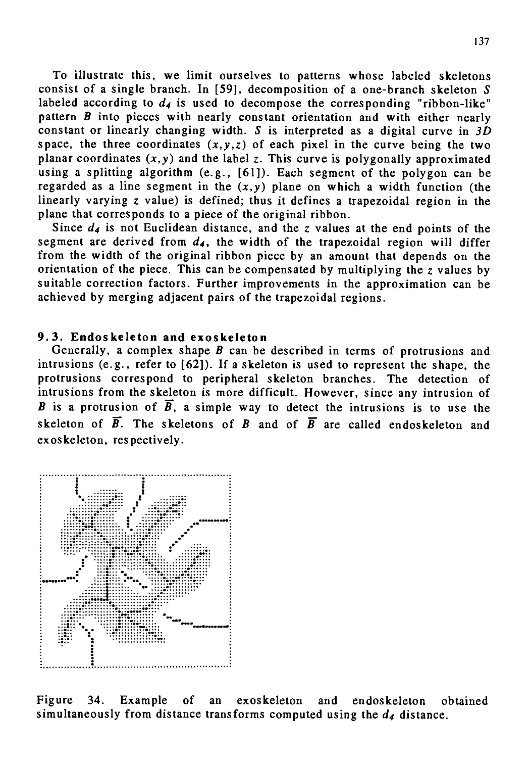
/


Author: Kong T. Yung Rosenfeld Azriel
Tags: information technology computer science
ISBN: 0 444 89754 2
Year: 1996


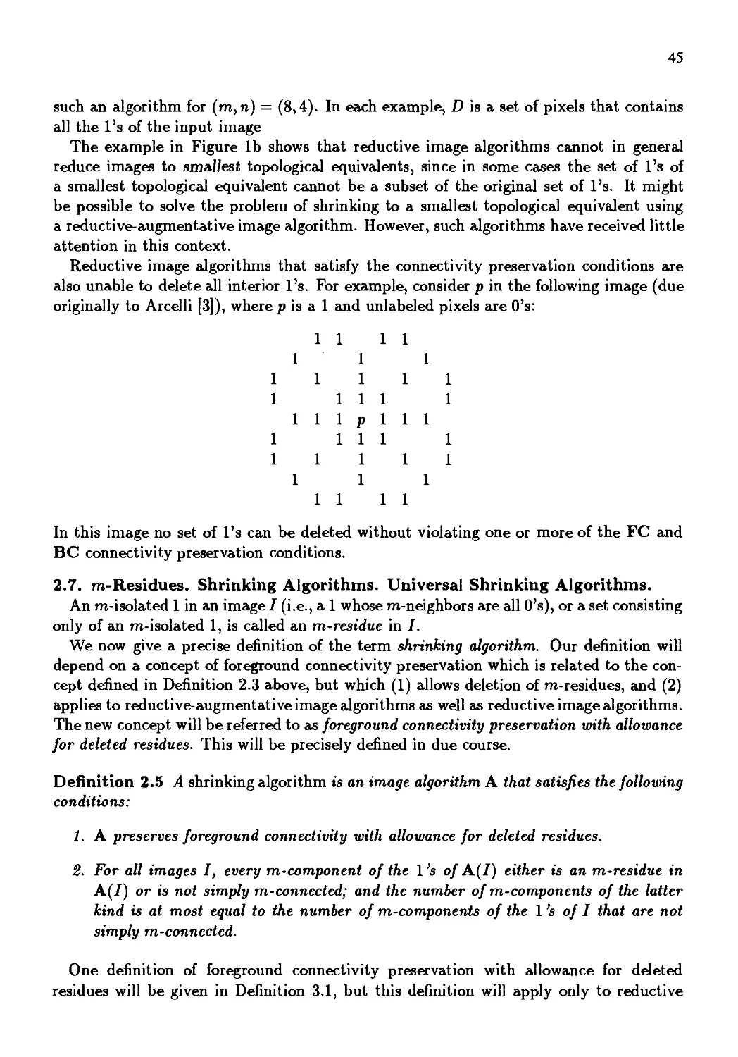
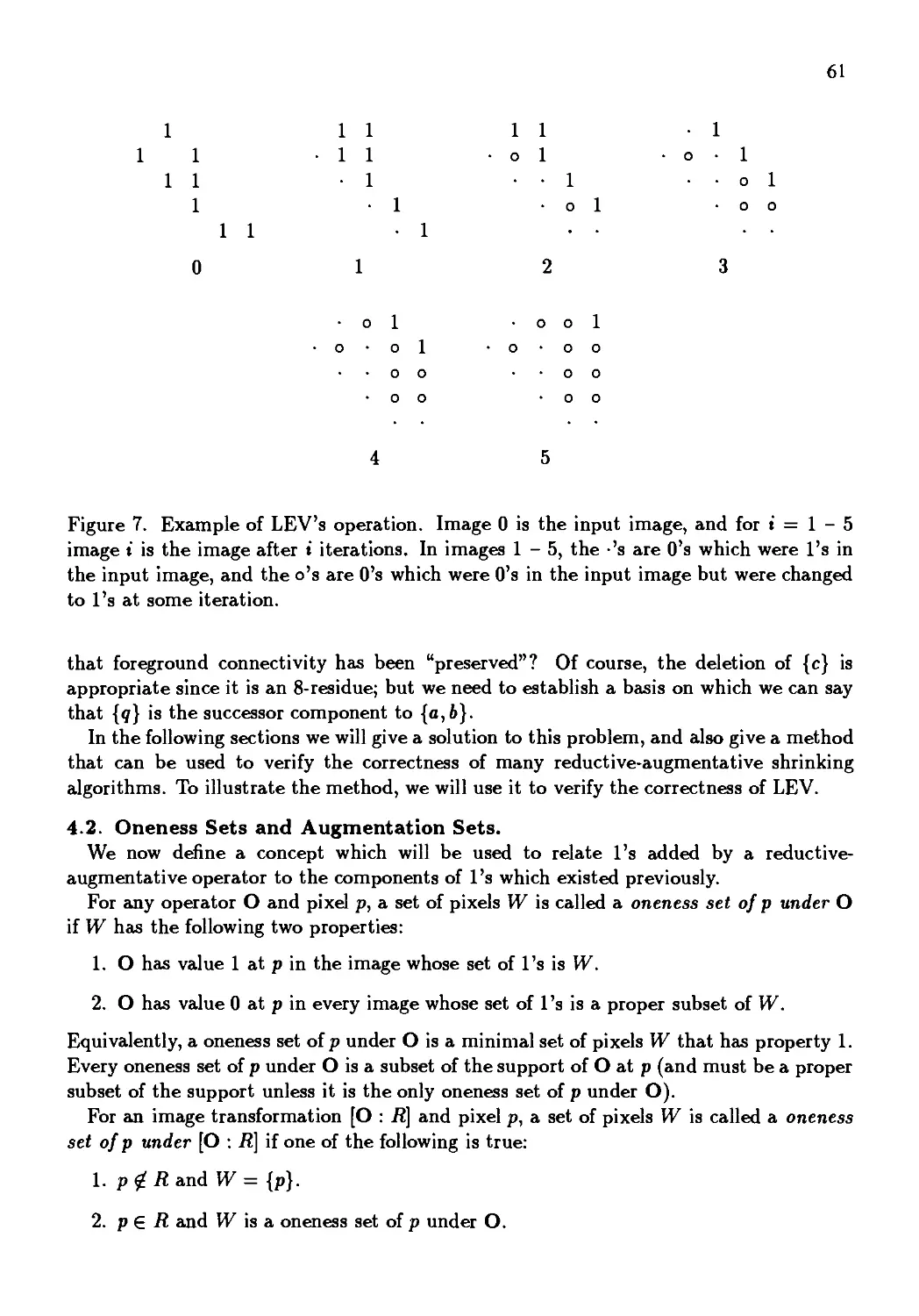
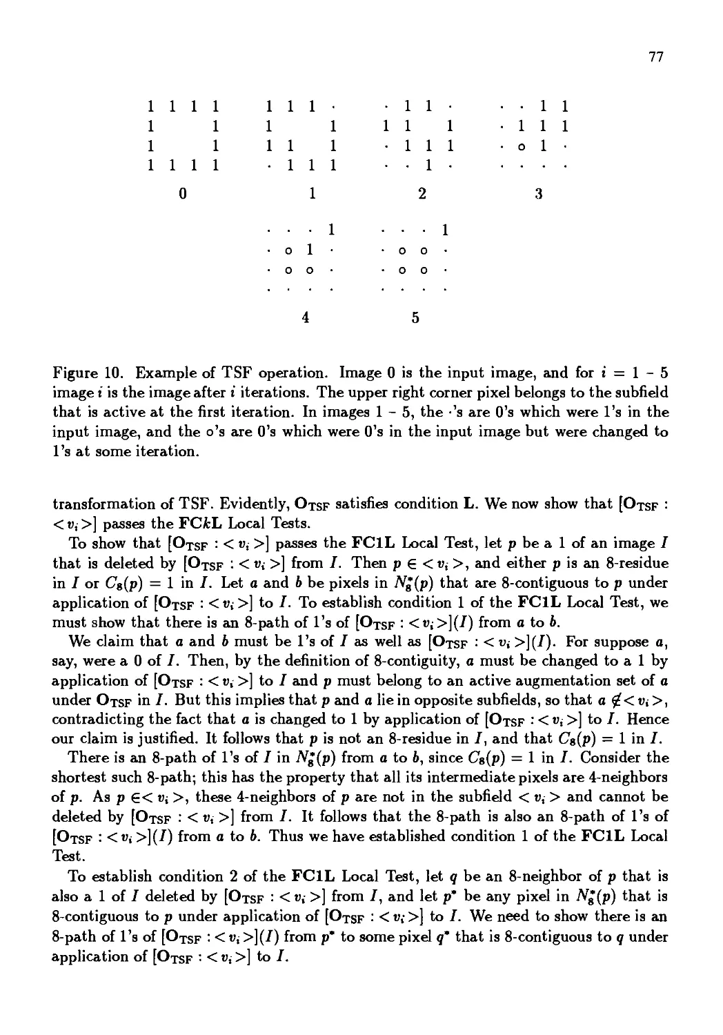
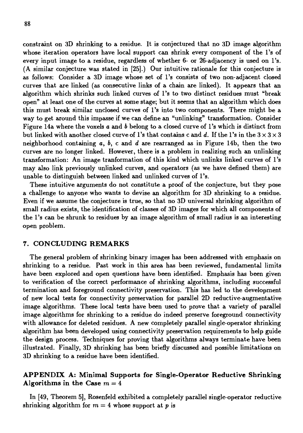
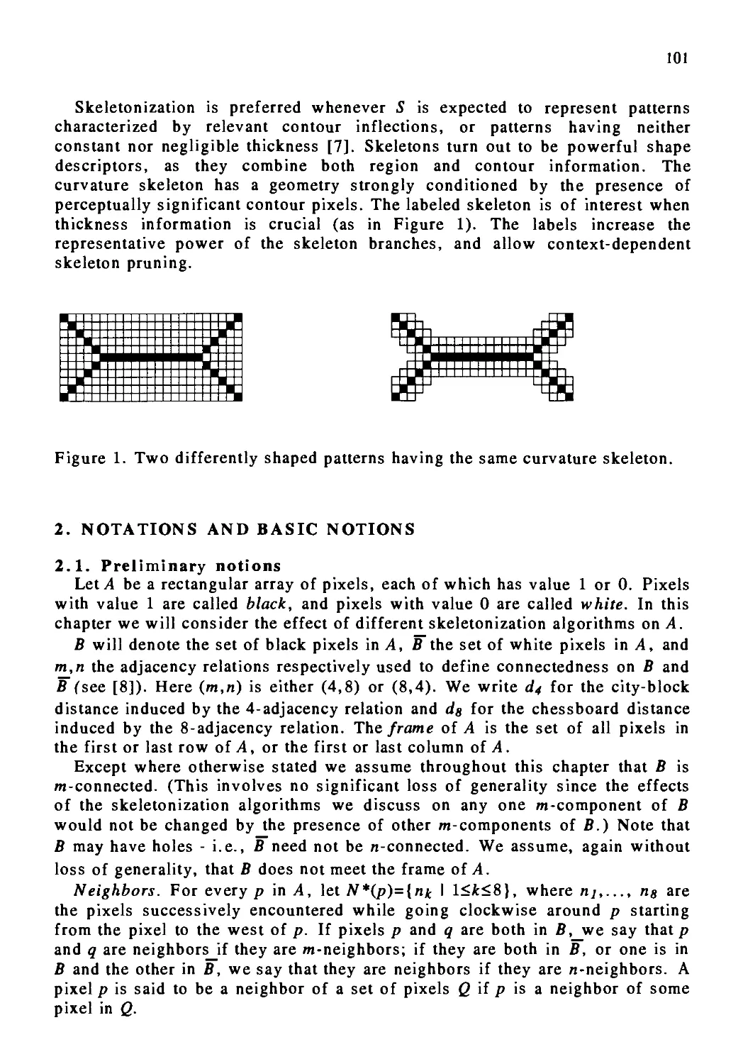
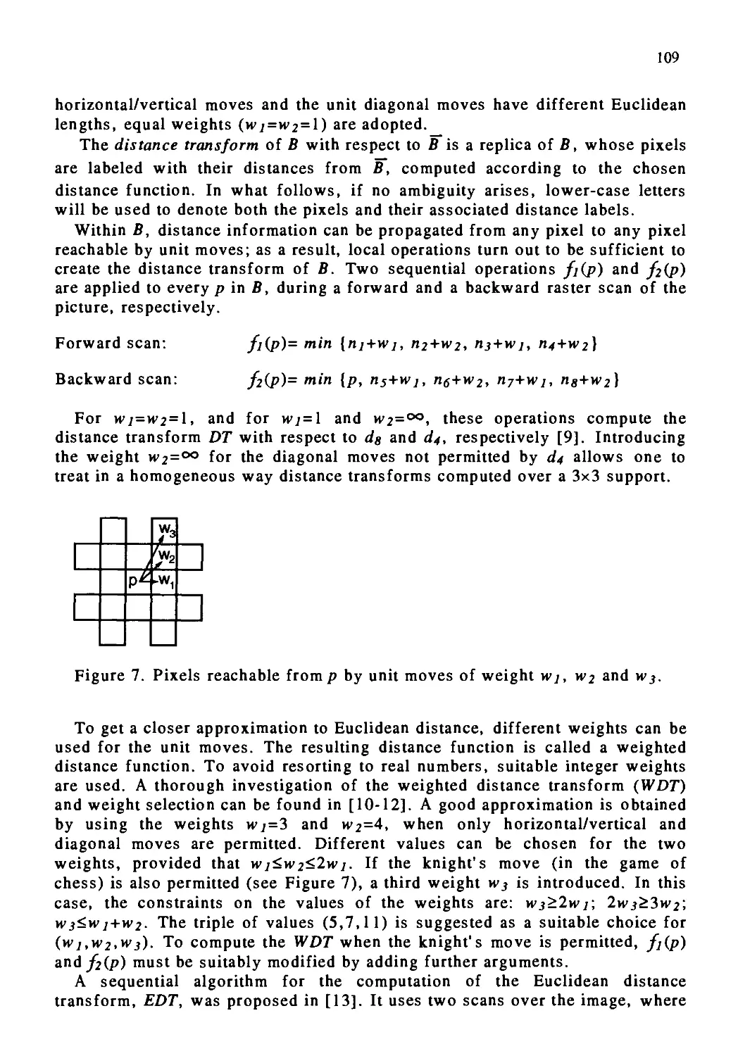
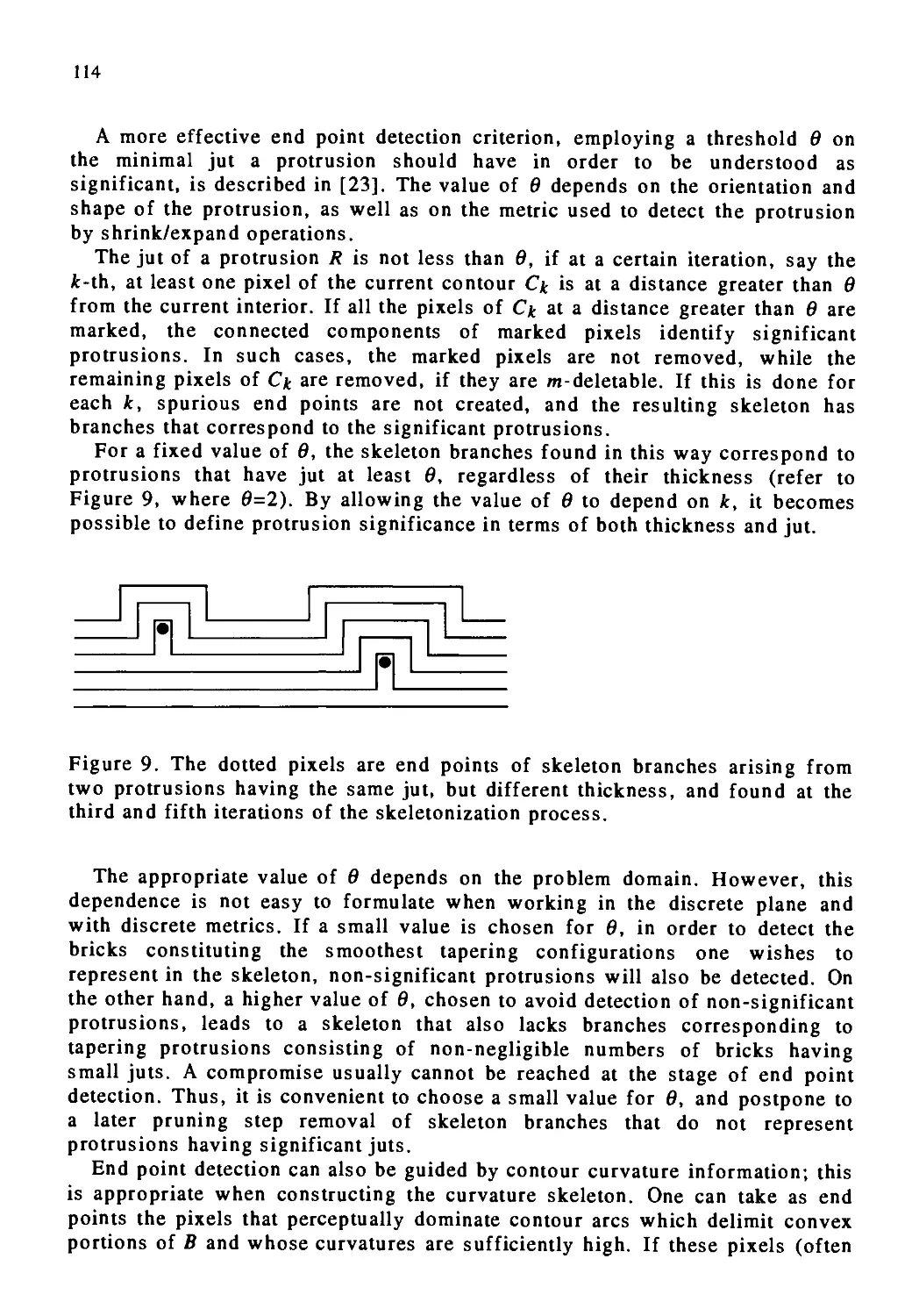
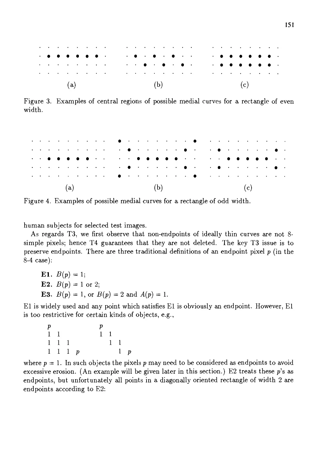
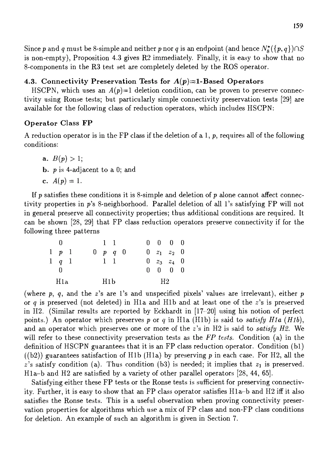
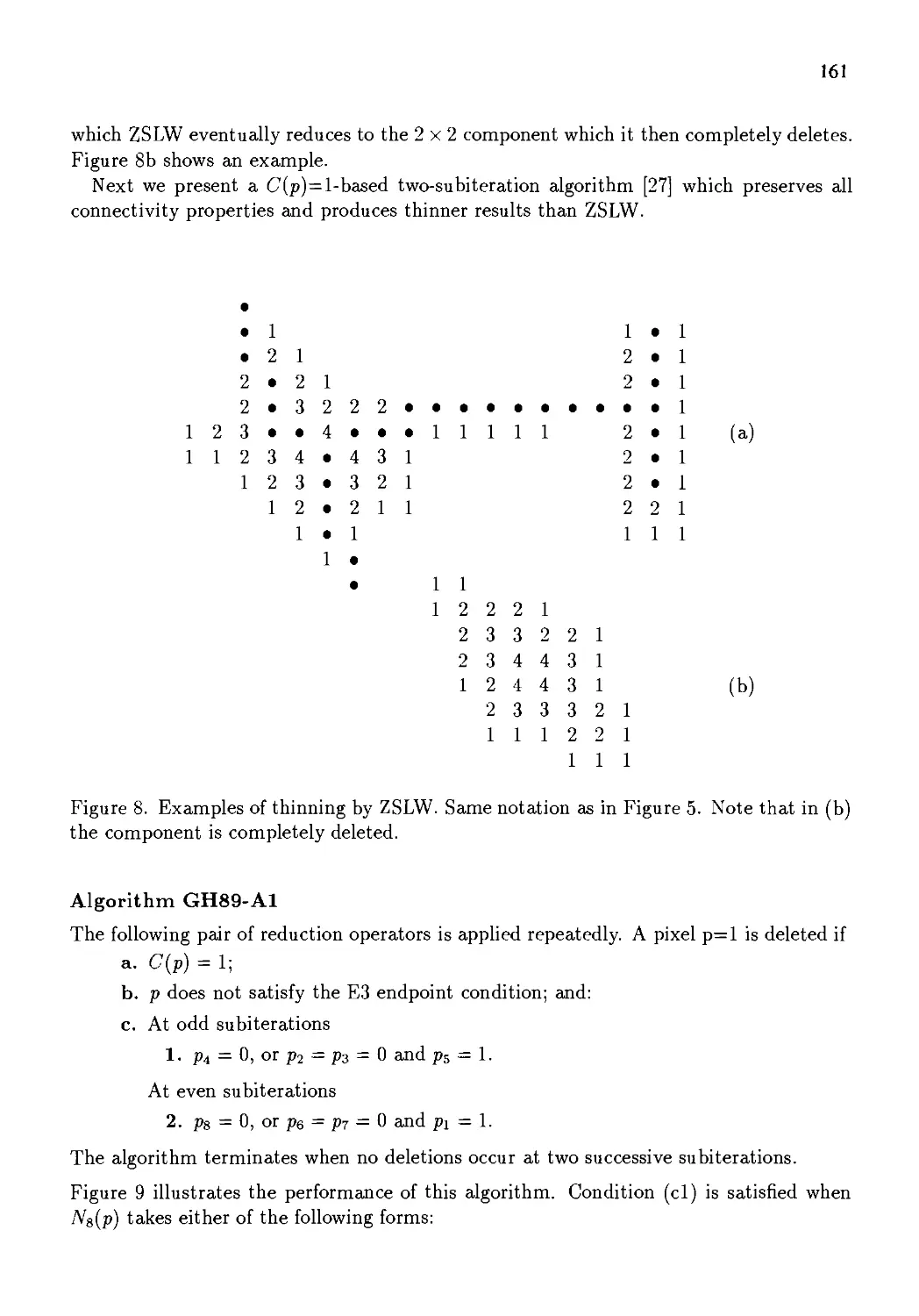
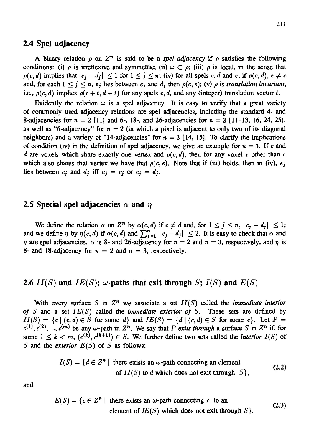
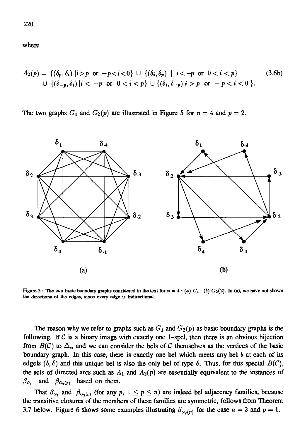
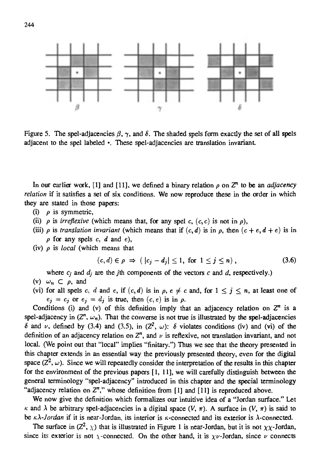
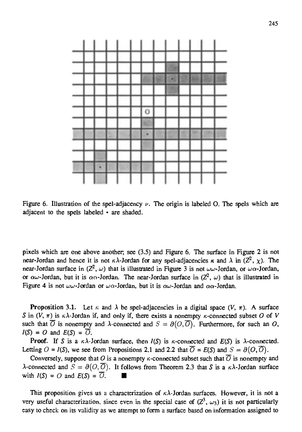
Text
--: я \ ■ :■< а ' ■■-. ■:■-.-
TOPOLOGICAL
ALGORITHMS FOR
DIGITAL IMAGE
PROCESSING
Edited by
T.Y. Kong
A Rosenfeld
ELSEVIER SCIENCE В. V.
Sara Burgerhartstraat 25
P.O. Box 211, 1000 AE Amsterdam, The Netherlands
ISBN: О 444 £9754 2
® 19% Elsevier Science B.V. All rights reserved.
No part of this* publication may be reproduced, stored in a retrieval system or transmitted in any form or
by any means, electronic, mechanical, photocopying, recording or otherwise, without the prior written
permission of the publisher, Elsevier Science B.V., Copyright & Permissions Department, P.O. Box 52 L
1000 ЛМ Amsterdam. The Netherlands,
Special regulations for readers in the U.S.A. - This publication has been registered with the Copyright
Clearance Center Inc, (CCC). Salem, Massachusetts. Information can be obtained from the CCC about
conditions under which photocopies of parts of this publication may be made in the U.S.A. All other
copyright questions, including photocopying outside of the U.S.A., should be referred to the copyright
owner. Elsevier Science B.V., unless oiherwisc specified.
No responsibility is assumed by the publisher for any injury and/or damage to persons or properly as a
matter of products liability, negligence or otherwise, or front any use or operation of any methods.
products, instructions or ideas contained in the materia I herein.
This book is printed on acid-free paper.
Printed in The Netherlands.
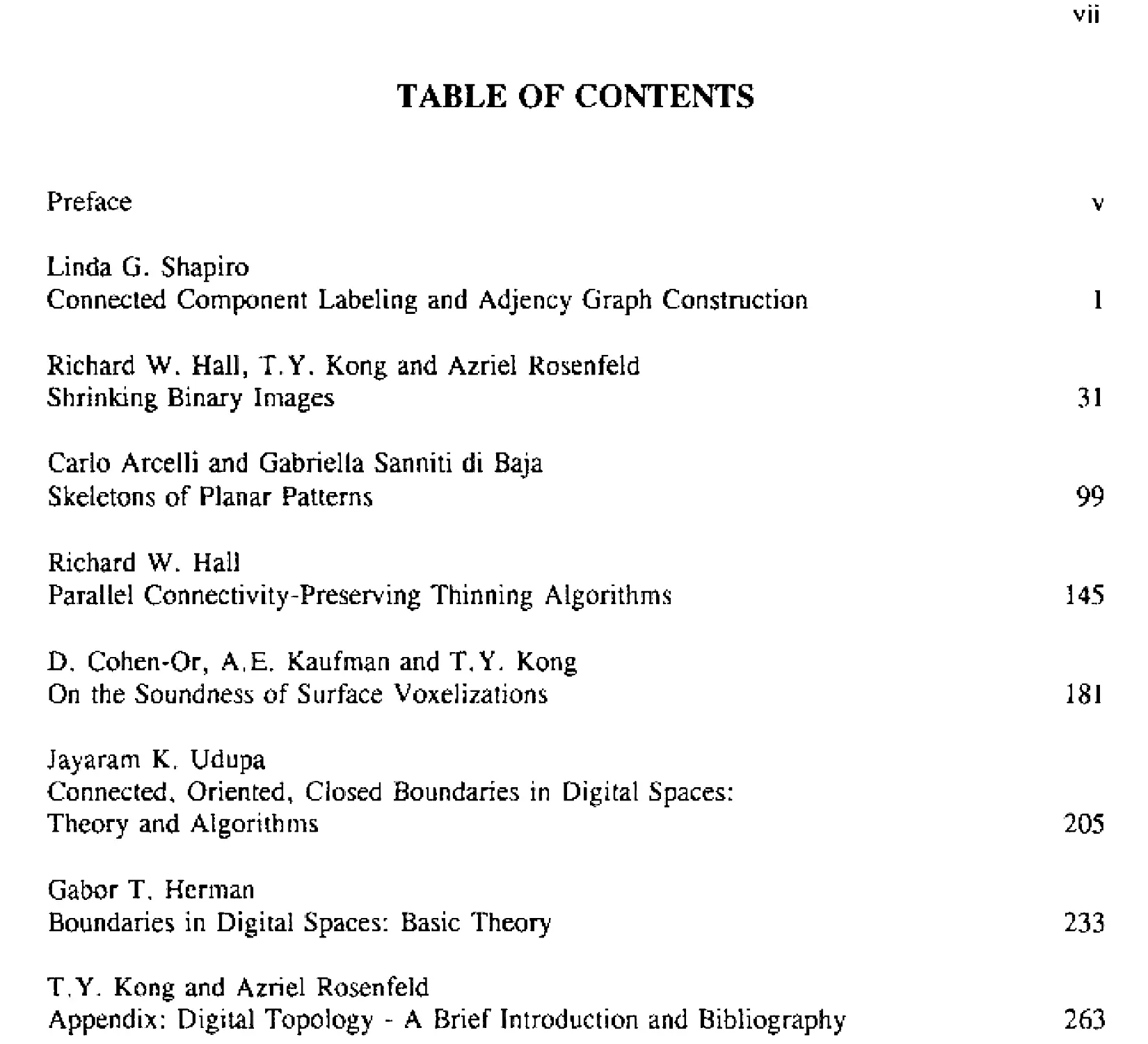
TABLE OF CONTENTS
Preface ν
Linda G. Shapiro
Connected Component Labeling and Adjency Graph Construction 1
Richard W. Hall, T.Y. Kong and Azriel Rosenfeld
Shrinking Binary Images 31
Carlo Arcelli and Gabriella Sanniti di Baja
Skeletons of Planar Patterns 99
Richard W. Hall
Parallel Connectivity-Preserving Thinning Algorithms 145
D, Cohen-Ог, A,E. Kaufman and T,Y. Kong
On the Soundness of Surface Voxelizations 181
Jayaram K, Udupa
Connected, Oriented, Closed Boundaries in Digital Spaces:
Theory and Algorithms 205
Gabor T, Herman
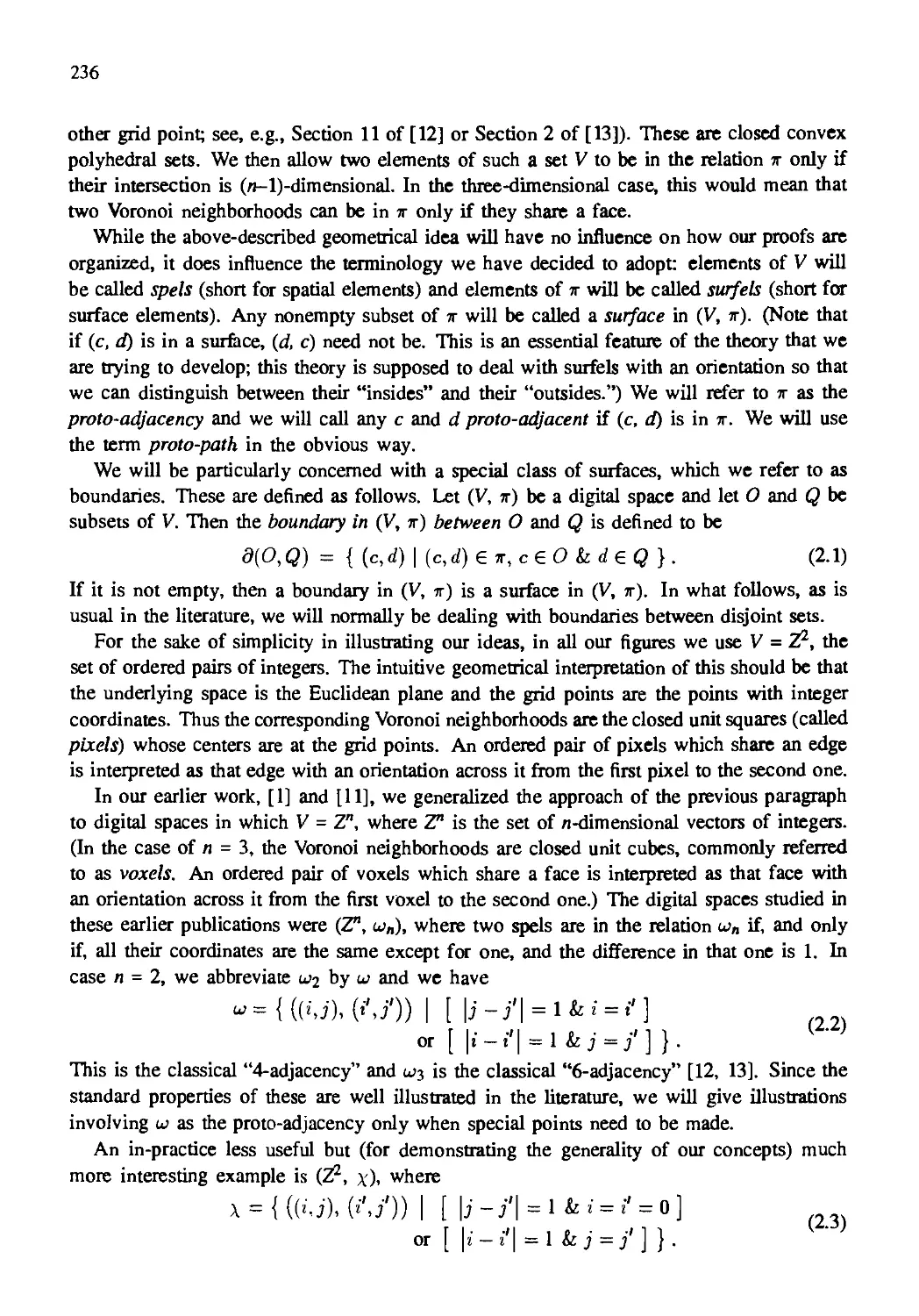
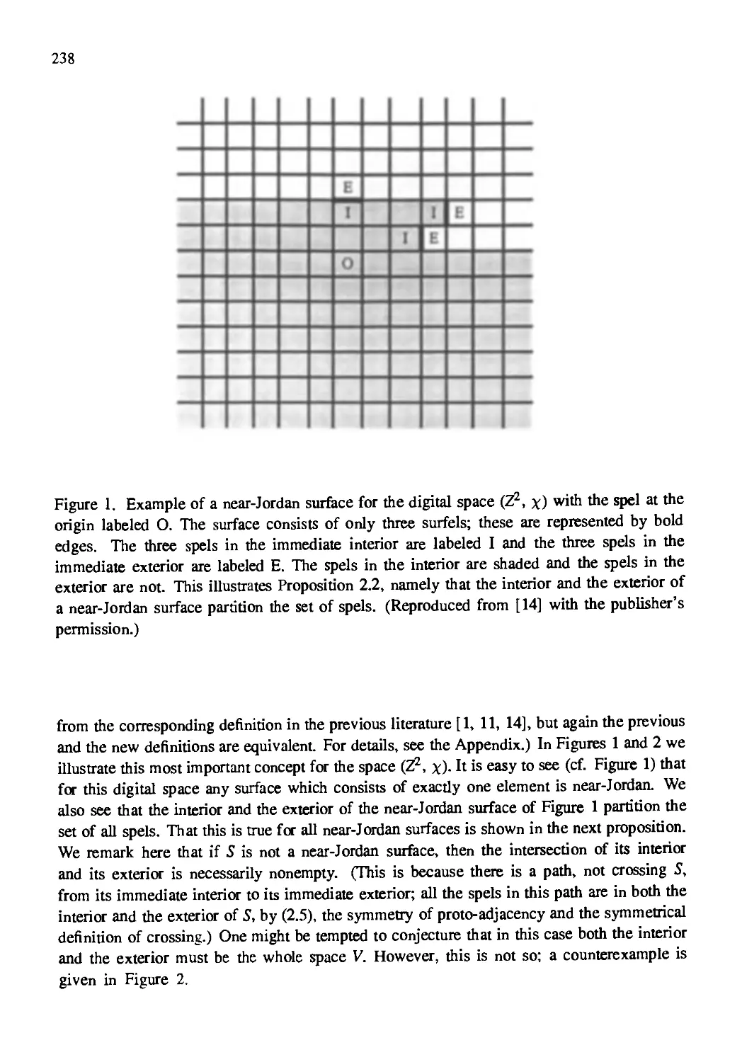
Boundaries in Digital Spaces: Basic Theory 233
T.Y. Kong and Azriel Rosenfeld
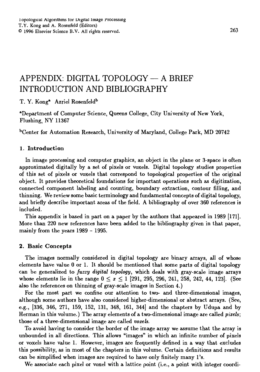
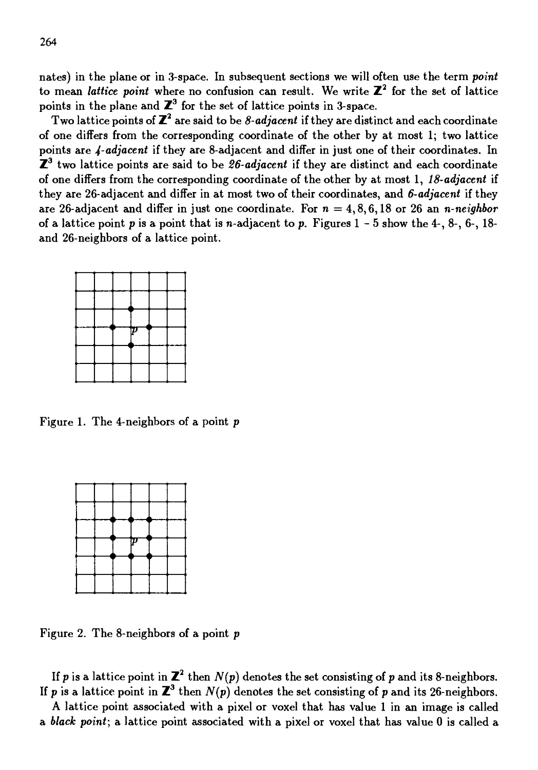
Appendix: Digital Topology - A Brief Introduction and Bibliography 263
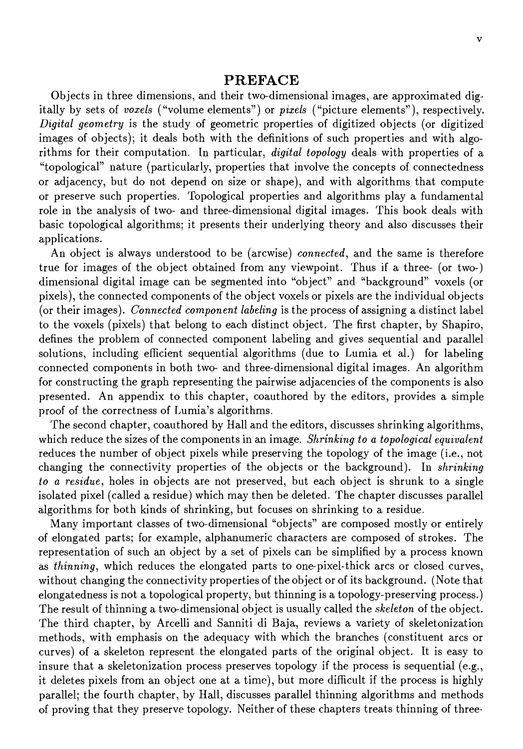
PREFACE
Objects in three dimensions, and their two-dimensional images, are approximated
digitally by sets of voxels ("volume elements") or pixels ("picture elements"), respectively.
Digital geometry is the study of geometric properties of digitized objects (or digitized
images of objects); it deals both with the definitions of such properties and with
algorithms for their computation. In particular, digital topology deals with properties of a
"topological" nature (particularly, properties that involve the concepts of connectedness
or adjacency, but do not depend on size or shape), and with algorithms that compute
or preserve such properties. Topological properties and algorithms play a fundamental
role in the analysis of two- and three-dimensional digital images. This book deals with
basic topological algorithms; it presents their underlying theory and also discusses their
applications.
An object is always understood to be (arcwise) connected, and the same is therefore
true for images of the object obtained from any viewpoint. Thus if a three- (or two-)
dimensional digital image can be segmented into "object" and "background" voxels (or
pixels), the connected components of the object voxels or pixels are the individual objects
(or their images). Connected component labeling is the process of assigning a distinct label
to the voxels (pixels) that belong to each distinct object. The first chapter, by Shapiro,
defines the problem of connected component labeling and gives sequential and parallel
solutions, including efficient sequential algorithms (due to Lumia et al.) for labeling
connected components in both two- and three-dimensional digital images. An algorithm
for constructing the graph representing the pairwise adjacencies of the components is also
presented. An appendix to this chapter, coauthored by the editors, provides a simple
proof of the correctness of Lumia's algorithms.
The second chapter, coauthored by Hall and the editors, discusses shrinking algorithms,
which reduce the sizes of the components in an image. Shrinking to a topological equivalent
reduces the number of object pixels while preserving the topology of the image (i.e., not
changing the connectivity properties of the objects or the background). In shrinking
to a residue, holes in objects are not preserved, but each object is shrunk to a single
isolated pixel (called a residue) which may then be deleted. The chapter discusses parallel
algorithms for both kinds of shrinking, but focuses on shrinking to a residue.
Many important classes of two-dimensional "objects" are composed mostly or entirely
of elongated parts; for example, alphanumeric characters are composed of strokes. The
representation of such an object by a set of pixels can be simplified by a process known
as thinning, which reduces the elongated parts to one-pixel-thick arcs or closed curves,
without changing the connectivity properties of the object or of its background. (Note that
elongatedness is not a topological property, but thinning is a topology-preserving process.)
The result of thinning a two-dimensional object is usually called the skeleton of the object.
The third chapter, by Arcelli and Sanniti di Baja, reviews a variety of skeletonization
methods, with emphasis on the adequacy with which the branches (constituent arcs or
curves) of a skeleton represent the elongated parts of the original object. It is easy to
insure that a skeletonization process preserves topology if the process is sequential (e.g.,
it deletes pixels from an object one at a time), but more difficult if the process is highly
parallel; the fourth chapter, by Hall, discusses parallel thinning algorithms and methods
of proving that they preserve topology. Neither of these chapters treats thinning of three-
dimensional objects, which is a more complicated subject; note that three-dimensional
objects can have two kinds of elongated parts, "stick-like" (which can be thinned to arcs
or curves) and "plate-like" (which can be thinned to one-voxel-thick "sheets").
The use of thin ("sheet-like") connected sets of voxels to represent surfaces in three-
dimensional Euclidean space, such as planes and spheres, is considered in the fifth chapter,
by Cohen-Or, Kaufman and Kong. They state precise conditions (some of which are due
to Morgenthaler and Rosenfeld) under which a set of voxels might be regarded as an
adequate representation of a mathematically defined surface, such as a plane specified by
an equation.
Assuming that voxels are defined as unit cubes, surfaces can also be represented by
sets of voxel faces (rather than by sets of voxels). This representation is quite natural for
surfaces that arise as boundaries of three-dimensional objects, and is readily generalized
to boundaries of η-dimensional "hyperobjects". The sixth chapter, by Udupa, describes
algorithms for extracting, labeling, and tracking boundaries represented in this way, in
any number of dimensions. The seventh chapter, by Herman, develops a general theory of
boundaries in abstract digital spaces, and shows that basic properties of connectedness and
separatedness of the interiors and exteriors of boundaries can be established in this general
framework. Fundamental soundness properties of algorithms such as those described in
Udupa's chapter can be deduced from special cases of results in Herman's chapter.
Because of the wide variety of topics treated in the seven chapters, we have not
attempted to standardize the notation and terminology used by their authors. However,
each chapter is self-contained and can be read independently of the others. Some of
the basic terminology and fundamental concepts of digital topology are reviewed in the
appendix, which also briefly describes important areas of the field and provides a
bibliography of over 360 references. The notations and terminologies used in this book will serve
to introduce its readers to the even wider variety that exists in the voluminous literature
dealing with topological algorithms.
T. Yung Kong
Queens, New York
Azriel Rosenfeld
College Park, Maryland
Topological Algorithms for Digital Image Processing
T.Y. Kong and A. Rosenfeld (Editors)
© 1996 Elsevier Science B.V. All rights reserved.
Connected Component Labeling and Adjacency Graph
Construction
Linda G. Shapiroa
"Department of Computer Science and Engineering, University of Washington, Seattle,
Washington 98195
Abstract
In machine vision, an original gray tone image is processed to produce features that
can be used by higher-level processes, such as recognition and inspection procedures.
Thresholding the image results in a binary image whose pixels are labeled as foreground or
background. Segmenting the image results in a symbolic image whose pixels are assigned
labels representing various classifications. In both cases, an important next step in the
analysis of the image is an operation called connected component labeling that groups the
pixels into regions, such that adjacent pixels have the same label, and pixels belonging to
distinct regions have different labels. Properties of the regions and relationships among
them may then be calculated. The most common relationship, spatial adjacency, can be
represented by a region adjacency graph. This chapter describes algorithms for connected
component labeling and region adjacency graph construction. In addition to giving several
sequential algorithms for two-dimensional connected component labeling, it also discusses
several parallel algorithms and an algorithm for three-dimensional connected component
labeling.
1. INTRODUCTION
Decomposition of an image into regions is a widely used technique in machine vision.
In many cases, the original gray tone image can be thresholded to produce a binary
image whose pixels are labeled as foreground or background. Objects of interest are the
connected regions composed of the foreground pixels. For example, in character
recognition, the image pixels comprising the characters form the foreground and the remaining
pixels the background. The general procedure is to produce the binary image, determine
the connected regions of its foreground pixels, calculate properties of these regions, and
apply a decision procedure to classify regions or select regions of interest. In character
recognition, the goal is to classify each of the characters.
In other applications, such as aerial image analysis, the image may be segmented into
many regions representing many different types of entities, such as buildings, streets,
grassy areas and forests. Each separate type of entity is represented by a different label
and the points of that entity are all assigned that label by the segmentation process. The
result is called a symbolic image. In this case, the general processing paradigm includes
segmenting the original image, determining the connected regions of pixels having each
2
label, calculating properties of each region, calculating the spatial relationships among
the regions, and applying a decision procedure to classify regions or sets of regions of
interest.
In both the binary case and the more general case, the analysis begins with an operation
called connected component labeling that groups adjacent image pixels that have the same
label into regions. In the general case, many different relationships among the regions
can be calculated. The most common relationship is spatial adjacency, which can be
represented by a graph structure called a region adjacency graph. This chapter describes
the algorithms required to perform connected component labeling and to construct the
region adjacency graph.
2. CONNECTED COMPONENT LABELING
Let us call the foreground pixels of a binary image the black pixels and the background
pixels the white pixels. Connected component analysis consists of connected component
labeling of the black pixels followed by property measurement of the component regions
and decision making. The connected component labeling operation changes the unit of
analysis from pixel to region or segment. All black pixels that are connected to each
other by a path of black pixels are given the same identifying label. The label is a unique
name or index of the region to which the pixels belong. A region has shape and position
properties, statistical properties of the gray levels of the pixels in the region, and spatial
relationships to other regions.
2.1. STATEMENT OF THE PROBLEM
Once a gray level image has been thresholded to produce a binary image, a connected
component labeling operator can be employed to group the black pixels into maximal
connected regions. These regions are called the (connected) components of the binary
image, and the associated operator is called the connected components operator. Its input
is a binary image and its output is a symbolic image in which the label assigned to each
pixel is an integer uniquely identifying the connected component to which that pixel
belongs. Figure 1 illustrates the connected components operator as applied to the black
pixels of a binary image.
Two black pixels ρ and q belong to the same connected component С if there is a
sequence of black pixels (ρο,Ρι, ■ ■ · ,Ρη) of С where p0 = ρ, ρη = q, and p,- is a neighbor of
p;_i (see Figure 2) for i = 1,..., n. Thus the definition of a connected component depends
on the definition of neighbor. When only the north, south, east, and west neighbors of
a pixel are considered to be in its neighborhood, then the resulting regions are called
^-connected. When the north, south, east, west, northeast, northwest, southeast, and
southwest neighbors of a pixel are considered to be in its neighborhood, the resulting
regions are called 8-connected. Whichever definition is used, the neighbors of a pixel are
said to be adjacent to that pixel. The border of a connected component of black pixels
is the subset of pixels belonging to the component that are adjacent to white pixels (by
whichever definition of adjacency is being used for the black pixels).
Rosenfeld (1970) has shown that if С is a component of black pixels and D is an
adjacent component of white pixels, and if 4-connectedness is used for black pixels and
3
0
0
1
0
0
0
0
1
1
1
0
3
3
3
1
1
1
0
0
3
3
0
0
0
0
0
3
3
2
2
2
2
0
3
0
0
0
0
2
0
3
0
0
2
2
2
0
0
0
0
0
1
0
0
0
0
1
1
1
0
1
1
1
1
1
1
0
0
1
1
0
0
0
0
0
1
1
1
1
1
1
0
1
0
0
0
0
1
0
1
0
0
1
1
1
0
0
0
(a) (b)
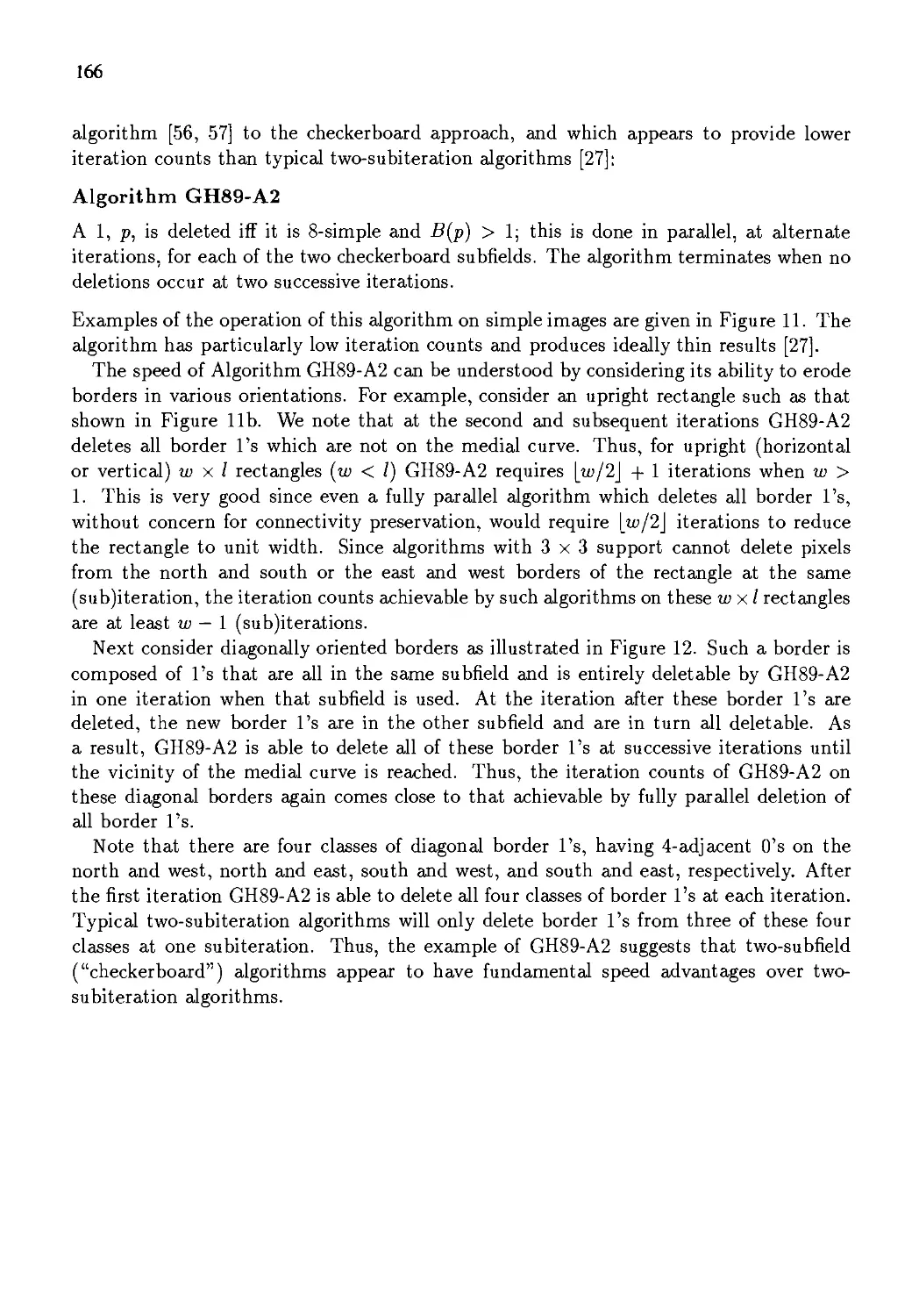
Figure 1. Application of the connected components operator to a binary image; (b)
Symbolic image produced from (a) by the connected components operator.
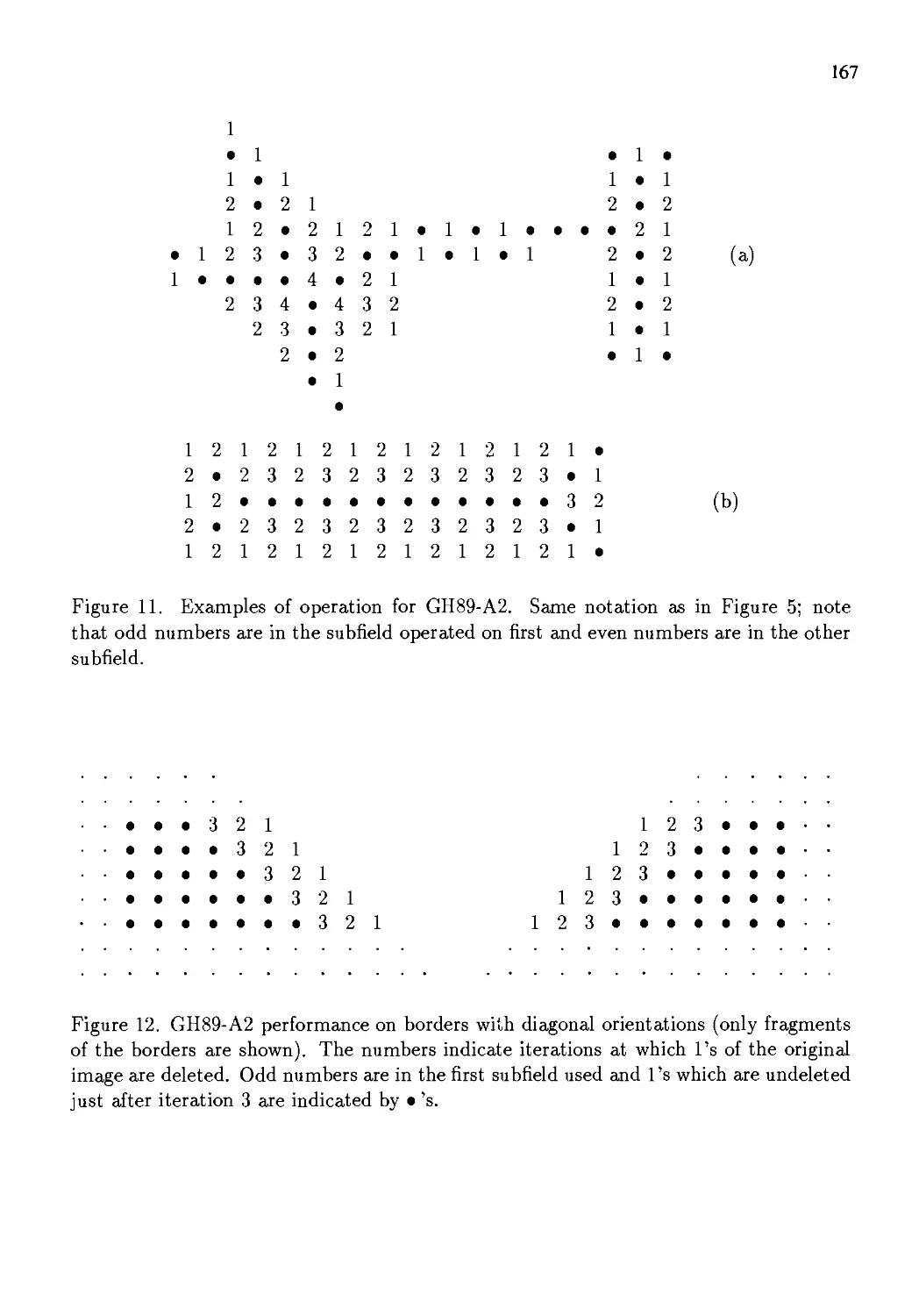
(a) (b)
Figure 2. (a) Pixels, ·, that are 4-neighbors of the center pixel x; (b) pixels, ·, that are
8-neighbors of the center pixel x.
8-connectedness is used for white pixels, then either С surrounds D (D is a hole in C)
or D surrounds С (С is a hole in D). This is also true when 8-connectedness is used for
black pixels and 4-connectedness for white pixels, but not when 4-connectedness is used
for both black pixels and white pixels and not when 8-connectedness is used for both
black pixels and white pixels. Figure 3 illustrates this phenomenon. The surroundedness
property is desirable because it allows borders to be treated as closed curves. Because
of this, it is common to use one type of connectedness for black pixels and the other for
white pixels .
The connected components operator is widely used in industrial applications where
an image often consists of a small number of objects against a contrasting background;
see Section 4 for examples. The speed of the algorithm that performs the connected
components operation is often critical to the feasibility of the application. In the next
three sections we discuss several algorithms that label connected components using two
sequential passes over the image.
All the algorithms process a row of the image at a time. Modifications to process a
rectangular window subimage at a time are straightforward. All the algorithms assign
new labels to the first pixel of each component and attempt to propagate the label of a
black pixel to its black neighbors to the right or below it (we assume 4-adjacency with a
left-to-right, top-to-bottom scan order). Consider the image shown in Figure 4. In the
first row, two black pixels separated by three white pixels are encountered. The first is
Ιο
0
0
ρ
1°
0
0
1
0
0
0
1
0
1
0
0
0
1
0
0
ol
0
0
0
0
(a)
a
a
a
a
a
a
a
1
a
a
a
1
a
1
a
a
a
1
a
a
a
a
a
a
a
alalala a|
a a 1 a a
a 2 b 3 a
a a 4 a a
a a|a|a(a|
(b)
alalala a|
a a 1 a a
a 1 b 1 a
a a 1 a a
a a|a(a(a|
(c)
(d)
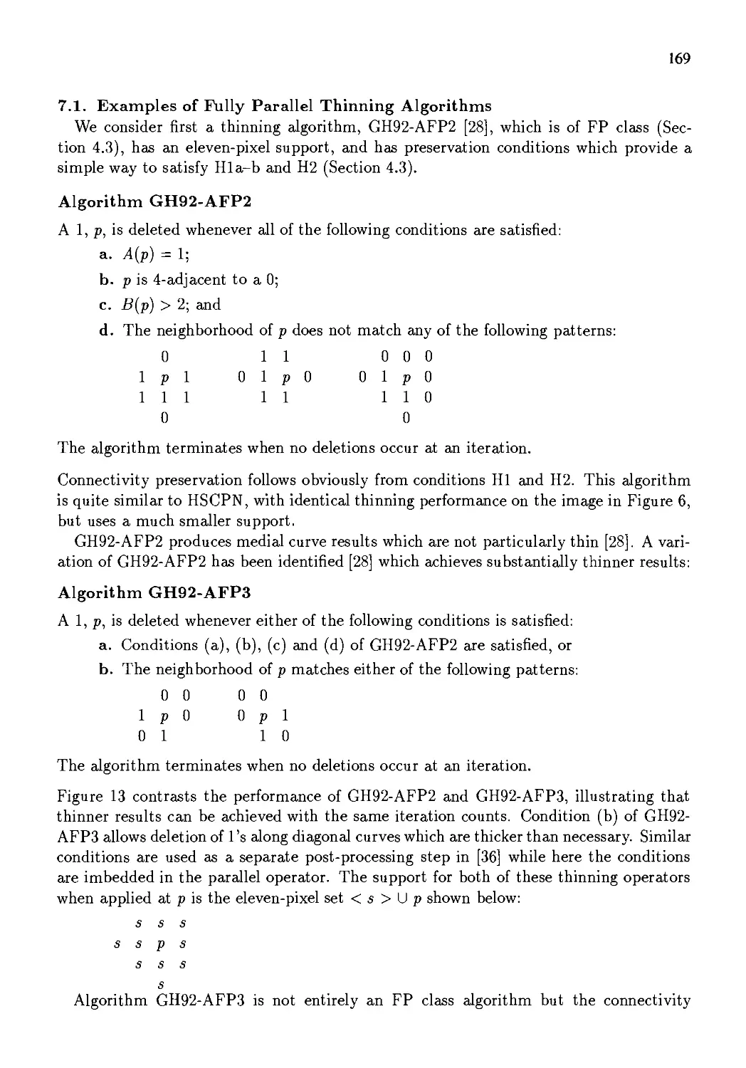
Figure 3. Phenomena associated with using 4- and 8-adjacency in connected component
analyses. Numeric labels are used for components of black pixels and letter labels for
white pixels, (a) Binary image; (b) connected component labeling with 4-adjacency used
for both white and black pixels; (c) connected component labeling with 8-adjacency used
for both white and black pixels; and (d) connected component labeling with 8-adjacency
used for black pixels and 4-adjacency used for white pixels.
assigned label 1; the second is assigned label 2. In row 2 the first black pixel is assigned
label 1 because it is a 4-neighbor of the already-labeled pixel above it. The second black
pixel of row 2 is also assigned label 1 because it is a 4-neighbor of the already-labeled pixel
on its left. This process continues until the black pixel marked A in row 4 is encountered.
Pixel A has a pixel labeled 2 above it and a pixel labeled 1 on its left, so that it connects
regions 1 and 2. Thus all the pixels labeled 1 and all the pixels labeled 2 really belong
to the same component; in other words, labels 1 and 2 are equivalent. The differences
among the algorithms are of three types, as reflected in the following questions.
1. What label should be assigned to pixel A?
2. How does the algorithm keep track of the equivalence of two (or more) labels?
3. How does the algorithm use the equivalence information to complete the processing?
2.2. THE CLASSICAL ALGORITHM
The classical algorithm, deemed so because it is based on the classical connected
components algorithm for graphs, was described in Rosenfeld and Pfaltz (1966). This algorithm
makes only two passes through the image but requires a large global table for recording
equivalences. The first pass performs label propagation, as described above. Whenever a
situation arises in which two different labels can propagate to the same pixel, the smaller
5
0
0
0
0
0
0
0
0
1
1
1
1
0
1
1
1
0
0
1
1
0
0
0
1
1
1
1
1
0
0
0
0
0
0
0
0
1
1
1
1
0
1
1
1
0
0
1
1
0
0
0
1
2
2
2
A
(a) (b)
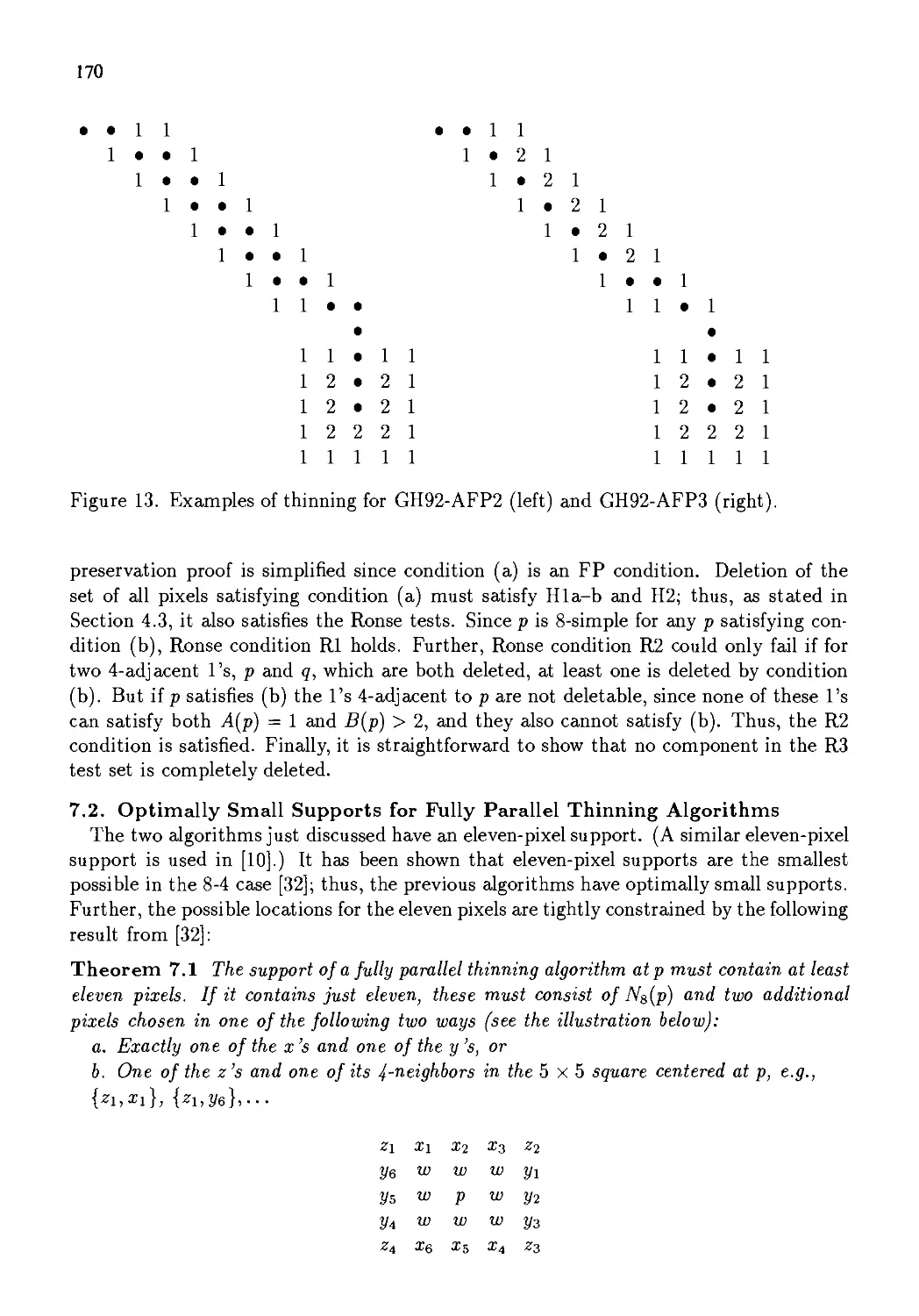
Figure 4. Propagation process. Label 1 has been propagated from the left to reach
point A. Label 2 has been propagated down to reach point A. The connected components
algorithm must assign a label to A and make labels 1 and 2 equivalent. Part (a) shows
the original binary image, and (b) the partially processed image.
label propagates and each such equivalence found is entered in an equivalence table. Each
entry in the equivalence table consists of an ordered pair, the values of its components
being the labels found to be equivalent. After the first pass, the equivalence classes are
found by taking the transitive closure of the set of equivalences recorded in the
equivalence table. Each equivalence class is assigned a unique label, usually the minimum (or
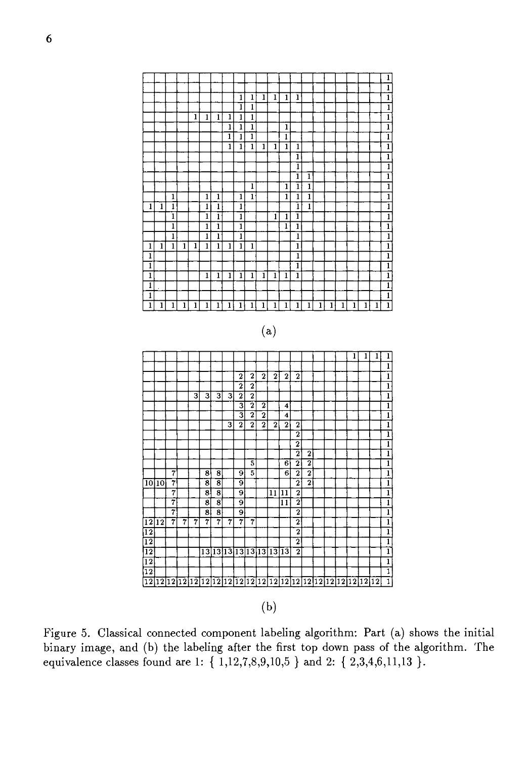
oldest) label in the class. Finally, a second pass through the image performs a translation,
assigning to each pixel the label of the equivalence class of its pass-1 label. This process
is illustrated in Figure 5, and an implementation of the algorithm is given below.
procedure CLASSICAL
"InitiaUze global equivalence table."
EQTABLE := CREATE( );
"Top-down pass 1"
for L := 1 to NROWS do
"Initialize all labels on row L to zero."
for Ρ := 1 to NCOLS do
LABEL(L,P) := 0
"Process the row."
for Ρ := 1 to NCOLS do
if I(L,P) = 1 then
A := NEIGHBORS((L,P));
if ISEMPTY(A)
then Μ := NEWLABEL( )
else
begin
Μ := MIN(LABELS(A));
for X in LABELS(A) and Χ Ο Μ do
ADD(X, M, EQTABLE)
(a)
Figure 5. Classical connected component labeling algorithm: Part (a) shows the initial
binary image, and (b) the labeling after the first top down pass of the algorithm. The
equivalence classes found are 1: { 1,12,7,8,9,10,5 } and 2: { 2,3,4,6,11,13 }.
LABEL(L,P) := Μ;
end for
"Find equivalence classes."
EQCLASSES := RESOLVE(EQTABLE);
for Ε in EQCLASSES do
EQLABEL(E) := MIN(LABELS(E))
"Top-down pass 2"
for L := 1 to NROWS do
for Ρ := 1 to NCOLS do
if I(L,P) = 1
then LABEL(L,P) := EQLABEL(CLASS(LABEL(L,P)))
end for
end for
end CLASSICAL
The notation NEIGHBORS((L,P)) refers to the already-encountered 1-valued neighbors
of pixel (L,P). The algorithm referred to as RESOLVE is simply the algorithm for finding
the connected components of the graph defined by the set of equivalences (EQTABLE)
defined in pass 1. The nodes of the graph are region labels, and the edges are pairs
of labels that have been found to be equivalent. The procedure, which uses a standard
depth-first search algorithm, can be stated as follows:
procedure RESOLVE(EQTABLE);
list_of_components := nil;
for each node N in EQTABLE
if N is unmarked then
current-component := DFS(N,EQTABLE);
add_toJist(list-of_components,current_component)
return LIST-OF-COMPONENTS
end RESOLVE
In this procedure, UsLof-Components is a list that will contain the final resultant
equivalence classes. The function DFS performs a depth-first search of the graph beginning
at the given node N and returns a list of all the nodes it has visited in the process. It
also marks each node as it is visited. A standard depth-first search algorithm is given in
Horowitz and Sahni (1982) and in most other data structures texts.
In procedure CLASSICAL, determination of the smallest equivalents of the labels
involves examining the labels in each equivalence class after all the equivalence classes have
been explicitly constructed. However, the smallest equivalent labels can be found a little
more efficiently by using the fact that if the labels in EQTABLE are processed in
ascending order, then N is the smallest equivalent of each label visited by DFS(N,EQTABLE).
The complexity of the classical algorithm for an η χ η image is 0{n2) for the two passes
through the image, plus the complexity of RESOLVE which depends on the number of
equivalent pairs in EQTABLE. The main problem with the classical algorithm is the
global table. For large images with many regions, the table can become very large. On
some machines there is not enough memory to hold the table. On other machines that
use paging, the table gets paged in and out of memory frequently. For example, on a VAX
11/780 system with 8 megabytes of memory, the classical algorithm ran (including I/O)
in 8.4 seconds with 1791 page faults on one 6000 pixel image, but took 5021 seconds with
23,674 page faults on one 920,000-pixel image. This motivates algorithms that avoid the
use of the large global equivalence table for computers employing virtual memory.
2.3. THE LOCAL TABLE METHOD. A SPACE EFFICIENT TWO-PASS
ALGORITHM
One solution to the space problem is the use of a small local equivalence table that
stores only the equivalences detected from the current row of the image and the row that
precedes it. Thus the maximum number of equivalences is the number of pixels per row.
These equivalences are then resolved, and the pixels are relabeled in a second scan of
the row; the new labels are then propagated to the next row. In this case not all the
equivalencing is completed by the end of the first (top-down) pass, and a second pass is
required for both finding the remainder of the equivalences and assigning the final labels.
The algorithm is illustrated in Figure 6. Note that the second pass is bottom-up. We
will give the general algorithm (Lumia, Shapiro, and Zuniga, 1983) and then describe, in
more detail, an efficient run-length implementation.
procedure LOCAL.TABLE.METHOD
"Top-down pass"
for L:=l to NROWS do
"Initialize local equivalence table for row L."
EQTABLE := CREATE( );
"Initialize all labels on row L to zero."
for Ρ := 1 to NCOLS do
LABEL(L,P) := 0
"Process the row."
for Ρ := 1 to NCOLS do
if I(L,P) = 1 then
begin
A := NEIGHBORS((L,P));
if ISEMPTY(A)
then Μ := NEWLABEL( )
begin
Μ := MIN(LABELS(A) );
for X in LABELS(A) and Χ ο Μ do
ADD (X,M, EQTABLE)
Figure 6. Results after the top-down pass of the local table method on the binary image
of Figure 5. Note that on the rows where equivalences were detected, the pixels have
different labels from those they had after pass 1 of the classical algorithm. For example,
on row 5 the four leading 3s were changed to 2s on the second scan of that row, after the
equivalence of labels 2 and 3 was detected. The bottom up pass will now propagate the
label 1 to all pixels of the single connected component.
LABEL(L,P) := M;
end for;
"Find equivalence classes detected on this row."
EQCLASSES := RESOLVE(EQTABLE);
for Ε in EQCLASSES do
EQLABEL(E) := MIN(LABELS(E))
"Relabel the parts of row L with their equivalence class labels."
for Ρ := 1 to NCOLS do
if I(L,P) = 1
then LABEL(L,P) := EQLABEL(CLASS(LABEL(L,P)))
end for
"Bottom-up pass"
for L := NROWS-1 to 1 by -1 do
"Initialize local equivalence table for row L."
EQTABLE := CREATE( );
"Process the row."
for Ρ := 1 to NCOLS do
10
if LABEL(L,P) <>0 then
LA := LABELS(NEIGHBORS(L,P));
for X in LA and X <> LABEL(L,P)
ADD (X,LABEL(L,P), EQTABLE)
end for
"Find equivalence classes."
EQCLASSES := RESOLVE(EQTABLE);
for Ε in EQCLASSES do
EQLABEL(E) := MIN(LABELS(E))
"Relabel the pixels of row L one last time."
for Ρ := 1 to NCOLS do
if LABEL(L,P) <> 0
then LABEL(L,P) := EQLABEL(CLASS(LABEL(L,P)))
end for
end LOCAL.TABLE_METHOD
Note that the set NEIGHBORS((L,P)) of already-processed 1-valued neighbors of pixel
(L,P) is different in the top-down and bottom-up passes.
The complexity of the local table method for an η χ η image is also 0(n2) + η times
the complexity of RESOLVE for one row of equivalences. However, in comparison with
the classical algorithm, the local table method took 8.8 seconds with 1763 page faults on
the 6000-pixel image, but only 627 seconds with 15,391 page faults on the 920,000-pixel
image, which is 8 times faster. For an even larger 5,120,000-pixel image, the local table
method ran 31 times faster than the classical method.
2.4. AN EFFICIENT RUN LENGTH IMPLEMENTATION OF THE LOCAL
TABLE METHOD
In many industrial applications the image used is from a television camera and thus
is roughly 512 x 512 pixels, or 256K, in size. On an image half this size, the local table
method as implemented on the VAX 11/780 took 116 seconds to execute, including I/O
time. But industrial applications often require times of less than one second. To achieve
this kind of efficiency, the algorithm can be implemented on a machine with some special
hardware capabilities. The hardware is used to rapidly extract a run-length encoding of
the image, and the software implementation can then work on the more compact run-
length data. Ronse and Devijver (1984) advocate this approach.
A run-length encoding of a binary image is a list of contiguous (typically, horizontal)
runs of black pixels. For each run, the location of the starting pixel of the run and either
its length or the location of its ending pixel must be recorded. Figure 7 shows the run-
length data structure used in our implementation. Each run in the image is encoded by
the locations of its starting and ending pixels. (ROW, START_COL) is the location of the
starting pixel and (ROW, END .COL) is the location of the ending pixel. PERM-LABEL
11
is the field in which the label of the connected component to which this run belongs will be
stored. It is initialized to zero and assigned temporary values in pass 1 of the algorithm.
At the end of pass 2, PERM-LABEL contains the final, permanent label of the run. This
structure can then be used to output the labels back to the corresponding pixels of the
output image.
1
2
3
4
5
ROW_START
1
3
5
0
7
ROW.END
2
4
6
0
7
(a) (b)
1
2
3
4
5
6
7
ROW
1
1
2
2
3
3
5
START.COL
1
4
1
5
1
5
2
END_COL
2
5
2
5
3
5
5
PERM.LABEL
0
0
0
0
0
0
0
(c)
Figure 7. Binary image (a) and its run-length encoding (b) and (c). Each run of black
pixels is encoded by its row (ROW) and the columns of its starting and ending pixels
(START.COL and END.COL). In addition, for each row of the image, ROW_START
points to the first run of the row and ROW_END points to the last run of the row. The
PERM_LABEL field will hold the component label of the run; it is initialized to zero.
Consider a run Ρ of black pixels. During pass 1, when Ρ has not yet been fully
processed, PERM_LABEL(P) will be zero. After Ρ has been processed and found to be
adjacent to some other run Q on the previous row, it will be assigned the current label
of Q, PERM.LABEL(Q). If it is found to be adjacent to other runs Qb Q2,..., QK also
on the previous row, then the equivalence of PERM.LABEL(Q), PERM-LABEL^),
PERM_LABEL(Q2),..., PERM.LABEL(Qk) must be recorded. The data structures
used for recording the equivalences are shown in Figure 8. The use of simple linked lists
to store equivalences makes the assumption that there will be very few elements in an
equivalence class that is based on only two rows of the image. For storing, accessing, and
dynamically updating large equivalence classes, the и
may be preferable.
m-find algorithm (Tarjan, 1975)
1
2
3
4
ROW
1
1
1
2
START_COL
4
20
30
7
END_COL
10
24
3Θ
35
PERM_LABEL
1
2
3
1
1
2
3
UBEL
1
1
1
3
0
m
Figure 8. Data structures used for keeping track of equivalence classes. In this example,
run 4 has PERM_LABEL 1; this is an index into the LABEL array that gives the
equivalence class label for each possible PERM-LABEL value. In the example, PERM.LABELS
1, 2, and 3 have all been determined to be equivalent, so LABEL(l), LABEL(2), and LA-
BEL(3) all contain the equivalence class label, which is 1. Furthermore, the equivalence
class label is an index into the EQ-CLASS array that contains pointers to the
beginnings of the equivalence classes; these are linked lists in the LABEL/NEXT structure.
In this example, there is only one equivalence class, class 1, and three elements of the
LABEL/NEXT array are linked together to form this class.
algorithm, PERM.LABEL(P), for a given run P, may be zer(
., then LABEL(PERM.LABEL(P)) may be zero or nonzero. If it is zero, then
PERM.LABEL(P) is the current label of the run and there is no equivalence class. If it is
non-zero, then there is an equivalence class and the value of LABEL(PERM-LABEL(P))
is the label assigned to that class. All the labels that have been merged to form this
class will have the same class label; that is, if run Ρ and run P' are in the same class, we
should have LABEL(PERM.LABEL(P)) = LABEL(PERM.LABEL(P')). When such an
equivalence is determined, if each run was already a member of a class and the two classes
were different, the two classes are merged. This is accomplished by linking together each
prior label belonging to a single class into a linked list pointed to by EQ-CLASS(L) for
class label L and linked together using the NEXT field of the LABEL/NEXT structure.
To merge two classes, the last cell of one is made to point to the first cell of the other,
and the LABEL field of each cell of the second class is changed to reflect the new label
of the class.
In this implementation the minimum label does not always become the label of the
equivalence class. Instead, a single-member class is always merged into and assigned the
label of a multimember class. This allows the algorithm to avoid traversing the linked list
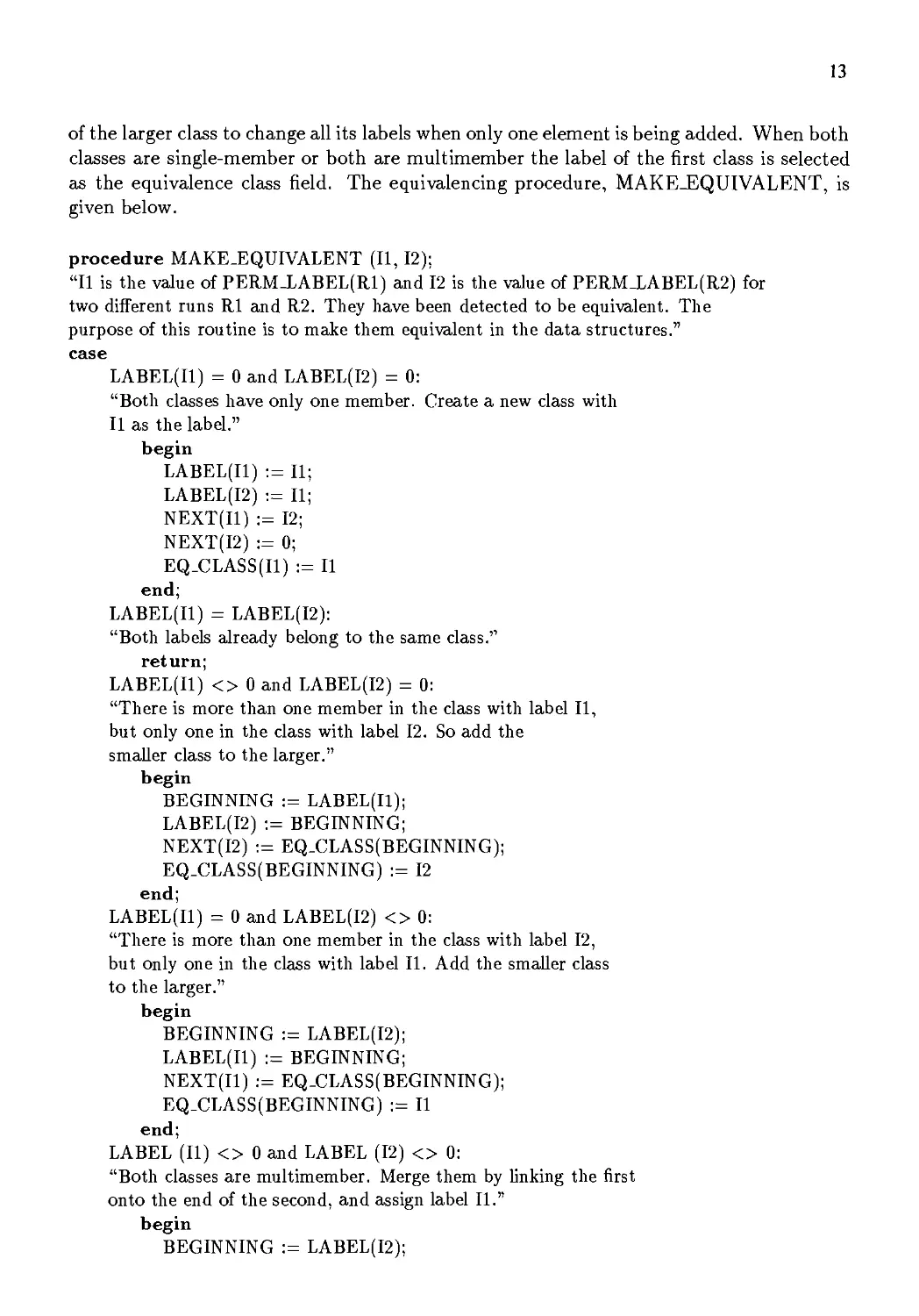
13
of the larger class to change all its labels when only one element is being added. When both
classes are single-member or both are multimember the label of the first class is selected
as the equivalence class field. The equivalencing procedure, MAKE_EQUIVALENT, is
given below.
procedure MAKE_EQUIVALENT (II, 12);
"II is the value of PERMJLABEL(Rl) and 12 is the value of PERM_LABEL(R2) for
two different runs Rl and R2. They have been detected to be equivalent. The
purpose of this routine is to make them equivalent in the data structures."
LABEL(Il) = 0 and LABEL(I2) = 0:
"Both classes have only one member. Create a new class with
И as the label."
begin
LABEL(Il) := II;
LABEL(I2) := II;
NEXT(Il) := 12;
NEXT(I2) := 0;
EQ_CLASS(I1) := И
LABEL(Il) = LABEL(I2):
"Both labels already belong to the same class."
return;
LABEL(Il) <> 0 and LABEL(I2) = 0:
"There is more than one member in the class with label II,
but only one in the class with label 12. So add the
smaller class to the larger."
BEGINNING := LABEL(Il);
LABEL(I2) := BEGINNING;
NEXT(I2) := EQ_CLASS(BEGINNING);
EQ_CLASS(BEGINNING) := 12
LABEL(Il) = 0 and LABEL(I2) <> 0:
"There is more than one member in the class with label 12,
but only one in the class with label II. Add the smaller class
BEGINNING := LABEL(I2);
LABEL(Il) := BEGINNING;
NEXT(Il) := EQ_CLASS(BEGINNING);
EQ_CLASS(BEGINNING) := II
end;
LABEL (II) <> 0 and LABEL (12) <> 0:
"Both classes are multimember. Merge them by Unking the first
onto the end of the second, and assign label II."
begin
BEGINNING := LABEL(I2);
MEMBER := EQ_CLASS(BEGINNING);
EQ_LABEL := LABEL(Il);
while NEXT(MEMBER) <> 0 do
LABEL(MEMBER) := EQ_LABEL;
MEMBER := NEXT(MEMBER)
end while;
LABEL(MEMBER) := EQ_LABEL;
NEXT(MEMBER) := EQ.CLASS(EQ.LABEL);
EQ_CLASS(EQ.LABEL) := EQ.CLASS(BEGINNING);
EQ_CLASS(BEGINNING) := 0
end case;
end MAKE_EQUIVALENT
Using this procedure and a utility procedure, INITIALIZE.EQUIV,
which reinitializes the equivalence table for the processing of a new line,
the run length implementation is as follows:
procedure RUNJLENGTHJMPLEMENTATION
"Initialize PERMJLABEL array."
for R := 1 to NRUNS do
PERM.LABEL(R) := 0
"Top-down pass"
for L := 1 to NROWS do
Ρ := ROW-START(L);
PLAST := ROW_END(L);
if L= 1
then begin Q := 0; QLAST := 0 end
else begin Q := ROW-START(L-l); QLAST := ROW_END(L-l) end;
if Ρ <> Oand Q <> 0
then
INITIALIZE.EQUIV( );
"SCAN 1"
"Either a given run is connected to a run on the previous row or
lot. If it is, assign it the label of the first run to which it
mected. For each subsequent run of the previous row to which it
is connected and whose label is different from its own, equivalence its
label with that run's label."
while P< PLAST and Q < QLAST do
"Check whether runs Ρ and Q overlap."
END.COL(P) < START_COL(Q):
"Current run ends before start of run on previous row"
Ρ := P+l;
END.COL(Q) < START_COL(P):
"Current run begins after end of run on previous row."
Q := Q + 1;
"There is some overlap between run Ρ and run Q."
begin
PLABEL := PERMJLABEL(P);
PLABEL = 0:
"There is no permanent label yet; assign Q's label."
PERMJLABEL(P) := PERMJLABEL(Q);
PLABEL <> 0 and PERMJLABEL(Q) <> PLABEL;
"There is a permanent label that is different from the
label of run Q; make them equivalent."
MAKE^EQUIVALENTf PLABEL, PERMJLABEL(Q));
"Increment Ρ or Q or both as necessary."
END_COL(P) > END_COL(Q):
Q := Q+l;
END_COL(Q) > END_COL(P);
Ρ := P + 1;
END_COL(Q) = END_COL(P):
begin Q := Q+l; Ρ := P+l end;
end case
end while;
Ρ := ROW_START(L);
"SCAN 2"
"Make a second scan through the runs of the current row.
Assign new labels to isolated runs and the labels of their
equivalence classes to all the rest."
if Ρ Ο 0 then
while Ρ < PLAST do
PLABEL := PERMJLABEL(P);
PLABEL = 0:
"No permanent label exists yet, so assign one."
PERM_LABEL(P) := NEW_LABEL( );
PLABEL <> 0 and LABEL(PLABEL) <> 0:
"P has permanent label and equivalence class;
assign the equivalence class label."
PERM_LABEL(P):=LABEL(PLABEL);
Ρ := Ρ + 1
"Bottom-up pass"
for L := NROWS-1 to 1 by -1 do
Ρ := ROW-START(L);
PLAST := ROW_END(L);
Q := ROW_START(L+l);
QLAST := ROW_END(L+l);
if Ρ <> Oand Q О О
begin
INITIALIZE_EQUIV( );
"SCAN 1"
while Ρ < PLAST and Q < QLAST do
END_COL(P) < START-COL(Q):
Ρ := P+l;
END_COL(Q) < START-COL(P):
Q := Q+l
else :
"There is some overlap; if the two adjacent runs have different labels,
then assign Q's label to run P."
begin
if PERMJLABEL(P) <> PERMJLABEL(Q) then
begin
LABEL(PERM.LABEL(P)) := PERMJLABEL(Q);
PERM-LABEL(P) := PERM_LABEL(Q)
"Increment Ρ or Q or both as necessary."
END_COL(P) > END_COL(Q):
Q := Q + 1
END_COL(Q) > END_COL(P):
Ρ := P+l
END.COL(Q) = END.COL(P):
begin Q := Q+l; Ρ := P+l end
end while
"SCAN 2"
Ρ := ROW.START(L);
while Ρ < PLAST do
"Replace P's label by its class label."
if LABEL(PERM.LABEL(P)) о О
then PERMJLABEL(P) := LABEL(PERM_LABEL(P));
end while
end RUN-LENGTHJMPLEMENTATION
There is another significant difference between procedure RUN_LENGTH.
IMPLEMENTATION and procedure LOCAL.TABLE_METHOD, in addition to their use
of different data structures. Procedure LOCAL_TABLE-METHOD computes
equivalence classes using RESOLVE both in the top-down pass and in the bottom-up
pass. Procedure RUN_LENGTH.IMPLEMENTATION updates equivalence classes in
the top-down pass using MAKE_EQUIVALENT, but in the bottom-up pass it only
propagates and replaces labels. This gives correct results not only in procedure
RUN_LENGTH.IMPLEMENTATION but also in procedure LOCAL_TABLE_METHOD.
(This was proved in Lumia, Shapiro, and Zuniga, 1983.)
2.5. A 3D CONNECTED COMPONENTS ALGORITHM
The images handled by our algorithms so far are two-dimensional images. Both the
definition of connected components and the algorithms can be generalized to three-
dimensional images, which are sequences of two-dimensional images called layers. The
generalization of the definition results straightforwardly from the generalization of the
concept of a neighborhood. Suppose that a 3D image consists of NROWS rows by NCOLS
columns by NLAYERS layers. Then the neighborhood of a voxel (in 3D we use this term
instead of "pixel") consists of voxels from neighboring rows, neighboring columns, and
neighboring layers. Kong and Rosenfeld (1989) define three standard kinds of 3D
neighborhoods: the 6-neighborhood, the 18-neighborhood, and the 26-neighborhood. These
are illustrated in Figure 9. Using these 3D neighborhoods, the definition of a 3D
connected component is identical to the definition of a 2D connected component. That is,
two black voxels ρ and q belong to the same connected component С if there is a sequence
of black voxels (ρο,Ρι, · · · ,Ρη) of С where po = ρ, ρη = q, and p; is a neighbor of p;_! for
Ζ
/
л
/
~7\
Ζ
d
Ρ
/
ν
v\
7
/
г
/
л
~л
7
—л
к
т~
к
7\
Р_\
к
/
γ
V
7
у
7
1
/
/\
7
Ζ
|
к
т~
2
7\
Р_\
к_.
-у
/
к
к
У
7
Figure 9. (a) Voxels, ·, that are 6-neighbors of voxel p; (b) voxels ·, that are 18-neighbor
of voxel p; (c) voxels, ·, that are 26-neighbors voxel p.
The local table method of computing connected components was generalized to 3D by
Lumia (1983). The 3D algorithm can be summarized as follows:
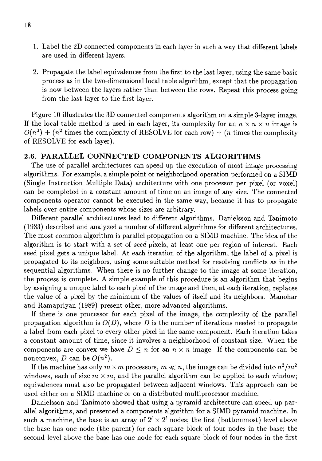
18
1. Label the 2D connected components in each layer in such a way that different labels
are used in different layers.
2. Propagate the label equivalences from the first to the last layer, using the same basic
process as in the two-dimensional local table algorithm, except that the propagation
is now between the layers rather than between the rows. Repeat this process going
from the last layer to the first layer.
Figure 10 illustrates the 3D connected components algorithm on a simple 3-layer image.
If the local table method is used in each layer, its complexity for an η χ η χ η image is
0(η3) + (η2 times the complexity of RESOLVE for each row) + (n times the complexity
of RESOLVE for each layer).
2.6. PARALLEL CONNECTED COMPONENTS ALGORITHMS
The use of parallel architectures can speed up the execution of most image processing
algorithms. For example, a simple point or neighborhood operation performed on a SIMD
(Single Instruction Multiple Data) architecture with one processor per pixel (or voxel)
can be completed in a constant amount of time on an image of any size. The connected
components operator cannot be executed in the same way, because it has to propagate
labels over entire components whose sizes are arbitrary.
Different parallel architectures lead to different algorithms. Danielsson and Tanimoto
(1983) described and analyzed a number of different algorithms for different architectures.
The most common algorithm is parallel propagation on a SIMD machine. The idea of the
algorithm is to start with a set of seed pixels, at least one per region of interest. Each
seed pixel gets a unique label. At each iteration of the algorithm, the label of a pixel is
propagated to its neighbors, using some suitable method for resolving conflicts as in the
sequential algorithms. When there is no further change to the image at some iteration,
the process is complete. A simple example of this procedure is an algorithm that begins
by assigning a unique label to each pixel of the image and then, at each iteration, replaces
the value of a pixel by the minimum of the values of itself and its neighbors. Manohar
and Ramapriyan (1989) present other, more advanced algorithms.
If there is one processor for each pixel of the image, the complexity of the parallel
propagation algorithm is 0(D), where D is the number of iterations needed to propagate
a label from each pixel to every other pixel in the same component. Each iteration takes
a constant amount of time, since it involves a neighborhood of constant size. When the
components are convex we have D < η for an η χ η image. If the components can be
nonconvex, D can be 0(n2).
If the machine has only mxm processors, m ·< n, the image can be divided into n2/m2
windows, each of size mxm, and the parallel algorithm can be applied to each window;
equivalences must also be propagated between adjacent windows. This approach can be
used either on a SIMD machine or on a distributed multiprocessor machine.
Danielsson and Tanimoto showed that using a pyramid architecture can speed up
parallel algorithms, and presented a components algorithm for a SIMD pyramid machine. In
such a machine, the base is an array of 2l χ 21 nodes; the first (bottommost) level above
the base has one node (the parent) for each square block of four nodes in the base; the
second level above the base has one node for each square block of four nodes in the first
19
Layer 1 Layer 2 Layer 3
l I l I l | 1 I l I l I l Ι Ί I 111 I ~|
11 1 1 1 1 ll
1 1 ι ι]
111111 ι 111 111 1 1111111 "j
a) Input binary 3-layer image
6 I 6 I 6 | 1 I 4 I 4 I 4 I ] I I 2 Ι Ι
6 6 4 2 1
1 1 2 l"
5 5 I 5 I | 3 | 3 [ | I 2 2 I 2
b) Image labels after the two-dimensional connected components algorithm has
been run on each layer separately, using labels that decrease from layer 1 to
layer 3.
6 | 6 I 6 Ι Ι I 6 I 6 I 6 Ι Ι Ι I 6 I I
6 6 6 6 1
5 | 5 | 5 1 | 1 5 1 I 5 | | 6 6 6
c) Image labels after the top-down pass of the three-dimensional part of the
algorithm
6 I 6 I 6 | I I 6 I 6 I 6 I I I I 6 I I
6 6 6 6 1
ZXXXJ LXXXj 6 ι
616161 [ 161 161 | 1616 j 61
d) Image labels after the bottom-up pass of the three-dimensional part of the
algorithm. These are the final component labels.
Figure 10. Illustration of the Lumia 3D connected components algorithm.
20
level; and so on, so that the topmost level has only a single node. The neighborhood of a
node in a pyramid includes itself, its 8-neighbors on its own level, its parent, and its four
children. The operation ANDPYR(X) in a pyramid X with a binary image in its base and
zeroes everywhere else is defined to compute the new value of each node at each level as
the logical AND of the old values of its four children. The conditional dilation operation
[DIL | Y](X) is defined to dilate the black pixels in pyramid X, i.e. to propagate black
values (l's) to all their pyramidal neighbors, on the condition that these neighbors are
black pixels in pyramid Y. If the base of X initially contains a single black seed pixel, the
base of Υ initially contains the binary image to be labeled and the pixels in the remaining
nodes of X and Υ are initially white, then the propagation algorithm for the component
of the binary image that contains the single seed pixel is given by
PYRAMIDJFILL(X,Y) = [DIL | ANDPYR/(Y)]t(X)
where the exponents denote repetition and / is the height of the pyramid (n, for a 2" χ 2"
Figure 11 illustrates the PYRAMIDJFILL algorithm on a simple image. The overall
complexity of the algorithm depends on the size and shape of the component of the
binary image that contains the seed pixel. If the component is convex, the complexity is
proportional to the logarithm of its diameter.
3. ADJACENCY GRAPH CONSTRUCTION
3.1. STATEMENT OF THE PROBLEM
This section is concerned with the spatial relationships among regions in a symbolic
(l?b~'- 1) image. We assume that some kind of segmentation process has already assigned
to ^. pixel of the image a symbolic label that represents the name or category of the
pixel. Thus we are starting with a symbolic image. The goal is to determine the spatial
adjacencies among the connected regions that have different labels and construct a graph,
the region adjacency graph, representing these spatial adjacencies. The graph may then be
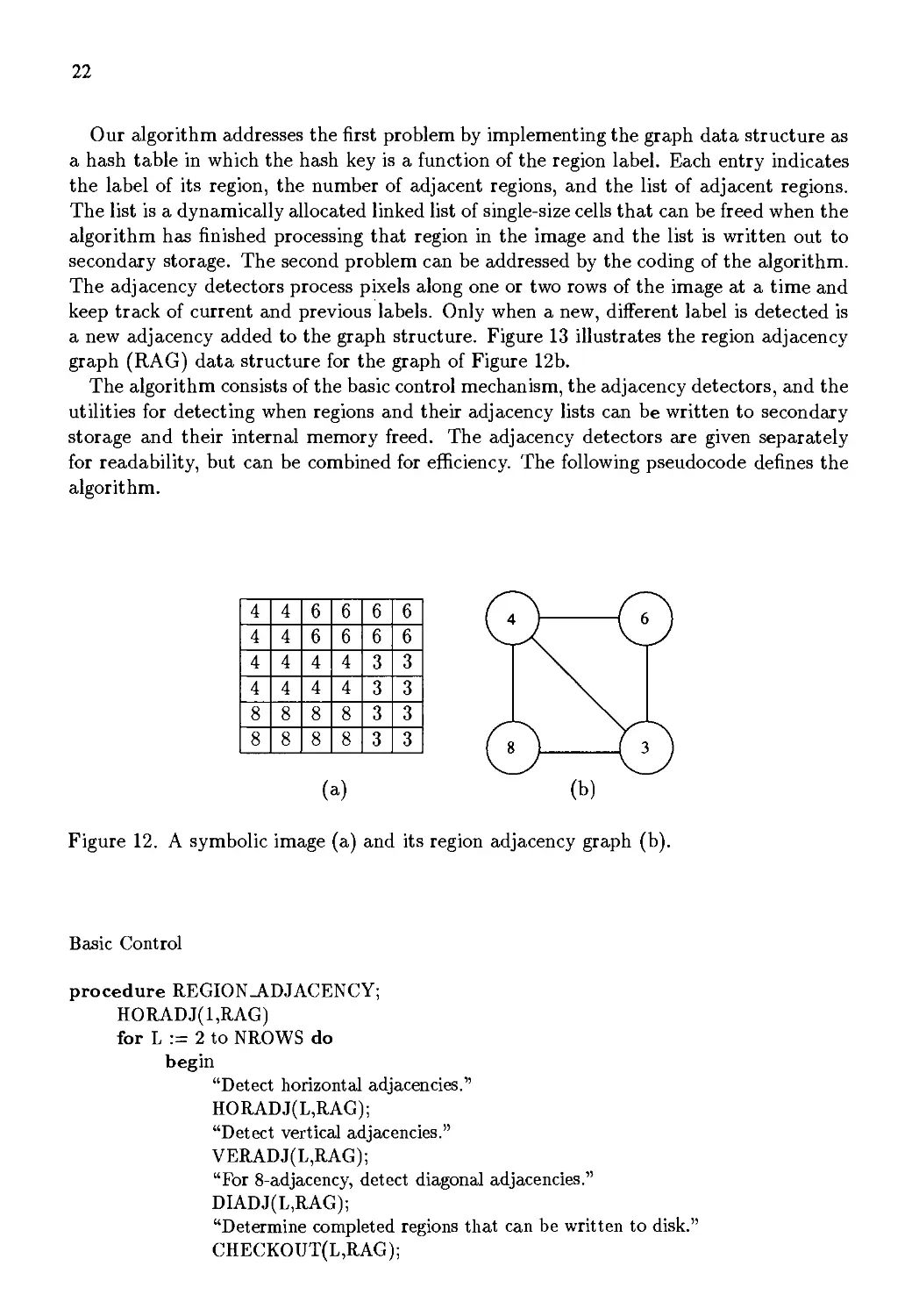
used in higher-level recognition/analysis algorithms. Figure 12 shows a simple symbolic
image representing a segmentation and the corresponding region adjacency graph.
3.2. A SPACE-EFFICIENT ALGORITHM
The algorithm for constructing a region adjacency graph is straightforward. It processes
the image, looking at the current row and the one above it. It detects horizontal and
vertical adjacencies (and if 8-adjacency is specified, diagonal adjacencies) between pixels
with different labels. As new adjacencies are detected, new edges are added to the region
adjacency graph data structure being constructed.
There are two issues related to the efficiency of this algorithm. The first involves space.
It is possible for an image to have tens of thousands of labels. In this case, it may not be
feasible, or at least not appropriate in a paging environment, to keep the entire structure
in internal memory at once. The second issue involves execution time. When scanning
an image, pixel by pixel, the same adjacency (i.e. the adjacency of the same two region
labels) will be detected over and over again. It is desirable to enter each adjacency into
the data structure as few times as possible.
D
D
(a)
G
(b)
G
0
1
2
3
4
4
5
1
1
2
3
4
4
1
2
3
2
2
2
3
2
2
3
3
3
3
4
4
5
Figure 11. (a) Seed pyramid for propagation; (b) AND pyramid from binary image; (c)
results of labeling; (d) labeling chronology (numbers indicate iterations at which labeling
occurred).
22
Our algorithm addresses the first problem by implementing the graph data structure as
a hash table in which the hash key is a function of the region label. Each entry indicates
the label of its region, the number of adjacent regions, and the list of adjacent regions.
The list is a dynamically allocated linked list of single-size cells that can be freed when the
algorithm has finished processing that region in the image and the list is written out to
secondary storage. The second problem can be addressed by the coding of the algorithm.
The adjacency detectors process pixels along one or two rows of the image at a time and
keep track of current and previous labels. Only when a new, different label is detected is
a new adjacency added to the graph structure. Figure 13 illustrates the region adjacency
graph (RAG) data structure for the graph of Figure 12b.
The algorithm consists of the basic control mechanism, the adjacency detectors, and the
utilities for detecting when regions and their adjacency lists can be written to secondary
storage and their internal memory freed. The adjacency detectors are given separately
for readability, but can be combined for efficiency. The following pseudocode defines the
algorithm.
4 I 4 I 6 I 6 I 6 I 6
4 4 6 6 6 6
4 4 4 4 3 3
4 4 4 4 3 3
8 8 8 8 3 3
8 | 8 | 8 | 8 | 3 | 3
(a) (b)
Figure 12. A symbolic image (a) and its region adjacency graph (b).
Basic Control
procedure REGION-ADJACENCY;
HORADJ(l,RAG)
for L := 2 to NROWS do
begin
"Detect horizontal adjacencies."
HORADJ(L,RAG);
"Detect vertical adjacencies."
VERADJ(L,RAG);
"For 8-adjacency, detect diagonal adjacencies."
DIADJ(L,RAG);
"Determine completed regions that can be written to disk."
CHECKOUT(L,RAG);
Π
region label
3
4
6
8
number of
adjacent regions
3
3
2
2
adjacent regions
4,6,8
3,6,8
3,4
3,4
Figure 13. RAG data structure representing the graph of Figui
FINALOUT(RAG)
end REGION-ADJACENCY
Horizontal Adjacencies
procedure HORADJ(L,RAG);
curval := I(L,1);
for Ρ := 1 to NCOLS do
newval := I(L,P);
if curval < > newval
then begin ADD-TO_RAG(curval,newval,RAG); curval := newval end
Vertical Adjacencies
procedure VERADJ(L,RAG);
oldvalp := 0;
oldvalc := 0;
for Ρ := 1 to NCOLS do
begin
newvalp := I(L-1,P);
newvalc := I(L,P);
if (newvalp <> newvalc) and
(newvalp <> oldvalp or newvalc <> oldvalc)
then ADD_TO_RAG(newvalp,newvalc,RAG);
oldvalp := newvalp;
oldvalc := newvalc;
end
end VERADJ
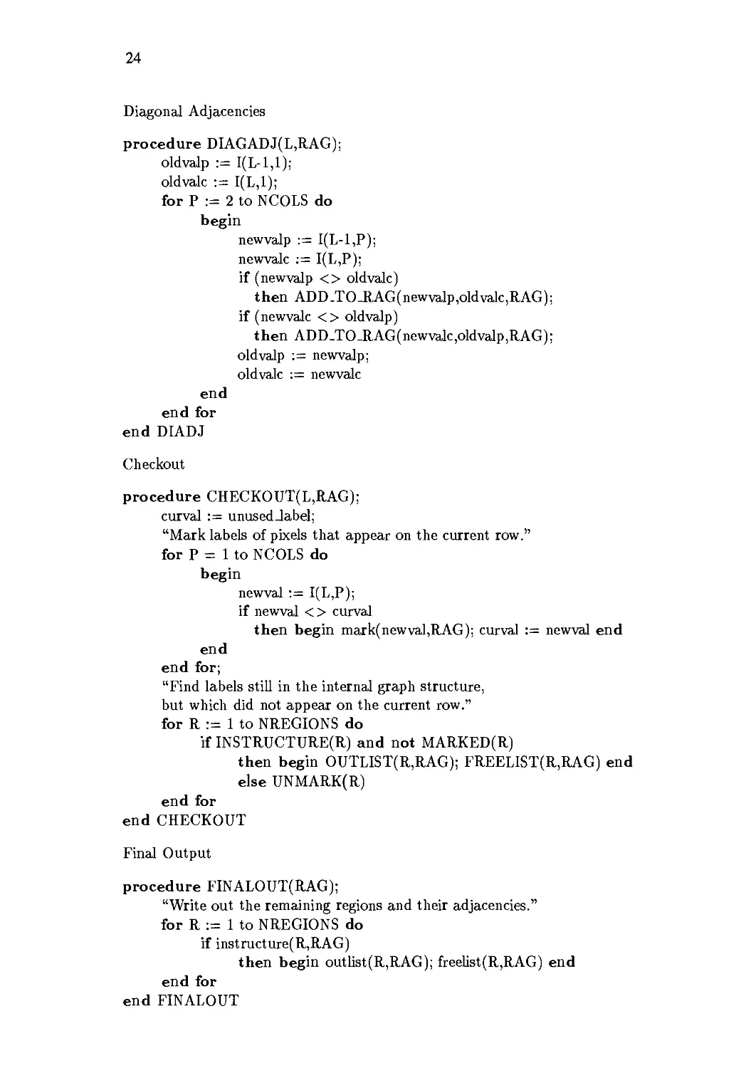
24
Diagonal Adjacencies
procedure DIAGADJ(L,RAG);
oldvalp := I(L-1,1);
oldvalc := I(L,1);
for Ρ := 2 to NCOLS do
begin
newvalp := I(L-1,P);
newvalc := I(L,P);
if (newvalp <> oldvalc)
then ADD.TO_RAG(newvalp,oldvalc,RAG);
if (newvalc < > oldvalp)
then ADD.TO_RAG(newvalc,oldvalp,RAG);
oldvalp := newvalp;
oldvalc := newvalc
end for
end DIADJ
Checkout
procedure CHECKOUT(L,RAG);
curval := unusedJabel;
"Mark labels of pixels that appear on the current row."
for Ρ = 1 to NCOLS do
begin
newval := I(L,P);
if newval < > curval
then begin mark(newval,RAG); curval := newval end
end
"Find labels still in the internal graph structure,
but which did not appear on the current row."
for R := 1 to NREGIONS do
if INSTRUCTURE(R) and not MARKED(R)
then begin OUTLIST(R,RAG); FREELIST(R,RAG) end
else UNMARK(R)
end CHECKOUT
Final Output
procedure FINALOUT(RAG);
"Write out the remaining regions and their adjacencies."
for R := 1 to NREGIONS do
if instructure(R,RAG)
then begin outlist(R,RAG); freelist(R,RAG) end
end FINALOUT
25
The algorithm makes one pass over the image. Whenever it detects an adjacency that
is different from the most recently detected one, it attempts to add the new adjacency
to the graph structure. This involves hashing to the entry for a region and adding the
adjacency to an ordered, linked list, if it is not already present. While the theoretical
worst case complexity is 0(n3) for an η χ η image, for practical purposes, the algorithm
executes in 0(n2) time, since most regions have a small number of neighboring regions.
The required size of the hash table in memory is dependent on the maximum number of
regions that can be active at once, which is bounded by n, the number of pixels in a row
of the image.
4. SOME APPLICATIONS
The connected components operator is a very basic operator that is used in many
different applications. It was a part of the so-called "SRI Vision Module", a package developed
at SRI International for analysis of binary images (Agin, 1980). The module consists of
thresholding, connected component labeling, property computation, and statistical
pattern recognition. Variants of this sequence can be used for such diverse tasks as character
recognition, where the components are characters or pieces of characters; surface-mounted
device board inspection, where the components are the devices; and surface inspection,
where the components are holes in or scratches on the surface.
Character recognition is a major field in its own right. While printed characters in
standard fonts are now recognized by commercial machines, handprinted character recognition
is not yet as reliable, and handwritten character recognition is still a research problem. A
major problem with handwritten character recognition and, to some extent, handprinted
character recognition is the segmentation of words into letters. The connected components
(extracted after a sequence of image processing operations, ending with a thresholding
operation) may represent parts of characters, whole characters, or groups of characters.
Another major application area where connected component algorithms are important
is medical imaging. When a CT scan has been segmented into components
representing organs and their surrounding bone and tissue, it may be necessary to use both the
properties of the components themselves and the properties of their neighboring regions
to identify the organs. Thus both the connected components operator and the region
adjacency graph algorithm are useful. Blob detection and recognition are also important
in military applications such as target detection and aerial image analysis.
The concepts described in this chapter are also useful in more advanced areas of
computer vision. For example, in motion detection, we may first detect components in a
sequence of images and then determine their correspondences from one image to the next
to determine the motions of the objects in the scene. Similarly, there are stereo algorithms
that use component matching. Thus connected components and their analysis are of very
wide interest to the computer vision community.
REFERENCES
1 G. Agin, "Computer Vision System for Industrial Inspection and Assembly," IEEE
Transactions on Computers, Vol. 14, 1980, pp. 11-20.
2 P.-E. Danielsson and S.L. Tanimoto, "Time Complexity for Serial and Parallel
Propagation in Images", in Architecture and Algorithms for Digital Image Processing, A.
Oosterlinck and P.-E. Danielsson, (eds.), Proceedings of the SPIE, Vol. 435, 1983,
pp. 60-67.
3 E. Horowitz and S. Sahni, Fundamentals of Data Structures, Computer Science Press,
Rockville, MD, 1982.
4 T.Y. Kong and A. Rosenfeld, "Digital Topology: Introduction and Survey", Computer
Vision, Graphics, and Image Processing, Vol. 48, 1989, pp. 357-393.
5 R. Lumia, L.G. Shapiro, and O. Zuniga, "A New Connected Components Algorithm
for Virtual Memory Computers," Computer Vision, Graphics, and Image Processing,
Vol. 22, 1983, pp. 287-300.
6 R. Lumia, "A New Three-Dimensional Connected Components Algorithm", Computer
Vision, Graphics, and Image Processing, Vol. 23, 1983, pp. 207-217.
7 M. Manohar and H.K. Ramapriyan, "Connected Component Labeling of Binary
Images on a Mesh Connected Massively Parallel Processor," Computer Vision, Graphics,
and Image Processing, Vol. 45, 1989, pp. 143-149.
8 C. Ronse and P.A. Devijver, Connected Components in Binary Images: The Detection
Problem, Research Studies Press, Letchworth, England, 1984.
9 A. Rosenfeld, "Connectivity in Digital Pictures," Journal of the Association for
Computing Machinery, Vol. 17, 1970, pp. 146-160.
10 A. Rosenfeld and J.L. Pfaltz, "Sequential Operations in Digital Picture Processing,"
Journal of the Association for Computing Machinery, Vol. 14, 1966, pp. 471-494.
11 R.E. Tarjan, "Efficiency of a Good but not Linear Set Union Algorithm", Journal of
the Association for Computing Machinery, Vol. 22, 1975, pp. 215-225.
Topological Algorithms for Digital Image Processing
T.Y. Kong and A. Rosenfeld (Editors)
© 1996 Elsevier Science B.V. All rights reserved.
27
Appendix: A Generalization of Lumia's Algorithm and a Proof of
Its Correctness
T. Yung Kong Azriel Rosenfeld
This appendix gives a generalization of the "local table" methods of connected
component labeling described in Sections 2.3 - 2.5, and proves that such methods work.
1. Relative Component Labeling
A labeling of a set S is a function £ with domain S; for every s e S, we call £(s) the
£-label of s. Each element of {£(s) | s G S} is called a label used by £.
Let X and Υ be disjoint sets of nodes of a graph G, and let £ be a labeling of X. We
say that two nodes у\,у? 6 Υ are adjacent relative to £ in G if у ι ψ y2 and at least one of
the following is true:
• у ι and у 2 are adjacent in G.
• There exist (not necessarily distinct) nodes xu x2 £ X with equal £-labels, such that
yi is adjacent to X\ and j/2 is adjacent to x2 in G.
The reflexive transitive closure of adjacency relative to £ in G is an equivalence relation
on У; each of the associated equivalence classes will be called a component of Υ relative
to £ in G. Note that if X = 0, so that £ is the "empty labeling", then nodes in Υ are
adjacent relative to £ in G if and only if they are adjacent in G, and a component of Υ
relative to i in G is just the set of nodes of a component of the subgraph of G induced
by Υ. More generally, if £ is any labeling of X such that nodes with the same £-label
always lie in the same component of G, then nodes of Υ that are adjacent relative to £ in
G always lie in the same component of G, which implies that nodes of Υ which lie in the
same component of Υ relative to £ in G lie in the same component of G.
A component labeling of Υ relative to £ in G is a labeling £' of Υ that satisfies both of
the following conditions:
• Two nodes of Υ have the same £'-label if and only if they belong to the same
component of Υ relative to £ in G.
• If / is any label that is used both by £' and by £, then there are nodes χ g X and
у £ Υ that are adjacent in G such that £(x) = £'(y) = I.
The following lemma follows from the first of these two conditions, and the observation
at the end of the previous paragraph.
LEMMA 1 Let X and Υ be disjoint sets of nodes of a graph G. Let £ be any labeling of
X such that nodes with the same £-label always lie in the same component of G, and let
£' be a component labeling of Υ relative to £ in G. Then nodes of Υ with the same £'-label
always lie in the same component of G.
28
Algorithms for producing a component labeling of Υ relative to £ in G are easily derived
from the "classical" graph component labeling algorithm referred to in Section 2.2. We
now outline one such algorithm. Suppose Υ consists of к nodes j/b г/2,...,ук- For each t/,·,
let P(yi) be the set of all the nodes in {ϊ/;- | j < i} that are adjacent to j/, in G, and let
Nx(yi) be the set of all the nodes in X that are adjacent to j/, in G. If initially Label[x] =
£(x) for all χ £ X then, when the following algorithm terminates, a component labeling
of Υ relative to i in G is given by i'(y) = Label[y] for all у in У:
Initialize Equivalence TableQ;
FOR i := 1 TO Jb DO
IF P(yi) U Nx(yi) = 0 THEN Labels := NewLabel()
ELSE BEGIN
Labe%,] := Label[FirstMemberOf(P(!/,) U Nx(yi))];
FOREACH и IN RestOf(P(yi) V Nx(y,)) DO MakeEquivalent(Label[u],Label[!/,])
END;
FOR i := 1 TO к DO Labe%,] := UniqueEquivClassRepresentative(Label[j/,-]);
2. A Generalization of Lumia's Algorithm
Let G be a graph whose set of nodes has been partitioned into subsets R1, R2,. .. ,Rn,
called rows, in such a way that adjacent nodes of G always lie either in the same row or
in consecutive rows.
We regard any 2-d binary image array in which 4- or 8-adjacency is used on the l's as
such a graph G: the l's are the nodes of G, and we take Д; to be the set of l's in the ith
row of the image array. Similarly, we regard any 3-d binary image array in which 6-, 18-
or 26-adjacency is used on the l's as such a graph. In this case we take Ri to be the set
of l's in the ith layer of the image array.
It follows from Theorem 1 below that the following two passes will produce a labeling
of the nodes of G such that two nodes have the same label if and only if they belong to
the same component of G.
Pass 1 Let До = 0 and let £0 be the empty labeling. For i = 1,2,..., η (in that order)
let £i be a component labeling of Д, relative to the labeling £;_i of i?,_i in G, such that
every label used by Ц is either a label used by £,_i or a new label that is not used by any
b, j < i.
At the end of pass 1, each node of G has a label: if у € Ri, then we regard ti(y) as the
label of у.
Pass 2 For i = n,n - 1,..., 2 (in that order) apply the following rule to row Ri\
R Whenever a node у € Д,- is adjacent to a node χ € Д,_! with a different label, all
nodes in i?,_i that have the same label as χ are given j/'s label.
Rule R assumes that no node in Д, with a label different from y's label can be adjacent
to a node in i?,_i with the same label as x. Equivalently, it assumes that two nodes
29
t/i,t/2 £ -Ri must have equal labels if there exist two (not necessarily distinct) nodes
Xi,x2 £ Ri-i with equal labels such that ϊ/ι is adjacent to Xi and ϊ/2 is adjacent to x2.
The possibility of performing pass 2 depends on the validity of this assumption for each
row R{ when rule R is about to be applied to that row, and will be established in the
third paragraph of the proof of Theorem 1.
Application of rule R to row Д, does not change any label in Д,; it can only change
labels in row Щ-\. Note that if two nodes in Д,_! have equal labels before application of
rule R to Ri, then they have equal labels afterwards.
THEOREM 1 It is always possible to perform pass 2 after pass 1. After pass 2, two
nodes of G have the same label if and only if they belong to the same component of G.
Proof. Consider how the nodes are labeled at the end of pass 1. At this time two nodes
in Ri have the same label if and only if they lie in the same component of Ri relative to
the labeling of iZ,-_i. We first deduce from this that the following conditions hold at the
1. Within each row, two nodes have equal labels if they are adjacent in G.
2. Within each row Д, where i > 1, two nodes y1 and j/2 have equal labels if there exist
two (not necessarily distinct) nodes Xi,x2 £ Ri-i with equal labels such that y\ is
adjacent to X\ and j/2 is adjacent to x2 in G.
3. Equally labeled nodes always belong to the same component of G.
Conditions 1 and 2 hold, since they are together equivalent to the condition that two
nodes of Ri have equal labels if they are adjacent relative to the labeling of i?,_i. Equally
labeled nodes in the row Ri must lie in the same component of G (e.g., by Lemma 1,
whose hypotheses are satisfied when A' = До = 0, Υ = Ri, I is the empty labeling £0, and
£' = i\). Based on this, we see by induction on i (using Lemma 1 with X = Ri-i, Υ = Ri,
£ = £;_i, and £' = £i) that, for each row Ri, equally labeled nodes in Ri must lie in the
same component of G. It follows from this and the second condition in the definition of a
component labeling relative to I that two equally labeled nodes in consecutive rows also
must lie in the same component of G. The same is true of two equally labeled nodes in
different, nonconsecutive, rows Ri and Rj, for if such nodes exist then there must exist a
node with the same label in each of the rows between Д, and Ry (This is because in pass
1 every label used in a row is either one of the labels used in the preceding row or a new
label that is not used in any previous row.) Hence condition 3 holds at the end of pass 1.
Next, we verify that it is always possible to perform pass 2 after pass 1. As we observed
above (just after the statement of pass 2) we need to show that condition 2 always holds
for Ri when rule R is about to be applied to Ri in pass 2. We know condition 2 holds
for all rows after pass 1. Thus it suffices to check that application of rule R to a row Д;
in pass 2 preserves the validity of condition 2 for the rows R,, i < j - 1, which are the
rows to which rule R will subsequently be applied. Application of rule R to Rj cannot
affect the validity of condition 2 for the rows R{, г < j - 2, since no labels in these rows
are changed. Application of rule R to Д, also preserves the validity of condition 2 for the
row Ri, ι = j - 1, since no labels in #,_2 are changed and nodes in Rj-ι that have equal
30
labels before must have equal labels afterwards. This confirms that it is always possible
to perform pass 2 after pass 1.
Conditions 1 and 3, which hold for all rows after pass 1, are preserved when rule R
is applied to any row. Condition 1 is preserved because nodes with equal labels before
application of rule R to a row have equal labels afterwards. Condition 3 is preserved
because in rule R the nodes in i?;_i with the same label as x, which are given j/'s label,
must belong to the same component as χ (by condition 3), and must therefore belong to
the same component as у and all other nodes with j/'s label. Thus conditions 1 and 3 still
hold at the end of pass 2.
Consider the labels of any two adjacent nodes at the end of pass 2. One of the following
must be true:
• The nodes lie in the same row, in which case they must have the same label by
condition 1.
• The nodes lie in consecutive rows i?i_i and Д; for some i, in which case they must
have the same label as a result of the application of rule R to Д,.
This shows that after pass 2 adjacent nodes always have the same label and so, since
condition 3 holds, two nodes have the same label if and only if they belong to the same
component. □
Each of the algorithms presented in Sections 2.3, 2.4 and 2.5 labels the l's of a 2-d or
3-d binary image array in a way that is an instance of pass 1 above. It then performs a
bottom-up pass whose effect on the labels is the same as that of pass 2. Note that in the
algorithm of Section 2.3, the following condition is satisfied at the start of the bottom-up
• For 1 < i < n, whenever у G Д, is adjacent to χ 6 -Rj-i, ϊ/'s label is less than or
equal to x's label.
A consequence of this is that in rule R, during pass 2, j/'s label would always be the
minimum of the labels of χ and y.
Topological Algorithms for Digital Image Processing
T.Y. Kong and A. Rosenfeld (Editors)
© 1996 Elsevier Science B.V. All rights reserved. 31
SHRINKING BINARY IMAGES
Richard W. Hall" Τ. Υ. Kongb Azriel Rosenfeldc
"Department of Electrical Engineering, University of Pittsburgh, Pittsburgh, PA 15261
bDepartment of Computer Science, Queens College, City University of New York,
Flushing, NY 11367
cCenter for Automation Research, University of Maryland, College Park, MD 20742
Abstract
The general problem of shrinking binary images is addressed with emphasis on the
problem of shrinking to a residue. Past work in this area is reviewed, fundamental limits
are discussed and open questions are identified. Emphasis is given to techniques which
can be used to verify correct performance of shrinking algorithms, including successful
algorithm termination and connectivity preservation. New connectivity preservation tests
are developed for parallel 2D reductive-augmentative algorithms and the application of
these tests is demonstrated for a variety of shrinking algorithms. A new 2D completely
parallel single-operator shrinking algorithm is developed using connectivity preservation
requirements to guide the design process. Issues in 3D shrinking are also reviewed.
1. INTRODUCTION
The "shrinking" of binary images to similarly connected representations that have
smaller foregrounds (i.e., fewer l's) has found application as a fundamental preprocessing
step in image processing. Two forms of such shrinking have been of greatest interest:
(1) The image is transformed to a "topologically equivalent" image that has fewer l's;
(2) connected components of the l's are shrunk to isolated single-pixel residues (which
may then be deleted). Figure 1 illustrates these two kinds of processes.
Figure la is an example of shrinking to a topological equivalent; it illustrates the effect of
a typical thinning algorithm. The result is a thin closed curve of l's along the approximate
midline of the set of l's in the input image. In Figures lb, d, and e, which are also
examples of shrinking to a topological equivalent, the input images are transformed to
smallest topological equivalents (i.e., topological equivalents having the smallest numbers
of l's). In this case the resulting set of l's need not (and in Figure lb cannot) be contained
in the original set of l's. Shrinking to a topological equivalent will be briefly discussed in
Section 2.6. The special case of thinning is addressed in detail in two other chapters in
this volume, by Arcelli and Sanniti di Baja and by Hall.
However, the main subject of this chapter is shrinking to a residue, in which every
simply-connected component of the l's (and possibly every component of the l's) of the
input image is transformed to an isolated single-pixel residue, which again may or may
not belong to the original set of l's. This is illustrated in Figures lc-e. Residues may be
32
deleted after they are produced; at that time they can also be detected, counted, etc., by
some other process.
Shrinking to a residue will often be referred to simply as shrinking. This type of process
has no additional geometric constraints. (As illustrated in Figure lc, the process may not
even preserve all of the topological properties of the input image: when a component
of l's that is not simply connected is shrunk to a residue, one or more holes must be
eliminated.) Shrinking to a residue has been used as a preliminary step in counting the
components of l's in an image [53], and to generate "seed" pixels for labeling connected
components of l's [1, 10].
A related type of process is (morphological) erosion, which is of fundamental importance
in mathematical morphology [26, 55] and has been used extensively in image processing
as a means of smoothing boundaries, removing small or thin components, etc. [26, 52]; see
also the chapter by Arcelli and Sanniti di Baja in this volume. However, erosion differs
from shrinking in that it removes l's without regard to connectivity preservation. It will
not be treated in this chapter.
2. BASIC CONCEPTS, TERMINOLOGY AND NOTATION
2.1. 2D Images.
We write Σ for the set of all pixels. Σ is in 1-1 correspondence with the set of points in
the plane that have integer coordinates. (In this chapter we only consider images based
on a rectangular tessellation. However, much of this work is readily extended to images
based on a hexagonal tessellation [22].) An image, I, assigns to each pixel in Σ a value
from the set {0,1}, but only a finite number of pixels may have value 1; 1-valued pixels
are called l's (of / or in /) and 0-valued pixels are called 0's.
When discussing a particular image, its set of l's is referred to as the foreground;
its set of 0's is referred to as the background. Elementary terms of digital topology
such as i-adjacent, i-neighbor, i-connected, simply i-connected, i-path, simple i-arc and
i-component, where t = 4 or 8, are used in the same sense as defined in the introduction
to digital topology in the appendix to this volume. To avoid connectivity "paradoxes"
the foreground and background are usually understood to have 8-connectivity and 4-
connectivity, respectively [49]; this combination is referred to as 8-4 connectivity. The
dual 4-8 definition could also be used, but the 8-4 definition seems to be more often
used by the image processing community. The variables m and η are used to denote the
foreground and background adjacency relations, respectively; thus (m,n) could be (8,4)
or (4,8), but is usually (8,4) in practical applications.
Unless otherwise indicated, a lower case letter other than m and η denotes a pixel, the
value of a pixel, or an integer; sets of pixels and paths are usually denoted by uppercase
letters. We identify the Boolean values true and false with the integers 1 and 0 respectively.
The symbols V and Λ denote Boolean OR and AND, and x' denotes the complement of a
Boolean value x. We will say two sets, X and Y, meet if XC\Y is non-empty. In discussing
illustrations of regions of an image, < s > will refer to the set of all pixels labeled s. Also,
in illustrations that show l's and do not show 0's, pixels at blank positions are 0's unless
otherwise indicated. If 0's are shown explicitly, the values of pixels at blank positions are
irrelevant or unspecified.
11111111
11111111
1111111
1111111
1111
1111111
1111111
111111
111111
(d)
111111
111111
Figure 1. Diagrams a, b, d and e show examples of shrinking to a topological equivalent;
c, d, and e show examples of shrinking to a residue. Blanks are O's of the input and the
output binary images; the -'s are O's of the output image that were l's in the input image.
An algorithm for shrinking to a residue may also delete the residues in c, d and e.
34
For ί = 4 or 8, Ni(p) denotes the set consisting of ρ and its t-adjacent neighbors, and
N'(p) ξ Ni(p) — {p}. When we refer to specific pixels in Ns(p) we may use the notation
given in Figure 2, where po = p. (We will extend this notation to 3D images in Section 6.)
We say that ρ = 1 is a border 1 if N*(p) contains a 0 (i.e., if ρ is η-adjacent to a 0); ρ
is called an interior 1 otherwise. Cm(p) denotes the number of distinct m-components of
l's in iVg(p) that are m-adjacent to p. We say a 1, p, is m-simple if ρ is a border 1 and
Cm(p) = 1.
Pi Рг Рз
Ps Po P4
P7 Pe Ps
Figure 2. Notation for the pixels in jV8(p); po = ρ
The following straightforward computation (first noted in [27]) can be used to determine
if ρ is 8-simple. ρ is 8-simple iff N£(p) satisfies the following condition, where the Boolean
results in brackets are treated as integers (1 or 0) for the addition operations:
\P2 Л (Рз V p4)] + \p'4 Λ (p5 V pe)} + \ρ'β Λ (pr V p8)] + [p8 Λ (Pl V p2)] = 1.
(Other similar criteria are found in [2, 53, 61].)
2.2. Operators and Operator Application.
This chapter deals with algorithms which shrink binary images by applying sequences
of operators. In this section we give general definitions of an operator and an operator
application.
Before giving our general definition of an operator, we discuss the special case of a 3 x 3
operator. Let О be any Boolean function of nine Boolean arguments Vb,V\,Vi,... ,Vs
such that О has value 0 when all nine of its arguments have value 0. Then we say О is a
3x3 operator. For any image / and pixel p, we define the value of О at ρ in I to be the
value of the Boolean function when each argument Vi is given the value (1 or 0) of the
pixel pi (see Figure 2) in /. Some simple examples of 3 x 3 operators are:
a) Vs, the operator which gives each pixel ρ the value of its left-hand neighbor in the
image (so that it "shifts" pixel values to the right).
b) VqI\V'i\ this operator gives a pixel ρ the value 1 iff its value in the image was 1 and
the value of the pixel above it was 0—i.e., iff ρ was a "north border" 1.
c) Vo Λ I \/ Vi J ; this operator gives ρ the value 1 iff its value in the image was 1 and
the values of all of its 8-neighbors were 0—i.e., iff ρ was an "isolated" 1.
d) Vo', this is the "identity" operator which gives each pixel the same value as it had
in the image.
35
Operators are commonly specified by stating the conditions under which they change the
value of a pixel from 0 to 1 and from 1 to 0. For example, the operator (b) above might
be specified as the operator which never changes a 0 to a 1, and which changes a 1 to a
0 iff its north neighbor is a 1.
We need a generalization of the concept of a 3 x 3 operator that will admit operators
whose value at a pixel ρ depends on the values of pixels which are not necessarily in Ns(p).
To define the value of such an operator at a pixel, we extend the numbering of pixels given
by Figure 2 to a numbering of all pixels in the image relative to a given pixel p. For any
odd positive integer t and pixel p, let NiXi(p) denote the t χ i neighborhood of p. This is
the upright t χ i square of pixels with ρ at its center. (The notation N{Xi(p) should not be
confused with the notation Ni(p) defined in Section 2.1. Although N8(p) = N3x3(p), Щр)
is not equal to ./V,x,(p) for any t.) Let рэ,рю,. · · ,Pu be the pixels in NSxS(p) — N3x3(p)
in clockwise order starting with the pixel in the top left-hand corner. More generally, for
any odd integer t let p,i,p,'i+n · · · iPfi+^-i be the pixels in N(i+2)x(i+2)(p) - Nixi(p) in
clockwise order starting with the pixel in the top left-hand corner.
Now we can give our general definition of an operator. An operator is a Boolean function
of a finite number of Boolean arguments V0, V\,... Vk (where к can be any non-negative
integer), with the property that the function has value 0 when all of its arguments have
value 0. As in the 3x3 case discussed above, for any image / and pixel ρ we define
the value of the operator at ρ in I to be the value of the Boolean function when each
argument 73, is given the value of the pixel p, in /. Note that in examples (a), (b) and
(d) above, the value of the operator depends only on the values of a proper subset of its
arguments—{-P8}, in case (a); {V0,V2}, in case (b); {Vo}, in case (d). The support of an
operator О is defined to be the set of O's arguments whose values sometimes affect the
value of the Boolean function. We will ignore any arguments of an operator which are not
in the operator's support, in the sense that we will consider Oj and Oj to be the same
operator if they have the same support and Oj has the same value as Oj for all possible
values of the arguments in their support.
For each pixel p, the set of pixels p, that correspond to arguments in O's support is
called the support of О at p. For example, the supports at ρ of the operators (a), (b), (c)
and (d) above are respectively {pe}, {ρ,Ρι}, Ns(p), and {p}. Note that for any two pixels
q and r, the support of an operator at г is just a translate of the support of the operator
We say that the support of an operator О is a k-pixel support if it consists of just к
elements. For any odd positive integers j and k, we say that the support of О is a j χ к
support, and that О is a j x к operator, if the support of О at any pixel ρ is a subset
of the j X к neighborhood of ρ (i.e., the upright j X к rectangle of pixels centered at
p). The radius of an operator О is the smallest non-negative integer ρ for which О is a
(2/>+l) x(2/>+l) operator.
We apply an operator О to a pixel ρ in an image / by changing the value of ρ in / to
the value of О at ρ in /. О is called a reductive operator if its application never changes
a 0 to a 1—i.e., if the value of О at a pixel ρ is 0 whenever ρ is a 0. О is called an
augmentative operator if its application never changes a 1 to a 0—i.e., if the value of О
at ρ is 1 whenever ρ is a 1. An operator which does not fall into either of these categories
is called a reductive-augmentative operator. Such an operator sometimes changes a 0 to
36
a 1 and sometimes changes a 1 to a 0.
We apply an operator О to a set of pixels R in an image / by simultaneously changing
the value of each г € R in / to the value of О at г in /. (An image / has only finitely many
l's. Application of О to R in / produces an image—i.e., only finitely many pixels are
given the value 1—even if R is an infinite set, because the operator О is required to have
value 0 when all of its arguments have value 0.) Operator application as defined here is
often called parallel application. A completely parallel application of О is an application
of О to Σ, the set of all pixels.
Sequential application of an operator О to a finite set D of pixels in an image means
application of О to the pixels in D, one at a time in some order. Evidently, the result of
sequential application may depend on the set D and on the order in which О is applied
to the pixels in D. For example, consider the operator V0 V Vg which gives a pixel ρ the
value 1 iff either ρ or its left-hand neighbor is 1, and let D be as shown in (a) below.
Sequential application of Vo V V% to this D in raster scan order gives the result shown in
(b), while sequential application in reverse raster order results in (c). Note that parallel
application of V0 VVsto D also results in (c).
00000 00000 00000
00100 00111 00110
00000 00000 00000
(a) (b) (c)
When l's in an image are changed to 0's by an application or a sequential application
of the operator O, those l's are said to be deleted. When 0's in an image are changed
to l's by an application or a sequential application of O, those l's are said to be added.
The process of deleting l's is sometimes called reduction, and the process of adding l's
is sometimes called augmentation. If application of О to a pixel ρ in an image / would
change p's value from 1 to 0, then we may say that О deletes ρ from I, or changes ρ from
1 to 0 t'n /·, we may also say that ρ satisfies deletion conditions for О t'n /, or is deletable
by О from I. Conversely, if ρ would be changed from 0 to 1 by application of О to ρ in
/, then we may say that О adds ρ to I, or changes ρ from 0 ίο 1 in /; we may also say
that ρ satisfies addition conditions for О t'n /, or is addable by О to I.
Both О and its support are said to be local if O's radius is small (e.g., if the radius is 1
or 2). Note that if О is the "translate right by к units" operator, which gives each pixel
the value of the pixel that is к units to its left, then O's support has just one element,
but O's radius is к and so О is not local if к is large.
Local operators are highly desirable in both sequential and parallel computer
implementations. The reason is that when applying any operator О at a pixel ρ it is necessary
to obtain the values of all pixels in O's support at p. If О is local then these values can
be obtained in a sequential implementation with low time cost, and in a parallel
implementation with low time cost and low interconnection complexity. Parallel application of
local operators can be implemented particularly effectively on sufficiently large parallel
mesh computers [11, 12, 14, 33, 39, 47].
37
2.3. Image Transformations. Image Algorithms. Single-Operator, Sequential,
Parallel and Completely Parallel Image Algorithms.
An image transformation is a function which maps images to images. The identity image
transformation maps every image to itself. We use the term proper image transformation
to mean an image transformation that is not the identity. For any operator О and any
set of pixels R, we write [O : R] for the image transformation Г such that, for all images
/, T(I) is the image obtained by (parallel) application of О to R in /. Not all image
transformations Г can be expressed in the form [O : R]. However, if a proper image
transformation Γ is expressible in this form then the operator О and the set of pixels R
are uniquely determined, and R is non-empty. In other words, if [O : R] = [O' : R'] is
proper then О = О' and R = Л? φ 0.
The radius of an image transformation Γ is the least integer ρ > 0 such that, for every
pixel ρ and image /, the value of ρ in T(I) depends only on the values in / of the pixels
in iV(2?+1)X(2i+1)(p). If no such integer ρ exists, then we say the radius of Γ is infinity.
If О is an operator with radius p, and R is any non-empty set of pixels, then the radius
of the image transformation [O : R] is also p. If Γι, T2,..., Γ/fe are image transformations
with finite radius then the radius of their composition Γ/fe ο Γ*_ι ο ... ο Γι is at most
Pi + Pi + · · · + Pk, where pi is the radius of Γ,·.
An image transformation Γ will be called reductive if for all images / the set of l's of
the image T(I) is a subset of the set of l's of /. An image transformation [O : R], R φ 0,
is reductive if and only if О is a reductive operator.
Next, we define the concept of image algorithm that will be used in this chapter.
Let J be the set of all non-empty finite sequences of images. A termination condition
is a Boolean function Τ : I —» {true,false}. Our image algorithms are determined by a
sequence of proper image transformations of the form [O : R] and a termination condition.
Specifically, let Oi,02,03,. .. be a sequence of operators and Ri,Rj, R3,... a sequence
of non-empty sets of pixels, where the sequences are either both infinite, or both finite
with the same number of terme. Let Τ be a termination condition. In the case where
the sequences of O's and Я'з are finite, suppose further that T(s) is true for all image
sequences s of length к + 1, where к is the length of the sequences of O's and R's.
An image algorithm associated with the sequence of proper image transformations [01 :
Ri], [Oj : R2], [O3 : R3],... and termination condition Τ is an algorithm whose behavior
can be specified as follows:
t' := 0;
INPUT an image /„;
WHILE NOT T((I0, ...,/,·)) DO
t" := t' + 1;
/; := [O, : /4(7^)
END WHILE;
OUTPUT I;
Here [O,· : Ri](Ii^i) denotes the image obtained by (parallel) application of O,· to Я,- in the
image /,_i. The actions performed at the tth iteration of the WHILE loop constitute the
38
tth iteration of the image algorithm. During execution of the algorithm, the value of t is
called the iteration number. Note that the iteration number is A:— 1 when the termination
condition is evaluated for the ikth time. The value of T((I0,...,/,)) will rarely depend
on all of the images in the sequence (/0,...,/;). In fact, the value of T((I0, ...,/,·)) will
frequently depend only on the final image /,·.
In the rest of this chapter the term image algorithm will always mean an image
algorithm that is associated with some sequence of proper image transformations [Oi :
Ri], [Oj : Ri], [03 : R3],... and some termination condition T. The O's here are called
the iteration operators of the algorithm, and O; is its tth iteration operator. If each of
the O's is the same operator, then the algorithm is called a single-operator image
algorithm. The sequence of image transformations [Οι : Λι],[02 : Д2],[03 : R3],... is
called the transformation sequence of the algorithm. Each member of this sequence is
called an iteration transformation of the algorithm; [O; : Ri] is called the tth iteration
transformation.
For any given input image, the number of iterations required for an image algorithm
to terminate (i.e., the number of iterations which are completed before the termination
condition is satisfied) is called the iteration count of the algorithm for that input image.
Later in this chapter we will have occasion to compare the "speeds" of image algorithms
by comparing their iteration counts.
Let A be an image algorithm that terminates for all input images. For any image /,
we write A(/) to denote the image that is output when A terminates, if / is input by
A. The image transformation defined by A is the image transformation that maps each
image / to the image A(/).
Image algorithms with different transformation sequences or different termination
conditions are considered to be different. Note that it is possible for image algorithms with
different transformation sequences to define the same image transformation. For example,
let Iz be the image with no l's, and let Oz be the "zero" operator which gives every pixel
the value 0. Let Tz be the termination condition that is satisfied if and only if the final
image in its argument sequence is Iz. Then every image algorithm whose termination
condition is Tz and whose transformation sequence includes [Oz : Σ] at some iteration
defines the same image transformation—the transformation that maps all images to Iz.
The radius of an image algorithm is the maximum of the radii of its iteration
operators. In the event that there is no maximum, we say the radius of the algorithm is
infinity. However, most image algorithms of practical interest have a finite radius. When
considering image algorithms that terminate for all input images, it should be borne in
mind that the radius of the image transformation defined by any such algorithm is likely
to be much greater than the radius of the algorithm. In fact the image transformation
defined by an image algorithm of finite radius quite commonly has a radius of infinity.
A reductive image algorithm is an image algorithm all of whose iteration operators are
reductive. Such an algorithm never adds a 1 at any iteration, regardless of the input
image. Similarly, an augmentative image algorithm is an image algorithm all of whose
iteration operators are augmentative. An image algorithm which is neither reductive nor
augmentative is called a reductive-augmentative image algorithm.
Let A be an image algorithm with transformation sequence [Οι : Λι],[02 : Д2],[Оэ :
R3],.... If each of the R's consists of just one pixel, then A is said to be sequential. If
39
each of the Я'з contains more than one pixel, then A is said to be parallel. If each of the
R's is the set Σ of all pixels, then A is said to be completely parallel.
2.4. Periodic Image Algorithms. Subiteration and Subfield Algorithms.
Many of the image algorithms that have been considered in the literature belong to the
class of periodic image algorithms, which we now define.
A sequence αϊ, α2, α3,... is said to be periodic if it is an infinite sequence and there
exists an integer π > 1 such that α,·+π = α,· for all positive integers i. In this case we call
the least such integer π the period of the sequence.
For finite image sequences s and s*, let s's denote the sequence of images obtained
by catenating the sequences s' and s, so that the initial and final images in s's are
respectively the initial image in s' and the final image in s. Say that a termination
condition Τ : I —» {true, false} is monotonic if T(s) implies T(s's) for all s,s' 6 I.
Simple and common examples of monotonic termination conditions are the conditions Τ
for which the Boolean value of T({Io,... ,Ιή) depends only on the final image /,-.
Some image algorithms can terminate only when the iteration number is a multiple of
a certain integer a. In our terminology, if Τ is the termination condition of an image
algorithm of this kind then T(s) can only be true when the length of the sequence s is
ka + 1 for some integer k. Such a termination condition is evidently not monotonic, but
it may have a related property which we now define. For any integer a > 1, say that a
termination condition Τ is a-monotonic if T(s) implies T(s's) for all s, s' € J such that
the length of s' is a multiple of a.
A termination condition is monotonic if and only if it is 1-monotonic. A monotonic
termination condition is α-monotonic for every integer a > 1. (More generally, an a-
monotonic termination condition is fca-monotonic for every integer к > 1.)
An image algorithm A is said to be periodic if there is some integer π > 1 for which
both of the following conditions are satisfied:
1. A's transformation sequence is periodic, and π is an integer multiple of the period
of that sequence.
2. A's termination condition is π-monotonic.
For any such algorithm, the least integer π > 1 for which these conditions hold is called
the period of the algorithm.
Let A be any periodic image algorithm with period ж > 1. The sequence of π iterations
from the (k — 1)π + 1st through the kw* is called a cycle of A or, more precisely, the
kth cycle of A. If A's transformation sequence is Tt, T2, T3,... then the composition 7*π ο
... о r(t_i)T+i of the image transformations applied in a cycle is called the cyclic image
transformation of A. (By condition 1 in the definition of a periodic image algorithm, this
does not depend on k.)
A periodic image algorithm with period 1 must evidently be a single-operator algorithm,
and must be completely parallel if there are to be no pixels whose values can never be
changed by the algorithm. Single-operator completely parallel image algorithms have
sometimes been called fully parallel.
A completely parallel periodic image algorithm A with period greater than 1 is
sometimes called a subiteration algorithm [4, 18, 41, 50, 52, 56, 62] or, more precisely, a
40
π-subiteration algorithm where π is the period of A. The reason for this terminology
is that, since the operator application at each iteration is completely parallel, the
algorithm's cyclic image transformation has the same effect as a single completely parallel
application of some operator; in other words, the algorithm's cyclic image transformation
is equivalent to [Ο* : Σ] for some operator O*. Thus the iterations within a cycle of A
can be viewed as "subiterations" of a single "macro-iteration" in which O* is applied to
Σ.
Let A be a periodic image algorithm with transformation sequence [Οι : Λι],[02 :
R2], [03 : R3],..., for which the sequence Ri, R2, R3, ■ ■ · has period тгд > 1. (тгд need not
be the period of A, but it must be a divisor of the period of A.) A is called a subfield
algorithm or, more precisely, а тгн-subfield algorithm [16, 18, 47] if every pixel lies in just
one of the sets Rlt..., R*K (so that {Ru .. .,&„} is a partition of Σ). Each of these R's
is then called a subfield of the algorithm. Note that only pixels in one of the subfields can
change state at any given iteration.
In most of the 2-subfield algorithms that have been considered in the past, the subfields
partition Σ in a way that is analogous to the partition of an infinite checkerboard into
black squares and white squares. More generally, it is usual for all the subfields of a
subfield algorithm to be congruent to each other, and to have the property that for any
two pixels p, q € Σ the translation which maps ρ to q also maps the subfield containing ρ
onto the subfield containing q.
The following two propositions are useful for proving that a subfield algorithm
terminates for all input images. Let ρ be a pixel and let [O : R] be the iteration transformation
applied at some iteration of an image algorithm A. Then that iteration is called a p-on
iteration of A if ρ € R, and is called a p-off iteration of A if ρ & R.
Proposition 2.1 When an image algorithm is executed:
1. If a pixel ρ has the same value at the end of every p-on iteration, starting with the
t"1 p-on iteration, then its value never changes after the end of the ith p-on iteration.
2. If a pixel ρ has the same value at the beginning of every p-on iteration, starting with
the t"1 p-on iteration, then its value never changes after the beginning of the ith p-on
iteration, except possibly at the last p-on iteration before termination.
Proof. The value of ρ cannot change at p-off iterations. To prove the first assertion,
suppose ρ has a given value at the end of every p-on iteration, starting with the tth. If
ρ has the opposite value at the beginning of the jth p-on iteration for some j > i, then
ρ must have had that value at the end of the previous p-on iteration, contradiction. To
prove the second assertion, suppose ρ has a given value at the beginning of every p-on
iteration, starting with the t'th. If ρ has the opposite value at the end of the jth p-on
iteration for some j > i, and this is not the last p-on iteration, then ρ would still have
that value at the beginning of the next p-on iteration, contradiction. Π
Proposition 2.2 Let q be any pixel. Then, when a subfield algorithm is executed, if a
pixel ρ has the same value at the beginning of every q-on iteration, starting with the ith
q-on iteration, then ρ 's value never changes after the beginning of the ith q-on iteration,
except possibly at the last p-on iteration before termination.
41
Proof. If ρ and q belong to the same subfield, then the g-on iterations are the same as
the p-on iterations, so the result follows from Proposition 2.1. Now let ρ and q belong to
different subfields. Then q-on iterations are p-off iterations, so that ρ does not change in
value from the beginning of a q-on iteration to the beginning of the next p-on iteration.
In particular, p's value at the beginning of a q-on iteration is the same as its value at the
beginning of the next p-on iteration, if there is one before the algorithm terminates. So
the result again follows from Proposition 2.1. □
2.5. Foreground and Background Connectivity Preservation by Reductive
Image Algorithms.
Connectivity preservation properties of a reductive image algorithm can be
characterized in several equivalent ways. In this section we present an approach which formed the
basis for early connectivity preservation proofs for parallel thinning algorithms [50, 56].
We first define two conditions on a reductive image transformation Τ and an input
image /:
FC1. No m-component of the l's of / contains two or more m-components of the
l's of Τ (I) (i.e., no m-component of the l's of / is split by T).
FC2. Every m-component of the l's of / contains an m-component of the l's of
T(I) (i.e., no m-component of the l's of / is completely eliminated by T).
If Τ and / satisfy FCk (where к = 1 or 2), then we may also say that Τ satisfies
FCk for the input image I. The image transformation Τ is said to preserve foreground
connectivity for the input image I if both FC1 and FC2 are satisfied. We say a reductive
image transformation satisfies FCk (where к = 1 or 2) if it does so for every input
image /. A reductive image transformation is said to preserve foreground connectivity if
it satisfies both FC1 and FC2 or, equivalently, if it preserves foreground connectivity for
every input image /.
Definition 2.3 For к = 1 or 2, a reductive image algorithm A is said to satisfy FCk if A
terminates for all input images and the image transformation defined by A satisfies FCk.
Similarly, a reductive image algorithm A is said to preserve foreground connectivity if
A terminates for all input images and the image transformation defined by A preserves
foreground connectivity (or, equivalently, if A satisfies both o/FCl and FC2).
A sufficient condition for a reductive image algorithm A that terminates for all input
images to preserve foreground connectivity is that each iteration transformation of A
should preserve foreground connectivity. We now prove a partial converse of this.
Proposition 2.4 Let A be a periodic reductive image algorithm that preserves foreground
connectivity. Let I be an image such that when A is executed with I as the input image,
the algorithm does not terminate before the end of the first cycle. Then the cyclic image
transformation of A preserves foreground connectivity for the input image I.
Proof. Let Τ be A's cyclic image transformation. Suppose Τ does not preserve foreground
connectivity for the input image /. This cannot be due to a violation of FC2 (i.e.,
complete elimination by Γ of a component of the l's of /), for in that case execution of
42
A with input / would eliminate the same component of the l's of /, since A is reductive
(contrary to the hypothesis that A preserves foreground connectivity). Hence Τ violates
FC1 for the input image /: application of Τ splits a component С of the l's of / into
two or more components. Let C\, C2 С С be two different components of the l's of the
resulting image T(I).
Consider the execution of A with T(I) as the input image. The algorithm terminates
after к iterations, for some integer к > 0. Let π be the period of A. Then execution of A
with input / must terminate after π + к iterations unless it terminates earlier, since the
first π iterations transform / to T(I), and A's termination condition is π-monotonic.
Thus when A is executed with input /, it terminates after π + k\ iterations, for some
ki < k. Consider the output image A(/). The sets of pixels C\ and C2 cannot both
contain a 1 of A(/), for otherwise A would not satisfy FC1 for the input image /—the
component С of the l's of / would be split by A. Hence one of C\ and C2—C\, say—does
not contain any 1 of A(/). Since k\ < к and A is reductive, C\ also does not contain
any 1 of A(T(I)). Hence the application of A to the image T(I) completely eliminates
the component d of the l's of T(I), and so A does not satisfy FC2 for the input image
T(I). This contradiction proves the proposition. D
Even when an image algorithm A preserves foreground connectivity, some iteration
transformation of A may fail to preserve foreground connectivity for some input images.
This is because it is possible that none of the images for which the tth iteration
transformation of A fails to satisfy FC1 or FC2 can ever be the output of the previous t — 1
iterations. Another possibility is that whenever a component is split at some iteration
of A, all but one of the resulting pieces are completely deleted at subsequent iterations.
We now give examples of these two possibilities. Suppose, for definiteness, that m = 8.
Consider the following three operators:
Let 00 be the reductive operator that deletes a 1, p, iff its neighborhood is as follows:
0 0 0 0
0 1 ρ 0
0 0 0 0
When the image transformation [00 : Σ] is applied to an image, any 8-component of the
l's that consists of two east-west adjacent pixels is reduced to a single pixel, but the image
is otherwise unchanged.
Let Оь be the reductive operator that deletes a 1, p, iff its neighborhood matches either
of the following:
0000 0000
0 ρ 1 0 0 1 ρ 0
0000 0000
Note that the image transformation [0& : Σ] does not satisfy FC2, since any 8-component
of the l's that consists of two east-west adjacent pixels is completely eliminated. The
image is otherwise unchanged.
Let Oc be the operator that deletes a 1, p, iff its neighborhood matches either of the
following:
43
000000 0000
0 1 1 ρ 1 0 0 1 ρ 0
000000 0000
Note that [Oc : Σ] does not satisfy FC1, since any 8-component of the l's that consists of
a row of four pixels is split. The only other change in the image is that any 8-component
of the l's that consists of two east-west adjacent pixels is reduced to just one pixel.
Let Ai be a completely parallel image algorithm which always terminates in exactly
two iterations, whose transformation sequence is [00) Σ], [0&, Σ]. Note that the image can
only change at the first iteration. Ai(/) is the same as / except that all 8-components of
the l's that consist of two east-west adjacent pixels are reduced to single pixels. Thus A!
preserves foreground connectivity despite the fact that [Оь : Σ] does not satisfy FC2.
For the second counterexample, let A2 be a completely parallel image algorithm
which always terminates in exactly two iterations, whose transformation sequence is
[Oc,E],[06,E]. А2(/) is the same as / except that all 8-components of the l's that
consist of two east-west adjacent pixels or a row of four pixels are reduced to single pixels.
Thus A2 preserves foreground connectivity, although [Oc : E] does not satisfy FC1 and
[Ob : E] does not satisfy FC2.
Background connectivity preservation can be defined in a similar way to foreground
connectivity preservation. Specifically, we say that a reductive image transformation Τ
preserves background connectivity if both of the following conditions are satisfied for all
images /:
BC3. No η-component of the 0's of T(I) contains two or more η-components of
the 0's of / (i.e., no two η-components of the 0's of / are merged by T).
BC4. Every η-component of the 0's of T(I) contains an η-component of the 0's
of / (i.e., no new η-component of 0's is created by T).
We say that an image algorithm A preserves background connectivity if A terminates
for all input images and the image transformation defined by A preserves background
For another view of connectivity preservation see Kawai's analysis in [30, 31] where a
criterion based on the adjacency tree image description is utilized.
2.6. Reductive Shrinking to a Topological Equivalent.
The connectivity preservation conditions stated in the previous section are important
in the theory of shrinking to a topological equivalent. Reductive image algorithms for
shrinking to a topological equivalent must satisfy all four of the conditions FC1, FC2,
ВСЗ, ВС4; in other words, they must preserve foreground and background connectivity.
However, such algorithms are not the main concern of this chapter, and will only be
considered briefly.
Let О be the reductive operator which deletes a 1, p, iff ρ is m-simple. Perhaps
the most obvious non-trivial examples of image algorithms that preserve foreground and
background connectivity are the sequential image algorithms that repeatedly apply the
operator О sequentially, in a conventional raster scan order, to a set of pixels D, until one
such sequential application deletes no l's. Figure 3 shows two examples of the progress of
1 2
12 13
19 20
24 25
29 30
34 35
41 42
3
14
•
•
•
36
43
4
•
•
44
5
•
•
45
6
•
•
46
7
•
•
47
8
15
•
•
•
37
48
9
16
21
26
31
38
49
10 11
17 18
22 23
27 28
32 33
39 40
50 51
(a)
10 987654321
10
10 10 10 10 10 10 10 10 10
10
12 12 12 12 12 12 · 11 10
11
10 987654321
(b)
Figure 3. Sequential deletion of 8-simple l's in raster scan order. The numbered pixels
and «'s are the l's of the input images; the «'s are the l's of the output images. In
(a), 51 of the 65 original l's are deleted, by a single sequential application of О to D in
conventional raster scan order; the numbers in (a) indicate the order in which the l's are
deleted. In (b), 40 of the 41 original l's are deleted, by 12 sequential applications of О
to D, all in conventional raster scan order; each number in (b) indicates the sequential
application (or "pass") during which the corresponding 1 is deleted.
45
such ал algorithm for (m,n) = (8,4). In each example, D is a set of pixels that contains
all the l's of the input image
The example in Figure lb shows that reductive image algorithms cannot in general
reduce images to smallest topological equivalents, since in some cases the set of l's of
a smallest topological equivalent cannot be a subset of the original set of l's. It might
be possible to solve the problem of shrinking to a smallest topological equivalent using
a reductive-augmentative image algorithm. However, such algorithms have received little
attention in this context.
Reductive image algorithms that satisfy the connectivity preservation conditions are
also unable to delete all interior l's. For example, consider ρ in the following image (due
originally to Arcelli [3]), where ρ is a 1 and unlabeled pixels are O's:
11 11
11 1
11111
1 111 1
1 1 1 ρ 1 1 1
1 111 1
11111
1 1 1
11 11
In this image no set of l's can be deleted without violating one or more of the FC and
ВС connectivity preservation conditions.
2.7. m-Residues. Shrinking Algorithms. Universal Shrinking Algorithms.
An m-isolated 1 in an image / (i.e., a 1 whose m-neighbors are all O's), or a set consisting
only of an m-isolated 1, is called an m-residue in /.
We now give a precise definition of the term shrinking algorithm. Our definition will
depend on a concept of foreground connectivity preservation which is related to the
concept defined in Definition 2.3 above, but which (1) allows deletion of m-residues, and (2)
applies to reductive-augmentative image algorithms as well as reductive image algorithms.
The new concept will be referred to as foreground connectivity preservation with allowance
for deleted residues. This will be precisely defined in due course.
Definition 2.5 A shrinking algorithm is an image algorithm A that satisfies the following
conditions:
1. A preserves foreground connectivity with allowance for deleted residues.
2. For all images I, every m-component of the l's of A(I) either is an m-residue in
A(I) or is not simply m-connected; and the number of m-components of the latter
kind is at most equal to the number of m-components of the l's of I that are not
simply m-connected.
One definition of foreground connectivity preservation with allowance for deleted
residues will be given in Definition 3.1, but this definition will apply only to reductive
46
image algorithms. A more general definition is needed for reductive-augmentative image
algorithms, and will be given in Definition 4.1.
A universal shrinking algorithm is a shrinking algorithm that satisfies the following
stronger version of condition 2:
2'. For all images /, every 1 of A(/) is an m-residue in A(/).
Thus a universal shrinking algorithm must reduce an m-component of l's to an m-residue
even if the m-component is not simply m-connected. It is an open question whether
universal reductive shrinking algorithms of finite radius exist. We show below that there
is no periodic universal reductive shrinking algorithm.
For any set of pixels D С Σ, a D-image is an image in which all the l's lie in D. A
(universal) shrinking algorithm for D-images is defined in the same way as a (universal)
shrinking algorithm, except that "For every image /" in condition 2 or 2' above is replaced
by "For every D-image /".
3. REDUCTIVE SHRINKING
Rosenfeld [49] showed that, for m = 8 or 4, every simply m-connected component of the
l's of any image must contain an m-simple 1 if it is not an m-residue. This will also follow
from Proposition 3.11 below, in the case m = 8, and Proposition A.4 in Appendix A, in
the case m = 4. Hence there are single-operator reductive shrinking algorithms whose
iteration operator has a 3 x 3 support: the operator which deletes ρ if and only if ρ
is m-simple could be the iteration operator of such an algorithm. (Moreover, an image
algorithm which repeatedly applies this operator sequentially to a finite set of pixels D,
in any order, is a single-operator sequential shrinking algorithm for D-images.)
In the case m = 8, we will show that a 3 x 3 operator support is the smallest possible for
a single-operator reductive shrinking algorithm whose iteration transformation preserves
foreground connectivity except for possible deletion of m-residues. We also show that the
operator support for a single-operator completely parallel reductive shrinking algorithm
must contain at least 19 pixels, and exhibit a completely parallel shrinking algorithm that
attains this lower bound. Analogous results for the case m = 4 are given in Appendix A.
In another direction, we will show that there is no periodic reductive universal shrinking
algorithm regardless of whether m = 8 or 4: periodic reductive image algorithms cannot
shrink all m-components of l's to m-residues, though they can successfully shrink simply
m-connected components of l's.
3.1. FC1R and FC2R; Foreground Connectivity Preservation with Allowance
for Deleted Residues.
In this section we give a definition of foreground connectivity preservation with
allowance for deleted residues, but only for reductive image algorithms. This is enough
to complete the definition of shrinking given above, in the case when the algorithm is
Image transformations that delete m-residues cannot satisfy the FC2 condition of
foreground connectivity preservation. An image transformation [O : R] which satisfies FC2
except that it may delete m-residues is said to satisfy FC2R. An image transformation
47
[О : R] which satisfies FC1 and FC2R is said to preserve foreground connectivity with
possible deletion of residues. Note that any image transformation [O : R] that preserves
foreground connectivity is also an image transformation that preserves foreground
connectivity with possible deletion of residues.
Foreground connectivity preservation with allowance for deleted residues is an analog
of this concept, for image algorithms. Loosely speaking, a reductive image algorithm
preserves foreground connectivity with allowance for deleted residues if the algorithm
satisfies the conditions FC1R and FC2R below, which are obtained by applying FC1 and
FC2 "after restoring all deleted m-residues to the output image". (All image algorithms
that satisfy FC1R will also satisfy FC1, and all image algorithms that satisfy FC2 will
also satisfy FC2R.) FC1R and FC2R will be precisely defined for image algorithms in
Definition 3.1, using the concept of an r-image which we now introduce.
An image with deleted residues, or i-image, is a pair (/, D) where / is an image and D
is a set of O's of / none of which is m-adjacent to any 1 of /. D is called the deleted residue
set of (I,D). l's, O's and m-residues in / are also referred to as l's, O's and m-residues
in(I,D).
Intuitively, we think of D as the set of all m-residues that have so far been deleted by an
image algorithm. The restored residues image of an г-image (I,D), denoted by (Ι,ϋ)π,
is the image whose set of l's consists of the l's of / and all the pixels in D.
An τ-image transformation is a function which maps г-images to г-images. For any
г-image transformation T, the restored residues image transformation associated with T,
written Ттг, is the image transformation such that, for every image /, Τπ(Ι) = T((1,0))".
If О is any reductive operator and R any set of pixels, then the г-image transformation
associated with the image transformation [O : R], denoted by [O : R]T, is defined as
follows. Let (/, D) be any г-image. The set of l's of [O : R}T((I, D)) is just the set of l's
of [O : R](I). The deleted residue set of [O : R]T((I, D)) is the union of D with the set of
all m-residues in / (if any) that are deleted by [O : R] from /. Note that [O : R}T((I, D))
is completely determined by [О : Я]г((/,0)). Indeed, the two differ only in their deleted
residue sets, and the former's deleted residue set is the union of the latter's deleted residue
set with D.
Let A be any reductive image algorithm that terminates for all input images. For
all integers t > 1, let [Oi : Л,·] be the tth iteration transformation of A. The i-image
transformation associated with A, denoted by Ar, is defined in a fairly obvious way, as
follows. Let (/, D) be an any г-image, and let j be the number of iterations of A that
occur before algorithm termination when A is executed with input /. Then Ar((/, D)) =
[0; : R,Y о [Oy_, : Д,-_,]' о ... о [О, : R^I,D)). Again, A*((I,D)) is completely
determined by Ar((/,0)), and differs from it only in its deleted residue set, which is the
union of the latter's deleted residue set with D.
The image transformation (Ar)rr, also written A", is called the restored residues image
transformation of A. Note that this is a reductive image transformation.
Definition 3.1 For к = 1 or 2, a reductive image algorithm A is said to satisfy FCfcR
if A terminates for all input images and its restored residues image transformation A"
satisfies FCk. Similarly, a reductive image algorithm A is said to preserve foreground
connectivity with allowance for deleted residues if A terminates for all input images
and its restored residues image transformation A" preserves foreground connectivity (or,
48
equivalently, if A satisfies both o/FClR <znrfFC2R).
If a reductive image algorithm A terminates for all input images, then an important
sufficient condition for A to preserve foreground connectivity with allowance for deleted
residues is that each iteration transformation of A should preserve foreground connectivity
with possible deletion of residues.
Proposition 2.4 has an analog for foreground connectivity preservation with allowance
for deleted residues. If A is a periodic reductive image algorithm with period π, then
the cyclic i-image transformation of A is given by [О** : Яьг]г ° [0*π_ι : R^-iY о
... о [0(*_!)π+1 : Λ(*_ι),Γ+1]Γ for any integer к > 1. By condition (1) in the definition
of a periodic image algorithm, this does not depend on k. If Τ is the cyclic r-image
transformation of A, then 1™ is called the cyclic restored residues image transformation
of A.
Proposition 3.2 Let A be a periodic reductive image algorithm that preserves foreground
connectivity with allowance for deleted residues. Let I be an image such that when A is
executed with I as the input image, the algorithm does not terminate before the end of
the first cycle. Then the cyclic restored residues image transformation of A preserves
foreground connectivity for the input image I.
This can be proved in much the same way as Proposition 2.4. The details are left to
the reader.
The concept of the radius of an image transformation is readily extended to r-image
transformations. Specifically, we define the radius of an r-image transformation Τ to be
the least integer ρ > 0 such that, for every pixel ρ and r-image (/, D), both the value of ρ
in T((I, D)) and whether or not ρ belongs to the deleted residue set of T((I, D)) depend
only on the values in / of the pixels in N(2P+i)x(2,h-i)(p) and on D П N(2p+i)x(2,h-i)(p)- К
no such integer ρ exists, then we say the radius of Τ is infinity.
The next lemma collects together some basic properties of the radius that will be used
later. These facts are easy to prove, and we leave the proofs to the reader.
Lemma 3.3
1. If О is an operator with radius p, and R is any non-empty set of pixels, then the
radius of the image transformation [O : R] is p; and if ρ > 1 then the radius of the
r-image transformation [O : R]1 is also p.
2. For any к image transformations or к r-image transformations ТЪТ2,... ,7* of
finite radius, the radius of their composition Tk о Ть-\ о ... ο Τλ is at most pi + p2 +
■ ■ ■ + pis, where pi is the radius of 7;.
3. For every r-image transformation T, the radius of Τ 's associated restored residues
image transformation T™ is less than or equal to the radius ofT.
An easy consequence of the first two parts of Lemma 3.3 is: -
49
Lemma 3.4 For t = 1,2,... let p{ be the radius of the tth iteration operator of an image
algorithm A. For к = 1,2,... let rk = p\ + pi + ... + pk. Let ρ be a pixel, к a positive
integer and I and Г images such that the values of all pixels in N(2rk+i)x(2rk+i)(p) ore the
same in I as in I'. Then the value of ρ after к iterations of A is the same when A is
executed with input I as when A is executed with input I'.
Proof. For t = 1,2,... let [О; : Д,] be the tth iteration transformation of A. Then the
radius of [О; : Д,] is at most />,, by part 1 of Lemma 3.3, and so the radius of the composite
image transformation Tk = [Ok : Rk] о... ο [Οι : Ri] is at most rk, by part 2 of Lemma 3.3.
As the values of all pixels in N(2rk+i)x(2rk+i)(p) are the same in / as in /', it follows from
the definition of the radius of Tk that p's value in Tk(I) is the same as its value in Тк(Г),
as asserted. □
3.2. Some Properties of Reductive Shrinking Algorithms.
In this section we establish some elementary properties of reductive shrinking
algorithms, and prove that there is no periodic reductive universal shrinking algorithm.
We first prove a result which implies that for any reductive shrinking algorithm there
exist input images for which the algorithm takes arbitrarily many iterations to terminate.
(In Appendix B, we prove an analogous result for reductive "shrinking algorithms'' that
satisfy FC1 and FC2 rather than FC1R and FC2R.)
Proposition 3.5 Let A be a reductive shrinking algorithm, let h and к be non-negative
integers and let ρ be a pixel. Then there is an image I such that:
1. The set of l's of I and all of its m-connected subsets are simply m-connected.
2. All l's of I lie outside N(2h+i)x(2h+i)(p)-
3. When A is executed with input I, it takes more than к iterations to terminate and
after к iterations there are still at least two 1 's in the image.
Proof. Let г be the sum of the radii of the first through kth iteration operators of A.
Let B\ and Bi be two columns of 2r + 4 pixels, both well outside N(2h+i)x(2h+i)(p)> such
that B2 is a translate of Βλ to the west by r + 2 pixels. For t = 1 and 2, let /,· be the
image whose set of l's is Bi. Conditions 1 and 2 both hold for I = I\ and / = /2. We
claim that condition 3 must hold either for / = /j or for / = I2.
Suppose otherwise. For t = 1 and 2 let b' be the m-residue in Arr(/j), and suppose b'
becomes an m-residue during the fc'h iteration when A is executed with input I,. Then
ki < к for t = 1 and 2, since condition 3 does not hold for / = Д. Let J be an image
whose set of l's is a simple m-агс consisting of B\ U Bi and the l's in an m-path outside
N(2h+i)x(2h+i)(p) U iV(2r+3)x(2r+3)(61) U Щ2т+з)х(2г+з)(Ь2) from an endpoint pixel of Βλ to
an endpoint pixel of B2. For every pixel in the 3x3 neighborhood of b\ all the pixels
in its (2r + 1) χ (2r + 1) neighborhood have the same values in J as in Д. However, the
sum of the radii of first through fc!h iteration operators of A is at most r, since kt < k.
So it follows from Lemma 3.4 that when A is executed with J as the input image neither
of the 6''s can become an m-residue before the fc'h iteration. Hence this execution of A
cannot terminate until after the (max(fco, fci))th iteration (by condition 2 in the definition
50
of a shrinking algorithm). Moreover, each of b1 and b2 will by that time have become an
m-residue (which may then have been deleted). This violates FC1R because the set of l's
of J is m-connected; the contradiction justifies our claim and proves the proposition. Π
Using Proposition 3.5, we obtain stronger versions of Propositions 2.4 and 3.2 for
reductive shrinking algorithms:
Proposition 3.6 Let A be a periodic reductive shrinking algorithm. Then the cyclic
restored residues image transformation of A preserves foreground connectivity.
Proof. Let Τ be the cyclic restored residues image transformation of A. Let J be any
image. Then we claim there is an image / such that:
1. When A is executed with / as its input image, A does not terminate before the end
of its first cycle.
2. If Τ preserves foreground connectivity for the input image /, then Τ also preserves
foreground connectivity for the input image J.
By Propositions 2.4 and 3.2, condition 1 implies that Τ preserves foreground connectivity
for the input image /. Condition 2 then implies that Τ preserves foreground connectivity
for the input image J. Thus if the claim is valid (for every image J), then the present
proposition is true.
It remains to justify the claim. Let ж be the period of A. Let г be the sum of the
radii of all the iteration operators in a cycle of A. By Proposition 3.5 there is an image
J' whose set of l's: (a) is simply m-connected; (b) has no m-connected subset that is not
simply m-connected; (c) lies outside the (2r + 1) X (2r -f 1) neighborhoods of all l's of J;
and (d) is such that when A is executed with input J' there still exist two l's ρ and q in
the image after π — 1 iterations. Let / be the image whose l's are the l's of J together
with the l's of J'.
Consider the execution of A with / as the input image. All pixels in the (2r+1) χ (2r +1)
neighborhoods of ρ and q have the same values in / as in J'. So it follows from property
(d) of J' and Lemma 3.4 that neither ρ nor q is deleted at any iteration before the π"1.
Hence condition 2 of our definition of a shrinking algorithm and property (b) of the l's
of J' imply that A cannot terminate before the ж iteration. Thus / satisfies condition
By Lemma 3.3, the radius of Τ is at most r. As all pixels in the (2r + 1) x (2r + 1)
neighborhoods of the l's of J have the same values in / as in J, all pixels that are l's
of J have the same values in Τ (I) as in Τ (J). It follows that / also satisfies condition 2
above. D
Corollary 3.7 Let A be any single-operator completely parallel reductive shrinking
algorithm, and let О be A 's iteration operator. Then A 's iteration transformation [Ο : Σ]
preserves foreground connectivity with possible deletion of residues.
Proof. A's cyclic restored residues image transformation does not delete m-residues,
but is otherwise the same as A's iteration transformation. It follows that A's cyclic
restored residues image transformation preserves foreground connectivity if and only if
A's iteration transformation preserves foreground connectivity with possible deletion of
residues. Hence the corollary follows from the proposition. D
Proposition 3.8 There is no periodic reductive universal shrinking algorithm.
Proof. Suppose A is a periodic universal reductive shrinking algorithm with period π.
Let г be the sum of the radii of the iteration operators used in each cycle of A. Let D be
a set of pixels in the form of the outline of a diamond, if m = 8, or an upright square, if
m = 4, such that the sides of D are much longer than r. Let Ir be an image whose set
of l's consists of three copies D\, Dj, D3 of D, each of which is much farther than г from
the other two.
For all integers t > 1, let [O; : Ri] be the t'th iteration transformation of A. As A is a
universal shrinking algorithm, there is a least integer j < π such that [Oy : Rj] changes
Ir. Let p1 be a 1 of Ir that is deleted by [Oy : Rj] from Ir.
Let Τ be A's cyclic restored residues image transformation. As [Oy : Rj] deletes p1
from Ir, and p1 is not an m-residue in Ir (indeed, there are no m-residues in Ir), Τ also
deletes p1 from Ir. Proposition 3.6 implies that Τ preserves foreground connectivity. To
complete the proof, we obtain a contradiction of this. Specifically, we construct an image
I\ such that an m-component of the l's of I\ is split by T.
By symmetry we may assume p1 is in D\. Since Τ preserves foreground connectivity,
it satisfies FC2. It follows that there are pixels p2 6 D2 and p3 € D3 each of which is a 1
in T(IT).
Let и and υ be non-adjacent pixels of D\ that are farther than r away from p1. Now
modify Ir in two steps as follows. First delete from D\ the "open m-агс" joining и to υ
that does not contain p1. Then join и to £)2, and υ to D3, by disjoint simple m-arcs of
l's that remain farther than r away from p1^2 and p3; the simple m-arcs must also be
so chosen that if p1 were deleted from the resulting image then Di and D3 would lie in
different m-components of the l's. Let I\ be the resulting image. Note that the set of
l's of I\ is m-connected.
By Lemma 3.3 the radius of Τ is at most r. Since all pixels in iV(2r+i)X(2r+1)(p1) have
the same values in I\ as in Ir, and since Τ deletes p1 from Ir, Τ must delete p1 from I\.
Again, since all pixels in N(2r+i)x(2r+i)(p2) and iV(2r+1)X(2r+i)(p3) have the same values in
/A as in Ir, Τ deletes neither p2 nor p3 from I\. Thus Τ splits the only m-component of
the l's of I\. This contradiction proves the proposition. D
3.3. Minimal Operator Supports for Single-Operator Reductive Shrinking
Algorithms in the Case m = 8.
We now show that for m = 8 a 3 χ 3 support is the smallest possible for any single-
operator reductive shrinking algorithm all of whose iteration transformations preserve
foreground connectivity with possible deletion of residues. In fact we will show that, for
any reductive shrinking algorithm whose iteration transformations preserve foreground
connectivity with possible deletion of residues, the union of the supports of the algorithm's
operators at any pixel ρ includes all the pixels in Ns(p). This follows from the following
proposition:
Proposition 3.9 Let m = 8. Let ρ be an arbitrary pixel and let q be any 8-neighbor of p.
Then for all integers h > 0 there exists an image Д with 0(h) 1 's that has the following
properties:
1. The set of 1 's of Ih is simply 8-connected.
2. Ih is unchanged by every image transformation [O : R] that preserves foreground
connectivity with possible deletion of residues in which О has radius at most h and
О 's support at ρ does not include q.
Proof. By symmetry we may assume that q is either the south or the south-east neighbor
of p. We shall suppose first that q is the south neighbor of p.
Evidently it suffices to prove the proposition for h > 5. The following three diagrams
of images are for the case h = 5. For any given h > 5 we consider analogous images with
more l's; the northernmost, easternmost and southernmost l's in Images 1 and 2 must
be at an 8-distance of h from p. In Images 1 and 2, ρ = 1. In the image Д, ρ = ρ* = 1.
Note that in the image Д the set of l's is simply 8-connected.
11111 11111
Let [O : R] be any foreground connectivity preserving image transformation in which
О has radius at most h and O's support at ρ does not include q. We need to show that
Ik is unchanged by [O : R].
Let PN and Ps be east-west 4-paths each of which consists of 2Λ + 1 pixels, where the
central pixel of Рщ is h + 2 pixels north of the northernmost 1 in Image 1, and the central
pixel of Ps is h + 2 pixels south of the southernmost 1 in the image.
Let / be the image whose l's are the pixels in Рц and Ps. Since [O : R] satisfies FC2R,
there are pixels pN and ps in P\ and Ps, respectively, that are not deleted by [O : R] in
/. Let гдг be an endpoint pixel of Рц that is at least h pixels away from ps, and let Г5 be
an endpoint pixel of Ps that is at least h pixels away from ps- Let Qm be an 8-path from
The image Ih
tn to the northernmost 1 of Image 1, and Qs an 8-path from rs to the southernmost 1
of Image 2, such that: (i) Qn is not 8-adjacent to Qs; (ii) neither 8-path is 8-adjacent to
any 1 in Image 1 other than the 1 that is its endpoint pixel; (iii) the intermediate pixels
of QN and Qs are all at an 8-distance of at least h + 1 from pN, ps and p.
Consider the effect of [O : R] on the image /' whose l's are those in Image 1 together
with the pixels in PN, QN, Ps and Qs. Since the pixel values in the (2Λ + 1) χ (2Λ + 1)
neighuorhoods of pN and ps are the same in /' as in /, neither p\ nor ps is deleted.
Therefore ρ is not deleted (for otherwise [O : R] would violate FC1). As the pixel values
in the (2Λ + 1) x (2Λ + 1) neighborhood of ρ are the same in /' as in Image 1, [O : R] also
does not delete ρ in Image 1.
Since the support of О at ρ does not include the south neighbor of p, [O : R] also
cannot delete ρ in the image shown in Image 2. Consequently, [O : R] deletes neither
ρ nor p* in the image Д. No other 1 can be deleted by [O : R] in this image without
violating FC1 by disconnecting ρ from p*. Hence the image Д is unchanged by [O : R],
as required.
To prove the Proposition in the case when q is the south-east neighbor, modify Images
1 and 2, and Д, by shifting all l's in the rows below ρ one pixel to the right. D
Corollary 3.10 Let m = 8. Let A be any reductive shrinking algorithm each of
whose iteration transformations preserves foreground connectivity with possible deletion
of residues. Then the union of the supports of A 's iteration operators at any pixel ρ
includes all the pixels in the 3 x 3 neighborhood of p.
Corollary 3.10 is not true if m = 4, as we show in Appendix A.
As we saw at the beginning of Section 3, a 3 x 3 support suffices for a single-operator
reductive shrinking algorithm. However, 3x3 does not suffice if the algorithm is also
required to be completely parallel. Indeed, Rosenfeld showed [49] that even j x 3 and
3 X к supports are not adequate. We will now give a completely parallel single-operator
54
reductive shrinking algorithm for m = 8 whose operator has a 19-pixel support; we will
then show (Theorem 3.12) that this support is the smallest possible for the operator of
such an algorithm.
Algorithm RH
At each iteration apply the following reductive operator, in parallel, to all pixels.
A pixel p=l is deleted if all of the following hold:
a. Cs(p) = 1.
b. One or both of the following conditions is satisfied:
1. ft = 0;
2. iVg(p) contains exactly one 1.
c. p's neighborhood does not match any of the following:
000 000 000
0100 0010 010 0000
0 0 ρ 0 OpOO OpO OlpO
000 000 000 0000
Terminate when no l's are deleted at some iteration.
We mentioned above that RH assumes m = 8. Conditions (a) and (b) are closely
related to the classical parallel thinning algorithm in [50], but they delete only north
border 8-simple pixels and endpoint pixels. Condition (c) preserves exactly one 1 in each
two-pixel 8-component. Results in [50], or the Ronse tests [22, 48] presented in the first
author's chapter on thinning in this volume, can be used to confirm that FC1 and FC2
are satisfied by the algorithm's iteration transformation and hence also by the algorithm
itself. (Since 8-residues are not deleted by the algorithm, FC1 and FC2 are equivalent
to FC1R and FC2R.)
To prove that a completely parallel single-operator reductive image algorithm shrinks
each simply m-connected m-component of the l's of every input image to an m-residue,
we only need to show that if G is a simply m-connected m-component of the l's of an
image / and |G| > 2, then G must contain at least one pixel that is deletable by the
algorithm's operator from /. For RH, this follows from the following proposition:
Proposition 3.11 Let G be a simply 8-connected 8-component of the 1 's of an image I
such that \G\ > 2. Then G contains at least two pixels that satisfy both condition (a) and
condition (b) ofRHinl.
Proof. If G has only one north border pixel in /, then G is a vertical line segment (i.e.,
the set of pixels of a north-south 4-path) and so has two endpoint pixels, both of which
satisfy conditions (a) and (b) of RH in /. Otherwise, let ρ and q be two north border
pixels of G in / such that the shortest 8-path from ρ to q within G is as long as possible,
say of length t.
Let ι be either one of ρ and q, and let у be the other. We will show there is a pixel i*
such that:
1. Either ι* = .τ, or ι and i* are respectively the northern and southern endpoint
pixels of a vertical line segment in G.
55
2. ι* satisfies conditions (a) and (b) of RH in /.
This will prove the proposition, since condition 1 and the fact that ρ and q are north
border pixels imply that ρ* φ q*.
If ι is 8-simple in / then ι* = ι satisfies conditions 1 and 2, and we are done. Now
suppose ι is not 8-simple in /. Then since G is simply 8-connected, G — {x} is not 8-
connected (e.g., by the 8-case of Proposition 7 of [49, p. 151]). Let G' be an 8-component
of G — {x} that does not contain y. Let /' be the image obtained from / by deleting i,
and let г be a north border pixel of G' in /'.
Any 8-path in G from г to у must pass through i; hence its length is greater than t.
Thus our definition of ρ and q implies that г cannot be a north border pixel in /. As г
is a north border pixel in /' but not in /, г must be the south neighbor of i. Thus G'
can have only one north border pixel in /', and so must be a vertical line segment if it
contains more than one pixel; moreover, ι is the north neighbor of the northernmost pixel
of G' (which is the unique north border pixel of G' in /'). Let i* be the southernmost
pixel of G'. Then i* satisfies conditions 1 and 2, as required. Π
The support of the operator used in RH consists of 19 pixels. We shall now show that in
the case m = 8 this support is in fact the smallest possible for the operator of a completely
parallel single-operator reductive shrinking algorithm.
Theorem 3.12 Let m = 8. Let A be any single-operator completely parallel reductive
shrinking algorithm. Then the support of A 's operator at any pixel ρ contains at least
19 pixels. If it contains just 19 pixels, then it consists of the nine pixels in the 3 x 3
neighborhood of p, together with the set< s> shown below or a rotation of this set around
ρ by a multiple of 90°, or a reflection of this set in a horizontal, vertical, or diagonal line
through p.
s . ρ
Proof. Let О be A's operator. We know from Corollary 3.7 that A's iteration
transformation [O : Σ] must satisfy FC1 and FC2R. We know from Corollary 3.10 that O's
support at any pixel ρ includes all nine pixels in the 3x3 neighborhood of p. Let Rp
denote the part of the support of О at ρ that is outside the 3x3 neighborhood of p.
We will prove that the support at ρ must contain at least 19 pixels by showing that Rp
contains at least 10 pixels. We will also prove that if Rp contains just 10 pixels, then it is
as specified above.
Consider the application of [Ο : Σ] to an image with just two l's, which are 4-adjacent
to each other. Since [Ο : Σ] satisfies FC2R but A must reduce the two-pixel component
of the l's to an 8-residue, just one of the l's is deleted. We may assume that if the l's are
east-west neighbors then only the western 1 is deleted, and that if they are north-south
neighbors then only the northern 1 is deleted. (We can always interpret "north" in such
a way that this is true.)
56
For each pixel p, let W(p) denote the set of 8-neighbors of ρ such that ρ is not deleted
by the application of [Ο : Σ] to any image whose set of l's consists just of ρ and one pixel
in W(p). The assumption made in the previous paragraph implies that the western and
northern 4-neighbors of ρ lie in W(p) but the eastern and southern 4-neighbors do not.
Next, consider the application of [Ο : Σ] to an image with just two l's, which are
northeast-southwest 8-neighbors of each other. Again, one of the l's is not deleted. Let
О be a j x к operator, and let O* be the к χ j operator obtained by "reflecting О in the
northwest-southeast line through the central pixel of the neighborhood". Then either О
or O* leaves the southwestern 1 undeleted. We may assume О has this property, since
O's support satisfies the conclusion of the theorem if 0"s support does. This assumption
implies that the northeastern 8-neighbor of ρ lies in W(p) but the southwestern 8-neighbor
does not.
Now consider the application of [Ο : Σ] to an image with just two l's, which are
northwest-southeast 8-neighbors of each other. We distinguish two cases: (a) the
southeastern 1 is not deleted; (b) the northwestern 1 is not deleted. The following diagrams
show the set W(p) in each case. Pixels in W(p) are labeled w.
w ρ . w ρ .
Case (a) Case (b)
Let г be the radius of О and let ρ be an arbitrary pixel. The support of О at ρ is
contained in the (2r + 1) χ (2r + 1) neighborhood of p. Consider all 8-paths of length at
least г (i.e., 8-paths consisting of at least г + 1 pixels) such that:
(i) ρ is the first pixel on the path.
(ii) The second pixel on the path lies in W(p).
(iii) The 8-distance from ρ is strictly increasing along the path.
Conditions (i) and (iii) imply that the г + 1" pixel on the path lies on the border of the
(2r + 1) χ (2r + 1) neighborhood of p.
We claim that every such 8-path must contain a pixel in Rp. For suppose otherwise.
Let с and d be two pixels whose (2r + 1) x (2r + 1) neighborhoods are disjoint and not
4-adjacent to each other. By hypothesis there exist 8-paths Pc and P& of length > r that
satisfy (i), (ii) and (iii) for ρ = с and ρ = d respectively, and which do not meet Rc and
Rd- Let Qci be a simple 8-arc whose endpoint pixels are the г + 1st pixel of Pc and the
г + 1st pixel of Pd, such that all intermediate pixels of Qc& (if there are any) lie outside
the (2r + 1) χ (2r + 1) neighborhoods of с and d. It is not hard to see that such a simple
8-arc must exist, because of our choice of с and d.
Now consider application of [Ο : Σ] to the image whose set of l's consists of the first г
pixels on each of Pc and Pj, and the pixels on Qcj. By our definitions of Pc, Pi and r, the
only l's of this image that lie in the support of О at с or at d are с and d themselves, and
the two l's in W(c) and W{d). So, by the definition of W(p), neither с nor d is deleted by
this application of [Ο : Σ]. No other 1 is deleted, for otherwise FC1 would be violated.
57
Hence this image is unchanged by [Ο : Σ], contrary to the hypothesis that A reduces
every simply 8-connected component of l's to an 8-residue. This contradiction justifies
our claim. Note that we must therefore have г > 1, because the claim would evidently be
false if r < 1.
Suppose case (a) applies. There exist 10 8-paths of length > г satisfying conditions
(i), (ii), and (iii) such that no two of the paths have a pixel in common outside the 3x3
neighborhood of p. Indeed, Figure 4 shows 10 such 8-paths, whose last six pixels are
shown in boldface roman type. (Figure 4 assumes г < 7, but the 8-paths can be extended
for larger values of r.) Each of these paths contains a pixel in Rp, and no two of these
pixels can be the same; this shows that in case (a) Rp contains at least 10 pixels.
g f ι e (id с
;g fierfd cc
;g fierfd cc
;g fierfd cc
g gf χ erfdcc
hhhhygfedcubbbb
hhhhhhiui^bbbbbb
i i i i ζ j . . . aaaaa
J j
У j
j J
У j
j
Figure 4. Case (a) of Theorem 3.12 (r < 7). The last six pixels on the 10 paths used to
show that Rp contains at least 10 pixels are: aaaaaa;bbbbbb; ..; j j j j j j.
The last six pixels on the 10 additional paths Pq are: & а а а а а,Ъ и b b b b, с и с с с с,
dddddd;exxxxx; fxxxxx; gygggg; hyhhhh; iziiii; jzjjjj.
Suppose Rp contains just 10 pixels. Then every pixel in Rp lies on one of the 10 paths.
Figure 4 shows that if q is any one of the 10 pixels labeled s in the figure accompanying
the statement of the theorem, then there is an 8-path Pq of length > г satisfying (i), (ii)
and (iii) that contains q, such that q is the only pixel on Pq outside the 3x3 neighborhood
of ρ that lies on any of the 10 original paths (so that q is the only pixel on Pq that can
lie in Rp). Since each of the paths Pq must contain a pixel in Rp, it follows that the 10
pixels labeled s are all in Rp. This completes the proof in case (a).
Similarly, as illustrated in Figure 5, in case (b) we can find 13 8-paths of length г that
satisfy (i), (ii) and (iii) such that no two of the paths have a pixel in common outside the
3x3 neighborhood of p. So in case (b) the set Rp contains at least 13 pixels and O's
58
support contains at least 22 pixels. Π
j km
j km
j km
j km
j km
j km
Figure 5. Case (b) of Theorem 3.12 (r < 7). The last six pixels on the 13 paths used to
show that Rp contains at least 13 pixels are: aaaaaa;bbbbbb;...;nnnnnn.
The single-operator hypothesis in Theorem 3.12 is necessary. In fact, there are 2-
subiteration reductive shrinking algorithms for m = 8 that use only 3x3 operators, as
shown by the following example:
At the t'th iteration of the algorithm, if t is odd, delete ρ if its 8-neighborhood matches
one of the following:
100 010 001 000
OpO OpO OpO Opl
000 000 000 000
If t is even, delete ρ if it is an 8-simple north border 1 that is 8-adjacent to at least two
l's, or if its 8-neighborhood matches one of the following:
000 000 000 000
lpO OpO OpO OpO
000 100 010 001
Terminate after the tth iteration if t > 2 and no 1 was deleted at the t — 1" and tth
iterations.
It is readily confirmed (e.g., using the Ronse tests mentioned above in connection with
RH) that this algorithm preserves foreground connectivity for m = 8. (In fact, it also
Ill 111
(a) (b)
Figure 6. In (a) ρ = q = a = b = 1 and the m-residue {p} is enclosed by a closed с
In (b) ρ = q = с = d = 1 and the image has been transformed so that the m-re
(which is now {q}) is no longer enclosed by the closed curve.
preserves background connectivity.) We know from Proposition 3.11 that in every image
each simply 8-connected 8-component G of the l's contains at least two l's which satisfy
conditions (a) and (b) of RH, unless G is an 8-residue. Since every 1 that satisfies (a) and
(b) also satisfies the deletion condition of the operator used at one of the two subiterations,
the algorithm shrinks each simply 8-connected 8-component of the l's of every input image
to an 8-residue.
Analogs for m = 4 of the results in this section are given in Appendix A.
4. REDUCTIVE-AUGMENTATIVE SHRINKING
As we mentioned earlier, it is an open question whether there exists a universal reductive
shrinking algorithm of finite radius. However, all of the reductive-augmentative shrinking
algorithms presented below are universal shrinking algorithms (of finite radius).
A reductive-augmentative shrinking algorithm can shrink an m-component of l's that
is not simply m-connected to an m-residue by shrinking the hole(s) in the component.
For example, a closed curve surrounding a hole can be deformed into smaller and smaller
closed curves and finally into an m-residue.
However, in reductive-augmentative shrinking the m-residue resulting from a particular
m-component of the l's need not be a pixel of the original m-component. In Section 4.3
we will show how an m-residue can be identified as arising from a certain m-component
of the l's of the input image by attaching labels to the pixels.
All known universal shrinking algorithms delete m-residues, and there is reason to
believe that deletion of m-residues is unavoidable. Suppose, for example, that m = 8.
Consider an image whose set of l's consists of a simple closed 8-curve surrounding an
8-residue p, as illustrated in Figure 6a. If a shrinking algorithm does not delete p, then
how can it reduce the surrounding closed 8-curve to an 8-residue without merging it with
p? The algorithm might break the curve at some pixel, but then it would probably split
8-components of the l's of other images. Alternatively, the algorithm might transform
Figure 6a to Figure 6b by changing a and Ь from 1 to 0 and с and d from 0 to 1. This
transformation could be performed by a 7 χ 7 operator, but it does not handle all possible
ways in which 8-residues might be enclosed by closed 8-curves.
60
4.1. Example of a Reductive-Augmentative Shrinking Algorithm.
We now present Levialdi's single-operator completely parallel universal shrinking
algorithm for m = 8 [38], which is easy to implement on a mesh computer. A very similar
algorithm which assumes m = 4 was given somewhat earlier by Beyer [9], but never
published. (An informal discussion of Beyer's algorithm, which can be viewed as a "dual"
of Levialdi's algorithm, can be found in Minsky and Papert's book on perceptions [44,
pp. 147-8].)
Levialdi's algorithm uses a reductive-augmentative iteration operator whose support
at a pixel ρ consists of just four pixels: ρ and its south, west, and southwest
neighbors. It reduces each 8-component of the l's to an 8-residue in an asymmetric way. The
northeastern corner of each 8-component's circumscribing upright rectangle remains at
the same position from iteration to iteration, while the rectangle itself shrinks, until the
8-component is reduced to an 8-residue in that position.
Algorithm LEV
At each iteration apply the following reductive-augmentative operator, in parallel, to
all pixels.
a. A pixel ρ = 1 is changed to 0 if pe = P7 = Pe = 0.
b. A pixel ρ = 0 is changed to 1 if pe = pg = 1.
Terminate when all l's in the image are 8-residues.
LEV's iteration operator will be denoted by Olev· The support of OlEV at a pixel ρ is
{p}U <s > in the following diagram:
s ρ .
Augmentation condition (b) allows holes to be filled. Deletion condition (a) tends to
delete l's along a 135° line which moves in the northeast direction. (During execution
of LEV, both reduction and augmentation tend to occur in the northeast direction.) An
example of LEV's operation is given in Figure 7, where LEV terminates in five iterations.
A proof of the correctness of LEV was given in [51]. We will give another proof of this
Before considering the proof, note that it is not immediately obvious how foreground
connectivity preservation should be defined for a reductive-augmentative image algorithm
such as LEV. Consider, for example, what happens when LEV's iteration transformation
[Olev : Σ] is applied to the image
b
where а, b and с are l's but all other pixels, including q, are 0's. All of the l's are deleted
and q is changed to a 1. Thus the 8-components {a, b] and {c} of l's are completely
deleted, and a new foreground 8-component {q} is created. In what sense can we say
Figure 7. Example of LEV's operation. Image 0 is the input image, and for t = 1 - 5
image t is the image after i iterations. In images 1-5, the 's are O's which were l's in
the input image, and the o's are O's which were O's in the input image but were changed
to l's at some iteration.
that foreground connectivity has been "preserved"? Of course, the deletion of {c} is
appropriate since it is an 8-residue; but we need to establish a basis on which we can say
that {q} is the successor component to {a,b].
In the following sections we will give a solution to this problem, and also give a method
that can be used to verify the correctness of many reductive-augmentative shrinking
algorithms. To illustrate the method, we will use it to verify the correctness of LEV.
4.2. Oneness Sets and Augmentation Sets.
We now define a concept which will be used to relate l's added by a reductive-
augmentative operator to the components of l's which existed previously.
For any operator О and pixel p, a set of pixels W is called a oneness set of ρ under О
if W has the following two properties:
1. О has value 1 at ρ in the image whose set of l's is W.
2. О has value 0 at ρ in every image whose set of l's is a proper subset of W.
Equivalently, a oneness set of ρ under О is a minimal set of pixels W that has property 1.
Every oneness set of ρ under О is a subset of the support of О at ρ (and must be a proper
subset of the support unless it is the only oneness set of ρ under O).
For an image transformation [O : R] and pixel p, a set of pixels W is called a
set of ρ under [O : R] if one of the following is true:
1. p$R and W= {p}.
2. ρ 6 R and W is a oneness set of ρ under O.
62
It follows that W is a oneness set of ρ under О if and only if W is a oneness set of ρ under
[°:Σΐ·
A oneness set is said to be active in an image / if all its pixels are l's of /. A oneness
set of ρ is called an augmentation set of ρ if it does not contain p. (Thus О is a reductive
operator if and only if there are no augmentation sets of ρ under O.)
The oneness sets of ρ under LEV's iteration operator Olev are {ρβ,Ρβ}, {PiPe}, {p,Ps}
and {p,P7}. Only the first of these sets is an augmentation set.
Recall that the "translate right by к units" operator gives each pixel the value of the
pixel that is к units to its left. The unique oneness set of ρ under this operator consists
of the pixel that is к units to the left of p. This is an augmentation set.
As another example, consider the well-known reductive-augmentative operator used in
Conway's game of Life. This operator's value at ρ is 1 if and only if ρ is a 1 and either
two or three of its 8-neighbors are l's, or ρ is a 0 and exactly three of its 8-neighbors are
l's. A pixel ρ has exactly C(9,3) oneness sets under this operator, namely the subsets of
iVg(p) that consist of just three pixels. C(8,3) of the oneness sets are subsets of N£(p)
and are augmentation sets.
Oneness and augmentation sets have the following fundamental properties:
• Suppose О has value 1 at ρ in an image /. Then at least one oneness set of ρ under
О is active in /.
• Suppose ρ is a 0 of / that is changed to 1 by О in /. Then at least one augmentation
set of ρ under О is active in /.
This is because in both cases the set of all l's of / has property 1 in the above definition of
a oneness set of ρ under O, and must therefore contain a minimal subset with property 1.
The minimal subset is a oneness / augmentation set of ρ under О that is active in /.
However, even if all of the oneness sets of ρ under О are active in /, Ο may still have
value 0 at ρ in /. For example, consider the reductive-augmentative operator Ox which
has value 1 at ρ in / if and only if one of the following conditions holds in /:
• All eight of the 8-neighbors of ρ are l's.
• One of the'^orner" 8-neighbors РьРз,Р5 and ργ of ρ is a 1 but the other seven
8-neighbors of ρ are O's.
The oneness sets of ρ under this operator are the sets {p;}, i = 1,3,5 or 7. Even if all
four of these oneness sets are active in /, Ox may have value 0 at ρ in /.
4.3. /-Images and /-Image Transformations. Regular Operators. Reductive-
Augmentative Image Algorithms that Preserve Foreground Connectivity
with Allowance for Deleted Residues.
In this section we give a definition of foreground connectivity preservation with
allowance for deleted residues for reductive-augmentative image algorithms. The definition
(Definition 4.1 below) will be based on assignments of component labels to the l's of
images. The concept of labeling is introduced only to facilitate the statement of this
definition. Our notion of an image algorithm remains the same as before, and does not
involve labeling of l's. Moreover, we will soon state a number of local tests that do
63
not involve component labels, but which are sufficient conditions for an image algorithm
to preserve foreground connectivity with allowance for deleted residues. A preliminary
version of some aspects of this work appeared in [24].
To deal with possible deletion of m-residues, we will also equip an image with a set
of labels of previously deleted m-residues. This is the "labeled analog" of the deleted
residue set of an г-image (as defined in Section 3.1). It is a set of labels rather than a
set of labeled pixels because the same pixel may be deleted as an m-residue more than
once during execution of a reductive-augmentative image algorithm such as LEV—a pixel
which is deleted as an m-residue might be changed back to a 1 at some subsequent iteration
and later deleted as an m-residue again.
A labeled image with residue labels, or l-image, is a triple ι = (/, /, V) where
1. / is an image.
2. / is a function whose domain is the set of l's of /.
3. L is a finite set.
/ is called the underlying image of ι, and / is called the labeling function of t. If ρ is any
1 of /, then /(p) is called the label of ρ in t. Each element of L is called a deleted residue
label of ι. Each element of {/(ρ) | ρ is a 1 of /} U L is called a label that occurs in ι. l's
and O's of / are also referred to as l's and O's of t.
A consistently labeled £-image is an £-image (/,/, L) such that:
1. For all l's ρ and qoi I, /(p) = f(q) if and only if ρ and q lie in the same m-component
of the l's of /.
2. For all l's ρ of /, /(p) £ L.
We emphasize that this is just a notion used in evaluating algorithm correctness. Labelings
that satisfy conditions 1 and 2 are not available to shrinking algorithms (or other image
algorithms) as we have defined them.
An t-image transformation is a function which maps each £-image to an Wmage. An l-
image transformation Τ is said to preserve foreground connectivity if, for every consistently
labeled £-image t, T(i) is also a consistently labeled £-image, and the set of labels that
occur in T(i) is the same as the set of labels that occur in ι. In other words, an l-
image transformation Τ preserves foreground connectivity if and only if the following four
conditions hold for all consistently labeled ^-images t:
FC1L. l's of T(i) having the same label belong to the same m-component of the
l'sofr(t).
FC2L. Every label that occurs in ι also occurs in Τ(ή.
FC3L. l's of T(i) that have distinct labels do not belong to the same m-component
of l's of Τ(ή.
FC4L. Every label that occurs in Τ(ή also occurs in t (i.e., no "new" label is
generated).
64
When FCfcL holds for ал £-image transformation Τ and an £-image t, we say that Τ
satisfies FCfcL for the input ί-image t. We say that the £-image transformation Τ satisfies
FCfcL if Τ satisfies FCfcL for every consistently labeled input £-image t.
Let О be an operator and let R be a set of pixels. The t-image transformation associated
with the image transformation [O : R], denoted by [O : R]e, will now be defined.
[O : RY((I,f,L)) = (l;f,Lm) where /· = [O : R](I), L' is the union of L with the
set of all m-residues in / that are deleted by [O : R], and /* is defined as follows. Let ρ
be any 1 of /* and let WT be the union of the oneness sets of ρ under [O : R] that are
active in /. Then if f[Wp] consists of just one label, we define /*(p) to be the unique label
in f[Wp]. But if f[WT\ does not consist of just one label, then we define /*(p) = f[Wp]
(i.e., ρ is given the "new" label {iui2, ■ ■ ■ ,4}, where the £;'s are all the labels in f[Wp\).
Notice that if ρ is a 1 of /* and ρ £ R, then ρ must also be a 1 of / and, since {p} is the
unique oneness set of ρ under [O : R], /*(p) = /(p).
We say that [O : R] satisfies FCkL if [O : R]e does so. We say that [O : R] preserves
foreground connectivity with allowance for deleted residues if [O : R]* preserves foreground
connectivity.
Assuming R φ 0, it is readily confirmed that the following is a necessary and sufficient
condition on О for [O : R] to satisfy FC4L:
• Whenever О has value 1 at ρ in an image /, the oneness sets of ρ under О that are
active in / all lie within a single m-component of the l's of /.
An operator О is said to be regular if it satisfies this condition. Note that if О is regular,
then it follows from the condition 1 in the definition of a oneness set of ρ under О that
every such set must be m-connected.
Three examples of regular reductive-augmentative operators are:
• LEV's iteration operator Olev (assuming m = 8).
• The "translate right by к units" operator.
• The operator Ox defined in Section 4.2.
The operator used in Conway's game of Life is not regular, since some of its oneness sets
are not 8-connected.
Note that our definition of a regular operator does not involve the concept of an l-
image. For any regular operator О we now state conditions, which also do not involve
the concept of an £-image, that are necessary and sufficient for [O : R] to satisfy FC1L,
FC2L and FC3L. However, these are conditions on the image transformation [O : R],
whereas regularity is a condition on the operator alone.
Let О be a regular operator. Then:
• [O : R] satisfies FC1L if and only if, for all images /, two l's of [O : R](I) belong
to the same m-component of the l's of [O : R](I) whenever their active oneness sets
under [O : R] in / lie in the same m-component of the l's of /.
• [O : R] satisfies FC2L if and only if, for all images /, whenever С is an m-component
of the l's of / that is not an m-residue, there is a 1 of [O : R}(I) one of whose oneness
sets under [O : R] is contained in C.
65
• [О : R] satisfies FC3L if and only if, for all images /, whenever two l's of [O : R](I)
belong to the same m-component of the l's of [O : R](I), their active oneness sets
under [O : R] m I lie in the same m-component of the l's of /.
Let A be any image algorithm that terminates for all input images. For all positive
integers i, let [O, : Ri\ be the ith iteration transformation of A. The t-image
transformation associated with A, denoted by A', is defined as follows. Let ι = (I, f, L) be any
£-image, and let j be the number of iterations of A that occur before algorithm
termination when A is executed with / as the input image. Then A'(t) = [Oy : Rj]e о [Оу_! :
Д,-_1]'о...о[О,:Д1]'(0.
An image algorithm is said to be regular if each of its iteration operators is regular.
Definition 4.1 For к = 1 - 4, an image algorithm A is said to satisfy FCfcL if A
terminates for all input images and A 's t-image transformation Ae satisfies FCfcL. A
regular image algorithm A is said to preserve foreground connectivity with allowance
for deleted residues if A terminates for all input images and A' preserves foreground
connectivity (or, equivalently, if A satisfies all of the conditions FCfcL).
It is not difficult to verify that when A is a regular reductive image algorithm, the
definition of foreground connectivity preservation with allowance for deleted residues given
here is consistent with Definition 3.1.
4.4. Condition L. Verification of Foreground Connectivity Preservation.
If A is any image algorithm that terminates for all input images, then an important
sufficient condition for A to preserve foreground connectivity with allowance for deleted
residues is that each of A's iteration transformations should do so. In the next three
sections we will give local tests which can be used to verify that A's iteration transformations
have this property.
Our tests are applicable to iteration transformations [O : R] where the operator О
satisfies the following condition:
L. The operator О is regular, and every augmentation set of a pixel under О is
m-adjacent to that pixel.
Condition L is evidently satisfied by all regular reductive operators (since they have no
augmentation sets), and when m = 8 it is also satisfied by all regular 3x3 operators.
(In particular, LEV's iteration operator Olev satisfies L for m = 8.) L is equivalent
to the condition that every oneness set of a pixel under the operator must contain or be
m-adjacent to that pixel. Thus if an operator О satisfies L then, for any image / and pixel
p, every active oneness set of ρ under О in / lies in the same m-component of the l's of /
as p. It follows that, for any such operator O, when [O : R]e is applied to any consistently
labeled £-image ι all l's of t that are not deleted have the same label in [O : R]e(i) as
they had in t.
For each of the conditions FC1L, FC2L and FC3L, we will give a local test which is
sufficient to insure that an image transformation [O : R] satisfies that condition, provided
that О satisfies condition L. It is not necessary to give such a test for FC4L, since [O : R]
satisfies FC4L whenever О is regular. An important property of our local tests for FCfcL
is that they do not involve the concepts of £-image and pixel label.
66
We first define a term which will be used in the statements of the local tests for FC1L
and FC2L.
Definition 4.2 Let ρ be a 1 of an image Ι, Ο an operator that satisfies condition L, and
R a set of pixels. A pixel p* is said to be m-contiguous to ρ under application of [O : R]
to / if p* is m-adjacent to ρ and satisfies one of the following conditions:
• p* is a I in I that is not deleted by [O : R] from I.
• p* is a 0 in / that is changed to 1 by the application of [O : R] to I, and one of the
active augmentation sets of p' under О tn / contains p.
Note that if p* is m-contiguous to ρ under application of [O : R] to /, then p* must
be a 1 of [O : R](I)· Moreover, for every consistently labeled £-image ι whose underlying
image is /, the label of p* in [O : R\l{C) is the same as the label of ρ in t.
To illustrate this definition, suppose m = 8 and [O : R] is LEV's iteration
transformation, so that О = Olev and R is the set Σ of all pixels. Let ρ be a 1 of an image /, and
let the neighbors of ρ be named as in the following diagram:
b ρ у
с b ζ
If w is a 1 of [Olev ·" Σ](/) then w is 8-contiguous to ρ under application of [Olev ·' Σ] to
/. For in that case if w is a 0 of / then iu's unique active augmentation set in / must be
{«,p}, which contains p. By a symmetrical argument, if у is a 1 of [Olev : Σ](/) then у
is 8-contiguous to ρ under application of [Olev : Σ] to /.
But it is readily confirmed that each of the other six 8-neighbors of ρ will only be
8-contiguous to ρ under application of [Olev ·" Σ] to / if it is a 1 both of / and of
[Olev "· Σ](/). For example, if χ is a 0 of / then ι cannot be 8-contiguous to ρ under
application of [Olev : Σ] to /—if ι is changed to 1 by application of [Olev : Σ] to /
(which would happen if w and у were l's of /) then the unique active augmentation set
of ι under Olev in / is {w, y], and this set does not contain p.
4.5. FC1L Verification.
We now state our local test for FC1L.
FC1L Local Test: Both of the following conditions hold for every image /:
1. If ρ is a 1 of / that is deleted by [O : R] from /, then every pair of m-neighbors
of ρ that are m-contiguous to ρ under application of [O : R] to / are joined by
an m-path of l's of [O : R](I).
2. If ρ and q are two m-adjacent l's of / both of which are deleted by [O : R] from
/, and p* is an m-neighbor of ρ that is m-contiguous to ρ under application
of [O : R] to /, then there is an m-neighbor qm of q that is m-contiguous to q
under application of [O : R] to /, such that p* and q' are joined by an m-path
of l's of [O : R](I).
67
Note that condition 2 holds trivially if p* is m-contiguous to q under application of [O : R]
to /. (For in that case the m-path of length 0 consisting of just the pixel p* is an m-path
of l's of [O : R](I) from p* to an m-neighbor of q that is m-contiguous to q.)
Proposition 4.3 Let О be an operator that satisfies condition L. Let [O : R] be an image
transformation that satisfies the FC1L Local Test. Then [O : R] satisfies FC1L.
Proof. Suppose the application of [O : R]* to a consistently labeled £-image ι = (/, /, V)
violates FC1L. Consider the set of m-paths Ρ with the following properties: (1) The two
endpoint pixels of Ρ are l's of [O : R](I) that belong to different m-components of the
l's of [O : R](I); (2) the intermediate pixels of Ρ are l's of /; (3) each endpoint pixel of
Ρ is m-contiguous to its neighbor on Ρ under application of [O : R] to /.
An m-path Ρ satisfying (1 - 3) exists. To see this, first observe that, since FC1L is
violated by the application of [O : R]* to t, there exist a pair of pixels и and ν which
belong to different m-components of the l's of [O : R]e(i) but have the same label / in
[O : RY(i). For ζ = и or ν, if ζ is a 1 in / then let z' = z, and if ζ is a 0 in / then let
z* be an m-neighbor of ζ that lies in an active augmentation set of ζ under О in /. In
the second case z* exists since О satisfies condition L. In both cases z* is a 1 of / that is
labeled / in ι (in the first case this follows from condition L). As ι is consistently labeled,
the l's labeled / in ι constitute an m-component of the l's of /. Hence there is an m-path
P' of l's of / from «* to «*. If и and ν are l's in / (so that «* = и and «* = «), then
Ρ = Ρ' is the desired path satisfying (1-3). If either « or ν is (or both are) 0 in /, we
obtain Ρ by adjoining и to the «* end of P* if и is a 0 in /, and adjoining ν to the «* end
of P' if υ is a 0 in /.
Let P0 be a shortest m-path satisfying (1 - 3). By (1), \P0\ > 3. Every intermediate
pixel of P0 must be a 0 in [O : R](I). For if any of these pixels were a 1 in [O : R](I)
then a shorter m-path satisfying (1 - 3) would exist between it and an endpoint pixel of
Po not belonging to the same m-component of the l's of [O : R](I).
Let a,6 and с be the first three pixels on P0. If \P0\ = 3, so that P0 = (a,b,c), then
it follows from the first condition of the FC1L Local Test, with ρ = b, that there is an
m-path of l's of [O : R](I) from a to c, contradicting property (1) of our set of paths.
Hence | P0| > 3.
Now each of b and с is a 1 of / that is deleted by [O : R] from /. By the second condition
of the FC1L Local Test (applied with ρ = b, p* = a and q = c) there is an m-path of l's
of [O : R](I) from α to a pixel c*, where c* is an m-neighbor of с that is m-contiguous to
с under application of [O : R] to /. Hence the m-path obtained by replacing the first two
pixels (i.e., a and b) in in P0 with c* is a shorter m-path than P0 that satisfies (1 - 3),
contradiction. D
To illustrate the use of the FC1L Local Test, we apply it in the case where [O : R]
is LEV's iteration transformation. Here m = 8. Suppose ρ is a 1 of an image / that is
deleted from / by [Olev : Σ]. Then с and both 6's are O's of / in the following diagram:
b ρ у
68
The b's and с are not 8-contiguous to ρ under application of [Olev '· Σ] to /: the 6's
are not changed to 1 (as с is 0 in /), and even if с is changed to 1 its active augmentation
set would not contain p.
Suppose the first condition of the FC1L Local Test fails to hold. Then two of v, w, x, у
and ζ must be 8-contiguous to ρ under application of [Olev '· Σ] to / (which implies they
are l's of [Olev '· Σ](/)), but they must not be joined by an 8-path of l's of [Olev : Σ](/).
But if ν is a 1 in [Olev : Σ](/) then w is also a 1 in [Olev : Σ](/), and if ζ is a 1 in
[Olev : Σ](/) then у is also a 1 in [OLEv : Σ](/). (For if ν is a 1 in [OLEv : Σ](/) then
ν must also be a 1 in /, since the b's are O's of /; and since both ρ and ν are l's in /, w
is also a 1 in [Olev '· Σ](/). The assertion regarding ζ and у is similarly valid.) This is
inconsistent with the claim in the previous paragraph. Hence the first condition of the
FC1L Local Test must hold.
To verify the second condition of the FC1L Local Test, suppose q is an 8-neighbor of ρ
which, like p, is a 1 of / that is deleted from / by [Olev : Σ]. Since q is a 1 of /, q cannot
be с or one of the 6's in the above diagram. Since ρ is a 1 of /, q also cannot be w, у or
ι in the above diagram (otherwise it would not be deleted), so q must be ν or z. Let p*
be an 8-neighbor of ρ that is 8-contiguous to ρ under application of [Olev : Σ] to /. The
following diagrams show four possibilities for q and p*:
q p* q a p* q a q a
b ρ b ρ b ρ ρ* b ρ α*
с Ь с Ь с Ь с Ь р*
Since q is a 1 of I, in the first case (shown in the diagram on the left) p* is a 1 of
[Olev : Σ](/) and is 8-contiguous to q under application of [Olev : Σ] to /. So in this
case condition 2 of the FC1L Local Test holds with q' = p*. In the other three cases, a is
8-contiguous to q under application of [Olev : Σ] to /. So in the second and third cases
condition 2 of the FC1L Local Test holds with q' = a. In the fourth case p* must be a
1 of / to be 8-contiguous to ρ under application of [Olev ·" Σ] to /. Hence a* is also a 1
in [Olev : Σ](/) and so, as in the second and third cases, condition 2 of the FC1L Local
Test holds with q' = a.
There are four other possibilities for q and p*, obtainable from the four shown above by
reflecting in the southwest-northeast diagonal through p. Symmetrical arguments apply
to these cases. Thus LEV's iteration transformation satisfies the FC1L Local Test.
4.6. FC2L Verification.
Our local test for FC2L is considerably simpler than the one for FC1L:
FC2L Local Test: For every image /, whenever a 1, p, which is not an m-residue,
is deleted by [O : R] from /, there exists an m-neighbor of ρ that is m-contiguous
to ρ under application of [O : R] to /.
The rationale for this test is similar to that for the C2-0bject Preservation proof in
[20]. Suppose О satisfies condition L and [O : R] satisfies the FC2L Local Test. To see
that [O : R] satisfies FC2L, let ι = (I, f, L) be any consistently labeled £-image, and let
ρ be any 1 of / that is not an m-residue in /. If ρ is not deleted by [O : R] from / then,
since О satisfies condition L, ρ has the same label in [O : u]'(t) as in ι. If ρ is deleted by
69
[О : R] from I, then since the FC2L Local Test is satisfied there is an m-neighbor p* of
ρ that is m-contiguous to ρ under application of [O : R] to /; p* will have the same label
in [O : R]'(i) as ρ has in ι.
Now we apply the FC2L Local Test to LEV's iteration transformation. Suppose ρ
is a 1 of an image / that is not an 8-residue but is deleted from / by LEV's iteration
transformation. Then p's 8-neighborhood in / is as shown in the following diagram, where
at least one of a, a*, b, b' and с is a 1.
α 6 с
0 ρ b-
0 0 α*
If α (α*) is a 1 of /, then b (b') is either a 1 of / that is not deleted by LEV's iteration
transformation, or a 0 of / that is changed to 1 by LEV's iteration transformation. In
the latter case the unique active augmentation set of b (6*) in / under Olev contains
p. Thus in both cases b (6*) is 8-contiguous to ρ under application of LEV's iteration
transformation to /, and the FC2L Local Test is satisfied.
If b, b' or с is a 1 of /, then that pixel is not deleted from / by LEV's iteration
transformation, and is therefore 8-contiguous to ρ under application of LEV's iteration
transformation to /. Again, the FC2L Local Test is satisfied.
4.7. FC3L Verification.
FC3L Local Test: For every image /, and any two m-adjacent l's q and q' of
[O : R](I), the active oneness sets of q and q' under [O : R] in I lie in the same
m-component of the l's of /.
Let О be any operator that satisfies condition L. If [O : R] satisfies the FC3L Local
Test then, for any consistently labeled £-image t, m-adjacent l's of [O : u]'(t) always have
the same label. This implies that [O : R] satisfies FC3L.
If О satisfies condition L, then the FC3L Local Test cannot be violated in the case
where the m-adjacent pixels q and q' are l's of / that are not deleted by [O : R] from
/. So in stating the test we may stipulate that q be a 0 of / that is changed to 1 by
application of [O : R] to /. Thus if О satisfies L then [O : R] satisfies the FC3L Local
Test if and only if both of the following conditions hold for every image /:
1. If q is any 0 of / that is changed to 1 by application of [O : R] to /, then every
1 of / that is m-adjacent to q and not deleted from / by [O : R] lies in the same
m-component of the l's of / as the active augmentation sets of q under О in /.
2. If q and q' are any two m-adjacent 0's of / that are changed to l's by application
of [O : R] to /, then the active augmentation sets of q and q' under О in / lie in
the same m-component of the l's of /.
We will refer to these two conditions as the first and second conditions of the FC3L Local
Test.
Now we apply the FC3L Local Test to LEV's iteration transformation. To verify the
first condition of the FC3L Local Test, suppose q is a 0 of an image / which is changed
to 1 by LEV's iteration transformation. The following diagram shows g's 8-neighborhood
70
in /. The two l's to the south and west of q constitute g's unique active augmentation
set in / under Olev·
6 a
1 q b
1
Here the pixels at blank positions could be l's or 0's. If the first condition of the FC3L
Local Test fails, then there is an 8-neighbor ρ of q such that: (1) ρ is a 1 of /; (2) ρ is
not deleted from / by LEV's iteration transformation; and (3) ρ does not lie in the same
8-component of the l's of / as g's active augmentation set under Olev in /. It follows
from (3) that ρ is the pixel a in the diagram, and that both 6's are 0's of /. But then
ρ is deleted from / by LEV's iteration transformation, contrary to (2). Thus the first
condition of the FC3L Local Test is satisfied.
To verify the second condition of the FC3L Local Test, let q and q' be two 8-adjacent
0's of / that are changed to l's by LEV's iteration transformation. In the following
diagram, <d> is the active augmentation set of q in / under Olev:
a b с
d q b
f e d a
f
It follows that the rf's are l's in /, so that q' g < d >; q' also cannot be in < b >, since
such 0's are not changed to l's by LEV's iteration transformation. If q' is in <<z>, then
its active augmentation set in / under Olev overlaps <d>. If q' is с or e then its active
augmentation set in / under Olev is < 6 > or < / >, both of which are 8-adjacent to
<d>. So in all cases the active augmentation set of q' in / under Olev lies in the same
8-component of the l's of / as g's active augmentation set <d>, and we are done.
Note that if О satisfies condition L, and the conditions required for a 0, q, to be changed
to 1 by О guarantee that N^(q) meets just one m-component of the l's of the image,
then the first condition of the FC3L Local Test is satisfied. This motivates the following
definition:
Definition 4.4 An operator belongs to class Os if changing of a 0, q, to 1 requires
Cm(q) = l.
If an operator О satisfies condition L and is of class Os, then [O : R] satisfies the first
condition of the FC3L Local Test. For example, when m = 8 the first condition is satisfied
if q can be changed from 0 to 1 only if its neighborhood matches one of the following:
1 1
1 Я 1 1 Я
0
Here the pixels at blank positions could be l's or 0's. Note that in the case m = 8, a 3 x 3
operator that is of class Os must satisfy condition L.
What further constraint can be placed on the image transformation [O : R] to guarantee
that the second condition of the FC3L Local Test is also satisfied? We first consider the
71
Definition 4.5 Let m = 8. An image transformation [O : R] belongs to class CAUGS if
(1) О belongs to Os, and (2) whenever any two 8-adjacent 0 's, q and q', are changed to
1 's by [O : R], JVg*(g) Π iVg*(9*) contains a 1.
Regarding condition (2) of CAUGS, note that if q and q' are 8-adjacent pixels then
Ns(q) Π Ng(q') must match one of the following:
a q a a
q' a q q'
Condition (2) is equivalent to the condition that, in each of these cases, if [O : R] changes
both q and q' from 0 to 1 then <a> must contain a 1.
Let m = 8, let О be an operator that satisfies condition L, and suppose the image
transformation [O : R] belongs to class CAUGS. Then [O : R] satisfies the second
condition of the FC3L Local Test (as well as the first). Indeed, let q and q' be 8-adjacent O's
of an image / that are changed to l's by [O : R]. Then, since О is of class Os, Cg(q) = 1
and Cg(q') = 1 in /, so all l's of / in N£(q) and Ng(q") are in the same 8-component of
the l's of / as a 1 in N£(q) Π N£(q'). Since the active augmentation sets of q and q' in
/ under О meet N£(q) and N8(q') respectively (by condition L), the two sets lie in the
same 8-component of the l's of /.
We can also define an analog of class CAUGS for the case m = 4:
Definition 4.6 Let m = 4. An image transformation [O : R] belongs to class CAUGS4
if (1) О belongs to Os, and (2) whenever any two 4-adjacent O's, q andq', are changed
to 1 's by [O : R], N8(q) U N8(q') must match the following or one of its rotations by a
multiple of 90°.
1 1
Я Я'
Here the pixels at blank positions could be l's or O's. If m = 4 and О is an operator
that satisfies condition L, then any image transformation [O : R] that belongs to class
CAUGS4 satisfies both conditions of the FC3L Local Test.
It may be of interest to obtain generalizations of the FCfcL Local Tests for image
algorithms whose iteration operators do not necessarily satisfy condition L. The "translate
right by 2 units" operator is a simple example of a regular operator that does not satisfy
condition L.
4.8. Termination.
To prove that a reductive-augmentative shrinking algorithm is a universal shrinking
algorithm, it is not enough just to show that the algorithm's iteration transformations
preserve foreground connectivity with allowance for deleted residues. It is also necessary
to prove that the algorithm terminates for all input images.
If all of the algorithm's iteration operators satisfy condition L, then it may be possible
to do this in two steps along the following lines: For any image there must exist an upright
"bounding" rectangle whose boundary consists entirely of O's, such that all the l's are
72
1 1
• 1 1
• 1 1111111
• 1 1 1
• 1 11111
BSOUTHWEST
Figure 8. Example of a bounding rectangle of an image and the line BSOUTHWEST.
The »'s, ζ and г are O's. Repeated application of LEV's iteration transformation will
eventually reduce the set of l's to an 8-residue at r. The number of iterations required is
exactly one less than the 4- (or "Manhattan") distance between the pixels ζ and r. This
4-distance is equal to the number %c defined in the text when С is the unique 8-component
of the l's of this image.
inside. The first step is to confirm that none of the boundary O's of such a rectangle
are changed to l's when the algorithm's iteration transformation is applied to the image,
regardless of where the internal l's are. When confirmed, this shows that changes in the
image during execution of the algorithm are permanently constrained to occur only inside
an upright bounding rectangle of the input image. (Here we are using the fact that the
iteration operators satisfy condition L.) The second step is to show that at each iteration
of any hypothetical non-terminating execution of the algorithm, there is a certain pixel
(e.g., the easternmost of the southernmost l's) that must be deleted at that iteration or
a subsequent iteration, and which can never be changed back to a 1. This implies that it
is impossible for the algorithm not to terminate.
We can prove that LEV terminates for all input images in this way. Given any image
/, consider an upright bounding rectangle for the set of l's (as shown in Figure 8, where
all the »'s are O's and there are no l's outside the rectangle). It is straightforward to show
that no O's on the boundary of such a rectangle can be changed to l's by application of
LEV's iteration transformation to /, regardless of where the internal l's are. As already
pointed out, this implies that when LEV is executed, the l's are permanently confined to
the inside of an upright bounding rectangle of the input image.
At any iteration of an execution of LEV, let BSOUTHWEST be the northwest-to-
southeast diagonal that has all the l's on its northeast side and is as far northeast as
possible (see Figure 8). If not all of the l's are 8-residues, then LEV's iteration
transformation deletes all l's that are 4-adjacent to BSOUTHWEST, so that BSOUTHWEST
73
moves northeast by at least one pixel. The l's that are 4-adjacent to BSOUTHWEST
and are deleted at any iteration can never be changed back to l's at a later iteration. It
follows that LEV must eventually terminate.
It is easy to give an upper bound on the iteration count for LEV. Since BSOUTHWEST
moves at least 1 pixel position to the northeast at each iteration, when all the l's in the
input image are contained in а к χ к square the worst case iteration count for LEV is
2k — 2 iterations. (Assuming that each iteration takes constant time, it follows that LEV
is an 0(d) algorithm where d is the distance between the two l's of the input image that
are furthest apart.) In fact the exact value of LEV's iteration count for any given input
image is also quite easily determined. For each 8-component С of the l's of the input
image, let ic be the smallest integer for which there exists an upright ic x ic square of
pixels that contains all the pixels of С on or above its northwest-southeast diagonal. (If
Ic is the image whose set of l's is C, and zc is the pixel where the lower boundary line of
/c's minimal upright bounding rectangle intersects /c's BSOUTHWEST boundary line,
then it is readily confirmed that ic is equal to the 4- or "Manhattan" distance between zc
and the pixel where the 8-residue for С is eventually formed—i.e., the southwest neighbor
of the northeast corner of the bounding rectangle. See Figure 8.) Every 8-component
С of the l's of the input image is reduced to an 8-residue in exactly ic — 1 iterations.
Hence LEV terminates in exactly к — 1 iterations, where к is the maximum of ic over all
8-components С of the l's of the input image.
Other shrinking algorithms have been designed with the aim of reducing the average
iteration count, typically by allowing reduction and augmentation to occur in more than
one direction; examples will now be given.
5. FURTHER EXAMPLES OF REDUCTIVE-AUGMENTATIVE
PARALLEL UNIVERSAL SHRINKING ALGORITHMS
5.1. A 4-Subiteration Universal Shrinking Algorithm for m = 8.
We now present an algorithm (Algorithm RPS below) that is a slightly modified version
of an algorithm presented by Kameswara Rao et al. [29]. It uses the following four 3x3
1. The augmentative operator which changes a 0, p, to 1 if at least three of the four
pixels in N4(p) are l's, or if Ns(p) matches either of the following:
1 0
pi pi
0 1
2. The reductive operator which deletes a 1, p, if ρ is an 8-residue, or if Ns(p) matches
any of the following:
000 0 000 000
ρ Ι ρ 0 Op ρ 0
1 0 0 110
3. The augmentative operator defined as in (1), except that the two 8-neighborhoods
of ρ are rotated 180°.
4. The reductive operator defined as in (2), except that the four 8-neighborhoods of ρ
are rotated 180°.
Algorithm RPS
At the ith iteration (i = 1,2,3,...) apply operator (i mod 4 + 1) from the above list,
in parallel, to all pixels.
Terminate when all l's in the image are 8-residues.
Figure 9 shows an example of RPS operation. In a sense, RPS attempts to shrink an
object symmetrically from all sides; but it does not achieve lower iteration counts than
LEV in reported tests [15].
11 111
11 11
11 oil
11 11
Figure 9. Example of RPS operation. Image 0 is the input image, and for i = 1 - 6
image i is the image after ί iterations. In images 2-6, the -'s are 0's which were l's in
the input image, and the o's are 0's which were 0's in the input image but were changed
to l's at some iteration.
It can be shown that RPS always terminates successfully. One way to prove this is as
follows. First, establish that the non-zero region of the image is permanently constrained
to lie inside the upright bounding rectangle which circumscribes the l's of the input image.
Then show that, at each iteration of a hypothetical non-terminating execution of RPS, a
certain pixel (the easternmost of the northernmost l's of the image) must be deleted at
that iteration or some subsequent iteration and can never be changed back to a 1. Similar
arguments will be given in some detail for the TSF and FPS algorithms presented below.
It can also be confirmed using the methods of Section 4 that RPS preserves foreground
connectivity with allowance for deleted residues, for m = 8. Thus RPS is a universal
75
shrinking algorithm. In fact, although reduction and augmentation are done at different
subiterations of RPS, one can show that the algorithm would preserve foreground
connectivity with allowance for deleted residues even if reduction and augmentation were
made to occur in parallel. In other words, if the two subiterations that apply operators
1 and 2 were combined into a single subiteration that simultaneously changed O's to l's
under the conditions of operator 1, and l's to O's under the conditions of operator 2, and
if the other two subiterations were similarly combined, then the resulting 2-subiteration
algorithm would still preserve foreground connectivity with allowance for deleted residues.
RPS differs from the algorithm originally presented in [29] in that its second and fourth
subiterations delete 8-residues. The original algorithm, which did not delete 8-residues,
was not a universal shrinking algorithm in our sense because there are certain input images
for which it would fail to shrink all 8-components of the l's to 8-residues. For example,
the following image would be invariant under all four of its iteration transformations:
1 1 1
1 1
1 1 1
1 1
5.2. A 2-Subfield Universal Shrinking Algorithm for m = 8.
The subfield approach is able to shrink from all directions at each iteration. In early
applications of the subfield methodology to parallel reductive image algorithms useful for
thinning [16, 47], m-adjacent pixels never belonged to the same subfield; consequently, the
m-neighbors of a deleted pixel could not change in value at the same iteration.
Connectivity preservation was insured since only m-simple l's were deleted. However, it is desirable
to use the minimum number of subfields (i.e., two) to help minimize the total number
of iterations, and in this case some 8-neighbors must be allowed to change together. A
2-subfield approach to parallel thinning, presented in [18], appears to require fewer
iterations than 2-subiteration approaches. A 2-subfield approach to parallel shrinking has also
been shown to lead to a fast algorithm [15].
The following pair of subfields was used in [15, 18]; this choice of subfields allows
particularly simple connectivity preservation proofs [22]. The image is partitioned like a
checkerboard into two disjoint sets (subfields) as illustrated below:
«1 «j «i «j «i ...
«2 «1 «j «i «2 · · ·
«1 «2 «1 «2 «1
Here < «! > and < «2 > are the two subfields. Note that the 4-neighbors of each pixel
belong to the opposite subfield. The following algorithm, which assumes m = 8, uses this
pair of subfields. Its iteration operator is applied in parallel to each subfield at alternate
iterations. This was one of several examples of a general class of 2-subfield algorithms
given in [15].
Algorithm TSF
Activate the two subfields defined above at alternate iterations (< «i >, < v2 >, < «i >,
<«2 >,...). At each iteration apply the following reductive-augmentative operator, in
parallel, to all pixels in the active subfield.
a. A pixel ρ = 1 is deleted if
(1) ρ is an 8-residue
or if all three of the following conditions are satisfied:
(2) CR(p) = 1, and
(3) Ng(p) contains a 4-path of three or more O's, and
(4) iVj(p) does not match either of the following:
10 0 0 0 0
0 ρ 0 0 ρ 0
0 0 0 10 0
b. A pixel ρ = 0 is changed to 1 if both of the following conditions are satisfied:
(1) Cs(p) = 1, and
(2) ре = Pa = 1 or ре = pe = 1.
Terminate when all l's in the image are 8-residues.
Deletion condition (a2) helps to preserve local foreground connectivity. Cs(p) = 1
implies that ρ is 8-simple when ρ is a border pixel, but it is also satisfied when ρ is an
interior pixel. Condition (a3) allows only border l's to be deleted, but l's can be deleted
from all sides. If we leave out (a3) then holes can be created which must be "filled'' with
augmentations at subsequent iterations, so that the iteration count of the algorithm may
increase. In fact TSF requires fewer iterations "on average" than other similar 2-subfield
algorithms with different or no (a3) condition [15]. Condition (a4) guarantees that only
one 1 is deleted from the isolated two-pixel diagonal 8-components
1 1
1 1
Augmentation conditions (Ы) and (b2) allow holes to be filled while avoiding the merging
of distinct objects. These conditions are straightforward extensions of the augmentation
conditions used by LEV's iteration operator Olev and are very similar to those used
by operator 3 of RPS. In general objects tend to be augmented towards northeast and
southeast corners while being eroded from all directions.
An example of TSF's operation is given in Figure 10, where TSF terminates in six
iterations. It is assumed in this example that the upper right-hand corner 1 of the input
image lies in the subfield < «i > which is activated at the first iteration.
We now prove that TSF preserves foreground connectivity with allowance for deleted
residues when m = 8, assuming that it terminates for all input images. (This assumption
will be justified in due course.) Let Οχ5ρ be TSF's iteration operator. The augmentation
sets of each pixel ρ under Otsf are {ps,Pi} and {ρβτΡβ}- Thus the augmentation sets of
a pixel under Otsf consist of 4-neighbors of that pixel and lie in the opposite subfield.
Let < Vi > be one of the two subfields of TSF, so that [Otsf :<«;>] is an iteration
Figure 10. Example of TSF operation. Image 0 is the input image, and for i = 1 - 5
image ί is the image after ί iterations. The upper right corner pixel belongs to the subfield
that is active at the first iteration. In images 1-5, the -'s are 0's which were l's in the
input image, and the o's are 0's which were 0's in the input image but were changed to
l's at some iteration.
transformation of TSF. Evidently, Otsf satisfies condition L. We now show that [Otsf :
<»,■>] passes the FCifcL Local Tests.
To show that [Otsf : < «, >] passes the FC1L Local Test, let ρ be a 1 of an image /
that is deleted by [Otsf :<«;>] from /. Then ρ € < w, >, and either ρ is an 8-residue
in / or C8(p) = 1 in /. Let a and b be pixels in Л£(р) that are 8-contiguous to ρ under
application of [0Tsf :<«;>] to /. To establish condition 1 of the FC1L Local Test, we
must show that there is an 8-path of l's of [OTSf : <«;>](/) from a to b.
We claim that a and b must be l's of / as well as [Otsf : < "i >](!)■ For suppose a,
say, were a 0 of /. Then, by the definition of 8-contiguity, a must be changed to a 1 by
application of [Otsf : < «. >] to / and ρ must belong to an active augmentation set of a
under Otsf in /. But this implies that ρ and a lie in opposite subfields, so that a £< Vi >,
contradicting the fact that a is changed to 1 by application of [Otsf ·' < «i >] to /. Hence
our claim is justified. It follows that ρ is not an 8-residue in /, and that Cs(p) = 1 in /.
There is an 8-path of l's of / in N'(p) from a to b, since Cg(p) = 1 in /. Consider the
shortest such 8-path; this has the property that all its intermediate pixels are 4-neighbors
of p. As ρ 6< «; >, these 4-neighbors of ρ are not in the subfield < «, > and cannot be
deleted by [Otsf : < «. >] from /. It follows that the 8-path is also an 8-path of l's of
[Otsf : <»< >](-0 from a to b. Thus we have established condition 1 of the FC1L Local
Test.
To establish condition 2 of the FC1L Local Test, let q be an 8-neighbor of ρ that is
also a 1 of / deleted by [Otsf : < «i >] from /, and let p* be any pixel in iVg (p) that is
8-contiguous to ρ under application of [Otsf : < «ί >] to /. We need to show there is an
8-path of l's of [Otsf : < «i >](!) from p* to some pixel q* that is 8-contiguous to q under
application of [Otsf : < «. >] to /.
78
As in the cases of a and b above, p* must be a 1 of / as well as [Otsf : < «. >](!)■
Evidently ρ* φ q, since p* is not deleted by [Otsf : < »i >] from /. There is an 8-path of
l's of / in iVg(p) from p* to q, since Cg(p) = 1 in /. Consider the shortest such 8-path.
This 8-path contains at least two pixels (since ρ* φ q) and has the property that all
its intermediate pixels are 4-neighbors of p, which are not in the subfield < «; >. The
intermediate pixels must therefore be l's of [Otsf : <ri>](^) as well as l's of /, just like
p*. By omitting q from this 8-path, we obtain an 8-path of l's of [Otsf : <Ъ>](1) from
p* to the predecessor q' of q. Moreover, since q' is a 1 of [Otsf '· <»,·>](/) as well as a 1
of /, q' is 8-contiguous to q under application of [Otsf : < «i >] to /, as required. This
completes the proof that [Otsf : <»<>] passes the FC1L Local Test.
Next, we show that [Otsf :<»·>] passes the FC2L Local Test. Let ρ be a 1 of an
image / that is deleted by [Otsf : < «i >] from / but is not an 8-residue of /. We have to
show that some 8-neighbor of ρ is 8-contiguous to ρ under application of [Otsf : < »j >]
to /. It is enough to show that some 8-neighbor of ρ is a 1 of / that is not deleted by
[Otsf : < «. >] from /.
If any of the 4-neighbors of ρ is a 1 of / then (since it lies in the opposite subfield to p) it
is not deleted by [Otsf :<«;>] from / and we are done. Now suppose all the 4-neighbors
of ρ are O's of /. Then since ρ is not an 8-residue of /, some pixel q 6 {РьРз,Р5,Р7} is
a 1 of /. No other pixel in {pi,P3,Ps,P7} is a 1 of /, for otherwise Cs(p) > 1 in / and ρ
would not be deleted by 0Tsf from / (by condition (a2)). Moreover, q cannot be pi or
p7, for otherwise ρ would not be deleted by Otsf from / (by condition (a4)). Thus q is
рз or p5. If some 8-neighbor of q other than ρ is a 1 of / then q is not deleted by Otsf
from / because Cs(q) > 1. But if no 8-neighbor of q other than ρ is a 1 of / then q is
not deleted by Otsf from / because of condition (a4). So in all cases q is not deleted by
[Otsf :<»<>] from /, and we are done.
To show that [Otsf :<«·>] passes the FC3L Local Test, first note that Otsf belongs
to class Os- Now let q and q' be any two 8-adjacent O's of an image / that are changed
to l's by application of [Otsf : <«·>] to /. Then q and q' cannot be 4-adjacent to each
other (since they are both in the subfield < Vi >). Assuming without loss of generality
that q' is further south than q, the two pixels must have a neighborhood that matches
one of the following:
q a q
a q' q'
Here a = 1, by condition (b2). Since a belongs to N;(q) Π N£(q'), [Otsf : < «; >] belongs
to class CAUGS, which implies that [Otsf : <«.>] passes the FC3L Local Test.
It remains to show that TSF terminates for all input images. Given any image, consider
an upright bounding rectangle for the set of l's (as shown in Figure 11, where all the »'s are
O's and there are no l's outside the rectangle). As in the case of LEV, it is straightforward
to confirm that none of the O's on or outside the bounding rectangle can be changed to
l's by TSF's iteration operator. So when TSF is executed with input /, at all iterations
the l's are confined to the inside of an upright bounding rectangle for the l's of /.
As in the proof that LEV always terminates, at any iteration of an execution of TSF let
BSOUTHWEST be the northwest-to-southeast diagonal that has all the l's on its
northeast side and is as far northeast as possible (see Figure 11). Consider the northernmost
79
BNORTHWEST
1 1
• 1 1
• 1 1111111
• 1 1 1
• 1 11111
BSOUTHWEST
Figure 11. Boundary line definitions for TSF and for FPS (see Section 5.3). The .'s
represent O's which form the bounding rectangle and two other boundary lines.
1, p, that is 4-adjacent to BSOUTHWEST. The pixels near ρ must be as follows:
0 а Ь с
О р d
Я 0 e
The three pixels shown as O's are part of the BSOUTHWEST boundary line, and so
g = 0 by our definition of BSOUTHWEST. By our definition of p, a = 0. Also, a, g,
and the pixels shown as O's can never be changed to l's; so they remain 0 indefinitely.
If ρ is deleted at any future iteration then it can never subsequently satisfy (b2) and be
changed back to a 1. So if we can show, under the hypothesis that the algorithm does
not terminate, that the pixel ρ must eventually be deleted, then we will be done. (For
this will imply that the algorithm must in fact terminate.) The result follows from the
following lemma:
Lemma 5.1 During a non-terminating execution of TSF, no pixel satisfies the following
condition:
There is some positive integer j such that, at all iterations after the j,h, the pixel is
a 1 and its northwest, west, southwest and south neighbors are 0 's. (a)
Proof. Consider any non-terminating execution of TSF. Suppose a pixel ρ satisfies (o).
Consider the values of pixels near ρ at iterations after the jth. At such iterations we label
the pixels near ρ as follows:
80
0 Ь с
0 ρ d
0 0 е
At the beginning of any p-on iteration after the jth iteration, ρ must fail (a2)—so that
d = 0, e = 1, and b Vc = 1. Hence, by Proposition 2.2, rf = 0 and e = 1 must remain true
at all times after the beginning of the first p-on iteration after the jth iteration, and hence
at all times after the j + 1" iteration. Now if с = 1 at the beginning of any rf-on iteration
after the j + 1" iteration, d would have value 1 at the beginning of the next iteration,
contradiction. Thus с = 0 at the beginning of all rf-on iterations after the j + 1"' iteration,
implying с = 0 at all times after the beginning of the first rf-on iteration after the j + 1"
iteration, and hence с = 0 at all times after the j + 2nd iteration. We thus have b = 1 at
the beginning of all p-on iterations after the j + 2nd iteration (since we know b V с = 1 at
that time); hence b = 1 at all times after the j + 3rd iteration. So all pixel values in iVg(p)
are indefinitely unchanging after the j + 3rd iteration, and N8(p) matches the following,
with с = d = 0:
0 1 с у
0 ρ d z
0 0 1
Since d satisfies (Ь2) but is never changed to 1, it must fail (bl) at the beginning of each
rf-on iteration after the j + 3rd iteration. Hence у = 1 and ζ = 0 at the beginning of every
rf-on iteration after the j + 3rd iteration, whence у = 1 and ζ = 0 at all times after the
j + 4th iteration. Similarly, in order for с to avoid changing to 1 at any c-on iteration, we
must have ι = 0 at all times after the j + 5th iteration. Thus у also satisfies (o).
We have shown that given any pixel ρ satisfying (a) there exists another such pixel that
is further north than p; hence there exists still another such pixel that is even further north,
and so on. This contradicts the fact that there is a bounded region of the image outside
which the pixels have value 0 at all iterations (and so cannot satisfy (a)). Therefore no
pixel can satisfy (α). Π
This completes the proof that TSF terminates for all input images. It follows that TSF
is a universal shrinking algorithm. In experiments by the first author and his coworkers
on artificial and natural images, the iteration counts for TSF were significantly lower than
for LEV and RPS—on average, TSF required only about 66% as many iterations as LEV
and less than 50% as many as RPS.
5.3. Designing a Fully Parallel Universal Shrinking Algorithm for m = 8.
In this section we will design a completely parallel single-operator universal shrinking
algorithm. We will assume m = 8, and will require the algorithm's iteration operator to
have a 3 x 3 support.
Recall that LEV is a completely parallel image algorithm that uses a single 3x3
operator. However, one limitation of LEV is that its iteration operator Olev deletes only
from one side and augments only in one direction. TSF's operator deletes from all sides
and augments in two directions, but TSF is not completely parallel. In designing the
81
new algorithm we will attempt to reduce iteration counts by using completely parallel
applications of an operator that deletes from more than one side and augments in more
than one direction.
Let О be the algorithm's iteration operator. О will be a reductive-augmentative 3x3
operator and will delete 8-residues. Let Од be the reductive operator that deletes l's
under exactly the same conditions as O, except that it does not delete 8-residues. We
will require O's deletion conditions to be such that the reductive image transformation
[Од : Σ] preserves foreground connectivity. The algorithm's iteration transformation
[Ο : Σ] must then satisfy FC2L, provided that it satisfies condition L; it will also be
quite likely to satisfy FC1L.
If we allow l's to be deleted from both north and south (or east and west) borders
simultaneously, we encounter difficulties in preserving foreground connectivity. So we will
only allow О to delete from north and west borders. In other words, we will require every
deletable 1, p, to match one of the following:
0
Ρ Ο ρ
We will not allow О to delete l's, p, for which C8(p) > 1. (It is not hard to show
that if О can delete such l's then [Од : Σ] does not satisfy FC1.) A consequence of this
restriction is that [Од : Σ] passes the Rl Ronse test in [22] and the first author's chapter
on thinning in this volume.
If we allowed two 4-adjacent l's ρ and q both to be deletable by О in configurations
such as
1 0 0
0 Ρ q 1 Ρ
1 0 q 1
then [Од : Σ] would violate the R2 Ronse test in [22] and would not satisfy FC1 (by
[22, Proposition 5.2] and the fact that Од is a 3 x 3 operator). All such "bad" cases are
avoided and [Од : Σ] passes the R2 Ronse test (whence [Од : Σ] satisfies FC1) if we
allow О to delete a 1, p, only when ρ is an 8-residue or Cg(p) = 1 and Ng(p) matches one
of the following:
0 0 0
ρ Ο ρ
We want [Од : Σ] to satisfy FC2 as well as FC1. Since [Од : Σ] passes the Rl and
R2 tests of [22], a necessary and sufficient condition for [Од : Σ] to satisfy FC2 is that
it should not completely eliminate any 8-component of l's that consists of two, three, or
four mutually 8-adjacent pixels. (This is the R3 Ronse test in [22] and the first author's
chapter on thinning.) The following are the only such 8-components all of whose l's could
satisfy the deletion condition:
11 11
1 1111
82
We prevent these components from being completely eliminated by [Од : Σ] by preserving
one of the l's in each case. In choosing which l's to preserve, we are guided by the need
to ensure that the algorithm always terminates. A key step in the proof of termination
will be to show that, at each iteration of a hypothetical non-terminating execution of
the algorithm, a certain critical 1 must be deleted either at that iteration or at some
subsequent iteration. With the proof of termination in mind, we choose to preserve from
deletion the l's, p, shown below:
ρ 1 ρ ρ ρ
These choices guarantee that ρ is never the critical 1 which must eventually be deleted.
Next, we consider O's augmentation conditions. We want to constrain the non-zero part
of the image, both to reduce iteration counts and to simplify the proof of termination.
If we allowed a 0, q, to be changed to 1 when Ng(q) contained only one 1, then there
would exist images / such that, for any fixed region R, repeated application of [Ο : Σ] to
/ eventually produces l's outside R, implying that the algorithm would never terminate
when applied to /. [Proof. Suppose О changes a 0 to a 1 when only one of its diagonal
neighbors, say its southwest neighbor, is 1. Then, for any image, application of [Ο : Σ]
moves the easternmost of the northernmost l's one unit to the northeast. Suppose next
that О changes a 0 to a 1 when only its south neighbor is 1, but not when only its southeast
or southwest neighbor is 1. (Symmetrical arguments apply to the other three principal
directions.) Then, for any image in which there is a unique northernmost 1, application
of [Ο : Σ] moves the unique northernmost 1 one unit to the north.] Thus we must use
augmentation conditions that require N£(q) to contain at least two l's. Moreover, we will
restrict our attention to augmentation conditions that require N^(q) to contain at least
In addition, we will make Cg(q) = 1 a requirement for changing q from 0 to 1. Thus О
will belong to class Os. This will imply that О satisfies condition L (since it is a 3 χ 3
operator and m = 8) and that [Ο : Σ] satisfies the first condition of the FC3L Local
Test. Note that Cs(q) = 1 implies that if there are just two l's in Nf(q), then those l's
must be 8-adjacent 4-neighbors, as in:
Augmentation in many directions can be desirable. For example, it would fill holes
more quickly in images like the following:
11111
10 0 0 1
10 0 0 1
10 0 0 1
11111
But, to satisfy FC3L we must restrict the augmentation conditions. Indeed, consider
what happens if we change q from 0 to 1 in both of the following situations:
1 q 1
1 q 1
These augmentations cause FC3L to be violated for a consistently labeled £-image whose
set of l's includes
1
1 Ρ
я ι
1
where the l's belong to two different 8-components. Here changing both ρ and q to
1 merges these components. Such observations lead us to the following augmentation
conditions, which are the same as the augmentation conditions used by Otsf- q is changed
from 0 to 1 when Cs(q) = 1 and Ng(q) matches either of the following:
1
1 Я 1 Я
1
Here the pixels at blank positions may be l's or O's. With these augmentation conditions,
it is readily confirmed that the algorithm's iteration transformation [Ο : Σ] is of class
CAUGS, so that [Ο : Σ] passes the FC3L Local Test.
It can be shown that [Ο : Σ] also passes the FC1L and FC2L Local Tests. Thus the
algorithm preserves foreground connectivity with allowance for deleted residues, assuming
that it terminates for all input images. A complete statement of the algorithm follows.
Algorithm FPS
At each iteration apply the following reductive-augmentative operator, in parallel, to
all pixels.
a. A pixel ρ = 1 is deleted if
(1) ρ is an 8-residue
or if all three of the following conditions are satisfied:
(2) Cs(p) = 1, and
(3) p! = p2 = 0 or pi = ps = 0, and
(4) iVj(p) does not match any of the following:
0 1 0 0 0 0 0 1
OpO lpO OpO
000 000 000
b. A pixel ρ = 0 is changed to 1 if both of the following conditions are satisfied:
(1) C8(p) = 1, and
(2) pe = P2 = 1 orp8=p8 = l.
Terminate when all l's in the image are 8-residues.
An example of FPS operation is given in Figure 12. It is easily verified that к х к square
components of l's are reduced to 8-residues by FPS in к — 1 iterations, which is just half
of the number of iterations required by LEV. In fact, in experiments by the first author
and his coworkers the iteration counts of FPS for a variety of input images were found to
be close to the iteration counts of TSF, and substantially lower than the iteration counts
of LEV and RPS.
Figure 12. Example of FPS operation. Image 0 is the input image, and for i = 1 - 5
image i is the image after i iterations. In images 1-5, the -'s are O's which were l's in
the input image, and the o's are O's which were O's in the input image but were changed
to l's at some iteration.
To show that FPS is a universal shrinking algorithm, we must also prove that FPS
terminates for all input images. As with LEV and TSF, when FPS is executed with
any input image /, all l's are permanently constrained to lie within an upright bounding
rectangle for the l's of/.
At any iteration of an execution of FPS, let BNORTHWEST be the southwest-to-
northeast diagonal that has all the l's on its southeast side and is as far southeast as
possible, as shown in Figure 11. Consider the northernmost 1 which is 4-adjacent to the
BNORTHWEST boundary line. If this pixel is deleted at the current iteration or a future
iteration then it can never be changed back to a 1. To prove that FPS must terminate, it
is enough to show, under the hypothesis that the algorithm does not terminate, that this
1 will eventually be deleted.
When FPS is executed, say that a pixel q is special at iteration j if at that iteration q is
a 1 whose north, northwest and west neighbors are all O's. Say that q is ultimately special
for an execution of FPS if q is special at all iterations after the ith, for some i. If at some
iteration the critical 1 identified in the previous paragraph is never subsequently deleted,
then it is an ultimately special pixel for the execution of FPS under consideration. The
following lemma implies that this is impossible if the execution of FPS fails to terminate.
Hence FPS must in fact terminate for all input images.
Lemma 5.2 No pixel is ultimately special for a non-terminating execution of FPS.
85
Proof. Consider any non-terminating execution of FPS. Suppose a pixel ρ is ultimately
special. Let ρ be special at all iterations after the ith. Then ρ is a 1 at all iterations after
the ith, and so ρ cannot be deleted at any iteration after the t'th. At such an iteration we
label the pixels near ρ as follows:
0 0 ι
0 ρ α
у b и
Suppose first that there is some integer j such that at all iterations after the jth either
ζ is a 0 or α is a 1. Now if у is a 0 or 6 is a 1 at any iteration after both the ith and the
jth then ρ is deleted at that iteration, which is impossible. So у is a 1 and Ь is a 0 at all
such iterations, which implies that ν must be special at all such iterations (to prevent b
from being changed to a 1 at that iteration). Hence ν is ultimately special.
Next, suppose no such j exists. Then ι is a 1 at all iterations after the ith, for if ζ is a 0
at any such iteration then ι can never subsequently be changed to a 1. The nonexistence
of j now implies that и is special at all iterations after the ith. For if и fails to be special
at some such iteration then, since ρ and ι are l's, α is a 1 at the next iteration and can
never be deleted thereafter. Hence и is ultimately special.
Thus we have shown that if an ultimately special pixel ρ exists, then there exists another
such pixel which is further south than p, and hence still another such pixel that is even
further south, and so on. This contradicts the fact that there is a bounded region outside
which the pixels have value 0 at all iterations and so are never special. Therefore no
ultimately special pixels exist for this execution of FPS. Π
6. PARALLEL 3-D SHRINKING
There is an increasing need for the development of image processing algorithms for 3D
images, such as those commonly used in medical diagnosis (see Udupa's chapter in this
volume). Parallelism can be particularly valuable in processing such images, because of
their large size. Parallel 3D mesh architectures have been commercialized [28, 32] and offer
a particularly good match to VLSI constraints [46]. Models of computation based on a 3D
mesh have also been shown to have good performance compared to higher connectivity
networks—such as hypercube networks [13]. 3D mesh architectures are therefore a natural
choice for implementing parallel image processing algorithms. All of this helps to motivate
the study of parallel local operators and algorithms for 3D images.
Research on 3D shrinking to a topological equivalent has focused mainly on the problems
of identifying simple l's in 3D images and of defining connectivity preservation for 3D
parallel reductive image algorithms [8, 34, 36, 37, 35, 40, 43, 45, 54, 57, 58], and on the
development of 3D thinning algorithms (typically using reductive operators) [17, 19, 59,
60].
3D parallel thinning algorithms have been designed using subiteration approaches
[17, 59, 60] and subfield approaches [7, 19]. The problem of defining connectivity
preservation for 3D parallel reductive image algorithms has been addressed in several ways.
Morgenthaler developed one approach and applied it to parallel thinning [45]. Tsao and
Fu [59, 60] demonstrated how the 2D "path-based" connectivity preservation proofs of
Rosenfeld [50] can be extended to 3D images. Gong and Bertrand applied Morgenthaler's
notions to their 6-subiteration parallel thinning algorithm [17]. A key issue in 3D
connectivity preservation is the preservation of 3D doughnut-type holes, which are sometimes
called tunnels [37, 45]. In fact, it is quite tricky even to give a precise definition of 3D
hole preservation. (One way is to use digital fundamental groups [34, 36].)
In the last few years, Hall has worked on the development of 3D connectivity
preservation tests for 2-subfield and 4-subfield algorithms [21], while Ma and Kong [35, 42] have
extended Ronse's work on 2D minimal non-deletable sets [48] and related connectivity
preservation tests for 2D image transformations [22] to 3D images. The resulting
connectivity preservation tests for 3D image transformations are relatively simple, and can be
useful in the development of parallel—especially completely parallel—3D reductive image
algorithms. Related work has been done by Bertrand [6]. (The development of 3D
completely parallel single-operator thinning algorithms had previously been hampered by the
difficulty of proving connectivity preservation for such algorithms.)
3D shrinking to a residue has received little attention since the early work of Arcelli
and Levialdi [5]. Note that difficulties associated with 3D hole preservation do not arise
in the 3D shrinking-to-a-residue problem, since 3D holes and cavities do not have to be
preserved. In [5], Arcelli and Levialdi presented a 3D version of the LEV algorithm for
images in which 26-adjacency is used on the l's and 6-adjacency on the 0's. (26- and
6-adjacency are the 3D analogs of 8- and 4-adjacency.) Their algorithm (Algorithm AL
below) will be stated using the following notation for specific 26-neighbors of p:
Pi ?! Й PlO Pll Pl2 Pl8 Pl9 P20
PS P9 ?4 Pl7 Ρ Pl3 P» Ρϊβ P21
P7 P8 P5 Pl6 Pl5 Pl4 Pu P23 Pn
Top Plane Middle Plane Bottom Plane
Algorithm AL
At each iteration, apply the following reductive-augmentative operator, in parallel, to
all voxels.
1. A voxel ρ = 1 is deleted if p10 = Pii = Pn = Pis = Pi9 = Pas = Pie = 0.
2. A voxel ρ = 0 is changed to 1 if (pu Λ p17) V (pu Л ри) V (рп Л рз6) V (pu Л pj9) V
(pi7 Л ргв) V (pu, Л рзб) = 1.
Terminate when all l's in the image are 26-residues.
An example of the operation of AL is given in Figure 13. However, there are some input
images for which AL does not satisfy (the 3D analog of) FC3L. Consider the following
3D image, where q is a 0, а, Ь and с are l's, and a does not lie in the same 26-component
of the l's as {b, c}:
Top Plane Middle Plane Bottom Plane
Figure 13. Example of AL operation. Image 0 is the input image, and for t = 1 - 4
image i is the image after t iterations. In images 1-4, the -'s are O's which were l's in
the input image, and the o's are O's which were O's in the input image but were changed
to l's at some iteration.
0 0
0 0 0 0 0 0
AL's iteration transformation does not delete a, b or с from this image, but it changes q
to a 1. This merges the component containing a with the component containing b and с
Arcelli and Levialdi state restrictions on input images under which AL will satisfy FC3L
[5]. Assuming FC3L is satisfied, if each 26-component of the l's of AL's input image is
contained in а к χ к χ к cube of voxels, then AL is sure to terminate in at most 3k — 3
iterations.
In an effort to design parallel 3D shrinking algorithms, 2-subfield approaches have been
developed [25]. However, there are input images for which the algorithms in [25] fail to
shrink every component of the l's to a residue. This may be rooted in a fundamental
88
constraint on 3D shrinking to a residue. It is conjectured that no 3D image algorithm
whose iteration operators have local support can shrink every component of the l's of
every input image to a residue, regardless of whether 6- or 26-adjacency is used on l's.
(A similar conjecture was stated in [25].) Our intuitive rationale for this conjecture is
as follows: Consider a 3D image whose set of l's consists of two non-adjacent closed
curves that are linked (as consecutive links of a chain are linked). It appears that an
algorithm which shrinks such linked curves of l's to two distinct residues must "break
open" at least one of the curves at some stage; but it seems that an algorithm which does
this must break similar unclosed curves of l's into two components. There might be a
way to get around this impasse if we can define an "unlinking" transformation. Consider
Figure 14a where the voxels a and b belong to a closed curve of l's which is distinct from
but linked with another closed curve of l's that contains с and d. If the l's in the 3x3x3
neighborhood containing a, b, с and d are rearranged as in Figure 14b, then the two
curves are no longer linked. However, there is a problem in realizing such an unlinking
transformation: An image tranformation of this kind which unlinks linked curves of l's
may also link previously unlinked curves, and operators (as we have defined them) are
unable to distinguish between linked and unlinked curves of l's.
These intuitive arguments do not constitute a proof of the conjecture, but they pose
a challenge to anyone who wants to devise an algorithm for 3D shrinking to a residue.
Even if we assume the conjecture is true, so that no 3D universal shrinking algorithm of
small radius exists, the identification of classes of 3D images for which all components of
the l's can be shrunk to residues by an image algorithm of small radius is an interesting
open problem.
7. CONCLUDING REMARKS
The general problem of shrinking binary images has been addressed with emphasis on
shrinking to a residue. Past work in this area has been reviewed, fundamental limits
have been explored and open questions have been identified. Emphasis has been given
to verification of the correct performance of shrinking algorithms, including successful
termination and foreground connectivity preservation. This has led to the development
of new local tests for connectivity preservation for parallel 2D reductive-augmentative
image algorithms. These local tests have been used to prove that a variety of parallel
image algorithms for shrinking to a residue do indeed preserve foreground connectivity
with allowance for deleted residues. A new completely parallel single-operator shrinking
algorithm has been developed using connectivity preservation requirements to help guide
the design process. Techniques for proving that algorithms always terminate have been
illustrated. Finally, 3D shrinking has been briefly discussed and possible limitations on
3D shrinking to a residue have been identified.
APPENDIX A: Minimal Supports for Single-Operator Reductive Shrinking
Algorithms in the Case m = 4
In [49, Theorem 5], Rosenfeld exhibited a completely parallel single-operator reductive
shrinking algorithm for m = 4 whose support at ρ is
89
яр
(a) (b)
Figure 14. Example of the problem of determining if two closed curves are linked. In
both (a) and (b) {a, b) and {c, d) belong to distinct closed curves of l's. The closed curve
containing {c, d] is assumed to extend above the page, and the closed curve containing
{a, b) is assumed to extend into the page. Thus, in (a) the two curves are linked and in
(b) they are not.
s ρ s s
We shall show in this appendix that this support is not quite the smallest possible—indeed,
that the support
s ρ s s
suffices (see the discussion following Theorem A.7). It will follow from Proposition A.4
that for sequential image algorithms still smaller supports suffice.
In the case m = 8, Corollary 3.10 states that if every iteration transformation of a
reductive shrinking algorithm preserves foreground connectivity with possible deletion of
residues, then the union of the supports of the algorithm's iteration operators at a pixel
ρ includes all pixels in Ns(p)- Similarly, in the case m = 4 the union of the supports of
Ш
90
the iteration operators of such an algorithm must include all pixels in N4(p). This is a
consequence of the following proposition, which can be proved in essentially the same way
as Proposition 3.9.
Proposition A.l Let m = 4. Let ρ be an arbitrary pixel and let q be any ^-neighbor
of p. Then for all integers h > 0 there exists an image Д with 0(h) 1 's that has the
following properties:
1. The set of 1 's of Ih is simply ^-connected.
2. Ih is unchanged by every image transformation [O : R] that preserves foreground
connectivity with possible deletion of residues in which О has radius at most h and
О 's support at ρ does not include q.
Corollary A.2 Let m = 4. Let A be any reductive shrinking algorithm all of whose
iteration transformations preserve foreground connectivity with possible deletion of residues.
Then the union of the supports of A's iteration operators at any pixel ρ includes all the
pixels in N4(p).
However, the union of the supports need not include all the 8-neighbors, as we now
Definition A.3 Let В be a subset of {north, south, east, west). Then a B-border 1
in an image I is a 1 of I such that, for each direction in B, the 1 's ^-neighbor in that
direction is α 0 of I.
Proposition A.4 Let С be a simply ^-connected {-component of the 1 's of an image I
such that |C| > 2. Then
1. С contains at least two pixels each of which is a 4-simple north border 1 or a {south,
east, west) border 1 of I.
2. С contains at least two pixels each of which is a i-simple {north, east) border 1 or
a 4-simple {south, west] border 1 of I.
Proof. The result evidently holds when \C\ = 2. Suppose as an induction hypothesis
that it holds when \C\ < k, for some integer к > 2. It remains to prove the result under
the assumption \C\ = k. Let ρ be the easternmost of the northernmost pixels in C, and
let 7] be the image obtained from / by deleting p.
Case 1: ρ is not 4-simple in /.
In this case p's 3 χ 3 neighborhood in / is as follows, where s and w are l's:
0 0
w ρ 0
0 s
91
Since С is simply 4-connected, s and w lie in different 4-components C, and Cw of
С — {ρ}. Now С, and Cw are 4-components of the l's of I\ and they contain fewer than к
pixels. So by the induction hypothesis either C, = {s}, or conditions 1 and 2 hold when
С is replaced by C, and /by I\. If C, = {s} then let s* = s; otherwise we can choose
s* € C, — {s} such that s* is a 4-simple north border or {south, east, west} border 1 of
/i. In both cases it is readily confirmed that s' 6 C, is a 4-simple north border 1 or a
{south, east, west} border 1 of /. By an analogous argument there also exists a pixel w*
in Cw with the same property. Hence condition 1 holds. A similar argument shows that
condition 2 also holds.
Case 2: ρ is 4-simple in /.
In this case ρ is a 4-simple {north, east} border 1 of /. To show condition 2 holds, let
q be the westernmost of the southernmost pixels in C. If q is also 4-simple in / then q is
a 4-simple {south, west} border 1 of /, and it follows immediately that condition 2 holds.
If q is not 4-simple in / then we can show that condition 2 holds using an argument that
is symmetrical with that given in Case 1.
To show that condition 1 holds, note that the 3x3 neighborhood of ρ in / is as follows:
a 0
w ρ 0
У s
Here at least one of w and s is a 1, and if ω is a 1 then α is a 0. Also, if both w and
s are l's then у is a 1. Since ρ is 4-simple in /, С - {ρ} is a component of the l's of Ιλ
that contains fewer than к l's. By the induction hypothesis С — {ρ} contains at least two
pixels r1, r2 each of which is either a 4-simple north border 1 or a {south, east, west}
border 1 of /].
Suppose only one of w and s is a 1 in /. Let г be one of r1 and r2 that is neither w
nor s. Since г is not 4-adjacent to p, г is also a north border 1 or a {south, east, west}
border 1 of /. It follows that г is 4-simple in / as well as I\. Thus condition 1 holds.
Now suppose w and s are both l's of /. Then α is a 0 and у is a 1 in /. As у cannot be
a north or a {south, east, west} border 1 of I\, neither r1 nor r2 is equal to y. Let г be
one of r1 and r2 that is not s. If г = w then г is a north border 1 of /, and г is 4-simple
in / as well as I\. If г φ w then г is not 4-adjacent to p, and so since г is a north border
1 or a {south, east, west} border 1 of Ix, r is a north border 1 or a {south, east, west}
border 1 of /. Again, г must be 4-simple in / as well as I\. Thus г is a 4-simple north
border 1 or a {south, east, west} border 1 of /, and condition 1 holds. D
Let Oi be the reductive operator that deletes a pixel ρ in an image / if and only if
ρ is a 4-simple north border 1 or a non-isolated {south, east, west} border 1 of /. Let
Oj be the reductive operator that deletes a pixel ρ in an image / if and only if ρ is a
4-simple {north, east} border 1 or 4-simple {south, west} border 1 of /. It follows from
Proposition A.4 that for m = 4 there exist reductive single-operator shrinking algorithms
whose only iteration operator is Oi or Oj. (Moreover, if D is any set of pixels then
repeated sequential application of Oi or of Oj to D will reduce every simply 4-connected
4-component of the l's of any D-image to a 4-residue.) The reader can verify that Oi's
support at ρ is
92
s ρ s
and that Oj's support at ρ is
s ρ s
The following proposition implies that these supports are minimal for a single-operator
reductive shrinking algorithm:
Proposition A.5 Let m = 4, and let X be a proper subset of the support of Oj or o/02
at a pixel p. Then there exists an image with the following property: If О is any operator
and R is any set of pixels such that the support of О at ρ is X and [O : R] preserves
foreground connectivity with possible deletion of residues, then the image is unchanged by
[O : R].
This result follows from Proposition A.l if X does not contain all of the 4-neighbors
of p. Now suppose X contains all of the 4-neighbors of p. Then X contains at most one
diagonal neighbor of p, and by symmetry we may assume that the southeast, northeast
and northwest neighbors of ρ are not in X. We claim that the following image, in which
the a's and b's are (4-simple) l's, has the required property:
111111111
1 1
αϊ αϊ
6 6 6 6
It remains to justify this claim. In the case of the a's, the pixel's 4-simplicity depends
on the fact that its southeast neighbor is a 1; in the case of the 6's, the pixel's 4-simplicity
depends on the fact that its northeast or northwest neighbor is a 1. Now let О be any
operator whose support at ρ is X. Since X does not contain the southeast, northeast and
northwest neighbors of p, if [O : R] deletes one of the a's or 6's then О will sometimes
delete pixels that are not 4-simple, in which case it is not hard to show that [O : R]
cannot satisfy FC1 and FC2R. But if [O : R] does not delete any of the a's and 6's, then
it cannot delete any other 1 in the image without violating FC1. This justifies our claim.
Proposition A.5 implies that Corollary A.2 can be strengthened:
Corollary A.6 Let m = 4. Let A be a reductive shrinking algorithm all of whose iteration
transformations preserve foreground connectivity with possible deletion of residues. Then
the union of the supports of the A 's iteration operators cannot be a proper subset of the
support ofO\ or the support o/Oj.
For completely parallel single-operator image algorithms, the analog of Theorem 3.12
for m = 4 (which can be proved in a very similar way to Theorem 3.12) is:
93
Theorem A.7 Let m = 4. Let A be any single-operator completely parallel reductive
shrinking algorithm. Then the support of A's operator contains at least 10 pixels. If
the support contains just 10 pixels, then the support at a pixel ρ consists of ρ and its
4-neighbors, together with the set <s> shown below or a rotation of this set around ρ by
a multiple of 90°.
ρ . s
To see that a 10-pixel support is in fact attainable, let 03 be the reductive operator
that deletes a pixel ρ if and only if both of the following conditions hold:
1. ρ is either a 4-simple north border 1 or a non-isolated {south, east, west} border 1.
2. p's neighborhood does not match either of the following:
It is readily confirmed that 03's support is
s ρ s s
The single-operator completely parallel image algorithm which applies 03 to all pixels at
each iteration is a reductive shrinking algorithm for m = 4. The (4,8) Ronse tests [48, 22]
can be used to show that the algorithm's iteration transformation [03 : Σ] preserves
foreground connectivity. At each iteration just one pixel is deleted from each 4-component
of the l's that consists of two pixels, and by Proposition A.4 at least two pixels are deleted
from each simply 4-connected 4-component of the l's that contains more than two pixels.
Hence the algorithm shrinks each simply 4-connected 4-component of the l's of any input
image to a 4-residue.
APPENDIX B: An Analog of Proposition 3.5 for Reductive Image Algorithms
that Satisfy FC1 and FC2 (rather than FC1R and FC2R)
We know from Proposition 3.8 that there is no periodic universal reductive shrinking
algorithm. However, our definition of a shrinking algorithm required such algorithms
to preserve foreground connectivity with allowance for deleted residues. For a reductive
shrinking algorithm, this means that FC1R and FC2R must be satisfied.
It is also of interest to consider reductive "shrinking algorithms" which satisfy FC1
and FC2 instead of FC1R and FC2R. Although FC2 is a slightly stronger condition
94
than FC2R, FC1 is a slightly weaker condition than FC1R. (Note that FC1 allows a
reductive image algorithm to split an m-component of the l's into two m-components at
some iteration, then reduce each of the two m-components to an m-residue, and finally
terminate after deleting just one of the two m-residues. FC1R does not allow this.)
In view of Proposition 3.8, it is natural to ask if there exist periodic reductive image
algorithms satisfying FC1 and FC2 that will shrink every m-component of the l's to an
m-residue. The answer is again negative. This can be proved in much the same way, but
a different argument is needed to prove the analog of Proposition 3.5. We now give a
proof of this result.
Proposition B.l Let A be a reductive image algorithm that satisfies FC1, FC2, and
condition 2 in our definition of a shrinking algorithm (Definition 2.5). Let h and к be
non-negative integers and let ρ be a pixel. Then there is an image I such that:
1. The set of l's of I and all of its m-connected subsets are simply m-connected.
2. All l's of I lie outside N{2h+i)x(2h+i)(p)-
3. When A is executed with input I, it takes more than к iterations to terminate and
after к iterations there are still at least two 1 's in the image.
Proof. Say that an image / is admissible if / satisfies conditions 1 and 2.
Suppose the proposition is false. For any admissible image /, let i/(I) be the number
of iterations required to produce an image with only one 1 when A is executed with / as
the input image. Then v{I) < к for every admissible image /. For every positive integer
t, let f(i) be the maximum value of v(I) for all admissible images / with at least t l's, so
that /(1) > /(2) > /(3).... Let ifco be the minimum of the /(t)'s, so that /(«') = hi for
all sufficiently large t. Then v(I) < ко for all admissible images / with sufficiently many
For any integer N there exists an admissible image IN with at least N l's such that
v(IN) = ко. Let CN be the set of l's of IN. Then when A is executed with IN as the
input image, at least two pixels in CN are still l's at the start of the k0h iteration.
Let г be the sum of the radii of the first through fc£h iteration operators of A. Let JN
be an image obtained by adding to IN a column BN of 2r + 2 or more l's, where BN lies
well outside N(2h+i)x(2ii+i)(p) and the (2r + 1) χ (2r + 1) neighborhoods of all pixels in
CN. (Here "well outside" means "far enough outside for there to be no doubt about the
existence of the admissible image J» defined below".)
Now consider the execution of A with JN as the input image. The two m-components
BN and CN of the l's of JN are both simply m-connected. So the set of l's of the output
image must consist of two m-residues b» € BN and c" € CN. At least ко iterations are
required to produce this output image, because at the start of the k0h iteration at least
two pixels in CN are still l's. (This follows from Lemma 3.4 and the fact that all pixels
in the (2r + 1) χ (2r + 1) neighborhoods of all l's in CN have the same values in JN as
inl».)
Among the easternmost, westernmost, northernmost and southernmost l's in CN, pick
a pixel c£ that is farthest from с". We may assume N is so large that <£ lies outside the
(2r + 1) χ (2r + 1) neighborhood of c". Let J,N be an admissible image obtained from JN
95
by adding l's so that there is an m-path of l's from some pixel in BN to c^, where the
added l's lie outside the (2r + 1) χ (2r + 1) neighborhoods of 6" and c".
All pixels in the (2r + 1) χ (2r + 1) neighborhoods of 6* and c" have the same values
in J? as in JN. So, by Lemma 3.4, when A is executed with J^ as the input image
instead of JN, it remains true that neither bF nor c" is deleted at the first fco iterations.
Hence at least one more iteration must occur to produce an image with no more than one
1, so that v(J?) > ко- As J^ has more than N l's, this is a contradiction when N is
sufficiently large. □
REFERENCES
1 H. M. Alnuweiri and V. K. Prasanna Kumar. Fast image labeling using local operators
on mesh-connected computers. IEEE Trans. Pattern Anal. Mach. Intell, 13:202-207,
1991.
2 С Arcelli. A condition for digital points removal. Signal Processing, 1:283-285, 1979.
3 C. Arcelli. Pattern thinning by contour tracing. Comput. Graphics Image Process.,
17:130-144, 1981.
4 C. Arcelli, L. Cordelia, and S. Levialdi. Parallel thinning of binary pictures.
Electronics Letters, 11:148-149, 1975.
5 C. Arcelli and S. Levialdi. Parallel shrinking in three dimensions. Comput. Graphics
Image Process., 1:21-30, 1972.
6 G. Bertrand. Sufficient conditions for 3D parallel thinning algorithms. In Proc. SPIE
Vision Geometry IV Conference, pages 52-60, San Diego, CA, 1995.
7 G. Bertrand and Z. Aktouf. A three-dimensional thinning algorithm using subfields.
In Proc. SPIE Vision Geometry III Conference, pages 113-124, Boston, MA, 1994.
8 G. Bertrand and G. Malandain. A new characterization of three-dimensional simple
points. Pattern Recognition Letters, 15:169-175, 1994.
9 W. T. Beyer. Recognition of Topological Invariants by Iterative Arrays. Ph.D.
Dissertation, M.I.T., 1969.
10 R. E. Cypher, J. L. C. Sanz, and L. Synder. Algorithms for image component labeling
on SIMD mesh-connected computers. IEEE Trans. Computers, 39:276-281, 1990.
11 A. L. DeCegama. The Technology of Parallel Processing: Parallel Processing
Architectures and VLSI Hardware, volume 1. Prentice-Hall, Englewood Cliffs, NJ, 1989.
12 M. J. B. Duff and T. J. Fountain, editors. Cellular Logic Image Processing. Academic
Press, New York, 1986.
13 Y. Feldman and E. Shapiro. Spatial machines: a more realistic approach to parallel
computation. Comm. ACM, 35:61-73, 1992.
14 T. J. Fountain and M. J. Shute, editors. Multiprocessor Computer Architectures.
North-Holland, Amsterdam, 1990.
15 M. Gokmen and R. W. Hall. Parallel shrinking algorithms using 2-subfields
approaches. Comput. Vision Graphics Image Process., 52:191-209, 1990.
16 M. J. E. Golay. Hexagonal parallel pattern transformations. IEEE Trans. Computers,
18:733-740, 1969.
17 W. X. Gong and G. Bertrand. A simple parallel 3D thinning algorithm. In Proc.
IAPR 10th International Conference on Pattern Recognition, pages 188-190, Atlantic
96
City, NJ, 1990.
18 Ζ. Guo and R. W. Hall. Parallel thinning with two-subiteration algorithms.
Comm. ACM, 32:359-373, 1989.
19 K. J. Hafford and K. Preston. Three-dimensional skeletonization of elongated solids.
Comput. Vision Graphics Image Process., 27:78-91, 1984.
20 R. W. Hall. Fast parallel thinning algorithms: parallel speed and connectivity
preservation. Comm. ACM, 32:124-131, 1989.
21 R. W. Hall. Connectivity preserving parallel operators in 2D and 3D images. In Proc.
SPIE Vision Geometry Conference, pages 172-183, Boston, MA, 1992.
22 R. W. Hall. Tests for connectivity preservation for parallel reduction operators.
Topology and Its Applications, 46:199-217, 1992.
23 R. W. Hall. Optimally small operator supports for fully parallel thinning algorithms.
IEEE Trans. Pattern Anal. Mach. Intel., 15:828-833, 1993.
24 R. W. Hall. Connectivity preservation tests for parallel reduction-augmentation
algorithms. In Proc. IAPR 12th International Conference on Pattern Recognition, pages
245-250, Jerusalem, Israel, 1994.
25 R. W. Hall and S. Kucuk. Parallel 3D shrinking algorithms using subfields notions.
In Proc. IAPR 11th International Conference on Pattern Recognition, Vol. I, pages
395-398, The Hague, The Netherlands, 1992.
26 R. M. Haralick and L. G. Shapiro. Computer and Robot Vision, volume 1. Addison-
Wesley, Reading, MA, 1992.
27 C. J. Hilditch. Linear skeletons from square cupboards. In B. Meltzer and D. Michie,
editors, Machine Intelligence 4, pages 403-420. American Elsevier, New York, 1969.
28 J. H. Jackson. The data transport computer: a 3-dimensional massively parallel SIMD
computer. Technical report, WAVETRACER, Inc., Acton, MA, 1992.
29 C. V. Kameswara Rao, B. Prasada, and K. R. Sarma. A parallel shrinking algorithm
for binary patterns. Comput. Graphics Image Process., 5:265-270, 1976.
30 S. Kawai. On the topology preservation property of local parallel operations. Comput.
Graphics Image Process., 19:265-280, 1982.
31 S. Kawai. Topology quasi-preservation by local parallel operations. Comput. Vision
Graphics Image Process., 23:353-365, 1983.
32 R. E. Kessler and J. L. Schwarzmeier. CRAY T3D: a new dimension for Cray research.
Proc. IEEE Computer Conference, pages 176-182, Spring 1993.
33 J. Kittler and M. J. B. Duff, editors. Image Processing System Architectures. Wiley,
New York, 1985.
34 T. Y. Kong. A digital fundamental group. Comput. and Graphics, 13:159-166, 1989.
35 Τ. Υ. Kong. On topology preservation in 2-D and 3-D thinning. International Journal
of Pattern Recognition and Artificial Intelligence, 9:813-844, 1995.
36 Τ. Υ. Kong, A. W. Roscoe, and A. Rosenfeld. Concepts of digital topology. Topology
and Its Applications, 46:219-262, 1992.
37 Τ. Υ. Kong and A. Rosenfeld. Digital topology: introduction and survey. Comput.
Vision Graphics Image Process., 48:357-393, 1989.
38 S. Levialdi. On shrinking binary patterns. Comm. ACM, 15:7-10, 1972.
39 H. Li and Q. F. Stout, editors. Reconfigurable Massively Parallel Computers. Prentice
Hall, Englewood Cliffs, NJ, 1991.
40 S. Lobregt, P. W. Verbeek, and F. C. A. Groen. Three-dimensional skeletonization:
principle and algorithm. IEEE Trans. Pattern Anal. Mach. Intell., 2:75-77, 1980.
41 H. E. Lu and P. S. P. Wang. A comment on "A fast parallel algorithm for thinning
digital patterns". Comm. ACM, 29:239-242, 1986.
42 С Μ. Ma. On topology preserving in 3D thinning. CVGIP: Image Understanding,
59:328-339, 1994.
43 G. Malandain and G. Bertrand. Fast characterization of 3D simple points. In Proc.
IAPR 11th International Conference on Pattern Recognition, Vol. Ill, pages 232-235,
The Hague, The Netherlands, 1992.
44 M. L. Minsky and S. A. Papert. Perceptrons, expanded edition. M.I.T. Press,
Cambridge, MA, 1988.
45 D. G. Morgenthaler. Three-dimensional simple points: serial erosion, parallel
thinning, and skeletonization. Technical Report TR-1005, University of Maryland, College
Park, MD, 1981.
46 M. Noakes and W. J. Dally. System design of the j-machine. In Advanced Research
in VLSI, Proc. Sixth MIT Conference, pages 179-213, 1990.
47 K. Preston and M. J. B. Duff. Modern Cellular Automata—Theory and Applications.
Plenum Press, New York, 1984.
48 C. Ronse. Minimal test patterns for connectivity preservation in parallel thinning
algorithms for binary digital images. Discrete Applied Math., 21:67-79, 1988.
49 A. Rosenfeld. Connectivity in digital pictures. J. ACM, 17:146-160, 1970.
50 A. Rosenfeld. A characterization of parallel thinning algorithms. Information and
Control, 29:286-291, 1975.
51 A. Rosenfeld. Picture Languages. Academic Press, New York, 1979.
52 A. Rosenfeld and А. С. Как. Digital Picture Processing. Academic Press, New York,
first edition, 1976.
53 A. Rosenfeld and А. С. Как. Digital Picture Processing, volume 2. Academic Press,
New York, second edition, 1982.
54 P. K. Saha, B. B. Chaudhuri, B. Chanda and D. D. Majumder. Topology preservation
in 3D digital space. Pattern Recognition, 27:295-300, 1994.
55 J. Serra. Image Analysis and Mathematical Morphology, volume 1. Academic Press,
New York, 1982.
56 R. Stefanelli and A. Rosenfeld. Some parallel thinning algorithms for digital pictures.
J. ACM, 18:255-264, 1971.
57 J.-I. Toriwaki, S. Yokoi, T. Yonekura, and T. Fukumura. Topological properties and
topology-preserving transformation of a three-dimensional binary picture. In Proc.
IAPR 6th International Conference on Pattern Recognition, pages 414-419, Munich,
Germany, 1982.
58 G. Tourlakis and J. Mylopoulos. Some results on computational topology. J. ACM,
20:439-455, 1973.
59 Y. F. Tsao and K. S. Fu. A parallel thinning algorithm for 3-D pictures. Comput.
Graphics Image Process., 17:315-331, 1981.
60 Y. F. Tsao and K. S. Fu. A 3D parallel skeletonwise thinning algorithm. In Proc.
IEEE Conference on Pattern Recognition and Image Processing, pages 678-683, Las
Vegas, NV, 1982.
98
61 S. Yokoi, J.-I. Toriwaki, and T. Fukumura. An analysis of topological properties
of digitized binary pictures using local features. Comput. Graphics Image Process.,
4:63-73, 1975.
62 T. Y. Zhang and С Υ. Suen. A fast parallel algorithm for thinning digital patterns.
Comm. ACM, 27:236-239, 1984.
Topological Algorithms tor Digital image rrocessing
T.Y. Kong and A. Rosenfeld (Editors)
© 1996 Elsevier Science B.V. All rights reserved. 99
Skeletons of planar patterns
Carlo Arcelli and Gabriella Sanniti di Baja
Istituto di Cibernetica, CNR
80072 Arco Felice, Naples, Italy
This chapter develops basic topics concerning the skeletonization of planar
patterns in binary pictures digitized on the square grid, and focuses on some
aspects of existing skeletonization methods designed for implementation on
conventional sequential computers. More details on iterative, non-iterative, and
other methods, as well as a comprehensive list of references, can be found in
[1,2].
1. INTRODUCTION
Skeletonization of a digital pattern is a process leading to the extraction of a
piecewise curvilinear subset, the skeleton, which is spatially placed along the
medial region of the pattern. A skeleton is a stick-like representation of the
pattern and, depending on the problem domain, is expected to account for
different shape properties, such as symmetry, elongation, width, and contour
curvature.
Most of the research on skeletonization has been influenced, at least
implicitly, by the work of Blum dealing with a geometry based on the primitive
notions of a symmetric point and a growth process [3-5]. In a continuous
pattern, a point ρ is called symmetric if at least two points of the boundary
exist, such that their distances from ρ are equal to the distance from ρ to the
boundary. For every symmetric point, the associated maximal disc is the largest
disc, obtained by growth of the symmetric point, which is contained in the
pattern. The set of symmetric points, each labeled with the radius of the
associated maximal disc, constitutes a skeleton of the pattern. The pattern can
be exactly reconstructed as the union of the maximal discs, the envelope of the
discs being the pattern boundary.
Skeletonization can also be understood by referring to the propagation of fire
fronts. Consider a flat uniform field of dry grass embedded in an environment
of wet grass, and imagine that, at a certain instant of time, a fire is lit
simultaneously at all points on the boundary of the field. As time passes, the
fire front propagates towards the inside with uniform velocity and disappears
wherever it intersects with itself. This occurs at those internal points of the
pattern, called extinction points, which are reached by the fire at the same
instant of time from different boundary points. Due to the constant velocity of
100
propagation of the fire front, any extinction point is a symmetric point as
defined in the last paragraph. The extinction points form a connected piecewise
curvilinear set, centered within the pattern. If each extinction point is labeled
with the value of the instant at which it is reached by the fire front, the set of
labeled extinction points constitutes a skeleton of the pattern.
In the digital case, unit velocity is usually assumed for the fire front. After
one unit of time, all the pixels at unit distance from the fire front are reached.
The label of any pixel is then equal to the distance of the pixel from the
complement of the pattern. Distance is generally computed using the "city-
block" or "chessboard" distance function. For these functions, a "disc" is
diamond-shaped or square-shaped, respectively. The set of pixels where the fire
extinguishes includes all the centers of the maximal discs, i.e., the discs not
properly included in any other disc, and the union of the maximal discs
coincides with the pattern.
Let В and В respectively denote a digital pattern and its complement, and let
S indicate a set resulting from skeletonization. Although the structure of S
depends on the algorithm employed for its computation, S always has one or
more of the following properties: 1) S has the same number of components as
B, and each component of S has the same number of holes as the corresponding
component of B. 2) S is centered within B. 3) S is a unit-wide union of simple
arcs and curves. 4) The pixels of S are labeled with their distances from B. 5)
S includes the centers of the maximal discs of B. 6) S has arcs that correspond
to regions of В bounded by contour subsets with sufficiently high curvatures.
Algorithms to generate S have been called, besides skeletonization, also
thinning and medial axis transformation, and the set S has received names such
as medial line, medial axis transform, skeleton, and labeled skeleton.
Classifying existing algorithms by using the names assigned to them by their
authors could lead to transformations with the same name, but producing
different results. To avoid such ambiguity, we use the following classification.
The process is called thinning, if S has properties 1), 2) and 3); medial axis
transformation, if S has properties 2), 4) and 5); curvature skeletonization, if S
has properties 1), 2), 3), and 6); and labeled skeletonization, if S has
properties 1), 2), 3), 4), and 5). In the future we will only use the term
"skeletonization" to refer to either of the two last mentioned types of processes.
Thinning is a topology preserving transformation, generally applied to
elongated patterns with nearly constant thickness, which produces a set S
whose structure is almost independent of both small size contour inflections and
large, gentle contour convexities. Intuitively, thinning reveals the underlying
linear structure of a pattern.
Medial axis transformation produces a set, the MAT, that is suited for storage
of patterns of any size and shape [6]. Even if the set of MAT pixels is not the
minimal set that allows exact reconstruction of the pattern, the compression
obtained by the MAT is of interest, because MAT computation can be
accomplished in a fairly simple way. The use of the MAT for shape description
purposes is questionable, since generally the MAT does not reflect the
topological properties of a pattern.
101
Skeletonization is preferred whenever S is expected to represent patterns
characterized by relevant contour inflections, or patterns having neither
constant nor negligible thickness [7]. Skeletons turn out to be powerful shape
descriptors, as they combine both region and contour information. The
curvature skeleton has a geometry strongly conditioned by the presence of
perceptually significant contour pixels. The labeled skeleton is of interest when
thickness information is crucial (as in Figure 1). The labels increase the
representative power of the skeleton branches, and allow context-dependent
skeleton pruning.
Figure 1. Two differently shaped patterns having the same curvature skeleton.
2. NOTATIONS AND BASIC NOTIONS
2.1. Preliminary notions
Let Л be a rectangular array of pixels, each of which has value 1 or 0. Pixels
with value 1 are called black, and pixels with value 0 are called white. In this
chapter we will consider the effect of different skeletonization algorithms on A.
В will denote the set of black pixels in Α, β"the set of white pixels in A, and
m_,n the adjacency relations respectively used to define connectedness on В and
В (see [8]). Here (m,w) is either (4,8) or (8,4). We write d4 for the city-block
distance induced by the 4-adjacency relation and ds for the chessboard distance
induced by the 8-adjacency relation. The frame of A is the set of all pixels in
the first or last row of A, or the first or last column of A.
Except where otherwise stated we assume throughout this chapter that В is
m-connected. (This involves no significant loss of generality since the effects
of the skeletonization algorithms we discuss on any one m-component of В
would not be changed by the presence of other m-components of B.) Note that
В may have holes -i.e., В need not be и-connected. We assume, again without
loss of generality, that В does not meet the frame of A.
Neighbors. For every ρ in A, let N*(p)={nk I 1<*<8}, where nj,..., ng are
the pixels successively encountered while going clockwise around ρ starting
from the pixel to the west of p. If pixels ρ and q are both in B,_we say that ρ
and q are neighborsjf they are m-neighbors; if they are both in B, or one is in
В and the other in B, we say that they are neighbors if they are и-neighbors. A
pixel ρ is said to be a neighbor of a set of pixels β if ρ is a neighbor of some
pixel in Q.
102
Figure 2. Black pixels denote skeleton elements. The 90° corner configuration
is preserved (a) when m=4, and not preserved (b) when m=8.
The contour С of В is the subset of В whose pixels are neighbors of B. The
skeleton is a subset of B, and as such it should be m-connected. In fact, the
skeleton may be the result of an iterated process which at every iteration
removes from the contour of the current set of black pixels (i.e., changes from
black to white) only pixels whose removal does not alter the m-connectedness
of B. Therefore, requiring the same type of connectedness for В, С and S is a
good starting point for developing a skeletonization algorithm. If different
types of connectedness are used for these three sets, ad hoc rules become
necessary to avoid obtaining a disconnected S or creating spurious branches.
The choice of m is not crucial in skeleton computation, but can be influenced
by the class of patterns to be skeletonized. For instance, m=4 is preferable for
patterns that are understood as unions of upright rectangles, because the
resulting skeleton shape better resembles the pattern shape; see Figure 2. Often
8-connected skeletons are preferred, due to their greater compactness and their
ease of use in further processing. Thus, when 4-connectedness is adopted for
the pattern, a reasonable compromise between shape and manageability of the
skeleton is to reduce each 4-connected component of the skeleton to an 8-
connected component. During this skeleton reduction 4-connectedness must be
adopted for the background. In the following, we assume that, for either m, the
skeleton consists of 8-arcs and 8-curves.
A black pixel ρ is called a 4-internal pixel (8-internal pixel), if its 4-
neighbors (8-neighbors) are all black.
The interior of В is the set I=B-C. By definition of C, I consists of 4-
intemal (8-internal) pixels of В when m=8 (m=4).
A set which is equal to its contour is called a thin set. The interior of a thin
set is empty. _ _
The exterior of В is the set B. Each и-component of В that does not contain
pixels of the frame of A is called a hole in B.
103
A path from pj to pn is a sequence of pixels pj, p2 Pn where each pixel,
except the first, is reached by a unit move from the preceding one. The
permitted unit moves depend on the distance function used. Only
horizontal/vertical moves are permitted when using d*. while diagonal moves
can also be made when using dg- Each pixel in the path, except the first, is a
neighbor of the preceding pixel. If weighted distance functions are used, other
kinds of unit moves may be allowed. Each kind of unit move is assigned a
length. The lengths of the unit moves are called their weights.
A 3x3 local operation updates the value of each pixel p, not in the frame of
A, to a function of the current value of ρ and the values of p's 8-neighbors. An
operation is said to be sequential if the pixel values are updated one pixel at a
time, so that if a pixel ρ is processed before its neighbor q, then the updated
value of ρ is used in computing the new value of q. An operation is said to be
parallel if the values of all pixels are updated simultaneously. A parallel
operation can be simulated on a sequential computer by scanning the picture
twice. During the first scan the new values of all pixels are computed and
stored in an auxiliary array, but the pixels' values are not changed. During the
second scan the value of each pixel is changed to the value stored in the array.
A sequential operation can be performed more efficiently on a conventional
sequential computer than the corresponding simulated parallel operation,
because the picture only has to be scanned once.
Shrink and expand are examples of parallel operations:
i) The 4-shrink operation removes from В (i.e., changes from black to white)
the pixels of В which have at least one white л*, к odd. The 8-shrink
operation removes from В the pixels of В which have at least one white л*,
1<*<8.
ii) The 4-expand operation removes from В (i.e., changes from white to black)
the pixels of В which have at least one black л*, к odd. The 8-expand
operation removes from В the pixels of В which have at least one black л*,
1<*<8.
2.2. Skeleton elements
Due to the discrete nature of the digital plane, the skeleton does not generally
completely fulfil the properties mentioned in the Introduction. For instance, the
labeled skeleton seldom includes all the centers of the maximal discs, because
this requirement is not compatible with unit width. Moreover, unit width may
be prevented by the topology preservation requirement, which implies that the
skeleton may include internal pixels. Only an ideal skeleton S^can be thought
of as a concatenation of 8-arcs and 8-curves, where each pixel has at least two
opposite л-neighbors, л* and л*+*, which are white.
Skeletonization can be accomplished by using iterative algorithms to process
the contour pixels in an a priori given order. At each iteration, pixels in the
current contour are removed provided that they are not associated with the tips
of significant protrusions of В (generally referred to as end points), and that
their removal does not change the topology of the picture. An alternative
criterion, based on the notion of multiple pixels on digital contours, can be
104
used to identify all the pixels not to be removed. An iterative algorithm
produces a finite sequence of sets Bj~B, B2, B3,..., Bf, in which each set
includes its successor, and Bf is generally a thin set. If Bf is unit wide, it is the
skeleton S. Otherwise, it is called the set of skeletal pixels, and is denoted by
SP. In this case, further processing is required to obtain S from SP.
A different approach is to identify and mark as skeletal pixels the pixels
associated with suitable local configurations of the distance transform of B.
Algorithms which work in this way are said to be non-iterative. In general the
set of skeletal pixels produced by a non-iterative algorithm is not unit wide, and
further processing is again required to obtain a skeleton. The resulting skeleton
is a labeled skeleton.
In general, the same process can be used to reduce SP to S, independently of
whether iterative or non-iterative algorithms were used to obtain SP. In fact,
the role of this process is just to reduce SP to unit width. S can also be pruned
to produce a skeleton with a simpler structure that still satisfactorily represents
B. Finally, it is sometimes desirable to remove or shift pixels, so as to get rid
of jaggedness and beautify S.
The skeleton consists of three types of pixels, termed end points, normal
points, and branch points. End points are extremes of arcs and correspond to
tips of pattern protrusions; branch points are common extremes of two or more
arcs/curves and correspond to overlaps of pattern subsets. To distinguish the
pixels of an ideal skeleton Sid, the following two equivalent criteria can be
employed:
Def. 1. A pixel ρ of Sid is called an end point, normal point, or branch
point, depending on whether the number of its black m-neighbors is 1, 2, or
greater than 2.
Def. 2. A pixel ρ of S;d is called an end point, normal point, or branch
point, depending on whether the number vp of и-connected components of white
pixels in N*(p) is 1, 2, or greater than 2.
These definitions are no longer equivalent when dealing with a non-ideal
skeleton S. This can be seen in Figure За-b, in which m=8 and и=4. In
particular, some pixels classified as branch points by Def. 1 are classified as
end points or normal points by Def. 2. Moreover, some pixels classified as end
points by Def. 2 are classified as branch points or normal points by Def. 1.
Thus, neither of these two definitions is adequate to classify the pixels of S. A
new definition, leading to the classification shown in Figure 3c, is suggested
below.
Def. 3. A pixel ρ of S is classified as:
an end point if vp =1.
a branch point if it is not an end point and has more than two black neighbors
and, if vp =2, it has no black neighbor q for which vq >2.
a normal point if it is neither an end point nor a branch point.
Figure 3. Pixels marked with black, gray, and white dots indicate end points,
normal points, and branch points, respectively. In (a), (b), and (c), Def. 1,
Def. 2, and Def. 3 are respectively used.
A simple arc contained in S that has non-normal points at its extremes is
called a skeleton branch. An elementary skeleton branch is a branch whose
points are all normal except for the two extremes. A peripheral skeleton branch
is an elementary skeleton branch that has at least one end point.
A simple closed curve contained in S is called a loop of S if its inside
contains a hole of S and each of its points is adjacent to that hole.
2.3. Protrusions
Shrink and expand operations can be used to give a simple classification of
protrusions. We will illustrate this by examples (Figures 4-6) for the case
(m.n)=(4,8).
Let Ik, k^\, be the set of black pixels at distance greater than к from B,
obtained by applying the и-shrink operation к times to B. Let E^ be the set
generated by applying the и-expand operation к times to /*.
Let h, Л>1, be the smallest integer such that /д is non-empty and E)t is not
all of В (assuming that such an integer exists). Let Rk=B-Eh,t. If В and B-Rk
have the same number of m-components and the same number of holes, each m-
component of Яд is said to be a (minimal-thickness) protrusion of B. The
thickness of the protrusion is 2Л. (Note that this definition does not allow a
protrusion to have odd thickness.) In Figure 4 we have ft=l, and the dark gray
regions show Яд. The regions in Figure 4a-d are protrusions, while those in
Figure 4e,f are not protrusions. (Note that even the region in Figure 4c has
thickness 2 by our definition.)
Figure 4. The dark gray regions are obtained by subtracting from the pattern the
light gray regions, resulting after applying the и-expand operation to the
regions delimited by heavy lines.
Now consider E\ for each j>h such that Ij is not empty. For simplicity,
suppose that each Rj consists of one m-component. It may happen that for all
such j, Rj=Rk (e.g., see Figure 4a and Figure 5a, where Яд (Л=1) and Rj
(2<j<5) are respectively shown); such an Rj is called a constant-thickness
protrusion. Otherwise, let t be the minimal value of У such that Ц*Ё}к . Then
Rt properly includes Яд. The regions R/, and Rt are respectively shown in
Figures 4 and 5. Any of the following cases (or a combination of them) may
occur: 1) Rt satisfies the definition of a protrusion of thickness 2f, but its
included R/, consists of more than one m-component; see Figure 5b, where f=3.
In this case Rt is called a multiple protrusion. 2) Rt satisfies the definition of a
protrusion of thickness 2f, and its included Rh consists of only one m-
component; see Figures 5c, d, where f=3 and f=2 respectively. In this case Rt is
called a tapering protrusion. 3) Rt satisfies the definition of a protrusion of
thickness 2f, but B-R/, is not connected; see Figure 5e, where i=3. In this case
Rt is called a bulbous protrusion. 4) R, does not satisfy the definition of a
protrusion; see Figure 5f, where f=3.
Figure 5. The dark gray region is (a) a constant-thickness protrusion, (b) a
multiple protrusion, (c,d) a tapering protrusion, (e) a bulbous protrusion. The
dark gray region (f) is not a protrusion.
Every Rt is associated with a subset S, of the labeled skeleton of B. In the
examples in Figures 4,5, when Rt is a constant-thickness protrusion, St is a
peripheral skeleton branch along which the labels have the same value. When Rt
is a multiple protrusion, St includes more than one peripheral skeleton branch.
When Rt is a tapering protrusion, St is a peripheral skeleton branch along
which the labels increase starting from the end point. When Rt is a bulbous
protrusion, St is a peripheral skeleton branch along which the labels decrease
108
starting from the end point. Finally, when Rt is not a protrusion, St is not a
peripheral skeleton branch.
A tapering protrusion can be interpreted as a concatenation of protrusions
with constant thicknesses (bricks, for short). A constant-thickness protrusion is
a special case of a tapering protrusion that consists of just one brick.
The и-shrink operation can be used to compute the jut of a tapering
protrusion. To compute the jut of a single brick with thickness 2s, it is
necessary to apply the и-shrink operation (ϊ~1) times to the set of black pixels,
so as to reduce the brick to a set Q consisting entirely of contour pixels. The jut
of the brick is one less than the number of unit moves in a minimal length 8-
path passing through pixels of Q, and linking Is to a pixel on the tip of Q. For
instance, to compute the jut of the brick of thickness 2s, j=3, shown as the
hatched region in Figure 6a, two applications of the и-shrink operation are
necessary.
In Figure 6b, the set Q is the hatched region, and the set Is is the region
delimited by heavy lines. The jut of a tapering protrusion is obtained by adding
the juts of its constituent bricks.
Figure 6. (a) A tapering protrusion consisting of two bricks. The set hatched i
(b) results from the brick hatched in (a) after twice applying the 8-shrin
operation.
2.4. Distance transform
The discrete distance between two pixels ρ and q is the length of a shortest
path from ρ to q. The degree of approximation to the Euclidean distance (or to a
multiple of it) depends both on the unit moves used to build the path, and on
the weights assigned to the unit moves when these have different Euclidean
lengths.
When the city-block distance function d* is used, the (horizontal/vertical)
unit moves have the same Euclidean length, and a unique weight (wi = l) is
adopted. When the chessboard distance function d$ is used, although the unit
109
horizontal/vertical moves and the unit diagonal moves have different Euclidean
lengths, equal weights (w7=w2=l) are adopted.
The distance transform of В with respect to β is a replica of B, whose pixels
are labeled with their distances from B, computed according to the chosen
distance function. In what follows, if no ambiguity arises, lower-case letters
will be used to denote both the pixels and their associated distance labels.
Within B, distance information can be propagated from any pixel to any pixel
reachable by unit moves; as a result, local operations turn out to be sufficient to
create the distance transform of B. Two sequential operations fi(p) and ^(p)
are applied to every ρ in B, during a forward and a backward raster scan of the
picture, respectively.
Forward scan: fi(p)= "tin [nj+wj, иг+и^, пз+wj, л^+и^}
Backward scan: fi(p)= "tin {p, n5+wj, n6+w2, n7+wj, n8+W2)
For w]=W2=l, and for wj = l and W2=°°, these operations compute the
distance transform DT with respect to d$ and d*. respectively [9]. Introducing
the weight н>2=°° for the diagonal moves not permitted by d* allows one to
treat in a homogeneous way distance transforms computed over a 3x3 support.
1
I
P*
IS
г
-w,
1
1
Figure 7. Pixels reachable from ρ by unit moves of weight wj, №2 and w3.
To get a closer approximation to Euclidean distance, different weights can be
used for the unit moves. The resulting distance function is called a weighted
distance function. To avoid resorting to real numbers, suitable integer weights
are used. A thorough investigation of the weighted distance transform (WDT)
and weight selection can be found in [10-12]. A good approximation is obtained
by using the weights wj=3 and W2=4, when only horizontal/vertical and
diagonal moves are permitted. Different values can be chosen for the two
weights, provided that wi<W2^2wi. If the knight's move (in the game of
chess) is also permitted (see Figure 7), a third weight w3 is introduced. In this
case, the constraints on the values of the weights are: W3>2wj; 2w3^3w2',
W3<W]+W2- The triple of values (5,7,11) is suggested as a suitable choice for
(.W],w2,w3). To compute the WDT when the knight's move is permitted, /}(p)
and f2(p) must be suitably modified by adding further arguments.
A sequential algorithm for the computation of the Euclidean distance
transform, EDT, was proposed in [13]. It uses two scans over the image, where
по
each scan goes forward and backward over each row. The algorithm is not
perfectly accurate. Improvements in both computational cost and accuracy can
be found in [14].
A pixel ρ in the distance transform, DT or WDT, belongs to the Jfc-th layer if
wix(k-l)<puwi*k. The layers of the DT are equilabeled sets of pixels (since
W] = l in the DT), and they are unions of 4-connected curves or of 8-connected
curves depending on whether dg or d4 is used to compute the DT. The layers of
the WDT may contain differently labeled pixels, and can be described as unions
of curves whose type of connectedness is not constant.
Any pixel ρ in the DT (WDT) is the center of a disc Dp that is contained in
the transform and includes pixels of the first layer. For each p, Dp can be
constructed using an auxiliary array in which all pixels are white except for one
pixel, which is labeled ρ and is placed in the position corresponding to that of ρ
in A. Two sequential local operations, βι(ς) and g2(q), are applied to every
pixel q not in the frame of the auxiliary array, during a forward and a backward
raster scan of the array, respectively. In the case of two weights, these
operations are as follows:
Forward scan: 3i(q)= max {q, nj-wj, n2-w2, n3-wi, n4-w2)
Backward scan: 3i(q)= max {q, n5-W], ng-w2, ηγ-ννι, n8-w2)
After these operations have been performed, the set of pixels with values
different from zero is just Dp. Its radius is given by (p~h), where h is the
minimal value in Dp and identifies the pixels at maximal distance from p. When
wi = \ (as in the cases of the city-block and chessboard distances) we have ft=l.
Size comparison among discs can be accomplished by comparing the labels of
their centers. The disc Dp can be understood as "circular", although it is
square-shaped (diamond-shaped) in the case of the chessboard (city-block)
distance.
For wj*l, not all the above statements are true. When using gi and β2 to
build the disc Dp, the value given to any pixel q is max(p-dw, 0), where dw is
the weighted distance from ρ to q. In the weighted distance transform of a set
(Dp, having the same shape and size as Dp, the labels of some pixels may differ
from the labels of the corresponding pixels in Dp. In other words, the value of
pixel q in Dp is not necessarily the same as the weighted distance of q from the
set of white pixels, as obtained by computing the WDT of <Dp using fj and f2.
In particular, the pixels labeled wj in the WDT of <Dp correspond to pixels
having different labels q, l<q<wj, in Dp. The pixels of Dp with the minimal
value h need not constitute a connected set. Moreover, it is not true that h is
always equal to 1, whatever the label of p. Although Λ>1 for only a small
number of labels of p, this possibility implies that two discs may be of the same
size even if their centers have different labels.
The only labels permitted in the WDT are linear combinations of the w; with
non-negative integer coefficients. Thus, if each label ρ is stored in position ρ of
a table, blank entries will occur. It is straightforward to check that in the disc
centered on any label immediately preceded in the table by at least one blank
Ill
entry, no pixel with value 1 is present. In this case, the notion of least
equivalent label is of interest. Consider two labels, say ρ and p+r (r>l),
separated in the table by r-1 blank entries. All the discs Dp+S, l<s<r, coincide
in shape and size, but only Dp+] includes pixels with value ft=l. The value p+\
is called the least equivalent label of p+r, although it is not a label permitted in
the WDT. For instance, in the WDT where the weights wj=8 and w2=U are
used, 20 is the least equivalent label of 22. See Figure 8.
2
5
2
2
10
13
10
2
5
13
21
13
5
2
10
13
10
2
2
5
2
1
4
1
1
9
12
9
1
4
12
20
12
4
1
9
12
9
1
1
4
1
Figure 8. The pixels labeled 20, 21 and 22 are centers of discs of equal size
and shape, built by using weights wj=8 and W2=l 1.
The disc Dp is called a maximal disc if it is not properly included in the disc
associated with any other pixel in the DT (WDT). To check this condition, it is
not necessary to resort to the disc building process. A comparison among the
(least equivalent) label of ρ and the (least equivalent) labels of all the л* (l<Jt<
8) is sufficient [15,16]. The pixel ρ is the center of a maximal disc if for every
qe.N*(p), we have
where i'=l if q is a 4-neighbor of p, and i=2 otherwise.
In the DT the center of a maximal disc is a pixel whose label is not smaller
than the labels of any of its neighbors, and is called a local maximum. In the
WDT, the centers of maximal discs do not necessarily have locally maximal
labels.
If the operations gi and gi are applied to any subset of the DT (WDT) of В
that includes all the centers of the maximal discs, the set obtained has the same
shape and size as B. In fact, the operations give the union of the discs centered
at the pixels of the chosen subset of the DT (WDT). Among these discs, only
the maximal ones make contributions to the union.
3. ITERATIVE ALGORITHMS
Skeletonization can be accomplished by using sequential or parallel 3x3
operations, applied by scanning the picture in a raster fashion, or by contour
tracing or contour generation.
112
3.1. Topology preserving pixel removal operations
A black pixel ρ is m-deletable if its removal does not change the number of n-
holes and of m-components in the set of black pixels.
It has been proved that if removal of ρ does not alter the topology of the 3x3
window centered at p, then ρ can be safely removed, since topology is also
globally maintained [17], and so ρ is m-deletable. More precisely, a 3x3
topology preserving removal operation may change a non-isolated pixel ρ from
black to white if a hole is not created, and m-connectedness is not broken, in
the set of black pixels in the 3x3 window centered at p.
A hole is not created if ρ is a neighbor of a component of white pixels, i.e.,
if at least one of the nk is white, with k={ 1,3,5,7} if m=8, and *={1,2 8}
if m=4. Assuming that removal of ρ does not create a hole, various arithmetic
checks can be performed to determine whether disconnection occurs. These
checks involve the crossing number Xm(p) [18,19] or the connectivity number
Cm(p) [20]. These_numbers are defined by the following four expressions,
where ng=ri], and л* = 1-й*:
■4(P)- L· \n2k-l П2к-1 хП2к хП2к+1'
Xs(p) = i-i^k where hk=·
C8(P)=X <*„_,-«„_,*« „**„ + ,)
Xs(p) and Cgip) count the 8-components of black pixels in N*(p), and so are
always equal. X4(p) counts the number of 4-components of black pixels in
N*(p), and C4(p) counts the number of these components of which ρ is a 4-
neighbor. Removal of ρ does not disconnect В if there is just one m-component
of black pixels in N*(p) of which ρ is an m-neighbor.
Since removal of a 4-deletable pixel does not change the number of 8-
components of black pixels, X4(p) and C4(p) can also be used when
skeletonizing an 8-connected B. (Of course, in order for 4-deletability to imply
8-deletability, it is necessary that one of the л* be white, with к odd.) The use
of X4(p) or C4(p), rather than Xs(p) or Cs(,p), although it does not allow us to
remove all the 8-deletable pixels, yields better shaped skeletons for certain
classes of patterns. The design of ad hoc 8-deletability rules allows one to
" 2k -1
either л,,
113
preserve 8-connectedness (but not 4-connectedness), while producing a well
shaped result.
There are other conditions that guarantee preservation of connectedness when
removing a black pixel ρ that is a neighbor of an и-component of white pixels.
For instance, removal of ρ does not break 8-connectedness if one of the
following relations holds [21]:
П1*П3*(П5+П7-П6+\)>\
wjxw5x(w7+w7-w8+l)^l
П5Х.П7х.(П]+пз-П2+1 )S: 1
n7xnix(n5+n3-n4+l)>l
Furthermore, as there is a one-to-one correspondence between the
configurations of the black and white pixels in N*(p) and the numbers 0-255, a
look-up table can be used to determine m-deletability [22].
3.2. End point detection
The validity of a skeletonization process also depends on the amount of
perceptually significant information about В that the skeleton retains. There
should be a correspondence between peripheral branches of the skeleton and
significant protrusions of В or, more generally, convex parts of В bounded by
perceptually significant contour arcs. We first discuss the detection of end
points in the case of protrusions.
A peripheral skeleton branch should lie in the medial region of any
protrusion. The end point is expected to correspond to the tip of the protrusion,
and its identification is crucial in skeletonization. Since end points are m-
deletable pixels, the skeleton branches are likely to be shortened or even to
disappear if the end points are not retained.
A criterion based on the number of black neighbors is not effective in
detecting end points during skeletonization, since this number usually depends
on the order in which removal operations are applied. Thus, it cannot be
guaranteed that all and only the expected end points are correctly identified,
since during removal some protrusions may be flattened, while regions bounded
by smooth contour arcs may be sharpened. Increasing the number of black
neighbors a pixel can have in order to be defined as an end point does not
necessarily favor the detection of expected end points, and it tends to increase
the number of spurious end points.
Pixels embedded in the same configuration, whatever its position or
orientation, should all be classified as end points or as non-end points. The end
points that correspond to tips of protrusions should therefore be detected in
parallel. Afterwards, skeleton pruning can be performed to identify the
peripheral branches which are significant.
Errors in end point detection can also be reduced by preliminary application
of suitable cleaning operations. Including cleaning as a preliminary step is
always advisable, especially for filling noisy holes in the set of the black
pixels. Otherwise, the skeleton will include loops surrounding the noisy holes,
which irreparably modify its structure.
A more effective end point detection criterion, employing a threshold 0 on
the minimal jut a protrusion should have in order to be understood as
significant, is described in [23]. The value of 0 depends on the orientation and
shape of the protrusion, as well as on the metric used to detect the protrusion
by shrink/expand operations.
The jut of a protrusion R is not less than 0, if at a certain iteration, say the
Jfc-th, at least one pixel of the current contour C* is at a distance greater than 0
from the current interior. If all the pixels of C* at a distance greater than 0 are
marked, the connected components of marked pixels identify significant
protrusions. In such cases, the marked pixels are not removed, while the
remaining pixels of C* are removed, if they are m-deletable. If this is done for
each k, spurious end points are not created, and the resulting skeleton has
branches that correspond to the significant protrusions.
For a fixed value of 0, the skeleton branches found in this way correspond to
protrusions that have jut at least 0, regardless of their thickness (refer to
Figure 9, where 0=2). By allowing the value of 0 to depend on k, it becomes
possible to define protrusion significance in terms of both thickness and jut.
№
Figure 9. The dotted pixels are end points of skeleton branches arising from
two protrusions having the same jut, but different thickness, and found at the
third and fifth iterations of the skeletonization process.
The appropriate value of 0 depends on the problem domain. However, this
dependence is not easy to formulate when working in the discrete plane and
with discrete metrics. If a small value is chosen for 0, in order to detect the
bricks constituting the smoothest tapering configurations one wishes to
represent in the skeleton, non-significant protrusions will also be detected. On
the other hand, a higher value of 0, chosen to avoid detection of non-significant
protrusions, leads to a skeleton that also lacks branches corresponding to
tapering protrusions consisting of non-negligible numbers of bricks having
small juts. A compromise usually cannot be reached at the stage of end point
detection. Thus, it is convenient to choose a small value for 0, and postpone to
a later pruning step removal of skeleton branches that do not represent
protrusions having significant juts.
End point detection can also be guided by contour curvature information; this
is appropriate when constructing the curvature skeleton. One can take as end
points the pixels that perceptually dominate contour arcs which delimit convex
portions of В and whose curvatures are sufficiently high. If these pixels (often
referred to as dominant points) are not removed, they become end points of
peripheral skeleton branches. The resulting skeleton structure does depend on
the shape of the contour, and can be used to discriminate among patterns which
differ in their contour curvature.
Since dominant points can identify the tips of significant protrusions, this
criterion also offers a partial solution to three problems which otherwise may
arise in end point detection. The first problem occurs in connection with
identically shaped, but differently oriented protrusions. These are not always
mapped consistently into skeleton branches. The second problem concerns
protrusions which barely protrude, but have juts comparable with that of a brick
of a tapering protrusion. The third problem occurs in connection with certain
simple protrusions whose sizes and shapes are not modified by the iterated
process. (See Figure 10.) Such a protrusion does not give rise to a peripheral
skeleton branch, but only distorts the geometry of the skeleton subset
associated with the region from which the protrusion juts out. This pher
also depends on the orientation of the protrusion.
Figure 10. Skeleton obtained when 8-connected contours are iteratively
processed. The protrusion is not mapped into a peripheral skeleton branch.
If dominant points related to curvature minima, as well as maxima, are
accepted as end points, the resulting skeleton has branches originating from
both contour convexities and concavities.
Several procedures for detecting dominant points can be found in the
literature (see for instance [24], which discusses the performance of many of
them). The following method [25] has been used in the context of
skeletonization (e.g., [26,27]). A curvature N-code c" is assigned to the i-th
contour pixel by using the differential chain codes c/ [28], in a contour
neighborhood of size (2ΛΜ) pixels. Each с", N>1, is derived from the cj's by
means of the following expression:
ν Σ (N-k)M
The value of N need not be large; for i
the dominant points on chromosome con
116
Depending on the class of patterns to be analyzed, one can compute the N-
codes associated with the pixels lying on the smoothest, but still significant
contour arcs that are expected to occur. The largest of these N-codes is then
used as a threshold τ. In any connected set of pixels whose N-codes are not
less than τ, one of them is selected as an end point. By varying τ, different sets
of end points, and hence different skeletons, can be obtained for a given
pattern. In particular, increasing τ results in skeletons that have branches only
for sharper and sharper convex regions [26].
It is difficult to find a significant set of dominant points when the contour
contains details of different sizes. A curvature-based definition of dominant
points is satisfactory only when the resolution at which the contour has to be
analyzed is known. To overcome this problem, one can extract sets of dominant
points at various resolutions, by changing the value of N in the N-code.
Skeletons at different resolutions can then be constructed and compared.
Persistence of a branch over a number of resolutions indicates a high level of
significance of the corresponding region [27].
3.3. Processing schemes
Verifying whether ρ is a contour pixel and, if so, possibly removing it
should not be done at every step of a raster scan when sequential operations are
used, because this would produce a skeleton biased in the direction of the
raster, and not centered within B. An example is shown in Figure 11, where the
dark gray pixels are those remaining in В after one forward raster scan. In this
example, all the pixels initially belonging to the interior of В are detected as
contour pixels, because the pixels on their left were previously detected as
contour pixels and immediately removed. This problem can be avoided if the
identification of contour pixels and their removal are performed in different
raster scans.
Skeletonization requires a number of iterations proportional to the maximal
thickness of B. Each iteration requires two steps (1. identification of the
contour pixels; 2. deletion of the m-deletable contour pixels that are not end
points); these steps are repeated until no m-deletable pixels remain. The interior
of the resulting set is expected to be empty; some exceptions are discussed in
Section 4.
At each iteration, end point detection is the main problem. If pixels having
just one black neighbor are detected as end points, the transformation is likely
to be non-isotropic. (See Figure 12, where ρ and q are pixels that have the
same neighborhood configuration. Неге р may not be detected as an end point
since, when it is checked for removal, it has more than one black neighbor. On
the other hand, q may be identified as an end point since, when it is checked,
two of its three initial black neighbors have already been removed.) Rather, end
points should be tentatively identified using criteria involving protrusion jut
(Section 3.2), or based on the notion of multiple pixels (Section 4). In both
cases, the components of skeletal pixels found at a given iteration are likely not
to be of unit width. The final identification of the end points is done at a later
stage when the skeleton branches are reduced to unit width. (Reduction of the
branches to unit width could also be accomplished iteratively, but generally this
possibility is not of interest, as it requires a greater computational effort.)
Figure 11. Bias caused by removal Figure 12. Pixels ρ and q may not
operations performed at every step both be detected as end points,
of a raster scan.
Iterated deletion by means of repeated raster scans has cost proportional to
the size of the array A, and to the maximal thickness of B. By using contour
tracing [26,29,30] or contour generation [31,32] the cost becomes proportional
to the area of B. In contour generation based algorithms, only the initial
contour is traced, and each successive contour is generated while identifying
the skeletal pixels on the current contour.
A method of constructing the labeled skeleton, which can be regarded as
related to the contour generation approach, is described in [33]. The pixels of
the skeleton are labeled with their distance values in the WDT computed using
three weights. (Preliminary computation of the WDT is unnecessary, as this is
generated in an auxiliary array during skeletonization.) Skeleton construction is
performed hi two stages. In the first stage, the pixels which are currently
nearest to В are deleted, provided they are not centers of maximal discs, and
are not needed to 8-connect two centers to each other. No end point detection
criterion is required, as the tips of the protrusions are represented by centers of
maximal discs. During the second stage, the set produced by the first stage is
reduced to unit width, and some of its elongated parts are shortened by
removing pixels that do not contribute significantly to the reconstruction of the
original pattern from the distance values. As in [34], buckets are used to store
the pixels at given distance from B, and to guide pixel deletion. A major
advantage of the method is that the skeleton contains most of the centers of the
maximal discs computed in a WDT that closely approximates the Euclidean
distance transform; this provides, to a great extent, invariance under rotation
and reconstructability of the original pattern.
4. MULTIPLE PIXELS
The pixels that should not be removed at the Jfc-th step of the iterated process
are located where B* is locally thin - that is, where C* folds on itself. Thus,
118
one can investigate the structure of C* and identify the pixels at which folding
occurs. In [35,36], it is shown that these pixels are multiple pixels, i.e., pixels
that prevent C* from being simple (as defined below).
In the digital plane a simple curve is a set of black pixels dividing the set of
white pixels into two connected subsets. The subset that contains the frame is
called the outside of the curve, and the other subset is called the inside of the
curve. Each black pixel is a neighbor of both the inside and the outside.
Because of the structural similarity of curves and contours, the definition of
a simple contour can be derived from that of a simple curve [35]. An important
difference between curves and contours concerns the metrics to be used for the
inside and the outside. When a curve is considered, both the inside and the
outside of the curve consist of white pixels, so that the same metric is used for
them. On the other hand, when the contour С of В is considered, its inside
consists of black pixels and its outside consists of white pixels, so that
different metrics are used for the inside and the outside. Note that if В is not
simply connected, the outside of its contour also includes the holes of B, and
so consists of more than one component. Moreover, in this case the contour
may not be connected, whereas a simple curve is always connected.
The contour С of В is termed simple if and only if the following conditions
are satisfied:
a) the inside of С is connected.
β) removal of any pixel of С locally disconnects C.
γ) С KJ В and В have the same number of и-components.
The third condition can be disregarded when В is simply connected.
Conditions α)-γ) do not provide a basis for identifying multiple pixels of C.
For example, in the case of the contour shown in Figure 13, where only a) fails
to be true, knowing that the inside of С is not connected is not enough to
identify the pixel centered in the neck of the pattern as multiple.
Figure 13. A non-simple 8-connected contour.
In [36], two sets of conditions equivalent to α)-γ) are given, for the cases
m=8 and m=4, respectively. Only local checks are required to determine contour
simplicity, and the multiple pixels are those at which any of the local checks
fails to be satisfied.
119
A contour C is simple if and only if both conditions (Ά1-Ά2, for m=8; Έ1-
Ъ2, for m=4) are satisfied for each of its pixels p:
Я1 For some l<Jt<4 a pair of neighbors ri2k-i, П2к+з (modulo 8) exists in
N*(p) such that ri2k-j belongs to the inside and П2к+з belongs to the
outside.
Я2 No triple of neighbors ri2k-i> П2к> "2*+; (modulo 8; l<Jt<4) exists in
N*(p) such that ti2k belongs to С while ri2k-i and ri2k+i belong to the
outside.
<B1 In N*(p) exactly two л* (Jt odd) belong to С and at least one л* (l<Jt<8)
belongs to the inside.
Ъ2 No triple of neighbors n2k-i, "2*. "2k+i (modulo 8; l<Jfc<4) exists in
N*(p) such that ri2k belongs to С while ri2k-i and ri2k+i belong to the
inside.
Any component of multiple pixels has the following two properties:
Tl It is a thin set.
T2 It is 8-adjacent to the inside, if the inside is not empty.
Validity of Ф2 is proved in [36] for both 8-connected and 4-connected contours.
Validity of Tl is guaranteed since a component of multiple pixels consists of
contour pixels, and so cannot have interior pixels.
Iterative deletion of non-multiple pixels can be used to construct an 8-
connected set of skeletal pixels. At each iteration, when the non-multiple pixels
are removed, the set of black pixels remains 8-connected. The process is
iterated until the contour is completely made up of multiple pixels. Ordinarily,
this will occur when the interior of the current set B* of black pixels is empty.
However, in some pathological cases, a contour consisting entirely of multiple
pixels can exist when the interior of B* is not empty. In either case, B* is taken
to be the set of skeletal pixels.
The pathological cases occur only for patterns of two special types. In the
first type (see Figure 14a) the contour of В contains subsets, symmetrically
placed and possibly far apart, which at some iteration originate components of
multiple pixels. At successive iterations, these components incorporate new
multiple pixels and converge towards a common region. The distances between
the components diminish until they merge into a single component surrounding
a non-empty inside. The cardinality of the inside is 12 pixels in the worst case,
when eight components of multiple pixels merge as shown in Figure 14a.
When topology preserving deletion operations, coupled with end point
detection, are applied to the set SP, some black pixels may be removed, but unit
width is not necessarily attained. For instance, some pixels can be removed in
Figure 14a, but none in Figure 14b, which is an irreducible set.
In Figure 14c, an example of a pathological pattern of the second type is
shown. The initial contour is lace-edged and surrounds an arbitrarily large
inside. The contour is an irreducible set; in fact, no pixel can be deleted withoul
altering the topology.
Figure 14. The dots indicate pixels, multiple due to failure of either Я1 or Я2,
found on successive contours of pathological 8-connected patterns.
If condition Έ1 is replaced by condition <B1' below, and contour pixels for
which Ъ1' or Έ2 fails are not removed at each iteration, the pixels that are not
removed can be used as a set of skeletal pixels for skeletonization of 4-
connected patterns.
Ъ1' In N*(p), at least one л* (l<Jt<8) belongs to the inside, and ρ is a 4-
neighbor of exactly two 4-components of contour pixels, each of which
has cardinality less than 3.
Using <ΒΪ instead of Ъ1 still allows us to identify all the multiple pixels on a
4-connected contour. Moreover, each component of skeletal pixels on C* is 4-
adjacent, rather than 8-adjacent, to the current inside, and 4-connectedness is
preserved during skeletonization. In fact, we can prove the following
propositions.
Proposition 1. In the case (т,л)=(4,8), if ρ is a multiple contour pixel either
31' or 32 fails.
Proof. Up is multiple because of failure of <B2, the proposition is true. If ρ
is multiple because of failure of Έ1, either no л* (l<Jt<8) belongs to the inside
(and the proposition is true), or a number of л* (к odd) different from 2 belong
to the contour. If just one л* (Jfc odd) belongs to the contour, ΦΪ fails because
in N*(p) only one 4-connected component of contour pixels includes an л* (к
odd). If more than two л* (к odd) belong to the contour, <ΒΪ fails since more
than two 4-connected components of contour pixels exist in N*(p), and/or the
cardinality of a component is greater than 2. D
Proposition 2. Suppose (т,л)=(4,8) and the inside is non-empty. Then each
4-component of the contour pixels for which <ΒΪ or Ъ2 fails is 4-adjacent to
the inside.
121
Proof. Let К be such a 4-component. If Ъ2 fails the Proposition holds. If
(SI' fails the following cases can occur.
Case I. Some pe if satisfies (Bl.
If any 4-neighbor of this ρ is a pixel of the inside then the Proposition holds,
so suppose no 4-neighbor of ρ is a pixel of the inside. By (SI, ρ is 8-adjacent
to the inside, so we may assume without loss of generality that the south-east
neighbor of ρ is in the inside. Then the south and east neighbors of ρ are not
O's, so they are contour pixels. (SI now implies that the north and west
neighbors of ρ are not contour pixels, so that they are O's. But now ρ satisfies
(SI', which is a contradiction.
Case 2. No ρ in К satisfies (SI.
Here every pixel in К is a multiple pixel, so by Proposition 1, К is a 4-
component of the multiple pixels.
By property T2, some peK is 8-adjacent to the inside. If this ρ is 4-adjacent
to the inside then the Proposition holds, so suppose ρ is not 4-adjacent to any
pixel of the inside.
Without loss of generality the south-east neighbor of ρ is a pixel q of the
inside, which implies that the south and east neighbors of ρ are l's. Thus the
south and east neighbors of ρ are contour pixels. Since Ή1 fails, at least one
other 4-neighbor of ρ is a contour pixel. Suppose without loss of generality that
the west neighbor of ρ is a contour pixel. This implies that the south neighbor
of ρ fails to satisfy (SI' (as ρ and its east and west neighbors are contour
pixels), and so the south neighbor of ρ lies in K. Therefore К is 4-adjacent to
the pixel q of the inside. D
Preservation of connectedness is not the only topological requirement to be
satisfied during skeletonization, since the number of components of white
pixels must also remain constant. Indeed, this number cannot increase, since
internal pixels are never deleted.
Figure 15. (a,b) Dots indicate multiple pixels detected on two successive 4-
connected contours. In (c), stars mark white pixels to be changed into black
when the set of skeletal pixels is understood as 8-connected.
When m=4, two 4-connected subsets of skeletal pixels can be very close to
each other, as shown in Figure 15a-b. The dotted pixels are identified as
skeletal pixels during the iteration process, due to failure of either (Bl' or (S2.
In Figure 15c, the dots show the resulting set of skeletal pixels. Note that the
two protrusions give rise to two 4-connected skeleton branches. To generate an
8-connected skeleton, we change (m,w) from (4,8) to (8,4); there is now only
one 8-connected "branch", but there are many one-pixel holes (starred in Figure
15c). We can obtain a thin 8-connected skeleton with only one branch by filling
these holes before removing any of the black pixels.
As in the m=8 case, irreducible sets may be found when using conditions
Ъ1'-32 to identify the skeletal pixels. Examples are shown in Figure 16.
Figure 16. Dots indicate skeletal pixels found on successive contours of
pathological 4-connected patterns.
An alternative approach to the definition of multiple pixels given in [36] can
be found in [29,37,38], for 8-connected contours. A multiple pixel ρ is
identified, while tracing the contour, as a pixel which satisfies at least one of
the following conditions:
a) p is traversed more than once.
b) ρ has no 8-neighbor in the interior.
c) ρ has at least one 4-neighbor which belongs to the contour, but which does
not occur immediately before or immediately after ρ while tracing the contour.
Figure 17. The dotted pixel is Figure 18. The dots indicate pixels
multiple only according to [29]; the that are multiple according to the
starred pixel only according to [36]. definition given by Pavlidis in [29].
Although the multiple pixels found by the above definition can be interpreted
as pixels at which the contour folds on itself, they do not coincide with the
123
multiple pixels at which either of the conditions Я1-Я2 fails. Indeed,
conditions (a-c) can be regarded as identifying locations at which the set of
black pixels is thin, whereas conditions Я1-Я2 are based on a characterization
of simple contours. Both criteria are equivalent for contour pixels at distance
ds>\ from the interior, but not for pixels in corner configurations, nor for
pixels that connect the interior to a component of the multiple pixels at
distances ds>\ from the interior; see Figure 17.
The difference, which might appear to be negligible, is significant in
skeletonization. In fact, if pixels like the one dotted in Figure 17 are accepted
as multiple, there exists another type of pathological contour consisting entirely
of multiple pixels, as shown in Figure 18.
5. THE LABELED SKELETON
5.1. Labeling the skeletal pixels _
In the labeled skeleton, each pixel is labeled with its distance from B. This
assigns a two-dimensional meaning to each pixel, since the label is directly
related to the size of the maximal disc (in B) centered on the pixel. Moreover,
the label values along skeleton branches provide information about the shapes
of the regions represented by the branches, e.g., whether they have nearly
constant or monotonically changing width, or contain narrow necks.
If an iterative process is used, the skeletal pixels can be labeled as soon as
they are identified [39]. Skeletal pixels found at the first iteration are labeled^ 1.
Removal of the non-skeletal pixels causes (some) pixels at distance 2 from В to
become contour pixels at the second iteration. Skeletal pixels detected at the
second iteration are labeled 2, provided they are not already labeled 1. By
repeating this_process we obtain skeletal pixels that are labeled with their
distances to В (d8 or d4). This process does not work correctly whenever
irreducible contour subsets exist, as in Figure 19, where some pixels are
labeled with iteration numbers greater than their distances from B.
Figure 19. Labels indicate the iteration numbers at which the pixels are detected
for the first time as contour pixels. Bold labels indicate the skeletal pixels.
Correct labeling can be achieved by AND'ing the skeleton with the distance
transform of B. However, the labeled skeleton so obtained is not guaranteed to
provide adequate information about the shape of β, if the skeleton does not
include the pixels which are centers of the maximal discs on the distance
transform. This is true for many thinning algorithms, e.g., [19,34].
Correct labeling is also obtained when the skeleton is constructed using an
algorithm based on the distance transform of B, and which does not delete the
centers of the maximal discs. Such algorithms are discussed in Section 6.
5.2. Reversibility
A correctly labeled skeleton can be used to recover В if it includes the centers
of all the maximal discs. In this case, the skeletonization is called reversible.
Reversibility is seldom achieved, because thinness and inclusion of all the
centers are generally mutually exclusive, and thinness is preferred in most
cases. Symmetric reduction of the set of centers results in a recovered set
whose shape is not significantly different from that of B, since the non-
recovered pixels tend to be fairly uniformly distributed along the contour of B;
see Figure 20. In addition, maximal disc centers may be deleted from the
skeleton to prevent it from possessing branches that arise from non-significant
parts of β. If the significant parts of the pattern are preserved in the
t is still appropriate to talk of reversible skeletonization.
Figure 20. The labeled pixels are local maxima according to ds- The dark gray
region is not recovered.
One might include in the labeled skeleton centers of maximal discs that are
not necessary for preserving topology only when the radii exceed a threshold.
For small thresholds, this would tend to eliminate peripheral skeleton branches,
arising from protrusions which are unions of maximal discs with radii below
the threshold.
The centers of the maximal discs do not generally constitute a minimal set
from which recovery of В is possible. An example, for и=8, is given in Figure
21a,b. Minimal sets are not unique and their identification is time consuming
[14]. Moreover, a minimal set may be incompatible with other requirements on
the skeleton, e.g., unit width and topology preservation (Figure 21b). A
reasonable compromise is shown in Figure 21c. More complete recovery of В
can be achieved at the expense of a well-shaped skeleton (Figure 21 d).
Incomplete recovery is also caused by skeleton branches that are shorter than
expected. The extent of non-recovery is difficult to predict when end point
detection is performed by using local information, e.g., the number of black
neighbors. On the other hand, the loss of information can be controlled when
the peripheral skeleton branches are found in correspondence with protrusions
having significant jut [23]. Finally, pruning of skeleton branches also leads to
incomplete recovery, but if context-dependent pruning is performed, loss of
information can be controlled [40,41].
Figure 21. (a) Bold labels indicate local maxima in the DT using dg. (b-d)
Different subsets of the local maxima yield different recovered patterns. The
dark gray squares are unrecovered pixels.
6. NON-ITERATIVE ALGORITHMS
6.1. Skeletonization using the distance transform
Early attempts to use the DT for skeletonization used only the set of local
maxima of the DT; but this set may not be connected even when the input
pattern В is connected, and (as indicated in Section 1) it is more properly called
the MAT rather than the skeleton. In this section we describe a D7"-based
method which, at least under some circumstances, yields the same result as the
iterative process of Section 4.
We first give a (recursive) definition of the set of skeletal pixels based on the
DT. Let Li be the set of pixels labeled ι in the DT. Let So=0\ let D,=(u/>;L/)
^ (v*<;-iS*); and let Si be the set of pixels in L; that are multiple pixels on
the contour of D;. A pixel will be called skeletal if it belongs to one of the Si's.
The set of skeletal pixels defined in this way is found to have the topological
properties expected of a skeleton.
A skeletal pixel will be called intrinsic if it is a multiple pixel on the contour
of U/>,Ly. The set of intrinsic skeletal pixels generally consists of the local
maxima of the DT together with "saddle pixels"; as illustrated by the underlined
labels in Figure 22, where d* is used, a saddle pixel may either have a neighbor
with the same label which is a local maximum, or may be the central pixel of a
"sand glass" configuration. The non-intrinsic skeletal pixels in Figure 22 have
circled labels.
126
An algorithm for finding the set of skeletal pixels, given the DT, in a single
raster scan coupled with a "path growing" process is described in [42]. The
skeletal pixels with label ι found during the scan include all multiple contour
pixels of DC, which is defined analogously to D, but using only the parts of the
Sjt's that have been found so far. Whenever a skeletal pixel ρ is found, it is
marked and the raster scan is temporarily interrupted. The neighbors of ρ in
positions already visited by the scan that have labels greater than p's are
checked to see whether any of them is induced by ρ to become a skeletal pixel.
If no such neighbor exists, the scan is resumed; if such neighbors are found,
they are marked and their neighbors are checked.
НИИ
12
21
1V
3
4
3
_l2
ТЕ
ΤΙ
2
3
2
il
1
?"
1
1I1I1I
Μ
1
2
1
IT
2 3
3 4
2 3
И 2
LE
Ή ■ ,
2 11 11
'зга 1 rg
2И| И
JJ
ТТЛ
2 2
3 3
2 2
l|ll
РП
2
зг
?
ш
π
amin
Figure 22. Bold labels, underlined Figure 23. The starred 2 is detected
labels and circled labels respectively as skeletal pixel during a path
indicate local maxima, saddle pixels growing process,
and other skeletal pixels.
The path growing process is necessary because a pixel may be induced to
become a skeletal pixel by a neighbor in a position not yet reached by the raster
scan. A simple example is shown in Figure 23. Both the circled and the starred
2 are skeletal pixels, but only the circled 2 can be detected while scanning the
picture in forward raster fashion. The starred 2 cannot be detected as a multiple
pixel when it is visited by the scan because its crossed neighbor, which has not
yet been visited, is interpreted as belonging to the outside. A modified version
of the algorithm, described in [43], interleaves detection of the skeletal pixels
and reduction to a skeleton of unit width during the same raster scan.
If the iterative process is well-behaved in a sense that we shall now define, it
yields the same set of skeletal pixels as the D7"-based process of [42].
Figure 24. Configuration violating the FCG property. The stars are skeletal
pixels, and each of χ and у is either an interior pixel or a skeletal contour pixel.
We say that the iterative process has the full contour generation property
(FCG, for short) if, at each iteration, all the black pixels belonging to the
127
current interior and и-adjacent to the current contour become elements of the
next contour, after the non-skeletal pixels of the current contour are deleted.
(Figure 24 shows how the FCG property can be violated for m=8.) It can be
shown that if FCG holds, the set of black pixels at the i-th iteration is just D(.
6.2. Using weighted and Euclidean distance transforms
The cardinality, labels and spatial distribution of the skeletal pixels may
change drastically with pattern orientation when using algorithms based on the
dg or d4 distance transform. Better results can be obtained by using the WDT
[44, 45], which provides a closer approximation to the EOT, or by using the
EOT directly [46,47]. However, a satisfactory definition of a multiple pixel for
these distance transforms has not yet been proposed.
The distance transform can be interpreted as a landscape, where the label of
every pixel indicates its height. In a distance transform, constraints exist on the
heights of neighboring pixels. In fact, labels of neighboring pixels can differ
only to a limited extent, so the landscape is characterized by gentle slopes
converging towards at most two-pixel wide ridges and peaks. Moreover,
plateaus cannot exist and craters exist only if they include a lake (of 0's).
3x3 local checks cannot be used to reliably detect ridges and peaks in the
WDT (EDT). On the other hand, using local operations with larger supports
could be prohibitively expensive.
The neighborhood of every pixel ρ generally includes pixels whose labels are
greater than, less than, or equal to that of p. In [44], the sets of these pixels are
called S>, £<, and S=. In two cases, the decision on whether to accept ρ as a
skeletal pixel can depend on the number and sizes of the components of S> and
S<. The pixel ρ is accepted if: i) Only components of S< exist; in this case, ρ is
understood as a peak (if S< has a unique component) or as located on a ridge (if
S< has at least two components), ii) Both S> and S< are present, and at least
one of them has more than one component; in this case, ρ is understood as a
saddle pixel.
When one component of S< and one component of S> exist, the size of the S<
component is compared with a threshold to decide on acceptance of p. If S< has
more than four pixels, ρ is accepted, since it is interpreted as located on the tip
of a peninsula (where the height of ρ is taken to be the jut above sea level). By
changing the threshold, peninsulas of different sharpnesses can be represented
in the skeleton.
To ensure skeleton connectedness, a path growing process is used. Paths
originate from already detected skeletal pixels and proceed in the direction of
the distance gradient upwards, until another already detected skeletal pixel is
found. When determining the gradient, the weights w, used to measure the unit
moves are taken into account. If ρ is a saddle pixel and q belongs to a
component of S>, the gradient to q from ρ is
grad q = (q-p)lwi
where the value of w, depends on the relative position of ρ and q. The pixel of
S> which maximizes the gradient is the next pixel in the path.
128
7. GETTING TO THE SKELETON
The skeleton is a unit-wide set, in the sense that the end points are the only
pixels which can be removed without changing its topology. This section
discusses methods of reducing the set of skeletal pixels to unit width in a single
raster scan. Reduction is accomplished by applying to SP removal operations
that both preserve topology and favor well-shapedness of the resulting 8-
connected set.
Ideally, SP should be an m-connected thin set, and so should be reducible to
a unit-wide set in one raster scan. However, SP is not always thin, since it may
include some и-internal pixels as a result of the existence of pathological
configurations.
The number of internal pixels depends on the value of m and on the criteria
used to identify the skeletal pixels. Reduction to a minimal 8-connected
skeleton S is especially complicated in the m=4 case, where SP is a 4-connected
set, since clusters of 4-internal pixels can occur in SP (see, e.g., [48]).
Moreover, these clusters may include sparse 8-internal pixels. In this situation,
obtaining an S centered within SP and without spurious end points is not trivial
to accomplish in one raster scan. On the other hand, when m=8, only a few
sparse 4-internal pixels generally exist in SP. Clusters of 4-internal pixels can
also occur when skeletal pixels are found using the WDT.
We briefly describe below an operation that can be used to reduce the set SP
to unit width in one raster scan when it includes at most a few sparse 4-internal
pixels (Case 1), and then describe the tasks that need to be performed when SP
includes also clusters of 4-internal pixels, as well as (possibly) a few sparse 8-
internal pixels (Case 2). The operations discussed below generally suffice to
produce a unit-wide S. However, especially in Case 2, some superfluous pixels
may remain in the resulting set. The input to the operations is a binary image in
which the pixels of SP are black and all other pixels are white.
Case 1
During the raster scan, each pixel ρ of SP is changed from black to white
provided that the following condition is satisfied by N*(p):
z~x у > 1
where ζ = njynjyn^ynj,
у = (nixn3x.n6 + п3уп5уп8 + И5ХИ7ХИ2 + n7y.njx.n4),
ζ = 1-z and и, = 1-й,
The application of this operation is illustrated in Figure 25.
The condition used in the operation preserves topology and prevents
shortening of branches. Creation of holes is prevented by requiring that at least
one л;, ι odd, does not belong to SP (see the term ζ ). It is easy to see that
(8,4)-connectedness is preserved, as ρ can only be deleted if y*0. Shortening is
almost completely prevented because the condition is false when applied to
129
pixels having just one и-neighbor in SP. Two-pixel wide columns (rows) of
skeletal pixels are reduced to unit width without any shortening, since as soon
as one of the two pixels on the tip of the column (row) is removed, the
condition becomes false for the second pixel on the tip, which remains in the
skeleton as an end point. Since the central pixel in an L-junction or T-junction
of SP is removed, S is free of pixels that are not necessary to preserve 8-
connectedness, except for the end points.
ttEFLJi
Figure 25. An 8-connected set of skeletal pixels that can be reduced to a
skeleton (dotted pixels) in one forward raster scan. Case 1 in the text.
Case 2
In this case we use a deletion criterion based on the number of black
neighbors. Centering S within SP is favored by avoiding deletion of pixels that
cause "digging" into SP (refer to Figure 26a). To obtain an S free of internal
pixels, some pixels are examined more than once.
a) b)
Figure 26. (a) Removal of pixels may cause digging, which yields a distorted
S. (b) The skeleton resulting when digging is avoided.
End point detection. A flag up, initially set to zero, is associated with each
skeletal pixel. When a pixel is deleted, the flags of its black neighbors that have
not yet been visited by the scan are increased by 1. Thus, the flag up of the
currently visited skeletal pixel ρ is equal to the number of its already deleted
neighbors. The number ep of skeletal neighbors ρ had in the original SP can be
computed as follows:
8
ep =L· nk + up
J*b
130
Since the value of ep is independent of the order in which the pixels are
visited, end point detection would in effect be "parallel". Any pixel ρ having
ep<3, might be regarded as being on a tip of SP; this would favor the detection
of end points corresponding to smooth tips of SP. However, this criterion
prevents the selection of only one end point at sharp tips of SP (see Figure 27).
We therefore allow deletion of a pixel ρ for which ep<3 if
(njy.n3y.ri6 + П}УП;УПй + И5ХИ7ХИ2 + П7УП1УП4) Φ 0
№Ф¥¥¥
кЫшт*
Figure 27. Both starred pixels identify the same tip of the set of skeletal pixels.
Prevention of digging. The skeleton must be forced to preserve
connectedness of cross-sections aligned in the direction of the raster. To this
end, a pixel is not deleted if it is located between two skeletal neighbors aligned
in the raster direction. For a forward raster, this condition can be written as
П1УП~3УП5 = 1
Figure 26b shows the effectiveness of this condition.
Deletion of internal pixels. A pixel ρ that was initially internal to SP remains
internal unless one of its neighbors и,· (ι odd) is deleted. Thus, the deletability
of ρ should be rechecked after the last of these и, (in the case of a forward
raster scan, this is И7) has been visited.
8. PRUNING
8.1. Skeleton modification
The skeleton can be modified by performing suitable operations before,
during, or after skeletonization.
An improved skeleton can be obtained by simplifying the input pattern prior
to skeletonization. An often used method of pattern simplification is based on
the application of a sequence of shrink and expand operations. If a small
number of expand steps is followed by the same number of shrink steps, the
result will be a version of the pattern that is free of small holes and thin
indentations; if the reverse is done, the result will be free of small components
and thin protrusions. The larger the number of steps that is performed, the more
significant is the smoothing of the pattern. Note that splitting or merging of
components or holes may also occur, if they are joined or separated by narrow
necks. The same results can be obtained at a smaller computational cost by
using the distance transform of the pattern to accomplish the required set of
shrink steps and then using the distance transform of the complement of the
shrunk pattern to accomplish all the required expand steps, or vice versa [49].
A further speed-up can be obtained by computing simultaneously the distance
transforms of both the pattern and its complement [50].
The structure of the skeleton can also be controlled during skeletonization,
by preventing the creation of unwanted skeleton branches. In particular, when
jut and curvature are used to identify the tips of significant protrusions, as
discussed in Section 3.2, the parameters of the process can be modified. If
skeletonization is based on the distance transform, it is possible to make
creation of branches depend on thickness. For example, skeletal pixels can be
required to have labels greater than a threshold value. Note that using this
criterion also prevents creation of branches in the middles of sufficiently
narrow necks, so that disconnected skeletons can be obtained.
Finally, the skeleton can be modified, after its construction, by pruning its
peripheral branches. Pruning may involve either deletion or shortening of
skeleton branches. Pruning techniques will be discussed in the remainder of
this section.
8.2. Pruning techniques
Suppose first that the skeleton is not labeled, or that our goal is thinning
rather than (curvature) skeletonization; in these cases, only elongated patterns
should be processed. If a pattern is elongated and of constant width, branches
of its skeleton can be discriminated according to their lengths; in particular,
short peripheral branches can be interpreted as unwanted features.
Discrimination is not as effective when pattern width is not constant, since the
lengths of an unwanted branch and a significant branch may not differ greatly,
as illustrated in Figure 28, for m=4.
Figure 28. The noisy branch cannot be pruned on the basis of its length, but
pruning can be done if the labels of the skeletal pixels are taken into account.
The labeled skeleton provides a much better basis for determining the
structural relevance of peripheral skeleton branches. A pruned skeleton
represents a pattern which would result from flattening some of the protrusions
of the input pattern. Thus, pruning criteria can be based on geometric properties
which allow discrimination between protrusions that are regarded as significant
132
and those that should be flattened. In our opinion, only tapering protrusions
should be flattened, but not bulbous protrusions, because the latter might be
regarded as significant regions in their own right. Thus a skeleton branch
should be pruned only if the sequence of distance labels encountered along the
branch, starting from its tip, never decreases. The pruning criteria described
below are designed to delete or shorten peripheral skeleton branches
corresponding to tapering protrusions.
Jut-based criteria. In general, a protrusion is significant if its jut is large
relative to its thickness. On the corresponding branch of the labeled skeleton, a
large fraction of the pixels will have labels that are local distance maxima; thus
if this fraction is small enough, the branch can be pruned. The distribution of
the maxima can also be used in defining a pruning criterion. If many of the
maxima are isolated, the corresponding protrusion is relatively flat, while
otherwise the protrusion is sharper, as illustrated in Figure 29 where dg is used
to compute the label values. Pruning will generally be appropriate in the first
case, but may not be appropriate in the second. A measure of protrusion
sharpness is the slope of the graph of label value as a function of position along
the skeleton branch. This slope is zero when the labels are equal (a constant-
width protrusion). The maximal slope, 45°, can occur only when all the pixels
in the branch have different labels, i.e., none of them is maximal.
Figure 29. Protrusions of different sharpness are mapped into skeleton
branches having different slopes in (pixel, label) coordinates, using dg to
compute the label values.
133
Figure 30. Shortening of a protrusion resulting from trimming its associated
skeleton branch.
Jut-based criteria can also be used to shorten a skeleton branch by pruning it
from its end point ρ up to its most internal pixel q such that the jut of the
protrusion generated from the shortened branch is not significantly less than
that of the original protrusion. A simple method of testing this for each q is to
compute X=p-q+dp>q, where dp>q is the distance between ρ and q according to
the metric used to label the skeletal pixels [45,51]. As illustrated in Figure 30
(where dp>q is the weighted distance with wj=3 and W2=4, and q=5A p=27), λ
denotes the amount by which the disc of radius ρ centered at pixel ρ extends
beyond the disc of radius q centered at pixel q - i.e., the amount by which the
protrusion is shortened when the branch is trimmed down to q.
Another basis for shortening a branch is to associate contour segments with
terminal segments of the branch (by identifying the pair of contour pixels at
minimal distance from each skeletal pixel [40]). A pruning criterion can then be
defined in terms of contour segment prominence.
Area-based criteria. In [41] a criterion for branch shortening is described,
based on the amount of area lost from the (reconstructed) protrusion when the
branch is shortened. For each sequence of equally-labeled local maxima on the
branch, let q be the outermost pixel in the sequence, let D(q) be the area of the
maximal disc centered at q, and let P(q) be the area of the protrusion
reconstructed from the portion of the branch from q to the end point (inclusive).
This portion of the branch (not including q itself) is a candidate for elimination
if D(q) is a sufficiently large fraction of P(q). More than one q can satisfy this
criterion. Thus, if qj qn.j (counting inward) satisfy it, and qn does not, we
prune the branch at qn-i-
Figure 31. Stars are pixels belonging to pruned subsets of skeleton branches.
135
Both classes of pruning criteria described above involve examination of the
peripheral skeleton branches starting from their end points. Search for the end
points can be avoided by creating a list of the end points that are found when
skeletal pixels are being identified.
Pruning eliminates skeleton branches which do not correspond to significant
portions of the input pattern and which therefore make the skeleton difficult to
interpret. The pruning process is particularly useful when the pattern to be
skeletonized may occur in different orientations. As an example see Figure 31,
which shows results for two orientations of a pattern, using a Euclidean
distance transform, as described in [51]. The resulting skeletons are quite
different from each other, but pruning increases their similarity and makes them
easier to use for shape analysis.
9. A TOOL FOR SHAPE ANALYSIS
9.1. Geometric properties
When the pixels of S are labeled according to d$, the discs associated with its
pixels are square-shaped, so that the pattern reconstructed from S is a union of
upright squares. Efficient methods have been proposed to compute geometric
properties of the pattern from S, both when S is the MAT [52], and when S is a
labeled skeleton [53,54]. Algorithms based on the labeled skeleton are outlined
below.
Area, perimeter, projections on the coordinate axes, and moments (which can
be defined in terms of the projections) can be computed while tracing S. For the
sake of simplicity, we assume that S has only one branch; generalizations to an
arbitrary S can be found in the above cited papers.
Figure 32. Basic displacements of DPitl (light gray region) with respect to
Dp. (dark gray region).
136
The maximal discs Dp. and Dp.+l associated with two successively
encountered local maxima p/ and pi+] partially overlap in a way which depends
on both the relative position and the labels of p,- and Pi+i- Only a few basic
configurations are possible for Dp. and Dp.+l (see Figure 32). Thus, it is
possible to identify the portion of Dp.+l which is not contained in Dp., and
accordingly to accumulate in registers the contributions of DPui to the
geometric properties of the set U* Dpr Multiple overlaps (see Figure 33) must
also be taken into account. A key feature of the algorithms is that such overlaps
can be identified without backtracking.
Figure 33. The dotted pixels belong to Dp.h and to the portion of Dp. not
overlapped by DPj; .
The algorithms hawe low computational cost since all the computations are
performed while tracing S. If we can associate parts of S with subsets of B, the
properties of each subset can be individually computed.
Extension of the algorithms to a skeleton whose pixels are labeled according
to d4, and whose maximal discs are diamond-shaped, is possible, but
extensions to weighted distance functions is more difficult. In the latter case,
the sides of a disc are not aligned only along the eight principal directions, and
it is not easy to predict overlaps between maximal discs.
9.2. Skeleton decomposition
The labeled skeleton can be used to define structural descriptions of patterns
having complex shapes. Decomposing the skeleton into subsets according to
specific rules (for instance, based on the numbers and labels of the centers of
maximal discs) allows one to decompose the original pattern without
reexamining the pattern. Examples of skeleton decomposition methods are given
in [55-60].
137
To illustrate this, we limit ourselves to patterns whose labeled skeletons
consist of a single branch. In [59], decomposition of a one-branch skeleton S
labeled according to d* is used to decompose the corresponding "ribbon-like"
pattern В into pieces with nearly constant orientation and with either nearly
constant or linearly changing width. S is interpreted as a digital curve in 3D
space, the three coordinates (x,y,z) of each pixel in the curve being the two
planar coordinates (x,y) and the label z. This curve is polygonally approximated
using a splitting algorithm (e.g., [61])- Each segment of the polygon can be
regarded as a line segment in the (x,y) plane on which a width function (the
linearly varying ζ value) is defined; thus it defines a trapezoidal region in the
plane that corresponds to a piece of the original ribbon.
Since d4 is not Euclidean distance, and the ζ values at the end points of the
segment are derived from d*. the width of the trapezoidal region will differ
from the width of the original ribbon piece by an amount that depends on the
orientation of the piece. This can be compensated by multiplying the ζ values by
suitable correction factors. Further improvements in the approximation can be
achieved by merging adjacent pairs of the trapezoidal regions.
9.3. Endoskeleton and exoskeleton
Generally, a complex shape В can be described in terms of protrusions and
intrusions (e.g., refer to [62]). If a skeleton is used to represent the shape, the
protrusions correspond to peripheral skeleton branches. The detection of
intrusions from the skeleton is more difficult. However, since any intrusion of
В is a protrusion of B, a simple way to detect the intrusions is to use the
skeleton of B. The skeletons of В and of W are called endoskeleton and
exoskeleton, respectively.
Figure 34. Example of an exoskeleton and endoskeleton obtained
simultaneously from distance transforms computed using the d* distance.
138
An algorithm to compute both skeletons simultaneously is of interest, since it
reduces the computational burden. For this purpose, non-iterative algorithms
are appropriate, since once the distance transforms of both В and В are
available the two skeletons can both be computed as described in Section 6.1.
The computational convenience of the algorithm increases if the two distance
transforms are also computed simultaneously.
A skeletonization algorithm of this kind is given in [63], where the two
distance transforms are computed using d*. An example of the output of the
algorithm is shown in Figure 34. We shall describe below how to compute the
two distance transforms simultaneously; the skeletonizing algorithm has already
been described in Section 6.1. Rather than using d*, we use the more general
WDT [50].
The two WDTs, say WDT(B) and WDT(B), are computed simultaneously
using the same pair of (forward and backward) raster scans. The pixels of the
frame of the array A, which are assumed to be white, are initially labeled with a
sufficiently high negative _value (e.g., equal to the size of A) to avoid an
incorrect labeling of WDT(B).
During the forward raster scan, each pixel ρ assumes the transformed value
p' defined as follows:
УреЁ
i-w} if Зя. (i odd) such that л.>0;
p'= l-w2 if Зл. (i even) such that n.>0,
andV η. (ι odd) и.SO;
l-minqntl+W; ,\n2\+w2,\n3\+ W],\n4\+w2) otherwise
Vpe В
[■Wj if Э л.(i odd) such that л. <0;
p'= Jw2 if 3w.(i" even) such that л.<0,
i and Vw. (i odd)w.>0;
[min (rij+Wj, n2 + w2,n3 + Wj,n4+w2) otherwise
Similarly, during the backward raster scan, ρ assumes the transformed value
p' defined as follows:
V ρ such thatp<0, and ρΦ-\νι (ί=1,2)
p'= -min (Iwjl+wj, \nu\+W2, \n7\+wi, \na\+w2, \p\)
V ρ such thatp>0, and p*wi (i"=l,2)
p'= min (n5+wi, H6+W2, n7+w]y na+w2, p)
At the end of the second scan, WDT(B) and WDT(B) are respectively given by
the positive labels and the negative labels.
Figure 35. Topological paradox which may arise by choosing m=w=8, when
computing both the exoskeleton and the endoskeleton.
Using the same distance transform to compute both exoskeleton and
endoskeleton may lead to topological paradoxes, as shown in Figure 35. (This
particular problem can be overcome by not checking pixels ±1 against
conditions Я1-Я2 of Section 4.)
Figure 36. (a) Exoskeleton of a pattern consisting of five components, (b)
Exoskeleton after elimination of peripheral branches, (c) Voronoi diagram of
the picture.
Computing the exoskeleton is also useful for constructing the Voronoi
diagram of a pattern. For a finite set P={pi, P2>···. Pn) of points in the
Euclidean plane, the Voronoi diagram can be defined as a subdivision of the
plane that associates with each p, the region Γ, closer to p; than to any pj, j*i.
The set 7",·, which is a convex polygon, is called the (open) tile of p,·.
Analogously, given a pattern В in the digital plane, we can define a tessellation
into tiles each of which contains one connected component К of B; the pixels of
140
K's tile are closer to К than to any other component of B. Due to the variable
shapes of the components of B, the tiles are not guaranteed to be digitally
convex and bounded by digital straight line segments. Moreover, a tile may be
adjacent to only one other tile, so that the set of edges of the tiles may be
disconnected. This occurs whenever one component of В is located in a hole or
a deep concavity of another component.
Each tile edge in the Voronoi diagram of В should be symmetrically placed
with respect to (i.e., at the same distance from) at least two components of B.
Similarly, the branches of the exoskeleton of В are required to be centered
within B. In fact, the exoskeleton contains the Voronoi diagram [64]- In
addition it contains branches equidistant from two parts of the contour of a deep
concavity of B; as we see in Figure 36, these branches are often, but not
always, peripheral. The branches that are not Voronoi edges can be removed
after the tiles have been colored, since they are surrounded by pixels belonging
to the same tile. The computational effort required is rather modest; five scans
of the picture suffice to obtain the Voronoi diagram.
Acknowledgment
We are grateful to Mr. Salvatore Piantedosi for his careful and patient work
in preparing the illustrations.
REFERENCES
1 F. Leymarie and M.D. Levine, Simulating the grassfire transform using an
active contour model, IEEE Trans. Patt. Anal. Mach. Intell., 14, 56-75,
1992.
2 L. Lam, S.W. Lee and C.Y. Suen, Thinning methodologies - A
comprehensive survey, IEEE Trans. Patt. Anal. Mach. Intell., 14, 869-
885, 1992.
3 H. Blum, A transformation for extracting new descriptors of shape, in W.
Wathen-Dunn, ed., Models for the Perception of Speech and Visual Form,
M.I.T. Press, Cambridge, MA, 1967, 362-380.
4 H. Blum, Biological shape and visual science, J. Theor. Biol, 38, 205-
287, 1973.
5 H. Blum and R.N. Nagel, Shape description using weighted symmetric
axis features, Pattern Recognition, 10, 167-180, 1978.
6 J.L. Pfaltz and A. Rosenfeld, Computer representation of planar regions
by their skeletons, Comm. ACM, 10, 119-125, 1967.
7 C. Arcelli, L. P. Cordelia and S. Levialdi, From local maxima to connected
skeletons, IEEE Trans. Patt. Anal. Mach. Intell., 3, 134-143, 1981.
8 Τ. Υ. Kong and A. Rosenfeld, Digital topology: Introduction and survey,
Comput. Vision Graphics Image Process., 48, 357-393, 1989.
9 A. Rosenfeld and J.L. Pfaltz, Sequential operations in digital picture
processing, J. ACM, 13, 471-494, 1966.
141
10 G. Borgefors, Distance transformations in arbitrary dimensions, Comput.
Vision Graphics Image Process., 27, 321-345, 1984.
11 G. Borgefors, Distance transformation in digital images, Comput. Vision
Graphics Image Process., 34, 344-371, 1986.
12 G. Borgefors, Another comment on "A note on 'Distance transformation in
digital images'", CVGIP: Image Understanding, 54, 301-306, 1991.
13 P.E. Danielsson, Euclidean distance mapping, Comput. Graphics Image
Process., 14, 227-248, 1980.
14 I. Ragnemalm, The Euclidean distance transform, PhD Dissertation No.
304, Dept. Electrical Engineering, Linkoping University, Sweden, 1993.
15 C. Arcelli and G. Sanniti di Baja, Finding local maxima in a pseudo
Euclidean distance transform, Comput. Vision Graphics Image Process.,
43, 361-367, 1988.
16 C. Arcelli and G. Sanniti di Baja, Weighted distance transforms: A
characterization, in V. Cantoni, V. Di Gesu and S. Levialdi, eds., Image
Analysis and Processing II, Plenum, New York, 1988, 205-211.
17 A. Rosenfeld, Connectivity in digital pictures, J. ACM, 17, 146-160,
1970.
18 D. Rutovitz, Pattern recognition, J. Royal Statist. Soc, 129 Series A,
504-530, 1966.
19 C.J. Hilditch, Linear skeletons from square cupboards, in B. Meltzer and
D. Michie, eds., Machine Intelligence IV, Edinburgh University Press,
Scotland, 1969, 403-420.
20 S.Yokoi, J.I. Toriwaki and T. Fukumura, An analysis of topological
properties of digitized binary pictures using local features, Comput.
Graphics Image Process., 4, 63-73, 1975.
21 C. Arcelli and G. Sanniti di Baja, On the sequential approach to medial
line transformation, IEEE Trans. Systems Man Cybernet., 8, 139-144,
1978.
22 U. Eckhardt, Digital topology I. A classification of 3x3 neighborhoods
with application to parallel thinning in digital pictures, Hamburger
Beitrage zur Angewandten Mathematik, Reihe A 8, 1987.
23 С Arcelli and G. Sanniti di Baja, A thinning algorithm based on
prominence detection, Pattern Recognition, 13, 225-235, 1981.
24 C.H. Teh and R.T. Chin, On the detection of dominant points on digital
curves, IEEE Trans. Patt. Anal. Mach. Intell., 11, 859-872, 1989.
25 G. Gallus and P.W. Neurath, Improved computer chromosome analysis
incorporating preprocessing and boundary analysis, Phys. Med. Biol., 15,
435-445, 1970.
26 C. Arcelli, Pattern thinning by contour tracing, Comput. Graphics Image
Process., 17, 130-144, 1981.
27 A.R. Dill, M.D. Levine and P.B. Noble, Multiple resolution skeletons,
IEEE Trans. Patt. Anal. Mach. Intell, 9, 495-504, 1987.
28 H. Freeman, On the encoding of arbitrary geometric configurations, IRE
Trans. Electronic Computers, 10, 260-268, 1961.
29 T. Pavlidis, A thinning algorithm for discrete binary images, Comput.
Graphics Image Process., 13, 142-157, 1980.
142
30 V.К. Govindan and A.P. Shivaprasad, A pattern adaptive thinning
algorithm, Pattern Recognition, 20, 623-637, 1987.
31 P.C.K. Kwok, A thinning algorithm by contour generation, Comm. ACM,
31, 1314-1324, 1988.
32 Y. Xia, Skeletonization via the realization of the fire front propagation and
extinction in digital binary shapes, IEEE Trans. Pan. Anal. Mach. Intell.,
11, 1076-1086, 1989.
33 C. Arcelli and M. Frucci, Reversible skeletonization by (5,7, ll)-erosion,
in С Arcelli, L.P. Cordelia, and G. Sanniti di Baja, eds., Visual Form
Analysis and Recognition, Plenum, New York, 1992, 21-28.
34 B.J.H. Verwer, Improved metrics in image processing applied to the
Hilditch skeleton, Proc.9th Int. Conf. on Pattern Recognition, Rome,
Italy, 137-142, 1988.
35 С Arcelli and G. Sanniti di Baja, On the simplicity of digital curves and
contours, Proc. 8th Int. Conf. on Pattern Recognition, Paris, France, 283-
285, 1986.
36 С Arcelli and G. Sanniti di Baja, A contour characterization for multiply
connected figures, Pattern Recognition Letters, 6, 245-249, 1987.
37 T. Pavlidis, Algorithms for Graphics and Image Processing, Springer-
Verlag, Berlin, Germany, 1982.
38 T. Pavlidis, An asynchronous thinning algorithm, Comput. Graphics
Image Process., 20, 133-157, 1982.
39 N.J. Naccache and R. Shinghal, SPTA: A proposed algorithm for thinning
binary patterns, IEEE Trans. Systems Man Cybernet., 14, 409-418, 1984.
40 S.B. Ho and C.R. Dyer, Shape smoothing using medial axis properties,
IEEE Trans. Patt. Anal. Mach. Intell., 8, 512-520, 1986.
41 L.P. Cordelia and G. Sanniti di Baja, Context dependent smoothing of
figures represented by their medial axis transform, Proc. 8th Int. Conf. on
Pattern Recognition, Paris, France, 280-282, 1986.
42 C. Arcelli and G. Sanniti di Baja, A one-pass two-operation process to
detect the skeletal pixels on the 4-distance transform, IEEE Trans. Patt.
Anal. Mach. Intell., 11, 411-414, 1989.
43 C. Arcelli and G. Sanniti di Baja, Distance driven skeletonization, Proc.
IEEE Conf. on Computer and Communication Systems, Hong Kong, 304-
308, 1990.
44 L. Dorst, Pseudo-Euclidean skeletons, Proc. 8th Int. Conf. on Pattern
Recognition, Paris, France, 286-288, 1986.
45 G. Sanniti di Baja, Well-shaped, stable and reversible skeletons from the
(3,4)-distance transform, J. Visual Comm. Image Repres., 5, 107-115,
1994.
46 F. Klein and O. Kubler, Euclidean distance transformations and model-
guided image interpretation, Pattern Recognition Letters, 5, 19-29, 1987.
47 C. Arcelli and G. Sanniti di Baja, Ridge points in Euclidean distance
maps, Pattern Recognition Letters, 13, 237-243, 1992.
48 C. Arcelli and G. Sanniti di Baja, A width-independent fast thinning
algorithm, IEEE Trans. Patt. Anal. Mach. Intell, 7, 463-474, 1985.
143
49 S. Suzuki and K. Abe, New fusion operations for digitized binary images
and their applications, IEEE Trans. Patt. Anal. Mach. Intell., 7, 638-651,
1985.
50 S. Ablameyko, C. Arcelli and G. Sanniti di Baja, Using distance
information for editing binary pictures, Proc. 6th Scand. Conf. on Image
Analysis, Oulu, Finland, 401-407, 1989.
51 C. Arcelli and G. Sanniti di Baja, Euclidean skeleton via centre-of-
maximal-disc extraction, Image and Vision Computing, 11, 163-173,
1993.
52 A.Y. Wu, S.K. Bhaskar and A. Rosenfeld, Computation of geometric
properties from the medial axis transform in 0(и log и) time, Comput.
Vision Graphics Image Process., 34, 76-92, 1986.
53 L.P. Cordelia and G. Sanniti di Baja, Geometric properties of the union of
maximal neighborhoods, IEEE Trans. Patt. Anal. Mach. Intell., 11, 214-
217, 1989.
54 G. Sanniti di Baja, O(N) computation of projections and moments from the
labeled skeleton, Comput. Vision Graphics Image Process., 49, 369-378,
1990.
55 L.P. Cordelia and G. Sanniti di Baja, Structural description of silhouettes,
Proc. 3rd Scand. Conf. on Image Analysis, Copenhagen, Denmark, 73-78,
1983.
56 S. Suzuki and K. Abe, Max-type distance transformation for digitized
binary pictures and its applications, Trans. Inst. Electron. Commun. Eng.,
Japan, E66, 94-101, 1983.
57 C. Arcelli and G. Sanniti di Baja, An approach to figure decomposition
using width information, Comput. Vision Graphics Image Process., 26,
61-72, 1984.
58 A. Montanvert, Medial line: Graph representation and shape description,
Proc. 8th Int. Conf. on Pattern Recognition, Paris, France, 430-432,
1986.
59 A. Chianese, L.P. Cordelia, M. De Santo and M. Vento, Decomposition of
ribbon-like shapes, Proc. 6th Scand. Conf. on Image Analysis, Oulu,
Finland, 416-423, 1989.
60 C. Arcelli, R. Colucci and G. Sanniti di Baja, On the description of digital
strips, in Μ.Η. Hamza, ed., Artificial Intelligence Applications and Neural
Networks, Acta Press, Anaheim, CA, 1990, 193-196.
61 U. Ramer, An iterative procedure for the polygonal approximation of
planar curves, Comput. Graphics Image Process., 1, 244-256, 1972.
62 L.G. Shapiro and R.M. Haralick, Decomposition of two-dimensional
shapes by graph-theoretic clustering, IEEE Trans. Patt. Anal. Mach.
Intell., 10, 10-20, 1979.
63 C. Arcelli and G. Sanniti di Baja, Endoskeleton and exoskeleton of digital
figures: An effective procedure, in V. Cappellini and R. Marconi, eds.,
Advances in Image Processing and Pattern Recognition, North-Holland,
Amsterdam, The Netherlands, 1986, 224-228.
64 C. Arcelli and G. Sanniti di Baja, Computing Voronoi diagrams in digital
pictures, Pattern Recognition Letters, 4, 383-389, 1986.
Topological Algorithms for Digital Image Processing
T.Y. Kong and A. Rosenfeld (Editors)
© 1996 Elsevier Science B.V. All rights reserved. 145
Parallel Connectivity-Preserving Thinning Algorithms
Richard W. Hall*
department of Electrical Engineering, University of Pittsburgh, Pittsburgh, PA 15261
Abstract
A variety of approaches to parallel thinning using operators with small supports are
reviewed, with emphasis on how one may preserve, and prove one has preserved,
connectivity. Tests are demonstrated for verifying connectivity preservation; and for fundamental
classes of parallel thinning algorithms, including fully parallel, two-subiteration, and two-
subfield, conditions are identified using these tests which are sufficient for preservation of
connectivity. Thus "design spaces" for connectivity preserving algorithms belonging to
these classes are identified. Some fundamental limitations on parallel thinning operators
for images with 8-4 connectivity are also reviewed, including constraints on support size
and shape. Parallel computation time issues are addressed and it is shown that existing
fully parallel thinning algorithms are nearly optimally fast.
1. INTRODUCTION
In digital image processing it is usually desirable to reduce the complexity of an image
by determining some simpler representation for parts of the image. For example an image
might be preprocessed into a binary image containing a set of distinct connected regions,
perhaps representing objects. Each of the regions might then be reduced to a simpler
representation. This representation might be a potentially unconnected digital version of
the medial axis skeleton as defined originally by Blum [5] or a connected approximation
of the medial axis for each region when these are composed of elongated parts [57]. These
connected approximations will be called medial curves. (These are not necessarily digital
arcs or curves as defined in [57]; they may branch (see, e.g., Figure 4), and if the original
object has holes (i.e., is not simply connected) its medial curve will also not be simply
connected.) A process which constructs these medial curves is usually referred to as
thinning. Although thinning algorithms can be defined for grey level images [16, 24, 35],
this chapter will address only the thinning of binary images.
Thinning processes typically reduce an object by successively removing border pixels
of the object while maintaining connectivity. An example of this process is illustrated in
Figure 1 (using the thinning algorithm in [36]). Processes or operators which transform
images only by removing object pixels will be called reduction operators; such operators
are typically used to perform thinning. Although it is sometimes of interest to be able
to reconstruct the original image from its thinned representation, investigators have
frequently focused solely on the reductive aspect of thinning since image reconstruction is
often not necessary. This chapter will focus on the reduction processes used to construct
medial curves.
146
1 1
1 1
1111
11111
1111
1111
О 1 2
Figure 1. Example of parallel thinning. The -'s represent deleted l's of the original image
and the · 's represent the medial curve. The iterations are numbered from 0 to 2 with 0
representing the original image.
For sequential reduction operators, which change only a single pixel at any one time,
there are well known necessary and sufficient conditions for preserving connectivity
properties [55, 64]. Parallel reduction operators are more difficult to analyze since large numbers
of pixels may change simultaneously, which complicates the proof of connectivity
preservation. In the image processing community parallel approaches to thinning using reduction
operators have received much attention, partly because parallel computers are becoming
more available and larger [12, 15, 23, 38, 42, 52]; but the care taken with connectivity
preservation has been mixed [6, 10, 13, 14, 30, 36, 44, 58, 61, 65]. If connectivity properties
are not preserved in a low level vision operation like thinning, then higher level processes
may have difficulty performing correctly. For example, in processing printed characters
a key problem is to identify distinct characters. If the raw images are tractable enough
to provide distinct connected image regions for distinct characters, then in performing a
thinning operation it is particularly desirable that a thinned connected component also
be connected. This assumption can ease the burden on further processing to identify the
individual characters.
Taking a contrary view, total connectivity preservation may not always be a critical
factor and in some cases it might be desirable to violate certain connectivity properties.
For example, if single-pixel holes are assumed to arise only because of "noise" in image
acquisition, then it might be desirable to "fill in" such holes before thinning. Similarly,
small regions in an image may not be of interest if one chooses to focus solely on larger
elongated regions. In such a case one might choose to completely remove small objects
(e.g., 2x2 squares) from the image at early stages of the algorithm. In both of these
cases the "topology" of the image is not preserved, but this may be irrelevant to further
processing. Regardless, in the design of algorithms one must be concerned with
identifying the connectivity properties which are preserved and with properly characterizing
situations in which connectivity is not preserved.
In this chapter a variety of approaches to parallel thinning will be reviewed with a view
147
towards showing how one may preserve and prove one has preserved connectivity. We will
also exhibit local conditions which are required for preservation of connectivity in various
classes of parallel algorithms, and based on these conditions we will characterize "design
spaces" for connectivity preserving operators within these classes.
2. PRELIMINARY NOTATION
2.1. Images
Pixel values are assigned from the set {0,1}; 1-valued pixels are called l's and 0-valued
pixels are called 0's. The non-zero region of the image is assumed to be finite in extent.
The set S of l's is referred to as the foreground, and its complement, the set S' of 0's, as
the background. Terms like i-path, i-adjacent, i-neighbor, i-connected, and i-component are
used in the same sense as in [39] for i = 4 and 8. To avoid connectivity "paradoxes", S and
S' are understood to have 8-connectivity and 4-connectivity, respectively; this is referred
to as 8-4 connectivity. The dual 4-8 definition could also be used, but the 8-4 definition
seems to be used more often by the image processing community and this presentation
will focus on that case.
Unless otherwise indicated the term object or component will refer to an 8-component of
S. Variables m and η will be used exclusively to refer to the foreground and background
adjacency relations, respectively; e.g., in the 8-4 case m = 8 and η = 4. Lower case
letters will be used to denote pixels or integer variables and upper case letters will be
used to denote sets of pixels and paths. N{(p) refers to the set consisting of ρ and its i-
adjacent neighbors; N'{p) = N,(p) - {p}; iV;(P) is the union of JV;(Pj) for all Pj in P; and
N"(P) ξ Ni(P) - P, all for i = 4 or 8. In illustrations of regions of an image < s > refers
to the set of all pixels labeled s in the illustration. In such illustrations, if l's are shown
but 0's are not (see, e.g., Figure 1), then pixels at blank positions are 0's unless otherwise
indicated. If certain pixels are explicitly labeled as 0's (see, e.g., the illustrations in the
statement of Proposition 4.2), then the values of pixels at blank positions are unspecified
and may be 0 or 1, unless otherwise indicated. In certain cases we specify 90° rotations
of given patterns; such rotations are taken clockwise.
2.2. Neighborhood Functions
When we refer to specific pixels in Ns(p) we will use the notation given in Figure 2.
We say that ρ = 1 is a border 1 if N*(p) contains a 0; ρ is called an interior 1 otherwise.
We define C(p) as the number of distinct 8-components of l's in N£(p). We say a 1, p,
is 8-simple if C(p) = 1 and ρ is a border 1. We define A(p) as the number of distinct
4-components of l's in iVg(p) and B(p) as the number of l's in iVg(p).
Pi P2 Рз
Ps Ρ Ρ4
P7 Ре Ръ
Figure 2. 8-neighborhood notation.
148
2.3. Parallel Reduction Operators and Algorithms
We will consider thinning algorithms which use operators that transform a binary image
only by changing some l's to O's (this is referred to as deletion of l's); we call these
reduction operators. Algorithms are defined by a sequence of operator applications; each
such application is termed an iteration. The support of an operator О applied at a pixel
ρ is the minimal set of pixels (defined with respect to p) whose values determine whether
p's value is changed by O. We assume that O's support at any other pixel q is just the
translation to q of the support at p. For example, the support of the operator which
deletes a 1, p, iff ρ is 8-simple is Ns(p); this is called a 3 χ 3 support. When the support
has small diameter it is referred to as a local support.
Thinning algorithms typically delete only border l's and we need to determine which
border l's can be deleted without disrupting connectivity. Two conditions have found
substantial application in the design of thinning operators: A(p)=l and C(p)=l. There
are straightforward ways to compute A(p) (e.g., A(p) is equivalent to the crossing number
CN of Tamura [63]) and efficient methods are known for testing the condition C(p) = l for
border l's ρ [1, 11, 27, 34, 64]. We will be concerned primarily with operators that have
local support and in particular with operators that have very small supports, e.g., 3x3.
Operators that require A(p) = 1 (C(p) = 1) for deletion, and algorithms that use only
such operators, are said to be A(p) = 1-based {C(p) = 1-based).
Algorithms apply operators over parts or all of the image in a sequence of iterations.
When an operator is applied to only one pixel at each iteration, it is called a sequential
operator; otherwise, it is called parallel. The term completely parallel operator is used to
denote an operator which is applied to the entire image at each iteration where it is applied.
Such operators can be particularly desirable when algorithms will be implemented on
parallel 2D mesh computers [12,15, 23, 38, 42, 52]. Operators with local support are highly
desirable in such implementations since larger supports require either higher time cost or
higher interconnection complexity for obtaining the values of the pixels in the support.
In particular thinning operators with 3 χ 3 (or smaller) supports are especially desirable;
but, unfortunately, a completely parallel reduction operator with 3x3 support cannot
provide adequate thinning if it is used exclusively [27, 32, 57] (this point is discussed in
Section 3.2). Investigators have worked around this problem using two basic approaches.
Subiteration algorithms apply an operator to the entire image at each iteration, but rather
than using the same operator at each iteration, they cycle through a small set of operators;
the iterations of the cycle are usually called subcycles or subiterations [3, 27, 44, 56, 57, 61,
65]. Subfield algorithms partition the image into subsets in some manner and a parallel
operator is applied to one of the subsets (a subfield) at each iteration, cycling through the
subsets [26, 27, 52]. An algorithm is called fully parallel if it applies the same completely
parallel operator at every iteration. We measure the parallel speed of a parallel thinning
algorithm on a given image by counting the number of iterations required for the algorithm
to terminate; this number is called the iteration count. We say a parallel algorithm is fast
(i.e., has high parallel speed) if it has low iteration count.
149
3. FUNDAMENTALS OF PARALLEL THINNING
3.1. Thinning Goals
A thinning algorithm typically makes use of reduction operators which are designed
to iteratively delete border l's until thin curves (medial curves) are obtained which lie
approximately along the midlines of elongated objects. A good thinning algorithm should
satisfy the following conditions:
Tl. Medial curve results must be thin;
T2. Medial curve results must approximate the medial axis;
T3. Thin curves and endpoints must be preserved;
T4. Connectivity of foreground and background must be preserved.
For parallel thinning algorithms, a further condition is
T5. Parallel speed should be substantially higher than that achievable with a
sequential algorithm.
As we shall now see, it is difficult to precisely define most of these goals, especially the
geometric goals T1-T3.
Consider condition Tl. A thin curve G of l's (in the 8-4 case) would ideally be expected
to be composed of all border l's, i.e., l's 4-adjacent to a 0. Further, most of the pixels
of G should have exactly two 8-neighbors in G and a few pixels in G could be endpoints
(e.g., only one 8-neighbor in G) or branch points (more than two 8-neighbors in G) [57].
A medial curve might be defined as ideally thin if no set of non-endpoint pixels on the
curve can be removed without violating connectivity properties. However, consider the
image whose l's are as shown below
1 1 1
1 1 1
1 1 1
1111111
1 1 1
1 1 1
1 1 1
Here all l's are either endpoints or are not 8-simple and the deletion of any set of non-
endpoint l's will violate connectivity properties; thus the image is ideally thin by our
definition, but it contains an interior 1.
An alternative to Tl might be that the medial curve should be a smallest set of
pixels satisfying T2-T4. However, this condition cannot in general be satisfied by a local
operator. For example, in the following two images, where e = ρ = q = 1
1 e e
if we want to preserve the endpoints labeled e and obtain the shortest 8-path between
them as the medial curve, then in the example on the left we must delete ρ while preserving
q and in the example on the right we must delete q and preserve p. We can create such
examples with diagonal lines of width two and any length. Thus, there is in general no
reduction operator with local support which can determine whether to delete ρ or q; but
clearly ρ or q must be deleted if we are to achieve a smallest medial curve.
Heuristic approaches are usually taken to produce medial curves which satisfy Tl. A
typical approach [36, 60] applies post-processing to do a final thinning using reduction
operators which delete l's, p, with 3x3 neighborhoods like the following:
0 0 0 1 10 0 0
1 ρ 0 1 ρ 0 Opl Opl
0 1 0 0 0 0 10
(1) (2) (3) (4)
The pixels that are left blank may be l's or 0's. (Similar deletion conditions were earlier
used in [3].) In order to preserve connectivity only certain subsets of these four deletion
conditions can be used in parallel. Using the Ronse techniques presented in Section 4, it
can be shown that a connectivity preserving parallel operator can delete ρ only for any
single one of the conditions or for the pairs of conditions (1) and (2), (1) and (4), (2)
and (3), and (3) and (4). It is also possible to add these conditions to the main thinning
operator and avoid post-processing [28]. An example of such an algorithm is given in
Section 7.1. Other issues relating to achieving thin medial curves are discussed in [60, 63].
Medialness (T2) can also be difficult to define precisely. For example, it is unclear what
the ideal medial curve should be for a ω χ /-pixel upright rectangle when the width w is
even. Figure 3 illustrates several alternatives for the part of the medial curve near the
center of the rectangle. Example (a) would usually be preferred by practitioners, although
the medial curve's vertical position is biased. Example (b) has a less biased vertical
position, but the medial curve is not straight. Example (c) has an unbiased vertical
position, but the medial curve is not ideally thin. For an odd-width rectangle, the midline
of the rectangle is thin, straight, and centered, but at the end of the rectangle the medial
curve may take several forms, as illustrated in Figure 4. In practice thinning algorithm
designers attempt to balance deletions from the four compass point directions in order
to achieve an approximation to isotropic erosion (while preserving connectivity). Davies
and Plummer [11] illustrate a methodology for evaluating the quality of a medial curve by
taking the union of the maximal disks contained in the object and centered at the pixels
of the medial curve. Analysis of the differences between this union and the original image
provides quantitative measures of how good the medial curve is geometrically. Plamondon
et al. [50] evaluate medial curves by comparing them to medial curves constructed by
(a) (b) (с)
Figure 3. Examples of central regions of possible medial curves for a rectangle of e
(a) (b) (c)
Figure 4. Examples of possible medial curves for a rectangle of odd width.
human subjects for selected test images.
As regards T3, we first observe that non-endpoints of ideally thin curves are not 8-
simple pixels; hence T4 guarantees that they are not deleted. The key T3 issue is to
preserve endpoints. There are three traditional definitions of an endpoint pixel ρ (in the
8-4 case):
El. B(p) = 1;
E2. B(p) = 1 or 2;
E3. B(p) = 1, or B(p) = 2 and A(p) = 1.
El is widely used and any point which satisfies El is obviously an endpoint. However, El
is too restrictive for certain kinds of objects, e.g.,
ρ ρ
II 11
III 11
1 1 1 ρ 1 ρ
where ρ = 1. In such objects the pixels ρ may need to be considered as endpoints to avoid
excessive erosion. (An example will be given later in this section.) E2 treats these p's as
endpoints, but unfortunately all points in a diagonally oriented rectangle of width 2 are
endpoints according to E2:
152
1 1
1 1
1 1
1 1
Nevertheless, E2 is useful in certain j4(p) = l-based thinning algorithms to avoid erosion
of certain diagonal lines [29, 44]. E3 properly handles the width-2 diagonally oriented
rectangle case; it is used in [27, 45, 62]. The difficult problem of distinguishing between
"true endpoints" and "noise spurs" leads some investigators to allow partial erosion of
endpoints [11, 62]. Typically the thinning operator initially allows endpoint deletions and
after a certain number of iterations (related to the investigator's notion of how long noise
spurs might be) the operator is changed to preserve endpoints at subsequent iterations
[62].
Connectivity preservation (T4) can be precisely defined and will be treated in some
detail in Section 4. One way to quantitatively express goal T5 is to argue that for w χ /
rectangles of l's where w <g / a parallel thinning algorithm should require only 0(w)
iterations. Such a definition is used in [32] and in the following subsection to simplify
arguments about support requirements for fully parallel thinning algorithms. A variety
of aspects of thinning algorithm performance and design are treated in [11, 22, 41, 48, 57,
59, 63].
There has been some work on operators with fairly large (i.e., 5 χ 5 or larger) support
[7, 43, 46]. For example, Li and Basu [43] use up to 9 χ 9 supports in order to better
preserve vertical strokes, so that characters like 'B' may be more easily distinguished
from characters like '8'. Nevertheless, thinning operators with small support are
usually preferred for reasons of efficiency. This chapter will focus on the goal of preserving
connectivity using parallel operators of small (i.e., 4 χ 4 or smaller) support.
3.2. Support Limitations
Small operator support sizes are desirable but, unfortunately, as already mentioned,
a completely parallel reduction operator with 3x3 support cannot provide adequate
thinning if it is used exclusively [27, 56, 57]. For example, a completely parallel thinning
operator which yields 90° rotated results for each 90° rotation of an object will either
completely delete a 2 χ 2 square or will completely preserve it [56]. Furthermore, we
know that a long 3 χ / horizontally oriented rectangle can be thinned in 0(1) iterations
using, say, the four-subiteration thinning algorithm of Rosenfeld [56]. But if we are using
a fully parallel algorithm, in order to avoid requiring 0(1) iterations and still satisfy T2
we must delete the north and south border l's of this long rectangle, except possibly near
the corners. The same algorithm applied to a long horizontal rectangle of width 2 will
then disconnect it, completely delete it, or delete all but at most two l's at one end or the
other of the rectangle. Thus, fully parallel thinning algorithms which use 3x3 reduction
operators are unable to meet our thinning goals. Note that if we omitted T2, we could
define a satisfactory fully parallel "thinning" algorithm with 3x3 support, e.g., using an
operator which deletes all north border 8-simple l's which are not endpoints [56]. This
subject is addressed more formally and completely in Section 7 and [32].
153
3.3. A C(p)=l-Based Thinning Algorithm
Some investigators have circumvented these support limitations by using subiterations.
We illustrate this using the well known four-subiteration thinning algorithm of Rosenfeld
[56, 57] which is based on a 3 χ 3 operator that deletes certain 8-simple l's:
Algorithm ROS
The following four reduction operators are applied at successive iterations to all pixels in
the image. A pixel ρ = 1 is deleted if
a. C(p) = 1,
b. ρ is not an endpoint (see below) and
c. р{ = 0;
where i takes the values 2, 6, 4, 8, 2, 6, 4,... at successive iterations. The algorithm
terminates when no deletions occur during four successive iterations.
Examples of ROS's performance are given in Figure 5 for two endpoint definitions. ROS
deletes 8-simple north, south, east, west, north,... border l's that are not endpoints at
successive iterations. Rosenfeld has shown that these four operators preserve connectivity.
ROS does quite well on goal Tl, producing ideally thin results. ROS also tends to produce
rather good medialness (T2) since deletions are performed from the four compass
directions. But the definition of an endpoint can impact on both the T2 and T3 performances
of ROS. Thus, if we use the El endpoint definition, ROS performs badly on the image
illustrated in Figure 5a, as the triangular shaped "endpoints" are successively deleted. A
more robust definition of an endpoint, such as E3, is needed to preserve such pixels. Then
ROS produces a more acceptable medial curve result, as illustrated in Figure 5b. The
definition of an endpoint does not typically affect connectivity preservation (T4) except
for certain very small objects.
3.4. An A(p)=l-Based Thinning Algorithm
In some thinning algorithms the C(p) = 1 condition is replaced by the more restrictive
A(p) = 1 condition. Border l's satisfying A(p) = 1 are 8-simple since for such l's we also
have C(p) = 1. But there are 8-simple pixels at which A(p) φ 1, e.g., ρ in
1 ρ
Most j4(p) = l-based thinning algorithms find their roots in the early work of Rutovitz [58].
Operators which require A(p) = 1 for deletion of a pixel ρ tend to produce thicker medial
curves than operators which allow deletion in C(p) = 1 cases; but this may be acceptable
in some applications. The following A(p) = l-hased thinning algorithm, HSCPN, is derived
from the fastest approach in [36] as modified in [29].
1
3 1
4 3 1
4 5 3 1
475311111111
1 14*7555
• · · 6 · · · · 3
2 4 6 7 6 6 3
2 4 6 3 2 2
2 4 3
2 3
3 1 4 · 3
5311111111...73
7555 4 · 3
• 9 · · 3 4 · 3
4 · 3
4 · 3
2 2 2
Figure 5. Examples of thinning by ROS: (a) Using El; (b) using E3. The numbers and
• 's indicate l's of the original image. The numbers indicate the iteration at which the 1
at that position is deleted and the · 's denote pixels in the medial curves.
Algorithm HSCPN
At successive iterations do both of the following:
a. Find those l's, p, for which A(p) = 1 and 3 < B(p) < 6.
b. Delete the l's that were found in (a), except those l's, p, that satisfy one of the
following conditions:
1. p2 = Pe = 1 and p4 is a 1 that was found in (a);
2· Pa = Ps = 1 and p6 is a 1 that was found in (a); or
3. Рл,Ръ, and pe are l's that were found in (a).
The algorithm terminates when no deletions occur during an iteration.
Connectivity preservation for HSCPN is proved in Section 4.
Figures 1 and 6 show examples of the operation of HSCPN. Although expressed differ-
ently, it is very close to the original Rutovitz algorithm [58] but preserves all connectivity
properties. (The original Rutovitz algorithm completely deletes 2x2 components of
l's.) Step (a) identifies potentially deletable pixels, and the conditions in step (b) are
preservation conditions which prevent the deletion of certain pixels in order to preserve
connectivity. Conditions (bl) and (b2) preserve ρ if its neighborhood looks like
6 11c a 0 b
0 ρ p4 0 or 1 ρ 1
respectively, where ρ = p4 = p6 =
Condition (b3) preserves one 1 in .
In Figure 6, HSCPN is viewed a
1 and {a, b} and {c,d} each contain at most о
2x2 component of l's.
being fully parallel with support < s > U p:
This is the support required to determine whether or not ρ will be deleted as a result
of steps (a) and (b). From this standpoint the operator is unchanged from iteration to
iteration. This algorithm can also be regarded as a two-subiteration thinning algorithm
when operators are restricted to 3 χ 3 supports. In this view step (a) is computed in
parallel in one iteration; but since step (b) uses intermediate results from step (a), it
requires a second parallel iteration. Step (a) is not a traditional subiteration operator
since no image pixels are transformed; rather, a flag is set for each 1 of the image that
satisfies (a).
• 2 1
2 · 2 1 1
• •32·
3 · · · 2
2 3 · 3 2
1 2 · 2 1
1 · 1
Figure 6. Example of thinning by HSCPN. Same notation a
Note that in HSCPN, deletions can occur from all four compass directions. As can be
seen by comparing Figures 1 and 6, HSCPN is substantially faster than ROS.
156
4. CONNECTIVITY PRESERVING REDUCTION OPERATORS
Connectivity preservation is a key design goal for parallel reduction processes like
thinning. There is a need for straightforward and efficient techniques for proving connectivity
preservation. When these proof techniques are stated as algorithms, they are referred to
as connectivity preservation tests. Using such proof techniques, algorithm designers can
more easily prove the correctness of their algorithms based on reduction operators. If
one has connectivity preservation tests which can be efficiently realized (i.e., with fast
execution times) in a computer program, algorithm designers can improve the efficiency
of their design processes by automating the proofs of connectivity preservation for their
algorithms or operators. To keep the complexity of manual or automatic proofs reasonable
we wish to have proof techniques which use local support for their computations. Such
approaches have been presented over the past two decades by Rosenfeld [56, 57], Ronse
[53, 54] and others [17-20, 27, 29, 31, 37] to prove preservation of connectivity for various
classes of thinning algorithms.
The proof techniques of Rosenfeld [56] provide a method for proving certain key
connectivity properties in thinning based on reduction operators. Kameswara Rao et al. [37]
gave a connectivity preservation test for a very restricted subset of such operators. Hall
[29] has determined simple local sufficient conditions for connectivity preservation for a
large class of parallel thinning algorithms which use j4(p) = l-based reduction operators.
Eckhardt [17-20] has reported related results using his notion of perfect points. Ronse [54]
has presented a set of sufficient conditions which constitute a particularly simple set of
connectivity preservation tests for arbitrary parallel thinning algorithms based on
reduction operators. Hall [31] has related the work of Ronse and Rosenfeld and has extended
the work of Ronse, deriving Ronse-like connectivity preservation tests for hexagonal
image spaces and giving conditions under which the Ronse tests are necessary as well as
sufficient. Some of this work will be presented in some detail in Sections 4.2 and 4.3.
4.1. Connectivity Properties to Preserve
Connectivity preservation can be characterized in many equivalent ways. In this
section a characterization is used which formed the basis for early connectivity preservation
proofs for parallel thinning algorithms [56, 61]. Recall that S refers to the set of l's and S'
to the set of 0's in a binary image and that (m, n) = (8,4) or (4,8). A reduction operator,
O, is said to preserve (m,n) connectivity if all of the following properties hold:
FC1. О must not split an m-component of S into two or more m-components of
l's;
FC2. О must not completely delete an m-component of 5;
ВСЗ. О must not merge two or more η-components of S' into one η-component of
0's; and
BC4. О must not create a new η-component of 0's.
The analogous (unstated) foreground conditions FC3, FC4 and background conditions
BCl, BC2 are always satisfied for reduction operators since no 0's may be changed to l's.
We will focus on operators which delete only border l's. For such operators BC4 holds
trivially and it will not be considered further. This classical definition of connectivity
157
preservation is applied to algorithms by requiring the conditions to hold for each operator
application. This strong condition is relaxed in the chapter on shrinking in this volume.
There is a fundamental class of reduction operators of substantial interest when
connectivity preservation is a concern; this class is the subject of most of the results in this
section.
Definition 4.1 A reduction operator, O, belongs to Class R when every 1 that is deleted
by О is 8-simple.
It has been shown that an (8,4) connectivity preserving reduction operator with 3x3
support must belong to Class R and that a sequential Class R operator always preserves
connectivity [55, 64].
4.2. Ronse Connectivity Preservation Tests
Ronse [54] has reported a rather simple, local set of sufficient conditions for a reduction
operator, O, to preserve (8,4) or (4,8) connectivity. We will focus on the (8,4) conditions.
Ronse has shown that an operator is connectivity preserving if it does not completely
delete certain small sets of l's. These critical sets are: single l's which are not 8-simple;
pairs of 4-adjacent l's, ρ and q, with special conditions on N£({p, q}); and 8-components
consisting of two, three, or four mutually 8-adjacent l's. Ronse defines an 8-deletable set
as a set which can be deleted while preserving connectivity in an 8-4 image. He shows
that a pair of 8-simple l's, {p,q}, is 8-deletable iff q is 8-simple after ρ is deleted.
The following set of sufficient conditions for connectivity preservation [31] can be
derived from Ronse's results [53, 54]:
Rl. If a 1 is deleted by О then it must be 8-simple;
R2. If two 4-adjacent l's are both deleted by O, then they must constitute an
8-deletable set;
R3. No 8-component composed of two, three, or four mutually 8-adjacent l's is
completely deleted by O.
Rl is a test to determine if О belongs to Class R. The test set for R3 is shown in Figure 7.
The bulk of the complexity in verifying the Ronse conditions arises in the R2 test. The
Ronse tests were originally formulated as sufficient conditions for proving connectivity
preservation [54] but they have also been shown to be necessary (i.e., connectivity
preservation implies satisfaction of the conditions) for completely parallel operators that satisfy
certain support restrictions, including 3x3 operators [31]. Pavlidis [49] addresses
similar issues when using his definitions of multiple and tentatively multiple l's to identify
deletable l's in connectivity preserving thinning algorithms. For a discussion of multiple
l's see the chapter by Arcelli and Sanniti di Baja in this volume.
We can measure the complexity of the Ronse tests in terms of the number of test
patterns required. For the Rl test one considers the 28 = 256 possible patterns of l's in
Ng(p) for a given 1, p, and determines those patterns for which ρ is not 8-simple. These
are the test patterns for which the reduction operator must not delete p; there are 140
such. For the R2 test (where it is assumed that Rl has been satisfied) one must consider
test patterns containing two 4-adjacent l's, ρ and q, where ρ and q are each 8-simple;
158
1 111 1
1 1 1
1111 1 1 11
1 1 11 11 11
Figure 7. Test patterns for Ronse's condition R3.
{p,q} is not 8-deletable; and N£({p, q}) Π S is non-empty, i.e., {p,q} is not a two-pixel
component of S—such components are part of the R3 test. For each of these test patterns,
either ρ or q must not be deleted by O. Of the 210 possible patterns of l's in Ng({p,q})
for each orientation of p, q (vertical or horizontal), 192 are of this sort. Examples of such
test patterns, for the case where ρ and q are horizontally adjacent, are:
0100 1100 0110
ΟρςτΟ ΙρςτΟ ΟρςτΟ
0010 0011 0110
The R3 test (where it is assumed that Rl is satisfied) is performed by determining that
the nine test patterns illustrated in Figure 7 are not completely deleted by O. A computer
implementation of the Ronse tests is reported in [31].
We do not have to consider all of the Ronse test patterns in detail in order to prove that
an operator satisfies the Ronse tests. The following results can be derived from Ronse's
work [53, 54] and help in applying the tests in proofs.
Proposition 4.2 A set {p,q} С S, where ρ is 4-adjacent to q, is 8-deletable iff
Ng({p,q}) Π S is an 8-connected nonempty subset of N£({p,q}) and either ρ or q is
4-adjacent to a 0.
This is probably the easiest condition to use for 8-deletability when doing proofs manually,
since it is an easily perceived property.
Proposition 4.3 If ρ andq are both 8-stmple and Ng({p,q})nS is non-empty, then {p,q}
is 8-deletable if Ns({p,q}) matches either of the following patterns or their rotations by
multiples of 90°.
0 0 0
p q p q ι
0
Note the relative simplicity of proofs using these notions as compared to the proofs in
[27, 29, 56].
For example, consider a proof that the ROS algorithm preserves connectivity. Here Rl
follows directly from the definition of the operator. For R2 we consider all possible cases
where two 4-adjacent l's, ρ and q, are deleted by the ROS operator (say for subiterations
where north border l's are deleted), giving
0 0
Since ρ and q must be 8-simple and neither ρ nor q is an endpoint (and hence N£({p, q})C\S
is non-empty), Proposition 4.3 gives R2 immediately. Finally, it is easy to show that no
8-components in the R3 test set are completely deleted by the ROS operator.
4.3. Connectivity Preservation Tests for A(p)=l-Based Operators
HSCPN, which uses an A(p) = l deletion condition, can be proven to preserve
connectivity using Ronse tests; but particularly simple connectivity preservation tests [29] are
available for the following class of reduction operators, which includes HSCPN:
Operator Class FP
A reduction operator is in the FP class if the deletion of a 1, p, requires all of the following
conditions:
a. B(p) > 1;
b. ρ is 4-adjacent to a 0; and
с A(p) = 1.
If ρ satisfies these conditions it is 8-simple and deletion of ρ alone cannot affect
connectivity properties in p's 8-neighborhood. Parallel deletion of all l's satisfying FP will not
in general preserve all connectivity properties; thus additional conditions are required. It
can be shown [28, 29] that FP class reduction operators preserve connectivity if for the
following three patterns
0 11 0 0 0 0
lpl ΟρςτΟ 0 zi 22 0
1 q 1 11 0 z3 zA 0
0 0 0 0 0
Hla Hlb H2
(where p, q, and the z's are l's and unspecified pixels' values are irrelevant), either ρ
or q is preserved (not deleted) in Hla and Hlb and at least one of the z's is preserved
in H2. (Similar results are reported by Eckhardt in [17-20] using his notion of perfect
points.) An operator which preserves ρ or q in Hla (Hlb) is said to satisfy Hla (Hlb),
and an operator which preserves one or more of the z's in H2 is said to satisfy H2. We
will refer to these connectivity preservation tests as the FP tests. Condition (a) in the
definition of HSCPN guarantees that it is an FP class reduction operator. Condition (bl)
((b2)) guarantees satisfaction of Hlb (Hla) by preserving ρ in each case. For H2, all the
z's satisfy condition (a). Thus condition (b3) is needed; it implies that z\ is preserved.
Hla-b and H2 are satisfied by a variety of other parallel operators [28, 44, 65].
Satisfying either these FP tests or the Ronse tests is sufficient for preserving
connectivity. Further, it is easy to show that an FP class operator satisfies Hla-b and H2 iff it also
satisfies the Ronse tests. This is a useful observation when proving connectivity
preservation properties for algorithms which use a mix of FP class and non-FP class conditions
for deletion. An example of such an algorithm is given in Section 7.
160
5. SUBITERATION-BASED THINNING ALGORITHMS
Since (as indicated in Section 3.2) fully parallel 3x3 reduction algorithms cannot
do successful thinning, many investigators—striving to restrict themselves to a 3 χ 3
support—have used a subiteration approach. In this approach, the operator is changed
from iteration to iteration with a period of typically two [8, 27, 44, 60, 61, 65], four
[4, 11, 35, 56, 57, 61], or eight [3]; each iteration of a period is then called a subiteration.
(Suzuki and Abe's [62] two-subiteration algorithm uses an operator with support larger
than 3 χ 3.) We presented a four-subiteration algorithm in Section 3. To reduce the total
number of (sub)iterations required for thinning it is desirable to reduce the period to a
minimum, i.e., two. We present examples of two-subiteration algorithms in the following.
5.1. Examples of Two-Subiteration Thinning Algorithms
The well known j4(p) = l-based algorithm of Zhang and Suen [65] as modified by Lii and
Wang [44] is presented first.
Algorithm ZSLW
The following pair of reduction operators is applied repeatedly. A pixel ρ = 1 is deleted
if
a. A(p) = 1;
b. 3 < B(p) < 6; and:
с At odd subiterations
1. p4 = 0 or p6 = 0 or p2 = ps = 0
At even subiterations
2. p2 = 0 or ps = 0 or p4 = рв = О
The algorithm terminates when no deletions occur at two successive subiterations.
Figure 8a illustrates the performance of this algorithm. Note the improvement over ROS
(see Figure 5) in iteration counts. Condition (cl) allows deletion of border l's on an east
or south boundary, or of northwest "corner" l's. Condition (c2) allows deletion of border
l's on a north or west boundary, or of southeast "corner" l's. (A similar condition was
earlier used by Deutsch in [13, 14].) The original presentation of this algorithm [65] used
2 < B(p) < 6 for condition (b), which reduces to a single 1 diagonally oriented rectangles
like the following:
1 1
1 1
1 1
1 1
The ZSLW operators [44, 65] for each subiteration are FP class operators and it is simple
to show that the HI conditions are satisfied. Unfortunately, the H2 condition is not
satisfied since the 2x2 component of l's is completely deleted. H2 would be satisfied if
the "corner" l's were not deleted in condition (c). A similar observation was made in [19]
to repair an analogous flaw in the original Rutovitz operator [58]. This deletion of 2 χ 2
components can be serious since there is a large (in fact unbounded) class of components
161
which ZSLW eventually reduces to the 2 χ 2 component which it then completely deletes.
Figure 8b shows an example.
Next we present a C(p)=1-based two-subiteration algorithm [27] which preserves all
connectivity properties and produces thinner results than ZSLW.
Figure 8. Examples of thinning by ZSLW. Same notation as in Figure 5. Note that in (b)
the component is completely deleted.
Algorithm GH89-A1
The following pair of reduction operators is applied repeatedly. A pixel p=l is deleted if
a. C(p) = 1;
b. ρ does not satisfy the E3 endpoint condition; and:
с At odd subiterations
1. p4 = 0, or p2 = Рз = 0 and p5 = 1.
At even subiterations
2. ps = 0, or p6 = p7 = 0 and ρλ = 1.
The algorithm terminates when no deletions occur at two successive subiterations.
Figure 9 illustrates the performance of this algorithm. Condition (cl) is satisfied when
Na(p) takes either of the following forms:
1
This allows deletion of certain east and north border l's. Condition (c2) is satisfied for
180° rotations of these two conditions, allowing deletion of certain south and west border
l's. Although this algorithm does not use FP class operators, connectivity preservation is
easily shown for this algorithm using the Ronse tests. Rl follows easily from the definition
of the operators. To show R2 we consider any two 4-adjacent 8-simple l's, ρ and q, at
(say) odd subiterations, and we find that one of the following conditions must hold:
0 0 0 0 0
Ρ Я
1
0
1 1
ρ 0
q 0
In each case {p,q} is 8-deletable by Proposition 4.3; and an analogous result follows for
even subiterations. Finally, it is straightforward to show that no member of the R3 test
set (Figure 7) is completely deleted.
1111111
Figure 9. Example of thinning by GH89-A1. Same notation a
5.2. Two-Subiteration Thinning Algorithm Design Space
It is of some interest to characterize the class of all connectivity preserving two-
subiteration thinning algorithms based on 3 χ 3 reduction operators. We pointed out
in Section 3.2 that north and south border l's, such as ρ and q in a long 2 χ /-pixel
horizontal rectangle, e.g.,
... 0 0 0 0 0 ...
... 1 1 ρ 1 1 ...
... 1 1 q 1 1 ...
... 0 0 0 0 0 ...
must not both be deleted if connectivity is to be preserved. Consideration of such
examples leads to the well known restriction that two-subiteration algorithms that use 3x3
operators should only delete north and west, north and east, south and west or south and
east border l's at any one subiteration [56, 57]. Thus, a typical two-subiteration operator
would have the following deletion conditions:
TSI Deletion Conditions (north and east deletions)
a. p2 = 0 or p4 = 0;
b. C(p) = 1; and
с ρ does not satisfy the E3 endpoint condition.
In addition there will be certain cases in which ρ must be preserved from deletion in
order to preserve connectivity. We can use the Ronse tests to identify these cases. It
can be verified that conditions Rl and R3 are implied by TSI. To insure R2 consider two
4-adjacent l's, ρ and q, which both satisfy TSI, but do not constitute an 8-deletable set,
so that if both were deleted, R2 would be violated. For example, suppose the l's p,q are
horizontally adjacent:
ρ q b
с d
By TSI condition (a), e = 0. Since {p,q} is not 8-deletable, by Proposition 4.3 α = 1 and
с and d cannot both be 0's; and since a = 1, we must have b = 0 in order that q satisfy
condition (a). Enumerating the allowed values of с and d for horizontally or vertically
adjacent ρ and q we find that the following six cases include all possible cases where {p, q}
is not 8-deletable:
г/ О 1 001 2/01 0 0 00
ζ у 0 0 0 ζ у
(1) (2) (3) (4) (5) (6)
where {у, ζ] are such that C(p) = 1 (i.e., у = 1 and ζ = 0 is not allowed) and the blank
pixels' values are irrelevant. Cases (4), (5) and (6) can be obtained by reflection in a
45° line through q from cases (1), (2) and (3). To insure that R2 holds, preservation
conditions must be added to the TSI deletion conditions to guarantee that at least one of
ρ and q is not deleted in each of these cases.
At the subiteration when south and west border l's may be deleted, preservation
conditions based on the 180° rotations of (1-6) must be used. Similar preservation conditions
hold for other border choices (e.g., south and east) for the l's deleted at one subiteration.
These requirements on the preservation conditions reveal the design space for connectivity
preserving two-subiteration thinning operators which satisfy the TSI deletion conditions.
Note that if TSI did not include the endpoint condition, then we would also have to
preserve from complete deletion the following small 8-components:
1111 11111 1
1 11 1 111
Another discussion of two-subiteration design spaces can be found in [8].
The TSI preservation conditions might be chosen to maximize the number of 3 χ I
neighborhoods of a 1, p, for which ρ is deleted. Alternatively, they can be chosen for thei
simplicity, as in the following example:
Algorithm TSIN
The following pair of reduction operator
s applied repeatedly. A pixel q = 1 is deleted
1. At odd subiterations, q's neighborhood satisfies the TSI north and east deletio
conditions, but does not match either of the following patterns:
0 1 0
1 q 0 q 1
1 0
(The first pattern preserves q in TSI preservation cases (1-3), and the second i
cases (4-6).)
2. At even subiterations, (jr's neighborhood satisfies the TSI south and west deletio
conditions, but does not match either of the following patterns:
0 q 1 0 1
10 1 q
The algorithm terminates when no deletions occur at two successive subiterations.
The performance of the algorithm is illustrated in Figure 10.
2 4
112 4
3 1111111
5 3
• •31
4 4 3 1
3 2 2 1
• 1
Figure 10. Example of thinning by TSIN. Same notation a
There are four-subiteration algorithms which give iteration counts comparable to those
of two-subiteration algorithms. In [4] a four-subiteration algorithm is defined which deletes
from the south and west, north and east, north and west, and south and east directions at
165
successive subiterations. Since deletions occur from two directions at each subiteration,
its iteration counts are comparable to those of fast two-subiteration algorithms such as
ZSLW. Further, this approach tends to produce more symmetrical medial curve results
than two-subiteration approaches.
6. SUBFIELD-BASED THINNING ALGORITHMS
Subfield approaches are useful in thinning, shrinking and more general image processing
tasks [25-27, 51, 52]. In these approaches the image is partitioned and at each iteration a
parallel operator is applied only over one member (subfield) of the partition. Golay and
Preston introduced this notion for images on a hexagonal grid [26, 51, 52]. Preston in
Chapter 6 of [52] proposed the use of the following partition into four subfields for images
on a rectangular grid:
Vi V2 Vi V2 Vi ...
v3 Щ v3 v4 v3 ...
Vi V2 Vl V2 Vl ...
Here no two 8-adjacent pixels belong to the same subfield. This property implies that
if a sequential operator preserves connectivity, so does the parallel operator, with the
same deletion conditions, defined on each subfield. For example, any operator which
deletes only 8-simple l's preserves connectivity if applied in parallel to any one of the
subfields of this partition. Preston presented thinning algorithms using four subfields for
the rectangular case [52] and three subfields for the hexagonal case [51, 52].
Since a smaller number of subfields tends to produce faster thinning, it is of interest
to consider two-subfield partitions; in particular, we shall consider the "checkerboard"
partition
Vl V2 Vl V2 Vl ...
Vi V2 Vi V2 Vl ...
Since only the l's in one subfield can be deleted at any iteration, a pixel p's 4-neighbors
do not change at the same iteration as p. Hence, it is obvious that for any "checkerboard"
reduction operator the Ronse R2 condition automatically holds. Thus, for such operators
only Rl and R3 need to be checked. Also, the only 8-components in the R3 test set which
could possibly be completely deleted are the two-pixel 8-components
1 1
1 1
where the l's are both in the same subfield. These l's are endpoints for any of the three
endpoint definitions given in Section 3.1. Thus, proving connectivity preservation for
checkerboard reduction operators is particularly easy. In fact any such operator which
deletes only 8-simple l's (thus satisfying Rl) which are not endpoints (thus satisfying R3)
is connectivity preserving.
A thinning algorithm has been defined which is an adaptation of the ROS thinning
166
algorithm [56, 57] to the checkerboard approach, and which appears to provide lower
iteration counts than typical two-subiteration algorithms [27]:
Algorithm GH89-A2
A 1, p, is deleted iff it is 8-simple and B(p) > 1; this is done in parallel, at alternate
iterations, for each of the two checkerboard subfields. The algorithm terminates when no
deletions occur at two successive iterations.
Examples of the operation of this algorithm on simple images are given in Figure 11. The
algorithm has particularly low iteration counts and produces ideally thin results [27].
The speed of Algorithm GH89-A2 can be understood by considering its ability to erode
borders in various orientations. For example, consider an upright rectangle such as that
shown in Figure lib. We note that at the second and subsequent iterations GH89-A2
deletes all border l's which are not on the medial curve. Thus, for upright (horizontal
or vertical) w χ / rectangles (w < I) GH89-A2 requires [w/2\ + 1 iterations when w >
1. This is very good since even a fully parallel algorithm which deletes all border l's,
without concern for connectivity preservation, would require [w/2\ iterations to reduce
the rectangle to unit width. Since algorithms with 3x3 support cannot delete pixels
from the north and south or the east and west borders of the rectangle at the same
(sub)iteration, the iteration counts achievable by such algorithms on these w χ / rectangles
are at least w — 1 (sub)iterations.
Next consider diagonally oriented borders as illustrated in Figure 12. Such a border is
composed of l's that are all in the same subfield and is entirely deletable by GH89-A2
in one iteration when that subfield is used. At the iteration after these border l's are
deleted, the new border l's are in the other subfield and are in turn all deletable. As
a result, GH89-A2 is able to delete all of these border l's at successive iterations until
the vicinity of the medial curve is reached. Thus, the iteration counts of GH89-A2 on
these diagonal borders again comes close to that achievable by fully parallel deletion of
all border l's.
Note that there are four classes of diagonal border l's, having 4-adjacent O's on the
north and west, north and east, south and west, and south and east, respectively. After
the first iteration GH89-A2 is able to delete all four classes of border l's at each iteration.
Typical two-subiteration algorithms will only delete border l's from three of these four
classes at one subiteration. Thus, the example of GH89-A2 suggests that two-subfield
("checkerboard") algorithms appear to have fundamental speed advantages over two-
subiteration algorithms.
167
• 1 · 1 ·
1 · 1 1 · 1
12 3 2 (b)
Figure 11. Examples of operation for GH89-A2. Same notation as in Figure 5; note
that odd numbers are in the subfield operated on first and even numbers are in the other
subfield.
Figure 12. GH89-A2 performance on borders with diagonal orientations (only fragments
of the borders are shown). The numbers indicate iterations at which l's of the original
image are deleted. Odd numbers are in the first subfield used and l's which are undeleted
just after iteration 3 are indicated by · 's.
168
GH89-A2 tends to preserve medial curve branches emanating from corners of objects
(see Figure 11). For example, if the corner с = 1 shown below
с d 1 1 ...
dill...
1 1 1 1 ...
is not in the subfield used at the first iteration, then the two l's labeled d are deleted
(since they are in that subfield) and on subsequent iterations с is preserved as an endpoint.
Conversely, if с is in the subfield used at the first iteration then after that iteration we
have the following configuration at the corner:
0 a 0 a ...
a b a 1 ...
0 α 1 1 ...
where a = b = 1. At the second iteration the l's labeled a are deleted and b is subsequently
preserved as an endpoint. Thus, GH89-A2 tends to produce a medial curve which looks
like a medial axis skeleton [5, 57]. The medial curves produced by the corners of upright
rectangles are symmetrical for rectangles with odd lengths and widths, since all corners
are in the same subfield. When the corners are not all in the same subfield, the resulting
medial curves are not precisely symmetrical. In general the performance of two-subfield
algorithms will vary somewhat depending on which subfield is used first.
GH89-A2 produces medial curves with a "zigzag" pattern for certain object orientations
and widths (for example upright rectangular regions of even width). This pattern can be
seen in one of the examples in Figure 11. Although visually disconcerting, these patterns
are of similar complexity to straight medial curves in a chain code representation. But
the patterns are a disadvantage if an interpixel distance of 21'2 between two diagonally
adjacent pixels is used when estimating curve length, and they also partially conceal the
essential linearity of the chain code. However, this form of medial curve can provide the
least biased estimate of the position of the medial axis of, for example, a long even-width
upright rectangle.
7. FULLY PARALLEL THINNING ALGORITHMS
Ideally, we would like to use fully parallel thinning algorithms, but we have observed
that fully parallel 3x3 algorithms cannot perform correct thinning. We will now relax the
3x3 support restriction. In Section 3 we gave an example (HSCPN) of a fully parallel
thinning algorithm which uses an operator with a sixteen-pixel support. We will now
look at some algorithms which have smaller supports. The earliest fully parallel thinning
efforts are found in [13, 14, 58], although connectivity is not entirely preserved in this
169
7.1. Examples of Fully Parallel Thinning Algorithms
We consider first a thinning algorithm, GH92-AFP2 [28], which is of FP class
(Section 4.3), has an eleven-pixel support, and has preservation conditions which provide a
simple way to satisfy Hla-b and H2 (Section 4.3).
Algorithm GH92-AFP2
A 1, p, is deleted whenever all of the following conditions are satisfied:
a. A(p) = 1;
b. ρ is 4-adjacent to a 0;
c. В(р) > 2; and
d. The neighborhood of ρ does not match any of the following patterns:
0 11 0 0 0
1 ρ 1 0 1 ρ 0 0 1 ρ 0
111 11 110
0 0
The algorithm terminates when no deletions occur at an iteration.
Connectivity preservation follows obviously from conditions HI and H2. This algorithm
is quite similar to HSCPN, with identical thinning performance on the image in Figure 6,
but uses a much smaller support.
GH92-AFP2 produces medial curve results which are not particularly thin [28]. A
variation of GH92-AFP2 has been identified [28] which achieves substantially thinner results:
Algorithm GH92-AFP3
A 1, p, is deleted whenever either of the following conditions is satisfied:
a. Conditions (a), (b), (c) and (d) of GH92-AFP2 are satisfied, or
b. The neighborhood of ρ matches either of the following patterns:
0 0 0 0
1 ρ 0 0 ρ 1
0 1 10
The algorithm terminates when no deletions occur at an iteration.
Figure 13 contrasts the performance of GH92-AFP2 and GH92-AFP3, illustrating that
thinner results can be achieved with the same iteration counts. Condition (b) of GH92-
AFP3 allows deletion of l's along diagonal curves which are thicker than necessary. Similar
conditions are used as a separate post-processing step in [36] while here the conditions
are imbedded in the parallel operator. The support for both of these thinning operators
when applied at ρ is the eleven-pixel set < s > U ρ shown below:
s s ρ s
Algorithm GH92-AFP3 is not entirely an FP class algorithm but the connectivity
1 · · 1 1 · 2 1
1 · · 1 1 · 2 1
1 · · 1 1 · 2 1
1 · · 1 1 · 2 1
1 · · 1 1 · 2 1
1 · · 1 1 · · 1
11·· 1 1 · 1
1 1 · 1 1 1 1 · 1 1
1 2 · 2 1 12.21
1 2 · 2 1 1 2 · 2 1
12 2 2 1 12 2 2 1
11111 11111
Figure 13. Examples of thinning for GH92-AFP2 (left) and GH92-AFP3 (right).
preservation proof is simplified since condition (a) is an FP condition. Deletion of the
set of all pixels satisfying condition (a) must satisfy Hla-b and H2; thus, as stated in
Section 4.3, it also satisfies the Ronse tests. Since ρ is 8-simple for any ρ satisfying
condition (b), Ronse condition Rl holds. Further, Ronse condition R2 could only fail if for
two 4-adjacent l's, ρ and q, which are both deleted, at least one is deleted by condition
(b). But if ρ satisfies (b) the l's 4-adjacent to ρ are not deletable, since none of these l's
can satisfy both A[p) = 1 and B(p) > 2, and they also cannot satisfy (b). Thus, the R2
condition is satisfied. Finally, it is straightforward to show that no component in the R3
test set is completely deleted.
7.2. Optimally Small Supports for Fully Parallel Thinning Algorithms
The two algorithms just discussed have an eleven-pixel support. (A similar eleven-pixel
support is used in [10].) It has been shown that eleven-pixel supports are the smallest
possible in the 8-4 case [32]; thus, the previous algorithms have optimally small supports.
Further, the possible locations for the eleven pixels are tightly constrained by the following
result from [32]:
Theorem 7.1 The support of a fully parallel thinning algorithm at ρ must contain at least
eleven pixels. If it contains just eleven, these must consist of Ns(p) and two additional
pixels chosen in one of the following two ways (see the illustration below):
a. Exactly one of the χ 's and one of the у 's, or
b. One of the ζ 's and one of its ^-neighbors in the 5 χ 5 square centered at p, e.g.,
{zux^.izuye},...
171
Figure 14. An infinite set of pixels, ρ U < s >, no subset of which can be a support for
the operator of a connectivity preserving fully parallel thinning algorithm.
The results in [32] can also be used to demonstrate that algorithms whose supports are
contained in the (infinite) set ρ U < s > illustrated in Figure 14 (and its 90° rotation)
cannot provide adequate fully parallel thinning. Thus, an infinite class of inadequate
supports has been identified.
7.3. Fully Parallel Thinning Algorithm Design Space
In this section we will characterize a large class of connectivity preserving fully parallel
thinning algorithms. A typical fully parallel thinning algorithm would use an operator
with the following deletion conditions:
FPT Deletion Conditions
a. p is 8-simple
b. ρ is not an E3 endpoint
There will be certain cases where ρ must be preserved from deletion in order to preserve
connectivity. We can use the Ronse tests to identify these cases. Consider two 4-adjacent
l's, ρ and q, both of which satisfy the FPT deletion conditions, but which do not constitute
an 8-deletable set (so that if both were deleted, R2 would be violated). We find, using
Propositions 4.2 and 4.3, that the only possible cases are those shown in Figure 15 and
their 90° rotations, where the pairs of adjacent pixels, {a, b}, are chosen so that C(p) = 1
and C(q) = 1 (i.e., a = 1 and b = 0 is not allowed). Preservation conditions must be
added to the FPT deletion conditions to guarantee that at least one of ρ and q is not
deleted in each case. Finally, we must avoid the complete deletion of a 2 χ 2 square
component of l's. These requirements reveal the design space for connectivity preserving
fully parallel thinning algorithms which satisfy the FPT deletion conditions. We now give
an example of an algorithm in which the preservation conditions are relatively simple.
172
α Ο 1 α О 1 001 10α 10α
Ъ ρ q b Ъ ρ q 0 0 ρ ςτ 0 b ρ q b 0 ρ q b
10α 11 001 α Ο 1 11
(1) (2) (3) (4) (5)
10 0 11 11 11
Ο ρ ςτ Ο b ρ q 0 Ορςτδ О ρ 9 Ο
10 0 α О 1 10α 11
(6) (7) (8) (9)
Figure 15. Cases where the l's ρ and q are both FPT-deletable but {p,q} is not 8-
deletable. The values of pixels that are left blank are irrelevant; and either α = 0 or b = 1
in each adjacent pair {a, b}, which ensures that C{p) = C(q) = 1.
Algorithm FPTN
The following completely parallel reduction operator is applied repeatedly. A pixel ρ = 1
is deleted if it satisfies the FPT deletion conditions, and its neighborhood does not match
any of the following patterns, or the 90° rotations of (a-e):
\ ζ г/1 01 10 11 000
Opl lpO pi pi OplO OplO
l у ζ I 10 01 11 011
0
(a) (b) (c) (d) (e) (f)
where {y,z } contains at least one 0. The algorithm terminates when no deletions occur
at an iteration.
Condition (a) preserves ρ from deletion in cases (5), (6), and (8) of Figure 15; condition
(b) preserves q in cases (2), (3), and (7); conditions (c), (d) and (e) preserve ρ in cases
(1), (4) and (9), respectively; and condition (f) prevents deletion of the 2x2 square. This
operator has an optimally small eleven-pixel support.
Typical performance of FPTN is illustrated in Figure 16. The iteration counts for
FPTN are not better than those of HSCPN and GH92-AFP2. We will see in the next
section that, in fact, these algorithms are already nearly optimally fast.
• 1
1 · 1
1 · 2 1
1 2 · 2 1 1 1
1····32··11111
1 1 2 3 4 · · 2 1
1 2 3 · 3 2 1
1 2 · 2 1 1
1
1
Figure 16. Example of thinning by FPTN. Same notation a
8. ITERATION COUNTS
Designers of parallel thinning algorithms strive to reduce the iteration count (i.e., the
total number of iterations required). Specific iteration counts can be measured by applying
q estimate of the best
)uld be able to measure
sen test image. We now
sually require that г
an algorithm to any given test image. It would be nice to ha\
achievable iteration count for any such image. With this we w
how close an algorithm's iteration count is to optimal for a chc
develop such estimates, which we call lower bound estimates.
In order to avoid the creation of holes, thinning algorithm
deletable 1 be a border pixel. (This requirement is necessary for small supports such a
those considered in this chapter, but parallel operators with sufficiently large supports
may be able to delete interior l's while preserving connectivity properties [46].) For
any algorithm which deletes only border l's, there would appear to be a lower bound
on the iteration count imposed by the "thickness" of the objects in the image. For
example, an algorithm which deletes only border l's requires at least [w/2\ iterations to
produce a medial curve of width one from an upright rectangle of size w χ /, w < I. For
general patterns a lower bound might be estimated by deleting border l's at successive
parallel iterations (without regard to connectivity preservation) and counting the number
of iterations required to reach a "final result". However, determining an appropriate final
result is problematical'. We could allow deletion to proceed until all remaining pixels are
border pixels; let us denote the corresponding lower bound by β0- But we would then fail
to delete any pixels of two-pixel wide upright rectangles. To address such cases we define
a more refined lower bound estimate by performing deletion until all remaining pixels are
border pixels, at which point we allow the estimate to include one more iteration if at
least one "deletable" pixel remains. For this purpose we define two alternative deletability
conditions:
Dl. A(p)= 1 and B(p) >2
D2. [C(p) = 1 and B{p) > 2] or [C{p) = 1 and B{p) = 2 and A(p) > 1].
Condition Dl is appropriate for j4(p)=l-based thinning algorithms in which the E2 end-
point definition is used. Condition D2 is appropriate for C(p)=l-based algorithms in
which E3 is used. We define two refined lower bound estimates, βι and β2, where βι uses
Dl and β2 uses D2.
We can give explicit definitions of the Д in the following manner. For any set of l's, S,
let
i(S)Emax{(i4(p,S') \ Ρ e S}
where <f4(p, S") denotes the length of the shortest 4-path between ρ and a 0. S will be
empty after exactly t(S) iterations; hence
/90=i(5)-l.
Next let
R(S) = {peS\d4(p,S') = t(S)}
which is the set of l's of S removed at the i(5)-th iteration. We then have
a — ί KS) if R(S) contains a pixel ρ satisfying Dl
"1 = y t(S) - 1 otherwise.
β2 is defined analogously, but using D2 instead of Dl. (Note that the Dl and D2 conditions
are computed for R(S), not for S.)
Consider the following example images whose l's are shown:
111111 1111
111111 1111
111111 1111
111111 1111
1111
(a) (b)
β0 = 1 for both examples; βλ = 2 for (a) and βλ = 1 for (b); and β2 = 2 for both examples.
βι estimates the time performance achievable by an j4(p)=l-based reduction operator
which uses the E2 endpoint definition; whereas β2 is more appropriate for C(p) = l-based
operators which use the E3 definition. For any image we have β0 < βι < β2.
The βί are not correct lower bounds for all images. Indeed, using an observation made
originally by Arcelli [2], we can construct images like the following whose l's (including
ρ = 1) are shown:
175
In this image no 1 can be deleted without violating connectivity preservation and any
correct thinning algorithm will terminate in 0 iterations; but β0 = βι = β? = 2 . (Eckhardt
et al. [20, 21] consider classes of similar irreducible sets with interior l's and with holes.)
Thus the β'в are only estimates of the best results achievable.
Table 1 gives typical results for HSCPN, GH92-AFP2 and GH92-AFP3 for artificial
and natural test images. Details of the test sets are given in [28]. The artificially created
rectangle test set included rectangles of various orientations and widths. HSCPN and
GH92-AFP2 are FP class algorithms and their iteration counts are compared to βι. GH92-
AFP3, which has a more liberal deletion condition (similar to that of a C(p)=l-based
algorithm), is compared to β2. The reported iteration counts do not include the final
iteration, at which no changes occur. The three algorithms approach closely or are even
better than their corresponding β estimates and for this reason we believe that they are
nearly optimally fast. GH92-AFP3 produces the thinnest medial curves yet reported for
a connectivity preserving fully parallel thinning algorithm. Since GH92-AFP3 produces
thin results with near-optimal iteration counts, it may be an ideal choice for practitioners
looking for fast effective fully parallel thinning algorithms with an optimally small operator
support.
Table 1
Lower bound estimates for four sets of test patterns, and iteration counts for three
algorithms applied to these patterns. Entries are average numbers of iterations; percentages
are relative to βι for the first two algorithms and relative to β2 for the third.
Lower Bounds Thinning Algorithms
Test Pattern Sets β0 βλ β2 HSCPN GH92-AFP2 GH92-AFP3
English Letters 4.25 4.75 4.75 4.58 (-3.5%) 4.58 (-3.5%) 4.67 (-1.8%)
Chinese Characters 5.67 5.83 6.17 5.75 (-1.4%) 5.75 (-1.4%) 6.17(0.0%)
Arabic Words 4.92 5.08 5.33 5.17(1.6%) 5.00 (-1.6%) 5.25 (-1.5%)
Rectangles 3.71 3.88 4.15 3.90 ( 0.5%) 3.90 ( 0.5%) 4.18 ( 0.7%)
The actual computing time for a given thinning algorithm implemented on a specific
machine will depend on the time complexity of the implementation of the operator(s) as
well as the iteration counts. But if we assume that sufficient hardware is available to
enable the computation of any given local operator in some fixed time—this would be
reasonable if, for example, operators are stored in lookup tables—then iteration counts
are an appropriate measure of computing time. Further, when the iteration counts for an
algorithm are given, it is possible to predict the performance of an implementation of the
algorithm on any particular machine by evaluating the time complexities of the required
operators.
Chen and Hsu [9] use the number of 3 χ 3 neighborhoods of a 1 for which the 1 is deleted
as another measure of parallel thinning operator efficiency. A variety of issues relevant to
the realization of parallel thinning algorithms on parallel architectures are addressed in
[10, 33, 40, 47, 49].
176
9. SUMMARY
A variety of approaches to parallel thinning using operators with small supports have
been reviewed, with some emphasis on how one may preserve, and prove one has preserved,
connectivity. Simple connectivity preservation tests have been presented for j4(p)=l-based
and C(p) = l-based parallel thinning operators and examples have been given of how to use
these tests to prove connectivity preservation for various thinning algorithms. For
fundamental classes of parallel thinning algorithms, including fully parallel, two-subiteration,
and two-subfield, conditions have been identified using these tests which are sufficient
for preservation of connectivity. Thus design spaces for connectivity preserving operators
belonging to these classes have been described. Some fundamental limitations on fully
parallel thinning algorithms have been reviewed, including constraints on support size and
shape. The outputs of the algorithms considered in this chapter tend to be fairly similar,
usually differing mainly in how well the endpoint condition prevents excessive erosion and
in the thinness of the medial curve. The algorithms are more clearly distinguished by
their iteration counts. Most existing fully parallel thinning algorithms seem to be nearly
optimally fast. This suggests that little further progress is attainable in improving their
time performance. There is some irony in the fact that the early thinning algorithms
of Rutovitz [58] and Deutsch [13, 14] were very similar to recently defined fully parallel
algorithms (e.g., GH92-AFP3 [28]) which appear to be near-optimal.
Acknowledgment
The author enjoyed the incisive comments of the editors, T.Y. Kong and A. Rosenfeld,
regarding many facets of the material in this chapter.
REFERENCES
1 C. Arcelli. A condition for digital points removal. Signal Processing, 1:283-285, 1979.
2 C. Arcelli. Pattern thinning by contour tracing. Comput. Graphics Image Process.,
17:130-144, 1981.
3 C. Arcelli, L. Cordelia, and S. Levialdi. Parallel thinning of binary pictures.
Electronics Letters, 11:148-149, 1975.
4 C. Arcelli, P.C.K. Kwok, and G. Sanniti di Baja. Parallel pattern compression by
octagonal propagation. Int. Journal of Pattern Recognition and Artificial Intell.,
7:1077-1102, 1993.
5 H. Blum. A transformation for extracting new descriptors of shape. In W. Wathen-
Dunn, editor, Models for the Perception of Speech and Visual Form, pages 362-380.
MIT Press, Cambridge, MA, 1967.
6 N.G. Bourbakis. A parallel-symmetric thinning algorithm. Pattern Recognition,
22:387-396, 1989.
7 Y.S. Chen and W.H. Hsu. A 1-subcycle parallel thinning algorithm for producing
perfect 8-curves and obtaining isotropic skeleton of an L-shape pattern. In Proceedings
177
IEEE Computer Society Conference on Computer Vision and Pattern Recognition,
pages 208-215, San Diego, CA, June 4-8, 1989.
8 Y.S. Chen and W.H. Hsu. A systematic approach for designing 2-subcycle and pseudo
1-subcycle parallel thinning algorithms. Pattern Recognition, 22:267-282, 1989.
9 Y.S. Chen and W.H. Hsu. A comparison of some one-pass parallel thinnings. Pattern
Recognition Letters, 11:35-41, 1990.
10 R.T. Chin, H.K. Wan, D.L. Stover, and R.D. Iverson. A one-pass thinning algorithm
and its parallel implementation. Comput. Vision Graphics Image Process., 40:30-40,
1987.
11 E.R. Davies and A.P.N. Plummer. Thinning algorithms: A critique and a new
methodology. Pattern Recognition, 14:53-63, 1981.
12 A.L. DeCegama. The Technology of Parallel Processing: Parallel Processing
Architectures and VLSI Hardware, volume 1. Prentice-Hall, Englewood Cliffs, NJ, 1989.
13 E.S. Deutsch. Towards isotropic image reduction. In Proceedings IFIP Congress 1971,
pages 161-172, Ljubljana, Yugoslavia, 1971. North-Holland.
14 E.S. Deutsch. Thinning algorithms on rectangular, hexagonal, and triangular arrays.
Comm. ACM, 15:827-837, 1972.
15 M.J.B. Duff and T.J. Fountain, editors. Cellular Logic Image Processing. Academic
Press, New York, 1986.
16 C.R. Dyer and A. Rosenfeld. Thinning algorithms for grayscale pictures. IEEE
Trans. Pattern Anal. Mach. Inteli, PAMI-l:88-89, 1979.
17 U. Eckhardt. Digital topology I. A classification of 3 χ 3 neighborhoods with
application to parallel thinning in digital pictures. Technical Report Reihe A, Preprint
8, Hamburger Beitrage zur Angewandten Mathematik, Hamburg, Germany, August
1987.
18 U. Eckhardt. Digital topology II. Perfect points on the inner boundary. Technical
Report Reihe A, Preprint 11, Hamburger Beitrage zur Angewandten Mathematik,
Hamburg, Germany, November 1987.
19 U. Eckhardt. A note on Rutovitz' method for parallel thinning. Pattern Recognition
Letters, 8:35-38, 1988.
20 U. Eckhardt and G. Maderlechner. Parallel reduction of digital sets. Siemens Forsch.-
u. Entwickl.-Ber., 17:184-189, 1988.
21 U. Eckhardt and G. Maderlechner. The structure of irreducible digital sets obtained by
thinning algorithms. In Proceedings Ninth IAPR International Conference on Pattern
Recognition, pages 727-729, Rome, Italy, November 14-17, 1988.
22 U. Eckhardt and G. Maderlechner. Thinning of binary images. Technical Report
Reihe B, Bericht 11, Hamburger Beitrage zur Angewandten Mathematik, Hamburg,
Germany, April 1989.
23 T.J. Fountain and M.J. Shute, editors. Multiprocessor Computer Architectures.
North-Holland, Amsterdam, 1990.
24 V. Goetcherian. From binary to grey tone image processing using fuzzy logic concepts.
Pattern Recognition, 12:7-15, 1980.
25 M. Gokmen and R.W. Hall. Parallel shrinking algorithms using 2-subfields
approaches. Comput. Vision Graphics Image Process., 52:191-209, 1990.
26 M.J.E. Golay. Hexagonal parallel pattern transformations. IEEE Trans. Computers,
C-18:733-740, 1969.
27 Ζ. Guo and R.W. Hall. Parallel thinning with two-subiteration algorithms.
Comm. ACM, 32:359-373, 1989.
28 Z. Guo and R.W. Hall. Fast fully parallel thinning algorithms. CVGIP: Image
Understanding, 55:317-328, 1992.
29 R.W. Hall. Fast parallel thinning algorithms: Parallel speed and connectivity
preservation. Comm. ACM, 32:124-131, 1989.
30 R.W. Hall. Comments on Ά parallel-symmetric thinning algorithm' by Bourbakis.
Pattern Recognition, 25:439-441, 1992.
31 R.W. Hall. Tests for connectivity preservation for parallel reduction operators.
Topology and Its Applications, 46:199-217, 1992.
32 R.W. Hall. Optimally small operator supports for fully parallel thinning algorithms.
IEEE Trans. Pattern Anal. Mach. Inteli, PAMI-15:828-833, 1993.
33 S. Heydorn and Ρ Weidner. Optimization and performance analysis of thinning
algorithms on parallel computers. Parallel Computing, 17:17-27, 1991.
34 C.J. Hilditch. Linear skeletons from square cupboards. In B. Meltzer and D. Michie,
editors, Machine Intelligence 4, pages 403-420. American Elsevier, New York, 1969.
35 C.J. Hilditch. Comparison of thinning algorithms on a parallel processor. Image and
Vision Computing, 1:115-132, 1983.
36 CM. Holt, A. Stewart, M. Clint, and R.H. Perrott. An improved parallel thinning
algorithm. Comm. ACM, 30:156-160, 1987.
37 C.V. Kameswara Rao, D.E. Danielsson, and B. Kruse. Checking connectivity
preservation properties of some types of picture processing operations. Comput. Graphics
Image Process., 8:299-309, 1978.
38 J. Kittler and M.J.B. Duff, editors. Image Processing System Architectures. Wiley,
New York, 1985.
39 T.Y. Kong and A. Rosenfeld. Digital topology: Introduction and survey. Comput.
Vision Graphics Image Process., 48:357-393, 1989.
40 J.T. Kuehn, J.A. Fessler, and H.J. Siegel. Parallel image thinning and vectorization
on PASM. In Proceedings IEEE Computer Society Conference on Computer Vision
and Pattern Recognition, pages 368-374, San Francisco, CA, June 10-13, 1985.
41 L. Lam, S-W. Lee, and C. Y. Suen. Thinning methodologies-Α comprehensive survey.
IEEE Trans. Pattern Anal. Mach. Inteli, PAMI-14:869-885, 1992.
42 H. Li and Q. F. Stout, editors. Reconfigurable Massively Parallel Computers. Prentice
Hall, Englewood Cliffs, NJ, 1991.
43 X. Li and A. Basu. Variable-resolution character thinning. Pattern Recognition
Letters, 12:241-248, 1991.
44 H.E. Lu and P.S.P. Wang. A comment on "A fast parallel algorithm for thinning
digital patterns". Comm. ACM, 29:239-242, 1986.
45 N.J. Naccache and R. Shinghal. An investigation into the skeletonization approach of
Hilditch. Pattern Recognition, 17:279-284, 1984.
46 L. O'Gorman. к х к thinning. Comput. Vision Graphics Image Process., 51:195-215,
1990.
47 J. Olszewski. A flexible thinning algorithm allowing parallel, sequential and
distributed application. ACM Trans. Math. Software, 18:35-45, 1992.
179
48 Т. Pavlidis. Algorithms for Graphics and Image Processing. Springer-Verlag, Berlin,
1982. Chap. 9.
49 T. Pavlidis. An asynchronous thinning algorithm. Corn-put. Graphics Image Process.,
20:133-157, 1982.
50 R. Plamondon and C. Y. Suen. Thinning of digitized characters from subjective
experiments: A proposal for a systematic evaluation protocol of algorithms. In A. Krzyzak,
T. Kasvand, and C.Y. Suen, editors, Computer Vision and Shape Recognition. World
Scientific, Singapore, 1989.
51 K. Preston. Feature extraction by Golay hexagonal pattern transforms. IEEE
Trans. Computers, C-20:1007-1014, 1971.
52 K. Preston and M.J.B. Duff. Modern Cellular Automata - Theory and Applications.
Plenum Press, New York, 1984.
53 C. Ronse. A topological characterization of thinning. Theoret. Comput. Sci., 43:31-
41, 1986.
54 C. Ronse. Minimal test patterns for connectivity preservation in parallel thinning
algorithms for binary digital images. Discrete Applied Math., 21:67-79, 1988.
55 A. Rosenfeld. Connectivity in digital pictures. J. ACM, 17:146-160, 1970.
56 A. Rosenfeld. A characterization of parallel thinning algorithms. Information and
Control, 29:286-291, 1975.
57 A. Rosenfeld and A.C. Как. Digital Picture Processing, volume 2. Academic Press,
New York, second edition, 1982.
58 D. Rutovitz. Pattern recognition. J. Royal Statist. Soc, 129:504-530, 1966.
59 R.W. Smith. Computer processing of line images: A survey. Pattern Recognition,
20:7-15, 1987.
60 J.H. Sossa. An improved parallel algorithm for thinning digital patterns. Pattern
Recognition Letters, 10:77-80, 1989.
61 R. Stefanelli and A. Rosenfeld. Some parallel thinning algorithms for digital pictures.
J. ACM, 18:255-264, 1971.
62 S. Suzuki and K. Abe. Binary picture thinning by an iterative parallel two-subcycle
operation. Pattern Recognition, 20:297-307, 1987.
63 H. Tamura. A comparison of line thinning algorithms from digital geometry viewpoint.
In Proceedings Fourth IAPR International Conference on Pattern Recognition, pages
715-719, Tokyo, Japan, 1978.
64 S. Yokoi, J. Toriwaki, and T. Fukumura. An analysis of topological properties of
digitized binary pictures using local features. Comput. Graphics Image Process., 4:63-
73, 1975.
65 T.Y. Zhang and C.Y. Suen. A fast parallel algorithm for thinning digital patterns.
Comm. ACM, 27:236-239, 1984.
lopological Algorithms tor Digital image Processing
T.Y. Kong and A. Rosenfeld (Editors)
© 1996 Elsevier Science B.V. All rights reserved. 181
ON THE SOUNDNESS OF SURFACE VOXELIZATIONS
D. Cohen-Or a A. E. Kaufman ь Τ. Υ. Kong c
aSchool of Mathematical Sciences, Tel Aviv University, Ramat Aviv 69978, Israel
bDepartment of Computer Science, State University of New York at Stony Brook, Stony
Brook, NY 11794-4400, U.S.A.
cDepartment of Computer Science, Queens College, City University of New York,
Flushing, NY 11367-1597, U.S.A.
Abstract
A voxelization of a mathematically defined continuous object in Euclidean 3-space is a
set of voxels that may be used as a discrete representation of the continuous object. The
generation of voxelizations is an important part of volume graphics. This chapter deals
with the voxelization of surfaces. In this case the voxelization should be a thin connected
set of voxels with appropriate local separation properties. The voxelization should be free
of small holes that would allow a discrete ray in its complement to pass from one side of
the continuous surface to the other. No part of the continuous surface should be far from
the voxelization, and no part of the voxelization should be far from the surface. We state
several mathematical conditions which express these requirements in a precise way. Some
of the conditions were proposed a number of years ago (in a rather different context) by
Morgenthaler and Rosenfeld. Two voxelizations of planes in 3-space are described, and
shown to satisfy all of the conditions.
1. Introduction
In recent years the use of 3-dimensional digital images has been encouraged by advances
in computer hardware and memory systems, and the development of more efficient
rendering algorithms for such images. Volume graphics is an emerging field that deals with
the creation, manipulation and rendering of 3-dimensional digital images [4].
Voxelization algorithms play an important role in volume graphics. These algorithms are used to
generate a set of voxels that is a discrete representation of a mathematically defined
continuous object in (Euclidean) 3-space, such as a curve or a surface specified by equations.
The set of voxels generated is called a voxelization of the continuous object.
The voxelization is expected to satisfy certain conditions. Topological properties of
the continuous object that is voxelized, such as its connectedness, should be reflected
in analogous properties of the voxelization. Moreover, the union of the voxels in the
voxelization should closely approximate the continuous object.
In this chapter we give a set of conditions to be satisfied by voxelizations of surfaces in
3-space. Two voxelizations of planes in 3-space will be described, and both of them will
be shown to satisfy the given conditions.
182
2. Basic Definitions
2.1. Voxels; X; the Supercover; Voxelizations
We suppose the whole of Euclidean 3-space IR3 has been subdivided into closed cubes
by equally spaced planes perpendicular to the three coordinate axes. Each of the closed
cubes is called a voxel. If X is a set of voxels then X denotes the set of all the voxels that
are not in X.
A set of voxels X is said to cover a set W С IR3, and to be a cover of W,ifWC\JX.
The supercover of a set W С IR3 is the set of all the voxels that meet W. The supercover
of W certainly covers W, but there may be proper subsets of the supercover that also
cover W.
By a voxelization of a set W С IR3 we mean a set of voxels that is intended to be a
discrete approximation to W. One might use the supercover of W as a voxelization of
W. However, this may be unsatisfactory because the supercover may contain too many
voxels. Indeed, in many applications the most appropriate voxelizations do not cover the
set in IR3 that is voxelized. For many surfaces S, no voxelization that covers S can satisfy
the thinness and local separation conditions MR2-26 and MR3-(26,6) stated below. The
two voxelizations of planes described in this chapter do not in general cover the plane.
Note that if W С IR3 is unbounded (e.g., if W is a plane), then voxelizations of W will
normally be unbounded. However, only a finite part of an unbounded voxelization would
be needed for display purposes, and a voxelization algorithm would only be required to
generate that finite part.
2.2. m-Adjacency, m-Connectedness and m-Components; N^v) and JVi2s(i>)
The three concepts of 6-connectedness, 18-connectedness, and 26-connectedness are
applied to sets of voxels as discrete models of connectedness in Euclidean space. We now
define these and some other related concepts.
Two voxels are said to be 26- adjacent if they are distinct and they share a face, an edge,
or a vertex. Two voxels are 18-adjacent if they are distinct and share a face or an edge.
Two voxels are ^-adjacent if they are distinct and share a face. Each of two m-adjacent
voxels (where m £ {6,18,26}) is said to be an m-neighbor of the other. A voxel ν is said
to be m-adjacent to a set of voxels X if ν is m-adjacent to some voxel in X. A set of
voxels X is said to be m-adjacent to a set of voxels Υ if some voxel in X is m-adjacent
A sequence of к voxels v\, υ2,..., ν/, (where к > 1) in which υ,- is m-adjacent to υ,+ι
for 1 < г < к is called an m-path from Vi to v^. The m-path is said to join the voxels
vi and Vk, and its length is к — 1. Note that every 6-path is an 18-path, and that every
18-path is a 26-path. A two-way infinite m-path is a two-way infinite sequence of voxels
..., υ_4, υ_3, υ_2, υ_ΐ5 ν0, νγ,ν2, ν3, ν4,... in which each υ,- is m-adjacent to υ,+ι.
The m-distance from a voxel и to a voxel ν is the length of the shortest m-path from и
to v. Thus the only voxel at m-distance 0 from a voxel υ is υ itself, and the only voxels
at m-distance 1 from ν are the m-neighbors of v.
A set X of voxels is m-connected if every two elements of X are joined by an m-path
consisting of elements of X. It follows that the empty set is m-connected, and that any
set which consists of just one voxel is m-connected. If X is a non-empty set of voxels,
then an m-component of X is a maximal m-connected subset of X—in other words, a
183
non-empty m-connected subset С of X such that no element of С is m-adjacent to an
element of X — C. Thus every element of a non-empty set of voxels X lies in a unique
m-component of X, and X is m-connected if and only if X has just one m-component.
If υ is a voxel then N27(v) denotes the set consisting of υ and its 26-neighbors, and
-Νΐ25(υ) denotes the set consisting of υ and all other voxels whose 26-distance from ν is at
most 2. N27(v) and N125(v) are also called the 3 x 3 χ 3 and the 5 χ 5 x 5 neighborhoods
of υ, respectively.
2.3. Paths in Euclidean 3-space; С(тг); Paths that Cross a Surface
In this chapter a path (in IR3) is a continuous function 7 : [0,r] —> IR3, where r may
be any positive real number. Here [0,r] denotes the closed interval {i £ IR | 0 < t < r}.
7(0) and 7(r) are respectively called the initial point and the final point of the path
7 : [0,r] -► IR3; we say 7 is a path from 7(0) to j(r). These and all other points in
{7(i) I t e [0,r]} are said to lie on 7. If some point in a set W lies on a path 7, then we
say 7 meets W. If W contains all points that lie on 7, then we say 7 lies in W.
We associate with each 26-path τ of length > 1 a piecewise linear path С(т) that joins
the centers of all the voxels in τ. The precise definition of С(т) will be given below.
Given two paths 7! : [0,r] -» IR3 and 72 : [0,s] -► IR3 such that ^(r) = 72(C)), the
catenation of 71 to 72, written 71 *72, is the path 7 : [0,r + s] —> IR3 such that */(t) = 71 (i)
for all t e [0,r] and 7(r + i) = 7г(0 for all t G [0,5]. This concept can be generalized to
three or more paths in a fairly obvious way. Specifically, for к = 3,4,5,..., if 71,72,..., 7/t
is any sequence of paths such that the final point of each */,, I < i < k, is the initial point
of 7i+1, then we define 71 * 72 * - - - * 7k = (71 * -. - * 7/t-i) * 7k-
If Pi,P2 G IR3, and г is a positive real number, then Cr(pi,P2) will denote the linear
path 7 : [0,r] -► IR3 such that 7(4) = (1 - i/V)Pi + (t/r)p2 for all t G [0,r]. (Assuming
Pi Φ Ρ-2, this path runs along the straight line segment that joins p\ to p2.) We write
C(pi,P2) for Ci(pi,P2)· If π is a 26-path vi,v2,...,vk where к > 2, then we define
С (π) = C(pi,p2) * С(р2,рз) * ... * C(pk-i,Pk), where each point pi is the center of the
By a surface in 3-space we mean a closed subset of IR3 that is a 2-manifold or a 2-
manifold with boundary. In other words, a surface in 3-space is a closed set S С IR3 such
that each point ρ £ S either has a neighborhood in S that is topologically equivalent to
a plane, or (if ρ is a boundary point of S) has a neighborhood in S that is topologically
equivalent to a closed half-plane. If every point on a surface S has a neighborhood in S
that is topologically equivalent to a plane, then S is a surface without boundary; otherwise
S is a surface with boundary. A plane and a sphere are surfaces without boundary. A
closed disk is a surface with boundary.
Let S be a surface in IR3. Informally speaking, we say the path 7 crosses S if every path
that is "sufficiently close" to 7 (including 7 itself) meets S. This concept can be defined
precisely as follows. For u g IR3, let ||u|| denote the maximum of the absolute values of
the three coordinates of u. We say the path 7 : [0,r] —> IR3 crosses S if there is some
e > 0 such that every path 7' : [0,r] —> IR3 satisfying sup(e[0r] ||7'(i) - 7(i)|| < e meets S.
To illustrate this concept, let S be the sphere of radius 10 centered at (0,0,0). Then
C((-5, 0,-15),(-5,0,15)), C((0,0,-10), (0,0,20)) and C((5,0,0), (5,0,25)) are three
paths that cross the surface S. These paths are shown in the left-hand diagram in Fig-
184
φ α
Figure 1. In both diagrams the circle is the cross section in the plane у = 0 of
a sphere S of radius 10 centered at (0,0,0). The diagram on the left shows the
three paths C((-5,0, -15), (-5,0,15)), C((0,0, -10), (0, 0,20)) and C((5, 0, 0), (5, 0,25));
each of these three paths crosses the surface S. The diagram on the right
shows three other paths C((-10,0,0), (-10, 0,15)), C((10,0,-10), (10, 0,15)) and
C((13, 0, -10), (13, 0,10)); these paths do not cross S.
ure 1. The right-hand diagram in Figure 1 shows three paths C((-10, 0,0), (-10,0,15)),
C((10, 0,-10), (10, 0,15)) and C((13, 0,-10), (13,0,10)), which do not cross S.
We end this section with an unsurprising lemma which will be needed later. The proof
is a fairly straightforward application of our definitions, but is quite messy to write out
in detail. (In fact the same could be said of a number of the other proofs in this chapter.)
Lemma 2.1 Lei 71 : [0,r] —> IR3 αηάη2 '■ [0,s] —> IR3 be two paths such that*/i(r) = 72(0).
Let S be a surface in IR3 such that neither 71 nor 72 crosses S, and the point 71 (r) = 72(0)
is a positive distance away from S. Then 7l * 72 does not cross S.
Proof. Let e be any positive real value. We have to show that there is some path
Γ : [0,r + s] -» IR3 satisfying sup(e[0r+s! ||Γ(ί) - (71 * 72)(ί)|| < « that does not meet S.
We may assume without loss of generality that e is less than or equal to twice the
distance from 71 (r) = 72(0) to S. Let Βφ be the open ball of radius e/2 centered at
7l(r) = 72(0). Then Βφ does not meet S.
Since 7i and 72 are continuous, there exists ί > 0 such that ||7ι(ί) —7ι(Γ)ΙΙ < e/4 for all
ί G [r - S,r], and ||72(ί) - 0-2(0)11 < e/4 for all t G [0,6]. Let Γ3 : [0,26] -> IR3 be the path
defined by Γ3(ί) = 7i(r - 6 + t) for all t G [0,6] and Γ3(ί) = 72(ί - 6) for all t G [6,26].
Then Γ3 lies in Вф.
Let Tj : [0, r - 6] -)· IR3 be the restriction of 7! to [0, r - 6]. Let Г2 : [0, s - 6] -► IR3 be
the path defined by Γ2(ί) = 72(ί + 6) for all te[0,s-6]. Then 7i * 72 = Ti * Γ3 * Г2.
Since neither ηλ nor 72 crosses S, there exist paths 7J : [0,r] —> IR3 and 72 : [0,5] —> IR3
that satisfy supie[M ||7;(i) - 7l(i)|| < e/4 and supie[M ||72(i) - 72(i)|| < e/4, and which
do not meet S. These conditions imply that ||7i(r — S) — 7i(r)|| < ||7ί(Γ~δ) — 7i(r— 6)\\ +
l|7i(r - *) - 7i(Oil < e/4 + e/4 = e/2, so that 7((r - δ) £ Βφ. Similarly, Ί'2{6) e Βε/2.
Let Γ3 : [0,2ί] -> IR3 be the linear path C2S("f[(r - δ),η'2(δ)). Since Βφ is convex and
the initial and final points of Г3 lie in Вф, the linear path Г3 lies in Вф and therefore
does not meet S.
Let Г; : [0,r-6] -» IR3 be the restriction of 7; to [0,r-6]. Let Г2 -. [0,s-6] -» IR3 be the
path defined by Γ2(ί) = i'2(t+6) for all t G [0, s-S]. Since η[ and 72 do not meet S, neither
do Γ; and Γ'2. Moreover, 8ир(е[01Г_г] ||Γ^(ί) — ΓΊ(ί)|| < e/4 and supie[0iJ_$] ||Γ'2(ί)-Γ2(ί)|| <
185
e/4, from the corresponding bounds on ||7{(*)-71(')Н alK* ΙΙτίί*) -72(0II· Since the paths
Γ3 and Γ3 both lie in Be/2, we also have sup(e[0i2i] ||Γ3(ί) - Γ3(ί)|| < е.
It follows that suPie[0r+s] ||(Γι *Γ3*Γ'2)(ί)- (Γι *Γ3*Γ2)(ί)|| < e· As none of Γ'ΐ5 Γ2 and
Г3 meet S, neither does p; *T'3*Г2. Since ^ * Г3 * Г2 = 7l * 72, the path Г = Г; * Г3 *Г2
has the properties stated in the first paragraph of the proof, and so we are done. □
3. Conditions to Be Satisfied by Surface Voxelizations
Let S С IR3 be a connected surface in 3-space. Sections 3.1 and 3.2 state a number of
conditions which we might expect a good voxelization Sv of S to satisfy.
Each of the conditions has several forms, corresponding to different values of the
variables m and n. These variables denote the kinds of digital connectedness (6-, 18- or 26-)
used on Sv and Sv, respectively, to model connectedness in Euclidean 3-space. For
example, m = 26 and η = 6 if 26-connectedness is used on Sv and 6-connectedness on Sv.
We always use 6-connectedness on one of Sv and Sv, but not on both. Thus (m, ή) may
be equal to (26,6), (18,6), (6,26) or (6,18). Reasons for prefering these to the other five
possible choices of (m, n) are given in [7, Sections 4.1 - 4.3].
The conditions MRl-m, MR2-n and MR3-(m,n) stated in Section 3.1, and the
conditions MR4-m and MR5-n which they imply, were introduced by Morgenthaler and
Rosenfeld [9] as defining conditions for a digital surface. (Other authors have proposed
somewhat similar but inequivalent conditions—see [5, 8]—which could perhaps be used
instead.) The MR conditions involve the set of voxels Sv but do not refer to S. They
express, in a precise way, our expectation that Sv will be a thin connected set of voxels
with surface-like local separation properties.
The conditions Sl-n and S2-n stated in Section 3.2 were introduced by the first two
authors [3]. They involve the surface S as well as Sv. When they hold, the accuracy of
Sv as a discretization of S is assured (except in places where the surface S is narrower
than the diameter of a voxel). These conditions also imply that Sv is just thick enough
to prevent discrete rays in Sv from passing through Sv where a continuous ray could not
pass through S.
3.1. Morgenthaler-Rosenfeld Conditions on the Structure of Sv
Since 5 is connected, we expect its voxelization Sv to satisfy an analogous condition:
MRl-m Sv is m-connected.
Now assume that the surface S is a surface without boundary. Planes, spheres, and
tori are examples of such surfaces. For all points ρ £ S, let Np be a ball centered at p,
whose radius is equal to the diameter of a voxel. Assuming that the surface S is fairly
well-behaved and that voxels have sufficiently small diameter, the point ρ lies on the
boundary of just two different connected components of Np — S. Analogously, we want
the following local separation condition to be satisfied by the voxelization Sv:
MR2-n Each voxel υ g Sv is η-adjacent to exactly two η-components of -/V27(jj) — Sv.
Again assuming that the surface S is fairly well-behaved and that voxels have sufficiently
small diameter, all points on the surface S near ρ lie on the boundary of each of the
186
components of Np — S. We want the voxelization Sv to have a discrete version of this
property:
MR3-(m,n) For all voxels υ G Sv, every m-neighbor of υ in Sv is η-adjacent to each
η-component of N2r(v) — Sv that is η-adjacent to v.
The conditions MRl-m, MR2-n and MR3-(m,n) are equivalent to three of the five
conditions used by Morgenthaler and Rosenfeld [9] to define surfaces in 3-d digital images.
Their other two conditions may be stated as follows:
MR4-m Each voxel ν £ Sv is m-adjacent to just one m-component of Sv Γ\Ν27(υ) — {υ}.
MR5-n Each voxel ν £ Sv is η-adjacent to two different η-components of Νι25(υ) — Sv.
Investigations of the Morgenthaler-Rosenfeld conditions by Reed and Rosenfeld [11],
Reed [10], and Kong and Roscoe [6] showed that if MRl-m, MR2-n and MR3-(m,n)
hold then MR4-m and MR5-n are automatically satisfied. See [6, Cor. to Prop. 16] in
the case of MR4. Regarding MR5, this work showed [10, Theorem 1][6, Prop. 13] that if
MRl-m, MR2-T! and MR3-(m,n) hold then S actually satisfies the following condition,
which is much stronger than MR5-n and is a discrete analog of the Jordan separation
theorem for closed connected surfaces in Euclidean 3-space:
• There are exactly two η-components of Sv, and every υ £ Sv is η-adjacent to both
of them.
It is possible that MR3-(m, n) is rather too restrictive when (m, n) = (26,6) or (18,6).
Indeed, if there is a 2 χ 2 χ 2 cube of voxels which meets Sv in either of the configurations
shown in Figure 2, then in each case MR2-6 and MR3-(26,6) cannot both hold at the
voxel v, because w's 26-neighbor w has just one 6-neighbor in N27(v) - Sv. It is also
not hard to show that in the case of the configuration on the right of Figure 2, υ cannot
satisfy both of MR2-6 and MR3-(18,6). The following alternative to MR3-(m,n) does
not exclude these configurations when (m,n) = (26,6) or (18,6):
MR3'-(m,n) For all voxels υ £ Sv, every m-neighbor of υ in Sv is η-adjacent to each
η-component of Ni25(v) — Sv that is η-adjacent to v.
MR3-(m, n) implies this condition. However, a voxelization which fails to satisfy MR3-
(m,n) may still satisfy MR3'-(m,n).
In stating the conditions MR2, MR3 and MR3' we have assumed that Sv is a
voxelization of a surface that has no boundary. If S is a surface with boundary (such as a
disk or a filled polygon in 3-space) then it would still be reasonable to expect MR2-n and
either MR3-(m,n) or MR3'-(m, n) to hold, except where some voxel in N27(v) meets
the boundary of S.
187
Figure 2. If either of these configurations occurs in Sv, then in each case either MR2-6
or MR3-(26,6) fails to hold at the voxel v. Moreover, in the case of the configuration on
the right, either MR2-6 or MR3-(18,6) fails to hold at v.
3.2. Absence of Small Holes in Sv; Closeness of \JSV to S
In this section S may be a surface with or without boundary. For reasons to be given
below, we want its voxelization Sv to satisfy the following two conditions:
Sl-n If π is any η-path in Sv of length > 1, then С(т) does not cross S.
S2-n For every ν G Sv, there is an η-path тг in S^U {v} for which С (π) crosses S.
Note that Sl-26 implies Sl-18, and that Sl-18 implies Sl-6. Sl-n serves two useful
purposes. First, Sl-n implies that Sv is free of small "η-holes" that will allow an n-path
in its complement to pass from one side of S to the other. This makes it possible to use
discrete ray tracing within the 3-d image [12] in rendering Sv, because no discrete "n-ray"
can pass from one side of S to the other without hitting Sv. Second, SI implies that all
points of S are less than one voxel diameter away from \JSV, except possibly in places
where the surface S is narrower than the diameter of a voxel.
When Sl-n holds, S2-n says that the removal of any voxel ν from Sv will invalidate
Sl-n: in other words, S2-n says that Sv is a minimal set of voxels satisfying Sl-n.
Note that if Sl-n holds, then it still holds when more voxels are added to Sv. Thus
Sl-n certainly does not ensure that all voxels in Sv are close to S. However, it follows
from the following three theorems that this will be true if S2-n also holds.
Theorem 3.1 Suppose Sl-6 and S2-6 hold. Then the distance from the center of any
voxel in Sv to the surface S cannot exceed the edge length of a voxel.
Proof. Suppose υ is a voxel in Sv whose center is farther away from S than the edge length
of a voxel. Since S2-6 holds, there is a shortest 6-path тг = wuw2,... ,wk in S^U {v} of
length > 1 such that С(т) crosses S. Note that wt = ν for some i, for otherwise π would
be a 6-path in S^7 and Sl-6 would not hold.
Suppose «)] = v. Let w* and w^ be the centers of ιυχ = ν and w2 respectively. As w* is
farther away from S than the edge length of a voxel (which is the distance from w^ to w^),
w2 and all other points lying on the path C(w\,w*2) are a positive distance away from S.
In particular, C(w*,w2) does not cross S. So, since С(т) does cross S, π cannot consist
only of Wi and w2; hence к > 3. Let τ' be the 6-path w2, «j3, ..., wk. As π is the shortest
188
6-path in 5^U{«} such that С(тг) crosses S, С(тт') does not cross S. Since C(w*,wJ) also
does not cross 5 and w^ is a positive distance away from S, it follows from Lemma 2.1
that the catenation of C(w\,wl) to С (π1) does not cross 5. But the catenation is just
C(t), which does cross S. This contradiction shows that Wi φ v. Similarly, w^ φ v.
Let π" and π'" be the parts of π from Wi to ω; = u, and from ω,- = υ to «jt,
respectively. Since i g {l,k}, π" and π'" are shorter than π and so С (π") and С (π'") do not
cross 5. Since v's center—the final point of С (π") and the initial point of С (τ'")—is a
positive distance away from S, it follows from Lemma 2.1 that the catenation of С(т") to
С (τ'") also does not cross S. But the catenation is just С (π), which does cross S. This
contradiction shows that ν cannot exist and proves the theorem. □
The next two theorems can be proved in essentially the same way as Theorem 3.1. The
details are left to the interested reader.
Theorem 3.2 Suppose Sl-18 and S2-18 hold. Let L be the edge length of a voxel. Then
the distance from the center of any voxel in Sv to the surface S cannot exceed \/2L.
Theorem 3.3 Suppose Sl-26 and S2-26 hold. Then the distance from the center of any
voxel in S to the surface S cannot exceed the diameter of a voxel.
When Sv covers S, the following four theorems give sufficient conditions on Sv for
Sl-n to hold:
Theorem 3.4 Suppose Sv covers S. Then Sl-6 holds.
Proof. Let π = «i, «2,. ■ ■, i>k be a 6-path in Sv of length > 1. For each i, let v* denote
the center of υ;. As V{ is 6-adjacent to υ,+ι, C(v^, v*+1) meets no voxel other than «,· and
«i+1. In particular, C(«*,«*+1) does not meet any voxel in Sv. So, since Sv covers S,
(7(υ,*, υ*+1) does not meet S. As this is true for 1 < i < к, С (π) does not meet S, and
hence does not cross S. Since this is true for every 6-path τ in Sv of length > 1, it follows
that Sl-6 holds. □
Theorem 3.5 Suppose Sv covers S, and there does not exist any 1 χ 2 χ 2, 2 χ Ι χ 2
or 2 χ 2 χ 1 block of voxels whose central point is in S, in which two diagonally opposite
voxels are in Sv but the other two voxels are not. Then Sl-18 holds.
Proof. Let π = v\, v2,..., V/, be an 18-path in Sv of length > 1. For each i, let v* denote
the center of «,·. By Theorem 3.4, Sl-6 holds. So if υ< is 6-adjacent to «,-+1 then C(v', v'+l)
does not cross S.
Now consider the case where υ; is 18-adjacent but not 6-adjacent to «,-+1. Let ρ be the
mid-point of the straight line segment joining v* to «*+1. Then C(v*, υ*+1) meets no voxel
other than υ; and Vi+i except at p. Thus if ρ $ S, then C(v*, v*+1) meets no voxel in the
cover Sv of S, so that C(y', w*+1) does not cross (or even meet) S.
Now suppose ρ G S. Let К be the 1 χ 2 χ 2, 2 χ 1 χ 2 or 2 χ 2 χ 1 block of voxels
centered at p. Then «,- and vi+i are diagonally opposite voxels in K, and neither is in Sv.
So it follows from a hypothesis of the theorem that there is a third voxel ν £ К that is
189
also not in Sv. The interior of «jUtU υ;+1 does not meet any other voxel; in particular,
it does not meet any voxel in Sv. So, since Sv covers S, the interior of «,- U ν U υ;+1 does
not meet 5. But there exist paths from v* to г>*+1 that lie in the interior of υ,- U ν U υ;+1,
and which are arbitrarily close to C(vf,v~+1). Since no such paths meet S, C(«,*,«*+1)
does not cross 5.
As C(v*, i>*+1) does not cross 5 for 1 < i < k, and each point v* is a positive distance
from (J Sv 2 S, it follows from Lemma 2.1 that C(7r) does not cross S. Since this is true
for every 18-path τ in 5^ of length > 1, it follows that Sl-18 holds. Π
Theorem 3.6 Suppose Sv covers S and Sl-18 holds, and there does not exist α 2 χ 2 χ 2
cube of voxels К whose central point is in S, in which two diametrically opposite voxels
are in different 6-components of К — Sv. Then SI-26 holds.
Proof. Let π = Vi,v2,- ■ ■ ,Vk be a 26-path in Sv of length > 1. For each i, let v* denote
the center of υ;. If v, is 18-adjacent to υ;+ι then, since Sl-18 holds, C{v*,v*+l) does not
cross S.
Now consider the case where υ,· is 26-adjacent but not 18-adjacent to Vi+i. Let ρ be the
mid-point of the line segment joining v* to υ*+1. Then C(«*,«,*+1) meets no voxel other
than Vi and υ;+1 except at p. Thus if ρ $ S, then C(«*, i>*+1) meets no voxel in the cover
Sv of S, so that С«,г>*+1) does not cross (or even meet) S.
Now suppose peS. Let A' be the 2 χ 2 χ 2 cube of voxels centered at p. Then υ;
and υ,+ι are diametrically opposite voxels in K, and neither is in Sv. So it follows from
a hypothesis of the theorem that they belong to the same 6-component of К — Sv. Thus
there is a 6-path υ, = w1,w2,...,wT = υ,+1 of voxels in К - Sv. The interior of the union
of the «j's does not meet any other voxel; in particular, it does not meet any voxel in Sv.
So, since Sv covers S, the interior of the union of the w's does not meet S. But since the
sequence of w's is a 6-path from υ,- to vi+i in the 2x2x2 cube K, there exist paths from
v* to «*+1 that lie in the interior of the union of the w's and which are arbitrarily close to
C(v*,v*+1). Since no such paths meet S, C(v*,v*+1) does not cross S.
As C(«*,«*+1) does not cross S for 1 < i < k, and each point v* is a positive distance
from \JSV Э S, it follows from Lemma 2.1 that С {π) does not cross S. Since this is true
for every 26-path тг in Sv of length > 1, it follows that Sl-26 holds. Π
Corollary 3.7 If Sv is the supercover of S then Sl-26 holds.
Proof. Let Sv be the supercover of S. Then in any 2x2x2 cube of voxels whose
central point is in S, all eight voxels are in Sv. Thus the hypotheses of Theorem 3.6 are
satisfied. □
Sl-n may be satisfied even if Sv does not cover S. For example, small protrusions of
S into voxels that are not in Sv will not cause Sl-n to be violated. Theorem 3.4 can be
generalized to certain voxelizations that are not covers of S:
Theorem 3.8 If the distance from each point in S to [j Sv is less than half the edge
length of a voxel, then Sl-6 holds.
190
This result can be proved using essentially the same argument as the proof of
Theorem 3.4. In the proof of Theorem 3.4, C(v*,v*+1) not only fails to meet any voxel other
than Vi and «i+1, but each point lying on C(v*, υ*+1) is at least half a voxel's edge length
away from any other voxel. In particular, each point lying on C(v*, v*+1) is at least half a
voxel's edge length away from any voxel in Sv. Thus if each point in S is less than half a
voxel's edge length away from a voxel in Sv, then C(v*, v*+1) cannot cross (or even meet)
S.
For many surfaces S, a set of voxels Sv that covers S and satisfies both Sl-26 and
S2-26 can be obtained as follows. A voxel has three pairs of opposite open faces, six pairs
of (diagonally) opposite open edges, and four pairs of (diametrically) opposite vertices.
(An open face is a face without its edges and vertices. An open edge is an edge without
its two endpoints.) We select one of each pair of opposite open faces, open edges and
vertices, as shown in Figure 3.
Figure 3. Definition of an .R26-voxel: the interior of the voxel, the three open faces
incident on p6, the solid open edges ρλρ5, ρ2ρβ, ρ5ρβ, p5Ps, ΡβΡ7, P7Ps, and the black
vertices Ρ2,ρ$,Ρβ,Ρτ all lie in the Д26-voxel.
The R.2%-voxel derived from a voxel υ is defined to be the union of the interior of υ with
the three selected open faces, six selected open edges and four selected vertices of v. Note
that each point in 3-space lies in at least one i?26-voxel. Two i?26-voxels are said to be
6-, 18- or 26-adjacent according as the (ordinary) voxels from which they are derived are
6-, 18- or 26-adjacent. Adjacent i?26-voxels overlap much less than the voxels from which
they are derived. 6-adjacent i?26-voxels share at most two open edges and one vertex.
i?26-voxels that are 18-adjacent but not 6-adjacent share at most one vertex. Distinct
i?26-voxels that are not 18-adjacent are disjoint.
The R2e-supercover of a set S С IR3 is the set of all voxels whose derived i?26-voxels
meet S. It covers S (because each point ρ £ S lies in some i?26-voxel). For many surfaces
S, both Sl-26 and S2-26 hold when Sv is the i?26-supercover of S. In fact the former
condition holds for every surface S, as we now show.
Theorem 3.9 Let Sv be the R2&-supercover of a surface S. Then Sl-26 holds.
Proof. Let К be a 1 χ 2 χ 2, 2 χ 1 χ 2 or 2 χ 2 χ 1 block of voxels whose central point is
in S. Then it follows from the definition of the i?26-supercover (and the fact that one of
191
each pair of diagonally opposite open edges of a voxel belongs to the derived i?26-voxel)
that each of the two pairs of diagonally opposite voxels in К contains a voxel in Sv. Since
it is never the case that two diagonally opposite voxels in К are in Sv but the other two
are not, it follows from Theorem 3.5 that Sl-18 holds.
Now let К be a 2 χ 2 χ 2 cube of voxels whose central point is in S. Then it follows from
the definition of the i?26-supercover (and the fact that one of each pair of diametrically
opposite vertices of a voxel belongs to the derived i?26-voxel) that each of the four pairs
of diametrically opposite voxels in К contains a voxel in Sv. Hence Theorem 3.6 implies
that Sl-26 holds. O.
The Rig-voxel derived from a voxel υ is defined to be the union of the interior of υ with
the three selected open faces and six selected open edges of v. The Re-voxel derived from
a voxel υ is defined to be the union of the interior of υ with the three selected open faces
of v. For η = 6 or 18 (as in the case η = 26), the R^-supercover of a set S С IR3 is the
set of all voxels whose derived i?„-voxels meet S.
Like the i?26-supercover, the Д18- and i?6-supercovers of a surface S are covers of S.
To see this, first note that each point ρ £ S that is not a vertex of a voxel lies in at
least one i?i8-voxel, and therefore lies in a voxel in the i?18-supercover of S. Similarly,
each point ρ £ S that is not a vertex of a voxel and does not lie on a voxel edge lies
in (exactly) one Дв-voxel, and therefore lies in a voxel in the Дв-supercover of S. Now
suppose a point ρ £ S is a vertex of a voxel or lies on a voxel edge. The surface S must
meet either an open voxel face that is incident on the vertex or edge, or the interior of
some voxel that is incident on the vertex or edge. This is a consequence of the fact that
ρ has a neighborhood in S that is topologically equivalent to a plane or (if ρ lies on the
boundary of S) a closed half-plane. If S meets the interior of a voxel υ that is incident on
the vertex or edge, then the R6- and Rig-voxels derived from υ meet 5; thus υ belongs to
the R6- and i?18-supercovers of S and contains p. If there is no such voxel υ then S meets
an open voxel face that is incident on the vertex or edge. In this case let υ and v' be the
voxels which share that open face. Then one of υ and v' has the property that its derived
R6- and i?18-voxels contain the open face and therefore meet S; so that voxel belongs to
the Re- and i?18-supercovers of S and contains p.
The Rig- and Дв-supercovers of S are thinner than the i?26-supercover. As voxelizations
of S they do not, in general, satisfy Sl-26, but they do satisfy Sl-18 and Sl-6 respectively:
Theorem 3.10 Let Sv be the Rn-supercover of S, where η = 6,18 or 26. Then Sl-n
The case η = 26 of this result is just Theorem 3.9. The case η = 18 can be proved
using the argument in the first paragraph of the proof of Theorem 3.9. The case η = 6
follows from Theorem 3.4.
The minimality condition S2-6 is not usually satisfied when Sv is the i?6-supercover of
S. In fact, for many surfaces S, no set of voxels Sv that covers S can satisfy both of Sl-6
and S2-6. Often one can find some 2x2x2 cube of voxels such that S passes through
the interiors of one voxel and its three 6-neighbors in the cube. If Sv covers S then Sv
must contain all four voxels, but it is quite likely that the voxel which is 6-adjacent to
each of the other three can be omitted from Sv without affecting the validity of Sl-6.
192
For a similar reason, there may well be no set of voxels Sv that covers a particular
surface S and satisfies both of Sl-18 and S2-18. Indeed, suppose S passes through the
interiors of seven of the eight voxels in a 2 χ 2 χ 2 cube of voxels. If Sv covers S then
Sv must contain all seven voxels, but it is quite likely that the "corner" voxel which is
18-adjacent to each of the other six can be omitted from Sv without affecting the validity
of Sl-18.
There are also surfaces S for which no set of voxels Sv that covers S can satisfy both of
Sl-26 and S2-26. Suppose voxels are unit cubes whose centers have integer coordinates,
and S is the surface ζ = 0.5 + 0.1 cos πχ. To cover this surface, Sv must include all voxels
whose centers lie on the plane ζ = 0, and all voxels whose centers lie on the plane 2 = 1.
But either of these two layers of voxels could be omitted from Sv without invalidating
Sl-26.
4. Voxelizations of Planes in 3-Space
4.1. T+VU; Weaving
In this and all subsequent sections we assume without loss of generality that voxels are
unit cubes centered at the points with integer coordinates. By the х-, у- or г-coordinate
of a voxel we mean the corresponding coordinate of its center. An ordered triple of
integers (i,j,k) will be used to denote the voxel whose center has coordinates (i,j,k).
If u = (i,j,k) and υ = (i',j',k') are voxels then u + υ and и - ν denote the voxels
(i + i',j + j', к + к') and (i - i',j - j', к - к') respectively; but we also sometimes use
в - « to denote the vector (ι — i',j - /, к — к') (i.e., the vector from the center of υ to
the center of u).
If Τ and U are two sets of voxels and υ is a voxel, then we write Τ +υ U to denote the
set of voxels (ιι + ί-«|(£ Γ and и e U]. In the special case where U is the set of
voxels of a 26-path and υ £ Τ, Τ +υ U is the set of voxels that is "swept" through when
Τ moves in such a way that the trajectory of its voxel ν is the 26-path U; U is called the
base and Τ is called the template of the sweeping process. When Τ and U are the sets of
voxels of two 26-paths and υ g Τ Π U, this sweeping process is called weaving [1, 2]. In
this case exactly the same set of voxels is generated if we switch the roles of the base and
the template, because Τ +VU = U +VT.
Weaving can be implemented very efficiently. If ij is the center of the ith voxel in the
template T, then the sequence of difference vectors tY — i0, i2 - ii, t3 — i2, ·.. is called the
template form. The template form can be computed at the outset and stored in an array.
Then, for each voxel и in the base, that array can be used to incrementally construct
a translate of the template, starting at u. The template form and the base might be
relatively expensive to compute, but they are computed only once.
Weaving is a natural technique for voxelizing surfaces which can be obtained by
sweeping some fixed curve through space in such a way that the orientation of the swept curve
remains unchanged throughout. We call such surfaces foils. Planes are the simplest
examples of foils. The first two authors have also developed variants of the weaving technique
that can be used to voxelize certain surfaces which are not foils—including cones, tori,
and spheres [1,2].
In the next section we describe two voxelizations of an arbitrary plane S passing through
193
the center of a voxel s. Both voxelizations are of the form L\ +v L2, where each of Lj
and L2 is the set of voxels in a two-way infinite 6- or 18-path obtained by voxelizing a
certain straight line in the plane S. Arbitrarily large portions of these voxelizations can
be generated by weaving.
4.2. Two Voxelizations of a Plane
Let S be a plane in IR" with equation Ax + By + Cz + D = 0, which passes through
the center of a voxel s. (Note that at least one of A, B and С must be non-zero.) Let
(xo, г/о, го) be the coordinates of the center of s.
We now give two voxelizations of S: S6,26 and S26,6. It will be shown that both
voxelizations satisfy the conditions stated in Sections 3.1 and 3.2.
Without loss of generality we assume that max(|A|, |B|, \C\) = \C\—the other two cases
can be dealt with in an analogous way. This assumption implies that С ф 0. Hence the
plane S meets the planes у = y0 and χ = x0 in two straight lines, which will be denoted
by £xz and £yz respectively. In statements that apply to both of £xz and £yz, we write £ to
denote either of the two lines.
The lines £xz and £yz intersect at (x0, Уо, zo)· The equation of £xz in the xz plane у = y0
is Ax + Cζ + (By0+D) = 0. Thatoff^ in the у ζ plane χ = x0 is By + Cz+ (Ax0+D) = 0.
Since max(|A|, \B\, \C\) = ]C\, the acute angle between £IZ and the x-axis in the plane
у = y0, and the acute angle between £yz and the y-axis in the plane χ = x0, do not exceed
45 degrees.
Our voxelizations of S are defined by S6·26 = £xz +s £\z and S26·6 = £\z +, £syz, where £4
and £s are voxelizations of £ which we now define.
£4 is the set of all voxels υ satisfying at least one of the following conditions:
1. £ passes through the interior of v.
2. £ passes through one of the lower edges of v.
The lower edges of υ referred to in condition 2 are the four edges of υ whose centers have
lowest 2-coordinate.
£s is the set of voxels {(i,j,ro\ind(z)) \ i,j G Ζ and (ij,z) G £}, where round(^) =
[г + 0.5J. Thus^_, is the set of voxels {(x0,i,round(^)) | j e Zand (x0,j,z) G £yz}, and
£8хг is the set of voxels {(i,y0,ro\md(z)) \ г G Ζ and (i,y0,z) G £xz}.
4.3. Properties of f and £8; a and β
£4 is the set of voxels in a two-way infinite 6-path. Each voxel in £4 is 6-adjacent to
exactly two other voxels in £4. It is readily confirmed that £xz and £yz have the properties
stated in the following lemma, since the acute angles between £xz and the x-axis in the
xz plane у = yo, and between £yz and the y-axis in the у ζ plane χ = x0, do not exceed 45
degrees:
Lemma 4.1 For any integer i, there will be just one or just two voxels in £4Z whose
x-coordinate is i, and if there are two then they must be Ъ-adjacent. Similarly, for any
integer j, there will be just one or just two voxels in £4Z whose y-coordinate is j, and if
there are two then they must be 6-adjacent.
194
It is also readily confirmed that £8 is the set of voxels in a two-way infinite 18-path,
that each voxel in β is 18-adjacent to exactly two other voxels in £8, and that ixz and iyz
have the properties stated in the following two lemmas:
Lemma 4.2 For any integer i, there is just one voxel in l?xz whose x-coordinate is i.
Similarly, for any integer j, there is just one voxel in £yz whose y-coordinate is j.
Lemma 4.3 s e isxz С ixz and s G ξζ С i\z. Consequently s £ S26·6 С S6·26.
Let α, β G {-1,1} be chosen so that aA/C < 0 and βΒ/C < 0. Then the slope of the
line ixz in the xz plane у = y0 (which is given by -A/C) either has the same sign as α
or is zero. Similarly, the slope of the line £yz in the yz plane χ = x0 (given by -BjC)
either has the same sign as β or is zero. The truth of the following three lemmas is readily
confirmed:
Lemma 4.4 For every w G isxz, either w + (a, 0,0) G £sxz or w + (a, 0,1) G £sxz, and
either w - (a, 0,0) e Pxz or w - (a, 0,1) G £sxz. Similarly, for every w G £8yz, either
™ + (0,/?,0)G^ orw + (0,/M)e^, and either w-(Q, β, Q)diyz οηυ-(ϋ,β,1)βί8υζ.
Lemma 4.5 For every w G ixz, either w + (a, 0,0) G ixz or w + (0,0,1) G txz, and
either w - (a,0,0) G ixz or w - (0,0,1) G ixz. Similarly, for every w G l\z, either
w + (0, β, 0) G i\z or w +(0,0,1) еРу2, and either w - (Ο,β,Ο) e £4yz or w- (0,0,1) G^.
Lemma 4.6 For every w G (*z and every negative integer k, w + (a, 0, k) $ £xz and
w-(a,0,k) £ ixz. Similarly, for every w G i*z and every negative integer k, ιν + (0,β, к) £
ί\ζ andw-(0J,k)^e4yz.
4.4. Structure of the Voxelizations 5m"
In this section we investigate the structure of 56,26 and 526,6. The results established
here will be used in the next section to show that the voxelizations satisfy the conditions
stated in Sections 3.1 and 3.2.
If X = S6'26 or S26'<4hen we define X+ = {(i,j, k) G Υ | 3«.(« < к and (i,j, κ) G X)}
and X- = {(i,j,k) G X | 3«.(« > к and (i,j>) G X)}.
Lemma 4.7 Let ρ = 4 or 8. Let и = ux + uy - s where uT G ivxz and uy G ivyz. Then и
and ux have the same x-coordinate, and и and uy have the same y-coordinate.
Proof. Since ux G £τζ and uy G Pyz, ux = (i,yo,k) and uy = (x0,j,k') for some integers
i',i,fcand k'. S'mces = (x0,yo,zo), и = ux + uy - s = {i,j,k+k'-z0). □
Theorem 4.8 For all integers ю and j0, S26·6 П {(г',;', к) \ j = jo} is a translate of isxz by
a vector parallel to the yz plane χ = x0. Similarly, 526,6П {(i,j,k) \ i = г'о} is a translate
of £yz by a vector parallel to the xz plane у = y0.
Proof. Let J = {(i,j, к) \ j = j0}- By Lemma 4.2 there is a unique voxel w0 in £yz with
a j/-coord'mate of j0. For all w G tyz, every voxel in ίχζ +s {w} has the same y-coordinate
as ω, by Lemma 4.7. Hence:
195
1. The y-coordinate of every voxel in isxz +s {w0} is j0. (Thus isxz +s {w0} С J.)
2. If w e isyz and w φ w0, then the voxels in isxz +s {w} have a y-coordinate that is
different from j0. (Thus U{4 +» W|»e^2- {ω0}} П J = 0.)
Therefore
526,enJ = (eiz+sei)nJ = {J{F2+5{w}\weesyz}nj
= (IK4 +· Wl»e £ - {«*}} η J) и ((4 +s {ωο}) η J)
= (4+.{«*}) η J = 4+.{«*}
where the two equalities on the last line follow from (2) and (1) respectively. Since
ixz +s {wo} is a translate of ίχζ by the vector w0 — s, the first assertion of the theorem is
proved. The second assertion can be proved by a symmetrical argument. □
Theorem 4.9 Let и and ν be two voxels in 526,6 with the same x-coordinate and the same
у-coordinate. Then и = v.
Proof. Suppose и φ v. Then и and υ have different ^-coordinates. Let W be the set
of all voxels in S26'6 that have the same y-coordinate as u and v. Then W contains two
voxels that have the same x-coordinate but different г-coordinates (namely и and v). By
Theorem 4.8, isxz is a translate of W. Hence iIZ also contains two voxels that have the
same x-coordinate but different г-coordinates, which contradicts Lemma 4.2. □
Theorem 4.10 Let и and υ be voxels in S26'6 that have the same z-coordinate and are
18-adjacent but not 6-adjacent. Then if one of the common ^-neighbors of и and ν is in
S26'6, so is the other.
Proof. Let w be a common 6-neighbor of и and ν that is in S26·6. Then the other
common 6-neighbor of и and «isu+ti-to.
Since и and υ have the same 2-coordinate, their common 6-neighbor w has the same
x-coordinate as one of u and v, and the same y-coordinate as the other. Assume without
loss of generality that w has the same x-coordinate as и and the same y-coordinate as v.
Since u,v e S26'6 = isxz +s isyz, we must have и = ux + uy - s and ν = vx + vy - s for some
voxels ux,vxe isxz and uy, vy G isyz. Consider the voxel ux + vy-se S26'6. By Lemma4.7,
this voxel has the same x-coordinate as ux + uy — s = u, and the same y-coordinate as
vx + vy — s = v. Hence it has the same x- and y-coordinates as w. So, by Theorem 4.9,
Ux + vy - s = w. It follows that « + t-i» = «I + «,-i + iI + »,-J-!ii = t, + «,-se
£sxz +s £syz = S26'6, as required. Π
Theorem 4.11 Let и be any voxel in S26'6. Then:
i. u + (o, o, i) e sf'6 and и - (о, о, i) e s!6'6.
2. Either и + (α, 0,0) e S26·6 or и + (α, 0,1) e S26·6.
3. Either и - (α, 0,0) e S26·6 or и - (α, 0,1) e S26·6.
196
4. Either и + (Ο, β, О) е S26·6 or и + (О, β, 1) е S26·6.
5. Either и - (О,/?, О) е S26'6 or и- (О, β, 1) G S26'6.
Proof. By Theorem 4.9, и + (0,0,1) and и - (0, 0,1) are both in 5^. Since и G S26'6,
the former is in 5+ ' and the latter is in 5_ ' . Hence (1) is true.
Let t/ be the set of all voxels in S26'6 that have the same y-coordinate as u. By
Theorem 4.8, U is a translate of ixz. So the properties of £xz stated in Lemma 4.4 are also
properties of U: for all w e U, either w + (a, 0,0) G U or w + (a,0,1) G U, and either
w - (a, 0, 0) G U or ω - (a, 0,1) G U. Putting ω = u, we deduce (2) and (3). (4) and (5)
can be proved by a symmetrical argument. □
Theorem 4.12 Let и be any voxel in S6·26. Then
1. Either и - (0,0,1) is in S6·26 or the three voxels и - (α, 0,0), и - (0,0,0) and
и-(α,/9,0) are all in S6·26.
2. Either и + (0,0,1) is in S6·26 or the three voxels и + (α, 0,0), и + (Ο,β,Ο) and
и+(а,/?,0) are all in S6·26.
Proof. Since и G S6'26 = i\z +s £4yz, и = ux + uy - s for some ux G Px2 and uy G i\z. By
Lemma 4.5, either (al) ux - (a, 0,0) G £4XZ or (a2) ux - (0,0,1) G txz. Similarly, either
(bl) uy - (0,0,0) G l\z or (b2) uy - (0,0,1) G i\z. If (a2) is true then u - (0,0,1) =
(ux - (0,0, l)) + uy-s e ixz +s £4yz = S6·26 and (1) holds. Similarly, if (b2) is true then
и - (0, 0,1) = ux + (uy - (0,0,1)) - s G S6'26, and (1) holds. If neither (a2) nor (b2) is true
then both (al) and (Ы) are true. In this case и - (α, 0,0) = (ux - (α, 0,0)) + «rsG S6·26,
и - (0, β, 0) = ux+ {uy - (0, β, 0))-s£ S6·26, and u - (α, β, 0) = (ux - (a, 0,0)) + {uy -
(0,0,0)) - s G S6'26, and again (1) holds.
This proves (1). (2) can be proved by a symmetrical argument. □
Theorem 4.13 Let и and ν be two voxels in S6,26 with the same x-coordinate and the
same y-coordinate. Then the z-coordinate of и cannot exceed that of ν by more than 2.
Moreover, if the z-coordinate of и exceeds that of ν by 2, then the voxel between и and ν
is also in S6·26.
Proof. Since u, ν G S6·26 = lxz +s £yz, there exist ux, vx G ixz and uy, vy G i\z such that
As ux,vx G £xz, they have the same y-coordinate, namely yo- By Lemma 4.7, ux has the
same x-coordinate as u, and vx has the same x-coordinate as v. Since и and ν have the
same x-coordinate, so do ux and vx. It follows from Lemma 4.1 that the 2-coordinate of ux
cannot exceed that of vx by more than 1. Similarly, uy and vy have the same x-coordinate
and the same y-coordinate, and the г-coordinate of uy cannot exceed that of vy by more
Therefore the г-coordinate of и = ux + uy — s cannot exceed the 2-coordinate of ν =
vx + Vy — s by more than 2, as asserted. Moreover, in order for the 2-coordinate of
и to exceed that of ν by 2, the г-coordinate of ux must exceed that of vx by 1, and
the 2-coordinate of uy must exceed that of vy by 1. In this case ux + vy — s is the
voxel between u = ux + uy - s and ν = vx + vy - s. Since ux G £xz and vy G £yz,
ux + Vy - s G il2 +s i\z = S6'26, as asserted. D
197
Theorem 4.14 Let X ^ S6·26 orS26·6. Then {X-,X+} is a partition ofX~.
Proof. Suppose (e,S,c)e!.We want to show that either {a, b, с) G Х+ or (a, b, c) G X.,
but not both.
X = lvTZ +s %z, where ρ might be 4 or 8. For all integers i and j, let u^ be a voxel in ivyz
whose j/-coordinate is j, and let vf be a voxel in (Pxz whose x-coordinate is i. (Such voxels
exist by Lemma4.1 in the case ρ = 4, and Lemma4.2 in the case ρ = 8.) Then v% + uvb — s
is a voxel in X — ipxz +s ipyz, and by Lemma 4.7 its x- and y-coordinates are respectively a
and b. If the 2-coordinate of this voxel is с then {a, b,c) G X, which contradicts the fact
that {a, b,c) G Jf. If the 2-coordinate of the voxel is less than с then {a, b,c) G X,.; if it
is greater than с then (a, 6,c) G X-. So either (a, 6,c) G X+ or (a, 6,c) G X-.
Now suppose (a, b,c) G Хь and (a, b,c) G -XI are both true. Then there are integers
h < с and k2 > с such that {a, b,h) and (a,b,fc2) are in Χ. Ιΐ X = S26·6 then the
slice {(i,j, k) £ X \ j = b] contains two voxels whose x-coordinate is a, which contradicts
Theorem 4.9. If X = S6·26 then (since h < с and fc2 > с imply fc2 - h > 1) it follows from
Theorem 4.13 that k2 — h = 2, and that the voxel (a, i>,c), which is between (a, 6, fcj) and
(a, 6, fc2), is also in Jf; this contradicts the fact that {a,b,c) G -X". These contradictions
show that {a, b, c) G X,. and {a, b, c) G X. are not both true. Π
Theorem 4.15
1. S+'26 = 5+6,6П5^б.
Proof. Suppose u G 5+' . Then u G S6'26. We claim u G S+ ' . For suppose otherwise.
Then, by Theorem 4.14, и G S26,6 U Si6'6. Hence there is some integer h > 0 such
that и + (0,0, /ι) G S26'6 С S6·26. Hence и G S6'26 U S!'26. Since и G 5+'26, we have
a contradiction of Theorem 4.14. This proves our claim that u G S2.6'6. Hence u G
S26'6 П S6·26. This proves 5°'26 С 526'6 П S6·26.
Now suppose и G S+6'6 Π 56,26. Since и G S+6'6, there is some integer h > 0 such that
и - (0, M)_G S26·6 С 56'26. This and the fact that и G 5^6 imply u G S+'26. This proves
S26'6 П S6·26 С Se/6.
(2) can be proved in the same way. □
Theorem 4.16 Let X = S6·26 or S26·6.
1. // и G X^ then и + (0,0,1), и - (α, 0,0) and и - (0, β, 0) are in X+.
2. Ifue X- then и-{0,0,1), и + {a,0,0) and и + (0,β,0) are гп Χ..
Proof. We will prove (1). Statement (2) can be proved by a symmetrical argument.
Suppose и G X+. Then it follows from Theorem 4.14 that и $ X-, so that и +
(0, 0,1) G X Since и G X+, there is an integer h > 0 such that и - (0, 0, h) G X. Now
{u + (0, 0,1)) - (0,0, h + 1) = и - (0,0, h) G X, and so и + (0,0,1) G X+ as asserted.
Suppose и — (α, 0, 0) ^ S2.6'6. We need to show this implies и $ S2.6'6. By Theorem 4.14,
u - (a, 0,0) G 526'6U Si6,6. Hence there is an integer h > 0 such that {u - (a, 0,0)) +
198
(0,0,/t) GS6'26. By Theorem 4.11, either u + (0,0,h) = (u-(a,0,0) + (0,0, h)) + (a, 0,0} G
526'6 or u + (0, 0, /i +1) = («-(a, 0, 0) + (0, 0, h)) + (a, 0,1) G S26'6. Hence и G S26'6US_6'6,
and so, by Theorem 4.14, u £ S26'6.
Suppose u-(a,0,0) £ Si'26. We need to show this implies и g 5+'26. By Theorem 4.14,
и - (a, 0, 0) G S6'26 U S!'2 . Hence there is at least one integer h > 0 such that (u -
(a, 0, 0)) + (0,0, h) G 56'26. By Theorem 4.13 there are at most three integers h satisfying
this condition. Let к be the largest such integer. Then и - (α, 0, 0) + (0,0, к) £ S6·26
but и - (α, 0, 0) + (0,0, к + 1) £ S6·26. Hence by part (2) of Theorem 4.12 и + (0,0, к) =
(и - (α, 0, 0) + (0,0, к)) + (а, 0,0) G S6'26. This implies that и G S6'26 U S!'26, whence, by
Theorem 4.14, и £ 5+' .
We have shown, both for X = S26'6 and for X = S6'26, that if u G JT+ then u- (a, 0,0) G
X,.. By analogous arguments, if и G A'+ then и - (0,β, 0) G X+. □
Theorem 4.17 Lei A = S6·26 or S26·6, and let ueX. Then и + (-α, -β, 1) G X+ and
* + (α,β,-1) eX-
Proof. If X = S26'6 then this result follows from part (1) of Theorem 4.11 and
Theorem 4.16. We now prove the result for X = S6·26.
Since и G S6·26 = i4xz +s i4yz, there exist ux G i4IZ and uy G l\z such that U:c + uy - s = u.
Let г be the x-coordinate of u. By Lemma 4.7, the x-coordinate of ux is also i. Thus
«i = (i,Vo,ki) for some integer k\.
Suppose u + (-α, -β, 1) G S6'26 U S6J26. Then u + (-α, -β, h) G S6'26 for some /i > 1.
So there exist vx G ^г and υν G i4yz such that υχ + vy - s = u + {-α,-β,Κ). By
Lemma 4.7, the x-coordinate of υ^ is equal to the x-coordinate of и + (—α, —β, h), and is
therefore г - a. Hence «j. = (г — α, !/o, ^г) f°r some integer k2. Thus υχ = ux - (a, 0, ко),
where k0 = k\ — k2. Since both uT and vx are in £^, it follows from Lemma 4.6 that
k0 > 0. Similarly, vy = uy - (0, β, k'0) for some integer k'0 > 0. Thus vx + vy - s =
(ux-(a,0,ko)) + (uy-(0^,kO))-s = ux+uy-s-(a^,ko + kO) = u-(a^,ko + ko),
where fc0,fc0 > 0· Butvx + vy-s = υ. + (-α,-β,(ι) = u-(a, β,-h),so к0 + к'0 = -h < -1.
This contradiction proves that и + (-α, -/?, 1) ^ ■S'6·26 U S6J26. Hence, by Theorem 4.14,
u+ (-α,-β,Ι) G 5+'26. By a symmetrical argument, u + (α,β,-I) G Si'26. □
Theorem 4.18 Two 6-adjacent voxels in 5^ are either both in S26'6 or both in Si6'6.
Proof. Let u and υ be 6-adjacent voxels in S26·6. If u and υ differ (only) in their z-
coordinates, then the result follows immediately from the definitions of X+ and X- and
Theorem 4.14. Now suppose и and υ differ (only) in one of the other two coordinates,
but one of them is in S2.6'6 and the other is in S26'6. We may assume without loss of
generality that и and υ differ in their x-coordinates. Thus, for some integers i,j and k,
и = (i,j,k) G S26·6 and ν = (i',j,k) G S26·6, where |г - i'\ = 1. Then, by the definition of
X+ and J5f_, there exist ki < к and k2 > к such that {i,j,ki),(i',j,k2) G S26'6. Note that
k2 > Jfci + 1.
Either i' = i + a or i' = i - a. In the first case part 2 of Theorem 4.11 (with и =
(i,j,ki)) implies that either (i',j, fci) or (i',j,h + 1) G S26·6. In the second case part 3
of Theorem 4.11 (with и = (г, J, fci)) implies that either (i',j,k}) or (i',j,fci - 1) G S26·6.
In both cases we have a contradiction of Theorem 4.9, because (i',j, k2) G 526·6, and k2 is
not equal to kx, k\ + 1 or kx — 1. □
199
Now we prove the corresponding result for S6'26. The result (Theorem 4.23 below) will
be deduced from several lemmas.
Lemma 4.19 Two 6-adjacent voxels in ~S^ are either both in 5+'26 or both in Si'26.
Proof. Let u and ν be 6-adjacent voxels in 56·26. Since S6·26 D S26·6 (by Lemma 4.3),
u,v G S26·6. It follows from Theorem 4.18 that either и and ν are both in S26'6, or they
are both in Si6'6. By Theorem 4.15, in the former case they are both in S^'26, and in the
latter case they are both in Sl,2e. □
Lemma 4.20 Let и and υ be voxels in S6·26 that are 18-adjacent but not 6-adjacent. Then
at least one of the common 6-neighbors of и and υ is also in S6·26.
Proof. By Theorem 4.14, и G 5+'26 U S6J26. We assume that и G 5+'26. A symmetrical
argument applies if u G Sj 6.
v = u + (i,j,k) where |г|, |j|, \k\ G {0,1} and |г| + |j| + \k\ = 2. Suppose к = 0. Then
υ = u + (i,j,0), where |г'| = |j| = 1. We must show that either ц + (г', 0,0) or n+(0,j,0) is in
S6·26. If г' = -α then, since и G S+'26, it follows from Theorem 4.16 that и + (г',0,0) G S6·26,
as required. Similarly, if j = -β then it follows from Theorem 4.16 that u + (0, j, 0) G S6·26,
as required. It remains to consider the case i = α and j = β (so that υ = u + (α, β, 0)).
In this case we assume both u+(г',0,0) = u+(a,0,0) andu + (0,j,0) = и + (0, β, 0) are
in 56·26, and derive a contradiction as follows. By Theorem 4.13, и + (α,Ο,ζ) G 56·26 for
at most three integers z. So, since и + (α, 0, 0) G S6'26, there must be some k! G {0,1,2}
such that и + (α, 0, к') G S6·26 but (u + (a,0,k')) + (0,0,1) $ S6·26. By part (2) of
Theorem 4.12 (applied to и + (α, 0, к') G S6'26), υ + (0, 0, к') =(u + (α, 0, к')) + (0, β, 0) G
S6'26. Since u G 5+'26, there is a least positive integer k" such that и - (0, 0, к") G S6·26.
Now (u - (0,0, fc")) + (0,0,1) i 56'26, and so by part (2) of Theorem 4.12 (applied to
и - (0, 0, к") G S6'26), υ - (0, 0, к") = (и - (0, 0, к")) + (α, β, 0) G S6·26. The fact that
«-(0, 0, к") and υ + (0, 0, к') are both in S6'26 but υ is not in S6'26 contradicts Theorem 4.13.
Having established the result in the case к = 0, we now suppose \k\ = 1. We may
assume without loss of generality that υ = и + (г,0, fc), where |г| = |fc| = 1. We must
show that at least one of the voxels и + (г, 0,0) and и + (0, 0, к) is in S6·26. If i = -a then,
since u G 5+'26, it follows from Theorem 4.16 that и + (г, 0, 0) is in 56·26 and we are done.
Similarly, if к = 1 then, since и G S®'26, it follows from Theorem 4.16 that и + (0, 0, к) is
in S6·26 and we are done. Finally, if г = a and к = -1 (so that υ = и + (α, 0, -1)), then
since neither (u + (a,0, 0)) - (α,0, 0) = и nor (u + (α, 0, 0)) - (0, 0,1) = υ jsjn S6·26, it
follows from part (1) of Theorem 4.12 that и + (α, 0, 0) = и + (г', 0, 0) is in S6·26, and we
Lemma 4.21 Two 18-adjacent voxels in S^ are either both in 5+'26 or both in Si'26.
Proof. By Lemma 4.19, the result holds for 6-adjacent voxels in S6·26. Let и and υ
be voxels in S6·26 that are 18-adjacent but not 6-adjacent. By Lemma 4.20, there is a
common 6-neighbor to of u and υ that is also in S6·26. By Lemma 4.19 both u and υ
belong to the same one of the sets 5+26 and Si'26 as w, so that they are either both in
5^'26 or both in S!'26. D
200
Lemma 4.22 Let и and ν be voxels in S6.26 that are 26-adjacent but not 18-adjacent.
Then at least one of the common 18-neighbors of и and ν is also in S6·26.
Proof. By Theorem 4.14, и G 5+'26 U SeJ2e. We assume that и G S6/6. A symmetrical
argument applies if и G SU.'26.
ν = u + (i,j,k) where |г'| = |j| = \k\ = 1. We must show that at least one of the six
voxels u + {i,0:0),u + {OJ:0),u+{0,0:k),u + {i,j:0),u + (0,j,k\u + (i,0,k) is in S**. If
г = -α then, since u G S6.'26, it follows from Theorem 4.16 that u + (г, О, О) is in S6·26 and
we are done. Similarly, if j = — β then it follows from Theorem 4.16 that и + (0,У, 0) is in
S6·26 and we are done. Again, if к = 1 then it follows from Theorem 4.16 that u + (0, 0, k)
is in S6·26 and we are done. Finally, if i = a, j = β and к = -1 (so that υ = u + (a, /?, -1))
then since (u + (α, β, 0)) - (0,0,1) = w ^ S6·26 and (u + (α, β, 0)) - (α, β,ϋ) = и $ S6'26,
it follows from part (1) of Theorem 4.12 that и + (α, β, 0) = и + (i,j, 0) £ S6'26, and we
Theorem 4.23 Two 26-adjacent voxels in i^e are ег%ег 6οί/ι in 56,26 or feof/i ^ ^,6,26
Proof. By Lemma 4.21, the result holds for 18-adjacent voxels in 56·26. Let u and ν
be voxels in 56·26 that are 26-adjacent but not 18-adjacent. By Lemma 4.22, there is a
common 18-neighbor w of of и and υ that is also in S6·26. By Lemma 4.21 both и and υ
belong to the same one of the sets 5+' and Sj as w, so that they are either both in
5е.'26 or both in S!·26. D
4.5. Soundness of the Voxelizations Sm-n
In this section we prove that, for (m, n) = (26,6) and (6,26), the five conditions MR1-
m, MR2-n, MR3-(m,n), Sl-n, and S2-n all hold when Sv is the voxelization Sm'n of
the plane S. It follows from remarks made in Section 3.1 that MR3'-(m,n), MR4-m,
and MR5-n also hold when Sv = 5m·".
Theorem 4.24 For (m,n) = (26,6) and (6,26), Sm'n is m-connected; i.e., MRl-m
holds when Sv = Sm'n.
Proof. Sm'n = tvxz + Pyz: where ρ = 4 or 8 according as (m, n) = (6,26) or (26,6). ivxz and
ivyz are the sets of voxels of two-way infinite m-paths, and are therefore m-connected. As
£xz is m-connected, so is its translate Pxz +s {v} for any voxel ν e £"yz. For all υ e Pyz, let
Av = (ixz +, {υ}) 1)£ζζ. Av is m-connected, since both Pxz +, {v} and Pyz are m-connected,
and ν lies in both sets. Since each of the sets Av is m-connected and every two of them
have non-empty intersection, their union \J{AV | υ G £pyz} is m-connected. But this union
is equal to \J{PXZ +s {v} | υ G Pyz] U %z = (£xz +s P>yz) U Py2 = £xz +s £Pyz = 5m·". Hence
Sm'n is m-connected. □
A non-empty set of voxels В will be called a block of voxels if В is of form {(i,j, к) \
i\ < i < i2,ii < j < J2,ki < к < k2}, where each of i'i,i2,Ji,j2, k\ and k2 may be an
integer, 00, or —00. Note that the set of all voxels is a block (put i'i,ji,fci = —00 and
ii,h,k2 = 00).
201
Theorem 4.25 Let X = Sm'n, where (m,n) = (6,26) or (26,6), and let В be a block of
voxels. Then each of the sets X+ Π В and Χ- Π Β is 6-connected, and is an n-component
of Χ Π Β if it is non-empty. Χ Π Β has no other n-component.
Proof. We first show that each of the sets X+ Π Β and Χ- Π Β is 6-cormected (and hence
n-connected).
Suppose В is a finite block. Let /, J and К be the greatest integers such that the voxel
(la, J β, -Κ) is in B. Let (iajfi, -k) be any voxel in B. Then the voxels in the 6-path
(ια,ίβ,^),(ια,]β,-^+1)),(ια,]β,-^ + 2)),...,(ία,)β,-Κ),
(г'а, (j + 1)β, -А'), (га, (j + 2)β, -К),..., (га, J β, -Κ),
((г + 1)а, J β, -К), ((г + 2)а, J β, -К),..., (la, J β, -Κ)
all lie in В (since every coordinate of each voxel lies between the corresponding coordinates
of {ia,ifi,-k) and (Ia,Jfi,-K)). By Theorem 4.16, if (m,j/?,-fc) £ X. then all the
voxels in this 6-path also lie in X_. Since every voxel is equal to (ία,ίβ,—к) for some
integers i,j and к, it follows that for every υ £ A'_ Π Β there exists a 6-path in Χ- Π Β
from ν to the voxel (la, J β, -Κ). Hence A_ П В is 6-co'nnected.
Next, suppose В is an infinite block. Let u, ν £ Jf_ ΠΒ. There is a finite block B' such
that {u, v] с В' С В. We have just shown that Χ- Π β' is 6-connected. Hence there is a
6-path in Χ- Π Β' from «tot. This 6-path is also a 6-path in Х- П B. Thus every two
voxels in A_ Π β are joined by a 6-path in Х- П β, and so A_ П В is 6-connected.
We have now shown that, whether В is finite or infinite, the set Χ- Π β is 6-connected.
By a symmetrical argument, X+ Π β is 6-connected.
The η-connected sets X+ П В and Х- П β are disjoint (by Theorem 4.14), and no voxel
in one is η-adjacent to a voxel in the other (by Theorems 4.18 and 4.23). Hence each of
these two sets either is empty, or is an n-component of their union. Evidently their union
can have no other n-component. By Theorem 4.14, their union is Χ Π Β. □
Corollary 4.26 Let X = Sm'n, where (m,n) =_(6,26) or (26,6). Then X+ and X_ are
6-connected, and are the two η-components of X.
Proof. Since neither X+ nor X- is empty, this result follows from the case of Theorem 4.25
in which β is the set of all voxels. □
Theorem 4.27 Let (m,n) = (6,26) or (26,6). Let ν £ Sm-n. Then N27(v) - Sm'n
has just two η-components, which are S™'n П N27(v) and S™'n П N27(v). Each of these
η-components is η-adjacent to v.
Proof. By Theorem 4.17, 5+'" П N27(v) and 5™'" П N27(v) are non-empty. On taking
β = N27(v) in Theorem 4.25, we deduce that 5+'" П N27(v) and 5™'" П N27(v) are n-
components of N27(v) — Sm,n, and the only η-components of that set. The fact that υ is
η-adjacent both to S™'" niV27(t!) and to S™'nC\N27(v) follows from part 1 of Theorem 4.11
if (m,n)= (26,6), and from Theorem 4.17 if (m, n) = (6, 26). □
202
Corollary 4.28 For (m,n) = (26,6) and (6,26), MR2-n holds when Sv = 5m·".
Theorem 4.29 For (m,n) = (26,6) and (6,26), MR3-(m,n) Ua when Sv = Sm·".
Proof. Let υ G 5m·", and let w be an m-neighbor of υ in 5m·". By Theorem 4.27,
5™'" П Л^И and 5™'" Π Λ^υ) are the only η-components of N27(v) - 5m·". Thus it
is enough to prove that w is η-adjacent to both of these sets. We will show that w is
η-adjacent to 5™'" П N27(v). The fact that w is η-adjacent to 5™'" П N27(v) follows from
a symmetrical argument.
We first consider the case where (m,n) = (26,6). Since w G S26·6, part 1 of
Theorem 4.11 implies that w + (0,0,1) G S26'6. So if w + (0,0,1) G N27(v) then, since ω
is 6-adjacent to w + (0,0,1), ω is 6-adjacent to 5+'™ Π N27{v), as required. Now
suppose w + (0,0,1) i N27(v). Then, since ω is 26-adjacent to v, w = ν + (i,j,l) where
i,j G { — 1,0,1}. As w € S26'6, г and j cannot both be equal to zero because part 1 of
Theorem 4.11 implies ν + (0,0,1) G 5+6,6. If one of i and j is equal to 0 then ω = v+ (i,j, 1)
is 6-adjacent to ν + (0,0,1) G Sf,6 П N27(v), as required. Thus we may assume neither i
nor j is equal to 0. In this case the voxels ν + (г, 0,1) and υ + (0, j, 1) are 18-adjacent but
not 6-adjacent. So, since their common 6-neighbor w = ν + (i,j, 1) is in S26·6 but their
other common 6-neighbor υ + (0,0,1) is not in S26·6, Theorem 4.10 implies that at least
one of υ + (г, 0,1) and υ + (0, j, 1) is in S26·6. By Theorem 4.18, that voxel is in 5+6'6,
because it is 6-adjacent to υ + (0, 0,1) G 526'6. So one of the 6-neighbors ν + (г', 0,1) and
υ + (0, j, 1) of w = υ + (i,j, 1) is in S26'6 П N2T(v), as required.
Now we consider the case where (m,n) = (6,26). Since v,w G S6·26, Theorem 4.17
implies that υ + (-α, -β, 1) and w + (-α, -β, 1) are in 5"+'26. Since ω is a 6-neighbor
of υ, w = v + (i,j,k) where (i,j,k) = (-α,Ο,Ο), (0, -β, 0), (0,0,1), (α, 0, 0), (0,/?, 0) or
(0, 0, -1). In the first three cases w is 18-adjacent to υ + (-α, -/?, 1) G S26'6 П N27(v). In
the other three cases w + (-a, -/?, 1) G N27(v), so that ω + (-α, -/?, 1) G S26'6 П N27(v).
Thus in all six cases w is 26-adjacent to S+6'6 П N27(v), as required. □
Theorem 4.30 For (m,n) = (26,6) and (6,26), Sl-n Wis ш/ien Sv = 5m·".
Proof. Let π be an η-path in Sm-n of length > 1. We need to show that С(т) does not
cross S. By Theorems 4.18 and 4.23 the voxels in тт are all in 5+'" or all in 5™'". We
assume they are all in 5+'™; the other case can be handled in a symmetrical way.
For all integers i and j, let (i,j,s(i,j)) be the unique point on S whose χ and у
coordinates are respectively i and j.
Claim 1: For all integers i and j, there is a voxel (i,j,v(i,j)) G Sm'n such that
\v(i,j)-s(i,j)\<l.
We now justify Claim 1. Let i and j be arbitrary integers. Then there are unique real
values z-ί and z2 such that (i,y0,z{) G ixz and (x0,j,22) G lyz. Since (i,t/o,«i), (х0,У,г2)
and (xo, г/о, ^o) all lie on the plane S, it follows that their affine combination (г, yo, Z\) +
(χα,ΐ,ζ-ι) - (xo,2/o,2o) = (i,j,zi + z2 - z0) is also a point on S. Since the χ and у
coordinates of this point are i and j, its г-coordinate must be equal to s(i,j). Thus
s(i,j)=z1 + z2-z0.
203
Let p = 8 or 4 according as (m,n) is (26,6) or (6,26). Since (i,j/o,Zi) G Lz, (xo,j,z2) G
£yz, and i,j G Z, there are voxels «] G (Pxz and υ2 G ££г such that (г, j/0, Zi) G «i and
(x0,i, г2) G v2. Here υι = (i,j/o, &i) and υ2 = (x0,j,k2) for some integers fci and k2
satisfying \h - *i| < 0.5 and \k2 - z2\ < 0.5. Now Vl + v2 - s G ^г +s ^г = Sm·", and
v1+v3-s = (i,yo,h)+{xo,j,h)-(x0,yo,z0) = (i,j,h+l°2-zo). Thus(i,j,v(i,j))eSm'n,
where «(i, j) = h + h - z0. Since |fci - xrj| < 0.5 and \k2 - z2\ < 0.5, \v(i,j) - s(i,j)\ =
|(fci + fc2 - го) - (zj + г2 - г0)| < 1. This justifies Claim 1.
Claim 2 If (i,j, k) G 5+'", then fc > s(j, j).
For suppose (i,j,k) G 51™'" and fc < s(i,j). Then by Claim 1 there is a voxel
(i,J,v(i,j)) G 5m·" such that »(i,j) > s{i,j) - 1 > fc - 1. Now »(i,j) > к - 1
implies v{i,j) > k. But e(i,j) > к and (i,j,t;(i,j)) e Sm'n imply (i, j,A:) G 5T'n U Sm·",
contradicting Theorem 4.14. This justifies Claim 2.
Since (i,j, s(i,j)) G 5 and each voxel of π lies in 5+'", it follows from Claim 2 that the
center of each voxel of π lies in the set {(x,y,z) \ (x:y,z') G S for some z' < z}. But
this is a convex subset of IR3. Hence any straight line segment that joins the centers of
two voxels of π must lie in this set. It follows that the path С(т) lies in this set. Hence,
for every t > 0, if we translate С(т) by (0, 0, e) then the resulting path will lie in the set
{(x,y,z+ ή | (x,y,z') G S for some z' < z}, which is disjoint from the plane S. Thus
there are paths that are arbitrarily close to С(т) but which fail to meet S. Hence С(т)
does not cross S. □
Theorem 4.31 For (m,n) = (26,6) and (6,26), S2-n holds when Sv = Sm'n.
Proof. Let ν be any voxel in Sm'n. If (m,n) = (26,6) then let v{ = υ + (0,0, г') for
all positive and negative integers i. If (m:n) = (6,26) then let v{ = υ + (-α,-/?,ί) and
V-i = υ + (α,/?, —г), for all positive integers i. Then υλ G 5+'™ and υ_ι G SH1'", by part
1 of Theorem 4.11 when (m,n) = (26,6), and Theorem 4.17 when (m,n) = (6,26). It
follows that Vi G S™,n and υ_; G S™'™ for all positive integers i, by Theorem 4.16.
For all positive integers fc, let π* be the η-path «_t,«_(fc_i),..., υ_1: υ, υι,..., «k_i, υ/t.
Then 7Tfc is an η-path in 5U1'" U {v} U 5+'" = 5m·" U {υ}. For sufficiently large к, С(тк)
must cross S. □
5. Concluding Remarks
We have stated a number of conditions which we want voxelizations of connected
surfaces in Euclidean 3-space to satisfy. Some of the conditions were first proposed some
years ago by Morgenthaler and Rosenfeld as defining conditions for discrete surfaces in
3-d binary images. Their conditions express our expectation that the voxelization should
be a thin connected set of voxels with surface-like local separation properties. Two other
conditions are intended to ensure that the union of the voxels in the voxelization
approximates the continuous surface well, and also to ensure that the voxelization is free of small
holes through which a discrete ray in its complement could pass from one side of the
continuous surface to the other.
204
Two voxelizations of planes in 3-space have been presented. The structure of these
voxelizations has been analyzed in some detail. Both voxelizations have been shown to
satisfy all of our conditions.
Acknowledgment
We are grateful to Azriel Rosenfeld for a number of improvements and corrections to
this chapter. Comments by Laurent Perroton were also appreciated. The work by the
first two authors has been supported by the National Science Foundation under grant
CCR-9205047.
REFERENCES
1 D. Cohen and A. E. Kaufman, Scan conversion algorithms for linear and quadratic
objects, in: A. E. Kaufman, Ed., Volume Visualization, IEEE Computer Society Press,
Los Alamitos, CA, 1990, 280 - 301.
2 D. Cohen, Three-dimensional scan conversion of geometric objects, Ph.D.
Dissertation, SUNY at Stony Brook, 1991.
3 D. Cohen-Or and A. E. Kaufman, Fundamentals of Surface Voxelization, to appear
in CVGIP: Graphical Models and Image Processing, 56(5), September 1995.
4 A. E. Kaufman, D. Cohen and R. Yagel, Volume graphics, IEEE Computer 26(7),
1993, 51 - 64.
5 С Ε. Kim, Three-dimensional digital planes, IEEE Transactions on Pattern Analysis
and Machine Intelligence 6, 1984, 639-645.
6 Τ. Υ. Kong and A. W. Roscoe, Continuous analogs of axiomatized digital surfaces,
Computer Vision, Graphics and Image Processing 29, 1985, 60 - 86.
7 Τ. Υ. Kong, A. W. Roscoe and A. Rosenfeld, Concepts of Digital Topology, Topology
and Its Applications 46, 1992, 219 - 262.
8 R. Malgouyres, A Characterization of Surfaces of Z3, Projet de memoire de these,
Laboratoire de Logique, d'Algorithmique, et d'Informatique de Clermont 1, France,
1994.
9 D. G. Morgenthaler and A. Rosenfeld, Surfaces in three-dimensional digital images,
Information and Control 51, 1981, 227 - 247.
10 G. M. Reed, On the characterization of simple closed surfaces in three-dimensional
digital images, Computer Graphics and Image Processing 25, 1984, 226 - 235.
11 G. M. Reed and A. Rosenfeld, Recognition of surfaces in three-dimensional digital
images, Information and Control 53, 1982, 108 - 120.
12 R. Yagel, D. Cohen and A. E. Kaufman, Discrete ray tracing, IEEE Computer
Graphics and Applications 12(5), 1992, 19 - 28.
Topological Algorithms for Digital Image Processing
T.Y. Kong and A. Rosenfeld (Editors)
© 1996 Elsevier Science B.V. All rights reserved. 205
Connected, oriented, closed boundaries in digital spaces:
Theory and algorithms
Jayaram K. Udupa
Medical Image Processing Group, Department of Radiology, University
of Pennsylvania, Philadelphia, PA 19104-6021, USA
Abstract. In many imaging applications, boundaries of objects need to be identified in
multidimensional digital image data for the visualization and analysis of object information
captured in the images. This chapter addresses the question of how to define boundaries in
multidimensional digital spaces so that they are "closed" and connected, and they partition the
digital space into an interior set that is connected and an exterior set that is connected. Using
adjacency relations defined on the elements of the digital space and on boundary elements,
we prove some basic results relating to these properties of boundaries. We examine in detail
some specific boundary element adjacency relations and present efficient algorithms that track
boundaries defined in binary images of any (finite) dimensionality.
1. INTRODUCTION
In many areas of science and engineering such as neuroscience [1], medical imaging
[2], industrial inspection [3], geoscience [4], astronomy [5], and fluid dynamics [6], a device
or a simulation procedure is used to generate data pertaining to a physical phenomenon
under study. The data represent a sampling of a function (usually scalar valued, but often
vector valued) of η independent real variables that describes the physical phenomenon. The
device or simulation procedure estimates the value of the function at discretized values of the
independent variables. Usually the discretization consists of subdividing the domain of the
function into small hypercuboidal spatial elements, which we call spels, by η sets of parallel
hyperplanes that are mutually orthogonal; the estimated values are averages of the function
values within each spel. The spels together with their values, are usually referred to as an
η-dimensional (nD) image. An example of a 3D image in medical imaging is the set of
cross-sectional (slice) digital images of a human organ, such as the head, generated by an
x-ray computerized tomography (CT) scanner. The estimated value associated with each spel
is a measure of the absorption of x-rays by the tissue contained in that spel.
Although 2D and 3D images are the most common at present, higher-dimensional images
are becoming available and are likely to become common in the future. The following are
some examples of higher-dimensional images encountered in the medical sciences: Magnetic
206
Resonance (MR) images [7] of a beating heart or of a moving joint (n = 4), the independent
variables being three spatial and one temporal; MR spectroscopic images [8] of a beating
heart (n = 5), the first four variables being as in the previous example and the fifth being
a spectral variable; dynamic phase-space representations of electronencephalagram signals
(n = 4 to 8) [9].
1.1 Why are boundaries needed?
In all of the above areas, there are certain "structures" or "objects" in the η D image
that may need to be visualized, manipulated, and analyzed in order to study the physical
phenomenon under consideration. The object may represent an internal organ in medical
imaging, a neuronal structure in neuroscience, or an industrial component with a possible
internal defect in industrial inspection. In all of these cases, the definition and extraction of
objects and their boundaries is fundamental to visualization, manipulation and analysis. For
a recent book on this topic in the medical area see [10]. Figures 1-3 provide some examples,
drawn from medical imaging using 3D and 4D images.
Figure 1: Examples of visualization using boundary surfaces, (a) A display of a surface derived from a 3D scene (obtained
via CT) showing a human skull. The top of the skull is cut open to reveal the interior.
Figure 1 continued : (b) A set of displays of the surface of a beating human heart derived from a 4D image obtained via
MR imaging. Each row shows a view of the heart at one of three equally spaced instants of the heart cycle and the columns
indicate different viewing directions.
Figure 2 : An example of manipulation using surfaces. The orbits of the skull of Figure la are cut out and moved for
repositioning in mock surgery.
208
Figure 3 : The four bones at the tarsal joint (the joint below the ankle) of a normal person displayed at one instant of a
complete motion sequence of the joint. 4D image data were obtained via MR imaging. The goal here is to analyze the
motion of the joint from a knowledge of the surfaces of the four bones. The top image illustrates the motion as it was
imaged and the bottom image shows the motion of the three smaller bones relative to the large bone.
There are two key considerations in the study of the boundaries of objects. The first is
boundary "connectedness" and the second is boundary "closedness" and "orientedness", which
guarantees that the boundary has a well-determined inside and outside. These considerations
are essential in many operations that are done on boundaries. For example, by defining a
distance function that assigns to spels a value (positive for spels inside the boundary and
negative for spels outside) that is an appropriate measure of distance from the boundary, it is
possible to carry out interpolation, filtering, growing, shrinking and peeling operations on the
boundary. The (hyper) volume enclosed by the boundary, which is obviously a useful size
parameter, is not defined if the boundary does not satisfy the second requirement.
In 2D images, topological issues related to the definition of boundaries that are
"legitimate" in the above senses have long been studied in the field of digital picture processing
(see [11] for a review). Since many of the results obtained for 2D images did not carry
over to 3D images, new algorithms and theories justifying them had to be developed (see
[11]). Although most of these approaches were rather ad hoc, they all produced legitimate
boundaries. Their ad hoc nature has been largely due to an emphasis on developing
efficient algorithms. Whenever a new, more efficient algorithm was developed, its mathematical
justification was established virtually independently of previous results ([12, 13, 14, 15, 16,
17, 18]). Dissatisfaction with the algorithm-specific and dimensionality-dependent nature of
past developments has led us to construct a general mathematical framework in which many
209
different approaches and algorithms for defining "legitimate" boundaries can be developed
and justified independently of dimensionality.
A precursor to the development of such a general approach in our group was an algorithm
reported in [19] and an improvement of it subsequently presented in [20]. The subsequent
mathematical development undertaken in this direction in our group and the associated results
are reported in [21—23], as well as in the chapter by Gabor Herman in this volume.
The general approach to digital topology, particularly to boundary definition and tracking,
taken in this chapter and in our previous work is motivated by our desire to find efficient
algorithms for structure visualization, manipulation, and analysis. Many other approaches
exist that are different in spirit from our work; see [11] and [24].
1.2 Outline of the chapter
We will begin by recalling some of the basic concepts and results from [21—23] that will
be used in our development. We concentrate mainly on boundaries in binary images. We
introduce a notion of connectedness for these boundaries based on a general definition of
an adjacency relation for boundary elements. Next we show how specific boundary-element
adjacency relations can be defined with the aid of the notion of a basic boundary graph, and
we establish some of the properties of these relations that are useful for efficient boundary
tracking. We then examine conditions under which boundaries whose interiors and exteriors
are connected in given images are connected components of the set of boundary elements.
Next we describe a general boundary tracking algorithm for finding components of boundary
elements and a more efficient tracking algorithm for a specific adjacency relation on boundary
elements. We establish the correct behavior of these algorithms under appropriate conditions.
2. DEFINITIONS AND PREVIOUS RESULTS
In this section, we summarize a number of concepts and results from [21—23] that will
be used in subsequent sections. A generalized treatment of these concepts can be found in
Gabor Herman's chapter in this volume.
2.1 /9-path, ^-connectedness, /^-components
Let Μ be a (fixed) set, let A be any subset of M, and let ρ be any binary relation on
M. For any с and d in A, the sequence c(I\..., c(m) of elements of A is said to be a p-path
in A connecting с to d if с*1) = c, c(m) = d and, for 1 < к < т, p(c^k\ C(*+I)). In
such a case we say that с is p-connected in A to d. We note that ^-connectedness in A
is a reflexive relation, since a path for which m = 1 vacuously satisfies the definition. If
^connectedness in A is symmetric, then it is an equivalence relation on A, and it partitions
210
A into p-components. A is said to be p-cormected if it has exactly one ^-component We
note that symmetry of ρ is a sufficient, but not necessary, condition for ^-connectedness in A
to be an equivalence relation. In the special case when A = M, we use the phrases p-path
and p-cormected instead of />-path in A and ^-connected in A. We use the notations pr, ps
and pl to denote respectively the reflexive, symmetric, and transitive closures of p.
2.2 Rn, Zn, spels, ω, digital space
Let η-dimensional Euclidean space Л" be subdivided into hypercuboids by η mutually
orthogonal families of parallel hyperplanes. We shall assume, with no loss of generality
for our purposes, that the hyperplanes in each family have equal unit spacing so that the
hypercuboids are unit hypercubes, and we shall choose coordinates so that the center of each
hypercube has integer coordinates. The hypercubes will be called spels (an abbreviation for
"space elements"). When η = 2, spels are called pixels, and when η = 3 they are called
voxels. The coordinates of the center of a spel are an η-tuple of integers, defining a point in
Zn. For any spel с and for 1 < j < n, we denote by c/ the jth coordinate of the center of с
Let ω be the symmetric binary relation on the set of spels such that ш(с, d) if there exists
an t for which \c< — d;| = 1 and cy = dj for j φ i. Since spels correspond to points in Z", we
will sometimes use Zn to denote the set of spels. The pair (Ζη,ω), which we call a digital
space, forms the basis of most of our development.
2.3 Surfels, Ση, surface, Δη, τ
For any spels с and d such that w(c,rf), we call the ordered pair (c,d) a surfel (an
abbreviation for "surface element"). We identify the surfel (c, d) with the (n — 1)-dimensional
face common to с and d, with orientation specified by the unit vector cd from the center of
с to the center of d. For η = 2, a surfel is thus identified with an oriented unit line segment
(pixel edge), and for η = 3, a surfel is identified with an oriented unit square (voxel face).
(Note that the term "surfel" is somewhat inappropriate when η < 3.) We denote the set of
all surfels in Zn by Σ„ and call any nonempty subset of Σ„ a surface in Zn. We use the
following notation for η-dimensional unit vectors: For 1 < t < n, i,- is the vector whose jth
component is 1 if j = i and is 0 otherwise, and £_; = — £;; and we define
Δ„ = {Si | 1 < i < n} U {*_; | 1 < ,· < n} . (2.1)
If b = (c, d) is a surfel in Zn, then cd = 8 for some 8 € Δ„. (8 is a unit vector normal to
b.) Let the function τ : Σ„ -► Δ„ be defined by т((с, d)) = cd. If b = (c, d) is a surfel, we
call r(6) its type. Clearly, there are 2n types of surfels in Zn.
211
2.4 Spel adjacency
A binary relation ρ on Zn is said to be a spel adjacency if ρ satisfies the following
conditions: (i) ρ is irreflexive and symmetric; (ii) ω С ρ; (iii) ρ is local, in the sense that
p(c, d) implies that |cy — d}-\ < 1 for 1 < j < n; (iv) for all spels c, d and e, if p(c, d), e φ с
and, for each 1 < j < n, ey lies between cy and dj then p(c, e); (ν) ρ is translation invariant,
i.e., p(c, rf) implies />(c + f, d -f f) for any spels c, rf, and any (integer) translation vector f.
Evidently the relation ω is a spel adjacency. It is easy to verify that a great variety
of commonly used adjacency relations are spel adjacencies, including the standard 4- and
8-adjacencies for η = 2 [11] and 6-, 18-, and 26-adjacencies for η = 3 [11-13, 16, 24, 25],
as well as "6-adjacency" for η = 2 (in which a pixel is adjacent to only two of its diagonal
neighbors) and a variety of "14-adjacencies" for η = 3 [14, 15]. To clarify the implications
of condition (iv) in the definition of spel adjacency, we give an example for η = 3. If с and
d are voxels which share exactly one vertex and p(c, d), then for any voxel e other than с
which also shares that vertex we have that p(c, e). Note that if (iii) holds, then in (iv), ey
lies between cy and rfy iff ey = cy or ey = rfy.
2.5 Special spel adjacencies a and η
We define the relation a on Zn by a(c, d) if с / d and, for 1 < j < n, |cy - rfy| < 1;
and we define η by η(ο, d) if a(c, d) and £y=i lc> ~^i\ — 2· It is easy to check that a and
η are spel adjacencies, a is 8- and 26-adjacency for η = 2 and η = 3, respectively, and η is
8- and 18-adjacency for η = 2 and η = 3, respectively.
2.6 II(S) and IE(S); ω-paths that exit through S; I(S) and E(S)
With every surface 5 in Zn we associate a set II(S) called the immediate interior
of S and a set IE(S) called the immediate exterior of S. These sets are defined by
II(S) = {c | (c, d) € 5 for some d) and IE(S) = {d \ (c, d) € 5 for some c}. Let Ρ =
cW, c<2),..., c(m) be any ω-path in Zn. We say that Ρ exits through a surface 5 in Zn if, for
some 1 < к < m, (C(*),c(*+I)) € 5. We further define two sets called the interior I(S) of
5 and the exterior E(S) of 5 as follows:
I(S) = {d € Zn | there exists an ω-path connecting an element
of II(S) to d which does not exit through 5},
and
E(S) = {c € Zn | there exists an ω-path connecting с to an
element of IE(S) which does not exit through S).
212
2.7 Near-Jordan surfaces
A surface 5 in Z" is said to be near-Jordan if every ω-path from an element of II(S)
to an element of IE(S) exits through 5.
We will need the following result about near-Jordan surfaces which is proved in [23].
Proposition 2.1. For any finite near-Jordan surface 5 in Zn, where η > 2:
(i) I(S) and E(S) partition Zn,
(ii) exactly one of them is finite, and
(iii) every ω-path from an element of I(S) to an element of E(S) exits through 5.
((i) and (iii) also follow from Propositions 2.1 and 2.2 in Gabor Herman's chapter in this
volume.)
Note that, unlike the Jordan curve theorem in the Euclidean plane, this proposition does not
say anything about the "connectedness" of I(S) and E(S) or of 5 itself. In our development,
we will gradually strengthen this result by introducing connectedness.
2.8 /c-objects, λ-backgrounds, the boundary operator d, κλ-borders, and κλ-
Jordan surfaces
Let к and λ be spel adjacencies. Any /c-connected nonempty proper subset О of Zn
is called a κ-object of Zn, and any λ-component of the complement О of О is called a
X-background of O. We define the boundary d(MllM2) between any two disjoint subsets
Mi and M2 of Z" as the set
d(Mi, M2) = {(c, d) I w(c, d) and с € Μι and d e M2}. (2.4)
If О is any /c-object and В is any of its λ-backgrounds, then d(0, B) is called a κλ-border.
For any spel adjacencies /c and A, a surface 5 in Z" is said to be κΧ-Jordan if 5 is near-
Jordan, I(S) is /c-connected and E(S) is λ-connected. It is shown in [23] that, for any spel
adjacencies к and A, every /cA-border 5 is /cA-Jordan. (This result also follows from Theorem
3.3 in Gabor Herman's chapter in this volume.) Further, E(S) = В and I(S) = B.
2.9 Images, binary images, 1-spels, 0-spels, U(C),N(C), slices of С
An image over Zn is a pair С = (C,f) where С = {с | - hj < cj < hj for some h €
Z\} (where Z" is the set of η-tuples of positive integers) and / is a function whose domain
is С and whose range is a set of numbers. We call С a binary image over Zn if С is an
image over Zn in which the range of / is {0,1} and /(c) = 0 whenever |c;| = hj for any
j, 1 < j < n. A binary image is called nonempty if there exists с € С such that /(c) = 1.
213
We define
U(C) = {c€C\f(c) = l} (2.5)
and
JV(C) = {ceC|/(c) = 0} (2.6)
and call the elements of U(C) \-spels and the elements of N(C) 0-spels. A set of all spels
с € С all but two of whose coordinates are fixed, together with the restriction of / to that
set, will be called a slice of С
2.10 Bels, B(C), κλ-boundaries, Jordan pairs for η
A surfel (c, d) in Σ„ is called a bel (an abbreviation for "boundary element") of a binary
image С over Zn if с e U(C) and d e N(C). We use B(C) to denote the set of all bels
of C. Let к and λ be spel adjacencies, and let О be any /c-component of U(C) and Q any
λ-component of N(C); then d(0, Q) is called a κΧ-boundary of C, provided it is nonempty.
Evidently, any bel b = (c, d) of С is contained in a unique /cA-boundary, which we denote by
BK\(b, C). If every /cA-boundary of every binary image over Zn is near Jordan, then (κ, λ)
is called a Jordan pair for n.
The following properties of /cA-boundaries, proved in [23], are crucial for our development
in the next section. (See also Gabor Herman's chapter in this volume, where Proposition 2.2
below follows from Corollary 4.7; Proposition 2.3 is explained in Section 5, third paragraph;
and (i) implies (ii) of Proposition 2.4 below follows from Proposition 4.1 and a very special
case of Lemma 5.2.)
Proposition 2.2. Every near-Jordan /cA-boundary in every binary image over Zn for any
η > 2 is a /cA-Jordan surface.
Proposition 23. For any η > 1, (л, A) is a Jordan pair for η if, and only if, (λ,/c) is
a Jordan pair for n. (For this reason, we can use the unordered notation {κ, Χ) for Jordan
pairs.)
Proposition 2.4 For any η > 1, any Jordan pair {κ, Χ) for n, and any surface 5 in Zn
the following two statements are equivalent
214
(i) 5 is a finite /cA-Jordan surface.
(ii) 5 is a /cA-boundary in some binary image over Zn.
Note that (ii) implies (i) follows immediately from Proposition 2.2 and the definition of
Jordan pair.
2.11 Boundary extraction and boundary labelling
Let С = (С J) be an image over Zn and let к and λ be spel adjacencies. When С is
a binary image over Z", we refer to the process of finding all bels belonging to the /cA-
boundary containing a bel b in C, given C, κ, λ and b, as η-boundary extraction. We refer
to the process of finding all bels belonging to each /cA-boundary in C, given С, к and A, as
η-boundary labelling.
As seen from Propositions 2.2 and 2.4, there are essential differences between /cA-borders
and /cA-boundaries; /cA-borders are near-Jordan for all к and A (as we pointed out at the end
of Section 2.8), but /cA-boundaries are not. These two classes of boundaries have different
connectedness properties as well. Consideration of the connectedness of /cA-boundaries of
binary images over Zn is important in solving the problem of η-boundary extraction. Although
both η-boundary extraction and labelling are problems of much current interest to us, we will
address only the first problem in this chapter.
3. CONNECTEDNESS OF BOUNDARIES
Given an image over Z" that contains information about certain objects, a common
approach to extracting object boundaries is to first apply a set of preprocessing operations to
the image (see [10] for the case η = 3) to convert it into a binary image С over Z" (so that
U(C) consists, as closely as possible, of the spels that belong to the objects we are seeking)
and then to solve the problem of η-boundary extraction. A possible straightforward approach
to extracting the /cA-boundary containing a given bel b = (c, d) is to find the к -component О
of U(C) containing с and the λ-component Q of N(C) containing d and (in the process) to
find all pairs (c, d) that are in d(0, Q). In this section, we introduce an alternative approach,
called η-boundary tracking, which is usually more efficient because d(0, Q) normally has
much smaller cardinality than О and Q themselves. This approach requires us to define a
concept of connectedness for sets of bels such that d(0, Q) is connected.
Our concept of bel connectedness is based on an adjacency relation on B(C) that has the
following properties: (i) it is local, roughly meaning that the coordinates of the spels defining
adjacent bels differ componentwise at most by 1; (ii) it is locally determined, roughly meaning
that whether or not two bels are adjacent depends only on the configuration of l's and 0's
in their "neighborhood"; and (iii) its reflexive, transitive closure is an equivalence relation
on B(C). (We will shortly make these properties precise.) If, in addition, the equivalence
classes of the relation are exactly the /cA-boundaries of C, then d(0, Q) can be found by a
graph traversal process that involves only local computations.
215
Let b = (c,d) and У = (d,<f) be any surfels in Z". We define the binary relation σ on
Σ„ by a(b, У) if b' φ b and, ar(c, J), ar(d, d), ar(c, c'), and ar(d, d). If a(b, b'), we say b
is local to У. By the symmetry of a it follows that σ is symmetric. Therefore, if b is local
to У, we also say that b and У are a local pair of surfels.
For η = 2, two distinct surfels (oriented unit line segments) are local if they share an
end point. For η = 3, two distinct surfels (oriented unit squares) are local if they share a
side or a corner. For any n, two distinct surfels are local if they share a point since this case
includes the cases where they share a higher-dimensional cell.
With every local pair of surfels b = (c, d) and У = (d,d), we associate a set Сьь· called
the minimal neighborhood of (b, У) defined by
Cw = {a € Zn\ for 1 < i < n, min {c;,4<*;,<} < a,- < max {c,·,4<*;,<}} . (3.1)
Let 6= (c,d) and У = (с1 J) be a local pair of bels in С =(C,f) ands = (x,y), s' = {x',y')
be a local pair of bels in C' =(C",/') such \hsx χ - с = у - d = x' - c1 = y' - d = t
(say). We say that (b, У) and (s, s') are locally equivalent in С and C' if f(a) = f'(a + i)
for all spels a in Сц>.
For all binary scenes C, we define a family β of binary relations fie on B(C) to be a bel
adjacency family if the following conditions are satisfied for every С and C:
(i) fie is irreflexive;
(ii) β\. is symmetric.
(iii) fic is local, i.e., fie С σ;
(iv) βο is locally determined, i.e., if (i, y) and (i', y') are locally equivalent
in scenes С and C, respectively, then βο(χ, у) iff βν{*', у')·
Note that (ii) is equivalent to the assertion that /Зс-connectedness is symmetric, even though
βα need not be. Thus /^-connectedness is an equivalence relation and it partitions B(C)
into /^-components.
It is easy to verify that σ, restricted to the bels of any binary image, satisfies all of the
above conditions. Therefore, σ-connectedness serves as a legitimate notion of connectedness
for surfaces in general. But we will not pursue this since our main interest here is in subsets
of Σ„ that constitute /cA-boundaries. Instead we will explore some specific bel adjacency
families which we will use in designing efficient algorithms for η-boundary tracking. First
we establish some preliminary results relating to near-Jordan surfaces and B(C).
Proposition 3.1. For any η > 2, every finite near-Jordan surface 5 in Zn has exactly
2n distinct types of surfels.
Proof. Let 5 be a given finite near-Jordan surface and suppose that δ € Δ„. We need
to prove that 5 has a surfel of type δ. By Proposition 2.1, either I(S) or E(S) is finite. We
assume that I(S) is finite; the proof in the other case is entirely analogous.
Let c(I) be any spel in I(S) and define, for all positive integers к, с<*+1) = c(i) + δ.
Since I(S) is finite, there exists a positive integer m, such that c(m) is not in I(S), and hence
216
by Proposition 2.1 it is in E(S). It follows that c^1),^2),....,«£") is an ω-path connecting
a spel in I(S) to a spel in E(S). By Proposition 2.1, this ω-path has to exit through 5. In
other words, there exists а к (1 < к < m), such that the type S surfel (cP\ c(i+I)) is in 5.
■
The following is an important property of B(C) that will be used later.
Proposition 3.2. For any nonempty binary image С = (C,f) over Z", B(C) is near-
Jordan.
Proof. Let с € ЩВ(С)), d € IE(В(С)) and с = cC),^),....,^») = rf be an ω-path.
Since с is a 1-spel in С and d is a 0-spel in C, there must exist а к such that 1 < к < т,
cW € f/(C), and c(i+I) € N(C). (Note that this claim is valid even if the ω-path goes outside
С due to the convention adopted in the definition of a binary image in Section 2.9.) This
implies (cW,c(*+I)) € B(C) and the ω-path exits through B(C). Hence B(C) is near-Jordan.
Theorem 33. Let С be any nonempty binary image over Z".
(i) B(C) has exactly 2n distinct types of bels.
(ii) If η > 2 and {κ, X] is a Jordan pair for n, then every /cA-boundary
in С has exactly 2n distinct types of bels.
Proof. If η = 1, then (i) is immediate from the definition of a nonempty binary image.
Otherwise, (i) follows from Propositions 3.1 and 3.2 and (ii) follows from the definition of a
Jordan pair and Proposition 3.1. ■
The following notion of an "edgel" plays a key role in the rest of our discussion in this
chapter, especially in specifying particular bel adjacency families.
Let b = (c,d) be a surfel in Zn. We call the pair (b,δ) an edgel of b if 6 e Δ„ and 6 is
neither dc nor cd. (The term "edgel" is an abbreviation for "edge element"; this terminology
is motivated by the case η = 3). Since Δ„ has 2n elements, every surfel has 2n — 2 edgels.
When η = 1, there are no edgels. When η = 2, we can think of an edgel of a surfel
as an end point of the oriented unit line segment representing the surfel, with δ indicating
the direction of the end point from the center of the line segment The number of edgels of
a surfel in this case is 2. For η = 3, each surfel (an oriented unit square) has four edgels,
which can be identified with the unit line segments bounding the square.
We say that a surfel У = (d,d!) meets a surfel b = (c,d) at an edgel e = (b,S) of b if,
and only if, b and У are a local pair, and Cy,· = {c, d, c+ δ, d+δ). We define a binary
relation σ£ on Σ„ by σ£(6, У) if, and only if, У meets Ь at some edgel of b.
Proposition 3.4. σ£ is symmetric.
Proof. Suppose ас(Ь,У) for some surfels b = (c,d) and У = (с'У) and let e = (b,6)
be the edgel of b at which У meets b. We need to show that b meets У at some edgel
It is easy to verify (see Figure (4a)) that exactly six surfels meet b at the edgel e.
These are: (c,c + δ), (с + δ,с), (d,d + δ), (d + δ,ά), (с + δ,ά + δ), (d + δ,с + ί).
Thus tf must be one of these, and for each of these cases e' = (У,6') is the
edgel of У at which b meets У, where the values of δ' are cd,cd,dc,dc, -δ and
-δ. Ш
Since σ£ is symmetric, if ae(b,b') we say 6 and V meet at an edgel. Clearly, σ£ С σ.
The notion of two surfels of Zn meeting at an edgel is essentially a two-dimensional concept,
as illustrated in Figure 4(a). The arrangement of surfels (their orientation and total number)
that meet at an edgel is information that is useful in determining whether or not any given
surface is near-Jordan. We will not pursue this here for arbitrary surfaces since our main
interest is in boundaries defined in binary scenes. We have the following results for the latter.
с
δ
d
e
c+δ
d+δ
Figure 4: (a) Illustration of the notion of я surfel b' meeting a surfel b = (с, d) at it» edgel e = (b, 6). The on
indicated by an arrow in the direction of cd, and the direction of 6 is also shown by an arrow. The possible v«
(c,c + 6), (c + S,c), (d,d + S), (d + S,d), (c + S,d + S), (d + S,c + S). (b) Mw(e), for 1 < i <
definition), meet b at e and locally preserve orientation at b.
Proposition 3.5. For any binary image С over Z", any bel b of C, and any edgel e of b,
there is exactly one bel or there are exactly three bels of С that meet b at e.
Proof. The proposition is vacuously true for η = 1. For η > 2, let b = (c,d) be any
bel of С and e = (b, δ) be any edgel of b (see Figure 4(a)). Ifc+iandrf+iare both
0-spels, then (с, с + δ) is the only bel of С that meets bate. If с + δ is a l-spel and d + δ
is a 0-spel, then (c + δ, d + δ) is the only bel that meets b at e. If с + δ is a O-spel and
d + δ is a l-spel, then (c, c + δ), (d + 6,c+ δ) and (rf + δ, d) are the only bels that meet
bate. Ifc+iandrf + iare both 1-spels, then (d + δ, d) is the only bel that meets b at
218
Proposition 3.6. Let 5 = д(0, Q) be a /cA-boundary of a binary image С over Zn where
η > 1, О is a /c-component of 1-spels and Q is a λ-component of 0-spels. If 5 is near-Jordan,
then, for every bel b of 5 and for each edgel e of b, there is exactly one bel in 5 that meets
b at e or there are exactly three bels in 5 that meet b at e.
Proof: The proposition is true vacuously for η = 1. For η > 2, let b = (c, d) be any bel
of 5, e = (6, δ) be any edgel of b, and mj denote the number of bels of 5 that meet b at
e. Obviously, by Proposition 3.5, ггц < 3. It is enough to prove that ггц φ 0 and ггц φ 2.
We prove this by contradiction.
If mb = 0, then с, с + £, rf + δ, d would be an ω-path from с € II(S) to rf € /£(5)
that does not exit through 5.
Suppose ггц = 2. The only way this can happen is when c+δ is a 0-spel, d+δ is a l-spel,
and three of (c,d), (c, c+ £),(<*+ £, c+ £) and (rf + £,rf) are in 5 = d(0,Q). This implies
that с and rf+ δ are both in О and c+ £ and rf are both in Q; but this implies that all four surfels
belong to 5, so that m/, = 3. Note that this part of the proof does not use the fact that 5 is near-
Jordan. ■
We need additional notation for specifying particular bel adjacency families. For any
edgel e = (6, δ) of every surfel b = (c,d), we define the surfels bU'\e), 1 < t < 3, as
follows (see Figure 4(b)):
( i) bbW(e) = (Clc+6) (3.2a)
(m) bb(2)(e) = (c + i, rf+ί) (3.2b)
(Hi) b&<3)(e) = (<*+£, d) . (3.2c)
It is easy to check that each of these surfels meets b at e. Note that
r(bb^(e))=6 (3.2d)
r(bb(2)(e))=r(b) (3.2e)
r(bbW(e))= -δ. (3.2f)
Our main interest is in bel adjacency families β that can be specified in two steps as
follows: In the first step, for each type of bel 7, we define a subset Δ7 of Δ„ such that for
all binary images C, if a bel b is of type 7, then there exists a bel У which meets b at its edgel
(b,6), and satisfies fic(b,bl), iff δ € Δ7. We represent the mapping 7 -> Δ7 by a directed
graph whose nodes are the elements of Δ„ and in which each node 7 is joined by an arc to
each δ € Δ7. In the second step, we specify for each edgel (b,6) where δ € ΔΓ(^, a bel
Фс(Ь,6) (where фс is as defined in (3.4b) below) which is the unique bel b' that meets b at
(b,6) and satisfies fic(b,b'). By Proposition 3.5, either there is one or there are three bels
b' that meet b at (b, δ). For each such b', whether or not fic(b, b') can only depend on the
219
values of the four spels in the minimal neighborhood См-, by condition (iv) in our definition
of a bel adjacency family.
More formally, let E„ denote the set of all edgels of surfels in Σ„:
E„ = {(b,6) | b € Σ„ and (b,6) is an edgel of b) . (3.3)
Let φ be the binary relation from Σ„ to E„ defined by
φ = {(b, (6,£)) | b € Σ„ and δ € ΔΓ(ί)} . (3.4a)
Let E(C) denote the set of all edgels of all bels of the binary image С Let фс be the
mapping from E(C) to B(C) defined by
(bb^{b,6), if ЬЬ^{Ь,6) is the only bel of С meeting b at (b,S)
(3.4b)
bbW(b,S), otherwise .
Finally, we define
& = Фс^Фс ■ (3.4c)
where фс is the restriction of φ to B(C). If βο is symmetric for all B(C), then β is a
bel adjacency family.
As noted above, φ can be described by a directed graph G = (Δ„, A), where A is the
set of arcs joining each 7 € Δ„ to each δ in Δ7 which we call a basic boundary graph. The
family β and the relation φ defined in this way will be denoted by βα and φα·
We now consider two specific examples of βα.
Let
σ, = (Δη,4,) , (3.5a)
where
Αι = {(Ίιδ)\Ί,δ€Δη;δ φ ±7}. (3.5b)
For a fixed p, 1 < ρ < η, let
G2(P) = (An,A2(p)) ,
(3.6a)
220
where
Mp)= {№,«··) I«>P or -P<«'<0} U {(ί,·,ίρ) I t<-p or 0<ί<ρ} (3.6b)
U {(ί-ρ,ί;) |t" < -ρ or 0< i < ρ} U {(ί,,ί-ρ)Ι· >p or - ρ < i < 0 }.
The two graphs Gi and G2(p) are illustrated in Figure 5 for η = 4 and ρ = 2.
δ-» δ, δ„
(a) (b)
Figure 5 : The two basic bonndaiy graphs considered in the text for η = 4 : (о) d, (Ь) Gj(2). In (aX we have not shown
the directions of the edges, since every edge is bidirectional.
The reason why we refer to graphs such as Gl and G2(p) as basic boundary graphs is the
following. If С is a binary image with exactly one 1-spel, then there is an obvious bijection
from B(C) to Δ„ and we can consider the bels of С themselves as the vertices of the basic
boundary graph. In this case, there is exactly one bel which meets any bel b at each of its
edgels (b, S) and this unique bel is also the only bel of type δ. Thus, for this special B(C),
the sets of directed arcs such as Αι and /h(p) are essentially equivalent to the instances of
βαι and β0ί{ρ) based on them.
That β0ι and β0ι{ρ) (for any p, 1 < ρ < n) are indeed bel adjacency families, because
the transitive closures of the members of these families are symmetric, follows from Theorem
3.7 below. Figure 6 shows some examples illustrating βα^ for the case η = 3 and ρ = 1.
Figure 6 : The figure 0eft) shows a binary image over Z3. For simplicity, we show only the seOJ(C) which is
{ceZ3 | |c,| = 0 or 1} - i/0*,/1',/2)}, where/0' = (0,0,0), /'> = (1,0,-1), and <r<2) = (0,-1,-1). Let
c<°> = (0,0,-1), c<'> = (1,0,0), c<2> = (0,-1,0), and i(0> = (c<°>,/<»), i<» = (c*1),/1)), i<2> = (с<0>,/1>),
t(3) = (c<o>i(JW). ь is easy to check that (ί<2), i<0)) e ,80а(1) (G2(l) is shown on the right), but
(i<°>, l<2>) g i9o3(i). Also (ί<2>, ί(1>) g &,а(1) but (δ(2>, ί(1)) e &а(1) . Note that none of the three
bels that meet i(3) at its edgel (J(3),i3) are j0oa(i)- adjacent to i(3) although they are all βα^,ι)-connected to
l<3). In fact. B(C) is ^(D-connected.
The following theorem gives a sufficient condition on G for all members βα<. of β0 to
have symmetric transitive closures (i.e., for all instances of /^-connectedness to be symmetric,
which implies that βα is a bel-adjacency family).
Theorem 3.7. Let the basic boundary graph G be a union of cycles of the form
(ίί,ί,-,ί_,·,*_,·). Then the members of βα have symmetric transitive closures.
Note that the hypothesis of the theorem is true for both of the graphs shown in Figure 5.
To prove the theorem, we first prove:
Proposition 3.8. Suppose the hypothesis of Theorem 3.7 is satisfied. Let b be a bel of
type Si. Then for all binary images С
1) fiGc(b,b') for some У that η
Sk in G.
2) fiGc{b', b) for some b' that π
b at (6,£jt) iff there is an arc from ί,- κ
6 at (6, £jt) iff there is an arc from Sk и
Proof: (1) follows immediately from the definition of φ. We now prove (2). Without
loss of generality, suppose that i,- and Sk are as shown in Figure 7. Consider the slice of
the binary image parallel to i,- and Sk that passes through the centroid of b. Since b is a
bel, locally this slice must have one of the configurations shown in Figures 7a-d. In (a), the
required b' exists iff there is an arc in G from £* to £;. In (b), it exists iff there is an arc in
G from Si to 6-k- In (c). it exists iff there is an arc in G from £_* to £_,·. Finally, by the
definition of фс, case (d) is the same as case (a). Since the existence of an arc from Si to £_*
or from 6-k to S-i is equivalent to the existence of an arc from Sk to S{ by the hypothesis of
the theorem, the proof is complete. ■
δ-k
Figure 7 : The possible local configurations of a bel b of type i, within the slice parallel to
223
Proof of Theorem 3.7. It follows from Proposition 3.8 that for all binary images C, the
βσ,.-indegree and /^-outdegree of b are respectively equal to the indegree and outdgree of
Si in G. Since the hypothesis of the Theorem implies that the indegree of each node of G
is equal to its outdegree, the /^-indegree and /^-outdegree of each bel must be equal. By
Lemma 3.9 below, it follows that β0(. has a symmetric transitive closure.
Lemma 3.9. Let ρ be a binary relation on a finite set 5 such that, for each χ €
5, {j/ e 5 | p(x, y)} has the same number of elements as {y € 5 | p(y, x)}. Then the transitive
closure p* of ρ is symmetric.
Proof: It suffices to show that p* D p~l. If this is false, let ρ be a minimal
counterexample. Then ρ is non-empty. Construct a longest possible sequence χ = ю, χι,. ■ ■ ., x„ such
that p(xi,ii+i),0 < i < n, and no two of the pairs (x,-,x;+i) are the same. We claim that
xn = x. Suppose not. Let x,·,,...., x1Jt, where η < ... < i* = n, be all the x,-'s that are equal
to x„. Then p(xjr-i,x„) for 1 < r < k. Hence by the hypothesis of the lemma there also
exist at least к elements s e 5 such that p(x„,s). At least one of these s's is not xlr+i for
any 1 < r < k. Appending this s to the sequence of x.'s yields a longer sequence satisfying
the same conditions, contradiction. Hence x„ = x. Let p' = {(x,·, x;+i) | 0 < i < n} and
p" = p—p'. Then p" satisfies the hypothesis of the lemma and is strictly smaller than p. Since
p' is a cycle, p" D p'~l; and since ρ was a minimal counterexample, p'" D p"~l. Hence
px D рпиР'п D p'^Up"'1 = p'1. U
As a corollary of Theorem 3.3 and Proposition 3.8 we have:
Proposition 3.10. If G = (A„, A) is a union of cycles of the form £,, δ}·, ί_,·, ί_>, then for
all nonempty binary images C, βα is symmetric iff φα is symmetric, provided С is nonempty.
It follows in particular that the members of βα^{ρ) же. not symmetric for any 1 < ρ < к.
We now come back to the study of bel adjacency families in a general way. We first
observe that, in designing boundary tracking algorithms, it is not enough to characterize all
Jordan pairs for all η. It is essential that we can devise a bel adjacency family β for a
given Jordan pair {κ, X] such that every /cA-boundary in every binary image С over Zn is a
/?c-component of B(C). Additionally, β should be simple from an algorithmic point of view.
For any η > 2 and any binary image С over Zn, and any bel adjacency family β, we
say that a /cA-boundary 5 in С is nXfic-Jordan if, and only if, 5 is both /cA-Jordan and a fic-
component of B(C). We call (κ, λ, β) a Jordan triple for η if, and only if, {κ, λ} is a Jordan
pair for η and every /cA-boundary in every С is a /^-component of B(C). It follows from
Proposition 2.2 that (κ, λ, β) is a Jordan triple for η if, and only if, every /cA-boundary in every
С is /cA/?c-Jordan. For η = 2 and η = 3, several (κ, λ, β) Jordan triples have been found [12,
13, 15, 25]. An important problem is to find simple characterizations of Jordan triples for all
η > 2. An important practical question is to find Jordan triples that lead to efficient boundary
tracking algorithms. Although most of the reported boundary tracking algorithms, especially
for η = 3, are sequential, parallel algorithms are possible (see [26] for an example). A
224
Jordan triple that is "efficient" for a sequential algorithm may not be "efficient" for a parallel
algorithm. In the sequential case, an ideal bel adjacency family would define a bijection on
B(C) for every С Given such a family, boundary tracking becomes very simple: for each bel
b found during tracking, the unique bel У adjacent to b is found using only local computation
(because of condition (iv) on bel adjacency) and every bel in the surface being tracked need
be visited only once. Therefore, whether or not such a family exists for all η > 2 is an
interesting question. For η = 2, such families do exist for some {κ, X) Jordan pairs and have
been used in boundary tracking but nothing guarantees their existence for all Jordan pairs.
In the next section, we will give examples of Jordan triples based on bel adjacency
families β0ι and β^) and present algorithms for tracking the corresponding components of
B(C). Before closing this section, we present a preliminary result about Jordan triples.
Proposition 3.11. For any η > 2, any spel adjacencies к and λ such that κ <£ η, and any
bel adjacency family β such that β с σ£, (κ, Χ, β) is not a Jordan triple.
Proof. For η = 2, the proposition is true vacuously since by condition (iii) of spel
adjacency, such а к does not exist.
For any η > 3, it suffices to show that there exists a binary image С over Z" and a
/cA-boundary BK\(b,C) containing a bel b of С such that BK\(b,C) is not /?c-connected.
Let С be such that U(C) has exactly two /c-adjacent 1-spels, с and d, which differ by 1 in
more than two coordinates (so that с and d are not //-adjacent). Since N(C) is A-connected,
BK\(b, C) = B(C) for any bel b of С Thus BK\(b, C) can be partitioned into two nonempty
subsets, consisting respectively of bels of the form (c,x) and (d,y). Consider any two bels
M1) = (c, i) and M2) = (d, y) that are local. Consider the minimal neighborhood С#щ, of
Wl\V) where У is a surfel that meets M1) at some edgel (b^l\δ) of bW. By definition,
С*щ, = {с,х, с+6, x + 6}.
Clearly d g Сцщ,. But d € Cj(i)j(j). Hence CjiDjm / Сцщ,. So, M2) / У and
therefore (bW,bW) $ β. It follows that ВкХ(Ь,С) = В (С) is not &-connected. ■
4. TRACKING OF BOUNDARIES
For any η > 2, any binary image С over Zn, any bel M°) of C, and any bel adjacency
family β, let В?Ы°),С\ denote the ^-component of B(C) that contains M°). (Note that
Ββ(ώ°\0\ is well defined since /^-connectedness is guaranteed to be an equivalence
relation.) Boundary tracking for β finds В0Ы°),с\, given C, β and 6<°). Of course, in
addition to being βα-connected, we would like the detected boundary to be near-Jordan and
to have a connected interior and a connected exterior. If β is chosen such that, for some
spel adjacencies к and λ, (κ,Χ,β) is a Jordan triple, then Ββ(^°\0) = BK\(b№,C\ and
225
is /cA/?c-Joidan, so that these properties are satisfied. Thus, it is in the choice of β that spel
adjacencies have to be taken into consideration; they are not needed explicitly in boundary
tracking. In fact, as already pointed out, tracking algorithms are efficient because they can
find ВК\\У-°\С\ without explicitly finding the к -component of U(C) and the A-component
of N(C) that define Д,д(*(0>,с).
Ββ(^°),0\ can be found by breadth-first graph traversal as follows.
Algorithm GBT(fi)
Input: C, b^ as defined above.
Output. Ββ(№\0\ as defined above.
Auxiliary Data Structures: a set ML of bels that have already been visited, a queue QU of
bels b that have been visited for which bels У satisfying fic(b, b')
are yet to be discovered; an output list OL.
begin
1. put 6(°) on QU and in ML;
2. while QU is not empty do
3. remove a bel b from QU and put it on OL;
4. find all bels b' such that fic{b, b');
5. for each У found in step 4 do
6. if b' is not in ML then put b' on QU and in ML;
endfor,
endwhile;
end.
Theorem 4.1. For any binary image С over Z" for any η > 2, for any bel M°) of С
and for any bel adjacency family β, Algorithm ΘΒΤ(β) terminates. When it does so, OL
contains exactly one copy of each bel in Ββ№°\ϋ).
Proof. By the transitivity of /^-connectedness, it is clear from steps 3, 4, and 5 that
all bels of С that are /?c-connected in B(C) to b^\ and no other bels, are found and placed
on QU. These form exactly В?Ы°),с). Further, every such bel is placed on QU exactly
once because of step 6. But one bel is removed from QU in step 3 at every iteration of
the loop starting in step 2. Since В0Ы°),с) С В(С) and B(C) is finite, so is В0Ы°),с)
is also finite. Hence, QU becomes empty after a finite number of executions of step 3 and
GBT(fi) terminates.
Since every bel is placed on QU exactly once, it is output exactly once in step 3.
Therefore, OL contains exactly one copy of each bel in Ββ\№\0\ when GBT(fi) terminates. ■
226
Corollary 4.2. For any η > 2, any binary image С over Zn, any bel M°) of C, and any
Jordan triple (κ,Χ,β) for n, Algorithm ΘΒΤ(β) tracks and outputs precisely the /cA-boundary
containing M°). Further, every such boundary is /cA/?c-Jordan. ■
We now consider the computational cost of Algorithm GBT(fi), with special reference
to steps 4 and 6. For any surfel b, the number ηβ(Κ) of bels У in С that satisfy fic(b, У) is
the same for all binary images С of which b is a bel. The greater this number, the greater is
the cost of step 4. For example, ηβθι (b) = 2n - 2 for all b € B(C), while п?0зЫ(Ь) = η - 1
when b is of type δρ or £_p and ri0Oi(p)(b) = 1 for all other types. If the number of bels
of each type is roughly the same in Ββ fM°),CJ, the ratio of costs in step 4 for β = β^^
and β = β0ι is roughly i.
A more critical cost is that encountered in step 6. It is readily seen that ML grows
gradually, and when GBT(fi) terminates, it contains every bel in Ββ(^°),0\. In medical
imaging, the cardinality of Ββ (M°),Cj can be over a million for η = 3. Because of memory
limitations, ML is usually represented in such a way (e.g., as an unsorted list) that it is time
consuming to determine whether a given bel is in ML when ML is so large. Step 6 can
therefore become very expensive. (GBT(fi) may take days to terminate for implementations
on modern workstations even for η = 3!) Besides, ML may take several megabytes of fast
storage space. (Storage of all or part of ML on disk would substantially increase the search
time.) Fortunately, when a specific bel adjacency family is given, its properties can often
be exploited to reduce the size of ML significantly, this in turn can reduce the computation
time from days to minutes. This point is illustrated in the following algorithm, which is
specialized for βα^ρ).
Algorithm βσ,^ΒΤ
Input: p, C, M°) (of type δρ or £_p).
Output. Ял^Д^.с).
Auxiliary Data Structures: a set ML which will contain those bels that have been visited,
but fewer times than the G2(p)-indegrees of their types; a counter
(of the number of visits) associated with each of these bels; a
queue QU of bels b that have been found for which bels b'
satisfying fio2(P)(b, V) are yet to be discovered; an output list OL.
begin
1. put 6(°) on QU and in ML and initialize its counter to 0;
2. while QU is not empty do
3. remove a bel b from QU and put it on OL;
4. find all bels b' such that 0o,(l,,(6, b');
5. for each У found in step 4 do
6a. if У is of type other than δρ and δ-ρ (so that the G2(p)-indegree of r(b')
is 1) then put it on QU;
227
6b. else if b' is not in ML then put 6' on QU and in ML and initialize its
counter to 1;
7. else «/the counter of У is less than η - 2 (1 less than the G2(p)-indegree
of its type),
then increment its counter by 1;
else remove b' from ML;
endfor,
endwhile;
end.
Theorem 43. For any binary image С over Zn for any η > 2, for any p, 1 < ρ < η,
and for any bel M°) of С of type δρ or £_p, Algorithm β0ι(ρ)ΒΤ terminates. When it does so,
OL contains exactly one copy of every bel in Ββ0ι(ρ) (b^°\C).
Sketch of Proof. Algorithm GBT(fic) visits each bel only as many time as its ficc-
indegree, which is equal to the G-indegree of its type. Thus if the type of M0) does not have
G-indegree 1, then the set of bels that it visits does not change if (1) bels whose types have
G-indegree 1 are not put in ML, or tested for their presence in ML, at step 6; (2) bels of
other types that have been visited as many times as the G-indegrees of their types are removed
from ML at step 6. With these modifications, Algorithm GBT(fi) becomes a generalization
of Algorithm βΟΜΒΤ; hence the latter is also correct. Note that only the validity of change
(1) depends on the type of M°) not being of G-indegree 1. ■
Our description of the definition of 0ο,<ρ), its properties, and of Algorithm βΟΜΒΤ
has been completely independent of any underlying spel adjacencies. Whether or not the
components of B(C) that are output by the algorithm correspond to "legitimate" boundaries
depends on the existence of spel adjacencies that together with βθ2(Ρ) form a Jordan triple.
Similar remarks would apply to an analogous algorithm based on βαι.
For these two bel adjacency families, the Jordan triples are provided by Theorem 4.4.
For any η > 1 and any p, 1 < ρ < η, (ω,η,β0ι) and (ω,Χρ,β0ί(ρ)) are Jordan triples, where
Ap is
Χρ=ω U {(c,d) | c,d€Zn and d = с + St + Sk for some (6t,6k) € Л2(р)}-
(It is easy to check that \p is a spel adjacency.)
A proof of this theorem will be given in [27]. It has been proved in [15] for η = 3.
The following is an immediate consequence of Theorems 4.3 and 4.4.
Corollary 4.5. Algorithm βθ2(ρ)ΒΤ tracks and outputs precisely the ω\ρ-boundary
containing any bel b^ of any binary image С over Z" for any η > 2 and any p, 1 < ρ < η.
Further, every such boundary is ωλρ/βθ2{ι,)(:.-Jordan.
228
We are aware of only one other algorithm [19] for tracking /cA-boundaries in binary
images over Zn for any η > 2. Although the near-Jordan, /cA-Jordan, and /cA/fc-Jordan
concepts were not formally developed in that paper, it conjectured that its algorithm output
closed and connected boundaries with connected interior and exterior. The bel adjacency
family developed in that paper is such that for every bel b of С there are η - 1 bels У such
that fic(b,V), and η — 1 bels У such that fic(b',b). In fact, for every binary image C, the
relation defined by βαι on B(C) is the symmetric closure of that relation, βα,ω is more
efficient than both of these bel adjacency families and Algorithm βαι(ρ)ΒΤ does less work in
finding the adjacent bels in step 4. More significant computational savings of βθ2(ρ)ΒΤ come
from steps 6a, 6b, and 7. Since bels of types other than 6P and δ-ρ are visited exactly once,
there is no need to put such bels in ML or to test whether they are in ML. (This depends
on the fact that M0) is of type δρ or δ-ρ.) Consequently, if the distribution of the number of
bels by bel type is roughly uniform, only about £ of the bels in Ββα^ρ)(^0\ϋ) need ever
be put in ML. Further, such bels are removed from ML (step 7) upon their (n — l)st visit.
As a result, the average number of bels in ML during the execution of βα^ρ)ΒΤ (which
determines the cost of step 6b) is far less than the cardinality of Ββ0^(ρ)Ы°\С\. Although
we have not done many experiments with βαι(ρ)ΒΤ for η > 4, for η = 3 we have found that
the maximum size of ML does not exceed about 0.5% of the cardinality of Ββ0ι(ρ) Ы°),С\
(and the average size of ML is much less than this); this makes β^^ΒΤ the most efficient
known boundary tracking algorithm. Figures la and 3 were generated based on surfaces
output by βαφφΤ for η = 4 and η = 3, respectively.
The study of βαι(Ρ) and Algorithm βα^Τ)ΒΤ for η = 2 and η = 3 is particularly instructive.
For η = 2, it is readily seen that ω and Ap are equivalent to 4- and 8-adjacency, that the basic
boundary graph G2(p) becomes a (directed) cycle, and that for every bel 6(0) of C, there exist
unique bels b and s of С such that βΟΜ (s, Μ°Λ and βΟΜ Ы0), b\. fi0lWBT now becomes
a contour tracker which simply goes from one bel (oriented pixel edge) to its unique adjacent
bel (of course, in this case, the algorithm can be simplified; in particular, there is no need for
QU and ML). Contour tracking is a well known process in two-dimensional digital topology,
and our general treatment reduces to it when η = 2. In fact, /9g,>0Gj(i>)· an^ several other
bel adjacency families ranging between them in efficiency all become equivalent for η = 2.
For η = 3, β0ι(Ρ) and β,^^ΒΤ are essentially equivalent to the voxel face adjacency relation
and the surface tracker developed in [14].
5. CONCLUDING REMARKS
Boundary definition and tracking in an η-dimensional digital space are problems of
considerable significance in a number of disciplines. In this chapter, we have developed
a general theory and algorithms for dealing with η-dimensional boundary-related concepts.
We have systematically introduced the notions of "closedness" of a boundary, "connectedness"
of its interior and exterior, and "connectedness:" of the boundary itself, through adjacency
relations defined on space elements (spels) and on boundary elements (bels). We have studied
229
the connectedness of bels at some length for binary images (in which the set of spels is
partitioned as part of the definition). One of the important open problems our theory poses is
how to choose the adjacency relations for spels and for bels so that the resulting boundaries
are closed and connected with a connected interior and a connected exterior. We have given
examples of such adjacency relations and presented algorithms for tracking boundaries in
binary images in a dimensionality-independent way.
ACKNOWLEDGMENTS
The work of the author in this area is supported by NIH Grant 56071. Written comments
by Dr. Gabor T. Herman on an earlier version of the paper and by Drs. A. Rosenfeld and T.Y.
Kong were useful in improving the presentation. An efficient implementation of Algorithm
βα2(Ρ)ΒΤ was developed by Mr. G. Grevera which enabled the creation of the displays shown
in Figure lb. The displays in Figures la and 2 were generated by programs developed by
Mr. Dewey Odhner. The displays in Figure 3 were created by Mr. Supun Samarasekera.
The MR data for this figure were collected in collaboration with Dr. Bruce Hirsch of the
Pennsylvania College of Podiatric Medicine, Philadelphia. The author is grateful to Steve
Strommer for the photos and to Mary A. Blue for typing the manuscript.
REFERENCES
[1] I. Sobel, С Levinthal, and E.R. Macagno. Special techniques for the automatic computer
reconstruction of neuronal structures. Annual Review of Biophysics and Bioengineering,
9:347-362, 1980.
[2] G.T. Herman, guest editor. Special issue on computerized tomography. IEEE Proceedings,
71:291^135, 1983.
[3] R.P. Kruger and T.M. Cannon. The application of computerized tomography, boundary
detection, and shaded graphics reconstruction to industrial inspection. Materials
Evaluation, 36:75-80, 1978.
[4] С Lin and M.H. Cohen. Quantitative methods for microgenetic modeling. Journal of
Applied Physics, 53:4152^1165, 1982.
[5] R. Grotjahn and R. Chervin. Animated graphics in meteorological research and
presentations. Bulletin of the American Meteorological Society, 65:1201-1208, 1984.
[6] L. Hesselink. Digital image processing in flow visualization. Annual Review of Fluid
Mechanics, 20:421-485, 1988.
[7] D.D. Stark and W.G. Bradley. Magnetic Resonance Imaging. C.V. Mosby, St. Louis,
MO, 172-174, 1988.
[8] D.G. Gadian. NMR and Its Application to Living Systems. Oxford University Press, Oxford,
UK, 1982.
[9] J.C. Principe, F.S. Yu, and S.A. Reid. Display of EEG chaotic dynamics. In Proceedings,
First International Conference on Visualization in Biomedical Computing, Atlanta, GA,
pages 346-351. ШЕЕ Computer Society Press, Los Alamitos, CA, 1990.
[10] J.K. Udupa and G.T. Herman, editors. 3D Imaging in Medicine. CRC Press, Boca
Raton, FL, 1991.
[11] T.Y. Kong and A. Rosenfeld. Digital topology: Introduction and survey. Computer
Vision, Graphics, and Image Processing, 48:357-393, 1989.
[12] E. Artzy, G. Frieder, and G.T. Herman. The theory, design, implementation and
evaluation of a three-dimensional surface detection algorithm. Computer Graphics and
Image Processing, 15:1-24, 1981.
[13] G.T. Herman and D. Webster. A topological proof of a surface tracking algorithm.
Computer Vision, Graphics, aid Image Processing, 23:162-177, 1983.
[14] D. Gordon and J.K. Udupa. Fast surface tracking in three-dimensional binary images.
Computer Vision, Graphics, and Image Processing, 45:196-214, 1989.
[15] T.Y. Kong and J.K. Udupa. A justification of a fast surface tracking algorithm. CVGIP:
Graphical Models and Image Processing, 54:162-170, 1992.
[16] J.K. Udupa, S.N. Srihari, and G.T. Herman. Boundary detection in multidimensions.
IEEE Transactions on Pattern Analysis and Machine Intelligence, PAMI-4:41-50, 1982.
[17] H.K. Liu. Two- and three-dimensional boundary detection. Computer Graphics and
Image Processing, 6:123-134, 1977.
[18] G.T. Herman and H.K. Liu. Dynamic boundary surface detection. Computer Graphics
and Image Processing, 7:130-138, 1978.
[19] J.K. Udupa. A unified theory of objects and their boundaries in multidimensional digital
images. In C.C. Jaffee H.U. Lemke, M.L. Rhodes and R. Felix, editors, Proceedings of
Computer Assisted Radiology, CAR'87, pages 779-784, Berlin, Germany, July 1-4, 1987.
[20] J.K. Udupa. Boundary tracking in multidimensions and some discrete topologic
problems. In SIAM Conference on Applied Geometry, Albany, NY, Abstracts, p. A36,
July 20-24, 1987.
[21] G.T. Herman. Discrete multidimensional Jordan surfaces. In R. Melter, P. Bhattacharya,
and A. Rosenfeld, editors, Vision Geometry, pages 85-94. American Mathematical
Society, Providence, RI, 1991.
[22] J.K. Udupa and G.T. Herman. Boundaries in multidimensional digital spaces: Theory
and algorithms. Technical Report MIPG182, Department of Radiology, University of
Pennsylvania, Philadelphia, PA, January 1992.
[23] G.T. Herman. Discrete multidimensional Jordan surfaces. CVGIP: Graphical Models
and Image Processing, 54:507-515, 1992.
[24] T.Y. Kong, A.W. Roscoe, and A. Rosenfeld. Concepts of digital topology. Topology
and Its Applications, 46:219-262, 1992.
[25] A. Rosenfeld, T.Y. Kong, and A.Y. Wu. Digital surfaces. CVGIP: Graphical Models
and Image Processing, 53:305-312, 1991.
231
[26] S.P. Raya, J.K. Udupa, and W.A. Bairett. A PC-based 3D imaging system: Algorithms,
software, and hardware considerations. Computerized Medical Imaging and Graphics,
14:353-370, 1990.
[27] T.Y. Kong and J.K. Udupa. Boundary tracking in multidimensional binary images, in
preparation.
Topological Algorithms tor Digital Image Processing
T.Y. Kong and A. Rosenfeld (Editors)
© 1996 Elsevier Science B.V. All rights reserved.
Boundaries in digital spaces: Basic theory
Gabor T. Herman
Medical Image Processing Group, Department of Radiology, University of Pennsylvania,
Philadelphia, PA, 19104, USA
Abstract We define a digital space to be a pair consisting of an arbitrary nonempty set V
and a symmetric binary relation π on V with respect to which V is connected. The boundary
between subsets О and Q of V is defined to be the set of those (c, d) in π for which с is in О
and d is in Q. We demonstrate that in spite of the extremely general nature of this definition,
a nontrivial theory of boundaries can be developed and, in particular, that results regarding
the connectedness and separability properties of the interiors and exteriors of boundaries in
classical digital topology (concerned with particular tessellations of some finite-dimensional
Euclidean space) become corollaries of corresponding theorems in our general environment.
1. INTRODUCTION
In [1] we began an attempt to provide a mathematical framework for a theory of surfaces in
multidimensional discrete spaces. Our motivation came from practical applications in which
boundaries needed to be identified in multidimensional data sets [2-8] with the further aim
of displaying them on a computer screen [9, 10]. Our definitions were biased towards such
applications. One of our aims was to characterize surfaces with a well-determined inside and
outside and to define boundaries of objects so that they are indeed surfaces of this type. (In
particular, this means that our surfaces must have an orientation, so that we can tell which side
is the inside as opposed to the outside.) Furthermore, we wanted to make our presentation
general enough to incorporate many of the reasonable but ad-hoc ways that notions such
as "connectedness" and "boundary" may be defined in digital geometry. This preliminary
work [1] was greatly extended in [11], which contained a number of basic theorems and thus
demonstrated that the framework is appropriate for a mathematical treatment of the intuitive
notion of a "surface with a connected inside and a connected outside" (a Jordan surface) in
the discrete multidimensional environment.
Nevertheless the framework provided in [1] and [11] was restricted to the type of approach
to digital topology which is based on an л-dimensional Euclidean space which is assumed to
be digitized by a tessellation by η sets of parallel planes. Each element in this digitization can
then be represented by an л-dimensional vector of integers, an element of Z". This restriction
left the framework general enough to deal with the ideas introduced in the specific papers
that motivated it [2-8]. However, there are many other approaches to digital topology (see,
e.g., Section 11 of [12] or Section 2 of [13]) and these are not covered by the framework of
234
[1] and [11]. Furthermore, it was far from clear that the conditions introduced in the specific
definitions of [1] were necessary for the essential ideas behind the proofs of the theorems
in [11]. It therefore seemed desirable to investigate whether or not one can introduce less
restrictive definitions (and thereby encompass more of what different researchers study in
digital topology) and yet retain the major theorems of [11].
This chapter reports on the outcome of this investigation. It turns out that the notion of
a "Jordan surface" and the theorems associated with that notion can be incorporated into
an extremely general framework — one which does not assume that there is an underlying
Euclidean space. Thus the results apply to a wide variety of geometrically meaningful special
cases, as well as to some which make no sense at all from the geometrical point of view.
The important theorems of our previous work [11] become corollaries to the results proven
below. Furthermore, we present some additional results, which yield previously unknown
consequences for the special approach of [1]. (Some of these results were first reported at the
Eighth Summer Conference on General Topology and Applications, Rushing, New York in
June of 1992 and were submitted to the proceedings of that conference under the title "Jordan
Pairs of Adjacency Relations over Multidimensional Discrete Grids." A journal publication
which has a large overlap with this chapter is [14].)
We now discuss some mathematical terminology which will be used throughout the chapter.
Some, but not all, of this terminology is quite standard. Let Μ be any set, and ρ be a symmetric
binary relation on Μ (i.e., ρ is a subset of M2, the set of all ordered pairs of elements of M,
such that (d, c) 6 ρ whenever (c, d) 6 p). If (c, d) 6 p, then we say that с and d are p-adjacent.
Let A be any subset of M. We define
R„(A) = {d\ {c,d)ep, for some
and, for any nonnegative integer /,
l'ja) = IA:. ι .. ч
We say that ρ is finitary if, for every с in M, RP({c}) is finite. (As usual, [c] denotes the
"singleton" set containing the sole element c.) We will make use of the fact that if ρ is finitary
and A is finite, then RP(A) is finite and Llp(A) is finite, for any nonnegative integer /.
For any с and d in A, the sequence c(1),..., c(m) of elements of Л is said to be a p-path in A
connecting с to d, if c(1) = c, c(m) = d and, for 1 < к < m, c(*+1) is p-adjacent to c^k). In such a
case we say that d is p-connected in A to с (We note that p-connectedness in Л is a reflexive
relation, since a p-path with m=l vacuously satisfies the requirements of the definition.) We
say that the set A is p-connected if, for arbitrary elements с and d of A, d is p-connected
in A to c. Since p-connectedness in Л is an equivalence relation on A, it partitions A into
p-components. Note that A is p-connected if, and only if, it has exactly one p-component.
In the special case when A = M, we use the phrases p-path and p-connected instead of
p-path in A and p-connected in A. We note in this case that, for arbitrary с and d in M, d is
p-connected to с if, and only if, d is in L'p({c}) for some nonnegative integer /.
The outline of the chapter is as follows. We define a digital space to be a pair (V, τ),
where V is an arbitrary nonempty set and π is a symmetric binary relation on V such that V
ceA}
if / = 0,
, if / > 0.
235
is π-connected. Because of our geometrical motivation, we refer to elements of V as spels
(short for "spatial elements") and to elements of π as surfels (short for "surface elements"),
but this is purely terminology which in no way restricts the generality of the underlying
mathematics. We call an arbitrary nonempty subset of π a surface and we define the notions
of the interior and the exterior of a surface. We also introduce the notion of a near-Jordan
surface; its interior and exterior partition V. We call a symmetric binary relation on V that
contains π a spel-adjacency. For spel-adjacencies к and λ, we call a surface κλ-Jordan if
it is near-Jordan and has a κ-connected interior and a λ-connected exterior. Our first main
result is that the surface "between" a κ-connected set and any λ-component of its complement
is κλ-Jordan. We introduce the notions of a binary picture in which there is an assignment
of a 1 or a 0 to elements of V and of a finite picture which is a binary picture with a finite
set of 1-spels. A κλ-boundary is defined as the surface "between" a κ-component of 1-spels
and a λ-component of 0-spels. We discuss the notion of tightness for spel-adjacencies. Our
next main result is that for tight spel-adjacencies к and λ, the interior of a κλ-boundary is
κ-connected, while its exterior is λ-connected. We say that (κ, λ} is a strong Jordan pair
(respectively, a Jordan pair), if к and λ are tight spel-adjacencies and every (respectively,
every finite) κλ-boundary (equivalently, every λκ-boundary) is near-Jordan. It then follows
from the previously stated result that if (κ, λ} is a strong Jordan pair (respectively, a Jordan
pair), then every (respectively, every finite) κλ-boundary is κλ-Jordan. This was conjectured
in [1] and proven in [11] for the special definition of a Jordan pair given in those papers
for certain types of finite pictures. We discuss the relation between the old and the new
definition of a Jordan pair; in cases of practical interest they turn out to be equivalent. A
particularly interesting result is that if (κ, λ} is a (strong) Jordan pair and к' and λ' are
tight spel-adjacencies containing к and λ, respectively, then (κ', λ'} is also a (strong) Jordan
pair. In our concluding section we briefly discuss the notion of boundary-tracking in this
very general environment and thus bring the chapter around to our motivation stemming from
[4-8]. For a more detailed discussion of the history and status of the boundary-tracking
problem the reader should consult the chapter by Udupa [15] in this book.
2. SURFACES IN DIGITAL SPACES
We begin this section with the definition of the basic concept of our chapter. A digital
space is a pair (V, π), where V is an arbitrary nonempty set and π is a symmetric binary
relation on V such that V is π-connected.
Note that this definition of a digital space is much more general than is necessary to do
"digital topology," since there is no geometrical restriction on the nature of the set V. (V, τ)
is essentially just a connected graph, except that we allow V to be infinite and a node to
be adjacent to itself; even (V, V2) is a legitimate example. Although this will not enter the
mathematical discussion at all, the way we imagine these spaces is much more restrictive. We
think of an л-dimensional Euclidean space and some arbitrary but fixed collection of "grid
points" in this space. Then we think of V as the set of so-called Voronoi neighborhoods
of the grid points. (The Voronoi neighborhood of a grid point is the set of all points in
the л-dimensional Euclidean space which are at least as close to that grid point as to any
other grid point; see, e.g., Section 11 of [12] or Section 2 of [13]). These are closed convex
polyhedral sets. We then allow two elements of such a set V to be in the relation π only if
their intersection is (n-l)-dimensional. In the three-dimensional case, this would mean that
two Voronoi neighborhoods can be in π only if they share a face.
While the above-described geometrical idea will have no influence on how our proofs are
organized, it does influence the terminology we have decided to adopt: elements of V will
be called spels (short for spatial elements) and elements of π will be called surfels (short for
surface elements). Any nonempty subset of π will be called a surface in (V, π). (Note that
if (c, d) is in a surface, (d, c) need not be. This is an essential feature of the theory that we
are trying to develop; this theory is supposed to deal with surfels with an orientation so that
we can distinguish between their "insides" and their "outsides.") We will refer to π as the
proto-adjacency and we will call any с and d proto-adjacent if (c, d) is in π. We will use
the term proto-path in the obvious way.
We will be particularly concerned with a special class of surfaces, which we refer to as
boundaries. These are defined as follows. Let (V, π) be a digital space and let О and Q be
subsets of V. Then the boundary in (V, π) between О and Q is defined to be
d(0,Q) = {(c,d)\(c,d)6ir,c60kd6Q}. (2.1)
If it is not empty, then a boundary in (V, π) is a surface in (V, π). In what follows, as is
usual in the literature, we will normally be dealing with boundaries between disjoint sets.
For the sake of simplicity in illustrating our ideas, in all our figures we use V = Z2, the
set of ordered pairs of integers. The intuitive geometrical interpretation of this should be that
the underlying space is the Euclidean plane and the grid points are the points with integer
coordinates. Thus the corresponding Voronoi neighborhoods are the closed unit squares (called
pixels) whose centers are at the grid points. An ordered pair of pixels which share an edge
is interpreted as that edge with an orientation across it from the first pixel to the second one.
In our earlier work, [1] and [11], we generalized the approach of the previous paragraph
to digital spaces in which V = Z", where Z" is the set of л-dimensional vectors of integers.
(In the case of η = 3, the Voronoi neighborhoods are closed unit cubes, commonly referred
to as voxels. An ordered pair of voxels which share a face is interpreted as that face with
an orientation across it from the first voxel to the second one.) The digital spaces studied in
these earlier publications were (Ζ", ω„), where two spels are in the relation ω„ if, and only
if, all their coordinates are the same except for one, and the difference in that one is 1. In
case η - 2, we abbreviate ω2 by ω and we have
«={((■■.;).C./)) I l\i-f\ = ibi = n
«[|.·-ί·μι*;-/]}. (2°
This is the classical "4-adjacency" and ω3 is the classical "6-adjacency" [12, 13]. Since the
standard properties of these are well illustrated in the literature, we will give illustrations
involving ω as the proto-adjacency only when special points need to be made.
An in-practice less useful but (for demonstrating the generality of our concepts) much
more interesting example is (Ζ2, χ), where
χ = {((·■-;),(·ν)) ι [\j-i4 = ibi = f = o]
ог[|,--?|-1*;-,-']}.
237
Here a pixel is proto-adjacent to its vertical (/-direction) neighbors only if it lies on the vertical
axis; otherwise a pixel is proto-adjacent only to its two horizontal (i-direction) neighbors.
Nevertheless, (Ζ2, χ) is a digital space, since χ is symmetric and Z2 is χ-connected. (We
can get from any pixel to any other pixel by first moving horizontally till the vertical axis
is reached, then moving along the vertical axis until we get to the horizontal location of the
pixel to be reached, and then finally reaching that pixel by horizontal steps.)
We now define the essential notions of the interior and the exterior of a surface. Let (V, π)
be a digital space and S a surface in it. We define the immediate interior //(5), the immediate
exterior /£(5), and the immediate neighborhood IN(S) of 5 as follows:
II(S) = {c\(c,d)eS for some d in V } ,
IE{S) = {d\ (c,d)eS for some с in V } , (2.4)
IN(S) = II(S) U IE(S) .
We say that a π-path c(1) c(m) crosses the surface S if, for some 1 < к < m, either
(С(*),с(*+1)) 6 5 or (c(fc+1>,cW) 6 S. The interior I(S) and the exterior E(S) of 5 are
defined as follows:
I(S) = { с 6 V I there exists a π-path connecting с to an
element of II(S) which does not cross S } ,
E(S) = { с 6 V | there exists a π-path connecting с to an
element of IE(S) which does not cross S } .
Note that these definitions are different from the definitions given for the same concepts
in our previous work [1, 11, 14]. However, even though the definitions differ, they are
equivalent; the set of spels in the interior (respectively, in the exterior) is the same whether
(2.5) or the definitions of [1, 11, 14] are used. This is proved in the Appendix. The new
definitions lead in some cases to simpler proofs than the definitions (which are reproduced in
the Appendix) of the previous papers. An example of this is the following result. (Compare
the proof given here with that appearing in [14].)
Proposition 2.1. For any surface 5 in a digital space (V, π),
I(S) U E{S) = V . (2.6)
Proof. Let с be an arbitrary element of V and d be an arbitrary element of IN(S). (By
definition, neither of these sets is empty.) Since V is π-connected, there exists a π-path
c(1) c(m) from с to d. Let к be the smallest positive integer such that cm is in IN(S). Then
c(1), ..., c(t) is a π-path connecting с to an element of I1(S) U IE(S) which does not cross
S. Hence с is in at least one of /(5) and £(5). ■
In this proof we have made essential use of the π-connectedness of V. It is easy to see that
the proposition would not be true if we did not insist that V be π-connected.
A surface 5 in a digital space (V, τ) is said to be near-Jordan if every π-path from any
element of //(5) to any element of 1E(S) crosses S. (Note that this definition is also different
238
Figure 1. Example of a near-Jordan surface for the digital space (Ζ2, χ) with the spel at the
origin labeled O. The surface consists of only three surfels; these are represented by bold
edges. The three spels in the immediate interior are labeled I and the three spels in the
immediate exterior are labeled E. The spels in the interior are shaded and the spels in the
exterior are not. This illustrates Proposition 2.2, namely that the interior and the exterior of
a near-Jordan surface partition the set of spels. (Reproduced from [14] with the publisher's
permission.)
from the corresponding definition in the previous literature [1, 11, 14], but again the previous
and the new definitions are equivalent. For details, see the Appendix.) In Figures 1 and 2 we
illustrate this most important concept for the space (Ζ2, χ). It is easy to see (cf. Figure 1) that
for this digital space any surface which consists of exactly one element is near-Jordan. We
also see that the interior and the exterior of the near-Jordan surface of Figure 1 partition the
set of all spels. That this is true for all near-Jordan surfaces is shown in the next proposition.
We remark here that if S is not a near-Jordan surface, then the intersection of its interior
and its exterior is necessarily nonempty. (This is because there is a path, not crossing 5,
from its immediate interior to its immediate exterior; all the spels in this path are in both the
interior and the exterior of S, by (2.5), the symmetry of proto-adjacency and the symmetrical
definition of crossing.) One might be tempted to conjecture that in this case both the interior
and the exterior must be the whole space V. However, this is not so; a counterexample is
given in Figure 2.
Figure 2. Example of a surface in the digital space (Ζ2, χ) that is not near-Jordan, with the
spel at the origin labeled O. The surface consists of only three surfels; these are represented
by bold edges. The three spels in the immediate interior are labeled I and the three spels in
the immediate exterior are labeled E. From either of the upper two spels in the immediate
interior there is a χ-path to the lowest spel in the immediate exterior which does not cross the
surface. There is a nonempty intersection between the interior and the exterior, but neither
contains all the spels. The spels in the shaded region are not in the exterior and the spels in
the upper part of the space are not in the interior. (Reproduced from [14] with the publisher's
permission.)
Proposition 2.2. Let 5 be a surface in a digital space (V, π). Then the following three
conditions are equivalent.
(i) S is near-Jordan.
(ii) Every π-path from any element of I(S) to any element of £(S) crosses S.
(iii) I(S) П E(S) = 0 .
Furthermore, if these conditions are satisfied, then it is also the case that
5 = d(I(S), E(S)). (2.7)
Proof. Let S be any surface in a digital space (V, ж). Suppose there is a π-path c(1), ..., c(m)
not crossing S connecting а с in I(S) to a d in £(5). By (2.5), there are also π-paths not
crossing S connecting с to an element e(k) of //(5) and connecting d to an element Ж1) of
1E(S), respectively. Then ea) e(1) = с = c(1), .... clm) = d = ^и, ..., cfl) is a π-path
240
not crossing S which connects an element of II(S) to an element of IE(S). Therefore, by
definition, S is not near-Jordan. This argument shows that (i) implies (ii). If /(5) and £(S)
have an clement с in common, then the trivial π-path с is from an element of /(5) to an
element of £(S) and does not cross S. This shows that (ii) implies (iii). That (iii) implies (i)
was essentially proven in the paragraph preceding the statement of the proposition. Finally,
it is the case for any surface S that it is a subset of d(I(S), E(S)). (This follows trivially
from the definitions of immediate interior and exterior and of interior and exterior.) Suppose
now that (i) - (iii) hold and that the surfel (c, d) is in d(I(S), E(S)). Then d belongs to £(5),
and so by (iii) d does not belong to I(S); hence (d, c) is not in S. The π-path c, d is from an
element of /(5) to an element of £(5) and so, as condition (ii) is satisfied, it crosses S. Hence
(c, d) is in S. This proves that any of the conditions (i) - (iii) implies (2.7). ■
We note that (2.7) does not imply conditions (i) - (iii), as can be easily seen by considering
the case when the surface S is chosen to be the whole of π.
Propositions 2.1 and 2.2 say that the interior and the exterior of a near-Jordan surface
partition V. Furthermore, the surface itself lies on the boundary of the interior and the exterior
and we cannot get from the interior to the exterior without crossing through the surface. All
this sounds like a "Jordan curve theorem" except for one essential point nothing is said about
the interior and the exterior being connected sets. This is not surprising, because while the
simple closed curves of the Jordan curve theorem are by definition connected, there is nothing
in our definitions which implies that a near-Jordan surface is in any sense "connected". In
the next section we consider connectedness of the interior and the exterior in our framework.
Another aspect of the Jordan curve theorem which is missing from Propositions 2.1 and
2.2 is that in the Jordan curve theorem exactly one component of the complement of the
curve is finite. It was proved in [1, 11] that, for η > 2, if S is a finite near-Jordan surface in
(Ζ", ω„), then exactly one of /(5) or £(5) is finite. However, this result does not carry over
to the more general framework of this chapter, even if we restrict V to be Z2. An example
is provided in Figure 1, in which a near-Jordan surface has only three elements, but both its
interior and its exterior are infinite.
We complete this section with two other characterizations of a near-Jordan surface. The
first of these, due to Τ. Υ. Kong, has a significant property that characterizations (ii) and (iii) in
Proposition 2.2 do not have: it gives an easy way to construct near-Jordan surfaces. It should
also help the reader to grasp the essential nature of such surfaces. (In the statement of this
theorem, as in the rest of the chapter, we use the standard notation, when using a particular
digital space (V, π), that if Λ is a subset of V, then ~~A denotes the complement of A in V.)
Theorem 2.3. Let 5 be a surface in a digital space (V, ж). Then the following three
conditions are equivalent,
(i) S is near-Jordan,
(ii) There exists a nonempty proper subset О of V such that
S = d{0,0). (2.8)
(iii) There exists a nonempty proper subset О of V such that /(S)=0 and E(S)^0.
241
Furthermore, if these conditions are satisfied, then the О of (ii) has to be I(S).
Proof. Let S be any surface in a digital space (V, π). Since, by definition, S is nonempty,
both /(5) and £(S) are nonempty. If S is also near-Jordan, then it follows from Proposition
2.2(iii) that /(5) is a nonempty proper subset of V and £(S) is the complement of /(5) in V.
By setting 0=I(S), we get that (i) implies (ii) from (2.7). Assume now that there is an O
that satisfies (ii). To show that for this О we must have I(S)=0 and £(£)=(?, it suffices (by
Proposition 2.1) to show that (2.8) implies
E(S) Π Ο = 0 (19)
and
/(5)nU = 0. (2.10)
We first note that (2.8) implies that //(5) is a subset of О and that IE(S) is a subset of О and
also that any proto-path from an element of О to an element (necessarily not the same) of
О must cross S. Suppose now that с is in O. Then any proto-path from с to an element of
/£(5) must cross 5, showing that с is not in £(5); which means that (2.9) is true. Suppose
now that d is in U. Then any proto-path from d to an element of II(S) must cross 5, showing
that d is not in /(5); which means that (2.10) is true. Thus, (ii) implies (in) and the О of (ii)
has to be /(5). Finally, (iii) of this theorem implies (iii) of Proposition 2.2, which is shown
there to be equivalent to (i). ■
3. CONNECTEDNESS IN DIGITAL SPACES
One of the general aims of our research is to find an acceptable definition of the notion of
a "Jordan surface" in a digital space. In view of the results of the last section, it is reasonable
to look for a definition which says something like: "a surface is Jordan if it is near-Jordan
and its interior and its exterior are both connected in some sense." The purpose of the current
section is to make precise the sense of this connectedness.
First we give a simple example (see Figure 3) to show that there is a near-Jordan surface in
(Ζ2, u>) for which neither the interior nor the exterior is ω-connected. We chose the commonly
used digital space (Ζ2, ω) for this example to make it clear that the phenomenon illustrated
by it is not due to the existence of some peculiar digital space allowed by our definitions.
One way to ensure that Jordan surfaces have the son of property that was deemed desirable
in the first paragraph of this section would be to define a surface in (V, π) to be Jordan if
it is near-Jordan and both its interior and its exterior are π-connected. However, this would
be too restrictive, since it would rule out many cases already found useful in the literature
[2—13]. An example is provided by Figure 4. We define on Z2 the binary relation
« = { ((i,i), (ЛЛ) ! \г~г\<\ к \j-j4 < 1 к (i,j) φ (,",/) } . (3.1)
This is the classical "8-adjacency" [12, 13]. For many reasons, it is the standard practice in
digital topology to allow different adjacencies to determine connectedness for the interior and
for the exterior of surfaces [4-13]. Using 8-adjacency (a) for the interior and 4-adjacency
(u>) for the exterior results in the surface of Figure 4 having both a connected interior and a
242
g I g I g
e 1*1 ° Ig Ie
I g | g I g I
Figure 3. Example of a near-Jordan surface in (Z2, w) for which neither the interior nor the
exterior is ω-connected. The bold edges correspond to surfels in 5; for each such surfel, the
first element is the spel labeled g and the second element is the spel on the other side of the
corresponding edge. In this case, /(5) = II(S) consists of the four spels labeled g. Elements
of IE(S) are о and the eight spels labeled e. All unlabeled spels are in the exterior of S.
Clearly, neither /(5) nor E(S) is ω-connected. (Reproduced from [11] with the publisher's
permission.)
connected exterior, and thus it would be considered "Jordan." This is how it would be viewed
by the standard approach in the literature. If we insisted on using 4-adjacency for both the
interior and the exterior, then the surface would not be considered "Jordan." In what follows
we adopt the approach of using different adjacencies for the interior and the exterior to our
more general environment. (Another relevant reason for using different adjacencies for the
interior and the exterior is that the resulting boundaries may be easier to track than if we used
a pair of identical adjacencies, even though this pair could not be rejected as unsuitable by
arguments based purely on Jordan surface properties; see [15].)
We call a symmetric binary relation ρ on V such that π с р a spel-adjacency in the digital
space (V, τ). Trivially, ж and V2 are spel-adjacencies in (V, π). The binary relations ω as
defined by (2.2) and a as defined by (3.1) are spel-adjacencies in both (Ζ2, χ) and (Ζ2, ω),
as are the binary relations β, η, δ, and // defined on Z2 by
Figure 4. Example of a near-Jordan surface in (Ζ2, u>) for which the interior is not ω-connected
but is α-connected and the exterior is ω-connected. The bold edges correspond to surfels in
5; for each such surfel, the first element is the spel labeled g and the second element is the
spel labeled e. In this case, I(S) = II(S) consists of the three spels labeled g. Elements of
/£(5) are the eight spels labeled e. All unlabeled spels are in the exterior of S. (Reproduced
from [14] with the publisher's permission.)
/? = {((«■,;).(*',;')) [ |;-;'|<i&|j-j'|<i π 2ч
& («--о*0"-;)}. ( }
* = {((м), (Л/)) I [ |;-/| = ι & («· = «·Ότ|.--."| = 2) ]
or[|i-f| = lfc,-e/]}.
and
"={((ί,Л. («".Я) I U = 3 & ix«">0] or
[ |.-/| = ι^·-Ί}· &)
Note that ω, α, β, η-, and Й are finitary, but // is not finitary. In Figure 5 we indicate the spels
which are β-, 7-, and i-adjacent to a given spel. In Figure 6 we illustrate the spel-adjacency v.
244
Figure 5. The spel-adjacencies β, η, and 8. The shaded spels form exactly the set of all spels
adjacent to the spel labeled ·. These spel-adjacencies are translation invariant.
In our earlier work, [1] and [11], we defined a binary relation ρ on Z" to be an adjacency
relation if it satisfies a set of six conditions. We now reproduce these in the order in which
they are stated in those papers:
(i) ρ is symmetric,
(ii) ρ is irreflexive (which means that, for any spel c, (c,c) is not in p),
(iii) ρ is translation invariant (which means that if (c, d) is in p, then (c + e, d + e) is in
ρ for any spels c, d and e),
(iv) ρ is local (which means that
(c,d)€P => ( \c, - d,\ < 1, for 1 < j < η) , (3.6)
where c;- and dj are the ;th components of the vectors с and d, respectively.)
(ν) ω„ С р, and
(vi) for all spels c, d and e, if (c, d) is in p, e ^ с and, for 1 < j < n, at least one of
e; = cj or e; = dj is true, then (c, e) is in p.
Conditions (i) and (v) of this definition imply that an adjacency relation on Z" is a
spel-adjacency in (Z", u>„). That the converse is not true is illustrated by the spel-adjacencies
S and v, defined by (3.4) and (3.5), in 0, ω): δ violates conditions (iv) and (vi) of the
definition of an adjacency relation on Z", and ν is reflexive, not translation invariant, and not
local. (We point out that "local" implies "finitary.") Thus we see that the theory presented in
this chapter extends in an essential way the previously presented theory, even for the digital
space (Ζ2, ω). Since we will repeatedly consider the interpretation of the results in this chapter
for the environment of the previous papers [ 1, 11], we will carefully distinguish between the
general terminology "spel-adjacency" introduced in this chapter and the special terminology
"adjacency relation on Z"," whose definition from [1] and [11] is reproduced above.
We now give the definition which formalizes our intuitive idea of a "Jordan surface." Let
к and λ be arbitrary spel-adjacencies in a digital space (V, π). A surface in (V, π) is said to
be κλ-Jordan if it is near-Jordan, its interior is κ-connected and its exterior is A-connected.
The surface in (Ζ2, χ) that is illustrated in Figure 1 is near-Jordan, but it is not χχ-Jordan,
since its exterior is not χ-connected. On the other hand, it is x'i/-Jordan, since υ connects
Figure 6. Illustration of the spel-adjacency v. The origin is labeled O. The spels which are
adjacent to the spels labeled · are shaded.
pixels which are one above another, see (3.5) and Figure 6. The surface in Figure 2 is not
near-Jordan and hence it is not κλ-Jordan for any spel-adjacencies к and λ in (Ζ2, χ). The
near-Jordan surface in (Ζ2, u>) that is illustrated in Figure 3 is not ш-Jordan, or ωα-Jordan,
or αω-Jordan, but it is αο-Jordan. The near-Jordan surface in (Ζ2, u>) that is illustrated in
Figure 4 is not u>u>-Jordan or ωα-Jordan, but it is αω-Jordan and aa-Jordan.
Proposition 3.1. Let к and λ be spel-adjacencies in a digital space (V, π). A surface
S in (V, π) is κλ-Jordan if, and only if, there exists a nonempty κ-connected subset О of V
such that Ό is nonempty and λ-connected and S = d(0,Ό). Furthermore, for such an O,
I(S) = О and £(S) = 0.
Proof. If 5 is a κλ-Jordan surface, then I(S) is κ-connected and E(S) is A-connected.
Letting О = /(5), we see from Propositions 2.1 and 2.2 that Ό = £(5) and S = d(0, Ό).
Conversely, suppose that О is a nonempty κ-connected subset such that О is nonempty and
λ-connected and S = d(0, 0). It follows from Theorem 2.3 that 5 is a κλ-Jordan surface
with /(5) = О and £(5) = 0. ■
This proposition gives us a characterization of κλ-Jordan surfaces. However, it is not a
very useful characterization, since even in the special case of (Z3, и>з) it is not particularly
easy to check on its validity as we attempt to form a surface based on information assigned to
246
individual spels. On the other hand, the following is a useful tool for proving connectedness
of the interiors and/or the exteriors of surfaces.
Lemma 3.2. Let 5 be a surface and let к and λ be spel-adjacencies in a digital space
(V, π).
(i) If for some /c-connected subset О of V
II{S) CO С I(S), (3.7)
then /(5) is κ-connected.
(ii) If for some λ-connected subset Q of V
IE(S) cQc E(S), (3.8)
then E(S) is A-connected.
Proof. We prove only (i), since the proof of (ii) is entirely analogous. We assume the
truth of the premise of (i). Let c\ and c-i be two spels in /(5); we need to prove that they are
κ-connected in /(5). By (2.5), for 1 < i < 2, there exists a d-, in U(S) such that there is a π-path
(hence, by the definition of a spel-adjacency, a κ-path) not crossing S (and hence entirely
in /(5)) connecting c,- to d;. By (3.7), d\ and аг are in О and are therefore κ-connected in
О and hence (again by (3.7)) in /(5). By combining these three /c-paths in /(5) into a single
κ-path (recall that к is symmetric by the definition of a spel-adjacency), we get the desired
result. ■
Note that the proof of this lemma made essential use of both conditions for a binary relation
to be a spel-adjacency — namely, that it must contain π and that it must be symmetric.
Since the following theorem is one of our main results, prior to stating it in a mathematically
concise way, we give a detailed description of an interesting special case of it. For an arbitrary
spel-adjacency к, we can start with any nonempty κ-connected proper subset О of V. We
consider this to be an "object" in the digital space. Any spel-adjacency A partitions the set
of spels not in the object into components. Let Q be one of these components and let S be
the surface between О and Q. Then the exterior of S is exactly Q. Its interior consists of all
the spels not in Q (and hence, in particular, contains all the spels in O) and is /c-connected.
Furthermore, one cannot get from any spel not in Q (and hence from any spel in O) to a
spel in Q without crossing S.
Theorem 3.3. Let к and A be spel-adjacencies in a digital space (V, π). Let О be a
nonempty κ-connected proper subset of V and let Q be a λ-connected union of π-components
of 0. (In particular, any one of the λ-components of О is a valid choice for Q.) Then
S = d(0, Q) is a κλ-Jordan surface. Furthermore, £(5) = Q and I(S) = Q.
Proof. We first observe that the hypotheses imply that
S = d(0,Q)=d(Q,Q). (3.9)
(The first boundary is a subset of the second one, since О С <?. On the other hand, if (c, d)
is in d(Q,0), then с must be in O; and hence (c, d) must be in d(0,Q). For otherwise,
247
the proto-adjacency of с and d would imply that they are in the same π-component of O,
contradicting the facts that d is in Q but с is not.) It therefore follows from Theorem 2.3
that S is near-Jordan and that I(S) = Q and E(S) = Q. To complete the proof, all we need
to show is that /(5) is κ-connected. This follows from Lemma 3.2(i), since (recalling again
that О С (?) we see that (3.7) holds. ■
As an illustration of this theorem, consider Figure 3. Let О be the α-connected set
consisting of the four spels labeled g. If we choose Q to be the ω-component of О which
consists of all the spels labeled e and all the unlabeled spels, then the resulting surface consists
of the twelve surfels which are pairs consisting of a spel labeled g and a spel labeled e. The
interior of this surface consists of the spels labeled g (that is, spels in O) and the spel labeled
o. The exterior of the surface is Q, as required by the theorem. If instead we choose Q to be
the ω-component of О which consists of the spel labeled o, then the resulting surface consists
of the surfels which are pairs of a spel labeled g and the spel labeled o. The interior of this
surface consists of the spels labeled g (that is, spels in 0), the spels labeled e, and all the
unlabeled spels. The exterior of the surface consists of the spel labeled о (that is, the only
spel in Q). Finally, if we choose Q to be the o-component consisting of all the spels not
in O, then the resulting surface consists of all surfels associated with bold edges in Figure 3
and its interior and exterior are just О and Q (= O), respectively.
We complete this section by introducing the notion of the "reverse-oriented version" of a
surface. For any surface 5 in a digital space, we define the surface S in the same space by
S = {(d,c)\(c,d)€S}. (3.10)
Proposition 3.4. Let 5 be a surface in a digital space (V, π).
(i) S = S.
(ii) S =_d(0,Q) if, and onlyjf, S = d(Q,0).
(iii) II{S) = IE(S) and IE(S) = II(S).
(iv) I(S) = E(S) and E(S) = /(5)^
(v) S is near-Jordan if, and only if, S is near-Jordan.
(vi) If к and λ are spel-adjacencies in (V, π), then 5 is a κλ-Jordan surface in (V, π) if,
and only if, S is a λκ-Jordan surface in (V, π).
Proof. These results are straightforward consequences of the definitions. For example,
(iv) follows from (iii), in view of (2.5) and the fact that a π-path crosses S if, and only if,
it crosses S. Then (v) follows from (iv), due to the necessary and sufficient condition for
a surface to be near-Jordan that is expressed in Proposition 2.2(iii). Finally, (iv) and (v)
immediately imply (vi). ■
4. BOUNDARIES IN BINARY PICTURES
We define a digital picture over the digital space (V, тг) to be a triple (V, π,/), where/is
a function whose domain is V. We will not concern ourselves with digital pictures in general,
but restrict our attention to binary pictures which are defined to be digital pictures in which
the range of /is {0, 1). We refer to those spels which map into 0 under/as 0-spels anc' we
248
refer to those spels which map into 1 under/as l-spels. On occasion, we will restrict our
attention further to finite (binary) pictures in which the set of l-spels is finite.
Let 5 be a surface and к and λ be spel-adjacencies in a digital space (V, π). We say that
5 is a κλ-boundary in the binary picture (V, π, Д if there is a /c-component О of the set
of l-spels and a λ-component Q of the set of 0-spels such that 5 = d(0, Q). This concept
is most important; much of the previous literature is taken up with the problem of finding
/^-boundaries in finite pictures for various choices of к and A; e.g., [4-8]. (We emphasize
something that will be used without further comment from now on: a /cA-boundary in a binary
picture is always a surface and so it is a nonempty set of surfels. Furthermore, we point out
that a κλ-boundary in a finite picture over a digital space (V, ж) with a finitary π is necessarily
a finite set of surfels.) Note that for every surfel (c, d) of a /cA-boundary in a binary picture
it is necessarily the case that с is a 1-spel and d is a 0-spel. It is therefore possible to develop
a theory of κλ-boundaries in binary pictures based on "unoriented surfels" {c, d), since the
orientation is automatically provided by the assignment of Os and Is. While this can lead
to some mathematically elegant proofs (e.g., [16]), we will not have any occasion to make
use of it in this chapter.
For reasons indicated in the introduction, we would like κλ-boundaries to be /cA-Jordan.
In Theorem 3.3 we have seen an example in which a surface defined as a boundary between
a κ-connected set of spels and a certain type of λ-connected set of spels is guaranteed to
be κλ-Jordan. Unfortunately, a similar result does not in general hold for /^-boundaries, as
we now show.
Consider Figure 3. Define the finite picture (Ζ2, ω, f) so that all the spels labeled g in
Figure 3 are l-spels and all other spels are 0-spels. There are eight u>u>-boundaries in this
binary picture; four of them containing one surfel each (between one of the spels labeled
g and the spel labeled o) and four of them containing three surfels each (between one of
the spels labeled g and the three ω-adjacent spels labeled e). It is easy to see that none of
these eight ωω-boundaries is ωω-Jordan; in fact, for all of them, both the interior and the
exterior is the whole of Z2. On the other hand, all the ωο-boundaries are ωα-Jordan (there
are four of these, each containing four surfels surrounding one of the spels labeled g), all the
αω-boundaries are αω-Jordan (there are two of these, one containing the four surfels between
a spel labeled g and the spel labeled о and the other containing the twelve surfels between
the four spels labeled g and the eight spels labeled e), and the one oo-boundary (consisting
of all sixteen surfels between a 1-spel and a 0-spel) is oo-Jordan.
A long-term aim of our research is to develop tools by which we can answer questions of
the following type: "Given spel-adjacencies к and A in a digital space (V, π), is it the case
that every κλ-boundary in every binary (respectively, finite) picture (V, π, f) is /cA-Jordan?"
Much of the rest of this chapter has been developed to help answer such questions.
Proposition 4.1. If к and A are spel-adjacencies in a digital space (V, π) and 5 is a
κλ-Jordan surface in that space, then there exists a binary picture (V, π, f) in which 5 is
the unique κλ-boundary.
Proof. By Proposition 3.1, since S is a κλ-Jordan surface in (V, π), there exists a
κ-connected subset О of V such that Ό is λ-connected and S = d(0,~0). Let/ be defined
249
so that elements of О are 1-spels and elements of Ό are 0-spels. Clearly, S is the unique
κλ-boundary in (V, ж, Д U
Proposition 4.2. Let к and λ be spel-adjacencies in a digital space (V, ж). A surface S
is a /cA-boundary in some binary picture over (V, ж) if, and only if, 5 is a λ/c-boundary in
some binary picture over (V, ж).
Proof. By Proposition 3.4(i), it is sufficient to prove that if S is a /cA-boundary in some
binary picture (V, ж, Д then S is a λκ-boundary in some binary picture (V, π, f). It follows
from Proposition 3.4(ii) that this will be the case if we define / by Дс) = 1 — Дс), for all
с in V. U
The same result does not hold in general if we replace in its statement "binary" by "finite."
For example, consider (Z1, u>i) with к chosen to be the set of all pairs of spels and A chosen
to be ωχ. If we define the finite picture (Z1, и>ь f) by ДО = 1 if, and only if, i = 0, then
one of the two resulting κλ-boundaries is S = ((0, 1)}. In this case, 5 = ((1, 0)}. It is easy
to see that this cannot be a λκ-boundary in any finite picture over (Ζ1, ωι). However, we
do have the following result.
Proposition 4.3. Let к and λ be spel-adjacencies in a digital space (V, ж), such that к
is finitary. If a surface 5 is a κλ-boundary in some finite picture over (V, ж), then 5 is a
λ/c-boundary in some finite picture over (V, ж).
Proof. If 5 is a κλ-boundary in some finite picture (V, ж, Д then there is a finite
«-component О of the set of 1-spels and a λ-component Q of the set of 0-spels such that
S = d(0, Q). This S is finite and nonempty, and therefore so are II(S) and IE(S). Let Q' be
a finite λ-connected subset of Q that contains IE(S). (Such a Q' exists; we can construct it as
the union of the elements of λ-paths in Q which connect pairs of elements of IE(S).) Note
that S = d(0, <?') and so S = d(Q', O). We define the finite set В = L\(0 U <?') and the
finite picture (V, π, f) by f(c) = 1 -Дс), if с is in β and Дс) = О, otherwise.
We now show that О is a κ-component in the set of 0-spels of (V, π, Д First of all, since
О is a subset of B, every spel in О is a 0-spel of (V, π, f). Also, Ο is κ-connected. All we
need to do, therefore, in order to complete this part of the proof is to show that any spel d
which is «-connected in the set of 0-spels of (V, π,β) to a spel с in Ο is in fact in O. We do
this by induction on the /;-path c(1), ..., c(m) connecting с to d in the set of 0-spels of (V, ж, f).
Since c(1) is c, it is in O. Assume that cik) is in O. Since c(*+1) is κ-adjacent to c№, it must
be in B, by the definition of B. From this and from the fact that it is a 0-spel of (V, π, Д it
follows that c(*+1) is a 1-spel of (V, π, f) and so it must be in O.
Now define Q" to be the λ-component in the set of 1-spels of (V, π, f) that contains Q'.
Recall that Q' is a subset of both Q and В (so its elements are 1-spels of (V, ж,/)) and that
it is λ-connected. We now prove that Q" is a subset of Q. Since Q is a λ-component of
the set of 0-spels of (V, π, Д it follows that any λ-connected set of 0-spels of (V, π, f) is
either contained in Q or is disjoint from Q. This implies that any λ-connected set of 1-spels
of (V, π, f) is either contained in Q or is disjoint from Q, because every 1-spel of (V, ж, f)
is a 0-spel of (V, ж, Д So, since Q" is a λ-connected set of 1-spels of (V, ж,/) and is not
disjoint from Q, it is contained in Q.
250
Let 5' = d(Q",0). Then 5' is a λ/c-boundary in the finite picture (V, w,f). Furthermore,
since Q' С Q" С Q, we have 5 = d(Q',0) С d{Q",0) С d(Q,0) = 5. It follows that
5 = 5' is a λ/c-boundary in the finite picture (V, π, f). ■
Note that a consequence of this proposition is that if both к and A are finitary spel-
adjacencies in a digital space (V, π), then a surface 5 is a /cA-boundary in some finite picture
over (V, π) if, and only if, 5 is a λκ-boundary in some finite picture over (V, π). The
restriction to finitary spel-adjacencies is not a serious one in practice; all spel-adjacencies that
have been studied with an application in mind are finitary.
Having proved these propositions which shed some light on the nature of /cA-boundaries,
we now work towards a much more significant result. Unfortunately, however, this result
does not hold for all spel-adjacencies in an arbitrary digital space. So before stating it, we
need to specify the type of spel-adjacencies for which it holds.
First we need a rather technical definition (based on an idea of T. Y. Kong). Let ρ be a
binary relation on a set V. We say that a sequence c(1),..., c(m) of elements of V is p-tight if
every k in the range 1 < k < m satisfies (c^\c^) € ρ or (с^т\с^) € ρ (or possibly both).
Now let ρ be a spel-adjacency in a digital space (V, π). We call ρ a tight spel-adjacency if
(c, d) € ρ => (there exists a p-tight π-path from clod). (4.1)
Trivially, π and V2 are tight spel-adjacencies in (V, ж). The binary relations u>, ο, β, η,
and <5 on Z2 (as defined by (2.2), (3.1), (3.2), (3.3), and (3.4), respectively) are tight spel-
adjacencies in (Ζ2, ω). On the other hand, they are not tight in (Ζ2, χ). This is because
two pixels with one immediately above the other are ω-, ο-, β-, η-, and 6-adjacent, but if
they are more than two pixels away from the vertical axis then there is no ω-, α-, β-, η-, or
6-tight χ-path from one to the other.
As a more complicated example, consider the non-finitary binary relation i/onZ2 defined
by (3.5). This is a tight spel-adjacency in both (Ζ2, χ) and in (Ζ2, u>), as we now show. If a
pair of pixels is in //, then either they are in the same row or one is immediately above the
other. In the former case, the horizontal χ-path from one to the other is i/-tight. In the latter
case, the χ-path which goes horizontally from the first pixel to the vertical axis, then makes
a single vertical step, and then goes horizontally to the second pixel is i/-tight. Since every
χ-path is also an ω-path, our argument is complete.
We now discuss the reasonableness of believing that condition (4.1) would be satisfied by
spel-adjacencies of practical interest. At a general heuristic level, we can justify (4.1) by
considering the unreasonableness of the alternative. If (4.1) does not hold, then there exist
spels с and d which are p-adjacent, but for all π-paths from с to d there is some intermediate
spel which is not p-adjacent to either с or d. This means that ρ "jumps over" spels between
с and d, an intuitively undesirable property of something that is to be called an "adjacency."
Much more specifically, consider the digital spaces (Z", u>„), which were the subject matter
of [1] and [11]. Our main concern here is locality, which is condition (iv) of the definition of
an adjacency relation on Z". For arbitrary и, the intuitive interpretation of the right hand side
of (3.6) is that the Voronoi neighborhoods of the two spels in и-dimensional Euclidean space
have a nonempty intersection. It turns out that we need only assume locality (i.e., (? 6)) to
251
insure that an arbitrary spel-adjacency in either of the spaces (Ζ2, ω) and (Z3, а>з) is tight
(i.e., satisfies (4.1)). (This is a significant statement, since some surveys on digital topology
restrict their attention nearly entirely to the digital spaces (Ζ2, ω) and (Z3, а>з) and deal with
local spel-adjacencies in those spaces almost exclusively; e.g., [12, 13].) In fact, we prove
a slightly more general result.
Let ρ be a spel-adjacency in a digital space (V, π) and let / be a nonnegative integer. We
say that ρ is l-limited if, for every с in V,
Rp({c})cL[({c}). (4.2)
The proto-adjacency itself is l-limited. An example of a 3-limited, but not 2-limited,
spel-adjacency in (Ζ2, u>) is δ, as defined by (3.4). More importantly, if ρ is a local
spel-adjacency in (Ζ2, u>), then ρ is 2-limited (and hence 3-limited) and if ρ is a local
spel-adjacency in (Z3, и>з), then ρ is 3-limited. A spel-adjacency which is not limited for
any / is said to be unlimited.
Proposition 4.4. Every 3-limited spel-adjacency in a digital space is tight.
Proof. Let ρ be a 3-limited spel-adjacency in a digital space (V, ж) and consider p-adjacent
spels с and d. Since (4.2) is satisfied with / = 3, we see from (1.2) that there exists a proto-path
c(1), ..., c(m) with m <, A from с to d. We now show that this proto-path is p-tight. The first
and last elements automatically satisfy the condition for p-tightness, since they are p-adjacent.
(This is trivially true in the case m = 1.) If m > 1, then the second element in the path is
p-adjacent to the first and the penultimate element is p-adjacent to the last, since π с р by
the definition of a spel-adjacency. Since there are at most four elements in the path, the proof
of its p-tightness is complete. ■
This proposition, combined with the paragraph before it, shows that every local spel-
adjacency in (Ζ2, u>) or in (Z3, и>з) is tight. Such automatic satisfaction of (4.1) cannot be
guaranteed for (Z", u>„) for η > 3, even if we insist on considering only local binary relations.
Nevertheless, requiring condition (4.1) is reasonable; in particular, all the adjacencies listed
in Section 2 of [13] are tight in their respective digital spaces.
Before continuing with our development, we make a technical comment concerning the
adjacency relations on Z" studied in our earlier work [1, 11]. First, it is easy to prove
that any adjacency relation on Z" is in fact a tight spel-adjacency in (Ζ", ω„). The proof
needs several of the conditions in the definition of an adjacency relation on Z"; the sixth of
these conditions plays the role corresponding to that played by tightness in the proofs below.
However, tightness is less restrictive than this condition; there are tight spel-adjacencies even
in (Z3, и>з), which satisfy the first five conditions but not the sixth. (An example is when
two distinct voxels are considered adjacent if, and only if, they share either a face or exactly
one vertex.)
Theorem 4.5. Let (V, π,/) be a binary picture and к and λ be tight spel-adjacencies in
(V, π). If О is a /.--component of the set of 1-spels, Q is a λ-component of the set of 0-spels,
and S is the /cA-boundary c)(0. Q), then О С I(S) and Q С E(S).
252
Proof. We prove only that О С I(S), since the proof that Q с E(S) is strictly analogous.
Let d € О, с € 7/(5) (С О), and с = c(1> с*"0 = d be а κ-path in 0. We prove by
induction that, for 1 < к < m, cW € /(5). This suffices to complete our proof.
Clearly, cW e 7(5). Assume now that the same is true for с**\ for some к <m. Since
(c(t))C(t+i)) € K> mere exists a κ-tight π-path e(1), .... «^ from c* to c<i+1). We now
prove by induction that, for 1 < t < T,
eW € 7(5) U 6?. (4.3)
Since е(Г) = c(*+1) is in О and so cannot be in Q, this shows that c(*+I) € 7(5) and so
completes our proof.
If t = 1, then (4.3) is satisfied, since e(1) = c(<:) is in I(S) by the hypothesis for the induction on
k. Assume now that (4.3) is satisfied for some t < T. In case eO € 7(5), either e(<+1) € 7(5)
(in which case we are done) or (eW,e(<+1)) € 5 (see (2.5)) and so e(<+1) € Q (and again we
are done). In case eW € Q, either e(/+1) is a 0-spel and is therefore in Q, since π с λ (in which
case we are done) or e(<+1) € O, since the π-path e(1), .... e^ from c* to c<t*1) is κ-tight
and both c<*> and c<*+1) are in O. In this latter case, (e(<+,),eW) € 5 and so e(<+1) € 7(5)
(and again we are done). ■
This theorem (the proof of which made essential use of the definition of tightness of
spel-adjacencies) provides us with our next major result.
Theorem 4.6. Let к and λ be tight spel-adjacencies in a digital space (V, ж). If S is a
κλ-boundary in a binary picture (V, π, f), then I(S) is κ-connected and E(S) is A-connected.
Proof. Let S = d(0,Q), for some κ-component Ο of the set of 1-spels and some
λ-component Q of the set of 0-spels. Then, by Theorem 4.5, О С 7(5) and Q с E(S) and
so, by Lemma 3.2, /(5) is κ-connected and £(5) is A-connected. ■
Note that in Theorem 4.6 S is not required to be near-Jordan. To demonstrate its power,
we now give an example of a ^-boundary (recall (3.2) and (3.3)) S in (Ζ2, ω), for which
I(S)C\E(S) φ 0 (and so, by Proposition 2.2, S is not near-Jordan), but nevertheless 7(5) / Z2
and E(S) φ Ζ"1. In spite of these properties, the interior of S is ^-connected and the exterior
of S is 7-connected, as indeed they have to be according to Theorem 4.6.
The assignment of Os and Is to elements of Z2 is shown in Figure 7. There are two
/^-components of 1-spels; these are assigned different heavy shades, with the heaviest shade
assigned to the /3-component used in the definition of the /37-boundary. There are three
7-components of 0-spels; the one which is used in the definition of the /?7-boundary is
assigned a lighter shade. The surfels in the /?7-boundary are indicated by the bold line
segments; the orientation is always from the 1-spel to the 0-spel.
By the definition of the interior in (2.5), we see that every spel in Z2 except one is in
the interior of S. The single exception is the 0-spel in the sixth row and eighth column. On
the other hand, the exterior of S consists of all the spels in the two finite 7-components
of 0-spels, together with the spels in the /^-component of 1-spels which was not used for the
definition of the /?->-boundary and a single 1-spel in the component used for the definition of
Figure 7. Assignment of Os and Is in the finite picture of our example following Theorem 4.6.
All spels not shown in the figure are 0-spels. There are two /^-components of l-spels; these
are assigned different heavy shades, with the heaviest shade assigned to the /^-component
used in the definition of the /?7-boundary. There are three 7-components of 0-spels; the one
which is used in the definition of the /?7-boundary is assigned a lighter shade. The surfels in
the /?7-boundary are indicated by the bold edges; the orientation is always from the 1-spel to
the 0-spel. (Reproduced from [11] with the publisher's permission.)
the /?7-boundary (the one in the eighth row and sixth column). Thus we see that I(S) φ Ζ"1
and E(S) φ Ζ2, but the intersection of the interior and the exterior is nonempty; in fact, it
contains both 0-spels and l-spels. It is easy to check that the interior is /^-connected and the
exterior is 7-connected, as they should be according to Theorem 4.6.
Corollary 4.7. Let /c and λ be tight spel-adjacencies and S be a surface in a digital space
(V, π). Then the following two statements are equivalent.
(i) S is a near-Jordan κλ-boundary in some binary picture (V, π, f).
(ii) S is /cA-Jordan.
Proof. Noting the definition of a /cA-Jordan surface, we see that "(i) implies (ii)"
follows immediately from Theorem 4.6 and that "(ii) implies (i)" follows immediately from
Proposition 4.1. ■
254
5. JORDAN PAIRS OF SPEL-ADJACENCIES
In certain digital spaces there exist pairs of tight spel-adjacencies к and λ such that every
κλ-boundary in every binary picture is near-Jordan. This section discusses the problem of
identifying such pairs of tight spel-adjacencies and related problems. The usefulness of this
is indicated by Corollary 4.7; for such к and A, every κλ-boundary in every binary picture
is κλ-Jordan.
An unordered pair (κ, λ} of tight spel-adjacencies in the digital space (V, ж) is said to be a
(i) strong Jordan pair for (V, ж), if every κλ-boundary in every binary picture over
(V, ж) is near-Jordan;
(ii) Jordan pair for (V, ж), if every finite κλ-boundary in every binary picture over (V, ж)
is near-Jordan;
(iii) weak Jordan pair for (V, ж), if every finite κλ-boundary and every finite λκ-boundary
in every finite picture over (V, ж) is near-Jordan.
Note that these concepts are defined only for tight spel-adjacencies and so if we say that
(κ, λ} is a (strong, weak) Jordan pair, then we automatically imply that both к and λ are
tight spel-adjacencies.
We first explain why it is possible to define the first two of these concepts for unordered
pairs (κ, λ} in an asymmetric way. Suppose 5 is a λκ-boundary in a binary picture over
(У, ж). Then, by Proposition 4.2, S is a κλ-boundary in some binary picture over (V, ж). So
if (κ, λ} is strong Jordan by the definition given above, then S is near-Jordan, and hence, by
Proposition 3.4(v), S is near-Jordan. So the order of к and λ does not matter for the definition
of a strong Jordan pair. Exactly the same argument can be repeated to justify the definition of
a Jordan pair, simply by noting that S is finite if, and only if, 5 is finite. The same argument
would fail for weak Jordan pairs; that is why their definition is made explicitly symmetrical.
We note that a strong Jordan pair is necessarily a Jordan pair and a Jordan pair is necessarily
a weak Jordan pair. We show below that for the latter case a converse is also true under
some very mild assumptions which are certainly valid for all spel-adjacencies of practical
interest. Thus, for all practical purposes, the concepts of a Jordan pair and of a weak Jordan
pair are equivalent.
As we have seen in the discussion following the definition of a κλ-boundary at the
beginning of the previous section, the pair [ω, ω} of finitary spel-adjacencies in the digital
space (Ζ2, u>) is not a Jordan pair for (Ζ2, ω), since we can define (based on Figure 3) a binary
picture over (Ζ2, ω) in which there are finite u>u>-boundaries which are not near-Jordan. On
the other hand, we claim that [χ, χ] is a strong Jordan pair for (Ζ2, χ). In order to see
this, consider any nonempty component О of 1-spels in a binary picture over (Ζ2, χ). We
distinguish between two possibilities. In the first О does not contain any spels on the ./-axis
(the vertical axis). In this case, О has to be a (possibly semi-infinite) horizontal run of
1-spels, only the end-one(s) of which may be χ-adjacent to a 0-spel. It is also easy to see
that if there happen to be two such 0-spels (because the run of 1-spels is finite), then these
two 0-spels cannot be χ -connected in the set of 0-spels. Hence, in this case, any resulting
λ'Λ-boundary contains exactly one surfel and is therefore, as pointed out before, near-Jordan.
The other possibility is that О contains at least one spel on the ./'-axis. In this case, О has to
be a (possibly semi-infinite or infinite) vertically contiguous stack of (possibly semi-infinite
255
or infinite) horizontal runs of 1-spels, each one of which contains a spel on the ./-axis. Again,
one can show that two 0-spels which are both χ-adjacent to some spel in Ο cannot possibly
be χ-connected in the set of 0-spels. Hence, in this case also, any resulting χχ-boundary
contains exactly one surfel and is therefore near-Jordan.
The strong Jordan pair of this last example is "minimal" in the sense that any spel-
adjacency in (Ζ2, χ) must contain χ. The following theorem provides motivation for finding
such minimal strong Jordan pairs (respectively, Jordan pairs or weak Jordan pairs).
Theorem 5.1. If (к, A} is a strong Jordan pair (respectively, a Jordan pair or a weak
Jordan pair) for a digital space (V, π) and к' and A' are tight spel-adjacencies in (V, ж) such
that к с к' and А С λ', then (κ', λ'} is also a strong Jordan pair (respectively, a Jordan pair
or a weak Jordan pair) for the digital space (V, π).
Proof. In the proof we assume that λ = A'. We can do this, since the result as stated in
the theorem will obviously follow from two applications of what we actually show.
Suppose that (к, A} is a strong Jordan pair (respectively, a Jordan pair) for a digital space
(V, π), κ' is a tight spel-adjacency in (V, ж) such that к С к', and S is a κ'λ-boundary
(respectively, a finite κ'λ-boundary) in some binary picture (V, π,/). Let с be in #(S) and d
be in /£(5). We need to show that every π-path from с to d crosses S.
Let О be the κ-component and O' be the к'-component of 1-spels in (V, π,/) which contain
с and let Q be the λ-component of 0-spels in (V, w,f) which contains d. Then 5 = д((У\Q).
Since к с к', we have О С О' and d(0,Q) С 5. Furthermore, d(0,Q) is not empty, since
the fact that с (which is in O) is in //(5) implies that there must be an e in IE(S) (and hence
in Q) such that (c,e)€ d(0,Q). If S is finite, so is d(0,Q). The fact that (κ, λ} is a strong
Jordan pair (respectively, a Jordan pair) for a digital space (V, π) implies that the κλ-boundary
d(0, Q) is near-Jordan. By Theorem 4.5, we also know that c, which is in O, is in the interior
of d(0,Q) and d, which is in Q, is in the exterior of d{0,Q). By Proposition 2.2, every
π-path from с to d crosses d(0, Q) and hence crosses S, since S is a superset of d(0, Q).
This completes the proof for strong Jordan pairs and Jordan pairs. The proof for weak
Jordan pairs is essentially the same, but the argument has to be given both for κ'λ-boundaries
and for λκ'-boundaries in finite pictures. ■
Clearly, this theorem provides us with a powerful tool for obtaining strong Jordan pairs
(respectively, Jordan pairs or weak Jordan pairs). Using it we can deduce from the fact that
(ω, a} is a Jordan pair for (Ζ2, ω) (see, e.g., [4]) that [a, a} is also a Jordan pair for (Ζ2, ω).
For (Z3, и>з), the fact that the pair consisting of the classical 6- and 18-adjacencies [12, 13]
is a Jordan pair (as discussed, e.g., in [5]) is in fact a consequence of the fact that the pan-
consisting of 6-adjacency and the 14-adjacency of [7] is a Jordan pair (see [8]). From the
fact that (χ, χ} is a strong Jordan pair for (Ζ2, χ) it follows that (χ, //} and (i/, v] are strong
Jordan pairs for (Ζ2, χ) — which is not itself obvious.
In the rest of this section we concentrate on discussing Jordan pairs, as opposed to strong
Jordan pairs. As can be seen from the previous paragraph, for (Ζ2, χ) these two concepts are
equivalent. (It is an open problem to characterize those digital spaces for which all Jordan
pairs are in fact strong Jordan pairs.)
256
The reason we wish to discuss Jordan pairs further is that in our previous work [11] an
alternative definition was given for a pair of adjacency relations on Z" to be a Jordan pair.
There we called a pair of adj'acency relations on Z" a Jordan pair for n, if every κλ-boundary
(equivalently, every λκ-boundary) in every finite picture over (Z", u>„) is near-Jordan. We
wish to clarify the relationship between the two definitions. It will follow from our next
theorem that, for any и and for any adjacency relations к and λ on Ζ", {κ, Χ] is a Jordan pair
for и according to the definition of [11] if, and only if, {к, A} is a Jordan pair for (Ζ", ω„)
according to the definition given near the beginning of this section. (We emphasize, though,
that the definition given in this chapter is applicable to a much larger class of pairs of binary
relations. The definitions are equivalent only if we restrict our attention to the situations
where the older definition is applicable.)
In order to give a concise statement of our next result we require an additional definition.
We say that a spel-adjacency ρ in the digital space (V, ж) is very tight if
(c, d) € ρ => (there exists a π-path c(1\..., c*"' from с to d,
such that (c, CW) € p, for 1 < k < m ).
This is equivalent to the condition that Rp({c}) U {c} be π-connected for all spels с Clearly,
a very tight spel-adjacency in a digital space is necessarily tight. By an argument which is
a simplified version of the proof of Proposition 4.4, it is easy to prove that every 2-limited
spel-adjacency in a digital space is very tight. It follows that the spel-adjacencies ω, ο, β,
and 7 on Ζ2 (defined by (2.2), (3.1), (3.2), and (3.3), respectively) are in fact very tight in
(Ζ2, ω). More importantly, it is easy to show that any adjacency relation on Z" as defined in
Section 3 is in fact a very tight spel-adjacency in (Z", u>„)· The non-limited binary relation ν
on Z2 (defined by (3.5)) is a very tight spel-adjacency in (Ζ2, ω); in (Ζ2, χ) it is not very tight,
although it is tight. A more interesting example is δ (defined by (3.4)), which is a 3-limited
(and hence tight) spel-adjacency in (Ζ2, u>), but which is nevertheless not very tight.
Lemma 5.2. Let к and λ be Unitary spel-adjacencies in a digital space (V, ж), such that
к is very tight. Let S be a finite κλ-boundary in a binary picture (V, ж, g). Then S is a
κλ-boundary in some finite picture (V, ж, f).
Proof. Let О be a κ-component of 1-spels and Q be a λ-component of 0-spels in (V, ж, g)
such that 5 = d(0, Q). Since S is finite and nonempty, the same is true for tf(S) and IE(S).
Let ϋ be a finite κ-connected subset of О that contains //(S) and let Q' be a finite λ-connected
subset of Q that contains IE(S). (Such 0' and Q' exist; they can be constructed as indicated
in the proof of Proposition 4.3.) Clearly, S = д((У, Q').
We define the sets A = 1?ких{<У U Q') and В = £*υΑ(0' U Qf) = LlKUX(A). Since both к
and λ are finitary (and therefore so is к U λ) and O' U Q' is finite, we know that both A and
В are finite. We define the finite picture (V, ж, f) by specifying / as follows. For any с in V,
<7(c), if с 6 AU[(B-A)0RK(0)\,
f(c) = 1, iic€(B-A)-RK(0), (5.2)
0, iicgB .
Let O" be the κ-component of 1-spels in (V, ж, f) which contains O' and Q" be the
λ-component of 0-spels in (V. τ./) which contains Q'. (These exist, since O' is a subset of
257
both О and A and so it is a κ-connected set of 1-spels in (V, ж,/), and similarly, Q' is a
λ-connected set of 0-spels in (V, π,/).) We are now going to show that 5 = d(0", Q"). This
is sufficient to prove the theorem. Clearly, S = d{0, Q1) is a subset of d(0", Q")· To prove
the converse, we now show that O" is a subset of О and Q" is a subset of Q.
Suppose that d is in O". Let с be any element of II(S). Then с is in O' (and hence in O")
and so there exists a κ-path c(i), ..., c(m) in 0" from с to d. We now use induction to show
that every element of this κ-path (in particular, d) is in O. Clearly, cw=c is in O. Suppose
now that c{k) is in O. It follows from (1.1) that c^'"1"1) € RK(0) and so (by (5.2) and using
the fact that it is a 1-spel of (V, π,») we get that c(*+1) is a 1-spel of (V, π, g). Since О is a
к-component of 1-spels in (V, ж, g), it follows that c(*+1) is in O.
Suppose that d is in Q". Let с be any element of IE(S). Then с is in Q1 (and hence in
Q") and so there exists a λ-path c(1), ..., c(m) in Q" from с to d. We now use induction
to show that every element of this λ-path (in particular, d) is in Q Π A. Clearly, cw=c is
in QC\ A. Suppose now that c(*> is in Q Π A. It follows from (1.1) that с<*+1) € R\(A),
which is a subset of B. So (by (5.2) and using the fact that it is a 0-spel of (V, π,/)) we
get that c(*+i) is a 0-spel of (V, π, g). Since Q is a A-component of 0-spels in (V, π, g), it
follows that c(bl) is in Q. In order to complete the induction, all we have to do is show
that c(*+1) is in A. We know that c(*+1) is a 0-spel of (V, w,f) in Q Π Β. To finish the proof
we show that all spels in Q Π (Β - A) are 1-spels of (V, w,f). By (5.2), it is sufficient to
show that Q Π RK(0) С A. Suppose c€QC\ RK(0). Since к was assumed to be very tight,
there exists a π-path <?(I) <?(Г) from an element e(I) of О to c, such that (e(1\ e(<)) € к, for
1 < f < Τ (see (5.1)). Consider now the s, 1 < s < Γ, such that g(e(I)) = 1, and s(e(/)) = 0 for
s < t < T. (Since g(<?(1)) = 1 and g(em) =g(c) = 0, such an s exists.) Since e(I) is in O, and
(e(')) e(s)) б к, <?(I) is in O. Since <?(Л = с is in Q, e(I+I) is in Q. It follows that ew is in /Д5)
and hence in (У. Therefore e^) € LlK{0') and с = ε<τ) € ^(°'). wnich is a subset of A. ■
Theorem 5.3. Let (κ, λ} be a weak Jordan pair for a digital space (V, π) such that к and A
are both finitary and at least one of them is very tight. Then (к, A} is a Jordan pair for (V, ж).
Proof. Without loss of generality, we may assume that к is very tight. Let S be an
arbitrary finite κλ-boundary in an arbitrary binary picture (V, π, g). By Lemma 5.2, S is a
κλ-boundary in some finite picture (V, π,/). It follows that S is near-Jordan. ■
This yields two immediate corollaries; one is the previously promised equivalence, for
those cases to which they are both applicable, of the old and current definitions of a Jordan
pair, and the other is the result corresponding to Theorem 5.1 for Jordan pairs for и (as
defined originally in [П])·
Corollary 5.4. For any positive integer η and for any adjacency relations к and A on Z",
(к, A} is a Jordan pair for η if, and only if, (к, A} is a Jordan pair for (Z", u>„).
Proof. Recall first that an adjacency relation on Z" is always a finitary very tight spel-
adjacency in (Ζ", ω„). Suppose now that (κ, λ} is a Jordan pair for n. Then every κλ-boundary
and every λκ-boundary in every finite picture over (Z", u>„) is near-Jordan. So, by definition,
(к, A} is a weak Jordan pair for (Ζ", ω„). Since both к and A are finitary and very tight, it
follows by Theorem 5.3 that (к, A} is a Jordan pair for (Ζ", ω„). Conversely, suppose that
258
(κ, λ} is a Jordan pair for (Ζ", ω„). If 5 is a κλ-boundary in a finite picture over (Z", u>„). then
it is finite. From the definition of a Jordan pair for (Z", u>„), it follows that S is near-Jordan.
This shows that (к, A} is a Jordan pair for п. Ш
Corollary 5.5. Let (к, A} be a Jordan pair of adjacency relations for some positive
integer η and к' and A' be adjacency relations on Z" such that к С к' and А С A'. Then
(κ', λ'} is also a Jordan pair for n.
Proof. By Corollary 5.4, if (к, A} is a Jordan pair of adjacency relations for some positive
integer л, then (κ, λ} is a Jordan pair for (Z", u>„). Since к' and A' are tight spcl-adjacencies in
(Z", u>„) such that к с к' and А С A', it follows by Theorem 5.1 that (κ\ λ'} is a Jordan pair
for (Ζ", ω„). By a second application of Corollary 5.4, (κ', λ'} is a Jordan pair for n. ■
6. DISCUSSION
In the preceding sections we have been able to prove revealing and potentially useful
theorems regarding boundaries in digital spaces and in binary pictures under quite general
definitions of the underlying concepts. Thus our theory applies to a number of alternative
approaches proposed in the literature. For example, in [13] a "binary digital picture" is
defined as a quadruple (V, κ, λ, B), in which V is a set, к and A are essentially symmetric
binary relations on V, and В is a subset of V. (In [13] β and ω are used instead of к and
A.) Under the rather minimal restriction that V is connected under the intersection of к and
A, we can incorporate this concept of a "binary digital picture" into our theory. If we let π
be any symmetric subset of the intersection of к and A such that V is π-connected, then we
see that к and A are automatically spel-adjacencies in the digital space (V, ж). Furthermore,
if we make the elements of В 1-spels and all other elements of V 0-spels, then the binary
picture (V, ж,/) can be studied in conjunction with the spel-adjacency к for 1-spels and the
spel-adjacency A for 0-spels — providing us exactly with the object of study that is described
by (V, κ, λ, Β) in [13].
The theory presented in this chapter has concerned itself mainly with conditions under
which we obtain "Jordan surfaces," i.e., surfaces which separate the underlying space into a
connected inside and a connected outside. This is a significant topic in itself, since for the
purpose of displaying and measuring the volume enclosed by a surface [9, 10] it is always
desirable, and often necessary, that it have such a Jordan property.
An important question that we have not discussed in this chapter is that of finding Jordan
surfaces in digital pictures. For example, suppose that we have already proved that (к, A}
is a Jordan pair for a digital space (V, π) and we are now given a binary picture (V, π, f)
together with a 1-spel с and a π-adjacent 0-spel d. Then we know that the κλ-boundary
between the κ-component of 1-spels containing с and the λ-component of 0-spels containing
d is κλ-Jordan; however, that knowledge by itself does not help us find it. Identifying all
the elements of this κλ-boundary from the given information can be achieved by boundary
tracking, which is the subject matter of [4-8] for various special cases of к and A.
The introduction of boundary tracking into the general approach of this chapter is an
active area of our current research [15, 17]. The discovery of computer algorithms which
perform boundary tracking in binary pictures over a wide variety of digital spaces, but
259
are nonetheless acceptably efficient in comparison with special-purpose boundary-tracking
algorithms developed for specific digital spaces, appears to be a difficult but very worthwhile
endeavor.
ACKNOWLEDGMENTS
The work of the author in this area is supported by NSF Grant IRI-9013341. He is
particularly grateful to Dr. Τ. Υ. Kong for suggesting and significantly contributing to the
investigation of the minimal conditions under which the theory of Jordan surfaces remains
valid and to Mr. E. Zhao, Mr. G. Grevera and, especially, Dr. J. K. Udupa, for comments
on the work which led to this chapter. Numerous improvements to an earlier draft are due
to the editors of this volume.
APPENDIX
In this appendix we discuss the relationship between the definitions of the interior and the
exterior of a surface as provided by (2.5) and the definitions of the same concepts as they
appeared in our previous work [1, 11, 14]. The latter definitions are as follows.
We say that a π-path c(1), .... с(л,) is exiting through the surface S if, for some 1 < к < m,
(c(*))C(*+0) e s. We define I'(S) and £(S) by:
1'{S) = { с e V I there exists a π-path, connecting an element
of II(S) to c, which is not exiting through S } ,
E'(S)= { с £ V | there exists a π-path, connecting с to an
element of IE(S), which is not exiting through S} .
Note that there is an asymmetry in these definitions. Previously we thought that this is a
necessary consequence of our desire to deal with surfaces with oriented surfels. However, it
was pointed out to us by both T. Y. Kong and J. K. Udupa that the asymmetry is not essential
to our development; Dr. Kong in fact proposed to us the alternative definitions given in (2.5).
We now show that (2.5) and (A.l) are indeed equivalent ways to define the same concepts.
Proposition A.l. For any surface S in a digital space (V, π),
/(5) = I'{S) and E(S) = E'(S). (A.2)
Proof. We prove only that 1(S) = /'(5), since the proof of E[S) = E'(S) is similar.
Suppose that с is in /(5) and let c=c{i\ ..., c(m) be the π-path connecting с to an element
oiII(S) which does not cross S. Then c(m), ..., c(1) is a π-path connecting an element of II(S)
to с which is not exiting through S. Hence, с is in I'(S).
Suppose now that с is in I'(S). Let c(1),.... c(m) be a shortest π-path connecting an element
of U(S) to с which is not exiting through S. Then c=c^m\ ..., c(1) is a π-path connecting с
to an element of II(S). This π-path does not cross S, since for any k such that m > к > 1
neither (c<*>,c<*-1') € S (for otherwise c№ would be in U(S) and so c№, ..., c(m) would
260
be a shorter π-path connecting an element of 11(S) to с which is not exiting through S) nor
(c'*~'',£.·'*') e S (for otherwise c(1), .... c(m) would be exiting through S). Hence, с is in
KS). ■
In this proof we have made use of the symmetry of ж. This symmetry is essential for
the proposition to be true. Interestingly, the seminal Proposition 2.1 holds even if π is not
symmetric, as long as V is π-connected (i.e., the transitive closure of π relates each point
in V to all other points in V), as can be easily seen by checking through the proof. The
corresponding result is not valid if interior and exterior are defined by (A.l), as we now show
by giving an example (Ζ2, ψ) in which Z2 is ^-connected, and hence (2.6) holds, and yet
I'{S) U E'(S) φ V . (A.3)
Let
^={((U), ('"'.Л) I [ |»-i'| = l&j=j'?iO] (A·4)
or [ ΐ - i' = 1 h j = j' = 0 ]
or [ \j - j'\ = 1 L· (i = ι = 10 χ к, for some integer k) ] } .
It is easy to check that Z2 is ^-connected. However, if we define the "surface"
S = ( ( (2,0), (1,0) ), ( (5,0), (4,0) ) } in (Ζ2, φ), then we see that the spel (3,0) is
neither in /'(5) nor in £ЧЯ On the other hand, it is in /(У), since the ψ-path (3,0), (2,0) connects
it to an element of the immediate interior without crossing S.
We now turn our attention to the concept of a near-Jordan surface. In the previous literature
[1, 11, 14] a surface S in a digital space (V, π) was defined to be near-Jordan in case every
π-path from any element of II(S) to any element of IE(S) is exiting through S. (Note again
the asymmetry of the definition.) The two definitions of near-Jordan are equivalent. To see
this, notice first of all that if every π-path from 11(S) to IE(S) is exiting through S, then
every π-path from II(S) to /£(5) crosses S. Conversely, suppose that every π-path from II(S)
to IE(S) crosses S. The we claim that every such π-path is exiting through S. For suppose
c(1), ..., c(m) is such a π-path. Since the path crosses S, there is a least ι such that one of c(,_1)
and c(,) is in II(S) and the other is in IE(S). Then c(1), ..., c(,_1) does not cross S. So, since
c(1) is in II(S), c^-0 is not in /£(5). Hence с(;-° is in II(S) and c(i) is in /£(5). Therefore
c(1), ..., c(m) is exiting through S.
REFERENCES
1 G.T. Herman. Discrete multidimensional Jordan surfaces. In R.A. Melter, A. Rosenfeld,
and P. Bhattacharya, editors, Vision Geometry, pages 85-94. American Mathematical
Society, Providence, RI, 1991.
2 H.K. Liu. Two- and three-dimensional boundary detection. Comput. Vision Graph. Image
Proc, 6:123-134, 1977.
261
3 G.T. Herman and H.K. Liu. Dynamic boundary surface detection. Comput. Graph. Image
Proc, 7:130-138, 1978.
4 E. Artzy, G. Frieder, and G.T. Herman. The theory, design, implementation and evaluation
of a three-dimensional surface detection algorithm. Comput. Graph. Image Proc, 15:1-
24, 1981.
5 G.T. Herman and D. Webster. A topological proof of a surface tracking algorithm. Comput.
Vision Graph. Image Proc, 23:162-177, 1983.
6 J.K. Udupa. A unified theory of objects and their boundaries in multidimensional digital
images. In Proc Comput. Assisted Radiol., CAR'87, pages 779-784, Berlin, 1987.
7 D. Gordon and J.K. Udupa. Fast surface tracking in three-dimensional binary images.
Comput. Vision Graph. Image Proc, 45:196-241, 1989.
8 T.Y. Kong and J.K. Udupa. A justification of a fast surface tracking algorithm. CVGIP:
Graph. Models Image Proc, 54:162-170, 1992.
9 G.T. Herman and H.K. Liu. Three-dimensional display of human organs from computed
tomograms. Comput. Graph. Image Proc, 9:1-21, 1979.
10 J.K. Udupa and G.T. Herman, editors. 3D Imaging in Medicine. CRC Press, Boca Raton,
FL, 1991.
11 G.T. Herman. Discrete multidimensional Jordan surfaces. CVG1P: Graph. Models Image
Proc, 54:507-515, 1992.
12 T.Y. Kong and A. Rosenfeld. Digital topology: Introduction and survey. Comput. Vision
Graph. Image Proc, 48:357-393, 1989.
13 T.Y. Kong, A.W. Roscoe, and A. Rosenfeld. Concepts of digital topology. Topology
Appl., 46:219-262, 1992.
14 G.T. Herman. Oriented surfaces in digital spaces. CVGIP: Graph. Models Image Proc,
55:381-396, 1993.
15 J.K. Udupa. Connected, oriented, closed boundaries in digital spaces: Theory and
algorithms. In this volume.
16 A. Rosenfeld, T.Y. Kong, and A.Y. Wu. Digital surfaces. CVGIP: Graph. Models Image
Proc, 53:305-312, 1991.
17 J.K. Udupa and G.T. Herman. Boundaries in multidimensional digital spaces: Theory
and algorithms. Technical Report MIPG182, Medical Image Processing Group, Dept. of
Radiology, University of Pennsylvania, Philadelphia, 1992.
lopological Algorithms tor Uigital image processing
T.Y. Kong and A. Rosenfeld (Editors)
© 1996 Elsevier Science B.V. All rights reserved. 263
APPENDIX: DIGITAL TOPOLOGY — A BRIEF
INTRODUCTION AND BIBLIOGRAPHY
T. Y. Kong» Azriel Rosenfeldb
"Department of Computer Science, Queens College, City University of New York,
Flushing, NY 11367
bCenter for Automation Research, University of Maryland, College Park, MD 20742
1. Introduction
In image processing and computer graphics, an object in the plane or 3-space is often
approximated digitally by a set of pixels or voxels. Digital topology studies properties
of this set of pixels or voxels that correspond to topological properties of the original
object. It provides theoretical foundations for important operations such as digitization,
connected component labeling and counting, boundary extraction, contour filling, and
thinning. We review some basic terminology and fundamental concepts of digital topology,
and briefly describe important areas of the field. A bibliography of over 360 references is
included.
This appendix is based in part on a paper by the authors that appeared in 1989 [171].
More than 220 new references have been added to the bibliography given in that paper,
mainly from the years 1989 - 1995.
2. Basic Concepts
The images normally considered in digital topology are binary arrays, all of whose
elements have value 0 or 1. It should be mentioned that some parts of digital topology
can be generalized to fuzzy digital topology, which deals with gray-scale image arrays
whose elements lie in the range 0 < χ < 1 [291, 295, 296, 241, 258, 242, 44, 123]. (See
also the references on thinning of gray-scale images in Section 4.)
For the most part we confine our attention to two- and three-dimensional images,
although some authors have also considered higher-dimensional or abstract arrays. (See,
e.g., [336, 346, 271, 159, 152, 131, 348, 161, 344] and the chapters by Udupa and by
Herman in this volume.) The array elements of a two-dimensional image are called pixels;
those of a three-dimensional image are called voxels.
To avoid having to consider the border of the image array we assume that the array is
unbounded in all directions. This allows "images" in which an infinite number of pixels
or voxels have value 1. However, images are frequently defined in a way that excludes
this possibility, as in most of the chapters in this volume. Certain definitions and results
can be simplified when images are required to have only finitely many l's.
We associate each pixel or voxel with a lattice point (i.e., a point with integer coordi-
264
nates) in the plane or in 3-space. In subsequent sections we will often use the term point
to mean lattice point where no confusion can result. We write 1? for the set of lattice
points in the plane and Z3 for the set of lattice points in 3-space.
Two lattice points of Z2 are said to be 8-adjacent if they are distinct and each coordinate
of one differs from the corresponding coordinate of the other by at most 1; two lattice
points are ^-adjacent if they are 8-adjacent and differ in just one of their coordinates. In
Z3 two lattice points are said to be 26-adjacent if they are distinct and each coordinate
of one differs from the corresponding coordinate of the other by at most 1, 18-adjacent if
they are 26-adjacent and differ in at most two of their coordinates, and 6-adjacent if they
are 26-adjacent and differ in just one coordinate. For η = 4,8,6,18 or 26 an n-neighbor
of a lattice point ρ is a point that is η-adjacent to p. Figures 1-5 show the 4-, 8-, 6-, 18-
and 26-neighbors of a lattice point.
I
Figure 1. The 4-neighbors of a point ρ
,
μ
Figure 2. The 8-neighbors of a point ρ
If ρ is a lattice point in Z2 then N(p) denotes the set consisting of ρ and its 8-neighbors.
If ρ is a lattice point in Z3 then N(p) denotes the set consisting of ρ and its 26-neighbors.
A lattice point associated with a pixel or voxel that has value 1 in an image is called
a black point; a lattice point associated with a pixel or voxel that has value 0 is called a
ш
Figure 3. The 6-neighbors of a point ρ
Figure 4. The 18-neighbors of a point ρ
Figure 5. The 26-neighbors of a point ρ
white point. In figures that show images, we show black points as · and white points as
0 , and we use the convention that the (infinitely many) lattice points not shown in the
figure are all white points.
3. Digital Pictures
Arguably, the starting point of research on digital topology was the simple but
important idea of using different adjacency relations for black and white points, a device which
as far as we know was first recommended by Duda, Hart and Munson [87]. The reason for
this at first sight rather bizarre decision was to avoid paradoxes such as those pointed out
in [301, 286]. For example, if 4-adjacency is used for all pairs of points in Figure 6, then
the black points are "totally disconnected" but still separate the central white point from
the other white points. If on the other hand 8-adjacency is used for all pairs of points
then the black points form the discrete analog of a Jordan curve but they do not separate
the white points.
ι. Connectivity paradoxes
These difficulties are resolved if we use 4-adjacency for the white points and 8-adjacency
for the black, or vice versa. In three dimensions analogous paradoxes are similarly avoided
if 6-adjacency is used for the white points and either 18- or 26-adjacency for the black,
The idea of using these pairs of different adjacency ι
motivates our definition of a digital picture.
slations for black and white points
s a quadruple (V,m,n,B), where
(4,8) or (8,4) ifV = Z2, and
DEFINITION 3.1 Л (conventional) digital picture
V = Z2 or V = Z3, В С V, and where (m,n) =
(m, n) = (6,26), (26,6), (6,18) or (18,6) if V = Z3.
A digital picture V = (V, m, n,B) is said to be two-dimensional or three-dimensional
according as V = 1? or V = Z3, and will also be called an (m, n) digital picture. The
elements of V are called the points of (or in) V. The points in В are called the black
points of V; the points in V — В are called the white points of V. Usually β is a finite
set; if so then V is said to be finite.
The digital picture V = (V, m, η, Β) may be viewed as an image whose black point set
is B, together with a pair of adjacency relations (the m- and η-adjacency relations). Two
black points of V are said to be V-adjacent if they are m-adjacent, and two white points
or a white point and a black point are said to be V-adjacent if they are n-adjacent.
Let · be V, or any of the integers 4, 8, 6, 18 or 26. If a point ρ is ■ -adjacent to a point q
then we say ρ is a · -neighbor of q. A point ρ is said to be · -adjacent to a set of points 5
if ρ is ■ -adjacent to some point in 5. Two sets of points 5 and Τ are said to be · -adjacent
to each other if some point in 5 is · -adjacent to some point in T. A black point is said
to be · -isolated if it is not ■ -adjacent to any other black point. See Figure 7.
p-A—f-
Figure 7. In a (4,8) digital picture V, both ρ and q would be P-isolated points. In a
(8,4) digital picture V, ρ would be a P-isolated point but q would not.
A set of points is ■ -connected if it is not a union of two disjoint non-empty sets that
are not · -adjacent to each other. A · -component of a non-empty set of points 5 is a
maximal · -connected subset of 5. Thus a ■ -component of 5 is a non-empty · -connected
subset of 5 that is not · -adjacent to any other point in 5. These concepts are illustrated
in Figure 8.
Figure 8. An 8-connected set with exactly three 4-components
For V = (К, m, η, В), a -P-component of В (or, equivalently, an m-component of B) is
called a black component of V. A P-component of V—В (or, equivalently, an n-component
of V — B) is called a white component of V. Figure 9 illustrates these concepts. A finite
white component is also called a hole of V in the 2D case and a cavity of V in the 3D
case. If V is a finite digital picture then it also has a unique infinite white component.
(This component is sometimes called the background of V. However, the term background
is also used to mean the set of all white points, while the set of all black points may be
referred to as the foreground.)
Figure 9. As an (8,4) digital picture this has three black components and three white
components. As a (4,8) digital picture it has five black components and two white
components.
A · -path is a sequence < Pi,P2,... ,Pk > of к > 1 points in which each point p; is
• -adjacent to p;+i (1 < i < к). If pi = p* then the · -path is said to be closed. A
degenerate one-point path < po > is a special case of a closed · -path. A · -path from ρ
to q is a · -path whose initial and final points are respectively ρ and q. It is easy to show
that two points ρ and q lie in the same · -component of a set of points 5 if and only if
there is a · -path in 5 from ρ to q.
A simple closed ■ -curve is a finite · -connected set of points in which each point is · -
adjacent to exactly two other points in the set. Figures 10 and 11 illustrate this concept.
A (simple) ■ -arc is a finite · -connected set of points in which there are two points, called
end points, each of which is · -adjacent to just one other point in the set, and in which
each point that is not an end point is · -adjacent to exactly two other points in the set.
Removal of any one point from a simple closed · -curve produces a · -arc.
Figure 10. A simple closed 8-curve
Figure 11. A simple closed 4-curve
We use the unprefixed terms adjacent, neighbor, isolated, connected, component, path,
arc and simple closed curve to mean P-adjacent, P-neighbor, ..., V-mc and simple closed
■P-curve, where V is whatever digital picture is currently being discussed.
A black point in a digital picture V is called a border point if it is adjacent to one or
more white points; otherwise it is called an interior point. The border (interior) of a
black component С of V is the set of all border points (resp., all interior points) in C.
The border of a black component С with respect to a white component D is the set of
points in С that are adjacent to D. Recall that in this context adjacent means n-adjacent
if V is an (m,n) digital picture. See Figures 12 and 13.
A related concept is that of the boundary between two disjoint sets of points Ρ and Q,
which may be defined as the set of all (unordered) pairs {p, q) in which ρ 6 P,q €Q and
ρ is 4- or 6-adjacent to q. Boundaries may instead be defined as sets of ordered pairs of
points, as in the chapters by Herman and by Udupa in this volume.
1111ί*1ί{ I
1 J Ι 1 J 1 I i 1 Ι
alalllalal
i 1 ■ Ι Ι Ι ■ j ■ Ι
ΙβΙββΙβφβΙ
ι · Ι I s Ι ί Ι я Ι
Ι ι Ι Ι ι Ι ι ι ι j
Ι Ι и в 1 i 1 I i 1
4—i—I—Ι В I—1—I i I
Figure 12. In an (8,4) digital picture the boxed points В would be border points; in a (4,8)
digital picture both the boxed points В and the ringed points · would be border points.
—Τ τ τ f t
IT II
a I I I a
• a a I a
I I i 1 i
Ι Ι I I
Ilia·
Figure 13. Same notation as in Figure 12, except that only those border points which
belong to the border of the black component with respect to the (unique) hole are marked.
271
A connected set of points X in V is said to surround a (not necessarily connected) set
of points Υ in V if every point in Υ is contained in a finite P-component of V — X (i.e.,
a 'P-component of V — X consisting of just finitely many points). This is a strict partial
order — i.e., an asymmetric, transitive relation — on connected sets of points. In a finite
digital picture the unique infinite white component surrounds all of the other points.
A white component of V which is both adjacent to and surrounded by a black
component С of V is called a hole of (or in) С if V is a 2D digital picture, and a cavity of (or
in) С if V is a 3D digital picture. In the 2D case, if a black component С has no holes
then we say С is a simply connected component.
An arbitrary set of points X in Z2 is said to be simply 4-connected if X is 4-connected
and Z2 — X does not have a finite 8-component. Symmetrically, X is said to be simply
8-connected if X is 8-connected and Z2 — X does not have a finite 4-component. (Thus
when X is finite and (m, n) = (8,4) or (4,8), X is simply m-connected if and only if X
is m-connected and Ζ — X is n-connected.)
These definitions of simple connectedness in 2D images are suggested by the fact that a
bounded plane polyhedron is simply connected if and only if both it and its complement in
the plane are connected. In Euclidean 3-space a bounded polyhedron is simply connected
if and only if it is connected and each connected component of its complement is simply
connected [169]. However, this characterization of simply connected bounded polyhedra
in 3-space also involves the concept of simple connectedness, and so it does not suggest
a definition of simple connectedness in 3D images. In fact it is not so easy to define
simple connectedness in 3D images. (It can be done using digital fundamental groups
or, for finite sets of points, the Euler characteristic [160, 170].) Note that "simple 6-
connectedness" is an ambiguous concept in a 3D image: Its meaning depends on whether
26- or 18-adjacency is used on the complement.
A black component of a digital picture V normally corresponds to an object; similarly,
a hole or cavity of V normally corresponds to a hole or cavity in an object. So component
labeling and counting is an important operation. It is an active research area, and is the
subject of Shapiro's chapter in this volume. Some other references on this and related
topics are [262, 243, 315, 214, 332, 285, 142, 340, 4, 141, 222, 73, 74, 125, 75, 316, 221,
70, 345, 127, 124, 11, 93, 104, 129, 66, 85, 33, 10, 358, 333, 95, 361, 43, 249, 53, 68, 8, 9,
267, 276, 310].
4. Thinning Algorithms
Let V = (V, m, n, B) and V = (V, m,n,B-D) be digital pictures, where D С В. Then
we say that V is obtained from V by deleting the points in D. Alternatively, we may say
that V is obtained from V by adding the points in D. A class of "topology-preserving"
point deletion algorithms that are much used in image processing are known as thinning
algorithms. They are the subject of two chapters in this volume, by Arcelli and Sanniti
di Baja, and by Hall.
Thinning originated in an attempt to compactly represent digital images of
alphanumeric characters or line drawings by sets of digital arcs and curves. A related goal was
to develop a digital version of the medial axis transformation proposed by Blum [45] for
shapes in the Euclidean plane. For this reason the output of a thinning algorithm is
272
sometimes called a medial line, as in [19, 34].
Another kind of digital approximation of Blum's transformation that does not always
preserve topology is the discrete medial axis transformation, which finds the black points
at which the distance from the white point set attains a local maximum. This normally
involves computing the distance transform of the image, in which each black point is
labeled with its distance from the white point set. These processes are used in some
thinning algorithms — see Section 6 in the chapter by Arcelli and Sanniti di Baja. References
on the discrete medial axis transformation, distance transforms and related topics include
[16, 78, 338, 22, 355, 311, 247, 49, 272, 23, 149, 334, 24, 268, 307, 308, 101, 309, 50, 58,
94, 99, 103, 158, 302, 312, 353].
A non-topological requirement on a thinning algorithm is that each elongated part of
the input black point set should be represented by an arc in the output black point set.
An algorithm that reduces the number of black points without necessarily satisfying this
condition, but which preserves the topology of the image, is said to perform shrinking to
a topological equivalent. A related type of process is shrinking to a residue [206, 275, 106],
in which holes are not preserved but each black component is shrunk to a single isolated
point (called a residue) which may then be deleted. The chapter by Hall, Kong and
Rosenfeld in this volume discusses both kinds of shrinking, but focuses on shrinking to a
Hall's chapter on thinning emphasizes issues related to topology preservation; non-
topological issues are addressed in the chapter by Arcelli and Sanniti di Baja. Surveys
of various parts of the literature on thinning are to be found in both chapters, and in
[331, 78, 137, 236, 190, 327, 199, 363, 269, 192, 193]. For the thinning of gray-scale — as
opposed to binary — images see [89, 137, 256, 360, 279, 185, 350, 347, 197, 1, 18]. Some
other references on or related to 2D thinning and shrinking are [303, 81, 82, 136, 286, 7,
83, 112, 235, 323, 84, 287, 359, 289, 15, 298, 19, 274, 13, 263, 14, 20, 251, 265, 97, 35, 362,
21, 213, 283, 67, 139, 224, 357, 90, 186, 284, 116, 113, 32, 138, 61, 46, 320, 226, 351, 62,
250, 63, 57, 108, 145, 109, 187, 356, 349, 135, 219, 317, 260, 208, 184, 48, 218, 209, 118,
114, 128, 246, 117, 257, 126, 354, 150, 146, 17, 96, 188, 248, 191, 189, 237, 91, 105, 60,
151, 304, 210, 181, 119, 86, 29, 330, 140, 329, 342, 92, 147, 270, 364, 47, 231, 98, 77, 325,
245, 255, 144, 230, 205, 120, 76, 102, 313, 3, 55, 69, 314, 324, 341, 365, 366]. Work on
or related to 3D thinning and shrinking is reported in [336, 322, 211, 228, 321, 337, 335,
339, 115, 160, 232, 233, 166, 282, 122, 306, 39, 36, 305, 216, 198, 37, 40, 162, 217, 223].
5. Borders, Boundaries and Surfaces
Border and boundary extraction algorithms have applications in object detection and
display (e.g., [285, 28, 346, 343]) and in thinning (e.g., [263, 14, 357, 186, 98]).
The chapter by Udupa in this volume deals with the theory of boundary tracking
algorithms in η-dimensional images; the case η = 3 is of greatest practical interest. The
chapter by Herman in this volume develops mathematics that can be used to verify that
boundaries output by such algorithms separate a digital space into well defined inside
and outside regions. This chapter uses a simple but extremely general concept of digital
space, which includes the η-dimensional Cartesian grid as a special case.
The separation property of boundaries considered by Herman is closely related to digital
273
Jordan curve and surface theorems, which essentially state that if the black points form
a simple closed curve in a 2D digital picture or an appropriately defined "simple closed
surface" in a 3D digital picture, then the white points are separated into exactly two
components [286, 287, 290, 293, 229, 278, 277, 167, 156, 326, 176, 244]. The chapter
by Cohen-Ог, Kaufman and Kong in this volume includes proofs that the sets of voxels
produced by certain digitizations of planes in Euclidean space always satisfy conditions
that have been used by other authors to define simple closed surfaces.
Discrete Jordan curve theorems can be used to justify connectivity-based contour filling
algorithms. These algorithms are used in computer graphics and picture analysis to find
the interior of a region when its border is given (see [264, ch. 8]).
Other work relating to digital borders, boundaries, surfaces, and Jordan surfaces can
be found in [7, 288, 133, 319, 292, 299, 134, 54, 281, 328, 30, 31, 168, 215, 224, 110, 157,
349, 345, 300, 170, 188, 143, 174, 131, 56, 132, 220, 161, 179, 344, 71, 100, 266].
6. Concluding Remarks
This appendix has presented some of the basic concepts and terminology of digital
topology and, in Sections 4 and 5, briefly introduced the areas of the subject related
to thinning and borders. Some other work in digital topology has not been covered,
including work on Euler characteristics and connectivity issues in 2D and 3D images
[111, 112, 259, 211, 88, 42, 169, 352, 202, 41, 203, 215, 160, 170, 59, 172, 204, 200,
273, 207, 348, 65, 201]; component adjacency trees [52, 288, 321, 31, 328, 170]; digital
pictures on non-orthogonal grids [107, 234, 235, 84, 318, 335, 271, 115, 177, 5, 170]; and
"topological" digital pictures [152-155, 178, 156, 130, 157, 163, 173, 176, 164, 165, 182,
183, 244, 175, 179, 180]. References on other topics in or related to digital topology
include [292, 294, 264, 299, 12, 148, 240, 297, 280, 227, 261, 225, 79, 253, 64, 238, 38, 239,
194, 51, 252, 2, 25-27, 6, 72, 80, 121, 195, 196, 212, 254].
REFERENCES
1 K. Abe, F. Mizutani and C. Wang, Thinning of gray-scale images with combined
sequential and parallel conditions for pixel removal, IEEE Transactions on Systems,
Man and Cybernetics 24, 1994, 294 - 299.
2 G. H. Abdel-Hamid and Υ. Η. Yang, Multiresolution skeletonization: An
electrostatic field-based approach, Proceedings, First IEEE International Conference on
Image Processing A, 1994, 949 - 953.
3 P. Ahmed, A neural network based dedicated thinning method, Pattern Recognition
Letters 16, 1995, 585 - 590.
4 P. Ahmed, P. Goyal, T. S. Narayanan and C. Y. Suen, Linear time algorithms for an
image labelling machine, Pattern Recognition Utters 7, 1988, 273 - 278.
5 N. Ahuja, B. An and B. Schachter, Image representation using Voronoi tessellation,
Computer Vision, Graphics and Image Processing 29, 1985, 286 - 295.
6 T. A. Albert and D. W. Slaaf, A rapid regional filling technique for complex binary
images, Computers and Graphics 19, 1995, 541 - 549.
274
7 J. C. Alexander and A. I. Thaler, The boundary count of digital pictures, Journal of
the ACM IS, 1971, 105- 112.
8 H. M. Alnuweiri, Constant-time parallel algorithms for image labeling on a recon-
figurable network of processors, IEEE Transactions on Parallel and Distributed
Systems 5, 1994, 320 - 326.
9 H. M. Alnuweiri, Parallel constant-time connectivity algorithms on a reconfigurable
network of processors, IEEE Transactions on Parallel and Distributed Systems 6,
1995, 105 - 110.
10 H. M. Alnuweiri and V. K. Prasanna, Parallel architectures and algorithms for image
component labeling, IEEE Transactions on Pattern Analysis and Machine
Intelligence 14, 1992, 1014-1034.
11 H. M. Alnuweiri and V. K. Prasanna Kumar, Fast image labeling using local operators
on mesh-connected computers, IEEE Transactions on Pattern Analysis and Machine
Intelligence 13, 1991, 202 - 207.
12 L. A. Ankeney and G. X. Ritter, Cellular topology and its applications in image
processing, International Journal of Computer and Information Sciences 12, 1983,
433 - 456.
13 С Arcelli, A condition for digital point removal, Signal Processing 1, 1979, 283 - 285.
14 C. Arcelli, Pattern thinning by contour tracing, Computer Graphics and Image
Processing 17, 1981, 130 - 144.
15 C. Arcelli, L. P. Cordelia and S. Levialdi, Parallel thinning of binary pictures,
Electronics Letters 11, 1975, 148 - 149.
16 C. Arcelli, L. P. Cordelia and S. Levialdi, From local maxima to connected skeletons,
IEEE Transactions on Pattern Analysis and Machine Intelligence 3, 1981, 134 - 143.
17 С Arcelli and M. Frucci, Reversible skeletonization by (5,7,ll)-erosion, in С Arcelli et
al., eds., Visual Form — Analysis and Recognition, Plenum, New York, 1992, 21 - 28.
18 С Arcelli and G. Ramella, Finding grey-skeletons by iterated pixel removal, Image
and Vision Computing 13, 1995, 159 - 167.
19 C. Arcelli and G. Sanniti di Baja, On the sequential approach to medial line
transformation, IEEE Transactions on Systems, Man and Cybernetics 8, 1978, 139 - 144.
20 С Arcelli and G. Sanniti di Baja, A thinning algorithm based on prominence
detection, Pattern Recognition 13, 1981, 225 - 235.
21 C. Arcelli and G. Sanniti Di Baja, A width-independent fast thinning algorithm, IEEE
Transactions on Pattern Analysis and Machine Intelligence 7, 1985, 463 - 474.
22 C. Arcelli and G. Sanniti di Baja, A one-pass two-operation process to detect the
skeletal pixels on the 4-distance transform, IEEE Transactions on Pattern Analysis
and Machine Intelligence 11, 1989, 411 - 414.
23 C. Arcelli and G. Sanniti di Baja, Ridge points in Euclidean distance maps, Pattern
Recognition Utters 13, 1992, 237 - 243.
24 C. Arcelli and G. Sanniti di Baja, Euclidean skeleton via centre-of-maximal-disc
extraction, Image and Vision Computing 11, 1993, 163 - 173.
25 C. Arcelli, G. Sanniti di Baja and P. С. К. Kwok, Parallel pattern compression by
octagonal propagation, International Journal of Pattern Recognition and Artificial
Intelligence 7, 1993, 1077 - 1102.
26 D. Arques and 0. Grange, Digital topology in 2.5D: An application to topological
275
filling of well-nested objects, Computers and Graphics 18, 1994, 373 - 393.
27 D. Arques and 0. Grange, A fast scan-line algorithm for topological filling of well-
nested objects in 2.5D digital pictures, Theoretical Computer Science 147, 1995, 211 -
248.
28 E. Artzy, G. Frieder and G. T. Herman, The theory, design, implementation and
evaluation of a three-dimensional boundary detection algorithm, Computer Graphics
and Image Processing 15, 1981, 1 - 24.
29 A. Arumugam, T. Radhakrishnan, C. Y. Suen and P. S. P. Wang, A thinning
algorithm based on the force between charged particles, International Journal of Pattern
Recognition and Artificial Intelligence 7, 1993, 987 - 1008.
30 H. H. Atkinson, I. Gargantini and M. V. S. Ramanath, Improvements to a recent
3D-border algorithm, Pattern Recognition 18, 1985, 215 - 226.
31 H. H. Atkinson, I. Gargantini and T. R. S. Walsh, Counting regions, holes and their
nesting level in time proportional to the border, Computer Vision, Graphics and
Image Processing 29, 1985, 196 - 215.
32 H. BefFert and R. Shinghal, Skeletonizing binary patterns on the homogeneous
multiprocessor, International Journal of Pattern Recognition and Artificial Intelligence 3,
1989, 207 - 216.
33 K. P. Belkhale and P. Banerjee, Parallel algorithms for geometric connected
component labeling on a hypercube multiprocessor, IEEE Transactions on Computers 41,
1992, 699 - 709.
34 A. Bel-Lan and L. Montoto, A thinning transform for digital images, Signal
Processing 3, 1981, 37 - 47.
35 G. Bertrand, Skeletons in derived grids, Proceedings, 7th International Conference on
Pattern Recognition, 1984, 326 - 329.
36 G. Bertrand, Simple points, topological numbers and geodesic neighborhoods in cubic
grids, Pattern Recognition Utters 15, 1994, 1003 - 1011.
37 G. Bertrand, A parallel thinning algorithm for medial surfaces, Pattern Recognition
Letters 16, 1995, 979 - 986.
38 G. Bertrand and G. Malandain, A new topological classification of points in 3D images,
in G. Sandini, ed., Computer Vision-ECCV'92, Springer, Berlin, 1992, 710 - 714.
39 G. Bertrand and G. Malandain, A new characterization of three-dimensional simple
points, Pattern Recognition Utters 15, 1994, 169 - 175.
40 G. Bertrand and G. Malandain, A note on "Building skeleton models via 3-D medial
surface/axis thinning algorithms", Graphical Models and Image Processing 57, 1995,
537 - 538.
41 H. Bieri, Computing the Euler characteristic and related additive functionals of
digital objects from their bintree representation, Computer Vision, Graphics and Image
Processing 40, 1987, 115 - 126.
42 H. Bieri and W. Nef, Algorithms for the Euler characteristic and related functionals of
digital objects, Computer Vision, Graphics and Image Processing 28, 1984, 166 - 175.
43 P. K. Biswas, J. Mukherjee and B. N. Chatterji, Component labeling in pyramid
architecture, Pattern Recognition 26, 1993, 1099 - 1115.
44 I. Bloch, Fuzzy connectivity and mathematical morphology, Pattern Recognition
Letters 14, 1993, 483 - 488.
276
45 Η. Blum, A transformation for extracting new descriptors of shape, in W. Wathen-
Dunn, ed., Models for the Perception of Speech and Visual Form, MIT Press,
Cambridge, Mass., 1967, 362 - 380.
46 N. G. Bourbakis, A parallel-symmetric thinning algorithm, Pattern Recognition 22,
1989, 387 - 396.
47 J. W. Brandt, Convergence and continuity criteria for discrete approximations of the
continuous planar skeleton, CVGIP: Image Understanding 59, 1994, 116 - 124.
48 J. W. Brandt and V. R. Algazi, Computing a stable, connected skeleton from
discrete data, Proceedings, IEEE Computer Society Conference on Computer Vision and
Pattern Recognition, 1991, 666 - 667.
49 J. W. Brandt and V. R. Algazi, Continuous skeleton computation by Voronoi diagram,
CVGIP: Image Understanding 55, 1992, 329 - 338.
50 H. Breu, J. Gil, D. Kirkpatiick and M. Werman, Linear time Euclidean distance
transform algorithms, IEEE Transactions on Pattern Analysis and Machine
Intelligence 17, 1995, 529 - 533.
51 E. Brisson, Representing geometric structures in d dimensions: Topology and order,
Discrete and Computational Geometry 9, 1993, 387 - 426.
52 0. P. Buneman, A grammar for the topological analysis of plane figures, in B. Meltzer
and D. Michie, eds., Machine Intelligence 5, Edinburgh University Press, Edinburgh,
U.K., 1969, 383 - 393.
53 J. Cabrera-Gamez and A. Falcon, Generation and codification of connected
components in images of pixel diagnosis, Cybernetics and Systems 25, 1994, 105 - 135.
54 D. W. Capson, An improved algorithm for the sequential extraction of boundaries
from a raster scan, Computer Vision, Graphics and Image Processing 28, 1984, 109 -
125.
55 R. C. Carrasco and M. L. Forcada, A note on the Nagendraprasad-Wang-Gupta
thinning algorithm, Pattern Recognition Letters 16, 1995, 539 - 541.
56 L. W. Chang and M. J. Tsai, A new surface tracking algorithm in 3D binary images, in
L. Shapiro and A. Rosenfeld, eds., Computer Vision and Image Processing, Academic
Press, Boston, 1992, 609 - 623.
57 C. S. Chen and W. H. Tsai, A new fast one-pass thinning algorithm and its parallel
hardware implementation, Pattern Recognition Letters 11, 1990, 471 - 477.
58 L. Chen and Η. Υ. Η. Chuang, An efficient algorithm for complete Euclidean distance
transform on mesh-connected SIMD, Parallel Computing 21, 1995, 841 - 852.
59 Μ. Η. Chen and P. F. Yan, A fast algorithm to calculate the Euler number for binary
images, Pattern Recognition Letters 8, 1988, 295 - 297.
60 Y. S. Chen, Comments on "A systematic approach for designing 2-subcycle and pseudo
1-subcycle parallel thinning algorithms", Pattern Recognition 25, 1992, 1545 - 1546.
61 Y. S. Chen and W. H. Hsu, A systematic approach for designing 2-subcycle and pseudo
1-subcycle parallel thinning algorithms, Pattern Recognition 22, 1989, 267 - 282.
62 Y. S. Chen and W. H. Hsu, A 1-subcycle parallel thinning algorithm for producing
perfect 8-curves and obtaining isotropic skeleton of an L-shape pattern, Proceedings,
IEEE Computer Society Conference on Computer Vision and Pattern Recognition,
1989, 208 - 215.
63 Y. S. Chen and W. H. Hsu, A comparison of some one-pass parallel thinnings, Pattern
277
Recognition Letters 11, 1990, 35 - 41.
64 F. Chiavetta and V. Di Gesu, Digital connectedness via connectivity graph,
Proceedings, 11th International Conference on Pattern Recognition C, 1992, 646 - 649.
65 F. Chiavetta and V. Di Gesu, Parallel computation of the Euler number via
connectivity graph, Pattern Recognition Letters 14, 1993, 849 - 859.
66 F. Chiavetta, V. Di Gesu and R. Renda, A parallel algorithm for analyzing connected
components in binary images, International Journal of Pattern Recognition and
Artificial Intelligence 6, 1992, 315 - 333.
67 R. T. Chin, H. Wan, D. L. Stover and R. D. Iverson, A one-pass thinning algorithm
and its parallel implementation, Computer Vision, Graphics and Image Processing
40, 1987, 30 - 40.
68 A. Choudhary and R. Thakur, Connected component labeling on coarse grain parallel
computers: An experimental study, Journal of Parallel and Distributed Computing 20,
1994, 78 - 83.
69 S. S. 0. Choy, С S. T. Choy and W. С Siu, New single-pass algorithm for parallel
thinning, Computer Vision and Image Understanding 62, 1995, 69 - 77.
70 P. Clermont and B. Zavidovique, Communication control in a pyramid computer-
application to region labeling, Proceedings, 10th International Conference on Pattern
Recognition D, 1990, 551 - 555.
71 D. Cohen-Ог and A. Kaufman, Fundamentals of surface voxelization, Graphical
Models and Image Processing 57, 1995, 453 - 461.
72 D. Coquin and P. Bolon, Discrete distance operator on rectangular grids, Pattern
Recognition Letters 16, 1995, 911 - 923.
73 R. Cypher, Hypercube and shuffle-exchange algorithms for image component labeling,
Journal of Algorithms 10, 1989, 140 - 150.
74 R. Cypher, J. L. С Sanz and L. Snyder, An EREW PRAM algorithm for image
component labeling, IEEE Transactions on Pattern Analysis and Machine Intelligence 11,
1989, 258 - 262.
75 R. E. Cypher, J. L. C. Sanz and L. Snyder, Algorithms for image component labeling
on SIMD mesh-connected computers, IEEE Transactions on Computers 39, 1990,
276 - 281.
76 A. d'Acierno, C. De Stefano, F. Tortorella and M. Vento, Can a sequential thinning
algorithm be parallelized?, Proceedings, 12th International Conference on Pattern
Recognition D, 1994, 360 - 362.
77 A. Datta and S. K. Parui, A robust parallel thinning algorithm for binary images,
Pattern Recognition 27, 1994, 1181 - 1192.
78 E. R. Davies and A. P. N. Plummer, Thinning algorithms, a critique and a new
methodology, Pattern Recognition 14, 1981, 53 - 63.
79 F. Dehne and S. E. Hambrusch, Parallel algorithms for determining fc-width
connectivity in binary images, Journal of Parallel and Distributed Computing 12, 1991,
12 - 23.
80 S. Dellepiane and F. Fontana, Extraction of intensity connectedness for image
processing, Pattern Recognition Letters 16, 1995, 313 - 324.
81 E. S. Deutsch, On some preprocessing techniques for character recognition,
Proceedings, Symposium on Computer Processing in Communications, Polytechnic Institute
278
of Brooklyn, 1969, 221 - 234.
82 Ε. S. Deutsch, Comments on a line thinning scheme, Computer Journal 12, 1969,
p. 412.
83 E. S. Deutsch, Toward isotropic image reduction, Proceedings, IFIP Congress, 1971,
1, 161 - 172.
84 E. S. Deutsch, Thinning algorithms on rectangular, hexagonal and triangular arrays,
Communications of the ACM9, 1972, 827 - 837.
85 M. B. Dillencourt, H. Samet and M. Tamminen, A general approach to connected-
component labeling for arbitrary image representations, Journal of the ЛСМ39, 1992,
253 - 280.
86 G. Dimauro, S. Impedovoand G. Pirlo, A new thinning algorithm based on controlled
deletion of edge regions, International Journal of Pattern Recognition and Artificial
Intelligence 7, 1993, 969 - 986.
87 R. 0. Duda, P. E. Hart and J. H. Munson, Graphical data processing research study
and experimental investigation, AD650926, March 1967, 28 - 30.
88 C. R. Dyer, Computing the Euler number of an image from its quadtree, Computer
Graphics and Image Processing 13, 1980, 270 - 276.
89 C. R. Dyer and A. Rosenfeld, Thinning algorithms for grayscale pictures, IEEE
Transactions on Pattern Analysis and Machine Intelligence 1, 1979, 88 - 89.
90 U. Eckhardt and G. Maderlechner, The structure of irreducible digital sets obtained
by thinning algorithms, Proceedings, 9th International Conference on Pattern
Recognition, 1988, 727 - 729.
91 U. Eckhardt and G. Maderlechner, Thinning binary pictures by a labeling procedure,
Proceedings, 11th International Conference on Pattern Recognition C, 1992, 582 - 585.
92 U. Eckhardt and G. Maderlechner, Invariant thinning, International Journal of
Pattern Recognition and Artificial Intelligence 7, 1993, 1115 - 1144.
93 J. El Mesbahi, Q(l) algorithm for image component labeling in a mesh connected
computer, IEEE Transactions on Systems, Man and Cybernetics 21, 1991, 427 - 433.
94 H. Embrechts and D. Roose, MIMD divide-and-conquer algorithms for the distance
transformation. 1. City block distance; 2. Chamfer 3-4 distance, Parallel
Computing 21, 1995, 1051 - 1076, 1077 - 1096.
95 H. Embrechts, D. Roose and P. Wambacq, Component labelling on a MIMD
multiprocessor, CVGIP: Image Understanding 57, 1993, 155 - 165.
96 C. Evers, Fast thinning algorithms for large binary images, in C. Arcelli et al., eds.,
Visual Form — Analysis and Recognition, Plenum, New York, 1992, 249 - 258.
97 A. Favre and H. Keller, Parallel syntactic thinning by recoding of binary pictures,
Computer Vision, Graphics and Image Processing 23, 1983, 99 - 112.
98 A. Ferreira and S. Ubeda, Ultra-fast parallel contour tracking, with applications to
thinning, Pattern Recognition 27, 1994, 867 - 878.
99 A. Ferreira and S. Ubeda, Parallel complexity of the medial axis computation,
Proceedings, Second IEEE International Conference on Image Processing B, 1995, 105 - 108.
100 J. Francpn, Discrete combinatorial surfaces, Graphical Models and Image
Processing 57, 1995, 20 - 26.
101 D. S. Fritsch, S. M. Pizer, B. S. Morse, D. H. Eberly and A. Liu, The multiscale
medial axis and its applications in image registration, Pattern Recognition Letters 15,
279
1994, 445 - 452.
102 Μ. Frucci and A. Marcelli, Parallel skeletonization by directional information,
Proceedings, First IEEE International Conference on Image Processing A, 1994, 681 - 685.
103 A. Fujiwara, T. Masuwaza and H. Fujiwara, An optimal parallel algorithm for the
Euclidean distance maps of 2-D binary images, Information Processing Letters 54,
1995, 295 - 300.
1041. Gargantini and Η. Η. Atkinson, Multiple-seed 3D connectivity filling for inaccurate
borders, CVGIP: Graphical Models and Image Processing 53, 1991, 563 - 573.
105 P. B. Gibbons and W. Niblack, A width-independent parallel thinning algorithm,
Proceedings, 11th International Conference on Pattern Recognition C, 1992, 708 -
711.
106 M. Gokmen and R. W. Hall, Parallel shrinking algorithms using 2-subfields
approaches, Computer Vision, Graphics and Image Processing 52, 1990, 191 - 209.
107 M. J. E. Golay, Hexagonal parallel pattern transformations, IEEE Transactions on
Computers 18, 1969, 733 - 740.
108 W. Gong and G. Bertrand, A note on "Thinning of 3-D images using the Safe Point
Thinning Algorithm (SPTA)", Pattern Recognition Letters 11, 1990, 499 - 500.
109 W. Gong and G. Bertrand, A simple parallel 3D thinning algorithm, Proceedings, 10th
International Conference on Pattern Recognition A, 1990, 188 - 190.
110 D. Gordon and J. K. Udupa, Fast surface tracking in three-dimensional binary images,
Computer Vision, Graphics and Image Processing 45, 1989, 196 - 214.
111 S. B. Gray, Local properties of binary images in two and three dimensions, Information
International, Boston, MA, 1970.
112 S. B. Gray, Local properties of binary images in two dimensions, IEEE Transactions
on Computers 20, 1971, 551 - 561.
113 Z. Guo and R. W. Hall, Parallel thinning with two-subiteration algorithms,
Communications of the ACM 32, 1989, 359 - 373.
114 Z. Guo and R. W. Hall, Fast fully parallel thinning algorithms, CVGIP: Image
Understanding 55, 1992, 317 - 328.
115 K. J. Hafford and K. Preston, Jr., Three-dimensional skeletonization of elongated
solids, Computer Vision, Graphics and Image Processing 27, 1984, 78-91.
116 R. W. Hall, Fast parallel thinning algorithms: parallel speed and connectivity
preservation, Communications of the ACM 32, 1989, 124 - 131.
117 R. W. Hall, Comments on "A parallel-symmetric thinning algorithm" by Bourbakis,
Pattern Recognition 25, 1992, 435 - 441.
118 R. W. Hall, Tests for connectivity preservation for parallel reduction operators,
Topology and Its Applications 46, 1992, 199 - 217.
119 R. W. Hall, Optimally small operator supports for fully parallel thinning algorithms,
IEEE Transactions on Pattern Analysis and Machine Intelligence 15, 1993, 828 - 833.
120 R. W. Hall, Connectivity preservation tests for parallel reduction-augmentation
algorithms, Proceedings, 12th International Conference on Pattern Recognition D, 1994,
245 - 250.
121 R. W. Hall and С. Ни, Time-efficient computations for topological functions in 3D
images, Proceedings, Second IEEE International Conference on Image Processing B,
1995, 97 - 100.
280
122 R. W. Hall and S. Kucuk, Parallel 3D shrinking algorithms using subfields notions,
Proceedings, 11th International Conference on Pattern Recognition A, 1992, 345 - 398.
123 S. Hambrusch, X. He and R. Miller, Parallel algorithms for gray-scale digitized
picture component labeling on a mesh-connected computer, Journal of Parallel and
Distributed Computing 20, 1994, 56 - 68.
124 S. Hambrusch and M. Luby, Parallel asynchronous connected components in a mesh,
Information Processing Letters 38, 1991, 257 - 263.
125 Y. Han and R. A. Wagner, An efficient and fast parallel-connected component
algorithm, Journal of the ACM 37, 1990, 626 - 642.
126 R. M. Haralick, Performance characterization in image analysis: Thinning, a case in
point, Pattern Recognition Letters 13, 1992, 5 - 12.
127 T. Hattori, A high-speed pipeline processor for regional labeling based on a new
algorithm, Proceedings, 10th International Conference on Pattern Recognition D, 1990,
494 - 496.
128 L. Hayat, A. Naqvi and Μ. Β. Sandler, Comparative evaluation of fast thinning
algorithms on a multiprocessor architecture, Image and Vision Computing 10, 1992,
210 - 218.
129 J. Hecquard and R. Acharya, Connected component labeling with linear octree,
Pattern Recognition 24, 1991, 515 - 531.
130 G. T. Herman, On topology as applied to image analysis, Computer Vision, Graphics
and Image Processing 52, 1990, 409 - 415.
131 G. T. Herman, Discrete multidimensional Jordan surfaces, CVGIP: Graphical Models
and Image Processing 54, 1992, 507 - 515.
132 G. T. Herman, Oriented surfaces in digital spaces, CVGIP: Graphical Models and
Image Processing 55, 1993, 381 - 396.
133 G. T. Herman and Η. Κ. Liu, Dynamic boundary surface detection, Computer
Graphics and Image Processing 7, 1978, 130 - 138.
134 G. T. Herman and D. Webster, A topological proof of a surface tracking algorithm,
Computer Vision, Graphics and Image Processing 23, 1983, 162 - 177.
135 S. Heydorn and P. Weidner, Optimization and performance analysis of thinning
algorithms on parallel computers, Parallel Computing 17, 1991, 17 - 27.
136 C. J. Hilditch, Linear skeletons from square cupboards, in B. Meltzer and D. Michie,
eds., Machine Intelligence 4, Edinburgh University Press, Edinburgh, U.K., 1969,
403 - 420.
137 C. J. Hilditch, Comparison of thinning algorithms on a parallel processor, Image and
Vision Computing 1, 1983, 115 - 132.
138 C. Holt and A. Stewart, A parallel thinning algorithm with fine grain subtasking,
Parallel Computing 10, 1989, 329 - 334.
139 С Μ. Holt, A. Stewart, M. Clint and R. H. Perrott, An improved parallel thinning
algorithm, Communications of the ACM 30, 1987, 156 - 160.
140 G. Hu and Z. N. Li, An X-crossing preserving skeletonization algorithm, International
Journal of Pattern Recognition and Artificial Intelligence 7, 1993, 1031 - 1053.
141 S. T. Huang and M. S. Tsai, A linear systolic algorithm for the connected component
problem, BIT 29, 1989, 217 - 226.
142 R. Hummel, Connected component labelling in image processing with MIMD archi-
281
tectures, in Μ. J. В. Duff, ed., Intermediate-Level Image Processing, Academic Press,
New York, 1986, 101 - 127.
143 Y. Ishiyama, С Funaoka, F. Kubo, H. Takahashi and F. Tomita, Labeling board
based on boundary tracking, Proceedings, 11th International Conference on Pattern
Recognition D, 1992, 34 - 38.
144 M. Y. Jaisimha, R. M. Haralick and D. Dori, Quantitative performance evaluation
of thinning algorithms under noisy conditions, Proceedings, IEEE Computer Society
Conference on Computer Vision and Pattern Recognition, 1994, 678 - 683.
145 B. K. Jang and R. T. Chin, Analysis of thinning algorithms using mathematical
morphology, IEEE Transactions on Pattern Analysis and Machine Intelligence 12,
1990, 541 - 551.
146 B. K. Jang and R. T. Chin, One-pass parallel thinning: Analysis, properties and
quantitative evaluation, IEEE Transactions on Pattern Analysis and Machine
Intelligence 14, 1992, 1128 - 1140.
147 B. K. Jang and R. T. Chin, Reconstructable parallel thinning, International Journal
of Pattern Recognition and Artificial Intelligence 7, 1993, 1145 - 1181.
148 L. Janos and A. Rosenfeld, Digital connectedness: An algebraic approach, Pattern
Recognition Letters 1, 1983, 135 - 139.
149 J. F. Jenq and S. Sahni, Serial and parallel algorithms for the medial axis transform,
IEEE Transactions on Pattern Analysis and Machine Intelligence 14, 1992, 1218 -
1224.
150 L. Ji and J. Piper, Fast homotopy-preserving skeletons using mathematical
morphology, IEEE Transactions on Pattern Analysis and Machine Intelligence 14, 1992, 653 -
664.
151 D. Kalles and D. T. Morris, A novel fast and reliable thinning algorithm, Image and
Vision Computing 11, 1993, 588 - 603.
152 E. Khalimsky, Pattern analysis of iV-dimensional digital images, Proceedings, IEEE
International Conference on Systems, Man and Cybernetics, 1986, 1559 - 1562.
153 E. Khalimsky, Topological structures in computer science, Journal of Applied
Mathematics and Simulation 1, 1987, 25 - 40.
154 E. Khalimsky, Motion, deformation and homotopy in finite spaces, Proceedings, IEEE
International Conference on Systems, Man and Cybernetics, 1987, 227 - 234.
155 E. Khalimsky, Finite, primitive and Euclidean spaces, Journal of Applied Mathematics
and Simulation 1, 1988, 177 -196.
156 E. Khalimsky, R. D. Kopperman and P. R. Meyer, Computer graphics and connected
topologies on finite ordered sets, Topology and its Applications 36, 1990, 1-17.
157 E. Khalimsky, R. D. Kopperman and P. R. Meyer, Boundaries in digital planes,
Journal of Applied Mathematics and Stochastic Analysis 3, 1990, 27 - 55.
158 R. Kimmel, D. Shaked, N. Kiryati and A. M. Bruckstein, Skeletonization via distance
maps and level sets, Computer Vision and Image Understanding 62, 1995, 382 - 391.
159 R. Klette, The m-dimensional grid point space, Computer Vision, Graphics and Image
Processing 30, 1985, 1 - 12.
160 T. Y. Kong, A digital fundamental group, Computers and Graphics 13, 1989, 159 -
166.
161 Τ. Υ. Kong, On boundaries and boundary crack codes in multidimensional digital
images, in Υ. L. 0 et al., eds., Shape in Picture: Mathematical Description of Shape
in Grey-Level Images, Springer-Verlag, Berlin, 1994, 71 - 80.
162 Τ. Υ. Kong, On topology preservation in 2-D and 3-D thinning, International Journal
of Pattern Recognition and Artificial Intelligence 9, 1995, 813 - 844.
163 T. Y. Kong and E. Khalimsky, Polyhedral analogs of locally finite topological spaces,
in R. M. Shortt, ed., General Topology and Applications: Proceedings of the 1988
Northeast Conference, Marcel Dekker, New York, 1990, 153 - 164.
164 Τ. Υ. Kong, R. Kopperman and P. R. Meyer, A topological approach to digital
topology, American Mathematical Monthly 92, 1991, 901 - 917.
165 Τ. Υ. Kong, R. Kopperman and P. R. Meyer, Guest editors' preface to Special Issue
on Digital Topology, Topology and its Applications 46, 1992, 173 - 179.
166 Τ. Υ. Kong, R. Litherland and A. Rosenfeld, Problems in the topology of binary
digital images, in J. van Mill and G. M. Reed, eds., Open Problems in Topology,
North-Holland, New York, 1990, 375 - 384.
167 Τ. Υ. Kong and A. W. Roscoe, Continuous analogs of axiomatized digital surfaces,
Computer Vision, Graphics and Image Processing 29, 1985, 60 - 86.
168 Τ. Υ. Kong and A. W. Roscoe, A theory of binary digital pictures, Computer Vision,
Graphics and Image Processing 32, 1985, 221 - 243.
169 T. Y. Kong and A. W. Roscoe, Characterizations of simply-connected finite polyhedra
in 3-space, Bulletin of the London Mathematical Society 17, 1985, 575 - 578.
170 Τ. Υ. Kong, A. W. Roscoe and A. Rosenfeld, Concepts of Digital Topology, Topology
and Its Applications 46, 1992, 219 - 262.
171 Τ. Υ. Kong and A. Rosenfeld, Digital topology: Introduction and survey, Computer
Vision, Graphics and Image Processing 48, 1989, 357 - 393.
172 Τ. Υ. Kong and A. Rosenfeld, If we use 4- or 8-connectedness for both the objects and
the background, the Euler characteristic is not locally computable, Pattern
Recognition Letters 11, 1990, 231 - 232.
173 Τ. Υ. Kong and A. Rosenfeld, Digital topology: A comparison of the graph-based
and topological approaches, in G. M. Reed, A. W. Roscoe and R. F. Wachter, eds.,
Topology and Category Theory in Computer Science, Oxford University Press, Oxford,
1991, 273 - 289.
174 T. Y. Kong and J. K. Udupa, A justification of a fast surface tracking algorithm,
CVGIP: Graphical Models and Image Processing 54, 1992, 162 - 170.
175 R. D. Kopperman, The Khalimsky line as a foundation for digital topology, in Y. L. О
et al., eds., Shape in Picture: Mathematical Description of Shape in Grey-Level
Images, Springer-Verlag, Berlin, 1994, 3 - 20.
176 R. Kopperman, P. R. Meyer and R.G. Wilson, A Jordan surface theorem for three-
dimensional digital spaces, Discrete and Computational Geometry 6, 1991, 155 - 161.
177 V. A. Kovalevsky, Discrete topology and contour definition, Pattern Recognition
Letters 2, 1984, 281 - 288.
178 V. A. Kovalevsky, Finite topology as applied to image analysis, Computer Vision,
Graphics and Image Processing 46, 1989, 141 - 161.
179 V. A. Kovalevsky, Topological foundations of shape analysis, in Y. L. О et al., eds.,
Shape in Picture: Mathematical Description of Shape in Grey-Level Images, Springer-
Verlag, Berlin, 1994, 21 - 36.
283
180 V. A. Kovalevsky, A new concept for digital geometry, in Y. L. 0 et al., eds., Shape in
Picture: Mathematical Description of Shape in Grey-Level Images, Springer-Verlag,
Berlin, 1994, 37 - 52.
181 R. Krishnapuram and L. F. Chen, Implementation of parallel thinning algorithms
using recurrent neural networks, IEEE Transactions on Neural Networks 4, 1993,
142 - 147.
182 Ε. Η. Kronheimer, A note on alternative digital topologies, Topology and Its
Applications 46, 1992, 269 - 277.
183 Ε. Η. Kronheimer, The topology of digital images, Topology and Its Applications 46,
1992, 279 - 303.
184 P. Kumar, D. Bhatnagar and P. S. Unapathi Rao, Pseudo one pass thinning algorithm,
Pattern Recognition Letters 12, 1991, 543 - 555.
185 Μ. Κ. Kundu, Β. Β. Chaudhuri and D. Dutta Majumder, A parallel greytone thinning
algorithm, Pattern Recognition Letters 12, 1991, 491 - 496.
186 P. С. К. Kwok, A thinning algorithm by contour generation, Communications of the
ACM 31, 1988, 1314- 1324.
187 P. С. К. Kwok, Thinning in a distributed environment, Proceedings, 10th International
Conference on Pattern Recognition B, 1990, 694 - 699.
188 P. С. К. Kwok, A new contour generation thinning algorithm, in С Arcelli et al.,
eds., Visual Form — Analysis and Recognition, Plenum, New York, 1992, 345 - 354.
189 P. С. К. Kwok, Non-recursive thinning algorithms using chain codes, Proceedings,
11th International Conference on Pattern Recognition C, 1992, 369 - 372.
190 L. Lam, S. W. Lee and C. Y. Suen, Thinning methodologies-Α comprehensive survey,
IEEE Transactions on Pattern Analysis and Machine Intelligence 14, 1992, 869 - 885.
191 L. Lam and C. Y. Suen, Automatic evaluation of skeleton shapes, Proceedings, 11th
International Conference on Pattern Recognition B, 1992, 342 - 345.
192 L. Lam and C. Y. Suen, Automatic comparison of skeletons by shape matching
methods, International Journal of Pattern Recognition and Artificial Intelligence 7, 1993,
1271 - 1286.
193 L. Lam and C. Y. Suen, An evaluation of parallel thinning algorithms for character
recognition, IEEE Transactions on Pattern Analysis and Machine Intelligence 17,
1995, 914 - 919.
194 L. Latecki, Topological connectedness and 8-connectedness in digital pictures, CVGIP:
Image Understanding 57, 1993, 261 - 262.
195 L. Latecki, Multicolor well-composed pictures, Pattern Recognition Letters 16, 1995,
425 - 431.
196 L. Latecki, U. Eckhardt and A. Rosenfeld, Well-composed sets, Computer Vision and
Image Understanding 61, 1995, 70 - 83.
197 L. Leboucher, T. Irinopoulu and S. Hazout, Gray-tone skeletons of elongated
objects using the concept of morphological automaton. Application to images of DNA
molecules, Pattern Recognition Letters 15, 1994, 309 - 315.
198 Т. С Lee, R. L. Kashyap and С N. Chu, Building skeleton models via 3-D medial
surface/axis thinning algorithms, CVGIP: Graphical Models and Image Processing 56,
1994, 462 - 478.
199 S. W. Lee, L. Lam and C. Y. Suen, A systematic evaluation of skeletonization al-
284
gorithms, International Journal of Pattern Recognition and Artificial Intelligence 7,
1993, 1203 - 1225.
200 С N. Lee, T. Poston and A. Rosenfeld, Winding and Euler numbers for 2D and 3D
digital images, CVGIP: Graphical Models and Image Processing 53, 1991, 522 - 537.
201 С N. Lee, T. Poston and A. Rosenfeld, Holes and genus of 2D and 3D digital images,
CVGIP: Graphical Models and Image Processing 55, 1993, 20 - 47.
202 С N. Lee and A. Rosenfeld, Connectivity issues in 2D and 3D images, Proceedings,
IEEE Computer Society Conference on Computer Vision and Pattern Recognition,
1986, 278 - 285.
203 C. N. Lee and A. Rosenfeld, Computing the Euler number of a 3D image, Proceedings,
First International Conference on Computer Vision, 1987, 567 - 571.
204 С N. Lee and A. Rosenfeld, Simple connectivity is not locally computable for
connected 3D images, Computer Vision, Graphics and Image Processing 51, 1990, 87 - 95.
205 С L. Lee and P. S. P. Wang, A new thinning algorithm, Proceedings, 12th
International Conference on Pattern Recognition A, 1994, 546 - 548.
206 S. Levialdi, On shrinking binary patterns, Communications of the ACM 15, 1972,
7-10.
207 N. Levitt, The Euler characteristic is the unique locally determined numerical ho-
motopy invariant of finite complexes, Discrete and Computational Geometry 7, 1992,
59 - 67.
208 X. Li and A. Basu, Variable-resolution character thinning, Pattern Recognition
Letters 12, 1991, 241 - 248.
209 B. Li and С Υ. Suen, A knowledge-based thinning algorithm, Pattern Recognition 24,
1991, 1211 - 1221.
210 Ε. Η. Liang and Ε. Κ. Wang, An efficient method for obtaining morphological
skeletons, Pattern Recognition Letters 14, 1993, 689 - 695.
211 S. Lobregt, P. W. Verbeek and F. С A. Groen, Three-dimensional skeletonization,
principle and algorithm, IEEE Transactions on Pattern Analysis and Machine
Intelligence 2, 1980, 75 - 77.
212 M. A. Lopez and R. Thurimella, On computing connected components of line
segments, IEEE Transactions on Computers 44, 1995, 597 - 601.
213 H. E. Lu and P. S. P. Wang, A comment on "A fast parallel algorithm for thinning
digital patterns", Communications of the ACM 29, 1986, 239- 242.
214 R. Lumia, L. Shapiro and 0. Zuniga, A new connected components algorithm for
virtual memory computers, Computer Vision, Graphics and Image Processing 22,
1983, 287 - 300.
215 W. H. H. J. Lunscher and M. P. Beddoes, Fast binary-image boundary extraction,
Computer Vision, Graphics and Image Processing 38, 1987, 229 - 257.
216 С Μ. Ma, On topology preservation in 3D thinning, CVGIP: Image
Understanding 59, 1994, 328 - 339.
217 С. М. Ma, A 3D fully parallel thinning algorithm for generating medial faces, Pattern
Recognition Letters 16, 1995, 83 - 87.
218 R. N. Mahapatra and H. Pareek, Modelling a fast parallel thinning algorithm for
shared memory SIMD computers, Information Processing Letters 40, 1991, 257 - 261.
219 S. A. Mahmoud, I. AbuHaiba and R. J. Green, Skeletonization of Arabic characters
285
using clustering based skeletonization algorithm (CBSA), Pattern Recognition 24,
1991, 453 - 464.
220 G. Malandain, G. Bertrand and N. Ayache, Topological segmentation of discrete
surfaces, International Journal of Computer Vision 10, 1993, 183 - 197.
221 E. Mandler and M. F. Oberlander, One-pass encoding of connected components in
multi-valued images, Proceedings, 10th International Conference on Pattern
Recognition C, 1990, 64 - 69.
222 M. Manohar and H.K. Ramapriyan, Connected component labeling of binary images
on a mesh connected massively parallel processor, Computer Vision, Graphics and
Image Processing 45, 1989, 133 - 149.
223 V. Marion- Poty, Two methodologies to implement 3D thinning algorithms on
distributed memory machines, International Journal of Pattern Recognition and
Artificial Intelligence 9, 1995, 699 - 717.
224 M. Martinez-Perez, J. Jimenez and J. Navalon, A thinning algorithm based on
contours, Computer Vision, Graphics and Image Processing 39, 1987, 186 - 201.
225 R. A. Melter and A. Rosenfeld, New views of linearity and connectedness in digital
geometry, Pattern Recognition Letters 10, 1989, 9 - 16.
226 F. Meyer, Skeletons and perceptual graphs, Signal Processing 16, 1989, 335 - 363.
227M. L. Minsky and S. A. Papert, Perceptions, expanded edition, M.I.T. Press,
Cambridge, Mass., 1988.
228 D. G. Morgenthaler, Three-dimensional simple points: Serial erosion, parallel thinning
and skeletonization, TR-1005, Computer Vision Laboratory, University of Maryland,
1981.
229 D. G. Morgenthaler and A. Rosenfeld, Surfaces in three-dimensional digital images,
Information and Control 51, 1981, 227 - 247.
230 D. S. Morris and M. Choo, Thinning by thickening: Using Gaussian filtering to
perform feature preserving thinning, Proceedings, 12th International Conference on
Pattern Recognition A, 1994, 532 - 535.
231 B. S. Morse, S. M. Pizer and A. Liu, Multiscale medial analysis of medical images,
Image and Vision Computing 12, 1994, 327 - 338.
232 J. Mukherjee and B. N. Chatterji, Thinning of 3-D images using the Safe Point
Thinning Algorithm (SPTA), Pattern Recognition Letters 10, 1989, 167 - 173.
233 J. Mukherjee, P. P. Das and B. N. Chatterjee, On connectivity issues of ESPTA,
Pattern Recognition Letters 11, 1990, 643 - 648.
234 J. Mylopoulos and T. Pavlidis, On the topological properties of quantized spaces I:
The notion of dimension, Journal of the ACM 18, 1971, 239 - 246.
235 J. Mylopoulos and T. Pavlidis, On the topological properties of quantized spaces II:
Connectivity and order of connectivity, Journal of the ACM 18, 1971, 247 - 254.
236 N. J. Naccache and R. Shingal, SPTA: a proposed algorithm for thinning binary
patterns, IEEE Transactions on Systems, Man and Cybernetics 14, 1984, 409 - 418.
237M. V. Nagendraprasad, P. S. P. Wang and A. Gupta, An improved algorithm for
thinning binary digital patterns, Proceedings, 11th International Conference on Pattern
Recognition C, 1992, 386 - 389.
238 A. Nakamura, Three-dimensional connected pictures are not recognizable by finite-
state acceptors, Information Sciences 66, 1992, 225 - 234.
239 A. Nakamura, Two-dimensional connected pictures are not recognizable by finite-state
acceptors, Information Sciences 69, 1993, 55 - 64.
240 A. Nakamura and K. Aizawa, On the recognition of properties of three-dimensional
pictures, IEEE Transactions on Pattern Analysis and Machine Intelligence 7, 1985,
708 - 713.
241 A. Nakamura and K. Aizawa, Some results concerning connected fuzzy digital pictures,
Pattern Recognition Letters 12, 1991, 335 - 341.
242 A. Nakamura and K. Aizawa, Connectedness of coherent fuzzy pictures, Information
Sciences 61, 1992, 123 - 133.
243 D. Nassimi and S. Sahni, Finding connected components and connected ones on a
mesh connected parallel computer, SIAM Journal on Computing 9, 1980, 744 - 757.
244 V. Neumann-Lara and R. G. Wilson, Digital Jordan curves — A graph theoretical
approach to a topological theorem, Topology and Its Applications 46, 1992, 263 - 268.
245 C. Neusius and J. Olszewski, A noniterative thinning algorithm, ACM Transactions
on Mathematical Software 20, 1994, 5 - 20.
246 C. Neusius, J. Olszewski and D. Scheerer, An efficient distributed thinning algorithm,
Parallel Computing 18, 1992, 47 - 55.
247 С W. Niblack, P. B. Gibbons and D. W. Capson, Generating skeletons and centerlines
from the distance transform, CVGIP: Graphical Models and Image Processing 54,
1992, 420 - 437.
248 W. Niblack, P. B. Gibbons and D. Capson, Generating connected skeletons for exact
and approximate reconstruction, Proceedings, IEEE Computer Society Conference on
Computer Vision and Pattern Recognition, 1992, 826 - 828.
249 C. J. Nicol, A systolic architecture for labeling the connected components of
multivalued images in real time, Proceedings, IEEE Computer Society Conference on
Computer Vision and Pattern Recognition, 1993, 136 - 141.
250 L. O'Gorman, к xk thinning, Computer Vision, Graphics and Image Processing 51,
1990, 195 - 215.
251 H. Ogawa and K. Taniguchi, Thinning and stroke segmentation for handwritten
Chinese character recognition, Pattern Recognition 15, 1982, 299 - 308.
252 R. L. Ogniewicz, Skeleton-space: A multiscale shape description combining region and
boundary information, Proceedings, IEEE Computer Society Conference on Computer
Vision and Pattern Recognition, 1994, 746 - 751.
253 R. Ogniewicz and M. Ilg, Voronoi skeletons: Theory and applications, Proceedings,
IEEE Computer Society Conference on Computer Vision and Pattern Recognition,
1992, 63 - 69.
254 R. L. Ogniewicz and О. КйЫег, Hierarchic Voronoi skeletons, Pattern Recognition 28,
1995, 343 - 359.
255 T. W. Pai and J. H. L. Hansen, Boundary-constrained morphological skeleton
minimization and skeleton reconstruction, IEEE Transactions on Pattern Analysis and
Machine Intelligence 16, 1994, 201 - 208.
256 S. K. Pal, Fuzzy skeletonization of an image, Pattern Recognition Letters 10, 1989,
17 - 23.
257 S. Pal and P. Bhattacharya, Analysis of template matching thinning algorithms,
Pattern Recognition 25, 1992, 497 - 505.
287
258 S. K. Pal and A. Rosenfeld, A fuzzy medial axis transformation based on fuzzy disks,
Pattern Recognition Letters 12, 1991, 585 - 590.
259 С. М. Park and A. Rosenfeld, Connectivity and genus in three dimensions, TR-156,
Computer Science Center, University of Maryland, 1971.
260 S. K. Parui, A parallel algorithm for decomposition of binary objects through
skeletonization, Pattern Recognition Letters 12, 1991, 235 - 240.
261 M. Pavel, Fundamentals of Pattern Recognition, Marcel Dekker, New York, 1989.
262 T. Pavlidis, Filling algorithms for raster graphics, Computer Graphics and Image
Processing 10, 1979, 126 - 141.
263 T. Pavlidis, A thinning algorithm for discrete binary images, Computer Graphics and
Image Processing 13, 1980, 142 - 157.
264 T. Pavlidis, Algorithms for Graphics and Image Processing, Computer Science Press,
Rockville, Md., 1982.
265 T. Pavlidis, An asynchronous thinning algorithm, Computer Graphics and Image
Processing 20, 1982, 133 - 157.
266 L. Perroton, A new 26-connected objects surface-tracking algorithm and its related
PRAM version, International Journal of Pattern Recognition and Artificial
Intelligence 9, 1995, 719 - 734.
267 B. Pharisi, Connected components labelling using Murray polygons, Computers and
Graphics 19, 1995, 405 - 411.
268 S. M. Pizer, С A. Burbeck, J. M. Coggins, D. S. Fritsch and B. S. Morse, Object shape
before boundary shape: Scale-space medial axes, Journal of Mathematical Imaging
and Vision 4, 1994, 303 - 313.
269 R. Plamondon, С Υ. Suen, Μ. Bourdeau and С Barriere, Methodologies for
evaluating thinning algorithms for character recognition, International Journal of Pattern
Recognition and Artificial Intelligence 7, 1993, 1247 - 1270.
270 V. Poty and S. Ubeda, A parallel thinning algorithm using KxK masks, International
Journal of Pattern Recognition and Artificial Intelligence 7, 1993, 1183 - 1202.
271 K. Preston, Jr., Multidimensional logical transforms, IEEE Transactions on Pattern
Analysis and Machine Intelligence 5, 1983, 539 - 554.
272 F. Preteux, Watershed and skeleton by influence zones: A distance-based approach,
Journal of Mathematical Imaging and Vision 1, 1992, 239 - 255.
273 K. Qian and P. Bhattacharya, Determining holes and connectivity in binary images,
Computers and Graphics 16, 1992, 283 - 288.
274 C. V. K. Rao, P. Danielsson and B. Kruse, Checking connectivity preservation
properties of some types of picture processing operations, Computer Graphics and Image
Processing 8, 1978, 299 - 309.
275 C. V. K. Rao, B. Prasada and K. R. Sarma, A parallel shrinking algorithm for binary
patterns, Computer Graphics and Image Processing 5, 1976, 265 - 270.
276 N. Ranganathan, R. Mehrotra and S. Subramanian, A high speed systolic architecture
for labeling connected components in an image, IEEE Transactions on Systems, Man
and Cybernetics 25, 1995, 415 - 423.
277 G. M. Reed, On the characterization of simple closed surfaces in three-dimensional
digital images, Computer Vision, Graphics and Image Processing 25, 1984, 226 - 235.
278 G. M. Reed and A. Rosenfeld, Recognition of surfaces in three-dimensional digital
288
images, Information and Control 53, 1982, 108 - 120.
279 S. Riazanoff, B. Cervelle and J. Chorowicz, Parametrisable skeletonization of binary
and multi-level images, Pattern Recognition Letters 11, 1990, 25 - 33.
280 G. X. Ritter, Topology of computer vision, Topology Proceedings 12, 1987, 117 - 158.
281 G. X. Ritter and J. T. Tou, The encoding of arbitrary surfaces in 3-dimensional space,
Pattern Recognition 17, 1984, 593 - 606.
282 F. Roll and, J. M. Chassery and A. Montanvert, 3D medial surfaces and 3D skeletons,
in C. Arcelli et al., eds., Visual Form — Analysis and Recognition, Plenum, New York,
1992, 443 - 450.
283 C. Ronse, A topological characterization of thinning, Theoretical Computer
Science 43, 1986, 31 - 41.
284 C. Ronse, Minimal test patterns for connectivity preservation in parallel thinning
algorithms for binary digital images, Discrete Applied Mathematics 21, 1988, 67 - 79.
285 C. Ronse and P. A. Devijver, Connected Components in Binary Images: The Detection
Problem, Wiley, New York, 1984.
286 A. Rosenfeld, Connectivity in digital pictures, Journal of the ACM 17, 1970, 146 -
160.
287 A. Rosenfeld, Arcs and curves in digital pictures, Journal of the ACM 20, 1973,
81 - 87.
288 A. Rosenfeld, Adjacency in digital pictures, Information and Control 26, 1974, 24 -
33.
289 A. Rosenfeld, A characterization of parallel thinning algorithms, Information and
Control 29, 1975,286-291.
290 A. Rosenfeld, A converse to the Jordan Curve Theorem for digital curves, Information
and Control 29, 1975, 292 - 293.
291 A. Rosenfeld, Fuzzy digital topology, Information and Control 40, 1979, 76 - 87.
292 A. Rosenfeld, Picture Languages, Academic Press, New York, 1979, Chapter 2.
293 A. Rosenfeld, Digital topology, American Mathematical Monthly 86, 1979, 621 - 630.
294 A. Rosenfeld, Three-dimensional digital topology, Information and Control 50, 1981,
119 - 127.
295 A. Rosenfeld, On connectivity properties of grayscale pictures, Pattern Recognition 16,
1983, 47 - 50.
296 A. Rosenfeld, The fuzzy geometry of image subsets, Pattern Recognition Letters 2,
1984, 311 - 317.
297 A. Rosenfeld, "Continuous" functions on digital pictures, Pattern Recognition
Letters 4, 1986, 177 - 184.
298 A. Rosenfeld and L. Davis, A note on thinning, IEEE Transactions on Systems, Man
and Cybernetics 6, 1976, 226 - 228.
299 A. Rosenfeld and А. С. Как, Digital Picture Processing, Academic Press, New York,
2nd ed., 1982, Vol. 2, Chapter 11.
300 A. Rosenfeld, T. Y. Kong and A. Y. Wu, Digital surfaces, CVGIP: Graphical Models
and Image Processing 53, 1991, 305 - 312.
301 A. Rosenfeld and J. L. Pfaltz, Sequential operations in digital picture processing,
Journal of the ACM 13, 1966, 471 - 494.
302 P. L. Rosin and G. A. W. West, Salience distance transforms, Graphical Models and
289
Image Processing 57, 1995, 483 - 521.
303 D. Rutovitz, Pattern Recognition, Journal of the Royal Statistical Society, Series
A 129, 1966, 504 - 530.
304 P. K. Saha, B. Chanda and D. Dutta Majumder, A single scan boundary removal
thinning algorithm for 2-D binary object, Pattern Recognition Letters 14, 1993, 173 -
179.
305 P. K. Saha and В. В. Chaudhuri, Detection of 3-D simple points for topology
preserving transformations with application to thinning, IEEE Transactions on Pattern
Analysis and Machine Intelligence 16, 1994, 1028 - 1032.
306 P. K. Saha, B. B. Chaudhuri, B. Chanda and D. Dutta Majumder, Topology
preservation in 3D digital space, Pattern Recognition 27, 1994, 295 - 300.
307 G. Sanniti di Baja, Well-shaped, stable, and reversible skeletons from the (3,4)-
distance transform, Journal of Visual Communication and Image Representation 5,
1994, 107 - 115.
308 G. Sanniti di Baja and E. Thiel, (3,4)-weighted skeleton decomposition for pattern
representation and description, Pattern Recognition 27, 1994, 1039 - 1049.
309 G. Sanniti di Baja and E. Thiel, The path-based distance skeleton: A flexible tool
to analyse silhouette shape, Proceedings, 12th International Conference on Pattern
Recognition B, 1994, 570 - 572.
310 H. Shi, Image algebra techniques for binary image component labeling with local
operators, Journal of Mathematical Imaging and Vision 5, 1995, 159 - 170.
311 F. Y. Shih and С. С Pu, Medial axis transformation with single-pixel and connectivity
preservation using Euclidean distance computation, Proceedings, 10th International
Conference on Pattern Recognition B, 1990, 723 - 725.
312 F. Y. Shih and С. С. Pu, A skeletonization algorithm by maxima tracking on Euclidean
distance transform, Pattern Recognition 28, 1995, 331 - 341.
313 F. Y. Shih and W. T. Wong, Fully parallel thinning with tolerance to boundary noise,
Pattern Recognition 27, 1994, 1677 - 1695.
314 F. Y. Shih and W. T. Wong, A new safe-point thinning algorithm based on the mid-
crack code tracing, IEEE Transactions on Systems, Man and Cybernetics 25, 1995,
370 - 378.
315 Y. Shiloach and U. Vishkin, An O(logn) parallel connectivity algorithm, Journal of
Algorithms 3, 1982, 57 - 67.
316 Y. Shima, T. Murakami, M. Koga, H. Yashiro and H. Fujisawa, A high speed
algorithm for propagation-type labeling based on block sorting of runs in binary images,
Proceedings, 10th International Conference on Pattern Recognition B, 1990, 655 - 658.
317 A. Sirjani and G. R. Cross, On representation of a shape's skeleton, Pattern
Recognition Letters 12, 1991, 149 - 154.
318 J. Sklansky and D. Kibler, A theory of non-uniformly digitized binary pictures, IEEE
Transactions on Systems, Man and Cybernetics 6, 1976, 637 - 647.
3191. Sobel, Neighborhood coding of binary images for fast contour following and general
binary array processing, Computer Graphics and Image Processing 8, 1978, 127 - 135.
320 J. H. Sossa, An improved parallel algorithm for thinning digital patterns, Pattern
Recognition Letters 10, 1989, 77 - 80.
321 S. N. Srihari, Representation of three-dimensional digital images, ACM Computing
290
Surveys 13, 1981, 400 - 424.
322 S. N. Srihari, J. K. Udupa and M. Yau, Understanding the bin of parts, Proceedings,
IEEE International Conference on Cybernetics and Society, 1979, 44 - 49.
323 R. Stefanelli and A. Rosenfeld, Some parallel thinning algorithms for digital pictures,
Journal of the ACM 18, 1971, 255 - 264.
324 N. Steffensen and N. Bourbakis, A method for parallel skeletonization of images,
Proceedings, Second IEEE International Conference on Image Processing B, 1995,
109 - 112.
325 A. Stewart, A one-pass thinning algorithm with interference guards, Pattern
Recognition Letters 15, 1994, 825 - 832.
326 L. N. Stout, Two discrete forms of the Jordan Curve Theorem, American Mathematical
Monthly 95, 1988, 332 - 336.
327 С Υ. Suen and P. S. P. Wang, guest editors, Special Issue — Thinning Methodologies
for Pattern Recognition, International Journal of Pattern Recognition and Artificial
Intelligence 7(5), October 1993, 965 - 1308.
328 S. Suzuki and K. Abe, Topological structural analysis of digitized binary images by
border following, Computer Vision, Graphics and Image Processing 30, 1985, 32 - 46.
329 T. Suzuki and S. Mori, Structural description of line images by the cross section
sequence graph, International Journal of Pattern Recognition and Artificial
Intelligence 7, 1993, 1055 - 1076.
330 S. Suzuki, N. Veda and J. Sklansky, Graph-based thinning for binary images,
International Journal of Pattern Recognition and Artificial Intelligence 7, 1993, 1009 - 1030.
331 H. Tamura, A comparison of line-thinning algorithms from a digital geometry
viewpoint, Proceedings, 4th International Joint Conference on Pattern Recognition, 1978,
715 - 719.
332 P. Thanisch, B. V. McNally and A. Robin, Linear time algorithm for finding a picture's
connected components, Image and Vision Computing 2, 1984, 191 - 197.
333 L. Thurfjell, E. Bengtsson and B. Nordin, A new three-dimensional connected
components labeling algorithm with simultaneous object feature extraction capability,
CVGIP: Graphical Models and Image Processing 54, 1992, 357 - 364.
334 J. Toriwaki, T. Saitoh and M. Okada, Distance transformation and skeleton for shape
feature analysis, in C. Arcelli et al., eds., Visual Form — Analysis and Recognition,
Plenum, New York, 1992, 547 - 563.
335 J. I. Toriwaki, S. Yokoi, T. Yonekura and T. Fukumura, Topological properties and
topology-preserving transformation of a three-dimensional binary picture,
Proceedings, 6th International Conference on Pattern Recognition, 1982, 414 - 419.
336 G. Tourlakis and J. Mylopoulos, Some results on computational topology, Journal of
the ACM 20, 1973, 439-455.
337 Y. F. Tsao and K. S. Fu, A parallel thinning algorithm for 3D pictures, Computer
Graphics and Image Processing 17, 1981, 315 - 331.
338 Y. F. Tsao and K. S. Fu, A general scheme for constructing skeleton models,
Information Sciences 27, 1982, 53 - 87.
339 Y. F. Tsao and K. S. Fu, A 3D parallel skeletonwise thinning algorithm, Proceedings,
IEEE Computer Society Conference on Pattern Recognition and Image Processing,
1982, 678 - 683.
291
340 L. W. Tucker, Labelling connected components on a massively parallel tree machine,
Proceedings, IEEE Computer Society Conference on Computer Vision and Pattern
Recognition, 1986, 124 - 129.
341 P. Tzionas, P. Tsalides and A. Thanailakis, A parallel skeletonization algorithm based
on two-dimensional cellular automata and its VLSI implementation, Real- Time
Imaging 1, 1995, 105 - 117.
342 S. Ubeda, A parallel thinning algorithm using the bounding boxes techniques,
International Journal of Pattern Recognition and Artificial Intelligence 7, 1993, 1103 - 1114.
343 J. K. Udupa, Applications of digital topology in medical three-dimensional imaging,
Topology and Its Applications 46, 1992, 181 - 197.
344 J. K. Udupa, Multidimensional digital boundaries, CVGIP: Graphical Models and
Image Processing 56, 1994, 311 - 323.
345 J. K. Udupa and V. G. Ajjanagadde, Boundary and object labelling in three-
dimensional images, Computer Vision, Graphics and Image Processing 51, 1990, 355 -
369.
346 J. K. Udupa, S. N. Srihari and G. T. Herman, Boundary detection in multidimensions,
IEEE Transactions on Pattern Analysis and Machine Intelligence 4, 1982, 41 - 50.
347 B. J. H. Verwer, L. J. Van Vliet and P. W. Verbeek, Binary and grey-value skeletons:
Metrics and algorithms, International Journal of Pattern Recognition and Artificial
Intelligence 7, 1993, 1287 - 1308.
348 K. Voss, Images, objects, and surfaces in Z", International Journal of Pattern
Recognition and Artificial Intelligence 5, 1991, 797 - 808.
349 A. M. Vossepoel, J. P. Buys and G. Koelewijn, Skeletons from chain-coded contours,
Proceedings, 10th International Conference on Pattern Recognition C, 1990, 70 - 73.
350 C. Wang and K. Abe, A method for gray-scale image thinning: The case without
region specification for thinning, Proceedings, 11th International Conference on Pattern
Recognition C, 1992, 404 - 407.
351 P. S. P. Wang and Υ. Υ. Zhang, A fast and flexible thinning algorithm, IEEE
Transactions on Computers 38, 1989, 741 - 745.
352 P. R. Wilson, Euler formulas and geometric modeling, IEEE Computer Graphics and
Applications 5(8), 1985, 24 - 36.
353 M. W. Wright, R. Cipolla and P. J. Giblin, Skeletonization using an extended
Euclidean distance transform, Image and Vision Computing 13, 1995, 367 - 375.
354 K. Y. Wu and W. H. Tsai, A new one-pass parallel thinning algorithm for binary
images, Pattern Recognition Letters 13, 1992, 715 - 723.
355 Y. Xia, Skeletonization via the realization of the fire front's propagation and
extinction in digital binary shapes, IEEE Transactions on Pattern Analysis and Machine
Intelligence 11, 1989, 1076 - 1086.
356 J. Xu, Morphological skeleton and shape decomposition, Proceedings, 10th
International Conference on Pattern Recognition B, 1990, 876 - 880.
357 W. Xu and C. Wang, CGT: a fast thinning algorithm implemented on a sequential
computer, IEEE Transactions on Systems, Man and Cybernetics 17, 1987, 847 - 851.
358 X. D. Yang, An improved algorithm for labeling connected components in a binary
image, in L. Shapiro and A. Rosenfeld, eds., Computer Vision and Image Processing,
Academic Press, Boston, 1992, 555 - 569.
359 S. Yokoi, J. Toriwaki and Т. Fukumura, Topological properties in digital binary
pictures, Systems, Computers, Controls 4, 1973, 32 - 40.
360 S. S. Yu and W. H. Tsai, A new thinning algorithm for gray scale images by the
relaxation technique, Pattern Recognition 23, 1990, 1067 - 1076.
361 S. G. Ziavras, Connected component labelling on the BLITZEN massively parallel
processor, Image and Vision Computing 11, 1993, 665 - 668.
362 T. Y. Zhang and C. Y. Suen, A fast parallel algorithm for thinning digital patterns,
Communications of the ACM 27, 1984, 236 - 239.
363 Υ. Υ. Zhang and P. S. P. Wang, Analytical comparison of thinning algorithms,
International Journal of Pattern Recognition and Artificial Intelligence 7, 1993, 1227 -
1246.
364 Υ. Υ. Zhang and P. S. P. Wang, A new parallel thinning methodology, International
Journal of Pattern Recognition and Artificial Intelligence 8, 1994, 999 - 1011.
365 Υ. Υ. Zhang and P. S. P. Wang, Analysis and design of parallel thinning algorithms
— A generic approach, International Journal of Pattern Recognition and Artificial
Intelligence 9, 1995, 735 - 752.
366 R. W. Zhou, С Quek and G. S. Ng, A novel single-pass thinning algorithm and an
effective set of performance criteria, Pattern Recognition Letters 16, 1995, 1267 - 1275.