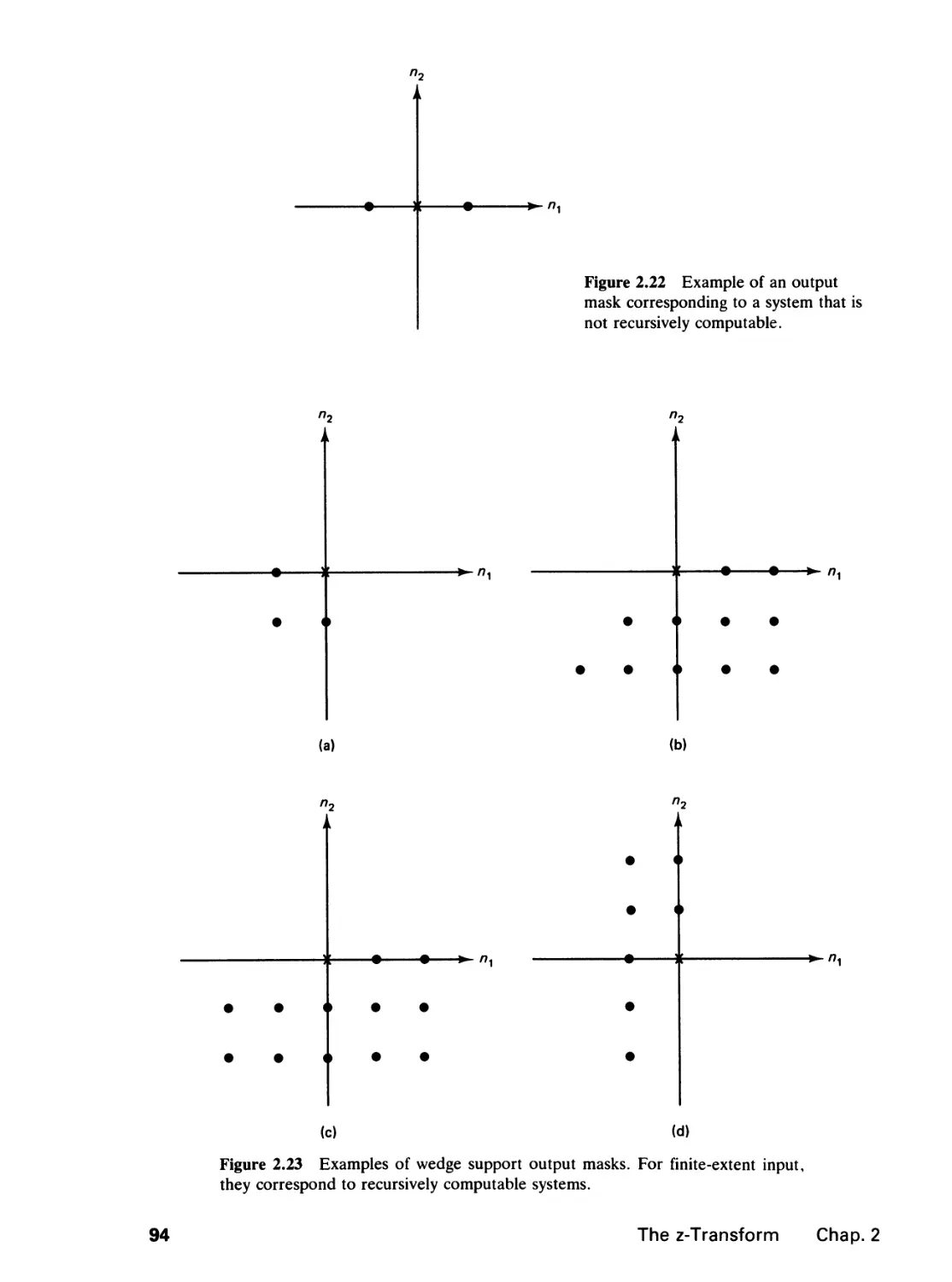
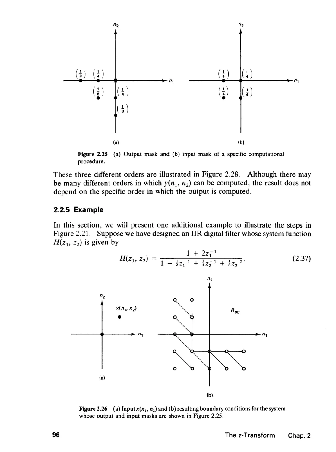
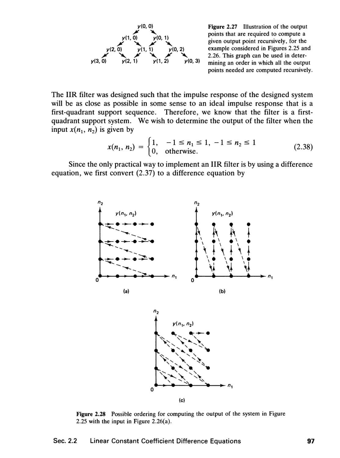
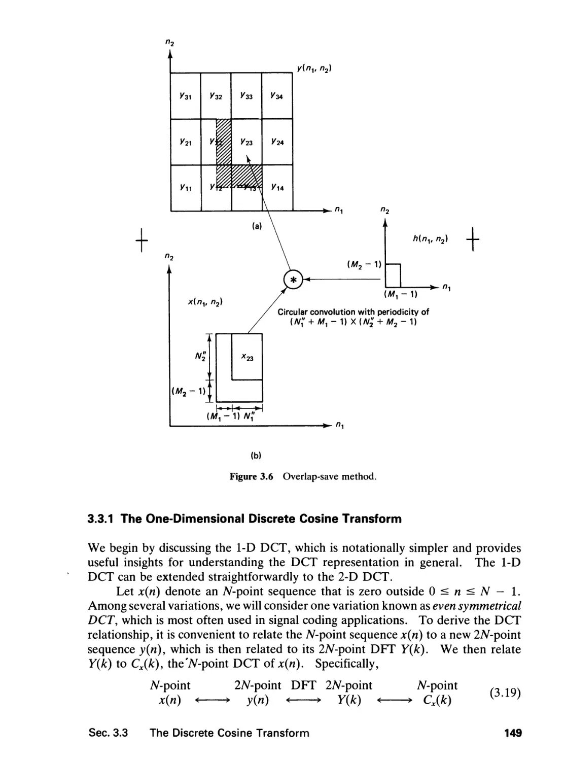
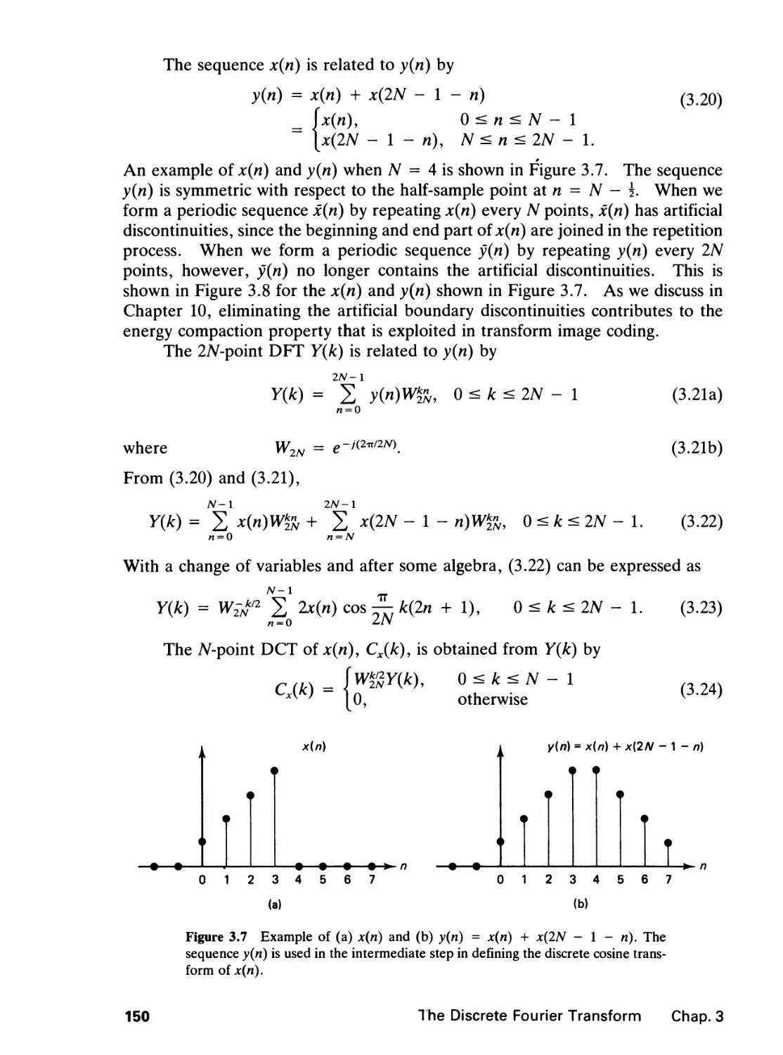
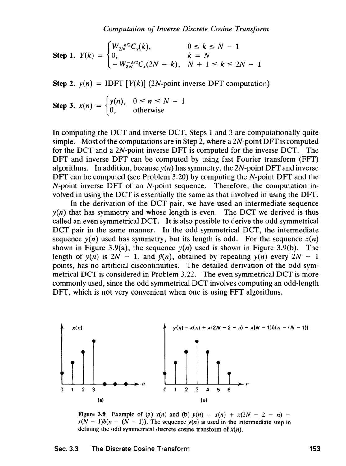
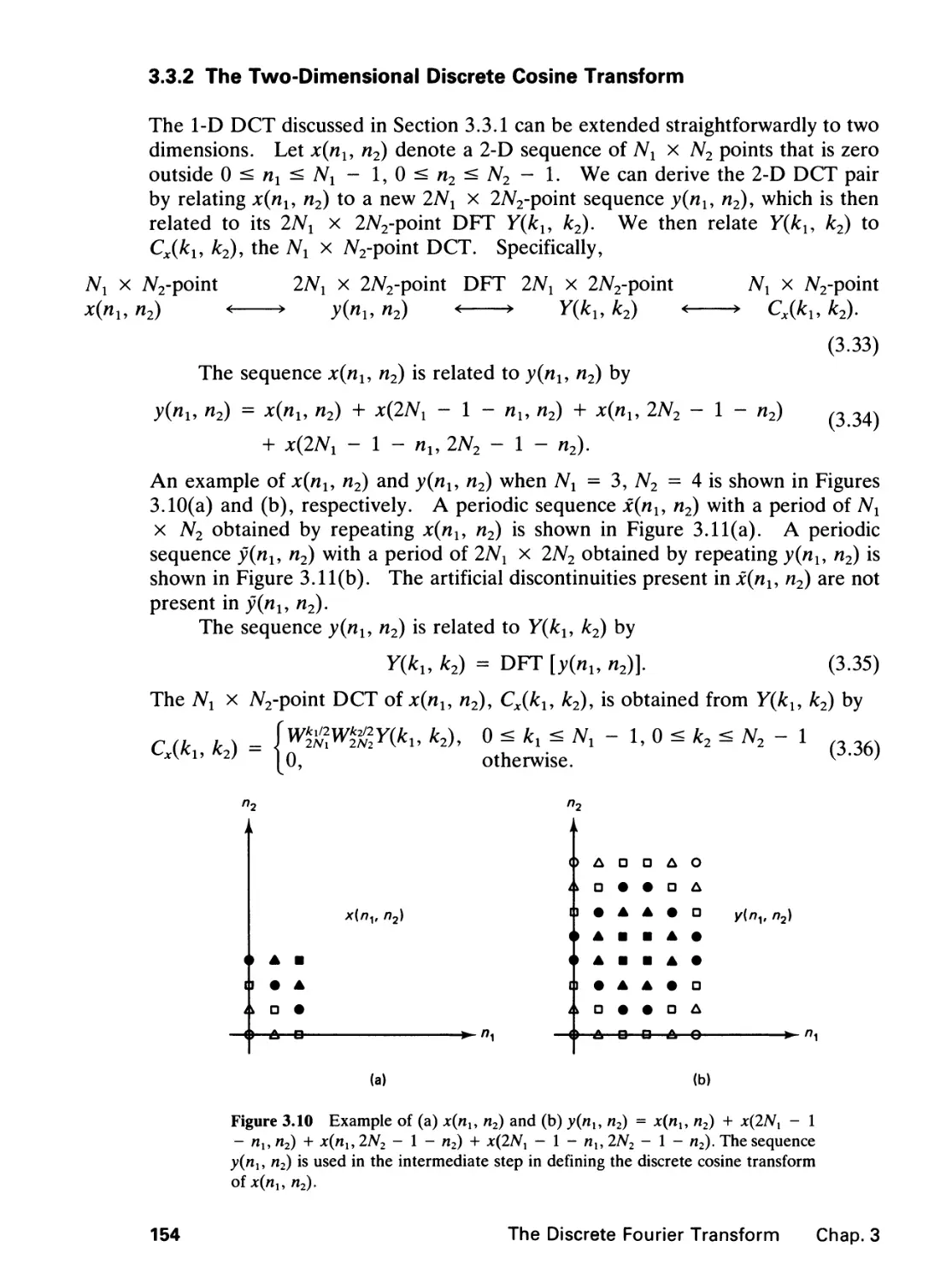
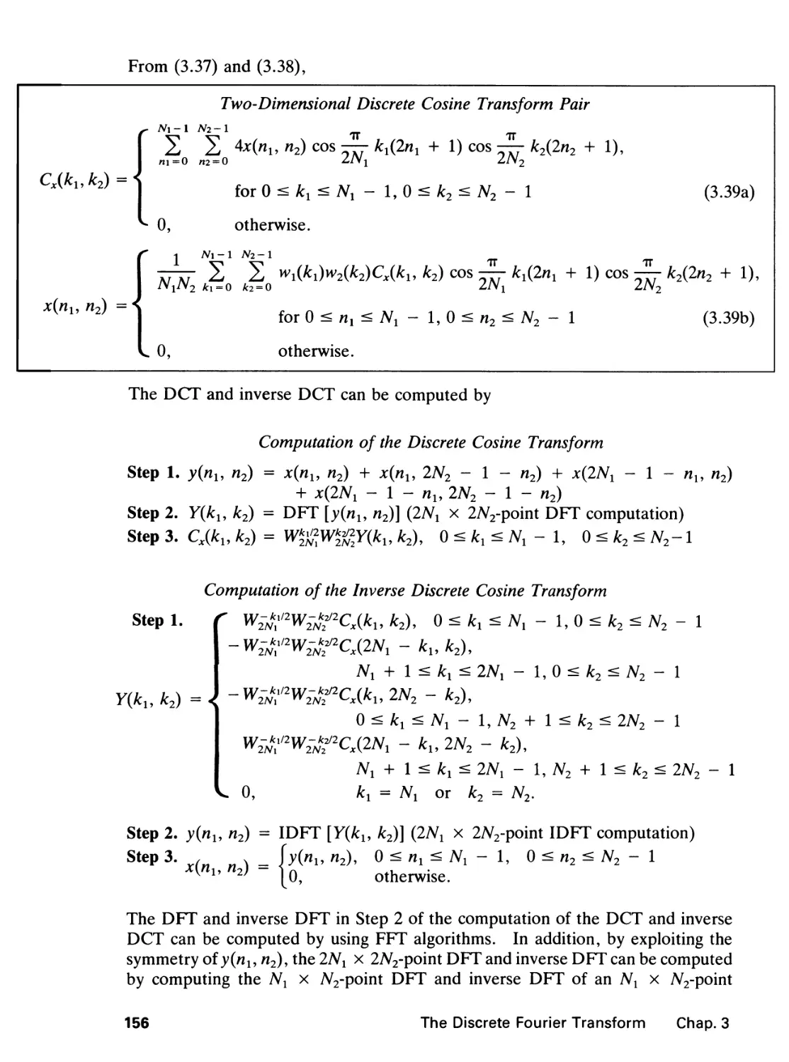
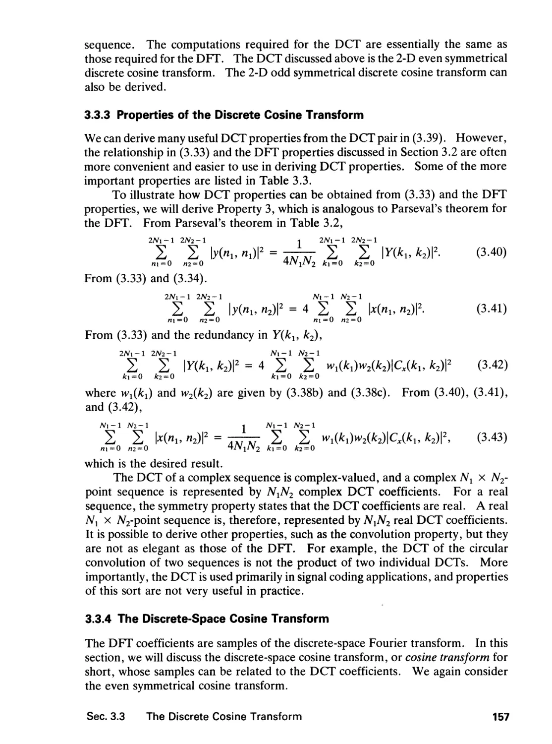
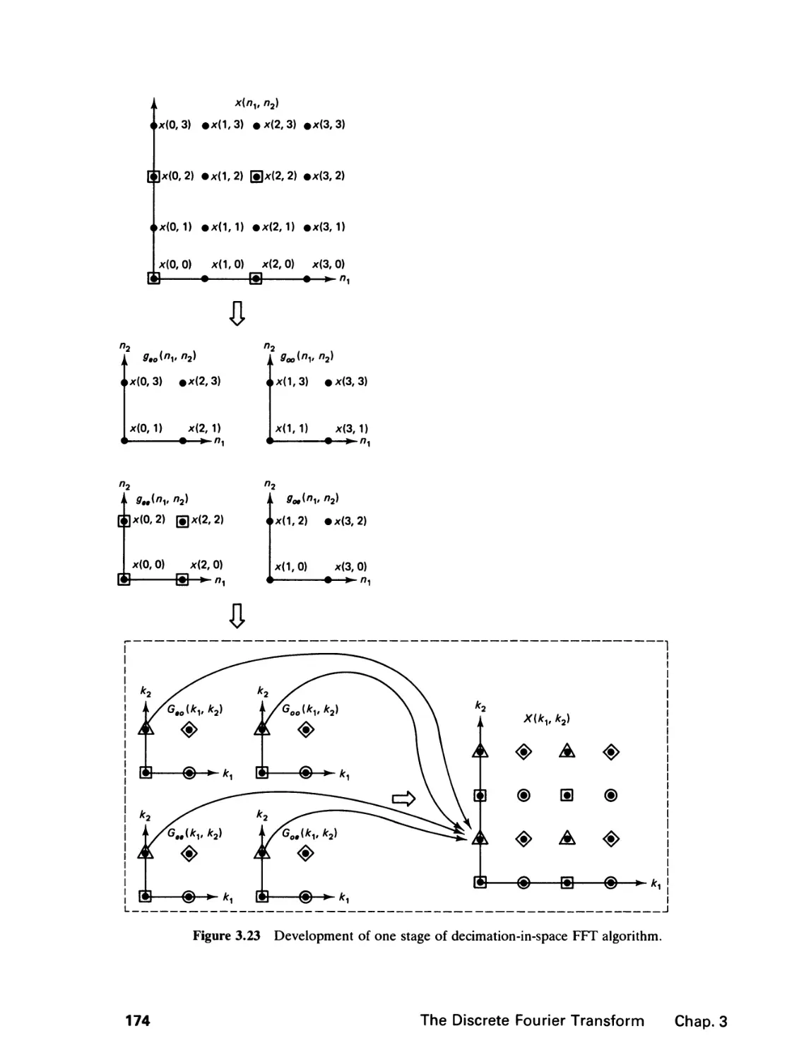
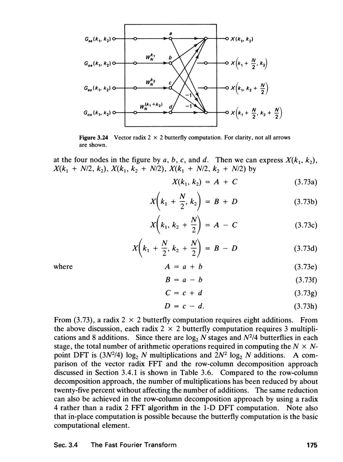
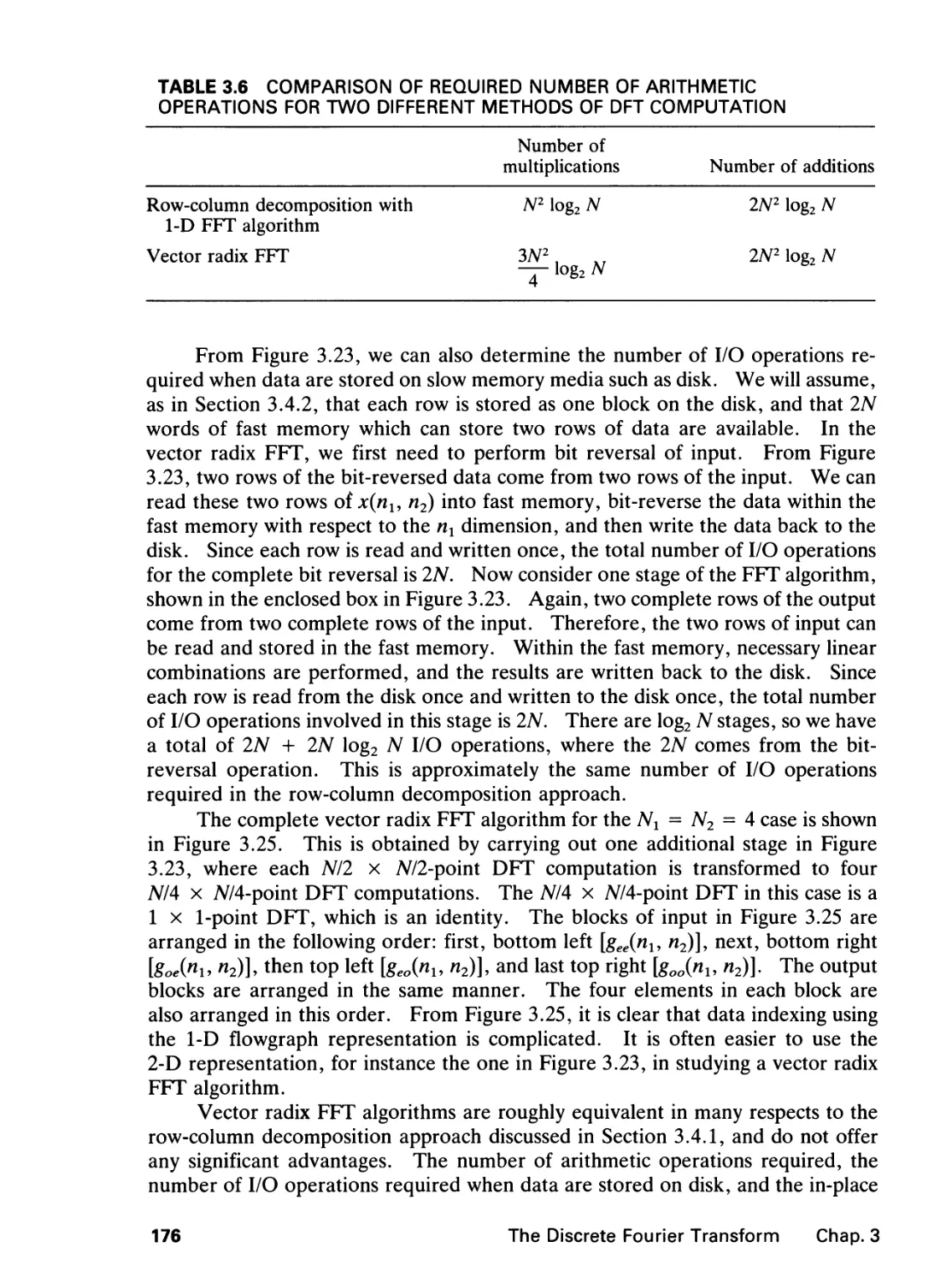
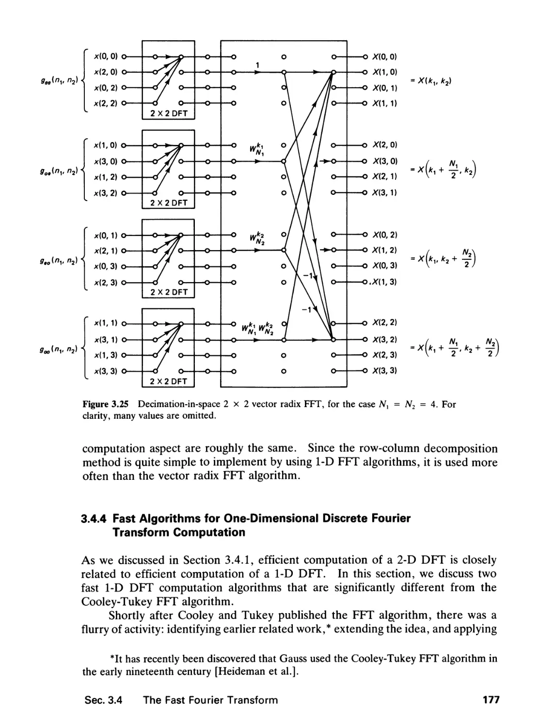
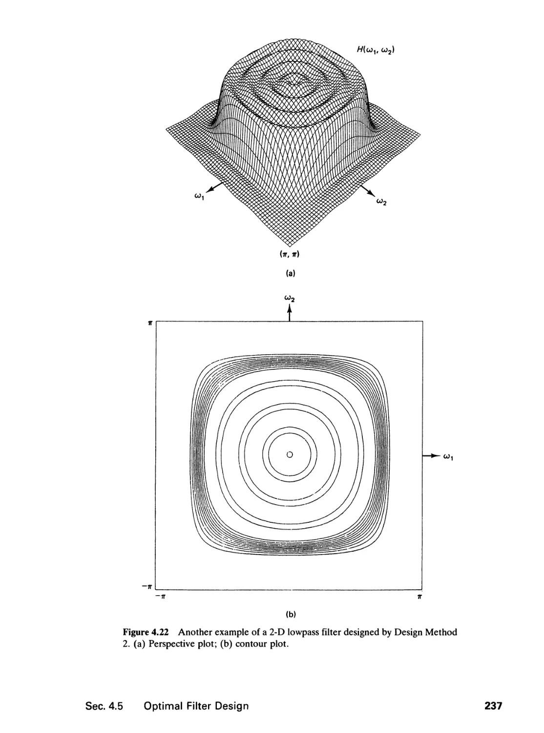
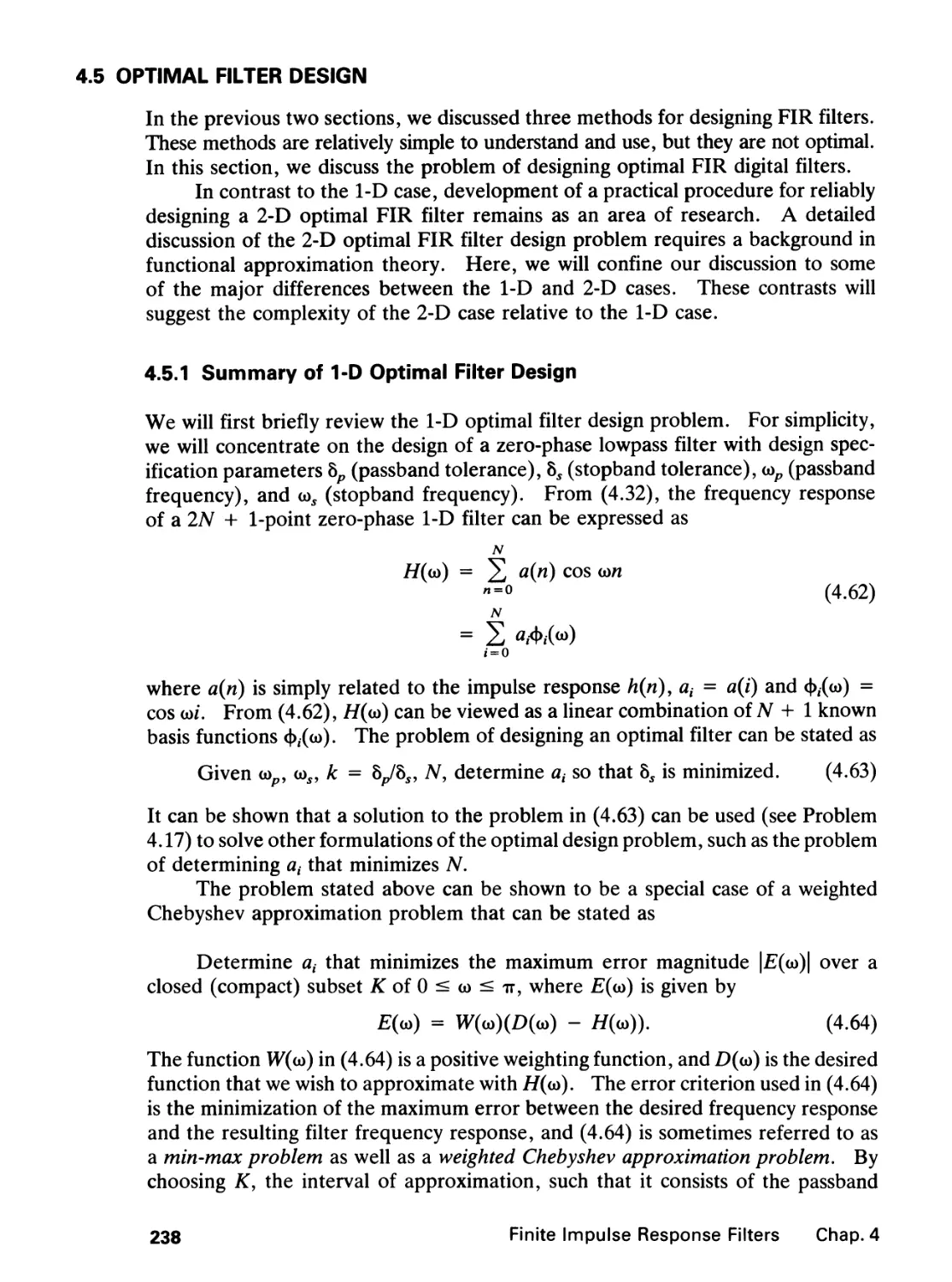
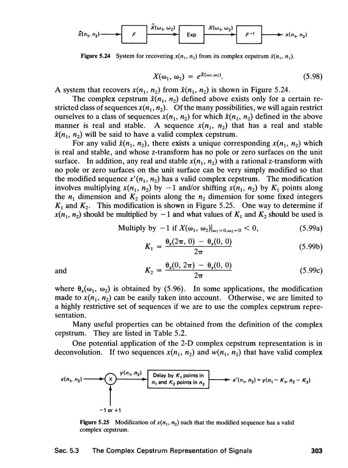
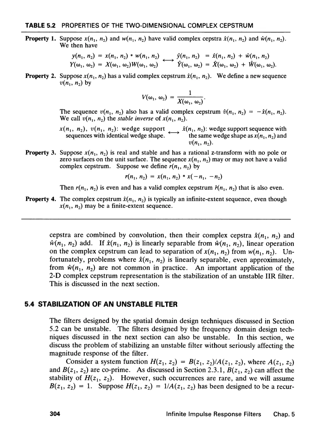
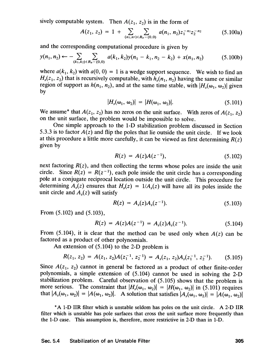
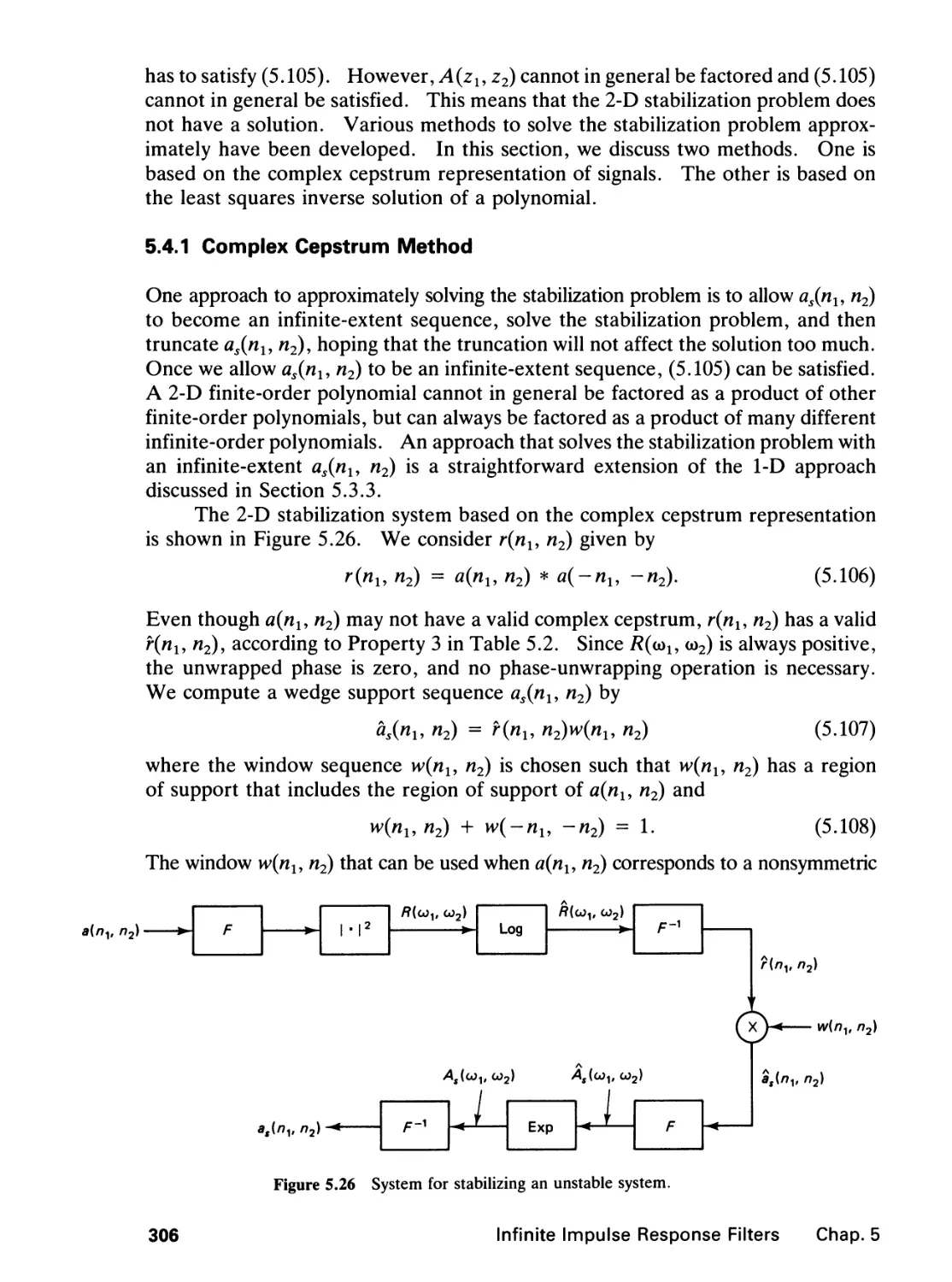
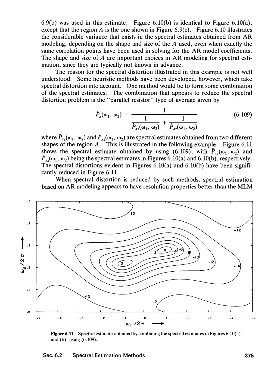
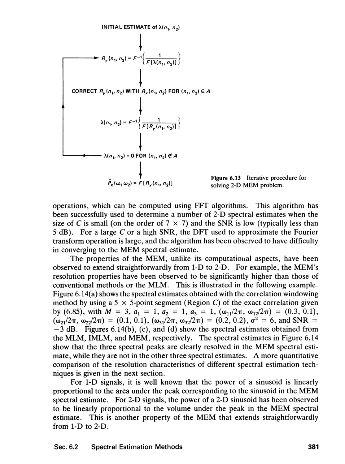
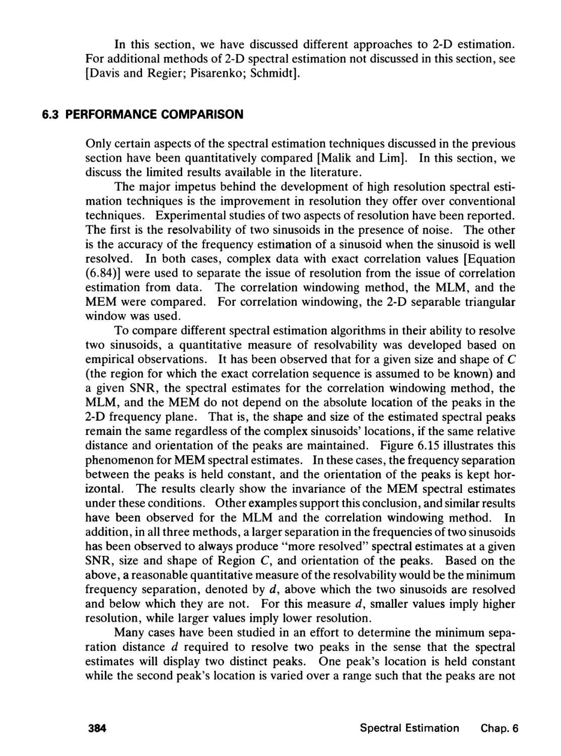
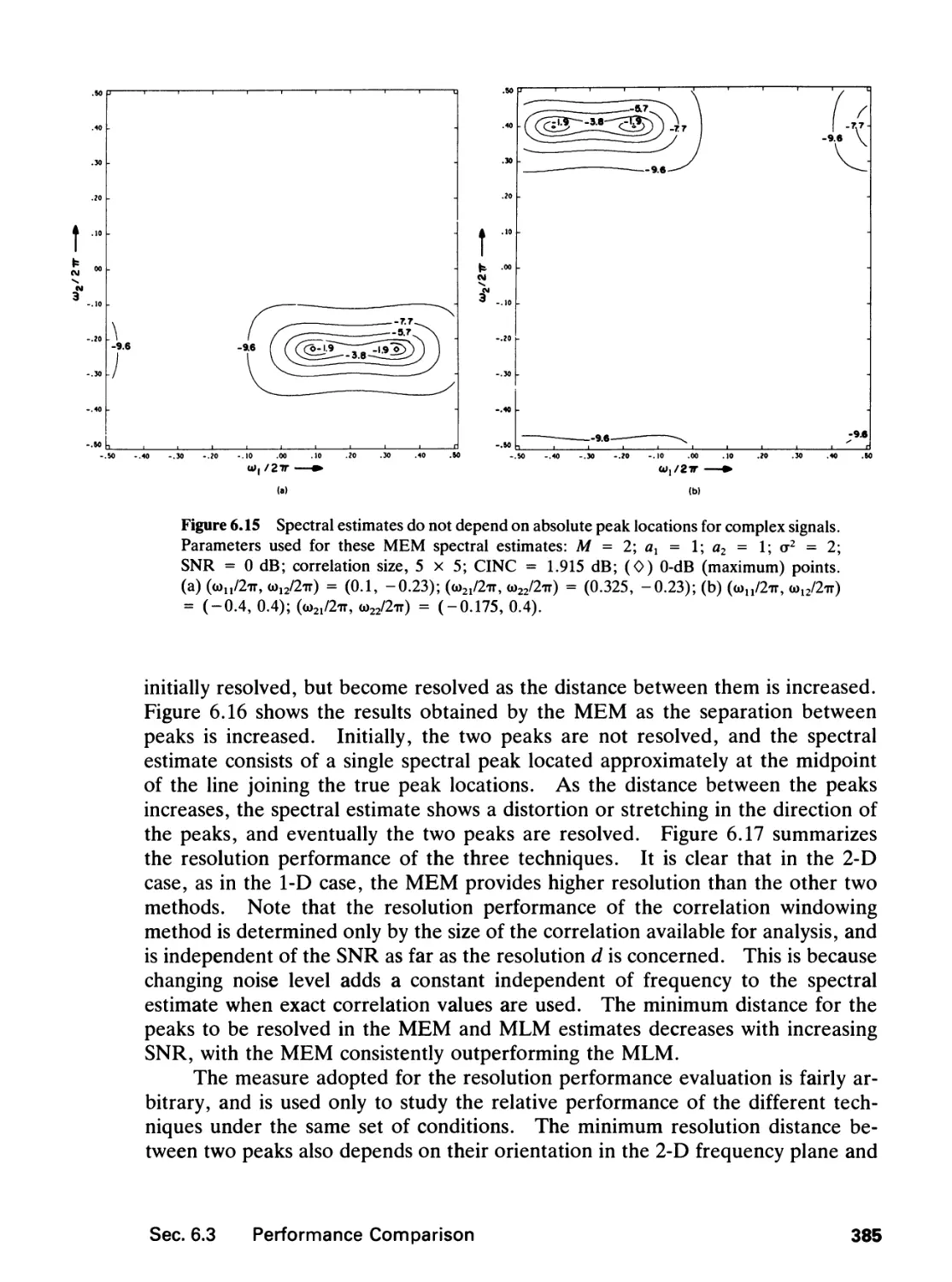
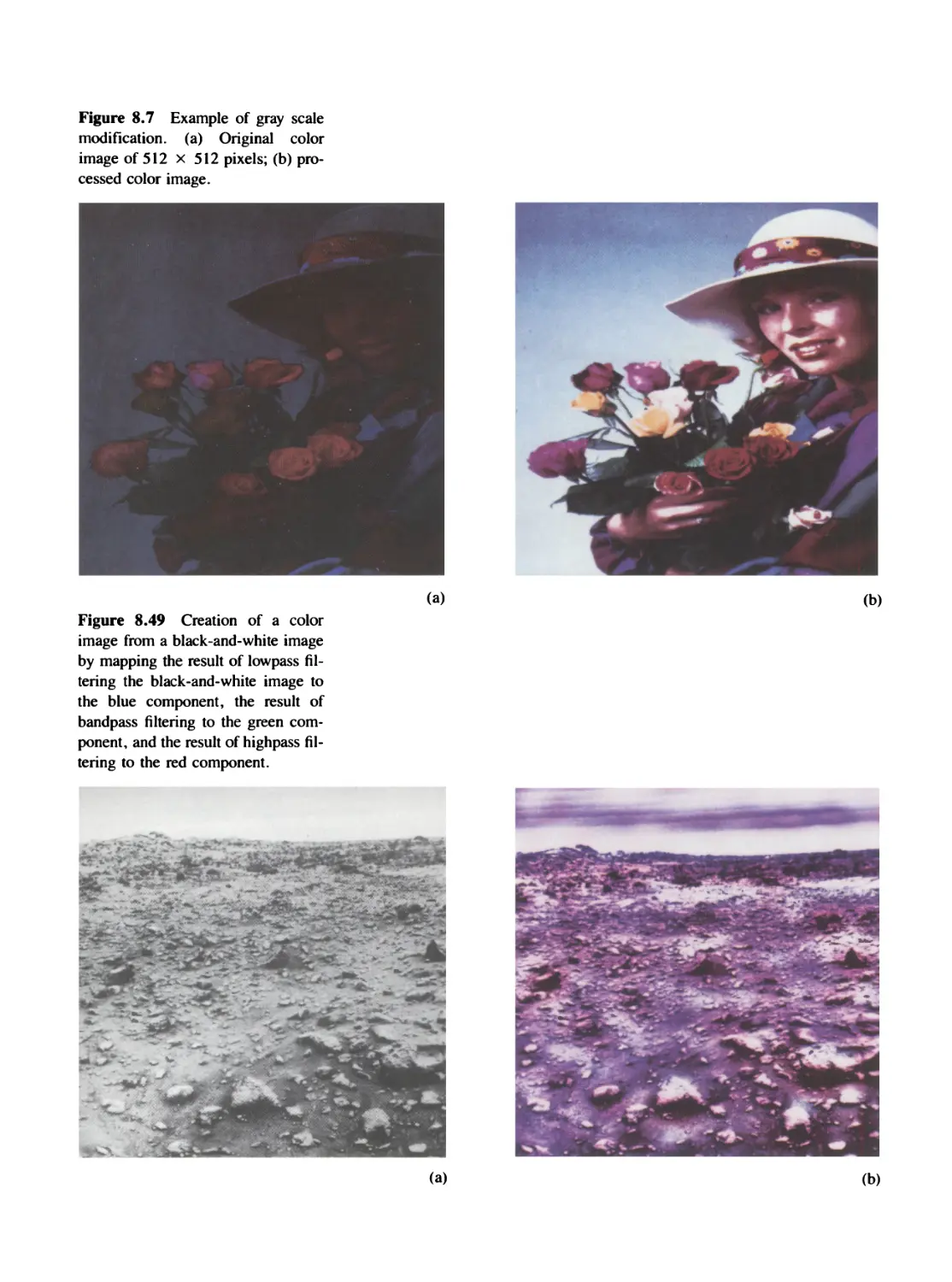
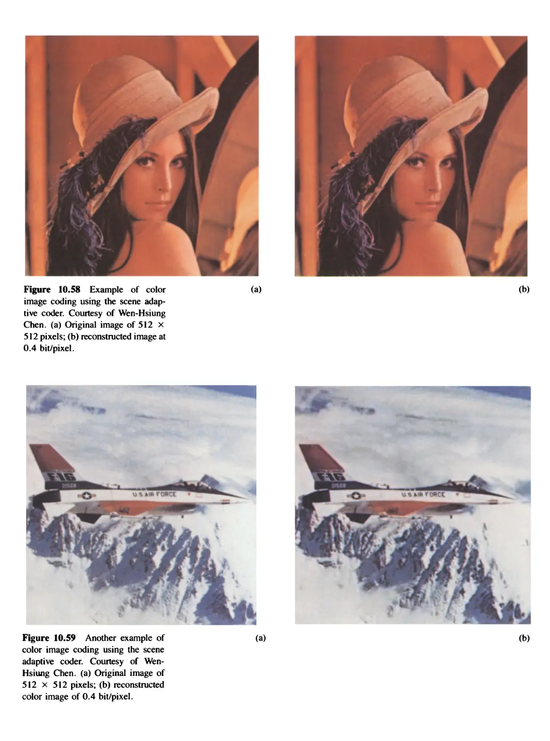
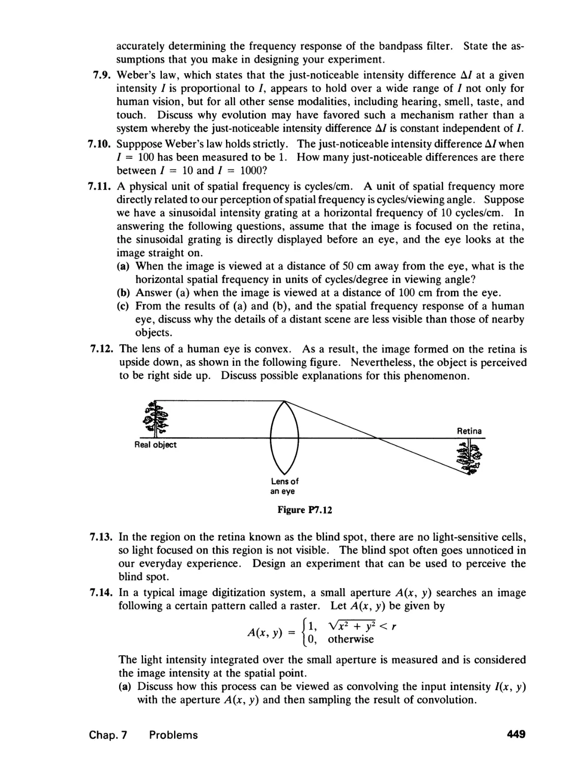
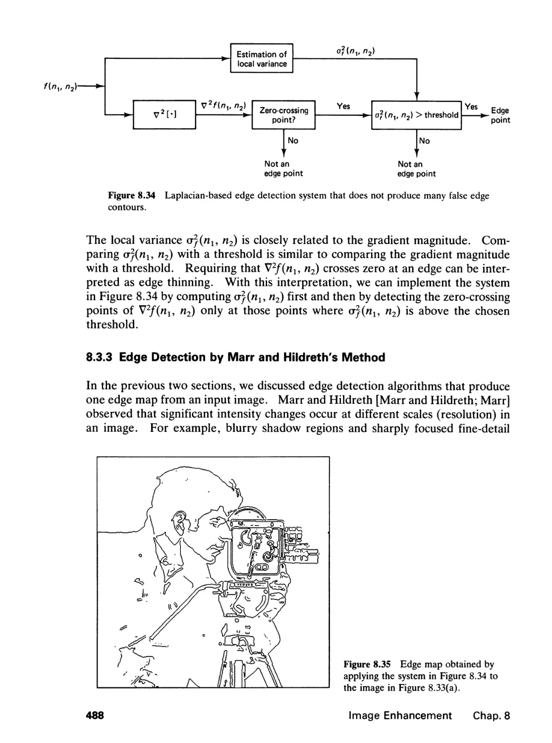
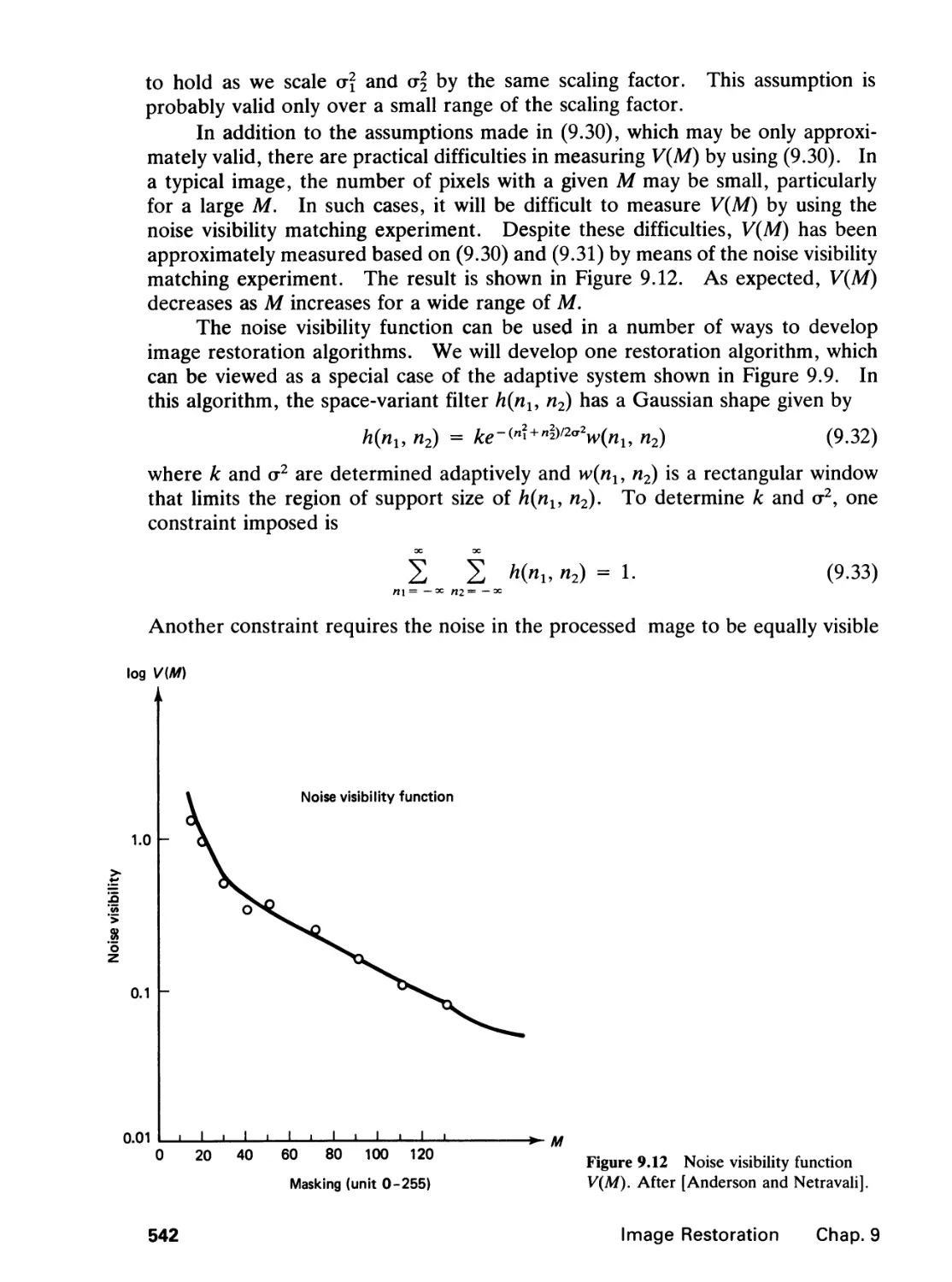
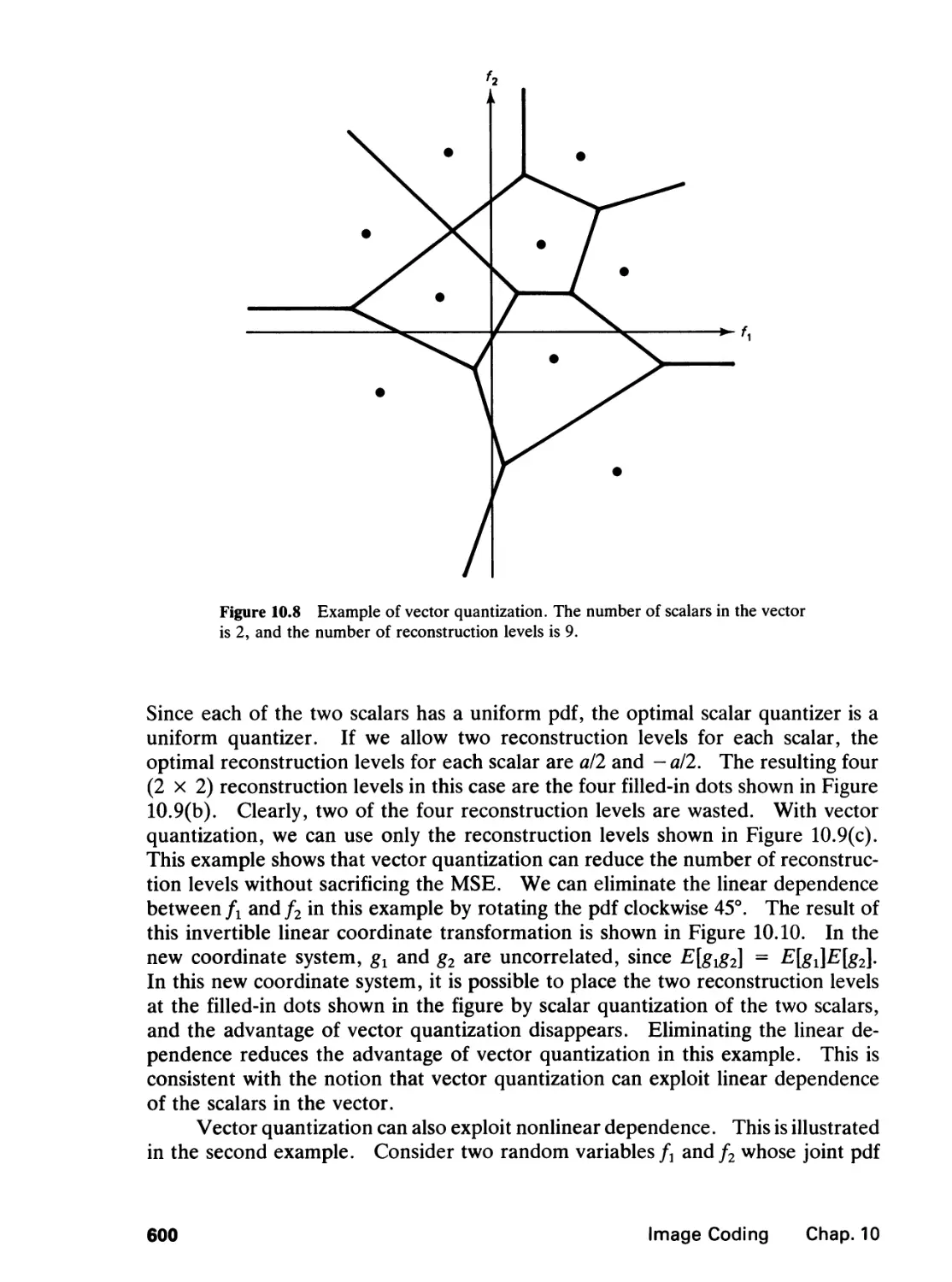
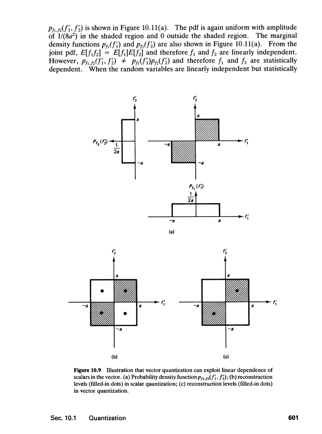
/


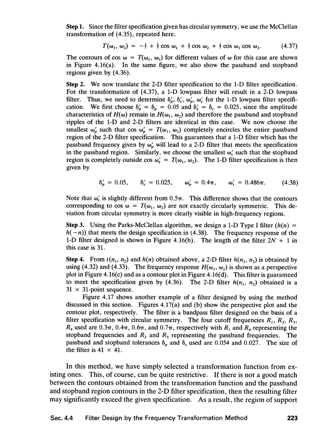
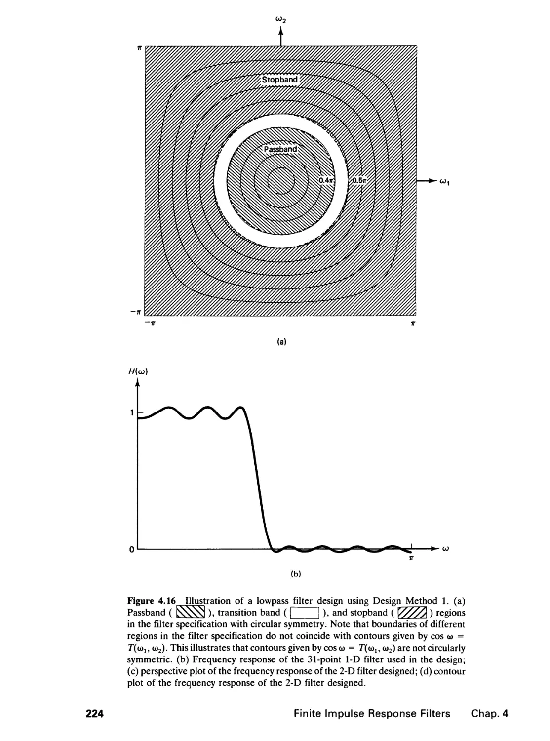


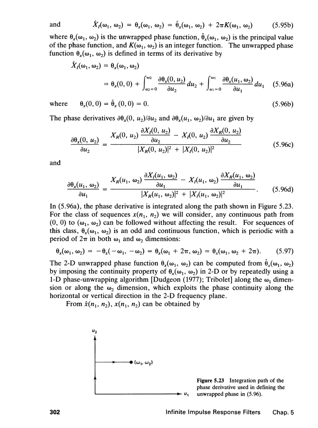


Author: Lim J.S.
Tags: computer science 2d graphics prentice hall edition signal processing
ISBN: 0-13-935322-4
Year: 1989


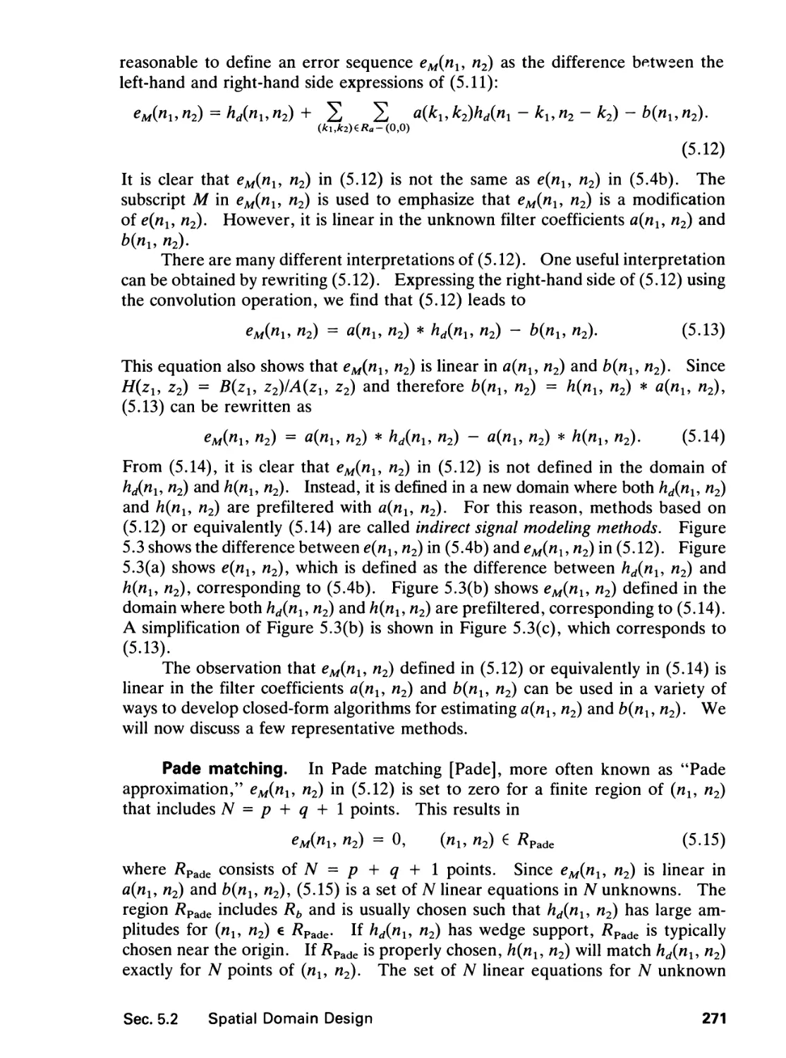
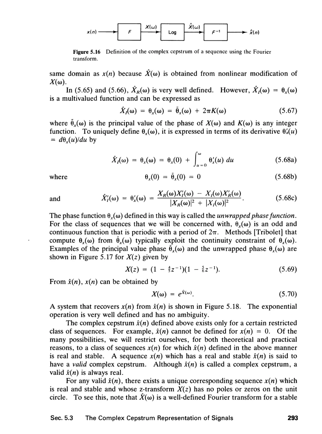
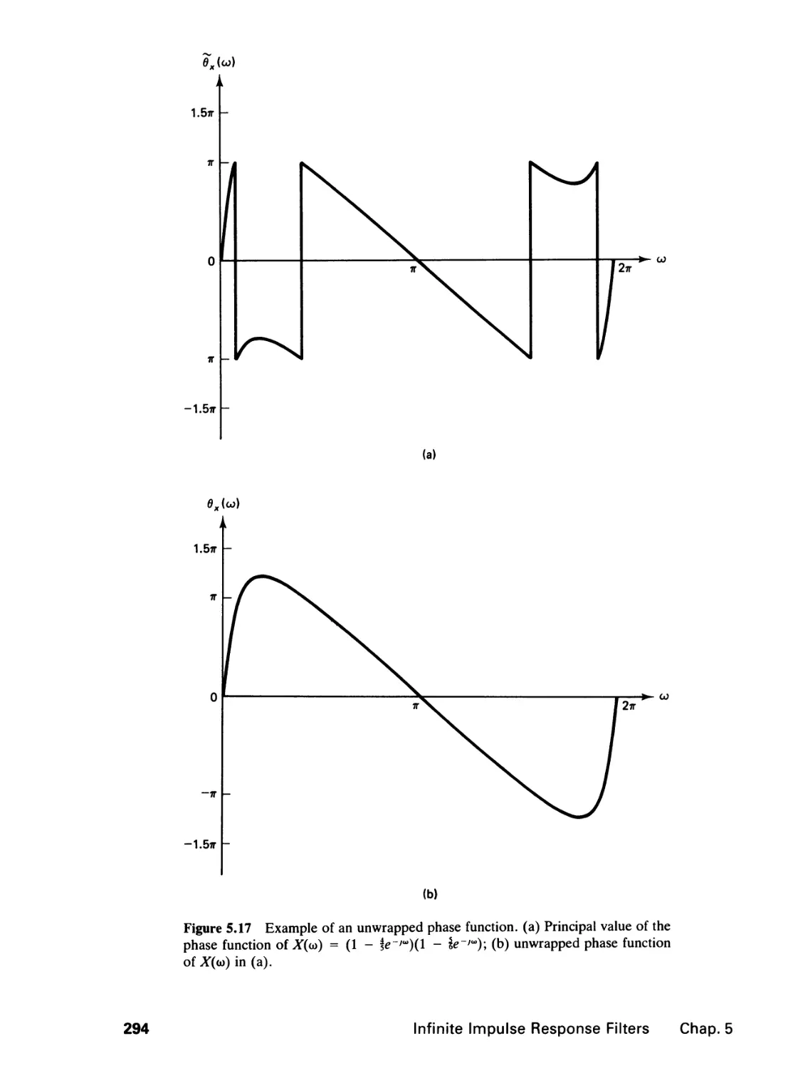
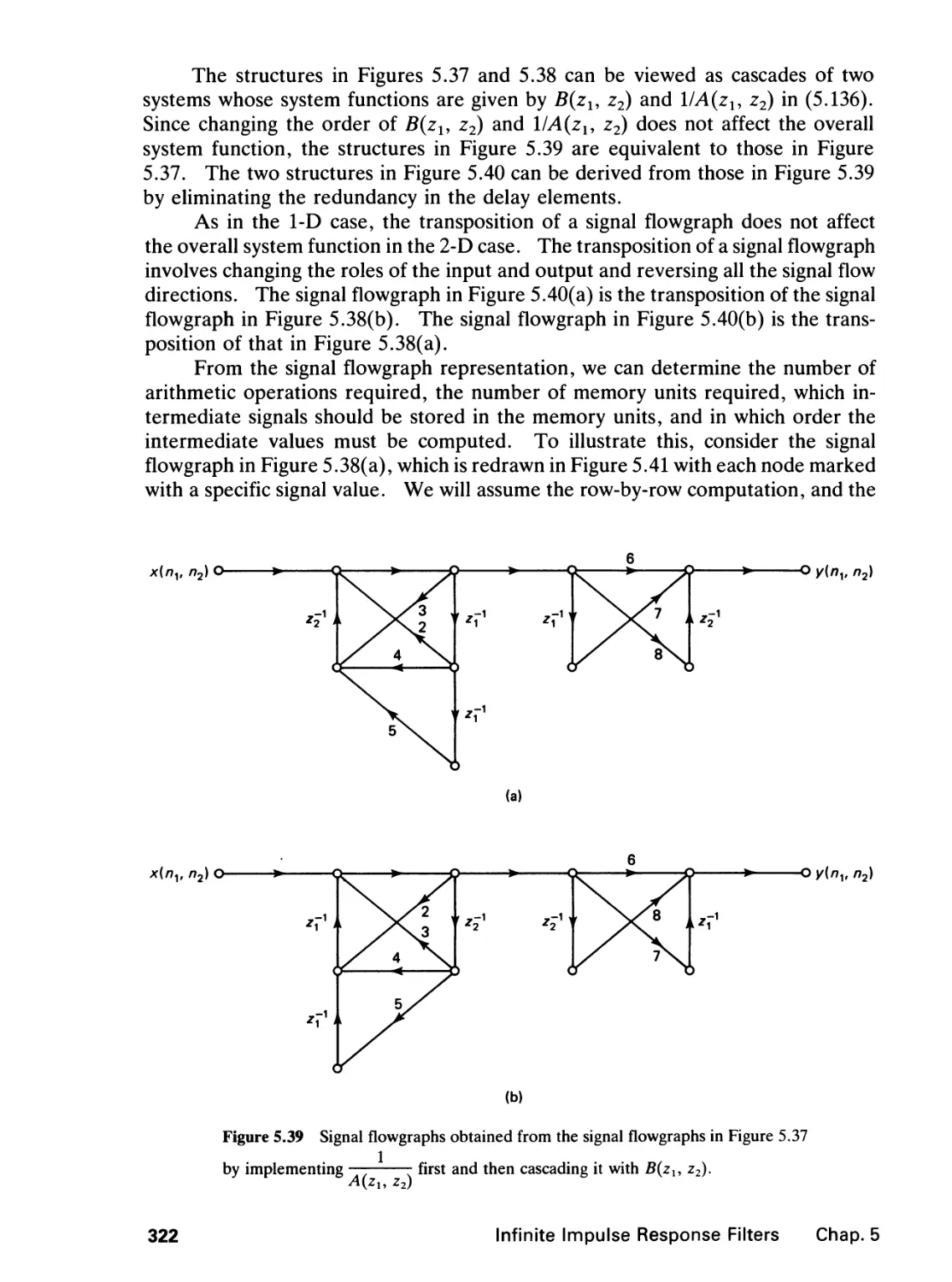
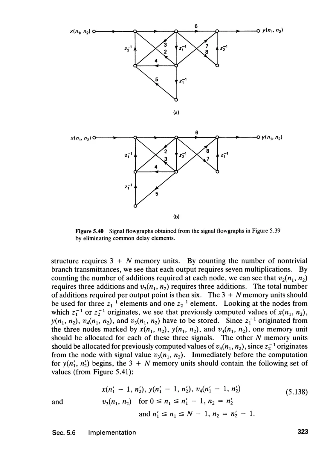
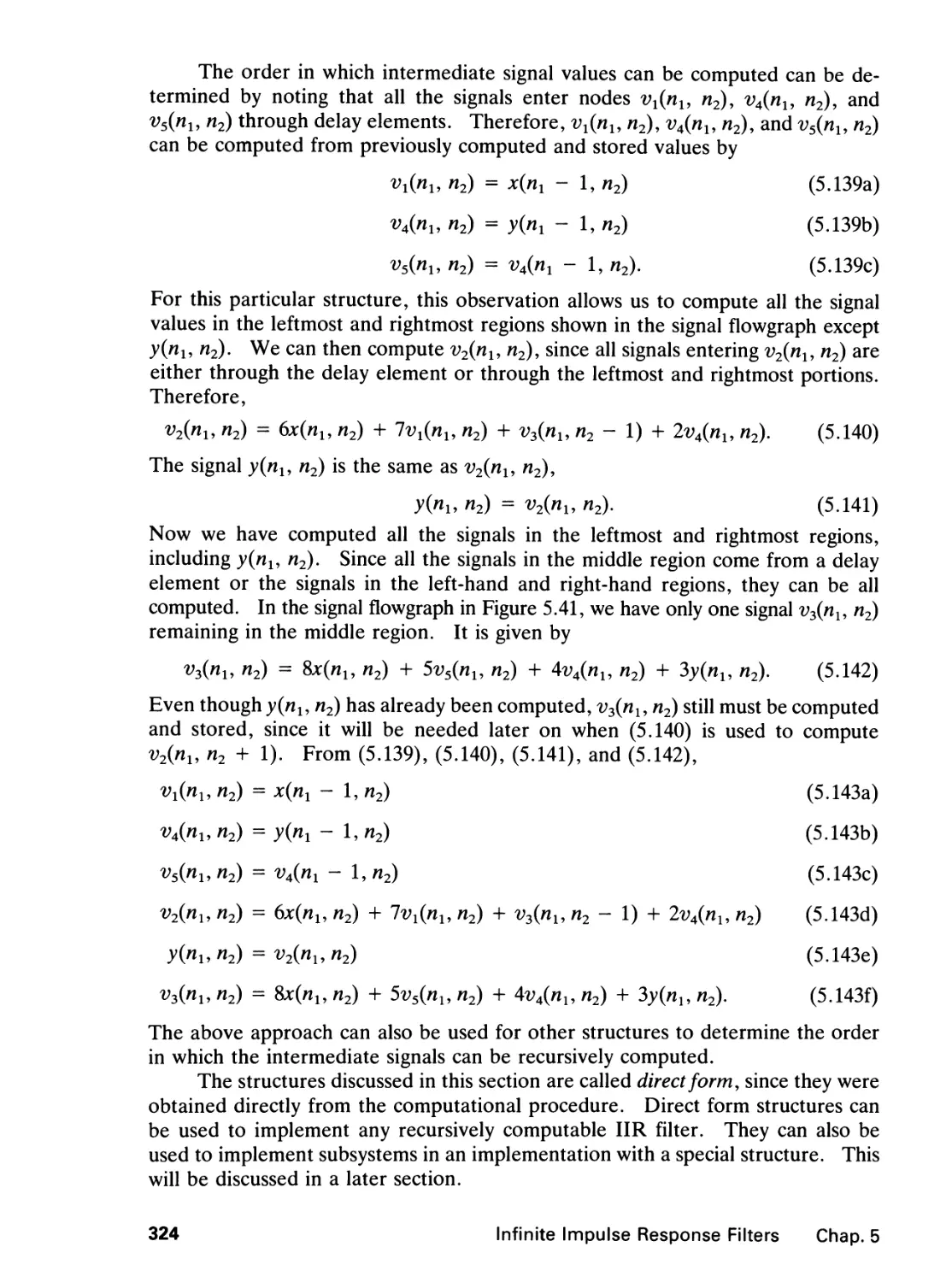
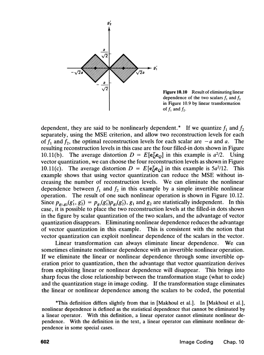
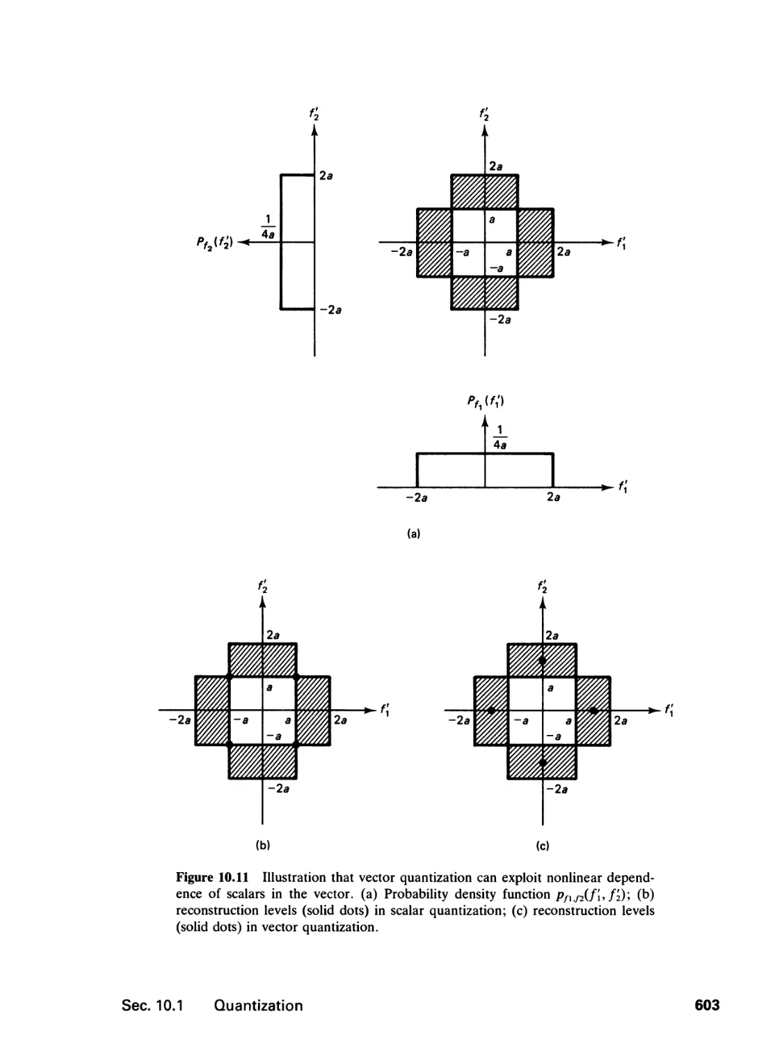
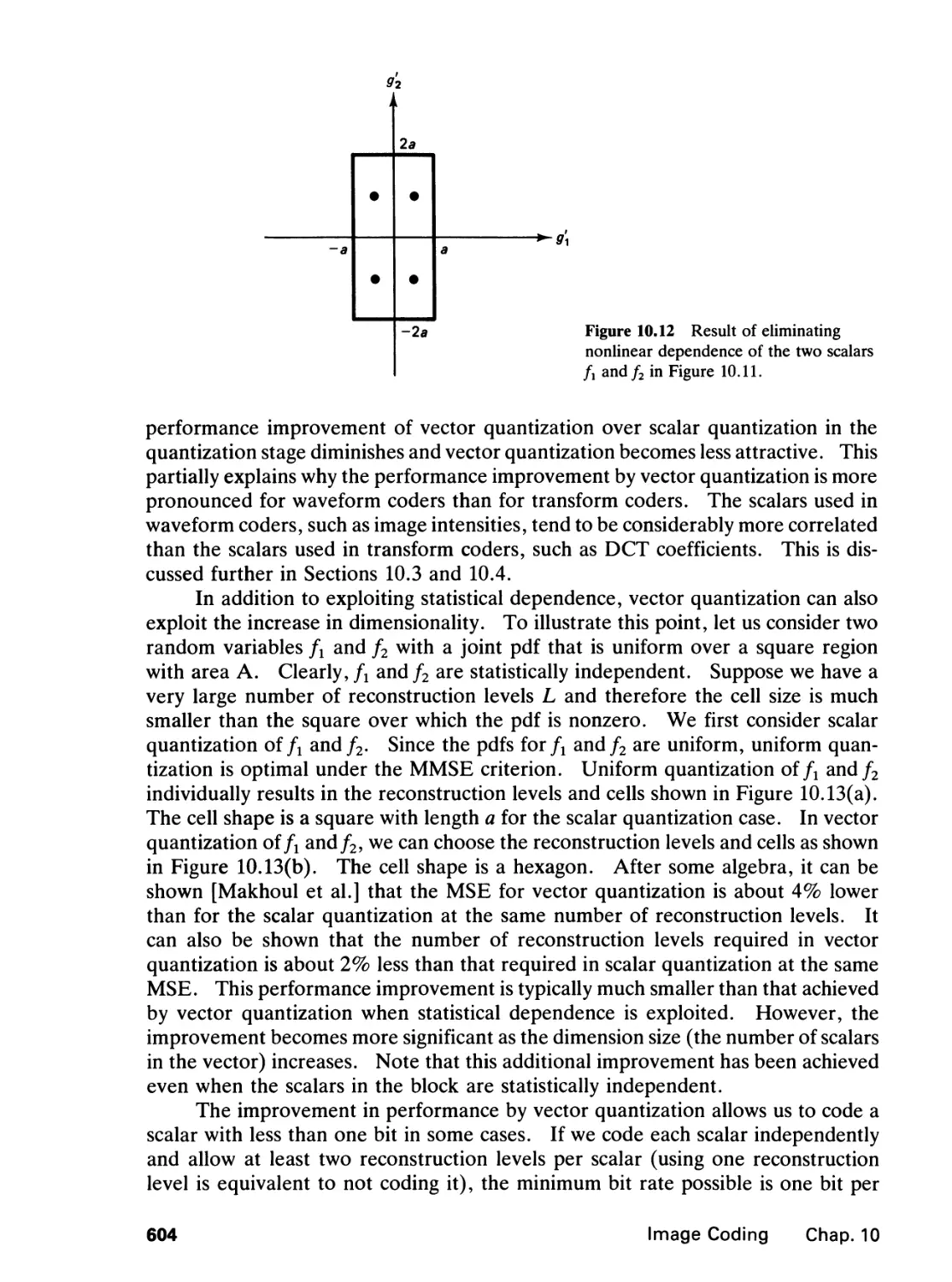
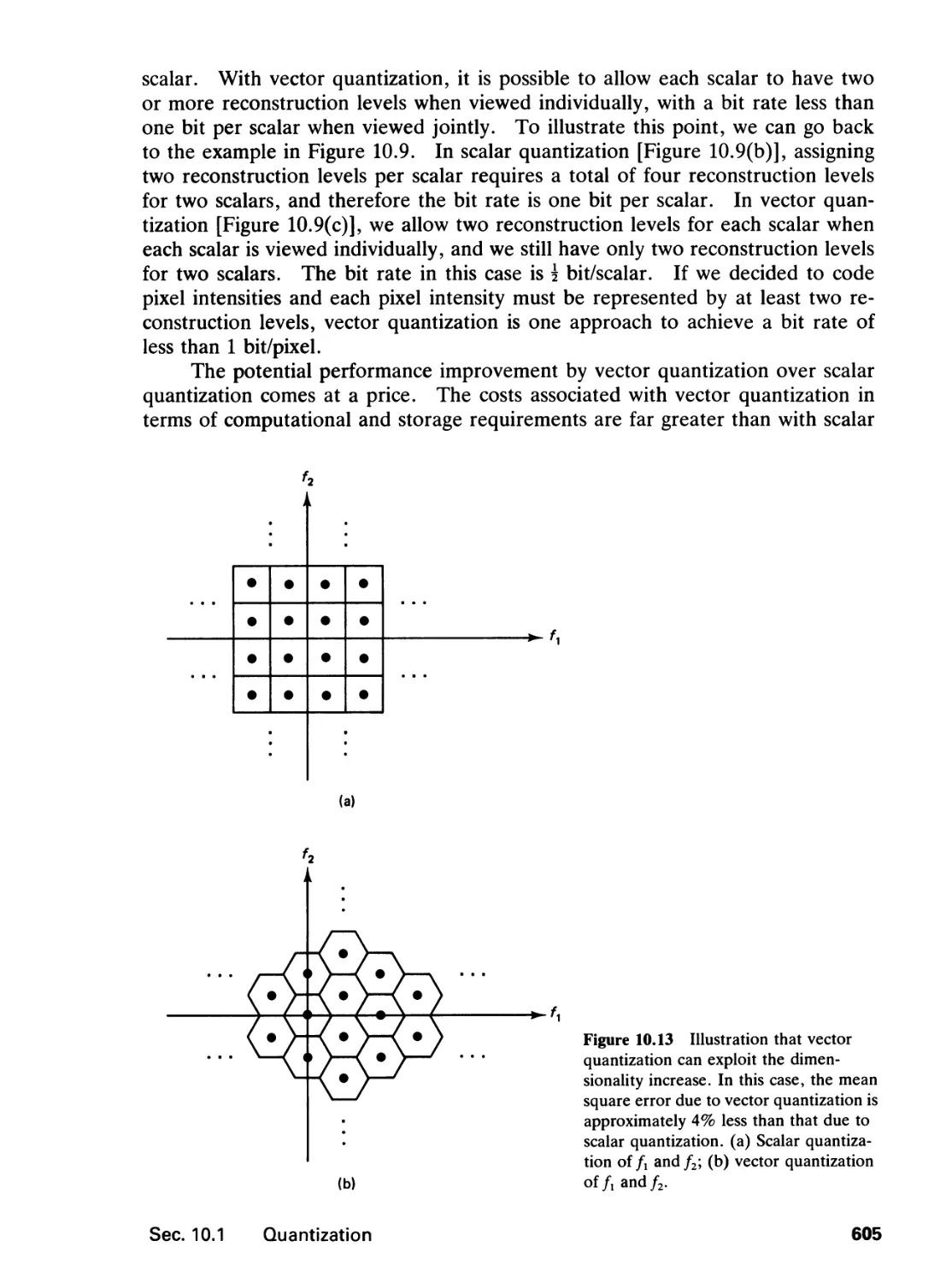
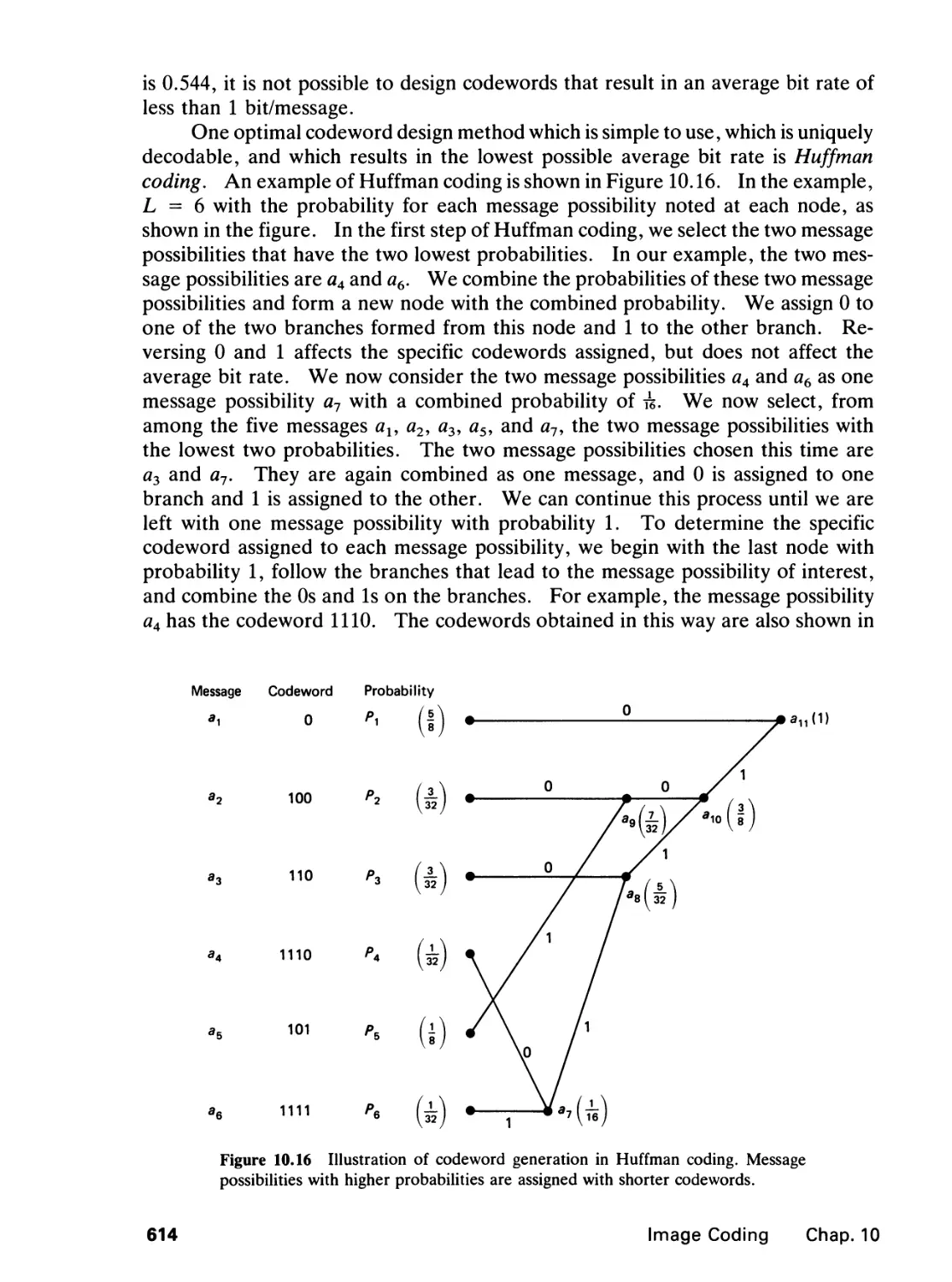
Text
~^rn~ ~nrn v^vji
PRENTICE HALL SIGNAL PROCESSING SERIES
ALAN V OPPENHEIM SERIES EDITOR
TWO-OMENSKMUI.
SIGNAL aw IMAGE
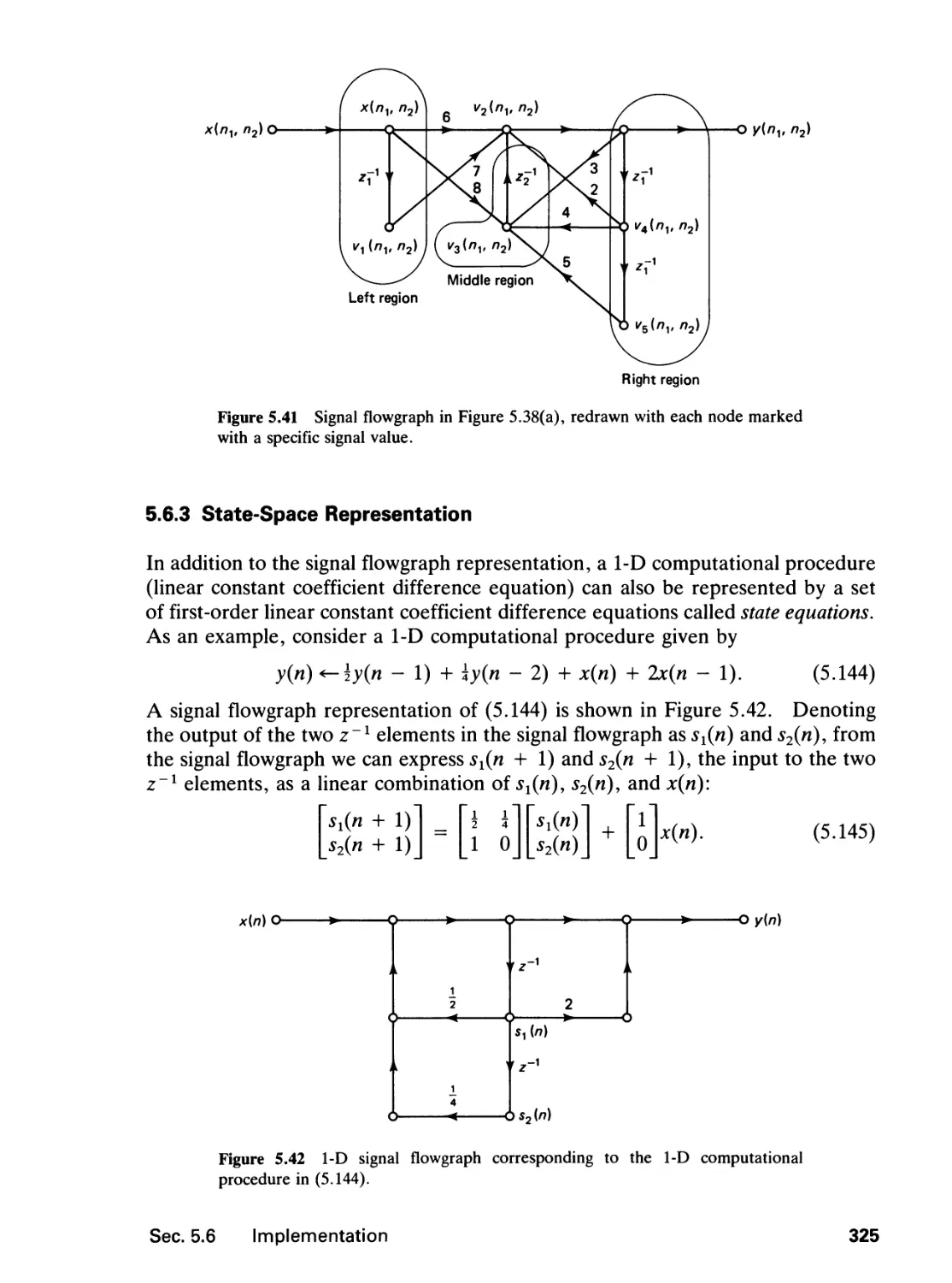
PROCESSING
JAE S. LIM
Department of Electrical Engineering
and Computer Science
Massachusetts Institute of Technology
PRENTICE HALL, Englewood Cliffs, New Jersey 07632
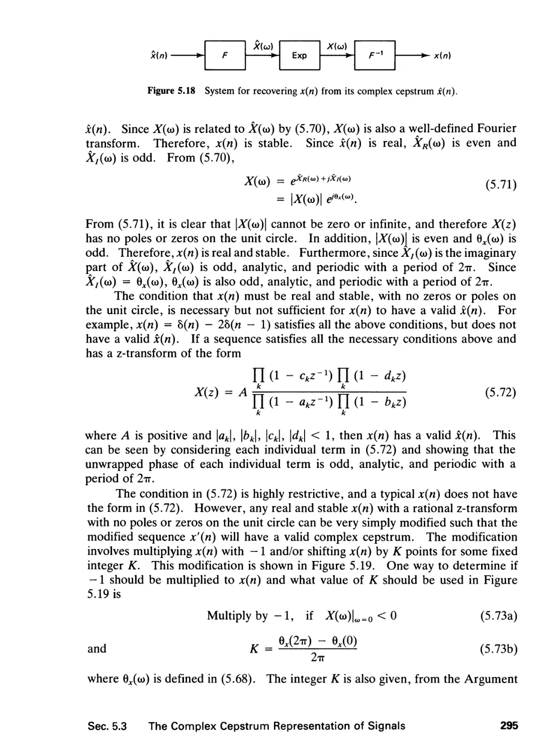
Library of Congress Cataloging-in-Publication Data
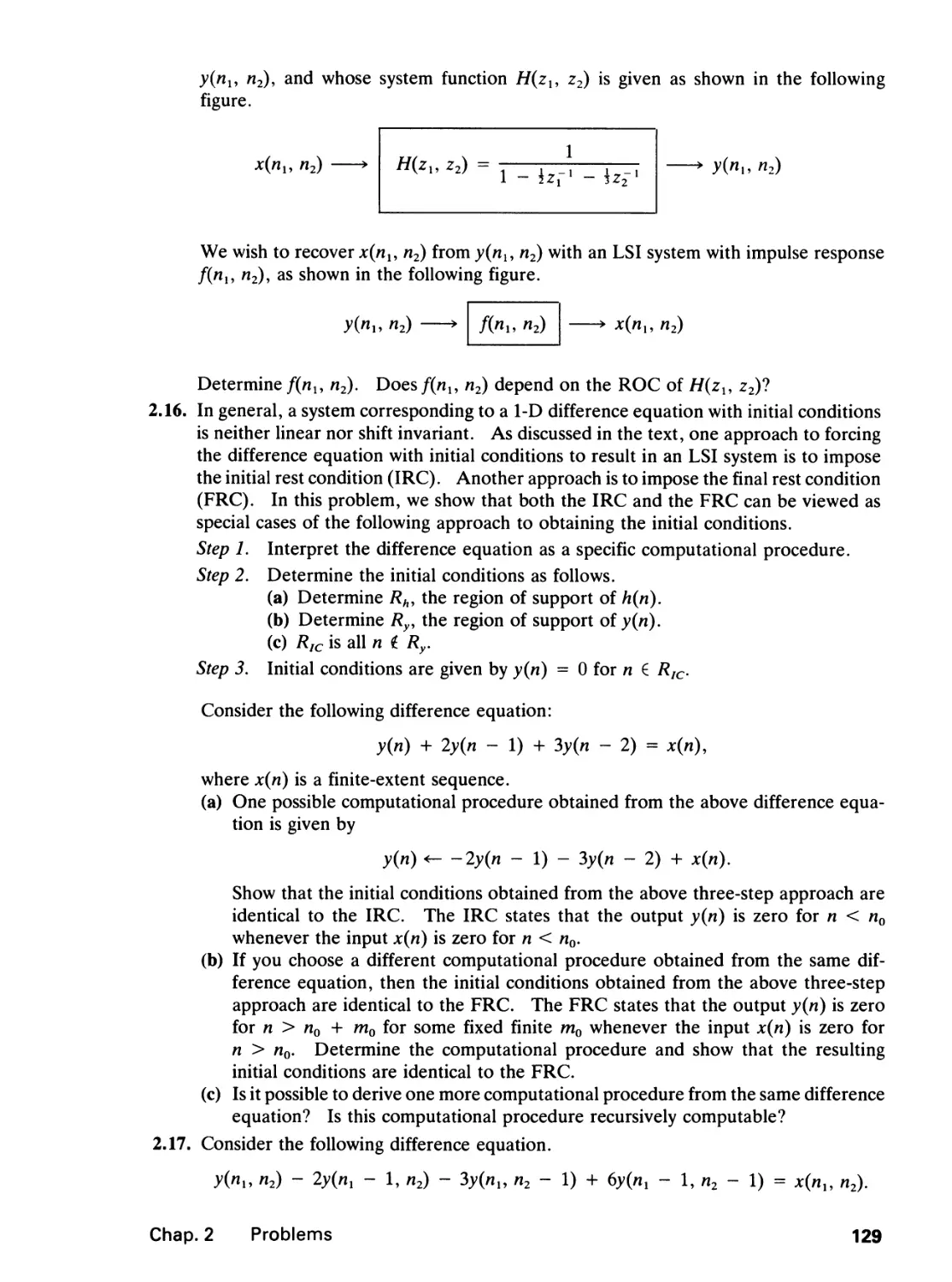
Lim, Jae S.
Two-dimensional signal and image processing / Jae S. Lim.
p. cm.—(Prentice Hall signal processing series)
Bibliography: p.
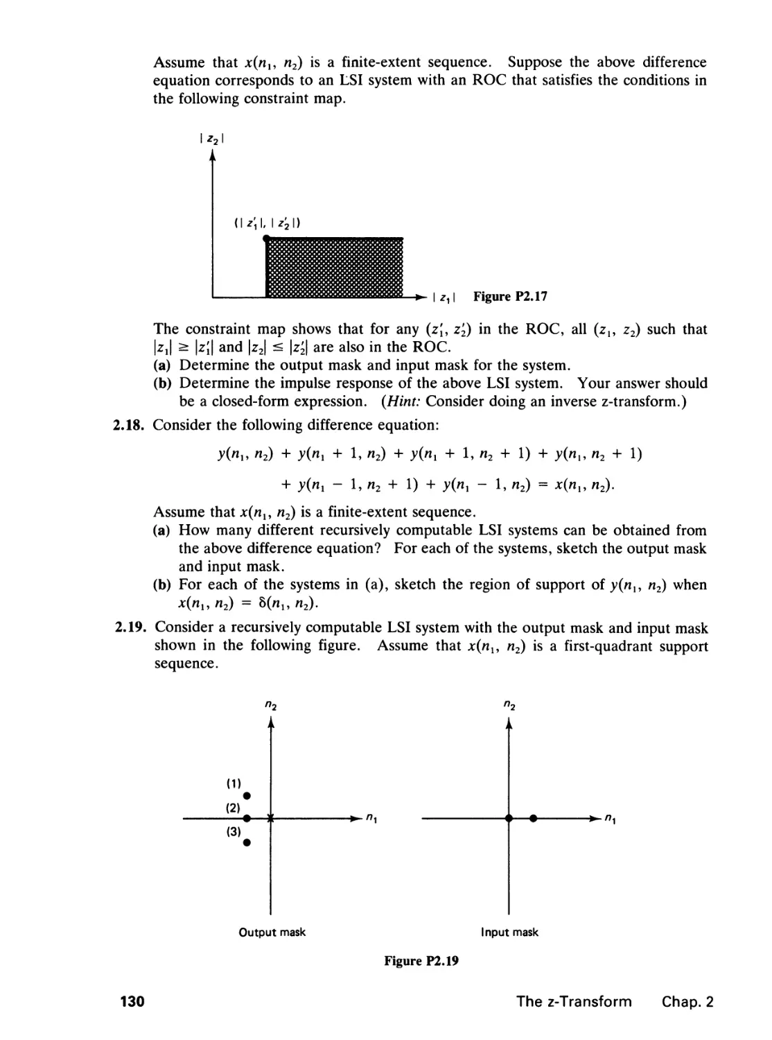
Includes index.
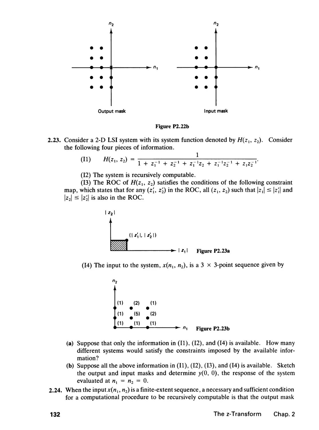
ISBN 0-13-935322-4
1. Signal processing—Digital techniques. 2. Image processing—
Digital techniques. I. Title. II. Series.
TK5102.5.L54 1990
621.382'2—dc20 89-33088
CIP
Editorial/production supervision: Raeia Maes
Cover design: Ben Santora
Manufacturing buyer: Mary Ann Gloriande
© 1990 by Prentice-Hall, Inc.
A Division of Simon & Schuster
Englewood Cliffs, New Jersey 07632
All rights reserved. No part of this book may be
reproduced, in any form or by any means,
without permission in writing from the publisher.
Printed in the United States of America
10 987654321
ISBN 0-13-^35322-14
Prentice-Hall International (UK) Limited, London
Prentice-Hall of Australia Pty. Limited, Sydney
Prentice-Hall Canada Inc., Toronto
Prentice-Hall Hispanoamericana, S.A., Mexico
Prentice-Hall of India Private Limited, New Delhi
Prentice-Hall of Japan, Inc., Tokyo
Simon & Schuster Asia Pte. Ltd., Singapore
Editora Prentice-Hall do Brasil, Ltda., Rio de Janeiro
TO
KYUHO and TAEHO
Contents
PREFACE xi
INTRODUCTION xm
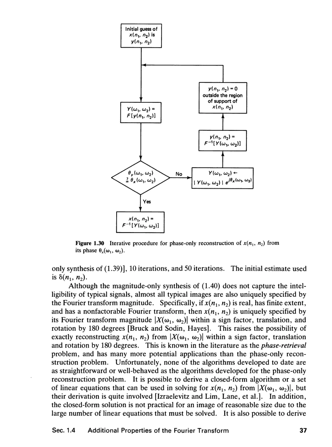
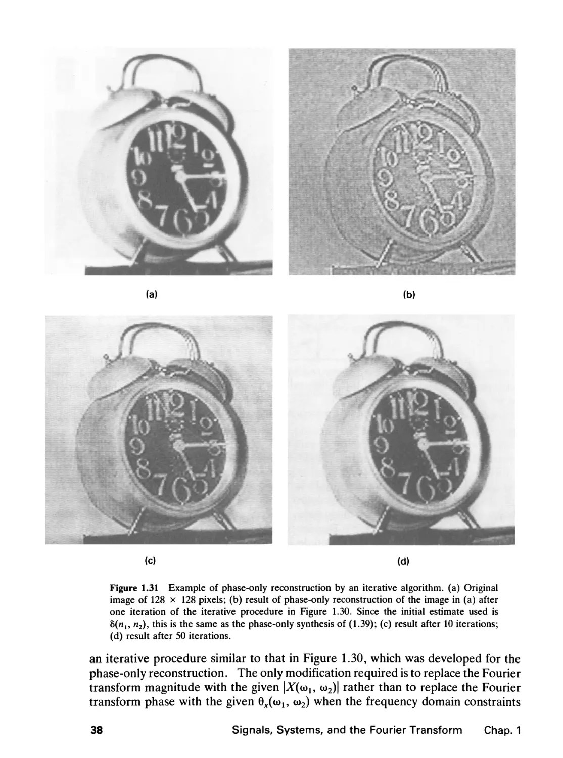
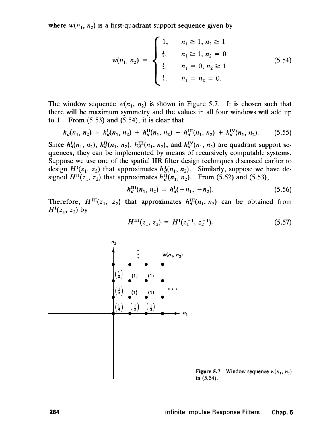
1 SIGNALS, SYSTEMS, AND THE FOURIER TRANSFORM 1
1.0 Introduction, 1
1.1 Signals, 2
1.2 Systems, 12
1.3 The Fourier Transform, 22
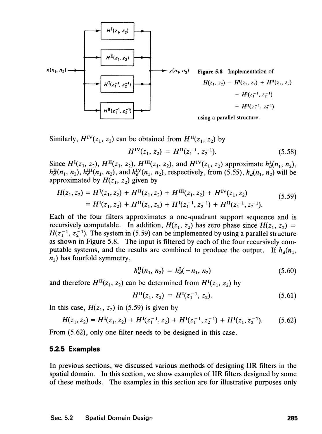
1.4 Additional Properties of the Fourier Transform, 31
1.5 Digital Processing of Analog Signals, 45
References, 49
Problems, 50
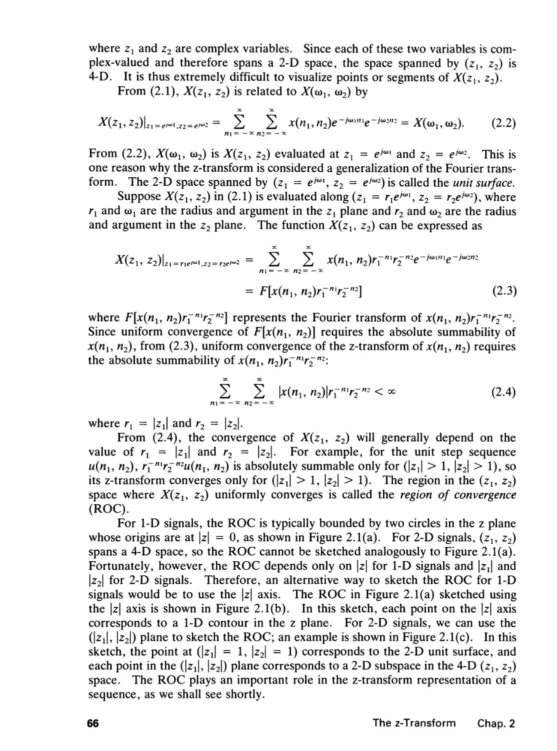
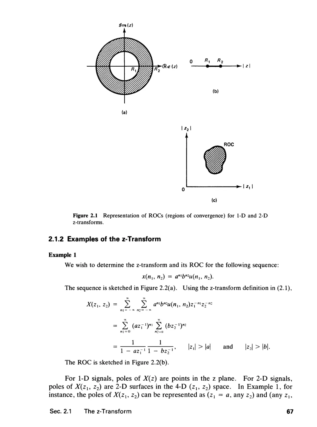
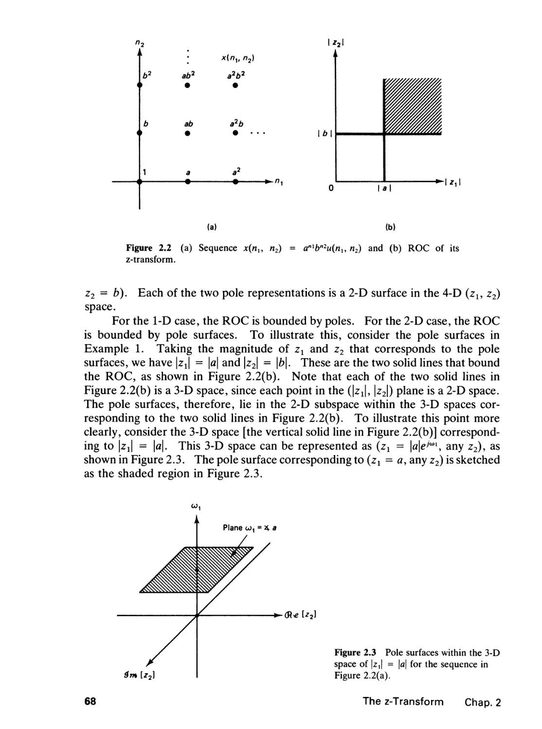
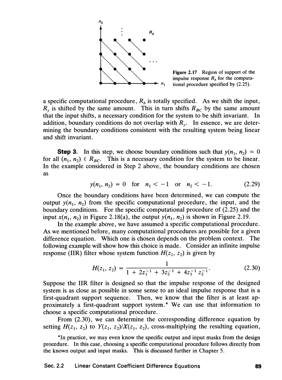
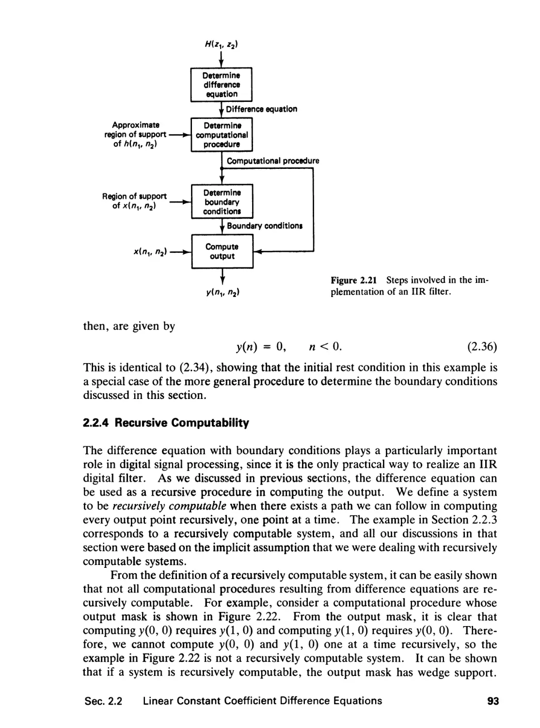
2 THE Z-TRANSFORM 65
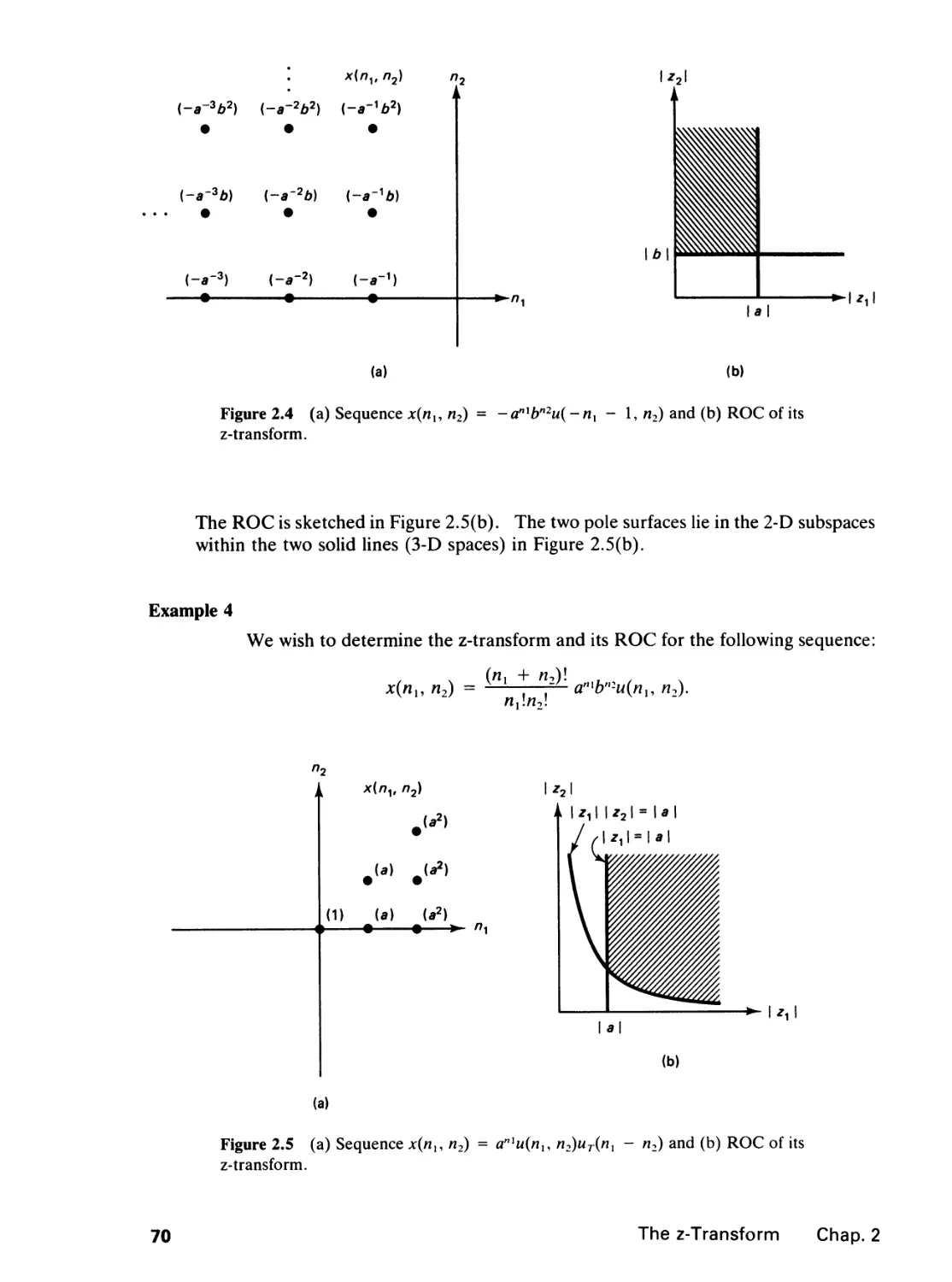
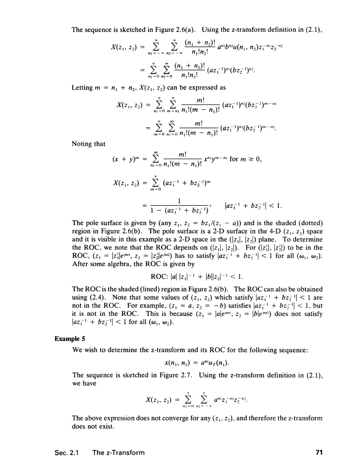
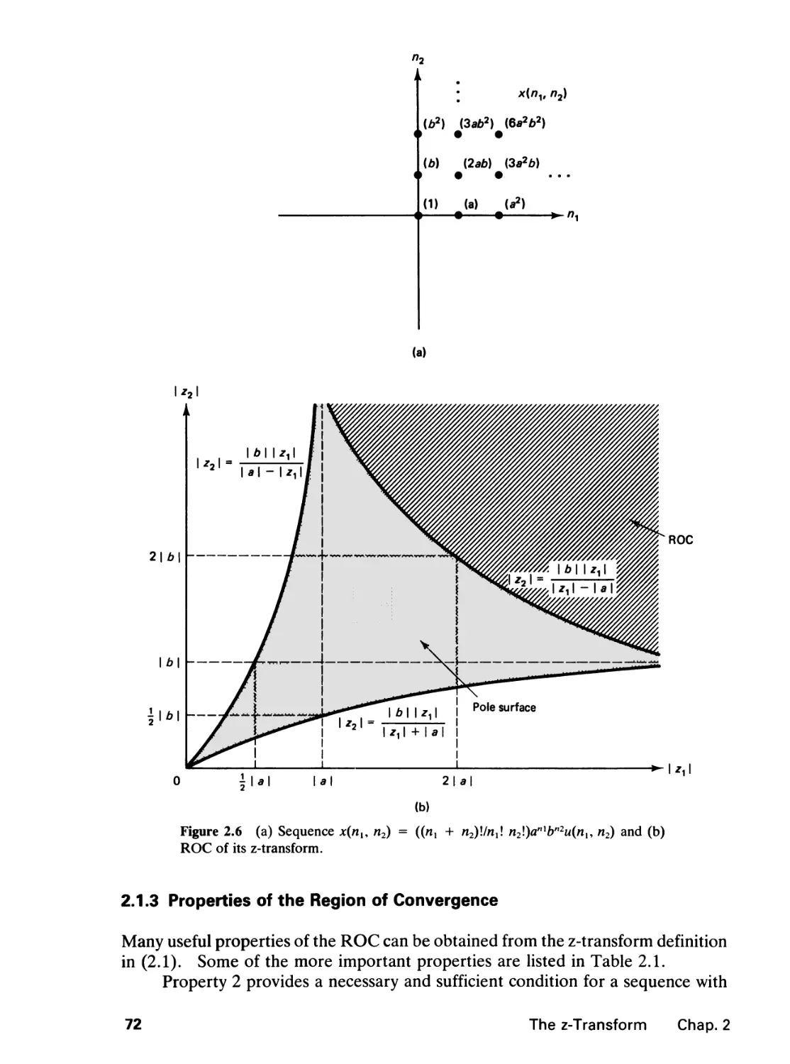
2.0 Introduction, 65
2.1 The z-Transform, 65
vii
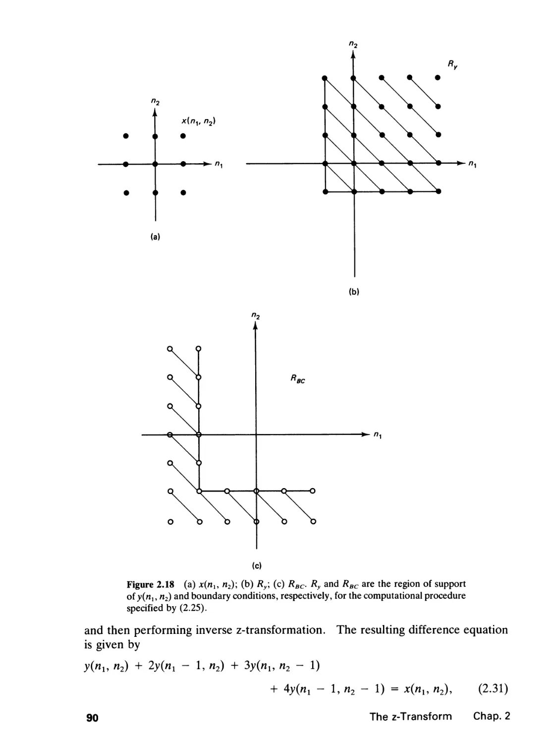
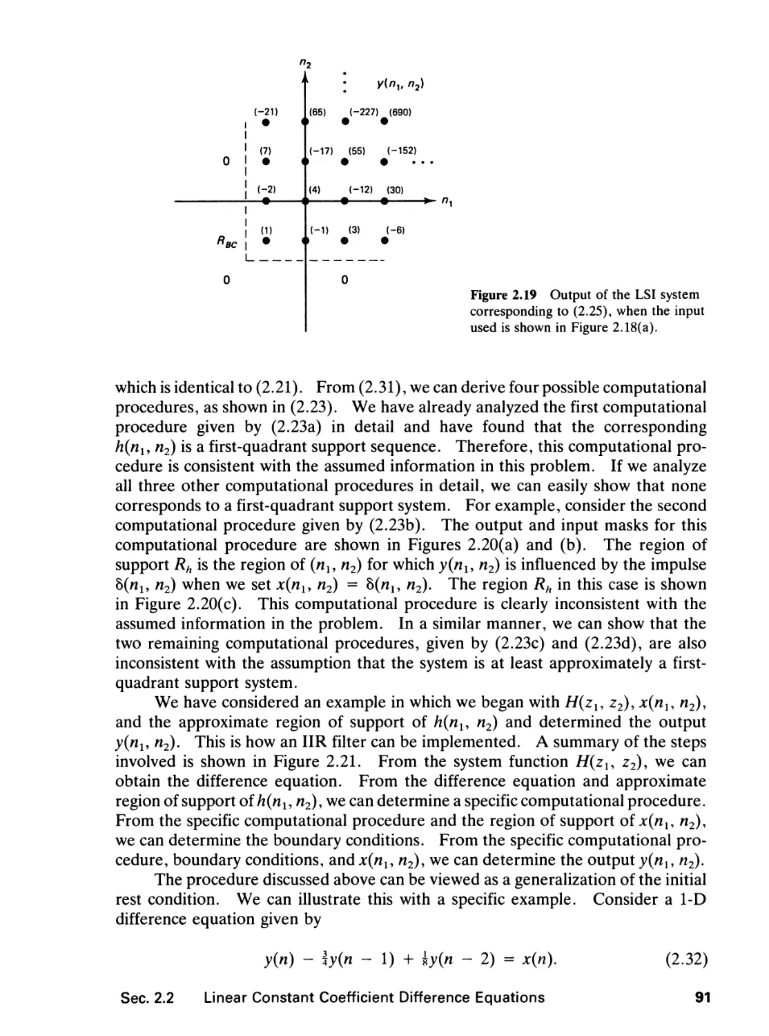
2.2 Linear Constant Coefficient Difference Equations, 78
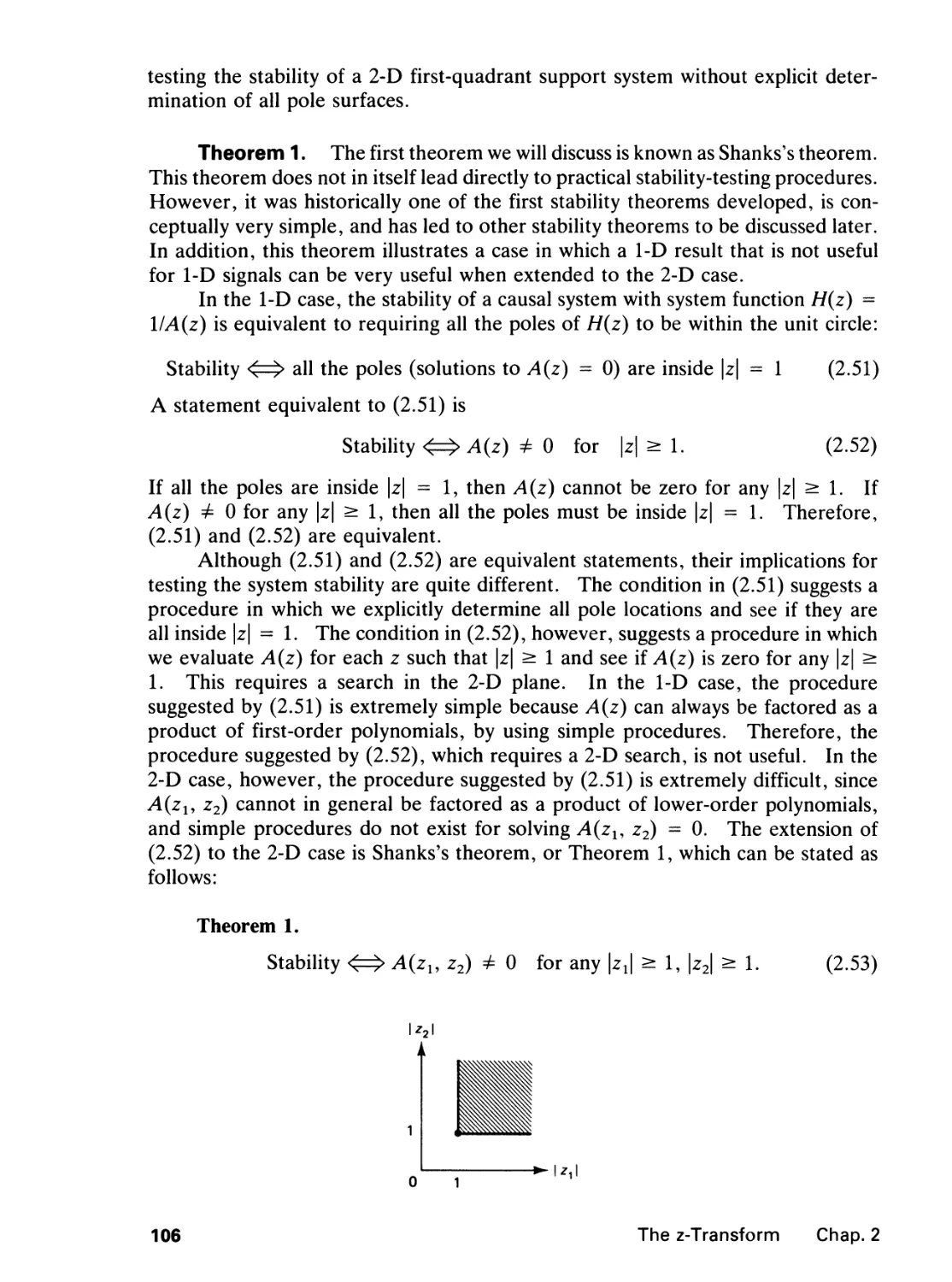
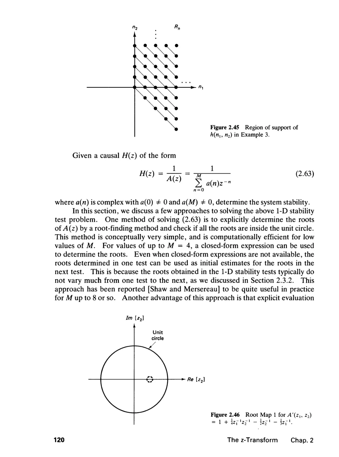
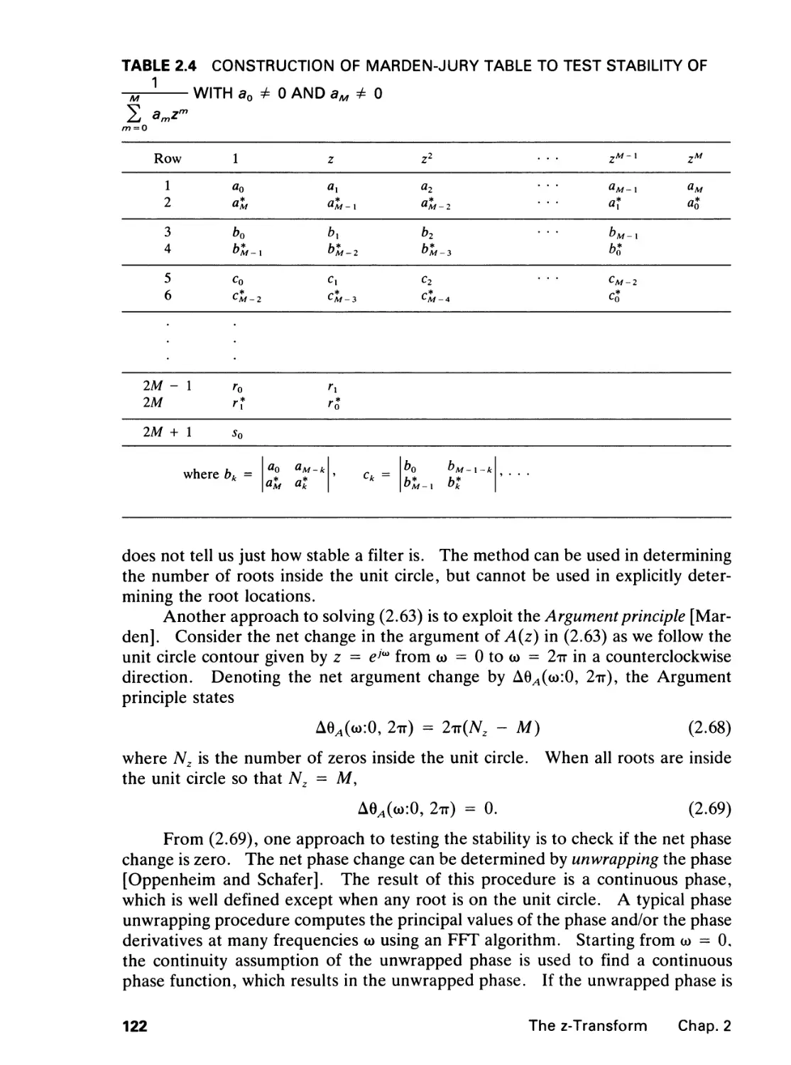
2.3 Stability, 102
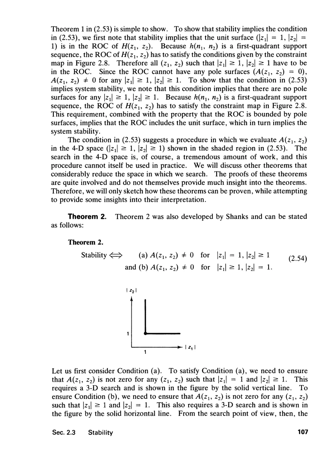
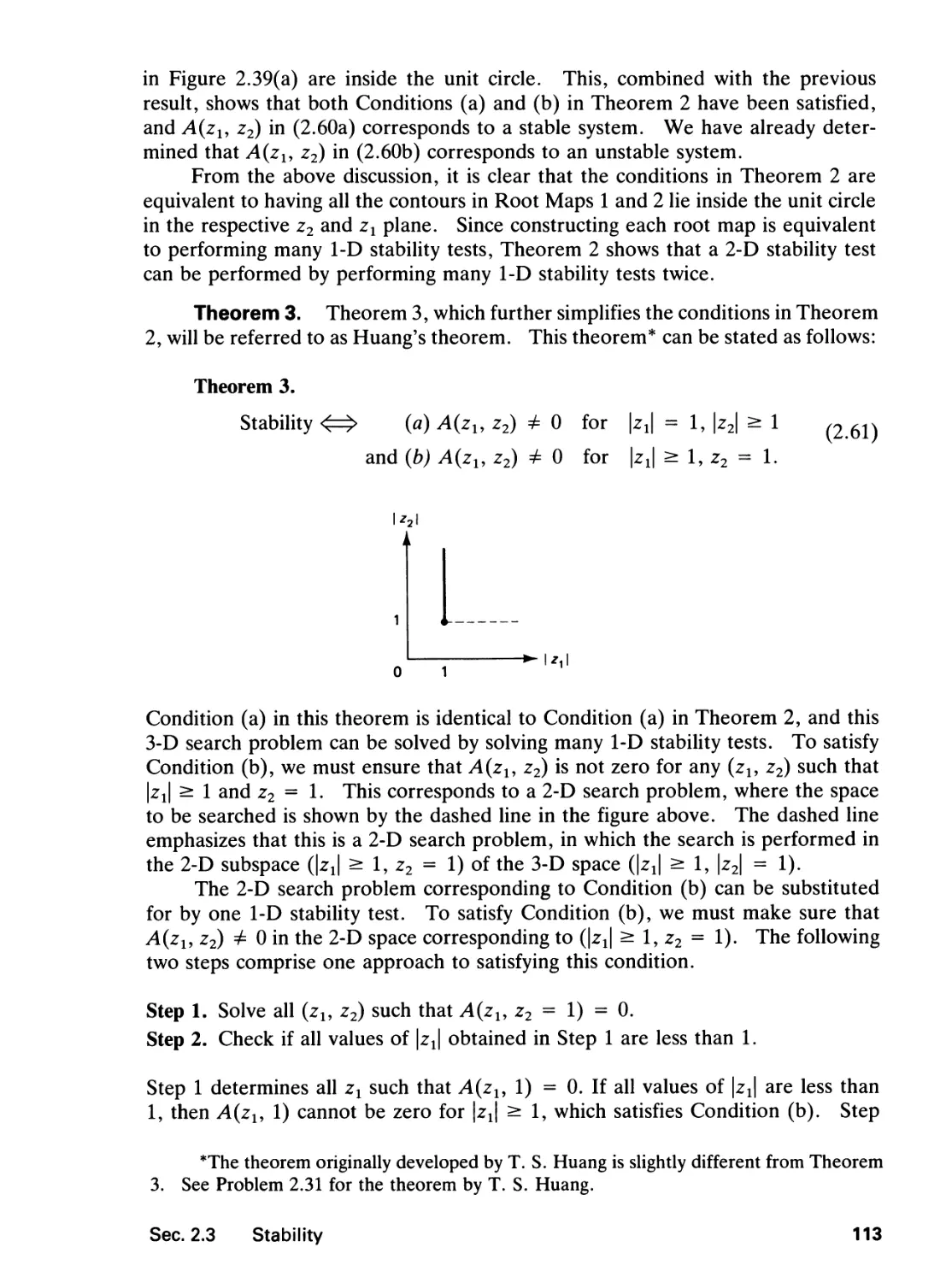
References, 124
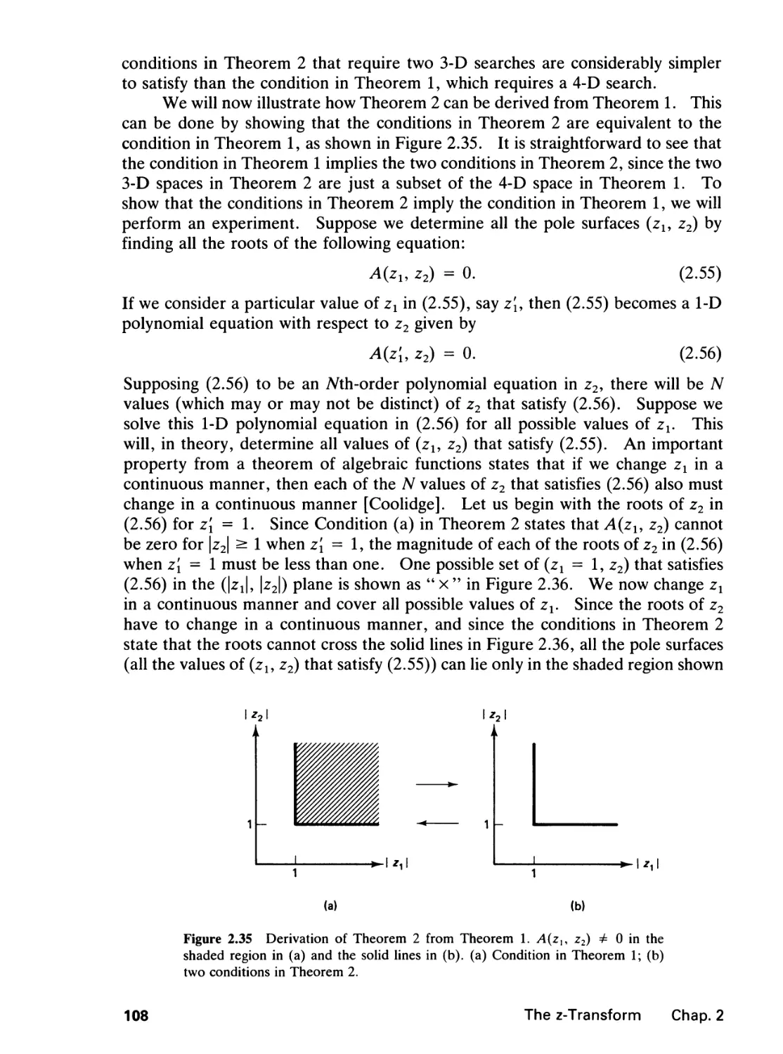
Problems, 126
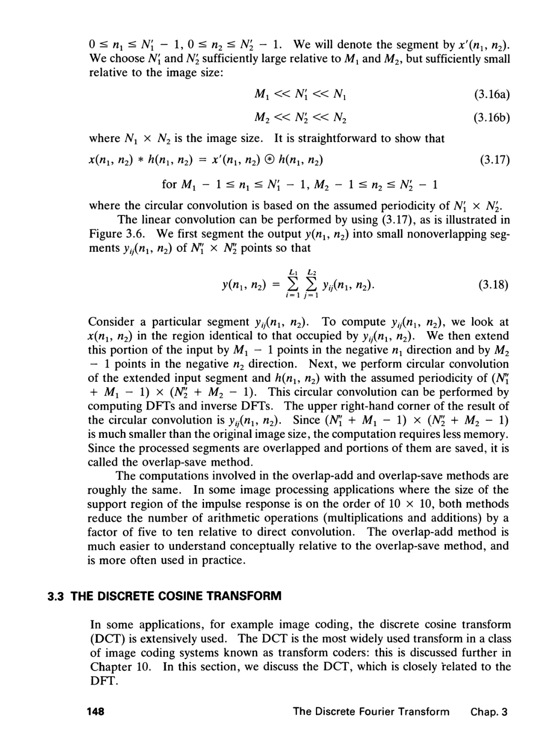
3 THE DISCRETE FOURIER TRANSFORM 136
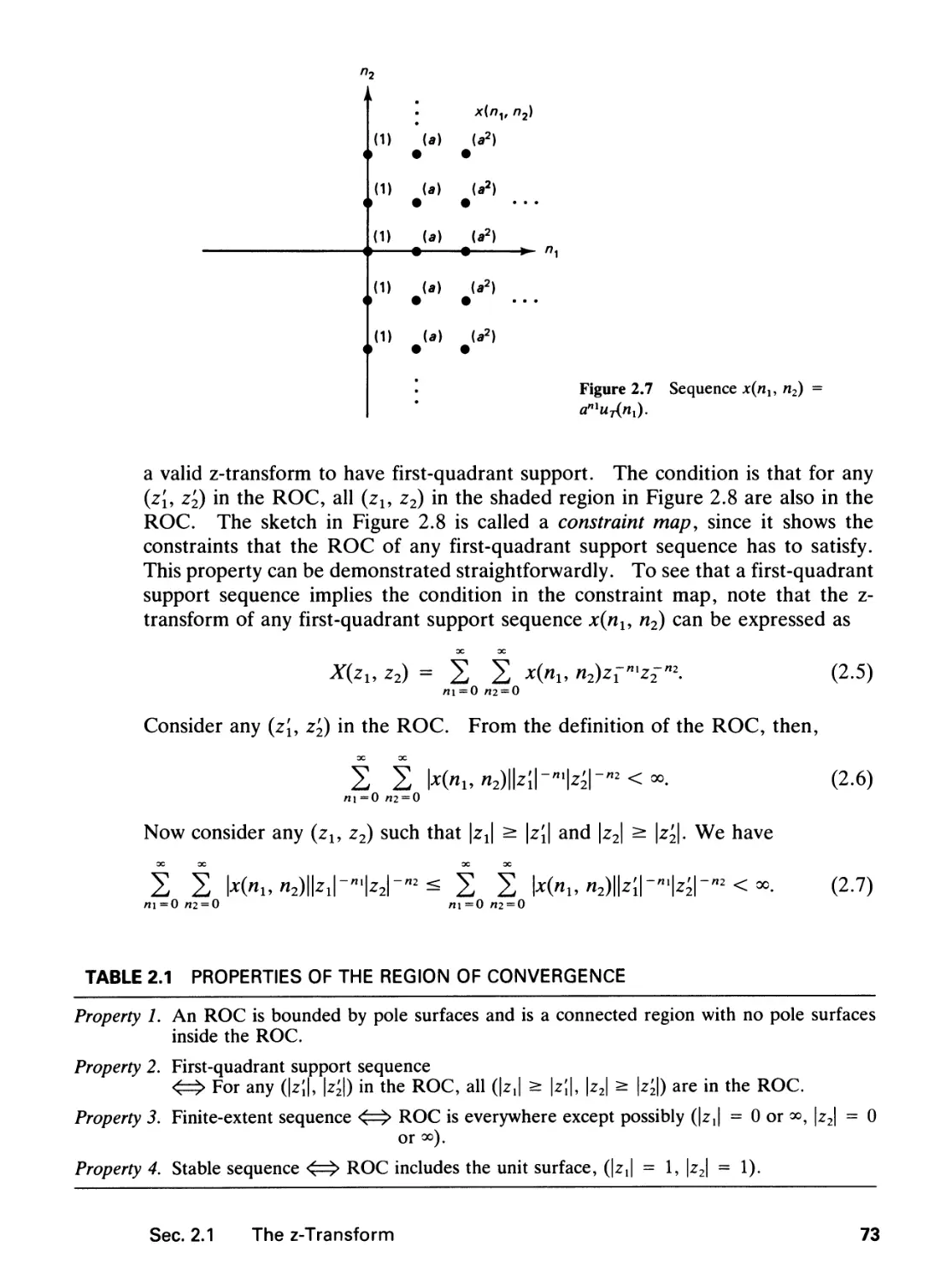
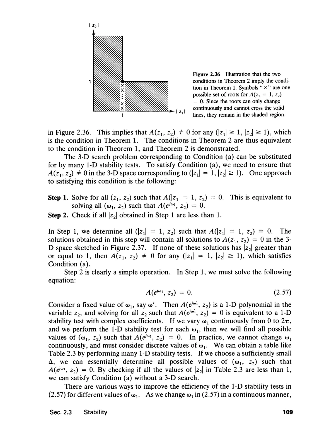
3.0 Introduction, 136
3.1 The Discrete Fourier Series, 136
3.2 The Discrete Fourier Transform, 140
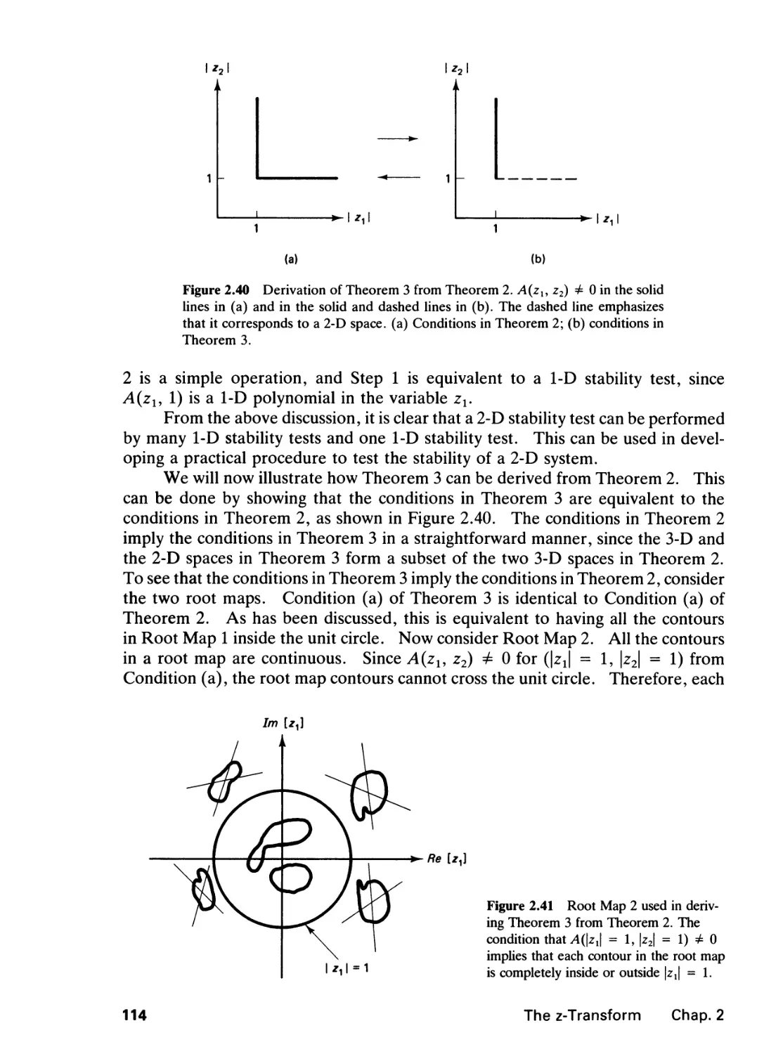
3.3 The Discrete Cosine Transform, 148
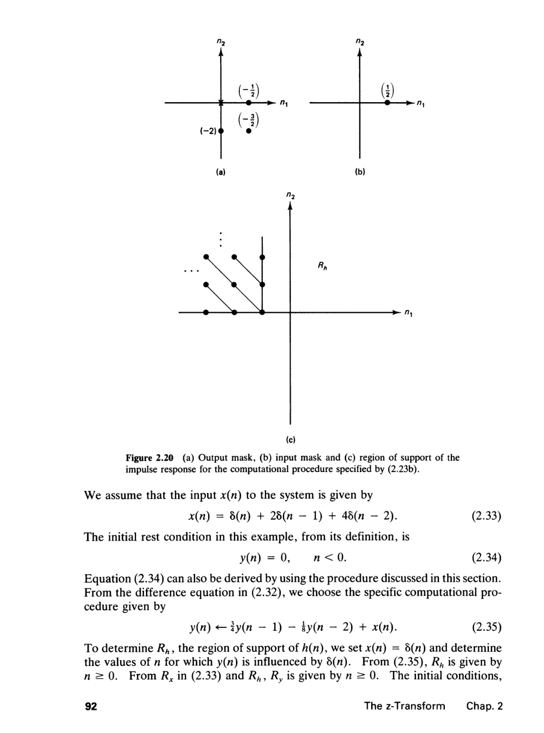
3.4 The Fast Fourier Transform, 163
References, 182
Problems, 185
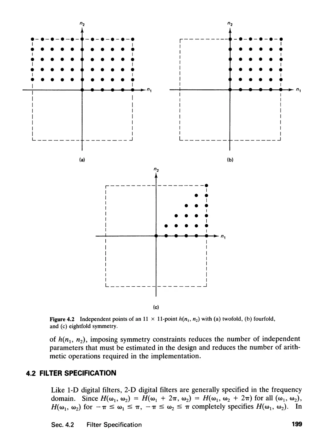
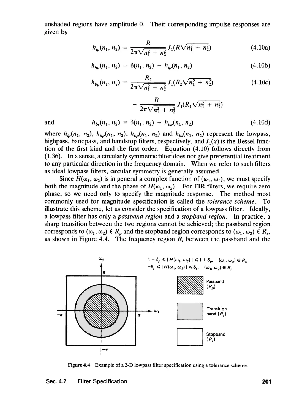
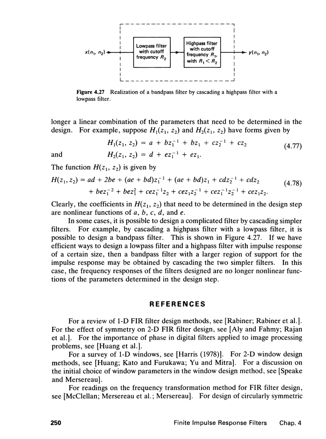
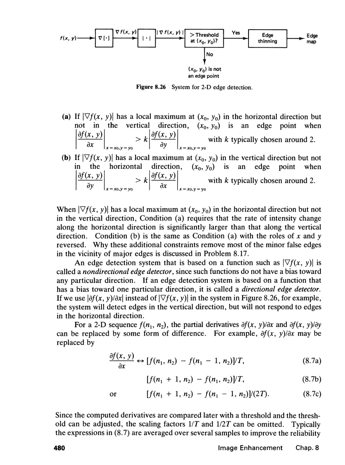
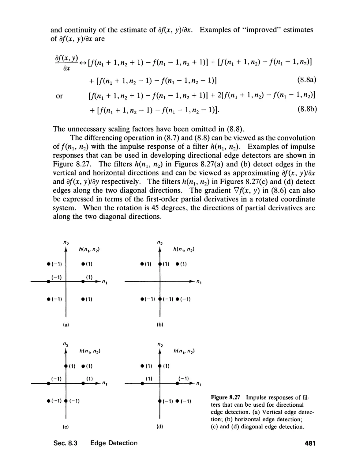
4 FINITE IMPULSE RESPONSE FILTERS 195
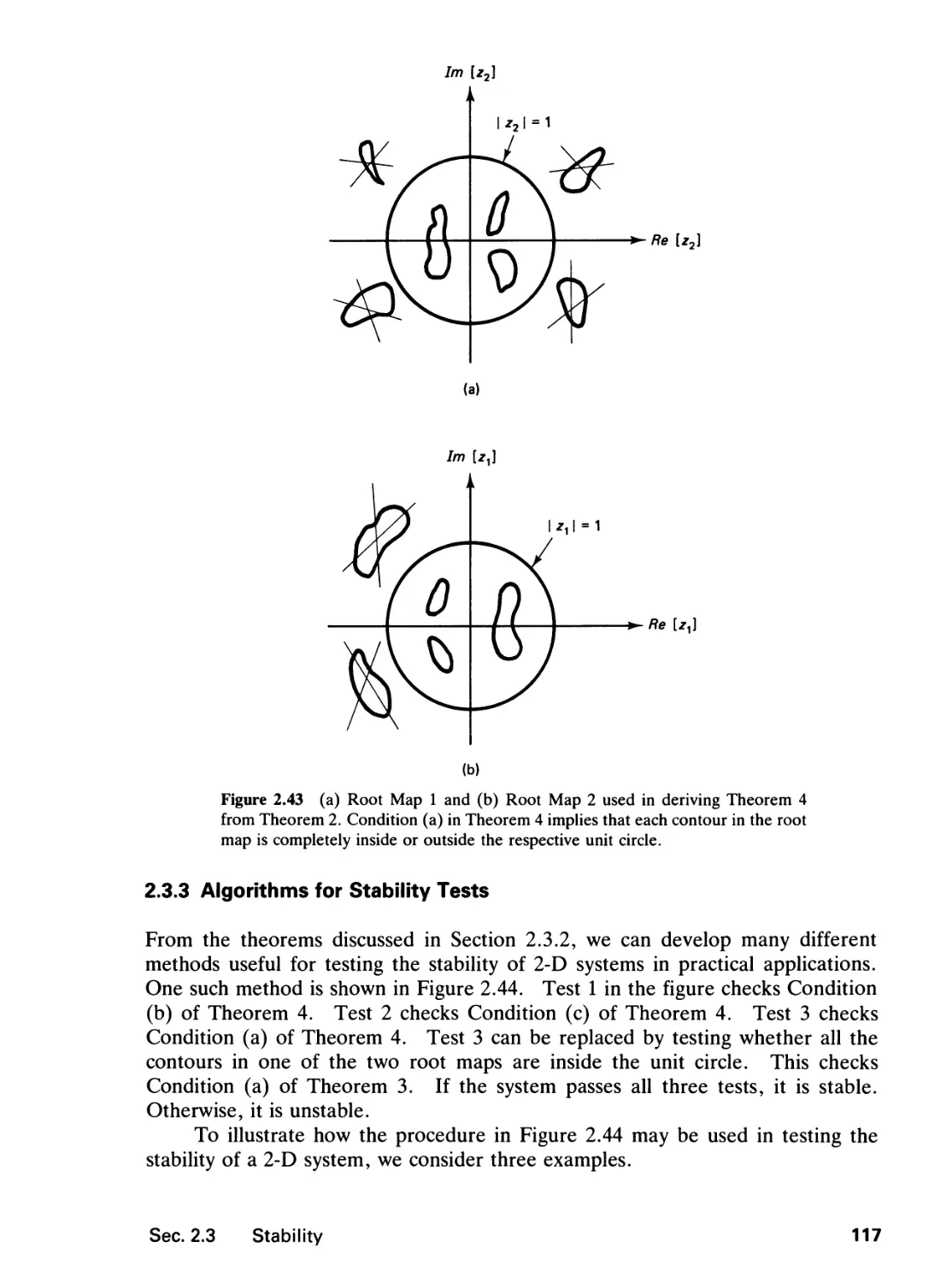
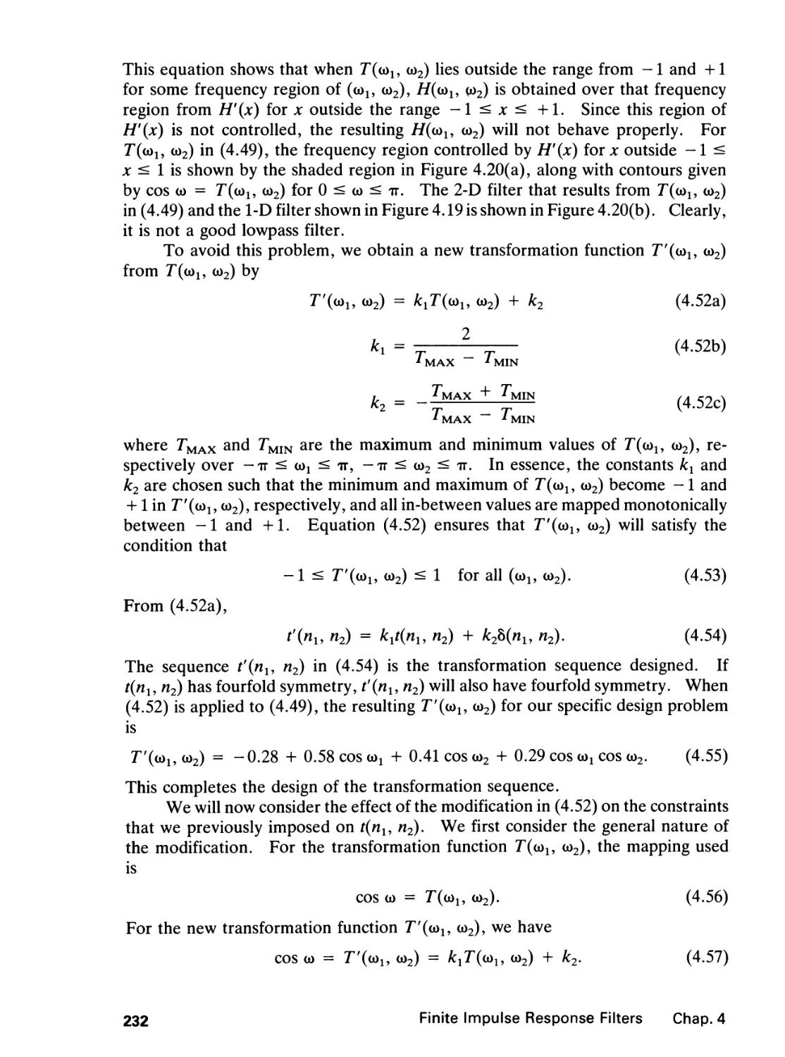
4.0 Introduction, 195
4.1 Zero-Phase Filters, 196
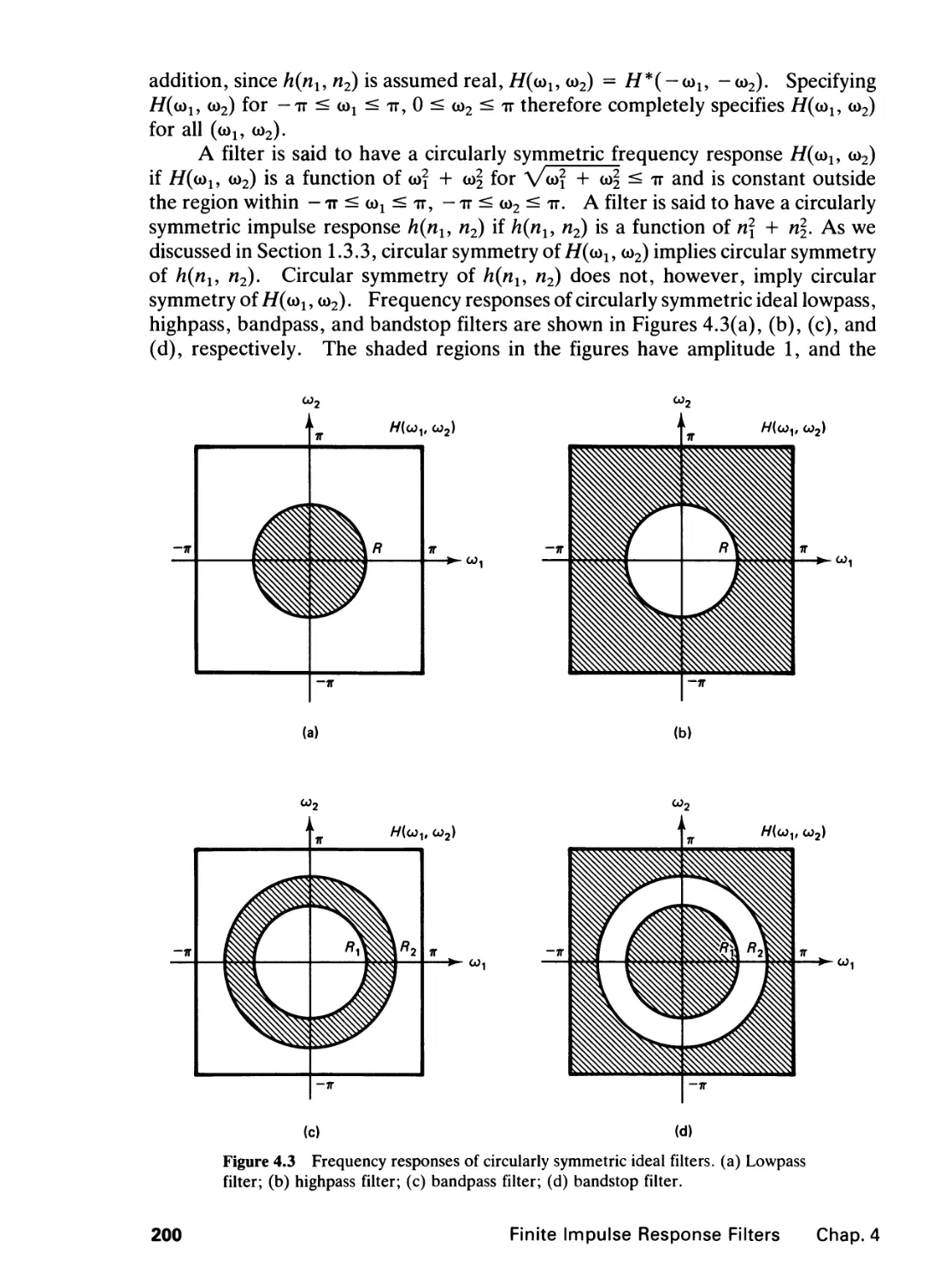
4.2 Filter Specification, 199
4.3 Filter Design by the Window Method and the
Frequency Sampling Method, 202
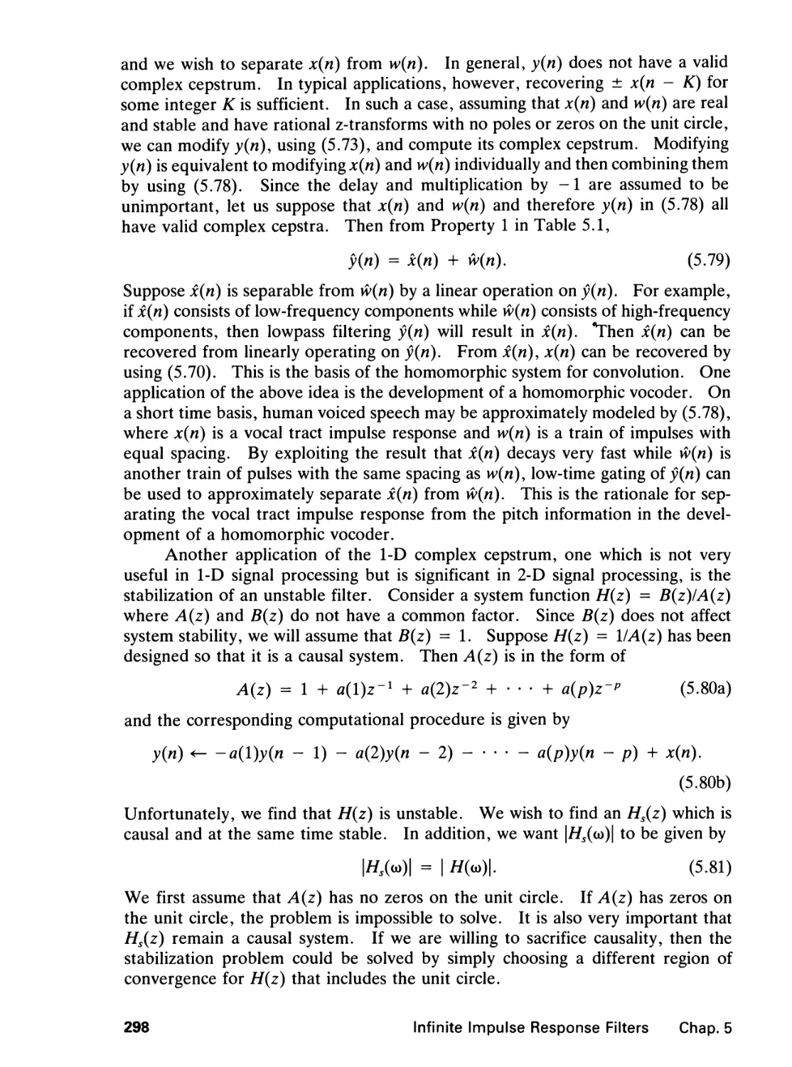
4.4 Filter Design by the Frequency Transformation
Method, 218
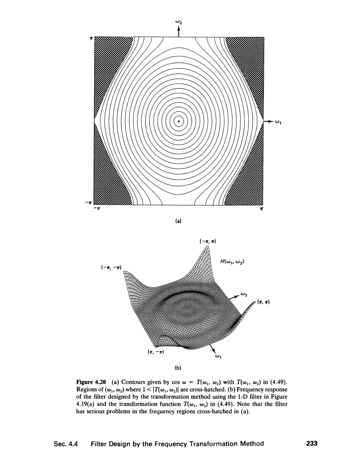
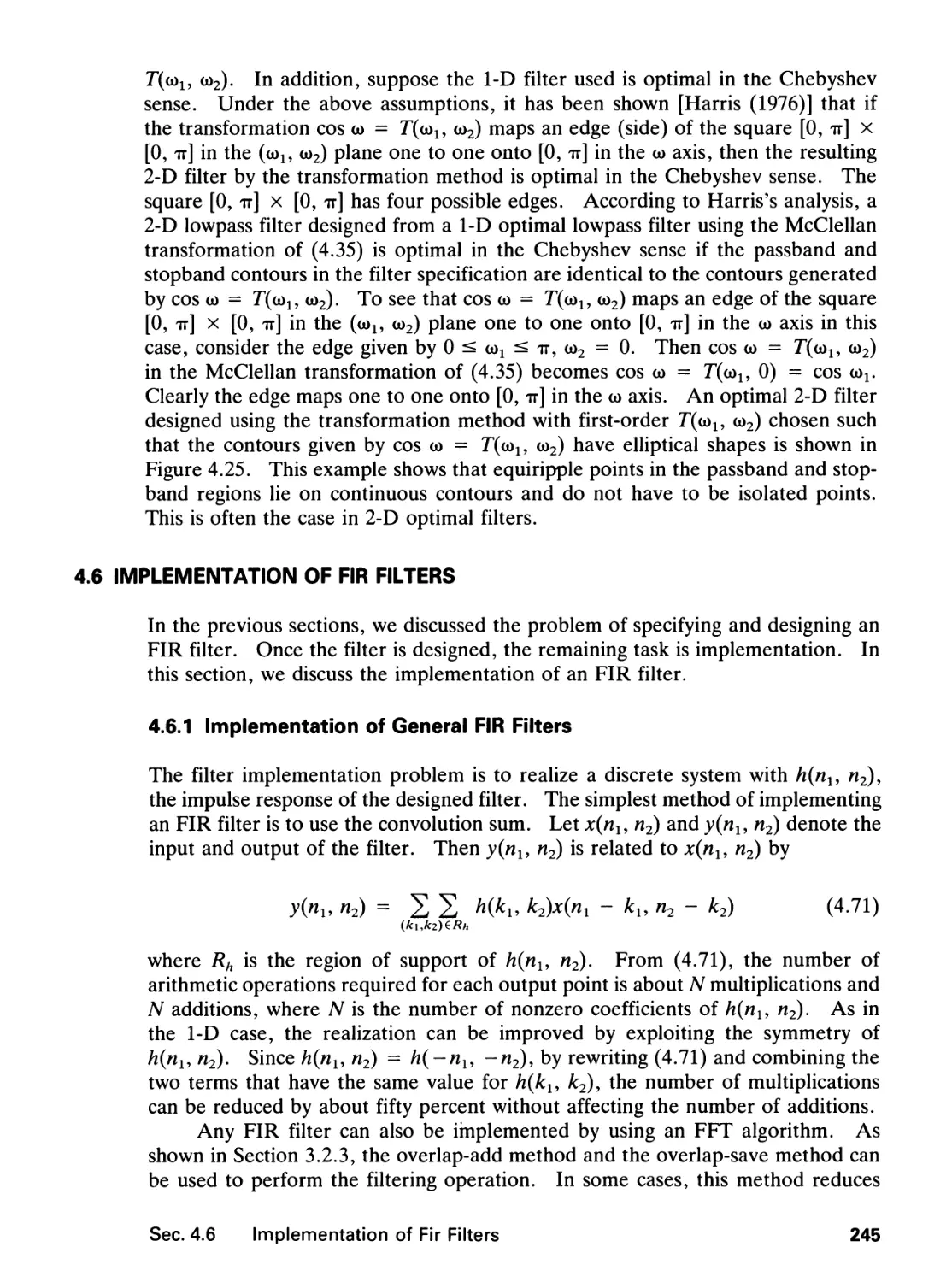
4.5 Optimal Filter Design, 238
4.6 Implementation of FIR Filters, 245
References, 250
Problems, 252
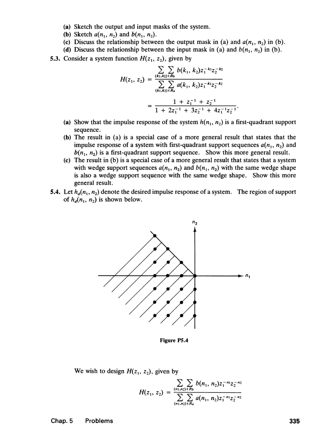
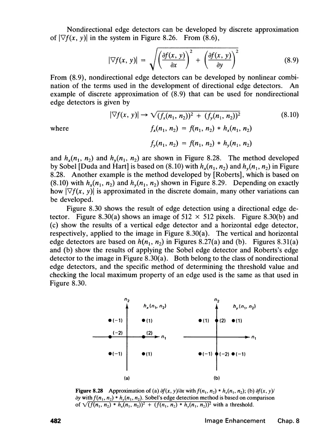
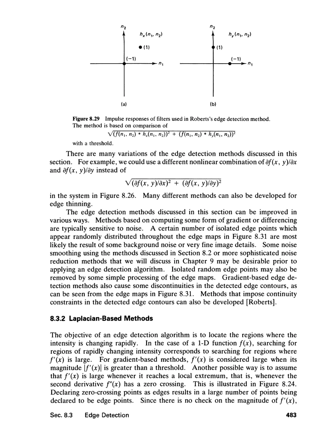
5 INFINITE IMPULSE RESPONSE FILTERS 264
5.0 Introduction, 264
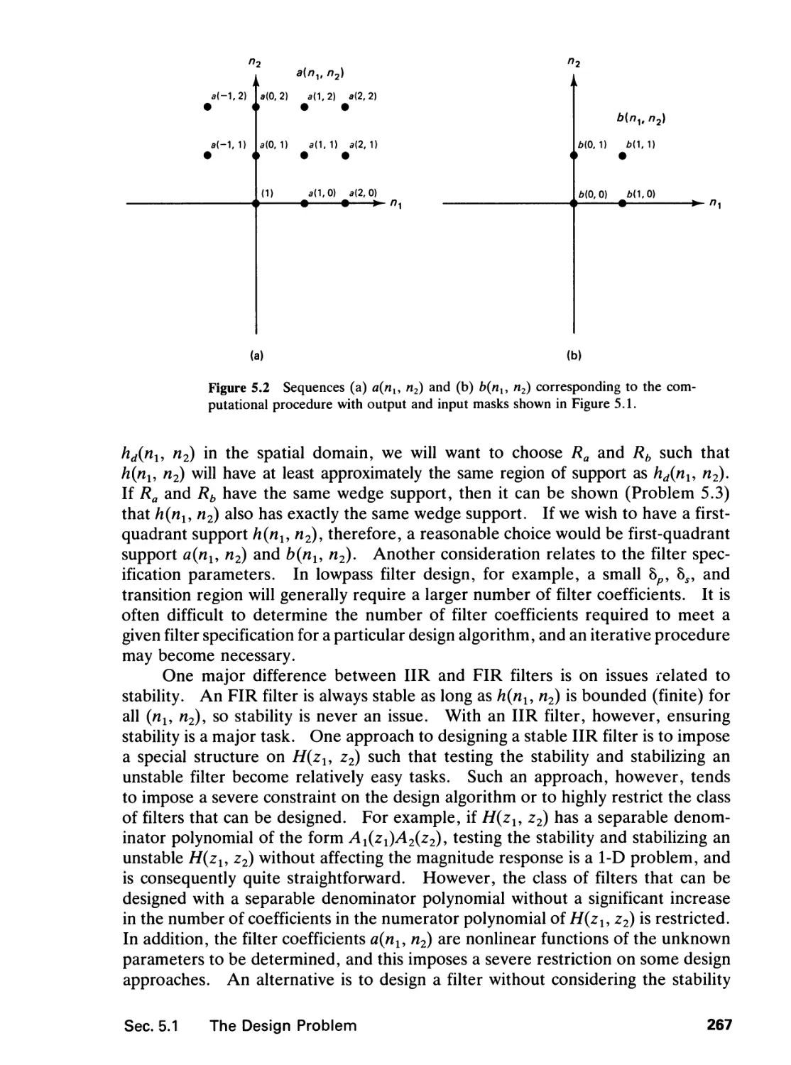
5.1 The Design Problem, 265
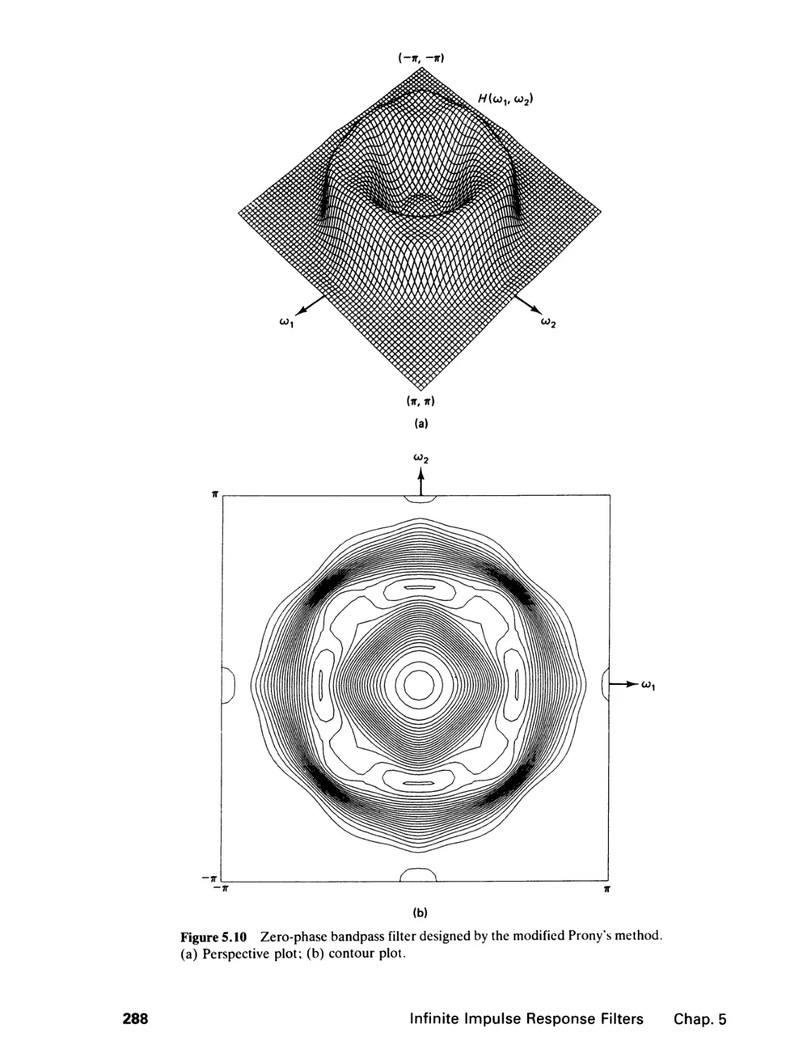
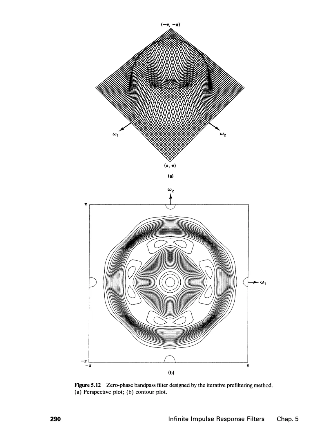
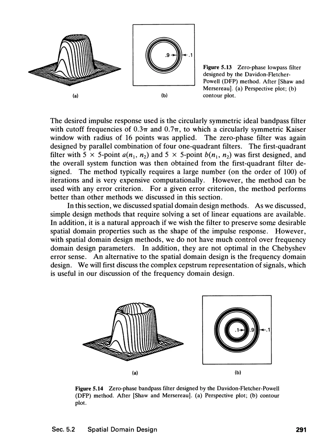
5.2 Spatial Domain Design, 268
5.3 The Complex Cepstrum Representation of Signals,
292
vi» Contents
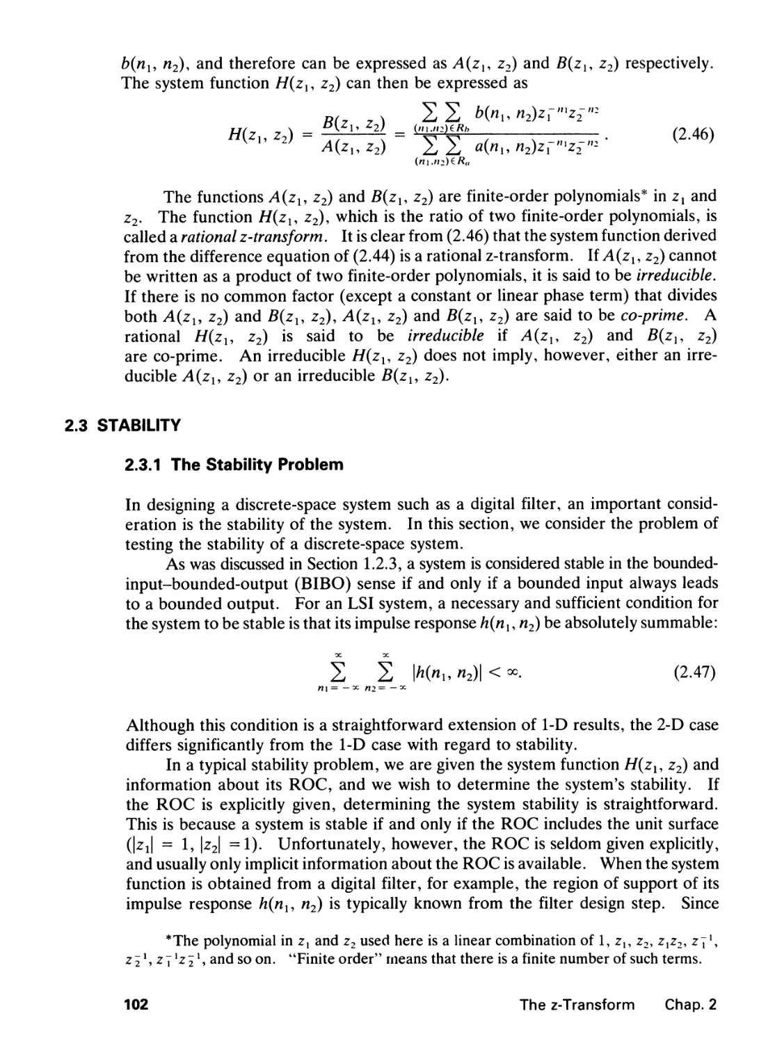
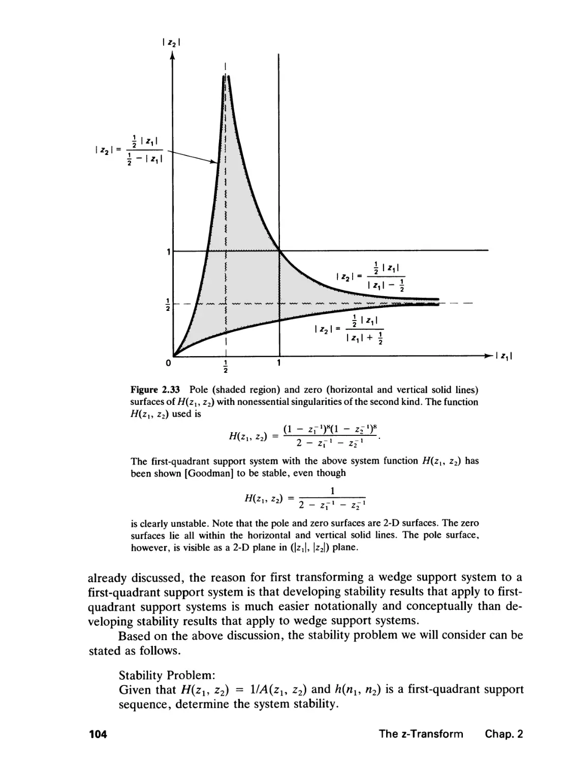
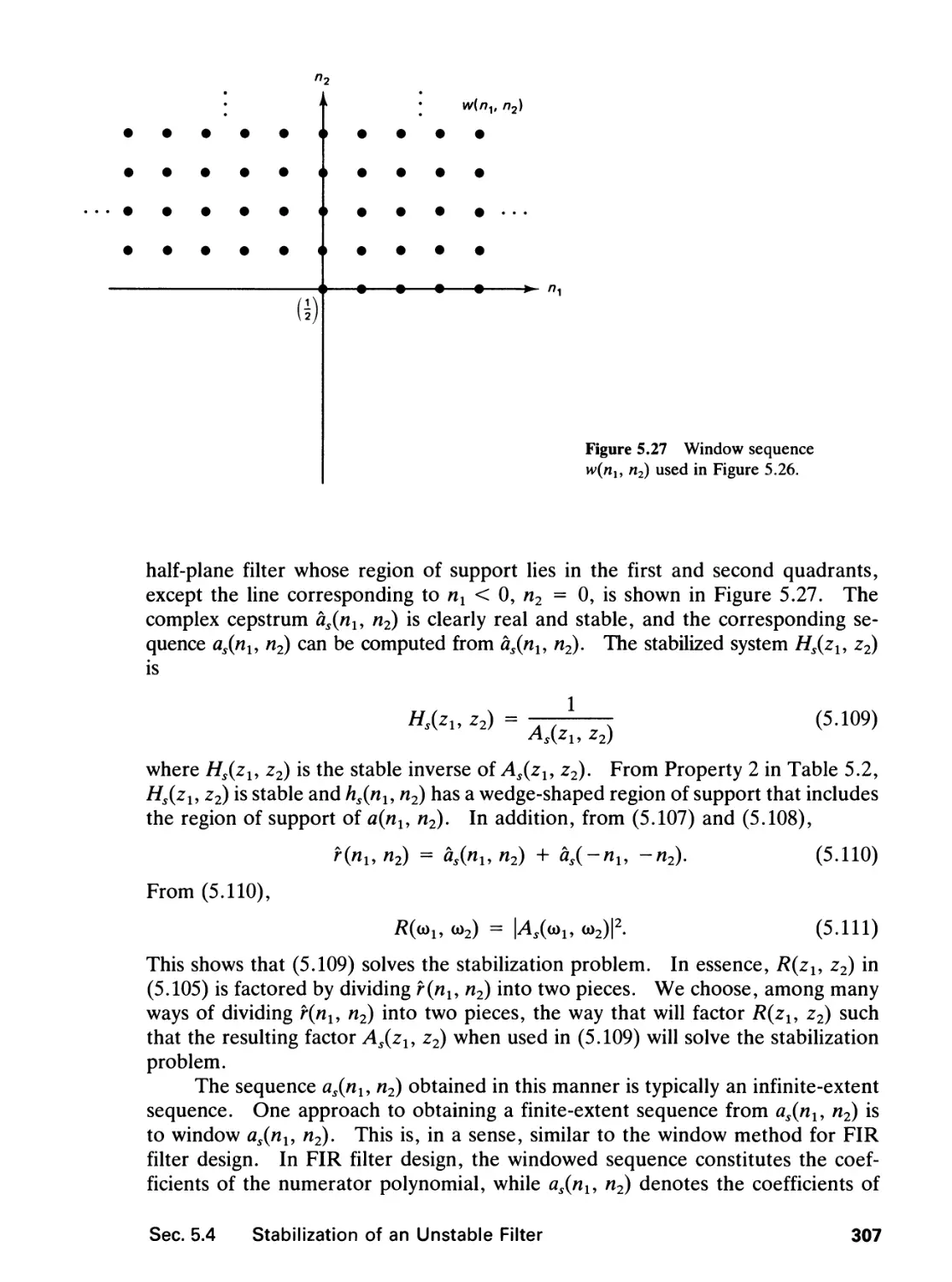
5.4 Stabilization of an Unstable Filter, 304
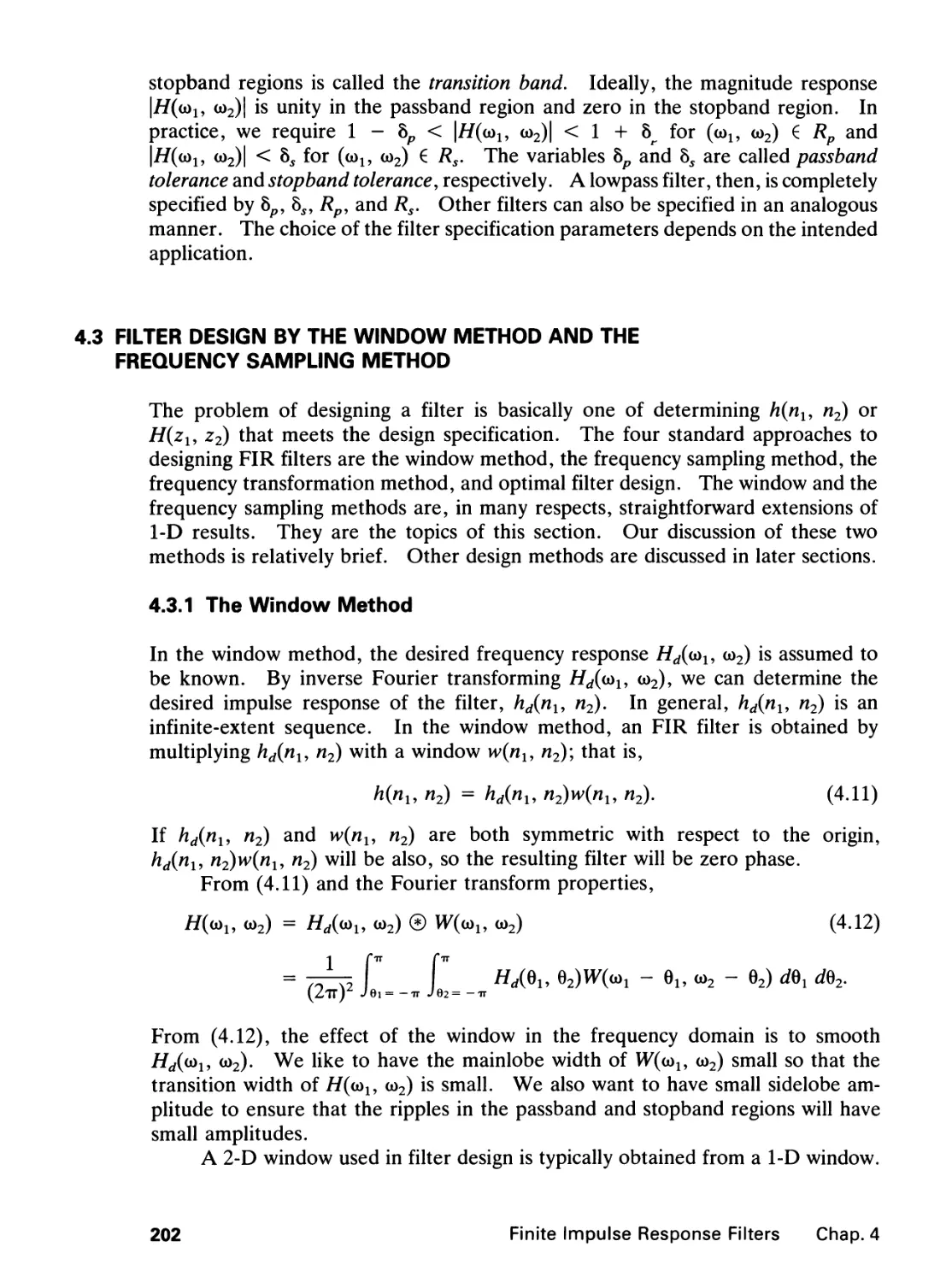
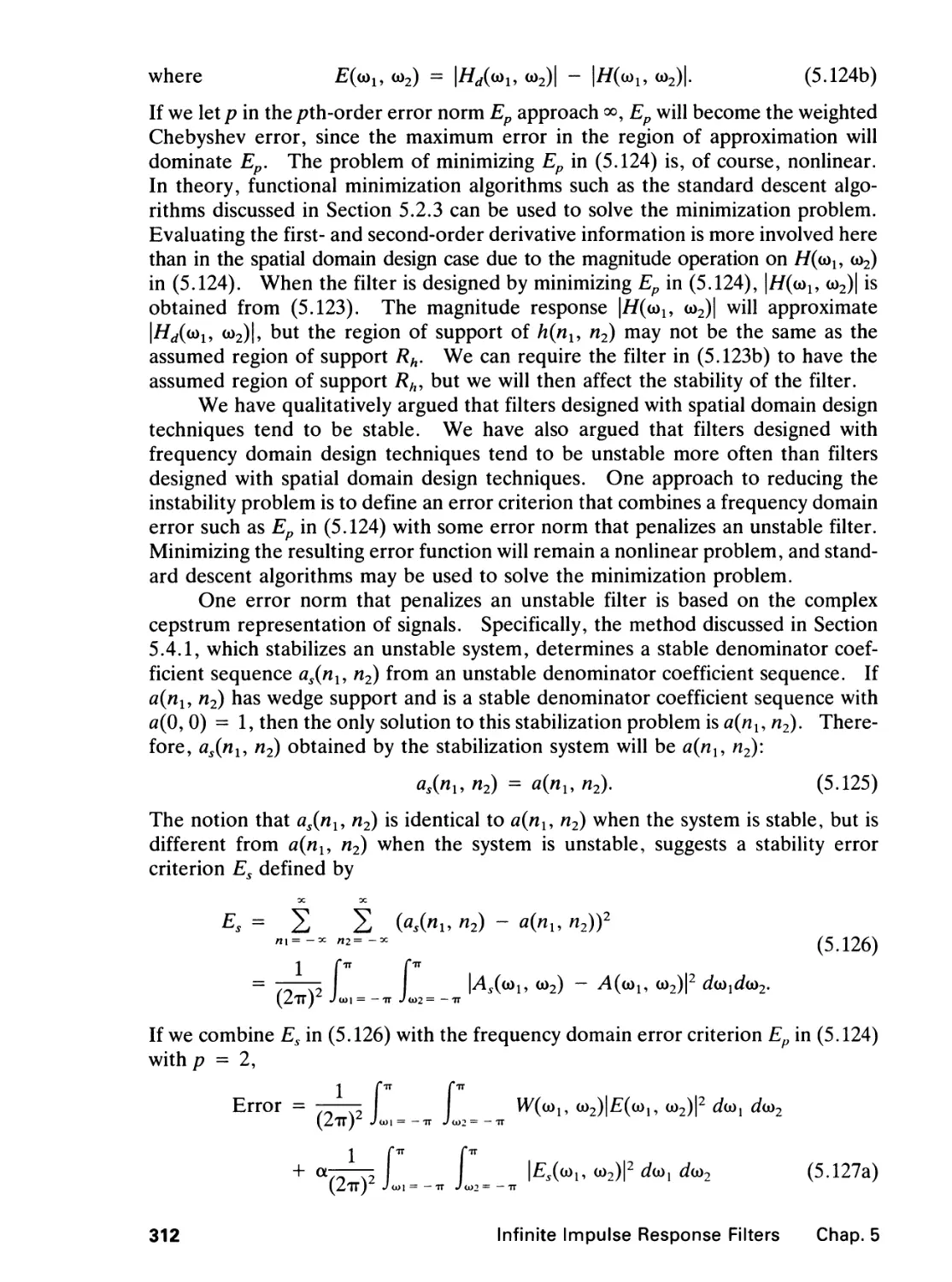
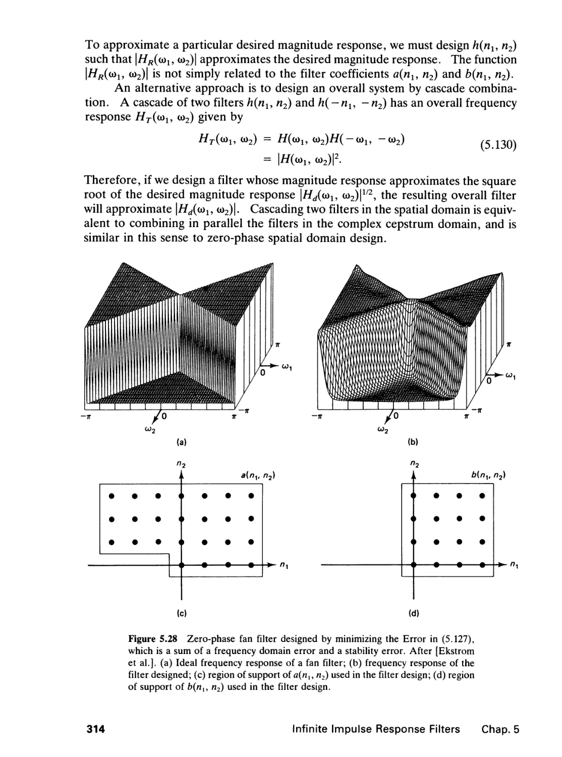
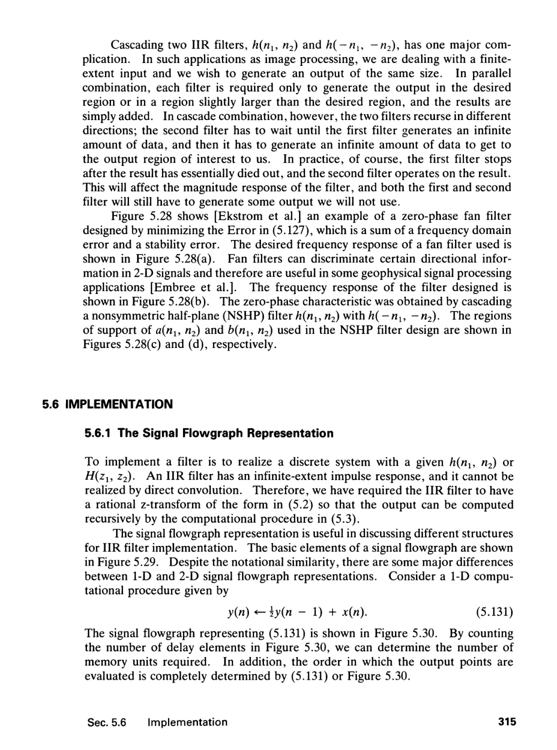
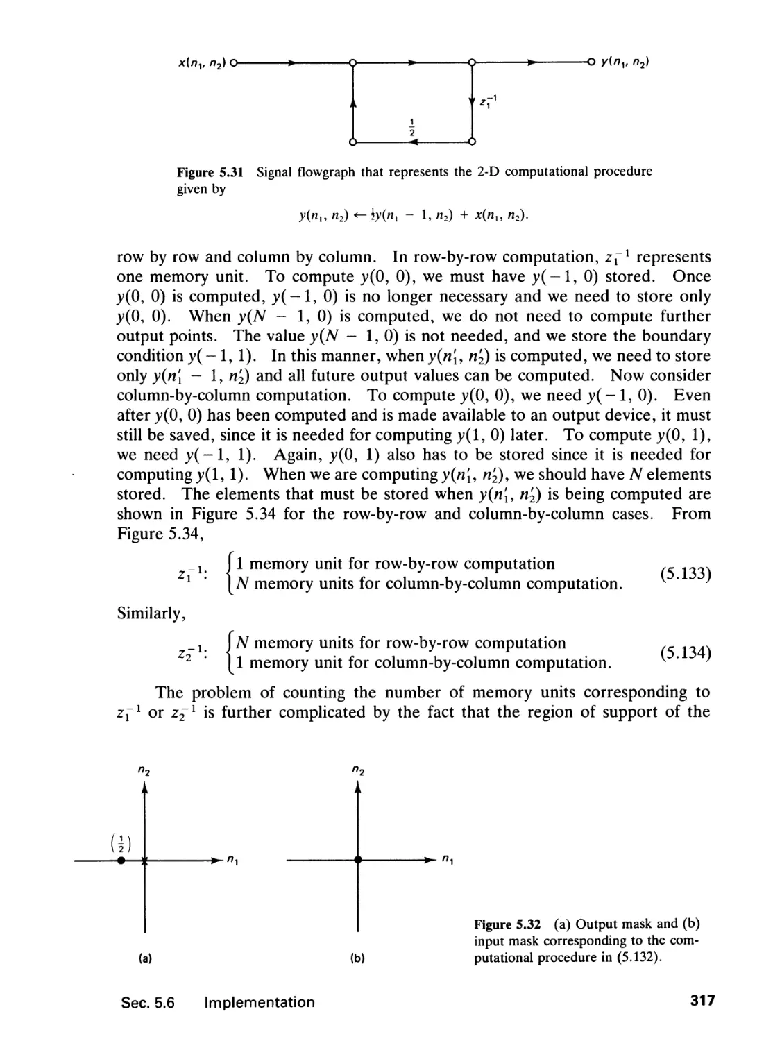
5.5 Frequency Domain Design, 309
5.6 Implementation, 315
5.7 Comparison of FIR and IIR Filters, 330
References, 330
Problems, 334
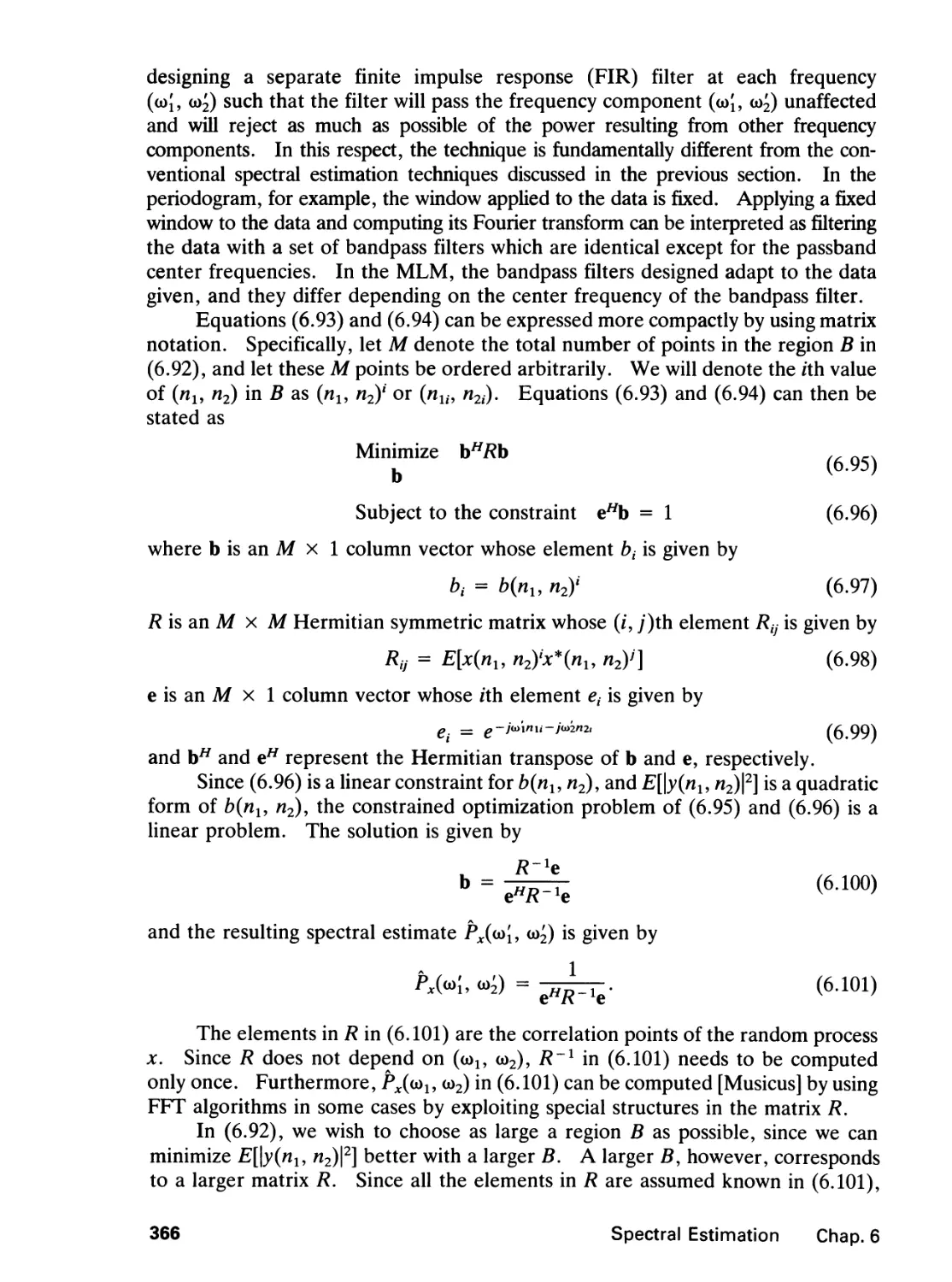
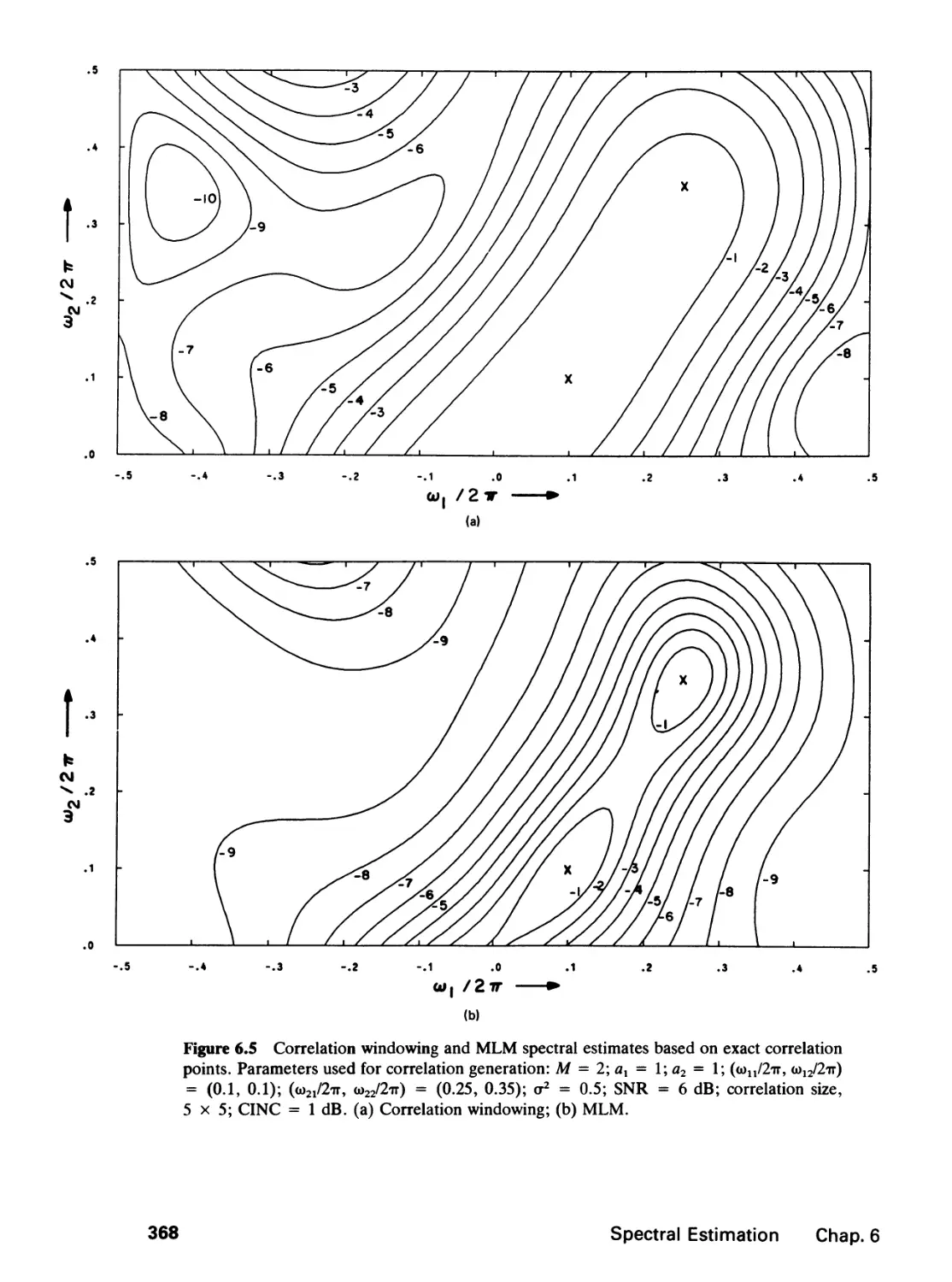
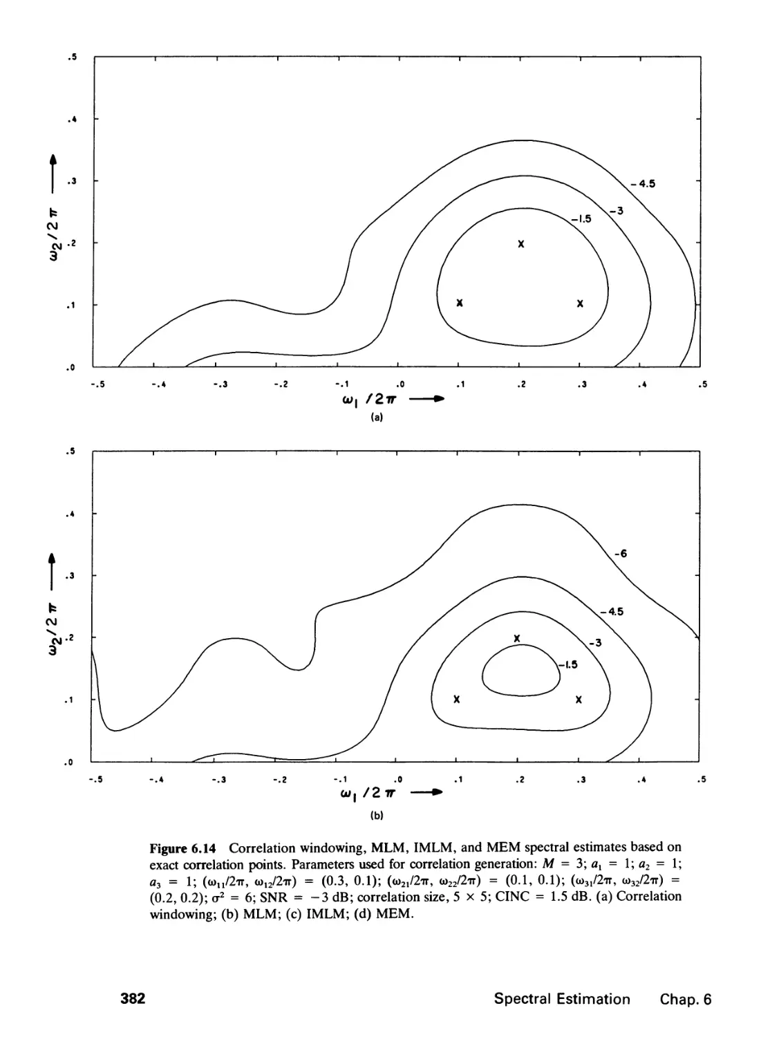
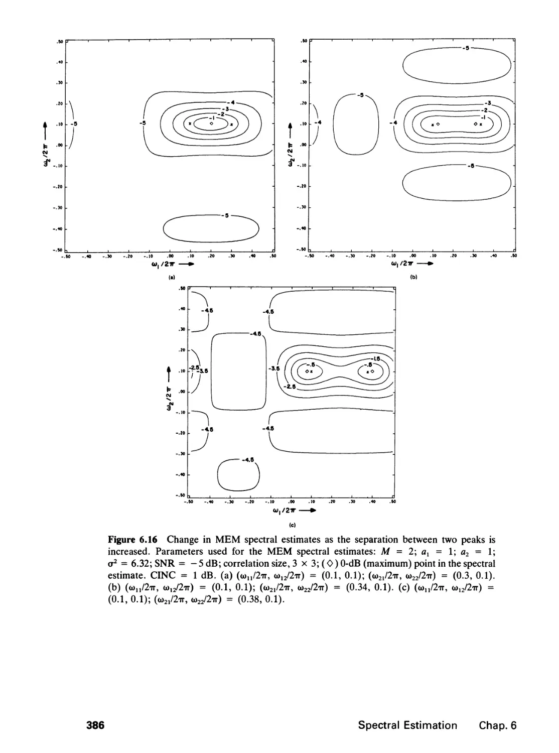
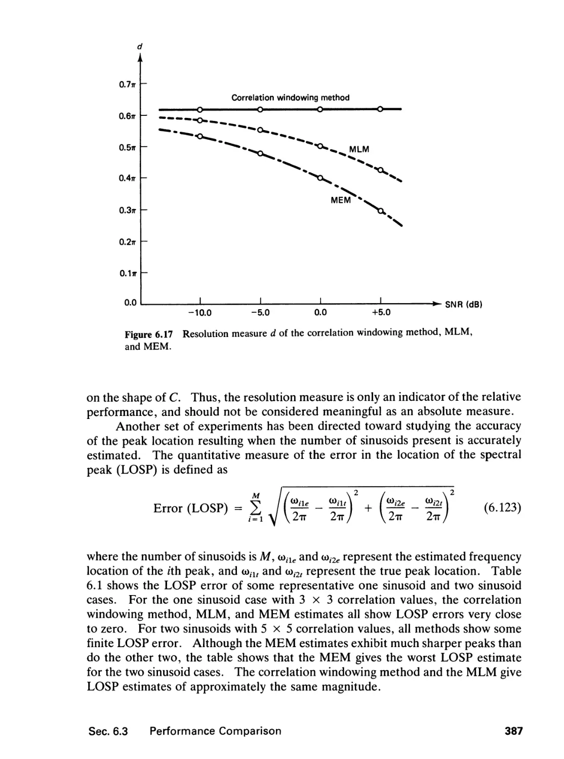
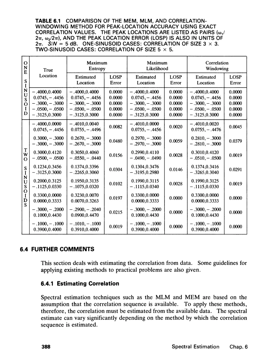
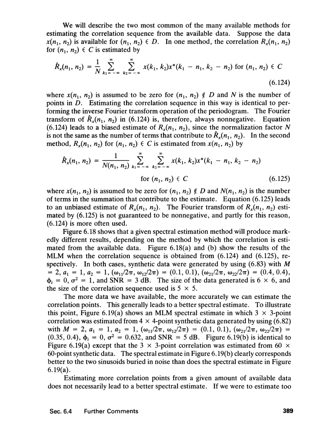
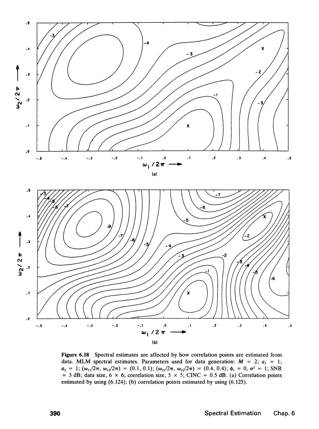
6 SPECTRAL ESTIMATION 346
6.0 Introduction, 346
6.1 Random Processes, 347
6.2 Spectral Estimation Methods, 359
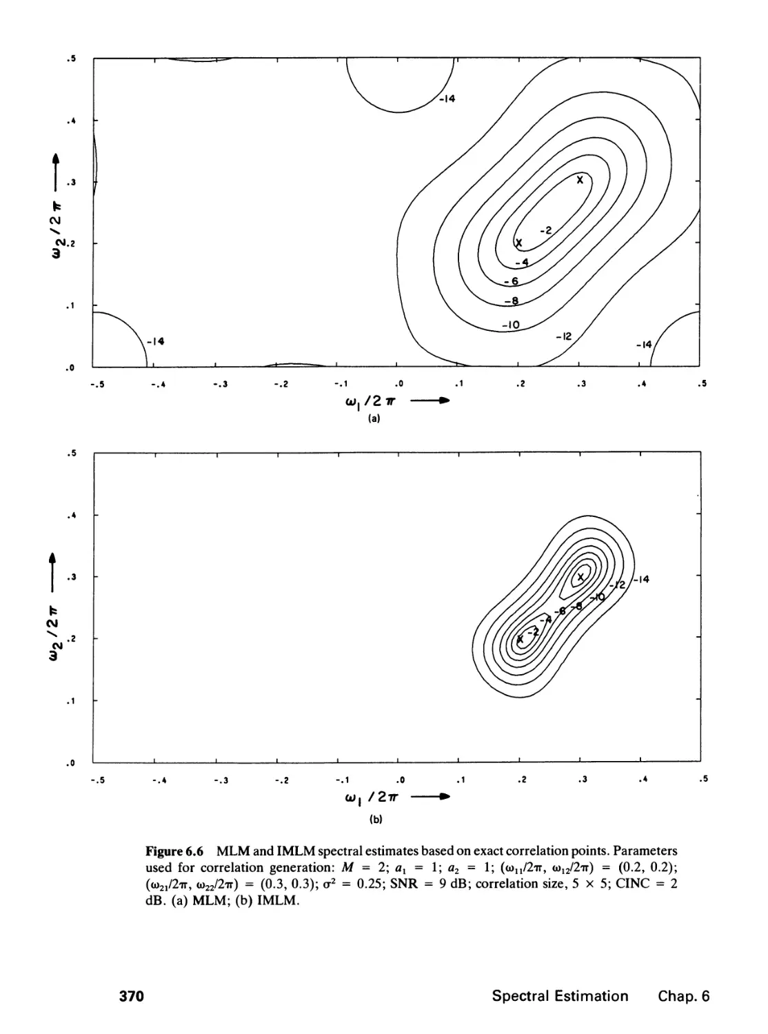
6.3 Performance Comparison, 384
6.4 Further Comments, 388
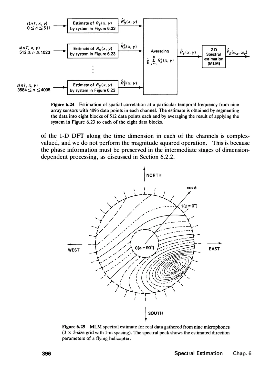
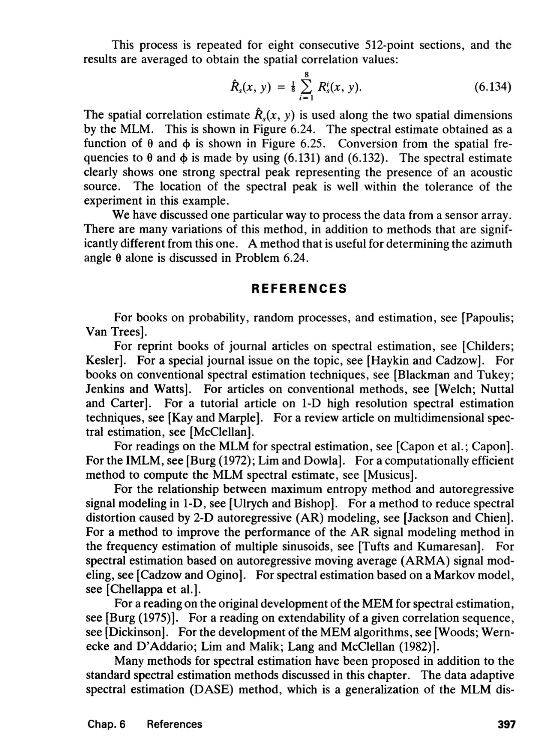
6.5 Application Example, 392
References, 397
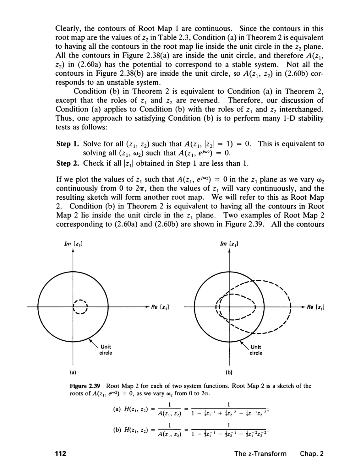
Problems, 400
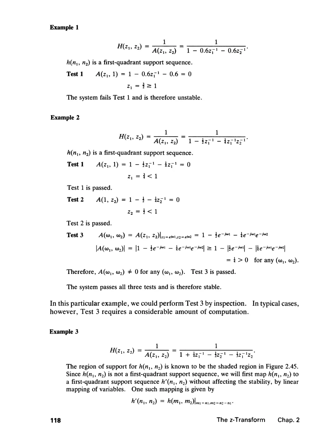
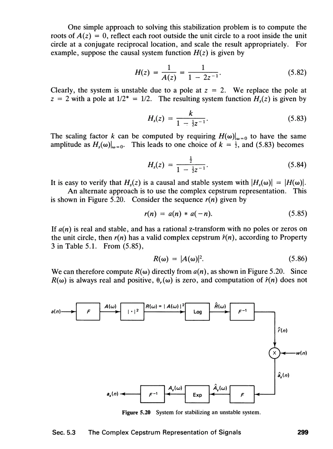
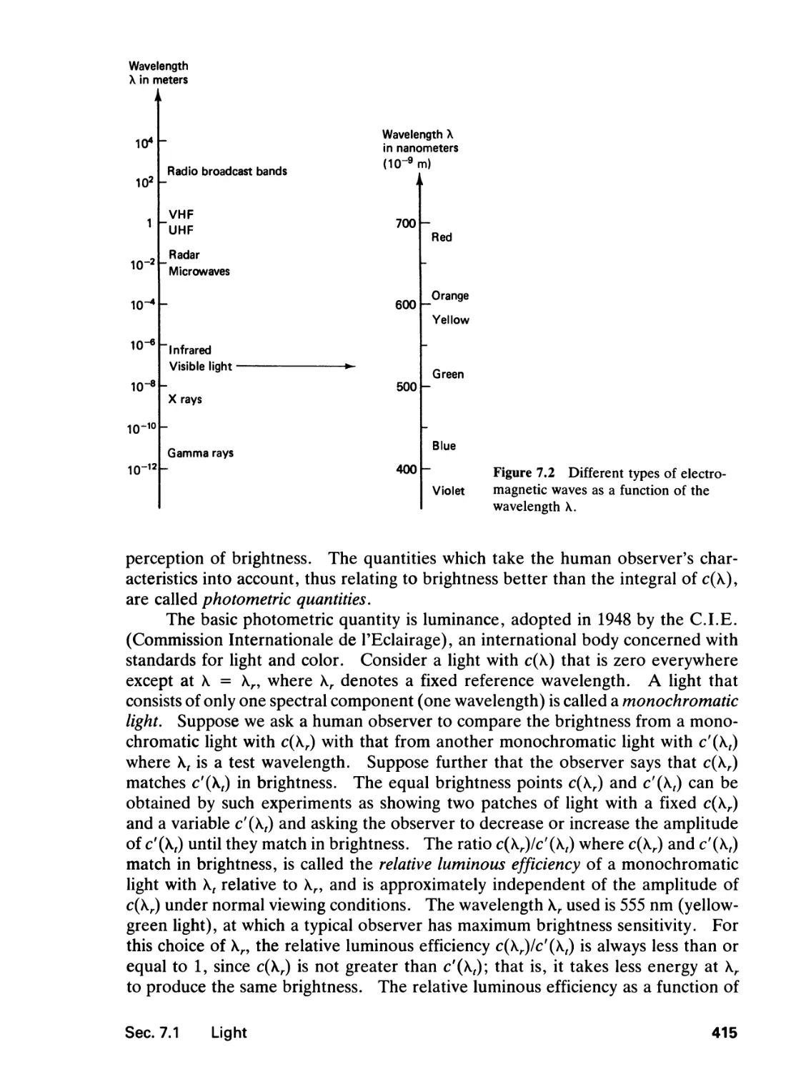
7 IMAGE PROCESSING BASICS 410
7.0 Introduction, 410
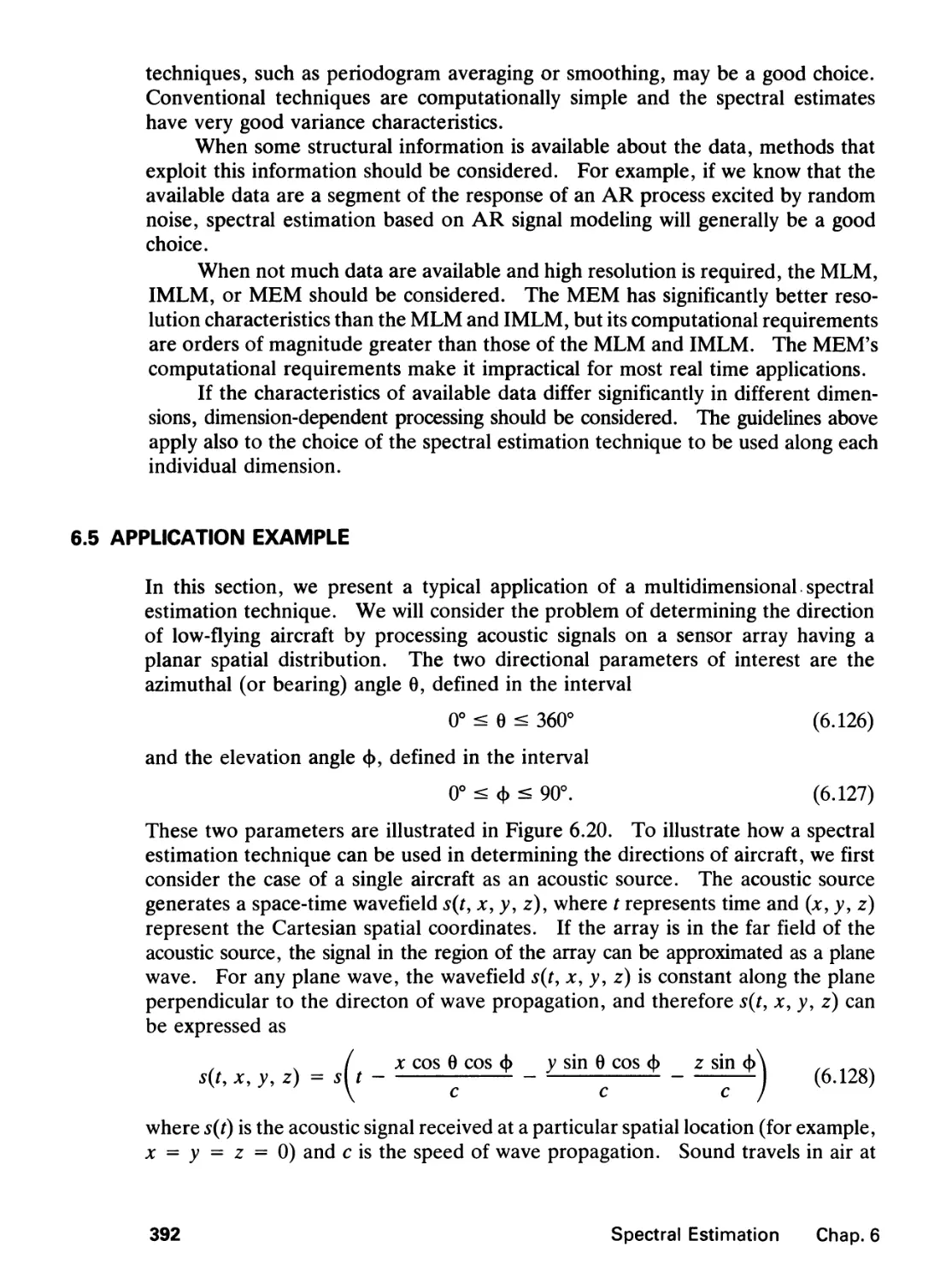
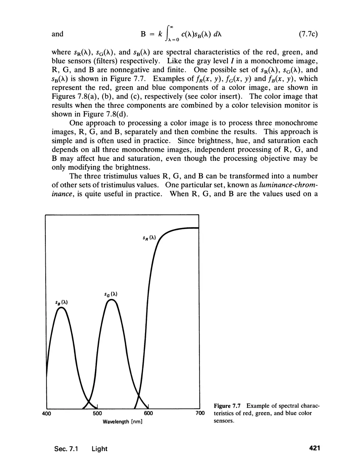
7.1 Light, 413
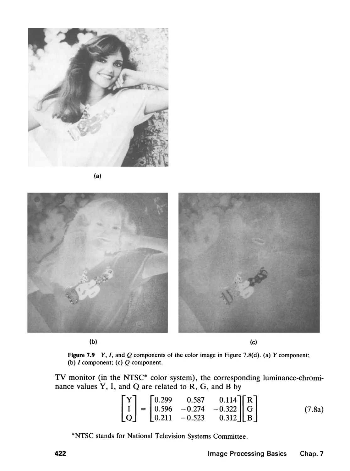
7.2 The Human Visual System, 423
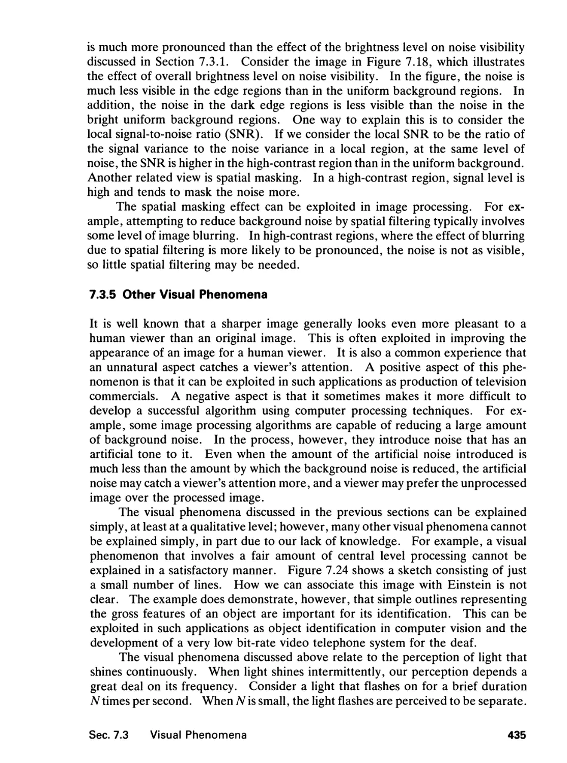
7.3 Visual Phenomena, 429
7.4 Image Processing Systems, 437
References, 443
Problems, 446
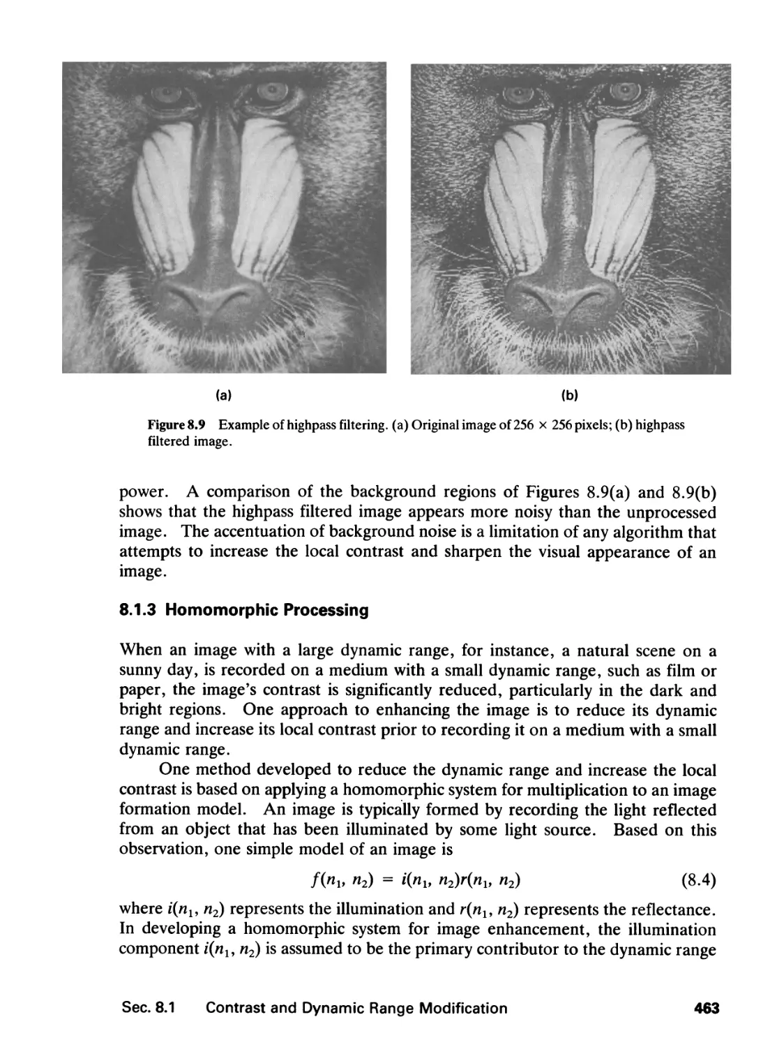
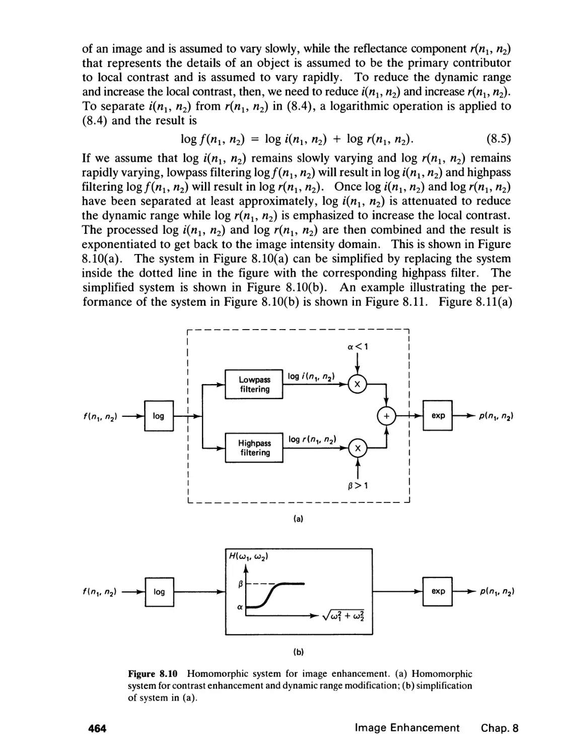
8 IMAGE ENHANCEMENT 451
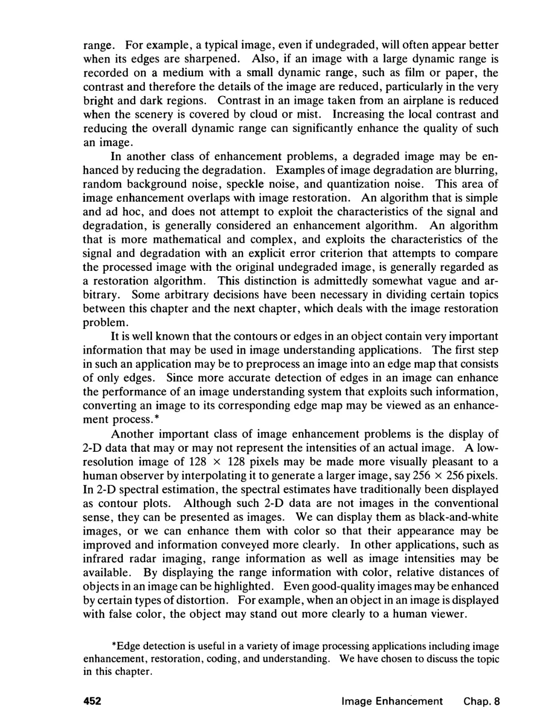
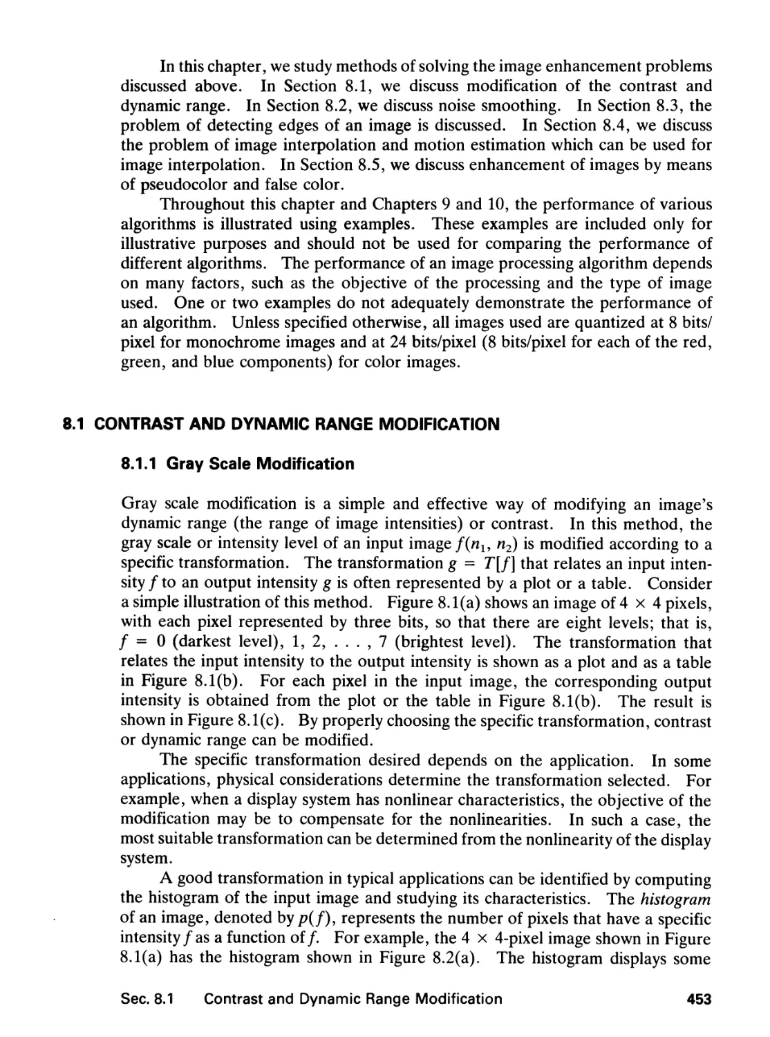
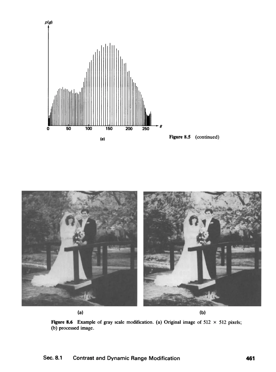
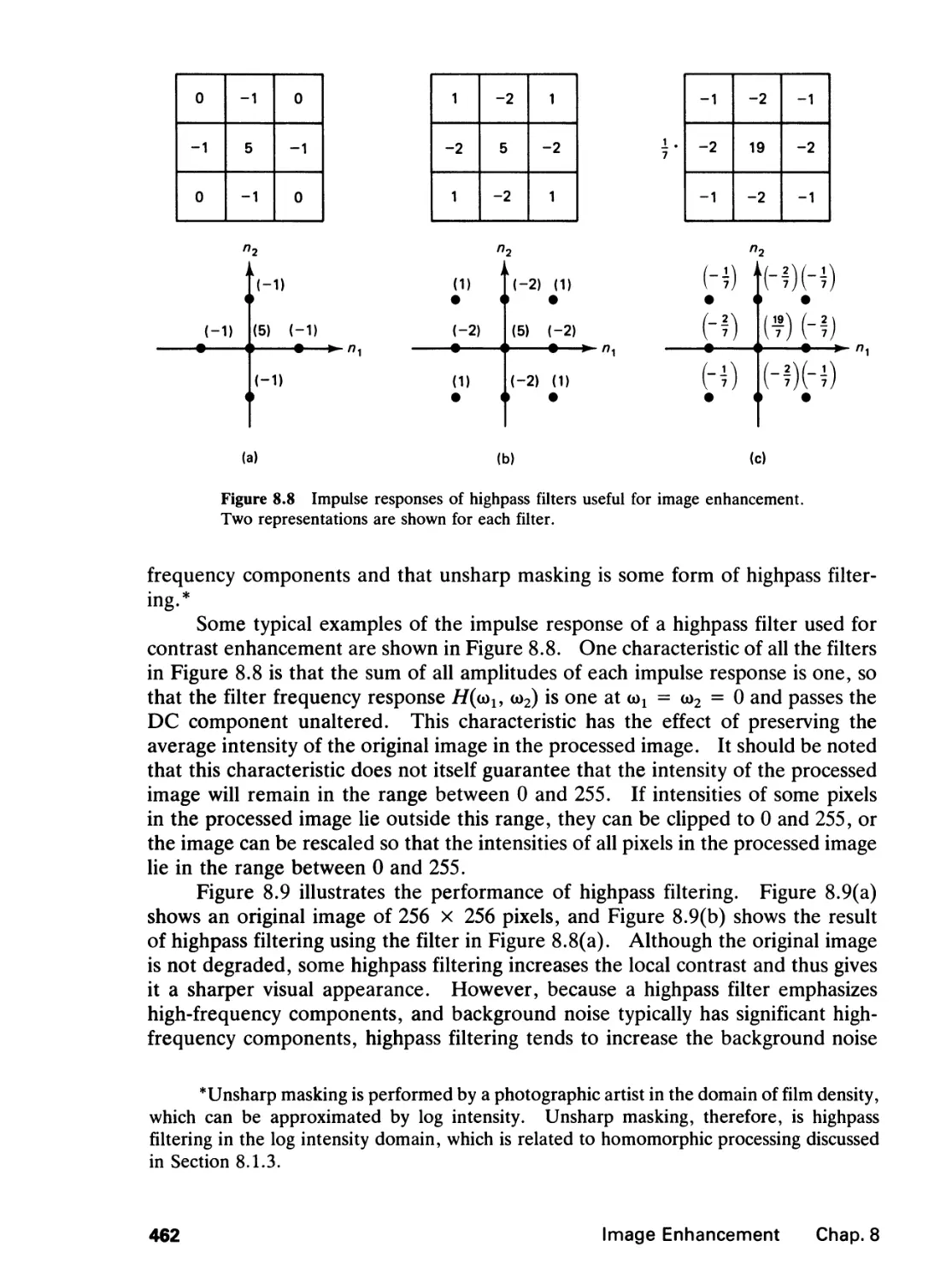
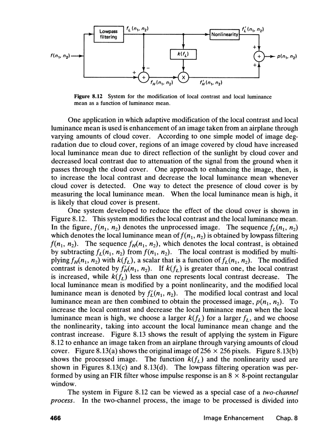
8.0 Introduction, 451
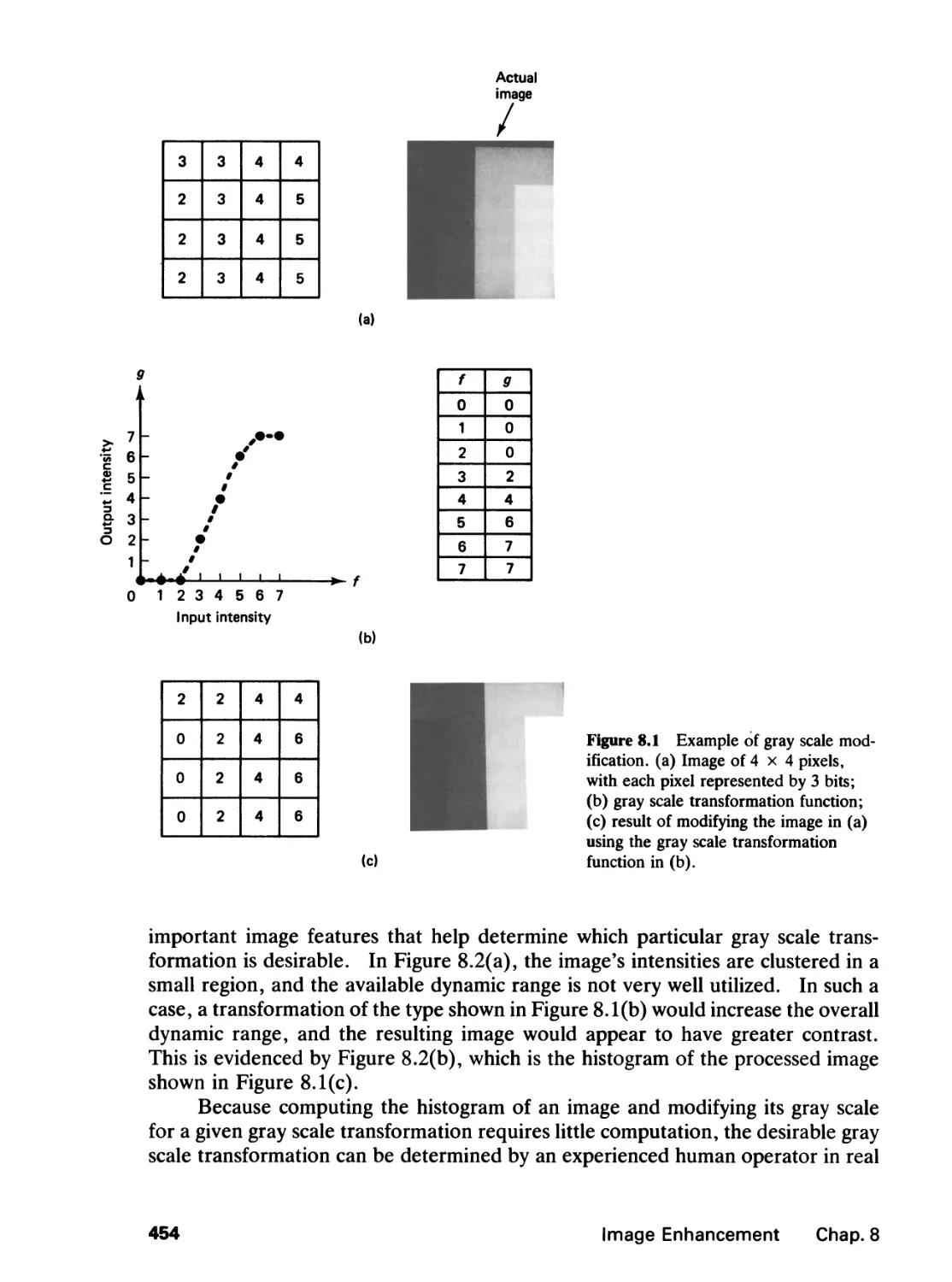
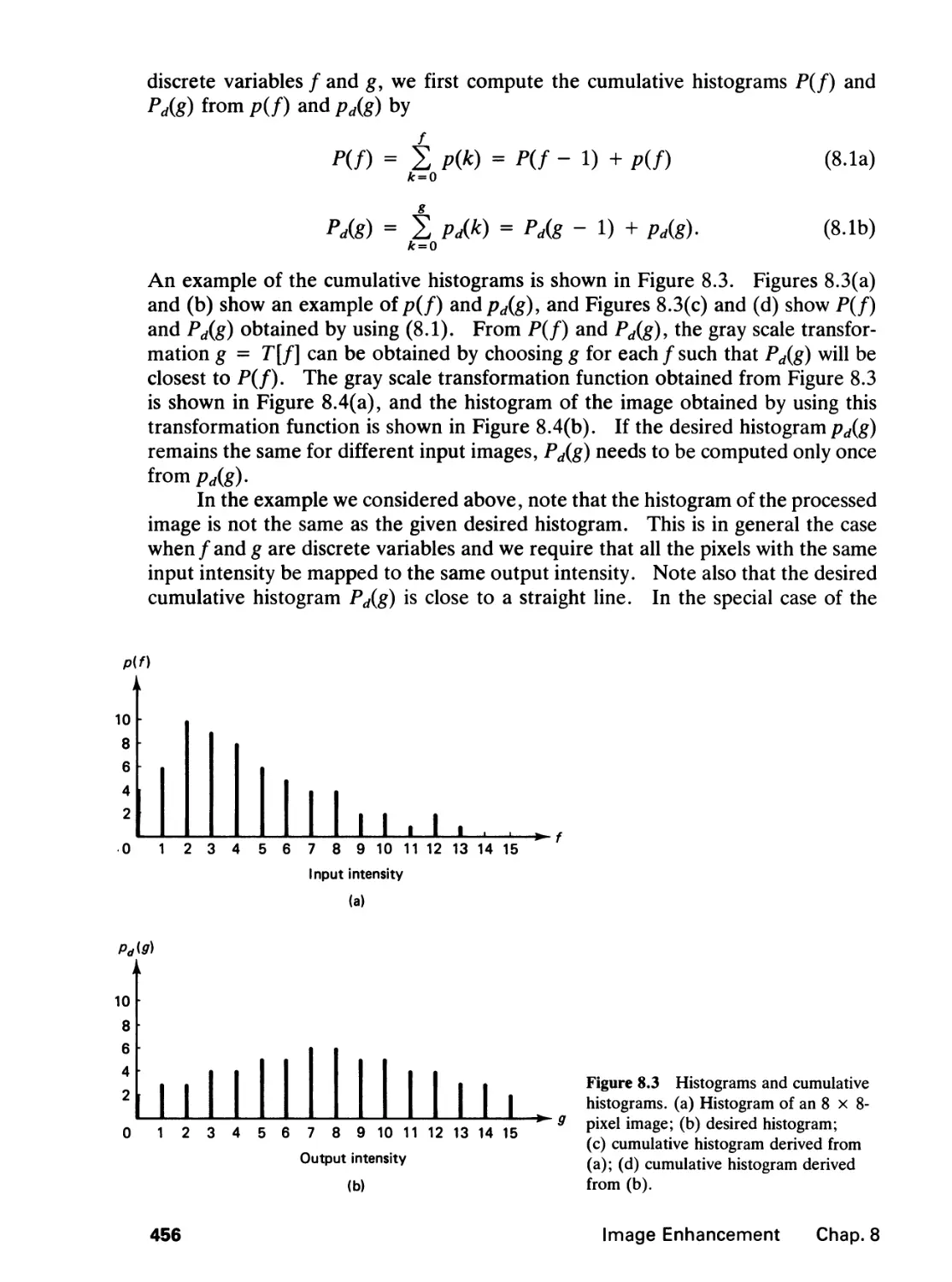
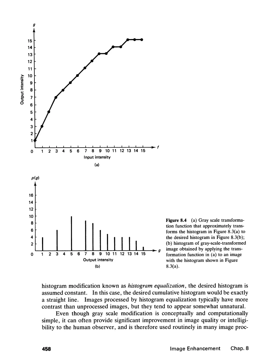
8.1 Contrast and Dynamic Range Modification, 453
8.2 Noise Smoothing, 468
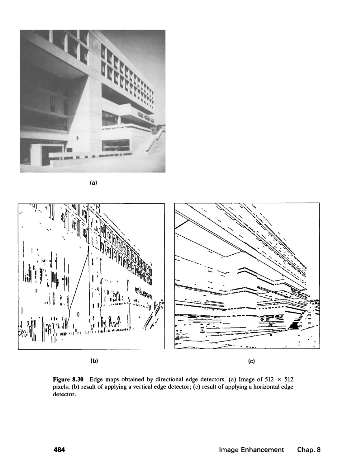
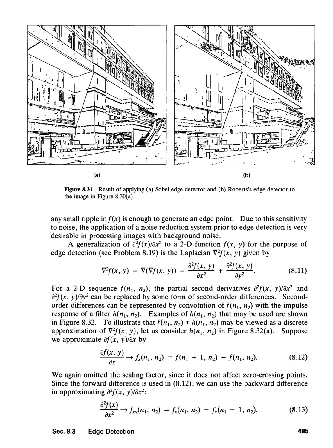
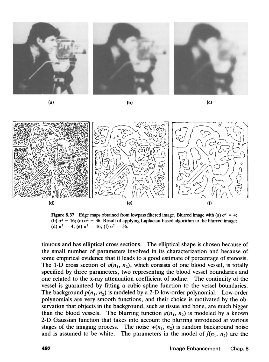
8.3 Edge Detection, 476
8.4 Image Interpolation and Motion Estimation, 495
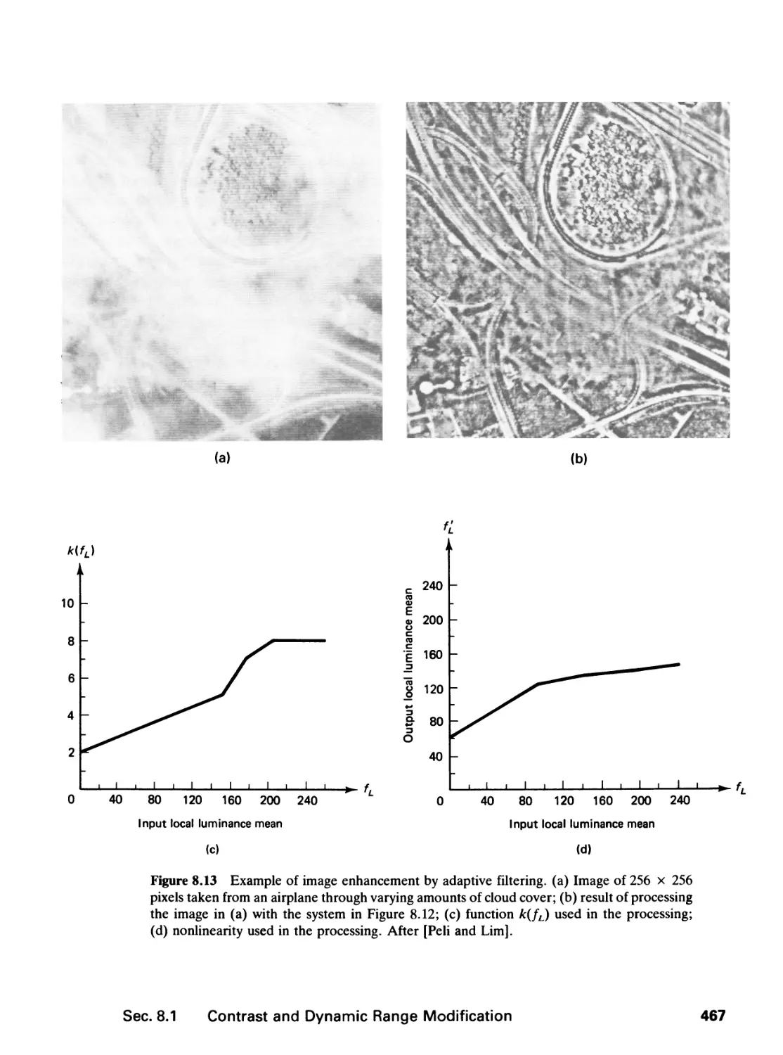
Contents
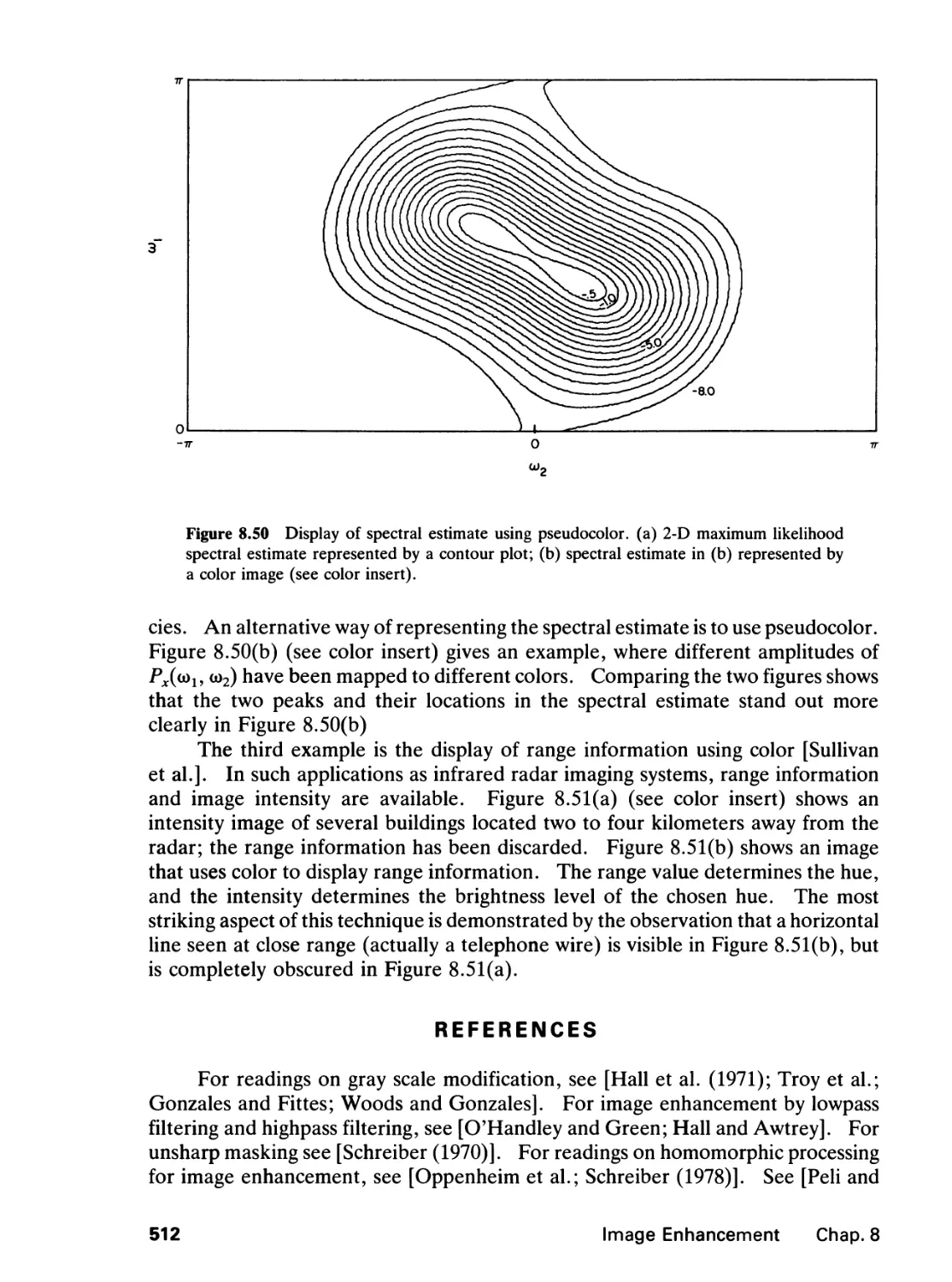
8.5 False Color and Pseudocolor, 511
References, 512
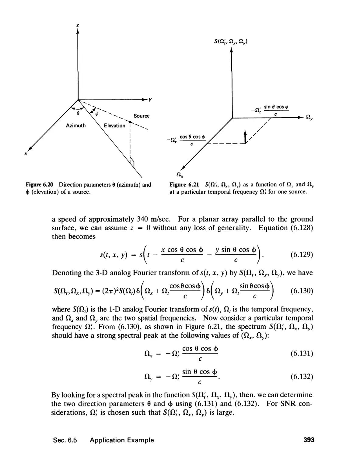
Problems, 515
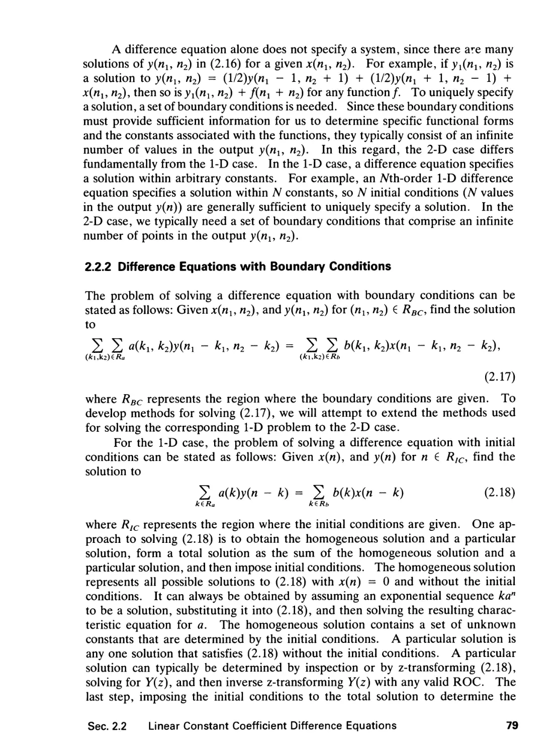
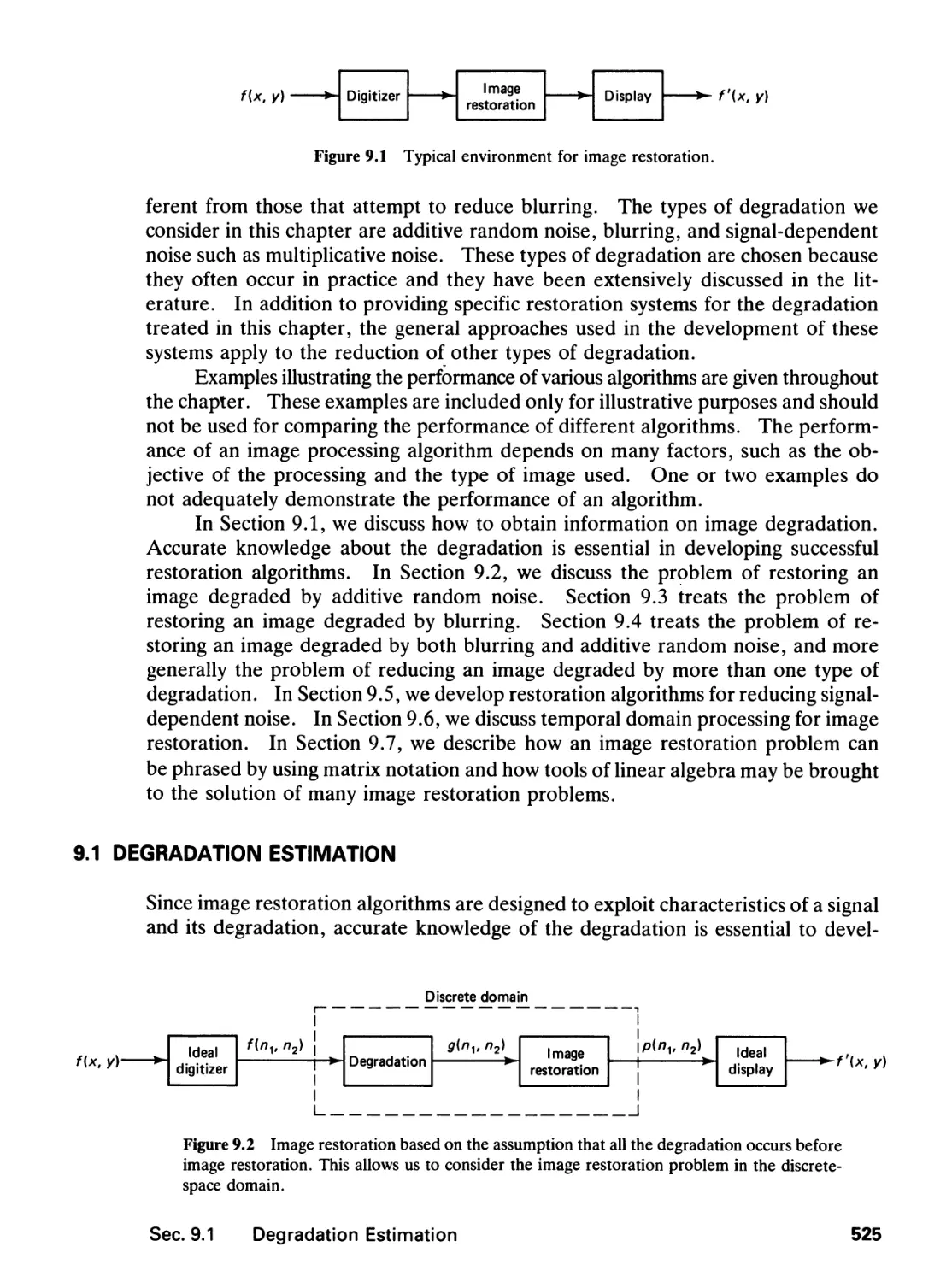
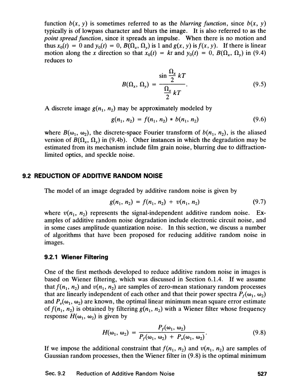
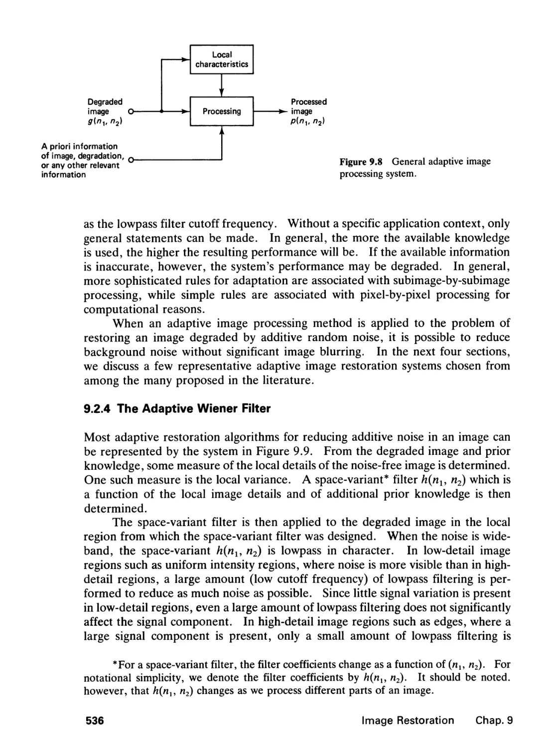
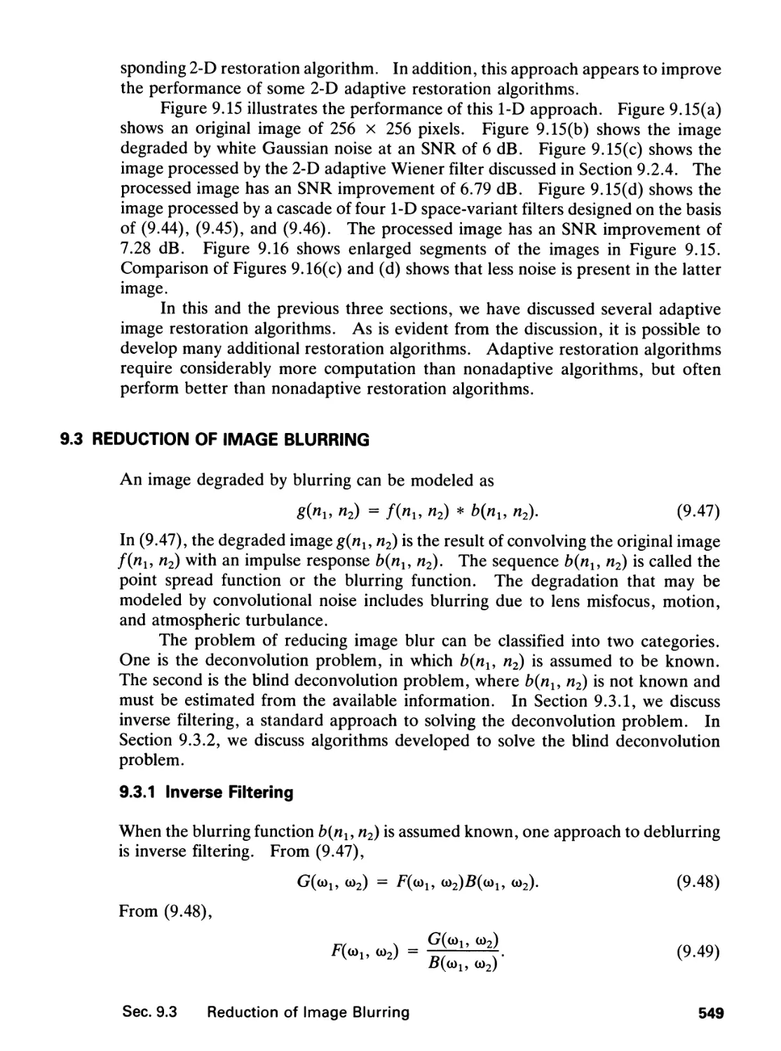
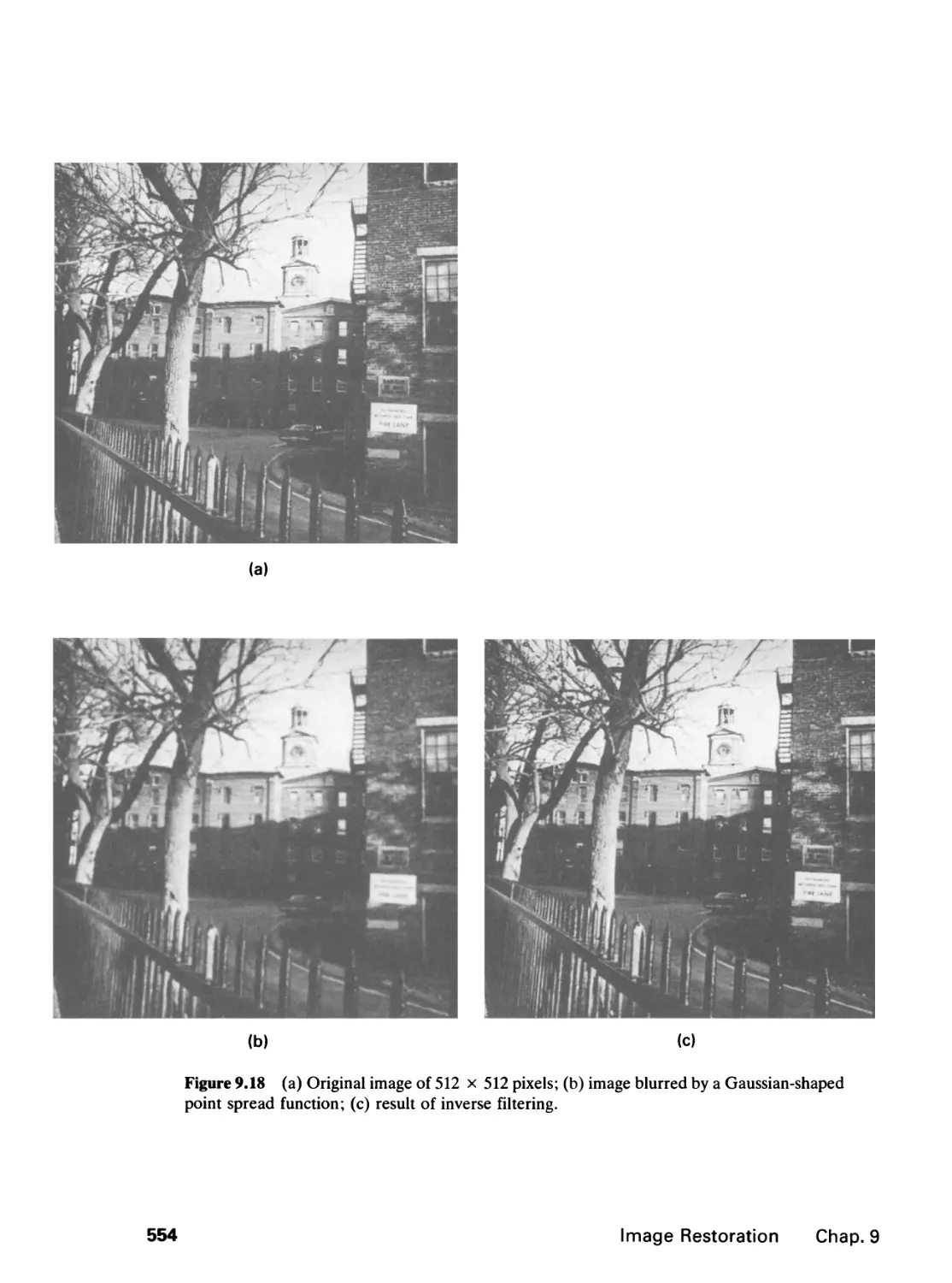
9 IMAGE RESTORATION 524
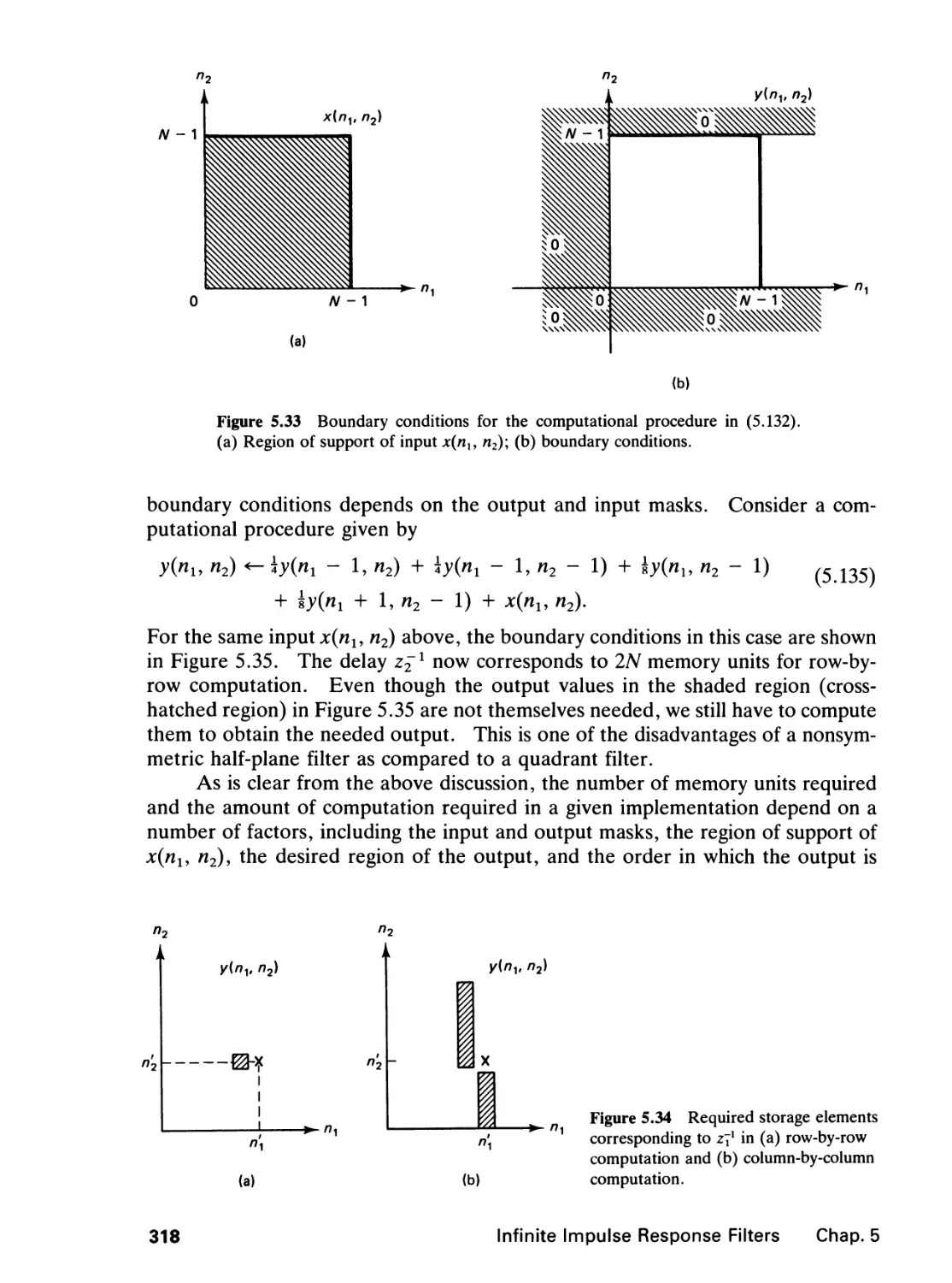
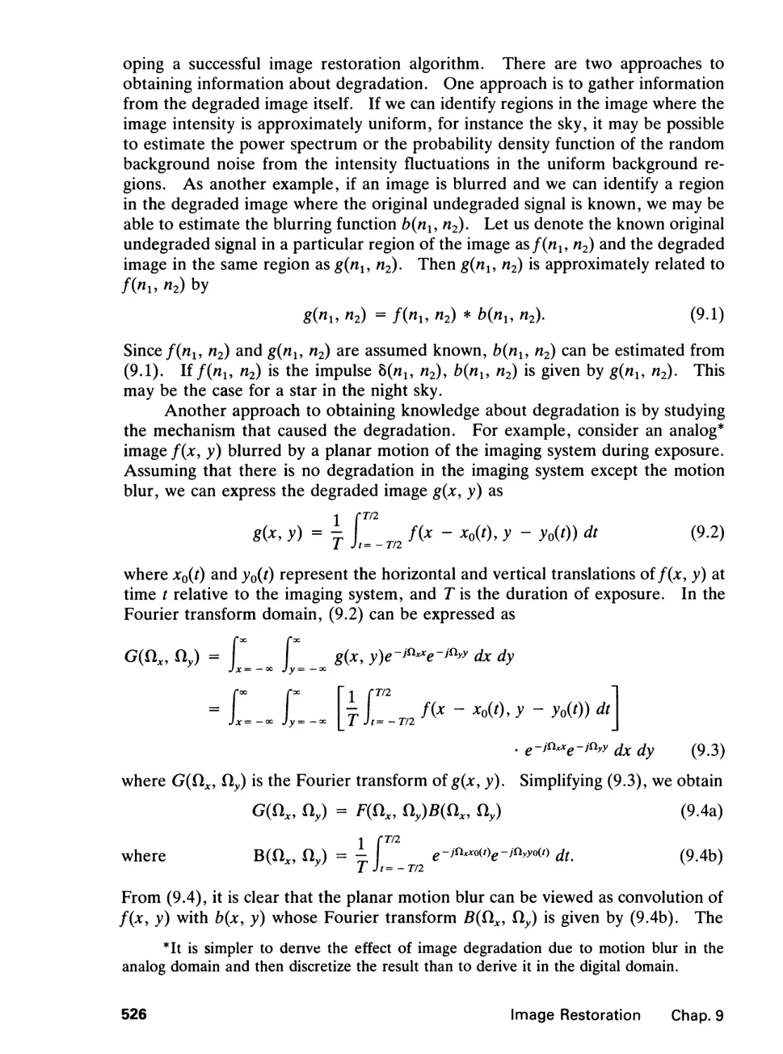
9.0 Introduction, 524
9.1 Degradation Estimation, 525
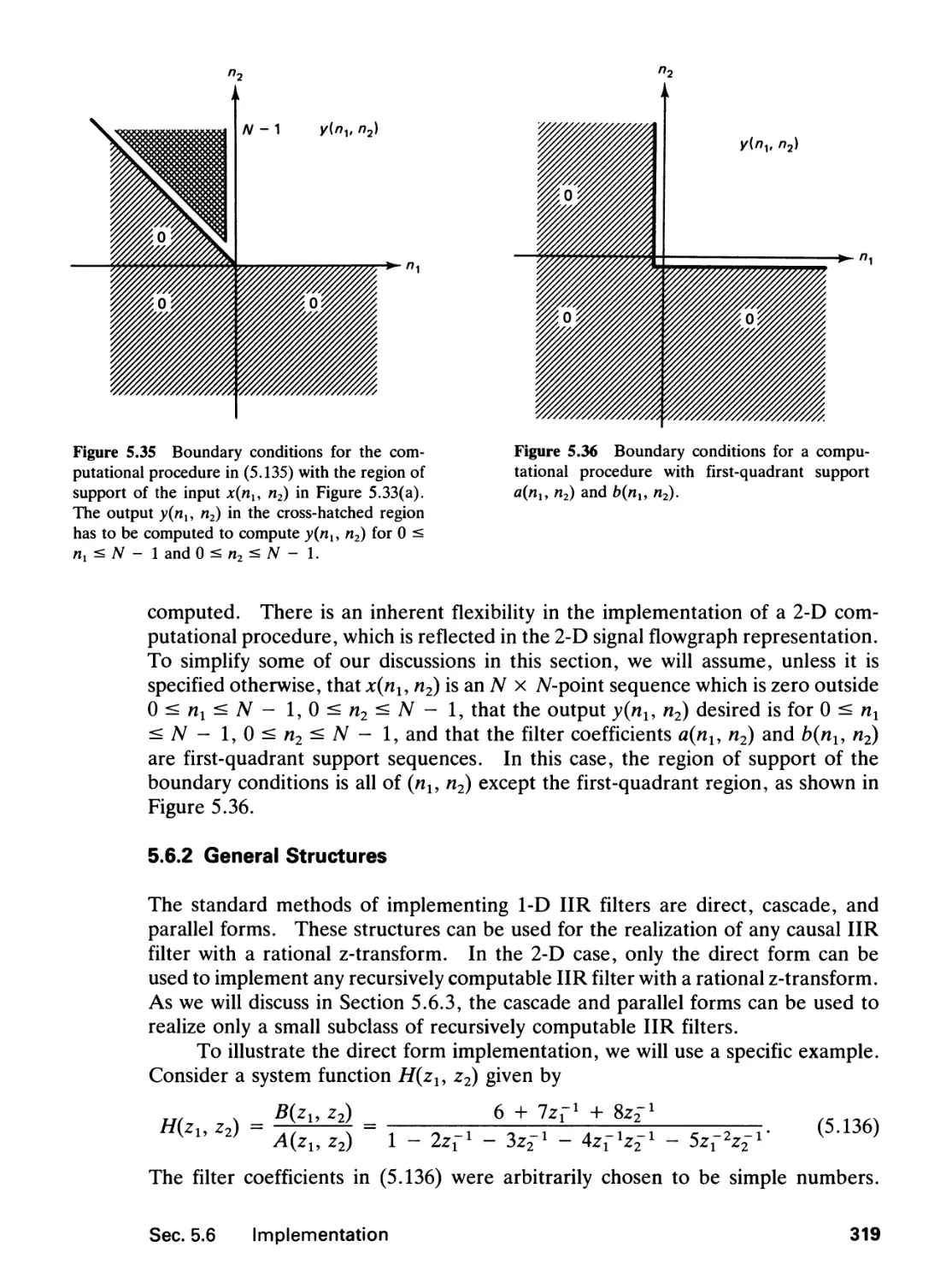
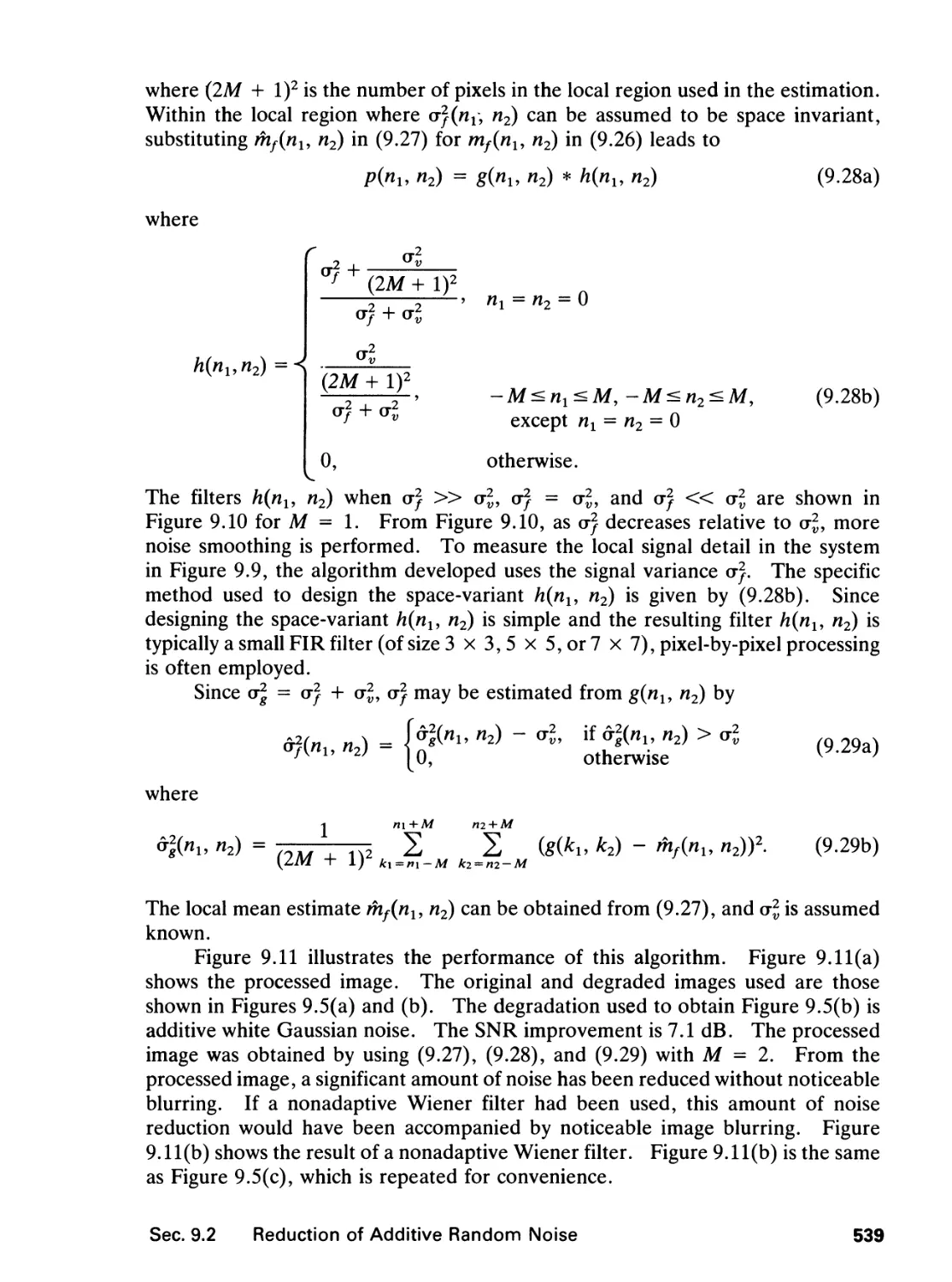
9.2 Reduction of Additive Random Noise, 527
9.3 Reduction of Image Blurring, 549
9.4 Reduction of Blurring and Additive Random Noise,
559
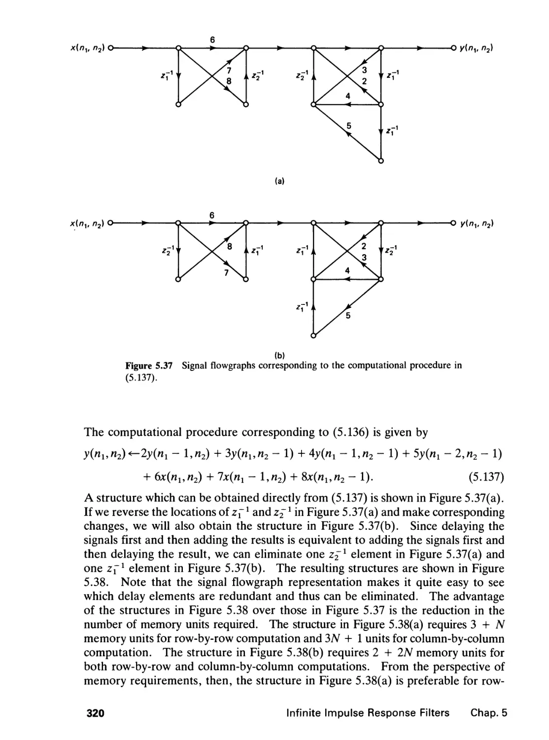
9.5 Reduction of Signal-Dependent Noise, 562
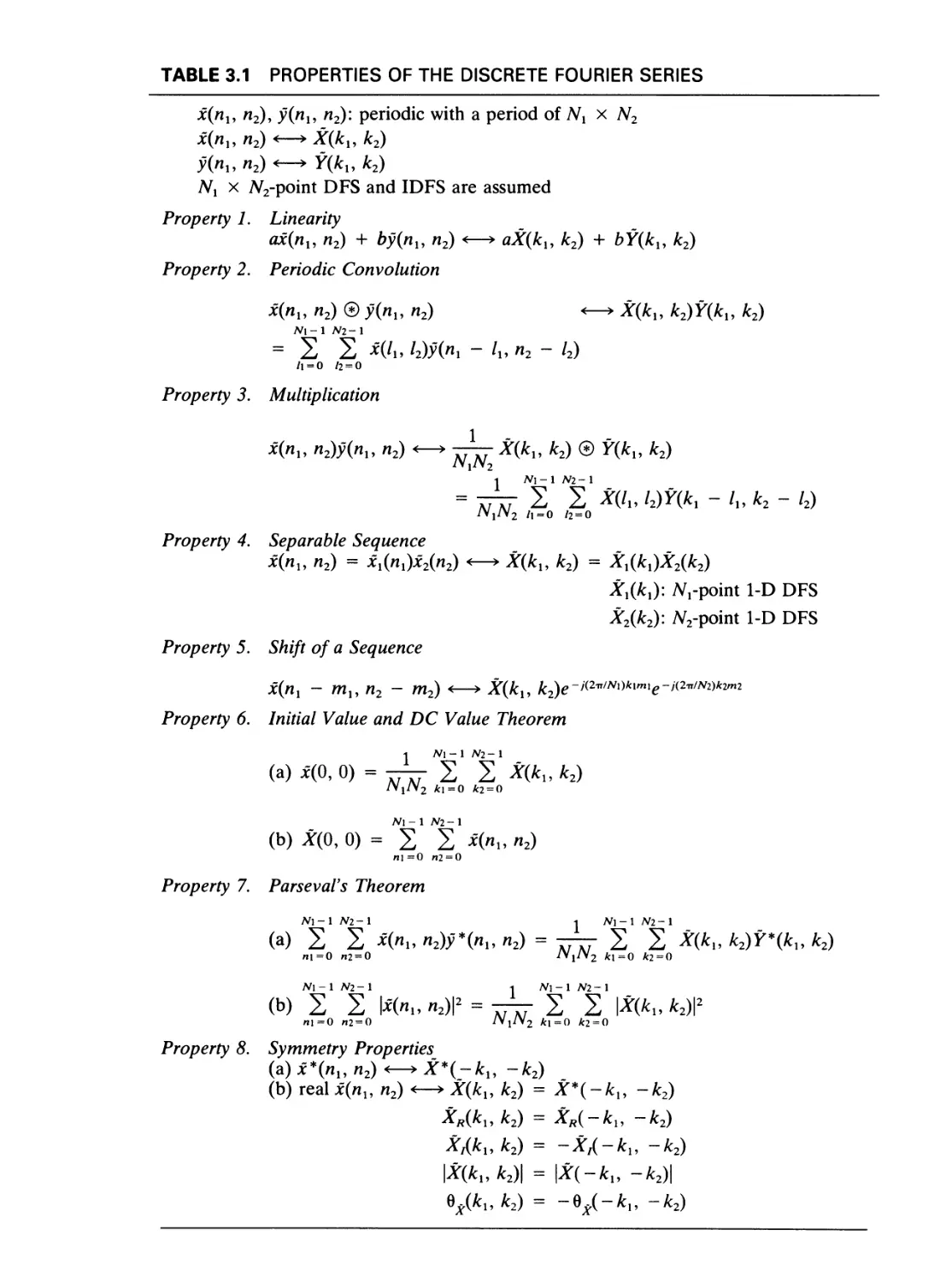
9.6 Temporal Filtering for Image Restoration, 568
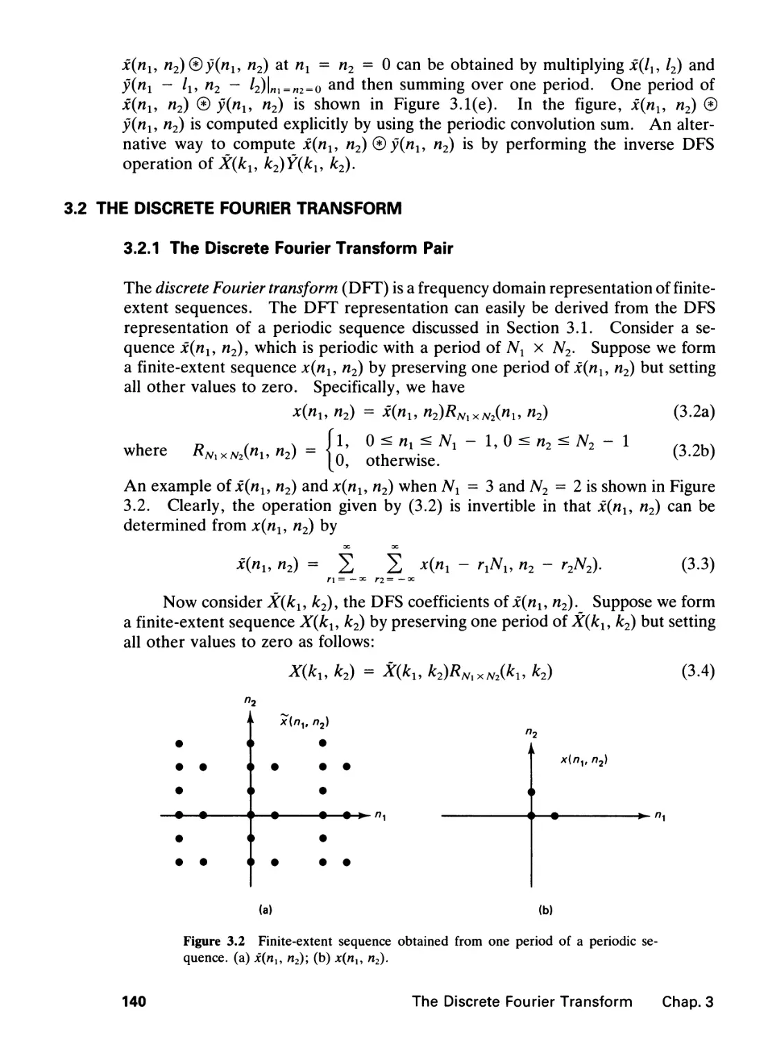
9.7 Additional Comments, 575
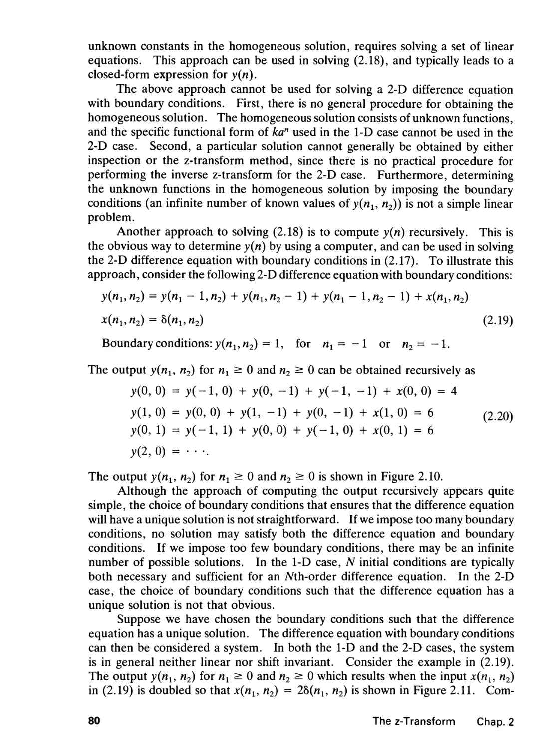
References, 576
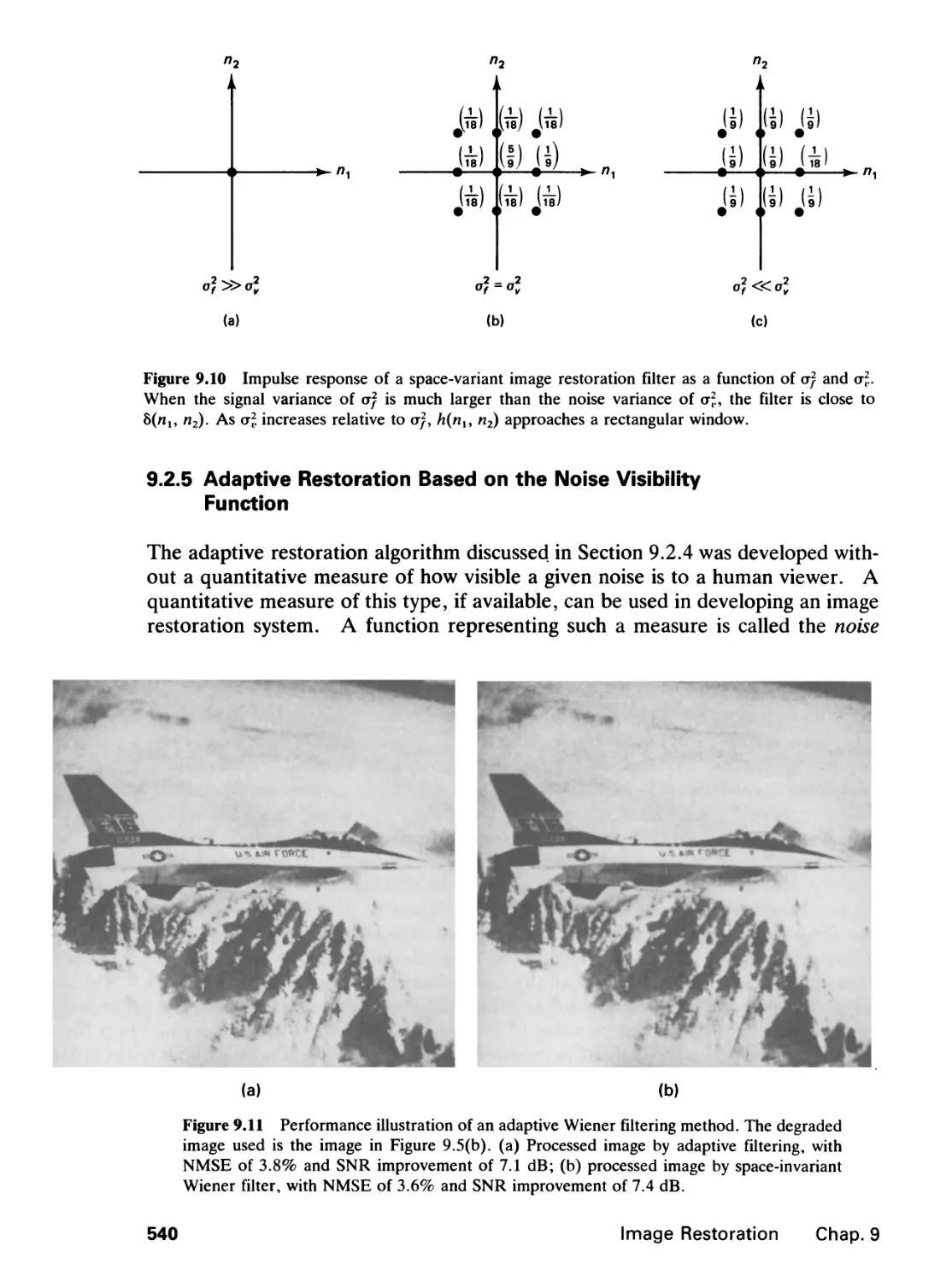
Problems, 580
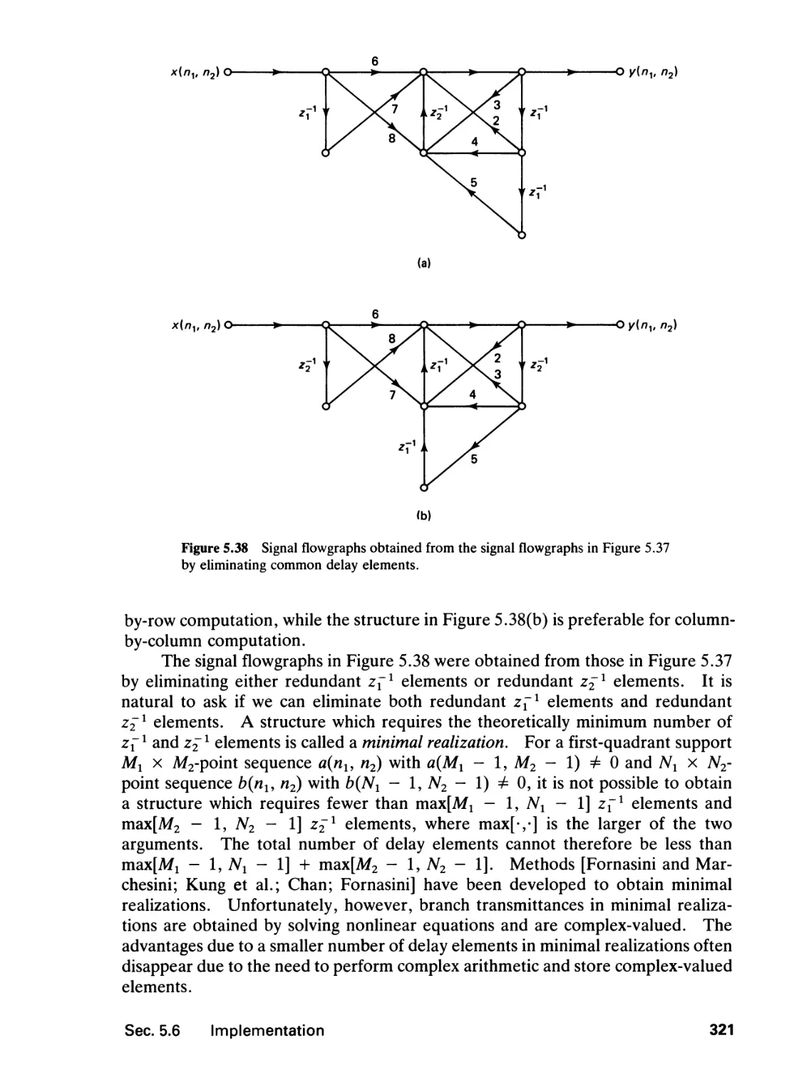
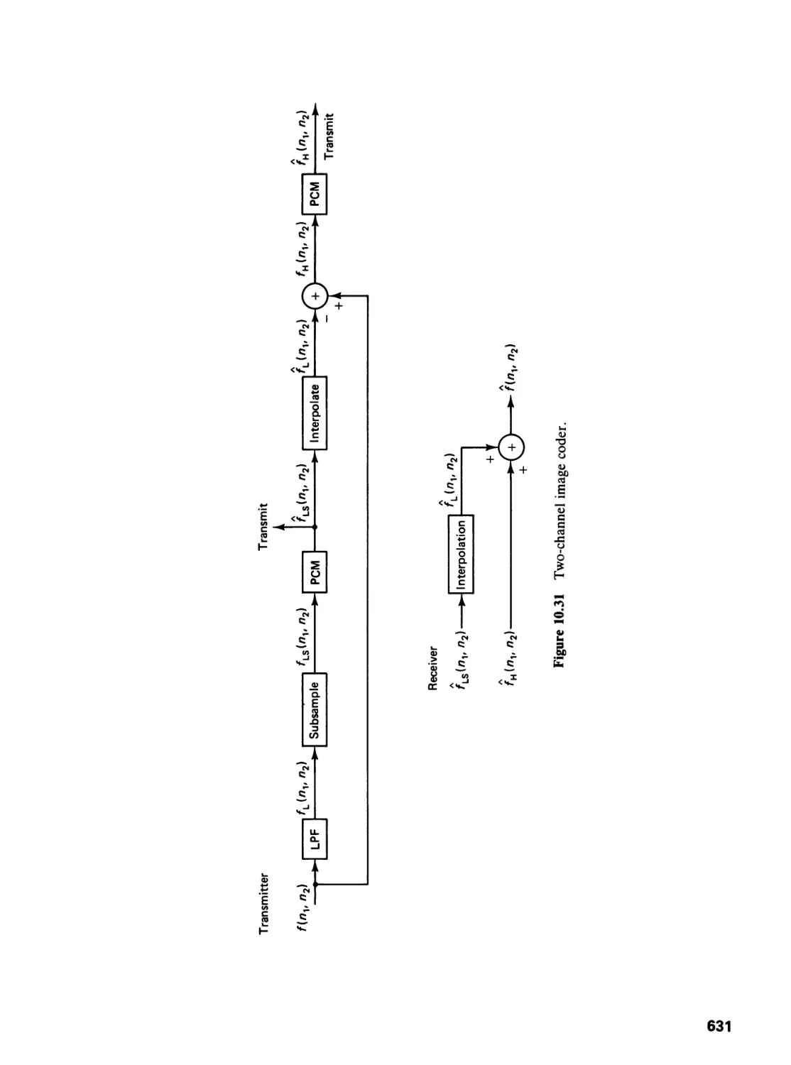
10 IMAGE CODING 589
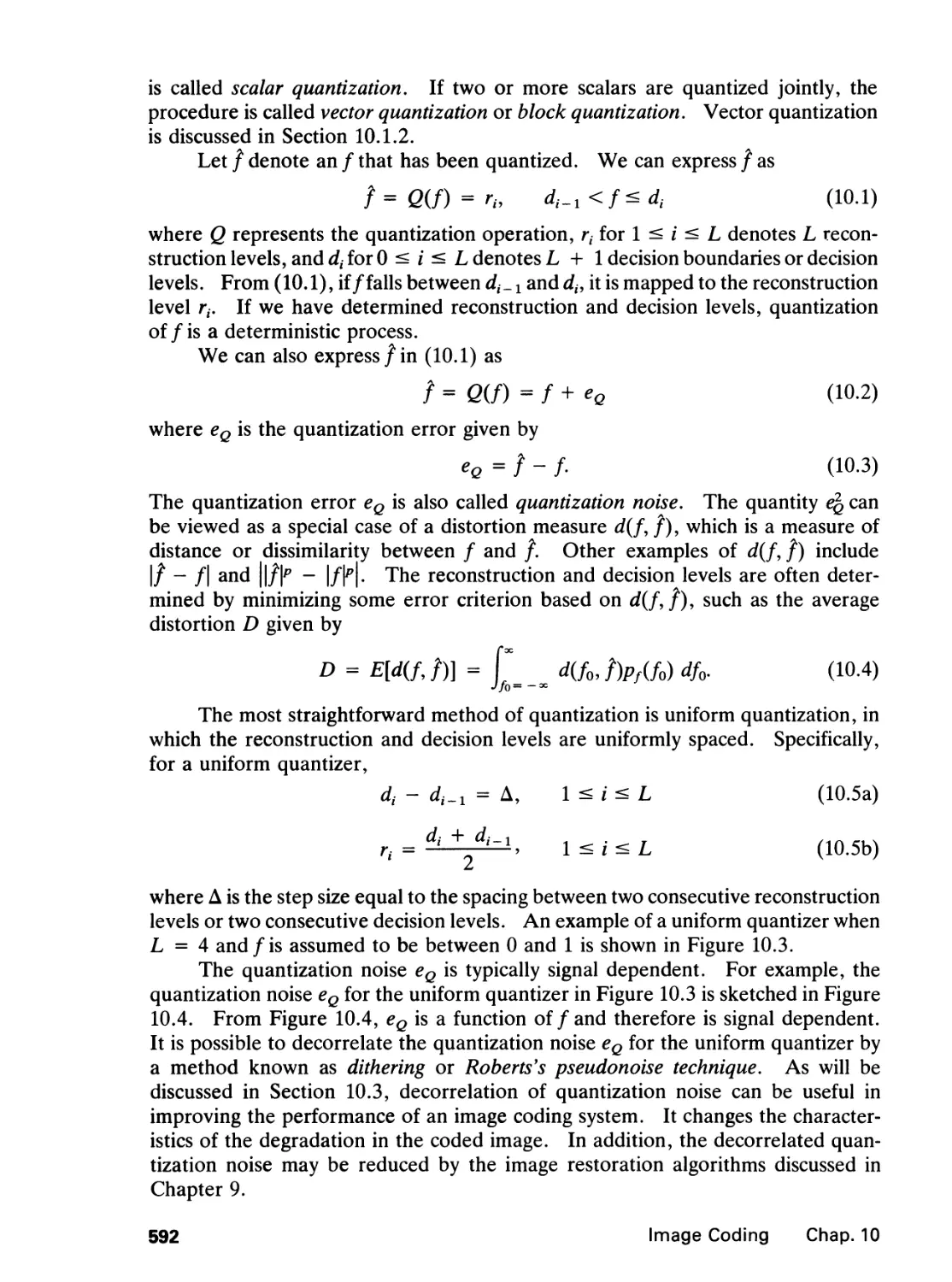
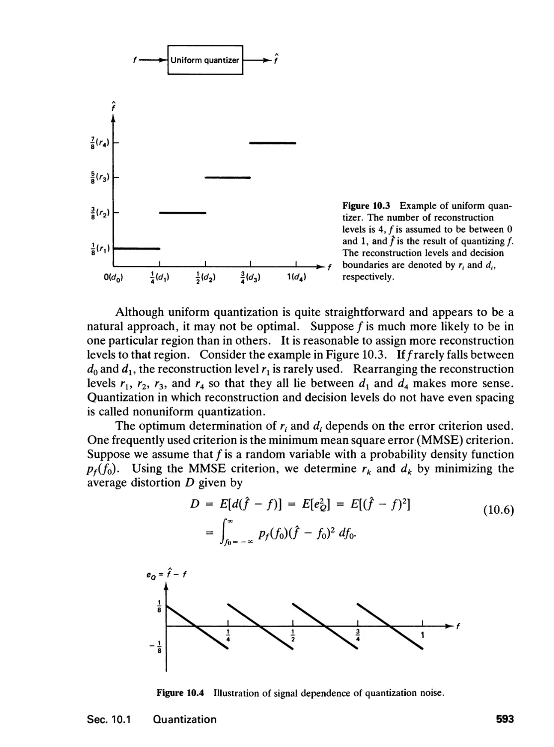
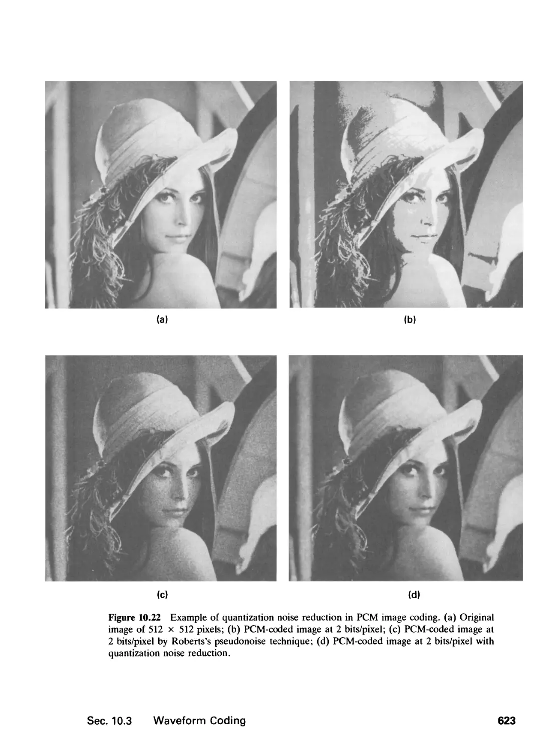
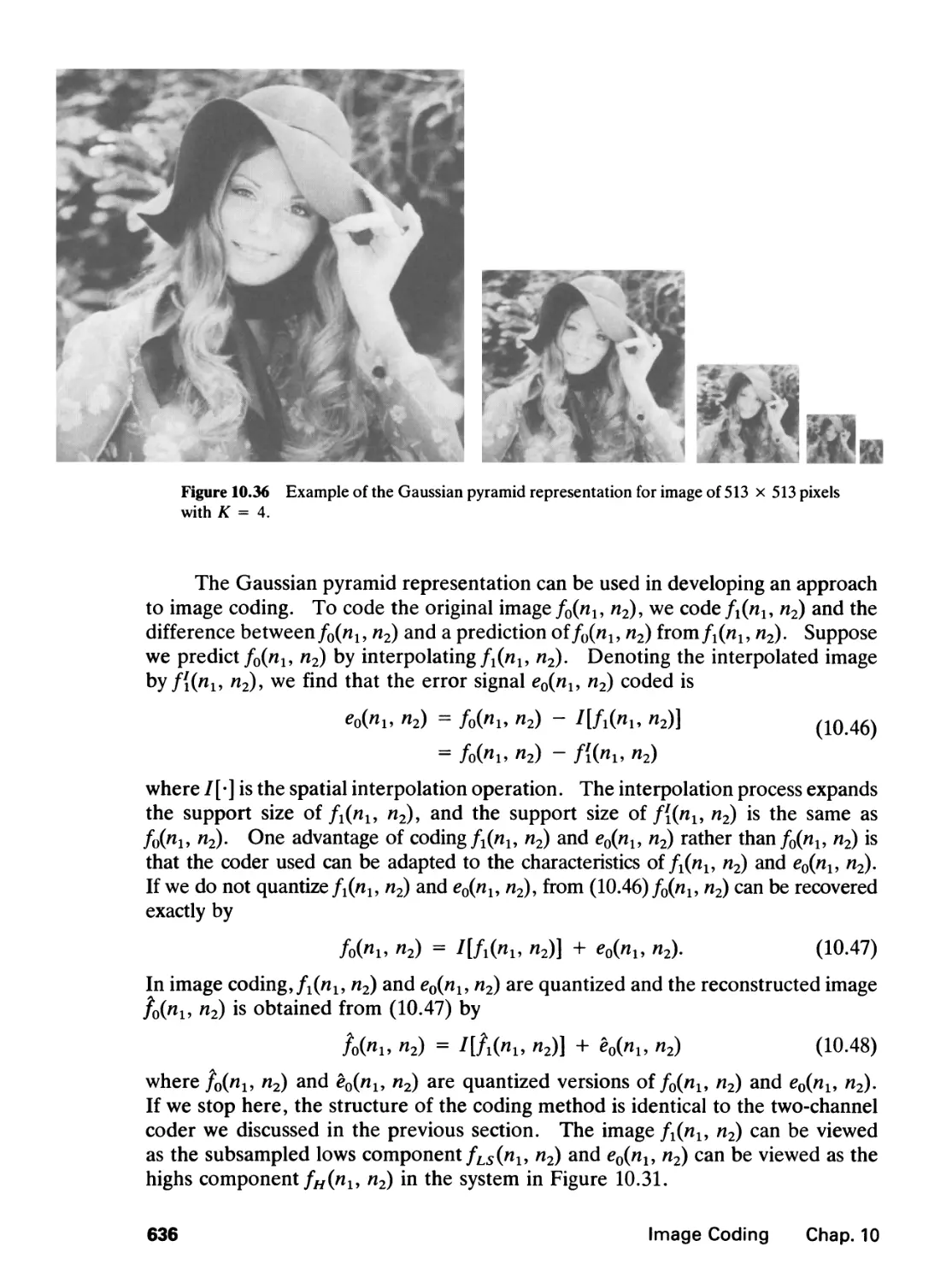
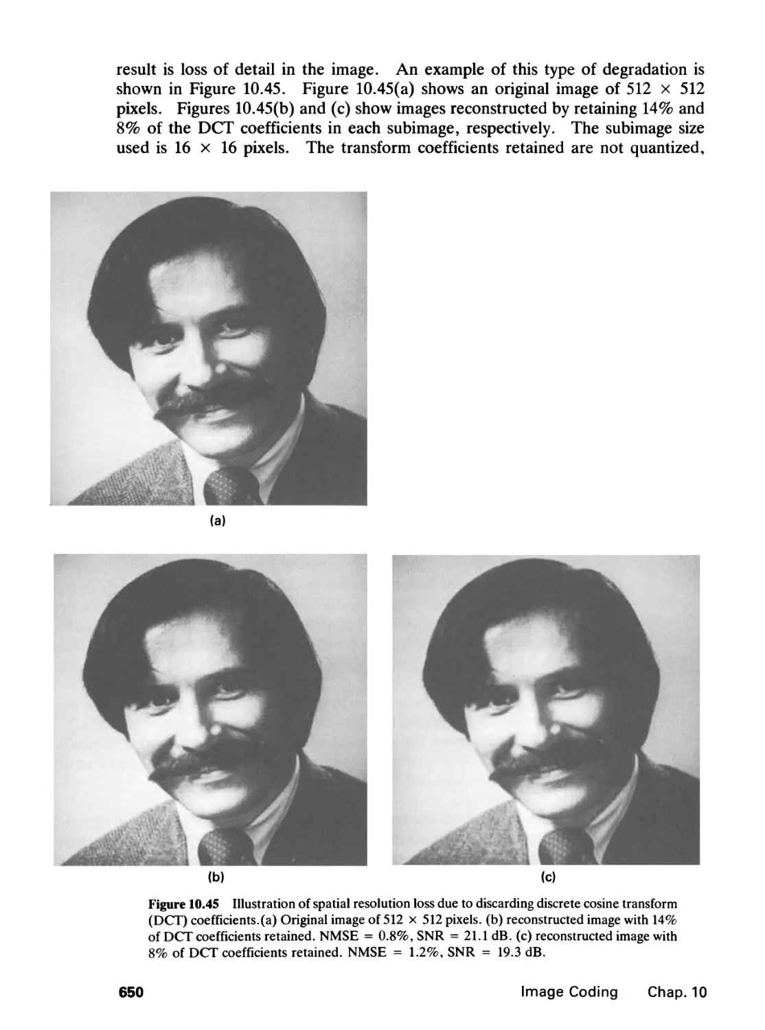
10.0 Introduction, 589
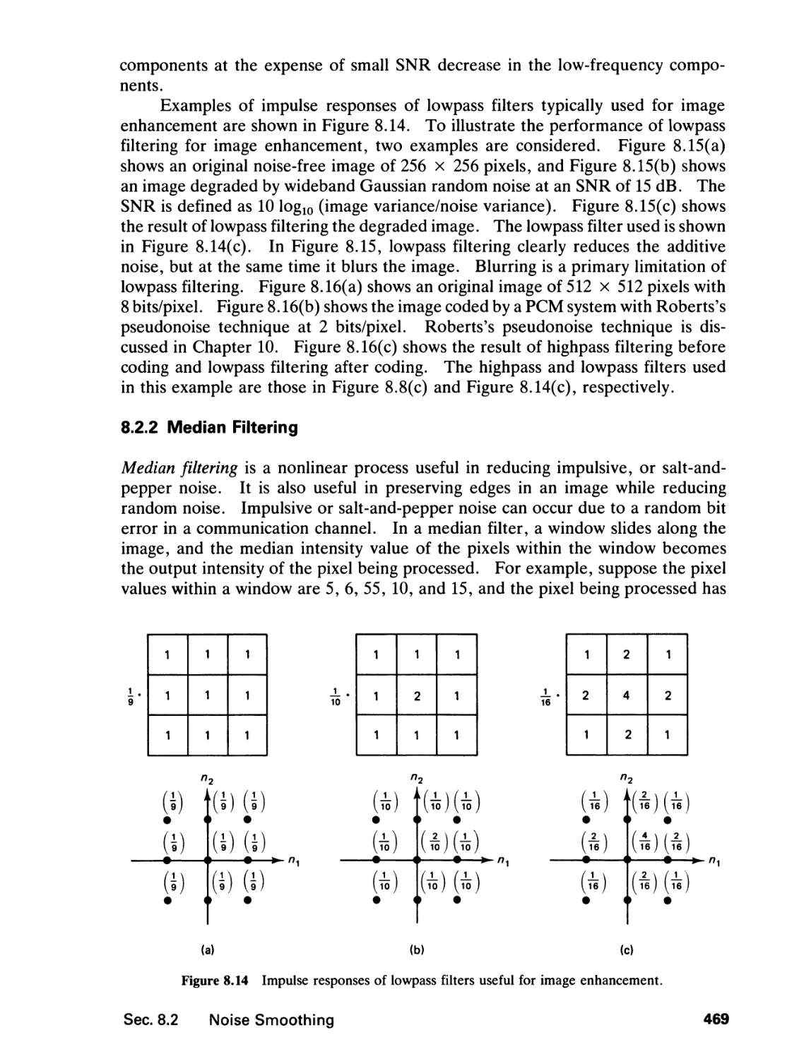
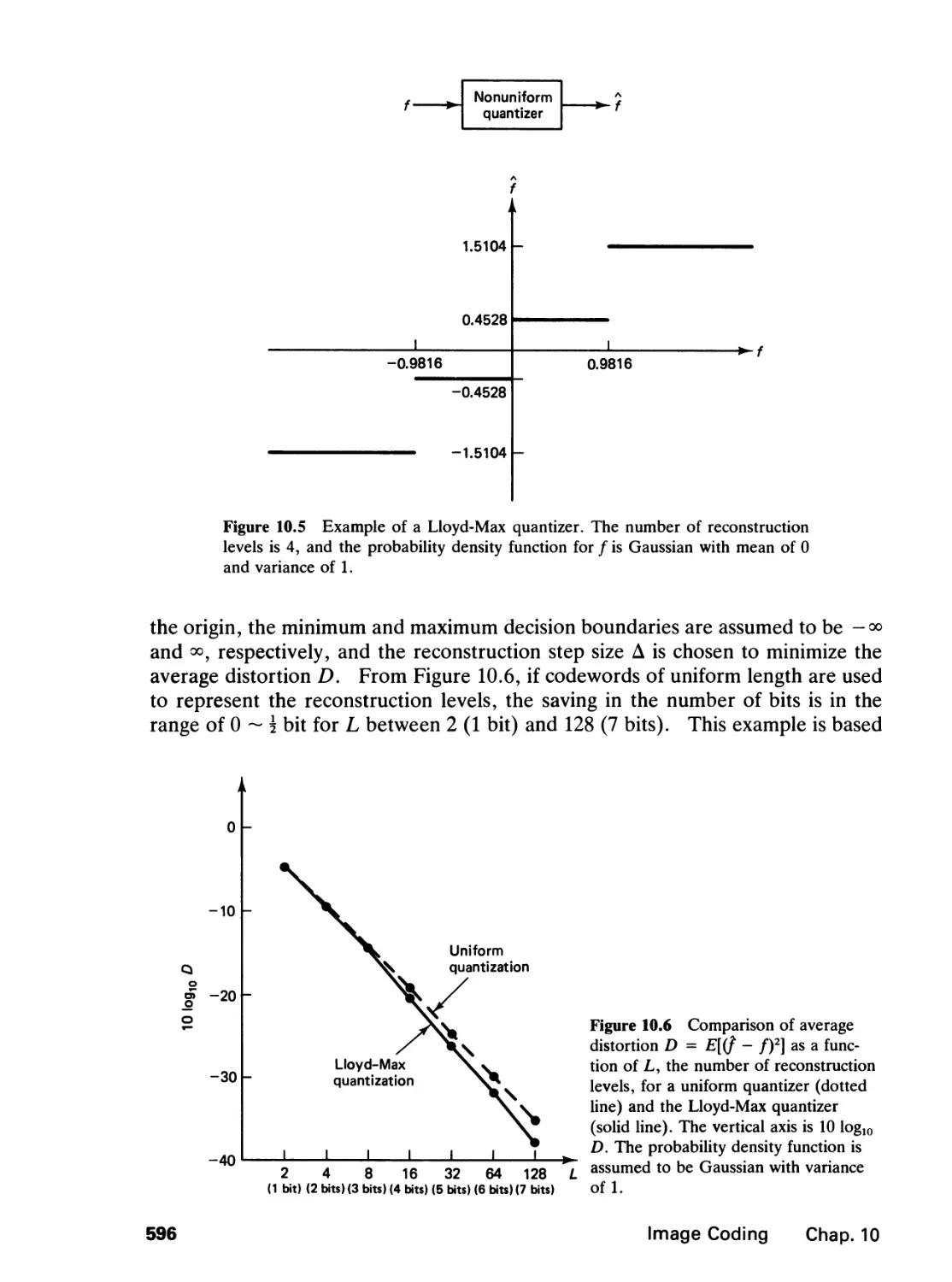
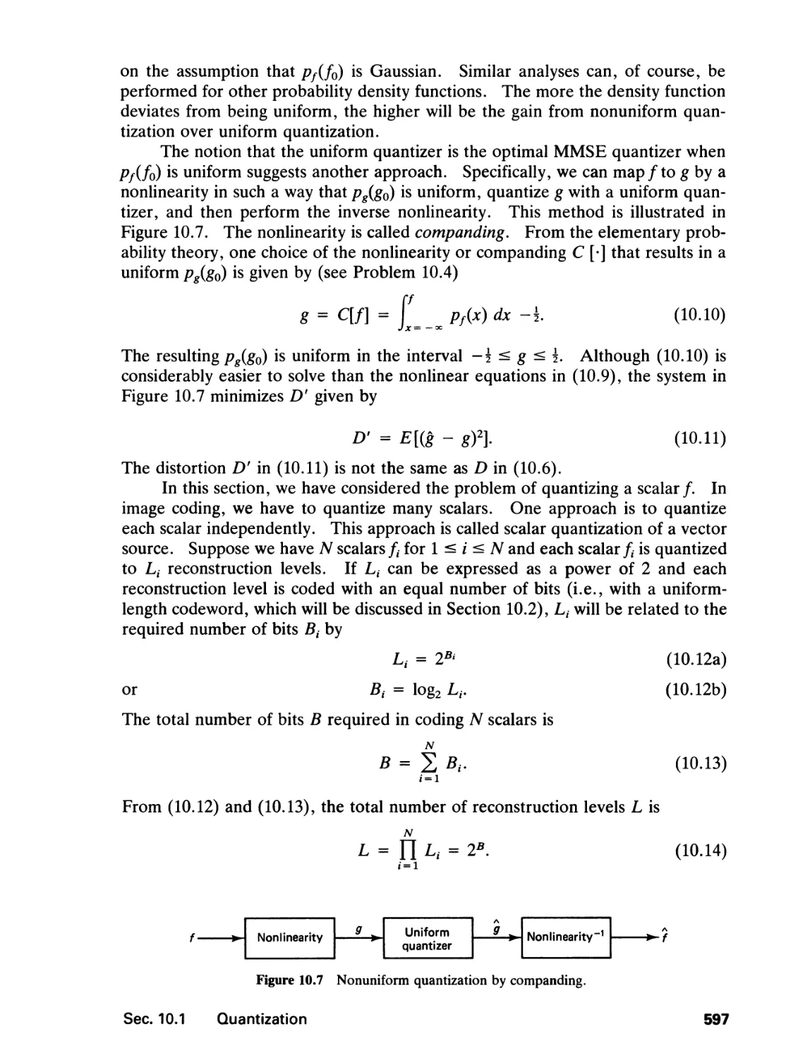
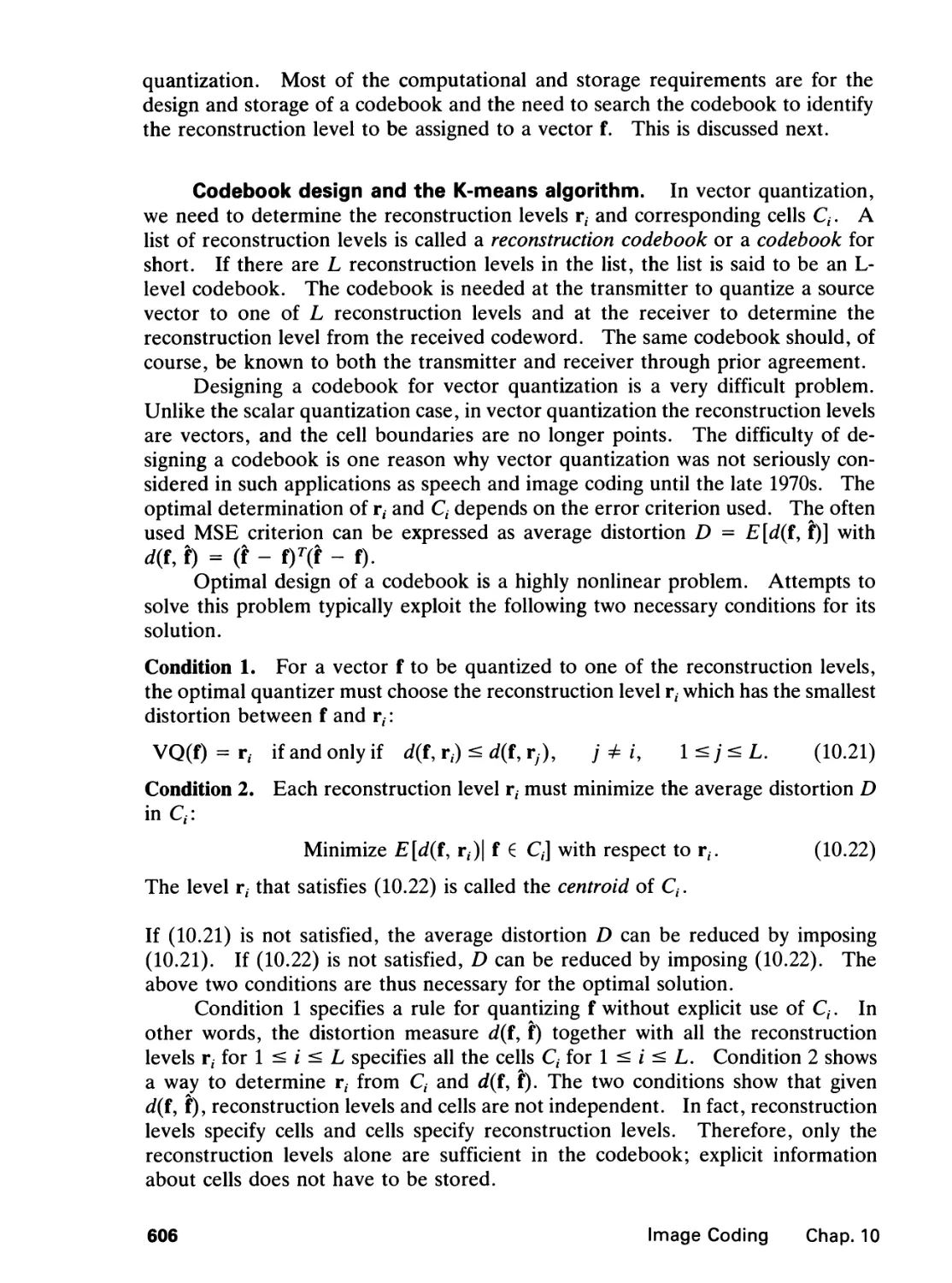
10.1 Quantization, 591
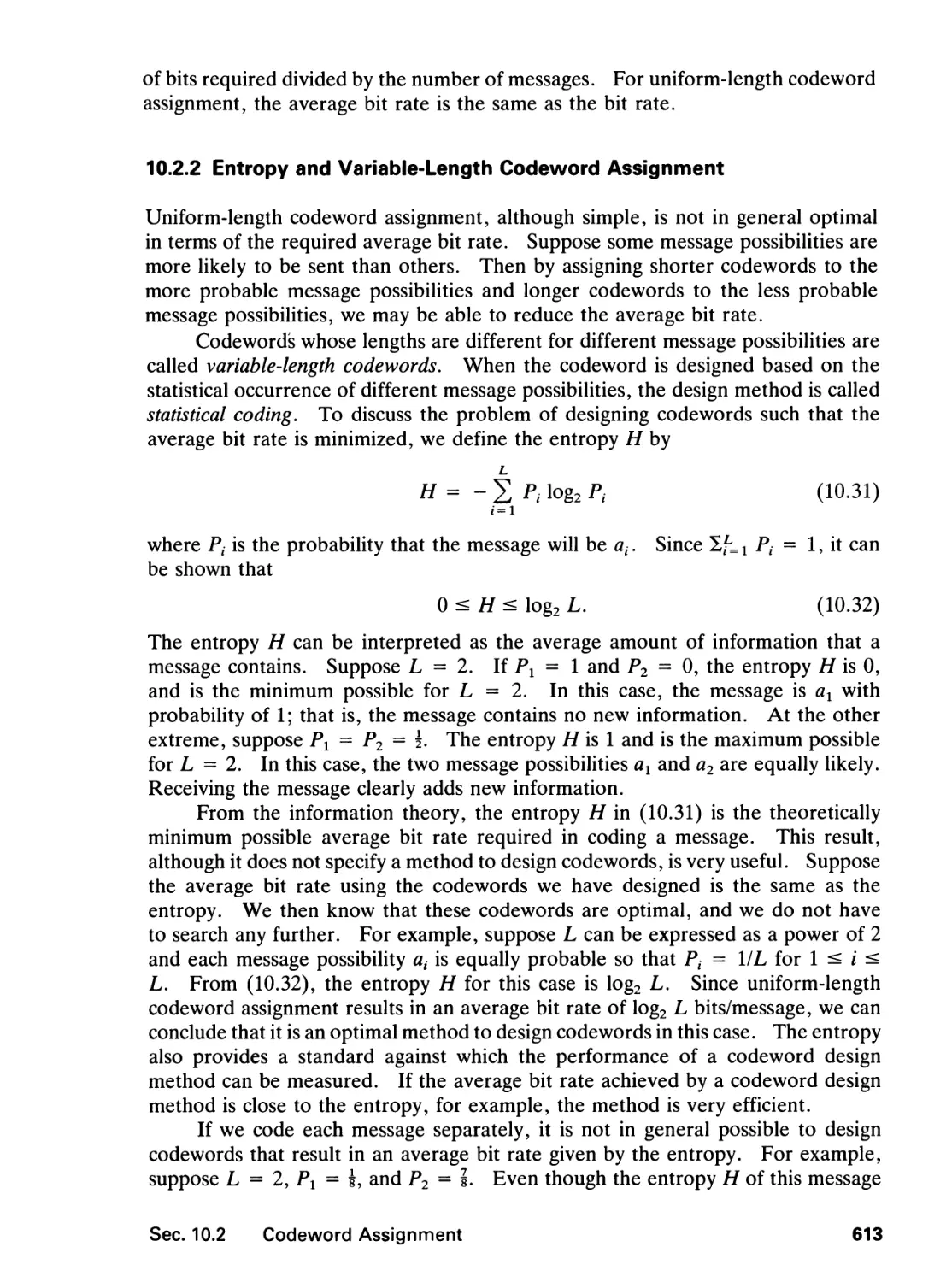
10.2 Codeword Assignment, 612
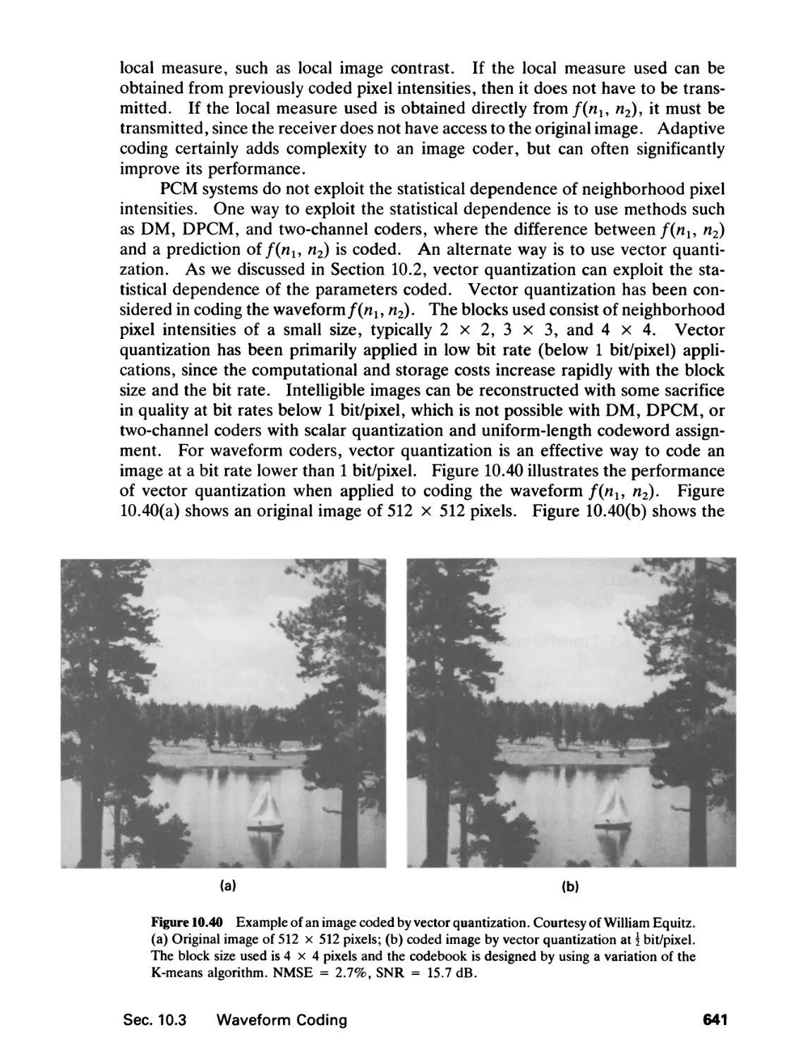
10.3 Waveform Coding, 617
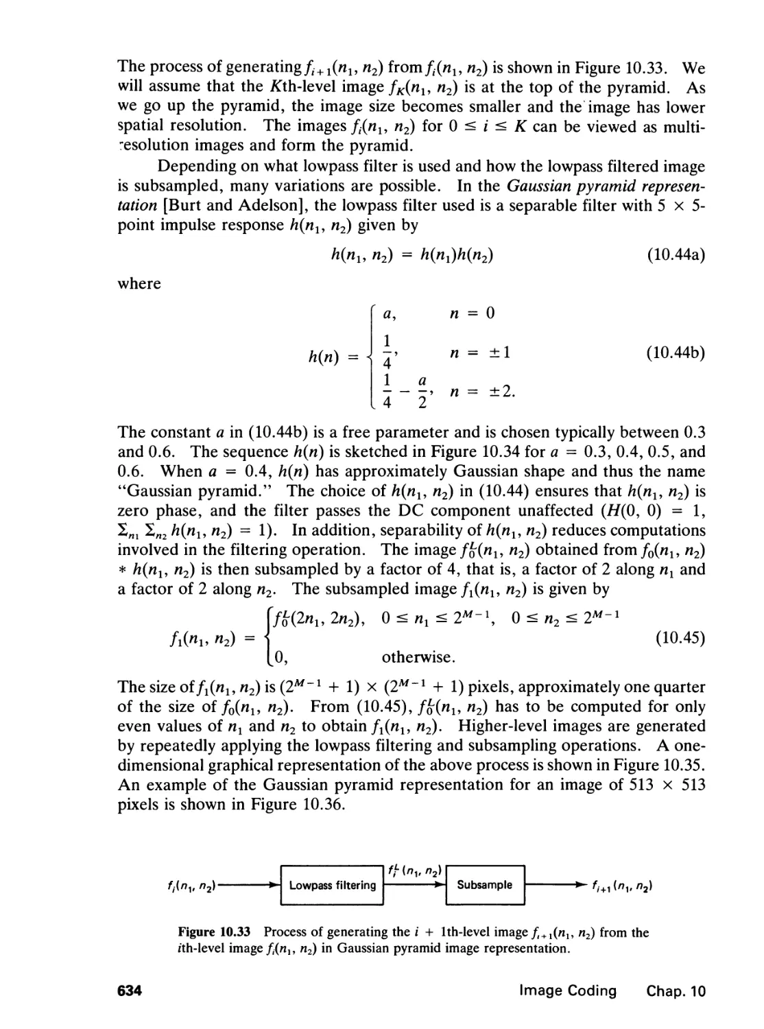
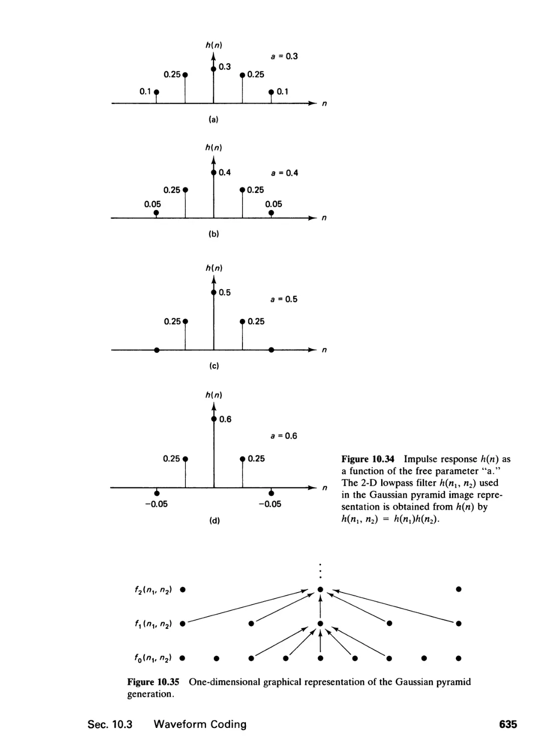
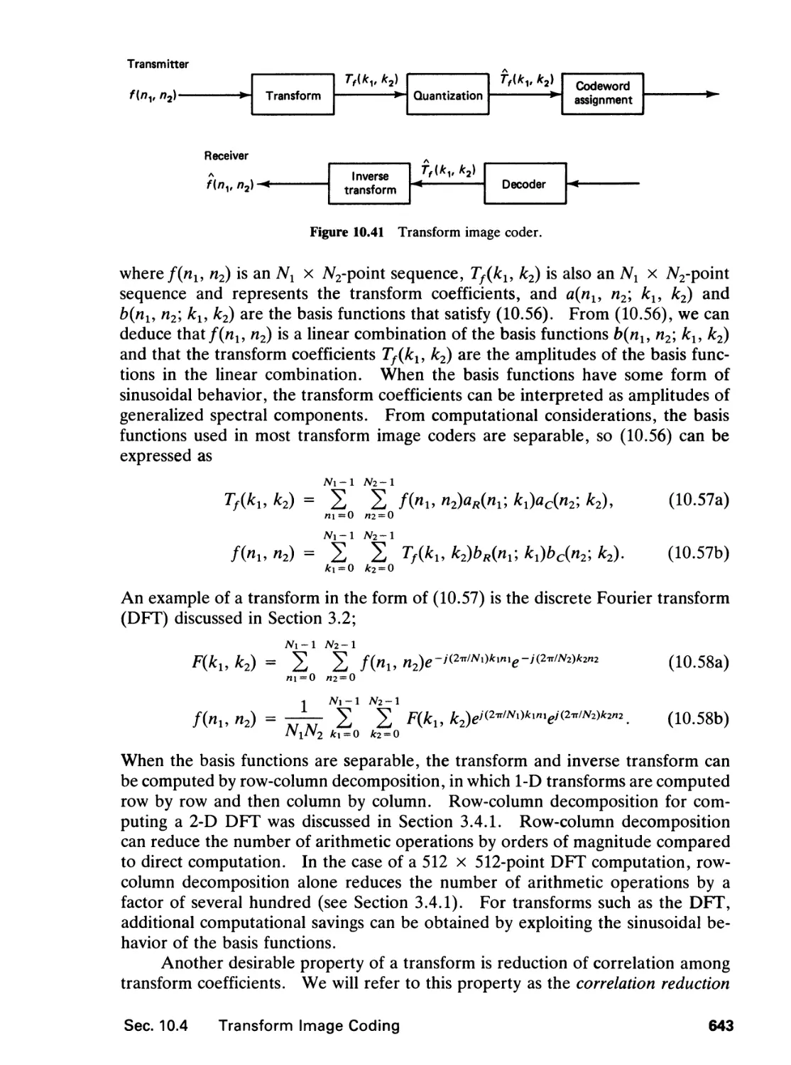
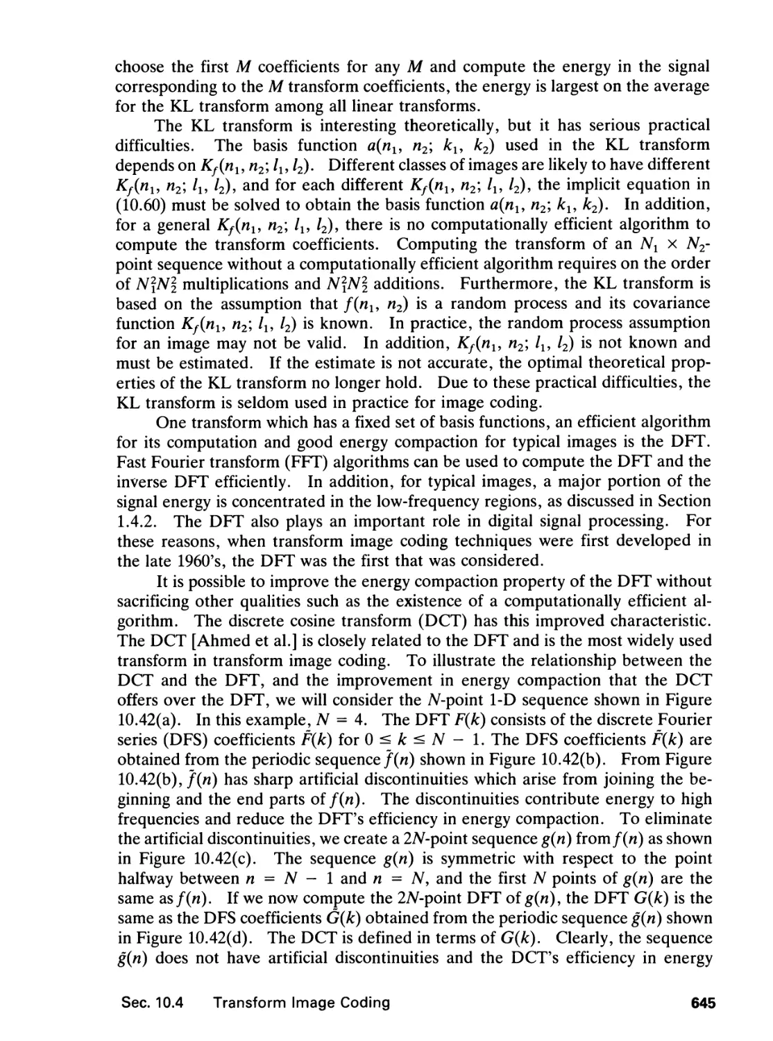
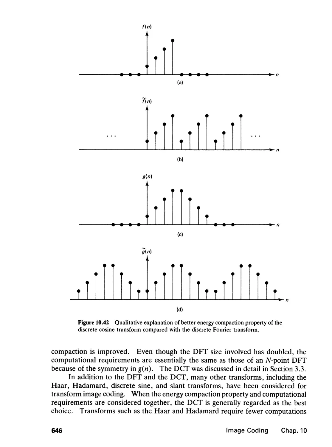
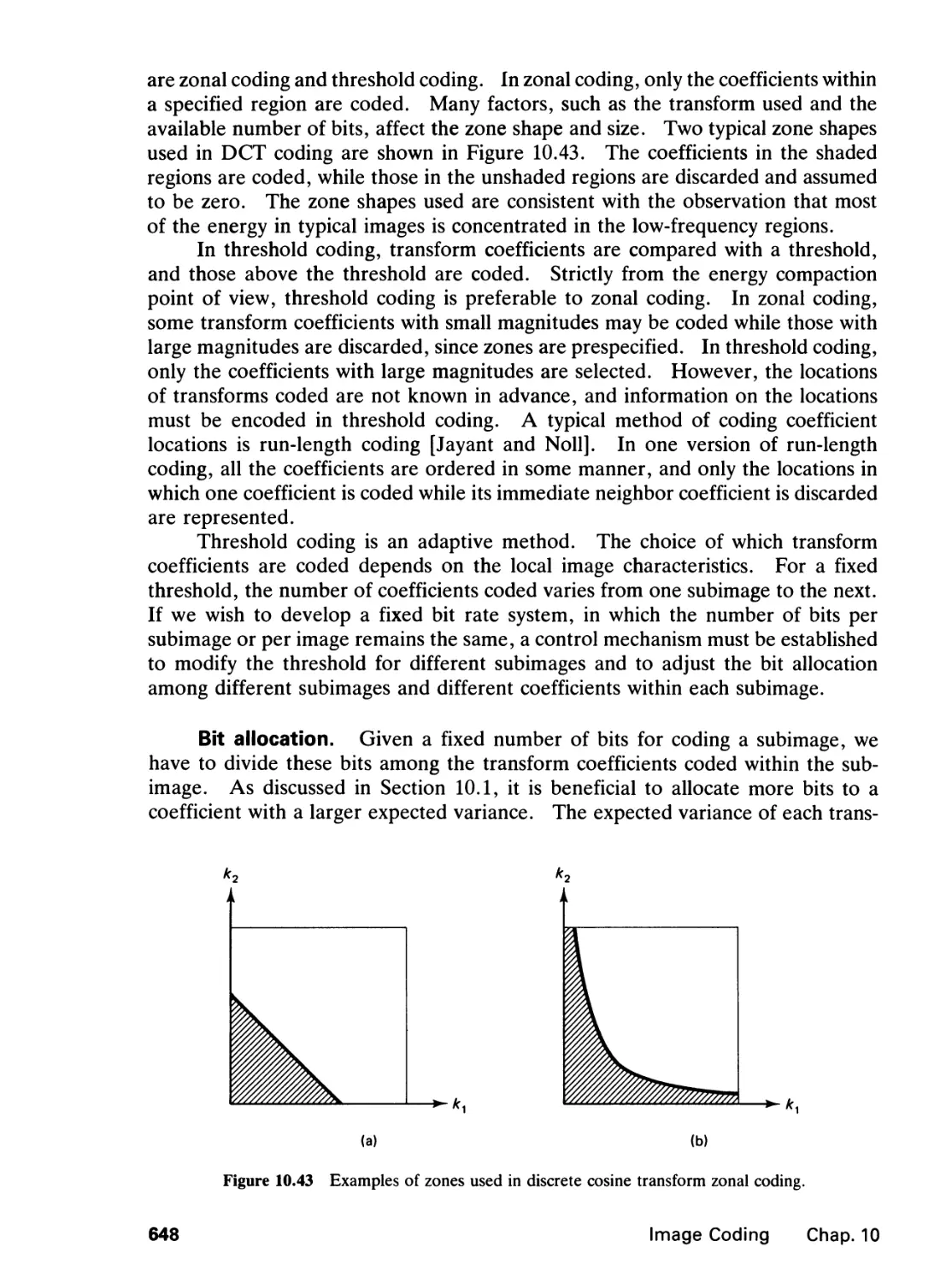
10.4 Transform Image Coding, 642
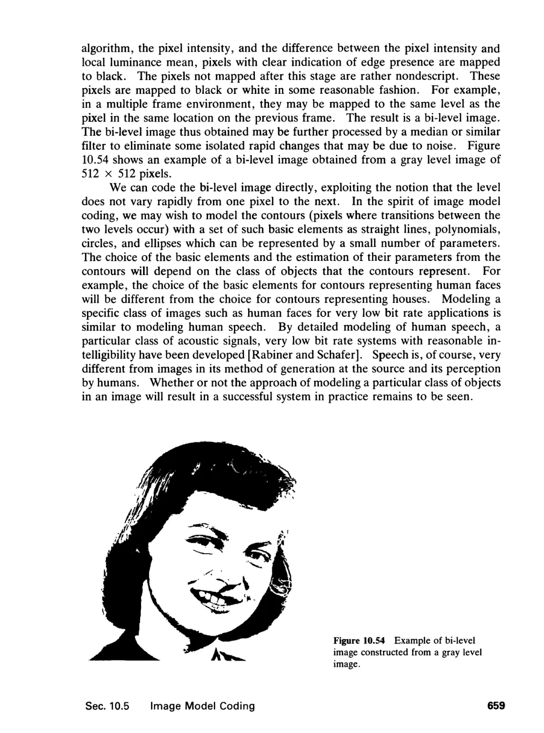
10.5 Image Model Coding, 656
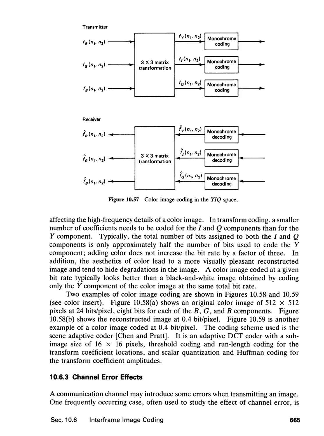
10.6 Interframe Image Coding, Color Image Coding,
and Channel Error Effects, 660
10.7 Additional Comments
10.8 Concluding Remarks, 669
References, 670
Problems, 674
INDEX 683
x
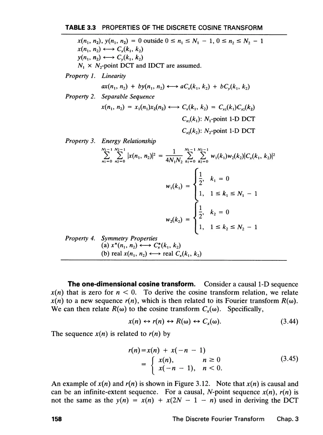
Contents
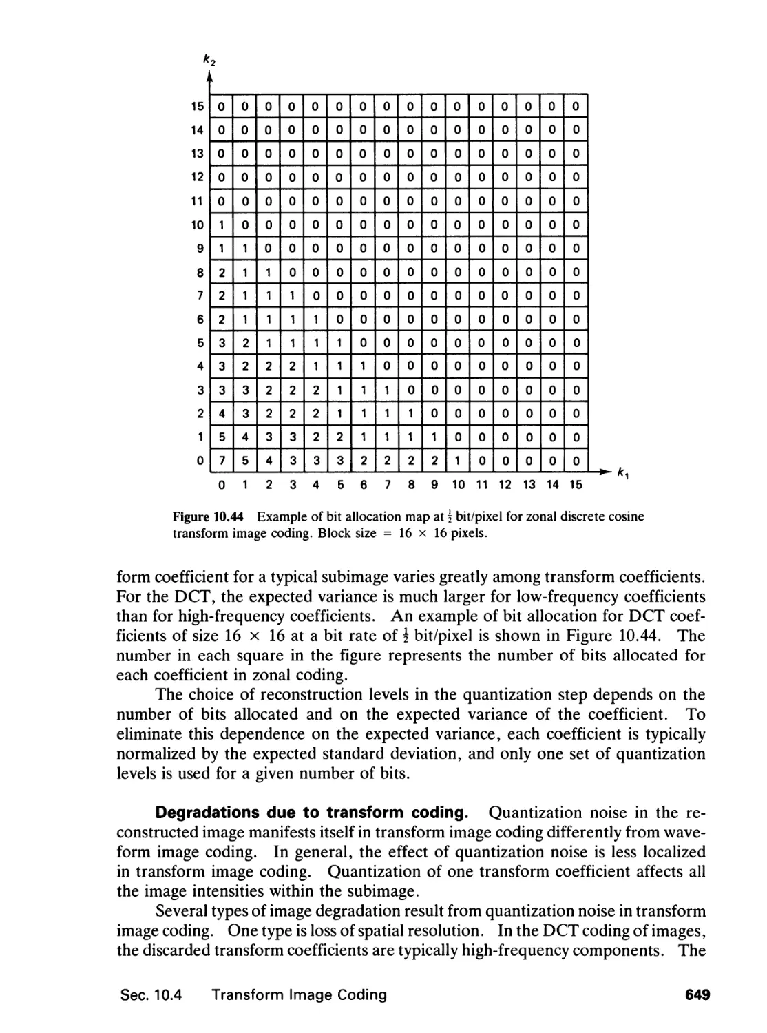
Preface
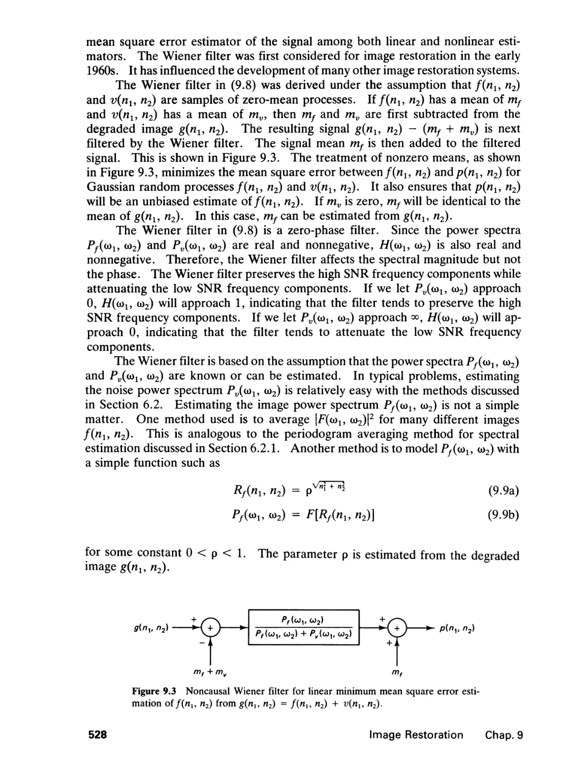
This book has grown out of the author's teaching and research activities in the field
of two-dimensional signal and image processing. It is designed as a text for an
upper-class undergraduate level or a graduate level course. The notes on which
this book is based have been used since 1982 for a one-semester course in the
Department of Electrical Engineering and Computer Science at M.I.T. and for a
continuing education course at industries including Texas Instruments and Bell
Laboratories.
In writing this book, the author has assumed that readers have prior exposure
to fundamentals of one-dimensional digital signal processing, which are readily
available in a variety of excellent text and reference books. Many two-dimensional
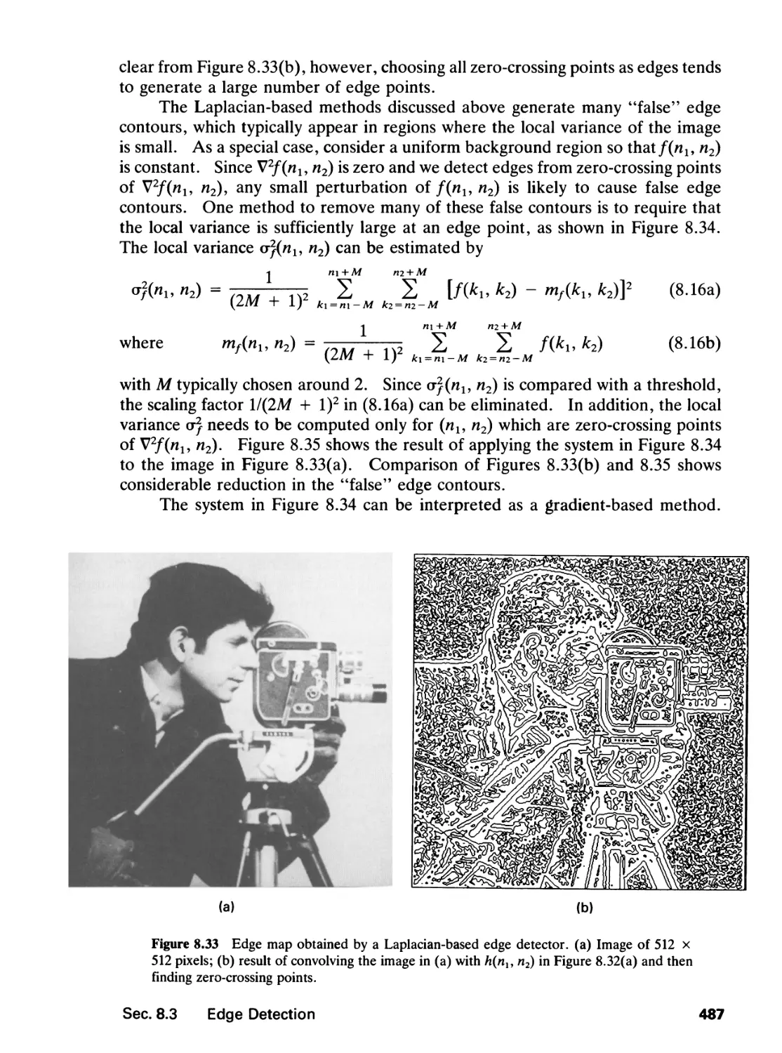
signal processing theories are developed in the book by extension and generalization
of one-dimensional signal processing theories.
This book consists of ten chapters. The first six chapters are devoted to
fundamentals of two-dimensional digital signal processing. Chapter 1 is on signals,
systems, and Fourier transform, which are the most basic concepts in signal
processing and serve as a foundation for all other chapters. Chapter 2 is on z-transform
representation and related topics including the difference equation and stability.
Chapter 3 is on the discrete Fourier series, discrete Fourier transform, and fast
Fourier transform. The chapter also covers the cosine and discrete cosine
transforms which are closely related to Fourier and discrete Fourier transforms.
Chapter 4 is on the design and implementation of finite impulse response filters. Chapter
5 is on the design and implementation of infinite impulse response filters. Chapter
6 is on random signals and spectral estimation. Throughout the first six chapters,
the notation used and the theories developed are for two-dimensional signals and
xi
systems. Essentially all the results extend to more general multidimensional signals
and systems in a straightforward manner.
The remaining four chapters are devoted to fundamentals of digital image
processing. Chapter 7 is on the basics of image processing. Chapter 8 is on image
enhancement including topics on contrast enhancement, noise smoothing, and use
of color. The chapter also covers related topics on edge detection, image
interpolation, and motion-compensated image processing. Chapter 9 is on image
restoration and treats restoration of images degraded by both signal-independent and
signal-dependent degradation. Chapter 10 is on image coding and related topics.
One goal of this book is to provide a single-volume text for a course that
covers both two-dimensional signal processing and image processing. In a one-
semester course at M.I.T., the author covered most topics in the book by treating
some topics in reasonable depth and others with less emphasis. The book can
also be used as a text for a course in which the primary emphasis is on either two-
dimensional signal processing or image processing. A typical course with emphasis
on two-dimensional signal processing, for example, would cover topics in Chapters
1 through 6 with reasonable depth and some selected topics from Chapters 7 and
9. A typical course with emphasis on image processing would cover topics in
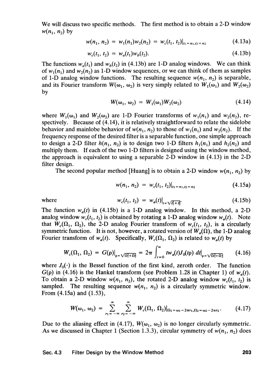
Chapters 1 and 3, Section 6.1, and Chapters 7 through 10. This book can also be
used for a two-semester course, the first semester on two-dimensional signal
processing and the second semester on image processing.
Many problems are included at the end of each chapter. These problems
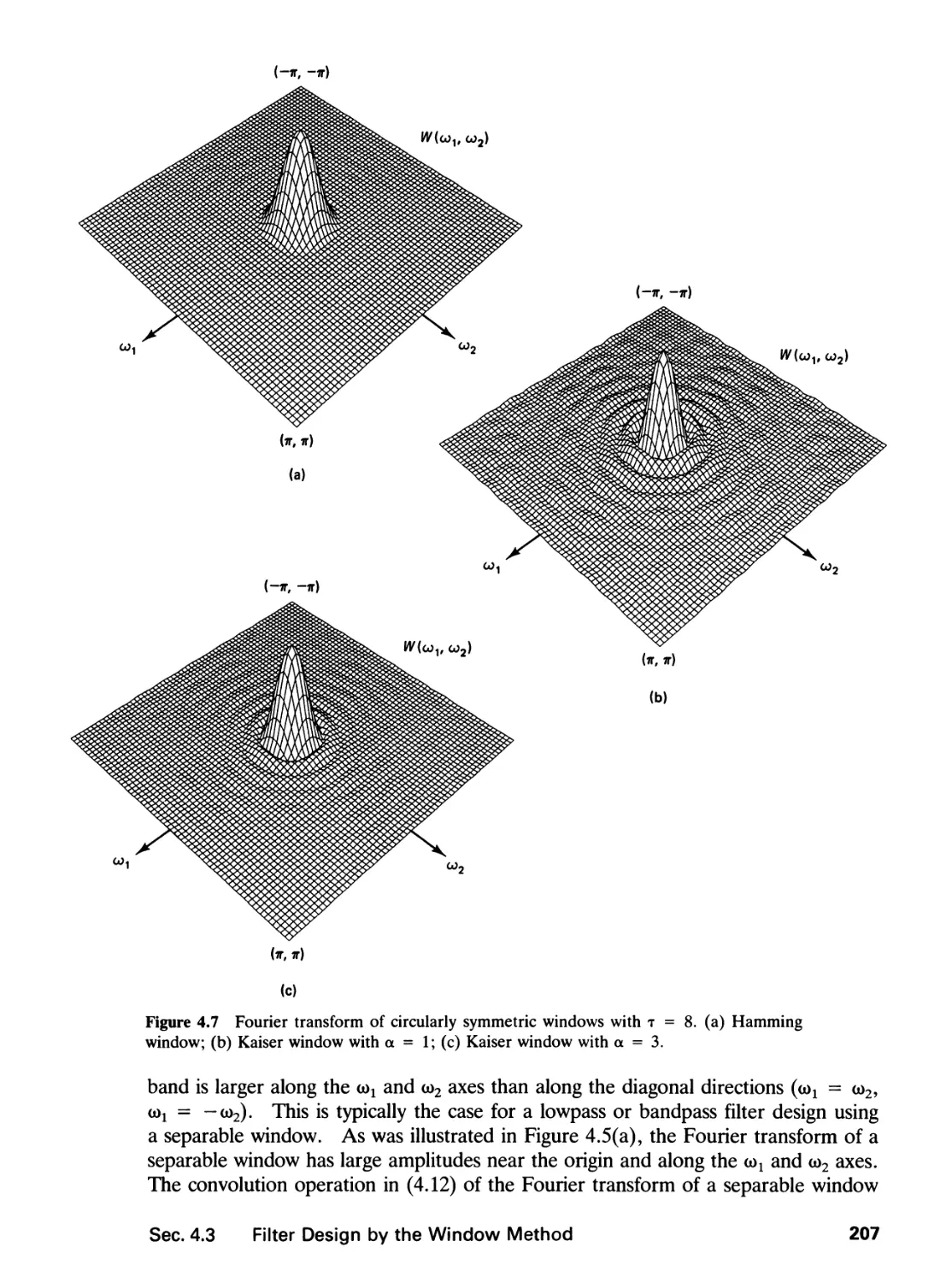
are, of course, intended to help the reader understand the basic concepts through
drill and practice. The problems also extend some concepts presented previously
and develop some new concepts.
The author is indebted to many students, friends, and colleagues for their
assistance, support, and suggestions. The author was very fortunate to learn digital
signal processing and image processing from Professor Alan Oppenheim, Professor
Russell Mersereau, and Professor William Schreiber. Thrasyvoulos Pappas, Sri-
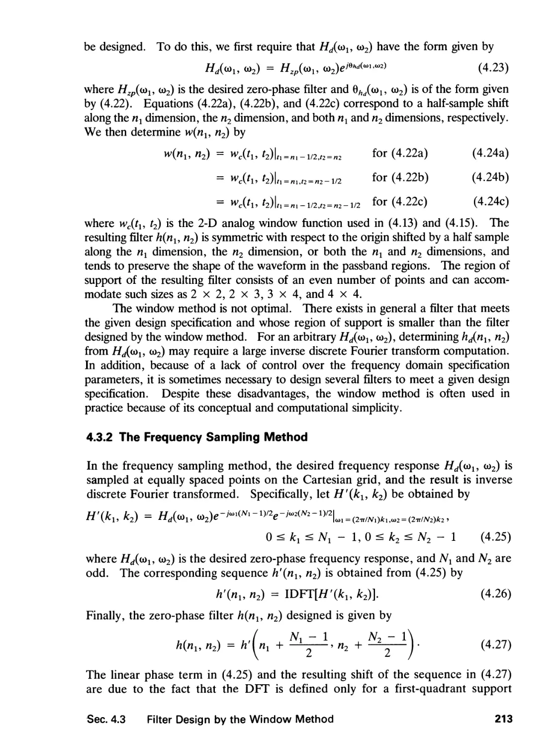
nivasa Prasanna, Mike Mcllrath, Matthew Bace, Roz Wright Picard, Dennis
Martinez, and Giovanni Aliberti produced many figures. Many students and friends
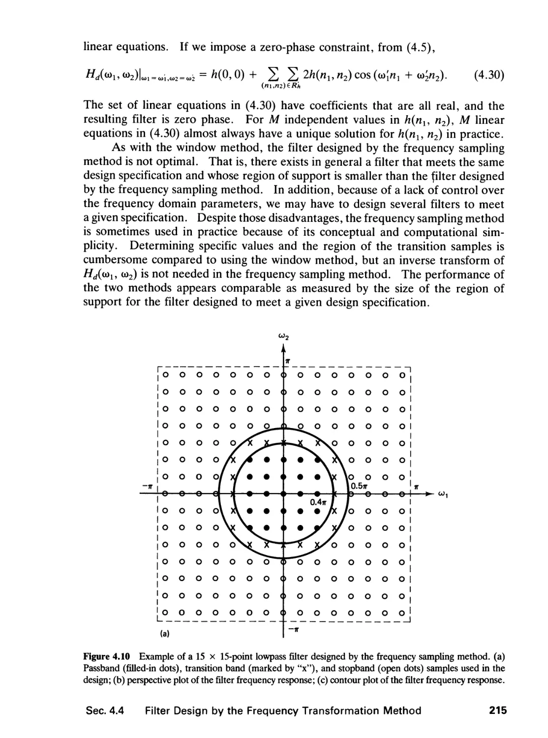
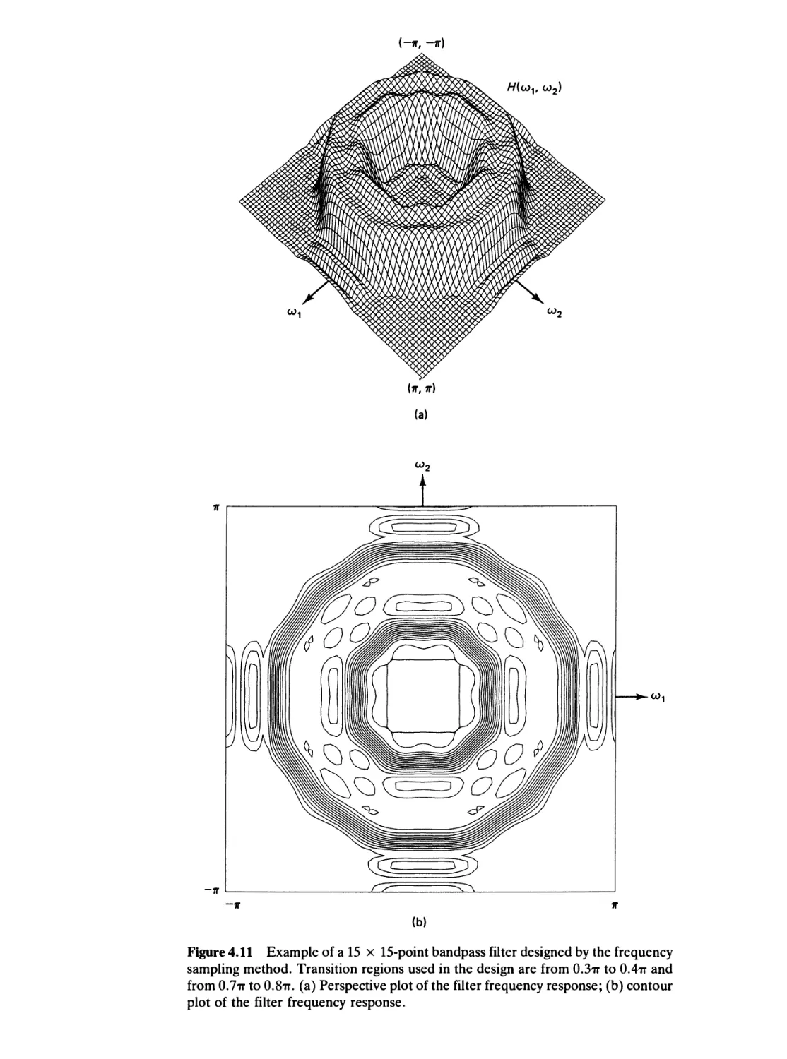
used the lecture notes from which this book originated and provided valuable
comments and suggestions. Many friends and colleagues read drafts of this book,
and their comments and suggestions have been incorporated. The book was edited
by Beth Parkhurst and Patricia Johnson. Phyllis Eiro, Leslie Melcer, and Cindy
LeBlanc typed many versions of the manuscript.
The author acknowledges the support of M.I.T. which provided an
environment in which many ideas were developed and a major portion of the work was
accomplished. The author is also grateful to the Woods Hole Oceanographic
Institution and the Naval Postgraduate School where the author spent most of his
sabbatical year completing the manuscript.
Jae 5. Lim
xii
Preface
Introduction
The fields of two-dimensional digital signal processing and digital image processing
have maintained tremendous vitality over the past two decades and there is every
indication that this trend will continue. Advances in hardware technology provide
the capability in signal processing chips and microprocessors which were previously
associated with mainframe computers. These advances allow sophisticated signal
processing and image processing algorithms to be implemented in real time at a
substantially reduced cost. New applications continue to be found and existing
applications continue to expand in such diverse areas as communications, consumer
electronics, medicine, defense, robotics, and geophysics. Along with advances in
hardware technology and expansion in applications, new algorithms are developed
and existing algorithms are better understood, which in turn lead to further
expansion in applications and provide a strong incentive for further advances in
hardware technology.
At a conceptual level, there is a great deal of similarity between
one-dimensional signal processing and two-dimensional signal processing. In
one-dimensional signal processing, the concepts discussed are filtering, Fourier transform,
discrete Fourier transform, fast Fourier transform algorithms, and so on. In two-
dimensional signal processing, we again are concerned with the same concepts.
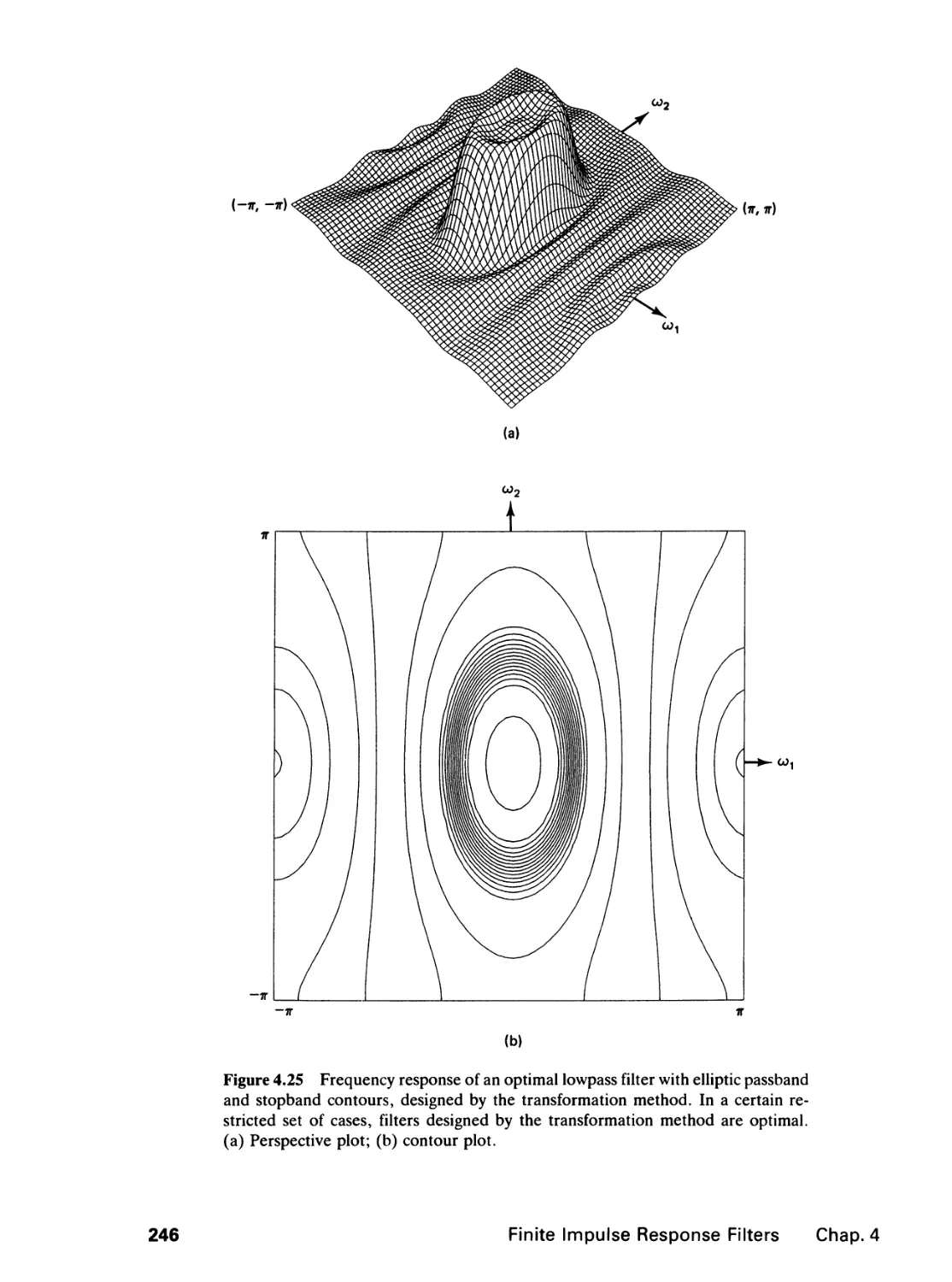
As a consequence, the general concepts that we develop in two-dimensional signal
processing can be viewed as straightforward extensions of the results in one-
dimensional signal processing.
At a more detailed level, however, considerable differences exist between
one-dimensional and two-dimensional signal processing. For example, one major
difference is the amount of data involved in typical applications. In speech pro-
xiii
cessing, an important one-dimensional signal processing application, speech is
typically sampled at a 10-kHz rate and we have 10,000 data points to process in a
second. However, in video processing, where processing an image frame is an
important two-dimensional signal processing application, we may have 30 frames
per second, with each frame consisting of 500 x 500 pixels (picture elements). In
this case, we would have 7.5 million data points to process per second, which is
orders of magnitude greater than the case of speech processing. Due to this
difference in data rate requirements, the computational efficiency of a signal
processing algorithm plays a much more important role in two-dimensional signal
processing, and advances in hardware technology will have a much greater impact
on two-dimensional signal processing applications.
Another major difference comes from the fact that the mathematics used for
one-dimensional signal processing is often simpler than that used for
two-dimensional signal processing. For example, many one-dimensional systems are
described by differential equations, while many two-dimensional systems are
described by partial differential equations. It is generally much easier to solve differential
equations than partial differential equations. Another example is the absence of
the fundamental theorem of algebra for two-dimensional polynomials. For one-
dimensional polynomials, the fundamental theorem of algebra states that any one-
dimensional polynomial can be factored as a product of lower-order polynomials.
This difference has a major impact on many results in signal processing. For
example, an important structure for realizing a one-dimensional digital filter is the
cascade structure. In the cascade structure, the z-transform of the digital filter's
impulse response is factored as a product of lower-order polynomials and the
realizations of these lower-order factors are cascaded. The z-transform of a two-
dimensional digital filter's impulse response cannot, in general, be factored as a
product of lower-order polynomials and the cascade structure therefore is not a
general structure for a two-dimensional digital filter realization. Another
consequence of the nonfactorability of a two-dimensional polynomial is the difficulty
associated with issues related to system stability. In a one-dimensional system,
the pole locations can be determined easily, and an unstable system can be stabilized
without affecting the magnitude response by simple manipulation of pole locations.
In a two-dimensional system, because poles are surfaces rather than points and
there is no fundamental theorem of algebra, it is extremely difficult to determine
the pole locations. As a result, checking the stability of a two-dimensional system
and stabilizing an unstable two-dimensional system without affecting the magnitude
response are extremely difficult.
As we have seen, there is considerable similarity and at the same time
considerable difference between one-dimensional and two-dimensional signal
processing. We will study the results in two-dimensional signal processing that are
simple extensions of one-dimensional signal processing. Our discussion will rely
heavily on the reader's knowledge of one-dimensional signal processing theories.
We will also study, with much greater emphasis, the results in two-dimensional
signal processing that are significantly different from.those in one-dimensional
signal processing. We will study what the differences are, where they come from,
xiv
Introduction
and what impacts they have on two-dimensional signal processing applications.
Since we will study the similarities and differences of one-dimensional and two-
dimensional signal processing and since one-dimensional signal processing is a
special case of two-dimensional signal processing, this book will help us understand
not only two-dimensional signal processing theories but also one-dimensional signal
processing theories at a much deeper level.
An important application of two-dimensional signal processing theories is
image processing. Image processing is closely tied to human vision, which is one
of the most important means by which humans perceive the outside world. As a
result, image processing has a large number of existing and potential applications
and will play an increasingly important role in our everyday life.
Digital image processing can be classified broadly into four areas: image
enhancement, restoration, coding, and understanding. In image enhancement,
images either are processed for human viewers, as in television, or preprocessed
to aid machine performance, as in object identification by machine. In image
restoration, an image has been degraded in some manner and the objective is to
reduce or eliminate the effect of degradation. Typical degradations that occur in
practice include image blurring, additive random noise, quantization noise,
multiplicative noise, and geometric distortion. The objective in image coding is to
represent an image with as few bits as possible, preserving a certain level of image
quality and intelligibility acceptable for a given application. Image coding can be
used in reducing the bandwidth of a communication channel when an image is
transmitted and in reducing the amount of required storage when an image needs
to be retrieved at a future time. We study image enhancement, restoration, and
coding in the latter part of the book.
The objective of image understanding is to symbolically represent the contents
of an image. Applications of image understanding include computer vision and
robotics. Image understanding differs from the other three areas in one major
respect. In image enhancement, restoration, and coding, both the input and the
output are images, and signal processing has been the backbone of many successful
systems in these areas. In image understanding, the input is an image, but the
output is symbolic representation of the contents of the image. Successful
development of systems in this area involves not only signal processing but also other
disciplines such as artificial intelligence. In a typical image understanding system,
signal processing is used for such lower-level processing tasks as reduction of
degradation and extraction of edges or other image features, and artificial intelligence
is used for such higher-level processing tasks as symbol manipulation and knowledge
base management. We treat some of the lower-level processing techniques useful
in image understanding as part of our general discussion of image enhancement,
restoration, and coding. A complete treatment of image understanding is outside
the scope of this book.
Two-dimensional signal processing and image processing cover a large number
of topics and areas, and a selection of topics was necessary due to space limitation.
In addition, there are a variety of ways to present the material. The main objective
of this book is to provide fundamentals of two-dimensional signal processing and
Introduction
xv
image processing in a tutorial manner. We have selected the topics and chosen
the style of presentation with this objective in mind. We hope that the
fundamentals of two-dimensional signal processing and image processing covered in this
book will form a foundation for additional reading of other books and articles in
the field, application of theoretical results to real-world problems, and advancement
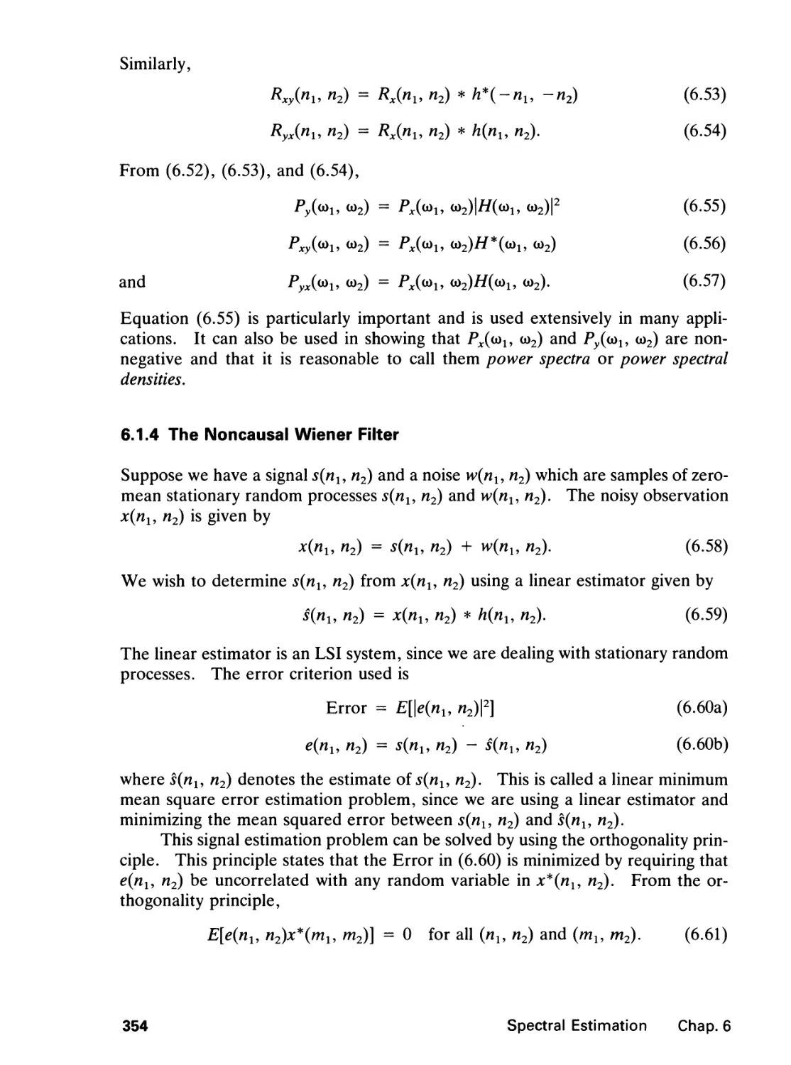
of the field through research and development.
xvi
Introduction
TWO-MMENSKMIAI.
SWNAl and IMAGE
PRDCESSIIK
7
Signals, Systems, and
the Fourier Transform
1.0 INTRODUCTION
Most signals can be classified into three broad groups. One group, which consists
of analog or continuous-space signals, is continuous in both space* and amplitude.
In practice, a majority of signals falls into this group. Examples of analog signals
include image, seismic, radar, and speech signals. Signals in the second group,
discrete-space signals, are discrete in space and continuous in amplitude. A
common way to generate discrete-space signals is by sampling analog signals. Signals
in the third group, digital or discrete signals, are discrete in both space and
amplitude. One way in which digital signals are created is by amplitude quantization
of discrete-space signals. Discrete-space signals and digital signals are also referred
to as sequences.
Digital systems and computers use only digital signals, which are discrete in
both space and amplitude. The development of signal processing concepts based
on digital signals, however, requires a detailed treatment of amplitude quantization,
which is extremely difficult and tedious. Many useful insights would be lost in
such a treatment because of its mathematical complexity. For this reason, most
digital signal processing concepts have been developed based on discrete-space
signals. Experience shows that theories based on discrete-space signals are often
applicable to digital signals.
A system maps an input signal to an output signal. A major element in
studying signal processing is the analysis, design, and implementation of a system
that transforms an input signal to a more desirable output signal for a given
application. When developing theoretical results about systems, we often impose
* Although we refer to "space," an analog signal can instead have a variable in time,
as in the case of speech processing.
1
the constraints of linearity and shift invariance. Although these constraints are
very restrictive, the theoretical results thus obtained apply in practice at least
approximately to many systems. We will discuss signals and systems in Sections
1.1 and 1.2, respectively.
The Fourier transform representation of signals and systems plays a central
role in both one-dimensional (1-D) and two-dimensional (2-D) signal processing.
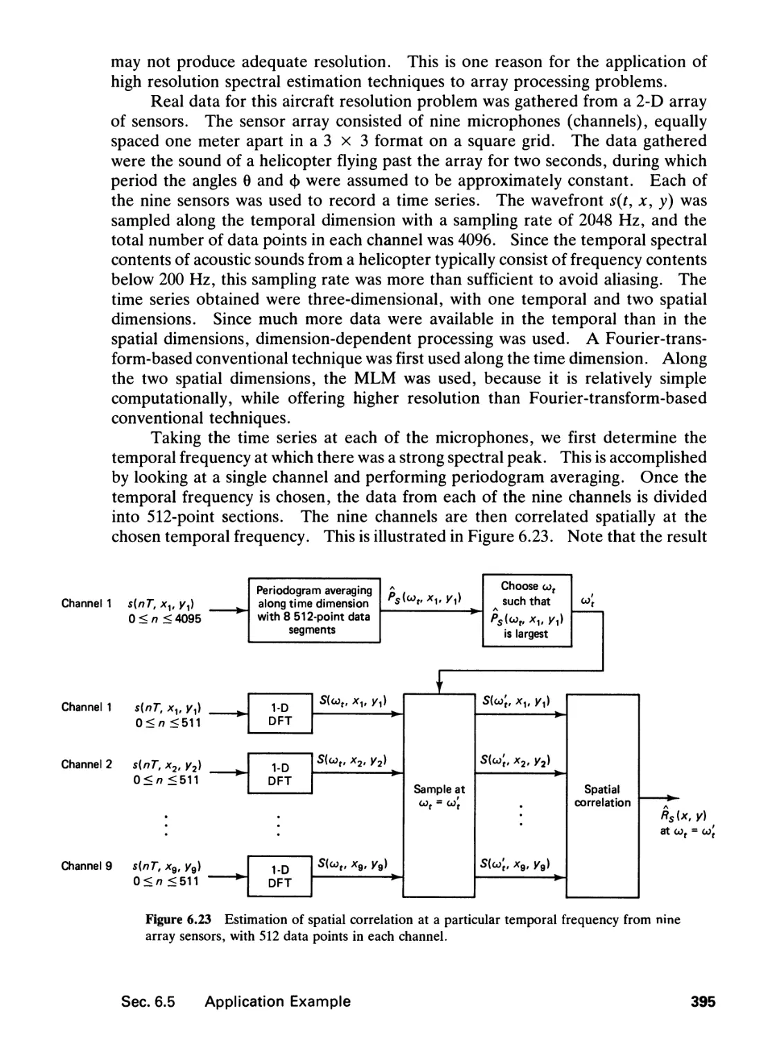
In Sections 1.3 and 1.4, the Fourier transform representation including some aspects
that are specific to image processing applications is discussed. In Section 1.5, we
discuss digital processing of analog signals. Many of the theoretical results, such
as the 2-D sampling theorem summarized in that section, can be derived from the
Fourier transform results.
Many of the theoretical results discussed in this chapter can be viewed as
straightforward extensions of the one-dimensional case. Some, however, are unique
to two-dimensional signal processing. Very naturally, we will place considerably
more emphasis on these. We will now begin our journey with the discussion of
signals.
1.1 SIGNALS
The signals we consider are discrete-space signals. A 2-D discrete-space signal
(sequence) will be denoted by a function whose two arguments are integers. For
example, x(nu n2) represents a sequence which is defined for all integer values of
nx and n2. Note that x(nl9 n2) for a noninteger nl or n2 is not zero, but is undefined.
The notation x(nu n2) may refer either to the discrete-space function x or to the
value of the function x at a specific (nu n2). The distinction between these two
will be evident from the context.
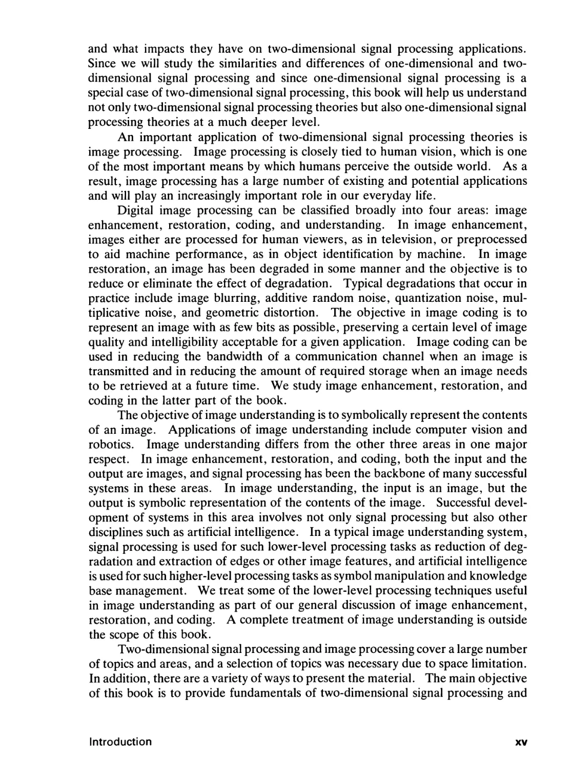
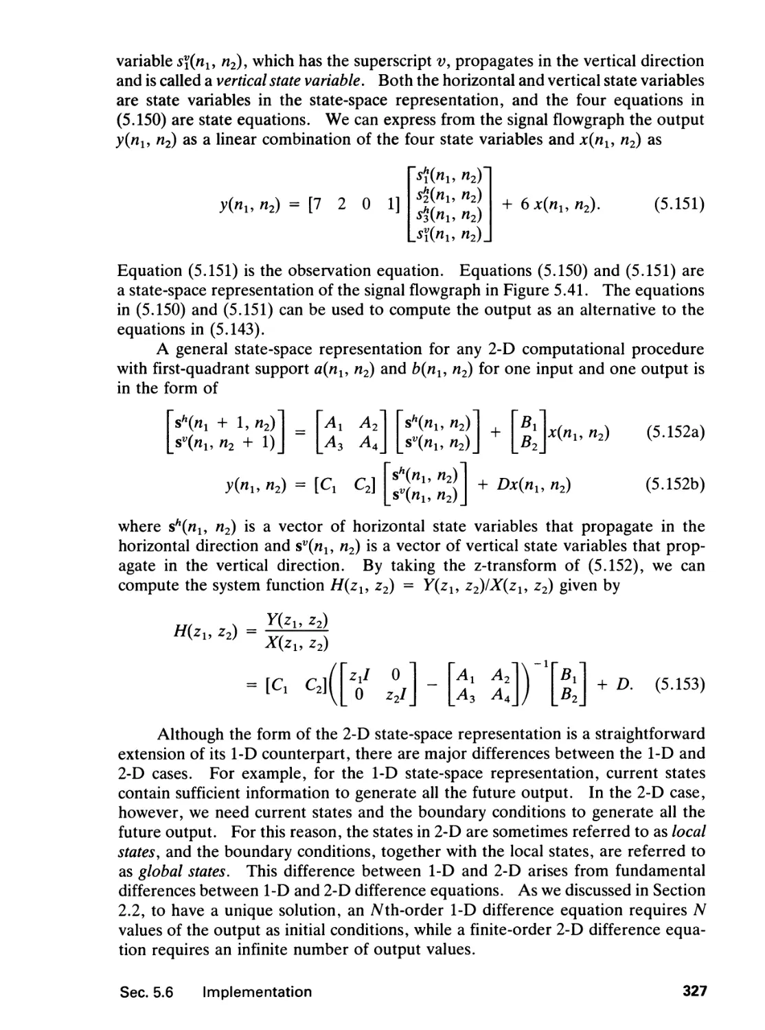
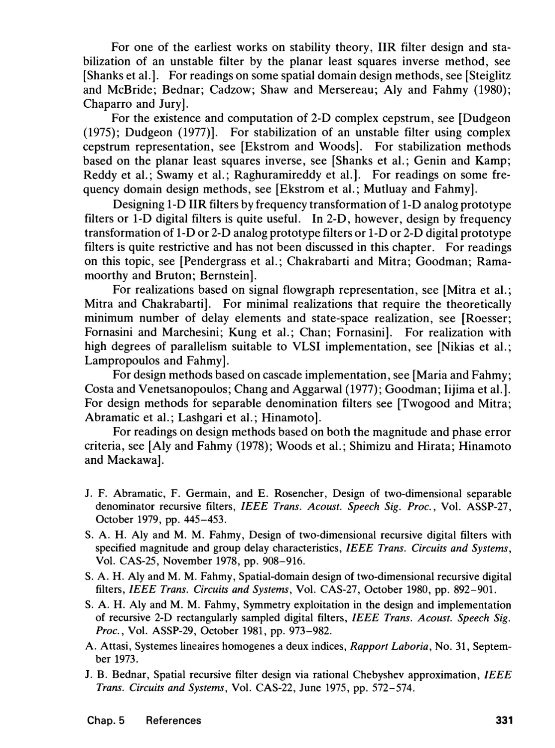
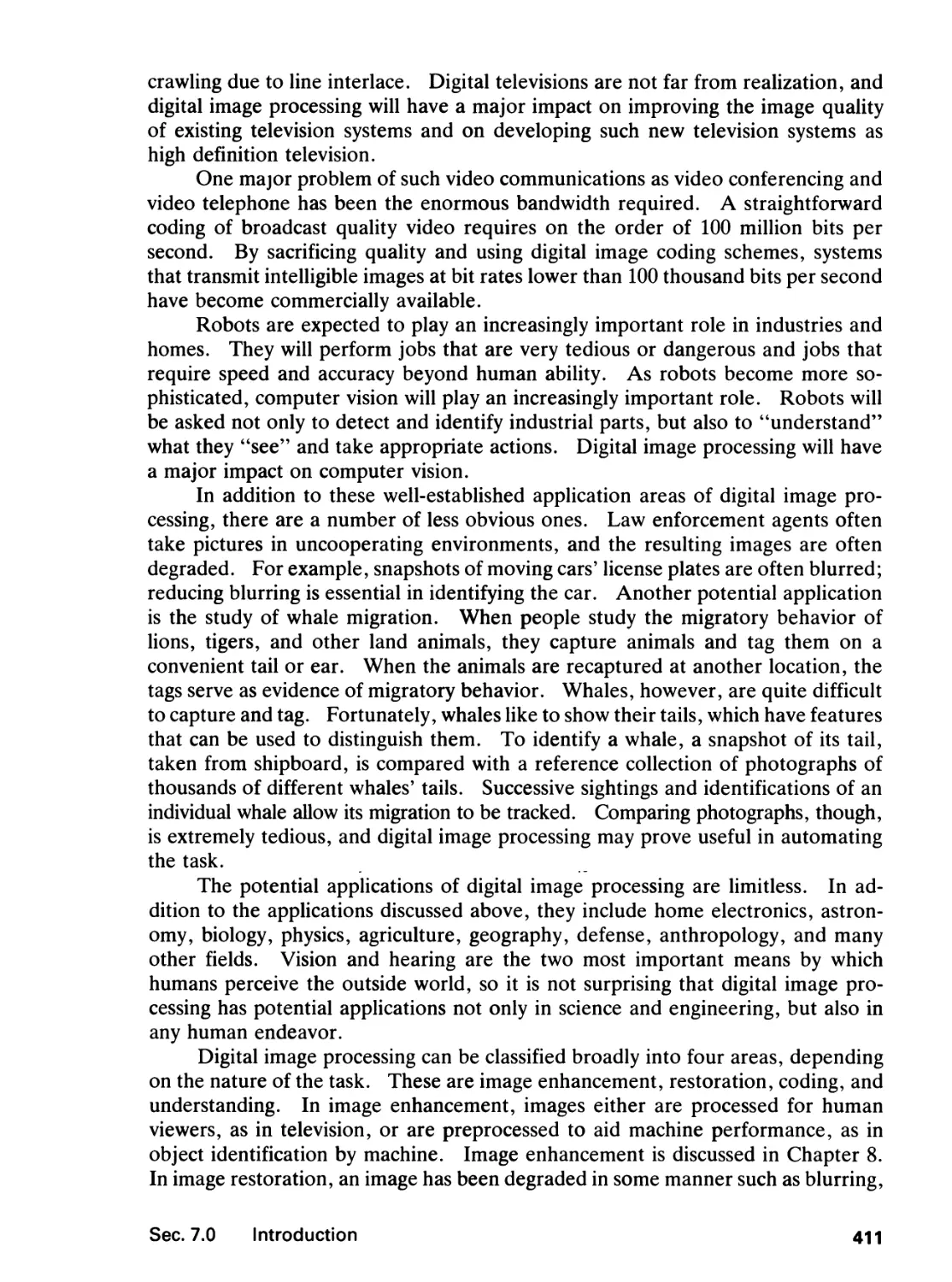
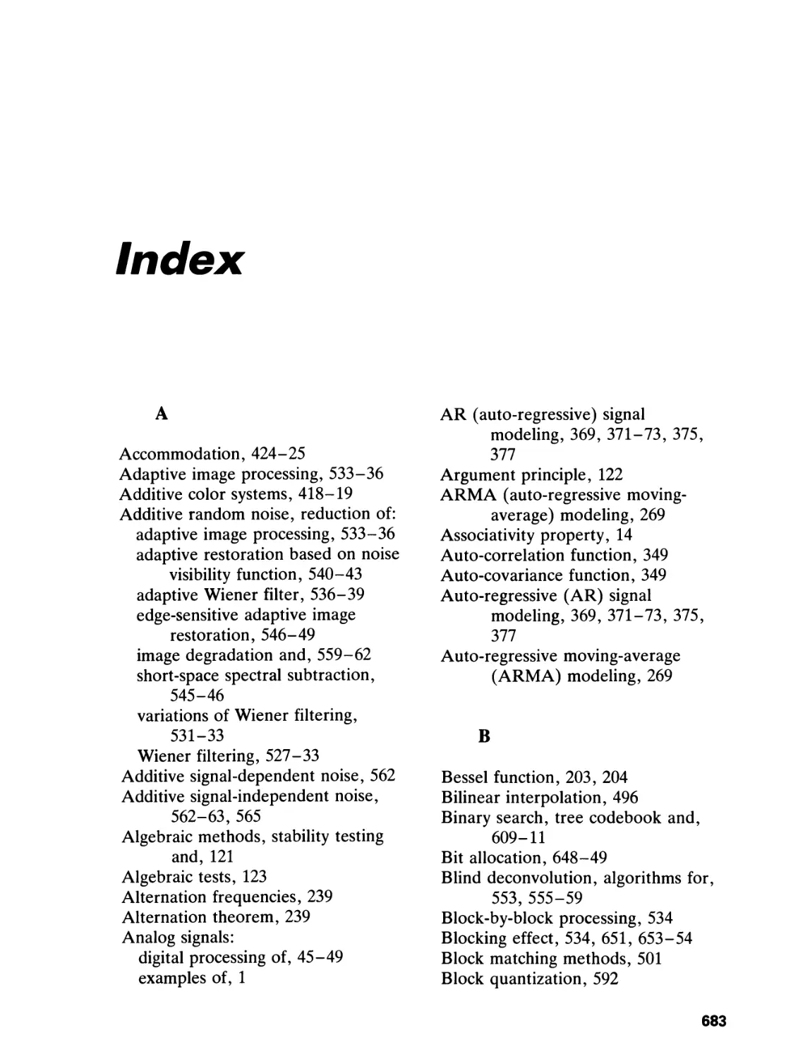
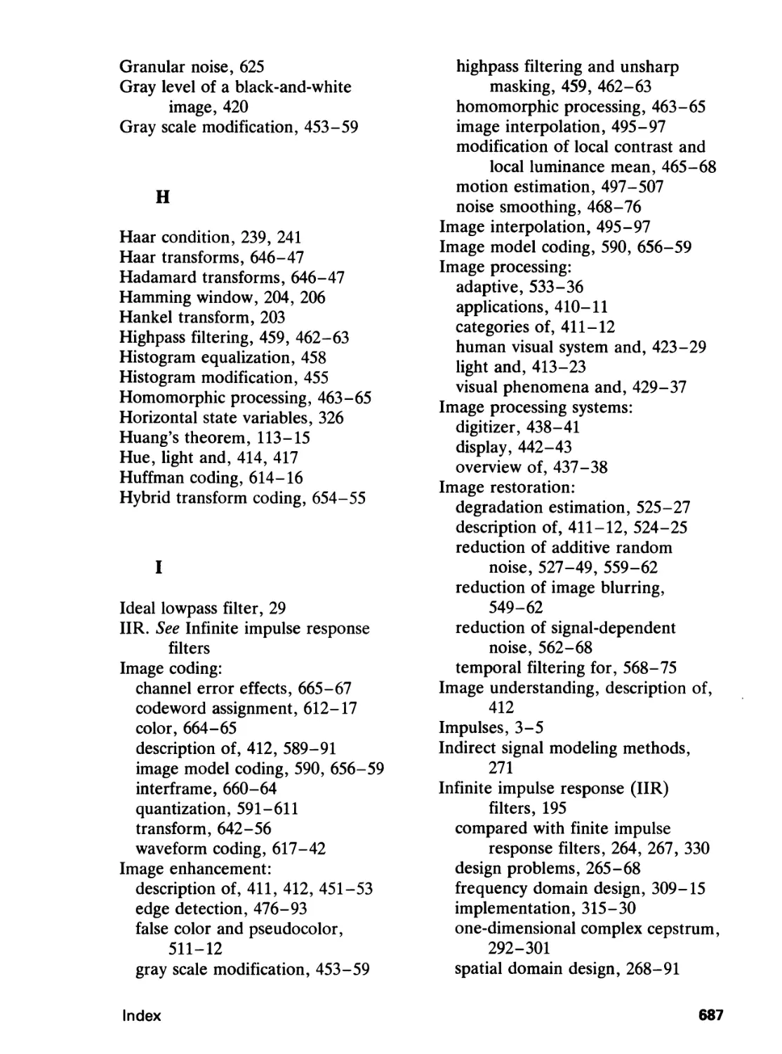
An example of a 2-D sequence x(nu n2) is sketched in Figure 1.1. In the
figure, the height at (nl, n2) represents the amplitude at (nu n2). It is often tedious
to sketch a 2-D sequence in the three-dimensional (3-D) perspective plot as shown
n2
/ x(nv n2)
• • • • ff • • • •
• • • • ft • • • •
• • % %XT T • •
• • Tt T37t<2>T T • •
•——• >-m '+ >* ' 1 • • *-"i
. . t T y' ? # .
. . T T t/? T . .
• • • • tf • • • •
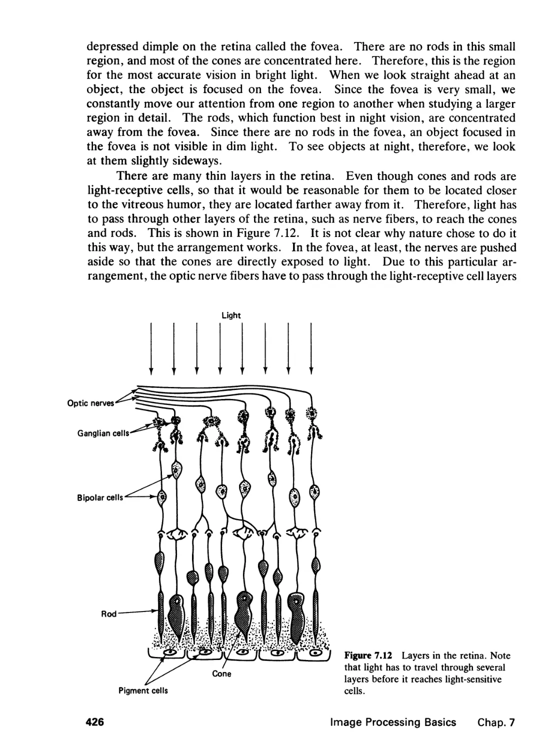
• • • • ft • • • •
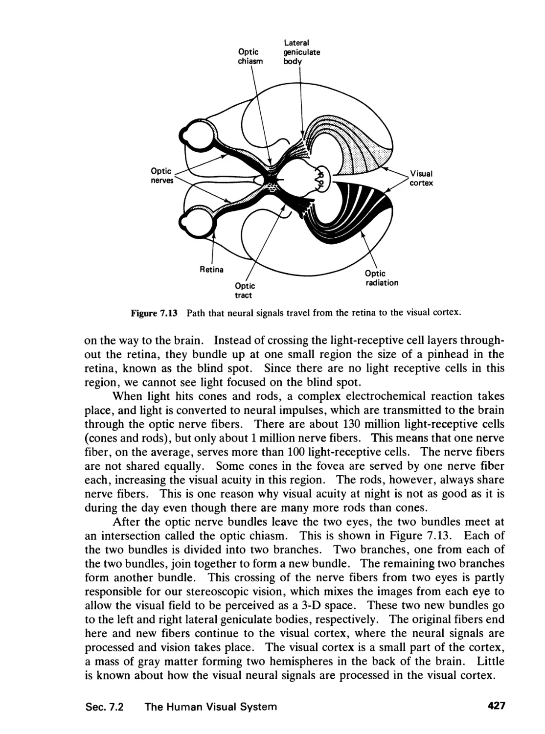
Figure 1.1 2-D sequence x(nu n2).
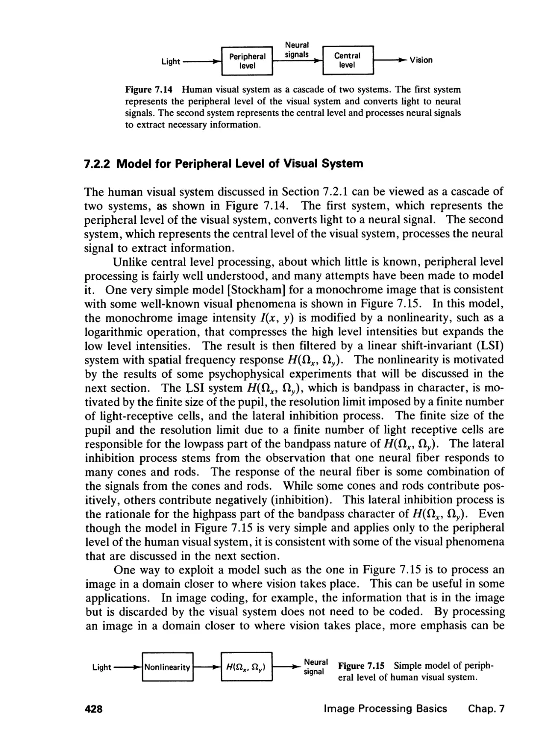
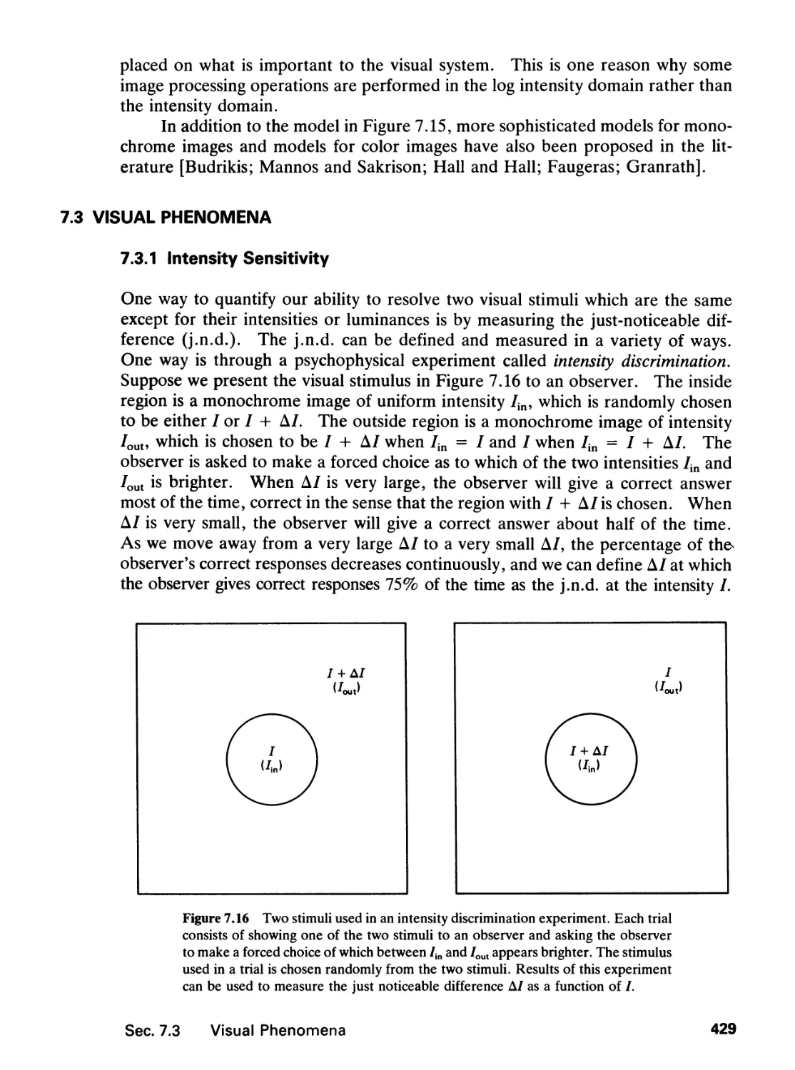
2
Signals, Systems, and the Fourier Transform Chap. 1
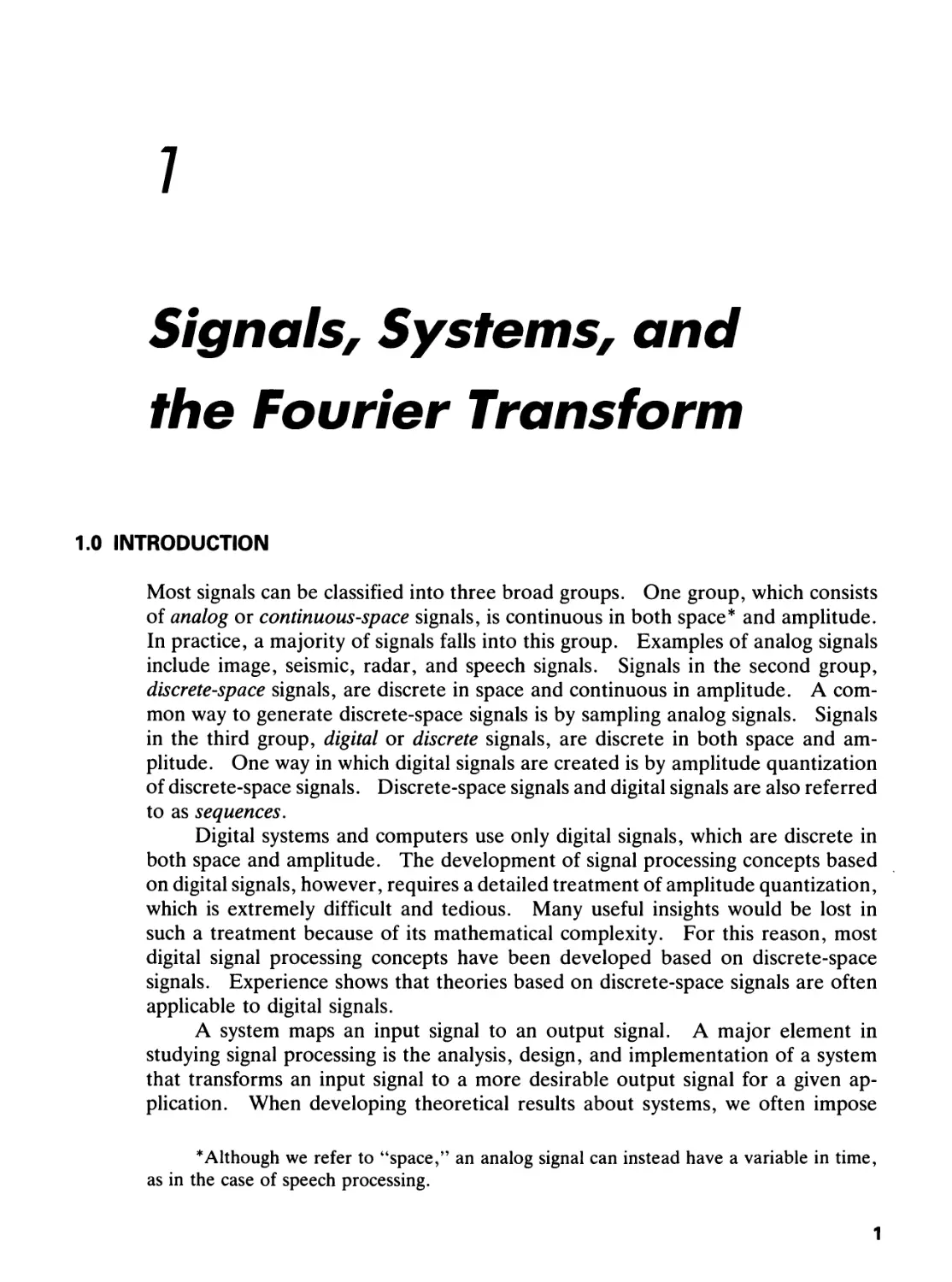
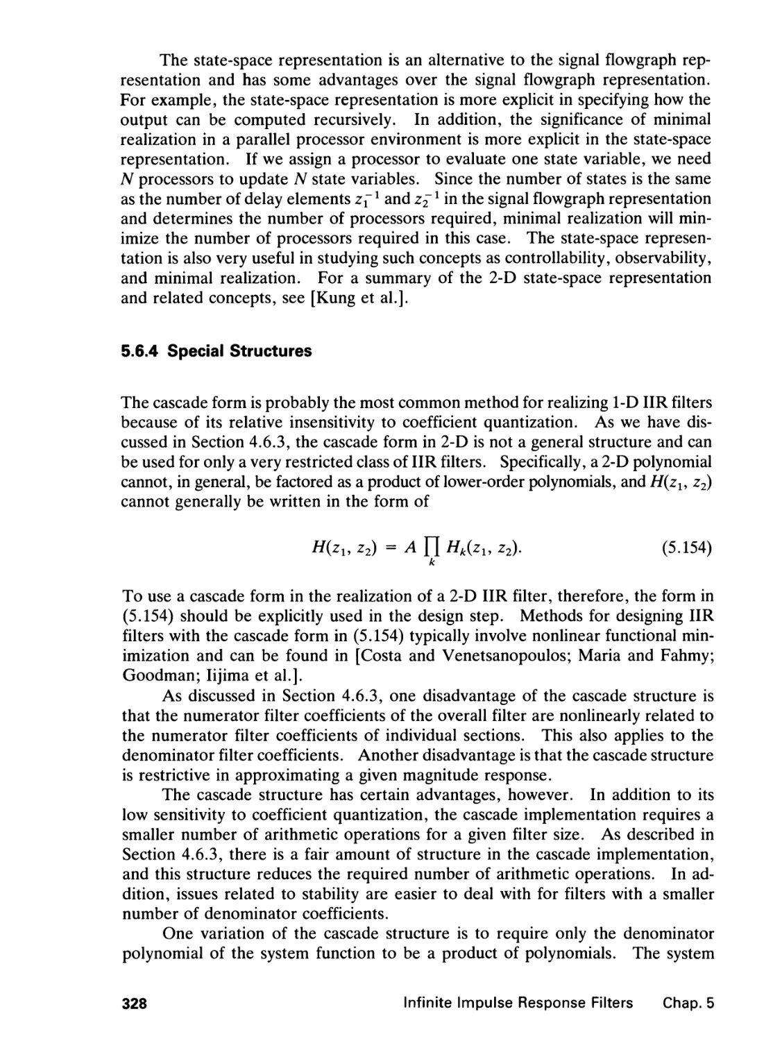
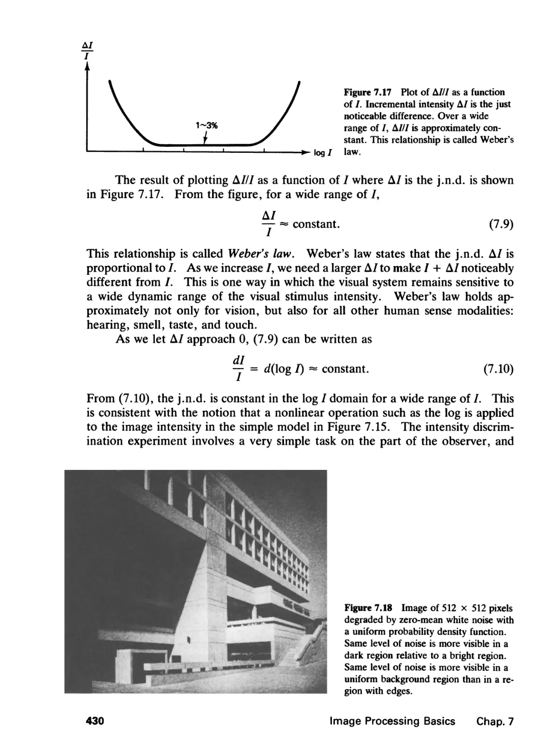
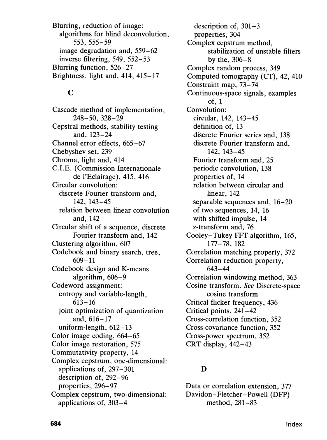
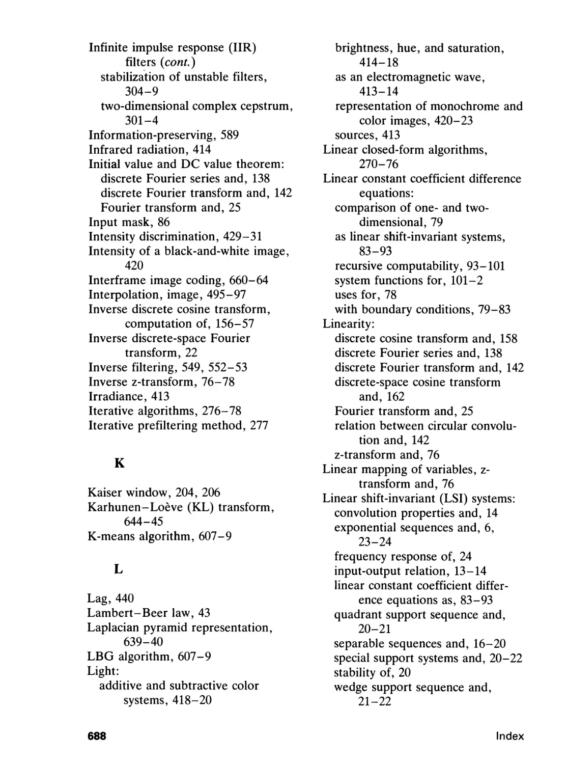
in Figure 1.1. An alternate way to sketch the 2-D sequence in Figure 1.1 is shown
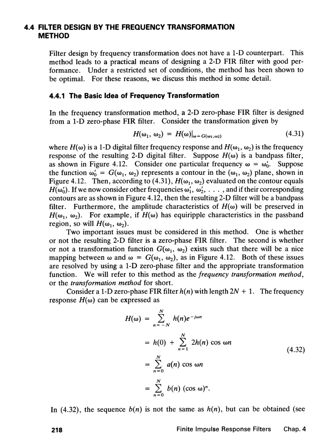
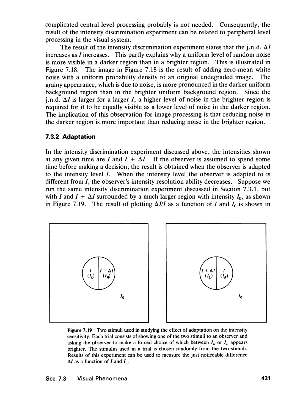
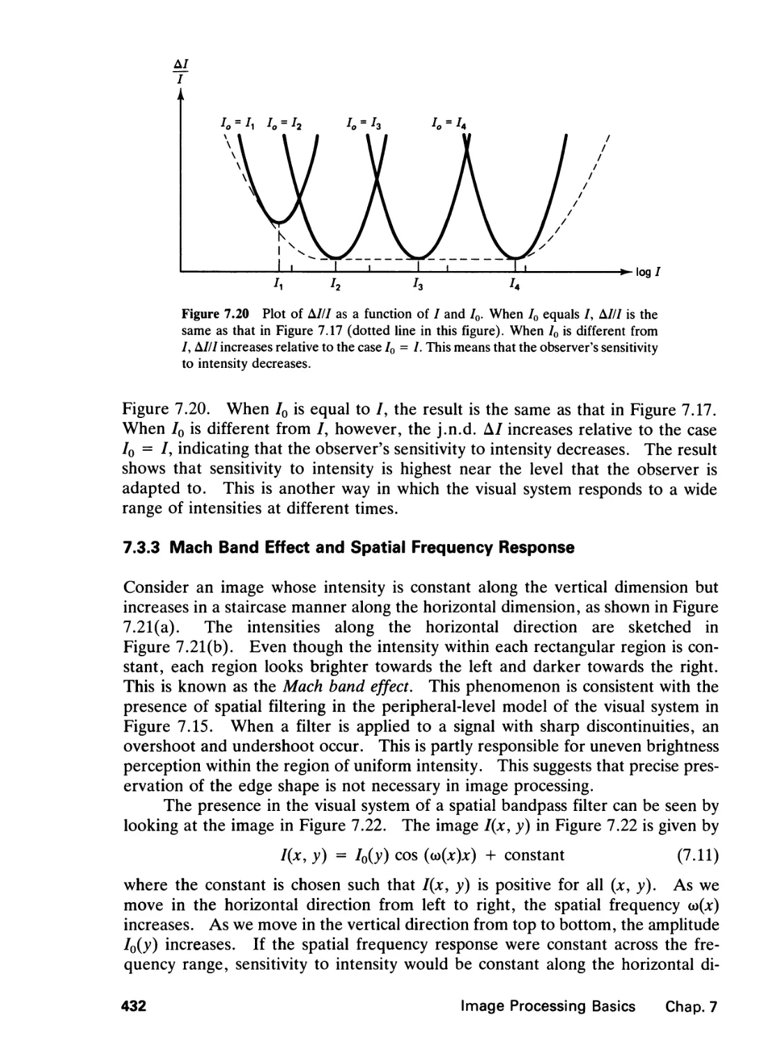
in Figure 1.2. In this figure, open circles represent amplitudes of 0 and filled-in
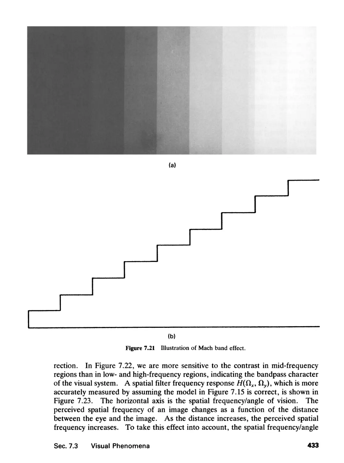
circles represent nonzero amplitudes, with the values in parentheses representing
the amplitudes. For example, jc(3, 0) is 0 and *(1, 1) is 2.
Many sequences we use have amplitudes of 0 or 1 for large regions of
(«!, n2). In such instances, the open circles and parentheses will be eliminated
for convenience. If there is neither an open circle nor a filled-in circle at a particular
(«!, n2), then the sequence has zero amplitude at that point. If there is a filled-
in circle with no amplitude specification at a particular (nu n2), then the sequence
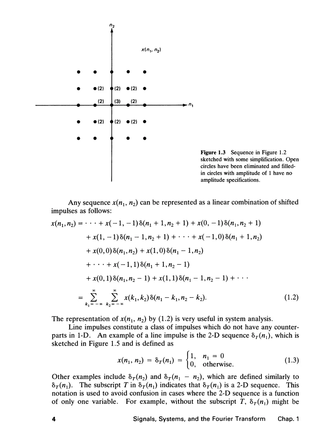
has an amplitude of 1 at that point. Figure 1.3 shows the result when this additional
simplification is made to the sequence in Figure 1.2.
1.1.1 Examples of Sequences
Certain sequences and classes of sequences play a particularly important role in
2-D signal processing. These are impulses, step sequences, exponential sequences,
separable sequences, and periodic sequences.
Impulses. The impulse or unit sample sequence, denoted by 8(«l9 n2), is
defined as
8K,«2) = i0) othenvise.
(1.1)
The sequence b(nu n2), sketched in Figure 1.4, plays a role similar to the impulse
b(n) in 1-D signal processing.
o
o
o
o
/\
o
o
o
o
o
o
o
o
o
o
o
o
o
o
o
•d)
• 0)
(1)
0
• 0)
• d)
o
o
n
i
o <
o <
• 0) <
• (2) <
(2)
• (2) (
• 0) i
o <
o <
2
i
>
)
MD
>(2)
(3)
>(2)
>(1)
>
>
o
o
• 0)
• (2)
(2)
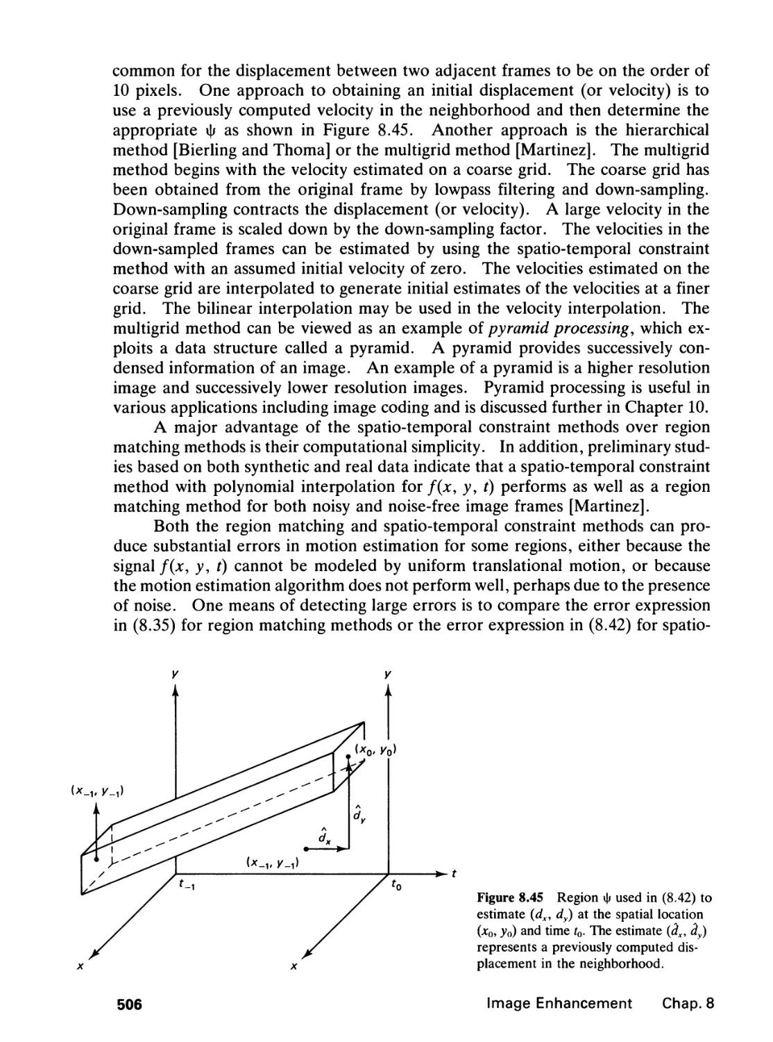
• (2)
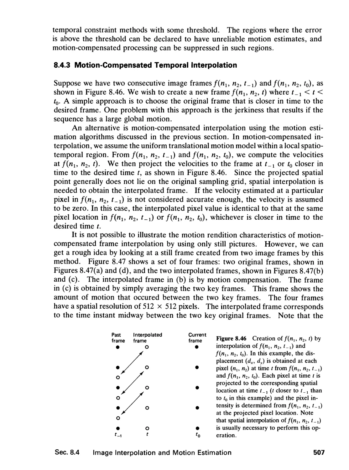
• (1)
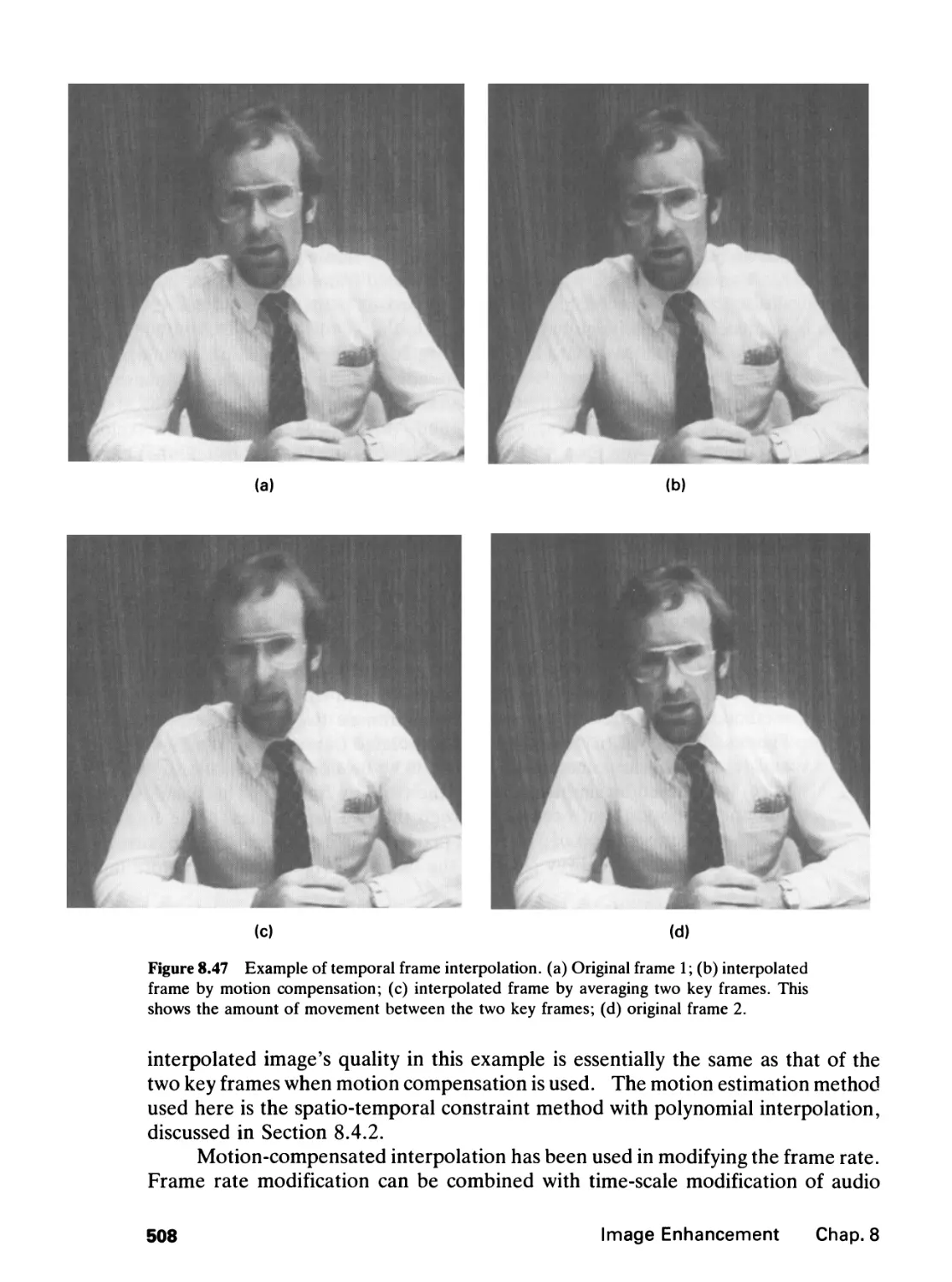
o
o
X(/7V
O
O
• (1)
• 0)
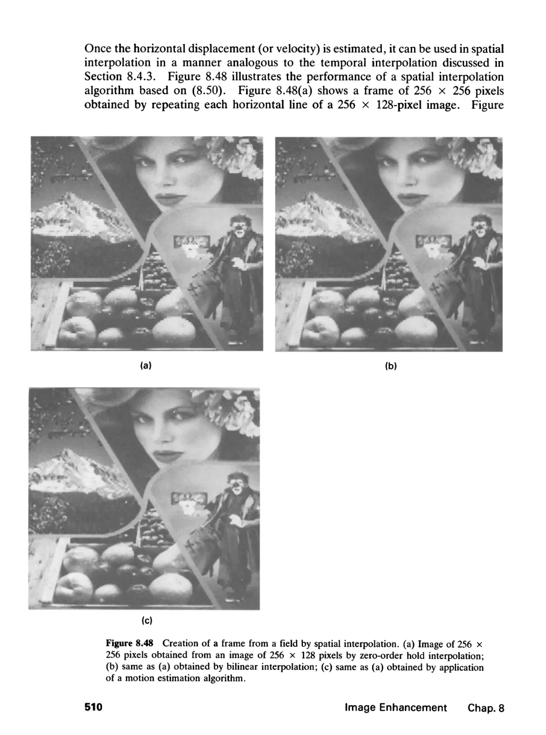
(1)
•
• 0)
• 0)
o
o
"2>
o
o
o
o
f\
o
o
o
o
o
o
o
o
o
o
o
o
Figure 1.2 Alternate way to sketch the
2-D sequence in Figure 1.1. Open
circles represent amplitudes of zero, and
filled-in circles represent nonzero
amplitudes, with values in parentheses
representing the amplitude.
Sec. 1.1 Signals
3
• (2)
(2)
• (2)
x(nv n2)
(2) •(2) •
(3) _ (2) _
(2) •(2) •
Figure 1.3 Sequence in Figure 1.2
sketched with some simplification. Open
circles have been eliminated and filled-
in circles with amplitude of 1 have no
amplitude specifications.
Any sequence x(nu n2) can be represented as a linear combination of shifted
impulses as follows:
x(nl9n2) = • • • +*(-l, -l)8(/i! + l,/i2 + 1) +x(0, -l)h(nun2 + 1)
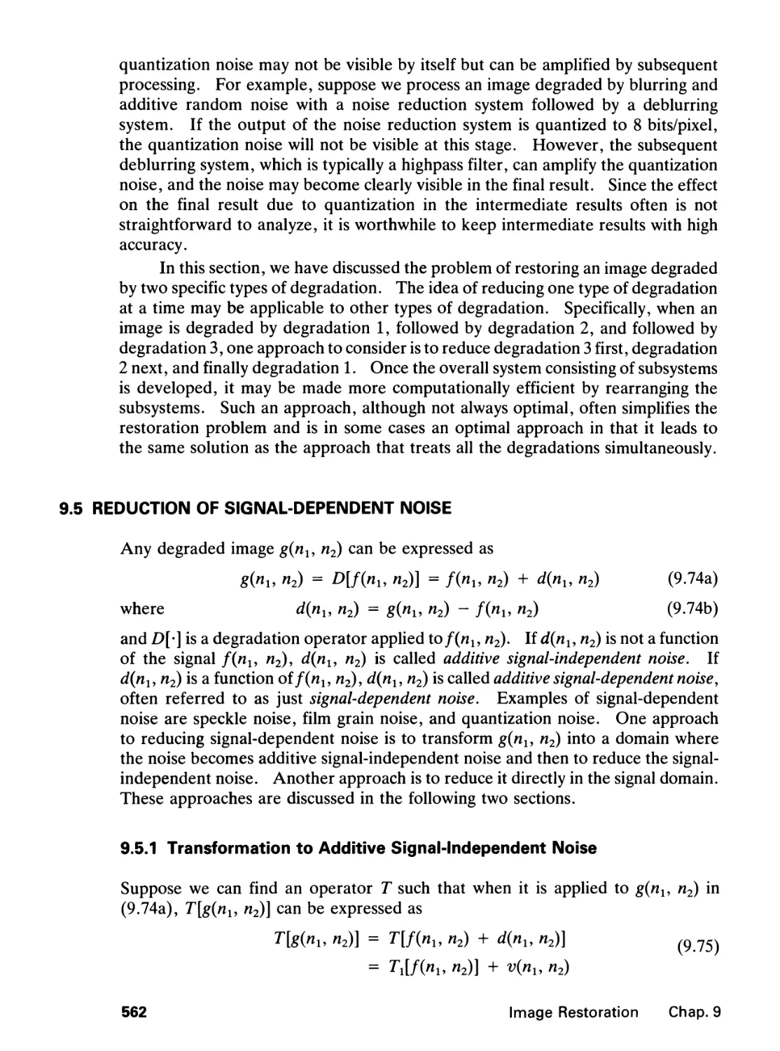
+ x(1,-1)8(h1- l,/i2 + 1) + • • • + x(-1,0)8(h1 + l,/i2)
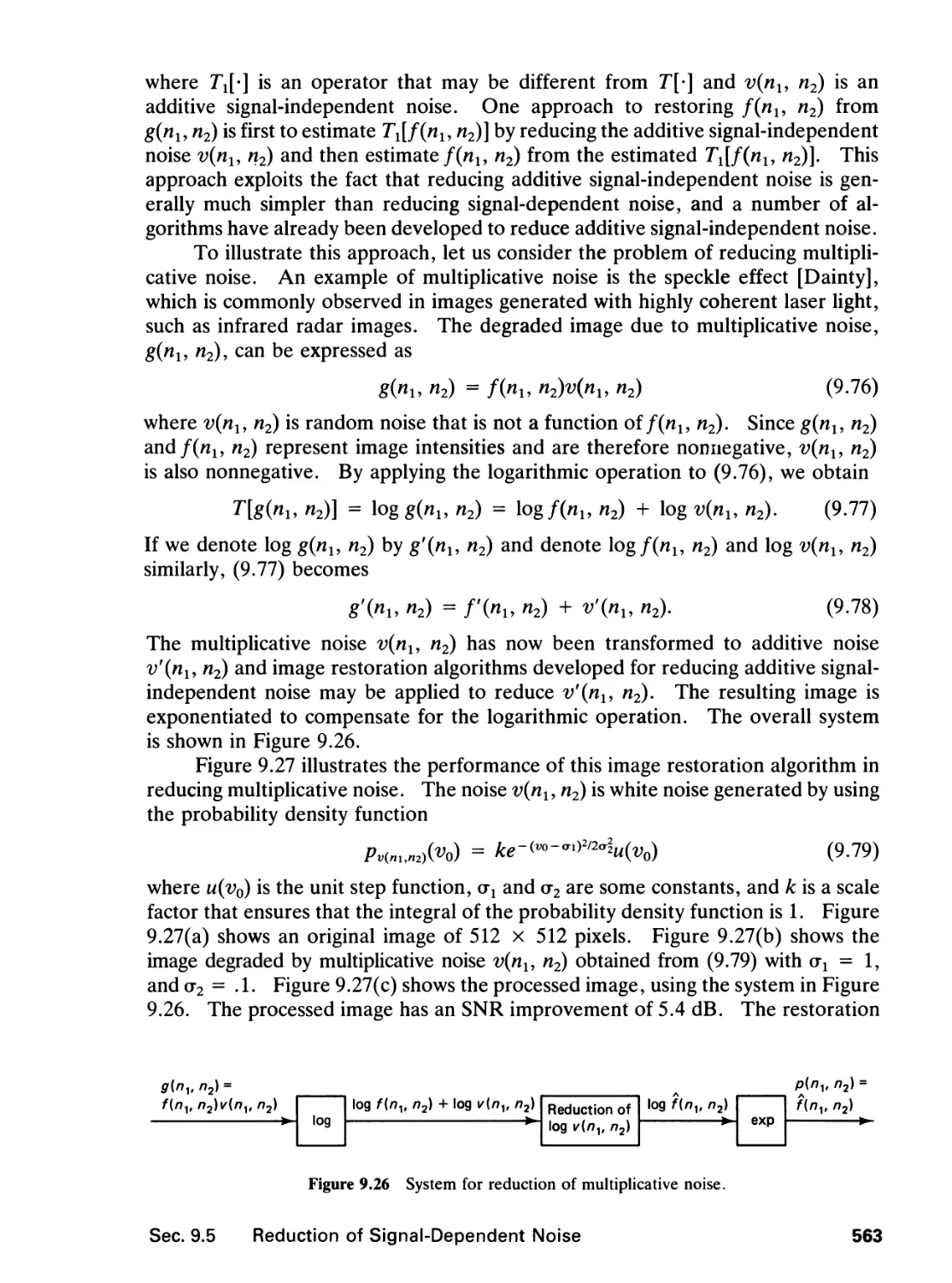
+ x(0,0)h(nl9n2) H-jc(1,0)8(w1 - l,/i2)
+ • • • +*(-l,l)8(/i1 + l,/i2- 1)
+ jc(0,1)8(/i1,/i2- 1) +jc(l,l)8(/i!- l,/i2- 1) + • • •
= 2 2 *(*i,*2)8(/ii-*i,/i2-*2).
A:, = — oc A:9= — *
(1.2)
The representation of x(nu n2) by (1.2) is very useful in system analysis.
Line impulses constitute a class of impulses which do not have any
counterparts in 1-D. An example of a line impulse is the 2-D sequence ^T(nx), which is
sketched in Figure 1.5 and is defined as
x(nu n2) = 8r(/i!) =
1, nx = 0
0, otherwise.
(1.3)
Other examples include hT(n2) and hT(nl - n2), which are defined similarly to
8r(/*i)- The subscript T in hT(ni) indicates that §T(ni) is a 2-D sequence. This
notation is used to avoid confusion in cases where the 2-D sequence is a function
of only one variable. For example, without the subscript T, hT(nx) might be
4
Signals, Systems, and the Fourier Transform Chap. 1
8{nv n2)
Figure 1.4 Impulse b(nly n2).
confused with the 1-D impulse 8(«i). For clarity, then, the subscript T will be
used whenever a 2-D sequence is a function of one variable. The sequence x^nj
is thus a 2-D sequence, while x(/*i) is a 1-D sequence.
Step sequences. The unit step sequence, denoted by u(n1, n2), is defined
as
M("i'*)=<), otherwise.
(1.4)
M"i>
-►"1
Figure 1.5 Line impulse S^rti).
Sec. 1.1 Signals
5
The sequence u(nly n2), which is sketched in Figure 1.6, is related to h(nly n2) as
u(nu n2) = 2 E 8(*i» ^2) (l-5a)
or
§(ni> ni) ~ M(wi> ni) ~ u(ni ~~ 1> w2) - w(wi, n2 "" 1) + u(ni ~ 1> n2 - 1).
(1.5b)
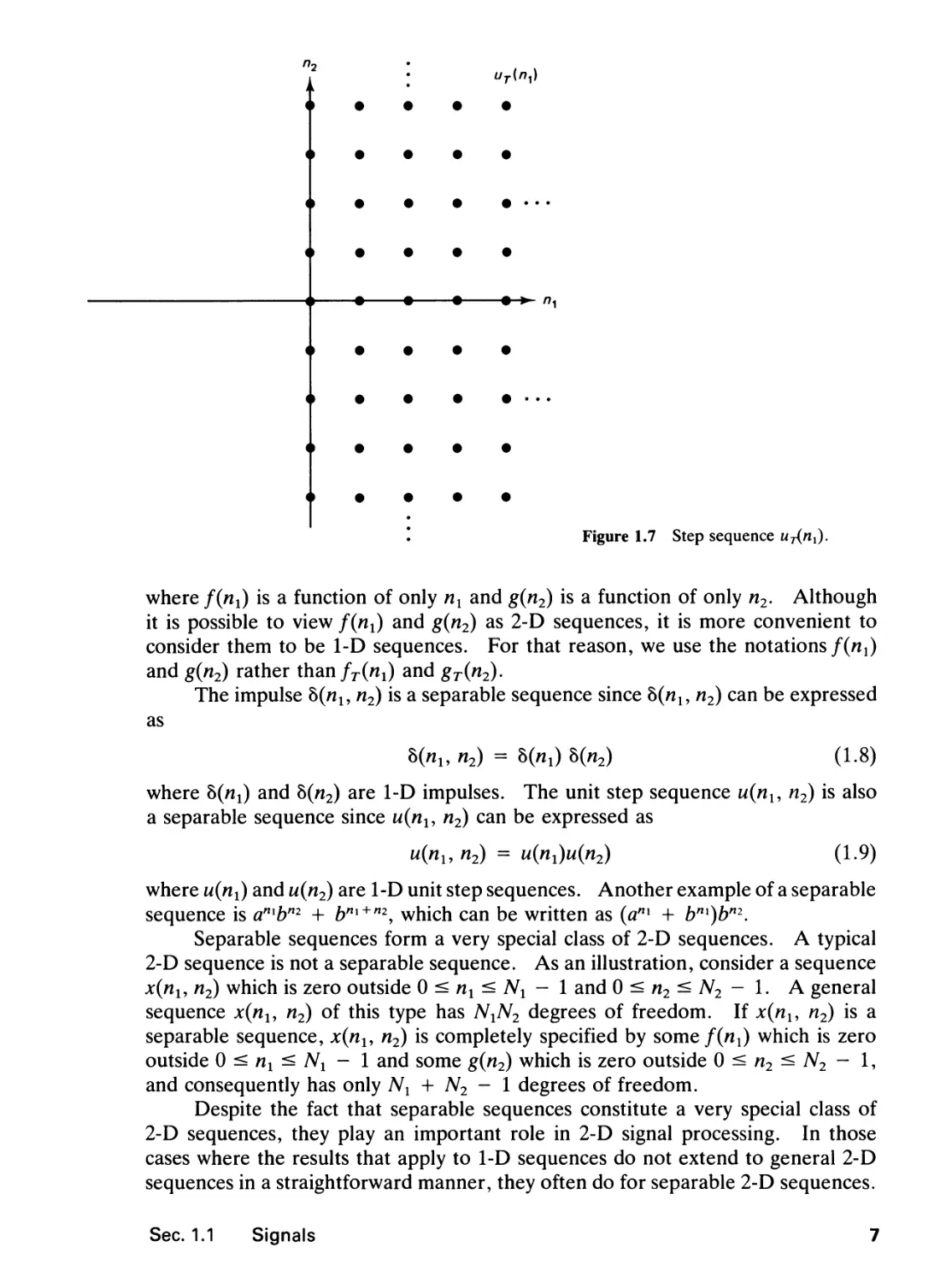
Some step sequences have no counterparts in 1-D. An example is the 2-D
sequence uT{nx), which is sketched in Figure 1.7 and is defined as
x(n1,n2) = ur(n1) = |0> otherwise>
(1.6)
Other examples include uT(n2) and u^! - h2)> which are defined similarly to
Wr(«i)-
Exponential sequences. Exponential sequences of the type x(nly rc2)
= Aani$n2 are important for system analysis. As we shall see later, sequences of
this class are eigenfunctions of linear shift-invariant (LSI) systems.
Separable sequences. A 2-D sequence x(nl, n2) is said to be a separable
sequence if it can be expressed as
x(nu n2) = /(«i)g(«2)
(1.7)
u(nv n2)
Figure 1.6 Unit step sequence u(nx, n2).
Signals, Systems, and the Fourier Transform Chap. 1
uT(ny)
Figure 1.7 Step sequence Mwi)-
where f(nx) is a function of only nl and g(n2) is a function of only n2. Although
it is possible to view f(nx) and g(n2) as 2-D sequences, it is more convenient to
consider them to be 1-D sequences. For that reason, we use the notations f(nx)
and g(n2) rather than fT(nx) and gT(n2).
The impulse b(nu n2) is a separable sequence since b(nu n2) can be expressed
as
h(nx, n2) = 8(/ii) 8(/i2)
(1.8)
where §(nx) and 8(w2) are 1-D impulses. The unit step sequence u{nu n2) is also
a separable sequence since u(nx, n2) can be expressed as
w(/*i> ni) ~ u(nx)u(n2)
(1.9)
where u(nx) and u(n2) are 1-D unit step sequences. Another example of a separable
sequence is anxbn2 + bm+"2, which can be written as (am + bni)b"2.
Separable sequences form a very special class of 2-D sequences. A typical
2-D sequence is not a separable sequence. As an illustration, consider a sequence
x(nu n2) which is zero outside 0 < nx < Nx - 1 and 0 ^ n2 ^ N2 - 1. A general
sequence x(nu n2) of this type has NXN2 degrees of freedom. If x{nx, n2) is a
separable sequence, x(nu n2) is completely specified by some f(nx) which is zero
outside 0 < nx < Nx - 1 and some g(fl2) which is zero outside 0 < n2 < N2 - 1,
and consequently has only Nx + N2 - 1 degrees of freedom.
Despite the fact that separable sequences constitute a very special class of
2-D sequences, they play an important role in 2-D signal processing. In those
cases where the results that apply to 1-D sequences do not extend to general 2-D
sequences in a straightforward manner, they often do for separable 2-D sequences.
Sec. 1.1 Signals
7
In addition, the separability of the sequence can be exploited in order to reduce
computation in various contexts, such as digital filtering and computation of the
discrete Fourier transform. This will be discussed further in later sections.
Periodic sequences. A sequence x(n1, n2) is said to be periodic with a
period of Nx x N2 ifx(nu n2) satisfies the following condition:
x(nu n2) = x(nx + Nu n2) = x(nu n2 + N2) for all (nu n2) (1.10)
where N1 and N2 are positive integers. For example, cos (irnl + (ir/2)w2) is a
periodic sequence with a period of 2 x 4, since cos (ir^ + (tt/2)«2) = cos
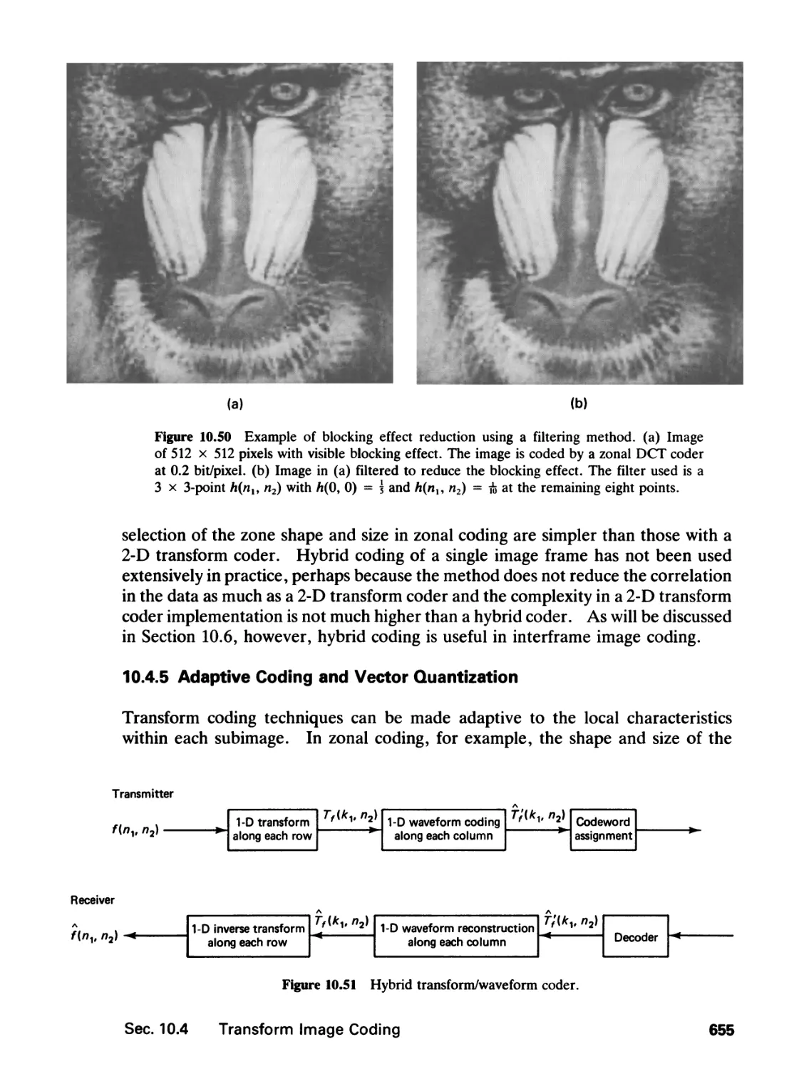
(ir(fli + 2) + (ir/2)n2) = cos (it^ + (ir/2)(w2 + 4)) for all (nu n2). The sequence
cos (nx + h2) is not periodic, however, since cos (nx + h2) cannot be expressed
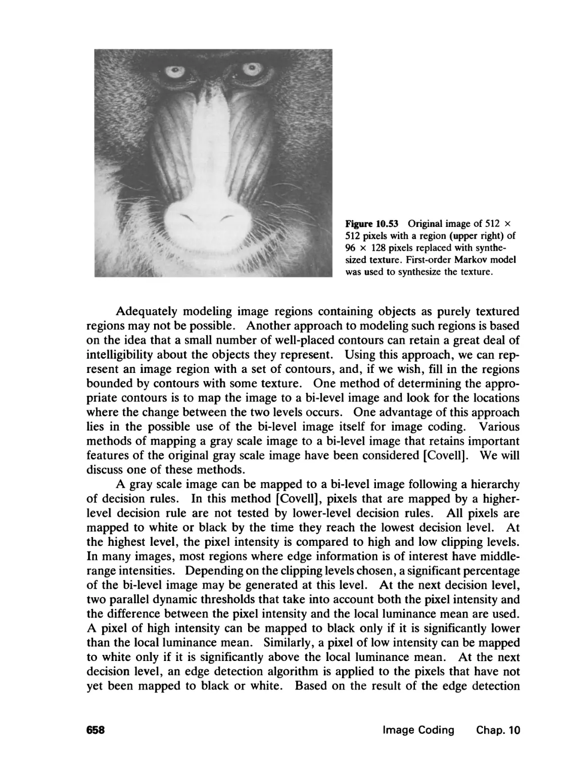
as cos ((«! + Nt) + h2) = cos (wi + (w2 + N2)) f°r all (nu n2) for any nonzero
integers Nx and N2. A periodic sequence is often denoted by adding a "~" (tilde),
for example, x(nl, n2), to distinguish it from an aperiodic sequence.
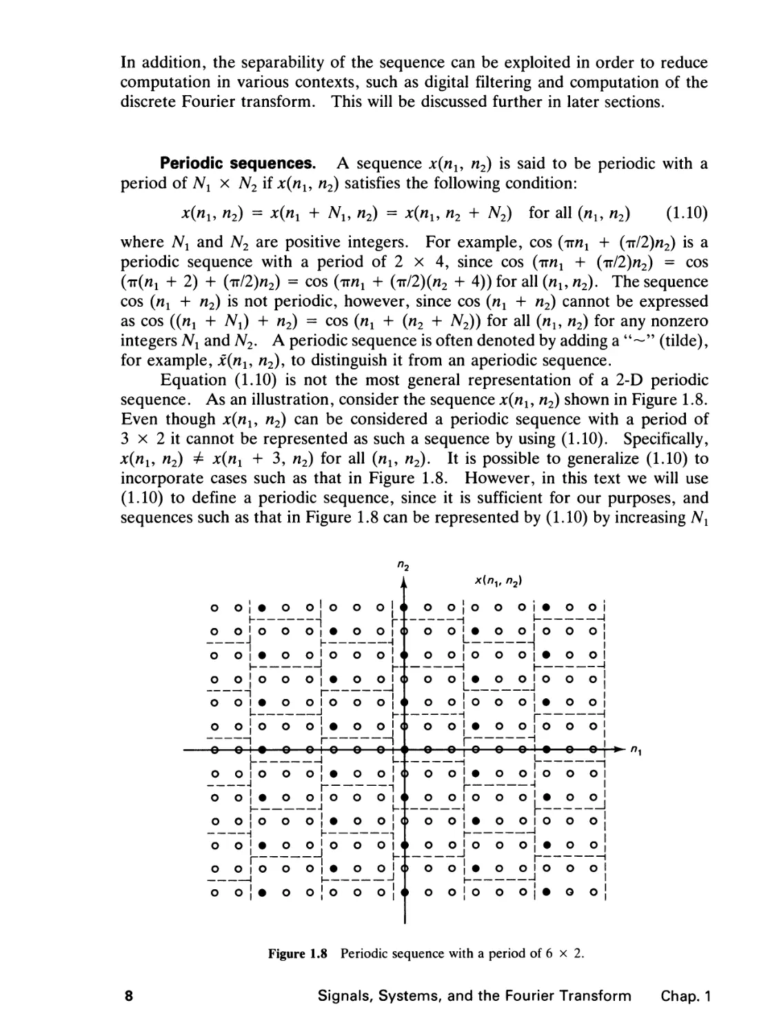
Equation (1.10) is not the most general representation of a 2-D periodic
sequence. As an illustration, consider the sequence x{nu n2) shown in Figure 1.8.
Even though x(nu n2) can be considered a periodic sequence with a period of
3 x 2 it cannot be represented as such a sequence by using (1.10). Specifically,
x(nx, n2) ± x(nx + 3, n2) for all (nu n2). It is possible to generalize (1.10) to
incorporate cases such as that in Figure 1.8. However, in this text we will use
(1.10) to define a periodic sequence, since it is sufficient for our purposes, and
sequences such as that in Figure 1.8 can be represented by (1.10) by increasing Nx
o o
o o
o o
• o o I o o o j 4
O O O 1 • O O 1 <t>
h -I T
• o o 1 o o o
, h.
o o o 1 • o o 1 <(>
I 1
• o o 1 o o o j
h
O I O
o o j 4>
-e—o 1 ♦
o o
o o
o o
o o
o o
x{nv n2)
o o
O I •
I—
I
O O I
1
o o j o o o
o o o 1 • o o
I
• O O I O O O
o o
O O 1 O O O
-e—o o 1 •
o o
o o
o o
o o
o o
o o
000
• o
I—
O I O
J
o o
o
I
—I
o 1
I-
o I
o o
o o
00 o , •
J. .j
• o 00 o 01
i 'i h
O O O 1 •
o o j
o ' o
o o
o o
o o
o o
• O O l O
1
o o o I •
•OOIOOO
1
• o
_l
• OOIOOO
I 1
o o 1 • 0 o
Figure 1.8 Periodic sequence with a period of 6 x 2.
8
Signals, Systems, and the Fourier Transform Chap. 1
and/or N2. For example, the sequence in Figure 1.8 is periodic with a period of
6 x 2 using (1.10).
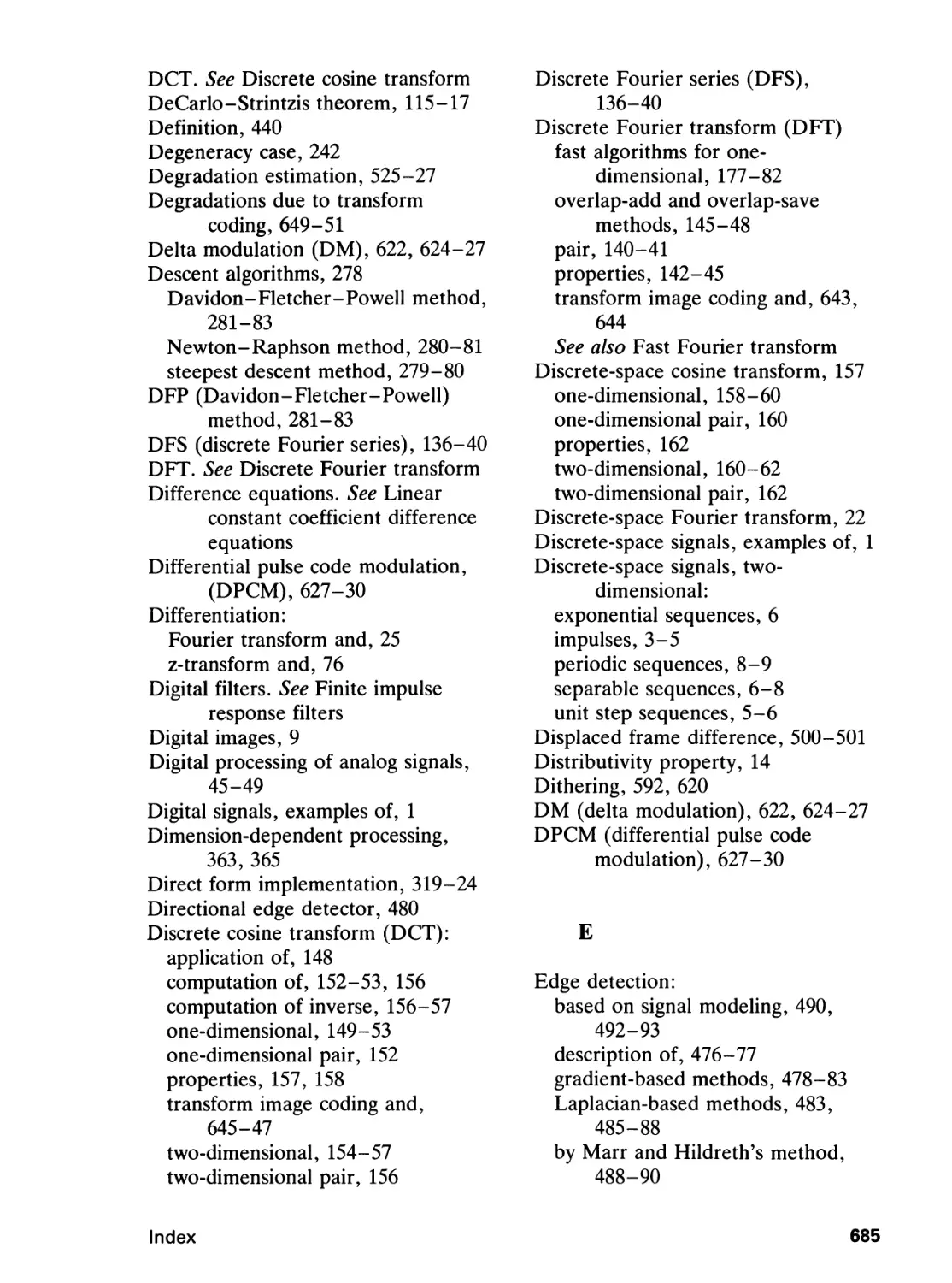
1.1.2 Digital Images
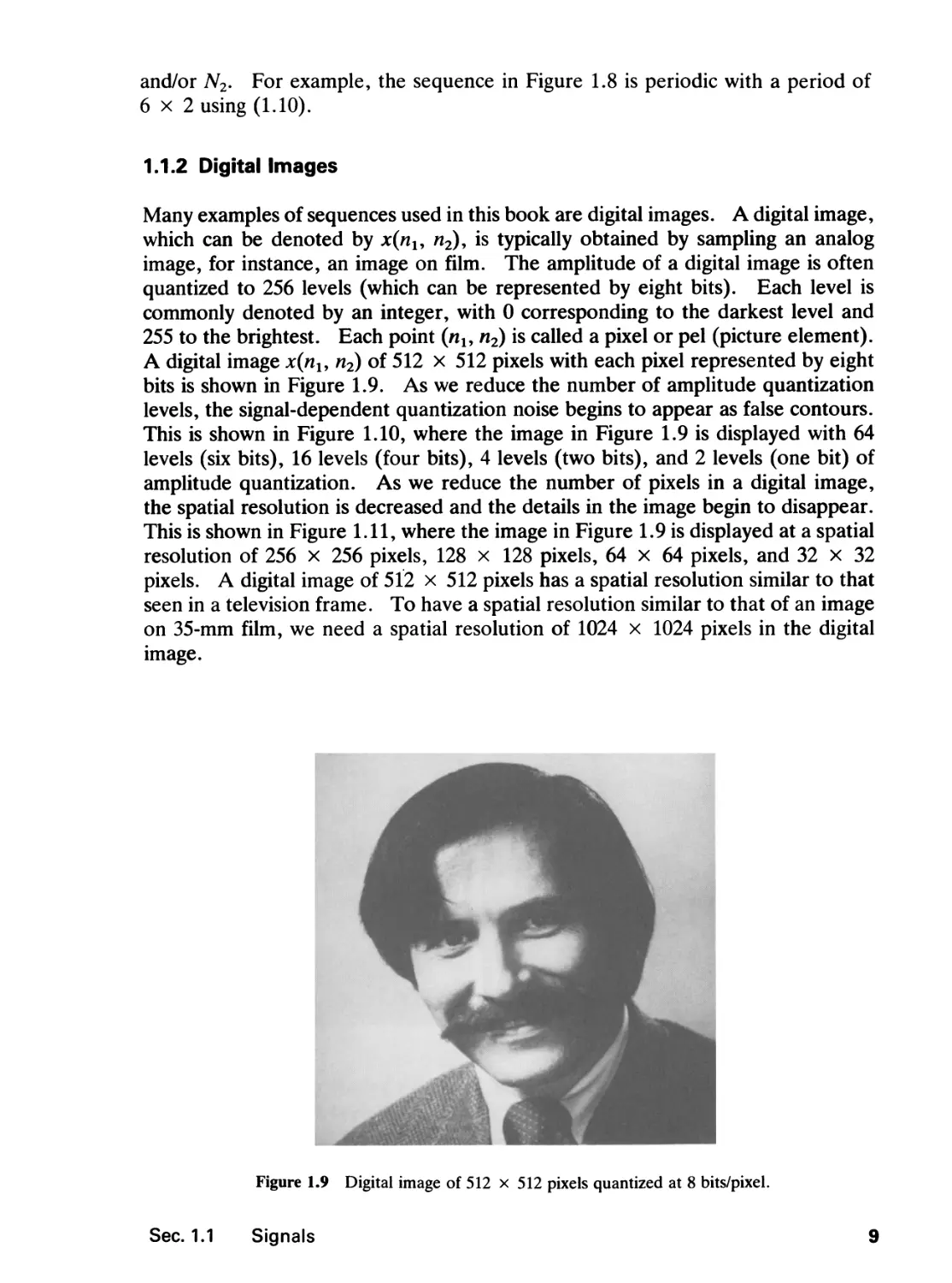
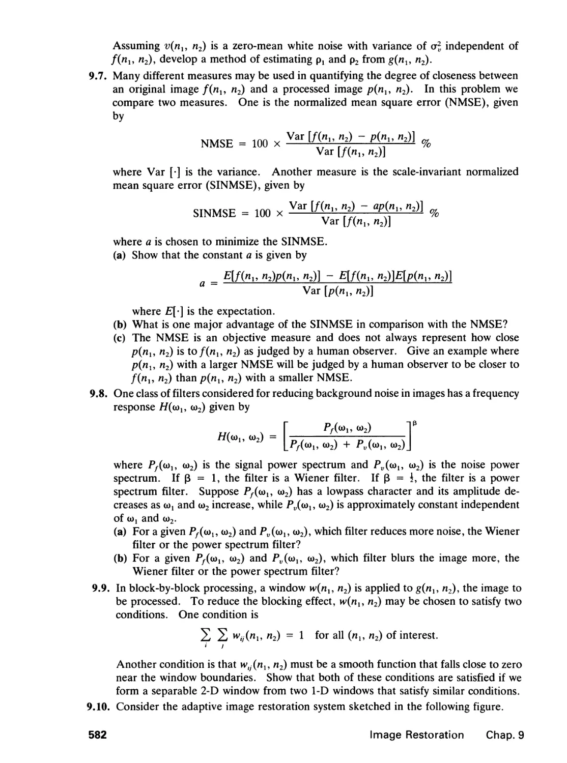
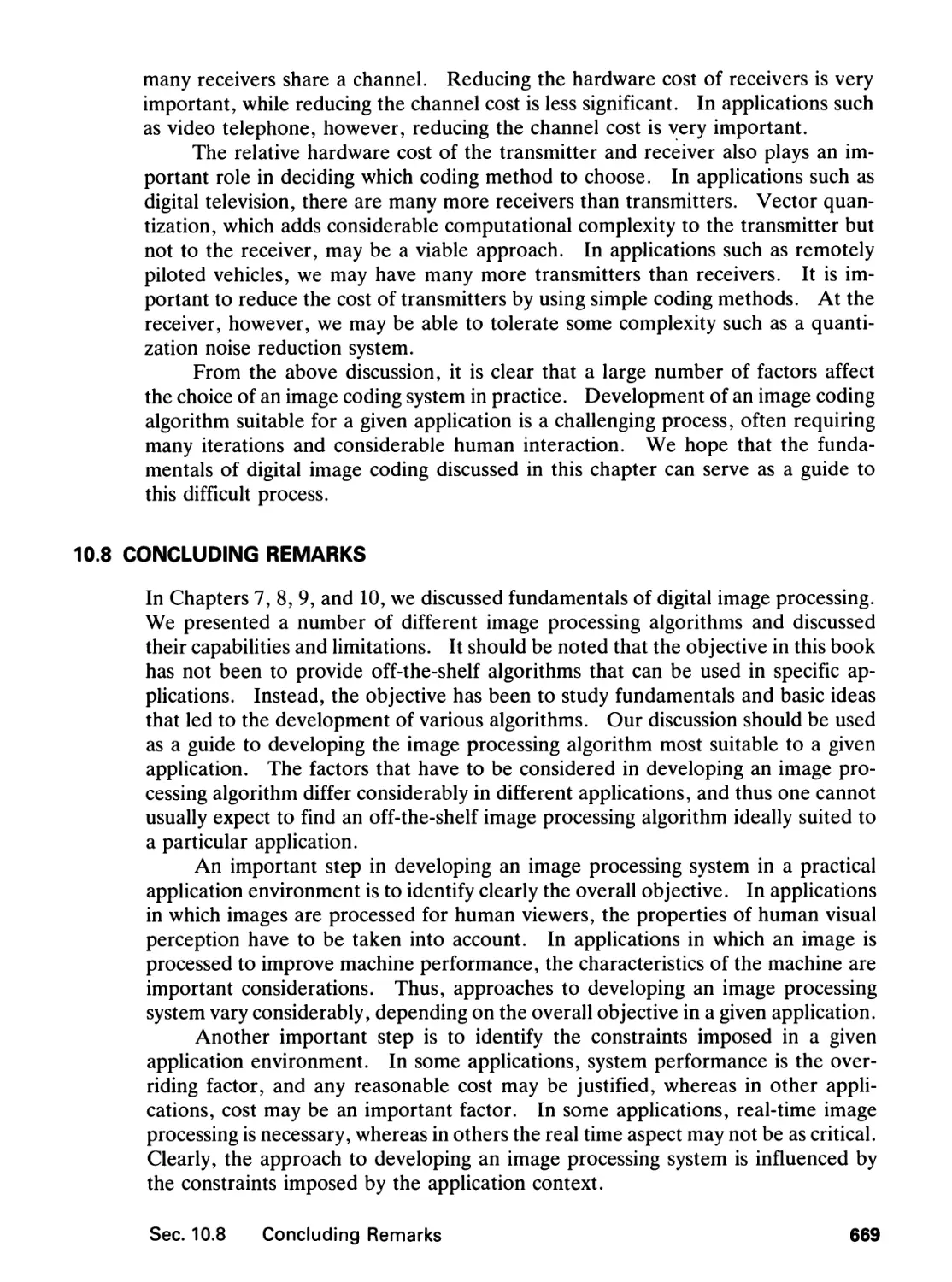
Many examples of sequences used in this book are digital images. A digital image,
which can be denoted by x(nu n2)y is typically obtained by sampling an analog
image, for instance, an image on film. The amplitude of a digital image is often
quantized to 256 levels (which can be represented by eight bits). Each level is
commonly denoted by an integer, with 0 corresponding to the darkest level and
255 to the brightest. Each point (nl9 n2) is called a pixel or pel (picture element).
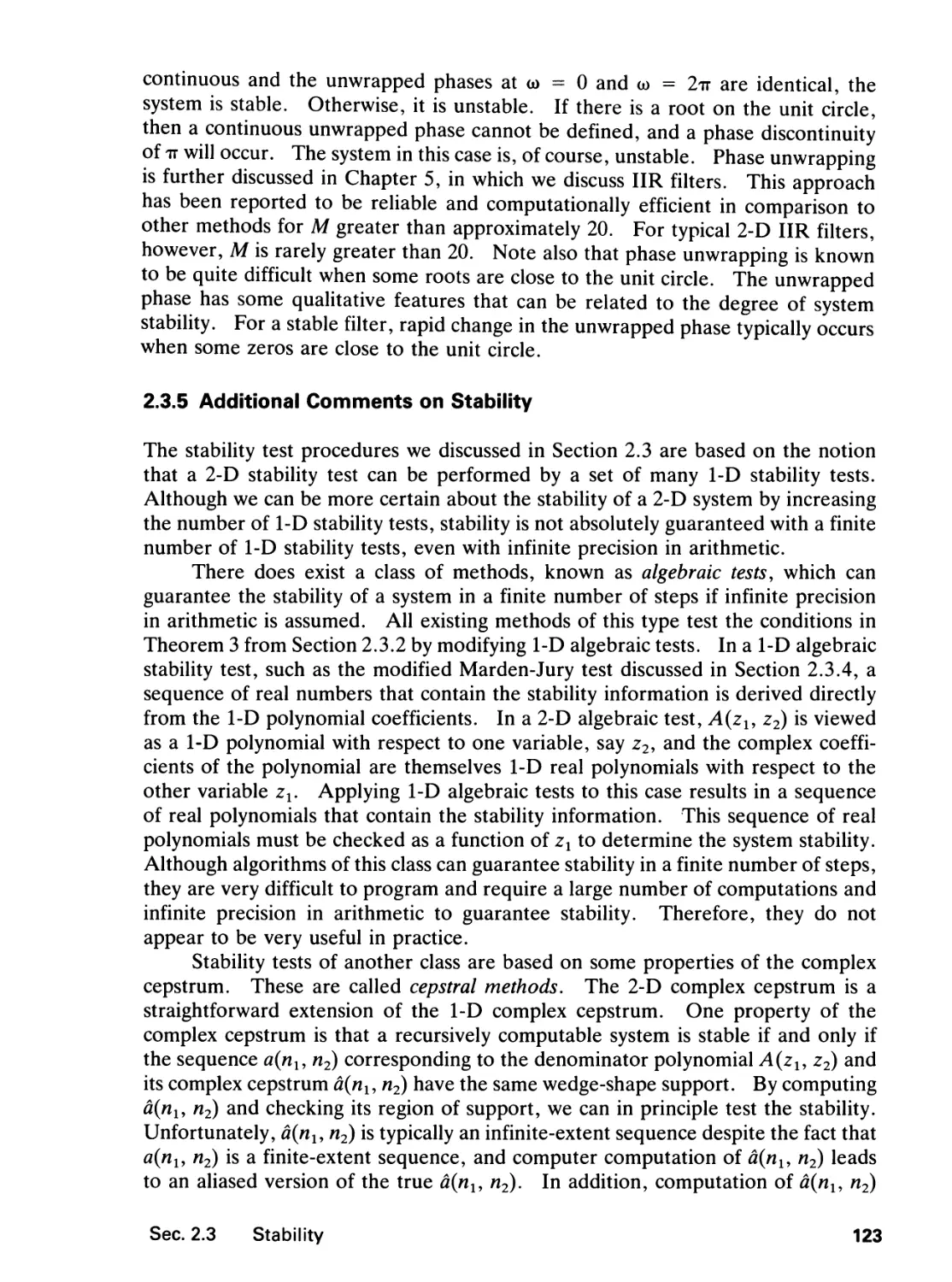
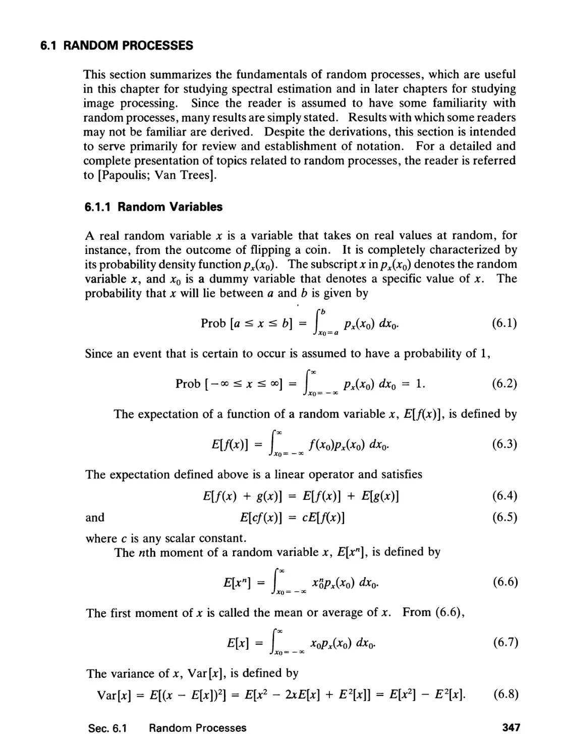
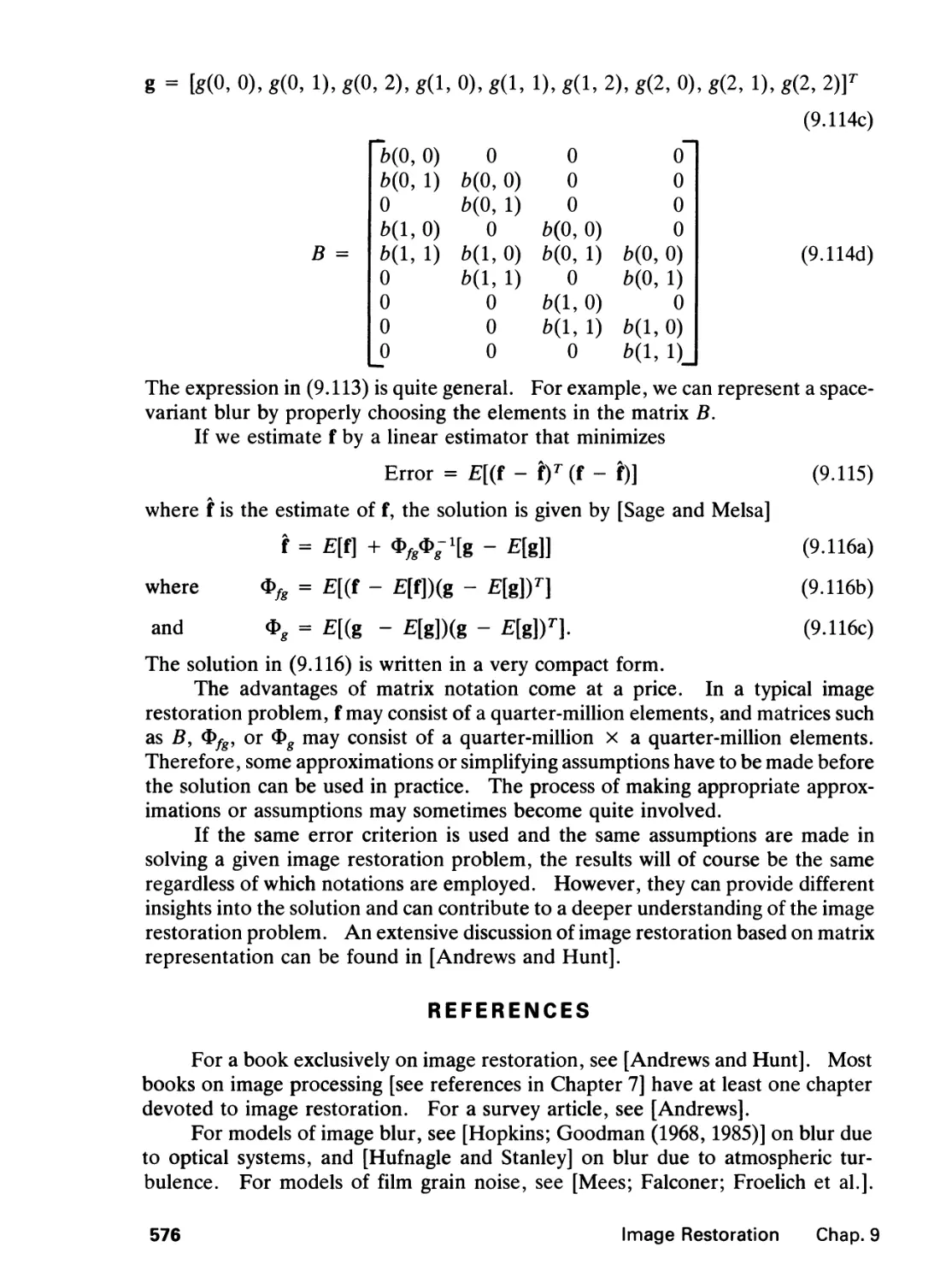
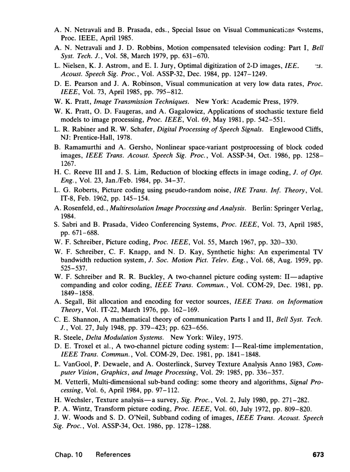
A digital image x(nl9 n2) of 512 x 512 pixels with each pixel represented by eight
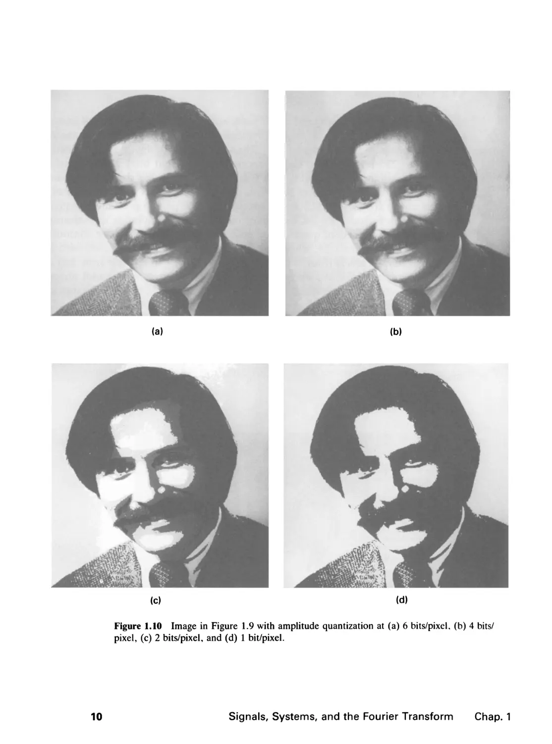
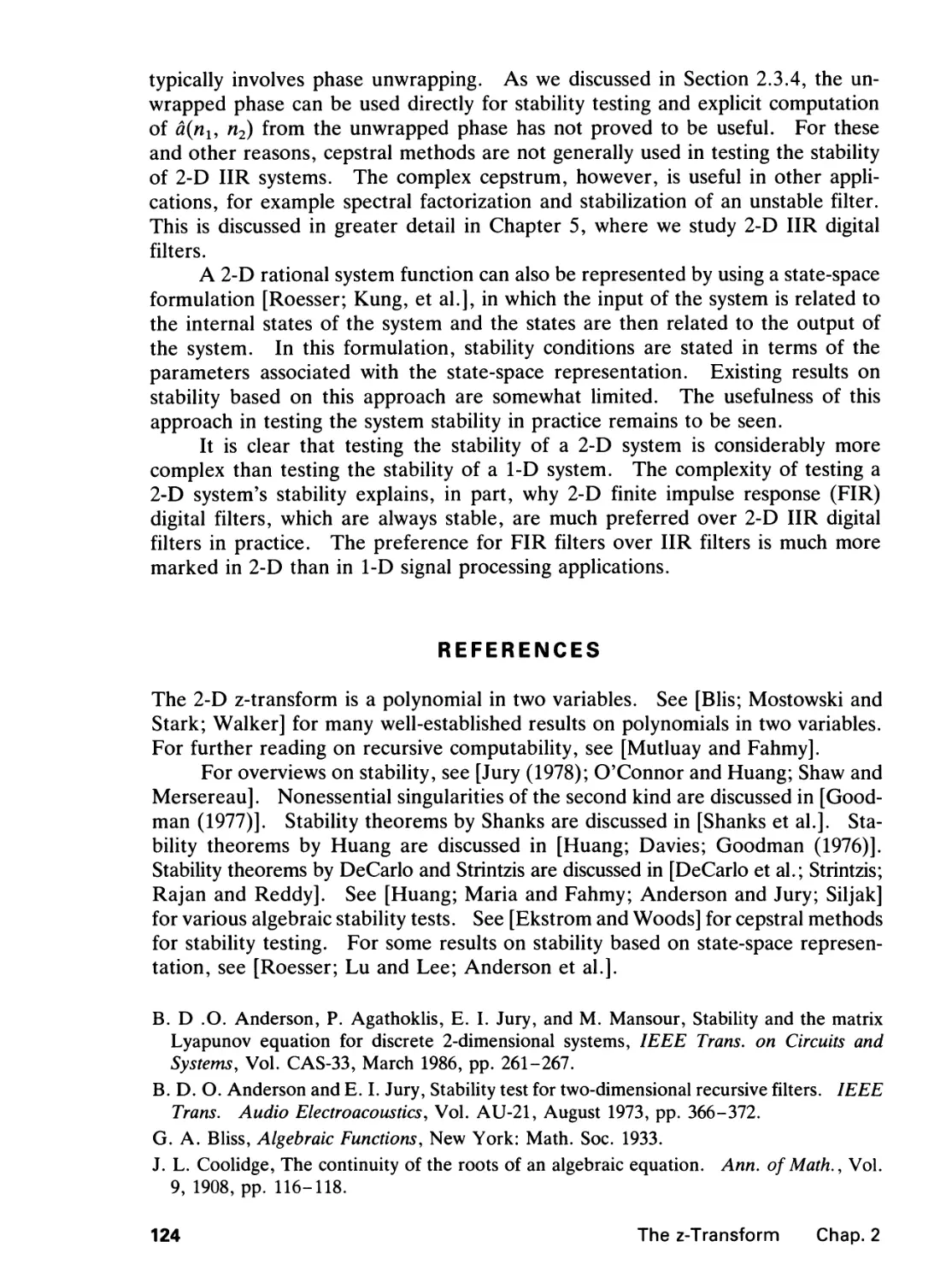
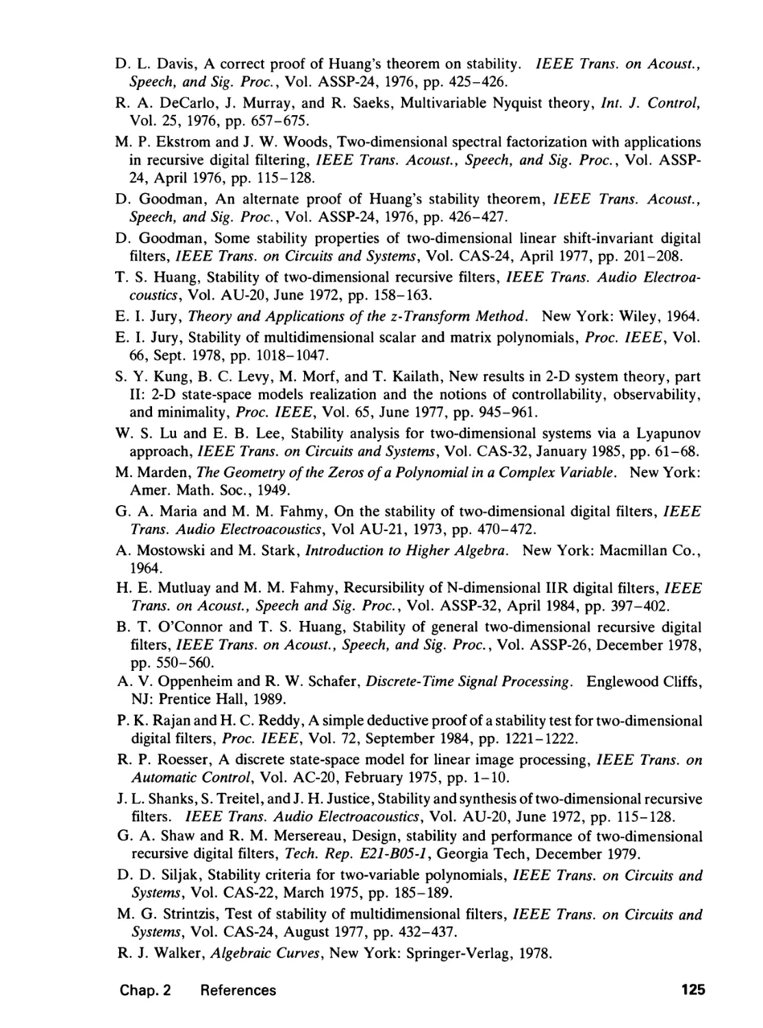
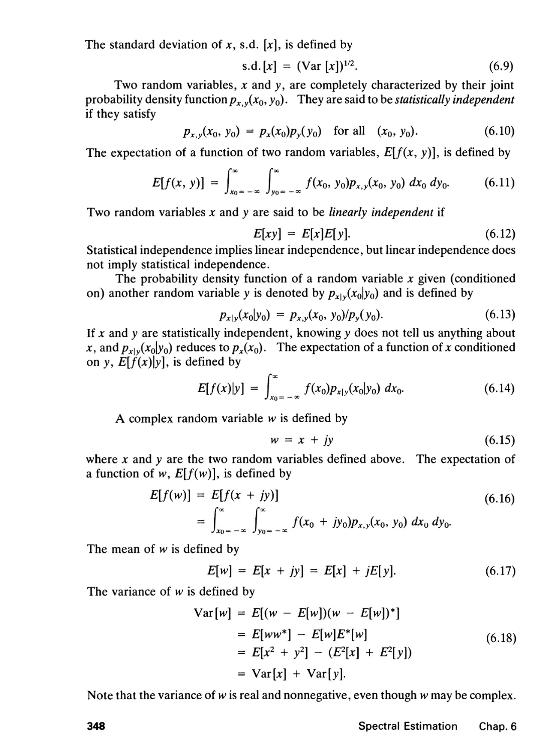
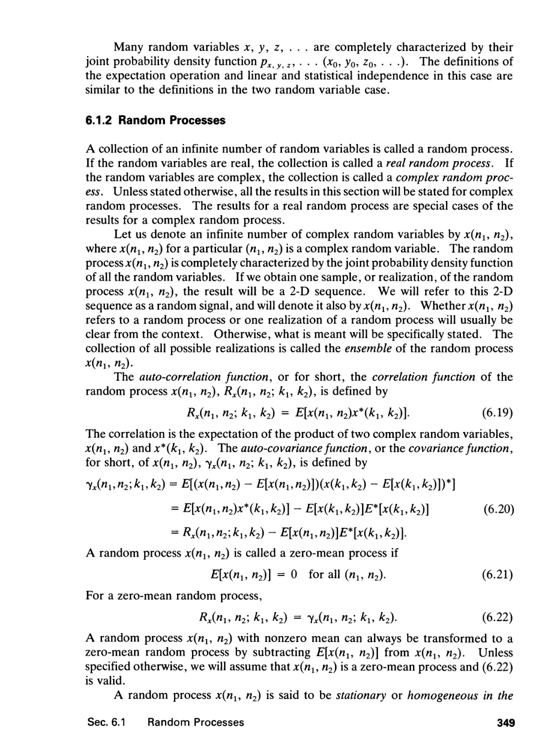
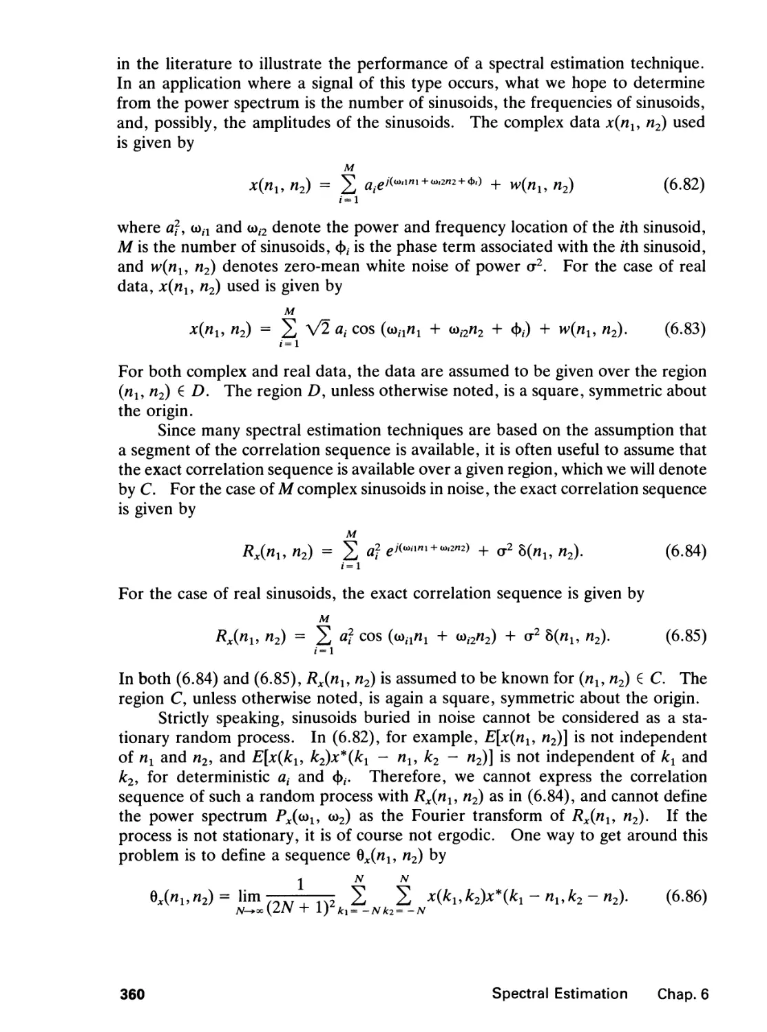
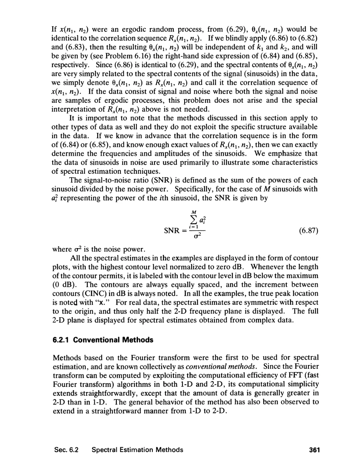
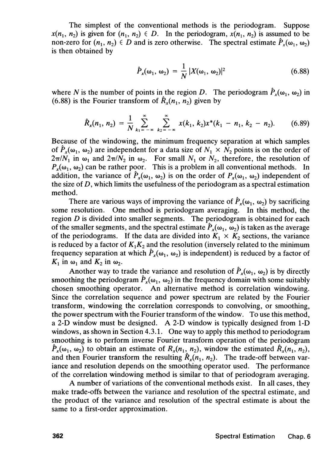
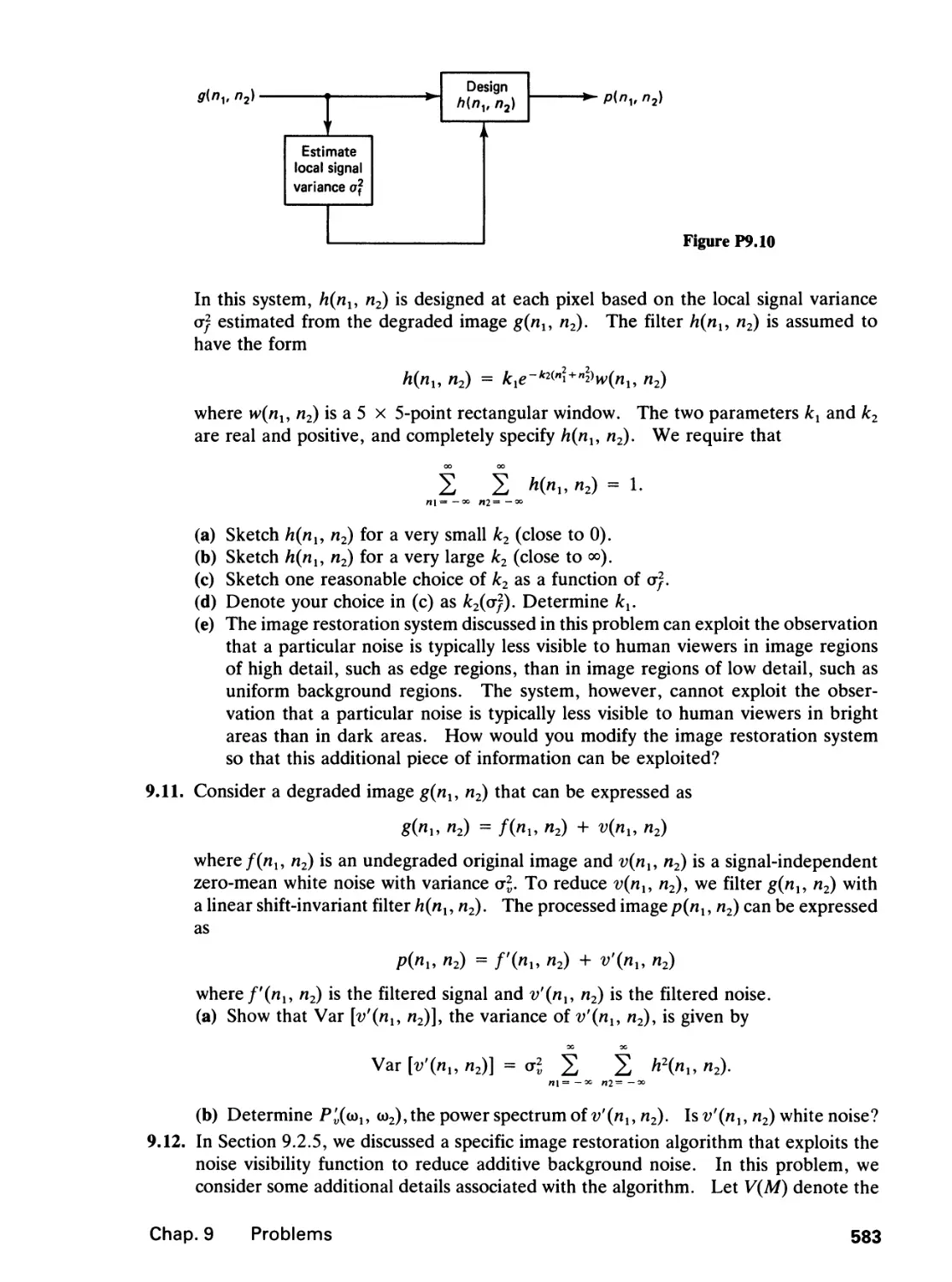
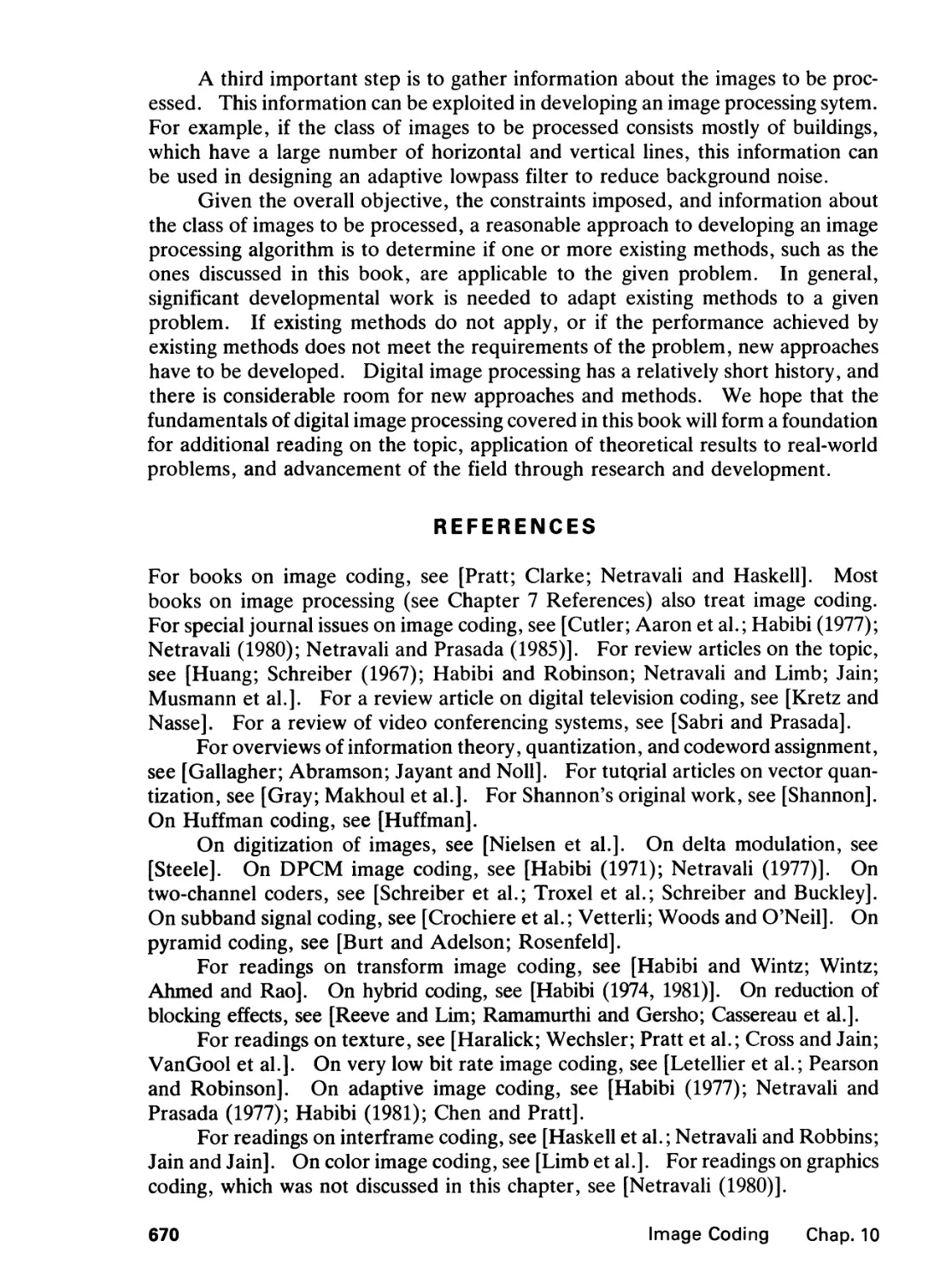
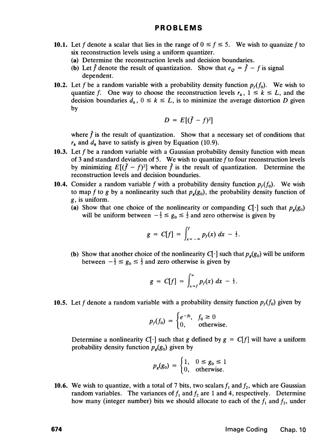
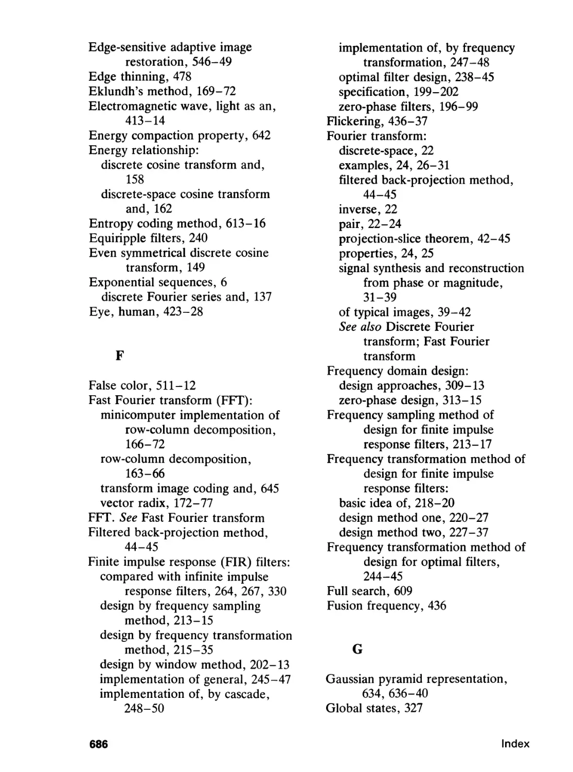
bits is shown in Figure 1.9. As we reduce the number of amplitude quantization
levels, the signal-dependent quantization noise begins to appear as false contours.
This is shown in Figure 1.10, where the image in Figure 1.9 is displayed with 64
levels (six bits), 16 levels (four bits), 4 levels (two bits), and 2 levels (one bit) of
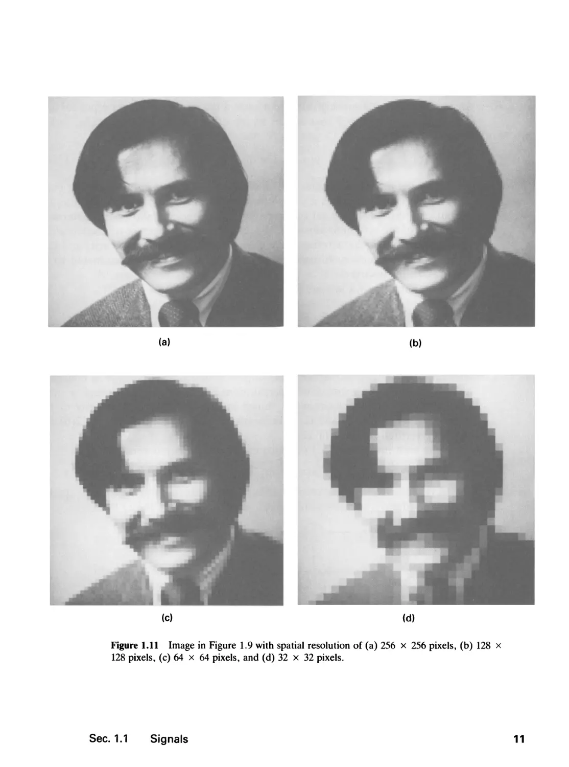
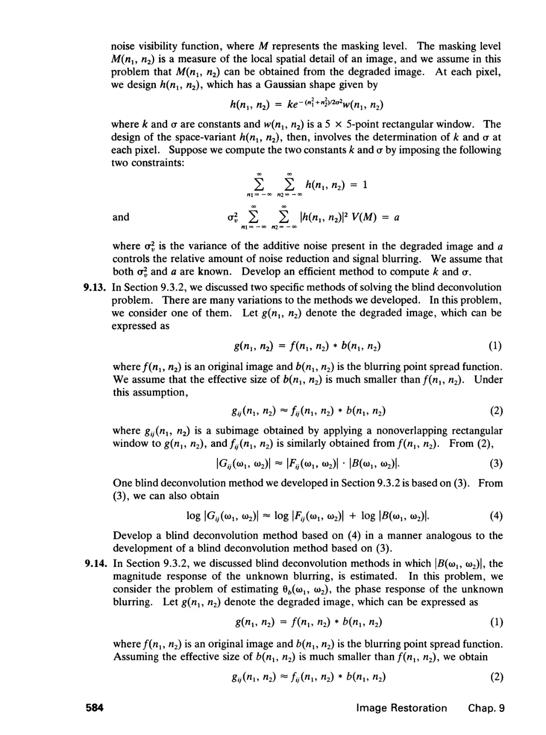
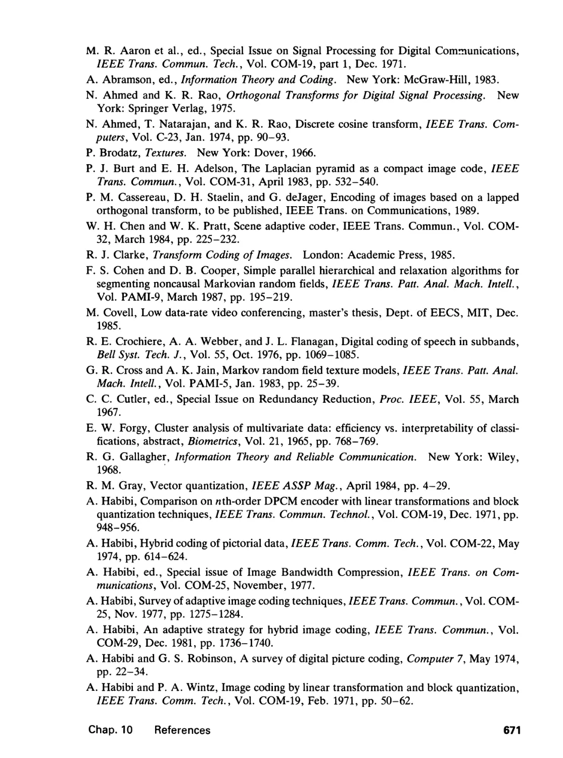
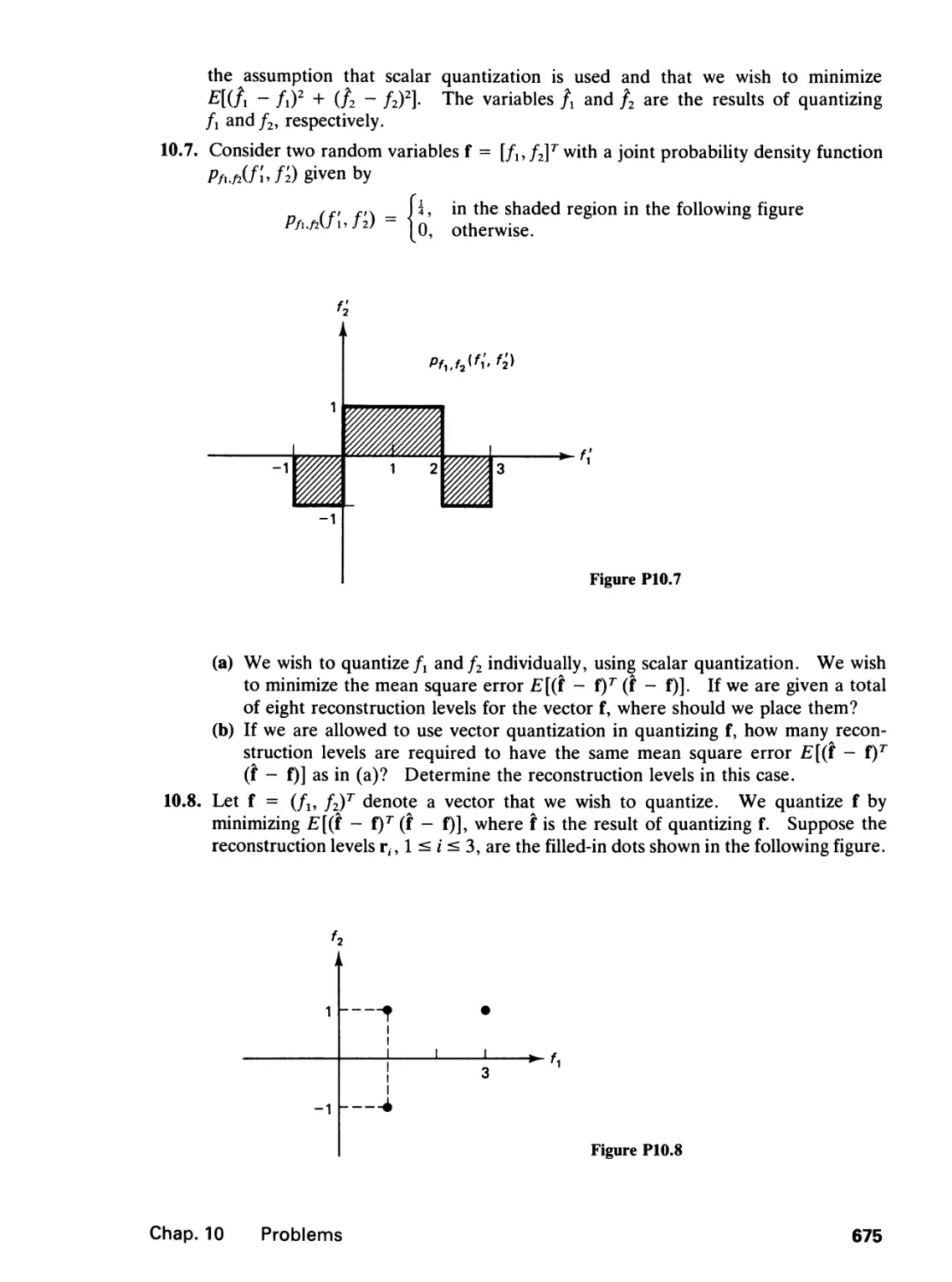
amplitude quantization. As we reduce the number of pixels in a digital image,
the spatial resolution is decreased and the details in the image begin to disappear.
This is shown in Figure 1.11, where the image in Figure 1.9 is displayed at a spatial
resolution of 256 x 256 pixels, 128 x 128 pixels, 64 x 64 pixels, and 32 x 32
pixels. A digital image of 512 x 512 pixels has a spatial resolution similar to that
seen in a television frame. To have a spatial resolution similar to that of an image
on 35-mm film, we need a spatial resolution of 1024 x 1024 pixels in the digital
image.
Figure 1.9 Digital image of 512 x 512 pixels quantized at 8 bits/pixel.
Sec. 1.1 Signals
9
(a)
(b)
W
?l
fti
sw
M
%\
^4
(c)
(d)
Figure 1.10 Image in Figure 1.9 with amplitude quantization at (a) 6 bits/pixel, (b) 4 bits/
pixel, (c) 2 bits/pixel, and (d) 1 bit/pixel.
10
Signals, Systems, and the Fourier Transform Chap. 1
(a) (b)
(0 (d)
Figure 1.11 Image in Figure 1.9 with spatial resolution of (a) 256 x 256 pixels, (b) 128 x
128 pixels, (c) 64 x 64 pixels, and (d) 32 x 32 pixels.
Sec. 1.1 Signals
11
1.2 SYSTEMS
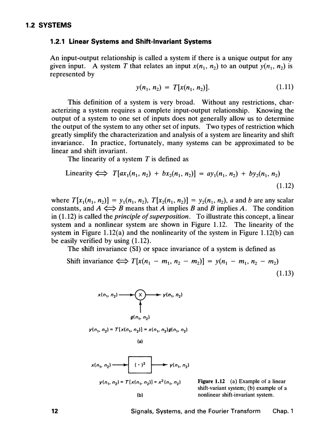
1.2.1 Linear Systems and Shift-Invariant Systems
An input-output relationship is called a system if there is a unique output for any
given input. A system T that relates an input x(nx, n2) to an output y(nly n2) is
represented by
y(nu n2) = T[x(nu n2)]. (1.11)
This definition of a system is very broad. Without any restrictions,
characterizing a system requires a complete input-output relationship. Knowing the
output of a system to one set of inputs does not generally allow us to determine
the output of the system to any other set of inputs. Two types of restriction which
greatly simplify the characterization and analysis of a system are linearity and shift
in variance. In practice, fortunately, many systems can be approximated to be
linear and shift invariant.
The linearity of a system T is defined as
Linearity <=> T[axx(nl9 n2) + bx2(nu n2)] = ayx(nu n2) + by2(nu n2)
(1.12)
where T[x1(n1, n2)] = yx{nly n2), T[x2(nu n2)] = y2(nu n2), a and b are any scalar
constants, and A <=> B means that A implies B and B implies A. The condition
in (1.12) is called the principle of superposition. To illustrate this concept, a linear
system and a nonlinear system are shown in Figure 1.12. The linearity of the
system in Figure 1.12(a) and the nonlinearity of the system in Figure 1.12(b) can
be easily verified by using (1.12).
The shift invariance (SI) or space invariance of a system is defined as
Shift invariance <=> T[x(nx - mx,n2 - m2)\ = y(nx - mx,n2 - m2)
(1.13)
x(nv n2) ►/ X ) > y{nv n2)
g(nv n2)
y{nv n2) = T[x{nv n2)] = x(nv n2)g(nv n2)
(a)
x(nv n2)-
(■)2
-► W"i, n2)
y(nv n2) = T[x(nv n2)} = x2(nv n2) Figure 1.12 (a) Example of a linear
shift-variant system; (b) example of a
(b) nonlinear shift-invariant system.
12
Signals, Systems, and the Fourier Transform Chap. 1
where y(nx, n2) = T[x(nx, n2)] and mx and m2 are any integers. The system in
Figure 1.12(a) is not shift invariant since T[x(nx - ml9 n2 - m2)] = x(nl - m,,
n2 ~~ m2)g(n\i n2) and y(«! - ml9 h2 ~ w2) = *(wi ~ m\-> n2 ~ m2)g{n\ ~ mi>
n2 ~ m2)- The system in Figure 1.12(b), however, is shift invariant, since
T[x(nl - mu n2 — m2)] = x2(n1 - mx, n2 - m2) and y(nx — mb n2 - m2) =
x2(nx — mx, n2 - m2).
Consider a linear system T. Using (1.2) and (1.12), we can express the
output y(nl9 n2) for an input x(nx, n2) as
y(nl9n2) = T[x(nl9n2)] = T
2 E *(*i > ^2) 8("i - *i, "2 - ^2)
= S 2 Jt^i.A^rMn,-*!,/^-^)]. (1.14)
^! = -ocfc2 = -*
From (1.14), a linear system can be completely characterized by the response of
the system to the impulse h(nl9 n2) and its shifts h(nx — kx,n2 - k2). If we know
T\h(nx - kl9 n2 - k2)] for all integer values of kx and k2, the output of the linear
system to any input x(nl9 n2) can be obtained from (1.14). For a nonlinear system,
knowledge of T[h(nx - kl9 n2 - k2)] for all integer values of kx and k2 does not
tell us the output of the system when the input x(nx, n2) is 2h(nl9 n2), h(nx, n2) +
h(nx - 1, n2), or many other sequences.
System characterization is further simplified if we impose the additional
restriction of shift in variance. Suppose we denote the response of a system T to an
input h(nl9 n2) by h(nx, n2)\
h(nl9n2) = T[b(nun2)]. (1.15)
From (1.13) and (1.15),
h(nx - kl9 n2 - k2) = T[b(nx - kl9 n2 - k2)] (1.16)
for a shift-invariant system T. For a linear and shift-invariant (LSI) system, then,
from (1.14) and (1.16), the input-output relation is given by
oc oc
y(nl9 n2) = T[x(nu n2)] = 2 E x(kl9 k2)h(nx - kl9 n2 - k2). (1.17)
k\ = — ac ki= — oc
Equation (1.17) states that an LSI system is completely characterized by the impulse
response h(nu n2). Specifically, for an LSI system, knowledge of h{nu n2) alone
allows us to determine the output of the system to any input from (1.17). Equation
(1.17) is referred to as convolution, and is denoted by the convolution operator
"*" as follows:
For an LSI system,
y(nl9 n2) = x(nl9 n2) * h(nl9 n2)
oc oc
= 2 E x(kl9 k2)h(nx - kx, n2 - k2).
k\ = - x ki = - «:
Sec. 1.2 Systems
13
Note that the impulse response h(nu n2), which plays such an important role for
an LSI system, loses its significance for a nonlinear or shift-variant system. Note
also that an LSI system can be completely characterized by the system response
to one of many other input sequences. The choice of b(nu n2) as the input in
characterizing an LSI system is the simplest, both conceptually and in practice.
1.2.2 Convolution
The convolution operator in (1.18) has a number of properties that are
straightforward extensions of 1-D results. Some of the more important are listed below.
Commutativity
x(nu n2) * y(nl9 n2) = y(nu n2) * x(nl9 n2) (1.19)
Associativity
(x(nl9 n2) * y(nl9 n2)) * z(nl9 n2) = x{nl9 n2) * (y(nu n2) * z(nl9 n2)) (1.20)
Distributivity
x(nu n2) * (y(nl9 n2) + z(nl9 n2))
= (x(nl9 n2) * y(nl9 n2)) + (x(nl9 n2) * z(nl9 n2)) (1.21)
Convolution with Shifted Impulse
x{nl9 n2) * b(nx - m1? n2 - m2) = x(nx - ml9 n2 - m2) (1.22)
The commutativity property states that the output of an LSI system is not
affected when the input and the impulse response interchange roles. The
associativity property states that a cascade of two LSI systems with impulse responses
hx(nl9 n2) and h2(nl9 n2) has the same input-output relationship as one LSI system
with impulse response hx(nx, n2) * h2(nl9 n2). The distributivity property states
that a parallel combination of two LSI systems with impulse responses hl(nl, n2)
and h2(nly n2) has the same input-output relationship as one LSI system with impulse
response given by hx(nl9 n2) + h2(nl9 n2). In a special case of (1.22), when mx
= m2 = 0, we see that the impulse response of an identity system is b(nl9 n2).
The convolution of two sequences x{nl9 n2) and h(nl9 n2) can be obtained by
explicitly evaluating (1.18). It is often simpler and more instructive, however, to
evaluate (1.18) graphically. Specifically, the convolution sum in (1.18) can be
interpreted as multiplying two sequences x{kl9 k2) and h(nx - kl9n2 - k2), which
are functions of the variables kx and k2, and summing the product over all integer
values of kx and k2. The output, which is a function of nx and n2, is the result of
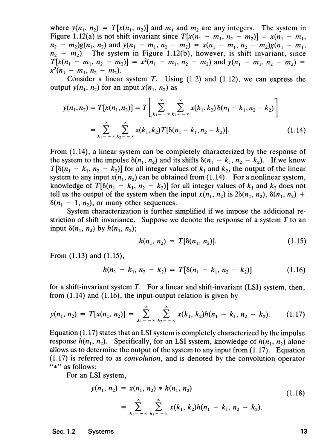
convolving x{nl9 n2) and h{nl9 n2). To illustrate, consider the two sequences
x(nl9 n2) and h(nl9 n2), shown in Figures 1.13(a) and (b). From x(nl9 n2) and
h(nly n2), x(kl9 k2) and h(nx - kl9 n2 - k2) as functions of kx and k2 can be
obtained, as shown in Figures 1.13(c)—(f). Note that g(kx - nl9 k2 - n2) is
14
Signals, Systems, and the Fourier Transform Chap. 1
x(nv n2)
-•—•-
-►"i
(a)
T
(3) (4)
• •
(1) (2)
h{nv n2)
(b)
K
i
i
i
2
k
► • •
► • •
x(kv k2)
(c)
h(ny - kv n2 - k2) = g(k^ - nv k2 - n2)
> (
4
(2) (1)
•—•
(4) {(3) f 1
h[kv k2)
(3) (4)
-»-*,
n
(d)
(e)
-►*,
-W2WIL
#(4) #(3,
g(kvk2) = h(-kv-k2)
-►*i
(f)
i
k /("v n2)
(3) (7) (7) (4)
• • • •
(4) (10) (10) (6)
• • • •
(4) (10) (10) (6)
• • • •
(1) (3) (3) (2)
(g)
Figure 1.13 Example of convolving two sequences.
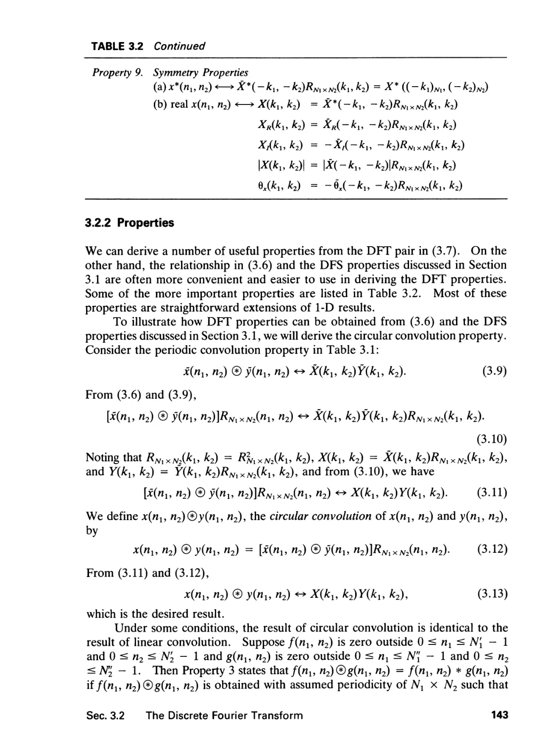
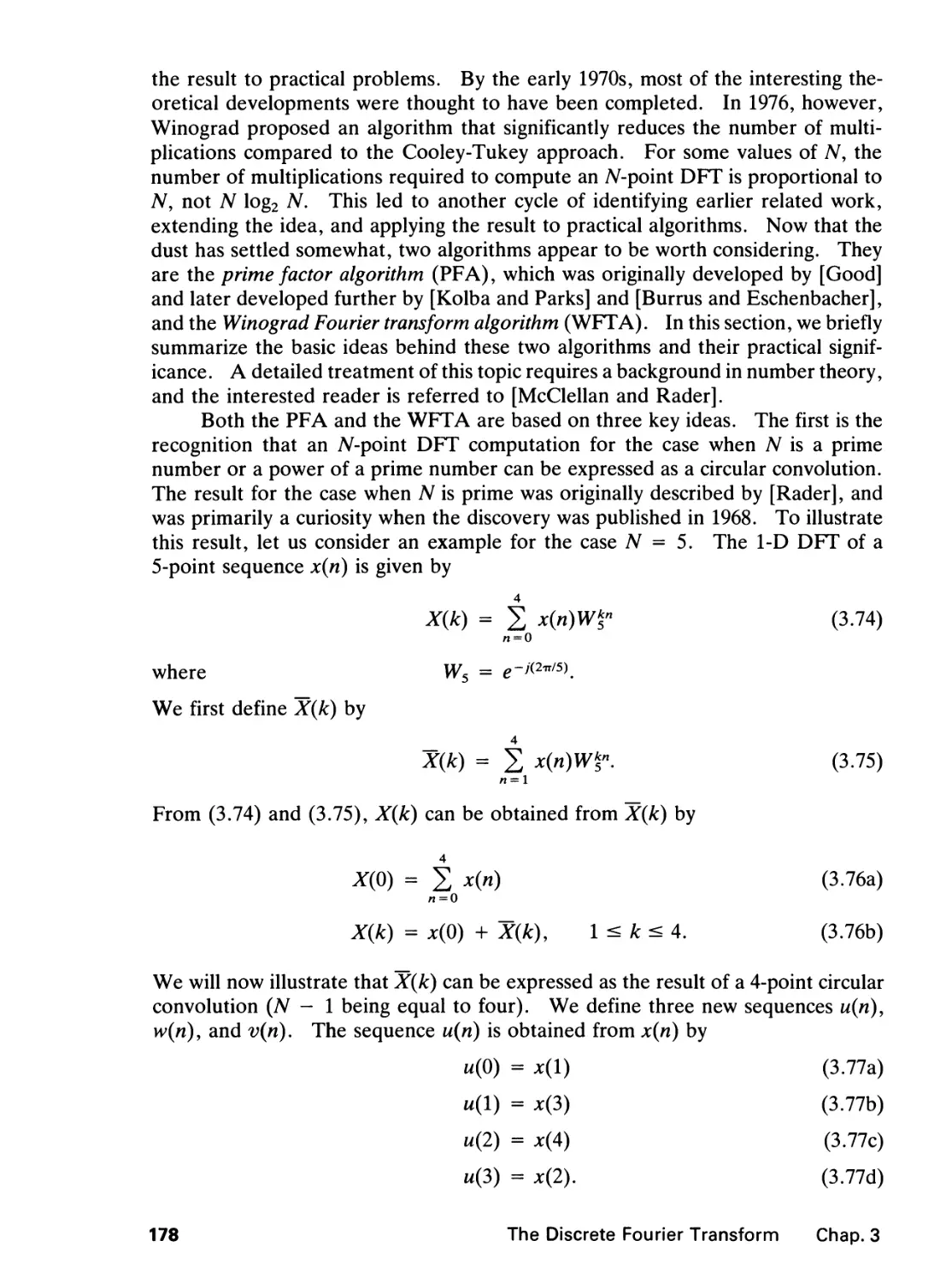
Sec. 1.2 Systems
15
g(kx, k2) shifted in the positive kx and k2 directions by nx and n2 points, respectively.
Figures 1.13(d)—(f) show how to obtain h(nx - ku n2 - k2) as a function of kx
and k2 from h(nu n2) in three steps. It is useful to remember how to obtain
h(nx - kx, n2 - k2) directly from h(nu n2). One simple way is to first change
the variables nx and n2 to kx and k2, flip the sequence with respect to the origin,
and then shift the result in the positive kx and k2 directions by nx and n2 points,
respectively. Once x(ku k2) and h(nx - kx, n2 - k2) are obtained, they can be
multiplied and summed over kx and k2 to produce the output at each different
value of (nly n2). The result is shown in Figure 1.13(g).
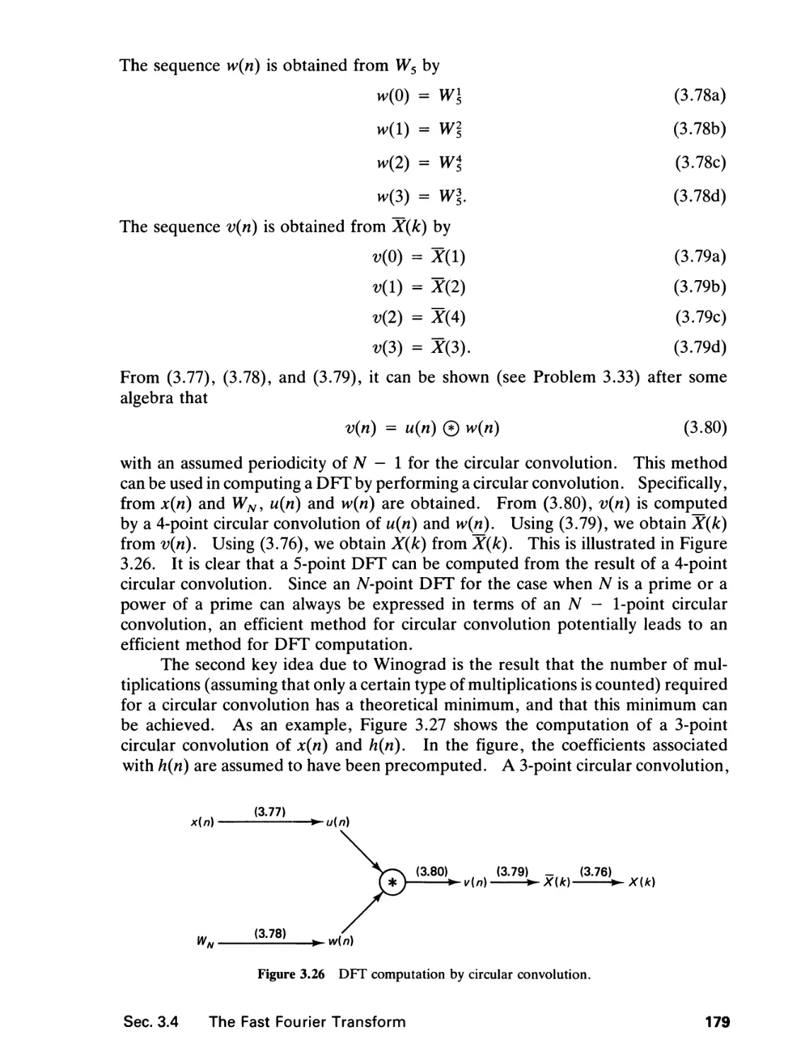
An LSI system is said to be separable, if its impulse response h(nx, n2) is a
separable sequence. For a separable system, it is possible to reduce the number
of arithmetic operations required to compute the convolution sum. For large
amounts of data, as typically found in images, the computational reduction can be
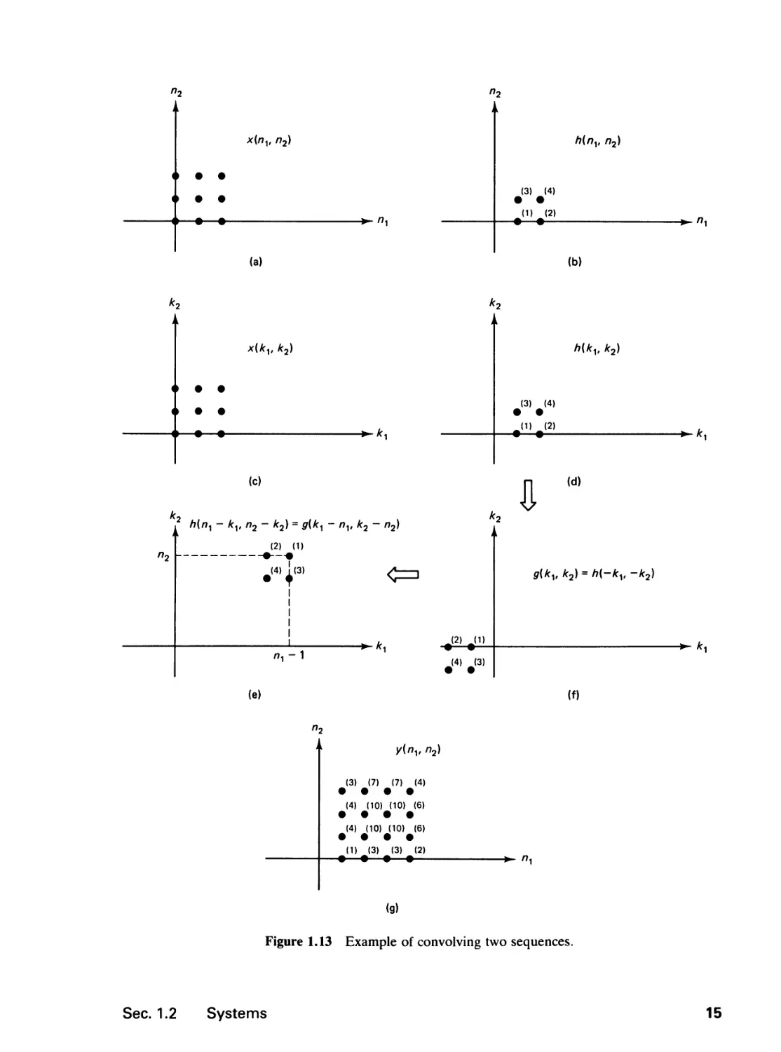
considerable. To illustrate this, consider an input sequence x(nx, n2) of N x N
points and an impulse response h(nx, n2) of M x M points:
x(nu ni) = 0 outside 0 < nx < N - 1, 0 < n2 < N - 1 n 23^
and h(nu n2) = 0 outside 0 < /ii < Af - 1, 0 < h2 < M - 1
where N » M in typical cases. The regions of (nu n2) where x(nx, n2) and
h(nx, n2) can have nonzero amplitudes are shown in Figures 1.14(a) and (b). The
output of the system, y{nu n2), can be expressed as
y(nu n2) = x(nl9 n2) * h(nu n2)
= 22 x(ku k2)h(nx - kun2 - k2).
k\ = — 3C kl= — OC
The region of (nx, n2) where y(nl9 n2) has nonzero amplitude is shown in Figure
1.14(c). If (1.24) is used directly to compute y(nx, n2), approximately (N + M
- \)2M2 arithmetic operations (one arithmetic operation = one multiplication and
one addition) are required since the number of nonzero output points is (N + M
- I)2 and computing each output point requires approximately M2 arithmetic
operations. If h(nx, n2) is a separable sequence, it can be expressed as
h(nl9 n2) = hx(nx)h2(n2)
hx(nx) = 0 outside 0 < nx < M - 1 (1.25)
h2(n2) = 0 outside 0 < n2 < M - 1.
From (1.24) and (1.25),
DC DC
y(nu n2) = 2 2 *(ki> ki)hi(ni - kx)h2(n2
k\ = — ac ki= -^
OC DC
= 2 M»l - *l) 2 *(*1. ^2)^2("2
^, = -OC k2= ~X
k2)
k2).
(1.26)
16 Signals, Systems, and the Fourier Transform Chap. 1
(/v-D
x[nv n2)
(M-1)
h(nv n2)
m
0 (M-1)
(b)
-►"1
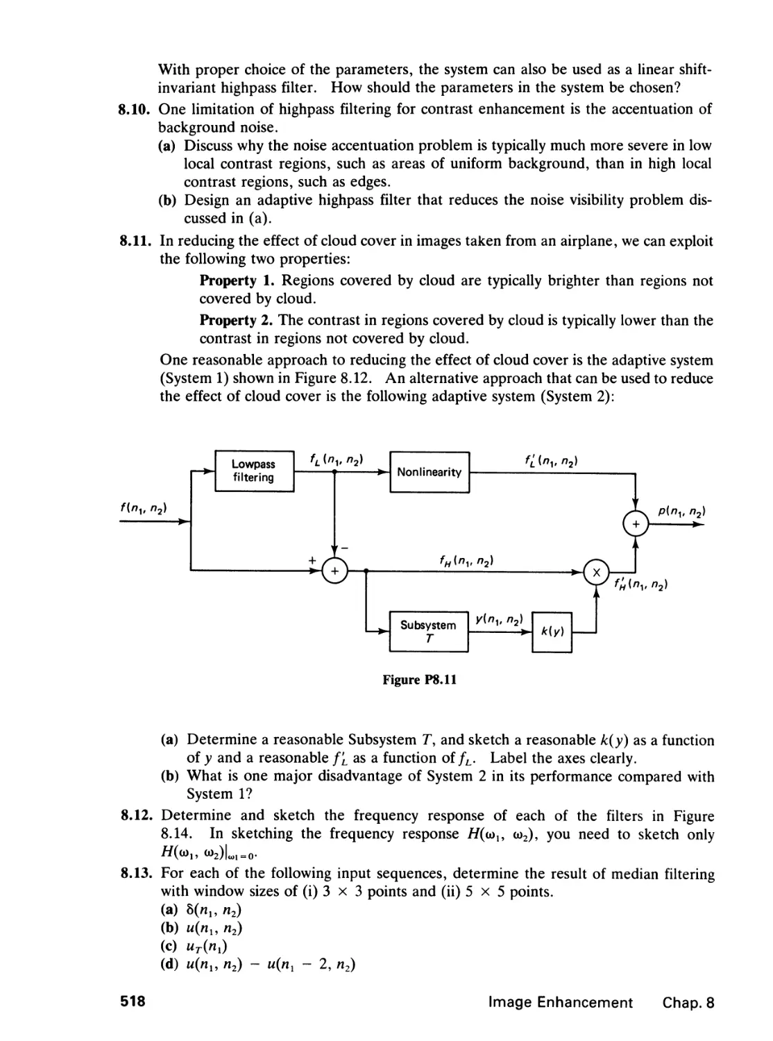
(N + M -2)
/(",, "2) = x^1» ^2) *^(^V ^2^
Figure 1.14 Regions of (/i,, w2) where x^, rc2), /i^, n2), and >>(«,, w2)
x^, n2) * ^(«!, w2) can have nonzero amplitude.
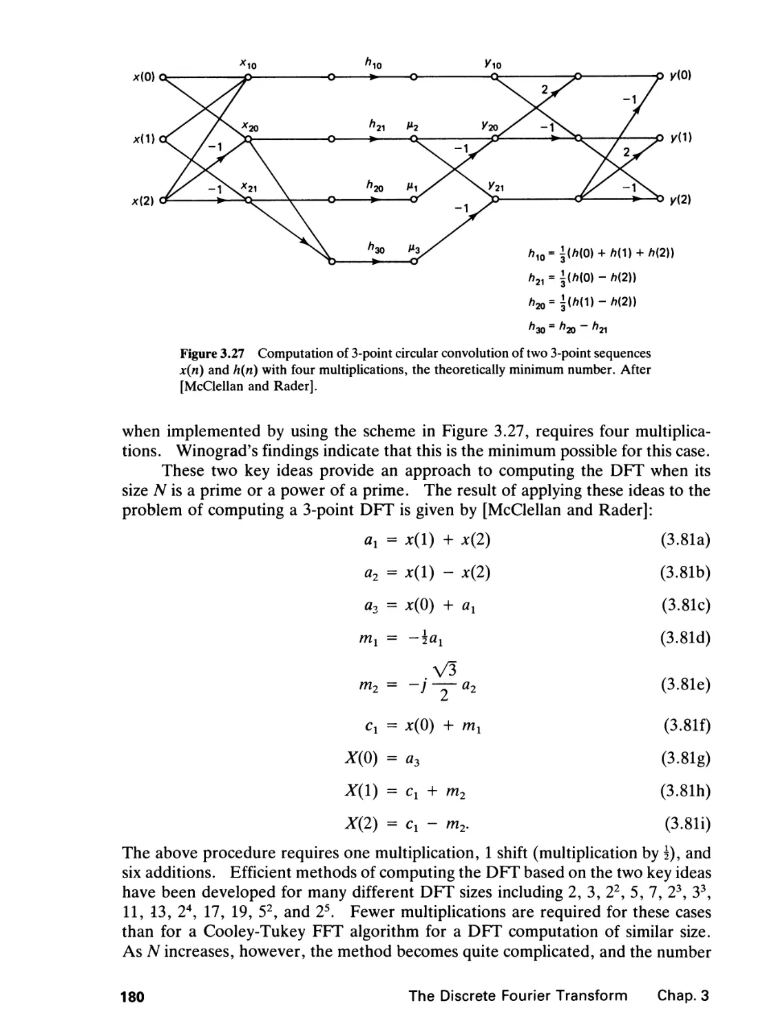
For a fixed kly 2£2=-oc x(ku k2)h2(n2 ~~ k2) in (1.26) is a 1-D convolution of
*(&!, n2) and h2(n2). For example, using the notation
/(&!, /i2) = 2 *(*i> ^2)^2(^2 ~ k2),
ki= — ac
(1.27)
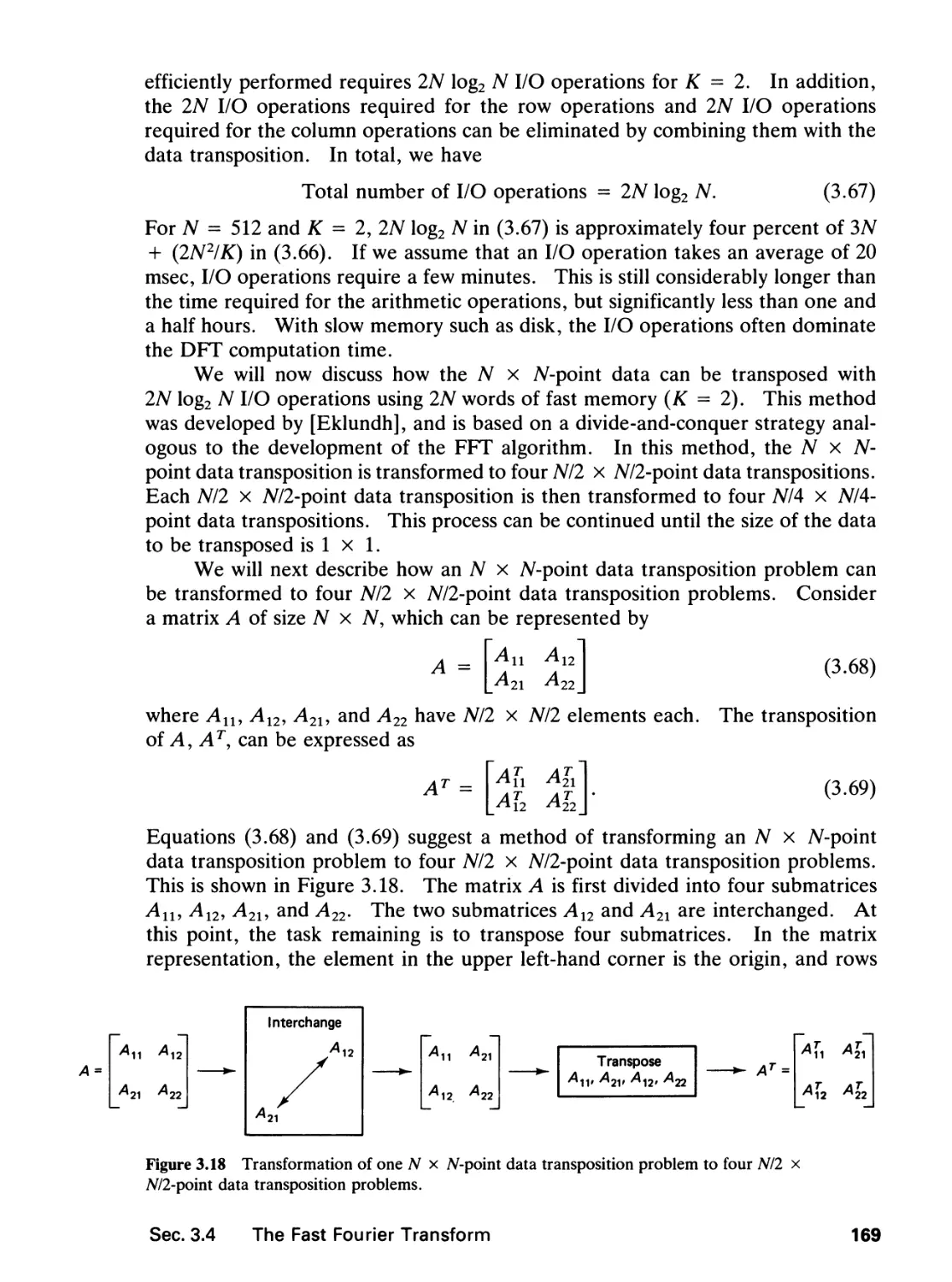
/(0, h2) is the result of 1-D convolution of x(0, h2) with h2(n2), as shown in Figure
1.15. Since there are N different values of kx for which x(ku k2) is nonzero,
computing f(ku n2) requires N 1-D convolutions and therefore requires
approximately NM(N + M - 1) arithmetic operations. Once f(ku n2) is computed,
y(ni> ni) can be computed from (1.26) and (1.27) by
y(nl9 n2) = 2 *i(»i ~ *i)/(*i, n2).
(1.28)
From (1.28), for a fixed n2, y(n1, n2) is a 1-D convolution of h^n^ and f(n1, n2).
For example, y(nu 1) is the result of a 1-D convolution of f(nu 1) and h^n^,
as shown in Figure 1.15, where/(nl9 n2) is obtained from f(ku n2) by a simple
Sec. 1.2 Systems
17
(/v-D
x(0, n2)
xiri), n2)
{N + M -2)
Column-wise
convolution
AT.
<*>
4
(/V-1)
/>,(/>,)
H
MO, n2)
f{ky, n2)
^7
M - 1
-►"1
0 M -1
_► n2
{N + M -2)
f{nv\)
(/V-1)
-►*i
<*>
Row-wise
convolution
i
2
• • • • • /("1'1)
(/V + M-2)
Figure 1.15 Convolution of x(nly n2) with a separable sequence /i(/i,, «2).
change of variables. Since there are N + M — 1 different values of h2>
computing y(nu n2) from f(ku n2) requires N + M - \ 1-D convolutions thus
approximately M(N + M - l)2 arithmetic operations. Computing y{nu n2) from
(1.27) and (1.28), exploiting the separability of h(nu n2), requires approximately
NM(N + M — 1) + M(N + M - l)2 arithmetic operations. This can be a
considerable computational saving over (N + M - \)2M2. If we assume N » M,
exploiting the separability of h{nu n2) reduces the number of arithmetic operations
by approximately a factor of Mil.
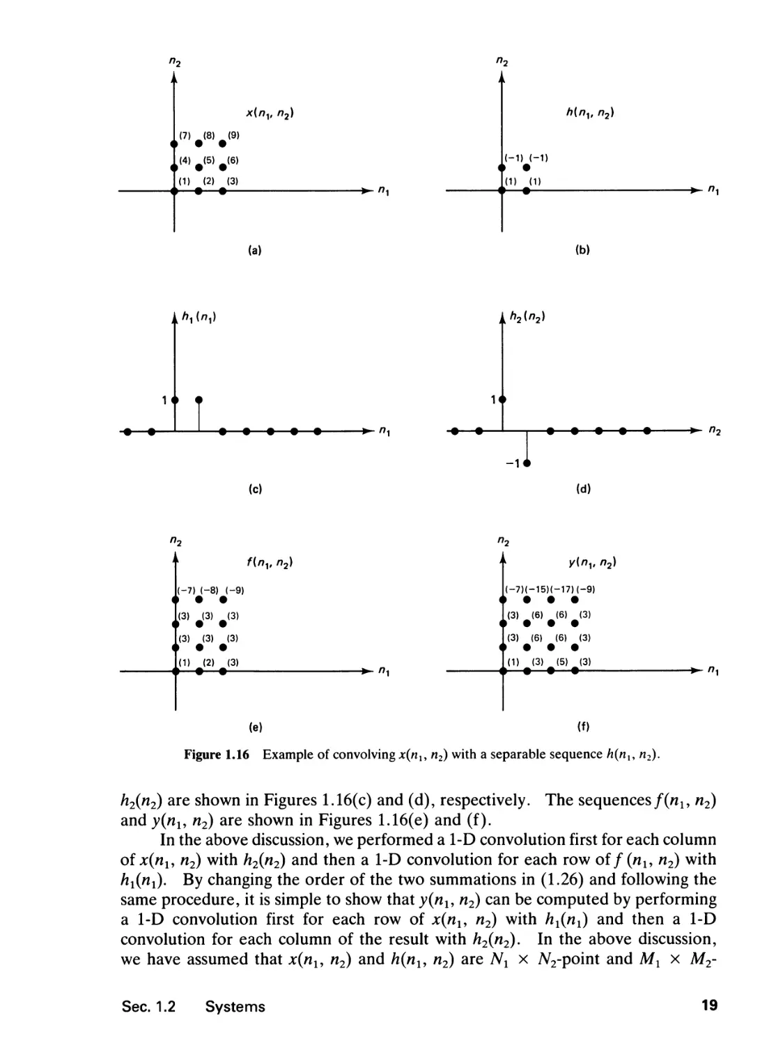
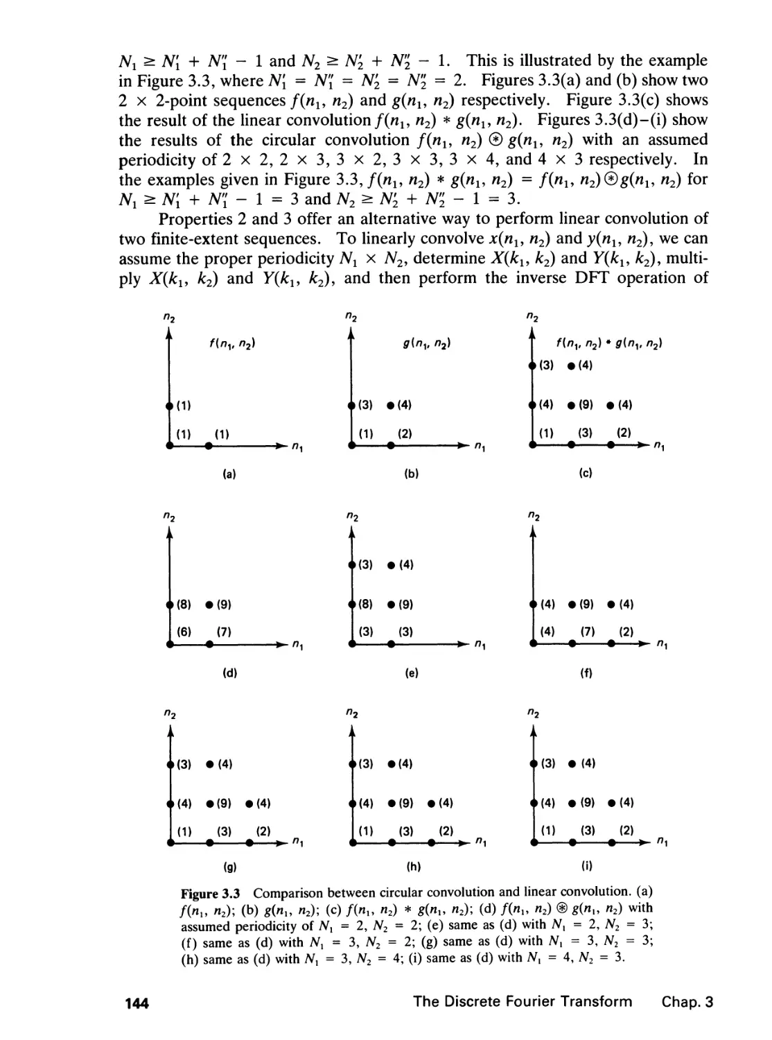
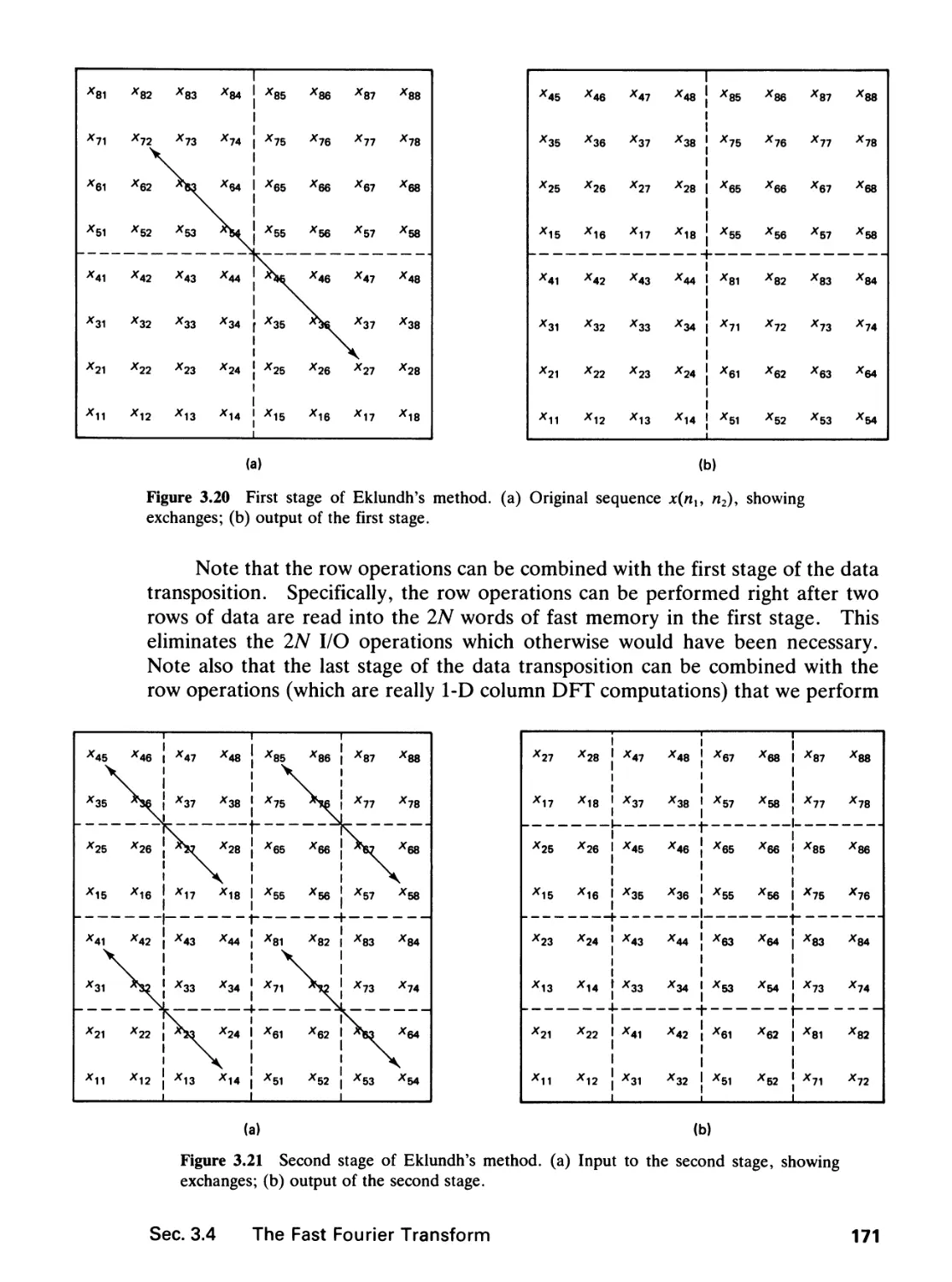
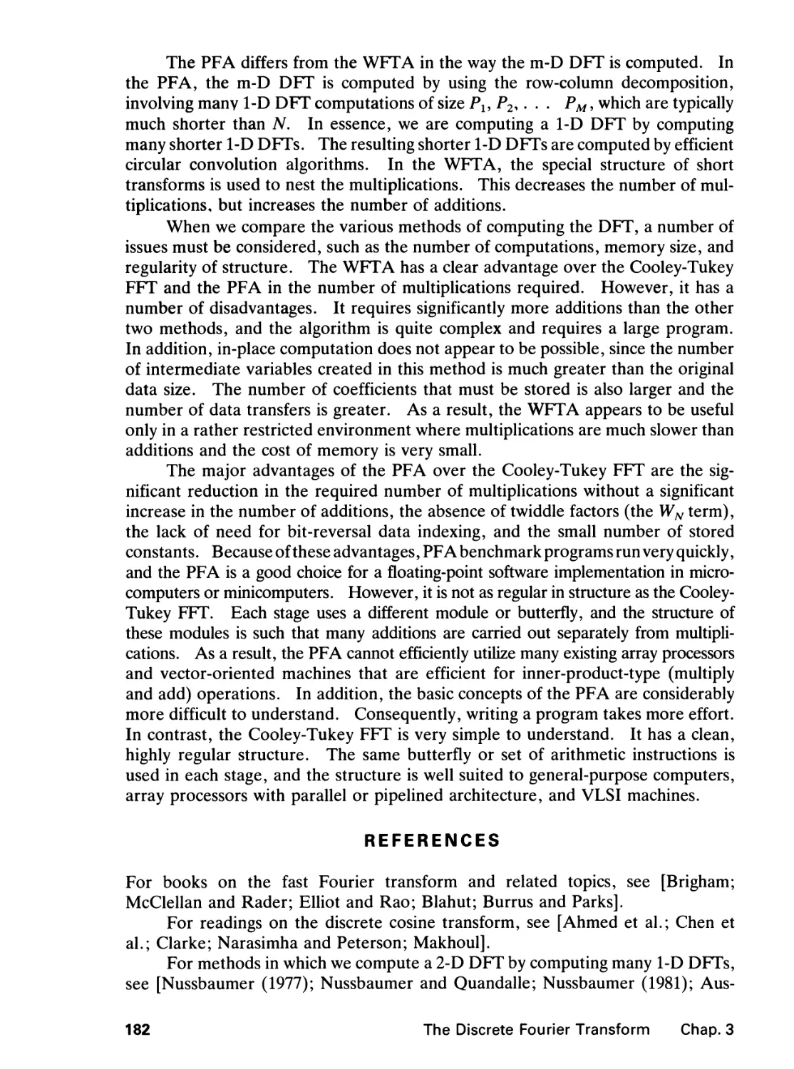
As an example, consider x(nx, n2) and h(nu n2), shown in Figures 1.16(a) and
(b). The sequence h(nl, n2) can be expressed as ^1(^1)^2(^2)* where h^n^ and
18
Signals, Systems, and the Fourier Transform Chap. 1
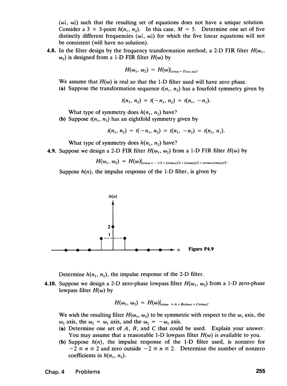
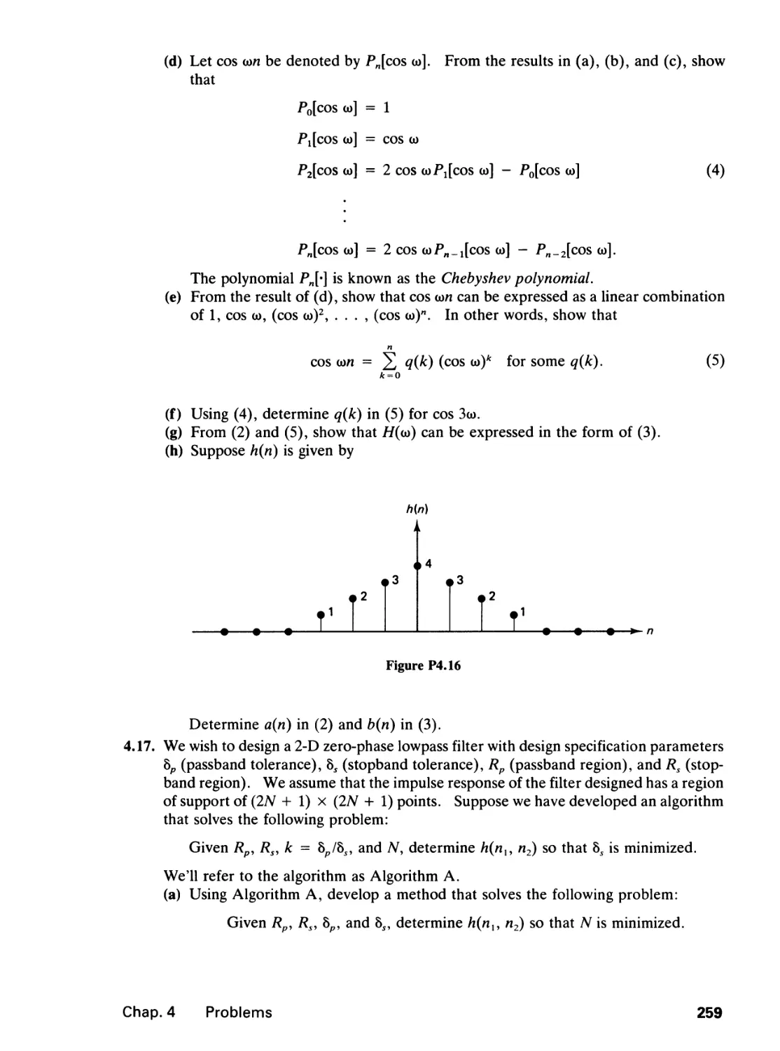
n
2
T
x(nv n2)
1(7) (8) (9)
T #
<
^(4) #(5) #(6)
(1) (2) (3)
T
l(-D (-D
4 •
(D d)
h{nv n2)
(a)
(b)
|M"i>
1*
1 h2{n2)
(0
-1*
(d)
->► n2
n
i
(
i
i
2
f(n,
(-7) (-8) (-9)
> • •
(3) (3) (3)
(3) (3) (3)
> • •
(1) (2) (3)
, n2)
y(nv n2)
(-7)(-15)(-17)(-9)
• • •
(3) (6) (6) (3)
• • •
(3) (6) (6) (3)
• • •
(1) (3) (5) (3)
i • • •
(e) (f)
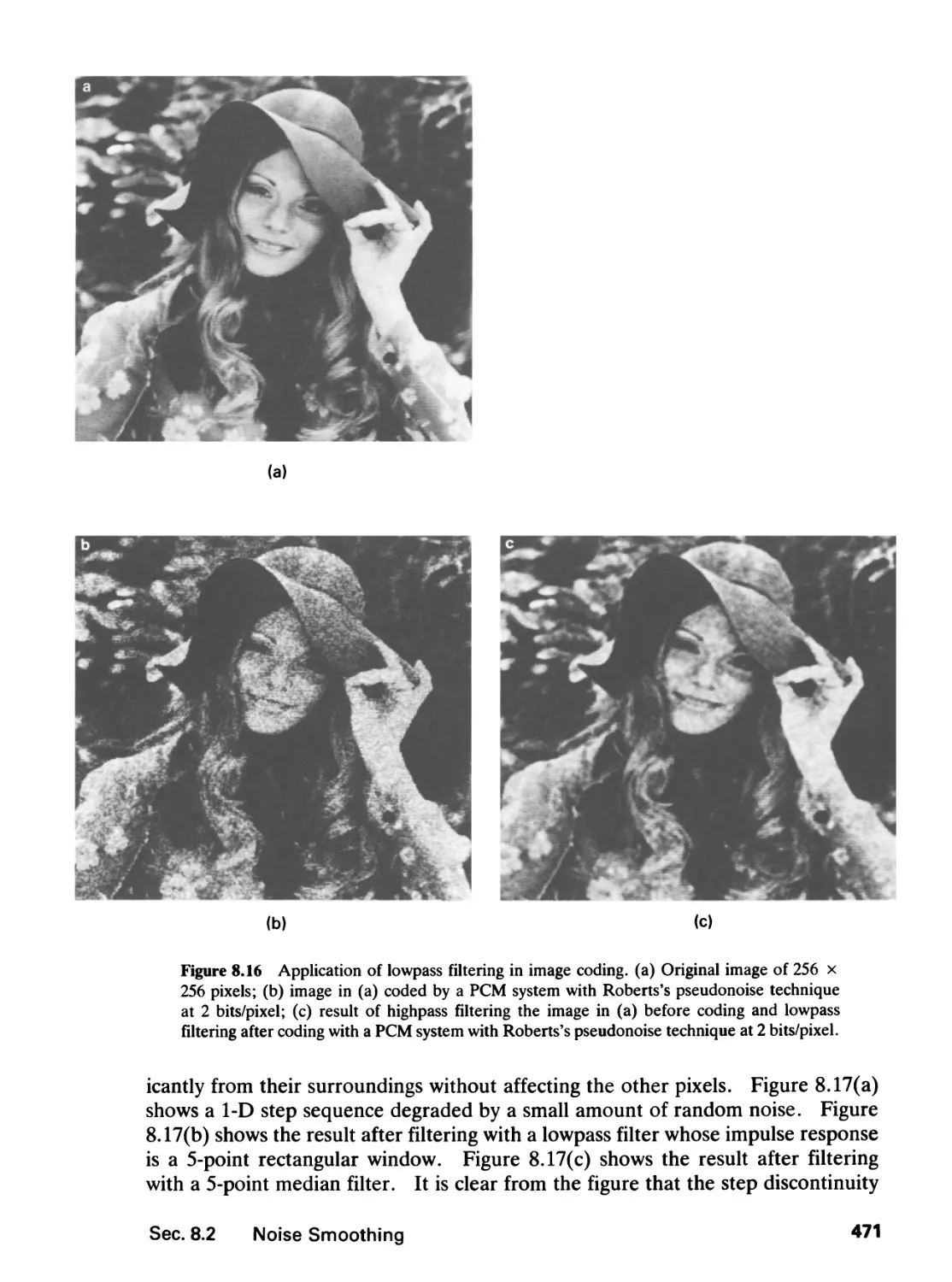
Figure 1.16 Example of convolving x{nu n2) with a separable sequence h(nu n2).
h2(n2) are shown in Figures 1.16(c) and (d), respectively. The sequences f(nly n2)
and y(nly n2) are shown in Figures 1.16(e) and (f).
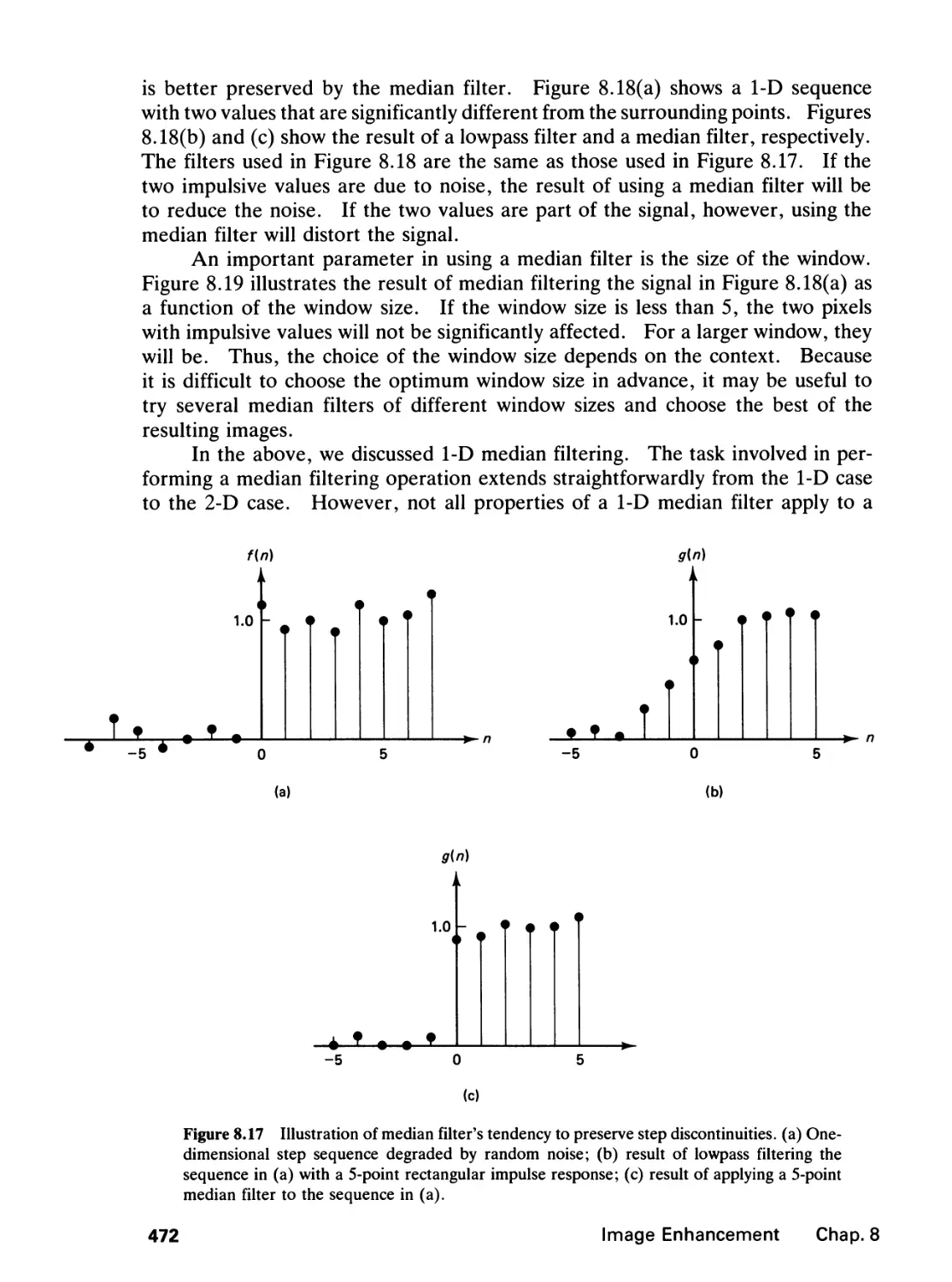
In the above discussion, we performed a 1-D convolution first for each column
of x(nu n2) with h2(n2) and then a 1-D convolution for each row oif(nly n2) with
h^n^. By changing the order of the two summations in (1.26) and following the
same procedure, it is simple to show that y{nu n2) can be computed by performing
a 1-D convolution first for each row of x{nu n2) with h^n^ and then a 1-D
convolution for each column of the result with h2(n2). In the above discussion,
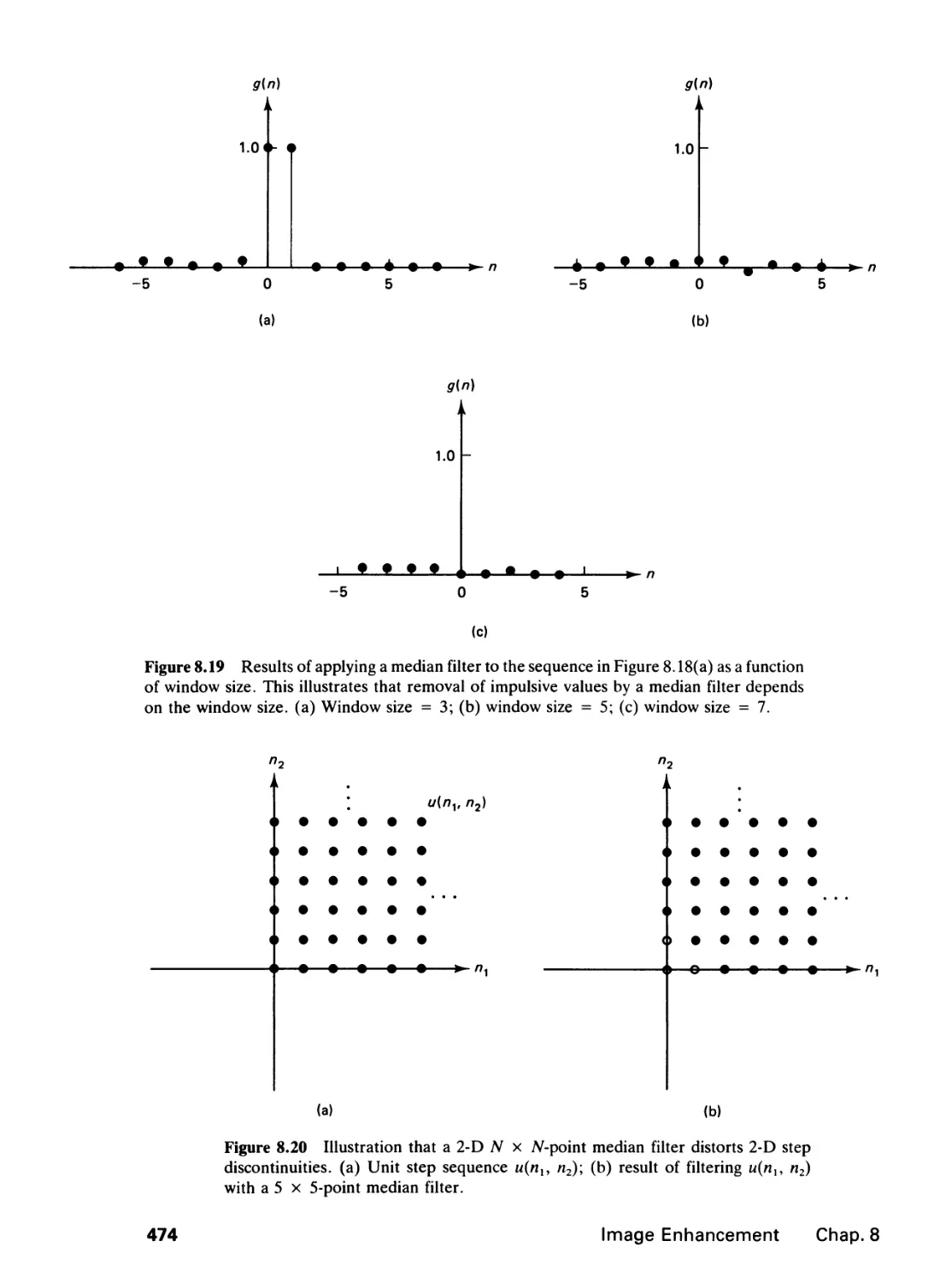
we have assumed that x(nu n2) and h(nl, n2) are Nx x N2-point and Mx x M2-
Sec. 1.2 Systems
19
point sequences respectively with Nx = N2 and Mx-M2. We note that the results
discussed above can be generalized straightforwardly to the case when NY + N2
and M1 ± M2.
1.2.3 Stable Systems and Special Support Systems
For practical reasons, it is often appropriate to impose additional constraints on
the class of systems we consider. Stable systems and special support systems have
such constraints.
Stable systems. A system is considered stable in the bounded-input-
bounded-output (BIBO) sense if and only if a bounded input always leads to a
bounded output. Stability is often a desirable constraint to impose, since an
unstable system can generate an unbounded output, which can cause system
overload or other difficulties. From this definition and (1.18), it can be shown that a
necessary and sufficient condition for an LSI system to be stable is that its impulse
response h(nu n2) be absolutely summable:
DC DC
Stability of an LSI system <=> 2 2 ^("i, n2)\ < °°. (129)
All = — 3C AI2= - x
Although (1.29) is a straightforward extension of 1-D results, 2-D systems differ
greatly from 1-D systems when a system's stability is tested. This will be discussed
further in Section 2.3. Because of (1.29), an absolutely summable sequence is
defined to be a stable sequence. Using this definition, a necessary and sufficient
condition for an LSI system to be stable is that its impulse response be a stable
sequence.
Special support systems. A 1-D system is said to be causal if and only
if the current output y(n) does not depend on any future values of the input, for
example, x(n + l),x(n + 2),x(n + 3), . . . . Using this definition, we can show
that a necessary and sufficient condition for a 1-D LSI system to be causal is that
its impulse response h(n) be zero for n < 0. Causality is often a desirable constraint
to impose in designing 1-D systems. A noncausal system would require delay,
which is undesirable in such applications as real time speech processing. In typical
2-D signal processing applications such as image processing, the causality constraint
may not be necessary. At any given time, a complete frame of an image may be
available for processing, and it may be processed from left to right, from top to
bottom, or in any direction one chooses. Although the notion of causality may
not be useful in 2-D signal processing, it is useful to extend the notion that a 1-D
causal LSI system has an impulse response h(n) whose nonzero values lie in a
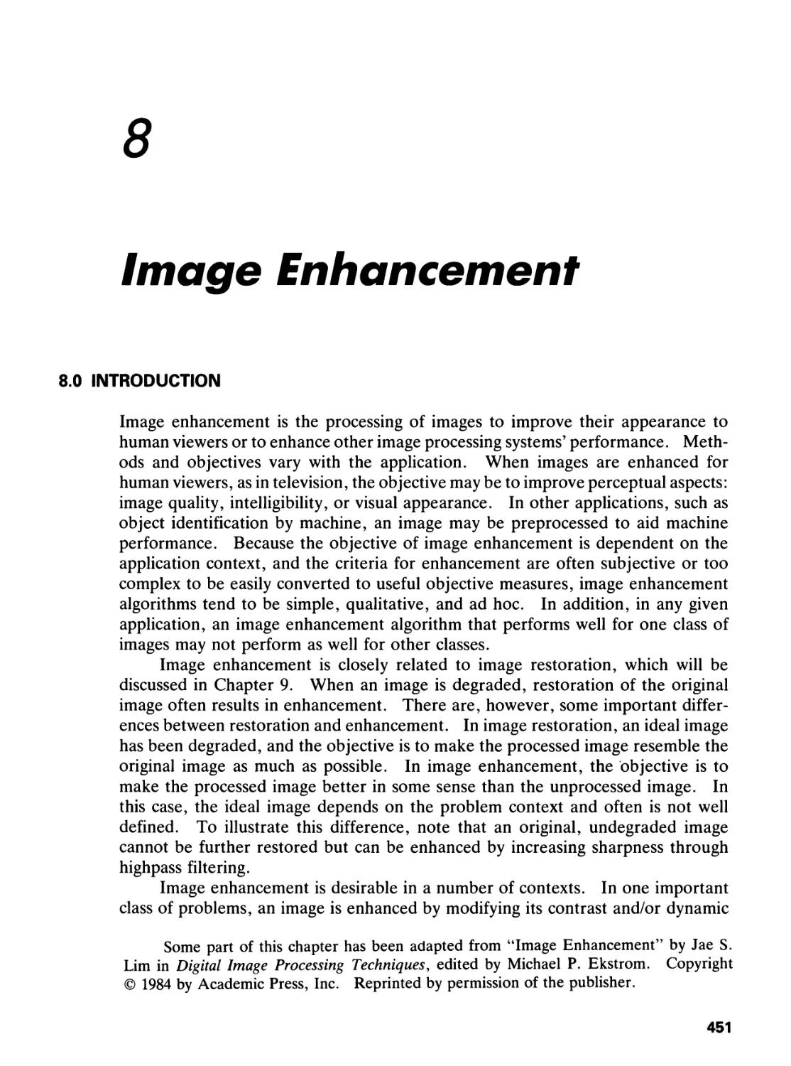
particular region. A 2-D LSI system whose impulse response h(nl, n2) has all its
nonzero values in a particular region is called a special support system.
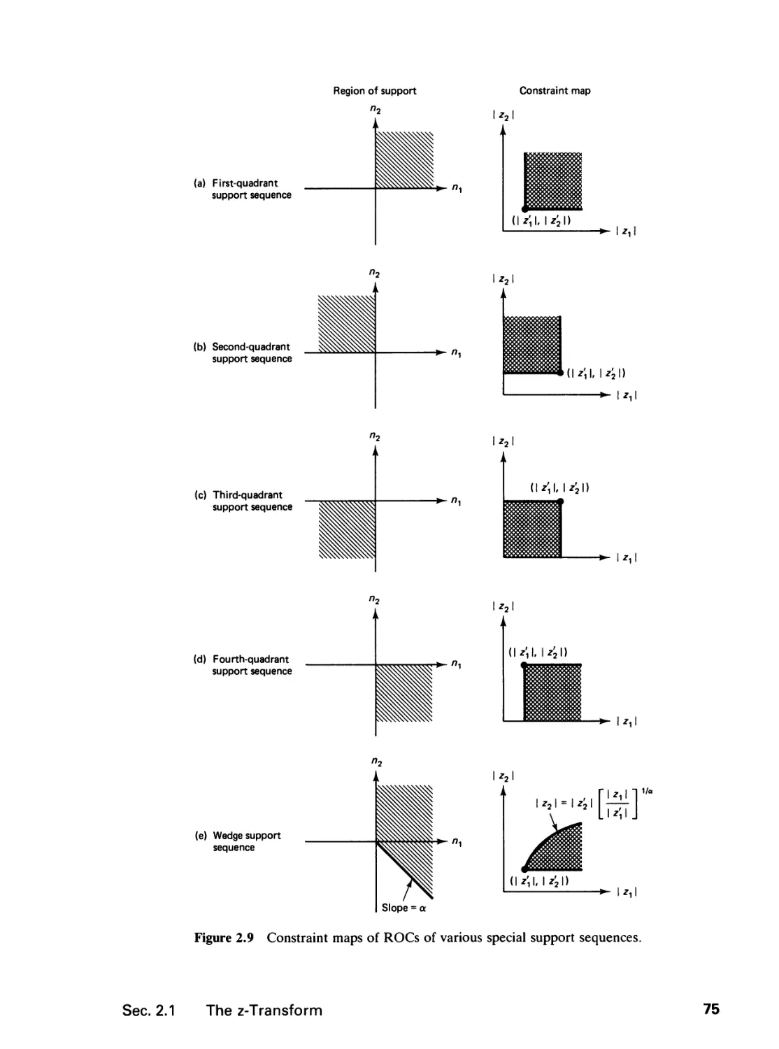
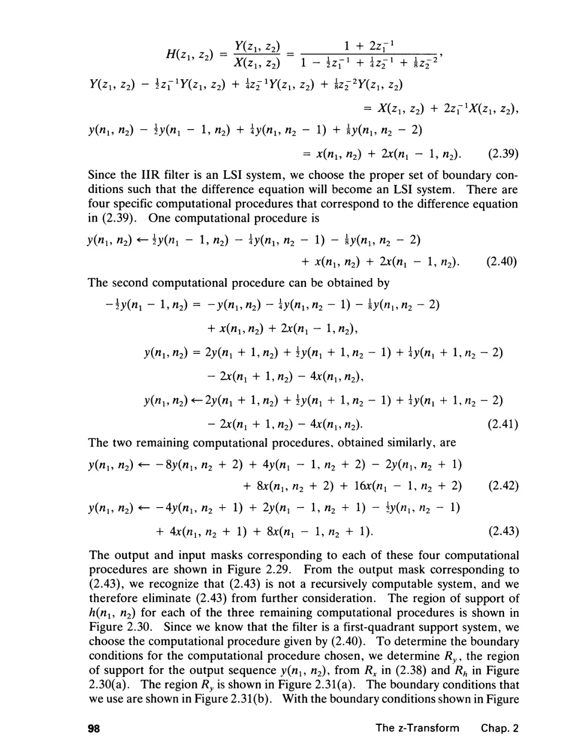
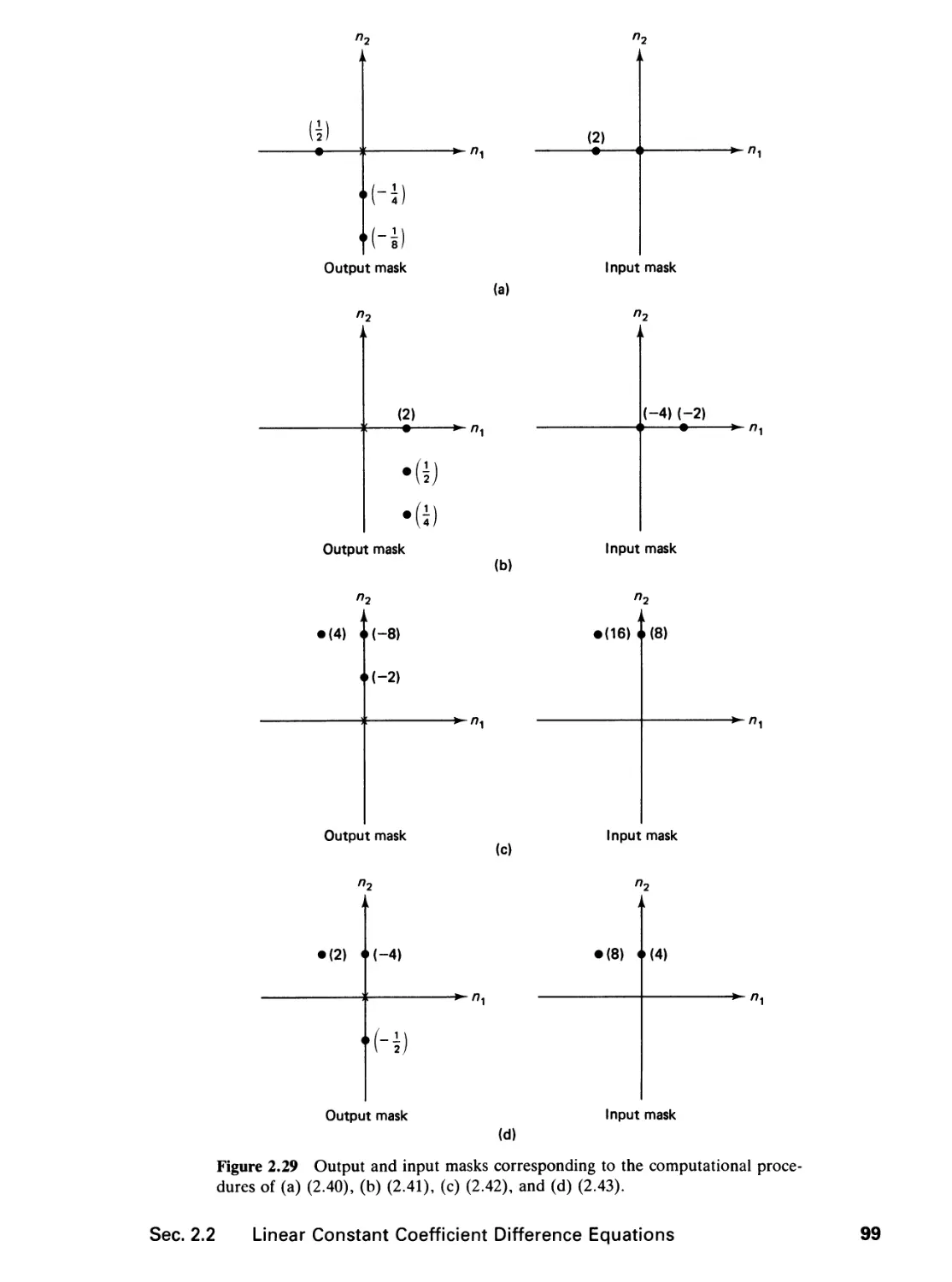
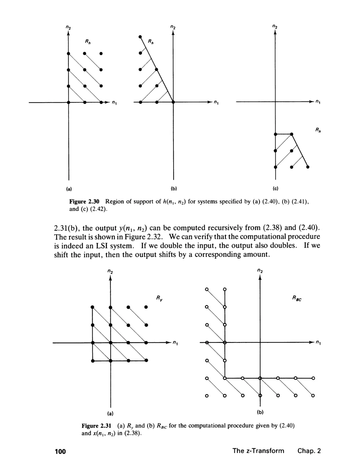
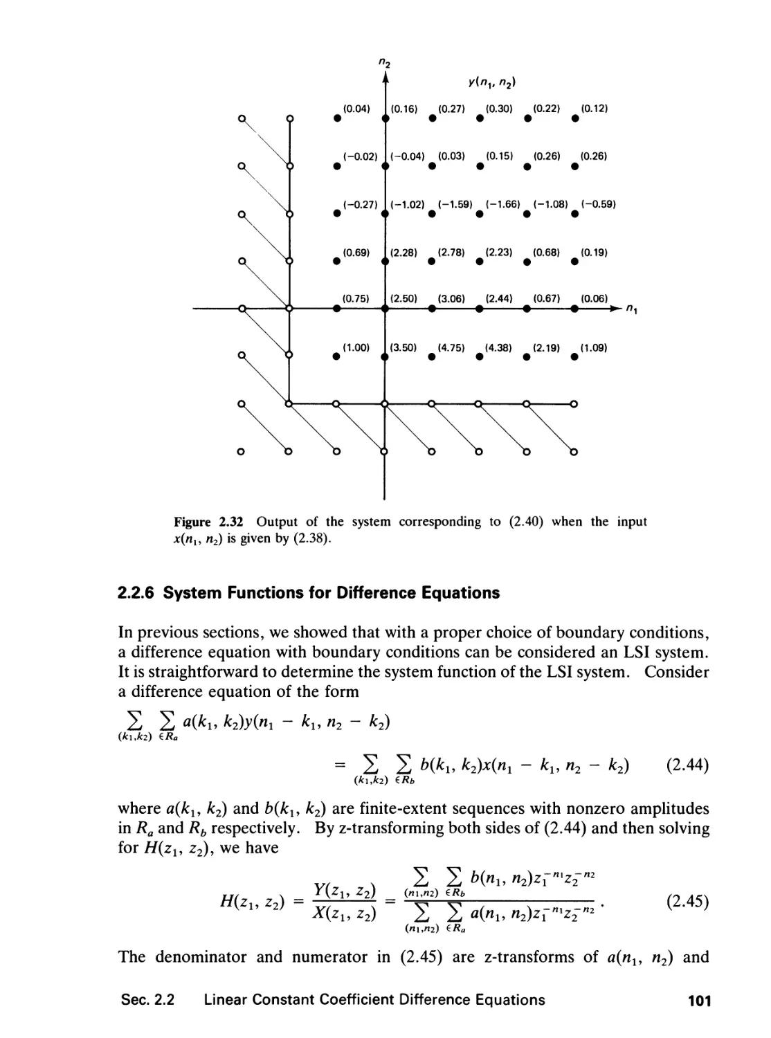
A 2-D LSI system is said to be a quadrant support system when its impulse
response h{nly n2) is a quadrant support sequence. A quadrant support sequence,
or a quadrant sequence for short, is one which has all its nonzero values in one
20 Signals, Systems, and the Fourier Transform Chap. 1
quadrant. An example of a first-quadrant support sequence is the unit step
sequence u(nu n2).
A 2-D LSI system is said to be a wedge support system when its impulse
response h(nly n2) is a wedge support sequence. Consider two lines emanating
from the origin. If all the nonzero values in a sequence lie in the region bounded
by these two lines, and the angle between the two lines is less than 180°, the
sequence is called a wedge support sequence, or a wedge sequence for short. An
example of a wedge support sequence x(nx, n2) is shown in Figure 1.17.
Quadrant support sequences and wedge support sequences are closely related.
A quadrant support sequence is always a wedge support sequence. In addition,
it can be shown that any wedge support sequence can always be mapped to a first-
quadrant support sequence by a linear mapping of variables without affecting its
stability. To illustrate this, consider the wedge support sequence x(nu n2) shown
in Figure 1.17. Suppose we obtain a new sequence y(nu n2) from x{nl, n2) by the
following linear mapping of variables:
(1.30)
where the integers lu /2, /3, and /4 are chosen to be 1, 0, -1 and 1 respectively.
The sequence y(nly n2) obtained by using (1.30) is shown in Figure 1.18, and is
clearly a first-quadrant support sequence. In addition, the stability of x(nu n2) is
equivalent to the stability of y{nu n2), since
OC OC DC DC
2 2 l*Oi> "2)1 = 2 2 \y("i> n2)\-
n\=-^n2=-yz n\ = —*. ni= —x
j(5) •(6) m(7) •(8) «(9)
1(4) •(5) •(6) m{7) •(8)
1(3) «(4) «(5) •(6) «(7)
1(2) «(3) «(4) •($) •(6) -.
1(1) (2) (3) (4) (5)
+ • • —• • > ny
• (1) *(2) •(3) •(4)
• (1) «(2) «(3)
• (1) m(2)
• (1) Figure 1.17 Example of a wedge sup-
I port sequence.
Sec. 1.2 Systems
21
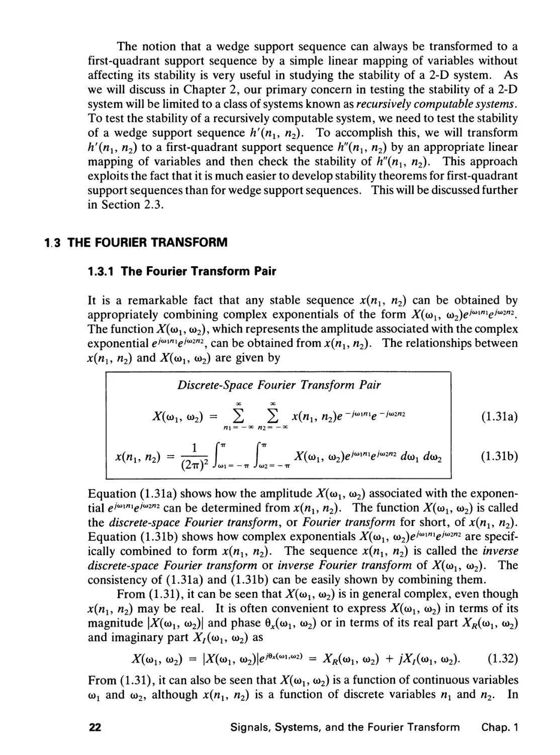
The notion that a wedge support sequence can always be transformed to a
first-quadrant support sequence by a simple linear mapping of variables without
affecting its stability is very useful in studying the stability of a 2-D system. As
we will discuss in Chapter 2, our primary concern in testing the stability of a 2-D
system will be limited to a class of systems known as recursively computable systems.
To test the stability of a recursively computable system, we need to test the stability
of a wedge support sequence h'(nl9 n2). To accomplish this, we will transform
h'(nl9 n2) to a first-quadrant support sequence h"(nl9 n2) by an appropriate linear
mapping of variables and then check the stability of h"(nl9 n2). This approach
exploits the fact that it is much easier to develop stability theorems for first-quadrant
support sequences than for wedge support sequences. This will be discussed further
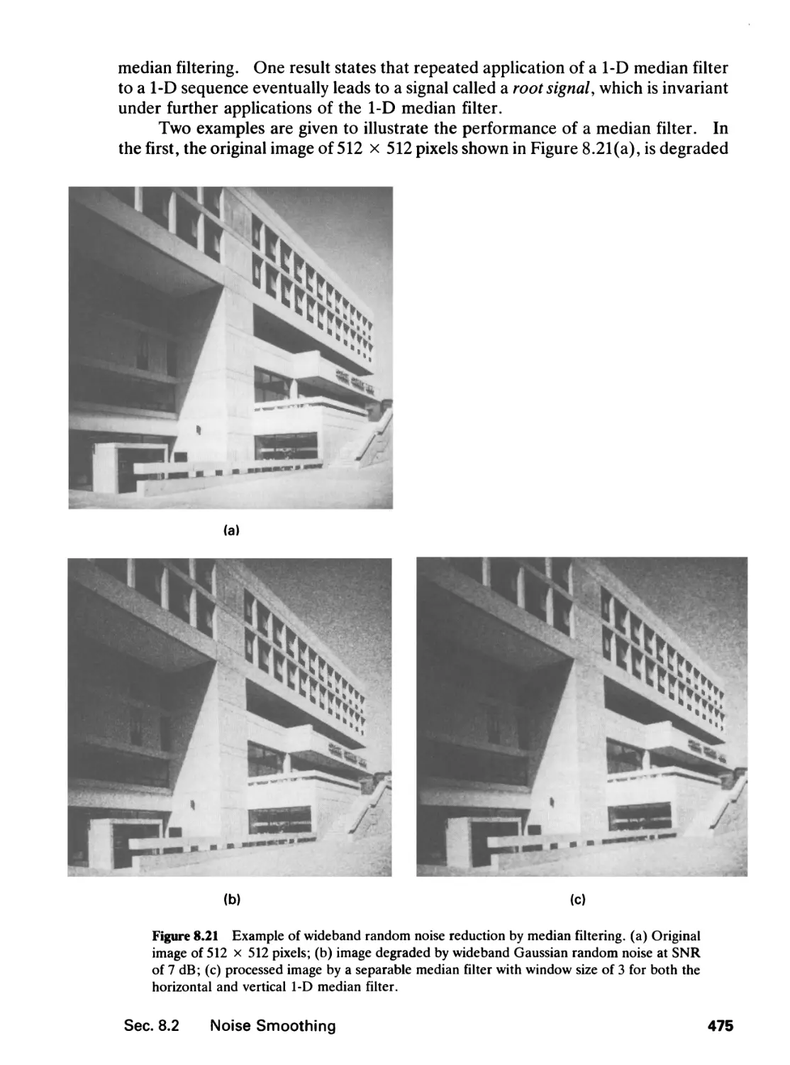
in Section 2.3.
13 THE FOURIER TRANSFORM
1.3.1 The Fourier Transform Pair
It is a remarkable fact that any stable sequence x(nu n2) can be obtained by
appropriately combining complex exponentials of the form X(u>l9 oi2)ejmnieJ<x>2n2.
The function X(u>l9 <o2), which represents the amplitude associated with the complex
exponential eJoiinieJoi2rt2, can be obtained from x{nu n2). The relationships between
x(nl9 n2) and X(o>l9 <o2) are given by
x(n1
X(<*
n2) =
Discrete-Spaa
1. W2>
1
(2*)2
oc
= 2
n\= -
f
= — TT
? Fourier Transform Pair
oc
* m= —
f
Jb>2= —
x(nl9 n2)e
X((jily (ji2)e
TX
joi\n\p -jb>2ri2
jmnieJo>2n2 ^
doy2
Equation (1.31a) shows how the amplitude X((jily co2) associated with the
exponential eJOiW1eJoi2n2 can be determined from x(nl9 n2). The function X(o}u co2) is called
the discrete-space Fourier transform, or Fourier transform for short, of x{nu n2).
Equation (1.31b) shows how complex exponentials X(u>u u>2)eiu>inieJu>2rt2 are
specifically combined to form x(nu n2). The sequence x(nu n2) is called the inverse
discrete-space Fourier transform or inverse Fourier transform of X(o>!, co2). The
consistency of (1.31a) and (1.31b) can be easily shown by combining them.
From (1.31), it can be seen that X(o>u <o2) is in general complex, even though
x(nu n2) may be real. It is often convenient to express X((ox, co2) in terms of its
magnitude \X(u>l, <o2)| and phase B^o)!, <o2) or in terms of its real part XR(u>u co2)
and imaginary part XI(o}l, co2) as
X(<ol9 <o2) = \X(ul9 (o2)|e^-^) = XR(ul9 <o2) + jXji^ co2). (1.32)
From (1.31), it can also be seen that X(u>l, <o2) is a function of continuous variables
(*>! and co2, although x(nl9 n2) is a function of discrete variables nx and n2. In
22
Signals, Systems, and the Fourier Transform Chap. 1
y(ny, n2)
♦ (5) • [*) •(5) •($) • ($)
4)
f(3) «(3) •(3) • O) #(3)
f(2) «(2) •(2) «(2) •(2)
(1) (D (D (D (D
• • • •—►"!
Figure 1.18 First-quadrant support
sequence obtained from the wedge
support sequence in Figure 1.17 by linear
mapping of variables.
addition, X((au <o2) is always periodic with a period of 2tt x 2tt; that is, X((au <o2) =
X(o>! + 2tt, co2) = X{iou <o2 + 2tt) for all a^ and co2. We can also show that the
Fourier transform converges uniformly for stable sequences. The Fourier
transform of x(nu n2) is said to converge uniformly when X((ou <o2) is finite and
lim lim ^ 2 x(ni> n2)e-J'mnie-J(x>2n2 = ^(<*>i, <o2) for all o^ and <o2.
TVj^oc Afe-** „1= _a^i n2= -N2
(1.33)
When the Fourier transform of x(/*i, fl2) converges uniformly, X(<a1, <o2) is an
analytic function and is infinitely differentiable with respect to u>l and co2.
A sequence x(nly n2) is said to be an eigenfunction of a system T if T[x(nly n2)]
= fac(n!, n2) for some scalar A:. Suppose we use a complex exponential
ejmnieju>2n2 as an jnpUt x(nl9 n2) to an LSI system with impulse response h(nu n2).
The output of the system y(nu n2) can be obtained as
OC OC
Aci = — ac £2 = — 3=
OC OC
= E E h(ku k2)e^l^-k^eJ'^n2-k2)
ki = — » A:2= — ^
OC OC
= 2 E Kku k^e-'»lkxe->'»2k2e>'»inie>v»n2
k\ = — » A:2 = — ^
= //(wj, w2)e/u,""e;a>2'
(1.34)
Sec. 1.3 The Fourier Transform
23
From (1.34), eJ<x>inieiu>2n2 is an eigenfunction of any LSI system for which //(<*>!, <o2)
is well defined and //(<*>!, <o2) is the Fourier transform of h(nu n2). The function
//(<*>!, <o2) is called the frequency response of the LSI system. The fact that
ej<*iniej<*2m js an eigenfunction of an LSI system and that H(<au <o2) is the scaling
factor by which eJ'mnieJ<x>2n2 is multiplied when it is an input to the LSI system
simplifies system analysis for a sinusoidal input. For example, the output of an LSI
system with frequency response //(<*>!, <o2) when the input is cos ((jy[n1 + <o2h2) can
be obtained as follows:
r[cos((oi«1 + o>2n2)] = T
+
2 2
= ^T[ei<x>iniej0i2n2] + jT[e~Ju>inie~J<x>2rt2] (1.35)
= 5//(o>;, <a£e'°inie'°*n2 + iH(-o>[, -ti£)e->t»'inie->to2n2.
1.3.2 Properties
We can derive a number of useful properties from the Fourier transform pair in
(1.31). Some of the more important properties, often useful in practice, are listed
in Table 1.1. Most are essentially straightforward extensions of 1-D Fourier
transform properties. The only exception is Property 4, which applies to separable
sequences. If a 2-D sequence x(nu n2) can be written as x1(nl)x2(n2), then its
Fourier transform, Xfa, <o2), is given by Ar1((o1)Ar2((o2), where X^ta^ and X2(<a2)
represent the 1-D Fourier transforms oix^nj and x2(n2), respectively. This
property follows directly from the Fourier transform pair of (1.31). Note that this
property is quite different from Property 3, the multiplication property. In the
multiplication property, bo\hx(nly n2) andy(«1? n2) are 2-D sequences. In Property
4, xx{nx) and x2(n2) are 1-D sequences, and their product x1(nl)x2(n2) forms a 2-D
sequence.
1.3.3 Examples
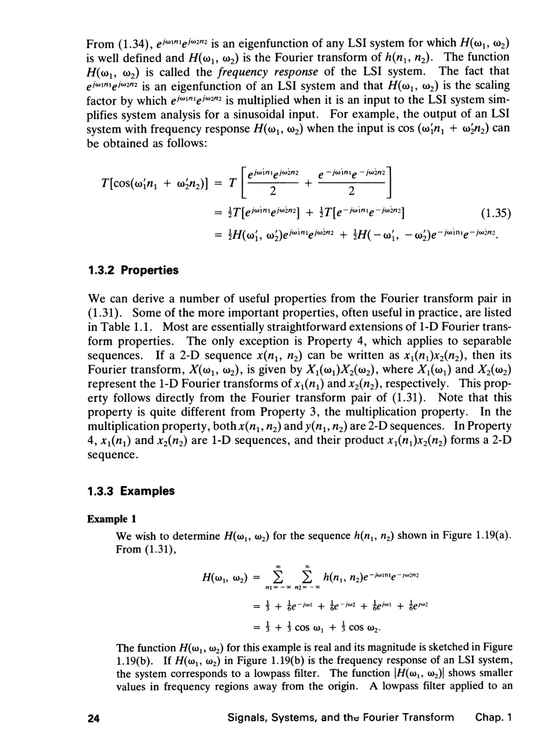
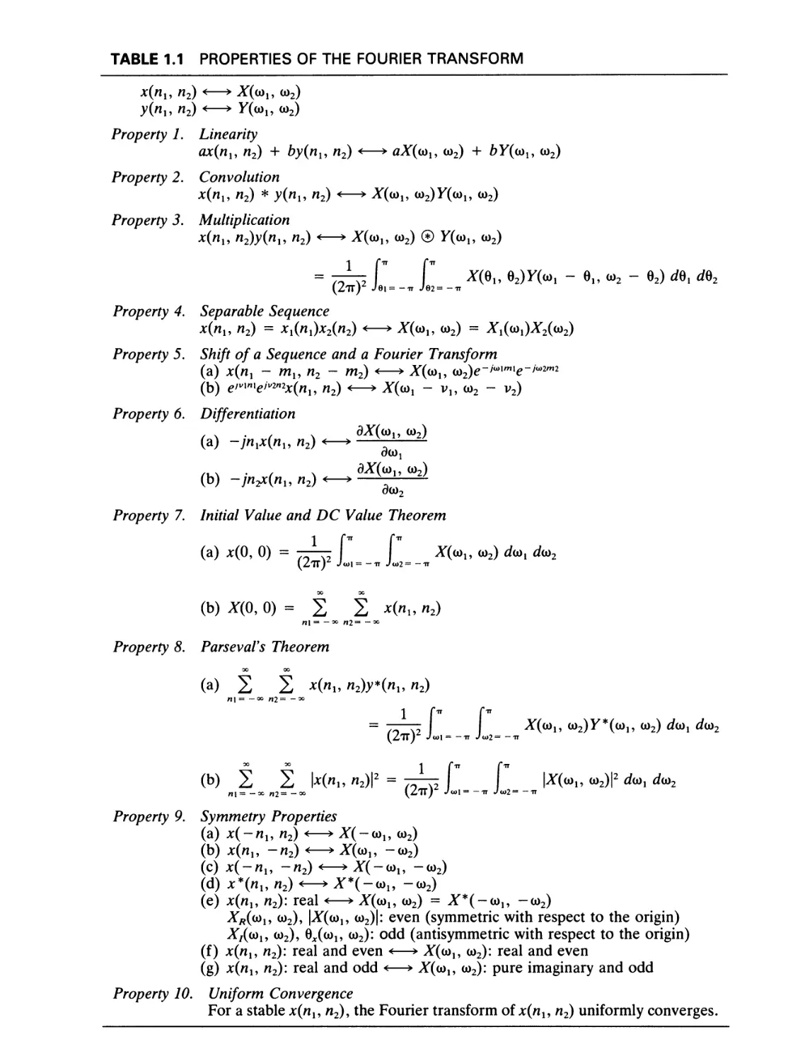
Example 1
We wish to determine //(cdj, oo2) for the sequence h(nu n2) shown in Figure 1.19(a).
From (1.31),
//(a>„ cd2) = X E h(nu n2)e-Jnxnle-^2n2
ni= -» n2= -»
= J + he-**1 + he-*1*2 + he*** + ze>"2
= 3 + 3 COS CDj + 5 COS C02.
The function H(<aly cd2) for this example is real and its magnitude is sketched in Figure
1.19(b). If //(a)!, oo2) in Figure 1.19(b) is the frequency response of an LSI system,
the system corresponds to a lowpass filter. The function |//(a>j, oo2)| shows smaller
values in frequency regions away from the origin. A lowpass filter applied to an
24
Signals, Systems, and the Fourier Transform Chap. 1
TABLE 1.1 PROPERTIES OF THE FOURIER TRANSFORM
x(nu n2) <—> X(o)ly o)2)
y{nu n2) <—> Y^, o>2)
Property 1. Linearity
ax{nx, n2) + by(nx, n2) <—> aX((ou cd2) + bY(ayu cd2)
Property 2. Convolution
x(nu n2) * y(nx, n2) <—> X((ou <aJY(<au a>2)
Property 3. Multiplication
x(nu n2)y(nl9 n2) <—> X((ou o>2) © Y((ou o>2)
= 7TV2 f f X^ e2)y(wi " e» ^ ~ 0^) d*> dQ2
(ITT) J9l= -it J62= -it
Property 4. Separable Sequence
x(nu n2) = ^(nO-^Oh) <—► *(«,, cd2) = ^(0)0^2(0)2)
Property 5. Shift of a Sequence and a Fourier Transform
(a) *(/i, - mx, n2 - m2) <—> X(tol9 ^e-j<axmxe-i<a2m2
(b) e>vlnle>v2n2x(nu n2) <—> X^ - v„ cd2 - v2)
Property 6. Differentiation
/ \ • / \ ^(CO!, fa>2)
(a) -]nxx(nu n2) <—>
00)!
(b) -jn^c(nl9 n2) <—>
do>2
Property 7. Initial Value and DC Value Theorem
(a) jc(0, 0) = -i- f" f *(«,, o>2) d(ot rfo)2
\LH) Jo>l= -it Ja>2= -tt
(b) X(0, 0) = i i *(«„ n2)
Hi = —» H2= -30
Property 8. ParsevaVs Theorem
(a) 5) 5) *(*!, /i2)y*(/i1, n2)
n\= -<x> n2= -00
= 7T^ *(wi' ^^"K, o)2) rfo)! do>2
IZTT) Jo>i= -it Jo>2= -it
Property 9. Symmetry Properties
(a) x(-nu n2) <—> X(-uu cd2)
(b) x(nu —n2) <—> X((o^ -cd2)
(c) x(-nu -n2) <—> X(-uu -o>2)
(d) x*(nun2)^^X*(-^ -o>2)
(e) x(nu n2): real <—> X((ou cd2) = AT*(-a>j, -cd2)
A^coi, cd2), |A^(col9 cd2)|: even (symmetric with respect to the origin)
Xf(a)u oo2), B^ooi, cd2): odd (antisymmetric with respect to the origin)
(f) x(nu n2): real and even <—> X(ayu oo2): real and even
(g) x(nly n2): real and odd <—> X(ayu cd2): pure imaginary and odd
Property 10. Uniform Convergence
For a stable x(nx, n2), the Fourier transform of x(nl9 n2) uniformly converges.
h(nv n2)
(J)
(a)
Figure 1.19 (a) 2-D sequence /i(/i,, n2)'y (b) Fourier transform magnitude
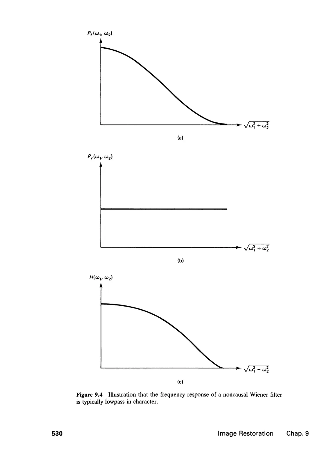
|//(a>!, o>2)| of /i(/i,, n2) in (a).
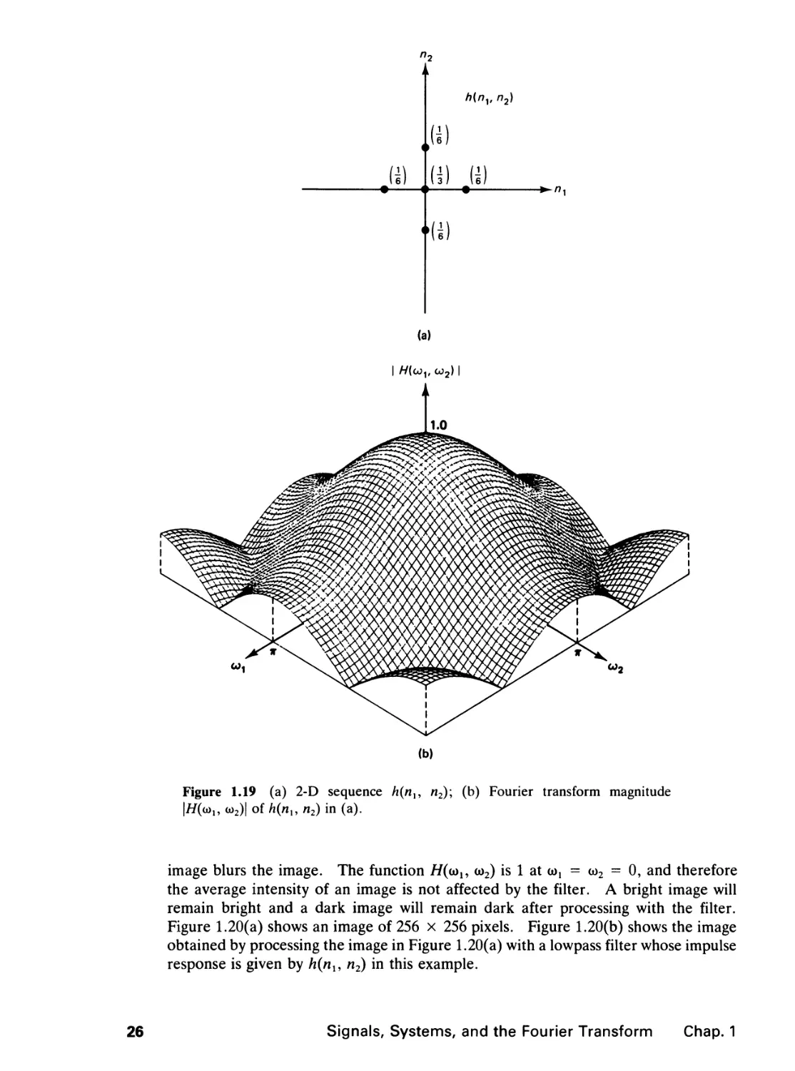
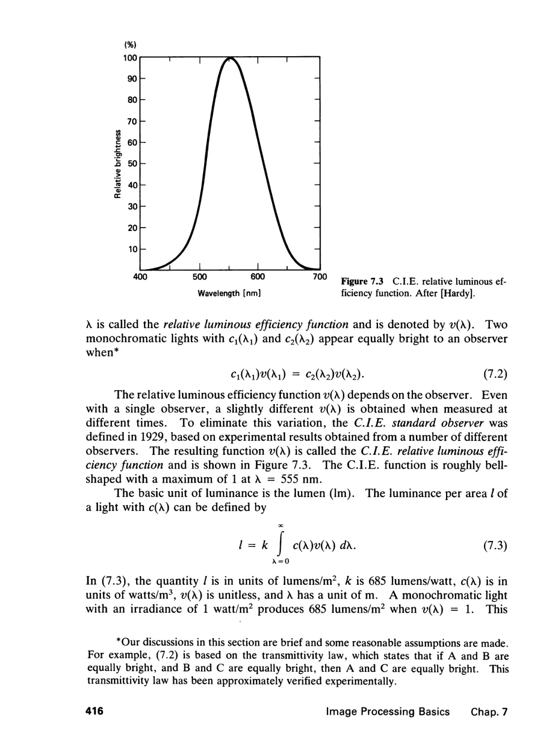
image blurs the image. The function //(u^, cd2) is 1 at coi = w2 = 0, and therefore
the average intensity of an image is not affected by the filter. A bright image will
remain bright and a dark image will remain dark after processing with the filter.
Figure 1.20(a) shows an image of 256 x 256 pixels. Figure 1.20(b) shows the image
obtained by processing the image in Figure 1.20(a) with a lowpass filter whose impulse
response is given by h{nu n2) in this example.
26
Signals, Systems, and the Fourier Transform Chap. 1
(a) (b)
Figure 1.20 (a) Image of 256 x 256 pixels; (b) image processed by filtering the image in
(a) with a lowpass filter whose impulse response is given by /i(n,, n2) in Figure 1.19 (a).
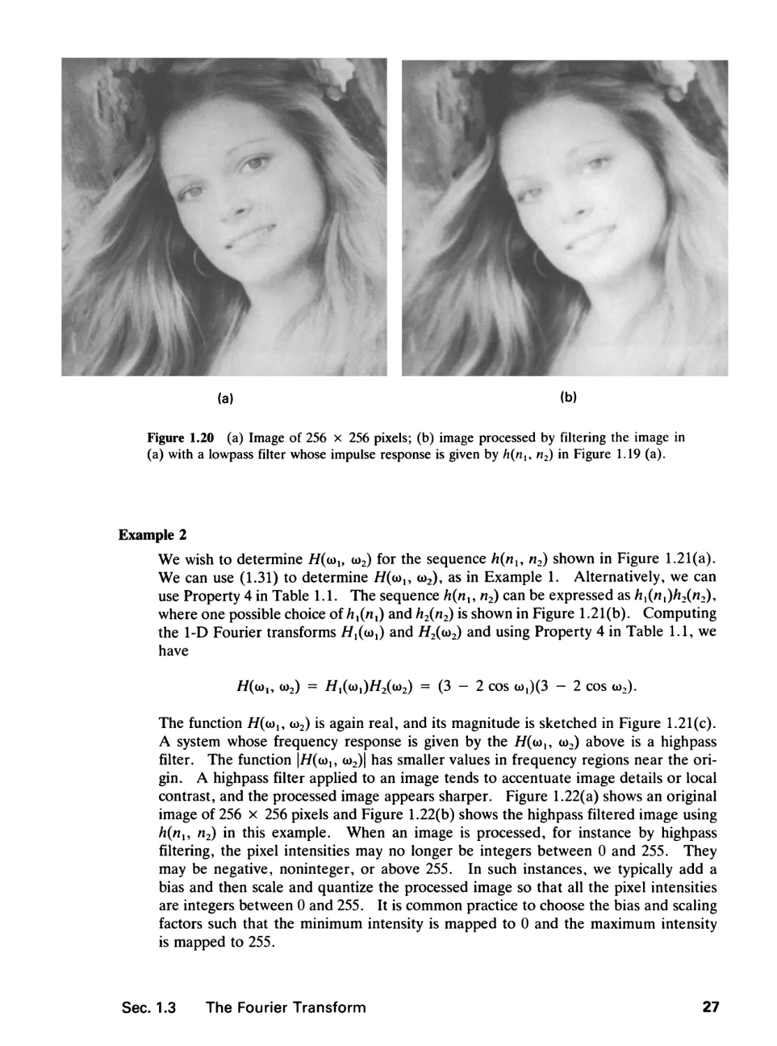
Example 2
We wish to determine //(oo^ o)2) for the sequence h(nu n2) shown in Figure 1.21(a).
We can use (1.31) to determine //(oo^ <o2), as in Example 1. Alternatively, we can
use Property 4 in Table 1.1. The sequence h{nx, n2) can be expressed as hx(n{)h2(n2),
where one possible choice of hx(nx) and h2{n2) is shown in Figure 1.21(b). Computing
the 1-D Fourier transforms //^cdj) and H2((o2) and using Property 4 in Table 1.1, we
have
//((o„ oo2) = 7/1(a)1)//2(a)2) = (3 - 2 cos a),)(3 - 2 cos co2).
The function H(<au a)2) is again real, and its magnitude is sketched in Figure 1.21(c).
A system whose frequency response is given by the //(co,, oo2) above is a highpass
filter. The function \H(<al9 oo2)| has smaller values in frequency regions near the
origin. A highpass filter applied to an image tends to accentuate image details or local
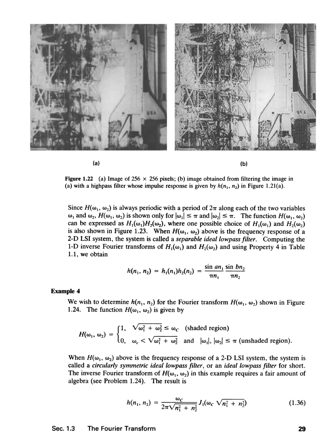
contrast, and the processed image appears sharper. Figure 1.22(a) shows an original
image of 256 x 256 pixels and Figure 1.22(b) shows the highpass filtered image using
h(nu n2) in this example. When an image is processed, for instance by highpass
filtering, the pixel intensities may no longer be integers between 0 and 255. They
may be negative, noninteger, or above 255. In such instances, we typically add a
bias and then scale and quantize the processed image so that all the pixel intensities
are integers between 0 and 255. It is common practice to choose the bias and scaling
factors such that the minimum intensity is mapped to 0 and the maximum intensity
is mapped to 255.
Sec. 1.3 The Fourier Transform
27
31 M»i>
. l«-3).
(-3)
h{ny, n2)
T
~z
-► "1
(9) (-3)
• * • ► n.
• ♦ •
(-3)
(a)
/M"2)
"^^
-►"2
(b)
I H(uv co2) |
(0
Figure 1.21 (a) 2-D sequence h(nu n2)\ (b) possible choice of /i,(/i,) and /i2("2)
where /i(/i,, n2) = hl{nx)h2(n2)\ (c) Fourier transform magnitude |//(u>i, o>2)| of
h{nu n2) in (a).
Example 3
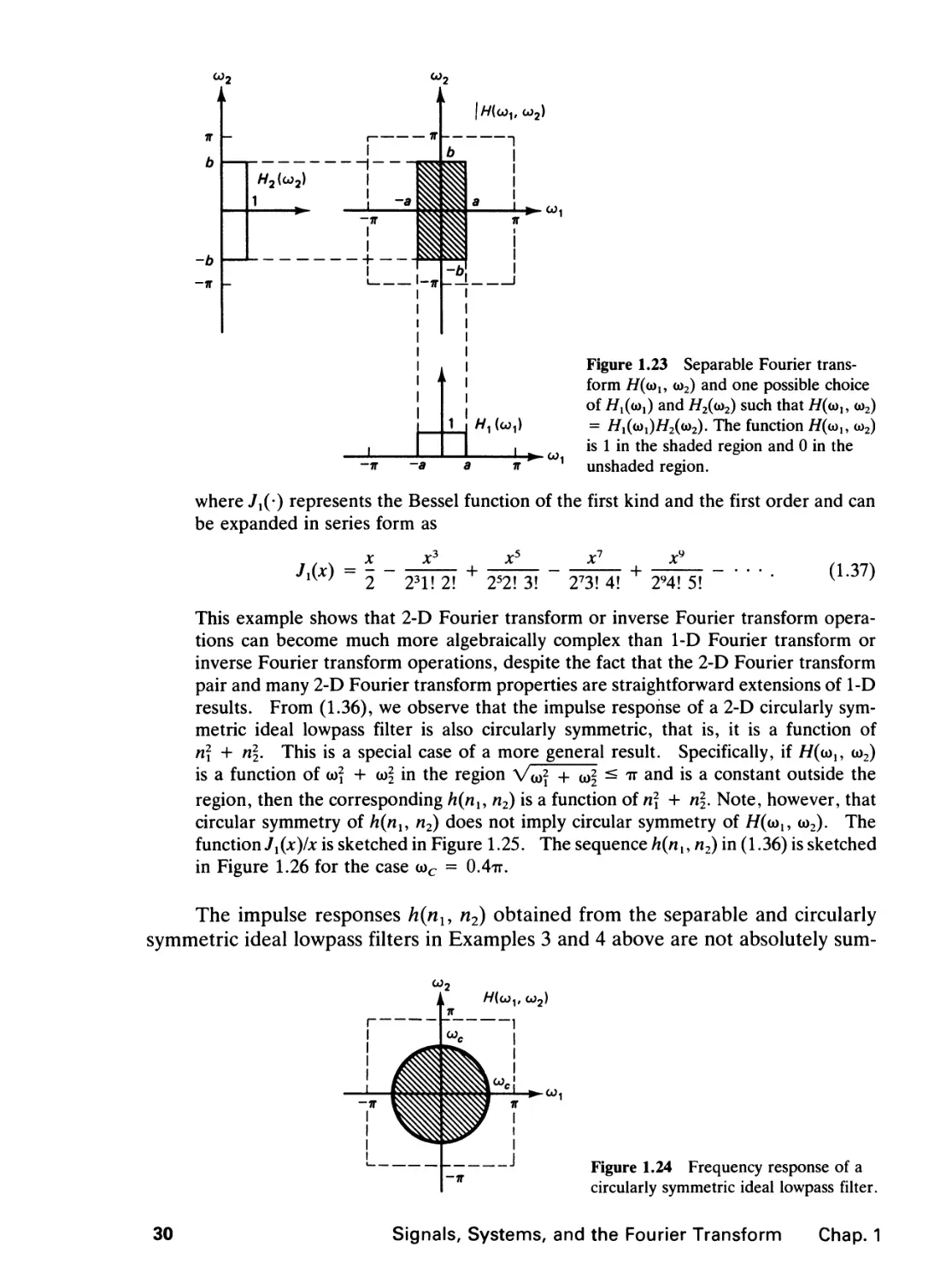
We wish to determine h(nu n2) for the Fourier transform //(co,, u)2) shown in Figure
1.23. The function H(mu oo2) is given by
rl, IcojI ^ 0 and |oo2| < 6 (shaded region)
|co2| ^ 7T (unshaded region).
H(o>
{1, IcdJ < 0 and |oo2| < 6
0, a < |(o,| < it or 6 <
28
Signals, Systems, and the Fourier Transform Chap. 1
"... <I^N •
(Ml" «^» '!
1HA
(a) (b)
Figure 1.22 (a) Image of 256 x 256 pixels; (b) image obtained from filtering the image in
(a) with a highpass filter whose impulse response is given by h(niy n2) in Figure 1.21(a).
Since //(oo,, oo2) is always periodic with a period of 2tt along each of the two variables
co, and co2, //(co,, co2) is shown only for |co,| ^ it and |co2| ^ it. The function //(co,, co2)
can be expressed as //,(oo,)//2(to2), where one possible choice of //,(oo,) and //2(oo2)
is also shown in Figure 1.23. When //(co,, co2) above is the frequency response of a
2-D LSI system, the system is called a separable ideal lowpass filter. Computing the
1-D inverse Fourier transforms of //,(ooi) and //2(oo2) and using Property 4 in Table
1.1, we obtain
sin an, sin frn2
TTrt, TTW2
Example 4
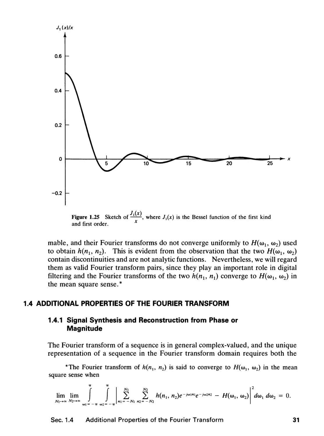
We wish to determine h(nu n2) for the Fourier transform //(cd,, go2) shown in Figure
1.24. The function //(oo,, oo2) is given by
fl, V<of + co^ < coc (shaded region)
//(oo,, cd2)
ri, Vcd? + cd§ <
10, 0)c < Vo)? +
oo^ and loo,!, |oo2| < it (unshaded region).
When //(oo,, oo2) above is the frequency response of a 2-D LSI system, the system is
called a circularly symmetric ideal lowpass filter, or an ideal lowpass filter for short.
The inverse Fourier transform of //(oo,, oo2) in this example requires a fair amount of
algebra (see Problem 1.24). The result is
Knx, #i2) = , 2C 7,(coc V*J + n?) (L36)
Sec. 1.3 The Fourier Transform
29
co2
i
ir
b
b
1T
i
-
H2(o>2)
1 >
Figure 1.23 Separable Fourier
transform H((ou o>2) and one possible choice
of H^Mi) and //2(<o2) such that //(<*>,, <o2)
= Hl(<j)l)H2((ii2)' The function //(<*>!, o>2)
is 1 in the shaded region and 0 in the
unshaded region.
where J^-) represents the Bessel function of the first kind and the first order and can
be expanded in series form as
f , v x _ x*
lW 2 231! 2!
252! 3! 273! 4! 294! 5!
(1.37)
This example shows that 2-D Fourier transform or inverse Fourier transform
operations can become much more algebraically complex than 1-D Fourier transform or
inverse Fourier transform operations, despite the fact that the 2-D Fourier transform
pair and many 2-D Fourier transform properties are straightforward extensions of 1-D
results. From (1.36), we observe that the impulse response of a 2-D circularly
symmetric ideal lowpass filter is also circularly symmetric, that is, it is a function of
n2 + n\. This is a special case of a more general result. Specifically, if //(co,, co2)
is a function of oo? + oo^ in the region Voo? + ^2 < ^ and is a constant outside the
region, then the corresponding h(nu n2) is a function of n2 + n\. Note, however, that
circular symmetry of h(nu n2) does not imply circular symmetry of //(co,, co2). The
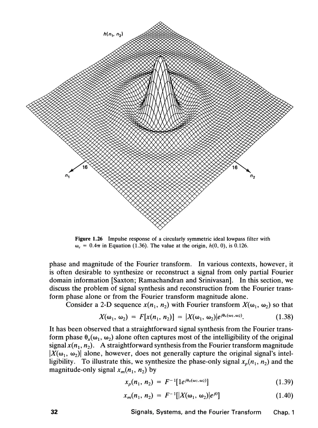
function Jx(x)lx is sketched in Figure 1.25. The sequence /i(n,, n2) in (1.36) is sketched
in Figure 1.26 for the case ooc = 0.4tt.
The impulse responses h(nl, n2) obtained from the separable and circularly
symmetric ideal lowpass filters in Examples 3 and 4 above are not absolutely sum-
Figure 1.24 Frequency response of a
circularly symmetric ideal lowpass filter.
30
Signals, Systems, and the Fourier Transform Chap. 1
J (x)
Figure 1.25 Sketch of ——, where Jx{x) is the Bessel function of the first kind
and first order. x
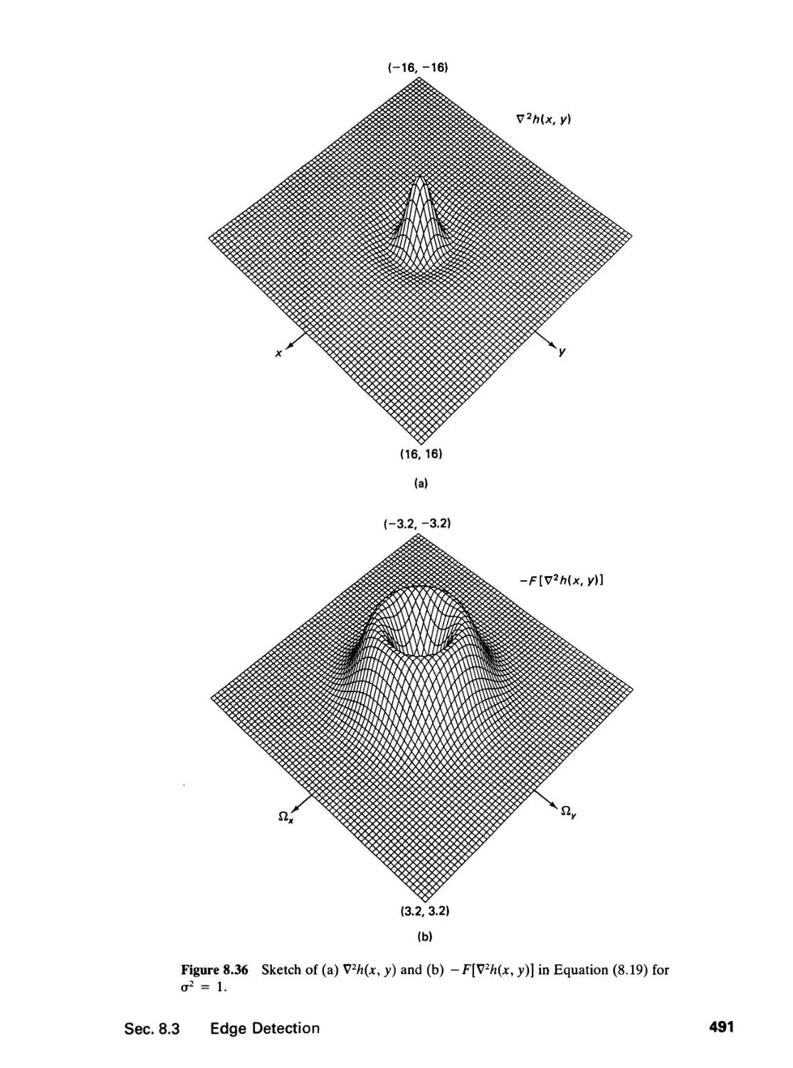
mable, and their Fourier transforms do not converge uniformly to H((ou <o2) used
to obtain h{nu n2). This is evident from the observation that the two H((ou <o2)
contain discontinuities and are not analytic functions. Nevertheless, we will regard
them as valid Fourier transform pairs, since they play an important role in digital
filtering and the Fourier transforms of the two h(nl9 nx) converge to H(<ou <o2) in
the mean square sense.*
1.4 ADDITIONAL PROPERTIES OF THE FOURIER TRANSFORM
1.4.1 Signal Synthesis and Reconstruction from Phase or
Magnitude
The Fourier transform of a sequence is in general complex-valued, and the unique
representation of a sequence in the Fourier transform domain requires both the
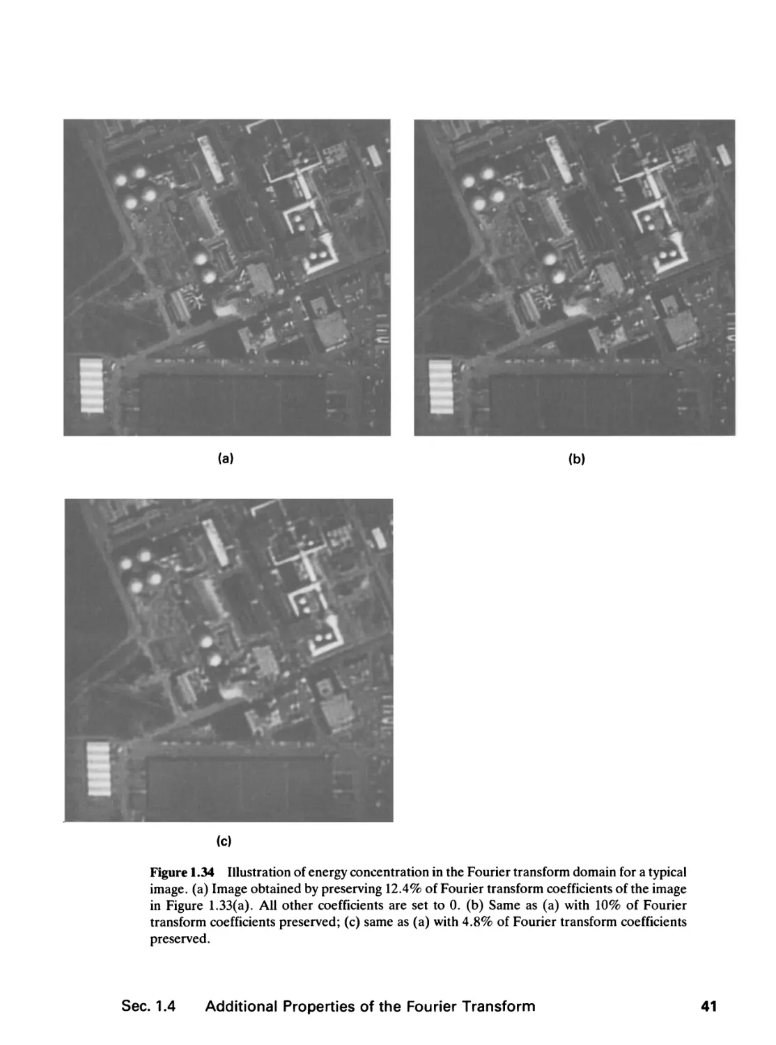
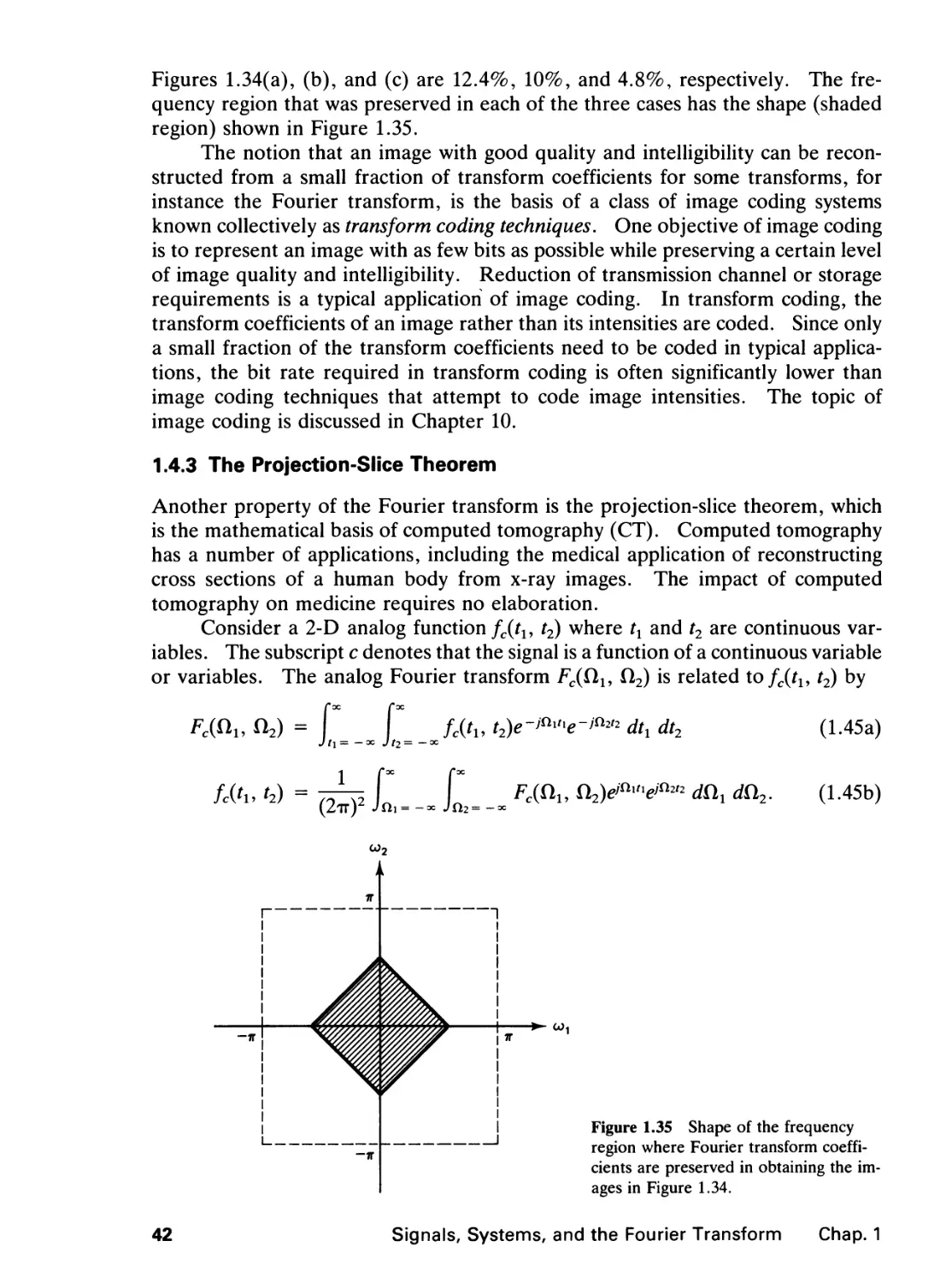
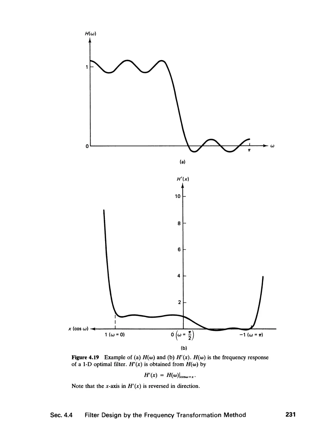
"The Fourier transform of /i(n,, n2) is said to converge to //(a),, oo2) in the mean
square sense when
lim lim
IT IT
/ /
<ji>1 = — IT 0>2 = — IT '
I N\ Nl
5) 5) Knu n2)e-^lnle-^2n2 - f/(<o„ cd2)
\m= -Ni m= -Ni
d(oY d(o2 = 0.
Sec. 1.4 Additional Properties of the Fourier Transform 31
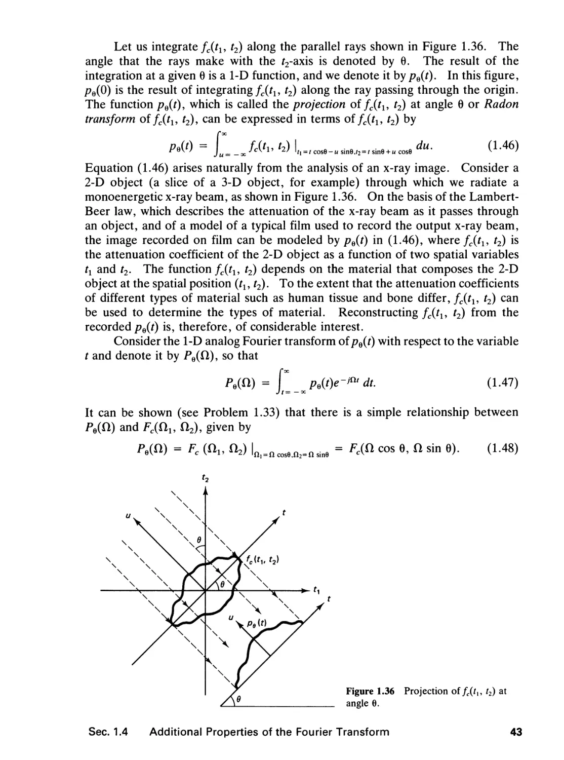
Figure 1.26 Impulse response of a circularly symmetric ideal lowpass filter with
o)c = 0.4tt in Equation (1.36). The value at the origin, h(0, 0), is 0.126.
phase and magnitude of the Fourier transform. In various contexts, however, it
is often desirable to synthesize or reconstruct a signal from only partial Fourier
domain information [Saxton; Ramachandran and Srinivasan]. In this section, we
discuss the problem of signal synthesis and reconstruction from the Fourier
transform phase alone or from the Fourier transform magnitude alone.
Consider a 2-D sequence x(nu n2) with Fourier transform X(u>l9 <o2) so that
X(ul9 <o2) = F[x(nl9 n2)] = \X(ul9 oy2)\e^^\ (1.38)
It has been observed that a straightforward signal synthesis from the Fourier
transform phase OjXoh, <o2) alone often captures most of the intelligibility of the original
signal x(n1, n2). A straightforward synthesis from the Fourier transform magnitude
\X(u>l9 co2)| alone, however, does not generally capture the original signal's
intelligibility. To illustrate this, we synthesize the phase-only signal xp(nu n2) and the
magnitude-only signal xm{nu n2) by
xp(nl9 n2) = F-i[ie>e*c»i.«2)] (L39)
xm{nun2) = F-'[\X(^<»2)\eV} (1.40)
32 Signals, Systems, and the Fourier Transform Chap. 1
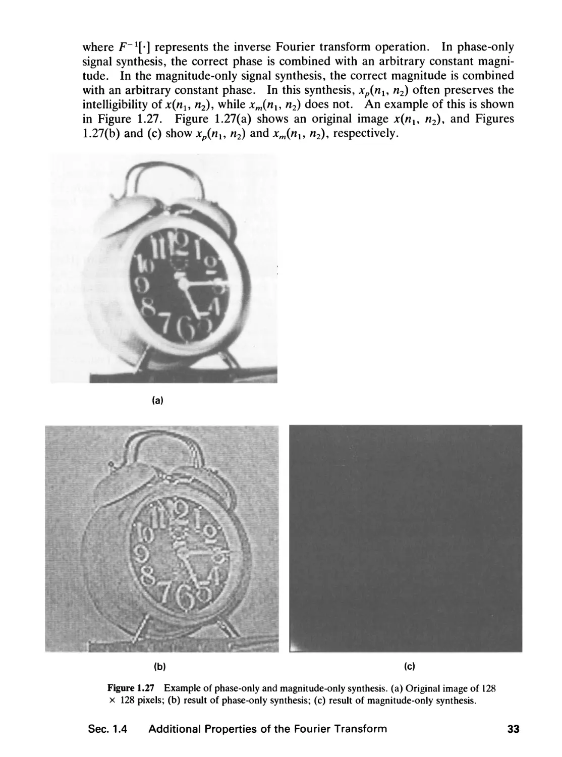
where F_1[-] represents the inverse Fourier transform operation. In phase-only
signal synthesis, the correct phase is combined with an arbitrary constant
magnitude. In the magnitude-only signal synthesis, the correct magnitude is combined
with an arbitrary constant phase. In this synthesis, xp{nx, n2) often preserves the
intelligibility of x(nl9 n2), while xm(nx, n2) does not. An example of this is shown
in Figure 1.27. Figure 1.27(a) shows an original image x{nx, n2), and Figures
1.27(b) and (c) show xp(nu n2) and xm(nl9 n2), respectively.
(a)
(b) (c)
Figure 1.27 Example of phase-only and magnitude-only synthesis, (a) Original image of 128
x 128 pixels; (b) result of phase-only synthesis; (c) result of magnitude-only synthesis.
Sec. 1.4 Additional Properties of the Fourier Transform
33
An experiment which more dramatically illustrates the observation that phase-
only signal synthesis captures more of the signal intelligibility than magnitude-
only synthesis can be performed as follows. Consider two images x(nl9 n2) and
y(nly n2). From these two images, we synthesize two other images/^, n2) and
g(nu n2) by
f(nl9 n2) = F-l[\Y(ul9 w^™"'-";)] (1.41)
g(nl9 n2) = F-l[\X(<»l9 (o2)|e>M—2)] (1 42)
In this experiment,/^!, n2) captures the intelligibility of x(nu n2), whileg(nu n2)
captures the intelligibility of y{nu n2). An example is shown in Figure 1.28.
Figures 1.28(a) and (b) show the two images x(nl9 n2) and y{nl9 n2) and Figures
1.28(c) and (d) show the two images f(nu n2) and g(nu n2).
The high intelligibility of phase-only synthesis raises the possibility of exactly
reconstructing a signal x{nu n2) from its Fourier transform phase Qx(iou <*>2). This
is known as the magnitude-retrieval problem. In fact, it has been shown [Hayes]
that a sequence x(nu n2) is uniquely specified within a scale factor if x(nu n2) is
real and has finite extent, and if its Fourier transform cannot be factored as a
product of lower-order polynomials in e'm and eJ<x>2. Typical images x(nl9 n2) are
real and have finite regions of support. In addition, the fundamental theorem of
algebra does not apply to 2-D polynomials, and their Fourier transforms cannot
generally be factored as products of lower-order polynomials in ejt»x and eJu>2.
Typical images, then, are uniquely specified within a scale factor by the Fourier
transform phase alone.
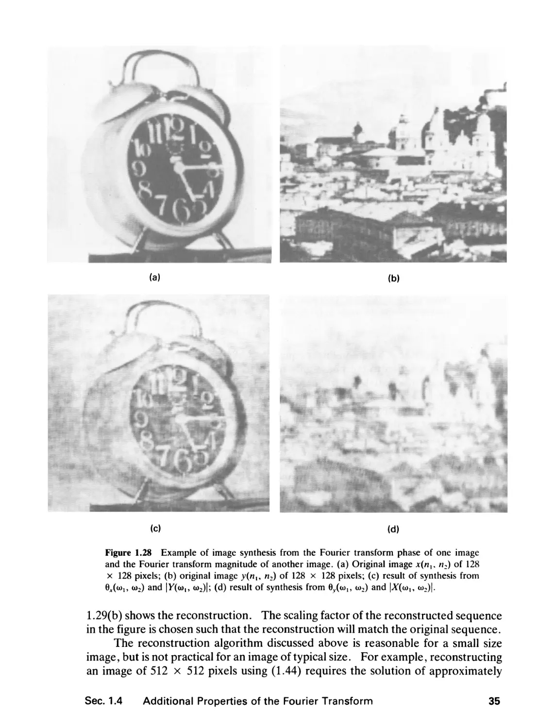
Two approaches to reconstructing a sequence from its Fourier transform phase
alone have been considered. The first approach leads to a closed-form solution
and the second to an iterative procedure. In the first approach, tan O^i, co2) is
expressed as
2 E x(nn n2) sin (co^ + <o2n2)
tan 0,(0)!, <o2) = A * 2; = - (1.43)
XR[ial9 (o2j 2j 2j x(ni> n2) cos ((jilnl + <o2n2)
(/Il,/l2)€/?.t
where Rx is the region of support of x(nl9 n2). Rewriting (1.43), we have
2 2 x(nu ni) cos (00^ + (o2«2) tan Qx(uu <o2)
(m,n2)£Rx
= - X 2 x(nu ni) sin (wi^i + <*>2ft2). (1-44)
(m,n2)ZRx
Equation (1.44) is a linear equation for the unknown values in x(nu n2) for each
frequency {iou <o2). If there are N2 unknown values in x(nu n2), we can obtain a
set of N2 linear equations for x(nl9 n2) by sampling (o>x, co2) at N2 points. If the
frequencies are sampled at distinctly different points, noting that 6,(0)!, co2) is an
odd function and is periodic with a period of 2tt x 2tt, the solution to the set of
N2 linear equations can be shown to be kx(n{, n2), where k is an arbitrary real
scaling factor. An example of signal reconstruction from phase using (1.44) is
shown in Figure 1.29. Figure 1.29(a) shows an image of 16 x 16 pixels, and Figure
34
Signals, Systems, and the Fourier Transform Chap. 1
(a) (b)
(c) (d)
Figure 1.28 Example of image synthesis from the Fourier transform phase of one image
and the Fourier transform magnitude of another image, (a) Original image x(n^ n2) of 128
x 128 pixels; (b) original image y(nx, n2) of 128 x 128 pixels; (c) result of synthesis from
0^(0)!, <o2) and |y((o,, o>2)|; (d) result of synthesis from dy(tal9 w2) and \X(&i, a>2)|.
1.29(b) shows the reconstruction. The scaling factor of the reconstructed sequence
in the figure is chosen such that the reconstruction will match the original sequence.
The reconstruction algorithm discussed above is reasonable for a small size
image, but is not practical for an image of typical size. For example, reconstructing
an image of 512 x 512 pixels using (1.44) requires the solution of approximately
Sec. 1.4 Additional Properties of the Fourier Transform
35
(a)
(b)
Figure 1.29 Example of phase-only reconstruction by a closed-form algorithm, (a) Original
image of 16 x 16 pixels. One pixel in the image is a large square block; (b) phase-only
reconstruction of the image in (a) by solving a set of linear equations in (1.44).
a quarter of a million linear equations. An alternate approach is to recognize that
the solution to the phase-only reconstruction problem must satisfy constraints in
both the spatial and frequency domains. Specifically, the solution must be real,
must be zero outside the known region of support, and must have a nonfactorable
Fourier transform. In addition, the phase of the Fourier transform of the solution
must be the same as the O^cOi, co2) given. A useful approach to solving such a
problem is an iterative procedure, in which we impose the spatial and frequency
domain constraints separately in each domain. An iterative procedure for the
phase-only reconstruction is shown in Figure 1.30. In the procedure, we begin
with an initial estimate of the signal. This can be any real sequence with the same
region of support as x(nu n2). We next compute its Fourier transform. We then
replace the Fourier transform with the given Qx(ml9 co2). The Fourier transform
magnitude is not affected. We then compute the inverse Fourier transform of the
modified Fourier transform. Due to the modification in the Fourier transform
domain, the sequence is no longer zero outside the known region of support of
x(nl, n2). We now impose the spatial domain constraint by setting the sequence
to zero outside the known region of support. The resulting sequence is a new
estimate of the solution. This completes one iteration in the iterative procedure.
When the initial estimate of the sequence chosen is real, the constraint that the
solution is real will automatically be satisfied. The above algorithm can be shown
to converge to the desired solution [Tom, et al.]. An example of signal
reconstruction from phase using the iterative procedure in Figure 1.30 is shown in Figure
1.31. Figure 1.31(a) shows an original image of 128 x 128pixels. Figures 1.31(b),
(c), and (d) show the results of the iterative procedure after one iteration [phase-
36 Signals, Systems, and the Fourier Transform Chap. 1
Initial guess of
x(nv n2) is
yinv n2)
i
r
Y(uv G)2) *
F[y(nv n2)]
y
'
^ 0y(ov co2)^
I0x(ut,u2)
s. No
outside the region
of support of
x(nv n2)
A
y(nv n2) =
F-*[Y{uvu2)}
1
y(w1f w2) «-
1 /(wlf <o2)
eJOx(wvw2)\
Yes
Y
x(nv n2) =
F-HY(ut,u2)]
Figure 1.30 Iterative procedure for phase-only reconstruction of jc(/i19 «2) from
its phase O^a^, (o2).
only synthesis of (1.39)], 10 iterations, and 50 iterations. The initial estimate used
is §(«!, n2).
Although the magnitude-only synthesis of (1.40) does not capture the
intelligibility of typical signals, almost all typical images are also uniquely specified by
the Fourier transform magnitude. Specifically, if x(n1, n2) is real, has finite extent,
and has a nonfactorable Fourier transform, then x(nly n2) is uniquely specified by
its Fourier transform magnitude \X(<ou <o2)| within a sign factor, translation, and
rotation by 180 degrees [Bruck and Sodin, Hayes]. This raises the possibility of
exactly reconstructing x{nu n2) from \X(<ou <o2)| within a sign factor, translation
and rotation by 180 degrees. This is known in the literature as the phase-retrieval
problem, and has many more potential applications than the phase-only
reconstruction problem. Unfortunately, none of the algorithms developed to date are
as straightforward or well-behaved as the algorithms developed for the phase-only
reconstruction problem. It is possible to derive a closed-form algorithm or a set
of linear equations that can be used in solving for x{nx, n2) from ^(coi, <o2)|, but
their derivation is quite involved [Izraelevitz and Lim, Lane, et al.]. In addition,
the closed-form solution is not practical for an image of reasonable size due to the
large number of linear equations that must be solved. It is also possible to derive
Sec. 1.4 Additional Properties of the Fourier Transform 37
(a) (b)
(c) (d)
Figure 1.31 Example of phase-only reconstruction by an iterative algorithm, (a) Original
image of 128 x 128 pixels; (b) result of phase-only reconstruction of the image in (a) after
one iteration of the iterative procedure in Figure 1.30. Since the initial estimate used is
&(h,, n2), this is the same as the phase-only synthesis of (1.39); (c) result after 10 iterations;
(d) result after 50 iterations.
an iterative procedure similar to that in Figure 1.30, which was developed for the
phase-only reconstruction. The only modification required is to replace the Fourier
transform magnitude with the given ^((Oj, <o2)| rather than to replace the Fourier
transform phase with the given Qx(mu co2) when the frequency domain constraints
38
Signals, Systems, and the Fourier Transform Chap. 1
are imposed. The algorithm has been observed to converge to the desired solution
when the initial estimate used is quite accurate or the signal x(nl, n2) has a special
characteristic such as a triangular region of support. The magnitude-only
reconstruction problem specifies x(nl9 n2) within a sign factor, translation, and rotation
by 180°, and, therefore, more than one solution is possible. Imposing an initial
estimate sufficiently close to a possible solution or imposing additional constraints
such as a triangular region of support appear to prevent the iterative procedure
from wandering around from one possible solution to another. In general,
however, the algorithm does not converge to the desired solution. Figure 1.32 shows
an example of signal reconstruction from the magnitude using a closed-form
algorithm [Izraelevitz and Lim]. Figures 1.32(a) and (b) show the original and the
reconstruction respectively. Developing a practical procedure that can be used to
reconstruct x(ni9 n2) from \X((au <o2)| remains a problem for further research.
In addition to the phase-only and magnitude-only signal synthesis and
reconstruction problems discussed above, a variety of results on the synthesis and
reconstruction of a signal from other partial Fourier transform information—for
instance, one bit of Fourier transform phase or signed Fourier transform
magnitude—have been reported [Oppenheim, et al. (1983)].
1.4.2 The Fourier Transform of Typical Images
The Fourier transforms of typical images have been observed to have most of their
energy concentrated in a small region in the frequency domain, near the origin
(a) (b)
Figure 1.32 Example of magnitude-only reconstruction by a closed-form algorithm,
(a) Original image of 24 x 24 pixels; (b) result of magnitude-only reconstruction of the image
in (a) using a closed-form algorithm. After [Izraelevitz and Lim.]
Sec. 1.4 Additional Properties of the Fourier Transform
39
and along the (Oj and co2 axes. One reason for the energy concentration near the
origin is that images typically have large regions where the'intensities change slowly.
Furthermore, sharp discontinuities such as edges contribute to low-frequency as
well as high-frequency components. The energy concentration along the a^ and
a>2 axes is in part due to a rectangular window used to obtain a finite-extent image.
The rectangular window creates artificial sharp discontinuities at the four
boundaries. Discontinuities at the top and bottom of the image contribute energy along
the <o2 axis and discontinuities at the two sides contribute energy along the (ox axis.
Figure 1.33 illustrates this property. Figure 1.33(a) shows an original image of
512 x 512 pixels, and Figure 1.33(b) shows \X(io^ <o2)|1/4 of the image in Figure
1.33(a). The operation (-)1/4 has the effect of compressing large amplitudes while
expanding small amplitudes, and therefore shows \X(u>u co2)| more clearly for higher-
frequency regions. In this particular example, energy concentration along
approximately diagonal directions is also visible. This is because of the many sharp
discontinuities in the image along approximately diagonal directions. This example
shows that most of the energy is concentrated in a small region in the frequency
plane.
Since most of the signal energy is concentrated in a small frequency region,
an image can be reconstructed without significant loss of quality and intelligibility
from a small fraction of the transform coefficients. Figure 1.34 shows images that
were obtained by inverse Fourier transforming the Fourier transform of the image
in Figure 1.33(a) after setting most of the Fourier transform coefficients to zero.
The percentages of the Fourier transform coefficients that have been preserved in
(a) (b)
Figure 1.33 Example of the Fourier transform magnitude of an image, (a) Original image
x(nu n2) of 512 x 512 pixels; (b) lA^o),, <o2)|1/4, scaled such that the smallest value maps to
the darkest level and the largest value maps to the brightest level. The operation (-)1'4 has
the effect of compressing large amplitudes while expanding small amplitudes, and therefore
shows \X(uly o)2)| more clearly for higher-frequency regions.
40
Signals, Systems, and the Fourier Transform Chap. 1
(a)
(b)
(O
Figure 1.34 Illustration of energy concentration in the Fourier transform domain for a typical
image, (a) Image obtained by preserving 12.4% of Fourier transform coefficients of the image
in Figure 1.33(a). All other coefficients are set to 0. (b) Same as (a) with 10% of Fourier
transform coefficients preserved; (c) same as (a) with 4.8% of Fourier transform coefficients
preserved.
Sec. 1.4 Additional Properties of the Fourier Transform
41
Figures 1.34(a), (b), and (c) are 12.4%, 10%, and 4.8%, respectively. The
frequency region that was preserved in each of the three cases has the shape (shaded
region) shown in Figure 1.35.
The notion that an image with good quality and intelligibility can be
reconstructed from a small fraction of transform coefficients for some transforms, for
instance the Fourier transform, is the basis of a class of image coding systems
known collectively as transform coding techniques. One objective of image coding
is to represent an image with as few bits as possible while preserving a certain level
of image quality and intelligibility. Reduction of transmission channel or storage
requirements is a typical application of image coding. In transform coding, the
transform coefficients of an image rather than its intensities are coded. Since only
a small fraction of the transform coefficients need to be coded in typical
applications, the bit rate required in transform coding is often significantly lower than
image coding techniques that attempt to code image intensities. The topic of
image coding is discussed in Chapter 10.
1.4.3 The Projection-Slice Theorem
Another property of the Fourier transform is the projection-slice theorem, which
is the mathematical basis of computed tomography (CT). Computed tomography
has a number of applications, including the medical application of reconstructing
cross sections of a human body from x-ray images. The impact of computed
tomography on medicine requires no elaboration.
Consider a 2-D analog function fc(h, t2) where tx and t2 are continuous
variables. The subscript c denotes that the signal is a function of a continuous variable
or variables. The analog Fourier transform Fc(ft1? ft2) is related to fc(tu t2) by
Fc(tll9 ft2)
f f
J/1= -oc Jt2= -=>
fc(h, t2)e->n^e-^ dtx dt2
(1.45a)
fc(h,t2) = -±-2\ \ F^Cl^'e^d^d^. (1.45b)
Figure 1.35 Shape of the frequency
region where Fourier transform
coefficients are preserved in obtaining the
images in Figure 1.34.
42
Signals, Systems, and the Fourier Transform Chap. 1
Let us integrate fc(h, t2) along the parallel rays shown in Figure 1.36. The
angle that the rays make with the f2-axis is denoted by 6. The result of the
integration at a given 6 is a 1-D function, and we denote it by pe(t). In this figure,
pQ(0) is the result of integrating fc(tu t2) along the ray passing through the origin.
The function pe(t), which is called the projection of fc(tu t2) at angle 0 or Radon
transform of fc(tu t2), can be expressed in terms of fc(tu t2) by
.(0
-r
J u =
fcih, h) l„
du.
^ev"/ I jcyif -z/ l/, =/cosB-« sin9,r2 = ^ sine+ w cosB
Equation (1.46) arises naturally from the analysis of an x-ray image.
(1.46)
Consider a
2-D object (a slice of a 3-D object, for example) through which we radiate a
monoenergetic x-ray beam, as shown in Figure 1.36. On the basis of the Lambert-
Beer law, which describes the attenuation of the x-ray beam as it passes through
an object, and of a model of a typical film used to record the output x-ray beam,
the image recorded on film can be modeled by pe(t) in (1.46), where fc(tu t2) is
the attenuation coefficient of the 2-D object as a function of two spatial variables
tx and t2. The function fc{tu t2) depends on the material that composes the 2-D
object at the spatial position (ju t2). To the extent that the attenuation coefficients
of different types of material such as human tissue and bone differ, fc(tu h) can
be used to determine the types of material. Reconstructing fc{tu t2) from the
recorded pe(t) is, therefore, of considerable interest.
Consider the 1-D analog Fourier transform of pQ(t) with respect to the variable
t and denote it by PQ(Cl), so that
Pe(ft)
-\:
pe(0e->"' dt.
(1.47)
It can be shown (see Problem 1.33) that there is a simple relationship between
Pe(ft) and Fc(ft1? ft2)> given by
P.(0) = Fc (ft,, ft2) |n,=ncos9,n2=nsin9 = Fc(ft cos 6, ft sin 6). (1.48)
Figure 1.36 Projection of /c(/,, t2) at
angle 0.
Sec. 1.4 Additional Properties of the Fourier Transform
43
n,
i Fc(ava2)
#■
*L
^(12)= Fc{Sl cos 0, ft sin0)
► ft.
Figure 1.37 Projection slice theorem.
Pe(fl) is the 2-D Fourier transform
Fc(&i, H2) evaluated along the dotted
line.
Expressed graphically, (1.48) states that the 1-D Fourier transform of the projection
pe(t) is Fc(ft1? ft2) evaluated along the slice that passes through the origin and
makes an angle of 0 with the ft! axis, as shown in Figure 1.37. The relationship
in (1.48) is called the projection-slice theorem.
The projection-slice theorem of (1.48) can be used in developing methods to
reconstruct the 2-D function/c(^, t2) from its projections pe(t). One method is to
compute the inverse Fourier transform of Fc(ft1? ft2) obtained from pQ(t).
Specifically, if we compute the 1-D Fourier transform of pe(t) with respect to t for all
0 < 6 < tt, we will have complete information on Fc(ft1? ft2). In practice, of
course, pQ(t) cannot be measured for all possible angles 0 < 0 < it, so Fc(ft1? ft2)
must be estimated by interpolating known slices of Fc(ft1? ft2).
Another reconstruction method, known as the filtered back-projection method,
is more popular in practice and can be derived from (1.45b) and (1.48). It can
be shown [Kak] that
Muh) = ^Je=0?eWU„cose+,2Sin9rfe = -^ J"e=o <?„(;, cose + f2sine)de
where qs(t) is related to pe(f) by
9e(0 = Pe(t) * h{t) = PeW - t) dr.
(1.49)
(1.50)
The function h(t), which can be viewed as the impulse response of a filter, is given
by
h(t) = t- I ' |n|<?'n' do.
(1.51)
where ftc is the frequency above which the energy in any projection pQ(t) can be
assumed to be zero. From (1.49) and (1.50), we can see that one method of
reconstructing/^, t2) from pe(t) is to first compute qe(t) by filtering (convolving)
pe(t) with h(t) and then to determine fc(tu t2) from qQ(t) by using (1.49). The
44
Signals, Systems, and the Fourier Transform Chap. 1
sin 0'
*-'i
Figure 1.38 Values of (tly t2) for which
fc(tu t2) is affected by qe(t') in the
filtered back-projection reconstruction
method. They can be described by /' =
/j cos 0' + t2 sin 0'.
process of determining/c(r1? t2) from qe(t) using (1.49) can be viewed as a back-
projection. Consider a particular 0 and t, say 0' and V. From (1.49), the values of
(tl9 t2) for which fc(tu t2) is affected by g6'(0 are given by t' = tx cos 0' + t2 sin 0'.
These values are shown by the straight line in Figure 1.38. Furthermore, the
contribution that g6'(0 makes lofc(t\, t2) is equal at all points along this line. In
essence, q$>(t') is back-projected in the (tly t2) domain. This back-projection takes
place for all values of t' and is integrated over all values of 0'. Since qQ(t) is a
filtered version of pe(t), this technique is called the filtered back-projection method.
In practice, pQ(t) is not available for all values of 0. As a result, qe(t) must be
interpolated from the known slices of qe(t).
In addition to the interpolation involved in both the direct Fourier transform
method and the filtered back-projection method, a number of practical issues arise
in reconstructing fc(t\, t2) from pQ(t). For example, the Fourier transform, inverse
Fourier transform, filtering, and integration require a discretization of the problem,
which raises a variety of important issues, including sampling and aliasing. In
practice, the measured function pe(t) may be only an approximate projection of
fcihi h)- 1° addition, the measured data may not have been obtained from parallel-
beam projection, but instead from fan-beam projection, in which case a different
set of equations governs. More details on these and other theoretical and practical
issues can be found in [Scudder, Kak]. We will close this section with an example
in which a cross section of a human head was reconstructed from its x-ray
projections. Figure 1.39 shows the reconstruction by the back-projection method.
1.5 DIGITAL PROCESSING OF ANALOG SIGNALS
Most signals that occur in practice are analog. In this section, we discuss digital
processing of analog signals. Since the issues that arise in digital processing of
analog signals are essentially the same in both the 1-D and 2-D cases, we will
briefly summarize the 2-D results.
Consider an analog 2-D signal xc(t\, t2). We'll denote its analog Fourier
Sec. 1.5 Digital Processing of Analog Signals
45
V
Figure 1.39 Cross section of a human
head reconstructed from its projections
by the filtered back-projection method.
Courtesy of Tamas Sandor.
transform by Xc(^i, ft2). Suppose we obtain a discrete-space signal x(n1, n2) by
sampling the analog signal xc{h, h) with sampling period (7\, T2) as follows:
x(nl9 n2) = xc(tl9 h)\tx^Txt^niTi. (1.52)
Equation (1.52) represents the input-output relationship of an ideal analog-to-
digital (A/D) converter. The relationship between X(<ol9 <o2), the discrete-space
Fourier transform of x(nl9 n2), and Xc(^i, ft2), the continuous-space Fourier
transform of xc(ti> h)i is given by
X^,oi2) = -^- i i Xc(^-^,^-^). (1.53)
Two examples of Xc(Q,l9 ft2) an(l X((ol9 <o2) are shown in Figure 1.40. Figure
1.40(a) shows a case in which l/7\ > ft^/ir and l/r2 > ft^/ir, where Cl'c and ft" are
the cutoff frequencies of Xc(fil9 ft2), as shown in the figure. Figure 1.40(b) shows
a case in which l/7\ < ft^/ir and \IT2 < ft"/iT. From the figure, when \ITX >
CL'c/tt and l/r2 > ft"/7T, xc(tl9 t2) can be recovered from x(nl9 n2). Otherwise,
Xc(h> h) cannot be exactly recovered from x(nl9 n2) without additional information
on xc(tl912). This is the 2-D sampling theorem, and is a straightforward extension
of the 1-D result.
An ideal digital-to-analog (D/A) converter recovers xc{tX9 t2) from x(nl9 n2)
when the sampling frequencies \ITX and \IT2 are high enough to satisfy the require-
46
Signals, Systems, and the Fourier Transform Chap. 1
xc(nvn2)
*-n.
-2tt
co2 = 2ir
n;r3
:r,
-2tt
(a)
X(cov co2)
CO, = 27T
(b)
Figure 1.40 Example that illustrates the relationship between -Yc(fti, ft2) and X((aly a>2)
given by (1.53). (a) No aliasing; (b) aliasing. Aliased regions are shown shaded.
ments of the sampling theorem. The output of the ideal D/A converter, yc(h, t2), is
given by
sin — fo - nxTx) sin — (t2 - n2T2)
oc oc
ydh, h) = S X *("i> "2)
7-,
«i = — ac n2= -x
— (rx - MjjTi) — (f2 - n2T2)
ll l2
(1.54)
The function yc(tu t2) is identical to xc(tu t2) when the sampling frequencies used
in the ideal A/D converter are sufficiently high. Otherwise, yc{tx, t2) is an aliased
version of xc(tu h)- Equation (1.54) is a straightforward extension of the 1-D
result.
Sec. 1.5 Digital Processing of Analog Signals
47
xc(fv t2)-
Prefilter
(lowpass)
A/D
Digital
processing
D/A
Yc^vh)
Figure 1.41 Digital processing of analog signals.
(a)
(b)
Figure 1.42 (a) Image of 128 x 128
pixels with little aliasing due to an
effective antialiasing filter; (b) image of
128 x 128 pixels with noticeable
aliasing.
48
Signals, Systems, and the Fourier Transform Chap. 1
An analog signal can often be processed by digital processing techniques using
the A/D and D/A converters discussed above. The digital processing of analog
signals can, in general, be represented by the system in Figure 1.41. The analog
lowpass filter limits the bandwidth of the analog signal to reduce the effect of
aliasing. In digital image processing, the analog prefiltering operation is often
performed by a lens and the scanning aperture used in converting an optical image
to an electrical signal. The importance of the antialiasing filter is illustrated in
Figure 1.42. Figure 1.42(a) shows an image of 128 x 128 pixels with little aliasing
due to an effective antialiasing filter used. Figure 1.42(b) shows an image of 128
x 128 pixels with noticeable aliasing.
The A/D converter of (1.52) is based on sampling on the Cartesian grid. The
analog signal can also be sampled on a different type of grid. Sampling on a
hexagonal grid is discussed in Problem 1.35.
REFERENCES
In this text, we have assumed that the reader is familiar with fundamentals of 1-D
digital signal processing. For a comprehensive treatment of 1-D digital signal
processing concepts, see [Oppenheim and Schafer (1975); Rabiner and Gold; Lim
and Oppenheim; Oppenheim and Schafer (1989)].
For different viewpoints or more detailed treatment of some topics in 2-D
digital signal processing, see [Huang; Huang; Dudgeon and Mersereau]. For
collections of selected papers on 2-D digital signal processing, see [Mitra and
Ekstrom; IEEE].
For a more detailed treatment of the Fourier transform theory, see [Papoulis].
For processing data obtained from sampling on any regular periodic lattice including
the rectangular lattice and hexagonal lattice, see [Mersereau; Mersereau and Speake].
Y. M. Bruck and L. G. Sodin, On the ambiguity of the image reconstruction problem, Opt.
Commun., September 1979, pp. 304-308.
D. E. Dudgeon and R. M. Mersereau, Multidimensional Digital Signal Processing. En-
glewood Cliffs, NJ: Prentice-Hall, 1983.
M. H. Hayes, The reconstruction of a multidimensional sequence from the phase or
magnitude of its Fourier transform, IEEE Trans, on Acoust., Speech, and Sig. Proc, Vol.
ASSP-30, April 1982, pp. 140-154.
T. S. Huang, ed., Two-Dimensional Digital Signal Processing /, in "Topics in Applied
Physics," Vol. 42. Berlin: Springer-Verlag, 1981.
T. S. Huang, ed.,Two-Dimensional Digital Signal Processing II, in "Topics in Applied
Physics," Vol. 43. Berlin: Springer-Verlag, 1981.
IEEE, ASSP Society's MDSP Committee, editor, Selected Papers in Multidimensional Digital
Signal Processing, IEEE Press, New York, 1986.
D. Izraelevitz and J. S. Lim, A new direct algorithm for image reconstruction from Fourier
Chap. 1 References
49
transform magnitude. IEEE Trans, on Acoust., Speech, and Sig. Proc, Vol. ASSP-35,
April 1987, pp. 511-519.
A. C. Kak, "Image Reconstruction from Projections," in Digital Image Processing
Techniques, edited by M. Ekstrom. Orlando, FL: Academic Press, 1984, Chapter 4.
R. G. Lane, W. R. Fright, and R. H. T. Bates, Direct phase retrieval, IEEE Trans, on
Acoust., Speech, and Sig. Proc, Vol. ASSP-35, April 1987, pp. 520-525.
J. S. Lim and A. V. Oppenheim, ed., Advanced Topics in Signal Processing, Englewood
Cliffs, NJ: Prentice-Hall, 1988.
R. M. Mersereau, "The processing of hexagonally sampled two-dimensional signals," Proc.
IEEE, Vol. 67, May 1979, pp. 930-949.
R. M. Mersereau and T. C. Speake, The processing of periodically sampled multidimensional
signals, IEEE Trans, on Acoust., Speech, and Sig. Proc, Vol. ASSP-31, February 1983,
pp. 188-194.
S. K. Mitra and M. P. Ekstrom, eds. Two-Dimensional Digital Signal Processing. Strouds-
burg, PA: Dowden, Hutchinson and Ross, 1978.
A. V. Oppenheim, J. S. Lim, and S. R. Curtis, Signal synthesis and reconstruction from
partial Fourier domain information, J. Opt. Soc Amer., Vol. 73, November 1983, pp.
1413-1420.
A. V. Oppenheim and R. W. Schafer, Digital Signal Processing. Englewood Cliffs, NJ:
Prentice Hall, 1975.
A. V. Oppenheim and R. W. Schafer, Discrete-Time Signal Processing. Englewood Cliffs,
NJ: Prentice Hall, 1989.
A. Papoulis, The Fourier Integral and Its Applications. New York: McGraw-Hill, 1962.
L. R. Rabiner and B. Gold, Theory and Application of Digital Signal Processing.
Englewood Cliffs, NJ: Prentice Hall, 1975.
G.N. Ramachandran and R. Srinivasan, Fourier Methods in Crystallography. New York:
Wiley-Interscience, 1978.
W. O. Saxton, Computer Techniques for Image Processing in Electron Microscopy. New
York: Academic Press, 1970.
H. J. Scudder, Introduction to computer aided tomography, Proc IEEE, Vol. 66, June
1978, pp. 628-637.
V. T. Tom, T. F. Quatieri, M. H. Hayes, and J. H. McClellan, Convergence of iterative
nonexpansive signal reconstruction algorithms, IEEE Trans, on Acoust., Speech, and Sig.
Proc, Vol. ASSP-29, October 1981, pp. 1052-1058.
PROBLEMS
1.1. Sketch the following sequences:
(a) h(nx + 2, n2 - 3) + 28(/i1, -n2 + 2)
(b) M^iM/ii, ni)
(c) (i)"257<n1 + n2)u(-nx + 1, -n2)
1.2. Consider a sequence x(nx, n2) sketched below:
50
Signals, Systems, and the Fourier Transform Chap. 1
n
2
T
x(nv n2)
4(4)
(2)
(1) (2)
• <F W
4(4)
Figure PI.2
Express x{nu n2) as a linear combination of h(nly n2) and its shifts.
1.3. We have defined a sequence x{nu n2) to be periodic with a period of Nx x N2 if
x{nx, n2) = jc(n! + Nx, n2) = jc(nlf n2 + N2) for all (n,, n2). (1)
More generally defined, the condition is
*("i>"2) = *("i + ^ii,w2 + ^12) = x(nl + N2„/i2 + N22) for all (/i„/i2) (2)
with the number of points in a period given by
1^11^22 " W12N2l|.
(a) Show that the condition in (2) reduces to the condition in (1) with a proper choice
of Nn, Nl2, N2l, andN22.
(b) Consider the periodic sequence x(nx, n2), which was shown in Figure 1.8. If we
use (1), the minimum choices of Nx and N2 are 6 and 2, respectively, and the
number of points in one period is 12. If we use (2), Nn, Nl2, N2l, and N22 can
be chosen such that \NnN22 - Nl2N2l\ = 6. Determine one such set of Nn, Nl2,
N2l, and N22.
(c) Show that any sequence that satisfies the condition in (2) will also satisfy the
condition in (1) as long as Nx and N2 are chosen appropriately. This result shows
that (1) can be used in representing any periodic sequence that can be represented
by (2), although the number of points in one period may be much larger when
(1) rather than (2) is used.
1.4. For each of the following systems, determine whether or not the system is (1) linear,
(2) shift invariant, and (3) stable.
(a) y(nl9 n2) = T[x{nx, n2)\ = **<"'•«>
(b) y(nl9n2) = T[x(n^n2)} = ink\t6nl.3x(ku n2)
(c) y(nl9n2) = T[x(nu n2)] = lp2 = 0x(nl9 k2)
1.5. The median filter is used in a number of signal processing applications, including
image processing. When a median filter is applied to an image, a window slides along
the image, and the median intensity value of the pixels (picture elements) within the
window replaces the intensity of the pixel being processed. For example, when the
Chap. 1 Problems
51
1.6.
pixel values within a window are 5, 6, 35, 10, and 5, and the pixel being processed
has a value of 35, its value is changed to 6, the median of the five values. Answer
each of the following questions. In your answer, use a 2-D median filter of size
3x3, with the center of the window corresponding to the pixel being processed.
(a) Is a median filter linear, shift invariant, and/or stable?
(b) Using an example, illustrate that a median filter tends to preserve sharp
discontinuities, such as steps.
(c) Using an example, illustrate that a median filter is capable of eliminating impulsive
values without seriously affecting the value of the pixel near those with the
impulsive values. A pixel has an impulsive value when its value is significantly
different from its neighborhood pixel values.
Consider a system T. When the input to the system is the unit step sequence
u(nu n2)9 the response of the system is s(nu n2) as shown below.
u{nv n2) -
-► s(nv n2)
Figure PI.6
For each of the following three cases, determine the class of inputs for which we can
determine the output of the system in terms of s(nu n2). For each input in the class,
express the output in terms of s{nx, n2).
(a) T is linear, but not shift invariant.
(b) T is shift invariant, but not linear.
(c) T is linear and shift invariant.
1.7. Compute x(nu n2) * h(nu n2) for each of the following two problems,
(a)
'. h(ny, n2) = u{nv n2)
• • •
• • •
n
i
M)<
(-1)
(-D<
2
k
x(nv n2)
>
(5)
(-1)
>
Figure P1.7
(b) x(nu #i2) = (i)"l(i)"M«i, n2)
h{nx, n2) = u(nx - 1, n2 - 2)
1.8. Convolve the sequence x(nx, n2) = ambnlu(nu n2) with the sequence shown in the
figure below. Assume |a| < 1. The filled-in circles represent samples with amplitude
of 1. The vertical lines at nx = -1, 0, 1 extend to oo, and the horizontal line at n2
= 0 extends to -<» and +o°.
52
Signals, Systems, and the Fourier Transform Chap. 1
n2
Figure PI.8
1.9. Consider a 2-D LSI system whose impulse response h(nx, n2) has first-quadrant
support. When the input x(nu n2) to the system is given by
*(/i„ n2) = 2"»"2w(n1, n2),
some portion of the output y{nx, n2) has been observed. Suppose the observed portion
of y(nu n2) is as shown in the following figure.
(4)
(4)
(2)
(D
• (22)
• (14)
y(nv n2)
not observed
outside the
boundary
• (8) • (14) #(23)
(3)
(4)
(4)
ni Figure PI.9
Determine /i(l, 1), the impulse response h(nx, n2) evaluated at nx = n2 = 1.
1.10. If the input x(nu n2) to an LSI system is periodic with a period of NY x N2, is the
output y(nu n2) of the system periodic? If so, determine the periodicity oiy(nu n2).
1.11. Consider the following system in which x(nx, n2) represents an input sequence and
/iXflj, n2) for i = 1, 2, 3, 4, 5 represents the impulse response of an LSI system.
Chap. 1 Problems
53
x(n^, n2)-
hy(nv n2)
h2(nv n2)
h2{ny, n2)
h5{n^, n2)
Figure PI. 11
hA[nv n2)
+ )—*~y(nvn2)
Without affecting the input-output relationship, the above system can be simplified
as
x(nun2)
h{n„ n2)
y("\, n2).
Express h{nu n2) in terms of hi(nu n2), h2(nu n2), h3(n^ n2), h4(n{, n2) and /i5(«„ n2).
1.12. Let h(nu n2, n3) be a separable, finite-extent, 3-D sequence of M x M x M points
which can be expressed as
h{nu n2, n3) = a{nx) b(n2) c(n3).
(a) The Fourier transform of h(nu n2, n3), //(co,, o>2, o>3), is defined by
7/(0)^(02,0)3)= X 2 2 h{nun2,n3)e-^rne-'ialnle-^n\.
n\= - at nj= -■*■ n}= --x.
Show that //(o),, o)2, w3) is a separable function that can be expressed in the form
ofi4(Wl)i?(w2)C(a>3).
(b) We wish to filter an input sequence x(n{, n2, n3) of N x N x N points using an
LSI system with impulse response h(nu n2, n3) as given above. Develop a
computationally efficient way to compute the output y{nx, n2, n3).
(c) How does your method compare to direct evaluation of the convolution sum for
each output point when N = 512 and M = 10?
1.13. An LSI system can be specified by its impulse response h(nly n2). An LSI system
can also be specified by its unit step response s(n,, n2), the response of the system
when the input is the unit step sequence u(nx, n2).
(a) Express y(nu n2), the output of an LSI system, in terms of the input x(n{, n2) and
the unit step response s(nl9 n2).
(b) In determining the output y(nx, n2) of an LSI system, which of the two methods
requires less computation: your result in (a), or convolving jc(«,, n2) with
h(nl9 n2)l
1.14. Show that an LSI system is stable in the BIBO (bounded-input-bounded-output) sense
if and only if the impulse response of the system h{nx, n2) is absolutely summable,
that is,
E i Mn^ n2)\ < *>.
54 Signals, Systems, and the Fourier Transform Chap. 1
1.15. For each of the following cases, determine the region of support of y(nx, n2) =
x{nu n2) * h(nl9 n2).
(a) x(nu n2) and h(nx, n2) are first-quadrant support sequences.
(b) x(nu n2) and h{nu n2) are second-quadrant support sequences.
(c) x(nx, n2) is a first-quadrant support sequence and h{nx, n2) is a fourth-quadrant
support sequence.
(d) x(nlt n2) is a first-quadrant support sequence and h(nx, n2) is a third-quadrant
support sequence.
1.16. Let x(nu n2) and y(nu n2) denote an input and the corresponding output sequence of
a 2-D system. We define a system to be pseudo-causal if y(nx, n2) does not depend
on x(nx - kx, n2 - k2) for kx < 0 or k2 < 0. Show that a necessary and sufficient
condition for an LSI system to be pseudo-causal is that its impulse response h(nx, n2)
must be a first-quadrant support sequence.
1.17. It is known that any wedge support sequence x{nx, n2) can be mapped to a first-
quadrant support sequence y(nx, n2) without affecting its stability by linear mapping
of variables:
y(nx, n2) = jt(ra,, m2) I ,
where /,, /2, /3, and /4 are integers. Consider the following wedge support sequence
*(/i„ n2).
n2
x(nv n2)
+^ny
Figure PI. 17
The shaded region in the figure is the region of (nx, n2) for which x(nx, n2) is nonzero.
Determine one specific linear mapping of variables that maps x(nx, n2) to a first-
quadrant support sequence y(nx, n2) without affecting its stability.
1.18. Determine if each of the following sequences is an eigenfunction of a general LSI
system.
(a) x(nu n2) = e>°>2n2
(b) *(/i„ n2) = am + b"2
(c) *(/i„ n2) = e^e'0*2"2
(d) x(nu n2) = e^meJO,2n2u(n^ n2)
1.19. Determine the Fourier transform of each of the following sequences.
(a) 8(n,, n2)
(b) a2n^n2u(nx,n2), \a\ < 1
(c) ambn2 5r(4n, - n2)uT(nx), \a\ < 1, \b\ < 1
(d) nx(\)"> (i)^u(nl9n2)
Chap. 1 Problems
55
1.20. The Fourier transform X(<au oo2) of the sequence x(nly n2) is given by
X((ou oo2) = 3 + 2 cos (*>! + /4 sin oo2 + Se~ime-Jto2.
Determine x(nl9 n2).
1.21. Consider the following sequence:
i
• (e) <
J6)
• (d) <
{
MO
(a)
MO
x(nv n2)
• (d)
Jb)
• (0
Figure P1.21
The coefficients a, b, c, d, and e are real.
(a) What can you say about X(<au oo2) without explicitly computing X((tily co2)?
(b) Determine *(0, 0).
(c) Determine X((ou cd2).
1.22. Using the Fourier transform pair of Equation (1.31), show that
00 °° 2 fir Tit
X X 1*0*1, "2)|2 = 77"^ !*(<*>,, W2)|2 ^0), ^0)2.
1.23. We wish to design a highpass filter with impulse response h(n{, n2) and frequency
response H((ou cd2).
(a) Determine one h(nx, n2) which can be viewed as a highpass filter and which has
the following property:
(0, CDj = CD2 = 0
1, ((Oj, 002) = (iT, 0), (iT, IT), (0, 7T), (-TT, Tr), ("IT, 0),
(-7T, -it), (0, -tt) and (tt, -it).
(b) For your answer in (a), determine //(ooi, oo2). Demonstrate that it can be viewed
as a highpass filter by evaluating H((ou co2) at a reasonable number of values of
(«1> W2)«
(c) Let jc(«!, n2) represent the intensity of a digital image. The amplitude of
x(nu n2) is real and nonnegative. We process x(nly n2) with the highpass filter
designed in (a) and denote the resulting output by y(nu n2). Determine
5) 5) y(nl9n2).
(d) From your answer to (c), discuss how 3>(fii, n2) will appear on a display device
that sets all negative amplitudes of y(nx, n2) to 0 (the darkest level) before it
displays y{nx, n2).
56
Signals, Systems, and the Fourier Transform Chap. 1
1.24. The impulse response of a circularly symmetric ideal lowpass filter with cutoff
frequency of coc is given by
^Vn\ + n\
where y^) is the Bessel function of the first kind and first order. In this problem,
we derive this result.
(a) The frequency response of the filter is given by
ft/ \ J1, 00? + co2. < co2
tf(»,,»2) = |0j othenvise.
The sequence h(nx, n2) is then given by
We now make the following change of variables:
r cos 0 = 0)!
r sin 0 = co2.
Show that h(nu n2) can be expressed as
1 fu)C fa + 2tt
for any real constant a.
(b) We next make the following change of variables:
n{ = n cos c|>
n2 = n sin c|>
Note that n2 = n\ + n^. Show that h(nu n2) can be written as
Knun2) = -±-[C rf{r)dr (2)
(lit) Jr = 0
where /(r) = i"+^ e*» ««•-♦> rfe. (3)
(c) It is known that
1 f2lT 1 f2'
«A)(*) = ^~ \ cos (* sm 8) dB = — cos (jc cos 0) d0 (4)
2tt Je = o 2tt Je = o
where J0(x) is the Bessel function of the first kind, zeroth order. From (3) and
(4) with a = c|>, show that
f(r) = 27r/0(rVn?T^2). (5)
(d) It is known that
xJx{x)\Ua = xJ0(x) dx
Jx = a
(6)
Chap. 1 Problems
57
where Ji(x) is the Bessel function of the first kind, first order. From (2), (5),
and (6), show that
M"i> ni) =
2irV"i + "2
/,((*), V"i + n\).
This is the desired result.
1.25. Determine the impulse response of each of the following two filters. You may use
the results of Problem 1.24.
(a) Circularly symmetric ideal highpass filter:
H( ^ = j^' w? + w2 - wc2 (unshaded region)
^ *' 2' [1, otherwise (shaded region)
nmetric ideal bandpass filter:
Hi \ = I1, R2{ ~ ^ + ^ - ^2 (shaded region)
^ *' [0, otherwise (unshaded region)
(b) Circularly symmetric ideal bandpass filter:
(a)
(b)
Figure P1.25
1.26. It is well known that circular symmetry of X(<al9 oo2) implies circular symmetry of
x(nx, n2). However, circular symmetry of x(nl9 n2) does not imply circular
symmetry of X(u>u o>2). To show the latter, determine a circularly symmetric sequence
x(nu n2) that is a function of n\ + n\ with the property that X(<x>x, o>2) cannot be
expressed as a function of <o? + a>| for <of + a>| < it2.
1.27. Evaluate the following expression:
12
I 2
n\= -w «2= -*
[/^V^i)]
n? + n|
where Z^-) is the Bessel function of the first kind and first order.
1.28. Let f{x, y) denote a 2-D analog function that is circularly symmetric and can therefore
be expressed as
f(*,y)=8(r)\,m
/x'+y*
58
Signals, Systems, and the Fourier Transform Chap. 1
Let F(Q,X, fly) denote the 2-D analog Fourier transform of /(*, y). For a circularly
symmetric/(x, y), F(nx, flv) is also circularly symmetric and can therefore be expressed
as
F(nl,n,) = G(P)|p=v*7i,
Note that the analog case is in sharp contrast with the discrete-space case, in which
circular symmetry of a sequence x(nx, n2) does not imply circular symmetry of its
Fourier transform X(o>x, o>2). The relationship between g(r) and G(p) is called the
zeroth-order Hankel transform pair and is given by
G(p) = 2tt r rg(r)J{)(r9) dr
and
g(r) = — pG(p)7(l(rp) dp,
where 7()(-) is the Bessel function of the first kind and zeroth order. Determine the
Fourier transform of f(x, y) when/(jc, y) is given by
/<*.» = {;;
Vx2 + y2 < 2
otherwise.
Note that */i(*)|J=„ = I *«A)M ^
where 7,(x) is the Bessel function of the first kind and first order.
1.29. Cosine transforms are used in many signal processing applications. Let x(nx, n2)
be a real, finite-extent sequence which is zero outside 0 < nx < Nx - 1, 0 < «2 <
N2 — 1. One of the possible definitions of the cosine transform C\(a>i, ca2) is
N\ - 1 N2 - 1
Q((Oi, (02) = X 2 ^(^1' ^2) C0S ^\n\ C0S W2/72.
/il=0 fi2 = 0
(a) Express C^co,, co2) in terms of X((ox, co2), the Fourier transform of x(/7,, /72).
(b) Derive the inverse cosine transform relationship; that is, express x(nx, n2) in terms
of Cx((ox, o>2).
1.30. In reconstructing an image from its Fourier transform phase, we have used an iterative
algorithm, shown in Figure 1.30. The method of imposing constraints separately in
each domain in an iterative manner in order to obtain a solution that satisfies all the
required constraints is useful in a variety of applications. One such application is the
band-limited extrapolation of a signal. As an example of a band-limited extrapolation
problem, consider x(nx, n2), which has been measured only forO<«i<N- 1,0<
n2 ^ N — 1. From prior information, however, we know that x(nx, n2) is band-
limited and that its Fourier transform X((jy^ co2) satisfies X(o>u a>2) = 0 for
Vw2 + col ^ (oc. Develop an iterative algorithm that may be used for determining
x(nx, n2) for all (n{, n2). You do not have to show that your algorithm converges to
TT
a desired solution. However, using N = 1, x(0, 0) = 1, and coc = —, carry out a
few iterations of your algorithm and illustrate that it behaves reasonably for at least
this particular case.
Chap. 1 Problems
59
1.31. Let x(nx, n2) represent the intensity of a digital image. Noting that lA^co,, co2)|
decreases rapidly as the frequency increases, we assume that an accurate model of
|A"(o)i, oo2)| is
I^.'«2)l = {0, otherwise.'
Suppose we reconstruct y(nly n2) by retaining only a fraction of the frequency
components of x(nA, n2). Specifically,
The fraction of the frequency components retained is ———> or approximately 1%.
By evaluating the quantity
X 2 *2("i, "2)
11= ~x n2= -*
discuss the amount of distortion in the signal caused by discarding 99% of the frequency
components.
1.32. For a typical image, most of the energy has been observed to be concentrated in the
low-frequency regions. Give an example of an image for which this observation may
not be valid.
1.33. In this problem, we derive the projection-slice theorem, which is the basis for
computed tomography. Let/(fi, t2) denote an analog 2-D signal with Fourier transform
F(H,, ft2).
(a) We integrate/(*!, t2) along the t2 variable and denote the result by /?0('i)*>tnat is,
P0C1) = /('1, h) dt2.
Express P0{£1) in terms of F(fil9 H2), where P0(fi) is the 1-D Fourier transform
ofpo('i) given by
Jt\= --x,
(b) We integrate f(tu t2) along the tl variable and denote the result by pw/2(f2); that
is,
P*n(h) = f(tut2)dtx.
Express /^(ft) in terms of F(D,l9 H2), where P^tl) is the 1-D Fourier transform
ofpw/2(f2) given by
P.nW = f* P^(t2)e-Jilndt2.
60
Signals, Systems, and the Fourier Transform Chap. 1
(c) Suppose we obtain a(t, u) from/(r1, t2) by the coordinate rotation given by
a[t, U) — f{tu yir,=,Cos8-wsin e,r2 = 'sin 8 + wcos8
where 0 is the angle shown in Figure PI.33(a). In addition, we obtain
Z?(fi;, H2) from F(ilu H2) by coordinate rotation given by
B(ilu I22) = ^("i» "2)ln, = nicose-nisine,n2=n'isine+ n'2cose
where 0 is the angle shown in Figure PI.33(b).
(a)
► fy
(b)
Figure PI.33
Show that B(fl[, H2) = A(£l[, H2) where
,4(11;, H2) = [ [ fl(r, u^-M'e-*1*
Jt= -30 Ju= -30
dt du.
The result states that when f{tx, t2) is rotated by an angle 0 with respect to the
origin in the (tu t2) plane, its Fourier transform F{£lu H2) rotates by the same
angle in the same direction with respect to the origin in the (flu Cl2) plane. This
is a property of the 2-D analog Fourier transform,
(d) Suppose we integrate f(tu t2) along the u variable where the u variable axis is
shown in Figure PI.33(a). Let the result of integration be denoted by pe(t). The
function p%{t) is called the projection of/(f,, t2) at angle 0. Using the results of
(a) and (c) or the results of (b) and (c), discuss how PJJl) can be simply related
to F(D,U H2), where
'e(ft) = £_
pMe-v dt.
The relationship between Pe(H) and F(ft,, H2) is the projection-slice theorem.
Chap. 1 Problems
61
1.34. Consider an analog 2-D signal sc(tn t2) degraded by additive noise w((r,, t2). The
degraded observation yc(tx, t2) is given by
y£ti, h) = st(ti, h) + w,(f„ t2).
Suppose the spectra of sc(t\, t2) and wc(t\, t2) are nonzero only over the shaded regions
shown in the following figure.
Se(ft1fft2)
*~ft«
*- ft.
Figure PI.34
We wish to filter the additive noise wc{t\, t2) by digital filtering, using the following
system:
^i.O-
Ideal A/D
ydnun2)
//(co,, co2)
s(nun2)
Ideal D/A
*c(W2)
^(wi, w2) = yAtx, t2)\n = mTut2 = n2T2
Sc(*i, h) = X X S("i,/i2)
sin — (r, - /i,r,) sin — (t2 - n2T2)
11 12
Assuming that it is possible to have any desired //(coi, co2), determine the maximum
7\ and T2 for which sc(tu t2) can be made to equal sc(t{, t2).
1.35. In Section 1.5, we discussed the results for the ideal A/D and D/A converters when
the analog signal is sampled on a rectangular grid. In this problem, we derive the
corresponding results when the analog signal is sampled on a hexagonal grid. Let
xc(ti> h) and ^c(^i» ^2) denote an analog signal and its analog Fourier transform.
Let x(nly n2) and A"(oo,, co2) denote a sequence and its Fourier transform. An ideal
A/D converter converts xc(t\, t2) to x{nx, n2) by
(*c('i> ^\n = nxTut2=nlTl, if b°tn nx and n2 are even, or
both nx and n2 are odd (1)
0, otherwise.
62 Signals, Systems, and the Fourier Transform Chap. 1
V3
The sampling periods Tx and T2 are related by 7\ = -— T{. The sampling grid used
in (1) is shown in the following figure.
2T2
• 7V,
-2rt -r,
h •
Ji 2r,
h •
-► t,
Figure PI.35a
We wish to derive the relationship between X((ol9 oo2) and ^(ft,, ft2). It is convenient
to represent (1) by the system shown below:
*c('i,f2)-
xs(tu h)
-+ x(nly n2)
The function pc(t\, t2) is a periodic train of impulses given by
PXU, t2) = J) J) 8(f, - 2nxTx, t2 - 2n2T2)
n\= -■*■ ni= -ac
(2)
where b(tu t2) is a dirac-delta function. The system G converts an analog signal
xs(h» '2)to a sequence x(nly n2) by measuring the area under each impulse and using
it as the amplitude of the sequence x{nu n2).
(a) Sketch an example of xc(t\, t2), xs(t\, t2) and x(nx, n2). Note, from (1), that
x(nu n2) is zero for even nx and odd n2 or odd n, and even n2.
(b) Determine Pc(£lu H2). Note that the Fourier transform of
2 2 8(^i - *i7\ r2 - n2r)
is given by
y) 2 2 »(n.
27^ 27^
r , 2 r
(c) Express A^ftj, H2) in terms of A"c(Hi, H2).
(d) Express X(<&u cd2) in terms of Xs(&>i, H2).
Chap. 1 Problems
63
(e) From the results from (c) and (d), express X((oly oo2) in terms of ^.(ft,, H2).
(f) Using the result from (e), sketch an example of Xc(Clly fy>) and of X(t»iu co2).
(g) Suppose xc(tx, t2) is band-limited to a circular region such that A^fl,, H2) has the
following property:
xe((il9 n2) = 0,
vftf+
n; > a.
Determine the conditions on Tx and T2 such that xc(t\, f2) can be exactly recovered
from x(nu n2).
(h) Comparing the result from (g) with the corresponding result based on using a
rectangular sampling grid, discuss which sampling grid is more efficient for
exactly reconstructing x£tl9 t2) from a smaller number of samples of xc(t\, t2) if
X££lu H2) is band-limited to a circular region.
Show that the sampling grid used in this problem is very efficient compared with
sampling on a rectangular grid when x£tl9 t2) is band-limited to the hexagonal
region shown below.
(i)
Figure PI.35b
We now derive the results for the ideal D/A converter for a hexagonal sampling grid.
When jtc(fj, t2) is sampled at a sufficiently high rate, the ideal D/A converter recovers
x£tu h) exactly from x(nu n2). It is convenient to represent the ideal D/A converter
by the system shown below:
x{nun2)
xs(ti,t2)
HJWu tt2)
yX*ut2)
The system G-1 is the inverse of the system G discussed above.
(j) Express jc,(^, t2) in terms ofx{nx, n2).
(k) Determine the frequency response H££lu il2) such that yc(tu t2) = x£tu t2).
Assume that x(nu n2) was obtained by sampling x£tl912) at a sufficiently high rate
on the hexagonal sampling grid.
(1) Using the results from (j) and (k), express yc(tu t2) in terms ofx(nx, n2).
64
Signals, Systems, and the Fourier Transform Chap. 1
2
The z-Transform
2.0 INTRODUCTION
The Fourier transform discussed in Chapter 1 converges uniformly only for stable
sequences. As a result, many important classes of sequences, for instance, the
unit step sequence u(nu n2), cannot be represented by the Fourier transform. In
this chapter, we study the z-transform signal representation and related topics.
The z-transform converges for a much wider class of signals than does the Fourier
transform. In addition, the z-transform representation of signals and systems is
very useful in studying such topics as difference equations and system stability. In
Section 2.1, we discuss the z-transform and its properties. Section 2.2 deals with
the linear constant coefficient difference equation, which is important in studying
digital filters. Section 2.3 treats topics related to system stability. In our discussion
of the z-transform, the linear constant coefficient difference equation, and system
stability, we will find fundamental differences between one-dimensional and two-
dimensional results.
2.1 THE z-TRANSFORM
2.1.1 Definition of the z-Transform
The z-transform of a sequence x(nu n2) is denoted by X(zu z2) and is defined by*
oc oc
X{zu z2) = 2 2 *(«i. n2)zrniZ2n (2-1)
The reader is cautioned that the notation used here creates an ambiguity between
X(<al9 oo2) and X(zl9 z2). For example, X(l9 1) could mean either X(zl9 z2)\2^U22=l or
X(<al9 <*>2)Li»i,«2-i> which is different. In addition, we also denote the discrete Fourier
transform discussed in Chapter 3 as X{kx, k2). Although this is clearly an abuse of notation,
we have adopted this notation for simplicity. In most cases, what is meant is clear from
the context or the variables used in the arguments. For example, X(zu z2) refers to the
z-transform. In cases where ambiguities arise, we will be explicit about what is meant, by
using such notations as X(zu z2)h-i.«-i and X(uu oo2)Li = i,a>2=i-
65
where zx and z2 are complex variables. Since each of these two variables is
complex-valued and therefore spans a 2-D space, the space spanned by (zx, z2) is
4-D. It is thus extremely difficult to visualize points or segments of X(zx, z2).
From (2.1), X(zx, z2) is related to X(<al9 co2) by
■x. -x.
X(z1,z2)\zl=el„K22=el„2= 2 E x(n1,n2)e-^'"e-'"'^ = X(oy1,(M2). (2.2)
«i = — x rt2= —*■
From (2.2), X(tal9 oo2) is X(zl9 z2) evaluated at zx = eim and z2 = eJui\ This is
one reason why the z-transform is considered a generalization of the Fourier
transform. The 2-D space spanned by (zx = eJm, z2 = eyW)is called the unit surface.
Suppose X(zx, z2) in (2.1) is evaluated along (zx = r^"1, z2 = r2eJ<*2), where
rx and a^ are the radius and argument in the zx plane and r2 and co2 are the radius
and argument in the z2 plane. The function X(zu z2) can be expressed as
DC DC
*(Zx, z2)l,-n*-..„-,^ = 2 2 *(«i. n2)rr'r2":e-'m"'e-i^-
= F[*K, n2)rx">r2"2] (2.3)
where F[x(«1? n2)rxnir2n2] represents the Fourier transform of x(«x, H^rf'rf"2.
Since uniform convergence of F[x(nx, n2)] requires the absolute summability of
x(nu n2), from (2.3), uniform convergence of the z-transform of x(nly n2) requires
the absolute summability of x(nu n2)rxnxr2n2:
■x. oc
2 2 \x("u n2)\rr'r2n2 < » (2.4)
aii= -ac m= -ac
where rx = IzJ and r2 = |z2|.
From (2.4), the convergence of X(zx, z2) will generally depend on the
value of rx = \zx\ and r2 = |z2|. For example, for the unit step sequence
u(nx, n2), rxnir2n2u(nu n2) is absolutely summable only for (\zx\ > 1, \z2\ > 1), so
its z-transform converges only for (\zx\ > 1, \z2\ > 1). The region in the (z1? z2)
space where X(zu z2) uniformly converges is called the region of convergence
(ROC).
For 1-D signals, the ROC is typically bounded by two circles in the z plane
whose origins are at \z\ = 0, as shown in Figure 2.1(a). For 2-D signals, (z1? z2)
spans a 4-D space, so the ROC cannot be sketched analogously to Figure 2.1(a).
Fortunately, however, the ROC depends only on \z\ for 1-D signals and \zx\ and
\z2\ for 2-D signals. Therefore, an alternative way to sketch the ROC for 1-D
signals would be to use the \z\ axis. The ROC in Figure 2.1(a) sketched using
the \z\ axis is shown in Figure 2.1(b). In this sketch, each point on the \z\ axis
corresponds to a 1-D contour in the z plane. For 2-D signals, we can use the
(lzil> tal) plane to sketch the ROC; an example is shown in Figure 2.1(c). In this
sketch, the point at (\zx\ = 1, \z2\ = 1) corresponds to the 2-D unit surface, and
each point in the (\zx\, \z2\) plane corresponds to a 2-D subspace in the 4-D (z1? z2)
space. The ROC plays an important role in the z-transform representation of a
sequence, as we shall see shortly.
66
The z-Transform Chap. 2
R< R0
M**U)
-►1*1
(b)
(a)
\z2\
4
ROC
"►l*tl
(0
Figure 2.1 Representation of ROCs (regions of convergence) for 1-D and 2-D
z-transforms.
2.1.2 Examples of the z-Transform
Example 1
We wish to determine the z-transform and its ROC for the following sequence:
x(nu n2) = ambn2u(nx, n2).
The sequence is sketched in Figure 2.2(a). Using the z-transform definition in (2.1),
*(*!, z2) = 2 Z <Txbn*u(nu n2)zr]Z2n2
m= -x «2= -*
= 2 («.-')- 2 (^2-')n2
«2 = 0
1
1 - azvx 1 - bz,~r
zj > M
and |z,| > |fc|.
The ROC is sketched in Figure 2.2(b).
For 1-D signals, poles of X(z) are points in the z plane. For 2-D signals,
poles of X(zu z2) are 2-D surfaces in the 4-D (zx, z2) space. In Example 1, for
instance, the poles of X(zu z2) can be represented as (z, = a, any z2) and (any zu
Sec. 2.1 The z-Transform
67
n
i
<
i
2
k
b2
>
b
>
1
;
ab2
•
ab
•
a
*{nv n2)
a2b2
•
a2b
• •
a2
\z2\
\b\
*H*J
(a)
Figure 2.2 (a) Sequence x^, n2)
z-transform.
(b)
anlbn2u(nu n2) and (b) ROC of its
z2 = b). Each of the two pole representations is a 2-D surface in the 4-D (z1? z2)
space.
For the 1-D case, the ROC is bounded by poles. For the 2-D case, the ROC
is bounded by pole surfaces. To illustrate this, consider the pole surfaces in
Example 1. Taking the magnitude of zx and z2 that corresponds to the pole
surfaces, we have |zj = \a\ and |z2| = \b\. These are the two solid lines that bound
the ROC, as shown in Figure 2.2(b). Note that each of the two solid lines in
Figure 2.2(b) is a 3-D space, since each point in the (IzJ, |z2|) plane is a 2-D space.
The pole surfaces, therefore, lie in the 2-D subspace within the 3-D spaces
corresponding to the two solid lines in Figure 2.2(b). To illustrate this point more
clearly, consider the 3-D space [the vertical solid line in Figure 2.2(b)]
corresponding to |zj = |a|. This 3-D space can be represented as (zx = \a\ej0i\ any z2), as
shown in Figure 2.3. The pole surface corresponding to (zx = a, any z2) is sketched
as the shaded region in Figure 2.3.
Plane a^ = * a
► (R* [z2\
dm [z2]
Figure 2.3 Pole surfaces within the 3-D
space of IzJ = |a| for the sequence in
Figure 2.2(a).
68
The z-Transform Chap. 2
Example 2
We wish to determine the z-transform and its ROC for the following sequence:
x(nl9 n2) = -ambnlu{-nx - 1, n2).
The sequence is sketched in Figure 2.4(a). Using the z-transform definition in (2.1),
and after a little algebra, we have
X(zu z2) = l X
1 - azr1 1 - bz2l
ROC: \Zl\ < H, \z2\ > \b\
Pole surfaces: (zx = a, any z2), (any zu z2 = b).
The ROC is sketched in Figure 2.4(b).
Examples 1 and 2 show the importance of the ROC in the z-transform
representation of a sequence. Even though the two sequences in Examples 1 and
2 are very different, their z-transforms are exactly the same. Given only the
z-transform, therefore, the sequence cannot be uniquely determined. Uniquely
determining the sequence requires not only the z-transform but also its ROC.
Example 3
We wish to determine the z-transform and its ROC for the following sequence:
x(nx, n2) = anlu(nu n2)uT(nx - n2).
The sequence is sketched in Figure 2.5(a). Using the z-transform definition in (2.1),
we have
*(*i» zi) = E 5) anlu(nu n2)uT(nx - n2)zx~n'z2nl
n\= -as «2= -*
= 5) 5) anizriz2-n2
= 2 (fl"1^r"12 22""2)
H1=0 \ «2 = 0 /
v 1 - (z2-|)n, + 1
m=o i — z2
1 ~" -2^2 \«1=0 hi=0 /
Since 2)"i-o fl"1^""1 converges to 1/(1 - azr1) for |azf '| < 1 and 2)ni=o anxzx~nxzinx
converges to 1/(1 - azx~lz2l) for |flzf1z2"1| < 1, after a little algebra,
*(z"Z2) = (i-«r')(i-«,-%-)'
ROC: |z,| > |a|, |z,z2| > |«|
Pole surfaces: (z, = a, any z2) ( any z, =£ 0, z2 = — I •
Sec. 2.1 The z-Transform 69
(-a~3b2)
•
(-a"36)
•
(-a"3)
.
(-a~2b2)
•
(~a-2b)
•
(-a"2)
*(",, "2) r
2
(-a"1*)2) t
•
(-a"1*)
•
(-a"1)
*H*t|
(a)
(b)
Figure 2.4 (a) Sequence x^, h2) =
z-transform.
-anXbn2u{-nx - l,n2) and (b) ROC of its
The ROC is sketched in Figure 2.5(b). The two pole surfaces lie in the 2-D subspaces
within the two solid lines (3-D spaces) in Figure 2.5(b).
Example 4
We wish to determine the z-transform and its ROC for the following sequence:
x(nl9 n2) = l , anW-u(nx, n2).
tti ,n->.
x(nv n2)
\z2\
J*2)
#(a) #(a2)
(1) (a) (a2)
• • ► "1
(b)
(a)
Figure 2.5 (a) Sequence x{nx, n2) = anlu(nu n2)uT{nx - n2) and (b) ROC of its
z-transform.
70
The z-Transform Chap. 2
The sequence is sketched in Figure 2.6(a). Using the z-transform definition in (2.1),
X{zx,z2) = S 2 ', , a»>l?"u(nl9n2)zrlZ2n2
<A ^ (nx + n2)\ . IX ..
= ZE ' , (azrir(bz2l)n2'
„, = o «2 = o nl\n2i
Letting m = nx + n2, X(zu z2) can be expressed as
x(z„z2)= E i m! wV(<"r')"'(fa2"')w""'
„1=o m = m nx\[m — nx)\
= n ., ' HV(«r')-(^-r--
Noting that
(x + y)m = X — xmym-m for m > 0,
„T=o/ii!(/n - n,)!
m = 0
= ~, ;—; r—k' \az^1 + bz-l\ < L
l - (az^1 + bz2l) ' ! *■ '
The pole surface is given by (any zH z2 = bzl/(zl - a)) and is the shaded (dotted)
region in Figure 2.6(b). The pole surface is a 2-D surface in the 4-D (z,, z2) space
and it is visible in this example as a 2-D space in the (IzJ, \z2\) plane. To determine
the ROC, we note that the ROC depends on (|z,|, |z2|). For (\z[\, |z2|) to be in the
ROC, (z, = \z\\e^\ z2 = \z2\eJo>2) has to satisfy \az;1 + bz[l\ < 1 for all (co,, co2).
After some algebra, the ROC is given by
ROC: M IzJ"» + \b\\z2\~*<l.
The ROC is the shaded (lined) region in Figure 2.6(b). The ROC can also be obtained
using (2.4). Note that some values of (z1? z2) which satisfy \az^1 + bz2l\ < 1 are
not in the ROC. For example, (zx = a, z2 = -b) satisfies \az^1 + bz2~l\ < 1, but
it is not in the ROC. This is because (z{ = \a\e'^\ z2 = |6|e'w2) does not satisfy
IflZf1 + bz2l\ < 1 for all (co,, co2).
Example 5
We wish to determine the z-transform and its ROC for the following sequence:
x(n„ n2) = an'uT(nx).
The sequence is sketched in Figure 2.7. Using the z-transform definition in (2.1),
we have
X{zu z2) = S 2 ^zr'z2-"\
The above expression does not converge for any (z,, z2), and therefore the z-transform
does not exist.
Sec. 2.1 The z-Transform
71
n2
x(nv n2)
(b2) (3ab2) iS^b2)
(6) (2ab) (3a2 b)
(1) (a) (a2)
(a)
ROC
(b)
Figure 2.6 (a) Sequence x^, n2) = ((^i + n2)l/n1\ n2l)anlbn2u(nu n2) and (b)
ROC of its z-transform.
2.1.3 Properties of the Region of Convergence
Many useful properties of the ROC can be obtained from the z-transform definition
in (2.1). Some of the more important properties are listed in Table 2.1.
Property 2 provides a necessary and sufficient condition for a sequence with
72
The z-Transform Chap. 2
n2
.
(1) (a)
•
(1) (a)
> •
(1) (a)
(1) (a)
•
(1) (a)
•
■
x(rtv "2)
(a2)
•
(a2)
• • ■ •
(a2)
(a2)
• • • •
(a2)
•
Figure 2.7 Sequence x^, n2)
fl"1!*^/!,).
a valid z-transform to have first-quadrant support. The condition is that for any
(zj, z2) in the ROC, all (z1? z2) in the shaded region in Figure 2.8 are also in the
ROC. The sketch in Figure 2.8 is called a constraint map, since it shows the
constraints that the ROC of any first-quadrant support sequence has to satisfy.
This property can be demonstrated straightforwardly. To see that a first-quadrant
support sequence implies the condition in the constraint map, note that the z-
transform of any first-quadrant support sequence x(nu n2) can be expressed as
oc oc
X{zn z2) = 2 2 *(«i> n2)zr"'z£n2- (2.5)
All =0 «2 = 0
Consider any (zj, z2) in the ROC. From the definition of the ROC, then,
oc oc
2 2 W«i,«2)lk|-",k2|-"2<00- (2.6)
Now consider any (z1? z2) such that |zj > |zj| and \z2\ ^ 1^1 • We have
C3C OC OC OC
2 2 k»i,«2)lki|-"'N-2^ 2 2 W»i,«2)lki|-"'k2|-"2<». (2.7)
/tl=0«2 = 0 /n=0«2 = 0
TABLE 2.1 PROPERTIES OF THE REGION OF CONVERGENCE
Property 1. An ROC is bounded by pole surfaces and is a connected region with no pole surfaces
inside the ROC.
Property 2. First-quadrant support sequence
<=> For any (|z;|, \z'2\) in the ROC, all (|z,| > |z',|, \z2\ > \z'2\) are in the ROC.
Property 3. Finite-extent sequence <=> ROC is everywhere except possibly (IzJ = 0 or 001 \z2\ = 0
or 00).
Property 4. Stable sequence <=> ROC includes the unit surface, (\z{\ = 1, \z2\ = 1).
Sec. 2.1 The z-Transform
73
1*2 I
Figure 2.8 Constraint map for ROC of
a first-quadrant support sequence. For
any {z'u z'2) in the ROC, all (z,, z2) in
the shaded region are also in the ROC.
Equation (2.7) shows that if (z{, z2) *s *n the ROC, then all (z1? z2) such that
kil — \zi\ and tal — \z'i\ wiU also be in the ROC; this is the condition in the
constraint map of Figure 2.8. To demonstrate that the condition in the constraint
map implies that the sequence will be a first-quadrant support sequence, we will
show that if the sequence is not a first-quadrant support sequence, then the
condition in the constraint map cannot be true. We can do this because "B implies
A" is logically equivalent to "Not A implies not B." If a sequence is not a first-
quadrant support sequence, then the z-transform of such a sequence can be
expressed as
OC OC
X(zu z2) = 2 2 *("i> n7)z\nxzin2 + additional term(s) (2.8)
n\=Q «2 = 0
where the additional term(s) are in the form z^z™2, where ml or m2 is a positive
integer. Because of the additional term(s), there is a pole surface at \z{\ = oc, \Zl\
= oo, or both. Hence, it is not possible for the ROC to include all (z1? z2) such
that IzJ > \z[\ and \z2\ > |z2| where (zj, z2) is in the ROC.
Examples of ROCs that satisfy the condition in the constraint map of Figure
2.8 were shown in Figures 2.2(b), 2.5(b), and 2.6(b). Three sequences whose z-
transforms have the three ROCs are x(nl, n2) = anib"2u(nu n2), x(nl9 n2) =
aniu(nly n2)uT(nl — n2), andx(nu n2) = ((nl + n2)\lnx\n2\) anxbn2u(nx, n2), as
discussed in Section 2.1.2. All three are first-quadrant support sequences.
Constraint maps can also be obtained for other quadrant support sequences
and other special support sequences. These are shown in Figure 2.9 along with
the constraint map for first-quadrant support sequences.
2.1.4 Properties of the z-Transform
Many properties of the z-transform can be obtained from the z-transform definition
in (2.1). Some of the more important properties are listed in Table 2.2. All the
properties except Property 3 and Property 7 can be viewed as straightforward
extensions of the 1-D case. Property 3 applies to separable sequences, and
Property 7 can be used in determining the z-transform of a first-quadrant support
sequence obtained by linear mapping of the variables of a wedge support sequence.
ROC includes this region
(i*; i, i ^i)
-►I*, I
74
The z-Transform Chap. 2
(a) First-quadrant
support sequence
Region of support
Constraint map
*2l
a*; i, i *21)
-► i*,i
(b) Second-quadrant ^
support sequence
l*2l
(I*; I, l*2D
I'll
(c) Third-quadrant
support sequence
1*2 I
(I*', I, l*2 I)
► l*,l
(d) Fourth-quadrant
support sequence
1*2 I
(e) Wedge support
sequence
1*2 I
1*2 I
■'«
(i*; i, 1*21)
-► i*,i
I Slope = a
Figure 2.9 Constraint maps of ROCs of various special support sequences.
Sec. 2.1 The z-Transform
75
TABLE 2.2. PROPERTIES OF THE Z-TRANSFORM
x(nu n2) <—» X(zu z2), ROC: Rx
y(nu n2) +-+ Y(zuz2), ROC: Ry
Property 1. Linearity
ax(nu n2) + by(nu n2) <—> aX(zu z2) + bY(zu z2) ROC: at least Rx n Ry
Property 2. Convolution
x(nu n2) * y(nu n2) <—> X(zu z2)Y{zu z2) ROC: at least Rx n /?y
Property 3. Separable Sequence
xx{nx)x2(n2) ^-> ^(z,)*^) ROC: |z,| € ROC of A^z,) and \z2\ € ROC of *2(z2)
Property 4. Shift of a Sequence
x{nx - mu n2 - m2) <—> A^, z2)z1-",1z2-",2
ROC: /?x with possible exception of \zx\ = 0, », |z2| = 0, <»
Property 5. Differentiation
(a) -n^n^n^^-^^'^z,, ROC:/?,
dZ!
(b) -n^, n2) <-> ^iiill Z2, ROC: /?,
dZ2
Property 6. Symmetry Properties
(a) **(/!„ n2) <—» A'*(zf, z*) ROC: flx
(b) *(-*,, -n2) <-> X{zt\ z,"1) ROC: |zf|, M in Rx
Property 7. Linear Mapping of Variables
x(nu n2) = y{mu m2)\ml=lim+lln2^m2=l3nl+l4n2 <—> y(z„ z2) = ^(z^3, zfz24)
ROC: (|zfz5|, |z?z24l) in K,
Note: For those points of y(mly m2) that do not correspond to any x(nu n2), y(mu m2)
is taken to be zero.
Property 8. Useful Relations
(a) For a first-quadrant support sequence, jc(0, 0) = lim lim X(zu z2)
Zl-+=o Z2-HO
(b) For a third-quadrant support sequence, jc(0, 0) = lim lim X(zu z2)
zi-*0 z2->0
2.1.5 The Inverse z-Transform
The z-transform definition in (2.1) can be used in determining the z-transform and
ROC of a 2-D sequence. As in the 1-D case, using (2.1) and Cauchy's integral
theorem, we can determine the inverse z-transform relation that expresses x(nl, n2)
as a function of X(zl9 z2) and its ROC. The inverse z-transform relation, which
is a straightforward extension of the 1-D result, is given by
■O
M2
*("i> "2) = 7T^5 j> j> X{zu z2)zV-1zr~1 dzx dz2 (2.9)
Cx Ci
where Cx and C2 are both in the ROC of X(zx, z2), Q is a closed contour that
encircles in a counterclockwise direction the origin in the zx plane for any fixed z2
on C2, and C2 is a closed contour that encircles in a counterclockwise direction the
origin in the z2 plane for any fixed zx on Cv
76
The z-Transform Chap. 2
Although the conditions that the contours Cx and C2 in (2.9) must satisfy
appear complicated, there exists a simple way to determine the contours Cx and
C2 when the ROC is given. Suppose (|zj|, |z2|) lies in the ROC. One set of the
contours Cx and C2 that satisfies the conditions in (2.9) is
Cx\ zx = \z[\e^\ co1:0to2TT (2 1Q)
C2: z2 = \z2\e^\ (o2: 0 to 2tt.
If the sequence is stable so that the ROC includes the unit surface, one possible
set of contours is
Cx: zx = ejui\ o>x: 0 to 2tt ^ 11\
C2: z2 = e>"\ co2: 0 to 2tt.
If this set of contours is chosen in (2.9), then (2.9) reduces to the inverse Fourier
transform equation of (1.31b). This again shows that the Fourier transform
representation is a special case of the z-transform representation.
From (2.9), the result of the contour integration differs depending on the
contours. Therefore, a sequence x(nu n2) is not uniquely specified by X(zx, z2)
alone. Since the contours Cx and C2 can be determined from the ROC of
X(zx, z2), however, a sequence x(nx, n2) is uniquely specified by both X(zx, z2)
and its ROC:
x(nu n2) ±* X(zx, z2), ROC. (2.12)
In theory, (2.9) can be used directly in determining x(nu n2) from X(zx, z2)
and its ROC. In practice, however, it is extremely tedious to perform the contour
integration even for simple problems. The curious reader may attempt (see
Problem 2.13) to determine a stable sequence by performing the contour integration in
(2.9) when X(zx, z2) is given by
*(*!• *2> = 1-lz-l-l2-tZ-f (2-13)
1 2 Zi — 4 Zj Z2
The sequence x(nu n2) in this problem is given by
x(nu n2) =
®ni (h)n\ nx > 0, n2 > 0, nx ^ n2
/ Ml \^/ \^/ ' 1 — ' "4 — v? '^1 — '"Z
(nx - n2)\n2\ ^ 14^
0 , otherwise.
For 1-D signals, approaches that have been useful in performing the inverse
z-transform operation without explicit evaluation of a contour integral are series
expansion, partial fraction expansion, and the inverse z-transform using the z-
transform properties. The partial fraction expansion method, combined with the
inverse z-transform using properties, is a general method that can always be used
in performing the inverse z-transform operation for any 1-D rational z-transform.
In the 1-D partial fraction expansion method, the z-transform X(z) is first expressed
Sec. 2.1 The z-Transform
77
as a sum of simpler z-transforms by factoring the denominator polynomial as a
product of lower-order polynomials as follows:
A(z)-^-A«,) + NM-
D{z) uv ' Dl(z)D2(z)D3(z) ■ ■ ■ DM(z)
No(2) + Dl(z) + D2(z) + + DM{z)-
(2.15)
The inverse z-transform is then performed for each of the simpler z-transforms,
and the results are combined to obtain x(n).
For 2-D signals, unfortunately, the partial fraction expansion method is not
a general procedure. In the 1-D case, the factorization of any 1-D polynomial
D(z) as a product of lower-order polynomials is guaranteed by the fundamental
theorem of algebra. A 2-D polynomial, however, cannot in general be factored
as a product of lower-order polynomials. Therefore, it is not generally possible
to use a procedure analogous to (2.15).
Partly because of the difficulty involved in the partial fraction expansion
method, no known practical method exists for performing the inverse z-transform
of a general 2-D rational z-transform. This limits to some extent the usefulness
of the 2-D z-transform as compared to the 1-D z-transform. For example, a
procedure involving an inverse z-transform operation may not be useful in 2-D
signal processing.
2.2 LINEAR CONSTANT COEFFICIENT DIFFERENCE EQUATIONS
2.2.1 Introduction to Linear Constant Coefficient Difference
Equations
Difference equations play a more important role for discrete-space systems than
do differential equations for analog systems. In addition to representing a wide
class of discrete-space systems, difference equations can also be used to recursively
generate their solutions. This latter feature can be exploited in realizing digital
filters with infinite-extent impulse responses.
In this section, we consider a class of linear constant coefficient difference
equations of the following form:
2 2 *(*i» k2)y("i - ku n2 - k2) = 2 2 b{k\, k2)x(nx - ku n2 - k2)
(ki,k2)£Ra (ki,k2)£Rb
(2.16)
where a(ku k2) and b(kly k2) are known real sequences with a finite number of
nonzero amplitudes, Ra represents the region in (A^, k2) such that a(kly k2) is
nonzero, and Rb is similarly defined. For convenience, we will refer to a linear
constant coefficient difference equation simply as a difference equation. In
addition, we assume that a(ku k2) is zero for (ku k2) i Ra and b(ku k2) is zero for
(*i, k2) i Rb.
78
The z-Transform Chap. 2
A difference equation alone does not specify a system, since there are many
solutions of y(nu n2) in (2.16) for a given x(nu n2). For example, if yl(nl, n2) is
a solution to y(nl, n2) = (\l2)y(nx - 1, n2 + 1) + (l/2)y(nl + 1, w2 ~ 1) +
x(nl9 n2), then so isyi(nu n2) + /(«! + h2) f°r any function/. To uniquely specify
a solution, a set of boundary conditions is needed. Since these boundary conditions
must provide sufficient information for us to determine specific functional forms
and the constants associated with the functions, they typically consist of an infinite
number of values in the output y{nu n2). In this regard, the 2-D case differs
fundamentally from the 1-D case. In the 1-D case, a difference equation specifies
a solution within arbitrary constants. For example, an Mh-order 1-D difference
equation specifies a solution within N constants, so N initial conditions (N values
in the output y(n)) are generally sufficient to uniquely specify a solution. In the
2-D case, we typically need a set of boundary conditions that comprise an infinite
number of points in the output y(nu n2).
2.2.2 Difference Equations with Boundary Conditions
The problem of solving a difference equation with boundary conditions can be
stated as follows: Given x(nu n2), and y{nu n2) for (nu n2) € RBC, find the solution
to
2 2 a(ku fc2M"i - kn ni ~ k2) = E E Kkn k2)x(nl - kl9 n2 - k2),
(kite)ZRa (ki,k2)ZRb
(2.17)
where RBC represents the region where the boundary conditions are given. To
develop methods for solving (2.17), we will attempt to extend the methods used
for solving the corresponding 1-D problem to the 2-D case.
For the 1-D case, the problem of solving a difference equation with initial
conditions can be stated as follows: Given x(n), and y(n) for n £ R/c, find the
solution to
2 a(k)y(n - it) = 2 b(k)x(n - k) (2.18)
where RIC represents the region where the initial conditions are given. One
approach to solving (2.18) is to obtain the homogeneous solution and a particular
solution, form a total solution as the sum of the homogeneous solution and a
particular solution, and then impose initial conditions. The homogeneous solution
represents all possible solutions to (2.18) with x(n) = 0 and without the initial
conditions. It can always be obtained by assuming an exponential sequence kan
to be a solution, substituting it into (2.18), and then solving the resulting
characteristic equation for a. The homogeneous solution contains a set of unknown
constants that are determined by the initial conditions. A particular solution is
any one solution that satisfies (2.18) without the initial conditions. A particular
solution can typically be determined by inspection or by z-transforming (2.18),
solving for Y(z), and then inverse z-transforming Y(z) with any valid ROC. The
last step, imposing the initial conditions to the total solution to determine the
Sec. 2.2 Linear Constant Coefficient Difference Equations 79
unknown constants in the homogeneous solution, requires solving a set of linear
equations. This approach can be used in solving (2.18), and typically leads to a
closed-form expression for y(n).
The above approach cannot be used for solving a 2-D difference equation
with boundary conditions. First, there is no general procedure for obtaining the
homogeneous solution. The homogeneous solution consists of unknown functions,
and the specific functional form of kan used in the 1-D case cannot be used in the
2-D case. Second, a particular solution cannot generally be obtained by either
inspection or the z-transform method, since there is no practical procedure for
performing the inverse z-transform for the 2-D case. Furthermore, determining
the unknown functions in the homogeneous solution by imposing the boundary
conditions (an infinite number of known values of y(nl9 n2)) is not a simple linear
problem.
Another approach to solving (2.18) is to compute y(n) recursively. This is
the obvious way to determine y(n) by using a computer, and can be used in solving
the 2-D difference equation with boundary conditions in (2.17). To illustrate this
approach, consider the following 2-D difference equation with boundary conditions:
y(nun2) = y(nx - M2) + y(nl9n2- 1) + y(nx - M2 - 1) + x(nun2)
x(nl9n2) = b(nl9n2) (2.19)
Boundary conditions: y(nun2) = 1, for nx = -1 or n2 = -1.
The output y{nl9 n2) for nx > 0 and h2 — 0 can be obtained recursively as
y(0,0) =y(-l,0) +y(09 -1) + y(-l9 -1) + *(0, 0) = 4
y(h 0) = y(0, 0) + y(h -1) + y(0, -1) + *(1, 0) = 6 (2.20)
y(09 1) = y(-h 1) + y(0, 0) + y(-h 0) + x(09 1) = 6
y(2,0) = •-•.
The output y(nl9 n2) for nx > 0 and n2 > 0 is shown in Figure 2.10.
Although the approach of computing the output recursively appears quite
simple, the choice of boundary conditions that ensures that the difference equation
will have a unique solution is not straightforward. If we impose too many boundary
conditions, no solution may satisfy both the difference equation and boundary
conditions. If we impose too few boundary conditions, there may be an infinite
number of possible solutions. In the 1-D case, N initial conditions are typically
both necessary and sufficient for an Mh-order difference equation. In the 2-D
case, the choice of boundary conditions such that the difference equation has a
unique solution is not that obvious.
Suppose we have chosen the boundary conditions such that the difference
equation has a unique solution. The difference equation with boundary conditions
can then be considered a system. In both the 1-D and the 2-D cases, the system
is in general neither linear nor shift invariant. Consider the example in (2.19).
The output y(nl9 n2) for nx > 0 and n2 > 0 which results when the input jc(n1? n2)
in (2.19) is doubled so that x{nl9 n2) = 28(nl9 n2) is shown in Figure 2.11. Com-
80
The z-Transform Chap. 2
y(nv n2)
(12) (70) (272) (810) (2004)
(10) (48) (154) (384) (810)
(8) #(30) #(76) #(154) #(272)
(6) #(16) #(30) (48) #(70)
(4) (6) (8) (10) (12)
• • • • » n.
-Boundary condition used
Figure 2.10 Output y(nx, n2) for nx > 0 and n2 ^ 0 of the system specified by
(2.19) with x(nu n2) = b(nly n2).
• y(nu n2)
(13) (79) (313) (939) (2325)
• • • •
(11) (55) (179) (447) (939)
• • • •
(9) (35) (89) (179) (313)
• • • •
(7) (19) (35) (55) (79)
• • • •
(5) (7) (9) (11) (13)
• • • • > "y
■ Boundary condition used
Figure 2.11 Output y(nu n2) for nx > 0 and n2 > 0 of the system specified by
(2.19) when x(nx, n2) = 2h(nu n2).
Sec. 2.2 Linear Constant Coefficient Difference Equations
81
parison of Figures 2.10 and 2.11 shows that doubling the input does not double
the output. When the input x(nu n2) in (2.19) is shifted so that x(nx, n2) =
8(«! - 1, n2 - 1), the corresponding output y(nu n2) for nx > 0 and n2 ^ 0 is
shown in Figure 2.12. Comparison of Figures 2.10 and 2.12 shows that the system
is not shift invariant.
Our main interest in the difference equation stems from the fact that the
difference equation is the only practical way to realize an infinite impulse response
(IIR) digital filter. Since a digital filter is a linear and shift-invariant (LSI) system,
we need to force the difference equation to become an LSI system. This can be
done by choosing a proper set of boundary conditions. Consider the difference
equation in (2.19) and its solution (2.20). From (2.20), we can express each output
value as a linear combination of the input and boundary conditions. Unless we
choose the boundary conditions as a linear combination of the input values, it is
impossible to have the output related linearly to only the input without setting the
boundary conditions to zero. The linearity constraint, therefore, requires zero
boundary conditions. To see a necessary condition imposed by the shift invariance
property, note that the boundary conditions can be viewed as part of the output.
If the output is to shift as the input is shifted, the boundary conditions must shift
following the input. For the difference equation with boundary conditions to
represent an LSI system, we require zero boundary conditions that shift as the
input is shifted.
The above conditions are necessary but are not sufficient to guarantee that
the difference equation with boundary conditions will be an LSI system. We have
to ensure, for example, that the difference equation with boundary conditions will
y(nv n2)
(11) (62) (238) (706) (1746)
• • • •
(9) (42) (134) (334) (706)
• • • •
(7) (26) (66) (134) (238)
• • • •
(5) (14) (26) (42) (62)
• • • •
(3) (5) (7) (9) (11)
• • » % > n.
Boundary conditions
Figure 2.12 Output y{nx, n2) for nx > 0 and «2 > 0 of the system specified by
(2.19) with*(n„ n2) = 8(n, - 1, n2 - 1).
82
The z-Transform Chap. 2
have a unique solution, so that it can be considered a system. We also have to
ensure that the boundary conditions which are part of the output will not overlap
with the result of convolving the input with the system's impulse response. If the
overlap occurs, the part of the output specified by the boundary conditions is
inconsistent with the output obtained from convolving the input with the system's
impulse response, meaning that the system is not linear and shift invariant.
In the 1-D case, one way to force a difference equation to be an LSI system
is by imposing an initial rest condition. An initial rest condition is defined as an
initial condition obtained by requiring that the output y(n) be zero for n < n0
whenever the input x(n) is zero for n < n0. Clearly, the initial rest condition
requires that zero initial conditions shift as the input shifts. The initial rest
condition leads to a causal system. Since causality is a constraint for typical 1-D
systems, imposing the initial rest condition is often the method of choice. In
2-D, causality is not typically a constraint, and boundary conditions that lead to
LSI systems which are not "causal" are useful in practice. It is possible, though
not straightforward, to generalize the basic idea behind the initial rest condition
such that its extension to 2-D leads to 2-D LSI systems which are not restricted to
be causal. Generalization of the basic idea behind the initial rest condition, its
extension to the 2-D case, and the methods that follow are discussed in the next
section.
2.2.3 Difference Equations as Linear Shift-Invariant
Systems
One way to force a difference equation with boundary conditions to be an LSI
system is to follow the three steps below in choosing the boundary conditions. As
we discuss later, the initial rest condition can be viewed as a special case which
results from following these three steps.
Step 1. Interpret the difference equation as a specific computational procedure.
Step 2. Determine RBC, the region (nl, n2) for which the boundary conditions are
applied, as follows:
(a) Determine Rh, the region of support of the impulse response h{nx, n2).
(b) Determine Ry, the region of support of the output y(nu n2), from Rh
and Rx, where Rx is similarly defined.
(c) RBC: all (nl9 n2) i Ry
Step 3. Boundary conditions: Set y{nl9 n2) = 0 for (nu n2) € RBC.
Step 1 ensures that we will choose one out of the many systems that can be derived
from a given difference equation. Step 2 ensures that boundary conditions will
be chosen such that they will shift as the input is shifted, and they will not overlap
with the result of convolving the input with the impulse response of the system.
Step 3 ensures that the boundary conditions we impose are zero boundary
conditions. When we choose the boundary conditions following these three steps, we
shall find that the resulting difference equation with boundary conditions will
become an LSI system. We will now discuss each of the three steps in detail.
Sec. 2.2 Linear Constant Coefficient Difference Equations 83
Step 1. In this step, we interpret a difference equation as a specific
computational procedure. The best way to explain this step is with an example.
Consider the following difference equation:
y(nl9 n2) + 2y(nx - 1, n2) + 3y(nl9 n2 - 1)
+ 4y(nx - 1, n2 - 1) = x(nu n2). (2.21)
Since there are four terms of the form y(nx - kl9 n2 - k2), we obtain four equations
by leaving only one of the four terms on the left-hand side of the equation:
y(n1, n2) = -2y(n1 - 1, n2) - 3y(nl, n2 - 1) (2.22a)
- Ay(nx - 1, n2 - 1) + x(nl9 n2)
y(nx - 1, n2) = -ly(nl9 n2) - iy(nl9 n2 - 1) (2.22b)
- 2y(nx - 1, n2 - 1) + -x(nl9 n2)
y(nx, n2 - 1) = -iy(nl9 n2) - \y{nx - 1, n2) (2.22c)
- iy(nx - 1, n2 - 1) + ix(/ti, «2)
y(«! - 1, n2 - 1) = -Jy(/ii, n2) - iy^ - 1, n2) (2.22d)
-Jy(/ii, /i2 - 1) + M*i> n2).
By a simple change of variables, (2.22) can be rewritten so that the left-hand side
of each equation has the form y(nl9 n2) as follows:
y(nl9 n2) = -lyfa - 1, n2) - 3y(nu n2 - 1) (2.23a)
-4y(n1 - 1, n2 - 1) + x(nl9 n2)
y{nl9 n2) = -iy(«x + 1, «2) - \y(nx + 1, «2 - 1) (2.23b)
-2y(«1? h2 - 1) + ix(«! + 1, n2)
y(nu n2) = -ty(nu n2 + 1) - iy^ - 1, /i2 + 1) (2.23c)
-$y(/ii - 1, n2) + 4x(/ii, «2 + 1)
y(/ii, h2) = — iy(/ii + 1, /i2 + 1) - iy(«i, "2 + 1) (2.23d)
~*y(/*i + 1, n2) + ix(«! + 1, n2 + 1).
Even though all four equations in (2.23) are derived from the same difference
equation, by proper interpretation they will correspond to four different specific
computational procedures and therefore four different systems. In the
interpretation we use, the left-hand side y(nl9 n2) is always computed from the right-hand
side expression for all (nX9 n2). When this interpretation is strictly followed, each
of the four equations in (2.23) will correspond to a different computational
procedure. This will be clarified when we discuss Step 2.
84 The z-Transform Chap. 2
It is often convenient to represent a specific computational procedure pic-
torially. Suppose we wish to pictorially represent the computational procedure
corresponding to (2.23a). To do so, we consider computing y(0, 0). Since
y{nx, n2) on the left-hand side is always computed from the right-hand side,
y(0, 0) in this case is computed by
y(0, 0)
-2y(-l,0) - 3y(0, -1) - 4y(-l, -1) + x(0, 0). (2.24)
We have used an arrow, (<—), to emphasize that y(0, 0) is always computed from
the right-hand side. Equation (2.24) is represented in Figure 2.13. The value
y(0, 0) that is computed is denoted by "x" in Figure 2.13(a). The values y(-1, 0),
y(0, -1) and y( -1, -1) that are used in obtaining y(0, 0) are marked by a filled-
in dot (•) with the proper coefficient attached to the corresponding point. The
value x(0, 0) used in obtaining y(0, 0) is marked by a filled-in dot in Figure 2.13(b).
To compute y(0, 0), therefore, we look at y(nu n2) and x(nu n2) at the points
marked by filled-in dots, multiply each of these values by the corresponding scaling
factor indicated, and sum all the terms. This is illustrated in Figure 2.13(c). Figure
(-2)
(-4)
•
n
i
\
J
(-3)
<
2
i
f
>
(a)
-►"1
(b)
(0
Figure 2.13 (a) Output mask and (b) input mask for the computational procedure
in (2.24) and (c) graphical sketch of how )>(0, 0) is computed.
Sec. 2.2 Linear Constant Coefficient Difference Equations
85
2.13(a) is called the output mask and Figure 2.13(b) is called the input mask, since
they are masks that are applied to the output and input to compute y(0, 0).
In the illustration, the output and input masks are sketched for the case when
y(0, 0) is computed. They are also very useful in visualizing how other points of
y(nu n2) are computed. Suppose we wish to compute y(3, 2) using the
computational procedure in Figure 2.13. The points used in determining y(3, 2) are
marked by filled-in dots in Figure 2.14 with the proper scaling factors attached.
Figure 2.14 is simply a shifted version of Figure 2.13.
As the above discussion suggests, a difference equation can lead to a number
of different computational procedures. Which procedure is chosen from these
possibilities depends on the context of the given problem. This point will be
discussed after we discuss Steps 2 and 3.
Step 2. In this step, we determine Ry, the region of support of the system's
output y(nl9 n2). To determine Ry, we first determine Rh, the region of support
of the system's impulse response. To see how Rh is determined, consider the
following computational procedure:
y(nu n2) < 2y(nl - 1, n2) - 3y(nu n2 - 1)
- 4y(n1 - 1, n2 - 1) + x(nl9 n2). (2.25)
The output and input masks for this computational procedure are those shown in
Figure 2.13. The region of support Rh is the region of (nu n2) for which y(nu n2)
(-2)
• X
(-4) (-3)
-I ►fl.
(a)
(b)
x(f?1f n2)
• • •
(0
Figure 2.14 (a) Output mask and (b) input mask in Figure 2.13 shifted to illustrate
(c) computation of >>(3, 2).
86
The z-Transform Chap. 2
is influenced by the impulse* §(nu n2) when we set x(nu n2) = §(nu n2). Consider
y(0, 0). From (2.25) or Figure 2.13, y(0, 0) is influenced by y(- 1, 6), y(0, - 1),
y(-l, -1) and 8(0, 0). Clearly y(0, 0) is influenced by the impulse &(/?,, n2).
Let us now consider y(l, 0), y(0, 1), and y(l, 1). From (2.25) or Figure 2.13,
y(l, 0) <- -2y(0, 0) - 3y (1, -1) - 4y(0, - 1) + 5(1, 0)
y(0, 1) <- -2y(-l, 1) - 3y(0, 0) - 4y(-l, 0) + 8(0, 1) (2.26)
y(l, 1) ±- -2y(0, 1) - 3y(l, 0) - 4y(0, 0) + 8(1, 1).
Since h(nu n2) has already influenced y(0, 0), and y(0, 0) in turn influences
y(l,0),y(0, l),andy(l,l) from (2.26), y(l,0),y(0,1), andy(l,l) will be influenced
by the impulse h{nu n2). Now consider y(-l, 0). From (2.25) or Figure 2.13,
y(- 1, 0) is obtained from
y(-l,0)^-2y(-2,0)-3y(-l,-l)-4y(-2, -l) + 8(-l,0). (2.27)
This is shown in Figure 2.15. The terms that influence y(-l, 0) in (2.27) are
obtained from
y(-2,0)^- -2y(-3,0) - 3y(-2, -1) - 4y(-3, -1) + 8(-2,0)
y(-l, -1) ±- -2y(-2, -1) - 3y(-l, -2) - 4y(-2, -2) + 8(-l, -1)
y(-2, -1) ±- -2y(-3, -1) - 3y(-2, -2) - 4y(-3, -2) + 8(-2, -1).
(2.28)
These are also shown in Figure 2.15. From Figure 2.15 and continuing the above
procedure, we can see that the points that influence y(-1, 0) are y(nu n2) in the
shaded region in Figure 2.16. Since the impulse x(nu n2) = 8^, n2) has its first
impact on y(0, 0), and y(0, 0) does not in any way affect y( — 1, 0), y(- 1, 0) is not
influenced by the impulse 8(nl9 n2). If we consider all other points of y(nly n2)
analogously, we can easily argue that the region of (nu n2) for which y(nu n2) is
influenced by x(nly n2) = h(nu n2) is the shaded region shown in Figure 2.17. This
is the region Rh. In essence, the impulse h(nu n2) has a direct effect only on
y(0, 0). Because of the specific computational procedure in (2.25), y(0, 0)
influences only the first-quadrant region. As a result, Rh is given by the shaded region
in Figure 2.17.
Once Rh is determined, Ry can be obtained from Rh and Rx. Suppose
x(ni> ni) is given by the 3 x 3-point sequence shown in Figure 2.18(a). By
convolving x(nu n2) and h(nu n2), Ry can be easily determined. Note that explicit
convolution is not necessary to determine Ry. For the Rh considered above, Ry
is given by the shaded region in Figure 2.18(b). RBC, the region (nu n2) for which
the boundary conditions are applied, is determined to be all (nu n2) outside Ry.
In the current example, RBC is given by the shaded region in Figure 2.18(c). Given
*If the right-hand side of (2.25) contains an additional term x(nx - 1, n2), then setting
x(nu n2) = 5(fli, n2) will cause two impulses b(nu n2) and h(nx - 1, n2) to be present in
(2.25). In this case, Rh is the region of (nx, n2) for which y(nx, n2) is influenced by either
8(^1, ni) and/or 8(nx - 1, n2).
Sec. 2.2 Linear Constant Coefficient Difference Equations 87
(-2)
(-4) (-3)
n2
A
y(nv n2)
►"!
(a)
(-2)
(-4)
•
A
w
(-3)
•
yin„ n2)
► ft
(b)
(-2)
•
(-4)
•
i
X
(-3)
•
(c)
(-2)
•
(-4)
•
A
X
(-3)
•
y(nv n2)
(d)
Figure 2.15 Output points that determine (a) y{-1, 0), (b) y(-2, 0), (c) y(-l,
-1), and(d)>>(-2, -1).
y(nv n2)
Figure 2.16 Output points that influence y( - 1, 0).
The z-Transform Chap. 2
n2
*a
Figure 2.17 Region of support of the
impulse response Rh for the computa-
n\ tional procedure specified by (2.25).
a specific computational procedure, Rh is totally specified. As we shift the input,
Ry is shifted by the same amount. This in turn shifts RBC by the same amount
that the input shifts, a necessary condition for the system to be shift invariant. In
addition, boundary conditions do not overlap with Ry. In essence, we are
determining the boundary conditions consistent with the resulting system being linear
and shift invariant.
Step 3. In this step, we choose boundary conditions such that y(nu n2) = 0
for all (nu n2) € RBc This is a necessary condition for the system to be linear.
In the example considered in Step 2 above, the boundary conditions are chosen
as
y(nl9 n2) = 0 for nx < -1 or n2 < -1. (2.29)
Once the boundary conditions have been determined, we can compute the
output y(nu n2) from the specific computational procedure, the input, and the
boundary conditions. For the specific computational procedure of (2.25) and the
input x(nly n2) in Figure 2.18(a), the output y(nu n2) is shown in Figure 2.19.
In the example above, we have assumed a specific computational procedure.
As we mentioned before, many computational procedures are possible for a given
difference equation. Which one is chosen depends on the problem context. The
following example will show how this choice is made. Consider an infinite impulse
response (IIR) filter whose system function H(z1, z2) is given by
H(zi> zi) = i ^—i T~, a—i 7- (2-3°)
v * 2; 1 + 2zfx + lz2l + 4zfl z2l v ;
Suppose the IIR filter is designed so that the impulse response of the designed
system is as close as possible in some sense to an ideal impulse response that is a
first-quadrant support sequence. Then, we know that the filter is at least
approximately a first-quadrant support system.* We can use that information to
choose a specific computational procedure.
From (2.30), we can determine the corresponding difference equation by
setting H(z1, z2) to Y(zly z2)/X(zly z2), cross-multiplying the resulting equation,
*In practice, we may even know the specific output and input masks from the design
procedure. In this case, choosing a specific computational procedure follows directly from
the known output and input masks. This is discussed further in Chapter 5.
Sec. 2.2 Linear Constant Coefficient Difference Equations
89
x{nv n2)
• ♦ •
• + • > n.
• ♦ •
(a)
(b)
(c)
Figure 2.18 (a) x{nu n2)\ (b) Ry; (c) RBC. Ry and /?BC are the region of support
of y(nly n2) and boundary conditions, respectively, for the computational procedure
specified by (2.25).
and then performing inverse z-transformation. The resulting difference equation
is given by
y(nu n2) + 2y(nl - 1, n2) + 3y(nl9 n2 - 1)
+ 4y(nx - 1, n2 - 1) = x(nl9 n2), (2.31)
90 The z-Transform Chap. 2
n
(-21)
i • <
1 (7)
0 1 • <
! (-2)
W 1
1 (1)
RBC | # '
L_
0
2
(65)
(-17)
(4)
(-1)
" y(nv n2)
(-227) (690)
• •
(55) (-152)
• •
(-12) (30)
^ ^ «- n
W W ^ 'I
(3) (-6)
• •
0
Figure 2.19 Output of the LSI system
corresponding to (2.25), when the input
used is shown in Figure 2.18(a).
which is identical to (2.21). From (2.31), we can derive four possible computational
procedures, as shown in (2.23). We have already analyzed the first computational
procedure given by (2.23a) in detail and have found that the corresponding
Knu ni) is a first-quadrant support sequence. Therefore, this computational
procedure is consistent with the assumed information in this problem. If we analyze
all three other computational procedures in detail, we can easily show that none
corresponds to a first-quadrant support system. For example, consider the second
computational procedure given by (2.23b). The output and input masks for this
computational procedure are shown in Figures 2.20(a) and (b). The region of
support Rh is the region of (nly n2) for which y(nl9 n2) is influenced by the impulse
§(«!, n2) when we set x(nu n2) = 8(«i, n2). The region Rh in this case is shown
in Figure 2.20(c). This computational procedure is clearly inconsistent with the
assumed information in the problem. In a similar manner, we can show that the
two remaining computational procedures, given by (2.23c) and (2.23d), are also
inconsistent with the assumption that the system is at least approximately a first-
quadrant support system.
We have considered an example in which we began with //(zl7 z2), x(nu n2),
and the approximate region of support of h(nl, n2) and determined the output
y(nu ni)- This is how an IIR filter can be implemented. A summary of the steps
involved is shown in Figure 2.21. From the system function H(zu z2), we can
obtain the difference equation. From the difference equation and approximate
region of support of h{nx, n2), we can determine a specific computational procedure.
From the specific computational procedure and the region of support ofx(nu n2),
we can determine the boundary conditions. From the specific computational
procedure, boundary conditions, and x(nl, n2), we can determine the output y(nu n2).
The procedure discussed above can be viewed as a generalization of the initial
rest condition. We can illustrate this with a specific example. Consider a 1-D
difference equation given by
y(n) - \y{n - 1) + iy(n - 2) = x(n).
(2.32)
Sec. 2.2 Linear Constant Coefficient Difference Equations
91
n2
(-2)*
tt)
(a)
(b)
(0
Figure 2.20 (a) Output mask, (b) input mask and (c) region of support of the
impulse response for the computational procedure specified by (2.23b).
We assume that the input x(n) to the system is given by
x(n) = 8(/i) + 2b(n - 1) + 48(/i - 2). (2.33)
The initial rest condition in this example, from its definition, is
y(n) = 0, n < 0. (2.34)
Equation (2.34) can also be derived by using the procedure discussed in this section.
From the difference equation in (2.32), we choose the specific computational
procedure given by
(2.35)
y(n) *-iy(n - 1) - ky(n - 2) + x(n).
To determine Rh, the region of support of h(n), we set x(n) = S(n) and determine
the values of n for which y(n) is influenced by S(n), From (2.35), Rh is given by
n > 0. From Rx in (2.33) and i?^, Ry is given by n > 0. The initial conditions,
92
The z-Transform Chap. 2
H(zv z2)
Determine
difference
equation
Approximate
region of support •
of h{nv n2)
Region of support
of x(nv n2)
1 Difference equation
Determine
computational
procedure
x(nv n2) -
Computational procedure
Determine
boundary
conditions
1 Boundary conditions
Compute
output
y(ny, n2)
Figure 2.21 Steps involved in the
implementation of an IIR filter.
then, are given by
y(n) = 0, n < 0.
(2.36)
This is identical to (2.34), showing that the initial rest condition in this example is
a special case of the more general procedure to determine the boundary conditions
discussed in this section.
2.2.4 Recursive Computability
The difference equation with boundary conditions plays a particularly important
role in digital signal processing, since it is the only practical way to realize an IIR
digital filter. As we discussed in previous sections, the difference equation can
be used as a recursive procedure in computing the output. We define a system
to be recursively computable when there exists a path we can follow in computing
every output point recursively, one point at a time. The example in Section 2.2.3
corresponds to a recursively computable system, and all our discussions in that
section were based on the implicit assumption that we were dealing with recursively
computable systems.
From the definition of a recursively computable system, it can be easily shown
that not all computational procedures resulting from difference equations are
recursively computable. For example, consider a computational procedure whose
output mask is shown in Figure 2.22. From the output mask, it is clear that
computing y(0, 0) requires y(l, 0) and computing y(l, 0) requires y(0, 0).
Therefore, we cannot compute y(0, 0) and y(l, 0) one at a time recursively, so the
example in Figure 2.22 is not a recursively computable system. It can be shown
that if a system is recursively computable, the output mask has wedge support.
Sec. 2.2 Linear Constant Coefficient Difference Equations
93
Figure 2.22 Example of an output
mask corresponding to a system that is
not recursively computable.
(a)
* • • ► n,
(b)
* •-
• •
(0
(d)
Figure 2.23 Examples of wedge support output masks. For finite-extent input,
they correspond to recursively computable systems.
The z-Transform Chap. 2
Examples of wedge support output masks are shown in Figure 2.23. The output
mask in Figure 2.23(a) is said to have quadrant support. The output masks in
Figures 2.23(c) and (d) are said to have nonsymmetric half plane support. Examples
of output masks that do not have wedge support are shown in Figure 2.24. The
output masks in Figures 2.24(a) and (b) are said to have half plane support. For
a finite-extent input x(nx, n2), the wedge support output mask is not only necessary,
but also sufficient for the system to be recursively computable.
For a recursively computable system, there may be many different paths we
can follow in computing all the output points needed. For example, consider a
computational procedure whose output and input masks are shown in Figure 2.25.
For the input x(nu n2) shown in Figure 2.26(a), the boundary conditions we need
are shown in Figure 2.26(b). We can compute y(nu n2) in many different orders,
using the graph shown in Figure 2.27. The figure shows which output points are
needed to compute a given output point recursively. For example, y(2, 0) and
y(l, 1) must be computed before we can compute y(2, 1). Specific orders that
can be derived from Figure 2.27 include
y(0, 0), y(l, 0), y(2, 0), y(3, 0), y(0, 1), y(l, 1), y(2, 1), . . .
or y(09 0), y(0, 1), y(09 2), y(0, 3), y(l, 0), y(l, 1), y(l, 2), . . .
or y(0, 0), y(l, 0), y(0, 1), y(2, 0), y(l, 1), y(0, 2), y(3, 0), . . . .
(a)
(b)
(0
(d)
Figure 2.24 Examples of output masks of systems that are not recursively
computable.
Sec. 2.2 Linear Constant Coefficient Difference Equations
95
(i)
U)
(*)
(«)
r
(i)
U)
(a)
(b)
Figure 2.25 (a) Output mask and (b) input mask of a specific computational
procedure.
These three different orders are illustrated in Figure 2.28. Although there may
be many different orders in which y(nu n2) can be computed, the result does not
depend on the specific order in which the output is computed.
2.2.5 Example
In this section, we will present one additional example to illustrate the steps in
Figure 2.21. Suppose we have designed an IIR digital filter whose system function
H(zl9 z2) is given by
«(*i> *2) = l !,-! t ?!-! , i-r (2.37)
1
2^1
1 i Ir-1 j_ Ir-2*
X(/I1f ^72)
(a)
(b)
Figure 2.26 (a) Input x(nx, n2) and (b) resulting boundary conditions for the system
whose output and input masks are shown in Figure 2.25.
96
The z-Transform Chap. 2
K(0, 0)
K(1,0) k(0, 1)
X X X X
K(2,0) k(1, 1) k(0,2)
X X X X X X
K(3,0) k(2, 1) k(1,2) k(0,3)
Figure 2.27 Illustration of the output
points that are required to compute a
given output point recursively, for the
example considered in Figures 2.25 and
2.26. This graph can be used in
determining an order in which all the output
points needed are computed recursively.
The IIR filter was designed such that the impulse response of the designed system
will be as close as possible in some sense to an ideal impulse response that is a
first-quadrant support sequence. Therefore, we know that the filter is a first-
quadrant support system. We wish to determine the output of the filter when the
input x(nu n2) is given by
x(nu n2) =
1,
0,
-1 < nx <
otherwise.
1, "I
1
(2.38)
Since the only practical way to implement an IIR filter is by using a difference
equation, we first convert (2.37) to a difference equation by
I y(nv n2)
| W"i
t ?
1\ fc
Vv *\
Ju<
1 \*
1 ^
1—i—
. n2)
«
1\
♦\
it'
\*
—4—
#
I
♦
U
\ *
—4 ►
(a)
(b)
y(nv n2)
N X N ^\
^ \ \ \
->—•—^—*-
(c)
Figure 2.28 Possible ordering for computing the output of the system in Figure
2.25 with the input in Figure 2.26(a).
Sec. 2.2 Linear Constant Coefficient Difference Equations
97
Mir r\= Y{^ Z2) = 1 + 2Z,-1
M{Zu Zl) X(zu z2) 1 - izf1 + \z^ + k2"2'
y^, z2) - lzrlY{*i, z2) + iz^^i, z2) + Az^z,, z2)
= X(zuz2) + 2zf1*(z1,z2),
y(/i!, /i2) - iy(«! - 1, n2) + iy(/ii, /i2 - 1) + iy(/ti, w2 - 2)
= ^(«i, n2) + 2x(«! - 1, w2). (2.39)
Since the IIR filter is an LSI system, we choose the proper set of boundary
conditions such that the difference equation will become an LSI system. There are
four specific computational procedures that correspond to the difference equation
in (2.39). One computational procedure is
y(nu n2) <- ky(nx - 1, n2) - iy(nx, n2 - 1) - iy(nl9 n2 - 2)
+ x(nu n2) + 2x(nx - 1, n2). (2.40)
The second computational procedure can be obtained by
-iy(nx - l,/i2) = -y(nun2) - \y(nun2 - 1) - ky(nun2 - 2)
+ ^(«i,n2) + 2x(nl - 1, w2),
y(«l9 n2) = 2y(«j + 1, n2) + iy^ + 1, /i2 - 1) + i.y(/i, + 1, n2 - 2)
- 2jc(«! + l,w2) - 4jc(w1,w2),
y(nl9n2) <^-2y(n1 + l,/i2) + iy^ + l,/i2 - 1) + \y{nl + 1, w2 - 2)
- 2jc(«! + l,/i2) - 4x(nun2). (2.41)
The two remaining computational procedures, obtained similarly, are
y(nu n2) < Sy(nl9 n2 + 2) + 4y(«! - 1, n2 + 2) - 2y(w!, «2 + 1)
+ &c(/il5 n2 + 2) + 16r(fi! - 1, n2 + 2) (2.42)
3>("i, "2) < 4:K"i> w2 + 1) + 2y(n1 - 1, /i2 + 1) - i)^!, n2 - 1)
+ 4x(nu n2 + 1) + &c(/i! - 1, n2 + 1). (2.43)
The output and input masks corresponding to each of these four computational
procedures are shown in Figure 2.29. From the output mask corresponding to
(2.43), we recognize that (2.43) is not a recursively computable system, and we
therefore eliminate (2.43) from further consideration. The region of support of
h(ni> ni) f°r each °f the three remaining computational procedures is shown in
Figure 2.30. Since we know that the filter is a first-quadrant support system, we
choose the computational procedure given by (2.40). To determine the boundary
conditions for the computational procedure chosen, we determine Ry, the region
of support for the output sequence y(nl, n2), from Rx in (2.38) and Rh in Figure
2.30(a). The region Ry is shown in Figure 2.31(a). The boundary conditions that
we use are shown in Figure 2.31(b). With the boundary conditions shown in Figure
98 The z-Transform Chap. 2
(2)
—•—
Output mask
(a)
n2
i
k
(2)
•&
•a)
> rt
Output mask
• (4)
n2
(-8)
♦ (-2)
Output mask
(b)
(c)
Input mask
(-4) (-2)
> •
Input mask
• (16)
(8)
Input mask
•(2)
(-4)
H)
Output mask
(d)
• (8) |(4)
Input mask
Figure 2.29 Output and input masks corresponding to the computational
procedures of (a) (2.40), (b) (2.41), (c) (2.42), and (d) (2.43).
Sec. 2.2 Linear Constant Coefficient Difference Equations
99
(a)
(b)
(0
Figure 2.30 Region of support of h{nx, n2) for systems specified by (a) (2.40), (b) (2.41),
and (c) (2.42).
2.31(b), the output y(nu n2) can be computed recursively from (2.38) and (2.40).
The result is shown in Figure 2.32. We can verify that the computational procedure
is indeed an LSI system. If we double the input, the output also doubles. If we
shift the input, then the output shifts by a corresponding amount.
Figure 2.31 (a) Ry and (b) RBC for the computational procedure given by (2.40)
and x(nu n2) in (2.38).
100
The z-Transform Chap. 2
y(nv n2)
1(0.16) (0.27) (0.30) (0.22) (0.12)
• • •
(-0.59)
Figure 2.32 Output of the system corresponding to (2.40) when the input
x(nly n2) is given by (2.38).
2.2.6 System Functions for Difference Equations
In previous sections, we showed that with a proper choice of boundary conditions,
a difference equation with boundary conditions can be considered an LSI system.
It is straightforward to determine the system function of the LSI system. Consider
a difference equation of the form
2 2 fl(*i» k2)y{nx - kun2 - k2)
(kl,k2) $Ra
= 22 b(ku k2)x(nx - kl9 n2 - k2) (2.44)
(kite) £Rb
where a(ku k2) and b(kl9 k2) are finite-extent sequences with nonzero amplitudes
in Ra and Rb respectively. By z-transforming both sides of (2.44) and then solving
for H(zu z2), we have
H(zu z2) =
v, x 2 2 b(nn n2)zrniZ2n2
y(Zl9 Z2) (ni,n2) €Rb
X(zi, z2) " 2 2 a(nl9 n2)zr'z2n2
(num) £Ra
(2.45)
The denominator and numerator in (2.45) are z-transforms of a{nl9 n2) and
Sec. 2.2 Linear Constant Coefficient Difference Equations
101
b(nu n2), and therefore can be expressed as A(z,, z2) and B(z,, z2) respectively.
The system function H(zu z2) can then be expressed as
R(7 7x 2 2 6(«i. n2)zrnz2-'»
H{zx, z2) = "Y1' Zl[ = <"^h , . (2.46)
The functions A(zx, z2) and B(zi, z2) are finite-order polynomials* in zx and
z2. The function iffo, z2), which is the ratio of two finite-order polynomials, is
called a rational z-transform. It is clear from (2.46) that the system function derived
from the difference equation of (2.44) is a rational z-transform. If A(zu z2) cannot
be written as a product of two finite-order polynomials, it is said to be irreducible.
If there is no common factor (except a constant or linear phase term) that divides
both A(zl9 z2) and B(zu z2), A(zu z2) and B(zu z2) are said to be co-prime. A
rational H(zu z2) is said to be irreducible if A(zu z2) and B(zx, z2)
are co-prime. An irreducible //(zl7 z2) does not imply, however, either an
irreducible A(zx, z2) or an irreducible B(zu z2).
2.3 STABILITY
2.3.1 The Stability Problem
In designing a discrete-space system such as a digital filter, an important
consideration is the stability of the system. In this section, we consider the problem of
testing the stability of a discrete-space system.
As was discussed in Section 1.2.3, a system is considered stable in the bounded-
input-bounded-output (BIBO) sense if and only if a bounded input always leads
to a bounded output. For an LSI system, a necessary and sufficient condition for
the system to be stable is that its impulse response h(n{, n2) be absolutely summable:
OC DC
2 2 lM»i, «2)l < *• (2-47)
n\ = — ac ri2= —^
Although this condition is a straightforward extension of 1-D results, the 2-D case
differs significantly from the 1-D case with regard to stability.
In a typical stability problem, we are given the system function H(zu z2) and
information about its ROC, and we wish to determine the system's stability. If
the ROC is explicitly given, determining the system stability is straightforward.
This is because a system is stable if and only if the ROC includes the unit surface
(tal = 1, \z2\ = 1). Unfortunately, however, the ROC is seldom given explicitly,
and usually only implicit information about the ROC is available. When the system
function is obtained from a digital filter, for example, the region of support of its
impulse response h(nu n2) is typically known from the filter design step. Since
The polynomial in zx and z2 used here is a linear combination of 1, zu z2, zxz2, z~x\
Zi\ z\xz~ix, and so on. "Finite order" means that there is a finite number of such terms.
102 The z-Transform Chap. 2
our main interest is testing the stability of digital filters, we will consider the problem
of testing the system stability given H(zu z2) and the region of support of h(n{, n2).
When H(zu z2) is a system function of a digital filter, there are restrictions
imposed on H(zu z2) and the region of support of h(nl9 n2). One restriction is
that H(zu z2) must be a rational z-transform, which can be expressed as
where A(zx, z2) and B(z1, z2) are finite-order polynomials in z, and z2. We will
assume that A{zu z2) and B(zu z2) are co-prime, so //(zl7 z2) is irreducible.
Another restriction is that the system must be recursively computable. With these
two restrictions, the system can be realized by a difference equation with boundary
conditions and the output can be computed recursively, one value at a time.
In the 1-D case, when the system function H(z) is expressed as B(z)/A(z),
where there are no common factors between A(z) and B(z), B(z) does not affect
the system stability. In the 2-D case, however, the presence of B(zu z2) in (2.48)
can stabilize an otherwise unstable system, even when there are no common factors
between A(zu z2) and B(zl, z2). In this case, pole surfaces (A(zx, z2) = 0) and
zero surfaces (B(zl, z2) = 0) intersect at the unit surface and the specific values
of (z1? z2) at which they intersect are known as nonessential singularities of the
second kind. An example of pole and zero surfaces where this situation occurs is
shown in Figure 2.33. In the figure, zero surfaces (horizontal and vertical solid
lines) intersect pole surfaces (shaded region) on the unit surface, but they do not
cancel the entire pole surface. Since this case occurs rarely and there is no known
procedure that can be used systematically to test the stability when it does occur,
and since an unstable system stabilized by B(z1, z2) is unstable for most practical
purposes, we will assume that the numerator polynomial B(zx, z2) does not affect
the system stability. To make this explicit, we will assume that B(z1, z2) = 1.
The system function can, then, be expressed as l/A(zu z2).
As we discussed in Section 2.2.4, recursive computability requires that the
output mask have wedge support, which in turn requires the impulse response
h(nu n2) corresponding to 1/A(zu z2) to have wedge support with a finite shift*
of h(nu n2). A finite shift of h{nu n2) does not affect the stability of h(nu n2),
and we will assume that this shift was made so that h{nu n2) would be a wedge
support sequence. As we saw in Section 1.2.3, it is always possible to find a linear
mapping of variables that transforms a wedge support sequence to a first-quadrant
support sequence without affecting the sequence's stability. Therefore, stability
results that apply to first-quadrant support sequences can be used for all recursively
computable systems. In our approach, a recursively computable system will first
be transformed to a first-quadrant support system by a linear mapping of variables.
This transformation changes the system function H(zu z2) to a new system function
H'(zi, z2). Stability results that apply to first-quadrant support systems will then
be applied to H'(zu z2). This approach is sketched in Figure 2.34. As we have
*A finite shift of h(nu n2) accounts for an arbitrary linear phase term that may have
been included as part of A(zu z2).
Sec. 2.3 Stability
103
Figure 2.33 Pole (shaded region) and zero (horizontal and vertical solid lines)
surfaces of H(zly z2) with nonessential singularities of the second kind. The function
H(zu z2) used is
H{zl9 z2)
(1 - Z^m - 22 ')8
The first-quadrant support system with the above system function H(zx, z2) has
been shown [Goodman] to be stable, even though
1
H(zu z2) = -
is clearly unstable. Note that the pole and zero surfaces are 2-D surfaces. The zero
surfaces lie all within the horizontal and vertical solid lines. The pole surface,
however, is visible as a 2-D plane in (IzJ, \z2\) plane.
already discussed, the reason for first transforming a wedge support system to a
first-quadrant support system is that developing stability results that apply to first-
quadrant support systems is much easier notationally and conceptually than
developing stability results that apply to wedge support systems.
Based on the above discussion, the stability problem we will consider can be
stated as follows.
Stability Problem:
Given that H(zu z2) = VA(zu z2) and h(n1, n2) is a first-quadrant support
sequence, determine the system stability.
104
The z-Transform Chap. 2
Recursively
computable
system
H{zvz2) = —1—-: Wedge support system
A\Zy, Z2)
Linear mapping
of variables
H'{zu z0) = : First-quadrant support system
A'(zvz2)
Apply
stability test
Figure 2.34 Approach to test the
stability of a 2-D recursively computable
Stability of H(zv z2) system.
Because H(zly z2) is a rational system function of a first-quadrant support system,
and since scaling and shifting h(nx, n2) do not affect system stability, we can assume
without loss of generality that A(zu z2) is in the form
M M
A(zu zi) = 2 2 a(ni> n2)zinxZ2n2 with a(0, 0) = 1 (2.49)
where M is sufficiently large. Unless specified otherwise, we assume that A(zu z2)
is in the form of (2.49). Note that, with this assumption on the form of A(zu z2),
the computational procedure is
M M
y(nu n2) < 2 2 a(kn k2)y(nx - kl9 n2 - k2) + x(nu n2). (2.50)
^1=0 k2 = 0
(kuk2)±(0,0)
In the following sections, we discuss several stability theorems and how they
can be used in testing the system stability.
2.3.2 Stability Theorems
In the 1-D case, the problem of testing the stability of a causal system whose system
function is given by H(z) = 1/A(z) is quite straightforward. Since a 1-D polynomial
A(z) can always be factored straightforwardly as a product of first-order
polynomials, we can easily determine the poles of H(z). The stability of the causal system
is equivalent to having all the poles inside the unit circle.
The above approach cannot be used in testing the stability of a 2-D first-
quadrant support system. That approach requires the specific location of all poles
to be determined. Partly because a 2-D polynomial A(zu z2) cannot in general
be factored as a product of lower-order polynomials, it is extremely difficult to
determine all the pole surfaces of H(zu z2) = \IA(zu z2), and the approach based
on explicit determination of all pole surfaces has not led to successful practical
procedures for testing the system stability. In this section, we discuss
representative stability theorems that can be used in developing practical procedures for
Sec. 2.3 Stability
105
testing the stability of a 2-D first-quadrant support system without explicit
determination of all pole surfaces.
Theorem 1. The first theorem we will discuss is known as Shanks's theorem.
This theorem does not in itself lead directly to practical stability-testing procedures.
However, it was historically one of the first stability theorems developed, is
conceptually very simple, and has led to other stability theorems to be discussed later.
In addition, this theorem illustrates a case in which a 1-D result that is not useful
for 1-D signals can be very useful when extended to the 2-D case.
In the 1-D case, the stability of a causal system with system function H{z) =
1/A(z) is equivalent to requiring all the poles of H(z) to be within the unit circle:
Stability <=> all the poles (solutions to A(z) = 0) are inside |z| = 1 (2.51)
A statement equivalent to (2.51) is
Stability <=> A(z) ± 0 for \z\ > 1. (2.52)
If all the poles are inside \z\ = 1, then A(z) cannot be zero for any |z| > 1. If
A(z) ± 0 for any \z\ > 1, then all the poles must be inside \z\ = 1. Therefore,
(2.51) and (2.52) are equivalent.
Although (2.51) and (2.52) are equivalent statements, their implications for
testing the system stability are quite different. The condition in (2.51) suggests a
procedure in which we explicitly determine all pole locations and see if they are
all inside \z\ = 1. The condition in (2.52), however, suggests a procedure in which
we evaluate A(z) for each z such that \z\ > 1 and see if A(z) is zero for any \z\ >
1. This requires a search in the 2-D plane. In the 1-D case, the procedure
suggested by (2.51) is extremely simple because A(z) can always be factored as a
product of first-order polynomials, by using simple procedures. Therefore, the
procedure suggested by (2.52), which requires a 2-D search, is not useful. In the
2-D case, however, the procedure suggested by (2.51) is extremely difficult, since
A(zu z2) cannot in general be factored as a product of lower-order polynomials,
and simple procedures do not exist for solving A(zu z2) - 0. The extension of
(2.52) to the 2-D case is Shanks's theorem, or Theorem 1, which can be stated as
follows:
Theorem 1.
Stability <=> A(zu z2) * 0 for any \z,\ > 1, \z2\ > 1. (2.53)
\z2\
1
106
The z-Transform Chap. 2
Theorem 1 in (2.53) is simple to show. To show that stability implies the condition
in (2.53), we first note that stability implies that the unit surface (IzJ = 1, \z2\ =
1) is in the ROC of H(zu z2). Because h(nu n2) is a first-quadrant support
sequence, the ROC of H(zl9 z2) has to satisfy the conditions given by the constraint
map in Figure 2.8. Therefore all (zl9 z2) such that \zx\ ^ 1, \z2\ ^ 1 have to be
in the ROC. Since the ROC cannot have any pole surfaces (A(zl, z2) = 0),
A(zu z2) + 0 for any \zx\ ^ 1, |z2| > 1. To show that the condition in (2.53)
implies system stability, we note that this condition implies that there are no pole
surfaces for any \zx\ ^ 1, |z2| ^ 1. Because h(nu n2) is a first-quadrant support
sequence, the ROC of H(zu z2) has to satisfy the constraint map in Figure 2.8.
This requirement, combined with the property that the ROC is bounded by pole
surfaces, implies that the ROC includes the unit surface, which in turn implies the
system stability.
The condition in (2.53) suggests a procedure in which we evaluate A(zu z2)
in the 4-D space (IzJ ^ 1, \z2\ ^ 1) shown in the shaded region in (2.53). The
search in the 4-D space is, of course, a tremendous amount of work, and this
procedure cannot itself be used in practice. We will discuss other theorems that
considerably reduce the space in which we search. The proofs of these theorems
are quite involved and do not themselves provide much insight into the theorems.
Therefore, we will only sketch how these theorems can be proven, while attempting
to provide some insights into their interpretation.
Theorem 2. Theorem 2 was also developed by Shanks and can be stated
as follows:
Theorem 2.
Stability <^> (a) A(zl9 z2) * 0 for \zx\ = 1, \z2\ > 1 (2 54)
and (b) A(zl9 z2) ± 0 for \zx\ > 1, \z2\ = 1.
1*2 I
1 *
I ► I*, I
Let us first consider Condition (a). To satisfy Condition (a), we need to ensure
that A(zu z2) is not zero for any (z1? z2) such that \zx\ = 1 and \z2\ > 1. This
requires a 3-D search and is shown in the figure by the solid vertical line. To
ensure Condition (b), we need to ensure that A(zl9 z2) is not zero for any (zl9 z2)
such that \zx\ ^ 1 and \z2\ = 1. This also requires a 3-D search and is shown in
the figure by the solid horizontal line. From the search point of view, then, the
Sec. 2.3 Stability
107
conditions in Theorem 2 that require two 3-D searches are considerably simpler
to satisfy than the condition in Theorem 1, which requires a 4-D search.
We will now illustrate how Theorem 2 can be derived from Theorem 1. This
can be done by showing that the conditions in Theorem 2 are equivalent to the
condition in Theorem 1, as shown in Figure 2.35. It is straightforward to see that
the condition in Theorem 1 implies the two conditions in Theorem 2, since the two
3-D spaces in Theorem 2 are just a subset of the 4-D space in Theorem 1. To
show that the conditions in Theorem 2 imply the condition in Theorem 1, we will
perform an experiment. Suppose we determine all the pole surfaces (z1? z2) by
finding all the roots of the following equation:
A(zl9 z2) = 0. (2.55)
If we consider a particular value of zx in (2.55), say z'u then (2.55) becomes a 1-D
polynomial equation with respect to z2 given by
A{z[, z2) = 0. (2.56)
Supposing (2.56) to be an Mh-order polynomial equation in z2, there will be N
values (which may or may not be distinct) of z2 that satisfy (2.56). Suppose we
solve this 1-D polynomial equation in (2.56) for all possible values of zv This
will, in theory, determine all values of (z1? z2) that satisfy (2.55). An important
property from a theorem of algebraic functions states that if we change zx in a
continuous manner, then each of the N values of z2 that satisfies (2.56) also must
change in a continuous manner [Coolidge]. Let us begin with the roots of z2 in
(2.56) for z[ = 1. Since Condition (a) in Theorem 2 states that A(zly z2) cannot
be zero for |z2| ^ 1 when z[ = 1, the magnitude of each of the roots of z2 in (2.56)
when z[ = 1 must be less than one. One possible set of (zx = 1, z2) that satisfies
(2.56) in the (IzJ, |z2|) plane is shown as " x " in Figure 2.36. We now change zx
in a continuous manner and cover all possible values of zv Since the roots of z2
have to change in a continuous manner, and since the conditions in Theorem 2
state that the roots cannot cross the solid lines in Figure 2.36, all the pole surfaces
(all the values of (z1? z2) that satisfy (2.55)) can lie only in the shaded region shown
\z2\ \z2\
(a) (b)
Figure 2.35 Derivation of Theorem 2 from Theorem 1. A{zx, z2) ± 0 in the
shaded region in (a) and the solid lines in (b). (a) Condition in Theorem 1; (b)
two conditions in Theorem 2.
-*-!*,!
1h
108
The z-Transform Chap. 2
in Figure 2.36. This implies that A(zu z2) + 0 for any (\zx\ ^ 1, \z2\ ^ 1), which
is the condition in Theorem 1. The conditions in Theorem 2 are thus equivalent
to the condition in Theorem 1, and Theorem 2 is demonstrated.
The 3-D search problem corresponding to Condition (a) can be substituted
for by many 1-D stability tests. To satisfy Condition (a), we need to ensure that
A(zu z2) + 0 in the 3-D space corresponding to (\zx\ = 1, \z2\ ^ 1). One approach
to satisfying this condition is the following:
Step 1. Solve for all (zu z2) such that A(\z<\ = 1, z2) = 0. This is equivalent to
solving all ((o1? z2) such that A(eJm, z2) = 0.
Step 2. Check if all \z2\ obtained in Step 1 are less than 1.
In Step 1, we determine all (\zx\ = 1, z2) such that A(\z<\ = 1, z2) = 0. The
solutions obtained in this step will contain all solutions to A(zx, z2) = 0 in the 3-
D space sketched in Figure 2.37. If none of these solutions has \z2\ greater than
or equal to 1, then A(zly z2) + 0 for any flzj = 1, \z2\ ^ 1), which satisfies
Condition (a).
Step 2 is clearly a simple operation. In Step 1, we must solve the following
equation:
A{fh\ z2) = 0. (2.57)
Consider a fixed value of (o1? say <o'. Then A(ej0i\ z2) is a 1-D polynomial in the
variable z2, and solving for all z2 such that A(ejui\ z2) = 0 is equivalent to a 1-D
stability test with complex coefficients. If we vary tol continuously from 0 to 2tt,
and we perform the 1-D stability test for each u>u then we will find all possible
values of ((o1? z2) such that A(eJui\ z2) = 0. In practice, we cannot change (ol
continuously, and must consider discrete values of (o1. We can obtain a table like
Table 2.3 by performing many 1-D stability tests. If we choose a sufficiently small
A, we can essentially determine all possible values of (iou z2) such that
A(ej0i\ z2) = 0. By checking if all the values of \z2\ in Table 2.3 are less than 1,
we can satisfy Condition (a) without a 3-D search.
There are various ways to improve the efficiency of the 1-D stability tests in
(2.57) for different values of m1. As we change u>l in (2.57) in a continuous manner,
Sec. 2.3 Stability
109
I*2 I
4
}
This region corresponds to
inside of the cylinder in (b)
-►I*! I
(a)
Im [z2]
► Re [z7]
(b)
Figure 2.37 3-D space corresponding to |z,| = 1. Condition (a) of Theorem 2
requires that all the roots to A(\zx\ = 1, z2) = 0 lie in the inside of the cylinder
shown in (b). (a) (|zj, \z2\) plane; (b) (<o,, z2) space.
the roots for z2 also change in a continuous manner. Therefore, once the roots
for A(eJui\ z2) = 0 are known, they can be used as initial estimates for finding the
roots of A(ei(oil+*\ z2) = 0 for any small A. Furthermore, if any of the roots has
magnitude greater than 1, the system is unstable and no additional tests are
necessary. In addition, if we sample <*>! at equally spaced points, then a fast Fourier
transform (FFT) algorithm can be used to compute the coefficients of the 1-D
polynomial in (2.57). Specifically, from (2.49) and (2.57),
M M
A(e'm9 z2) = 2 2 «("i» n2)e-^z2n\
m=0 «2 = 0
(2.58)
If we sample (2.58) at o^ = (2-nlN)k for 0 < k < N - 1 and rewrite (2.58),
M
A^ei(2^iM)k^ Zi) = ^ c(k, n2)z2n2
«2 = 0
(2.59a)
where
c(k9 n2) = £ a(nl9 n2)e-^'^knK
n\=0
(2.59b)
For a sufficiently small M relative to N, computing c(k, n2) in (2.59b) directly is
the most efficient approach. Otherwise, using an FFT algorithm may be more
efficient. From (2.59b), c(k, n2) for a fixed n2 is the 1-D discrete Fourier transform
(DFT) of one row of a(nu n2). By computing c(/c, n2) using a 1-D FFT algorithm
for each n2 and storing the results, all the coefficients of the 1-D polynomial in
(2.57) for different values of a^ will have been obtained.
110
The z-Transform Chap. 2
TABLE 2.3
CO,
0
A
2A
2tt
SOLUTION TO ^
(e**\z2) --
= 0
z2
aOf **0> COi d0,
au bu cl9 du • • •
a2, b2, c2, d2, • - -
aOf ^0? C0> "0>
Suppose we plot the values of z2 such that A(ejuix, z2) = 0 in the z2 plane as
we vary ^ continuously from 0 to 2ir. Then the values of z2 will vary continuously.
The resulting sketch is called a root map. We will refer to it as Root Map 1. Two
examples of Root Map 1 are shown in Figure 2.38 for A(zl9 z2) given by
Mzu zi) = 1 " izf1 + \z22 - \z{x z2l
Mzu zi) = 1 - izf1 - \z2
1--2~-2
5ZX Z2 .
(2.60a)
(2.60b)
Im [z2]
(a)
+~ Fte [z2]
Unit
circle
Im [z2]
j+Re [z2]
Unit
circle
(b)
Figure 2.38 Root Map 1 for each of the system functions. Root Map 1 is a sketch of the
roots of i4(e",>1, z2)> as we vary a^ from 0 to 2ir.
(a) H(zl9 z2) =
(b) H{zu z2) =
1
1
A(zl9z2) 1 - iz^1 + \zi
ir-2 _ Ir-lr-2
-7- 4Zl Z2
1
1
2y-l _ ir-l _ lT-2r-2'
A(zl9 z2) 1 - jzf1 - 2^2"! - 3Zf2z;
Sec. 2.3 Stability
111
Clearly, the contours of Root Map 1 are continuous. Since the contours in this
root map are the values of z2 in Table 2.3, Condition (a) in Theorem 2 is equivalent
to having all the contours in the root map lie inside the unit circle in the z2 plane.
All the contours in Figure 2.38(a) are inside the unit circle, and therefore A(zx,
z2) in (2.60a) has the potential to correspond to a stable system. Not all the
contours in Figure 2.38(b) are inside the unit circle, so A(zu z2) in (2.60b)
corresponds to an unstable system.
Condition (b) in Theorem 2 is equivalent to Condition (a) in Theorem 2,
except that the roles of zx and z2 are reversed. Therefore, our discussion of
Condition (a) applies to Condition (b) with the roles of zx and z2 interchanged.
Thus, one approach to satisfying Condition (b) is to perform many 1-D stability
tests as follows:
Step 1. Solve for all (z1? z2) such that A(zx, \z2\ = 1) = 0. This is equivalent to
solving all (z1? <o2) such that A(zu ejo>2) = 0.
Step 2. Check if all \zx\ obtained in Step 1 are less than 1.
If we plot the values of zx such that A(zx, ej0i2) = 0 in the zx plane as we vary co2
continuously from 0 to 2ir, then the values of zx will vary continuously, and the
resulting sketch will form another root map. We will refer to this as Root Map
2. Condition (b) in Theorem 2 is equivalent to having all the contours in Root
Map 2 lie inside the unit circle in the zx plane. Two examples of Root Map 2
corresponding to (2.60a) and (2.60b) are shown in Figure 2.39. All the contours
Im [z,]
Im [z,]
^Re [z,]
Unit
circle
) »-*• [*,]
Unit
circle
(a)
(b)
Figure 2.39 Root Map 2 for each of two system functions. Root Map 2 is a sketch of the
roots of A(z^ eyo>2) = 0, as we vary o>2 from 0 to 2tt.
(a) H{zu z2) =
(b) H{zu z2) =
1
1
A{ZU 22) 1 - 4Z1"1 + 4Z2''
1 1
4Z1 lZ2 '
A(zuz2) 1 - Izf1 - fc2-' -izr2^2'
112
The z-Transform Chap. 2
in Figure 2.39(a) are inside the unit circle. This, combined with the previous
result, shows that both Conditions (a) and (b) in Theorem 2 have been satisfied,
and A(zu z2) in (2.60a) corresponds to a stable system. We have already
determined that A(zu z2) in (2.60b) corresponds to an unstable system.
From the above discussion, it is clear that the conditions in Theorem 2 are
equivalent to having all the contours in Root Maps 1 and 2 lie inside the unit circle
in the respective z2 and zx plane. Since constructing each root map is equivalent
to performing many 1-D stability tests, Theorem 2 shows that a 2-D stability test
can be performed by performing many 1-D stability tests twice.
Theorem 3. Theorem 3, which further simplifies the conditions in Theorem
2, will be referred to as Huang's theorem. This theorem* can be stated as follows:
Theorem 3.
Stability <=> (a) A(zl9 z2) * 0 for \zx\ = 1, \z2\ ^ 1 ^^
and (b) A(zu z2) ± 0 for \zx\ > 1, z2 = 1.
\z2\
1
Condition (a) in this theorem is identical to Condition (a) in Theorem 2, and this
3-D search problem can be solved by solving many 1-D stability tests. To satisfy
Condition (b), we must ensure that A(zu z2) is not zero for any (z1? z2) such that
\zx\ ^ 1 and z2 = 1. This corresponds to a 2-D search problem, where the space
to be searched is shown by the dashed line in the figure above. The dashed line
emphasizes that this is a 2-D search problem, in which the search is performed in
the 2-D subspace (|zj > 1, z2 = 1) of the 3-D space (\zx\ ^ 1, \z2\ = 1).
The 2-D search problem corresponding to Condition (b) can be substituted
for by one 1-D stability test. To satisfy Condition (b), we must make sure that
A(zu z2) + 0 in the 2-D space corresponding to (\zx\ > 1, z2 = 1). The following
two steps comprise one approach to satisfying this condition.
Step 1. Solve all (z1? z2) such that A(zx, z2 = 1) = 0.
Step 2. Check if all values of |zj obtained in Step 1 are less than 1.
Step 1 determines all zx such that A{zx, 1) = 0. If all values of \zx\ are less than
1, then A(zly 1) cannot be zero for \zx\ > 1, which satisfies Condition (b). Step
The theorem originally developed by T. S. Huang is slightly different from Theorem
3. See Problem 2.31 for the theorem by T. S. Huang.
-W I 7 I
Sec. 2.3 Stability
113
I*2 I
1*2 I
-►I*, I
I'll
(a)
(b)
Figure 2.40 Derivation of Theorem 3 from Theorem 2. A(zu z2) =£ 0 in the solid
lines in (a) and in the solid and dashed lines in (b). The dashed line emphasizes
that it corresponds to a 2-D space, (a) Conditions in Theorem 2; (b) conditions in
Theorem 3.
2 is a simple operation, and Step 1 is equivalent to a 1-D stability test, since
A(zly 1) is a 1-D polynomial in the variable zx.
From the above discussion, it is clear that a 2-D stability test can be performed
by many 1-D stability tests and one 1-D stability test. This can be used in
developing a practical procedure to test the stability of a 2-D system.
We will now illustrate how Theorem 3 can be derived from Theorem 2. This
can be done by showing that the conditions in Theorem 3 are equivalent to the
conditions in Theorem 2, as shown in Figure 2.40. The conditions in Theorem 2
imply the conditions in Theorem 3 in a straightforward manner, since the 3-D and
the 2-D spaces in Theorem 3 form a subset of the two 3-D spaces in Theorem 2.
To see that the conditions in Theorem 3 imply the conditions in Theorem 2, consider
the two root maps. Condition (a) of Theorem 3 is identical to Condition (a) of
Theorem 2. As has been discussed, this is equivalent to having all the contours
in Root Map 1 inside the unit circle. Now consider Root Map 2. All the contours
in a root map are continuous. Since A(zl9 z2) ± 0 for flzj = 1, \z2\ = 1) from
Condition (a), the root map contours cannot cross the unit circle. Therefore, each
Im [z,]
Re [zy]
Figure 2.41 Root Map 2 used in
deriving Theorem 3 from Theorem 2. The
condition that ^([zj = 1, \z2\ = 1) =£ 0
implies that each contour in the root map
is completely inside or outside |zi| = 1.
114
The z-Transform Chap. 2
contour in the root map is either completely outside or completely inside the unit
circle, as shown in Figure 2.41. Now we impose Condition (b) of Theorem 3.
Consider all the values of zx such that A(zl9 1) = 0. Condition (b) of Theorem
3 requires that these values of zx all have magnitude less than 1. Since the contours
in Root Map 2 represent the values of zx such that A(zx, eio>2) = 0 as we change
<o2 continuously from 0 (this corresponds to z2 = 1) to 2ir, one point of each
contour in Root Map 2 must be inside the unit circle. This implies that all the
contours in Root Map 2 are inside the unit circle, equivalent to Condition (b) of
Theorem 2. This demonstrates the validity of Theorem 3.
There are many variations to Theorem 3. One is
Stability <=> (a) A(zl9 z2) + 0 for \zx\ > 1, \z2\ = 1
and (b) A(zl9 z2) ± 0 for zx = 1, \z2\ > 1.
1 *■
This variation is the same as Theorem 3 except that the roles of zx and z2 have
been interchanged.
Theorem 4. One additional theorem, DeCarlo-Strintzis's theorem, can be
stated as follows:
Theorem 4.
Stability <=> (a) A(zl9 z2) ± 0, \zx\ = \z2\ = 1
and (b) A(zl9 1) * 0, \zx\ > 1 (2.62)
and(c),4(l,z2) ± 0, \z2\ > 1.
1 *-
Each of the three conditions in this theorem corresponds to a 2-D search problem.
Condition (a) requires A(zl9 z2) to be nonzero on the 2-D unit surface shown by
the filled-in dot in the figure. Conditions (b) and (c) require A(zl9 z2) to be
Sec. 2.3 Stability
115
nonzero in the 2-D spaces shown by the dotted lines in the figure. From the search
perspective, therefore, the conditions imposed by Theorem 4 are considerably
simpler than those in Theorem 3, which require a 3-D search.
In practice, however, this theorem is not much simpler than Theorem 3.
Condition (b) in Theorem 4 is the same as Condition (b) in Theorem 3, which can
be checked by a 1-D stability test. In Theorem 4, Conditions (b) and (c) are the
same, with the roles of zx and z2 interchanged. Condition (c) can therefore be
checked by one 1-D stability test. In the case of Condition (a), however, the 2-D
search problem cannot be simplified by one 1-D stability test, and a full 2-D search
on the unit surface is generally necessary. The amount of computation required
for this 2-D search is often comparable to that required to run a set of 1-D stability
tests to test Condition (a) of Theorem 3.
We will now derive Theorem 4 from Theorem 2. This can be done by showing
that the conditions in Theorem 4 are equivalent to the conditions in Theorem 2,
as shown in Figure 2.42. It is straightforward to show that the conditions in
Theorem 2 imply the conditions in Theorem 4. We now show that the conditions
in Theorem 4 imply the conditions in Theorem 2. Consider again the two root
maps. From Condition (a) in Theorem 4, none of the contours in the two root
maps can cross the unit circle. Each contour in the two root maps, then, must lie
either completely inside or completely outside the unit circle, as shown in Figure
2.43. As we discussed in the derivation of Theorem 3, Condition (b) of Theorem
4, which is identical to Condition (b) of Theorem 3, requires that all the contours
in Root Map 2 be inside the unit circle (jzj = 1). Since Conditions (b) and (c)
of Theorem 4 are identical except that the roles of zx and z2 afe interchanged,
Condition (c) requires that all the contours in Root Map 1 be inside the unit circle
(|z2| = 1). Since all the contours in both root maps are inside their respective
unit circles, the conditions of Theorem 2 are satisfied. This demonstrates the
validity of Theorem 4.
1*2 I
T
I
I
I
I
I
(a) (b)
Figure 2.42 Derivation of Theorem 4 from Theorem 2. A{zx, z2) =£ 0 in the solid
lines in (a), and the filled-in dot and dashed lines in (b). (a) Conditions in Theorem
2; (b) conditions in Theorem 4.
I *2I
116
The z-Transform Chap. 2
► Re [z2]
(a)
I *, I - 1
*- Re [zy\
(b)
Figure 2.43 (a) Root Map 1 and (b) Root Map 2 used in deriving Theorem 4
from Theorem 2. Condition (a) in Theorem 4 implies that each contour in the root
map is completely inside or outside the respective unit circle.
2.3.3 Algorithms for Stability Tests
From the theorems discussed in Section 2.3.2, we can develop many different
methods useful for testing the stability of 2-D systems in practical applications.
One such method is shown in Figure 2.44. Test 1 in the figure checks Condition
(b) of Theorem 4. Test 2 checks Condition (c) of Theorem 4. Test 3 checks
Condition (a) of Theorem 4. Test 3 can be replaced by testing whether all the
contours in one of the two root maps are inside the unit circle. This checks
Condition (a) of Theorem 3. If the system passes all three tests, it is stable.
Otherwise, it is unstable.
To illustrate how the procedure in Figure 2.44 may be used in testing the
stability of a 2-D system, we consider three examples.
Sec. 2.3 Stability
117
Example 1
1
H(zu z2) =
A(zu z2) 1 - O^zf1 - 0.6z2"
Kn\> n2) is a first-quadrant support sequence.
Test 1 A(zl9 1) = 1 - 0.6zrl - 0.6 = 0
zx = i ^ l
The system fails Test 1 and is therefore unstable.
Example 2
1 1
H(z» z2) =
A{zx, z2) 1 - \zxl - \zx~lz21'
h(nx, n2) is a first-quadrant support sequence.
Test 1 A(zu 1) = 1 - izf1 - izf1 = 0
zx = i < 1
Test 1 is passed.
Test 2 ,4(1, z2) = 1 - i - iz2-J = 0
z2 = i < 1
Test 2 is passed.
Test 3 A(iou o>2) = ^(z,, z2)U-e/-i.z2-ew = 1 " ^"/<01 " \e~^e~^
\A(&X, cd2)| = |1 - ie-'wl - le-^e-^l > 1 - |k_"i - |le->,1e-'"2|
= i > 0 for any (cdj, cd2).
Therefore, ^(ah, oo2) =£ 0 for any (a)!, cd2). Test 3 is passed.
The system passes all three tests and is therefore stable.
In this particular example, we could perform Test 3 by inspection. In typical cases,
however, Test 3 requires a considerable amount of computation.
Example 3
1 1
H(zu z2) =
A(zu z2) 1 + izf1 - \z2l - \zxxz2
The region of support for h(nx, n2) is known to be the shaded region in Figure 2.45.
Since h(nx, n2) is not a first-quadrant support sequence, we will first map h(nl9 n2) to
a first-quadrant support sequence h'{nu n2) without affecting the stability, by linear
mapping of variables. One such mapping is given by
h'{nu n2) = him,, m2)\ml = n
l.m2 = «2-ni •
118
The z-Transform Chap. 2
Test 1
Test 2
Test 3
A{zv z2)
t
T
4(zlf1)*0
for | zt I > 1
Yes
A(\,z2)±0
for | z2 | > 1
Yes
T
A(e'"\eJ"*)*0
for any o>1f co2
Sta
Yes
r
ble
No
No
No
1
Unsi
r
table
Figure 2.44 One approach to test the
stability of a first-quadrant support
system
H(zu z2) =
1
A(zu z2)
Using Property 7 of the z-transform properties from Table 2.2, we have
H(zuz2) = H'(Zlz2-\z2y
From this relationship and the given H(zx, z2),
1 1
\z^x A'(zl,z2)'
We now apply the stability test to H'(zu z2).
Testl A'(zu 1) = i - T^zf1 = 0
z1 = i<l
Test 1 is passed.
Test 2 A'(l9z2) = \ - \z2x = 0
z2 = i < l
Test 2 is passed.
Test 3. To test whether ^4'(co,, oo2) = 0 for any (w,, cd2), we sketch Root Map 1,
which can be obtained by solving A'(eJm, z2) = 0 as we vary cdj from 0 to 2tt. Root
Map 1 is shown in Figure 2.46. From Root Map 1, all the contours are inside \z2\ = 1.
Therefore, Test 3 is passed.
The system passes all three tests and is therefore stable.
2.3.4 One-Dimensional Stability Tests
In Sections 2.3.2 and 2.3.3, we have described how a 2-D stability test can be
performed by a set of many 1-D stability tests. From (2.49) and (2.57), the 1-D
stability test problem that arises can be stated as follows:
Sec. 2.3 Stability
119
*-"1
Figure 2.45 Region of support of
h(nlt n2) in Example 3.
Given a causal H(z) of the form
1
H(z) =
A(z)
1
M
2 a(n)Z~
(2.63)
where a(n) is complex with a(0) + 0 and a(M) + 0, determine the system stability.
In this section, we discuss a few approaches to solving the above 1-D stability
test problem. One method of solving (2.63) is to explicitly determine the roots
of A(z) by a root-finding method and check if all the roots are inside the unit circle.
This method is conceptually very simple, and is computationally efficient for low
values of M. For values of up to M = 4, a closed-form expression can be used
to determine the roots. Even when closed-form expressions are not available, the
roots determined in one test can be used as initial estimates for the roots in the
next test. This is because the roots obtained in the 1-D stability tests typically do
not vary much from one test to the next, as we discussed in Section 2.3.2. This
approach has been reported [Shaw and Mersereau] to be quite useful in practice
for M up to 8 or so. Another advantage of this approach is that explicit evaluation
Im [z7]
Unit
circle
*- Re [z2]
Figure 2.46 Root Map 1 for A'(zx, z2)
= 1 + 1ZX Z2 ~ jZ{ — SZf .
120
The z-Transform Chap. 2
of the roots provides us considerable insight into exactly how stable a stable filter
is. If none of the roots determined is very close to the unit circle, the filter is very
stable.
Algebraic methods make up another class of methods for solving (2.63). One
algebraic method that is quite efficient computationally is the modified Marden-
Jury test [Marden, Jury (1964)]. This method requires the construction of a Mar-
den-Jury table. To illustrate the table's construction, it is useful to rewrite A(z)
in (2.63) as
A(z) = 2 a(n)z
n = 0
M
2 «(»)
zM-n
(2.64)
M
2
m = 0
2 a(M - m)z"
Denoting a(M - m) by am, we have
M
2 amzm
A^) = m~\u ■ (2-65)
From (2.65), the roots to A(z) = 0 are the same as the roots to X£?=0 amzm ~ 0.
In the construction of the Marden-Jury table, we will consider the roots to
M
2
m = 0
A'(z) = 2 amzm = 0. (2.66)
Table 2.4 illustrates the construction of the Marden-Jury table. Rows 1 and
2 are obtained directly from the coefficients am in (2.66). The remaining rows are
obtained iteratively, that is, rows 3 and 4 from rows 1 and 2, rows 5 and 6 from
rows 3 and 4, and so on. The necessary and sufficient conditions for stability (all
roots inside \z\ = 1) are given by the following M conditions:
(2.67)
b0 < 0, c0 > 0, d0 > 0, e0 > 0, • • • r0 > 0, s0 > 0.
Since the coefficients 60, c0 • • • are obtained recursively one at a time, the procedure
can terminate early when the system is unstable. This method is computationally
very efficient, requiring approximately M2 multiplications and M2 additions.
Another advantage, common to all algebraic methods, is that the stability is exactly
determined in a finite number of steps, if infinite precision for the arithmetic is
assumed. Other methods, such as explicit root determination, lack this property.
This method has been reported to be computationally efficient and reliable for M
up to 20 or so, which covers most infinite impulse response (IIR) filters considered
in practice [O'Connor and Huang]. One disadvantage of this method is that it
Sec. 2.3 Stability
121
TABLE 2.4 CONSTRUCTION OF MARDEN-JURY TABLE TO TEST STABILITY OF
-ivT^ WITH a0 ± 0 AND aM * 0
£ amzm
m = 0
Row
1
2
3
4
5
6
1
a0
a*M
bo
«r-i
c0
r*
z
ax
aM- 1
bi-2
Cx
r*
LM-3
z2
a2
alr-2
b2
%-3
c2
r*
LM-4
. . . ZM~l
aM-\
at
bM-x
h*
' CM-2
r*
ZM
aM
at
2M -
2M
2M +
1
1
r0
So
where bk =
a0
a*M
aM_
at
r*
'0
-k
ck =
bo bM -x-k
bli-x «
does not tell us just how stable a filter is. The method can be used in determining
the number of roots inside the unit circle, but cannot be used in explicitly
determining the root locations.
Another approach to solving (2.63) is to exploit the Argument principle [Mar-
den]. Consider the net change in the argument of A(z) in (2.63) as we follow the
unit circle contour given by z = eJi° from co = 0 to co = 2tt in a counterclockwise
direction. Denoting the net argument change by A6^(<o:0, 2ir), the Argument
principle states
Ae^coiO, 2<tt) = 2ir(Nz - M) (2.68)
where Nz is the number of zeros inside the unit circle. When all roots are inside
the unit circle so that Nz = M,
A0^((o:O, 2tt) - 0. (2.69)
From (2.69), one approach to testing the stability is to check if the net phase
change is zero. The net phase change can be determined by unwrapping the phase
[Oppenheim and Schafer]. The result of this procedure is a continuous phase,
which is well defined except when any root is on the unit circle. A typical phase
unwrapping procedure computes the principal values of the phase and/or the phase
derivatives at many frequencies co using an FFT algorithm. Starting from co = 0,
the continuity assumption of the unwrapped phase is used to find a continuous
phase function, which results in the unwrapped phase. If the unwrapped phase is
122
The z-Transform Chap. 2
continuous and the unwrapped phases at <o = 0 and co = 2tt are identical, the
system is stable. Otherwise, it is unstable. If there is a root on the unit circle,
then a continuous unwrapped phase cannot be defined, and a phase discontinuity
of tt will occur. The system in this case is, of course, unstable. Phase unwrapping
is further discussed in Chapter 5, in which we discuss IIR filters. This approach
has been reported to be reliable and computationally efficient in comparison to
other methods for M greater than approximately 20. For typical 2-D IIR filters,
however, M is rarely greater than 20. Note also that phase unwrapping is known
to be quite difficult when some roots are close to the unit circle. The unwrapped
phase has some qualitative features that can be related to the degree of system
stability. For a stable filter, rapid change in the unwrapped phase typically occurs
when some zeros are close to the unit circle.
2.3.5 Additional Comments on Stability
The stability test procedures we discussed in Section 2.3 are based on the notion
that a 2-D stability test can be performed by a set of many 1-D stability tests.
Although we can be more certain about the stability of a 2-D system by increasing
the number of 1-D stability tests, stability is not absolutely guaranteed with a finite
number of 1-D stability tests, even with infinite precision in arithmetic.
There does exist a class of methods, known as algebraic tests, which can
guarantee the stability of a system in a finite number of steps if infinite precision
in arithmetic is assumed. All existing methods of this type test the conditions in
Theorem 3 from Section 2.3.2 by modifying 1-D algebraic tests. In a 1-D algebraic
stability test, such as the modified Marden-Jury test discussed in Section 2.3.4, a
sequence of real numbers that contain the stability information is derived directly
from the 1-D polynomial coefficients. In a 2-D algebraic test, A(zu z2) is viewed
as a 1-D polynomial with respect to one variable, say z2> an(J the complex
coefficients of the polynomial are themselves 1-D real polynomials with respect to the
other variable zx. Applying 1-D algebraic tests to this case results in a sequence
of real polynomials that contain the stability information. This sequence of real
polynomials must be checked as a function of zx to determine the system stability.
Although algorithms of this class can guarantee stability in a finite number of steps,
they are very difficult to program and require a large number of computations and
infinite precision in arithmetic to guarantee stability. Therefore, they do not
appear to be very useful in practice.
Stability tests of another class are based on some properties of the complex
cepstrum. These are called cepstral methods. The 2-D complex cepstrum is a
straightforward extension of the 1-D complex cepstrum. One property of the
complex cepstrum is that a recursively computable system is stable if and only if
the sequence a(nly n2) corresponding to the denominator polynomial A(zx, z2) and
its complex cepstrum d(nu n2) have the same wedge-shape support. By computing
a(nu n2) and checking its region of support, we can in principle test the stability.
Unfortunately, a{nx, n2) is typically an infinite-extent sequence despite the fact that
a(ni> ni) is a finite-extent sequence, and computer computation of d(nu n2) leads
to an aliased version of the true a(nu n2). In addition, computation of d(nl9 n2)
Sec. 2.3 Stability
123
typically involves phase unwrapping. As we discussed in Section 2.3.4, the
unwrapped phase can be used directly for stability testing and explicit computation
of d(nl, n2) from the unwrapped phase has not proved to be useful. For these
and other reasons, cepstral methods are not generally used in testing the stability
of 2-D IIR systems. The complex cepstrum, however, is useful in other
applications, for example spectral factorization and stabilization of an unstable filter.
This is discussed in greater detail in Chapter 5, where we study 2-D IIR digital
filters.
A 2-D rational system function can also be represented by using a state-space
formulation [Roesser; Kung, et al.], in which the input of the system is related to
the internal states of the system and the states are then related to the output of
the system. In this formulation, stability conditions are stated in terms of the
parameters associated with the state-space representation. Existing results on
stability based on this approach are somewhat limited. The usefulness of this
approach in testing the system stability in practice remains to be seen.
It is clear that testing the stability of a 2-D system is considerably more
complex than testing the stability of a 1-D system. The complexity of testing a
2-D system's stability explains, in part, why 2-D finite impulse response (FIR)
digital filters, which are always stable, are much preferred over 2-D IIR digital
filters in practice. The preference for FIR filters over IIR filters is much more
marked in 2-D than in 1-D signal processing applications.
REFERENCES
The 2-D z-transform is a polynomial in two variables. See [Blis; Mostowski and
Stark; Walker] for many well-established results on polynomials in two variables.
For further reading on recursive computability, see [Mutluay and Fahmy].
For overviews on stability, see [Jury (1978); O'Connor and Huang; Shaw and
Mersereau]. Nonessential singularities of the second kind are discussed in
[Goodman (1977)]. Stability theorems by Shanks are discussed in [Shanks et al.].
Stability theorems by Huang are discussed in [Huang; Davies; Goodman (1976)].
Stability theorems by DeCarlo and Strintzis are discussed in [DeCarlo et al.; Strintzis;
Rajan and Reddy]. See [Huang; Maria and Fahmy; Anderson and Jury; Siljak]
for various algebraic stability tests. See [Ekstrom and Woods] for cepstral methods
for stability testing. For some results on stability based on state-space
representation, see [Roesser; Lu and Lee; Anderson et al.].
B. D .O. Anderson, P. Agathoklis, E. I. Jury, and M. Mansour, Stability and the matrix
Lyapunov equation for discrete 2-dimensional systems, IEEE Trans, on Circuits and
Systems, Vol. CAS-33, March 1986, pp. 261-267.
B. D. O. Anderson and E. I. Jury, Stability test for two-dimensional recursive filters. IEEE
Trans. Audio Electro acoustics, Vol. AU-21, August 1973, pp. 366-372.
G. A. Bliss, Algebraic Functions, New York: Math. Soc. 1933.
J. L. Coolidge, The continuity of the roots of an algebraic equation. Ann. of Math., Vol.
9, 1908, pp. 116-118.
124
The z-Transform Chap. 2
D. L. Davis, A correct proof of Huang's theorem on stability. IEEE Trans, on Acoust.,
Speech, and Sig. Proc, Vol. ASSP-24, 1976, pp. 425-426.
R. A. DeCarlo, J. Murray, and R. Saeks, Multivariate Nyquist theory, Int. J. Control,
Vol. 25, 1976, pp. 657-675.
M. P. Ekstrom and J. W. Woods, Two-dimensional spectral factorization with applications
in recursive digital filtering, IEEE Trans. Acoust., Speech, and Sig. Proc, Vol. ASSP-
24, April 1976, pp. 115-128.
D. Goodman, An alternate proof of Huang's stability theorem, IEEE Trans. Acoust.,
Speech, and Sig. Proc, Vol. ASSP-24, 1976, pp. 426-427.
D. Goodman, Some stability properties of two-dimensional linear shift-invariant digital
filters, IEEE Trans, on Circuits and Systems, Vol. CAS-24, April 1977, pp. 201-208.
T. S. Huang, Stability of two-dimensional recursive filters, IEEE Trans. Audio
Electroacoustics, Vol. AU-20, June 1972, pp. 158-163.
E. I. Jury, Theory and Applications of the z-Transform Method. New York: Wiley, 1964.
E. I. Jury, Stability of multidimensional scalar and matrix polynomials, Proc. IEEE, Vol.
66, Sept. 1978, pp. 1018-1047.
S. Y. Kung, B. C. Levy, M. Morf, and T. Kailath, New results in 2-D system theory, part
II: 2-D state-space models realization and the notions of controllability, observability,
and minimality, Proc. IEEE, Vol. 65, June 1977, pp. 945-961.
W. S. Lu and E. B. Lee, Stability analysis for two-dimensional systems via a Lyapunov
approach, IEEE Trans, on Circuits and Systems, Vol. CAS-32, January 1985, pp. 61-68.
M. Marden, The Geometry of the Zeros of a Polynomial in a Complex Variable. New York:
Amer. Math. Soc, 1949.
G. A. Maria and M. M. Fahmy, On the stability of two-dimensional digital filters, IEEE
Trans. Audio Electroacoustics, Vol AU-21, 1973, pp. 470-472.
A. Mostowski and M. Stark, Introduction to Higher Algebra. New York: Macmillan Co.,
1964.
H. E. Mutluay and M. M. Fahmy, Recursibility of N-dimensional IIR digital filters, IEEE
Trans, on Acoust., Speech and Sig. Proc, Vol. ASSP-32, April 1984, pp. 397-402.
B. T. O'Connor and T. S. Huang, Stability of general two-dimensional recursive digital
filters, IEEE Trans, on Acoust., Speech, and Sig. Proc, Vol. ASSP-26, December 1978,
pp. 550-560.
A. V. Oppenheim and R. W. Schafer, Discrete-Time Signal Processing. Englewood Cliffs,
NJ: Prentice Hall, 1989.
P. K. Rajan and H. C. Reddy, A simple deductive proof of a stability test for two-dimensional
digital filters, Proc IEEE, Vol. 72, September 1984, pp. 1221-1222.
R. P. Roesser, A discrete state-space model for linear image processing, IEEE Trans, on
Automatic Control, Vol. AC-20, February 1975, pp. 1-10.
J. L. Shanks, S. Treitel, and J. H. Justice, Stability and synthesis of two-dimensional recursive
filters. IEEE Trans. Audio Electroacoustics, Vol. AU-20, June 1972, pp. 115-128.
G. A. Shaw and R. M. Mersereau, Design, stability and performance of two-dimensional
recursive digital filters, Tech. Rep. E21-B05-1, Georgia Tech, December 1979.
D. D. Siljak, Stability criteria for two-variable polynomials, IEEE Trans, on Circuits and
Systems, Vol. CAS-22, March 1975, pp. 185-189.
M. G. Strintzis, Test of stability of multidimensional filters, IEEE Trans, on Circuits and
Systems, Vol. CAS-24, August 1977, pp. 432-437.
R. J. Walker, Algebraic Curves, New York: Springer-Verlag, 1978.
Chap. 2 References
125
PROBLEMS
2.1. Determine the z-transform and its region of convergence (ROC) for each of the
following sequences.
(a) b(nu n2)
(b) (i)"1(3)"^(-n1 - 1, -n2 - 2)
(c) hjiri! - 2n2)u(-nu -n2)
6, n2) + en2h(nu n2 + 2)
(d) sin —nx S^
(e) (i)"2w(-"i> ^^("i + "2)
(f) bnlu(-nu -n2)uT(n2 - 2nx)
2.2. Let X(zl9 z2) and Rx denote the z-transform and its ROC for x(nu n2). For each of
the following sequences, determine the z-transform and ROC in terms of X(zu z2)
and Rx.
(a) x(nx + 5, n2 - 6)
(b) a"*x(nu n2)
(c) n^in^ n2)
(d) *(/i„ n2) * x(-nu -n2)
2.3. Let X(zu z2) and Rx denote the z-transform and its ROC for x(nu n2). Suppose we
form a new sequence y(nu n2) by the following linear mapping of variables:
y{nu n2) = x(mu m2)|ml =
- n 1 ,m2 = — nl + 3n l *
Determine Y(zu z2) and Ry, the z-transform and its ROC for y(nu n2).
2.4. Consider a sequence x(nx, n2) given by
*("i, "2) = (i)"1 (i)"M"i> "2).
The ROC of X(zly z2), the z-transform of x(nly n2), is sketched below:
► IzJ
Figure P2.4
Consider the 2-D surface represented by \zx\ = 1/2 and \z2\ = 1/3, shown as a filled-
in dot in the above figure. Determine and sketch the intersection of this 2-D surface
with the pole surfaces of X(zu z2).
2.5. Consider a sequence x(nu n2) given by
*(/i„ n2) = hT{nx - n2)u(nu n2).
Determine and sketch the intersection of the pole surfaces of X{zx, z2) with the unit
surface.
126
The z-Transform Chap. 2
2.6. Suppose jc(«i, n2) is a second-quadrant support sequence. Show that the constraint
map in Figure 2.9(b) is a necessary and sufficient condition for the sequence to be a
second-quadrant support sequence.
2.7. Consider a sequence x(nu n2) whose region of support is the shaded region of the
(nly n2) plane shown below. Let X(zu z2) denote the z-transform of x(nu n2).
Figure P2.7
(a) What constraints does the ROC of X(zu z2) have to satisfy?
(b) Consider a sequence y(nu n2) given by
y(nu n2) = u^) S^) + a"2 M"i ~ n2)u(-nly -n2).
Determine Y(zu z2) and its ROC. Is your answer consistent with your result in
(a)?
2.8. Consider a separable system with system function H(zl9 z2) = Hl(zl)H2(z2). How is
the stability of the 2-D system H(zu z2) related to the stability of the two 1-D systems
Hx(zx) and H2(z2)l
2.9. Consider a sequence x(nu n2) given by
*(rti> ni) = ambn2u{nu n2).
(a) Determine the range of values of a and b for which x{nx, n2) is stable by imposing
the condition of absolute summability.
(b) Answer (a) by determining the ROC of X(zl9 z2) and using a property of the
ROC.
2.10. Determine all sequences x(nx, n2) with the same z-transform, which is given by
X(zu z2)
1
(1 -izrW -2Z2-1)'
2.11. Consider a stable sequence x{nx, n2) whose z-transform X(zly z2) is given by
1
X(zu z2)
1 - 2zf2z2-1 - hz^5z2l - izf8z2-1'
Determine jc( - 8,1), the sequence x(nly n2) evaluated at n x = - 8 and n2 = 1. Explain
your answer.
Chap. 2 Problems
127
H(Zx
H(z,
.22) =
,z2) =
1
1
zf2
-izr
zr2
- 2zf
1
'zi<
%-'
2.12. Determine the inverse z-transform of each of the following system functions. In all
cases, assume that the ROC includes the unit surface.
(a)
(b)
(C) -X-..-2, (1 - izf>)(l + 3z2-')
2.13. In this problem, we determine a stable sequence whose z-transform X(z„ z2) is given
by
X(Zu Z2) = 1 - izf - izfz2-'-
(a) Using the inverse z-transform formula, we can express x(nu n2) as
x(nl9 n2) = —ty ( —q> ; ;—-. : :—: dzx W"1 dz2.
v l 2J 2-ny Jci \2ttjJcx 1 - \z^1 - UylZ2l J
For a fixed z2, the expression inside the parenthesis can be viewed as the 1-D
inverse z-transform of G(zx). Determine g{nx), the 1-D inverse z-transform of
G(z1). The sequence g(«i) is a function of z2.
(b) Using the result of (a), we obtain
x(nl9 n2) = ^yc2^i)z22_1 dz2.
The right-hand side expression of this equation can be viewed as the 1-D inverse
z-transform of F(z2). Using the series expansion formula
a + xy = t
*~0 (n - *)!*!'
show that x(nu n2) is given by
t
f (i)n'+n2 7 n'\, ,' «i ^ 0, n2 > 0, n, a n2
*<»,, "2) = (Wl ~ M2)!n2'
[0, otherwise.
(c) Sketch x(nu n2) in (b).
2.14. When the input x(nl9 n2) to an LSI system is the unit step sequence u(nu n2), the
output^!, n2) is
y(nnn2) = (i)"1"1^! + 1,12)
(a) Find the system function //(Zi, z2) and sketch its pole surfaces.
(b) Determine the impulse response h(nu n2).
(c) Is the system stable?
2.15. Consider an LSI system whose input and output are denoted by x(nu n2) and
128
The z-Transform Chap. 2
y(nu n2), and whose system function H(zu z2) is given as shown in the following
figure.
x(nu n2)
H(zl9 z2) =
1
izr1 -izi
y(nl9 n2)
We wish to recover x(nu n2) from y(nu n2) with an LSI system with impulse response
/(wi» n2), as shown in the following figure.
y(nu n2)
f(nl9 n2)
*(/i„ n2)
Determine f(nu n2). Does f(nu n2) depend on the ROC of H(zu z2)l
2.16. In general, a system corresponding to a 1-D difference equation with initial conditions
is neither linear nor shift invariant. As discussed in the text, one approach to forcing
the difference equation with initial conditions to result in an LSI system is to impose
the initial rest condition (IRC). Another approach is to impose the final rest condition
(FRC). In this problem, we show that both the IRC and the FRC can be viewed as
special cases of the following approach to obtaining the initial conditions.
Step 1. Interpret the difference equation as a specific computational procedure.
Step 2. Determine the initial conditions as follows.
(a) Determine RhJ the region of support of h(n).
(b) Determine Ryj the region of support of v(n).
(c) RIC is all n £ Rr
Step 3. Initial conditions are given by y(ri) = 0 for n 6 RIC.
Consider the following difference equation:
y(n) + 2y(n - 1) + 3y(n - 2) = x(n),
where x(n) is a finite-extent sequence.
(a) One possible computational procedure obtained from the above difference
equation is given by
y(n)
-2y(n - 1) - 3y(n - 2) + x(n).
2.17.
Show that the initial conditions obtained from the above three-step approach are
identical to the IRC. The IRC states that the output y(n) is zero for n < n0
whenever the input x(n) is zero for n < n0.
(b) If you choose a different computational procedure obtained from the same
difference equation, then the initial conditions obtained from the above three-step
approach are identical to the FRC. The FRC states that the output y(n) is zero
for n > n0 + m0 for some fixed finite ra0 whenever the input x(n) is zero for
n > n0. Determine the computational procedure and show that the resulting
initial conditions are identical to the FRC.
(c) Is it possible to derive one more computational procedure from the same difference
equation? Is this computational procedure recursively computable?
Consider the following difference equation.
y(nu n2) - 2y{n, - 1, n2) - 3v(n1? n2 - 1) + ty(nx - 1, n2 - 1) = x(nu n2).
Chap. 2 Problems
129
Assume that x(nu n2) is a finite-extent sequence. Suppose the above difference
equation corresponds to an LSI system with an ROC that satisfies the conditions in
the following constraint map.
1*2 I
(i*; i, i*i i>
|z,| Figure P2.17
The constraint map shows that for any (z|, z2) in the ROC, all (z,, z2) such that
|z,| ^ |zj| and |z2| < |z2| are also in the ROC.
(a) Determine the output mask and input mask for the system.
(b) Determine the impulse response of the above LSI system. Your answer should
be a closed-form expression. (Hint: Consider doing an inverse z-transform.)
2.18. Consider the following difference equation:
y(/i„ n2) + y(nx + 1, n2) + y(nx + 1, n2 + 1) + y(nx, n2 + 1)
+ y(nx - 1, n2 + 1) + y(nx - 1, n2) = x(nx, n2).
Assume that x(nx, n2) is a finite-extent sequence.
(a) How many different recursively computable LSI systems can be obtained from
the above difference equation? For each of the systems, sketch the output mask
and input mask.
(b) For each of the systems in (a), sketch the region of support of y(nx, n2) when
x(nu n2) = h(nu n2).
2.19. Consider a recursively computable LSI system with the output mask and input mask
shown in the following figure. Assume that x{nu n2) is a first-quadrant support
sequence.
1
(1)
•
(2). )
(3)
•
k
f w
Output mask Input mask
Figure P2.19
130
The z-Transform Chap. 2
(a) Write the difference equation that has the above output and input masks.
(b) Find the boundary conditions that lead to a linear and shift-invariant system.
(c) Determine Rh, the region of support of the impulse response of the LSI system
obtained in (b).
(d) Determine one recursion direction that can be used for the LSI system obtained
in (b).
(e) Determine the system function.
2.20. Suppose we have designed an IIR filter whose system function is given by
H(zu z2) = 1 V1 ,—7-
The IIR filter is an LSI system. Suppose the filter was designed by attempting to
approximate a desired second-quadrant support sequence hd(nly n2) with h{nx, n2).
We wish to filter the following 2 x 2-point input x(nly n2).
n2
t
<
x(nv n2)
•
Determine the output y(nu n2).
2.21. Consider an LSI system with a third-quadrant support output mask and a third-
quadrant support input mask. Show that the impulse response of the system has first-
quadrant support. A digital filter with a first-quadrant support impulse response is
sometimes referred to as a causal or spatially causal filter.
2.22. Consider a digital filter whose impulse response h(nu n2) has all its nonzero values
in the shaded region in the following figure.
n2
*-"i
Figure P2.22a
A digital filter of this type is called a nonsymmetric half plane filter. Show that a
filter whose output and input masks are shown in the following figure is a nonsymmetric
half plane filter.
Chap. 2 Problems
131
t
•—•—X +~n
• • I
• • 1
Output mask
Input mask
Figure P2.22b
2.23. Consider a 2-D LSI system with its system function denoted by H(zx, z2). Consider
the following four pieces of information.
(11) H(ZU Z2) = ; ■ ; ; ; -.
v ' v 2' 1 + z^1 + z2-! + Zilz2 + z^lz2~l + zxz2x
(12) The system is recursively computable.
(13) The ROC of H(zu z2) satisfies the conditions of the following constraint
map, which states that for any (z{, z2) in the ROC, all (zu z2) such that \zx\ ^ \z[\ and
\z2\ < |z2| is also in the ROC.
Iz2|
(i^;i, \z'2\)
► I ^11 Figure P2.23a
(14) The input to the system, x(nu n2), is a 3 x 3-point sequence given by
(1)
(D
(1)
(2) (1)
(5) (2)
(1) (D
—► n\ Figure P2.23b
(a) Suppose that only the information in (II), (12), and (14) is available. How many
different systems would satisfy the constraints imposed by the available
information?
(b) Suppose all the above information in (II), (12), (13), and (14) is available. Sketch
the output and input masks and determine v(0, 0), the response of the system
evaluated at nx = n2 = 0.
2.24. When the input x(n {, n2) is a finite-extent sequence, a necessary and sufficient condition
for a computational procedure to be recursively computable is that the output mask
132
The z-Transform Chap. 2
have wedge support. When the input x(nu n2) is an infinite-extent sequence, the
condition that the output mask have wedge support is necessary but not sufficient for
the system to be recursively computable. To illustrate this, consider the following
specific computational procedure:
y(nu n2) «- y{nx - 1, n2) + y{nx, n2 - 1) + y(nx - 1, n2 - 1) + x(nu n2).
Determine an infinite-extent quadrant support input x(nly n2) such that the boundary
conditions obtained to force the computational procedure to be an LSI system do not
make sense. In this case, the system is not recursively computable, even though the
output mask has wedge support.
2.25. Determine whether or not the following filters are stable. Assume that they have
first-quadrant support impulse responses.
1
(a)
(b)
(c)
(d)
(e)
(f)
H{zuz2) =
H(zuz2) =
H(zuz2) =
H(zuz2) =
H(zuz2) =
H(zu z2) =
(1 "
1 +
10 -
1 +
1 -
■izr
5zf'
- 2zf
4V
0.6Z;
1
+ 3z2-! +
1
1 - 2z2-J -
1
+ 3z2l +
1
r1 - o.siz
i
)(i
2zf
- 3z,
- 2z2
>22"3 +
->z2-'
Zi'z22 +
"%"
1
')
3z2"6
Zi*
1 - O.Szf1 - 0.7Z2"1 + 0.56zf1z2"1
2.26. Consider a first-quadrant support system with the system function H(zl9 z2) given by
"(Z" Zz) = 1 - azr' - tef
Determine the conditions on a and b for which the system is stable.
2.27. Consider an LSI system whose output mask is sketched below.
U>
-•-*
(»
(i)
-►^1
Figure P2.27
Determine whether or not the system is stable.
Chap. 2 Problems
133
2.28. The stability theorems discussed in Section 2.3.2 apply to first-quadrant support
systems.
(a) Modify Theorem 2 so that it applies to fourth-quadrant support systems.
(b) State your result in (a) in terms of root maps.
2.29. Let h{nx, n2) denote the impulse response of a one-quadrant support system. The
system function H(z1, z2) is in the following form:
where A(zu z2) is a finite-order polynomial in the two variables. It is known that a
necessary and sufficient condition for the stability of the system is given by
A(zuz2) ± Ofor(a) |z,| = 1, \z2\ > 1
(b) \Zl\ ^ 1, \z2\ = 1.
(a) Show that the following set of conditions is equivalent to the above set of
conditions.
i. A(zu z2) * 0 for |z,| = \z2\ = 1
ii. A(zu - /) * 0 for |z,| < 1
iii. A(j, z2) ± 0 for \z2\ ^ 1
(b) Suppose that for every oo2 we find all values of zx such that A(zu 3eju>2) = 0.
Suppose we sketch all the above values of zx in the zx plane. If the system is
stable, where do the values of zx lie in the zx plane?
2.30. We have a one-quadrant support system whose system function H(zl9 z2) is given by
H(zl9 z2) = —-,
v " 2/ Azx + azx4z2-6
where a is a real constant. Determine the range of a for which the system is stable.
2.31. Consider a first-quadrant support LSI system whose system function is denoted by
The stability theorem originally obtained by Huang is
Stability <$=$> A(zu z2) ± 0 for (a) \z\ = 1, \z2\ ^ 1
(b) |z1|>l,Z2 = oc.
Show the above theorem. You may use any of the stability theorems discussed in
Section 2.3.2.
2.32. Theorem 2 from Section 2.3.2 suggests a procedure that involves performing many
1-D stability tests twice, while Theorem 3 from the same section suggests a procedure
that involves performing many 1-D stability tests once. It would appear, therefore,
that Theorem 3 reduces the problem complexity by half. This is not the case.
Suppose we fix the total number of 1-D stability tests. We can use all of them to test
Condition (a) of Theorem 3. Alternatively, we can use half of them to test Condition
(a) of Theorem 2 and the remaining half to test Condition (b) of Theorem 2. Explain
why one approach is not necessarily better than the other by relating each of the two
approaches to Condition (a) of Theorem 4.
134 The z-Transform Chap. 2
2.33. A 2-D stability problem can be solved by solving many 1-D stability problems. An
efficient method of testing the stability of a 1-D system is by using the Marden-Jury
table discussed in Section 2.3.4. Using the Marden-Jury table, determine the stability
of the following 1-D causal system functions.
(a) H(z) =
(b) H(z) =
(c) H(z) =
1 - 2z - 3z2
1
1 - \z - 2z2 + 3z3 - }z4
1
1 - 3z -h 5z2 -h 2z3 - z4 -I- z5 + z6
Chap. 2 Problems
135
3
The Discrete Fourier
Transform
3.0 INTRODUCTION
In many signal processing applications, such as image processing, we deal with
finite-extent sequences. For such sequences, the Fourier transform and
z-transform uniformly converge and are well defined. The Fourier transform and
z-transform representations X(u>ly <o2) and X(zu z2), however, are functions of
continuous variables {iou <o2) and (z1? z2). For finite-extent sequences, which can
be represented by a finite number of values, the Fourier transform and z-transform
are not efficient frequency domain representations. The discrete Fourier transform
represents a finite-extent sequence in the frequency domain with a finite number
of values.
In this chapter, we study the discrete Fourier transform and algorithms to
compute it efficiently. We also study the discrete cosine transform, which is closely
related to the discrete Fourier transform. In Section 3.1, we discuss the discrete
Fourier series representation of periodic sequences. The discrete Fourier series
representation can be used in deriving the discrete Fourier transform
representation. In Section 3.2, the discrete Fourier transform representation of finite-extent
sequences is discussed. In Section 3.3, the discrete cosine transform representation
of finite-extent sequences is discussed. In Section 3.4, we discuss algorithms that
can be used in computing the discrete Fourier transform efficiently.
3.1 THE DISCRETE FOURIER SERIES
The discrete Fourier series (DFS) is a frequency domain representation of a periodic
sequence. We will begin with a discussion of the DFS, since it naturally leads to
the discrete Fourier transform (DFT), the main topic of this chapter.
136
A sequence x(nl9 n2) is said to be periodic with a period of Nx x N2 when
x(ni> ni) ~ *(ni + Nl9 n2) = x(nl9 n2 + N2) for all (nl9 n2). Since jc(«1? n2)rxmr2n2
is not absolutely summable for any rx and r2, neither the Fourier transform nor
the z-transform uniformly converges for a periodic sequence.
As in the 1-D case, a periodic sequence x{nl9 n2) with a period of Nx x N2
can be obtained by appropriately combining complex exponentials of the form
X(kl9 k2)e^INl)kxmej^INl)k2n2. The exponential sequence X(kl9 k2)e>^IN^mej^IN2)k2ni
for 0 < kx < Nx - 1,0 < k2 ^ N2 - 1 represents all complex exponential sequences
that are periodic with a period of Nx x N2. The sequence X{kl9 k2)9 which
represents the amplitude associated with the complex exponential, can be obtained
from x(nl9 n2). The relationship between x(nl9 n2) and X(kl9 k2) is given by
Discrete Fourier Series Pair
Ni-l N2-l
X(K k2) = 2 2 x(nl9 n2)e-KMN»kinie-XMN*k2»2
«1=0 «2 = 0
-1 Ni-l N2-I
x(nl9 n2) = -f— 2 2 *(*i» k2)e*MNl*™e*2'*/N'>k™
NlN2 fc1 = o ^2 = 0
(3.1a)
(3.1b)
Equation (3.1a) shows how the amplitude X(kl9 k2) associated with the exponential
ej(2-n/Ni)kini^(2ir/N2)k2n2 can be determined from x(nl9 n2). The sequence X(kl9 k2)
is called the DFS coefficients of x(nl9 n2). Equation (3.1b) shows how complex
exponentials X{kl9 k2)e^MNl)kinie^2lt,N2^k2n2 are specifically combined to form
x(nl9 n2). The sequence x(nl9 n2) is called the inverse DFS of X(kl9 k2). By
combining (3.1a) and (3.1b), they can easily be shown to be consistent with each
other.
From (3.1a) and (3.1b), x{nl9 n2) is represented by X(kl9 k2) for 0 < kx <
Nx - 1, 0 < k2 < A^2 - 1. The sequence X(kl9 k2) can, therefore, be defined
arbitrarily for (kl9 k2) outside 0 < kx < Nx - 1, 0 < k2 < N2 - 1. For convenience
and by convention, X{kl9 k2) is defined to be periodic with a period of Nx x N2,
with one period of X(kl9 k2) given by X(kl9 k2) for 0 < kx < Nx - 1, 0 < k2 <
A^2 - 1. Also by convention, (3.1b) has a scaling factor of l/(NxN2). This scaling
factor can be distributed to (3.1a) and (3.1b) equally as l/y/NlN2 if desired. Since
x{nl9 n2) and X(kl9 k2) are periodic with a period of Nx x N2 in the variables
(«!, n2) and (A:1? fc2), respectively, and since e±J(2lT/Nl)kinie±jX2'IT/N2)k2n2 is periodic with
a period of A^ x N2 in both sets of variables (nl9 n2) and (kl9 k2)9 the limits of
summation in (3.1a) and (3.1b) can be over any one period.
We can derive a number of useful properties from the DFS pair of (3.1a) and
(3.1b). Some of the more important properties are listed in Table 3.1. These
are essentially the same as in the 1-D case, except Property 4, which applies to
separable 2-D sequences. Property 2 states that when two sequences x(nl9 n2) and
y(nl9 n2) are periodically convolved, their DFS coefficients X(kl9 k2) and Y(kx, k2)
multiply. The periodic convolution, denoted by a circled asterisk (©), is very
similar in form to the linear convolution. The difference lies in the limits of the
summation. Specifically, x(lu l2)y(nx - lx, n2 - l2) is summed over only one
Sec. 3.1 The Discrete Fourier Series
137
TABLE 3.1 PROPERTIES OF THE DISCRETE FOURIER SERIES
x(nl9 n2), y(nu n2): periodic with a period of Nx x N2
x(/i„ n2) <—> X{ku k2)
y(nu n2) *—> Y(ku k2)
Nx x Appoint DFS and IDFS are assumed
Property 1. Linearity
ax(nl, n2) + by(nu n2) <—> aX(ku k2) + bY(ku k2)
Property 2. Periodic Convolution
x(nu n2) ® y{nu n2) <^> X{ku k2)Y{ku k2)
N\-\ N2-1
= 2 2 *(li, li)y(n\ - h,n2 - l2)
/! = 0 /2 = 0
Property 3. Multiplication
x{nu n2)y{nu n2) ^-^ j^- X(ku k2) © Y{ku k2)
i N\-\ Nl-\
= T7TT 2 2 *(/„ W, ~ /„ k2 - l2)
I\lI\2 /i=0 /2 = 0
Property 4. Separable Sequence
x(nu n2) = xx{nx)x2{n^ <^> X(ku k2) = X^kJX^kJ
Xfa): Appoint 1-D DFS
X2(k2): Appoint 1-D DFS
Property 5. Shift of a Sequence
x(nl - mu n2 - m2) <^> X(ku k2)e-'^m)kxm'e-^,Nl)k2m2
Property 6. Initial Value and DC Value Theorem
i N\-\ N2-1
(a) je(0, 0) = — 2 E *(*„ k2)
Nl-1 N2-1
(b) X(0, 0) = X S *(«>, n2)
nl=0 n2 = Q
Property 7. Parseval's Theorem
N]-l N2-1 1 N\-\ N2-1
(a) 2 X *(«., «2)>*(n., «2) = T7T7 E 2 *(*.. k2)Y*(ku k2)
n\=0 «2 = 0 ^Vl'*2 *l=0 >t2=0
Nl-1 N2-1 i N\-\ N2-1
(b) X 2 W«., «a)|2 = T7T7 2 2 |*(*„ *2)|2
„,=0 «2 = 0 'M'>2 *1=0 ^2 = 0
Property 8. Symmetry Properties
(a) ^(ii,,*,) «—>**(-*„ -*2)
(b) real i(/i„ n2) «—> *(*,, *2) = **(-*„ ~k2)
XR{kly k2) = A^( —A:l5 — k2)
xikuk2) = -*,(-*„ -**)
\X(kuk2)\ = \X(-kiy -k2)\
e^*i,*2) = -e*(-*i, -**)
period (0 < lx < Nx - 1, 0 < l2 ^ N2 - 1) in the periodic convolution jc(«1? n2)
®y(nu n2), while x(lu /2)y(«i - 'i, w2 - /2) is summed over all values of lx and
l2 in the linear convolution x(n1, n2) * y(nu n2). An example of x{nu n2) ®
y(ni> ni) is shown in Figure 3.1. Figures 3.1(a) and (b) show one period of
x(nu n2) and y(nu n2), each periodic with a period of 3 x 2. Figures 3.1(c) and
(d) show one period of x(lu l2) and y(nx - lu n2 - /2)L=„2=o- The result of
n2
T
r t
| 4 •
1 1(4) (5)
" 1(1) (2)
L.L
7("i, n2)
1
• 1
(6) |
(3) |
J
(a)
(b)
x(lvl2)
1
O I
-►'1
yln,-li,n2-l2)\n^0n2 = 0
1
(4) (6) (5) I
(1) (3) (2) ]
1 • •—I *^U
(c)
(d)
x(nv n2) 0 y(nv n2)
1
• • I
(16) (17) (18) I
(10) (11) (12)!
-I-
(e)
Figure 3.1 Example of periodic convolution. Only one period is shown, (a)
Periodic sequence x(nu n2) with a period of 3 x 2; (b) periodic sequence y{nu n2)
with a period of 3 x 2; (c) *(/„ /2); (d) y{nx - /,, n2 - /2)|„1=„2=0; (e) x{nx, n2)
® y(ni> ni) computed with an assumed period of 3 x 2. Note that x(nu n2) ®
y{nu n2) at n1 = n2 = 0 is given by
2 2 *(/i, h)Kni
/1=0 /2 = 0
h, "2 ~ h
2)\n\=n2 = Q
= 1+3 + 2 + 4= 10
Sec. 3.1 The Discrete Fourier Series
139
x(nl9 n2)®y(nl9 ni) at n\ = ni = 0 can be obtained by multiplying x(lu l2) and
y(ni ~~ 'i> n2 ~~ ^2)U=/i2=o and then summing over one period. One period of
x(ni, ni) ® y(n\> ni) ls shown in Figure 3.1(e). In the figure, x(nl9 n2) ®
y(ni> ni) is computed explicitly by using the periodic convolution sum. An
alternative way to compute x(nx, n2) ® y(ni> ni) *s by performing the inverse DFS
operation of X(ku k2)Y(kl, k2).
3.2 THE DISCRETE FOURIER TRANSFORM
3.2.1 The Discrete Fourier Transform Pair
The discrete Fourier transform (DFT) is a frequency domain representation of finite-
extent sequences. The DFT representation can easily be derived from the DFS
representation of a periodic sequence discussed in Section 3.1. Consider a
sequence x(nl9 n2)9 which is periodic with a period of Nx x N2. Suppose we form
a finite-extent sequence x(nl9 n2) by preserving one period of x(nu n2) but setting
all other values to zero. Specifically, we have
x(nu n2) = x(nu n2)RNlxN2(nu n2) (3.2a)
where R (n n ) - \h ° " n" ' Nl ~ h ° " "2 ~ "2 " X (3 2M
where KNlxN2(nl9 n2) - ^ otherwise (3.2b)
An example of x(nly n2) and x(nu n2) when Nx = 3 and N2 = 2 is shown in Figure
3.2. Clearly, the operation given by (3.2) is invertible in that x(nl9 n2) can be
determined from x(nl9 n2) by
OC OC
x(nu n2) = 2 E x(ni - rxNx, n2 - r2N2). (3.3)
r\ = — oc ri = — «:
Now consider AT^, A:2), the DFS coefficients of x(nx, n2). Suppose we form
a finite-extent sequence X(kl9 k2) by preserving one period of X(kl9 k2) but setting
all other values to zero as follows:
X(ku k2) = X(kl9 k2)RNlxN2(ku k2) (3.4)
n2
I x(nv n2)
I n2
i
<
x(nv n2)
>
(a) (b)
Figure 3.2 Finite-extent sequence obtained from one period of a periodic
sequence, (a) i(/i,, n2)\ (b) x(nly n2).
140
The Discrete Fourier Transform Chap. 3
where RNlXN2(ki> ^2) is defined by (3.2b). This operation is also invertible, since
X(kl9 k2) can be obtained from X(kl9 k2) by
*(*i, k2) = 2 2 *(*i " ^i> ^ " r2N2).
ri = - * r2 =
From the above, the sequence x(nu n2) is related to X(kl9 k2) by
x(nu n2) <-> x(nu n2) <-> X(ku k2) <-> X(ku k2)
(3.5)
(3.6)
where "<->" denotes an invertible operation. The relationship between x(nl9 n2)
and X(kl9 k2) can be easily obtained from (3.6) and the DFS pair in (3.1). The
DFT pair is given by
X{ku k2)
Discrete Fourier Transform Pair
fNi-l N2-I
2 2 x(nl9 n2)e-i^IN^k™e-*2*,N*k2n\
m = o «2 = o
0 < ^ < A^ - 1, 0 < fc2 < N2 - 1
1^0, otherwise.
1 Ni-l N2-I
2 2 *(*i» fc2)^/(27r/;Vi)A:im^(27r/;V2)to2,
*(*!, /la) = <
A^A^ fci=0 fc2 = 0
0 < /l! < A^ - 1, 0 < /I2 < N2 - 1
0, otherwise.
(3.7a)
(3.7b)
From (3.7), an Nx x A^-point sequence x(«1? h2) is represented in the frequency
domain by an N1 x A^-point sequence A^, k2). The sequence A^, A:2) is called
the DFT of x(nl9 n2)9 and x(nu n2) is called the inverse DFT (IDFT) ofX(kl9 k2).
The DFT pair above is defined only for a finite-extent first-quadrant support
sequence. This is not a serious restriction in practice, since a finite-extent sequence
can always be shifted to have first-quadrant support, and this shift can easily be
taken into account in many application problems.
For a finite-extent first-quadrant support sequence x{nu n2) that is zero
outside 0 < nx < Nx - 1 and 0 < n2 < N2 - 1, the DFT X(ku k2) is very simply
related to the discrete-space Fourier transform X(o>l9 co2). From (3.7a), it is clear
that
X(ku k2) — A((Ol9 to2)\m=(2Tr/Ni)ki,i»2 = (2'n/N2)k2>
(3.8)
0 < kx < Nx - 1, 0 < k2 < N2 - 1.
Equation (3.8) states that the DFT coefficients of x(nl9 n2) are samples of X((ou <o2)
at equally spaced points on the Cartesian grid, beginning at o^ = co2 = 0. Since
X(kl9 k2) completely specifies x(nl9 n2)9 which in turn completely specifies X(u>l9 co2),
X(iou <o2) has considerable redundant information; that is, Nx x N2 samples of
X((ou <o2) completely specify X(u>l9 co2).
Sec. 3.2 The Discrete Fourier Transform
141
TABLE 3.2 PROPERTIES OF THE DISCRETE FOURIER TRANSFORM
x(nX9 n2)9 y(nX9 n2) = 0 outside 0 < nx < Nx - 1, 0 < w2 < N2 - 1
x(nl9n2) *—*X(kl9 k2)
y(nX9 n2) <—» Y(kX9 k2)
Nx x Appoint DFT and IDFT are assumed.
Property 1. Linearity
ax(nX9 n2) + by(nX9 n2) <—► aX(kl9 k2) + bY(kX9 k2)
Property 2. Circular Convolution
x(nl9 n2) ® y(nX9 n2) <—> X(kl9 k2)Y(kX9 k2)
= [x(nl9 n2) ® y(nX9 n2)]RNlxN2(nX9 n2)
Property 3. Relation between Circular and Linear Convolution
f(nl9 n2) = 0 outside 0 < nx < N[ - 1, 0 < n2 < N2 - 1
g(nX9 n2) = 0 outside 0 < nx < N" - 1, 0 < n2 < N'i - 1
f(nun2)*g(nun2) = f(nX9n2)®g(nl9n2) with periodicity Nx >N'X + N'x' - 1,
n2*n!l + n"2- i
Property 4. Multiplication
x(nX9 n2)y(nX9 n2) ~ j^- X(kX9 k2) ® Y(kl9 k2)
1 [X(kl9 k2) ® f(kl9 k2))RNlxN2(kX9 k2)
NXN2
Property 5. Separable Sequence
x(nX9 n2) = xx(nx)x2(n2) <—> X(kl9 k2) = Xx(kx)X2(k2)
Xx(kx): Appoint 1-D DFT
X2(k2): Appoint 1-D DFT
Property 6. Circular Shift of a Sequence
x(nx - ml9n2 - m2)RNlxN2(nX9 n2) <—> X(kl9 k2)e-*2™,Nl)klmle-*2™,N»k2m2
= x((nx - mx)Nl9 (n2 - m2)N2)
Property 7. Initial Value and DC Value Theorem
i N\-\ N2-\
(a)*(0,0) = — 2 2 X(kx,V)
Ni-l N2-1
(b) X(0, 0) = 2 2 *(«i, n2)
«1=0 «2 = 0
Property 8. ParsevaVs Theorem
N\-\ N2-1 -i Nl-l N2-1
(a) 2 2 *(»., »2)>'*(n„ n2) = —- 2 2 *(*., *i)y*(*,. *a)
m=0 «2 = 0 'M'V2 *l-0 Jt2 = 0
Nl-l N2-1 1 Nl-l N2-1
(b) 2 2 W»„ »a)|2 = T7TT 2 2 \X(ku htf
m=0 «2 = 0 ^1^2 *1«0 Jt2 = 0
142
The Discrete Fourier Transform Chap. 3
TABLE 3.2 Continued
Property 9. Symmetry Properties
(a)x*(nun2)^X*(-ku -k2)RN,xN2(kuk2) = X* ((-*,)„„ (-k2)N2)
(b) real x(nu n2) ~ X(ku k2) = X\-kiy -k2)RN,xN2(ku k2)
XR(k1, k2) = XR( — kl, — k2)RNlxN2[<klJ k2)
Xj(ku k2) = —Xr{ — kly ~k2)RNlxN2{kly k2)
\X(kuk2)\ = \X(-ku -k2)\RNlxN2(kuk2)
fytC^l, k2) = — ®x\~ *1> "^/^Mx^b k2)
3.2.2 Properties
We can derive a number of useful properties from the DFT pair in (3.7). On the
other hand, the relationship in (3.6) and the DFS properties discussed in Section
3.1 are often more convenient and easier to use in deriving the DFT properties.
Some of the more important properties are listed in Table 3.2. Most of these
properties are straightforward extensions of 1-D results.
To illustrate how DFT properties can be obtained from (3.6) and the DFS
properties discussed in Section 3.1, we will derive the circular convolution property.
Consider the periodic convolution property in Table 3.1:
x(nl9 n2) ® y(nl9 n2) *» X(kl9 k2)Y(kl9 k2). (3.9)
From (3.6) and (3.9),
[x(nl9 n2) ® y(nl9 n2)]RNlXN2(nu n2) ±* X(ku k2)Y(ku k2)RNlxN2(ku k2).
(3.10)
Noting that RNlxN,(ku k2) = R2NlxN2(kl9 k2), X(kl9 k2) = X(kl9 k2)RNlXN2(ku k2)9
and Y(kl9 k2) = Y(kl9 k2)RNlxN2(kly k2), and from (3.10), we have
[x(nl9 n2) ® y(nl9 n2)]RNlxN2(nu n2) ±* X{kl9 k2)Y(ku k2). (3.11)
We define x(nl, n2)®y(nly n2), the circular convolution of x(nl9 n2) and y(nu n2),
by
x{nl9 n2) ® y(nu n2) = [x(nl9 n2) ® y(nu n2)]RNlXN2(nu n2). (3.12)
From (3.11) and (3.12),
x(nl9 n2) ® y(nl9 n2) *» X(kl9 k2)Y(kl9 k2), (3.13)
which is the desired result.
Under some conditions, the result of circular convolution is identical to the
result of linear convolution. Suppose f(nl9 n2) is zero outside 0 < nx < N[ - 1
and 0 < n2 < N2 - 1 and g(nl9 n2) is zero outside 0 < nx < N'{ - 1 and 0 < n2
< N2 - 1. Then Property 3 states thai f(nly n2)®g(nl, n2) = f{nl9 n2) * g(nl9 n2)
if /(«!, n2)®g(n1, n2) is obtained with assumed periodicity of Nx x N2 such that
Sec. 3.2 The Discrete Fourier Transform
143
Nx > N[ + N" - 1 and N2 > N2 + JVJ - 1. This is illustrated by the example
in Figure 3.3, where N[ = Ni' = A^ = N2 = 2. Figures 3.3(a) and (b) show two
2 x 2-point sequences/(«!, h2) and g(wi> w2) respectively. Figure 3.3(c) shows
the result of the linear convolution f{nu n2) * g{nl9 n2). Figures 3.3(d)—(i) show
the results of the circular convolution f(nu n2) ® g(nu n2) with an assumed
periodicity of 2 x 2, 2 x 3, 3 x 2, 3 x 3, 3 x 4, and 4x3 respectively. In
the examples given in Figure 3.3, f(nl9 n2) * g(nx, n2) = f(nu n2)®g(nl9 n2) for
Nx > N[ + N'[ - 1 = 3 and N2 > N2 + N"2 - 1 = 3.
Properties 2 and 3 offer an alternative way to perform linear convolution of
two finite-extent sequences. To linearly convolve x(nl9 n2) and y(nly n2), we can
assume the proper periodicity Nx x N2, determine X(kx, k2) and Y(kl9 k2),
multiply X(kl9 k2) and Y(kl9 k2), and then perform the inverse DFT operation of
n2
i
f{ny, n2)
(1)
(1) (1)
•
f
1(3)
1(1)
0("i
• (4)
(2)
•
, n2)
►
f(nv n2) * g(nv n2)
(3) m(A)
(4) •(9) #(4)
(1) (3) (2)
• • > n<
(a)
(b)
(0
(8) • O)
(6) (7)
•
"2
(3) «(4)
4(8) •O)
(3) (3)
•
(4) •O) «(4)
(4) (7) (2)
• • ► /?,
(d)
(e)
(f)
♦ (3) •(4)
4(4) •O) «(4)
(1) (3)
(2)
-• ► "!
(9)
n2
I
(3) «(4)
4(4) • (9) «(4)
(1) (3)
(2)
(h)
4(3)
4(4)
(1)
4
• (4)
• (9) «(4)
(3) (2)
• • ► n\
(i)
Figure 3.3 Comparison between circular convolution and linear convolution, (a)
/(*i> n2)\ (b) g(nu n2)\ (c) /(/i„ n2) * g(/i„ /i2); (d) /(n„ /i2) ® g(/i„ /i2) with
assumed periodicity of N, = 2, N2 = 2; (e) same as (d) with Af, = 2, N2 = 3;
(f) same as (d) with N, = 3, N2 = 2; (g) same as (d) with AT, = 3, Af2 = 3;
(h) same as (d) with N, = 3, Af2 = 4; (i) same as (d) with Af, = 4, Af2 = 3.
144
The Discrete Fourier Transform Chap. 3
X(ku ^2)^(^1? ^2)- Although this approach appears quite cumbersome, it
sometimes reduces the amount of computation involved in performing linear convolution
in practical applications. This is discussed in the next section.
3.2.3 The Overlap-Add and Overlap-Save Methods
Linear convolution of two sequences is desirable in a variety of contexts. In many
cases, the region of support of the input data x{nu n2) is very large, while the
region of support of the impulse response h(nu n2) is relatively small. In image
processing, for example, an image may be 512 x 512 pixels (picture elements) in
size, while the impulse response of a filter may be about 10 x 10 points. If the
image signal x(nly n2) were filtered by using the convolution sum directly, we would
need to perform about 100 multiplications and 100 additions per output sample.
An alternative to the direct convolution in the example above is to perform
the inverse DFT of X(ku k2)H(kly k2), where the DFT size is chosen to be greater
than or equal to (512 + 10 - 1) x (512 + 10 - 1). As we will discuss in Section
3.4, there exist fast Fourier transform (FFT) algorithms that compute the 2-D DFT
and inverse DFT very efficiently. If these methods are used in the DFT and
inverse DFT computations, performing the inverse DFT of X(ku k2)H(k1, k2)
requires less computation than performing the convolution directly. One problem
with this approach, however, is the amount of on-line storage involved.
Specifically, we need the entire x(nly n2) before we can compute X(kx, k2), and X(k1, k2)
and H(ku k2) must be stored.
In the example above, the DFT size has to be greater than or equal to 521
x 521. As will be discussed in Section 3.4, 2-D FFT algorithms typically require
the size to be a highly composite number. If, for example, we require the size to
be 2Mx x 2M\ then the DFT size required will be 1024 x 1024, four times the
original size.
To reduce the amount of memory and computation required in this example,
one ad-hoc method is to use DFT and inverse DFT sizes of 512 x 512. This will
result in circular rather than linear convolution. The result of circular convolution
is an aliased version of the result of linear convolution, and the regions in which
circular and linear convolution give differing results are the image boundaries.
When the effective region of support of h{nu n2) is small, the affected regions are
small, and circular convolution often results in acceptable images. When the region
of support of h(nu n2) is large, however, noticeable degradation sometimes results
near the image boundaries. One such example is shown in Figure 3.4. Figure
3.4(a) shows an image of 512 x 512 pixels degraded by blurring and additive noise.
Figure 3.4(b) shows the same image processed by Wiener filtering, which has been
implemented by using DFTs and IDFTs of size 512 x 512. The effect of circular
convolution is clearly visible near the image boundaries. Image restoration systems
will be discussed in greater detail in Chapter 9.
Suppose the DFT size of 512 x 512 still requires too much memory. Suppose
in addition that we really wish to perform the true linear convolution but still
exploit the computational efficiency of FFT algorithms. Two methods that will
satisfy all these requirements are the overlap-add and the overlap-save methods.
Sec. 3.2 The Discrete Fourier Transform
145
(a)
(b)
Figure 3.4 Illustration of boundary effect due to circular convolution, (a) Image degraded
by blurring and additive noise; (b) image processed by Wiener filtering.
Since these methods are straightforward extensions of 1-D techniques, we will
briefly summarize them.
In the overlap-add method, x(nu n2) is divided into many segments Xij(nl9 n2),
as shown in Figure 3.5. The sequence x(nl9 n2), then, can be represented by
u l2
x(nl9 n2) = 2 2 xiAnu "i), (3.14)
where LXL2 is the number of segments in the image. Convolving x(nl9 n2) with
h(nl9 n2) and using the distributive property of convolution, we obtain
/ Li L2 \
x(nl9 n2) * h(nl9 n2) = I 2 2 *«y(*i> ni) * h("n n2)
v=1>=1 / (3.15)
= E S (Xij(nu n2) * h(nu n2)).
i=ij=\
Since xiJ(n1, n2) is a sequence whose region of support is much smaller than
x(nl9 n2), xij(nl, n2) * h(nl9 n2) can be computed by performing the inverse DFT
operation of XiJ(kl, k2)H(ku k2) with a much smaller size DFT and IDFT. Since
the DFT and IDFT used are much smaller in size, this computation requires much
less memory. The overlap-add method is so named because the results of
xij(ni> ni) * h(ni-> ni) are overlapped and added, as shown in Figure 3.5.
In the overlap-save method, we again consider a small segment of x(nl9 n2).
Let h(nl9 n2) be an Mx x M2-point sequence, zero outside 0 < nx < Ml - 1,
0 < n2 < M2 - 1. Consider a segment of x(nl, n2). The segment is zero outside
146
The Discrete Fourier Transform Chap. 3
x21(^71, n2) * h(nv n2)
xu(nv n2) * h(nv n2)
x(nv n2)
h(nv n2)
► "i
x22(^71, n2) * h(nv n2)
x12(/?1f n2) * h(nv n2)
xfrt,, f?2) * /)(/?,, n2) = I I X//^1» "2) * ^^1' ^
/=1 y -1
-►"1
Figure 3.5 Overlap-add method.
Sec. 3.2 The Discrete Fourier Transform
147
0 < nx < N[ - 1, 0 < «2 — N'i ~ 1- We will denote the segment by x'(nl9 n2).
We choose N[ and N2 sufficiently large relative to Mx and M2, but sufficiently small
relative to the image size:
Mx « N[ « Nx (3.16a)
M2« N2 « N2 (3.16b)
where A^ x N2 is the image size. It is straightforward to show that
x(nx, n2) * h(nl9 n2) = x'(/ii, fl2) © Knu ni) (3.17)
for Afj - 1 <«!< iVJ - 1, Af2 - 1 < /i2 < A^ - 1
where the circular convolution is based on the assumed periodicity of N[ x N2.
The linear convolution can be performed by using (3.17), as is illustrated in
Figure 3.6. We first segment the output y(nx, n2) into small nonoverlapping
segments yij(nu n2) of N[ x N2 points so that
Li L2
y("u n2) = 2 2 tt/("i» n2). (3.18)
Consider a particular segment yjj(nu n2). To compute y/y(«i, n2), we look at
^(«i, n2) in the region identical to that occupied by yjj(nu n2). We then extend
this portion of the input by Mx - 1 points in the negative nx direction and by M2
- 1 points in the negative n2 direction. Next, we perform circular convolution
of the extended input segment and h(nu n2) with the assumed periodicity of (A^'
+ Mx - 1) x (A^ + M2 - 1). This circular convolution can be performed by
computing DFTs and inverse DFTs. The upper right-hand corner of the result of
the circular convolution is y/y(«i, n2). Since (N'i + Mx - 1) x (A^ + M2 - 1)
is much smaller than the original image size, the computation requires less memory.
Since the processed segments are overlapped and portions of them are saved, it is
called the overlap-save method.
The computations involved in the overlap-add and overlap-save methods are
roughly the same. In some image processing applications where the size of the
support region of the impulse response is on the order of 10 x 10, both methods
reduce the number of arithmetic operations (multiplications and additions) by a
factor of five to ten relative to direct convolution. The overlap-add method is
much easier to understand conceptually relative to the overlap-save method, and
is more often used in practice.
3.3 THE DISCRETE COSINE TRANSFORM
In some applications, for example image coding, the discrete cosine transform
(DCT) is extensively used. The DCT is the most widely used transform in a class
of image coding systems known as transform coders: this is discussed further in
Chapter 10. In this section, we discuss the DCT, which is closely related to the
DFT.
148
The Discrete Fourier Transform Chap. 3
+
y(nv n2)
*-"i
(M2-1)
h(ny, n2) -L
x{nv n2)
(Af,-1)
Circular convolution with periodicity of
(/v; + M, - 1) X(/v"2 +M2- 1)
(M2-1)
1
T
T
T
X23
1«>I« »1
(m^d/v;
-►^i
(b)
Figure 3.6 Overlap-save method.
3.3.1 The One-Dimensional Discrete Cosine Transform
We begin by discussing the 1-D DCT, which is notationally simpler and provides
useful insights for understanding the DCT representation in general. The 1-D
DCT can be extended straightforwardly to the 2-D DCT.
Let x(n) denote an Appoint sequence that is zero outside 0 < n < N - 1.
Among several variations, we will consider one variation known as even symmetrical
DCT, which is most often used in signal coding applications. To derive the DCT
relationship, it is convenient to relate the Appoint sequence x(n) to a new 2N-point
sequence y(n), which is then related to its 2N-point DFT Y(k). We then relate
Y(k) to Cx(k), the'N-point DCT of x(n). Specifically,
N-point
x(n) <-
2N-point DFT 2N-point
y(n) « > Y(k)
N-point
Cx(k)
(3.19)
Sec. 3.3 The Discrete Cosine Transform
149
The sequence x(n) is related to y(n) by
y{n) = x(,
(3.20)
x(n) + x(2N - 1 - n)
\x(n), 0 < n < N - 1
(x(2W - 1 - /i), N<n<2N - 1.
An example of x(h) and y(n) when N = 4 is shown in Figure 3.7. The sequence
y(n) is symmetric with respect to the half-sample point at n = N — i. When we
form a periodic sequence x(n) by repeating x(n) every N points, x(n) has artificial
discontinuities, since the beginning and end part of x(n) are joined in the repetition
process. When we form a periodic sequence y(n) by repeating y(n) every 2N
points, however, y(n) no longer contains the artificial discontinuities. This is
shown in Figure 3.8 for the x(n) and y(n) shown in Figure 3.7. As we discuss in
Chapter 10, eliminating the artificial boundary discontinuities contributes to the
energy compaction property that is exploited in transform image coding.
The 2N-point DFT Y(k) is related to y(n) by
2N-1
Y(Q = 2 y(n)W2N, 0 < k < 2N - 1
n = 0
(3.21a)
where W2N = e-^,2N^. (3.21b)
From (3.20) and (3.21),
N-l 2N-1
Y(k) = 2 x(ri)W& + 2 *(2N - 1 - n)W&, 0 < k < 2N - 1. (3.22)
« = 0 « = N
With a change of variables and after some algebra, (3.22) can be expressed as
N~l IT
Y(k) = W^2 2 2x(n) cos — k(2n + 1), 0 < k < 2JV - 1. (3.23)
„=o 2/V
The N-point DCT of x(h), Q(A:), is obtained from Y(k) by
Ctt) = MW, O^k^N-l
xK ' [0, otherwise v ' ;
• •
x(n)
• • • • » n
1
• •—
k
/(")
<
<
i
>
►
>
= x(
► <
/?) +
x(2/V -1-/7)
►
<
►
<
>
U-.
0 12 3 4 5 6 7
(a)
0 12 3 4 5 6 7
(b)
Figure 3.7 Example of (a) x(n) and (b) y(n) = x(n) + x(2N - 1 - n). The
sequence y(n) is used in the intermediate step in defining the discrete cosine
transform of x(ri).
150
The Discrete Fourier Transform Chap. 3
x(n)
i
4
3
2
1 <
k
t t t
i
UJ
»
<
9
I T I I
»
•
•
I T I I
► n
(a)
y(
i
4
3
2
1 <
/?)
k
^
^
1
>
1
»
» <
►
1
9 9
i±
j_„
(b)
Figure 3.8 Periodic sequences x(n) and y(n) obtained from x(n) and y{ri) in Figure
3.7.
From (3.23) and (3.24),
y. 2x(n) cos ^-, jfe(2n + 1), 0 < & < N - 1
Q(fc) = „^o 2N v
0,
otherwise.
(3.25)
Equation (3.25) is the definition of the DCT of x(n). From (3.25), Cx(k) is an
N-point sequence, and therefore N values of x(n) are represented by N values of
Cx{k). If x(n) is real, Cx(k) is real. If x(n) is complex, so is Cx(k).
To derive the inverse DCT relation, we relate Cx(k) to Y(k), Y(k) to y(n),
and then y(n) to x(n). We first consider determining Y(k) from Q(A:). Although
y(fc) is a 2/V-point sequence and Cx(k) is an N-point sequence, redundancy in Y(k)
due to the symmetry of y{n) allows us to determine Y(k) from CJJk). Specifically,
from (3.23),
Y(k) =
_ \Wjj}Y(2N - k), 0 < k =s 2N - 1
0,
JV.
(3.26)
From (3.24) and (3.26),
Y(k) =
w™k,2cx(k),
o,
-W^/2CX(2N - k), N+l<k<2N-l.
0< k< N
k = N
(3.27)
Sec. 3.3 The Discrete Cosine Transform
151
The sequence Y(k) is related to y(n) through the 2N-point inverse DFT relation
given by
i 2N-1
y(n) = xr, 2 Y(k)W;Nk», 0sfls2A/-l.
101 k = 0
y(n)9 0 < n < N - 1
0, otherwise.
From (3.20), x(n) can be recovered from y(n) by
From (3.27), (3.28), and (3.29), and after some algebra,
h[^f1 + %CAk)C0S^ki2n + 1)\ °-n"JV-1
0, otherwise.
Equation (3.30) can also be expressed as
T, I* "(k)Cx(k) cos ^ *(2n + 1), 0 < it < N - 1
otherwise.
*(«) = 1
x(n) = i
N k=0
0,
2N'
where
w(k) = 1
i.*-.
1, 1 < A:< N - 1.
Equation (3.31) is the inverse DCT relation. From (3.25) and (3.31),
Cx[k) = «
x(n) = <
Discrete Cosine Transform Pair
2 2*(/i) cos —- k(2n + 1), 0 < A: < N - 1
«=o 2/V
^ 0, otherwise.
7, 2 «>{k)Cx(k) cos -^ fc(2n + 1), 0 < it < AT - 1
L 0, otherwise.
(3.28)
(3.29)
(3.30)
(3.31a)
(3.31b)
(3.32a)
(3.32b)
From the derivation of the DCT pair, the DCT and inverse DCT can be computed
by
Computation of Discrete Cosine Transform
Step 1. y(n) = x(n) + x(2N - 1 - n)
Step 2. Y(k) = DFT [y(n)] (2N-point DFT computation)
Step3 C (k) = lW™Y{k)> 0***N-1
Mep 3. CAV |0? otherwise
152
The Discrete Fourier Transform Chap. 3
Computation of Inverse Discrete Cosine Transform
Step 1. Y(k) =
W2-Nk/2Cx(k),
0,
0< k< N - 1
k = N
W
-k/2t
CX(2N - k)9 N+l<k<2N-l
Step 2. y(n) = IDFT [y(A:)] (2N-point inverse DFT computation)
\y(n)9 0 < /i < N - 1
Step 3. jc(w) =
0,
otherwise
In computing the DCT and inverse DCT, Steps 1 and 3 are computationally quite
simple. Most of the computations are in Step 2, where a 2N-point DFT is computed
for the DCT and a 2N-point inverse DFT is computed for the inverse DCT. The
DFT and inverse DFT can be computed by using fast Fourier transform (FFT)
algorithms. In addition, because y(n) has symmetry, the 2N-point DFT and inverse
DFT can be computed (see Problem 3.20) by computing the N-point DFT and the
Appoint inverse DFT of an Appoint sequence. Therefore, the computation
involved in using the DCT is essentially the same as that involved in using the DFT.
In the derivation of the DCT pair, we have used an intermediate sequence
y(n) that has symmetry and whose length is even. The DCT we derived is thus
called an even symmetrical DCT. It is also possible to derive the odd symmetrical
DCT pair in the same manner. In the odd symmetrical DCT, the intermediate
sequence y(n) used has symmetry, but its length is odd. For the sequence x(n)
shown in Figure 3.9(a), the sequence y(n) used is shown in Figure 3.9(b). The
length of y(n) is 2N - 1, and y(n), obtained by repeating y(n) every IN - 1
points, has no artificial discontinuities. The detailed derivation of the odd
symmetrical DCT is considered in Problem 3.22. The even symmetrical DCT is more
commonly used, since the odd symmetrical DCT involves computing an odd-length
DFT, which is not very convenient when one is using FFT algorithms.
x(n)
y(n) = x(n) + x(2/V -2- n)-x(N - 1)5(a7 - (N - 1))
0 12 3
(a)
2 3 4 5 6
(b)
Figure 3.9 Example of (a) x(n) and (b) y(n) = x(n) + x(2N - 2 - n) -
x(N - l)h(n - (N - 1)). The sequence y{n) is used in the intermediate step in
defining the odd symmetrical discrete cosine transform of x(n).
Sec. 3.3 The Discrete Cosine Transform
153
3.3.2 The Two-Dimensional Discrete Cosine Transform
The 1-D DCT discussed in Section 3.3.1 can be extended straightforwardly to two
dimensions. Let x(nu n2) denote a 2-D sequence of Nx x N2 points that is zero
outside 0 < nx < Nx - 1, 0 < n2 < N2 - 1. We can derive the 2-D DCT pair
by relating x(nx, n2) to a new 2^ x 2N2-point sequence y(nu n2), which is then
related to its 2^ x 2N2-point DFT Y(ku k2). We then relate Y(kx, k2) to
Cx(kl9 k2), the Nx x Appoint DCT. Specifically,
x Appoint
2NX x 2N2-point DFT 2^ x 2N2-point
-* y(nl9 n2) < ► Y(ku k2) <-
Nx x Appoint
-> Cx(ku k2).
(3.33)
(3.34)
The sequence x{nl9 n2) is related to y(nx, n2) by
y(wi> ni) = *(wi> ^2) + x(2Nx - 1 - nx, h2) + x(«1? 2N2 - 1 - w2)
+ x(2A^i - 1 - nl9 2N2 - 1 - n2).
An example of x(nu n2) and y(«1? n2) when Nx = 3, N2 = 4 is shown in Figures
3.10(a) and (b), respectively. A periodic sequence jc(«1? n2) with a period of Nx
x N2 obtained by repeating x(nu n2) is shown in Figure 3.11(a). A periodic
sequence y(nu n2) with a period of 2NX x 2N2 obtained by repeating y(nx, n2) is
shown in Figure 3.11(b). The artificial discontinuities present in x(nu n2) are not
present in j^Wi, n2).
The sequence y(nu n2) is related to Y(kx, k2) by
Y(kl9 k2) = DFT [y(nu n2)]. (3.35)
The Nx x Appoint DCT of x(nu n2), Cx(ku k2), is obtained from Y(ku k2) by
Cx(kl, k2) —
\w^W%\Y(kl9 k2), 0 < kx ^ Nx - 1, 0 < k2 < N2 - 1
[0, otherwise.
(3.36)
▲ ■
• A
a •
A D
x{nv n2)
(a)
A D D A O
A D • • D A
• A A • D y(nvn2)
-►"1
• A A • D
D • • D A
A D D A O
-►"l
(b)
Figure 3.10 Example of (a) x{nx, n2) and (b) y(nu n2) = x(nl9 n2) + x(2Nx - 1
- /ii, «2) + Jt(/ii, 2N2 - 1 - n2) + ^(2^ - 1 - /i,, 2N2 - 1 - w2). The sequence
^(/i,, n2) is used in the intermediate step in defining the discrete cosine transform
of x(nly n2).
154
The Discrete Fourier Transform Chap. 3
r - -;- - -i
(fa • A| O • A o • A|
A a • ' A a • ! A a •'
X(^7V /72)
~I~iTV
I
d> A D | O A DO A D |
/ iu' "i w i
-►"1
.2 7(^i, n2)
f
JT A D D A oj O AD D A 0~|
A O • • O A|A O • • D A|
1 • A A • DID • A A • dI
(L«aa«o!o«aa«o|
Ad##da|ad##daI
(1) A D D A O O A D D A Oi
(Fa d d a OjO a a q a ol
A a • • a aIa d • • d aI
i) • A A t D D f A A • □,
1 • A A • qId f A A f D
1d#«DA|AD««DA|
(a)
(b)
Figure 3.11 Periodic sequences i(/i„ n2) and y(nu n2) obtained from x{nx, n2)
and y(nu n2) in Figure 3.10.
From (3.34), (3.35), and (3.36), and after some algebra,
~ Ni-l N2 - 1
2 2 4*K> "2) cos rfr fc^ + 1) cos -£- *2(2/!2 + 1),
Cx(kuk2) =<
x(n1, n2) =^
for 0 < fcx < Ni - 1,0< k2< N2 - 1
.0, otherwise. (3.37)
Equation (3.37) is the definition of the 2-D DCT.
The inverse DCT can be derived by relating Cx{kx, k2) to Y(k1, k2), exploiting
the redundancy in Y(ku k2) due to the symmetry of y(nu n2), relating Y(ku k2)
to y(nu n2) through the inverse DFT relationship, and then relating y(nu n2) to
x(n1, n2). The result is
J Wl-l N2~l
xTTT 2 2 ^i(ki)w2(k2)Cx(kuk2)cos-—k1(2nl + l)cos^
NlI\2 ki = o k2=o INi 2N2
-0,
where
forO^^- l,0<n2<N2- 1
otherwise.
»*<**> h;; ^\°sa,2-i.
(3.38a)
(3.38b)
(3.38c)
Sec. 3.3 The Discrete Cosine Transform
155
From (3.37) and (3.38),
Cx(kuk2)=<
x(nu n2) = <
Two-Dimensional Discrete Cosine Transform Pair
^ Ni-l N2-l ^ ^
2 2 4*("i> "2) cos ^77 ^i(2"i + !) cos T^T ^(2«2 + 1),
m=0 n2 = 0 Z/Vi Z/V2
for 0 < *! < Nj - 1, 0 < fc2 < N2 - 1 (3.39a)
^ 0, otherwise.
r j Ni-l N2-l
T7TT 2 2 ^1(^1)^2(^2)^(^1, k2) cos — kl(2nl + 1) cos — fc2(2rt2 + 1),
1 J\iJ\2 ki=o k2=o z/Vj z/v2
for 0 < /!, < ty - 1, 0 < /i2 < Af2 - 1 (3.39b)
L 0, otherwise.
The DCT and inverse DCT can be computed by
Computation of the Discrete Cosine Transform
Step 1. y(nx, n2) = x(nl9 n2) + x(nu 2N2 - 1 - n2) + jc(2A^x - 1 - h1? n2)
+ x(2Nx - 1 - /i!, 2W2 - 1 - h2)
Step 2. y(A:1? A:2) = DFT [y(nl9 n2)] (2NX x 2N2-point DFT computation)
Step 3. Cx(ku k2) = Wk2£Wk2%22Y(ku k2), 0 < *! < ty - 1, 0 < fc2 < N2-1
Step 1.
Computation of the Inverse Discrete Cosine Transform
f W^W^Cx(ku k2), 0 < *! ^ ^ - 1, 0 < *2 < N2 ~ 1
n*i, *2) = <
- W2-^/2^2Af22/2C,(2N1 - kl9 k2),
Nx + 1 < ^ < 2^ - 1, 0 < fc2 ^ N2 - 1
W#/*W^C,(*lf 2N2 - *2),
0 < ^ < A^ - 1, N2 + 1 < fc2 < 2N2 - 1
^2n\iI2^^2Cx{2Nx - kl9 2N2 - *2),
^ 0,
Nx + 1 < kx < 2^ - 1, N2 + 1 < fc2 < 2N2
^1 = ^1 0r ^2 = ^2-
Step 2. y^, «2) = IDFT [Y(ku k2)] (2NX x 2N2-point IDFT computation)
SteP3rf„ wu(^4 0 < «! < A^x - 1, 0<rt2<N2-l
n"i>"2J - i0? otherwise.
The DFT and inverse DFT in Step 2 of the computation of the DCT and inverse
DCT can be computed by using FFT algorithms. In addition, by exploiting the
symmetry of y(nl9 n2), the 2NX x 2N2-point DFT and inverse DFT can be computed
by computing the Nx x Appoint DFT and inverse DFT of an Nx x Appoint
156
The Discrete Fourier Transform Chap. 3
sequence. The computations required for the DCT are essentially the same as
those required for the DFT. The DCT discussed above is the 2-D even symmetrical
discrete cosine transform. The 2-D odd symmetrical discrete cosine transform can
also be derived.
3.3.3 Properties of the Discrete Cosine Transform
We can derive many useful DCT properties from the DCT pair in (3.39). However,
the relationship in (3.33) and the DFT properties discussed in Section 3.2 are often
more convenient and easier to use in deriving DCT properties. Some of the more
important properties are listed in Table 3.3.
To illustrate how DCT properties can be obtained from (3.33) and the DFT
properties, we will derive Property 3, which is analogous to Parseval's theorem for
the DFT. From Parseval's theorem in Table 3.2,
2M-1 27V2-1 i 2Ni-l 2N2-1
2 2 W»i, »i)l2 = TJTaT 2 2 M*i,*2)P. (3-40)
From (3.33) and (3.34).
2/Vi-l 2N2-1 Ni-1 N2-l
2 2 lK»i, n2)\2 = 4 2 2 l*(«i, »2)l2. (3-41)
m=0 «2 = 0 m=0 /i2 = 0
From (3.33) and the redundancy in Y(kl9 k2),
2M-1 2/V2-I Ni-l N2-I
2 2 M*i, *2>l2 = 4 2 2 "liiciWcjic^, k2)\2 (3.42)
A;i=0 A:2 = 0 k\=0 k2 = 0
where wx(ki) and w2(k2) are given by (3.38b) and (3.38c). From (3.40), (3.41),
and (3.42),
Ni-1 N2-I 1 M-l JV2-I
2 2 Hnun2)\2 = —— 2 2 w,(*iW*2)|Cx(*i, M2, (3.43)
m=0 «2 = 0 *N\rv2 ki=0 k2 = 0
which is the desired result.
The DCT of a complex sequence is complex-valued, and a complex N1 x
Appoint sequence is represented by N^ complex DCT coefficients. For a real
sequence, the symmetry property states that the DCT coefficients are real. A real
Ni x A^-point sequence is, therefore, represented by iViA^ real DCT coefficients.
It is possible to derive other properties, such as the convolution property, but they
are not as elegant as those of the DFT. For example, the DCT of the circular
convolution of two sequences is not the product of two individual DCTs. More
importantly, the DCT is used primarily in signal coding applications, and properties
of this sort are not very useful in practice.
3.3.4 The Discrete-Space Cosine Transform
The DFT coefficients are samples of the discrete-space Fourier transform. In this
section, we will discuss the discrete-space cosine transform, or cosine transform for
short, whose samples can be related to the DCT coefficients. We again consider
the even symmetrical cosine transform.
Sec. 3.3 The Discrete Cosine Transform
157
TABLE 3.3 PROPERTIES OF THE DISCRETE COSINE TRANSFORM
x(nu n2), y(nu n2) = 0 outside 0 < nx < Nx - 1, 0 < n2 < N2 - 1
x(nu n2) *—> Cx(kx, k2)
y(nu n2) <^> Cy(ku k2)
Nx x Appoint DCT and IDCT are assumed.
Property 1. Linearity
ax(nu n2) + by(nx, n2) <—> aCx(kx, k2) + bCy(kx, k2)
Property 2. Separable Sequence
x(nu n2) = xx(nx)x2(n2) <^> Cx{kx, k2) = Cxl(kx)Cx2(k2)
Cxx{kx)\ Appoint 1-D DCT
Cx2(k2): Appoint 1-D DCT
Property 3. Energy Relationship
Nl-l N2-1 -j Ni-l N2-1
X 2 \x(nu «2)|2 = -rrrrr 2 2 ".(^WM^,, M2
Wl(£l)
w2(*2)
\ K = o
1, 1 < *! < N, - 1
, *2 = 0
1, 1 < k2 < W2 - 1
Property 4. Symmetry Properties
(a) x*(nx, n2) *-* Q(kx, k2)
(b) real x{nx, n2) <—> real Cx(kXj k2)
The one-dimensional cosine transform. Consider a causal 1-D sequence
x(n) that is zero for n < 0. To derive the cosine transform relation, we relate
x(n) to a new sequence r(n), which is then related to its Fourier transform /?(co).
We can then relate /?(<o) to the cosine transform Cx(o>). Specifically,
x(n) <-> r(n) <-> ^(w) <-► Cx(w).
The sequence x(n) is related to r(/z) by
(3.44)
r(n)=x(n) + x(-n - 1)
x(n), n > 0
x(-h - 1), h < 0.
(3.45)
An example of x(n) and r(n) is shown in Figure 3.12. Note that x(n) is causal and
can be an infinite-extent sequence. For a causal, N-point sequence x(n), r(n) is
not the same as the y(n) = x(n) + x(2N - 1 - n) used in deriving the DCT
158
The Discrete Fourier Transform Chap. 3
x(n)
-•—•—• •
-►/?
•
•
•
/•(
n)
T
1
•
•
(a)
(b)
Figure 3.12 Example of (a) x{n) and (b) r(n) = x(n) + x( -n - 1). The sequence
r(n) is used in the intermediate step in defining the cosine transform of x(n).
relation. However, a periodic sequence f(n) formed by repeating r(ri) every 2N
points is identical to y(n) obtained by repeating y(n) every 2N points.
The sequence r(n) is related to its Fourier transform i?(co) by
#(<*>) = 2 r(n)e-^n.
From (3.45) and (3.46),
Rewriting (3.47), we obtain
oc
/?(<•>) = e"*'2 2 2x(n) cos (w(/i + i)).
(3.46)
(3.47)
(3.48)
The cosine transform Cx(w) is related to i?(co) by
Cx(<a) = e-'W2i?(<o) = 2 2jc(/i) cos <o(/i + i).
n=0
(3.49)
Equation (3.49) is the definition of the cosine transform of x(n). Note that Cx(w)
is an even function of <o. From (3.32) and (3.49), for an N-point causal sequence
x(n),
Cx(k) = C» L.(2w/2A0Jt, 0 < A: < iV - 1.
(3.50)
This states that the DCT coefficients Cx(k) are the cosine transform Cx(<a) sampled
at equally spaced points. This result is analogous to the relation between the DFT
and the Fourier transform.
To derive the inverse cosine transform relation, we relate Cx(<a) to i?(<o),
i?(co) to r(n), and r{n) to x(n). From (3.49),
R(o>) = e'W2C». (3.51)
Sec. 3.3 The Discrete Cosine Transform
159
From (3.44) and (3.51),
1 f77
2TT J(x)= — TT
Noting that Cx(<a) is an even function of <o, from (3.45) and (3.52), we have
f 1 f w
J — Q.(<*>) cos (ji(n + i) dco, « > 0,
(3.52)
*(n) = r(«) =
2ir
[0, otherwise.
(3.53)
c» =
x(/i) = «
Cosine Transform Pair
oc
2 2jc(/i) cos <o(h + 3)
« = 0
r 1 f77
— Q(<«>) cos <o(fl + 3) dco, n
0, otherwise.
>0
Equation (3.53) is the inverse cosine transform relation. From (3.49) and (3.53),
(3.54a)
(3.54b)
The two-dimensional cosine transform. The 1-D cosine transform
discussed above can be extended straightforwardly to the 2-D case. Let x(nu n2)
denote a first-quadrant support sequence. We can derive the 2-D cosine transform
by relating x{nu n2) to a new sequence r(nu n2), which is then related to its Fourier
transform R(o>u <o2). We can then relate R((au <o2) to the cosine transform Cx(u>ly
(o2). That is,
x(nl9 n2) <-> r(nu n2) <+ R(<al9 <o2) <+ Cx(<au <o2). (3.55)
The sequence x{nu n2) is related to r(nu n2) by
r(nu n2) = x(nu n2) + x(-nx - 1, /i2)
+ x(«1? - n2 - 1) + x(-nx - 1, - w2 - 1). (3.56)
An example of x(«1? h2) an(J Knu ni) is shown in Figure 3.13. The sequence
r(ni> ni) is symmetric with respect to the half-sample point at nx = -3 and h2 =
-i. By expressing /?(<«>!, <o2) in terms of x(«1? «2) using (3.56) and by defining
the cosine transform Cx((ou <o2) as
C>1? (o2) = e-^^e-^^co!, <o2), (3.57)
Cx(<ax, (o2) = 2 2 4x(«1? «2) cos <*>i(fti + 3) cos (o2(n2 + 3). (3.58)
,,,=0 «2 = 0
160
The Discrete Fourier Transform Chap. 3
x(nv n2)
4(3) *{4) •(5)
(3) m(4) •(*)
(1) (2) (2)
• •
(a)
-►"1
• (5)
••■ «(4)
(2)
• (2)
■•• «(4)
• (5)
.
• (4)
• (4)
(2)
9
• (2)
• (4)
• (4)
n
j
• (3) <
• (3) <
(1)
W 1
• (3) <
• (3) <
2
>(3)
>(3)
(1)
Ml)
M3)
>(3)
•
• (4)
• (4)
(2)
• (2)
• (4)
• (4)
/•("v n2)
• (5)
• (4) •••
J2)
• (2)
• (4)
• (5)
(b)
Figure 3.13 Example of (a) x{nx, n2) and (b) r(n,, «2) = -*(«i> "2) + x(-«i
- 1, w2) + x(nly -n2 - 1) + x{-nx - 1, -w2 - 1). The sequence r(nx, n2) is
used in the intermediate step in defining the cosine transform of x(nly n2).
From (3.39) and (3.58), for an N1 x Appoint first-quadrant support sequence,
Cx(ku k2) = Q((o1? co2)
(3.59)
01 = (2<n/2Ni)ki,(x>2 = (2<n/2N2)k2
which states that the DCT coefficients Cx(ku k2) are samples of the cosine transform
Cx(u>ly <o2) at equally spaced points on the Cartesian grid.
Sec. 3.3 The Discrete Cosine Transform
161
To derive the inverse cosine transform relation, we relate Cx((au <o2) to
i?(co1, <o2) using (3.57), relate R(<aly u>2) to r(nu n2) using the inverse Fourier
transform relation, and then relate r{nu n2) to x{nu n2) using (3.56). The result
is
1 p7 f71
x(nu n2) = v2 Cx((ai, <o2) cos (Jii(nx + 3) cos <o2(ft2 + i) ^wi d<o2,
Wl>0,w2>0. (3.60)
From (3.58) and (3.60)
Q(<*>1> W2) =
JC(/Ii, tt2) = <
Cosine Transform Pair
OC DC
2 2 4jc(«1? h2) cos wi(wi + 2) cos (o2(«2 + 3).
«1=0 «2 = 0
r 1 f17 f77
—"— C^, <D2) COS (O^fl! + 2) COS (02(fl2 +
( ZTT ) Jwi= "IT Jlli2= "IT
Wl > 0, n2 > 0
^ 0, otherwise.
(3.61a)
5) dcoj d(ji2
(3.61b)
Many properties of the cosine transform can be derived from (3.61), or (3.55)
and the Fourier transform properties. Some of the more important properties are
listed in Table 3.4. From the symmetry properties, Cx(<s)u a>2) is an even function
and in addition is symmetric with respect to the coj and co2 axes. When x(nu n2)
is real, its cosine transform Cx(tol, <o2) is also real.
TABLE 3.4 PROPERTIES OF THE COSINE TRANSFORM
x(nu n2), y(nu n2) = 0 outside n{ > 0, n2 ^ 0
x{nu n2) <—> Cx(uiy co2)
y(nu n2) <—> Cy(ul9 <o2)
Property 1. Linearity
ax(nx, n2) + by(nu n2) <—> aCx(i*x, o)2) + bCy(iau a>2)
Property 2. Separable Sequence
x{nu n2) = x,{nx)x2{n2) <—> C,(o>,, w2) = Cxl(^i)Cx2((a2)
Property 3. Energy Relationship
Z Z K"i> "2)|2 = 777-^ |C,(a),, a)2)|2 rfco, d<a2
Property 4. Symmetry Properties
(a) C^O)!, (02) = Q(-O)!, (02) = C^to,, -0)2) = C,(-0)!, -0)2)
(c) real x(«i, ai2) <—> real Q (<«>!, a>2)
162
The Discrete Fourier Transform Chap. 3
3.4 THE FAST FOURIER TRANSFORM
3.4.1 Row-Column Decomposition
The DFT discussed in Section 3.2 is used in a variety of signal processing
applications. Thus it is of considerable interest to efficiently compute the DFT and
inverse DFT. As we discussed in Section 3.3, methods to compute the DFT and
inverse DFT can also be used in computing the DCT and inverse DCT. In this
section, we will discuss an efficient way to compute the 2-D DFT. We will refer
to this method as the fast Fourier transform (FFT) by row-column decomposition.
This method is simple, uses 1-D FFT algorithms, and offers considerable
computational savings over direct computation. It is also the most popular 2-D FFT
algorithm.
To appreciate the computational efficiency of the row-column decomposition
method, we will first consider computing the DFT directly. We consider only the
DFT computation, since the inverse DFT computation is essentially the same.
Consider a complex Nx x A^-point sequence x(nx, n2) that is zero outside 0 < nx
< Nx - 1, 0 < «2 — ^2 ~" 1- Since we are using complex data, we use the
terms "multiplication" and "addition" in this section to refer to complex
multiplications and complex additions, unless specified otherwise. The DFT of x(n x, n2),
X(ku k2), is related to x(nu n2) by
Ni - 1 N2 - 1
X(ku k2) = 2 2 x(nl9 n2)e-^IN^k^e-^'N^k2n2. (3.62)
From (3.62), directly computing X(ku k2) for each (ku k2) requires NXN2 - 1
additions and NXN2 multiplications. Since there are NXN2 different values of
(ku k2), the total number of arithmetic operations required in computing X(ku k2)
from x(nu n2) is N\N\ multiplications and NlN2(NlN2 - 1) additions.
To develop the row-column decomposition method, we rewrite (3.62) as
follows:
N2-I Ni-l
X(kuk2)= 2 2 x{nun2)e-^,N^k^e-^IN^-n\ (3.63)
„2 = 0 /ll=0
We first compute/^, n2) from x(nu n2) and then X(kY, k2) from f(ku n2).
Consider a fixed n2, say n2 = 0. Then x(nly n2)\n2=0 represents a row ofx(nl9 n2), and
f(ku n2)\n2=0 is the 1-D Appoint DFT of x(nl9 n2)\n2=0 with respect to the variable
nv Therefore, f(ku 0) can be computed from x(nu n2) by computing one 1-D
A^-point DFT. Since there are N2 different values of n2 in f(ku n2) that are of
interest to us, f(ku n2) can be computed from x(nl9 n2) by computing N2 1-D
Appoint DFTs. This is illustrated in Figure 3.14.
Once f(ku n2) is computed, from (3.63) we can compute X(kl9 k2) from
f(ku n2) by
N2-1
X(ku k2) = 2 f(ki, n2)e-^,N^n\ (3.64)
«2 = 0
Sec. 3.4 The Fast Fourier Transform
163
x(nv n2)
(A/2-1)
k • •
1-D
/V,-point DFT
f(kvn2)
-►*i
(/V, -1)
(N, -1)
(a)
(b)
Figure 3.14 Computation of/(&,, w2) from *(«!, «2) by computing N-, Appoint
1-D DFTs.
To compute X(kl9 k2) from f(kl9 n2), consider a fixed kl9 say kx = 0. Then
/(&i> w2)U=0 represents one column of f(kl9 n2), and X(kl9 k2)\kl=0 in (3.64) is
nothing but the 1-D Appoint DFT of f(kl9 n2)\kx=0 with respect to the variable n2.
Therefore, X(0, k2) can be computed from f(kl9 n2) by computing one 1-D
Appoint DFT. Since there are Nx different values of kx in X(kl9 k2) that are of interest
to us, X(kl9 k2) can be computed from f(kl9 n2) by computing Nx 1-D A^-point
DFTs. This is illustrated in Figure 3.15.
From the above discussion, X{kl9 k2) can be computed from x(nl9 n2) with a
total of N2 1-D Appoint DFTs for the row operations and Nx 1-D Appoint DFTs
for the column operations. Suppose we compute the 1-D DFTs directly. Since
direct computation of one 1-D N-point DFT requires N2 multiplications and about
fikv n2)
(/V2-1)
1-D
/V2-point DFT
• • • > k.
X{kv k2)
• • • > k<
(N, -1)
(/V, - 1)
(a)
(b)
Figure 3.15 Computation of X(kly k2) from /(&,, n2) by computing N, Appoint
1-D DFTs.
164
The Discrete Fourier Transform Chap. 3
N2 additions, the total number of arithmetic operations involved in computing
X(ku k2) is NXN2(NX + N2) multiplications and NlN2(Nl + N2) additions. This
is a significant computational saving over the N\N\ multiplications and N2Nj
additions required for the direct computation of X(ku k2).
To further reduce the number of arithmetic operations, we can of course use
any of a variety of 1-D FFT algorithms to compute the 1-D DFTs. When N =
2M, a 1-D N-point FFT algorithm based on the Cooley-Tukey approach [Cooley
N
and Tukey] requires — log2 N multiplications and N log2 N additions. To compute
N21-D Appoint DFTs and Nx 1-D Appoint DFTs using 1-D FFT algorithms when
Nx = 2Mx and N2 = 2M\ we need a total of ——-^ log2 (NXN2) multiplications and
^1^2 •°g2 (^1^2) additions. This is a significant computational saving over the
direct computation of the 1-D DFTs. If we represent the total number of points
NXN2 as N, then the number of computations involved can be expressed as
N
— log2 N multiplications and N log2 N additions. These are exactly the same
expressions as those from a 1-D N-point DFT computation using an FFT algorithm
such as a decimation-in-time algorithm.
To illustrate the computational savings involved, Table 3.5 shows the relative
number of computations for the three methods considered. From the table, when
Ni = N2 = 512, row-column decomposition alone reduces the number of
multiplications and additions by a factor of approximately 250 as compared to the direct
DFT computation. A reduction by an additional factor of approximately 110 for
multiplications and 55 for additions is obtained by using 1-D FFT algorithms. The
total reduction in the number of computations by row-column decomposition and
1-D FFT algorithms is a factor of approximately 28,000 for multiplications and
14,000 for additions for Nx = N2 = 512 as compared to the direct DFT computation.
In the derivation of the row-column decomposition approach, we expressed
X(kx, k2) in the form of (3.63). This led to a procedure in which row operations
TABLE 3.5 COMPUTATION OF REQUIRED NUMBER OF ARITHMETIC
OPERATIONS FOR THREE METHODS OF DFT COMPUTATION
Direct computation
Row-column decomposition with
direct 1-D DFT computation
Row-column decomposition with
1-D FFT algorithm
Number of
multiplications
(#, = N2 = 512)
N2XN22
(100%)
(0.4%)
~log2WV2)
(0.0035%)
Number of additions
(ty = N2 = 512)
N2N22
(100%)
N.N^N, + N2)
(0.4%)
N,N2 log2 (AW
(0.007%)
Sec. 3.4 The Fast Fourier Transform
165
were performed before the column operations. An alternative way to write (3.63)
is
N\-l N2-l
X(K k2) = 2 2 x(nl9 n2)e-K2*IN*k™e-W^nK (3.65)
«1=0 «2 = 0
If (3.65) is used in computing X(ku k2), then the column operations are performed
before the row operations. The number of computations involved in this case
remains the same as in the previous case, where the row operations were performed
first.
In the row-column decomposition approach, we compute a 2-D DFT by
computing many 1-D DFTs. Other approaches to compute a 2-D DFT by
computing many 1-D DFTs have also been developed. In one approach [Nussbaumer
and Quandalle], a 2-D DFT is transformed to many 1-D DFTs using a transform
called polynomial transform. For aniVx N-point DFT, this approach requires
computation of N + 1 1-D DFTs. This is approximately half of what is required
in the row-column decomposition approach. Since the polynomial transform does
not require any multiplications, the number of multiplications required in this
approach is approximately half of that required in the row-column decomposition
approach. The number of additions required remains approximately the same,
however, due to the polynomial transform. The advantage of this approach
compared to the row-column decomposition approach becomes more significant as we
increase the number of dimensions. For an ra-dimensional DFT of size Nm points,
the approach requires (Nm - 1)/(N - 1) 1-D DFTs. The row-column
decomposition approach requires mNm~l 1-D DFTs. The number of multiplications is
reduced in this approach by a factor of approximately ra, while the number of
additions remains about the same. Other approaches [Nussbaumer (1981), Aus-
lander, et al.] that require computation of (Nm - 1)/(N - 1) 1-D DFTs to compute
an Appoint m-dimensional DFT have also been developed. In all these methods
developed so far, the number of multiplications is reduced, but the number of
additions remains approximately the same or significantly increases in comparison
with the row-column decomposition method. In addition, they are more difficult
to understand conceptually and more difficult to program. Detailed discussions of
these approaches are found in [Nussbaumer (1977); Nussbaumer and Quandalle;
Nussbaumer (1981); Auslander et al.].
3.4.2 Minicomputer Implementation of Row-Column
Decomposition Method
The computation of a 2-D DFT of reasonable size requires a fair amount of memory.
When we compute a 512 x 512-point DFT, we need about a quarter of a million
memory units. As fast semiconductor memory becomes cheaper, the amount of
memory space required for a DFT computation may become only a minor issue
in practical applications. Where memory is relatively small, however, as in mini-
166
The Discrete Fourier Transform Chap. 3
computers, data may have to be stored on slow memory media such as disks. One
I/O (input-output: read or write) operation on disk typically takes on the order of
10 to 100 milliseconds (msec), which is 104 to 105 times longer than one
I/O operation on semiconductor memory. As a result, the required I/O time in
a minicomputer environment is typically much greater than the time required for
arithmetic operations in computing a DFT, and reducing the number of I/O
operations is very important. In this section, we will consider the problem of reducing
the required number of I/O operations in the row-column decomposition approach
to the DFT computation.
Consider the problem of computing anAfx N-point DFT, where N = 2M.
Since the I/O operation using disk memory is slow, one block of data is read or
written at a time. Suppose each block consists of N words, corresponding to one
row or one column of data. We will assume that each row of x(nl9 n2) is stored
as a block, as shown in Figure 3.16(a). In addition, we will assume that
KN words of fast memory are available, as shown in Figure 3.16(b). In a typical
implementation, K would be small, much less than N. For simplicity, we will
assume that NIK is an integer.
We first consider a straightforward approach to performing the row and
column operations. We then consider an approach that uses I/O operations much
-N words-
Row 1
Row 2
Row 3
Row N
(a)
«« K words-
lb)
Figure 3.16 Memory arrangement
assumed for efficient minicomputer
implementation of row-column decomposition
method, (a) One row of x(nly n2) is
assumed to be stored in one block; (b)
KN words of fast memory are assumed
available.
Sec. 3.4 The Fast Fourier Transform
167
more efficiently. In the straightforward approach, we first perform the row
operations. Each row is read once, and it is written into fast memory, where the
1-D DFT is computed. The result is written back to the disk. If the original
x(nly n2) does not need to be saved, the result can be stored in its original space.
Processing each row in this manner requires two I/O operations: one read and one
write. Since there are N rows, the row operations require a total of 2N I/O
operations. Now consider the column operations. Since the data are stored row
by row, we cannot read one column with one read operation. A simple approach
is to read each row and save the first K words of each row in the fast memory.
By reading all the rows, we would write K columns of data into the fast memory.
We can now compute the 1-D DFT for each of the K columns. Once the K column
operations are performed, they must be written on the disk. To do this, we read
one row at a time, replace the first K words for each row with the data in the fast
memory, and write the result back onto the disk. Before we write it onto the
disk, however, we can read the next K words of data and store them in the fast
memory, in anticipation of the next K column operations. The total number of
I/O operations required so far is N reads, N reads, and N writes, in other words
3N I/O operations. This completes the first K column operations. For the next
K column operations, the data are already in the fast memory, so the first N reads
are not necessary and only 2N I/O operations are needed. Since we must perform
K column operations NIK times, the total number of I/O operations needed for
the column operations is 2A^/AT + N. Combining this with the 2N I/O operations
for the row operations, we have
2N2
Total number of I/O operations = 3N + -—. (3.66)
K
For N = 512, K = 2, if it is assumed that an I/O operation takes an average of
20 msec, the amount of time required for the I/O operations alone in computing
a 512 x 512-point DFT is approximately one and a half hours.
An alternative approach is to perform the row operations first and then
transpose the data. The columns will now be rows. By again performing the row
operations on the transposed data, we perform the column operations. The result
can then be transposed to restore the rows and columns in their correct places.
This is shown in Figure 3.17. In practice, the second transposition in Figure 3.17
is often not necessary. When a DFT is computed, it is modified in some way, and
then the inverse DFT is computed. For the inverse DFT computation, we can
perform the column operations first and then the row operations; this way, only
one transposition will be needed for the DFT computation. In this discussion, we
will assume that only one data transposition is necessary.
The row and column (row in the transposed data) operations in Figure 3.17
require 4N I/O operations. As we will discuss shortly, the data transposition when
<(nv n2)
Row DFTsby
row operations
x(kv n2)
Transpose
x(n2, kj
Column DFTs by
row operations
X(k2, k})
Transpose
X(kv k
Figure 3.17 Implementation of row-column decomposition method.
168
The Discrete Fourier Transform Chap. 3
efficiently performed requires 2N log2 N I/O operations for K = 2. In addition,
the 2N I/O operations required for the row operations and 2N I/O operations
required for the column operations can be eliminated by combining them with the
data transposition. In total, we have
Total number of I/O operations = 2N log2 N.
(3.67)
For N = 512 and K = 2, 2N log2 N in (3.67) is approximately four percent of 3N
+ (2N2/K) in (3.66). If we assume that an I/O operation takes an average of 20
msec, I/O operations require a few minutes. This is still considerably longer than
the time required for the arithmetic operations, but significantly less than one and
a half hours. With slow memory such as disk, the I/O operations often dominate
the DFT computation time.
We will now discuss how the N x Appoint data can be transposed with
2N log2 N I/O operations using 2N words of fast memory (AT = 2). This method
was developed by [Eklundh], and is based on a divide-and-conquer strategy
analogous to the development of the FFT algorithm. In this method, the N x
Appoint data transposition is transformed to four N/2 x M2-point data transpositions.
Each N/2 x M2-point data transposition is then transformed to four N/4 x N/4-
point data transpositions. This process can be continued until the size of the data
to be transposed is 1 x 1.
We will next describe how aniVx N-point data transposition problem can
be transformed to four N/2 x M2-point data transposition problems. Consider
a matrix A of size N x N, which can be represented by
[A2l
A\2
A22
where A1U A12, A2U and A22 have N/2 x N/2 elements each,
of Ay AT, can be expressed as
Us
(3.68)
The transposition
(3.69)
Equations (3.68) and (3.69) suggest a method of transforming aniVx N-point
data transposition problem to four N/2 x M2-point data transposition problems.
This is shown in Figure 3.18. The matrix A is first divided into four submatrices
An, A12j A2lJ and A22. The two submatrices A12 and A21 are interchanged. At
this point, the task remaining is to transpose four submatrices. In the matrix
representation, the element in the upper left-hand corner is the origin, and rows
11 ^12
Interchange
Ay2
A2y
Ay2
A2\
A 22
Transpose
^11' ^21' ^12' ^22
> AT -
AT
AT
AT\
AT
M22
Figure 3.18 Transformation of one N x Appoint data transposition problem to four Nil x
M2-point data transposition problems.
Sec. 3.4 The Fast Fourier Transform
169
and columns are counted relative to that point. In the signal representation, the
origin is the element in the lower left-hand corner. The result of making this
notational change to Figure 3.18 is shown in Figure 3.19. Each of the four Nil
x M2-point data transpositions can be carried out following a similar procedure.
In the above approach, the first stage transforms aniVx N-point problem
to four N/2 x M2-point problems. The second stage transforms an N/2 x N/2-
point problem to four N/4 x M4-point problems. The number of stages required
until we have 1 x 1-point problems, then, is given by
Number of stages = log2 N.
(3.70)
We now will illustrate how each stage can be carried out with only 2N I/O
operations when K = 2. We will use an 8 x 8-point data transposition problem
as an example. Consider an 8 x 8-point sequence x{nu n2), as shown in Figure
3.20(a). In the first stage, the upper left-hand quarter of x(nl9 n2) is exchanged
with the lower right-hand quarter. The result of the first stage is shown in Figure
3.20(b). To carry out this stage, we read the first row and the fifth [(M2) + 1]
row into fast memory. In the fast memory, the first half of the first row is exchanged
with the second half of the fifth row. The results are written back onto the disk.
This requires four I/O operations (one read and one write for each row). We then
read the second and sixth rows, and the process continues. In this way, the first
stage is completed with 2N I/O operations. Figure 3.21(a) shows the input to the
second stage, which is the result of the first stage in Figure 3.20. The operations
required in the second stage are also shown in Figure 3.21(a). The result of this
stage is shown in Figure 3.21(b). This time, we read the first row and the third
[(N/4) + 1] row. The first and third quarters of the first row are exchanged with
the second and fourth quarters of the third row, respectively. After these
exchanges are made in the fast memory, the results are written back to the disk.
This requires four I/O operations. The next rows to be read are the second and
fourth rows, and the process continues. The second stage, then, also requires a
total of 2N I/O operations. The third stage, shown in Figure 3.22, can also be
carried out by 2N I/O operations by first reading the first and second [(N/8) + 1]
rows, then reading the third and fourth rows, and so on. In this example, three
(log2 N = 3) stages are required. Since each stage requires 2N I/O operations,
and since from (3.70) there is a total of log2 N stages, the total number of I/O
operations required in the data transposition is given by
Total number of I/O operations for data transposition = 2N log2 N,
which is what we assumed in our previous analysis.
(3.71)
x{ny, n2)'-
X21
L*11
X22
X12
Interchange
X21
\
X12
X12
X11
X22
X21
Transpose
X11' X12' X21' X22
XT
A12
x11
Figure 3.19 Transformation of one N x Appoint x(nu n2) transposition problem to four
N/2 x M2-point sequence transposition problems.
170
The Discrete Fourier Transform Chap. 3
X81
X71
X61
X51
x41
X31
X21
X11
X82
X72
X62
X52
X42
X32
X22
X12
X83
X73
X53
X43
X33
X23
X13
X84
X74
X64
X44
X34
X24
X14
X85
I
| X75
I
I
I X65
I
I
X55
I ^v
I
1 X
\ x35
] X25
1
1
X15
I
X86
x76
X66
x56
x46
x26
x16
x87
X77
X67
X57
X47
X37
X27
X17
X88
x78
X68
X58
x48
X38
x28
x18
X45
X35
X25
X15
X41
x31
X21
X11
X46
X36
X26
X16
X42
X32
X22
X12
X47
X37
X27
X17
X43
X33
X23
x13
x48
X38
X28
x18
x85
X75
X65
X55
h
X44
X34
X24
X14
x81
X71
x61
X51
x86
X76
X66
X56
X82
X72
X62
X52
X87
X77
X67
X57
X83
X73
X63
X53
x88
x78
X68
X58
x84
X74
X64
X54
(a)
(b)
Figure 3.20 First stage of Eklundh's method, (a) Original sequence x(nu n2)y showing
exchanges; (b) output of the first stage.
Note that the row operations can be combined with the first stage of the data
transposition. Specifically, the row operations can be performed right after two
rows of data are read into the IN words of fast memory in the first stage. This
eliminates the 2N I/O operations which otherwise would have been necessary.
Note also that the last stage of the data transposition can be combined with the
row operations (which are really 1-D column DFT computations) that we perform
, i i ,
X15 X16 X17 X18 I X55 X56 ! X57 X58
_ I I I
X43 X44 | X81 X82 | X83 X84
I V I
I \ I
X33 X34 ! x71 *12 ' x73 x74
I I
I I
13 x14 | x51 X52 | x53 X54
I I
X27
X17
X25
X15
X23
X13
X21
X11
X28
x18
X26
X16
X24
X14
X22
X12
j X47
] X37
_|
I X45
I x35
-+
j X43
| X33
-I
I X41
j X31
x48
x38
x46
x36
X44
X34
x42
X32
| X67
I X57
1
, X65
] X55
] X63
] X53
+
| x61
| x51
X68
x58
x66
X56
x64
X54
x62
x52
I x87
| X77
_|
I x85
! X75
■r
| X83
I x73
■1
| X81
| X71
X88
X78
X86
X76
X84
X74
X82
X72
(a)
(b)
Figure 3.21 Second stage of Eklundh's method, (a) Input to the second stage, showing
exchanges; (b) output of the second stage.
Sec. 3.4 The Fast Fourier Transform
171
I *« ! *4
.>l—4—X—!-
K
x18 • X37 I X38
_, 4.
• I
X26 X45 I X46
1 V
K
v
X57 • X58 ] X77 j X78
I I I
65v j x66 i Xa
-f-Hr-t~V-t-1v-
* 16 | X35 j x36
*55
I *R
*75 | X76
—■«-—J—H—!—1—|—i
x63 • x64 I x83 I X84
I v |
I I
X24 I X43 I X44
:4vV-h_Vl-:-V-
X14 I x33 I X34
— -j- f j
X22 | X41 j X42
X53 I x54 I x73 I X74
—\—+ v — -\
I
I
X61v I X62 | X81v | X82
-f-V4-V4-V
X12
X5.1 I X52 | X71 | X72
I I I
(a)
x18 | X28 , X38 x48 | x58 I X68 X78 I X88
—i—j-—i—i—j—-j—t—
X17 ] X27 | X37 | X47 ] X57 | X67 ] X77 | X87
S-—| •-—»—|—j—-I 1
III
x16 j X26 | X36 j X46 I X56 j X66 j X76 | X86
L___i L__t__|__4__1 u__J
X15 ! X25 ! X35 | X45 I X55 I X65 ! X75 ' X85
L.|.4..|_|..t.t.+.J
X14 I X24 j X34 X44 I x54 X64 i x74 ! X84
L__;___i——|__J__.|__4—
x13 X23 I X33 X43 ' x53 ' x63 X73 ' X83
1 'I! I J
X12 j X22 I X32 j X42 j X52 | X62 j X72 X82
1- y 1 1. } 1 1
I I I I
X11 ! X21 ! X31 X41 I x51 X61 X71 X81
(b)
Figure 3.22 Third and final stage of Eklundh's method, (a) Input to the third stage, showing
exchanges; (b) output xT{nu n2) = x(n2, nx).
on the transposed data. Specifically, the results in the 2N words of fast memory,
before they are written back to the disk in the last stage, are two rows [which are
really columns of x(nu n2)] of the transposed data. The row operations can be
performed before the results are written onto the disk. This eliminates the 2N
I/O operations that otherwise would have been necessary for the second set of row
operations in Figure 3.17.
In this discussion, we have assumed that Nx = N2 = N = 2M and K = 2.
This general idea can be extended to the case when Nx ± N2, N ± 2M, and K
> 2 as long as Nx and N2 are highly composite numbers. Examples of such
extensions can be found in Problems 3.27 and 3.28.
3.4.3 The Vector Radix Fast Fourier Transform
In the section above, we discussed the row-column decomposition method, in which
the 2-D DFT computation is transformed to many 1-D DFT computations and
1-D FFT algorithms are used to compute the 1-D DFTs. An alternative approach
is to extend the idea behind the 1-D FFT algorithm development directly to the
2-D case. This leads to vector radix FFT algorithms.
Although there are many variations, most 1-D FFT algorithms are based on
one simple principle: an N-point DFT can be computed by two M2-point DFTs,
or three M3-point DFTs, and so on. This simple principle can be extended to the
2-D case in a straightforward manner. Specifically, an Nx x A^-point DFT can
be computed by four NXI2 x N2/2-point DFTs, or six Nx/2 x N2/3-point DFTs, or
nine Nx/3 x N2/3-point DFTs, and so on. In this manner, various 1-D FFT
algorithms, such as the decimation-in-time and decimation-in-frequency algorithms,
can be extended directly to the 2-D case. Since the extension is conceptually
172
The Discrete Fourier Transform Chap. 3
straightforward, we will only summarize the main results. Keeping track of the
data indices, however, is more complicated in 2-D, so careful attention should be
paid to them.
Consider an N1 x A^-point sequence x(nx, n2) that is complex and is zero
outside 0 < nx < Nx - 1, 0 < n2 < N2 - 1. We will assume that Nx = N2 = N
= 2M for convenience and consider the extension of the 1-D decimation-in-time
algorithm. Rewriting X(kx, k2), we have
N-l N-l
X(kx,k2) = 2 2 x(nl,nde-*M*k™e-*2'"'N>i™2
m=o «2 = o
«i:even «2:even m:odd «2:even «i:even «2:odd «i:odd «2:odd
= GJkM + G^^Wft + Geo(knk2)W% + G^,*,)^*2
(3.72)
where tt^ = e-^2ttt/N>9 Gee(kx, k2) is the M2 x M2-point DFT of gee(nx, n2) =
x(2«1? 2h2) and is assumed to be periodic with a period of N/2 x A72, and
Goe(kx, k2), Geo(kx, k2), and G00(A:1, A:2) are similarly defined. Equation (3.72) is
illustrated in Figure 3.23 for the case N = 4. The symbol □ in x(«1? n2) shows
the points that contribute to gee(nx, fl2). The symbols □, O, A, and 0 in the
figure indicate which points of Gee(kx, k2), Goe(kx, k2), Geo(kx, k2), and G00(kx, k2)
contribute to which points of X(kx, k2). The figure clearly shows that the N x
N-point DFT computation has been transformed to four Nil x M2-point DFT
computations. In the next stage of the algorithm's development, each Nil x Nil-
point DFT computation is transformed to four N/4 x M4-point DFT computations,
and the process can continue. The part of the figure within the box in Figure 3.23
shows one stage of the resulting algorithm.
Figure 3.23 shows only one stage of the algorithm for a very small N(N =
4), but with some imagination we can make various observations about the overall
algorithm. From the figure, four elements of X(kx, k2) are affected by only four
elements, one each from Gee(kx, k2), Goe(kx, k2), Geo(kx, k2), and G00(kx, k2).
This is the basic computational element in all stages and is called a vector radix
2 x 2, or radix 2 x 2 for short, butterfly computation. To illustrate this more
clearly, Figure 3.24 shows a general radix 2x2 butterfly computation where the
input is arranged in the order of Gee(kx, k2), Goe(kx, k2), Geo(kx, k2), and
G00(kx, k2) and the output is arranged in the order of X(kx, k2), X(kx + N/2, k2),
X(kx, k2 + N/2), and X(kx + N/2, k2 + N/2). Note that both the input and the
output blocks are arranged with the bottom left coming first, then bottom right,
next top left, and finally top right.
From Figure 3.24, a radix 2x2 butterfly computation requires three
multiplications, one for each of the three nontrivial branch transmittances W%\ WkJ,
and W%l + k2. Since four branches meet at each output node, a simple
implementation requires three additions at each node, for a total of twelve additions per
butterfly computation. To reduce the number of additions, we denote the values
Sec. 3.4 The Fast Fourier Transform
173
x(nv n2)
Ax(0,3) %xC\,3) •x(2,3) #x(3,3)
[gx(0,2) %xC\,2) 5)x(2,2) •x(3f2)
x(0, 1) ©x^D %x(2,1) «x(3, 1)
x(0,0) x(1,0) x(2,0) x(3,0)
m-
-ffl-
o
4x(0,3) #x(2,3)
n2
x(0, 1) x(2, 1) |x(1,1) x(3,1)
•—*-ny • . » > ny
9oo(nvn2)
x(1,3) •xO,^
l]x(0,2) gx(2,2)
x(0, 0) x(2, 0)
H-^"i
j 9o»(nV n2J
x(1,2) ©xO^)
x(1,0) x(3,0)
• > ny
4
Figure 3.23 Development of one stage of decimation-in-space FFT algorithm.
174
The Discrete Fourier Transform Chap. 3
GM(kvk2)o-
Goe(kvk2)o-
Geo(kvk2)&-
G00lkvk2)o-
WZ
V<*1+*2>
■oX(kvk2)
^*(*1+f.*a+f)
Figure 3.24 Vector radix 2x2 butterfly computation. For clarity, not all arrows
are shown.
at the four nodes in the figure by a, b, c, and d. Then we can express X(kx, k2),
X(kx + N/2, k2), X(kl9 k2 + N/2), X(k, + M2, A:2 + M2) by
*(*!, k2) = i4 + C
*( *i + f, *2
*f*i,
A:? +
N
*( kx + -, *2 + -
= 5 + D
= i4 - C
= B - D
where
i4 = 0 + fc
5 = 0-6
C = c + rf
D = c - rf.
(3.73a)
(3.73b)
(3.73c)
(3.73d)
(3.73e)
(3.73f)
(3.73g)
(3.73h)
From (3.73), a radix 2x2 butterfly computation requires eight additions. From
the above discussion, each radix 2x2 butterfly computation requires 3
multiplications and 8 additions. Since there are log2 N stages and N2/4 butterflies in each
stage, the total number of arithmetic operations required in computing the N x
Appoint DFT is (3^/4) log2 N multiplications and 2N2 log2 N additions. A
comparison of the vector radix FFT and the row-column decomposition approach
discussed in Section 3.4.1 is shown in Table 3.6. Compared to the row-column
decomposition approach, the number of multiplications has been reduced by about
twenty-five percent without affecting the number of additions. The same reduction
can also be achieved in the row-column decomposition approach by using a radix
4 rather than a radix 2 FFT algorithm in the 1-D DFT computation. Note also
that in-place computation is possible because the butterfly computation is the basic
computational element.
Sec. 3.4 The Fast Fourier Transform
175
TABLE 3.6 COMPARISON OF REQUIRED NUMBER OF ARITHMETIC
OPERATIONS FOR TWO DIFFERENT METHODS OF DFT COMPUTATION
Number of
multiplications Number of additions
Row-column decomposition with N2 log2 N IN2 log2 N
1-D FFT algorithm
Vector radix FFT 3N2, XT 2N2 log2 N
— log2 N
From Figure 3.23, we can also determine the number of I/O operations
required when data are stored on slow memory media such as disk. We will assume,
as in Section 3.4.2, that each row is stored as one block on the disk, and that 2N
words of fast memory which can store two rows of data are available. In the
vector radix FFT, we first need to perform bit reversal of input. From Figure
3.23, two rows of the bit-reversed data come from two rows of the input. We can
read these two rows of x(nu n2) into fast memory, bit-reverse the data within the
fast memory with respect to the nx dimension, and then write the data back to the
disk. Since each row is read and written once, the total number of I/O operations
for the complete bit reversal is IN. Now consider one stage of the FFT algorithm,
shown in the enclosed box in Figure 3.23. Again, two complete rows of the output
come from two complete rows of the input. Therefore, the two rows of input can
be read and stored in the fast memory. Within the fast memory, necessary linear
combinations are performed, and the results are written back to the disk. Since
each row is read from the disk once and written to the disk once, the total number
of I/O operations involved in this stage is IN. There are log2 N stages, so we have
a total of IN + IN log2 N I/O operations, where the IN comes from the bit-
reversal operation. This is approximately the same number of I/O operations
required in the row-column decomposition approach.
The complete vector radix FFT algorithm for the Nx = N2 = 4 case is shown
in Figure 3.25. This is obtained by carrying out one additional stage in Figure
3.23, where each N/2 x M2-point DFT computation is transformed to four
N/4 x M4-point DFT computations. The N/4 x M4-point DFT in this case is a
1 x 1-point DFT, which is an identity. The blocks of input in Figure 3.25 are
arranged in the following order: first, bottom left [gee(«i, n2)], next, bottom right
[goe(nu "2)], then top left \geo(nl9 n2)], and last top right [g00(nu n2)]. The output
blocks are arranged in the same manner. The four elements in each block are
also arranged in this order. From Figure 3.25, it is clear that data indexing using
the 1-D flowgraph representation is complicated. It is often easier to use the
2-D representation, for instance the one in Figure 3.23, in studying a vector radix
FFT algorithm.
Vector radix FFT algorithms are roughly equivalent in many respects to the
row-column decomposition approach discussed in Section 3.4.1, and do not offer
any significant advantages. The number of arithmetic operations required, the
number of I/O operations required when data are stored on disk, and the in-place
176
The Discrete Fourier Transform Chap. 3
gee(nv n2) <{
x(0, 0) o
x(2, 0) o
x(0, 2) o-
x(2, 2) o
x(1,0) o
909(nv n2) <
9^nvn2)<
9ooinvn2) <
x(3, 1) O
x(1,3) O-
x(3, 3) O
-O X(0, 0)
-O X(1,0)
-o X(0, 1)
-O X(1,1)
= X(kv k2)
-O X(2,0)
-O X(3,0)
-O X(2, 1)
!*(*i+ y^2)
-O X(3, 1)
-o X(0, 2)
-O X(1,2)
-O X(0, 3)
-^1.^2+y)
-o.X(1,3)
-o X(2, 2)
-O X(3,2)
-O X(2,3)
/ Ny N2\
-O X(3, 3)
Figure 3.25 Decimation-in-space 2x2 vector radix FFT, for the case N, = N2 = 4. For
clarity, many values are omitted.
computation aspect are roughly the same. Since the row-column decomposition
method is quite simple to implement by using 1-D FFT algorithms, it is used more
often than the vector radix FFT algorithm.
3.4.4 Fast Algorithms for One-Dimensional Discrete Fourier
Transform Computation
As we discussed in Section 3.4.1, efficient computation of a 2-D DFT is closely
related to efficient computation of a 1-D DFT. In this section, we discuss two
fast 1-D DFT computation algorithms that are significantly different from the
Cooley-Tukey FFT algorithm.
Shortly after Cooley and Tukey published the FFT algorithm, there was a
flurry of activity: identifying earlier related work,* extending the idea, and applying
*It has recently been discovered that Gauss used the Cooley-Tukey FFT algorithm in
the early nineteenth century [Heideman et al.].
Sec. 3.4 The Fast Fourier Transform
177
the result to practical problems. By the early 1970s, most of the interesting
theoretical developments were thought to have been completed. In 1976, however,
Winograd proposed an algorithm that significantly reduces the number of
multiplications compared to the Cooley-Tukey approach. For some values of N, the
number of multiplications required to compute an N-point DFT is proportional to
N, not N log2 N. This led to another cycle of identifying earlier related work,
extending the idea, and applying the result to practical algorithms. Now that the
dust has settled somewhat, two algorithms appear to be worth considering. They
are the prime factor algorithm (PFA), which was originally developed by [Good]
and later developed further by [Kolba and Parks] and [Burrus and Eschenbacher],
and the Winograd Fourier transform algorithm (WFTA). In this section, we briefly
summarize the basic ideas behind these two algorithms and their practical
significance. A detailed treatment of this topic requires a background in number theory,
and the interested reader is referred to [McClellan and Rader].
Both the PFA and the WFTA are based on three key ideas. The first is the
recognition that an TV-point DFT computation for the case when N is a prime
number or a power of a prime number can be expressed as a circular convolution.
The result for the case when N is prime was originally described by [Rader], and
was primarily a curiosity when the discovery was published in 1968. To illustrate
this result, let us consider an example for the case N = 5. The 1-D DFT of a
5-point sequence x(n) is given by
4
X(k) = 2 x(n)Wk5" (3.74)
n = 0
where W5 = e-^2lt,s\
We first define X(k) by
X(k) = £ x(n)Wp. (3.75)
4
2
n = l
From (3.74) and (3.75), X(k) can be obtained from X(k) by
4
X(0) = 2 x(n) (3.76a)
n = 0
X(k) = x(0) + X(k), 1 < A: < 4. (3.76b)
We will now illustrate that X(k) can be expressed as the result of a 4-point circular
convolution (N - 1 being equal to four). We define three new sequences u(n),
w(n), and v(n). The sequence u(n) is obtained from x(n) by
ii(0) = x(l) (3.77a)
m(1) = x(3) (3.77b)
w(2) = jc(4) (3.77c)
m(3) = x(2). (3.77d)
178
The Discrete Fourier Transform Chap. 3
The sequence w(n) is obtained from W5 by
w(0) = W\ (3.78a)
w(l) = ^ (3.78b)
w(2) = H^ (3.78c)
w(3) = W|. (3.78d)
The sequence v(«) is obtained from X(k) by
v(0) = AT(1) (3.79a)
v(l) = X(2) (3.79b)
v(2) = X(4) (3.79c)
v(3) = X(3). (3.79d)
From (3.77), (3.78), and (3.79), it can be shown (see Problem 3.33) after some
algebra that
v(n) = u(n) © w(n) (3.80)
with an assumed periodicity of N - 1 for the circular convolution. This method
can be used in computing a DFT by performing a circular convolution. Specifically,
from x(n) and WN, u(n) and w(n) are obtained. From (3.80), v(n) is computed
by a 4-point circular convolution of u(n) and w(n). Using (3.79), we obtain X(k)
from v(n). Using (3.76), we obtain X(k) from X(k). This is illustrated in Figure
3.26. It is clear that a 5-point DFT can be computed from the result of a 4-point
circular convolution. Since an N-point DFT for the case when N is a prime or a
power of a prime can always be expressed in terms of an N — 1-point circular
convolution, an efficient method for circular convolution potentially leads to an
efficient method for DFT computation.
The second key idea due to Winograd is the result that the number of
multiplications (assuming that only a certain type of multiplications is counted) required
for a circular convolution has a theoretical minimum, and that this minimum can
be achieved. As an example, Figure 3.27 shows the computation of a 3-point
circular convolution of x(n) and h(n). In the figure, the coefficients associated
with h(n) are assumed to have been precomputed. A 3-point circular convolution,
/ (3.77)
x[n) >~u(n)
(3.79) _ (3.76)
v[n) ► X(k) ► X(k)
¥N '
(3-78) , win)
Figure 3.26 DFT computation by circular convolution.
Sec. 3.4 The Fast Fourier Transform
179
x(0)<
x(1)<
x(2)
^10 "
h2\ =
h2Q =
h30 =
■■■-v w yj y
l(/7(0) + /7(1) + /7(2))
i(M0) -
I<W>-
/720 - /?2,
M2))
M2))
I
Figure 3.27 Computation of 3-point circular convolution of two 3-point sequences
x(n) and h(n) with four multiplications, the theoretically minimum number. After
[McClellan and Rader].
when implemented by using the scheme in Figure 3.27, requires four
multiplications. Winograd's findings indicate that this is the minimum possible for this case.
These two key ideas provide an approach to computing the DFT when its
size N is a prime or a power of a prime. The result of applying these ideas to the
problem of computing a 3-point DFT is given by [McClellan and Rader]:
(3.81a)
(3.81b)
(3.81c)
(3.81d)
(3.81e)
(3.81f)
(3.81g)
(3.81h)
(3.81i)
The above procedure requires one multiplication, 1 shift (multiplication by i), and
six additions. Efficient methods of computing the DFT based on the two key ideas
have been developed for many different DFT sizes including 2, 3, 22, 5, 7, 23, 33,
11, 13, 24, 17, 19, 52, and 25. Fewer multiplications are required for these cases
than for a Cooley-Tukey FFT algorithm for a DFT computation of similar size.
As N increases, however, the method becomes quite complicated, and the number
ax = x(l) + jc(2)
a2 = x(l) - jc(2)
a3 = x(0) + ax
ml = —ial
V3
m2 = -j — a2
cx = x(0) + mx
X(0) = a3
X(l) = cx + m2
X(2) = cx - m2.
180
The Discrete Fourier Transform Chap. 3
of additions required goes up very rapidly. This problem is solved by the third
key idea.
The third key idea is that when the DFT length N can be expressed as
N = P,P2 Pm (3.82)
where the set P, is mutually prime, the 1-D DFT can be expressed as a
multidimensional (m-D) DFT of size Px x P2 x • • • x PM. A set Pt 1 < i < M is
called mutually prime if the only common divisor of all Pt is 1. This particular
mapping of a 1-D problem to an m-D problem was first proposed by [Good]. The
method is based on the Chinese remainder theorem, which requires that all the
factors be mutually prime. The requirement that the factors be mutually prime
eliminates the important case of N = 2M. As an example, consider N = Px P2
= 2-3. Clearly 2 and 3 are mutually prime. From x(n), we define a new 2 x
3-point sequence w(nl9 n2) by
w(0, 0) = x(0)
w(0, 1) = x(2)
w(0, 2) = x(4)
w(l, 0) = x(3)
w{\, 1) = x{5)
w(l, 2) = *(1)
From X(k), we define a new 2 x 3-point sequence W(ku
W(0, 0) = X(0)
W(0, 1) = X(4)
W(0, 2) = X(2)
W(l, 0) = X(3)
W(l, 1) = X(l)
W(l, 2) = *(5).
k2) by
(3.83a)
(3.83b)
(3.83c)
(3.83d)
(3.83e)
(3.83f)
(3.84a)
(3.84b)
(3.84c)
(3.84d)
(3.84e)
(3.84f)
From (3.83), (3.84), and the 2-D DFT definition of (3.7), it can be shown that
W(kl9 k2) is the 2 x 3-point DFT of w(nu n2), that is,
W(kl9 k2) = 2 2 w(nl9 n2)Wk2^Wk3™. (3.85)
m=0 «2 = 0
From x(n), a 2-D sequence w(nu n2) is obtained by using (3.83). The 2-D DFT
W(kx, k2) is next computed from w{nu n2). The 1-D DFT X(k) is then obtained
from W(kly k2) by using (3.84). This is illustrated in Figure 3.28.
(3.83) (3.85) (3.84)
x(n) ► w(nv n2) ► W(kv k2) ' ► X(k)
Figure 3.28 1-D DFT computation by m-D DFT computation.
Sec. 3.4 The Fast Fourier Transform
181
The PFA differs from the WFTA in the way the m-D DFT is computed. In
the PFA, the m-D DFT is computed by using the row-column decomposition,
involving many 1-D DFT computations of size Pl9 P2,. . • Pm > which are typically
much shorter than N. In essence, we are computing a 1-D DFT by computing
many shorter 1-D DFTs. The resulting shorter 1-D DFTs are computed by efficient
circular convolution algorithms. In the WFTA, the special structure of short
transforms is used to nest the multiplications. This decreases the number of
multiplications, but increases the number of additions.
When we compare the various methods of computing the DFT, a number of
issues must be considered, such as the number of computations, memory size, and
regularity of structure. The WFTA has a clear advantage over the Cooley-Tukey
FFT and the PFA in the number of multiplications required. However, it has a
number of disadvantages. It requires significantly more additions than the other
two methods, and the algorithm is quite complex and requires a large program.
In addition, in-place computation does not appear to be possible, since the number
of intermediate variables created in this method is much greater than the original
data size. The number of coefficients that must be stored is also larger and the
number of data transfers is greater. As a result, the WFTA appears to be useful
only in a rather restricted environment where multiplications are much slower than
additions and the cost of memory is very small.
The major advantages of the PFA over the Cooley-Tukey FFT are the
significant reduction in the required number of multiplications without a significant
increase in the number of additions, the absence of twiddle factors (the WN term),
the lack of need for bit-reversal data indexing, and the small number of stored
constants. Because of these advantages, PFA benchmark programs run very quickly,
and the PFA is a good choice for a floating-point software implementation in
microcomputers or minicomputers. However, it is not as regular in structure as the Cooley-
Tukey FFT. Each stage uses a different module or butterfly, and the structure of
these modules is such that many additions are carried out separately from
multiplications. As a result, the PFA cannot efficiently utilize many existing array processors
and vector-oriented machines that are efficient for inner-product-type (multiply
and add) operations. In addition, the basic concepts of the PFA are considerably
more difficult to understand. Consequently, writing a program takes more effort.
In contrast, the Cooley-Tukey FFT is very simple to understand. It has a clean,
highly regular structure. The same butterfly or set of arithmetic instructions is
used in each stage, and the structure is well suited to general-purpose computers,
array processors with parallel or pipelined architecture, and VLSI machines.
REFERENCES
For books on the fast Fourier transform and related topics, see [Brigham;
McClellan and Rader; Elliot and Rao; Blahut; Burrus and Parks].
For readings on the discrete cosine transform, see [Ahmed et al.; Chen et
al.; Clarke; Narasimha and Peterson; Makhoul].
For methods in which we compute a 2-D DFT by computing many 1-D DFTs,
see [Nussbaumer (1977); Nussbaumer and Quandalle; Nussbaumer (1981); Aus-
182
The Discrete Fourier Transform Chap. 3
lander et al.]. For a fast method for matrix transposition, see [Eklundh]. For
vector radix FFT algorithms, see [Harris et al.; Rivard].
For a tutorial presentation of number theory and its application to fast Fourier
transform algorithm development, see [McClellan and Rader]. For readings on
Winograd Fourier transform algorithm, see [Winograd (1976, 1978); Silverman;
Nawab and McClellan; Morris]. For prime factor algorithms, see [Kolba and
Parks; Burrus and Eschenbacher; Johnson and Burrus].
For FFT algorithms for real-valued data, see [Vetterli and Nussbaumer; Sor-
ensen et al.]. For in-place FFT algorithms, see [Pitas and Strintzis]. For FFT
algorithms defined for arbitrary periodic sampling lattices such as hexagonal
sampling, see [Mersereau and Speake; Guessoum and Mersereau].
N. Ahmed, T. Natarajan, and K. R. Rao, Discrete cosine transform, IEEE Trans. Comput.,
Vol. C-23, January 1974, pp. 90-93.
L. Auslander, E. Feig, and S. Winograd, New algorithms for the multidimensional discrete
Fourier transform, IEEE Trans, on Acoust., Speech and Sig. Proc, Vol. ASSP-31, April
1983, pp. 388-403.
R. E. Blahut, Fast Algorithms for Digital Signal Processing, Reading, MA: Addison-Wesley,
1985.
E. O. Brigham, The Fast Fourier Transform. Englewood Cliffs, NJ: Prentice-Hall, 1974.
C. S. Burrus, Index mappings for multidimensional formulation of the DFT and convolution,
IEEE Trans, on Acoust., Speech and Sig. Proc, Vol. ASSP-25, June 1977, pp. 239-242.
C. S. Burrus and P. W. Eschenbacher, An in-place, in-order prime factor FFT algorithm,
IEEE Trans, on Acoust., Speech and Sig. Proc, Vol. ASSP-29, August 1981, pp. 806-
817.
C. S. Burrus and T. W. Parks, DFT/FFT and Convolution Algorithms. New York: Wiley,
1985.
W. H. Chen, C. H. Smith, and S. C. Fralick, A fast computational algorithm for the discrete
cosine transform, IEEE Trans. Commun., Vol. COM-25, September 1977, pp. 1004-1009.
R. J. Clarke, Transform Coding of Images. London: Academic Press, 1985.
J. W. Cooley and J. W. Tukey, An algorithm for the machine calculation of complex Fourier
series, Math. Comput., Vol. 19, April 1965, pp. 297-301.
J. O. Eklundh, A fast computer method for matrix transposing, IEEE Trans. Comput.,
Vol. C-21, July 1972, pp. 801-803.
D. F. Elliot and K. R. Rao, Fast Transforms, Algorithms, Analyses, Applications. New
York: Academic Press, 1982.
I. J. Good, The relationship between two fast Fourier transforms, IEEE Trans, on
Computers, Vol. C-20, March 1971, pp. 310-317.
A. Guessoum and R. M. Mersereau, Fast algorithms for the multidimensional discrete
Fourier transform, IEEE Trans, on Acoust., Speech and Sig. Proc., Vol. ASSP-34, August
1986, pp. 937-943.
D. B. Harris, J. H. McClellan, D. S. K. Chan, and H. W. Schuessler, Vector radix fast
Fourier transform, Proc. Int. Conf. Acoust., Speech and Sig. Proc, April 1977, pp. 548-
551.
M. T. Heideman, D. H. Johnson, C. S. Burrus, Gauss and the history of the fast Fourier
transform, IEEE ASSP Magazine, Vol. 1, October 1984, pp. 14-21.
Chap. 3 References
183
H. W. Johnson and C. S. Burrus, The design of optimal DFT algorithms using dynamic
programming, IEEE Trans, on Acoust., Speech and Sig. Proc., Vol. ASSP-31, April 1983,
pp. 378-387.
D. P. Kolba and T. W. Parks, A prime factor FFT algorithm using high-speed convolution,
IEEE Trans, on Acoust., Speech and Sig. Proc, Vol. ASSP-25, August 1977, pp. 281-
294.
J. Makhoul, A fast cosine transform in one and two dimensions, IEEE Trans, on Acoust.,
Speech and Sig. Proc, Vol. ASSP-28, February 1980, pp. 27-34.
J. H. McClellan and C. M. Rader, Number Theory in Digital Signal Processing. Englewood
Cliffs, NJ: Prentice-Hall, 1979.
R. M. Mersereau and T. C. Speake, A unified treatment of Cooley-Tukey algorithms for
the evaluation of the multidimensional DFT, IEEE Trans, on Acoust., Speech and Sig.
Proc, Vol. ASSP-29, October 1981, pp. 1011-1018.
L. R. Morris, A comparative study of time efficient FFT and WFTA programs for general
purpose computers, IEEE Trans, on Acoust., Speech and Sig. Proc., Vol. ASSP-26, April
1978, pp. 141-150.
M. J. Narasimha and A. M. Peterson, On the computation of the discrete cosine transform,
IEEE Trans. Commun., Vol. COM-26, June 1978, pp. 934-936.
H. Nawab and J. H. McClellan, Bounds on the minimum number of data transfers in WFTA
and FFT programs, IEEE Trans, on Acoust., Speech and Sig. Proc., Vol. ASSP-27, August
1979, pp. 394-398.
H. J. Nussbaumer, Digital filtering using polynomial transforms, Electron. Lett., Vol. 13,
June 1977, pp. 386-387.
H. J. Nussbaumer, New polynomial transform algorithms for multidimensional DFT's and
convolutions, IEEE Trans, on Acoust., Speech and Sig. Proc, Vol. ASSP-29, February
1981, pp. 74-83.
H. J. Nussbaumer and P. Quandalle, Fast computation of discrete Fourier transforms using
polynomial transforms, IEEE Trans, on Acoust., Speech and Sig. Proc, April 1979, pp.
169-181.
I. Pitas and M. G. Strintzis, "General in-place calculation of discrete Fourier transforms of
multidimensional sequences, IEEE Trans, on Acoust., Speech and Sig. Proc., Vol. ASSP-
34, June 1986, pp. 565-572.
C. M. Rader, Discrete Fourier transforms when the number of data samples is prime, Proc.
IEEE, Vol. 56, June 1968, pp. 1107-1108.
G. E. Rivard, Direct fast Fourier transform of bivariate functions, IEEE Trans, on Acoust.,
Speech and Sig. Proc, Vol. ASSP-25, June 1977, pp. 250-252.
H. F. Silverman, An introduction to programming the Winograd Fourier transform algorithm
(WFTA), IEEE Trans, on Acoust., Speech and Sig. Proc, Vol. ASSP-25, April 1977,
pp. 152-165.
H. V. Sorensen et al., Real-valued fast Fourier transform algorithms, IEEE Trans, on
Acoust., Speech and Sig. Proc, Vol. ASSP-35, June 1987, pp. 849-863.
M. Vetterli and H. J. Nussbaumer, Simple FFT and DCT algorithms with reduced number
of operations, Signal Processing, Vol. 6, 1984, pp. 267-278.
S. Winograd, On computing the discrete Fourier transform, Proc National Academy of
Sciences, USA, Vol. 73, April 1976, pp. 1005-1006.
S. Winograd, On computing the discrete Fourier transform, Math. Comput., Vol. 32, January
1978, pp. 175-199.
184 The Discrete Fourier Transform Chap. 3
PROBLEMS
3.1. Suppose x(nu n2) is a periodic sequence with a period of Nx x N2. The sequence
x(nu n2), then, is also periodic with a period of 2NX x 2N2. Let X(ku k2) denote the
discrete fourier series (DFS) coefficients oix(nu n2)y considered as a periodic sequence
with a period of A^ x N2 points, and X'(ku k2) denote the DFS coefficients of
x(nu n2), considered as a periodic sequence with a period of 2^ x 2N2 points.
(a) Express X'(ku k2) in terms of X(ku k2).
(b) Verify your result in (a) when i(n,, n2) is as shown below.
^2
k
1(3)
4
Id)
4
l(3)
4
Id)
4
(2)
•
^
(3)
•
(1)
•
(3)
•
-!1L
X(^7V
(2)
•
<2>_
n2)
(3)
•
(1)
•
(3)
•
-V2L
#(2)
-^L_
►
► "i Figure P3.1
3.2. Prove Parseval's theorem, which states that
N\-\ Ni-\
2 X i^(«i, «2)i2 w K1
„1=0 «2 = 0 'M'*2 *1=0 *2 = 0
i A^l — 1 A^2 — 1
E 2 l*(*.,*2)l2,
where jc^, n2) is periodic with a period of N1 x N2 and A^, A:2) is tne ^i x N2-
point DFS of x{nu n2).
3.3. Let x(nx, n2) denote a periodic sequence with a period of Nx x N2 and A^, A:2) denote
the Nx x A^-point DFS of x(nu n2). Show each of the following properties.
(a) The DFS of i*(/i„ n2) is X(-ku -k2).
(b) If £(/!„ n2) is real, *(*„ *2) = **(-*i, -*2)-
(c) If x(nl9 n2) is real, \X(kl9 k2)\ = |*(-*„ -*2)|.
3.4. The discrete Fourier transform (DFT) pair is given by Equation (3.7). Verify that
the DFT pair is a consistent relationship.
3.5. The 2-D DFT pair that relates an N, x Appoint sequence x(n{, n2) to its Nx x
Appoint DFT X(ku k2) can be expressed in a matrix form as
X = PxQ
x = PlXQl,
where X and x are Nx x N2 matrices, P is an Nx x A^ matrix, Q is an N2 x N2 matrix,
and P~l and Q~l are inverses of P and Q respectively. The element at the (kl + l)th
row and (k2 + l)th column of X is X(ku k2), and the element at the (nx + l)th row
and (n2 + l)th column of x is jc^, n2). Determine P and Q.
3.6. Let x(nx, n2) denote an Nx x Appoint sequence that is zero outside 0 < nl < ty -
1, 0 < /i2 < N2 - 1. Let A^i, fc2) denote the Nx x Appoint DFT of *(/i„ n2).
Determine the Nx x Appoint DFT of x(-n{ + N{ - 1, n2).
Chap. 3 Problems
185
3.7. Consider a 20 x 20-point finite-extent sequence x(nu n2) that is zero outside 0 < nx
< 19, 0 ^ n2 — 19, and let X(<ol9 co2) represent the Fourier transform of x(nu n2).
(a) If we wish to evaluate X((ou co2) at cOi = ^luiy^k^ and co2 = (2Ti/3)k2 for all values
of {kx, k2) by computing one M x M-point DFT, what is the smallest value of M
that can be used? Develop a method of computing the Fourier transform samples
using the smallest possible M.
(b) If we wish to evaluate X(<au oo2) at (oY = (IOtt/27)^ and oo2 = (10ir/27)A:2 for all
values of (kx, k2) by computing one L x L-point DFT, what is the smallest possible
L we can use? Develop a method of computing the Fourier transform samples
using the smallest L.
3.8. Consider a 4 x 4-point sequence x(nu n2) which is zero outside 0 ^ nx < 3, 0 ^ n2
< 3. Develop a method of evaluating X(<au oo2) at the following sixteen points in the
(cdj, oo2) plane by computing only one 4 x 4-point DFT.
u
i
7ir
4
5ir
4
3tt
4
7T
4
>2
k
--#
--•
--•
I
•
•
•
T
I
•
•
•
T
I
•
•
•
T
3?r
4
5tt
4
7tt
4
^ co1
4 4 4 4 Figure P3.8
3.9. Consider the following two sequences, x(nu n2) and /i^, n2)> sketched below:
T
l(6)
4
1(4)
1(1)
4
#(5)
(2)
-•
X(^!, ^72)
J3) n
/*("!, "2)
(D #(D
(D 0)
• ► "1 Figure P3.9a
(a) Determine x(nu n2) * h(nu n2), the linear convolution of x(nu n2) and h{nu n2).
(b) Determine x(nly n2) © /i(n,, n2)> vvith the assumed periodicity of 3 x 3 for the
circular convolution.
(c) What is the minimum size of the assumed periodicity for the circular convolution
for which *(/i„ n2) * h(nu n2) = x{nu n2) © h(nl9 n2)l
(d) Determine x{nx, n2) © h(nx, n2) by computing
IDFT [DFTW/i,, /i2)]DFT[/i(/ii, /i2)]]
186
The Discrete Fourier Transform Chap. 3
with the assumed periodicity of the circular convolution given by your answer in
(c). Is your answer the same as that in (a)?
(e) The DFT is defined only for first-quadrant support sequences. This is not a serious
restriction in practice, however. To illustrate this, consider two new sequences,
x'(nx, n2) and h'(nu n2), shown below:
(6)
•
(4)
•
(1)
•
(5)
•
(2)
n
i
<
(3) I
k
>
x'[nv n2)
h'(nv n2)
-►"1
(1) (D
(1) (D
Figure P3.9b
Determine x'(nl, n2) * h'(nu n2), using your result in (d).
3.10. An FFT algorithm can be used in computing the result of linear convolution. Suppose
we have a finite-extent sequence x(nu n2) that is zero outside 0 < nx < Nx - 1,0
< n2 ^ N2 - 1. It is often useful to compute Rx(nu n2) defined by:
R*(ni, ni) = x{nu n2) * x{-nu -n2).
Develop a procedure to compute Rx{nu n2) exploiting the computational efficiency
of an FFT algorithm. Note that the DFT is not defined for x(-nx, -n2).
3.11. Consider an image x(nu n2) of 512 x 512 pixels. We wish to filter x(nx, n2)~with a
system whose impulse response is given by h{nu n2). The sequence h(nu n2) is an
11 x 11-point sequence that is zero outside 0 < nx < 10, 0 ^ n2 < 10. Let y(nx, n2)
and w(nu n2) be defined by
y(nu n2) = x(nu n2) * h(nx, n2)
and w(nl9 n2) = IDFTlDFTMrt!, n2)]I)YT[h(nx, n2)]],
where the DFT and IDFT are 512 x 512 points in size. For what values of (nu n2)
does w(nu n2) equal y(nu n2)l
3.12. Consider an Nx x A^-point image x(nu n2) which is zero outside 0 < n1 < Nx - 1
and 0 < n2 ^ N2 - 1. In transform coding, we discard the transform coefficients
with small magnitudes and code only those with large magnitudes. Let X(kx, k2)
denote the Nx x Appoint DFT of x(nx, n2). Let Y(kx, k2) denote X(kx, k2) modified
by
v(ir t^ = \x(ku **)> when \X(kx, k2)\ is large
n*u *2) |0> otherwise
Let
N\-l N2-1
S S |y(*.,M2
fr1=Q fr2 = 0
N\-\ N2-\
2 S \X(kuk2)\2
k\=0 *2 = 0
9_
10*
Chap. 3 Problems
187
We reconstruct an image y(nl9 n2) by computing the Nx x A^-point inverse DFT of
Y(ku k2). Express
2 2 (x(nl9 n2) - y(nlyn2))2
N\-l N2-1
in terms of 2 2 *2(wi> ni)-
3.13 Let x(nl9 n2) be an Nx x A^-point sequence that is zero outside 0 < nx < ty - 1,
0 < n2 — N2 - 1. We wish to express the Nx x A^-point DFT of x*(nl9 n2) in terms
oiX(kl9 k2)9 the A^ x Appoint DFT ofx(nl9 n2). Let Y(kl9 k2) denote the N, x N2-
point DFT of x*(nl9 n2). From the definition of the DFT,
N\-\ N2-1
Y(kl9 k2) = 2 2 x*(nl9 n2)e-*2-*,N»k™e-*2'*,N»k™. (1)
Taking the complex conjugate of (1), we have
N\-\ Ni-\
Y*(kl9 k2) = 2 2 x(nl9 n2)e^IN^k^e^'N^n\ (2)
From the definition of the DFT,
N\-\ Ni-\
X(kl9 k2) = £ 5) *("i> /i2)e-'<2*w»*>',>e-^2*W2>*w. (3)
H1=0 «2 = 0
From (2) and (3), Y*(ku k2) = X(-ku -k2). (4)
From (4), Y(kl9 k2) = DFT[x*(nl9 n2)] = X*(-kl9 -k2). (5)
(a) The result obtained in (5) is not correct. Which step in the above derivation is
wrong?
(b) By relating the DFT to the DFS representation and using the properties of the
DFS, express the DFT of x*(nl9 n2) in terms of X(kl9 k2).
3.14. Determine a sequence x(nl9 n2) that satisfies all of the following conditions:
Condition 1. X(m19 oo2), the Fourier transform of x(nl9 n2), is in the form of
X(<al9 cd2) = A + B cos (a)! + co2) + C cos ((oY — co2)
where A, B, and C are all real numbers.
Condition 2. Let Y(kl9 k2) denote the 4 x 4-point DFT of x{nx - 2, n2 - 2). It is
known that 7(0, 0) = 13.
Condition 3. Let w(nl9 n2) denote the following sequence:
n2
A w{nv n2)
1(1) (D
IP1—m^l ► ny Figure P3.14
188
The Discrete Fourier Transform Chap. 3
Let v(nx, n2) denote w(nx, n2)®x(nl — 2, n2 — 2) based on the assumed periodicity
of 4 x 4. It is known that v(0, 0) = 2.
Condition 4. Let s(nu n2) = vv(nl5 n2) * x(nx, n2), where w(nx, n2) is given in Condition
3. It is known that 5(1, 0) = 5.
3.15. Consider the 2-D sequence sketched below.
x{nv n2)
1(3) #(4,
j(1) «(2) ^ /it Figure P3.15
(a) Determine Cx{ku k2), the 2 x 2-point DCT of *(/i„ n2).
(b) For the sequence x(nx, n2), verify the energy relationship given by Equation (3.43)
with Nx = N2 = 2.
3.16. Let x(nu n2) be zero outside 0 < nx < Nx - 1, 0 < n2 — N2 — 1. The sequence
x(nu n2) is also a separable sequence so that
x(nu n2) = xx{nx)x2{n2).
Show that Cx(kx, k2) = Cxl(kx)Cx2(k2), where Cx(kx, *2) is the 2-D A^ x Appoint
DCT of x{nu n2), C^(^) is the 1-D Appoint DCT of jc^/iO, and CJk2) is the 1-D
Appoint DCT of x2(n2).
3.17. Let jc(n!, n2) be an A^ x Appoint sequence and Cx(kx, k2) be an Nx x Appoint DCT
of Jc(nM n2).
(a) Show that the Nx x Appoint DCT of jc*(/i„ n2) is C*(kXJ fc2).
(b) Show that if Jt(nj, n2) is real, CX&i, k2) will also be real.
3.18. Let x(nx, n2) denote a first-quadrant support sequence, and let Cx(<ax, cd2) denote the
cosine transform of x(nx, n2). Show each of the following symmetry properties.
(a) 0,(0),, 0)2) = C,(-o)„a)2) = Cx(<ox, -<o2) = C^-ah, -a>2).
(b) The cosine transform of x*(nx, n2) is given by C*((ox, cd2).
(c) Cx(<ax, cd2) of a real sequence jc(nx, n2) is real.
3.19. Let x(nu n2) denote a first-quadrant support sequence, and let Cx(<au cd2) denote the
cosine transform of x(nx, n2). Show that
2 i l*("i, n2)|2 = jprr2 f f |C>„ o>2)|2 da>, rfa>2.
3.20. Let Jt(n) denote an N-point sequence that is zero outside 0 < n ^ N - 1. In computing
the N-point DCT of x(n), the major computations involved are the 2N-point DFT
computation of v(n), which is related to x(n) by
y(n) = x(n) + x(2N - 1 - n).
In this problem, we show that the 2N-point DFT Y(k) can be computed by computing
one N-point DFT.
Chap. 3 Problems
189
(a) We first divide y(ri) into two TV-point sequences v(n) and w(n) by
v(n) = y(2n), 0 < n < TV - 1,
w(n) = y(2n + 1), 0 < n < TV - 1.
By sketching an example of y(n), v(n)y and w(n), illustrate that
w(n) = v(N - 1 - n), 0 < n < TV - 1.
(b) From the definition of Y(k),
2N-1
Y(k) = 2 >(*)W&,
H = 0
where W%r = e-J{2ll/2N)kn.
Substituting y(n) in the above expression with v(n) and w(n), show that
N-l N-l
Y(k) = 2 v(n)Wft + W£„ X w(/i)WJr, 0 < A: < 2TV - 1.
(c) Combining the results of (a) and (b), show that
N-l N-l
Y(k) = 2 v{n)W%n + W2~Nk S v(w)W^*", 0 < A: < 2TV - 1.
(d) We define V(k), the TV-point DFT of v(n), by
N-i
V(k) = 2 v(w)WJr, 0 < k < TV - 1.
From (c), express K(A:) for 0 < k < TV - 1 in terms of V(k) for 0 < A: < TV - 1.
The above result shows that the 2TV-point DFT Y(k) for 0 < A: < TV - 1 can be
computed by computing one TV-point DFT V(k). We note that the TV-point DCT
Cx{k) can be computed from Y{k) for 0 < k < TV - 1, and Y{k) for TV < A: < 2TV
- 1 does not have to be computed. This problem shows that the computations
involved in computing the TV-point DCT of an TV-point sequence are similar to
those of computing the TV-point DFT of the TV-point sequence,
(e) The major computation involved in computing the inverse DCT of CJJc) is the
2TV-point inverse DFT of Y(k). To show that the 2TV-point inverse DFT of Y(k)
can be computed by computing one TV-point inverse DFT, express V(k) in terms
of Y(k). From V(k), v(n) can be obtained by computing the TV-point inverse DFT
of V(k). From v(n)y y(n) and therefore x(n) can be obtained by using the result
in (a). Alternatively, x(ri) can be obtained directly from v(ri).
3.21. In Problem 3.20, we showed that the computations involved in computing the TV-point
DCT of an TV-point 1-D sequence are similar to those involved in computing the TV-
point DFT of the TV-point sequence. In this problem, we show that this result can
be extended to the 2-D case straightforwardly. Let x(nly n2) denote an Nx x TV2-
190
The Discrete Fourier Transform Chap. 3
point sequence that is zero outside 0 < nx < Nx - 1 and 0 < n2 ^ N2 - 1. We
discussed in Section 3.3.2 that the major computations involved in computing the Nx
x A^-point DFT of x(nx, n2) are the 2NX x 2N2-point DFT computation of y(nx, n2),
which is related to x(nu n2) by
y(nu n2) = x{nx, n2) + x(2Nx - 1 - nu n2) + x(nx, 2N2 - 1 - n2)
+ x(2Nx - \ - nu2N2 - \ - n2).
To show that the 2NX x 2N2-point DFT Y(kx, k2) can be computed by computing one
Nx x A^-point DFT, we first divide y(nx, n2) into four Nx x Appoint sequences
v^, n2), Wi("i, "2), w2("i, n2) and w3(/i„ n2) by
!>(«!, n2) = ^(2«i, 2n2)
Wi("i, «2) = y(2"i + 1, 2n2)
w2("i, "2) = ^(2^!, 2n2 + 1)
w3(nu n2) = y(2nl + 1, 2n2 + 1)
I, 0^/ii^Nj-l, 0</i2<N2-l.
(a) By following steps analogous to those taken in Problem 3.20, show that Y(kx, k2)
for 0 ^ kx < A^ - 1, 0 < A:2 — N2 - 1 can be expressed in terms of V(ku k2),
the Nx x A^-point DFT of v(nx, n2). This problem shows that the computations
involved in computing the Nx x A^-point DCT of an Nx x A^-point sequence are
similar to those involved in computing the Nx x A^-point DFT of the Nx x
Appoint sequence.
(b) The major computations involved in computing the inverse DCT of Cx(kx, k2) are
those in the 2NX x 2N2-point inverse DFT of Y{ku k2). To show that the 2NX
x 2N2-point inverse DFT of Y(kx, k2) can be computed by computing one Nx x
Appoint inverse DFT, express V(kx, k2) in terms of Y(kx, k2). From v(nXj n2),
x(nx, n2) can be obtained directly.
3.22. Let x(ri) denote an N-point 1-D sequence that is zero outside 0 < n ^ N
defining the DCT of x(n)y we first related x(ri) to y(ri) by
1. In
(n) = (*(*),
nn) \x(2N-l-n)9
0< n < N-\
N <n <2N-1.
We then related y(n) to its DFT Y(k), and then related K(A:) to the N-point DCT
Cx(k). It is possible to define the DCT in a slightly different way. We first relate
x(n) to r{n) by
r{n)
Un),
[x(2N-
0 <n < N-l
■2-/i), N <n<2N-2.
Note that r(n) is a 2N-l-point sequence, while y(n) is a 2N-point sequence. We
then relate r(n) to its 2N-l-point DFT R{k), which is then related to the N-point
DCT of x{ri). Since r(n) is an odd-length sequence, the resulting DCT C'x(k) is said
to be an odd symmetrical DCT.
(a) Sketch an example of x(n) and r(n), and show that repeating r(n) every 2N-1-
points does not result in artificial boundary discontinuities.
Chap. 3 Problems
191
(b) Determine the relationship between R(k) and C'x(k). Note that we want to ensure
that Cx(k) will be real for a real sequence x(n).
(c) Express the DCT Cx{k) in terms of x(n).
(d) Express x(n) in terms of C'x{k).
(e) Express ^"J |jc(n)|2 in terms of C'x(k).
The results in this problem can be extended straightforwardly to define the odd
symmetrical DCT for a 2-D sequence.
3.23. Let x(nu n2) denote an Nx x Appoint sequence and let X(ku k2) denote the N{ x
A^-point DFT of x(n1, n2). In Section 3.4.1, we showed that X(ku k2) can be computed
by performing first row operations and then column operations. Show that X(ku k2)
can be computed by column operations first and then row operations.
3.24. One approach to efficiently computing a 2-D DFT is the row-column approach, which
involves many 1-D DFT computations. A 2-D DCT can also be computed efficiently
with a row-column approach that involves many 1-D DCT computations.
(a) Show that the row-column approach can be used to compute the 2-D DCT.
(b) Show that the row-column decomposition alone significantly reduces computations
by comparing the computational requirements for direct computation of an Nx x
Appoint DCT with that of the row-column approach, where 1-D DCTs are
computed directly.
3.25. Consider a sequence x(nu n2) given by
n2
1(3) #(4)
1(1) (2)
* • ► "1 Figure P3.25
Let X(ku k2) denote the 2 x 2-point DFT of jc(/i„ n2).
(a) Compute X(ku k2) directly from its definition.
(b) Compute X(ku k2) by the row-column decomposition method.
3.26. Consider a digital image of 512 x 512 pixels. We wish to process this image with a
lowpass filter whose impulse response has a support of 16 x 16-points. Let Nl9 N2,
and N3 represent the following numbers:
Ni = total number of complex multiplications when the convolution is
performed directly
N2 = total number of complex multiplications when the overlap-add
method is used with a 64 x 64-point DFT and inverse DFT
N3 = total number of complex multiplications when the overlap-save
method is used with a 64 x 64-point DFT and inverse DFT
(a) Determine NJN^.
(b) Determine N3/Nx.
192
The Discrete Fourier Transform Chap. 3
In your calculation, assume that both the image and the filter impulse response are
complex sequences. Assume also that the DFT and inverse DFT are computed using
the row-column decomposition method with a decimation-in-time 1-D FFT algorithm.
3.27. Let x(nx, n2) denote a complex TV x TV-point sequence with TV = 3M. We wish to
compute X(ki, k2), the TV x TV-point DFT of x(nx, n2), by using the row-column
decomposition approach. Unfortunately, jc(/i„ n2) is stored row by row in a slow
disk memory and we have only 3TV words of fast memory available to us. To reduce
the number of I/O operations, we need an efficient way to transpose x(nu n2).
Develop an efficient way to transpose x(nl9 n2) and determine the number of I/O
operations required in your method. One I/O operation corresponds to reading or
writing one row of data. Show concisely and clearly how you obtained the number
of I/O operations. You may want to use a simple sketch.
3.28. We wish to filter a complex sequence x(nu n2) with an LSI system whose impulse
response is given by the complex sequence h(nu n2). Answer the following questions.
(a) Suppose the size of x(nu n2) is 200 x 200 points and the size of h{nu n2) is 40 x
40 points. If the sequence is filtered by using DFT and inverse DFT operations
to exploit the computational efficiency of the 1-D FFT through the row-column
decomposition approach, how many complex multiplications are required?
Assume that a radix-2 1-D FFT routine is used, and only one inverse DFT operation
is allowed.
(b) Suppose we wish to compute an TV x TV-point DFT with TV = 2M for some integer
M, using the row-column decomposition approach. If slow memory, for example
disk memory, is used for the DFT computation, it is important to develop
algorithms that will transpose the data in the slow memory with a small number of
I/O operations. Suppose fast memory of TV x K words in size is available for
the DFT computation. If K = 2, Eklundh's method requires 2TV log2 TV I/O
operations, where one I/O operation corresponds to reading or writing one row
of data. If K> 2, then further reduction in the required I/O operations is possible.
Determine the number of I/O operations required when K = 2L for an integer
L<M.
3.29. Let x(nu n2) denote a complex TV x TV-point sequence with TV = 3M. We wish to
use a decimation-in-time vector radix FFT to compute the TV x TV-point DFT
X(kl9 k2). We consider the first stage in the development of a decimation-in-time 9
x 9-point DFT computation. Sketch a figure analogous to Figure 3.23 that shows
the first stage in the development.
3.30. Sketch a general vector radix 2x3 butterfly computation.
3.31. Suppose we have a complex Nx x TV2-point sequence x(nu n2) that is zero outside
0 < nx < Nx - 1, 0 < n2 < N2 - 1. Let X(ku k2) denote the TV, x Appoint DFT
of x(nu n2). Suppose TV, = 3M and TV2 = 2M. Determine the number of complex
additions required to compue X(ku k2)y using a decimation-in-time vector radix FFT
algorithm.
3.32. Consider an TV x TV-point sequence x(nu n2), where TV = 2M for some integer M. In
Section 3.4.3, we developed a vector radix FFT algorithm by extending the decimation-
in-time FFT algorithm to the 2-D case. It is also possible to develop a vector-radix
FFT algorithm by extending the decimation-in-frequency FFT algorithm to the 2-D
case. Show the first stage of this development and derive a figure analogous to Figure
3.23.
. 3 Problems 193
3.33. One idea exploited in the development of the prime factor algorithm (PFA) and the
Winograd Fourier transform algorithm (WFTA) is the concept that an TV-point DFT
computation for the case where N is a prime or a power of a prime number can be
expressed as a circular convolution. Consider the 5-point sequence x(n) sketched
below.
x(n)
•—
—•—
—•-
i
5
4
3
2
1<
k
-
-
-
•
•
•
•
H
•
•—
—*~n
Figure P3.33
Using the results in Section 3.4.4, verify that the 5-point DFT X(k) can be computed
by a circular convolution.
194
The Discrete Fourier Transform Chap. 3
4
Finite Impulse Response
Filters
4.0 INTRODUCTION
Three steps are generally followed in using digital filters. In the first step, we
specify the characteristics required of the filter. Filter specification depends, of
course, on the intended application. For example, if we wish to restore a signal
that has been degraded by background noise, the filter characteristics required
depend on the spectral characteristics of the signal and the background noise. The
second step is filter design. In this step, we determine h(nl, n2), the impulse
response of the filter, or its system function H(zl9 z2), that will meet the design
specification. The third step is filter implementation, in which we realize a discrete
system with the given h(nu n2) or H(zl9 z2).
These three steps are interrelated. It does not make much sense, for example,
to specify a filter that cannot be designed. Nor is it worthwhile to design a filter
that cannot be implemented. However, for convenience, we will discuss the three
steps separately. From time to time, though, we will point out their
interrelationships.
For practical reasons, we will restrict ourselves to a certain class of digital
filters. One restriction is that h(nly n2) must be real. In practice, we will deal
with real data. To ensure that the processed signal will be real, we will require
h(ni> ni) t0 be real. Another restriction is the stability of h(nu n2)\ that is,
2*1= _3c 2~2= _oc \h(nu n2)\ < °°. In practice, an unbounded output can cause many
difficulties, for example, system overload. We will restrict our discussion, then,
to the class of digital filters whose impulse response h(nu n2) is real and stable.
Digital filters can be classified into two groups. In the first group, h(nu n2)
is a finite-extent sequence, so the filters in this group are called finite impulse
response (FIR) filters. In the second group, h(nly n2) is of infinite extent, so the
filters in this group are called infinite impulse response (IIR) filters. We concentrate
195
on FIR filters in this chapter. IIR filters are discussed in Chapter 5. In 2-D, as
in 1-D, FIR filters differ considerably in design and implementation from IIR filters.
A major advantage of the FIR filter is that its stability is never an issue in design
and implementation.
In Section 4.1, we discuss some FIR filter characteristics and properties. We
refer to these properties throughout the chapter. In Section 4.2, we discuss the
filter specification problem. In Sections 4.3, 4.4, and 4.5, we discuss different
methods of FIR filter design. In Section 4.3, we discuss the window method and
frequency sampling method, which are in many respects similar to their 1-D
counterparts. Our discussions here are relatively brief. In Section 4.4, we discuss the
frequency transformation method for filter design. Since this method is useful in
practice and has no 1-D counterpart, we discuss it in some detail. In Section 4.5,
we discuss the optimal (in the Chebyshev sense) filter design problem. We find
that the 1-D results do not extend to 2-D, and that developing a practical, reliable
method remains an area for further research. Section 4.6 treats the problem of
realizing an FIR filter.
4.1 ZERO-PHASE FILTERS
A digital filter h(nl, n2) is said to have zero phase when its frequency response
//((*>!, co2) is a real function so that
//(<*!, <o2) = //*(<*!, <o2). (4.1)
Strictly speaking, not all filters with real frequency responses are necessarily zero-
phase filters, since H(<ou <o2) can be negative. In practice, the frequency regions
for which //(<*>!, co2) is negative typically correspond to the stopband regions, and
a phase of 180° in the stopband regions has little significance.
From the symmetry properties of the Fourier transform, (4.1) is equivalent
in the spatial domain to the following:
Knu ni) - h*(-nly -n2). (4.2)
Since we consider only real h(nu n2), (4.2) reduces to
h(nun2) = h(-nu -n2). (4.3)
Equation (4.3) states that the impulse response of a zero-phase filter is symmetric
with respect to the origin.
One characteristic of a zero-phase filter is its tendency to preserve the shape
of the signal component in the passband region of the filter. In applications such
as speech processing, the zero-phase (or linear phase) characteristic of a filter is
not very critical. The human auditory system responds to short time spectral
magnitude characteristics, so the shape of a speech waveform can sometimes change
drastically without the human listener's being able to distinguish it from the original.
In image processing, the linear phase characteristic appears to be more important.
Our visual world consists of lines, scratches, etc. A nonlinear phase distorts the
proper registration of different frequency components that make up the lines and
196
Finite Impulse Response Filters Chap. 4
scratches. This distorts the signal shape in various ways, including blurring.
Figure 4.1 illustrates the significance of the zero-phase characteristic in images. Figure
4.1(a) shows an original image of 512 x 512 pixels. Figure 4.1(b) shows the image
processed by applying a zero-phase lowpass filter to the image in Figure 4.1(a).
Figure 4.1(c) shows the image processed by applying a nonzero-phase lowpass filter
(a)
(b) (c)
Figure 4.1 Illustration of the importance of zero-phase filters in image processing, (a)
Original image of 512 x 512 pixels; (b) processed image by a zero-phase lowpass filter;
(c) processed image by a nonzero-phase lowpass filter.
Sec. 4.1 Zero-phase Filters
197
to the image in Figure 4.1(a). The magnitude responses of the two lowpass filters
used in Figures 4.1(b) and (c) are approximately the same. The zero-phase
characteristic is quite useful in applications such as image processing, and zero phase
is very easy to achieve with FIR filters, due to (4.3). In addition, design and
implementation are often simplified if we require zero phase. For these reasons,
we will restrict our discussion of FIR filters to zero-phase filters.
Consider a zero-phase impulse response h(nl9 n2). From (4.3) and the Fourier
transform definition of (1.31), the frequency response H(<ou <o2) can be expressed
as
//(<*>!, <o2) = 2 E Knu n2)e-^inie-^2n2
(n\yni)£Rh
= h(09 0) + X S K*u n2)e-^inie-^2n2 (4.4)
(nitft2)€R'h
+ 2 E Knu n2)e-^inie-^2n2
(n\,n2)ZR"h
where Rh is the region of support of h(nx, n2) and consists of three mutually exclusive
regions: (0, 0), R'h and /?{[. The region R'^ is R'h flipped with respect to the
origin. Combining the two terms in the right-hand side expression of (4.4) and
noting that h(nu n2) = h(-nl, -n2), we can express (4.4) as
#(<*>!, <*2) = A(0, 0) + 2 E (Knu n2)e~Ju>wle-^2n2 + h(-nl9 -n2)e^ime^2n2)
(ni,n2)€R'h
= h(0, 0) + X S 2h(nl9 n2) cos (oo^ + o>2n2). (4.5)
(n\,n2)ZR'h
From (4.5), H((al9 <o2) for a zero-phase FIR filter can always be expressed as a
linear combination of cosine terms of the form cos (co^ + u>2n2).
The zero-phase filter h(nly n2) is symmetric with respect to the origin, so
approximately half of the points in h(nl9 n2) are independent. As a result, the
filter is said to have twofold symmetry. In some applications, such as the design
of circularly symmetric filters, it may be useful to impose additional symmetries
on h(nl9 n2). One such constraint is a fourfold symmetry given by
h(nu n2) = h(-nu n2) = h(nu -n2). (4.6)
In the Fourier transform domain, (4.6) is equivalent to
//(<»!, <o2) = //(-oh, co2) = H(<ol9 -<o2). (4.7)
Another such symmetry constraint is an eightfold symmetry given by
h(ni> n2) ~ K~ni> ni) - Kni> ~ni) ~ h(n29 nx). (4.8)
In the Fourier transform domain, (4.8) is equivalent to
//(<*>!, <02) = H( — iOl9 (02) = //(<*>!, -0)2) = //((02, (Oj). (4.9)
The independent points of h{nl9 n2) in the twofold, fourfold, and eightfold
symmetries are shown in Figure 4.2 for the case when the region of support of
h(nl9 n2) is 11 x 11 points with square shape. For a given region of support
198
Finite Impulse Response Filters Chap. 4
n
l_
2
1
1
1
1
1
1
1
1
1
1
1
1
J
(b)
(c)
Figure 4.2 Independent points of an 11 x 11-point h{nx, n2) with (a) twofold, (b) fourfold,
and (c) eightfold symmetry.
of h{nu n2), imposing symmetry constraints reduces the number of independent
parameters that must be estimated in the design and reduces the number of
arithmetic operations required in the implementation.
4.2 FILTER SPECIFICATION
Like 1-D digital filters, 2-D digital filters are generally specified in the frequency
domain. Since //((o1? <o2) = //(<*>! + 2tt, <o2) = H(<au <o2 + 2tt) for all (<au <o2),
//(a)!, co2) for -tt < (Oi < tt, -tt < co2 < tt completely specifies H(<ou co2). In
Sec. 4.2 Filter Specification
199
addition, since h(nu n2) is assumed real, H((au <o2) = //*(-co1, -<o2). Specifying
H((ol9 <o2) for -tt < a)! < tt, 0 < co2 ^ tt therefore completely specifies H(<ou o>2)
for all ((Oi, <o2).
A filter is said to have a circularly symmetric frequency response H(<ou o>2)
if //(<*>!, co2) is a function of cof + a>2 for V<*>i + co^ ^ it and is constant outside
the region within - it ^ u>1 ^ it, - it < co2 ^ it. A filter is said to have a circularly
symmetric impulse response h{nl9 n2) if h{nl9 n2) is a function of h? + n2. As we
discussed in Section 1.3.3, circular symmetry of H(<ou <o2) implies circular symmetry
of h{nl9 n2). Circular symmetry of h(nu n2) does not, however, imply circular
symmetry of H(u>ly co2). Frequency responses of circularly symmetric ideal lowpass,
highpass, bandpass, and bandstop filters are shown in Figures 4.3(a), (b), (c), and
(d), respectively. The shaded regions in the figures have amplitude 1, and the
H(G3v G32)
H(ojv co2)
(a)
(b)
H(uy, co2)
H(G)V G32)
(0
(d)
Figure 4.3 Frequency responses of circularly symmetric ideal filters, (a) Lowpass
filter; (b) highpass filter; (c) bandpass filter; (d) bandstop filter.
200
Finite Impulse Response Filters Chap. 4
unshaded regions have amplitude 0. Their corresponding impulse responses are
given by
J^RVn* + n\)
hhp(nl9 n2) = b(nl9 n2) - hlp(nl9 n2)
R
hbp(nu n2) =
Ri
Jx{R2\/n\ + «i)
(4.10a)
(4.10b)
(4.10c)
2irVfl2 + /i|
/^V"? + /ll)
and
M"i> "2) = s("i> "2) ~ V("i' "2)
(4.10d)
where /^(/h, n2), hhp(nu n2), hbp(nu n2) and hbs(nu n2) represent the lowpass,
highpass, bandpass, and bandstop filters, respectively, and Jx{x) is the Bessel
function of the first kind and the first order. Equation (4.10) follows directly from
(1.36). In a sense, a circularly symmetric filter does not give preferential treatment
to any particular direction in the frequency domain. When we refer to such filters
as ideal lowpass filters, circular symmetry is generally assumed.
Since H(ial9 <o2) is in general a complex function of (tal9 <o2), we must specify
both the magnitude and the phase of H(<al9 <o2). For FIR filters, we require zero
phase, so we need only to specify the magnitude response. The method most
commonly used for magnitude specification is called the tolerance scheme. To
illustrate this scheme, let us consider the specification of a lowpass filter. Ideally,
a lowpass filter has only a passband region and a stopband region. In practice, a
sharp transition between the two regions cannot be achieved; the passband region
corresponds to (<ol9 <o2) € Rp and the stopband region corresponds to (o>l9 o>2) € Rs,
as shown in Figure 4.4. The frequency region Rt between the passband and the
1 - 6P < I H(cov w2) I < 1 + 8p, (co,, w2) e Rp
-8S < I H(ojv co2) I < 8S, (cj1f cj2) e Rs
Passband
Transition
band(/?,)
Stopband
Figure 4.4 Example of a 2-D lowpass filter specification using a tolerance scheme.
Sec. 4.2 Filter Specification 201
stopband regions is called the transition band. Ideally, the magnitude response
\H((au <o2)| is unity in the passband region and zero in the stopband region. In
practice, we require 1 - bp < \H(tal9 <o2)| < 1 + 8^ for (coj, <o2) £ Rp and
\H((al9 co2)| < 85 for (a)!, <o2) € i?5. The variables 8p and 85 are called passband
tolerance and stopband tolerance, respectively. A lowpass filter, then, is completely
specified by 8p, 85, Rp, and i?5. Other filters can also be specified in an analogous
manner. The choice of the filter specification parameters depends on the intended
application.
4.3 FILTER DESIGN BY THE WINDOW METHOD AND THE
FREQUENCY SAMPLING METHOD
The problem of designing a filter is basically one of determining h(nl9 n2) or
H(zl9 z2) that meets the design specification. The four standard approaches to
designing FIR filters are the window method, the frequency sampling method, the
frequency transformation method, and optimal filter design. The window and the
frequency sampling methods are, in many respects, straightforward extensions of
1-D results. They are the topics of this section. Our discussion of these two
methods is relatively brief. Other design methods are discussed in later sections.
4.3.1 The Window Method
In the window method, the desired frequency response Hd((al9 <o2) is assumed to
be known. By inverse Fourier transforming Hd(u>ly co2), we can determine the
desired impulse response of the filter, hd(nl9 n2). In general, hd(nl9 n2) is an
infinite-extent sequence. In the window method, an FIR filter is obtained by
multiplying hd{nl9 n2) with a window w(nl9 n2)\ that is,
h(nl9 n2) = hd(nl9 n2)w(nu n2). (4.11)
If hd{nl9 n2) and w(nl9 n2) are both symmetric with respect to the origin,
hd{nl9 n2)w(nl9 n2) will be also, so the resulting filter will be zero phase.
From (4.11) and the Fourier transform properties,
H(ul9 <o2) = Hd(o>u <o2) © W(o>u <o2) (4.12)
= 7TT2 f f H&> ^W{^ - e1? o>2 - e2) d%x de2.
(2/tt)z Jei=-7r Je2= —a
From (4.12), the effect of the window in the frequency domain is to smooth
Hd(iol9 <o2). We like to have the mainlobe width of W((al9 <o2) small so that the
transition width of H((ol9 co2) is small. We also want to have small sidelobe
amplitude to ensure that the ripples in the passband and stopband regions will have
small amplitudes.
A 2-D window used in filter design is typically obtained from a 1-D window.
202
Finite Impulse Response Filters Chap. 4
We will discuss two specific methods. The first method is to obtain a 2-D window
w(nx, n2) by
w(nl9n2) = wx(nx)w2(nj = wc(tl9 t2)\tx=nut2=rt2 (4.13a)
Wcduh) = wa(h)Wb(h). (4-13b)
The functions wa(tx) and wb(t2) in (4.13b) are 1-D analog windows. We can think
of wx{n^) and w2(n2) as 1-D window sequences, or we can think of them as samples
of 1-D analog window functions. The resulting sequence w(nu n2) is separable,
and its Fourier transform W(<ou <o2) is very simply related to W^^) and W2(<o2)
by
W(<o„ "2) = W^JW^ (4.14)
where W^cOi) and W2(<o2) are 1-D Fourier transforms of w^n^ and w2(n2),
respectively. Because of (4.14), it is relatively straightforward to relate the sidelobe
behavior and mainlobe behavior of w(nl9 n2) to those of wx(nx) and w2(n2). If the
frequency response of the desired filter is a separable function, one simple approach
to design a 2-D filter h(nl9 n2) is to design two 1-D filters hx(nx) and h2(n2) and
multiply them. If each of the two 1-D filters is designed using the window method,
the approach is equivalent to using a separable 2-D window in (4.13) in the 2-D
filter design.
The second popular method [Huang] is to obtain a 2-D window w(nu n2) by
w(nl9 n2) = wc(tu t2)\tl=nut2=n2 (4.15a)
where wc(tl9 t2) = Wa(t)\tmyft+$ (4.15b)
The function wa(t) in (4.15b) is a 1-D analog window. In this method, a 2-D
analog window wc(h, t2) is obtained by rotating a 1-D analog window wa(t). Note
that Wc(Cll9 ft2), the 2-D analog Fourier transform of wc(tl9 t2)9 is a circularly
symmetric function. It is not, however, a rotated version of Wa(Q), the 1-D analog
Fourier transform of wa(t). Specifically, Wc(ft1? ft2) is related to wa(t) by
Wc(Slu H2) = G(p)|p.VBFig = 2tt \"_o twa(t)UtP) dr|p=v1i^ (4.16)
where /o(0 is the Bessel function of the first kind, zeroth order. The function
G(p) in (4.16) is the Hankel transform (see Problem 1.28 in Chapter 1) of wa(t).
To obtain a 2-D window w(nl9 n2), the rotated 2-D analog window wc(tl9 t2) is
sampled. The resulting sequence w(nx, n2) is a circularly symmetric window.
From (4.15a) and (1.53),
00 00
(4.17)
n= —oo rz= —°°
Due to the aliasing effect in (4.17), W(oil9 <o2) is no longer circularly symmetric.
As we discussed in Chapter 1 (Section 1.3.3), circular symmetry of w(nu n2) does
Sec. 4.3 Filter Design by the Window Method
203
not guarantee circular symmetry of its Fourier transform W(<ou co2). The function
W((&u co2) can deviate from circular symmetry considerably for (iou <o2) away from
the origin. Near the origin, however, the aliasing effect is less and W(u>u co2) tends
to be close to being circularly symmetric. If the desired filter has a circularly
symmetric frequency response, the circularly symmetric window of (4.15) tends to
have better performance for a fixed window size than the separable window of
(4.14).
Examples of 1-D analog windows that can be used in obtaining a 2-D window
are the rectangular, the Hamming, and the Kaiser windows. Their functional
forms are given below.
The Rectangular Window
[0, ot
^ = ln Sl^Ue. (4-18)
The Hamming Window
wM = |0.54 + 0.46 cos <*). M^ (4,9)
The Kaiser Window
2'
r
0, otherwise.
where /0 is the modified Bessel function of the first kind, order zero, and a is a
parameter. Note that wa(i) is zero at |r| = t. If t is an integer, therefore, the 1-D
window w(n) obtained by w(n) = wa{t)\t=n will be a 2t - 1-point sequence. The
rectangular window has a very good mainlobe behavior (small mainlobe width), but
a poor sidelobe behavior (large sidelobe peak). It is very simple to use and is optimal,
based on the minimum mean square error criterion. Specifically, h(nx, n2) designed
by using the rectangular window minimizes
oc oc
Error = X E \Kni> "i) " hd(nu n2)\2
„1=-oc „2=-oc (4.21)
= TT^i \H(<»n <*2) ~ Hd(uu co2)|2 do)! dco2
IZTT) J<xil= —TT J<xi2— —TT
for a fixed region of support of h{nlJ n2). The Hamming window does not have a
good mainlobe behavior, but does have a good sidelobe behavior. It is also very
simple to use. The Kaiser window is a family of windows. The Kaiser window's
mainlobe and sidelobe behavior can be controlled by the parameter a. Improving the
mainlobe behavior will generally result in a poorer sidelobe behavior and vice versa.
The Kaiser window involves a Bessel function; evaluating the function is somewhat
more complicated than using the rectangular or Hamming windows.
204
Finite Impulse Response Filters Chap. 4
Figure 4.5 shows the Fourier transform of a separable window and a circularly
symmetric window obtained from the analog rectangular window with t = 8. Figure
4.5(a) corresponds to the (2t - 1) x (2t - l)-point separable window and Figure
4.5(b) corresponds to the circularly symmetric window. The regions of support of
the separable window (225 nonzero points) and the circularly symmetric window (193
nonzero points) used in Figure 4.5 are shown in Figures 4.6(a) and (b), respectively.
(-*, -ir)
Or.*)
(a)
Or,ir)
(b)
Figure 4.5 Fourier transform of (a) separable window and (b) circularly symmetric
window obtained from the analog rectangular window with t = 8.
Sec. 4.3 Filter Design by the Window Method
205
-►"1
"2
k
8J
s
/
/
1 * ~ « ~ « « ~ 1
\
\
-8
s
N
\
\
/
/
(a)
Figure 4.6 Support region of W^, n2) for t
(b) circularly symmetric window.
(b)
8. (a) Separable window;
As is expected from (4.14), the Fourier transform of a separable window has large
amplitudes near the origin and along the ^ and <o2 axes. The Fourier transform of
a circularly symmetric window is circularly symmetric approximately with a very good
approximation near the origin in the ((o1? <o2) plane. Figure 4.7 shows the Fourier
transforms of circularly symmetric windows obtained from the Hamming window in
(4.19) and Kaiser window in (4.20). Figure 4.7(a) corresponds to the Hamming
window and Figures 4.7(b) and (c) correspond to the Kaiser window with a = 1 and
3, respectively. In all cases, the value of t is 8.
The shape of the window affects both the mainlobe and sidelobe behavior. The
size of the window, however, primarily affects the mainlobe behavior. Since the
sidelobe behavior (and therefore passband and stopband tolerance) is affected by only
the shape of the window, the window shape is chosen first on the basis of the passband
and stopband tolerance requirements. The window size is then determined on the
basis of the transition requirements. Two examples of digital filters designed by the
window method are shown in Figures 4.8 and 4.9. Figure 4.8 shows the result of a
lowpass filter design using the Kaiser window with t = 8 and a = 2. The desired
impulse response hd(nly n2) used is the circularly symmetric ideal lowpass filter of
(4.10a) with cutoff frequency R = 0.4tt. Figure 4.8(a) is based on the separable
window design, and Figure 4.8(b) is based on the circularly symmetric window design.
In each case, both the perspective plot and contour plot are shown. Note that the
number of nonzero values of h(nu n2) is not the same in the two cases (see Figure
4.6). It is 225 for Figure 4.8(a) and 193 for Figure 4.8(b). Figure 4.9 is the same
as Figure 4.8 except that the desired impulse response used is the circularly symmetric
ideal bandpass filter of (4.10c) with cutoff frequencies Rx = 0.3tt and R2 = 0.7tt.
In Figure 4.9(a), the deviation from the desired frequency response in the stop-
206
Finite Impulse Response Filters Chap. 4
(-*. -»)
(c)
Figure 4.7 Fourier transform of circularly symmetric windows with t = 8. (a) Hamming
window; (b) Kaiser window with a = 1; (c) Kaiser window with a. = 3.
band is larger along the a^ and co2 axes than along the diagonal directions (<*>! = co2,
(Oj = -o)2). This is typically the case for a lowpass or bandpass filter design using
a separable window. As was illustrated in Figure 4.5(a), the Fourier transform of a
separable window has large amplitudes near the origin and along the oil and co2 axes.
The convolution operation in (4.12) of the Fourier transform of a separable window
Sec. 4.3 Filter Design by the Window Method
207
(-». -»)
(a)
Figure 4.8 Frequency responses of lowpass filters designed by the window method.
The desired impulse response was obtained by using (4.10a) with R = 0.4-ir. The
1-D Kaiser window was used. The support regions of the windows are those shown
in Figure 4.6. Both perspective and contour plots are shown, (a) Separable window
design; (b) rotated circularly symmetric window design.
208
Finite Impulse Response Filters Chap. 4
ir, -ir)
H(0)y, G32)
(b)
Figure 4.8 (continued)
Sec. 4.3 Filter Design by the Window Method
209
G>1
(*.*)
(a)
Figure 4.9 Frequency responses of bandpass filters designed by the window method.
The desired impulse response was obtained by using (4.10c) with Rx = 0.3tt and
R2 = 0.7tt. The 1-D Kaiser window was used. The support regions of the windows
are those shown in Figure 4.6. Both perspective and contour plots are shown,
(a) Separable window design; (b) rotated circularly symmetric window design.
Finite Impulse Response Filters Chap. 4
H(g)i, co2)
(*.*)
(b)
Figure 4.9 (continued)
Sec. 4.3 Filter Design by the Window Method
211
with a circularly symmetric ideal lowpass filter results in a larger deviation in the
stopband from the desired frequency response along the (ox and co2 axes than along
the diagonal directions.
It has been empirically observed that the passband and stopband tolerances of
a typical 2-D filter designed by the window method depend not only on the sidelobe
amplitudes of the window but also on their distributions in the frequency plane. In
addition, for a typical lowpass filter designed (see Figure 4.8), the passband tolerance
has been observed to be larger than the stopband tolerance by an average of
approximately 25% for the separable window design and 50% for the circularly symmetric
window design. This is in sharp contrast with the 1-D case. The passband and
stopband tolerances of a typical 1-D filter depend primarily on the maximum sidelobe
amplitude of the window and are approximately equal.
The separable window and circularly symmetric window are designed from a
1-D window in the spatial domain and therefore preserve spatial domain characteristics
of the 1-D window. A 2-D window can also be designed from a 1-D window in the
frequency domain to preserve frequency domain characteristics of the 1-D window.
In one such method [Kato and Furukawa], the Fourier transform of a 1-D window
is circularly rotated to obtain the Fourier transform of a 2-D window. In another
method [Yu and Mitra], a 2-D window is obtained from a 1-D window by the frequency
transformation method discussed in Section 4.4. Even though these methods can
preserve such frequency domain characteristics as maximum sidelobe amplitude and
can design a 2-D window whose Fourier transform is more circularly symmetric than
the methods discussed in this section, the filters designed by them do not appear to
have better performance.
The window method is quite general. We have discussed it in the context of
designing a zero-phase filter, but it can be used for nonzero-phase filter design as
well. When HJ^^ <o2) has a nonzero-phase component, we can still determine
hjjii, ni) by inverse Fourier transforming Hd(u>ly <o2), and a window such as a zero-
phase window can be applied to hd(nx, n2). The resulting filter, of course, will not
have exactly the same phase as Hd(u>u <o2), but it can be reasonably close. The
window method can also be used to design a filter with linear phase due to a half-
sample delay. From (4.5), the number of nonzero values of h(nu n2) must be odd
when h(0, 0) ± 0. Therefore, h(nu n2) with rectangular regions of support of such
sizes as 2x2,2x3,3x4, and 4x4 cannot have zero phase. By allowing a
linear phase term 0hJ{ial9 <o2) in HJ^^ co2) where 6/Joh, <o2) is of the form
(4.22a)
(4.22b)
(4.22c)
a filter with an even number of nonzero values and with essentially the zero-phase
characteristic (which preserves the shape of the waveform in the passband region) can
®hd ~
=
0>1
2'
-y,or
(*>! + (02
212
Finite Impulse Response Filters Chap. 4
be designed. To do this, we first require that Hd(u>l9 co2) have the form given by
Hd(o>u <o2) = Hzp(al9 (o2)e>^—) (4.23)
where Hzp((s)l9 co2) is the desired zero-phase filter and Qhd(<*>i, <o2) is of the form given
by (4.22). Equations (4.22a), (4.22b), and (4.22c) correspond to a half-sample shift
along the nx dimension, the n2 dimension, and both nx and n2 dimensions, respectively.
We then determine w(nl9 n2) by
w(nl9 n2) = wc(tl9 t2)\n=nx_ll2,2=n2 for (4.22a) (4.24a)
= *Au t2)\tl=nut2=n2-1/2 for (4.22b) (4.24b)
= wc(h,t2)\n = nx_y2,2 = n2_ll2 for (4.22c) (4.24c)
where wc(tl9 t2) is the 2-D analog window function used in (4.13) and (4.15). The
resulting filter h(nl9 n2) is symmetric with respect to the origin shifted by a half sample
along the nx dimension, the n2 dimension, or both the nx and n2 dimensions, and
tends to preserve the shape of the waveform in the passband regions. The region of
support of the resulting filter consists of an even number of points and can
accommodate such sizes as 2 x 2, 2 x 3, 3 x 4, and 4x4.
The window method is not optimal. There exists in general a filter that meets
the given design specification and whose region of support is smaller than the filter
designed by the window method. For an arbitrary Hd(u>l9 co2), determining hd(nx, n2)
from HJ^l9 <o2) may require a large inverse discrete Fourier transform computation.
In addition, because of a lack of control over the frequency domain specification
parameters, it is sometimes necessary to design several filters to meet a given design
specification. Despite these disadvantages, the window method is often used in
practice because of its conceptual and computational simplicity.
4.3.2 The Frequency Sampling Method
In the frequency sampling method, the desired frequency response Hd(u>l9 <o2) is
sampled at equally spaced points on the Cartesian grid, and the result is inverse
discrete Fourier transformed. Specifically, let H'(kl9 k2) be obtained by
H'(kl9 k2) = HA»19 ^K^"1-1^-^
0 < kx < Nx - 1, 0 < k2 < N2 - 1 (4.25)
where Hd(u>l9 co2) is the desired zero-phase frequency response, and Nx and N2 are
odd. The corresponding sequence h'(nl9 n2) is obtained from (4.25) by
h'(nl9 n2) = lDVT[H'(ku k2)]. (4.26)
Finally, the zero-phase filter h(nly n2) designed is given by
h(nl9 n2) = h'U + ^^> n2 + ^~^) ' (4.27)
The linear phase term in (4.25) and the resulting shift of the sequence in (4.27)
are due to the fact that the DFT is defined only for a first-quadrant support
Sec. 4.3 Filter Design by the Window Method 213
sequence, which cannot be zero phase. The inverse DFT in (4.26) can be computed
by using an FFT algorithm for highly composite numbers Nx and N2. From the
definition of the Fourier transform and the DFT, the frequency response of the
designed filter //(o^, <o2) can be shown to be related to H'(kly k2) and therefore
to Hd(o>u <o2) by
eJ<»i(Ni-l)/2eJ<»2(N2-l)/2fl _ e~j*»iNi\n _ e-j<x>2N2\
"(«!, «2> = ^
A^1A^1 H'(kl9 k2)
When Hd(iol9 <o2) is sampled by using (4.25) strictly to design piecewise
constant filters such as lowpass filters, H'(kl9 k2) changes sharply from 1 to 0 near
transition regions. As a result, both the stopband and passband behaviors of the
filter H((ji1, co2) in (4.28) are rather poor. They can be improved considerably if
some transition samples are taken in the frequency region where Hd((ou <o2) has a
sharp transition. Determining the values of the transition samples optimally is not
simple and requires linear programming methods. However, a reasonable choice,
such as linear interpolation of samples, will work well. Two examples of digital
filters designed by the frequency sampling method are shown in Figures 4.10 and
4.11. Figure 4.10 shows the result of a lowpass filter design with A^ = 15 and
N2 = 15. The region of the transition samples used is shown in Figure 4.10(a),
and the transition samples used are samples of a circularly symmetric linear
interpolation between 0 and 1. The perspective plot and the contour plot of the
frequency response of the resulting filter are shown in Figures 4.10(b) and (c),
respectively. Figure 4.11 is the same as Figure 4.10, except that a bandpass filter
is designed. The values of the transition samples are again obtained from samples
of a circularly symmetric linear interpolation between 0 and 1.
Like the window method, the frequency sampling method is quite general.
When Hd((oly co2) has a nonzero-phase component, we can still use (4.25), (4.26),
and (4.27). The method can also be used to design a filter with linear phase
resulting from a half-sample delay. The modification made to Hd{^x, co2) to
incorporate the half-sample delay is identical to that in the window design case, and
the modified Hd(tox, <o2) can be used in (4.25) and (4.26). The half-sample delay
can be incorporated in the right-hand side expression of (4.27) by subtracting \
from nl9 n2, or both nx and n2. The frequency sampling method can also be used
when the desired frequency samples are obtained on a non-Cartesian grid. The
basic objective behind the frequency sampling method is to ensure that H(<ol9 <o2)
is identical to some given Hd(<ol9 <o2) at a set of frequencies (<o{, (02), that is,
/I(<*>!, <*>2)|a)i = a)i,u>2 = <02 = "dV^U w2)Li = a>i ,a>2 = a>2 (A 90)
= 2 2 M»i, n2)e-'^e-'^\m=^u>^U)i.
At a fixed frequency (<oi, 002), (4.29) is a linear equation for the unknown
coefficients h(nu n2). By considering many different frequencies of (<o{, (02), not
necessarily on the Cartesian grid, h(nl9 n2) can be determined by solving a set of
214
Finite Impulse Response Filters Chap. 4
linear equations. If we impose a zero-phase constraint, from (4.5),
Hd(o>uo>2)\
u>l =(j>i,(j>2 = o>2
= h(0,0) + X S 2h(nl9 n2) cos (oi[nl + <o2n2). (4.30)
The set of linear equations in (4.30) have coefficients that are all real, and the
resulting filter is zero phase. For M independent values in h(nl9 n2), M linear
equations in (4.30) almost always have a unique solution for h(nu n2) in practice.
As with the window method, the filter designed by the frequency sampling
method is not optimal. That is, there exists in general a filter that meets the same
design specification and whose region of support is smaller than the filter designed
by the frequency sampling method. In addition, because of a lack of control over
the frequency domain parameters, we may have to design several filters to meet
a given specification. Despite those disadvantages, the frequency sampling method
is sometimes used in practice because of its conceptual and computational
simplicity. Determining specific values and the region of the transition samples is
cumbersome compared to using the window method, but an inverse transform of
Hd(o>l9 co2) is not needed in the frequency sampling method. The performance of
the two methods appears comparable as measured by the size of the region of
support for the filter designed to meet a given design specification.
Figure 4.10 Example of a 15 x 15-point lowpass filter designed by the frequency sampling method, (a)
Passband (filled-in dots), transition band (marked by "x"), and stopband (open dots) samples used in the
design; (b) perspective plot of the filter frequency response; (c) contour plot of the filter frequency response.
Sec. 4.4 Filter Design by the Frequency Transformation Method
215
(-«, -ir)
H(cjv co2)
CZD
CZD
r ~\
(c)
Figure 4.10 (continued)
216
Finite Impulse Response Filters Chap. 4
H{uv <*)2)
(b)
Figure 4.11 Example of a 15 x 15-point bandpass filter designed by the frequency
sampling method. Transition regions used in the design are from 0.3tt to 0.4tt and
from 0.7tt to 0.8tt. (a) Perspective plot of the filter frequency response; (b) contour
plot of the filter frequency response.
4.4 FILTER DESIGN BY THE FREQUENCY TRANSFORMATION
METHOD
Filter design by frequency transformation does not have a 1-D counterpart. This
method leads to a practical means of designing a 2-D FIR filter with good
performance. Under a restricted set of conditions, the method has been shown to
be optimal. For these reasons, we discuss this method in some detail.
4.4.1 The Basic Idea of Frequency Transformation
In the frequency transformation method, a 2-D zero-phase FIR filter is designed
from a 1-D zero-phase FIR filter. Consider the transformation given by
#(<*>!, ^2) = ^(<">)L«G(»,,«2) (4-31)
where //(<*>) is a 1-D digital filter frequency response and H(u>ly co2) is the frequency
response of the resulting 2-D digital filter. Suppose //(<*>) is a bandpass filter,
as shown in Figure 4.12. Consider one particular frequency <o = coq. Suppose
the function coq = G(u>l, <o2) represents a contour in the (u>l, co2) plane, shown in
Figure 4.12. Then, according to (4.31), H(<ou o>2) evaluated on the contour equals
H((Oq). If we now consider other frequencies <oJ, <o2, . . . , and if their corresponding
contours are as shown in Figure 4.12, then the resulting 2-D filter will be a bandpass
filter. Furthermore, the amplitude characteristics of //(<*>) will be preserved in
//((*>!, <o2). For example, if //(<*>) has equiripple characteristics in the passband
region, so will H(u>l, <o2).
Two important issues must be considered in this method. One is whether
or not the resulting 2-D filter is a zero-phase FIR filter. The second is whether
or not a transformation function G(o>ly <o2) exists such that there will be a nice
mapping between co and <o = G(o>ly <o2), as in Figure 4.12. Both of these issues
are resolved by using a 1-D zero-phase filter and the appropriate transformation
function. We will refer to this method as the frequency transformation method,
or the transformation method for short.
Consider a 1-D zero-phase FIR filter h(n) with length 2N + 1. The frequency
response //(<*>) can be expressed as
N
//((o) = 2 h(n)e-><»"
n= -N
N
= ^(0) + 2 2/i(h) cos o>n
" = 1 (4.32)
N
= 2 a(n) C0S <sin
n = 0
N
= 2 b(n) (cos (°)AI-
n = 0
In (4.32), the sequence b(n) is not the same as h(n), but can be obtained (see
218
Finite Impulse Response Filters Chap. 4
G(G3v G32) = <*>1
G((ov co2) = g/2
Figure 4.12 Illustration of the principle behind the design of a 2-D filter from a
1-D filter by frequency transformation.
Problem 4.16) simply from h(ri). The 2-D frequency response //(oh, <o2) is obtained
by
tf(Wl, <o2) = //(a>)|cos,„=7-oo,.»2) = X b{n){T{^ <o2))" (4.33)
« = 0
where T(<aly <o2) is the Fourier transform of a finite-extent zero-phase sequence,
so that r(a)1? co2) can be expressed as
(«l,«2)€/?r
= X S C("l> «2) COS ((0^! + (02«2)
(«l,«2)€/?c
(4.34)
where Rt and i?c represent the region of support of t(nu n2) and c(nu n2),
respectively. The sequence c(nu n2) is simply related to t{nu n2) and can be easily
obtained from t(nu n2). An example of T((ou <o2) often used in practice is given
by
7,((01,(02) = — 5 + 5COSO)! + 5COS(02 + 4COS((01 + <02) + 7COS((01 — <02)
= — 3 + 2COSO)! + 2COS(02 + 5 COS 0)! COS (02.
(4.35)
Sec. 4.4 Filter Design by the Frequency Transformation Method 219
The sequences t(nu n2) and c(nu n2) that correspond to r((o1? co2) in (4.35) are
shown in Figure 4.13. Equation (4.35) originally proposed by [McClellan] is known
as the McClellan transformation.
From (4.33) and (4.34), H((ou <o2) is always real, so the resulting 2-D filter
has zero phase. In addition, it is an FIR filter. For example, when t(nu n2) has
a region of support of size (2MX + 1) x (2M2 + 1) and the length of h(n) is
2N + 1, the resulting 2-D filter //(<*>!, <o2) will be a finite-extent sequence of size
(2MXN + 1) x (2M2N + 1). If N = 10 and Mx = M2 = 1, ffo, n2) will be a
3 x 3-point sequence and h{nu n2) will be a 21 x 21-point sequence. In this
example, the 2-D filter obtained has a large region of support, even though h(n)
is short and t{nu n2) has a small region of support. This is typically the case.
Since h{nu n2) is completely specified by h(n) and t(nu n2), there is considerable
structure in h(nu n2). As discussed in Section 4.6, this structure can be exploited
in reducing the number of arithmetic operations when the filter is implemented.
By choosing T(<ou <o2) in (4.34) properly, we can obtain many different sets
of contours that can be used for 2-D filter design. For the transformation function
T(<a1, co2) in (4.35), the set of contours obtained by cos <o = T((ax, <o2) for co =
0, tt/10, 2tt/10, . . . , tt are shown in Figure 4.14. This can be used to design many
different 2-D FIR filters. From a 1-D lowpass filter of 21 points in length whose
//(<*>) is shown in Figure 4.15(a), we can obtain a 2-D filter whose frequency
response is shown in Figure 4.15(b). Note that the amplitude characteristics of
//(<*>) are preserved in //(<*>!, co2). For example, the equiripple characteristics of
//(<*>) in the passband and stopband regions are preserved in H(u>u <o2). If we
begin with a 1-D highpass or bandpass filter, the resulting 2-D filter based on (4.35)
would be a highpass or bandpass filter. Due to the approximate circular symmetry
of the contours corresponding to cos <o = T(<ou <o2) with T((ol9 <o2) in (4.35),
//((*>!, <o2) obtained has approximately circular symmetry particularly in the low-
frequency regions.
The basic idea behind the transformation method discussed in this section
can be used to develop specific methods of designing 2-D zero-phase FIR filters.
The next two sections treat two specific design methods.
4.4.2 Design Method 1
In the transformation method, h(nu n2) is completely specified by the
transformation sequence t(nu n2) and the 1-D filter h(n). Therefore, designing h(nu n2)
involves designing t{nu n2) and h(n). Designing t(nu n2) and h(n) jointly is a
highly nonlinear problem, and they are designed separately in practice. Even with
this suboptimal approach, the transformation method often results in filters with
very good performance.
One method of designing h{nu n2) is
Step 1. Choose t(nu n2).
Step 2. Translate the given specification of //(coj, co2) to the specification of //(co).
Step 3. Design h(n).
Step 4. Determine h(nu n2) from t(nl9 n2) and h(n).
220
Finite Impulse Response Filters Chap. 4
•u:
t(nv n2)
(i) •(*)
HLU)
•(*)
•U)
► "1
•U) Hi)
HU*)
► "1
Figure 4.13 Transformation sequence
t(nly n2) and the corresponding
sequence c(nly n2) in (4.34) often used in
the transformation method.
In Step 1, we choose t{nl9 n2) from the results that are already available in
the open literature [McClellan; Mersereau et al.]. For a circularly symmetric filter
design, for example, the McClellan transformation of (4.35) may be used. In Step
2, we translate the filter specification of H(o>ly <o2) to the specification of //(<o),
using the transformation function selected in Step 1. This translation should be
made such that when h(n) is designed meeting the 1-D filter specification, the
resulting h(nu n2) will meet the 2-D filter specification. In Step 3, we design the
1-D filter h(n) that meets the specification determined in Step 2. The optimal
1-D filter design technique developed by [Parks and McClellan] can be used here.
In Step 4, we determine h(nl9 n2) from t(nl9 n2) and h(n) using (4.32) and (4.33).
To illustrate these four steps, let us consider a specific design example.
t
Figure 4.14 Contours obtained by cos a> = T(u>u a>2) for a> = 0, 0.1-ir, 0.2-ir,
1.0-ir. The transformation function T(^x, cd2) used is given by (4.35).
Sec. 4.4 Filter Design by the Frequency Transformation Method
221
H(g>)
Or.*)
(b)
Figure 4.15 Example of a lowpass filter designed by the transformation method,
(a) Frequency response of the 21-point 1-D filter used in the design; (b) frequency
response of the 21 x 21-point 2-D filter designed.
Design Example
We wish to design a 2-D lowpass filter that meets the following circularly
symmetric filter specification:
hp (passband tolerance) = 0.05, 55 (stopband tolerance) = 0.025
cdp (passband cutoff frequency) = 0.4tt, oo5(stopband cutoff frequency) = 0.5tt
(4.36)
222 Finite Impulse Response Filters Chap. 4
Step 1. Since the filter specification given has circular symmetry, we use the McClellan
transformation of (4.35), repeated here.
T((ou oo2) = — i + i cos cdj + i cos oo2 + i cos oo! cos cd2. (4.37)
The contours of cos oo = Tfa, oo2) for different values of oo for this case are shown
in Figure 4.16(a). In the same figure, we also show the passband and stopband
regions given by (4.36).
Step 2. We now translate the 2-D filter specification to the 1-D filter specification.
For the transformation of (4.37), a 1-D lowpass filter will result in a 2-D lowpass
filter. Thus, we need to determine 5^, 5^, ay'pJ oo, for the 1-D lowpass filter
specification. We first choose b'p = hp = 0.05 and h's = 55 = 0.025, since the amplitude
characteristics of //(oo) remain in //(oh, oo2) and therefore the passband and stopband
ripples of the 1-D and 2-D filters are identical in this case. We now choose the
smallest wp such that cos (o'p = T((ou co2) completely encircles the entire passband
region of the 2-D filter specification. This guarantees that a 1-D filter which has the
passband frequency given by ayp will lead to a 2-D filter that meets the specification
in the passband region. Similarly, we choose the smallest m's such that the stopband
region is completely outside cos (o's = T((ou co2). The 1-D filter specification is then
given by
5; = 0.05, 5; = 0.025, o>; = 0.4tt, o>; = 0.486tt. (4.38)
Note that m's is slightly different from 0.5tt. This difference shows that the contours
corresponding to cos oo = T({ox, co2) are not exactly circularly symmetric. This
deviation from circular symmetry is more clearly visible in high-frequency regions.
Step 3. Using the Parks-McClellan algorithm, we design a 1-D Type I filter (h(n) =
h(-n)) that meets the design specification in (4.38). The frequency response of the
1-D filter designed is shown in Figure 4.16(b). The length of the filter 2N + 1 in
this case is 31.
Step 4. From t(nu n2) and h(n) obtained above, a 2-D filter h(nu n2) is obtained by
using (4.32) and (4.33). The frequency response H((ou co2) is shown as a perspective
plot in Figure 4.16(c) and as a contour plot in Figure 4.16(d). This filter is guaranteed
to meet the specification given by (4.36). The 2-D filter /i(n,, n2) obtained is a
31 x 31-point sequence.
Figure 4.17 shows another example of a filter designed by using the method
discussed in this section. Figures 4.17(a) and (b) show the perspective plot and the
contour plot, respectively. The filter is a bandpass filter designed on the basis of a
filter specification with circular symmetry. The four cutoff frequencies Ru R2, R3,
R4 used are 0.3tt, 0.4tt, 0.6tt, and 0.7tt, respectively with RY and R4 representing the
stopband frequencies and R2 and R3 representing the passband frequencies. The
passband and stopband tolerances bp and 55 used are 0.054 and 0.027. The size of
the filter is 41 x 41.
In this method, we have simply selected a transformation function from
existing ones. This, of course, can be quite restrictive. If there is not a good match
between the contours obtained from the transformation function and the passband
and stopband region contours in the 2-D filter specification, then the resulting filter
may significantly exceed the given specification. As a result, the region of support
Sec. 4.4 Filter Design by the Frequency Transformation Method
223
(a)
"M
(b)
Figure 4.16 Illustration of a lowpass filter design using Design Method 1. (a)
Passband ( Ex^^l), transition band (| |), and stopband ( Y//rf[) regions
in the filter specification with circular symmetry. Note that boundaries of different
regions in the filter specification do not coincide with contours given by cos o> =
T((s)u a>2). This illustrates that contours given by cos o> = T(d)u a>2) are not circularly
symmetric, (b) Frequency response of the 31-point 1-D filter used in the design;
(c) perspective plot of the frequency response of the 2-D filter designed; (d) contour
plot of the frequency response of the 2-D filter designed.
224
Finite Impulse Response Filters Chap. 4
H{uv co2)
(d)
Figure 4.16 (continued)
Sec. 4.4 Filter Design by the Frequency Transformation Method
225
co2
Or,ir)
(a)
(b)
Figure 4.17 Frequency response of a bandpass filter designed by using Design
Method 1. (a) Perspective plot; (b) contour plot.
226
Finite Impulse Response Filters Chap. 4
of the designed filter may be considerably larger than necessary. In the next
section, we discuss a method in which we design t(nu n2) rather than selecting one
from existing ones.
4.4.3 Design Method 2
In this method, we first design the transformation sequence t(nu n2). Once
Knu ni) is designed, the remaining steps are identical to those of Design Method
1. The four steps involved in Method 2 can be stated as
Step 1. Design t(nu n2).
Step 2. Translate the given specification of H((ol9 <o2) to the specification of //(co).
Step 3. Design h(n).
Step 4. Determine h(nu n2) from t(nu n2) and h(n).
We will discuss Step 1 by considering a specific example. Consider the
problem of designing a 2-D lowpass filter whose specification is shown in Figure
4.18(a). The passband contour Cp and the stopband contour Cs are ellipses that
can be represented by
(4.39a)
(4.39b)
Passband contour C * ( —r-1 4- I —-
v \0.5tt/ \0.fj
Stopband contour C, (^) + (^) = 1.
(a)
H(
i
1.08
0.92
0.08
-0.08
w)
k
CJ«
s
W
(b)
Figure 4.18 Illustration of Design Method 2. (a) 2-D lowpass filter specification with elliptical
passband and stopband contours, (b) 1-D lowpass filter specification. The 1-D filter that
meets this specification is used in designing the 2-D filter specified in (a).
Sec. 4.4 Filter Design by the Frequency Transformation Method
227
The passband tolerance hp and the stopband tolerance 85 are given by
8„ = 0.08, 8, = 0.08. (4.39c)
Consider a 1-D lowpass filter whose specification is shown in Figure 4.18(b)
and is given by
% = 0.08, 85 = 0.08, <op, <o,. (4.40)
The 1-D filter specification in (4.40) comes from Step 2, but to show how Step 1
is done, we will assume that (4.40) is given. Despite this assumption, we will see
that Step 1 does not require the result of Step 2. The passband and stopband
tolerances are the same in both the 1-D and 2-D filter specifications, since we map
the passband and stopband regions of the 1-D filter to the passband and stopband
regions, respectively, of the 2-D filter.
One approach to designing t(nu n2) is to satisfy the following conditions:
cos up = T(uu <o2), (<*>!, <o2) € Cp (4.41a)
cos o>s = T(oy1, co2), (o^, co2) € Cs (4.41b)
cos colo^^p = T(tal9 (»2)\(itiUl02)£Rp (4.41c)
where Rp includes the passband region
cos coU^^ = T((ou <02)|(wi>fc>2)6l?4 (4.41d)
where Rs includes the stopband region
and the region of support of t(nu n2) is as small as possible. (4.41e)
Equations (4.41a) and (4.41b) are the constraints to map <o = <op to the pass-
band contour Cp and co = u>s to the stopband contour Cs in (4.39). If this can be
done, we can reduce the amount by which the designed filter exceeds the
specification. Equations (4.41c) and (4.41d) are the constraints to map the 1-D filter's
passband and stopband regions to the 2-D filter's passband and stopband regions.
The constraint in (4.41e) is intended to minimize the region of support of the resulting
2-D filter h(nl9 n2). Since the conditions in (4.41a) and (4.41b) apply to an infinite
number of points on the Cp and Cs contours, they cannot in general be satisfied
exactly with a finite number of terms in t(nu n2). In addition, attempting to satisfy
all the conditions in (4.41) simultaneously becomes a highly nonlinear problem.
One suboptimal method to solve (4.41), and thus to complete Step 1 of Design
Method 2, is given by
Step 1.1. Assume a shape and size for the region of support of t(nu n2).
Step 1.2. Impose a structure on t(nl, n2).
Step 1.3. Assume an o>p and <o5, and design t(nl, n2) so that (4.41a) and (4.41b)
are approximately satisfied:
cos o>p « T(o>u <o2), (coj, a)2) £ Cp
COS <D5 « T((J)U <D2), (<*)!, 0)2) € Cs.
Step 1.4. Design a new t'(nu n2) from t(nu n2) in Step 1.3 to ensure that (4.41c)
and (4.41d) are satisfied.
228
Finite Impulse Response Filters Chap. 4
Because these steps are somewhat involved and interrelated, it is important to
study each of the steps carefully. After understanding each of the steps involved,
the reader will be able to develop an overall perspective of the design procedure.
We now discuss each of the steps.
Step 1.1. To design t(nly n2), we first assume a size and shape of the region
of support of t{nu n2). If the region of support of t(nu n2) is too large, it will
unnecessarily increase the region of support of the resulting filter h(nu n2). If it
is too small, there may not be enough degrees of freedom in t(nu n2), and the set
of contours given by cos <o = T((ou co2) may not be flexible enough to accommodate
the filter specification. For relatively simple filters, such as lowpass filters, a
reasonable shape and size is a square of 3 x 3 points and is given by
t(nu n2) = 0 outside - 1 < nx < 1, - 1 < n2 < 1. (4.42)
Step 1.2. We now impose some structure on t{nu n2). We first impose
the zero-phase constraint on t{nu n2) so that
t(nun2) = t(-nu -n2). (4.43)
With this constraint, there are five independent parameters in t(nl, n2). We then
consider the filter specification. Since the specification in our example has fourfold
symmetry, it is reasonable to impose the same fourfold symmetry on t(nly n2).
The result is given by
t(l, 1) = '(-1,1). (4.44)
Imposing the constraints of (4.43) and (4.44) on t(nu n2), we can express T(<ou <o2)
in the form of
T((ou co2) = A + B cos <*)! + C cos co2 + D cos a^ cos <o2 (4.45)
for some real constants A, B, C, and D. The McClellan transformation of (4.35)
is a special case of (4.45). Since a 1-D lowpass filter is transformed to a 2-D
lowpass filter, we may impose the constraint that <o = 0 be mapped to m1 = <o2
= 0 and therefore
COS (O^o = r(a>i, <*>2)L,=o,a>2=o- (4.46)
From (4.45) and (4.46),
A + B + C + D=l. (4.47)
From (4.45) and (4.47), designing t(nl9 n2) is equivalent to determining three
independent parameters. It is possible to impose further constraints, such as
cos o)|a)=7r = T(iou <o2)|wl=w>W2S=w. However, imposing too many constraints
reduces the number of degrees of freedom that may be necessary to satisfy other
constraints, for instance, the passband and stopband constraints. Increasing the
region of support size of t{nu n2) is possible, but it will increase the region of
support size of the resulting 2-D filter h(nly n2).
Sec. 4.4 Filter Design by the Frequency Transformation Method 229
Step 1.3. In this step, we impose the passband and stopband contour
constraints. We first choose initial values of u>p and <o5. These frequencies will be
modified later, and the performance of the resulting filter is not very sensitive to
the specific initial choices of cop and co5. Since there are an infinite number of
((*>!, co2) on the contours Cp and Cs, it is not in general possible to satisfy the
passband and stopband constraints of (4.41a) and (4.41b) exactly with a finite
number of parameters in t(nu n2). Therefore, we define an error criterion such
as
Error = I I (cos oyp - T(oy1, <o2))2 ddyl d<o2
(a>l,a>2)€Cp
+ I I (cos <os - T((ou <o2))2 do)! dco2. (4.48)
(<i>i,<i>2)€Q
Since T((au co2) is a linear combination of the unknown parameters t(n1, n2) and
the Error in (4.48) is a quadratic form of the unknown parameters, minimization
of the error expression with respect to t(nx, n2) is a linear problem. In our particular
design problem, we minimize the Error in (4.48) with respect to A, #, C, and D
under the constraint of (4.47). The solution to this problem with the choice of
(op = 0.5tt and <o5 = 0.6tt is given by
T(&i, <*>2) = -0.47 + 0.67 cos ^ + 0.47 cos <o2 + 0.33 cos o}x cos <o2. (4.49)
Step 1.4. The transformation function in (4.49) ensures that T(<ou co2) will
have fourfold symmetry, co = 0 will map exactly to (<*>!, co2) = (0, 0), and co =
(op and co = co5 will map approximately to (coj, <o2) (! Cp and (wl, co2) £ Cs. It
does not ensure, however, that T((s)ly co2) will be between -1 and +1 for all (u>ly
<o2). Since the frequency transformation used is cos co = T((o1, co2), and — 1 <
cos co < 1 for all real <o, T((oly co2) less than -1 or greater than +1 leads to an
unacceptable result. To understand this problem more clearly, we consider (4.32)
rewritten as
H\x) = //(co)
2 b(n) (cos oi)n
n = 0
= 2 b{n)xr. (4.50)
When a 1-D filter //(co) is designed, b(n) is estimated such that //(<o) approximates
the desired frequency response over 0 < co < tt. This is equivalent to estimating
b(n) such that H'(x) approximates some desired function over the interval -1 <
x < 1. Examples of //(co) and H'(x) are shown in Figure 4.19. Figure 4.19(a)
shows the 1-D lowpass filter designed by the Parks-McClellan algorithm for hp =
0.08, hs = 0.08, oip = 0.5tt, co5 = 0.6tt. The corresponding function H'(x) is
shown in Figure 4.19(b). It is clear that H'(x) is a well-controlled function for
-1 < jt < 1 but does not behave in a controlled manner outside that range. In
2-D filter design by the transformation method, H(<al9 <o2) is obtained by
#(<*>!, 0>2) = ^Hlcoso>-r(o>i,a>2) = ffWL=^i,«)' (4'51)
230
Finite Impulse Response Filters Chap. 4
Mw)
1h
x (cos co) -<■
1 (co = 0)
(b)
-1 (co = jt)
Figure 4.19 Example of (a) H(<a) and (b) H'(x). H(<a) is the frequency response
of a 1-D optimal filter. H'{x) is obtained from H((o) by
H'(x) = H(u)\costa=x.
Note that the x-axis in H'(x) is reversed in direction.
Sec. 4.4 Filter Design by the Frequency Transformation Method
231
This equation shows that when T(<au co2) lies outside the range from -1 and +1
for some frequency region of (o>ly co2), //((o1? (o2) is obtained over that frequency
region from H'(x) for x outside the range -1 < x ^ +1. Since this region of
H'(x) is not controlled, the resulting H(u>ly <o2) will not behave properly. For
T((*i, o>2) in (4.49), the frequency region controlled by H'(x) for x outside -1 <
x ^ 1 is shown by the shaded region in Figure 4.20(a), along with contours given
by cos (o = T(<ou <o2) for 0 < <o < it. The 2-D filter that results from T((ou <o2)
in (4.49) and the 1-D filter shown in Figure 4.19 is shown in Figure 4.20(b). Clearly,
it is not a good lowpass filter.
To avoid this problem, we obtain a new transformation function T'((ou <o2)
from T((3)u <o2) by
r'(<*>i, co2) = kxT((al9 (o2) + k2 (4.52a)
kx = 1-rT~ (4.52b)
i MAX L MIN
*i = -!MAX!!"IN (4.52c)
* MAX ^ MIN
where TMAX and TMIN are the maximum and minimum values of T{&x, co2),
respectively over -it < a)! < it, -tt < (o2 < tt. In essence, the constants A:x and
A:2 are chosen such that the minimum and maximum of T(u>ly co2) become -1 and
+1 in T'(u>l, <o2), respectively, and all in-between values are mapped monotonically
between -1 and +1. Equation (4.52) ensures that T'^, co2) will satisfy the
condition that
- 1 < r'(a)!, co2) < 1 for all (<al9 co2). (4.53)
From (4.52a),
t'(nl9 n2) = kYt(nu n2) + fc28(«i, ^2)- (4.54)
The sequence t'(nu n2) in (4.54) is the transformation sequence designed. If
t(n1, n2) has fourfold symmetry, t'(nu n2) will also have fourfold symmetry. When
(4.52) is applied to (4.49), the resulting T'(<al9 co2) for our specific design problem
is
T'(<au co2) = -0.28 + 0.58 cos ^ + 0.41 cos <o2 H- 0.29 cos a)! cos co2. (4.55)
This completes the design of the transformation sequence.
We will now consider the effect of the modification in (4.52) on the constraints
that we previously imposed on t(nu n2). We first consider the general nature of
the modification. For the transformation function r(co1, <o2), the mapping used
is
cos (o = T((&u <o2). (4.56)
For the new transformation function T'((au <o2), we have
cos (o = r'((«>!, <o2) = ^7(0)!, co2) + k2. (4.57)
232 Finite Impulse Response Filters Chap. 4
(a)
(-ir,ir)
(-«, -ft)
H(uv co2)
(ir.n)
(b)
Figure 4.20 (a) Contours given by cos a> = T((ou a>2) with T((au a>2) in (4.49).
Regions of (a>„ a>2) where 1 < \1\iau (o2)| are cross-hatched, (b) Frequency response
of the filter designed by the transformation method using the 1-D filter in Figure
4.19(a) and the transformation function Ti^, o>2) in (4.49). Note that the filter
has serious problems in the frequency regions cross-hatched in (a).
Sec. 4.4 Filter Design by the Frequency Transformation Method
233
Rewriting (4.57), we obtain
cos (o - k2
= T((*u <o2). (4.58)
From (4.56) and (4.58), the modification does not affect the shape of the contours.
It only affects the 1-D frequency <o associated with each contour.
We now consider the effect of the modification on specific constraints imposed
on t(n1, n2). We first consider the passband and stopband contour constraints.
From Step 1.3,
T(o>u «h)\im,»2)tcP ~ cos <*V (4.59a)
and 7(0)!, <02)|(ttl>tt2)€O * cos <o,. (4.59b)
From (4.52) and (4.59),
T'(wl9 <o2)|(ttlttt2)€Cp * kx cos o>p + k2 = cos «; (4.60a)
7"(«i, u2)\(uiUOi2HCs * *i cos w* + ^2 = cos <*>;. (4.60b)
From (4.60), it is clear that the Cp and Q contours will map approximately to new
frequencies u>'p and u>'s. Therefore, the 1-D filter specification we assumed in Step
1.1 for the purpose of designing f'(wi> n2) must be modified. The result is consistent
with the observation that the modification does not affect the shape of the contours,
but affects the 1-D frequency associated with each contour. The modification of
the 1-D filter specification is automatically done in Step 2, where the 2-D filter
specification is translated to the 1-D filter specification based on the t'(nu n2)
designed in Step 1. Step 2, together with a small number of degrees of freedom
for r(co1, co2), will ensure that the passband regions of the 1-D filter specification
will map to at least the passband regions of the 2-D filter specification. This
satisfies the condition in (4.41c). Similarly, (4.41d) that applies to the stopband
region is also satisfied. From (4.49) and (4.55),
r(o, o) = r(o, o) = rmax = 1 = cos o. (4.6i)
Therefore, the constraint in (4.46) that <o = 0 must map to iox = co2 = 0 is also
satisfied in this example. This type of constraint, however, may not be satisfied
in general after the original transformation function is modified. Even though
(4.46) was a reasonable constraint to impose, it was not necessary.
Steps 2, 3, and 4 were discussed in detail in Section 4.4.2. This completes
Design Method 2. Figure 4.21(a) shows the contours given by cos co = T'(<ol9 <o2)
with T'(<ol9 <o2) in (4.55). Figures 4.21(b) and (c) show the perspective plot and
the contour plot of the 2-D filter H(iau <o2) designed by following Steps 2, 3, and
4 with T'((ou <o2) in (4.55). The size of the filter's region of support is 27 x 27.
One additional example of a filter designed by Design Method 2 is shown in Figure
4.22. Figure 4.22 shows the design of another lowpass filter. In designing the
filter, the passband and stopband contours in the specification had square shape,
the passband and stopband frequencies used were 0.5tt and 0.75tt, respectively,
234
Finite Impulse Response Filters Chap. 4
on the (ox axis, and the passband and stopband tolerances used were 0.05 and 0.025,
respectively. The size of the filter's region of support is 25 x 25. Both the
contour and perspective plot are shown in the figure. Due to the square-shaped
passband and stopband contours used in the filter specification, the resulting figure
has approximately square shape near the transition regions. Note that this example
is intended primarily to illustrate the flexibility of the transformation method. For
truly square-shaped passband and stopband contours, designing a separable 2-D
filter by designing two 1-D filters and then multiplying their impulse responses
would be preferable to the transformation method.
Although the transformation method is somewhat more complex conceptually
than either the window method or the frequency sampling method, its performance
appears to be better than that of the other two methods. The filter designed by
the transformation method has been shown to be optimal in a certain restricted
set of cases, to be discussed in the next section. Since reliable, practical procedures
for designing optimal filters have not yet been developed, the frequency
transformation method should be considered in sophisticated applications requiring high
performance.
Figure 4.21 (a) Contours given by cos o> = Tfa, o>2) with T(iau o>2) in (4.55);
(b) frequency response of the 2-D filter designed by Design Method 2. Perspective
plot; (c) contour plot.
Sec. 4.5 Optimal Filter Design
235
H(uv co2)
<W2
(-ir,-ir)<
> dr. w)
(bt
(c)
Figure 4.21 (continued)
236
Finite Impulse Response Filters Chap. 4
Or,*)
(a)
"1
(b)
Figure 4.22 Another example of a 2-D lowpass filter designed by Design Method
2. (a) Perspective plot; (b) contour plot.
Sec. 4.5 Optimal Filter Design
4.5 OPTIMAL FILTER DESIGN
In the previous two sections, we discussed three methods for designing FIR filters.
These methods are relatively simple to understand and use, but they are not optimal.
In this section, we discuss the problem of designing optimal FIR digital filters.
In contrast to the 1-D case, development of a practical procedure for reliably
designing a 2-D optimal FIR filter remains as an area of research. A detailed
discussion of the 2-D optimal FIR filter design problem requires a background in
functional approximation theory. Here, we will confine our discussion to some
of the major differences between the 1-D and 2-D cases. These contrasts will
suggest the complexity of the 2-D case relative to the 1-D case.
4.5.1 Summary of 1-D Optimal Filter Design
We will first briefly review the 1-D optimal filter design problem. For simplicity,
we will concentrate on the design of a zero-phase lowpass filter with design
specification parameters 8p (passband tolerance), 8, (stopband tolerance), <op (passband
frequency), and o*s (stopband frequency). From (4.32), the frequency response
of a 2N + 1-point zero-phase 1-D filter can be expressed as
N
H(u>) = 2 a(n) cos °>n
»-° (4.62)
N
= 2 M>i(<°)
i = 0
where a(n) is simply related to the impulse response h(n), at = a(i) and 4>,-(<o) =
cos <oi. From (4.62), //(<o) can be viewed as a linear combination of N + 1 known
basis functions 4>,-(a>). The problem of designing an optimal filter can be stated as
Given <op, (os, k = 8p/85, N, determine at so that 8, is minimized. (4.63)
It can be shown that a solution to the problem in (4.63) can be used (see Problem
4.17) to solve other formulations of the optimal design problem, such as the problem
of determining at that minimizes N.
The problem stated above can be shown to be a special case of a weighted
Chebyshev approximation problem that can be stated as
Determine at that minimizes the maximum error magnitude |£(<o)| over a
closed (compact) subset K of 0 < <o < it, where £(<o) is given by
£((0) = W((o)(D(co) - #(«)). (4.64)
The function W(<o) in (4.64) is a positive weighting function, and Dfa) is the desired
function that we wish to approximate with //(co). The error criterion used in (4.64)
is the minimization of the maximum error between the desired frequency response
and the resulting filter frequency response, and (4.64) is sometimes referred to as
a min-max problem as well as a weighted Chebyshev approximation problem. By
choosing K, the interval of approximation, such that it consists of the passband
238
Finite Impulse Response Filters Chap. 4
region Rp (0 < <o < <op) and the stopband region Rs (co5 < <o < it), by choosing
the weighting function W(co) to be 1 in Rp and fc in Rs, and by choosing the desired
frequency response D(o>) to be 1 in Rp and 0 in Rs, it can be shown that (4.64)
reduces to (4.63).
The weighted Chebyshev approximation problem in (4.64) has been studied
extensively in mathematics. Suppose we define an (N + 1) x 1-column vector
V(co) at a particular frequency <o by
V(co) = [<t>0((o), ^(co), <t>2(co), . . . , <M<o)F. (4.65)
If V((o/) for 0 < / < Af are independent vectors for any choice of distinctly different
(o, € K, then the basis functions <|>/(<o) are said to form a Chebyshev set and to
satisfy the //aar condition. The set of basis functions <t>,(<o) = cos u>i can be shown
to satisfy the Haar condition for 0 ^ <o < it. When <t>/(<o) satisfies the Haar
condition, a powerful theorem known as the alternation theorem applies to the
weighted Chebyshev approximation problem. The alternation theorem states that
there is a unique solution to (4.64). In addition, the theorem states that a necessary
and sufficient condition for the unique solution is that the error function £(co)
exhibit at least N + 2 alternations on K. The frequencies at which alternations
occur are called alternation frequencies. At an alternation frequency, |£(<o)| reaches
its maximum over co€AT, the domain of approximation. When the theorem is
applied to the lowpass filter design problem of (4.63), the alternation frequencies
of the resulting lowpass filter will include <op, u>s, and all local extrema (minimum
or maximum) of //(<*>) with the possible exception of co = 0 or tt. An example
of an optimal filter //(co) is shown in Figure 4.23 for the case N = 9, <op = 0.5tt,
<o5 = 0.6ir, and k = hplhs = 1. The value 8, in this case is 0.08. The function
Figure 4.23 Frequency response of a 19-point 1-D optimal lowpass filter.
Sec. 4.5 Optimal Filter Design 239
//(<*>) in Figure 4.23 shows equiripple behavior in the passband and stopband
regions. This is typical of optimal filters, and optimal filters are thus sometimes
called equiripple filters.
The Remez multiple exchange algorithm exploits the necessary and sufficient
condition given by the alternation theorem to solve the weighted Chebyshev
approximation problem. This exchange algorithm was first used to solve the optimal
filter design problem by [Parks and McClellan], so it is referred to as the Parks-
McClellan algorithm. The optimal filter design method based on the Remez
exchange algorithm is an iterative procedure in which the filter is improved in each
iteration. Each iteration consists of two steps. One step is determining candidate
coefficients at from candidate alternation frequencies. In this step, we attempt to
impose the condition that the magnitude of the error function E(m) must reach its
maximum at the alternation frequencies. The step involves solving N + 2 linear
equations for 85 and N + 1 coefficients of at of the form
#(<•>,•-!) =
#(«>,.) =
# K) =
tfto) =
H{<*,) =
H(«m) =
1 -
1 +
1 -
8,
-8,
8,
where co, denotes the candidate alternation frequencies and //(<*>) is a linear
combination of at given by (4.62). Note that (4.66) can be obtained straightforwardly
once the alternation frequencies are known. The other step is the determination
of candidate alternation frequencies from the candidate coefficients at. In this
step, we attempt to impose the condition that the local extrema of the error function
£((o), with the possible exception of co = 0 or it, constitute most of the alternation
frequencies. The step involves evaluating //(<*>) on a dense grid on co and looking
for local extrema of //(co). Once the local extrema are found, new candidate
alternation frequencies can be determined straightforwardly from the local extrema
and bandedge frequencies (<op and <o5). The iterative algorithm is guaranteed to
converge and is widely used to design 1-D optimal FIR filters.
4.5.2 Comparison of 1-D and 2-D Optimal Filter Design
We will now contrast the 1-D optimal filter design problem, discussed above, with
the 2-D case. Consider the problem of designing a 2-D zero-phase lowpass filter
with design specification parameters bp, 85, Rp (passband region), and Rs (stopband
240
Finite Impulse Response Filters Chap. 4
region). From (4.5), the frequency response of a 2-D zero-phase filter can be
expressed as
//(0>) = //(<*>!, (02) = 2 2 a(ni> Hl) C0S (^l^l + W2W2)
(m,n2)£Ra
N
= 2 0/<M<*>i> <*>2) (4.67)
i = 0
N
= E «i<i>.<w)
i = 0
where N 4- 1 is the number of parameters in a{nu n2), at is one parameter in
a(nu n2) for a particular (n[, n2), and ^/((O!, <o2) = cos (co^'i + <o2h2)- M there is
additional symmetry to h(nu n2), for instance, fourfold or eightfold symmetry,
H(io) can still be expressed in a form similar to (4.67). From (4.67), //(co) can
be viewed as a linear combination of N + 1 known basis functions <t>/(co). The
problem of designing an optimal filter can be stated as
Given Rp, Rs, k = 8p/85, and N, determine at so that 85 is minimized. (4.68)
As in the 1-D case, it can be shown that a solution to (4.68) can be used to solve
other formulations of the optimal filter design problem such as the problem of
determining at that minimizes N.
The problem stated in (4.68) can be shown to be a special case of a more
general problem, which can be stated as
Determine at that minimizes the maximum error magnitude
\E(io)\ over a compact subset K of (-ir ^ oyx ^ it, 0 < co2 < it) (4.69)
where £(co) is given by £(co) = W(a>)(Z)(a>) - //(co)).
In (4.69), W{a>) is a positive weighting function and Z)(co) is the desired frequency
response that we wish to approximate with //(co). By proper choice of K, W(co),
Z)(co), and //(co), the problem in (4.69) can be shown to reduce to the problem in
(4.68). So far, the extensions are straightforward.
In contrast to the 1-D case, the 2-D basis functions <|>;(co) do not satisfy the
Haar condition. In other words, the N + 1 column vectors V(co/) are not always
independent for any N + 1 distinct sets of co, in K. In fact, no set of nontrivial
2-D functions satisfies the Haar condition, and the powerful alternation theorem
does not apply to the problem in (4.69). The theoretical results that apply to
(4.69), although less powerful than the alternation theorem, do serve as a basis
for an algorithm development for solving (4.69). One theoretical result states that
the functional approximation problem in (4.69) does not have a unique solution.
This is not too much of an issue, since we need to find only one of many possible
solutions. One theorem states that the necessary and sufficient condition for an
optimal solution is that the solution have a critical point set that consists of p critical
points where p < N + 2. The critical points are similar to the alternation fre-
Sec. 4.5 Optimal Filter Design
241
quencies in that |£(co)| reaches the maximum at the critical points. But they are
different from the alternation frequencies in that only a small subset of the extremal
points where |£(co)| reaches maximum forms a critical point set and they have to
satisfy some additional conditions.*
An iterative procedure analogous to the Remez exchange algorithm can be
developed by exploiting the necessary and sufficient conditions for a solution. In
the algorithm, we need to determine p. In the 1-D case, the alternation theorem
states that the unique solution must have at least N + 2 alternations, so the choice
of p in the algorithm is p = N + 2. In the 2-D case, however, all we know is
that/7 < N + 2. What is typically done is to choosep = N + 2. The case when
p < N + 2 is called the degeneracy case. When it happens, the iterative procedure
does not converge. This does not appear to happen very often, however. As in
the 1-D case, the iterative procedure attempts to improve the filter in each iteration.
Each iteration consists of two steps. One step is the determination of candidate
coefficients at from candidate critical point frequencies. This step involves solving
a set of N + 2 linear equations for 85 and N + 1 parameters in at of the form
#(»,■) = 1 + <r(cof.)A:8, for co, in Rp ^ ^
H((o;) = a(coy-)85 for <oy in Rs
where co, and coy are the candidate critical point frequencies, H(to) is a linear
combination of ah and a(co/) and a(coy) are either 1 or -1 and are determined
when candidate critical point frequencies are chosen.
The other step in the iteration is determining candidate critical point
frequencies from the candidate coefficients at. This step involves evaluating //((Oj, co2)
on a dense grid of (o>u co2) and looking for some local extrema of H(<ou <o2).
Evaluating H((au <o2) on a dense grid typically requires several orders of magnitude
more computations than does evaluating //(<o) on a dense grid. For example, for
a 1-D filter design, the rule of thumb is to evaluate //(<*>) on a grid about 20 times
the length of the filter. When h(n) has 51 points, the number of grid points used
*A critical point set is a set of extremal points of minimum size such that the zero
vector lies in the convex hull of the associated signed characteristic vectors a(col-)Vl-(co/)
where *(«,) = {" J; %$l%l
By minimum size, we mean that if any point were removed from the set, the zero vector
would no longer be within the convex hull of the reduced set.
If a set of vectors vf- is finite, then a vector v is said to lie in the convex hull of the
set vf- if and only if there exist constants a, that satisfy all the following three conditions:
(a) v = X a«v« (b) <*, > 0 for all i (c) 2 a« = 1-
i i
Qualitatively, the convex hull of a set of vectors is the space bounded by straight lines that
join one vector to another vector in the set, where the straight lines are chosen so that the
enclosed space includes all straight lines that join any vector in the set to any other vector
in the set.
242
Finite Impulse Response Filters Chap. 4
is around 1000. In designing a 2-D filter whose sizes range from 5 x 5 to 9 x 9,
the number of grid points used is typically 256 x 256 on the Cartesian grid. In
addition, H((ou <o2) is also evaluated on a dense grid on the bandedge (such as the
passband and stopband) contours, since a critical point set often includes critical
points on the bandedge contours. Once //(o^, <o2) is evaluated on a dense grid,
local extrema are located. Finding local extrema is much more involved in the
2-D than in the 1-D case. The 2-D function //(<*>!, co2) can have ridges, or nearly
flat edges along which the error function may not vary much. As a result, the
2-D function must be carefully searched along many directions. In the 1-D case,
finding local extrema involves searching //(<o) in one direction. Once the local
extrema are found, new candidate critical point frequencies are determined from
local extrema and current candidate critical point frequencies. This is
straightforward in the 1-D case, since all local extrema, with the possible exception of <o
= 0 or tt are alternation frequencies. Furthermore, all the alternation frequencies
can be replaced with new ones in each iteration. In the 2-D case, choosing a set
of frequencies that form a new improved critical point set from local extrema and
current critical points is quite involved, partly because the critical point set has to
satisfy a certain set of conditions.* In addition, not all the critical points are
replaced in each iteration, and this tends to increase the number of iterations
required relative to the 1-D case.
Partly due to the difficulties cited above, iterative algorithms of the Remez
exchange type developed so far are very expensive computationally, and have not
been demonstrated to reliably converge to a correct solution when used to design
optimal filters. The reason that existing algorithms do not always converge to a
correct solution is not well understood. When the roundoff error in computation
is reduced in one existing algorithm, for example, the convergence characteristic
becomes worse. A comparison of several existing algorithms which are based on
the Remez exchange type of iterative procedure discussed above and which differ
in their implementation details can be found in [Harris and Mersereau].
Developing a computationally efficient algorithm to design 2-D optimal filters remains
an area for research.
Figure 4.24 shows four examples of optimal lowpass filters designed by using
the algorithm developed by [Harris and Mersereau]. In all cases, circular symmetry
was assumed in the design specification, and eightfold symmetry was assumed for
h(nu n2). This assumption significantly reduces the number of coefficients at for
a given size of h(nu n2). In all cases, the passband and stopband frequencies were
0.4tt and 0.6tt, respectively, and k = bp/bs = 1. The sizes of the filters are 5x5,
7 x 7, 9 x 9, and 11 x 11 in Figures 4.24(a), (b), (c), and (d), respectively.
In this section, we have confined our discussion to some of the major
differences between the 1-D and 2-D cases to suggest the complexity of the 2-D case
relative to the 1-D case. A detailed discussion of the 2-D optimal FIR filter design
problem requires a background in functional approximation theory. An interested
reader is referred to [Cheney; Rice; Kamp and Thiran] for a more detailed
discussion on the topic.
*See the footnote, p. 242.
Sec. 4.5 Optimal Filter Design
243
(a) (b)
(c) (d)
Figure 4.24 Frequency responses of 2-D optimal lowpass filters. In all cases,
circularly symmetric filter specification with o>p = 0.4tt, <ds - 0.6tt, and k =
hp/hs = 1 was used. After [Harris and Mersereau]. (a) 5 x 5-point filter with
hp = 0.2670; (b) 7 x 7-point filter with 8p = 0.1269; (c) 9 x 9-point filter with
hp = 0.1141; (d) 11 x 11-point filter with 8P = 0.0569.
4.5.3 Optimal Filter Design by Frequency Transformation
A filter designed by the transformation method discussed in Section 4.4 is not in
general an optimal filter. To see this qualitatively, note that the filter h(nl9 n2)
designed by using the transformation method has a great deal of structure built
into it. As part of this structure, the contours given by cos <o = T(<au <o2) are
constrained by the region of support size of t(nl9 n2) and the functional form of
T(o>l9 <o2). Since the boundaries of passband and stopband regions in the filter
specification do not generally coincide with contours given by cos co = Tfa, <o2),
the filter designed by the transformation method has to exceed the filter
specification. By eliminating the structure imposed on h(nu n2) by the transformation
method, we can in general design a filter that exceeds the given filter specification
by less than what is possible with the transformation method.
In a very restricted set of cases, however, it is possible to show that an optimal
filter can be designed by using the transformation method discussed in Section 4.4.
Suppose the transformation sequence t(nu n2) used in the transformation method
is first-order (3x3 size) with fourfold symmetry along the nx and n2 axes, and
the contours (such as the passband and stopband contours in the lowpass filter
design) in the filter specification exactly match the contours given by cos co =
244
Finite Impulse Response Filters Chap. 4
T((al9 co2). In addition, suppose the 1-D filter used is optimal in the Chebyshev
sense. Under the above assumptions, it has been shown [Harris (1976)] that if
the transformation cos <o = T(<ou co2) maps an edge (side) of the square [0, tt] x
[0, tt] in the (iou <o2) plane one to one onto [0, it] in the <o axis, then the resulting
2-D filter by the transformation method is optimal in the Chebyshev sense. The
square [0, it] x [0, it] has four possible edges. According to Harris's analysis, a
2-D lowpass filter designed from a 1-D optimal lowpass filter using the McClellan
transformation of (4.35) is optimal in the Chebyshev sense if the passband and
stopband contours in the filter specification are identical to the contours generated
by cos (o = T(<au co2). To see that cos <o = T(u>ly co2) maps an edge of the square
[0, tt] x [0, tt] in the (o>ly co2) plane one to one onto [0, it] in the <o axis in this
case, consider the edge given by 0 < (ox < it, <o2 = 0. Then cos <o = T(<ou <o2)
in the McClellan transformation of (4.35) becomes cos <o = T((au 0) = cos cop
Clearly the edge maps one to one onto [0, it] in the co axis. An optimal 2-D filter
designed using the transformation method with first-order T(u>ly <o2) chosen such
that the contours given by cos <o = T((s)ly co2) have elliptical shapes is shown in
Figure 4.25. This example shows that equiripple points in the passband and stop-
band regions lie on continuous contours and do not have to be isolated points.
This is often the case in 2-D optimal filters.
4.6 IMPLEMENTATION OF FIR FILTERS
In the previous sections, we discussed the problem of specifying and designing an
FIR filter. Once the filter is designed, the remaining task is implementation. In
this section, we discuss the implementation of an FIR filter.
4.6.1 Implementation of General FIR Filters
The filter implementation problem is to realize a discrete system with h(nx, n2),
the impulse response of the designed filter. The simplest method of implementing
an FIR filter is to use the convolution sum. Let x(nu n2) and y(nl9 n2) denote the
input and output of the filter. Then y(n1, n2) is related to x(nly n2) by
y(nu n2) = 2 2 K^u ^W«i - kl9 n2 - k2) (4.71)
(ki,k2)£Rh
where Rh is the region of support of h(nu n2). From (4.71), the number of
arithmetic operations required for each output point is about N multiplications and
N additions, where N is the number of nonzero coefficients of h(nu n2). As in
the 1-D case, the realization can be improved by exploiting the symmetry of
h(nu n2). Since h(nly n2) = h(-nly —n2), by rewriting (4.71) and combining the
two terms that have the same value for h(ku k2), the number of multiplications
can be reduced by about fifty percent without affecting the number of additions.
Any FIR filter can also be implemented by using an FFT algorithm. As
shown in Section 3.2.3, the overlap-add method and the overlap-save method can
be used to perform the filtering operation. In some cases, this method reduces
Sec. 4.6 Implementation of Fir Filters
245
(-*,-*)<
' (», W)
(a)
(b)
Figure 4.25 Frequency response of an optimal lowpass filter with elliptic passband
and stopband contours, designed by the transformation method. In a certain
restricted set of cases, filters designed by the transformation method are optimal,
(a) Perspective plot; (b) contour plot.
246
Finite Impulse Response Filters Chap. 4
the number of arithmetic operations significantly, relative to realization by direct
convolution.
Using the convolution sum or an FFT algorithm to implement an FIR filter
is very general, in that it applies to any FIR filter independent of how it is designed.
If there is some structure in h{nl9 n2), however, it can be used to reduce the number
of arithmetic operations required. For example, the number of multiplications
required in the direct convolution case can be reduced by about fifty percent by
exploiting the symmetry of h(nu n2). An implementation that exploits a special
structure of h(nu n2) is generally applicable to only that class of h{nu n2). The
next two sections treat the implementation of FIR filters whose impulse
responses have special structures in addition to the structure resulting from h{nu n2)
= h(-nu -n2).
4.6.2 Implementation of FIR Filters Designed by the
Transformation Method
If a filter is designed by the transformation method discussed in Section 4.4, the
number of arithmetic operations required in its implementation can be reduced
significantly. Suppose a 2-D filter has been derived from a 1-D filter of length
2N + 1 and a transformation sequence t(nl9 n2) in (4.34) of size (2MX 4- 1) x
(2M2 + 1). The resulting filter h(nl9 n2) is of size (2MXN 4- 1) x (2M2N 4- 1).
If the filter is implemented by direct convolution exploiting the property that
Knu ni) = K~ni> ~n2)y then the number of arithmetic operations per output
sample will be around (2MXN + 1)(2M2N 4- l)/2 multiplications and (2MXN 4- 1)
x (2M2N 4- 1) additions, which is proportional to N2. The filter designed by the
transformation method, however, has a great deal of structure in addition to the
structure resulting from h(n1, n2) = h(-nly -n2). To see this, suppose 7V = 10
and Mx = M2 = 1. The resulting filter h(nl9 n2) is of size 21 x 21. The sequence
Kni> ni)-> which consists of 441 parameters, is totally specified by a 21-point h(n)
that consists of 11 independent parameters and a 3 x 3-point t(nl, n2) that consists
of 5 independent parameters.
To exploit the structure present in h(nu n2), we exploit the fact [Equations
(4.32) and (4.33)] that H(<aly <o2) designed by the transformation method has the
following form:
N
//(<*>!, <o2) = 2 <*(n) cos Hcosa> = 7Xa>,,a>2) (4.72a)
= 0
or H((ou(o2) = 2 ftW(coso))1cosa)=nwiiW2). (4.72b)
The most straightforward implementation results when (4.72b) is used directly. From
(4.72b), //(<*>!, co2) can be viewed as a parallel combination of 6(0), b^Tfa, co2),
b(2)T2(u>u co2), . . . , and b(N)TN(u>l, <o2). Since Ti(oyl, <o2) can be obtained from
cascading Ti~1(o>1, <o2) with T(<au <o2), a straightforward implementation of (4.72b)
results in the structure shown in Figure 4.26. Since T((a{, <o2) corresponds to a
finite-extent sequence of (2Ml 4- 1) x (2M2 4- 1) points, the number of arithmetic
Sec. 4.6 Implementation of Fir Filters
247
operations per output point is about (2M1 + 1)(2M2 + 1)N multiplications and
(2M1 + 1)(2M2 + l)N which is proportional to N. For large values of N, this
represents considerable computational savings. When N = 20 and Mx = M2
= 1, direct convolution with only symmetry exploitation requires approximately
850 multiplications and 1700 additions per output point, while the realization in
Figure 4.26 involves about 180 multiplications and 180 additions. If the symmetry
of t(n1, n2) is also exploited, then the number of multiplications can be further
reduced by approximately half.
From Figure 4.26, keeping two intermediate results would be sufficient in the
implementation. For example, once fi(nu n2) and gi(nl9 n2) are computed,
x(nl9 n2) is not needed. Once f2(nu n2) and g2(nly n2) are computed, fi(nu n2)
and g1(nl, n2) can be eliminated. At any given time, therefore, we need to store
only two intermediate results, and the amount of storage required in this
implementation will be approximately twice as much as in the direct convolution case.
It has been observed that the implementation in Figure 4.26 tends to be
somewhat sensitive to finite precision arithmetic. This characteristic can be
improved by using (4.72a) and expressing cos o>n in terms of cos o>(n - 1) and
cos (ji(n - 2). See Problem 4.22 for further discussion.
4.6.3 Cascade Implementation
The cascade structure is a general method of implementing a 1-D filter.
1-D cascade form, the system function H(z) is expressed as
In the
H{z) = A\[ Hk(z).
(4.73)
Since a 1-D polynomial can always be factored as a product of lower-order
polynomials, H(z) can always be expressed in the form of (4.73). In contrast, the
cascade form is not a general structure that can be used in implementing 2-D filters.
x(nv n2)-
b(0)
T(cjv cj2)
am
9y(nvn2)
T(ljv cj2)
6(2)
92^vn2)
y{ny, n2)
Figure 4.26 Computationally efficient method for implementation of a 2-D filter designed
by the transformation method. In the figure,
fi{nun2) =/,_,(/!„ n2) * t{nu n2)
andg,("i, n2) = &_,(/!„ n2) + b(i - lJ/.^/i,, n2).
248
Finite Impulse Response Filters Chap. 4
A 2-D polynomial cannot, in general, be factored as a product of lower-order
polynomials, and H(zu z2) cannot generally be written in the form of
H(zu z2) = A ]1 Hk(zl9 z2). (4.74)
k
To use a cascade form in the realization of a 2-D FIR filter, therefore, the form
in (4.74) should be used explicitly in the design step.
If H(zi, z2) can be expressed in the form given by (4.74), that information
can be exploited in reducing the number of arithmetic operations. To see this,
suppose H(zly z2) can be expressed as
H(zu z2) = Hx(zu z2)H2(zl9 z2). (4.75)
Suppose further that Hl(zl, z2) corresponds to an M x M-point FIR filter and
that H2(zu z2) corresponds to an N x Appoint FIR filter. The resulting H(zu z2)
will correspond to an FIR filter of size (M + N - 1) x (M + N - 1). If
H(zXj z2) is directly implemented by using convolution without exploiting the
symmetry of h{nu n2), computation of each output sample will require approximately
(M + N - l)2 multiplications and (M + N - l)2 additions. If H(zu z2) is
implemented by exploiting the structure in (4.75), but without exploiting the
symmetry of hx(nx, n2) or h2(nx, n2), computation of each output sample will require
approximately M2 + N2 multiplications and M2 + N2 additions. The M2
multiplications and M2 additions result from H1(zl, z2) and the N2 multiplications and
N2 additions result from H2(zx, z2). When M = N, exploiting the structure in
(4.75) reduces the number of arithmetic operations by fifty percent. If H(zly z2)
can be expressed as a product of L terms, where each term has the same size, the
number of arithmetic operations can be reduced by a factor of L by exploiting the
cascade form.
The notion that the cascade form in (4.75) imposes a structural constraint on
H(zu z2) can be easily demonstrated. In the above example, since H(zu z2) is
totally specified by Hx(zi, z2) and H2(zx, z2), (M + N - l)2 values of H(zl9 z2)
are totally specified by M2 values of H1(zl, z2) and N2 values of H2(zl, z2). As
a result, H(zu z2) in the form of (4.75) has a smaller number of parameters or
degrees of freedom (by about fifty percent when N = M) relative to a general
H(zu z2) of the same size. A general H(zu z2), therefore, cannot always be
expressed in the form of (4.75).
In the 1-D case, the cascade form does not impose any structural constraint
on H(z). Suppose H(z) is expressed as
H(z) = Hx{z)H2(z). (4.76)
If Hx(z) and H2(z) in (4.76) correspond to an M-point and an N-point sequence,
respectively, H(z) corresponds to an M + N - 1-point sequence. In contrast to
the 2-D case, the total number of parameters in Hx(z) and H2(z) is not less than
that in H(z). The cascade form in (4.76) does not impose any structural constraint
on H(z) and cannot be exploited to reduce the number of arithmetic operations.
Imposing the structural constraint on H(zu z2) in the form of (4.75) typically
makes the design problem considerably more complicated, since //(co,, <o2) is no
Sec. 4.6 Implementation of Fir Filters
249
x{nv n2)+-
Lowpass filter
with cutoff
frequency R2
Highpass filter
with cutoff
frequency Rv
with R^ < R2
-► y(nv n2)
Figure 4.27 Realization of a bandpass filter by cascading a highpass filter with a
lowpass filter.
longer a linear combination of the parameters that need to be determined in the
design. For example, suppose Hx(zly z2) and H2(zu z2) have forms given by
(4.77)
(4.78)
^i(zi> z2) = a + bzx x + bzx + cz2 * + cz2
and H2(zl, z2) = d + ezxl + ezx.
The function H(z1, z2) is given by
H(zuz2) = ad + 2be + (ae + bd)z1~1 + (<ie + bd)zx + cdz2_1 + cdz2
+ 6ezf2 + 6ezj + cez{lz2 + cez1z2"1 + cezf1z2"1 + cezjZ2.
Clearly, the coefficients in H(zu z2) that need to be determined in the design step
are nonlinear functions of «, b, c, d, and e.
In some cases, it is possible to design a complicated filter by cascading simpler
filters. For example, by cascading a highpass filter with a lowpass filter, it is
possible to design a bandpass filter. This is shown in Figure 4.27. If we have
efficient ways to design a lowpass filter and a highpass filter with impulse response
of a certain size, then a bandpass filter with a larger region of support for the
impulse response may be obtained by cascading the two simpler filters. In this
case, the frequency responses of the filters designed are no longer nonlinear
functions of the parameters determined in the design step.
REFERENCES
For a review of 1-D FIR filter design methods, see [Rabiner; Rabiner et al.].
For the effect of symmetry on 2-D FIR filter design, see [Aly and Fahmy; Rajan
et al.]. For the importance of phase in digital filters applied to image processing
problems, see [Huang et al.].
For a survey of 1-D windows, see [Harris (1978)]. For 2-D window design
methods, see [Huang; Kato and Furukawa; Yu and Mitra]. For a discussion on
the initial choice of window parameters in the window design method, see [Speake
and Mersereau].
For readings on the frequency transformation method for FIR filter design,
see [McClellan; Mersereau et al.; Mersereau]. For design of circularly symmetric
250
Finite Impulse Response Filters Chap. 4
filters using the transformation method, see [Rajan and Swamy; Hazra and Reddy].
For implementation of filters designed by the transformation method, see [Meck-
lenbrauker and Mersereau; McClellan and Chan].
For books on functional approximation theory, see [Cheney; Rice]. For the
Parks-McClellan algorithm for 1-D optimal filter design, see [Parks and McClellan;
McClellan et al.]. For one of the earlier attempts to design 2-D optimal FIR filters
based on a computationally very expensive linear programming approach, see [Hu
and Rabiner]. For the Remez exchange type approach to the 2-D optimal FIR
filter design problem, see [Kamp and Thiran; Harris and Mersereau]. For a design
based on the lp norm, which can be used to design an optimal filter approximately,
see [Lodge and Fahmy]. For an optimal filter design approach based on general
functional optimization methods, see [Charalambous].
For an approach to the design of FIR filters with a special structure such as
the cascade of simple filters, see [Abramatic and Faugeras].
J. F. Abramatic and O. D. Faugeras, Sequential convolution techniques for image filtering,
IEEE Trans. Acoust., Speech and Sig. Proc, Vol. ASSP-30, February 1982, pp. 1-10.
S. A. H. Aly and M. M. Fahmy, Symmetry in two-dimensional rectangularly sampled digital
filters, IEEE Trans. Acoust., Speech and Sig. Proc, Vol. ASSP-29, August 1981, pp.
794-805.
C. Charalambous, The performance of an algorithm for minimax design of two-dimensional
linear phase FIR digital filters, IEEE Trans. Circuits Syst., Vol. CAS-32, October 1985,
pp. 1016-1028.
E. W. Cheney, Introduction to Approximation Theory. New York: McGraw-Hill, 1966.
D. B. Harris, Iterative procedures for optimal Chebyshev design of FIR digital filters,
S.M. thesis, MIT EECS Dept., February 1976.
D. B. Harris and R. M. Mersereau, A comparison of algorithms for minimax design of two-
dimensional linear phase FIR digital filters, IEEE Trans. Acoust., Speech and Sig. Proc.,
Vol. ASSP-25, December 1977, pp. 492-500.
F. J. Harris, On the use of windows for harmonic analysis with the discrete Fourier transform,
Proc. IEEE, Vol. 66, January 1978, pp. 51-83.
S. N. Hazra and M. S. Reddy, Design of circularly symmetric low-pass two-dimensional
FIR digital filters using transformation, IEEE Trans. Circuits Syst., Vol. CAS-33, October
1986, pp. 1022-1026.
J. V. Hu and L. R. Rabiner, Design techniques for two-dimensional digital filters, IEEE
Trans. Audio Electroacoust., Vol. AU-20, October 1972, pp. 249-257.
T. S. Huang, Two-dimensional windows, IEEE Trans. Audio Electro acoust., Vol. AU-20,
March 1972, pp. 88-90.
T. S. Huang, J. W. Burnett, and A. G. Deczky, The importance of phase in image processing
filters, IEEE Trans. Acoust., Speech and Sig. Proc, Vol. ASSP-23, December 1975, pp.
529-542.
Y. Kamp and J. P. Thiran, Chebyshev approximation for two-dimensional nonrecursive
digital filters, IEEE Trans. Circuits Syst., Vol. CAS-22, March 1975, pp. 208-218.
H. Kato and T. Furukawa, Two-dimensional type-preserving circular windows, IEEE Trans.
Acoust., Speech and Sig. Proc, Vol. ASSP-29, August 1981, pp. 926-928.
Chap. 4 References
251
J. H. Lodge and M. F. Fahmy, An efficient lp optimization technique for the design of two-
dimensional linear phase FIR digital filters, IEEE Trans. Acoust., Speech and Sig. Proc,
Vol. ASSP-28, June 1980, pp. 308-313.
J. H. McClellan, The design of two-dimensional digital filters by transformation, Proc. 7th
Annu. Princeton Conf. Inform. Sci. Syst., 1973, pp. 247-251.
J. H. McClellan and D. S. K. Chan, A 2-D FIR filter structure derived from the Chebyshev
recursion, IEEE Trans. Circuits Syst., Vol. CAS-24, July 1977, pp. 372-378.
J. H. McClellan, T. W. Parks, and L. R. Rabiner, A computer program for designing
optimum FIR linear phase digital filters, IEEE Trans. Audio Electroacoust., Vol. AU-
21, December 1973, pp. 506-526.
W. F. G. Mecklenbrauker and R. M. Mersereau, McClellan transformations for
two-dimensional digital filtering: II. Implementation, IEEE Trans. Circuits Syst., Vol. CAS-
23, July 1976, pp. 414-422.
R. M. Mersereau, The design of arbitrary 2-D zero-phase FIR filters using transformations,
IEEE Trans. Circuits Syst., Vol. CAS-27, February 1980, pp. 142-144.
R. M. Mersereau, W. F. G. Mecklenbrauker and T. F. Quatieri, Jr., McClellan
transformations for two-dimensional digital filtering: I. Design, IEEE Trans. Circuits Syst., Vol.
CAS-23, July 1976, pp. 405-414.
T. W. Parks and J. H. McClellan, Chebyshev approximation for nonrecursive digital filters
with linear phase, IEEE Trans. Circuit Theory, Vol. CT-19, March 1972, pp. 189-194.
L. R. Rabiner, Techniques for designing finite-duration impulse-response digital filters,
IEEE Trans. Commun. Technol, Vol. COM-19, April 1971, pp. 188-195.
L. R. Rabiner, J. H. McClellan, and T. W. Parks, FIR digital filter design techniques using
weighted Chebyshev approximation, Proc. IEEE, Vol. 63, April 1975, pp. 595-610.
P. K. Raj an, H. C. Reddy, and M. N. S. Swamy, Fourfold rational symmetry in two-
dimensional functions, IEEE Trans. Acoust.y Speech and Sig. Proc, Vol. ASSP-30, June
1982, pp. 488-499.
P. K. Raj an and M. N. S. Swamy, Design of circularly symmetric two-dimensional FIR
digital filters employing transformations with variable parameters, IEEE Trans. Acoust.,
Speech and Sig. Proc, Vol. ASSP-31, June 1983, pp. 637-642.
J. R. Rice, The Approximation of Functions, Vol. 2, Nonlinear and Multivariate Theory,
Reading, MA: Addison-Wesley, 1969.
T. S. Speake and R. M. Mersereau, A note on the use of windows for two-dimensional
FIR filter design, IEEE Trans. Acoust., Speech and Sig. Proc, Vol. ASSP-29, February
1981, pp. 125-127.
T. H. Yu and S. K. Mitra, A new two-dimensional window, IEEE Trans. Acoust., Speech
and Sig. Proc, Vol. ASSP-33, August 1985, pp. 1058-1061.
PROBLEMS
4.1. Let //(a)!, oo2) and h{nx, n2) denote the frequency response and impulse response of
an FIR filter. For each of the following constraints that //(ooi, oo2) satisfies, give an
example of a 3 x 3-point h{nx, n2).
(a) //(«!, oj2) = //(«!, -o>2)
(b) //(coj, oo2) = //(o)2, -a)!)
252
Finite Impulse Response Filters Chap. 4
4.2. Let h(nu n2) and w(nu n2) denote two zero-phase sequences. Show that h(nu n2)w(nu n2)
is also a zero-phase sequence.
4.3. Consider a band-limited analog signal xa(tu k) whose Fourier transform ^fl(ft,, H2)
has the following property:
Xa(^u ^2) = 0 outside IftJ < 2tt • 10,000, |ft2| < 2tt • 10,000.
We wish to filter xa{t) with an analog filter whose magnitude response |/fa(H1, H2)|
satisfies a certain set of specifications. Suppose the analog filter above is implemented
by digital processing as follows:
Ideal A/D
with
T,= T2=T
x(nv n2)
H(g)v cj2)
y(nv n2)
Ideal D/A
with
T,= T2=T
Figure P4.3
The sampling frequency fs = \IT in both the A/D and D/A converters is 30 kHz.
Suppose the digital filter //(to,, oo2) is a highpass filter that meets the following design
specification:
1 - 8, < |//(o),, w2)| < 1 + 8„, for co, < Vo)2 + a)2
17/(0)!, o)2)| < 55, for 0 < Vw? + o)2, < oo5.
Suppose o)p = tt/2, o)5 = tt/4, 5p = 0.1, 55 = 0.05. What filter specifications will the
analog filter |f/fl(n„ ft2)| satisfy?
4.4. Let hi(n) denote the impulse response of a 1-D FIR lowpass filter. One simple way
to design a 1-D FIR highpass filter h{n) is by
h(n) = (~l)%(n).
(a) Show that h(n) is the impulse response of a highpass filter.
(b) Let /?/(«!, n2) denote the impulse response of a 2-D FIR lowpass filter. A
straightforward extension of the above method is to design a 2-D FIR highpass filter
h(nly n2) by
h(nun2) = (-l^-l)"^,,^).
Is this a good method of designing a highpass filter?
4.5. In this problem, we use the window method to design a 2-D FIR filter.
(a) Suppose we wish to design a zero-phase bandstop filter with the following design
specifications:
0.95 < //(«!, o)2) < 1.05 for (a>„ o)2) £ {co? + o)2, < (0.3tt)2}
-0.04 < //(co„ o)2) < 0.04 for (<o„ o)2) € {(0.4tt)2 < o)2 + o)2 < (0.6tt)2}
0.95 < f/(<o„ o)2) < 1.05 for (a^, o)2) € {(0.7tt)2 < o)2 + o)|}.
Determine /^(^i, n2), the impulse response of the ideal bandstop filter, to be used
in the window method.
Chap. 4 Problems
253
(b) A flowchart of the process of designing a lowpass filter with circularly symmetric
filter specification is shown below.
Filter Specification
5p, 55, o)p, a),
1
Assume circular shape of Rw
(support region of window)
and window w(nu n2) is obtained
by sampling a circularly rotated
1-D Kaiser window.
4
Estimate a and N, where a is the
Kaiser window parameter and <
N is the size of the support region.
4
M«i» «a) = M"i. n2)w(nu n2)
I
No
Satisfactory oop, oo5, 5p, 55?
I Yes
Done
If 5,,, 5S is a problem,
increase a by a finite fixed Act.
If (o5 - (0^ is a problem,
increase N by 1.
Suppose a filter that meets the design specification is obtained by using the above
procedure. Let the values of a and N of the designed filter be denoted by a'
and N'. Give two reasons why a different choice of a and N (a = a", N = N")
might lead to a more optimal filter than the filter designed (more optimal in the
sense that N" < N' still meets the required design specification).
4.6. We wish to design a zero-phase bandpass filter whose ideal magnitude response
|#*(«i, oo2)| is given by
\Hd(<»n <*>2)|
ft
0.2tt < Vw?
otherwise.
Co* ^ 0.4ir
We wish to design an FIR filter whose impulse response h(nx, n2) is zero outside -5
< nx < 5 and -5 ^ n2 — 5 by minimizing
Error = -— |#<,K, o>2) - //(c^, co2)|2 do),
IZTTj Jo>l= -it Ja>2= -it
dco2
where //(a)!, cd2) is the frequency response of the resulting digital filter. Determine
h(nu n2) and show that it minimizes the above error expression.
4.7. In the frequency sampling method, we ensure that H((ou oo2), the 2-D filter designed,
will be identical to some given HJj*^ co2) at a set of frequencies. The frequencies
in the chosen set do not have to be on the Cartesian grid, and the zero-phase filter
h(nu n2) can be determined by solving a set of linear equations of the form
Hd((ou o)2)|
o>l =a>i,a>2 = <*>2
= /i(0, 0) + XX ^(/ij, n2) cos(a);n1 + a)2n2)-
(ni,n2)ZRh
For M independent values in h(nu n2), M linear equations almost always have a unique
solution for h(nun2). However, it is possible to select a set of M distinct frequencies
254
Finite Impulse Response Filters Chap. 4
(o){, 0)2) such that the resulting set of equations does not have a unique solution.
Consider a 3 x 3-point h(nu n2). In this case, M = 5. Determine one set of five
distinctly different frequencies (ooi, 002) for which the five linear equations will not
be consistent (will have no solution).
4.8. In the filter design by the frequency transformation method, a 2-D FIR filter H((ou
oo2) is designed from a 1-D FIR filter //(oo) by
#(<»>i, w2) = //(o))|cosa> = r(a>la>2).
We assume that //(oo) is real so that the 1-D filter used will have zero phase.
(a) Suppose the transformation sequence t(nu n2) has a fourfold symmetry given by
t(nu n2) = t(-nu n2) = t(nu -n2).
What type of symmetry does h(nu n2) have?
(b) Suppose t(nu n2) has an eightfold symmetry given by
Knu "2) = K~nu n2) = t(nu -n2) = t(n2, nx).
What type of symmetry does h(nu n2) have?
4.9. Suppose we design a 2-D FIR filter H(<au cd2) from a 1-D FIR filter 7/(oo) by
M[<(jyl, 0)2) = ^(w)|cosa>== -l/2 + (coso>l)/2 + (cosa>2)/2 + (cosa>lcosa>2)/2-
Suppose h(n), the impulse response of the 1-D filter, is given by
h(n)
_1
Figure P4.9
Determine h(nu n2), the impulse response of the 2-D filter.
4.10. Suppose we design a 2-D zero-phase lowpass filter H(<au oo2) from a 1-D zero-phase
lowpass filter H((o) by
H(<au 0)2) = /l((*))|cosa> =/i+Bcosa>l + Ccosa>2-
We wish the resulting filter H(ayu oo2) to be symmetric with respect to the ^ axis, the
oo2 axis, the cd2 = (*>! axis, and the oo2 = -^ axis.
(a) Determine one set of A, B, and C that could be used. Explain your answer.
You may assume that a reasonable 1-D lowpass filter //(oo) is available to you.
(b) Suppose h{n), the impulse response of the 1-D filter used, is nonzero for
-2 < n < 2 and zero outside -2 < n < 2. Determine the number of nonzero
coefficients in h{nx, n2).
Chap. 4 Problems
255
4.11. We wish to design a 2-D FIR filter from a 1-D FIR filter by the transformation method.
Suppose the transformation sequence t(nx, n2) is zero except for the five points shown
in the following figure.
t(nv n2)
(b)#
L_
-1
(d)#
-
1
t
-1
k
(a)
►
#(0
i
1
•(e)
Figure P4.ll
(a) What are the minimum constraints on the coefficients a, b, c, d, and e for the
resulting 2-D filter to be zero phase [i.e., for the filter frequency response
H(a)u oo2) to be real]? Assume the 1-D filter used in the transformation method
is zero phase.
(b) Suppose a = b = e = 0 and c = d = 1/2. Suppose also that the 1-D zero-phase
filter used is a lowpass filter with a passband region given by - ir/2 < o> < tt/2.
Sketch the complete passband region (or regions) of the resulting 2-D filter. Label
the axes in your sketch.
4.12. Suppose we design a 2-D FIR filter H(uu cd2) from a 1-D FIR filter //(co) by
//((I)], U)2) = "(w)|costo>=r(to>i,to>2) = cos(tt»l-to>2)'
(a) Determine t(nu n2), the transformation sequence.
(b) If H((o) is the frequency response of a highpass filter, what type of filter is H((ou
0)2)?
4.13. In FIR filter design by the frequency transformation method, the 2-D filter frequency
response H((ou oo2) is obtained from the 1-D filter frequency response //(to) by
//(a),, (D2) = //(w)|coso> = ;r(a>i,a>2)-
The filter designed by using the above transformation is typically not circularly
symmetric. One clever student suggested the following approach:
//(<o„ <o2) = H(io)\
Is this a good approach? If so, explain why. If not, discuss the problems of this
approach.
256
Finite Impulse Response Filters Chap. 4
4.14. Consider a 3 x 3-point transformation sequence t(nl9 n2). We design a 2-D zero-
phase filter //(a),, oo2) from a 1-D zero-phase filter //(co) by
*/(«„ o>2) = //((o)|
coso>= 7"(u>l,u>2)
where r(a)i, cd2) is the Fourier transform of t(nu n2).
(a) If we impose the zero-phase constraint of t(nx, n2) such that t(nu n2) =
t(~nn ~ni)i show that T((ou co2) can be expressed in the form
T((jyly (o2) = A + B cos (ol + C cos co2 + D cos u^ cos u)2 + £ sin cdj sin co2.
(b) We wish to design a filter whose ideal-frequency response Hd{mu co2) is shown in
the following figure.
Hd(uy, u2) ••
1, in the shaded region
0, in the unshaded region
Figure P4.14
Determine one set of A, B, C, D, and E that could be used in the design of a
2-D filter,
(c) With the choice of parameters in (b), what type of 1-D filter //(oo) do we need
to design the filter in (b)?
4.15. Suppose we design a 2-D zero-phase lowpass filter H(ayu oo2) from a 1-D zero-phase
filter H(<o) by
VW1' W2/ ~~ " iWlcosw = - 1/2 + (coso>i)/2 + (cosa>2)/2 + (cosa>icosa>2)/2 *
The 2-D filter H(<au cd2) has to satisfy the following specification:
0.95 < //(ooi, cd2) ^ 1.05, (oo^ co2) e passband region (see figure)
-0.02 < H((ou oo2) ^ 0.02, (co,, cd2) e stopband region (see figure)
Determine the filter specification that the 1-D filter //(oo) has to satisfy so that the
resulting 2-D filter H(ayu oo2) will be guaranteed to meet the above filter specification.
Chap. 4 Problems
257
STOP
Figure P4.15
4.16. Consider a 1-D zero-phase FIR filter h{n) with length 2N + 1. The frequency
response //(oo) can be expressed as
n= -N
(1)
= X a(n) COS '
(2)
where a(0) = h(0) and a(n) = 2h{ri) for n > 1. In this problem, we show that //(co)
can also be expressed in the form of
#(<*>) = 2 *K") (cos a))"
(3)
where fc(«) can be simply related to a(ri) or h{n). Note that
cos (>l + B) = cos .4 cos B - sin A sin Z?
and sin (A + 5) = sin ^4 cos 5 + cos A sin /?.
(a) Show that cos 2to = 2 cos oo cos oo - 1.
(b) Show that cos 3oo = 2 cos oo cos 2oo - cos oo.
(c) More generally, show that for n > 2,
cos con = 2 cos oo cos oo(n - 1) - cos oo(n - 2).
258
Finite Impulse Response Filters Chap. 4
(d) Let cos oon be denoted by P„[cos oo]. From the results in (a), (b), and (c), show
that
P0[cos oo] = 1
P^COS 0)] = COS CD
P2[cos oo] = 2 cos oo i^ [cos oo] - P0[cos oo] (4)
Pjcos oo] = 2 cos ooP„_![cos oo] - P„_2[cos oo].
The polynomial Pn[m] is known as the Chebyshev polynomial.
(e) From the result of (d), show that cos oon can be expressed as a linear combination
of 1, cos oo, (cos oo)2, . . . , (cos oo)". In other words, show that
n
cos oon = X <?(£) (cos ^Y f°r some q(k). (5)
* = 0
(f) Using (4), determine q(k) in (5) for cos 3oo.
(g) From (2) and (5), show that //(oo) can be expressed in the form of (3).
(h) Suppose h(n) is given by
h(n)
<
... T'l 1
i
>3
>4
<
>3
ft'. . .,
Figure P4.16
Determine a(n) in (2) and b(ri) in (3).
4.17. We wish to design a 2-D zero-phase lowpass filter with design specification parameters
hp (passband tolerance), 55 (stopband tolerance), Rp (passband region), and Rs (stop-
band region). We assume that the impulse response of the filter designed has a region
of support of (2N + 1) x (2N + 1) points. Suppose we have developed an algorithm
that solves the following problem:
Given Rp, Rs, k = hp/hs, and N, determine h(nu n2) so that 55 is minimized.
We'll refer to the algorithm as Algorithm A.
(a) Using Algorithm A, develop a method that solves the following problem:
Given Rp, Rs, bp, and 55, determine h(nx, n2) so that N is minimized.
Chap. 4 Problems
259
(b) Suppose Rp is given by
and Rs is given by
Vco? + a>i < co_
Vcd? + ooi > (o5.
Using Algorithm A, develop a method that solves the following problem:
Given oop, 5p, 55, and N, determine /i(n,, n2) so that o>5 is minimized.
4.18. Consider an FIR filter with a region of support of (2N + 1) x (2N + 1) points. If
we implement the filter by direct convolution, the number of multiplications required
per output point will be (2N + l)2. If /i(n,, n2) has some symmetry, this symmetry
can be exploited to reduce the number of multiplications. Suppose h{nx, n2) has a
fourfold symmetry given by
h(nu n2) = h(-nu n2) = h(nu -n2).
Discuss how this can be used to reduce the number of multiplications. Approximately
how many multiplications can be reduced in this case? Is it possible to reduce the
number of additions required by exploiting the symmetry?
4.19. Suppose we define an (N + 1) x 1-column vector V(w) = V(cd1, o>2) at a particular
frequency w by
v(«) = Ha©), *,(«), 4>2(o>),... , M<»)]T.
If V(wl) for 0 < / < N are independent vectors for any choice of distinctly different
to, e K where K is some known region, then the functions <t)/(w) are said to form a Che-
byshev set or satisfy the Haar condition. Show that <t)/(w) = cos (coi^'i + a>2Ai2) for
integers n\ and n'2 do not satisfy the Haar condition for K given byO<o>i<7r,0<
cd2 ^ it.
4.20. In some geographical applications, it is useful to design a fan filter whose ideal
frequency response Hd(tou oo2) is shown in the following figure.
f 1, in
W-|W"W21' to, in
1, in the shaded region
the unshaded region
Figure P4.20
260
Finite Impulse Response Filters Chap. 4
One approach suggested is to design a 2-D zero-phase fan filter //(coi, co2) from a
1-D zero-phase filter //(oo) by
H(toi, 0)2) = /i(w)|cosa>=r(a>Ka>2) = (cos<J1>1)/2-(cosa>2)/2-
(a) What type of 1-D filter do we need?
(b) Suppose the boundaries of the passband and stopband regions in the fan filter
specification coincide with the contours given by cos oo = T^, oo2). Also suppose
that the 1-D filter is designed by using the Parks-McClellan algorithm. Is the
2-D filter //(ooj, oo2) designed optimal in the Chebyshev sense?
4.21. Suppose an FIR filter that meets its design specification has been obtained. The
region of support of the digital filter h(nu n2) is 25 x 25 points in size. We consider
realizing this filter using the overlap-add method to exploit the computational
efficiency of an FFT algorithm. The size of the DFT used is N x N, where N can be
expressed as a power of 2. What is the approximate number of multiplications per
output point in terms of N? Assume that the region of support of the input x(nu n2)
is very large and that the row-column decomposition method with a decimation-in-
time FFT algorithm for the 1-D DFT computation is used.
4.22. The frequency response //(a)!, oo2) of an FIR filter designed by the transformation
method can be expressed as
N
H(uu oj2) = X a(n) cos wn|cosa> = r(a>Ka>2) (1)
N
or //(«!, <o2) = 2 b(") (cos w)"|cosa> = r(a>1,a>2). (2)
* = 0
In Section 4.6.2, we developed an implementation method based directly on (2). An
alternate implementation method can be developed by using (1) and expressing cos con
in terms of cos oo(n - 1) and cos oo(n - 2). Specifically, let cos con be denoted by
P„[cos oo]. From (1),
//K, o>2) = f a(n)Pn[T(^ co2)]. (3)
n = 0
From Problem 4.16, P„[«] is the nth-order Chebyshev polynomial and is given by
Po[x] = 1
P,W = x
P2[x] = 2xPx[x\ - Pn[x] (4)
Pm[x] = 2xPH.,[x] - P„.2[x].
(a) Show that P„[T(inu oj2)] for n > 2 can be obtained from P„-,[T(n>,, a>2)] and
Pn_2[r(o>„a)2)]by
Chap. 4 Problems 261
/,n.2t7"(cj1, cj2)]
©-
-► Pn[Tio)vu2)]
Pn-l [T(G)V G)2)]
27"(co1, g)2)
Figure P4.22(a)
(b) From (3) and the result in (a), show that //(ooi, oo2) for N = 6 can be implemented
by Figure P4.22(b).
(c) Compare the computational requirements (arithmetic operations) using the
structure in (b) with direct convolution of h(nu n2) with the input.
4.23. Let H(zl9 z2, z3) represent a 3-D FIR filter. Suppose H(zu z2, z3) can be expressed
as
H(zl9 z2, z3) = Hx(zu z2, z3)H2(zu z2, z3)
where H1(zl9 z2, z3) and H2(zu z2, z3) each has a region of support of N x Nx N
points.
(a) Compare the number of arithmetic operations required for convolving the input with
h(nl9 n29 n3) to the number required for convolving the input with h^n^ n29 n3)
first and then convolving the result with h2(nu n2, n3).
(b) Considering the number of degrees of freedom, argue that H(zu z2, z3) in general
cannot be expressed as H^z^ z2, z3)/f2(z1, z2, z3). A cascade structure, therefore,
is not a general structure that can be used in the implementation of a general FIR
filter H(zu z2, z3).
(c) Repeat (a) when H(zl9 z2, z3) can be expressed as
K
H(zu z2, z3) = n Hi(z\, z2j z3),
where each component of Ht{zl9 z2, z3) has a region of support oi N x N x N
points.
262
Finite Impulse Response Filters Chap. 4
-1
-1
-1
Input
x{nv n2)\
T{cjv cj2)
2T{uv co2)
U/+J | » 27"(co1, a>2) U/+J t» 27"(co1, co2) UY+J f » 27"(cj1, co2) U/+J »> 27"(co1, co2) U-/ + )—■
0(0)
ad)
a(2)
-1
a(3)
a(4)
a(5)
a(6)
© •© *0 «© -0 KE>S
Output
n7)
Figure P4.22(b)
ro
5
Infinite Impulse Response
Filters
5.0 INTRODUCTION
An infinite impulse response (IIR) digital filter has an impulse response that is
infinite in extent. As a result, an IIR filter differs in some major respects from
an FIR filter. For example, stability is never an issue for FIR filters, while it is
a very important and problematic issue for IIR filters. On the other hand, an IIR
filter typically requires a significantly smaller number of coefficients to meet a
particular magnitude specification than does an FIR filter. In this chapter, we
study a number of issues related to IIR filters.
An IIR filter with an arbitrary impulse response h(nu n2) cannot be realized,
since computing each output sample requires a large number of arithmetic
operations. As a result, in addition to requiring h(nu n2) to be real and stable, we require
h(nx, n2) to have a rational z-transform corresponding to a recursively computable
system. Specifically, we require H(zu z2), the z-transform of h(nu n2), to be a
rational function of the following form:
H(2',2j)" s z «*.,**,-'■*,-* (M)
(*1,*2) ZRa
where Ra is the region of support of a(ku k2) and Rb is the region of support of
b(ku k2). In addition, we require the system to have a wedge support output
mask. As discussed in Section 2.2, a recursively computable system derived from
a linear constant coefficient difference equation requires a rational system function
with a wedge support output mask.
As with FIR filters, using IIR filters involves filter specification, design, and
implementation. In filter specification, we need to specify both the magnitude
264
and phase of the frequency response //(<*>!, co2). For an FIR filter, linear phase
is very easy to achieve, and we have required all FIR filters to have linear phase
in our discussion. With an IIR filter, however, controlling the phase characteristic
is very difficult. As a result, only the magnitude response is specified when an
IIR filter is designed. The phase characteristic of the resulting filter is then
regarded as acceptable. If zero phase is necessary, two or more IIR filters are
combined to obtain zero phase for the overall filter. This is discussed further in
Sections 5.2 and 5.5. The magnitude specification that can be used is the tolerance
scheme discussed in Section 4.2.
The IIR filter design problem is treated in Section 5.1. In Sections 5.2, 5.3,
5.4 and 5.5, we discuss two different approaches to designing IIR filters. In Section
5.2, the spatial domain design approach is discussed. In Section 5.3, we discuss
the complex cepstrum representation of signals, which is useful in developing a
method for stabilizing an unstable filter and in understanding the frequency domain
design. In Section 5.4, the problem of stabilizing an unstable filter is discussed.
In Section 5.5, the frequency domain design approach is discussed. In Section
5.6, we discuss the problem of realizing IIR filters. In Section 5.7, we discuss the
advantages and disadvantages of FIR and IIR filters.
5.1 THE DESIGN PROBLEM
The problem of designing an IIR filter is to determine a rational and stable
H(zl9 z2) with a wedge support output mask that meets a given design specification.
In other words, we wish to determine a stable computational procedure that is
recursively computable and meets a design specification.
In discussing the filter design problem, it is helpful to use a system function
and a computational procedure interchangeably. However, as we discussed in
Section 2.2.3, a given rational system function H(zl9 z2) in (5.1) can lead to many
different computational procedures. To make the relationship unique, we will
adopt a convention in expressing H(zl9 z2). Specifically, we will assume that
fl(0, 0) in (5.1) is always 1, so H(zu z2) will then be in the form
2 2 Kk» k2)z^z2k*
H(z*>Z^ = \—v—v—7,—7T~k—r (5-2)
1+2 2 <*(kl9 k2)z^k*z2k*
(*i,*2) €/?«-• (0,0)
where Ra - (0, 0) represents the region of support of a(ku k2) except the origin
(0, 0). In addition, we will assume that the term a(0, 0) = 1 contributes y(nu n2)
in the expression of a computational procedure. The unique computational
procedure corresponding to (5.2) is then given by
y(nl9 n2) < 2 2 a(kn ^M^i ~ ku n2 - k2)
(ki,k2) €/?«-(0,0)
+ 22 KK k2)x(nx - kl9 n2 - k2). (5.3)
(k\M) ZRb
To obtain H(zl9 z2) from (5.3), we compute the z-transform of both sides of (5.3),
Sec. 5.1 The Design Problem
265
without allowing any multiplication of terms (for instance, by a constant or
z^z?2), and solve for H(zl9 z2) = Y(zu z2)/X(zl9 z2). This will result in (5.2).
If we follow the convention stated above for interpreting H(zu z2), then there will
be a unique relationship between the system function in (5.2) and the computational
procedure in (5.3). Just as we earlier obtained a specific computational procedure
from a difference equation by adopting a notational convention, we have here
obtained a specific computational procedure from H(zl9 z2) by adopting a notational
convention. Unless otherwise specified, the convention of expressing H(zl9 z2) in
the form of (5.2) and equating it to the computational procedure in (5.3) will be
followed throughout this chapter.
The computational procedure in (5.3) can be represented by the output and
input masks shown in Figure 5.1 for a specific choice of Ra and Rb. The system
function in (5.2) can be represented by the two sequences a(nl9 n2) and b(nl9 n2)
shown in Figure 5.2. From Figures 5.1 and 5.2, the output and input masks are
very simply related to a(nl9 n2) and b(nl9 n2). The regions of support of the output
and input masks, for example, are reflections of the regions of support of a(nl9 n2)
and b(nl9 n2) with respect to the origin. Since the output and input masks are
uniquely related to a(nl9 n2) and b(nX9 n2), they can be used interchangeably. The
sequences a(nl9 n2) and b(nl9 n2) will be referred to as the filter coefficients of an
IIR filter.
The first step in the design of an IIR filter is usually an initial determination
of Ra and Rb, the regions of support of a(nl9 n2) and b(nl9 n2). The regions of
support of a(nl9 n2) and b(nl9 n2) are determined by several considerations. One
is that the resulting system must be recursively computable; this requires a(nl9 n2)
to be a wedge support sequence. Another consideration is the approximate region
of support that we wish the resulting filter h(nl9 n2) to have. If we determine the
filter coefficients by attempting to approximate some desired impulse response
i
6(1.0) 6(0,0)
6(1,1) 6(0,1)
•
k
>
i
-a(2,0) -a(1,01
3(2,1) -3(1,1) -3(0,1)
• •
3(2,2) -3(1,2) -3(0,2)
• •
k
-3(-1, 1)
•
-3(-1,2)
•
(a) (b)
Figure 5.1 (a) Output mask and (b) input mask corresponding to the
computational procedure in (5.3) for a specific choice of Ra and Rh.
266
Infinite Impulse Response Filters Chap. 5
n2
a(-1,2)
a(-1, D
afrt,, n2)
a(0,2) a(1,2) a(2, 2)
a(0, 1) a(1,1) a(2, 1)
(1) 3(1,0) a(2,0)
• • ►H,
b(nun2)
b(0, 1) 6(1,1)
6(0,0) 6(1,0)
, • ► n*
(a)
(b)
Figure 5.2 Sequences (a) a(nu n2) and (b) b{nu n2) corresponding to the
computational procedure with output and input masks shown in Figure 5.1.
hd(ni> ni) in the spatial domain, we will want to choose Ra and Rb such that
Knii ni) will have at least approximately the same region of support as hd(nu n2).
If Ra and Rb have the same wedge support, then it can be shown (Problem 5.3)
that h(nu n2) also has exactly the same wedge support. If we wish to have a first-
quadrant support h(nu n2), therefore, a reasonable choice would be first-quadrant
support a(nu n2) and b(nu n2). Another consideration relates to the filter
specification parameters. In lowpass filter design, for example, a small hp, 85, and
transition region will generally require a larger number of filter coefficients. It is
often difficult to determine the number of filter coefficients required to meet a
given filter specification for a particular design algorithm, and an iterative procedure
may become necessary.
One major difference between IIR and FIR filters is on issues related to
stability. An FIR filter is always stable as long as h{nu n2) is bounded (finite) for
all (nu n2), so stability is never an issue. With an IIR filter, however, ensuring
stability is a major task. One approach to designing a stable IIR filter is to impose
a special structure on H(zu z2) such that testing the stability and stabilizing an
unstable filter become relatively easy tasks. Such an approach, however, tends
to impose a severe constraint on the design algorithm or to highly restrict the class
of filters that can be designed. For example, if H(zu z2) has a separable
denominator polynomial of the form Al(zi)A2(z2), testing the stability and stabilizing an
unstable H(zu z2) without affecting the magnitude response is a 1-D problem, and
is consequently quite straightforward. However, the class of filters that can be
designed with a separable denominator polynomial without a significant increase
in the number of coefficients in the numerator polynomial of H(zu z2) is restricted.
In addition, the filter coefficients a(nu n2) are nonlinear functions of the unknown
parameters to be determined, and this imposes a severe restriction on some design
approaches. An alternative is to design a filter without considering the stability
Sec. 5.1 The Design Problem
267
issue, and then test the stability of the resulting filter and attempt to stabilize it if
it proves unstable. Although testing stability and stabilizing an unstable filter are
not easy problems, this approach does not impose severe constraints on design
algorithms and does not unduly restrict the class of filters that can be designed.
For these reasons, we will stress this approach to designing stable IIR filters in this
chapter.
In the 1-D case, there are two standard approaches to designing IIR filters.
One is to design the filter from an analog system function, and the other is to
design directly in the discrete domain. The first approach is typically much simpler
and more useful than the second. Using an elliptic analog filter's system function
and bilinear transformation, for example, we can design optimal IIR lowpass,
highpass, bandpass, and bandstop filters by following a few simple steps.
Unfortunately, this approach is not useful in the 2-D case. In the 1-D case, this approach
exploits the availability of many simple methods to design 1-D analog filters.
Simple methods do not exist for the design of 2-D analog filters.
The second approach, designing an IIR filter directly in the discrete domain,
can be classified into two categories. The first is the spatial domain design
approach, where filters are designed by using an error criterion in the spatial domain.
The second is the frequency domain design approach, where filters are designed
by using an error criterion in the frequency domain. The magnitude response of
an IIR filter is often specified by using the tolerance scheme discussed in Section
4.2, and the performances of different design algorithms are often compared on
the basis of the tolerance scheme. Therefore, the weighted Chebyshev error
criterion, also known as the min-max error criterion, is a natural choice for designing
IIR filters. An error criterion of this type, however, leads to a highly nonlinear
problem. As a result, IIR filters are often designed in the spatial or frequency
domain based on some reasonable error criterion that leads to simpler design
algorithms. This is analogous to FIR filter design by the window, frequency
sampling, and transformation methods, which are not based on the weighted
Chebyshev error criterion. In Section 5.2, we discuss spatial domain IIR filter design.
In Section 5.5, frequency domain IIR filter design is discussed.
5.2 SPATIAL DOMAIN DESIGN
In spatial domain IIR filter design, some desired or ideal spatial domain response
of a system to a known input is assumed given. The filter coefficients are estimated
such that the response of the designed filter to the known input is as close as
possible in some sense to the desired response. This does not, of course, minimize
the Chebyshev error norm, but it is a natural approach if we wish the filter to
preserve some desirable spatial domain properties. The input often used in IIR
filter design is 8(nl9 n2), and the desired impulse response that is assumed given is
denoted by hd(nx, n2).
Spatial domain design can be viewed as a system identification problem. The
system identification problem occurs in a number of different contexts, so it has
received considerable attention in the literature. Suppose we have an unknown
268
Infinite Impulse Response Filters Chap. 5
system that we wish to model with a rational system function H{zu z2). Suppose
further that we use b(nu n2) as an input to the system and observe hd(nu n2), the
output of the unknown system. One approach to estimating the system model
parameters [filter coefficients a(nu n2) and b(nu n2) in our case] is to require the
impulse response of the designed system to be as close as possible in some sense
to hd(nu n2).
In the system identification literature, modeling a system by H(zu z2) in (5.2)
is called auto-regressive moving-average (ARMA) modeling. When all b(kl9 k2)
in (5.2) are zero except 6(0, 0), so that the numerator is a constant, it is called
auto-regressive (AR) or all-pole modeling. When all the values of a(k1, k2) in (5.2)
are zero except «(0, 0), so that the denominator is a constant, it is called moving-
average (MA) or all-zero modeling. Designing an IIR filter can be viewed as
ARM A modeling, and designing an FIR filter can be viewed as MA modeling.
Among many possibilities, one error criterion often used in the filter design
is
Error = £ 2 e2(nn n2) (5.4a)
(n\,n2)ZRe
where e(nu n2) = hd(nx, n2) - h(nu n2) (5.4b)
and Re is the region of support of the error sequence. Ideally, Re is all values of
(nu n2). In practice, however, it extends only over a finite region of (nu n2),
where hd(nly n2) has significant energy. The mean square error in (5.4) is chosen
because it is used widely in a number of system identification problems and some
variation of it serves as the basis for a number of simple methods developed to
estimate system parameters.
Minimizing the Error in (5.4) with respect to a(nu n2) and b{nu n2) is a
nonlinear problem. To illustrate this, let us consider a simple example where
H(zl9 z2) is given by
1 + axzx l + a2z2 l
where au a2, and b are the filter coefficients to be estimated. The computational
procedure corresponding to (5.5) is given by
y(nl9 n2) < a{y(nx - 1, n2) - a^n^ n2 - 1) + bx(nu n2). (5.6)
When x(nly n2) = h(nu n2), y(nx, n2) is h(nu n2) which is given by
ft(0, 0) = b (5.7a)
A(l, 0) = -axb (5.7b)
h(09 1) = -a2b (5.7c)
h(l9 1) = 2axa2b (5.7d)
Sec. 5.2 Spatial Domain Design
269
From (5.4) and (5.7), the error is given by
Error = (^(0, 0) - b)2 + (hd(l, 0) + axbf + (hd(09 1) + «26)2 (5 8)
+ (hd(l, 1) - 2axa2bf + • • •.
Clearly, minimizing the Error in (5.8) with respect to the filter coefficients al9 a2,
and b is a nonlinear problem.
One approach to minimizing the Error in (5.4) is to use well-known standard
descent or hill-searching algorithms, which apply to a wide class of system
identification problems, or to use somewhat ad hoc iterative procedures that are specific
to the IIR filter design problem. An alternate approach is to slightly modify the
Error in (5.4), so that the resulting algorithm leads to closed form solutions that
require solving only sets of linear equations. We will begin with these suboptimal,
but much simpler algorithms.
5.2.1 Linear Closed-Form Algorithms
The algorithms we discuss in this section lead to closed-form solutions that require
solving only sets of linear equations. They are considerably simpler
computationally than the iterative procedures discussed in the next two sections. However,
none of them minimizes the Error in (5.4).
The methods discussed in this section are based on the observation that a
reasonable modification of the error expression in (5.4) transforms a nonlinear
problem to a linear one. Consider a computational procedure given by
y(nl9 /i2) <- - 2 2 fl(*i» *2M"i ~ kl9n2 - k2)
(ki,k2)ZRa-(0,0)
+ SS b(kl9 k&fa - kl9 n2 - k2). (5.9)
(ki,k2)ZRb
We will assume that there are p unknown values of a(nl9 n2) and q + 1 unknown
values of b(nl9 n2), and thus a total of N = p + q + 1 filter coefficients to be
determined. Replacing* x{nl9 n2) with h(nl9 n2) and y(nl9 n2) with h(nl9 n2) in
(5.9) and noting that X 2 K^u k2) Hni ~ kl9 n2 - k2) is b(nl9 n2), we have
(kuk2)ZRb
h(nu n2) «- - 2 S a(ki> k2)h("i ~ *i, «2 ~ kz) + b(nu n2). (5.10)
(kl,k2)ZRa-(0,0)
If we replace h(nl9 n2) in both sides of (5.10) with the given hd(nl9 n2), then the
equality in (5.10) will not hold:
hd(nu n2) <4- - 2 E a(kn kiihfa - kl9 n2 - k2) + b(nl9 n2). (5.11)
(ki,k2)^Ra-(0,0)
Since we wish to approximate hd(nl9 n2) as well as we can with h(nl9 n2), it is
*The general philosophy behind the methods we develop does not restrict us to this
choice of x(nu n2).
270
Infinite Impulse Response Filters Chap. 5
reasonable to define an error sequence eM(nu n2) as the difference between the
left-hand and right-hand side expressions of (5.11):
eM(nu n2) = hd(nu n2) + ]£ 2 «(^i, k^hd(nx - kun2- k2) - b(nun2).
(5.12)
It is clear that eM(nl9 n2) in (5.12) is not the same as e(nu n2) in (5.4b). The
subscript M in eM(nl9 n2) is used to emphasize that eM(nu n2) is a modification
of e(n1, n2). However, it is linear in the unknown filter coefficients a(nu n2) and
b(nl9 n2).
There are many different interpretations of (5.12). One useful interpretation
can be obtained by rewriting (5.12). Expressing the right-hand side of (5.12) using
the convolution operation, we find that (5.12) leads to
*a#("i> ni) = a(nn n2) * hd(nl9 n2) - b(nu n2). (5.13)
This equation also shows that eM(nl9 n2) is linear in a{nu n2) and b(nu n2). Since
H(zly z2) = B(zu z2)/A(zu z2) and therefore b(nl9 n2) = h(n1, n2) * a(nl9 n2)9
(5.13) can be rewritten as
^("i, ni) = <*(nu n2) * hd(nu n2) - a(nl9 n2) * h(nu n2). (5.14)
From (5.14), it is clear that eM(nu n2) in (5.12) is not defined in the domain of
hd(nl9 n2) and h(nly n2). Instead, it is defined in a new domain where both hd(nu n2)
and h(nu n2) are prefiltered with a(nu n2). For this reason, methods based on
(5.12) or equivalently (5.14) are called indirect signal modeling methods. Figure
5.3 shows the difference between e(nl9 n2) in (5.4b) and eM(nu n2) in (5.12). Figure
5.3(a) shows e(nu n2), which is defined as the difference between hd(nl9 n2) and
h(nl9 n2)9 corresponding to (5.4b). Figure 5.3(b) shows eM(nu n2) defined in the
domain where both hd(nu n2) and h(nu n2) are prefiltered, corresponding to (5.14).
A simplification of Figure 5.3(b) is shown in Figure 5.3(c), which corresponds to
(5.13).
The observation that eM(nu n2) defined in (5.12) or equivalently in (5.14) is
linear in the filter coefficients a(nl9 n2) and b(nu n2) can be used in a variety of
ways to develop closed-form algorithms for estimating a(nl9 n2) and b(nu n2). We
will now discuss a few representative methods.
Pade matching. In Pade matching [Pade], more often known as "Pade
approximation," eM(nu n2) in (5.12) is set to zero for a finite region of (nu n2)
that includes N = p + q + 1 points. This results in
eM{nl9 n2) = 0, (nx, n2) € i?Pade (5.15)
where i?Pade consists oiN = p + q + l points. Since eM(nl9 n2) is linear in
a(nl9 n2) and b(nu n2), (5.15) is a set of N linear equations in N unknowns. The
region i?Pade includes Rb and is usually chosen such that hd(nl9 n2) has large
amplitudes for (nl9 n2) € i?Pade. If hd(nu n2) has wedge support, i?Pade is typically
chosen near the origin. If i?Pade is properly chosen, h(nl9 n2) will match hd(nl9 n2)
exactly for N points of (nu n2). The set of N linear equations for N unknown
Sec. 5.2 Spatial Domain Design
271
8(fl1f n2)
B(zv z2)
A{zy, z2)
h(nv n2)
-► e{ny, n2)
(a)
6{nv n2)
(b)
► **(/?!./?2)
8(/?1f "2)
(C)
eM(nvn2)
Figure 5.3 Mean square and modified mean square errors, (a) e(nly n2) used in
the mean square error criterion; (b) eM(nly n2) used in the modified mean square
error criterion; (c) simplification of (b).
parameters in (5.15) typically has a unique solution. If there are multiple solutions,
the number of unknown parameters N can be reduced or RPade can be expanded.
If there are no solutions, one approach is to choose a different region i?Pade.
One problem with Pade matching is that the resulting filter may not be stable.
This is typically the case with other spatial domain design techniques, which we
will discuss, but the problem is more severe with Pade matching. As we will
discuss later, other methods attempt to reduce eM(nu n2) for all regions of (nly n2).
As long as hd(nu n2) is stable, it is likely that h(nu n2) will be stable. Another,
much more serious, problem with Pade matching is that eM(nly n2) is minimized
only over N = p + q + 1 points of (nu n2), an area that is typically much smaller
than the effective extent of hd(nu n2). If we wish to reduce eM(nu n2) over a
larger region of (nu n2), then we have to increase the model order of the filter.
The only exception is when the desired hd(nu n2) can be exactly represented by a
low-order rational model; in practice, this is not likely to be the case. If we wish
272
Infinite Impulse Response Filters Chap. 5
to reduce eM{nu n2) over a larger region of (n1, n2) without increasing the model
order, we must employ a different method. Prony's method, discussed next,
accomplishes this objective.
Prony's method. In Prony's method, the error expression minimized is
Error = 2 2 £mO*i> "2) (5.16)
where eM(nx, n2) is given by (5.12).
The Error in (5.16) is a quadratic form of the unknown parameters a(nl, n2)
and b(nu n2), and minimizing the error expression with respect to the unknown
parameters requires solving a set of linear equations. The p + q + 1 linear
equations are given by
777^ = 0, {luQZR.- (0,0) (5.17a)
da(/i, h)
and ^TT-^0^ Ci^)***- (517b)
db(lu l2)
Careful observation of the Error in (5.16) shows that (5.17) can be solved by first
solving p linear equations for a(nx, n2) and then solving q + 1 linear equations for
b(nx, n2). To see this, it is useful to rewrite (5.16) as
Error = Ex + E2 (5.18a)
where Ex = ^ ^ e2M(nu n2) (5.18b)
(n\,rt2)£Rb
and £2= n «U«i, n2). (5.18c)
{n\,m)£Rb
The expression £x in (5.18b) consists of q + 1 terms, and £2 in (5.18c) consists of
a large number of terms. Consider E2 first. From (5.12) and (5.18c), E2 can be
expressed as
Ei = 2 2 (fcd("i> "2) + E E *(*i> k2)hd(nx - kun2 - k2)
(m,n2)£Rb (ki,k2)ZRa- (0,0)
-&("i, "2))2. (5.19)
For («!, n2) i Rb, b(nu n2) = 0, and therefore (5.19) simplifies to
E2= 2 2(M«i,«2)+ 2 2 «(*i,*2)Mn,-*„/!2-*2))2. (52°)
(m,«2)*/?6 (^l,^2)6/?fl-(0,0)
We observe that £2 does not depend on b(nu n2). Now consider Ex. Since Ex
consists of q + 1 terms which are quadratic in a(nu n2) and b(nx, n2) and there
are q + 1 terms of 6(«1? h2)> we can choose 6(«1? h2) such that Ex is zero for any
set of a(nu n2). This means that minimizing the Error in (5.18a) with respect to
a(nx, n2) is equivalent to minimizing E2 with respect to a(nu n2). This observation
Sec. 5.2 Spatial Domain Design 273
can also be verified by explicitly writing down p + q + 1 linear equations given
by (5.17).
Minimizing E2 in (5.18) with respect to a(nl9 n2) results in/? linear equations
for p unknowns given by
X 2 a(k1,k2)r{kl,k2;ll,lJ=-r(0,0;li,Q, (/i.fe) */?„ - (0,0) (5.21a)
(*i,*2)€/?a-(0,0)
where r^, fc2; ll9l2) = 2 2 ^</("i ~ fci> "2 ~ k2)hd(nx - '1, "2 - '2)- (5.21b)
(/n,«2)£/?&
Equation (5.21) is called a set of normal equations, and is a straightforward
extension of 1-D normal equations.
Once a(nl9 n2) is determined, we can minimize the Error in (5.18a) with
respect to b(nl9 n2). Since E2 does not depend on b(nl9 n2)9 minimizing the Error
in (5.18a) with respect to b(nl9 n2) is equivalent to minimizing Ex in (5.18b) with
respect to b(nl9 n2). The error Ex can be minimized by differentiating Ex with
respect to b(ll9 l2) and setting the result to zero, or alternatively by observing that
Ex can be reduced to zero by
eM(nl9 n2) = 0 for (nl9 n2) £ Rb. (5.22)
In either case, the resulting equations for b(nl9 n2) are given by
b(nl9 n2) = hd(nl9 n2) + 2 S «(*i, ^2)^(^1 ~ kun2- k2)9 (nun2) £ Rb.
(kite)ZRa-(P,0)
(5.23)
We can see from (5.23) that b(nl9 n2) does not require solving q + 1 simultaneous
linear equations, and the coefficients of b(nl9 n2) can be solved one at a time.
Noting that «(0, 0) = 1, we can also express (5.23) as
b(nl9 n2) = hd(nl9 n2) * a(nl9 n2)9 (nl9 n2) € i?6. (5.24)
Equation (5.24) can also be obtained from (5.13) and (5.22). The method discussed
above can be viewed as a straightforward application of a system identification
method developed by [Prony] to the problem of designing a 2-D IIR filter. Since
this method was first applied to the 2-D IIR filter design problem by [Shanks et
al.], it is sometimes referred to as Shanks's method.
The advantages of Prony's method over Pade matching are clear. Like Pade
matching, Prony's method will estimate the model parameters exactly if hd(nl9 n2)
can be represented exactly by a low-order rational model. In addition, the error
eM(nl9 n2) is reduced over a much larger region of (nl9 n2). Although there is no
guarantee that Prony's method will result in a stable filter, it is more likely than
Pade matching to do so. Qualitatively, an unstable filter is likely to result in
h(nl9 n2) with large amplitude, and e(nl9 n2) in (5.4) or eM(nl9 n2) in (5.12) will
tend to be large for some region of (nl9 n2) for a stable hd(nl9 n2). Since Prony's
method attempts to reduce the total square error, the resulting filter is likely to
be stable.
274
Infinite Impulse Response Filters Chap. 5
There are a number of variations to the method described above. For
example, both a(nu n2) and b(nu n2) have been estimated by minimizing the Error
in (5.16). Because of the specific choice of eM(nl, n2), however, b(nl9 n2) was
determined essentially from only q + 1 terms of eM(nu n2). One approach to
improving the estimate of b(nl9 n2) is to use the original error expression in (5.4),
which is repeated:
Error = X E e2(nun2)
(m,/.2)€K, (5#25)
= 2 2 (hd(nun2) - h(nun2))2.
(ni,rt2)€Re
Even though minimization of the Error in (5.25) with respect to both a(nl, n2) and
b(nl9 n2) is a nonlinear problem, it becomes linear if we assume that a(n1, n2) is
given. This is illustrated in Figure 5.4. We first estimate a(nl9 n2) using Prony's
method. Then, assuming that a(n1, n2) is given, we compute v(nu n2), the output
of 1/A(zu z2) with the input of b{nu n2). If VA(zl9 z2) is unstable, v(nu n2) is
likely to grow in amplitude, and we will not be able to continue. In this case, it
is not useful to estimate b(nl9 n2). Instead, we should estimate a(nl9 n2) better.
Assuming that we can proceed, we can rewrite (5.25) in terms of v(nly n2) as
Error =22 (^("i> "2) ~ v(nl9 n2) * b(nu n2))2
(ni*2)SRe (5.26)
= 2 2(^K>"2)~ 2 2 b(kl9k2)v(nx - kl9n2 - k2))2.
{n\,n2)<iRe {k\,ki)^Rb
Since hd(nx, n2) and v{nl9 n2) are known in (5.26), the Error in (5.26) is a quadratic
form of the unknown parameters b(nu n2) and therefore can be estimated by solving
a set of linear equations. Differentiating the Error in (5.26) with respect to
b(lu l2) for (lu l2) d Rb and setting it to zero yields
2 2 b(ku k2)\ 2 2 v(nx - kly n2 - k2)v(nx - ll9 n2 - l2) I
(kuk2)£Rb \(nUn2)ZRe /
= 22 hd(nu n2)v{nx - lun2- /2), (lx, l2) d Rb.
(nun2)£Re
(5.27)
Equation (5.27) is a set q + 1 linear equations for q + 1 unknowns of b(nu n2).
One major advantage of all the methods discussed in this section is that they
lead to closed-form solutions that require solving sets of linear equations. This
has been accomplished by modifying the original error function in (5.4). Although
such methods as Prony's produce reasonable results in terms of the Error in (5.4),
hd{nv n2)
«<*,. n2) »J __J B{Zv 2A ^T\ ^e{„v „a)
Figure 5.4 Error signal e(nu n2) used in estimating b(nly n2) in the modified
Prony's method.
Sec. 5.2 Spatial Domain Design
275
none of these methods minimizes it. Some examples of filters designed by the
methods discussed in this section will be shown in Section 5.2.5 after we discuss
other spatial domain design techniques. In the next two sections, we will consider
iterative algorithms that attempt to reduce the Error in (5.4) better than do the
closed-form methods discussed in this section.
5.2.2 Iterative Algorithms
The methods discussed in the previous section suggest an ad hoc iterative procedure
that may improve algorithm performance in reducing the Error in (5.4). Suppose
we estimate a{nl9 n2) by solving (5.21). We can then estimate b(nu n2) by solving
(5.27). If we assume we know b{nu n2), we will be able to reestimate a{nu n2)
by minimizing the Error in (5.18). When we estimate both a(nu n2) and b{nu n2),
Ex in (5.18b) is used in estimating b(nu n2) and the equations in (5.21) are derived
by minimizing only E2 in (5.18c). Since b(nu n2) is now assumed known, both Ex
and E2 can be used in deriving a new set of equations for a(nu n2). With a new
estimate of a(nx, n2), we can reestimate b(nx, n2) by solving (5.27), and the iterative
procedure continues.
Another iterative procedure that has somewhat better properties than that
above is an extension of a 1-D system identification method [Steiglitz and McBride].
From (5.14), e(nx, n2) = hd(nx, n2) - h(nu n2) is related to eM{nx, n2) by
*a#("i> n2) = a(nun2) * e(nl9n2). (5.28)
Equation (5.28) can be rewritten as
e(nu n2) = v(nx, n2) * eM(nu n2) (5.29a)
where V(zl9 z2) = } (5.29b)
The sequence v(n1, n2) is the inverse of a(nu n2).
From (5.13) and (5.29a),
e(nly n2) = v(nu n2) * eM(nu n2)
= v(nun2) * (a(nun2) * hd{nx,n2) - b(nun2)).
Equation (5.30) can also be derived from
E(zuz2) = Hd(zuz2) - H(zl,z2)
-H(z z, g(*i.*2)
(A(z1,z2)HAzl,z2)-B(zl,z2))
(5.30)
(5.31)
A(zu z2)
= Viz^zMAiZuZjH&uzJ - B(zuz2)).
276
Infinite Impulse Response Filters Chap. 5
From (5.30), if v{nu n2) is somehow given, then e(n1, n2) is linear in both a(nu n2)
and b(nu n2), so minimization of £m£„2 e2(nu n2) with respect to a(nu n2) and
b(nu n2) is a linear problem. Of course, if v(n1, n2) is given, then a(nu n2) will
automatically be given by (5.29b). However, the above discussion suggests an
iterative procedure, where we begin with some initial estimate of a(nl9 n2), obtained
using a method such as Prony's, obtain v(nu n2) from a(nu n2), and then minimize
2m2„2 e\nx, n2) with respect to both a(nu n2) and b(nu n2) by solving a set of
linear equations. We now have a new estimate of a(nu n2), and the process
continues. Since v{nu n2) is obtained from the previous estimate of a(nly n2) and
it "prefilters" eM(nu n2) to obtain e(nu n2), this procedure is called the iterative
prefiltering method. The method is sketched in Figure 5.5.
In neither of the two iterative procedures discussed in this section, is the
algorithm guaranteed to converge. In addition, the conditions under which either
algorithm converges are not known. Both methods require computation of
v(nu n2), the inverse of a{nu n2), in each iteration. If l/A(zu z2) is unstable at
any point, the iterative procedure cannot proceed any further. Despite these
problems which have been encountered in practice, the iterative prefiltering method
has been successfully used in the design of some IIR filters [Shaw and Mersereau].
The algorithm is usually terminated before convergence. The filter designed, when
the method is successful, appears to be "good" within a few iterations, and the
error based on e(nu n2) in (5.30) decreases very slowly after a few iterations. If
the iterative prefiltering method does converge, then the converging solution can
Initial estimate
of a(nv n2)
,(„1,Wa)byVU,.,a)--n-L_
Minimize 2 2 e2 (nv n2) with respect to
a(n}, n2), b(nv n2), where
e{nv n2) = v{nv /72)#U(/71( n2)*hd(nv n2) - b(nv n2))
New estimate of
a(nv n2) and b(nv n2)
Desired
a{nv n2), b(nv n2)
Figure 5.5 Iterative prefiltering
method.
Sec. 5.2 Spatial Domain Design
277
be shown to be the solution that minimizes £m 2„2 e\nx, n2). Examples of filters
designed using the iterative prefiltering method along with filters designed using
the linear closed-form methods described in the previous section are shown in
Section 5.2.5.
The iterative procedures developed in this section are ad hoc in the sense
that they attempt to minimize 2m2„2 (hd(nu n2) - h(nun2))2 indirectly by some
"reasonable" exploitation of the specific structure present in the problem. An
alternative to this is to solve the nonlinear problem of minimizing £„, 2„2 (hd(nu n2)
- h(nu n2))2 directly by using well-known functional minimization methods. This
is the topic of the next section.
5.2.3 Descent Algorithms
The problem of estimating unknown variables by minimizing (or maximizing) a
scalar function arises in many different contexts. A number of approaches to this
problem have been developed. In this section, we briefly summarize a few
representative methods.
In theory, the methods discussed in this section are applicable not only to
spatial domain IIR filter design, but also to FIR filter design and optimal IIR filter
design. However, these methods are not usually considered for FIR filter design,
since there exist computationally simple methods that produce reasonable results.
In addition, if the error is defined in the spatial domain as £m 2„2 (Jtd{nu n2) -
h(nl9 n2))2, the window method with a rectangular window minimizes it. Nor are
these methods usually considered in optimal filter design, since they require
evaluation of either the first-order or both the first- and second-order partial derivatives
with respect to the unknown parameters. As a result, they become computationally
very expensive when applied to the minimization of the weighted Chebyshev error
criterion.
Suppose we wish to solve the following minimization problem:
Minimize/(6) with respect to 6. (5.32)
In (5.32), 6 is an N x 1-column vector consisting of N parameters given by
e = [e1? e2, e3,..., nN]T (5.33)
and/(6) is a scalar function of the parameters 6 we wish to estimate. In the filter
design problem, 6 would consist oip parameters in a(nly n2) and q + 1 parameters
in b{nly n2). We use 6 to represent the unknown parameters for notational
simplicity and to emphasize that these methods apply to a wide range of problems.
A standard approach to solving (5.32) is a descent algorithm, where the parameters
denoted by 6 are perturbed in each iteration to decrease/(6).
Any iterative descent algorithm for estimating 6 can be expressed as
Qi+1 = 6< + a'p< (5.34)
where 6/+1 is the result of the /th iteration, p' is the direction of search used in the
ith iteration, and a' is a positive scaling factor that can be used to adjust the step
size. For the class of descent algorithms known as gradient methods, the direction
278
Infinite Impulse Response Filters Chap. 5
of p' used in (5.34) can be expressed in terms of the gradient of /(6) at © = 6' as
p- = -fl'V/(0<) (5.35)
where R' is an N x N matrix and V/(0') is the gradient of/(0) at 0 = 6' given by
'3/(0) 3/(6)
ae2
v/(oo =
From (5.34) and (5.35),
30!
a/(e)~T
.,..., i
(5.36)
6' + i = 6' - aWV/(0').
(5.37)
One desirable characteristic for R' is that it be positive definite. For a positive
definite /?'', if V/(8') =£ 0, it is guaranteed that
/(e<+1)</(e<)
(5.38)
for a sufficiently small positive a'. In addition, it is reasonable to choose a' such
that (5.38) holds. We will briefly discuss three representative and well-known
descent algorithms: the steepest descent method, the Newton-Raphson (NR) method,
and the Davidon-Fletcher-Powell (DFP) method. All three methods can be
expressed in the form of (5.37), but they differ in how a' and R' are specified. These
methods have many variations, so we will discuss only the basic ideas behind each
method.
The steepest descent method. The steepest descent method is based on
the well-known fact that a function decreases locally fastest in the direction of the
negative gradient. Because of its simplicity, this is the most widely used method
in system identification. In this method, we have
0/+1 = e/ _ a<V/(e''). (5.39)
For the special case when 6 consists of one element (0X = a), (5.39) reduces to
a1
da
\a = a' •
(5.40)
Figure 5.6 illustrates this. In the figure, f(a) has a positive gradient (slope^, so
the search will be in the negative direction of a. Figure 5.6 illustrates why the
Figure 5.6 Method of steepest descent,
^ a with a' and ai+1 denoting the estimate
of a after i - ith and ith iterations.
Sec. 5.2 Spatial Domain Design
279
gradient is a reasonable indicator of the search direction. Comparison of (5.37)
and (5.39) shows that R' chosen is the identity matrix I. The step size a' should
be chosen carefully. If a' is too large, 8/+ * may overshoot and go into an oscillation
around the true solution. If a' is too small, the method will approach the solution
very slowly. Many reasonable methods of choosing a' exist. One approach is to
choose a' such that/(8/+1) = /(81 - a'V/(8')) is minimum. This does introduce
a separate optimization problem, but in many cases it reduces the number of
iterations needed. It is thus useful when computing V/(6') is difficult.
The steepest descent method relies only on the first-order derivative
information, so it is very simple computationally compared to the NR and DFP methods
discussed later. It is also very effective in decreasing the function in the initial
stage of the algorithm, when the iterative solution is far from the true solution.
However, the algorithm is known to converge only linearly, and the method can
be very slow as the iterative solution approaches the true solution. In addition,
the steepest descent method always searches in the direction of negative gradient,
which can cause a problem in the presence of valleys or ridges in/(6). As a result,
this method is often used only in the initial stage, with a different method which
has better convergence characteristics being substituted as the method nears
convergence.
The Newton-Raphson method. The Newton-Raphson (NR) method
exploits both the first- and second-order derivative information in determining the
search direction. This significantly improves the convergence characteristics as
the iterative solution approaches the true solution. The NR method is based on
the Taylor series expansion of /(6) at 6 = 8'. Specifically,/(8) near 8 = 8' can
be expressed as
/(e) = /(80 + V/(80(8 - 80 + 1(8 - 80^/(80(8 - 80
+ higher-order terms
(5.41)
where ///(e) is the Hessian matrix given by
tf,(0) =
>/(e)
d2/(0)
a2/(Q)'
d8ideN
a2/(Q)
(5.42)
When 8 is sufficiently close to 8', the higher-order terms in (5.41) are negligible.
In the NR method, it is assumed that
/(e) = /(eo + v/(eo(e - eo + i(e - eor//,(eo(e - eo. (5.43)
Since (5.43) is a quadratic form in 8, minimization of /(8) in (5 A3) with respect
to 8 can be performed straightforwardly. Choosing 8/+1 as the solution to this
280
Infinite Impulse Response Filters Chap. 5
minimization problem, we have
6, + 1 = 6' - Hf\#)Vf(#). (5.44)
When 0 consists of one element (6i = a), (5.43) and (5.44) reduce to
/(«) = /(«<) + /'(«<)(« - a') + !/"(«')(« - «02 (5-45)
and «'+1 = «' - ^j/V) (5-46)
where/'(«) is df(a)/da and f"(a) is d2f(a)/da2. Comparison of (5.37) and (5.44)
shows that a'R' is chosen to be Hf1^). The step size a' is automatically chosen
in the NR method.
The choice of R' in the NR method may not have the positive definite property
desirable for convergence. In fact, the NR method may not converge if the iterative
solution is not close to the true solution. The NR method is considerably more
complex than the steepest descent method. It requires the computation of N(N
+ l)/2 second-order partial derivatives and the inverse ofanNx Af matrix Hf(Q)
in each iteration. When the iterative solution is sufficiently close to the true
solution, the method has the highly desirable property of quadratic convergence.
The Davidon-Fletcher-Powell method. The Davidon-Fletcher-Powell
(DFP) method, which was originated by Davidon and later modified by Fletcher
and Powell, is in a sense a combination of the steepest descent and the NR methods.
In the earlier stage in the iterative algorithm, it behaves like the steepest descent
method. In the later stage, it behaves like the NR method. For this reason, it
is sometimes referred to as the steepest descent with accelerated convergence method.
In the DFP method, 6/+1 is again updated from 6' by
e«+i = e* - awy/xeo (5.47)
where Rl is also updated recursively. The key idea is to recursively build Rl into
an approximation to the inverse Hessian matrix while using the first-order
derivatives of/(6). The matrix R° in the initial iteration is usually chosen to be the
identity matrix I. Therefore, this method starts out as a steepest descent method.
The matrix i?' in (5.47) is then updated recursively from /?'" \ 6' - 8'" \ and V/(80
as follows:
Rl = R'-1 + -Arf-r - v / '„. , . > i: = 1, 2, 3, . . . (5.48a)
(r')rs' (sO^'-V v ;
where r' = 8' - 8'"1 (5.48b)
and s1' = V/(80 - V/^''"1). (5.48c)
When 8 consists of one element (Q1 = a), (5.48) reduces to
* - t4tt^y (5-49)
Sec. 5.2 Spatial Domain Design
281
Equation (5.47) in this case reduces to
It is not obvious why the update equation for R is a good choice. However, this
choice has some very desirable properties. Fletcher and Powell showed that if R'
is updated by (5.48) and a' is chosen as the value a that minimizes/(6' - a#V/(6')),
then R' will always be a positive definite matrix as long as the initial choice R° is
positive definite. R° = / is, of course, positive definite. The property that R' is
positive definite is desirable for algorithm convergence. In addition, under some
conditions R' becomes identical to Hf1^'), which is the same R' used for the NR
method. The DFP method can be observed to behave at least approximately like
the NR method by comparing the two methods for the case when 6 contains only
one element (0X = a). Comparing (5.46) corresponding to the NR method with
(5.50) corresponding to the DFP method, we see that
From (5.51), the DFP matrix Rl can be viewed as the inverse of a finite difference
approximation to the second-order derivative. Equation (5.51) is the approximate
result from the Taylor series expansion. More generally, Rl in the DFP method
can be shown to approximate the inverse Hessian matrix Hfl(W) by the Taylor
series expansion and requires calculation of only V/(8). Since no second-order
derivatives are calculated, the DFP method requires far less computation in each
iteration than the NR method.
The DFP method starts out like the steepest descent method, which is known
to be very effective in reducing/(6) in the earlier stage. The method then adapts
itself to become more like an NR method, which is known to have the desirable
behavior of quadratic convergence when the iterative solution is sufficiently close
to the true solution. Unlike the NR method, the DFP method has the property
that Rl can be forced to remain positive definite, which is desirable for algorithm
convergence. The method has proven very successful in a wide variety of
parameter and state estimation problems.
The methods discussed in this section require first-order or both first- and
second-order derivative information of the form d/(6)/d0, and a2/(6)/a0/a0y. Since
the error to be minimized in the spatial domain IIR filter design is of the form
2n,2„2(/id(wi, n2) - h(nx, n2))2, we need to compute dh(nu n2)/dQi and d2h{nx, n2)/dQtdQj,
where the parameters are the filter coefficients a{nu n2) and b(nu n2). Exploiting
the form of the computational procedure in (5.10) that governs h(nu n2), we can
develop [Cadzow] relatively simple procedures for determining dh(nl9 n2)ld^t and
d2h(nu nJ/dQidtij.
These methods have been applied [Cadzow; Shaw and Mersereau] to the
design of IIR filters by minimizing 2ni2„2(Arf(/ii, n2) - h(nu n2))2. The steepest
descent method has not been very successful when used alone, due to its slow
282
Infinite Impulse Response Filters Chap. 5
linear convergence. Nor has the NR method been very successful when used
alone, since the inverse Hessian matrix Hf1^') is not always positive definite,
particularly when the iterative solution is not close to the true solution. The NR
algorithm has been observed to diverge in many cases. The DFP method, which
does not suffer from the limitations of the steepest-descent method or the NR
method, has been successfully applied to the design of IIR filters. Some examples
of filters designed by using the DFP method are shown in Section 5.2.5 after we
discuss the problem of designing zero-phase IIR filters.
The techniques discussed in this section are well-known standard descent
methods. They apply to a wide variety of problems in addition to the spatial
domain IIR filter design problem treated here. Their convergence characteristics
and the conditions under which they will converge are well known. The methods,
however, are quite general and are not designed to exploit the specific
characteristics of a particular problem. In contrast, other iterative methods, such as those
discussed in Section 5.2.2, are ad hoc and less general, but cleverly exploit detailed
structural information present in specific filter design problems. Therefore, if such
algorithms do work and converge to a reasonable solution, they tend to do so faster
than standard descent methods.
5.2.4 Zero-Phase Filter Design
In some applications, zero-phase design may be necessary. As we discussed in
Chapter 4, it is simple to design zero-phase FIR filters. It is impossible, however,
for a single recursively computable IIR filter to have zero phase. To have zero
phase, h(nu n2) must be equal to h{-nx, -n2). An IIR filter requires an infinite
extent h(nl9 n2). Recursive computability requires the output mask to have wedge
support. These requirements cannot all be satisfied at the same time. It is
possible, however, to achieve zero phase by using more than one IIR filter. A method
particularly well suited to spatial domain design is to divide hd{nl9 n2) into different
regions, design an IIR filter to approximate hd(nl9 n2) in each region, and then
combine the filters by using a parallel structure.
Suppose we have a desired hd(nx, n2). Since zero phase is desired, we assume
that
hd(nu n2) = hd(-nu -n2). (5.52)
We can divide hd(nx, n2) into an even number of regions: two, four, six, eight, or
more. Suppose we divide hd(nly n2) into four regions by
hld(nl9 n2) = hd(nl9 n2)w(nl9 n2) (5.53a)
hldl(nu n2) = hd(nu n2)w(-nu n2) (5.53b)
hdll(nu n2) = hd(nl9 n2)w(-nu -n2) (5.53c)
and hldv(nun2) = hd(nl9 n2)w(nl9 -n2) (5.53d)
Sec. 5.2 Spatial Domain Design
283
where w(nu n2) is a first-quadrant support sequence given by
w(nu n2) = 1
1,
nx > 1, n2 — 1
«! > 1, n2 = 0
«i = 0, n2 — 1
«! = «2 = 0-
(5.54)
The window sequence w(nl9 n2) is shown in Figure 5.7. It is chosen such that
there will be maximum symmetry and the values in all four windows will add up
to 1. From (5.53) and (5.54), it is clear that
hd("u n2) = hld(nu n2) + hd\nu n2) + hdu(nu n2) + h?(nu n2). (5.55)
Since h1d(n1, n2), hlJ(nu n2), hldl\nu n2), and hdv(nly n2) are quadrant support
sequences, they can be implemented by means of recursively computable systems.
Suppose we use one of the spatial IIR filter design techniques discussed earlier to
design Hl(zly z2) that approximates hld(nl, n2). Similarly, suppose we have
designed Hn(zu z2) that approximates hld\n1, n2). From (5.52) and (5.53),
hd»(nun2) = hd(-nu -n2). (5.56)
Therefore, Hlll(zu z2) that approximates hld\nly n2) can be obtained from
H\zu z2) by
Hm(zuz2) = //I(zf1,z2-1). (5.57)
w(nv n2)
• • •
(2) (1) (1)
• • •
(2) (1) (1)
© u) a) *
-•—► ^1
Figure 5.7 Window sequence w(nu n2)
in (5.54).
284
Infinite Impulse Response Filters Chap. 5
1
»
H1{Z„ 22)
Hn(zv z2)
hHzt\ *?)
HHz?, z2"1)
*
-► y{nv n2) Figure 5.8 Implementation of
H{zu z2) = W{zu z2) + H"{zu z2)
+ IP(zr\z2l)
+ fl"(2r',22-')
using a parallel structure.
Similarly, Hlv(z1, z2) can be obtained from Hu(zly z2) by
//IV(z1?z2) = Jf^zf1^-1). (5.58)
Since Hl(zu z2), //"(zi, z2), //m(zi, z2), and Hlv(zly z2) approximate Ai(/ix, fl2),
^"(wi> H2), hldu(nly n2)y and hdv(nly n2), respectively, from (5.55), ^(«1? n2) will be
approximated by H(zu z2) given by
//(z1? z2) = //'(z^ z2) + H"(zl9 z2) + if^, z2) + //IV(z1? z2) (5 59)
= H\zuz2) + //n(z1?z2) + J^zf1^"1) + //"(zfSzf1).
Each of the four filters approximates a one-quadrant support sequence and is
recursively computable. In addition, H(zu z2) has zero phase since H(zu z2) =
H(zix, z2l). The system in (5.59) can be implemented by using a parallel structure
as shown in Figure 5.8. The input is filtered by each of the four recursively
computable systems, and the results are combined to produce the output. If hd(nly
n2) has fourfold symmetry,
hdl(nun2) = hld(-nun2) (5.60)
and therefore Hu(zu z2) can be determined from H\zl9 z2) by
H"{zl9z2) = H\zrl,z2). (5.61)
In this case, H(zu z2) in (5.59) is given by
H(zl9z2) = H\zl9z2) + H\Zl-\z2) + H\z;\z2') + H\zuz2l). (5.62)
From (5.62), only one filter needs to be designed in this case.
5.2.5 Examples
In previous sections, we discussed various methods of designing IIR filters in the
spatial domain. In this section, we show examples of IIR filters designed by some
of these methods. The examples in this section are for illustrative purposes only
Sec. 5.2 Spatial Domain Design
285
and are not intended to support a detailed comparison of different design methods'
performances.
Figure 5.9 shows the frequency response of a zero-phase lowpass filter
designed by using the modified Prony's method. Figures 5.9(a) and (b) show the
perspective plot and contour plot, respectively. In the modified Prony's method,
the denominator coefficients a(nly n2) are estimated first by using Prony's method
and the numerator coefficients b(nl9 n2) are then estimated by solving (5.27). The
desired impulse response used is the circularly symmetric ideal lowpass filter with
cutoff frequency of 0.4ir, to which a circularly symmetric Hamming window with
radius of 11 points was applied. The window forces the desired impulse response
used in the design to become a more stable sequence, and the filter designed is
more likely to be stable. The zero-phase filter was designed by using the method
discussed in Section 5.2.4. The first-quadrant filter with 3 x 3-point a(nu n2) and
3 x 3-point b(nl9 n2) was first designed and the overall system function was obtained
by using (5.62).
Figure 5.10 shows another example of a filter designed by the modified Prony's
method. The desired impulse response used is the circularly symmetric ideal
bandpass filter with cutoff frequencies of 0.3tt and 0.7tt, to which a circularly
symmetric Hamming window with radius of 11 points was applied. The zero-phase
filter was designed by using the same method used to design the filter in Figure
5.9 except that a 4 x 4-point a(nl, n2) and 4 x 4-point b{nl9 n2) were used. Even
though the modified Prony's method does not guarantee the stability of the filter
designed, the filters designed are often stable. If the filter designed is not stable,
the stabilization methods discussed in Section 5.4 may be considered to stabilize
the filter.
Figures 5.11 and 5.12 show the frequency responses of the zero-phase lowpass
and bandpass filters designed by using the iterative prefiltering method discussed
in Section 5.2.2. The desired impulse response and the zero-phase filter design
method used are identical to those used to generate the examples in Figures 5.9
and 5.10. The initial estimate of the denominator coefficients a(nu n2) was
obtained by using Prony's method. The iterative prefiltering method often has a
stability problem within a few iterations. When the method does not encounter
a stability problem, the method has been observed to decrease the error very slowly
after a few iterations. The method is, therefore, terminated within a few iterations.
The performance of the method, even when successful, does not appear to be
significantly better than that of the modified Prony's method.
Figure 5.13 shows the frequency response of a zero-phase lowpass filter
designed by using the Davidon-Fletcher-Powell (DFP) method to minimize the error
expression in (5.4). The desired impulse response used is the circularly symmetric
ideal lowpass filter with cutoff frequency of 0.5tt, to which a circularly symmetric
Kaiser window with radius of 11 points was applied. The zero-phase filter was
designed by parallel combination of four one-quadrant filters. The first-quadrant
filter with 4 x 4-point a(nx, n2) and 4 x 4-point b(nu n2) was first designed and
the overall system function was obtained by using (5.62).
Figure 5.14 shows another example of a filter designed by the DFP method.
286
Infinite Impulse Response Filters Chap. 5
(-7T, -W)
Figure 5.9 Zero-phase lowpass filter designed by the modified Prony's method,
(a) Perspective plot; (b) contour plot.
Sec. 5.2 Spatial Domain Design
287
(-». -ft)
(ir,ir)
(a)
(b)
Figure 5.10 Zero-phase bandpass filter designed by the modified Prony's method,
(a) Perspective plot; (b) contour plot.
288
Infinite Impulse Response Filters Chap. 5
wv w2)
(b)
Figure 5.11 Zero-phase lowpass filter designed by the iterative prefiltering method,
(a) Perspective plot; (b) contour plot.
Sec. 5.2 Spatial Domain Design
289
(-*, -ir)
(7r,ir)
(a)
Figure 5.12 Zero-phase bandpass filter designed by the iterative prefiltering method,
(a) Perspective plot; (b) contour plot.
290
Infinite Impulse Response Filters Chap. 5
Figure 5.13 Zero-phase lowpass filter
designed by the Davidon-Fletcher-
Powell (DFP) method. After [Shaw and
Mersereau]. (a) Perspective plot; (b)
(a) (b) contour plot.
The desired impulse response used is the circularly symmetric ideal bandpass filter
with cutoff frequencies of 0.3tt and 0.7tt, to which a circularly symmetric Kaiser
window with radius of 16 points was applied. The zero-phase filter was again
designed by parallel combination of four one-quadrant filters. The first-quadrant
filter with 5 x 5-point a(nl9 n2) and 5 x 5-point b(nl9 n2) was first designed, and
the overall system function was then obtained from the first-quadrant filter
designed. The method typically requires a large number (on the order of 100) of
iterations and is very expensive computationally. However, the method can be
used with any error criterion. For a given error criterion, the method performs
better than other methods we discussed in this section.
In this section, we discussed spatial domain design methods. As we discussed,
simple design methods that require solving a set of linear equations are available.
In addition, it is a natural approach if we wish the filter to preserve some desirable
spatial domain properties such as the shape of the impulse response. However,
with spatial domain design methods, we do not have much control over frequency
domain design parameters. In addition, they are not optimal in the Chebyshev
error sense. An alternative to the spatial domain design is the frequency domain
design. We will first discuss the complex cepstrum representation of signals, which
is useful in our discussion of the frequency domain design.
(a) (b)
Figure 5.14 Zero-phase bandpass filter designed by the Davidon-Fletcher-Powell
(DFP) method. After [Shaw and Mersereau]. (a) Perspective plot; (b) contour
plot.
Sec. 5.2 Spatial Domain Design
291
5.3 THE COMPLEX CEPSTRUM REPRESENTATION OF SIGNALS
5.3.1 The One-Dimensional Complex Cepstrum
The complex cepstrum representation of a 2-D sequence is in many respects a
straightforward extension of the 1-D case. However, the problems to which they
have been applied differ markedly. The 1-D complex cepstrum is primarily used
for deconvolution problems; the 2-D complex cepstrum, for problems related to
IIR filter design. We will first summarize results on the 1-D complex cepstrum
representation and then discuss how they can be applied to solving problems related
to 1-D IIR filter design. The complex cepstrum is not very useful in 1-D filter
design applications, due to the existence of simpler methods, but the general ideas
can be extended to the corresponding 2-D problems.
The complex cepstrum of a 1-D sequence x(n) is defined by the system shown
in Figure 5.15. The complex cepstrum is denoted by x(n), and its z-transform
X(z) is related to X(z) by
X{z) = logX(z). (5.63)
Although it is not necessary from a theoretical point of view, we will assume that
the region of convergence of X(z) and X(z) includes the unit circle. Replacing
the z-transform with the Fourier transform in Figure 5.15, we have the system
shown in Figure 5.16. The relation between X(u>) and X(u>) is given by
X(o>) = log Jf(<o). (5.64)
Rewriting X(o>) in (5.64) in terms of its magnitude |AT(co)| and phase B^co), we have
£(<o) = log Jf(<o)
= log [|*(<o)|*e*<w>] (5.65)
= log |*(<o)| + /e».
Denoting the real and imaginary parts of X(u>) by XR(<o) and ^/(<o), respectively,
from (5.65), we obtain
**(<■>) = log |*(<o)| (5.66a)
*/(<*>) = 6x(<o). (5.66b)
The term complex is used because X(to) is in general complex and the logarithmic
operation used in (5.64) is a complex logarithm. The term cepstrum comes from
reversing the letters in the first syllable of "spectrum." The complex cepstrum
x(n) is the inverse Fourier transform of a spectrum, but in a sense it is not in the
z
X(z)
Log
X(z)
z"1
Figure 5.15 Definition of the complex cepstrum of a sequence using the
z-transform.
292
Infinite Impulse Response Filters Chap. 5
x(n)-
XM
Log
XM
x(/i)
Figure 5.16 Definition of the complex cepstrum of a sequence using the Fourier
transform.
same domain as x(n) because X(u>) is obtained from nonlinear modification of
In (5.65) and (5.66), XR(u>) is very well defined. However, A/(<o) = Qx(<o)
is a multivalued function and can be expressed as
X,(o>) = 6» = 6» + 2irK(<o)
(5.67)
where 6^(co) is the principal value of the phase of X(m) and /C(co) is any integer
function. To uniquely define B^co), it is expressed in terms of its derivative 0i(w)
= dQx(u)/du by
where
and
*/<■>) = 6,(0)) = 6,(0) + f e»
e,(0) = e,(0) = o
dw
x;(w) = e» =
**(<o)XX<o) - ^,(<o)^((o)
|^(co)|2 + lA-Xco)!2 •
(5.68a)
(5.68b)
(5.68c)
The phase function 6^(cd) defined in this way is called the unwrapped phase function.
For the class of sequences that we will be concerned with, O^od) is an odd and
continuous function that is periodic with a period of 2ir. Methods [Tribolet] that
compute dx(oi) from dx(<a) typically exploit the continuity constraint of 8^(<o).
Examples of the principal value phase ^(w) and the unwrapped phase B^od) are
shown in Figure 5.17 for X(z) given by
lz-
')•
(5.69)
X(z) = (1 - fz-i)(l
From x(n), x(n) can be obtained by
JT(<o) = e*("\ (5.70)
A system that recovers x(n) from x(«) is shown in Figure 5.18. The exponential
operation is very well defined and has no ambiguity.
The complex cepstrum x(n) defined above exists only for a certain restricted
class of sequences. For example, x(n) cannot be defined for x(n) = 0. Of the
many possibilities, we will restrict ourselves, for both theoretical and practical
reasons, to a class of sequences x(ri) for which x(n) defined in the above manner
is real and stable. A sequence x(n) which has a real and stable x(n) is said to
have a valid complex cepstrum. Although x(n) is called a complex cepstrum, a
valid x(n) is always real.
For any valid x(n), there exists a unique corresponding sequence x(n) which
is real and stable and whose z-transform X(z) has no poles or zeros on the unit
circle. To see this, note that X(to) is a well-defined Fourier transform for a stable
Sec. 5.3 The Complex Cepstrum Representation of Signals
293
1.57Th
-1.5JT
1.57T
2tt
-1.5ffh
(b)
Figure 5.17 Example of an unwrapped phase function, (a) Principal value of the
phase function of *(<*>) = (1 - ie~^)(l - ie~'^)\ (b) unwrapped phase function
of *(a>) in (a).
294
Infinite Impulse Response Filters Chap. 5
x(n)-
X(u)
Exp
X(o>)
-► x(n)
Figure 5.18 System for recovering x(n) from its complex cepstrum x(n).
x(n). Since X(o>) is related to X(u) by (5.70), X(u>) is also a well-defined Fourier
transform. Therefore, x(n) is stable. Since x(n) is real, XR(oi) is even and
£,(«) is odd. From (5.70),
(5.71)
From (5.71), it is clear that ^(co)! cannot be zero or infinite, and therefore X(z)
has no poles or zeros on the unit circle. In addition, \X(<o)[ is even and 6,(01)) is
odd. Therefore, x(n) is real and stable. Furthermore, since X/((o) is the imaginary
part of X((o), Xj((o) is odd, analytic, and periodic with a period of 2tt. Since
Xj(o>) = 6,(<o), 6,(<o) is also odd, analytic, and periodic with a period of 2tt.
The condition that x(n) must be real and stable, with no zeros or poles on
the unit circle, is necessary but not sufficient for x(n) to have a valid x(n). For
example, x(n) = b(n) - 2b(n - 1) satisfies all the above conditions, but does not
have a valid x{n). If a sequence satisfies all the necessary conditions above and
has a z-transform of the form
X{z) = A
IT (1 "V-'JllO - dkz)
_k k
]1 (1 - akz-') n (1 - bkz)
(5.72)
where A is positive and \ak\, \bk\, \ck\, \dk\ < 1, then x(n) has a valid x(n). This
can be seen by considering each individual term in (5.72) and showing that the
unwrapped phase of each individual term is odd, analytic, and periodic with a
period of 2tt.
The condition in (5.72) is highly restrictive, and a typical x(n) does not have
the form in (5.72). However, any real and stable x(n) with a rational z-transform
with no poles or zeros on the unit circle can be very simply modified such that the
modified sequence x'(ri) will have a valid complex cepstrum. The modification
involves multiplying x(n) with -1 and/or shifting x(n) by K points for some fixed
integer K. This modification is shown in Figure 5.19. One way to determine if
-1 should be multiplied to x(n) and what value of K should be used in Figure
5.19 is
Multiply by - 1, if X(<a)\„_0 < 0
and
K =
6,(2tt) - 6,(0)
2lT
(5.73a)
(5.73b)
where 6,(0)) is defined in (5.68). The integer K is also given, from the Argument
Sec. 5.3 The Complex Cepstrum Representation of Signals
295
x(n)-
&
Delay by K points
x'(n) = y(n - K)
-1or+1
Figure 5.19 Modification of x(n) such that the modified sequence has a valid
complex cepstrum.
Principle, by
K = number of zeros of X(z) inside the unit circle
(5.74)
- number of poles of X{z) inside the unit circle.
In some applications, the modification made to x(n) can be very easily taken into
account. If the modification cannot be taken into account in a simple manner,
we are constrained to a highly restrictive set of sequences if we wish to use the
complex cepstrum representation.
5.3.2 Properties of the One-Dimensional Complex
Cepstrum
A number of useful properties can be derived from the definition of the complex
cepstrum. They are listed in Table 5.1.
All the properties in Table 5.1 can be shown from the properties of the Fourier
transform and from the definition of the complex cepstrum. Property 1 states that
TABLE 5.1 PROPERTIES OF THE ONE-DIMENSIONAL COMPLEX CEPSTRUM
Property 1. Suppose x(ri) and w(n) have valid complex cepstra x(n) and w(n). We then have
y(n) = x(n) * w(n) y(n) = x(n) + w(n)
Y(io) = X(io)W(io) ^^ y(o>) = X((o) + W(co)
Property 2. Suppose x(n) has a valid complex cepstrum x(n). We define a new sequence v(n)
by
y(w) - ifcy
The sequence v(ri) also has a valid complex cepstrum v(n) = —x(n). We call v(n)
the stable inverse of x(n).
x(n), v(n): causal <—> x(n): causal.
Property 3. Suppose x(n) is real and stable, and has a rational z-transform with no poles or zeros
on the unit circle. The sequence x(n) may or may not have a valid complex cepstrum.
Suppose we define r(n) by
r(n) = x(n) * x{-ri).
Then r(n) is even and has a valid complex cepstrum r(n) which is also even.
Property 4. The complex cepstrum x(n) is typically an infinite-extent sequence, even though x(n)
may be a finite-extent sequence.
296
Infinite Impulse Response Filters Chap. 5
if two sequences are convolved, then their complex cepstra add. This is the basis
behind its application to deconvolution problems. Alternatively, if the complex
cepstra add, then the corresponding spectra multiply. This is the basis behind its
application to spectral factorization problems.
Property 2 defines the stable inverse v(n) for a sequence x(n) that has a valid
complex cepstrum. The stable inverse v(n) is related to x(n) by
V^ = W~Y (5-75)
It is important to note that v(n) in (5.75) is guaranteed to be stable, but its region
of support can be different from that of x(n). From Property 2, a causal x(n)
implies a causal x(n) and v(n). A sequence is called a minimum phase sequence
if x(n) is causal. If a minimum phase sequence x(n) has a rational z-transform,
all its poles and zeros will be inside the unit circle. Since v(n) is guaranteed to
be stable, v(n) is a causal and stable sequence for a minimum phase sequence x(n).
This property, together with Properties 3 and 4, can be used in stabilizing an
unstable filter, as will be discussed in the next section.
Property 3 states that even if x(n) does not have a valid complex cepstrum,
r(n) = x(n) * x(-n) can have a valid complex cepstrum. In this case, both r(n)
and r(n) are even sequences.
Property 4 states that x(n) is typically an infinite-extent sequence, even though
x(n) may be a finite-extent sequence. Suppose x(n) = b(n) - jb(n - 1). Its
complex cepstrum x(n) is given by
x(n) = ~\ Q) u(n - 1). (5.76)
This property shows that computing the complex cepstrum can be a problem in
practice. If we replace the Fourier transform and inverse Fourier transform
operations in Figure 5.18 by the TV-point DFT and inverse DFT operations, then
xc(n), the computed complex cepstrum, will be given by
oc
xc(n) = 2 x{n - rN). (5.77)
r= —x
Fortunately, x(n) typically decays fast. Equation (5.77) is based on the assumption
that the samples of the unwrapped phase function are accurate. If N is not large,
there may be an error in the unwrapped phase, and the computed xc(n) will be
degraded further.
5.3.3 Applications of the One-Dimensional Complex
Cepstrum
The 1-D complex cepstrum representation is most often used in solving
deconvolution problems. Suppose two sequences x(n) and w(n) are combined by
convolution
y(n) = x(n) * w(n) (5.78)
Sec. 5.3 The Complex Cepstrum Representation of Signals 297
and we wish to separate x(n) from w(n). In general, y(n) does not have a valid
complex cepstrum. In typical applications, however, recovering ± x(n - K) for
some integer K is sufficient. In such a case, assuming that x(n) and w(n) are real
and stable and have rational z-transforms with no poles or zeros on the unit circle,
we can modify y(n), using (5.73), and compute its complex cepstrum. Modifying
y(n) is equivalent to modifying x(n) and w(n) individually and then combining them
by using (5.78). Since the delay and multiplication by -1 are assumed to be
unimportant, let us suppose that x(n) and w(n) and therefore y(n) in (5.78) all
have valid complex cepstra. Then from Property 1 in Table 5.1,
y(n) = x(n) + w(n). (5.79)
Suppose x(n) is separable from w(n) by a linear operation on y(n). For example,
if x(n) consists of low-frequency components while w(n) consists of high-frequency
components, then lowpass filtering y(n) will result in x(n). Then x(n) can be
recovered from linearly operating on y(n). From x(n), x(n) can be recovered by
using (5.70). This is the basis of the homomorphic system for convolution. One
application of the above idea is the development of a homomorphic vocoder. On
a short time basis, human voiced speech may be approximately modeled by (5.78),
where x(n) is a vocal tract impulse response and w(n) is a train of impulses with
equal spacing. By exploiting the result that x(n) decays very fast while w(n) is
another train of pulses with the same spacing as w(n), low-time gating of y(n) can
be used to approximately separate x(n) from w(n). This is the rationale for
separating the vocal tract impulse response from the pitch information in the
development of a homomorphic vocoder.
Another application of the 1-D complex cepstrum, one which is not very
useful in 1-D signal processing but is significant in 2-D signal processing, is the
stabilization of an unstable filter. Consider a system function H(z) = B(z)/A(z)
where A(z) and B(z) do not have a common factor. Since B(z) does not affect
system stability, we will assume that B(z) = 1. Suppose H(z) = VA(z) has been
designed so that it is a causal system. Then A(z) is in the form of
A(z) = 1 + a{\)z~l + a(2)z~2 + • • • + a(p)z~P (5.80a)
and the corresponding computational procedure is given by
y(n) <- -a(l)y(n - 1) - a(2)y(n - 2) a(p)y(n - p) + x(n).
(5.80b)
Unfortunately, we find that H(z) is unstable. We wish to find an Hs(z) which is
causal and at the same time stable. In addition, we want |//5(co)| to be given by
|tf,(«)l = | H(w)\. (5.81)
We first assume that A(z) has no zeros on the unit circle. If A(z) has zeros on
the unit circle, the problem is impossible to solve. It is also very important that
Hs(z) remain a causal system. If we are willing to sacrifice causality, then the
stabilization problem could be solved by simply choosing a different region of
convergence for H(z) that includes the unit circle.
298
Infinite Impulse Response Filters Chap. 5
One simple approach to solving this stabilization problem is to compute the
roots of A(z) = 0, reflect each root outside the unit circle to a root inside the unit
circle at a conjugate reciprocal location, and scale the result appropriately. For
example, suppose the causal system function H(z) is given by
H(z) =
1
1
A{z) 1 - 2z"
(5.82)
Clearly, the system is unstable due to a pole at z = 2. We replace the pole at
z = 2 with a pole at 1/2* = 1/2. The resulting system function Hs(z) is given by
Ht(z) =
1 - iz-1'
(5.83)
The scaling factor k can be computed by requiring //(a))|m=0 to have the same
amplitude as Hs(w)\0>=0. This leads to one choice of k = I, and (5.83) becomes
#,(z) =
1 - iz
1t-1'
(5.84)
It is easy to verify that Hs(z) is a causal and stable system with |//5(co)| = |//(<o)|.
An alternate approach is to use the complex cepstrum representation. This
is shown in Figure 5.20. Consider the sequence r(n) given by
r(n) = a(n) * a(-n).
(5.85)
If a(n) is real and stable, and has a rational z-transform with no poles or zeros on
the unit circle, then r(n) has a valid complex cepstrum r(n), according to Property
3 in Table 5.1. From (5.85),
i?(co) = \A(<»)\\
(5.86)
We can therefore compute i?(<o) directly from a(n), as shown in Figure 5.20. Since
i?(co) is always real and positive, 6r(<o) is zero, and computation of f(n) does not
ain)-
r(n)
F
A(g>)
l-l2
/?M= \A{0))\2
Log
/?M
F-i
T
F-*
As(o)
Exp
As(g>)
F
(*y* win)
as(n)
Figure 5.20 System for stabilizing an unstable system.
Sec. 5.3 The Complex Cepstrum Representation of Signals
299
w(n)
Figure 5.21 Window sequence w(ri)
-► n used in Figure 5.20.
require a phase-unwrapping operation. We compute a causal as(n) from r(n) by
as(n) = HnMn) (5.87)
where
w(h) = \
0,
2,
« <o
n = o
n > 0.
(5.88)
The sequence w(n) is sketched in Figure 5.21. With this choice of w(n),
w(n) + w(-n) = 1. (5.89)
The complex cepstrum as(n) is clearly real and stable, so the corresponding sequence
as(n) can be computed from as(n). The stabilized system is
Hs(z) =
1
As(z)
(5.90)
where Hs(z) is the stable inverse of As(z). To see that this is a solution of the
stabilization problem, note that as(n) is causal and therefore, from Property 2 in
Table 5.1, its stable inverse Hs(z) is also causal and stable. All that must be shown,
then, is that |//5(w)l = l#(w)l- From (5.87) and (5.89), and noting from Property
3 in Table 5.1 that r(n) is even, we obtain
as(n) + as(-n) = f(n)w(n) + r(-n)w(-n)
= r(n)[w(n) + w(-n)] (5.91)
= Hn).
From (5.70), (5.86), and (5.91),
i?(co) = \A(o>)\* = \As(o>)\2. (5.92)
This shows that (5.90) solves the stabilization problem. In essence, we have
factored R(z) by dividing the even sequence r(n) into the causal part as(ri) and the
anticausal part as( -n). By exploiting the property that a causal as(n) has a stable
and causal inverse and the fact that i?(<o) = ^^(co)!2, the stabilization problem is
solved.
To illustrate this approach with an example, let us consider the causal but
unstable system given by (5.82). The functions A(co), i?(<o), £(<*)), r(n), as(n),
A5(co), As((ji), and Hs(z) are given by
i4(<o) = 1-2*-
(5.93a)
300
Infinite Impulse Response Filters Chap. 5
R(u) = A(<a)A*(<a) = 4(1 - ie*")(l - ie~/-)
&(co) = log /?(«) = log 4 - 2
[(l/2)g*"]*
[(l/2)g-*"]*
*-i
r(") = 2 log 2 8(/i) - £ &p- h(n + *) - 2 ^ 8(/i - *)
x n/2^
*,(") = r(»)w(/i) = log 2 8(/i) - 2 ^"T1- 8(/i - *)
* = i Ac
i5M = log 2 + log(l - ie~**)
As(o>) = 2(1 - fe"/»)
1 i
#,(*) =
As(z) 1 - iz"1'
(5.93b)
(5.93c)
(5.93d)
(5.93e)
(5.93f)
(5.93g)
(5.93h)
In (5.93b), we have expressed i?(co) such that each of its factors corresponds to a
sequence that has a valid complex cepstrum. In this way, we can use Property 1
in Table 5.1 to obtain £(<o) in (5.93c) and r(n) in (5.93d). The result in (5.93h)
is identical to the result in (5.84). Using the complex cepstrum is, of course,
considerably more complicated than the approach that led to (5.84). However,
the approach of flipping the poles does not extend readily to the 2-D case, while
the approach based on the complex cepstrum extends to the 2-D case in a
straightforward manner.
5.3.4 The Two-Dimensional Complex Cepstrum
The results developed in the previous three sections for the 1-D complex cepstrum
representation can be extended to the 2-D case in a straightforward manner. In
this section, we summarize the results of Sections 5.3.1 and 5.3.2 extended to the
2-D case.
The complex cepstrum of a 2-D sequence x(nu n2) is defined by the system
shown in Figure 5.22. The complex cepstrum denoted by x(nu n2) is related to
x(nu n2) by
ArK, <o2) = logJTK,^). (5.94;
Rewriting &(<al9 <o2) in terms of its real part XR(u>u <o2) and imaginary part
A'/cDi, <o2), we have
**(«i, "2) = log \X(ul9 co2)| (5.95a)
x(f?1f n2)~
X(<*)v cj2)
►
Log
X(o
-*-x(nv n2)
Figure 5.22 Definition of the complex cepstrum of a two-dimensional sequence.
Sec. 5.3 The Complex Cepstrum Representation of Signals
301
and
Xj(0)u <D2) = 0^(0)!, <D2) = Qx(wl9 (02) + 2TtK(<al9 0)2)
(5.95b)
where O^cOi, <o2) is the unwrapped phase function, Qx(iou <o2) is the principal value
of the phase function, and Kfa, <o2) is an integer function. The unwrapped phase
function 6^.(0)!, co2) is defined in terms of its derivative by
Xi(o>i,o>2) = 8,(0)!, 0)3)
= 0,(0,0)+ r £Mo^i,M2+r ^^,Mi
*v ' Ju2=o aw2 Ju,=o awx *
where 6,(0,0) = 0, (0,0) = 0.
The phase derivatives 30^.(0, u2)/du2 and dQx(uu (s)2)/dul are given by
and
36,(0, u2)
du2
dOx(ul9 fa)2)
^.jSW-^,,,^
dU2
dU0
\XR{0, u2)\2 + \X,(0, u2)\2
, aAX«i, 0)2) v, ar*(Mi, (o2)
(5.96a)
(5.96b)
(5.96c)
du.
dwt
|^(Ml, <o2)|2 + |*7(Wl, <o2)|2
(5.96d)
In (5.96a), the phase derivative is integrated along the path shown in Figure 5.23.
For the class of sequences x(nu n2) we will consider, any continuous path from
(0, 0) to ((«>!, <o2) can be followed without affecting the result. For sequences of
this class, 6,(0)!, <o2) is an odd and continuous function, which is periodic with a
period of 2tt in both a^ and co2 dimensions:
6*(<*>i><*>2) = -^(-oh, -<o2) = 6,(0)! + 2tt, co2) = 6,(0)!, <o2 + 2ir). (5.97)
The 2-D unwrapped phase function 6,(0)!, co2) can be computed from Qx(<ou <o2)
by imposing the continuity property of Qx(u>u <o2) in 2-D or by repeatedly using a
1-D phase-unwrapping algorithm [Dudgeon (1977); Tribolet] along the (ox
dimension or along the <o2 dimension, which exploits the phase continuity along the
horizontal or vertical direction in the 2-D frequency plane.
From x(nu n2), x{nx, n2) can be obtained by
-#(cov cj2)
Figure 5.23 Integration path of the
phase derivative used in defining the
-*- ^1 unwrapped phase in (5.96).
302
Infinite Impulse Response Filters Chap. 5
x(nv n2)-
X(oi, co2)
Exp
Xici), G)2)
>.
-► x(n}, n2)
Figure 5.24 System for recovering x(nx, n2) from its complex cepstrum i(/i,, n2).
*(«i, <*i) = e*<»^2>. (5.98)
A system that recovers x(nly n2) from x(nly n2) is shown in Figure 5.24.
The complex cepstrum x(nly n2) defined above exists only for a certain
restricted class of sequences x(nl, n2). Of the many possibilities, we will again restrict
ourselves to a class of sequences x(nu n2) for which x(nl9 n2) defined in the above
manner is real and stable. A sequence x(nu n2) that has a real and stable
x(nl9 n2) will be said to have a valid complex cepstrum.
For any valid x(nl9 n2), there exists a unique corresponding x(nl9 n2) which
is real and stable, and whose z-transform has no pole or zero surfaces on the unit
surface. In addition, any real and stable x(nu n2) with a rational z-transform with
no pole or zero surfaces on the unit surface can be very simply modified so that
the modified sequence x'(nu n2) has a valid complex cepstrum. The modification
involves multiplying x(nu n2) by -1 and/or shifting x(nu n2) by Kx points along
the nx dimension and K2 points along the n2 dimension for some fixed integers
Kx and K2. This modification is shown in Figure 5.25. One way to determine if
x(n1, n2) should be multiplied by -1 and what values of Kx and K2 should be used is
and
Multiply by — 1 if X((au <*>2)Li=o,a>2=o
<0.
K, =
K2 =
6,(2ir, 0) -
2-77
6,(0, 2tt) -
6,(0, 0)
6,(0, 0)
2tt
(5.99a)
(5.99b)
(5.99c)
where Qx(o>i, <o2) is obtained by (5.96). In some applications, the modification
made to x(nl9 n2) can be easily taken into account. Otherwise, we are limited to
a highly restrictive set of sequences if we are to use the complex cepstrum
representation.
Many useful properties can be obtained from the definition of the complex
cepstrum. They are listed in Table 5.2.
One potential application of the 2-D complex cepstrum representation is in
deconvolution. If two sequences x(nu n2) and w{nl9 n2) that have valid complex
x[nv n2) ^(v
y(n}, n2)
Delay by K} points in
ny and K2 points in n2
x'(nv n2) * y{ny - Ky, n2 - K2)
-1 or+1
Figure 5.25 Modification oix(nu n2) such that the modified sequence has a valid
complex cepstrum.
Sec. 5.3 The Complex Cepstrum Representation of Signals
303
TABLE 5.2 PROPERTIES OF THE TWO-DIMENSIONAL COMPLEX CEPSTRUM
Property 1. Suppose x(nu n2) and w(nu n2) have valid complex cepstra x(nu n2) and w(nu n2).
We then have
y(nu n2) = x(nu n2) * w(nu n2) ^ y(nu n2) = t(nl9 n2) + w(nu n2)
Property 2. Suppose Jt^, n2) nas a valid complex cepstrum x(nu n2). We define a new sequence
v(nu n2) by
V((ou o)2) = — -.
The sequence v(nu n2) also has a valid complex cepstrum v(nu n2) = -x(nu n2).
We call v(nu n2) the stab/e inverse oi x(nx, n2).
x(nx, n2), v(nu n2)\ wedge support x{nu n2)\ wedge support sequence with
sequences with identical wedge shape. the same wedge shape as x(nx, n2) and
v(nu n2).
Property 3. Suppose x(nx, n2) is real and stable and has a rational z-transform with no pole or
zero surfaces on the unit surface. The sequence x(nx, n2) may or may not have a valid
complex cepstrum. Suppose we define r(nu n2) by
r(nu n2) = x(nu n2) * x(-nly -n2)
Then r(nly n2) is even and has a valid complex cepstrum r(nu n2) that is also even.
Property 4. The complex cepstrum x(nly n2) is typically an infinite-extent sequence, even though
x(nl9 n2) may be a finite-extent sequence.
cepstra are combined by convolution, then their complex cepstra Jc(«1? n2) and
w(n1, n2) add. If x(n1, n2) is linearly separable from w(nx, n2), linear operation
on the complex cepstrum can lead to separation of x(nl9 n2) from w(nl9 n2).
Unfortunately, problems where £(nu n2) is linearly separable, even approximately,
from w(n1, n2) are not common in practice. An important application of the
2-D complex cepstrum representation is the stabilization of an unstable IIR filter.
This is discussed in the next section.
5.4 STABILIZATION OF AN UNSTABLE FILTER
The filters designed by the spatial domain design techniques discussed in Section
5.2 can be unstable. The filters designed by the frequency domain design
techniques discussed in the next section can also be unstable. In this section, we
discuss the problem of stabilizing an unstable filter without seriously affecting the
magnitude response of the filter.
Consider a system function H(zl9 z2) = B(zl9 z2)/A(zl9 z2), where A(zl9 z2)
and B(zl9 z2) are co-prime. As discussed in Section 2.3.1, B(zl9 z2) can affect the
stability of H(zl9 z2). However, such occurrences are rare, and we will assume
B{zu zi) = 1- Suppose H(zl9 z2) = l/A(zl9 z2) has been designed to be a recur-
304 Infinite Impulse Response Filters Chap. 5
sively computable system. Then A(zl9 z2) is in the form of
A(zl9z2) = l + 2 2 a(nl9n2)zrnizin2 (5.100a)
(m,/i?)€/?fl-(0,0)
and the corresponding computational procedure is given by
y(nl9 n2) «- - 2 2 <#i> ^M^i - *i, n2 - k2) + x(«1? /i2) (5.100b)
(*i,*2)€/?«-(0,0)
where «(A:1? k2) with «(0, 0) = 1 is a wedge support sequence. We wish to find an
Hs(zl9 z2) that is recursively computable, with hs(nl9 n2) having the same or similar
region of support as h(nl9 n2)9 and at the same time stable, with \Hs(<ou <o2)| given
by
|//5K, co2)| = |//K, (o2)|. (5.101)
We assume* that A(zl9 z2) has no zeros on the unit surface. With zeros of A(zl9 z2)
on the unit surface, the problem would be impossible to solve.
One simple approach to the 1-D stabilization problem discussed in Section
5.3.3 is to factor A(z) and flip the poles that lie outside the unit circle. If we look
at this procedure a little more carefully, it can be viewed as first determining R(z)
given by
R(z) = A(z)A(z~1)9 (5.102)
next factoring R(z)9 and then collecting the terms whose poles are inside the unit
circle. Since R(z) = R(z~1)9 each pole inside the unit circle has a corresponding
pole at a conjugate reciprocal location outside the unit circle. This procedure for
determining As(z) ensures that Hs(z) = VAs(z) will have all its poles inside the
unit circle and As(z) will satisfy
R(z) = As(z)As(z-*). (5.103)
From (5.102) and (5.103),
R(z) = A(z)A(z'1) = As(z)As(z->). (5.104)
From (5.104), it is clear that the method can be used only when A(z) can be
factored as a product of other polynomials.
An extension of (5.104) to the 2-D problem is
R(zu z2) = A(zl9 z2)A(zr\ Z2"1) = Aa(zl9 z2)As{z^9 z^). (5.105)
Since A(zl9 z2) cannot in general be factored as a product of other finite-order
polynomials, a simple extension of (5.104) cannot be used in solving the 2-D
stabilization problem. Careful observation of (5.105) shows that the problem is
more serious. The constraint that \Hs(<ou <o2)| = \H(u>l9 <o2)| in (5.101) requires
that ^((Ou co2)| = \A(u>l9 co2)|. A solution that satisfies |>if(a>l9 <o2)| = \A(<al9 co2)|
*A 1-D IIR filter which is unstable seldom has poles on the unit circle. A 2-D IIR
filter which is unstable has pole surfaces that cross the unit surface more frequently than
the 1-D case. This assumption is, therefore, more restrictive in 2-D than in 1-D.
Sec. 5.4 Stabilization of an Unstable Filter
305
has to satisfy (5.105). However, A(zu z2) cannot in general be factored and (5.105)
cannot in general be satisfied. This means that the 2-D stabilization problem does
not have a solution. Various methods to solve the stabilization problem
approximately have been developed. In this section, we discuss two methods. One is
based on the complex cepstrum representation of signals. The other is based on
the least squares inverse solution of a polynomial.
5.4.1 Complex Cepstrum Method
One approach to approximately solving the stabilization problem is to allow as(nly n2)
to become an infinite-extent sequence, solve the stabilization problem, and then
truncate as(nl9 n2), hoping that the truncation will not affect the solution too much.
Once we allow as(nly n2) to be an infinite-extent sequence, (5.105) can be satisfied.
A 2-D finite-order polynomial cannot in general be factored as a product of other
finite-order polynomials, but can always be factored as a product of many different
infinite-order polynomials. An approach that solves the stabilization problem with
an infinite-extent as(nu n2) is a straightforward extension of the 1-D approach
discussed in Section 5.3.3.
The 2-D stabilization system based on the complex cepstrum representation
is shown in Figure 5.26. We consider r(nXJ n2) given by
r(nl9 n2) = a(nu n2) * a(-nu -n2).
(5.106)
Even though a(nu n2) may not have a valid complex cepstrum, r(nl9 n2) has a valid
r(nu n2), according to Property 3 in Table 5.2. Since R((ou <o2) is always positive,
the unwrapped phase is zero, and no phase-unwrapping operation is necessary.
We compute a wedge support sequence as{nu n2) by
as(nu n2) = r(nu n2)w(nx, n2)
(5.107)
where the window sequence w(nl, n2) is chosen such that w(nly n2) has a region
of support that includes the region of support of a{nu n2) and
w(nu n2) + w( — nu —n2) = 1. (5.108)
The window w{nx, n2) that can be used when a{nx, n2) corresponds to a nonsymmetric
a{nv n2)
F
l-l2
/?(w1f co2)
Log
R(G3y, G)2)
F-1
1
*Mv n2^ ~**~
Ag{cjvcj2)
1
Exp
At(cjv co2)
rinv n2)
as{nv n2)
Figure 5.26 System for stabilizing an unstable system.
306
Infinite Impulse Response Filters Chap. 5
n2
($)
Figure 5.27 Window sequence
w(nu n2) used in Figure 5.26.
half-plane filter whose region of support lies in the first and second quadrants,
except the line corresponding to nx < 0, n2 = 0, is shown in Figure 5.27. The
complex cepstrum as{nu n2) is clearly real and stable, and the corresponding
sequence as(rii, n2) can be computed from as(nx, n2). The stabilized system Hs(zu z2)
is
Hs(zu z2) =
1
As(zu zi)
(5.109)
where Hs(zly z2) is the stable inverse of As(zu z2). From Property 2 in Table 5.2,
Hs(zu z2) is stable and hs(nl, n2) has a wedge-shaped region of support that includes
the region of support of a(nu n2). In addition, from (5.107) and (5.108),
From (5.110),
r(nu n2) = as(nx, n2) + as(-nl9 -n2).
#(<*>!, W2) = \AS(W19 0)2)|2.
(5.110)
(5.111)
This shows that (5.109) solves the stabilization problem. In essence, R(zu z2) in
(5.105) is factored by dividing r(nu n2) into two pieces. We choose, among many
ways of dividing r{nu n2) into two pieces, the way that will factor R(zu z2) such
that the resulting factor As(zx, z2) when used in (5.109) will solve the stabilization
problem.
The sequence as(nu n2) obtained in this manner is typically an infinite-extent
sequence. One approach to obtaining a finite-extent sequence from as{nly n2) is
to window as(nu n2). This is, in a sense, similar to the window method for FIR
filter design. In FIR filter design, the windowed sequence constitutes the
coefficients of the numerator polynomial, while as(nu n2) denotes the coefficients of
Sec. 5.4 Stabilization of an Unstable Filter
307
the denominator polynomial. Windowing as(nl9 n2) may affect the stability of
Hs(zly z2), and the magnitude constraint in (5.101) is no longer exactly satisfied.
In addition, spatial aliasing results when the Fourier transform and inverse Fourier
transform operations are replaced by DFTs and inverse DFTs. In typical cases,
as(ni> ni) decays rapidly, and the windowing operation tends to preserve stability
without significantly affecting the magnitude. The choice of sufficiently large DFT
and inverse DFT sizes, combined with rapid decay of both as(nu n2) and r(nu-n2),
reduces the spatial aliasing problem. In essence, solving the 2-D stabilization
problem exactly is not theoretically possible, and some constraint must be relaxed.
The system in Figure 5.26 provides one approach to approximately solving the
2-D stabilization problem.
5.4.2 Planar Least Squares Inverse Method
In the complex cepstrum method, we allowed As(zu z2) to be an infinite-order
polynomial, solved the stabilization problem exactly, and then truncated the
resulting As(zl9 z2). In the method discussed in this section, we require As(zl9 z2)
to be a finite-order polynomial but allow ^(oh, co2)| to be only approximately
equal to ^((o^ <o2)|.
Let a(nl, n2) be an Nx x Appoint first-quadrant support sequence. Let
i(n1, n2) denote an inverse of a(nl, n2), so that
a(nu ni) * Knu ni) = &(/*i> ni) (5.112a)
and A(zu z2)I(zu z2) = 1. (5.112b)
The sequence i(nl, n2) is an infinite-extent sequence. We wish to approximate
Kn\-> ni) with an Mi x M2-point first-quadrant support sequence c(nu n2). If we
replace i(nu n2) in (5.112a) with c(nu n2), then (5.112a) will not hold exactly. We
can define an error sequence e{nx, n2) by
e(nu n2) = §(nu n2) - a(nu n2) * c(nu n2). (5.113)
Given a(nu n2), we can estimate c(nu n2) by minimizing
Error = 2 E e\n\> ni)
ni= —x n2= —x
OC C3C
= S 2 [8(«i, n2) - «(«„ n2) * c(nu n2)f. (5.114)
The Error in (5.114) can also be expressed in the frequency domain as
Error = ——- |1 - i4(<o1,a)2)C(a)1,<o2)|2rfa)1rfa)2. (5.115)
From (5.114), the error expression is a quadratic form of the unknown parameters
c(nx, n2), and therefore its minimization with respect to c(nu n2) is a linear problem.
The solution c(nu n2) to the above minimization problem is called the least squares
inverse of a(nu n2). The least squares inverse of a 2-D sequence is often referred
308
Infinite Impulse Response Filters Chap. 5
to as the planar least squares inverse (PLSI). Since c{nu n2) is an approximate
inverse of a(nu n2), we expect that
c^-^"m^>- <5116>
As we increase Mx and M2 [the size of c(nly n2)], C(u>ly <o2) will approximate
l/A((jil, co2) better, but determining c(nly n2) will require more computations.
Shanks conjectured [Shanks et al.] that a first-quadrant support system with
system function 1/C(z1? z2), where C(zx, z2) is the z-transform of the PLSI c(nu n2)
of any first-quadrant support sequence a(nu n2), is stable. This is known as
Shanks's conjecture. Suppose Shanks's conjecture is true. We can determine an
Nx x Appoint first-quadrant support sequence d(nu n2) by computing the PLSI
of c{nly n2). Note that the region of support size of d(nly n2) is chosen to be the
same as that of a(nx, n2). The sequence d(nx, n2) is called a double PLSI of a(nu n2).
Clearly, the first-quadrant support system with system function 1/D(zl, z2) would
be stable. In addition,
D(i»ui»2)~ 1 (5.117)
From (5.116) and (5.117),
D(<ou <o2) « A((ou co2). (5.118)
An approximate solution to the stabilization problem would then be given by
D(zu z2)
where d{nu n2) is a double PLSI of a(nu n2).
Shanks's conjecture has been verified for many examples. However, for
some examples with A((s)ly <o2) = 0 for some (a^, co2), it has been shown [Genin
and Kamp] that Shanks's conjecture does not hold. A counterexample that
disproves the modified Shanks's conjecture, which is Shanks's conjecture with the
constraint that A(u>ly <o2) + 0 for any (u>u co2), has not yet been found.
The resulting filter obtained from the PLSI method has the magnitude
response which is only approximately equal to the given magnitude response. In
addition, it is not yet known if the resulting filter is guaranteed to be stable.
However, the method is simple and can be easily generalized [Chang and Aggarwal
(1978)] to solve stabilization problems that involve nonsymmetric half-plane filters.
5.5 FREQUENCY DOMAIN DESIGN
5.5.1 Design Approaches
In frequency domain IIR filter design, some desired or ideal frequency domain
response to a known input is assumed given. The filter coefficients are estimated
such that the response of the designed filter in the frequency domain will be as
Sec. 5.5 Frequency Domain Design
309
close as possible in some sense to the desired response. As with the spatial domain
IIR filter design, an input often used is b(nu n2), and the desired frequency response
that is assumed given is Hd(o>ly <o2), which either includes both the magnitude and
phase responses or only includes the magnitude response \Hd(<ou co2)|.
If we define a filter to be optimal when it minimizes the weighted Chebyshev
error norm, an obvious error criterion will be the minimization of the maximum
weighted error over the domain of approximation. This error criterion, however,
makes the minimization problem highly nonlinear. Even though the standard
descent algorithms discussed in Section 5.2.3 can in theory be used, computing the
first- and second-order partial derivative information typically required in such
algorithms is quite involved. As a result, this approach has been considered only
for the design of very low-order filters.
Another frequency domain error criterion that has been considered is
Error = -±- f f \W{^ (*2)\2\E(«>U <o2)|2 diox d«>2 (5.120a)
where £(<*h, ^2) = Hd(u>ly co2) - H((ol, co2) (5.120b)
and where W(u>ly <o2) is a positive weighting function that can take into account
the relative importance of different frequency components. The error criterion
in (5.120) can be very simply related to a spatial domain error criterion. Using
Parseval's theorem, we find that (5.120) is equivalent to
oc oc
Error =2 E 0("i> "2) * e(nu n2))2 (5.121a)
where e{nu n2) = hd{nx, n2) - h(nXJ n2). (5.121b)
When W(o>!, co2) = 1 so that equal weight is given to all frequency components,
w(ni, n2) = §(«!, n2), and the Error in (5.120) reduces to
3C OC
Error = E S (M«i. "2) - h(nu n2)f. (5.122)
m= —x n2= —x
This is precisely the same error criterion that we considered in Section 5.2, and all
the methods discussed in Section 5.2 apply to the minimization of the Error in
(5.120) with W(o>!, co2) = 1. Furthermore, the spatial domain design techniques
discussed in Section 5.2 can easily be extended to incorporate w(nu n2) in (5.121).
Since w(nu n2) is a known sequence, the presence of w(nu n2) does not affect the
linearity or nonlinearity of the methods we discussed. In other words, solving a
set of linear equations with w{nu n2) = b{nu n2) will remain the problem of solving
a set of linear equations with a general w(nXJ n2).
Although (5.120) and (5.121) are equivalent error criteria, there are some
differences between the two in practice. In spatial domain design based on (5.121),
a specific Rh (the region of support oih(nXJ n2)) is assumed and h{nu n2) is compared
to hd(nu n2). Therefore h{nu n2) designed will always have Rh as its region of
support, will approximate hd(nu n2) for (nu n2) € Rh, and will tend to be stable
310
Infinite Impulse Response Filters Chap. 5
for a stable hd{nu n2). In frequency domain design based on (5.120), H(<ou <o2)
is obtained by evaluating H(zu z2) on the unit surface:
//(<*>!, <o2) = H(zu z2)\zl=e,„ljZ2=ejo,2 (5.123a)
2 2 b(kl9 k2)z^z2^
where H(zl9 z2) = (*ff)€\ _„ .fe- (5.123b)
1 + 2j 2j a(kn ki)zi kxz2 k2
(kuk2)iRa-(0,0)
The region of support of h(nl9 n2) obtained by minimizing (5.120) with H((ox, <o2)
in (5.123a) now depends on the specific choice of the filter coefficients a(nu n2)
and b(nu n2). If Rhd, the region of support of hd(nu n2), is approximately the
same as Rh, a(nu n2), b(nu n2) and h(nu n2) obtained from both spatial and
frequency domain designs are likely to be the same. If Rhd is significantly different
from the assumed Rh, a(nl9 n2) and b(nl9 n2) obtained can be different. In this
case, the region of support of the filter designed may no longer be the same as the
assumed Rh. We can require the filter in (5.123b) to have the same region of
support as the assumed Rh, but we will then be affecting the stability of the filter.
Therefore, if we require the resulting filter to have the assumed region of support
Rh to ensure that the filter is recursively computable, the filter obtained from
frequency domain design is likely to be unstable more often than the filter obtained
from spatial domain design. In essence, we have assumed that the filter designed
has a particular region of support Rh in spatial domain design, and we have assumed
that the filter designed is stable in frequency domain design. These two
assumptions are not always the same and can lead to two different filters. An example
that illustrates this point can be found in Problem 5.22.
In addition to the difference between (5.120) and (5.121) discussed above,
there is another difference in practice. In the spatial domain, hd(nu n2) is typically
truncated after a certain point, and h(nl9 n2) approximates a truncated version of
hd{nu n2). In the frequency domain, Hd(<ou <o2) and H(u>u a>2) are typically
evaluated on a Cartesian grid, and samples of H(<ox, <o2) approximate samples of
Hd((au <o2). When this is interpreted in the spatial domain, an aliased version of
h(nl9 n2) approximates an aliased version of hd(nu n2). When a sufficiently large
region of hd{nly n2) is used in the spatial domain and a sufficiently large number
of samples are used in the frequency domain, the difference should be minor.
Experience has shown that this is the case. This difference in practice between
(5.120) and (5.121) suggests a way of checking how significant truncating the tail
of hd{nu n2) is in spatial domain design. Once h{nu n2) is estimated, the error
can be computed by both (5.120) and (5.121). Since the tail parts of hd(nl9 n2)
and h{nu n2) affect (5.120) and (5.121) differently, a small difference in the two
computed errors is a reasonable indication that truncation of hd(nx, n2) is not very
significant.
Another error criterion that has been considered is
Ep = 7TV2 f P w^ <°2)|£(<Oi, o>2)\? dio, do>2 (5.124a)
Sec. 5.5 Frequency Domain Design
311
where £(<*>i, <o2) = |//rf(o)1? co2)| - |//(co1? <o2)|. (5.124b)
If we let p in the pth-order error norm Ep approach °°, Ep will become the weighted
Chebyshev error, since the maximum error in the region of approximation will
dominate Ep. The problem of minimizing Ep in (5.124) is, of course, nonlinear.
In theory, functional minimization algorithms such as the standard descent
algorithms discussed in Section 5.2.3 can be used to solve the minimization problem.
Evaluating the first- and second-order derivative information is more involved here
than in the spatial domain design case due to the magnitude operation on H(<au <o2)
in (5.124). When the filter is designed by minimizing Ep in (5.124), \H((ou co2)| is
obtained from (5.123). The magnitude response !//(<*>!, co2)| will approximate
\Hd{iou co2)|, but the region of support of h{nu n2) may not be the same as the
assumed region of support Rh. We can require the filter in (5.123b) to have the
assumed region of support Rh, but we will then affect the stability of the filter.
We have qualitatively argued that filters designed with spatial domain design
techniques tend to be stable. We have also argued that filters designed with
frequency domain design techniques tend to be unstable more often than filters
designed with spatial domain design techniques. One approach to reducing the
instability problem is to define an error criterion that combines a frequency domain
error such as Ep in (5.124) with some error norm that penalizes an unstable filter.
Minimizing the resulting error function will remain a nonlinear problem, and
standard descent algorithms may be used to solve the minimization problem.
One error norm that penalizes an unstable filter is based on the complex
cepstrum representation of signals. Specifically, the method discussed in Section
5.4.1, which stabilizes an unstable system, determines a stable denominator
coefficient sequence as(nu n2) from an unstable denominator coefficient sequence. If
a(nly n2) has wedge support and is a stable denominator coefficient sequence with
a(0, 0) = 1, then the only solution to this stabilization problem is a(nu n2).
Therefore, as(nu n2) obtained by the stabilization system will be a(nu n2):
<*s(nu n2) = a(nl9 n2). (5.125)
The notion that as{nlf n2) is identical to a{nu n2) when the system is stable, but is
different from a{nu n2) when the system is unstable, suggests a stability error
criterion Es defined by
DC DC
Es = 2 2 (fls("i> ni) ~ a(nu n2))2
ni=~x n2=~x (5.126)
= 7TT5 K(<*>i, <o2) ~ M<*n <»2)\2 d^d^.
JZTT) JtO\= —IT JOi2= —IT
If we combine Es in (5.126) with the frequency domain error criterion Ep in (5.124)
with p = 2,
1 f17 f71
Error = —— W(uu co^l^co,, co2)|2 dco, da>2
+ <*—-— 1^,(^1, co2)|2 dco, dco2 (5.127a)
312
Infinite Impulse Response Filters Chap. 5
where E(<al9 <o2) = \Hd(wu <o2)| - \H(ul9 <o2)| (5.127b)
and Es(<au <o2) = As(<ol9 <o2) - A(wl9 <o2). (5.127c)
The parameter a in (5.127a) controls the relative importance of the magnitude
approximation error and the stability error. Since Es penalizes an unstable filter,
an IIR filter designed by using the error criterion in (5.127) is more likely to result
in a stable filter than is a filter designed without incorporating the stability error.
Minimization of the Error in (5.127) is, of course, a nonlinear problem, and descent
algorithms such as those discussed in Section 5.2.3 must be employed. An example
of a zero-phase IIR filter designed by minimizing the Error in (5.127) will be shown
after we discuss the zero-phase design problem in the next section.
From (5.125), the denominator polynomial coefficients denoted by a(nu n2)
corresponding to a stable and recursively computable system have a valid complex
cepstrum. Then the unwrapped phase Qa(<ai, <o2) is odd, continuous, and periodic
with a period of 2tt along both the m1 and co2 dimensions. In fact, the above
condition on the unwrapped phase can be shown [O'Connor and Huang] to be
necessary and sufficient for a(nl9 n2) with a positive a(0, 0) to be a denominator
polynomial coefficient sequence of a recursively computable and stable system:
Stability <=> 6a(ul9 <o2) = -Qa(-<al9 -<o2)
= 6,(0)! + 2tt, <d2) = 8,(0)!, <o2 + 2tt) (5.128)
and Qa(iol9 <o2) is continuous.
One advantage of (5.128) over the stability tests discussed in Section 2.3 is that
a(nu ni) does not have to be a first-quadrant support sequence when (5.128) is
used. Practical algorithms to test the stability of a 2-D filter can be developed
based on (5.128). The computations involved in such algorithms, however, are
essentially equivalent to performing many 1-D stability tests where each 1-D
stability test is performed by a 1-D phase-unwrapping operation. Thus, such
algorithms do not offer any computational advantages over the approaches discussed
in Section 2.3.
5.5.2 Zero-Phase Design
As we discussed in Section 5.2.4, it is not possible to design a recursively computable
IIR filter that has zero phase. For spatial domain design techniques, a natural
approach for designing a zero-phase filter is to design filters that approximate
different regions of the desired impulse response and then design the overall system
by parallel combination. For frequency domain design techniques, however, this
approach is not very useful. A parallel combination of two filters h(nu n2) and
h(-nu -n2), for example, has an overall frequency response HT((au <o2) given by
HT(iol9 <o2) = //(<*>!, (o2) + JFf(-co1, — <o2)
= //(<*>!, <D2) + //*(<*>!, <D2) (5.129)
= 2Re[H(<al9 <o2)] = 2HR(<al9 <o2).
Sec. 5.5 Frequency Domain Design
313
To approximate a particular desired magnitude response, we must design h(nu n2)
such that \HR(tol9 <o2)| approximates the desired magnitude response. The function
\HR(o>u co2)| is not simply related to the filter coefficients a(nu n2) and b(nu n2).
An alternative approach is to design an overall system by cascade
combination. A cascade of two filters h(nl9 n2) and h(-nu -n2) has an overall frequency
response HT(u>l9 co2) given by
HT(<al9 co2) = H(<al9 o>2)H(-<ou
= \H(<*X, <o2)|2.
(02)
(5.130)
Therefore, if we design a filter whose magnitude response approximates the square
root of the desired magnitude response \Hd(ul9 <o2)|1/2, the resulting overall filter
will approximate \Hd(tal9 <o2)|. Cascading two filters in the spatial domain is
equivalent to combining in parallel the filters in the complex cepstrum domain, and is
similar in this sense to zero-phase spatial domain design.
a(nv n2)
b(nv n2)
• • •
• • •
• • •
(c)
(d)
Figure 5.28 Zero-phase fan filter designed by minimizing the Error in (5.127),
which is a sum of a frequency domain error and a stability error. After [Ekstrom
et al.]. (a) Ideal frequency response of a fan filter; (b) frequency response of the
filter designed; (c) region of support of a(nl9 n2) used in the filter design; (d) region
of support of b(nu n2) used in the filter design.
314
Infinite Impulse Response Filters Chap. 5
Cascading two HR filters, h(nu n2) and /z(-nl7 -n2), has one major
complication. In such applications as image processing, we are dealing with a finite-
extent input and we wish to generate an output of the same size. In parallel
combination, each filter is required only to generate the output in the desired
region or in a region slightly larger than the desired region, and the results are
simply added. In cascade combination, however, the two filters recurse in different
directions; the second filter has to wait until the first filter generates an infinite
amount of data, and then it has to generate an infinite amount of data to get to
the output region of interest to us. In practice, of course, the first filter stops
after the result has essentially died out, and the second filter operates on the result.
This will affect the magnitude response of the filter, and both the first and second
filter will still have to generate some output we will not use.
Figure 5.28 shows [Ekstrom et al.] an example of a zero-phase fan filter
designed by minimizing the Error in (5.127), which is a sum of a frequency domain
error and a stability error. The desired frequency response of a fan filter used is
shown in Figure 5.28(a). Fan filters can discriminate certain directional
information in 2-D signals and therefore are useful in some geophysical signal processing
applications [Embree et al.]. The frequency response of the filter designed is
shown in Figure 5.28(b). The zero-phase characteristic was obtained by cascading
a nonsymmetrichalf-plane (NSHP) filter h{nu n2) with h(-nl, -n2). The regions
of support of a(nl, n2) and b{nu n2) used in the NSHP filter design are shown in
Figures 5.28(c) and (d), respectively.
5.6 IMPLEMENTATION
5.6.1 The Signal Flowgraph Representation
To implement a filter is to realize a discrete system with a given h(nu n2) or
H(zu z2). An IIR filter has an infinite-extent impulse response, and it cannot be
realized by direct convolution. Therefore, we have required the IIR filter to have
a rational z-transform of the form in (5.2) so that the output can be computed
recursively by the computational procedure in (5.3).
The signal flowgraph representation is useful in discussing different structures
for IIR filter implementation. The basic elements of a signal flowgraph are shown
in Figure 5.29. Despite the notational similarity, there are some major differences
between 1-D and 2-D signal flowgraph representations. Consider a 1-D
computational procedure given by
y(n)^iy(n - 1) + x(n). (5.131)
The signal flowgraph representing (5.131) is shown in Figure 5.30. By counting
the number of delay elements in Figure 5.30, we can determine the number of
memory units required. In addition, the order in which the output points are
evaluated is completely determined by (5.131) or Figure 5.30.
Sec. 5.6 Implementation
315
x{nv n2)0-
-Oy(nv n2)
y(nv n2) = ax(nv n2)
x(nv n2)
w(nv n2)
y(nv n2)
y(nv n2) = x(ny, n2) + w(nv n2)
x{nv n2)0-
-Oy(nv n2)
y{nv n2) = x(ny - 1, n2)
x(nv n2)0-
-Oy(nv n2)
y(nv n2) = x(nv n2- 1)
Figure 5.29 Basic elements used in the signal flowgraph representation of a digital
filter.
Consider a 2-D computational procedure given by
y(nu n2) ^- \y{nx - 1, n2) + x(nu n2). (5.132)
The signal flowgraph representing (5.132) is shown in Figure 5.31. Neither (5.132)
nor its signal flowgraph specifies in what order the output elements should be
computed. The output can be computed in many different orders. In addition,
the number of memory units required by the delay element z{1 varies depending
on the order in which the output values are computed. Suppose we have an
N x Appoint input sequence x(nu n2) that is zero outside 0 < nx < N - 1,0<h2
^ N - 1, and we wish to compute the output y(nly n2) in the same region, that
is, 0 < nx < N - 1, 0 < n2 < N - 1. The output and input masks for (5.132)
are shown in Figure 5.32. As was shown in Section 2.2.3, the boundary conditions
can be computed from the output and input masks and x(nu n2). The region of
support of x(nl9 n2) and the boundary conditions are shown in Figure 5.33. We
will consider two of the many different orders in which the output can be computed,
x(n)0
Oy(n)
Figure 5.30 Signal flowgraph that represents the 1-D computational procedure
given by
y(n)+-\y(n - 1) + x(n).
316
Infinite Impulse Response Filters Chap. 5
x(nv n2) O-
O y(nv n2)
Figure 5.31 Signal flowgraph that represents the 2-D computational procedure
given by
y(nu n2) ^hy{nx - 1, n2) + x(nu n2).
row by row and column by column. In row-by-row computation, z^1 represents
one memory unit. To compute y(0, 0), we must have y( — l, 0) stored. Once
y(0, 0) is computed, y(-l, 0) is no longer necessary and we need to store only
y(0, 0). When y(N - 1, 0) is computed, we do not need to compute further
output points. The value y(N - 1, 0) is not needed, and we store the boundary
condition y( - 1, 1). In this manner, when y(n[, n^) is computed, we need to store
only y(n[ — 1, n^) and all future output values can be computed. Now consider
column-by-column computation. To compute y(0, 0), we need y(- 1, 0). Even
after y(0, 0) has been computed and is made available to an output device, it must
still be saved, since it is needed for computing y(l, 0) later. To compute y(0, 1),
we need y(-l, 1). Again, y(0, 1) also has to be stored since it is needed for
computing y(l, 1). When we are computing y(n[, n^), we should have N elements
stored. The elements that must be stored when y(n[, n^) is being computed are
shown in Figure 5.34 for the row-by-row and column-by-column cases. From
Figure 5.34,
Similarly,
1 memory unit for row-by-row computation
N memory units for column-by-column computation.
N memory units for row-by-row computation
1 memory unit for column-by-column computation.
(5.133)
(5.134)
The problem of counting the number of memory units corresponding to
Zi1 or z2_1 is further complicated by the fact that the region of support of the
(a)
-*-"i
-►"1
(b)
Figure 5.32 (a) Output mask and (b)
input mask corresponding to the
computational procedure in (5.132).
Sec. 5.6 Implementation
317
N - 1
{
lil
x(n
H|
,n2)
' ► n
N - 1
y(nv n2)
(a)
(b)
Figure 5.33 Boundary conditions for the computational procedure in (5.132).
(a) Region of support of input x(nu n2); (b) boundary conditions.
boundary conditions depends on the output and input masks. Consider a
computational procedure given by
(5.135)
y(nu n2) <- \y(nx - 1, n2) + \y(nx - 1, n2 - 1) + $y(nu n2 - 1)
+ sy(nl + 1, n2 - 1) + x(nl9 n2).
For the same input x(nu n2) above, the boundary conditions in this case are shown
in Figure 5.35. The delay z2x now corresponds to 2N memory units for row-by-
row computation. Even though the output values in the shaded region (cross-
hatched region) in Figure 5.35 are not themselves needed, we still have to compute
them to obtain the needed output. This is one of the disadvantages of a nonsym-
metric half-plane filter as compared to a quadrant filter.
As is clear from the above discussion, the number of memory units required
and the amount of computation required in a given implementation depend on a
number of factors, including the input and output masks, the region of support of
x(nu n2), the desired region of the output, and the order in which the output is
n2
n2
y(n^, n2)
-%fy
(a)
y(nv n2)
i
(b)
Figure 5.34 Required storage elements
corresponding to Z71 in (a) row-by-row
computation and (b) column-by-column
computation.
318
Infinite Impulse Response Filters Chap. 5
Figure 5.35 Boundary conditions for the
computational procedure in (5.135) with the region of
support of the input x(nu n2) in Figure 5.33(a).
The output y(nly n2) in the cross-hatched region
has to be computed to compute y(nu n2) for 0 <
nt< N - 1 and 0 < n2 < N - 1.
y(nv n2)
Figure 5.36 Boundary conditions for a
computational procedure with first-quadrant support
a(nu n2) and b{nu n2).
computed. There is an inherent flexibility in the implementation of a 2-D
computational procedure, which is reflected in the 2-D signal flowgraph representation.
To simplify some of our discussions in this section, we will assume, unless it is
specified otherwise, that x(nu n2) is an N x N-point sequence which is zero outside
0 < nx < N - 1, 0 < n2 < N - 1, that the output y(nx, n2) desired is for 0 < nx
< N - 1, 0 < «2 — N - 1, and that the filter coefficients a{nu n2) and b(nu n2)
are first-quadrant support sequences. In this case, the region of support of the
boundary conditions is all of (nu n2) except the first-quadrant region, as shown in
Figure 5.36.
5.6.2 General Structures
The standard methods of implementing 1-D IIR filters are direct, cascade, and
parallel forms. These structures can be used for the realization of any causal IIR
filter with a rational z-transform. In the 2-D case, only the direct form can be
used to implement any recursively computable IIR filter with a rational z-transform.
As we will discuss in Section 5.6.3, the cascade and parallel forms can be used to
realize only a small subclass of recursively computable IIR filters.
To illustrate the direct form implementation, we will use a specific example.
Consider a system function H(z1, z2) given by
H(zl9 z2) =
6 + Izr1 4- 8z2~
B(zu z2) =
A(zu z2) 1 - Izr1 - 3z2~l - Azr'zi1 - 5zf2z2"
2-y-l*
(5.136)
The filter coefficients in (5.136) were arbitrarily chosen to be simple numbers.
Sec. 5.6 Implementation
319
►——O y(nv n2)
T1
1 > O y(nv n2)
(b)
Figure 5.37 Signal flowgraphs corresponding to the computational procedure in
(5.137).
The computational procedure corresponding to (5.136) is given by
y(nun2)<-2y(n1 - l,/i2) + 3y(nun2 - 1) + Ay^ - l,/i2 - 1) + 5y(nx - 2,n2 - 1)
+ 6x(n1,n2) + 7x(«! - l,n2) + 8x(«1?«2 ~~ !)• (5.137)
A structure which can be obtained directly from (5.137) is shown in Figure 5.37(a).
If we reverse the locations of zx x and z2 * in Figure 5.37(a) and make corresponding
changes, we will also obtain the structure in Figure 5.37(b). Since delaying the
signals first and then adding the results is equivalent to adding the signals first and
then delaying the result, we can eliminate one z2l element in Figure 5.37(a) and
one Zi1 element in Figure 5.37(b). The resulting structures are shown in Figure
5.38. Note that the signal flowgraph representation makes it quite easy to see
which delay elements are redundant and thus can be eliminated. The advantage
of the structures in Figure 5.38 over those in Figure 5.37 is the reduction in the
number of memory units required. The structure in Figure 5.38(a) requires 3 + N
memory units for row-by-row computation and 3N + 1 units for column-by-column
computation. The structure in Figure 5.38(b) requires 2 + 2N memory units for
both row-by-row and column-by-column computations. From the perspective of
memory requirements, then, the structure in Figure 5.38(a) is preferable for row-
x(ny, n2) O-
kZ2
(a)
x(nv n2) O
320
Infinite Impulse Response Filters Chap. 5
x(ny, n2) O ►
> O y{ny, n2)
(a)
x{nv n2)0 >
> Oy(/?|, n2)
(b)
Figure 5.38 Signal flowgraphs obtained from the signal flowgraphs in Figure 5.37
by eliminating common delay elements.
by-row computation, while the structure in Figure 5.38(b) is preferable for column-
by-column computation.
The signal flowgraphs in Figure 5.38 were obtained from those in Figure 5.37
by eliminating either redundant z±l elements or redundant z2l elements. It is
natural to ask if we can eliminate both redundant z^1 elements and redundant
z2~l elements. A structure which requires the theoretically minimum number of
Zi * and z2 l elements is called a minimal realization. For a first-quadrant support
Mx x M2-point sequence a(nl9 n2) with a(M1 - 1, M2 - 1) =/= 0 and Nx x
Appoint sequence b(nu n2) with b(N1 - 1, N2 - 1) ± 0, it is not possible to obtain
a structure which requires fewer than max[Mx — 1, N1 — 1] zf"1 elements and
max[M2 - 1, N2 - 1] z2l elements, where max[v] is the larger of the two
arguments. The total number of delay elements cannot therefore be less than
max[M1 - 1, Nx - 1] + max[M2 - 1, N2 - 1]. Methods [Fornasini and Mar-
chesini; Kung et al.; Chan; Fornasini] have been developed to obtain minimal
realizations. Unfortunately, however, branch transmittances in minimal
realizations are obtained by solving nonlinear equations and are complex-valued. The
advantages due to a smaller number of delay elements in minimal realizations often
disappear due to the need to perform complex arithmetic and store complex-valued
elements.
Sec. 5.6 Implementation
321
The structures in Figures 5.37 and 5.38 can be viewed as cascades of two
systems whose system functions are given by B(zx, z2) and l/A(zu z2) in (5.136).
Since changing the order of B(zly z2) and \IA(zXf z2) does not affect the overall
system function, the structures in Figure 5.39 are equivalent to those in Figure
5.37. The two structures in Figure 5.40 can be derived from those in Figure 5.39
by eliminating the redundancy in the delay elements.
As in the 1-D case, the transposition of a signal flowgraph does not affect
the overall system function in the 2-D case. The transposition of a signal flowgraph
involves changing the roles of the input and output and reversing all the signal flow
directions. The signal flowgraph in Figure 5.40(a) is the transposition of the signal
flowgraph in Figure 5.38(b). The signal flowgraph in Figure 5.40(b) is the
transposition of that in Figure 5.38(a).
From the signal flowgraph representation, we can determine the number of
arithmetic operations required, the number of memory units required, which
intermediate signals should be stored in the memory units, and in which order the
intermediate values must be computed. To illustrate this, consider the signal
flowgraph in Figure 5.38(a), which is redrawn in Figure 5.41 with each node marked
with a specific signal value. We will assume the row-by-row computation, and the
x(nv n2) O-
-O y(nv n2)
(a)
x(nv n2) O-
-Oy(nvn2)
z?K
(b)
Figure 5.39 Signal flowgraphs obtained from the signal flowgraphs in Figure 5.37
by implementing — first and then cascading it with B{zu z2).
322
Infinite Impulse Response Filters Chap. 5
x{nv n2) O
x(nv n2)&
O y(ny, n2)
(a)
Oy(nv n2)
(b)
Figure 5.40 Signal flowgraphs obtained from the signal flowgraphs in Figure 5.39
by eliminating common delay elements.
structure requires 3 + N memory units. By counting the number of nontrivial
branch transmittances, we see that each output requires seven multiplications. By
counting the number of additions required at each node, we can see that v2(nu n2)
requires three additions and v3(nly n2) requires three additions. The total number
of additions required per output point is then six. The 3 + N memory units should
be used for three z^x elements and one z2x element. Looking at the nodes from
which Zi1 or z2l originates, we see that previously computed values of x(nl, n2),
y(ni> h2), v4(nu n2), and v3(nly n2) have to be stored. Since z{x originated from
the three nodes marked by x{nu n2), y{nu n2), and v4(nu n2), one memory unit
should be allocated for each of these three signals. The other N memory units
should be allocated for previously computed values ofv3{nu n2), since z2 * originates
from the node with signal value v3(nly n2). Immediately before the computation
for y(n[, n2) begins, the 3 + N memory units should contain the following set of
values (from Figure 5.41):
and
x(n[ - 1, h2), y(n[ - 1, n2), v4(n[ - 1, n'2)
and n[ < nx < N - 1, n2 = n2 - 1.
(5.138)
Sec. 5.6 Implementation
323
The order in which intermediate signal values can be computed can be
determined by noting that all the signals enter nodes v1(n1, n2), v4(nly n2), and
^5(^1, "2) through delay elements. Therefore, vx{nl9 n2), v4(nu n2), and Vs(nl9 n2)
can be computed from previously computed and stored values by
vi(fli, ni) = *(nx - 1, n2) (5.139a)
v4(nu n2) = y(nx - 1, n2) (5.139b)
vs(nl9 n2) = v4(nx - 1, n2). (5.139c)
For this particular structure, this observation allows us to compute all the signal
values in the leftmost and rightmost regions shown in the signal flowgraph except
y(nl9 n2). We can then compute v2(nl9 n2), since all signals entering v2(nly n2) are
either through the delay element or through the leftmost and rightmost portions.
Therefore,
^2(^1, n2) = 6x(nx, n2) + lvx(nly n2) + v3(nl9 n2 - 1) + 2v4(nu n2). (5.140)
The signal y(nu n2) is the same as ^2(^1, n2),
y(nun2) = v2(nl9 n2). (5.141)
Now we have computed all the signals in the leftmost and rightmost regions,
including y(nl9 n2). Since all the signals in the middle region come from a delay
element or the signals in the left-hand and right-hand regions, they can be all
computed. In the signal flowgraph in Figure 5.41, we have only one signal v3(nu n2)
remaining in the middle region. It is given by
v3(nl9 n2) = 8x(nu n2) + 5vs(nl9 n2) + 4vA(nl9 n2) + 3y(nu n2). (5.142)
Even though y(nl9 n2) has already been computed, v3(nl9 n2) still must be computed
and stored, since it will be needed later on when (5.140) is used to compute
v2(nl9 n2 + 1). From (5.139), (5.140), (5.141), and (5.142),
vl(nl,n2) = x(nx - l,n2) (5.143a)
v4(nl9 n2) = y(nx - 1, n2) (5.143b)
v5(«i, n2) = v4(nx - 1, n2) (5.143c)
^2(^1, n2) = 6x(nl9 n2) + lvx{nl9 n2) + v3(nl9 n2 - 1) + 2v4(/i1, n2) (5.143d)
y(nl9 n2) = v2(nu n2) (5.143e)
v3(n1,n2) = %x(nl9n2) + 5v5(nl,n2) + 4v4(n1,n2) + 3y(nun2). (5.143f)
The above approach can also be used for other structures to determine the order
in which the intermediate signals can be recursively computed.
The structures discussed in this section are called direct form, since they were
obtained directly from the computational procedure. Direct form structures can
be used to implement any recursively computable IIR filter. They can also be
used to implement subsystems in an implementation with a special structure. This
will be discussed in a later section.
324
Infinite Impulse Response Filters Chap. 5
x(nv n2)o-
-O y(nv n2)
Left region
Right region
Figure 5.41 Signal flowgraph in Figure 5.38(a), redrawn with each node marked
with a specific signal value.
5.6.3 State-Space Representation
In addition to the signal flowgraph representation, a 1-D computational procedure
(linear constant coefficient difference equation) can also be represented by a set
of first-order linear constant coefficient difference equations called state equations.
As an example, consider a 1-D computational procedure given by
y(n)^-\y(n - 1) + \y(n - 2) + x(n) + 2x(n - 1).
(5.144)
A signal flowgraph representation of (5.144) is shown in Figure 5.42. Denoting
the output of the two z_1 elements in the signal flowgraph as s^n) and s2(n), from
the signal flowgraph we can express s^n + 1) and s2(n + 1), the input to the two
z_1 elements, as a linear combination of s^n), s2(n), and x(n):
(n)O » C
t
(
I
) > C
2
1
4
!> « i
> * <j
2
\s2(n)
) » C
!>
Oy(n)
Figure 5.42 1-D signal flowgraph corresponding to the 1-D computational
procedure in (5.144).
Sec. 5.6 Implementation
325
The two variables sx(n) and s2(n) are state variables, and the two equations in
(5.145) are state equations. We can also express from the signal flowgraph the
output y(n) as a linear combination of sx(n), s2(n), and x(n) as
y(n) = [2i
4 [s2(n)\
+ x(n).
(5.146)
Equation (5.146) is called the observation equation. Equations (5.145) and (5.146)
are a state-space representation of the computational procedure in (5.144).
A general state-space representation for any 1-D causal computational
procedure with one input and one output is in the form of
s(n + 1) = As(n) + Bx(n)
y(n) = Cs(n) + Dx(n)
(5.147a)
(5.147b)
where s(n) is a vector of state variables. In the state-space representation, we
relate the input to state variables and relate the state variables to the output. The
states summarize the past history of the system. The state and observation
equations in (5.147) can be used in generating future state and output values.
As in 1-D, a 2-D computational procedure with first-quadrant support a(nu n2)
and b(nu n2) can be expressed in a state-space form. Among several variations
[Attasi; Roesser; Fornasini and Marchesini] proposed, the form proposed by [Roes-
ser] is the most general, and we will consider this model. As an example of a
2-D state-space representation, consider the computational procedure in (5.137).
A signal flowgraph corresponding to (5.137) was previously shown in Figure 5.41.
Denoting the output of the three zx~l elements in the signal flowgraph as
Si(nu n2), s^(nl9 h2), and s$(nl9 n2),
shi(nun2) = vl(nl,n2)
4(nl9 n2) = v4(nl9 n2)
*3("i,"2) = v5(nun2).
(5.148a)
(5.148b)
(5.148c)
Denoting the output of the z2 * element in the signal flowgraph as s\(nu n2), we
have
s\{nl,n2) = v3(nl,n2 - 1).
(5.149)
Note that s\{nly n2) is not v2(nly n2). From the signal flowgraph and after some
algebra, we can express s\(nx + 1, n2), s2(fli + 1> ni)i si(n\ + 1> ni) and s\(nu n2 + 1),
the input to the three z±l elements and one z2_1 element, as a linear combination of
*i("i> ni)> 4(nu "2), 4(nl9 h2), s\(nl9 h2), and x(nu n2):
'shx{nx + 1, n2)
sh2{nx + 1, n2)
5§(/i! + 1, n2)
s\(nl9 n2 + 1)J
0
7
0
.1
0
2
1
10
0
0
0
5
01
1
0
3J
'shi(nu n2)
4(nl9 n2)
4{nl9 n2)
*i("i> "2) J
' 1"
6
0
26
x(nun2). (5.150)
Clearly, sx(nu n2), s2(fli, n2), and s*(nl9 n2) propagate in the horizontal direction.
They are called horizontal state variables and have the superscript h. The state
326
Infinite Impulse Response Filters Chap. 5
variable s\(nu n2), which has the superscript v, propagates in the vertical direction
and is called a vertical state variable. Both the horizontal and vertical state variables
are state variables in the state-space representation, and the four equations in
(5.150) are state equations. We can express from the signal flowgraph the output
y(ni> ni) as a linear combination of the four state variables and x(nu n2) as
y(nl9 n2) = [7201]
"*i("i, "2)
4(nu n2)
Ss(nl9 n2)
s\(nl9 n2)_\
+ 6x(nl9 n2).
(5.151)
Equation (5.151) is the observation equation. Equations (5.150) and (5.151) are
a state-space representation of the signal flowgraph in Figure 5.41. The equations
in (5.150) and (5.151) can be used to compute the output as an alternative to the
equations in (5.143).
A general state-space representation for any 2-D computational procedure
with first-quadrant support a(nl9 n2) and b(nu n2) for one input and one output is
in the form of
|>K + 1, n2)] = \
lsv(nl9 n2 + 1) J L
A,
A3
A2
A4
y(nl9 n2) = [Q C2]
[2S:3]-[2K"=
iv(nu n2)\
+ Dx(iti, n2)
) (5.152a)
(5.152b)
where sh(nl, n2) is a vector of horizontal state variables that propagate in the
horizontal direction and s"(n1, n2) is a vector of vertical state variables that
propagate in the vertical direction. By taking the z-transform of (5.152), we can
compute the system function H(z1, z2) = Y(zly z2)/X(zly z2) given by
H(zu z2) =
Y{zlf z2)
X(zu z2)
= [Cx C2]
zxl 0
0 z2I
A,
A*
A2
A4
])""M
+ D. (5.153)
Although the form of the 2-D state-space representation is a straightforward
extension of its 1-D counterpart, there are major differences between the 1-D and
2-D cases. For example, for the 1-D state-space representation, current states
contain sufficient information to generate all the future output. In the 2-D case,
however, we need current states and the boundary conditions to generate all the
future output. For this reason, the states in 2-D are sometimes referred to as local
states, and the boundary conditions, together with the local states, are referred to
as global states. This difference between 1-D and 2-D arises from fundamental
differences between 1-D and 2-D difference equations. As we discussed in Section
2.2, to have a unique solution, an Nth-order 1-D difference equation requires N
values of the output as initial conditions, while a finite-order 2-D difference
equation requires an infinite number of output values.
Sec. 5.6 Implementation
327
The state-space representation is an alternative to the signal flowgraph
representation and has some advantages over the signal flowgraph representation.
For example, the state-space representation is more explicit in specifying how the
output can be computed recursively. In addition, the significance of minimal
realization in a parallel processor environment is more explicit in the state-space
representation. If we assign a processor to evaluate one state variable, we need
N processors to update N state variables. Since the number of states is the same
as the number of delay elements z{* and z2~* in the signal flowgraph representation
and determines the number of processors required, minimal realization will
minimize the number of processors required in this case. The state-space
representation is also very useful in studying such concepts as controllability, observability,
and minimal realization. For a summary of the 2-D state-space representation
and related concepts, see [Kung et al.].
5.6.4 Special Structures
The cascade form is probably the most common method for realizing 1-D IIR filters
because of its relative insensitivity to coefficient quantization. As we have
discussed in Section 4.6.3, the cascade form in 2-D is not a general structure and can
be used for only a very restricted class of IIR filters. Specifically, a 2-D polynomial
cannot, in general, be factored as a product of lower-order polynomials, and H(z1, z2)
cannot generally be written in the form of
H(zuz2) =Al\Hk(z1,z2). (5.154)
k
To use a cascade form in the realization of a 2-D IIR filter, therefore, the form in
(5.154) should be explicitly used in the design step. Methods for designing IIR
filters with the cascade form in (5.154) typically involve nonlinear functional
minimization and can be found in [Costa and Venetsanopoulos; Maria and Fahmy;
Goodman; Iijima et al.].
As discussed in Section 4.6.3, one disadvantage of the cascade structure is
that the numerator filter coefficients of the overall filter are nonlinearly related to
the numerator filter coefficients of individual sections. This also applies to the
denominator filter coefficients. Another disadvantage is that the cascade structure
is restrictive in approximating a given magnitude response.
The cascade structure has certain advantages, however. In addition to its
low sensitivity to coefficient quantization, the cascade implementation requires a
smaller number of arithmetic operations for a given filter size. As described in
Section 4.6.3, there is a fair amount of structure in the cascade implementation,
and this structure reduces the required number of arithmetic operations. In
addition, issues related to stability are easier to deal with for filters with a smaller
number of denominator coefficients.
One variation of the cascade structure is to require only the denominator
polynomial of the system function to be a product of polynomials. The system
328
Infinite Impulse Response Filters Chap. 5
function H(zu z2) in this case is of the form
H(zl9 z2) = ^^ = *(**'*»> . (5.155)
k
This structure is designed to exploit the stability advantages of the cascade structure
without being too restrictive in approximating the desired frequency response.
Again, in this case, the form of (5.155) must be explicitly incorporated in the design
algorithm.
A separable denominator system function is a special case of (5.155) and is
of the form
A separable denominator system function is more restrictive in approximating a
desired frequency response than the form in (5.155). Limited preliminary studies
[Shaw and Mersereau] based on zero-phase lowpass filters designed with circularly
symmetric filter specification indicate that the number of independent filter
coefficients required to meet a given specification is significantly greater with a separable
denominator filter than with a general IIR filter. However, it has a major
advantage in testing the system stability and stabilizing an unstable filter. Assuming
that the numerator polynomial B(zu z2) does not affect the system stability, the
stability of H(zu z2) can be determined by testing the stability of two 1-D systems
with system functions \IAx(z^) and 1/A2(z2). An unstable filter can be stabilized
by stabilizing 1-D systems with system functions \IAx{z^) and/or 1/A2(z2). Specific
methods for designing IIR filters with separable denominator system functions can
be found in [Twogood and Mitra; Abramatic et al.; Lashgari et al.; Hinamoto].
As discussed in Section 5.5.2, the cascade structure naturally arises in
frequency domain zero-phase IIR filter design. In addition, as described in Section
4.6.3, one approach to designing a complicated filter is by cascading simpler filters.
For example, a bandpass filter can be designed by cascading a highpass filter with
a lowpass filter.
In the 1-D parallel form realization, the system function H(z) is expressed
as
H(z) = 2 Hk(z). (5.157)
k
The parallel form also requires the factorization of the denominator polynomial,
so it cannot be used as a general procedure for realizing a 2-D IIR filter. Like
the cascade form, the parallel form can be used when the form in (5.157) is used
explicitly in the design step.
The disadvantage of the parallel form is that it is restrictive in approximating
the desired frequency response. In addition, the filter coefficients of the overall
filter are nonlinearly related to the filter coefficients of smaller individual filters.
The parallel form's advantage is that issues related to stability are easier to deal
with, since each individual filter has a smaller number of denominator coefficients
Sec. 5.6 Implementation
329
than the overall filter. In addition, parallel form implementation requires fewer
arithmetic operations than does the method of combining all the individual filters
and then implementing the overall filter.
As discussed in Section 5.2.4, the parallel form naturally arises in spatial
domain zero-phase IIR filter design. In addition, a complicated filter can also be
designed by parallel combination of simpler filters. For example, the parallel
combination of a lowpass filter and a highpass filter can result in a bandstop filter.
5.7 COMPARISON OF FIR AND IIR FILTERS
FIR filters have many advantages over IIR filters. Stability is not an issue in FIR
filter design or implementation. For IIR filters, however, testing filter stability
and stabilizing an unstable filter without significantly affecting the magnitude
response are very big tasks. Zero phase is simple to achieve for FIR filters.
Designing zero-phase IIR filters is possible, but is more involved than designing zero-
phase FIR filters. In addition, design methods are simpler for FIR than for IIR
filters.
The main advantage of an IIR filter over an FIR filter is the smaller number
of arithmetic operations required for implementation in direct form. To meet the
same magnitude specification, an FIR filter requires significantly more arithmetic
operations (typically by a factor of 5 to 30) per output sample than an IIR filter.
If an FIR filter is implemented by exploiting the computational efficiency of FFT
algorithms, however, the IIR filter's advantage is likely to disappear. IIR filters
are useful, therefore, mainly in those applications where low-cost implementation
is very important. Because of their overwhelming general advantage over IIR
filters, FIR filters are much more common in practice. However, design and
implementation of 2-D FIR and IIR filters are active areas of research. The impact
that this research will have on the practical application of 2-D FIR and IIR filters
remains to be seen.
Significant differences between the 1-D and 2-D cases also exist in the design
and implementation of digital filters. In 1-D, there are practical methods to design
optimal FIR and IIR filters. In 2-D, practical methods that can be reliably used
to design optimal FIR or IIR filters have not yet been developed. In 1-D, checking
the stability of an IIR filter and stabilizing an unstable filter without affecting the
magnitude response are quite simple. In contrast, checking the stability and
stabilizing an unstable filter without significantly affecting the magnitude response is
a big task in 2-D. In 1-D, the cascade and parallel forms are general
implementation methods for rational system functions. In 2-D, the cascade and parallel
forms cannot generally be used for the realization of rational system functions.
Design and implementation are more complex for 2-D than for 1-D digital filters.
REFERENCES
For a tutorial overview of 2-D digital filtering, see [Mersereau and Dudgeon].
For constraints imposed by symmetry on filter design and implementation, see [Aly
and Fahmy (1981); Pitas and Venetsanopoulos].
330
Infinite Impulse Response Filters Chap. 5
For one of the earliest works on stability theory, IIR filter design and
stabilization of an unstable filter by the planar least squares inverse method, see
[Shanks et al.]. For readings on some spatial domain design methods, see [Steiglitz
and McBride; Bednar; Cadzow; Shaw and Mersereau; Aly and Fahmy (1980);
Chaparro and Jury].
For the existence and computation of 2-D complex cepstrum, see [Dudgeon
(1975); Dudgeon (1977)]. For stabilization of an unstable filter using complex
cepstrum representation, see [Ekstrom and Woods]. For stabilization methods
based on the planar least squares inverse, see [Shanks et al.; Genin and Kamp;
Reddy et al.; Swamy et al.; Raghuramireddy et al.]. For readings on some
frequency domain design methods, see [Ekstrom et al.; Mutluay and Fahmy].
Designing 1-D IIR filters by frequency transformation of 1-D analog prototype
filters or 1-D digital filters is quite useful. In 2-D, however, design by frequency
transformation of 1-D or 2-D analog prototype filters or 1-D or 2-D digital prototype
filters is quite restrictive and has not been discussed in this chapter. For readings
on this topic, see [Pendergrass et al.; Chakrabarti and Mitra; Goodman; Rama-
moorthy and Bruton; Bernstein].
For realizations based on signal flowgraph representation, see [Mitra et al.;
Mitra and Chakrabarti]. For minimal realizations that require the theoretically
minimum number of delay elements and state-space realization, see [Roesser;
Fornasini and Marchesini; Kung et al.; Chan; Fornasini]. For realization with
high degrees of parallelism suitable to VLSI implementation, see [Nikias et al.;
Lampropoulos and Fahmy].
For design methods based on cascade implementation, see [Maria and Fahmy;
Costa and Venetsanopoulos; Chang and Aggarwal (1977); Goodman; Iijima et al.].
For design methods for separable denomination filters see [Twogood and Mitra;
Abramatic et al.; Lashgari et al.; Hinamoto].
For readings on design methods based on both the magnitude and phase error
criteria, see [Aly and Fahmy (1978); Woods et al.; Shimizu and Hirata; Hinamoto
and Maekawa].
J. F. Abramatic, F. Germain, and E. Rosencher, Design of two-dimensional separable
denominator recursive filters, IEEE Trans. Acoust. Speech Sig. Proc, Vol. ASSP-27,
October 1979, pp. 445-453.
S. A. H. Aly and M. M. Fahmy, Design of two-dimensional recursive digital filters with
specified magnitude and group delay characteristics, IEEE Trans. Circuits and Systems,
Vol. CAS-25, November 1978, pp. 908-916.
S. A. H. Aly and M. M. Fahmy, Spatial-domain design of two-dimensional recursive digital
filters, IEEE Trans. Circuits and Systems, Vol. CAS-27, October 1980, pp. 892-901.
S. A. H. Aly and M. M. Fahmy, Symmetry exploitation in the design and implementation
of recursive 2-D rectangularly sampled digital filters, IEEE Trans. Acoust. Speech Sig.
Proc, Vol. ASSP-29, October 1981, pp. 973-982.
A. Attasi, Systemes lineaires homogenes a deux indices, Rapport Laboria, No. 31,
September 1973.
J. B. Bednar, Spatial recursive filter design via rational Chebyshev approximation, IEEE
Trans. Circuits and Systems, Vol. CAS-22, June 1975, pp. 572-574.
Chap. 5 References
331
R. Bernstein, Design of inherently stable two-dimensional recursive filters from
one-dimensional filters, IEEE Trans. Acoust. Speech Sig. Proc, Vol. ASSP-32, February 1984,
pp. 164-168.
J. A. Cadzow, Recursive digital filter synthesis via gradient based algorithms, IEEE Trans.
Acoust. Speech Sig. Proc, Vol. ASSP-24, October 1976, pp. 349-355.
S. Chakrabarti and S. K. Mitra, Design of two-dimensional digital filters via spectral
transformations, Proc. IEEE, Vol. 65, June 1977, pp. 905-914.
D. S. K. Chan, A simple derivation of minimal and non-minimal realizations of 2-D transfer
functions, Proc. IEEE, Vol. 66, April 1978, pp. 515-516.
H. Chang and J. K. Aggarwal, Design of two-dimensional recursive filters by interpolation,
IEEE Trans. Circuits and Systems, Vol. CAS-24, June 1977, pp. 281-291.
H. Chang and J. K. Aggarwal, Design of two-dimensional semicausal recursive filters, IEEE
Trans. Circuits and Systems, Vol. CAS-25, December 1978, pp. 1051-1059.
L. F. Chaparro and E. I. Jury, Rational approximation of 2-D linear discrete systems, IEEE
Trans. Acoust. Speech Sig. Proc, Vol. ASSP-30, October 1982, pp. 780-787.
J. M. Costa and A. N. Venetsanopoulos, Design of circularly symmetric two-dimensional
recursive filters, IEEE Trans. Acoust. Speech Sig. Proc, Vol. ASSP-22, December 1974,
pp. 432-442.
D. E. Dudgeon, The computation of two-dimensional cepstra, IEEE Trans. Acoust. Speech
Sig. Proc, Vol. ASSP-25, December 1977, pp. 476-484.
D. E. Dudgeon, The existence of cepstra for two-dimensional rational polynomials, IEEE
Trans. Acoust. Speech Sig. Proc, Vol. ASSP-23, April 1975, pp. 242-243.
M. P. Ekstrom, R. E. Twogood, and J. W. Woods, Two-dimensional recursive filter design—
a spectral factorization approach, IEEE Trans. Acoust. Speech Sig. Proc, Vol. ASSP-
28, February 1980, pp. 16-26.
M. P. Ekstrom and J. W. Woods, Two-dimensional spectral factorization with applications
in recursive digital filtering, IEEE Trans. Acoust. Speech Sig. Proc, Vol. ASSP-24, April
1976, pp. 115-128.
P. Embree, J. P. Burg, and M. M. Backus, Wide-band velocity filtering—the pie-slice
process, Geophysics, Vol. 28, 1963, pp. 948-974.
R. Fletcher and M. J. D. Powell, A rapidly convergent descent method for minimization,
Computer J., Vol. 6, July 1963, pp. 163-168.
E. Fornasini, On the relevance of noncommutative power series in spatial filters realization,
IEEE Trans. Circuits and Systems, Vol. CAS-25, May 1978, pp. 290-299.
E. Fornasini and G. Marchesini, State-space realization theory of two-dimensional filters,
IEEE Trans. Automat. Contr., Vol. AC-21, August 1976, pp. 484-492.
Y. Genin and Y. Kamp, Counterexample in the least-square inverse stabilization of 2-D
recursive filters, Electron. Lett., Vol. 11, July 1975, pp. 330-331.
D. M. Goodman, A design technique for circularly symmetric low-pass filters, IEEE Trans.
Acoust. Speech Sig. Proc, August 1978, pp. 290-304.
T. Hinamoto, Design of 2-D separable-denominator recursive digital filters, IEEE Trans.
Circuits and Systems, Vol. CAS-31, November 1984, pp. 925-932.
T. Hinamoto and S. Maekawa, Design of two-dimensional recursive digital filters using
mirror-image polynomials, IEEE Trans. Circuits and Systems, Vol. CAS-33, August 1986,
pp. 750-758.
R. lijima, N. Haratani, and S. I. Takahashi, Design method for 2-D circularly symmetric
recursive filters, IEEE Trans. Acoust. Speech Sig. Proc, October 1983, pp. 1298-1299.
332
Infinite Impulse Response Filters Chap. 5
S. Y. Kung, B. Levy, M. Morf, and T. Kailath, New results in 2-D systems theory, Part
II: 2-D state-space models-realization and the notions of controllability, observability and
minimality, Proc. IEEE, Vol. 65, June 1977, pp. 945-961.
G. A. Lampropoulos and M. M. Fahmy, A new realization for 2-D digital filters, IEEE
Trans. Acoust. Speech Sig. Proc, Vol. ASSP-35, April 1987, pp. 533-542.
B. Lashgari, L. M. Silverman, and J. F. Abramatic, Approximation of 2-D separable in
denominator filters, IEEE Trans. Circuits and Systems, Vol. CAS-30, February 1983, pp.
107-121.
G. A. Maria and M. M. Fahmy, An lp design technique for two-dimensional digital recursive
filters, IEEE Trans. Acoust. Speech Sig. Proc, Vol. ASSP-22, February 1974, pp. 15-21.
R. M. Mersereau and D. E. Dudgeon, Two-dimensional digital filtering, IEEE Proc, Vol.
63, April 1975, pp. 610-623.
S. K. Mitra and S. Chakrabarti, A new realization method for 2-D digital transfer functions,
IEEE Trans. Acoust. Speech Sig. Proc, Vol. ASSP-26, December 1978, pp. 544-550.
S. K. Mitra, A. D. Sagar, and N. A. Pendergrass, Realization of two-dimensional recursive
digital filters, IEEE Trans. Circuits and Systems, Vol. CAS-22, March 1975, pp. 177-
184.
H. E. Mutluay and M. M. Fahmy, Frequency-domain design of N-D digital filters, IEEE
Trans. Circuits and Systems, Vol. CAS-32, December 1985, pp. 1226-1233.
C. L. Nikias, A. P. Chrysafis, and A. N. Venetsanopoulos, The LU decomposition theorem
and its implications to the realization of two-dimensional digital filters, IEEE Trans.
Acoust. Speech Sig. Proc, Vol. ASSP-33, June 1985, pp. 694-711.
B. O'Connor and T. S. Huang, An efficient algorithm for bilinear transformation of mul-
tivariable polynomials, IEEE Trans. Acoust. Speech Sig. Proc, Vol. ASSP-26, August
1978, pp. 380-381.
B. T. O'Connor and T. S. Huang, Stability of general two-dimensional recursive digital
filters, IEEE Trans. Acoust. Speech Sig. Proc., Vol. ASSP-26, December 1978, pp. 550-560.
H. H. Pade, Sur la representation approchee d'une fonction par des fractions rationelles,
Annates Scientifique de L'Ecole Normale Superieure, Vol. 9, 1892, pp. 1-93.
N. A. Pendergrass, S. K. Mitra, and E. I. Jury, Spectral transformations for two-dimensional
digital filters, IEEE Trans. Circuits and Systems, Vol. CAS-23, January 1976, pp. 26-35.
J. K. Pitas and A. N. Venetsanopoulos, The use of symmetries in the design of
multidimensional digital filters, IEEE Trans. Circuits and Systems, Vol. CAS-33, September
1986, pp. 863-873.
G. R. B. Prony, Essai experimentale et analytique sur les lois de la dilatabilite de fluides
elastiques et sur celles de la force expansion de la vapeur de l'alcohol, a differentes
temperatures, Journal de VEcole Polytechnique (Paris), Vol. 1, 1795, pp. 24-76.
D. Raghuramireddy, G. Schmeisser, and R. Unbehauen, PLSI polynomials: stabilization
of 2-D recursive filters, IEEE Trans. Circuits and Systems, Vol. CAS-33, October 1986,
pp. 1015-1018.
P. A. Ramamoorthy and L. T. Bruton, Design of stable two-dimensional analogue and
digital filters with applications in image processing, Int. J. Circuit Theory Appl, Vol. 7,
April 1979, pp. 229-245.
P. S. Reddy, D. R. R. Reddy, and M. N. S. Swamy, Proof of a modified form of Shanks'
conjecture on the stability of 2-D planar least square inverse polynomials and its
implications, IEEE Trans. Circuits and Systems, Vol. CAS-31, December 1984, pp. 1009-
1015.
Chap. 5 References
333
R. P. Roesser, A discrete state-space model for linear image processing, IEEE Trans.
Automat. Contr., Vol. AC-20, February 1975, pp. 1-10.
J. L. Shanks, S. Treitel, and J. H. Justice, Stability and synthesis of two-dimensional recursive
filters, IEEE Trans. Audio Electro-acoust., Vol. AU-20, June 1972, pp. 115-128.
G. A. Shaw and R. M. Mersereau, Design stability and performance of two-dimensional
recursive digital filters, Tech. Rep. E21-B05-1, Georgia Tech., December 1979.
K. Shimizu and T. Hirata, Optimal design using min-max criteria for two-dimensional
recursive digital filters, IEEE Trans. Circuits and Systems, Vol. CAS-33, May 1986, pp.
491-501.
K. Steiglitz and L. E. McBride, A technique for the identification of linear systems, IEEE
Trans. Automatic Control, Vol. AC-10, October 1965, pp. 461-464.
M. N. S. Swamy, L. M. Roytman, and E. I. Plotkin, Planar least squares inverse polynomials
and practical-BIBO stabilization of n-dimensional linear shift-invariant filters, IEEE Trans.
Circuits and Systems, Vol. CAS-32, December 1985, pp. 1255-1259.
J. M. Tribolet, A new phase unwrapping alogrithm, IEEE Trans. Acoust. Speech Sig. Proc.,
Vol. ASSP-25, April 1977, pp. 170-177.
R. E. Twogood and S. K. Mitra, Computer-aided design of separable two-dimensional
digital filters, IEEE Trans. Acoust. Speech Sig. Proc, Vol. ASSP-25, April 1977, pp.
165-169.
J. W. Woods, J. H. Lee, and I. Paul, Two-dimensional IIR filter design with magnitude
and phase error criteria, IEEE Trans. Acoust. Speech Sig. Proc, Vol. ASSP-31, August
1983, pp. 886-894.
PROBLEMS
5.1. Consider a system function H(zly z2) given by
//(Zl'Z2)-l + 2z- + 3z2-i-
(a) If we use the notational convention discussed in Section 5.1, H(zx, z2) above will
correspond to one particular computational procedure. Determine the
computational procedure.
(b) Sketch the output and input masks of the computational procedure in (a).
(c) If we do not assume the notational convention discussed in Section 5.1, more than
one computational procedure will have the above system function H(zu z2).
Determine all computational procedures that have the above system function.
5.2. Consider a system function H(zu z2), given by
2 2 KK k2)zrk^z2-^
Tj, v _ (ki,k2)ZRb
(Zu Z2) = 2 2 «*,, k,)zr"'z2-
(kl,k2)*Ra
_ 1 + 2zf* + 3Z2"1
~" 1 + 2zrJ + 3z2_1 + 4zf1z2-1'
334
Infinite Impulse Response Filters Chap. 5
2 2 *(*.
2 2 «(*.,
(ki,k2)*Ra
1 + Z
k2)zl
k2)z{
r1 +
Z2
Z2
Z2l
(a) Sketch the output and input masks of the system.
(b) Sketch a{n^ n2) and b(nx, n2).
(c) Discuss the relationship between the output mask in (a) and a(nx, n2) in (b).
(d) Discuss the relationship between the input mask in (a) and b(nu n2) in (b).
5.3. Consider a system function H(zu z2), given by
H(zu z2)
1 + 2zrJ + 3z2_1 + 4zf1z2"1
(a) Show that the impulse response of the system h(nu n2) is a first-quadrant support
sequence.
(b) The result in (a) is a special case of a more general result that states that the
impulse response of a system with first-quadrant support sequences a(nu n2) and
b(nu n2) is a first-quadrant support sequence. Show this more general result.
(c) The result in (b) is a special case of a more general result that states that a system
with wedge support sequences a{nu n2) and b(nu n2) with the same wedge shape
is also a wedge support sequence with the same wedge shape. Show this more
general result.
5.4. Let hd(n^ n2) denote the desired impulse response of a system. The region of support
of hd(nu n2) is shown below.
Figure P5.4
We wish to design H(zu z2), given by
H(zl9 z2)
2 2 b(nu n2)zrxz2nl
(n\,m)<iRb
2 2 «(«i, n2)zr">z{™
(n\,m)ZRa
Chap. 5 Problems
335
that best approximates hd(nu n2). Determine one reasonable region of support of
a(nu n2) and b(nu n2) that could be used.
5.5. Consider a system function H(zu z2) = B(zu z2)/A(zu z2), where a(nu n2) is an M
x M-point first-quadrant support sequence and b(nu n2) is an N x TV-point first-
quadrant support sequence. We wish to design a zero-phase filter with a circularly
symmetric filter specification by a parallel combination of H(zu z2), H(z^1, z2),
H(zu z2-1), and H(z^\ z2l). For a fixed M and N, imposing symmetry on H(zu z2)
reduces the number of independent parameters in H(zu z2) and therefore may reduce
the complexity of the filter design problem.
(a) What type of symmetry is reasonable to impose on H(zu z2)?
(b) To achieve the symmetry in (a), what type of symmetry is reasonable to impose
on A(zu z2) and B(zu z2)?
(c) For the symmetry imposed on A(zlyz2) and B(zu z2) in (b), how many independent
parameters do we have in H(zu z2)?
5.6. Suppose H(zu z2), the system function of an IIR filter, is given by
H(zl9 z2) =
1
az;
bz2
Assuming that the desired impulse response hd(nly n2) is a first-quadrant support
sequence, use the Pade matching method to estimate a, b, c, and d. Express your
answer in terms of hd(0y 0), hd(0, 1), hd(\, 0), and hd(\, 1).
5.7. Consider a system function H(zu z2), given by
H(zl9 z2) =
1 + z;1
1 - izf1 - iz2
(a) Determine h{nu n2), the impulse response of the system.
(b) Assume that h(nu n2) in (a) is the desired impulse response hd(nu n2). Suppose
we estimate the parameters a, b, c, and d in the system function F(z{, z2) given
by
cv ^ c + dz^
F(Z" Z2) = 1 + az-S + te2-
using the Pade matching method. Show that a = -3, b = -\,c = 1, and d = 1.
(c) If we estimate the parameters a, b, c, and d in (b) using Prony's method, do we
get the same results as in (b)?
5.8. We have measured hd(nx, n2), the impulse response of an unknown first-quadrant
support LSI system, as shown in the following figure.
b(nl9 n2)
Unknown
LSI System
-» ^("i> "2)
We wish to model the unknown system by a rational system function, as shown in the
following figure.
h(nun2)
a + bz\x + cz2
1 - iz^1 - \z2
K*\> "2)
We wish to determine the parameters a, b, and c by minimizing the following error
function:
336
Infinite Impulse Response Filters Chap. 5
Error = £ 2 (M"i, ni) ~ K"i> "i))2-
n\ =0 «2 = 0
Is the resulting set of equations linear or nonlinear? If the equations are linear,
explicitly determine a, b, and c. If the equations are nonlinear, explain why.
5.9. Suppose we are given a desired zero-phase infinite impulse response hd(n{, n2). We
wish to design a zero-phase IIR filter whose impulse response is as close as possible
in some sense to hd(nu n2). One approach, which we discussed in Section 5.2.4, is
to divide hd(nu n2) into four quadrants, design four one-quadrant IIR filters, and then
implement them in an appropriate way. We will refer to this as Approach 1. Another
approach, which we will call Approach 2, is to divide hd{nx, n2) into two segments,
design two IIR filters, and then implement them in an appropriate way.
(a) To design the IIR filter only once in Approach 2, how should we segment hd(nu n2)l
Specify the window to be used in the segmentation.
(b) After one filter is designed in (a), how should that filter be used for the second
filter?
(c) If we wish to design an IIR filter whose impulse response approximates a desired
impulse response that is nonzero everywhere, which approach would you
recommend? Explain why one of the two approaches is inappropriate.
5.10. Suppose we wish to design a 2-D IIR filter whose impulse response h(nu n2)
approximates the desired impulse response hd(nu n2). The sequence hd{nu n2) is circularly
symmetric; that is, hd(nu n2) = f(n2 + nj). One such example is
hjjiu n2) = "c Ji(iocVn2 + n\Y
^\n\ + n\
The 2-D IIR filter h(nu n2) should have the following three characteristics:
(1) The sequence h(nu n2) should have a maximum amount of symmetry and should
be symmetric with respect to as many lines as possible that pass through the origin.
One such line is the n2 axis, in which case h{nu n2) = h{-nu n2).
(2) The sequence h(nu n2) should be designed as a combination of recursively
computable IIR subfilters h({nu n2). Only one subfilter should be designed. Let
#i(zi> zi) denote the system function of this subfilter. All others should be
derivable from Hx(zx, z2) by inspection, exploiting only symmetry considerations.
(3) The desired impulse response that Hx(zu z2) approximates should have as small
a region of support as possible. This simplifies the design of Hx(zu z2).
Develop an approach that will achieve the above objectives. Show that your approach
will have the desired characteristics. Clearly state the system functions of all the
subfilters in terms of Hx(zu z2), the system function of the subfilter you designed.
5.11. Consider a sequence x(nx, n2) which has a valid complex cepstrum. We can express
X(a)u oo2), the Fourier transform of x(nx, n2), in terms of its real and imaginary part
as
X(uu o)2) = XR(<al9 o)2) + /A'Xco,, w2).
We can also express ^((Oi, co2), the Fourier transform of x(nu n2), in terms of its real
and imaginary part as
^(O)!, 0)2) = lOg ^(O)!, 0)2) = lOg \X(tOl9 (02)| + 79,(0)!, 0)2).
(a) Express dX((ox, u)2)/dooi in terms of XR(<alt o>2) and ^(co,, o>2).
Chap. 5 Problems
337
(b) By considering the imaginary part of dA(a>j, a>2)/d<i>i obtained in (a), express
d6x(a)!, co^/dcOi in terms of XR((ou co2) and Xr(o)u cd2). Compare your result with
(5.96).
5.12. For any valid (real and stable) complex cepstrum x(nu n2), show that there is a unique
corresponding sequence x(nu n2), which is real and stable, and whose z-transform has
no pole or zero surfaces on the unit surface.
5.13. Determine the complex cepstrum of each of the following sequences. If modification
by shifting the sequence and/or multiplying the sequence by -1 is needed, determine
the complex cepstrum of the modified sequence.
(a) b(nu n2)
(b) -h(nu n2)
(c) 28(11! - 1, n2)
(d) h(nun2) - ^(n, - 1, n2 - 2)
(e) §(«!, n2) — 25(rt! - 1, n2 — 2)
5.14. Consider a sequence x(nu n2) given by
x(nu n2) = b(nu n2) - 2h{nx - 1, n2).
(a) Show that x(nu n2) without any modification does not have a valid complex
cepstrum.
(b) We define r(nly n2) by
r(nu n2) = x(nx, n2) * x{-nx, ~n2).
Show that r(nly n2) has a valid complex cepstrum and determine r(nl9 n2), the
complex cepstrum of r(nu n2).
5.15. Let 0x(cd) represent the principal value of the phase of X(u), the Fourier transform
of x(n), and let 0^(00) represent the odd and continuous phase function of X(oi).
Suppose 6^(00) has been sampled at 00 = {2nlN)k and that Qx(k) = ^x(^)\^=2vk,N is
shown below.
BAk)
Of
-*-*
10
Figure P5.15
338
Infinite Impulse Response Filters Chap. 5
(a) Assuming that \Qx(k) - Qx(k - 1)| < ir for all k, determine Qx(k) for 0 < k < 10.
(b) If we cannot assume that \Qx(k) - Qx(k - 1)| < tt for all /c, discuss why it may
not be possible to determine Qx(k) from Qx(k).
This problem illustrates the difficulty associated with the phase unwrapping operation.
Increasing N reduces the possibility of the phase unwrapping errors, but increases the
number of computations. In addition, there is no simple systematic way to determine
N for a given x(n) such that the phase-unwrapping errors can be avoided.
5.16. The real cepstrum of x(nx, n2) is defined by
x{nv n2)
l-l
Log
x'(nv n2)
Figure P5.16
The sequence x'{nx, n2) is called the real cepstrum of x{nx, n2), since the logarithmic
operation is applied to \X(<al9 o>2)| and therefore does not have to be complex. Relate
jc'(/i„ n2) and x(nl9 n2), the complex cepstrum of x(nl9 n2). Assume that x(nl9 n2)
has a valid complex cepstrum.
5.17. Consider a 1-D causal system whose system function H(z) is given by
H(z) =
1
1
1
1
A(z) 1 - iz"1 1 - 5z~l 1 - 2z~
Determine the system function of a system that is causal and stable without changing
|//(co)|, using each of the following methods:
(a) By reflecting each root outside the unit circle to a root inside the unit circle at a
conjugate reciprocal location.
(b) By using the complex cepstrum.
5.18. Let x(nu n2) denote a real and stable sequence that has a rational z-transform
X(zl9 z2) with no pole or zero surfaces crossing the unit surface. Suppose we wish
to factor X(zl9 z2) as a product of four z-transforms as follows:
X(zu z2) = Xx(zu z2) X2(zl9 z2) X3(zl9 z2) X4(zl9 z2\
The function Xt(zl9 z2) represents the z-transform of a sequence that has the /th-
quadrant support region. For example, X2(zl9 z2) represents the z-transform of a
second-quadrant support sequence. Develop a method to perform the above spectral
factorization. Note that X,{zu z2) may not be a rational z-transform.
5.19. Let a(nu n2) denote a real, finite-extent, and stable sequence with its Fourier transform
denoted by A(a>u oo2). The sequence a(nu n2), in addition, satisfies the following
properties:
(1) A(ayu oo2) ± 0 at any (o^, cd2).
(2) a(nu n2) = a(-nu n2) = a(nl9 -n2) = a{-nx, -n2).
(3) a{nu n2), the complex cepstrum of a(nx, n2), is well defined without any
modification of a(nly n2).
Suppose we obtain a sequence b(nu n2) by the system in Figure P5.19. Note that
l{nl9 n2) is a third-quadrant support sequence.
Chap. 5 Problems
339
a(nv n2) ►]
Log
a(nv n2)
(x)-* Hnvn2)
b{ny, n2) -*-
Exp
(i) ($) (i)
-• • •
• (1) •(1) #(1)
• (1) •(1) •(D
• (1) • (1) #<1)
I
I
(1)
*-"l
Note: /(0,0) = 1
Figure P5.19
(a) Let a sequence c(nu n2) denote the inverse of b(nu n2)\ that is,
1
C(a>,, o)2) =
B(o>u o)2)'
Is c(nu n2) a well-defined sequence; that is, is C(<al9 cd2) a valid Fourier transform?
Explain your answer,
(b) Can you recover a(nu n2) from b(nu n2)l If so, express a(nu n2) in terms of
b(nu n2). If not, explain why a(nu n2) cannot be recovered from b(nu n2).
5.20. Suppose an image jc(n1? n2) is degraded by blurring in such a way that the blurred
image y{nu n2) can be represented by
y(nu n2) = x{nu n2) * b(nx,n2)
where b(nu n2) represents the impulse response of the blurring system. Using the
complex cepstrum, develop a method to reduce the effect of b(nl9 n2) by linear filtering
in the complex cepstrum domain. This type of system is referred to as a homomorphic
system for convolution. Determine the conditions under which the effect of b(nu n2)
can be completely eliminated by linear filtering in the complex cepstrum domain.
5.21. Consider a 2 x 2-point first-quadrant support sequence a(nu n2) sketched in the
following figure.
340
Infinite Impulse Response Filters Chap. 5
n2
T
»> U)
Figure P5.21
Let b(nly n2) be a 2 x 1-point sequence that is zero outside 0<ni<l,Ai2 = 0.
Determine b(nx, n2), the planar least squares inverse of a(nx, n2).
5.22. In this problem, we study one significant difference between spatial and frequency
domain methods. For simplicity, we consider the 1-D case. The result extends
straightforwardly to the 2-D case. Let the desired impulse response hd(n) be given
by
K(n) = (i)nu(n) + 8(4)"k(-" - 1).
(1)
Let the desired frequency response Hd((o) be the Fourier transform of hd{n). We
wish to design an IIR filter with the system function given by
H(z)
1 + az~l + bz
-2'
(2)
Let h(n) denote the impulse response of the filter.
(a) In a spatial domain design method, we assume that the computational procedure
is given by
y(n) < ay(n - 1) - by(n - 2) 4- cx(ri).
We estimate the filter coefficients a, b, and c by minimizing
Error = f) {hd{n) - h(n))2.
(3)
(4)
Show that a = -i, b = 0, c = 1, and h(n) is given by h(ri) = (j)nu(n).
(b) Is the system in (a) stable?
(c) In a frequency domain design method, we assume that
1 + ae~Ji0 + be-'2"'
We estimate a, b, and c by minimizing
Error = 7- f \Hd((o) - //(a>)|2 du.
2,71 •/<*>= —it
(5)
(6)
Chap. 5 Problems
341
Show that a = -9/2, b = 2, c = -7, and /i(n) obtained by inverse Fourier
transforming //(oo) is given by
h(n) = ®"w(") + 8(4)"w(-n - 1). (7)
Note that the filter is stable, but it does not have the same region of support as
h(n) in (a), and it is not even recursively computable.
(d) Suppose we use the a, b, and c obtained in (c) but use the computational procedure
in (3). Determine h(n) and show that the system is unstable.
(e) Suppose hd{n) = (i)"u(n). Show that the impulse responses obtained from the
spatial domain design method in (a) and the frequency domain design method in
(c) are the same.
Even though Parseval's theorem states that the two error criteria in (4) and (6) are
the same, they can lead to different results in practice, depending on how they are
used.
5.23. One error criterion that penalizes an unstable filter is given by (5.127). If we let the
parameter a in (5.127) approach <», is the filter designed guaranteed to be stable? Is
minimizing the Error in (5.127) while letting a approach °° a good way to design an
IIR filter?
5.24. In one design method by spectral transformation, a 2-D IIR filter is designed from a
1-D IIR filter. Let H(z) represent a 1-D causal and stable IIR filter. The filter is
a lowpass filter with cutoff frequency of it/2. We design two 2-D filters Hx(zx, z2)
and H2(zx, z2) by
Hx(zu z2) = H(zx)H(z2)
H2(zuz2) = H(zxz2)H(zxz2*).
(a) What is the approximate magnitude response of Hx(zx, z2)l
(b) Is Hx(zx, z2) stable and recursively computable?
(c) What is the approximate magnitude response of H2(zXj z2)l
(d) Is H2(zu z2) stable and recursively computable?
(e) We design another 2-D filter HT(zu z2) by
HT(Zi, z2) = Hx{z„ z2)H2{zu z2).
What is the approximate magnitude response of HT(zx, z2)l
5.25. Let H(zXj z2) denote a system function given by
"^•^(l-izr'Xi'-izf)-
(a) Sketch a signal flowgraph that realizes the above system function using a direct
form.
(b) Sketch a signal flowgraph that realizes the above system function using a cascade
form.
5.26. Consider the following computational procedure:
y(nXJ n2) <- 2y(nx - 1, n2) + 3y(nu n2 - 1) + 4y(nx - 3, n2) + x(nu n2)
+ \x{nx - 2, n2) + hx(nx, n2 - 4).
Draw a signal flowgraph that requires the smallest (within a few storage elements
from the minimum possible) number of storage units when the input is available row
342
Infinite Impulse Response Filters Chap. 5
by row. You may assume that the input x(nl, n2) is zero outside 0 < nx < N - 1,
0 < n2 < N - 1 where N » 1, and that we wish to compute v(nl5 n2) for 0 < rtj <
N - 1,0</i2< N - 1.
5.27.
X(/7V rt2)
*- /(/»v "2)
Figure P5.27
(a) Write a series of difference equations that will realize the above signal flowgraph.
(b) Determine the system function of the above signal flowgraph.
5.28. Consider a first-quadrant support IIR filter whose system function is given by
H(zu z2) =
1 + Zi1 + Z2l
1 + az^x + bz2l + cz^lz2~
The filter may or may not be stable, depending on the coefficients, a, b, and c.
(a) If a = 2, b = 4, and c = 8, the filter is unstable. Determine H'(zl9 z2) which
is stable and is a first-quadrant support system, and which has the same magnitude
response as H(zu z2). Note that the denominator polynomial is factorable for
this choice of a, b, and c.
(b) We wish to implement H(zu z2), even though it may be unstable. Sketch a signal
flowgraph of H(zu z2), which minimizes (within a few storage elements from the
minimum possible) the number of storage elements needed when the input is
available column by column. Find the total number of storage elements needed
when the input is zero outside 0 < nx < N - 1, 0 < n2 < N - 1 and we wish to
compute the output for 0 < nx < N - 1, 0 < n2 < N - 1.
5.29. Consider the following signal flowgraph, which implements an IIR filter:
x(nv n2) o
Vy{n
*r\
,n2)
k
v2{n
i
,n2)
<*?
v$(n
i
1'"2>
,*r1
v2(ny, n2)
v*(nv n2)
Figure P5.29
"s^l* n2>
y(nv n2)
Chap. 5 Problems
343
(a) Write a difference equation that relates x(n{, n2) to y(nx, n2).
(b) Determine the system function of the system represented by the above signal
flowgraph.
(c) Determine an order in which vx(nl9 n2), v2(nu n2), v3(nun2), v4(n{, n2), v5(nu n2),
and v6(nl9 n2) can be computed from x(nx, n2). Assume that all previously
computed values of vx, v2, v3, v4, vs, v6, and y are available. For example, you may
assume that y(nx - 2, n2 - 3) is given.
(d) Suppose the input x(nu n2) is zero outside 0 < nx < 9, 0 < n2 < 9. We wish to
compute y(nu n2) for 0 < nx < 9, 0 < n2 < 9 row by row. From the signal
flowgraph, determine the number of storage elements required and what values
they should have stored when we compute y(nu n2) at nx = n2 = 1. You can
ignore temporary storage elements.
5.30. Consider a system whose output and input masks are shown below.
n2
.U)
-►/?!
Figure P5.30a
(a) Determine the computational procedure.
(b) Determine the system function.
(c) Suppose the input x(nl9 n2) is zero outside 0 < nx <511,0<n2<511. We wish
to compute the output y(nu n2) for 0 < nx < 511, 0 < n2 < 511. Is it possible
to compute y(nx, n2) in only the desired region without computing any other output
points? If not, what is the region for which the output is not desired but has to
be computed?
(d) If the output is computed column by column, how many storage elements are
required to realize zx * and z2 ! elements, respectively? Assume that the input
is available in any order desired.
(e) Can the output be computed row by row?
(f) Answer (d) if the output is computed in the direction shown below.
344
► /?,
Figure P5.30b
Infinite Impulse Response Filters Chap. 5
5.31. For the signal flowgraph shown in Problem 5.27, give a state-space representation.
5.32. Consider the following state-space representation.
'ol
sh(nx + 1, n2)
sv(nx, n2 + 1)
= |~1 2l|>(#iI,>i2)l [0
[3 4j|_s»(*i,*2)J + |_1.
*(/i„ n2)
y(nn n2) = 55/,(«i, n2) + 6sl,(«i, n2) + 2x(nx, n2).
Sketch a signal flowgraph that has the same input-output relationship as the state-
space representation.
5.33. Consider a separable denominator system function H(zx, z2) given by
1
H(zu z2) =
ax(zx)a2(z2)
where
Ax(zx) = X ax(nx)zrx
and
Mz2) = 5) <*2(n2)z2nl.
To implement the system, we consider two approaches. In the first approach
(Approach 1), we use a computational procedure that relates x(nu n2) to y(nx, n2) directly.
In the second approach (Approach 2), we implement \IAx{zx) first with a
computational procedure that relates x(nx, n2) to r(nx, n2), and then implement \/A2(z2) with
a computational procedure that relates r(nx, n2) to y(nx, n2).
(a) How many multiplications and additions do we need to evaluate one output point
using Approach 1?
(b) Determine the computational procedure that relates x(nx, n2) to r(nx, n2).
(c) Determine the computational procedure that relates r(nx, n2) to y(nx, n2).
(d) How many multiplications and additions do we need to evaluate one output point
using Approach 2?
5.34. One approach to designing a zero-phase IIR filter is by cascading more than one IIR
filter. Let H(zu z2) denote a first-quadrant support IIR filter. We now cascade
H(zu z2), H(zx\ z2), H(zx, z2-1), and H(zx\ z2-1), as shown below.
x{nx, n2)-
H[zy, z2)
V\(nvn2)
►
H{Zy\ Z2)
y2(nx,n2)
H(zv z2y)
Vz(nvn2)
►
MZy\ Z2"1)
-*~y(nv n2)
Figure P5.34
(a) Show that F(zu z2) given by
F(zu z2) = H(zu z2)H(zx\ z2)H{zu z2')H(zx\ z2')
is a zero-phase filter.
(b) Let the input x(nx, n2) denote aniVx TV-point finite-extent sequence that is zero
outside 0 < nx < N - 1, 0 < n2 < N - 1. What is the region of support of
y1(nlJ n2)y the output of the system H(zu z2)?
(c) If we do not truncate the infinite-extent sequence yx(nx, n2), is it possible to
implement H(zx\ z2) with a recursively computable system?
Chap. 5 Problems
345
6
Spectral Estimation
6.0 INTRODUCTION
Estimating the power spectrum associated with a random process is desirable in
many applications. For example, Wiener filtering is one approach to solving image
restoration problems in which a signal is degraded by additive random noise. The
frequency response of a noncausal Wiener filter requires knowledge of the spectral
contents of the signal and background noise. In practice, they often are not known
and must be estimated from segments of data. As another example, spectral
contents of signals received from an array of sensors contain information on the
signal source, such as the direction of low-flying aircraft in the case of an acoustic
sensor array application.
This chapter treats the 2-D spectral estimation problem. At a conceptual
level, 2-D spectral estimation methods are straightforward extensions of 1-D
methods, or can be derived straightforwardly from them. However, some 2-D spectral
estimation methods differ considerably from the corresponding 1-D methods in
such details as computational complexity and properties. We examine both
similarities and differences, with more emphasis on topics where there are significant
differences between the 1-D and 2-D cases.
In Section 6.1, we briefly summarize some fundamental results related to
discrete-space random processes. Readers familiar with the material may wish to
skim this section, but should give some attention to the notation used. In Section
6.2, we discuss various issues related to spectral estimation and different approaches
to spectral estimation. In Section 6.3, the performance of several different spectral
estimation methods is compared. Section 6.4 contains some additional comments
on the spectral estimation problem. In Section 6.5, we illustrate the application
of a spectral estimation technique to data from an array of acoustic microphones.
Parts of this chapter appeared in "Multi-dimensional Spectral Estimation," by Jae S.
Lim, Chapter 6 of Advances in Computer Vision and Image Processing: Image Enhancement
and Restoration, edited by Thomas S. Huang, JAI Press, 1986.
346
6.1 RANDOM PROCESSES
This section summarizes the fundamentals of random processes, which are useful
in this chapter for studying spectral estimation and in later chapters for studying
image processing. Since the reader is assumed to have some familiarity with
random processes, many results are simply stated. Results with which some readers
may not be familiar are derived. Despite the derivations, this section is intended
to serve primarily for review and establishment of notation. For a detailed and
complete presentation of topics related to random processes, the reader is referred
to [Papoulis; Van Trees].
6.1.1 Random Variables
A real random variable x is a variable that takes on real values at random, for
instance, from the outcome of flipping a coin. It is completely characterized by
its probability density function px(x0). The subscript x in px(x0) denotes the random
variable x, and x0 is a dummy variable that denotes a specific value of x. The
probability that x will lie between a and b is given by
Prob [a < x < b] = px(x0) dx0. (6.1)
Since an event that is certain to occur is assumed to have a probability of 1,
Prob [-00 < x < oo] = px(Xo) dx0 = 1. (6.2)
The expectation of a function of a random variable x, E[f(x)], is defined by
£[/(*)] = f f(*o)Px(*o) dx0. (6.3)
JX0= -oc
The expectation defined above is a linear operator and satisfies
E[f(x) + g(x)] = £[/(*)] + E[g(x)] (6.4)
and E[cf(x)] = cE[f(x)] (6.5)
where c is any scalar constant.
The nth moment of a random variable x, E[x"], is defined by
e[X"] = r
Jxc
XoPxM dx0. (6.6)
The first moment of x is called the mean or average of x. From (6.6),
E[x] = x0px(x0) dx0. (6.7)
The variance of x, Var[x], is defined by
Var[x] = E[(x - E[x])2] = E[x2 - 2xE[x] + E2[x]] = E[x2] - E2[x], (6.8)
Sec. 6.1 Random Processes
347
The standard deviation of x, s.d. [x], is defined by
s.d.[x] = (Var [x])1/2. (6.9)
Two random variables, x and y, are completely characterized by their joint
probability density function pXty(x0j y0). They are said to be statistically independent
if they satisfy
Px,y(xo> yo) = Px(xo)Py(yo) for all (*0, y0). (6.10)
The expectation of a function of two random variables, E[f(x, y)], is defined by
E[f(x, y)] = f(x0, yo)px,y{x0, y0) dx0 dy0. (6.11)
Jxo= -oe Jy0= -oc
Two random variables x and y are said to be linearly independent if
E[xy] = £[*]£[>>]. (6.12)
Statistical independence implies linear independence, but linear independence does
not imply statistical independence.
The probability density function of a random variable x given (conditioned
on) another random variable y is denoted by px\y(x0\y0) and is defined by
Px\y(Xo\yo) = Px,y(X0> ^VP^o)- (6-13)
If x and y are statistically independent, knowing y does not tell us anything about
x, and /^(xobo) reduces to px(x0). The expectation of a function of x conditioned
on y, E[f(x)\y], is defined by
E[f(x)\y] = f(x0)Px\y(xo\yo) dx0. (6.14)
JXo=-x
A complex random variable w is defined by
w = * + jy (6.15)
where x and y are the two random variables defined above. The expectation of
a function of w, E[f(w)], is defined by
E[f(w)] = E[f(x + jy)] (6.16)
f(x0 + jy0)Px,y(x0, y0) dx0 dy0.
The mean of w is defined by
EM = E[x + M = £[x] + y£[y]. (6.17)
The variance of w is defined by
Var[w] = E[(w - E[w])(w - E[w])*]
= E[ww*] - E[w]E*[w] (6 18)
= £[x2 + y2] - (^[x] + ^[y])
= Var[x] + Var[y].
Note that the variance of w is real and nonnegative, even though w may be complex.
348 Spectral Estimation Chap. 6
Many random variables x, y, z, . . . are completely characterized by their
joint probability density function/?^ yz, . . . (x0, y0, z0, . . .). The definitions of
the expectation operation and linear and statistical independence in this case are
similar to the definitions in the two random variable case.
6.1.2 Random Processes
A collection of an infinite number of random variables is called a random process.
If the random variables are real, the collection is called a real random process. If
the random variables are complex, the collection is called a complex random
process. Unless stated otherwise, all the results in this section will be stated for complex
random processes. The results for a real random process are special cases of the
results for a complex random process.
Let us denote an infinite number of complex random variables by x(nu n2),
where x(nl9 n2) for a particular (nl9 n2) is a complex random variable. The random
processx(nl9 n2) is completely characterized by the joint probability density function
of all the random variables. If we obtain one sample, or realization, of the random
process x(nl9 n2)9 the result will be a 2-D sequence. We will refer to this 2-D
sequence as a random signal, and will denote it also by x(nl, n2). Whether x(nl9 n2)
refers to a random process or one realization of a random process will usually be
clear from the context. Otherwise, what is meant will be specifically stated. The
collection of all possible realizations is called the ensemble of the random process
x(nu n2).
The auto-correlation function, or for short, the correlation function of the
random process x{nu n2), Rx(nl9 n2\ ku k2), is defined by
Rx(nl9 n2; kl9 k2) = E[x(nu n2)x*(ku k2)]. (6.19)
The correlation is the expectation of the product of two complex random variables,
x(nl9 n2) and x*(kl9 k2). The auto-covariance function, or the covariance function,
for short, of x(nl9 n2)9 yx(nl9 n2\ kl9 k2), is defined by
lx(nun2;kuk2) = E[(x(nl9n2) - E[x(nl9n2)])(x(kl9k2) - E[x(kl9k2)])*]
= E[x(nun2)x*(kuk2)] - E[x(kuk2)]E*[x(kuk2)] (6.20)
= Rx(nl9n29kl9k2) - E[x(nl9n2)]E*[x(kuk2)].
A random process x(nl9 n2) is called a zero-mean process if
E[x(nu n2)] = 0 for all (nu n2). (6.21)
For a zero-mean random process,
Rx(nl9 n2\ kl9 k2) = yx(nl9 n2\ kl9 k2). (6.22)
A random process x(nu n2) with nonzero mean can always be transformed to a
zero-mean random process by subtracting E[x(nl9 n2)] from x(nl9 n2). Unless
specified otherwise, we will assume that x(nu n2) is a zero-mean process and (6.22)
is valid.
A random process x(nu n2) is said to be stationary or homogeneous in the
Sec. 6.1 Random Processes
349
strict sense if the joint probability density function does not depend on the origin
of the index (nl9 n2):
Px(n\,nb),x(ni,n2),..\Xl9X2>- ' ') = Px(n\ + k\,n2 + k2),x(n\ + ki,n2 +k2),..AXl'X2i * * *) (6.23)
for any fixed kx and k2. For a stationary random process x(nl9 n2)9 E[x(nl9 n2)]
is a constant independent of nx and n2, and Rx(nl9 n2; kl9 k2) is a function of only
nx — kx and n2 — k2:
E[x(nl9 n2)\ = mx for all (nl9 n2) (6.24)
Rx{n\ - kun2 - k2) = Rx(nx - kl9 n2 - k2\ 0, 0) ^^
= E[x(nx - kl9 n2 - k2)x*(0, 0)].
Rewriting (6.25), we obtain
Rx(nu ni) = E[x(ku k2)x*(k1 - nl9 k2 - n2)] for all (kl9 k2). (6.26)
Note that the arguments nx and n2 in Rx(nl9 n2) in (6.26) are kx - nx subtracted
from kx and k2 — n2 subtracted from k2. A random process that satisfies (6.24)
and (6.26), but does not necessarily satisfy (6.23), is said to be stationary in the
wide sense. From (6.26),
Rx(nun2) = R*(-nl9 -n2). (6.27)
From (6.27), it is clear that the correlation sequence has complex conjugate
symmetry.
A stationary random process x(nl9 n2) is said to be ergodic if the time (or
space) average equals the ensemble average. Suppose we wish to estimate mx =
E[x(nl9 n2)] from realizations, or samples, of a stationary x(nl9 n2). Since mx
represents an ensemble average, we need an ensemble (an entire collection of all
possible outcomes) of x(nl9 n2) for any particular (nl9 n2). If the random process
is ergodic, then mx can be computed from one realization of x(nl9 n2) by
i N N
mx = E[x(nl9 n2)] = lim £ 2 *("i> "2)- (6.28)
Similarly, for an ergodic process,
Rx(*i> ni) = E[x(kl9 k2)x*{kx - nl9k2 - n2)]
1 N N
= lim nisi 4. U2 2 S *(*i. *2)**(*i - nu k2 - n2). (6.29)
Equations (6.28) and (6.29) allow us to determine mx or Rx(nl9 n2) from one
realization of x(nl9 n2). Note that ergodicity implies stationarity (in the wide
sense), but stationarity does not imply ergodicity.
The power spectrum of a stationary random process x(nl9 n2)9 Px((ol9 co2), is
defined by
oc oc
Px(wu co2) = F[Rx(nu n2)) = X X RA.ni, n2)e-'^"'e-'^"\ (6.30)
350 Spectral Estimation Chap. 6
From (6.27) and (6.30),
P>1? <o2) = p;(iol9 <o2). (6.31)
From (6.31), Px((au <o2) is always real. Furthermore, it can be shown that Px(<al9 <o2)
is always nonnegative; that is,
Px(<»i, o>2) > 0 for all (<*>!, (o2). (6.32)
From (6.26) and (6.30),
Rx(0, 0) = dl = E[x(nu n2)x*(nu n2)]
= JZ—2 Px(0)u 0)2) do)! d(02
IZTTj J<x>l=— TT J(D2= - TT
(6.33)
(2ir)2
It can also be shown that
Rx(09 0) > !/?,(»!, /i2)| for all (nl9 n2). (6.34)
The value o^ is called the average power of the random process x(nly n2).
A random process is called a white noise process if
Rx(*i, n2\ kl9 k2) = £[x(/ii, /t2)**(*i, *2)] (5.35)
= \oi(nl9 w2), nx = kun2 = k2
[0, otherwise.
For a stationary white noise process, then,
Rx(nl9 n2) = E[x(kl9 k2)x*(kx - nl9 k2 - n2)] ^6 36^
= v2x b(nl9 n2).
From (6.30) and (6.36), the power spectrum of a stationary white noise process is
given by
Px(o>i, o)2) = &l for all (<*>!, (o2). (6.37)
The power spectrum is constant for all frequencies; hence the term "white."
For a real random process x(nl9 n2), (6.19), (6.26), (6.27), and (6.29) reduce
to
Rx(nl9 n2\ ku k2) = E[x(nu n2)x(ku k2)\ (6.38)
Rx(ni,n2) = E[x(kl9k2)x(kx - nl9k2 - n2)] (6.39)
for all (kl9 k2) for a stationary process
Rx(nl,n2) = Rx(-nu-n2) (6.40)
and Rx(nun2) = lim rnKT,^2 2 2 4i»Wi " «i»*2 - "2) (6.41)
W-*.3c(//V + L) ki=-N ki=-N
for an ergodic process.
Sec. 6.1 Random Processes
351
From (6.40),
/>>!, <o2) = Px(-<»n -<»2). (6.42)
Since Px(o>i, <*>2) is periodic with a period of 2tt in both the variables a^ and a>2,
from (6.42) Px(u>u <o2) for a real random process is completely specified by Px(ial9 ^2)
for -tt < a)! < tt, 0 < co2 < tt. For a real random process, therefore, Px(tal9 o>2) is
often displayed only for -it < a^ < it, 0 ^ <o2 < it.
Two complex random processes x(nu n2) and y(nu n2) are completely
characterized by the joint probability density function of the random variables in
x(ni, ni) and y(ni> ni)- The cross-correlation function of x(nl9 n2) and y(nly «2),
Rxy(nu n2\ kl9 k2) is defined by
Rxy(nl9 n2\ kl9 k2) = E[x(nu n2)y*(ku k2)]. (6.43)
The cross-covariance function of x(nu n2) andy(«1? n2), yxy(nl, n2\ kl9 k2), is defined
by
lxy(nu n2; kl9 k2) = E[(x(nu n2) - E[x(nu n2)])(y*(ku k2) - E*[y(kl9 k2)])].
(6.44)
From (6.43) and (6.44), for zero-mean processes x(nl9 n2) and y(nl9 n2),
Rxy(nn n2; ku k2) = yxy(nl9 n2\ kl9 k2). (6.45)
For stationary processes x(nl9 n2) and y(nl9 n2),
RXy(ni, "2) = E[x(ku k2)y*(kx - nl9 k2 - n2)] independent of (kl9 k2). (6.46)
For ergodic processes x(nl9 n2) and y{nl9 n2),
Rxy(nl9 n2) = E[x(kl9 k^y*{kx - nl9 k2 - n2)] ^ ^
1 N N
= lim n\/x i\2 2 2 *(*i» *2))>*(*i - nl9 k2 - n2).
W—oc^Z/V + 1) k\=-N k2=-N
The cross-power spectrum of two jointly stationary processes x(nl9 n2) and y(«1? n2),
/^(oh, co2), is defined by
Pxy(<»l, <*>2) = ^[^("l, «2)] (6 48)
DC DC
= 2 2 K<y(»i> n2)c"yw,",c"/"2"2.
6.1.3 Random Signals as Inputs to Linear Systems
Consider a stationary complex random process x(nl9 n2) with mean of mx and
correlation of Rx(nu n2). Suppose we obtain a new random process y(nu n2) by
passing x(nl9 n2) through an LSI system with the impulse response h(nu n2), as
352
Spectral Estimation Chap. 6
x(nv n2) •
h{nv n2)
H(g)}, cj2)
Figure 6.1 Deterministic linear shift-
invariant system with an input random
y{ny, n2) signal x{nu n2) and the corresponding
output random signal y(n„ n2).
shown in Figure 6.1. Clearly, y{nu n2) is related to x(nu n2) by
y(nu n2) = h{nx, n2) * x(nl9 n2)
OC OC
k\ = - » k.2 = — x
(6.49)
Note that x(nu n2) is a random process, while h(nu n2) is a deterministic signal.
In practice, h(nu n2) would typically be a real signal, but we will derive here a
more general result that applies to a complex h{nu n2).
We wish to determine E[y(nl9 n2)], Ry{nu n2\ ku k2), Rxy{nly n2\ ku k2), and
Ryx(ni> ni\ &i> ki)- We shall find that y(nl9 n2) is a stationary random process.
To determine E[y{nl9 n2)], the expectation operator is applied to (6.49), recognizing
that h(nu n2) is a deterministic signal:
OC OC
E[y{nx, n2)] = E E E[x(ku k2)]h(nx - ku n2 - k2)
k\ = — ac &2 = —3=
= mxH(0, 0) for all («1? n2) (6.50)
For a zero-mean x{nl, n2), y(nu n2) is also zero mean.
To obtain Ry(nlf n2; kx, k2) from (6.49),
Ryin^n^k^kJ = E[y(n1,n2)y* (kuk2)]
= £ £ £ £ h(lul2)h*(mi,m2)
l\ = — ac fc = — *mi= -xm2= —ac
•£[x(«! - /!,n2"~ '2)^*^1 ~~ ^1^2 ~ ^2)] (6.51)
OC OC OC OC
= 2 2 2 2 a(/i,/2)a*(»»i,»'2)
/1= -oc/2= -ocmi= —xm2= - oc
• i?^(«i — ^1 — /1 + mi,n2 — k2 — l2 + m2).
From (6.51), /?j,(/ii, fl2; ^i> ^2) is a function of nx - ^ and n2 - fc2> an(J so, denoting
Ry(nu ni\ 0, 0) by /?3,(/ii, fl2)> w^ can rewrite (6.51) as
oc oc oc oc
Ry(nun2)= 2 2 2 2 A(/1,(2)A*(m1,/n2)
/l= — oc/2= — xmi= -a=W2= — ^
• i?^(«i - /1 + mu n2 - /2 + m2)
= Rx(nun2)*h(nun2)*h*(-nu -n2). (6.52)
Sec. 6.1 Random Processes
353
Similarly,
Rxy(nl9 n2) = Rx(nl9 n2) * h*(-nu -n2) (6.53)
RyX(nl9 n2) = /?,(«!, /i2) * h(nl9 n2). (6.54)
From (6.52), (6.53), and (6.54),
Py(iol9 <o2) = Px(<ol9 o>2)\H(o>u co2)|2 (6.55)
Pxy(o>n <*>2) = P^o)!, <o2)//*(<*)!, co2) (6.56)
and *V(<*>i, <o2) = P,(<«>i» <02)#(<«>i> (o2). (6.57)
Equation (6.55) is particularly important and is used extensively in many
applications. It can also be used in showing that Px((au <o2) and /^(oh, co2) are non-
negative and that it is reasonable to call them power spectra or power spectral
densities.
6.1.4 The Noncausal Wiener Filter
Suppose we have a signal s(nl9 n2) and a noise w(nl9 n2) which are samples of zero-
mean stationary random processes s(nl9 n2) and w(nl9 n2). The noisy observation
x(nl9 n2) is given by
x(nu n2) = s(nl9 n2) + w(nl9 n2). (6.58)
We wish to determine s{nl9 n2) from x(nu n2) using a linear estimator given by
s{nl9 n2) = x(nl9 n2) * h(nl9 n2). (6.59)
The linear estimator is an LSI system, since we are dealing with stationary random
processes. The error criterion used is
Error = E[\e(nl9 n2)\2] (6.60a)
e(nl9 n2) = s(nl9 n2) - s(nu n2) (6.60b)
where s(nu n2) denotes the estimate ois(nl9 n2). This is called a linear minimum
mean square error estimation problem, since we are using a linear estimator and
minimizing the mean squared error between s(nu n2) and s(nu n2).
This signal estimation problem can be solved by using the orthogonality
principle. This principle states that the Error in (6.60) is minimized by requiring that
e(nl9 n2) be uncorrected with any random variable in x*{nl9 n2). From the
orthogonality principle,
E[e(nl9 n2)x*(ml9 m2)] = 0 for all (nl9 n2) and (ml9 m2). (6.61)
354
Spectral Estimation Chap. 6
From (6.59), (6.60b), and (6.61),
E[s(nl9n2)x*(ml9m2)] = E[s(nu n2)x*(mum2)]
= E[(h(nun2) *x(nl9n2))x*(ml9m2)]
fci = — oc ki= — 3c
(6.62)
Rewriting (6.62), we have
K«("i ~ rnx,n2 - m2)
= E E ^(*i» k^RJjt^ - kx - ml9n2 - k2 - m2). (6.63)
fcl = -ac &2= -*
From (6.63),
K«("i, n2) = h(nl9 n2) * Rx(nl9 n2) (6.64)
and therefore
r^o)!, (o2)
The filter H((au <o2) in (6.65) is called the noncausal Wiener filter.
Suppose s(nl9 n2) is uncorrelated with w{nu n2). Then we have
E[s(nu n2)w*(mu m2)] = E[s(nl9 n2)]E[w*(ml9 m2)]. (6.66)
From (6.66) and noting that s(nl9 n2) and w(nl9 n2) are zero-mean processes, we
obtain
Rsx(nl9 n2) = /?5(/ii, w2) (6.67a)
Rx(nl9 n2) = Rs(nl9 n2) + /J^, /i2). (6.67b)
From (6.67),
Psx(<»u <*>2) = P5(o>i, <o2) (6.68a)
^>i, w2) = Ps(<»i, «h) + ^>>i, ^2). (6.68b)
From (6.65) and (6.68), the noncausal Wiener filter H(oyl, <o2) is given by
Application of the noncausal Wiener filter in (6.69) to the signal estimation problem
is shown in Figure 6.2. The noncausal Wiener filter has been the basis of many
systems developed in such applications as speech enhancement and image
restoration.
Sec. 6.1 Random Processes
355
Signal % f^\
Observation
x{nv n2)
H(cjv cj2) •
Ps(cjv co2)
Pf (w1f <*>2) + Pw{uv co2)
-*-s{nvn2)
Noise
w(nv n2)
Figure 6.2 Application of the noncausal Wiener filter for linear minimum mean
square error signal estimation.
These results can also be applied to solving the linear mean square error
estimation problem when ms and mw, the means of the signal and noise processes,
are nonzero. The solution in this case involves subtracting E[x(nu n2)] = ms +
mw from the noisy observation x(nly n2), applying the noncausal Wiener filter
developed for zero-mean processes, and adding ms to the resulting signal. This is
illustrated in Figure 6.3.
6.1.5 Statistical Parameter Estimation
Suppose 6 denotes a column vector of the parameters we wish to estimate and x
denotes a column vector of the observations. We assume that there is a
probabilistic mapping between 6 and x with a point 6 in the parameter space mapped
to a point x in the observation space. The parameter estimation problem is to
estimate 6 from the observation x, using some estimation rule. This is
fundamentally different from the problem of estimating the filter coefficients discussed
in Section 5.2. In the filter design problem, the impulse response h(nu n2) is a
deterministic function of the estimated parameters, and there is no probabilistic
mapping between the parameters 6 and the observation x.
The three estimation rules, known as maximum likelihood (ML), maximum
a posteriori (MAP), and minimum mean square error (MMSE) estimation, have
many desirable properties and have been extensively studied. For nonrandom
parameters, the ML estimation rule is often used. In ML estimation, the parameter
value is chosen such that it most likely results in the observation x. Thus, the
value of 6 is chosen such that px\q(xq\%) *s maximize(J f°r the observed x by the
Observation
Signal
s{nv n2)
^-^ x{nv n2)
■^
- t
-^
J
\
Noncausal
Wiener Filter
+r
*\
+ A
-►T+) ► s(nv n2
Noise E[x(nv n2)] = ms + mw ™s
w(n}, n2)
Figure 6.3 Linear minimum mean square error estimation of a signal when the
signal and noise processes have nonzero means.
356
Spectral Estimation Chap. 6
chosen value of 6. One important property of ML estimation is that the resulting
estimate has the minimum variance under a certain set of conditions.
The MAP and MMSE estimation rules are commonly used for parameters
that can be considered random variables whose a priori density functions are known.
In the MAP estimation rule, the parameter value is chosen such that the a posteriori
density Pe\x(%\\0) is maximized. ML and MAP estimation rules lead to identical
estimates of the parameter value when the a priori density of the parameters in
the MAP estimation rule is assumed to be flat over the parameter space. For this
reason, the ML estimation rule is often viewed as a special case of the MAP
estimation rule. In the MMSE estimation rule, the estimate 6 is obtained by
minimizing the mean square error E[(d - 6)r(6 - 6)]. The MMSE estimate of
6 is given by £[6|x], the a posteriori mean of 6 given x. Therefore, when the
maximum of the a posteriori density function /?e|x(®olxo) coincides with its mean,
the MAP estimation and MMSE estimation rules lead to identical estimates.
To illustrate these three estimation rules, let us consider a simple example.
Suppose we have a biased coin that has probability 0 of coming up heads and
probability 1 - 6 of coming up tails in any given toss. We toss the coin N times,
and we wish to estimate the parameter 0 from the experimental outcome. Let a
random variable x denote the experimental outcome as follows:
_ J1, when the result is a head ,, 70.
[0, when the result is a tail. ^ ' '
The results of N tosses are denoted by xu x2, • . • , xN. We will first assume that
0 is nonrandom, and will estimate 0 using the ML estimation rule. From (6.70),
Px|e(xo|60) is 8iven by
Px|e(x0|e0) = W - 0o)"-M (6.71)
N
where M = £ *,■ (6.72)
and M represents the number of heads in N trials. To maximize /?x|e(^ol^o) in
(6.71) with respect to 0O, we differentiate/?x|e(xo|0o) with respect to 0O, set the result
to zero, and solve for 0O. The result is
N
&ML = ~N = ^ (6*73)
where 0ML is the ML estimate of 0. The result in (6.73) is quite reasonable. We
count the number of heads and divide it by the total number of trials.
We will next assume that 0 is random and that the a priori probability density
function pe(%) is given by
Sec. 6.1 Random Processes
357
To use the MAP estimation rule, we determine/?e|x(0o|xo). From (6.13), we obtain
Pe|x(0o|Xo) " „/v \ • (6-75)
Px(Xo)
Since px(\0) in (6.75) does not depend on 0, maximizing pe\x(%\xo) with respect to
60 is equivalent to maximizing/7x|e(xo|0o)/?e(^o) with respect to 0O. From (6.71),
(6.74), and (6.75), maximizing Pq\x(%\\q) with respect to 0O leads to
M + 1
N
+ i
6map = YTY = N+l * (676)
When M = 1 and N = 2 (one head out of two trials), 0ML is i, while 0MAP is i
The reason for the higher value for 0MAP is that pQ(%) in (6.74) assumes higher
probability for larger values of 0. If pe(%) is constant over 0 < 0O < 1, then
0MAP is identical to 0ML.
The minimum mean square error estimate of 0, 0Mmse> is given by
Bmmse = £[6|x] = J 0oPe|x(eo|xo) d% (6.77)
where Pq\x(%\\0) is given by (6.75). Evaluating (6.77) for a general M and N is
possible but somewhat involved, so we will consider the specific case of M = 1
and N = 2. Determining 0Mmse is typically more involved than determining
6ML or 0MAP. From (6.71), (6.74), and (6.75),
/MBolxo) = %i\~*f%- (6.78)
To determine/?x(x0), note that/7e,x(0o, Xo) is given by px\Q(xoK)Pe(%) from (6.13).
We have, then,
Px(x0) = Pe,x(Go, *o) d% = Px|e(xo|6o)/?e(0o) d0o
J 6o = 0 J 6o = 0 '
-I
1 l
e0(i - e0)2e0 d% = -.
(6.79)
/eo=o
From (6.78) and (6.79),
/76|x(eo|xo) = 1268(1 - 60). (6.80)
From (6.77) and (6.80),
Ommse = f 1263(1 - e„) d% = |. (6.81)
The estimate 0Mmse f°r this case is greater than 0ML, but is less than 0MAP.
358
Spectral Estimation Chap. 6
6.2 SPECTRAL ESTIMATION METHODS
Let x(nu n2) denote a stationary random process. The correlation sequence and
power spectrum of the random process x are denoted by Rx(nu n2) and Px(u)i, <*>2)>
respectively. The spectral estimation problem is to estimate P^oh, <o2) in (6.30)
from a segment of a sample of the random process x. Specifically, with x(nl9 n2)
denoting a sample of the random process x, the problem can be stated as
Problem Statement 1. Given x{nu n2) for (nu n2) £ D, estimate Px(o>i, <o2).
The notation D represents the region in which the data are assumed available. In
the spectral estimation problem, we hope to estimate Px(u>i, <o2) from a sample of
the random process x. For this reason, the random process is typically assumed
to be ergodic. For an ergodic process x, the ensemble average is the same as the
time (or space) average [see (6.28) and (6.29)], and Rx(nly n2) can be determined
from x(nl9 n2), a sample of the random process.
For the purpose of developing some spectral estimation techniques, it is useful
to phrase the spectral estimation problem as
Problem Statement 2. Given Rx(n1, n2) for (nly n2) £ C, estimate Px((oly <o2).
The notation C represents the region in which the correlation is available. Problem
Statement 2 is clearly related to the original problem statement, since Rx(nu n2)
can be estimated more accurately and for a larger region C as the amount of
x(ni> ni) available increases. In practice, a segment of Rx(nly n2) is not available.
To use spectral estimation techniques based on Problem Statement 2, therefore,
Rx(nl9 n2) must first be estimated from x(nu n2). Issues related to estimating
Rx(nl9 n2) from x(nl9 n2) are discussed in Section 6.4.1.
Many approaches to spectral estimation exist. We discuss some of them in
this section. We treat Fourier-transform-based conventional techniques,
dimension-dependent processing, the maximum likelihood method (MLM), autoregres-
sive (AR) signal modeling, data or correlation extension, and the maximum entropy
method (MEM).
Conceptually, 2-D spectral estimation techniques are straightforward
extensions of 1-D techniques, or can be derived straightforwardly from them. For some
methods, however, 2-D spectral estimation differs considerably in computational
complexity or properties from 1-D spectral estimation. We give special attention
to the methods for which the extension is not straightforward.
To illustrate the types of spectral estimates that can be expected from the
various techniques, we show examples of spectral estimates. These examples,
however, are only for illustrative purposes and are not intended to provide a
comparison of the performance of different methods. A quantitative comparison
of the resolution capabilities of several different methods is given in Section 6.3.
The data used in the examples in this section and those following are derived
from sinusoids buried in white Gaussian noise. Signals of this class are used
because they occur in some array processing applications, and they are often used
Sec. 6.2 Spectral Estimation Methods
359
in the literature to illustrate the performance of a spectral estimation technique.
In an application where a signal of this type occurs, what we hope to determine
from the power spectrum is the number of sinusoids, the frequencies of sinusoids,
and, possibly, the amplitudes of the sinusoids. The complex data x(nl9 n2) used
is given by
M
x(nl9 n2) = 2 aie*'*'im+'*2»2++') + w(nu n2) (6.82)
where aj9 <% and co/2 denote the power and frequency location of the jth sinusoid,
M is the number of sinusoids, <(>, is the phase term associated with the ith sinusoid,
and w(nl9 n2) denotes zero-mean white noise of power cr2. For the case of real
data, x(nl9 n2) used is given by
M
x(nl9 n2) = 2 V2 fl; cos (<annx + o>i2n2 + <(>,) + w(nl9 n2). (6.83)
For both complex and real data, the data are assumed to be given over the region
(nl9n2) € D. The region D9 unless otherwise noted, is a square, symmetric about
the origin.
Since many spectral estimation techniques are based on the assumption that
a segment of the correlation sequence is available, it is often useful to assume that
the exact correlation sequence is available over a given region, which we will denote
by C. For the case of M complex sinusoids in noise, the exact correlation sequence
is given by
M
Rx(*i> ni) = 2 a2 e><w'im + w'2"2> + a2 &(/!!, n2). (6.84)
/=i
For the case of real sinusoids, the exact correlation sequence is given by
M
Rx(*i> ni) = E a2i cos Ki"i + <*nni) + °"2 8(wi» ni)' (6.85)
i = i
In both (6.84) and (6.85), Rx(nu n2) is assumed to be known for (nu n2) e C. The
region C, unless otherwise noted, is again a square, symmetric about the origin.
Strictly speaking, sinusoids buried in noise cannot be considered as a
stationary random process. In (6.82), for example, E[x(nu n2)] is not independent
of nx and n2, and E[x(kl9 k2)x*(k1 - nl9 k2 - n2)] is not independent of kx and
k29 for deterministic at and <)>,•. Therefore, we cannot express the correlation
sequence of such a random process with Rx(nl9 n2) as in (6.84), and cannot define
the power spectrum Px(o>i, <o2) as the Fourier transform of Rx(nl9 n2). If the
process is not stationary, it is of course not ergodic. One way to get around this
problem is to define a sequence Qx(nl9 n2) by
^ n n
^x{nl9n2)=\\m-———2 2 2 x(kl9k2)x*(kx- nl9k2- n2). (6.86)
N-+~\£iV -r l) k\= -Nk2=-N
360
Spectral Estimation Chap. 6
If x(nu n2) were an ergodic random process, from (6.29), 6x(nu n2) would be
identical to the correlation sequence Rx{nu n2). If we blindly apply (6.86) to (6.82)
and (6.83), then the resulting Qx{nu n2) will be independent of kx and A:2, and will
be given by (see Problem 6.16) the right-hand side expression of (6.84) and (6.85),
respectively. Since (6.86) is identical to (6.29), and the spectral contents of 6x(nu n2)
are very simply related to the spectral contents of the signal (sinusoids) in the data,
we simply denote §x(nly n2) as Rx(nu n2) and call it the correlation sequence of
x(nu ni)' If the data consist of signal and noise where both the signal and noise
are samples of ergodic processes, this problem does not arise and the special
interpretation of Rx(n1, n2) above is not needed.
It is important to note that the methods discussed in this section apply to
other types of data as well and they do not exploit the specific structure available
in the data. If we know in advance that the correlation sequence is in the form
of (6.84) or (6.85), and know enough exact values of Rx(nu n2), then we can exactly
determine the frequencies and amplitudes of the sinusoids. We emphasize that
the data of sinusoids in noise are used primarily to illustrate some characteristics
of spectral estimation techniques.
The signal-to-noise ratio (SNR) is defined as the sum of the powers of each
sinusoid divided by the noise power. Specifically, for the case of M sinusoids with
a? representing the power of the ith sinusoid, the SNR is given by
M
SNR = l-^r (6.87)
cr
where a2 is the noise power.
All the spectral estimates in the examples are displayed in the form of contour
plots, with the highest contour level normalized to zero dB. Whenever the length
of the contour permits, it is labeled with the contour level in dB below the maximum
(0 dB). The contours are always equally spaced, and the increment between
contours (CINC) in dB is always noted. In all the examples, the true peak location
is noted with "x." For real data, the spectral estimates are symmetric with respect
to the origin, and thus only half the 2-D frequency plane is displayed. The full
2-D plane is displayed for spectral estimates obtained from complex data.
6.2.1 Conventional Methods
Methods based on the Fourier transform were the first to be used for spectral
estimation, and are known collectively as conventional methods. Since the Fourier
transform can be computed by exploiting the computational efficiency of FFT (fast
Fourier transform) algorithms in both 1-D and 2-D, its computational simplicity
extends straightforwardly, except that the amount of data is generally greater in
2-D than in 1-D. The general behavior of the method has also been observed to
extend in a straightforward manner from 1-D to 2-D.
Sec. 6.2 Spectral Estimation Methods
361
The simplest of the conventional methods is the periodogram. Suppose
x(nly n2) is given for (nly n2) £ D. In the periodogram, x(nly n2) is assumed to be
non-zero for (nly n2) € D and is zero otherwise. The spectral estimate Px(<»>i, <o2)
is then obtained by
£>i,"2) = ^|Jf(<o1,«2)|2 (6.88)
where N is the number of points in the region D. The periodogram Px(u>i, <o2) in
(6.88) is the Fourier transform of Rx(nu n2) given by
-t ac ac
&(«i, «2) = T, 2 S *(*!, *2)**(*i - «1; *2 - n2). (6.89)
iV ^! = -DC kl= — 3C
Because of the windowing, the minimum frequency separation at which samples
of Px(u>i, <o2) are independent for a data size of Nt x N2 points is on the order of
2tt/N1 in a^ and 2tt/N2 in <o2. For small A^ or N2j therefore, the resolution of
Px(o>i, o>2) can be rather poor. This is a problem in all conventional methods. In
addition, the variance of Px(toi, <o2) is on the order of Px(iou co2) independent of
the size of Z), which limits the usefulness of the periodogram as a spectral estimation
method.
There are various ways of improving the variance of Px(i*>i, o>2) by sacrificing
some resolution. One method is periodogram averaging. In this method, the
region D is divided into smaller segments. The periodogram is obtained for each
of the smaller segments, and the spectral estimate Px(u>u <o2) is taken as the average
of the periodograms. If the data are divided into Kx x K2 sections, the variance
is reduced by a factor of KXK2 and the resolution (inversely related to the minimum
frequency separation at which Px{iau <o2) is independent) is reduced by a factor of
Kx in a)! and K2 in co2.
Another way to trade the variance and resolution of Px(<»>i, <o2) is by directly
smoothing the periodogram Px((al9 <o2) in the frequency domain with some suitably
chosen smoothing operator. An alternative method is correlation windowing.
Since the correlation sequence and power spectrum are related by the Fourier
transform, windowing the correlation corresponds to convolving, or smoothing,
the power spectrum with the Fourier transform of the window. To use this method,
a 2-D window must be designed. A 2-D window is typically designed from 1-D
windows, as shown in Section 4.3.1. One way to apply this method to periodogram
smoothing is to perform inverse Fourier transform operation of the periodogram
Px(u>i, o>2) to obtain an estimate of Rx(nu n2), window the estimated fcx(nu n2),
and then Fourier transform the resulting Rx(nu n2). The trade-off between
variance and resolution depends on the smoothing operator used. The performance
of the correlation windowing method is similar to that of periodogram averaging.
A number of variations of the conventional methods exist. In all cases, they
make trade-offs between the variance and resolution of the spectral estimate, and
the product of the variance and resolution of the spectral estimate is about the
same to a first-order approximation.
362
Spectral Estimation Chap. 6
Figure 6.4(a) shows the spectral estimate obtained by a correlation windowing
method. In obtaining the spectral estimate, real data derived from two sinusoids
buried in white Gaussian noise are used. Specifically, the data x(n1, n2) were
generated for 0 < nx < 5, 0 < n2 ^ 5 (Region D) by using (6.83) with M = 2, ax
= 1, a2 = 1, (o>n/2>n, <d12/2<tt) = (-0.2, 0.2), (<d21/2<tt, <d22/2<tt) = (0.3, 0.3), & =
0, a2 = 1 and SNR = 3 dB. From x{nu n2) generated above, first a periodogram
is obtained and then the correlation is estimated by inverse Fourier transforming
the periodogram. The resulting estimated correlation is windowed by a 2-D
separable triangular window of size 9x9 (Region C). The windowed correlation is
then Fourier transformed to obtain the spectral estimate, which is displayed in
Figure 6.4(a). Figure 6.4(b) shows the spectral estimate obtained by applying a
2-D separable triangular window directly to the exact correlation given by (6.85).
All the parameters used, including the window size for Figure 6.4(b), are identical
to those used for Figure 6.4(a). If we increase the data size without changing the
shape and size of the window, the spectral estimate in Figure 6.4(a) will approach
that in Figure 6.4(b). This is because the correlation estimated from the data will
approach the exact correlation as we increase the data size. The effect of data
size on the resulting spectral estimate is further discussed in Section 6.4.1.
When a large amount of data is available, so that many correlation points
can be estimated reliably, conventional methods perform very well in both variance
and resolution. In addition, such methods are quite simple computationally, since
the major computations involved are Fourier transforms, which can be computed
using FFT algorithms. In 2-D, however, the data are often limited in size. For
example, in array processing, the amount of data available in the spatial dimension
is limited by the number of sensors. Techniques that give higher resolution than
do conventional techniques are called modern or high resolution spectral estimation
techniques. These are discussed in the next sections.
6.2.2 Dimension-Dependent Processing
In some spectral estimation problems, there may be much more data along one
dimension than along others. In such cases, it is reasonable to apply different
spectral estimation techniques along different dimensions. For example, in array
processing, there are typically much more data along the time dimension than along
the spatial dimension. We may wish to apply Fourier-transform-based
conventional techniques along the time dimension and high resolution spectral estimation
techniques, such as the maximum entropy method (MEM), along the spatial
dimensions.
In applying different spectral estimation techniques along different
dimensions, it is important to preserve the phase information until the data have been
processed for all dimensions. The necessity of preserving the phase information can
be shown by rewriting the relationship between the correlation sequence Rx(nx, n2)
and the power spectrum Px((&\, <o2) as
oc
f,(»i, «2> = X e-^"^x(nly o)2) (6.90)
n\ = —»
Sec. 6.2 Spectral Estimation Methods
363
Figure 6.4 Conventional spectral estimates by correlation windowing. Parameters used for
data generation: M (number of sinusoids) = 2; ax (amplitude of the first sinusoid) = 1;
«2 = 1; (<*>n/2Tr, (o12/27r) = (-0.2, 0.2); (o>21/27r, a>22/27r) = (0.3, 0.3); <t>, (phase of the ith
sinusoid) = 0; a2 (noise power) = 1; SNR = 3 dB; correlation size (region C), 9x9; CINC
(increments in decibels between contours) = 2 dB. (a) Estimated correlation from data size
of 6 x 6 was used; (b) exact correlation was used.
364
Spectral Estimation Chap. 6
where ^x(nx, cd2) is given by
<M»i, «2) = 2 **(«i. «2)«-/"W2. (6-91)
n2= — oc
The function <$>x(nl, <o2) can be determined by applying 1-D Fourier transform
operations to Rx(n1, n2) along the n2 dimension, and Px((o1, <o2) can be determined
by applying 1-D Fourier transform operations to $x(nu <o2) along the nx dimension.
Although P^(o>i, o>2) is real and nonnegative, the intermediate function fyx(nu <o2)
is in general complex. If $x(nl9 <o2) is forced to be real and nonnegative in (6.91),
the expression on the right-hand side of (6.90) will not be equal to Px((^i, <o2).
For dimension-dependent processing, it is not necessary to apply a 1-D
spectral estimation method to each dimension. For 3-D data, for example, a 1-D
spectral estimation method may be applied along one dimension and a 2-D spectral
estimation method along the remaining two dimensions. In a planar array
environment, where the data are 3-D (one time dimension and two spatial dimensions),
for example, first a conventional 1-D spectral estimation method can be applied
along the time dimension, and then a 2-D high-resolution spectral estimation
technique, such as the maximum likelihood method (MLM), can be applied along the
two spatial dimensions.
6.2.3 Maximum Likelihood Method
The maximum likelihood method (MLM) was originally developed [Capon] for
nonuniformly sampled data. "Maximum likelihood" is a misnomer, in that this
method is not an ML estimator as discussed in Section 6.1. The computation and
performance aspects of this method are essentially the same in both 1-D and 2-D
except for the amount of data involved.
Consider a specific frequency (coj, <o2) at which we wish to estimate the power
spectrum Px(<ol9 <o2). To develop the MLM, we first obtain y(n1, n2) by linearly
combining (filtering) the random signal x(nu n2) by
y(nl9 n2) = 2 2 b{k\, k2)x{nx - kl9 n2 - k2) (6.92)
{kite) SB
where B is a specified region, to be discussed later. The coefficients b(n1, n2) in
(6.92) are determined by minimizing -E[K«i, n2)\2], the average power in the output,
subject to the constraint that b(nu n2) pass the frequency component of x(n1, n2)
at (<oj, co2) without attenuation, that is,
Minimize E[\y(nu n2)\2]
b(ku k2) K ' )
Subject to £(<o;, <o2) = 2 2 b(nn n2)e-^n'e~^n2 = 1. (6.94)
(m,n2)ZB
The average power £[[y(«1? n2)\2] with this choice of b{nl9 n2) is then considered
the spectral estimate Px(o>[, <o2). In essence, the MLM estimates Px(<»>i, <o2) by
Sec. 6.2 Spectral Estimation Methods
365
designing a separate finite impulse response (FIR) filter at each frequency
(a)}, (02) such that the filter will pass the frequency component (coj, co2) unaffected
and will reject as much as possible of the power resulting from other frequency
components. In this respect, the technique is fundamentally different from the
conventional spectral estimation techniques discussed in the previous section. In the
periodogram, for example, the window applied to the data is fixed. Applying a fixed
window to the data and computing its Fourier transform can be interpreted as filtering
the data with a set of bandpass filters which are identical except for the passband
center frequencies. In the MLM, the bandpass filters designed adapt to the data
given, and they differ depending on the center frequency of the bandpass filter.
Equations (6.93) and (6.94) can be expressed more compactly by using matrix
notation. Specifically, let M denote the total number of points in the region B in
(6.92), and let these M points be ordered arbitrarily. We will denote the ith value
of (nl9 n2) in B as (nl9 n2)1 or (nlh n2i). Equations (6.93) and (6.94) can then be
stated as
Minimize bHRb ,, rkC.
b [p.95)
Subject to the constraint eHb = 1 (6.96)
where b is an M x 1 column vector whose element bt is given by
bi = b(nu n2y (6.97)
R is an M x M Hermitian symmetric matrix whose (/, j)th element Rtj is given by
Rt, = E[x(nl9 n2yx*(nu n2y] (6.98)
e is an M x 1 column vector whose ith element et is given by
e. = e-j»\nu-jw2n2. (6.99)
and bH and eH represent the Hermitian transpose of b and e, respectively.
Since (6.96) is a linear constraint for b(nl9 n2)9 and £[|y(«!, n2)\2] is a quadratic
form of b(nl9 n2)9 the constrained optimization problem of (6.95) and (6.96) is a
linear problem. The solution is given by
R~xe
■> = ^rre (6-100)
and the resulting spectral estimate /^((oj, m'2) is given by
£>;,<^) = ^n;. (6.101)
The elements in R in (6.101) are the correlation points of the random process
x. Since R does not depend on (u>l9 co2), R'1 in (6.101) needs to be computed
only once. Furthermore, Px((*l9 <o2) in (6.101) can be computed [Musicus] by using
FFT algorithms in some cases by exploiting special structures in the matrix R.
In (6.92), we wish to choose as large a region B as possible, since we can
minimize £[|y(«1? n2)\2] better with a larger B. A larger B9 however, corresponds
to a larger matrix R. Since all the elements in R are assumed known in (6.101),
366
Spectral Estimation Chap. 6
the size of B can be increased only to the extent that all the elements in R can be
reliably estimated from the available data. The elements in R are Rx(nl - lu
n2 ~~ '2) f°r (wi> ni) £ B and d> '2) £ B. If the data x(n1, n2) or its shifted version
is available for a region that includes #, then all the elements in R may be estimated
from the available data.
In array processing applications, the data along the time dimension are typically
processed first by using 1-D conventional methods. The available data x(nly n2)
typically represent the data at the sensor locations (nu n2) at a certain temporal
frequency. If the region D represents all the sensor locations, some elements in the
matrix R in (6.101) must be estimated from only one sample; that is, i?^(«i - ll9
n2 ~~ '2) ^ x(nu ni) x*Qi> k)' This is a verY Poor estimate of Rx{nl - ll9 n2 - l2)
and can degrade the performance of the MLM. This problem is more serious when
the sensors are nonuniformly located. Spacing the sensors nonuniformly leads to a
larger number of distinct elements in i?^(«i - lly n2 - l2) for a given number of
sensors. This trade-off should be considered in designing arrays.
The MLM generally performs better than the Fourier-transform-based
conventional methods. This is illustrated in the following example. Figure 6.5(a)
shows the spectral estimate obtained from the correlation windowing method using
the 5 x 5-point segment of the exact correlation given by (6.85) with M = 2,
ax = 1, a2 = 1, ((on/2ir, <o12/2ir) = (0.1, 0.1), ((o2i/2ir, oi22/2ir) = (0.25, 0.35),
a2 = 0.5, and SNR = 6 dB. Figure 6.5(b) shows the spectral estimate obtained
by the MLM using exactly the same correlation segment used in Figure 6.5(a).
The two figures illustrate the higher resolution characteristics of the MLM relative
to a conventional spectral estimation technique.
As will be discussed in Section 6.2.6, the MLM does not perform as well as
the maximum entropy method (MEM) in resolving peaked spectra. Nevertheless,
in practice the MLM is used more often than the MEM because of its computational
simplicity. One method for retaining the computational simplicity of the MLM
while improving resolution properties was developed by heuristically extending the
relationship that exists between the MLM and the MEM in 1-D to 2-D signals.
Specifically, for 1-D signals whose correlation Rx(n) is either known or
estimated for — N < n < N, Burg (1972) has shown the following relationship:
MLM(o) : AO P=o MEM(<o : p) v ' '
where MLM(<o : N) represents the MLM spectral estimate, and MEM(<o : p) represents
the MEM spectral estimate based on Rx(n) for -p<n<p. By rewriting (6.102),
we can express MEM(w : AO in terms of MLM(w : N) and MLM(<o : N - 1) as
MEM(a) : AO = ■ . (6.103)
MLM(o) : AO ~ MLM(a) : N - 1)
Equation (6.103) is the basis for the algorithm.
Now suppose that Rx(nl9 n2), the correlation of a 2-D signal, is either known
or estimated for (nl9 n2) € C. A straightforward extension of (6.103) to 2-D signals
Sec. 6.2 Spectral Estimation Methods
367
oil /2ir *•
(b)
Figure 6.5 Correlation windowing and MLM spectral estimates based on exact correlation
points. Parameters used for correlation generation: M = 2; ax - \\a2- 1; (iau/2irf a>12/27r)
= (0.1, 0.1); (a>21/27r, a)22/27r) = (0.25, 0.35); a2 = 0.5; SNR = 6 dB; correlation size,
5x5; CINC = 1 dB. (a) Correlation windowing; (b) MLM.
368
Spectral Estimation Chap. 6
can be expressed as
IMLM(co1, <o2 : C, C) = (6.104)
MLM(co1, co2 : C) " MLM(co1, <o2 : C")
where MLM(co1, co2 : C) represents the MLM spectral estimate based on all the
known correlation points, MLM(co1, <o2 : C") represents the MLM spectral estimate
with C chosen as a subset of C, and IMLM(co1, co2: C, C") is the new 2-D spectral
estimate. Since the new spectral estimate is not the same as the MEM spectral
estimate and, with a proper choice of C", has better resolution properties than the
MLM spectral estimate, the new spectral estimate is referred to as the "improved
MLM" (IMLM). From (6.104) it appears that the IMLM spectral estimate requires
about twice the computation required for the MLM. However, when the two
terms in the right-hand side of (6.104) are combined appropriately, the amount of
computation required for the IMLM can be shown [Dowla] to be essentially the
same as that required for the MLM.
In using (6.104) as a method for spectral estimation, we must ensure that the
resulting IMLM(co1, <o2 : C, C") will be nonnegative. By rewriting (6.104) in matrix
form and with some algebraic manipulation, the IMLM(co1, <o2 : C, C) can be
shown to always be nonnegative as long as C is a subset of C. Another issue to
consider is the choice of C". From (6.103), it is reasonable to require the size of
C to be less than but close to the size of C. In addition, it has been empirically
observed that the correlation points that are in C but not in C should be chosen
to be as symmetric as possible with respect to the origin. For example, when
Rx(nl9 n2) is given for - N < nx < N, -N < «2 < N (Region C), the choice of C
that excludes RX(N, N), Rx(-N, N), Rx(-N, -N), and RX(N, -N) from Region
C is a good one and meets both of the above requirements.
The performance of the IMLM in resolving peaked spectra appears to be
somewhere between the MLM and MEM, closer to the MLM for a small C (below
7x7) and closer to the MEM for a large C (above 7x7).
The MLM and the IMLM are compared in the example in Figure 6.6. Figure
6.6(a) shows the spectral estimate obtained from the MLM by using the 5x5-
point segment (Region C) of the exact correlation given by (6.85) with M = 2, ax
= 1, a2 = 1, ((*n/2TT, (o12/2ir) = (0.2, 0.2), ((o21/2ir, (o22/2ir) = (0.3, 0.3), a2
= 0.25, and SNR = 9 dB. Figure 6.6(b) shows the spectral estimate obtained by
the IMLM using exactly the same correlation segment used in Figure 6.6(a). The
choice of C was made by excluding Rx(2, 2), Rx(-2, 2), Rx(-2, -2), and Rx
(2, -2) from Region C. The two figures illustrate the higher resolution
characteristics of the IMLM relative to the MLM.
6.2.4 Spectral Estimation Based on Autoregressive Signal
Modeling
If the random process x can be modeled as the response of a parametric system
excited by white noise, one approach to estimating Px(o>i, <o2) is to estimate the
system model parameters from which Px(o>i, <o2) can be determined. The model
Sec. 6.2 Spectral Estimation Methods
369
cj,/2tt
(a)
(b)
Figure 6.6 MLM and IMLM spectral estimates based on exact correlation points. Parameters
used for correlation generation: M = 2; ax = 1; a2 = 1; (ian/2ir9 o>12/27r) = (0.2, 0.2);
(o)21/27r, (o22/27r) = (0.3, 0.3); a2 = 0.25; SNR = 9 dB; correlation size, 5x5; CINC = 2
dB. (a) MLM; (b) IMLM.
370
Spectral Estimation Chap. 6
w(nv n2) -
(kvk2)eA
x{nv n2)
Figure 6.7 Two-dimensional autoregressive random process.
most often used is autoregressive (AR), since estimating the AR model parameters
is a simple linear problem for many cases of interest.
In AR signal modeling, the random process x is considered to be the response
of an AR model excited by white noise w(nl9 n2) with variance cr2, as shown in
Figure 6.7. From x(nl9 n2), a(nl9 n2) for (nl9 n2) € A and cr2 are estimated. Since
the input random process has a constant power spectrum of amplitude a2, from
(6.55) the spectral estimate Px(ial9 <o2) is given by
>>1' W2) = |1+ 2 2 a(nl n2)e-^e-^f {6A05)
(n\,m)*A
To estimate a(nl9 n2), we express the system by a difference equation as
x(nu n2) = - X E a(ku k2)x(nr ~ kl9 n2 - k2) + w(nl9 n2). (6.106)
Suppose the difference equation in (6.106) is recursively computable, so that x(nl9 n2)
can always be computed from previously computed values and an appropriate set
of boundary conditions. Multiplying both sides of (6.106) with x*(nx - ll9 n2 -
l2) and taking the expectation, we have
Rx{li, y-SS <kl9 k2)Rx(lx - kl9 l2 - k2)
(k\,k2)ZA
+ E[w(nl9 n2)x*(nx - ll9 n2 - l2)]. (6.107)
If we choose (ll912) such thatx*(«! - ll9 n2 - l2) represents a previously computed
point relative to x(nl9 n2)9 x*(«! - ll9 n2 - l2) is uncorrected with w(nl9 n2).
Since w(nl9 n2) is assumed to be white noise with zero mean, for such values of
Ci> '2) ? (6.107) reduces to
RxVu '2)=-n <kl9 k2)Rx(lx - kl9 l2 - k2). (6.108)
(kuk2)ZA
Equation (6.108) is a linear set of equations for a(nl9 n2). Once a(nl9 n2) is
determined, a2 can be obtained from (6.107) with lx = l2 = 0. When lx = l2 = 0,
E[w(nl9 «2)x*(«! - ll9 n2 - l2)] in (6.107) becomes a2. Equation (6.108) is based
on the recursive computability assumption, which limits the shape of Region A.
Computing a(nl9 n2) for a nonrecursively computable system is a nonlinear problem.
Partly for this reason, (6.107) is sometimes used for any shape of Region A.
Equation (6.108) is called the normal equation and can be very easily related
to (5.21), which is used in designing an IIR filter, as discussed in Section 5.2.1.
However, there are two major differences between the filter design problem and
AR modeling for spectral estimation. The filter design problem is a deterministic
problem in the sense that the input to the system is a fixed known sequence such
Sec. 6.2 Spectral Estimation Methods
371
as b(nu n2), so the parameters (filter coefficients) completely determine the output
of the system, which is compared to a fixed known desired output sequence. In
AR modeling for spectral estimation, the input is assumed to be a random signal,
and the output of the system is characterized by the model parameters only in a
stochastic sense. Another difference is that the designed filter is required to be
recursively computable and stable, since it is used to filter the data. In spectral
estimation, using the system itself to filter the data is not an objective, so recursive
computability is not required except in those cases when the system is used to
extend the available data or correlation.
To consider (6.108) as a linear set of equations for a(nu n2), the Rx(ll9 l2)
and Rx(li - kl9l2 ~ k2) used in (6.108) must be known. There are many different
sets of Rx(n1, n2), from which a(nl9 n2) can be determined, depending on the (ll912)
used in (6.108). Typically, (ll9 l2) is chosen such that (ll9 l2) € A. An example
of the region A and the region of (nu n2) for which Rx(nl9 n2) must be known is
shown in Figure 6.8.
From Figure 6.8, the number of independent correlation points required to
determine the unknown coefficients [eight points in this case, since Rx(nl9 n2) =
R*( -Hi, - n2)] is greater than the number of unknown coefficients (six) in a(nu n2)
and cr2. This is the case, in general, in 2-D AR modeling. If the correlation
points were exact and had truly come from the assumed AR model, then the
correlation sequence obtained by inverse Fourier transforming Px{i*i, <o2) in (6.105)
would agree with the correlation points used in (6.108). This is called the
correlation matching property. In practice, however, the correlation points used in
(6.108) must be estimated from the data and the data may not have come from
the assumed model. As a consequence, since the number of independent
correlation points is greater than the number of system parameters, and since the system
parameters completely determine Px((ol, <o2), the correlation sequence obtained by
inverse Fourier transforming Px(iou <o2) will not agree with the correlation points
used in (6.108). This differs fundamentally from 1-D AR modeling, where the
number of independent correlation points used in the normal equations is the same
as the number of system parameters, and the correlation matching property holds.
i
a(nv n2)
> • •
(a) (b)
Figure 6.8 (a) AR model coefficients to be estimated; (b) correlation points
required to estimate the AR model coefficients in (a), using (6.108).
372
Spectral Estimation Chap. 6
Rx{nv n2)
(a)
a(ny, n2)
-►"1
(b)
•
•
i
• <
• <
k
>
>
*("!
, ^
a{nu n2)
(c)
(d)
Figure 6.9 (a) Correlation points required to estimate the AR model coefficients
in (b), (c), or (d) by using (6.108); (b)-(d) examples of AR model coefficients that
can be estimated using (6.108).
As discussed in Section 6.2.6, the absence of the correlation matching property
explains why AR modeling differs from the maximum entropy method in 2-D.
We assumed above that the region A for which a(nu n2) is nonzero is assumed
known. In practice, the data may not have come from an AR system, or the
available data may not be sufficient to estimate the correlation points needed for
(6.108). As a result, the shape and size of A are generally unknown and are
constrained by the correlation points that can be estimated from the data. If Rx(nx,
n2) can be estimated for (n1, n2) € C, for any given C, several choices of A can be
made in using (6.108). Figure 6.9 shows examples of the shapes and sizes of A
that can be used in (6.108), if the region C corresponds to -2 < nx < 2, -2 <
n2 ^ 2, as shown in Figure 6.9(a).
For a given set of correlation points, the spectral estimate Px(iau <o2) based
on AR modeling can vary considerably, depending on the shape and size of A
used. This is illustrated in Figure 6.10. Figure 6.10(a) shows the spectral estimate
obtained by AR modeling using the exact correlation given by (6.85) with M = 2,
ax = 1, a2 = 1, (con^ir, <o12/2ir) = (-0.1, 0.22), (<o21/2ir, <d22/2<tt) = (0.1, 0.28),
a2 = 1, and SNR = 3 dB. For the estimate in Figure 6.10(a), the region C [the
region for which Rx(nu n2) is assumed known] used is the one shown in Figure
6.9(a). The region A [the region for which a(nu n2) is estimated] shown in Figure
Sec. 6.2 Spectral Estimation Methods
373
Figure 6.10 Spectral estimates by AR signal modeling based on exact correlation points.
Parameters used for correlation generation: M = 2; ax = 1; a2 = 1; (b}u/2*n, o>12/2Tr) =
(-0.1, 0.22); (o>21/27r, a>22/2ir) = (0.1, 0.28); a2 = 1; SNR = 3 dB; correlation size, 5x5;
CINC = 2 dB. (a) AR model coefficients have the region of support shape shown in Figure
6.9(b); (b) same as (a) with the shape shown in Figure 6.9(c).
374
Spectral Estimation Chap. 6
6.9(b) was used in this estimate. Figure 6.10(b) is identical to Figure 6.10(a),
except that the region A is the one shown in Figure 6.9(c). Figure 6.10 illustrates
the considerable variance that exists in the spectral estimates obtained from AR
modeling, depending on the shape and size of the A used, even when exactly the
same correlation points have been used in solving for the AR model coefficients.
The shape and size of A are important choices in AR modeling for spectral
estimation, since they are typically not known in advance.
The reason for the spectral distortion illustrated in this example is not well
understood. Some heuristic methods have been developed, however, which take
spectral distortion into account. One method would be to form some combination
of the spectral estimates. The combination that appears to reduce the spectral
distortion problem is the "parallel resistor" type of average given by
£>i, "2) = 1 1 (6.109)
where Pxi(<*>i, ^2) an(J Kii^u ^2) are spectral estimates obtained from two different
shapes of the region A. This is illustrated in the following example. Figure 6.11
shows the spectral estimate obtained by using (6.109), with Pxi(u>i, ^2) an(J
PX2(u>i, <o2) being the spectral estimates in Figures 6.10(a) and 6.10(b), respectively.
The spectral distortions evident in Figures 6.10(a) and 6.10(b) have been
significantly reduced in Figure 6.11.
When spectral distortion is reduced by such methods, spectral estimation
based on AR modeling appears to have resolution properties better than the MLM
Figure 6.11 Spectral estimate obtained by combining the spectral estimates in Figures 6.10(a)
and (b), using (6.109).
Sec. 6.2 Spectral Estimation Methods
375
-.5 -.A -.3 -.2 -.1 .0 .1
cu| /2ir
(a)
-.5 -.A -.3 -.2 -.1 .0
(jjx /2w
.2 .3
.A .5
(b)
Figure 6.12 MLM and IMLM spectral estimates. Parameters used are the same as those in
Figure 6.10: (a) MLM; (b) IMLM.
376
Spectral Estimation Chap. 6
and similar to the IMLM. Figures 6.12(a) and 6.12(b) show the spectral estimates
obtained from the MLM and IMLM, respectively, for the correlation set used in
Figures 6.10 and 6.11.
AR signal modeling is not the only signal modeling approach to spectral
estimation. Other models, such as the ARMA (autoregressive moving average)
model, can also be used for spectral estimation.
6.2.5 Data or Correlation Extension
In the previous section, a random process was modeled by a parametric model,
and the parameters of the model were then estimated from the data. The power
spectrum was directly determined from the estimated model parameters. An
alternative approach is to extend the data or correlation sequence using the model
and then use Fourier-transform-based conventional techniques to estimate the power
spectrum. In this case, it is desirable for the system to be recursively computable
and stable. For AR modeling, the data or correlation can be extended by using
the following relations:
x(nu n2) = ~ E S a(ku k2)x(nl - ku n2 - k2) (6.110)
RM, n2) = - 2 2 a(ku k2)Rx(m ~ *i, n2 - k2). (6.111)
(kuk2)<iA
Data or correlation extension has an important advantage over the signal
modeling approach discussed in Section 6.2.4. When the data do not follow the
model, the data or correlation extension method tends to be less sensitive to model
inaccuracy than the signal modeling method. This is because the original data or
correlation is part of the overall data or correlation used in the Fourier-transform-
based conventional techniques. Disadvantages of the data or correlation extension
method include the greater computational complexity and the requirement of
recursive computability and stability in the system. If the system is unstable, the
extended data can grow unbounded, and the resulting spectral estimate can be
dominated by a small portion of the extended data. Testing the stability of a
2-D system based on models such as an AR model is much more difficult than in
the 1-D case.
This method has been used successfully in 1-D when the data or correlation
sequence has scattered missing points. In such a case, the missing points are first
filled in by the data or correlation extension method, and then the spectral estimate
is obtained from the extended data set. The data and correlation extension
methods would probably be useful in 2-D as well when the data or correlation sequence
has scattered missing points.
6.2.6 The Maximum Entropy Method
Because of its high resolution characteristics, the maximum entropy method (MEM)
for spectral estimation has been studied extensively. For 1-D signals with no
missing correlation points, the MEM is equivalent to spectral estimation based on
Sec. 6.2 Spectral Estimation Methods
377
AR signal modeling and the MEM spectral estimate can be obtained by solving a
set of linear equations. The 2-D MEM, in contrast, is a highly nonlinear problem,
and a closed-form solution has not yet been found. The properties of the MEM,
however, extend straightforwardly from 1-D to 2-D.
Suppose the correlation Rx{nu n2) is known (or estimated from data) for
(«!, n2) d C. In the MEM, Rx(nl9 n2) is estimated for (nl9 n2) f. C by maximizing
the entropy, and the power spectrum is determined from the known and extended
correlation. The MEM spectral estimation problem can be stated as
Given Rx(nl9 n2) for (nl9 n2) € C, determine Px(ial9 <o2) such that the entropy*
H, which is given by
H = 7TV2 f J lo8 ^>i> "2) dio, do>2 (6.112)
is maximized and
Rx(nl9 n2) = F-l[Px(ul9 <o2)] for (nl9 n2) € C (6.113)
Rewriting Px(o>l9 o>2) in terms of the given Rx(nl9 n2) for (nl9 n2) £ C and
Rx(n\> ni) f°r (ni> ni) f C> we have
£>i, "2) = 2 2 **("i, /i2)«->tt,',^-/w2n2
(«1,«2)€C
+ E E^(wi» n2)e->'»inie->'*2n2. (6.114)
(/I1,«2)*C
To maximize // in (6.112) with respect to Rx(nu n2) in (6.114),
^ ^ = _!_ p f* 1 tf>i> ^2) dw dw
dRx(jll9 tt2) (2tt)2 Ja>i=-Tr Jo>2=-tt Px(u>i, <02) ^^((Oj, (02) * 2
= 7^T-2 I f T-T i e-^e-''™ doy, do>2 (6.115)
(2'TT)Z Jo>i=-ir Ja>2=-ir Jr^O)!, (02)
= 0 for (nl9 n2) jf C
From (6.115), and noting that Px(o>i, <o2) = ^(<0i, <o2) from (6.31), we obtain
jAi f J ^7^ -e^e**™ di»x do>2 = 0 for K, /i2) jE C
(27T)Z Jm=-TT Jo>2=-tt Px{Oii, (02)
(6.116)
The expression in (6.116) is the inverse Fourier transform of l/Px(iol9 <o2), and
therefore from (6.116),
\(nl9 n2) = F l
«>1> W2)J
x| „ forfo,^) jE C. (6.117)
The entropy expression in (6.112) is valid for a stationary Gaussian random process
[Burg (1975)].
378
Spectral Estimation Chap. 6
From (6.117), k(nu n2) is a finite-extent sequence which is zero for (nu n2) f. C
so /^((O!, <o2) can be expressed as
K(<»u <*>2) = v v w x—: :—• (6.118)
(«1,/I2)€C
Equation (6.118) states that the finite-extent sequence k(nu n2) completely specifies
Px(o>i, o>2). From (6.118), the MEM spectral estimation problem in (6.112) and
(6.113) can be stated as
Given Rx(nu n2) for (nu n2) € C, determine Px(o>i, <o2) such that Px(o>i, <o2)
is in the form of
K(<»1, <02) = ^ ^ ; : : (6.119)
(«1,/I2)€C
and /?,(/!!, n2) = F-1^^, <o2)] for («l9 /i2) £ C. (6.120)
The MEM problem above generally has a unique solution if the given Rx(nu n2)
for (nu n2) € C is extendable, that is, is a part of some positive definite correlation
function (meaning that its Fourier transform is positive for all (<*>!, co2)). In general,
it is difficult to determine if the given segment of the correlation is part of some
positive definite correlation sequence, although this is often the case in practice.In
the following discussion, we will assume that the given Rx(nu n2) for (nly n2) £ C
is extendable.
Even though the MEM problem statement of (6.119) and (6.120) applies,
with appropriate dimensionality changes, to signals of any dimensionality, the
solutions depend strongly on dimensionality. For 1-D signals with no missing
correlation points, the spectral estimate obtained from AR signal modeling is in
the form of (6.119) and satisfies the correlation matching property of (6.120), so
it is the same as the spectral estimate given by the MEM. This is not the case for
2-D signals. In the 2-D case, the spectral estimate obtained from AR signal
modeling is in the form of (6.119), but does not satisfy the correlation matching
property of (6.120). As discussed in Section 6.2.4, this is because the number of
independent correlation points needed in solving the 2-D normal equation of (6.108)
is greater than the number of AR model parameters, and because the spectral
estimate is completely determined by the AR model parameters. As a result, the
spectral estimate obtained from AR signal modeling does not have enough degrees
of freedom to satisfy (6.120). Because of this difficulty, no closed-form solution
for the 2-D MEM problem has yet been found.
Many attempts have been made to solve the 2-D MEM problem. In all cases,
the resulting algorithms are iterative ones which attempt to improve the spectral
estimate in each iteration. Burg (1975) has proposed an iterative solution which
requires the inversion of a matrix in each iteration, with the matrix dimension
being on the order of the number of the given correlation points. No experimental
results using this technique have yet been reported. Wernecke and D'Addario
have proposed a scheme in which the entropy is numerically maximized. The
Sec. 6.2 Spectral Estimation Methods
379
maximization is done by continuously adjusting the spectral estimate and evaluating
the expression for the entropy and its gradient. The procedure is computationally
expensive and is not guaranteed to have a solution. Woods expresses the MEM
spectral estimate as a power series in the frequency domain and attempts to
approximate the MEM spectral estimate by truncating the power series expansion.
This method is restricted to that class of signals for which power series expansion
is possible. Lang and McClellan have shown that the MEM spectral estimation
problem involves the optimization of a convex functional over a convex set. A
number of standard algorithms that are guaranteed to converge can thus be used
to solve the MEM spectral estimation problem.
The iterative procedure proposed by Lim and Malik was used* to generate
the 2-D MEM spectral estimates in this and following sections, although it has not
been shown to converge. To develop this algorithm, we express a power spectrum
Py(u>i, <o2) as
oc oc
Py(<o„ w2) = F[Ry(nu n2)) =22 *y(«i, n2)e-'^e-'^ (6.121)
n\= —x rt2= ~x
and
— = F[\(nl9 n2)] = S S Hnu r^e-^e-i™. (6.122)
From (6.121) and (6.122), it is clear that Ry(nl9 n2) can be obtained from k{nu n2),
and vice versa, through Fourier transform operations. Now from (6.119) and
(6.120), Py((*i, o>2) is the MEM spectral estimate if and only if \(nu n2) = 0 for
(nu n2) f. C and Ry(nl9 n2) = Rx(nl9 n2) for (nu n2) € C. Thus, we see that for
Py(o>i, <o2) to be the desired MEM spectral estimate, we have constraints on Ry(nl9 n2)
and k(nl, n2). Recognizing this, we can develop a simple iterative algorithm by
going back and forth between Ry{nu n2) (the correlation domain) and k(nu n2)
(the coefficient domain), each time imposing the constraints on Ry(nl9 n2) and \{nl9 n2).
Thus, starting with some initial estimates of \{nu n2), we obtain an estimate of
Ry(n\> ni)- This estimate is then corrected by the given Rx(nu n2) over Region C
and is used to generate a new k(nly n2). The new k(nly n2) is then truncated to
the desired limits, and the procedure is repeated. This iterative procedure is
illustrated in Figure 6.13.
The procedure discussed above is very similar in form to other iterative
techniques discussed in Section 1.4.1 for reconstructing a signal from its Fourier
transform phase. The conditions under which the algorithm converges are not yet
known, but if the algorithm does converge, the converging solution will satisfy both
(6.119) and (6.120), and consequently will be the desired MEM spectral estimate.
The major computations in each iteration of the algorithm are Fourier transform
The use of this method for generating examples in this chapter reflects the algorithm's
accessibility to the author, and does not imply that this is the most computationally efficient
method. A comparison of different methods of computing the MEM spectral estimates is
not available in the open literature.
380
Spectral Estimation Chap. 6
INITIAL ESTIMATE of \(nv n2)
I
I ► Ry{nv n2) = F-A——! -1
\
CORRECT Ry(nv n2) WITH /?„(*,, n2) FOR (*„ *2) G /*
1
I I
1 « X(/?1f n2) * 0 FOR (/?„ n2) £ /*
1
a ' Figure 6.13 Iterative procedure for
/>„(«, co2) - F[Ry(nv n2)) solving 2-D MEM problem.
operations, which can be computed using FFT algorithms. This algorithm has
been successfully used to determine a number of 2-D spectral estimates when the
size of C is small (on the order of 7 x 7) and the SNR is low (typically less than
5 dB). For a large C or a high SNR, the DFT used to approximate the Fourier
transform operation is large, and the algorithm has been observed to have difficulty
in converging to the MEM spectral estimate.
The properties of the MEM, unlike its computational aspects, have been
observed to extend straightforwardly from 1-D to 2-D. For example, the MEM's
resolution properties have been observed to be significantly higher than those of
conventional methods or the MLM. This is illustrated in the following example.
Figure 6.14(a) shows the spectral estimates obtained with the correlation windowing
method by using a 5 x 5-point segment (Region C) of the exact correlation given
by (6.85), with M = 3, ax = 1, a2 = 1, a3 = 1, (<on/2>n, <o12/2ir) = (0.3, 0.1),
(o)21/2tt, (o22/2ir) = (0.1, 0.1), (o>31/2ir, <d32/2<tt) = (0.2, 0.2), a2 = 6, and SNR =
-3 dB. Figures 6.14(b), (c), and (d) show the spectral estimates obtained from
the MLM, IMLM, and MEM, respectively. The spectral estimates in Figure 6.14
show that the three spectral peaks are clearly resolved in the MEM spectral
estimate, while they are not in the other three spectral estimates. A more quantitative
comparison of the resolution characteristics of different spectral estimation
techniques is given in the next section.
For 1-D signals, it is well known that the power of a sinusoid is linearly
proportional to the area under the peak corresponding to the sinusoid in the MEM
spectral estimate. For 2-D signals, the power of a 2-D sinusoid has been observed
to be linearly proportional to the volume under the peak in the MEM spectral
estimate. This is another property of the MEM that extends straightforwardly
from 1-D to 2-D.
Sec. 6.2 Spectral Estimation Methods
381
M
CVJ
3
| T ■ ""
h
r
[
f i
1 ■ i ■ 1
^^ ; ~~~T^
/ I x
1 L
1
X
,
1
N^l.5
X
,
\-3
—i
-4.5
\ \ 1
/
-.1 .0
a>l /2ir -
(a)
CM'2
3
Oil /2w
(b)
Figure 6.14 Correlation windowing, MLM, IMLM, and MEM spectral estimates based on
exact correlation points. Parameters used for correlation generation: M = 3; ax = 1; a2 = 1;
a3 = 1; (o)u/27r, o)12/2tt) = (0.3, 0.1); (o)21/2tt, o)22/27r) = (0.1, 0.1); (o)31/27r, o)32/27r) =
(0.2, 0.2); a2 = 6; SNR = -3 dB; correlation size, 5 x 5; CINC = 1.5 dB. (a) Correlation
windowing; (b) MLM; (c) IMLM; (d) MEM.
382
Spectral Estimation Chap. 6
CM
-.5 -.A -.3 -.2 -.1 .0
oj| /2ir
(0
.A .5
Figure 6.14 (continued)
Sec. 6.2 Spectral Estimation Methods
383
In this section, we have discussed different approaches to 2-D estimation.
For additional methods of 2-D spectral estimation not discussed in this section, see
[Davis and Regier; Pisarenko; Schmidt].
6.3 PERFORMANCE COMPARISON
Only certain aspects of the spectral estimation techniques discussed in the previous
section have been quantitatively compared [Malik and Lim]. In this section, we
discuss the limited results available in the literature.
The major impetus behind the development of high resolution spectral
estimation techniques is the improvement in resolution they offer over conventional
techniques. Experimental studies of two aspects of resolution have been reported.
The first is the resolvability of two sinusoids in the presence of noise. The other
is the accuracy of the frequency estimation of a sinusoid when the sinusoid is well
resolved. In both cases, complex data with exact correlation values [Equation
(6.84)] were used to separate the issue of resolution from the issue of correlation
estimation from data. The correlation windowing method, the MLM, and the
MEM were compared. For correlation windowing, the 2-D separable triangular
window was used.
To compare different spectral estimation algorithms in their ability to resolve
two sinusoids, a quantitative measure of resolvability was developed based on
empirical observations. It has been observed that for a given size and shape of C
(the region for which the exact correlation sequence is assumed to be known) and
a given SNR, the spectral estimates for the correlation windowing method, the
MLM, and the MEM do not depend on the absolute location of the peaks in the
2-D frequency plane. That is, the shape and size of the estimated spectral peaks
remain the same regardless of the complex sinusoids' locations, if the same relative
distance and orientation of the peaks are maintained. Figure 6.15 illustrates this
phenomenon for MEM spectral estimates. In these cases, the frequency separation
between the peaks is held constant, and the orientation of the peaks is kept
horizontal. The results clearly show the invariance of the MEM spectral estimates
under these conditions. Other examples support this conclusion, and similar results
have been observed for the MLM and the correlation windowing method. In
addition, in all three methods, a larger separation in the frequencies of two sinusoids
has been observed to always produce "more resolved" spectral estimates at a given
SNR, size and shape of Region C, and orientation of the peaks. Based on the
above, a reasonable quantitative measure of the resolvability would be the minimum
frequency separation, denoted by d, above which the two sinusoids are resolved
and below which they are not. For this measure d, smaller values imply higher
resolution, while larger values imply lower resolution.
Many cases have been studied in an effort to determine the minimum
separation distance d required to resolve two peaks in the sense that the spectral
estimates will display two distinct peaks. One peak's location is held constant
while the second peak's location is varied over a range such that the peaks are not
384
Spectral Estimation Chap. 6
Figure 6.15 Spectral estimates do not depend on absolute peak locations for complex signals.
Parameters used for these MEM spectral estimates: M = 2; ax = 1; a2 = 1; a2 = 2;
SNR = 0 dB; correlation size, 5 x 5; CINC = 1.915 dB; (0) 0-dB (maximum) points,
(a) ((d^tt, (o12/27r) = (0.1, -0.23); (a>21/27r, a>22/2<Tr) = (0.325, -0.23); (b) ((d^tt, a>12/2<Tr)
= (-0.4, 0.4); ((o21/27T, a>22/2<Tr) = (-0.175, 0.4).
initially resolved, but become resolved as the distance between them is increased.
Figure 6.16 shows the results obtained by the MEM as the separation between
peaks is increased. Initially, the two peaks are not resolved, and the spectral
estimate consists of a single spectral peak located approximately at the midpoint
of the line joining the true peak locations. As the distance between the peaks
increases, the spectral estimate shows a distortion or stretching in the direction of
the peaks, and eventually the two peaks are resolved. Figure 6.17 summarizes
the resolution performance of the three techniques. It is clear that in the 2-D
case, as in the 1-D case, the MEM provides higher resolution than the other two
methods. Note that the resolution performance of the correlation windowing
method is determined only by the size of the correlation available for analysis, and
is independent of the SNR as far as the resolution d is concerned. This is because
changing noise level adds a constant independent of frequency to the spectral
estimate when exact correlation values are used. The minimum distance for the
peaks to be resolved in the MEM and MLM estimates decreases with increasing
SNR, with the MEM consistently outperforming the MLM.
The measure adopted for the resolution performance evaluation is fairly
arbitrary, and is used only to study the relative performance of the different
techniques under the same set of conditions. The minimum resolution distance
between two peaks also depends on their orientation in the 2-D frequency plane and
Sec. 6.3 Performance Comparison
385
Figure 6.16 Change in MEM spectral estimates as the separation between two peaks is
increased. Parameters used for the MEM spectral estimates: M = 2; ax = 1; a2 = 1;
a2 - 6.32; SNR = - 5 dB; correlation size, 3 x 3; (0) 0-dB (maximum) point in the spectral
estimate. CINC = 1 dB. (a) (a>n/2iT, a>12/2ir) = (0.1, 0.1); (a)21/27r, a)22/27r) = (0.3, 0.1).
(b) (a>n/2iT, a>12/2ir) = (0.1, 0.1); (a)21/27r, a)22/27r) = (0.34, 0.1). (c) (a>n/2iT, a)12/2ir) =
(0.1, 0.1); (a)21/27r, a)22/27r) = (0.38, 0.1).
386
Spectral Estimation Chap. 6
i
0.77T
0.67T
0.5ir
0.47T
0.37T
0.27T
0.17T
0.0
k
-
-
*-«
■_^^^r^_^_i
I
Correlation windowing method
^*^~~ ^*»^ MLM
I
MEM %^
X
I I ^
-10.0
-5.0
0.0
4-5.0
► SNR (dB)
Figure 6.17 Resolution measure d of the correlation windowing method, MLM,
and MEM.
on the shape of C. Thus, the resolution measure is only an indicator of the relative
performance, and should not be considered meaningful as an absolute measure.
Another set of experiments has been directed toward studying the accuracy
of the peak location resulting when the number of sinusoids present is accurately
estimated. The quantitative measure of the error in the location of the spectral
peak (LOSP) is defined as
Error (LOSP) = 2
(6.123)
where the number of sinusoids is M, taile and &i2e represent the estimated frequency
location of the /th peak, and (Ofif and (0/2/ represent the true peak location. Table
6.1 shows the LOSP error of some representative one sinusoid and two sinusoid
cases. For the one sinusoid case with 3x3 correlation values, the correlation
windowing method, MLM, and MEM estimates all show LOSP errors very close
to zero. For two sinusoids with 5x5 correlation values, all methods show some
finite LOSP error. Although the MEM estimates exhibit much sharper peaks than
do the other two, the table shows that the MEM gives the worst LOSP estimate
for the two sinusoid cases. The correlation windowing method and the MLM give
LOSP estimates of approximately the same magnitude.
Sec. 6.3 Performance Comparison
387
TABLE 6.1 COMPARISON OF THE MEM, MLM, AND CORRELATION-
WINDOWING METHOD FOR PEAK-LOCATION ACCURACY USING EXACT
CORRELATION VALUES. THE PEAK LOCATIONS ARE LISTED AS PAIRS («,/
2tt, o)2/2tt), AND THE PEAK LOCATION ERROR (LOSP) IS ALSO IN UNITS OF
2tt. S/N = 5 dB. ONE-SINUSOID CASES: CORRELATION OF SIZE 3x3.
TWO-SINUSOID CASES: CORRELATION OF SIZE 5x5.
o
N
E
s
I
N
u
s
o
I
D
T
W
O
s
I
N
u
s
o
I
S
True
Location
- .4000,0.4000
0.0745,-.4456
- .3000, - .3000
-.0500,-.0500
- .3125,0.3000
- .4000,0.0000
0.0745,-.4456
0.3000, - .3000
-.3000,-.3000
0.3000,0.4120
- .0500, - .0500
0.1234,0.3456
- .3125,0.3000
0.2000,0.3125
-.1125,0.0330
0.3300,0.0000
0.0000,0.3333
- .3000, - .2000
0.1000,0.4430
-.1000,-.1000
0.3900,0.4000
Maximum
Entropy
Estimated
Location
- .4000,0.4000
0.0745,-.4456
-.3000,-.3000
-.0500,-.0500
-.3125,0.3000
- .4010,0.0040
0.0755,-.4496
0.2670,-.3000
-.2670,-.3000
0.3050,0.4060
-.0550,-.0440
0.1374,0.3396
- .2265,0.3060
0.1950,0.3135
-.1075,0.0320
0.3230,0.0070
0.0070,0.3263
-.2900,-.2040
0.0900,0.4470
-.1010,-.1000
0.3910,0.4000
LOSP
Error
0.0000
0.0000
0.0000
0.0000
0.0000
0.0082
0.0480
0.0156
0.0304
0.0102
0.0197
0.0215
0.0019
Maximum
Likelihood
Estimated
Location
- .4000,0.4000
0.0745,-.4456
-.3000,-.3000
-.0500,-.0500
-.3125,0.3000
- .4010,0.0000
0.0755,-.4456
0.2970, - .3000
-.2970,^.3000
0.2990,0.4110
- .0490, - .0490
0.1304,0.3476
-.3195,0.2980
0.1990,0.3115
-.1115,0.0340
0.3300,0.0000
0.0000,0.3333
- .3000, - .2000
0.1000,0.4430
-.1000,-.1000
0.3900,0.4000
LOSP
Error
0.0000
0.0000
0.0000
0.0000
0.0000
0.0020
0.0059
0.0028
0.0146
0.0028
0.0000
0.0000
0.0000
Correlation
Windowing
Estimated
Location
- .4000,0.4000
0.0745,-.4456
-.3000,-.3000
-.0500,-.0500
- .3125,0.3000
- .4010,0.0020
0.0755,-.4476
0.2810, - .3000
-.2810,-.3000
0.3010,0.4120
-.0510,-.0500
0.1374,0.3416
- .3265,0.3040
0.1990,0.3125
-.1115,0.0330
0.3300,0.0000
0.0000,0.3333
-.3000,-.2000
0.1000,0.4430
-.1000,-.1000
0.3900,0.4000
LOSP
Error
0.0000
0.0000
0.0000
0.0000
0.0000
0.0045
0.0379
0.0019
0.0291
0.0019
0.0000
0.0000
0.0000
6.4 FURTHER COMMENTS
This section deals with estimating the correlation from data. Some guidelines for
applying existing methods to practical problems are also given.
6.4.1 Estimating Correlation
Spectral estimation techniques such as the MLM and MEM are based on the
assumption that the correlation sequence is available. To apply these methods,
therefore, the correlation must be estimated from the available data. The spectral
estimate can vary significantly depending on the method by which the correlation
sequence is estimated.
388
Spectral Estimation Chap. 6
We will describe the two most common of the many available methods for
estimating the correlation sequence from the available data. Suppose the data
x(nl, n2) is available for (nl, n2) € D. In one method, the correlation Rx(nu n2)
for (nu n2) € C is estimated by
&x("i> ni) = t; 2 2 *(*i> *2)**(*i ~ «i» ^2 ~ "2) for ("i> "2) € c
iV fcl = — oc fc2= ~x
(6.124)
where x(«1? h2) is assumed to be zero for (n1? h2) £ D and N is the number of
points in D. Estimating the correlation sequence in this way is identical to
performing the inverse Fourier transform operation of the periodogram. The Fourier
transform of Rx(nl9 n2) in (6.124) is, therefore, always nonnegative. Equation
(6.124) leads to a biased estimate of Rx(nl9 n2), since the normalization factor N
is not the same as the number of terms that contribute to Rx(nu n2). In the second
method, Rx(nl9 n2) for (nl9 n2) € C is estimated from x(nu n2) by
-t OC OC
Rx{nu n2) = 2 S x(kl9 k2)x*(kx - nl9 k2 - n2)
for (nl9 n2) e C (6.125)
where x(nl9 n2) is assumed to be zero for (nl9 n2) f. D and N(nl9 n2) is the number
of terms in the summation that contribute to the estimate. Equation (6.125) leads
to an unbiased estimate of Rx(nl9 n2). The Fourier transform of Rx(nl9 n2)
estimated by (6.125) is not guaranteed to be nonnegative, and partly for this reason,
(6.124) is more often used.
Figure 6.18 shows that a given spectral estimation method will produce
markedly different results, depending on the method by which the correlation is
estimated from the available data. Figure 6.18(a) and (b) show the results of the
MLM when the correlation sequence is obtained from (6.124) and (6.125),
respectively. In both cases, synthetic data were generated by using (6.83) with M
= 2, ax = 1, a2 = 1, (con^ir, <o12/2ir) = (0.1, 0.1), (<o21/2ir, <d22/2<tt) = (0.4, 0.4),
fa = 0, a2 = 1, and SNR = 3 dB. The size of the data generated is 6 x 6, and
the size of the correlation sequence used is 5 x 5.
The more data we have available, the more accurately we can estimate the
correlation points. This generally leads to a better spectral estimate. To illustrate
this point, Figure 6.19(a) shows an MLM spectral estimate in which 3 x 3-point
correlation was estimated from 4 x 4-point synthetic data generated by using (6.82)
with M = 2, ax = 1, a2 = 1, {ialll2fn9 (o12/2ir) = (0.1, 0.1), ((o2i/2ir, (o22/2ir) =
(0.35, 0.4), & = 0, a2 = 0.632, and SNR = 5 dB. Figure 6.19(b) is identical to
Figure 6.19(a) except that the 3 x 3-point correlation was estimated from 60 x
60-point synthetic data. The spectral estimate in Figure 6.19(b) clearly corresponds
better to the two sinusoids buried in noise than does the spectral estimate in Figure
6.19(a).
Estimating more correlation points from a given amount of available data
does not necessarily lead to a better spectral estimate. If we were to estimate too
Sec. 6.4 Further Comments 389
Figure 6.18 Spectral estimates are affected by how correlation points are estimated from
data. MLM spectral estimates. Parameters used for data generation: M = 2; ax = 1;
a2 = 1; (a>n/2iT, a>I2/2ir) = (0.1, 0.1); (a>21/27r, a)22/27r) = (0.4, 0.4); <j>, = 0, a2 = 1; SNR
= 3 dB; data size, 6x6; correlation size, 5x5; CINC = 0.5 dB. (a) Correlation points
estimated by using (6.124); (b) correlation points estimated by using (6.125).
390
Spectral Estimation Chap. 6
Figure 6.19 Spectral estimates are affected by the data size used in estimating correlation
points of a given size. MLM spectral estimates. Parameters used for data generation:
M = 2; ax = 1; a2 = 1; (a>„/2iT, a>12/2ir) = (0.1, 0.1); (a>21/27r, a>22/27r) = (0.35, 0.4);
<|)| = 0, a2 = 0.632; SNR = 5 dB; correlation size, 3x3. (a) Data length, 4 x 4; CINC
= 1.45 dB; (b) data length 60 x 60; CINC = 1.26 dB.
many correlation points from the data, those correlation points with large lags
would be estimated from a small amount of data and consequently might not be
reliable. Using unreliable correlation points can sometimes do more harm than
good to the resulting spectral estimate. Determining the optimum size and shape
of the correlation points to be estimated depends on many factors, including the
type of data, the specific spectral estimation technique used, and the method by
which the correlation points are estimated from available data. Despite some
studies [Burg et al.] on this problem, few concrete results are available.
In summary, a spectral estimate can be significantly affected by the way in
which the correlation points are estimated from available data. Estimating the
correlation points to optimize the performance of a given spectral estimation method
remains an area in need of further research.
6.4.2 Application of Spectral Estimation Methods
Determining which method is best for any given application is an important issue
in using spectral estimation techniques. Since the various methods were developed
on the basis of different assumptions, and since only limited comparisons of the
methods' performance are available, choosing the best method for a given
application problem is a difficult task. We offer here some general guidelines for
choosing a spectral estimation method.
If enough data are available so that resolution is not a problem, conventional
Sec. 6.4 Further Comments
391
techniques, such as periodogram averaging or smoothing, may be a good choice.
Conventional techniques are computationally simple and the spectral estimates
have very good variance characteristics.
When some structural information is available about the data, methods that
exploit this information should be considered. For example, if we know that the
available data are a segment of the response of an AR process excited by random
noise, spectral estimation based on AR signal modeling will generally be a good
choice.
When not much data are available and high resolution is required, the MLM,
IMLM, or MEM should be considered. The MEM has significantly better
resolution characteristics than the MLM and IMLM, but its computational requirements
are orders of magnitude greater than those of the MLM and IMLM. The MEM's
computational requirements make it impractical for most real time applications.
If the characteristics of available data differ significantly in different
dimensions, dimension-dependent processing should be considered. The guidelines above
apply also to the choice of the spectral estimation technique to be used along each
individual dimension.
6.5 APPLICATION EXAMPLE
In this section, we present a typical application of a multidimensional spectral
estimation technique. We will consider the problem of determining the direction
of low-flying aircraft by processing acoustic signals on a sensor array having a
planar spatial distribution. The two directional parameters of interest are the
azimuthal (or bearing) angle 0, defined in the interval
0° < 0 < 360° (6.126)
and the elevation angle <|>, defined in the interval
0° < <(> < 90°. (6.127)
These two parameters are illustrated in Figure 6.20. To illustrate how a spectral
estimation technique can be used in determining the directions of aircraft, we first
consider the case of a single aircraft as an acoustic source. The acoustic source
generates a space-time wavefield s(t, x, y, z), where t represents time and (x, y, z)
represent the Cartesian spatial coordinates. If the array is in the far field of the
acoustic source, the signal in the region of the array can be approximated as a plane
wave. For any plane wave, the wavefield s(t, x, y, z) is constant along the plane
perpendicular to the directon of wave propagation, and therefore s(t, x, y, z) can
be expressed as
/ x cos 0 cos <b y sin 0 cos <b z sin <b\
s(t, x, y, z) = s\t * _ I E _^j (6.i28)
where s{i) is the acoustic signal received at a particular spatial location (for example,
x = y = z = 0) and c is the speed of wave propagation. Sound travels in air at
392
Spectral Estimation Chap. 6
*-K
Source
Figure 6.20 Direction parameters 6 (azimuth) and
<J> (elevation) of a source.
s(n't, nxl sly)
v sin 0 cos 0
-► ft„
__1
Figure 6.21 S(ft',, ftx, ft,) as a function of ft* and ft,
at a particular temporal frequency ft', for one source.
a speed of approximately 340 m/sec. For a planar array parallel to the ground
surface, we can assume z = 0 without any loss of generality. Equation (6.128)
then becomes
s(t, x, y) = sit -
x cos 0 cos <|> y sin 0 cos <|>
(6.129)
Denoting the 3-D analog Fourier transform of s(t, x, y) by S(ft,, ft*, fty), we have
cos0cos<t>\ ^/^ ^ sin0cos<()^
S(ft„ft*,ft.,) = (2<rr)2S(ft,)8 ft* + ft,
^)»(n, + Or
(6.130)
where S(ft,) is the 1-D analog Fourier transform of s(i), ft, is the temporal frequency,
and ft* and Cly are the two spatial frequencies. Now consider a particular temporal
frequency ft/. From (6.130), as shown in Figure 6.21, the spectrum S(ft,', ft*, Cly)
should have a strong spectral peak at the following values of (ft*, Ciy):
ft* = -ft;
, cos 0 cos <|>
ft, = -ft;
, sin 0 cos <|>
(6.131)
(6.132)
By looking for a spectral peak in the function 5(ft;, ft*, fty), then, we can determine
the two direction parameters 0 and <|> using (6.131) and (6.132). For SNR
considerations, ft; is chosen such that S(ft,', ft*, Cly) is large.
Sec. 6.5 Application Example
393
s(Q,'tl nx, ny)
*- ft„
Figure 6.22 S(ft'/, ft,, ft,) as a
function of flx and ft, at a particular
temporal frequency ft', for two sources.
If there are N sources at different azimuths and elevations, s(t, x, y) can be
expressed as
x v< / x cos 0, cos <t>, y sin 0, cos <(>A
s(t, x, y) = 2 ^ \ ~ " Lc "J • (6.133)
At a particular temporal frequency ft,', the spectrum S(ft,', ft*, Cly) should have N
strong spectral peaks. An example of S(ft,', ft*, Cly) for N = 2 is shown in Figure
6.22. For each of these spectral peaks, the directional parameters can be
determined by using (6.131) and (6.132). It is clear from the above discussion that the
number of sources and the direction parameters for each source can be determined
through spectral analysis of s(t, x, y).
In the above discussion, determining the number of sources and their direction
parameters was a straightforward task that involved evaluating the Fourier
transform of s(t, x, y). This is because s(t, x, y) was assumed to be available for all
(f, x, y). In practice, s(t, x, y) is sampled in both the temporal and spatial
dimensions and only a finite number of samples are available. Along the spatial
dimensions, the number of array sensors limits the number of spatial samples. Along
the temporal dimension, an aircraft can be assumed to be coming from a constant
direction only for a limited amount of time, and this limits the number of samples.
Sampling s(t, x, y) repeats S(ft,, ft*, Cly) periodically in the frequency domain, and
sampling periods should be chosen to avoid aliasing effects. The limitation on the
number of samples can be viewed as signal windowing, which smoothes the
spectrum in the frequency domain. As a result, the spectral peaks in S(ft,', ft*, Cly)
are no longer impulses but have finite widths. This will clearly make it more
difficult to resolve two aircraft coming from sirrfilar directions, particularly when
the number of samples within the window is small. Another potential problem
area is noise. The wavefront s(t, x, y) may be degraded by noise, further reducing
resolution. Simply computing the discrete Fourier transform of samples of s(t, x, y)
394
Spectral Estimation Chap. 6
may not produce adequate resolution. This is one reason for the application of
high resolution spectral estimation techniques to array processing problems.
Real data for this aircraft resolution problem was gathered from a 2-D array
of sensors. The sensor array consisted of nine microphones (channels), equally
spaced one meter apart in a 3 x 3 format on a square grid. The data gathered
were the sound of a helicopter flying past the array for two seconds, during which
period the angles 0 and $ were assumed to be approximately constant. Each of
the nine sensors was used to record a time series. The wavefront s(t, x, y) was
sampled along the temporal dimension with a sampling rate of 2048 Hz, and the
total number of data points in each channel was 4096. Since the temporal spectral
contents of acoustic sounds from a helicopter typically consist of frequency contents
below 200 Hz, this sampling rate was more than sufficient to avoid aliasing. The
time series obtained were three-dimensional, with one temporal and two spatial
dimensions. Since much more data were available in the temporal than in the
spatial dimensions, dimension-dependent processing was used. A
Fourier-transform-based conventional technique was first used along the time dimension. Along
the two spatial dimensions, the MLM was used, because it is relatively simple
computationally, while offering higher resolution than Fourier-transform-based
conventional techniques.
Taking the time series at each of the microphones, we first determine the
temporal frequency at which there was a strong spectral peak. This is accomplished
by looking at a single channel and performing periodogram averaging. Once the
temporal frequency is chosen, the data from each of the nine channels is divided
into 512-point sections. The nine channels are then correlated spatially at the
chosen temporal frequency. This is illustrated in Figure 6.23. Note that the result
Channel 1
s(nT, xv yj
0 < n < 4095
Channel 1 s(nT, xv yy)
0</7 <511
Channel 2 s(nT, x2, y2)
0</7 <511
Channel 9 s(nT, x9, yQ)
0<n <511
Periodogram averaging
along time dimension
with 8 512-point data
segments
1-D
DFT
1-D
DFT
1-D
DFT
PsfapXvyi)
S{o)t, xv /j)
S(c)t, x2, y2)
S(G)t, x9, k9)
Sample at
Choose cof
such that
ps(°>t> xv yJ
is largest
S(u'v xv yy)
S(oj't, x2, y2)
S(u't> x9> Kg)
Spatial
correlation
at cjt = cj't
Figure 6.23 Estimation of spatial correlation at a particular temporal frequency from nine
array sensors, with 512 data points in each channel.
Sec. 6.5 Application Example
395
s{nT, x, y)
0<n <511
s(nT, x, y)
512 <n< 1023
s(nT, x, y)
3584 < n <4095
Estimate of Rs(x, y)
by system In Figure 6.23
Estimate of Rs(x, y)
by system in Figure 6.23
Estimate of Rs(x, y)
by system in Figure 6.23
*JU, K)
*!<*, /)
*|U, K>
Averaging
1 J^U, y)
fl5(x,/)
2-D
Spectral
estimation
(MLM)
Ps(o
,Uy)
Figure 6.24 Estimation of spatial correlation at a particular temporal frequency from nine
array sensors with 4096 data points in each channel. The estimate is obtained by segmenting
the data into eight blocks of 512 data points each and by averaging the result of applying the
system in Figure 6.23 to each of the eight data blocks.
of the 1-D DFT along the time dimension in each of the channels is complex-
valued, and we do not perform the magnitude squared operation. This is because
the phase information must be preserved in the intermediate stages of dimension-
dependent processing, as discussed in Section 6.2.2.
WEST
NORTH
COS0
EAST
SOUTH
Figure 6.25 MLM spectral estimate for real data gathered from nine microphones
(3 x 3-size grid with 1-m spacing). The spectral peak shows the estimated direction
parameters of a flying helicopter.
396
Spectral Estimation Chap. 6
This process is repeated for eight consecutive 512-point sections, and the
results are averaged to obtain the spatial correlation values:
Rs(x,y) = itRi(x,y). (6-134)
1=1
The spatial correlation estimate Rs(x, y) is used along the two spatial dimensions
by the MLM. This is shown in Figure 6.24. The spectral estimate obtained as a
function of 0 and <|> is shown in Figure 6.25. Conversion from the spatial
frequencies to 8 and <|> is made by using (6.131) and (6.132). The spectral estimate
clearly shows one strong spectral peak representing the presence of an acoustic
source. The location of the spectral peak is well within the tolerance of the
experiment in this example.
We have discussed one particular way to process the data from a sensor array.
There are many variations of this method, in addition to methods that are
significantly different from this one. A method that is useful for determining the azimuth
angle 0 alone is discussed in Problem 6.24.
REFERENCES
For books on probability, random processes, and estimation, see [Papoulis;
Van Trees].
For reprint books of journal articles on spectral estimation, see [Childers;
Kesler]. For a special journal issue on the topic, see [Haykin and Cadzow]. For
books on conventional spectral estimation techniques, see [Blackman and Tukey;
Jenkins and Watts]. For articles on conventional methods, see [Welch; Nuttal
and Carter]. For a tutorial article on 1-D high resolution spectral estimation
techniques, see [Kay and Marple]. For a review article on multidimensional
spectral estimation, see [McClellan].
For readings on the MLM for spectral estimation, see [Capon et al.; Capon].
For the IMLM, see [Burg (1972); Lim and Dowla]. For a computationally efficient
method to compute the MLM spectral estimate, see [Musicus].
For the relationship between maximum entropy method and autoregressive
signal modeling in 1-D, see [Ulrych and Bishop]. For a method to reduce spectral
distortion caused by 2-D autoregressive (AR) modeling, see [Jackson and Chien].
For a method to improve the performance of the AR signal modeling method in
the frequency estimation of multiple sinusoids, see [Tufts and Kumaresan]. For
spectral estimation based on autoregressive moving average (ARMA) signal
modeling, see [Cadzow and Ogino]. For spectral estimation based on a Markov model,
see [Chellappa et al.].
For a reading on the original development of the MEM for spectral estimation,
see [Burg (1975)]. For a reading on extendability of a given correlation sequence,
see [Dickinson]. For the development of the MEM algorithms, see [Woods; Wern-
ecke and D'Addario; Lim and Malik; Lang and McClellan (1982)].
Many methods for spectral estimation have been proposed in addition to the
standard spectral estimation methods discussed in this chapter. The data adaptive
spectral estimation (DASE) method, which is a generalization of the MLM dis-
Chap. 6 References
397
cussed in Section 6.2.3, is discussed in [Davis and Regier]. Pisarenko's method,
which is based on a parametric model of the spectrum consisting of impulses and
a noise spectrum with a known shape is discussed in [Pisarenko; Lang and McClellan
(1983)]. This method requires eigenanalysis of the correlation. A description of
multiple signal classification (MUSIC), which is related to Pisarenko's method, can
be found in [Schmidt].
For readings on performance comparison of different spectral estimation
methods, see [Lacoss (1971); Cox; Malik and Lim]. For the effect of correlation
estimation on spectral estimation, see [Burg, et al.].
For applications of spectral estimation to sonar and radar signal processing,
see [Oppenheim]. For a tutorial article on array processing, which is one of the
main applications of 2-D spectral estimation, see [Dudgeon]. For estimation of
the bearing angle and elevation angle for array sensors through
dimension-dependent spectral estimation, see [Lacoss, et al.]. For methods to estimate the
bearing angle through spectral estimation, see [Johnson; Nawab, et al.].
R. B. Blackman and J. W. Tukey, The Measurement of Power Spectra. New York: Dover,
1958.
J. P. Burg, Maximum entropy spectral analysis, Ph.D. Thesis. Stanford, CA: Stanford
University, 1975.
J. P. Burg, The relationship between maximum entropy spectra and maximum likelihood
spectra, Geophysics, Vol. 37, 1972, p. 375.
J. P. Burg, D. G. Luenberger, and D. L. Wenger, Estimation of structured covariance
matrices, Proc. IEEE, Vol. 70, September 1982, pp. 963-974.
J. A. Cadzow and K. Ogino, Two-dimensional signal estimation, IEEE Trans. Acoust.
Speech Sig. Proc, Vol. ASSP-29, June 1981, pp. 396-401.
J. Capon, High-resolution frequency-wavenumber spectrum analysis, Proc. IEEE, Vol. 57,
August 1969, pp. 1408-1419.
J. Capon, R. J. Greenfield, and R. J. Kolken, Multi-dimensional maximum likelihood
processing of a large aperture seismic array, Proc. IEEE, Vol. 55, February 1967, pp.
192-211.
R. Chellappa, Y. H. Hu, and S. Y. Kung, On two-dimensional Markov spectral estimation,
IEEE Trans. Acoust. Speech Sig. Proc, Vol. ASSP-31, August 1983, pp. 836-841.
D. G. Childers, ed., Modern Spectral Analysis. New York: IEEE Press, 1978.
H. Cox, Resolving power and sensitivity to mismatch of optimum array processors, J. Acoust.
Soc Am., Vol. 54, 1973, pp. 771-785.
R. E. Davis and L. A. Regier, Methods for estimating directional wave spectra from
multielement arrays, J. Marine Res., Vol. 35, 1977, pp. 453-477.
B. W. Dickinson, Two-dimensional Markov spectrum estimates need not exist, IEEE Trans.
Inf. Theory, Vol. IT-26, January 1980, pp. 120-121.
F. U. Dowla, Bearing estimation of wideband signals by multidimensional spectral
estimation, Ph.D. Thesis, Cambridge, MA: M.I.T., 1984.
D. E. Dudgeon, Fundamentals of digital array processing, Proc. IEEE, Vol. 65, June 1977,
pp. 898-904.
S. Haykin and J. A. Cadzow, eds., Special issue on Spectral Estimation, Proc. IEEE,
September 1982.
398
Spectral Estimation Chap. 6
L. B. Jackson and H. C. Chien, Frequency and bearing estimation by two-dimensional linear
prediction, Proc. 1979 Int. Conf. Acoust. Speech Sig. Proc, April 1979, pp. 665-668.
G. M. Jenkins and D. G. Watts, Spectral Analysis and Its Applications. San Francisco:
Holden-Day, 1968.
D. H. Johnson, The application of spectral estimation methods to bearing estimation
problems, Proc. IEEE, Vol. 70, September 1982, pp. 1018-1028.
S. M. Kay and S. L. Marple, Jr., Spectrum analysis—a modern perspective, Proc. IEEE,
Vol. 69, November 1981, pp. 1380-1419.
S. B. Kesler, ed., Modern Spectrum Analysis, II. New York: IEEE Press, 1986.
R. T. Lacoss, Data-adaptive spectral analysis methods, Geophysics, Vol. 36, August 1971,
pp. 661-675.
R. T. Lacoss, et al., Distributed sensor networks, Semiannual Tech. Rep., M.I.T. Lincoln
Lab, May 1980.
S. W. Lang and J. H. McClellan, Multi-dimensional MEM spectral estimation, IEEE Trans.
Acoust. Speech, Sig. Proc, Vol. ASSP-30, December 1982, pp. 880-887.
S. W. Lang and J. H. McClellan, Spectral estimation for sensor arrays, IEEE Trans. Acoust.
Speech, Sig. Proc, Vol. ASSP-31, April 1983, pp. 349-358.
J. S. Lim and F. U. Dowla, A new algorithm for high-resolution two-dimensional spectral
estimation, Proc. IEEE, Vol. 71, February 1983, pp. 284-285.
J. S. Lim and N. A. Malik, A new algorithm for two-dimensional maximum entropy power
spectrum estimation, IEEE Trans. Acoust. Speech, Sig. Proc, Vol. ASSP-29, June 1981,
pp. 401-413.
N. A. Malik and J. S. Lim, Properties of two-dimensional maximum entropy power spectrum
estimates, IEEE Trans. Acoust. Speech, Sig. Proc, Vol. ASSP-30, October 1982, pp.
788-798.
J. H. McClellan, Multi-dimensional spectral estimation, Proc. IEEE, Vol. 70, September
1982, pp. 1029-1039.
B. R. Musicus, Fast MLM power spectrum estimation from uniformly spaced correlations,
IEEE Trans. Acoust. Speech, Sig. Proc, Vol. ASSP-33, October 1985, pp. 1333-1335.
S. H. Nawab, F. U. Dowla, and R. T. Lacoss, Direction determination of wideband signals,
IEEE Trans. Acoust. Speech, Sig. Proc, Vol. ASSP-33, October 1985, pp. 1114-1122.
S. H. Nuttal and G. C. Carter, Spectral estimation using combined time and lag weighting,
Proc. IEEE, Vol. 70, September 1982, pp. 1115-1125.
A. V. Oppenheim, ed., Applications of Digital Signal Processing. Englewood Cliffs, NJ:
Prentice-Hall, 1978, pp. 331-428.
A. Papoulis, Probability, Random Variables, and Stochastic Processes. New York:
McGraw-Hill, 1965.
V. F. Pisarenko, On the estimation of spectra by means of nonlinear functions of the
covariance matrix, Geophys. J. Roy. Astron. Soc, Vol. 28, 1972, pp. 511-531.
R. O. Schmidt, A signal subspace approach to emitter location and spectral estimation,
Ph.D thesis. Stanford, CA: Stanford University, August 1981.
D. W. Tufts and R. Kumaresan, Estimation of frequencies of multiple sinusoids: making
linear prediction perform like maximum likelihood, Proc. IEEE, Vol. 70, September
1982, pp. 975-989.
T. J. Ulrych and T. N. Bishop, Maximum entropy spectral analysis and autoregressive
decomposition, Rev. Geophys. Space, Phys., Vol. 13, February 1975, pp. 183-200.
Chap. 6 References
399
H. L. Van Trees, Detection, Estimation and Modulation Theory. New York: Wiley, 1968.
P. D. Welch, The use of the fast Fourier transform for the estimation of power spectra: a
method based on time averaging over short, modified periodograms, IEEE Trans. Audio
Electron., Vol. AU-15, June 1967, pp. 70-73.
S. J. Wernecke and L. R. D'Addario, Maximum entropy image reconstruction, IEEE Trans.
Comput., Vol. C-26, April 1979, pp. 351-364.
J. W. Woods, Two-dimensional Markov spectral estimation, IEEE Trans. Inf. Theory, Vol.
IT-22, September 1976, pp. 552-559.
PROBLEMS
6.1. Let x and y be uncorrelated real random variables. Define a new random variable
w by w = x + y.
(a) Show that E[w] = E[x] + E[y].
(b) Show that Var [w] = Var [jc] + Var [y], where Var [w] represents variance of w
and Var [x] and Var [y] are similarly defined. You may use the result of (a).
6.2. Let x denote a real random variable whose probability density function px(x0) is given
by
6.3.
Px(x0) = jo'
0 < jc0 ^ 4
otherwise.
(a) Determine k.
(b) What is the probability that x will lie between 2 and 3?
(c) Determine E[x], the mean of jc.
(d) Determine Var [x\, the variance of jc.
Let jc and y denote two real random variables with a joint probability density function
PxAxo> yo) given by
Px,y(xo> yo)
-ft
in the shaded region
otherwise.
Px,yl*0.yo)
Figure P6.3
(a) Are jc and y statistically independent?
(b) Are jc and y linearly independent?
(c) Are the results in (a) and (b) consistent with the fact that statistical independence
implies linear independence, but linear independence does not imply statistical
independence?
400
Spectral Estimation Chap. 6
6.4. Let x and y denote two real random variables with a joint probability density function
given by
in the shaded region
otherwise.
px,yix^ yo)
ft
PXly(*0. Yq)
Figure P6.4
(a) Determine p;eb(^obo)U= 1/2 = P,|y(*o|i).
(b) Determinepy{y0)\yQ=m = py(i).
(c) From the results of (a) and (b), show that
P*|y(*obo)|:
>>0=l/2
= Ac,y(Wo)
Py(yo)
y0=l/2
(d) Show that pxly(x0\y0) = px,y(x0, y0)/py(yo) for all y0.
6.5. Let w denote a complex random variable given by
w = x + jy.
The joint probability density function of x and y is given by
pxAxo> yo)
fi, i
|0, c
in the shaded region
otherwise.
i
Px.y^O.Yo)
Figure P6.5
(a) Determine E[w],
(b) Determine Var [w].
6.6. Let x denote an N x 1-column vector that consists of N real random variables. The
N random variables are said to be jointly Gaussian if their joint probability density
Chap. 6 Problems
401
function px(xo) is given by
Px(Xo) =
1
. e - (xo - E[x))TA - l(xo - E[x])/2
(2<tt)"/2|A|1/2
where A is an N x N covariance matrix and |A| is the determinant of A. The i/th
element of A, Xiy, is given by
X, = £[(*, - E[x])(xj - E[Xj])]
where xt is the ith element in x.
(a) Let a and b denote two independent real random variables whose probability
density functions are Gaussian with means of 5 and 0, respectively, and standard
deviations of 2 and 3, respectively. We define a new random variable r by
r = 2a + 3b.
Determine pr(r0), the probability density function of r.
(b) Show that a linear combination of jointly Gaussian random variables is Gaussian.
Is your result in (a) consistent with this result?
6.7. Let Rx(nu n2) denote the correlation sequence of a stationary random process. Show
that
Rx(0, 0) > \Rx(nu n2)\ for all nx and n2.
6.8. Let x(nu n2) denote a stationary white noise process whose power spectrum Px(^u <*>2)
satisfies
— Px((ou o>2) d(ox d(o2 = 1.
TT) Jo>i= —ix J<a2= —it
(2*y
Determine Rx(nu n2), the correlation sequence of x(nu n2).
6.9. Let jc(nj, n2) denote a stationary complex random process.
(a) Suppose Rx(nx, n2) is known for n2 > 0. Is it possible to determine Rx(nu n2) for
all (tt1? n2)l
(b) Suppose /^(ooi, cd2) is known for -it < cdj < it, 0 < cd2 ^ it. Is it possible to
determine Px{mu oo2) for all (cdj, oo2)?
6.10. Suppose the correlation function Rx(nly n2) of a stationary random process is given
by
(a)
^An\' n2^
f(Oi)
(1) (a)
(a)
Figure P6.10
For what values of a is Rx(nu n2) a valid correlation function? Assume a is real.
402
Spectral Estimation Chap. 6
6.11. Let f(nl, n2) denote a deterministic signal. We have two observations of f(nl9 n2),
rx(nl9 n2) and r2(nu n2), given by
ri(nu n2) = f(nu n2) + wx{nx, n2)
r2{nu n2) = /(/i„ n2) + w2(/i„ n2).
The sequences h>j(hj, n2) and h>2(hi, n2) are samples of zero-mean white Gaussian
noise processes each with variance of a2. One simple way to estimate/^, n2) from
r\(n\, ni) anc* ri(nu ni)ls
i, „ x _ rx(nu n2) + r2(nu n2)
Assume that f(nu n2), wx{nx, n2) and w2(nu n2) are all real. Assume also that wx{nx, n2)
and w2(nu n2) are independent.
(a) Determine E[}{nu n2)].
(b) Suppose we express/^, n2) as
A"i, ni) = /("i, "2) + w("u n2).
Determine E[w2(nu n2)] and compare it with E[w2(nl9 n2)\
(c) Is w(nu n2) defined in (b) a zero-mean white Gaussian noise?
(d) Determine Pw(&x, oo2), the power spectrum of w(nu n2). The sequence w(nl9 n2)
is defined in (b).
6.12. Consider a linear shift-invariant system whose impulse response h(nu n2) is as shown
below.
h(nv n2)
(D
Figure P6.12
Suppose the response of the system to a real, stationary, zero-mean, and white noise
process with variance of 1 is denoted by x(nu n2), as shown below.
zero-mean
white noise
w(nu n2)
h(nx, n2)
-> x(nu n2).
(a) Determine Px(<*i> w2)> the power spectrum of x{nu n2).
(b) Determine Rx(nu n2), the correlation sequence of x{nu n2).
(c) Determine E[x(nu n2)].
(d) Determine E[x2(nl9 n2)].
Chap. 6 Problems
403
6.13. Consider a linear shift-invariant system whose impulse response is real and is given
by /i(n,, n2). Suppose the responses of the system to the two inputs x(nl9 n2) and
v(nly n2) are y(nu n2) and z(nu n2), as shown in the figure below.
x(nl9n2)-
v{nun2)-
h(nu n2)
h(nu n2)
•y(ni,n2)
' z{nu n2)
The inputs x(nlf n2) and v(nly n2) in the figure represent real stationary zero-mean
random processes with autocorrelation functions Rx(nl9 n2) and Rv(nl9 n2), the power
spectra Px((ou co2) and Pw(a)j, co2), cross-correlation function Rxv(nl9 n2), and cross-
power spectrum P,w(a>j, cd2).
(a) Given Rx(nu «2), Rv(nl9 «2), Rxv(nu n2), Px(<ou o>2), Pv(<au a>2), and Pxv(uu oo2),
determine Pyz(o>\> <*>2)> tne cross-power spectrum of y(nu n2) and z(nly n2).
(b) Is the cross-power spectrum /^(wi, cd2) always nonnegative? That is, is /^(ooi, oo2)
> 0 for all (a)!, cd2)? Justify your answer.
6.14. Let s(nu n2) and w(nu n2) denote two stationary zero-mean random processes. The
power spectra of the two processes P^i* ^2) and ^(^i* ^2) are given by
P,(<»i, "2) = i
.,?
!_ /_^L + _^L, Vo,? + 0>2 < TT
(2lf>2 (2lf>2
^0, otherwise
and P^Ccdj, cd2) = 1 for all (<al9 cd2). The observation process is given by
K"i> "2) = *("i> "2) + w(/i„ n2).
Determine the frequency response of the noncausal Wiener filter that can be used to
estimate $(«!, n2) from r{nx, n2). Assume that s(nl, n2) and w(nly n2) are uncorrelated
with each other.
6.15. Let r denote an observation variable that can be modeled by
r = s + w
where s is the variable we wish to estimate and w is a Gaussian random variable with
mean of 0 and variance of a^; that is,
(a) Assuming that s is nonrandom, determine sML, the maximum likelihood estimate
of s.
(b) Suppose s is a random variable which has a Gaussian probability density function
with mean of ms and variance of a2. Determine 5MAP, the maximum a posteriori
estimate of s. Discuss how sMAP is affected by r, m5, of, and cr^. Does your answer
make sense?
(c) Suppose s is again assumed to be a random variable which has a Gaussian
probability density function with mean of ms and variance of a2. Determine 5MMSE, the
minimum mean square error estimate of s. You do not have to evaluate your
expression explicitly. What is 5MMSE when r = m5?
6.16. Signals such as sinusoids buried in noise are not samples of stationary random proc-
404
Spectral Estimation Chap. 6
esses. Consider x(nu n2) given by
M
x(nl9 n2) = X aie>(o,llrn+m2n2+*') + w(/i„ n2)
1-1
where the sinusoidal components are deterministic and w(nl9 n2) is zero-mean white
noise with variance of <j2w. Clearly, E[x(ku k2)x*(kl - nu k2 - n2)] depends not only
on nx and n2 but also on kx and k2, so x(nl9 n2) is not a stationary random process.
One way to eliminate the dependence on kx and k2 is to define Qx(nl9 n2) by
i N N
9>i, n2) = lim X S *(*i, *2>^*(^i - nl9 k2 - n2)
n-*oo yZIy -r 1) *1 = -n m= -n
and assume that Qx(nl9 n2) is the correlation function. Show that Qx(nl9 ni) f°r tne
above x(nl9 n2) is given by
M
&*(rti, "2) = 2 a}e*'*'w+,*ani> + c£ 8(/i!, n2).
/ = i
6.17. Let x(nl9 n2) be a sample of a 2-D stationary random process. The sequence
x(nl9 n2) is given for (nl9 n2) £ D. In spectral estimation based on a periodogram,
x(nl9 n2) is assumed to be zero for (nl9 n2) f. D, and the spectral estimate
Px((ou cd2) is obtained by
Px(<»u co2) = -Wwi, w2)|2
where N represents the number of points in the region D. Show that the periodogram
/*,(<«>!, oo2) is the Fourier transform of Rx(nl9 n2) given by
i r °° °° i
Rx(nu n2) = - 2 S *(*i> *2)**(*i " ii, ^2 ~ "2) •
6.18. Let x(nl9 n2) be a sample of a 2-D stationary random process. The sequence x(nl9 n2)
is given for 0 < nx < Nx - 1, 0 < n2 < N2 - 1. In spectral estimation based on a
periodogram, x{nl9 n2) is assumed to be zero outside 0 < nx < A^ - 1, 0 < n2 < N2
- 1 and the spectral estimate Px(<al9 oo2) is obtained by
*>1,«2) =^|^(0)1,0)2)|2.
The periodogram /*,(<«>!, cd2) is often computed by using FFT algorithms. Suppose
we compute the periodogram by computing an Mx x M2-point DFT. If Mj > Nx or
M2 > N2j we can pad x{nl9 n2) with enough zeros before we compute its DFT. Does
the choice of Mx and M2 affect the resolution characteristic of the periodogram?
6.19. In this problem, we show that a periodogram can be viewed as filtering the data with
a bank of bandpass filters that are identical except for their passband center
frequencies. Let x(nl9 n2) be a sample of a 2-D stationary random process. The sequence
x(nl9 n2) is assumed to be given for 0 < nx ^ Nx - 1, 0 ^ n2 < N2 - 1. In computing
the periodogram, x(nl9 n2) is assumed to be zero outside 0 ^ nx ^ Nx — 1, 0 ^ n2
^ N2 - 1. This is equivalent to windowing x(nl9 n2) with a rectangular window
Hni> n2) given by
(«i, n2) = [J;
H"i>"2) - \n otherwise>
Chap. 6 Problems
405
Let xw(n^ n2) denote the windowed signal so that
xw(nu n2) = x(nu n2)w(nu n2).
The periodogram Px(<au oo2) is given by
1
Px(^u w2) =
NXN2
l*„(«l, ^)|2.
Consider Xw(<u)l9 cd2). From the Fourier transform definition,
Xw(<*l9 cd2) = 2 5) xw(nu n2)e-^lnle-^2n2.
HI = -oo n2= -oo
(a) Show that ^(w,, cd2) can be interpreted as
Sample at
n< = n-) = 0
x(/iv w2)-^xy-H^(/ilf n2) - w(-/i1# -n2)r*~\y~*~
-► X„(a>1f co2)
p/wi"i ju2n2
e'
Figure P6.19
where h(nl9 n2) = w(-n1? — n2) is tne impulse response of the filter.
(b) From the result in (a), show that the periodogram P,(a>j, oo2) can be viewed as
the result of filtering the data with a bank of bandpass filters that are identical
except the passband center frequencies. Sketch the shape of one bandpass filter.
The result in (b) shows that the characteristics of the bandpass filter do not change
for different frequencies. This contrasts sharply with the maximum likelihood method,
in which a different bandpass filter is designed at each frequency.
6.20. Let x(nt, n2) denote a stationary zero-mean random process. The correlation function
Rx(nu >h) is given only for -1 < n, < 1, -1 < n2 < 1, as shown in the following
figure.
Figure P6.20
Determine Px(<a19 oo2), the MLM spectral estimate of x(nl9 n2).
406
Spectral Estimation Chap. 6
6.21. Let x(nu n2) denote a stationary random process whose correlation function Rx(nx, n2)
is assumed to be known only for -N < nx ^ N, -N < n2 ^ N. To estimate the
power spectrum, we model x(nx, n2) as the response of an auto-regressive model
excited by white noise with variance of a2, as shown in the following figure.
w(nu n2)
1
1+22 a(nu n2)e-'<axnle-Jo,2n2
(k],k2)ZA
>x(nun2)
(a) Suppose the region A is chosen as shown in Figure P6.21a. Determine and sketch
the region of support of the correlation points that are used in estimating the
model parameters a(nu n2) with the smallest possible choice of N.
Figure P6.21a
(b) Suppose the region A is chosen as shown in Figure P6.21b. Determine and sketch
the region of support of the correlation points that are used in estimating the
model parameters a(nu n2) with the smallest possible value of N.
• i
• ►
Figure P6.21b
(c) Suppose we conjecture that the resolution of the spectral estimate is better along
Chap. 6 Problems
407
the direction where more correlation points are used. Using this conjecture and
the results of (a) and (b), explain the spectral distortions in Figures 6.10(a) and
6.10(b).
(d) Assuming that the conjecture in (c) is correct, approximately sketch the spectral
estimate obtained from one sinusoid buried in noise using a first-quadrant support
a(nu n2).
(e) Answer (d), using a second-quadrant support a(nu n2).
6.22. The correlation function Rx(nu ni) of a stationary random process x(nu n2) is assumed
known only for -1 < nx < 1 and -1 < n2 < 1. Determine one possible maximum
entropy spectral estimate. You may choose any nonzero Rx(nu ni) within the above
constraints on Rx(nu n2).
6.23. Consider a 3-D analog signal s(f, jc, y) given by
/ x cos 0 cos <b y sin 0 cos <b
s(t, x, y) = s[t ^ - c
Show that the 3-D analog Fourier transform S(ft,, ft,, ft,) of s(f, jc, y) is given by
5(n„ ft,, ft,) = (2*ys(si,) 8(n, + ft,cos 9;os ») t(a, + ft, SLifSii)
where S(ft,) is the 1-D analog Fourier transform of s(t), ft, is the temporal frequency,
and (ft*, fty) are two spatial frequencies corresponding to the spatial variables (x,y).
6.24. In this problem, we discuss a method developed for estimating the bearing angle from
the data for a planar array. For a planar array, a space-time wavefield s(f, jc, y) based
on the plane wave assumption can be expressed as
/ x cos 0 cos <)) y sin 0 cos <\>
s(f, x, y) = si r
where s(t) is the wavefield received at jc = y = 0, 0 is the bearing angle, and <)> is the
elevation angle, as shown in Figure 6.20. The Fourier transform of s(f, jc, y) is given
by
5(ft„ ft,, ft,) = (2^s(ft,) s(n. + n,^f^) s(n, + asin e co^
where S(ft,) is the 1-D analog Fourier transform of s(f), ft, is the temporal frequency,
and (ft,, Cly) are the two spatial frequencies. Suppose we estimate Ps(£lt, ft,, ft,),
the power spectrum of s(f, jc, y), by
Ps(fln£lx,£ly) = *|S(ft„ ft,, ft,)|2
where A: is a normalization constant. As sketched in Figure P6.24a, P5(^> At> %)ln,=n;
has a strong spectral peak at
cos9cos<|>
c
rineoosi
C
where c is the speed of wave propagation.
408
Spectral Estimation Chap. 6
_0, sin 0 cos0
""' c
► ft„
Figure P6.24a
(a) Suppose we consider a different temporal frequency ft". Sketch P5(ft", ^*> %)
and determine the (ft*, ft,) at which the spectral peak occurs.
(b) Suppose |S(ft,)|2 is given by Figure 6.24b. Sketch Pzz>(ft„ ft,) =
P5(ty, ftx, ft,) dft,. The subscript ZD in PZD(ftx, ft,) refers to "zero delay," for
reasons to be discussed shortly.
► £2r Figure P6.24b
(c) Develop a method of estimating the bearing angle 0 from PZD(ftx, ft,).
(d) Explain why the elevation angle <)> cannot be estimated from PZD(£lx, ft,).
(e) Let Rs(t, x, y) denote the correlation function of s(f, jc, y) defined by
R,(t,x,y) = F-*[Ps(£ll9£lx9£ly)].
We define RZD(x, y) by
Rzd(x, y) = /?,(*, x, r)Uo-
What is the relationship between RZD(x, y) and PZD(£lx, ft,)? Since /?zd(jc, y)
does not require correlation along the temporal dimension, it is said to be a zero
delay correlation function,
(f) Since RZD(x, y) does not require correlation along the temporal dimension,
estimating RZD(x, y) or PZD(x9 y) is considerably simpler computationally than
estimating Rs(t, x, y) or Ps(t, x, y). Discuss the circumstances under which it is
better to estimate the bearing angle from PZD(£lx, ft,) than from P5(ft,\ ft*, ft,)
at some particular temporal frequency ft,'.
Chap. 6 Problems
409
7
Image Processing
Basics
7.0 INTRODUCTION
In the previous six chapters, we studied the fundamentals of 2-D digital signal
processing. In the next four chapters, we will study digital image processing, an
important application of 2-D digital signal processing theories.
Digital image processing has many practical applications. One of the earliest
applications was processing images from the Ranger 7 mission at the Jet Propulsion
Laboratory in the early 1960s. The imaging system mounted on the spacecraft
had a number of constraints imposed on it, such as size and weight, and images
received had such degradations as blurring, geometric distortions, and background
noise. These images were successfully processed by digital computers, and since
then images from space missions have been routinely processed by digital
computers. The striking pictures of the moon and the planet Mars we see in magazines
have all been processed by digital computers.
The image processing application which probably has had the greatest impact
on our lives is in the field of medicine. Computed tomography, which has its basis
in the projection-slice theorem discussed in Section 1.4.3, is used routinely in many
clinical situations, for example, detecting and identifying brain tumors. Other
medical applications of digital image processing include enhancement of x-ray
images and identification of blood vessel boundaries from angiograms.
Another application, much closer to home for the average person, is the
improvement of television images.* The image that we view on a television
monitor has flickering, limited resolution, a ghost image, background noise, and motion
*It may be argued that improving the quality of television programs is a much more
urgent problem. We point out, though, that improving image quality probably will not make
mediocre programs any worse.
410
crawling due to line interlace. Digital televisions are not far from realization, and
digital image processing will have a major impact on improving the image quality
of existing television systems and on developing such new television systems as
high definition television.
One major problem of such video communications as video conferencing and
video telephone has been the enormous bandwidth required. A straightforward
coding of broadcast quality video requires on the order of 100 million bits per
second. By sacrificing quality and using digital image coding schemes, systems
that transmit intelligible images at bit rates lower than 100 thousand bits per second
have become commercially available.
Robots are expected to play an increasingly important role in industries and
homes. They will perform jobs that are very tedious or dangerous and jobs that
require speed and accuracy beyond human ability. As robots become more
sophisticated, computer vision will play an increasingly important role. Robots will
be asked not only to detect and identify industrial parts, but also to "understand"
what they "see" and take appropriate actions. Digital image processing will have
a major impact on computer vision.
In addition to these well-established application areas of digital image
processing, there are a number of less obvious ones. Law enforcement agents often
take pictures in uncooperating environments, and the resulting images are often
degraded. For example, snapshots of moving cars' license plates are often blurred;
reducing blurring is essential in identifying the car. Another potential application
is the study of whale migration. When people study the migratory behavior of
lions, tigers, and other land animals, they capture animals and tag them on a
convenient tail or ear. When the animals are recaptured at another location, the
tags serve as evidence of migratory behavior. Whales, however, are quite difficult
to capture and tag. Fortunately, whales like to show their tails, which have features
that can be used to distinguish them. To identify a whale, a snapshot of its tail,
taken from shipboard, is compared with a reference collection of photographs of
thousands of different whales' tails. Successive sightings and identifications of an
individual whale allow its migration to be tracked. Comparing photographs, though,
is extremely tedious, and digital image processing may prove useful in automating
the task.
The potential applications of digital image processing are limitless. In
addition to the applications discussed above, they include home electronics,
astronomy, biology, physics, agriculture, geography, defense, anthropology, and many
other fields. Vision and hearing are the two most important means by which
humans perceive the outside world, so it is not surprising that digital image
processing has potential applications not only in science and engineering, but also in
any human endeavor.
Digital image processing can be classified broadly into four areas, depending
on the nature of the task. These are image enhancement, restoration, coding, and
understanding. In image enhancement, images either are processed for human
viewers, as in television, or are preprocessed to aid machine performance, as in
object identification by machine. Image enhancement is discussed in Chapter 8.
In image restoration, an image has been degraded in some manner such as blurring,
Sec. 7.0 Introduction
411
and the objective is to reduce or eliminate the effect of degradation. Image
restoration is closely related to image enhancement. When an image is degraded,
reducing the image degradation often results in enhancement. There are, however,
some important differences between restoration and enhancement. In image
restoration, an ideal image has been degraded and the objective is to make the
processed image resemble the original as much as possible. In image enhancement,
the objective is to make the processed image look better in some sense than the
unprocessed image. To illustrate this difference, note that an original, undegraded
image cannot be further restored, but can be enhanced by increasing sharpness.
Image restoration is discussed in Chapter 9. In image coding, one objective is to
represent an image with as few bits as possible, preserving a certain level of image
quality and intelligibility acceptable for a given application such as video
conferencing. Image coding is related to image enhancement and restoration. If we
can enhance the visual appearance of the reconstructed image, or if we can reduce
degradation from such sources as quantization noise from an image coding
algorithm, then we can reduce the number of bits required to represent an image at a
given level of image quality and intelligibility. Image coding is discussed in Chapter
10.
In image understanding, the objective is to symbolically represent the contents
of an image. Applications of image understanding include computer vision,
robotics, and target identification. Image understanding differs from the other three
areas in one major respect. In image enhancement, restoration, and coding, both
the input and the output are images, and signal processing has been the backbone
of many successful systems in these areas. In image understanding, the input is
an image, but the output is typically some symbolic representation of the contents
of the input image. Successful development of systems in this area involves both
signal processing and artificial intelligence concepts. In a typical image
understanding system, signal processing is used for such lower-level processing tasks as
reduction of degradation and extraction of edges or other image features, and
artificial intelligence is used for such higher-level processing tasks as symbol
manipulation and knowledge base management. We treat some of the lower-level
processing techniques useful in image understanding as part of our general
discussion of image enhancement, restoration, and coding. A more complete
treatment of image understanding is beyond the scope of this book.
The theoretical results we studied in the first six chapters are generally based
on a set of assumptions. In practice, these assumptions rarely are satisfied exactly.
Some results may not be useful in image processing; others may have to be modified.
We need to know the basics of image processing if we are to understand the theories'
applicability and limitations and to modify them when necessary to adapt to real-
world problems. Moreover, the first six chapters have focused on general theories
that apply not only to image processing, but also to other 2-D signal processing
problems such as geophysical data processing. Some important theoretical results
specific to image processing have not yet been discussed. Some basic knowledge
of image processing is needed to understand these theories. In this chapter, we
present the basics of image processing. These basics will lay a foundation for later
chapters' discussion of image enhancement, restoration, and coding. In Section
412
Image Processing Basics Chap. 7
7.1, we discuss basics of the images we process. In Sections 7.2 and 7.3, we discuss
the basics of the human visual system. In Section 7.4, we discuss the basics of a
typical image processing environment.
7.1 LIGHT
7.1.1 Light as an Electromagnetic Wave
Everything that we view is seen with light. There are two types of light sources.
One type, called a primary light source, emits its own light. Examples of primary
light sources include the sun, lamps, and candles. The other type, called a
secondary light source, only reflects or diffuses the light emitted by another source.
Examples of secondary light sources include the moon, clouds, and apples.
Light is part of a vast, continuous spectrum of electromagnetic radiation. An
electromagnetic wave carries energy, and the energy distribution of the wave
passing through a spatial plane can be represented by c(x, y, t, X), where x and y are
two spatial variables, t is the time variable, and X is the wavelength. The function
c(x, y, t, X) is called radiant flux per (area x wavelength) or irradiance per
wavelength. The wavelength X is related to the frequency/by
X = elf (7.1)
where c is the speed* of an electromagnetic wave, approximately 3 x 10⁸ m/sec
in vacuum and air. Although the function c(x, y, t, X) can be expressed in terms
of the frequency /, it is more convenient to use the wavelength X. The unit
associated with c(x, y, t, X) is energy per (area x time x wavelength) and is joules/
(m3 sec) in the MKS (meter, kg, second) system. If we integrate c(x, y, t, X) with
respect to X, we obtain irradiance that has the unit of joules/(m2 sec) or watts/m2.
Radiation from the sun that passes through a spatial plane perpendicular to the
rays has 1350 watts/m2 of irradiance in the absence of atmospheric absorption. If
we integrate c(x, y, t, X) with respect to all four variables x, y, t and X, we obtain
the total energy (in joules) of the electromagnetic wave that passes through the
spatial plane.
Light is distinguished from other electromagnetic waves—for instance, radio
transmission waves—by the fact that the eye is sensitive to it. Suppose we consider
a fixed spatial point (*', y') and a fixed time t'. The function c(x, y, t, X) can be
viewed as a function of X only. We can express it as c(x', y', t', X), or c(X) for
convenience. An example of c(X) for the radiation from the sun is shown in Figure
7.1. The eye is sensitive to electromagnetic waves over an extremely narrow range
of X, that is, approximately from 350 nm to 750 nm. (1 nm = 10~9 meter). Figure
7.2 shows different types of electromagnetic waves as a function of the wavelength
X. Electromagnetic radiation with large X, from a few centimeters to several
thousand meters, can be generated by electrical circuits. Such radiation is used
The variable c is used both as the speed and as the energy distribution function of
an electromagnetic wave. Which is meant will be apparent from the context.
Sec. 7.1 Light
413
I
a
10
00
90
80
70
60
50
40
10
1 1 I
- J S**^*
-S /
1 /
7 /
/ /
f /
/
/
I
1
1
)-
-
i I i
1 ' '
-^r-^^ —— J
^^"^^v """ "* i
j
H
-J
, 1 1
400
500 600
Wavelength [nm]
700
Figure 7.1 Spectral contents of the
sun's radiation, above the earth's
atmosphere (solid line) and on the ground
at noon in Washington (dotted line).
After [Hardy].
for radio transmission and radar. Radiation with X just above, the visible range is
called infrared; with A. just below the visible range, it is called ultraviolet. Both
infrared and ultraviolet radiations are emitted by typical light sources such as the
sun. Radiation with X far below the visible range includes X rays, 7 rays, and
cosmic rays; for cosmic rays, X is less than 10"5 nm or 10"14 m.
7.1.2 Brightness, Hue, and Saturation
Human perception of light with c(X) is generally described in terms of brightness,
hue, and saturation. Brightness refers to how bright the light is. Hue refers to
the color, such as red, orange, or purple. Saturation, sometimes called chroma,
refers to how vivid or dull the color is. Brightness, hue, and saturation are
perceptual terms, and they depend on a number of factors, including the detailed
shape of c(X), the past history of the observer's exposure to visual stimuli, and the
specific environment in which the light is viewed. Nevertheless, it is possible to
relate them very approximately to specific features of c(X).
To relate the human perception of brightness to c(X), it is useful to define
photometric quantities. The quantities associated with c(X), such as radiant flux,
irradiance, and watts/m2, are called radiometric units. These physical quantities
can be defined independent of a specific observer. The contributions that c(\i)
and c(X2) make to human perception of brightness are in general quite different
for X! ± X2 even though c(Xx) may be the same as c(X2). For example, an
electromagnetic wave with c(X) is invisible to a human observer as long as c(X) is
zero in the visible range of X, no matter how large c(X) may be outside the visible
range. Even within the visible range, the brightness depends on X. For this
reason, a simple integral of c(X) over the variable X does not relate well to the
414
Image Processing Basics Chap. 7
Wavelength
X in meters
104
102
1
10"2
10"4
10-6
10"8
10
10-
-10
Radio broadcast bands
VHF
UHF
Wavelength X
in nanometers
(10"9 m)
i
700 h-
Radar
Microwaves
Infrared
Visible light ■
X rays
Gamma rays
600
500
400
Red
Orange
Yellow
Green
Blue
Violet
Figure 7.2 Different types of
electromagnetic waves as a function of the
wavelength X.
perception of brightness. The quantities which take the human observer's
characteristics into account, thus relating to brightness better than the integral of c(X),
are called photometric quantities.
The basic photometric quantity is luminance, adopted in 1948 by the CLE.
(Commission Internationale de l'Eclairage), an international body concerned with
standards for light and color. Consider a light with c(k) that is zero everywhere
except at X = Xr, where Xr denotes a fixed reference wavelength. A light that
consists of only one spectral component (one wavelength) is called a monochromatic
light. Suppose we ask a human observer to compare the brightness from a
monochromatic light with c(kr) with that from another monochromatic light with c'(kt)
where X, is a test wavelength. Suppose further that the observer says that c(kr)
matches c'(X,) in brightness. The equal brightness points c(kr) and c'(kt) can be
obtained by such experiments as showing two patches of light with a fixed c(kr)
and a variable c'(kt) and asking the observer to decrease or increase the amplitude
of c'(X,) until they match in brightness. The ratio c(Xr)/c'(X,) where c(kr) and c'(kt)
match in brightness, is called the relative luminous efficiency of a monochromatic
light with kt relative to Xr, and is approximately independent of the amplitude of
c(kr) under normal viewing conditions. The wavelength Xr used is 555 nm (yellow-
green light), at which a typical observer has maximum brightness sensitivity. For
this choice of Xr, the relative luminous efficiency c(kr)/c'(kt) is always less than or
equal to 1, since c(Xr) is not greater than c'(X,); that is, it takes less energy at Xr
to produce the same brightness. The relative luminous efficiency as a function of
Sec. 7.1 Light
415
400
500 600
Wavelength [nm]
700
Figure 7.3 CLE. relative luminous
efficiency function. After [Hardy].
X is called the relative luminous efficiency function and is denoted by v(k). Two
monochromatic lights with c^k^ and c2(k2) appear equally bright to an observer
when*
Ci(XiMXi) = c2(k2)v(k2).
(7.2)
The relative luminous efficiency function v(k) depends on the observer. Even
with a single observer, a slightly different v(k) is obtained when measured at
different times. To eliminate this variation, the CLE. standard observer was
defined in 1929, based on experimental results obtained from a number of different
observers. The resulting function v(k) is called the CLE. relative luminous
efficiency function and is shown in Figure 7.3. The CLE. function is roughly bell-
shaped with a maximum of 1 at X = 555 nm.
The basic unit of luminance is the lumen (lm). The luminance per area / of
a light with c(k) can be defined by
-*/
c(k)v(k) dk.
(7.3)
\ = 0
In (7.3), the quantity / is in units of lumens/m2, k is 685 lumens/watt, c(k) is in
units of watts/m3, v(k) is unitless, and X has a unit of m. A monochromatic light
with an irradiance of 1 watt/m2 produces 685 lumens/m2 when v(k) = 1. This
*Our discussions in this section are brief and some reasonable assumptions are made.
For example, (7.2) is based on the transmittivity law, which states that if A and B are
equally bright, and B and C are equally bright, then A and C are equally bright. This
transmittivity law has been approximately verified experimentally.
416
Image Processing Basics Chap. 7
occurs when X = 555 nm. At other wavelengths, v(k) < 1, so the irradiance of
the monochromatic light must be greater than 1 watt/m2 to generate a luminance
per area of 685 lumens/m2. Many other photometric units such as footcandle
(lumen/ft2) and phot (lumen/cm2) can be defined in terms of lumen.
It is important to note that the luminance or luminance per area does not
measure human perception of brightness. For example, a light with 2 lumens/m2
does not appear twice as bright to a human observer as a light with 1 lumen/m2.
It is also possible to create an environment where a light with a smaller luminance
per area looks brighter than a light with a larger luminance per area. However,
luminance per area is related more directly than an integral of c(X) to human
perception of brightness. Furthermore, in typical viewing conditions (light neither
too weak nor excessive), a light with larger luminance per area is perceived to be
brighter than a light with smaller luminance per area.
Hue is defined as that attribute of color which allows us to distinguish red
from blue. In some cases, the hue of a color can be related to simple features of
c(X). Light with approximately constant c(k) in the visible range appears white
or colorless. Under normal viewing conditions, a monochromatic light appears
colored and its color depends on k. When an observer is shown a succession of
monochromatic lights side by side, the color changes smoothly from one hue to
another. Light can be split into a succession of monochromatic lights by a prism,
as shown in Figure 7.4. This was first done in 1666 by Newton. Newton divided
the color spectrum in the visible range into seven broad categories: red, orange,
yellow, green, blue, indigo, and violet, in the order of longer to shorter k. These
are known as the seven colors of the rainbow. Newton originally began with only
red, yellow, green, blue and violet. He later added orange and indigo to bring
the number to seven (in keeping with the tradition of dividing the week into seven
days, the musical notes into seven, and so on).
When a light is not monochromatic but its c(k) is narrow band in the sense
that most of its energy is concentrated in k' - AX < X < k' + AX for small AX,
the perceived hue roughly corresponds to monochromatic light with X = X'. The
color will appear less pure, however, than a monochromatic light of a similar hue.
When c(X) is some arbitrary function, it is difficult to relate the hue to some simple
features of c(X). By proper choice of c(X), it is possible to produce hues that do
not correspond to any monochromatic light. By mixing red and blue lights, for
example, it is possible to produce purple light.
Figure 7.4 White light split into a succession of monochromatic lights by a prism.
Sec. 7.1 Light
417
Saturation refers to the purity or vividness of the color. A monochromatic
light has very pure spectral contents, and looks very vivid and pure. It is said to
be highly saturated. As the spectral content of c(k) widens, the color is perceived
as less vivid and pure, and the color is said to be less saturated. Color saturation
is related very approximately to the effective width of c(\).
7.1.3 Additive and Subtractive Color Systems
When two lights with c^K) and c2(X) are combined, the resulting light has c(K)
given by
c(X) = Cl(X) + c2(X). (7.4)
Since the lights add in (7.4), this is called an additive color system. By adding
light sources with different wavelengths, many different colors can be generated.
For example, the lighted screen of a color television tube is covered with small,
glowing phosphor dots arranged in groups of three. Each of these groups contains
one red, one green, and one blue dot. These three colors are used because by
proper combination they can produce a wider range of colors than any other
combination of three colors; they are the primary colors of the additive color
system. Colors of monochromatic lights change gradually, and it is difficult to
pinpoint the specific wavelength corresponding to red (R), green (G), and blue
(B). The CLE. has chosen X = 700 nm for red, X = 546.1 nm for green, and
X = 435.8 nm for blue.
The three primary colors of the additive color system are shown in Figure
7.5. In the additive color system, a mixture of equal amounts of blue and green
produces cyan. A mixture of equal amounts of red and blue produces magenta,
and a mixture of equal amounts of red and green produces yellow. The three
colors yellow (Y), cyan (C), and magenta (M) are called the secondary colors of
the additive color system. When roughly equal amounts of all three colors R, G,
Red
\ Yellow /\ Magenta /
\^/ White \y/
Green \ Cyan / Blue
Figure 7.5 Primary colors of the
additive color system.
418
Image Processing Basics Chap. 7
and B are combined, the result is white. When roughly equal amounts of R, G,
and B components are used in a color TV monitor, therefore, the result is a black-
and-white image. By combining different amounts of the R, G, and B components,
other colors can be obtained. A mixture of a red light and a weak green light
with no blue light, for example, produces a brown light.
Nature often generates color by filtering out, or subtracting, some wavelengths
and reflecting others. This process of wavelength subtraction is accomplished by
molecules called pigments, which absorb particular parts of the spectrum. For
example, when sunlight, which consists of many different wavelengths, hits a red
apple, the billions of pigment molecules on the surface of the apple absorb all the
wavelengths except those corresponding to red. As a result, the reflected light
has a c(k) which is perceived as red. The pigments subtract out certain
wavelengths, and a mixture of two different types of pigments will result in a reflected
light whose wavelengths are further reduced. This is called a sub tractive color
system. When two inks of different colors are combined to produce another color
on paper, the subtractive color system applies.
The three primary colors of a subtractive color system are yellow (Y), cyan
(C), and magenta (M), which are the secondary colors of the additive color system.
The three colors are shown in Figure 7.6. By mixing the proper amounts of these
colors (pigments), a wide range of colors can be generated. A mixture of yellow
and cyan produces green. A mixture of yellow and magenta produces red. A
mixture of cyan and magenta produces blue. Thus, the three colors, red, green,
and blue, the primary colors of the additive color system, are the secondary colors
of the subtractive color system. When all three primary colors Y, C, and M are
combined, the result is black; the pigments absorb all the visible wavelengths.
It is important to note that the subtractive color system is fundamentally
different from the additive color system. In the additive color system, as we add
colors (lights) with different wavelengths, the resulting light consists of more
wavelengths. We begin with black, corresponding to no light. As we then go from
Yellow
\ Green /\ Red /
x. / Black \ >/
Cyan \ Blue / Magenta
Figure 7.6 Primary colors of the sub-
tractive color system.
Sec. 7.1 Light
419
the primary colors (RGB) to the secondary colors (YCM) and then to white, we
increase the spread of the wavelengths in the resulting light. In a subtractive color
system, we begin with white, corresponding to no pigments. As we go from the
primary colors (YCM) to the secondary colors (RGB) and then to black, we
decrease the spread of the wavelengths in the resulting reflected light.
In an additive color system, we can think of red, green, and blue light as the
result of passing white light through three different bandpass filters. Mixing two
colors can be viewed as passing white light through a filter which is a parallel
combination of the two corresponding bandpass filters. In a subtractive color
system, we can think of yellow, cyan, and magenta as the result of passing white
light through three different bandstop filters. Mixing two colors can be viewed
as passing white light through a cascade of the two corresponding bandstop filters.
7.1.4 Representation of Monochrome and Color Images
For a black-and-white image, a light with c(k) can be represented by one number
/ given by
oc
I = k J c(k)sBW(k) dk (7.5)
\=o
where sBW(\) is the spectral characteristic of the sensor used and k is some scaling
constant. Since brightness perception is the primary concern with a black-and-
white image, sBW(\) is typically chosen to resemble the relative luminous efficiency
function discussed in Section 7.1.2. The value / is often referred to as the
luminance, intensity, or gray level of a black-and-white image. Since / in (7.5) represents
power per unit area, it is always nonnegative and finite; that is,
0 ^ / ^ /max (7.6)
where /MAX is the maximum / possible. In image processing, / is typically scaled
such that it lies in some convenient arbitrary range, for example, 0 < / < 1 or
0 < / ^ 255. In these cases 0 corresponds to the darkest possible level and 1 or
255 corresponds to the brightest possible level. Because of this scaling, the specific
radiometric or photometric units associated with / become unimportant. A black-
and-white image has, in a sense, only one color. Thus, it is sometimes called a
monochrome image.
A color image can be viewed as three monochrome images. For a color
image, a light with c(k) is represented by three numbers which are called tristimulus
values. One three-number set that is frequently used in practice is R, G, and B,
representing the intensity of the red, green, and blue components. The tristimulus
values R, G, and B are obtained by
R = k J c(k)sR(k) dk (7.7a)
G = k J _ c(k)sG(k) dk (7.7b)
420
Image Processing Basics Chap. 7
and
B
= k j _ c(k)sB(k) dk
(7.7c)
where sR(\), sG(k), and sB(k) are spectral characteristics of the red, green, and
blue sensors (filters) respectively. Like the gray level / in a monochrome image,
R, G, and B are nonnegative and finite. One possible set of sR(\), sG(k), and
sB(k) is shown in Figure 7.7. Examples of fR(x, y), fG(x, y) and fB(x, y), which
represent the red, green and blue components of a color image, are shown in
Figures 7.8(a), (b), and (c), respectively (see color insert). The color image that
results when the three components are combined by a color television monitor is
shown in Figure 7.8(d).
One approach to processing a color image is to process three monochrome
images, R, G, and B, separately and then combine the results. This approach is
simple and is often used in practice. Since brightness, hue, and saturation each
depends on all three monochrome images, independent processing of R, G, and
B may affect hue and saturation, even though the processing objective may be
only modifying the brightness.
The three tristimulus values R, G, and B can be transformed into a number
of other sets of tristimulus values. One particular set, known as
luminance-chrominance, is quite useful in practice. When R, G, and B are the values used on a
400
500 600
Wavelength [nm]
Figure 7.7 Example of spectral charac-
700 teristics of red, green, and blue color
sensors.
Sec. 7.1 Light 421
M
(a)
(b)
(0
Figure 7.9 V, /, and Q components of the color image in Figure 7.8(d). (a) Y component;
(b) / component; (c) Q component.
TV monitor (in the NTSC* color system), the corresponding
luminance-chrominance values Y, I, and Q are related to R, G, and B by
0.299 0.587 0.114
0.596 -0.274 -0.322
0.211 -0.523 0.312
(7.8a)
*NTSC stands for National Television Systems Committee.
422
Image Processing Basics Chap. 7
and
1.000 0.956 0.621
1.000 -0.273 -0.647
1.000 -1.104 1.701
(7.8b)
The Y component is called the luminance component, since it roughly reflects the
luminance / in (7.3). It is primarily responsible for the perception of the brightness
of a color image, and can be used as a black-and-white image. The I and Q
components are called chrominance components, and they are primarily responsible
for the perception of the hue and saturation of a color image. The fY(x, y), fj(x, y),
and/0(x, y) components, corresponding to the color image in Figure 7.8, are shown
as three monochrome images in Figures 7.9(a), (b), and (c), respectively. Since
fj(x, y) and/0(x, y) can be negative, a bias has been added to them for display.
The mid-gray intensity in Figures 7.9(b) and (c) represents the zero amplitude of
fj(x, y) and fQ(x, y). One advantage of the YIQ tristimulus set relative to the
RGB set is that we can process the Y component only. The processed image will
tend to differ from the unprocessed image in its appearance of brightness. Another
advantage is that most high-frequency components of a color image are primarily
in the Y component. Therefore, significant spatial lowpass filtering of I and Q
components does not significantly affect the color image. This feature can be
exploited in the coding of a digital color image or in the analog transmission of a
color television signal.
When the objective of image processing goes beyond accurately reproducing
the "original" scene as seen by human viewers, we are not limited to the range
of wavelengths visible to humans. Detecting objects that generate heat, for
example, is much easier with an image obtained using a sensor that responds to
infrared light than with a regular color image. Infrared images can be obtained
in a manner similar to (7.7) by simply changing the spectral characteristics of the
sensor used.
7.2 THE HUMAN VISUAL SYSTEM
7.2.1 The Eye
The human visual system is one of the most complex in existence. Our visual
system allows us to organize and understand the many complex elements of our
environment. For nearly all animals, vision is just an instrument of survival. For
humans, vision is not only an aid to survival, but an instrument of thought and a
means to a richer life.
The visual system consists of an eye that transforms light to neural signals,
and the related parts of the brain that process the neural signals and extract
necessary information. The eye, the beginning of the visual system, is approximately
spherical with a diameter of around 2 cm. From a functional point of view, the
eye is a device that gathers light and focuses it on its rear surface.
A horizontal cross section of an eye is shown in Figure 7.10. At the very
front of the eye, facing the outside world, is the cornea, a tough, transparent
membrane. The main function of the cornea is to refract (bend) light. Because
Sec. 7.2 The Human Visual System
423
Sclera
Choroid
Aqueous
humor
s ot Figure 7.10 Horizontal cross section of
a right human eye, seen from above.
of its rounded shape, it acts like the convex lens of a camera. It accounts for
nearly two-thirds of the total amount of light bending needed for proper focusing.
Behind the cornea is the aqueous humor, which is a clear, freely flowing
liquid. Through the cornea and the aqueous humor, we can see the iris. By
changing the size of the pupil, a small round hole in the center of the iris, the iris
controls the amount of light entering the eye. Pupil diameter ranges between 1.5
mm ~ 8 mm, with smaller diameter corresponding to exposure to brighter light.
The color of the iris determines the color of the eye. When we say that a person
has blue eyes, we mean blue irises. Iris color, which has caught the attention of
so many lovers and poets, is not functionally significant to the eye.
Behind the iris is the lens. The lens consists of many transparent fibers
encased in a transparent elastic membrane about the size and shape of a small
bean. The lens grows throughout a person's lifetime. Thus, the lens of an eighty-
year-old man is more than fifty percent larger than that of a twenty-year old. As
with an onion, cells in the oldest layer remain in the center, and cells in newer
layers grow further from the center. The lens has a bi-convex shape and a refractive
index of 1.4, which is higher than any other part of the eye through which light
passes. However, the lens is surrounded by media that have refractive indices
close to its own. For this reason, much less light-bending takes place at the lens
than at the cornea. The cornea has a refractive index of 1.38, but faces the air,
which has a refractive index of 1. The main function of the lens is to accurately
focus the incoming light on a screen at the back of the eye called the retina. For
a system with a fixed lens and a fixed distance between the lens and the screen, it
is possible to focus objects at only one particular distance. If faraway objects are
in sharp focus, for example, close objects will be focused behind the screen. To
be able to focus close objects at one time and distant objects at some other time,
a camera changes the distance between the fixed lens and the screen. This is what
the eyes of many fish do. In the case of the human eye, the shape of the lens,
rather than the distance between the lens and screen, is changed. This process of
changing shape to meet the needs of both near and far vision is called accommo-
424
Image Processing Basics Chap. 7
dation. This adjustability of the shape is the most important feature of the lens.
Accommodation takes place almost instantly and is controlled by the ciliary body,
a group of muscles surrounding the lens.
Behind the lens is the vitreous humor, which is a transparent jelly-like
substance. It is optically matched so that light which has been sharply focused by the
lens keeps the same course. The vitreous humor fills the entire space between
the lens and the retina and occupies about two-thirds of the eye's volume. One
of its functions is to support the shape of the eye.
Behind the vitreous humor is the retina, which covers about 65% of the inside
of the eyeball. This is the screen on which the entering light is focused and light-
receptive cells convert light to neural signals. All of the other eye parts we have
discussed so far serve the function of placing a sharp image on this receptor surface.
The fact that an image is formed on the retina, so the eye is simply an image
catching device, was not known until the early seventeenth century. Even though
the ancient Greeks knew the structure of an eye accurately and performed delicate
surgery on it, they theorized that light-like rays emanate from the eye, touch an
object, and make it visible. After all, things appear "out there." In 1625, Scheiner
demonstrated that light enters the eye and vision stems from the light that enters
the eye. By exposing the retina of an animal and looking through it from behind,
he was able to see miniature reproductions of the objects in front of the eyeball.
There are two types of light-receptive cells in the retina. They are called
cones and rods because of their shape. The cones, which number about 7 million,
are less sensitive to light than rods, and are primarily for day (photopic) vision.
They are also responsible for seeing color. The three types of cones are most
sensitive to red, green, and blue light, respectively. This is the qualitative
physiological basis for representing a color image with red, green, and blue monochrome
images. The rods, which number about 120 million, are more sensitive to light
than cones, and are primarily for night (scotopic) vision. Since the cones
responsible for color vision do not respond to dim light, we do not see color in very dim
light.
Rods and cones are distributed throughout the retina. However, their
distribution is highly uneven. The distribution of the rods and cones in the retina is
shown in Figure 7.11. Directly behind the middle point of the pupil is a small
20° 40° 60° Figure 7.11 Distribution of rods (dot-
Temporal on retina ted line) and cones (solid line) on the
Perimetric angle, degrees
retina. After [Pirenne].
Sec. 7.2 The Human Visual System
425
depressed dimple on the retina called the fovea. There are no rods in this small
region, and most of the cones are concentrated here. Therefore, this is the region
for the most accurate vision in bright light. When we look straight ahead at an
object, the object is focused on the fovea. Since the fovea is very small, we
constantly move our attention from one region to another when studying a larger
region in detail. The rods, which function best in night vision, are concentrated
away from the fovea. Since there are no rods in the fovea, an object focused in
the fovea is not visible in dim light. To see objects at night, therefore, we look
at them slightly sideways.
There are many thin layers in the retina. Even though cones and rods are
light-receptive cells, so that it would be reasonable for them to be located closer
to the vitreous humor, they are located farther away from it. Therefore, light has
to pass through other layers of the retina, such as nerve fibers, to reach the cones
and rods. This is shown in Figure 7.12. It is not clear why nature chose to do it
this way, but the arrangement works. In the fovea, at least, the nerves are pushed
aside so that the cones are directly exposed to light. Due to this particular
arrangement, the optic nerve fibers have to pass through the light-receptive cell layers
Light
Pigment cells
Figure 7.12 Layers in the retina. Note
that light has to travel through several
layers before it reaches light-sensitive
cells.
426
Image Processing Basics Chap. 7
Figure 7.13 Path that neural signals travel from the retina to the visual cortex.
on the way to the brain. Instead of crossing the light-receptive cell layers
throughout the retina, they bundle up at one small region the size of a pinhead in the
retina, known as the blind spot. Since there are no light receptive cells in this
region, we cannot see light focused on the blind spot.
When light hits cones and rods, a complex electrochemical reaction takes
place, and light is converted to neural impulses, which are transmitted to the brain
through the optic nerve fibers. There are about 130 million light-receptive cells
(cones and rods), but only about 1 million nerve fibers. This means that one nerve
fiber, on the average, serves more than 100 light-receptive cells. The nerve fibers
are not shared equally. Some cones in the fovea are served by one nerve fiber
each, increasing the visual acuity in this region. The rods, however, always share
nerve fibers. This is one reason why visual acuity at night is not as good as it is
during the day even though there are many more rods than cones.
After the optic nerve bundles leave the two eyes, the two bundles meet at
an intersection called the optic chiasm. This is shown in Figure 7.13. Each of
the two bundles is divided into two branches. Two branches, one from each of
the two bundles, join together to form a new bundle. The remaining two branches
form another bundle. This crossing of the nerve fibers from two eyes is partly
responsible for our stereoscopic vision, which mixes the images from each eye to
allow the visual field to be perceived as a 3-D space. These two new bundles go
to the left and right lateral geniculate bodies, respectively. The original fibers end
here and new fibers continue to the visual cortex, where the neural signals are
processed and vision takes place. The visual cortex is a small part of the cortex,
a mass of gray matter forming two hemispheres in the back of the brain. Little
is known about how the visual neural signals are processed in the visual cortex.
Sec. 7.2 The Human Visual System
427
Light -
Peripheral
level
Neural
signals
Central
level
- Vision
Figure 7.14 Human visual system as a cascade of two systems. The first system
represents the peripheral level of the visual system and converts light to neural
signals. The second system represents the central level and processes neural signals
to extract necessary information.
7.2.2 Model for Peripheral Level of Visual System
The human visual system discussed in Section 7.2.1 can be viewed as a cascade of
two systems, as shown in Figure 7.14. The first system, which represents the
peripheral level of the visual system, converts light to a neural signal. The second
system, which represents the central level of the visual system, processes the neural
signal to extract information.
Unlike central level processing, about which little is known, peripheral level
processing is fairly well understood, and many attempts have been made to model
it. One very simple model [Stockham] for a monochrome image that is consistent
with some well-known visual phenomena is shown in Figure 7.15. In this model,
the monochrome image intensity I(x, y) is modified by a nonlinearity, such as a
logarithmic operation, that compresses the high level intensities but expands the
low level intensities. The result is then filtered by a linear shift-invariant (LSI)
system with spatial frequency response //(ft*, fty). The nonlinearity is motivated
by the results of some psychophysical experiments that will be discussed in the
next section. The LSI system //(ft*, fty), which is bandpass in character, is
motivated by the finite size of the pupil, the resolution limit imposed by a finite number
of light-receptive cells, and the lateral inhibition process. The finite size of the
pupil and the resolution limit due to a finite number of light receptive cells are
responsible for the lowpass part of the bandpass nature of //(ft*, Cly). The lateral
inhibition process stems from the observation that one neural fiber responds to
many cones and rods. The response of the neural fiber is some combination of
the signals from the cones and rods. While some cones and rods contribute
positively, others contribute negatively (inhibition). This lateral inhibition process is
the rationale for the highpass part of the bandpass character of //(ft*, Cly). Even
though the model in Figure 7.15 is very simple and applies only to the peripheral
level of the human visual system, it is consistent with some of the visual phenomena
that are discussed in the next section.
One way to exploit a model such as the one in Figure 7.15 is to process an
image in a domain closer to where vision takes place. This can be useful in some
applications. In image coding, for example, the information that is in the image
but is discarded by the visual system does not need to be coded. By processing
an image in a domain closer to where vision takes place, more emphasis can be
Light -
Nonlinearity
H[SIXI av)
Neural
signal
Figure 7.15 Simple model of
peripheral level of human visual system.
428
Image Processing Basics Chap. 7
placed on what is important to the visual system. This is one reason why some
image processing operations are performed in the log intensity domain rather than
the intensity domain.
In addition to the model in Figure 7.15, more sophisticated models for
monochrome images and models for color images have also been proposed in the
literature [Budrikis; Mannos and Sakrison; Hall and Hall; Faugeras; Granrath].
7.3 VISUAL PHENOMENA
7.3.1 Intensity Sensitivity
One way to quantify our ability to resolve two visual stimuli which are the same
except for their intensities or luminances is by measuring the just-noticeable
difference (j.n.d.). The j.n.d. can be defined and measured in a variety of ways.
One way is through a psychophysical experiment called intensity discrimination.
Suppose we present the visual stimulus in Figure 7.16 to an observer. The inside
region is a monochrome image of uniform intensity 7in, which is randomly chosen
to be either / or / + A/. The outside region is a monochrome image of intensity
/out, which is chosen to be / 4- A/ when 7in = / and / when /in = / + A/. The
observer is asked to make a forced choice as to which of the two intensities 7in and
7out is brighter. When A/ is very large, the observer will give a correct answer
most of the time, correct in the sense that the region with / + A/ is chosen. When
A/ is very small, the observer will give a correct answer about half of the time.
As we move away from a very large A/ to a very small A/, the percentage of the^
observer's correct responses decreases continuously, and we can define A/ at which
the observer gives correct responses 75% of the time as the j.n.d. at the intensity /.
I I + AI
\ {lJ
I
<'«,«>
I *
\ </J
/ + A/
</oo,>
Figure 7.16 Two stimuli used in an intensity discrimination experiment. Each trial
consists of showing one of the two stimuli to an observer and asking the observer
to make a forced choice of which between /in and /out appears brighter. The stimulus
used in a trial is chosen randomly from the two stimuli. Results of this experiment
can be used to measure the just noticeable difference A/ as a function of /.
Sec. 7.3 Visual Phenomena
429
A/
/
Figure 7.17 Plot of A/// as a function
of /. Incremental intensity A/ is the just
noticeable difference. Over a wide
1~3% / range of /, A/// is approximately con-
f ^/ stant. This relationship is called Weber's
' ' ► log I law.
The result of plotting A/// as a function of / where A/ is the j.n.d. is shown
in Figure 7.17. From the figure, for a wide range of /,
A/
— « constant. (7.9)
This relationship is called Weber's law. Weber's law states that the j.n.d. A/ is
proportional to /. As we increase /, we need a larger A/ to make / + A/ noticeably
different from /. This is one way in which the visual system remains sensitive to
a wide dynamic range of the visual stimulus intensity. Weber's law holds
approximately not only for vision, but also for all other human sense modalities:
hearing, smell, taste, and touch.
As we let A/ approach 0, (7.9) can be written as
— = d{\og I) * constant. (7.10)
From (7.10), the j.n.d. is constant in the log / domain for a wide range of /. This
is consistent with the notion that a nonlinear operation such as the log is applied
to the image intensity in the simple model in Figure 7.15. The intensity
discrimination experiment involves a very simple task on the part of the observer, and
Figure 7.18 Image of 512 x 512 pixels
degraded by zero-mean white noise with
■~- - a uniform probability density function.
* "~ Same level of noise is more visible in a
dark region relative to a bright region.
m M Same level of noise is more visible in a
uniform background region than in a
region with edges.
430 Image Processing Basics Chap. 7
complicated central level processing probably is not needed. Consequently, the
result of the intensity discrimination experiment can be related to peripheral level
processing in the visual system.
The result of the intensity discrimination experiment states that the j.n.d. A/
increases as / increases. This partly explains why a uniform level of random noise
is more visible in a darker region than in a brighter region. This is illustrated in
Figure 7.18. The image in Figure 7.18 is the result of adding zero-mean white
noise with a uniform probability density to an original undegraded image. The
grainy appearance, which is due to noise, is more pronounced in the darker uniform
background region than in the brighter uniform background region. Since the
j.n.d. A/ is larger for a larger /, a higher level of noise in the brighter region is
required for it to be equally visible as a lower level of noise in the darker region.
The implication of this observation for image processing is that reducing noise in
the darker region is more important than reducing noise in the brighter region.
7.3.2 Adaptation
In the intensity discrimination experiment discussed above, the intensities shown
at any given time are / and / + A/. If the observer is assumed to spend some
time before making a decision, the result is obtained when the observer is adapted
to the intensity level /. When the intensity level the observer is adapted to is
different from /, the observer's intensity resolution ability decreases. Suppose we
run the same intensity discrimination experiment discussed in Section 7.3.1, but
with / and / + A/ surrounded by a much larger region with intensity I0, as shown
in Figure 7.19. The result of plotting A/// as a function of / and /0 is shown in
II + AI
\ Ul)
I \
W J
4>
Figure 7.19 Two stimuli used in studying the effect of adaptation on the intensity
sensitivity. Each trial consists of showing one of the two stimuli to an observer and
asking the observer to make a forced choice of which between IR or IL appears
brighter. The stimulus used in a trial is chosen randomly from the two stimuli.
Results of this experiment can be used to measure the just noticeable difference
A/ as a function of / and /0.
Sec. 7.3 Visual Phenomena
431
A/
/
1
I \ % ft fl If tf I
\ \ \ I \ / ¥ /
\\\/ 1/ k I
\\ \ I \l l\ I
\ \/ A / \ / /
x\ Y #\ / \ / t
\ A /\ /\ //
V 1\ I \ I \ I /
\r \ I \ I \ I /
| LJ 1 1 1 , U ►log/
h h h h
Figure 7.20 Plot of A/// as a function of / and /0. When I0 equals /, A/// is the
same as that in Figure 7.17 (dotted line in this figure). When I0 is different from
/, A/// increases relative to the case I0 = I. This means that the observer's sensitivity
to intensity decreases.
Figure 7.20. When /0 is equal to /, the result is the same as that in Figure 7.17.
When I0 is different from /, however, the j.n.d. A/ increases relative to the case
/0 = /, indicating that the observer's sensitivity to intensity decreases. The result
shows that sensitivity to intensity is highest near the level that the observer is
adapted to. This is another way in which the visual system responds to a wide
range of intensities at different times.
7.3.3 Mach Band Effect and Spatial Frequency Response
Consider an image whose intensity is constant along the vertical dimension but
increases in a staircase manner along the horizontal dimension, as shown in Figure
7.21(a). The intensities along the horizontal direction are sketched in
Figure 7.21(b). Even though the intensity within each rectangular region is
constant, each region looks brighter towards the left and darker towards the right.
This is known as the Mach band effect. This phenomenon is consistent with the
presence of spatial filtering in the peripheral-level model of the visual system in
Figure 7.15. When a filter is applied to a signal with sharp discontinuities, an
overshoot and undershoot occur. This is partly responsible for uneven brightness
perception within the region of uniform intensity. This suggests that precise
preservation of the edge shape is not necessary in image processing.
The presence in the visual system of a spatial bandpass filter can be seen by
looking at the image in Figure 7.22. The image I(x, y) in Figure 7.22 is given by
/(*, y) = I0(y) cos ((o(x)x) + constant (7.11)
where the constant is chosen such that I(x, y) is positive for all (x, y). As we
move in the horizontal direction from left to right, the spatial frequency co(x)
increases. As we move in the vertical direction from top to bottom, the amplitude
I0(y) increases. If the spatial frequency response were constant across the
frequency range, sensitivity to intensity would be constant along the horizontal di-
432
Image Processing Basics Chap. 7
(a)
(b)
Figure 7.21 Illustration of Mach band effect.
rection. In Figure 7.22, we are more sensitive to the contrast in mid-frequency
regions than in low- and high-frequency regions, indicating the bandpass character
of the visual system. A spatial filter frequency response //(ft*, ft^), which is more
accurately measured by assuming the model in Figure 7.15 is correct, is shown in
Figure 7.23. The horizontal axis is the spatial frequency/angle of vision. The
perceived spatial frequency of an image changes as a function of the distance
between the eye and the image. As the distance increases, the perceived spatial
frequency increases. To take this effect into account, the spatial frequency/angle
Sec. 7.3 Visual Phenomena
433
Figure 7.22 Modulated sinewave grating that illustrates the bandpass character
of the peripheral level of the human visual system.
of vision (spatial frequency relative to the spatial domain in the retina) is often
used in determining //(ft*, Cly). The frequency response //(ft*, Cly) is maximum
at the spatial frequency in the range of approximately 5 — 10 cycles/degree and
decreases as the spatial frequency increases or decreases from 5 ~ 10 cycles/degree.
7.3.4 Spatial Masking
When random noise of a uniform level is added to an image, it is much more visible
in a uniform background region than in a region with high contrast. This effect
10.0
Spatial frequency (cycles/deg.)
Figure 7.23 Frequency response
//(ft*, ft,) in the model in Figure 7.15.
After [Davidson].
434
Image Processing Basics Chap. 7
is much more pronounced than the effect of the brightness level on noise visibility
discussed in Section 7.3.1. Consider the image in Figure 7.18, which illustrates
the effect of overall brightness level on noise visibility. In the figure, the noise is
much less visible in the edge regions than in the uniform background regions. In
addition, the noise in the dark edge regions is less visible than the noise in the
bright uniform background regions. One way to explain this is to consider the
local signal-to-noise ratio (SNR). If we consider the local SNR to be the ratio of
the signal variance to the noise variance in a local region, at the same level of
noise, the SNR is higher in the high-contrast region than in the uniform background.
Another related view is spatial masking. In a high-contrast region, signal level is
high and tends to mask the noise more.
The spatial masking effect can be exploited in image processing. For
example, attempting to reduce background noise by spatial filtering typically involves
some level of image blurring. In high-contrast regions, where the effect of blurring
due to spatial filtering is more likely to be pronounced, the noise is not as visible,
so little spatial filtering may be needed.
7.3.5 Other Visual Phenomena
It is well known that a sharper image generally looks even more pleasant to a
human viewer than an original image. This is often exploited in improving the
appearance of an image for a human viewer. It is also a common experience that
an unnatural aspect catches a viewer's attention. A positive aspect of this
phenomenon is that it can be exploited in such applications as production of television
commercials. A negative aspect is that it sometimes makes it more difficult to
develop a successful algorithm using computer processing techniques. For
example, some image processing algorithms are capable of reducing a large amount
of background noise. In the process, however, they introduce noise that has an
artificial tone to it. Even when the amount of the artificial noise introduced is
much less than the amount by which the background noise is reduced, the artificial
noise may catch a viewer's attention more, and a viewer may prefer the unprocessed
image over the processed image.
The visual phenomena discussed in the previous sections can be explained
simply, at least at a qualitative level; however, many other visual phenomena cannot
be explained simply, in part due to our lack of knowledge. For example, a visual
phenomenon that involves a fair amount of central level processing cannot be
explained in a satisfactory manner. Figure 7.24 shows a sketch consisting of just
a small number of lines. How we can associate this image with Einstein is not
clear. The example does demonstrate, however, that simple outlines representing
the gross features of an object are important for its identification. This can be
exploited in such applications as object identification in computer vision and the
development of a very low bit-rate video telephone system for the deaf.
The visual phenomena discussed above relate to the perception of light that
shines continuously. When light shines intermittently, our perception depends a
great deal on its frequency. Consider a light that flashes on for a brief duration
N times per second. When N is small, the light flashes are perceived to be separate.
Sec. 7.3 Visual Phenomena
435
Figure 7.24 Sketch of Einstein's face
with a small number of lines.
As we increase N, an unsteady flicker that is quite unpleasant to the human viewer
occurs. As we increase N further, the flicker becomes less noticeable, and
eventually the observer can no longer detect that the light intensity is changing as a
function of time. The frequency at which the observer begins perceiving light
flashes as continuous light is called the critical flicker frequency or fusion frequency.
The fusion frequency increases as the size and overall intensity of the flickering
object increase. The fusion frequency can be as low as a few cycles/sec for a very
dim, small light and may exceed 100 cycles/sec for a very bright, larger light. When
a flicker is perceived, visual acuity is at its worst.
Intermittent light is common in everyday vision. Fluorescent lights do not
shine continuously, as they appear to, but flicker at a sufficiently high rate (over
100 times/sec) that fusion is reached in typical viewing conditions. Avoiding the
perception of flicker is an important consideration in deciding the rate at which a
CRT (cathode ray tube) display monitor is refreshed. As is discussed further in
Section 7.4, CRT display monitors are illuminated only for a short period of time.
For an image to be displayed continuously without the perception of flicker, the
monitor has to be refreshed at a sufficiently high rate. Typically, a CRT display
monitor is refreshed 60 times per second. With 2:1 interlace, which is discussed
further in Section 7.4, this corresponds to 30 frames/sec. The current NTSC
(National Television Systems Committee)* television system employs 30 frames/
The NTSC is a group formed in the United States in 1940 to formulate standards
for monochrome television broadcast service. It was reconvened in 1950 to study color
television systems and recommended a standard system for the United States. The NTSC
system is used in North America and Japan. Both the SEC AM (Sequential Couleur a
Memoire) System used in France, the USSR and Eastern Europe, and the PAL (Phase
Alternating Line) system used in South America, Africa, and Western Europe except France
employ 25 frames/sec with 2:1 interlace.
436
Image Processing Basics Chap. 7
sec with 2:1 interlace. For motion pictures, 24 frames per second are shown, with
one frame shown twice. The effective flicker rate is therefore 48 frames/sec. In
addition, the typical viewing condition in a cinema is very dark, decreasing the
fusion frequency to below 40 cycles/sec. For this reason, flickering is not visible
in a motion picture, even though the screen is dark for approximately half of the
time.
Even though each frame of a motion picture or television broadcast is actually
still, and only a finite number of frames are shown in a second, the objects in the
scene appear to be moving in a continuous manner. This effect, known as motion
rendition, is closely related to the phi phenomenon [Kinchla et al]. Consider two
pulsating light sources separated by approximately 1 degree of an observer's viewing
angle. When the lights shine for one msec each with a separation of 10 msec, the
light is perceived to move continuously from one source to the other. When the
time difference between the two lights is on the order of 1 msec, they appear to
flash simultaneously. When the time difference is more than 1 second, they are
perceived as two separate flashes. This is known as the phi phenomenon.
In general, frame rates that are sufficiently high to avoid flicker are adequate
for motion rendition. The fact that an object appears to move in a continuous
manner in a motion picture or television broadcast does not necessarily imply that
the sampling rate along the temporal dimension is above the Nyquist rate. For
objects with sufficiently rapid motion, sampling the temporal dimension 24 times/
sec or 30 times/sec is far lower than the Nyquist rate, and temporal aliasing occurs.
Temporal aliasing does not always cause motion discontinuity. In a movie, we
sometimes see a wheel that moves continuously, but backwards. In this case,
motion rendition is present, but significant temporal aliasing has occurred. Our
current knowledge of the flicker effect, motion rendition, the temporal aliasing
effect, and their interrelations is far from complete. A comprehensive
understanding of this topic would be useful in a number of applications, such as bit rate
reduction by frame elimination in a sequence of image frames.
7.4 IMAGE PROCESSING SYSTEMS
7.4.1 Overview of an Image Processing System
A typical image processing system that involves digital signal processing is shown
in Figure 7.25. The input image source I(x, y) is generally an object or a natural
scene, but it may be an image produced by another system, such as a filter, a
cathode ray tube (CRT) display monitor, or a video cassette recorder (VCR). The
digitizer converts the input source to an electrical signal whose amplitude represents
the image intensity and digitizes the electrical signal using an analog-to-digital
(A/D) converter.
The sequence f(nu n2) that results from the digitizer is then processed by a
digital image processing algorithm. The algorithm may be implemented on a
general purpose computer, a microprocessor, or a special purpose hardware. The
specific algorithm used depends on the objective, which may involve image en-
Sec. 7.4 Image Processing Systems
437
Hx, y)
Digitizer
f(ny, n2)
Digital
processing
9(nv n2)
Display
/'U, y)
Figure 7.25 Typical overall image processing system.
hancement, restoration, coding, understanding, or any combination of them. The
result of processing is then displayed, generally for human viewing, but sometimes
as an input to another system. The display typically used is a CRT monitor, but
may be a photograph or VCR tape. If the result is some symbolic representation,
as in image understanding, the display used can also be just a printer.
7.4.2 The Digitizer
The digitizer converts the input image source to an electrical signal and then samples
the electrical signal, using an A/D converter. The specific functions performed
by a digitizer depend on the input image source. When the input is already in the
form of an electrical signal, as in the case of a VCR tape, the digitizer is interfaced
to the input source and is used in sampling the electrical signal following the format
used in converting the input source to an electrical signal.
When the input source is in the form of an image, an electronic camera
converts the image to an electrical signal, and the result is digitized by using an
A/D converter. In some camera systems, parallel paths allow light intensities at
many spatial points to be measured simultaneously. In typical systems, however,
there is only one path, and the light intensity at only one spatial point can be
measured at a given time. In this case, the entire image is covered by scanning.
In most scanning systems, a small aperture searches the image following a certain
pattern called a raster. The light intensity integrated over a small aperture is
measured, is converted to an electrical signal, and is considered to be the image
intensity at that spatial point. This process can be viewed as convolving the input
image intensity I(x, y) with the aperture and then sampling the result of the
convolution. The effect of the aperture is, therefore, lowpass filtering /(*, y). This
limits the spatial resolution of /(*, y) and can be used for antialiasing necessary in
an A/D converter. For a still image, the image is generally scanned once, but
may be scanned more times for noise reduction through frame averaging. For a
moving scene, the image is scanned at periodic time intervals.
When the input is a film or a photograph, a common device used to convert
the image intensity to an electrical signal is a flying spot scanner. In this
arrangement, a small spot of light scans the input source, and the light that is reflected by
the photograph or transmitted through the film is collected by wide-area photo-
detectors. The source of the small light spot is a CRT screen. The CRT is
discussed in greater detail in Section 7.4.3.
When the input image source is an object or a natural scene, the most common
device for converting light intensity to an electrical signal has been the vidicon and
its relatives such as a Saticon and Newvicon. The vidicon and its relatives were
employed until the early 1980s in practically all TV applications, including broad-
438
Image Processing Basics Chap. 7
Target ring
Photosensitive layer
Light
—~m
Glass faceplate /
Transparent '
and electrically
conductive layer
Video output
Figure 7.26 Construction of a Vidicon camera.
casting, small portable video cameras, and surveillance cameras. The construction
of a vidicon camera tube is shown in Figure 7.26. At one end (the left end in the
figure) of the tube inside the glass envelope is an image plate. The plate has two
layers. Facing the light from the input source is a thin layer of tin oxide coating
that is transparent to light but is electrically conductive. Facing the electron gun
is the second layer. This second layer has a coating of photosensitive material,
antimony trisulfide for a basic vidicon. The light from the input source passes
through an optical lens that is the focusing mechanism, through an optically flat
glass plate, and through the first layer of the image plate. The light is then focused
on the second layer. The photosensitive image plate (the second layer) is scanned
by an electron gun, and the resulting electrical current is the camera signal that is
digitized by an A/D converter. The scanning pattern used is from right to left,
bottom to top. Since the input source is inverted by the lens, this scanning pattern
is equivalent to scanning left to right, top to bottom, in the input image plane.
The photosensitive layer is a semiconductor, which acts as an insulator when
no light is present. As light hits this layer, electrons move to the electrically
conductive tin oxide layer, creating positive charges on the image-plate surface
facing the electron gun. The number of electrons that move, or alternatively the
number of positive charges facing the electron gun, represents the image intensity
at that spatial point. As the low-energy electron beam from the electron gun scans
the image plate, it drops enough electrons to neutralize the positive charges. This
discharge current is collected at a metal target ring that is electrically attached to
the tin oxide layer. The current at the metal target ring is the camera signal. The
electrons originate at the cathode, which is at the other end of the vidicon camera
tube. Electrons converge to a narrow beam by means of the electrostatic lens and
magnetic focusing.
The spectral response of a basic vidicon for a black and white image is very
similar to the CLE. relative luminous efficiency function discussed in Section 7.1.2.
For color images, a color camera optically separates the incoming light into red,
green, and blue components. Each component is the input to a vidicon camera
tube. A color camera, therefore, houses three separate tubes.
Sec. 7.4 Image Processing Systems
439
The camera signal, which represents the intensity of the input image source,
is sampled by an A/D converter to obtain digital images. Common digital image
sizes are 128 x 128, 256 x 256, 512 x 512, and 1024 x 1024 pixels. As we
reduce the number of pixels, the spatial resolution, which is also referred to as
definition, is decreased and the details in the image begin to disappear. Examples
of images of different sizes can be found in Figure 1.11. The amplitude of each
pixel is typically quantized to 256 levels (represented by 8 bits). Often, each level
is denoted by an integer, with 0 corresponding to the darkest level and 255
corresponding to the brightest. As we decrease the number of amplitude quantization
levels, the signal-dependent quantization noise begins to appear first as random
noise and then as false contours. Examples of images quantized at different
numbers of quantization levels can be found in Figure 1.10. For a color image, each
of the red, green, and blue components is typically quantized to 8 bits/pixel, a total
of 24 bits/pixel.
The vidicon and its relatives are called photo-conductive sensors or tube
sensors, and were employed until the early 1980s in practically all TV applications.
Since the mid-1980s, however, there has been a rapid growth in solid-state sensors.
In a typical solid-state sensor, a 2-D array of sensor elements is integrated on a
chip. One sensor element is located spatially at each pixel location and senses
the light intensity at the pixel, the value of which is then read by a scanning
mechanism.
The charge coupled device (CCD) is an example of a solid-state sensor
element. When a CCD array is exposed to light, charge packets proportional to the
light intensity develop. The stored charge packets are shifted to the storage CCD
array which is not exposed to light. The light intensity values are then read from
the storage array. Depending on how the imaging and storage CCD arrays are
configured, different methods [Flory] have been developed to read the light
intensity values from the storage array.
Solid-state sensors have many advantages over photo-conductive sensors.
They are inherently more stable and compact. A solid-state sensor also has a well-
defined structure and the location of every pixel is known accurately in both space
and time. As a result, color extraction requires simpler signal processing and
better color uniformity can be obtained. Solid-state sensors also have the potential
for much higher sensitivity of light detection. In a typical photo-conductive sensor,
each pixel is examined one at a time by a single light sensor. The time for light
detection is measured in microseconds in a typical TV application and the sensitivity
of light detection is low. In a typical solid-state sensor, an array of sensor elements,
one for each pixel, is used. Each sensor element, therefore, needs to be checked
once per picture. The light energy can be integrated over the time of one frame
rather than one pixel, increasing the potential for light sensitivity by orders of
magnitude. A solid-state sensor also has a lower lag factor than a photo-conductive
sensor. The lag is the residual output of a sensor after the light intensity is changed
or removed.
Solid-state sensors have some disadvantages in comparison with
photo-conductive sensors. One is the spatial resolution. A higher spatial resolution requires
440
Image Processing Basics Chap. 7
Figure 7.27 Odd (solid line) and even
(dotted line) fields in a 2:1 interlace.
a larger number of pixels, meaning a larger number of sensor elements that need
to be integrated on a chip. Another is the relatively low signal-to-noise ratio.
Despite some of these disadvantages, the solid-state technology is advancing
rapidly, and it is expected that solid-state sensors will replace photo-conductive sensors
in almost all TV applications in the near future. More details on solid-state sensors
can be found in [Baynon and Lamb; Kosonocky; Flory; Declerck].
In the NTSC television broadcasting, 30 frames are transmitted every second.
Each frame consists of 525 horizontal scan lines, which are divided into two fields,
the odd field and the even field. Each of the two fields is scanned from left to
right and from top to bottom, and covers 262*/2 horizontal lines. The odd field
consists of odd-numbered lines, and the even field, of even-numbered lines. The
horizontal lines in the odd and even fields are interlaced to form a frame. This
is shown in Figure 7.27 and is called a 2:1 interlace. The 2:1 interlace is used so
that the vertical resolution will be 525 lines per frame at the rate of 30 frames/sec,
but the flickering frequency will be 60 cycles/sec, reducing the perception of flicker
at the receiver monitor. Without the interlace, a frame would have to be displayed
twice to achieve a flicker frequency of 60 cycles/sec, and this requires frame storage
or more transmission bandwidth. The spatial resolution of a television frame
displayed as a still image is similar to that of a 512 x 512-pixel digital image. In
the television broadcast, the signal remains in the same analog form both at the
transmitter and receiver. Digital processing of these signals involves sampling
using an A/D converter.
The output of the digitizer is a sequence of numbers. Although the output
is represented by a 2-D sequence f(nu n2) in Figure 7.25, the output may be three
sequences, fR{nu n2), /g(/*i> ni)i and/B(nl9 n2), corresponding to the red, green,
and blue components for a color image. The output may also be a 3-D sequence
f(n1, n2, nt), which is a function of two spatial variables and a time variable for a
sequence of frames. These signals are then processed by digital image processing
algorithms, which may be implemented on a general purpose computer, a
microprocessor, or a special purpose hardware. Digital processing of these signals is
the topic of Chapters 8, 9, and 10.
Sec. 7.4 Image Processing Systems
441
7.4.3 Display
The most common display device in an image processing environment is a CRT.
A CRT consists of an electron gun and a phosphor screen, as shown in Figure
7.28. The electron gun produces a beam of electrons that are focused in a narrow
region on the phosphor screen through the electrostatic lens, which involves the
use of an electrostatic and a magnetic field. The electron beam excites the
phosphor to generate light. For monochrome tubes, one beam is used. For color
tubes, three separate beams are used to excite the phosphor for each of the three
colors. The screen is typically scanned from left to right and from top to bottom
to cover the whole screen.
The phosphor chemicals are generally light metals, such as zinc, in the form
of sulfide and sulfate. The phosphor material is processed to obtain very fine
particles, which are applied to the inside of the glass plate. For monochrome
tubes, the phosphor coating is a uniform layer. For color tubes, the phosphor is
deposited in dots or vertical layers for each color.
When the high-velocity beams excite the phosphor, electrons in the atoms of
the phosphor move to a high energy level. As the electron beams move to a
different spot on the screen in raster scanning, the electrons move back to a lower
energy level and emit light. The radiation of light from the screen is called
luminescence. When the light is extinguished, the screen fluoresces. The time it
takes for light emitted from the screen to decay to 1% of the maximum value is
called the screen persistence. For medium to short persistence, generally used for
television monitors, the decay time is about 5 msec. Long persistence phosphor
exists, but can cause merging of two frames, resulting in substantial blurring for a
sequence of images with motion.
Since their screen persistence is short, most CRTs used for display are
brightened for short periods of time as the electron beams scan the screen. To display
a still image or a sequence of images, the screen must be refreshed continuously.
Display monitors often have semiconductor random access memory (RAM) for
Light
generated by
phosphor
excitation
Electron
gun
Glass
envelope
Figure 7.28 Construction of a cathode
ray tube.
442
Image Processing Basics Chap. 7
refresh. The refresh memory, which can typically hold more than one image frame
of a reasonable size, is used to refresh the screen.
The display monitor used in an image processing environment is typically a
high quality industrial type. A typical monitor has an aspect ratio (width to height)
of 1* and is typically calibrated to display a square frame. Standard display sizes
are 512 x 512 and 1024 x 1024, but other sizes, such as 640 x 480 and 1024 x
1280, are available. The refresh rate has traditionally been 30 frames/sec with a
2:1 interlace, the same as for television broadcasting. Individual scan lines are
sharply defined on high quality monitors. A sharp horizontal line, therefore, may
appear only in the odd field or only in the even field, so the flicker rate for this scan
line would become 30 cycles/sec. At this rate, the flicker may be visible. To avoid
this problem, displays which refresh the screen at 50 frames/sec or 60 frames/sec
without interlace are available. This provides a display that is essentially flicker-
free and is more pleasant to the human viewer.
In many displays, the refresh memory is used not only for refreshing the
screen but also for processing. The displayed image can be zoomed, scrolled, or
processed with a simple filter in the refresh memory in real time. As hardware
advances continue, the display unit will gain even more sophisticated capabilities.
An image displayed on a CRT screen is considered soft since it is in a sense
a temporary image. One approach to making a hard copy is to photograph the
CRT screen on film. Special camera systems that have their own small CRT screens
are available for such purposes. There are many additional hard copy devices
[Schreiber]. To obtain multiple copies, for example, methods such as letterpress,
lithography (offset), and gravure exist.
REFERENCES
For books on digital image processing, see [Rosenfeld (1969); Lipkin and Rosen-
feld; Andrews (1970); Huang (1975); Andrews and Hunt; Pratt (1978); Hall (1979);
Castleman; Pratt (1979); Moik; Huang (1981); Rosenfeld and Kak; Green; Brad-
dick and Sleigh; Ekstrom; Rosenfeld (1984); Yaroslavsky; Niblack; Jensen; Huang
(1986); Young and Fu; Gonzalez and Wintz]. For collections of selected papers
on digital image processing, see [Andrews (1978); Chellapa and Sawchuck]. For
special journal issues on digital image processing, see [Andrews and Enloe;
Andrews (1974); Netravali and Habibi; Hunt (1981); Hwang (1983); Netravali and
Prasada (1985)].
For readings on light and human vision, see [Graham, et al.; Mueller, et al.;
Le Grande; Gregory; Cornsweet; Kupchella]. For a computational view of visual
perception, see [Barrow and Tenenbaum]. For readings on color and color vision,
see [Wyszecki and Stiles; Yule; Boynton]. On models of human visual system,
see [Stockham; Budrikis; Mannos and Sakrison; Hall and Hall; Faugeras; Gran-
* Currently, television receivers have an aspect ratio of 4:3, which is the same ratio
used in conventional motion pictures. In high resolution or high definition television
systems, the aspect ratio will increase to approximately 5:3 or 16:9.
Chap. 7 References
443
rath]. On mathematical models of images, see [Jain]. For readings on image
processing systems, including cameras and displays, see [Hunt and Breedlove;
Weimer; Reader and Hubble; Grob; Flory; Schreiber; Declerck].
H. C. Andrews, Computer Techniques in Image Processing. New York: Academic Press,
1970.
H. C. Andrews, ed., Special Issue on Digital Image Processing, Computer, Vol. 7, May
1974.
H. C. Andrews, ed., Tutorial and Selected Papers in Digital Image Processing. New York:
IEEE Press, 1978.
H. C. Andrews and L. H. Enloe, eds., Special Issue on Digital Picture Processing, Proc.
IEEE, Vol. 60, July 1972.
H. C. Andrews and B. R. Hunt, Digital Image Restoration. Englewood Cliffs, NJ: Prentice-
Hall, 1977.
H. C. Barrow and J. M. Tenenbaum, Computational vision, Proc. IEEE, Vol. 69, May
1981, pp. 572-595.
J. D. Baynon and D. R. Lamb, Charge Coupled Devices and Their Applications. London:
McGraw-Hill, 1980.
R. M. Boynton, Human Color Vision. New York: Holt, Rinehart and Winston, 1979.
O. J. Braddick and A. C. Sleigh, eds., Physical and Biological Processing of Images. Berlin:
Springer-Verlag, 1983.
Z. L. Budrikis, Visual fidelity criterion and modeling, Proc. IEEE, Vol. 60, 1972, pp. 771-
779.
K. R. Castleman, Digital Image Processing. Englewood Cliffs, NJ: Prentice-Hall, 1979.
R. Chellapa and A. A. Sawchuck, eds., Digital Image Processing and Analysis: Vol. 1,
Digital Image Processing. New York: IEEE Press, 1985.
T. N. Cornsweet, Visual Perception. New York: Academic Press, 1970.
M. L. Davidson, Perturbation approach to spatial brightness interaction in human vision,
J. Opt. Soc. of Am., Vol. 58, Sept. 1968, pp. 1300-1308.
G. J. Declerck, ed., Solid State Imagers and Their Applications, SPIE, Vol. 591, 1986.
M. P. Ekstrom, ed., Digital Image Processing Techniques. Orlando, FL: Academic Press,
1984.
O. D. Faugeras, Digital color image processing within the framework of a human visual
model, IEEE Trans. Acoust. Speech, and Sig. Proc, Vol. ASSP-27, August 1979, pp.
380-393.
R. E. Flory, Image Acquisition Technology, Proc. IEEE, Vol. 73, April 1985, pp. 613—
637.
R. C. Gonzalez and P. Wintz, Digital Image Processing, 2nd ed. Reading, MA: Addison-
Wesley, 1987.
C. H. Graham et al., eds., Vision and Visual Perception. New York: Wiley, 1965.
D. J. Granrath, The role of human visual models in image processing, Proc. IEEE, Vol.
69, May 1981, pp. 552-561.
W. B. Green, Digital Image Processing, A Systems Approach. New York: Van Nostrand
and Reinhold Comp., 1983.
R. L. Gregory, Visual Illusions, Scientific American, November 1968, pp. 66-76.
B. Grob, Basic Television and Video Systems. 5th ed. New York: McGraw-Hill, 1984.
444 Image Processing Basics Chap. 7
E. L. Hall, Computer Image Processing and Recognition. New York: Academic Press,
1979.
C. F. Hall and E. L. Hall, A nonlinear model for the spatial characteristics of the human
visual system, IEEE Trans. Syst.,Man. and Cybern., Vol. SMC-7, March 1977, pp. 161-
170.
A. C. Hardy, Handbook of Colorimetry. Cambridge, MA: MIT Press, 1936.
T. S. Huang, ed., Picture Processing and Digital Filtering. Berlin: Springer-Verlag, 1975.
T. S. Huang, ed., Image Sequence Analysis. Berlin: Springer-Verlag, 1981.
T. S. Huang, ed., Advances in Computer Vision and Image Processing, Vol. 2. New York:
JAI Press, 1986.
B. R. Hunt, ed., Special Issue on Image Processing, Proc. IEEE, May 1981.
B. R. Hunt and J. R. Breedlove, Scan and display considerations in processing images by
digital computer, IEEE Trans. Computers, Vol. C-24, Aug. 1975, pp. 848-853.
K. Hwang, ed., Special Issue on Computer Architectures for Image Processing, Computer,
Vol. 16, January 1983.
A. K. Jain, Advances in mathematical models for image processing, Proc. IEEE, Vol. 69,
March 1981, pp. 502-528.
J. R. Jensen, Introductory Digital Image Processing. A Remote Sensing Perspective. En-
glewood Cliffs, NJ: Prentice-Hall, 1986.
D. H. Kelly, Theory of flicker and transient responses, I: Uniform Fields, J. Opt. Soc. Am.,
Vol. 61, April 1971, pp. 537-546.
R. A. Kinchla et al., A theory of visual movement perception, Psych. Rev., Vol. 76, 1968,
pp. 537-558.
W. F. Kosonocky, Visible and infra-red solid-state sensors, 1983 IEDM Tech. Dig., Int.
Elec. Dev. Meeting, Dec. 1983, pp. 1-7.
C. E. Kupchella, Sights and Sounds. Indianapolis, IN: The Bobbs-Merrill Company, 1976.
Y. LeGrand, Light, Color, and Vision, translated from Lumiere et Couleurs. Chapman
and Hall, 1968.
B. S. Lipkin and A. Rosenfeld, eds., Picture Processing and Psychopictorics. New York:
Academic Press, 1970.
J. L. Mannos and D. J. Sakrison, The effects of a visual fidelity criterion on the encoding
of images, IEEE Trans. Inf. Theory, Vol. IT-20, July 1974, pp. 525-536.
J. K. Moik, Digital Processing of Remotely Sensed Images. NASA, 1980.
C. G. Mueller, M. Rudolph, and the editors of LIFE, Light and Vision. New York: Time,
1966.
W. Niblack, An Introduction to Digital Image Processing. Englewood Cliffs, NJ: Prentice-
Hall, 1986.
A. N. Netravali and A. Habibi, Special Issue on Picture Communication Systems, IEEE
Trans. Commun., Vol. COM-29, Dec. 1981.
A. N. Netravali and B. Prasada, Special Issue on Visual Communications Systems, Proc.
IEEE, Vol. 73, April 1985.
M. H. Pirenne, Vision and the Eye, 2nd ed. London: Associated Book Publishers, 1967.
W. K. Pratt, Digital Image Processing. New York: Wiley, 1978.
W. K. Pratt, ed., Image Transmission Techniques. New York: Academic Press, 1979.
C. Reader and L. Hubble, Trends in image display systems, Proc. IEEE, Vol. 69, May
1981, pp. 606-614.
Chap. 7 References
445
A. Rosenfeld, Picture Processing by Computer. New York: Academic Press, 1969.
A. Rosenfeld, ed., Multiresolution Image Processing and Analysis. Berlin: Springer-Verlag,
1984.
A. Rosenfeld and A. C. Kak, Digital Picture Processing, 2nd ed. New York: Academic
Press, 1982.
W. F. Schreiber, Fundamentals of Electronic Imaging Systems. Berlin: Springer-Verlag,
1986.
T. G. Stockham, Jr., Image processing in the context of a visual model, Proc. IEEE, Vol.
60, July 1972, pp. 828-842.
P. K. Weimer, A historical review of the development of television pickup devices (1930-
1976), IEEE Trans. Electron. Devices, Vol. ED-23, July 1976, pp. 739-752.
G. W. Wyszecki and W. S. Stiles, Color Science. New York: Wiley, 1967.
L. P. Yaroslavsky, Digital Picture Processing: An Introduction. Berlin: Springer-Verlag,
1985.
T. Y. Young and K. S. Fu, eds., Handbook of Pattern Recognition and Image Processing.
Orlando, FL: Academic Press, 1986.
J. A. C. Yule, Principles of Color Reproduction. New York: Wiley, 1967.
PROBLEMS
7.1. Let X denote the wavelength of an electromagnetic wave propagating in a vacuum
and let / denote its frequency. For each of the following wavelengths, determine the
corresponding frequency /.
(a) X = 100 m (radio broadcast)
(b) X = 1 m (VHF, UHF)
(c) X = 10-1 m (radar)
(d) X = 5 • 10 "7 m (visible light)
(e) X = 10 "9 m (X rays)
(f) X = 10"n m (gamma rays)
7.2. Let c(X) denote the energy distribution of a light as a function of its wavelength X.
Let A and B denote two lights with energy distributions of cA(\) and cB(X), respectively,
as shown below.
J ^ 1 1 * 1 ► X (nm)
100 200 300 400 500 600 700
Figure P7.2
Under identical normal viewing conditions, which light will appear brighter to a human
viewer?
7.3. Consider a monochromatic light with wavelength of 555 nm which has irradiance of
446 Image Processing Basics Chap. 7
50 watts/m2. We wish to have another monochromatic light with wavelength of 450
nm to appear to the CLE. standard observer to be as bright, under identical normal
viewing conditions, as the monochromatic light with wavelength of 555 nm.
Determine the irradiance of the monochromatic light with wavelength of 450 nm.
7.4. Let c(X) denote the energy density of a light as a function of the wavelength X. Let
A and B denote two lights with energy density of cA(\) and cfi(X), respectively, as
shown below.
cA(\)
I ^ 1 1 ■ ^ 1 ► X (nm)
400 500 600
Figure P7.4
Under identical normal viewing conditions, which light will appear to be more
saturated (more pure or vivid) to a human viewer?
7.5. Let the energy densities of two lights be denoted by c^X) and c2(X), as shown in the
following figure.
yS \C, (X)
-j/L 1 ZSl 1 ►X (nm)
350 500 650 800
yS >w C2(X)
1 ^ 1 -^ ►X (nm)
350 500 650 800
Figure P7.5
(a) Suppose we mix the two lights. Let c(X) denote the energy density of the combined
light. Sketch c(X).
(b) Suppose that Cj(X) denotes the energy density of light reflected by a particular
ink illuminated by white light. Suppose further that c2(X) denotes the energy
density of light reflected by a second ink illuminated by the same white light. We
now mix the two inks in equal amounts and illuminate the mixture with the same
white light. Sketch c(X), the light reflected by the mixture of the two inks.
7.6. A color image can be viewed as three monochrome images, which we will denote by
//?(fli> n2)yfc(niy ni)i and/B(nj, n2), representing the red, green, and blue components,
respectively. Alternatively, we can transform thef^n^, n2),/g(«i> n2), and fB(nly n2)
Chap. 7 Problems
447
components to the luminance component /y(nl5 n2) and the two chrominance
components fr(nu n2) and fQ(nu n2). Consider the system shown in the following figure.
/*("l,/!2)-
h(nl9 n2)
'/k("i, n2)
fG(nun2)-
h(nu n2)
'fG{nun2)
/b("i,"2)-
h(nu n2)
^/flC^i, n2)
In the above system, each of the three components fR(nu n2)yfG(nu n2), andfB(nu n2)
is filtered by a linear shift-invariant system with impulse response h(nu n2). Now
consider the system shown in the following figure.
"u n2)
"i, n2)
"i, "2)
Transformation
/y(/ii,
fK*u
ni)
ni)
fQ(nu ni)
h{nu n2)
h(nu n2)
h(nu n2)
fY{n\
//(ni,
Mm
,«2)
ni)
, "2)
Inverse
Transformation
/g("i, n2)
/b("i, "2)
In the figure, /i^, n2) is the same as in the previous system. How are fR(nx, n2),
/g("i, "2), and/;,(«!, n2), related to fR(nu n2)JG(nu n2), and }B(nu n2)l
7.7. Consider a light represented in terms of its three components, red (R), green (G),
and blue (B). Suppose the intensities R, G, and B are in the following ranges:
0 < R < RMAX
0 < G < GMAX
0 < B < 5MAX
Note that R, G, and B are nonnegative. Another way of representing the same light
is in terms of the luminance component Y and the two chrominance components /
and Q.
(a) The possible ranges of K, /, and Q are
*MIN — Y — iMAX
*MIN — I — 'MAX
Qn
Q^Q*
Determine Vmin> ^max> ^min> *max> Gmin> anc* Gmax-
(b) Does any set of Y, /, and Q in the ranges obtained in (a) correspond to a valid
light, valid in the sense that it corresponds to a set of nonnegative R, G, and B?
7.8 Figure 7.22 illustrates that the peripheral level of the human visual system is
approximately bandpass in character. Design an experiment that can be used in more
448
Image Processing Basics Chap. 7
(a)
(b)
Figure 7.8 Red, green, and blue
components of a color image, (a) Red
component; (b) green component; (c)
blue component; (d) color image of
512 x 512 pixels.
(c)
\
(d)
Figure 8.7 Example of gray scale
modification, (a) Original color
image of 512 x 512 pixels; (b)
processed color image.
\
(a) (b)
Figure 8.49 Creation of a color
image from a black-and-white image
by mapping the result of lowpass
filtering the black-and-white image to
the blue component, the result of
bandpass filtering to the green
component, and the result of highpass
filtering to the red component.
'.. *** '*~* *.,;:
^
(a)
(b)
Figure 8.50(b)
Figure 8.51 Display of range infor- (a) (b)
mation with color. After [Sullivan et
al.]. (a) Intensity image from an
infrared radar imaging system with
range information discarded; (b)
image in (a) with range information
displayed with color.
Figure 10.58 Example of color
image coding using the scene
adaptive coder. Courtesy of Wen-Hsiung
Chen, (a) Original image of 512 x
512 pixels; (b) reconstructed image at
0.4 bit/pixel.
(a)
(b)
\^
u«t r »c
Figure 10.59 Another example of
color image coding using the scene
adaptive coder. Courtesy of Wen-
Hsiung Chen, (a) Original image of
512 x 512 pixels; (b) reconstructed
color image of 0.4 bit/pixel.
(a)
(b)
accurately determining the frequency response of the bandpass filter. State the
assumptions that you make in designing your experiment.
7.9. Weber's law, which states that the just-noticeable intensity difference A/ at a given
intensity / is proportional to /, appears to hold over a wide range of / not only for
human vision, but for all other sense modalities, including hearing, smell, taste, and
touch. Discuss why evolution may have favored such a mechanism rather than a
system whereby the just-noticeable intensity difference A/ is constant independent of /.
7.10. Supppose Weber's law holds strictly. The just-noticeable intensity difference A/ when
/ = 100 has been measured to be 1. How many just-noticeable differences are there
between / = 10 and / = 1000?
7.11. A physical unit of spatial frequency is cycles/cm. A unit of spatial frequency more
directly related to our perception of spatial frequency is cycles/viewing angle. Suppose
we have a sinusoidal intensity grating at a horizontal frequency of 10 cycles/cm. In
answering the following questions, assume that the image is focused on the retina,
the sinusoidal grating is directly displayed before an eye, and the eye looks at the
image straight on.
(a) When the image is viewed at a distance of 50 cm away from the eye, what is the
horizontal spatial frequency in units of cycles/degree in viewing angle?
(b) Answer (a) when the image is viewed at a distance of 100 cm from the eye.
(c) From the results of (a) and (b), and the spatial frequency response of a human
eye, discuss why the details of a distant scene are less visible than those of nearby
objects.
7.12. The lens of a human eye is convex. As a result, the image formed on the retina is
upside down, as shown in the following figure. Nevertheless, the object is perceived
to be right side up. Discuss possible explanations for this phenomenon.
Retina
Real object
Figure P7.12
7.13. In the region on the retina known as the blind spot, there are no light-sensitive cells,
so light focused on this region is not visible. The blind spot often goes unnoticed in
our everyday experience. Design an experiment that can be used to perceive the
blind spot.
7.14. In a typical image digitization system, a small aperture A(xy v) searches an image
following a certain pattern called a raster. Let A(x, v) be given by
a( \ = I1' v*2 + y2 <
^'^ [0, otherwise
The light intensity integrated over the small aperture is measured and is considered
the image intensity at the spatial point.
(a) Discuss how this process can be viewed as convolving the input intensity I(x, v)
with the aperture A(x, y) and then sampling the result of convolution.
Chap. 7 Problems
449
(b) Suppose we have an image of 5 cm x 5 cm, and we wish to sample it with uniform
sampling on a Cartesian grid at 512 x 512 points. What is a reasonable size of
r for the aperture? What is the effect of choosing a very small r? a very large
r?
7.15. In television broadcasting, a horizontal line time is the time interval during which the
scanner traces one horizontal line and retraces to the beginning of the next horizontal
line.
(a) What is the approximate horizontal line time in an NTSC television system?
Assume that the time it takes the scanner to retrace from the end of one field to
the beginning of the next is negligible.
(b) Approximately 16% of the horizontal line time is used to allow the retrace from
the end of one horizontal line to the beginning of the next horizontal line. The
picture intensity information is blanked out during this period, which is called a
horizontal blanking period. What is the approximate time used as horizontal
blanking periods during the period the scanner scans one complete field in an
NTSC television system?
7.16. In NTSC television broadcasting, the frame rate used is 30 frames/sec. Each frame
consists of 525 horizontal lines which are divided into two fields, odd and even. The
field rate used is, therefore, 60 fields/sec. The spacing in time between any two
consecutive fields is the same. The 2:1 interlace is used to give a vertical resolution
of 525 lines/frame at the rate of 30 frames/sec, but with a flicker frequency of 60
cycles/sec to reduce the perception of flicker. The 2:1 interlace, however, causes
some artifacts. By considering a solid circle moving in the horizontal and vertical
directions, discuss what distortion in the circle may be visible. Assume that all the
lines in a given field are displayed at the same time.
450
Image Processing Basics Chap. 7
8
Image Enhancement
8.0 INTRODUCTION
Image enhancement is the processing of images to improve their appearance to
human viewers or to enhance other image processing systems' performance.
Methods and objectives vary with the application. When images are enhanced for
human viewers, as in television, the objective may be to improve perceptual aspects:
image quality, intelligibility, or visual appearance. In other applications, such as
object identification by machine, an image may be preprocessed to aid machine
performance. Because the objective of image enhancement is dependent on the
application context, and the criteria for enhancement are often subjective or too
complex to be easily converted to useful objective measures, image enhancement
algorithms tend to be simple, qualitative, and ad hoc. In addition, in any given
application, an image enhancement algorithm that performs well for one class of
images may not perform as well for other classes.
Image enhancement is closely related to image restoration, which will be
discussed in Chapter 9. When an image is degraded, restoration of the original
image often results in enhancement. There are, however, some important
differences between restoration and enhancement. In image restoration, an ideal image
has been degraded, and the objective is to make the processed image resemble the
original image as much as possible. In image enhancement, the objective is to
make the processed image better in some sense than the unprocessed image. In
this case, the ideal image depends on the problem context and often is not well
defined. To illustrate this difference, note that an original, undegraded image
cannot be further restored but can be enhanced by increasing sharpness through
highpass filtering.
Image enhancement is desirable in a number of contexts. In one important
class of problems, an image is enhanced by modifying its contrast and/or dynamic
Some part of this chapter has been adapted from "Image Enhancement" by Jae S.
Lim in Digital Image Processing Techniques, edited by Michael P. Ekstrom. Copyright
© 1984 by Academic Press, Inc. Reprinted by permission of the publisher.
451
range. For example, a typical image, even if undegraded, will often appear better
when its edges are sharpened. Also, if an image with a large dynamic range is
recorded on a medium with a small dynamic range, such as film or paper, the
contrast and therefore the details of the image are reduced, particularly in the very
bright and dark regions. Contrast in an image taken from an airplane is reduced
when the scenery is covered by cloud or mist. Increasing the local contrast and
reducing the overall dynamic range can significantly enhance the quality of such
an image.
In another class of enhancement problems, a degraded image may be
enhanced by reducing the degradation. Examples of image degradation are blurring,
random background noise, speckle noise, and quantization noise. This area of
image enhancement overlaps with image restoration. An algorithm that is simple
and ad hoc, and does not attempt to exploit the characteristics of the signal and
degradation, is generally considered an enhancement algorithm. An algorithm
that is more mathematical and complex, and exploits the characteristics of the
signal and degradation with an explicit error criterion that attempts to compare
the processed image with the original undegraded image, is generally regarded as
a restoration algorithm. This distinction is admittedly somewhat vague and
arbitrary. Some arbitrary decisions have been necessary in dividing certain topics
between this chapter and the next chapter, which deals with the image restoration
problem.
It is well known that the contours or edges in an object contain very important
information that may be used in image understanding applications. The first step
in such an application may be to preprocess an image into an edge map that consists
of only edges. Since more accurate detection of edges in an image can enhance
the performance of an image understanding system that exploits such information,
converting an image to its corresponding edge map may be viewed as an
enhancement process.*
Another important class of image enhancement problems is the display of
2-D data that may or may not represent the intensities of an actual image. A low-
resolution image of 128 x 128 pixels may be made more visually pleasant to a
human observer by interpolating it to generate a larger image, say 256 x 256 pixels.
In 2-D spectral estimation, the spectral estimates have traditionally been displayed
as contour plots. Although such 2-D data are not images in the conventional
sense, they can be presented as images. We can display them as black-and-white
images, or we can enhance them with color so that their appearance may be
improved and information conveyed more clearly. In other applications, such as
infrared radar imaging, range information as well as image intensities may be
available. By displaying the range information with color, relative distances of
objects in an image can be highlighted. Even good-quality images may be enhanced
by certain types of distortion. For example, when an object in an image is displayed
with false color, the object may stand out more clearly to a human viewer.
*Edge detection is useful in a variety of image processing applications including image
enhancement, restoration, coding, and understanding. We have chosen to discuss the topic
in this chapter.
452
Image Enhancement Chap. 8
In this chapter, we study methods of solving the image enhancement problems
discussed above. In Section 8.1, we discuss modification of the contrast and
dynamic range. In Section 8.2, we discuss noise smoothing. In Section 8.3, the
problem of detecting edges of an image is discussed. In Section 8.4, we discuss
the problem of image interpolation and motion estimation which can be used for
image interpolation. In Section 8.5, we discuss enhancement of images by means
of pseudocolor and false color.
Throughout this chapter and Chapters 9 and 10, the performance of various
algorithms is illustrated using examples. These examples are included only for
illustrative purposes and should not be used for comparing the performance of
different algorithms. The performance of an image processing algorithm depends
on many factors, such as the objective of the processing and the type of image
used. One or two examples do not adequately demonstrate the performance of
an algorithm. Unless specified otherwise, all images used are quantized at 8 bits/
pixel for monochrome images and at 24 bits/pixel (8 bits/pixel for each of the red,
green, and blue components) for color images.
8.1 CONTRAST AND DYNAMIC RANGE MODIFICATION
8.1.1 Gray Scale Modification
Gray scale modification is a simple and effective way of modifying an image's
dynamic range (the range of image intensities) or contrast. In this method, the
gray scale or intensity level of an input image f{nu n2) is modified according to a
specific transformation. The transformation g = T[f] that relates an input
intensity/to an output intensity g is often represented by a plot or a table. Consider
a simple illustration of this method. Figure 8.1(a) shows an image of 4 x 4 pixels,
with each pixel represented by three bits, so that there are eight levels; that is,
/ = 0 (darkest level), 1, 2, . . . , 7 (brightest level). The transformation that
relates the input intensity to the output intensity is shown as a plot and as a table
in Figure 8.1(b). For each pixel in the input image, the corresponding output
intensity is obtained from the plot or the table in Figure 8.1(b). The result is
shown in Figure 8.1(c). By properly choosing the specific transformation, contrast
or dynamic range can be modified.
The specific transformation desired depends on the application. In some
applications, physical considerations determine the transformation selected. For
example, when a display system has nonlinear characteristics, the objective of the
modification may be to compensate for the nonlinearities. In such a case, the
most suitable transformation can be determined from the nonlinearity of the display
system.
A good transformation in typical applications can be identified by computing
the histogram of the input image and studying its characteristics. The histogram
of an image, denoted by /?(/), represents the number of pixels that have a specific
intensity/as a function of/. For example, the 4 x 4-pixel image shown in Figure
8.1(a) has the histogram shown in Figure 8.2(a). The histogram displays some
Sec. 8.1 Contrast and Dynamic Range Modification
453
3 3 4 4
2 3 4 5
2 3 4 5
2 3 4 5
(a)
*•••
t
»+-+-
1 2 3 4 5 6 7
Input intensity
-*- f
Actual
image
/
f
0
1
2
3
4
5
6
7
9 I
0
0
0
2
4
6
7
7
(b)
|2
0
0
0
2
2
2
2
4
4
4
4
4
6
6
6
(0
Figure 8.1 Example of gray scale
modification, (a) Image of 4 x 4 pixels,
with each pixel represented by 3 bits;
(b) gray scale transformation function;
(c) result of modifying the image in (a)
using the gray scale transformation
function in (b).
important image features that help determine which particular gray scale
transformation is desirable. In Figure 8.2(a), the image's intensities are clustered in a
small region, and the available dynamic range is not very well utilized. In such a
case, a transformation of the type shown in Figure 8.1(b) would increase the overall
dynamic range, and the resulting image would appear to have greater contrast.
This is evidenced by Figure 8.2(b), which is the histogram of the processed image
shown in Figure 8.1(c).
Because computing the histogram of an image and modifying its gray scale
for a given gray scale transformation requires little computation, the desirable gray
scale transformation can be determined by an experienced human operator in real
454
Image Enhancement Chap. 8
p(f)
1
6
5
4
3
2
1
-
-
-
-
i i &.
0 12 3 4 5 6 7
Input intensity
(a)
Pig)
T
6
5
4
3
2
1
_ f
o 1 :
2 3 4 5 6 7
Output intensity
(
b)
Figure 8.2 Histogram of 4 x 4-pixel image (a) in Figure 8.1(a); (b) in Figure
8.1(c).
time. On the basis of the initial histogram computation, the operator chooses a
gray scale transformation to produce a processed image. By looking at the
processed image and its histogram, the operator can choose another gray scale
transformation, obtaining a new processed image. These steps can be repeated until
the output image satisfies the operator.
In such circumstances as when there are too many images for individual
attention by a human operator, the gray scale transformation must be chosen
automatically. A method known as histogram modification is useful in this case.
In this method, the gray scale transformation that produces a desired histogram is
chosen for each individual image. The desired histogram of the output image,
denoted by pd(g), that is useful for typical images has a maximum around the
middle of the dynamic range and decreases slowly as the intensity increases or
decreases. For a given image, we wish to determine the transformation function
so that the resulting output image has a histogram similar to pd(g). This problem
can be phrased in terms of a problem in elementary probability theory.
Specifically, the histograms p(f) and pd(g) can be viewed as scaled probability density
functions of random variables/and g, respectively. For example, p(3)/16 in Figure
8.2(a) is the probability that a randomly chosen pixel in the 4 x 4-pixel image in
Figure 8.1(a) will have an intensity level of 3. We wish to find a transformation
g = T[f] with the constraint that T[f] must be a monotonically nondecreasing
function of /such that p(g) is equal to or close to pd(g). One approach to solving
this probability problem is to obtain the probability distribution functions P(f) and
Pd(g) by integrating the probability density functions /?(/) and pd(g) and then
choosing the transformation function such that P(f) will be equal to or close to
Pd(g) at g = T[f]. Imposing the constraint that T[f] must be a monotonically
nondecreasing function ensures that a pixel with a higher intensity than another
pixel will not become a pixel with a lower intensity in the output image.
Applying this approach to the histogram modification problem which involves
Sec. 8.1 Contrast and Dynamic Range Modification
455
discrete variables / and g, we first compute the cumulative histograms P(f) and
Pd(g) from p(f) and pd(g) by
P(f) = 2 P(*) = ^(/ " 1) + />(/)
A: = 0
(8.1a)
W = 2 Pd(*) = % " 1) + Pd(g)-
k = 0
(8.1b)
An example of the cumulative histograms is shown in Figure 8.3. Figures 8.3(a)
and (b) show an example of /?(/) and pd(g), and Figures 8.3(c) and (d) show P(f)
and Pd(g) obtained by using (8.1). From P(f) and Pd(g), the gray scale
transformation g = T[f] can be obtained by choosing g for each /such that Pd(g) will be
closest to P(f). The gray scale transformation function obtained from Figure 8.3
is shown in Figure 8.4(a), and the histogram of the image obtained by using this
transformation function is shown in Figure 8.4(b). If the desired histogram pd(g)
remains the same for different input images, Pd(g) needs to be computed only once
from pd(g).
In the example we considered above, note that the histogram of the processed
image is not the same as the given desired histogram. This is in general the case
when/and g are discrete variables and we require that all the pixels with the same
input intensity be mapped to the same output intensity. Note also that the desired
cumulative histogram Pd(g) is close to a straight line. In the special case of the
p(f)
k
10
8
6
4
2
I I , I ,
1 2 3 4 5 6 7 8 9 10 11 12 13 14 15
Input intensity
(a)
-►f
PdW
i
10
8
6
4
2
k
ail
1 1
llllll.
1 2 3 4 5 6 7 8 9 10 11 12 13 14 15
Output intensity
(b)
Figure 8.3 Histograms and cumulative
histograms, (a) Histogram of an 8 x 8-
pixel image; (b) desired histogram;
(c) cumulative histogram derived from
(a); (d) cumulative histogram derived
from (b).
456
Image Enhancement Chap. 8
P(f)
64 [
60 [
561
52 I
48 I
44^
40 [
36 [
32 [
28 [
20 I
16 L
12 | „
8I
, (64) (64) (64)
(56)
(48)
Pd(9)
1
64 L
60 [
56 [
52 I
48 h
44f
40 I
36 [
32 [
28 \
24 h
20 I
16 [
12 h
8r
4 1
2 3 4 5 6 7 8 9 10 11 12 13 14 15
Input intensity
(0
(56)
+ f
2 3 4 5 6 7 8 9 10 11 12 13 14 15
Output intensity
(d)
-*~g
Figure 8.3 (continued)
Sec. 8.1 Contrast and Dynamic Range Modification
12 3 4 5 6
7 8 9 10 11 12 13 14 15
Input intensity
(a)
P(9)
A
16 |
14
12 I
10 I
8 I
6 |
4
2 [
_L
1 2 3 4 5 6 7 8 9 10 11 12 13 14 15
Output intensity
(b)
-+-9
Figure 8.4 (a) Gray scale
transformation function that approximately
transforms the histogram in Figure 8.3(a) to
the desired histogram in Figure 8.3(b);
(b) histogram of gray-scale-transformed
image obtained by applying the
transformation function in (a) to an image
with the histogram shown in Figure
8.3(a).
histogram modification known as histogram equalization, the desired histogram is
assumed constant. In this case, the desired cumulative histogram would be exactly
a straight line. Images processed by histogram equalization typically have more
contrast than unprocessed images, but they tend to appear somewhat unnatural.
Even though gray scale modification is conceptually and computationally
simple, it can often provide significant improvement in image quality or
intelligibility to the human observer, and is therefore used routinely in many image proc-
458
Image Enhancement Chap. 8
essing applications. This is illustrated in the following two examples. Figure
8.5(a) shows an original image of 512 x 512 pixels, with each pixel represented
by eight bits. Figure 8.5(b) shows the histogram of the image in Figure 8.5(a).
The histogram clearly shows that a large number of the image's pixels are
concentrated in the lower intensity levels of the dynamic range, suggesting that the image
will appear very dark with a loss of contrast in the dark regions. By increasing
the contrast in the dark regions, the details can be made more visible. This can
be accomplished by using the transformation function shown in Figure 8.5(c). The
processed image using the function in Figure 8.5(c) is shown in Figure 8.5(d), and
the histogram of the processed image is shown in Figure 8.5(e). Another example
is shown in Figure 8.6. The unprocessed image is shown in Figure 8.6(a) and the
image processed by gray scale modification is shown in Figure 8.6(b).
The histogram modification method discussed above can also be applied to
color images. To improve the image contrast with only a relatively small effect
on the hue or saturation, we can transform RGB images fR(nu n2),fG(nl, n2), and
/z?K, n2) to YIQ images/y^i, n2), f£nly n2), and/e(«1? n2) by using the
transformation in (7.8). Gray scale modification can be applied to only the Y image
/y(wi, n2), and the result can be combined with the unprocessed fI(n1, n2) and
fQ(nly n2). Again using the transformation in (7.8), the processed RGB images
g/?(wi> n2)> £g(wi> n2)> an(J gfl(tti, n2) can be obtained. Figure 8.7(a) (see color
insert) shows an original color image of 512 x 512 pixels, and Figure 8.7(b) shows
the image processed by the gray scale transformation discussed above.
8.1.2 Highpass Filtering and Unsharp Masking
Highpass filtering emphasizes the high-frequency components of a signal while
reducing the low-frequency components. Because edges or fine details of an image
are the primary contributors to the high-frequency components of an image, high-
pass filtering often increases the local contrast and sharpens the image.
Unsharp masking, which has been known to photographic artists for a long
time, is closely related to highpass filtering. In unsharp masking, the original
image is blurred (unsharpened) and a fraction of the unsharp image is subtracted
from, or masks, the original. The subtraction is performed by adding the negative
of the unsharp image to the original. The image processed by unsharp masking
can be expressed as
g(nv n2) = af(nv n2) - bfL(nv n2) (8.2)
where f(nl9 n2) is the original image, fL(nl9 n2) is the lowpass filtered or unsharp
image, a and b are positive scalars with a> b, and g(nl9 n2) is the processed image.
Rewriting f(nl9 n2) as a sum of the lowpass filtered image fL(nu n2) and the highpass
filtered image fH{nly n2), we can write (8.2) as
g(nlt n2) = (a - b) fL(nlt n2) + afH(nv n2). (8.3)
From (8.3), it is clear that high-frequency components are emphasized over low-
Sec. 8.1 Contrast and Dynamic Range Modification
459
p(f)
(a)
50 100 150 200 250
(b)
250 f
200 r
|150r
>!l0XH
50 h
I l
50
100 150
Input intensity
(c)
200
250
(d)
Figure 8.5 Example of gray scale modification, (a) Original image of 512 x 512 pixels;
(b) histogram of the image in (a); (c) transformation function used in the gray scale
modification; (d) processed image; (e) histogram of the processed image in (d).
460
Image Enhancement Chap. 8
Pig)
li
0 50 100 150 200 250
(e)
Figure 8.5 (continued)
(a)
(b)
Figure 8.6 Example of gray scale modification, (a) Original image of 512 x 512 pixels;
(b) processed image.
Sec. 8.1 Contrast and Dynamic Range Modification
461
0
-1
0
-1
5
-1
0
-1
0
1
-2
1
-2
5
-2
1
-2
1
-1
-2
-1
-2
19
-2
-1
-2
-1
i
(-1)
i
(-1)
(5) (-1)
(-1)
>
(1)
(-2)
-#
(-2) (1)
(5) (-2)
• > n<
(-2) (1)
n
H) '
•
•
;(-f)H)
H)H)
•
(a)
(b)
(c)
Figure 8.8 Impulse responses of highpass filters useful for image enhancement.
Two representations are shown for each filter.
frequency components and that unsharp masking is some form of highpass
filtering.*
Some typical examples of the impulse response of a highpass filter used for
contrast enhancement are shown in Figure 8.8. One characteristic of all the filters
in Figure 8.8 is that the sum of all amplitudes of each impulse response is one, so
that the filter frequency response H(o>ly <o2) is one at a^ = co2 = 0 and passes the
DC component unaltered. This characteristic has the effect of preserving the
average intensity of the original image in the processed image. It should be noted
that this characteristic does not itself guarantee that the intensity of the processed
image will remain in the range between 0 and 255. If intensities of some pixels
in the processed image lie outside this range, they can be clipped to 0 and 255, or
the image can be rescaled so that the intensities of all pixels in the processed image
lie in the range between 0 and 255.
Figure 8.9 illustrates the performance of highpass filtering. Figure 8.9(a)
shows an original image of 256 x 256 pixels, and Figure 8.9(b) shows the result
of highpass filtering using the filter in Figure 8.8(a). Although the original image
is not degraded, some highpass filtering increases the local contrast and thus gives
it a sharper visual appearance. However, because a highpass filter emphasizes
high-frequency components, and background noise typically has significant high-
frequency components, highpass filtering tends to increase the background noise
* Unsharp masking is performed by a photographic artist in the domain of film density,
which can be approximated by log intensity. Unsharp masking, therefore, is highpass
filtering in the log intensity domain, which is related to homomorphic processing discussed
in Section 8.1.3.
462
Image Enhancement Chap. 8
J*
" \
(a) (b)
Figure 8.9 Example of highpass filtering, (a) Original image of 256 x 256 pixels; (b) highpass
filtered image.
power. A comparison of the background regions of Figures 8.9(a) and 8.9(b)
shows that the highpass filtered image appears more noisy than the unprocessed
image. The accentuation of background noise is a limitation of any algorithm that
attempts to increase the local contrast and sharpen the visual appearance of an
image.
8.1.3 Homomorphic Processing
When an image with a large dynamic range, for instance, a natural scene on a
sunny day, is recorded on a medium with a small dynamic range, such as film or
paper, the image's contrast is significantly reduced, particularly in the dark and
bright regions. One approach to enhancing the image is to reduce its dynamic
range and increase its local contrast prior to recording it on a medium with a small
dynamic range.
One method developed to reduce the dynamic range and increase the local
contrast is based on applying a homomorphic system for multiplication to an image
formation model. An image is typically formed by recording the light reflected
from an object that has been illuminated by some light source. Based on this
observation, one simple model of an image is
f(nv n2) = i(nlt n2)r(nlt n2) (8.4)
where i(nl9 n2) represents the illumination and r(nl9 n2) represents the reflectance.
In developing a homomorphic system for image enhancement, the illumination
component i(nu n2) is assumed to be the primary contributor to the dynamic range
tf&c
Sec. 8.1 Contrast and Dynamic Range Modification
463
of an image and is assumed to vary slowly, while the reflectance component r(nly n2)
that represents the details of an object is assumed to be the primary contributor
to local contrast and is assumed to vary rapidly. To reduce the dynamic range
and increase the local contrast, then, we need to reduce i{nl9 n2) and increase r(nx, n2).
To separate i(nu n2) from r(nl, n2) in (8.4), a logarithmic operation is applied to
(8.4) and the result is
log f(nu n2) = log i(nl9 n2) + log r(nl9 n2). (8.5)
If we assume that log i(nl, n2) remains slowly varying and log r(nly n2) remains
rapidly varying, lowpass filtering log f(nly n2) will result in log i(nu n2) and highpass
filtering log f(nly n2) will result in log r{nly n2). Once log i(nu n2) and log r(nl9 n2)
have been separated at least approximately, log i(nu n2) is attenuated to reduce
the dynamic range while log r(nly n2) is emphasized to increase the local contrast.
The processed log i(n1, n2) and log r(nu n2) are then combined and the result is
exponentiated to get back to the image intensity domain. This is shown in Figure
8.10(a). The system in Figure 8.10(a) can be simplified by replacing the system
inside the dotted line in the figure with the corresponding highpass filter. The
simplified system is shown in Figure 8.10(b). An example illustrating the
performance of the system in Figure 8.10(b) is shown in Figure 8.11. Figure 8.11(a)
f(nv n2)
p("i, n2)
(a)
f(nv n2)
log
H(o>
i
ot
w /, p 1 , ,9
'■■ ^ Vw1 ' w2
exp
p("i, n2)
(b)
Figure 8.10 Homomorphic system for image enhancement, (a) Homomorphic
system for contrast enhancement and dynamic range modification; (b) simplification
of system in (a).
464
Image Enhancement Chap. 8
shows an original image of 256 x 256 pixels and Figure 8.11(b) shows the processed
image using the system in Figure 8.10(b).
A system like that in Figure 8.10, which performs a logarithmic operation
followed by a linear operation followed by an exponentiation operation, is called
a homomorphic system for multiplication. This is the origin of the terms homo-
morphic processing and homomorphic filtering. The logarithmic operation
transforms multiplicative components to additive components. The linear operation
performs the separation by exploiting characteristics of the resulting additive
components and processes the separated components. The exponentiation operation
brings the processed signal back to the original signal domain.
Although the system in Figure 8.10 was developed from a model of image
formation and a homomorphic system, the system can be viewed simply as highpass
filtering in the log intensity domain. Performing highpass filtering in the log
intensity domain is also reasonable in light of human visual system. As discussed
in Section 7.2.2, the image intensity appears to be modified at the peripheral level
of a human visual system by some form of nonlinearity such as a logarithmic
operation. Thus, the log intensity domain is, in a sense, more central to the human
visual system than is the intensity domain.
8.1.4 Adaptive Modification of Local Contrast and Local
Luminance Mean
In some applications, it is desirable to modify the local contrast and local luminance
mean as the local characteristics of an image vary. In such applications, it is
reasonable to process an image adaptively.
\
!
(a) (b)
Figure 8.11 Example of homomorphic processing for image enhancement, (a) Original
image of 256 x 256 pixels; (b) processed image by homomorphic system for multiplication.
After [Oppenheim et al.].
Sec. 8.1 Contrast and Dynamic Range Modification
465
f(nv n2)-
Lowpass
filtering
fL^nv "2)
KD—
Nonlinearity
f[lnv n2^
f+)""► ^nV n2*
+ 4
f'H{ny,n2)
Figure 8.12 System for the modification of local contrast and local luminance
mean as a function of luminance mean.
One application in which adaptive modification of the local contrast and local
luminance mean is used is enhancement of an image taken from an airplane through
varying amounts of cloud cover. According to one simple model of image
degradation due to cloud cover, regions of an image covered by cloud have increased
local luminance mean due to direct reflection of the sunlight by cloud cover and
decreased local contrast due to attenuation of the signal from the ground when it
passes through the cloud cover. One approach to enhancing the image, then, is
to increase the local contrast and decrease the local luminance mean whenever
cloud cover is detected. One way to detect the presence of cloud cover is by
measuring the local luminance mean. When the local luminance mean is high, it
is likely that cloud cover is present.
One system developed to reduce the effect of the cloud cover is shown in
Figure 8.12. This system modifies the local contrast and the local luminance mean.
In the figure, f(nu n2) denotes the unprocessed image. The sequence fL(nu n2)
which denotes the local luminance mean of f{nu n2) is obtained by lowpass filtering
f(nu ni)- The sequence///(«!, n2), which denotes the local contrast, is obtained
by subtracting fL(nly n2) from f{nu n2). The local contrast is modified by
multiplying fH(nl9 n2) with k(fL), a scalar that is a function of fL(nu n2). The modified
contrast is denoted by f'H(nx, n2). If k(fL) is greater than one, the local contrast
is increased, while k(fL) less than one represents local contrast decrease. The
local luminance mean is modified by a point nonlinearity, and the modified local
luminance mean is denoted by fi(nl9 n2). The modified local contrast and local
luminance mean are then combined to obtain the processed image, p(nl9 n2). To
increase the local contrast and decrease the local luminance mean when the local
luminance mean is high, we choose a larger k(fL) for a larger fL, and we choose
the nonlinearity, taking into account the local luminance mean change and the
contrast increase. Figure 8.13 shows the result of applying the system in Figure
8.12 to enhance an image taken from an airplane through varying amounts of cloud
cover. Figure 8.13(a) shows the original image of 256 x 256 pixels. Figure 8.13(b)
shows the processed image. The function k(fL) and the nonlinearity used are
shown in Figures 8.13(c) and 8.13(d). The lowpass filtering operation was
performed by using an FIR filter whose impulse response is an 8 x 8-point rectangular
window.
The system in Figure 8.12 can be viewed as a special case of a two-channel
process. In the two-channel process, the image to be processed is divided into
466
Image Enhancement Chap. 8
V
^
(a)
(b)
10 h
40 80 120 160 200 240
Input local luminance mean
(c)
i
240
200
£ 160
1 120
80
40
_i L
_L
J i L_j L
l
40 80 120 160 200 240
Input local luminance mean
(d)
— fL
Figure 8.13 Example of image enhancement by adaptive filtering, (a) Image of 256 x 256
pixels taken from an airplane through varying amounts of cloud cover; (b) result of processing
the image in (a) with the system in Figure 8.12; (c) function k(fL) used in the processing;
(d) nonlinearity used in the processing. After [Peli and Lim].
Sec. 8.1 Contrast and Dynamic Range Modification
467
two components, the local luminance mean and the local contrast. The two
components are modified separately and then the results are combined. In the system
in Figure 8.12, the local luminance mean is modified by a nonlinearity, and the
local contrast is modified by the multiplication factor k(fL). As Chapters 9 and
10 show, a two-channel process is also useful in image restoration and coding.
The notion of adapting an image enhancement system to changing local
characteristics is generally a very useful idea that can be applied in a number of different
contexts. For example, gray scale transformation and highpass filtering, discussed
earlier, can be modified so that they adapt to some varying local characteristics.
Even though an adaptive system often requires considerably more computations
than a nonadaptive system, the adaptive system's performance is generally
considerably better. It is worthwhile to explore adaptive systems in solving an image
enhancement problem that requires high performance. Adaptive processing of
images is also very useful in image restoration and coding, and is discussed further
in Chapters 9 and 10.
8.2 NOISE SMOOTHING
In addition to enhancement of images by contrast and dynamic range modification,
images can also be enhanced by reducing degradations that may be present. This
area of image enhancement overlaps with image restoration. In this section, we
discuss very simple algorithms that attempt to reduce random noise and salt-and-
pepper type of noise. Algorithms that are more mathematical and complex and
algorithms that address other types of degradation will be discussed in Chapter 9.
8.2.1 Lowpass Filtering
The energy of a typical image is primarily concentrated in its low-frequency
components. This is due to the high spatial correlation among neighboring pixels.
The energy of such forms of image degradation as wideband random noise is
typically more spread out over the frequency domain. By reducing the high-
frequency components while preserving the low-frequency components, lowpass
filtering reduces a large amount of noise at the expense of reducing a small amount
of signal.
Lowpass filtering can also be used together with highpass filtering in
processing an image prior to its degradation by noise. In applications such as image
coding, an original undegraded image is available for processing prior to its
degradation by noise, for instance, quantization noise. In such applications, the
undegraded image can be highpass filtered prior to its degradation and then lowpass
filtered after degradation. This may result in some improvement in the quality or
intelligibility of the resulting image. For example, when the degradation is due
to wideband random noise, the effective SNR (signal-to-noise ratio) of the degraded
image is much lower in the high-frequency components than in the low-frequency
components, due to the lowpass character of a typical image. Highpass filtering
prior to the degradation significantly improves the SNR in the high-frequency
468
Image Enhancement Chap. 8
components at the expense of small SNR decrease in the low-frequency
components.
Examples of impulse responses of lowpass filters typically used for image
enhancement are shown in Figure 8.14. To illustrate the performance of lowpass
filtering for image enhancement, two examples are considered. Figure 8.15(a)
shows an original noise-free image of 256 x 256 pixels, and Figure 8.15(b) shows
an image degraded by wideband Gaussian random noise at an SNR of 15 dB. The
SNR is defined as 10 log10 (image variance/noise variance). Figure 8.15(c) shows
the result of lowpass filtering the degraded image. The lowpass filter used is shown
in Figure 8.14(c). In Figure 8.15, lowpass filtering clearly reduces the additive
noise, but at the same time it blurs the image. Blurring is a primary limitation of
lowpass filtering. Figure 8.16(a) shows an original image of 512 x 512 pixels with
8 bits/pixel. Figure 8.16(b) shows the image coded by a PCM system with Roberts's
pseudonoise technique at 2 bits/pixel. Roberts's pseudonoise technique is
discussed in Chapter 10. Figure 8.16(c) shows the result of highpass filtering before
coding and lowpass filtering after coding. The highpass and lowpass filters used
in this example are those in Figure 8.8(c) and Figure 8.14(c), respectively.
8.2.2 Median Filtering
Median filtering is a nonlinear process useful in reducing impulsive, or salt-and-
pepper noise. It is also useful in preserving edges in an image while reducing
random noise. Impulsive or salt-and-pepper noise can occur due to a random bit
error in a communication channel. In a median filter, a window slides along the
image, and the median intensity value of the pixels within the window becomes
the output intensity of the pixel being processed. For example, suppose the pixel
values within a window are 5, 6, 55, 10, and 15, and the pixel being processed has
1
2
1
2
4
2
1
2
1
1
1
1
1
2
1
1
1
1
1
1
1
1
1
1
1
1
1
n2 n2 n2
(To) '
•
(f.)
•
> •
•
•
;(*)(*)
(*)(*)
•
•
(i)
•
;(*) (i)
'(*) (i)
> •
(a) (b) (c)
Figure 8.14 Impulse responses of lowpass filters useful for image enhancement.
Sec. 8.2 Noise Smoothing
469
(a)
(b) (c)
Figure 8.15 Example of noise reduction by lowpass filtering, (a) Original image of 256 x
256 pixels; (b) original image degraded by wideband Gaussian random noise at SNR of 15
dB; (c) result of processing the image in (b) with a lowpass filter.
a value of 55. The output of the median filter at the current pixel location is 10,
which is the median of the five values.
Like lowpass filtering, median filtering smoothes the image and is thus useful
in reducing noise. Unlike lowpass filtering, median filtering can preserve
discontinuities in a step function and can smooth a few pixels whose values differ signif-
470
Image Enhancement Chap. 8
1
(a)
(b) (c)
Figure 8.16 Application of lowpass filtering in image coding, (a) Original image of 256 x
256 pixels; (b) image in (a) coded by a PCM system with Roberts's pseudonoise technique
at 2 bits/pixel; (c) result of highpass filtering the image in (a) before coding and lowpass
filtering after coding with a PCM system with Roberts's pseudonoise technique at 2 bits/pixel.
icantly from their surroundings without affecting the other pixels. Figure 8.17(a)
shows a 1-D step sequence degraded by a small amount of random noise. Figure
8.17(b) shows the result after filtering with a lowpass filter whose impulse response
is a 5-point rectangular window. Figure 8.17(c) shows the result after filtering
with a 5-point median filter. It is clear from the figure that the step discontinuity
Sec. 8.2 Noise Smoothing
471
is better preserved by the median filter. Figure 8.18(a) shows a 1-D sequence
with two values that are significantly different from the surrounding points. Figures
8.18(b) and (c) show the result of a lowpass filter and a median filter, respectively.
The filters used in Figure 8.18 are the same as those used in Figure 8.17. If the
two impulsive values are due to noise, the result of using a median filter will be
to reduce the noise. If the two values are part of the signal, however, using the
median filter will distort the signal.
An important parameter in using a median filter is the size of the window.
Figure 8.19 illustrates the result of median filtering the signal in Figure 8.18(a) as
a function of the window size. If the window size is less than 5, the two pixels
with impulsive values will not be significantly affected. For a larger window, they
will be. Thus, the choice of the window size depends on the context. Because
it is difficult to choose the optimum window size in advance, it may be useful to
try several median filters of different window sizes and choose the best of the
resulting images.
In the above, we discussed 1-D median filtering. The task involved in
performing a median filtering operation extends straightforwardly from the 1-D case
to the 2-D case. However, not all properties of a 1-D median filter apply to a
fin)
1.0
Ijl
* -5*
gin)
A
1.0
■JLi
(a)
(b)
gin)
i
1.0
<
* t . . t
k
r <
>
> <
► <
>
>
—►
(c)
Figure 8.17 Illustration of median filter's tendency to preserve step discontinuities, (a) One-
dimensional step sequence degraded by random noise; (b) result of lowpass filtering the
sequence in (a) with a 5-point rectangular impulse response; (c) result of applying a 5-point
median filter to the sequence in (a).
472
Image Enhancement Chap. 8
fin)
T
1.0 i- •
_t_f_
9(
i
1.0
,..t'
> <
n)
-
► <
> I
^
i ►-
0
(a)
0
(b)
g(n)
1
1.0
-5
(0
Figure 8.18 Illustration of a median filter's capability to remove impulsive values, (a) One-
dimensional sequence with two consecutive samples significantly different from surrounding
samples; (b) result of lowpass filtering the sequence in (a) with a 5-point rectangular impulse
response; (c) result of applying a 5-point median filter to the sequence in (a).
2-D median filter. For example, median filtering a 1-D unit step sequence u(n)
preserves the step discontinuity and does not affect the signal u(n) at all. Suppose
we filter a 2-D step sequence u(nu n2) with a 2-D N x N-point median filter.
Figure 8.20(a) shows u(nl9 n2) and Figure 8.20(b) shows the result of filtering u(nl9 n2)
with a 2-D 5 x 5-point median filter. From Figure 8.20(b), the intensity
discontinuities which can be viewed as 1-D steps (for large nx at n2 = 0 and large n2 at
nx = 0 ) are not affected. However, the discontinuities which are truly 2-D steps
(nx = n2 = 0) are seriously distorted. One method that tends to preserve 2-D
step discontinuities well is to filter a 2-D signal along the horizontal direction with
a 1-D median filter and then filter the result along the vertical direction with another
1-D median filter. This method is called separable median filtering, and is often
used in 2-D median filtering applications. When a separable median filter is applied
to u(nu n2), the signal u(nu n2) is not affected.
A median filter is a nonlinear system, and therefore many theoretical results
on linear systems are not applicable. For example, the result of separable median
filtering depends on the order in which the 1-D horizontal and vertical median
filters are applied. Despite this difficulty, some theoretical results have been
developed [Gallagher and Wise; Nodes and Gallagher; Arce and McLoughlin] on
Sec. 8.2 Noise Smoothing
473
gin)
gin)
1.0*- •
1.0h
t * #
• • + • •
-5
(a)
0
(b)
I
1.0 r-
• • • •
(0
Figure 8.19 Results of applying a median filter to the sequence in Figure 8.18(a) as a function
of window size. This illustrates that removal of impulsive values by a median filter depends
on the window size, (a) Window size = 3; (b) window size = 5; (c) window size = 7.
u(nv n2)
(a)
6 O
(b)
Figure 8.20 Illustration that a 2-D N x N-point median filter distorts 2-D step
discontinuities, (a) Unit step sequence u(nu n2); (b) result of filtering u{nu n2)
with a 5 x 5-point median filter.
474
Image Enhancement Chap. 8
median filtering. One result states that repeated application of a 1-D median filter
to a 1-D sequence eventually leads to a signal called a root signal, which is invariant
under further applications of the 1-D median filter.
Two examples are given to illustrate the performance of a median filter. In
the first, the original image of 512 x 512 pixels shown in Figure 8.21(a), is degraded
(a)
(b) (c)
Figure 8.21 Example of wideband random noise reduction by median filtering, (a) Original
image of 512 x 512 pixels; (b) image degraded by wideband Gaussian random noise at SNR
of 7 dB; (c) processed image by a separable median filter with window size of 3 for both the
horizontal and vertical 1-D median filter.
Sec. 8.2 Noise Smoothing
475
by wideband Gaussian random noise at an SNR of 7 dB. The degraded image is
shown in Figure 8.21(b). Figure 8.21(c) shows the image processed by a separable
median filter with a window size of 3 for both the horizontal and vertical 1-D
median filters. Although the very sharp edges are not blurred, median filtering
blurs the image significantly. In the second example, the original image from
Figure 8.21(a) is degraded by salt-and-pepper noise. The degraded image is shown
in Figure 8.22(a) and the image processed by the same separable median filter used
in Figure 8.21 is shown in Figure 8.22(b). This example shows that median filtering
is quite effective in removing salt-and-pepper noise.
8.2.3 Out-Range Pixel Smoothing
Like median filtering, out-range pixel smoothing is a nonlinear operation and is
useful in reducing salt-and-pepper noise. In this method, a window slides along
the image, and the average of the pixel values, excluding the pixel being processed,
is obtained. If the difference between the average and the value of the pixel
processed is above some threshold, then the current pixel value is replaced by the
average. Otherwise, the value is not affected. Because it is difficult to determine
the best parameter values in advance, it may be useful to process an image using
several different threshold values and window sizes and select the best result.
Figure 8.23 illustrates the performance of out-range pixel smoothing. The
image in Figure 8.23 is the result after processing the image in Figure 8.22(a) using
out-range pixel smoothing with a threshold value of 50 and a 3 x 3-point window.
8.3 EDGE DETECTION
An edge in an image is a boundary or contour at which a significant change occurs
in some physical aspect of an image, such as the surface reflectance, illumination,
or the distances of the visible surfaces from the viewer. Changes in physical aspects
manifest themselves in a variety of ways, including changes in intensity, color, and
texture. In our discussion, we are concerned only with the changes in image
intensity.
Detecting edges is very useful in a number of contexts. For example, in a
typical image understanding task such as object identification, an essential step is
to segment an image into different regions corresponding to different objects in
the scene. Edge detection is often the first step in image segmentation. As
another example, one approach to the development of a low bit-rate image coding
system is to code only the detected edges. It is well known that an image that
consists of only edges is highly intelligible.
The significance of a physical change in an image depends on the application;
an intensity change that would be classified as an edge in some applications might
not be considered an edge in other applications. In an object identification system,
an object's boundaries may be sufficient for identification, and contours that rep-
476
Image Enhancement Chap. 8
'^ %
(a) (b)
Figure 8.22 Example of salt-and-pepper noise reduction by median filtering, (a) Image in
Figure 8.21(a) degraded by salt-and-pepper noise; (b) processed image by the same separable
median filter used in Figure 8.21.
resent additional details within the object may not be considered edges. An edge
cannot be defined, then, outside of the context of an application. Nevertheless,
edge detection algorithms that detect edges that are useful in a broad set of
applications have been developed. In this section, we discuss some of the more
representative edge detection algorithms.
Figure 8.23 Example of salt-and-
pepper noise reduction by outrange
pixel smoothing. Image in Figure
8.22(a) processed by outrange pixel
smoothing with threshold value of 50
and window size of 3 x 3.
Sec. 8.3
Edge Detection
477
8.3.1 Gradient-Based Methods
Consider an analog* function/(*) which represents a typical 1-D edge, as shown
in Figure 8.24(a). In typical problems, it is reasonable to consider the value x0 in
the figure an edge point. One way to determine x0 is to compute the first derivative
f'(x) or the second derivative/"(*)• Figures 8.24(b) and (c) show/'(*) and/"(*)•
From the figure, the value x0 can be determined by looking for the local extremum
(maximum or minimum) of f'(x) or by looking for a zero crossing of f'(x) where
f'(x) changes its sign. In this section, we discuss methods that exploit the
characteristics off'(x). In the next section, we discuss methods that exploit the
characteristics of /"(*).
In addition to determining the possible edge point x0, f'(x) can also be used
in estimating the strength and direction of the edge. If |/'(*)| is very large, f{x)
is changing very rapidly and a rapid change in intensity is indicated. If f'{x) is
positive, f(x) is increasing. Based on the above observations, one approach to
detecting edges is to use the system shown in Figure 8.25. In the system, first
\f'(x)\ is computed from f(x). If \f'(x)\ is greater than some threshold, it is a
candidate to be an edge. If all values of x such that |/'(*)l is greater than a certain
threshold are detected to be edges, an edge will appear as a line rather than a
point. To avoid this problem, we further require |/'(*)l to have a local maximum
at the edge points. It may be desirable to determine whether f(x) is increasing
or decreasing at x = x0. The necessary information is contained in/'(jt) at x =
x0. The choice of the threshold depends on the application. As the threshold
increases, only the values of x where f(x) changes rapidly will be registered as
candidate edges. Since it is difficult to choose the threshold optimally, some trial
and error is usually involved. It is also possible to choose the threshold adaptively.
The system in Figure 8.25 is based on the particular type of edge shown in Figure
8.24(a), but it is generally applicable to detecting various other types of edges.
The generalization of f (x) to a 2-D function/(x, y) is the gradient V/(x, y)
given by
V/(*,)0- dx i,+ dy h (8.6)
where ix is the unit vector in the x-direction and iy is the unit vector in the y-
direction. A generalization of the edge detection system in Figure 8.25 based on
V/(x, y) is shown in Figure 8.26. The magnitude of V/(x, y) is first computed
and is then compared with a threshold to determine candidate edge points. If all
values of (x, y) such that |V/(x, y)\ is greater than a certain threshold are detected
to be edges, the edges will appear as strips rather than lines. The process of
determining an edge line from a strip of candidate edge points is called edge
thinning. In one simple edge thinning algorithm, the edge points are selected by
* Sometimes, it is more convenient to develop results in the analog domain. In such
instances, we will begin the development of results in the analog domain and then discretize
the results at some later point in the development.
478
Image Enhancement Chap. 8
fix)
(a)
fix)
(b)
(0
Figure 8.24 (a) /(*), (b) /'(*), and (c) f\x) for a typical 1-D edge.
checking if |V/(jc, y)\ is a local maximum in at least one direction. The property
that | V/(x, y)\ achieves its local maximum in at least one direction is usually checked
along a few specified directions. In most cases, it is sufficient to check for local
maxima in only the horizontal and vertical directions. If |V/(x, y)\ is a local
maximum along any one of the specified directions at a potential edge point, the
potential edge point is considered to be an edge point. One difficulty with this
simple edge thinning algorithm is that it creates a number of minor false edge lines
in the vicinity of strong edge lines. One simple method to remove most of these
minor false edge lines is to impose the following additional constraints:
fix)-
d(-)
dx
f'(x)
l-l
f'(x) |
►
> Threshold
I No
Yes
Is | f'(x) I a
local maximum?
I No
Yes
edge point
x0 is not
an edge
x0 is not
an edge
Figure 8.25 System for 1-D edge detection.
Sec. 8.3 Edge Detection
479
fix, K)-
V[-
Vf(x, y)
►
I'l
\Vf[x.y)\
►
> Threshold
at (x0, k0)?
Yes
No
(x0. K0) is not
an edge point
Edge
thinning
Edge
map
Figure 8.26 System for 2-D edge detection.
(a) If |V/(jc, y)\ has a local maximum at (jc0, y0) in the horizontal direction but
not in the
*f(x,y)\
dx
vertical
> k
= xo,y=yo
direction,
V(x,y)\
dy
(*o> y<>) is an edge point when
with k typically chosen around 2.
\x=xo,y=yo
(b) If |V/(x, y)\ has a local maximum at (jc0, y0) in the vertical direction but not
in the horizontal direction, (x0, y0) is an edge point when
df(x, y)
dy
> k
X = XO,y=yo
*/(*, y)
dx
with k typically chosen around 2.
* = *o,y = yo
When | V/(jc, y)\ has a local maximum at (jc0, y0) in the horizontal direction but not
in the vertical direction, Condition (a) requires that the rate of intensity change
along the horizontal direction is significantly larger than that along the vertical
direction. Condition (b) is the same as Condition (a) with the roles of x and y
reversed. Why these additional constraints remove most of the minor false edges
in the vicinity of major edges is discussed in Problem 8.17.
An edge detection system that is based on a function such as |V/(x, y)\ is
called a nondirectional edge detector, since such functions do not have a bias toward
any particular direction. If an edge detection system is based on a function that
has a bias toward one particular direction, it is called a directional edge detector.
If we use \df(x, y)/dx\ instead of | V/(jc, y)\ in the system in Figure 8.26, for example,
the system will detect edges in the vertical direction, but will not respond to edges
in the horizontal direction.
For a 2-D sequence f(nly n2), the partial derivatives df(x, y)/dx and df(x, y)/dy
can be replaced by some form of difference. For example, df(x, y)/dx may be
replaced by
*/(*, y)
dx
or
[f(nun2) -fin, - 1, n2)]/T,
[fin, + 1, n2) - f(nl9 n2)]/T,
[f(nx + 1, n2) - f(nx - 1, n2)]/(2T).
(8.7a)
(8.7b)
(8.7c)
Since the computed derivatives are compared later with a threshold and the
threshold can be adjusted, the scaling factors \IT and 1/27 can be omitted. Typically
the expressions in (8.7) are averaged over several samples to improve the reliability
480
Image Enhancement Chap. 8
and continuity of the estimate of df(x, y)/dx. Examples of "improved" estimates
of df(x, y)/dx are
V(x,y)
±*[fin, + l,/i2 + 1) -fin, - l,/i2 + 1)] + [fin, + M2) -/K - l,/i2)]
ax
+ [fin, + M2 - 1) -fin, -hn2-l)] (8.8a)
or [fin, + l,/i2 + 1) -/(/i! - l,/i2 + 1)] + 2[/(/i1 + l,/i2) -fin, - l,/i2)]
+ [/("i + 1,"2 - 1) "/("i - 1,«2 - 1)1- (88b)
The unnecessary scaling factors have been omitted in (8.8).
The differencing operation in (8.7) and (8.8) can be viewed as the convolution
oifin,, n2) with the impulse response of a filter h(nu n2). Examples of impulse
responses that can be used in developing directional edge detectors are shown in
Figure 8.27. The filters h(nu n2) in Figures 8.27(a) and (b) detect edges in the
vertical and horizontal directions and can be viewed as approximating dfix, y)/dx
and dfix, y)/dy respectively. The filters h{nu n2) in Figures 8.27(c) and (d) detect
edges along the two diagonal directions. The gradient V/(jc, y) in (8.6) can also
be expressed in terms of the first-order partial derivatives in a rotated coordinate
system. When the rotation is 45 degrees, the directions of partial derivatives are
along the two diagonal directions.
• (-D
• (-D
(a)
h(nv n2)
• (1)
• 0)
•d)
• (-1)
h(nv n2)
(1) •d)
(-1) •(-!)
(b)
(-1)
• (-1)
h{nv n2)
(1) •(!)
(1)
(-1)
(c)
• d)
(1)
♦ 0)
h(nvn2)
(-1)
(-1) •(-!)
(d)
Figure 8.27 Impulse responses of
filters that can be used for directional
edge detection, (a) Vertical edge
detection; (b) horizontal edge detection;
(c) and (d) diagonal edge detection.
Sec. 8.3 Edge Detection
481
Nondirectional edge detectors can be developed by discrete approximation
of |V/(jc, y)\ in the system in Figure 8.26. From (8.6),
From (8.9), nondirectional edge detectors can be developed by nonlinear
combination of the terms used in the development of directional edge detectors. An
example of discrete approximation of (8.9) that can be used for nondirectional
edge detectors is given by
IW(*, y)\ - \Z(fx(nu n2)f + (fy(nu n2)f (8.10)
where fx(nl9 n2) = f(nl9 n2) * hx(nl9 n2)
fy(nn n2) = f(nu n2) * hy(nl9 n2)
and hx{nl9 n2) and hy{nl9 n2) are shown in Figure 8.28. The method developed
by Sobel [Duda and Hart] is based on (8.10) with hx(nl9 n2) and hy{nl9 n2) in Figure
8.28. Another example is the method developed by [Roberts], which is based on
(8.10) with hx{nl9 n2) and hy(nl9 n2) shown in Figure 8.29. Depending on exactly
how |V/(jc, y)\ is approximated in the discrete domain, many other variations can
be developed.
Figure 8.30 shows the result of edge detection using a directional edge
detector. Figure 8.30(a) shows an image of 512 x 512 pixels. Figure 8.30(b) and
(c) show the results of a vertical edge detector and a horizontal edge detector,
respectively, applied to the image in Figure 8.30(a). The vertical and horizontal
edge detectors are based on h(nl9 n2) in Figures 8.27(a) and (b). Figures 8.31(a)
and (b) show the results of applying the Sobel edge detector and Roberts's edge
detector to the image in Figure 8.30(a). Both belong to the class of nondirectional
edge detectors, and the specific method of determining the threshold value and
checking the local maximum property of an edge used is the same as that used in
Figure 8.30.
1
• (-1)
(-2)
•(-D
, hH[nvi
•(1)
t(2),
•d)
>
• d) <
• (-1) <
k hy(ny,n
M2) •(1)
M-2) •(-!)
(a) (b)
Figure 8.28 Approximation of (a) df(x, y)ldx with f(nx, n2) * hx{nx, n2)\ (b) df(x, y)l
dy with/(flu n2) * hy(nly n2). Sobel's edge detection method is based on comparison
of V(/(/ii, n2) * hx(nu n2))2 + (/(n„ n2) * hy(nu n2))2 with a threshold.
482
Image Enhancement Chap. 8
1
1(1)
hy{nv n
(-1)
(a) (b)
Figure 8.29 Impulse responses of filters used in Roberts's edge detection method.
The method is based on comparison of
V(/(«„ n2) * hx(nu n2))2 + (/(/ilf n2) * hy{nu n2))2
with a threshold.
There are many variations of the edge detection methods discussed in this
section. For example, we could use a different nonlinear combination of df(x, y)/dx
and d/(jt, y)/dy instead of
V(d/(x, y)ldxf + (df(x9 y)ldyf
in the system in Figure 8.26. Many different methods can also be developed for
edge thinning.
The edge detection methods discussed in this section can be improved in
various ways. Methods based on computing some form of gradient or differencing
are typically sensitive to noise. A certain number of isolated edge points which
appear randomly distributed throughout the edge maps in Figure 8.31 are most
likely the result of some background noise or very fine image details. Some noise
smoothing using the methods discussed in Section 8.2 or more sophisticated noise
reduction methods that we will discuss in Chapter 9 may be desirable prior to
applying an edge detection algorithm. Isolated random edge points may also be
removed by some simple processing of the edge maps. Gradient-based edge
detection methods also cause some discontinuities in the detected edge contours, as
can be seen from the edge maps in Figure 8.31. Methods that impose continuity
constraints in the detected edge contours can also be developed [Roberts].
8.3.2 Laplacian-Based Methods
The objective of an edge detection algorithm is to locate the regions where the
intensity is changing rapidly. In the case of a 1-D function /(*), searching for
regions of rapidly changing intensity corresponds to searching for regions where
f'(x) is large. For gradient-based methods, /'(*) is considered large when its
magnitude \f'(x)\ is greater than a threshold. Another possible way is to assume
that f'(x) is large whenever it reaches a local extremum, that is, whenever the
second derivative /"(*) has a zero crossing. This is illustrated in Figure 8.24.
Declaring zero-crossing points as edges results in a large number of points being
declared to be edge points. Since there is no check on the magnitude of /'(*),
Sec. 8.3 Edge Detection
483
ti
(a)
HtM
II- •
(b)
(0
Figure 8.30 Edge maps obtained by directional edge detectors, (a) Image of 512 x 512
pixels; (b) result of applying a vertical edge detector; (c) result of applying a horizontal edge
detector.
484
Image Enhancement Chap. 8
(a)
(b)
Figure 8.31 Result of applying (a) Sobel edge detector and (b) Roberts's edge detector to
the image in Figure 8.30(a).
any small ripple inf(x) is enough to generate an edge point. Due to this sensitivity
to noise, the application of a noise reduction system prior to edge detection is very
desirable in processing images with background noise.
A generalization of d2f(x)/dx2 to a 2-D function f(x, y) for the purpose of
edge detection (see Problem 8.19) is the Laplacian V2/(x, y) given by
V2f(*,y) = V(V/(*,y)) =
d2f(x,y) , ?>2f{x,y)
dx2
+
By2
(8.11)
For a 2-D sequence f(nl, n2), the partial second derivatives d2f(x, y)/dx2 and
d2f(x, y)/dy2 can be replaced by some form of second-order differences. Second-
order differences can be represented by convolution of f{nu n2) with the impulse
response of a filter h(nu n2). Examples of h{nu n2) that may be used are shown
in Figure 8.32. To illustrate thatf(nl9 n2) * h{nl9 n2) may be viewed as a discrete
approximation of V2f(x, y), let us consider h(nu n2) in Figure 8.32(a). Suppose
we approximate df(x, y)/dx by
*/(*, y)
dx
■*/*(»!. n2) = /(iii + 1, n2) - /(«!, n2).
(8.12)
We again omitted the scaling factor, since it does not affect zero-crossing points.
Since the forward difference is used in (8.12), we can use the backward difference
in approximating d2f(x, y)/dx2:
92m
dx2
■*fxx(nu n2) = fx(nu n2) - fx{nx - 1, n2).
(8.13)
Sec. 8.3 Edge Detection
485
(1)
1 h{nv n2)
♦ (1)
-4) (1)
♦ (1)
(a)
1 h(nv n2)
• (1) i(1) #d)
(1) l(-8) (1)
• (1) id) #d)
(b)
h{nv n2)
• (-1) f(2) •(-1)
(2)
(-4) J2) ^ „
• (-1) #(2) •(-!)
(0
Figure 8.32 Examples of h(nly n2) that
may be used in approximating V2/(*, y)
with/(«!, n2) * h(nu n2).
From (8.12) and (8.13),
d2f(x, y)
dx2
>fxx(ni, n2) = f(nx + 1, «2) - 2/K, «2) + f(nx - 1, «2). (8.14)
From (8.11) and (8.14), and approximating d2f(x, y)/dy2 in a similar manner, we
obtain
V2/(x,y)-^V2/(Wl,«2) = fxx(nu n2) +fyy(nun2)
= f(n1 + l,/i2) +/(/!! - l,/i2) +/(/ii,/i2 + 1)
+ /K,"2- !) -4/(/i!,/i2).
(8.15)
The resulting V2f(nl, n2) is f(nl9 h2) * A(wi, n2) with /z(«1? h2) in Figure 8.32(a).
Depending on how the second-order derivatives are approximated, it is possible
to derive many other impulse responses h(nu n2), including those shown in Figures
8.32(b) and (c).
Figure 8.33 shows an example where edges were detected by looking for zero-
crossing points of V2f(nl, n2). Figure 8.33(a) shows an image of 512 x 512 pixels.
Figure 8.33(b) shows the zero-crossing points of V2f(ni> n2)-> obtained from (8.15)
and using the image in Figure 8.33(a) as f(nl9 n2). Since zero-crossing contours
are boundaries between regions, they tend to be continuous lines. As a result,
edge thinning necessary in gradient-based methods is not needed in Laplacian-
based methods. In addition, algorithms that force continuity in edge contours are
not as useful in Laplacian-based methods as in gradient-based methods. As is
486
Image Enhancement Chap. 8
clear from Figure 8.33(b), however, choosing all zero-crossing points as edges tends
to generate a large number of edge points.
The Laplacian-based methods discussed above generate many "false" edge
contours, which typically appear in regions where the local variance of the image
is small. As a special case, consider a uniform background region so that/^, n2)
is constant. Since V2f(nu n2) is zero and we detect edges from zero-crossing points
of V2f(nu n2), any small perturbation of f(nu n2) is likely to cause false edge
contours. One method to remove many of these false contours is to require that
the local variance is sufficiently large at an edge point, as shown in Figure 8.34.
The local variance oj(nu n2) can be estimated by
-• n\+M rt2 + M
°M>"2) = nM \ u2 2 2 [m,k2) - mf(ku k2)Y (8.16a)
-i m+M m + M
where mf(nu n2) = 2 2 /(*i, k2) (8.16b)
with M typically chosen around 2. Since a}(nl9 n2) is compared with a threshold,
the scaling factor l/(2Af + l)2 in (8.16a) can be eliminated. In addition, the local
variance aj needs to be computed only for (nu n2) which are zero-crossing points
of V2/(«!, n2). Figure 8.35 shows the result of applying the system in Figure 8.34
to the image in Figure 8.33(a). Comparison of Figures 8.33(b) and 8.35 shows
considerable reduction in the "false" edge contours.
The system in Figure 8.34 can be interpreted as a gradient-based method.
(a) (b)
Figure 8.33 Edge map obtained by a Laplacian-based edge detector, (a) Image of 512 x
512 pixels; (b) result of convolving the image in (a) with h(nl9 n2) in Figure 8.32(a) and then
finding zero-crossing points.
Sec. 8.3 Edge Detection
487
f(nv n2)-
v2H
Estimation of
local variance
V2f{nvn2)
Zero-crossing
point?
No
Y
o2f(nvn2
)
Yes
t
o2{nv n2) > threshold
1
No
Yes
Edge
point
Not an
edge point
Not an
edge point
Figure 8.34 Laplacian-based edge detection system that does not produce many false edge
contours.
The local variance v}(n1, n2) is closely related to the gradient magnitude.
Comparing cr/(fli, n2) with a threshold is similar to comparing the gradient magnitude
with a threshold. Requiring that V2f(nu n2) crosses zero at an edge can be
interpreted as edge thinning. With this interpretation, we can implement the system
in Figure 8.34 by computing &j(nu n2) first and then by detecting the zero-crossing
points of V2/(«1? n2) only at those points where v}(nly n2) is above the chosen
threshold.
8.3.3 Edge Detection by Marr and Hildreth's Method
In the previous two sections, we discussed edge detection algorithms that produce
one edge map from an input image. Marr and Hildreth [Marr and Hildreth; Marr]
observed that significant intensity changes occur at different scales (resolution) in
an image. For example, blurry shadow regions and sharply focused fine-detail
Figure 8.35 Edge map obtained by
applying the system in Figure 8.34 to
the image in Figure 8.33(a).
488
Image Enhancement Chap. 8
regions may be present in the same image. "Optimal" detection of significant
intensity changes, therefore, generally requires the use of operators that respond
to several different scales. Marr and Hildreth suggested that the original image
be band-limited at several different cutoff frequencies and that an edge detection
algorithm be applied to each of the images. The resulting edge maps have edges
corresponding to different scales.
Marr and Hildreth argue that edge maps of different scales contain important
information about physically significant parameters. The visual world is made of
elements such as contours, scratches, and shadows, which are highly localized at
their own scale. This localization is also reflected in such physically important
changes as reflectance change and illumination change. If the same edge is present
in a set of edge maps of different scale, it represents the presence of an image
intensity change due to a single physical phenomenon. If an edge is present in
only one edge map, one reason may be that two independent physical phenomena
are operating to produce intensity changes in the same region of the image.
To bandlimit an image at different cutoff frequencies, the impulse response
h(x, y) and frequency response //(ft*, fty) of the lowpass filter proposed [Marr
and Hildreth; Canny] is Gaussian-shaped and is given by
h(x,y) = e-(*2+*2)/(2™2) (8.17a)
//(ft,, ft,) = 2TT2<j2e-™2«l*+a>2 (8.17b)
where cr determines the cutoff frequency with larger cr corresponding to lower
cutoff frequency. The choice of Gaussian shape is motivated by the fact that it is
smooth and localized in both the spatial and frequency domains. A smooth h(x, y)
is less likely to introduce any changes that are not present in the original shape.
A more localized h(x, y) is less likely to shift the location of edges.
From the smoothed images, edges can be detected by using the edge detection
algorithms discussed in the previous two sections. Depending on which method
is used, the lowpass filtering operation in (8.17) and the partial derivative operation
used for edge detection may be combined. For example, noting that V2[*] and
convolution * are linear, we obtain
nf(x, y) * h(x, y)) = f(x, y) * [V2/*(*, y)} (g lg)
= /(xj)
*
d2h(x, y) d2h(x,y)
dx2 dy2
For the Gaussian function h(x, y) in (8.17), V2h(x, y) and its Fourier transform
are given by
e-(Xl+yl)/(2TT<Tl)
(™2)2
F[\/2h(x,y)] = -2Tr2<j2e-™2(a*+W,2(n2x + ft"). (8.19b)
\72h(x, y) = 7Zri- (x2 + y2 - 2w2) (8.19a)
Marr and Hildreth chose, for simplicity, to detect edges by looking for zero-crossing
points of V2/(x, y). Bandlimiting/(x, y) tends to reduce noise, thus reducing the
noise sensitivity problem associated with detecting zero-crossing points. The func-
Sec. 8.3 Edge Detection
489
tions S/2h(x, y) and -F[S72h(x9 y)] in (8.19) are sketched in Figure 8.36. Clearly,
computing/(jc, y) * V2/z(jc, y) is equivalent to bandpass filtering/(jc, y) where a2
in (8.19) is a parameter that controls the bandwidth of the bandpass filter. For a
sequence f(nu n2), one approach is to simply replace x and y in (8.19) with nx and
n2.
Figure 8.37 shows an example of the approach under discussion. Figures
8.37(a), (b), and (c) show three images obtained by blurring the original image in
Figure 8.33(a) with h(nl9 n2) obtained by replacing x and y of h(x9 y) in (8.17) with
nx and n2 with cr2 = 4, 16, and 36, respectively. Figures 8.37(d), (e), and (f) show
the images obtained by detecting zero crossings of f(nl, n2) * V2/z(jc, y)\x=nxy=n29
with S72h(x, y) given by (8.19a) for a2 = 4, 16, and 36, respectively. Marr and
Hildreth used the edge maps of different scales, such as those in Figures 8.37(d),
(e), and (f) for object representation in their image understanding work.
8.3.4 Edge Detection Based on Signal Modeling
The edge detection algorithms discussed above are general methods, in that they
are developed independent of an application context. An alternative approach is
to develop an edge detection algorithm specific to a particular application problem.
If we know the shape of an edge, for example, this information can be incorporated
in the development of an edge detection algorithm. To illustrate how an edge
detection algorithm specific to an application problem may be developed, we
consider the problem of detecting boundaries of coronary arteries from an angiogram
[Abrams].
The coronary arteries are the blood vessels which encircle the heart and supply
blood to the heart muscle. Narrowing of the coronary arteries prevents adequate
blood supply from reaching the heart, causing pain and damage to the heart muscle.
Such damage is called coronary disease. To determine the severity of coronary
disease, a coronary angiogram is used. An angiogram is an X ray picture of arteries
taken after a contrast agent, typically iodine, has been injected into the vessels.
The contrast agent is injected directly into the arteries through a catheter in order
to achieve high concentrations. An example of a coronary angiogram is shown in
Figure 8.38. Different observers making conventional visual evaluations of an
angiogram will give widely varying evaluations of the severity of the disease.
The most commonly used measure of an obstruction is percentage of stenosis,
which is defined as the maximum percentage of arterial narrowing within a specified
length of the vessel. One approach to estimating the percentage of stenosis begins
with determining the vessel boundaries from an angiogram. We will be concerned
with the problem of detecting the vessel boundaries.
One reasonable model of an angiogram f(nu n2) is given by
/("i, n2) = (v(nu n2) + p(nl9 n2)) * g(nl9 n2) + w(nl9 n2) (8.20)
where v(nu n2) denotes the vessel, p(nu n2) denotes the background, g(nl9 n2)
denotes blurring, and w(nu n2) denotes the background noise. The vessel function
v(nl9 n2) is derived from a generalized cone model of a 3-D vessel which is con-
490
Image Enhancement Chap. 8
(-16,-16)
(16, 16)
(a)
(-3.2, -3.2)
F[V2h(x, y)]
Figure 8.36 Sketch of (a) V2h(x, y) and (b) - F[V2h(xy y)] in Equation (8.19) for
a2 = 1.
Sec. 8.3 Edge Detection
491
(a) (b) (c)
Figure 8.37 Edge maps obtained from lowpass filtered image. Blurred image with (a) a2 = 4;
(b) a2 = 16; (c) a2 = 36. Result of applying Laplacian-based algorithm to the blurred image;
(d) a2 = 4; (e) a2 = 16; (f) a2 = 36.
tinuous and has elliptical cross sections. The elliptical shape is chosen because of
the small number of parameters involved in its characterization and because of
some empirical evidence that it leads to a good estimate of percentage of stenosis.
The 1-D cross section of v(nu n2), which consists of one blood vessel, is totally
specified by three parameters, two representing the blood vessel boundaries and
one related to the x-ray attenuation coefficient of iodine. The continuity of the
vessel is guaranteed by fitting a cubic spline function to the vessel boundaries.
The background p(nu n2) is modeled by a 2-D low-order polynomial. Low-order
polynomials are very smooth functions, and their choice is motivated by the
observation that objects in the background, such as tissue and bone, are much bigger
than the blood vessels. The blurring function g(nl9 n2) is modeled by a known
2-D Gaussian function that takes into account the blurring introduced at various
stages of the imaging process. The noise w(nu n2) is random background noise
and is assumed to be white. The parameters in the model of f(nu n2) are the
492
Image Enhancement Chap. 8
Figure 8.38 Coronary angiogram.
vessel parameters, the polynomial coefficients of p(nu n2), and the noise variance.
The vessels, tissues, bones, and the radiographic imaging process are much
more complicated than suggested by the simple model presented above.
Nevertheless, the model has been empirically observed to lead to good estimates of the
vessel boundaries and corresponding percentage of stenosis. The model
parameters may be estimated by a variety of different procedures. One possibility is the
maximum likelihood (ML) parameter estimation method discussed in Section 6.1.5.
In the ML method, the unknown parameters denoted by 6 are estimated by
maximizing the probability density function P/(Wlfn2)|e(/o(wi> w2)l®o) where f(ni9 n2) is
the angiogram observation and 6 represents all the unknown parameters to be
estimated. The ML method applied to vessel boundary detection is a nonlinear
problem, but has been solved approximately [Pappas and Lim]. Figures 8.39 and
8.40 illustrate the results of applying the ML parameter estimation method to the
detection of the blood vessels using the 1-D version of the 2-D model in (8.20).
In the 1-D version, f(nu n2) in (8.20) is considered a 1-D sequence with variable
nx for each n2. Computations simplify considerably when the 1-D model is used.
Figure 8.39(a) shows the original angiogram of 80 x 80 pixels, and Figure 8.39(b)
shows the detected vessel boundaries superimposed on the original image. Figure
8.40 is another example. Developing an edge detection algorithm specific to an
application problem is considerably more complicated than applying the general
edge detection algorithms discussed in previous sections. However, it has the
potential of leading to much more accurate edge detection.
Sec. 8.3 Edge Detection
493
(a)
(b)
Figure 8.39 Example of vessel boundary detection from an angiogram by signal modeling,
(a) Angiogram of 80 x 80 pixels; (b) vessel boundary detection.
(a) (b)
Figure 8.40 Another example of vessel boundary detection from an angiogram by signal
modeling, (a) Angiogram of 80 x 80 pixels; (b) vessel boundary detection.
494
Image Enhancement Chap. 8
8.4 IMAGE INTERPOLATION AND MOTION ESTIMATION
In signal interpolation, we reconstruct a continuous signal from samples. Image
interpolation has many applications. It can be used in changing the size of a digital
image to improve its appearance when viewed on a display device. Consider a
digital image of 64 x 64 pixels. If the display device performs zero-order hold,
each individual pixel will be visible and the image will appear blocky. If the image
size is increased through interpolation and resampling prior to its display, the
resulting image will appear smoother and more visually pleasant. A sequence of
image frames can also be interpolated along the temporal dimension. A 24 frames/
sec motion picture can be converted to a 60 fields/sec NTSC signal for TV through
interpolation. Temporal interpolation can also be used to improve the appearance
of a slow-motion video.
Interpolation can also be used in other applications such as image coding.
For example, a simple approach to bit rate reduction would be to discard some
pixels or some frames and recreate them from the coded pixels and frames.
8.4.1 Spatial Interpolation
Consider a 2-D sequence f(n1, n2) obtained by sampling an analog signal fc(x, y)
through an ideal A/D converter:
f(nl9 n2) = fc(x9 y)\x==ni (8.21)
If fc(x, y) is bandlimited and the sampling frequencies l/7\ and \IT2 are higher
than the Nyquist rate, from Section 1.5 fc(x, y) can be reconstructed from/(«1, n2)
with an ideal D/A converter by
oc oc
fc(x,y)= E 2 f(nl9 n2)h(x - nxTl9 y - n2T2) (8.22)
where h(x, y) is the impulse response of an ideal separable analog lowpass filter
given by
sin — x sin — y
h(x, y) = l 2—. (8.23)
~^r x ~^r y
Tx T2y
There are several difficulties in using (8.22) and (8.23) for image interpolation.
The analog image fc(x, y), even with an antialiasing filter, is not truly bandlimited,
so aliasing occurs when fc(x, y) is sampled. In addition, h(x, y) in (8.23) is an
infinite-extent function, so evaluation of /c(x, y) using (8.22) cannot be carried out
in practice. To approximate the interpolation by (8.22) and (8.23), one approach
is to use a lowpass filter h(x, y) that is spatially limited. For a spatially limited
Sec. 8.4 Image Interpolation and Motion Estimation
495
h(x, y), the summation in (8.22) has a finite number of nonzero terms. If h(x, y)
is a rectangular window function given by
h(x, y) = 1,
Tx Tx
2 2
^y
(8.24)
2 J 2
then it is called zero-order interpolation. In zero-order interpolation, fax, y) is
chosen asf(nl9 n2) at the pixel closest to (x, y). Other examples of h(x, y) which
are more commonly used are functions of smoother shape, such as the spatially
limited Gaussian function or the windowed ideal lowpass filter.
Another simple method widely used in practice is bilinear interpolation. In
this method, fax, y) is evaluated by a linear combination of f(nx, n2) at the four
closest pixels. Suppose we wish to evaluate f(x, y) for nxTx < x < (nx + 1)TX
and n2T2 < y < (h2 + 1)T2, as shown in Figure 8.41. The interpolated/c(jc, y)
in the bilinear interpolation method is
fax, y) = (1 - AJ(1 - by)f(nx, n2) + (1 - AJA,/K, n2 + 1)
+ A,(l - by)f(nx + 1, /i2) + AA/(«i + 1, /i2 + 1)
where A^. = (x - nxTx)ITx
and Ay = (j - n2T2)IT2.
Another method is polynomial interpolation. Consider a local spatial region,
say 3 x 3 or 5 x 5 pixels, over which f(x, y) is approximated by a polynomial.
The interpolated image fax, y) is
fax, y) = 2 S,<M*, jO (8.26)
(8.25a)
(8.25b)
(8.25c)
where <)>,•(*, y) is a term in a polynomial. An example of <(>,•(*, y) when N = 6 is
<t>,(x, y) = 1, x, y, x2, y2, xy. (8.27)
t
(n2 + m2
y
n T
n2i 2
H
4_d
> (
j(x,y)
■<—*-\
>
1 ►
nyTy x (n^ + 1)7",
Figure 8.41 Region where /c(x, y) is
interpolated from the four neighboring \Asl-
els/^r,,/!^,/,((/!, + 1)TU n2T2)y
fc{nji,{n2+ 1)72), and/,((*, + 1)7,,
(n2 + 1)72).
496
Image Enhancement Chap. 8
The coefficients S, can be determined by minimizing
Error = £ 2 [/(*, )0 " 2 W*. )0 I I (8.28)
(ni,/i2)€* L ' = 1 J \x = nlTuy = n2T2
where i|/ denotes the pixels over which/(x, y) is approximated. Solving (8.28) is
a simple linear problem, since the <(>,•(*, y) are fixed. Advantages of polynomial
interpolation include the smoothness of fc{x, y) and the simplicity of evaluating
d/c(jt, y)ldx and d/c(x, y)/dy, partial derivatives which are used in such applications
as edge detection and motion estimation. In addition, by fitting a polynomial with
fewer coefficients than the number of pixels in the region i|/ in (8.28), some noise
smoothing can be accomplished. Noise smoothing is particularly useful in
applications where the partial derivatives d/c(x> y)l<*x anc* dfc(xy y)/dy are used.
Spatial interpolation schemes can also be developed using motion estimation
algorithms discussed in the next section. One example, where an image frame
that consists of two image fields is constructed from a single image field, is discussed
in Section 8.4.4.
Figure 8.42 shows an example of image interpolation. Figure 8.42(a) shows
an image of 256 x 256 pixels interpolated by zero-order hold from an original
image of 64 x 64 pixels. Figure 8.42(b) shows an image of 256 x 256 pixels
obtained by bilinear interpolation of the same original image of 64 x 64 pixels.
8.4.2 Motion Estimation
New image frames can be created from existing ones through temporal
interpolation. Unlike spatial interpolation, temporal interpolation requires a large amount
(a) (b)
Figure 8.42 Example of spatial interpolation, (a) Image of 256 x 256 pixels interpolated
by zero-order hold from an original image of 64 x 64 pixels; (b) image of 256 x 256 pixels
obtained by bilinear interpolation of the same original image used in (a).
Sec. 8.4 Image Interpolation and Motion Estimation
497
of storage. Therefore a new frame is usually created from two adjacent frames,
one in the past and one in the future relative to the frame being created.
The simplest method, often used in practice, is the zero-order hold method,
in which a new frame is created by repeating the existing frame which is closest in
time. In transforming a 24 frames/sec motion picture to a 60 fields/sec NTSC
signal, three consecutive fields are created from a single motion picture frame, and
the next two consecutive fields are created from the next motion picture frame.
This process is repeated for the entire motion picture. This is known as the 3:2
pull-down method. For most scenes without large global motion, the results are
quite good. If there is large global motion, however, zero-order hold temporal
interpolation can cause noticeable jerkiness of motion. One method to improve
the performance of temporal interpolation is through motion compensation.
A motion picture or television broadcast is a sequence of still frames that are
displayed in rapid succession. The frame rate necessary to achieve proper motion
rendition is usually high enough to ensure a great deal of temporal redundancy
among adjacent frames. Much of the variation in intensity from one frame to the
next is due to object motion. The process of determining the movement of objects
within a sequence of image frames is known as motion estimation. Processing
images accounting for the presence of motion is called motion-compensated image
processing.
Motion-compensated image processing has a variety of applications. One
application is image interpolation. By estimating motion parameters, we can create
a new frame between two adjacent existing frames. The application of motion-
compensated processing to image interpolation is discussed in the next section.
Another application is image restoration. If we can estimate the motion
parameters and identify regions in different frames where image intensities are expected
to be the same or similar, temporal filtering can be performed in those regions.
Application to image restoration is discussed in Chapter 9. Motion-compensated
image processing can also be applied to image coding. By predicting the intensity
of the current frame from the previous frames, we can limit our coding to the
difference in intensities between the current frame and the predicted current frame.
In addition, we may be able to discard some frames and reconstruct the discarded
frames through interpolation from the coded frames. Application to image coding
is discussed in Chapter 10.
The motion estimation problem we consider here is the translational motion
of objects. Let/(x, y, t_x) and/(x, y, t0) denote the image intensity at times t_x
and t0, respectively. We will refer to /(*, y, t_x) and /(jc, y, t0) as the past and
current frame. We assume that
/(*, y, to) = f(x - dX9y - dy9 t_x) (8.29)
where dx and dy are the horizontal and vertical displacement between t_x and t0.
An example of f(x, y, t_x) and/(x, y, t0) which satisfy (8.29) is shown in Figure
8.43. If we assume uniform motion between t_x and f0,
f(x9 y, i) = fix - vxit - *_!>, y - vyit - t-x), t_x), t_x<t< t0 (8.30)
where vx and vy are the uniform horizontal and vertical velocities.
498 Image Enhancement Chap. 8
t
I ^ \dy
^ J
(a) f(x,y,t_y)
(b) f(x, y, t0)
Figure 8.43 Image translated with displacement of (dx, dy). (a) /(*, y, t_l);
(b)/(*,.Mo).
A direct consequence of (8.30) is a differential equation which relates vx and
vy to d/(jt, y, r)/ax, a/(jt, y, t)/dy, and a/(x, y, t)/dt, which is valid in the spatio-
temporal region over which uniform translational motion is assumed. To derive
the relationship, let/(;c, y, t_^) be denoted by s(x, y):
s(x,y) = /(*, y, t-J.
From (8.30) and (8.31),
f(x9 y9 t) = s(a(x, y, t), p(x, y9 f)),
where a(x, y, t) = x — vx(t - t_x)
t-, ^ t< tn
and
P(x,y,ty= y - vy(t - f_0.
(8.31)
(8.32a)
(8.32b)
(8.32c)
From (8.32), assuming df(x, y, i)ldx, df(x, y, t)/dy, and df(x, y, t)ldt exist, we obtain
(8.33a)
df(x, y, t) _ ds da ds dp _ ds
dx da dx dp dx da
a/(jc, y, t) _ ds_ da ds_d$ _ ds
dy ~ da dy dp dy " dp
df(x, y, t) _ ds da ds d$ _ ds
dt ~~ da dt dp dt x da
From (8.33),
ax
+ vx
*/(*, y9 t) df(x,y,t)
dy
+
dt
ds_
ap*
= o.
(8.33b)
(8.33c)
(8.34)
Equation (8.34) is called a spatio-temporal constraint equation and can be
generalized to incorporate other types of motion, such as zooming [Martinez].
The assumption of simple translation that led to (8.29) and the additional
assumption of translation with uniform velocity that led to (8.34) are highly re-
Sec. 8.4 Image Interpolation and Motion Estimation
499
strictive. For example, they do not allow for object rotation, camera zoom, regions
uncovered by translational object motion, or multiple objects moving with different
vx and vy. However, by assuming uniform translational motion only locally and
estimating the two motion parameters (dx, dy) or (vx, vy) at each pixel or at each
small subimage, (8.29) and (8.34) are valid for background regions that are not
affected by object motion and for regions occupied by objects which do indeed
translate with a uniform velocity. Such regions occupy a significant portion of a
typical sequence of image frames. In addition, if we identify the regions where
motion estimates are not accurate, we can suppress motion-compensated processing
in those regions. In image interpolation, for example, we can assume that vx and
vy are zero.
Motion estimation methods can be classified broadly into two groups, that
is, region matching methods and spatio-temporal constraint methods. Region
matching methods are based on (8.29), and spatio-temporal constraint methods
are based on (8.34). We first discuss region matching methods.
Region matching methods. Region matching methods involve
considering a small region in an image frame and searching for the displacement which
produces the "best match" among possible regions in an adjacent frame. In region
matching methods, the displacement vector (dx, dy) is estimated by minimizing
Error = J J C[f(x, y, t0), f(x - dx, y - dy, t.J] dx dy (8.35)
(x,y)ZR
where R is the local spatial region used to estimate (dx, dy) and C [•,•] is a metric
that indicates the amount of dissimilarity between two arguments. The integrals
in (8.35) can be replaced by summation if /(*, y, t) is sampled at the spatial variables
(x, y). If we estimate (dx, dy) at time t0, the region R is the local spatial region
that surrounds the particular spatial position at which (dx, dy) is estimated. The
size of R is dictated by several considerations. If it is chosen too large, the
assumption that (dx, dy) is approximately constant over the region R may not be
valid and evaluation of the error expression requires more computations. If it is
chosen too small, the estimates may become very sensitive to noise. One
reasonable choice based on these considerations is a 5 x 5-pixel region. There are many
possible choices for the dissimilarity function C [•, •]. Two commonly used choices
are the squared difference and absolute difference between the two arguments.
With these choices of C [•, •], (8.35) reduces to
Error = J J [/(*, y, t0) - f(x - dx,y - dy, t_x)]2 dx dy (8.36)
(x,y)£R
Error = J J \f(x9 y, t0) - f(x - dx,y - dy9 t.x)\ dx dy. (8.37)
(x,y)£R
The function /(*, y, t0) - f(x — dXJ y — dy, t_1) is called the displaced frame
difference. In typical applications of motion-compensated processing, the system
performance is not very sensitive to the specific choice of the dissimilarity function.
500
Image Enhancement Chap. 8
To the extent that (8.29) is valid, the error expression in (8.36) or (8.37) is zero
at the correct (dx, dy).
Minimizing the Error in (8.36) or (8.37) is a nonlinear problem. Attempts
to solve this nonlinear problem have produced many variations, which can be
grouped into block matching and recursive methods. We discuss block matching
methods first.
One straightforward approach to solve the above minimization problem is to
evaluate the Error for every possible (dx, dy) within some reasonable range and
choose (dx, dy) at which the Error is minimum. In this approach, a block of pixel
intensities at time t0 is matched directly to a block at time t_x. This is the basis
of block matching methods. Since the error expression has to be evaluated at
many values of (dx, dy), this method of estimating (dx, dy) is computationally very
expensive and many methods have been developed to reduce computations. In
one simplification, we assume that (dx, dy) is constant over a block, say of 7 x 7
pixels. Under this assumption, we divide the image into many blocks and we estimate
(dx, dy) for each block. Even though we generally choose the block size to be the
same as the size of R in (8.35), it is not necessary to do so. In another simplification,
we can limit the search space to integer values of (dx, dy). In addition to reducing
the search space from continuous variables (dx, dy) to discrete variables, limiting
the search space to integer values allows us to determine f(nx - dx, n2 - dy, t_x),
necessary in the evaluation of the error expression, without interpolation.
However, the estimates of (dx, dy) are restricted to discrete values.
We can reduce the computational requirements in block matching methods
further by using a more efficient search procedure than a brute force search. One
such method is called a three-step search method, illustrated in Figure 8.44. In
the first step of this method, the error expression is evaluated at nine values of
(dx, dy) which are marked by "1" and filled circles. Among these nine values, we
choose (dx, dy) with the smallest Error. Suppose the smallest Error is at (dx =
3, dy = -3). In the second step, we evaluate the error expression at eight
additional values of (dx, dy) which are marked by "2" and filled squares. We now
choose (dxy dy) from nine values [eight new values and (dx = 3, dy = -3)]. This
procedure is repeated one more time. At the end of the third step, we have an
estimate of (dx, dy). This procedure can be easily generalized to more than three
steps to increase the range of possible (dx, dy). Another search method is to
estimate dx first by searching (dx, 0). Once dx is estimated, say dx, dy is estimated
by searching (dx, dy). If we wish to improve the estimate further, we can reestimate
dx by searching (dx, dy) where dy is the estimate of dy obtained in the previous
step. At each step in this procedure, we estimate only one parameter, which is
considerably simpler than estimating two parameters jointly. These heuristic
methods reduce the number of computations by reducing the number of values of
(dx, dy) at which the error expression is evaluated. However, the Error at the
estimated (dx, dy) may not be the global minimum.
In block matching methods, we estimate (dx, dy) by explicitly evaluating the
Error at some specified set of (dx, dy). As an alternative, we can use descent
algorithms such as the steepest descent, Newton-Raphson, and Davidon-Fletcher-
Powell methods discussed in Section 5.2.3, to solve the nonlinear problem of
Sec. 8.4 Image Interpolation and Motion Estimation
501
n, - 8 /?, - 7 n, - 6 n, - 5 /», — 4 /?, — 3 /», — 2 ny - 1 n, /?, + 1 n, + 2 n, + 3 n, + 4 n, + 5 n, + 6 n, + 7 n, + 8
2
2
2
3
3 2
3
i
3
/
/
/
3
1
\
\
\
2
1
1
3
3
3
\
\
\
s
2
2
\
s
1
1
1
2
1
1
1
Figure 8.44 Illustration of three-step search method.
minimizing the Error with respect to (dx, dy). In this class of algorithms, a recursive
(iterative) procedure is used to improve the estimate in each iteration. For this
reason, they are called recursive methods.
Let (dx(k), dy(k)) denote the estimate of (dx, dy) after the kth iteration. In
recursive methods, the estimate of (dx, dy) after the k + 1th iteration, (dx(k + 1),
dy(k + 1)), is obtained by
dx{k + 1) = dx(k) + ux(k) (8.38a)
dy(k + 1) = dy(k) + uy(k) (8.38b)
where ux(k) and uY(k) are the update or correction terms. The update terms vary
502
Image Enhancement Chap. 8
depending on the descent method used. If we use the steepest descent method,
for example, (8.38) becomes
dx(k + 1) = dx(k)
dy(k + 1) = dy(k)
where € is a step size that can be adjusted and Error(dA:, dy) is the Error in (8.35)
as a function of dx and dy for a given R. Recursive methods typically involve
partial derivatives and tend to be sensitive to the presence of noise or fine details
in an image. Smoothing the image before motion estimation often improves the
performance of recursive methods.
In recursive methods, (dx, dy) is not limited to integer values and can be
estimated within subpixel accuracy. Update terms typically include evaluation of
partial derivatives of Error^, dy), which involves evaluation of/(jc, y, t_x) and
its partial derivatives at an arbitrary spatial point. In practice,/(x, y, t_ x) is known
only at jc = nlTl and y = n2T2. To evaluate the necessary quantities at an arbitrary
spatial point (x, y), we can use the spatial interpolation techniques discussed in
Section 8.4.1.
In recursive methods, (dx, dy) is typically estimated at each pixel. In using
the recursion relationship in (8.38), (^(0), dy(0)) is typically obtained from the
estimate at the adjacent pixel in the same horizontal scan line, in the adjacent scan
line, or in the adjacent frame. These methods are called pel (picture element)
recursive estimation with horizontal, vertical, and temporal recursion, respectively.
Given (dx(k), dy(k)), we can use the recursion relation in (8.38) only once for a
pixel and then move on to the next pixel. Alternatively, we can use the recursion
relation more than once for a more accurate estimate of (dx, dy) before we move
on to the next pixel.
Although we classified region matching methods into block matching methods
and recursive methods to be consistent with the literature, the boundary between
the two classes of methods is fuzzy. By choosing a finer grid at which the error
expression is evaluated, we can also estimate (dx, dy) within subpixel accuracy with
block matching methods. In addition, the three-step search procedure discussed
as a block matching method can be viewed as a recursive method in which the
estimate is improved iteratively. A major disadvantage of region matching
methods is in the amount of computation required. Even though only two parameters,
dx and dy, must be estimated, solving the nonlinear problem at each pixel or at
each small subimage can be computationally very expensive.
Spatio-temporal constraint methods. Algorithms of this class are based
on the spatio-temporal constraint equation (8.34), which can be viewed as a
linear equation for two unknown parameters vx and vy under the assumption that
d/(jt, y, t)ldx, df(xy yy t)/dy, and d/(jt, y, t)/dt are given. By evaluating df(x, y, t)/dx,
dError (dx, dy)
ddx
dError (dx, dy)
ddv
dx = dx(k),dy = dy(k)
dx = dx(k),dy = dy(k)
(8.39a)
(8.39b)
Sec. 8.4 Image Interpolation and Motion Estimation
503
df(x, y, t)ldy and df(x, y9 t)/dt at many points (xi9 yi9 tt) for 1 < i < N at which vx and
vy are assumed constant, we can obtain an overdetermined set of linear equations:
*/(*, y, 0
ax
+ v.
*/(*, y, 0
(jfi^i.fi)
ay
+
«/(*, y, 0
(x,,y,,t,)
dt
(x,,y,,t,)
- 0, 1 < i < N.
(8.40)
The velocity estimates can be obtained by minimizing
Error = ^
N
a/(*, y. 0
d*
+ V,
a/(*. y> 0
(x„yi,t.)
dy
(W.'<)
df(x,y,t)\ V
9t Lo>„<J
(8.41)
Since the error expression in (8.41) is a quadratic form of the unknown parameters
vx and vy9 the solution requires solving two linear equations. More generally,
suppose (8.34) is valid in a local spatio-temporal region denoted by i|i. To estimate
vx and vy9 we minimize
Error
= jjj L ^ia + Vy m^iA + m^A) dx dy dL (8.42)
(x,y,t)£i\>
dx
dy
dt
The integrals in (8.42) may be replaced by summations. One such example is
(8.41). Differentiating the Error in (8.42) with respect to vx and vy and setting
the results to zero leads to
W\ = 7
(8.43a)
where
W =
m
(x,y,t)ZA>
[III
df^yj)
dX
dx dy dt
df(x9 y9 t) df(x9 y91)
dX
dy
dx dy dt
m
ix,y,t)^
III
(x,y,t)t*
Bf(x, y, t) df(x, y, t)
dx
a/(*. y> 0
dy
dx dy dt
dy
dx dy dt
(8.43b)
v = [vx, vy]T
(8.43c)
7 =
1
J
1
'({ ¥(x,y,
)} dx
'[[ sf(x,y,
0 «>/(*. y,
dt
0 Bf(x, y,
0
A
(x,y.t)ti\t
dy
dt
dx dy dt
dx dy dt
(8.43d)
504
Image Enhancement Chap. 8
The two linear equations in (8.43) may have multiple solutions. Suppose
f(x9 y9 t) is constant in the spatio-temporal region i|/. Then df(x, y9 t)/dx, df(x, y, t)l
dy9 and df(x9 y, t)/dt are all zero, and all the elements in W and 7 in (8.43) are
zero. Therefore, any (vX9 vy) will satisfy (8.43a). Any velocity in a uniform
intensity region will not affect/(x, y, i)9 so the true velocity cannot be estimated
from/(x, y9 t). Suppose f(x9 y9 t) is a perfect step edge. The velocity along the
direction parallel to the step edge will not affect f{x9 y91) and therefore cannot be
estimated. These problems have been studied, and a solution has been developed
[Martinez]. Let \x and k2 denote the eigenvalues of W, and let ax and a2 denote
the corresponding orthonormal eigenvectors. A reasonable solution to (8.43) is
given by (see Problem 8.24)
Case 1. v = 0, kl9 k2 < threshold (8.44a)
Case 2. v = KlK, ki>>k2 (8.44b)
Case 3. v = W~ly9 otherwise (8.44c)
Case 1 includes the uniform intensity region, where the velocity is set to zero.
Case 2 includes the perfect step edge region, and the velocity estimate in (8.44b)
is along the direction perpendicular to the step edge.
Solving the linear equations in (8.43) requires evaluation of df(x9 y9 t)/dx,
df(x9 y9 t)/dy9 and df(x9 y9 t)/dt at arbitrary spatio-temporal positions. This can be
accomplished by extending the spatial polynomial interpolation method to 3-D,
which has the advantage over other approaches in computational simplicity and
robustness to noise. In the 3-D polynomial interpolation, the interpolated
/(*> y> 0 is
1 = 1
An example of $;(x9 y9 i) for N = 9 is
cM>, y,t) = 1, x, y919 x2, y29 xy9 xt9 yt. (8.46)
The coefficients S, can be determined by minimizing
2
Error = £22 ( f{x, y, t) - 2 SM*, y, 0
(«1,/I2,/I3)6l|l
(8.47)
x = n i T\ ,y = m T2 ,t = «3 T3
One reasonable choice of the region \\t typically contains 50 pixels: 5 for nl9 5 for
nl9 and 2 for t. Minimizing the error expression in (8.47) with respect to S, requires
solving a set of linear equations. Note that the partial derivatives d/(x, y9 t)/dx9
df(x9 y9 t)/dy9 and df(x9 y9 t)/dt used in (8.43) can be precomputed in terms of S,.
The motion estimation algorithms discussed above require determination of
the spatio-temporal regions denoted by \\f over which the uniform translational
motion can be assumed. Since a local spatial region in a frame is on the order of
5x5 pixels in size, determining a reasonable \\i requires an initial displacement
estimate within a few pixels of the true displacement. In practice, it is not un-
Sec. 8.4 Image Interpolation and Motion Estimation
505
common for the displacement between two adjacent frames to be on the order of
10 pixels. One approach to obtaining an initial displacement (or velocity) is to
use a previously computed velocity in the neighborhood and then determine the
appropriate \\f as shown in Figure 8.45. Another approach is the hierarchical
method [Bierling and Thoma] or the multigrid method [Martinez]. The multigrid
method begins with the velocity estimated on a coarse grid. The coarse grid has
been obtained from the original frame by lowpass filtering and down-sampling.
Down-sampling contracts the displacement (or velocity). A large velocity in the
original frame is scaled down by the down-sampling factor. The velocities in the
down-sampled frames can be estimated by using the spatio-temporal constraint
method with an assumed initial velocity of zero. The velocities estimated on the
coarse grid are interpolated to generate initial estimates of the velocities at a finer
grid. The bilinear interpolation may be used in the velocity interpolation. The
multigrid method can be viewed as an example of pyramid processing, which
exploits a data structure called a pyramid. A pyramid provides successively
condensed information of an image. An example of a pyramid is a higher resolution
image and successively lower resolution images. Pyramid processing is useful in
various applications including image coding and is discussed further in Chapter 10.
A major advantage of the spatio-temporal constraint methods over region
matching methods is their computational simplicity. In addition, preliminary
studies based on both synthetic and real data indicate that a spatio-temporal constraint
method with polynomial interpolation for/(x, y, i) performs as well as a region
matching method for both noisy and noise-free image frames [Martinez].
Both the region matching and spatio-temporal constraint methods can
produce substantial errors in motion estimation for some regions, either because the
signal /(*, y, t) cannot be modeled by uniform translational motion, or because
the motion estimation algorithm does not perform well, perhaps due to the presence
of noise. One means of detecting large errors is to compare the error expression
in (8.35) for region matching methods or the error expression in (8.42) for spatio-
y y
k k
Figure 8.45 Region i|/ used in (8.42) to
estimate (dxi dy) at the spatial location
(xq, y0) and time t0. The estimate {clx, iy)
represents a previously computed
displacement in the neighborhood.
► t
506
Image Enhancement Chap. 8
temporal constraint methods with some threshold. The regions where the error
is above the threshold can be declared to have unreliable motion estimates, and
motion-compensated processing can be suppressed in such regions.
8.4.3 Motion-Compensated Temporal Interpolation
Suppose we have two consecutive image frames f(nly n2, t_x) and f(nl, n2, t0), as
shown in Figure 8.46. We wish to create a new frame f{nu n2, i) where t_x < t <
t0. A simple approach is to choose the original frame that is closer in time to the
desired frame. One problem with this approach is the jerkiness that results if the
sequence has a large global motion.
An alternative is motion-compensated interpolation using the motion
estimation algorithms discussed in the previous section. In motion-compensated
interpolation, we assume the uniform translational motion model within a local spatio-
temporal region. From/(«1? n2, t_x) and/(«1? n2, t0), we compute the velocities
at f(nu n2, t). We then project the velocities to the frame at t_x or t0 closer in
time to the desired time t, as shown in Figure 8.46. Since the projected spatial
point generally does not lie on the original sampling grid, spatial interpolation is
needed to obtain the interpolated frame. If the velocity estimated at a particular
pixel in/(/&!, n2, r_x) is not considered accurate enough, the velocity is assumed
to be zero. In this case, the interpolated pixel value is identical to that at the same
pixel location in f(nl9 n2, t_x) or f{nu n2, f0), whichever is closer in time to the
desired time t.
It is not possible to illustrate the motion rendition characteristics of motion-
compensated frame interpolation by using only still pictures. However, we can
get a rough idea by looking at a still frame created from two image frames by this
method. Figure 8.47 shows a set of four frames: two original frames, shown in
Figures 8.47(a) and (d), and the two interpolated frames, shown in Figures 8.47(b)
and (c). The interpolated frame in (b) is by motion compensation. The frame
in (c) is obtained by simply averaging the two key frames. This frame shows the
amount of motion that occured between the two key frames. The four frames
have a spatial resolution of 512 x 512 pixels. The interpolated frame corresponds
to the time instant midway between the two key original frames. Note that the
Figure 8.46 Creation of /(/i,, n2y t) by
interpolation of /(/ilf n2, /_i) and
/(«!, n2y t0). In this example, the
displacement (dxy dy) is obtained at each
pixel (nly n2) at time t from f(nl9 n2, t_l)
and/(/!], n2, t0). Each pixel at time / is
projected to the corresponding spatial
location at time /_! (/ closer to t_x than
to /0 in this example) and the pixel
intensity is determined from f{nu n2y t_l)
at the projected pixel location. Note
that spatial interpolation of/(/ilf /i2, f-i)
is usually necessary to perform this
operation.
Past Interpolated
frame frame
• O
Current
frame
O
t
Sec. 8.4 Image Interpolation and Motion Estimation
507
(a)
(b)
(0 (d)
Figure 8.47 Example of temporal frame interpolation, (a) Original frame 1; (b) interpolated
frame by motion compensation; (c) interpolated frame by averaging two key frames. This
shows the amount of movement between the two key frames; (d) original frame 2.
interpolated image's quality in this example is essentially the same as that of the
two key frames when motion compensation is used. The motion estimation method
used here is the spatio-temporal constraint method with polynomial interpolation,
discussed in Section 8.4.2.
Motion-compensated interpolation has been used in modifying the frame rate.
Frame rate modification can be combined with time-scale modification of audio
508
Image Enhancement Chap. 8
[Lim] to modify the length of a motion picture or a TV program. Experience with
typical scenes indicates that frame rate modification of video through motion-
compensated interpolation can produce video of quality comparable to the original,
except for somewhat unnatural motion rates for such actions as walking and talking
[Martinez] which occur when the rate modification factor is sufficiently high.
8.4.4 Application of Motion Estimation Methods to Spatial
Interpolation
The general idea behind motion-compensated temporal interpolation can be used
to develop new algorithms for spatial interpolation. To examine these new
algorithms, let us consider a specific spatial interpolation problem. As discussed in
Section 7.4, an NTSC television system uses a 2:1 interlaced format, scanned at a
rate of 30 frames/sec. A frame consists of 525 horizontal scan lines which are
divided into two fields, the odd field consisting of odd-numbered lines and the even
field consisting of even-numbered ones. Creating a frame at time t from a field
at time t through spatial interpolation can be useful in many applications, including
a 60 frames/sec television without bandwidth increase and improved vertical
resolution of frozen frames.
The spatial interpolation techniques discussed in Section 8.4.1 may be used
in creating a frame from a field, but incorporating some additional knowledge
about images may improve the performance of spatial interpolation algorithms.
Many elements in the visual world, such as contours and scratches, are spatially
continuous. This information can be exploited in creating a frame from a field.
Let/(x, y_i) and/(x, y0) denote image intensities of two adjacent horizontal scan
lines of a field. We wish to create a new horizontal scan line between /(*, y_x)
and /(jc, y0). One model that takes into account the spatial continuity of such
elements as contours and scratches is
f(x,y0)=f{x-d„y.1) (8.48)
where dx is a horizontal displacement between y_x and y0. Equation (8.48) can
be viewed as a special case of the uniform translational velocity model of (8.29).
The spatial variable y in (8.48) has a function very similar to the time variable t in
(8.29), and there is only one spatial variable x in (8.48), while there are two spatial
variables x and y in (8.29). As a result, all our discussions in Section 8.4.2 apply
to the problem of estimating dx in (8.48). For example, under the assumption of
uniform velocity, (8.48) can be expressed as
f(x, y) = f(x - vx(y - y_x), y.J, y.^y^ y0 (8.49)
which leads directly to
tf^ + #^ = 0. (850)
* dx dy y J
Equation (8.48) can be used to develop region matching methods and (8.50) can
be used to develop spatio-temporal constraint methods for estimating dx or vx.
Sec. 8.4 Image Interpolation and Motion Estimation
509
Once the horizontal displacement (or velocity) is estimated, it can be used in spatial
interpolation in a manner analogous to the temporal interpolation discussed in
Section 8.4.3. Figure 8.48 illustrates the performance of a spatial interpolation
algorithm based on (8.50). Figure 8.48(a) shows a frame of 256 x 256 pixels
obtained by repeating each horizontal line of a 256 x 128-pixel image. Figure
(a)
(b)
(c)
Figure 8.48 Creation of a frame from a field by spatial interpolation, (a) Image of 256 x
256 pixels obtained from an image of 256 x 128 pixels by zero-order hold interpolation;
(b) same as (a) obtained by bilinear interpolation; (c) same as (a) obtained by application
of a motion estimation algorithm.
510
Image Enhancement Chap. 8
8.48(b) shows the frame obtained by bilinear spatial interpolation. Figure 8.48(c)
shows the frame obtained by estimating the horizontal displacement based on (8.50)
and then using the estimate for spatial interpolation. Spatial continuity of lines
and contours is preserved better in the image in Figure 8.48(c) than in the other
two images in Figures 8.48(a) and (b).
8.5 FALSE COLOR AND PSEUDOCOLOR
It is well known that the human visual system is quite sensitive to color. The
number of distinguishable intensities, for example, is much smaller than the number
of distinguishable colors and intensities. In addition, color images are generally
much more pleasant to view than black-and-white images. The aesthetic aspect
of color can be used for image enhancement. In some applications, such as
television commercials, false color can be used to emphasize a particular object in an
image. For example, a red banana in a surrounding of other fruits of natural color
will receive more of a viewer's attention. In other applications, data that do not
represent an image in the conventional sense can be represented by a color image.
In this case, the color used is called pseudocolor. As an example, a speech
spectrogram showing speech energy as a function of time and frequency can be
represented by a color image, with silence, voiced segments, and unvoiced segments
distinguished by different colors and energy represented by color brightness.
The use of color in image enhancement is limited only by artistic imaginations,
and there are no simple guidelines or rules to follow. In this section, therefore,
we will concentrate on three examples that illustrate the type of image enhancement
that can be achieved by using color. In the first example, we transform a
monochrome (black and white) image to a color image by using a very simple rule. To
obtain a color image from a monochrome image, the monochrome image is first
filtered by a lowpass filter, a bandpass filter, and a highpass filter. The lowpass
filtered image is considered to be the blue component of the resulting color image.
The bandpass filtered image is considered the green component, and the highpass
filtered image is considered the red component. The three components—red,
green, and blue—are combined to form a color image. Figure 8.49(a) (see color
insert) shows an original monochrome image of 512 x 512 pixels. Figure 8.49(b)
shows the color image obtained by using this procedure. The color is pleasant,
but this arbitrary procedure does not generate a natural-looking color image.
Changing classic black-and-white movies such as Casablanca or It's A Wonderful
Life to color movies requires much more sophisticated processing and a great deal
of human intervention.
In the second example, we consider the display of a 2-D spectral estimate on
a CRT. The 2-D spectral estimate, represented by Px(<oly <o2) in dB, is typically
displayed by using a contour plot. An example of a 2-D maximum likelihood
spectral estimate for the data of two sinusoids in white noise is shown in Figure
8.50(a). The maximum corresponds to 0 dB and the contours are in increments
of 0.5 dB downward from the maximum point. As we discussed in Chapter 6, in
such applications as detection of low-flying aircraft by an array of microphone
sensors, we wish to determine the number of sinusoids present and their frequen-
Sec. 8.5 False Color and Pseudocolor
511
Figure 8.50 Display of spectral estimate using pseudocolor, (a) 2-D maximum likelihood
spectral estimate represented by a contour plot; (b) spectral estimate in (b) represented by
a color image (see color insert).
cies. An alternative way of representing the spectral estimate is to use pseudocolor.
Figure 8.50(b) (see color insert) gives an example, where different amplitudes of
Px(u>i, o>2) have been mapped to different colors. Comparing the two figures shows
that the two peaks and their locations in the spectral estimate stand out more
clearly in Figure 8.50(b)
The third example is the display of range information using color [Sullivan
et al.]. In such applications as infrared radar imaging systems, range information
and image intensity are available. Figure 8.51(a) (see color insert) shows an
intensity image of several buildings located two to four kilometers away from the
radar; the range information has been discarded. Figure 8.51(b) shows an image
that uses color to display range information. The range value determines the hue,
and the intensity determines the brightness level of the chosen hue. The most
striking aspect of this technique is demonstrated by the observation that a horizontal
line seen at close range (actually a telephone wire) is visible in Figure 8.51(b), but
is completely obscured in Figure 8.51(a).
REFERENCES
For readings on gray scale modification, see [Hall et al. (1971); Troy et al.;
Gonzales and Fittes; Woods and Gonzales]. For image enhancement by lowpass
filtering and highpass filtering, see [O'Handley and Green; Hall and Awtrey]. For
unsharp masking see [Schreiber (1970)]. For readings on homomorphic processing
for image enhancement, see [Oppenheim et al.; Schreiber (1978)]. See [Peli and
512
Image Enhancement Chap. 8
Lim] for adaptive image enhancement. For an overview of median filtering, see
[Arce et al.]. For readings on theoretical results of median filtering, see [Gallagher
and Wise; Nodes and Gallagher; Arce and McLoughlin]. For fast algorithms for
median filtering, see [Huang et al.; Ataman et al.].
For a survey of edge detection methods, see [Davis; Shaw; Peli and Malah].
For readings on signal and image interpolation, see [Crochiere and Rabiner;
Dubois]. For a survey of motion estimation methods, see [Musmann et al.; Aggarwal
and Nandhakumar]. For region matching methods, see [Netravali and Robbins;
Huang and Tsai; Srinivasan and Rao]. For spatio-temporal constraint methods,
see [Paquin and Dubois; Martinez]. For readings on false color and pseudocolor,
see [Gazley et al.; Sheppard; Kreins and Allison; Sullivan et al.].
H. L. Abrams, ed., Coronary Artiography. Boston: Little, Brown and Company, 1983.
J. K. Aggarwal and N. Nandhakumar, On the computation of motion from sequences of
images—a review, Proc. IEEE, Vol. 76, August 1988, pp. 917-935.
G. R. Arce, N. C. Gallagher, and T. A. Nodes, Median filters: Theory for one or two
dimensional filters, Advances in Computer Vision and Image Processing, T. S. Huang,
ed., Greenwich, CT: JAI Press, 1986.
G. R. Arce and M. P. McLoughlin, Theoretical analysis of the max/median filter, IEEE
Trans. Acoust., Speech and Sig. Proc, Vol. ASSP-35, January 1987, pp. 60-69.
E. Ataman, V. K. Aatre, and K. M. Wong, A fast method for real-time median filtering,
IEEE Trans. Acoust., Speech and Sig. Proc, Vol. ASSP-28, August 1980, pp. 415-421.
M. Bierling and R. Thoma, Motion compensating field interpolation using a hierarchically
structured displacement estimator, Signal Processing, Vol. 11, December 1986, pp. 387-
404.
J. Canny, A computational approach to edge detection, IEEE Trans, on Patt. Ana. Mach.
Intell., Vol. PAMI-8, November 1986, pp. 679-698.
R. E. Crochiere and L. R. Rabiner, Interpolation and decimation of digital signals—a
tutorial review, Proc. IEEE, Vol. 69, March 1981, pp. 300-331.
L. S. Davis, A survey of edge detection techniques, Computer Graphics and Image
Processing, Vol. 4, 1975, pp. 248-270.
L. S. Davis and A. Mitiche, Edge detection in textures, Computer Graphics and Image
Processing, Vol. 12, 1980, pp. 25-39.
E. Dubois, The sampling and reconstruction of time-varying imagery with application in
video systems, Proc. IEEE, Vol. 73, April 1985, pp. 502-522.
R. O. Duda and P. E. Hart, Pattern Classification and Scene Analysis. New York: Wiley,
1973.
N. C. Gallagher, Jr. and G. L. Wise, A theoretical analysis of the properties of median
filters, IEEE Trans. Acoust., Speech and Sig. Proc, Vol. ASSP-29, December 1981, pp.
1136-1141.
C. Gazley, J. E. Reiber, and R. H. Stratton, Computer works a new trick in seeing
pseudocolor processing, Aeronaut. Astronaut., Vol. 4, 1967, p. 76.
R. C. Gonzales and B. A. Fittes, Gray-level transformation for interactive image
enhancement, Mech. Mach. Theory, Vol. 12, 1977, pp. 111-122.
J. E. Hall and J. D. Awtrey, Real-time image enhancement using 3x3 pixel neighborhood
operator functions, Opt. Eng., Vol. 19, May/June 1980, pp. 421-424.
Chap. 8 References
513
E. L. Hall, R. P. Kruger, S. J. Dwyer, III, D. L. Hall, R. W. McLaren, and G. S. Lodwick,
A survey of preprocessing and feature extraction techniques for radiographic images,
IEEE Trans. Computer, Vol. C-20, 1971, pp. 1032-1044.
T. S. Huang and R. Y. Tsai, Image Sequence Analysis. Berlin: Springer-Verlag, 1981,
Chapter 1.
T. S. Huang, G.J. Yang, and G. Y. Tang, A fast two-dimensional median filtering algorithm,
IEEE Trans. Acoust., Speech and Sig. Proc, Vol. ASSP-27, February 1979, pp. 13-18.
E. R. Kreins and L. J. Allison, Color enhancement of nimbus high resolution infrared
radiometer data, Appl. Opt., Vol. 9, 1970, p. 681.
J. S. Lim, ed., Speech Enhancement. Englewood Cliffs, NJ: Prentice-Hall, 1983.
D. Marr, Vision, A Computational Investigation into the Human Representation of Visual
Information. New York: W. H. Freeman and Company, 1982.
D. Marr and E. Hildreth, Theory of edge detection, Proc. R. Soc, London, Vol. B207,
1980, pp. 187-217.
D. M. Martinez, Model-based motion estimation and its application to restoration and
interpolation of motion pictures, Ph.D. Thesis, M.I.T., Dept. of Elec. Eng. Comp. Sci.,
1986.
H. G. Musmann, P. Pirsch, and H. Grallert, Advances in picture coding, Proc. IEEE, Vol.
73, April 1985, pp. 523-548.
A. N. Netravali and J. D. Robbins, Motion-compensated coding: some new results, The
Bell System Tech. J., Vol. 59, November 1980, pp. 1735-1745.
T. A. Nodes and N. C. Gallagher, Jr., Two-dimensional root structures and convergence
properties of the separable median filter, IEEE Trans. Acoust., Speech and Sig. Proc,
December 1983, pp. 1350-1365.
D. A. O'Handley and W. B. Green, Recent developments in digital image processing at
the image processing laboratory at the Jet Propulsion Laboratory, Proc. IEEE, Vol. 60,
July 1972, pp. 821-828.
A. V. Oppenheim, R. W. Schafer, andT. G. Stockham, Jr., Nonlinear filtering of multiplied
and convolved signals, Proc. IEEE, Vol. 56, 1968, pp. 1264-1291.
T. N. Pappas and J. S. Lim, A new method for estimation of coronary artery dimensions
in angiograms, IEEE Trans. Acoust., Speech and Sig. Proc, Vol. ASSP-36, September
1988, pp. 1501-1513.
R. Paquin and E. Dubois, A spatio-temporal gradient method for estimating the
displacement field in time-varying imagery, Computer Vision, Graphics, and Image Processing,
Vol. 21, 1983, pp. 205-221.
T. Peli and J. S. Lim, Adaptive filtering for image enhancement, J. Opt. Eng., Vol. 21,
January/February 1982, pp. 108-112.
T. Peli and D. Malah, A study of edge detection algorithms, Computer Graphics and Image
Processing, Vol. 20, 1982, pp. 1-20.
L. G. Roberts, Machine perception of three-dimensional solids, in Optical and Electro-
Optical Information Processing, J. T. Tippett et al., eds., Cambridge, MA: MIT Press,
1965, pp. 159-197.
W. F. Schreiber, Image processing for quality improvement, Proc. IEEE, Vol. 66, December
1978, pp. 1640-1651.
W. F. Schreiber, Wirephoto quality improvement by unsharp masking, J. Pattern
Recognition, Vol. 2, 1970, pp. 117-121.
514
Image Enhancement Chap. 8
G. B. Shaw, Local and regional edge detectors: some comparisons, Computer Graphics and
Image Processing, Vol. 9, 1979, pp. 135-149.
J. J. Sheppard, Jr., Pseudocolor as a means of image enhancement, Am. J. Opthalmol.
Arch. Am. Acad. Optom., Vol. 46, 1969, pp. 735-754.
R. Srinivasan and K. R. Rao, Predictive coding based on efficient motion estimation, IEEE
Trans, on Comm., Vol. COM-33, August 1985, pp. 888-896.
D. R. Sullivan, R. C. Harney, and J. S. Martin, Real-time quasi-three-dimensional display
of infrared radar images, SPIE, Vol. 180, 1979, pp. 56-64.
E. G. Troy, E. S. Deutsch, and A. Rosenfeld, Gray-level manipulation experiments for
texture analysis, IEEE Trans. Sys. Man. Cybernet., Vol. SMC-3, 1973, pp. 91-98.
R. E. Woods and R. C. Gonzales, Real-time digital image enhancement, Proc. IEEE, Vol.
69, May 1981, pp. 643-654.
PROBLEMS
8.1. Let/(nj, n2) denote an image of 256 x 256 pixels. The histogram of f(nu n2) is
sketched below.
Pif)
i
► f Figure P8.1
What can we say about /(n,, n2)l Approximately sketch a transformation function
which is likely to improve the contrast of the image when it is used to modify the gray
scale of the image.
8.2. Suppose we have an image of 8 x 8 pixels as shown below.
0
0
0
2
2
0
1
2
2
2
2
2
2
0
1
2
2
2
2
2
2
0
1
2
2
3
3
3
3
0
1
3
3
3
3
4
4
0
1
4
4
5
5
6
7
Figure P8.2
Chap. 8 Problems
515
We wish to modify the gray scale of this image such that the histogram of the processed
image is as close as possible to being constant in the range between 0 and 7. This is
known as histogram equalization.
(a) Determine a transformation function that will achieve the above objective.
(b) Determine the processed image based on the transformation function you obtained
in (a).
Modifying a histogram so that the output image has a histogram which has a maximum
around the middle of the dynamic range and decreases slowly as the intensity increases
or decreases does not always result in an output image more useful than the original
unprocessed image. Discuss one such example.
In this problem, we consider an elementary probability problem closely related to the
histogram modification problem. Let / denote a random variable with probability
density function pf(f0). We define g as g = T[f]. The function T[*] is a deterministic
monotonically increasing function. The variable g is a random variable with
probability density function pg(g0).
(a) Let Pf(fo) be a uniform probability density function given by
Pr(fo) = {j;
otherwise.
Suppose T[f] is given by
8 = T[f] = ef.
Determine pg(g0).
(b) More generally, develop a method to determine pg(g0) given pf(f0) and T[-].
(c) Let Pf(fo) be the same uniform probability density function as in (a). Suppose
Pg(go) is given by
Pg(8o) = e-&>u(g0)
where u(g0) is the unit step function. Determine T[-].
(d) More generally, develop a method to determine 7[-], given pf(f0) andpg(g0).
(e) Discuss how the solution to (d) can be used as a basis for developing a histogram
modification method.
Consider a color image represented by fR(nu n2), fG(nn ni)^ and/s^, n2), the red,
green, and blue components. We modify the gray scale of each of the three
components using histogram modification.
(a) Suppose the desired histogram used in modifying the gray scale is the same for
each of the three components. Does the modification affect the hue and saturation
of the color image?
(b) Suppose we filter fR(nu n2) with a system whose impulse response is h(nl9 n2) and
then modify the gray scale of the filtered signal, as shown in the following figure.
/*("!, n2)
h(nu n2)
Gray scale
Modification
/*("i, *2)
Suppose we change the order of the filtering and gray scale modification, as shown
below.
/*("!, ni)
Gray scale
Modification
/i(n,, n2)
f'k{nun2)
Image Enhancement Chap. 8
If the gray scale is modified by histogram modification by using the same desired
histograms in both systems, are the results the same; that is, f'R(nu n2) =
/k("i, n2)l
8.6. Let VlN denote the input voltage to a display monitor and /OUt denote the output
intensity actually displayed on the display monitor. Ideally, we wish to have /OUt
proportional to VlN. In practice, however, the relationship between VIN and 7Qut is
nonlinear and is called gamma. Suppose the nonlinear relationship is given
approximately by
(a) What effect does the nonlinear relation have on a black-and-white image?
(b) What effect does the nonlinear relation have on a color image?
(c) One way to compensate for the gamma effect is to process KIN prior to its input
to the display monitor. Discuss a method of processing VIN so that the gamma
effect can be taken into account. In practice, such processing is not necessary,
since the correction can be incorporated in the camera design.
8.7. Determine and sketch the frequency response of each of the filters in Figure 8.8. In
sketching the frequency response H(ayu oo2), you need to sketch only //(a)!, a>2)Li-o-
8.8. In homomorphic processing for contrast enhancement, an image /(«,, n2) is
logarithmically transformed, highpass filtered, and then exponentiated, as shown in the
following figure.
/("i, ni)
log
Highpass
filtering
exp
-> p{nu n2)
We assume in this problem that the highpass filter used is a linear shift-invariant
system.
(a) In practice, the scale of f(nu n2) is arbitrary. For example, f(nu n2) may be
scaled such that 0 corresponds to the darkest level and 1 corresponds to the
brightest. Alternatively, f(nu n2) may be scaled such that 0 corresponds to the
darkest level and 255 corresponds to the brightest. What is the effect on the
processed image p(nu n2) of the choice of scale for f(nu n2)l
(b) The logarithmic operation has an undesirable behavior for the amplitude of
f(nu n2) close to zero. One system proposed to eliminate this undesirable
behavior is shown below.
f(ni,n2)
(')"
Highpass
filtering
(.)!■
P\nu n2)
8.9.
In the figure, a is a positive real constant. What is a reasonable choice of the
constant a in order for this to approximate the homomorphic system?
(c) In the system in (b), what effect does the choice of scale for f(nu n2) have on the
processed image p'{nu n2)l
(d) One sometimes-cited advantage of the homomorphic system is the property that
the processed imagep(nu n2) always has nonnegative amplitude. Does the system
in (b) have this property?
The system in Figure 8.12 modifies the local contrast as a function of the local
luminance mean and modifies the local luminance mean through some nonlinearity.
Chap. 8 Problems
517
With proper choice of the parameters, the system can also be used as a linear shift-
invariant highpass filter. How should the parameters in the system be chosen?
8.10. One limitation of highpass filtering for contrast enhancement is the accentuation of
background noise.
(a) Discuss why the noise accentuation problem is typically much more severe in low
local contrast regions, such as areas of uniform background, than in high local
contrast regions, such as edges.
(b) Design an adaptive highpass filter that reduces the noise visibility problem
discussed in (a).
8.11. In reducing the effect of cloud cover in images taken from an airplane, we can exploit
the following two properties:
Property 1. Regions covered by cloud are typically brighter than regions not
covered by cloud.
Property 2. The contrast in regions covered by cloud is typically lower than the
contrast in regions not covered by cloud.
One reasonable approach to reducing the effect of cloud cover is the adaptive system
(System 1) shown in Figure 8.12. An alternative approach that can be used to reduce
the effect of cloud cover is the following adaptive system (System 2):
f(nv n2)
Lowpass
filtering
fL(n
1
xc
1'"2>
Nonlinearity
h
(nv n2
)
/A^ p(nvn2)
r-
*KJ
F
Subsystem
T
igure P8.ll
t
^
i
T
y(nv n2)
k(y)
(a) Determine a reasonable Subsystem T, and sketch a reasonable k(y) as a function
of y and a reasonable f'L as a function of fL. Label the axes clearly.
(b) What is one major disadvantage of System 2 in its performance compared with
System 1?
8.12. Determine and sketch the frequency response of each of the filters in Figure
8.14. In sketching the frequency response //(co,, oo2), you need to sketch only
8.13. For each of the following input sequences, determine the result of median filtering
with window sizes of (i) 3 x 3 points and (ii) 5x5 points.
(a) §(«!, n2)
(b) u(nu n2)
(c) uT(nx)
(d) u(nu n2) - u{n, - 2, n2)
518
Image Enhancement Chap. 8
8.14. Repeated application of a 1-D median filter to a 1-D sequence eventually leads to
what is called a root signal, which is invariant under further applications of the 1-D
median filter. Consider the 1-D sequence x(n) shown below.
x(n)
J 1 1 #—#—# ► n
Figure P8.14
(a) Determine the root signal of x(n), using a 3-point median filter.
(b) Is it possible to recover x(n) from the root signal without additional information
about x(ri)l
(c) A median filter without additional specification refers to a nonrecursive median
filter. It is possible to define a recursive median filter. Let y{n) denote the
output of a recursive 3-point median filter. The output y{n) is given by
y{n) = Median [y(n - 1), x(n), x(n + 1)].
Determine the output y(n) when a recursive 3-point median filter is applied to
x(n) above.
(d) Applying a 1-D recursive median filter to a 1-D sequence x(n) is known to result
in the root signal of x(n) without repeated application of the filter. Are your
results in (a) and (c) consistent with this?
8.15. A useful property of a median filter is its tendency to preserve step discontinuities.
An N x TV-point median filter, however, distorts the unit step sequence u(nly n2).
One method that preserves step discontinuities better than an N x TV-point median
filter is to use a separable N x TV-point median filter. In this method, a 1-D TV-point
median filter is applied along the horizontal direction and then along the vertical
direction. Another method is to use a star-shaped window for the median filter.
The star-shaped 3 x 3-point window is shown below.
Figure P8.15
For this filter, the output y(nu n2) for an input x(nu n2) is determined by
y(nun2) = Median[x(nun2),x(nun2 + l),jt(n,,n2 - \),x(n1 - \,n2),x(nx + l,n2)].
Chap. 8 Problems
519
(a) Does the star-shaped TV x TV-point median filter distort u(nx, n2)l
(b) Which method preserves step discontinuities better, a separable TV x TV-point
median filter, or a star-shaped TV x TV-point median filter? Consider steps with
various orientations.
(c) Suppose the input is a uniform background degraded by wideband random noise.
Which method reduces more background noise, a separable TV x TV-point median
filter or a star-shaped TV x TV-point median filter?
8.16. In gradient-based edge detection algorithms, a gradient is approximated by a
difference. One component of the gradient is d/(jt, y)/dx. Suppose df(x, y)/dx is
approximated by
(a) f(nl9 n2) - f{nx - 1, n2)
(b) f(nx + 1, n2) - /(/i„ n2)
(c) /(*, + 1, n2 + 1) - /(*, - 1, h2 + 1) + 21/(11! + 1, n2) - f(nx - 1, n2)]
+ fin, + 1, n2 - 1) - f(nx - 1, n2 - 1)
The differencing operation in each of the above three cases can be viewed as
convolution of/(«!, n2) with some impulse response of a filter h(nu n2). Determine
Knu ni) f°r eacn case-
8.17. Consider an image/(n,, n2) oil x 1 pixels shown in Figure P8.17a. The numbers
in the boxes represent the pixel intensities.
60
60
70
100
130
140
140
60
60
70
100
130
140
140
62
62
72
102
132
142
142
65
65
75
105
135
145
145
68
68
78
108
138
148
148
70
70
80
110
140
150
150
70
70
80
110
140
150
150
40.79
160.20
240.13
160.20
40.79
44.72
161.25
240.83
161.25
44.72
46.65
161.79
241.20
161.79
46.65
44.72
161.25
240.83
161.25
44.72
40.79
160.20
240.13
160.20
40.79
Figure P8.17a Figure P8.17b
(a) Show that when the Sobel edge detector is used, the result of discrete
approximation of |V/(jc, >>)| is given by Figure P8.17b. We will denote this result by
\W(nn n2)\- At pixel locations at the image boundary, we cannot compute
|y/(nl9 n2)\ based on the Sobel edge detector.
(b) Suppose we choose a threshold of 100. Determine the candidate edge points.
(c) From your result in (b), edge thinning may be necessary to avoid wide strips of
edges. Suppose we decide that any point among the candidate edge points is a
520
Image Enhancement Chap. 8
true edge point if it is a local maximum of \Vf(nu n2)\ in either the horizontal or
the vertical direction. On the basis of this assumption, determine the edge points.
(d) By looking at f(nu n2) and using your own judgment, determine edge points of
f(nu n2).
(e) Suppose we impose the following additional constraints in (c):
(i) If \Vf(nu n2)\ has a local maximum at (n[, n2) in the horizontal direction but
not in the vertical direction, (n'u n2) will be an edge point when fixf{nx, n2)\ is
significantly larger than \Vyf(nu n^l- The functions ^xf{nx, n2) and ^yf(nx, n2)
are the horizontal and vertical components, respectively, of V/(nx, n2).
(ii) The same constraint described in (i) with the horizontal direction jc and vertical
direction y interchanged.
Solve (c) with these two constraints imposed.
(f) Compare your results in (d) and (e).
8.18. One way to approximate the Laplacian V2/(jc, y) in the discrete domain is to convolve
f(nu n2) with h(nu n2), shown below.
• d)
(1)
• (1)
h(nv n2)
(1) #0)
(-8) (1)
(1) • 0)
Figure P8.18
Show that the above approximation is reasonable.
8.19. In this problem, we illustrate that a reasonable generalization of f"{x) to a 2-D function
/(jc, y) for the purpose of edge detection is the Laplacian V2/(jc, y). Consider an
"ideal" 2-D edge, shown in Figure P8.19a. Given that the edge is in the direction
perpendicular to the w-axis and that the point (0, 0) lies on the edge contour, as shown
in the figure, it is possible to model the function /(jc, y) in the neighborhood of
(0, 0) by
f(*,y) = g(w)L-,cose + y.ine
where g(u) is shown in Figure P8.19b. Note that /(jc, y) is constant in the direction
of the edge line. In this case, the 2-D problem of locating the edge of /(jc, y) in the
neighborhood of (0, 0) can be viewed as a 1-D problem of locating the edge in g(w).
(a) For (jc, y) on the M-axis, show that
i*'(«)i-.
xcose+ysine
|v/(*. y)l
This is consistent with the generalization of |/'(jc)| to |V/(jc, y)| m gradient-based
methods for edge detection,
(b) For (jc, y) on the M-axis, show that
g"(u)l
= wx V) = m*'y) + 92fiX'y)
= xcos6 + >>sine VMA>// ;jv2 T £V2
ajc2
Chap. 8 Problems 521
+-U
Figure P8.19a
Figure P8.19b
This is consistent with the generalization of f"(x) to V2/(jc, v) in Laplacian-based
methods for edge detection,
(c) The result in (b) is not valid for 2-D edges with sharp corners. Discuss how this
could effect the performance of Laplacian-based edge detection methods. You
may want to look at some edge maps obtained by Laplacian-based edge detection
methods.
8.20. Let /(jc, v) denote a 2-D function that is sampled on a Cartesian grid. The samples
of/(jc, v) are shown in the following figure.
y
1
4(3)
1(2)
1(1)
f(*. v)
• (2) •O)
• (3) m(2)
(2) (3)
H
Figure P8.20
The values in parentheses in the figure represent the amplitudes of /(jc, y) evaluated
at the spatial points corresponding to the filled-in dots. Suppose we wish to estimate
/(jc, v) by using bilinear interpolation.
(a) Determine /(jc, v) for 0 < jc < 2, 0 < v < 1.
(b) Are df(x, y)ldx and d/(jc, y)ldy well defined for all 0 < jc < 2 and 0 < v < 1?
522
Image Enhancement Chap. 8
8.21. In image interpolation, /(jc, y) is approximated by
fa, y) = S SA(x, y)
where <)),(*, y) is a set of predetermined functions. One method of estimating 5, from
samples of/(jc, y) is by minimizing
N
Error = ES ifix, y) - 2 £■ <M*> )0)2Unmo-n27i
("l,"2)€i|i 1=1
where i|> denotes the pixels over which /(jc, y) is approximated.
(a) Determine the set of linear equations for S, that results from solving the above
minimization problem.
(b) Suppose N = 3, ^(x, v) = 1, <)>2(;t, v) = x, <t>3(;t, v) = ry,/(0, 0) = l,/(0, 1)
= /(l, 0) = 2, and/(l, 1) = 3. Determine/(jc, v), the interpolated result
obtained by solving the above minimization problem.
8.22. Let /(jc, v, t) denote an image intensity as a function of two spatial variables (jc, y)
and a time variable t. Suppose /(jc, y, t) is generated from one image frame by
translational motion with uniform velocities of vx and vy along the horizontal and
vertical direction, respectively. Suppose/(jc, y, 0) is given by
/(jc, y, 0) = jc + y + 3jry
(a) Determine/(jc, y, t).
(b) For the/(jc, y, t) obtained in (a), show that
djc y dy dt
8.23. The motion estimation methods we discussed in Section 8.4.2 are based on the
assumption of translational motion given by (8.29):
fix, y, t0) = fix ~ dx,y - dy, r_0
If the overall illumination varies over time, a better model is given by
fix, y, to) = <*/(* - dx9 y - dyy r_0
where a is some unknown constant. Discuss how we would develop region matching
methods based on this new signal model.
8.24. In motion estimation methods based on the spatio-temporal constraint equation, we
solve two linear equations for the velocity vector ivx, vy). The two equations can be
expressed as
W\ = 7
where v = [vx, vy]T and where W and 7 are given by (8.43). Let ^ and \2 denote
the eigenvalues of W, and let 0^ and a2 denote the corresponding orthonormal
eigenvectors.
(a) Suppose fix, yy t) is constant. Show that \x = \2 = 0, and that a reasonable
estimate of v is 0.
(b) Consider/(x, y, t) which does not depend on jc and which results from uniform
translational motion. Let \x > \2. Show that \2 = 0, and that a reasonable
estimate of v is v = [a?7]aAi-
Chap. 8 Problems
523
9
Image Restoration
9.0 INTRODUCTION
In image restoration, an image has been degraded in some manner and the objective
is to reduce or eliminate the degradation. Simple and heuristic enhancement
algorithms for reducing degradation were discussed in Chapter 8. In this chapter,
we study image restoration algorithms. Restoration algorithms are typically more
mathematical and complex than enhancement algorithms. In addition, they are
designed to exploit detailed characteristics of the signal and degradation.
A typical environment for an image restoration system is shown in Figure
9.1. If the digitizer and display were ideal, the output image intensity/'(*, y)
would be identical to the input/(x, y) without any restoration. In practice, many
different types of degradation may be present in the digitizer and display. With
an image restoration system we attempt to deal with the degradation, so that the
output f'(x, y) will be as close as possible to the input/(x, y).
For the purposes of studying image restoration, we will assume that all the
degradation occurs before the image restoration system is employed, as shown in
Figure 9.2. This will allow us to consider the image restoration problem entirely
in the discrete-space domain (dotted line in Figure 9.2). We can consider/^, n2)
as the original digital image, g(nl, n2) as the degraded digital image, and p(nl, n2)
as the processed digital image. The objective of image restoration is to make the
processed image p(nu n2) be as close as possible to f(nu n2). It is not always
reasonable to assume that all the degradation occurs before the restoration system
is employed. One such example is additive random noise degradation in a display.
In this case, it is more reasonable to process an image in anticipation of future
degradation. However, many different types of degradation, such as blurring in
the digitizer or display, can be modeled as occurring before the restoration system
is applied. In this chapter, we assume that the original image f{nl9 n2) is degraded
and an image restoration system attempts to restore f(nl9 n2) from the degraded
image g(nl9 n2), as shown in Figure 9.2.
The development of an image restoration system depends on the type of
degradation. Algorithms that attempt to reduce additive random noise are dif-
524
Digitizer
Image
restoration
Display
Figure 9.1 Typical environment for image restoration.
ferent from those that attempt to reduce blurring. The types of degradation we
consider in this chapter are additive random noise, blurring, and signal-dependent
noise such as multiplicative noise. These types of degradation are chosen because
they often occur in practice and they have been extensively discussed in the
literature. In addition to providing specific restoration systems for the degradation
treated in this chapter, the general approaches used in the development of these
systems apply to the reduction of other types of degradation.
Examples illustrating the performance of various algorithms are given throughout
the chapter. These examples are included only for illustrative purposes and should
not be used for comparing the performance of different algorithms. The
performance of an image processing algorithm depends on many factors, such as the
objective of the processing and the type of image used. One or two examples do
not adequately demonstrate the performance of an algorithm.
In Section 9.1, we discuss how to obtain information on image degradation.
Accurate knowledge about the degradation is essential in developing successful
restoration algorithms. In Section 9.2, we discuss the problem of restoring an
image degraded by additive random noise. Section 9.3 treats the problem of
restoring an image degraded by blurring. Section 9.4 treats the problem of
restoring an image degraded by both blurring and additive random noise, and more
generally the problem of reducing an image degraded by more than one type of
degradation. In Section 9.5, we develop restoration algorithms for reducing signal-
dependent noise. In Section 9.6, we discuss temporal domain processing for image
restoration. In Section 9.7, we describe how an image restoration problem can
be phrased by using matrix notation and how tools of linear algebra may be brought
to the solution of many image restoration problems.
9.1 DEGRADATION ESTIMATION
Since image restoration algorithms are designed to exploit characteristics of a signal
and its degradation, accurate knowledge of the degradation is essential to devel-
Discrete domain
1
I
Ideal
digitizer
f{ny, n2) |
I
Degradation
9(nv n2)
Image
restoration
\p(nvn2)
I
Ideal
display
I I
Figure 9.2 Image restoration based on the assumption that all the degradation occurs before
image restoration. This allows us to consider the image restoration problem in the discrete-
space domain.
Sec. 9.1 Degradation Estimation
525
oping a successful image restoration algorithm. There are two approaches to
obtaining information about degradation. One approach is to gather information
from the degraded image itself. If we can identify regions in the image where the
image intensity is approximately uniform, for instance the sky, it may be possible
to estimate the power spectrum or the probability density function of the random
background noise from the intensity fluctuations in the uniform background
regions. As another example, if an image is blurred and we can identify a region
in the degraded image where the original undegraded signal is known, we may be
able to estimate the blurring function b(nly n2). Let us denote the known original
undegraded signal in a particular region of the image asf(nly n2) and the degraded
image in the same region as g(nx, n2). Then g(nu n2) is approximately related to
f(nu n2) by
g(nu n2) = f(nu n2) * b(nu n2). (9.1)
Since f(nl, n2) and g(nl, n2) are assumed known, b(nu n2) can be estimated from
(9.1). If/(«!, n2) is the impulse b(nu n2), b(n1, n2) is given by g(nu n2). This
may be the case for a star in the night sky.
Another approach to obtaining knowledge about degradation is by studying
the mechanism that caused the degradation. For example, consider an analog*
image f(x, y) blurred by a planar motion of the imaging system during exposure.
Assuming that there is no degradation in the imaging system except the motion
blur, we can express the degraded image g(x, y) as
g(x, y) = j £/2_ m f{x - x0(t), y - y0(t)) dt (9.2)
where x0(t) and y0(t) represent the horizontal and vertical translations of /(*, y) at
time t relative to the imaging system, and T is the duration of exposure. In the
Fourier transform domain, (9.2) can be expressed as
G(£lx, fty) = g(x, y)e-'Xi^e-'a>y dx dy
Jx= —oc Jy = —oc
. e-jaxxe-jayy dx dy (93)
where G(Clx, Cly) is the Fourier transform of g(x, y). Simplifying (9.3), we obtain
G(ft„ ft,) = F(ft„ Cly)B(nx, ft,) (9.4a)
1 f772
where B^, ft,) = - J _ _ e-PW)e-Phrt*) dt. (9.4b)
From (9.4), it is clear that the planar motion blur can be viewed as convolution of
f(x, y) with b(x, y) whose Fourier transform ^(ft^, ft,) is given by (9.4b). The
*It is simpler to denve the effect of image degradation due to motion blur in the
analog domain and then discretize the result than to derive it in the digital domain.
526
Image Restoration Chap. 9
function b(x, y) is sometimes referred to as the blurring function, since b(x, y)
typically is of lowpass character and blurs the image. It is also referred to as the
point spread function, since it spreads an impulse. When there is no motion and
thus x0(t) = 0 and y0(t) = 0, B(Clx, Cly) is 1 and g(x, y) isf(x, y). If there is linear
motion along the x direction so that x0(t) = kt and y0(t) = 0, B(Clx, Cly) in (9.4)
reduces to
ft
sin -^ kT
B(tlX9 ft,) = — . (9.5)
A discrete image g(nl9 n2) may be approximately modeled by
g(nl9 n2) = f(nl9 n2) * b(nl9 n2) (9.6)
where B(<ol9 <o2), the discrete-space Fourier transform of b(nl9 n2), is the aliased
version of B(Clx, Cly) in (9.4b). Other instances in which the degradation may be
estimated from its mechanism include film grain noise, blurring due to diffraction-
limited optics, and speckle noise.
9.2 REDUCTION OF ADDITIVE RANDOM NOISE
The model of an image degraded by additive random noise is given by
g(nl9 n2) = f(nl9 n2) + v(nl9 n2) (9.7)
where v(nl9 n2) represents the signal-independent additive random noise.
Examples of additive random noise degradation include electronic circuit noise, and
in some cases amplitude quantization noise. In this section, we discuss a number
of algorithms that have been proposed for reducing additive random noise in
images.
9.2.1 Wiener Filtering
One of the first methods developed to reduce additive random noise in images is
based on Wiener filtering, which was discussed in Section 6.1.4. If we assume
that/(«!, n2) and v(nl9 n2) are samples of zero-mean stationary random processes
that are linearly independent of each other and that their power spectra //(oh, <o2)
and Pv(o>i, <o2) are known, the optimal linear minimum mean square error estimate
of /(«!, n2) is obtained by filtering g(nl9 n2) with a Wiener filter whose frequency
response H(<al9 <o2) is given by
Pf(oil, <*2)
#("i> "2) = Try T^T v <9-8)
If we impose the additional constraint that/(«1? n2) and v{nl9 n2) are samples of
Gaussian random processes, then the Wiener filter in (9.8) is the optimal minimum
Sec. 9.2 Reduction of Additive Random Noise
527
mean square error estimator of the signal among both linear and nonlinear
estimators. The Wiener filter was first considered for image restoration in the early
1960s. It has influenced the development of many other image restoration systems.
The Wiener filter in (9.8) was derived under the assumption that f(nl9 n2)
and v(nl9 n2) are samples of zero-mean processes. If f(nl9 n2) has a mean of mf
and v(nl9 n2) has a mean of mV9 then mf and mv are first subtracted from the
degraded image g(nl9 n2). The resulting signal g(nl9 n2) - (mf + mv) is next
filtered by the Wiener filter. The signal mean mf is then added to the filtered
signal. This is shown in Figure 9.3. The treatment of nonzero means, as shown
in Figure 9.3, minimizes the mean square error between f(nl9 n2) andp(nl9 n2) for
Gaussian random processes f(nl9 n2) and v(nl9 n2). It also ensures that p(nl9 n2)
will be an unbiased estimate of f(nl9 n2). If mv is zero, mf will be identical to the
mean of g(nl9 n2). In this case, mf can be estimated from g(nl9 n2).
The Wiener filter in (9.8) is a zero-phase filter. Since the power spectra
Pf(o>l9 <o2) and Pv(<al9 <o2) are real and nonnegative, H(u>l9 <o2) is also real and
nonnegative. Therefore, the Wiener filter affects the spectral magnitude but not
the phase. The Wiener filter preserves the high SNR frequency components while
attenuating the low SNR frequency components. If we let Pv(a>l9 <o2) approach
0, //(oh, co2) will approach 1, indicating that the filter tends to preserve the high
SNR frequency components. If we let Pv(o>i, <o2) approach °°, H(<ol9 <o2) will
approach 0, indicating that the filter tends to attenuate the low SNR frequency
components.
The Wiener filter is based on the assumption that the power spectra //(<*>!, <o2)
and Pv((ol9 <o2) are known or can be estimated. In typical problems, estimating
the noise power spectrum Pv(<au <o2) is relatively easy with the methods discussed
in Section 6.2. Estimating the image power spectrum P/((al9 <o2) is not a simple
matter. One method used is to average \F(<ol9 <o2)|2 for many different images
/(wi> ni)- This is analogous to the periodogram averaging method for spectral
estimation discussed in Section 6.2.1. Another method is to model Pf((al9 <o2) with
a simple function such as
.v^T
R/(nl9 n2) = p
Pf(wl9 co2) = F[Rf(nl9 n2)\
(9.9a)
(9.9b)
for some constant 0 < p < 1.
image g(nl9 n2).
The parameter p is estimated from the degraded
9inv n2)
Pf((*)v G)2)
Pfiuv co2) + Pv(g)v cj2)
mf + m„
*~ p(nv n2)
Figure 9.3 Noncausal Wiener filter for linear minimum mean square error
estimation of /(/i,, n2) from g(/i,, n2) = f{nx, n2) + v(nx, n2).
528
Image Restoration Chap. 9
The Wiener filter is generally implemented in the frequency domain by
p(nl9 n2) = IDFT [G(kl9 k2)H(kl9 k2)]. (9.10)
The sequences G{kl9 k2) and H(kl9 k2) represent the discrete Fourier transforms
(DFTs) of g(nl9 n2) and h(nl9 n2). In (9.10), the size of the DFT and inverse DFT
is at least (N + M - 1) x (N + M - 1) when the image size is N x N and the
filter size is M x M. As was discussed in Section 3.2.2, if the DFT size is less
than(N + M-l)x(N + M- 1), then the IDFT [G(kl9 k2)H(kl9 k2)] will not
be identical to g(nl9 n2) * h{nl9 n2) near the boundaries of the processed image
p(ni> ni) because of aliasing effects. In most cases, however, the effective size of
Kni> n2) *s small, and adequate results can be obtained with a DFT and inverse
DFT of size N x N. One way to obtain H(kl9 k2) is to sample the Wiener filter
frequency response H((al9 <o2) by
(9.11)
where the size of the DFT and inverse DFT is L x L.
The Wiener filter is typically a lowpass filter. As we discussed in Section
1.4.2, the energy of a typical image is concentrated in low-frequency regions. Since
random background noise is generally wideband, the Wiener filter is lowpass in
character. This is illustrated in Figure 9.4. Figure 9.4(a) shows an example of a
//(<*>!, <o2) which decreases in amplitude as a^ and co2 increase. Figure 9.4(b)
shows an example of a Pv((ol9 <o2) that is constant independent of o^ and <o2. The
resultant Wiener filter H(a>l9 <o2) given by (9.8) is lowpass in character, as shown
in Figure 9.4(c).
Throughout this chapter, we will rely on a subjective comparison of original,
degraded, and processed images by a human observer to illustrate the performance
of each image restoration algorithm. In addition when the information is available,
we will provide the normalized mean square error (NMSE) between the original
image/(/il9 n2) and the degraded image g(nl9 n2), and that between the original
image f(nl9 n2) and the processed image p(nl9 n2). The NMSE between f(nl9 n2)
and p(nl9 n2) is defined by
kt^cit r<v \ ( w inn v Var [f(nl9 n2) - p(nl9 n2)]
NMSE [f(nl9 n2), p(nl9 n2)] = 100 x Var \f(n n2)\ ^ '
where Var [•] is the variance. Using the variance ensures that the NMSE will not
be affected by adding a bias \op{nl9 n2). The measure NMSE [f(ni9 n2), g(nl9 n2)]
is similarly defined. The SNR improvement due to processing is defined by
SNR improvement = 10 log10 ^gg jff"' "*\- «*> ^j dB. (9.13)
NMSE \f(nl9 n2)9 p(nl9 n2)\
A human observing two images affected by the same type of degradation will
generally judge the one with the smaller NMSE to be closer to the original. A
very small NMSE generally can be taken to mean that the image is very close to
the original. It is important to note, however, that the NMSE is just one of many
possible objective measures and can be misleading. When images with different
Sec. 9.2 Reduction of Additive Random Noise
529
P¥(uv co2)
(b)
H[uv co2)
y/J] +<
*~ >/cj? + u\
(c)
Figure 9.4 Illustration that the frequency response of a noncausal Wiener filter
is typically lowpass in character.
530
Image Restoration Chap. 9
types of degradation are compared, the one with the smallest NMSE will not
necessarily seem closest to the original. As a result, the NMSE and SNR
improvements are stated for reference only and should not be used in literally
comparing the performance of one algorithm with another.
Figure 9.5 illustrates the performance of a Wiener filter for image restoration.
Figure 9.5(a) shows an original image of 512 x 512 pixels, and Figure 9.5(b) shows
the image degraded by zero-mean white Gaussian noise at an SNR of 7 dB. The
SNR was defined in Chapter 8 as
SNRindB = 10 1og4ar[/^^j. (9.14)
Var [v(nl9 n2)]
Figure 9.5(c) shows the result of the Wiener filter applied to the degraded image.
In the Wiener filter, Pv(mi, <o2) was assumed given and Pf{ial9 co2) was estimated
by averaging \F(u>l9 <o2)|2 for ten different images. For white noise degradation,
Pv(<ol9 <o2) is constant independent of (a^, co2). The processed image has an SNR
improvement of 7.4 dB. As Figure 9.5 shows, Wiener filtering clearly reduces the
background noise. This is also evidenced by the SNR improvement. However,
it also blurs the image significantly. Many variations of Wiener filtering have been
proposed to improve its performance. Some of these variations will be discussed
in the next section.
9.2.2 Variations of Wiener Filtering
The Wiener filter discussed in Section 9.2.1 was derived by minimizing the mean
square error between the original and processed signals. The mean square error
is not, however, the criterion used by a human observer in judging how close a
processed image is to the original. Since the objective criterion consistent with
human judgment is not known, many ad hoc variations have been proposed. One
variation is power spectrum filtering. In this method, the filter used has the
frequency response //(<*>!, co2) given by
"<--> = (^rrfc))'° (91S|
The function H(a>l9 <o2) in (9.15) is the square root of the frequency response of
the Wiener filter. If f(nl9 n2) and v(nl9 n2) are samples of stationary random
processes linearly independent of each other, the output of the filter will have the
same power spectrum as the original signal power spectrum P/((al9 <o2). The method
is thus known as power spectrum filtering. To show this,
PpK» <»2) = \H(wl9 o>2)\2Pg(<»u <*>2) (9.16)
= \H(<ol9 (a2)\2(Pf(ial9 <o2) + Pv(tal9 <o2)).
From (9.15) and (9.16),
Pp(o>uo>2) = P/K,^). (9.17)
Sec. 9.2 Reduction of Additive Random Noise
531
^ usMpro«ct *
(a)
tQ u % m« ro^tt
\-
(b)
(0
Figure 9.5 (a) Original image of 512 x 512 pixels; (b) degraded image at SNR of 7 dB,
with NMSE of 19.7%; (c) processed image by Wiener filtering, with NMSE of 3.6% and
SNR improvement of 7.4 dB.
Several variations of Wiener filtering that have been proposed for image
restoration can be expressed by the following H(u>l, <o2):
/ Pf(iOl9 <02) \P
\Pf(«>i, o>2) + aPv(tal9 (o2)/
where a and 0 are some constants. When a = 1 and 0 = 1, //(<*>!, <o2) reduces
532
Image Restoration Chap. 9
*
Figure 9.6 Image in Figure 9.5(a)
processed by power spectrum filtering.
The processed image has NMSE of
4.3% and SNR improvement of 6.6 dB.
to Wiener filtering. When a = land (3 = 5, H(<ol9 o>2) reduces to power spectrum
filtering. When a is a parameter and 0 = 1, the result is called a parametric
Wiener filter. Since //(a>i, <o2) in (9.18) is a straightforward generalization of a
Wiener filter, all the comments made in Section 9.2.1 apply to this class of filters.
Specifically, they are zero-phase filters, and tend to preserve high SNR frequency
components. The power spectra Pf(o>i, o>2) and Pv((s>i, co2) are assumed known,
and such filters are typically implemented by using the DFT and inverse DFT. In
addition, these filters are typically lowpass. They reduce noise but blur the image
significantly. The performance of the power spectrum filtering is shown in Figure
9.6. The original and degraded images used are those shown in Figure 9.5. The
SNR improvement is 6.6 dB.
9.2.3 Adaptive Image Processing*
One reason why the Wiener filter and its variations blur the image significantly is
that a fixed filter is used throughout the entire image. The Wiener filter was
developed under the assumption that the characteristics of the signal and noise do
not change over different regions of the image. This has resulted in a space-
invariant filter. In a typical image, image characteristics differ considerably from
one region to another. For example, walls and skies have approximately uniform
background intensities, whereas buildings and trees have large, detailed variations
in intensity. Degradations may also vary from one region to another. It is
reasonable, then, to adapt the processing to the changing characteristics of the image
and degradation. The idea of adapting the processing to the local characteristics
*Some parts of this section were previously published in J. S. Lim, "Image
Enhancement," in Digital Image Processing Techniques" (ed. M. P. Ekstrom). New York:
Academic Press, 1984, Chapter 1.
Sec. 9.2 Reduction of Additive Random Noise
533
of an image is useful not only in image restoration but in many other image
processing applications, including image enhancement discussed in Chapter 8.
Two approaches to adaptive image processing have been developed. In one
approach, called pixel-by-pixel processing, the processing is adapted at each pixel.
At each pixel, the processing method is determined based on the local characteristics
of the image, degradation, and any other relevant information in the neighborhood
region centered around that pixel. Since each pixel is processed differently, this
approach is highly adaptive and does not suffer from artificial intensity
discontinuities in the processed image. However, the approach can be computationally
expensive and is typically implemented only in the spatial domain.
In another approach, called subimage-by-subimage or block-by-block
processing, an image is divided into many subimages, and each subimage is processed
separately and then combined with the others. The size of the subimage is typically
between 8x8 and 32 x 32 pixels. For each subimage, a space-invariant
operation appropriate to the subimage is chosen on the basis of the local characteristics
of the image, degradation, and any other relevant information in the subimage
region. Because the processing that is applied to a subimage is a space-invariant
operation, there is generally more flexibility in implementation than exists in pixel-
by-pixel processing. For example, a lowpass filter may be implemented in either
the spatial domain or the frequency domain. In addition, subimage-by-subimage
processing is generally computationally less expensive than pixel-by-pixel
processing, since the type of processing to be performed must be determined only
once for the whole subimage. Because the type of processing changes abruptly
as we move from one subimage to the next, artificial intensity discontinuities may
appear along the boundaries of adjacent subimages in the processed image. This
is called the blocking effect. In some applications, such as restoration of an image
in a high SNR environment, the blocking effect may not be visible and need not
be considered. In other applications, such as low bit-rate transform coding, the
blocking effect can be quite pronounced and may be the most objectionable feature
in the processed image.
The blocking effect can be reduced in some cases by lowpass filtering the
processed image in only the subimage boundary regions. Another method of
reducing the blocking effect is overlapping the subimages. In this method, to
obtain a subimage, a window w^n^ n2) is applied to g(nu n2), the image to be
processed. The window w^in^ n2) is chosen to satisfy two conditions. The first
condition can be expressed as
22 wij(ni> ni) = 1 f°r a'l (nu ni) °f interest. (9.19)
« i
This condition guarantees that simple addition of the unprocessed subimages will
result in the original image. The second condition requires Wij(nl9 n2) to be a
smooth function that falls close to zero near the window boundaries. This tends
to reduce possible discontinuities or degradation that may appear at the subimage
boundaries in the processed image.
One of the many ways to find a smooth 2-D window function that satisfies
534
Image Restoration Chap. 9
both of these conditions is to form a separable 2-D window from two 1-D windows
that satisfy similar conditions:
WiMi, ni) = w,-("i)wy(*2). (9-20)
Two such window functions are the 2-D separable triangular and Hamming windows
overlapped with their neighboring windows by half the window duration in each
dimension. The 2-D separable triangular window is shown in Figure 9.7. In
processing a subimage, the window used to obtain the subimage has to be taken
into account.
There are many variations to pixel-by-pixel and subimage-by-subimage
processing. For example, a filter may be designed only once every 8 x 8 to 32 x 32
pixels but implemented in a pixel-by-pixel processing manner.
A general adaptive image processing system is shown in Figure 9.8. The
processing to be done at each pixel or subimage is adapted to the local characteristics
of the image, the degradation, and any other relevant information. Knowledge
of these characteristics can be obtained from two sources. One is some prior
knowledge of the problem at hand. We may know, for example, what class of
images to expect in a given application, or we may be able to deduce the degradation
characteristics from our knowledge of the degrading source. Another source of
information is the image to be processed. By such measured features as local
variance, it may be possible to determine the presence of significant high-frequency
details.
Determining what type of processing to use depends on a number of factors.
These include the type of knowledge we have about the image and how this
knowledge can be exploited in estimating the parameters of a processing method, such
w_y{nj wQ(ny) wy{nj w2(n^)
\XXX/OC
0 K 2K 3K
w_y(n2) w0{n2) wy(n2) w2(n2)
0 L 2L 3L
w0{nun2)= Wf{n^)Wj(n2)
Figure 9.7 Example of two-dimensional separable triangular window.
Sec. 9.2 Reduction of Additive Random Noise
535
Degraded
image O-
9(nvn2)
A priori information
of image, degradation, ~
or any other relevant
information
Local
characteristics
Processing
Processed
-► image
p(nv n2)
Figure 9.8 General adaptive image
processing system.
as the lowpass filter cutoff frequency. Without a specific application context, only
general statements can be made. In general, the more the available knowledge
is used, the higher the resulting performance will be. If the available information
is inaccurate, however, the system's performance may be degraded. In general,
more sophisticated rules for adaptation are associated with subimage-by-subimage
processing, while simple rules are associated with pixel-by-pixel processing for
computational reasons.
When an adaptive image processing method is applied to the problem of
restoring an image degraded by additive random noise, it is possible to reduce
background noise without significant image blurring. In the next four sections,
we discuss a few representative adaptive image restoration systems chosen from
among the many proposed in the literature.
9.2.4 The Adaptive Wiener Filter
Most adaptive restoration algorithms for reducing additive noise in an image can
be represented by the system in Figure 9.9. From the degraded image and prior
knowledge, some measure of the local details of the noise-free image is determined.
One such measure is the local variance. A space-variant* filter h(nly n2) which is
a function of the local image details and of additional prior knowledge is then
determined.
The space-variant filter is then applied to the degraded image in the local
region from which the space-variant filter was designed. When the noise is
wideband, the space-variant h(nu n2) is lowpass in character. In low-detail image
regions such as uniform intensity regions, where noise is more visible than in high-
detail regions, a large amount (low cutoff frequency) of lowpass filtering is
performed to reduce as much noise as possible. Since little signal variation is present
in low-detail regions, even a large amount of lowpass filtering does not significantly
affect the signal component. In high-detail image regions such as edges, where a
large signal component is present, only a small amount of lowpass filtering is
*For a space-variant filter, the filter coefficients change as a function of (nu n2). For
notational simplicity, we denote the filter coefficients by h(nu n2). It should be noted,
however, that h{nx, n2) changes as we process different parts of an image.
536
Image Restoration Chap. 9
A priori
knowledge
Degraded
9(nv n2)
A priori Q
knowledge
Space-variant
h(nv n2)
I
Measure of
local image
detail
Processed
image
p(nv n2)
Figure 9.9 Typical adaptive image
restoration system for additive noise
reduction.
performed so as not to distort (blur) the signal component. This does not reduce
much noise, but the same noise is less visible in the high-detail than in the low-
detail regions.
A number of different algorithms can be developed, depending on which
specific measure is used to represent local image details, how the space-variant
h(nl, n2) is determined as a function of the local image details, and what prior
knowledge is available. One of the many possibilities is to adaptively design and
implement the Wiener filter discussed in Section 9.2.1. As Figure 9.3 shows, the
Wiener filter requires knowledge of the signal mean mf, noise mean rav, signal
power spectrum Pf(iou <o2), and noise power spectrum Pv(o>i, <o2). Instead of
assuming a fixed mf, mv, Pf(u>i, <o2), and Pv((o1, <o2) for the entire image, they can
be estimated locally. This approach will result in a space-variant Wiener filter.
Even within this approach, many variations are possible, depending on how mf,
mv, Pf{<*>!, <o2), and Pv(<oly co2) are estimated locally and how the resulting space-
variant Wiener filter is implemented. We will develop one specific algorithm to
illustrate this approach.
We first assume that the additive noise v(nly n2) is zero mean and white with
variance of cr*. Its power spectrum Pv(iou <o2) is then given by
Pvi^U <»2) = <*l
(9.21)
Consider a small local region in which the signal/(h^ n2) is assumed stationary.
Within the local region, the signal f(nu n2) is modeled by
f(nu n2) = mf + <r/w(nl9 n2)
(9.22)
where mf and ay are the local mean and standard deviation of f(nu n2), and
w(nu ni) is zero-mean white noise with unit variance.* There is some empirical
evidence that (9.22) is a reasonable model for a typical image [Trussell and Hunt;
Kuan et al. (1985)].
In (9.22), the signal f(nl9 n2) is modeled by a sum of a space-variant local
The notation w{nx, n2) is used to represent both a window function and white noise.
Specifically which is meant will be clear from the context.
Sec. 9.2 Reduction of Additive Random Noise
537
mean mf and white noise with a space-variant local variance &}. Within the local
region, then, the Wiener filter H(u>u <o2) is given by
#(<*>i, o>i) =
Pf((Ou (02)
Pf(o>u <o2) + Pv(<*i, <*>2) ^9 23)
*}
*f +
From (9.23), h(nl, n2) is a scaled impulse response given by
of
h(nu n2) = . , 8(n„ n2). (9.24)
°}
p{nu n2) = mf(nu n2) + ' ^2 (g(nt, n2) - m^, w2)). (9.26)
From (9.24) and Figure 9.3, the processed image p(nu n2) within the local region
can be expressed as
crj
p(nu n2) = mf + (g(nu n2) - mf) * 2 2 8(nj, n2)
0/ ■+" "■»
a? (9.25)
= m/ + ^ + „2 fe(»i. n2) ~ mf)-
If we assume that mf and cr^ are updated at each pixel,
Q/("i, "2)
<T/("l> "2) + 0"2
Equation (9.26) is the essence of the algorithm developed by [Lee (1980)].
The algorithm based on (9.26) can be viewed as a special case of a two-
channel process. In the two-channel process, the image to be processed is divided
into two components, the local mean mf(nx, n2) and the local contrast g{nu n2) -
Wf(ni9 n2). The local mean and local contrast are modified separately and then
the results are combined. In the case of (9.26), the local mean remains unmodified
while the local contrast is scaled according to the relative amplitudes of vj and
crl. If vj is much larger than a*, the local contrast of g(nu n2) is assumed to be
primarily due to f(nly n2) and the local contrast of g{nu n2) is not attenuated. In
this case, p{nly n2) is approximately the same as g(nu n2); little processing is done
in such regions. If aj is much smaller than a*, the local contrast of g(nly n2) is
assumed to be primarily due to v(nl9 n2) and the local contrast of g(nly n2) is significantly
attenuated. In this case, p(nl9 n2) is approximately mf; g(nu n2) is smoothed
significantly. Another example of the two-channel process is the adaptive algorithm
developed in Section 8.1.4 to reduce the effect of cloud cover in an image taken from
an airplane.
Noting that mf is identical to mg when mv is zero, we can estimate mf(nly n2)
in (9.26) from g(nl9 n2) by
*/("i> "2) = nM , u2 S X S(*.,*2) (9-27)
538 Image Restoration Chap. 9
where (2M + l)2 is the number of pixels in the local region used in the estimation.
Within the local region where cr2(fli, n2) can be assumed to be space invariant,
substituting mf(nl9 n2) in (9.27) for mf(nx, n2) in (9.26) leads to
p(nu n2) = g(nl9 n2) * h(nl9 n2) (9.28a)
where
CT? +
/ nM j- i\2
(2M + l)2
vf + erf,
h(nl9n2) =S
(2M + l)2
cr? + a2
Wl = n2 = 0
-Af^/i^Af, -M<n2<M, (9.28b)
except «! = «2 = 0
0, otherwise.
The filters h(nl9 n2) when aj » a2, o^ = cr2, and a2 « a2 are shown in
Figure 9.10 for M = 1. From Figure 9.10, as aj decreases relative to cr2, more
noise smoothing is performed. To measure the local signal detail in the system
in Figure 9.9, the algorithm developed uses the signal variance cr2. The specific
method used to design the space-variant h{nl9 n2) is given by (9.28b). Since
designing the space-variant h(nl9 n2) is simple and the resulting filter h(nl9 n2) is
typically a small FIR filter (of size 3 x3,5x5,or7x 7), pixel-by-pixel processing
is often employed.
Since cr2, = a2 + cr2, a2 may be estimated from g{nl9 n2) by
^■n,)-\f"^-< "JgX?** (9.29a)
where
°>l> "J = (OM 4- \\2 2 2 (g(*L *2> " %(«!, »2))2- (9.29b)
^ZM + i) ki=m-M k2 = n2-M
The local mean estimate mf(nl9 n2) can be obtained from (9.27), and cr2 is assumed
known.
Figure 9.11 illustrates the performance of this algorithm. Figure 9.11(a)
shows the processed image. The original and degraded images used are those
shown in Figures 9.5(a) and (b). The degradation used to obtain Figure 9.5(b) is
additive white Gaussian noise. The SNR improvement is 7.1 dB. The processed
image was obtained by using (9.27), (9.28), and (9.29) with M = 2. From the
processed image, a significant amount of noise has been reduced without noticeable
blurring. If a nonadaptive Wiener filter had been used, this amount of noise
reduction would have been accompanied by noticeable image blurring. Figure
9.11(b) shows the result of a nonadaptive Wiener filter. Figure 9.11(b) is the same
as Figure 9.5(c), which is repeated for convenience.
Sec. 9.2 Reduction of Additive Random Noise
539
n2
i
a) » a\
(a)
-►"1
J*
(A)
Ji)
ffl (j)
2 2
(b)
-►"1
o2f«a2v
(c)
Figure 9.10 Impulse response of a space-variant image restoration filter as a function of v} and of..
When the signal variance of vj is much larger than the noise variance of of, the filter is close to
8(n,, n2). As a I increases relative to crjy h(nlt n2) approaches a rectangular window.
9.2.5 Adaptive Restoration Based on the Noise Visibility
Function
The adaptive restoration algorithm discussed in Section 9.2.4 was developed
without a quantitative measure of how visible a given noise is to a human viewer. A
quantitative measure of this type, if available, can be used in developing an image
restoration system. A function representing such a measure is called the noise
u *> iu** r wet
(a)
(b)
Figure 9.11 Performance illustration of an adaptive Wiener filtering method. The degraded
image used is the image in Figure 9.5(b). (a) Processed image by adaptive filtering, with
NMSE of 3.8% and SNR improvement of 7.1 dB; (b) processed image by space-invariant
Wiener filter, with NMSE of 3.6% and SNR improvement of 7.4 dB.
540
Image Restoration Chap. 9
visibility function. The visibility of noise depends on the type of noise and also
on the type of signal to which it has been added. The same level of white noise
and colored noise will generally have different effects on the human observer. A
high-detail region in an image tends to mask noise more than a low-detail region.
There are many ways to define and measure the noise visibility function. We
will discuss one used by [Anderson and Netravali] in developing an image
restoration system. We will assume white noise for the degrading background noise,
although this approach applies to other types of noise as well. Let M{nu n2)
denote some measure of local image detail of the original image f(nl9 n2). The
function M(nl9 n2) is called the masking function, since a high-detail (high M)
region masks a given level of noise better than a low-detail region. The noise
visibility function V(M) is defined to represent the relative visibility of a given level
of noise at the masking level M. Specifically, suppose noise with variance of cr2
at M = Mx has been judged by a human viewer to be as visible as noise with
variance of cr2 at M = M2. The function V(M) is defined by
v\V(Mx) = v22V(M2). (9.30)
The higher the noise visibility V(M) at M = Ml9 the lower the level of noise cr2
required to reach equal visibility to a fixed level of noise v2 at a fixed masking
level M2. Since the same level of noise is more visible in the low-detail region
(small M), V(M) is expected to decrease as M increases.
The noise visibility function V(M) can be measured within a scaling factor,
at least in theory, by using (9.30). Suppose we add noise with variance cr2 to a
local image region with a masking level of M1. We can ask a human viewer to
compare the noise visibility in the local region with that in another image region
where M is M2 and the noise level used is cr2. We allow the viewer to vary cr2 so
that the noise in the two regions is equally visible, and denote the value of a2
chosen as v2. We will refer to this psychophysical experiment as a noise visibility
matching experiment. From the cr2 used in the experiment and the cr2. chosen
by the human viewer, we can determine V(M2)/V(Ml) by crf/cr2*.
Equation (9.30) is based on various assumptions. In (9.30), for example,
V(M) is assumed to depend only on M. Therefore, the masking function M(nu n2)
has to be chosen such that the same level of noise is equally visible in all image
regions with the same M. One choice of M proposed in [Anderson and Netravali]
is
n\ + L m +L
M(nu n2) = 2 2 0.35^'-"^^-^(\f(k1 + 1, k2)
k\ = n\-L k2 = ri2-L (Q 1k'\\
- /(*! - 1, M + |/(*., *2 + 1) - /(*., kl ~ 1)1)
where f(nu n2) is the noise-free image and (2L + 1) x (2L + 1) is the size of
the local region used in measuring the masking level M at (nl9 n2). In (9.31),
M(nu n2) increases as the horizontal and vertical slopes of f(nu n2) increase and
the contributions that the horizontal and vertical slopes make on M(nl9 n2) decrease
exponentially as the Euclidean distance between (nly n2) and the point at which
the slopes are measured increases. In (9.30), the equal noise visibility is assumed
Sec. 9.2 Reduction of Additive Random Noise
541
to hold as we scale cr? and v2 by the same scaling factor. This assumption is
probably valid only over a small range of the scaling factor.
In addition to the assumptions made in (9.30), which may be only
approximately valid, there are practical difficulties in measuring V(M) by using (9.30). In
a typical image, the number of pixels with a given M may be small, particularly
for a large M. In such cases, it will be difficult to measure V(M) by using the
noise visibility matching experiment. Despite these difficulties, V(M) has been
approximately measured based on (9.30) and (9.31) by means of the noise visibility
matching experiment. The result is shown in Figure 9.12. As expected, V(M)
decreases as M increases for a wide range of M.
The noise visibility function can be used in a number of ways to develop
image restoration algorithms. We will develop one restoration algorithm, which
can be viewed as a special case of the adaptive system shown in Figure 9.9. In
this algorithm, the space-variant filter h(nu n2) has a Gaussian shape given by
h(nu n2) = ke-rf+"l>,2°2w(nu n2) (9.32)
where k and cr2 are determined adaptively and w(nly n2) is a rectangular window
that limits the region of support size of h(nl, n2). To determine k and cr2, one
constraint imposed is
oc oc
2 2 *(«i. n2) = 1. (9.33)
Another constraint requires the noise in the processed mage to be equally visible
g V(M)
Noise visibility function
1.0 h
0.1
0.01
J I I I I I I I I I L_J L.
20 40 60 80 100 120 " Figure 9.12 Noise visibility function
Masking (unit 0-255) V(M). After [Anderson and Netravali].
542
Image Restoration Chap. 9
throughout the entire image. To impose this constraint, note from elementary
stochastic processes theory (see Chapter 6) that when the degrading noise v{nu n2)
is white with variance of cr2, the noise in the processed image is colored with
variance of cr2 where
°S = °5 2 i |A(»i, «2)l2- (9-34)
ni = -oc ni = — oc
If we choose ft^, n2) in each local region such that cr2 satisfies
a2y(M) = instant, (9.35)
the level of noise that remains in the processed image will be equally visible to the
extent that V(M) accurately reflects the definition in (9.30) and V(M) is
approximately the same for the white and colored noise. The constant in (9.35) is chosen
such that some balance between noise reduction and signal distortion (blurring) is
reached. If the constant chosen is too large, little background noise will be
reduced. If the constant chosen is too small, noise will be reduced, but significant
signal distortion will occur. At each pixel, the space-variant h(nu n2) can be
determined from (9.32), (9.33), (9.34), and (9.35). Since the filter parameters k
and cr2 depend only on M in this algorithm, k and cr2 can be precomputed and
stored in a table as a function of M. To restore an image, M{nu n2) of the noise-
free image/(«!, n2) is estimated from the degraded image and k{nx, n2) and v2(nu n2)
can be determined from the precomputed table. At each pixel (nu n2), the space-
variant h(nl9 n2) can be determined from (9.32) by using the k and a2 that have
been determined.
The algorithm developed above is based on the concept that the noise in the
processed image is equally visible throughout the image, independent of local image
detail. The amount of blurring that will result in the processed image, however,
is not explicitly controlled. Fortunately, in the high-detail regions, where it is
desirable to have as little signal blurring as possible, M is large, V(M) is small, the
noise level cr2 that remains in the processed image is relatively large, and relatively
little blurring occurs.
Figure 9.13 illustrates the performance of this algorithm. Figure 9.13(a)
shows an original image of 512 x 512 pixels. Figure 9.13(b) shows the image
degraded by white Gaussian noise at an SNR of 7 dB. Figure 9.13(c) shows the
processed image, with an SNR improvement of 7.7 dB. The processed image was
obtained by adapting the filter at each pixel and determining the masking function
M(nu n2) from the original noise-free image.
Despite the various assumptions and approximations made in this algorithm's
development, significant noise reduction is achieved with little noticeable signal
blurring. In practice, the original noise-free image is not available for use in
estimating M(nu n2). If M{nl9 n2) is obtained from the noisy image, the
performance of the algorithm deteriorates. Figure 9.13(d) shows the image processed by
the algorithm when M(nly n2) is obtained from the degraded image. The image
has an SNR improvement of 4.5 dB. This algorithm is just one example of
exploiting the noise visibility function V(M). There are many other possible
definitions of V(M) and many other ways to exploit V(M) in the development of image
restoration algorithms.
Sec. 9.2 Reduction of Additive Random Noise
543
(a) (b)
(c) (d)
Figure 9.13 Performance illustration of an adaptive image restoration algorithm based on
the noise visibility function, (a) Original image of 512 x 512 pixels; (b) image degraded by
white noise, with SNR of 7 dB and NMSE of 19.8%; (c) processed image using the noise
visibility function obtained from the original image, with NMSE of 3.4% and SNR
improvement of 7.7 dB; (d) processed image using the noise visibility function obtained from the
degraded image, with NMSE of 7.0% and SNR improvement of 4.5 dB.
544
Image Restoration Chap. 9
9.2.6 Short-Space Spectral Subtraction
The method discussed in this section is a straightforward extension of the method
developed to reduce additive random noise in speech [Lim]. Since the design and
implementation of the space-variant filter in this method is computationally
expensive, subimage-by-subimage processing is used.
Applying a window w(n1, n2) to the degraded image g(nl9 n2)9 we obtain
g(nl9 n2)w(nu n2) = f(nl9 n2)w(nu n2) + v(nl9 n2)w(nl9 n2). (9.36)
Rewriting (9.36), we have
gw(nl9 n2) = fw(nl9 n2) + vjnl9 n2). (9.37)
The window is chosen such that the subimage gw(nl9 n2) can be assumed to be
approximately stationary. With G^o^, o)2), Fw(<al9 <*>2)> an(J Vw(<al9 <*>2) denoting
the Fourier transforms of gw(nl9 n2)9fw(nl9 n2)9 and vw(nl9 n2)9 respectively, from
(9.37)
\GJiol9 <*>2)|2 = |/\vK, w2)|2 + 1^(0)!, o)2)|2 + Fw(<al9 o)2)V^*(o)!, o)2) ^g)
+ F*(o)1,o)2)Kvv(o)1,o)2).
The functions V*(o)1? o)2) and F*(o)1? o)2) are complex conjugates of Vw((al9 o)2)
and Fw{iol9 o)2). Rewriting (9.38), we obtain
\K(<»n <*>2)|2 = \Gw(tal9 o)2)|2 - \Vw(wl9 o)2)|2 - Fw(<ol9o)2) V*(o)1? o)2) ^939^
-F*(o)l9 0)2)^(0)!, o)2).
In the spectral subtraction method, \Fw(o>l9 o)2)| is estimated based on (9.39). From
the degraded subimage gw(nl9 n2)9 \Gw(<ol9 o)2)|2 can be obtained directly. The terms
1^(0)!, o)2)|2, Fw(<al9 o)2)K*(o)1, o)2), and F*(o)1? m2)Vw((j)19 o)2) cannot be obtained
exactly, and are approximated by EflV^o)!, o)2)|2], E[Fw(<al9 o)2)V*(o)1, o)2)], and
F[F*(o)1? 0)2)^(0)^ o)2)]. For vw(nu n2) which is zero mean and uncorrected with
f(nl9 n2)9 E[Fw(o>l9 o)2)V*(o)!, o)2)] and F[F*(o)1? a^V^i, o)2)] are zero and an
estimate of \Fw(o>l9 o)2)|2 is suggested from (9.39) as
\K(.<*i, co2)|2 = |G>x, co2)|2 - Efl^K, co2)|2] (9.40)
where £[|Vrlv(o>1, o)2)|2] is obtained from the known or measured properties of
v(nu ni)- The estimate \Fw(o>l9 o)2)| in (9.40) is not guaranteed to be nonnegative.
To ensure that \Fw(o>l9 o)2)| will be nonnegative, \Fw(o>l9 o)2)| is assumed zero if
|Gw(<*h, <*>2)|2 is less than E[\Vw(o>l9 o)2)|2].
Given an estimate of \Fw(o>l9 o)2)|, there are many different ways to estimate
fw(nl9 n2). One method which is frequently used and is consistent with the idea
that minimum mean square error filters, such as Wiener filters, are zero phase is
to approximate 6fw(iol9 o)2) by Qgw(<ol9 o)2), so that
K(<»i, <*>2) = \K(<»i, o)2)|e^—> (9.41a)
and fw{nl9 n2) = F~l[Pw{^l9 o)2)]. (9.41b)
Sec. 9.2 Reduction of Additive Random Noise
545
From (9.40), it is clear that |F„,(<«>i, <o2)| is estimated by subtracting a bias
term £[| V^o*!, o)2)|2] from \Gw(<al9 <o2)|2. This leads to the term spectral subtraction.
Since IV^cou <o2)|2 can be viewed as a periodogram, as discussed in Section 6.2.1,
and since the variance of a periodogram is known to be very large, subtraction of
£[|^w(wi> w2)|2] does not reduce the background noise sufficiently. To reduce
more noise at the expense of more signal distortion, aE[\Vw((jil9 co2)|2] with a > 1
is often subtracted. In this case, the estimate Fw(o>l9 co2) is obtained from
[[\GJul9 <o2)|2 - aE[\Vw(o>n (o2)|2]]1/2e^—>,
K(<»i, "2) = \ \Gw(ul9 co2)|2 > aE[\Vw(al9 co2)|2] (9.42)
[0, otherwise
where a is a parameter that controls the level of noise reduction. Since (9.42) is
used for each subimage and the processed subimages are combined to form the
whole image, the method is called short-space spectral subtraction. When a speech
signal is processed in a segment-by-segment manner, the method is called short-
time speech processing.
The spectral subtraction method can be viewed as enhancing the SNR. Since
the same function is subtracted from \Gw(u>l9 <*>2)|2, in both high-detail and low-
detail regions, the subtraction has a relatively small effect in high-detail regions
where \Gw(u>l9 <o2)|2 is relatively large. In low-detail regions, where \Gw(<ou <o2)|2
is relatively small and consists of primarily the noise component, the subtraction
eliminates a relatively large portion of \Gw(m19 <o2)|2.
Figure 9.14 illustrates the performance of the short-space spectral subtraction
method. Figure 9.14(a) shows an original image of 256 x 256 pixels. Figure
9.14(b) shows the image degraded by white Gaussian noise at an SNR of 10 dB.
Figure 9.14(c) shows the processed image with a = 2 in (9.42). The subimage
size used is 32 x 32 pixels, and a separable overlapped triangular window was
used in the subimage-by-subimage processing method.
9.2.7 Edge-Sensitive Adaptive Image Restoration
In the previous three sections, we have discussed adaptive image restoration
algorithms that adapt to the local characteristics of an image. Within the local region,
the image is typically assumed to be a sample of a stationary random process. One
problem with this assumption arises in edge regions, where the signal cannot be
adequately modeled even locally as a sample of a stationary random process. A
filter based on this assumption will preserve edges by leaving a significant amount
of noise near them. Although noise is less visible near edge regions than near
uniform intensity regions, removing more noise near edges can be beneficial.
One approach to reducing more noise near edges without additional edge
blurring is to model the image more accurately (by considering an edge as a
deterministic component, for example) and to develop an image restoration algorithm
based on the new model. However, modeling an image accurately is a difficult
task, and an image restoration algorithm based on a detailed and accurate image
model is likely to be quite complex. Another approach is to first detect edges
using the edge detection algorithms discussed in Section 8.3 and then to use the
546
Image Restoration Chap. 9
(a)
(b) (c)
Figure 9.14 Performance illustration of the short-space spectral subtraction method, (a)
Original image of 256 x 256 pixels; (b) image degraded by white noise, with SNR of 10 dB;
(c) processed image by short-space spectral subtraction.
detected edges in designing and implementing an adaptive filter. Edges, for
example, can be used in defining boundaries of local image regions over which the
image is assumed stationary. When a space-variant filter h(nl, n2) is designed,
the region of support of h(nu n2) can be chosen such that h{nu n2) does not cover
pixels that lie in more than one region where the regions are bounded by edges.
This approach, however, requires explicit determination of edges, and detection
of edges in the presence of noise is not a simple task.
Sec. 9.2 Reduction of Additive Random Noise
547
Another approach is to use a cascade of 1-D adaptive filters without changing
the image model or the basic principle used in the development of a 2-D image
restoration system. If one of the 1-D filters is oriented in the same direction as
the edge, the edge can be avoided and the image can be filtered along it. Other
1-D filters that cross the edge in the local region will perform little processing and
will preserve the edge.
Let T;[-] (1 ^ / < N) represent a 1-D filter that is obtained in the same way
as a 2-D adaptive filter but determined from a local 1-D region oriented in the ith
direction. For practical reasons, N is typically chosen to be four, and the four
directions are chosen to have angles of 0°, 45°, 90°, and 135°. The degraded image
is filtered by a cascade of the four 1-D filters as if the image were a 1-D signal for
each of the filters. The processed image p(nu n2) is
P(nl9 n2) = UUHUginu n2)]}]]. (9.43)
The operators r,[-] are space variant. Because the image is filtered sequentially,
the signal and noise characteristics change after each filter and have to be updated
for subsequent filtering.
To illustrate this approach of 1-D processing for adaptive image restoration,
let us consider its application to the adaptive Wiener filter developed in Section
9.2.4. Equations (9.26), (9.27), and (9.29) define the restoration algorithm.
Consider a 1-D space-variant filter oriented in the horizontal direction and designed
and implemented by using the same principle as the 2-D restoration algorithm.
The equations that define the output of the 1-D filter Pi(nu n2) are
2/ \
Pi("i>"2) = "»/("i»"2) + ., ^"+"t„ „xte("i>*2) ~ rnf(nl9n2))9 (9.44)
1 n\ + M
mf(nun2) = . . 2 g(*i>"2), (9.45)
\Lm + i)ki=ni-M
x [^("i^-c^K,^), if&2g(nun2)>dl(nun2)
and of(nl9n2) = \ (9.46a)
l0, otherwise
1 m + M
where &2g(nun2) = 2 (g(*i,*2) ~ >hf(kun2))2. (9.46b)
ylm + i)ki = m-M
Equations (9.44), (9.45), and (9.46) correspond to (9.26), (9.27), and (9.29). The
second 1-D filter, say the vertical filter, is obtained in a similar way and applied
to Pi(nl9 n2). The noise term vl(nl9 n2) should be updated, since the filter has
reduced the noise power. The reduced noise power can be computed from the
space-variant 1-D filter and o-l(nl9 n2). Extension to the two remaining 1-D filters
along the diagonal directions is similar.
The resulting system is a cascade of 1-D filters capable of adapting to the
edge orientation in the image. A sharp edge inclined at a large angle to the filtering
direction will remain practically intact, while the noise near the edge will be reduced
by the filter oriented in directions close to the direction of the edge. The
computational requirement of this approach is typically less than that of the corre-
548
Image Restoration Chap. 9
sponding 2-D restoration algorithm. In addition, this approach appears to improve
the performance of some 2-D adaptive restoration algorithms.
Figure 9.15 illustrates the performance of this 1-D approach. Figure 9.15(a)
shows an original image of 256 x 256 pixels. Figure 9.15(b) shows the image
degraded by white Gaussian noise at an SNR of 6 dB. Figure 9.15(c) shows the
image processed by the 2-D adaptive Wiener filter discussed in Section 9.2.4. The
processed image has an SNR improvement of 6.79 dB. Figure 9.15(d) shows the
image processed by a cascade of four 1-D space-variant filters designed on the basis
of (9.44), (9.45), and (9.46). The processed image has an SNR improvement of
7.28 dB. Figure 9.16 shows enlarged segments of the images in Figure 9.15.
Comparison of Figures 9.16(c) and (d) shows that less noise is present in the latter
image.
In this and the previous three sections, we have discussed several adaptive
image restoration algorithms. As is evident from the discussion, it is possible to
develop many additional restoration algorithms. Adaptive restoration algorithms
require considerably more computation than nonadaptive algorithms, but often
perform better than nonadaptive restoration algorithms.
9.3 REDUCTION OF IMAGE BLURRING
An image degraded by blurring can be modeled as
g(nl9 n2) = f(nl9 n2) * b(nl9 n2). (9.47)
In (9.47), the degraded image g{nu n2) is the result of convolving the original image
f(ni> ni) with an impulse response b(nu n2). The sequence b{nl9 n2) is called the
point spread function or the blurring function. The degradation that may be
modeled by convolutional noise includes blurring due to lens misfocus, motion,
and atmospheric turbulance.
The problem of reducing image blur can be classified into two categories.
One is the deconvolution problem, in which b(nu n2) is assumed to be known.
The second is the blind deconvolution problem, where b(nu n2) is not known and
must be estimated from the available information. In Section 9.3.1, we discuss
inverse filtering, a standard approach to solving the deconvolution problem. In
Section 9.3.2, we discuss algorithms developed to solve the blind deconvolution
problem.
9.3.1 Inverse Filtering
When the blurring function b(nl9 n2) is assumed known, one approach to deblurring
is inverse filtering. From (9.47),
G(<al9 <o2) = F((o1? (02)5(0)!, o)2). (9.48)
From (9.48),
^W2) - irfv (949)
Sec. 9.3 Reduction of Image Blurring
549
(a)
(b)
(c) (d)
Figure 9.15 Performance illustration of an edge-sensitive image restoration system, (a)
Original image of 256 x 256 pixels; (b) image degraded by white noise, with SNR of 6 dB
and NMSE of 25.1%; (c) processed image by 2-D adaptive filtering, with NMSE of 5.2%
and SNR improvement of 6.8 dB; (d) processed image by 1-D adaptive filtering, with NMSE
of 4.7% and SNR improvement of 7.3 dB.
550
Image Restoration Chap. 9
(a)
(b)
(c) (d)
Figure 9.16 Enlarged segments of the images in Figure 9.15. (a) Original; (b) degraded;
(c) processed by 2-D adaptive filtering; (d) processed by 1-D adaptive filtering.
Sec. 9.3 Reduction of Image Blurring
551
From (9.49), a system that recovers/^, n2) from g(nu n2) is an inverse filter,
shown in Figure 9.17.
The inverse filter in Figure 9.17 tends to be very sensitive to noise. When
#((*)!, co2) is very small, UB((al9 co2) is very large, and small noise in the frequency
regions where l/Bfa, co2) is very large may be greatly emphasized. One method
of lessening the noise sensitivity problem is to limit the frequency response
l/B(oi1, <o2) to some threshold 7 as follows:
H((s)1, <o2) = <
1 ., 1
if 7— < 7
otherwise.
#(a>i> <o2) \B(tal9 <o2)|
(9.50)
|ff(o>i, Q)2)l
J5((0!, (02)
The inverse filter IIB{&19 co2) and its variation in (9.50) can be implemented
in a variety of ways. We may design a filter whose frequency response
approximates the desired one, using the filter design techniques discussed in Chapters 4
and 5, and then convolve the blurred image with the designed filter. Alternatively,
we can implement the system, using DFTs and inverse DFTs in a manner analogous
to the Wiener filter implementation discussed in Section 9.2.1.
Another method of implementing the inverse filter is to use an iterative
procedure where an estimate of the signal f(nu n2) is updated in each iteration
[Schafer et al.]. Let fk(nl9 n2) denote the signal estimate after k iterations. If
Jk(ni> ni) is a good estimate of f(n1, n2), fk{nx, n2) * b(nl9 n2) will be close to
g(ni> ni)- The signal estimate after k + 1 iterations, ?k + i(nl, n2), is obtained by
adding to/A:(«1, n2) a correction term which consists of a scaling constant X
multiplied to the difference between g{nx, n2) and?k(nu n2) * b{nx, n2). Using Xg(«i, n2)
as the initial estimate f0(nl, n2), the iterative procedure is
/o("i, n2) = kg(nu n2) (9.51a)
A+i("i, ni) = A("i> ni) + M#("i> n2) - fk(nu n2) * b(nu n2)) (9.51b)
where X is a parameter which is positive and which can be used to control the
convergence behavior of the iterative procedure.
To see how (9.51) is related to the inverse filter, we express (9.51) in the
frequency domain:
F0(o>u <o2) = XG^, <o2), (9.52a)
^*+i(<«>i> ^2) = £*(<*>!, <*2) + MG(wi> <*>2) ~ Fk(<»u <*>2)#(<*>i, <*>2))- (9.52b)
Solving for Fk(o>ly co2) recursively, using (9.52), we obtain
Pk(<»i,<»2) = XG((o1,(o2)[l + (1 - kB(<ol9<*2)) + • • • + (1 - kB(t»u(»2))k]
552
Image Restoration Chap. 9
9(nv n2)
1
B{Uy, G)2)
-► f{nv n2) Figure 9.17 Inverse filtering for image
restoration.
From (9.53), as k approaches °°, Fk((au <o2) approaches G(m19 m2)/B((})19 <o2), which
is the result of inverse filtering provided that
|1 - \B(wl9 a^)! < 1. (9.54)
To the extent that X which satisfies (9.54) can be found, (9.51) can be used in
performing inverse filtering. One advantage of the iterative procedure is that it
can be stopped after a finite number of iterations. The result after a finite number
of iterations is not in general the same as that of inverse filtering, but it is less
sensitive to the presence of noise in some cases.
Figure 9.18 illustrates the performance of inverse filtering. Figure 9.18(a)
shows an original image of 512 x 512 pixels. Figure 9.18(b) shows the original
image blurred by a Gaussian-shaped point spread function. The resulting image
size is larger than 512 x 512 pixels, but is windowed by a 512 x 512-point
rectangular window. The model of the degraded image in this case is
g(nl9 n2) = [f(nl9 n2) * b(nl9 n2)]w(nl9 n2). (9.55)
Figure 9.18(c) shows the image processed by inverse filtering. The processed image
P(ni> ni) is computed by
p(nl9 n2) = IDVT[G(kl9 k2)H(kl9 k2)] (9.56)
where G(kl9 k2) is the DFT of g(nl9 n2) and H(kl9 k2) is obtained by
1
H(kl9 k2) =
B((0U <D2)
(9.57)
<oi = 2irki/N,u2 = 2-nk2/N
The DFT and inverse DFT sizes used are 512 x 512. In the absence of noise
and very small B(tal9 <o2), inverse filtering works quite well despite the fact that
g(nl9 n2) in (9.55) is affected by windowing.
9.3.2 Algorithms for Blind Deconvolution
If the blurring function b(nl9 n2) is not accurately known, b(nl9 n2) must be estimated
prior to inverse filtering. Since we are attempting to deconvolve g(nu n2) without
detailed knowledge of b{nl9 n2), this is called the blind deconvolution problem.
If we know nothing about f(nl9 n2) or b(nl9 n2), it is not possible to solve the
blind deconvolution problem. The problem is analogous to determining two
numbers from their sum when nothing is known about either of the two numbers. To
solve the blind deconvolution problem, therefore, something must be known about
finu n2)y b(nl9 n2)9 or both. Blind deconvolution algorithms differ depending on
what is assumed known and how that knowledge is exploited.
Sec. 9.3 Reduction of Image Blurring
553
<M
I
^
(a)
'* \ *? <
• J!'
* r
1 - -|T.
(b) (c)
Figure 9.18 (a) Original image of 512 x 512 pixels; (b) image blurred by a Gaussian-shaped
point spread function; (c) result of inverse filtering.
554
Image Restoration Chap. 9
Figure 9.19 Modulation transfer
function for a thin circular lens, as a
function of the misfocus level. A higher
number corresponds to a higher level of
misfocus. After [Hopkins].
Suppose/(«!, n2) and b(nu n2) are finite extent sequences with nonfactorable*
z-transforms F(zu z2) and B(zu z2). Then we can recover f{nu n2) within
translation and a scale factor from g(nu n2) = f{nu n2) * b{nu n2), using a polynomial
factorization algorithm. Specifically, G(zx, z2), the z-transform of g{nu n2), is
given by F(z1, z2)B(zu z2). Since we assume that f(nu n2) and b(nu n2) are finite-
extent sequences, G(zly z2) is a finite-order 2-D polynomial in z^1 and z2_1. In
addition, we assume that F(zly z2) and B(z1, z2) are nonfactorable, and therefore
the only nontrivial factors of G(zx, z2) are F(zx, z2) and B(zl9 z2). Polynomial
factorization algorithms that determine nontrivial factors of G(zly z2) are available
[Izraelevitz and Lim] and may be used in determining F(zu z2) or f(n1, n2) within
translation and a scale factor. Unfortunately, this approach to solving the blind
deconvolution problem has serious practical difficulties. Polynomial factorization
algorithms developed to date are very expensive computationally. In addition,
the algorithms are extremely sensitive to any deviation from the assumption that
G(zu z2) = F(zu z2)B(zl9 z2) or g(nu n2) = f(nu n2) * b(nu n2). In practice,
the convolutional model of g(nl9 n2) = f{nu n2) * b{nu n2) is not exact due to the
presence of some background noise or due to approximations made in the modeling
process.
One practical blind deconvolution algorithm is based on the assumption that
\B((tiu co2)| is a smooth function. This assumption is approximately valid in some
applications. When an image is blurred by a thin circular lens, the modulation
transfer functiont \H(fiXJ fiy)\ is a fairly smooth circularly symmetric lowpass filter
shown in Figure 9.19. When a long-exposure image is blurred by atmospheric
turbulence, the blurring function b(x, y) and its Fourier transform B(Clx, Cly) are
approximately Gaussian-shaped [Goodman (1968)]. When an image is blurred by
* As we discussed in Chapter 2, a finite-extent 2-D sequence usually has a nonfactorable
z-transform.
tThe frequency response of an optical lens is called the optical transfer function. The
amplitude function and phase responses of the optical transfer function are called the
modulation transfer function and phase transfer function, respectively.
o
z
0.25 0.50 0.75 1.0
Normalized frequency
Sec. 9.3 Reduction of Image Blurring
555
horizontal motion, B(Clx, Cly) is a sine function [Equation (9.5)] and \B(Clx, ily)\ is
smooth except in the regions where B(ilx, ily) crosses zero.
To estimate \B(u>ly <o2)| under the assumption that \B(<ou oj2)| is smooth, we
first note that
|G(o)1? oj2)| = |F(o)1? oj2)| • \B((ou <o2)|.
(9.58)
Examples of |F(o)1? oj2)|, \B((au oj2)|, and |G(o)1? oj2)| are shown in Figures 9.20(a),
(b), and (c). The function |F(o)1? o)2)| can be viewed as a sum of two components,
a smooth function, denoted by |F(o)1? <o2)|L, and a rapidly varying function, denoted
by |F(o)1? a>2)\H:
|F(o)l9 c^)! = |F(o)1? co2)|L + |F(o)1? (o,)^. (9.59)
The functions |F(o)1? oj2)|l and |F(o)1? <o2)\h f°r I^C^i* (02)l in Figure 9.20(a) are
shown in Figures 9.20(d) and (e). From (9.58) and (9.59),
|F(o)1? o)2)|L • |B(o)1? o)2)| + |F(o)1? o)^ • |B(Wl, o)2)| = |G(o)1? o)2)|. (9.60)
I ^((O,, W2) I
(0
(d)
I F(cjv g)2) I w
= | F(uy, u2) |
(e)
| ^((Oj, G)2) I /. ' I fl(<*>v W2) |
I ^((O,, W2) | w • | £((*>!, W2) |
I G{uv co2) |
► <*> |VWVV
(f) (g)
Figure 9.20 Development of a blind deconvolution method.
556
Image Restoration Chap. 9
The functions \F(<al9 <o2)\l ' \B((al9ia2)\ and \F((ol, a>2)\H' l#(<*h> <*>2)l f°r this particular
example are shown in Figures 9.20(f) and (g). Suppose we apply a smoothing
operator 5 to (9.60). Assuming the smoothing operation 5 is linear, we have
S[\F(o>u co2)L ' \B(o>u co2)|] + S[\F(o>l9 coa)!* • \B(ul9 <o2)|] = S[\G(ul9 co2)|].
(9.61)
Since both |F(col9 <o2)|L and |£(<ol9 <o2)| are smooth functions, smoothing will not
affect \F{<al9 <o2)|L • \B(<al9 <o2)| significantly. From Figure 9.20(g), however, smoothing
will reduce \F(<al9 u>2)\H * \B(<al9 <o2)| significantly. Based on this observation, (9.61)
reduces to
From (9.62),
l*K, (o2)U • \B(<*19 co2)| « 5110(0)!, <o2)|]. (9.62)
■ p. ■ ^^((O!, 0)2)|]
#(<*>i, <*>2) - TE7 77—- (9.63)
Equation (9.63) is the basis for estimating |£(<ol9 <o2)|. The numerator term
5[|G(co1, o)2)|] can be determined from the blurred image g(nl9 n2). The
denominator term \F(<al9 <o2)|L is estimated from the empirical observation that \F(<al9 <o2)|L
is approximately the same for similar classes of images. Differences in the image
details affect \F(<al9 u>2)\H, but they do not appear to significantly affect \F(tal9 <o2)|L.
Based on this observation,
\K<»i, <»2)\l « \F'(iol9 co2)U (9.64)
where |F'(a>!, <o2)| is obtained from an original undegraded image that is similar in
content to f(nl9 n2). From (9.63) and (9.64),
,£w , S[\G(ul9 o)2)|] {Q ..
|5((01'W2)l " |F'K, <o2)L • (9*65)
Despite various assumptions and heuristics used in the derivation of (9.65),
a reasonable estimate of |£(<ol9 <o2)| can be obtained from (9.65). It is possible to
derive an expression for the phase B^o)!, co2) in a manner analogous to the derivation
of \B((ol9 co2)| in (9.65). This approach has not yet been successful, however, partly
because an image's details affect the phase function, and the phase of one image
appears to contain little information about the phase of another image, even when
the two images have similar contents. In the absence of a good method to estimate
Qb(u>l9 <o2), BzXoh, <o2) is assumed to be zero. Once B(m19 <o2) is estimated, inverse
filtering or its variation, discussed in Section 9.3.1, can be used to reduce blurring.
Figure 9.21 illustrates the performance of a blind deconvolution method.
Figure 9.21(a) shows a blurred image of the 'Titanic" obtained with an underwater
camera. Figure 9.21(b) shows the processed image. Since the blurring in this
example is real (not introduced synthetically), the original unblurred image is not
available. In processing the image, the blurring function B(m19 co2) was estimated
using a variation of the blind deconvolution method discussed above. The inverse
filtering operation was implemented using the iterative procedure of (9.51). Com-
Sec. 9.3 Reduction of Image Blurring
557
(a)
(b)
Figure 9.21 Performance illustration of a blind deconvolution method. Courtesy
of Jules Jaffe. (a) Original blurred image of 512 x 340 pixels; (b) processed image.
parison of the unprocessed and processed images shows that blurring has been
reduced significantly. However, the background noise present has been
accentuated. Reduction of both blurring and background noise will be discussed in
Section 9.4.
Another blind deconvolution method can be developed by assuming that the
effective size (region of support) of b(nl, n2) is much smaller than/^, n2). In
this method, the degraded image g(nu n2) is segmented into subimages gij(nu n2)
by using nonoverlapping rectangular windows. The window size is chosen such
558
Image Restoration Chap. 9
that it is much larger than the effective size of b(nl9 n2) but much smaller than the
size of f(nl9 n2). The subimage gij(nl9 n2) is then assumed to be
giMl9 n2) ~ fij(nl9 n2) * b(nl9 n2) (9.66)
where fij(n1, n2) is the original image segmented by the same window used to obtain
8ij(ni> ni)- Equation (9.66) is not accurate near the boundaries of the subimage,
but is a good representation away from the subimage boundaries. From (9.66),
|G/>i, "2)1 ~ I^K, co2)| - \B(o>l9 <o2)|. (9.67)
By summing both sides of (9.67) over all subimages and rewriting the expression,
we obtain
2 2 lG//(Wl> (Oa)!
1^(0)!, <o2)| « ' ' -. (9.68)
2, 2j I^K, <*>2)l
Equation (9.68) is the basis for estimating IB^, <o2)|. The numerator term S, S;
|Giy((«>!, co2)| is obtained fromg^, h2). The term S, S; ^(oh, co2)| can be estimated
from the empirical observation that
2 2 I^K, co2)| = 2 2 |f;k, «o2)| (9.69)
where F'^^ co2) is obtained from an undegraded image that is similar in content
to f(nly n2). From (9.68) and (9.69), \B(<al9 <o2)| is estimated by
2 2 \Gijiwu oj2)|
"c---J|-i;^w(-..ji- <9'70)
The performance of the blind deconvolution method based on (9.70) is similar to
the method based on (9.65).
9.4 REDUCTION OF BLURRING AND ADDITIVE RANDOM NOISE
In the previous two sections, we developed image restoration algorithms to reduce
blurring and additive random noise separately. In practice, an image may be
degraded by both blurring and additive noise:
g(nl9 n2) = f(nl9 n2) * b(nl9 n2) + v(nl9 n2). (9.71)
This is shown in Figure 9.22.
From (9.71), one reasonable approach to restoring/^, n2) is to apply a
noise reduction system to estimate r(nl9 n2) = f(nl9 n2) * b(nl9 n2) from g(nl9 n2)
and then to apply a deblurring system to estimate f(nl9 n2) from the estimated
r(nl9 n2)9 as shown in Figure 9.23.
The approach of reducing one degradation at a time allows us to develop a
restoration algorithm for each type of degradation and simply combine them when
Sec. 9.4 Reduction of Blurring and Additive Random Noise 559
/"("!, n2)
f(nv n2) ►(*) *( + ) ►Sr("i, n2)
Figure 9.22 Model of image
degradation by blurring and additive random
b(nv n2) v(nv n2) noise
more than one type of degradation is present in the degraded image. In addition,
it is an optimal approach in some cases. For example, suppose f{nu n2) and
v(wi, ni) are samples of zero-mean stationary random processes that are linearly
independent from each other. In addition, suppose b(nu n2) is known. Then the
optimal linear estimator that minimizes E[(f(nly n2) - f(nu n2))2] is an LSI system
with a frequency response H(u>ly co2) given by
//(<«>!, <02)B*(<01, <D2)
"^ W2) = Pfa, »J\B{»U »tf + n(co1)W2)- (9J2)
Equation (9.72) can be derived in a manner analogous to the derivation of the
Wiener filter in Section 6.1.4. Equation (9.72) can be expressed as
/>>i, tt^JSK, <o2)|2 1
//(<*>!, <D2) =
P/o)!, (o2)\B((ou co2)|2 + Pv(tau co2) B(o>u <o2) ^ ^
Pri^U ^2) + A;(<*>1> ^2) #(<*>1, <*>2)
The expression Pr(o>i, w2)/(Pr((0i? <*>2) + AXwi> °>2)) is a noise reduction system by
Wiener filtering. The system estimates r(nu n2) = f(nu n2) * b{nu n2) from
g(ni> w2). The expression 1/5(0)!, co2) is the inverse filter, which estimates/^, n2)
from the estimated r(nly n2). The overall system is thus a cascade of a noise
reduction system and a deblurring system. This is shown in Figure 9.24.
Figure 9.25 illustrates the performance of the image restoration system when
an image is degraded by blurring and additive noise. Figure 9.24(a) shows an
original image of 512 x 512 pixels. Figure 9.25(b) shows the original image blurred
by a Gaussian-shaped point spread function and then degraded by white Gaussian
noise at an SNR of 25 dB. Figure 9.25(c) shows the image processed by the noise
reduction system discussed in Section 9.2.4 followed by inverse filtering. The
result of inverse filtering alone without noise reduction is shown in Figure 9.25(d).
It is clear that inverse filtering is sensitive to the presence of noise, as was discussed
in Section 9.3.1.
In processing an image, it is important to keep intermediate results with high
accuracy to avoid a possible harmful effect of quantization. A small amount of
9(nv n2)-
Reduction of
v{nv n2)
r(nun2)
►
Deblurring
-►
p(nvn2) =
f{ny, n2)
Figure 9.23 Reduction of blurring and additive random noise by cascade of a
noise reduction system and a deblurring system.
560
Image Restoration Chap. 9
g(nv n2)-
Pr{uv co2)
Pr{(*iv co2) + P¥l<*v ^
r(nv n2)
►
1
B{G)V G32)
p(nv n2) =
f(nv n2)
Figure 9.24 Cascade of a Wiener filter for reduction of random noise and an
inverse filter for reduction of blurring.
(a)
(b)
(c)
(d)
Figure 9.25 (a) Original image of 512 x 512 pixels; (b) image degraded by blurring and
additive random noise with SNR of 25 dB; (c) image processed by an adaptive Wiener filter
for random noise reduction and an inverse filter for reduction of blurring; (d) image processed
by an inverse filter alone.
Sec. 9.4 Reduction of Blurring and Additive Random Noise
quantization noise may not be visible by itself but can be amplified by subsequent
processing. For example, suppose we process an image degraded by blurring and
additive random noise with a noise reduction system followed by a deblurring
system. If the output of the noise reduction system is quantized to 8 bits/pixel,
the quantization noise will not be visible at this stage. However, the subsequent
deblurring system, which is typically a highpass filter, can amplify the quantization
noise, and the noise may become clearly visible in the final result. Since the effect
on the final result due to quantization in the intermediate results often is not
straightforward to analyze, it is worthwhile to keep intermediate results with high
accuracy.
In this section, we have discussed the problem of restoring an image degraded
by two specific types of degradation. The idea of reducing one type of degradation
at a time may be applicable to other types of degradation. Specifically, when an
image is degraded by degradation 1, followed by degradation 2, and followed by
degradation 3, one approach to consider is to reduce degradation 3 first, degradation
2 next, and finally degradation 1. Once the overall system consisting of subsystems
is developed, it may be made more computationally efficient by rearranging the
subsystems. Such an approach, although not always optimal, often simplifies the
restoration problem and is in some cases an optimal approach in that it leads to
the same solution as the approach that treats all the degradations simultaneously.
9.5 REDUCTION OF SIGNAL-DEPENDENT NOISE
Any degraded image g(nl9 n2) can be expressed as
g(nl9 n2) = D[f(nl9 n2)] = f(nl9 n2) + d(nl9 n2) (9.74a)
where d(nl9 n2) = g(nl9 n2) - f(nl9 n2) (9.74b)
and £>[•] is a degradation operator applied to f(nl9 n2). If d(nl9 n2) is not a function
of the signal f(nl9 n2)9 d(nl9 n2) is called additive signal-independent noise. If
d{nl9 n2) is a function of f(nl9 n2), d(nl9 n2) is called additive signal-dependent noise,
often referred to as just signal-dependent noise. Examples of signal-dependent
noise are speckle noise, film grain noise, and quantization noise. One approach
to reducing signal-dependent noise is to transform g(nl9 n2) into a domain where
the noise becomes additive signal-independent noise and then to reduce the signal-
independent noise. Another approach is to reduce it directly in the signal domain.
These approaches are discussed in the following two sections.
9.5.1 Transformation to Additive Signal-Independent Noise
Suppose we can find an operator T such that when it is applied to g(nl9 n2) in
(9.74a), T[g(nl9 n2)] can be expressed as
T[g(nl9 n2)\ = T[f(nl9 n2) + d(nl9 n2)\ ^^
= Tx\f(nl9 n2)] + v(nl9 n2)
562
Image Restoration Chap. 9
where T^-] is an operator that may be different from T[-] and v(n1, n2) is an
additive signal-independent noise. One approach to restoring f(nl9 n2) from
g(nl9 n2) is first to estimate Tx[f{nl9 n2)] by reducing the additive signal-independent
noise v(nu n2) and then estimate f(nu n2) from the estimated Tx[f(nl9 n2)\. This
approach exploits the fact that reducing additive signal-independent noise is
generally much simpler than reducing signal-dependent noise, and a number of
algorithms have already been developed to reduce additive signal-independent noise.
To illustrate this approach, let us consider the problem of reducing
multiplicative noise. An example of multiplicative noise is the speckle effect [Dainty],
which is commonly observed in images generated with highly coherent laser light,
such as infrared radar images. The degraded image due to multiplicative noise,
g(ni> w2), can ^e exPressed as
g(nl9 n2) = f(nl9 n2)v(nu n2) (9.76)
where v(nl9 n2) is random noise that is not a function of f(nl, n2). Since g(n1, n2)
and/(«1? n2) represent image intensities and are therefore nonnegative, v(nl9 n2)
is also nonnegative. By applying the logarithmic operation to (9.76), we obtain
T[g("n n2)] = log g(nu n2) = log f(nl9 n2) + log v{nl9 n2). (9.77)
If we denote log g(nl9 n2) by g'(nl9 n2) and denote log f(nl9 n2) and log v(nl9 n2)
similarly, (9.77) becomes
g'(nl9 n2) = f'(nl9 n2) + v'{nl9 n2).
(9.78)
The multiplicative noise v(nl9 n2) has now been transformed to additive noise
v'(nl9 n2) and image restoration algorithms developed for reducing additive signal-
independent noise may be applied to reduce v'(nl9 n2). The resulting image is
exponentiated to compensate for the logarithmic operation. The overall system
is shown in Figure 9.26.
Figure 9.27 illustrates the performance of this image restoration algorithm in
reducing multiplicative noise. The noise v(nu n2) is white noise generated by using
the probability density function
PHnun2)(Vo) = ke-^-'^uiVo) (9.79)
where u(v0) is the unit step function, ax and cr2 are some constants, and A: is a scale
factor that ensures that the integral of the probability density function is 1. Figure
9.27(a) shows an original image of 512 x 512 pixels. Figure 9.27(b) shows the
image degraded by multiplicative noise v(nl9 n2) obtained from (9.79) with a1 = 1,
and ct2 = .1. Figure 9.27(c) shows the processed image, using the system in Figure
9.26. The processed image has an SNR improvement of 5.4 dB. The restoration
g(nv n2) =
f{nv n2)v(nv n2)
log
log f(f?lf n2) + log v(nv n2)
Reduction of
log v(nv n2)
log f(nv n2)
exp
p(ny, n2) =
f{nv n2)
Figure 9.26 System for reduction of multiplicative noise.
Sec. 9.5 Reduction of Signal-Dependent Noise
563
>
(a)
(b) (c)
Figure 9.27 Performance illustration of the multiplicative noise reduction system in Figure
9.26. (a) Original image of 512 x 512 pixels; (b) image degraded by multiplicative noise
with NMSE of 5.1%; (c) processed image, with NMSE of 1.5% and SNR improvement of
5.4 dB.
564
Image Restoration Chap. 9
system used for reducing additive noise is the adaptive Wiener filter, discussed in
Section 9.2.4.
Image blurring, discussed in Section 9.3, is also signal-dependent noise. The
inverse filter developed to reduce image blurring can also be viewed as
transformation of image blurring to an additive signal-independent component, reduction
of the additive component, and then transformation back to the signal domain.
Specifically, from the model of degradation due to blurring,
G(o>u <o2) = F(uu 0)2)^(0)!, o)2). (9.80)
Applying a complex logarithmic operation to (9.80), we obtain
log G(o)1? o)2) = log F(o)1? o)2) + log B(o>l9 o)2). (9.81)
Subtracting the additive component log B(u>l9 o)2) from log G(u>l9 o)2) and
exponentiating the result are equivalent to inverse filtering. Another example of the
transformation of a signal-dependent noise to an additive signal-independent noise
for its reduction is the decorrelation of quantization noise in image coding, which
is discussed in Chapter 10.
9.5.2 Reduction of Signal-Dependent Noise in the Signal
Domain
A major advantage of the approach discussed in the previous section is its simplicity.
The approach, however, is based on the assumption that a domain can be found
in which the signal-dependent noise becomes an additive signal-independent
component. Such a domain may not exist for some types of signal-dependent noise.
Even when such a domain can be found, the image restoration problem will be
solved in the new domain. This may cause some degradation in performance. To
see this, suppose an algorithm has been developed to reduce the signal-independent
noise v(nl9 n2) in
g(nl9 n2) = f(nl9 n2) + v(nl9 n2) (9.82)
by attempting to minimize
Error = E[(f(nl9 n2) - f(nl9 n2)f\ (9.83)
If the same algorithm is used to reduce the signal-independent noise v(nl9 n2) in
T\g(nl9 n2)] = Tx[f(nl9 n2)] + v(nl9 n2) (9.84)
it will attempt to reduce
Error = E[(Tx[f{nl9 n2)] - tx\f(nl9 n2)]f]. (9.85)
The error expressions in (9.83) and (9.85) are not the same.
An alternative approach is to reduce the signal-dependent noise by using the
error criterion in (9.83) directly. As was briefly discussed in Section 6.1.5, the
optimal solution that minimizes the Error in (9.83) is given by
/(*!, n2) = E[f(nl9 n2)\g(nl9 n2)]9 (9.86)
Sec. 9.5 Reduction of Signal-Dependent Noise
565
which is the conditional expectation of f(nl9 n2) given g(nl9 n2). Even though
(9.86) appears simple, its evaluation is typically very difficult. To simplify the
solution, the estimator can be assumed to be linear:
?(nu n2) = E E g(ku k2)h(nu n2; ku k2) + c(nl9 n2) (9.87)
where h(nly n2\ ku k2) and c(nu n2) are chosen to minimize E[(f(nx, n2)
- /(«!, n2))2]. The solution to the linear optimization problem can be written
compactly by using matrix notation. As will be discussed in Section 9.7, the general
solution is still very computationally expensive and requires such first- and second-
order statistics as the cross covariance function of the signal f(nl9 n2) and the signal-
dependent noise d(nl9 n2), which may be very difficult to estimate in practice. If
we make some assumptions, however, the solution may be simplified considerably.
As an example, suppose we assume that the signal f(nl9 n2) and
signal-dependent noise d(nl9 n2) are samples of stationary random processes. Then the
solution to the linear minimum mean square error estimation of f(nl9 n2) is
f{nl9 n2) = mf + (g(nu n2) - mg) * h(nl9 n2)9 (9.88)
PfJtol, 0)2)
H{<*u <o2) = F[h(nu n2)] = /gV 2', (9.89)
PglPu <*2)
where mf = E[f(nly n2)], mg = E[g(nly n2)], Pfg(<*i, <o2) is the cross power spectrum
of f(nl9 n2) and the degraded signal g(nl9 n2) and Pg((*i9 o>2) is the power spectrum
of g(nl9 n2). This is the Wiener filter solution discussed in Section 6.1.4. When
d(rii, n2) is signal independent, (9.89) simplifies to the Wiener filter discussed in
Section 9.2. Since the signal f(nl9 n2) and the signal-dependent noise d(n1, n2)
cannot be assumed stationary in an image restoration problem, the filter in (9.88)
and (9.89) may be implemented locally in an adaptive manner to the extent that
Pfg(o>i, <*>2) and Pg(o>i, <o2) can be estimated locally.
In another example where the solution to the linear minimum mean square
error signal estimation problem is greatly simplified, the signal f(nl9 n2) is modeled
as
f(nu n2) = mf(nl9 n2) + uf{nl9 n2)w(nu n2) (9.90)
where mf(nu n2) is E[f(n1, n2)], cr^(«1? n2) is the variance oif(nl, n2) and w(nl9 n2)
is zero-mean white noise with unit variance. This is the same model used in the
image restoration algorithm developed in Section 9.2.4. For a certain class of
signal-dependent noise which includes multiplicative noise and Poisson noise, the
signal model (9.90) leads to a particularly simple algorithm. To illustrate this, we
again consider the problem of reducing multiplicative noise.
Consider a degraded image g(nl9 n2) given by
g(nu n2) = f(nl9 n2)v(nu n2) (9.91)
where v(nl9 n2) is a stationary white noise with mean of mv and variance of cr^.
From (9.90) and (9.91),
g(nu n2) = (mf(nl9 n2) + uf(nl9 n2)w(nl9 n2))v(nl9 n2). (9.92)
566
Image Restoration Chap. 9
Since both w(nly n2) and v(nl, n2) are white, all the relevant information about
f(nl9 n2) at a particular (n[, n2) is contained in g(n[, n2). Therefore, we can consider
the problem of estimating/^, n2) at each pixel as estimating one random variable
/ from one observation g given by
g - fo = (mf + a/w)v. (9.93)
Assuming a linear estimator, we obtain
/ = ag + b (9.94)
where a and b can be simply determined. From the elementary estimation theory,
E[(f - f)2] is minimized by imposing the orthogonality principle, which imposes
the following two conditions when applied to the above estimation problem:
E[f - /] = 0 (9.95a)
and £[(/ - f)g\ = 0. (9.95b)
From (9.94) and (9.95),
E[f - ag - b] = 0 (9.96a)
and E[(f - ag - b)g] = 0. (9.96b)
Solving the two linear equations in (9.96) for a and b, we obtain
and b = E[f] - E[g]a (9.97b)
where cr^ is the variance of g. From (9.93), (9.94), and (9.97),
/="*/+(*- «> (9.98a)
where a = —f-. (9.98b)
From (9.93) and (9.98) and after some algebra (see Problem 9.18),
/ = — + (S ~ m2) TT~o ^- (9.99)
mv V5 8'mv<j2g(<j2v + ml) v ;
Since (9.99) can be used for estimating/(nl9 n2) at every pixel,
(9.100)
The noise statistics vl and mv are assumed known. To the extent that the signal
model is valid, and mg{nl9 n2) and &l(nl9 n2) can be estimated from the local
neighborhood at each pixel from g(nu n2)9f(nl9 n2) may be estimated from (9.100).
This approach can be used to develop algorithms for reducing other types of signal-
dependent noise, including Poisson noise [Kuan et al. (1985)].
Sec. 9.5 Reduction of Signal-Dependent Noise 567
Figure 9.28 Image in Figure 9.27(b)
processed by a multiplicative noise
reduction system based on (9.100). The
processed image has NMSE of 2.8%
and SNR improvement of 2.5 dB.
Figure 9.28 shows the result of applying (9.100) to reduce multiplicative noise.
The degraded image used is the one in Figure 9.27(b). The processed image shown
in the figure has an SNR improvement of 2.5 dB.
9.6 TEMPORAL FILTERING FOR IMAGE RESTORATION
In the previous sections, we discussed spatial filtering algorithms for image
restoration. In applications such as motion pictures, a sequence of images correlated
in the temporal dimension is available, and this temporal correlation may be
exploited through temporal filtering. One major advantage of temporal filtering
over spatial filtering is its potential of reducing degradation without signal
distortion. In this section, we discuss temporal'filtering algorithms.
9.6.1 Frame Averaging
The simplest method of temporal filtering is frame averaging, which is very effective
in processing a sequence of image frames in which the image does not change from
frame to frame but the degradation does. There are many different types of frame
averaging. The simplest and most common form of frame averaging is estimating
an image f(nl9 n2) from a sequence of N degraded image frames gi(nl9 n2) for
1 < i < N by
Knl9 n2) = j- 2 gi(nl9 n2). (9.101)
Another example of frame averaging is
/ n \1/N
?(ni,n2) = (JTI g,("i, "2)J • (9.102)
568
Image Restoration Chap. 9
The specific type of temporal averaging that is best in a given application depends
on various factors, including the error criterion used and the assumptions made
about the image degradation.
Suppose a sequence of degraded images gi(nl9 n2) can be expressed as
gi(nl9 n2) = f(nl9 n2) + v£(nl9 n2), 1 < i < N (9.103)
where Vi(nl9 n2) is zero-mean stationary white Gaussian noise with variance of cr^
and Vi(nu n2) is independent from Vj(nl9 n2) for / ± j. If we assume thatf{nl9 n2)
is nonrandom, the maximum likelihood (ML) estimate of f{nl9 n2) that maximizes
Pgi(nun2Mnun2)(g'Mi> n2)\f'(nl9 n2)) is given by (see Problem 9.19)
KnunJ = ^f,gi(nl,n2). (9.104)
TV / = i
From (9.103) and (9.104),
1 N
Knl9 n2) = f(nl9 n2) + - 2 vMi> ni)- (9.105)
TV ,- = i
From (9.105), the degradation in the frame-averaged image remains a zero-mean
stationary white Gaussian noise with variance of o^/N, which represents a reduction
of noise variance by a factor of N in comparison with vt(nl9 n2). Since the noise
characteristics in this example remain the same while the variance is reduced, the
processed image will not suffer from any blurring despite the noise reduction.
Frame averaging in (9.104) is often used in reducing noise that may occur in the
digitization of a still image using an imaging device such as a vidicon camera.
As another example, suppose gi(n1, n2) can be expressed as
gi(nu n2) = f(nl9 n2)Vi(nl9 n2) (9.106)
where Vi(nly n2) for each / and (nu n2) is an independent sample derived from the
following probability density function:
pv(v0) = \e-kv°u(Vo). (9.107)
where u(-) is the unit step function. The speckle noise can be modeled in some
cases by the multiplicative noise in (9.106) and (9.107) with X = 1 [Dainty]. If
we denote gi(nl9 n2) at a particular / and (nu n2) by g and denote the corresponding
f(n\9 ni) and vi(n\> ni) by/and v9 from (9.106) and (9.107)
Pg\f(go\fo) = j e-w*uig0). (9.108)
Jo
From (9.106) and (9.108), if we assume that f(nl9 n2) is nonrandom, the ML
estimate of f(nl9 n2) is given by (see Problem 9.20)
/K,"2) = ^2 fc("i> "2). (9.109)
TV /=i
From (9.106) and (9.109),
X N
f(nl9 n2) = f(nl9 n2) - 2 vt{nl9 n2). (9.110)
TV / = i
Sec. 9.6 Temporal Filtering for Image Restoration
569
From (9.110), the type of degradation in the processed image remains as
multiplicative noise in this example.
The ML estimation method used in the above two examples is typically much
simpler than the minimum mean square error (MMSE) estimation method or the
maximum a posteriori (MAP) estimation method. In the ML estimation method
(see Section 6.1.5), we assume that no prior knowledge of the parameters (or
signal) estimated is available, so a useful solution is generally obtained when the
number of parameters estimated is less than the number of observations. In (9.104)
and (9.110), for example, if N = 1, so that the number of parameters estimated
is the same as the number of observations,/^, n2) is just the degraded signal or
a scaled version of the degraded signal. This is one reason why we have relied
on the MMSE criterion rather than the ML criterion in the development of spatial
filtering algorithms in previous sections. The MMSE criterion combines some
prior knowledge of the parameters to be estimated with the observations. To the
extent that the prior knowledge available is accurate and significant, a useful
estimation procedure can be developed even when the number of parameters
estimated is comparable to the number of observations.
Figures 9.29 and 9.30 illustrate the performance of frame averaging. Figure
9.29(a) shows an original image of 512 x 512 pixels. Figure 9.29(b) shows an
image degraded by zero-mean stationary white Gaussian noise at an SNR of 2 dB.
Figure 9.29(c) shows the result of averaging eight degraded image frames using
(9.104). Figure 9.30(a) shows the original image in Figure 9.29(a) degraded by
the multiplicative noise of (9.106) and (9.107) with X = 1. Figure 9.30(b) shows
the result of averaging eight degraded image frames using (9.110).
In addition to temporal filtering, spatial filtering can be performed. For
example, the processed image in Figure 9.30(b) can be modeled as an original
image degraded by multiplicative noise whose characteristics can be derived from
the noise characteristics in the single degraded frame. If we apply the method
described in Section 9.5.2 to reduce the multiplicative noise in the image in Figure
9.30(b), we obtain the image shown in Figure 9.30(c). In this example, separable
processing, where temporal and spatial filtering are performed separately, has been
used. It is possible to design and implement a more general 3-D spatio-temporal
filter, but this approach is typically much more computationally expensive than
separable processing, without offering significant performance improvement.
Although frame averaging in some form is typically very simple and effective,
precise signal registration is essential for its success. In such applications as motion
pictures and television, the image may change from one frame to the next due to
object movement, camera movement, and the like. To apply some form of frame
averaging to such image frames, we need to estimate the movement of the image
from one frame to the next. Motion-compensated image restoration is discussed
in the next section.
9.6.2 Motion-Compensated Image Restoration
In motion-compensated image restoration, typically the motion parameters are
estimated first; then the image frames are filtered along estimated motion trajec-
570
Image Restoration Chap. 9
(a)
>• ,
* H
. V
*v^,
(b) (c)
Figure 9.29 Performance illustration of frame averaging, (a) Original image of 512 x 512
pixels; (b) image degraded by white noise, with SNR of 2 dB and NMSE of 65.2%; (c)
processed image by frame averaging (8 frames). The processed image has NMSE of 8.5%
and SNR improvement of 8.8 dB.
Sec. 9.6 Temporal Filtering for Image Restoration
571
V
(a)
V
V
(b)
(0
Figure 9.30 Performance illustration of frame averaging, (a) Image in Figure 9.29(a)
degraded by multiplicative noise, with NMSE of 28.8%; (b) processed image by frame averaging
(8 frames), with NMSE of 4.7% and SNR improvement of 7.9 dB; (c) image processed by
applying a spatial filter to the image in (b). The processed image has NMSE of 4.3% and
SNR improvement of 8.3 dB.
572
Image Restoration Chap. 9
tories. The motion estimation algorithms discussed in Section 8.4.2 can be used
to estimate motion trajectories. Since the algorithms in Section 8.4.2 were
developed under the assumption that noise-free image frames are available, it may
be necessary to take degradation into account prior to motion estimation. Some
motion estimation algorithms, such as the spatio-temporal constraint motion
estimation algorithm with polynomial interpolation of signals discussed in Section
8.4.2, tend to be less sensitive to the presence of noise. For other algorithms,
some simple form of degradation reduction prior to motion estimation can improve
performance.
The type of filtering performed along the motion trajectories depends on the
type of degradation. The motion-compensated image restoration considered in
the literature has been primarily used for the reduction of additive random noise.
For additive random noise reduction, the image intensities in the different frames
along the motion trajectories are lowpass filtered. Both FIR and HR filters have
been considered. Since temporal filtering involves storage of frames, only low-
order FIR and HR filters are generally used. An example of a three-point FIR
filter applied along the motion trajectories is illustrated in Figure 9.31. The middle
frame g(nl9 n2, t0) in the figure is the current frame being processed. The processed
imagef(nl9 n2, t0) is obtained from g(nl9 n2, t0), the past frame g(nu n2, t_x), and
the next frame g(nl9 n2, ^). At each pixel in the current frame, two velocities (or
displacements) are computed, one fromg(nly n2, t_x) andg(nu n2, t0) and the other
from g(nl9 n2, t0) and g(nl9 n2, tx). The two displacements are used in identifying
the spatial positions corresponding to times t_x and tl9 as shown in Figure 9.31.
The three image intensities at the corresponding three pixels are then averaged to
obtain f{nl9 nl9 t0) at the pixel. Since the corresponding spatial positions at times
t_x and tx do not generally fall on the sampling grid, spatial interpolation is required
to determine g(x, y9 t_x) and g(x, y, tx) at the desired spatial locations.
Figure 9.32 illustrates the performance of a three-point temporal FIR filter
applied along the motion trajectories. Figure 9.32(a) shows the current frame
degraded by zero-mean white Gaussian noise. Figure 9.32(b) shows the result of
motion-compensated frame averaging. A sequence of three degraded frames (past,
Past Current Future
frame frame frame
1
i
i
i
PastC
1
i
t.
\ 1 1
» • i
* • /«
5 ^ Current
1 • <
1 • i
-1 *0 '
I
> Future
Figure 9.31 Motion-compensated
image restoration.
Sec. 9.6 Temporal Filtering for Image Restoration
573
(a)
(b) (c)
Figure 9.32 Performance illustration of motion-compensated image restoration, (a)
Degraded current frame; (b) processed image by motion-compensated frame averaging; (c)
processed image by frame averaging without motion compensation. The blurring in this image
shows the amount of motion present in the sequence of three image frames used.
current, and future) were used in the processing. The motion estimation algorithm
used is the spatio-temporal constraint method with polynomial signal interpolation
discussed in Section 8.4.2. After the motion parameters are estimated, the spatial
interpolation required for temporal filtering is performed by using the truncated
ideal interpolation filter. Figure 9.32(c) shows the result of frame averaging with-
574
Image Restoration Chap. 9
out motion compensation. The blurring in this image shows the amount of motion
present in the sequence of three image frames used.
9.7 ADDITIONAL COMMENTS
In this chapter, we used monochrome images to illustrate the performance
of various image restoration systems. Most of our discussions also apply to the
restoration of color images. As we discussed in Chapter 7, a color image can be
represented by three monochrome images. To restore a color image, we can
process each of the three monochrome images separately and combine the results.
Alternatively, we can restore a vector of three monochrome images jointly,
exploiting our knowledge of the signal and degradation within each monochrome
image and the correlation among them. The general principles and basic
approaches we discussed in this chapter to develop various image restoration systems
for a monochrome image also apply to a vector of monochrome images
In this chapter, we developed image restoration algorithms, using notations
typically employed in developing digital signal processing theories. Image
restoration algorithms can also be developed by using matrix notation. Major
advantages of the matrix notation include the compact form in which a restoration
algorithm can be represented and the availability of extensive results of linear
algebra and numerical analysis.
Consider an image f(nu n2) of N x N pixels. The N2 elements in f(nu n2)
can be represented by an N2 x 1-column vector f. There are many ways to order
the N2 elements in forming f. One method is to order the elements from bottom
to top and left to right; that is,
* = [/(0,0),/(0,1),. . . ,/(0, N - 1),/(1,0),/(l, 1),. . . ,/(l, N - 1),. . . ,
f(N - 1, 0),/(N -1,1),... ,/(N - 1, N - l)f.
(9.111)
Consider an image degradation model given by
g(nl9 n2) = f(nu n2) * b(nu n2) + v(nl9 n2). (9.112)
Equation (9.112) can be expressed as
g = Bf + v (9.113)
with a proper choice of g, B, f, and v. For example, suppose that f(nly n2) and
b(niy n2) are 2 x 2-point sequences, zero outside 0 < nl < 1, 0 < n2 < 1, and
that g(nl9 n2) and v(nl9 n2) are 3 x 3-point sequences, zero outside 0 < nx < 2,
0 < n2 < 2. Then one set of f, B, v, and g is
f = 1/(0, 0), /(0, 1), /(l, 0), f{X, 1)]T (9.114a)
v = [v(0, 0), v(0, 1), v(0, 2), v(l, 0), v(l, 1), v(l, 2), v{2, 0), v(2, 1), v{2, 2)f
(9.114b)
Sec. 9.7 Additional Comments
575
g = [8(0, 0), g(0, 1), g(0, 2), g(l, 0), g(l, 1), g(l, 2), g(2, 0), g(2, 1), g(2, 2)]^
(9.114c)
B =
6(0,
6(0,
0
6(1,
6(1,
0
0
0
0
0)
1)
0)
1)
0
6(0, 0)
6(0, 1)
0
6(1, 0)
6(1, 1)
0
0
0
0
0
0
6(0, 0)
6(0, 1)
0
6(1, 0)
6(1, 1)
0
0
0
0
0
6(0, 0)
6(0, 1)
0
6(1, 0)
6(1, 1)
(9.114d)
The expression in (9.113) is quite general. For example, we can represent a space-
variant blur by properly choosing the elements in the matrix B.
If we estimate f by a linear estimator that minimizes
Error = £[(f - f)T (f - f)] (9.115)
where f is the estimate of f, the solution is given by [Sage and Melsa]
f = £[f] + <Pfg^[g - E[g]] (9.116a)
where <D/g = E[(f - £[f])(g - E[g])T]
and 4>g = E[(g - E[g])(g - E[g])T}.
(9.116b)
(9.116c)
The solution in (9.116) is written in a very compact form.
The advantages of matrix notation come at a price. In a typical image
restoration problem, f may consist of a quarter-million elements, and matrices such
as B, 4>/g, or 4>g may consist of a quarter-million x a quarter-million elements.
Therefore, some approximations or simplifying assumptions have to be made before
the solution can be used in practice. The process of making appropriate
approximations or assumptions may sometimes become quite involved.
If the same error criterion is used and the same assumptions are made in
solving a given image restoration problem, the results will of course be the same
regardless of which notations are employed. However, they can provide different
insights into the solution and can contribute to a deeper understanding of the image
restoration problem. An extensive discussion of image restoration based on matrix
representation can be found in [Andrews and Hunt].
REFERENCES
For a book exclusively on image restoration, see [Andrews and Hunt]. Most
books on image processing [see references in Chapter 7] have at least one chapter
devoted to image restoration. For a survey article, see [Andrews].
For models of image blur, see [Hopkins; Goodman (1968,1985)] on blur due
to optical systems, and [Hufnagle and Stanley] on blur due to atmospheric
turbulence. For models of film grain noise, see [Mees; Falconer; Froelich et al.].
576
Image Restoration Chap. 9
For models of speckle noise, see [Dainty; Goodman (1976, 1985)].
For readings on Wiener filtering for image restoration, see [Helstrom; Slepian;
Horner; Hunt]. For variations of Wiener filtering, see [Cannon et al.]. The
Wiener filter we discussed is a noncausal Wiener filter. For a "causal" Wiener
filter in two dimensions, see [Ekstrom]. A Kalman filter adapts to changing signal
and noise parameters and can be viewed as a generalization of a Wiener filter.
For Kalman filtering in two dimensions, which was not discussed in this chapter,
see [Woods and Radewan; Woods and Ingle].
For simple image models involving nonstationary mean and variance, see
[Hunt and Cannon; Trussell and Hunt; Kuan et al. (1985)]. For adaptive
restoration of images degraded by blurring and additive noise, see [Anderson and
Netravali; Trussell and Hunt; Lee (1980); Lim; Frost et al.; Rajala and de
Figueiredo; Abramatic and Silverman]. For edge-sensitive adaptive image
restoration, see [Nagao and Matsuyama; Lee (1981); Chin and Yeh; Chan and Lim;
Bovik et al.]. For image restoration based on a feasible solution that satisfies all
known constraints on the solution, see [Youla and Webb; Sezan and Stark; Trussell
and Civanlar; Civanlar and Trussell].
For inverse filtering, see [McGlamery; Sondhi; Robbins and Huang]. For
implementation of an inverse filter using an iterative procedure, see [Schafer et
al.]. For blind deconvolution methods, see [Stockham et al.; Cannon; Pohlig et
al.].
For reduction of signal-dependent noise such as multiplicative noise, see
[Walkup and Choens; Froehlich et al.; Lim and Nawab; Kuan et al. (1985, 1987)].
For temporal filtering for image restoration, see [Dennis; Dubois and Sabrij.
For color image restoration, see [Mancill].
J. F. Abramatic and L. M. Silverman, Nonlinear restoration of noisy images, IEEE Trans.
Patt. Anal. Mack. Intell., Vol. PAMI-4, March 1982, pp. 141-149.
G. L. Anderson and A. N. Netravali, Image restoration based on a subjective criterion,
IEEE Trans. Syst., Man, Cybern., Vol. SMC-6, December 1976, pp. 845-853.
H. C. Andrews, Digital image restoration: a survey, Computer, Vol. 7, May 1974, pp. 36-
45.
H. C. Andrews and B. R. Hunt, Digital Image Restoration. Englewood Cliffs, NJ: Prentice-
Hall, 1977.
A. C. Bovik, T. S. Huang, and D. C. Munson, Jr., Edge-sensitive image restoration using
order-constrained least squares method, IEEE Trans. Acoust., Speech Sig. Proc, Vol.
ASSP-33, October 1985, pp. 1253-1263.
T. M. Cannon, Blind deconvolution of spatially invariant image blurs with phase, IEEE
Trans. Acoust., Speech Sig. Proc, Vol. ASSP-24, February 1976, pp. 58-63.
T. M. Cannon, H. J. Trussell, and B. R. Hunt, Comparison of different image restoration
methods, Appl. Opt., Vol. 17, November 1978, pp. 3384-3390.
P. Chan and J. S. Lim, One-dimensional processing for adaptive image restoration, IEEE
Trans. Acoust., Speech Sig. Proc, Vol. ASSP-33, February 1985, pp. 117-126.
R. T. Chin and C. L. Yeh, Quantitative evaluation of some edge-preserving noise-smoothing
techniques, Computer Vision, Graphics, and Image Processing, Vol. 23, 1983, pp. 67-
91.
Chap. 9 References
577
M. R. Civanlar and H. J. Trussell, Digital signal restoration using fuzzy sets, IEEE Trans.
Acoust., Speech and Sig. Proc, Vol. ASSP-34, August 1986, pp. 919-936.
J. C. Dainty, The Statistics of Speckle Patterns, in Progress in Optics, ed. E. Wolf, Vol.
XIV. Amsterdam: North-Holland, 1976.
T. J. Dennis, Nonlinear temporal filter for television picture noise reduction, IEE Proc,
Vol. 127, Pt. G, No. 2, April 1980, pp. 52-56.
E. Dubois and S. Sabri, Noise reduction in image sequences using motion-compensated
temporal filtering, IEEE Trans, on Commun., Vol. COM-32, July 1984, pp. 826-831.
M. P. Ekstrom, Realizable Wiener filtering in two dimensions, IEEE Trans. Acoust., Speech
Sig. Proc, Vol. ASSP-30, February 1982, pp. 31-40.
D. G. Falconer, Image enhancement and film-grain noise, Optica Acta, Vol. 17, September
1970, pp. 693-705.
B. R. Friden, Image enhancement and restoration, in Picture Processing and Digital Filtering,
ed. T. S. Huang. New York: Springer-Verlag, 1975.
G. K. Froehlich, J. F. Walkup, and T. F. Krile, Estimation in signal-dependent film-grain
noise, Appl. Opt., Vol. 20, October 1981, pp. 3619-3626.
V. S. Frost, J. A. Stiles, K. S. Shanmugam, J. C. Holtzman, and S. A. Smith, An adaptive
filter for smoothing noisy radar images, Proc. IEEE, Vol. 69, January 1981, pp. 133-
135.
J. W. Goodman, Introduction to Fourier Optics. New York: McGraw-Hill, 1968.
J. W. Goodman, Some fundamental properties of speckle, J. Opt. Soc. Amer., Vol. 66,
November 1976, pp. 1145-1150.
J. W. Goodman, Statistical Optics. New York: Wiley, 1985.
C. W. Helstrom, Image restoration by the method of least squares, J. Opt. Soc. Amer.,
Vol. 57, March 1967, pp. 297-303.
H. H. Hopkins, The frequency response of a defocused optical system, Proc. Roy. Soc,
Vol. 231, 1955, pp. 91-103.
J. L. Horner, Optical spatial filtering with the least mean-square-error filter, J. Opt. Soc.
Amer., Vol. 50, May 1969, pp. 553-558.
R. E. Hufnagle and N. R. Stanley, Modulation transfer function associated with image
transmission through turbulent media, J. Opt. Soc. Amer., Vol. 54, January 1964, pp.
52-61.
B. R. Hunt, The application of constrained least squares estimation to image
restoration by digital computer, IEEE Trans. Comput., Vol. C-22, September 1973, pp. 805-
812.
B. R. Hunt and T. M. Cannon, Nonstationary assumptions for Gaussian models of images,
IEEE Trans. Syst., Man, Cybern., Vol. SMC-6, December 1976, pp. 876-882.
D. Izraelevitz and J. S. Lim, A new direct algorithm for image reconstruction from Fourier
transform magnitude, IEEE Trans. Acoust., Speech Sig. Proc., Vol. ASSP-35, April 1987,
pp. 511-519.
D. T. Kuan, A. A. Sawchuk, T. C. Strand, and P. Chavel, Adaptive noise smoothing filter
for images with signal-dependent noise, IEEE Trans. Patt. Ana. Mach. Int., Vol. PAMI-
7, March 1985, pp. 165-177.
D. T. Kuan, A. A. Sawchuk, T. C. Strand, and P. Chavel, Adaptive restoration of images
578
Image Restoration Chap. 9
with speckle, IEEE Trans. Acoust., Speech Sig. Proc, Vol. ASSP-35, March 1987, pp.
373-383.
J. S. Lee, Digital image enhancement and noise filtering by use of local statistics, IEEE
Trans. Patt. Ana. Mach. Int., Vol. PAMI-2, March 1980, pp. 165-168.
J. S. Lee, Refined filtering of image noise using local statistics, Comput. Graphics Image
Proc, Vol. 15, 1981, pp. 380-389.
J. S. Lim, Image restoration by short space spectral subtraction, IEEE Trans. Acoust.,
Speech Sig. Proc, Vol. ASSP-28, April 1980, pp. 191-197.
J. S. Lim and H. Nawab, Techniques for speckle noise removal, Opt. Eng., Vol. 20, May/
June 1981, pp. 472-480.
C. E. Mancill, Digital color image restoration, University of Southern California, Image
Processing Institute, USCIPI Report 630, August 1975.
B. L. McGlamery, Restoration of turbulence-degraded images, J. Opt. Soc. Amer., Vol.
57, March 1967, pp. 293-297.
C. E. K. Mees, ed., The Theory of the Photographic Process. New York: McMillan
Company, 1954.
M. Nagao and T. Matsuyama, Edge preserving smoothing, Computer Graphics Image Proc,
Vol. 9, 1979, pp. 394-407.
S. C. Pohlig et al., New techniques for blind deconvolution, Optical Eng., Vol. 20, March/
April 1981, pp. 281-284.
S. A. Rajala and R. J. P. de Figueiredo, Adaptive nonlinear image restoration by a modified
Kalman filtering approach, IEEE Trans. Acoust., Speech Sig. Proc, Vol. ASSP-29,
October 1981, pp. 1033-1042.
G. M. Robbins and T. S. Huang, Inverse filtering for linear shift-variant imaging systems,
Proc. IEEE, Vol. 60, July 1972, pp. 862-872.
A. P. Sage and J. L. Melsa, Application Theory with Applications to Communications and
Control. New York: McGraw-Hill, 1971.
R. W. Schafer, R. M. Mersereau, and M. A. Richards, Constrained iterative restoration
algorithms, Proc. IEEE, Vol. 69, April 1981, pp. 432-450.
M. I. Sezan and H. Stark, Image restoration by the method of convex projections: part 2—
applications and numerical results, IEEE Trans. Med. Imaging, Vol. MI-1, October 1982,
pp. 95-101.
D. Slepian, Linear least-squares filtering of distorted images, J. Opt. Soc. Amer., Vol. 57,
July 1967, pp. 918-922.
M. M. Sondhi, Image restoration: The removal of spatially invariant degradations, Proc.
IEEE, Vol. 60, July 1972, pp. 842-853.
T. G. Stockham Jr., T. M. Cannon, and R. B. Ingebretsen, Blind deconvolution through
digital signal processing, Proc. IEEE, Vol. 63, April 1975, pp. 678-692.
H. J. Trussell and M. R. Civanlar, The feasible solution in signal restoration, IEEE Trans.
Acoust., Speech Sig. Proc, Vol. ASSP-32, April 1984, pp. 201-212.
H. J. Trussell and B. R. Hunt, Sectioned methods in image processing, IEEE Trans. Acoust.,
Speech Sig. Proc, Vol. ASSP-26, April 1978, pp. 157-164.
J. F. Walkup and R. C. Choens, Image processing in signal-dependent noise, Opt. Eng.,
Vol. 13, May/June 1974, pp. 258-266.
Chap. 9 References
579
J. W. Woods and V. K. Ingle, Kalman filtering in two dimensions: Further results, IEEE
Trans. Acoust., Speech Sig. Proc, Vol. ASSP-29, April 1981, pp. 188-197.
J. W. Woods and C. H. Radewan, Kalman filtering in two dimensions, IEEE Trans. Inform.
Theory, Vol. IT-23, July 1977, pp. 473-482.
D. C. Youla and H. Webb, Image restoration by the method of convex projections: part
1—theory, IEEE Trans. Med. Imaging, Vol. MM, October 1982, pp. 81-94.
PROBLEMS
9.1. Consider an image restoration problem in which we wish to develop a restoration
system to compensate for blurring in an image display system. One model for this
restoration problem is shown in the following figure.
f(nv n2)-
Restoration
■&
b(nv n2)
-► p{nvn2)
Figure P9.1a
In the figure, /(n,, n2) is the original image, b{nu n2) is the blurring function, and
p{nu n2) is the processed image. The restoration system in this problem is placed
prior to the image degradation, since the display system displays the processed image.
The restoration problem we discussed in this chapter is based on a model in which
the degradation occurs before the restoration system is applied, as shown in the
following figure.
f(nv n2)-
Degradation
9(ny, n2)
►
Restoration
-► p(nv n2)
Figure P9.1b
9.2.
9.3.
Discuss how the model in Figure P9.1b can be used in solving the restoration problem
in Figure 9.1a.
Let g(nx, n2) denote the response of an LSI system when the input f(nl9 n2) is a line
impulse o>(rti). From g(nu n2), what can we say about the impulse response
h(nu n2) and the frequency response H(ayu oo2) of the LSI system?
In developing image restoration systems, it is necessary to determine the characteristics
of image degradation. In this problem, we consider the degradation due to speckle
noise that occurs in infrared radar images. Let g(nu n2) denote the original noise-
free image f(nu n2) degraded by speckle noise. Suppose the degraded image is
sampled coarsely enough so that the degradation at any pixel can be assumed to be
independent from all other pixels. According to a model derived theoretically and
580
Image Restoration Chap. 9
verified experimentally, g(nl9 n2) at each pixel (nl9 n2) is an independent sample from
the following density:
, , . i i, forg > 0
where "fe) = in otherwise.
ft
From the above probability density function, speckle noise can be modeled as
multiplicative noise v(nlJ n2) such that
g(nl9 n2) = /(«!, n2)v(nu n2).
Show thatpv(v0), the probability density function from which v(nu n2) is obtained, is
given by
Pv(v0) = e-^uivo).
9.4. In Section 9.1, we derived a model for image restoration when an analog image/(jc, y)
is blurred by a planar motion of an imaging system during the exposure time. Assume
that the exposure time is for 0 < t < T.
(a) Suppose the planar motion during the exposure time has a constant horizontal
velocity vx. Determine b(x, y), the point spread function of the blurring. Does
your answer make sense?
(b) Suppose the planar motion during the exposure time has a horizontal velocity vx(t)
given by
vx(t) = 2r, 0 < t < T.
Determine the point spread function b(x, y) and its Fourier transform B(£lx, ily).
9.5. At the peripheral level of the human visual system, the image intensity appears to be
subjected to some form of nonlinearity, such as a logarithmic operation. This is
evidenced in part by the approximate validity of Weber's law. Weber's law states
that the just-noticeable difference in image density (logarithm of image intensity) is
independent of the density. Since the image density domain is, then, more central
to the human visual system than is the intensity domain, it appears that processing
an image in the density domain may be more effective than processing an image in
the intensity domain. Although the above reasoning sounds logical and has been
used in the development of image restoration and enhancement systems, in many
instances processing an image in the intensity domain rather than in the density domain
makes more sense. Give one such example.
9.6. Let g(nu n2) denote a degraded image that can be expressed as
g("i, n2) = /(/t„ n2) + v(nu n2)
where f(nu n2) is a signal and v(nu n2) is a background noise. In Wiener filtering,
we assume that Pf{^u ^2) is given. One method of estimating Pf((oly oo2) is to model
the correlation function Rf(nu n2) by
n / \ l«ll l«2|
Rf(ni, "2) = P\ P2
and then obtain Pf(<ou oo2) by
Pf(tol9 o>2) = F[Rf(nl9 n2)].
Chap. 9 Problems
581
Assuming v(nl9 n2) is a zero-mean white noise with variance of v2v independent of
f(nu n2), develop a method of estimating px and p2 from g(nu n2).
9.7. Many different measures may be used in quantifying the degree of closeness between
an original image f(nly n2) and a processed image p(nly n2). In this problem we
compare two measures. One is the normalized mean square error (NMSE), given
by
NMSE = 100 x Var[f(n, ig-p^iOl %
Var [/(/i,, n2)]
where Var [•] is the variance. Another measure is the scale-invariant normalized
mean square error (SINMSE), given by
SINMSE = 100 x V*r[f(n n)-ap(nun2)] %
Var [/(/!,, n2)]
where a is chosen to minimize the SINMSE.
(a) Show that the constant a is given by
a = £[/("i, n2)p(nu n2)] - E[f(nu n2)]E[p{n„ n2)]
Var [p(nu n2)]
where £[•] is the expectation.
(b) What is one major advantage of the SINMSE in comparison with the NMSE?
(c) The NMSE is an objective measure and does not always represent how close
p(nu n2) is to f(nu n2) as judged by a human observer. Give an example where
p(nu n2) with a larger NMSE will be judged by a human observer to be closer to
f(nly n2) than p(nu n2) with a smaller NMSE.
9.8. One class of filters considered for reducing background noise in images has a frequency
response H(ayu oo2) given by
r PM>«h> r
"<"» «*> - Lp/(a>„ a>2) + P>„ a>2)J
where Pf(<ou cd2) is the signal power spectrum and Pv(<ou id2) is the noise power
spectrum. If p = 1, the filter is a Wiener filter. If p = i, the filter is a power
spectrum filter. Suppose Pf((»u oo2) has a lowpass character and its amplitude
decreases as oo! and oo2 increase, while Pv(o)i, oo2) is approximately constant independent
of (*>! and co2.
(a) For a given Pf(<ou co2) and Pv((ou co2), which filter reduces more noise, the Wiener
filter or the power spectrum filter?
(b) For a given /^(ah, oo2) and Pv(a>u oo2), which filter blurs the image more, the
Wiener filter or the power spectrum filter?
9.9. In block-by-block processing, a window w(nx, n2) is applied to g{nu n2), the image to
be processed. To reduce the blocking effect, w(nu n2) may be chosen to satisfy two
conditions. One condition is
X 2 wij(nn ni) ~ 1 f°r all (^i, n2) of interest.
Another condition is that wtj{nu n2) must be a smooth function that falls close to zero
near the window boundaries. Show that both of these conditions are satisfied if we
form a separable 2-D window from two 1-D windows that satisfy similar conditions.
9.10. Consider the adaptive image restoration system sketched in the following figure.
582 Image Restoration Chap. 9
9(nvn2)-
Estimate
local signal
variance oj
Design
h(nv n2)
-► p{nvn2)
Figure P9.10
In this system, h(nu n2) is designed at each pixel based on the local signal variance
dj estimated from the degraded image g{nx, n2). The filter h(nu n2) is assumed to
have the form
h(nu n2) = *1e-*2<"i+',2>iv(/!1, n2)
where w{nx, n2) is a 5 x 5-point rectangular window. The two parameters kx and k2
are real and positive, and completely specify h{nu n2). We require that
2 E h("u n2) = 1.
n\= -oo /!2= -oo
(a) Sketch h(nu n2) for a very small k2 (close to 0).
(b) Sketch h(nu n2) for a very large k2 (close to oo).
(c) Sketch one reasonable choice of k2 as a function of v}.
(d) Denote your choice in (c) as k2(crj). Determine kx.
(e) The image restoration system discussed in this problem can exploit the observation
that a particular noise is typically less visible to human viewers in image regions
of high detail, such as edge regions, than in image regions of low detail, such as
uniform background regions. The system, however, cannot exploit the
observation that a particular noise is typically less visible to human viewers in bright
areas than in dark areas. How would you modify the image restoration system
so that this additional piece of information can be exploited?
9.11. Consider a degraded image g(nu n2) that can be expressed as
g("u n2) = /("i, "2) + v(nl9 n2)
where f(nu n2) is an undegraded original image and v(nu n2) is a signal-independent
zero-mean white noise with variance ct£. To reduce v(nu n2), we filter g(nu n2) with
a linear shift-invariant filter h{nx, n2). The processed image p(nx, n2) can be expressed
as
P(nu n2) = /'(/i„ n2) + v'(/i„ n2)
where/'(«!, n2) is the filtered signal and v'(nly n2) is the filtered noise.
(a) Show that Var [v'(nu n2)], the variance of v'(nu n2), is given by
Var [v'(nu n2)] = v2v £ 2 h\nu n2).
n\= -30 «2= -»
(b) Determine P'v(<ou o)2),the power spectrum of v'(nu n2). Is v'(nu n2) white noise?
9.12. In Section 9.2.5, we discussed a specific image restoration algorithm that exploits the
noise visibility function to reduce additive background noise. In this problem, we
consider some additional details associated with the algorithm. Let V(M) denote the
Chap. 9 Problems
583
noise visibility function, where M represents the masking level. The masking level
M(nl9 n2) is a measure of the local spatial detail of an image, and we assume in this
problem that M(nx, n2) can be obtained from the degraded image. At each pixel,
we design h(nl9 n2), which has a Gaussian shape given by
M"i> "2) = ke-^i+n^/2<r2w(nu n2)
where k and a are constants and w(nu n2) is a 5 x 5-point rectangular window. The
design of the space-variant h(nu n2), then, involves the determination of k and a at
each pixel. Suppose we compute the two constants k and a by imposing the following
two constraints:
E E Knu "2) = 1
ni= -00 nl— -<x>
and *l f, £ \h(nu n2)\2 V(M) = a
/il= — 00 /i2= — °°
where aj is the variance of the additive noise present in the degraded image and a
controls the relative amount of noise reduction and signal blurring. We assume that
both &1 and a are known. Develop an efficient method to compute k and a.
9.13. In Section 9.3.2, we discussed two specific methods of solving the blind deconvolution
problem. There are many variations to the methods we developed. In this problem,
we consider one of them. Let g(nu n2) denote the degraded image, which can be
expressed as
g(nu n2) = /(n,, n2) * b(nu n2) (1)
where f(nl9 n2) is an original image and b(nu n2) is the blurring point spread function.
We assume that the effective size of b(nx, n2) is much smaller than f(nu n2). Under
this assumption,
giMu n2) « fijin,, n2) * b(nu n2) (2)
where gij(nu n2) is a subimage obtained by applying a nonoverlapping rectangular
window to g(n,, n2), and£,(«!, n2) is similarly obtained ixomf{nx, n2). From (2),
IG.K, o)2)| « 1^(0),, o)2)| • |B(Wl, o)2)|. (3)
One blind deconvolution method we developed in Section 9.3.2 is based on (3). From
(3), we can also obtain
log IG.K, o)2)| « log IF0K, o>2)| + log \B(uu o)2)|. (4)
Develop a blind deconvolution method based on (4) in a manner analogous to the
development of a blind deconvolution method based on (3).
9.14. In Section 9.3.2, we discussed blind deconvolution methods in which \B((ou oo2)|, the
magnitude response of the unknown blurring, is estimated. In this problem, we
consider the problem of estimating 6^(0)!, oo2), the phase response of the unknown
blurring. Let g(nl9 n2) denote the degraded image, which can be expressed as
g("i, n2) = f(nu n2) * b(nu n2) (1)
where f(nl9 n2) is an original image and b(nu n2) is the blurring point spread function.
Assuming the effective size of b(nx, n2) is much smaller than/(nj, n2), we obtain
giMi, "2) * fij(ni, n2) * b{nu n2) (2)
584
Image Restoration Chap. 9
where g^n^ n2) is a subimage obtained by applying a nonoverlapping rectangular
window to g(nu n2) and fij(nl9 n2) is similarly obtained hom f(nu n2).
(a) From (2), determine an approximate relationship among 0g(,(o>i, cd2), 8^(o)!, oo2)
and 81,(0)!, cd2). The functions 8^(0^, cd2), 8^.(0)!, cd2), and 8^(0)!, cd2) are the phase
functions of gl7(nl5 n2)> ///(wi> w2) and £>(«!, n2)» respectively. Clearly define the
phase function you use. For example, can the phase function you use be the
principal value of the phase function?
(b) Develop a method of estimating 81,(0),, oo2) in a manner analogous to estimating
15(d)!, cd2)|, discussed in Section 9.3.2. Clearly state the assumptions you make.
(c) Discuss if the assumptions you made in (b) are reasonable.
9.15. Consider a degraded image g(nly n2) which can be expressed as
g(nu n2) = f(nl9 n2) * b(nu n2) + v(nu n2)
where/(«!, n2) is an original image, b{nl9 n2) is a known point spread function, and
v(nu n2) is background noise. Assuming that f(nu n2) and v(nx, n2) are samples of
zero-mean stationary random processes that are linearly independent of each other,
show that the optimal linear estimator that minimizes E[(f(nu n2) - f(nu n2))2] is a
linear shift-invariant system with its frequency response H((ou oo2) given by
f/K, o)2)£*(o)i, o)2)
«(<o„ o)2) =
Pf(<*l9 o)2)|5(o)!, o)2)|2 + Pv(uu o)2)
where P^cdj, cd2) and Pv(<ol9 cd2) denote the power spectrum off(nu n2) and v(nu n2),
respectively. You may wish to refer to the derivation of the noncausal Wiener filter
in Section 6.1.4, where b{nl9 n2) is assumed to be h(nu n2).
9.16. Let/(«!, n2) denote an original signal. Let g(nu n2) denote /(n,, n2) degraded by
two different additive random noises v(nl9 n2) and w(nu n2), as shown in the following
figure.
x(nv n2) ^-^
f{nv n2) M + ) —►( + ) ► g(nv n2)
v(n^, n2) w(nv n2) Figure P9.16a
Assume that f(nu n2), v(nu n2), and w(nl9 n2) represent zero-mean stationary random
processes that are independent of each other and have known power spectra Pf(o)u oo2),
Pv(o)!, cd2), and Pw(<au cd2), respectively. We wish to estimate/(nl9 n2) using a linear
estimator that minimizes
£[(/("i, n2) - f{nu n2)Y]
where/(«!, n2) is the estimate of f(nu n2).
(a) One approach is to model g(nu n2) as
g(*u "2) = f(nu n2) + r(nu n2)
where r(/i„ n2) = v(nu n2) + w(nu n2),
and then design one linear shift-invariant filter H(<au cd2) that estimates f(nu n2)
from g(nu n2) directly. Determine H(<aly cd2).
Chap. 9 Problems
585
(b) Another approach is to estimate x(nu n2) = f(nu n2) + v(nly n2) from g(nu n2)
and then estimate/^, n2) from the estimated x(nu n2), as shown in the following
figure.
Hy ((*>,, W2)
x(nv n2)
H2{g)}, cj2)
Figure P9.16b
We design /^(wi, oo2) by minimizing £[(jc(nl5 n2) - x(nu n2))2]. We then assume
that x{nly n2) is the true Jt(ftj, n2) and design //2(o)i, oo2) by minimizing
£[(/(wi> ni) ~ Knn n2))2]- Determine //i(o>i, cd2) and H2{{jyx, cd2).
(c) Compare the estimated signal f(nl9 n2) from each of the two approaches discussed
in (a) and (b).
9.17. Let g(nu n2) denote a degraded image that can be expressed as
g("i, n2) = [fin,, n2)]«»^
where f(nl9 n2) is an original image and v(nu n2) is random noise that is independent
of f(nu n2). We assume that/(nl5 n2) and v(nx, n2) satisfy
f(nly n2) > 1 for all (nu n2)
and v(nu n2) > 0 for all (nu n2).
One approach to estimating/^!, n2) from g(nly n2) is to transform g(nu n2) into a
domain where the degradation due to v(nu n2) becomes additive and apply an additive
noise reduction system in the new domain. Develop a method based on this approach
to estimate/(ri^ ft2) from g(nu n2).
9.18. Consider g = fv, where / is a random variable with mean of mf and variance of a}
and v is a random variable with mean of mv and variance of ctJ. The two random
variables / and v are statistically independent. We denote the mean and variance of
g by mg and v2g. From Equations (9.94) and (9.97), one method of estimating / from
the observation g is
/ = ag + b
where a = E\Jg] - E[f]E[g]
and & = £[/]- E[g]a.
(a) Show that a = mv<j}l<j2g and b = mf. The result is Equation (9.98).
(b) Using the result in (a), show that
mv<j2g(<j2v + ml)
mg
and b = —.
mv
The result is Equation (9.99).
586
Image Restoration Chap. 9
9.19. Consider a sequence of degraded images gj(nu n2) that can be expressed as
g,("i, n2) = f(nl9 n2) + vt{n^ n2), 1 < i < N
where v,(nu n2) is zero-mean stationary white Gaussian noise with variance of al and
Vi(nu n2) is independent from Vj(nl9 n2) for / =£ /. We assume that f(nu n2) is
nonrandom and wish to estimate/^, n2) using the maximum likelihood (ML) method.
(a) Explain why the ML estimate of f(nu n2) at a particular pixel (nu n2) is affected
by gi(nl9 n2) at only that pixel.
(b) From (a), we can consider one pixel at a time, and therefore we can consider the
problem of estimating one nonrandom variable / from N observations g, given by
8i■ = / + vi■» 1 - * - N
where v{ is N independent samples obtained from the zero-mean Gaussian density
function with variance of ct£. Determine pgug2 ^/(gl, g2, • • • , gAr|/), the
probability density function of g, for 1 < i < N conditioned on /.
(c) Show that the ML estimate of / obtained by maximizing pgug2 gfAf (gj, g2,
• • • » £nI/) obtained in (b) is given by
1 N
/ml = t; 2j §i-
Since the above result applies to each pixel,
1 N
/ml("i, n2) = — X gt(nu n2).
9.20. Consider a sequence of degraded images gt{nu n2) that can be expressed as
8i(nu n2) = /(/i„ n2)vf-(/ii, "2)
where Vi(nu n2) for each i and (n,, n2) is an independent sample derived from the
following probability density function:
pv(v0) = ke-^u(v0)
where w(v0) is the unit step function. We assume that f(nu n2) is nonrandom, and
we wish to estimate f(nu n2) using the maximum likelihood (ML) method. Following
the steps analogous to those in Problem 9.19, show that the ML estimate of f(nu n2)
is given by
/ml("i, n2) = - X gi(nu n2).
9.21. Consider a sequence of degraded images gi(nly n2) that can be expressed as
g,("i, n2) = f(nl9 n2) + ^.(/i,, n2)
where i is the time variable, vt(nu n2) is zero-mean stationary white Gaussian noise
with variance of aj, and Vi(nl9 n2) is independent from Vj(nu n2) for i ± /. We
assume that g,(ni, n2) has been observed for a long time. To reduce the noise
Vi(nu n2), we consider performing frame averaging by
1 '
Pi(nu n2) = - X gi(»i, "2)
/V / = i-n+i
where pf(«i, n2) is the processed image at time index /.
Chap. 9 Problems
587
(a) Determine the signal-to-noise ratio (SNR) improvement in dB achieved by the
above frame averaging method. The SNR improvement in dB is defined as
10 log 77—T-: T2 T, 7T dB
Var [p(nu n2) - /(/i„ n2)]
where Var [•] is the variance.
(b) The processing method used above requires storage of N frames. One method
of reducing the storage requirement is to obtain the processed image Pt(nu n2)
by
P,("i, n2) = ap.-^ni, n2) + (1 - a)gi(nu n2)
where a is a real constant between 0 and 1. This method requires the storage of
only one frame Pi-i(nu n2) in addition to the current observed frame g,-(nj, n2).
Determine the value of a required to achieve an SNR improvement equal to that
in (a).
(c) The two methods considered in this problem are based on the assumption that
/(fij, n2) does not change from frame to frame. Suppose this assumption is valid
only over some small finite number of frames. Which of the two methods will
perform better in this environment?
588
Image Restoration Chap. 9
10
Image Coding
10.0 INTRODUCTION
A major objective of image coding is to represent an image with as few bits as
possible while preserving the level of quality and intelligibility required for the
given application. Image coding has two major application areas. One is the
reduction of channel bandwidth required for image transmission systems.
Examples of this application include digital television, video conferencing, and
facsimile. The other application is reduction of storage requirements. Examples of
this application include reduction in the storage of image data from space programs
and of video data in digital VCRs.
The levels of image quality and intelligibility required vary widely, depending
on the application. In such applications as storage of image data from space
programs and images of objects with historical value that no longer exist,
regeneration of the original digital data may be very expensive or even impossible. In
such applications, we may want to preserve all the information in the original digital
data for possible future use. Image coding techniques which do not destroy any
information and which allow exact reconstruction of the original digital data are
said to be information-preserving. In applications such as digital television, it is
not necessary for the coder to be information-preserving. In such applications,
high quality is very important, but some information in the original data may be
destroyed, so long as the decoded video on the TV monitor is acceptable to human
viewers. In applications such as remotely piloted vehicles (RPVs), image
intelligibility is essential, but we may be able to sacrifice a significant degree of quality.
The more quality and intelligibility we can sacrifice, the lower will be the required
bit rate.
Image coding is related to image enhancement and restoration. If we can
enhance the visual appearance of the reconstructed image or if we can reduce the
degradation that results from the image coding algorithm (quantization noise being
an example), we may be able to reduce the number of bits required to represent
an image at a given level of quality and intelligibility, or conversely to hold the
number of bits steady while improving the image quality and intelligibility.
589
A typical environment for image coding is shown in Figure 10.1. The digital
image is encoded by an image coder, also referred to as a source coder. The
output of the image coder is a string of bits that represents the source image. The
channel coder transforms the string of bits to a form suitable for transmission over
a communication channel through some form of modulation. The modulated signal
is then transmitted over a communication channel. The communication channel
typically introduces some noise, and provision for error correction is usually made
in the channel coder to compensate for this channel noise. At the receiver, the
received signal is demodulated and transformed back into a string of bits by a
channel decoder. The image decoder reconstructs the image from the string of
bits. For human viewing, the reconstructed image is typically displayed on a CRT
monitor or printed out. In contrast to the communication environment in Figure
10.1, no communication channel is involved in applications of image coding for
storage reduction. In storage reduction applications, the string of bits from the
image coder is stored in proper format on a recording medium, ready for future
retrieval. In this chapter, we are concerned primarily with the image coder and
decoder.
The image coder in Figure 10.1 consists of three elements, shown in Figure
10.2. The first and most important element is the transformation of the image to
the most suitable domain for quantization and codeword assignment. In essence,
this element determines what specifically is coded. Image coding algorithms are
classified into three broad categories, depending on what aspect of an image they
code. In one class of algorithms, called waveform coders, the image intensity itself
or some very simple variation of image intensity, such as the difference between
two consecutive pixel intensities, is coded. In another class of algorithms,
transform coders, an image is transformed to another domain such as the Fourier
transform or cosine transform domain, which is significantly different from the intensity
domain, and the transform coefficients are coded. In the third class of algorithms,
image model coders, an image or some portion of an image is modeled and the
model parameters are coded. The image is then synthesized from the coded model
parameters. The performance and complexity of coding algorithms vary greatly,
depending on what specifically is coded.
Transmitter
Image
source
Receiver
Reconstructed
image
Image
coder
Channel
encoder
Image
decoder
Channel
decoder
i
'
Channel
590
Figure 10.1 Typical environment for image coding.
Image Coding
Chap. 10
>
Transformation
Quantization
Codeword
assignment
Figure 10.2 Three major components in image coding.
The second element in the image coder is quantization. To represent an
image with a finite number of bits, image intensities, transform coefficients, or
model parameters must be quantized. Quantization involves assignment of the
quantization (reconstruction) levels and decision boundaries. The third element
in the image coder is assignment of codewords, the strings of bits that represent
the quantization levels.
Each of these three elements attempts to exploit the redundancy present in
the image source and the limitations of the display device and the human visual
system. As a result, the elements are closely interrelated. For example, we will
see that if the transformation element in the coder decorrelates the data sufficiently,
the potential gain from vector quantization over scalar quantization is reduced. If
the reconstruction levels in the quantizer are chosen such that each level is used
with equal probability, the potential gain from variable-length codewords over
fixed-length codewords is reduced. Despite this interrelation, we will study the
elements separately for convenience. We will, however, point out the
interrelationships at various points in our discussion.
In Section 10.1, we discuss quantization. Section 10.2 concerns codeword
assignment. In the following three sections, we discuss the problem of what to
code. Section 10.3 covers waveform coding. Section 10.4 covers transform coding
and Section 10.5 covers image model coding. In Section 10.6, we discuss the
problem of coding a sequence of image frames and color images. We also discuss
the effects of channel errors.
Throughout this chapter, examples illustrating the performance of the various
algorithms are given. These examples are intended for illustrative purposes only
and are not intended for comparison of the performances among different
algorithms. As we pointed out in Chapters 8 and 9, the performance of an image
processing algorithm depends on many factors, such as the application for which
the algorithm was developed and the class of images used. One or two examples
cannot adequately demonstrate the performance of an algorithm.
10.1 QUANTIZATION
10.1.1 Scalar Quantization
Let / denote a continuous scalar quantity that may represent a pixel intensity,
transform coefficient, or image model parameter. To represent / with a finite
number of bits, only a finite number of reconstruction or quantization levels can
be used. We will assume that a total of L levels are used to represent /. The
process of assigning a specific/to one of L levels is called amplitude quantization,
or quantization for short. If each scalar is quantized independently, the procedure
Sec. 10.1 Quantization
591
is called scalar quantization. If two or more scalars are quantized jointly, the
procedure is called vector quantization or block quantization. Vector quantization
is discussed in Section 10.1.2.
Let / denote an / that has been quantized. We can express / as
/=£(/) = ',, dl.1<f^di (lo.i)
where Q represents the quantization operation, r, for 1 < / < L denotes L
reconstruction levels, and dt for 0 < / ^ L denotes L + 1 decision boundaries or decision
levels. From (10.1), if/falls between di_l and di9 it is mapped to the reconstruction
level rt. If we have determined reconstruction and decision levels, quantization
of/is a deterministic process.
We can also express /in (10.1) as
/ = Q(f) =f+eQ (10.2)
where eQ is the quantization error given by
eQ=!~f. (10.3)
The quantization error eQ is also called quantization noise. The quantity e£ can
be viewed as a special case of a distortion measure d(f, /), which is a measure of
distance or dissimilarity between / and /. Other examples of d(/, /) include
|/ - /| and \\f\p - \f^\. The reconstruction and decision levels are often
determined by minimizing some error criterion based on d(f, /), such as the average
distortion D given by
D = E[d(fJ)] = T d(f0J)pf(f0) df0. (10.4)
Jfo=-x
The most straightforward method of quantization is uniform quantization, in
which the reconstruction and decision levels are uniformly spaced. Specifically,
for a uniform quantizer,
d{ - di.l = A, 1 </< L (10.5a)
r. = di * di'l> 1<i<L (10.5b)
where A is the step size equal to the spacing between two consecutive reconstruction
levels or two consecutive decision levels. An example of a uniform quantizer when
L = 4 and/is assumed to be between 0 and 1 is shown in Figure 10.3.
The quantization noise eQ is typically signal dependent. For example, the
quantization noise eQ for the uniform quantizer in Figure 10.3 is sketched in Figure
10.4. From Figure 10.4, eQ is a function of/and therefore is signal dependent.
It is possible to decorrelate the quantization noise eQ for the uniform quantizer by
a method known as dithering or Roberts's pseudonoise technique. As will be
discussed in Section 10.3, decorrelation of quantization noise can be useful in
improving the performance of an image coding system. It changes the
characteristics of the degradation in the coded image. In addition, the decorrelated
quantization noise may be reduced by the image restoration algorithms discussed in
Chapter 9.
592
Image Coding Chap. 10
Uniform quantizer
-►f
i^4> h
1^3) h
Ur,)
0(d0)
>1>
\U2)
-►f
rW3)
1(</4)
Figure 10.3 Example of uniform
quantizer. The number of reconstruction
levels is 4, / is assumed to be between 0
and 1, and / is the result of quantizing /.
The reconstruction levels and decision
boundaries are denoted by rt and dh
respectively.
Although uniform quantization is quite straightforward and appears to be a
natural approach, it may not be optimal. Suppose/is much more likely to be in
one particular region than in others. It is reasonable to assign more reconstruction
levels to that region. Consider the example in Figure 10.3. If/rarely falls between
d0 and dl9 the reconstruction level rx is rarely used. Rearranging the reconstruction
levels rl9 r2, r3, and r4 so that they all lie between dx and d4 makes more sense.
Quantization in which reconstruction and decision levels do not have even spacing
is called nonuniform quantization.
The optimum determination of rt and dt depends on the error criterion used.
One frequently used criterion is the minimum mean square error (MMSE) criterion.
Suppose we assume that / is a random variable with a probability density function
Pfifo)- Using the MMSE criterion, we determine rk and dk by minimizing the
average distortion D given by
D = E[d{f - /)] = E[el] = £[(/ - f)')
= T PfVo)(? - /o)2 dU
(10.6)
■■ f~ f
Figure 10.4 Illustration of signal dependence of quantization noise.
Sec. 10.1 Quantization
593
Noting that/is one of the L reconstruction levels obtained by (10.1), we can write
(10.6) as
D = t P a PfiMn - /o)2 dU (10.7)
;=1 Jfo = di-i
To minimize D,
drk
^ = 0, lsi<t-l
dL = oo.
(10.8)
From (10.7) and (10.8),
[ . foP/Vo) df0
rk = J7J^1 ' l*k*L (10.9a)
I „ Pf(fo)df0
Jfo = dk-\
dk = H±Jh±l9 i < k < L - i (io.9b)
d0 = -o° (10.9c)
dL = oo. (io.9d)
The first set of equations in (10.9) states that a reconstruction level rk is the centroid
of Pf(fo) over the interval dk_x < f0 < d^.. The remaining set of equations states
that the decision level dk except d0 and dL is the middle point between two
reconstruction levels rk and rk + l. Equation (10.9) is a necessary set of equations for
the optimal solution. For a certain class of probability density functions, including
uniform, Gaussian, and Laplacian densities, (10.9) is also sufficient.
Solving (10.9) is a nonlinear problem. The nonlinear problem has been
solved for some specific probability density functions. The solutions when pf(f0)
is uniform, Gaussian, and Laplacian are tabulated in Table 10.1. A quantizer
based on the MMSE criterion is often referred to as a Lloyd-Max quantizer [Lloyd;
Max]. From Table 10.1, the uniform quantizer is the optimal MMSE quantizer
when Pf(fo) is a uniform probability density function. For other densities, the
optimal solution is a nonuniform quantizer. For example, the optimal
reconstruction and decision levels for the Gaussian pf(f0) with variance of 1 when L = 4 are
shown in Figure 10.5.
It is useful to evaluate the performance improvement that the optimal MMSE
quantizer gives over the simpler uniform quantizer. As an example, consider a
Gaussian pf(f0) with mean of 0 and variance of 1. The average distortion D in
594
Image Coding Chap. 10
C/)
tU S Q
_I3UJ
< LL Q_
Z 0- 7?
<£=>LU|
cc . «-
llQCQ
zx
:*<
LU
< '
-J < ?
0-§P
I "J
r- Q 00
CO CC^
h- ll D
> b
Q 5
< 5
LL >
O '«
0)
<^l;
2 II
LU —
^ ^
PQ
o
o
o
o
On O On
VO O vO
MO(N
i-H O i-H
H O H
I I
t-h t-h O CO CO O
t^ r- rf On On rf
o o m t-h t-h m
r- r- co rf rf co
vO l^ (N O (N l^ On
On (N m O m (N vO
i^ in m o m in i^
en cn in © in cn en
r>i t-h o o o t-h r>i
I I I
vorNcnmmmrNvo
coi^mmmmi^oo
OvOCOCNCNOOvOO
rf l^ l^ rf On vO vO
O rf r- CO -
00 Tf VO t-H O
ON r£ f- f- Tf
<^c^T^i-HoooooooT-HT-H(Ncn
I I I I I I I
HO\mXOhOOOOOOhOOOC^O\H
rfOr—tirjr—tr^T^r—tr—trfr^T-Hirjr—tOrf
o o
o
o
o
o
T—I O O T—I
I I
VO O vO
T-H O i-H
00 O 00
On O On
d o d
m t-h o o o o ■
I I I I
i m
rf m cn
I I I
T-tOOOOOOT-HT-HCNmrf
I I I I
I I
7979
,7979
o o
1
Tf 00 00 Tf
O <N <N O
t-H IT) IT) T-H
IT) Tf Tf IT)
t-h d d t-5
1 1
On O ir> O ir> O On
l^ © © © © © l^
Tf IT) O O O IT) Tf
r^ © in © in © r^
T-H r-H O O O T-H T-H
I I I
OnOn©t-ht-hOOnOn
T—tcnvoininvomT-H
inTfinrfrfinrfin
T-Hcni^cNcNi^mT-H
(NT-HOOdOT-JcN
I I I I
ooinT-HcninrfcNOcNTfincnT-Hinoo
O^^0N0N(N00O00(N0\0\hOO
OTfcnaNONCNinoincNaNONcnTfo
TfooTfor^incNocNinr^OTfooTf
^HHHdododdoHHHri
I I I I I I I
vOOOCNmoOOTfrfOOOmcNOOVO
MO\XvOMvOX000000^O(NvOXOnM
mvOT-HinTfinoocNCNooinTfinT-Hvom
r^ovor^ONvocnT-HT-HcnvooN(Nvoor^
cNCNT-HT-HoddddddoT-Hr-HCNCN
I I I I I I I I
o o
oo______________
oooooooooinoinoinoin__, ...._. ...._..... _...., _
ooooinoinooi^incNOCNini^ooooi^voinmcN^HOT-HCNminvoi^ooo
•oooooooooooooooooooooooooooooo
"OOOOOOOOOOOOO •"
Soinoinoinoinoinoinoinoin _
oi^incNOi^incNOcNinr^ocNinr^o
t-hOt-Ht—iOOOt-ht-hOOOOOOO'
I II I I I I
o o o o o o
o o o o o o
o o in in in in
in in i^ (N(N r-
o o
I
© © © ©
I I
oooooooo
inininininininin
oovomT-Hr-Hcnvooo
c6c6d>d>c6u6u6u6
I I I I
«t-hOOOOOOOOOOOOOOO*-h
I I I I I I I I
inininininininininininininininin
mT-HoovomT-Hoovovooo^HcnvoooT-Hcn
aNOOvoinrfc^T-HOOT-HcnTfinvoooaN
<£dciu6Sc6c6c6cSc6c6c6<£u6c6c6
I I I I I I I I
d>
gur
Uh
a
£
sho
</3
evels L
ction L
3
U*
of reconst
U*
d)
X>
E
3
C
d>
of th
function
(10.6)
cd ^
Cfl d)
**
tion
otte
S3
4-*
T3 <D
ca c
e aver
m qua
). Th
unifor
CD d>
C _C
solid li
.6 for t
U* T—1
uantiz(
Figure
^c
MMSE
shown i
optimal
L is also
or the
on of
10.6 f
functi
o
t3
CD
Oh
res
J5
'1
:tri
cu
symm
to be
c
cd
e chos
Ui
cd
</3
13
lev
c
o
tructi
e recons
ich th
in wh
o
CD
1S1
this
c
ded
ten
X
been e
.5) has
o
T-H
on by (
zatii
uanti
uT
B
Ut
of uni
efinition
Thed
8*
and
8
1
c
CD
CD
inge be
ue can ra
hose va
£
^
ble
.2
03
>
E
o
Gaussian rand
it for a
accour
in
0)
in
ation
Quantiz
0.1
Sec. 1
Nonuniform
quantizer
-+~f
f
|
1.5104 k
0.4528
-0.9816
-0.4528
-1.51041-
J_
0.9816
-►f
Figure 10.5 Example of a Lloyd-Max quantizer. The number of reconstruction
levels is 4, and the probability density function for / is Gaussian with mean of 0
and variance of 1.
the origin, the minimum and maximum decision boundaries are assumed to be -»
and °°, respectively, and the reconstruction step size A is chosen to minimize the
average distortion D. From Figure 10.6, if codewords of uniform length are used
to represent the reconstruction levels, the saving in the number of bits is in the
range of 0 ~ i bit for L between 2 (1 bit) and 128 (7 bits). This example is based
Uniform
quantization
2 4 8 16 32 64 128
(1 bit) (2 bits) (3 bits) (4 bits) (5 bits) (6 bits) (7 bits)
Figure 10.6 Comparison of average
distortion D = E[(f - f)2] as a
function of L, the number of reconstruction
levels, for a uniform quantizer (dotted
line) and the Lloyd-Max quantizer
(solid line). The vertical axis is 10 log10
D. The probability density function is
assumed to be Gaussian with variance
of 1.
596
Image Coding Chap. 10
on the assumption that pf(f0) is Gaussian. Similar analyses can, of course, be
performed for other probability density functions. The more the density function
deviates from being uniform, the higher will be the gain from nonuniform
quantization over uniform quantization.
The notion that the uniform quantizer is the optimal MMSE quantizer when
Pf(fo) is uniform suggests another approach. Specifically, we can map/to g by a
nonlinearity in such a way that pg(g0) is uniform, quantize g with a uniform
quantizer, and then perform the inverse nonlinearity. This method is illustrated in
Figure 10.7. The nonlinearity is called companding. From the elementary
probability theory, one choice of the nonlinearity or companding C [•] that results in a
uniform pg(g0) is given by (see Problem 10.4)
g=cm = r Pf(x) dx -i
JX= — oc
(10.10)
The resulting pg(g0) is uniform in the interval —\ < g < \. Although (10.10) is
considerably easier to solve than the nonlinear equations in (10.9), the system in
Figure 10.7 minimizes D' given by
D' = E[(g - g)2].
(10.11)
The distortion D' in (10.11) is not the same as D in (10.6).
In this section, we have considered the problem of quantizing a scalar/. In
image coding, we have to quantize many scalars. One approach is to quantize
each scalar independently. This approach is called scalar quantization of a vector
source. Suppose we have N scalars/ for 1 ^ / < N and each scalar/ is quantized
to Li reconstruction levels. If Lt can be expressed as a power of 2 and each
reconstruction level is coded with an equal number of bits (i.e., with a uniform-
length codeword, which will be discussed in Section 10.2), Lt will be related to the
required number of bits B( by
or Bt = log2 L^
The total number of bits B required in coding N scalars is
(10.12a)
(10.12b)
B = 2 *,.
From (10.12) and (10.13), the total number of reconstruction levels L is
(10.13)
L = FK = 2*.
1=1
(10.14)
Nonlinearity
Uniform
quantizer
Nonlinearity"
-►f
Figure 10.7 Nonuniform quantization by companding.
Sec. 10.1 Quantization
597
It is important to note from (10.13) and (10.14) that the total number of bits B is
the sum of Bh while the total number of reconstruction levels L is the product of
If we have a fixed number of bits B to code all N scalars using scalar
quantization of a vector source, B has to be divided among N scalars. The optimal
strategy for this bit allocation depends on the error criterion used and the
probability density functions of the scalars. The optimal strategy typically involves
assigning more bits to scalars with larger variance and fewer bits to scalars with
smaller variance. As an example, suppose we minimize the mean square error
XfL i E[(fi - /))2] with respect to Bt for 1 < / < N, where/) is the result of quantizing
/). If the probability density functions are the same for all the scalars except for
their variance and we use the same quantization method such as the Lloyd-Max
quantizer for each of the scalars, an approximate solution to the bit allocation
problem is given by [Huang and Schultheiss; Segall]:
Bi = Jj + \,og2 rAlw' i*t*N (io.i5)
[fl ^J
where of is the variance of the ith scalar/). From (10.15),
U = 2* = 2B,N *' w> 1^/^. (10.16)
From (10.16), the number of reconstruction levels for/) is proportional to o,, the
standard deviation of/). Although (10.15) is an approximate solution obtained
under some specific assumptions, it is useful as a reference in other bit allocation
problems. We note that Bt in (10.15) can be negative and is not in general an
integer. In scalar quantization, Bt is a nonnegative integer. This constraint has
to be imposed in solving a bit allocation problem in practice.
10.1.2 Vector Quantization
In the previous section, we discussed scalar quantization of a scalar source and a
vector source. An alternate approach to coding a vector source is to divide scalars
into blocks, view each block as a unit, and then jointly quantize the scalars in the
unit. This is called vector quantization (VQ) or block quantization.
Let f = [/i, f2, . . . , fN]T denote an N-dimensional vector that consists of N
real-valued, continuous-amplitude scalars/). In vector quantization, f is mapped
to another N-dimensional vector r = [rl9 r2, . . . , rN]T. Unlike f, whose elements
have continuous amplitudes, the vector r is chosen from L possible reconstruction
or quantization levels. Let f denote f that has been quantized. We can express
fas
f = vQ(f) = r„ f € Q (10.17)
598
Image Coding Chap. 10
where VQ represents the vector quantization operation, r, for 1 < i < L denotes
L reconstruction levels, and C, is called the /th cell. If f is in the cell C,, f is
mapped to r,. An example of vector quantization when N = 2 and L = 9 is
shown in Figure 10.8. The filled-in dots in the figure are reconstruction levels,
and the solid lines are cell boundaries. Note that a cell can have an arbitrary size
and shape in vector quantization. This is in sharp contrast with scalar quantization,
where a cell (the region between two consecutive decision levels) can have an
arbitrary size but its shape is fixed. Vector quantization exploits this added
flexibility.
As in the scalar case, we can define a distortion measure d(f, f), which is a
measure of dissimilarity between f and f. An example of d(f, f) is e£ee, where
the quantization noise eQ is defined by
eQ = f - f = VQ(f) - f. (10.18)
The reconstruction levels r, and the boundaries of cells C, are determined by
minimizing some error criterion, such as the average distortion measure D given
by
D = E[d(t, f)]. (10.19)
If d{t, i) is e£eG, from (10.18) and (10.19),
D = E[e£e0] = £[(f - f)r(? - f)]
= / /I ' " ' / <* _ f°)r(f " fo)^fo) dt° (10-20)
= 2 ///•••/ ('/ - fo)r(r. - to) dto.
fo€G
The average distortion in (10.20) is the mean square error (MSE) and is a
generalization of (10.7).
A major advantage of vector quantization is its performance improvement
over scalar quantization of a vector source. Vector quantization can lower the
average distortion D with the number of reconstruction levels held constant or can
reduce the required number of reconstruction levels when D is held constant.
There are various ways that vector quantization can improve its performance over
scalar quantization. The most significant way is to exploit the statistical
dependence among the scalars in the block.
To illustrate that vector quantization can exploit statistical dependence, let
us consider two examples. In the first example, we consider the exploitation of
linear dependence (correlation). Consider two random variables/! and/2 with a
joint probability density function (pdf) pfuf2(f'i, f^) shown in Figure 10.9(a). The
pdf is uniform with amplitude of l/2a2 in the shaded region and zero in the unshaded
region. The two marginal pdfs pfl(fi) and p^if?) are also shown in the figure.
Since £[/i/2] + £[/i]£[/2],/i and/2 are correlated or linearly dependent. Suppose
we quantize fx and/2 separately, using scalar quantization and the MMSE criterion.
Sec. 10.1 Quantization
599
*2
T I
s X # /
>^ ^v / #
^^^^ y- ^v >
Figure 10.8 Example of vector quantization. The number of scalars in the vector
is 2, and the number of reconstruction levels is 9.
Since each of the two scalars has a uniform pdf, the optimal scalar quantizer is a
uniform quantizer. If we allow two reconstruction levels for each scalar, the
optimal reconstruction levels for each scalar are a/2 and - a/2. The resulting four
(2 x 2) reconstruction levels in this case are the four filled-in dots shown in Figure
10.9(b). Clearly, two of the four reconstruction levels are wasted. With vector
quantization, we can use only the reconstruction levels shown in Figure 10.9(c).
This example shows that vector quantization can reduce the number of
reconstruction levels without sacrificing the MSE. We can eliminate the linear dependence
between/i and/2 in this example by rotating the pdf clockwise 45°. The result of
this invertible linear coordinate transformation is shown in Figure 10.10. In the
new coordinate system, gx and g2 are uncorrected, since £[gig2] = £[gi]£[g2]-
In this new coordinate system, it is possible to place the two reconstruction levels
at the filled-in dots shown in the figure by scalar quantization of the two scalars,
and the advantage of vector quantization disappears. Eliminating the linear
dependence reduces the advantage of vector quantization in this example. This is
consistent with the notion that vector quantization can exploit linear dependence
of the scalars in the vector.
Vector quantization can also exploit nonlinear dependence. This is illustrated
in the second example. Consider two random variables/ and/2 whose joint pdf
600
Image Coding Chap. 10
P/,,/2(/i, f'2) is shown in Figure 10.11(a). The pdf is again uniform with amplitude
of l/(8a2) in the shaded region and 0 outside the shaded region. The marginal
density functions pfx(f[) and pf2(f2) are also shown in Figure 10.11(a). From the
joint pdf, £[/i/2] = £[/i]£[/2] and therefore fx and f2 are linearly independent.
However, P/,,/2f/l,/2) ± P/i(/i)P/2(/2) and therefore fx and f2 are statistically
dependent. When the random variables are linearly independent but statistically
W^T
2a
(b)
(0
Figure 10.9 Illustration that vector quantization can exploit linear dependence of
scalars in the vector, (a) Probability density function^^^(/J, fe); (b) reconstruction
levels (filled-in dots) in scalar quantization; (c) reconstruction levels (filled-in dots)
in vector quantization.
Sec. 10.1 Quantization
601
7 *"~
V2a
Figure 10.10 Result of eliminating linear
dependence of the two scalars fx and f2
in Figure 10.9 by linear transformation
of/, and/2.
dependent, they are said to be nonlinearly dependent.* If we quantize/! and/2
separately, using the MSE criterion, and allow two reconstruction levels for each
of/x and/2, the optimal reconstruction levels for each scalar are -a and a. The
resulting reconstruction levels in this case are the four filled-in dots shown in Figure
10.11(b). The average distortion D = £[e£ee] in this example is a2/2. Using
vector quantization, we can choose the four reconstruction levels as shown in Figure
10.11(c). The average distortion D = £[e£ee] in this example is 5a2/12. This
example shows that using vector quantization can reduce the MSE without
increasing the number of reconstruction levels. We can eliminate the nonlinear
dependence between fx and f2 in this example by a simple invertible nonlinear
operation. The result of one such nonlinear operation is shown in Figure 10.12.
Since pgug2(g[, g2) = Pgl(g[)pg2(g2), gi and g2 are statistically independent. In this
case, it is possible to place the two reconstruction levels at the filled-in dots shown
in the figure by scalar quantization of the two scalars, and the advantage of vector
quantization disappears. Eliminating nonlinear dependence reduces the advantage
of vector quantization in this example. This is consistent with the notion that
vector quantization can exploit nonlinear dependence of the scalars in the vector.
Linear transformation can always eliminate linear dependence. We can
sometimes eliminate nonlinear dependence with an invertible nonlinear operation.
If we eliminate the linear or nonlinear dependence through some invertible
operation prior to quantization, then the advantage that vector quantization derives
from exploiting linear or nonlinear dependence will disappear. This brings into
sharp focus the close relationship between the transformation stage (what to code)
and the quantization stage in image coding. If the transformation stage eliminates
the linear or nonlinear dependence among the scalars to be coded, the potential
This definition differs slightly from that in [Makhoul et al.]. In [Makhoul et al.],
nonlinear dependence is defined as the statistical dependence that cannot be eliminated by
a linear operator. With this definition, a linear operator cannot eliminate nonlinear
dependence. With the definition in the text, a linear operator can eliminate nonlinear
dependence in some special cases.
602
Image Coding Chap. 10
PfM)^r
4a
2a
-2a
i
4a
-►'i'
-2a
(a)
2a
(b)
*-'{
(0
Figure 10.11 Illustration that vector quantization can exploit nonlinear
dependence of scalars in the vector, (a) Probability density function PfXyp.(f\if'?)\ (b)
reconstruction levels (solid dots) in scalar quantization; (c) reconstruction levels
(solid dots) in vector quantization.
Sec. 10.1 Quantization
603
92
2a
-►*
-2a
Figure 10.12 Result of eliminating
nonlinear dependence of the two scalars
/! and/2 in Figure 10.11.
performance improvement of vector quantization over scalar quantization in the
quantization stage diminishes and vector quantization becomes less attractive. This
partially explains why the performance improvement by vector quantization is more
pronounced for waveform coders than for transform coders. The scalars used in
waveform coders, such as image intensities, tend to be considerably more correlated
than the scalars used in transform coders, such as DCT coefficients. This is
discussed further in Sections 10.3 and 10.4.
In addition to exploiting statistical dependence, vector quantization can also
exploit the increase in dimensionality. To illustrate this point, let us consider two
random variables fx and f2 with a joint pdf that is uniform over a square region
with area A. Clearly, fx and f2 are statistically independent. Suppose we have a
very large number of reconstruction levels L and therefore the cell size is much
smaller than the square over which the pdf is nonzero. We first consider scalar
quantization of fx and/2. Since the pdfs for fx and/2 are uniform, uniform
quantization is optimal under the MMSE criterion. Uniform quantization oifx and/2
individually results in the reconstruction levels and cells shown in Figure 10.13(a).
The cell shape is a square with length a for the scalar quantization case. In vector
quantization of fx and/2, we can choose the reconstruction levels and cells as shown
in Figure 10.13(b). The cell shape is a hexagon. After some algebra, it can be
shown [Makhoul et al.] that the MSE for vector quantization is about 4% lower
than for the scalar quantization at the same number of reconstruction levels. It
can also be shown that the number of reconstruction levels required in vector
quantization is about 2% less than that required in scalar quantization at the same
MSE. This performance improvement is typically much smaller than that achieved
by vector quantization when statistical dependence is exploited. However, the
improvement becomes more significant as the dimension size (the number of scalars
in the vector) increases. Note that this additional improvement has been achieved
even when the scalars in the block are statistically independent.
The improvement in performance by vector quantization allows us to code a
scalar with less than one bit in some cases. If we code each scalar independently
and allow at least two reconstruction levels per scalar (using one reconstruction
level is equivalent to not coding it), the minimum bit rate possible is one bit per
604
Image Coding Chap. 10
scalar. With vector quantization, it is possible to allow each scalar to have two
or more reconstruction levels when viewed individually, with a bit rate less than
one bit per scalar when viewed jointly. To illustrate this point, we can go back
to the example in Figure 10.9. In scalar quantization [Figure 10.9(b)], assigning
two reconstruction levels per scalar requires a total of four reconstruction levels
for two scalars, and therefore the bit rate is one bit per scalar. In vector
quantization [Figure 10.9(c)], we allow two reconstruction levels for each scalar when
each scalar is viewed individually, and we still have only two reconstruction levels
for two scalars. The bit rate in this case is h bit/scalar. If we decided to code
pixel intensities and each pixel intensity must be represented by at least two
reconstruction levels, vector quantization is one approach to achieve a bit rate of
less than 1 bit/pixel.
The potential performance improvement by vector quantization over scalar
quantization comes at a price. The costs associated with vector quantization in
terms of computational and storage requirements are far greater than with scalar
'2
1
• I • I • I •
• I • I • I •
• I • I • I •
• I • I • I •
-►'l
(a)
(b)
Figure 10.13 Illustration that vector
quantization can exploit the
dimensionality increase. In this case, the mean
square error due to vector quantization is
approximately 4% less than that due to
scalar quantization, (a) Scalar
quantization of/! and/2; (b) vector quantization
of/! and/2.
Sec. 10.1 Quantization
605
quantization. Most of the computational and storage requirements are for the
design and storage of a codebook and the need to search the codebook to identify
the reconstruction level to be assigned to a vector f. This is discussed next.
Codebook design and the K-means algorithm. In vector quantization,
we need to determine the reconstruction levels r, and corresponding cells C,. A
list of reconstruction levels is called a reconstruction codebook or a codebook for
short. If there are L reconstruction levels in the list, the list is said to be an L-
level codebook. The codebook is needed at the transmitter to quantize a source
vector to one of L reconstruction levels and at the receiver to determine the
reconstruction level from the received codeword. The same codebook should, of
course, be known to both the transmitter and receiver through prior agreement.
Designing a codebook for vector quantization is a very difficult problem.
Unlike the scalar quantization case, in vector quantization the reconstruction levels
are vectors, and the cell boundaries are no longer points. The difficulty of
designing a codebook is one reason why vector quantization was not seriously
considered in such applications as speech and image coding until the late 1970s. The
optimal determination of r, and Ct depends on the error criterion used. The often
used MSE criterion can be expressed as average distortion D = E[d(f, f)] with
d(t, f) = (f - f)r(f - f).
Optimal design of a codebook is a highly nonlinear problem. Attempts to
solve this problem typically exploit the following two necessary conditions for its
solution.
Condition 1. For a vector f to be quantized to one of the reconstruction levels,
the optimal quantizer must choose the reconstruction level r, which has the smallest
distortion between f and r,:
VQ(f) = r, if and only if d(t9 r,) < rf(f, ry), j ± i, 1 <; < L. (10.21)
Condition 2. Each reconstruction level r, must minimize the average distortion D
in Ct:
Minimize E[d(f, r,)| f £ CJ with respect to r,-. (10.22)
The level rf- that satisfies (10.22) is called the centroid of Ct.
If (10.21) is not satisfied, the average distortion D can be reduced by imposing
(10.21). If (10.22) is not satisfied, D can be reduced by imposing (10.22). The
above two conditions are thus necessary for the optimal solution.
Condition 1 specifies a rule for quantizing f without explicit use of C,. In
other words, the distortion measure d(f, f) together with all the reconstruction
levels r, for 1 < i < L specifies all the cells Ct for 1 < / < L. Condition 2 shows
a way to determine r, from Ct and d(f, f). The two conditions show that given
d(f, f), reconstruction levels and cells are not independent. In fact, reconstruction
levels specify cells and cells specify reconstruction levels. Therefore, only the
reconstruction levels alone are sufficient in the codebook; explicit information
about cells does not have to be stored.
606
Image Coding Chap. 10
The two necessary conditions suggest an iterative procedure for designing an
optimal codebook. Suppose we begin with an initial estimate of r,. Given r, and
the distortion measure d(f, f), we can determine Ciy at least in theory, by
determining the corresponding r, for all possible values of f, using Condition 1 in (10.21).
Given an estimate of Ct, we can determine r, by computing the centroid of C, using
Condition 2 in (10.22). The r,- obtained is a new estimate of the reconstruction
levels, and the procedure can be continued. This iterative procedure has two
practical difficulties. First, it requires the determination of r, for all possible f.
Second,/7f(f0) which is required to compute the centroid of C, is not given in practice.
Instead, we have training vectors that are representative of the data to be coded.
A modification of the above iterative procedure which takes into account these
two practical difficulties is the K-means algorithm. In our case K = L. The K-
means algorithm was discovered by Lloyd in 1957 for the scalar case (N = 1). It
was described by [Forgy] in 1965 for the vector case. The algorithm is also called
the LBG algorithm, since Y. Linde, A. Buzo, and R. M. Gray [Linde et al.] have
shown that the algorithm can be used with many different distance measures and
have popularized its use in the application of vector quantization to speech and
image coding.
To describe the K-means algorithm, let us suppose that we have M training
vectors denoted by f, for 1 < / < M. Since we estimate L reconstruction levels
from M training vectors, we assume that M » L. In typical applications, M is
on the order of 10L to 50L or more. The reconstruction levels r, are determined
by minimizing the average distortion, defined by
i M
D = -2/(li,i)- (10-23)
In the K-means algorithm, we begin with an initial estimate of rf- for 1 < / < L.
We then classify the M training vectors into L different groups or clusters
corresponding to each reconstruction level, using (10.21). This can be done by
comparing a training vector with each of the reconstruction levels and choosing the
level that results in the smallest distortion. Note that we quantize only the given
training vectors, not all possible vectors of f. A new reconstruction level is
determined from the vectors in each cluster. For notational convenience, suppose
f, for 1 < / < Mx are Mx training vectors quantized to the first reconstruction level
IV The new estimate of xx is obtained by minimizing 2,fL\ d(tt, rl)/Ml. If the
d(f, f) used is the squared error (f - f)r (f - f), then the new estimate of rx is
just the average of Mx vectors f., 1 < / < Mx. A new estimate of all other
reconstruction levels r, for 2 < i < L is similarly obtained. This is a modification
of (10.22), made so as to be consistent with D in (10.23). This completes one
iteration of the procedure, which can be stopped when the average distortion D
does not change significantly between two consecutive iterations. This iterative
algorithm, the K-means algorithm, is shown in Figure 10.14. Due to the clustering
involved, this algorithm is known as the clustering algorithm in the pattern
recognition literature.
The K-means algorithm has been shown to converge to a local minimum of
D in (10.23) [Linde, Buzo, and Gray]. To determine r, with D closer to the global
Sec. 10.1 Quantization
607
Initial codebook vectors
r„ 1 < / < L
I
Classification of M training vectors
to L clusters by quantization
J
Estimation of r} by computing
centroid of the vectors within
each cluster
Yes ^^Significant^^
<\^ change in D ^?
|No
Figure 10.14 Codebook design by the
K-means algorithm for vector
quantization.
minimum, we can repeat the algorithm with different initial estimates of r, and
choose the set that results in the smallest average distortion D.
The most computationally expensive part of the K-means algorithm is the
quantization of training vectors in each iteration. For each of M training vectors,
the distortion measure must be evaluated L times (once for each reconstruction
level), so ML evaluations of the distortion measure are necessary in each iteration.
If we assume that there are N scalars in the vector, R bits are used per scalar, and
a uniform-length codeword is assigned to each reconstruction level, then L is related
to N and R by
L = 2B = 2NR (10.24)
where B is the total number of bits used per vector. If we further assume that
the distortion measure used is the squared error e^e^, one evaluation of the
distortion measure requires N arithmetic operations (N multiplications and N
additions). The number of arithmetic operations required in the training vector
quantization step of each iteration is given by
Number of arithmetic operations = NML = NM • 2NR. (10.25)
From (10.25), the computational cost grows exponentially with N (the number of
scalars in a vector) and R (number of bits per scalar). When N = 10, R = 2,
and M = 10L = 10 • 2NR = 10 • 220, the number of arithmetic operations given
by (10.25) is 100 trillion per iteration.*
The choice of NR = 20 was made to illustrate how fast the number can grow when
it depends exponentially on NR. In typical applications of vector quantization, NR chosen
is significantly less than 20.
Stop
Codebook designed: List of r
608
Image Coding Chap. 10
In addition to the computational cost, there is also storage cost. Assuming
that each scalar requires one unit of memory, storage of the training vectors requires
MN memory units and storage of the reconstruction levels requires LN memory
units. Therefore,
Total number of memory units required = (M + L)N = (M + 2NR)N. (10.26)
Since M is typically much greater than L, memory requirements are dominated by
the storage of training vectors. When N = 10, R = 2, and M = 10L = 10-2 20,
the number of memory units given by (10.26) is on the order of 100 million. Since
the number in (10.26) again grows exponentially with N and i?, both computational
and storage requirements dictate that vector quantization will mainly be useful for
a small number of scalars in the vector and a small number of bits per scalar.
So far we have discussed the computational and storage requirements of
designing a codebook. Once the codebook is designed, it must be stored at both
the transmitter and the receiver. Since the training vectors are no longer needed
once the codebook is designed, only the reconstruction levels need to be stored.
The amount of storage required is still very large. In this case,
Number of memory units required in a codebook = NL = N • 2NR. (10.27)
When N = 10 and R = 2, the number in (10.27) is on the order of 10 million.
For each vector f to be quantized, the distortion measure d(f, r,) has to be
computed for each of the L reconstruction levels at the transmitter. Therefore,
for each vector,
Number of arithmetic operations = NL = N • 2NR. (10.28)
When N = 10 and R = 2, the number in (10.28) is on the order of 10 million.
From (10.27) and (10.28), both the number of memory units required in the code-
book and the number of arithmetic operations required in quantizing one vector
f grow exponentially with N (scalars per vector) and R (bits per scalar). Note that
the above arithmetic operations are required at the transmitter. Fortunately, the
receiver requires only simple table look-up operations.
Tree codebook and binary search. The major computations involved in
codebook design by the K-means algorithm are in the quantization of the training
vectors. Quantization of vectors is also required when the codebook is used at
the transmitter. When a codebook is designed by the K-means algorithm,
quantization of a vector during the design and the data transmission necessitates
evaluating a distortion measure between the vector and each of the L reconstruction
levels. This is called a/u// search and is responsible for the exponential dependence
of the number of computations involved on the number of scalars in the vector
and the number of bits per scalar. Various methods have been developed to
eliminate this exponential dependence [Makhoul et al.]. They achieve a reduction
in computations by modifying the codebook, by sacrificing performance in achieved
average distortion, and/or by increasing storage requirements. We will describe
one such method, which results in what is termed a tree codebook.
Sec. 10.1 Quantization
609
The basic idea behind the tree codebook is to divide the N-dimensional space
of f into two regions using the K-means algorithm with K = 2, then divide each
of these two regions into two more regions, again using the K-means algorithm,
and continue the process. Specifically, assuming that L can be expressed as a
power of 2, we first design a codebook with two reconstruction levels rx and r2
using the K-means algorithm. We then classify all the training vectors into two
clusters, one cluster corresponding to rx and the other to r2. Each of the two
clusters is treated independently, and a codebook with two reconstruction levels
is designed for each cluster. This process is repeated until we have a total of L
reconstruction levels at the last stage. This is shown in Figure 10.15 for the case
where L = 8. By this process, the tree codebook is designed.
We first consider the computational and storage requirements in designing
the codebook. We again assume that one evaluation of the distortion measure
requires N arithmetic operations. Since there are log2 L stages and the distortion
measure is evaluated only twice for each of M training vectors for each stage and
for each iteration of the K-means algorithm,
Total number of arithmetic operations/iteration = 2NM log2 L. (10.29)
When this number is compared with the corresponding number in (10.25), for the
full search case, the reduction in the number of computations is seen to be by a
factor of LI {2 log2 L) or 2NR/(2NR). When N = 10 and R = 2, the reduction in
computation is by a factor of 26,000. The storage required in the design of the
tree codebook is slightly more than in the case of K-means algorithm, since the
storage requirement is dominated in both cases by the need to store all the training
vectors.
We will now consider the computation involved in quantizing a vector f using
the tree codebook. In the first stage, we compute the distortion measure between
f and the two reconstruction levels rx and r2 in Figure 10.15. Suppose d(f, r2) is
smaller than d(f, rx), so we choose r2. In the second stage, we compute the
distortion measure between f and the two reconstruction levels r5 and r6 in Figure
10.15 and choose the reconstruction level that results in the smaller distortion
Figure 10.15 Example of a tree code-
r7 r8 r9 r10 rl1 r12 r13 rl4 bOOk.
610 Image Coding Chap. 10
measure. Suppose r5 is chosen. In the third stage, we compare f to rn and r12
in Figure 10.15. This procedure is continued until we reach the last stage; the
reconstruction level chosen at the last stage is the reconstruction level of f. If L
= 8 and r12 has been chosen in the third stage in the above example, r12 will be
the reconstruction level of f. In this procedure, we simply follow the tree and
perform a search between two reconstruction levels at each node of the tree. Since
the search is made between two levels at a time, it is said to be a binary search.
Since log2 L stages are involved and the distortion measure is evaluated twice at
each stage, the number of arithmetic operations required to quantize f using the
tree codebook is given by
Number of arithmetic operations = 2N log2 L = 2N2R. (10.30)
From (10.30), the computational cost does not increase exponentially with N and
R. When the number in (10.30) is compared with the corresponding number in
(10.28) for the full search case, the computational cost is reduced by a factor of
2NR/(2NR). When N = 10 and R = 2, the reduction is by a factor of 26,000.
The reduction in the number of computations has a cost. The codebook
used at the transmitter must store all the intermediate reconstruction levels as well
as the final reconstruction levels, because the intermediate levels are used in the
search. The codebook size is, therefore, increased by a factor of two over the
codebook designed by the K-means algorithm. In addition, the tree codebook's
performance in terms of the average distortion achieved is reduced slightly in typical
applications as compared to the codebook designed by the K-means algorithm. In
many cases, however, the enormous computational advantage more than
compensates for the twofold increase in storage requirements and the slight decrease in
performance.
The binary search discussed above is a special case of a more general class
of methods known as tree-searched vector quantization. It is possible, for example,
to divide each node into more than two branches. In addition, we can terminate
a particular node earlier in the design of the codebook when only a very small
number of training vectors are assigned to the node.
In this section, we have discussed vector quantization. The advantage of
vector quantization over scalar quantization lies in its potential to improve
performance. The amount of performance improvement possible depends on various
factors, for instance, the degree of statistical dependence among the scalars in the
vector. This performance improvement, however, comes at a price in computation
and storage requirements. Whether or not the performance improvement justifies
the additional cost depends on the application. Vector quantization is likely to
be useful in low bit rate applications, where any performance improvement is
important and the additional cost due to vector quantization is not too high due
to the low bit rate. Vector quantization can also be useful in such applications as
broadcasting, where the number of receivers is much larger than the number of
transmitters and the high cost of a transmitter can be tolerated. The receiver in
vector quantization has to store the codebook, but it requires only simple table
look-up operations to reconstruct a quantized vector.
Sec. 10.1 Quantization
611
10.2 CODEWORD ASSIGNMENT
10.2.1 Uniform-Length Codeword Assignment
In Section 10.1, we discussed the problem of quantizing a scalar or a vector source.
As the result of quantization, we obtain a specific reconstruction level. To transmit
to the receiver which of the L possible reconstruction levels has been selected, we
need to assign a specific codeword (a string of 0s and Is) to each of the L
reconstruction levels. Upon receiving the codeword, the receiver can identify the
reconstruction level by looking up the appropriate entry in the codebook. For the
receiver to be able to uniquely identify the reconstruction level, each reconstruction
level must be assigned a different codeword. In addition, since more than one
reconstruction level may be transmitted in sequence, the codewords have to be
designed so that they can be identified when received sequentially. A code having
these characteristics is said to be uniquely decodable. When L = 4, assigning 00
to ru 01 to r2, 10 to r3, and 11 to r4 results in a uniquely decodable code. A code
constructed by assigning 0 to ru 1 to r2, 10 to r3, and 11 to r4 is not uniquely
decodable. When 100 is received, for example, it could be taken to represent
either r3rx or r2r1rv
It is convenient to think of the result of quantizing a scalar or a vector as a
message that has L different possibilities ah 1 < / < L, with each possibility
corresponding to a reconstruction level. The simplest method of selecting
codewords is to use codewords of uniform length. In this method each possibility of
the message is coded by a codeword that has the same length as all the other
possibilities of the message. An example of uniform-length codeword selection
for L = 8 is shown in Table 10.2. The length of each codeword in this example
is log2 L = log2 8 = 3 bits. We will refer to the number of bits required to code
a message as the bit rate. The bit rate in our example is 3 bits/message. If we
code more than one message, the average bit rate is defined as the total number
TABLE 10.2 AN
EXAMPLE OF UNIFORM-
LENGTH CODEWORD
SELECTION FOR A
MESSAGE WITH EIGHT
POSSIBILITIES.
Message Codeword
ax 0 0 0
a2 0 0 1
a3 0 10
a4 0 11
a5 10 0
a6 10 1
a7 110
a, 111
612
Image Coding Chap. 10
of bits required divided by the number of messages. For uniform-length codeword
assignment, the average bit rate is the same as the bit rate.
10.2.2 Entropy and Variable-Length Codeword Assignment
Uniform-length codeword assignment, although simple, is not in general optimal
in terms of the required average bit rate. Suppose some message possibilities are
more likely to be sent than others. Then by assigning shorter codewords to the
more probable message possibilities and longer codewords to the less probable
message possibilities, we may be able to reduce the average bit rate.
Codewords whose lengths are different for different message possibilities are
called variable-length codewords. When the codeword is designed based on the
statistical occurrence of different message possibilities, the design method is called
statistical coding. To discuss the problem of designing codewords such that the
average bit rate is minimized, we define the entropy H by
L
H = -2 Pi log2 Pi (10.31)
i=l
where Pt is the probability that the message will be at. Since Xfi x Pt = 1, it can
be shown that
0 < H < log2 L. (10.32)
The entropy H can be interpreted as the average amount of information that a
message contains. Suppose L = 2. If Px = 1 and P2 = 0, the entropy H is 0,
and is the minimum possible for L = 2. In this case, the message is ax with
probability of 1; that is, the message contains no new information. At the other
extreme, suppose Px = P2 = i The entropy H is 1 and is the maximum possible
for L = 2. In this case, the two message possibilities ax and a2 are equally likely.
Receiving the message clearly adds new information.
From the information theory, the entropy H in (10.31) is the theoretically
minimum possible average bit rate required in coding a message. This result,
although it does not specify a method to design codewords, is very useful. Suppose
the average bit rate using the codewords we have designed is the same as the
entropy. We then know that these codewords are optimal, and we do not have
to search any further. For example, suppose L can be expressed as a power of 2
and each message possibility a( is equally probable so that Pt = 1/L for 1 < / <
L. From (10.32), the entropy H for this case is log2 L. Since uniform-length
codeword assignment results in an average bit rate of log2 L bits/message, we can
conclude that it is an optimal method to design codewords in this case. The entropy
also provides a standard against which the performance of a codeword design
method can be measured. If the average bit rate achieved by a codeword design
method is close to the entropy, for example, the method is very efficient.
If we code each message separately, it is not in general possible to design
codewords that result in an average bit rate given by the entropy. For example,
suppose L = 2, Px = i, and P2 = I. Even though the entropy H of this message
Sec. 10.2 Codeword Assignment
613
is 0.544, it is not possible to design codewords that result in an average bit rate of
less than 1 bit/message.
One optimal codeword design method which is simple to use, which is uniquely
decodable, and which results in the lowest possible average bit rate is Huffman
coding. An example of Huffman coding is shown in Figure 10.16. In the example,
L = 6 with the probability for each message possibility noted at each node, as
shown in the figure. In the first step of Huffman coding, we select the two message
possibilities that have the two lowest probabilities. In our example, the two
message possibilities are a4 and a6. We combine the probabilities of these two message
possibilities and form a new node with the combined probability. We assign 0 to
one of the two branches formed from this node and 1 to the other branch.
Reversing 0 and 1 affects the specific codewords assigned, but does not affect the
average bit rate. We now consider the two message possibilities a4 and a6 as one
message possibility a7 with a combined probability of tz. We now select, from
among the five messages al9 a2, a3, a5, and a7, the two message possibilities with
the lowest two probabilities. The two message possibilities chosen this time are
a3 and a7. They are again combined as one message, and 0 is assigned to one
branch and 1 is assigned to the other. We can continue this process until we are
left with one message possibility with probability 1. To determine the specific
codeword assigned to each message possibility, we begin with the last node with
probability 1, follow the branches that lead to the message possibility of interest,
and combine the 0s and Is on the branches. For example, the message possibility
a4 has the codeword 1110. The codewords obtained in this way are also shown in
Message Codeword Probability
*i 0
*2 100 P2
a3 110 P3
a4 1110 P4
a5 101 P5
a6 1111 P6
Figure 10.16 Illustration of codeword generation in Huffman coding. Message
possibilities with higher probabilities are assigned with shorter codewords.
614
Image Coding Chap. 10
the figure. Message possibilities with higher probability can clearly be seen to be
assigned shorter codewords, and message possibilities with lower probability, longer
codewords.
To compare the performance of Huffman coding with the entropy H and
uniform-length codeword assignment for the above example, we compute the
average bit rate achieved by uniform-length codeword assignment, variable-length
codeword assignment by Huffman coding, and the entropy. The results are as
follows.
• Uniform-length codeword: 3 bits/message
• Huffman coding: i • 1 +&-3+&-3+&-4 + i-3 + &-4 = g bits/
message —1.813 bits/message
• Entropy: - (I log2 § + & log2 A + A log2 A + A log2 h. + s log2 s + & log2
32) — 1.752 bits/message
In the above example, Huffman coding results in an average bit rate that is close
to the entropy and that is lower by more than 1 bit/message than the rate associated
with uniform-length codeword assignment.
The potential reduction in the average bit rate when variable-length codeword
assignment is used instead of uniform-length codeword assignment comes with cost.
The actual bit rate is variable. When message possibilities with low probability
of occurrence are coded one after another, the actual bit rate may be considerably
higher than the average bit rate. In the opposite situation, the actual bit rate may
be considerably lower than the average bit rate. To transmit messages with
variable-length codewords through a fixed bit rate system, a buffer that can store the
messages when the actual bit rate increases must be maintained. Maintaining a
buffer imposes additional complexity on the coding system and also involves delay.
If we are allowed to collect as many messages as we wish and then assign a
codeword jointly, we can design codewords with an average bit rate per message
arbitrarily close to the entropy H. For this reason, Huffman coding is also called
an entropy coding method. Consider the case when L = 2, Px = g, and P2 = I.
The entropy H in this case is 0.544 bit. If we assign a codeword to one message
at a time, the average bit rate is 1 bit/message. Suppose we wait until we have
two messages and then assign codewords jointly. Table 10.3 shows the codewords
TABLE 10.3 HUFFMAN CODES FOR CODING
TWO MESSAGES JOINTLY. THE TWO
MESSAGES ARE INDEPENDENT AND EACH
MESSAGE HAS TWO POSSIBILITIES WITH
PROBABILITIES OF i and I
Joint message
a\a\
axa2
a2al
a2a2
Probability
1
64
7
64
7
64
49
64
Huffman Code
0 0 0
0 0 1
0 1
1
Sec. 10.2 Codeword Assignment
615
obtained by Huffman coding. The average bit rate in this case is 0.680 bit/message.
As we increase the number of messages that are coded jointly, the average bit rate
obtained by Huffman coding approaches the entropy. In practice, we cannot
generally wait for a large number of messages, since doing so would involve delay
and would require a large additional codebook. The average bit rate achieved by
Huffman coding, therefore, will be typically higher than the entropy.
10.2.3 Joint Optimization of Quantization and Codeword
Assignment
In Section 10.1, we discussed the quantization problem. So far in Section 10.2,
we discussed the problem of assigning codewords to reconstruction levels.
Although these topics have been discussed separately, they are closely related. For
example, suppose we quantize a scalar / with a nonuniform probability density
function using a uniform quantizer. The reconstruction levels in this case are not
equally probable, and variable-length codeword assignment has the potential to
significantly reduce the average bit rate from that associated with uniform-length
codeword assignment. On the other hand, if reconstruction levels are chosen in
the quantization step such that they have approximately equal probabilities of
occurrence, variable-length codeword assignment will not offer a significant
performance advantage. Clearly, what is done in the quantization stage affects what
can be done in the codeword assignment stage.
The close relationship between the quantization stage and the codeword
assignment stage suggests that optimizing each stage separately may not be optimal
in solving the overall problem. In Section 10.1, we considered the problem of
minimizing the average distortion given a fixed number of reconstruction levels L,
or alternatively the problem of minimizing the number of reconstruction levels at
a given average distortion. In practice, our interest is often not in minimizing the
number of reconstruction levels but in minimizing the number of bits. If we require
uniform-length codeword assignment, then the number of bits will specify the
number of reconstruction levels and the two problems can be viewed as equivalent.
If variable-length codewords are used, however, a smaller number of reconstruction
levels will not necessarily imply fewer bits. For example, four reconstruction levels
with unequal probabilities of occurrence can have a lower entropy than two
reconstruction levels with equal probabilities of occurrence. Minimizing the number
of reconstruction levels at a given average distortion and then minimizing the
average bit rate by designing codewords optimally for the given reconstruction
levels will not in general minimize the average bit rate at a given average distortion.
Minimizing the average bit rate at a given average distortion by joint optimization
of the quantization stage and codeword assignment stage is a highly nonlinear
problem, and approximate solutions are available only for some special cases [Mak-
houl et al.].
In Sections 10.1 and 10.2, we discussed various approaches to quantization
and codeword assignment. Our main concern in the discussion has been
minimizing the average bit rate at a given average distortion. In practice, a number
616
Image Coding Chap. 10
of factors, such as the computational and storage requirements and acceptable
amount of delay, must be considered. Furthermore, our discussion in Sections
10.1 and 10.2 has been based on the assumption that the necessary statistics such
as Pf(fo) and the distortion measure d(f, f) are known. In practice, the necessary
statistics must be estimated, and the distortion measure consistent with a given
application is not generally known. Inaccuracies in the estimated statistics or
assumed distortion measure will, of course, affect the results. For these reasons,
the theoretical results of the various methods of quantization and codeword
assignment should be considered only as guidelines in deciding which method to
employ in a given image coding application.
10.3 WAVEFORM CODING
In Sections 10.1 and 10.2, we discussed quantization and codeword assignment,
which are the second and third of the three stages in image coding. We now
discuss the first stage, transforming an image into the most suitable domain for
quantization and codeword assignment. This part of the process determines what
specifically is coded. Image coding algorithms are classified broadly into three
categories, depending on what aspect of an image is coded. In this section, we
will discuss one class of algorithms, waveform coders. In Sections 10.4 and 10.5,
we discuss transform coders and image model coders, respectively, the other two
classes of algorithms.
In waveform coding, we code the image intensity itself or some simple
variation of image intensity such as the difference between two consecutive pixel
intensities. One major advantage of waveform coding over transform coding and
image model coding is its simplicity. Since the waveform itself is coded, the coders
are very simple both conceptually and computationally. Waveform coding
techniques attempt to reconstruct the waveform faithfully without detailed exploitation
of information specific to a particular class of signals, and can therefore be used
in coding many different classes of signals, such as images and speech. In addition,
the bit rate reduction that can be achieved by waveform coders is comparable to
that of transform coders in applications such as digital television, where high quality
images are required. In applications such as video conferencing and remotely
piloted vehicles, where bit rate reduction is important and some sacrifice in quality
can be tolerated, waveform coders do not generally perform as well as transform
coders.
In principle, we can use any of the quantization and codeword assignment
methods discussed in Sections 10.1 and 10.2 in waveform coding. However, scalar
quantization and uniform-length codeword assignment have been predominantly
used because of their simplicity. In all our discussions in this section, we will
assume that scalar quantization and uniform-length codeword assignment are used
unless specified otherwise.
In this section and throughout this chapter, we will use examples to illustrate
the performance of different image coding algorithms. In addition, when the
Sec. 10.3 Waveform Coding
617
information is available, we will provide the NMSE (normalized mean square error)
and the SNR (signal to noise ratio) defined as
NMSE in % = Wv"t/^ % (10.33a)
V Var [f(nl9 n2)] )
SNR in dB = 10 log (NMS^m %) dB (10.33b)
where f(nu n2) is the original image, and/(«1? n2) is the coded image. The NMSE
measure in (10.33a) is identical to the NMSE used in Chapter 9. The use of
variance ensures that adding a bias to ?(nu n2) will not affect the NMSE.
10.3.1 Pulse Code Modulation (PCM)
The simplest waveform coding method is the basic pulse code modulation (PCM)
system, in which the image intensity f(nu n2) is quantized by a uniform quantizer.
The basic PCM system is shown in Figure 10.17. The image intensity f(nu n2)
that has been quantized is denoted by ?(nu n2) in the figure. The PCM system
can be used not only to code image intensities, but also to code transform
coefficients and image model parameters. However, it was first used, and is still
extensively used, in coding waveforms. Therefore, a PCM system without
additional specification is regarded as a waveform coder. This also applies to other
waveform coders, such as delta modulation (DM) and differential pulse code
modulation (DPCM), which will be discussed later.
The basic PCM system in Figure 10.17 is typically used in obtaining an original
digital image f(nu n2) from an analog image in most digital image processing
applications. The spatial resolution of a digital image f(nu n2) is primarily
determined by its size (number of pixels). The size of f(nu n2) is chosen on the
basis of the resolution desired in a given application. A digital image of 1024 x
1024 pixels has resolution comparable to that of 35 mm film. A digital image of
512 x 512 pixels has resolution comparable to that of a TV frame (two fields).
Digital images of 256 x 256 pixels and 128 x 128 pixels are also used in such
applications as video telephone. As we decrease an image's size, its resolution is
decreased, and details begin to disappear. This was illustrated in Figure 1.11.
The bit rate used in the original monochrome digital image in most applications is
8 bits/pixel. Except where a very accurate representation of the original analog
image is required, such as in medical image processing, the basic PCM system at
8 bits/pixel preserves sufficient quality and intelligibility for most applications. A
digital image with a bit rate of 8 bits/pixel will be considered an original image in
our discussions of monochrome image coding.
The bit rate used in our discussion is expressed in bits/pixel. It is important
to note that the measure bits/pixel can be misleading. For example, if we obtain
a digital image by sampling the analog image at a rate much higher than can be
f{nv n2) -
Uniform quantizer
2, . Figure 10.17 Basic pulse code modula-
■f(nvn2) .6 r
tion system.
618
Image Coding Chap. 10
resolved by a human visual system, the number of bits/pixel can be reduced without
any visible resolution decrease by simply undersampling the digital image. A more
meaningful measure is the number of bits/frame in single frame image coding or
the number of bits/sec in the case of image sequence coding. For convenience,
however, the bit rate measure we use is bits/pixel. In addition, we will specify an
image frame size in single frame image coding and, when applicable, both the size
and the number of frames/sec in image sequence coding.
If the input signal fluctuates sufficiently and if the quantization step size is
small enough in the basic PCM system, the quantization noise can be modeled
approximately as additive random noise. For typical images the quantization noise
begins to be visible as random noise at about 5 to 6 bits/pixel. As we lower the
bit rate below 3 to 4 bits/pixel, the signal-dependent quantization noise becomes
visible as false contours, due to a luminance jump in the reconstructed image in
regions where the original image intensity varies slowly. This is illustrated in Figure
10.18. Examples of images coded by the basic PCM system at different bit rates
were previously shown in Figure 1.10. Several simple ways to improve the
performance of the basic PCM system have been developed. These are discussed
next.
Pulse code modulation with nonuniform quantization. A simple way
to improve the performance of the basic PCM system is to use nonuniform
quantization. Image intensities are not generally distributed equally in the available
dynamic range. In such cases, performance can be improved by nonuniform
quantization, as was discussed in Section 10.1. One method of performing nonlinear
quantization is to apply a nonlinearity to f(nl, n2) prior to uniform quantization
and then apply the inverse nonlinearity after uniform quantization. The
nonlinearity can be chosen such that the output is approximately equally probable throughout
the available dynamic range. Even though nonuniform quantization can improve
the performance of a basic PCM system, the amount of improvement is not very
large for typical images. As was discussed in Section 10.1.1 (see Figure 10.6),
nonuniform quantization can reduce the mean square error by less than 3 dB for
a Gaussian-shaped image histogram for bit rates up to 7 bits/pixel. When the
image histogram deviates considerably from a uniform histogram, however,
nonuniform quantization can improve the performance of a basic PCM system
considerably. For example, suppose the intensities of an image are concentrated in
Figure 10.18 Illustration of luminance
jumps that cause false contours in PCM
image coding.
Luminance
jump
Sec. 10.3 Waveform Coding
619
a few very narrow intensity ranges. Uniform quantization in this case will place
many reconstruction levels which are wasted. Through nonuniform quantization,
the reconstruction levels can be placed in the intensity regions where they are
needed.
Roberts's pseudonoise technique. Another approach to improving the
performance of a PCM system is to remove the signal dependence of the
quantization noise, which appears as false contours at low bit rates. In this approach
[Roberts], we transform the signal-dependent quantization noise to less annoying
signal-independent random noise. Roberts's pseudonoise technique, also known
as dithering, is a method that removes the signal dependence of the quantization
noise. The method is shown in Figure 10.19. In this method, a known random
noise w(nu n2) is added to the original image f(nu n2) before quantization at the
transmitter and then the same w(nly n2) is subtracted at the receiver. Since w(nx, n2)
is known at both the transmitter and the receiver prior to image transmission, it
does not have to be transmitted. A white noise sequence with a uniform pdf
Pw(wo) given by
Pw(™o)
A' 2
0, otherwise
w°*2
(10.34)
where A is the quantizer step size can be used as the random noise w(nu n2). With
Pw(wo) in (10.34), it can be shown that the reconstructed image f(nu n2) can be
modeled approximately as the original image f(nl9 n2) degraded by
signal-independent additive random noise which is white and has the same uniform pdf as
(10.34).
Simply removing the signal dependence of the quantization noise alone
significantly improves the performance of a PCM system. In addition, it allows us
to apply any of the additive random noise reduction systems discussed in Chapter
9 to reduce the signal-independent quantization noise. A system that includes
Transmitter
w{nv n2)
w(nv n2)
Receiver
f{ny, n2)
Figure 10.19 Decorrelation of quantization noise by Roberts's pseudonoise
technique.
620
Image Coding Chap. 10
Transmitter
w{nv n2)
Uniform
quantizer
^©
w(nv n2)
Receiver
Noise
reduction
f(nv n2)
Figure 10.20 Reduction of quantization noise in PCM image coding.
quantization noise reduction in addition to Roberts's noise technique is shown in
Figure 10.20. The noise reduction system is attached only at the receiver. This
type of system may be useful in applications such as spacecrafts and remotely piloted
vehicles, where it is desirable to have a simple transmitter and where some
complexity in the receiver can be tolerated.
To more clearly illustrate the concept of eliminating the signal dependence
of quantization noise, let us consider an example involving al-D signal. Figure
10.21(a) shows a segment of noise-free voiced speech. Figure 10.21(b) shows the
speech waveform reconstructed by a PCM system with uniform quantization at 2
bits/sample. The effect of signal-dependent quantization noise is quite visible in
the staircase shape of the waveform. Figure 10.21(c) shows the result of adding
and then subtracting dither noise in a PCM system with a 2 bits/sample uniform
quantizer. The result can be modeled by the original signal degraded by signal-
independent additive random noise. Figure 10.21(d) shows the result obtained by
applying a noise reduction system [Lim and Oppenheim] to the waveform in Figure
10.21(c).
Figure 10.22 shows an example that involves an image. Figure 10.22(a) shows
an original image of 512 x 512 pixels at 8 bits/pixel. Figure 10.22(b) shows the
result of a PCM system with a 2 bits/pixel uniform quantizer. Figure 10.22(c)
shows the result of Roberts's pseudonoise technique. Although the two images
in Figures 10.22(b) and (c) have essentially the same NMSE, the image in Figure
10.22(c) is more visually pleasing. Figure 10.22(d) shows the result of applying
the adaptive Wiener filter discussed in Section 9.2.4 to the image in Figure 10.22(c).
The process of removing the signal dependence of the quantization noise and
subsequently reducing it by an image restoration algorithm can be applied to any
system that has a uniform quantizer as a component. For example, consider the
PCM system with a nonuniform quantizer shown in Figure 10.23(a). Roberts's
pseudonoise can be added prior to the uniform quantizer and subtracted after it.
This is shown in Figure 10.23(b). The signal g{nu n2) can be viewed as g{nu n2)
degraded by additive random noise independent of g(n1, n2). If noise reduction
is desired, a noise reduction system can be applied to g(nu n2), as shown in Figure
10.23(b).
Sec. 10.3 Waveform Coding
621
(a)
TIME
(b)
TIME
TIME
Figure 10.21 Example of quantization
noise reduction in PCM speech coding,
(a) Segment of noise-free voiced
speech; (b) PCM-coded speech at 2 bits/
sample; (c) PCM-coded speech at 2 bits/
sample by Roberts's pseudonoise
technique; (d) PCM-coded speech at 2 bits/
sample with quantization noise
reduction.
10.3.2 Delta Modulation (DM)
In the PCM system, the image intensity is coded by scalar quantization, and the
correlation among pixel intensities is not exploited. One way to exploit some of
the correlation, still using scalar quantization, is delta modulation (DM). In the
DM system, the difference between two consecutive pixel intensities is coded by
a one-bit (two reconstruction levels) quantizer. Although the dynamic range of
the difference signal is doubled as a result of differencing, the variance of the
difference signal is significantly reduced due to the strong correlation typically
present in the intensities of two pixels that are spatially close.
In discussing DM, it is useful to assume that the pixels in an image have been
arranged in some sequential manner so that/(«1? n2) can be expressed as a 1-D
signal f(n). If f(n) is obtained by reading one row of f(nly n2) and then reading
the next row, it will preserve some of the spatial correlation present in f(n1, n2).
A DM system is shown in Figure 10.24. In the figure, f(n) represents f(n)
reconstructed by DM. To code/(h), the most recently reconstructed/^ - 1) is
subtracted from/(h). The difference signal e(n) = f(n) - f(n - 1) is quantized
622
Image Coding Chap. 10
•*
(a) (b)
(c) (d)
Figure 10.22 Example of quantization noise reduction in PCM image coding, (a) Original
image of 512 x 512 pixels; (b) PCM-coded image at 2 bits/pixel; (c) PCM-coded image at
2 bits/pixel by Roberts's pseudonoise technique; (d) PCM-coded image at 2 bits/pixel with
quantization noise reduction.
Sec. 10.3 Waveform Coding
623
f(nv n2)-
Non linearity
9(nv n2)
>
Uniform
quantizer
9(nvn2)
Nonlinearity 1
(a)
-*- f(n„ n2)
Transmitter
Nonlinearity
g(nv n2)
wD-J Unif?rm h--^+>v
+ Vl/ quantizer | + \J
w(nv n2) -
9(nv n2)
I -*
w(nv n2)
Noise
reduction
Receiver
Nonlinearity"
-f(n^n2)
(b)
Figure 10.23 Quantization noise reduction in a PCM system with nonuniform quantizer,
(a) PCM system; (b) PCM system with quantization noise reduction.
to A/2 if e(n) is positive and -A/2 otherwise, where A is the step size. The
difference signal e(n) quantized by the one-bit quantizer is denoted by e(n), and
e(n) is sent at the transmitter. At the receiver, e(n) is added tof(n - 1) to obtain
f(ri). The reconstructed/(h) is also needed at the transmitter, since f(ri) is used
in coding f(n + 1). The dotted line in the figure represents a delay and indicates
that/(h) is computed so that it can be used in coding the next sample f(n + 1).
Transmitter
S(«)-f or -f
Receiver
e[n) ►
<*>
-| ►fl/?)
f(n -1)-*--
I
624
Figure 10.24 Delta modulation system.
Image Coding Chap. 10
The equations that govern the DM system in Figure 10.24 are
e(n) = f(n) - /(« - 1)
f -
Kn) = J'
^ 2
e(n) > 0
otherwise
Kn) = Kn - 1) + e(n).
(10.35a)
(10.35b)
(10.35c)
From (10.35a) and (10.35c), the quantization noise eQ(n) is given by
eQ(n) = Kn) ~ f(n) = e(n) ~ e(n). (10.36
In DM, e(n) quantized is the difference between f(n) and f(n - 1). If
/(« - 1) is used instead of f(n - 1), the transmitter does not have to include the
receiver structure to compute f(n - 1). However, the quantization noise can
accumulate from one pixel to the next. This is illustrated in Figure 10.25. The
solid staircase ifx{n)) is the result of DM when f(n ~~ 1) *s used. The dotted
staircase (f2(n)) ls the result when/(« - 1) is used. The reconstructed signal can
be significantly different from f(n) in this case, since the receiver does not have
f(n - 1) and therefore uses/(« - 1) in reconstructing/(«), while the error e(n)
quantized at the transmitter is based on f(n - 1).
An important design parameter in DM is the step size A. Consider a signal
reconstructed by DM, as shown in Figure 10.26. In the region where the signal
varies slowly, the reconstructed signal varies rapidly around the original signal.
This is called granular noise. A large A results in a correspondingly large amount
of granular noise, so a small A is desired. When the signal increases or decreases
rapidly, however, it may take many pixels before f(ri) can catch up with/(h) using
a small A. The reconstructed f(n) will appear blurred in such regions. This is
called slope overload distortion. A small A results in a correspondingly large degree
of slope overload distortion, so a large A is desired. Clearly, reduction of the
granular noise and reduction of the slope overload distortion are conflicting re-
__j
I f2(n)
I
fykn)
Figure 10.25 Illustration that
quantization noise accumulates in delta
modulation when f(n - 1) is used in predicting
f(n) instead of f{n - 1). The solid
staircase denoted by fx{ri) is the
reconstruction when/(n — 1) is used. The
dotted staircase denoted by f2{ri) is the
reconstruction when f(n - 1) is used.
Sec. 10.3 Waveform Coding
625
Slope overload
Granular noise
Figure 10.26 Granular noise and slope-
->~n overload distortion in delta modulation.
quirements, and the step size A is chosen through some compromise between the
two requirements.
Figure 10.27 illustrates the performance of a DM system. Figures 10.27(a)
and (b) show the results of DM with step sizes of A = 8% and 15%, respectively,
of the overall dynamic range of f(nu n2). The original image used is the 512 x
512-pixel image in Figure 10.22(a). When A is small [Figure 10.27(a)], the granular
noise is reduced, but the slope overload distortion problem is severe and the
resulting image appears blurred. As we increase A [Figure 10.27(b)], the slope
overload distortion is reduced, but the graininess in the regions where the signal
varies slowly is more pronounced.
(a) (b)
Figure 10.27 Example of delta-modulation (DM)-coded image. The original image used is
the image in Figure 10.22(a). (a) DM-coded image with A = 8% of the overall dynamic
range. NMSE = 14.8%, SNR = 8.3 dB; (b) DM-coded image with A = 15%, NMSE =
9.7%, SNR = 10.1 dB.
626
Image Coding Chap. 10
Figure 10.28 DM-coded image at 2
bits/pixel. The original image used is the
image in Figure 10.22(a). NMSE =
2.4%, SNR = 16.2 dB.
To obtain good quality image reconstruction using DM without significant
graininess or slope overload distortion, 3-4 bits/pixel is typically required. A bit
rate higher than 1 bit/pixel can be obtained in DM by oversampling the original
analog signal relative to the sampling rate used in obtaining/(/zl9 n2).
Oversampling reduces the slope of the digital signal f(n) so a smaller A can be used without
increasing the slope overload distortion. An example of an image coded by DM
at 2 bits/pixel is shown in Figure 10.28. To obtain the image in Figure 10.28, the
size of the original digital image in Figure 10.22(a) was increased by a factor of
two by interpolating the original digital image by a factor of two along the horizontal
direction. The interpolated digital image was coded by DM with A = 12% of the
dynamic range of the image and the reconstructed image was undersampled by a
factor of two along the horizontal direction. The size of the resulting image is the
same as the image in Figure 10.27, but the bit rate in this case is 2 bits/pixel.
10.3.3 Differential Pulse Code Modulation
Differential pulse code modulation (DPCM) can be viewed as a generalization of
DM. In DM, the difference signal e(n) = f(n) - f{n - 1) is quantized. The
most recently coded f(n - 1) can be viewed as a prediction of f(n) and e(n) can
be viewed as the error between f(n) and a prediction of /(n). In DCPM, a
prediction of the current pixel intensity is obtained from more than one previously
coded pixel intensity. In DM, only one bit is used to code e(ri). In DPCM, more
than one bit can be used in coding the error.
A DPCM system is shown in Figure 10.29. To code the current pixel intensity
f(nu ni)9 f(ni9 n2) is predicted from previously reconstructed pixel intensities. The
predicted value is denoted by f'(nu n2). In the figure, we have assumed that
j(nx - 1, n2),f{nu ni - l)>/(wi - 1, n2 - 1), ... were reconstructed prior
to coding /(«!, n2). We are attempting to reduce the variance of
Sec. 10.3 Waveform Coding
627
e(nu n2) = f(nl9 n2) - f'(n1, n2) in this system by using previously coded pixels
in the prediction oif(nl, n2). The prediction error e{nu n2) is quantized by a PCM
system with a uniform or nonuniform quantizer. The quantized e(nu n2), e(nu n2),
is then transmitted. At the receiver, e(nu n2) is combined with f'(nu n2), the
prediction of f(nu n2). Since the previously reconstructed pixel values and the
specific way to predict f(nu n2) from the previously reconstructed pixel values are
known at the transmitter and the receiver, the same/'(nl9 n2) is obtained at the
transmitter and the receiver. The reconstructed f(nu n2) is also needed at the
transmitter, since it is used in coding the pixel intensities which have not yet been
coded. The dotted line in the figure indicates that/(«1? n2) is computed to code
these pixel intensities. As in DM, previously reconstructed values are used to
avoid propagating the quantization noise.
The equations that govern the DPCM system in Figure 10.29 are
e(nl9 n2) = f(nl9 n2) - f'(nl9 n2)
(10.37a)
e(nu n2) = Q[e(nl9 n2)] (10.37b)
f{nl9 n2) = f(nl9 n2) + e(nl9 n2) (10.37c)
where Q[e(nl9 n2)] is the quantization ofe(nl9 n2) by a PCM system. From (10.37a)
and (10.37c), the quantization noise eQ(nu n2) is given by
eQ(nl9 n2) = f{nl9 n2) - f(nl9 n2) = e(nl9 n2) - e(nl9 n2). (10.38)
The DPCM system in (10.37) can also be viewed as a generalization of PCM.
Specifically, DPCM reduces to PCM when/'(«!, n2) is set to zero.
In DPCM, /(«!, n2) is predicted by linearly combining the previously
reconstructed values:
/'("i, n2) = 2S <ku k2)f(ni - ku n2 - k2) (10.39)
(kl,k2)ZRa
Transmitter
+ /^\G(nv n2)
f{nv n2)—►( +) **
f'(nv n2)
PCM
Receiver
S(/?1f n2) a
*- e{nv n2) ►{ +
+ t
tO
Prediction
f'inv n2)
f{ny. n2) ;(^1 _ lf njf ?{n^ „2 _ 1)f
hn^-\,n2-\),...
Previously coded pixel intensities
f{ny - 1, n2), f(nv n2 - 1),
hny-\.n2- 1),...
-*~f{nu n?)
Figure 10.29 Differential pulse code modulation system.
628
Image Coding Chap. 10
where Ra is the region of (kl9 k2) over which a(kl9 k2) is nonzero. Typically,
f'(nl9n2) is obtained by linearly combining f(nx - 1, n2)9f(nl9 n2 - 1), and
f{nx - 1, n2 - 1). Since the prediction of f(nl9 n2) is made in order to reduce
the variance of e(nl9 n2), it is reasonable to estimate a(kl9 k2) by minimizing
E[e2(nun2)] = E[(f(nl9 n2) - £2 a(kl9 £2)/("i - kl9 n2 - k2)f\ (10.40)
(kuk2)ZRa
Sincef(nl9 n2) is a function of a(kl9 k2) and depends on the specific quantizer used,
solving (10.40) is a nonlinear problem. Since f(nu n2) is the quantized version of
f(nl9 n2), and is therefore a reasonable representation of f(nl9 n2)9 the prediction
coefficients a(kl9 k2) are estimated by minimizing
(/(»i, n2) - 22 a(klt k2)f{n, - ku n2 - k2))A. (10.41)
(ki,k2)£Ra J
Since the function in (10.41) minimized is a quadratic form of a(ku k2), solving
(10.41) involves solving a linear set of equations in the form of
RfVu h) = 22 a(ku k2)Rf(h ~ ku l2 - k2) (10.42)
(kl,k2)ZRa
where f(nu n2) is assumed to be a stationary random process with the correlation
function Rf(nl9 n2). The linear equations in (10.42) are the same as those used
in the estimation of the autoregressive model parameters discussed in Chapters 5
and 6.
Figure 10.30 illustrates the performance of a DPCM system. Figure 10.30
shows the result of a DPCM system at 3 bits/pixel. The original image used is the
image in Figure 10.22(a). The PCM system used in Figure 10.30 is a nonuniform
quantizer. The prediction coefficients a(kl9 k2) used to generate the example are
Figure 10.30 Example of differential
pulse code modulation (DPCM)-coded
image at 3 bits/pixel. Original image
used is the image in Figure 10.22(a),
NMSE = 2.2%, SNR = 16.6 dB.
Sec. 10.3 Waveform Coding
629
a(l, 0) = a(0, 1) = 0.95 and «(1, 1) = -0.95. At 3 bits/pixel, the result of a
DPCM system is typically an image of good quality.
Since a PCM system is a component of a DPCM system, it is possible to use
Roberts's pseudonoise technique in a DPCM system. However, the error signal
e(ni> ni) that is quantized in a DPCM system typically varies rapidly from pixel to
pixel, and the reconstructed image suffers less from the false contour problem in
a DPCM system than it does in a PCM system. For this reason, Roberts's
pseudonoise technique, which is very useful in PCM systems, is not as useful in DPCM
systems. In addition, reducing quantization noise by using an image restoration
system is less useful in a DPCM system. Both the error sequence e(nl9 n2) and
the quantization noise eQ(nl9 n2) have broad-band spectra, and reducing eQ{nl9 n2)
in e(nl, n2) = e(n1, n2) + eQ(nl9 n2) is not very effective.
Since the prediction of f(nl9 n2) from neighborhood pixels is more difficult
in regions such as edges where the local contrast is relatively high, the error signal
e(nl, n2) is likely to be large in such regions. A given level of noise is known to
be less visible in high-contrast than in low-contrast regions. This knowledge can
be exploited [Netravali (1977)] in determining the reconstruction levels of e(nl9 n2)
in a DPCM system, since the amplitude of e(nl9 n2) can be related to the amount
of local contrast.
10.3.4 Two-Channel Coders
A two-channel coder [Schreiber et al.; Troxel et al.; Schreiber and Buckley] is an
example of two-channel processing, which was discussed in Sections 8.1.4 and 9.2.4.
In a two-channel coder, an image f(nl9 n2) is divided into two components, the
lows and highs. The lows component fL(nl9 n2) consists primarily of low-frequency
components and represents the local luminance mean of f(nl9 n2). The highs
component fH(nl9 n2) consists primarily of high-frequency components and
represents the local contrast of f(nl9 n2). Since the lows component is a lowpass
filtered version of f(nl9 n2), it can be severely undersampled depending on the
lowpass filter used. The highs component can be coarsely quantized, since it does
not include the local luminance mean information, and since regions with large
amplitude of fH(nl9 n2) have high local contrast, so a given level of noise will be
less visible.
A two-channel coder is shown in Figure 10.31. The original image f(nl9 n2)
is lowpass filtered by an FIR filter. The lows component fL(nl9 n2) is subsampled,
typically by a factor of 8 x 8. This subsampled lows component fLS(nx, n2) is
quantized by a PCM system and the result is transmitted. Although fLS(ni9 n2) is
accurately represented, typically by 8 to 10 bits/pixel, its contribution to the overall
bit rate is on the order of 0.1 to 0.2 bit/pixel due to severe undersampling. An
estimate of the original lows component fL(nl9 n2) is obtained by interpolating
?Ls(nl9 n2) and is denoted by?L(nl9 n2). The highs component///^, n2) is obtained
by subtracting fL(nl9 n2) from f(nl9 n2)9 and is quantized by'a PCM system which
may incorporate nonuniform quantization and Roberts's pseudonoise technique.
We can choose the reconstruction levels in the nonuniform quantizer exploiting
the notion that the same level of noise is less visible in regions with high local
630
Image Coding Chap. 10
Transmitter
f(nv n2)
LPF
fL(nvn2)
Subsample
f in n \
'LS'"1' n2'
PCM
Transmit
T
'LS'"1' "2'
""
Interpolate
'l>1
' "2' /"""N 'H*"1' nV
* \L) ^
+T
PCM
f in n~\
rH\nv n2)
Transmit
00
Receiver
?ls(/»v"2>-
fH{nvn2)-
Interpolation
f\\ny, n2*
W+ ) +~f(nvn2)
Figure 10.31 Two-channel image coder.
contrast. Allowing 3 bits/pixel to code fH(nu n2) results in good quality for
typical images. At the receiver, ?L(nu n2) is obtained by interpolating the received
/ls(/*i> w2). ^he Yesu^ ls combined with the received ?H(nu n2) to obtain the
reconstructed image f{nly n2).
A two-channel coder is similar to a DPCM system. The lows component
fL(nl9 n2) can be viewed as the DPCM prediction/'^, n2), and the highs component
///(wi, n2) can be viewed as the DPCM error e(nly n2) = f(nu n2) - f\nu n2).
The difference lies in the way in which fL(nu n2) andf'(nu n2) are obtained. In
a two-channel coder, fL(nu n2) is obtained directly from f(nl, n2). Since the
receiver does not have f(nu n2), ?L(nu n2) has to be transmitted. In a DPCM
system, f'(nu n2) is obtained from previously reconstructed pixel intensities, so it
does not have to be transmitted. Transmission of fL(nu n2), although increasing
the bit rate, offers some advantages. In a DPCM system, f'(nu n2) is obtained
recursively from previously reconstructed pixel intensities, so what is done in coding
the current pixel intensity affects all the pixels coded in the future. Therefore,
any channel error in the transmission will affect not only the current pixel intensity,
but also all future pixel intensities. In addition, modifying the difference signal
e(nly n2), perhaps to enhance the image, is difficult, since modifying e(nl, n2) at
the current pixel intensity affects all future pixel intensities. The effect of the
channel error or modification of the local contrast fH(nu n2) is much more localized
in a two-channel coder.
A two-channel coder can be viewed as a special case of a subband image
coder. In a two-channel coder, an image is divided into two channels, that is, the
lowpass and highpass, and each component is coded by a coder that is adapted
specifically to that channel. We can, of course, divide an image into many bands
(typically 16 bands in image coding) by using bandpass filters and code each band
with a coder specifically adapted to it. A coding method in which a signal is
divided into many channels and each channel is then coded with its own coder is
called subband signal coding. The subband signal coding method was first applied
to speech coding [Crochiere, et al.] and then later to image coding [Vetterli; Woods
and O'Neil].
Figure 10.32 illustrates the performance of a two-channel coder. Figure
10.32(a) shows an original digital image of 512 x 512 pixels at 8 bits/pixel. Figure
10.32(b) shows the result of a two-channel coder at 3s bits/pixel. The subsampling
rate used to generate fLS(nu n2) is 1:64 andfLS{nu n2) is quantized at 8 bits/pixel.
Therefore, the bit rate used for coding the lows component fL(nu n2) is g bit/pixel.
The highs component fH(nl, n2) is quantized at 3 bits/pixel.
10.3.5 Pyramid Coding
A pyramid is a data structure that provides successively condensed information of
an image. A pyramid is useful in a variety of image processing applications,
including image coding and analysis. The multigrid approach for motion estimation
that we discussed in Section 8.4.2 is an example of pyramid image processing. We
will refer to a coding method that exploits the data structure of a pyramid as pyramid
coding.
632
Image Coding Chap. 10
X
(a) (b)
Figure 10.32 Example of image coding by a two-channel coder, (a) Original image of 512
x 512 pixels; (b) coded image at 34 bits/pixel. NMSE = 1.0%, SNR = 19.8 dB.
It is possible to develop many image representations [Rosenfeld] that can be
viewed as pyramids. In this section, we discuss one particular representation
developed by [Burt and Adelson]. This pyramid representation consists of an
original image and successively lower resolution (blurred) images and can be used
for image coding.
Let f0(nl, n2) denote an original image of N x N pixels where N = 2M + 1,
for example, 129 x 129, 257 x 257, 513 x 513, and so forth. It is straightforward
to generate an image of (2M + 1) x (2M + 1) pixels from an image of 2M x 2M
pixels, for example, by simply repeating the last column once and the last row
once. We assume a square image for simplicity. We will refer to f0(nl, n2) as
the base level image of the pyramid. The image at one level above the base is
obtained by lowpass filtering f0(n1, n2) and then subsampling the result. Suppose
we filter f0(nu n2) with a lowpass filter h^n^ n2) and denote the result by
fo(ni> ni) so that
/o(«i, n2) = L[f0(nl9 n2)] = f0(nu n2) * h0(nl9 n2) (10.43)
where L[-] is the lowpass filtering operation. Since fo(nx, n2) has a lower spatial
resolution than/o^, n2) due to lowpass filtering, we can subsample/o(«i, n2). We
denote the result of the subsampling operation by fi(nu n2). The image fi(nu n2)
is smaller in size than f0(nl9 n2) due to subsampling and is the image at one level
above the base of the pyramid. We will refer to/i^, n2) as the first-level image
of the pyramid. The second-level image, f2(nl9 n2), is obtained by lowpass filtering
the first-level image fi(nu n2) and then subsampling the result. This procedure
can be repeated to generate higher level images f3(nu n^.f^n^ n2), and so forth.
Sec. 10.3 Waveform Coding
633
The process of generating fi+1(nu n2) iromfi(nly n2) is shown in Figure 10.33. We
will assume that the ATth-level image fK(nl9 n2) is at the top of the pyramid. As
we go up the pyramid, the image size becomes smaller and the image has lower
spatial resolution. The images ft(nl9 n2) for 0 < i < K can be viewed as multi-
resolution images and form the pyramid.
Depending on what lowpass filter is used and how the lowpass filtered image
is subsampled, many variations are possible. In the Gaussian pyramid
representation [Burt and Adelson], the lowpass filter used is a separable filter with 5x5-
point impulse response h(nl9 n2) given by
h(nly n2) = h{nx)h{n2)
where
h(n) = <
a, n = 0
1 a
, > n = ±2.
I 4 2
(10.44a)
(10.44b)
The constant a in (10.44b) is a free parameter and is chosen typically between 0.3
and 0.6. The sequence h(n) is sketched in Figure 10.34 for a = 0.3, 0.4, 0.5, and
0.6. When a = 0.4, h(n) has approximately Gaussian shape and thus the name
"Gaussian pyramid." The choice of h(nl9 n2) in (10.44) ensures that h{nl9 n2) is
zero phase, and the filter passes the DC component unaffected (//(0, 0) = 1,
2m 2„2 h(nl9 n2) = 1). In addition, separability of h{nl9 n2) reduces computations
involved in the filtering operation. The image fo(nl9 n2) obtained ixomf0{nl9 n2)
* h(nu n2) is then subsampled by a factor of 4, that is, a factor of 2 along nx and
a factor of 2 along n2. The subsampled image fi(nu n2) is given by
/i("i, n2)
fk(2nl92n2), 0 < nx < 2M~
[0, otherwise.
0</i, <2Af"1
(10.45)
Thesizeof/1(«1,«2)is(2M_1 + 1) x (2M~1 + 1) pixels, approximately one quarter
of the size of f0(nl9 n2). From (10.45), fo(nl9 n2) has to be computed for only
even values of nx and n2 to obtain fi(nl9 n2). Higher-level images are generated
by repeatedly applying the lowpass filtering and subsampling operations. A one-
dimensional graphical representation of the above process is shown in Figure 10.35.
An example of the Gaussian pyramid representation for an image of 513 x 513
pixels is shown in Figure 10.36.
f,(n^n2)-
Lowpass filtering
ft ("i» n2^
Subsample
-► f/+1 (nv n2)
Figure 10.33 Process of generating the i + lth-level image f, + l(nu n2) from the
ith-level image ft(nu n2) in Gaussian pyramid image representation.
634
Image Coding Chap. 10
h(n)
4
a=0.3
0.25 •
>0.3
• 0.25
0.1 «
J ► n
(a)
hin)
0.25 •
0.05
0.4 a = 0.4
fO.25
0.05
t
(b)
h(n)
io.5
0.25 #
a = 0.5
• 0.25
(c)
0.25 <
-0.05
h(n)
► 0.6
(d)
a=0.6
>0.25
-0.05
Figure 10.34 Impulse response h(n) as
a function of the free parameter "a."
The 2-D lowpass filter h{nu n2) used
in the Gaussian pyramid image
representation is obtained from h(n) by
K"u n2) = h{n{)h{n2).
f2inv n2) •
U (nv n2) •
^0^1' n2* •
Figure 10.35 One-dimensional graphical representation of the Gaussian pyramid
generation.
Sec. 10.3 Waveform Coding
635
Figure 10.36 Example of the Gaussian pyramid representation for image of 513 x 513 pixels
with K = 4.
The Gaussian pyramid representation can be used in developing an approach
to image coding. To code the original image f0(nl9 n2)9 we codefi(nl9 n2) and the
difference between f0(nu n2) and a prediction of f0(nl9 n2) from/i^, n2). Suppose
we predict/0(«i, n2) by interpolating fi(nl9 n2). Denoting the interpolated image
by/{(«i, n2), we find that the error signal e0(nl9 n2) coded is
*o("i> n2) = f0(nl9 n2) - I[fi(nu n2)] (10.46)
= fo(nl9 n2) - f[(nl9 n2)
where / [ • ] is the spatial interpolation operation. The interpolation process expands
the support size of fx{nl9 n2), and the support size of f[(nl9 n2) is the same as
f0(nu n2). One advantage of coding fi(nl9 n2) and e0(nl9 n2) rather ihanf0(nl9 n2) is
that the coder used can be adapted to the characteristics of f^n^ n2) and e0(nl9 n2).
If we do not quantize fi(nl9 n2) and e0(nly n2), from (10.46) f0(nl9 n2) can be recovered
exactly by
/o("i, n2) = I[fx{n^ "2)] + e0(nl9 n2). (10.47)
In image coding, fi(nu n2) and e0(nl9 n2) are quantized and the reconstructed image
f0{nl9 n2) is obtained from (10.47) by
/o("i, n2) = /[A(/ii, n2)\ 4- e0(nl9 n2) (10.48)
where fQ{nl9 n2) and e0(nl9 n2) are quantized versions of f0(nl9 n2) and eQ(nl9 n2).
If we stop here, the structure of the coding method is identical to the two-channel
coder we discussed in the previous section. The image fi(nl9 n2) can be viewed
as the subsampled lows component fLS(nl9 n2) and e0(nl9 n2) can be viewed as the
highs component fH(nl9 n2) in the system in Figure 10.31.
636
Image Coding Chap. 10
The idea that an image can be decomposed into two components with very
different characteristics can also be applied to coding fx(nl9 n2), the first-level image
in the Gaussian pyramid. Instead of coding fi(nly n2), we can code/2(«i, n2) and
ti(nu "2) given by
*i("i> n2) = fx{nl9 n2) - I[f2(nu n2)\. (10.49)
This procedure, of course, can be repeated. Instead of coding fi(nu n2), we can
code/;+!(«!, n2) and et(nx, n2) given by
*«("i, ni) = fi(nl9 n2) - I[fi+1(nl9 n2)\ (10.50)
If we do not quantize fi+i(nu n2) and e^n^ n2), from (10.50) fi(nu n2) can be
recovered exactly from fi+1(nu n2) and ei(n1, n2) by
fMu n2) = I[fi+i(nu n2)] + e^n^ n2). (10.51)
We can repeat the above process until we reach the top level of the pyramid. This
is shown in Figure 10.37. Instead of coding f0{nu n2), we code ei(nl, n2) for
0 < / < K - 1 and/^^!, n2). An example of e^n^ n2) for 0 < / < K - 1 and
fK(nl, n2) for an original image f0{nu n2) of 513 x 513 pixels for K = 4 is shown
in Figure 10.38. If e,-(wi, fl2) for 0 < / < AT - 1 and/*^, h2) are not quantized,
then f0(nly n2) can be reconstructed exactly from them by recursively solving (10.51)
for i = K - 1, K - 2, . . . , 0. Note that (10.51) is valid independent of the
specific choice of the interpolation operation /[•]. Equation (10.51) can be used
for reconstructing f0(nl9 n2) from quantized ei(nu n2) for 0 < / < K - 1 and
The images fK(n\, ^2) and £;(/h> w2) for 0 < / < AT - 1 form a pyramid called
the Laplacian pyramid, where et(nx, n2) is the /th-level image of the pyramid and
fK(nly n2) is the top level image of the pyramid. From (10.50),
*o("i> n2) = /0(/ii, fl2) ~ /[/ifai, «2)]. (10.52)
From Figure 10.33, fi(nu n2) is the result of subsampling f0(nu n2) * h(nu n2).
Approximating the interpolation operation /[•] as the reversal of the subsampling
operation,
*o("i> n2) - /0(/ii, «2) ~ /o("i, "2) * h(nl9 n2)
= /oK, n2) * (&(/!!, /i2) - h(nl9 n2)).
Since A(«!, fl2) has lowpass character, e0{nu n2) has a highpass character. Now
consider ex(nx, n2), the first-level image of the Laplacian pyramid. Following the
steps similar to those that led to (10.53) and making a few additional
approximations, we obtain
I[ex(nl9 n2)] - f0(nl9 n2) * hx(nl9 n2) (10.54)
where h1(n1, n2) = h(nu n2) - h(nl9 n2) * h(nl9 n2). (10.55)
From (10.54), the result of interpolating ex{nx, n2) such that its size is the same as
fo(n1, n2) is approximately the same as the result of filtering/0(wi, n2) with hl(n1, n2).
Sec. 10.3 Waveform Coding
637
f0(nvn2)
Interpolation
fy (/?lf n2) ( e0(nvn2)^
Interpolation
f2(nvn2) QeA{nvn2) J
A
0-
Interpolation
(eK_2(nvn2)^
Figure 10.37 Laplacian pyramid
generation. The base image f0(nu n2) can be
( fK(n..n2) ^ (eK.,(nvn2)) reconstructed from e,(nu n2) for 0 < i <
y y > . s K - 1 and/^(«!, n2).
Since h(nu n2) is a lowpass filter, hl(n1, n2) in (10.56) is a bandpass filter. If we
continue the above analysis further, we can argue that the result of repetitive
interpolation of ei(nl, n2) for 1 < i < K - 1 is approximately the same as the
result of filtering f0(nu n2) with a different bandpass filter. As we increase i from
1 to K - 1, the frequency response of the bandpass filter has a successively smaller
effective bandwidth with successively lower passband frequencies. If h(nu n2) has
approximately Gaussian shape, then so will h(nx, n2) * h(nu n2). For a Gaussian-
shaped h(nx, n2), from (10.56) the bandpass filter has an impulse response that is
638
Image Coding Chap. 10
Figure 10.38 Example of the Laplacian pyramid image representation with K = 4. The
original image used is the 513 x 513-pixel image f0(nx, n2) in Figure 10.36. e£nl9 "2) for
0<i < 3 and f4(nu n2).
the difference of the two Gaussian functions. The difference of two Gaussians
can be modeled [Marr] approximately by the Laplacian of a Gaussian, hence the
name "Laplacian pyramid."
From the above discussion, the pyramid coding method we discussed can be
viewed as an example of subband image coding. As we have stated briefly, in
subband image coding, an image is divided into different frequency bands and each
band is coded with its own coder. In the pyramid coding method we discussed,
the bandpass filtering operation is performed implicitly and the bandpass filters
are obtained heuristically. In a typical subband image coder, the bandpass filters
are designed more theoretically [Vetterli; Woods and O'Neil].
Figure 10.39 illustrates the performance of an image coding system in which
fK(nu n2) and e,(#ilf n2) for 0 < i < K-\ are coded with coders adapted to the
signal characteristics. Qualitatively, higher-level images have more variance and
more bits/pixel are assigned. Fortunately, however, they are smaller in size.
Figure 10.39 shows an image coded at 5 bit/pixel. The original image used is the 513
x 513-pixel image f0(nu n2) in Figure 10.36. The bit rate of less than 1 bit/pixel
was possible in this example by entropy coding and by exploiting the observation
that most pixels of the 513 x 513-pixel image e0(nl9 n2) are quantized to zero.
One major advantage of the pyramid-based coding method we discussed
above is its suitability for progressive data transmission. By first sending the top-
level image fK(nu n2) and interpolating it at the receiver, we have a very blurred
image. We then transmit eK_x(nx, n2) to reconstruct fK-\(nu n2)> which has a
higher spatial resolution than fK(nu n2). As we repeat the process, the
reconstructed image at the receiver will have successively higher spatial resolution. In
some applications, it may be possible to stop the transmission before we fully
^
x
N
Sec. 10.3 Waveform Coding
639
Figure 10.39 Example of the Laplacian
pyramid image coding with K - 4 at
5 bit/pixel. The original image used is
the 513 x 513-pixel image /0(/ii, n2) in
Figure 10.36.
recover the base level image f0(nu n2). For example, we may be able to judge
from a blurred image that the image is not what we want. Fortunately, the images
are transmitted from the top to the base of the pyramid. The size of images
increases by approximately a factor of four as we go down each level of the pyramid.
In addition to image coding, the Laplacian pyramid can also be used in other
applications. For example, as we discussed above, the result of repetitive
interpolation of et{nu n2) such that its size is the same as that of f0(nu n2) can be viewed
as approximately the result of filtering f0(nl9 n2) with the Laplacian of a Gaussian.
As we discussed in Section 8.3.3, zero-crossing points of the result of filtering
fo(ni-> ni) with the Laplacian of a Gaussian are the edge points in the edge detection
method by Marr and Hildreth.
10.3.6 Adaptive Coding and Vector Quantization
The waveform coding techniques discussed in previous sections can be modified
to adapt to changing local image characteristics. In a PCM system, the
reconstruction levels can be chosen adaptively. In a DM system, the step size A can
be chosen adaptively. In regions where the intensity varies slowly, for example,
A can be chosen to be small to reduce granular noise. In regions where the intensity
increases or decreases rapidly, A can be chosen to be large to reduce the slope
overload distortion problem. In a DPCM system, the prediction coefficients and
the reconstruction levels can be chosen adaptively. Reconstruction levels can also
be chosen adaptively in a two-channel coder and a pyramid coder. The number
of bits assigned to each pixel can also be chosen adaptively in all the waveform
coders we discussed. In regions where the quantized signal varies very slowly, for
example, we may want to assign a smaller number of bits/pixel. It is also possible
to have a fixed number of bits/frame, while the bit rate varies at a pixel level.
In adaptive coding, the parameters in the coder are adapted based on some
640
Image Coding Chap. 10
local measure, such as local image contrast. If the local measure used can be
obtained from previously coded pixel intensities, then it does not have to be
transmitted. If the local measure used is obtained directly from f(nu n2), it must be
transmitted, since the receiver does not have access to the original image. Adaptive
coding certainly adds complexity to an image coder, but can often significantly
improve its performance.
PCM systems do not exploit the statistical dependence of neighborhood pixel
intensities. One way to exploit the statistical dependence is to use methods such
as DM, DPCM, and two-channel coders, where the difference between f(nu n2)
and a prediction oif(nx, n2) is coded. An alternate way is to use vector
quantization. As we discussed in Section 10.2, vector quantization can exploit the
statistical dependence of the parameters coded. Vector quantization has been
considered in coding the waveform f(nl9 n2). The blocks used consist of neighborhood
pixel intensities of a small size, typically 2 x 2, 3 x 3, and 4x4. Vector
quantization has been primarily applied in low bit rate (below 1 bit/pixel)
applications, since the computational and storage costs increase rapidly with the block
size and the bit rate. Intelligible images can be reconstructed with some sacrifice
in quality at bit rates below 1 bit/pixel, which is not possible with DM, DPCM, or
two-channel coders with scalar quantization and uniform-length codeword
assignment. For waveform coders, vector quantization is an effective way to code an
image at a bit rate lower than 1 bit/pixel. Figure 10.40 illustrates the performance
of vector quantization when applied to coding the waveform f(nu n2). Figure
10.40(a) shows an original image of 512 x 512 pixels. Figure 10.40(b) shows the
(a) (b)
Figure 10.40 Example of an image coded by vector quantization. Courtesy of William Equitz.
(a) Original image of 512 x 512 pixels; (b) coded image by vector quantization at \ bit/pixel.
The block size used is 4 x 4 pixels and the codebook is designed by using a variation of the
K-means algorithm. NMSE = 2.7%, SNR = 15.7 dB.
Sec. 10.3 Waveform Coding
641
result of vector quantization at { bit/pixel. The block size used is 4 x 4 pixels,
and the codebook in this example was designed by using a variation of the K-means
algorithm discussed in Section 10.1.2. The training data used are all the blocks
of four different images.
10.4 TRANSFORM IMAGE CODING
In transform image coding, an image is transformed to a domain significantly
different from the image intensity domain, and the transform coefficients are then
coded. In low bit rate applications (below 1 or 2 bits/pixel) such as video
conferencing, transform coding techniques with scalar quantization typically perform
significantly better than waveform coding techniques with scalar quantization. They
are, however, more expensive computationally.
Transform coding techniques attempt to reduce the correlation that exists
among image pixel intensities more fully than do waveform coding techniques.
When the correlation is reduced, redundant information does not have to be coded
repeatedly. Transform coding techniques also exploit the observation that for
typical images a large amount of energy is concentrated in a small fraction of the
transform coefficients. This is called the energy compaction property. Because
of this property, it is possible to code only a fraction of the transform coefficients
without seriously affecting the image. This allows us to code images at bit rates
below 1 bit/pixel with a relatively small sacrifice in image quality and intelligibility.
In coding transform coefficients, we can use any of the quantization methods
discussed in Section 10.1. However, the method that has been used most frequently
is scalar quantization, because of its simplicity. In this section, we will assume
scalar quantization unless otherwise specified.
10.4.1 Transforms
A schematic diagram of a transform image coder is shown in Figure 10.41. At
the transmitter, the image f(nl9 n2) is transformed and the transform coefficients
Tf(kl9 k2) are quantized. The quantized tf(kl9 k2) are then coded. At the
receiver, the codewords are decoded and the resulting quantized transform
coefficients tf(kl9 k2) are inverse transformed to obtain the reconstructed image
/("i, "2)-
Several properties are desirable in the transform. Since we compute the
transform at the transmitter and the inverse transform at the receiver, it is important
to have efficient ways to compute them. Transforms which have been considered
for image coding are linear transforms that can be expressed as
7Vi-l N2-I
Tf(kl9 k2) = 2 2 f(nu n2)a(nl9 n2; kl9 k2) (10.56a)
m=0 «2 = 0
7Vi-l N2-l
f(nu n2) = 2 2 Tf(kl9 k2)b(nl9 n2; kl9 k2) (10.56b)
*1=o k2=o
642 Image Coding Chap. 10
Transmitter
Transform
Tf(kv k2)
Quantization
Tf(kv k2)
Codeword
assignment
Inverse
transform
Tfikv k2)
Decoder
Figure 10.41 Transform image coder.
where f(nl9 n2) is an Nt x Appoint sequence, Tf(kl9 k2) is also an A^ x Appoint
sequence and represents the transform coefficients, and a(nl9 n2\ kl9 k2) and
b(ni> n2\ k\, k2) are the basis functions that satisfy (10.56). From (10.56), we can
deduce that/(«1? n2) is a linear combination of the basis functions b(n1, n2\ ku k2)
and that the transform coefficients Tf(kly k2) are the amplitudes of the basis
functions in the linear combination. When the basis functions have some form of
sinusoidal behavior, the transform coefficients can be interpreted as amplitudes of
generalized spectral components. From computational considerations, the basis
functions used in most transform image coders are separable, so (10.56) can be
expressed as
Ni-l N2~l
Tf(kl9 k2) = 2 2 f(ni> «2K("i; kx)ac(n2\ k2), (10.57a)
7Vi-l N2-l
/("I. n2)= 2 2 T,(ku k2)bR(nu *i)M»2; k2). (10.57b)
An example of a transform in the form of (10.57) is the discrete Fourier transform
(DFT) discussed in Section 3.2;
Ni-l N2-l
F(ki, k2) = 2 2 f("i> n2)e-^,N*k™e-^,N*k™ (10.58a)
ni=0 «2 = 0
1 Ni-l N2-l
f(ni9n2) = —— 2 2 F(kly k2)e^/N^n'e^,N^k2n2. (10.58b)
When the basis functions are separable, the transform and inverse transform can
be computed by row-column decomposition, in which 1-D transforms are computed
row by row and then column by column. Row-column decomposition for
computing a 2-D DFT was discussed in Section 3.4.1. Row-column decomposition
can reduce the number of arithmetic operations by orders of magnitude compared
to direct computation. In the case of a 512 x 512-point DFT computation, row-
column decomposition alone reduces the number of arithmetic operations by a
factor of several hundred (see Section 3.4.1). For transforms such as the DFT,
additional computational savings can be obtained by exploiting the sinusoidal
behavior of the basis functions.
Another desirable property of a transform is reduction of correlation among
transform coefficients. We will refer to this property as the correlation reduction
Sec. 10.4 Transform Image Coding
643
property. By proper choice of the basis function b(nu n2\ kl9 k2), the correlation
among the coefficients can be reduced. Another desirable property related to the
correlation reduction property is energy compaction. Compaction of most energy
into a fraction of the transform coefficients allows us to discard many coefficients
without seriously affecting the image. Note that correlation reduction contributes
to energy compaction but is not by itself sufficient for energy compaction. For
example, an amplitude of a random white noise signal is uncorrelated with any
other amplitude of the signal, but the signal does not have the energy compaction
property. Fortunately, typical images have been observed to have the energy
compaction property, when the correlation among the pixel intensities is reduced
by a transform operation.
An issue closely related to the energy compaction property is the preservation
of some measure of energy in the transform domain. In other words, a transform
coefficient with little energy should contribute only a small amount to the signal
energy. The DFT has such a property. Specifically, ParsevaPs theorem states
that
M-l N2-l 1 Ni-1 N2-I
2 2 l/(«i, n2)\2 = — 2 2 \F(ku k2)\\ (10.59)
m=0 M2 = 0 ^\^2 A:i=0 k2 = 0
From (10.59), a DFT coefficient with small magnitude contributes only a small
amount to the signal energy. Discarding DFT coefficients with small magnitudes,
therefore, does not seriously distort the signal. All the linear transforms* that
have been considered for image coding have properties similar to (10.59).
Many different transforms have been considered for transform image coding.
They differ in efficiency in energy compaction and in computational requirements.
The Karhunen-Loeve (KL) transform is the best of all linear transforms for energy
compaction. In the KL transform, the basis functions a(nu n2\ kl9 k2) are obtained
within a scaling factor by solving
Ni-1 N2-I
\(kl9 k2)a(nl9 n2\ kl9 k2) = 2 2 Kf(nn n2\ lu l2)a(lu l2\ kl9 k2) (10.60)
/1=o /2=o
where
*/(«i, "2; /1, h) = E[(f(nu n2) - £[/(#!„ nJlXfl/,, l2) - E[f(lu/2)])]. (10.61)
In (10.60), it is assumed that/(nl9 n2) is a random process with a known covariance
function Kf(nl9 n2\ ll9 l2). To the extent that this assumption is valid, the
coefficients of KL transforms are completely uncorrelated and the KL transform has the
best energy compaction property. Specifically, suppose we order the transform
coefficients from the largest expected squared magnitude to the smallest. If we
The energy preservation property holds for all unitary transforms. The forward and
inverse unitary transforms can be expressed as F = Qi and f = QHFy respectively, where
H represents the Hermitian (conjugate transpose) operation, f is a column vector (see Section
9.7) obtained from /(n,, n2), and F is a column vector obtained from Tf(ku k2). From the
forward and inverse transforms, signal energy = Ft = (QHF)H(QHF) = FHQ Q"F = F"F.
The DFT is a unitary transform to within a scale factor.
644
Image Coding Chap. 10
choose the first M coefficients for any M and compute the energy in the signal
corresponding to the M transform coefficients, the energy is largest on the average
for the KL transform among all linear transforms.
The KL transform is interesting theoretically, but it has serious practical
difficulties. The basis function a(nl9 n2\ kly k2) used in the KL transform
depends on Kf(nl, n2\ h, /2)- Different classes of images are likely to have different
Kf(nly n2\ /i, l2), and for each different Kf{nu n2, lu l2), the implicit equation in
(10.60) must be solved to obtain the basis function a(nu n2; ku k2). In addition,
for a general Kf(nu n2\ ll9 l2), there is no computationally efficient algorithm to
compute the transform coefficients. Computing the transform of an Nx x
Appoint sequence without a computationally efficient algorithm requires on the order
of N\N2 multiplications and N\N\ additions. Furthermore, the KL transform is
based on the assumption that f(nu n2) is a random process and its covariance
function Kf(nu n2\ lly l2) is known. In practice, the random process assumption
for an image may not be valid. In addition, Kf(nl, n2; /1? l2) is not known and
must be estimated. If the estimate is not accurate, the optimal theoretical
properties of the KL transform no longer hold. Due to these practical difficulties, the
KL transform is seldom used in practice for image coding.
One transform which has a fixed set of basis functions, an efficient algorithm
for its computation and good energy compaction for typical images is the DFT.
Fast Fourier transform (FFT) algorithms can be used to compute the DFT and the
inverse DFT efficiently. In addition, for typical images, a major portion of the
signal energy is concentrated in the low-frequency regions, as discussed in Section
1.4.2. The DFT also plays an important role in digital signal processing. For
these reasons, when transform image coding techniques were first developed in
the late 1960's, the DFT was the first that was considered.
It is possible to improve the energy compaction property of the DFT without
sacrificing other qualities such as the existence of a computationally efficient
algorithm. The discrete cosine transform (DCT) has this improved characteristic.
The DCT [Ahmed et al.] is closely related to the DFT and is the most widely used
transform in transform image coding. To illustrate the relationship between the
DCT and the DFT, and the improvement in energy compaction that the DCT
offers over the DFT, we will consider the N-point 1-D sequence shown in Figure
10.42(a). In this example, N = 4. The DFT F(k) consists of the discrete Fourier
series (DFS) coefficients F(k) for 0 < k < N - 1. The DFS coefficients F(k) are
obtained from the periodic sequence f(n) shown in Figure 10.42(b). From Figure
10.42(b), f(n) has sharp artificial discontinuities which arise from joining the
beginning and the end parts of f(n). The discontinuities contribute energy to high
frequencies and reduce the DFT's efficiency in energy compaction. To eliminate
the artificial discontinuities, we create a 2N-point sequence g(n) from/(h) as shown
in Figure 10.42(c). The sequence g(n) is symmetric with respect to the point
halfway between n = N - 1 and n = N, and the first N points of g(n) are the
same as/(rc). If we now compute the 2N-point DFT of g(n), the DFT G(k) is the
same as the DFS coefficients G(k) obtained from the periodic sequence g(n) shown
in Figure 10.42(d). The DCT is defined in terms of G(k). Clearly, the sequence
g(n) does not have artificial discontinuities and the DCT's efficiency in energy
Sec. 10.4 Transform Image Coding
645
fin)
• •
• • • •
(a)
-►fl
fin)
gin)
(b)
f •
• • •
• •
(c)
gin)
i
• •
• •
11
-►rt
(d)
Figure 10.42 Qualitative explanation of better energy compaction property of the
discrete cosine transform compared with the discrete Fourier transform.
compaction is improved. Even though the DFT size involved has doubled, the
computational requirements are essentially the same as those of an N-point DFT
because of the symmetry in g(n). The DCT was discussed in detail in Section 3.3.
In addition to the DFT and the DCT, many other transforms, including the
Haar, Hadamard, discrete sine, and slant transforms, have been considered for
transform image coding. When the energy compaction property and computational
requirements are considered together, the DCT is generally regarded as the best
choice. Transforms such as the Haar and Hadamard require fewer computations
646
Image Coding Chap. 10
than the DCT, but their energy compaction properties are not as good as that of
the DCT for typical images. Since the DCT is the most widely used transform,
we will use it in our subsequent discussion unless specified otherwise. Many of
our discussions, however, apply to other transforms as well.
10.4.2 Implementation Considerations and Examples
Subimage-by-subimage coding. In transform image coding, an image is
divided into many subimages or blocks, and each block is coded separately. By
coding one subimage at a time, the coder can be made adaptive to local image
characteristics. For example, the method of choosing quantization and bit
allocation methods may differ between uniform background regions and edge regions.
Subimage-by-subimage coding also reduces storage and computational
requirements. Since one subimage is processed at a time, it is not necessary to store the
entire image. To see the reduction in computational requirements, consider an
image f(nu n2) of N x N pixels where N can be expressed as a power of 2. We
divide f(nu n2) into many subimages. The size of each subimage isMxM pixels,
where M can also be expressed as a power of 2. The number of subimages in the
image is N2/M2. If we assume that the number of arithmetic operations involved
in computing an M x M-point transform is M2 log2 M2, the total number of
arithmetic operations required in computing all the transforms in an image is
(N2/M2)M2 log2 M2 = N2 log2 M2. Computing the transform of one N x
Appoint image requires N2 log2 N2 arithmetic operations. When N = 512 and M
= 8, the computation required in subimage-by-subimage coding is log2 M2/log2 N2
= 5 of the computation required in transforming the entire image. Furthermore,
in a multiple processor environment, transforms of subimages can be computed in
parallel.
Although a smaller size subimage is more efficient computationally and allows
us to design a coder more adaptive to local image characteristics, the subimage
size cannot be reduced indefinitely. As we divide an image into smaller segments,
transform coding exploits less of the correlation present among image pixel
intensities. As the subimage size decreases, the correlation among neighboring
subimages increases. However, each subimage is coded independently, and the
increasing correlation among neighboring subimages is not exploited. This
diminishes the performance of transform image coding and imposes a lower limit on
the subimage size. Subimage sizes typically used in transform image coding are
8x8 and 16 x 16. Note that the size used in transform coding is much larger
than that used in vector quantization. The block size used in vector quantization
is typically 2 x 2, 3 x 3, or 4 x 4, due to the exponential dependence of the
computational and memory requirements on the block size. In this respect, scalar
quantization of transform coefficients has the potential to exploit the correlation
present among pixel intensities better than vector quantization of the waveform.
Zonal and threshold coding. Transform image coding exploits the energy
compaction property. Only a small fraction of the transform coefficients is typically
coded. Two approaches used to determine which transform coefficients to code
Sec. 10.4 Transform Image Coding
647
are zonal coding and threshold coding. In zonal coding, only the coefficients within
a specified region are coded. Many factors, such as the transform used and the
available number of bits, affect the zone shape and size. Two typical zone shapes
used in DCT coding are shown in Figure 10.43. The coefficients in the shaded
regions are coded, while those in the unshaded regions are discarded and assumed
to be zero. The zone shapes used are consistent with the observation that most
of the energy in typical images is concentrated in the low-frequency regions.
In threshold coding, transform coefficients are compared with a threshold,
and those above the threshold are coded. Strictly from the energy compaction
point of view, threshold coding is preferable to zonal coding. In zonal coding,
some transform coefficients with small magnitudes may be coded while those with
large magnitudes are discarded, since zones are prespecified. In threshold coding,
only the coefficients with large magnitudes are selected. However, the locations
of transforms coded are not known in advance, and information on the locations
must be encoded in threshold coding. A typical method of coding coefficient
locations is run-length coding [Jayant and Noll]. In one version of run-length
coding, all the coefficients are ordered in some manner, and only the locations in
which one coefficient is coded while its immediate neighbor coefficient is discarded
are represented.
Threshold coding is an adaptive method. The choice of which transform
coefficients are coded depends on the local image characteristics. For a fixed
threshold, the number of coefficients coded varies from one subimage to the next.
If we wish to develop a fixed bit rate system, in which the number of bits per
subimage or per image remains the same, a control mechanism must be established
to modify the threshold for different subimages and to adjust the bit allocation
among different subimages and different coefficients within each subimage.
Bit allocation. Given a fixed number of bits for coding a subimage, we
have to divide these bits among the transform coefficients coded within the sub-
image. As discussed in Section 10.1, it is beneficial to allocate more bits to a
coefficient with a larger expected variance. The expected variance of each trans-
►*i
►*i
(a) (b)
Figure 10.43 Examples of zones used in discrete cosine transform zonal coding.
648
Image Coding Chap. 10
*2
0
0
0
0
0
1
1
2
2
2
3
3
3
4
5
I 7
0
0
0
0
0
0
1
1
1
1
2
2
3
3
4
5
0
0
0
0
0
0
0
1
1
1
1
2
2
2
3
4
0
0
0
0
0
0
0
0
1
1
1
2
2
2
3
3
0
0
0
0
0
0
0
0
0
1
1
1
2
2
2
3
0
0
0
0
0
0
0
0
0
0
1
1
1
1
2
3
0
0
0
0
0
0
0
0
0
0
0
1
1
1
1
2
0
0
0
0
0
0
0
0
0
0
0
0
1
1
1
2
0
0
0
0
0
0
0
0
0
0
0
0
0
1
1
2
0
0
0
0
0
0
0
0
0
0
0
0
0
0
1
2
0
0
0
0
0
0
0
0
0
0
0
0
0
0
0
1
0
0
0
0
0
0
0
0
0
0
0
0
0
0
0
0
0
0
0
0
0
0
0
0
0
0
0
0
0
0
0
0
0
0
0
0
0
0
0
0
0
0
0
0
0
0
0
0
0
0
0
0
0
0
0
0
0
0
0
0
0
0
0
0
o]
0
0
0
0
0
0
0
0
0
0
0
0
0
0
0
0 1 2 3 4 5 6 7 8 9 10 11 12 13 14 15
Figure 10.44 Example of bit allocation map at \ bit/pixel for zonal discrete cosine
transform image coding. Block size = 16 x 16 pixels.
form coefficient for a typical subimage varies greatly among transform coefficients.
For the DCT, the expected variance is much larger for low-frequency coefficients
than for high-frequency coefficients. An example of bit allocation for DCT
coefficients of size 16 x 16 at a bit rate of \ bit/pixel is shown in Figure 10.44. The
number in each square in the figure represents the number of bits allocated for
each coefficient in zonal coding.
The choice of reconstruction levels in the quantization step depends on the
number of bits allocated and on the expected variance of the coefficient. To
eliminate this dependence on the expected variance, each coefficient is typically
normalized by the expected standard deviation, and only one set of quantization
levels is used for a given number of bits.
Degradations due to transform coding. Quantization noise in the
reconstructed image manifests itself in transform image coding differently from
waveform image coding. In general, the effect of quantization noise is less localized
in transform image coding. Quantization of one transform coefficient affects all
the image intensities within the subimage.
Several types of image degradation result from quantization noise in transform
image coding. One type is loss of spatial resolution. In the DCT coding of images,
the discarded transform coefficients are typically high-frequency components. The
Sec. 10.4 Transform Image Coding
649
result is loss of detail in the image. An example of this type of degradation is
shown in Figure 10.45. Figure 10.45(a) shows an original image of 512 x 512
pixels. Figures 10.45(b) and (c) show images reconstructed by retaining 14% and
8% of the DCT coefficients in each subimage, respectively. The subimage size
used is 16 x 16 pixels. The transform coefficients retained are not quantized,
(a)
(b) (c)
Figure 10.45 Illustration of spatial resolution loss due to discarding discrete cosine transform
(DCT) coefficients.(a) Original image of 512 x 512 pixels, (b) reconstructed image with 14%
of DCT coefficients retained. NMSE = 0.8%, SNR = 21.1 dB. (c) reconstructed image with
8% of DCT coefficients retained. NMSE = 1.2%, SNR = 19.3 dB.
650
Image Coding Chap. 10
Figure 10.46 Illustration of graininess
increase due to quantization of DCT
coefficients. A 2-bit/pixel uniform
quantizer was used to quantize each DCT
coefficient retained to reconstruct the
image in Figure 10.45(b).
and are selected from a zone of triangular shape shown in Figure 10.43(a). From
Figure 10.45, it is clear that the reconstructed image appears more blurry as we
retain a smaller number of coefficients. It is also clear that an image reconstructed
from only a small fraction of the transform coefficients looks quite good, illustrating
the energy compaction property.
Another type of degradation results from quantization of the retained
transform coefficients. The degradation in this case typically appears as graininess in
the image. Figure 10.46 shows the result of coarse quantization of transform
coefficients. This example is obtained by using a 2-bit uniform quantizer for each
retained coefficient to reconstruct the image in Figure 10.45(b).
A third type of degradation arises from subimage-by-subimage coding. Since
each subimage is coded independently, the pixels at the subimage boundaries may
have artificial intensity discontinuities. This is known as the blocking effect, and
is more pronounced as the bit rate decreases. An image with a visible blocking
effect is shown in Figure 10.47. A DCT with zonal coding, a subimage of 16 x
16 pixels, and a bit rate of 0.15 bit/pixel were used to generate the image in Figure
10.47.
Examples. To design a transform coder at a given bit rate, different types
of image degradation due to quantization have to be carefully balanced by a proper
choice of various design parameters. As was discussed, these parameters include
the transform used, subimage size, selection of which coefficients will be retained,
bit allocation, and selection of quantization levels. If one type of degradation
dominates other types of degradation, the performance of the coder can usually
be improved by decreasing the dominant degradation at the expense of some
increase in other types of degradation.
Figure 10.48 shows examples of transform image coding. Figure 10.48(a)
Sec. 10.4 Transform Image Coding
651
Figure 10.47 DCT-coded image with
visible blocking effect.
and (b) show the results of DCT image coding at 1 bit/pixel and { bit/pixel,
respectively. The original image is the 512 x 512-pixel image shown in Figure
10.45(a). In both examples, the subimage size used is 16 x 16 pixels, and adaptive
zonal coding with the zone shape shown in Figure 10.43(b) and the zone size adapted
to the local image characteristics has been used.
(a) (b)
Figure 10.48 Example of DCT image coding, (a) DCT-coded image at 1 bit/pixel. NMSE
= 0.8%, SNR = 20.7 dB. (b) DCT-coded image at \ bit/pixel. NMSE = 0.9%, SNR =
20.2 dB.
652
Image Coding Chap. 10
10.4.3 Reduction of Blocking Effect
When the bit rate is sufficiently low, the blocking effect, which results from
independent coding of each subimage, becomes highly visible. Reconstructed images
exhibiting blocking effects can be very unpleasant visually, and blocking effects
that are clearly visible often become the dominant degradation.
Two general approaches to reducing the blocking effect have been considered.
In one approach, the blocking effect is dealt with at the source. An example of
this approach is the overlap method, which modifies the image segmentation
process. A typical segmentation procedure divides an image into mutually exclusive
regions. In the overlap method, the subimages are obtained with a slight overlap
around the perimeter of each subimage. The pixels at the perimeter are coded in
two or more regions. In reconstructing the image, a pixel that is coded more than
once can be assigned an intensity that is the average of the coded values. Thus,
abrupt boundary discontinuities caused by coding are reduced because the
reconstructed subimages are woven together. An example of the overlap method is
shown in Figure 10.49. In the figure, a 5 x 5-pixel image is divided into four 3
x 3-pixel subimages by using a one-pixel overlap scheme. The shaded area
indicates pixels that are coded more than once. The overlap method reduces blocking
effects well. However, some pixels are coded more than once, and this increases
the number of pixels coded. The increase is about 13% when an image of 256 x
256 pixels is divided into 16 x 16-pixel subimages with a one-pixel overlap. This
increase shows why overlap of two or more pixels is not very useful. It also shows
a difference between image coding and other image processing applications such
as image restoration in dealing with blocking effects. As was discussed in Section
9.2.3, a blocking effect can occur in any subimage-by-subimage processing
environment. In image restoration, the cost of overlapping subimages is primarily an
increase in the number of computations. An overlap of 50% of the subimage size
is common in subimage-by-subimage restoration. In image coding, however, the
cost of overlapping subimages is an increase in the number of computations and,
more seriously, a potential increase in the required bit rate. An overlap of more
than one pixel is thus seldom considered in DCT image coding.
Figure 10.49 Example of one-pixel
overlap in the overlap method for
reducing blocking effect.
Sec. 10.4 Transform Image Coding
653
Another example of the general approach to deal with the blocking effect at
the source is to use a different transform. In one class of transforms called lapped
orthogonal transforms [Cassereau et al.], the subimages used are overlapped.
However, the total number of transform coefficients remains the same as the
number of pixels in the image. This is accomplished by representing a subimage
with a smaller number of transform coefficients than the subimage size. Even
though a subimage cannot be reconstructed exactly from the transform coefficients
of the subimage, the entire image can be reconstructed exactly from the transform
coefficients of all the subimages. Overlapping subimages reduces the blocking
effect. Unlike the previous method where the DCT is used, the total number of
lapped orthogonal transform coefficients necessary for exact reconstruction remains
the same as the image size.
Another approach to reducing the blocking effect is to filter the image at the
decoder after the blocking effect has occurred. In this approach, the coding
procedure is not changed. For example, subimages remain mutually exclusive. The
type of filter used is lowpass, since boundary discontinuities caused by segmentation
are similar to sharp edges, which contribute to high-frequency components. In
addition, the filter is typically applied only at or near the subimage boundaries to
avoid unnecessary image blurring. Since the segmentation procedure used at the
encoder is known at the decoder, locations of the artificial image discontinuities
are known. Unlike the overlap method, the filtering method does not increase
the number of pixels coded. In a limited study, the filtering method was shown
to be more effective than the overlap method using the DCT in reducing the
blocking effect at a given bit rate [Reeve and Lim]. How the filtering method
compares in performance with the overlap method using the lapped orthogonal
transforms has not yet been studied. Figure 10.50 shows an example of reduction
of the blocking effect by the filtering method. Figure 10.50(a) shows an image
with visible blocking effect. Figure 10.50(b) shows the image processed by applying
a 3 x 3-point FIR filter with lowpass characteristics to only the pixels at the
subimage boundaries in the image in Figure 10.50(a).
10.4.4 Hybrid Transform Coding
Transform coding methods perform very well in low bit rate applications, while
waveform coding methods are very simple to implement. A hybrid transform/
waveform coder, or hybrid coder for short, combines waveform and transform
coding methods to achieve performance better than waveform-coding methods at
low bit rates, while requiring simpler implementation than true 2-D transform
coders.
In a hybrid coder, an image f(nu n2) is transformed by a 1-D transform, such
as a 1-D DCT, along each row (or column). The result Tf(kl9 n2) is then coded
by a waveform coder, such as DPCM, along each column (or row). This is
illustrated in Figure 10.51. The 1-D transform decorrelates each row of data well.
The remaining correlation is reduced further by DPCM. Due to the transform,
the correlation in the data is reduced more than it would have been by waveform
coding alone. Since a 1-D transform is used, the implementation issues such as
654
Image Coding Chap. 10
(a)
(b)
Figure 10.50 Example of blocking effect reduction using a filtering method, (a) Image
of 512 x 512 pixels with visible blocking effect. The image is coded by a zonal DCT coder
at 0.2 bit/pixel, (b) Image in (a) filtered to reduce the blocking effect. The filter used is a
3 x 3-point h(nXy n2) with /i(0, 0) = 5 and A(n,, n2) - ib at the remaining eight points.
selection of the zone shape and size in zonal coding are simpler than those with a
2-D transform coder. Hybrid coding of a single image frame has not been used
extensively in practice, perhaps because the method does not reduce the correlation
in the data as much as a 2-D transform coder and the complexity in a 2-D transform
coder implementation is not much higher than a hybrid coder. As will be discussed
in Section 10.6, however, hybrid coding is useful in interframe image coding.
10.4.5 Adaptive Coding and Vector Quantization
Transform coding techniques can be made adaptive to the local characteristics
within each subimage. In zonal coding, for example, the shape and size of the
Transmitter
1-D transform
along each row
Tf[kv n2)
1-D waveform coding
along each column
T}[ky, n2)
Codeword
assignment
Receiver
1-D inverse transform
along each row
Tf[kv n2)
1-D waveform reconstruction
along each column
Tfikv n2)
Decoder
Figure 10.51 Hybrid transform/waveform coder.
Sec. 10.4 Transform Image Coding 655
zone can be adapted. In addition, the number of bits allocated to each subimage
and each coefficient within a subimage can be adapted. For example, we may
wish to code fewer coefficients and allocate fewer bits in uniform background
regions than in edge regions.
A coding method may be adapted continuously based on some measure such
as the variance of pixel intensities within a subimage. If the local measure can be
obtained from previously coded subimages, it does not have to be transmitted.
An alternative to continuous adaptation is to classify all subimages into a small
number of groups and design a specific coding method for each group. An
advantage of this approach is the small number of bits necessary to code the group
that a given subimage belongs to. If the number of bits/frame is fixed in adaptive
coding, a control mechanism that allocates the appropriate number of bits to each
subimage is required. For a variable bit rate coder, a buffer must be maintained
to accommodate the variations in local bit rates.
Adaptive coding significantly improves the performance of a transform coder
while adding to its complexity. Transform coding methods are used extensively
in low bit rate applications where reducing the bit rate is important, even if it
involves additional complexity in the coder. Many transform coders used in
practice are adaptive.
In transform coding, the pixel intensities in a block are transformed jointly.
In this respect, transform coding is similar to vector quantization of a waveform.
The transform coefficients, however, are typically quantized by scalar quantization.
It is possible to use vector quantization to quantize transform coefficients.
However, the additional complexity associated with vector quantization may not justify
the performance improvement that vector quantization can offer. Transform
coefficients are not correlated much with each other, while correlation among scalars
is a major element exploited by vector quantization.
10.5 IMAGE MODEL CODING
In image model coding, an image or some portion of an image is modeled and the
model parameters are used for image synthesis. At the transmitter, the model
parameters are estimated from analyzing the image, and at the receiver the image
is synthesized from the estimated and quantized model parameters. An image
model coder is shown in Figure 10.52. It can be viewed as an analysis/synthesis
system. Image model coders have the potential to synthesize intelligible images
at a bit rate substantially lower than that necessary for waveform or transform
coders. However, they are still at the research stage, and much needs to be done
before their use becomes feasible in very low bit rate applications, such as video
telephones for the deaf. Developing a simple model capable of synthesizing
intelligible images is not an easy problem. In addition, estimating model parameters
and synthesizing an image from them are likely to be very expensive
computationally.
Image model coding exploits the notion that synthesizing intelligible images
does not require detailed reproduction of image intensities. For example, back-
656
Image Coding Chap. 10
Transmitter
f{nv n2) —
Receiver
f{nv n2) -+-
Analysis
Synthesis
Model
parameters
Quantized
model
parameters
Encoder
Decoder
Figure 10.52 Image model coder.
ground regions of an image, such as grass, sky, and wall, may not be essential to
image intelligibility, and we may be able to replace them with similar backgrounds
that can be synthesized with a simple model. As another example, a cartoonist
can draw a very intelligible image with a small number of simple lines. In image
model coding, we attempt to retain the features of an image essential to its
intelligibility and grossly approximate nonessential features, using simple image models.
This approach contrasts sharply with waveform and transform coding, in which we
attempt to accurately reconstruct the image intensity f(nu n2). In waveform and
transform coding, the difference between f(nu n2) and the reconstructed ?(nu n2)
comes from the quantization of the parameters, and/(«1? n2) can be reconstructed
exactly if the parameters used are not quantized. In image model coding, the
difference between f(nly n2) and the synthesized f(nl, n2) is due both to quantization
of the model parameters and to modeling error. It is generally not possible to
exactly reconstruct/^, n2) from the model parameters, even if we do not quantize
them. The number of parameters involved is likely to be much smaller in image
model coding than in waveform and transform coding, indicating the image model
coding's potential for application to the development of very low bit rate systems.
A typical image consists of various regions with different characteristics. It
is convenient to model different classes of regions with different models. Regions
such as grass, water, sky, and wall have order or repetitive structure analogous to
the texture of cloth. We will refer to such regions as texture regions [Brodatz].
There are two basic approaches to texture modeling. One is to use some basic
elementary pattern and repeat it according to some deterministic or probabilistic
rule. Another approach is to model a texture region as a random field with some
given statistics. Studies indicate that when two textures have similar second-order
statistics, they will usually appear to human viewers to have similar textures. Many
models can be used to model texture as a random field with some given second-
order statistics [Pratt et al.]. Figure 10.53 shows an example of a texture region's
synthesis by a random process model. The figure shows an original image of 512
x 512 pixels with a region of 96 x 128 pixels replaced by texture synthesized by
using a first-order Markov model [Cross and Jain; Cohen and Cooper] with 3
unknown model parameters. Even though more than 10,000 pixel intensities have
been synthesized by using only 3 parameters, the synthesized texture blends well
with the rest of the image. To use an approach of this type, some method of
segmenting an image into regions of similar texture must also be developed.
Sec. 10.5 Image Model Coding
657
Figure 10.53 Original image of 512 x
512 pixels with a region (upper right) of
96 x 128 pixels replaced with
synthesized texture. First-order Markov model
was used to synthesize the texture.
Adequately modeling image regions containing objects as purely textured
regions may not be possible. Another approach to modeling such regions is based
on the idea that a small number of well-placed contours can retain a great deal of
intelligibility about the objects they represent. Using this approach, we can
represent an image region with a set of contours, and, if we wish, fill in the regions
bounded by contours with some texture. One method of determining the
appropriate contours is to map the image to a bi-level image and look for the locations
where the change between the two levels occurs. One advantage of this approach
lies in the possible use of the bi-level image itself for image coding. Various
methods of mapping a gray scale image to a bi-level image that retains important
features of the original gray scale image have been considered [Covell]. We will
discuss one of these methods.
A gray scale image can be mapped to a bi-level image following a hierarchy
of decision rules. In this method [Covell], pixels that are mapped by a higher-
level decision rule are not tested by lower-level decision rules. All pixels are
mapped to white or black by the time they reach the lowest decision level. At
the highest level, the pixel intensity is compared to high and low clipping levels.
In many images, most regions where edge information is of interest have middle-
range intensities. Depending on the clipping levels chosen, a significant percentage
of the bi-level image may be generated at this level. At the next decision level,
two parallel dynamic thresholds that take into account both the pixel intensity and
the difference between the pixel intensity and the local luminance mean are used.
A pixel of high intensity can be mapped to black only if it is significantly lower
than the local luminance mean. Similarly, a pixel of low intensity can be mapped
to white only if it is significantly above the local luminance mean. At the next
decision level, an edge detection algorithm is applied to the pixels that have not
yet been mapped to black or white. Based on the result of the edge detection
*\
658
Image Coding Chap. 10
algorithm, the pixel intensity, and the difference between the pixel intensity and
local luminance mean, pixels with clear indication of edge presence are mapped
to black. The pixels not mapped after this stage are rather nondescript. These
pixels are mapped to black or white in some reasonable fashion. For example,
in a multiple frame environment, they may be mapped to the same level as the
pixel in the same location on the previous frame. The result is a bi-level image.
The bi-level image thus obtained may be further processed by a median or similar
filter to eliminate some isolated rapid changes that may be due to noise. Figure
10.54 shows an example of a bi-level image obtained from a gray level image of
512 x 512 pixels.
We can code the bi-level image directly, exploiting the notion that the level
does not vary rapidly from one pixel to the next. In the spirit of image model
coding, we may wish to model the contours (pixels where transitions between the
two levels occur) with a set of such basic elements as straight lines, polynomials,
circles, and ellipses which can be represented by a small number of parameters.
The choice of the basic elements and the estimation of their parameters from the
contours will depend on the class of objects that the contours represent. For
example, the choice of the basic elements for contours representing human faces
will be different from the choice for contours representing houses. Modeling a
specific class of images such as human faces for very low bit rate applications is
similar to modeling human speech. By detailed modeling of human speech, a
particular class of acoustic signals, very low bit rate systems with reasonable
intelligibility have been developed [Rabiner and Schafer]. Speech is, of course, very
different from images in its method of generation at the source and its perception
by humans. Whether or not the approach of modeling a particular class of objects
in an image will result in a successful system in practice remains to be seen.
Figure 10.54 Example of bi-level
A1^, image constructed from a gray level
image.
Sec. 10.5 Image Model Coding
659
10.6 INTERFRAME IMAGE CODING, COLOR IMAGE CODING, AND
CHANNEL ERROR EFFECTS
10.6.1 Interframe Image Coding
We have discussed so far the problem of coding a single image frame. Coding a
single frame exploits only the spatial correlation and is called intraframe coding.
Applications such as motion pictures and television present a sequence of frames.
A typical scene often does not change rapidly from one frame to the next, and the
high correlation between neighboring frames can be exploited in image coding.
Exploiting the temporal correlation as well as spatial correlation to code a sequence
of images is called interframe coding.
Interframe coding requires storage of the frames used in the coding process.
If we use N previous frames in coding the current frame, then these previous N
frames have to be stored. In addition, there may be some inherent delay if all N
frames are needed at the same time in coding the current frame, as in transform
coding. This limits the number of frames that can be used in interframe coding.
In most cases, only one or two additional frames are used in coding the current
frame.
One approach to interframe coding is to simply extend 2-D intraframe coding
methods to 3-D interframe coding. In DPCM waveform coding, for example, we
can predict the current pixel intensity being coded as a linear combination of
previously coded neighborhood pixel intensities in both the current and the previous
frames. Transform coding methods can also be extended in a straightforward
manner. A strong temporal domain correlation will manifest itself as an energy
concentration in the low temporal-frequency regions, and transform coefficients in
the high temporal-frequency regions may be discarded without seriously distorting
the image frame intensities. Some studies [Pratt] indicate that in typical scenes,
the bit rate can be reduced by a factor of five without sacrificing intelligibility or
quality if a 3-D DCT with a subimage size of 16 x 16 x 16 pixels is used instead
of a 2-D DCT with a subimage size of 16 x 16 pixels. In practice, the storage
requirements and delay involved make using sixteen frames difficult in most cases.
Hybrid transform/waveform coding can also be extended to interframe coding.
We can compute a 2-D transform for each frame and then apply a waveform coder
such as DPCM along the temporal dimension, as shown in Figure 10.55. The
sequence/(«!, n2, n3) in the figure represents the intensities of image frames, with
nx and n2 denoting two spatial variables and n3 denoting the time variable. At
each n3, a 2-D transform is computed with respect to variables nx and n2, and the
result is denoted by Tf(kly k2, n3). At each kx and k2, a waveform coder is used
to quantize Tf(ku k2, n3). The result is 7}(fcl5 k2, n3). The process is reversed
at the decoder. The 2-D transform used is typically the DCT, and the waveform
coder used is typically DPCM. Hybrid coders have several advantages over
transform coders in interframe coding. When we are restricted to using only a small
number of frames, which is typically the case in practice, the advantage of transform
coding along the temporal dimension over waveform coding in terms of correlation
reduction and energy compaction diminishes significantly. In hybrid coding, 2-D
660
Image Coding Chap. 10
Transmitter
f (nv n2, n3)
2-D transform
for each n3
Tf(k), k2, n3)
Waveform coding
along n3
at each (kv k2)
A
T}{kv k2, n3)
Codeword
assignment
Receiver
A
f [nv n2, n3)
2-D inverse transform
for each n3
A
Tf{kv k2, n3)
Waveform reconstruction
along n3
at each (kv k2)
T{(kv k2, n3)
Decoder
Figure 10.55 Interframe hybrid coder.
transforms are first computed. Since many coefficients are discarded at this point,
waveform coding is applied to only a fraction of transform coefficients. In
transform coding, however, all the transform coefficients have to be computed first.
In addition, transform coding imposes an inherent delay, because computing any
one transform coefficient requires all the frames involved. In hybrid coding, the
current frame is predicted from one or two previously coded frames and significant
delay is not necessary.
Interframe hybrid coding can be viewed as an example of
dimension-dependent processing, which was discussed in Section 6.2.2. In dimension-dependent
processing, a different processing method is applied to each different dimension,
chosen on the basis of the dimension's particular characteristics. Many data points
are available along the two spatial dimensions, and transform coding, which exploits
the correlation among the data points, is used. Along the temporal dimension,
only a few data points are typically available, and waveform coding is used.
The frame replenishment method which is related to DPCM codes the
difference between the current frame and the previously coded frame. Let f(nu n2, n3)
represent the current frame and/(«1? n2, n3 - 1) represent the previously coded
frame. In the simplest form of the frame replenishment method, f{nu n2, n3) is
predicted as ?(nl, n2, n3 — 1), and e(n1, n2, n3) = f(nx, n2, n3) - f(nu n2, n3 - 1)
is quantized. Since \e(nu n2, n3)\ is typically very small except in the small regions
where there is motion, only e(nu n2, n3) with magnitude above a certain threshold
is coded along with its spatial location. At the decoder, the quantized e(nu n2, n3)
is combined with/(«1? n2, n3 - 1) to reconstruct the current frame f(nl, n2, n3).
Since the number of pixels at which e(nl, n2, n3) is retained depends on the local
frames involved, a buffer must be established to smooth out the higher-than-
average data rates in frames with large motion and the lower-than-average data
rates in frames with little motion. An example of the frame replenishment method
applied to bi-level images is shown in Figure 10.56. Figure 10.56(a) shows a
sequence of sixteen original image frames. The size of each frame is 128 x 128
pixels. Each of the sixteen frames is mapped to a bi-level image by using the
method described in Section 10.5, and the resulting bi-level images are coded by
using the frame replenishment method. The result at a bit rate of 0.08 bit/pixel
is shown in Figure 10.56(b). When a frame rate of 15 frames/sec is used, the
resulting bit rate is approximately 20 kbits/sec. We note that it is very difficult to
Sec. 10.6 Interframe Image Coding
661
*
(a)
Figure 10.56 Example of the frame replenishment method applied to bi-level image coding,
(a) 16 original frames. The size of each frame is 128 x 128 pixels. The sequence of the frames
is from left to right (first row), right to left (second row), left to right (third row), and right
to left (fourth row), (b) Reconstructed frames at 0.08 bit/pixel by application of the frame
replenishment method to the bi-level images obtained from the gray level images in (a). The
method used to generate bi-level images is the same as that used in Figure 10.54.
visualize from Figure 10.56 how the frames will appear when displayed in a
sequence. For example, a random fluctuation of intensity from one frame to the
next in the same local region may not be annoying when the frames are viewed
one frame at a time. However, when the frames are displayed as a video sequence,
the random fluctuations may appear as an annoying flicker in the local region. In
662
Image Coding Chap. 10
*t-»
*/
\ e^
V
s .-
-0
i
(b)
Figure 10.56 (continued)
addition, degradations such as the dirty window effect and crawling, which are due
to correlation between frames, may not be that apparent when one frame at a time
is viewed.
One way to improve the performance of this frame replenishment method is
to predict the current frame f(nu n2, n3) by using motion estimation algorithms.
Specifically, we can form e(nl9 n2, n3) by e(nl9 n2, n3) = f(nu n2, n3) - f(n1 - dx,
n2 - dy, n3 — 1), where dx and dy are the horizontal and vertical displacements,
which are functions of pixel location. To the extent that the intensity change
between the current frame and the previously coded frame is due to motion that
can be modeled as translational motion at least at the local level, and that the
Sec. 10.6 Interframe Image Coding
663
displacements can be estimated accurately, e(n1, n2, n3) obtained by using motion
compensation will have smaller magnitude. As a result, a smaller number of pixels
will be coded at a given threshold level with motion compensation than they would
with the frame replenishment method. The problem of estimating the
displacements (or motion velocities) was discussed in Section 8.4.2. If the displacements
dx and dy are not integers, the closest integers may be chosen or/(«1? n2, n3 - 1)
will have to be spatially interpolated.
If we estimate motion parameters from f(nl9 n2, n3) and f(nl9 n2, n3 - 1)
in encoding f(nl9 n2, n3), the decoder will not have access to f(nu n2, n3), so
the motion parameter will have to be encoded. As an alternative, we can estimate
motion parameters from/(nl5 n2, n3 - 1) and f(nu n2, n3 - 2) and assume that
the same motion parameters are valid during the time interval between n3 - 1 and
n3. In this case, the decoder will have access to both f(nu n2, n3 - 1) and
f(n1, n2, n3 - 2), and the motion parameters will not have to be encoded.
Another method of using motion compensation in interframe coding is to
reduce the frame rate by discarding some frames and then reconstructing the
discarded frames from the coded frames at the decoder. Motion-compensated
frame interpolation was discussed in Section 8.4.3. It should be noted that
discarding half of the frames will not necessarily result in a bit rate reduction by a
factor of two. Discarding frames is likely to reduce the correlation between two
consecutive frames to be coded. In addition, replacing a discarded frame with a
new frame created from two coded frames may not result in a frame as high in
quality as that produced by coding the discarded original frame.
10.6.2 Color Image Coding
Thus far we considered the problem of coding monochrome images. Many of the
monochrome image coding methods can be extended directly to color image coding.
As discussed in Section 7.1.4, a color image can be viewed as three monochrome
images//*(«!, H2)>/g(wi> n2)-> andfB{nly n2), representing the red, green, and blue
components. Each of the three components can be considered a monochrome
image, and the coding methods we discussed can be applied directly.
The three components fR{nu n2),fG{nx, n2), and/fl(nl9 n2) are highly
correlated with each other, and coding each component separately is not very efficient.
One approach that exploits the correlation is to transform the three components
to another set of three components with less correlation. One such set is fY(nu n2),
fi(ni> n2)-> and /<2(wi> n2)y where fY(nu n2) is the luminance component and
fi(nu w2) and/<2(wi> n2) are the two chrominance components. The linear 3x3
matrix transformation between i?, G, and B components and Y, /, and Q
components was discussed in Section 7.1.4. The approach to transform the R, G, and
B components to the Y, /, and Q components and then code the Y, /, and Q
components is illustrated in Figure 10.57.
One advantage of coding Y, /, and Q components rather than i?, G, and B
components is that most high-frequency components of a color image are
concentrated in the Y component. Therefore, the chrominance components / and Q can
be undersampled by a factor of 2 x 2 to 4 x 4 in waveform coding without seriously
664
Image Coding Chap. 10
Transmitter
3X3 matrix
transformation
fY(nv n2)
fjiriy, n2)
fQ(nvn2)
Monochrome
coding
Monochrome
coding
Monochrome
coding
Receiver
3X3 matrix
transformation
fY{nvn2)
fj(nv n2)
fQ(nvn2)
Monochrome
decoding
Monochrome
decoding
Monochrome
decoding
Figure 10.57 Color image coding in the YIQ space.
affecting the high-frequency details of a color image. In transform coding, a smaller
number of coefficients needs to be coded for the / and Q components than for the
Y component. Typically, the total number of bits assigned to both the / and Q
components is only approximately half the number of bits used to code the Y
component; adding color does not increase the bit rate by a factor of three. In
addition, the aesthetics of color lead to a more visually pleasant reconstructed
image and tend to hide degradations in the image. A color image coded at a given
bit rate typically looks better than a black-and-white image obtained by coding
only the Y component of the color image at the same total bit rate.
Two examples of color image coding are shown in Figures 10.58 and 10.59
(see color insert). Figure 10.58(a) shows an original color image of 512 x 512
pixels at 24 bits/pixel, eight bits for each of the R, G, and B components. Figure
10.58(b) shows the reconstructed image at 0.4 bit/pixel. Figure 10.59 is another
example of a color image coded at 0.4 bit/pixel. The coding scheme used is the
scene adaptive coder [Chen and Pratt]. It is an adaptive DCT coder with a sub-
image size of 16 x 16 pixels, threshold coding and run-length coding for the
transform coefficient locations, and scalar quantization and Huffman coding for
the transform coefficient amplitudes.
10.6.3 Channel Error Effects
A communication channel may introduce some errors when transmitting an image.
One frequently occurring case, often used to study the effect of channel error, is
Sec. 10.6 Interframe Image Coding
665
the reversal of a bit from 0 to 1 or from 1 to 0 with some given probability. The
effect of a reversed bit on a reconstructed image will vary depending on what the
bit represents. For example, if the reversed bit is part of a location representation,
an incorrect location will be decoded. In our discussion, we will assume that the
reversed bit represents the amplitude of a waveform or a transform coefficient.
In PCM coding, a bit reversal error affects only the particular pixel whose
intensity is represented by the bit in error. An example of an image reconstructed
with bit reversal error with error probability of 0.5% is shown in Figure 10.60.
The bit reversals appear as noise of the impulsive type. This noise can be reduced
by such methods as median filtering and out-range pixel smoothing, discussed in
Section 8.2.3.
In DPCM image coding, the effect of a bit reversal error is not limited to
one pixel intensity. Instead, the error propagates until a pixel intensity is
reinitialized at some later time. When a bit reversal occurs in the error signal at a
certain pixel, the pixel reconstructed at the transmitter is different from the pixel
reconstructed at the receiver. Since reconstructed pixel intensities are used
recursively in DM or DPCM encoding and since the encoder does not know that an
error has occurred, the error affects all subsequent pixel intensities from that point
on until reinitialization at the encoder and decoder. This error propagation is one
reason why the predicted value is typically multiplied by a leakage factor of less
than one in forming the error signal to be quantized in DM or DPCM. Figure
10.61 shows an example of a reconstructed image with bit reversal error probabilities
of 0.5%. The images were obtained by applying a 1-D DM coder along each row
and the pixel intensity was reinitialized at the beginning of each row. The effect
of channel error manifests itself as noise of a streaking type in these examples.
Such noise can be reduced by applying a 1-D median filter along the vertical
direction.
A bit reversal in transform image coding affects one particular coefficient.
•j"
Figure 10.60 Illustration of channel
error effect in pulse code modulation
image coding. Reconstructed image at <
bits/pixel with error probability of
0.5%.
666
Image Coding Chap. 10
Figure 10.61 Illustration of channel
error effect in delta modulation image
*/ coding. Reconstructed image at 1 bit/
pixel with error probability of 0.5%.
However, each transform coefficient affects all the pixel intensities within the
subimage. Figure 10.62 shows an example of an image coded at \ bit/pixel with
bit reversal error probability of 0.5%. An adaptive zonal DCT coder was used
in the example.
10.7 ADDITIONAL COMMENTS
In this chapter, we discussed a number of image coding methods. We now briefly
summarize their relative advantages. One major advantage of waveform coders
over transform coders is their simplicity. Since the waveform itself or some simple
. ' " i " '■ ' '■
Figure 10.62 Illustration of channel
error effect in discrete cosine transform
image coding. Reconstructed image at \
bit/pixel with error probability of 0.5%.
Sec. 10.7
Additional Comments
667
variation is coded, the coders are very simple both conceptually and
computationally. In addition, in applications such as digital television where high quality images
are required, waveform coders can perform as well as transform coders at a given
bit rate.
Transform coders are typically more expensive computationally than
waveform coders, since an image must be transformed at the transmitter and inverse
transformed at the receiver. In low bit rate applications such as video telephones
and remotely piloted vehicles, where some quality can be sacrificed, transform
coders generally perform better than waveform coders.
Image model coders are likely to be the most expensive computationally,
since the model parameters of an image are estimated at the transmitter and an
image is synthesized at the receiver. However, they have the potential to be useful
in very low bit rate applications, such as video telephones for the deaf, where
intelligibility is the major concern and a significant amount of quality may be
sacrificed to reduce the required bit rate. Image model coders are still at the
research stage, and much needs to be done before they can be considered for
practical applications.
Vector quantization improves the performance of a given coding algorithm
over scalar quantization in the required bit rate. The amount of performance
improvement possible depends on various factors, such as the degree of
statistical dependence among scalars in the vector. Vector quantization generally
improves the performance of waveform coders more than that of transform coders.
The parameters coded in waveform coders typically have more correlation among
them than those coded in transform coders. The performance improvement by
vector quantization comes at a price. Vector quantization adds considerable
complexity in the computational and storage requirements. However, it is important
to note that most of the computational complexity is at the transmitter. In
applications such as broadcasting, where the number of receivers is much larger than
the number of transmitters, the cost of additional complexity due to vector
quantization may not be significant.
Adaptive image coding methods generally perform considerably better in the
required bit rate than nonadaptive methods. Even though adaptive coding adds
additional complexity to a coder, the performance improvement often justifies the
cost.
Interframe coding is quite useful in applications such as television and motion
pictures where the sequence of frames has significant temporal correlation.
Interframe coding, however, requires storage of the frames required in the coding
process and may involve some inherent delay.
In general, the reduction in the required bit rate is accompanied by an increase
in computational and memory costs. The required bit rate is directly related to
the cost of using a communication channel (or cost of storage medium in the case
an image is coded to reduce the storage cost). The computational and memory
costs are directly related to the hardware cost of the transmitter (encoder) and
receiver (decoder). The relative importance of reducing the channel bandwidth
and hardware cost varies drastically, depending on the application, and often
dictates which coding algorithm to choose. In such applications as digital television,
668
Image Coding Chap. 10
many receivers share a channel. Reducing the hardware cost of receivers is very
important, while reducing the channel cost is less significant. In applications such
as video telephone, however, reducing the channel cost is very important.
The relative hardware cost of the transmitter and receiver also plays an
important role in deciding which coding method to choose. In applications such as
digital television, there are many more receivers than transmitters. Vector
quantization, which adds considerable computational complexity to the transmitter but
not to the receiver, may be a viable approach. In applications such as remotely
piloted vehicles, we may have many more transmitters than receivers. It is
important to reduce the cost of transmitters by using simple coding methods. At the
receiver, however, we may be able to tolerate some complexity such as a
quantization noise reduction system.
From the above discussion, it is clear that a large number of factors affect
the choice of an image coding system in practice. Development of an image coding
algorithm suitable for a given application is a challenging process, often requiring
many iterations and considerable human interaction. We hope that the
fundamentals of digital image coding discussed in this chapter can serve as a guide to
this difficult process.
10.8 CONCLUDING REMARKS
In Chapters 7, 8, 9, and 10, we discussed fundamentals of digital image processing.
We presented a number of different image processing algorithms and discussed
their capabilities and limitations. It should be noted that the objective in this book
has not been to provide off-the-shelf algorithms that can be used in specific
applications. Instead, the objective has been to study fundamentals and basic ideas
that led to the development of various algorithms. Our discussion should be used
as a guide to developing the image processing algorithm most suitable to a given
application. The factors that have to be considered in developing an image
processing algorithm differ considerably in different applications, and thus one cannot
usually expect to find an off-the-shelf image processing algorithm ideally suited to
a particular application.
An important step in developing an image processing system in a practical
application environment is to identify clearly the overall objective. In applications
in which images are processed for human viewers, the properties of human visual
perception have to be taken into account. In applications in which an image is
processed to improve machine performance, the characteristics of the machine are
important considerations. Thus, approaches to developing an image processing
system vary considerably, depending on the overall objective in a given application.
Another important step is to identify the constraints imposed in a given
application environment. In some applications, system performance is the
overriding factor, and any reasonable cost may be justified, whereas in other
applications, cost may be an important factor. In some applications, real-time image
processing is necessary, whereas in others the real time aspect may not be as critical.
Clearly, the approach to developing an image processing system is influenced by
the constraints imposed by the application context.
Sec. 10.8 Concluding Remarks
669
A third important step is to gather information about the images to be
processed. This information can be exploited in developing an image processing sytem.
For example, if the class of images to be processed consists mostly of buildings,
which have a large number of horizontal and vertical lines, this information can
be used in designing an adaptive lowpass filter to reduce background noise.
Given the overall objective, the constraints imposed, and information about
the class of images to be processed, a reasonable approach to developing an image
processing algorithm is to determine if one or more existing methods, such as the
ones discussed in this book, are applicable to the given problem. In general,
significant developmental work is needed to adapt existing methods to a given
problem. If existing methods do not apply, or if the performance achieved by
existing methods does not meet the requirements of the problem, new approaches
have to be developed. Digital image processing has a relatively short history, and
there is considerable room for new approaches and methods. We hope that the
fundamentals of digital image processing covered in this book will form a foundation
for additional reading on the topic, application of theoretical results to real-world
problems, and advancement of the field through research and development.
REFERENCES
For books on image coding, see [Pratt; Clarke; Netravali and Haskell]. Most
books on image processing (see Chapter 7 References) also treat image coding.
For special journal issues on image coding, see [Cutler; Aaron et al.; Habibi (1977);
Netravali (1980); Netravali and Prasada (1985)]. For review articles on the topic,
see [Huang; Schreiber (1967); Habibi and Robinson; Netravali and Limb; Jain;
Musmann et al.]. For a review article on digital television coding, see [Kretz and
Nasse]. For a review of video conferencing systems, see [Sabri and Prasada].
For overviews of information theory, quantization, and codeword assignment,
see [Gallagher; Abramson; Jayant and Noll]. For tutQrial articles on vector
quantization, see [Gray; Makhoul et al.]. For Shannon's original work, see [Shannon].
On Huffman coding, see [Huffman].
On digitization of images, see [Nielsen et al.]. On delta modulation, see
[Steele]. On DPCM image coding, see [Habibi (1971); Netravali (1977)]. On
two-channel coders, see [Schreiber et al.; Troxel et al.; Schreiber and Buckley].
On subband signal coding, see [Crochiere et al.; Vetterli; Woods and O'Neil]. On
pyramid coding, see [Burt and Adelson; Rosenfeld].
For readings on transform image coding, see [Habibi and Wintz; Wintz;
Ahmed and Rao]. On hybrid coding, see [Habibi (1974, 1981)]. On reduction of
blocking effects, see [Reeve and Lim; Ramamurthi and Gersho; Cassereau et al.].
For readings on texture, see [Haralick; Wechsler; Pratt et al.; Cross and Jain;
VanGool et al.]. On very low bit rate image coding, see [Letellier et al.; Pearson
and Robinson]. On adaptive image coding, see [Habibi (1977); Netravali and
Prasada (1977); Habibi (1981); Chen and Pratt].
For readings on interframe coding, see [Haskell et al.; Netravali and Robbins;
Jain and Jain]. On color image coding, see [Limb et al. ]. For readings on graphics
coding, which was not discussed in this chapter, see [Netravali (1980)].
670
Image Coding Chap. 10
M. R. Aaron et al., ed., Special Issue on Signal Processing for Digital Communications,
IEEE Trans. Commun. Tech., Vol. COM-19, part 1, Dec. 1971.
A. Abramson, ed., Information Theory and Coding. New York: McGraw-Hill, 1983.
N. Ahmed and K. R. Rao, Orthogonal Transforms for Digital Signal Processing. New
York: Springer Verlag, 1975.
N. Ahmed, T. Natarajan, and K. R. Rao, Discrete cosine transform, IEEE Trans.
Computers, Vol. C-23, Jan. 1974, pp. 90-93.
P. Brodatz, Textures. New York: Dover, 1966.
P. J. Burt and E. H. Adelson, The Laplacian pyramid as a compact image code, IEEE
Trans. Commun., Vol. COM-31, April 1983, pp. 532-540.
P. M. Cassereau, D. H. Staelin, and G. deJager, Encoding of images based on a lapped
orthogonal transform, to be published, IEEE Trans, on Communications, 1989.
W. H. Chen and W. K. Pratt, Scene adaptive coder, IEEE Trans. Commun., Vol. COM-
32, March 1984, pp. 225-232.
R. J. Clarke, Transform Coding of Images. London: Academic Press, 1985.
F. S. Cohen and D. B. Cooper, Simple parallel hierarchical and relaxation algorithms for
segmenting noncausal Markovian random fields, IEEE Trans. Pan. Anal. Mach. Intell,
Vol. PAMI-9, March 1987, pp. 195-219.
M. Covell, Low data-rate video conferencing, master's thesis, Dept. of EECS, MIT, Dec.
1985.
R. E. Crochiere, A. A. Webber, and J. L. Flanagan, Digital coding of speech in subbands,
BellSyst. Tech. J., Vol. 55, Oct. 1976, pp. 1069-1085.
G. R. Cross and A. K. Jain, Markov random field texture models, IEEE Trans. Patt. Anal.
Mach. Intell, Vol. PAMI-5, Jan. 1983, pp. 25-39.
C. C. Cutler, ed., Special Issue on Redundancy Reduction, Proc. IEEE, Vol. 55, March
1967.
E. W. Forgy, Cluster analysis of multivariate data: efficiency vs. interpretability of
classifications, abstract, Biometrics, Vol. 21, 1965, pp. 768-769.
R. G. Gallagher, Information Theory and Reliable Communication. New York: Wiley,
1968.
R. M. Gray, Vector quantization, IEEE ASSP Mag., April 1984, pp. 4-29.
A. Habibi, Comparison on nth-order DPCM encoder with linear transformations and block
quantization techniques, IEEE Trans. Commun. Technol, Vol. COM-19, Dec. 1971, pp.
948-956.
A. Habibi, Hybrid coding of pictorial data, IEEE Trans. Comm. Tech., Vol. COM-22, May
1974, pp. 614-624.
A. Habibi, ed., Special issue of Image Bandwidth Compression, IEEE Trans, on
Communications, Vol. COM-25, November, 1977.
A. Habibi, Survey of adaptive image coding techniques, IEEE Trans. Commun., Vol. COM-
25, Nov. 1977, pp. 1275-1284.
A. Habibi, An adaptive strategy for hybrid image coding, IEEE Trans. Commun., Vol.
COM-29, Dec. 1981, pp. 1736-1740.
A. Habibi and G. S. Robinson, A survey of digital picture coding, Computer 7, May 1974,
pp. 22-34.
A. Habibi and P. A. Wintz, Image coding by linear transformation and block quantization,
IEEE Trans. Comm. Tech., Vol. COM-19, Feb. 1971, pp. 50-62.
Chap. 10 References
671
R. M. Haralick, Statistical and structural approaches to texture, Proc. IEEE, Vol. 67, May
1979, pp. 786-804.
B. G. Haskell, F. W. Mounts, and J. C. Candy, Interframe coding of videotelephone
pictures, Proc. IEEE, Vol. 60, July 1972, pp. 792-800.
T. S. Huang, PCM picture transmission, IEEE Spectrum, Vol. 12, Dec. 1965, pp. 57-63.
J. J. Y. Huang and P. M. Schultheiss, Block quantization of correlated Gaussian random
variables, IEEE Trans. Comm. Syst., Sept. 1963, pp. 289-296.
D. A. Huffman, A method for the construction of minimum redundancy codes, Proc. IRE,
Vol. 40, Sept. 1952, pp. 1098-1101.
A. K. Jain, Image data compression: A review, Proc. IEEE, Vol. 69, March 1981, pp. 349-
389.
J. R. Jain and A. K. Jain, Displacement measurement and its application in interframe
image coding, IEEE Trans. Commun., Vol. COM-29, Dec. 1981, pp. 1799-1808.
N. S. Jay ant and P. Noll, Digital Coding of Waveforms, Englewood Cliffs, NJ: Prentice-
Hall, 1984.
F. Kretz and D. Nasse, Digital television: transmission and coding, Proc. IEEE, Vol. 73,
April 1985, pp. 575-591.
P. Letellier, M. Nadler, and J. F. Abramatic, The telesign project, Proc. IEEE, Vol. 73,
April 1985, pp. 813-827.
J. S. Lim and A. V. Oppenheim, Reduction of quantization noise in PCM speech coding,
IEEE Trans. Acoust. Speech Sig. Proc, Vol. ASSP-28, Feb. 1980, pp. 107-110.
J. O. Limb, C. B. Rubinstein, and J. E. Thomson, Digital coding of color video signals—
A review, IEEE Trans. Commun., Vol. COM-25, Nov. 1977, pp. 1349-1385.
Y. Linde, A. Buzo, and R. M. Gray, An algorithm for vector quantizer design, IEEE Trans.
Commun., Vol. COM-28, Jan. 1980, pp. 84-95.
S. P. Lloyd, Least squares quantization in PCM, IEEE Trans. Inform. Theory, Vol. IT-28,
March 1982, pp. 129-137.
J. Makhoul, S. Roucos, and H. Gish, Vector quantization in speech coding, Proc. IEEE,
Vol. 73, Nov. 1985, pp. 1551-1588.
J. Max, Quantizing for minimum distortion, IEEE Trans. Inform. Theory, Vol. IT-6, March
1960, pp. 7-12.
D. Marr, Vision, A Computational Investigation into the Human Representation and
Processing of Visual Information. New York: W. H. Freeman and Company, 1982.
H. G. Musmann, P. Pirsch, and H. J. Grallert, Advances in picture coding, Proc. IEEE,
Vol. 73, April 1985, pp. 523-548.
A. N. Netravali, On quantizers for DPCM coding of picture signals, IEEE Trans. Inform.
Theory, Vol. IT-23, May 1977, pp. 360-370.
A. N. Netravali, ed., Special Issue on Digital Encoding of Graphics, Proc. IEEE, Vol. 68,
July 1980.
A.N. Netravali and B. G. Haskell, Digital Pictures: Representation and Compression. New
York: Plenum Press, 1988.
A. N. Netravali and L. O. Limb, Picture coding: A review, Proc. IEEE, Vol. 68, March
1980, pp. 366-406.
A. N. Netravali and B. Prasada, Adaptive quantization of picture signals using spatial
masking, Proc. IEEE, Vol. 65, April 1977, pp. 536-548.
672
Image Coding Chap. 10
A. N. Netravali and B. Prasada, eds., Special Issue on Visual Communications Svstems,
Proc. IEEE, April 1985.
A. N. Netravali and J. D. Robbins, Motion compensated television coding: Part I, Bell
Syst. Tech. J., Vol. 58, March 1979, pp. 631-670.
L. Nielsen, K. J. Astrom, and E. I. Jury, Optimal digitization of 2-D images, IEE* zs.
Acoust. Speech Sig. Proc, Vol. ASSP-32, Dec. 1984, pp. 1247-1249.
D. E. Pearson and J. A. Robinson, Visual communication at very low data rates, Proc.
IEEE, Vol. 73, April 1985, pp. 795-812.
W. K. Pratt, Image Transmission Techniques. New York: Academic Press, 1979.
W. K. Pratt, O. D. Faugeras, and A. Gagalowicz, Applications of stochastic texture field
models to image processing, Proc. IEEE, Vol. 69, May 1981, pp. 542-551.
L. R. Rabiner and R. W. Schafer, Digital Processing of Speech Signals. Englewood Cliffs,
NJ: Prentice-Hall, 1978.
B. Ramamurthi and A. Gersho, Nonlinear space-variant postprocessing of block coded
images, IEEE Trans. Acoust. Speech Sig. Proc, Vol. ASSP-34, Oct. 1986, pp. 1258-
1267.
H. C. Reeve III and J. S. Lim, Reduction of blocking effects in image coding, J. of Opt.
Eng., Vol. 23, Jan./Feb. 1984, pp. 34-37.
L. G. Roberts, Picture coding using pseudo-random noise, IRE Trans. Inf. Theory, Vol.
IT-8, Feb. 1962, pp. 145-154.
A. Rosenfeld, ed., Multiresolution Image Processing and Analysis. Berlin: Springer Verlag,
1984.
S. Sabri and B. Prasada, Video Conferencing Systems, Proc. IEEE, Vol. 73, April 1985,
pp. 671-688.
W. F. Schreiber, Picture coding, Proc IEEE, Vol. 55, March 1967, pp. 320-330.
W. F. Schreiber, C. F. Knapp, and N. D. Kay, Synthetic highs: An experimental TV
bandwidth reduction system, J. Soc Motion Pict. Telev. Eng., Vol. 68, Aug. 1959, pp.
525-537.
W. F. Schreiber and R. R. Buckley, A two-channel picture coding system: II—adaptive
companding and color coding, IEEE Trans. Commun., Vol. COM-29, Dec. 1981, pp.
1849-1858.
A. Segall, Bit allocation and encoding for vector sources, IEEE Trans, on Information
Theory, Vol. IT-22, March 1976, pp. 162-169.
C. E. Shannon, A mathematical theory of communication Parts I and II, Bell Syst. Tech.
J., Vol. 27, July 1948, pp. 379-423; pp. 623-656.
R. Steele, Delta Modulation Systems. New York: Wiley, 1975.
D. E. Troxel et al., A two-channel picture coding system: I—Real-time implementation,
IEEE Trans. Commun., Vol. COM-29, Dec. 1981, pp. 1841-1848.
L. VanGool, P. Dewaele, and A. Oosterlinck, Survey Texture Analysis Anno 1983,
Computer Vision, Graphics, and Image Processing, Vol. 29: 1985, pp. 336-357.
M. Vetterli, Multi-dimensional sub-band coding: some theory and algorithms, Signal
Processing, Vol. 6, April 1984, pp. 97-112.
H. Wechsler, Texture analysis—a survey, Sig. Proc, Vol. 2, July 1980, pp. 271-282.
P. A. Wintz, Transform picture coding, Proc. IEEE, Vol. 60, July 1972, pp. 809-820.
J. W. Woods and S. D. O'Neil, Subband coding of images, IEEE Trans. Acoust. Speech
Sig. Proc, Vol. ASSP-34, Oct. 1986, pp. 1278-1288.
Chap. 10 References
673
PROBLEMS
10.1. Let / denote a scalar that lies in the range of 0 ^ / < 5. We wish to quaniize / to
six reconstruction levels using a uniform quantizer.
(a) Determine the reconstruction levels and decision boundaries.
(b) Let / denote the result of quantization. Show that eQ = / - / is signal
dependent.
10.2. Let /be a random variable with a probability density function pf(f0). We wish to
quantize /. One way to choose the reconstruction levels rk, 1 < k < L, and the
decision boundaries dkJ 0 < k < L, is to minimize the average distortion D given
by
d = e[{? - m
where / is the result of quantization. Show that a necessary set of conditions that
rk and dk have to satisfy is given by Equation (10.9).
10.3. Let / be a random variable with a Gaussian probability density function with mean
of 3 and standard deviation of 5. We wish to quantize / to four reconstruction levels
by minimizing £[(/ - /)2] where / is the result of quantization. Determine the
reconstruction levels and decision boundaries.
10.4. Consider a random variable / with a probability density function pf(f0). We wish
to map/to g by a nonlinearity such that pg(g0), the probability density function of
g, is uniform.
(a) Show that one choice of the nonlinearity or companding C[-] such that pg(gQ)
will be uniform between - \ < g0 < \ and zero otherwise is given by
g = c[n= r Pf{x)dx-\.
(b) Show that another choice of the nonlinearity C[-] such thatpg(g0) will be uniform
between - \ < g0 ^ i and zero otherwise is given by
8 = C[f] = /" pf(x)dx-{.
10.5. Let / denote a random variable with a probability density function pf(f0) given by
p^o) |0, ot
otherwise.
Determine a nonlinearity C[] such that g defined by g = C[f] will have a uniform
probability density function pg(g0) given by
ft
ptei) = r> o<go<i
*Ww I n otherwise.
10.6. We wish to quantize, with a total of 7 bits, two scalars/j and/2, which are Gaussian
random variables. The variances of/j and/2 are 1 and 4, respectively. Determine
how many (integer number) bits we should allocate to each of the fx and /2, under
674
Image Coding Chap. 10
the assumption that scalar quantization is used and that we wish to minimize
£[(/i ~ /i)2 + (A ~ fi)2\ The variables fx and f2 are the results of quantizing
fx and /2, respectively.
10.7. Consider two random variables f = [/,, f2]T with a joint probability density function
P/i./s(/I»/0 given by
PnAfi
''^ " (o, c
in the shaded region in the following figure
otherwise.
Pfy.hVl-W
Figure P10.7
10.8.
(a) We wish to quantize/j and/2 individually, using scalar quantization. We wish
to minimize the mean square error E[(f - f)T (f - f)]. If we are given a total
of eight reconstruction levels for the vector f, where should we place them?
(b) If we are allowed to use vector quantization in quantizing f, how many
reconstruction levels are required to have the same mean square error E[(f - f)T
(f - f)] as in (a)? Determine the reconstruction levels in this case.
Let f = (/j, f2)T denote a vector that we wish to quantize. We quantize f by
minimizing E[(f - f)T (f - £)], where f is the result of quantizing f. Suppose the
reconstruction levels rf, 1 < / ^ 3, are the filled-in dots shown in the following figure.
r~ -t
J i—-'i
Figure P10.8
Chap. 10 Problems
675
Determine the cells C,, 1 < i < 3. Note that if f is in C,, it is quantized to r,.
10.9. Let f = (/i, f2)T denote a vector to be quantized by using vector quantization.
Suppose the four training vectors used for the codebook design are represented by
the filled-in dots in the following figure.
Figure P10.9
Design the codebook using the K-means algorithm with K = 2 (two reconstruction
levels) with the average distortion D given by
D = E[(i - i)T(i - f)]
where f is the result of quantizing f.
10.10. Consider a message with L different possibilities. The probability of each possibility
is denoted by Pif 1 < i < L. Let H denote the entropy.
(a) Show that 0 < H < log2 L.
(b) For L = 4, determine one possible set of Pt such that H = 0.
(c) Answer (b) with H = log2 L.
(d) Answer (b) with H = \ log2 L.
10.11. Suppose we wish to code the intensity of a pixel. Let/denote the pixel intensity.
The five reconstruction levels for/are denoted by r,, 1 < / < 5. The probability
that/will be quantized to r, is Pif and it is given in the following table.
20
68
95
150
220
i
8
1
16
2
16
I
4
(a) Suppose we wish to minimize the average bit rate in coding /. What is the
average number of bits required? Design a set of codewords that will achieve
this average bit rate. Assume scalar quantization.
(b) Determine the entropy H.
(c) Suppose we have many pixel intensities that have the same statistics as/. Discuss
676
Image Coding Chap. 10
a method that can be used in coding the pixel intensities with the required average
bit rate being as close as possible to the entropy,
(d) What codebook size is needed if the method you developed in (c) is used?
10.12. Suppose we have an image intensity/, which can be viewed as a random variable
whose probability density function pf(fQ) is shown in the following figure.
Pf(f0)
T
1 ■
1 ■ ►'b
0 1 Figure P10.12
Given the number of reconstruction levels, the reconstruction levels and decision
boundaries are chosen by minimizing
Error = E[(f - /)2]
where £[•] denotes expectation and/denotes the reconstructed intensity. We wish
to minimize the Error defined above and at the same time keep the average number
of bits required to code / below 2.45 bits. Determine the number of reconstruction
levels, the specific values of the reconstruction levels and decision boundaries, and
the codewords assigned to each reconstruction level.
10.13. Consider an image intensity / which can be modeled as a sample obtained from the
probability density function sketched below:
Pf(f0)
T
7 [__
4 r
1
0 2 1 Figure P10.13
Suppose four reconstruction levels are assigned to quantize the intensity /. The
reconstruction levels are obtained by using a uniform quantizer.
(a) Determine the codeword to be assigned to each of the four reconstruction levels
such that the average number of bits in coding/is minimized. Specify what the
reconstruction level is for each codeword.
(b) For your codeword assignment in (a), determine the average number of bits
required to represent /.
Chap. 10 Problems 677
(c) What is a major disadvantage of variable-length bit assignment relative to
uniform-length bit assignment? Assume that there are no communication channel
errors.
10.14. Let /denote a pixel value that we wish to code. The four reconstruction levels for
/are denoted by r,, 1 < / < 4. The true probability that/will be quantized to r( is
P,. In practice, the true probability P, may not be available and we may have to
use PJ, an estimate of P,. The true probability P, and the estimated probability
P[ are shown in the following table.
r,
50
100
150
200
P,
i
i
4
4
P'i
i
4
J
*
If more than one pixel is coded, we will code each one separately.
(a) What is the minimum average bit rate that could have been achieved if the true
probability Pf had been known?
(b) What is the actual average bit rate achieved? Assume that the codewords were
designed to minimize the average bit rate under the assumption that P/ was
accurate.
10.15. Let/(nl5 n2) denote a zero-mean stationary random process with a correlation
function Rf(nu n2) given by
#/("i> ni) = p'^'p1"21* where 0 < p < 1.
(a) In a PCM system, f{nXJ n2) is quantized directly. Determine <jjy the variance
of /(/ii, n2).
(b) In a DM system, we quantize the prediction error el{nl, n2) given by
*i("i, "i) = f(nl9 n2) - a fin, - 1, n2)
where a is a constant and/(nj - 1, n2) is the quantized intensity of the previous
pixel coded. Determine a reasonable choice of a. With your choice of a,
determine E[e\(nu n2)\ Clearly state any assumptions you make.
(c) In a DPCM system, we quantize the prediction error e2(nu n2) given by
e2("i> n2) = /(/t^ n2) - af(nx - 1, n2) - bf{nx, n2 - 1) - cf{nx - 1, n2 - 1)
where a, b, and c are constants, and/(«! - 1, n2),f(nly n2 - 1), and/(nx - 1,
n2 - 1) are the quantized intensities of previously coded pixels. Determine a
reasonable choice of a, b, and c. With your choice of a, b, and c, determine
£[ei(rti> ni)\ Clearly state any assumptions you make.
(d) Compare a}, E[e\(nu n2)] and E[el(nu n2)], obtained from (a), (b), and (c).
Based on this comparison, which of the following three expressions would you
code if you wished to minimize the average bit rate at a given level of distortion:
/(«!, n2), ex(nx, n2)9 or e2(nu n2)l
(e) State significant advantages of quantizing/^, n2) over quantizing ex(nu n2) and
e2(nu n2).
10.16. Consider the following two different implementations of a two-channel image coder.
In Figure P10.16, f(nu n2) is the image, fL(nu n2) is the lows component, and
678
Image Coding Chap. 10
f{nv n2)
Transmit
4
LPF
fL{nvn2)
►
Subsample
fLS(nv n2)
PCM
fLS(nv n2)
Interpolate
System A
System B
Figure P10.16
H^—*
PCM
fin n \ .-... 4
'\n}i n2>
LPF
fLl»i
fLS(nvn
k
,n2)
Subsample
PCM
2)
fLS(nv n2)
Interpolate
\C\
+1
fH(nvn2)
PCM
-**- fH("v"2)
-► f*("v "2*
CO
fH(nu n2) is the highs component. How do the two systems differ? Which system
is preferable?
10.17. We wish to code a 257 x 257-pixel image using the Laplacian pyramid coding method
discussed in Section 10.3.5. The images we quantize avef3(nu n2), e2(nu n2), ex(nu n2),
and e0(nu n2), where f3(nu n2) is the top-level image and e0(nu n2) is the base image
in the pyramid. Suppose we design the coders such that 2 bits/pixel, 1 bit/pixel, 0.5
bit/pixel are allocated to quantize f3(nu n2), e2(nx, n2), ex{nu n2), and eQ(nl9 n2),
respectively. What is the bit rate (bits/pixel) of the resulting coding system?
10.18. One way to develop an adaptive DM system is to choose the step size A adaptively.
(a) In regions where the intensity varies slowly, should we decrease or increase A
relative to some average value of A?
(b) In regions where the intensity varies quickly, should we decrease or increase A
relative to some average value of A?
(c) To modify A according to your results in (a) and (b), we have to determine if
the intensity varies quickly or slowly, and this information has to be available to
both the transmitter and receiver. Develop one method that modifies A
adaptively without transmission of extra bits that contain information about the rate
of intensity change.
10.19. In transform coding, the class of transforms that have been considered for image
coding are linear transforms that can be expressed as
Ni - 1 Ni - 1
Tf(ku k2) = 2) 5) /("i, n2)a(nu nx\ ku k2) (1)
where/(«!, n2) is an image, a{nu n2\ ku k2) are basis functions, and Tf(ku k2) are
transform coefficients. If a{nu n2\ kx, k2) is separable so that Tf(ku k2) can be
expressed as
N\-\ N2-1
Tf(ku k2) = £ £ f(nl9 n2)aR(nx\ kx)ac(n2; k2), (2)
the required number of computations can be reduced significantly.
(a) Determine the number of arithmetic operations required in computing Tf{kx, k2)
for the case when a{nu n2\ kx, k2) is not separable.
(b) Determine the number of arithmetic operations required in computing Tf(kx, k2)
for the case when a(nu n2; kly k2) is separable and the row-column decomposition
method is used in computing Tf(kly k2).
10.20. Let/(n2, n2) denote an Nx x N2-point sequence, and let Cf(ku k2) denote the discrete
cosine transform (DCT) of f(nu n2). Show that discarding some coefficients
Cf(kl9 k2) with small amplitude does not significantly affect %nl X„2 (?(nu n2)
~ f(nl9 n2))2, where/(«!, n2) is the image reconstructed from Cf(ku k2) with small
amplitude coefficients set to zero.
10.21. Let f(nl9 n2) denote a stationary random process with mean of mf and correlation
function Rf(nl9 n2) given by
Rf(ni, ni) = p'"l| + M + mj, where 0 < p < 1.
Let fw(nu n2) denote the result of applying a 2 x 2-point rectangular window to
f(nu n2) so that
0 < n, < 1, 0 < n2 < 1
otherwise.
£ t \ )f(nU H2),
fw(nu n2) = |y^
Let Fw(ku k2) denote the 2 x 2-point DFT of fw(nl9 n2).
680
Image Coding Chap. 10
(a) In transform coding, we exploit the property that a properly chosen transform
tends to decorrelate the transform coefficients. This allows us to avoid repeatedly
coding the redundant information. Illustrate this correlation reduction property
by comparing the correlation of fw(nu n2) and the correlation of Fw(ku k2). Note
that there is an arbitrary scaling factor associated with the DFT definition, and
proper normalization should be made in the comparison.
(b) A property related to the correlation reduction property is the energy compaction
property. The energy compaction property allows us to discard some coefficients
with small average amplitudes. Illustrate the energy compaction property by
comparing fw{nu n2) and Fw(kly k2).
(c) Answer (a) with mf = 0.
(d) Answer (b) with mf = 0.
10.22. Consider a 4 x 4-pixel subimage/fn!, n2). The variances of the 4 x 4-point DCT
coefficients of f(nu n2) are shown in the following figure.
k2
f
16
64
256
1024
4
16
64
256
2
4
16
64
1
2
4
16
►
For a 2 bits/pixel DCT coder, determine a good bit allocation map that can be used
in quantizing the DCT coefficients.
10.23. In a subband image coder, we divide an image into many bands (typically 16 bands)
by using bandpass filters and then code each band with a coder specifically adapted
to it. Explain how we can interpret the discrete Fourier transform coder as a subband
coder with a large number of bands.
10.24. The notion that we can discard (set to zero) variables with low amplitude without
creating a large error between the original and reconstructed value of the variable
is applicable not only to transform coefficients but also to image intensities. For
example, if the image intensity is small (close to zero), setting it to zero does not
create a large error between the original and reconstructed intensities. Zonal coding
and threshold coding are two methods of discarding variables with low amplitudes.
(a) Why is zonal coding useful for transform coding but not for waveform coding?
(b) Why is threshold coding useful for transform coding but not for waveform coding?
10.25. In some applications, detailed knowledge of an image may be available and may be
exploited in developing a very low bit rate image coding system. Consider a video
telephone application. In one system that has been proposed, it is assumed that the
primary changes that occur in the images will be in the eye and mouth regions.
Suppose we have stored at both the transmitter and the receiver the overall face and
many possible shapes of the left eye, the right eye, and the mouth of the video
Chap. 10 Problems
681
telephone user. At the transmitter, an image frame is analyzed, and the stored eye
shape and mouth shape closest to those in the current frame are identified. The
identification numbers are transmitted. At the receiver, the stored images of the
eyes and mouth are used to create the current frame.
(a) Suppose 100 different images are stored for each of the right eye, the left eye,
and the mouth. What is the bit rate/sec of this system? Assume a frame rate
of 30 frames/sec.
(b) What type of performance would you expect from such a system?
10.26. Let an Nt x N2 x Appoint sequence f(nx, n2, n3) denote a sequence of frames,
where nx and n2 represent the spatial variables and n3 represents the time variable.
Let F(ku k2, k3) denote the Nx x N2 x A^-point discrete Fourier transform (DFT)
of /(n„ n2,n3).
(a) Suppose f(nx, n2, n3) does not depend on n3. What are the characteristics of
F(ku *2, k3)l
(b) Suppose/(j*!, n2j n3) = f(nx - n3j n2 - n3j 0). What are the characteristics of
F(ku *2, k3)l
(c) Discuss how the results in (a) and (b) may be used in the 3-D transform coding
of f(nu n2, n3).
10.27. Let f(nu n2, n3) for 0 < n3 < 4 denote five consecutive image frames in a motion
picture. The variables (nu n2) are spatial variables. Due to the high temporal
correlation, we have decided to transmit only /(n,, n2j 0), f(nu n2, 4), and the
displacement vectors dx(nu n2) and dy(nu n2) that represent the translational motion
in the five frames. We assume that the motion present can be modeled approximately
by uniform velocity translation in a small local spatio-temporal region. At the
receiver, the frames f(nl9 n2, 1), f(nu n2j 2), and f(nu n2, 3) are created by
interpolation. Since dx(nu n2) and dy(nl9 n2) do not typically vary much spatially, the
hope is that coding dx(nu n2) and dy(nl9 n2) will be easier than coding the three
frames.
(a) One method of determining dx(nu n2) and dy(nu n2) is to use only f(nu n2, 0)
and f(nu n2, 4). An alternate method is to use all five frames. Which method
would lead to a better reconstruction of the three frames/^, n2, l),f(nu n2, 2),
and/(#!!, n2, 3)?
(b) Determine one reasonable error criterion that could be used to estimate dx(nx, n2)
and dy(nl9 n2) from all five frames. Assume that we use a region-matching
method for motion estimation.
10.28. Let/X^, n2) denote an image intensity. When/^, n2) is transmitted over a
communication channel, the channel may introduce some errors. We assume that the
effect of channel error is a bit reversal from 0 to 1 or from 1 to 0 with probability
P.
(a) Suppose we code f(nu n2) with a PCM system with 8 bits/pixel. When P =
10~3, determine the expected percentage of pixels affected by channel errors.
(b) Suppose we code f(nu n2) with a PCM system with 4 bits/pixel. When P =
10"3, determine the expected percentage of pixels affected by channel errors.
(c) Based on the results of (a) and (b), for a given coding method and a given P,
does the channel error affect more pixels in a high bit rate system or in a low
bit rate system?
(d) Suppose we code/X^, n2) with a DCT image coder with an average bit rate of
1 bit/pixel. When P = 10"3, determine the expected percentage of pixels
affected by the channel error. Assume that a subimage size of 8 x 8 pixels is
used.
682
Image Coding Chap. 10
Index
A
Accommodation, 424-25
Adaptive image processing, 533-36
Additive color systems, 418-19
Additive random noise, reduction of:
adaptive image processing, 533-36
adaptive restoration based on noise
visibility function, 540-43
adaptive Wiener filter, 536-39
edge-sensitive adaptive image
restoration, 546-49
image degradation and, 559-62
short-space spectral subtraction,
545-46
variations of Wiener filtering,
531-33
Wiener filtering, 527-33
Additive signal-dependent noise, 562
Additive signal-independent noise,
562-63, 565
Algebraic methods, stability testing
and, 121
Algebraic tests, 123
Alternation frequencies, 239
Alternation theorem, 239
Analog signals:
digital processing of, 45-49
examples of, 1
AR (auto-regressive) signal
modeling, 369, 371-73, 375,
377
Argument principle, 122
ARMA (auto-regressive moving-
average) modeling, 269
Associativity property, 14
Auto-correlation function, 349
Auto-covariance function, 349
Auto-regressive (AR) signal
modeling, 369, 371-73, 375,
377
Auto-regressive moving-average
(ARMA) modeling, 269
B
Bessel function, 203, 204
Bilinear interpolation, 496
Binary search, tree codebook and,
609-11
Bit allocation, 648-49
Blind deconvolution, algorithms for,
553, 555-59
Block-by-block processing, 534
Blocking effect, 534, 651, 653-54
Block matching methods, 501
Block quantization, 592
683
Blurring, reduction of image:
algorithms for blind deconvolution,
553, 555-59
image degradation and, 559-62
inverse filtering, 549, 552-53
Blurring function, 526-27
Brightness, light and, 414, 415-17
C
Cascade method of implementation,
248-50, 328-29
Cepstral methods, stability testing
and,123-24
Channel error effects, 665-67
Chebyshev set, 239
Chroma, light and, 414
CLE. (Commission Internationale
de l'Eclairage), 415, 416
Circular convolution:
discrete Fourier transform and,
142, 143-45
relation between linear convolution
and, 142
Circular shift of a sequence, discrete
Fourier transform and, 142
Clustering algorithm, 607
Codebook and binary search, tree,
609-11
Codebook design and K-means
algorithm, 606-9
Codeword assignment:
entropy and variable-length,
613-16
joint optimization of quantization
and, 616-17
uniform-length, 612-13
Color image coding, 664-65
Color image restoration, 575
Commutativity property, 14
Complex cepstrum, one-dimensional:
applications of, 297-301
description of, 292-96
properties, 296-97
Complex cepstrum, two-dimensional:
applications of, 303-4
description of, 301-3
properties, 304
Complex cepstrum method,
stabilization of unstable filters
by the, 306-8
Complex random process, 349
Computed tomography (CT), 42, 410
Constraint map, 73-74
Continuous-space signals, examples
of, 1
Convolution:
circular, 142, 143-45
definition of, 13
discrete Fourier series and, 138
discrete Fourier transform and,
142, 143-45
Fourier transform and, 25
periodic convolution, 138
properties of, 14
relation between circular and
linear, 142
separable sequences and, 16-20
of two sequences, 14, 16
with shifted impulse, 14
z-transform and, 76
Cooley-Tukey FFT algorithm, 165,
177-78, 182
Correlation matching property, 372
Correlation reduction property,
643-44
Correlation windowing method, 363
Cosine transform. See Discrete-space
cosine transform
Critical flicker frequency, 436
Critical points, 241-42
Cross-correlation function, 352
Cross-covariance function, 352
Cross-power spectrum, 352
CRT display, 442-43
D
Data or correlation extension, 377
Davidon-Fletcher-Powell (DFP)
method, 281-83
684
Index
DCT. See Discrete cosine transform
DeCarlo-Strintzis theorem, 115-17
Definition, 440
Degeneracy case, 242
Degradation estimation, 525-27
Degradations due to transform
coding, 649-51
Delta modulation (DM), 622, 624-27
Descent algorithms, 278
Davidon-Fletcher-Powell method,
281-83
Newton-Raphson method, 280-81
steepest descent method, 279-80
DFP (Davidon-Fletcher-Powell)
method, 281-83
DFS (discrete Fourier series), 136-40
DFT. See Discrete Fourier transform
Difference equations. See Linear
constant coefficient difference
equations
Differential pulse code modulation,
(DPCM), 627-30
Differentiation:
Fourier transform and, 25
z-transform and, 76
Digital filters. See Finite impulse
response filters
Digital images, 9
Digital processing of analog signals,
45-49
Digital signals, examples of, 1
Dimension-dependent processing,
363, 365
Direct form implementation, 319-24
Directional edge detector, 480
Discrete cosine transform (DCT):
application of, 148
computation of, 152-53, 156
computation of inverse, 156-57
one-dimensional, 149-53
one-dimensional pair, 152
properties, 157, 158
transform image coding and,
645-47
two-dimensional, 154-57
two-dimensional pair, 156
Discrete Fourier series (DFS),
136-40
Discrete Fourier transform (DFT)
fast algorithms for one-
dimensional, 177-82
overlap-add and overlap-save
methods, 145-48
pair, 140-41
properties, 142-45
transform image coding and, 643,
644
See also Fast Fourier transform
Discrete-space cosine transform, 157
one-dimensional, 158-60
one-dimensional pair, 160
properties, 162
two-dimensional, 160-62
two-dimensional pair, 162
Discrete-space Fourier transform, 22
Discrete-space signals, examples of, 1
Discrete-space signals, two-
dimensional:
exponential sequences, 6
impulses, 3-5
periodic sequences, 8-9
separable sequences, 6-8
unit step sequences, 5-6
Displaced frame difference, 500-501
Distributivity property, 14
Dithering, 592, 620
DM (delta modulation), 622, 624-27
DPCM (differential pulse code
modulation), 627-30
E
Edge detection:
based on signal modeling, 490,
492-93
description of, 476-77
gradient-based methods, 478-83
Laplacian-based methods, 483,
485-88
by Marr and Hildreth's method,
488-90
Index
685
Edge-sensitive adaptive image
restoration, 546-49
Edge thinning, 478
Eklundh's method, 169-72
Electromagnetic wave, light as an,
413-14
Energy compaction property, 642
Energy relationship:
discrete cosine transform and,
158
discrete-space cosine transform
and, 162
Entropy coding method, 613-16
Equiripple filters, 240
Even symmetrical discrete cosine
transform, 149
Exponential sequences, 6
discrete Fourier series and, 137
Eye, human, 423-28
F
False color, 511-12
Fast Fourier transform (FFT):
minicomputer implementation of
row-column decomposition,
166-72
row-column decomposition,
163-66
transform image coding and, 645
vector radix, 172-77
FFT. See Fast Fourier transform
Filtered back-projection method,
44-45
Finite impulse response (FIR) filters:
compared with infinite impulse
response filters, 264, 267, 330
design by frequency sampling
method, 213-15
design by frequency transformation
method, 215-35
design by window method, 202-13
implementation of general, 245-47
implementation of, by cascade,
248-50
implementation of, by frequency
transformation, 247-48
optimal filter design, 238-45
specification, 199-202
zero-phase filters, 196-99
Flickering, 436-37
Fourier transform:
discrete-space, 22
examples, 24, 26-31
filtered back-projection method,
44-45
inverse, 22
pair, 22-24
projection-slice theorem, 42-45
properties, 24, 25
signal synthesis and reconstruction
from phase or magnitude,
31-39
of typical images, 39-42
See also Discrete Fourier
transform; Fast Fourier
transform
Frequency domain design:
design approaches, 309-13
zero-phase design, 313-15
Frequency sampling method of
design for finite impulse
response filters, 213-17
Frequency transformation method of
design for finite impulse
response filters:
basic idea of, 218-20
design method one, 220-27
design method two, 227-37
Frequency transformation method of
design for optimal filters,
244-45
Full search, 609
Fusion frequency, 436
G
Gaussian pyramid representation,
634, 636-40
Global states, 327
686
Index
Granular noise, 625
Gray level of a black-and-white
image, 420
Gray scale modification, 453-59
H
Haar condition, 239, 241
Haar transforms, 646-47
Hadamard transforms, 646-47
Hamming window, 204, 206
Hankel transform, 203
Highpass filtering, 459, 462-63
Histogram equalization, 458
Histogram modification, 455
Homomorphic processing, 463-65
Horizontal state variables, 326
Huang's theorem, 113-15
Hue, light and, 414, 417
Huffman coding, 614-16
Hybrid transform coding, 654-55
I
Ideal lowpass filter, 29
IIR. See Infinite impulse response
filters
Image coding:
channel error effects, 665-67
codeword assignment, 612-17
color, 664-65
description of, 412, 589-91
image model coding, 590, 656-59
interframe, 660-64
quantization, 591-611
transform, 642-56
waveform coding, 617-42
Image enhancement:
description of, 411, 412, 451-53
edge detection, 476-93
false color and pseudocolor,
511-12
gray scale modification, 453-59
highpass filtering and unsharp
masking, 459, 462-63
homomorphic processing, 463-65
image interpolation, 495-97
modification of local contrast and
local luminance mean, 465-68
motion estimation, 497-507
noise smoothing, 468-76
Image interpolation, 495-97
Image model coding, 590, 656-59
Image processing:
adaptive, 533-36
applications, 410-11
categories of, 411-12
human visual system and, 423-29
light and, 413-23
visual phenomena and, 429-37
Image processing systems:
digitizer, 438-41
display, 442-43
overview of, 437-38
Image restoration:
degradation estimation, 525-27
description of, 411-12, 524-25
reduction of additive random
noise, 527-49, 559-62
reduction of image blurring,
549-62
reduction of signal-dependent
noise, 562-68
temporal filtering for, 568-75
Image understanding, description of,
412
Impulses, 3-5
Indirect signal modeling methods,
271
Infinite impulse response (IIR)
filters, 195
compared with finite impulse
response filters, 264, 267, 330
design problems, 265-68
frequency domain design, 309-15
implementation, 315-30
one-dimensional complex cepstrum,
292-301
spatial domain design, 268-91
Index
687
Infinite impulse response (IIR)
filters (cont.)
stabilization of unstable filters,
304-9
two-dimensional complex cepstrum,
301-4
Information-preserving, 589
Infrared radiation, 414
Initial value and DC value theorem:
discrete Fourier series and, 138
discrete Fourier transform and, 142
Fourier transform and, 25
Input mask, 86
Intensity discrimination, 429-31
Intensity of a black-and-white image,
420
Interframe image coding, 660-64
Interpolation, image, 495-97
Inverse discrete cosine transform,
computation of, 156-57
Inverse discrete-space Fourier
transform, 22
Inverse filtering, 549, 552-53
Inverse z-transform, 76-78
Irradiance, 413
Iterative algorithms, 276-78
Iterative prefiltering method, 277
K
Kaiser window, 204, 206
Karhunen-Loeve (KL) transform,
644-45
K-means algorithm, 607-9
L
Lag, 440
Lambert-Beer law, 43
Laplacian pyramid representation,
639-40
LBG algorithm, 607-9
Light:
additive and subtractive color
systems, 418-20
brightness, hue, and saturation,
414-18
as an electromagnetic wave,
413-14
representation of monochrome and
color images, 420-23
sources, 413
Linear closed-form algorithms,
270-76
Linear constant coefficient difference
equations:
comparison of one- and two-
dimensional, 79
as linear shift-invariant systems,
83-93
recursive computability, 93-101
system functions for, 101-2
uses for, 78
with boundary conditions, 79-83
Linearity:
discrete cosine transform and, 158
discrete Fourier series and, 138
discrete Fourier transform and, 142
discrete-space cosine transform
and, 162
Fourier transform and, 25
relation between circular
convolution and, 142
z-transform and, 76
Linear mapping of variables, z-
transform and, 76
Linear shift-invariant (LSI) systems:
convolution properties and, 14
exponential sequences and, 6,
23-24
frequency response of, 24
input-output relation, 13-14
linear constant coefficient
difference equations as, 83-93
quadrant support sequence and,
20-21
separable sequences and, 16-20
special support systems and, 20-22
stability of, 20
wedge support sequence and,
21-22
688
Index
Linear systems, 12-14
Lloyd-Max quantizer, 594
Local contrast and local luminance
mean, modification of, 465-68
Local states, 327
Lowpass filter, specification of a,
201-2
Lowpass filtering, noise smoothing
and, 468-69
LSI. See Linear shift-invariant
systems
Luminance, 415-17, 420
Luminance-chrominance, 421-23
Luminescence, 442
M
McClellan transformation, 220
Mach band effect and spatial
frequency response, 432-34
Magnitude-retrieval problem, 34
MAP (maximum a posteriori)
estimation, 356, 357, 358
Marden-Jury test, 121-22
Maximum a posteriori (MAP)
estimation, 356, 357, 358
Maximum entropy method (MEM),
377-81
Maximum likelihood (ML)
estimation, 356, 357
Maximum likelihood method (MLM)
estimation, 365-67, 369
Median filtering, 469-76
MEM (maximum entropy method),
377-81
Minimal realization, 321
Minimum mean square error
(MMSE) estimation, 356, 357,
358
Min-max problem, 236, 268
ML (maximum likelihood)
estimation, 356, 357
MLM (maximum likelihood method)
estimation, 365-67, 369
MMSE (minimum mean square
error) estimation, 356, 357,
358
Monochromatic light, 415
Motion-compensated image
processing, 498
Motion-compensated image
restoration, 570, 573-75
Motion-compensated temporal
interpolation, 507-9
Motion estimation:
description of, 497-500
region matching methods, 500-503
spatial interpolation and, 509-11
spatio-temporal constraint
methods, 503-7
Motion rendition, 437
Multiplication:
discrete Fourier series and, 138
discrete Fourier transform and,
142
Fourier transform and, 25
N
National Television Systems
Committee (NTSC), 436-37,
441
Newton-Raphson (NR) method,
280-81
Noise smoothing:
lowpass filtering, 468-69
median filtering, 469-76
out-range pixel smoothing, 476
Noise visibility function, 540-43
Noncausal Wiener filter, 354-56
Nondirectional edge detector, 480
Nonessential singularities of the
second kind, 103
NR (Newton-Raphson) method,
280-81
NTSC (National Television Systems
Committee), 436-37, 441
Index
689
o
Observation equation, 326
One-dimensional:
comparison of one- and two-
dimensional linear constant
coefficient difference
equations, 79
comparison of one- and two-
dimensional optimal filter
design, 240-43
complex cepstrum, 292-301
discrete cosine transform, 149-53
discrete Fourier transform and fast
Fourier algorithms, 177-82
discrete-space cosine transform,
158-60
optimal filter design, 238-40
stability tests, 119-23
Optimal filter design:
comparison of one- and two-
dimensional, 240-43
by frequency transformation,
244-45
summary of one-dimensional,
238-40
Output mask, 86, 95
Out-range pixel smoothing, 476
Overlap-add and overlap-save
methods, 145-48
P
Pade approximation, 271-73
Parallel form implementation,
329-30
Parks-McClellan algorithm, 240
Parseval's theorem:
discrete Fourier series and, 138
discrete Fourier transform and, 142
Fourier transform and, 25
Passband region, 201
Passband tolerance, 202
PCM, See Pulse code modulation
Periodic convolution, discrete Fourier
series and, 138
690
Periodic sequences, 8-9
discrete Fourier series and, 136-40
Periodogram, 362
PFA (prime factor algorithm), 178-
82
Phase, unwrapping the, 122
Phase-retrieval problem, 37
Phi phenomenon, 437
Photo-conductive sensors, 440
Photometric quantities, 415
Pixel-by-pixel processing, 534
Planar least squares inverse method,
308-9
Point spread function, 527
Polynomial interpolation, 496-97
Polynomial transform, 166
Power spectra/spectral densities, 354
Power spectrum:
filtering, 531
of a stationary random process,
350-51
Primary light source, 413
Prime factor algorithm (PFA),
178-82
Principle of superposition, 12
Projection-slice theorem, 42-45
Prony's method, 273-75
Pseudocolor, 511-12
Pulse code modulation (PCM):
description of basic, 618-19
Roberts's pseudonoise technique,
620-21
with nonuniform quantization,
619-20
Pyramid coding, 632-34, 636-40
Pyramid processing, 506
Q
Quadrant support sequence, 20-21
Quantization:
adaptive coding and vector,
640-42, 655-56
block, 592
joint optimization of codeword
assignment and, 616-17
Index
Lloyd-Max, 594
noise, 592
pulse code modulation with
nonuniform, 619-20
scalar, 591-98
vector, 598-611
R
Radiant flux, 413
Radiometric units, 414
Radon transform, 43
Random processes, 349-52
Random signals as inputs to linear
systems, 352-54
Random variables, 347-49
Raster, 438
Real random process, 349
Reconstruction codebook, 606
Rectangular window, 204
Recursively computable systems, 22
linear constant coefficient
difference equations and, 93-101
Recursive methods, 502-3
Region matching methods, 500-503
Region of convergence:
definition of, 66
properties of, 72-74
Relative luminous efficiency, 415,
416
Remez multiple exchange algorithm,
240
Roberts's edge detection method, 483
Roberts's pseudonoise technique,
592, 620-21
ROC. See Region of convergence
Root map, 111-13
Root signal, 475
Row-column decomposition, 163-66
S
Saturation, light and, 414, 418
Scalar quantization, 591-98
Screen persistence, 442
Secondary light source, 413
Separable ideal lowpass filter, 29
Separable median filtering, 473
Separable sequences, 6-8
convolution and, 16-20
discrete cosine transform and, 158
discrete Fourier series and, 138
discrete Fourier transform and, 142
discrete-space cosine transform
and, 162
Fourier transform and, 25
z-transform and, 76
Sequences. See under Discrete-space
signals; Separable sequences;
Shift of a sequence
Shanks's conjecture, 309
Shanks's theorem, 106-13
Shift-invariant (SI) systems, 12-14
Shift of a sequence:
discrete Fourier series and, 138
discrete Fourier transform and, 142
Fourier transform and, 25
z-transform and, 76
Short-space spectral subtraction,
545-46
SI (shift-invariant) systems, 12-14
Signal-dependent noise, reduction of:
in the signal domain, 565-68
transformation to additive signal-
independent noise, 562-63,
565
Signal flowgraph representation,
315-19
Signals, types of, 1
Slope overload distortion, 625-27
Sobel's edge detection method, 482
Solid-state sensors, 440-41
Source coder, 590
Space invariance of a system, 12-14
Spatial domain design, 268
auto-regressive moving-average
modeling, 269
descent algorithms, 278-83
examples of, 285-91
iterative algorithms, 276-78
Index
691
Spatial domain design (cont.)
linear closed-form algorithms,
270-76
zero-phase filter design, 283-85
Spatial frequency response, mach
band effect and, 432-34
Spatial interpolation, 495-97
motion estimation methods and,
509-11
Spatial masking, 434-35
Spatial resolution, 440, 441
Spatio-temporal constraint equation,
499
Spatio-temporal constraint methods,
503-7
Special support systems, 20-22
Spectral estimation, random
processes and, 347-58
Spectral estimation methods:
application of, 391-97
based on autoregressive signal
modeling, 369, 371-73, 375,
377
conventional methods, 361-63
data or correlation extension, 377
dimension-dependent processing,
363, 365
estimating correlation, 388-89, 391
maximum entropy method, 377-81
maximum likelihood method,
365-67, 369
modern or high resolution, 363
performance comparisons of,
384-88
Spectral subtraction, short-space,
545-46
Stability:
algorithms for testing, 117-19
one-dimensional tests, 119-24
problem of testing, 102-5
theorems, 105-17
Stabilization of unstable filters, 304
by the complex cepstrum method,
306-8
by the planar least squares inverse
method, 308-9
Stable systems, 20
State-space representation, 325-28
Stationary random process, 349-50
Statistical coding, 613
Statistical parameter estimation,
356-58
Steepest descent method, 279-80
with accelerated convergence
method, 281
Stopband region, 201
Stopband tolerance, 202
Subband signal coding, 632, 639
Subimage-by-subimage coding, 647
Subimage-by-subimage processing,
534
Subtractive color systems, 419-20
Symmetry properties:
discrete cosine transform and, 158
discrete Fourier series and, 138
discrete Fourier transform and, 142
discrete-space cosine transform
and, 162
Fourier transform and, 25
z-transform and, 76
Systems:
convolution, 14-20
linear, 12-14
purpose of, 1-2
shift-invariant, 12-14
special support, 20-22
stable, 20
See also Linear shift-invariant
systems
T
Television images, improving,
410-11
Temporal filtering for image
restoration:
frame averaging, 568-70
motion-compensated, 570, 573-75
Threshold coding, 647-48
Tolerance scheme, 201
692
Index
Transform image coding:
adaptive coding and vector
quantization, 655-56
description of, 42, 590, 642
hybrid, 654-55
implementation considerations and
examples, 647-52
properties of, 642-44
reduction of blocking effect,
653-54
type of coders, 644-47
Transition band, 202
Tree codebook and binary search,
609-11
Tristimulus values, 420-21
Tube sensors, 440
Two-channel coders, 466, 468, 538,
630, 632
Two-dimensional:
comparison of one- and two-
dimensional linear constant
coefficient difference
equations, 79
comparison of one- and two-
dimensional optimal filter
design, 240-43
complex cepstrum, 301-4
discrete cosine transform, 154-57
discrete-space cosine transform,
160-62
See also Discrete-space signals,
two-dimensional
U
Ultraviolet radiation, 414
Uniform convergence, Fourier
transform and, 25
Uniform-length codeword
assignment, 612-13
Uniquely decodable, 612
Unit sample sequence, 3-5
Unit step sequence, 5-6
Unit surface, 66
Unsharp masking, 459, 462-63
Useful relations, z-transform and, 76
V
Variable-length codeword
assignment, 613-16
Vector quantization, 598-611
adaptive coding and, 640-42,
655-56
Vector radix fast Fourier transforms,
172-77
Vertical state variables, 327
Video communications and
conferencing, 411
Vidicon, 438-40
Visual system, human:
adaptation, 431-32
the eye, 423-28
intensity discrimination, 429-31
mach band effect and spatial
frequency response, 432-34
model for peripheral level of,
428-29
other visual phenomena, 435-37
spatial masking, 434-35
W
Waveform coding:
advantages of, 617
delta modulation, 622, 624-27
description of, 590
differential pulse code modulation,
627-30
pulse code modulation, 618-21
pyramid coding, 632-34, 636-40
subband coding, 632, 639
two-channel coders, 630, 632
Index
693
vector quantization and adaptive,
640-42
Weber's law, 430
Wedge support output mask, 95
Wedge support sequence, 21-22
Weighted Chebyshev approximation
problem, 236, 239, 268
White noise process, 351
Wiener filtering:
adaptive, 536-39
noncausal, 354-56
reducing additive random noise
and, 527-31
variations of, 531-33
Window method of design for finite
impulse response filters,
202-13
Winograd Fourier transform
algorithm (WFTA), 178-82
Z
Zero-mean random process, 349
Zero-order interpolation, 496
Zero-phase filter design:
frequency domain design, 313-15
spatial domain design, 283-85
Zero-phase filters, 196-99
Zonal coding, 647-48
z-transform:
definition of, 65-66
examples of, 67-72
inverse, 76-78
linear constant coefficient
difference equations and,
78-102
properties of, 74, 76
rational, 102
stability and, 102-24
694
Index