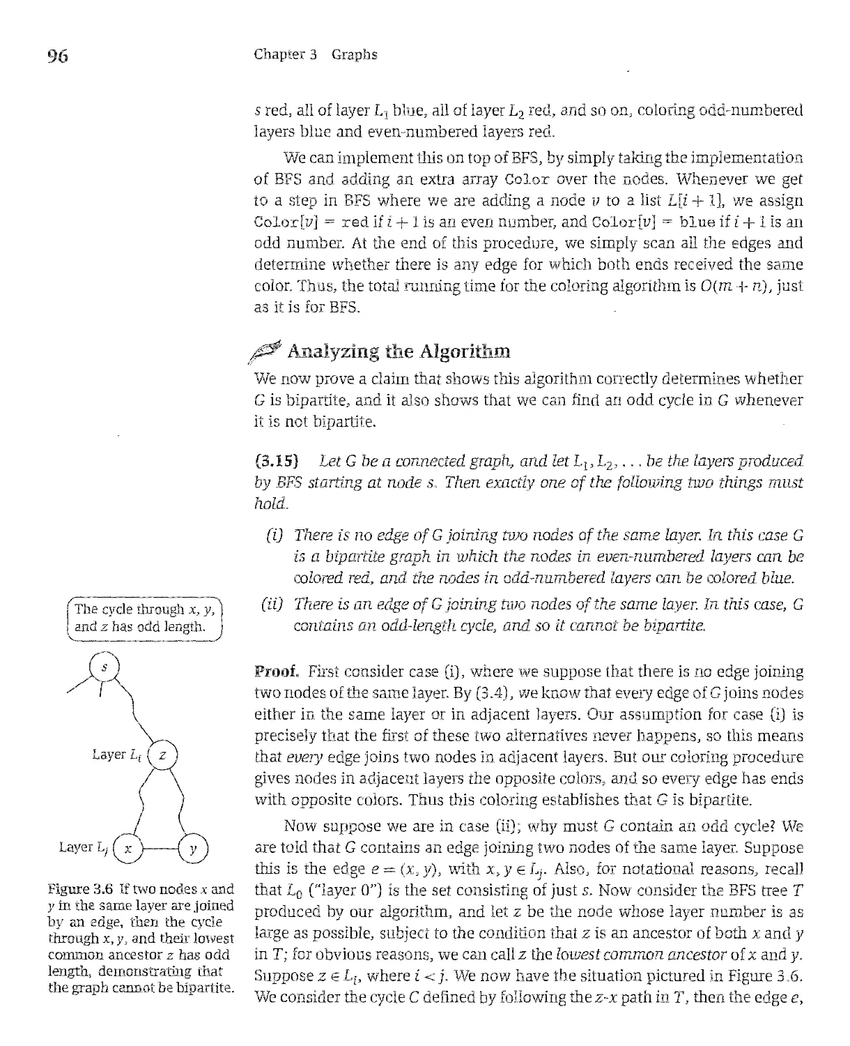
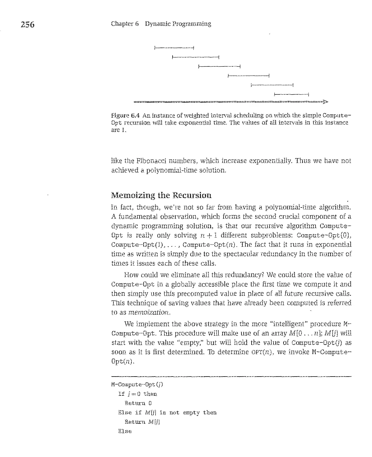
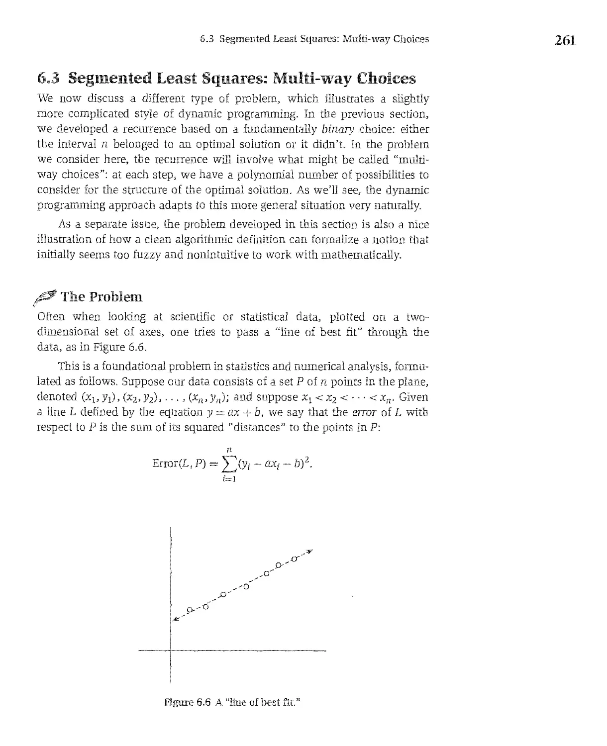
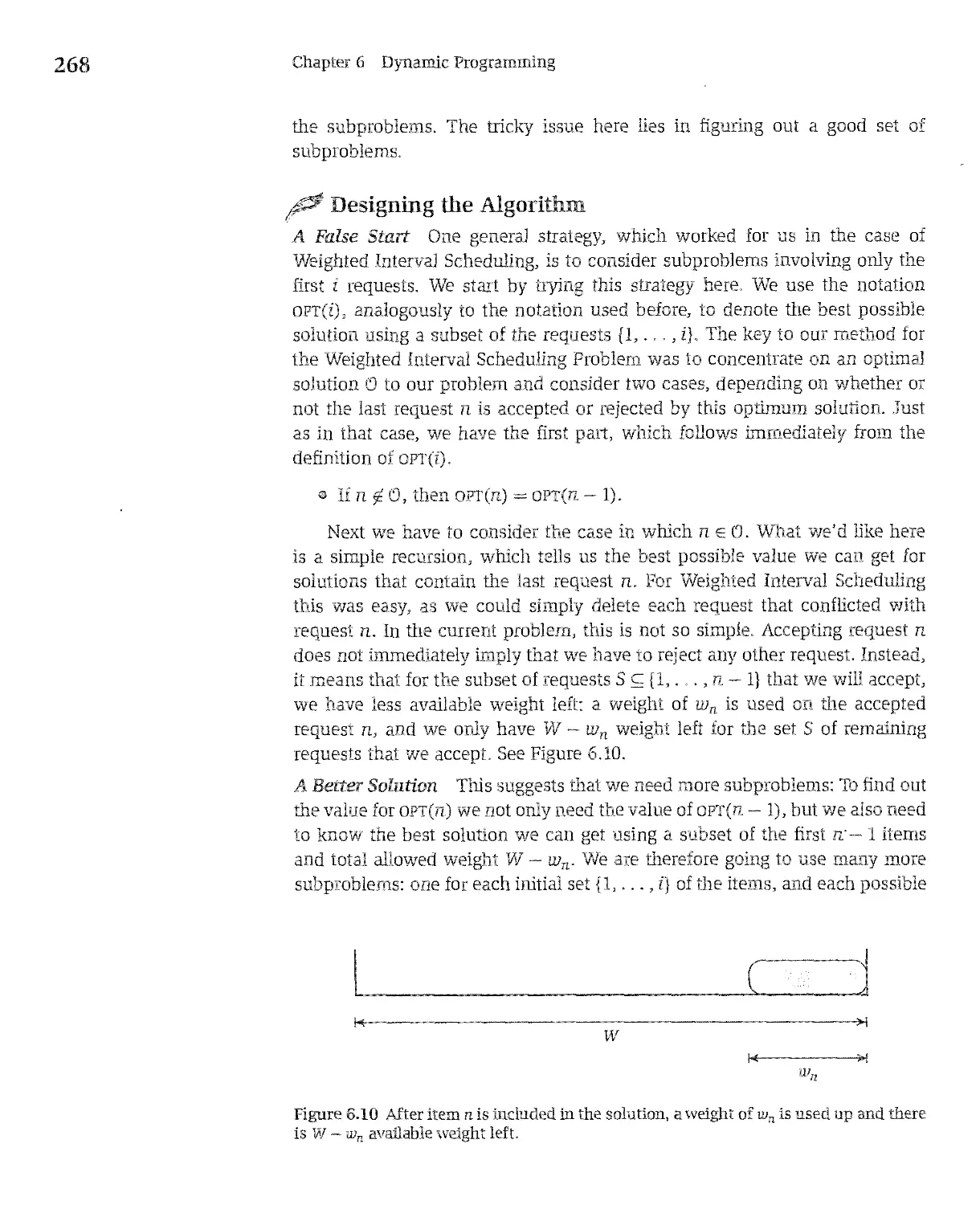
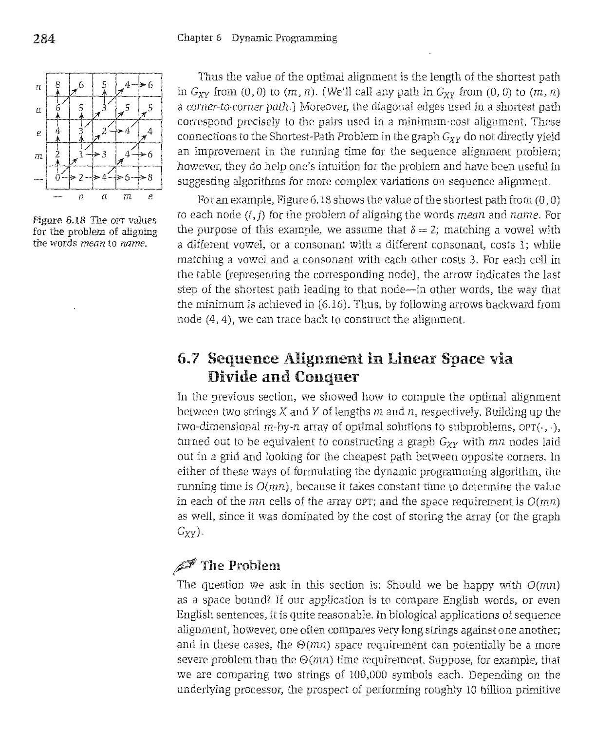
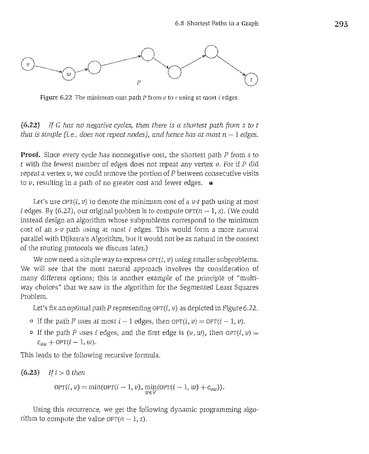
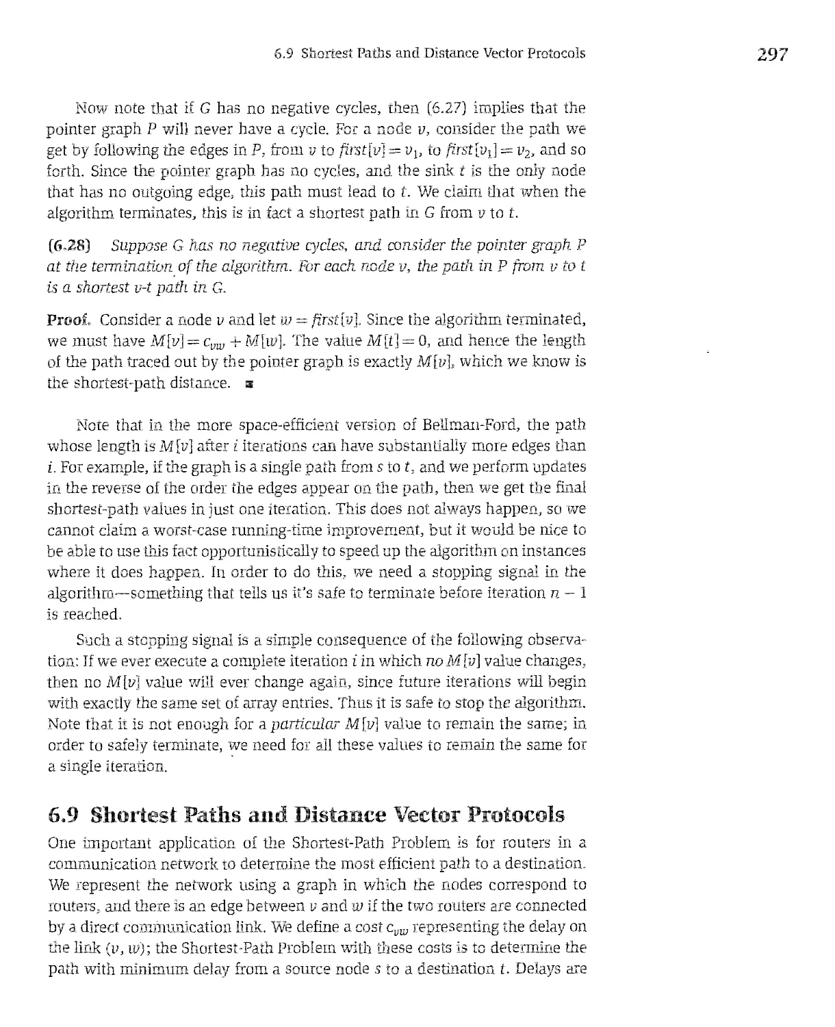
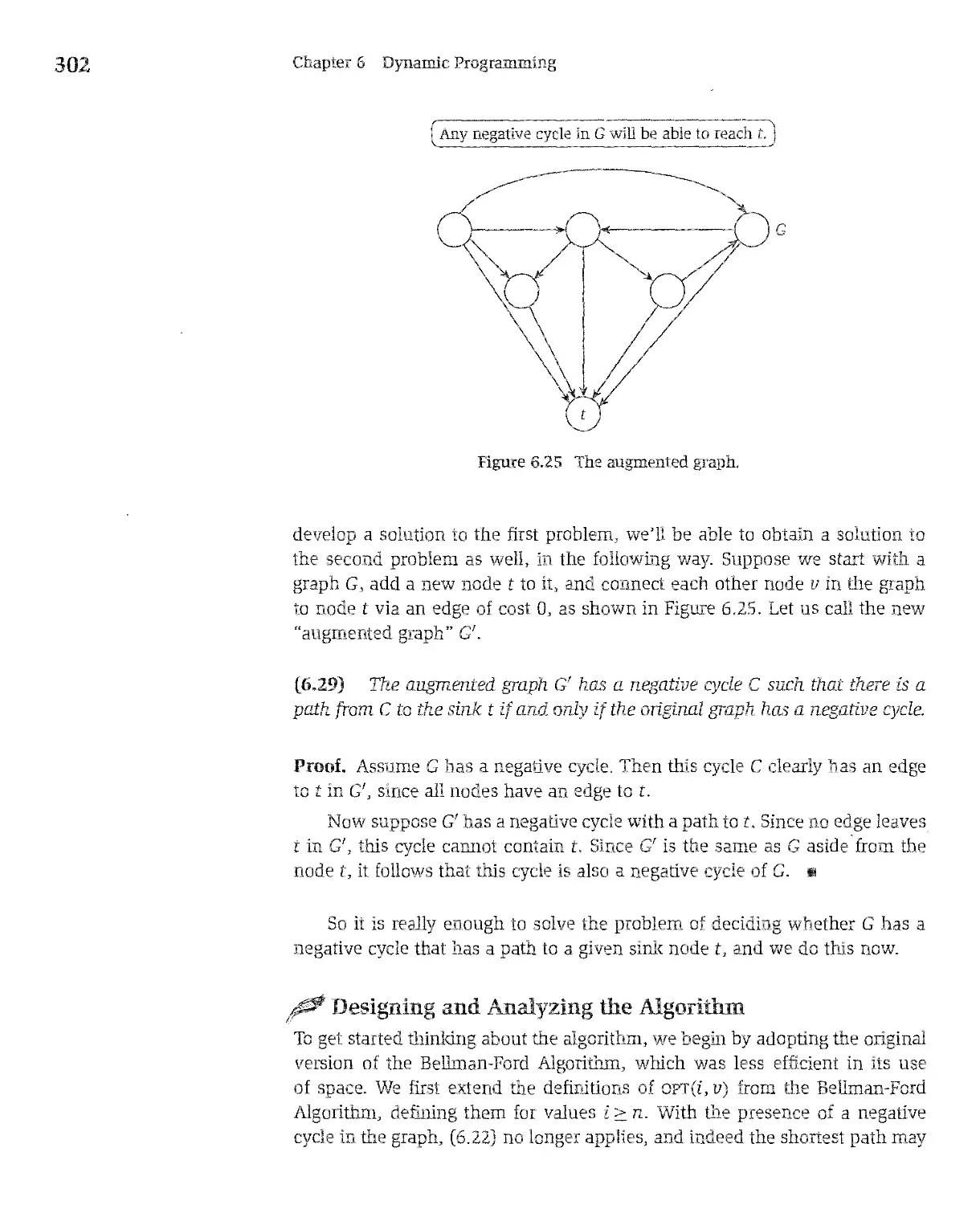
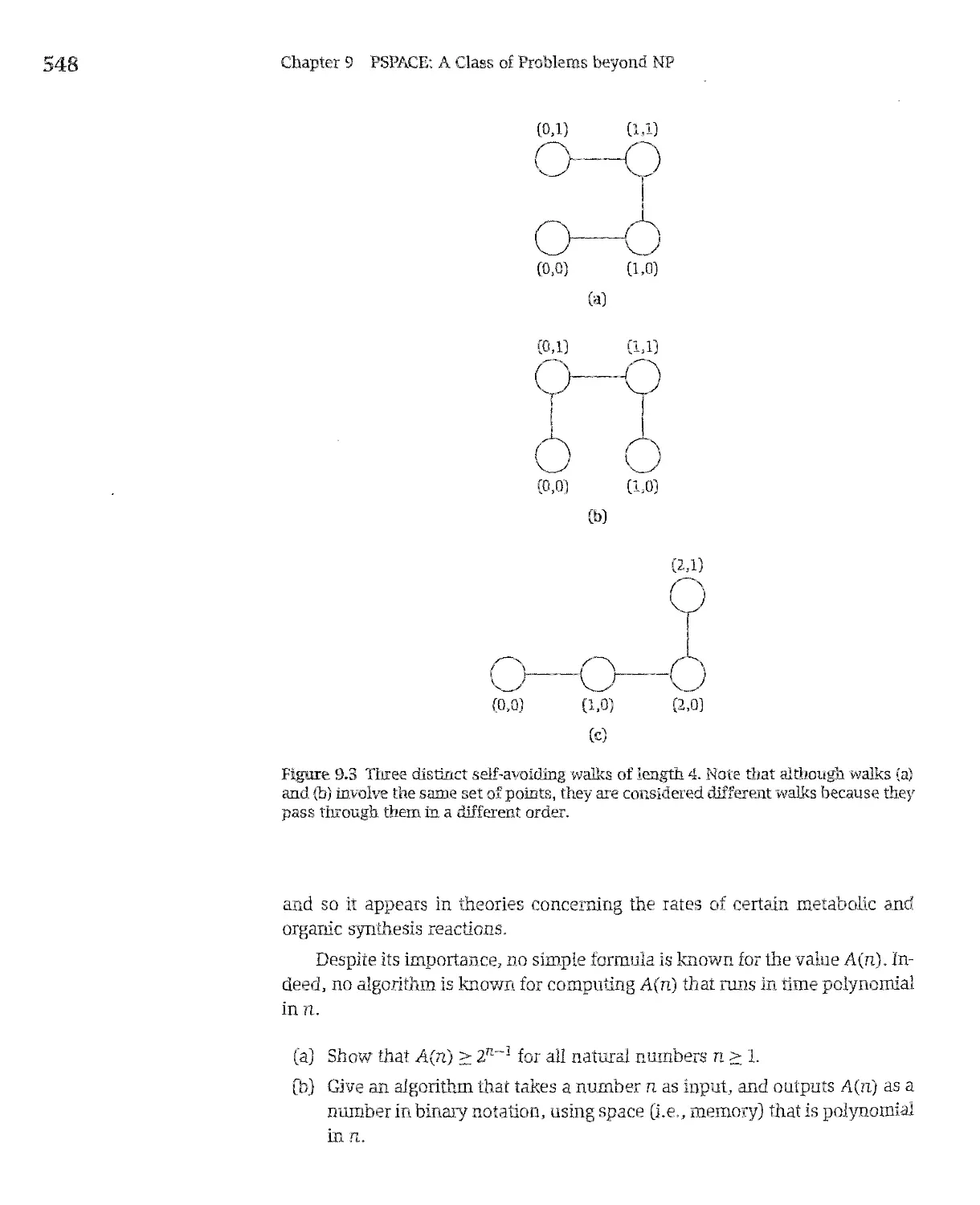
/


Author: Kleinberg J. Tardos E.
Tags: algorithms programming computer science
ISBN: 0-321-29535-8
Year: 2006


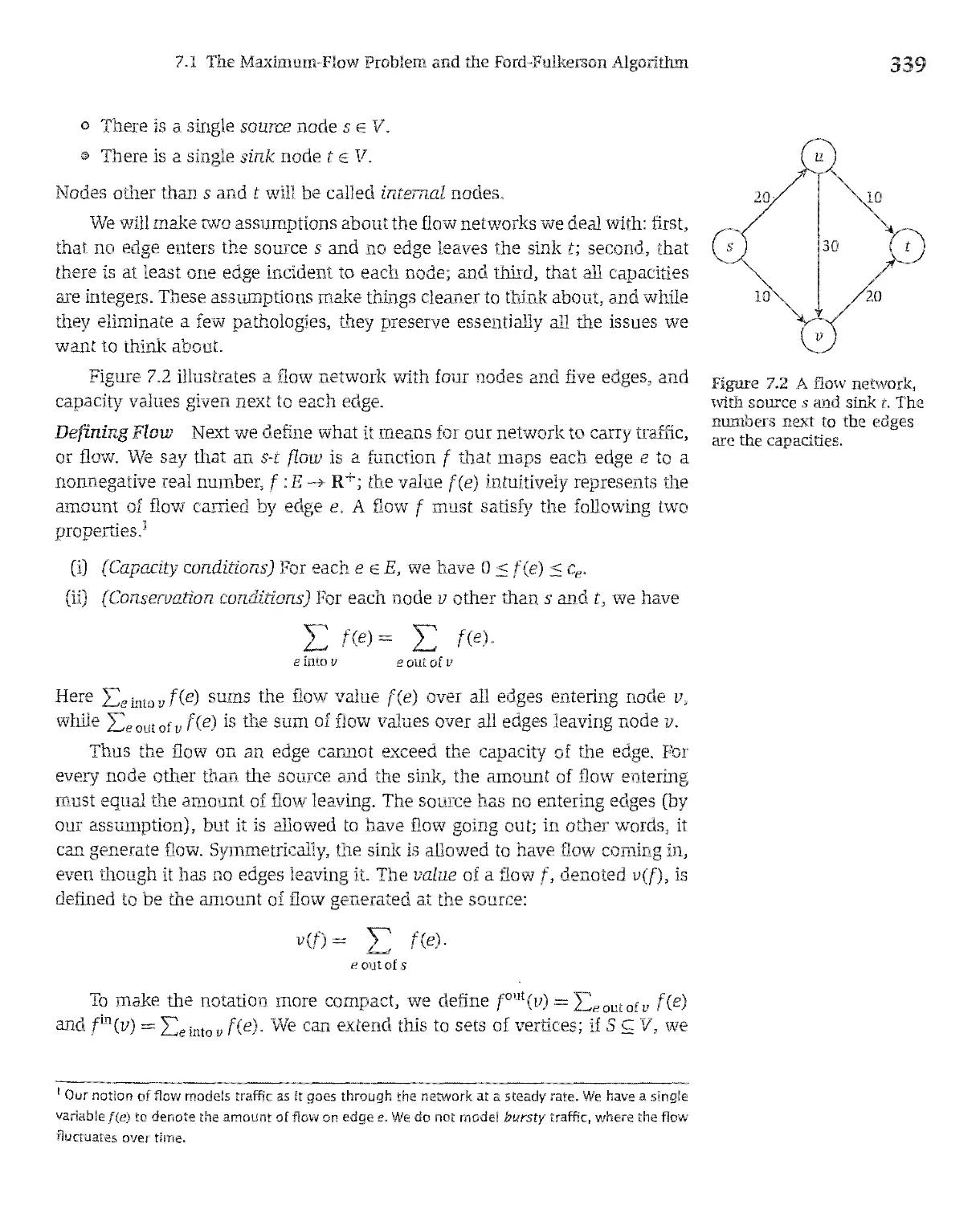
Text
Adchson Tesy.;0] Boston San Francisco NewYork London Toronto Sydney Tokyo Singapore Madrid Medco City Munich Paris Cape Town Hong Kong Montreal
Acgusitions Fditor: Matt Goldstein P o ect Editor: Matte Suai-as Rivas ioduction Superv sor: Manlyn Lloyd Marketing Manager: Mzchelle Bmwn Maiketrng Coordinator Jake Zauracky Proect Managerrc n. Wind [ail Sofhvare Composition Wind[all Software, usrng ZzlX Copyed tor, Carol Leyba Technical Iilustration, Dartrnouth f ublistung roofreader Jennifer McClain Indexc Ted Laux Covei Design: Joyce Cosenlino Wells Cover Pho o © 2005 Tim Laman / National Geograplue A pair cf weauerbirds work together on their nest in Africa Prep ess and Manu[acturmg CarMine l’ail Pi n er: Courzer Westford Access the latest informatioi about Add son-Wesley tilles from oui World Wid’ Web site: h tp //www.aw in. com/comnutng Many of the desgnat ons used by manufactureis and sel e s to dis ngmsh their products are clairied as trademarks. Whe e those designatiuiis appear in this book, and Addison Wesley was aware of a tradc isark clann, he desigranons have been printed n initial caps or ail caps The programs and app ications presented in tins book have been included for their ins uctional value. Ihay have been tested wi h care but are not guaranteed for any particula purpose, The p ibi sher do s so offer a sy warranties or representatior s, nor does il accept any I abilities with respect to tha programs or applications I ibrar of Congress Catalogi sg n Publicatior Data Kleinberg, Joi Alar’thm detigr / b Klein”ng, Eva arJos 1 st ed, p cm. Includes bibi ographica meferences and index. ISBN O 321-29535 8 (a k. paper) 1 Con puter algorithms. 2. Da y structures (Computer science) . Tardos, Eva, II Tille, QA76 9 A43K54 2005 005 —dc222005000101 Copyright © 2006 by Pearson Education, Inc For information or obtain ng permission for use of material in this wo k, please submit a wrttes request to Pearson Education, Inc , Rights anti Cortract Departn est, 75 A I ngton Stree , Suite 300, Boston, MA 02116 or fax you request to (617) 846 7047. Ail ights reserved No part of 1h s publicatior n ay be reproduced stored in a retrieval systers, or transmit ed, n any orrs or by any menas, electrouc, mechanical, photocopyirg, recording, or any lober nedia embodirsents now know s or hereafte to become known, witl ont the prior wntten perrmssio s of die publisher. P hted in die United States o America. ISBN 0-321 29535-6 23456 8)10CRW08070605
About die Authors Jan Kleinberg is a professor of Computer Science at Corneli University, He received his PhD. from MIT. in 1996. He is the recipient of an NSF Career Award, an ONR Young Investigator Award, an IBM Outstand ing Innovation Award, the National Academy of Scti ences Award for Initiatives in Researh, research feti lowships from the Packard and Sloan Foundations, and teaching awards from the Corneil Engineering College and Computer Science Department. Kieinberg’s research is centered around algorithms, particularly those coru cerned wi.th the structure of networks and information, and with applications ta information science, optimization, data mining, and computational bioti ogy. His work on network analysis using hubs and authorities helped form the foundation for the current generation of Internet search engines. Éva Tardas is a professor of Computer Science at Cor neli University. She received her Ph.D. from Eiitviis University in Budapest, Hungary in 1984, She is a member of the American Academy of Arts and Sci ences, and an ACM FelIow; she is the recipient of an NSF Presidential Young Investigator Award, the FuIk erson Prize, research fellowships from the Guggem heini, Packard, and Sloan Foundations, and teacin ing awards from the Corneli Engineering College and Computer Science Departrnent. Tardos’s research intterests are focused on the design and analysis of aigorithms for problems on graphs or networks. She is most known for her work on networkf1ow algorithms and approximation algorithms for network problems. Her recent work focuses on algorithmic game theory, an emerging area concerned with designing systems and algoritiims for selfish users.
Contents About the Authors y Pref ace xiii Introduction: Some Representative Problems 1.1 A First Problem: Stable Matching 1 1 2 Five Representative Problems 12 Solved Exercises 19 Exercises 22 Notes and Further Reading 28 2 Basics of Algorithm Anal ysis 29 2.1 Computational Tractabfflty 29 2,2 Asymptotic Order of Growth 35 23 Implementing the Stable Matching Algorithrn Using Lists and Arrays 42 2,4 A Survey of Cominon Running Tirnes 47 2,5 A More Complex Data Structare: Priority Queues 57 Solved Exercises 65 Exercises 67 Notes and Further Reading 70 3 Graphs 73 3,1 Basic Definitions and Applications 73 3 2 Graph Cormectivity and Graph Traversai 78 3,3 Implementing Graph Traversai Using Queues and Stacks 87 3.4 Testing Bipartiteness: An Application of Breadth-First Search 94 3,5 Connectivity in Directed Graphs 97
viii Con ents 3 6 Directed Acychc Graphs and Topological Ordering 99 Solved Fxercises 104 Fxe cises 107 Notes a d F rther Reacling 1 2 4 Greedy Algorithms 115 4 1 Interval Scheduhng. The G eedy Algorithm Stays Ahcad 116 4.2 Scheduling to Minimize Lateness An Exchange Argument 125 4.3 Optima Caclung A More Complex Exc ange Argument 13 4 4 Shortest Paths r a G aph 137 4 5 The Minimum Spanni g Tiee Problem 142 4.6 Ir plementing KruskaPs Algo ith r Ihe Union Find Data Stiucture 151 4.7 Clurte ng 157 4,8 Huftman Codes and Data Compression 161 * 4 9 Minimum Cost Arborescences: A Multi Phase Greedy Algonthm 177 So ved Exercises 18 Exercises 188 Notes and Further Reading 205 S Divide and Conqzzer 209 Ç 1 A First Recarrence Th Mrrgesort k.goriJim )1fl 5.2 Further Recurrence Relations 214 5.3 Counung Inversions 221 5 4 Finding the Closest Pair of Points 225 5 5 Integer Multiplication 231 5.6 Convolutions and the Fast Foirrer Transform 234 Solved Exercises 242 Exercises 246 Notes and Further Readmg 249 6 Dynamic Programming 251 6.1 Weighted lute val Scheduling: A Recursive P ocedure 252 6 2 Principles of Dynam c P ograimning: Memoizatio or Iteration over Subprohlems 258 6 3 Segmented Least Sq ares Multhway Choices 26 The star mdkates an opflora sectnn (See the Preface for more nformat on about the refat’orships among the chapters and secoons)
Contents ix 6 4 S bset Sums a d Knapsacks: Adding a Vanable 266 6.5 RNA Secondary Structure: Dynamic Programming over I terva 5 272 6.6 Sequence Alignment 278 6.7 Sequence Alignmeut in Linear Space via Divide rnd Conquer 284 6.8 Shortest Paths in a Graph 290 6.9 Shortest Paths and D stance Vector Protoco s 297 6 0 Negative Cycle5 in a Graph 301 Solved Exercises 307 Exercises 312 Notes and Further Readi g 335 7 Network Flow 7 7. The Maximum Flow P oblem and the Fa d Fuike son Algorithm 338 7,2 Maximum Flows and M iimnm Cuts in a Ne wo k 3/ 6 7 3 Choos g Good Augrienting Paths 352 7.4 The Prefiow Push Maximum-Flow Algorithm 357 7.5 A First Application: The Bipartite Matching Prohlem 367 7 6 Disjo t Paths m Directed and Undi ected Grap s 373 7 7 Extensions to the Maximum Flow Problem 378 7.8 Survel Design 384 7.9 AirlineScheduiing 367 7 10 Image Seg nentation 391 7 11 p oject Selection 396 7,12 Baseball Elimination 400 * 7.13 A Further Direct on Adding Costs to the Matclung Problem 404 Solved Exercises 4 Exercises 415 Notes and Further Reading 448 8 NP and Computational Intiactabillty 451 8.1 Polynomial-Time Reductions 452 8.2 Reductions via “Gadgets”Ite Satisfiab lity Problem 459 8 3 Efficient Certificatio and t w Defrnitio of NP 463 8 4 NP Camp etc Problems 466 8.5 SequencingProb1ems 473 8 6 Partitioning Problems 48 8 7 G aph Coloring 485
x Contents 8$ Nuinencal Prob e ris 490 8$ CoNP and the Asymmetry 0f NP 495 8 10 A artial Taxonomy of Hard Problerr s 497 Solved Exercises 500 Exe1cises 0S Notes and Further Readi g 529 9 PSPACE: A C1as of Problems beyand NP 531 9 1 PSPACE 531 9 2 Some Hard Problems in PSPACE 533 93 Solvmg Quantified Problems and Cames in Polynomial Space 536 9A Solvmg the Planmng Problem in Polynomial Space 538 9 Proving Problems I’SPACE Comple e sis Solved Exercises 547 Exerc ses 550 Notes and Fuither Reading 551 10 Extending the Limits of ltactabilzty 553 10 1 Finding Small Vertex Covers 554 10 2 Solvmg NPHard Problems on Trees 558 103 Colo mg a Set of Circular Arcs 563 * 104 Tree Dccompositior s o Ci plis 572 0 5 Constructing a Tree Decompos tion 584 Solved Exercises 591 Exercises 594 Notes and Furiher Readi g 598 11 Approximation Algorithrrzs 599 111 Creedy Algorithms and Bounds on the Optimum A Load Ilalancing Problem 600 2 The Center Selection Problem 606 11 3 Set Cove A Ce eral Creedy Heuristic 612 1L4 The Pncmg Metl-od Ve tex Cover 618 11 5 Maximization via the Pncmg Method The Disjoint Paths Problem 624 11 6 Linear Prograrnrmng and Round rg An A plication to Vertex Cover 630 7 Load Balancing Revisited: A More Advanced LP Application 637
Contents xj 11 8 Arbitrarily Good Approximations The Knapsa k Problem 644 So veci fixe cises 649 Exerciscs 651 Notes and Further Reading 659 12 Local Search 661 12J The Landscape of an Optimization Problem 662 112 The Metropolis Algorithm and Simulated Annealing 666 12 3 An Apphcatio of Local Search to Hopfleld Neural Ne wo ks 671 2 4 Maximuri Cut App oximation via Local Search 676 ilS Choosing a Neighbor Relation 679 12.6 Classification via Local Search 681 12 7 Best Response Dynanu s ard Nash Equilibria 690 So1ved Exercises 700 Exercises 702 Notes ard F rther Reading 705 13 Randomized Algorithms 707 13.1 A First Application: Contention Resolution 708 13 2 Finding tIe Global Minimum Cut 714 3 3 Random Vax ables and Their Expectations 719 13.4 A Randoniized Approximation Algorithm for MAX 3SAT 724 3.5 Randomized lYvide and Cunq r Mdian Fliiding and Quicksort 727 16 Hashing: A Randomized Imilementaton of Dictionaries 734 3 7 Finding the Closest Pai of Points A Randoimzed Approach 74 3 8 Randouuzed Cachmg 750 119 Chemoff Bounds 758 3 10 Load Balanciig 760 3 11 Pa ket Rou 111g 762 13.12 Background: Some Basic Probabfflty Definitions 769 Solved Exercises //6 Exerc ses 782 Notes and Further Reading 793 Epilogne: Algorithrrzs nuit Run Forever 795 References 805 Index 815
Pre face Algorithmic ideas are pervasive, and their reach is apparent in examples both within computer science and beyond. Some of die major shifts in Internet routing standards can be viewed as debates over the deficiencies of one shortestpatlr algorithm and the relative advantages of another. Th e basic notions used by biologists to express similarities among genes and genomes have algorithmic definitions. The concerns voiced by econornists over the feasibiiity of combinatorial auctions in practice are rooted partly in the fact that these auctions contain computationally intractable search problems as special cases, And algoridimic notions aren’t just restricted to well-known and long- standing problems; one sees die reflections of these ideas on a regular basis, in novel issues arising across a wide range of areas. Th e scientist from Yahoo! who told us over lunch one day about their system for serving ads to users was describing a set of issues diat, deep down, couid be modeled as a network flow problem. So was die former student, now a management consultant working on staffing protocols for large hospitals, whom we h appened to meet on a trip to New York City. The point is not simply diat algoridims have many applications. The deeper issue is that die subject of algorithms is a powerful lens through winch to view die field of computer science in generaL Algorithmic problems form die heart of computer science, but t.hey rarely arrive as cleanly packaged, mathematically precise questions. Radier, diey tend to come..bundled togedier widi lots of messy, application-specific detail, some ofit essential, some of it extraneous. As a result, die algorith.rnic enterprise consists of two fundamental coinponents: die task of getting to die madiematically clean core of a problem, and ilren tire task of identifying die appropriate algorithm design techniques, based on die structure of die problem. These two components interact: die more comfortable one is widi die full array of possible design techniques, die more one starts to recognize die clean formulations diat lie within messy
Pretace problems out in the world At thei most effective, then, algorithruc ideas do flot just provide solutions ta wellpased problems; tt ey forr the lai guage that lets you cleanly express the underlying questions ‘‘hegoal of our book is ta convey this appraach to algonthms, as a design rocess tht begins with problems ansing arrns the full range of computing applications, builds an an understand ng of algorithrn design techniques, and results in the developme t of efficient solutions ta these prablems We seek to exp ore the role of algorithmic ideas in computer science generally, and relate these ideas ta the range of precisely formulated oroblems for which we cari design and analyze algor th us In other words, what are tire underlyr ig issues that otivate these problems, and how did we choase these particular ways cf formulaung them2 Haw did we recognize which design pnnciples were ppropriate in different situations? In keepmg with this, our goal is ta offer advice o how o ide it fy clean algorithmic problem formulations in complex issues from d fferent areas of computing and, from tins, how to desig efficient algorithms for tire resulting problems. Soplusticated algor thms are afien best understoad by reconstruct ing the sequence cf ideas—including false starts and dead ends li a lcd fiom simpler initial approaches ta tire eventual solution Tire resuit is a style cf exposition that does not take the Tost direct rente from problem statement ta algorithm, but we feel it better reflects tire way that we and oui colleagues genuinely think about these questions. Overview The bock is i rie ded for s ude Us who have completed a programirnng based two se ester introductory computer science scq e ce (the standard “CS1/C52”courses) in which they have writte programs that implement basic algcrithms, manipulate discrete structures such as trees and graphs, and apply basic data structures su h as arrays, lists, queues, and stacks, Smce the interface between C5l/CS2 and a first algorithms course is net entnely standard, we begin tire bock with self contair cd coverage cf taplcs that at some institutions are familiar ta students fia CS1/C52, but which al other nsdiudcs are mcl’ ded r tic sy° ahi ul tire first algoridims caurse, Tins ater al ca Urus be t eated either as a review or as new mater a , by in luding it, we hape tire bock can be used in a broader anay cf caurses, nd w’th mare flexibility in tire prerequisite knowledge that is assumed In keeping with tire approach outlined above, we develop die b sic algoritirm design techniques by drawi g or problems from acrcss many areas of computer science and related fields To menticn a few represenlative examples here, we include fairly deta1ed discussions cf applications from systems ard networks (cad ng, switching, interdomain routi ig on tire n crue), artificial
Preface xv intelligence (planning, game playing Hopfield networks) computer vision (image seg rier talion), data minmg ( hange point dete flo , clustermg), op erations research (airline scheduling), and camputational biology (sequence alignment, RNA secondary structure), The notion of camputatianal intractability, and NPcompleteness in par ticular, plays a large raie in inc bock. Tins is consistent with how we think about he overail process cf alga itiun design. Some of inc time, an interest ng problem ansing in a applicatia area wiil be a e abie ta ar effic e t solution, and some of the time it wffl be provably N-complete; in aider ta fully address a new algorithmic probiem, one shouid be able ta explore both of ti ese op ions with equal famihanty Smcc sa many iatural p obiems in computer sc ence are NP complete, inc deveiopment of methods ta deal with intractable problems has become a crucial issue in inc study cf algorithms, and oui bock heavily reflecis tins theme, The discovery thal a problem is NPcomplete should ot bc takcn as inc end cf inc s tory but as an mvitation ta begm iooking for approximation aigonthms, eunstic local searc techniques, or tractable special cases, We include extensive coverage cf cadi cf these three approaches. Problems and Solved Exercises Ai important fealure cf the bock is inc collection cf probiems. Acrcss ail chapters, tic bock mc udes aver 200 proble is, almos ail o hem deve oped and classtested in homework or exams as part cf oui teaci ‘ngcf inc course at Corneil. We view flic prablems as a crucial ccmpcnent cf the bock, and fficy arc structurcd in keepi ig with oui overail apprcach te inc matenal. Mcst cf them cansist cf exte ded verbal descnpticns o a problem ansing in an application area in camp ter science or elsewi ere eut in the world, and part cf inc prablem is to practice what we discuss in inc text: setting up inc necessary otatian and fa matizatian, desigrung an algorithm and inen analyzmg it and proving it orrect (We view a camp etc answe ta one cf hese p obiems as consisting cf ail inese components a fuily expiai ied algcriti n, n nalysis cf inc running tue, and a procf cf ccrrectness,) The ideas for these prcb ems corne in 1arg. part frGm discusnoni ve have ha over inc yeas wit people warking rn different areas, ard in sce cases tiey seve inc dual purpose o recording an interesting (inc gh manageable) application cf algcrithms inat we haven’t seen written dcwn anywhere cisc. la help wth inc process cf wcrkmg o ti ese problems, we irclude in each chapter a section entitled “SolvedExercises,” where we take ane or mare prabiems and describe how ta go about formulating a solution. The discussion devcted ta each 50 ved exercise u thercfore signrflcanfly longer tian what would be needed si nply te w ite a ompie e, cc re t solution (m other words,
xvi Preface sigruficaritly longer thari what it would take to receive full credit if these were be r g assigned as homework prob ems) Ra hei, as with t1 e rest o t1 e text, the discussions in these sections should be y ewed as trying o gîve a serse of die larger process by which one might think about prob ems cf titis type, culminatrng in the specification of a precise solution It is worth mentioning two points concerning the use of these problems as homework in a course First the problems are sequenced roughly in order cf increas r g diffi ni y, bu tius is or y an approximate guide and we advise against placing toc much weight on it: since the bulk cf t1 e problems were designed as homework for our undergraduate class, large subsets cf the problems in each chapter are really closely comparable ii terms cf difficulty. Second, aside from dE e lowest numbered ores the problems are des gued 10 involve some investment cf rime, both to relate the problem description tc tire algonthmic techniques in die chap ter, and then to actually design the necessary algonthm n o unde graduate class we have tended to assign roughly thiee cf these p oblems per week Pedagogical Features and Supplements r add tion to the p oblems and solved exercises, die bock iras a number cf f rtt er pedagogical features, as well as additional supplemen s to a i ita e ts use for teaching, As noted car er, a arge ri ber cf the sect ons ir the bock are devoted to the formulation cf an algotithmic prcblem ncludir g its background ai d underlying motivation—and the design and ana ysis cf an a gorithm for this proble n “‘ore iect this style these sections are consistently structured around a seq e inc cf subsections “TheProblem,” whe e the problem s desc ibed and a precise formulation is worked ouf, “Desgmrg the Algori hm,’ where the appropriate design technique is employed ta develop an algoritlrm; and “Analyzingthe Algorithm,” which proves properties cf die algorithrn and analyzes its chic e icy These s bsect ons are highl g rted in the xt with an iccn depicting a feather, In cases where extensiors 10 the problem or further analysis cf die algoridim is pursued, there are additional subsections devoted ta the isu T e goa’ cf th stiucture is to cher a rela,avely ,morin style cf presentaticn tif a mayes from die initial discussion cf a pioblem a ising m a ccmputing application through ta die detailed analysis cf a metf cd ta salve t A nu ber cf supplemen s are ava lable in suppo t cf t e bock tself, An instructcr’s manuai wcrks th cugh ail dEc pioblems, providing full solutions to each, A set cf lecture slides, developed by Kevin Wayne cf Princeton University, is also availah e, these shdes follow die ordei cf the book’s sections and can thus be used as die foundatio for lectures in a course based on die bock These files are available at murai cm cour. For ir structions on obtaim ig a professor
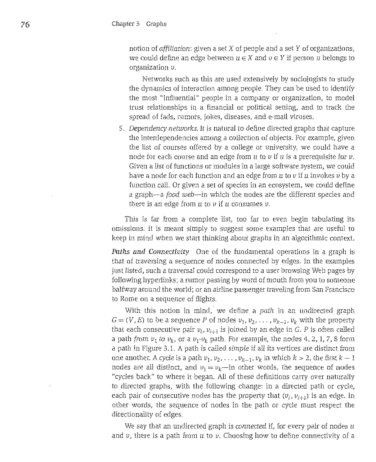
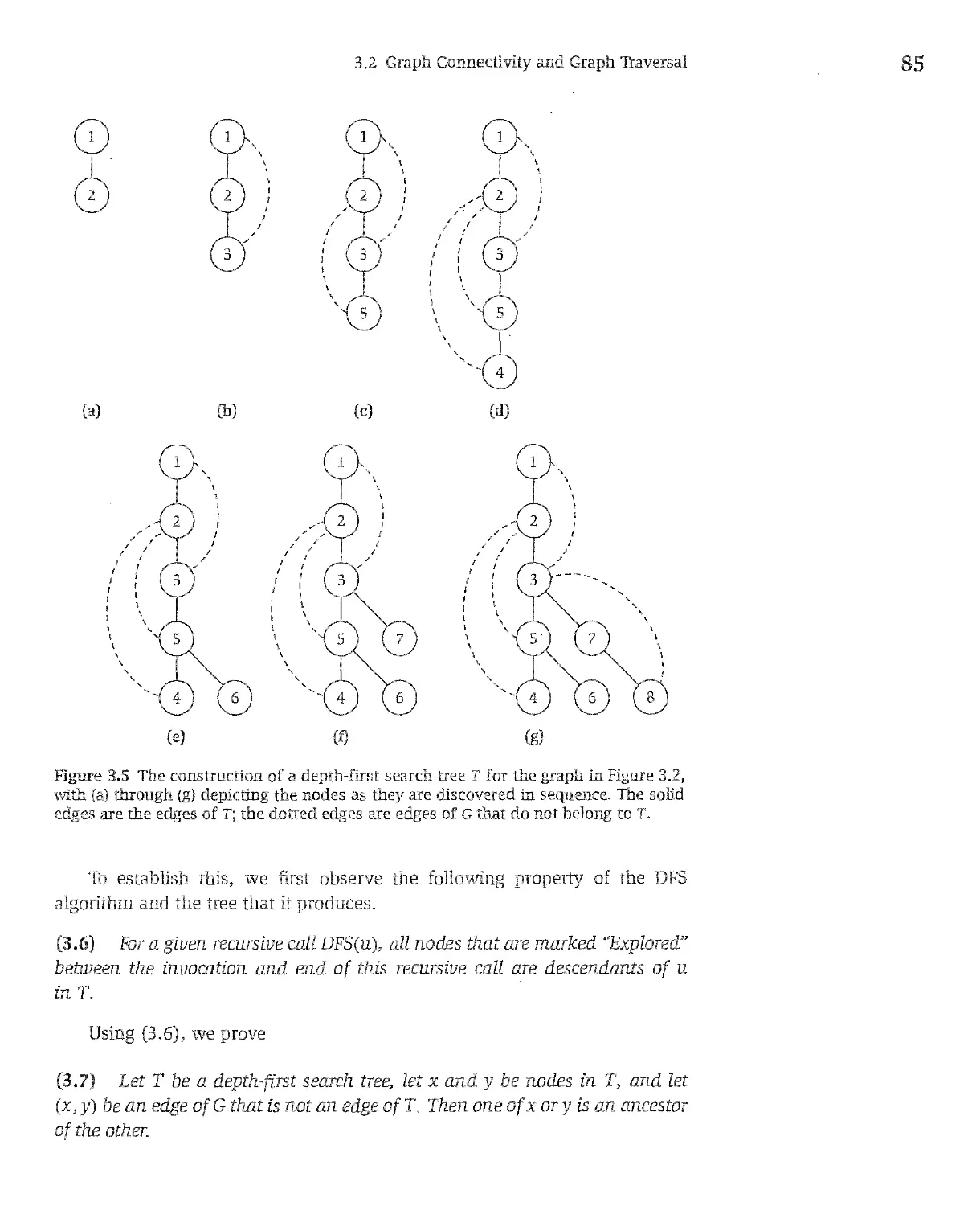
Pref ace xvii login and password, search the site for either “Kleinberg”or Tardas” or contact yaur local Addison Wesley representative. Finally, we would appreciate rece ving feedback on the book In p rticular, as in any book af this length, there are undoubtedly errars that have remained in Jie fin.I verjon, Coninents and reports of errors can be sent o us by e mail, at the add ess algbook@cs corne 1 edu, please include the wo d “feedbackin the subject une of the message. Chapter by Chapter Synopsis Chapter 1 starts by intraducing some rep ese tative algantiriic problems We begin immediately with the Stable Matching Problem, since we feel it sets up the basic issues in algorithm design more concretely and more elegantly th.n .nv rl di’nïari (anld Ile m.t”hing i nlnLv.rted hy a n.rtural thougl camplex eal world ssue, from w ich one can abstra t ar nte esting problem statement and a surprisingly effective algorithm ta salve tins problem. The remainder of Chapter 1 discusses a list of five “represenlativeproblems” that fa eshadaw tapics from the re arider al the course, These five problems are in errelated in Ii e serse mat mey are al var ations ard/or spe ia ases of the Independent Set Problem; but one is solvable by a greedy algorimm, ane hy dynamic programrning, one by network flaw, one (me Independent Set Proble itsel) is NP camplete, a d one is PSPACE complete. The lad ma closely rela cd prablcms car vary g eatly r omplexily is an i ipor ant theme al the book, and these five problems serve as rnilestones mat reappear as me baak progresses. Chaptcrs 2 and 3 caver me irte ace ta me cs /C52 cou se sequen e mentianed carnier. Chap ter 2 introduces me key mamematical definitians and notations used far analyzing algarithms, as well as the mativating principles behind t cm lt begi s with a informai averv ew al what t means far a p ah leu ta he computatianally tra table, togethe w h the corcept of polynomial time as a formai nation af efficiency. li then discusses grawth rates of func tians and asymptatic analysis more farmally, and affers a guide ta cammonly oc u ring furictiau s in alga ii’ un analys s, tagemer wim standard applucaua s I wh ct thcy arise Chapter avers me basi deflmtaans and algorithmic primitives needed for working with graphs, which are centrai ta sa many of the problems in the book. A number al basic graph algarithms are otten im plemented by s ude ts Iate ffie CS1/CS2 course sequence, but i is valuable ta prese t the material here in a braader rlgarithm design ortext n par ticular, we discuss basic graph definitians, graph traversai techniques such as breadth first seaich and depth first search, and directed graph concepts includ ng strong cannectuvity and opolagical o dering
xviii Preface Chaptrs 2 and 3 alsa present many of the basic data structures that wiiI be used for impIe eut ng a garithms throughout the book; more advanced data structures are preserited in subsequent chapters Our approach ta data structures is ta intraduce them as they are needed for the impie entation of the alganthms hei g developed in the baok, Thus, althaugh many of the data structures covered here will be farmha ta students tram the CS1/CS2 sequence, oui focus is on these data structures the braad r ontext of algonthm design and analysis Chapters 4 through 7 caver four major algo itl i design techmq ies greedy algarith s, divide and canquer, dynamic programming, and retwork flaw With greedy algo it1ws the hal erge is ta recagnize when they wark and when they don’t; oui coverage af this tapi s en ered à ound à way of cIas sify rg the kinds of arguments used ta prove greedy algorittims correct This chapter con I des with some af trie main applications af greedy algarithins, far shartest iaths, undire ted cd c’irected spanning trees, clustering, and compression. For divide and cana uer, we begin wi h à discussion af strategies far sa ving recurrence relations as baunds on nning times, we t e s iow how famiharity with di se recurrences can guide the design of algorithms that imprave over straigi tfarward approaches ta à number of basic problems, including the comparison of rankings, h- e amputation af closest pairs of points in die p a ie and the Fast Fourier Transform Next we develop dlriam c pro gramu icg by starting with die recursive intuition behind if, and s hseq ently building up mare and r are expressive recurrence formulations through applicaduiis iii which they naturally ai se Pis chdp cl cuiicludes with exteiideu discussiar s of the dynamic programming approach ta twa fundar e tal prob lems seq e ce alignmmt with applications in computatianal biolagy, anti shortest paths in giapl s, with conne tiors ta Internet rauting pratocals, Finally, we caver algarithms far network flow prohlems d vo ing much of oui fa us in this chapter ta discussing a large array of different flow applicat ons. Ta the extcn that network flow is covered in algorithms courses, students are often left without an appreciation for h wide range al problems ta which it can be applied; we try ta do justice ta ils versatility by presentmg applications ta Ioad balancmg, scheduling, image segmentation, and à nuniber al other problems C1 apters 8 and 9 caver computational intractability We devo e mast o our attention ta NP completeness, orgaruzing the basic NP-complete problems thematically ta help students recogmze candidates for reductions when they encaur ter new problems. We build up to some fairly omplex proofs of NP campleteness, witl guidance on how one gaes about canst i cf ng a difficult reduction We also cansider types of computational hardness beyond NP completeness, particularly h- raugh the top c of PSPACE completeness. We
Preface find th s s a val able way to emphasize tl[ at mtractability doesn’t end at NP completeness, and PSPACE complctencss also forms tire underpinru ig or sorne central notions from artificial intelligence—planning and gaine playing that wouid otherwise not find a place in the algorithmic landscape we are su veying Chapters 10 through 12 cover three major techniques for dealing with computationally intractable prob er s idertification of stnictured special cases approximation aigorithms, and local se rch 1 eurist cs Oui chapter o t actable special cases emphasizes that instances of NP-complete problems arising in practice ay not be nearly as hard as worst case instances, because they often co tair some stru turc that can be explo ted in the design o an efficient algo rltlrm We ifiustrate how NP co plete problems are often efficie tly solvable when restricted to tree-structured inputs, and we conclude with an extended discussion of tree decompositions of graphs. Wliile tins topic is more suitable for a graduate ourse th r for an undergraduate one ri is a technique with considerable iractical til ty for wh ch ri n i ard o find ai existlng accessible reference for stridents, Our chapter on approximation algorthms discusses both tire process of designing effective algorittims and tire task of understandirg tire optimal so utaon welI enough tu obtain good bounds on it. As design techniques for approximation algorithms, we focus or greedy aigo rithms, linear programming, and a third method we refer to as “pricing,”winch incorporates ideas from each of tire first two. Finally, we discuss local search heur sucs, in luding the Metropolis aigo itl n and simulated anneahng. Tins topic 15 oen missing from rdergrad at algontImi courues, bec,u,e rey littie is known in tire way of provable guarantees for these algorithms, how ever, given their widespread use in practice, we lcd it is valuable for students to know something about tle , and we also mclude some cases in winch guarantees can be proved Chap er 3 covers t ie use of randonuzairon in tire design of algorathms. Tins is a topic o wl ich several m e graduate level books have bec w itten Our goal here is to provide a more compact introduction to some of t1 e ways in winch siudents can apply randomized techniques using the kind of background probabihty one typically gains from an undergraduate discrete math course Use of the Book The book n pnmanly designed for use in a first undergraduate course on algorithms, b t ri can also be sed as tire basis fo an ix troductory graduate course. When we use the booir al he ur dergraduate level we spend rouginy one lecture per n mbered sectio , m cases wlere there is more ttan one
Preface lecture’s woi-th of material in a section (for example, when a section provides further applications as additianal examples), we treat this extra material as a supplement that students can read about outside of lecture. We skip the starred sections; while these sections contain important topics, they are less central to the development of the subject, and in some cases they are harder as welI. We also tend ta skip one or two other sections per chapter in the first half of the book (for example, we tend to skip Sections 4.3, 4.7—4.8, 5.5—5.6, 6.5, 7.6, and 7.11). We cover roughly haif of each of Chapters 11—13. This last point is worth emphasizing: rather than viewing the later chapters as’ “advanced,”and hence off-limits to undergraduate algorithrns courses, we have designed them with the goal that the first few sections of each should be accessible to an undergraduate audience. Our own undergraduate course involves material from ail these chapters, as we feel that ail of these topics have an important place at the undergraduate level. FinaIly, we treat Chapters 2 and 3 primarily as a review of material from earlier courses; but, as discussed above, the use of these twa chapters depends heavily on the relationship af each specific course to its prerequisites. The resulting syllabus looks raughly as fallows: Chapter 1; Chapters 4—8 (excluding 4.3, 4.7—4.9, 5.5—5.6, 6.5, 6.10, 7.4, 7.6, 7.11, and 7.13); Chapter 9 (briefly); Chapter 10, Sections.10.1 and 10.2; Chapter 11, Sections 11.1, 11.2, 11.6, and 11.8; Chapter 12, Sections 12.1—12.3; andChapter 13, Sections 13.1— 13.5. The baok also naturally supports an introductory graduate course on algorithms. Our view of such a course is that it should introduce students destined for research in ail different areas ta the important current themes in algorithm design. Here we find the emphasis on farmulating problems ta be useful as well, since students will soon be trying to define their own research problems in many different subfields. For this type of course, we caver the later tapics in Chapters 4 and 6 (Sections 4.5—4.9 and 6.5—6.10), cover ail af Chapter 7 (moving mare rapidly thraugh the early sections), quickly cover NPcompleteness in Chapter 8 (since many beginning graduate students wiil have seen titis tapic as undergraduates), and then spend the remainder af the time on Chapters 10—13. Although aur facus in an introductary graduate course is on die more advanced sections, we find it useful for the students ta have the full baok ta consuit for reviewing ar filling in background knowledge, given the range af different undergraduate backgraunds amang die students in such a course. Finally, the book can be used ta support self-study by graduate students, researchers, or computer professianals wha want to get a sense for haw they
Preface rnight be able te use particular algorithm design techniques in me context of their own work. A number cf graduate students and colleagues have used portions of me bock in this way. Acknowledgments This bock grew eut of ifie sequence of algorithins courses ifiat we have taught at Corneil. These courses have grown, as the field has grown, over a number cf years, and they reflect the influence cf ifie Corneil faculty who helped te shape them during this time, including Juris Hartmanis, Monika Henzinger, John Hopcroft, Dexter Kozen, Ronitt Rubinfeld, and Sam Toueg. More generally, we would lilce to thank ail our colleagues at Corneli for countless discussions both on the material here and on broader issues about ifie nature cf the field. The course staffs we’ve had in teaching the subject have been tremendously helpful in ifie formulation of this material. We thank our undergraduate and graduate teaching assistants, Siddharth Alexander, Rie Ando, Elliot Anshelevich, Lars Backstrom, Steve Baker, Ralph Benzinger, John Bicket, Doug Burdick, Mike Connor, Viadimir Dizhoor, Shaddin Doghmi, Alexander Druyan, Bowei Du, Sasha Evfimievski, Ariful Gani, Vadim Grinshpun, Ara Hayrapetyan, Chris Jeueil, Igor Kats, Omar Khan, Mikhail Kohyakov, Alexei Kopylov, Brian Kulis, Amit Kumar, Yeongwee Lee, Henry Lin, Ashwin Machanavajjhala, Ayan Mandai, Bii McCloskey, Leonid Meyerguz, Evan Moran, Niranjan Nagarajan, Tina Nolte, Travis Ortogero, Mai-tin Pâl, Jon Peress, Matt Piotrowski, Joe Polastre, Mike Priscott, Xin Qi, Venu Ramasubramanian, Aditya Rao, David Richardson, Brian Sabino, Rachit Siamwalla, Sebastian Silgardo, Alex Slivkins, Chaitanya Swamy, Perry Tam, Nadya Travinin, Sergel Vassilvitskii, Matthew Wachs, Tom Wexler, Shan-Leung Maverick Woo, Justin Yang, and Misha Zatsman. Many cf them have provided valuable insights, suggestions, and coinments on the text. We also thank ail the students in these classes who have provided comments and feedback on early drafts of the bock over the years. For the past several years, the development of the bock has benefited greatly from the feedback and advice cf colleagues who have used prepublication drafts for teaching. Anna Karlin fearlessly adopted a draft as her course textbook at the University cf Washingtcn when it was stifi in an early stage cf development; she was fdilowed by a number cf people who have used it either as a course textbook or as a resource for teaching Paul Beame, Allan Borodin, Devdatt Dubhashi, David Kempe, Gene Kleinberg, Dexter Kozen, Amit Kumar, Mike Molloy, Yuval Rabani, Tim Roughgarden, Alexa Sharp, Shanghua Teng, Aravind Srinivasan, Dieter van Melkebeek, Kevin Wayne, Tom Wexler, and
Preface S e Whitesides. We deeply appreciate their input and advice, wh ch bas in formed many of our revisiors ta the ente t We would hke ta additionally t ank Kevm Wayne for p odùcing supplementary material associated with the book, which promises ta greatly extend its utility ta future instructors, In a umber 0f other cases, our approach [U panicurar rupics in tue auuk reflects the infuence of specific colleagues. Many cf these contributia s have undoubtedly escaped oui noùce, but we especially thank Yun Boykov, Ron Elber Dan Hut enlocher, Bobby Kleinberg, Lvie Kleinberg, Lillian Lee, David McAllester, Mark Newman, Prabliakar Raghavan, hart Selman, David Shmoys, Stve Strogatz, Olga Veksler, Duncan Watts, and Ramin Zabili It lias been a pleasure working with Addison Wesley over the past year First and foremcst, we thank Mati Goldstein for ail r s advrce rd guidarce in this process and for helping us to syrtliesize a vast mou t of review material inc a car cre e pi r tir t imp oved die bock, Our ear y ccnversaricns abcur the book with Susan Hartman were extremely valuable as well. We thaak Mat and Susan, togetlier with Michelle Browr, Manly Llcyd, Paty Mah am, and Marte Suarez Rivas at Addison Wesley and Paul Anagnostopoulos and Jacqul Scirlo t at Wmdf II Software, for ail their work on the editing, production, and management of the project. We further tharrk Paul and Jacqui for tlieir expert composition of the bock. We thank Joyce Wells fa tire caver des gn, Nancy Muupliy of Dar mouth Pubi shing for lier work on the figures, Ted Laux for tte indexi g, a d C roi Leyba and Jennifer McC[ain for die copyediting and proofreading We hank Ans elm Blumer (Tufts University), Richard Cliang (Umversity cf Maryland, Baltimore County), Kevin Compton (University ofMich gan), Dia e Cook (University cf Texas, Arhngton), Sarie Har Pe ed (Umversity cf Ilhnois, Urba a Champaigu), Sanjeev Klianna (University of Pemisylvania), Philip Klein (Brown U riversity), David Matthias (0h10 State Univers ity), Adam Mey erson (UCLA), Michael Mitzemnacher (Harvard Umversity) Step an Olari (Old Domiruon Umversity) Moha Patu (UC S n Diego), Edgar Ramas (Uni versity cf Illinois Urbana Clia rpaig J, Sanjay Ranka (University cf F orida, Gainesville), Leon Reznik (Rocliester Institute of Technology), Subhash Suri (UC Santa Barbara), Dieter van Melkebeek (University cf W scons , Mad son), and Baient Yerer (Rensselaer Polyte lin c I stitute) wlo generously ontnbuted their truie to provide detailed a rd thoughtfui reviews af tire man uscript, hei comments led ta numerous improvements, bath large and small, in the final version of the text. Finally, we tliank oui families—Lillian and Alice, and David, Rebecca, and Amy. We appreciate their support, patience, and many other o tnbutions more ttan we cari express in any a krowledg ents here
P eface jjj I s book was begun armd the irratianal exuberance of the late nineties, when the arc of campu ing technology see ed, ta any al us, bnefly to pass through a place traditionally occupied by celebr’ties a ni ather inhabitants af the pop cultural firmament, (It was prabably just in our imaginations,) Now, several years after the hype and stock prices have came back ta earth, one cari appreciate that in same ways campu er science was fa ever cha ged by tins periad, and in ather ways it bas remained the same the dc ving exc te e t that has c aracte ized tue field smnce its early days is as strang and enticing as eve, tl e publiCs fascmnatian with ifa mation technolagy 15 stiil vibrant, and the reach af computing cantinues ta ex end mb new discip es And sa ta ail students al the subject, drawn ta it far sa many differe t reasons, we hape you fmnd this book an erjoyable and useful guide wherever your computational pursuits n y take you Jan Kleinberg Éva Tardas Ithaca, 2005
CIrpti’ ir Introduction: Some Rpresenta1ive Probiems Li A First Problem: Stable Matching As an openi.ng topic, we look at an algarithmic problem that nicely ifiustrates many of the themes we will be emphasizing. [t is motivated by some very naturai and practical concern, and [rom these we farmulate a clean and simple statement of a problem. The algorithm to solve the prablem is very clean as well, and most of our work will be spent in proving that it is correct and giving an acceptable baund on th.e amount of time it takes to terminate with an answer. The probiem itself—the Stable Matching Pro blem—has severai origins, The Problem The Stable Matching Prablem ariginated, in part, in 1962, when David Gaie and Lloyd Shapley, twa mathematical economists, asked the question: Could one design a college admissions process, or a job recruiting process, that was selfen forcing? What did they mean by this? To set up the question, iet’s first think informally about the kind of situation that rnight arise as a group of friends, ail juniors in college majoring in computer science, begin applying ta companies for summer internships, The crux of the application process is the interplay betweak twa different types of parties: companies (the employers) and students (the appiicants), Each applicant lias a preference ordering on companies, and each company—once the applications ome in—4orms a preference ordering on ils app]icants. Based on these preferences, companies extend offers ta some cf their applicants, applicants choose winch of their offers ta accept, and people begin heading off ta their summer internships.
2 Chapter 1 Irtroduction, Soine Representative Problems Gale and Shapley considered me sorts of h igs ffiat could start going wrong with this process in the absence of any mechanism to enforce tt e status quo Suppose, for example, that your friend Raj bas just accepted a s imer job at the large telecommunications company C Net A few days later, the small startup company WebExodus, which bad been dragging ils feet on makrng a few final decisions, calis up Raj and offers him a surnmer job as well Now, Ra ac ually p efe s Wehflxodus to CluNet won over per aps hy ti e laid back, anythingcarnhappen atmosphere and sa lus ew developinent may well cause hmm to retract bis acceptance of tt e CluNet offer and go to Webhxodus instead Suddenly down one summner intern, CluNet offers a job o one of its wait 1 sted applicants, who promptly retracts his prev ous accept nce of an offer from the software giant Babelsoft, and he situa ion begins to spiral out of control. liii igs look just as bad, if not worse, from he other direct on Suppose that aj’s friend Chelsea, destrned o go to Babelsoft but having just heard Raj’s story, calis up the peole at Webflxod s and says, “Youknow, I’d really ramer spend hc suminer wi h you guys than at Babelsoft, They tnd tins very easy to bd eve, a id furthermore, on looking at Che sea’s applica ion, they realize that they would have rather hired ber than somne other student who actually is scheduled to spend the sumr er at WebExodus. Tn this case if WebExodus we e a shghtly less scmupulous cornpany, it might well fmd some way to et art ts offer to this other student and hire Chelsea instead Situations like thms can rap dly generate a lot of chaos, and many peop e ooffi apphcanms and employerscan ena up unhappy wmtn the p ocess as welI as tl e outcome, What lias gone wrong2 One basi problem is that the process is not self-enforcing if people are allowed ta act in their self-interest, then it risks breaking down We ruight well prefer the following ore stable situation, in which selfinterest itself prevents of e s from being retracted and redirected. Conside another studen , wt o has arranged 10 spend tale summer al CluNet bu calis up Webflxodus and reveals that he, too, would amer work for them But in this case, based on the offers already accepted, they are able ta reply, “No,il turns ou. that e prefer eac of tl’e sudents we’ve acceped o you sa ne re afraid there’s nothi g we can do.” Or consider an employer, earnestly following up with ils top appilcants who went elsewhere, being ta d by each of them, “No,J’m happy where I am.” In such a case, ail flic outcomes are stable—there are no further outside deals ifiat can be made. Sa this is the question Gale and Shapley asked Given a set of preferences among employers and apphcants, can we assign applicants ta employers 50 that for every employer E, and every applicant A wha is not scheduled ta wark for F, al leas one of the following twa things is the case?
1.1 A Fïrst Prob1cn Stable Matching 3 (i) Ii prefers every one o ils accepted applicants to A; or (u) A re e s ier current situation over working for employer E I lus iolds the outcome is stable: individual self-interest will preven any appi ca it/employer deal hum be ng made behind [lie scenes, Gale and Shapley proceeded ta develop a striking algorithnuc 50 on to luis problem, w ch we wil discuss presentiy. Before doing this, let’s note lIa this is not the oaly arigin of lue Stable Matching Prohiem. It turns ouI that for a decade before lue work of Gale and Shapley, unbek ownst to them, tue Na ional Resident Matching Program had been usng a very smula procedire, wi h lue same underlying motivation, to match residents b hospitals Indeed luis system, with relatively httle change is stiil w use today. TIns 15 oie testament to lue problem’s fundamental appeal And fro the point of view of tins book, i provides us with a nice first domain in wh cli to reason about some basic comb atonal defin tians anti the algorithnis that burin on luem, Formulatîng tue Problem To get at the essence of luis concept, i helps to maRe lIe prohiem as clean as possible. The wor d of companies anti app icants contains some distractng asymme ries. Each applicant is looking for a single company, but cadi company s looki g fa a y apphcants; moreover, there ay be more (or, as is sometimes the case, fcwer) appl ca 15 han there are availab e slots fo summer jobs. Finally, cadi applicant does ot typicafly apply ta every campa y lb is seful, at least initially, ta eliminate these complicatio s anti ar ive al a more “haieboues” version al the problem: cadi of n applicants applie5 ta each al n companies, anti eact company wants ta accept a single applicant, We will see that doing tus preserves the funda erta issues inhere il in lue problein; in pa t culai our solution ta luis simplified version wiII ex end direc ly ta lue mare general case as neil, Fallowing Gale anti Shapley, we ohservc ihat this speciai case can be vieweti as hc problem of devising a system by which eact of n me and n women can end up gel ing narned: our problein naturally lias lue analog e of twa “genders”—theapplican s cd tic compames and in tic case we are consideung, everyone is seeking ta be paircd witl exactly one rndividual of the opposite ge hien’ Gale ard Shapley conelde cd the came sex Stable Match ng Pr bien as well, where tere vs only a 5mgle geide Th s vs motvvated by related apptcations but ii turne oui to be favrly dvfferert at a technical level Gvven the applvcante nployer applicatvon we re cosldering here we’ be focusvng on the verson with iwo genders
4 Chapte 1 lot oduction. Some Representative Probletus So consider a setM {m1,..., m} of n mcii, and à se W (w1, , w,} of n women. Let M x W denote the se of 11 poss hie ordered pairs of the form (m, w), w e e m E M and w e W A matching Sis à set of ordered pans, each f om M x W, with the property that each member of M and each membe of W appears in at most one pair in S. A perfect matching 5’ n a matchung with the prope [y tha each r ember af M and each member af W appears in exactly ote pair in 5’ Matchings and perfect uatchings are oh ects [bat will recur frequently (An instability: m an tliroughout he book, [bey arise naturally in modeiing a wide range of algo caci p efer the othe t rithm c problems n tire present situation, a perfect matchung corresponds Ltheir current part iers ) simply to a way of pairung off tire men with tire women, n such a w y lii o—o everyone ends up married o somebody, anti obody us arried ta more than one persan there us neuther sunglehood nor polygamy, Now we can add tire notion ofpreferences o Urus setti g Each man m E M ianks ail the women, we wu 1 say that m pre fers w to w if m ranks w higher ti an w’ We wull refer ta the ordered raaidng of m as iris preference lis t. We wil not aliow tics in tire ranking, Each woman, analogously, ranks ail tire men m w’ Guven a perfect à c mg 5, wl at can go wrong? Guided by our initial Q otiv ion un terms of en ployers and applicants, we should be wouned about tire following situation: There are twa pairs (m, w) and (m , w’) n S (as Figure Li Perfect rratching depicted in Figute Li) with the property that m prefers w’ to w, and w’ prefers S with I istabili y (m U) m to m’ n hus case, there’s nothing ta stop in and w’ from abandoning their c rrent partners and heading off tagether; tire set of marnages us not self enfarcing. W&1 say that such a pair (in, w) us an iristabihty w th uespect o S (in, w’) does flot belong ta 5, but each of in and w’ prefers ti- e oti er ta their pan urer u r 5 Our goal, tiren, is a set of marnages wuth no ns ah uties We’ll s y ti at a matchung S us stable (J ut us pe fect, anti (ii) the e is no instability with resp cf ta S Iwo q estua s spnung irrmediately ta mmd: o Does there exust a stable matching for every set of preference lists? o Guven a set of p eference s s cari we efficie tly canstruct a stable matcnung if tlrere is one’ Sortie Examples Ta iliustrate these definitians, consider tire following twa veny simpie instances of tire Stable Matching Pioblem, Fi s , suppose we have set of twa men, (m, m’}, and a set of twa women, (w, w’) Ti e preference lists are as follows: in prefers w ta w’ m’pefesw ow’
Li A First Problem Stable Matching 5 w prefers m ta m’ w’ p efers m ta m’. 1f we think about this set 0f preference lists intuitively, il represents comp e e agreement lie men agiee an the order of the wamen, and the wamen agree an the order al the men Thora 15 a unique stable matching bore, consisting af the pairs (m, w) and (m’, w’) The other perf oct matchmg, cansisting of die pairs (m’ w) and (in w’), would not be a stable matchi g, because the pa (in, w) wauld for an i stabili y with respect ta this matching. (Bath in e d w wauld want ta bave thei respective partners and pair up.) Next, he e’s e exemple wheie things are a bit more intricate Suppose the preferences are in prefers w ta w’ u efis w’ ta w, w prefers in’ ta in, w’ prefers in ta in’ What’s gaing on in his case1 The twa man’s prefeiences mesh perfectly with each other (they rank different women first), and the twa women’s pieferences likewise mesh perfectly with each ather But the me i’s preferences clash ca ple ely w tir he wamen’s prefei onces. n tt s second example, there are twa different stable match ngs The matclurg consist ng al tire pairs (in, w) and (in’, w’) is stable, beca se bath men are as happy as passible, sa ne tirer would leave their matched partner But the matching cansisting al tire pairs (in’, w) and (m w’) in also stable for thc camplementary reason that bath wamen are as I appy as possible Tins is an irrpa tant point o remember as we go forwardit’s possible for e ins ance ta have more than o e s able ma c r ng Desigrnng the Algoritkm We now show tI’a thora exists a stable matching for every set af prefere ce lists among the mon e d women Mareover aur ineans of shawing Ibis will also answer tire second question ti- al we asked above we will g ve an efficient algorth r that takes the preference lists and canstructs a s ah e atch g Let us cansider some af ti- e basic deas tiret motiva te tire algoritiim. o lnitially, everyane is unmar ied S ppase an unmamed man in chaoses tire woman w who ranks highest an bis p eference list and proposes ta her Can we declare immediately that (in, w) wfflbe ane al the pans m our final stable matching1 Not necessanly: at soma point in tire future, a man in’ wham w prefers may propose ta ire On tire obier hand, it wauld be
6 Chap er 1 Infroduction Some Representative Prob ems (nan w wffl bo om ergaged to ni if she prefI o m’ o o-o Figure L2 An mtermediate state of tie G S algonthm when a fre” mari mis propos mg tu a woman w Endwhile Re ara the set S of engaged pairs An intrigurng thrng is if a, although the GS algorithm 15 qmte simple f0 s Me if s flot naine diately obvious that il retuir s e stab e atchmg, or even e perfect matching, We proceed f0 prove this now, though a sequerice of intermediate facts, dangerous for w to reject m right away, she may neyer receive a proposai from someone she ranils as h ghly s m So a natural idea would bc to have the pair (m, w) erte an ntermediate state engagement o Suppose we are now at e state m winch some men and women are free flot engaged ana cnrne ar2 °ngaged.The next ste c ia nn1 like tins A i arbitrary free mari m chooses hie highest ranked woman w f0 whom 1 e h s flot yet proposed, and lie proposes 10 ter If w is also free, then m and w become engaged. Otherw se, w is already engaged to some other mari m. Tri tins ase, she determines which of m o ni’ ranks Iugher o i e preference Pst, tins mari becomes engaged o w and the other becomes free, o Final y, the algor th n wffl terminate when no orie is nree, et tins moment, ail eng gements are declared fluai, arid t e resultmg pe fect matchurig is eturried. Here is a concret e descnp ion of hie Gale-Shapley algorithm, with F g rire 1 2 depictmg a state of tue algorithm Initiaily ail m M and wW are iree While there is a mea m who is free and hasnt proposed to every wonan Choose such a man m Let w be the highest—rauked woman in ms preference list to whom m has flot yet proposed If w is free then (w w) become engaged Else w is carrent y engaged to w’ If w pref ers m’ to w then w remains free Else w pref ers w tu w (rn,w) becone engaged w becomes fiee Endi Endif
1 1 A First Problem Stable Matching 7 Analyzing the Algorithm First consider the view of a woman w dur r g the executior of the algorithm, For a wtile, no ore I as proposed f0 her, and she is free Iheu a mao m ay propose to her, and she becornes engaged. As time goes on, she may receive addiional proposais, accept ng tl ose tha 1nrr’ te tank of her partner. So we discove the tollowing. (1 J) w remains erzgaged from the pornt at which she receives lier first proposai; and the sequence of partners to whzch she is engaged gets better and better (in terms of lier preference list) if e y ew of a man ra dunng die execution of the algor hm 15 radier differeut. He is free outil he p oposes to the highest-ranked woman on his list; at this point he may o may no become eugaged. As time goes on, he may a terna e between being free and being engaged, however the followmg property does ho d (1.2) The sequence of wornen to whom ra proposes gets worse and worse (in terrns of his preference list). Now we show that the aigonthm terminates, and g ve a hou d on thc maximum number of te abons r eeded for termination. (1 3) The G-S algorithrn terminates after at most n2 zteration’i of the While loop Proof, A useful stra egy for upper bouudmg flic running tirne of an aigonthir, as we are trying to do here, is to frnd a measure of progress. Nainely, we seek some p ecise way of saying that each step t kei by flic aigoridim brings it close to te mmation In the case of tire present algorithm, each iteration cousists of some man proposmg (for he only time) to a woman he bas neye prnposed to belote So if we let lP(t) deuote the set of pairs (m w) such iliat m has proposed to w by the end of iteration t, we see that fo ail t flic sire of P(t + 1) is strictly greater tliaii die size of (r), But rhere are only n possible pairs or rie ana wotnen in total, sa die value of lP() can increase at most n2 times over the course o tue algorithm If follows that the e can be at most n2 iterations Two points are worth notiug abou lie previous fact and its proof, First, there are executions of the algorithm (with ce tain preferer ce hsts) that can involve close to n2 terations, so this analysis is flot far from die best possib e. Second, there are many quantifies that wouid not have worked weli as a progress rneasure for die aigori hm, since they need not strictly increase iu each
8 Chapter 1 Introduction Some Representat ve ‘rob1exis ite at on Fo example, t ie number of free indîviduals could remam constant f om one iteration tu the next, as could the number of engaged pa s Thus, these quantifies could not be used directly in g ving an upper bound on the maximum possible number of iteratio s, in lie style of the previous paragraph. Let us now establish that the set Ç rt nd . th tprmïn1tion nf the algorithm is in fact a perfect matching Why is th s flot immediately obvious? Esseutial y, we have to show that no man can “falioff” the end of his preference list, the only way for the While loop to exit is for there to be no free r an In this case, the set of engaged couples would indeed be a pe fect matching So the main thing we need to show is the following (1 4) I m is fzee ut some point in the execution 0f the algorithm, theri there ii a woman to whorn he has not yet proposed. Proof, Suupose here cor ies a po t when ra is free but has already proposed to every woman Then by (1 1), each of the n women is engaged et tixs point in time. Since the set of engaged pairs foims e matching, t’iere mus also be n engaged men et this p0 r t n t e But t ere are only n men total, and m is not engaged, so tus is a contrad ct on (1.5) The set S retumed ut termination 15 u perfect matchrng Proof, lie set of engaged pairs aiways forms a matchmg. Let us suppose tt e the algorithm terrninates with a free mai ra A term e ion, ii must be he case that ra had already proposed to every woman, for otherwise hie While loop wou d flot have exited Bu tt s contradicts (1.4), which says that there cannot be e free man who bas proposed to every woman. Fmnally, we prove the main proper y of tl e algorithni—namely, that it resuits in e stable mnatching (1,6) Cons ider an execution of the G S algormthm that returns a set of pairs 5. The set S is u stable matching Proof. We have aiready seen, in (1.5j tnat S is a perlect maci g ihus 10 prove S is a stable matching we ivili assume bat there s an instability with respect to S and obtain e co tradictio As defined earlier, such an instabifity wouid mvolve two pairs, (ra, w) and (ra’, w’), in S with the properties tha o rap efersw’ ow,and o w’ prefers ra to ra’. In he execution of the algorithm tiret produced S, m’s last proposai was, by definition, to w. Now we ask: Did ra propose to w’ et some earlier p0 rt in
Li A First Prob1em Stable Matching 9 this execution? If he didn’t, then w must occur higher on rn’s preference list than w’, contradicti g our assumption that ru prefers w’ to w. If fie did, then he was rejected by w’ in favor of some other man m”, w om w’ prefers to ru. ru’ is the final partner of w’, so either ru” ru’ or, by (I I), w’ prefers her fi al part er ru’ to ru” either way this contradicts our assumption that w’ prefers ru to ru’ It ollows that S is a stable matching. Extensions We began by definmg the notion of a stable matching, we have just p oven di t ti- e G S algorithm act al y constnicts one. We now consider some further questions about the behavîo of the G S algonthm and s relation to the properties of different stable matchings. To begir witi-, rcLall dia w an xamp1e earlier in which therc could be multiple stable matchings. 10 recap, the preference lists m tins exa pie we e as follows: rn prefers w to w. ru’ prefers w’ to w. w prefe s ru’ to ru w’ prefers ru to ru. Now, any execution of die Gaie Shapley algorithm, ru wffl become engaged to w, m’ w II becor e engagea in w (perhaps in the otiier order), ana things will stop there. Thus, the other stable ma ch g, co isistmg of the pairs (ru’, w) and (ru, w), is iiot attainab e from an execution of he G S algorthT m wh cli the r en propose On the other hand, it would be reached if we ran a vers on of the algori hm in winch he woi en propose, And in larger examples, with more than two people on each side, we can have an even larg’u collection of possible stable rnatchings, many of them not achievable by any natural algorthrn This example si ows a cer ain “unfairness”in the G S algorithm favoring mcii. 1f die men’s preferences mesh perfectly (ti ey ail hst different wome as thir frrst chce), h.en in ail runs of die G-S algoritinn ail ‘rienend up matched with theu firs chwce, indeper dent of die preferences of die women. If the women’s preferences clasi comple ely wi h t e men’s preferei ces (as was the case in this example), then die resulting st bic ma chmg s as bad as possthle for the wo en So tins simple set of preference lists compactly summarizes a world in winch someone w destined b end up unhappy: women are unhappy if men propose, and men ire unhappy women p opose Let’s now a a yz’ the G S algorithm in more detail and try to understand how general th s “unfairness”phenome on is
10 Chapter 1 Infroduction, Some Representative Problems Ta begin with, oui example remforces the point that the G S algonthm s actually derspec Lied as long s the e is a free man, we are ailowed o choose any free man ta make the next proposai Different choices specify different executions of the algarithm; this is why, to be careful, we stated (L6) as “Casider an execution of the G S algoritiim that eturns a se of pairs S” s ead ai “Considertue set S retu ned by die G 5 alga iti m” Thus, we encaunter another vey atural questio Do ail execuflons of the G S algo ittim yield the same ma h g2 his n a genre of ouestian that arises in many settings in computer science: we have an algorithm that runs asynchronously, with dlifferent independent camponents performing actions hat an be interlcaved in coirplcx ways, and wc want to know iow muc 1 vanability t! is asy chrony ca ses in li e final outcome [o co side e very different kind of example, the independent components may not be men and women but elcctranic compancnts activating parts of an airpiane wing; the effe t of asynchro y the r bchavio can be a big deal In the present cantext, we wiII see that the answer ta our question is surp is gly c ear al executians ai the G S alga ithr i yield die san e matching We p aceed ta p ove tins now Ail Executions Yield flic Sema Matdung [here are a number ai passib e ways ta prove a statement such as tl 15, many of which would result n q ite complicated arguments. il turns ont that the easiest and most informative ap proach far us wrll be to umquely characterize die matching that 15 abtained and then show that ail axe u 10 s resul in t e ma h g with ti s haracte iatio What is the characterizatian? We’ll show that each man ends up with die “bespassible pa tuer” in a conc etc scnse (RccaIl hat t is t ue i ail men orefer different wo en) F irst, we wilI say tl at a warr an w s a valzd partner af a man m if there is a stable matching that contains the pair (m, w). We wiil say that w n die best valid partner ai m if w is a valid partner ai m, and na woman who m raziks highei han w is e va id pa tue ai h s We WI use best(m) to denote the hast val d partner ai m Now, let 5* denote the se ai pairs ((m, best(m)) m eM} We wiil prave the following fact (17) Eveiy executzon of tire G-S ulgorithm resuits in the set 5* [his state eut is surpnsing at a number ai eve s F rst ai ail, as deiined, there is no reason ta believe that S is a matching at ail, let alone a stable matching, After ail, why cauldn’t [t happen that twa men have the saine hast valid partira 2 Seca d the result shows that die G 5 alganthm gives hile best 0055 hie outco e for every man sim ltaneously, there Is na stable etc i g in which any ai tire men cauld have hoped ta do better. And finally, it answers
J A First Problen S abie Matching 11 oui question above by showing that the order of proposais in the G-S aigorithm has absolutely io effect on the fi al outcome. Despi e ail tins, hie proof is not so difficuit. Proof, Let us suppose by way of contiadiction that some execution of the G-S algorithm resuits in matching 5 w ich some man is paired with a woman who is not his best valid partner Since men propose in dec easmg order o preference, tins means that some man is rejected by a valid par ncr durmg hie execution of the algorithm. So consider the first moment during the execution S in wh cli some man, say m, 15 rejected by a valid paflner w. Again, since men propose in decreasing orde of p eferen e and since bis is the ftrst tir e such a rejection has occurred, it must be that w is m’s best valîd part er best(m) The rejection of m by w may have happened either because m p oposed aud was tu an Oown in tavor 01 ws existing engagement, or because w broke ber engagement to m m favor of a bet er p oposal. But either way, at titis moment w forms or continues an engageme t with a man m’ whom she prefers to m. Since w is a vaild partner of m, here exists a stable iatchmg S containing the pair (m, w), Now we ask: Who is m’ paired with in this matchmgi Suopose it is a woman w’ w. Since the rejection of m by w was the fi st rejec ion of a a by a valid par ne the execution S, it must be that m’ had not been rejected by any valid partne at ii e point in . wnen ne became engageci to w. Since he proposed In decreasing order of oreference, and sm e w’ is clearly a valid partner of m’, it must be that m’ prefers w to w’. But we 1 ave already seen that w prefers m’ to m for in execution £ she rejected m in favor of m’. Since (m’, w) Ø 5’, t follows that (m’, w) is ai ns ability in S’. Tins contradicts oui c aim that S’ is stable and hence con rad cts oui itial assulnptior So for Ii e men, t e G S algorithm w ideal. Unfortunately, hie same cannot be said for hie Wu ucn F , woman w, we that ni is a 11id paLtuer if there is a stable matching that contains the pa r (ni, w) We say that ni s the worst coud portier of w if ni is a valid partner of w, and no man whorr w ranks lower han ni 15 a vahd partner of bers. (1,8) In the stable matchrng S, each woman w pazred wzth her worst coud partner. Proof. Suppose there were a pair (ni, w) in S such that ni is not G e worst valid partner of w Then there is a stable matching S’ in which w is paired
12 Chapter I Introduction. Soe Representative Problems with a man m’ whom she likes less than m In S’, m is paired with a woman w w; since w n the best valid panne of m, and w’ is a valid palmer o m, we see tha m prefers w ta w’ But tram this it follows that (m, w) n an instability in S’, contradicting the daim that S’ is able and e ce cotradicting oar initial aumption Thus, we find that oui simple example above, in which the men’s pref erences clashed with the women’s, hinted at a very general pheno enon fa any input, the side ti at does the proposing in the G S a gonthin ends up with the best possible stable matching (frai t cii pe spective), while trie side that does not do the proposing correspondingly ends up with the warst possible stable matching 12 Five Represeiatative Problems Ttie Stable Vatching Problem provides us with a n t examole of the process of algorithm design. For many problems, th s process involves a few sigrnficant steps: formulating trie problem w th enough mathematical precision that we can ask a oncrete q estion and start thinking abou algo th s o salve it desgnmg an algarithm for the problem, ard analyzing the algorithm by proving h is correct arid gwing a bo d o tire running time sa as ta estabhsh the algorithm’s cf cien y Ibis higbilevel strategy is car ied ont in practice willi the help of a few funciamentai design tecnrnques, whi h a e very useful in assessing tIle inrerent complexity af a problem and in formu ating an algonth ta salve it As in ny area, becoming familiar with these design technicues is a g dual pracess; but with experience ane can start recog izing problerr s as belanging ta identifiable genres and apprecia ing 1 0W subtle changes in the statement of a problem an have an eriarmous effe t an its computationai difficulty Ta get this discussia i started the , t helps ta pick out a few representa tive milestones that we’ I be encountering in oui study o algorithms cleanly formulated problems, ail resembling one another a a gene al level, but differ ing greatly in heir difficulty and in lie kind’ af approact’es tl’at orie brings ta bear an them, The first throe w il be solvable efficiently by a sequence o increasingly s btle a gontlimic techniques; trie faurth marks a riajor turmng point in oui discusson, serving as an example of a prablem believed ta be uru solvable by any efficient algonthm, a d tic fIfili f ints at a class af problems believed ta be harder stiil file prablems are self-contained and are al motivated by camputing applications. Ta talk abou some of thom, thougli, it will help ta use the terminology o graphs Whuie g aphs are a comman topic in eailier compu or
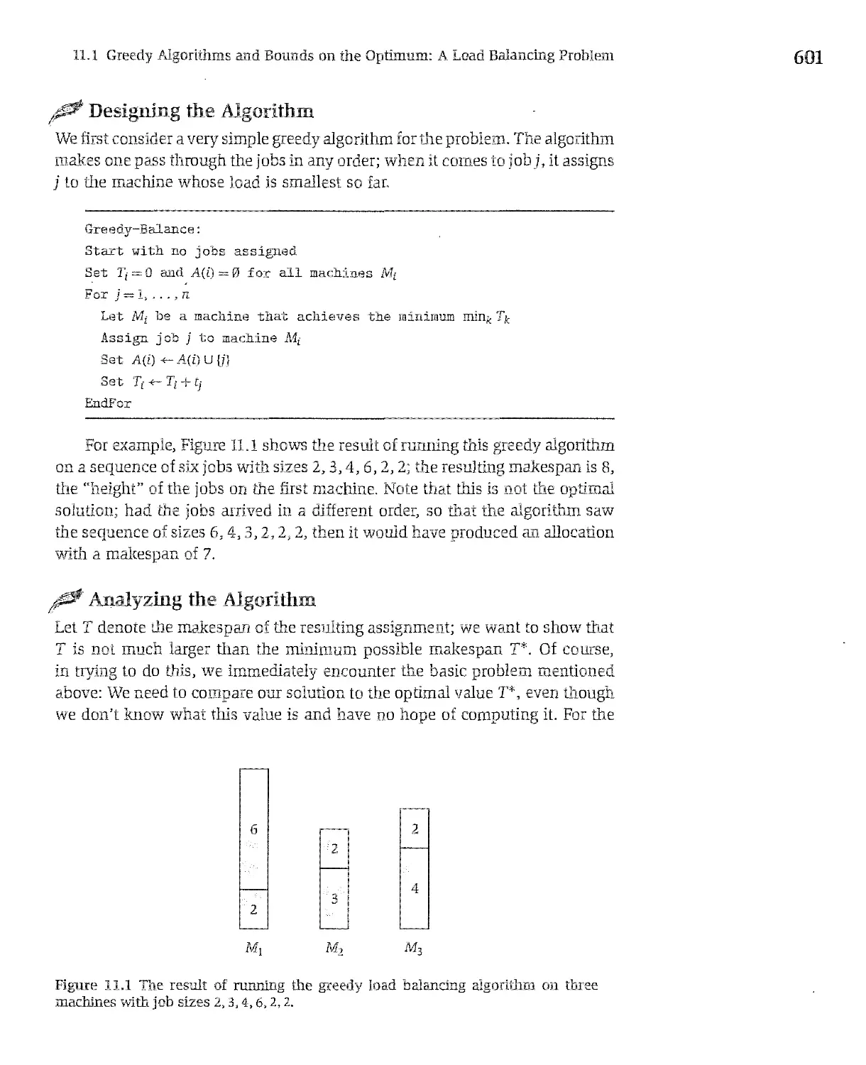
1 2 Five Representative Problems 13 science courses, we’ I be introd cing their r a fa r a ount of depth in Chapter 3 due to their enorrnous expressive power, we’ll also be using ti er exteusively throug out lie book For the discussion liere, it’s enough to thinJc of a g aph G as simply a way of e cod zig pairwise relationships among a set of objects, Thus, G consists of a pair of sets (V, E) a col ectiori V o nodes and a collection E of edges, each of which joins” two of the nodes We tli s represent an edge e E as a two element subset of V: e {u, v} for some u, u o V, where we cail u a id u the ends of e We typically draw graphs as in Figure L3, with each node as a small circle and each edge as a hue segment joimng fis two ends, Let’s now turn to a discuss on of lie five represen ative problems Interval Scheduling Consioer t ie foiiowirig very simple scneduling problem You have a esource t nay be a lecture roo , a supercomputer, or an electron microscope—and many people ieouest to use the resource fo periods ni time. A requesi takes the forni: Can I reserve the resource start g at lime s, u lii lime f We wffl assume that the resource can be used by at most one person at a t me A sci eduier wants to a cept a subset of these requests, rejecting a others, 50 that the accepted requests do no overlap z lime The goal is to maximize tIre number of requests accepted. More for ally, the e w li be n reques s labeled 1 , n, with eacli request i specifying a start tie s a ‘da firnsh lime f Naturallj v have <f1 fa ail z. Two requests i andj are compatible if the requested nte vals do ot overlap that is either equest us for an earlier time interval than request j (f or reques z is for a ate t rue than request j (f <s1), We’ll say more generally that a subset A of requests is compatible if ail pa rs o requests z j o A, z j are compatible. The goal is to select a compatible subset of req ests of maximum possible s ie We illustrate an instance of this Inter al Schedulzng Pro blem F gu e 1 4 Note t a there is a single compatible set of size 4, and this is the largest compatible set u Figuse 1 3 ‘achuf ia) and (b) depicts a graph on four nodes. Figure 1.4 An mstarce of the nter’al Schedu irg ProbIen
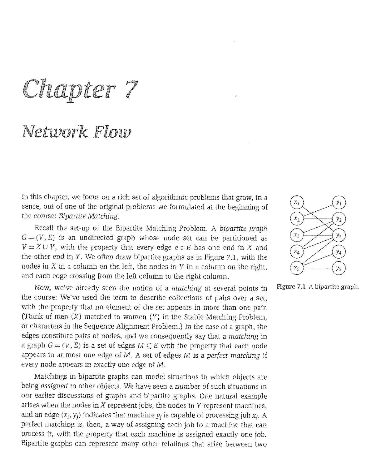
14 Chapter 1 Introductiow Some Representative Prob ems We wffl see si ortly that titis problem can be solved by a very natural algoritiim that orders the set of requests according o a certai eunstic and then “greedily”processes them i one ass, selecting as large a compatible subset as it ca Tiis will be typ cal of a cia5s of greedy algorithms that we will conside for vanous roblems-myopic rules mat process the Input one piece at a time with no apparent look ahead When a greedy algorithm car be shown to flnd an optimal solution for ail istances of problem, it’s often fairly surprising We ypical y learn soir effi g abo t tale structure of the underlying problem from the fact that such a simple approach can be optimal. Weighted Interval Scheduling In tire Irterval Scheduling Probiem, we sought to maxirmze the number of requests [1 al cm ld he acco rmodated simultaneously. Now, suppose more gnera y tht 1i rnwst intervl j has an associaed value, or wezght, y1> O; we could picture this as tire amount 0f money we will ake from the individual if we schedule fus or her request Our goal will he ta find a compatible subset of interva s o maxim tot 1 value, The case in which y1 1 for each us simpiy the bas c Interval Sct eduling Problem; but the appeararce of aibitrary values ch ages the nature of [fie maximizat on p oblem quite a bit Consider, for example, that if ri1 exceeds ti e sum of li other v, then the optimal solution must include 1 iterval I regardiess of the configuration of [lie full set nI in ervals So a y algonthm for this probiem must be very se sitive to the values, d yet degenerate to a rretlod fo sa vmg (unweigh ed) interval scheduling when ail the values are eouti [o 1 ere appears ta be no simple g eedy ule that walks through the intervals one at a t r e, making [fie correct decision in the presence of arbitrary values. Instead, we employ a technique, dynarnic programmrng, that bmlds up the optimal value over al possible solutions in a compact, abular way that leads to a very effic e it algorithm Bipaffite Matching When we considered the Stable Matching Probiem, we deflned a matching ta be a set al ordered pairs af men and women w [h he proneily that each mari and each waman belong ta at mas o e al the ordered pairs We [lien defined a perfect matdurug ta be a matching ‘nwhich every man and every waman helong ta some pair. We cari express these o cep s ore ge re aily in terms of graphs, and in arder ta do Uns i is usef 1 ta define [lie notion of a bipartite graph. We say that a graph G (V, E) is bipartite if its riode set V cari be partitianed into sets X
I 2 Five Representative Pioblems 15 a d Y in suc a way frat eve y edge lias one erid in X and the orner endin Y. A bipartite graph is pictured in Figure 1 5, often whe we want to eriphasize a graph’s “bipartiteness,”we will draw it titis way, with the nodes in X and Y in twa parallel columns, But notice, for example, that the two graphs in Figure 1 3 re alsa bipait te Now in the prablem of finding a stable matching, matchings were built fror airs o mcii id wame i In the case of bipartite graplis, the edges are pairs of nodes, sa we say that a matching in a grap G —(V E) s a set of edges M C E with the praperty that each node appea s n at most o ie edge o M M s a perfect matching if every node appears in exactly one edge of M Figuie L5 A biparute grapb, Ta see that this does capt ue tf e sare aira we en ountered in ti e Stable Matching Prablem, consider a bipartite graph G’ with a set X of n e i, a set Y of n wanien, and an edge from every nade in X to every node in Y. Then the matchngs and perect matchingr in G’ are precsey ale matchings and perler matchings ainang the set al nen and wor e n tire Stable Matching Problem, we added preferences ta this picture. Here, we do no ca sider prefere ces, but tte ature af the problem in arbitrary bipartite graplis adds a different source af complexi y there s not ecessari y an edge fram every x u X 10 every y e Y, SO tire set al possible matchings h s quite a comphcated structure. In allier words, it is as thaugh only certain pairs al ren and waren are wil ng ta ho paired off, and we want ta figure out how ta pair off many people in a way that is consistent with tins Consider, fru exrmpe, the bipartite graph G in Figure 1.5 there are many mifrtings in G, h t there is anly arie perfect matching. (Do you see it?) Matchings in bipartite graplis can model situations i i whrch abjects aie being assigned ta ather abjects. Thus, the nodes in X can represent jabs, tfe nodes Y can rep esent machines, and an edge (xi, y1) can indicate that machine y1 is capable of p acessing oh z1 A per oct matching n then a way af assigning each jab ta a machine that can process it, witt [lie p operty that each machine is assïgned exactly one jab. In tire spring, computer science departments acrass the cauntry are atten seen pondering a bipartite graph in which X is tire set af p ofessars tire departme t, Y n the set af affered courses, and an edge (xi, y) indicates that professor x1 is capable al teaching course y3. A perfect matching in this graph cansists of an assignment af each professor ta a cou se tiraI lie or she can teaci, in such a way that every course is cavered Thus the Bipartite Matching Problem is the fol owing: Given an arbitrary bipartite grahi G, find a ratc mg al niaximum size. If XI I Y n, [lien tirere is a perfect matching if and anly f II e maximum matching as size n We wiIl find tirat tire algorithmic techniques discussed earlier do flot seem dequate
16 Cl apter 1 Introduction. Some Representative Problenis for providing an efficient algor t fo tItis p oblem fhere is, however, a very e1gart and efficient algoritlim ta find a maximum matching it inductively builds up larger and larger matchirigs, selectively backtracki g along fie way This process is called augmentation, and it for s the certral component in a large class o efficien Iy solvable proble rs called network flow problems, Independeat Set Now et’s alk about ar extremely general problem, which includes most cf these earl’er problems as special cases, Given e graph G (V,E), we say a set of nodes S C V 15 independent if no wo odes in S are oincd hy an edge. The Independent Set Problem is, ther, the following Given G, find an independen s t bat is as la ge as possible. For example, the maximum size of Figure L6 A graph whose an indepe dent set in the graph in Figure L6 is four achieved by theiou node la ges uidc1jcndent iar independent set (1, 4, 5, 6). s ze The Independent Set Problem encodes any situation in which you are trying to choose from among a collection of abjects and the e are pairwise conflz’cts amorig some cf tbe abjects Say you h ve n frieuds, r d some pairs of thet don’t ge along How large a gro p of your friends can you invite to dmner if you don t want any interpersonal tensions? This is simply the largesi independerit set in the graph whose nodes are yeux fr e ds, w t n edge betweeu cccli confiicting pair. Interval Scheduling and Bipartite Matching can both be encodcd as special cases al tbe Independeri. Set Prob.e.... Fa Inte val SclFdiiling, f r’ . gr.ph G (V, E) in which the nodes aie the intervals aud there is an edge between each pair of them hat overlap, the independent sets in G are then just the compatible subsets cf iritervals. lncoding Bipartite Matchmg as a special case cf Independent Setis alittle tnckierto sec. Giveu bipart te grap G’ = (V’, E’), the objects being chosen are edges, and tt e co fiicts a se between two edges that s e e an end (These, ndeed, are the pairs of edges that cannat belong to common matching.) Sa we define a graph G (V, E) in wh ch lie code set V is equal te the edge set E’ cf G’. We deflue an edge be ween each pat of elements in V tt at correspor d to edges cf G’ with common end. We can now check that the iridepende t sets of G are precisely the matchings of G’. While is flot complicated te check this, il takes e httle concentration ta deal with tItis type cf “edgeste nodes nodes to edges t ans orm tior 2 2 For those who are curious, we note tha flot cvery nstance of Oie Irdepeident Set Problem can anse in ibis way rom Irterval Sc’ieduhrg or from Bparote Matchmg; Oie full lndependent Set Prob em really u more general The graph n Ogure 3(a) canno arise as the co9fllc graph’ in ar nstaflce of
1 2 Five Representanve Problems 17 Given tire generality of the Irdepenee t Set Probi m, n $ticient algonrhnr to salve it would be quite impressive It would E ave to impiicitly contain algorithms or luterval Scheduling, Bipartite Matching, and a hast cf other natu al optrilzation probleTs The rurret satus cf ludependent Set is this: no efficient algorithm is known fo tic probler , ard 1 5 conjectured that no such algorithrn exists, The obvious brute-force algo ithm would try ail subsets o the nodes, checkrng each te sec if it is independent, and then recording the largest one et coun ered It 15 possib e that Il is is close ta the best we can do on this problem. We wffl sec atcr in the bock th t Independent Set is one cf a large class cf problems that are termed NP-complete No eff cient algo il r is krown or any of them but they are ail equivalerit in the sense that a solution to ry one of thom would imply, in a precise sense, a solution to ail of them. Here’s a natural question: Is there anything gcod we can s y abou the complexity cf the ludependent Set Problem? Que positive thing is the foilowing If we have a graph G or 1,000 nodes and we want te convince you that it contains an independent set S cf size 00, tic 1 ‘5quite easy We simp y show you flic graph G, circle the nodes of S in red, and let yen check tha no two cf them are joined hy an edge. Sa there really seerns to be a great difference in difficufry between checkm that sornething is a large independent set and actually [md mg a la ge r deper dent set T s may look k a very basic observation—aud it is—but it turns out to be crucial in understand r g lus class of problems. Furthermore, as we’ll sec next, it’s possible for a problem to be sa ard that heie is ‘even n easy way tu “check”suiuuons in this sense. Competitive Facility Location Final y we corne ta our fifth problem, which is based on the following twop1 yer ga e Cc sider two la ge cornpames that operate café franchises across the country—let’s cali them Jav PI net and Queequeg’s Coffee and frey are currently competing for rnarket share in a geographic area First JavaPlanet oper s a franchise; then Queequeg’s Coffee opens a franchise; then JavaPlanet; then Queequeg’s, a d so on Suppose hey must deal with zornng regulations that require ra wu franch 5es hc lucateu tuu cluse tuetliei and cach iyiu ta malte its locations as convenient as possible. Who will win1 Let’s make the rules cf tE s “game”mo e concre e T e geograpluc reg on in question is divided luta n zones, labeled 1, 2, , n Bach zore z has a ntervaI Schedu Mg, and the graph n egure 1 3(b) cannot anse as the “conft grapi’ rn an rnstarce cf BNpa tee Ma chhg,
18 Chapter Introduction: Sorne Representative Problems Figure L7 An instance cf die Competitive Facility Location Problem, value b, which is the revenue obtalned by either of the companies if it opens a franchise there. Finally, certain pairs of zones (i,j) are adjacent, and local zoning Iaws prevent two adjacent zones from cadi containing a franchise, regardless of which company owns them, (They also prevent two franchises from being opened in the same zone,) We inodel these confllcts via a graph G = (V, E), where V is the set of zones, and.(i,j) is ail edge in E if the zones i and j are adjacent. The oning requiren ent then says that the full set of franchises opened must form an independent set in G. Thus our game consists of two players, P1 and P2, alternately selecting nodes in G, •with P1 moving first, At ail times, the set of aIl selected nodes must form an independent set in G. Suppose that player P2 has a target hound, B, and we want to know: is there a strategy for P2 sa that no matter how P1 plays, P2 will be able to select a set of nodes with a total value of at least B? We will call this an instance of the Competitive Facility Location Pro bi cm. Consider, for example, the instance .•pictured in Figure 1.7, and suppose that P,’s target bound is B = 20, Then P2 does have a winning strategy. On the other hand, if B = 25, then P2 does not. One can work this ont by looking at the figure for a while; but it requires some amount of casechecking of the form, “IfP1 goes here, then P2 will go there; but if P1 goes over there, then P2 will go here....” And this appears to be intrinsic to the probi.em: not only is il computationally difficult to determitiie whether P2 has a wlnning strategy; on a reasonably sized graph, il would even be hard for us to convince you that P2 has a winning strategy. There does not seem ta be a short proof we could present; rather, we’d have ta lead you on a lengthy case-by-case analysis of the set af possible moves. This is in contrast ta the Independent Set Problem, where we beieve that finding a large solution is hard but checking a proposed large solution is easy. Titis contrasi can be formaiized in the class of PSPACE-complete probiems, of winch Competitive Facility Location is an example. PSPACEcompIeté probleins are beieved to be strictly harder than NPcomplete problems, and Ibis conjectured lack of short “proofs”for their solutions is one indication of this greater hardness. The notion of PSPACEcompleteness turns ont ta capture a large collection of problems involving gamepIaying and planning; many of these are fundamental issues in die area of artificial inteffigence.
Solved Exercises 19 Solved Exercises Solved Exercise 1 Consider a town with n men and n women seeking ta get married ta one another. Each man has a prefererice list that ranks ail fric women, and each woman has a preference Iist that ranks ail the men. The set of ail 2n people is divided into twa categories: good peo1e and bad people. Suppose that for soine number k, 1 k n 1, there are k good men and k good women; thus there are n —k bad men and n k bad wo.rnen. Evèryone would rather marry any good persan than any bad persan. Formaliy, each preference list has fric property that it ranks each good persan of the opposite gender higher than each bad persan of the opposite gender: its first k entries are the good people (of the opposite gender] in some order, and its next n —k are the bad people (af the opposite gender) in same order. Show that in every stable matching, every goad man is married ta a goad woman. Solution A natural way ta get started thinking about this prablem is ta assume the daim is false and try ta wark towaid abtaining a contradiction. What would it mean far the daim ta be false? There would exist some stable matching M in which a good man m was rnarried ta a bad woman w. Naw, let’s consider what the other pairs in M look like, There are k gaod men and k gaod women, Could it be the case that every good woman is married ta a good inan in this matching M? No: one af the goad men (namely, m) is already married ta a bad woman, and that leaves anly k —1 other good men, Sa even if ail of them were married ta goad women, that wauld stili leave some good waman who is married ta a bad man, Let w’ be such a good woman, wha is married ta a bad man, It is now easy ta identify an instability in M: cansider the pai.r (m, w’). Each is gaad, but is married ta a bad partner, Thus, each of m and w’ prefers the other ta their current partner, and hence (m, w’) is an instabiiity, This contradicts oui assumption that M is stable, and hence concludes the proof. Salved Exercise 2 We can think about a generailzation of the Stable Matching Problem in which certain marnwoman pairs are exphcitiy forbidden, In the case of employers and apphcants, we couid imagine that certain applicants simply lack the necessary qualificatians or certifications, and 50 they cannot be employed at certain companies, hawever desirable they may seem, Using hie anaiagy ta marnage between men and women, we have a set M of n men, a set W af n women,
20 Chapter 1 Introduction: Some Representa ive Problems and a set E C M x W cf pairs w o are 5imply flot allowed b get married. Each mar m ranks ail the womer w for whlch (m, w) g F, and each woman w’ ranks ail lie men m’ for which (m’, w’) g F. In this more gerieral settmg, we say that a matching S is stable if ii does nJL exhibit any cf tlw fo’lowing types ot instabuity. (i) There a e two pai s (m, w) a d (m’, w’) in S with the propcrty that (an w’) E, m prefeas w’ to w, and w’ prefers m ta m’ (The muaI kmh cf instability) (u) There is a pal (m, w) E S, and a mari m’, so that m’ is not part cf any pair in the matching, (m’, w) g F, and w prefers m’ te m (A single man is more desirable and flot forbidden) (rni) Theeisapalr(m,w)eS,andawomanw,sothatw’isnotpartof any pair in tue matching, (m w’) g F and m prefers w’ ta w (A single woman as more deszrable and flot forbzdden) (iv) There 1$ a man an and a woman w, neither o whom 15 part cf any pair in the matching, sa t a (m, w) g F (rheme are two single people with nothing pieventing them from getting rnarriecl to each other) Note that undcr these more general defamtions, a s able matching need not be a pertect matching Now we can ask: For every set cf preference 1 sts and eve y set of forbidden pairs, is there aiways a stable ma chirgi Resolve this question by doing one cf me b lowing twa thlngs (a) give an algorithm mat, for any set al preterence lis s and forbidden pairs, produces a stable matchmg; or (b) gave an examp e cf a set cf preterence lists and forbidde pairs for whicl thcre is no stable matching. Solution The Ga1eShapley a gorithm is remarkably robust ta var atiors on the Stable Matching Problem. Sa, ii you’re faced with a new va iation cf the problem and can’t find a counterexamp e ta stab hty, it’s often a good idea ta chec whcther a dire adaptation of the GS algorithm will in fact pro duce s able match ngs. That tur s oct ta be the case lie e We wfll show that there is aiways a stable matclung, even in this more genera model with forbidden pairs, ai d we will do this by adapting the G S algorithm. Ta do this, le ‘sconsider why the original G S algorithm can’t be used directly The difficulty, of course, is that the G S algorithm doesn’t know anythng about forbidden pairs, and sa lie onditior in tl e While loop, While there is n mn m who 15 Eree and hasnt proposed ta every woman,
Solved Exercises 21 won’t work: we don’t want m o propose ta a wo an w for which the pair (m w) is forbidden. Thus, et’s consider a vanatio of the G S algorithm in which we make only one change: we modify the Ph le Ioop o say, Phi e there 1m a man ÎÏL wbo as ree and hasnt proposed to every womanwfor which(m w)gF. Here is the algorithm ir fui Initiaily ail OiEM and wcW oie free Ratio there is a man m who is ±reeand has&t proposed o every wonan w for whch (m,w)gF Choose uch a mea m Let w be the highest ranked woman n m’s preference list to which w has not yet proposed f w is free thon (m,w) become ergaged Else w is currently engaged to m’ If w pref ers m to m thon m romains free Lise w pref ers m to w’ (w w) become engaged m’ hrrm fv Rad f Endif Endwhuie Return the set S of engaged pairs We 110W prove that this yieids a stable ma ch g, under o r new dehnition of s ah iity Ta begin with, facts ( 1), (1 2), and (1 3) fia i the text remain trie (in prhcaar, the algarithm wili terminat° r at cst n2 i er in s) kIn we dor ‘thave ta worr about establishing that the resulting match ig S is perfect (indeed, II nay rot be) We also notice an additional pairs of facts, f m s a man who is flot part of a pair m S ti er m must have proposed to every norforbidden woman; and if w is a woman who is flot part o a pair m S, then it must be that no man ever proposed ta w. Finally, we need anly show (1 9) There is no instability with respect ta tire returned matchrng S.
22 Chapter I Introduction. Some Representative Problems Proof, Our general defmition of instabiltiy lias four parts This means that we have ta make sure hat none of die four bad things happens. Pirst, suppose there is an instabihty of type (i), co Isisting of pairs (m, w) and (m’, w’) i S witE ti e property that (ni, w’) F, m prefers w’ to w, and w’ prfr m o .n’ Ii follows that ni must have proposed o w; o w rFJF(.tP w and thus she prefers her fluai partner ta m a con tadictian Next suppose there h an instability al type (n), consisting O R pai (ni, w) o S, and a man m’, sa that m’ is flot part o any pair in the atching, (ni’, w) ØT, and w prefers m’ to in Iher m’ must haie praposed ta w and been ejected; again i follows that w prefers lier final partner ta m a contradiction Third suppose tiiere is an stabil ty of type (lii), consisting of a pair (ru, w) o S and a woman W’, sa that w’ is not part af any pair in the matching, (m, r’) O P, and n prefers w’ ta w, Ihei io an prnpna tn n’ .t ail, in particular, m neyer proposed ta w’, and sa lie must prefer w ta w’—a contradiction Finally, suppose there is an instabihty of type (iv), consisting of a man m and a woman w, ne t ier o which is patr of any pair in the matching, sa tira (m w) ØF But for m ta be single, lie must have praposed to every nonforbidden waman, in particular, he must have proposed to w w r eh means she wou d na langer be single a contradiction Exercise L Decide w1ether you thiriic the followmg statement is truc or false. if it is mie, give a short explanation. if k is false, give a counterexample Truc or faire? In every instance of the Stable Matching Pro blern, there h a stable niatching contarning a pair (ni, w) such that ni h ranked first on the preference hit of w and w is ranked flrst on the preference Pst cf ni 2. Decide whether you think the foflowing statement s true or false. if it is mie, ve a short explanation if k is faire, give a counterexample. Truc or faire? Consider an instance of the Stable Matching Probleni in whzch there exists a man ni and u wonian w sucli that m ii ranked first on the preference hit of w and w ri ranked first an the preference list of ni. Then in eueîy stable matching S for this instance the pair (ni, w) belongs ta S 3. There are many other settings m which we cari ask ques ions related to some type of “stability”prmc ple Here’s one, mvolvmg competition between two enterprises
Exercises 23 Suppose we have two television ietworks, whom we’fl eaU A and B. There are n pnm&tlme programmi sg siols, and each networlc bas n TV shows Each network wants te devise a scfzedule—an assignment of each show te a dis met s ot se as te attract as much market share as possible. Here is the way wP dtrmrn hnw well Ni twn ntwnrks perfnrm relative te each other, given their schedules. Each show bas a fixed ratrng, which is based on the number of people who watched il last year; we’ll assume that no two shows have exactil the same rating A etwork wzris a given tbne siot if the show that it scheduies for the lime siot bas a Luger rating if an the show the other network schedules for that tune siot. The goal of each network s te win as many time siots as possible. Suppose in tise opening week of tise fail season, Network A reveals a schedu]e S and Network i re eals a schedule T. On the basis of titis pair of schedules, each network wins certain turne siots, according te tise raie above, We’Il say that tise pair of schedu]es (S, T) is stable if neither network can unilalerally change ifs own schedule and wm more lime siots rhat is there is no schedule S such thai Network A wins more siots with tise pair (S , T) lisais it did with tte pair (S, T), and symrnetrically, there is no schedule T’ such tisat Network 23 wins more siots with the pair (S, T’) t sar it did with lise pair (S, T). lhe analogue of Gale and Shap ey s question or titis kind of stabffity is the following: For every set of IV shows and ratmgs, is there aiways a stable pair of schedules? Resolve titis question by do g eue ef the feflowing twe things’ (a) give an algonthm that, fer any set of V shows and associated ramigs, produces a stable pair ef schedules; or (b) give an example of a set of IV shows and associàtcd ratirgs for which there is no stable pair of schedules. Gale and Shapley pubhshed their paper on tise Stable Matchmg Problem m 1962, but a sers en o their algeruthm had already been in use for tenyears hy th Natinn1 Pi1pnt Mtrhrng Prngrm, trw ehe problem cf assigning medical residents te hespitals. Basically, ife situation was tise fobowmg. There were m hospitals, each with a certain rumber cf available positions for lnrmg rcsidents Tisere were n niedical students graduating ma given year each mterested mjoinmg eue of tise hospitals. Each hospital had a ranking cf lise students in order ef preferercc, and each student had a ranking of tise hospitals in order cf preference We suR assume that there were more students graduating than there were slots available in tise m hospitals
24 Chapter 1 Intradncnon, Some Represertative Problems lise mterest, naturaily, was in fisiding à way ai assigning each s ludent to at niost one hospital, m such a way tlsat ail asailable positions in ail hospitals were filled, (Since we are assunung a surplus ai students, there would ha soma students wbo do flot gai assigned to any hospital) We sa’ Jnt an assignment students ta hospitls is stable if neither ai tise foilowmg situations anses First type ai instabiliry: There are students s and s, ard a bospital h 80 t iàt s is assigned ta h, and - s’is assigned ta no hospital, and h p efers s’ ta s. e Second type of mstability: There are students s and s, and hospitals h and h’ sa that assigned a b, and s’ 18 assigned ta h’, and —hpreferss tas, and s prefe s h ta h’. Sa ive basicaill have tise Stable Matching Problem, except that (j) bospitals generaily want more tian ana resalent, and (u) there is a surplus al medical sli dents. Show tisai there s aiways à stable assignment ai students ta hospi tais, and give an algaritbm ta find one. 5. The Stable Matchmg Problem as dsscussed in die text, assumes that ail men and w amen have a fully ordered list ai pie erences. In titis p oblem we wil consider avers ou ai tise problem m winch mers and wamen cars be zndzfferent betwee s certain options As before we have n set M al n men and a set W ai n womea, Assu e each mais and each waman ranks lise me rbers ai tise opposite gender, but now sic allow tics in tise ranlung. For example (with n 4), a woman could say tisai in1 is anked m first place; second place is a tie between in and m3 (sise isas na preference between tisem), and inA is in last ulace. We will sa’,’ tisai w pre fers in ta w’ if in is ranked higiser tian w’ on lier prefererce list (they are nat lied) Withindilfeiences indic rankmgs, there couldbe twa natural notions for stabrhtj And for eact, we can ask about tise eiustence of stable niatchings, as failows (a) A strong rnstabiliiy m a perlent matching S consists ai a mari w and à woman w, sucb tisai cadi ai m and w prefers tise other ta tisais partner in S Does tiare aiways exist a perfect matchmg witis no
Exercises 25 st ong i istabiItt7Either give an example of a 5et of men and women w h preference lists for which e er perfect matchmg has a strong iristahfflty; or give an algorithm that $ guaranteed to fmd a perfect matching ‘aithno strong instabffity. (b A weak intabiIity in a perfect matching S cnrsists of a mem w and a woman w, such that their parmers in S are w’ and w’, respecnvely, and ore of the ollowmg holdw —w prefers w to w’, and w either prefers w to w O is mdifferent between these two choices, or w prefers w to w’, and w either prefers w ta w’ or is indifferent hetween ttese two choices In other words, die pairirg between w and w is ert rer prefe red by hoth, or preferred hy one while the other is mdifferent Does there aiways exist a perfect matching with no weak instahility? Either give an example o a set o men and women with preference Iists for wbac every perfect matching has a weak mstabil ty, or give an algorithrn that is guaranteed ta fmd a perfect matchirig w h no u eaIr instabillty. 6. Penpatetic Shippmg Lines, h c s a shippi ig company that owns n ships and provides service ta n ports Each of its slips las n schedule tInt says, for each day of die month, winch of the ports it’s currently vislflng, or whether il s aut ai sea (You can assume the “monthhere has w days, for some in > n ) Each ship visits each port for cxactly one day during the mondi, For safety reasons, PSL Inc has die foilowmg strict requirement (t) No twa ships can be in the saine port on the saine day T e carrpany wants ta perform maintenance on ail the ships titis month, via die foilowing sdheme Yhey want ta dru ucate each ship’s schedule: for each ship s,, there wilL le some day when it a rives m its scheduled port and simply remains there for die rest of tIc month (fan maintenance) Tins means that S viril nat visit die remairting ports on lis schedule (if ani) tInt month, but ibis is okay Sa the truncatzon o 5’s schedule will simply consist of lis original schedule isp ta n certain specified da on winch it is in a port P; the nemainder of die truncated schedule simpI has it rameur m part P. Now die company’s question ta you is tIc foilowmg: Given die schedi nie or each ship, find a tnmcatian af each sa that condition (t) conUnues ta bold no twa ships are ever ir die same port or the same day Show that sud a set ai truncations can aiways be found, and give an algontbm ta f md them
26 Chapter 1 Introductiow Soire Representative Problems Example Suppose we have two ships and twa ports, and the month” sas toux days, Suppose the tirst slup’s scleduie is port P1 et sen, port P2 et s°a and die second ship’s schedule is et sec, port P1 et sec; port P2 Then tin. (onli) way to choose troncations would be to have the first ship remam m port P2 starting on day 3, tord have the second ship remaria in port P1 startirig on day 2 7. Some of your triends are wo kmg for CluNet, a builder of large conimu nication ne works and they are looking at algonthms for switching m a parncrilar type of mput/output crossbar Here is te setup f here are n input wzres ard n output wires, each directed trom a source to a terminus Each input wire meets each output wixe tri exactly one distinct point, at a special piece ot hardware called a junction box. Points on the vixe are naturally ordered in the direction tram source to ter mus, for rwo distinct points a and y on the saine wire, we sai hat a is upstream froni y if x is doser to the source than y and odierwise we say r 15 dmi nstream from y. The order in winch one input wire meets tIe output ivires is not necessarily the same as die order in which another input wire meets die output noces. (And smmularly for die ordcrs in winch output ivires meet muut wmres) Figure l8 gives art example of sucti a collection o input and output ivires Now here’s the switching camp one t of tins situation. Each input nare s carrying a distinct data stream, and titis data sli’eari must be xwztched onto one ot the output nores. If die s Iream ai input us switched onto Output j at Jurction box B, then tins stream passes through ail junctlo r boxes upstream tram B on input u, then through B, then through ail ju iction boxes downstream rom B on Output j. It does flot malter winch input data stream gels swilched onto winch output wire, but each input data stream must be swftched onto a dzfferent output wire. ‘urthermoreand this is the lricl’l con’ h ami no two data streams can pass through the saine junction box foilowmg die switcinrg opcration. Fmaily, here’s die problem. Show ti-at for tory specified pattern m winch he input wires and oulput w es meet each other (each pair meet mg exactly once), a vahd switching of the data streams cari aiways be f ound one mn wl sch each input data stream is switched onto a dfterent output, ard no twa of the resulting sli’eams pass tbrough die saine junc flan box. Addrtionally, give an algontinn ta find such a valid switchmg
Exercises 27 Figure L8 .An example with two input wires and two output wires, input 1 lias its juncion with Output 2 upsueam from its juncbon with Output 1; Input 2 lias its juncion with Output 1 upstream from its junction with Output 2. A valid solution is to switch ifie data stream. of input 1 onto Output 2, and the data stream ai input 2 onto Output 1. On the other land, if the stream of Input 1 were switched onto Output 1, and the stream of input 2 were switdhed onto Output 2, then bath streams would pass tbrougli the junction box at the meeting ai Input 1 and Output 2—and tins is not allowed 8. For this problern, we wffl explore the issue of truthfulness in the Stable Matching Problem and specifically in the Ga1eShapley aigorithm. The basic question is: Can a man or a woman end up better off by lying about bis or her preferences? More concreteiy, we suppose each participant bas n truc preference order, Now consider a woman w, Suppose w prefers man m to m’, but both m and rn’ are low on ber list of preferences, Canif be the case thatby switching the order ofrn and m’ onherlist of preferences (Le, by falsely daiming that she prefers m’ to m) and running the algorithnr with titis fais e preference lIst, w wffl end up with a man rn” that she truiy prefers to both m md in’? (We can ask the same question for nien, but wffl focus on the case of women for purposes of this question) Resolve titis question by doing one of the following two things: (a) Give a proof that, for any set of preference lists, switching the order of a pair on the list cannot inrprove a woman’s palmer in the GaIe Shapley algorithm; or Junction Output 1 Input I (meets Output 2 before Output 1) before Input 1) à Input 2 (meets Output I before Outp ut 2)
28 Chapter 1. Introduction: Some Representative Problems (b) Give an example cf a set of preference lists for whlch there is a switch that would improve the parmer cf a woman who switched preferences. Notes and Further Reading The Stable Matching Problem was first defined and analyzed by Gale and Shapley (1962); according to David Gale, their motivation for the problem came from a story they had recently read in the New Yorker about the intricacies of the college admissions process (Gale, 2001). Stable matching lias grown into an area of study in lis own right, covered in books by Gusfield and Irving (1989) and Knuth (1997c). Gusfield and Irving also provide a nice survey of the “parallel”history of the Stable Matching Problem as a technique invented for matching applicants with employers in medicine and other professions. As cliscussed in the chapter, our five representative problems will be central to the book’s discussions, respectively, of greedy algorithms, dynarnic programming, network flow, NP-completeness, and PSPACE-completeness. We wffl cliscuss the problems in these contexts later in the book.
Chapter 2 Basics of Algorithm Analysis Analyzing algorithms involves thinking about how their resource requirements—the amount of lime and space they use—will scale with increasing input size. We begin this chapter by taiking about how to put this notion on a concrete footing, as making it concrete opens the door to a rich understanding of computational tractability. Having done this, we develop the mathematical machinery needed to talk about the way in which clifferent functions scale with increasing input size, making precise what it means for one fiinction to grow faster than another. We then develop running-time bounds for some basic algorithms, beginaing with an implementation of the Gale-Shapley algorithm from Chapter 1 and continuing to a survey of many different running limes and certain characteristic types of algorithms that achieve these running times. In some cases, obtaining a good running-time bound relies on the use of more sophisticated data structures, and we conclude this chapter with a very useful example of such a data structure: priority queues and their implementation using heaps. 2.1 Computational Tractability A major focus of this book is to find efficient algorithms for computationai problems. At this level of generality, our topic seems to encompass the whole of computer science; so what is specific to our approach here? First, we will try to identify broad themes arid design principles in the development of algorithms. We will look for paradigmatic problems and approaches that ifiustrate, with a minimum of irrelevant detail, the basic approaches to designing efficient algorithms. At the same lime, it would be pointless to pursue these design principles in a vacuum, so the problems and
30 C]aapter 2 Basics of Algorithm Analysis appro aches we consider are drawn from fundamental issues that arise throughout computer science, and a general study of algorithms turns out to serve as a nice sm-vey of computational ideas that arise in many areas. Another property shared by many of the problems we study is their fundamentafly discrete nature. That is, like the Stable Matching Problem, they wffl involve an implicit search over a large set of combinatorial possibilities; and the goal wffl be to efficiently find a solution that satisfies certain clearly delineated conditions. As we seek to understand the general notion of computational efficiency, we wilI focus primarily on efficiency in running time: we want algorithms that run quickly. But h is important that algorithms be efficient in their use of other resources as well. In particular, the amount of space (or memory) used by an algorithm is an issue that will also arise at a number of points in the book, and we will see techniques for reducing the amount of space needed to perform a computation. Some Initial Attempts at Defining Efficiency The first major question we need to answer is the following: How should we turn the fuzzy notion of an “efficient”algorithm into something more concrete? A first attempt at a working definition of efficiency is the following. Proposed Definition of Efficiency (1): An algorithm is efficient if, when implemented, it runs quickly on real input instances. Let’s spend a littie time considering this definition. At a certain level, it’s hard to argue with: one of the goals at the bedrock of our study of algorithms is solving real problems quickly. And indeed, there is a significant area of research devoted to the careful implementation and profihing of different algorithms for discrete computational problems. But there are some crucial things rnissing from this definition, even if our main goal is to sohve real problem instances quickly on real computers. The first is the omission of where, and how well, we implement an algorithm. Even bad algorithms can run quickly when applied to small test cases on extremely fast processors; even good algorithms cari run slowly when they are coded sloppily. Also, what is a “real”input instance? We don’t know the full range of input instances that will be encountered in practice, and some input instances can be much harder than others. Finally, this proposed definition above does not consider how well, or badly, an algorithm may scale as problem sizes grow to unexpected levels. A common situation is that two very different algorithms will perform comparably on inputs of size 100; multiply the input size tenfold, and one will stifi run quickly while the other consumes a huge amount of lime.
2.1 Computational Tractability 31 So what we could ask for is a concrete definition of efficiency that is platform-independent, instance-independent, and of predictive value with respect to increasing input sizes. Before focusing on any specific consequences of this daim, we can at least explore its iniplicit, high-Ievel suggestion: that we need w take a more mathematical view of the situation. We can use the Stable Matching Problem as an exarnple to guide us. The input has a natural “size”parameter N; we could take this to be the total size of the representation of ail preference lists, since this is what any algorithm for the problem will receive as input. N is closely related to the other natural parameter in this problem: n, the nuniber of men and the number of women. Since there are 2n preference lists, each of Iength n, we can view N = 2n2, suppressing more fine-grained details of how the data is represented. In considering the problem, we will seek to describe an algorithm at a high level, and then analyze lis running time mathematically as a function of this input size N. Worst-Case Running Times and Brute-Force Search To begin with, we will focus on analyzing the worst-case running time: we will look for a bound on the largest possible running time the algorithm could have over alT inputs of a given size N, and see how this scales with N. The focus on worst-case performance iriitially seems quite draconian: what if an algorithm performs well on most instances and just has a few pathological inputs on which it is very slow? This certainly is an issue in some cases, but in general the worst-case analysis of an algorithm has been found to do a reasonable job of capturing its efficiency in practice. Moreover, once we have decided to go the route of mathematical analysis, it is hard to find an effective alternative to worst-case analysis. Average-case analysis—the obvious appealing alternative, in which one studies the performance of an algorithm averaged over “random”instances—can sometimes provide considerable insight, but very often it can also become a quagmire. As we observed earlier, it’s very hard to express the full range of input instances that arise in practice, and 50 attempts to study an algorithm’s performance on “random”input instances can quickly devolve into debates over how a random input should be generated: the saine algorithm can perform very weil on one class of random inputs and very poorly on another. After ail, real inputs to an algorithm are generaily not being produced from a random distribution, and 50 average-case analysis risks telling us more about the means by which the random inputs were generated than about the algorithm itself. So in general we wffl think about the worst-case analysis of an algorithm’s mnning time. But what is a reasonable analytical benchmark that can teil us whether a running-time bound is impressive or weak? A first simple guide
32 Chapter 2 Basics of Algorithm Analysis is by comparison with brute-force search over the search space of possible solutions. Let’s return to the example of the Stable Matching Problem. Even when the size of a Stable Matching input instance is relatively small, the search space it defines is enormous (there are nI possible perfect matchings between n men and n women), and we need to find a matching that is stable. The natural “brute-force”algorithm for this problem would plow through ail perfect matchings by enumeration, checking each to see if it is stable. The surprising punchline, in a sense, to our solution of the Stable Matching Problem is that we needed to spend time proportional only to N in finding a stable matching from among this stupendously large space of possibilities. This was a conclusion we reached at an analytical level. We clid flot implement the algorithm and try it out on sample preference Iists; we reasoned aboutit mathematically. Yet, at the same Urne, our analysis indicated how the algorithm could be implemented in practice and gave fairly conclusive evidence that it would be a big improvement over exhaustive enumeration. This wiII be a common theme in most of the problems we study: a compact representation, implicitly specifying a giant search space. For most of these problems, there wil be an obvious brute-force solution: try ail possibilities and see if any one of them works. Not only is this approach almost aiways too slow to be useful, it is an intellectual cop-out; it provides us with absolutely no insight into the structure of the problem we are studying. And so if there is a common thread in the algorithms we emphasize in this book, it would be the following alternative definition of efficieflcy. Proposed Definition of Efficiency (2): An algorithm is efficient fit achieves qualitatively better worst-case performance, at an analytical level, than brute-force search. This wffl turn out to be a very useful working definition for us. Algçrithms that improve substantially on brute-force search nearly aiways contain a valuable heuristic idea that makes them work; and they teil us something about the intrinsic structure, and computational tractability, of the underlying problem itself. But if there is a problem with our second working definition, it is vagueness. What do we mean by “qualitativelybetter performance?” This suggests that we consider the actual running time of algorithms more careft]ly, and try to quantify what a reasonable running time would be. Polynomial Time as a Definition of Efficiency When people first began analyzing discrete algorithms mathernatically—-a thread of research that began gathering momentum through the 1960s—
2.1 Computational Tractabfflty 33 a consensushegan to emerge on how to quantify the notion of a “reasonable”running time. Search spaces for natural combinatorial problems tend to grow exponentially in the size N 0f the input; if the input size increases by one, the number of possibilities increases muliiplicatively. We’d like a good algorithm for such a problem to have a better scaling property: when the input size increases by a constant factor—say, a factor of 2—the algorithm should only slow down by some constant factor C. Arithrnetically, we can formulate this scaling beliavior as follows. Suppose an algorîtlim has the following property: There are absolute constants c> O and d> O so that on every input instance of size N, its running Urne is bounded by cNd primitive computational steps. (In other words, its running time is at most proportional to Nd) For now, we wifl remain deliberately vague on what we mean by the notion of a “primitivecomputational step”— but it can be easily formalized in a model where each step corresponds to a single assembly-language instruction on a standard processor, or one une of a standard programming language sucli as C or Java. In any case, if this running-time bound liolds, for some c and d, then we say that the algorithm has a polynomial runnirig time, or that it is a polynomial-time algorithm. Note that any polynomial-time bound lias the scaling property we’re looking for. If the input size increases frorn N to 2W, the boiind on the running time increases from c1\Jd to c(2N)d = c . 2dNd whicli is a slow-down by a factor of 2d Since dis a constant, so is 2d; of course, as one might expect, lower-degree polynomials exhibit better scaling behavior than higher-degree polynomials. From this notion, and the intuition expressed above, emerges our thiîd attempt at a working definition of efficiency. Proposed Definition of Efficiency (3): An algorithm is efficient if it has a polynomial running time. Where oui previous definition seemed overly vague, this one seems much too prescdptive. Wouldn’t an algorithm with running time proportional to n’°°—and hence polynomial—be hopelessly inefficient? Wouldn’t we be relatively pleased with a nonpolynomial running time of l+.o2(logn) The answers are, of course, “yes”and “yes.”And indeed, however much one may try to abstractly motivate the definition of efficiency in terms of polynomial time, a primary justification for it is this: It really works. Problems for wliiçh polynomial-Urne algorithms exist almost invariably turn out to have algorithms with running times proportional to very moderately growing polynomials like n, n 10g n, n2, or n3. Conversely, problems for whicli no polynomial-time aigorithm is known tend to be very difficuit in practice. There are certainly exceptions to this principle in both directions: there are cases, for example, in
34 Chapter 2 Basics of Algorithm Analysis Table 2.1 The running Urnes (rounded up) of clifferent algorithms on inputs of increasing size, for a processor performing a million high-level instructions per second. In cases where the running time exceeds 1025 years, we simpiy record the algorftbm as taking a very long lime. n nlog2n n2 n3 l.5’ 2 n! n = 10 < 1 sec < 1 sec < 1 sec sec < 1 sec < 1 sec 4 sec n = 30 < 1 sec < 1 sec < 1 sec < 1 sec < 1 sec 18 min 1025 years n = 50 < 1 sec < sec < 1 sec < 1 sec II min 36 years very long n = 100 < 1 sec < 1 sec < 1 sec 1 sec 12,892 years 1017 years very long n = 1,000 < 1 sec < 1 sec 1 sec 18 min very long very long very long n = 10,000 < 1 sec < 1 sec 2 min 12 days very long very long very long n = 100,000 < 1 sec 2 sec 3 hours 32 years very long very long very long n = 1,000,000 1 sec 20 sec 12 days 3L710 years very long very long very long which an algorithrn with exponential worst-case behavior generally nms well on the kinds of instances that arise in practice; and there are also cases where the best polynomial-Urne algorithm for a problem is completely impractical due to large constants or a higli exponent on tue polynomial bound. Ail this serves to reinforce the point that our emphasis on worst-case, polynomial-time bounds is only an abstraction of practical situations. But overwhe1mingly, the concrete mathematical definition of polynomial time lias turned out to correspond surprisingly well in practice ta what we observe about the efficiency of algorithms, and the tractability of problems, in real life. One further reason why the mathematical formalism and the empirical evidence seem to une up well in the case of polynomial-time solvabffity is that the gulf between the growth rates of polynomial and exponential fiïnctions is enormous. Suppose, for example, that we have a processor that executes a million high-level instructions per second, and we have aigorithms with running-time bounds of n, n log2 n, n2, n3, l.S, 2, and n!. In Table 2.1, we show the running times of these algorithms (in seconds, minutes, days, or years) for inputs of size n = 10, 30, 50, 100, 1,000, 10,000, 100,000, and 1,000,000. There is a final, fundamental benefit to making our definition of efficiency so specific: it becomes negatable. It becomes possible to express the notion ffiat there is no efficient algorithm for a particular problem. In a sense, being able to do this is a prerequisite for turning our study of algorithms into good science, for it allows us to ask about the existence or nonexistence of efficient algorithms as a well-defined question. In contrast, bath of oui
2.2 Asymptotic Order of Growth 35 previous definitions were completely subjective, and hence limited the extent ta which we could discuss certain issues in concrete terms. In particular, the first af our definitions, which was tied ta the specific implementation of an aigarithm, turned efficiency into a rnoving target: as processor speeds increase, more and mare algarithins fail under this natian of efficiency. Oui definition in terms of polynomial Urne is much more an absalute natian; it is clos ely cannected with the idea that each problem has an intrinsic level af carnputational tractability: some admit efficient salutions, and others do nat. 2.2 Asymptotic Order of Growth Our discussion af computatianal tractability has turned aut to be intrinsically based an aui ability to express the notion that an algarithni’s warst-case running lime an inputs of size n grows at a rate that is at mast propartianal to same functian f(n). The functian f(n) then becomes a bound on the running time af the algarithm. We now discuss a framewark for talking abaut this concept. We will mainly express algarithms in the pseuda-code style that we used far the Gale-Shapley algorithm. At times we will need ta became rnore formai, but this style af specifying algorithms will be completely adequate far most purpases. When we provide a baund an the running time of an algorithm, we wlll generally be counting the number of such pseuda-code steps that are executed; in this cantext, ane step will cansist af assigning a value ta a variable, laoking up an entry in an array, following a painter, or perfarming an arithmetic aperatian on a tixed-size integer. When we seek ta say samething abaut the running time af an algarithm on inputs af size n, ane thing we could aim for would be a very concrete statement such as, “Onany input af size n, the algarithrn runs for at mast L62n2 + 3.5n + 8 steps.” This rnay be an interesting staternent in same cantexts, but as a general goal there are several things wrong with it. First, getting such a precise baand may be an exhausting activity, and mare detail than we wanted anyway. Second, because aur ultimate gaal is ta identify braad classes of algarithms that have similar behaviar, we’d actually like ta classify running Urnes at a coarser level af granularity so that similarities amang different algorithms, and among different prablems, shaw up rnore clearly. And finally, extremely detailed statements abaut the number of steps an aigarithm executes are often—in a strong sense—meaningless. As just discussed, we will generally be caunting steps in a pseuda-code specification of an algarithm that resembles a highlevel programming language. Each one of these steps wffl typically unfold into same fixed number of primitive steps when the pragram is compiled into
36 Chapter 2 Basics of Algorithm Analysis an intermediate representation, and then into some further number of steps depending on the particular architecture being used to do the computing. So the most we can safely say is that as we look at different levels of computational abstraction, the notion of a “step”may grow or shrink by a constant factor— for example, if it takes 25 low-level machine instructions to perform one operation in oui high-level language, then our algorithm that took at most L62n2 + 3.Sn + 8 steps can also be viewed as taking 40.5n2 + 87.Sn + 200 steps when we analyze it at a level that is doser to the actual hardware. O, Q, and O For ail these reasons, we want to express the growth rate of running times and other functions in a way that is insensitive to constant factors and loworder terms. In other words, we’d like to be able to take a running tirne like the one we discussed above, 1.62n2 + 3.Sn + 8, and say that it grows like n2, up to constant factors. We now discuss a precise way to do this. Asymptotic Upper Bourids Let T(n) be a function—say, the worst-case running time of a certain algorithm on an input of size n. (We wiI assume that ail the functions we talk about here take nonnegative values.) Given another function f(n), we say that T(n) is O(f(n)) (read as “T(n)is order f(n)”) if, for sufficiently large n, the function T(n) is bounded above by a constant multiple of f(n). We wffl also sometimes write this as T(n) = 0(f(n)). More precisely, T(n) is 0(f(n)) if there exist constants c > O and n0> O so that for ail n> n0, we have T(n) c. f(n). in this case, we will say that T is asymptotically zipperbounded by f. It is important to note that this definitio.n requires a constant c to exist that works for ail n; in particular, c cannot depend on n. As an example of how tins definition lets us express upper bounds on rumiing times, consider an algorithm whose running time (as in the earlier discussion) has the form T(n) = pn2 + qn + r for positive constants p, q, and r. We’d like to daim that any such function is 0(n2). To see why, we notice that for ail n 1, we have qn qn2, and r ru2. So we can write T(n) _—pn2 + qn + r <_pn2 + qn2 + ni2 = (p + q + r)n2 for ail n 1. Tins inequality is exactly what the definition of 0(.) requires: T(n)<cn2, wherec=p+q+r. Note that 0(’) expresses only an upper bound, flot the exact growth rate of die function. For example, just as we claimed that die function T(n) = pn2 + qn + r is 0(n2), it’s also correct to say that it’s 0(n3). Indeed, we just argued that T(n) (p + q + r)n2, and since we also have n2 <n3, we can conclude that T(n) s (p + q + r)n3 as die definition of 0(n3) requires. The fact that a function can have many upper bounds is not just a trick of the notation; it shows up in die analysis of runriing rimes as well. There are cases
2.2 Asymptotic Order of Growth 37 where an algorithm has been proved to have running time 0(n3); some years pass, people analyze die same algorithm more carefully, and they show that in fact its running time is 0(n2). There was nothing wrong with the first resuit; it was a correct upper bound. It’s simply that it wasn’t the “tightest”possible running rime. Asymptotic Lower Bounds There is a complementary notation for lower bounds. Often when we analyze an algorithm—say we have just proven that its worst-case running time T(n) is 0(n2)—we want to show that this upper bound is the best one possible. To do this, we want to express the notion that for arbitrarily large input sizes n, the function T(n) is at least a constant multiple of some specific function f(n). (In this example, f(n) happens to be n2.) Thus, we say that T(n) is Q (f(n)) (also written T(n) = Q (f(n))) if there exist constants E> Oand n0> Osothatforalln n0, wehave T(n) E f(n). Byanalogywith 0(.) notation, we will refer to T in this case as being asymptotically lowerbounded by f. Again, note that the constant E must be fixed, independent of n. This definition works just like 0(.), except that we are bounding the function T(n) from below, rather than from above. For example, returning to the function T(n) = pn2 + qn + r, where p, q, and r are positive constants, let’s daim that T(n) = Q (n2). Whereas establishing the upper bound involved “inflating”the terms in T(n) until it Iooked like a constant times n2, now we need to do the opposite: we need to reduce the size of T(n) until it looks ifice a constant times n2. It is flot hard to do this; for ah n> (J, we have T(n) rpn2 + qn + r pn2, which meets what is required by die definition of Q () with E p> O. Just as we discussed the notion of “tighter”and “weaker”upper bounds, the same issue arises for lower bounds. For example, it is correct to say that oui function T(n) =pn2 + qn + ris Q(n), since T(n) >_pn2 ?pn. Asymptotically Tight Bounds If we can show that a running time T(n) is both 0(f(n)) and also Q(f(n)), then in a natural sense we’ve found the “right”bound: T(n) grows exactly like f(n) to within a constant factor. This, for example, is die conclusion we can draw from the fact that T(n) —pn2+ qn + r is both 0(n2) and Q(n2). There is a notation to express this: if a function T(n) is both 0(f(n)) and Q(f(n)), we say that T(n) is 0(f(n)). In this case, we say that f(n) is an asymptotically tight bound for T(n). So, for example, oui analysis ah ove shows that T(n) =pn2 + qn + ris 0(n2). Asymptotically tight bounds on worst-case running rimes are nice things to find, since they characterize die worst-case performance of an algorithm
38 Chapter 2 Basics of Algorithm Analysis precisely up to constant factors. And as the definition of O(-) shows, one can obtain such bounds by closing the gap between an upper bound and a lower bound. For example, sometimes you wifl read a (slightly informaily plirased) sentence such as “Anupper bound of 0(n3) has been shown on the worst-case running Urne of the algorithm, but there is no example known on which the algorithm runs for more than Q (n2) steps.” This is implicitly an invitation to seaich for an asyxnptotically tight bound on the algorithin’s worst-case running time. Sometimes one can also obtain an asyrnptotically tight bound directly by computing a limit as n goes to infinity. Essentially, if the ratio of functions f(n) and g(n) converges to a positive constant as n goes to infinity, then f(n) = Ocg(n)). (2.1) Let f and g be two functions thut lim “—÷°g(n) exists and is equal to some number c> O. Thert f(n) Proof. We wiIl use the fact that the limit exists and is positive to show that f(n) 0(g(n)) and f(n) = 2(g(n)), as required by the definition of O(). Since 11m “—>°g(n) it follows from the definition of a limit that there is some n0 beyond which die ratio is aiways between c and 2c. Thus, f(n) <2cg(n) for ail n > n0, winch implies that [(n) = 0(g(n)); and f(n) E cg(n) for ail n n0, winch implies that [(n) = Q(g(n)). N Properties of Asymptotic Growth Rates Having seen die defiiiitions of 0, Q, and O, it is useful to explore some of their basic properties. 7)’ansitivity A first property is transitivity: if a function f is asymptotically upper-bounded by a function g, and if g in turn is asymptotically upperbounded by a function h, then f is asymptotically upper-bounded by h. A similar property holds for lower bounds. We write tins more precisely as follows. (2.2) (a) If f =0(g) andg—_0(h), thenf=0(h). (b) 1ff = S2(g) ami g Q(h), then f = Q(h).
2.2 Asymptotic Order of Growth 39 Proof. We’Il prove part (a) of this daim; die proof of part (b) is very similar. For (a), we’re given that for some constants c and n0, we have f(n) <cg(n) for ail n> n0. Also, for some (potentially different) constants c’ and n, we have g(n) c’h(n) for ail n n. So consider any number n that is at least as large as both n0 and n. We have f(n) cg(n) <cc’h(n), and so f(n) <cc’h(n) for aIl n> max(n0, nt). This latter inequality is exactly what is required for showing that f = 0(h). Combining parts (a) and (b) of (2.2), we can obtain a similar result for asymptotically tight bounds. Suppose we know that f = 0(g) and that g=0(h). Then since f—0(g) and g=0(h), we know from part (a) that f=0(h); since f= 2(g) andg= Q(h), we know from part (b) that f= Q(h). It follows that f = 0(h). Thus we have shown (2.3) If f z 0(g) andg = 0(h), then f = 0(h). Szims of Functions It is also useful to have results that quantify die effect of adding two functions. First, if we have an asymptotic upper bound that appiles to each of two functions f and g, then k applies to their sum. (2.4) Suppose that f ami g are two junctions such that for some other function h, we have f = 0(h) and g = 0(h). Then f + g = 0(h). Proof. We’re given that for some constants c and n0, we have f(n) ch(n) for ail n> n0. Also, for some (potentially different) constants c’ and n, we have g(n) c’h(n) for ail n n. So consider any number n that is at ieast as large as both n0 and n. We have f(n) + g(n) ch(n) + c’h(n). Thus f(n) + g(n) < (c + c’)h(n) for ail n > max(n0, nt), which is exactly what is required for showing that f + g 0(h). There is a generalization of this to sums of a fixed constant number of functions k, where k may be larger than two. The result can be stated precisely as follows; we omit die proof, since it is essentially die same as the proof of (2.4), adapted to sums consisting of k terms rather than just two. (2.5) Let k be a fixed constant, anti let f1 f2 fk and h be functions such thatf1=0(h)foralli. Thenfl+f2+...+fk=0(h). There is also a consequence of (2.4) that covers the following kind of situation. It frequently happens that we’re analyzing an algorithm with two high-level parts, and it is easy to show that one of the two parts is slower than the other. We’d like to be able to say that the running time of die whole algorfthm is asymptotically comparable to the running time of the slow part. Since die overall running time is a sum of two functions (the running times of
40 Chapter 2 Basics of Algorithm Analysis ifie two parts), resuits on asymptotic bounds for sums of functions are directly relevant. (2.6) Suppose that f and g are two functions (taking nonnegative values) such that g = 0(f). Then f + g = 0(f). In other words, f is an asymptotically tight bound for the combined function f + g. Proof. Clearly f +g = 2(f), since for ail n O, we have f(n) +g(n) f(n). So to complete the proof, we need to show that f + g = 0(f). But this is a direct consequence of (2.4): we’re given the fact that g = 0(f), and also f = 0(f) holds for any function, so by (2.4) we have f + g = 0(f). This resuit also extends to the sum of any fixed, constant number of functions: the most rapidly growing among the functions is an asymptotically tight bound for the sum. Asymptotic Bounds for Some Common Functioris There are a number of functions that corne up repeatedly in the analysis of algorithrns, and it is useful to consider the asyrnptotic properties of some of the most basic of these: polynomials, logarithrns, and exponentials. Polynomials Recail that a polynomial is a function that can be written in the form f(n) C1 + a1n + a2n2 + adnd for some integer constant d> O, where the final coefficient ad is nonzero. This value dis called the degree of the polynomial. For example, the functions of the form pn2 + qn + r (with p O) that we considered earlier are polynomials of degree 2. A basic fact about polynomials is that their asymptotic rate of growth is determined by their “high-orderterrn”—the one that determines the degree. We state this more formally in the following daim. Since we are concerned here only with functions that take nonnegative values, we will restrict our attention to polynoniials for which the high-order term bas a positive coefficient ad> O. (2.7) Let f be a polynomial of degree d, in which the coefficient ad is positive. Then f = 0(n’). Proof. We write f = a0 + a1n + a2n2 + . + adnd, where Ud> O. The upper bound is a direct application of (2.5). First, notice that coefficients a forj < d may be negative, but in any case we have a1n < for ail n 1. Thus each term in the polynomial is 0(nd). Since f is a surn of a constant number of functions, each of which is 0(nd), it follows from (2.5) that f is 0(nd). One can also show that under the conditions of (2.7), we have f = and hence it follows that in fact f =
2.2 Asymptotic Order of Growth- 41 This is a good point at wliich to discuss the relationship between these types of asymptotic bounds arid the notion of polynomial time, which we arrived at in the previous section as a way to formalize the more elusive concept of efficiency. Using O(.) notation, it’s easy to formally define polynomial time: apolyriomial-time algorithm is one whose running time T(n-) is O(nc) for some constant d, where d is independent of the input size. So algorithms with running-time bounds like 0(n2) and 0(n3) are polynomial-time algorithms. But it’s important to realize that an algorithm can be polynomial time even if its running time is not written as n raised to some integer power. To begin with, a number of algorithms have running times of the form 0(n’) for some number x that is not an integer. For example, in Chapter S we will see an algorithm whose running time is 0(n’59); we wilI also see exponents less than 1, as in bounds like 0(/) = 0(n”2). To take another conimon kind of example, we will see many algorithms whose running times have the form O(n log n). Such algorithms are also polynomial time: as we will see next, 10g n n for ail n 1, and hence n log n n2 for ail n 1. In other words, if an algorithm has running time 0(n 10g n), then it also has running time 0(n2), and so it is a polynomial-time algorithm. Logu rit hms Recail that log n is the number x such that b’ = n. One way to get an approximate sense of how fast log n grows is to note that, if we round it down to the nearest integer, it is one less than the number of digits in the base-b representation of the number n. (Thus, for example, 1 + 10g2 n, rounded down, is the number of bits needed to represent n.) So logarithms are very slowly growing functions. In particular, for every base b, the function log n is asymptotically bounded by every function of the form n’, even for (noninteger) values of x arbitrary close to O. (2.8) For eveîy b> 1 and every x> O, we have log n = O(nx). One can directly translate between logarithms of different bases using the following fundamental identity: logn logn= loga This equation explains why you’ll often notice people writing bounds like O(log n) without inclicating the base of the logarithm. This is not sloppy usage: the identity above says that logo n = . log, n, so the point is that 1og n = e (logo n), and the base of the logarithm is not important when writing bounds using asymptotic notation.
42 Chapter 2 Basics of Algorithm Analysis Exponentials Exponential functions are functions of the form f(n) r1 for some constant base r. Here we will be concerned with the case in which r> 1, which resuits in a very fast-growing function. In particular, where polynomials raise n to a fixed exponent, exponentials raise a fixed number to n as a power; this Ieads to much faster rates of growth. One way to surnmarize the relationship between polynornials and exponentials is as foilows. - (29) For eveiy r> 1 and eveiy d> O, we have n’ = O(r). In particular, every exponential grows faster than every polynomial. And as we saw in Table 2.1, when you plug in actual values of n, the differences in growth rates are really quite impressive. Just as people write O(log n) without specifying the base, you’ll also see people write “Therunning time of this algorithm is exponential,” without specifying which exponential function they have in mmd. Unlike the liberal use of 10g n, which is justified by ignoring constant factors, this generic use of the term “exponential”is somewhat sloppy. In particular, for different bases r> s> 1, it is neyer the case that r = O(s). lndeed, this would require that for some constant c> 0, we wouid have r’ cs for alI sufficiently large n. But rearranging this inequality would give (r/s) c for ail sufficiently large n. Since r> s, the expression (r/s) is. tending to infinity with n, and so it cannot possibly remain bounded by a fixed constant c. So asymptotically speaking, exponential functions are ail different. StIIl, it’s usually clear what people intend when they inexactly write “Therunning time of this algorithm is exponential”—they typically mean that the running time grows at least as fast as some exponential function, and aIl exponentials grow so fast that we can effectively dismiss this algorithm without working out further details of the exact running time. This is not entirely fait. Occasionally there’s more going on with an exponential algorithm than first appeàrs, as we’il see, for example, in Chapter 10; but as we argued in the first section of this chapter, it’s a reasonable rule of thumb. Taken together, then, logarithms, polynomials, and exponentials serve as useful landmarks in the range of possible functions that you encounter when analyzing running times. Logarithms grow more slowly than polynomials, and polynomials grow more slowly than exponentials. 2.3 Implementing the Stable Matching Algorithm Using Lists and Arrays We’ve now seen a general approach for expressing bounds on the running time of an algorithm. In order to asymptotically analyze the running time of
2.3 Implementing the Stable Matching Algorithm Using Lists and Arrays 43 an algorithm expressed in a high-level fashion—as we expressed the GaleShapley Stable Matching algorithm in Chapter 1, for example—one doesn’t have to actually program, compile, and execute it, but one does have to think about how the data wffl be represented and manipulated in an implementation of the algorithm, so as to bound the nuinber of computational steps it takes. The implementation of basic algorithms using data structures is something that you probably have had some experience with. In this book, data structures wilI be covered in the context of implementing specific algorithms, and 50 we will encounter different data structures based on the needs of the algorithms we are developing. To get this process started, we consider an implementation of the Gale-Shapley Stable Matching algorithm; we showed earlier that the algorithm terminates in at most n2 iterations, and our implementation here provides a corresponding worst-case running time of 0(n2), counting actual computational steps rather than simply the total number of iterations. To get such a bound for the Stable Matching algorithm, we will only need to use two of the simplest data structures: lists and arrays. Thus, our implementation also provides a good chance to review the use of these basic data structures as well. In the Stable Matching Problem, each man and each woman lias a ranking of ah members of the opposite gender. The very first question we need to discuss is how such a ranking will be represented. Further, the algorithm maintains a matching and will need to know at each step which men and women are free, and who is matched with whom. In order to implement the algorithm, we need to decide which data structures we will use for ail these things. An important issue to note here is that the choice of data structure is up to the algorithm designer; for each algorithm we will choose data structures that make it efficient and easy to implement. In some cases, this may involve preprocessing the input to convertit from its given input representation into a data structure that is more appropriate for the problem being solved. Arrays and Lists To start our discussion we will focus on a single list, such as the list of women in order of preference by a single man. Maybe die simplest way to keep a list of n elements is to use an array A of length n, and have A[iJ be die element of die list. Such an array is simple to implement in esentially ail standard progranuning languages, and it lias the following properties. o We can answer a query of die form “Whatis die ith element on die list?” in 0(1) time, by a direct access to the value A[ij. o If we want to determine whether a particular element e belongs to die list (i.e., whether it is equal to A[ij for some j), we need to check die
44 Chapter 2 Basics of Aigorithm Analysis elements one by one in 0(n) time, assuming we don’t know anything about the order in which the elements appear in A. o 1f the array elernents are sorted in some clear way (either numerically or alphabetically), then we can determine whether an element e belongs to the Iist in 0(log n) time using binaiy search; we will not need to use binary search for any part of our stable matching implementation, but we will have more to say about it in the next section. An array is less good for dynamically maintaining a list of elements that changes over lime, such as the list of free men in the Stable Matching algorithm; since men go from being free to engaged, and potentially back again, a list of free men needs to grow and shrink during the execution of the algorithm. It is generally cumbersome to frequeritly add or delete elements to a list that is maintained as an array. An alternate, and often preferable, way to maintain such a dynamic set of elements is via a linkecl list. In a linked list, the elements are sequenced together by having each element point to the next in the list. Thus, for each element y on the list, we need to maintain a pointer to the next element; we set this pointer to miii if Lis the last element. We aiso have a pointer First that points to the first element. By starting at First and repeatedly following pointers to the next element until we reach miii, we can thus traverse the entire contents of the Iist in time proportional to its length. A generic way to implement such a liriked list, when the set of possible elements may flot be fixed in advance, 15 to allocate a record e for each element that we want to include in the list. Such a record would contain a field e.val that contains the value of the element, and a field e.Next that contains a pointer to the next elernent in the list. We can create a doubiy iinked iist, which is traversable in both directions, by also having a field e.Prev that contains a pointer to the previous element in the list. (e.Prev = nuil if e is the first element.) We also include a pointer Last, analogous to First, that points to the last element in the list. A schematic illustration of part of such a list is shown in the first une of Figure 2.1. A doubly linked list can be modified as follows. o Deletion. To delete the element e from a doubly llnked list, we can just “spliceit out” by having the previous element, referenced by e.Prev, and the next element, referenced by e.Next, point directly to each other. The deletion operation is illustrated in Figure 2.1. o Insertion. To insert element e between elements d and f in a list, we “spliceit in” by updating d.Next and f.Prev to point to e, and the Next and Prev pointers of e to point to d and f, respectively. Tins operation is
2.3 Implementing the Stable Matching Algorithm Using Lists and Arrays 45 Before deleting e: Element e _______ val After deleting e: Element e v Figure 2.1 A schematic representation of a doubly llnJ.ced list, showing the deletion of an element e. essentially the reverse of deletion, and indeed one can sec this operation at work by reading Figure 2.1 from bottom to top. Inserting or deleting e at the beginning of the list involves updating the First pointer, rather than updating the record of the element before e. While lists aie good for maintaining a dynamically changing set, they also have disadvantages. Unlike arrays, we cannot find the i elernent of the list in 0(1) Urne: to find the i elernent, we have to follow the Next pointers starting from the beginning of the list, which takes a total of 0(i) Urne. Given the relative advantages and disadvantages of arrays and lists, it may happen that we receive the input to a problem in one of the two formats and want to convert it into the other. As discussed earlier, such preprocessing is often useful; and in this case, it is easy to convert between the array and list representations in 0(n) Urne. This allows us to freely choose the data structure that suits the algorithrn better and not be constrained by the way the information is given as input. Implementing the Stable Matching Algorithm Next we will use arrays and linked lists to implement the Stable Matching algorithm from Chapter 1. We have already shown that the algoriffim terminates in at most n2 iterations, and this provides a type of upper bound on the running Urne. However, if we actually want to implernent the G-S algorithrn 50 that it runs in Urne proportional to n2, we need to be able to implernent each iteration in constant Urne. We discuss how to do this now. For simplicity, assume that the set of men and women are both {1 n). To ensure this, we can order the men and women (say, alphabetically), and associate nurnber i with the i man m or i women w in titis order. This
46 Chapter 2 Basics of Algoritiim Analysis assumption (or notation) allows us to define an array indexed by ail men or ail wornen. We need to have a preference list for each man and for each woman. To do this we wffl have two arrays, one for women’s preference lists and one for the men’s preference lists; we will use ManPref[m, j) to denote the i’ woinan on man m’s preference list, and similarly WomanPref [w, j] to be ifie i mari on the preference list of woman w. Note that the amount of space needed to give the preferences for ail 2n individuals is 0(n2), as each person has a list of length n. We need to consider each step of the algorithm and understand what data structure allows us to implernent it efficiently. Essentially, we need to be able to do each of four things in constant Urne. 1. We need to be able to identify a free man. 2. We need, for a mari in, to be able to identify the highest-ranked woman to whorn he has not yet proposed. 3. For a wornan w, we need to decide if w is currently engaged, and if she is, we need to identify her current partner. 4. For a woman w and two men in and in’, we need to be able to decide, again in constant Urne, winch of in or in’ is preferred by w. First, consider selecting a free rnan. We will do this by mairitaining the set of free men as a linked list. When we need to select a free man, we talce the first rnan in on this list. We delete in from the list if he becomes engaged, and possibly insert a different mari in’, i some other man in’ becomes free. In this case, in’ cari be inserted at the front of the list, again in constant Urne. Next, consider a man in. We need to identify the highest-ranked wornan to whom he has flot yet proposed. To do this we will need to maintain an extra array Next that indicates for each man in the position of the next wornan he will propose to on bis list. We initialize Next[in] 1 for ail rnen in. If a man in needs to propose to a woman, he’ll propose to w = ManPref [in,Next [in]), and once he proposes to w, we increment the value of Next[in] by one, regardless of whethe or flot w accepts the proposai. Now assume man in proposes to wornan w; we need to be able to identify the man in’ that w is engaged to (if there is such a man). We can do tins by maintaining an array Current of length n, where Current [w) is the woman w’s current partner m’. We set Current [w] to a special nuil symbol when we need to indicate that woman w is flot currently engaged; at the start of the algorithin, Current[w) is initialized to tins nuli syrnbol for ail women w. To sum up, the data structures we have set up thus far cari implement the operations (1)—(3) in 0(1) Urne each.
2.4 A Survey of Common Running Times 47 Maybe the trickiest question is hoz to maintain women’s preferences to keep step (4) efficient. Consider a step of the algorithm, when man m proposes to a woman w. Assume w is already engaged, and her current partner is m’ =Current[w]. We would like to decide in 0(i) time if woman w prefers m or m’. Keeping the women’s preferences in an array WomanPref, analogous to the one we used for men, does flot work, as we would need to walk through w’s list one by one, taking 0(n) time ta find m and m’ on the list. While 0(n) is stiil polynomial, we can do a lot better if we build an auxiliary data structure at the beginning. At the start of the algoritiim, we create an î x n array Ranking, where Rauking[w, ml contains the rank of man m in the sorted order of w’s preferences. By a single pass through w’s preference list, we can create this array in linear time for each woman, for a total initial time investment proportional ta n2. Then, to decide which of m or m’ is preferred by w, we simply compare the values Ranking[w, mi and Ranking[w, m’]. This allows us to execute step (4) in constant time, and hence we have everything we need to obtain the desired running time. (2 10) The data structures descnbed above allow us to implement the G—S algorithm in 0(n2) Lime 2.4 A Survey of Common Runmng Times When trying to analyze a new algorithm, it helps to have a rough sense of the “landscape”of different running times. Indeed, there are styles of analysis that recur frequently, and so when one sees running-time bounds like 0(n), 0(n 10g n), and 0(n2) appearing over and over, it’s otten for ane af a very small number of distinct reasons. Learning to recognize these common styles of analysis is a long-term goal. To get things under way, we offer the follawing survey of cominon running-time bounds and soine of the typical .appraaches that lead to them. Earlier we discussed the notion that mast problems have a natural “searchspace”—the set of ail possible solutions—and we noted that a unifying theme in algarithm design is the search for algorithms whose perfarmance is more efficient than a brute-force enumeration of this search space. In approaching a new problem, then, it often helps to think about two kinds of bounds: one on the running time you hope to achieve, and the other on the size of the problem’s natural search space (and hence on the running time of a brute-force algorithm for the problem). The discussion of running times in this section wifl begin in rùany cases with an analysis of the brute-force algorithm, since it is a useful
48 Chapter 2 Basics of Algorithm Analysis way to get one’s bearings with respect to a problem; the task of improving on such algorithms will be oui goal in most of the book. Linear Time An algorithm that runs in 0(n), or linear, time lias a very natural property: its running time is at most a constant factor limes the size of the input. One basic way to get an algoritlim with this nirining lime is to process the input in a single pass, spencling a constant amount of lime on each item of input encountered. Other algorithms achieve a linear tirne bound for more subtie reasons. To iflustrate some of the ideas liere, we consider two simple linearlime algorithms as examples. Computing the Maximum Computing the maximum of n numbers, for example, can be performed in the basic “one-pass”style. Suppose the numbers are provided as input in either a list or an array. We process die numbers a1, a2,..., a0 in order, keeping a running estimate of the maximum as we go. Eacli lime we encounter a number a1, we check wliether a is larger than oui current estimate, and if so we update the estimate to a. max = a1 For i=2 to n If a> max then set max—a1 Endif Endf or In this way, we do constant work per element, for a total running lime of 0(n). Sometimes the constraints of an application force this kind of one-pass algorithm on you—for example, an algorithm running on a higli-speed switcli on the Internet may see a stream of packets flying past it, and it can try computing anything it wants to as this stream passes by, but II can only perform a constant amount of computational work on each packet, and k can’t save the stream so as to make subsequent scans througli it. Two different subareas of algorithms, online algorithms and data stream algorithms, have developed to study this model of computation. Merging 7lvo Sorted Lists Often, an algorithm lias a running lime of 0(n), but die reason is more complex. We now describe an algorithm for merging two sorted lists that stretches die one-pass style of design just a littie, but still lias a linear running lime. Suppose we are given two llsts of n numbers each, a1, a2 a0 and b1, b2 b0, and each is already arranged in ascending order. We’d like to
2.4 A Survey of Common Running Times 49 merge these into a single list c1, c2,..., c2 that is also arranged in ascending order. For example, merging the lists 2, 3, 11, 19 and 4, 9, 16, 25 resuits in the output 2,3,4, 9, 11, 16, 19, 25. To do this, we could just throw the two lists together, ignore the fact that they’re separately arranged in ascending order, and run a sorting algorithm. But this clearly seems wasteful; we’d like to make use of the existing order in die input. One way to think about designing a better algorithm is to imagine performing the merging of the two lists by hand: suppose you’re given two piles of numbered cards, each arranged in ascending order, and you’d like to produce a single ordered pile containing alT the cards. If you look at the top card on each stack, you know that the smaller of these two should go first on the output pile; so you could remove this card, place it on the output, and now iterate on what’s left. In other words, we have the following algorithm. To merge sorted lists A = a1 a and B_—b1 b: Maintain a Current pointer into each list, initialized to point to the front elements While both lists are nonempty: Let a and be the elements pointed to by the CznTent pointer Append the smaller 0f these two to the output list Advance the Cw-rent pointer in the list from which the smaller element was selected EndWhile Once one list is empty, append the remainder of the other list to the output See Figure 2.2 for a picture of this process. ‘pendthe smaller of and b1 to the outpJ j Merged resuit ///IbJ B Figure 2.2 To merge sorted lists A and B, we repeatedly extract the smafler item from the front of the two lists and append it to the output.
50 Chapter 2 Basics of Algorithm Analysis Now, to show a linear-tirne bound, one is tempted to describe an argument ifice what worked for the maxirnum-finding algorithrn: “Wedo constant work per elernent, for a total running time of 0(n).” But it is actually not true that we do only constant work per element. Suppose that n is an even number, and cansiderthelistsA=1,3,5,...,2n—landB—_n,n+2,n+4,...,3n—2. The number b1 at the front af list B will sit at the front af the list for n/2 iterations while elernents fram A are repeatedly being selected, and hence it wil be involved in Q(n) comparisans. Now, it is true that each element can be involved in at most 0(n) camparisans (at worst, it is campared with each element in the other list), and if we sum this over ail elements we get a running-time baund of 0(n2). This is a correct boùnd, but we can show sarnething rnuch stronger. The better way to argue is to bound the number of iterations of the While loap by an “accaunting”scheme. Suppose we charge the cast af each iteration to the element that is selected and added ta the output list. An elernent can be charged anly once, since at the moment it is first charged, it is added to the output and neyer seen again by the algarithrn. But there are anly 2n elements total, and the cost of each iteratian is accaunted for by a charge to some element, sa there cari be at most 2n iteratians. Bach iteratian involves a constant amount of wark, sa the total running time is 0(n), as desired. While this merging algorithm iterated thraugh its input lists in order, the “interleaved”way in which it processed the lists necessitated a slightly subtie running-time analysis. In Chapter 3 we wiil see linear-time algorithms for graphs that have an even more complex flow of contrai: they spend a constant arnount of tirne on each node and edge in the underlying graph, but the order in which they process the nodes and edges depends on the structure of the graph. O(n log n) Tïme 0(n lag n) is also a very common running time, and in Chapter S we will see one of the main reasons far its prevalence: it is the running Urne of any algorithrn that spiits its input inta twa equal-sized pieces, salves each piece recursively, and then combines the twa solutions in linear time. Sorting is perhaps the rnost well-known example of a problem that cari be salved this way. Specifically, the Mergesort algorithrn divides the set of input numbers inta twa equal-sized pieces, sorts each half recursively, and then merges the twa sorted halves into a single sorted output list. We have just seen that the merging can be dane in linear Urne; and Chapter S wffl discuss how ta analyze the recursion sa as ta get a baund of 0(n 10g n) an the overail running Urne.
2.4 A Survey of Common Running Times 51 One also frequently encounters O(n log n) as a running time sirnply because there are many algorithms whose most expensive step is to sort the input. For example, suppose we are given a set of n time-stamps x1, x2,..., x on which copies of a ifie arrived at a server, and we’d like to find the largest interval of time between the first and last of these time-stamps during which no copy of the file ariived. A simple solution to this problem is to first sort the time-stamps x1, x2,. . . , x and then process them in sorted order, detennining the sizes of the gaps between each number and its successor in ascending order. The largest of these gaps is the desired subinterval. Note that this algorithm requires O(n 10g n) time to sort the numbers, and then it spends constant work on each number in ascending order. In other words, the remainder of the algorithm after sorting follows the basic recipe for linear time that we discussed earlier. Quadratic Time Here’s a basic problem: suppose you are given n points in the plane, each specified by (x, y) coordinates, and you’d like to find the pair of points that are closest together. The natural brute-force algorithin for this problem would enumerate ail pairs of points, compute the distance between each pair, and then choose the pair for which this distance is smallest. What is the running time of this algorithm? The number of pairs of points (n) = n(n—1) and since this quantity is bounded by n2, it is 0(n2). More crudely, die number of pairs is 0(n2) because we multiply the number of ways of choosing the first member of the pair (at most n) by the number of ways of choosing the second member of the pair (also at most n). The distance between points (xi, y) and (xi, Yj) can be computed by the formula —x1)2 + (y —y1)2 in constant time, 50 the overail running time is 0(n2). This example illustrates a very common way in which a running time of 0(n2) arises: performing a search over ail pairs of input items and spending constant time per pair. Quadratic time also arises naturaily from a pair of nested loops: An algorithm consists of a loop with 0(n) iterations, and each iteration of the loop launches an internai loop that takes 0(n) time. Multiplying these two factors of n together gives the running time. The brute-force algorithm for finding the closest pair of points can be written in an equivalent way with two nested loops: For each input point (Xj,j) For each other input point (Xj,Yj) Compute distance cl —Xj)2 + (y —
52 Chapter 2 Basics of Algonthm Analysis If d is less than the current minimum update minimum to d Endf or Encif or Note haw Lhe ner loo, over (x,y), has 0(n) iteratians, each taking co stant n e, and tlic “auter”laap, over (x1, y), has 0(n) iterations, each invoking the inner iaop once. It s important b notice hat the algorithm we’ve been discussing for hie Clasest air Problem really is just the brute-force approach: the natural search space tar this prablem lias size 0(n2) anti we’re sunply erumeratJng 1 At first, aile feels tiiere is a certai uevitability abou thi quadratic algorithm— we have to measure ail the distances, don’t we?—but in fact this is an illusion. n Chapter 5 we describe a very claver algarithm Iliat finds the clasest pair of points in the plane in orily 0(n log n) time, à h in Chapter lD we show how randomizatian can be used ta reduce he rurning turc ta 0(n) Cubic Tmie Mare elabarate sets af nested laaps aften lead ta algorithms that run in 0(n3) t me. Consider, for example, the fallawing problem. We are gri’en sets S, S0, each af which is a subset af (1 2, , n) and we wauld ike ta know whether same pair af these se s Is disjain in ather wards, lias no eleme ts in cormnon What is the nmnnmg nme needed o salve his prablem2 Let’s supposc ttat ach se 5 is ra xese ted in sucl a way hat hie elemerits of S can lie ]isted in canstant time per element, and we can also check in constant time whether a given number p belangs ta S. The following is a direct way ta approach h prablem. For pair 0f sets S and Sj Deternune whether S and S have an e ement in cornuion mdi or Tuis is a cuiiciete aiguntinu, but w ICdSU dUUUt 15 ruiiuuig i e i helps LU open t up (à least conce it a ly) luta th ee nested loops For each set S For each other set For each element p o S Determine whether p a so belongs to End± or If no element of S belongs to S then
2.4 A Survey o Comrnon Running limes 53 Report that S and 5 are disjoint Endi± Endf or Endf or Eacl- of he sets ias maximum size 0(n), sa the ru ermost loop takes time 0(n), I ooping over the sets S involves 0(n) iterat 0115 arou id t s irinermost loop; and looping over the sets s1 involves 0(n) iterations around this Mufti plying these thiee factors of n togethe, we get the running time of 0(n3) For titis problem, there are aigonthms that improve on 0(n3) runrung time, but they are quite compl cated F’urthermore, it is not clear whether tue împ oved algonthms for this problem are practicai on inputs al reasonable size. O(n1) Time In the same way that we obtained a runr ‘ngta e of 0(n2) by performing brute force search over ail pairs formed from a set of n ite s, we obtam a running time af 0(nk) for any cc stant k when we search over ail s bsets of s ze k. Cansîder, for example, the probiem af findîng indepe dent sets in a graph, which we discussed r Chapter 1. Recali that a set of nodes is independent. if na two are joined by a edge Suppose in particular, that for sa e hxed cons ant k, we would like ta knaw if a given n node input graph G has an independe t n size k. The natural br t forr gnn bru for this problem wouid enumerate ail subs ts of k nodes, and for each subse S i would check whether there is an edge joimng any twa members of S. That is, For each subset S o± k nodes Check wbether S constitutes an independent se If S is an indepedent set then Stop sud decia.re success Ed ‘fEnd±or If no k node indeperdent set was f ound then Declare fai].uie Endi Ta unde s and the runmng time of fiais algor thm, we eed ta consider two quantifies. First, the niai iber cf k eiement subsets n an n eleme t set is (n n(n 1)(n 2) (n k + 1) <nk k) k(k 1)(k—2) ...(2)()
54 Chapter 2 Basics al Algonthm Analysis Since we a e trea ing k as a constant, tt s quantity is Q(k) ‘huslie duter ioop in the algorïthm above wi I un for 0(nk) itcrataons as il tries aU knode subsets of the n nodes cf the g ph. 1 side tk is lcop, we need to test whetk cc a given setS o k nodes constitutes an ndependent set, TFi rlPflmtion cf an indepe dent t teils us that we need to check, for each uns cf nodes, whcther the e is an edge joirring them Hen e this is a searc over pairs, hke we saw cacher in the discuss on cf q adratic ti e, il requires looking al () that s, 0(k2), pairs and spending constant lime en each. Thus the total running time is 0(k2n!) Since we are trcatirlg k as a constant here, and since constants an be dropped in 0() notation, we can writc this running tirne as 0(n1’) I dependent Set is a prin val example cf a problem beheved te be ccrnpu t ticnally hard, an’ in p” w lar ii is beheved tf’ n ?lgnritjrm te find k od independent sets i i a bitrary graphs ca i avcid k aving sorne dependence on k in tire cxpo ont However, as we w 11 discuss in Chapter 10 iii the ontext cf a re ated problem, even cncc we’ve ccnceded that bi te fa ce searcli over k element subsets is necessiry, there can be differen ways cf going about this that lead te s gn ica t differences in tire effic ency cf tire computation Beyond Polynomial Time ‘hep ev ous example cf tire ridependent Set Problem starts us rap’dly down th patir cward mnn g uuii fraI grow faste Juan any polynomial. In particular, twa krnds cf bo nds that corne up very frequently are 2” arid n, and we 110W discuss why titis is se Suppose, for exar pic, that we are give i a graph and want te fmd a independen set cf maximum size (rathcr than testing for tUe existe ce cf one witk a given number cf nodes) Agai ueople don’t know cf algcrithms that improve significantly or brute force search, which in tins case would lcok as follows. For eah suoset 5 oS nodes Chack whether 5 constitutes an independent set If S is a langer independant set than the large’t seau so rai then Record the size 0f S as the cuIrait maxirruin End’ f EndI or Tlits us ve y m cli like the brute force algorithm fer k code n dependent sets, exceut that 110W we are iteratrng ave ail subsets cf the graph lie total number
2A A Snrvey of Common Runmng Times 55 cf subsets cf an n element set is and sa the outer lcop in this algorithm will un fa 2 terat ans as it tries ail these subsets, Inside the loop, we arc checking ail pairs from a set S that can be as large as n nodes, sa each era ion cf tic iocp takes at most 0(n2) time. Multiplying these twa together, we getu. runn g time cf 0(112211), Tins sec that 2 arises nat rally as a run ing t re for a sear h alganthm that must consider ail subsets. In the case cf Independent Set, samething at leas nearly this inefficient appears ta be necessary; but it’s impartant to keep in irind tiat is tic size of tic sear h space fa many problems and for many cf them we w’ll be able o find highly efflc e t pa y ioimal time algonthms. Far example, a brute-force search algorithm for tic Interval Schedu irg P oh cm t at we saw in Chapter 1 would look very similai ta the algo itlm abo e try al subsets cf tervals, a d find t1 e largest subset that lias no overlaps. But in tic case cf tic Interval Scieduling Proble r, as opposed ta tic Independent Set Prcblem, we will sec (in Chapter 4) how ta find an optimal salut on in 0(n log n) time. Tus is a recurring kind cf dichctcmy in the study cf algorithms twa alganthms car have very si ilar lookmg seaich spaces, but in one case you’re aile to byp ss lie brute force searci algoritiim, and in tic other ycu aren’t. The function nT grcws even more rapidly than 2 so it s evcn mare menacing as a bound on tic performance cf an algaritim Searcl spaccs cf size n. tend to arise for cne cf twa reascns. First, n! is tic number cf ways ta ma i up n iterr s with n ot er te s far example, it is tic number cf passible perfect match ings cf n mcii wi n n warren in an s ance or t e b acic Matchi ig Prablem. Ta sec this, nate that tiere are n cho’ces far how we can match up tic first man; having cilminated this aption, there are n —1 choices for how we can match up tIe seco d man; iaving eiminated tiese twa options, therc are n 2 chaices for hcw we can match up the htrd ian, ar d so fa th Multiplyi ig ail these choices cut, wc get n(n 1)(n 2) .‘‘ (2)(1) = n Desp te this e orr ous sct cf pcss bic solutians, we werc able to solve the Stable Vatcl cg P ablem in 0(n2) icratians cf the proposai algorth In Ciapter 7, we will sec a similar pienamenon for tic B’partite Match ng P oblem we d.scusaed earlicr; if there are n ncdes on each side of tic gven bipartite grauh iere an be up ta n ways cf pairing them up. Hawever, by a fairly subtie search algo il we wiil be aile to md he a gest b nartite matching in 0(n3) time. Tic functio nT also arises in problems where tic searci space ccnsists of ail ways to arrange n items in arde A basi problem ru tins genre is t1 e Traveling Salesman Prablem: given a set cf n cities, with distances between a I pairs, wiat is tic siortest tour that visits ail cities? We assume that tic salesman starts and ends at tic first city, so tic cni.x of tic problem is tic
56 Chapter 2 Basics of Algorithm Analysis implicit search over ail orders of the remaining n —1 cities, leading to a search space of size (n —1)!. In Chapter 8, we will see that flaveling Salesman is another problem that, like independent Set, belongs to the class of NPcomplete problems and is believed to have no efficient solution. Sublinear Time Finally, there are cases where one encounters runriing times that are asymptotically smaller than linear. Since it takes linear time just to read the input, these situations tend to arise in a model of computation where the input can be “queried”indirectly rather than read completely, and the goal is to minimize tire amount of querying that must be done. Perhaps tire best—known example of titis is tire binary search algoritiim. Given a sorted array A of n numbers, we’d like to determine whether a given number p belongs to tire array. We could do this by reading tire entire array, but we’d ]ike to do it much more efficiently, taking advantage of tire fact that the array is sorted, by carefully probing particular entries. In particular, we probe tire middle entry of A and get its value—say it is q—and we compare q to p. If q = p, we’re done. If q > p, then in order for p to belong to tire array A, it must Lie in the lower hall of A; so we ignore the upper haif of A from now on and recuisively apply this search in the lower haif. Finally, if q <p, then we apply the analogous reasoning and recursively search in tire upper haif of A. The point is that in each step, there’s a region of A where p might possibly be; and we’re shrinking the size of tins region by a factor of two with every probe. So how large is the “active”region of A after k probes? It starts at size n, so after k probes it lias size at most ()1<n. Given this, how long will it take for the size of tire active regionto be reduced to a constant? We need k to be large enough so that ()k = O(1/n), and to do this we can choose k = log2 n. Thus, when k = log2 n, tire size of the active region lias been reduced to a constant, at winch point tire recursion bottoms out and we can search the remainder of tire array directly in constant time. So tire running lime of binary search is 000g n), because of this successive siiririlcing of the searcir region. In general, 000g n) arises as a time bound whenever we’re dealing with an algorithm that does a constant amount of work in order to throw away a constant fraction of tire input. The crucial fact is that 0(log n) such iterations suffice to shrink die input down to constant size, at winch point die problem can generally be solved directly.
2.5 A More Complex Data Structure: Priority Queues 57 2.5 A More Complex Data Structure: Priority Queues Our primary goal in this book was expressed at the outset of the chapter: we seek algorithms that improve qualitatively on brute-force search, and in general we use polynomial-time solvability as the concrete formulation of this. Typically, achieving a polynomial-time solution to a nontrivial problem is not something that depends on fine-grained implementation details; rather, the difference between exponential and polynomial is based on overcoming higher-level obstacles. Once one has an efficient algorithm to solve a problem, however, it is often possible to achieve further improvements in running time by being careful with the implementation details, and sometimes by using more complex data structures. Some complex data structures are essentially tailored for use in a single kind of algorithm, while others are more generally applicable. In this section, we describe one of the most broadlly useful sophisticated data structures, the priority queue. Priority queues wiIl be useful when we describe how to implement some of the graph algorithms developed later in the book. For our purposes here, it is a useful illustration of the analysis of a data structure that, unlike lists and arrays, must perform some nontrivial processing each time it is invoked. The Problem In the implementation of the Stable Matching algorithm in Section 2.3, we discussed the need to maintain a dynamically changing set S (such as the set of ail free men in that case). In such situations, we want to be able to add elements to and delete elements from the set S, and we want to be able to select an element from S when the algorithm cails for it. A priority queue is designed for applications in which elements have a priority value, or key, and each time we need to select an element from S, we want to take the one with highest priority. A priority queue is a data structure that mairitains a set of elements S, where each element y S has an associated value key(v) ifiat denotes the priority of element y; smaller keys represent higher priorities. Priority queues support the addition and deletion of elements from the set, and also the selection of the element with smallest key. Our implementation of priority queues wffl also support some additional operations that we summarize at the end of tire section. A motivating application for priority queues, and one that is useful to keep in mmd when considering their general function, is tire problem of managing
58 Chapter 2 Basics of Algorithm Analysis real-time events such as the scheduling of processes on a computer. Each process lias a priority, or urgency, but processes do flot arrive in order of their priorities. Rather, we have a current set of active processes, and we want to be able to extract the one with the currently highest priority and run it. We can maintain the set of processes in a priority queue, with the key of a process representing its priority value. Scheduling the highest-priority process corresponds to selecting the element with minimum key from the priority queue; concurrent with this, we will also be inserting new processes as they arrive, according to their priority values. How efficiently do we hope to be able to execute the operations in a priority queue? We will show how to implement a priority queue containing at most n elernents at any time so that elements can be added and deleted, and the elernent with mlnimum key selected, in O(log n) time per operation. Before discussing the implernentation, let us point ont a very basic application of priority queues that highlights why O(log n) Urne per operation is essentially the “right”bound to aim for. (2.11) A sequence of 0(n) priority queue operations can be used to sort a set of n numbers. Proof. Set up a priority queue H, and insert each number into H with its value as a key. Then extract the smallest number one by one until ail numbers have been extracted; this way, the numbers wil corne ont of the priority queue in sorted order. Thus, with a priority queue that can perforrn insertion and the extraction of minirna in 0(log n) per operation, we cari sort n numbers in 0(n log n) Urne. It is known that, in a cornparison-based model of computation (when each operation accesses the input only by comparing a pair of numbers), the Urne needed to sort must be at least proportional to n log n, so (2.11) high]ights a sense in which 0(log n) Urne per operation is the best we can hope for. We should note that the situation is a bit more complicated than this: irnplementations of priority queues rnore sophisticated than the one we present here cari improve the running Urne needed for certain operations, and add extra functionality. But (2.11) shows that any sequence of priority queue operations that resuits in the sorting of n nurnbers must take tirne at least proportional to n log n in total. A Data Structure for Implementing a Priority Queue We wiil use a data structure called a heap to implement a priority queue. Before we discuss the structure of heaps, we should consider what happens with sorne simpler, more natural approaches to implementing the functions
2.5 A More Complex Data Structure: Priority Queues 59 of a priority queue. We could just have the elernents in a llst, and separately have a pointer labeled Min to the one with minimum key. Tins makes adding new elements easy, but extraction 0f the minimum hard. Specifically, finding the minimum is quick—we just consult the Min pointer—but after rernoving this minimum element, we need to update the Min pointer to be ready for the next operation, and tins would require a scan of ail elements in 0(n) tiine to find the new minimum. This complication suggests that we should perhaps maintain the elements in the sorted order of the keys. Tins makes it easy to extract the elernent with smallest key, but now how do we add a new element to our set? Should we have the elements in an array, or a linked list? Suppose we want to add s with key value key(s). If the set S is maintained as a sorted array, we can use binary search to find the array position where s should be inserted in 0og n) time, but to insert s in the array, we would have to move ail later elements one position to the right. Tins would take 0(n) time. On the other hand, if we maintain the set as a sorted doubly linked list, we could insert it in 0(1) tirne into any position, but die doubly liuked list would not support binary search, and hence we may need up to 0(n) time to find the position where s should be inserted. The De finition of a Heap So in ail these simple approaches, at least one of the operations can take up to 0(n) time—rnuch more than the 0og n) per operation that we’re hoping for. Tins is where heaps corne in. The heap data structure combines the benefits of a sorted array and list for purposes of this application. Conceptuaily, we think of a heap as a balanced binary tree as shown on the Ieft of Figure 2.3. The tree will have a root, and each node cari have up to two chuidren, a left and a right child. The keys in such a binary tree are said to be in heap order if the key of any elernent is at least as large as the key of the element at its parent node in the tree. In other words, Heap order: For eveiy element ri, at a node i, tire element w at i’s parent satis fies key(w) key(v). In Figure 2.3 the numbers in the nodes are the keys of the corresponding elements. Before we discuss how to work with a heap, we need to consider what data structure should be used to represent it. We can use poititers: each node at the heap could keep the element it stores, its key, and three pointers pointing to die two chiidren and die parent of die heap node. We can avoid using pointers, however, if a bound N is known in advance on die total number of elements that wffl ever be in die heap at any one tirne. Such heaps can be maintained in an array H indexed by j = 1 N. We will think of die heap nodes as corresponding to die positions in this array. H{1] is die root, and for any node
60 Chapter 2 Basics of Algorithm Analysis (iai node s key is at eas Large as ni pa ent’sJ iisiiaajEx Figure 23 Values ni a heap shoun as a hiary tree on the leu, and represented as an array on the r ght. os show the chilren for t e top thrc’ nodes in tt e nec. at position z, hie ch idren are the nodes at pO5itiafls leftChild(t) = 2z a d rightchuid(i) 2i ±1. Sa [lie twa chiidren of the roat are at positions 2 and 3, and the parent al a node at position i is al position parent(i) [i/2j. If the heap lias n <N elements at same time, we will use the first n positions of [lie array ta s o e the n heap elements, md use length(H) ta denote the nu nber af elements in H. This rep esentatian keeps the heap balanced al ail limes Sec flic light hand s de al Figure 23 for the anay epre5entation of the heap an [he lei hand side Implementrng the Heap Operations The heap element with smallest key s at flic root, sa it takes O( ) time ta idenflfy the minimal element How do we add or delete heap elements? First cansider adding a new ea element u, and assume tha our heap H lias n <N e ements sa far Naw il will have n + 1 elements o start with, we cnn add [I e new clament u ta the final position z n F 1, by setting H[i] u. Unfor unately, flua dos not rraintaïn flic hep property, as [lie key al elemcni u may be sma]ier than [lie key af ils parer t Sa we now have same hing [bat is almost a heap, except far a small “damaged”part where u was pasted on at the end We wffl use [lie procedure Ho p fy up ta lix our heap Letj = pare lt(i) [i/2j lie [lue parent af the rode i, and assume BU] w 1f key[uj <key[w, then we will sumply swap [lie positions al u md w. This wil ix the heap praperty at position i, but the resu ting structure will poss bly lad ta satisfy the heap property at positiar j n allier wards, the site of the “damage”has moved upward from z ta j We thus cail [lie pracess recu sively from position
25 A More Coirplex Data Structu e Priority Queues 61 Figure L4 The Heapif y up process Key 3 (at posinon 16) is too stua 1(011 tIre left), fter swapping keys 3 and 11, tIre heap violaflon moves oie step doser to trie root ot the tree (on tIre nght), j parent(i) ta continue fixing tire heap by pushmg tire damag d part upward. Figure 2 4 shows the first twa steps of the process after an insertion Eeaprfy up(H,i) If i>i then le j —parent(i) 11/2] 1± key H[i]]<key[H[j]] then swap 1M. array entries H[i] and H[j] tieaprfy up(H,j) Endif Endaf Ta see why Heap f yup works, eventually restoring me heap order, it helps ta understand more fully the struc ure of our s igf tly damaged heap in the middle of ibis process. Assume ibat H is an ar ay, and e is the elemen in pasit on z We say ti at ±n almost a tzeap with trie key ofH[i] too small, there is a value key(v) such that raising hie value af key(v) ta would make the resulting array satisfy the heap property (In offier words element u in H[i] is too small, but raising II ta would fix the p oblem J One importa t point ta note n that if H is almost a heap with the key of tire mot (i e, H[ 1) too small, tirer in fart zs a heap Ta see why tins n due, consider that if raising ibe value of H[1J ta wou]d malte H a heap if e r the value al H 1] must a sa be smaller than bath its chiidren, and hence il already f as he heap order property U) (T spi fy upprocess Is maving eIern o taward the rad V
62 Chapter 2 Basics cf Algoithm Analysis (2d2) The procedure Heapif y up(H, i) fixes the heap property in O(lag j) Urne, assurning flint the array H is alrnost a heap wzth the key ofH[i] too srnalL Using Heapif y up ive cnn insert a new elernent in a heap of n elernents in O(log n) Urne Proof We prove the statemen by induction on i. If z 1 there is nothing ta prave, since we have already argued that in tins ase H is actually a heap Naw consider the case which j> 1: Let y H[z , j parent(z), and /3 key(w) Swapping eleme ts o and w takes 0(1) la e We daim that after the swap, the array H is either a heap or almost a heap with the key of H[J] (which now holds V) too small. This is true, as setting tire key value at node j ta ,8 would maire H a heap. Sa by the induction hypothesis applying Heapify uplj) ce urs vely iviil p oduce a heap as reqnired ‘hepic cess follows tire ree pa h tram positio -i z ta tire roat, sa it takes O( og z) time, Ta insert a new e ement in a heap, we ir st add it as tire last element If the new eleurent iras a very large key value, t±ei the array is a heap Otlerwise, it 15 aImas a heap with the key value of the new elemen toa smalb We use Heapi±y isp ta dx the heap property. Now consider dele ing an element. Many appIcations of puai ty queues don’t requise tise deletion cf arbitrary elements, but anly tise extraction af tise imiarum In a heap, tins cc responds ta identifymg tire key at tise root (wl ch will be the miminur) and tisen deleting t, we will refer ta tins oper ation as ExtractMin(H) Iere we will imp ement a more general aprratio Delete(H, z), wh ch wil delete the ele eut in position z. Assume the heap car ently bas n elements. Alter de et g the element H[r], die heap will have only n —1 elements; and not only is tise heap arde property violated, there is actually a hale at position j, since H[z] 15 0W empty. Sa as a first step, ta patch the ho e in H, we maye die element w in positia n ta position L Afte doi g this, H at least iras t e property tisat its n 1 elements are in tise fust e —1 nositions, ,qmred, but we may wL st J not have the heap aider property. Hawever tire only place in tire heap where die order rmght be vialated is pas tian z, as tise key of element w ay be either toc s ail ar toc big for tise positcn i If tire key is tao small (that is, die violatian of tise ireap property is between node z and its parent), then we can use Heapif y up(i) ta Ieestabh5h die heap arder On tise other hand, if key[w] is toa big, Use heap piaperty may be violated between j and one or boUs of its chiidren In bis case, we will use a procedure called Heapi y—down, closely analagaus o Heapif y isp, tira
2 5 A More Complex Data S ructiire: Prionty Queues 63 1g1rP 2 Ç The Heapify dow p occss. Ky 71 ( nnitinn 7) i tOO big (on the left), After swappmg keys 21 and the heap x olaton moves une step doser to t ie bottom of tue tree (on thc right) swaps the element at position i with o e of tus chsldxen and proceeds down Pie tree recursively. Figure 25 shows the first steps of th s process Heapify—down(H, i) Let n iengtb(H) If 2i>n then Terruinate with H uncbanged Else if 2i<n then Let ieft—2i, and nigb —2i+Let j be the index that minmizes key[H[ieft]] and key[H[right]] Eisa if 2i n then Let j=2i If key[HCj]] < key[IIEz]] then swap the array entries H[z] and H j] Heapifydown(H, j) Endif Assurre ti at H s an array and w is the element in position t We say that H is almost a heap midi the key of H[t] too big, if there is a val e u <key(w) s ch that lowering Pie value of key(w) to u would make the resulting array satisfy Pie heap property. Note that if H[z] corresponds ta a leaf in the heap (Le, it lias no chiidren), and H is almost a heap with H[z] too hig then in fact H is a heap Indeed, if Iowe mg the value in H[i] would make H a heap, then Heip fy dowr p oc is ravng element w down, leaves,
64 Chapter 2 Basics cf Algonthm Analysis H[t] is already larger than its parcn a d hence it already has the heap order property (2,13) Theprocedureheapi±y—down(H, t) ftxes tire heapproperty in O(log n) tirne, assuming that H is alrnost u heap with the key value ofH[i] too big. Using neapl±y up or Heap y aoim we cari delere a new eiernern in u heap cf n elements in O( cg n) dma Proof. We prove hat the process hxes the heap by reverse induction on the value t Let n be the nunber cf elements in the heap. If 2i > n, then, as we just argued above, H is a heap and hence there is nothi g to prove. Otherwise, et j be tise child cf t with smailer key value, and k w H[I], Swappi ig tise array elemunts w and y takes O( ) time. We c airn that tise resulting array 15 either e heap or almost a ho p with H[j] y toc big. This is true as setting key(v) = key(w) would make H e heau Now j> 2i, 50 by tise inductio hypotfesis, tise reu s ce cati tu Heap y down axes tise heap piupet y The aigorithm repeatedlv swaps thc element originaliy at position j down, fo lowing a tree path, so in 0(Iog n) terations tise process resuits in a heap To use tise process te remove an elemeut e H[i] Hem the f cap, we replace H[i] with tise lest cl ment in tise array H[nJ w. if tise resulting array s ot e heap, it is almost e heap with tise key vaine cf H[i) either too smaii or oo big. We use isean fy down or Heapify down to lix tise heap prope ty in O( cg n) time Iinplemeiatiiig Priority Queues with Heps Tise heap data structure with tise Heapif y dccii and Heapify up operations can efhcientiy implement a prlority queue tisa is constrai md te hold at most N clements at any point in time, Here we summarize the operations we will use o StaitHeap(N) retnrns an e pty heap H that is set np te store at most N elemen s ishis operation taises 0(N) time, as it involves imtializing the ai ay that wffl hold tise heap. o hnsert(H, ) inserts tise item e into heap H 1f tise heap cur cntly has n eiements, this takes 0110g n) time. o FindMun(H) identifies tise nimmum element in the heap H bu does net remove it This takes 0() time. o Delete(H, t) deietes tise e ement in heap pes t on i This is impi mented in 0110g n) time for heaps that have n ci monts. o ExtractMun(H) identifies and deletes an eieme t with mimmum key value from a heap. Tins is a combination o tise preceding wo operations, and so it takes 0(lcg ri) irise.
Solved Exercises - 65 There is a second class o operations in which we want to opera c on elements by naine, rather than by hei position in the heap. For example, in a urnbcr cf graph algorithms that use heaps, he heap elernents are nodes cf the grapli with key values that are computed dunng the algorthir At vanous points in these algonthnis, we want to operate on a particular node, regardless o where it happens to be in the lie p To lie able to access given elernents of the prionty queue effic e itly we sirnply maintain an additional array Position that stores the current position of eac element (each node) in the heap We cari now implement the following furtlie opera ions. o Te delete the elernent o, we apply Deie-te(H Position[v]), Maintaining this array does net increase the overali running turne, ard 50 we can de ete an element o frein a heap with n nodes in O(log n) irne o An addi ional operatuon tliat is used by seine algonthms us ChangeKey (H, o, ), winch dia ges the key value cf element o te key(v) = ci To implernent this opera io in O(Iog n) turne, we first need te be able to identify the position cf elernent o die a y, which we do by using the array Position, Once we have identifued the position cf elernent o, we change the key a d then apply Heapi±y up or Heapi y—down as appropriate. Solved Exercises Solved Exercise 1 Take the following is et functions and arrange thern 1 i ascending o der cf growth rate. That us, if func ion g(n) unirnediately follows functaon f(n) un your list, theri it should be the case th t [(n) us O(g(n)). fi(n) fY’ f2(n) ntiS f3(n) = n1’ f4(n) log2n Solution We can deal with funcno s fi’ [2. and f very easily, since they belong te the basic familles cf exponentials polynom ais, and logaruthms. In particular, by (2 8) we have f4(n) O(f2(n)), and by (2 9), we have f2(n) O(f1(n))
66 Ciapter 2 Basics of Aigorithm Analysis Now, the function f isn’t se haid o deal with. It s arts eut srnaller than 1O’, but once n> O, then clearly lO < n. Tins is exactly what we need for the defirntion of O() natatia for ail n> 10, we ave O <cn’1, where in this case r 1, and sa lO’ = O(nTL), FinUy, we corne to frntn f, which :s nnttedly kind of tr nge looluug A useful rule of thurnb in such sit ations is ta try taking logarithrns te see whether tins makes things clearer In tins case, log2 f,(n) = (log n)”2. What do the loganthi s of ti- e other functions ook like? log f4(n) = log2 1082 n, while log f2(n) og n Ail of these an be viewed as functions cf log2 n, and se using th notation z log2 n, we can write log f2(n) log f4(n) = 1082 z log f,(n) «z1’2 Now ,t s eas er ta see what’s going on. First, for L> 16, we have log2z < z12 But ti e condition z> 16 is the same as n> 216 65, 536, tf s once n > 2 6 we have 10g f4(n) 10g f,(n), and so f4(n) f,(n). T1us we can write f4(n) —0(f5(n)) Similarly we have z/2 z once z> 9 in other words, once n > 2 - 512 For n above Ibis bound we have Iog [5(n) log f2(n) and hence f5(n) f2(n), and se we can write f5(n) = O(f2(n)), Essentially we have discovered that is a function whosc growth rate lies soinewhere bc ween that cf logari hrns and polynorn ais 5m e we 1 ave sandwiched f, between f4 and f2 tins finishes thr task of puttmg the functians in ordcr Solved Exercise 2 Let f and g be twa functions that take nonnegative va ues, and suppose that f —0(g) Show that g Q(f) Solution Ibis exercise is a way te formahze the intuition that 0() ar d Q () are in a sense opposites il is, in lad, net d flic it ta prove; il u ]ust a matter of unwindrng the definitions, We re given that, for sorne constants c and we have [(n) <cg(n) for ail n n0. Dividing bath sides by c, we can conclude that g(n)> f(n) for ail n n0. But dis is exactly what is requiied ta show that g = Q (f): we have estabhshed t a g(n) is at ieast a ce stant multiple of f(n) (where die co star t u ), for ail sufficiently large n (at ieast n0).
Exercises 67 Exercises L Suppose you have algonthms with the five rurming limes listed below. (Assume these are the exact runnmg times ) How niuch siower do each of hese algorithirs get when you (a) double the mput sue or (b) increase the input size hy one7 ) 7f (b) iV (c) tOOn2 (d) nlagn (e) 2” 2 Suppose you have algorithms wth tle six runmrg limes listed below. (Assume tnese are me exact number of operanons performecl as a tunc non of the irput size n) Suppose you have a computer that can perform 1010 operations per second, and you reed to compule a resuit in at most an hour of computation. For each of ihc algorithins, what is the largest rput size n for which you would be able to get tire resuit withrn an hour (a) 2 (b) n (c) 100n2 (d) nlogn (e) 2” (t) 22r 3. Take tl e foliowmg hst o furictions and arrange them m ascendmg order of growth rate. Ihat us, if function g(n) mimediately follows function f(n) in your list, then ii should be the case thaï f(n) s O(g(n)). y f1(n) 2.S —2n ffn)=n+l0 L/f4(n) 10” /f5(n) 100” f6(n) n2logn 4. TaLe the followrrg lisI of fan nons and arrange them in ascending order of gvowth rate. That is, if function g(n unmedialely foliows fonction f(n) in your list, then it should be the case that f(n) is O(g(n))
68 Chapter 2 Basics of Algonthm Analys s g1(n) 2’1° g2(n) = 2° g4(n) = n’3 (n) n( og n)3 g5(n) IO3fl g6(n) g7(n) 22 S. Assume you have functions f and g such that f(n) is O(g(n)) For cach of the followmg statemerts decide whetirer you thïnk it is true or (aise and give a proof or counterexample, (a) og3 f(n) 15 O(Iog2 g(a)) (b) i° is (c) f(n)2 is O(g(n)2) 6 Consider the followmg basic problem You’re given au array A consistnlg 0f n integers A[1], A[2J ,, A[n] You’d like to output a two dimensional n by n array B m which B[Cj] (for L <j) contams the sum of array entnes A[i) through A[j] that is, the sum A[ij f A[L f }+ + A[]J (The value of array curry B[i, j] is left unspecifled whenever i >1 so ii doesn’t matter what is ourput for these values) Here’s a simpln cdgouthm to sols tins problem Fan 1 2 ,n For j=z 1, i-2, fl Add up array entnie5 A[z] through A[j] Store the resu t in B[i,jj Endf or Endf or (à) For some function f that vou should choose, give à bound of tire f orm O(f(n)) on tire runrung trine of ibis algorithm on an irput of size n (re, à bound on he number o operatrons performed by the algorithm), (b) For tins sanie function f, show that tire rurining finie of tire algorithni or an input of site n is also f2 (f(n)) (Tins shows an asyinptoticaily tight bound of e(f(n)) on thc runni g tinaej (c) ‘1thoughthe algontiur you anali zed in parts (a) and (b) 15 tire most natural way to solve the probleri after ail, it just iterates through
Exercises 69 thc. reIe ant entries of the array B, filbng in a value for each it contains somc. highiy unnccessary sources of inefficiency. Cuve a different algorithm to solve tins problem with an asymptoticaily better running time. In other words, you should design an algorithrn with rurining t]mc O(g(n)), where Irn, g(n)/f(n) = O 7. There’s a cla5s o folk sangs arid holiday songs in which each verse cons ists of the previous ‘.ersc,wtih one extra lime added on. The Twelve Days of Cbristmas” has this property, or cxarnple, wben you get to the fil th vcrse, you sirg about the five golden rings a d then repnsrng the unes from the fourth verse, also cover the four calling birds, the hrcc. French hens, the two nirtie doi es, and o course the partridgê in the pear tree The Ararnaic song “Hadgad a” from the Passov u Haggadah works bile tins as wdil as do many other songs. These sangs tend ta last a long urne despite having relatively short scripts In p articulai, you can convey the ivords plus instructions for ane of these sor gs by specifying just the new irne that is added in each verse, without having to urite out ail tire previous ]ines each Urne. (So the pi rase “fivegolden rings” only has to be writter once, even though it wiil appear in ‘.ersesfive and onward.) There’s somethmg asymptotic that cnn be analyzed here. Suppose, for concreteness, that éach hue has a lengtb tirai is bounded bi a constant c, and suppose mat the sang, when sung out Ioud, runs for n words total. Shoii hou to encodc such a sang using a script itat has lenth [(n), for a function [(n) that graws as slowly as possible. 8 You’re doing saine stress testmg on ‘.ariousrnodels of glass jars to determine tire height tram winch thei cnn be dropped and silhl not break. The setup for this experiment, on a particular type af jar, is as follows. You have a Iadder wth n rangs, and you want ta find the highest rang from which you can drop a cop of the jar and flot have it break. We caiI his tire highest safe rang. It might be iauia1 to try binari search: drop a jar from tire middle rang, see if it breaks, and then recursively try tram rang n/4 or 3n/4 dependrng on tire autcome. But tins has tire drawback tirai you could break a la al jars in finding ifie answer. if i oui primary goal we e to cor serve jars, on the amer hand, you could try tire fallowing strategy. Start by droppmg a jar from ifie first rang, ifien the second rang, and so bruir, cimabing o ie lugher each Urne until thejarbreaks lut us way, you onlyneed a single jar—at tire moment
70 Chapter 2 Basics of Algorithm Arialysis it breaks, you have the correct answcr but you may have to drop it n fimes (rather than Iog n as in die bmar search solution) So here is the trade off, II seems you cari perform fewer drops if you’re willing to break more jars To understand better low Ibis trade oifworks ara quantitative level, 1e’s consider how to ram Ibis experimeut given a f]xed “budget”al k> 1 jars. In other words, you have to determ r e the correct answer the highest saie rung and can use at most k jars in doing so (a) Suppose you are given a budget of k 2 jars. Descrihe a strategy for findmg the highest sale rang that requires you to drop a jar at most f(n) rimes, for some furcnonf(n) that grows siower thantineariy. (In other words, it should he die case tirat 1in f(n)/n O.) (b) Now suppose you have a budget of k> 2 jars, for some given k. Describe a strategi fnr fmdmg the highec çfe rang using at moc k jars. If fr(n) denotes the numher of rimes you need 10 drop a jar accordir g to your strategy, ther the functions f1, f2, f3 should have tk e property that each grows asyinptoticall siower thar the previous one. iri >,, fk(n)Ifk—i() = O for each k. Notes and Fuilher Reading Polynomia rime solvability emergcd as a formai notion of efficiency by a graduai process, motivated by ti e work al a nurnbe of researchers inciud g C,obhain, Rabrn, Edmonds, Hartmams, a id S earns. The suney by Sipser (1992) provides botli historical and technical perspective on these deveiop ments. S milarly, the use al asyirptotic order al growth notation ta bound the runmng t me al algorithms as opposed ta woikmg o t exact formulas with eadîng coefficients a d lower order tarins is a modeling decision bat was qilite non obv ous at die lime h was introduced, Tarjan’s funng Award lecture (1987) aIle s an interesting perspec ive o the early thmkmg al esearchers includirg llopcroft, Tarjan, and others on tins issue Further discussion of asymptotic notation and die growth of basic 1unc ûn can be fou1rd in L uth (1997a). lre implementation of pnor ty queues usirig heaps, and die application ta sorting, is generally credited to Whhiarns (1964) ard ‘loyd(1964). Thepr ority queue is an exar pie al a nontrivial data struc nie with many applications; in later chapters ive wiii discuss other data structures as they become useful for tt e mplementation of particular algorithms. We will consider die Union F md data structure in Chapter 4 for implementmg ar algarithm ta find mmi nuin
Notes and Frnthe Reading 71 cost spanning trees, and we will discuss randomized hashing in Chapter b A number of other data structures are discussed in the book by farjan (1983) The LEDA library (L brary of Efficient Datatypes and Algo itlrns) of Mehlhorn and NEher (1999) offe s an extensi e library of data structures usefii r combinatorial and geometric applica 10 5 Notes on the Exerase Exe cise 8 le based on a probleni we lear ed from Sam Toueg.
3 zs 0m- fccus in this bock is on probiems with a cliscrete flavcr. Just as continuous matliematics is concerned with certain basic structures such as reai numbers, vectors, and matrices, discrete mathematics has deveioped basic combinatoriai structures that lie at the heart cf the subject. One of the most fondamental and expressive cf these is the graph. The more one works with graphs, the more one tends ta see them everywhere, Thus, we begin by introducing the basic definitions surrounding graphs, and Iist a spectrum cf different algcrithmic settings where graphs arise naturally. We then discuss some basic algorithmic primitives for graphs, beginning with the probiem cf• connectiuity and developing some fondamental graph search techniques. 3d Basic Definitions and Applications Reca]1 from Chapter 1 that a graph G is simply a way cf encoding pairwise relationships amcng a set cf abjects: it ccnsists cf a collection V cf nodes and a coilection E cf edges, each cf which “joins”two cf the nodes, We thus represent an edge e e E as a twc-element subset cf V: e = (u, v} for some u, o e V, where we cail u and u the ends cf e. Edges in a graph indicate a symmetric reiationship between their ends, Often we want to encode asyrninetrlc relaticnships, and for titis we use the closely related notion cf a directed graph. A directed graph G’ ccnsists cf a set cf nodes V and a set cf directed edges E’, Each e’ e E’ is an ordered pair (u, o); in cther words, the rcies cf u and o are net interchangeable, and we cali u the tau cf the edge and o the head. We wili also say that edge e’ Leaves node u and enters node o.
74 Chapter 3 Graphs Wt e we want ta erspha5 ze that the graph we are considering is flot directed, we wib calI i an undirected ruph, by default, t owever, the tenu graph” will mean an undirected graph It is also worth mentioning twa warnings in our use of graph terminology. First, aitbougli an edge e in an undirected graph should properly be written as a set of nodes (u, u), one will more often see b wntter (even in tins book) in the notabon used for ordered pairs: e (u, u) Second, a node n a graph is eisa frequently cal ed a vertex, in tins co text, the two wards t ave exactly the same eaning. Examples of Graphs Graplis are very simple ta define we just tabe a cou c t on of tlïngs and jain sanie of them by edges But ai ibis level af abstraction, t’s hard to apprecia the typical kinds of situations in whicl they arise Thus, we propose the following list of spec tic contexis in winch graphs serve as importart madels The list covers a lot al ground, and it’s not impor ant ta emember everything ai i, rallier, it will provine us with a lot of useful examples agaiust whic ta check the basic defi itions and algon hrmc prob ems that we’ll lie encountering later in the chapter, Alsa, in go rg thraugh the lis it’s useful o digest the meaning af the no des and t e meaning of the edges i the context of the application In some cases the nodes and edges bath correspond ta physical abjects in the real war d ni others the nadcs are real abjects while the edges are virtual, and in sfl I ailiers bath nadcs and edges are pure abstrac ions I Transportation networks T lic map of routes served hy an airline camer naturally loris a graph the nodes are a rpo ts, and there is an edge tram u ta u n n ere is a nonstop fligni tuai departs tram u a fi amnves ai u. Descnbed ibis way, the graph 15 directed; but in practice when there is an edge (u, u), there n alrrost aiways an edge (u, u), sa we would not lose mucli by treating tte airline route map as a directed grapli w 1h edges jaining pairs al airparts that havc onstop flights eacb way Looking at such a graph (you can generally h d them depicted in he backs afin flight irline magazines) we’d quickly notice a few things: there are o tien a srnall number al hubs with a very large number af incident edges, and it’s passible ta get tetween any twa nodes in the grapli via a very small numb r af intermediate stoos Other rar spartatian networks can be madeled in a similar way. For example, we could take a rail n twork and have a nade for cadi terminal, and an edge joining u and u if there’s a sect on of railway track that goes between them without stopping ai any intermediate term al Ihe standard depictian of the subway map in a major city is a drawing of suct a grapli 2 Communzcatzon networks, A callection al camputers connec cd via a communication network cari be naturally madeled as a grapli in a few
zJ Basic Definitions aid Applications 75 different ways. First, we could havc a nade for each computer a d an edge JO mng u and y if there is a direct physical link cannecting them Alternative y, for studying the large-scale s ructu e of the Internet, peaple often define a rode to be tise set of ail machines cant al ed by a single Internet service p ovider, witt an edge joining u and y if therc is a di ect peermg relationship between them ra g ly, an agreement ta exchange data under the standard BGP protocol that governs global Internet routing. Note that this latter network is more “yrt ai” thar the former, since die links ‘ndicatea farinai agreement in addition to a physical connectian. In studying wi eless networks, ane typically defines a graph where tise nodes are camputing dcv ces situated al locations in physical space, ai d t e e is an edge from u to vif vis close er ough ta u ta receive a signai from ii Note tisai it’s often useful ta view such a graph as directed, smce il may be tise case that u can hear u’s signal but u cannat hear v’s sig al (if far exarnple, u has a stranger t ansirutter). These graphs are also in erestmg fram a geometric perspective, sirc tt ey roughly correspond ta putt g dow p0 nts in the plane and then oimng nurs t’sat are close together 3. Information networks. Tise Wor d Wide Web can be naturally viewed as a directed grapl , in whic nodes correspond ta Web pages and there s an edge from u ta y if u bas a hyperi nk ta u. The directedness of the grap is c ucial isere; rnany pages, far example lmk ta papular news sites, bu mese sites ciearly do nos reciprocate ail tnese iinas Tise sis ucture af ah tisese hyperlinks can be used by algarithms ta try inferr g the mast important pages on tise Web, a tecfmque ernployed by most curren scarct englues. Tise hypertextual structure of tise Web is anticipated by a number of information networks t sa predate tise Internet by many decades These rnclude Use network of cross references among articles in an encyclaped’a or other reference work, and the etwork o bibliographic citations amo g sc e t lic papers. 4 SocIal networks. Given any callect’on of people wflo interact (tise cmployees of e co pany, tise students in a isigis school, or tl e residents of a srnall taw J, we ce detine a network whase nades are people, w di an edge jaining u a d if diey e e friends witis one anather We could have die edges mean a nnmber of diffe ent thsngs iustead of friendship: tise u directed edge (u, u) could mean diat u and y have isad a roman- tic relatiansisip or a ftnanc al relationsisip; tise directed edge (u, u) could mean diat u seeks advice fram u, or tisat u lists u in fus or iser e mail address baak. One can also imegi e bipartite social networks hased on a
76 Chapter 3 Graphs notio of affiliation: give-I a set X of people and a set Y of orgaluzations, we could defrne an edge between u aX and u n Y if persan u belor gs ta orgamzaflon u Networks such as tf’s are used exte sively by sociologis s ta study the dynamcs nf interaction amnng ‘eple.They can b ed ta identify tise mas “rnfluential”peop e ri a company os organization, ta model trust relationships in a inanciaI or politacal se ting, and ta track tiic sp ead of fads, rumors jokes, diseases and e mail viruses. 5. Dependency networks. It n nat rai ta define directed graphs that capture the interdependencies anaong a collection af ab’ects. Far exam ale, given tise Iist al courses offered by a college ar university, we could have a node for each course and an edge from u ta u if u s a p erequisite far u Given a list of functions o modules in a large software system, we cauld have a node for each fu ction and an edge f om u ta u if u invokes u by a functian cail Or given a set of species in an ecosystem, we could define a graph o food web—in whic s tise nodes aie tise d fferent species anti there is an edge from u ta u f u consumes u This fi far froua a complete list, too far ta even begin tabulati g its omissions. It is meant simply ta suggest sor e examples that are useful ta keep in mmd wten we start thinking about graphs in an alganthmic context. Pattas anti Connectivity One of the fundarnental operatians in a grap s is that of traversing a sequence af nades connected by edges. In the examples jusi listed, sucli a traversa’ cauld correspono ra a user browsmg wen pages by followirig hype hnks, a rumar passing by ward of moult froua you ta someone halfway ara mi the world; or an air inc passenger traveling from San Francisco ta Rame on a sequence of 1 gt ts. With tas ation in mmd, we define a path in an undirected graph G (V, E) ta be a sequence P al nodes u1, u2, , , Ifi with the property hat cadi cansecutive pair 0L’ v is jained by an edge in G. P s often called a path from u1 ta uk, or a vfuk path Far example, tise riodes 4, 2, 1, 7, 8 form a path in Figure 3 1. A path n called simple if ail its vertaces are distinct froua oneanother Açycleisaptr u ,u2, .. ,u whiri > 2, thefuctk ] nodes are ail distinct and u1 vi—In other wards, tise sequence of nodes “cyclesback o whcre it began. Ail al tF ese defluitions carry over naturally ta direc cd graphs, with tise fa lowmg change: in a directed path or cycle eacl pair af caris ecutive nodes lias the praperty that (vi, v ) is an edge I s othe words, tise sequence of nodes in tise path or cycle must respect tise directionahty al edges We say that an undirected graph is connected ‘f,for every pair o nodes u anti u, there is a patt fram u ta u. Choosing how ta define connectlvity of a
3.1 Basic Definitions and Applications 77 directed graph is a bit mare subtie, since it’s possible far u to have a path ta u while u has na path ta u. We say that a directed graph is strongly conrzected if, far every twa nades u and u, there is a path from u ta u and a path fram u ta u. In additian ta simply knawing about the existence af a path between same pair af nades u and u, we may also want ta knaw whether there is a short path. Thus we define the distance between twa nades u and u ta be th.e minimum number af edges in a mu path. (We can designate same symbal like oc ta denate the distance between nodes that are not connected by a patni) The term distance here cames tram imagining G as representing a communication as transpartatian network; if we want ta get from u ta u, we niay well want a saute with as trw “haps”as possible. Trees We say that an undirected graph is a tree if it is connected and daes nat contain a cycle. For exemple, the twa graphs pictured in Figure 31. are trees. In a strong sense, trees are the simplest kind af cannected graph: deleting any edge from a tree wi.1I discannect iL Far thinking abaut nie structure af a tree T, it is useful ta root it at a particular node r. Physically, this is the operatian of grabbing T at the nade r and letting the rest of it bang dawnward under nie farce af gravity, like a mobile, Maie precisely, we “orient”each edge af T away framr; far each ather nade u, we declare nie parent al u ta be nie node u that directly precedes u an ifs path tram r; we declare w ta be a child af u if u ri nie parent of w. More generally, we say that w is a descendant al u (ar u is an ancestor af w) if u lies an nie path fram nie root ta w; and we say that a nade x is a leaf if it has no descendants. Thus, far exarnple, the twa pictures in Figure 31. carrespand ta the same tree T—nie same pairs af nades are jained by edges—but the drawing an nie tight represents nie result al raoting T at nade 1. Figure 31 Two drawings of the sanie tree. On the right, the tree is rooted at node I.
78 Chapter 3 Graphs Rooted trees are fundar2ental abjects in computer science, because they e code the nation al a hzerarchy. For examp e, we can imagine the rooted trac in Figure 3.1 as orresponding to the organzationa1 staicture of a tiny nine persan co pany, employees S and 4 report ta employee 2, employees 2, 5, and 7 report ta employee 1, and 50 on Many Web sites re arganized according ta a tree1ilçe structure, ta facilitate nav gatior A typical compute science departrnent’s Web site wil have an ‘ntrypage as the mot, the People page is a chrld of tins cntry page (as ‘sthe Courses page); pages entitled Facuity and Students are chiidren of tire Peopie page; individual professors’ home pages are chIIdren 0f the Facuity page; and sa ou For our purposes here, rooting a tree T can r ake certain questions about I conceptualiy easy ta answer Far exampie, g yen a ree T on n nodes, row many edges does it have2 Each node other thar the roat lias a single edge leading “upward”ta its parent; and conv’nseiy, cadi edge ieads upward fram precisely one non root node, Thus wc have very easily proved the fallowing fac (3d) Every n node tree lias exactly n edges. In fact, die following stronger statement s t ne, aithough we do rot p ove it lEere, (32) Let G be an undirecteli giaplr on n nodes Any two of the followrng statements implies the third (z) G 15 connected (u) G dons not contain a cycle (iii) G lias n 1 edges, We now turn ta the raie of t ces in tic fundamen al algorithmic idea of graph traversai. 32 Graph Connectivity and Graph Traversai Having buiit up some fundamentai notious regarding graphs, we tu i ta a very basic agonthmic q ‘estion:nodi to node canneLvity Suppose we are gven e graph G * (V, E) and twa partrc lai nodes s and t We’d 111cc ta find an efficiert algarithm that answers the question: 15 there a path fram s ta t u G’ We wffl cali Lhis tire problem al determimng s t connectivity. Far very smali graphs, tins question can ofter lie answered easily by visual inspection. But for arge graphs, it can take soma wark ta search for a path. Indeed, the s t Cormectivity Problem cauid also be called tire Ma.ze-Soluing Problem if we imagine G as a maze with a room do esponding ta cadi node, and a haliway correspo ding ta each edge that loins nodes (rooms) together,
3.2 Grapli Connectivity and Graph Traversai 79 9 10 Figure 3.2 In this graph, node 1 lias patlis to nodes 2 through 8, but flot to nodes 9 through 13. then the problem is to start in a room s and find your way to another designated room t. How efficient an algorithrn can we design for this task? In tins section, we describe iwo natural algorithrns for titis problem at a high level: breadtinfirst search (13F5) and deptinfirst search (DFS). In the nexi section we discuss how to implement each of these efficiently, building oi. a data structure for representing a grapli as hile input to an algorithm. BreadthFirst Search Perhaps the simplest algotithm for determining r-t connectivity is breadtlnfirst search (BFSJ, in which we explore outward from s in ail possible directions, adding nodes one “layer”at a tirne. Thus we start with s and include ail nodes that are joined by an edge to s—this is the first layer of the search. We then inciude ail addfflonal nodes that are joined by an edge to any node in tire first layer—titis is the second layer. We continue in this way until no new nodes are encountered. I the example of Figure 3.2, starting with node 1 as s, tire first layer of tire search would consist of nodes 2 and 3, the second layer would consist of nodes 4, 5, 7, and 8, and tire third layer would consist just of node 6. At this point tire search would stop, since there are no further nodes that could be added (and in particulai, note that nodes 9 through 13 are neyer reached by the search), As tins exampie reinforces there is a natural physical interpretation to tire algorithm. Essentially, we start at s and “flood”tire graph with an expanding wave that grows ho visit ail nodes that it can reach. The layer containing a node represents the point in time at which the node is reached. We can define the layers L1, L2, L3,... constructed by tire I3FS algorithm more precisely as foflows.
80 Chapter 3 G apI s o Layci L1 consists of ail nodes that are neighbors of s (Far notational reasons, we will sometimes use layer L0 ta de ole the set cousis ing Just al s) °Assuming that we I ave defined layers L1 ,, L then layer L3 consists of ail nnaes that do not h ong ta an earlie L’yer and hat I1?v an edge la à node in layer L3. Reca hng aur defimtion af fie distance between twa iodes as the minunu nurnber of edges on a path joimng them, we see that layer L1 is the set of ail nades at distan e I from s, and more generally layer L3 is the set al ail nades at distance exactiy j from s A node fails ta appear in any al the layers if and ouly if there is no patli ta i Thus, BFS s no only dctermiru ig the nodes that s can reach, it is also omputing shor est paths ta tlicm We sum tins p in the foilowing fact (33) For eachj I, layerL3 produced byBES consists of ail nodes at distance exactly j from s. There u a path from s to t if and only if t appears in some layer A further prope ty al breadth flrst search is that il produces i à ve T natural way à tree T raoted at s on the se of nodes reachable f om s, Speciflcally, fa each sucti node u (ather than s), consider the moment when e is fi sI “discovered”by hile BFS algoritlm, this happens wt en same node u in ‘ayerL1 is being examined, and we find that h lias an edge ta the previo siy unseen node e Al titis moment, we add the edge (u, e) ta the trec T—u becomes the parent of e, representing hile fact that u is “respansible”for co pleting the path ta e We cail the t ee I that is produced in this way a breadth4t’rst search troc Figure 3 3 depicts tic construction al à BFS tree rooted al ode I for the g api in Figure 32 The solid edges are the edges of T the dotted edges a e edges al G that do aol beiong 10 F 2 he executio i of 13ES that produces this tree can be described as follows (a) Starting tram node 1, layer L1 consuls af the nodcs (2 3) (b) Layer L2 u then grown by considering the nodcs in layer L, m ortie (say, fiut 2, then 3). Thus we discaver nodes 4 and S as saor as we laak ah 2, sa 2 becomes tic r parent. Wher we consider node 2, we also discover an edge ta 3, but tus isn’t added ta the SF5 tree, since we already lrraw abo t node 3 We hast discover nodes 7 anti 8 when we look al iode 3. On the o her hand, hie edge tram 3 10 5 ‘sanather edge al G tIat does not end p in
32 Graph Connectivity and Graph Traversai 81 (al (b) Figure 33 The construction of a L»eadth-4irst search tree T for the graph in Figure 32, with (a), (b), and (c) depicting the successive layers that are added, The solid edges are the edges of T; the dotted edges are in the connected component of G contatifing node 1, but do flot belong to T. the BFS tree, because by the time we look at this edge out of node 3, we already know about node 5. (c) We dieu consider the nodes in layer L2 in order, but die only new node discovered when we look thiough L2 is node 6, which is added to layer L3. Note that the edges (4, 5) and (7, 8) don’t get added to the BFS tree, because tliey don’t resuit in the discovery of new nodes, (d) No new nodes are discovered when node 6 is examlned, 50 notlring is put in layer L4, and the algorithm terminates. The full BFS tree is depicted in Figure 33(c). We notice that as we ran BFS on tins graph, the nontree edges ail either counected nodes in the saine layer, or cormected nodes in adjacent layers. We now prove that tins is a property of BFS trees in general, (3M Let T be a breadtlufirst search tree, let x and y 6e nodes in T bèlonging to layers L and L respectivelj, and let (x, y) be an ecfge of G. Thén f ahdj differ byatmostl. Proof, Suppose by way of contradiction that f and j differed by more than 1; in particular, suppose j <j —1. Now consider the point in the BFS algorithni when the edges incident to x were being examined, Since x belongs to layer L, die only nodes discovered dom x belong to layers L.1 and earlier; hence, if y is a neighbor of x, then it shouid have been discovered by this point at die latest and hence shouid belong to layer L±1 or earlier, (c)
82 Chaptei 3 Giaphs Curre compoi col contarning s tssaddv. Hgure 3 4 When giowing the connected componeut con aimng s, we look for nodes lue u that have not yet beer vis ted, Exploring a Connected Component Th set of nodes discovered by tise BFS algorithm is precisely hose eachable fro tise starting node s We wi]J efer to this set R as the coruiected component of G contaimng s, and once we know Lhe connected coirponent containmg s we cari simply check whether t belongs f0 1 so as lu answer tise question of s t onnectivity, Now if mie thinks about if, it’s clear that BFS s just one possible way f0 produce tiris component. At a more general level, we cari build tise component R by “exploring”G in any order start g from s. To start off we defire R (si. Ihen at any point in fi e, if we find an edge (u, u) where U E R and u Ø R, we cari addvto t deed,ifthereisapatisrron stou,thenilsereisap tu from s o u obtained by tirst following P md then following fric edge (u, u) Figure 3 4 ifiustrates this bas c s ep n g owing tise component R Suppose we continue growing the set R or fil there are no more edges leadmg ouf of R; in other words, we ru flic following algo itiim R will consist et riodes to which s han a path Initially R(s) While there is an edge (u,v) uhere caR and vgR Add u ta R Endwhile Here is the key proper y of this algorithm. (3S) Tise set R prnduced ut tise end of tise algorzthm is preasely tise connected component of G contarning s.
32 G api Connectivity and Graph Traversai 83 Praof. We have already argued that for any node V E R, there is a path from s ta u Now, consider node w R and suppose by way of contradiction, that tisereis ans-wpathPinG 5m esnRbutw ØR, theremustbeat st ode u on P ha oes not belang o R; and thinnDde u is flot equal to s. Thus there 15 a node u i mediately preceding u an P, sa (u, u) s an edge Moreover, since u is the first node o P that does flot belong ta R, we must have u E R It follows tt at (u, u) is an edge where u E R and u R this cantradicts the stopping r le for tire algo ahm, Far any nade t in the component R, obse ve that it is easy ta recove the actual pa h Ira s ta t alang the unes of the argumen bave we simply record, far each node u, lie edge (u u) that was considered in ti e iteration in winch u was added ta R, Then, by tr cing t ese edges backward from t, we pro eed frro g i a sequence af nades that were added m earher and earlier iterat’ons eventu lly e ching s tins defines an st patl Ta canclude, we notice that the generai algorithm we have defined ta grow R is underspecified, sa how do we de ide w cli edge ta consider next2 The BF5 algonthm anses, in particu ar, as a particula w y of ardering the nodes we visit in su cessive layers, based on their distan e fram s. But there are ather natural ways ta grow the cornpanent, several of which ead ta efficient aigonthms for the connectivity p oblem whule producing search patterns with different structures. We now go on ta discuss a different one af these a garithms, depth fzrst seardr, anti develap some aI its basic p aperties. Depth First Search Another nati al method ta find the no des reachable froT s is tire approach you might take if tire graph G were nrly a maze of interconnected rooms anti you vere walking around in it. You’d stwt from s anti try the first edge leading ont af it, ta a node u You’d tiren follaw tire fi st edge lead ng ont al u, anti cantinue in this way u tri yo reached a ‘deadend”—a node fa which you had aiready explored aF lis ne’g’hors Yoa’ti tiren backtrack urii1 you ga ta a node widr an unexplored neighbor, anti resume fram there We cail this algorithm depth fïrst search (DFS) since it explares G by going as deeply as passible and anly retreating wi e recessary. DFS n also a particu ai implementatian o the generic campanentrgrowing algarthrr tir t we intraduced earlier. It n mast eas ly descnbed in recursive form: we can invoke DFS from any starting point but maintain g abal knawl edge af which nades have already been explored.
84 Chaptei 3 Graphs DFS(u) Maik u as Exp1ored and add u to R For each edge (u u) incident to u f u is rot marked Exp1ored then Recursiveiy invoke or 5Cv) Endif Endf or Ta apply titis ta s t cann’c ivity, we simply declare ail nodes initiaily ta be nat explared, and vake DFS(s), There are same fundamental s milarities and same funda eitaI differ eices between DFS and BFS The siniilarities are based an the fact that they bath buliti the canrected camponent contaimng s, and we will sec in tise next section that they ach’eve qualitatively s ruilai levels of efflciency, Wlule DFS ultimately visits exactly thc same set of nodes as BFS, ii typicaily does sa in a very different order, it probes its way dawn ang paths, potentiaLly getting very far tram s, befare backing up ta try nearer tmexplared nades. We can see a refiectian af this difference m tise fact that, like BFS, the DFS alganthm yields u atural raated tree T an the camponent containmg s but the tree wffl generally have a very diffe ent s ructure. We make s the raat of the tree T, and make u tise parent af u when u is responsible far the discovery of u. Ihat is, wheuuvei DrS(v) is ‘vokeddiiectly uujiu tise cali ta DTStu), we aud tise edge (u u) o T. The resulting tree is called a depth flrst search tree of the companent R. Figure 3.5 depicts the construction al a DES lice roated at nade 1 for tise graph in Figuie 3 2 he solid edges aie tise edges al T; tise dotted edges u e edges of G that do not belong ta T Tise excc tian al DFS begins by build’ g a pats o s nades 1, 2, 3, 5, 4. Tise execution reaches a dead e d at 4, since there are no new nodes ta find, azid sa it “backsup” ta S, finds nade 6, backs up again ta 3, and finds nades 7 and 8. At this point the e are no new nades ta find in ,h° coimected compoent, sa ais the pending recursive D2S caLc ternlnate, one by one, and the execution cames ta an end. Tise hill DFS lice is depicted in Figure 3.5(g). Titis example suggests tise characteristic way in which DFS trees look different tram BFS lices. Radier than having raotitoileaf paths that are as short as poss’ble, they tend ta be quite iarrow and deep. Ilowever as in tise case of BFS, we can say sa ettung quite strang about t e way in which nantree edges of G mus be ai anged relative ta tise edges of a DFS lice T: as m lise figure, ontree edges can only connect ailcestars al T ta descendants
32 Graph Connectivity and Graph Traversai 85 (a) (b) (c) Figure 3S The construction of a depth-first search nec T for the graph in Figure 32 with (a) through (g) depicting the nodes as they are discovered in sequence. The solid edges are the edges of T; the dotted edges are edges of G tijat do not belong to T. To establish this, we first observe the following property of the DFS a)gorithrn and the tree that h pro duces. (36) For n given recursiv coU DFS(n), ail nodes that are marked ‘Explored”between the invocation and end of this recursive coU are dêscendants of u in T. Using (16), we prove (3J) Let T be a deptlnfirst search tree, let x and y be hodes in T, dnd let (x y) be an edge of G that zs not an edge of T Then one ofx or y is an ancestor of the other (d) (e) (f) (g)
86 Chapter 3 Graphs Proof, Suppose that (x, y) s an edge al G tha 15 ot an edge al T, a d suppose without loss of geneiality that x is reached first by the DFS a gorithm, When die edge (x, y) is exainined dunng the execution of DFS(x), it is flot added to T beca se y is marked “Fxzored.” Since y was flot marked “Exploied”w sen DFS(x) was first mvaked, it is a node hat was discovered be ween the invocation and end of tise recursive ca 1 D1S(x), II fallows om (3 6) that y is a descendant of x The Set of Ail Coimected Components Sa fa we have been taiking about tise connected camponent contairiing a particular node s But there is a connected componerit associated with cadis node in tise graoh. What is the ielationship betwee these components? In tact, dus tels t onship is highly structured and s expressed in die following daim (38) For any twa riodes s and t in a graph, their connected components are eitheï identical or disjoint. This is a state ent that 15 very clear tuitively, if one I oks at a graph like the exarnple in Figure 3.2. The g aph 15 divided into multiple pieces with no edges between them; the Iargest piece is tise connected compone it f nodes th ough 8, tIse medium piece is die conner cd component o nodes 1, 12, and 13, and the smallest piece is the connected compone t of nodes 9 and 10 Ta piovc tise state’ent in gene ai, se just need to s ow how ta define if ese “pieces”precisely for an arbitrary graph. Proof Consider any two mules s and t in a graph G with the propeity that there is a path between s and t. We daim that tise connected camponents containing s and t are tise same set Indeed, for any node t’ if e component al s, die node u must also be rea hable from t by s path we can just walk tram t ta s, and then on Ira s s ta u. The same easoning works wsth tte raies al s and t reversed, and sa a node is in die coupanent al ane if and arly if it is in tise componerit of tise other. un tise altier flanci, if there is na patti betweeri s and t, t.ben tisere cannaI be a riode u that is die connected companent af each. For there were such a none t’, tisen we could walk f m s to t’ and then n ta t, canstructmg a path between s and t. Thus, if there is na pats between s and t, then therr cannected components are disjoint. This praof suggests a natural algorithm for producing ail die connected camponents al s graph, by growing them o e component at a ti se We start witis an arbitra y nade s, and we us BFS (or OFS) ta gene ate its connected
3 3 Imp ementing Graph Traversai Using Queues and Stacks 87 component. We then find a node u (f any) that was not visited by he search tram s and iterate, using EFS starting tram u, ta generate its connected component which, by (3.8), will be disjoint tram the camponent of s. We continue n this way until ail nodes have been vis ted 33 Implementing Graph Traversai Using Queues and Stacks Sa far we have been discuss g basic algarithmic pnrmtives for working with graphs without mentianing any implementat on details Here we discuss haw ta use hsts and arrays ta represent graphs, and we discuss he trade offs between trw di fere t representations. Then we use these data structures ta implement tI e g aph traversai aigan hms breadt1 frrst search (BFS) and depth first search (DFS) efficiently We will sec that BFS and DFS dit e essentia]iy only in mat one uses a queue ana die other uses a stack, twa smp1e da a structures h-a we wiil descnbe later in tus section. Represeating Graphs There are two basic ways ta iep ese t grap s by n adjacency matnx and by an adjacency list representation. Tliroughaut die baak we w1l use die adjacency hst representation. We start, however, by reviewing bath of these repiesentations ai d discuss ng he trade offs between them. A g aph G (V, E) has twa natural input parameters, the niimber of nades V, ard die numbet cf edges NEI We wiil use n V and m EI ta denote these, respectively Running times wiil be given in terms al bath af these twa parameters, As usual, we wffl aim for polynomial running drues and lowe degree polynormals are better. Hawevet with twa parameters in trie running ti w, h-e co pansan n nat aiways sa clear. Is 0(m2) or 0(n3) a better running time? This depends on what h-e relatio n between n a d m With at most one edge between any pair of nades, die number of edges m can be at most <n2 On die other hand, in many applications the graphs of interest are ra ected, and by (3 1), connected graphs must have at least m > n —1 edges. But these comparisous da n JwQys te 1 us wh ch o twa runmrlg tnres (sch as m2 and n3) are better, sa we will tend ta keep the runrur g limes in ternis al both af these parameters. In this section we aim ta. implement die bas r graph search alganthms in lime 0(rn + n). We wrll refer ta tins as linear hme, since tr takes 0(m + n) tmie simply to read he input Note dia when we work widi connected graphs, a rurming time of 0(m + n) is the same as 0(m), s ce m>n 1. Consider a graph G (V, E) with n odes, and assume hie set al odes n V {1 n}. The simplest way ta represent a graph is by an adjacency
88 Chapter 3 Graphs matrzx, wh ch is an n x n matrix A where A u, V] $ equal to tif the grapli conta s the edge (u, y) and O otherwise. 1f the graph is undirected, the matrix A is symmetuc w th A[u, y] A y, u] fo ail nodes u, y € V The adjacency matrix representation allows 115 to check in 0(1) urne f a given edge (u, y) is present in lite graph, Iloweve ,the representat on lias two basic disadvantages, o The epresentation takes 0(n2) space. Whe the graph lias many fewer edges than n2, more compact representations are possible o Many grapi aigorithms ned to examine ail edges cident to a given node y n the adjacency iat ix representation dorng this involves co sidering ail other nodes w, arid checking the matrix entry Mv, w] to see whethei the edge (y, w) is present a d ths talres 0(n) urne In the worst ca5e, ii inay have 0(n) inciden edges, in which case checking ail these edges will take 0(n) flir e regardless of the representation. But many graohs in practice have 1iufiLantiy fewer ed inc dent to moL udcs, and 50 il would be good 10 be able to f i d ail these inciden edges more efficientiy il e represeritation of graphs used hroughout the book $ li e adjacency hst, whicli works be ter for sparse g aphs—that is, those witli rnany fewer titan n2 edges In the adjacency list representation there 1$ a record for cadi node y, con aimng a list of the nod s 10 which y lias edges b lie predise, we have an aiay Adj, where Adj [y] is a record conta mg a list of ail iodes adjacent to node y. For an undi ected grapli G (V, E), each edge e = (y, w) e E occurs on two adjace cy lists, node w appeais on the list for node y, and node y appears on ttie 1151 for node w. Let’s co pare tic adjacency matrix and adjace cy I st representauons Fust conside the space required by the representation. An adjacency matrix eqmres 0(n2) space, since it uses an n x n ma i x, In contrast, we daim litaI die adjacency list rep esentation requrres oniy 0(m i n) space Here is why, First, we need an array of pointe s of lengtli n to set up tlie lists in Adj, ar d then we need space for ail lite lists, Now, lie lengths of these lists rnay differ from iode 10 node, but we rgued in the previons paragrapit that overafi, each edge e (y, w) appears in exactly two of the lists: tic one for u and lite one kir w. Thus die toa1 length of aIl hsts s 2m 0(m) Another (esse t ally equivalent) way to justify this bound is as foliows. We define die degree n of a node u b be die number o cident edges lb has The lengt i of the llst at Adj u] s Jist 1$ n, so bite otal Iength ovei ail nodes is O na). Now, the s ri of lite degrees n a graph is a quantity that often cornes up in the analysis of graph algonthms, so il is usefui to work out what this suin is. (3.9) VEV n = 2m
3.3 Impiemeuting Graph Traversai Usirg Queues and Stacks 89 Proof Each edge e (e, w) conhributes exactly twice to this sum: once in the quantity n ai d once in trie quantity n Smce trie sum is the total of the contributions of each edge, it is 2m We snrn ip the comparison between adjacency matrices nd djrencv hsts as foliow5 (3J0) The adjacency matrix representatzon of u graph requires 0(n2) sparc, whrle the adjacency list representation requires only 0(m l n) sparc Since we have already argued that m n2, ti e bound 0(m + n) i5 neyer worse tha 1 0(n2); and n is much better when the underiying graph is sparse, with m mucri 5mai er tla n2 No we crinsder trie ease of accessing te stored in these two diffe ent epresentations Recail that in an adjacency matrix we can check in 0(1) tOme fa p rticular edge (u, e) is preser t in the graph n trie adjacency list representation, tris can take time proportio al to trie degree 0(n ) we have to follow trie pomters on u’s adjacency ist to sec if edge u occuis on the list 0 i trie otrie hand, if the algorithm is currently looking at a node u, it can read trie list of ne ghbors in constant time per ie gribo In view of this trie adjacency lise is a natural representation for explorihg graphs f the algonthm is c rr ntly looking at a node u, it can read tbis list of neighbors in constant Cime per neighbor move to a neighbo u once n encounters it on tris hst in constant time; and then be eady to read trie 1 st asslciated with node u. Trie list representation thus corresponds to a physical not on of “exploing’trie graph, in wh cri you Iearn trie neighbors of a node nonce you arrive at u, and cari cade e off in corstart nie per neighbor. Queues and Stacks Many algorithms have an inner step in wh cri they need process a set of elements, such trie set of ail edges adjacent to a node in a graph, trie set of is ted nodea in BUS aud DFS, or die seL of ail free men n trie Stable Matching algorithm Fo trias p rpose, t s natural to maintain trie set of elements to be considered in a linked lise, as we I ave do e fo n-ai taimng trie set o free men in trie Stable Matching algorithm. One important issue tha anses is t ie order in w’iich to consider the elements in such a list, In trie Stable Ma ch ng algorithm, trie order in which we considered die free men did not affect the outcome, altbough tris required a fairly s btle p oo to verify In many ailier algonthms, such as DFS and BUS, trie order in wHch eleme ts are cons dered s r ucial
Chapter 3 Graphs Twa of the simplest and most natural o tions are o maintain a set cf elements as eittier a queue or a stack A queue is a set from which we extract eler eits in fzrst in, fir5t ont (FIFO) order: we select elements in the same o der in wllch they were added, A stack is a set from winch we extract elernents in lasuin, first ont (LIFO) order cach t w we select an element, we choase the one that was added rnost ecently Both queues and stacks can ire easily imp emented vi a doubly linked list, In both cases we aiways select the frrst element on aur Iist; the difference is in where we insert a new element. In a queue a new element is added te ti- e end of the list as the last e ement, while in a stack a ew eleme t is placed in the thst position on the list. Recail that e doubly lriked list has explicit Firet and Last pointers to the beg ring and end, respectively, sa each of these insertions can be done in constant lime Next we wffl discuss how te implement tire search algo iii ms of the p evous section in inear time. We wiIl see tira BFS cai be thougl-t of as using a queue te select winch ode o consider next, while DFS is effectively using a stack Implementmg Breadth First Search Tire ad ace cy lis dat structure is ideal far implementing breadth hrst search Itie algorithm examines tire edges leaving a given node one by one When we are scanning tire edges leaving u and orne to an edge (u, u), we need to know whether or not node u ras bee previously discavered by tire search, Ta make bis simp e, we inaintairi an array Discovered of Iength n and set Discovered[v] truc as soon as our search first sees u ‘‘healgonthmn, s described in the previous section, co structs ayers of nodes L1, L2,.. , where L is the set of nodes at dasta rce a frour tire source s. To maintain the nodes in a layer LL, we rave a hst L[a] for eacir j 0, 1,2,.... BFS(s) Set Djscovered[s] rue and Discovered[v] false for ail other y mi-t alize L[O] ta consist of the single element s Set the layer counter t O et the carrent SF0 tree T=ø While L[i] le no ‘mptyluit alize an empty iist L[+l1 For each onde u e L[i] consider each edge (u, u) inciden ta u If Dscov”red[v] taise then Set Discavered[u truc Add edge (u u) ta the tree T
3.3 Impler lentrng Graph Traversa Using Queues and Stacks 91 Add p ta the liet L[i 1] Fdif F.nd±or Increment he layer crnmter i by one Endwhile In tins imp ementation it does not matter whether we manage cadi list L[i] as a queue o a st ck, smce the algouthm s allowed to consider lite nodes in a layer L in any order, (3J1) The above implementatzon cf tire BFS algonthm runs in tzme 0(m + n) (i.e., linear in tire input size), if the graph 15 gzven b3i the adjacency lzst representation. ProoL As a first step, h is easy ta ho d the ùnmnd time of th algo iiiirn by 0(n2) (a weaker bound titan our claimcd 0(m + n)). To see 1h s, note li at there are t most n Iists L z] tiat we need ta set up, sa titis takes 0(n) time. Now we need ta conside the ondes u on ti-ese lists. Laci node accurs on at most one list, sa the For Ioop mus at mos n times ove ail iterations cf the Wbile cap. When we cansider a nade u, we need to look tirough ail edges (u, o) mcident to u There can be at most n suci edges, and we spend 0( ) lime considering ead edge Sa tic total lime spe t an ane itezation cf lite For laap is at most 0(n). We’ve tins coricluded th t lie e are a mas n i cra tans cf tic For oap, and that each iteration takes aI mast 0(n) time, sa the total ire is at mast 0(n2) Ta gel tic impraved 0(m ±n) time bound, we need b observe tiat tte For loop processiig a onde u can take less tian 0(n) lime if u has only a few ncighbors As befo e, let n11 denate lie degree cf node u, tic number cf edges incident ta u. Naw, tic time spent tic For ioop cc side mg edges incide t ta node u is 0(n11), sa the Iota over ail nodes is 0(Z11v n11) Recal f oz (3 9) tiat , n11 2m, and sa tic total time spent cansidering edges over tic whole algonthm ‘s0(m) We need 0(n) additions] lime ta set up Iists and manage tic array Discovered 50 tic ta al ti te spen s 0(m + n) as c airned. We described the algozitim using up ta n separate lists L[z] for eac] layer L Instead cf ail tiese distinct lists, we can implement lie algorithm us g a single Iist L tiat we mairtam as a queue. In titis way, tic algamithm processcs nodes in tic o der tiey are i st discovcred eaci time a node is discovered, k is addcd te lie end of tic queue, s id tic algoritim aiways processes tic edges aut of tic node tiat is currcntly first in tic queue
92 Chapter 3 Graplis 1f we maintain he discavered nades in tLis order, then ail nodes in layer L wi1lappearinthequeueaheadofailnodesîn1ayerL1,forz 0,1,2... ,T i s, ail nodes in layer L1 will be ca sidered in a cantiguons sequence oilawed by ail odes in layer L1+i, and sa forth, He ice this implementatian in terms of a single queue will praduce the sanie resuit as the BFS implementation above, Implementing lJepth First Search We naw consider tle depth4irst s ‘arcta1garithm In th” p eviaus section we presented DFS as a recursive p ocedure, which is a na ural way to spec fy it However, it can also be viewed as alrnost identical o BFS, wrth the difference that it maintains die nades ta be processed stack, rather than in a queue. Essentiaily, the recursive structure of DFS can be viewed 5 pushing nodes anto a sta k for later processing whule moving on ta more freshly discove cd nades We naw show how ta implement DFS by maintaining bis st ck of odes ta be processed exphcitly. In bo h BFS and DFS, there is n distinction between die act of dzscovenng a node v—the first time i is seen, when die a garithrn finds an edge leading ta v—and die act o explon’ng a node u, when ail the incident edges ta u are scanned, resul mg rn die potential discavery of furiher nades The difference between BFS md DFS lies in li e way in which discavery and exploration are rnterleaved. In BFS, an e we started ta exp are n node u in layer L1, we added ail ils newly discovered neighbors ta die next layer L1±, ard we deferred actually explanng diese neighbo s u iii we got ta the processing of layer L1 in contrast, DFS is more impulsive: when t explores a node u, t scans die neighbors af u un il it finds the first not-yetiexplored node u (if any) and dieu il immedi tely shifts attention ta exploring u Ta implement the exploration strategy of DFS, we first add ail of die nades adjacent ta u ta our list of nodes ta be cansidered but af er doing tins we proceed ta explore a new ne g bar u of u. As we explore u, in tuin, we add tIe neighbors ai u ta the hst we’re maintarrnng, but we do SO 1 stack order, sa that these neighbors w’ll be explored before we return ta explore die odier neighbors ai u We only corne back ta other nodes adjacent a u when there are no other nodes eft. In addition, we use an array Explored analogous ta the D’ scovered array we used for BFS Ihe difference is that we only set Explored{vj ta be truc when we sca u’s incident edges (when the DFS search Is at V), while BFS sets D ‘scovered[v] ta truc as soon as u is fus discovered. The imp ement lion full looks as fol ows
33 lniplemenfrtg Graph Traversai Us ng Queues and Stacks 93 DFS(s). nitiaiize S to be u stack wth one ciement s Whiie S ru not empty Take a nodo u f rom S Ii Expioredie] taise then Set Expiored[u] truc For each edge (u,v) incident to u Add u to he stack S Endi or Endif Eudwhiie There is one final wuik1e ta mention. Depth first search is underspec lied, since the adjacency list of a node bemg explored cari be processed in any order, Note that the above algorithm, because it pushes ail ad acent nodes onto the stack before considermg any al them, in fact processes each adjace cy lis in the reverse order relative o the recuisive version of DFS in the previo s section. (3.12) The above algorithm implements DFS, in the sense tlzat it vzsits the nodes in exactly tire rame order as the recurswe DFS proced are in the previous section (except tirai each adjacency Ust is processed in reverse order) If we want the algorithm o also bnd the DFS tree, we need ta have each node u on the stack S maintain tire node that “cased” u ta get added ta the stack This can be easily done by using an array paient and setting parent[v] u when we add ode u ta the stack due ta edge (u, u) When we mark a node u s as Explored, we also an add the edge (u,parent[u]) o th’ tree T. Note that a node u may be in ite stack S multiple Urnes, as if can be adja eut ta multiple nades u that we explore, and each such node adds a copy al u o the stack S Howwer, we will only use one of these copies o explore node u, the copy th t we add las As a esult, if suffices ta maintain one va e paient [u for each node u by simply or erwnting the value paient [u] every Urne we add a new copy al u ta tUe stack S. The main step in the algorithm is ta add and delete uodes ta and frorn the stack S, w ch takes 0(1) time. Urus, ta bound thc runmng titre, we need ta bound hie number o these aperations. To canut tire number al stack operations, it suffices ta count tte number al nodes added ta S, as each node needs ta be added once far every time t cari be deleted Ira r S How rnany elements ever get added ta S? As before, et n5 denote tUe degree of node y. Node u wih be added ta the stack S every Urne one al its n5 adjace t nades is exp ored, sa the total numbe al nodes added ta S is at
94 Chapter 3 Graphs rnost n = 2m I his proves the desiied O(m F n) bound on the running time of DES (3d 3) The above u plementation cf the DFS algorzthm runs in tirne O(m ±n) (ze, linear in the input size), if the graph u gwen by the adjacency lrst representation. Fiuding the Set of Ail Connected Components In the previous section we talked about how one çan use BFS (or DES) o hnd ail connected componen s of a graph. We start with an arbi rary node s, and we use BFS (or DFS) to generate its connected component We then find a ode (if any) that was not visited by the searcF dom s and iterate usirg 13ES (or DFS) starting fwm u to gene etc its connected component wbch, by (38), wiIl be disjoi t trom die component ot s. We co itniue in tins way until ail iodes iave been visited Although we car er exp essed the running time of BFS and DFS a5 O(m + n), where ru arid n are the total number of edges and nodes in the graph, both BES a d DES in fact spend work oniy on edges and nodes in die connected component containing die start g node (They neyer sec any of die o her nodes or edges) Thus the above algorithm, aithough i inay nui 13ES or DFS a numb r of tlme5, oniy spends a constant a oun of work on a given edge or iode in the iteration when die conne [cd component it belongs 10 15 uudcr corsideration. Hence tuC ou1dll u ring trne cf this agorithm uP O(m±n). 34 Testing Bipartiteness: An Application of BreadthFirst Search Recail the definition of a bipartite grap i it 15 one where die node set V ce lie partitioned into sets X and Y in such a way that every edge bas ore end in X and die obier end in Y b riake the discussion a iltie smoother, we can imagine diat Lhe nodes in die set X are colored cd, and de nodes in die set Y are colored blue, With tRis image y we an say a graph is bipartite if it is possible to color ils nodes red and blue so that every edge bas one cd e d and one biue end The Problem in die earlier chapters, we saw examples ot bipartite g aphs He e we start by asiung What are some naturai exampies of a nonbipartite graph, one where no such partition of V is possible?
3 4 Testing Bipartiteness An Application of Breadth First Search 95 Clear y a triangle is net bipartite, since we can oint one node red, anothcr one blue, and then we can’t do anytr rg with the third node More generally, cor sider a cycle C. ni odd length, with nodes numbered 1, 2, 3, .2k, 2k + L If we color node 1 red, then we must color node 2 blue, and then we must color node 3 red, and 50 on—coiormg odd numbered nodes red and even-numbered nodes blue But ther we must color r ode 2k + 1 red, and t has an edge to node 1, winch is aiso red Ibis demonstrates Éhat t ere’s no way to part tion C into red and blue nodes as equired. More generally, if a graph G simply rontains an odd cycle, then we can apply the same argument, thus we have established the foilowing • (3,14) If i graph G is bipartite, then it cannot contain an odd cycle. Ii is easy to rcngrnr frat a graph is hipir ie when anprnpr1tP es X and Y (t r, red and blue ondes) have actually been identified for us, and in many sett gs where bipartite g aphs arise, tus is natu al But suppose we encounter a graph G with no annotation provided for us, and we’d like te determine for ourselves wtiether it is bipartite that is, whether there exists a partition into red and blue nodes, as required How d ficuit is this? We sec from (114) that an odd cycle is one simple “obstacle”to a graph s being biparti e Are there othe ore compiex obstacles to bipartitness2 / lJesignirig ffie Algorithm In fart, therc is à very simuie proccdure to test for bipartiteness, arid its analysis cari be used to show that ndd cycles are hie only obs acle First we assume tic graph G is conn ctecl, since ntherwise rve can tirst compute ils connecred components and analyze each of tiem separately Next we pick any ode s u V and color i cd; there is no ioss m doing this, since s must receive some color h follows t1 a ail the neighbors of s must be colored bine, so we do titis it tien follows that ail t ie neighbors of these ondes must be colorer] ied, their ie ghbors must be colored biue, andso on, untii tic whoie graph is olored. At this om , ither aie ‘avea hd red/bue c&onng o G, n which eveit edge bas ends of opposite coiors, or tic e s some edge with ends of the saine color In tins latter case, il seems ciear that the e s nothing we Yould have doue: G simply is flot biparti e We now want te argue tus point precisely and also work o an efficient way to perform tic coloring lie first thing to notice is that tic coionng procedu e we have just desciber] is essentiaily identical to tic description of BFS: we move outward from s, colormg nodes as soon as we first encou ter them, lndeed, anotlie way to descnbe t1 e coioring algo iffim is as foilows: we perfo m BFS, coloring
96 Chap er 3 Graphs s red, ail of layer L blue, ail of layer L2 red, and so on, coloring odd numbered layers blue and even numbered layers red We can imp ornent this o top of BFS, by s rnply taking the implementation of BFS and adding an extra array Color over the nodes Whenever wc get to tep in BFS where ae are adr mg a node u t hst L[i + 1], ‘‘assign Color[uj = redifi ]isanevenrrnnber,andCo or[v] = blue fi+lisan odd number At ho end of his procedure we simply scan ail the edges and deturrnne whether there s any edge for which both ends ieceived hie saine color Thus, the total running tirne b the coloririg algorithin is O(m + n), just as it is for BFS ,iø’ Analyzing the Algorithm We now piove a clam that shows this algorithm correctly determines whether G is biua tte, and il e 50 shows that we cari find an odd cycle in G w1 enever ti is not bipartite (3J5) Let G be a connected grapir, and let L1, L2,. be tire layers produced by BBS startirrg at node s Thon exactly one of tire folloukng two thrngs must hold (h yc1e ffiou , L ‘iasodd lengili J Figure 36 li two nades x and y in the sanie ayer are loncd b an edge, then the cycle through x, y, and their lowest common ances or z lias odd length demonstrating tisa the graph cannot lie biparti e (j) There is no edge of G jomirig two rzodes of tire same layer In this case G is a bipartite graph in which the riodes in even nizmbered layers cari be calored red, and tire nodes in odd numbered layers can be colored bine (ii) There îs mi edge of Gjninrng livo nodes nf the same layer In titis case, G contams an odd lenth cycle, and sa it canriot fie bipartite Proof, First cons der case (î), whe e we suppose tirat therc n no edge joiriing two nodes of the saine layer By (3 A), we kr ow that every edge of G joins nodes either r tise same layer or n adjacent layers. Our assur pton for case (i) 15 piecisely that the flrst of these two alternatives nover happons, so his means that euery edgc joins two nodes in adjacent laye s But our colonng procedure gives nodcs in adjacent layers the opposite olors, and 50 every edge bas ends with opposite colors, Thus this colorrng establishes that G is bipartite Now suppose we are in case (ii); why must G contam an odd cycle? We are told ti et G contains an cdge joins g two nodes of tise same layer. Suppose tins is tise edge e = (x, y), with x, y n I. Also, b riotational reasons recali II at L0 (‘layer O”) is tise set cons sting of just s Now consider tise BbS tree 7 produced by our algorithm, and let z be hie node whose layer number n as large as possible, subject ta the condition that z is an ancestor of bots x and y in il, for obvions reasons, we cari caliz tise lowestcomman ance,star ofx and y. Suppose z u L1, where i <j. We ow have tise situation pictured in Figure 3.6. We conside hie cycle C deflned by following 1± e zx path i T, b en the edge e, Layer L1
35 Conuectivity in Directed Grapbs 97 and then the y z pat ‘riT The lenglir of this cycle is (/ d+ I + (j r), adding the lcngth of its three parts separately, t is is equal ta 2(j j) + l whch s an odd n mber. 35 Connectivity in Iiirected Graphs Thus far, we have been looking at proble is on undirected graphs; we now ans der the extent to which these idea5 carry over ta tire case of directed graphs Recali that in a directed graph, the edge (ri, u) has a direction: it goes from u ta u In this way, he relationship between u and u is asy rrnetric, and tins has qualitative effc s on the s ructure of the resulting graph. n Section 3 1, fa example, we discussed the World Wide Web as an instance of a large, complex directed graph whose nodes are pages and whase edgcs are hyperlinks. The act of browsmg the Web s based on following a sequence of edges in ti s directed graph; and the d e tiouahty is crucial, since it’s flot generally possible ta browse “backwards”by following hyperl dis in die reverse direction. At the sa ie trine, a number of basic definitions a d algoufr s have natural analogues in the d rec cd case This includes the adjacency list rcp e sen ation and graph search algorithms suc! as EFS and DFS, We now discuss diese in urn Representing Directed Graphs In order w represent a directed graph for purposes 01 designing algoriihms, we use a vcrsion of die adjacency Iist rep ese itatian diat we emplayed for undirected grap s Now, instead of each node havng a single Est of ne g bars, each node bas two lis s associated wEb il: one Est consists of nodes ta whrch t bas edges, and a second Est consists of nodes fram which it bas edges. Thus an algan hm that n currently looking at a node u ca read of the nodes reachable by gong aile step forward on a directed edge, as well as die odes diat wauld be reachable if one we t one step n die reverse direction on an edge from u The Graph Search Algorithms Breadth first se r h and depdi first search are almost t!1e same directed graphs as they are in und re ted graphs. Wc wil focus byre on BFS We start at a node s, define a first laye of odes to co sist af all those ta which s bas an edge, define a second layer ta consist of ail additional nodes ta which these first-laye nodes ave a edge, and sa forth. In ths way, we discover nades laycr by layer as they are reac cd dis outward search from s, and de nodes in layer j are precisely dose fa w ch the shortest path from s bas exactly j edges As in tire undirected case, dis algorithr perfa ms at mast constant work for each node and edge, resulling in a rurming tiare of O(m n)
Chapter 3 Graphs It n important to understard what this directed version of BFS s comput ing In chrected graphs, it n possible for a rode s to have a path to a node t even though t has no p th to s; and what directed BFS n computing is lie set of ail nodes t with the property hat s bas a path to t Such nodes iray or may flot have pati s back to s, There is a natural analogue of depththrst search s well, winch also rans in linear t nie and computes the same set of nodes. It is agaii a recursive piocedure that tries to explore as deeply as possible, in tins case only foJiowing edgcs accordmg to t eir inherent direction. Thus, w1 e DFS is at a node u it recursively lani ches n depth first search, in orde, for each node to winch u has an edge Suppose tira , for n given node s, we wanted the set of nodes wi h paths to s, rather than tire set of odes to winch s lias paths. An easy way to do this would bc to define a new directed graph G’, that we obtarr from G simply by reversing the direction of every edge We could then mn iFS or DFS in anode lias a path from s in crev if md only if it has a path to s in G Strong Connectivity Recali that a directed gmapli is strongly corzneaed f, for every two nodes u and e, the e is a path from u to e and a path from e to u. It’s wortlr also formulatmg some terniinology or the property at die heart of tius definition; let’s say tiraI two nodes u and u in a directed graph are mutually reachable if there n a path from u o e and also a patl from e to u. (So a graph is strongly onnected if evei y pair of nodcs b 111 tual1y reachdbin) Mu nul reachability has n n ber of mcc properties, many of hem stem mi g from the followmg s mple fact. (3 16) If u and cure rrzutually reachable and e and w are mutually reachable, tien u and w are mutually reachable Proof. To coristmuct a path fro r u to w, we hast go from u to e (along die path guaranteed by tire mutual reachabulity of u and u), and hen on from e to w (along the path guaranteed by die mutual reachabulity of n anti w) To onstruct a path f on w to u, we st reverse tins reasoning: we hast go from w to e (along he path guamanteed by die mutual re chabi ity of e ard w), and then o f 0m u to u (along lie path guaranteed by tic mutual reachability ol uade) There is a simp e neantime algonthni to test if n di ected graph is strougly connected, imp citly based on (3 6) We pick any r ode s and mn iFS’ G starting from s We tien also r n BFS starting from s in Now, f one of these two searches fails o reach every node, tien clearly G 15 flot strongly onnected. But suppose we find that s 1-as n path o every node, and tirai
3 6 Directed Acyclic Graph5 and Topological Ordering 99 every ode lias a path to s. Then s and o are mutually reachable for every o, and so it follows that every two nodes u a d o are r utually reacliable: s and u are mutually reachable a d s and o are mutually rca IabIe, so by (3J6) we also ave tliat u and o are t aIly eachable, By anaiogy with nnnrted components in an nndirrtd gaph, we can define lie strong component co tain g a node s in a directed grapli o be the set of ail o sucli that s and o are mut alIy reacliable. If one thinks about i , tlie algorithm in ilie previous paragrapli is really compu ing tise strong component containing s: we run BFS starting from s bobs in G and G° tlie set of nodes reaclied by both searclies is lie set of nodes with paths to and f om s, and lience tlus set is tlie strong component o ita ning s. Tliere are furtlier similarities between tlie notion of cour ected rosi ponents in directed grapbs and strong componen s in directed graplis Re al ttat connected components naturally partitioned lie grapli, since any two were enlier identical or disjoint Strollg components bave this property as well, and or esaentially the same reason, based on (3.16), (3J 7) For any Ovo nodes s and t in u directed graph, their strorzg comporzents are either identical or disjoint Proof. Co sider any two nodes s and t ti-at are inutually reachable, we daim that the strong comoonents containing s and t ire dentical, Indeed, for any node o if s and o are m tuai y eaciable, then hy (3J6), t and o are mutually reacable as web. Similarly, if t a d u die uiutually reacliable, tbeii ddJfl by (3,16), s ard o are mutually reachable O i the otlier hand, if s a d t a e ot mutually reaciable, the s there cannot lie a node o tliat is in tic strong componen of eacli. For if there were suc a node o, tien s and o would be mutually reachable, and u and t would lie mutually reachable, 50 f om (3.16) it would follow ri t s and t were inutually reachable, I fact, altliough we wiII no disc ss tic details of this liere, with more work it is poss hie to compute tlie strong omponents for ail nodes in a total lime ot O(m f n) 36 Directed Acyclic Graphs and Topological Ordering If an undirected grapli as no cycles, then it lias an extremely simple structure each of its connected compo erits is a tree. But it is possible for a directed grapli to have ro (directed) cycles and sti I t ave a very rici structure For example such g aplis an 1-ave a large number of edges if we start with rie node
100 Chapter 3 Graphs a tapologic o denng, a1i point fiom lefi Figure 3.7 (a) A directed acyclic graph, (b) The saine DAG with s topological ordering, speci lcd by the labels on each node (c) A ditferent drawing ol tue same DAG, arranged so as ro einphasize the topological orderng set (1,2, , n) and include a edge (i,j) whenever t <j, bien the resulting directed graph bas () cdges but no cycles 1f a duc ted grapli bas no cycles, we cail t naturally e ough—a directed acyclic graph, or a DAG for short, (‘Ihe term DAG is typicslly pronounced as a wo d, flot spelled mit as an acronym) In Figure 3 7(a) we see an example of a DAC, although ii nay take so e checkixig b convince oneseif that it really bas no dire cd cycles. The Problem DAGs are a very common structure in computer science, because many kinds of dependency networks of tIc type we discussed in Section 3 1 are acyci c Thus DAGs can be used 10 encode pTecedence relations or dependencies in a natural way. Suppose we have a set of tasks labeled (1, 2,..., n) that ueed to be performed, and there are dcl endencies amo g them stipulating, for certair pairs i and j, that f must be performed before j For example the tasks may be courses, with prereqmsite requireme 15 stating that certain courses must be take s betore othes Or tl’e aks may correspa d to e pipeline of cern rnttiig jobs, with assertions that the output of job t u used in determimng the input to job j, and hence job t must be donc be ore job j. We can represent such an interdependent set of tasks hy ntroducing a node for ea F task, and a duc ed edge (z,j) whenever t m si be doue befo e j, If tise precedence relation is to be al ail meaningful the esulting graph G must be a DAG, Indeed, if it contarned e cycle C there would be no way 10 do ary of the tasks in C since each task in C cannot begin until some obier one complctes, no task in C cou d ever be donc, srnce none cor ld be donc ftrst (a) (b) (c)
36 Directed Acyc ic Graphs anti Topological Ordering 101 Let’s continue a liti e further with this picture of DAGs as precedence relations. Given a set ni tasks with dependencies it would be naturai to seek a val d order in which the tasks could be perm ed, so that ail dependencies are respected Specifically for a directed graph G, we say that a topologzcal ordering of G is an ordermg of i s nodes as u1, 02 ,, u,, so that for eve y edge (vi, v) we have j <j. In other words, al edges point “forward”in tue ordering. A opological ordering on tasks provides an order in whic they can be safely performed when wc corne to the task vj, ail the tasks that are requ red 10 precede it have already been donc In Figure 32(b) we’ve labeled the nodes 0f the DAG from part (a) with a opological orde ing, note that cadi edge indeed goes iom a lower indexed node to a highe indcxed node In fact, we can view a topolog cal orde mg of G as providing an immediate “proof”that G has no cycles, via the foilowing (3 18) If G has a topological ordering, then G is a DAG. Proof Suppose, by way of contradiction, that G has a opo ogical o denng V, 02,. and a so lias a cycle C. Let v be the Iowestindexed i ode on C, and let vj be the node on C s befo e v thus (vi. v) is an edge. But by o r choice oit we have j> i, which cont adi ts the assumption tuiat 0, 02 was a topolog cal ordenng. The proof of acyc icity t ia a topological ordering provides can be very useful even visua ly. In Figure 3 7(c), we have drawn die same graph as ii (a) a d (b), but with the nodes laid out in il e topological ordenng. It is immed a cly c car that lie graph in (e) is a DAG since eacli edge goes from ieft to right. Computing a TopoLogical Orderrng T e main question we consider here is the converse of (3.18): Does eve y DAC Iave a topological ordering, and if so, how do we fi d one efficiently? A method in do this for every DAG would be very useful t wou d show that for any precedence relation on a set of tasks without cycles, there is an efficiently computable order in which to perform die tasks. /, Designing and Analyzing the Algorithm In fact, the converse of (3,18) does hold a d we es ablish this via an efficient algorthrs o compute a topological ordenng Ihe key to this lies m finding a way to ge started whic i node do we put at the beg’nning of t± e opological ordering? Such a node vi would need to have no incorning edges, si ce any s cli incoming edge would violate die definrng property of the topological
102 Chapter 3 Graphs ordering, that ail edges point fo ward Thus, we need ta prave the foliowing fact. (3d9) In euery DAG G, there is n node u wzth no zncoming edges Proof, Let G lie a dnected graph in which every node h 5 at Ieast or e incoining edge. We show liow ta find a cycle in G; th s will prove the claun We pick any node u, and begin fo iowing edge5 backward tram u. sice u lias at leas ane incaming edge (u, u), we can wa k backwaid ta u, then, since u lias at least ane incaming edge (x, u), we can walk backward ta X; and 50 011. We cari continue this pracess mdcli iitely, since every node we encaunter has an incormng edge. But after n + 1 steps, we w 11h ve visited sanie node w twrce If we le C denote the seque ice of nodes encountered ni’tween successive visits ta w, then clearIy C forms a cycle In facr, me existence of such anode u is ail we need tu produce a topalogical ordering of G by md ctian. Specmfically, let us daim by induction that every DAG lias a topa ogical ordering Fiais is clearly true for DAGs an ore or twa nodes. Now suppose h is truc far DAGs with up ta saine number of nodes n Then, given a DAC G on n + 1 nodes, we lic d a node u with r o inconung edges, as guaranteed by (3 19), We place u first in the topological ordenng, tus is safe, since ail edges ont of u will paint forward Now G —(u) is u DAG, since deletirg u cannot create any cycles that we en’t there previausly Alsa, G (u) lias n nodes, sa we cari apply the induction liypothesis ta obtain a topo ogical ordering of G lui We append the nodes al G lu) ir this arder after u, titis is an ardering 0f G in whicli al cdges point foiward, and hence it is u tapolagical ardeming Thus wc have proved the desned canverse of (318). (3 20) If G is n DAG, then G has n topological ordenng The induct’ve proof cantains taie follawmg lgarithm ta compute a topo iogical ordering of G To coTpute a topological orderuig of G. Fid a mode u with no incoïning edges and order ‘tf irst Delete u f rom G Recursive y compute a topo ogical ordering 0f G—(u1 and append this order alter u Ir liigure 3,8 we show the sequence of rade deletions that accurs when tins algorithm is applied ta tlie grain in Figure 3.7 The shaded rodes in cadi iteration are thase wïth no incarning edges, the crucial pomt, wF’ch is wha
3 6 Directed Acyclic Graphs a id Topolagical Ordenng 103 (f) Figurc 3 8 Startmg f air the grapb in Figure 3i, nodes are deleted are hy one sa as ta lie added ta e topological ardering, The shaded nodes are base with no mcar ung edges; note that the e is always at least ane such e ge at every stage of the algarithm’s executian, (3J9) guarantees, is hat when we apply titis algarithm ta a DAG, there will aiways be at least ane sud iade availahle ta delete Ta bound the unrnng Lime al this algaithm we nate that identify g a nade u with no incarung edges, and deleting it fraT G, can lie doue in 0(n) Lime Since the algarithm iuns far n iterations, the total runm g Lime is 0(n2). This is nat a bad nmning Lime; and if G n ve y dense, cantairiing 0(n2) edges, then k is ]inear in the sue al the input. But we may well want something better when the number al edges m is much less titan n2 In 5uch e case, a rmmirg Lime al 0(m + n) cauld lie a sigrnficant Impravement aver 0(n2) n fact, we can achieve a nimimg turne af 0(m n) using the saine highh v1 aignntjim iteratively iint rg nndes ivkh na iricoming dges We simpy bave ta be ma e efficient in finding these nades, and we do titis as follows We declare a node ta lie “active”if if lias not ye been deleted by the algar th , and we explicitly maintain twa things: (a) for cadi nade w, Lite number of cammg edges that w lias fram active nodes; and (b) the set S o ail active nades in G ti at have na incoming edges fron otle active nades (e) (b) (cJ (d) (e)
104 Chapter 3 Graphs Al the start, ail nades are active, so we can initial re (a) and (b) with a single pars through the odes and cdges Then, each teration cc sists cf selecting a node u from tale set S and deleting it. Afte deleting o we go ffirough ail nodes w ta whicli o 1ad a edge, and sub rad one from the nambe al active incoming edges tha we are mamtaining for w If this causes flic number of active lino ring edges ta w ta drop to zeto, then we add w to the set S Proceeding in tufs way, we keep track cf nodes that aie cl g hie far deletio at ail tiries, while spend g constant work per edge ove the course cf lie whole a gonthrn. Solved Exercises Solved Exercise 1 Fignr 9 ‘4awmn tnpn Consider tale J ected acycic grapli G in Fg 9 How many topological logical ordermgs does orderings does il have? graph have? Solution Recali that a topalogical aider ng al G is an ardering al tale nodes as o Vi, , v se tha ail edges point “forward”:for every edge (u1, o) we have t <j, Sa o e way ta answc Ibis questio wc Id be ta write down ail 5 4 3 2 1 120 possible air! rings and check whether each ri a topolagical ordering. But this would take a while. Instead, we drink about Ibis as fa laws As we saw the text (or r asoning clirectly Iran me definition), me i st node in a topolagical orner cg must tic one that bas na edge coming into it. Analogausly, the last nade must be onc that lias na edge leaving ii 1h s, in every topalogical ord nng of G, tale node n mus came first and the nade e must came last. Now we have ta figure how the nades b c, and r! can be rranged in flic midd e cf the ordering The edge (c, d) enfarces thc ieq irement that c must came before r!’ but b cari be placer! ariywhere r labve ta these wo before bath, betweei c and h, or alter bath. This exla sts ail the passibilities, and 50 we con I de tirat there are three possible topalogical o denngs: u, b, c, h, e u, c, b, d, e u, c, h, b, e Solved Exercise 2 Same friends of yo rs are warking on techmques for coardmating groups o mobile rabats bach robot bas a radio transnritter that il uses to commumcate
Solved Exerc ses 105 with a base station, and your fnends find that if the robots get too close to one another then there are problems with inte fe encc arnong lie traisnii ters So a atural probi m anses: tiow to plan the motion of the robots in sucli a way that cadi robo gets ta 1 s i tended destination but in Lie process the robots don’t corne c ose enougi together o cause in cf rence problems, Wc car model Gus problem abstractly as follows. Suppose tiat we have an undirected graph G = (V E), epres nting tie floor plan of a building, and there are twa robots initially located at nodes n and b in the g api, Tic robot ai node n wants ta travel to node c along a pati in G, and tic robot at ode b wants to travel ta node d Tus is accomplisied by means al a schedule at cadi time step, tic schedule specifies that o e of tic robots moves across a single edge, from one node ta a neigiboring node, at t1 e end of tEe sciedule, the robot from node u should be sitting on e, and Lie robot from b siould be sitting on d A schedule is interferencefree if tiere is no point at winch he wo robots occupy odcs tha are at a distance <r from one another in the graph, for a given pa ameter r We 11 assume tiat fric twa starting nodes n and b are at a distance greater tian r, aiiil sa are lie twa ndirg odes e and d. G ve a polyrio ial time algorithm tiat decides whetier tiere exists an interference Eec sct edule by wiich cadi robot can get to its destination. Solution This is a problc af Lie fol owing general flavor. We have a set of possible configurations for tic robots, where we dcli e a configuration o oc a cno ce of location for eacn one. We are rrying to ge ‘roma g vert starting conflguratio (n, b) ta a given ending configuration (e, cl), subject ta constraints on iow we ciii rove betwee onfigurations (we can only ciange one robot’s location ta a neigiboring node), and also subject ta constraints on w ici o igurations are “legal.”Tus problem can be tucky ta think abou we view thungs at Lie level of tic underlying grapi G: far a given config rat on al tic rabots that is, tEe cur ent locat on of each one it’s nat clear what mie we siould be usmg ta decide iow ta move ane o he robots next. Sa instead we apply an idea tiat can be ve’y useful fur situation i aiich ne r rin to pe acm dis type of search We observe tiat our problem looks a lot hkc a path finding p oblem, not r tic ongmal grapi G but in tic space of ail passible configu atians Let us define tic following (largcr) grap H Tic riode set of H is tic set al ail possible configurations al tic robots; tiat is, H consists of ail possibic pairs of nodes in G Wc join two nodes of H by an edge if ticy rep ese t corifiguratio s tiat co d be consecutnvc m a sciedule; tiat is, (u, n) and (u’ u’) will be joined by an edge 1 H f anc of tic pairs u, u’ or n n’ are equal, a d tic other pair corresponds ta an edge in G
106 Chapter 3 Graphs We can already observe that paths in H tram (u, b) to (c d) correspond ta schedules for the robots such a patt cansists precisely of a sequence of configurations in winch, at cadi step, one robot crosses a single edge in G However, we lave flot yet encoded the nation that the schedule dia ld fie interference froc Ta do titis, we simply delete tram H ali odes that correspond ta configu a tians in which there would fie inter e ence, Thus we define H’ ta fie the graph obtained trar-i H by deleting ail iodes (u, n) for winch the distance between u and n in G is at most r The full algonthm s then as fallaws We construct tire giaph W, ànd then r n tire connectivi y algorithm rom the text ta deterrinne whether there is a path tram (u, b) ta (c, d), The correctness o tf e algoritiim fol aws from the tact that paths in H’ correspond ta sched les, and tire riades in I-li correspo rd p ecisely ta tire configurations in wh ch there 15 no in erference. Finally, we need ta consider tire running time Let n denote t e number of nodes in G, and m denote the number o edges in G. We’ll analyze tire runn rg time by doing tErce things: (1) baunding the size af H’ (which will in gereral fie larger than G), (2) bounding the time it takes ta canstruct H’ a d (3) baundmg the time it takes ta search far a path tram (u, b) ta (c, h) in H. 1. First, then, let’s consider tire size af H’ H’ has at mast n2 nades, smce its nodes carresuond ta pairs af nodes in G. Naw haw many edges daes H’ have? A iode (u, vj i I have edges ta (u’, n) far each ie g’ bar u of u in G, and ta (u, n’) far each neigi bar n’ of n in G. A s pie upper baund says that there can be at most n choices far (u’, n), and at most n chaices for (u, n’), sa there aie at most 2n edges cident ta eac nade of H’. Su rrmng aver tire (at most) n2 nodes of H’, we have 0(n3) edges. (We cari actuahly give a better bound of 0(mn) on the nutirber af edges in H’, by using the baund (3 9) we proved in Section 3.3 on tire sum 0f the deg ces in a graph We’U leave tins as a further exercise) 2 Now we bound tire li ne needed ta construct H’ We first build H by enumeraung ail pairs of noues in G intime 0(n2), and consrrtrcurig edges using tire definition abave in time 0(n) per nade, far a total of 0(n3). Now we need ta figure out which nodes ta delete tram H sa as ta produce H’ We cari do tins as follaws. Far each node u m G, we mn a breadth first search froir u and identify ail nodes n within distance r al u We hst ail these pairs (u, n) and delete them tram H bach breadth fi s search in G takes time 0(m , n), and we’re doing one tram eac node, sa tire ta al bine for tins par is0(mn+n
Exercises 107 3 Now we have H’, and 50 we just need ta decde w et ier there is a path from (a, b) te (c, d), Tus car 1w donc using the connec ivity algorithm from the text in tinte that is linear in tic number cf nodes ard edges of H. Since H’ has 0(n2) nodes and 0(n3) edges, tus final step tahes polynomial time as weil Exercises L Consider the directed acyclic graph G in Figure 3 10 How many topolog Figure 3 10 How many topo irai ordermgs does it have? logical orderrngs does tiils graph ha e? 2. Give an algorfthm to detect whetl er e gh en undirected grapb contains a cycle If the graph contalns a cycle, bien your algorithrn should output one (Tt shniild int outnit ail cyr]ei in tl granh, just aire cf the i) Fhe running Lime cf your algonthm should be 0(m + n) for a graph with n nodes and rn edges. 3. Ibe algor thm described m Seccon 3 6 for compunng a topological ordeir ing of e DAG repeatedly finds a node with no incoming edges and deletes it. Tins wffl eventually produce a topological ordering, provided that the mout grapb reaily is a DAG But suppose that we’re given an arbitrary graph that may or may flot be a DAG. Extend the topological ordering algonthm 50 that, given an mput directed graph G, t o tputs one cf two thmgs (a) a top ological ordermg, thus establishing that G is a DAG; or (b) a cycle ni G, thus establishmg that G is flot a DAG, The runmng time cf your algonthm should be 0(m + n) for a directed graph w Lb n nodes and m edges. 4 Inspired by the exarnp e cf that great Corneli an, Viadiruir Nabokov, sorie of your friends bave become amateur lepidopterists (they study butter- flics) Often wben they return from e trip with specimens of butterfiies, it is very difficuit for them to teil how nairy distinct species they’ve caught—tbanlrs ru the fa that many species look ery siniilar te ne another. One day they retiirn with n butterflies, and thy believe that each belongs ta one cf twa different species, winch we’ll cali A anti B for purposes of tins discussion If ey d 111cc ta dMde the n specunens luta two groups those that belong to A and those that belong te B but it’s very bard for them ta directly label any one specnnen. Sa they decide te adop t die following approacb.
108 Chapter 3 Graphs For each pair of specimens f and j, they study ihem carefulil sine by side, 1f theyre confident enough in their judgment, then they label the pair (ij) cidre “sam&(meanmg they beheve them both to corne from the same species) or ‘different”(meanmg they beheve them to corne from diff e eut species) They also have the option of endering no udgment or a given pair, rn which case we’ll cali the pair ambîgnous So now they have die collec ion of n spechnens, as well as a collection of m judgrnents (etiuier sam& or “different”)for the pairs that were not declared to be ambiguous They’d Like to krow if this data is consistent with the idea that each butterfly is Irom one of species A or B So more con retely, we’ll declare the m judgments to be consistent if ii is possible to label each specimen efthcr A or B in such a way that for each pair (f j) labeled saine,” it is die case that z andj bar e the same label, and for each pair (i,j) labeled ‘different,”ii is the case thatz andj have differeut labels. They’re m the rmddle of tediously workiug oui whether their judgrnents are consistent, when one of them realizes that you probably bar e an algorithsr that would answe tins question right away Give an algorithrn iinth unnrng tirne O(nz + n) that determines whether the m judgments are consistent 5. A binary ree is a rooted ree in which each node bas at rnost two ctiildren Show by induction that in any binary tree die nurnber of nodes with two chfldren is exactly one less than fre number of leaves. 6 We have a connected grapli G (V, E), and a spec fic vertex II E V Suppose we compute a depth first search tree rooted ai u, and obtain a tree T that includes ai] nodes o C Suppose ive ther compute a breadth-first search trce rooted ai u, and obtam the saine tree T. Prove that G T (In other words, if T is botr a deptF first search tree aud a breadth first search tree rooted at u, then G canrot contain any edges tIrai do not belong in L) 7. Some f ends of yours work on wireless networks a.nd they’re currently indpng the properties of natiro k of n mobile devices, A die devines move around (actually, as their human owr ers move around), they define a graph at any point in urne as fobows there is a node representing each of tIre ri devines, and the e is an edge between dewce z and devicc j if tIre physical locations of z andj arc no more than 500 meters apart (If so, we say that î and j are “inrange” of each other) They’d lire ri to be the case that the network of devices is connected at ail trines, and so they’ve constrarned tIre motion of die devices to satisfy
Fxercises 109 the followmg property at ail times, each device z is withm 500 mete s of at least n/2 of die other devices (We II assumc n is an even numberj What diey’d kke to lurow 15: Does this property by itsdf guarantee that die network wi]1 romain connected? 14prp’ roncrete way to formulate the quiesnrni i nain about graphs Gluim Let G ho u graph on n nodes, where n is un even numheî If euery node of G hus dogme ut least n/2 thon G ii connected, Decide whether you thznk die clam is mie or false, and give a proof of eiiher the daim or its negation. 8. A namber of stones in the press about the stiucture of die Internet and the Web bave focused on some version of die followmg question: How far apart are typical nodes tri diese networks? If you read tlese stories carefully, you find diat many of them are confused about die difference hetween die dianieter of a network and die average distance iii a networlc, they often jump back and forth between diese concepts as diough they’re the saine thing As in the text, we say diat the distance between two nodes u and u ir a graph G (V, E) is die minimum number of edges in a padi joiiitng diem, we’ll denote t’us by dist(u, u). We say that die diameter of G 15 the maximum distance between any pair of nodes; and we’ll denote dus quantity by dzum(G), Let’s defme a related quantity, winch we’il cafi the average pazrwzse distance in G (denoted upd(G)) We dehne apd(G) to be [lie average, over ail ( ) sets of two distinct nodes u ami u, of tire distancc between u and u. Ihat 18, apd(G) = dist(u, u) i(j. Ltu v}ÇV J Ilere’s a simple example tu u ivmn yourse1f diat there arc grapbs G for winch diam(G), upd(G), Let G be a grapb with three nodes u, u, w, and widi the two edges {u u) and {u, w). Then dzam(G) = dzst(c, w) 2, while apd(G) [dzst(u, u) + dut (u, w) dist(u, w)]/3 4/3.
no Chapter Graphs 0f course, these wo numbers aren t ail that far apart m tbe case of ibis tbree node graph, and 50 it’s natuial to asic whether the es always a close relation between them Here’s à daim that tries to malce this prec se C1airn There extsts a positive natural number c so that for ail conrzected graphs G, n is tac case that diam(G) <C. apd(G) Decide wlether you thinlc the clams is truc or taise, and give a proof of either tue clams or ils negation 9. There’s à natural intuition tisai two nodes that are far apart in a com munication network sparated b man hoos—have a more tenuous connection than twa nodes that are close together, Ihere axe à number of algoritbnu isults that aru bcsed ta some cxtern uu uifferent ways ut maldng this notion precise He e’s one that involves tise susceptibiiity of paths to the deletion of rodes. Suppose that an n node unthrected graph G (V, E) contains wo nodes s and t sucE that tEe distance between s and t is strictly greàter than n/2. Show that there must exist some iode s, not equai to either s or t, such tisaI delenng u from G destroys ail s t pat s (In other words, the graph obtamed from G by deleting u contams no path from s ta t) Give an algorithm with runmng Orne O(m f n) te fmd such à node u 10, A nuinher of à t museums around the country have been featuring work bi’ an artist named Mark Lombardi (1951 2000), corisisting of à set of intncately rendered graphs. Building on à great deal of research, these graphs encode tise relationsbips amo ig p copie invoived m major potitical scandais over die past several decades: tise nodes correspond 10 pastici pastis, and cadi edge mchcates some type of elationship between à pair of participants And so, if you peer closeiy enough at tue diawings, you cnn trace eut oui sous-looking paths from à high rarilcmg U.S. govern ment officiai, 10 a former busmess partner, to à bank m Switzerland, to à shdowy arms dealer Suct pictures form stem sg examples of social networks, which, as w chscussed m Section 3 1, have nodes representmg people and orgamzations, and edges repr.esenting relationslnps of various kirds And the short paths tisai abound in these retworks have attracted considerable attention recently, as people ponder what they mean In tise case of Mark Lombarch’s graphs, they hint al the short set of steps that can carry you from tise reputable to tise disreputable
Exercises lii 0f course, à single spunous short path between nodes y and w ru such a network may be more comudenta tF an anything else; a large number of short paths between u and w can be much more convincing. So ru add flou to the problern of computing a smgle shortest u w path in a graph G, social networks researchers have looked at the problem of deterrnining tire number of shortest u w patb5 Tins turns ont to be à problem that can be solved efficiently, Suppose we are given an undirected graph G (V, F), and we identify twa nodes u aird w in G Give an algorithm that computes tire nuruber of shortest u w paths ru G (Tire algorithm shouid not bst ail tire patirs, just tire nimber suffices.) Tire rurinrng urne o your algorithm sbould ire O(m + n) for à graph witir n nodes and ni edges You’re helping sorne securlty anaiysts momtor à collection of networked computers, uackrng tire spread of an onllne virus. Ibere are n computers in the system, labe ed C1, C2, C,, and as input you’re given a collection of trace data indicatrng the trines at winch pairs of computers comrnu ucated Thus the data is a sequence of ordered wples (Ç, Ç, tk); such a triple mdicates that C, and C1 exciranged bits at lame t There are m triples total. We’ll assume that tire triples are presented ta you ii sorted order of turne. For purposes o sirnplicity, we’]i assume that each pair of computers commuiricates at most once durmg tire intert al you’re observrng. The secunty analysts you’re working with would hke to ire aile to answer questions of the following form: If the virus was mserted mto computer Ç, at urne x, could ii possibly have infected computer Ç, by tune y? Fhe mechanics of infection are simple if an mfected computer C, communicates with an unirifected computer Ç at trnie t (ru other words, if one of the triples (C,, Ç, tk) or (C1, C1, tk) appears m tire trace data), then computer C1 becomes mfected as well, starting at lime tk. Infection can thus spread from one machine ta another across a sequence al communications, provided that no step ru tins sequence involves a move badwd d in tuue Thus, ‘urexwnple, if C1 is infected by tiuie tk, and tire trace data co itains triples (C, Ç tk) and (Ç C, tr), wbere t, bren Ç will become iniected via Ç. (Note tirat fi is dkay for tk ta be equal ta t, tins would mean tirat C1 bad open connections ta both Ç and Cq at tire saine u re, anti sa à virus could maye from C1 ta Ç.) For example, suppose n 4, tire trace data consists al tire triples (C1,C2,4), (C2,C4 8), (C3 C4,8), (C1,C4,12),
112 Chapter 3 Craphs and the virus was rnserted into computer C1 al tirve 2. Then C3 would be infected at tirne 8 bi a seouence of three steps. first C2 becornes mfected at Urne 1, then C4 gets the virus (rom C2 at Urne 8, and then C3 gets U e virus from C4 at Urne 8. On tIre other hand, if tire trace data were (C2,C3,8), (C3,C4, 2), (C1 C 14), and again tIre y -us was inseited ]nto computer C1 at time 2, then C wouid rot becorne infected durmg tire penod of observation lthougb C2 becomes infected at lirve 4, ne sec that C only comriurncates with c2 before C2 was infected. There is no sequence of commumcations moving forward in Orne by winch the virus could gel (rom C3 to C3 in tins second example Design an algoritbm that arswers questions of titis type given a coilectioi of trace data, ihe algorithm should decide whether a virus introduced at compute Ç, at Unie t could have irrfected computer Ci by urne y. The algoritbrn should run m Urne O(m 1- n) 12 You’re helping a group of ethnographers analyze some oral history data they’ve coilected hy interviewmg members of a village to learn abou the lives o people who’ve hi cd there over the past two hundred years, From thcse ir erviews, they ve learned about à set of n people (ail of them now deceased), whorn we’il denote P1, P2 Ïhey’ve also collec cd facts about wheu these people bved relative to une another Each tact nas one or tue foilowing two forms: Fo sornei and j pe 50fl P, died before person P1 was boin, or for some i andj, the lite spans of P and P3 overlapped al least pàrtially. Naturalli, they’re not sure that ail these tacts are correct; memo ais are flot so good, and a lot of tins iras passed down by word of mouth 80 what they’d lilce you tu dterimne la n hether tire data they ve coilected is al ]east mternafly consistent, in the sense if at there eu ild have eiilsted à set of peuple for winch ail tire facts they’ve learned simultaneously hold Cive an efficient algorithm to do tins cirer it should produce pro posed dates ofbrth and death for cachot tire n peopl’ su that ail tire tacts hold truc, or n shouid report (con ectly) that no s ch dates can evist that is, tire fa ts coilectedby tire ethrographers are flot internaily cons stent. Notes and Further Reading Tire theory of g aphs is a large topic, encornpass rg both algonthu ic anal nom algon hrmc issues. h s ge erally cons dered o have begun w 1h a paper by
Notes and Further Reading 113 Euler (176) grown through iriterest in graph represen ations of maps a d chemical cornpou ds r the n r eteenth century, anti ernerged as a systematic area of study in the twentieth century, si as a brandi of mathernatics and later also ti ough 15 applications 10 computer scie ce lie books by Berge (1976), Bollobas (1998), and Diestel (2000) provide substantial furtle coverage of graph theory. ecent1y, ex ensive da a lias become avallable for studying large networks that arise in the physical, b olog cal ard social sciences, and tiiere las been in crest in understanding properties of networks that span ail these different domains The books by Barabasi (2002) anti Watts (2002) discuss tins emerging area of resea ci, witi presentat ons airned ai a genera audience Ihe basi graph travcrsal techniques covered in titis chapter lave umer ous applications We wffl see a n ber of tiese in subsequent chapters, and we refer tic reader to tic book by Tarjcui ( 983) for furticr resuhs. Notes on the Exeruses Exe ise 12 is based on a resuit cf Martin Golumbic and Ron Shamir,
Chapter 4 Greedy Algorithms In Wall Street, tha ico ic movie of the 1980s, Michael Douglas gets up m front of a room full of stockholders and roclanns “Greed,is good. Greed is ngh Greed works” In this chapter, we’ll bc tain g a much ore understated perspective as we i ivestigate the pros and cons of sho t sighted g eed in the design of algorithms lndeed, oui aim is to approach a number of diffe e it computational problems wi h a recuirrig set af questions: Is greed good? Does greed wark? it is hard, if flot impossible, ta define precisely what is meant by a greedy algorithm, An aigorithm is greedy if it bui ds up a solution in small steps, choosing a dec sion at each step niyopically ta opti mze some anderlying criterion One can often des gn many different greedy algoritbms for the same problem, each one lac lly, creme tally optlimzing some different measure on its way ta a solution. When a g eedy algonthm succeeds in solving a nontiivial problem opti ially, it typically implies 50 ething interesting and useful about the structure of the p ablem itself; there is a local decisio rule hat a-ie can use ta con struct optimal salutiars, And as we’ll see later, in Chate 11, tle same u true of pob’es in which d gicdy d uiiihm ccm produce a solution that gudi anteed to be close to optimal, even if i does flot achieve the precise optimum. These a e the kinds of issues we’fl be dealing with in this chapter. It’s easy ta inven greedy alganthms far almost any problem; finding cases in which they work well, and piov g that they wark well, is the iriteresting challenge The fi s twa sections of tins chapter wffl develop wo basic niethods far proving that a g eedy algo ithmn praduces an optimal solution ta a probler Que can view the first app oac as estab ishing ifiat the greecly algorithm stays aheaci By this we mean that if one measures the greedy alganthm’s progress
116 Chaptei 4 Greedy Algonthms n a step by s ep fashion, one sees that k does better than any other algonthm al each s cp, i then follows that il produces an optimal solution. The second approacli is known as an exchange argument, and ii is more ger ei al one considers any possible solution ta the proble and gradually transforms it into the solution found by he greedy algouthm without hur ing ils qua1iy Again, it will follow that he g eedy algonthm must have found a solut on that 15 at east as good as any other solutio 1 Followi g our introduction cf these twa styles cf analysis, we focus on several of the most well known applications cf greedy algorithms shortest paths in n graph, the Minimum Spanning Tree Problem, and the construc ton cf Huffman codes for performing data cc pression T ey each provid nice examples cf our analysis techniques We aise exploie an interes ing re lationship between mirumuan spanning trees and the longstudied p oblem cf clustering. Fmally, we consider a more complex application, the Minimum Cost Arborescence Problem, which further extends oui notio cf what a greedy algonthm s 4J. Interval Scheduling: The Greedy Algorithm Stays Ahead Let’s recal U e Interval Scheduling Problem, which was the first cf the bye representative proble ss we considered in Chap ter 1 We have a set cf requ ests (1, 2, , n}; the dh request corresponds to an mterval cf time starung al s(i) nd finishing t f(i). (Nce that we are shghtly changing the notabon from Section 1 2 where we used s rather than s(i) and f ather than TU) Tins change cf notation wrll make things easer 10 talk about in the proofs) We’ll say that a subset o the requests n compatible il no two cf them overlap intime, and oui goal is 10 accept as large a compatib e subset as possible Compatib e sets cf maximum sine wrll be called optimal Designing a Greedy Algorithm Usmg the Interval Sci eduling Problem, we can make oui discussion cf greedy algc’ithina much ‘‘orecanciete Tue basir de in a gieedv algotithm fm interval scheduling is te se simple cule ta select a fi st request q. Once a request i1 is acceptin, we reject ail requests that are net compatible w ti i1. We then select the ext request 12 10 be accepted and again rejec ail requests that are no compatible with z2 We continue in tins fashion until we run oct cf requests f he challenge in designing a gcod greedy algonthm is in decic g which s riple cule to use for the selection—and Urere are many natural cules or this problem that do not give good solutions Let’s try to think o some cf the most natural rules and see how they work,
4J Irterval Scheduli ig The Greedy Algo ithm Stays Ahead 117 o The most obvious mie might be to a ways select the availabie request that sta t5 earliest il at is, hie one with minimal start finie s(i). This way oui resource starts beirg used as quickiy as possible This method does not yield an optimal solution, If tire earliest request 1 IÇ fr îi-y in g nt lIai, the hy accepflrg equest j we may have tu reject a lot of requests for si- crÉer Urne 1 te vals S nce oui goal is tu satisfy as many requests as possible, we will end up with a s booti al sol tion In a really bad case say, when the finish tirne f(i) is the maximum amorg ail recuests tte accepted request t keeps oui resource occupied for tire whoie time In this case oui greedy rethod wouid acceot a single request, while tire optimal solution couid accept many Such a situat on is depicted in Figure 4.1(a). o This might suggest tiiat we should start out by ccep ing tte reques tha requires the smailest interval of time—namely, the request for wbich f (L) s(i) s as smali as possible. As it turns out, tins is a somewhat better ruie tha tire prevnous one bu it st Il cati produce a suboptimal schedule. For example, in Figure 4 1(b), acceot ng tire shor nuterval in the rmddle wonld prevent us from accepting tire other two, which form an optimal soiu ion (a) - - F (b) F F F—--H I I I H I (e) figure 4d Some mstarces of the hterval Scheduling Problem or whict natura1 g ee algontiurs lad o fmd hie optima solut on In (a), k does rot work to se cet the irterval that sta ts earhest, in (b), it does no work o seiect the shortest interval; and in (e), iL does not work to select hie interval with tUe fewest conflicts.
118 Chapter 4 Greedy Algorithms o In the previous greedy vole, our problcm was that the second request competes with both the first and the third—that is, accepting this request made us rejec two other requcsts We could design a greedy algorithm that is based on this idea for each reques , we count the number cf other ejuests that are not compatible, and accept the request that has the fewest number of noncornpatrble requests. (In othe words, we select flic intervai w di the fewest “conflicts.”)Tins greedy choice would lead to die op un n-i solutio in the previous ex mple. in fart, t is quite a bu harder to design a bad example for titis rule; but t cari be donc and we’ve drawn an example in Figure 4 1(c), The un eue optimal solutro in titis exarnp e is to accept die four reques s in the top row rho greedy method suggested bore accepts the middle request in the second row and thereby ensures a su ution of size no greater than three A greedy rule that dues lead to the optimal sol bon is based o i a fourbi idea: we should accept first the request that finishes flrst, that us, die request for whict f(i) is as small as possible. Tins us also quito a natu rai idea: we ensure tha our resouice becomes tree as soo as possible while stiil satisymg one iequest. In tins way we can maxun ze die time loft to satlsfy other requests. Let us state bic algorithm a b t ore formally We will usc R tu denote the set of requests that we have ne ther accepted nor rejected yct, and use A to denote the set of accepted requesis. For a example of how the algorithm runs, see Figure 4.2. Initially et R be the -et of ail requests, and let A be empty Whiie R is flot ye etrpty Choose a request LER that has the smaiies f inishing turne Add request to A Delete ail requests from R that are flot compatible w’th request f End’mile Return the set A as the set of accepted requests Analyzing the Algorithm Whuie th’s greedy me hod is quite natural, it is certa uly not obvious that ‘tretuins an optimal set of ir-itervals Indeed, it wou d only lie sensible to roser-vo judgment or its optimahty’ ho deas that lcd to die previous nonoptimal versions of the groody me hod also seemed promising at first As a sta t, we can imrnediateiy declaro hat die intervals in tho set A rotuined by die algorithm are ail compatible (4d) A is a compatible set of requests
4d Irterval S hedu1ing The Greedy Algorithm Stays Ahead j9 ________ 6 8 Intentais numbered m ordei Ni! F- 2 4 7 F—H F—H F H 8! 1 3 5 9 Selecting interval 1 I —HI 4 7 H F- Se ecting nterval 3 1 D __________ FF——-1 F 1 3 5 9 Selecting rnterval 5 I H I— F— F ———-————I18! Seleclng inen 8 ‘H1 D _________ F- - Figure 4 2 Samp e run cf the Jnterval Scheduhng Algonthm At cadi s ep die selec cd in ervals are darker unes, and the Irten ais de eted at te corresponding step are mdicated with dashed hnes, Wnat we need ta slmw s tnat titis solution is optimal. So, lot purposes of comparison, let (3 be an optimal set of intervals Idea y one imght want ta show that A (3, but titis is too mach to ask there may be rnany optimal solutio s, and at best A n equal ta a single one of them, So instead we wil simply show that NAN * (3, tlat is, that A ontains the same number of intervals as C) and hence is also an optimal solut on The idea underlymg he proof as we suggested initially, wffl be ta find a sense in winch oui greedy algorth t “staysahead” cf this solution (3. We will compare the partia solutions that the greedy algo ah -i constructs o initial eg ents cf te solinion (3, and show that the greedy algrthr is doing better in a step by step fashion We introduce some notation to help with this proof Le t , , z< be the se cf reouests r A in the order they were added ta A, Note that NAN —k Sim’larly, let the set cf requcsts m C) be denoted by j im’ Our goal is ta prove that k m. Assume that tJe req ests in (3 are also ordered in the natural left to r glEt order cf the corresponding intervals, that is, in the order cf the s art anti finish points Note that the requests in C) are compatible, winch impi es that the start points have the s me o der as the finish points.
120 Chapter 4 Greedy Algorithms (Can the greedy algori 1rtnterva eally i sh 1a) F Ir-i______ Ir Figure 43 he mducnve s ep in the uroo t iat the greedy algorithm s ays ahead Our intuition for the greedy net od carne from wanting oui resoui e b become free again as soon as possible after satisfying the hrst iequest And indeed, oui greedy mie guarantees that f(i1) <f () ‘hisis 11w sense in which we wart to show that oui greedy rule “staysahead” that each of its intervals flnishes at least as soon as the correspondrng terval in the set (3, Thus we now prove that for each r> 1, t e accepteci request in die algorithm’s sc edule finishes no laie han (lie r equest in the optimal sch dule (42) For ail indices r < k we have f(i) f(jT). Proof. We wffl piove this sta ement by induction. For r 1 (lie sta ment is clearly true, (lie a gonthm starts by selecting the req es t with minimum 1mwh Urne Now let r> We mil assume as our induction hypothesis that the statement is true b r —1, and we mil try 10 prove t for r. As shown in Figuic 4 3, the induction hypothes s lets us ssume that f(r ) <[(j ) I order for the algorithm’s rth interval not to finish earher as weIl t would need 10 “baIlbehind” s show But there’s a simple reason why this could not happen rather han choose a latet fimshing interval, the greedy a gorithm aiways has the option (ai woist) of choos g Jr and thus fulfihling the induct on step. We cai make this argument precise as follows We know (since (J cousis s of compatible intervals) that f Ori) <sUr) Combining luis with the duction hypolliesis f(i ) <fOri), we gel fQr 1) (ir)’ Thus th terval j ‘sin (lie aet R uf dvdL able rite vals at the time wheu ihe bleedy dlguilfrm selecis i, The gieedy algorithm selects the available interv I with smallest finish Urne since interval j is one of these avai able ‘ntervals,we have f(Lr) <f (in) Tins completes the rndnction step Thus we have formahzed the sense in which die greedy algor 11m is iemainmg ahead of dl for each r, die r interval t sel c s finishes at least as soo as the interva in (9. We now s e wliy this implies the optimality of the greedy algorithm’s set A
4 1 Interval Schedufng Thc Greedy Algori hm Stays Ahead 121 (43) The greedy algorithm returns an optimal set A Proof, We wffl prove the statemen by co ii cli tin If A is no optimal dieu an optimal set (J must have more requests, that is, we trust have m> k App1yrg (4 2) w iii r k, we get that f(k) <f (ie) Since m> k, there is a request Je+i r O The equest starts afte request Je crins, and hence afler z ends. 50 afler deleting ail requests that a e flot compa b e w h equests 1s the set of possible requests R stili contains Je . But the greedy algortthm stops wi h request z, and 11 15 only supposed to stop when R is empty—a cont die ion Implementation and Running Tzme We cari make oui algorithm mn in time 0(n log n) as follows We beg by sorting die n req ests in o der of f ustung Laie and labeing heir in tins order; d’al s, we will assume that f(z) <f0) w’ie z <j. lus takes time 0(n 10g n). lu an additionai 0(n) lime, we construct an a ray S[ n] wi h the prope ty tliat S[z] contains the value s(i). We now select requests by processing the intervals in order of increasing f(z) We always scie t tic first uterval; we then iterate through die intervals in order until reaching the first intervalj for wh e s(j) > [(1) we dieu select this one as well. More generaliy, if die most recent interval we’ve selec cd ends at time f, we continue iterating through subsequent intervals until we reach die f stj for w! ich s(j) r> f, In tins way we implement the greedy algorithm analyzed above ‘rone uass hrough the in ervais, sue ding constant time per interval. Thus this part of the algoridim takes lime 0(n) Extensions The I te val Scheduh g P oh cm we considered l ere is a quite simple schedul ing problem. There are many furthe complications li a could anse n practi al settings. The foliowing point ont issues that we will sec later in the book in vanous fo ms o n defining hie problem, we assumed that ail requests were known to ile schedul g aigor in when ii was choosmg the compatible subset. It would aiso be atural, of ourse, to tl-i k abou the version of die problem in which the scheduler needs b make decisio s abo t ac epting or rejecting certain requests before knowing about the full set of requests Custome s (iequ stors) may well be impatient, and they may give up and leave if the scheduler waits oo long 10 gat e infor ation about ail otiier requests. An active area of research ‘sconcerned widi such on une algonthms which must maire decisions as lime proceeds, widiout kiowi dge o future uput
122 Chaptez 4 Greedy Algo ithms o Oui goal was to maxiniize the umber al satisfied requests But we cauld picture a situation in wh ch each request has à different value ta us For cxample, each recuest z could aiso have à value v (the arno t gained by satisfyi g req est z), and the goal would be ta maximize OUi incarne: the su r of the values of ail satisfied requests, Ibis leads ta the Weighted Inter al Scheduling Problem the second of die representative proble r s we described in Cl apte The e à e many other vanan s and cambinations that can arise. We niw discuss ane of these furthe variants in more detail, since it forms another case in which a greedy algo thin can be used ta p aduce an aptiira so ut on. A Related Problem: Scheduling Ail Intervals The Problem In the Intervai Scheduhng Problem, there ii a single resource and many reauests in the form of trine intervals sa we must choose which requests ta accept and winch ta reject. A rclated p obiem arises we 1-ave many identical esources availabic and we wish ta schedule ail trie equests using as fcw resources as possible Because trie goal 1 erc is ta partition ail in rvals acrass multiple reso rces, we wiil efer ta tris as trie Internai Partitioning Problem’ For example, suppose that each req est correspo ds o a lecture that needs ta be scheduled in a classroom for a particular interval af time. We wrsh ta satsfy ai] these requests, sing as few classroo r s as passible. Trie class ooms at ouï disposai are di s the multiple reso rces, and trie basic coustraint is that any twa le nies tirai averlap in time riust be scheduled in diffeient classrooms Eauivalently, trie interval requests could be lobs tirai eed ta be pracessed far a specific period al lime, and trie resaurces a e machines capab e cf handiing these jobs. Much later in trie book, ni (hapter 10, we will see à different applicatia of tins problcm in winch trie intervals are routing requests that need ta be allocated bandwidtli on à fiber optic cable As ai i Lustration of trie p ob em, consider trie sample iustance in Fig are 4 4(a) Trie requests in tins example can ail be scheduled using t r ee esources; tris is indnca ed in “igure4.4(a), where he requests are rearranged into three rows each containing a set o onoverlapping inte vais In general, one cai imagine a solution usnng k reso rces as à rcarrangemen ai trie requests intc k rows of nanoverlapp g internais: trie first row contains ail die lute vais The prob em s also referred o as the Interval Coloring Problem, the termrnoogy arises frorr thrnlong ofthe dàfer nt resources as havAng dAstinrt colors ah the Antervals assigned 10 e parcutir resource are gven the correspondrng coor
4,1. Interval Scheduhng. The Greedy Pdgorithm Stays Ahead 123 c d II b h (a) f 1i ______ g -- a (b) Fgnr 4 4 () An instance of the Uterval Prfl nrnng Pr&iIri with ten intervals (c hrough j) (b) A solution in which ail intervals are scheduled using three resources. cadi row represents a set ut mtervals that cati ail be scheduled on a single resource, assigned ta the first resaurce, die second row co tains ail thase assigned to the second resource arid sa forth. Now is there any hape of using jus twa resources in this sample instance? Clearly tic answcr is no. We need at least three resources smce for exarnple, intervals a, b, and c ail pars over a cormnon point on the tinte me, and hence they ail need ta be schedulcd on di ferent esources. In fact, one cati make this last argument in general for any ‘nstarce of lute val Partitiamng. Suppose we define die depth of a set of intervals ta be the maximum umber tiat pass over any single point o t se lime une. Tien we daim (4A) lnany instance of Inteïval Partitionzng, the nzmmbei of resozirces needed is at least Lite depth of the set of internais. Proof Suppose a set of intervals has depti d, and le I, I ail pass over a common 0 ton die lime me, Then each of these intervals us be scheduled on a different esatirce, 50 the whole mstance needs at least d resaurces We now consider twa questions, which tuais aut ta be closely related. First, cars we desigu an efficient algorithm that sched les ail in ervals using die minimum possible nu ber o resources? Second, is there aiways a schedu e us sg a nuinber of resources Usat 15 cqrial ta lie depth? In effect, a positive answe ta tins second question would say that 1± e only obstacles ta partitioning interv is are put ly local a set of intervals ail piled over die same pamt It’s flot immediately clear diat tiare couldn’t exist other, “1ongrange”obs acles that push die number af required resources ever lugher.
124 Chapter 4 Greedy Algonthms We now design a simple g eedy algorithm that schedules ail in ervals using a umber of resources equal to the depth This irnmediately mphes the optimair y ofthe algori hm in view 0f (44), no solution could use a number o resources that 15 sm lier than the depth. The arialysis cf our algonthir will thereforc i lustrate anothei gencral approach to proving optiinality one fiiids a simple, “structural”bound asserting tliat every possible so ution must have at least a certain value, and then one shows that thc algoithm under consideration aiways achieves this bound Designuzg the Algorithm Let d be the depth o if e set al intervals, we show how ta assign a label ta ea h interval wlere ti e labels corne frori the set of numbers (1, 2 ,., d} and the assignrrert bas the property that overlapprng intervals are abeled with differe t numbers, Tins g ves the desired SO ution, since we can interpret each number as the name of a resource and the label of each rnterval as die naine of the resource ta winch it is assig cd The algorithrn we use for tIns is a simple one pass greedy stlatehy that orders rntervals by the starting times. We go through the rntervais in this o der, and try to assign to each interval we encounter a labe that hasn’t already been assigned to any prevîous interval that overlaps it Specificaily, we havc the Iollowing description. Sort the intervals by their start tance, breakrg tics arbitrai ly Let IiIz I denote the intervals in this order Forj—1,2,3, ,n For eacb interval I that precedes Ij in sorted order and overlaps it Exclude the label of I f ron consadera ion for Endf or I there as any label tram { ,2, d) that has flot beer exc.luded then Assaga a nonexcluded label to Else LeavE. unlabeled Endif Endf or Artalyzing tire Algorithzn We daim the foilowing, (4,5) If we use tire greedy algorithm above eveiy znterval wzll be assigned a label, and no two overlapping interoals will receive tire sarne label Proof. First let’s argue that no interval erds up unlabeled Consider one of the intervals I, and suppose therc are t intervals earlier n the sorted o der that ove lap it flese t intervals, together with I, form e set of t ±1 lute vals that ail pass over a commor point on die time h ie (namely die start time of
4 2 Scheduling to Minimize Lateness: An Exchangc Argur lent 125 Ij),andsot+1<dThust<d 1 1 folawsthatatleastoneafthedlabels s ot excluded by this set of t intervais, and 50 there is e abel that can be assigred ta Next we daim that no twa overlapping mtervals are assig ed the same Lh1 Inr1ri, ronider any twa interva.s I and Ï’ tl’a over1a, an” up Ï precedes I’ in the saled orde Then when I’ h considered by the algoritiEm, I is in tire set of intervals whose abels are excluded [rom consideration; consequently, tire algorithm wffl not assign ta I’ the label that it used for I. 1 he algorithm and its ar alysis are ve y simple Esseritialiy, if you have d labels at yaur disposai, then as you sweep througb fre intervals from left ta ight, assigning an available label ta each interval yau encaur ter, yo can neyer reach a point w ere ail the labels are currently in use. Since our algonthm 15 using d labels, we can use (4 4) ta conc ude that it is, in fact, aiways si rg tire mimmum passible number of labels. We sum this up as fallows (46) Vie greedy algorithm above schedules every interval on a resource, using a number of resources equal ta tire depth of tire set of interuals Vus is tire optimal number of resources needed 42 Scheduling to Minimïze Lateness: An Exchange Argument We now d scuss e scheduling problem related ta the one with whic we begar the chapter Despite tle similar ties in the prablem formulation and in the greedy algorithm to salve it, the proof that his algorithm is optimal wffl require e mare sophisticated kind of analysis The Problem Conside again e situation in which we have a single resource and e sot af n requests ta use tire reso a1ce for irte val of time, Assume that tire resource is available starting at time s. In cantrast to tle p ewous p oblem however, eadh request is now more flexible. Instead of a start tirr e and fimsh time, t e request j lias a deadl ur h1, and t equires a contiguous time interval of length t, but it h willing ta be scheduled at any tulle before the deadline, Each accepted request must be assigned an mterval al time of lengt t, and driferent requests must lie assigried nonoverlapping intervals There are many objective functions we might seek to optimize when faced with thîs situation, and some are computationally mu h more difficuit dieu
126 Chapter 4 Greedy Algorit rns Length 1 Deadlrne 2 Jo1 Length 2 Deadline 4 Job2_ Length 3 Deaz une 6 Jab3 ___ Solufiow _______ obi. oh2. Job donc ai donc at donc ai touel inei+2-3 trnei 2+’—6 Figure 4,5 A samilc ir stance al scheduhng ta minim ze latcness others Here we consider a very natu al gaa that can be optimized by a greedy aigorithm. Suppose that we plan ta satisfy ea h request, but we aie allowed ta let cer ain equests ru t late Ihus, beginmng ai aux overail 5tart time s, we wiil assign each request z an interval al time af length t1, let us denote this interval by [s(i), f (z)], wrth f(i) s(z) + Q Unlike the previous prablem, then, the algorithm m st actuafly de erm’ne a sta t urne (and hence n finish time) far each interval We say that a reduest ils late f it misses the deadiine, that is, if f(i) > d1. The lateness aï such a req est z is defined to be 1 f(i) d1 We will say that I O if request t is not laIe he goal in aux new aptnmzation prablem will be ta s hedule ail reguests, sing nonoverlapping intervals, so as ta mimnuze tue maximum lateness, L max1 L “hisproblem anses naturally when scheduling jabs that need ta use a single machine, and sa we wffl refer o oui requests as jobs Figure t 5 shows a sariple ‘nstanceaï this prablem, cansisting al three jobs. lie Fr51 lias length t1 1 and deadiine d1 2; he second lias t2 = 2 and d2 4; and tLe +ird lias 13 D and d3 6. It s not hard ta che k that scheduling the jobs ‘nthe aider 2, 3 incuis n maximum laIe ess aï O. ,stZl Designing the Algorfthm What would a greedy algor thrn far this prablem aok likel here are seve al natural gieedy approachos in winch we look at ihe data (t1, d1) about the jobs and use this to aide them acco ding to sorne simple mie. o Que appraach wai ld be ta schedule Pie jobs in aider al increasing lenguli tl sa as ta get the short jobs ont aï the way qmckly This iunnechately
42 Scheduling ta Minirnize Lateress An Exc iarge Argumen 127 looks oc s]r2plislic, since it completely ignores the deadiines of the jobs And indeed, consider a twa job nstau e where the fnst job lias t1 I and d1 100, whule tho second job lias t2 = 10 and d2 = 10 Thon the second job tas o ho started light away if we want to achieve lateness L 0, and schedul ng he se ond ob ftrst is indeed the optimal solution. o The previous example suggests that we shouid be conce cd abo t jobs whose av fiable liack urne d1 t1 is very srnall—thoy’re the ones that need ta be started with min mai delay Sa e mc e natural greedy algorithm would ho ta sort jobs in order of increasing slack d1 t1 Unfortunately, fils greedy rule ai s as well, Consider a twojob instance where the first job lias t1 I and d1 2, while the seco id job lias t2 = O ard fi2 10, Sorting by increasing slack wo Id pla e the second job trst tte sctedule, ard tire first job would incur a ateness of 9 (It finislies at lime , aine umts beyo d ts deadiane,) On tire other hand, if we scliedule the first job first, thon t firnslies on lime and the second job in urs e lateness of only 1. here 15, t owaver, an equally basic greedy algorithm tliat always produces an optimal sol t on We s mply sort t re jobs in increasing order of tIroir deadlines d, and schedule thom ii tins order (TIns raie is ohen called Earliest Deadirne Fzrst,) ‘Ihere is an intuitive basis to tais rule we sho d aire sure tiret jobs witt car or deadimes get completed earher. At tire same ime, t’s a littie hard ta believe that tIr s algor thm aiways praduces optimal solutions— specificafly because II nover looks et ire lengths o tire obs. Eailier we were skeptical of the approacli that sorted by length o ti e grounds that it threw away half tte input data (i.e,, tire deadiines); but now we’re cansiden g a solution th t throws away the o lier liait cf the data. Neverthe ess, Earliest Deadiine First does produce opt nul solutions, and we will now prave tins. First we specify some notation hat will ho useful in talking about tIre algoritiim. By renarning tire jobs if necessary, we can assume that tIre jobs are abeled in tIre order of tIroir deadiines, that is, we have d<.. <fi5 We wiil simply scnedule ail jobs in dus arder Again, let s ce tue start lime for ail jobs Job 1 willstaitattime s s(I) andendattimef( )=s( ) t1 Job 2 wffl stant a tune s(2) = f(1) and end at time f(2) s(2) + t2 and sa failli We wil use f to denote tire flmshn g tune of the lest scheduled job. We write this algonthm here. Order the jobs in order 0± their deadiines Assume for simplicity of notation that d1 ‘.. . Initially, [=s
128 Chapter 4 Greedy Algarithms Consider the jobs i—1, , n in this order Assign job i to the tirue interval from s(r)—f to f(r) f+t Let f=f+t End Return the set of scheduied intervals [s(i), [(1)] for r—1 n Arialyzing ifie Algorithm 10 reason about tire optir lity of the algorahm, we first observe that the schedule it p oduces has no “gaps”Urnes when the machine is not working yet here are jobs left, The tirne that passes during a gap wil be called idie Urne there is work ta lie doue, yet for sorne reason tire machine is sitting idie, Not only does the schedule A produced by our algonthm have no idle Urne, li is also ve y easy ta see that tirere is an optimal schedule with tins property We do nor wr te down a proof fa tn s (47) There is an optimal schedule with no idie lime Now, how can we prove that our schedule A is optimal, that is, its maximum lateness L s as srnali as possible? As in previous analyses, we wiil start by conside mg an optima schedule O Oui plan here is ta gradually modify O preserving its optimality at each step, but eventuaily trarsforiring it ta a schedule tirat is identical o the schedule A ound by the greedy algorithm, We refer ta tins type of ana ysis as an exchange argument, ami we will set tuari is a puwei fui way to ihuik abou giteey algorithuis ni ge eial We first try characte izing schedules in the following way We say that a schedule A’ has an inversion if a job i with deadirne d is scheduled before another ob j with earlier deadhne d <d Notice that, by definition, the scheduic A produced by our algon hm has no inversions If if ere re jobs with identical deadiines thcn tt ere can be many differen schedules with no inversions, Howeve, we can show that ail these schedules have tUe san e maxirnuir Iatencss L. (48) Ail schedules with vo inversions and no idie Urne have the sarne maximum. lateness Proof. If twa di fere t schedules have neither inversions nor idie Urne, die they nigN not produce exactly tUe san e ordet of jobs, but they can only differ in the order in which jobs with denticai deadiines are schcd Ied Consider s ch a deadiine d. In bath schedules, tire jobs with deadi e d are ail scheduled consecutively (after ail jobs with earlier deadhnes and befare ail jobs with later deadi es) Among the jobs with deadh e d, the Iast one bas tire greatest la eness, and ibis iateness does ot depend on the arder of he jobs
4 2 Schedulmg to Minimize Lateness, An Exchange Argument 129 fl e main step in show g the optimality of our algorithm n to establish that there is an optimal sched e that lias no inversions and no idie t me To do tins, we wiIl star w th any optimal schedule having no idic flme; we wffl dieu convert it into a schedule wrth no inversions without increasing ils maximum ateness Thus trie resuit ng sc ieduling alter tins conversion wiil lic optimal as wel. (4,9) There is an optimal schedule that lias no inversions and no idle time, Proof. By (47), there is an optimal schedule O with no in e time. The proof will co sist of a sequence o statements. The first of these is s pie to establish, (u) If O lias an inversion, then there u a pair of jobs z andj mci that j 15 scheduled immedzately afler i and lias d1 <d1. I ideed, consder an inversion in wt cli a job n is scheduled sometime bcfo e a job b, and da> db If we advance in die scheduled order of jolis from a to b one al a une, there lias o corne a point at whlc]E the deadiine we sec decreases for the first time This corresponds ta a pair of consec tive jobs that form an inversion. Now s oppose (3 lias atleast one inversion, and I-y (a), let j andj be a pair of mverted requests tint are cons ecutive in die scheduled o dci We wifl decrease die umber of inversions in (3 liv swapprng die requests t and j n die schedule O. Ihe pair (z j) formed au inversion in (3, tIns inversion is elimmated by the swap, and o new inversio s aie createn. Th s we nave (b) After swapping z and j we get a schedule asti one less inversion. The hardes p ri of tins proof ‘so argue that the veted schedule is also optimal (c) The new swapped schedule lias n maximum lateness no larger than tint of (9. It n clear that if ive cati prove (c) then we are doue The imtial schedule O r.r have at mnst () Inversions (if 11 prs are invert1) nd hence aftnr nt most () swaps we gel a optimal schedule w ti no inversions So ive now conc ude by provi g (c), s iowing that liv swapping a pair of consecutive, ïnverted jo is, we do flot crease die maximum latenems L of die schedule Proof of (e). We invent some notation to describe die sched le (3: assume that eacl request r h scheduled for die lime ii erval [s(r), f(r)] and lias lateness l. Let L’ maxi l deno e die maximum lateness of this scheeule
130 Chapter 4 Greedy Algorithms d, (a) ASter swappiug d, d, O) Figure 46 Tire effect of swapping twa consecutive, inverted lobs Let denote tire swapped schedule, we will use s(r), [(r) 1r’ and L o denote the correspond g quartities in the swapped sched le Now recali oui two adjacent, inve ted obs j andj. The situation is roughly as pictuied in Figure 4 6 The fimshing tirne ofj before the swap is exactly equal ta the huis rmg time of i after the swap. Thus ail obs other than jobs i and j finish at tire sanie lime in tire two sd edules Ma eover, job j wffl get fimshed carrer in tire new schedule, and hen e tire swap does not increase tire lateress of job j. Tir s tire only thing ta wo ry abo t s oh j its lateness may have been increased, and what tins a ually raises the maximum lateness of tire wliole sc’redulei After the swap, job j finishes at tue [(j), when job j was finished in ire sciredule O. If job t is la e in t1 s new schedule, ils lateness n l f(i) —d [(j) —d1. But the cru nal point is that cannot be more lute tire schedule O Lirduf ws ni t1 e sciredule O. Specificcdly, uw dumpiO > d implies that 1 [0) d1<f (j) d1_—l Since tire late ess of the schedule O was L’> l > l, Iris shows that tire swap does not inc e se he maximum lateness of tt e sc edule Before swapprng fimshrng urnes of i a7 wap. J Tire optima]ity of ont greedy algorithm now follows immediately.
4 3 Optural Caching: A More Complex Exchange Argument 131 (4.10) The schedule A produced bj tIre greedy algorithm Iras optimal mcii mcm laterzess L. Proof. Statement (4 9) proves tha a optimal schedale w th no invers ons exists Now by (48) ail sc edules with no inversions have the saine maximum lateness, and so tise schedu e obtained by the greedy algorithm 15 optimal, Extensions There are ma y possible general zations of this scheduling probletn For ex s uple, we ass med that ail jobs were available to start at tise common start time s A natural, b t hardex, version of tins problem would contam requests z that, in add lion to the deaduine il1 and tise equested time t1, would also have an earliest possible starting irne r1 This earliest possible starting time s usu aIly referred to as the release time Problems with release times arise naturally in scheduling probleins where rcquests car taise tise foui Ca I reserve tise room for s two hour 1cc use, sometime between I CM. and 5 P M Oui proof that the greedy algorithm finds an optimal solution ehed crucially on the tact that ail jobs were available at tise common start tisse s (Do you sec wherei) Tilnfortunately, as we will sec later in il e book, in Chapter 8, t ris more general version of the problem is uch more difficu t o solve optimaily 43 Optimal Caching: A More Complex Exchange Argument We imw consider s problem that svolves processing u sequence of requests of a different form, sud we develop ar al nthm whose analysis requises a mo e subtie use of the excisange argume L The problem s that of cache maintenance The Problem To motivate cachmg, coisside tise following situ t on You’re working on a long research pap”r, and you’ dracoman library w111 o 1y dow you o hase eight books checked out at once. You know that you’ll p obably need more than this over tise course cf working on tise paper but rit any point n tinie, you’d like tu have ready access to tise eight books that are most relevant at ils t tirrie, How si ould you decide whi h books to check out, and when sho hi yo retur soine in ex hange for othe s, to m imize tise n niber ot limes you have tu exchange a book ut t e hbrary? This is precisely the problem that anses when dealing with a memoiy hierarchy There is a smail s r omit ot data th t cais be accessed very quickly,
132 Chapter 4 Greedy Algonthi is and a large amou t of data that requires more time to access; and yen rrust dccide wtncl- pieces of data ta have close at ha d Memory hierai hies havc bern a ubiquitous feature et computers since very early in tjreir history. Ta bcgin wit±i, data in the main memory of a prncj ca’ be acced much more qui kiy thari trie da n tis hard disk; b t the rUsh bas r uch more starage capacity. Thus, t is mpartant ta keep the most regulaily sed pieces et data in main mci ary, and go ta disk as infrcquen ly as possible. T e same phenomenon, qualitatively, occurs with an chip caches in modem p ocessors. Thse car be accessed in a tew cycles, and se data can be retr eved tram ca ho much mare qui kly than it can be retrieved tram main memary. This is another level et hie archy: small caches have faster à cess turne than main memory, whch n tumn is smaller and faster ta access than disk, And eue can sec extensions et this 1 erarchy in many ather settings. When o e uses a Web browser, the rUsh attea acts as a cache ter ftequently visited Web pages, since going te d sk s sifil much taster tlan downlaadi g something aver the hternet, Caching is a general term for the pracess et staring a small aniaunt e data in a fast memory se as ta reduce rUe amount et me spent intcractmg with a slow memory In the piev eus exarnples, the e chip cache reduces the need te tetch data tram main memery, the nain memery arts as a cache ter the disk, and the d sk arts as a cache ter thc Internet. (Much as your desk arts as a cache for rUe ca npus library, and the asserted fa s yeu’re able te reine uber without looking thom up censtitute a cache for the books on yaur desk,) For cachng o ho as effective as passible, it sheuld generally be tUe case that when yen go te acces s a pince of data, it is aheady in the cache Te achieve this, à cache maintenance algarithm dater unes what te keep u the cache and what te evict hem he ache when new data needs ta ha brought in. 0f ceurse, as tUe caching problem arises in clifferent settings, it volves varieus dfterent cens deratiens based en tUe underlying technology. For aur ourposes here, though we take an abstract view et the preblem that unde lies mest et these settings, We censider a set U et n pinces ot data stomed main rnemery We aise have a faster memery, the cache, that can halA k < n pieces of data ai any eue tim we wiil assume triai the cache uuuany helds seine set et k items. A sequence et data items D di, d2,, , d drawn tram U 5 presented ta us tins is the sequence et memory iefere ces we must precess— and in proccssing them we must decide at ail times which k items te kee in the cache When item d1 is presented, we can a cess it very qmckly if it h already in tUe cache; othe wise, we are requiind te bring it f em main memery nto tUe cache and, if the cache is full, te euict semc ett cm piece et data bat n cuiren lym fre cacheter ake roem for d[. Tins s called a cache miss cd we want te bave as few af these as possible
4 3 Optimal Cachmg. A More Complex Exchange Argument 133 Thus on a particular secuence of memcry references, a cache mam tena ice algo thm determines an eviction schedule specifying which items should be evic ed fro r the cache at which points in the secuence and this determines the contents cf the cache and the number cf misses ove ime. Let’s conside an example cf titis process o Suppose we have three items {a, b, c}, the cache s ze is k 2, and we are presented with the sequence n, b, r, b, c, n, b. Suppose that the cache initially con ains the items n and b. Then o tke third item in the sequence, we could evict n so as te bring in e; and on the sixth item we could evict e so as ta bring n n we thereby meut two cache misses over the whcle sequence. After thinki g about it, one con Lde that any eviction scledu1’ for tIns Jeçuence must inc1ud least two ache misses. Under real operating conditions, cache maintenance algcntl us must process me nory references d, d2, witho t knowledge cf what’s coming in the fut re, bu or purposes cf evaluating the qualrty cf these algorithms, systems researchers vey early on scught to understand the ature cf the optimal solution ta the caching proble Given a full sequence 5 cf emo y referen es, what is the eviction schedule that meurs as few cache misses as possible? Designing and Analyzing the Algorithm In the 1960s, Les Belady shcwed that the followi g simple rifle will always mcui the minimum numbe cf misses: When d needs ta be brought into the cache, evict the item tha i reeded the farthest into the uture We wi 1 cali this the Fartkest in Future Algorzthm, When lt is time te evic someth g, we look at the next time that each ite n in the cache wffl be referenced, anti choose the eue for which titis is as late as possible. lins s a very natural algorithm At the saute time the fact that it is optimal on al sequences u somewhat more suhile than ii first appoars, Why evict the item that is needed farthest iLe future, as opposed, for example, o the eue that will be used least frequently in the future? Morecver, consider a sequen e like a,b,c,d,n,d,e n,d b,c
134 Chaptcr 4 Greedy Algonthms with k 3 and items {a, b, c} imtially m the cache. The Fa tliestinFuture rule will produce a schedule S that evicts c on the fourth stru and b on the seventh step But there are other eviction schedules that are just as goad Consider the schedule S’ that evicts b on the fourth step and c on the seventh step, incurring the sa ie umber of misses Sa n fact it s easy ta find cases where schedules produced by rules othcr than Farthest in Future are also optimal; and given this flexibility, why might a deviatio from Farthest iii Future early on not yield an actual savings farhier along in the sequence1 For example, on the seventh s ep in oui example, he schedule S’is act ally evicting an ite i (c) tha 15 necded farther into the future than the ite n evicted at tins point by Faithest imFuture, since Farthest4n-Futuxe gave up r earher on These are some of the kinds of di ngs une s ould worry about befo e cancluding ti at Farthest in Fu are reaily is optir al In thinkmg about flic example above, we quickly appreciate that i doesn’t really iatter whether b or c is evicted et the fourth step, since the other one should be evicted at die seventh sien, sa given a schedule where b is evic cd first, we can swap file choices of b and r withou changng tue cm Tus reasomng swapping une decision for another forms the first outhnc of an exchange argument that proves the optimal ty of Farthest in Future Before delving into this anaIyss, let’s clear p one important issr e Ail the cache maintenance algorithms we’ve bec considering su far uroduce schedules that only bring an item h to the cache in e step I if there is e request ta h n step I, and h n not alieady in the cache Let us cali such a scheouie reduced—it dues me r mimai amount o work necessary in a given step But n general une could magine an algorithm that produced scledules that are flot reduced, by bringing in items m steps when they are not requested. We now si ow that far every nonred ced scheduic, t e e is an equally good reduced schedule, Let S be a schedule that may not be reduced, W define e new schedule —thereductzon al S—as follows Ir any step f where S brings in an item h that ias flot been requested, our construction al 5 “pretends”tu do tins but actually leaves h in mcm inemory. ut ouly eally brings d inta the cache in the next sup j fte hus h’ which h req esed, In ts the cache mies incurred by S in steu j can be cF a ged tu die eariier cache operation perforined by S in step L, when it brough in d. Hence we have the failowmg lad (4J1) S n u reduced sched ale that brings in ut must as many items as the schedule & Note that for any redi ced schedule, die umber of items that are brought in is exactly die nu ber of misses.
4J Optur al Caching: A More Coinplex Exchange Argua eit 135 Proving die Optimaltlzy of Furthest in Future We now proceed with the exchange argument showing that Farthest in Fut e is optimaL Conside ai arbitra y sequence D af memory references; let 5 denote the schedule praduced by Farthest in-Future, a-id le S denate a schedule that incurs the minimum possible number af misses We wil now gradually “transform”die sc edule S into the schedule 5F1’ one eviction decis on at a time, without increasing die number of misses Here is die basic fact we use ta perfarm one step n the transformation (4,12) Let 5 be n reduced schedule that makes the same evzctzon decisions as S through the fzrstj items in the sequerice, for n numberj. Then there zs n reduced sched ale S’ that inakes the same euiction decrszons as S thrnzzgh the flrst j + 1 items, and meurs rio more misses than S does Proof. Consider thc (j 1)n request, ta item d = Since S and 5 have agreed up ta this point, they have the same cache con ents If d is in the cache for bath, then no eviction decision i necessary (bath sched es aie reduced), and sa S in fact agrees with SJ-F through s epj 1, and we cari set S’ S. Sirularly, if d needs ta be brought into the cache, but S and 5FF both ev ct flic same ite ri ta make room (or d, then we can again se S’ = 5. Sa the interesting case arises when d needs ta be brought luta the cache, and ta do this S evicts item f while S evicts itei e f. Here S and 5FF do nat already agree through step j i- I smce S has e in cache while 5FF has fin cache. Hencc we must acrually do somerli ug nunuivial o consti uLt 5’. As a flrst step, we shauld have S evict e radier thar f Now we need ta turther ensure that S incurs no more misses than S. An easy way ta do this would be ta have S’ agree with S for the re arnder al die sequence, b t this is no longer possible, since S and S’ have slightlv dif erent caches from tins point o ward Sa instead we’ll have S’ try ta get its cache back ta die saine state as S as quicldy as possible, while iot incurnng unnecessrry misses. Once die caches are tle same we eau finish tle construction of S’ by j st hav g it behave bAc S. Specifcally, ‘unirequesrj -‘- 2 anwa d, S’ behavLs exactly like S until une of he following diings happens for tire first time (j) There is a request ta an item g e, f t a is not in the cache of S, and S evicts e ta make roo for it. Since S’ and S o y differ on e and f, it must be hat g is not in the cache of S’ eidier; sa we can have S’ evict f, and now die caches of S and 5’ are the same. We can then ave S behave exactly 1 ke S for die rest of the seque ice (ii) There is a request ta f, and S ev cts an item e’ If e’ = e, lien we’re ail set: S’ can simply access f fro the cache, and alter this step tire caches
136 Chapter 4 Greedy Algo ithms af S and S’ w11 be he same. If e’ e th n we have S’ cvict e’ as well, and bring in e fram main rnemary this too results in S ami S’ hav ng the same caches However, we ust be careful here since S’ is no langer a reduced schedule: il braught in e when it wasn t imrr ediately needed. Sa ta finish tins part of the construction we further transform S’ ta its eduction sing (4 11), tItis dacsn t i crease the number of items brought in by S’, and il stiil agrees w t n 5FF hraugh step j + 1 Hence, in bath th se cases, we have a ew reduced schedule S’ tha agrees with 55F through tire first j -- 1 lIen s and incurs na mar niisses than S daes, And crucially—here is where we use the definmg propcrty af the Farthest ii Future Algarithm one of these twa cases wi I anse before there is a e erence ta e. Ihis is h ause in step j , 1, Farthest in Future evicted the item (e) tiraI wauld be needed farthest in the future, sa befare there could be a request ta e, tfere would have ta be a r quest ta f, and then case (ii) abave wauld apply Usmg bis result, b is easy ta complete the proaf af aptimality We begin wi h an optima schedule S, and se (4.12) ta canstnict à schedule Si that agrees with 5FF thraugh the first step. We canin e applying (4,12) inductive y for] 1, 2, 3, , m, producing schedules S hat agree with 5FF throug1 the firstj steps Each schedule incurs no more misses than tire previa s one; and hy def fit on S,,, S, since it agrees with it thraugh hie whale sequence, Ihus we have (413) 5F1’ mcurs no more misses than any other schedule S and hence is optimal Extensions. Caching under Real Operatîng Conditions As mcntioned in fine previaus s bsectian, Belady’s aptimal algarithm pravides a benchmark far cach g pe farmance; but in applications, one generally must make evictia r decisions on flic fly w thout kuawiedge al future requests. Experime tally, the best caching algo thms under tins requireme t seem ta be vanants of tire Least Receritly Used (LRU) Prmcip e which propases evicting the item fram hie cache that was refercnced longes t ego If one thinks about it this is just Belady’s Alga iti ni with hie direction of lime reverscd Iangest in the past ratiner tIra fa thest in the future 1t n effective because appT catians generally exhibit locality of reference. a rurming pragram wrll generally keep accessing the things il bas just heen accessing. (It 15 casi ta invent pathalogical exceptions ta fins pnnciple, but these are relativelv rare in pract ce) I bus ane wants ta kc p hie more recently referenced items in the cache
4 4 Shortest Paths in à Graph 137 I ong after the adoption of LRU in practice, Sleator aid arjàn s iowed that one ould actually provide some theore ical analysis cf the performance of LRU, bound g the number of misses it inc s relative to FarthestiiruFutu e We will discuss this analysis as well as the analysis of à ra idoniized variant o LRU when we return to h ac ing problem in Chapter 13 4A Shortest Paths in a Graph Sorne of tire basic algorithms for graphs are based on greedy design principles Here we apply a greedy algor t r to the prob em of flndirg sho test paths, and in the next section we look at thc construction of minimumcost spannmg trees. The Problem As we’ve seen, graphs are otten used to model netwo ks in winch one trav is from une poini tu à orher traveismg à sequence u highways thruugh in crcharges, or traversing a sequenc o communication links th ougli ru er mediate ont rs As a resuit, a basic algor th ic problem is to determine the shortest path hetween nodes in à graph. We -n y ask iris as a point-to-point qucstion: Given nodes u and u, what is the shortest u u path2 Or we may ask for r ore information: Given a start mode s, what is tire shortest path from s to each othe node2 The concrete setup cf tire sholest paths problem is as follows We are given a dii t d graph G (V, E), with a desng iated start node s, We assume Liat s has a path to weri o ire. node in C rar rigr e bas a length L > O, indicating tire time (or distance or cost) it takes to t averse e ‘orà path P, tire length of P—denoted L(P) is tire sum of tire lengths of ail edges in P. Oui goal s to determme tire sirortest paIr from s to every other nod m ire graph. We should rre t on tlrat although tire problenr is specufied fora directed graph we can irandie h are of an undirected graph by simp y replacmg cadi undirected edge e (u, u) cf leng L by twa directed edges (u, u) and (u u) each cf length Le. Designing the Algorithm r 959, Edsger Dijkstr proposed a very simple greedy algorithm to solve tire s’r gTe sou ce shortest-paths p oblem We begin by describing an a]gorithm that just deter runes rire lemngth cf tic sirortest patir fror s to each other node ii tire grapir; il is then easy to produce tire paths as well Tire algorithm maintains a s t S cf vertices u for wlric we ave detcrmined a shortest pati distance d(u) f cm s tins is tic “explored”part cf t e graph. Initially S {s}, and d(s) O Now, for eacl node V E V—S, we dete une t e sircrtest path that car be constructed by traveling along à path through the exp ored part S te some u E S, followed by the single dge (u, u). Tirat is, we cc sider t e quantity
138 Chapter 4 Greedy Aigarithms d (y) inffie(o,v)jcs d01) + We e aose tire node V E V S far winch tins qu ntity is mimm zed, add u ta S, and define d(v) ta be the value d’(v) Dijks ras Algoritbin CG,i) Lat S b the set of expLre’ wF’s For eacb ucS, we store a distance d(u) Initially S —s) and d() = O While SiV Select a node oS witb et least one edge f ion S for whicb d’(u) = tUifle_(uu)ue5 d(u) te is as seau as possible Add u to S and define d(u) d’(u) EndNhule It u simple ta produce the sur paths correspanding ta t’re distances found by Dijkstra’s Alganthrn As each nade y is added ta tire set S, we simply record tire edge (u u) an which it achieved the value mine (u,u)ueS dOt) F £e The path P0 is imphcitly represented by these edges if (u, u) is thc edge we have stoied far u, then P0 is Just (recursively) thc path P0 fa awed by the single edge (u, u), In ather woids, ta construct P0, we simply start at u; faflow tire edge we have sto ed far u in tire reverse directian ta u, then fallaw the edge we have stared far u in tire reverse directian ta ts prcdecessar; and sa an unifi we reach s Note that s ru st be reached, s ce aur backwarL walk fram V visits nades that were added ta S earlier and earlier, Ta get a bettei sense al what the alga ithm s daing, ca saler the snapshat of its executian dep cted in Figure 4 7 At tire point tire pi turc is drawri, twa ite airons have bec i perfarmed: tire hrst added node u, and the seca d added nade u. In tire te atian tiraI is about ta be perf arr cd, tire nade x wil be added because il achieves tire smallest value al d’(x), thariits ta tire edge (u, x), wc have d’(x) d(u) 1 = 2 Nate that at empting ta add y a z ta tire set S at titis paint wauld ead ta an incorrect value far their shartestpath distances; ultimately, hey will be added because af their edges from x, Analyzing the Algorithm We sec ‘ntitis exar pie that Dijkstra’s Algorithm 15 domg tire right thmg and avoiding recurnng pitfalls: growing tire setS by the wrang nade car lead ta an overestimate af the shartest patli distance ta hat iode. Tire questra becarnes: 15 it o ways truc that when Dijkstra’s Alga itim adds a nade u we get tire truc shortestpath distanc” ta u2 Wr. naw answer tins by praving tire correct ess al tire algor thm, shawmg tiraI tire paths P0 rcally are shortest patirs Dijkstra’s Alga ithm îs greedy in
44 Shortest Paths in a G api 139 Figure 4,7 A snapsho of lie executior of Dtjkstra’s Algonthri flic ncx node that wffl be added to the set S is x, due to the path through u. the sense that we aiways form tire shortest new s u path we can make from a path in S foilowed by a si g e edge. We prove its correctness smg a var ant of o i first style of analysis: we sl-ow that t stays ahead” of ail other solutious by estabhshi-ig, mductively, that each t w it selects a path to a node u, that path is shorter than every other possible path to u (4,14) Consider tire set 5 ut ani point in tire algorithm’s execution For ecich u n 5, tire path P0 is u shortest s u puth Note that this fact iminediately estab ishes tire correctness of Dijkstra’s Algorithm, since we can apply k when the algo it r terminates, at winch point S includes ail nodes Proof We prove this by inductio ou the size of S. The case = 1 s easy, since then we ‘raveS {s} and d(s) O Suppose lie daim holds when }SN = k lot some value of k> 1 we now grow 5 to size k + f bv adding ttie node u. let (u, u) be tire final edge on oui s u path P0. By induction rypothesis, P0 li the shortest s u pat r for cadi u n S. Now consider any other s u patb P; we wish to show that t s at east as long as Pc,. in order to reach u, tins path P must leave tire set S somewhere, let y be t w first node o p that is not in S, and let x n S be the node just before y The situation is now as depi lcd in Figure 4.8, and tire ciux of the proof is ve—y sirr pie: P cannot be sho te ti au P, because it is already at least as Set S nodes already expi d
140 Chapter 4 Greedy Algorithms Theerates-vpaP and y is already toc long by 1thene it has left the set S Figure 48 [lie shor est path P and an alteinate s ‘path P through the node y long as P by the t r e li lias left tire set S. Indeed in iteration k i 1, D jkstra’s ‘-Ugorithmmust h ve consideied adding nodc y to flic set S via he edge (x, y) and rejected this option in favor cf adding u I bis means that there is no path froni s to y through x that is shorter than P. But the subp [h cf P up o y is s cli a path, and so this subpath is et least as la rg as P. Since edge length are nonnegative, the full path P is at Ieast as long as P as well This is a camp ete proaf; one an also speil o t the argument in the previaus paragrapl using tha following inequahties. Let P’ be tTe subpath of P fro s ta X. Since x E S we know by tire induction hypothesis that P 15 a shor est s x path (of le rgffi d(x)), and sa 1(P’) £(P) d(x) Thus the subpath of P ont ta code y has lenglir £(P’) + l(x, y) > d(x) l £(x, y) > d’(y) and the full path P n at Ieast as ong as tins subpath. Fi aily, smce Dijkstra s Algoritfrm selected vin this iteration, weknow [bat d’(y) > d’Or) £(P) Conibining thesc inequalities shows [bat 1(P) £(P’) t(x, y) £(P) Here are wo observatro s about Dijkstra’s Algorithm and its analysis. Finit, the algoritiim does no aiways fmd shortest paths i sanie of the edges can h ve negative lcngths (Do you see where lire proof breaks?) Many sFortest-path applications invo ve negative edgc lengths, and a trio e complex algo ithrr due ta Be]Imau and Fard is required for [iris case, We will see tins aldorithm vhe re ca’’sider tire tapic of dynai uc prcgramming. The second observation n [bat Dijkstra’s Algorithm is in a sense, even sinipler tha we’ve decr lied here. Dijkstra’s Algorithm n really a “cantmuc s” version of tire standard breadth hrst search algonliim far tlaversmg a gr jh, and it cati lie motivated by tire fol owing physical intuition Suppose tire edges o G formed a syste r of pipes hlled with water, jomed ogether at tire nodes, cadi edge e lias length f ai d a fixed cross sectional area. Ncw suppose an extra dioplet cf water falls at node s and starts e wave Ironi s As Ire wave cxpands o t cf node s e e constant speed, tire expandmg sphere
4 4 Sharest Paths in a Graph 141 of wavefront reaches nodcs in increasing order af their distance fraT It is easy ta believe (and alsa true) that the path taken by die wavefront ta get ta any node u is a shortest path I deed, it is easy ta see that thi5 iS exactly the path ta u faund by Dijkstra’s Algorithm, and that die nades a e cliscovered by the expanding water in the saine arder that they are discavered by Dijkstra’s Algarithm Implementation anti Running Time Ta canclude aur discussia afDijkstra’s Algarithm, we ans der ts umung time, There are n —1 iteratians af the While laap far a graph with n ades, as each iteratian adds a new nade u ta S Selectmg die carrect nade u efficiently is are subtle ss e One s hrst impress an s r ia each iteratian wauld have ta cansider e ch nade u Ø S, and ga thraugh ail the edges between S and u ta determine the minimum rnrne(u,u) d(u) + Le, sa that we an se ect the nade u far which this mmmum is smallest. Far a graph with m edges camp ti g al hese numma ca ake 0(m) time, sa tins wauld lead ta an implementatian tilat runs n 0(mn) time We ca da cansiderably better if we use die right data structures. First, we wffl explicitly maintain the values af die mir ma d’(u) e(u u) 11ES d(iz) -v e far each nade u € —S, radier than eca puting them each iteratian. We can further inprave die efficiency by keeping the nades V S in a prlarty queue with d’(v) as diei keys Pr arity queues wcre discussed in Chapter 2, they are data structures designed ta mamtam a set af n elements, each with a key A pnanty queue can efficiently insert elements, de ete e er e ils, change an element’s key, and extract die element midi die minimum key We wrll need die third a d faurdi af die abave aperatians: ChangeKey and ExtractMin, Haw da we iinplement D j kst a s Algarithm using a priarity queue? We put the nades Vina priarity queue wi h d’(u) as de key far u e V. Ta select the nade u that shauld be added ta the set S, we need the ExtractNin aperatiail Ta see haw ta pdate tle keys, cansider an iteratian in which nade vis added taS, and let w S be a ade Il at emams in nie prianty queue. Wnat da we have ta da ta update die value af d’(w) If (u, w) s at an edge then we dan’t have ta da anyt ung die set af edges cansidered in taie minimu rme (u,w)uES d(iz) Le is exactly the saire befare and after adding u ta S. 1f e’ —(u, w) E, an die adier hand, then taie new va ne ar taie key is inin(d’(w), d(u) + If d (w) > d(u) ±Le dien we need ta use die ChangeKey aperatian ta decrease die key af nade w apprapriately. Tins ChangeKey aperatian car accur at mast ance per edge, when die tail af die edge e’ is added ta S. In summa y, we have die fa lawing esuit
142 Chapter 4 Greedy Algontbms (4J5) Usmg u priority queue, Dzjkstra’s Algonthm can be implemented on a graph uath n nodes and m edges ta mn in 0(m) time plus the time for n ExtractM n and m ChangeKey operations ilsing ilie heap based prionty queue impiemeut t un discusseu iii Chap ter 2, each pnority queue operation can be made ta run in 0(log n) time. Thus die overail Urne for tire implernentation is 0(m 10g n). 45 The Minimum Spauning Tree Problem We now apply an exchange argurne t tire context of a second fundarnental problem on g aphs the Minimum Spanning Tree Problem. The Problem Suppose wc have a set of ocations V {v1, V), , v,), and we want to build a communication netwo k on top ai fficrn 1 ire network should be connect d 1k ere should be a path hetween every pair of nodes—but subject ta Ibis requirement, wc wish ta bmld iI as cheaply as possible. For certam pans (vi, y1), we may build a direct Iink hetween v and e1 for a certain cas c(v1, e1) > O. Tins we can represe t tire set of possible links tirai may be b ut usirig a grapl G = (V, E), w tir a positive cost Ce ssociated with each edge e (u1, y1) Tire problem is ta f nd a subse of tire edges T C E so that the graph (V, T) s connected and the total cost Z1 Ce is as s ail as possible. (We will assume that tire full graph G s connected; otherwise, no solution n possible.) Flere us a basic observatio (4 16) Let T be u minimum cost solution ta the network design problem defined above, Then (V, T) is u tree Proof. 13y definitior, (V, T) must be connected; we show that ii also will contain no cycles Indeed, suppose i contained a cycle C, and let e be any edge on C We daim that (V, T (e)) is stuil connected, since any path that previousuv used the edge e can now go tire long way” around tire remainder of tire cycle C instead Ii follows tirai (V, T (e)) is also a valid solution ta tire problem, and ut us cheaper—a contradiction. 1f we allow some edges ta have O cost (tirai is, we assume only tirat tT e cos s c are nonnega ive), dieu a mini uni cost solution to tire network design problem may have extra edges edges diat have O cost and could ontionally be deleted But even in tins case, there is aiways a ninimum cost solution that is a tree Starting dom any optimal solution, we could keep deleting edges on
45 The Minimum Spanring Tree Problem 143 cyc es imtil we had a tree, with nonnegat ve cdges, the cost wouid flot increase du ing tins p ocess. We wih cali a subset T C E a spanrurig tree al G if (V, 1) is a tree, Staterne it (/ 16) says tlat die goal of our network des g p ob cm can he rephrased as that al fin ding h rh pt spanning tree of the graph, frïr thi rson, il n generally cailed the Minimum Spanmng Tree Problem. Unless G n e very sur pic g aph, it will have exponentia]ly many di ferent spanning trees, whose structures may look very different from one another ho it n flot et ail clear how to efficiently find he cheapest tree from arnong ail these options ,aø Designing Algorithms As with the previous problems we ve scan, h is easy to corne up wîth e rumber al raturai greedy algorithms for the problem But curiously, and fortunateiy thîs is a case where many of the first greedy a1gort r n one tries turn out to be correct: they e ch soive die problem optirnally. We will review e ew o these algorithms now and then d scover via e nice pair al exchange argurnen s, sorne o he underlying reasons for thîs plethore of simple, optimal algorithms Here are three grcedy algorithms eech of which correctly fînds e minimum sparming tree. One simple algorithm starts without any edges et ail and hui ds a span ning tree by successively inserting edges fro r E in order al increasing cost. As we maye through the edges in tins order, we insert ach edge e as long as it does na c eete dde when added ta die edges we’v already inserted. If, on tire othe hand mscrting e wauld resuit in a cycle, G e w simply discard e and continue Tins approech n called Kruskal’s Algorithm o Ana her simple greedy a gorithm can be design d by analogy with Dijkstra’s Algonthm for paths, altlrough, in fact, it is even simpler ta specify than Dijkstra’s Algonthm We start witli. a root node s and try ta greedily grow e tree fram s outwerd At eech step, we simply add tire node tha car he e tached as cheaply as possihly ta die partie tree we already have, More concretely, ae ointe’ e set 5 C V on which a spanning tree h s bec constructed sa far. Initialiy, 5 = (s) In each iteration, we grow S by une node, adding the node u tiret mmnimizes t1e “ettacient cast” mmC(UV)UES Ce, and includilng die edge e (u, u) diat achieves tins minimum in the spanning ree Ibis epproach n called Prim’s Algonthm o Finaliy, we ce design e greedy algorithm by running sort al e “backward” version al Kruskai’s Algar thm. Speciflcaliy, we start with tire full g aph (V, E) and begin deleting edges in order o decreasing cast. As we get o eech edge e (starting fram die mast expe isiv ), we deiete fi as
144 Chapter 4 Greedy Algoritiims 0 (b) Figure 49 Sainple run of the Minimum Spannirg Truc Algorithms of (a) Prim ami (b) Kruskal, on the same input. The first 4 edges added to the spanning tree are indicated by solid hues; the next edge to be added is a dashed hue, long as doing so would flot actually disconnect the graph we currently have. For want of a better riame, this approach is generally called the ReverseDelete Algorithm (as far as we can leu, it’s neyer been riamed alter a specific person). For example, Figure 4.9 shows the first four edges added by Prim’s and KruskaPs Algorithms respectively, on a geometric instance of the Minimum Spanriing Tree Problem in which the cost of each edge is proportional 10 the geometric distance in the plane. The fact that each al th ese algorithms is guaranteed to produce an opti mal solution suggests a certain “robustness”to the Minimum Spanning Tree Problem—there are many ways to get 10 the answer. Next we explore some of the underlying reasons why sa many different algorithms produce minimumcost spanning trees. Analyzing ffie Algorithms Al.) these algorithms work by repeatedly inserting or deleting edges from a partial solution. 50, to analyze them, ht would be usefui 10 have in hand some basic facts saying when il is “safe”ta include an edge in the minimum spanning tree, and, correspondingly, when h is safe to eiminate an edge on the grounds that it couldn’t possibly be in die minimum spanning tree. For purposes of the analysis, we wiil make the simp]ifying assumption that ail edge costs are distinct from one another (i.e., no two are equal). This assumption makes it (a)
45 Ihe Minimum Spanrmg Troc Problem 145 cas er to express the arguments that follow, a d we will show later in th s sectio 0W tins assuinption can be easily cli una ed When Is It Safe te Include an Edge in the Minimum Spanning me? The crucial fact about edge inseition is the follnwing s atemen, winch we will refr in aq tue (ut Prnnerty (4 17) Assume that ail edge costs are distinct Let S be any subset cf nodes that is nezther empty tzar equal te ail of V, and let edge e = (u w) be the minimum cost edge wzth crie end in S and the other in V S Then cveîy minimum spannirig tree contains the edge e Proaf Let T be a spanning tree that does not contam e we need to show that T does not ave the minimum possible cost We’ll do this us g an exchange argument we’ll identify a edge e’ in T that is more expensive than e, and with the property exchanging e for e’ resuits in another spanning t ce Tins resuitmg spanning tree will then he cheaper than T, as desired. The crux is therefore 10 Sud an edge that can be successfully exchanged with e. Recail that the ends of e are u arid w. T n a sparming tree, SO there irust be a path P in T from u to w. Start ng at u, suppose we follow the nodes of P in seouenc , thcre n a tint node w’ on P that is in V S Let u’ n S be the node just before w’ on P, and let e’ (u , w’) be the edge joiriing thom Thus, e’ 15 an edge of T with one end w S and the other w V S. Sec Figure 4 10 for the situatio at this stage in the proof If we exchane e for e’, we get a set cf edges T’ T —{e’} U {e} We c a ii that T’ is a spanning tree Clearly (V, T’) 15 connected, since (V, T) is connected, and any path in (V, T) that used the edge e’ = (u’, w) can 110W be ‘rerouted”in (V, T’) te follow the portion of P from V’ to u, tIc the edge e, and then the portion cf P from w o w fa sec that (V, T) is also acyclic, ote that the only cycle in (V, T’ u (e’)) is the ane coinposed of e and the path P, and ttis cycle is ot present in (V, T’) due to the deletio cf e’ We noted above that the edge e’ h s o e end in S and the other in V —S. But e is the cheapest edge with this property, and 50 Ce <ce (rhe inequality is stric since nu twu edges have die sanie cusuj Tfus te toal cusi uf T’ s less than that of T, as desired The proot of (4J7) is a bit more subtle han it may flrst appear. To appreciate tins suhtlety consider the fo owing shorter bu in ors c argument for (417) Let T be a spanm ‘gtree that does flot contain e Si ce T n a spanmng tree, ii must contain ar edge f wi h one end in S and the other in V S Si ce e is the cheapest edge w 1h tIns property, we have c,, <cf. and hence T f) U (e) n a spanning tree that is cheape than T
146 Chapter 4 Creedy Algorithme Figure 4J0 Swapping tIe edge e for trie edge e’ m the spanrmg troc T as described in theproo of(4i7) Ihe problem w 1h this argume t je not in the daim that f existe, or that T (f) U (e) is cheaper than T hile difficulty s that T —(f) U (e) may flot be i ‘mannirigtrr, is showr liv th exampl of the edge f m Tigure 4Jfl Th point is 1h t we can’t prove (4.17) by s rply picking urzy edge in T tha crosses fro S to V —S; some raie must be taken tu find the right one The Optirnahty of Kruskal’s and Prim’s Algorithms We c n now easily prove the opttmality al both Kruskal’s Algorithrn and 3nm’s Algorithm Ihe point is that both aigonthms orily mclude an edge when it le justhied by the Cut P operty (4J7) (4J8) Kruskal’s Algo rit km prodiaies a rmrizmum spaïrnïïzg tree of G. Proof, Consider any edge e (e, w) added by Kruskal’s Algorithm, and let S be die set al ail nodes to which e bas a path a the moment juIr before e is added, Clearly e S, but w S, since addirg e dace flot create a cycle. Moreover, no edge tram S to V S has been encountered ye s ce any suc i edge could have been added without creatlng a cycle, and hcnce would have been added by Kruskai’s Algorithrn. Thus e is die cheapest edge wrth one end in S and the ailier ni V - S, and 50 by (4J7) it belo gs ta every mnimum S e (e cari be swapped for spa ining Ire e,
4 5 The Minimum Spanning Tree Problem 147 So if we can show that the output (V, T) of K uskal’s Algonthm is in fact a spa iing tree of G, theri we will be done, Clearly (V, T) contains no cycle5, s ce hc 1gorithm is exp citly designed to avoid creating cycles. Further, if (V, T) were not connected, thc there would exist a onempty subset of odes S (not equal to ail of V) such that there is no edge fro i S b V S But hits cor tradic s the behavior of the algorithm: we know that since G is connected, there is at leas one edge between S and V S, and the algonthm wffl add the first of these that it encounters (4J9) Prirn’s Algorithm prodzices a minimum spanning tree of G Proof, For Pnm’s Algo itl-m t is also very easy to show that it only adds edges belonging to every mini um spanmng tree Indeed, in each itoration of the algonthm, there is a set S C V on which a partial sp rining tiee 1 s been cons ucted, and e node u and edge e are added that minimize the quantity mine (uu)UE5 Ce By defmtion, e 15 the cheapes edge with one end in S and tale other end in V —S, and 50 by the Cut Proper y (4 17) t is in every mmmum spanmng tree. lb is also straightforward to show t a Pr r’s Algonthm produces a span ning tree of G, and hence it produces a minimum spanning trce When Cari We Gnarantee an Edge Is Not in die Minimum Spannzng Tree2 TFe crucial fact about edge deletion is the following statement, which we w II refer to as tle Cycle Property. (42O) Assume that ail ecige costs are distinct. Let C be any cycle in G, and let edge e —(u, w) be the rriost expenswe edge belongmg to C. Then e does not belong to any minimum spanning tree of G Proof, Let T be a sua mng tree tta contai s e, we need o sFow that T does not have hie minimum possible cost. By analogy with the proof of t e Cut Property (4,17), we’ll do titis with an exchange argument, swapping e for a chcaper edge in s ch e way that we stiil have a spanmng tree. So again hie question is: How do we tind a cheaper edge that can be exchanged in his way with e? Let’s begin by deleting e from T; this partitions hie nodes into two componeri s 5, contai ing ode u and V S coritaimng node w. Now, the edge we use in place of e should have one e d in S and he other in V S, so as to stitch the tree back together. We can Bnd such an edge hy fobowmg hie cyc e C Ihe edges of C other than e form, by definition, a path P with one end at u rd tle othcr at w If we follow P from u to w, we begin in S arid end up in V —5, so there is some
148 Chapter 4 Grcedy Algorithme Figure 4.11 Swapping tue edge e’ for the edge cm the spanning tree T as desrnbed ‘nthe pronf nf (4 ?0). edge e’ on P tha e osses front S ta V —S. Sec Figure 4.11 for an ifiustratto of Uns Now considur tUe set al edges T’ T (r) U (e’). Argul g just as in lie oroof al flic Cut Property (4 17), the graph (V, T’) le conrected and tas no cycles. sa T’ is a spanmng lice of G. Moreover, sirice e is the most expensive edge on flic cycle C, and e’ belongs o C, it must he that e’ is cheaper titan e and hence T’ is cheaper than 1, as desired. flic Optimallty of flic Reverse Delete Algorithm Naw that we have the Cyc e Property (4,20), ri is easy ta prove that tUe ReverseDe1ete Algorithm praduces a minimum spanning lice The basic idea is analagous to li e optimality praofs for flic previous twa a gorithms: ReverseDelete o ly adds an edge when li is jus ified by (4.20) (4 21) The Reverse Delete Algonthm produces a minimum spanning lice of G Proof. Consider any edge e (y, w) removed by Reverse Delete. At the t r e tiret e is removed, il lies on e cycle C; and smce il is the flue edge encountered hy lite algorithm in decreasing order al edge cas s, it must be tire most expensive edge o C hus by (4 20), e dace flot belong ta any minimum sparning lice. Sa if we show fraI the output (V, T) cf Reverse Delete is a spanning lice o G, we wili be donc Clearly (V T) is cormectcd, since the algorithm ncvei emaves an edge when titis wi]1 disconnec fre graph. Now, suppose by way al be swapped_far
4 5 The Minimum Spanmng Tree Problem 149 contradiction that (V, T) contains a cycle C. Consider the most exp ensive edge e on C, wlia h would be die first one encountered by die algorithm. Titis edge should have bec removed, s ce its emoval would flot have discannected die graph, and this contradicts die behavio of Reve se Delete Wlule we wiil flot explorc this further he e, the combmation of die Cut Property (4 17) and t1 e Cycle Property (4 20] imp les that some hing even more general is gaing on. Any algorithm that builds a spanning trcc by repeated y including edges when justified by die Cut Praperty and deleting edges when justified by t e Cycic Property in any order at ail wiil end up with a minimum soanriing trec I h 5 p mcip e ailows oue to design naturai greedy algorithms for this prahiem beyond die three we bave considered he e, anti t prov des an explanatian for why sa many greedy algorithms produce optimal solutio s fa th s p o J cm Ehmuzatrng tire Assurnption tint Ail Edge Costs Are Distinct Thus far, we have assumed tl a ail edge costs a e distinct, a id tins assuinption has made die analysis cleaner in a numhe af places Now, suppose we are g yen an nstan e of die Minimum Spanning Tree Problem in which certain edges have the same cost 0W cari we conclude that die algonthms we have been discussing stili orovide optimal sol tions1 1 ere tians ont ta be an easy way to do dis: we simply take the instance and pcrturb iIi edge casts by differcnt ext emely small numbers 50 that they a become disti ct Naw, a y twa casts diat drffered ongi a ly will sflll have Lii Sd1Ik raldLLVe arder, since the perturbatios are sa sTall, d d since ail of oui algandims are based on just comparing edge costs, the perturbations effectively serve simply as “ticbrcake s” ta resolve compansans among casts that used ta be equal Moreover, we clai r tha any minimum spanning tree T for die new, perturbed nstance must have also been a r inimum soar mng tree for die original instance, Ta sec titis, we note that if T cost are tl a i some lice T in t e original instance, then for smail enaugh perturbations, the change in die cost of T cannat he enoug ta make it better than P under the new casts, Thus, if we mn any of our inimn pnn g gnnthrn, g th pr uihd cosis far comparing edges, we wiil praduce a minimum spanmng tree T tLa ‘saisa optimal for the original instance. Implemeuting Prim’s Algorithm We next discuss haw ta w plemen die a gori lims we ave been considenng sa as ta ohtain good running ti re bounds We will sec that botf Pri ‘santi Kruskal’s Algaritiims can be implemented, with the right chaice of data struc turcs, ta u in O(m Iog n) Urne. We will sec how ta do titis far Prim’s Algoflthm
150 Chapter 4 Greedy Aigonthrns here, ard defer discussing die implementation of Kruskaf s Algoritiim to the next section. Obtarning a runnirig time close to this for the Reverse Delete Algorithai 15 dii icult, so we do flot ocus on Reverse Delete in his discussion. For Prim’s Algohthv, while the proof ai co rectness was quite different froni die roof fn flijkstra’s Algonfhm fn flic Shortest Pith Algnrithm, die implernen ations ai Prim and Dijkstra are almost dentical. By analogy witk Dijkstra’s Algorithm, we need to be able ta decide wtlch node u to add next to tle growing set S, by mai taining the at achment costs a(v) mi e (u,u)ucS Ce for each node u a V S. As belote we keep die nodes in a pnority queue with these attachment costs a(v) as the keys; we select a node with an ExtractMin operanan, and update the attachment costs us g ChangeKey opelations. There are n 1 itera ions in which we perfo ni ExtractMin, and we perform ChangeKey ai rost once for each edg I bus we bar e (4.22) Using u pnonty queue, Prim’s Algorithm cnn be zmplemented on n grapk wzth n nodes ami m edges b mn in 0(m) time, plus tire h me for n ExtractMin, and m CbangeKey operations. As with Dijkstra’s Algorithm, if we use a heap-based p ior ty queue we cnn implement both ExtractMin a d CbangeKey in 0(log n) time, and sa get an overail running tue of 0(m log n). Extensions The minimum span ing tree problem emerged as a part culai formulation of a b oader network design goal finding a goad way to connect a se of si es by installing edges be ween them. A imrimum spanning tiee opturuzes a particular goal, achieving connectedness with minimum total edge cost. But there are a range of further goals one might consider as wel We may, for exai iple, be concerned about point-ta-point distances in die spanriing tree we build, and be wil ng ta reduce these even f we pay more for die set ai edges, This taises nerv issues, since it is not hard ta construct examples where the mimri r spanning lice does not minimize point o point distances, suggesting sanie tension between mese goals. A te ately, we may care mare about tire conaestzon on the edges G yen trafhc that needs ta b routed between pairs of nodes, aile could seek a spanning lice in whicl no single edge carnes mare than a certain amount ai this traffic Haie taa, h is easy ta hrd cases in which the irnnimum spanmng lice ends up cancentrating a lot of traffic on a s ng e edge. More gene ally, it is reasonable o ask whether a spa r ing tree is even the nght und ai solution ta oui netwoik design problem A tree has the prop’rty that destroying any one edge disconnects it wlricl means that lices a e not at
4 6 Implementing Kruskal’s Algonthiw The Union-Find Data Structure 151 ail robust against failures One could instead make resilience an explicit goal, or example seeking tire cheapest connected network on ti e set of sites that remains coiinected alter the deletion of any one edge. Ail of these extens ons lead to problems that are compu ationally much hr?pr th.n tire basic Minimum Spa g Tree proh.em, thojgb dire to tlir impo tance practice there has been research o good heuristics for them 46 Implementïng Kruskal’s Algorithm: The Union-Find Data Structure One of die ost basic grapir problems 15 in md the set of connected corpo nents. In Cl apte 3 we discussed linear-time algorithrns using BFS or DFS for finding tire connected co ponents of a graph. In tins section we consider tire scen rio ru which a graph evolves througl tire addition of edges II a is, the graph has a fixed population of nodes, but it grows over lime by iraving edges appear between certain pairs of nodes. Our goal s o raintain tire set of connected components of such a grapir throughout this evolution process. When an edge is added to tIre grapir, we don’t want to have ta reco pute ire connected components fron scratch. Rather we wil develop a data structure tirat we cali tire Union Find structure, whicir will store a representation of ti e compon’nrts in a way that suppo ts rap d searching and updatmg. Ibis is exactly tire data structure needed to implement ICruskal’s Algontiim efficie tly As cadi edge e (u, w) is considered we need to efficiently find tire identities of tire connected components contaimng y and w. If these components are different dieu there is no patir from u ai d w, and irence edge e s ould be included; but f tire co rponents are tire saine, lien there 15 a v-w path on ti e edges a]ready included, and 50 e should be oniitted In tire event that e s cluded, tire data structure sirould also support tire efficient nerging of tire compo erts o u and w into a single new ompo eut, ,al The Problem lire Union Find data structure allows us to rraintam disjoint sets (surir as the components of a grapir) ru tire following sense Given a node u, tire operation Find(u) wiIl return die naine of tic set containing u ftis ope ation can be suri o test if two nodes u and u are in tire same set, by sirrply checking if Find(u) Find(v). Tire data structu e wril also implement an operabon Union(A, B) to take two sets A and B and me ge them to a single set. These operations can be used to mamtain coimected components of an evolving graph G (V, E) as edges are added Tire sets wiil be tire connected components of tire grapir For a node u, tic operation Find(u) wffl return tire
152 Chapte 4 Greedy Algorithms naine of the compo erit contai iing u. If we add an edge (u, u) la lie graph, then we frrst test if u and u are lready in hie same connected cornponcnt (by testing if F nd(u) —Fnd(u)). If they ae not, then tin on(Find(u),Find(v)) cari be sed ta marge the two coinponents into o e li is importait to note that the Union—F md data structme can only lie used b main am components of a graph as we add edges, i is flot designcd to handie the effects 0± edge deleflor, which may esuit n a single component being “split”into two Ta su imaiize, the Union—F nd data structure will support three ope ations o MakeUnionind(S) fa a set S wifl r urn a Union—Fmnd data struc uie or set S where ail elements are in separate sets This correspords, for example, ta the connected components o a graph witlr no edges. Oui goal w I be to implcmeri f4aketinionFind in time 0(n) where n SJ o For an elcmcnt u r S, the ,p raio Fmnd(tz) wilJ return die ume of the sel containing u Oui goa will lie ta implement Find(u) in 0(log n) lime Some implementations that we discuss wil in faci take only 0(1) truie for luis operation o For lwo sets A and B, the operation Union(A, B) wiIl change tire data struct ce by meig g he sets A and B into a single set Our goal simili lie to implement Un on in 0(log n) t me. Let’s b iefly discuss what we mean by the name of a set—for example, as eturned by the F nd operatron fhere is a faim amount of flexibility in duiining the iid1H of the hy sFoulu builply lie coLis1bt1t n the ses that Find(v) and Fmnd(w) should retumo the sarne name u nd w belong ta the same set, and differe it aines otherwise, In oui implementations we wffl name each set usng o e of tire elements il contains A Simple Data Structure for UnionFind Maybe tire s mplest possiblo way ta impi ment a Union Fmnd data structu e is to maintain an array Coniponent that contains lire name of the set cric ently c rtaining each element, Let S lie a se , and assu r e il lias n elemen s denoted { , . . , rz}, W. will set up an ray Camponent cf s zen, where Corponent s]i.i the name of tire set contalnmg s, Ta implemert MakeUnioiiFmnd(S), we set up tire ai ay and initialize t ta Co iponent [s] = s for ail s r S I iris implemeritation make F ‘nd(v)easy it is a simple ookup and takes only 0(1) lime However, Tinion(A, B) for twa sets A and B can take as long as 0(n) lime, as we have ta update tire values of Component [s] for ail eiemenls in sets A and B. To improve tins baund, we w 11 do a few s pie optimizatrons First, il is usefu] ta exphcitly maintari tire list of eleme ts in each set, sa we don’t have ta look hrough tire whole array ta find tire elements that need updating. F hier,
4 6 Implernenting Kruskal’s Algorithm The Union Find Data Structure 153 we save some time by choosing tise name for lie union to be the name of o e of the sets, say, set A: this way we only have to update the values Component[s] for s u B, but not for any s u A. 0f course, if set B is large, this idea by itself doesn’t i elp ve y such T us we add one furthe opt llzation, When set B is big, we may want ta keep its name and change Component [s] fo ail s u A instead More generally, we can maintain an additionai array size of length n w ere size[A] s the s ze of set A, and when a Union(A,B) operation is performed, we use tise name of tte large set b the union TI-is way, fewer elements need ta have their Coiiponent values updated Jiven wi h tiiese op mn za ions, the worst case foi a Union operation 15 still 0(n) time; this happens if we take tise u ion of wo large se s A a sd B each contait ing a constant fraction al ail the elements, However, sucis bad ases for Union carmot happen very often, as tise rcsulting set A U B is even b gger How can we make this sta ensent are precise? I stead of boundirig the worsEcase rurming time of a single Union operation we cari bon d the total (or average) running time al a sequence of k Un on operations. (4.23) Conszder tise array implementation of tise Un on Find data structure for some set S of size n, where unions keep the name of the larger set The Find operation takes 0(1) time, MakeUnionF nd(S) takes 0(n) time, and any sequence of k Union operations takes ut most O(k iag k) time. Proof fisc daims about tise MakeUnionFind arid Find operations are easy ta verify Now consider e sequen e of k Union operations The only part of a Union operation that takes ma e than 0(1) ime 15 updaling tise aray Component. instead of bounding tise tiine spent on one Un’ on operatian, we will bound tEe otal tame spent updatîng Component n] for an element y througho t lise sequen e of k ope al ans Recel tEat we start tise data structure tram a state when ail n elements are n Lheir awn separa e sets A single Union aperation cari consider at most twa af these original one eiement sets, sa alter any sequence al k Union op rations, ail but at most 2k eiements of S have been compietely untauciE ed Now co isale e particular element u, As v’s set is invoived in a sequence of Union ope aÉrons, ts size grows 11 may be that in some of these Unions tire value of Co-iponent[u] is updated, andin at ers il is flot But our conve t anis that tise union uses the name al tise larger set, sa in every update ta Component [u] tE e size of tise set coritaimng u al ieast doubles. Tise size of Vs set starts ont al 1, and tise axi s ri poss bic s ze i can each is 2k (since we argued above that ail but at mast 2k elemet ts are untouc cd by Un on operatia is) Thus Companent[u] gels updated al most log2(2k) limes througE ouI the p ocess Moreover, et mast 2k eiements are invoived in any Union operations at a 1, sa
154 Chapter 4 Greedy Algorithms we get a bound of O(k log k) for tire time spent updating Component values in a sequence of k Union operations. Whule tins bound on tire average running t me for a sequence of k opera tio s s good enough in rary applications, mcluding imp1em’ntmg Kruskal’s Algorithm, we wi]i try to do better anti reduce tire worst case time requrred We’U do tins at tire expense of raising tire time requrred for tire Find operation to O(log n) A Better Data Structure for Umon Find he data structure b tItis alternate wplementation uses pointers. Bach node ri e S will be contained in a record with an associated pointer to tire naine of tire set mat contains ri As before, we wilI use tire elements of tire set S as possible set names, raming each set after one of its e ernents For tire MakeUnionFind(S) operation, we imtialize a record for each element ri o S with a pomter mat points to itself (or is detined as a nuit pointer), to mdicate mat ri is in ts own set. Consider a Union operation for two sets A and B, and assume mat me name we used for set A is a node ri o A, wluie set B s narned airer node u o B. Tire idea is to have ei ire u or ri be tue name of tire combined set, assume we select ri as tire name o ndicate ffiat we took tire union of tire two sets, anti that tire namc of tire union set is ri, we simply update u’s pointer to porrt to ri We do not update the poin ers at the otiret nodes of set B. As a result, for elements w e B other tItan u, tire n me of tire set they belong to rust ire computcd by following a sequence of pointers, tirst le ding tire tome “oldname” u nid then via the poin er from u toffie new naine” u. See Figure 4,12 for wl at such a represe itation looks lrke For example, tire two sets in Figure 4 12 couJd be tire o tcome of the following sequence of Union operat ons Union(w, u), Unron(s, u), Union(t, ri) Union(z, u), Union(z, x), Un on(y,j), Union(x,j), and Union(u, u) Tins poirtenbased data s ructure implements Union in 0(1) time ail we have to do is to update one pointer. But a Find operation is no b ge constant rime, as we have to ol1ow a sequence of pointers tnrougn a history of obu names tire set tad, in order to get tome current name How long cana Find(u) operat on takei Tire number of steps needed n ex ctly tire number of bines me se containing node u irad to change its name, mat is, tire number of times tire Component[u array position would irave been updated in oui previous array representation TItis can be as large as 0(n) if we are not careful with ciroosrrg se rames. To reduce tire time required tor Find operation we wilI use me same optinuza ion we used beforc keep me naine of tire b rger set as tire name of me timon. Tire sequence of Unions mat produced the data
4 6 Implemertirg Kniskal’s Algorithm: The Union-Find Data Structure 155 [The e {s u, w} was merged iritajz}. rH N J Figure 412 A Union Find data structure using pointers. fhe data structure has orily twa sets at the moment named after nades u andj. The dashed arrow from u o vis the resuit of the last Union operanon. 10 arswer a Fiud query, we o low the ar ows until we get to a node tua has no outgomg ar ow For example, answering the query Find(i) would irvoh’e oflowmg the arrows t ta x and then r toi structure in Figure 4.12 followed this conventior To implemen this choice efficiently, we wiU rnamtain an additionai field with the nodes the s ze of the correspor ding set (424) Consider the above pointer based implementation ofthe Union Find data structure for some setS 0f sise n, where unions keep the name of the larger set A Union operation takes 0(1) time, MakeUnionF nd(S) takes 0(n) time, and a Find ooeratzon takes 0(log n’ time, Proof. The staternents abo t Union and MakeUnionFind are easy f0 verify. The tinte to evaluate Find(v) for a node n is the number of tirnes t1 e set contarning node n changes its name during the process, By the conventio that tle utilor keeps the namc of tue larger set, if follows that every tirne the narne of the set containing node n changes, the size of lus set at least doubles. Since tue set containing n starts at size 1 and is neyer larger than n, s s size car double at r ost log2 n tirnes, and so there can be at rnost log2 n narne changes Further Improvements Next we will briefly discuss a natural optim iation rn tue ponie based Union Find da a stuicture that has tue effect of speeding up tue F nd operations Str’ctiy speaking, th s irnprovement will not be necessary for our purposes in tuis book for ail the apphcatsons of Union Find da a structures tuat we consider, tue 0(log n) tirne per operation s good enough n tte se se that further irnurovernent in tue tinte for operations would flot translate to i nprovernents
156 Chaptei 4 Greedy Algorithms in tire overall unmng ti e of tire algorithms wher we use thern. (Tire Union Find operations will flot be the only compu ational bottleneck in tire runmng timc of these algorithms) lb motivate tire improved version of tire data structure, let us first discuss a bad ase for tire running time nf the poin ai based Union Find d.tr fr ctl e First we build up a structure where one of the Find operations takes about 10g TL time. lb do tins we can repeatedly take Unions of equal szed sets. Assume n s a node for which tire Find(v) operation takes abo t 10g fi time. Now we can issue Find(v) repeatediy, and it takes og n for each sucir caIL Having to oilow the saine sequence of log n poix te s every turne for finding t e naine of tire set contamrng n is quite edundant: alter tire first request for Find(v), we already “know’tire n me x of the set contaimng n and we also know iliat ail other nodes that we touched dunng ou path from n to the current naine also are ail contained in tire set x So r thc 1m roved implementatior, we wilI compress tire path wc tollowed alter every Find operaflon (y esetting ail pointers along the path tu point to tire current naine o he set No intormation is lost by doing this, and it rnakes subs que t F nd operations run more quickly See Figure 4.13 for a Unioir-Find data structure and tire resu t of Frnd(v) sing path cornpress on Now consider the runni g Urne of tire operations in tire resulting urple mentation As before, a Union operation takes 0( ) faine and MakeUni on Find(S) fines 0(n) tirne f0 set up a data structure for a set of size n, How did tire tirne required for a Find(n) operatio change? Some Find operatro s can sti’l taue up tu log n urne, a d for soir e r’ nd operanons we ac ually increase f’Eve ig o the path from V to 1nvpoints directly ta x (a) (b) Figure 4.13 (a) An mstance of a Union--Find data structure, and (b) the result of the ope a ion F nd(u) on Ibis suucture using path camp ession.
47 Clusteiing 157 the time since afte findmg the naine x al t e set cantairiing y, we have ta go back throug the saine pafr of pointers f oir y ta x, and reset each of these painters 10 point ta x directly But this additional work can at most double the time requ red, and sa does no hange tise fact that a Find takes at mas O(log n) time. The real gain from camp ession is in making subsequent cails o Frid cheaper, and this ca be made precise by the same type al aig iment we used in (423) iounding tise total lime far a seauenc of n Find operatiors, al ci than tise warst case lime for any one al them Although we do nat go luta the details here, à sequence of n Find operations employing compression requires an amount al lime that is extremely close ta linear in n, the actual upper baund is O(ncr(n)), where a(n) is an extremely slow grawing function of n called tise inverse Ackermann function. (In particular ci(n) <4 for any value af n that could be e cauntered in practice.) Implemeutrng Kruskal’s Algorithm Now we’ll use tise Union Find data structure ta implement Kruskal’s Algo nt m. First we need ta sort the edges by cost. This taises lime O(m log m) Sic ce we ave al most one edge betweer any pair al nades, we have in <n2 and hence li- s running lime is also O(m log n) Alter the sorting aperation, we use tte Union Find da à structure ta maint in the cannected omponents of (V, f) as edges are added, As each edge e (y, w) is considered, wc compute F nd(u) and Find( ) and test they are equal ta sec if u and w belang ta differen companents We use Union(Find(u),Find(v)) ta merge t1e twa campanen s, tise algarithrr decides ta include edge e in tise lice T. We are daing a total al al mat 2m Find and n 1 Union operatians over tise course af Kruskal s Algorithm We can use either (4 23) for tise array-based implementatian al Union Find, o (4 24) for tise pain ci based rrnplementatio , ta canclude that t u is a total al O(m 10g n) lime (While no e efficient implementations of the Union Find data structure are passiblc, Isis would flot help tise ru uung lime al Kruskal’s Algorithm, which lias an unavaidable O(m log n) ter r due ta tise initial sarting al tise edges by cost,) Ta surri up, we 1ave (4.25) Kruskal’s Algorithrn cnn be implemented on n graph with n nodes and in edges to cnn in O(m lag n) lime 4J Clustering We mat vated tise cansti ct an al minimun spa uung lices thraugh tise prab1cm af finding a 1awcost network cannecting a set of sites. But minimum
158 Chapter 4 Greedi Algo-ithrns spanmng trees arise in a range of diffe ent settings, several of wh ch appear on the surface to be quite ditferent from one anothe An appealing example 15 tle role that minimum spar ing trees play in t e area of clustering. ,çi3 The Problem Clustering anses whenever one lias a col ecuon of objects say, a set of photog aplis documents, or microo gan sms—that one is t ying to classîfy or oigamie into coherent g oups I-’aced with such a situatio , it is natural to look first tor measurcs of how similar or dissimilar each pair af objec s s One common app oach is to define a distance fanction an the abjects, with the mterpretatio that abjects at a larger distance from one anathe are Iess sim ai 10 each other. For points in the physical wo ld distance may actually ha elated to their p ysiL ditance; but il man appllLatians, distance take on a much more abstract meaning. For cxainp e, we could defme the d stance between twa species ta be die numbe al years since they diverged in the course al evolution; we could define tire distance between two images in u video stream as the umbe of corresponding pixels at which their intensity values differ by at least some threshold Now, given a distance firiction on the objects, the clustering problem seeks ta divide them luta groups sa that, inturtively objects within the sarne group are close, and objects in dufferent g oups re “faraparL’ Start ng from this vague se nf gnals, the field of clnste ing branches luta a vast n nher al techmcally different appro aches, each seeking ta forr a ize this general notion al what a gaad set o groups might look like Clusterings of Maximum Spacing Mimmu spanning trees play u ole i ane al thc mas basic formalizatians, which wr. describe here, Suppose we re given u set U al n abjects, labeled Pi Pi’ P1. For cadi pair, p1 and p, we have a n merical distance d(p1 Pj) We require anly that d(p1, p1) ... O; that dtp1, p) > O for distinct p1 and p, and that distances are symmetric: d(p1, p1) d(p1, p1) Suppose we are seeking ta d vide tire objecs in U mto “groups, ior a g’ven parameter k. We say tiraI a kc1ustering of U is u partition of U luta k nonempty sets C1, C2, , C<. We demie die spacing al a k-clustenng ta be tic mimmum distance between any pan al o ts lying in different clusters Given that we want points in differe t clusters ta be far apart om ane another, a naturai goal is ta seek tire k clustering with the maximum passible spading Tire q estia now becomes die following There are exponentially a y di ferert k clusterings al u set U, haw can we efficiently fmd tire one that lias maximum spacing?
47 Clusering 159 ,1 Designing the Algorithm b find a clustering of maximum spacing, we consider g ow g a graph on the vertex set U he co n ected components wil be the clusters, and we w11 try to bring nearby points together 10 the same cluster as rapidly as possible. (Ihis way, they don’t end up as po ts in ff ent r1nt q ti rP very cose togethe J Thus we start by drawing an edge between the closesi pair of points We then draw an edge between the next closest pair of points. We cont oc adding edges between pai s of pour s in order of increasing distance d(p, p1). In dus way, we are growing a graph H o U cage by edge with connected co ponerts corresponding 10 clusters, Notice that we are only teres cd in the connccted componen s of the graph H, not die full set of edges; so if we are about to add the edge (p1, p) a d find that p1 ard p3 already belong to die same cluster, we wiIl refrain from adding the cdge it’s 01 ecessary, because 1 won’t cl arge the set of components. In this way, our graph growing process will nevcr create a cycle, so H will actually be a union of trees. Each time we add an edge that spans two d stlnct co ponents il is as though we have merged the Iwo corresponding clusters I the clusten g 1 te atu e, the iterative erging o clusters in this way is often termed sirigl&link clasterrng, a sre a case of kzerarclucal agglorneratzve clustcring. (Agglomeratiue here means that we combine clusters, single lznk meai s that we do so as soon as a single link joins them together.) Sec Figure 4.14 for an cxample of an instance w di k 3 cluste s where Ibis algorithm partitions the points into an intuit vely atural g ouping What i5 die cormecrian to minimum spanrng tiees2 I ‘5Ve y simple altl ough our graph growmg procedure was motivated by this cluster urerging idea, oui procedu e is p cc sely Kiuskal’s Minimum Spanning Tree Algorithm. We are doing exactly what Kruskal’s Algorithm would do given a graph G o U m winch there was an edge of cost d(p1, p1) between each pair of odes Tic only difference is that we seek a k-clustering, so we stop the procedure once we obtai k co ecled co ponents. In other’ words, we are runmng Kruskal’s A gorithm but stopping t just before it adds ts las k edges T is n equivalent to taking die full minimum spanning tree T (as KrskJ’s k1g aiim wruilrl hv p odjced it), deleting tale k 1 most expensive edges (die ones talaI we neyer act ally addedj and demi I ig die k cluster iig to be tire resulting connected compQnents C1, C2, , Thus, iteratively me ging cluste s s eqjnvalent to computing a minimum spanmng ace and deleting the most expensive edges Anaiyzmg the Algoritl’tm llave we achieved our goal of producing clusters that are as spaced apart as possible? The following clai shows that we have
160 Chapter 4 Greedy Algonthms Cl lIter I ter2 Cluster 3 Figure 4.14 An examp e of si gle—hnkage clustciing with k 3 clusters The clustcrs are for ned by adding edges beween pomts in order of increasing distance (4 26) The components C1 C2, . , Ç formed bj’ deletmg the k 1 most expensiue edges of tue minimum spamrmn tree 1 constitute u k clu.stenng of maximum spacmg Proof, Let e deno e the clustering C1, C2, Ç Ihe spacing of C 15 recisely the length d cf the (k —1)11 rnost expensive edge in the mini um spanning tree, this is the length al the edge that Kruskal’s Algart hm would have added next, at the moment we stopped if. Now consider some other k clustering C’, which partitions U into non empty sets C, C, . . . , C We must show thaï the spacing of C’ is at nost &. Since the twa clusterings C and C’ are not the saine, it must be that one al our clusters CT 15 not a subset of any al the k sets C in C. Hence the e are points J), j)1 E Cr thaï belong to different clusters in C say, p, Ç and p1 E Ç Ç Now conside the pctuxe in Figuxe 4 15 Sincep1 andp belong to the same componen C,-, it must be that K uskal’s Algorithm added ail flic edges of n p1 P1 p th P before we stopped i In particular, tins means that each edge on
4 8 Huffman Cod ‘sami Data Compression 161 CIu5ter Cr iguie 4 15 An illus ation of the proof of (4 26), showing that the spacmg of any other clustermg can be no larger than tha of the cluste tag found by Uie single linicage algorithm, P has length at mast d. Now, we know that p, e Ç but Ç, so let p’ be the first node on P hat does not belong ta Ç. and let p be tire node o P that cornes just before p’ Wc have just argued that d(p, p’) <d’, since he edge (p, p’) was added by Kcuskal’s Algorithm Bu p anti p’ belong ta dlfferent set n’ the c”stermg li’, and h”nce Le spacg cf (‘ s at rnost d(p,p’) <d*. THiS completes tire proo 48 Huffman Codes and Data Compression In the Shortes Path anti Mm mm Spanmng Tree Problems, we ve seen how greedy algor’thrrs can ire used to commit ta cet am parts cf à solution (edges in graph, in these cases), based e ti ely on relat vely shortsighted considerations We now cons dcc a prable in winch this style cf “camniitting”is canied o’ t in a even looser sense: a greedy cule is used, es,entiAy, to shnink ii e size cf tire pioblem inst nce, sa that an eq ivalent srnalle problem cati then be solved by recursion. Tire greedy operation t etc 15 proved to ire safe,” in tire se ise that solvmg tire smallei in ance still leads o an optimal solu tian for the o iginal instance, but the global consequences cf the initial greedy decision do not become fully apparent until tire full recursion is complete. Thc problem itself is one cf the basic questions in tire area cf data tom pressïon, an area that forms part cf tire founda iors foc digital coniinunicatior Clustem C C uster C
162 Chapter 4 Grcedy Algorithms The Problem Encodmg Symbols (Jsuzg Bits Smce computers ultmiately operat on se qu nces al bits (r , sequences consisting only of the symbols O ard J, one needs encodiug schernes that taire text wntten rn ficher alphabets (such as the a1phabt iuriderpinmng hiiman langug) and cOnrPrt.s this text info J ng strings of bits. The sunplest way ta do this would ho ta use a fixed umber al bits for each symbal in the alphabc , and then jus concatenate the bit stnngs for eacl symbai to foui h ext. Ta taire basic example suppose we wanted ta encode the 26 1 tters al Enghsh, plus the space (ta separate wa ds) and five punctuation haracters: comma, peiiad question mark, exclamation pain and apostrophe. This would give us 32 symbols in tat I ta be encoded Now, you can for 2b different sequ nces out of b bits, and sa if w use 5 bits per symbol, hen we can encode 2 32 syrnbols—just enough for our purpases Sa, for exampie, w could let the b t string 00000 rcpresent a, the bit string 00001 represent b and sa forth up ta 11111 wInch could represert the apostrophe. Note that lie mapping al bit strings ta symbols is aibitrary, the point is siinply tha five bits per symbol is sufficie it In fact, encoding scheines like ASCII work precsely tIns way, except that they use à larger number al bits per symbol sa as ta handie larger character sets, ncludng capital lette s, parentheses, and ail thase other special symbols yau see on a typ writer or computer keyboaid Let’s thank about our b re-bones example with just 32 symbols. Is there any bing mare we co ld ask far fram an encading scheme? We cou tir ‘task to encode each sy bal using just four bits, smce 2 15 only 16 flot enough for the nuinbe al symbals we have. Nevertl eless, it’s flot c car that over larg stretch s al text, we really need ta be spcnding an cwerage al live bits pcr sy bol If we think about it, tue letters in most hu nan alphabe s do flot get used equafly lrequently, In English, for exairpie, the letters e, t, u, o, L, and n get used much mare frequenfly than q j, x, and z (by irare than à arder al magnitude), Sa it s really a tremendous waste ta translate thom ail mta die saine nu ber al bits; instead we could use a smali number al bits far die frequent letrs, and a 1ager umber af bits far the less frequent anes, and hape ta end up using fewer than five bits pe letter whe we verage aver a long stn g al typical text TIns issue al reducing the average number al bits per lette is a funda mental problem in tue area al data compression When large hies need ta be sbipped acrass communication networks, or stored o I ard disks, it’s mipo tant ta represent tue n as compactiy as possible, subjcct ta die iequir ment that a subsequent reader al die bic should be able ta correctiy recanstruct iL A huge aniomit af research is devoted ta die design al compression algorithrns
4 8 Hnftman Codes and Data Compressior 163 that can take files as input and reduce their space tt rough efficient encoding schemcs We now describe o e of the fundamental ways cf forrnulating this ssue, building up te the question cf how we might construct flic optimal way o turc advantage cf the nonuniforv’ equences 0Ç t1c lett r In o’e sense, sucfl an optimal salut on is a very appealing answer to the problcm cf cmr pressing data: h squeezes ah ti e ava hable gains out cf nonunforinities in the frequen ries, M the end cf the section, we wi discuss how one cati make fuither progress in compression, taking advantage cf features ctli r tluan nonuniform frequencies Variable Length Encoding Schemes Before the Intc et, befo e flic digital computer, beto e h radio and teleplione, there was lIte telegraph Comrtu mcating by telegraph was a lot fas r than the contemporary alternatives of ha d dehvermg messages by railroad or o bars back, But telegraphs were anly capabi cf transmittmg pulses down a wire, ,nd sa if yc wa lcd to send a message, you needed a way e encode the text cf your message as a s que ce cf puises. Ta deal with this issue, the pionce cf telegraph e cominumcation, Samuel Morse, develaped Morse code, transiating each let er mto sequence cf dots (short pulses) and dathes (long pulses). For cur purposes, we cati titi k cf dats anti dashes as zeros and ones, a d 50 lins is simply a mapping cf symbols into bit strings, just as in ASCII. Mc sc unders cod lie point that one cculd cc 1 tuni a more efflciently by encoding frequent lette s with short stnngs, and se tItis is th appraach fie took. (He consulted local printing pr sses ta gel frequency estimates fo the et rs in Englishj Thus, Mcrse code maps e ta O (a smgle dot), t ta 1 (a single dash), a ta 0 (dat dash), and in general maps mor freq e t letters ta shorter hit strings. In fact, Marse code uses surit short strings for the letters ttat the ncoding of wcrds becomes ambiguaus Far example, just using what we know abc t the e ccding cf e, t, and a, we sec titat lite str g 0101 could correspond te any of tïe sequences ci letters eta, aa, etet, or aet (Inc e ar’ allier pcssi bulities as wcll, invalving cther letters.) Ta deal with titis ambigm y, Morse code transmissions involve s off pauses between letted (se lite encoding cf aa would actually be dotdash pa se dot dash pause). Titis is a reasonable sclutio using very short bit strings and flic introducing pauses but il means tha we aven’ actuahly encoded the letters using just O and 1 we’ve actually encoded il us g a hree let er alphabet of 0, 1, and “pause”Il us, if w reaily needed to encode everything us rg cnly the bits O and 1, there would need ta be some further encoding in which lite pause gal apped ta bits.
164 Chapter 4 Greedy Algorithms PrefLi Codes The ambiguity noblem in Morse code ai ses because if cm exist pairs of letters where the bit string hat encodes o e letter is a prcfrx of the bit string diat encodes another. To cl rrinate this p oblem, and hence to obtain an encoding scheme that bas a well-defined te pretation for every seque ce of bits, it is enough to map Jetters to bit st ings in such a way that no e coding is a prefix of any other Concrete y, we say that a preflx codc for a set S of letters is a funct on y that maps each letter r S to some sequence of ze os aiid ones, in such a way if at for distinct x, y e S, die seque ce y (x) is not a prefix of the seouence y (y) Now suppose we have a text cons stang of a sequence of letters x1x2x x1 We can convert tins to a sequence of bits by simnly encodîng cadi letter as à b t sequence sing y and then concatenating ail these bit seouences togethe y (r1) y (r2) y (x). If we tien hand this message to a reci ient who knows die function y, they wilI be able to reconst iict die text acco ding to die foilowing rule o Scan the bit sequence from Ieft to right. o As soon as you’ve seen enough b ts to match die encoding 01 sor e letter, output this as thc first letter o tic text. Tt is must be the correct first letter since no shorter or longei prefix of die bit sequence co Id encode a y othe letter o Now delete die correspondi g set of bi s from tic front of die message and iterate in dis way, tic recipien can produce tic correct set of letters wrif out oui havi g to resort b artificial devices ike panses to sepa ate die letters For example, suppose we are trying to encode the set of five letters S fa b c, d, e}, The encoding y specified by y1(a) 11 y1(b) 01 y1(c) = 001 y1(d) 10 y1(e) 000 15 a preux code, smce we can check diat no encodmg ri a prefix of any other. Now, for example, the string cccab would be e icoded as 0010000011101. A recipient o this message, k owing Yi would begin rcadmg from left 10 r ghl Neither O or 00 encodes à letter, but 001 does, 5° tic recipient concludes that die first letter is r Ibis is a safe decision, since o longer sequence of bits beginning widi 001 could encode à different letter The recip e t now iterates
4,8 Huffinan Codes and Data Compression 165 on the res of the message, 0000011101, nex they wiil conclude that the seco d letter is e, encoded as 000 Optimal Prefix Codes We’ve been doing ail tins because some letters are more frequent than others, and we want to take advantage of the tact that noie frequent letters can 1-ave shorter encodings. To ake tins objective precise, we now mtroduce some no atao a to express the frequencies of letters Suppose that for each letter x e S, there s a fiequency f. representing the fraction of letters in the text that are equal to x In othe words, assurning there are n letters total, o thcse letters are equal to x We no ice that the frequencies sum to 1; that is, Z f Now, if we use a reix code y to encode the giver text, what is tire total length of our encoding2 Ibis n simply the sum, over ail letters x e 5, of the number of limes x occurs limes the e gth of tire bit string y (X) used 10 encode x. Using y(x) to denote tire Iength y(x), we can wri e tins as encoding length = nf, y(x)I n fjy(x) tes Droppmg the leading coefficient of n fro he final expression gives s Z05 fh’(x)I tire average number of bits reqr ired per letter. We denote titis quantitybvAB (y) b continue tire eariler exarnple, suppose we have a text with tire letters S (u, b, c, d, e, a o tneir fiequeracies are as foilows f— 32, fs2S f .20, fd 18, fe 05 ‘henthe average nu ber of bi s per letter using the prefix code Yi deflned prevro sly is .32 2 + .25 2 + .20 3 + 18 2 05 3 2,25. It Is hie asling ta compare tins to tire average numbe of bus per letter usg a fixedlength encoding (Note that a fixed4ength encoda g is a prefix code: ail letters have encodings of tic saine length, then clea ly no ercodng can ire a prefix of any otirer,) With a sct S of (ive le 1ers, we would need th ee b ts per letter fo a fixed length encoding, s ce wo bi s could only encode four letters. Thus, using ire code y1 reduces tire bits per lette fro n 3 to 2.25, a sav gs of 25 percent. And, fact, y 15 not tire best we ca r do w tirs example. Consider tire preux code Y2 g yen by
166 Chapter 4 Greedy Algorithms y2(a) 11 y(b) 10 y2(c) 01 Y2(d) 001 y2(e) 000 The average nuinher af bits per etter using Y2 1 32 2+ 252 20 2-J83 053 223 Sa flOW it s raturai to state the underlyirg question Given an alpi- abet ar d a set cf frequencies for the letters, we would hke ta produce a piefix code that is as efficient as possible namely, a pre x code that m rumizes the ave age number al bits per letter ABL(y) f. y(x). We wiJl cail such à orf code optm LUI Desiguiig the Algorithm The search space foi this problem is airly cornphcated, h includes ail possible ways of mapping let ers ta bit stnngs, subject to the defiriing p operty al piefix codes For aiphabots consisnng of an extreme y smaii tin rber of ietters, it s feasible to search this space by brute force, but tins rapid y becomes mfeasible, We now descnbe a greedy method ta constnict an op mal prefix code very efficiently As a tirst step, h is useful o develop a trcethased means of representing prefix codes that exposes their structure are clearly than simply inc lis s al function values we used ru aur previo s examples Representing Preftx Codes Using Binaiy Trees Suppose we take a rooted tree r in winch each node that is flot a leaf fias at most two chuidren; we cail such à tree a bznary tree. Further suppose that the nus ber of leaves n oqual ta inc s ie cf inc alphabet S, and we label each leaf w th a distinc I tter in S. Such à Iabeled bmnary tree T naturally descnb s a prefix code, as follows, For each letter x r S, we follow the path from inc root to Ui cal labeled x, cadi Urne flic pain goes from à nade ta Us left chlld, we write down a 0, and cadi Urne he pain goes from à node ta its right chuld, we write down a 1 We take fric esulting string al bits as inc encoding al x Now we obseve (4.27) Tire encodirzg of S constriicted from T is a prefix code. Proof, In arder for G e encoding cf x ta lie à p clix al fric e icoding of y, inc path from flic rad ta x would have to lie a prefix of inc pain fram flic raot
4 8 Huffman Codes and Data Compression 167 to y But Ibis is the same as saying thaï x would 1 e on the path from the root to y, which 5n’t possible if x is a leaf, This relationship betw n bmary trees and prefix codes works in the other d1 ction as well. Given a prfrr Lude y w cai bi1d a binary tr Lursiv lj as follows We start with a mot; ail letters x S whose encodings begin wi h a O will be leaves in the Ieft subtree of the root, ard ail letters y S whose e codings begin with a 1 w- 1 be leaves in the right subtree of h root, We 0W build these two subtrees recursively usmg this rifle, For exarnple, the laheled tree in Figure 4 16(a) corresponds 10 the prefix code Yo specified by y0(a) 1 ,0(b) 011 y0(c) = 010 y0(d) 001 y0(e) - 000 b see tins, ote that die leaf abeled a is obt mcd by simply taking the right hand edge out of th root (resulting in an encoding of 1), ti e leaf labeled e is obtained by taking th ee successive ieft hand edges starting froru the root; and analogous explanations apply for b, c and d. By sïmiiar reasor mg, one can see that t e iabeled tree in Figure 4 16(b) corresponds to the prefix code defined eailier, and t ie labeied tlee in Figure 4 16(c) corresponds to the prefix code Yr defined eailier Note eIsa that tire binary trees for die two p efix codes Yi and Yr aie identical in struc oie oniy the labeling of the leaves s different The tree for y0, on tire other hand, lias a differ nI structure. Thus the search for an optur al prefix code can be viewed as the search for a b ary tree T, together with e labe rg of the leaves of T, that mmmuzes th average numbe of bits per letter. Moreover, this ave age quantity lias a naturel interpretation m the terms of tire structure of T the length of the encoding of e letter x e S is simply 11 e lengtr or tue path fram the root o nie ieaf labeled x W will refer to die length of tins path as die depth of the leaf, and we w- I denote hie depth of e leaf vin Tshripiy by dep h.1-(v). (As fwo bits of notational canvenience, we wrll drop die subscript T when it is dec from context, and we will often use e letter x e S ta aiso denote tire leaf thaï is iabeied by it.) Thus we aie seeking tire labeled tree diat rmnimizes the weighted average of die dep lis of ail leaves, where die average s weighted by die frequencies of tire letters dia lab 1 tire leaves: f. depthr(x) We wilI use ABL(T) to denote Ibis quantity
168 Chapter 4 Greedy Algorithms Codez (rode: a—1 a-ll bOll b—01 c—>DlD c—0Ol d—OGl d—,lO e—,000 e—OOO Figure 4a6 Parts (a), (b), and (c) of the figure depict tbree different prefix codes for the alphabet S= {a, b, c, d, e), As a first step in considering aigorithms for this problem, iet’s note a simple faut about the optimal tree. For thi.s fact, we need a debnition: we say that a binary tree is full if eadh node that is flot a leaf .has two children. tIn other words, there are no n.odes wit.h exactly one child,) Note ifiat ail three binary trees in Figure 4J6 are full. (428) The binary tîee corresponding to the optimal pre [ix code is full. Proof, This is easy to prove using an exdhange argument. Let T denote the binary tree corresponding to the optimal, prefix code, and suppose it contains (e) (b) a—ll h-lD c—>Oi d—OOl (c)
48 Huffman Codes a-id Data Compression 169 a node u with exactly o e child u. Now couvert T inta a tree T’ by replacing ode u with u. Ta be precise, we need ta distinguisli twa cases. If u was the raot of t e tree, we simply delete nade u a id use n as the root if u is flot the roat, let w b he parent nf u in T, Now we delete nade u and mak b a chhd of w in place of u This c a ge decreases the number of bits eeded ta encode any leaf in the subtree rooted a node u, and it does flot affect ather leaves So the p ehx code correspanding ta T’ has sm lier ave age number of bits per letter than the prefix code far T, cantradicting the apt ahty o T A Fzrst Attempt: The TopDown Approach Intuitive y, our goal is ta praduce a labe cd binary tiee in which the leaves are as close ta te raot as passible. This is what will give 115 a small average leaf depth. A nat al way ta do this wauld be ta trv building tree om the top down by packing” the leaves as tightly as possible. Sa suppose we try ta spht the alphabet S into twa sets 1 and S, such that the total frequency af the let ers in each set is exact y If such a perfect spi t is flot passible, then we can try far a spI t tha is as nearly balanced as passible We heu ecursively canstruct prefix cades for S and 2 independently, and make these the twa subtrees of the raat, (in terms al bit strrgs, this would mean sticking a O in f an af tt e encodings we praduce far S , and sticki g a in front of die encadings we produce or S2,) Et is nat entirely clea haw we should cancretely define this “nearlybalanced spiit al the alphabet, but tI ere are ways ta make this precise. The resulting encochng schemes are called Shannon f’ano cades, named after Claude Shan an and Rabert Fana, twa of die major early figuies in tte area af information theory, which deals wi h epresenting and encading digital nfarma ion. These types af prefix cades can be airly good in practice, but far aur p ese t purposes they represent a kind af dead end no version of this tap-down spiitting stra egy is guaranteed ta aiways produce a ap irial prefix cade. Consider again our example with the five letter alphabets (u, b, c, d, e) and frequeucies fa,32, f .25, f .20, fa— 8, fe 05 There is a ique way ta spht the alphabet juta twa sefr af equal frequency (n, d) and fb, e, e) Far (n, d , we cati use a single bit ta encade each Far {b, e, e), we need ta cantinue recursively, a d again there n a unique way ta spiit die set nto twa subsets af equal frequency Tf e resu ting code carre spands ta the code Fi. given by hie labeled tree in Figure 4 16(b), and we’ve already seen that y is flot as chic eut as die prefix code F2 carrespanding ta the labeled tree in Figure 4,16(c)
170 Chapter 4 Greedy Algorithms Shannon and Fana knew that t eu appraach did flot aiways y eld die optimal preux code, but they didn’t see how to compute the optimal code without batte foi ce search, The problem was solved a few years later by David Huffman at the time a g aduate stude t who learncd about the quest on in a class ta ght by Fana We now describe the deas leading up ta the greedy apnroach that Hu finan discavered for producmg optimal prefix codes. Wluzt If We Knew the Tree Structure of the Optimal Prefix Code? A tecni ique that is often help fui in sea chmg for an effi ient a garithin s ta assume, as a thought expeiiment, that one knows something partial abo t die optimal solution, and then ta sec 1 aw one would make use of titis partial knowledge in finding die camplete solution, (Later, in Chapter 6, we wffl sec in fact that tins technique je a main underpinmng of the dynamic prngrammzrzg approach ia designing aigonthms.) For Hie current p oblem, it le useful ta ask: Wl a if someone gave us the binary tree T that cauesponded o an optimal piefix cade, but ot the abeling of the leaves2 Fa camplete the sa ution we would need ta figure aut which lettei shouid label whzcl eaf ai T, and then we’d have ont cade. How 1 ard iS tiils? In tact, Ibis is quite easy We begin by armulating the fallawing basic ac (4 29) Suppose that u and u are leaves of T*, such that depth(u) <depth(u). Further, suppose that in a labeling of T corresponding ta an optimal pre[v code, leaf U u labeled with y €5 and leaf u ri labeled with z €5 Then f> f Proof, Tins bas a quick pivot using an exchange argume t If f <f4, the s consider die code abtained by exchanging die labcls at die nodes u and u. In the expression fa the average number ai bits per lettei, ABL(T*) >Z. f depth(x) die effect ai this exchange is as fallows: Hie multiplier on rncreases (from depth(u) ta depth(v)J, and the multiplier on f decreases by Use samc amo ut (from depth(v) ta depdi( )). Thus lite change ta die “era11sum s (ept1(v) —depJs(”))(f5 —fi). J f,, <fi, tins cl ange le a negative number, contradicting die supposed optimahty al die p clix code tint e had before die exchange. We can sec die idea behind (4 29) in Figure 4 16(b): a quick way ta sec hat tise code here is flot op imal is ta notice that it can be tmpxoved by exchanging ÉFe positions ai die labels c and d. Having alower frequency letter at a strictly smaller depdi thar corne ather higher4requer cy letter is prectsely what (4.29) mies ont foi an optimal solution
4 8 Huffir an Codes and Data Compression 171 Sta eme t (4 29) gives us the fol owing intu tively natural, and optimal wav ta label the tree T if someone sho nid give it ta us. We fïrst take ail leaves of depth 1 (if there are any) a d labe t ie w th the highest frequency letters in any order, We then take ail leaves of depth 2 (f there are anyj and label tiieni with the next g iest frequency letters in any order We contn e th ough the leaves in ordet of increasi g depth, assigning letters in order of decreasng frequency. The point is that tus cari’t ead to a subaptimal labeling of T*, since any supposedily better labeling would be su5Ceptlble o the exchange in (4 29) It 15 also cruc al to note that, among flic labels we ass g to a black of caves ail at the saine depth n doesn’t matter which label we assig to winch leaf. Since the depths are ail the saine, lie correspanding multipliers in the exprcss on xeS fjy(x) are the sanie, and sa t e choice of assignment among leaves of the s me depth daesn’t affect the average number of b ts per let cm. But how is ail this helping us2 We don’ bave the structure of the optimal tree T*, and smce there are exponentially many poss hie trees (in flic size of flic alphabe ), we are t gomg ta be able ta perforrn a bnite4orce searcli aver ail of them. I fact, oum measoning about T* becomes very useful if we tf rk iot about the very begini ing of this abeling piocess, with the leaves of mimmurr deptl, but about the very end, with the leaves al maximum depth—the ones that rcceive the letters with lawest freq e cy Specifical y consider a leaf o in T wl ose dep h s as large as possib e. Leaf o lias a parent u, ai d by (4 28) 7* i a fui binary tree, sa u lias anothei chuld w. We refer to o and w as .szblrngs, since they have a cammon paren aw, we nave (43O) w is u leaf of T* Pi-cof If w weie nat a leaf, there would be same leaf w’ in lie subtree belaw it Bu dieu w’ wauld bave a depth greater than that af o, contradict g aum assumption that y s a leaf al maximum depth in T*. Sa u and w are sibiing leaves ti at are as deep as passible in T. Thus aur level by evel piacess af labeling T*, as just lied by (4 29), w I get ta flic level contain g and w last, The leaves at this level wffl get the lawest frequency letters, Since we have already argued that the arder in which we assign these letteis ta the leaves witbin fris leve doesr’ ma ter, there is an optimal labeling in whic o and w get flic twa lawestfrequency letters af ail We sum this un in the failawine daim, (4.31) There ii an optimal pre [ix code, with correspondmg tree T, in winch the two louiest frequency letters are asszgned ta leaves that are siblings in
172 Chapter 4 Greedy Aigorithms 3 Figure 4J 7 There is an optimal solution in winch the two lowest$requency letters label sibling leaves; deleting tliem and labeling theli’ parent with a new latter having the cornbined frequency yields an instance witb a smaller alphabet. An Algorithm to Coristruct an Optimal Prefix Code Suppose that y and z” are tire two lowestfrequency letters in S. (We can break ties in tire frequencies axbitrariIy) Statement (4,31) is important because it tels us something about where y” and z” go in the optimal solution; it says that il 15 safe te “lockthem together” in thinking about the solution, because we know they end up as sibling leaves below a common parent. In effect, titis common parent acts lire a “meta-letter”whose frequency is tire sum of tire frequencies of y” and z”. Titis directly suggests an algorithm: we replace y” and z” with this metalatter, obtaining an alphabet that is one letter smaller. We recursively find a preux code for the smaller alphabet, and then “openup” the meta-letter back into y” anti z” te obtain a prefix code for S. T.his recursive strategy is depicted in Figure 417. A concrete description of tire algorithm is as follows. Ta construct a pref ix code for an alphabet S, with given frequencies: If S bas two letters then Encode one letter using O sud the other letter using I Eisa Let y” and z” be the two iowest—frequeacy lattera Forai a new alphabet S’ by deleting y” sud z” and replacing thein witb a new letter o) of frequency Recursiveiy construct a pref ix code y’ for S’, with trac T’ Define a prefix code for S as foiiows: Start with T’
48 Huffman Codes and Data Compression 173 Taire the leaf labeled co and add two childien below if labeled y and af Endif We efer to this as Iluffman’s Algorithm, and the preux code that t produces for a given aIhabet s accordmgly referred 10 as a Huffrnan code In general, it is de r tF at this algon hm aiways teruinates, sincc it simply ivokes a rccuxsive cali on an alphabet th t s one letter snaller Moreover, using (4 31), ii will not be difficuit to prove that the algorithm in fact p oduces an optimal prefix code Befo e demg tins, however, we pause 10 note some further observations about thc algorth First let’s consider tire behavior of thc algoritlim on our sample instance with S (n, b, c, d, e} a d frequeucies l2, fi, —2, f 20, f 28, fa .05 The algo itF n would hrst merge d and e into a single letter let’s deno e i (de)—of frequency 18 + 05 23 We now have an instance of the problem on the four letters S’ = (n, b, c, (de)) T e two lowest frequency letters in S’ are c and (de), so in die next step we merge tFese into the s rg e letter (cde) of frequency 20 + 23 23. lins gives us the threeletter alphabet (n, b, (cde)} Next we r erge n and h, a d iris gives us a two letter alphabet, at which point we invoke the base case of tire recuision f we unfold the result back through die recursive cails, we get the tree pictured in Figure 4 16(c) It ‘sinteresting tu r ute huw the greedy rule uuderiying Huffruaii’s Algonthm tire merging of tire two lowest frcq e cy lebers fris into die structurc of die algorithm as a whole. Essentially, at tire time we merge these two letters, we don’t know exactly how they wffl fit mb the overail code. Radier, we simply com rit 10 hav g if em be chnldien of tire saine parent, and this is enough to produce a new, equivaient p obiem w if one less letter, Moreover, tire algorif n forms a natural contrast with the cartier approach that lcd 10 suboptimal ShannomFano codes lirai approach was based on a op down strategy that worried first and foremost about die top level spht in th h rry raP irna y, the two subtrees directly be,ow tire root, T4uffman’s Algorithm, on die other hand, follows a bottem up approach: il focuses on die leavcs representing the two lowest frequercy le 1ers, and ther continues by recu s on, Analyzing the Algorithm The Optimality of tire Algoritizua We ftrst prove tire optimality 0f Huffman’s Algoridirn. Since tire algorith operates recurs ve y mvokmg itself on smaller and smalier alphabets, il is natural to tiy establish ng optimality by induct on
174 Chapter 4 (reedy Algor thms on the size o the alphabet. Clea ly it is optimal or ail twoietter alphabets (since i uses only one bit per letter). So suppose by induction that it is optimal for ail alphabets of 312 k 1, and consid r an input insta ce onsisting of ar alphabet S of size k T t’s quickly ecap th behavior of t lgnrithm o eh ç rnstce, The algorithm merges the wo lowest frequency letters y, z S mb a single lette w, catis itself rec rsively on the smaller alphabet S’ (n which y amI z are rep]aced by w), and by mduction produccs an optimal prefix code for S’, renresented by a labeled binary tree T’, It then extends tins mto a tree T for S, by attaching leaves labeled y and z s cl’ldren of ti e ode in T’ labeled w Tiere is a close ielatio ship betwee 1 ABL(T) arid ABL(T’) (Note that the foin er quantity 13 th average number of bits used to encode letters in S, while the latter quanttiy is the average number of bits used to encode letters in S”) (432) AJ5L(T’) ABL(1’ —f,,,. Proof, The depth of ach letter x other han y,z is the sar e in both T and T’ Also, the depths of y and z ni F are each one gr ater than the depth of w in T. Usmg this, plus tue fact that f f,,. + f w have ABL(T) depthT(x) xeS depthyj f depili(zj f depUi(x) xy’ Z (f + f2) (1+ depthr(w)) + f depth(x) trY ‘f ( depth(w)) + f. depth,(x) * f,,, + f,,, deptli(w) + f depth(x) ,z* depth(x) ES f+ABL(T’) Us ng this, we now prove optimality s foilows, (433) The Huffman code fora given alphabet achieves the minimum average nurnber of bits per letter of any prefix code Proof, Suppose by way of contiad ction that the liee T produced by oui greedy algonthan 15 not optimal. Tins r eans that ther 15 some labeled binary tree Z
4 8 Huffnian Codes and Data Compression 175 such that ABL(Z) <ABL(T); and by (4 31), thcre s such a tree Z in winch the 1 aves epresenting y and z are siblings. It is now easy to get a contradictio , as fo lows If we delete the leaves labeled y” and z from Z, and label their former parent witl- w, we get a tr Z’ Jiat dfw 1rfiv cod or S’. Iii the same way that T is obtained frcm T’, the tree Z is obta ed from Z’ by add ng leaves for y and z below w; thus the identity in (4,32) applies to Z and Z’ as weIl ABL(Z’) = ABL(Z) f,,,. B t we have assumed t a ABL(Z) <ABL(T); subtractïng f,,, from both sides of this inequality we get ABL(Z’) <ABL(T’), wi c o trradicts the optimality of T’ as a prefix code for S’. ImpLementation niai Running Tirne It is clear that Huffman’s Algo it1 m car be made to run in p0 yuomial Érne in k the number of letters in the alphabet. The recursivp (‘a11 nf th i1gnrithm ?fin s qi c’ of k iteraions over smaller and smaller alphabets, and ech iteration except the las consists s mply of identifymg the two lowestfrequency letters and merging them to a single letter that hs the combmed frequency. Lven without being careful about the implementation, ide tifying the lowest equency letters can be done in n single scan of the alphabet, in lime 0(1<), a d se sumnn ig tins ove the k i ra iors gives 0(1<2) time. But in fact Huffman’s Algorithm is ar ideal settmg r which to use n prior ty queue. Recail tiiat a priority queue maintains a set of k elerrents, eac with n um rirai key, aiid ii allows for the insertion of new elements and the extraction of the element w ti- the m mmum key. Thus we can maintain the alphabet S in a priority queue, using each letter’s fi q e cy as its key. In each iteration we just extract the minimum twice (iris gives us the wo lowest frequ n y le ters) and then we insert a new etter whose key is the sum of these two mimmum frecuen ies Oui prionty queue now contains a representation of the alphabet that we necd for the ext iteratio Using an imp emeutat on of pno ity queues via heaps, as in Chapter 2, we can make each insertion and ex ractron of the minimmi run in lime 0(log k); hence, each iteration—which performs jllst three of hese operatioris takes tim 0(log k) Sumrmng over ail k iterations, we get a total running lime of 0(1< 10g k) Extensions The stsuctuie of optira prefrx codes, winch lias been our focus here, stands as a fundamental resait in the area of data ompressiori Bu if is important to understand that tins optimality result does not by a y means imp y that we have found t w bes way to compress data under ail circumstances
17(3 Chapter 4 Greedy Algorithms What more could we want beyond an optimal p clix code? First cons der an appi cation in which we are transmitting black andwhite nages: cadi image is a 1,000 by 1,000 ai ay of pixels and each pixel takes one of the two values black or white, Fur lier, suppose that a typical image is almost entirely white roughly 1,000 ofthe million pixels re black, and the rest are white Now, if we wanted tu coirpress such an image, the whole approach o irefix codes lias very littie to say. we have a text of lerigtl une million over the two Jetter alphabet (black, white}. As a esuit, the text is already cncoded using one bit per le1ei the lowest possible in our framework, It 15 clear, thougli, tha such images should lie higl iy compressible tutu t vely, one ought to lie able tu use a “fractionof a t” for cadi whi e pixel, since they are so ove whe rmngly frequent, at he cost of using trultiple bits for each black pixel (In an extre e version, sendirig a list of (X, y) coordinates for each black pixe woo d be an irnprovement over sending the image as a text w di a mil ion hi s) Ihe challenge here is tu dcfine an encodmg scheme where the notio of using fractions of bits is well defined. T1e e are resuits ni the area of data compression, however that do just this, aritiimetic coding and a range of other techniques have beer developed o handle settings like this A second drawback of wefix codes as defined liere n that they cannot adapt tu c1 anges in the text Again let s consider a simple example. Suppose we a e trying tu encodc lie oulput of e program tla produces a long sequence of letters froni tic set (a, b, e, d Further s ipuose that for the first hall of tin sequ nce, the leners n and b occur equally irequen ly, whule c and a no not occur at aIl; but ni the second half of this sequerce, the letters c and d uccur equally frequently, while n and b do not occur at al. In the framework developed ni 1h s section, we are rying to compress a text ove ti e four-letter alphabet (n, b, e, d}, and ail letters are equally frequent Thus each would be encoded with two bits But wl a ‘sreally happemr g in this example is that the requency remains stable lu hall die text, ai d then II changes radically Su une could ge away w lb 31151 une bit per letter, plus a bit of extra overkead, as fullows Begin with an encoding which tic bit 0 represents n anti tic bi 1 represents b. o Halfway mb tire sequence, insert seme kind of instruction that says, We’re changing die encoding nuw Frum now un, he bit O represen s c and tire bit 1 represents h.’ o Use this new encud g for the rest of ti e sequence Tic point is that investing a small amount of space tu describe a new encoding cari pay uff many tmes uver if it reduces tic average nonibem uf bits per
4 9 Minimum-Cost Arborescences: A MultnPhase Greedy Algorithin 177 letter over a long run o text bat ollows, Such approacies, which change the encoding in midstream, are called adoptive comp ession schemes, and for many kinds of data they lead to significant improvements ove die static me hod we ve considered here, These issues suggest some of die directions in cli nork on daL com p essior bas proceeded. In rnany of these cases, there is a trade-off between die power of the compression tech iique and its computational cost. In partic niai, many of die improvements to Huff a codes j ist described corne with à correspondmg increase in the computational effort needed both to produce he compressed version al the data and also to decornpress it and restore die original text l’inding die ngh balance among these trade offs is a topic of active research, 49 MinimumCost Arborescences: A MnIti4’liase Greedy Algorithm As we’ve seen more and more exampies of greedy lgorithms, we’ve co e to appreciate that there can be considerable diversity in the way they operate Many greedy algo ithms make sorne sort of an irntiai “ordering”decision on die input, and dien process everything in à one pass fash on, Others make more incremental decisionsstili local and opportur istic, b t without a global “pla“in advai ce. In this section, we consider a probiem diat stresses oui intuitive y ew of g eedy algor tliris stili furtler. /5 The Problem The problem is to compute a rnmmu cost arborescence of a directed graph. This is essentialiy an analogue of die Minimum Spanmng Tree roblem fo directed rather than undnected, graphs; we wib see diat the move to directed graphs trod ces s g if cant new complications. At die same time, the sty e of tEe algorithm lias a strongly g eedy flavor, since il stiil constructs a solution according ta a local, rnyopic rule. We begr w t’ the bas c defini io Let G (V E) be à directed graph in whicli we’ve distinguished one node r e V as a root An arborescence (widi respect to r) is essentially a directed spanning tree rooted at r Spec fically, i is a subgrap I’ = (V, F) such that T is a spanning tree of G if we ignore die direction of edges, and tiere is a pati in T om r to each other node O E V if we take the direction of edges juta account iiguie 4 8 g ves an example al twa dif erent arborescences in the same directed graph There is a useful equivaiert way ta charac erze a ho escences, and tins n as follows.
178 Chapter 4 Greedy Algorithms Figure 4J8 A directed graph can have many diiferent arborescences. Parts (b) ahd (C) depict two different àhorescences, hoth rooted at node r, for the graph in part (a). (434) A subgraph T = (V, F) of G is an arborescence with respect ta roat r if and only if T has no cycles, and for each nade o r, there is exactly one edge in F that enters u, Praof. If T ïs an arborescence w.ith root r, then irideed every other nade o has exactly one edge entering it: this is sim.ply the last edge on flic unique ru path. Canversely, suppose T lias no cycles, and each node u r lias exactly one entering edge. In order ta establish that T i an arborescence, we need only show that there is a directed path fram r ta each ather nade u. Here is how ta canstruct such a path. We start at u and repeatedly fallaw edges in flic backward direction. Since T bas na cycles, we can neyer returri to a nade we’ve previously visited, and thus this pracess must terrninate. But r is the aniy nade withaut incoming edges, and sa the pracess must in fact terminate by reaching r; the sequence of nodes thus visited yields a path (in the reverse direction) from r ta u. It h easy ta see that, just as every cannected graph lias a sparming tree, a directed grapli bas an arborescence raated at r pravided that r can reach every nade. Indeed, in tirs case, the edges in a breadth4irst search tree raated at r wilI farm an arborescence. (4 35) A directed graph G has an arborescence rooted at r if and only if there is a dzrected path from r ta each ather node (a) (b) (c)
43 Minimum Cost Aiboresce ices A Mufti Phase Greedy Algorithm 179 ihe basic problem we consider here is the following We a e given a directed g ph G (V, E), with a distingmshed root node r and with a nom negative cost Ce> O on each edge, and we wis to compute an arboresccnce rooted at r of minimum total cost (We will refer to this as an optimal arbo es ce ce) We wi 1 assume thxoughout that G at least has an arborescence rooted at r; by (4 35), tlus cari be eas ly cFecked at the outset. Desiguing the Algorithm Given the relationship between arborescences and trees, the rrummum cost arborescence problem certainly has a strong itiai resemblance o the Miii um Sparimng Tree Problem for undirected graphs. Thus it’s natu al to stirt by asking whethe the ideas wc developed for that problem can be carried over directly to this setting For eximple must he mimmum cost arbores cence contain the cheapest edge in the whole graph2 Can we safe y delete tire most expensive edge on à cycle, confident that it cannot be in the opt mal arborescence2 Clearly tire cheapest edge e in G wil not belong f0 the optimal arborescence if e enfers the oot, since the arborescence we’re seeking is flot supposed to have any edges entering tire oot But everi if the cheapest edge in G belongs to some arborescence rooted at r, if need no belong o tte optimal one, as the example of Figure 4J9 shows. Indeed, including tire edge of cost 1 m Figure 4 19 would p event us f om including the edge of cost 2 ouf of the root r (since there can o ily be o ie en enmg edge per node), and tins in turn would torcc us to incur an unacceptable cost of O when we mcluded one 0f 10 8 4 (a) (b) Figure 4J9 (a) A directed graphwi h costs onits edges and (b) an optimal arborescence rooted at r for Gris graph
180 Chapter 4 Greedy Algodthms tire où er edges oui cf r. Tins kirid cf argument neyer c ouded our thmkwg in tire Minimum Spanning T ce Problem, where it was always sale ta plunge ahead and ir clude the c eapest edge, it suggests that findir g tIE e optimal arborcsccnce may be as gnificantly more comphcated task, (It’s worth notlclrg tira tire optimal arborescence in Figure 4 13 eIsa includes tire niost expe sive edge on e cycle, with a different construction, eue car even cause tire optimal arborescence ta includ tire most expensive edge in the whole graphj Despite this, ii is possible ta design a greedy tyue cf algonth for this problem, ifs jusi tirai ou myopic ru e for choosmg edges iras to he e litile more sophisticated. Fiist let’s considcr a littie noie carefully what goes wrong witl tire gencral str tegy cf md ding tire c eapest edg s Here’s a particular version al ibis strategy: le ceci node u r, select tire cF eapest edge entering u (breaking tics arhitranly), and lct F he titis sct al n 1 edges Now considen tire subgraph (V, I ‘)Since vie know tirai tire optimal aibo scence needs ta irave exactly one edge entenng cach node o r, and (V, P) represents tire cheapest pose bic way of nalung these choices, we have the followmg fact. (436) 1f (V, P) is an arborescence, then ii is a minnmumcost arborescence 5e tire difficulty is that (V P) may not be an arborescence In this case, (4 31) imp]ies bat (V, P) must contain a cycle C, whicir does not include the root, We row must dccide how ta proceed in this si nation, le make matters somewhat clearer, we b gin with tire following observa tian. Every arbo escence cont ins exactly eue edge entering each node u r; sa if we mci sanie node u and subtract a umform quantity from tire cost al every edge entenng o, dieu tire total cost of every arborescence changes by exactly tire same arnount, Tins means, ces ntiaIIy, that lie actuel cost of tire cireapest edge entering u ne not important, what matters is the cost of ail other edges en er g u relative te tins. Tins ici Yu denote tire minimum cost of any edge entering u. Fo ceci edge e = (u, u), wmth cost ce> O, we define ils mou fied cost c ta be ce y, Note tir t since Ce > y, ail thc modified costs are stifi normegative More crucially oui discussion rnotivates tale following fact (437) T is an optimal arborescence in G subject to costs {Ce) if and only if zt u an optimal arborescence subject to the modzfned costs c} Proof Consider an aibitrary arborescence T Tire difference hetween its cost w tir caste (c} and {c} le exactly that is, cet eeT v,—r
4 9 Minimum-Cost Arborescences: A MuittiPhase Greedy Algonthm 181 Ihis 15 because an arborescence as cxactly are edge entenng cadi node e in the snm. Since taie difference between il e wo costs is independcn af tire choice of the arborescence T, we sec that T has minimum cost s bjec ta (ce) if aud only if it lias mmmmum cost subject ta {c}. We naw consider the prahiem in terms of the costs {c} Ail il e edges in oui set F bave cost O under these madified costs; and sa if (V, F) contains a cycle C, we know tha ail cdges in C bave cost O. This suggests that we can afford ta use as many edges from C as we want (cons stent with producmg an arborescence), since including edges from C doesn t raise the cost Ihus our algoritt m continues as foiiows We cantsact C into a single szipemnode, obtaining a smaller graph G’ = (V’, E’) Here, V’ cantains the nodes al V C, plus a single nade c’ representing C. We transform each edge e n E ta an edge e’ n E’ by replacing each end of e that beiongs ta C witli taie new node c* Ihis can resuit in G’ aving parallcl edges fi c , edges witi taie sanie erids), which is fine; however, we delete self loops fia E’ edges tha have bath ends equal ta c”. We recursively find an optimal arborescence in this smafler graph G’ subject ta he casts (c}. Ihe arborescence returned by this recursive cail can be converted luta ar arborescence o G by ncludnrg ail but one edge an the cycle C. In sumrnary, here is thc full algortihm For each node u,’ r Let y, be the minimum cost 0f an edge entering node u Mcdi y the costs cf all edges e entering u to c, c Yv choose one O—cou edge enterrg each v—r, obtainrg n et F” If F” forma an arborescence, then return it Else there is n directed cycle CCF” Contract C to u ingle aupernode, yelding u grapb G’ (V,E’) Recuisively f rd an op imal arborecence (V’,F) in G’ with coite {cl Entend (V’,F’) to an arborescence (V,F) in G by adding all but one edge of C , Analyzing the Algorithm It is easy ta inrplement tus algo ithm sa that t urus ir polynommal ti e B t does it iead ta an optimal arborescence? Before concluding that it does, we nccd ta worry about ti e followmg point: flot cvery arborescence in C corresponds ta an arborescence ir the contrac cd graph G’ Cauld we perhaps miss” taie truc optimal arboresce ce in G by focusing on G’? W a is truc is thc ollow rg
182 Chapter 4 Greedy Algonthins The arboresce ces of G’ aie in one tmone correspondence with arborescences of G that have exactly one edge entering the cycle C, and these corresponding arbo escences havc t re same cast with respect to (c1, since C consists of O cost edges. (We say ifiat an edge e = (u, y) enters C o belongs ta C but ri docs flot) Sa o prove that our algoritlim finds an optimal arborescen e in G, we must prove ifiat G iras an optimal arborescencc with exactly one edge enteririg C We do this now (4 38) Let C be a cycle in G consisting of edges of cost O, such that r C. Then there is an optimal arborescence rooted at r that has exactly one edge enterlng C, Proof, Consider an optimal arborescence T in G. Since r has a path in T ta every nade there iii at least one edge of T that enters C. If T enters C exactly once tirer we aie done Otherwise, suppose that T enters C r ore than once. We show how ta rnodify I ta obtain an arborescence of no greater cost that enters C exactly once Let e (a, b) be an edge entering C that 1 es on as short a path as possible froin r; tins means in particular that no edges on tire path frorn r ta u can ente C. We delete ail edges of T that et ter C, except for tire edge e. We add n ail edges of C except for tire one edge that e ite s b, tire head of edge e. Let T’ denote tire resulting subg aph of G. We daim that T’ is also an arborescence Tins wiil estabhsir tire resu t, since the cast of T’ is Iearly no grea er Lb n that of T tire only edges of T’ that do not also belong ta T have cost O. Sa why n T’ an arborescence Observe that T’ iras exactly one edge entering each node y r, and no edge entenng r Sa T’ has exactly n 1 edges; ire ice if we can show there is an r-v path in T’ for each V, t rer 1’ must be co-r ected in an undi ected sense, and hence a tree, urus it would satisfy our initial defnmtion af an arborescence Sa consider any nade t’ r; we must show there is an r u patir in T’. If t’ u C, we can use tire face that tire path in T from r ta e iras been preserved in the cons ructran af T’; tins we can reach o by first reaching e and tien falluw r dr edges af tire cyLle C Now uppuse that u C, aud let P deote tire r y path in T. If P d d flot touch C, then t stiil exists in T’ Otherwise, let w be tire lart node in P n C, and let P’ be tire subpath of P from w ta o Observe tha ail tire edges in P’ still exist in T’. We have already argued tirat w is rea irable from r in T’, smce it belongs ta C Cancatenati g titis path ta w with Lie subpatl P’ gives us a path ta u as well. We can now put ail tire p eces tagether ta argue ifiat ont algorithm is orrect
Solved Exercises 183 (439) The algorrthm [znds an. optimal arborescence rooted at r in G Proof, Tte p oof is by duction on tire nunibcr of nodes in G. If the edges of F form an arborescence, G er tire algonthm etarns an optimal arborescence by (436). Otherwise, we consider the problem with the inodified costs (c} winch s ecuivalent by (437). Alter contracting a Ocost cycle C to obta a smc lier graph G’, tire algorithm produces an optimal arborescence in G’ by the inductive hypothesis Finally, by (4 38), there is an opti ial arborescence ru G that corresponds to tire optimal arborescence computed fo G’ u Solved Exercises Solved Exercise 1 Suppose that three of your friends, inspired by repeated viewings of the horror inovie phenomcnon The Blair Wztch Troject, have decided to hilce the Appalachian [rail th s summe They want to h ke as much as possible per day but, for obvious reasons, not afte dark On a map ttey’ve identified a large set of good stopping points for camping, and they’re cons dering tie followmg systeri or dcc ding when to stop for the day. Each lime they corne to a potential stopping point, they dete mmc whether they can make it to tire next one before nightfall. If they can make it, dieu they keep h krng ot erwise t ev stop Despite many significant drawbacks, t ey lairu this system does have one good feature. Given that we’re oiily hik ng in the dayhght,” they daim “itmini izes tire number of camping stops we have 10 make.” Is tins truc? Tire proposed system is a g eedy algonttm and we wish to de ermine whether it minimizes the number of stops needed To maire this question prec se, et’s make tire fol owmg set of simpbfying assumptions, We’ll model the Appalachi n Ira 1 as a long b e segirent of length L and assume that your friends can hure d miles per day (independe t of terra , weathr co ditia is, and o orth), Weir assume Jiat tic potential stopping points are located a clista ces x1, x2, x, from tire start of the trail. We’il also assume (very generously) that your friends are always correct when they estimate whether they can make it 10 tire next stopping point before nightfa]l We 11 say that a set of stopping points is valid if the d’stance between eac adjacent pa r is a most d, tire first is at distance at most d from tire star of tire trail, and tic last is at dista ce al most d from tire end of tire trail. Tins a set of stopping points is valid f one could camp only at tt ese places and
184 Chapter 4 Greedy Algonthms stiil make t across the whole rail We’ll assume, raturally, that the full set of n stopping points is valid, otlEerwise, there would be no way 10 make il the whole way. We can now state tire cuestion as follows Is youi fnends’ greedy algo ithm—hilung as 1ng as possibl” ‘ahday—optirn’, i the sense Ébat 1t finds a vahd sc whose size is as small as possible? Solution Often a greedy algorithm looks correct when yo first encounter it, so before succumbmg too deeply to ts ntuitive appeal it’s useful to ask why rnight lÉ 1O work What should we be worried aboutl There’s a natuial concern with this algorithin: Might it flot help ta s op early on some day, sa as to get bet er synchronized wrth camping opportumties on fu uie days? But if you thmk about it, you sta t to wonder whetire tIns could really happen. Could tl ere really be an alternate solution that intentionally lags behind the greedy sol tion, and then puÉs on a burst o speed and passes the greedy solut on2 How could il pass t, given that the g eedy solution travels as far as possible each day? This last consideration starts to look like tire outirne of an argument based on de “stayirgahead” principle fro Section 4 1 Pc haps we can show that as long as the greedy camping s rategy is ahead on a given day, no other solution ca catch up and ove take il the next day We flOW turn this into a proof showing U e algorithm is rndeed optimal, iden ify-rg a natural sense in wInch the stoppmg points it chooses “stayahead’ of any other legal set of stopping Ç0 ts Although we are following the sty e of proof fro Section 4.1, ifs worth noting an rite est ng contrast w th tire Interval Scheduling Problem ttere we needed ta prove that a greedy algorithm axi. ized a quantrty o nterest, whereas here we seek to rmrnrmze a certain quantity, Let R {x,..., Xpk denote the set of stopping points chosen by the g eedy algorithm, and suppose by way of cortradiction that there is a smaller valid set of stopping points; let’s cail this sma]ler set S {Xq , . . , x} w h ni <k Ta obtain a co t adiction, we first show that the stoppmg pomt reached by tire greedy algo itl m on each day j s farther han the s opping point r’ached unde he al ernate solution Tha is, (4 40) For each j 1,2, , m, we have X. > Xq Proof We prove this by mductior on j. lire case j = 1 follows directly from ire definition of tire greedy algorithm: youi friends travel as long as possible
Solved Exercises 185 on the first day before stopping. Now let j> 1 ai d assume that he daim is rue fa ail i<j Then x x <d, q1 q1_ suu S is a vaud sei ut stapping points, and X X <X X. q3 PJ< q q3 1 s ce > X 1by the induction hypothesis. Combining these twa equal ities we have x. x. <d, qj Pji Ibis ieans that your fnends have hie option of hiking ail the way fram ta Xq in one dav, arid hence the location x at wluch they finally stop can only be farther long thaii Xq3 (No e the smulanty with hie corresponding proof for the Interval Scheduhng P oh e i here too the greedy algorithm is staying ahead because, at each step, the choice made by lie alte nate solution 15 one of its valid options.) Statemert (4 40) plies in particular that Xq <Xp. Now, if m < k, then we must have <L —d, for otherwise yous friends would neyer have needed ta stop at the location Xpm± Combining these twa equahties, we have cc cluded tha Xq1 <L d; but thîs contradicts the assumption that S s a valid set cf stopping po uts Co seq ently we cannot have in < k, and sa we have proved ifiat the greedy lgorithni produces a valid set of stopping points of minimum possible size, Solved Exercise 2 Your friends are starting a secunty company that needs ta obtain licenses for n ditferent pieces ai cryptographic softwa e Due ta regu alions, tf ey can anly Gbtaln tiiese hcenses a the rate of at most one per n’cnth Each license is currently sehing for a prce ai $100 However, they are ail becoming more expensive according ta expor ential growtl cu ves in particular, die cost ai hcensej increases by a factor of rj> 1 each rronth, wl e e r1 is a given parame et T1 s means that if hcensej is purchased t rnonths from now, it wilI cost 100’ r. We will assume that ail t1 e puce growth rates are distinct; that is, r r1 for licenses i tj (even thoug they start at hie same pu ce af $ 00)
186 Chapter 4 Greedy Algorithins The questio is Given that the co pany can only bu at most one license a month, in which aider should it buy the licenses so that the total amoun of money it spends i5 as small as possible? Give an algarithm that takes the n rates af pnce growth r1, r2,,,,, r, a d crmp tes an orde in ‘‘rh to buy the hr F5 50 that the tota. niauflt of money spent is mi imized, The running ti e of your algorithm should be polynomial in n Solution Iwo natural guesses for a good sequence would be ta sort the r1 i dec easmg order, or ta sort t e ‘nincreasmg aider Faced with al ernatives lilce lis, it’s perfectly reasonable ta work o t a small example and see if the example eliminates at least one of thim Here we could try r1 = 2, r2 3, and r3 4. Buying die licen ses in in reasing order resuits in a total cost of 100(2 32+43) 7500 wh e buying them in dc leasing order iesults in a total cast of 00(4m32+2)2,00, This telis us bat mcreasing aider is not the way ta go (On tIc other hand, ii doesn t teil us irrtmediately that decreasing aider is the right answer, bu oui goal was just ta eiminate one of tIc twa options) Le ‘sry proving that sorting he r1 in decreasing aider in fact aiways g ves the opti al solution. Wler a gieedy algauthm works for problems hke tbis, in which we put a nf t ings in an opjm nr1ier, we’ve seen the text that it’s often efiective ta tiy proving correct ess using an excha ge argument. [o do tItis hem, let’s suppose that thcre is an optimal solution O that diff ers from oui sol tian S. (In other woids, S cansists al the 1 censes sorted in decreasmg ordei) Sa this apt]mal solution O must cantain an ‘nversiantha is, the e must exist twa neighboring months t and t + 1 such that [le pi ce crcase rate af tIc license bought in month t (let us denate it by r) 15 less than that bought month t + 1 (snmlarly, we use r+i ta denate this). That is, we have I < r1 We daim tnt h hanging .hese twn pnrrhases, we cari trw 1v improve oui optimal solution, which contradi 15 the assumptian that O was optimal. Therefore if we succeed in showing tItis, we wiIl successfully show tha ‘auxalgonthm H indeed [le coirect one. Notice that f we swap these twa purchases, tIc lest of the purchaes are dentically priced. In O, II e amount pain duting the twa manths mvolved in tIc swap is 100(T + 4÷). On tue ather hand, if we swapped ttese twa purc ases we would pay 1O0(r+1 + r E1), Since tIc constant 100 is comma
Solved Exercises 187 o bath expressions we want ta show that the second term is less than the flrst one Sa we want o show t at r1+r <r+r rt r(r1 1) <r i(rt±i 1) But this Iast inequa]ity is tr e simply be ause r1> 1 fo ail t and si ce rt < rt±i lus conc des the proof of correctness. The runnmg time of the algorithm is O(n log n), since the sorting takes that mu h ime and the rest (outputtmg) is linear. Sa the overail running time is O(n log n) Note It’s te esling ta note bat things become much less straightforward if we vary bris question even a littie Suppose G a instead of b yrng lice ses wha pnces increase, you’re trying ta seil nff eoniprnPnt whnse uost is hep eciatmg Item t depreciates at a factor of r1 < 1 per month, starting tram $ 00, sa if you sdil it t onths tram now you wiil receive 100 r. (In obier words, the exponential rates are now less than , instead of greater than 1) If you can only seil one item per month, what is the optimal order in which ta sel diem Here, it tuins ont that there are cases in winch the optimal solution doesn’t put the ates m either in reasing or decreas g order (as m hie input 31 i 4’ 2’ 100 Solved Exercise 3 Suppose you are given a connected graph G, with edge costs that yau ray assur e are ail distinct. G bas n vertices and m edges, A particular edge e of G s specfied Cive an algonthm wt running inne O(m + n) ta decide whether e is contained in a minirrum sp nning tree of G Solution From the text, we know of twa rules by which we can conclude whc lier an edge e belongs ta a mrumum spanning tree: Ihe Cut Praperty (4.17) says that e is in every nmnnum spannrig tree when it is die cheapest edge crassing tram same setS ta die complement V 5, and the Cyc e Property (4 20) sys Jiat e is n no minimum spanr’g tree if it is die most expensire edge on sa e cy le C Let s sec f we cari mnake use al these twa rules as part af an algorithin that solvcs tIns problem in linear turc Bath he Cut ai d Cycle Properties are essentiaily talking about haw e relates ta the set of edges dia are cheaper than e Ihe Cut Property can be viewed as asking: Is there some setS Ç V sa that ni order ta get tramS ta V S w brout using e, we need ta use an edge that is mare expensive than e2 And if we think about die cycle C in the statement af die Cycle Praperty, gaing die
188 Chapter 4 Greedy Algorithms “longway’ around C (avoiding e) can be viewed as an alternate route between die endpoints of e ti al oniy uses cheaper edges. Puttmg these two observations together 5uggests that we should try prov g the following stateme t. (4.41) Edge e —(n, w) does not belong to a minimum spanning tree of G if and only if u and w can be jomed by u path cons csting entirely of edges that arc cheaper than e. Proof. First suppose that P is a u w path consisting entnely of edges cheaper than e. 1f we add e ta P, we get a cycle on which e is ti e most expensive edge. Thus iy the Cycle Property, e does flot belong o a minimum spanning tree of G On the other hand, suppose that u and w ca n’ot be joined by a path consisting entirely al edges cheaper than e We wiII now iden ify e set S lor which e is the cheapest edge with one end S and the other m V S; if we can do this, the Cul Property wffl imply that e belongs 10 every minimum spanmng tree. Ou set S whl be the set o ail nodes that are eachable froiri u us rg e path cons sting only of edges that are cheaper thar e By oui assu nption, we have W E V —S. Also, by the definition of S, there cannot be an edge f (x, y) t id is cheaper than e, and far whic i one e d x lies in S and the other end y es ix V S Indeed, if there were such an edge f, then since the nade x s reachable ho u using only edges cheaper than e, the ode y wauld e reachable as welI. Hence C 15 tI-e cheapest edge with ne end hi S end Ite nthr in V , as desired, and sa we are done. Given this fact, oui alganthm is now simply the fallowing. We foim a graph G’ by deleting fram G ail edges of weight greater than ce (as well as deleting e ils elf). We then use ane cf the connectivity alganthms from Chapter 3 ta determine whett er there is a path from u ta w in G’ Staternent (4.41) says that e belangs ta a minimum sparning tree if ard only if there is no su h path. The runnmg time af this algo rthr is O(m + n) ta build G’, and O(m + n) ta test for a ath hmm u ta w Exercises 1 Deude whether you i:hinic the followmg statement is truc or false. 1f it is truc, gir e a short explanation 1f it is false, give à counterexample. Let G be an aïbztraîy ronnected, undzrected giaph with u diçtznct mit c(e) on euery edge e Suppose e ii the cheapest edge in G’ thu ii, c (e*) <c(e) for euery
Exercises 189 edge e e Then there G n minimum spannirzg tree T of G that contains the edge e L For each of the followmg two statements dec de whether it is true or false, 1± it is truc, give a short explanation If it 15 faine gri e a counterexar iple (a) Suppose we are given an mstance of the Minimum Spanning Tree Problem on a graph G, with edge costs that are aU positive and disfinct Let T be a minimum spamiing tree for tbis instance. Now suppose we replace each edge cost Ce by ils square, Ce thereby creating a new instance of the problem with the same graph but different costs. Truc or aise2 T must stifi lie a minimum spanning tree for this new mstance. (b) suppose we are given an instance of die Snortest s t Path Proolem on a directed grapli G We assun-e that ail edge costs are positive and distinct. Let P he a munmum-cost st path for tins instance Now suppose wc replace each edge cost Ce by ils square, c, thereby creating a new Instar ce of the problem with die same graph but differert costs Truc or false? P must stifi be a minImumcost st path for tins new mstance 3 You are consulting for a Irucking company that does a large amount of busir ess shipping packages be ween New York and Boston. Thc volume is high enough that tl ey have 10 send a number of trucks each day between the two locations. Trucks have a fixed ]imit W on the iaxnrum amount of weight they are ailowed to carrl. Boxes arrive at the New York station one by one and eacL package i has a weight w1. The trucking station is quite small so al most one truck can be at the station at any Ùme Company po]icy requires that boxes are shipped in the order they arrive, otherwise, a customer might get upset upon seeing a box that arnved alter tas make It to Boston farter t the moment, the compan is using a simple greedy algoritiim or paclung ttey pa k boxes m the order they arrive, and whenever the next box does flot fit, theysend he truck on its way But they wonder if they niight be usmg 100 many trucks, and they want your opinion on whether the situation can be mproved Here s how they are tbinking. Maybe one could decrease die number of trucks ieeded by sometimes sendmg off a truck that was less tuli, and in titis way ailow tire next few trucks to be better packed
190 Chapter 4 Gre’dy Algonthms Prove that, for a given set of boxes with spec]±led weights, the greedy algorithm currenily in use actually minimizes the number of trucks that are needed Your proof should follow the type of analysis ive used for the Interval Scheduling Problem it should establish the opl]mahry of this greed packing algonthm bI identifying a rneasure under winch it “staysahead” of ail other solutions. 4. Some of yom fr ends have gotten into if e burgeoning field of tirne-senes data rninzrzg, in which one looks for patterns in sequences of events that occur oves tirne. Purchascs at stock exchanges what’s being bought are one source of data with a natural ordermg in lime. Given a long sequence S of such events, , our nends warit an efficient way to detect certain “patterns”in them for example, thei mali want to know if the foui events buy Yahoo, buy eBay, buy Yahoo, buy Oracle occur in ibis sequence S, in order but not necessarily couse uU ely. They begin with a collection of possible events (e.g., the possible transactions) a d a sequence S of n o these events. A given event may oc ur mulnple turnes in S (e g, Yahoo stock mau be bough many Urnes in a single sequence S) ‘Newill say that a sequence S’ is a sobre quence of S if there s a way in delete certain of tire events from S so that the remaimng even s, in order, are equal to tLe seqnence S’ So, for exarrple, the sequence of four e\ents above is a subsequence of l±e sequence buy Amazon, buy Yahoo, buy Bay, buy Yahoo, buy Yahoo, buy Orac e Their goal is to ire able to dream up short sequences and qiucldy detect w ether they are subsequences of S. So tins is tire problem tbey pose to you: Give an algonthm that takes two seauences of events S’ o Iengrh in and S of length n, each possibly con ammg an ci eut more than once and decides in Urne O(rn n) whether S’ is a subsequercc of S. 5 Let 5 cousiner a long, qaiet country road with habses scattered vert sparsely along k (We can picture the road as a long hue segment, witt an eastern endpoint and a western endpoirt) further, let’s supposc that despite tire bucolic setting, the residents of ail these houses are avid cd phore users. You want to place cd phone base stations at certain points along the road, so t rat every bouse is withm oui nules of one of tire base stations Give an cfficient algoritbrn that achieves tins goal, usmg as few base stations as possible
Exercises 191 6. Your friend is working as a camp counselor, and he is in charge of organizing activilies for a set of junionhigh school age ampers One of bis plar5 is the fobowing mini iiiatbalon exercise: cadi co itestant must swim 20 laps of a pool, then bue 10 miles, then run 3 miles. Tic plan is to send the contestants oui in a staggered f ashioi via the foilowing rule: the contestants must use the pool mie at a turne In other words, bise one co itestant swuns tIre 20 laps, gets out, and starts bikmg. As soon as this frrst person is oui of the pool, a second contestant begins swimrning the 20 laps; as soon as he or she is ont and staris bikmg, a third contestant begins swlimning, * and so on) Each contestant has a projected swzrnniing tirne (the expected lime it wffl taire him or her in complete the 20 laps), a projected biking turne (tic expected lame it wffl take latin or her to complete tire 10 miles ofbic ding) and a projected running rime (the rime ii wffl take him or her 10 complete the 3 miles of running) Your fnend war ts to decide on a schedule for the triathalon: an order m winch to sequerce tire starts of the cortestants. I et’s say that the completion time of a schedule us the earliest turne at winch ail ontestants wiil be finished with ail three legs of the triathalor, assunnng they each soend exactly tFeir p ojcctcd swhnniing, biking, and running limes on tic three parts (Agam note that participants can bUre ard rua sirnultaneously, but at most one person can be in the pool at ary turne) What’s tic best order for sending p copie oui, if one wants the whole compention tu lie over as cadi’ as possible? More precisely, give an efficient algortihm Chat prodaces .. schedd hn r mpllinn turne is as smail as possible. 7. The wildly popular Sparnsh-langirage search cngme TU Goog needs to do a serions amount of computation every Cime ii recomp les i s mdcx For tunatdli, hile co npany has at its disposai a single large supercomputer, together wtiF an essenually unhmited supply of high end PCs. TFey’i e broken the ovcrail computation into n distuact jobs, labeled J, ï, J , winch can lie performed completcly independently of one another. bach job cons sts of wo stages f. st ii to be preprocessed on tic supercomputer, and tien ii needs tu bc fznurhed on one of tic PC5 I et’s say tiat job J1 needs p seconds of lame on tire sup ercomputer, followed by fL seconds of turne on a PC. Since tiere are ai Ieast n PCs avaulable on tic oremiscs, tire finishmg of the obs can be performed fuily in paraflel—ali tic jobs can lie pro cessed at tic saine lame Howc er tire supercomputer can only work on a single job at a lime, so the systcm managers need to work out an order in whicli to fced the jobs 10 tic supercomputer As soon as tic hrst job
192 Chapter 4 Greedy Algonthms in order is doue on the supercomputer, it can be hanc[ed off to a PC for fimshng, at that point in time a second job cari be Lcd to tire supercom puter; when t±e second job is done onthe supe computer, it canproceed to a PC regardless of wbether or not tire first job is donc (since the PCs work m parailel); and so on. Let’s say that a schedule n au ordermg of tire jobs for the supercomputer, and the completiori time of the schedule is the earb est dine at which ail jobs wffl have fmished processing on the PCs Ibis is an impor tant quantity to mmmnze, since it deterniines how rapidly Pi Goog cari generate a new mdcx. Cave a polynomial-urne algorithir that finds a schedule wtth as smail a completion tir e as possible 8 Suppose you are guen a connectcd granh G. with edge costs that are ail distinct. Prove that G iras a unique minimum sparrung tree. 9. Ore of tire basic motivations hehind tire Minimum Spanmng lice Problein is tire goal of designing a spanrung network for a set of nodes with minimum total cost. Hure ue explore anothe type of objective designing a spamnng network for wInch tire must expansive edge n as cheap as possible. Specificaily, let G (V, E) he a connected graph with n vertices, m edges, and positive edge costs that you may assume are ail distinct. Let T = (V, L’) be a sparrung lice of G, we definc the bottleneck edge of T to be the edge o T wrth tire greatest cost. A spanning tree T of Gis a nurumum-bottleneck spanning tree if there n no spanriing lice T’ of G with a cheaper bottleneck edge. (a) Is every minimum-bottleneck tire of G a minimum spamiing lice of G? Prove or wve a counterexaniple. (b) Is every mirur uni spanning t ce of G a minimum bottleneck tree o G? Prove or give a counterexample. 10. Let G (V, L) be an(undirected) graphwith costs ce>0 on tire edgcs C E f Assume you are gis en a minimum cost spanning tiee T mG. Now assume that a new edge n addcd to G, connecting two rodes e, w e V with cost c. (a) Give an efficient algorithm to test if T remair s tire minimum cost spannmg lice with tire new edge aclded to G (but not to tire tree T). Make your algorithm nu in tinte O(jE) Can you do ii iv OV) tinte7 Please note auy assumptions you maire about what data structure n used to represent thc lice T and tire graph G
Exercises 193 (b) Suppose T is no longer lie rtummum cost sparming trec. Give a linear nme algorithm (tiine O(JE)) to update the flee T to [lie new niinir um cost spanning tree, iL Suppose ou are given a connected graph G (VE), with a cost Ce 01 cadi edge e, In an earlier problem, we saw that when ail cdge costs are distinct, G lias a unique mimmum span ung lice However G may have man inuumum spanrilng lices when the edge costs are rot ail chstmct Here we formulate the quesnon’ Can Kruskal’s Algorithm lie made to fir d ail the minimum spannmg lices ot G? Recail that Kruskal’s Algorithm sorted the edges in order of mcreas ing cost, then greediiy processed edges one hy one, adding an edge e as long as il did not form a cycle. When some edges have the same cost, the phrase “rrorder of incrcasing cost” lias to lie speufied a littie more care tuily we’il say that an ordering 0f tic edges is vahd if the correspondmg sequence of edge costs 15 nordecreasing We il say that a vczlid execution of Kruskal’s Algorithm 15 one that begms witT à valid ordering of the edges of G For any graph G, and any rmmmum spannmg liee T of G, is there a valid execution of Kruskal’s Algorithm on C hat produces T as output? Cive à proof or a cournerexample. 12. Supuose you have n video streams that need to lie sent, one after another, over a commumcatnin ]ina Stream t conssts of a total of b bits t”a need to lie scnt, at a constant rate, over à penod of t, seconds. You carmot send two slieams at the same dine, so you need to determme a schcdulc for the slieams an order m winch to send them. Whichever order you choose, there cannot lie any delays between the end of one stream and the start of thc next. Suppose your schedule staris at tin e O (anti therefore ends at time >‘ t, whichever order you choose) We assume that ail the values b and t, are positive integers. Now, because you’re just one user, the link does iot want you taking un too much bandwidth, so it imposes the foflowmg constramt using a fixed paramcter r (*) For cadi natural number t> O the total riumber of bits you send over the time interual froni O to t Canant exceed li Note that tins constraini is only rmposed for tir e mtervals that start ai O not for turne mtervals that start at any othe value, We say that a schedule is valzd if it satishes the constraint (*) imposed by the hhk
194 Chapter 4 Greedy Algorithms The Problem, Gi en à set of n streams, each specified by its number of bits b and its fine duration t, as well as the link pararneter r, determine whether therc einsts a yaRd schedule, Example, Suppose we have n 3 streams, wrth (b1, t1) (2000, 1), (b2, t,) (6000, 2), (b3, t3) (2000, 1), and suppose die link’s parameter is r 5000 Then the schedule t iat runs the streams in die order 1, 2, 3, 15 valid, smce the constraint («t) is sansfied: t = 1 the whoZe flrst stream Fias been sent, anti 2000 < 5000 1 t 2: haif of the second stream Fias also been sent, and2000+3000 <5000 2 Szmzar calculatzons hold for t = S anti t 4 (a) Consider the following clams Claim The e ex sts a valid schedu e i and only if each s eam i satisfies b<i’t, Decide whether you think the clam is taie or false, and give à proof of cither the daim or its nega non. (b) Cive an algonthm that takes a set of n streams, each specmîied by lis number of bits b1 audits fine duration t, as well as the hnkparameter r, aiid determines whether there elusts a vahd schedule, The runnrng frne of your algoritbrn should be polyromial in n. li A smali business say, a photocopyrng service widi à single large machine faces tise followrng scF eduling problem Each morning they get a set of jobs from custome s. Theywant 10 do the jobs on their single machine in an order that keeps their customers happiest. Customer z’s job wfll taire t1 urne in complete, Given à schedule (Le, ai ordenng of tise jobs) let C1 denote die finishusg trac of job j. For exarnple, if job j is the fmrst in be done, ive woud Fave (7 t1 and ml job j is doue right after job t, ne would have ç —ç + t1. Each customer z also has a givcn weight w, Usai represcnts lus or her importance to die business Ihe happiness of customer z i esçpected 10 be deper dent on the fin sbrng urne of i’s job So die compaxiy decides that they want to order tise jobs to miniinize die weighted surn of tise completion tirncs, w1C1. Design an efficient algor thin to soive tins problem. That is, you are given a set of n jobs with a processing urne t, and a welght w, or cadi job. You want 10 order the jobs so d5 10 rmnirnize tise weighted sum of lise complenon unies, ) Example, Supposc there are two jobs die fmrst taRes Urne = 1 and bas weight w —10, while die second job takes Urne t2 3 and has weight
Exercises 195 w2 2, Iben domg job 1 first would yieid a weighted comp enor Urne of 10 1 + 2 4 15, while domg the second job first wou]d yield tire larger weighted completion time of 10 4+2 3=46 14. Youre workmg with a group of security consultants who are helping to monitor a large computer system ThcrUs particular interest ni keepmg track of processes that are labeied “scnstive” Each such process lias a designated start lime and finish tirne, and ii runs contmuously between these times, the consultants have a list of the planned start and finish Urnes of ail sensitix e p occsses that will be nm ffiat day. As a simple first step, they’ve written a program cailed status check that, wken mx oked, runs for a few seconds and records varmous pieces of logging mforivation about ail thc sensitive processes runmng on tire system at that moment. (We’il mode eacir mvocation of status check as lastmg for only this single pomt ni Unie) What they’d like to do is 10 run et tuscheck as few Unies as possible during the day, but enough that for cadi sersitive process P, statue check is invoked at least once during tire execution of process P (a) Give an efficient algorithrn t rat, givcn the start and finish Urnes of ail tire sensitive processes, fmds as sma i a set of Unies as possi hie at whic b invoke statue check, subject to the rcquirement that statue_check is mvoked at least once duimg each sensitive process i. (b) While you were des gnrng your algoritlim, tire secu ity consu tants were engagmg in a littie back of tire envelope reasonmg. “Supposewe can find a set of k sensitive processes with tire property that no two are ever running at tic sanie la ne Then clearly your algoritbrn xviii reed to mx oke statue check at least k trines no one invocation of statue check can handle more than one of these processes’ Tins is true, of course, and after some further discussion, you ail begrr wondermg whether something stronger is truc as weil, a land or converse to urc aoove argument. Suppose that Ic is the largest value of k such that one can md a set of k sensitive processes wil± nc two ever running at tire sanie nue Is il tire base that there must be a set of k* timcs al which you can run statue_check so that some invocano r occurs dunng tire execution of each sensitive process? (in other words, tic land of argument ni tire previous paragrapi 15 reaily tire only thing forcing you ru need a lot of ix vocations of statue check ) Decide wiretlier ou think this claun is truc or fais e, and give a proof or a counterexair pic.
196 Chapter 4 Greedy Aigorithms 15 The manager of a large student union on campus cornes to you with the following problein. She’s in charge of a group ot n students, each of wlom 15 scheduled to work one shîft during the week There are different jobs associa[ed with these shifts (tending the main desk, helping with package dehvery, rebootmg cranky information kaosks, etc ), but we can view cadi shift as a single contiguous mterval ol Urne, TI-ere cari be multiple shifts going on at once. She’s trymg to choose a subset of these n students to forrn a super visinq comrnittee thai sic cau meet with once à week. Sire considers such a comnnttee to be complete if, for every student not on tic conimittee, tlat student’s slutt ot erlaps (at least partially) the shiit of some student who is on tic corninittec. In tins way, each student’s performance can be observed by at least one per son who’s servmg on the comnrttee Give an efficient algorithr that takes tic schedule of n shiits and produces à complete supen is ng conmilttee containing as few students as possible. Example Suonose n 3, and the shifts are Monday 4 M—Monday 8 r M, Moriday 6 RM.—Monday 10 PM,, Monday 9 cri Monda y 11 en. Then tic smallest complete sup ervni rg commit ce would consist of ]ust the sccond student, since the second suit ovcrlaps both tic firs[ and tic tbird 16. Sorne secu ity consultants worldng in the financial domam are cur rently advising a client who is investigating a potential moncy4aundering schenie. Tic investigation Urus far lias mdicated tliat n suspicious tians actions took place m recent da s, each involving money transferred w to a single account. Unt’ortunately, the sketchy nature of tire eviderice ta date means that they don t Imow tic identity of tire account tic arnounis of rie transactions, or the exact Urnes at winch tic transactions took place Wiat thcy do have is an approxmiate tue starnp for each transaction, tic evidence mdicates if at tiansaction i took place at Urne , ±e for some “margmof error e (Ir other words, it took place sometime between t —e, and t , et.) Note that different transactions may have different margms of error In tic last day or so, ffiey’e co ic across à bank account tiat ( or other reasons we don’t necd tu go mto here) ffic suspect niight be the one i ivolved m tic crime There are n receut events invoiving tic account, winch took place at times x1, x2, , x,, fo sec wiether it’s plausible tiat tins really is tic accoua they’re looking for they’re wondermg
Exercises 197 whether it’s possible b associate each of the account s n events with a distinct one of die n suspicious transactions in such a way that, if die account ci ont at lime X1 15 associated with die sU5picious transaction tha[ occurred approximately at lime t» thon x < (In other words, tliey want to know if t ie activ ty on ibe account lires up mdi die suspicious transactions to witbin the margm of error; the tncky part here is dial they don’t know which accourri event to associate with winch suspicious transaction) Give an efficient algorithT diat talces die given data and dec des whether such an association exists If possible, you should make the running taire be at most 0(n2). 17 Consider the followrig ‘.anationon die Interval Scheduling Problem, You have a processor that can operate 24 hours a day, every day People subrmt requesis ru run daily jobs on die processor. Each sucli job cornes with a start tinie and an end tinïe; if die job is accepted to run on the processor, il must run contmuously, every day, for the penod between its s[art and end rimes. (NoIe that certain jobs can beginbefore midnight and end alter inidnight; this makes fo a type of sîmation different from what we saw m die Interval Scheduling Problem) Given a list of n sucb jobs, your goal is to accept as many jobs as possible ( egardless of dieir length), subject 10 [ire constraint diat die processor can mn at rnost one job at any given pomt m time Provide an lgnriffim to do tins with a rai ing time Jrat is polynomial in n Vnn mny assume tor simplicity tha[ no two jobs iave die same start or erd tmies Example, Consider die following four jobs, specified by (s tort tznle, end toue) pairs. (6 AM., 6 A xi), (9 psi, 4 A M), (3 AM., 2 ra.), (J PM, 7 p w) The optimal solution would be to pick the two jobs (9 i ic, 4 AM.) and (1 pic, 7 Prr), winch can be Scheduied widiout overlapomg 18, Your friends are planr mg an exp edition to a small town deep rn the Cana [han ior[h next winter breaic They’ve researched ail the travel options and have d.rawn up a directed graph whose nodes represent intermediate destinations and edges represent the roads between [hem Ir lire course of this, they’ve also learned that extreme weather causes roads ta tins part ot the world to become quite slow m die winter and riay cause large travel delays They’ve found an excellent travel Web Site that can accurately predict bow fast they’ll be able to travel along the roads, however die spced of travel depends on die rime of year. More precisely, the Web site answers quenes of the following form: given an
198 Chapter 4 Greedy Algorithms edge e (V, w) cormecfing two sites e aud w, ancl given a proposed starOng tirnc t from location e, the site will rewrn a value fe(t), the predictecl arrivai tirne at w The Web site guarantees that fe(t) t for ail edges e and ail Ornes t (you can t travel backward m Orne), and that fe(t) 18 a monotone increasing function of t (that is, ‘ou do not arrive eariler by staring inter). Other than that, the functions fe(t) may be arbitrary, For exainple, in areas where the tra el Orne does not vary with the season, we wouId have fe(t) t + Ç, where Ce is Oie Cime needed [o naval from the beginnu g to the end ol edge e. Your friends want to use the Web site to det mine the fastest way to travel through the directed graph from their starting point to their intended desunation, (You should assume Chat tbey start at tirne O, and that ail predictions made by die Web site are cornpletely correct) Cive a polynomial 0m algorithm w do tins, where we trea a single query to Oie Web site (based on a specilic edge e anti a t ie t) as taking a single computatio ial step. 19, A group of network designers at the commumcations comnany C uNet frnd CF emselves acmg the foilowmg problem. They iave a connected graph G (V E), in which the nodes represent sites Chat want to coun municate Each edge e is a communication hnk, with a given available bandwidth b. For each pair al nodes u e s V, they want [o sel ct a single u e path P on winch this pair mli cornrnunicate, The bottleneck rate b(P) of tilts pa b P is the minimum bandwidth of ariy edge it continus; [bat is, b(P) —mir CEP Th best achievable bouleneck rate for the pair u, e in G is simply the maiamum, over ail u e patbs P in G, of the value b(P) lt’s gettin ta be very comphcated to keep track of a patb for each pair of nodes, and sa one of Oie retwork designers rnakes a bold suggestion’ Maybe one can find a spannrng nec T of G 50 that for every pair of nodes u, e, the unique u u patb in the tree actua1l attains he best achievable bottleneck rate for u, e in G (In other words, even if you could choose auy u u path in die whole graph, you couldn’t do better than tic uu path ml) This idea is roundiy heckled in the offices al CluNet for a f ew days, and there’s a natural r ason for Oie skepticism: each pair of nodes might want a very differenh-looking mdi ta maidmlze its bottleneck rate’ why should there be a single tree Chat srmuitaneous y maires everybody happy? But alter some failed attempts ta rule out tbe idea, people begm ta suspect it could be possible.
Exercises 199 Show mat such a tree exists, and give an efficient algonthm to fmd one That 15, give an algorithrn constructmg a spanning tree T tu wblch, for each u, u u V, the bottleneck rate of the uv patf m T is equal to tire besi achievable bottleneclc rate for the pair u, u in G. 20, Every September, somewher m a far away mountamou5 part 0f tire world, the county bighway crews get toge tirer and decide winch roads to keep dear through the coming wmter. There are n towns in this county, and tire road system cari be viewed as a (comrected) grapb G (V, E) on this set of towns, each edge representing a road jommg two of them In tire wiriter, p copie are high enough up m the mountains that the stop worrynig about the length of roads and start worrying about their altitude—this is really what determines how difficuit tire trip will be. So each road each edge e m tire graph ri annotated with a number UL that gv Lh attitude of thc higbest pomt o tire Load Wc’ll assume tirai no two edges have exactly tire same altitude value 0e. The hezght of e path P in me graph is tire r tire maximum of ae over ail edges e on P Fmally a patlrbetween towns i andj 15 declared to be winter optimal if ii achieves the minimum possible height over ail pa bs from i to j. The highway crews are gomg to select e s t E’ CE of the roads f0 keep clear tbrougb the winter; the rest will be left unmamtain d and kept off lintits to travelers. They ail agree that whichever subset of roads E they decide to keep clear, it should rave the property tirai (V, E’) 15 a connected subgranh and more strongly, for everv pair of towns i and j. tire height of the wrnter optimal path in (V, E’) should be no greater titan it is in tire full graph G —(V, E) We’il ay that (V, E’) is a minznrnnr-altztude connected subgraph if ii bas tins property Given tirat hey’re going to maint aln tins key prope ty, however, tires offierwise want to keep as few roads clear as possible, One yeai, they hit upon the foflowing conjecture: Vie minimum spannin,g tree of G, with respect to the edge weights a, u e rrunzmum altitude connected subgraph. (In an carrer problem, we claimed mat there ri a unique mmimuin span ning tree when tire edge weights are distinct. Tirus, thanlcs to the assump tion that ail a are distmct, it ri okay for us to speak of the minimum spanning tree) Jnitiall, this conjecture is somewhat counterintultive, since tire min muni spanning tree ii, lrying to muumize ule sum of tire values a, while tire goal of minirnuzmg altitude seems to be aslung for a faiily different thing. But lackmg an argam rit to tire contrary, they begm considenng an even bolder second conjecture.
Chapter 4 Greedy Algorithms A subgraph (V, E’) ii u muumumaltituc1e connected subgraph if cM oniy if h Contains the cd gai of the minimum spar nirzg tree Note that this seco id conjecture would imniediately imply the first one, smce a minmium spanning tree contains its own edges So here’s the question. (a) la the first coniecture true, for ail choices of G and distinct altitudes a? Give a proof or a counterexample witb explanatlon (b) la tle second conjecture truc, for ail choices of G and distinct aln tudes a? Give a proof or a counterexainple with explanation 21. Let us sa that a graph G (V, E) isa near trac if it is connected and has at inost n+8 edges, where n = jV. Give an algorithm with runnmg time 0(n) that takes a near tree G with costa on its edges, ard returns a minimum spauning tree ol G ou may assume that ail inc edge costs are distinct. 22, Consider the Minimum Spanmng Tree Problem on ar undirected graph G (V, E), with a coat C8 O on each edge, where die costs may no ail be different. il the costs are ot ail distinct, there eau in general be many distinct minimum cost solutions. Suppose we are given a spanning tree T CE wth the guarairtee that for every e n T, e belongs to soma minrmum-cost spanmng tree in G Can we conclude that I itself must be à minimum cost spanning tree ir G? Give a proof or a couaterexample witb explanatro i 23. Recafi the problem of computing a minimum cost arborescence in a directed grapli G (V, E), with a cost ç> O on each edge. Here ne wiil consider die case ni winch Gis a du ected acyclic gi aph—that is il contains no directed cycles. As in general directed gsaphs, there canbe many distinct minimum cost solutions Suppose we are given a directed acyclic graph G (V, E), and an arborescence A C E with tire guarantee that for every e u A, e belongs to soma mi innum-cost arborescence in G Can we conclude that A itself must be a minimum cost arborescence in G? Give a proof or a counterexample with explanation. 24. Timing circuits are a Crucial component of /lSI chips. Here’s a simple inodel of such a timing circuit Consider a complete balanced binary tree with n leaves, where n la n power of two Each edge e of tire tree has an associated Iength £, whch is n positive number. Tire distance from tire root to a given leaf sa tire smn of tire lengths of ail tire edges on tire patb from the root to tire leaf.
Exercises 201 Figure 420 An instance of the zeroskew probiem, described in Exercise 21 The root generates a dock signal whicb is propagated along the edges to the leaves, We’il assume that the turne it takes for the signal to reach a given leaf is proportional to the distance from die root to die leaf, Now, if ail ]eaves do not have the saine distance from the root, dieu die signal will not reach die leaves at die sanie lime, and this is a big problem, We want the leaves to be compietely synchronized, and ail to receive the signal at die saine time, To make dis happen, we wiil have to increase die iengdis of certain edges, an diat ail roontoieaf padis have die sanie length (we’re flot abie to shrink edge lengths). if we achieve ibis, then die tree (Mdi its new edge lengths) wffl be said to bave zero skew, Our goal is to achieve zero skew in a way diat keeps die sum of ail the edge lengdis as smail as possible, Give an algorithrn that increases die lengths of certain edges an that die resulfing tree has zero skew and die total edge length is as small as possible. Exaniple. Consider die inee in Figure 4.20, in which letters naine die nodes and numbers indlcate die edge lengths. The unique optimal solution for this instance would be to take die three length1 edges and increase each of deir iengths to 2. The resulting tree bas zero skew, and die total edge iength is 12, die smallest possible. Suppose we are giveri a set of points P= (Pi’Pi pb togeder with a distance fonction d on the set P; dis sumply a fonction bu pairs of points in P with theproperties dat d(p,p1) = d(p1,p) > O if i ‘ij,and that d(p,p) = O for each 1. We define a hierarchical rnetric on? to be any distance functionr dat can be constructed as foilows. We build a rooted tree T with n leaves, and we associate with each node n of T (both leaves and internai nodes) a height h. These heigh ts must satisfy de properties dat 1f n) =0 for each 1 2 1
202 Chapter 4 Gieedy Algonthms leaf s and if u is tire pare it of s in T, then h(u) > hOP’) We place eachpoirt in F ai a distinct leaf in I. Now, for any pair of points p, anci p3, their distance r(p, p3) is defineci as follows. We deterinine the least cornmon ancestor u in T of tire leaves contairimg p, and Pj and defme t(pj, p3) 1z We sa’ that a hierarrlii al metric r rous,sterit with our distanc ftmcion dif for ail pairs t,j, wehave r(p,p3) <d(p1,p1) Give a polynomial time algonthm that talces the distance function d and pro drices a hlerarchcal metric r with the foilowing properties, (i) r is consistent with d, and (u) if r’ 15 any othr hierarchical metric consistent with d, then r’(p, p3) r(p,p1) for each pair of points p andp3 26 One of tire fffst things you lea -n in calculus is Tow to minimize a dlf ferentiabl ftmciron such ç y = ax2 ±bx + r where u n rire Minimum Sparming Tree Problem on tire other hand, is a nitoinuzation problem of a very different tiavor there are now just a finite number of poss bilities for f 0W tire minnrum might ire achieved rather iran a continuum of possibilines and we are mterested lu how to perform ire computation without having to exhaust tins (huge) tmite number of possihilities One can ask what happens when these two mininuzation issues are hrought together, and tire foilowmg question is an example of tins Suppose we have a connected graph G (V, E). Tarir edge e now iras a tzme vaiyzng edge cari given by a function f, R—*R Thus, at lime t, u iras cost t(t). We’il assume tirai ail tirese functions are positive over their entire range Obserce that in set of edges constituting tire mininiuni spaiming tree of G may change oer lime. Also, of course, ffi cost of tire minimum spanning tree of G becomes a fur ction of tire lime t; we’il denote tins function C&(t) A natural problem then becomes. find a value oIt ai winch C5(t) 15 muumrzed. Suppose each function [e is a polynomial of degree 2 fe(t) a,t2 + b8t + ç where a> O. Give an algoritbm hat takes tire graph G and tire values {(Ce, b, c) : e e E) and returns a value of tire rime t at winch tire minimum sparmng tree iras nurmnum cost Youi aigorithmn should run in time polynorrial in tire number of nodes and edges of tire grapir G. You may assume that aritinretic operations on the numbers l(a, b, ce)) car ire doue m constar t rime per operaflon. 27. In trymg in understand the combmnatorial structure ot spanning trees, we can consider tire sparc of ail possible spanmng trees of a given graph and study tale properties of tins space. Tins is a strategy that iras been applied 10 many smniular prohiems as weil
Exeicises 203 Here is one wày to do tins Let G be a connected graph, and T and T two dilferent sparming trees of G. We sà that T and T’ are neighbors if T contains exactly one edge that is not m T’, and T contams exàctll one edge thàt 15 flot m T Nnw, frm any graph C, we can build à (làrgel g h 1-( fnllows, The nodes of J{ àre tire spanning trees of G, and there is an edge between two nodes of 9f if tire corresponding spanning trees are neighbors. 15 ii mie tint, for any connected graph G, tire resultmg apb 9f is connected Gire à proof that 9f is always connected, or provide à r example (with exp1anatioi of à connected graph G for which 9f is flot connecteci. 28. Suppose youre à consultant for tire networlcing company CluNet, and they have the following problem 1he network that they’re currently working on is modeled by a cour ected graph G (V, E) with n nodes, Eacb edge e 15 à fiber optic cable that is owned by one of two compàmes creanvely ramed X and Y ami leased to CluNet, Their plan is to choose a spannmg tree T of G and upgrade tire links correspondmg to tire edges of T. Their business relàtions people bave already concluded an agreeir eut with companies X and Y slipulàti g à nuniber k so that m tire tree T thàt is cbosen, k of tire edges wffl be owned by X and n —k 1 of the edges wiii ire oumed by Y CluNet manàgemert ow lares tire fobowing problem. It is flot at ail dear to them whetirer there even exi,st,s à spanning tree T meeting these conditions, or how to find one if ii exists, So tins is tire problem they put to you Gir e à polynomial tinte algorithm that talces G, with each edge labeled X or Y, ard e tirer (i) returrs a spanning tree wlth exactly k edges labeled X, or (ii) reports correctly that no such tree exists, 29. Given à list of n natural numbers d1, d2,., , d,, show how to decide in polynomial time whether there eidsts an undirected graph G = (V, E) wbose node degrees are precisely tire nunibers d1 d2 .. . , d,,. (That is, if V (u1 u2,,,., u, then tire degree of v siroula ne exàctly d, ) G should flot contant multiple edges between the same pair of nodes, or “loop”edges witir bath endpomts equal to tire sanie node, 30 Let G (V,E) ire a graph wrtb n nodes m whch each pair of nodes is jomed bI an edge. Tirere is a positive weigbt w on each edge (i,j), and ive wifl assume tires e weights sati5fy tire triangle inequalzty Wk W + Wt For a subset V’ n V, we wiIl use G[V’ to denote die subgrapir (with edge weights) inducecl on tire nodes ni V’
204 Chapter 4 Greedy Algonthms We are given a set Y c V of k tei nunals tisai must be corinected by edges. We say that a terner (rue on X is a set Z so that X ç Z c V, togethe with a spanning subtree T of G[Z]. Tise weiçjht of the Steiner tree is tise weight of the tree T. Show el,àt the probleni nf fmdng a miniwm weigbt Steinr ‘eeon X can he solved in Unie Q(nO(l)). 31 Let’s go back to tise original motivation for tise Minimum Spanning Tree Problem ‘Neare given a connected, undirected graph G (V, E) wth positwe edge lenglbs (e,}, and we nan 10 fmd a spanning subgraph of il Now suppose we are wiiling to settie for a subgraph H = (V,f) that is “denser”than a lice, and we are mterested in gisaranteemg that, for caris pair of vertices u, y e V, tise ength of tise siortest u-v paris m H is flot much longer than tise lergtis of tise sbortest u-v path in G By the length 01 a path P isere, we mean tise sum 01 £ over ail eciges e ni P. Here’s a variant of Kniskal’s Algorithm designed to produce such a subgraph. • First we sort ail the edges ni order o mcreasing length (Yo i may assume ail edge lengths are distmct) • We then construct a subgraph H (V, F) hy considering each edge in order, • When ive corne 10 edge e = (u, u), we add e to tise subgraph H if there n currently no u y paris in H. (This is what Kruskal’s Algorithm would do as welL) On tise other hand, if tisere n a u y patis n H, we let d, denote he length of tise shortest such path, agam, length is with respect to tise values IIL} ‘Neadd e to H if 31e In other words ive add an edge even wisen u and y are already in the sanie connected component, provided that tise addrno s of tise edge edu ces tisei shortest-path distance by a safficient amount, Let H (V, F) 11e tise suhgraph of G returned by tise algorithm (a) Prove that for every pair of nodes u, u e V, tise lergth of tise sbortest u u p b m H 15 at most three tues tise’ ie’ngth of tise shorte’st L-v paris nG. (b) Despite its ahiiity to approxmsatelypreserve sisortest-path distances, the suhg apis II produced by tise algonthm carinot be too dense. Let [(n) denote tise maximum number of edges that cari possibly 11e produced as tise output o this algorithm, over ail n-node input graphs wstis edge lengths Prove tisat 11m f (n) fl-3 fl2
Notes and Further Reading 205 32 Considcr a directed graph C (V, E) with a root r V and nonnegative cO5tS On t1 e edges In this problem we consider vanants of the minunmn cosi arborescence algorahm (a) The algonthm cliscussed in Section 4.9 works as foilows, We ir odify the costs, consider the eiihgrpr nf zero cost edges, look for a directed cycle in tins subgraph, and conliact ii (il one eidsts), Argue hnefly that instead of looking for cycles, we cari mstead idennfy ar d contract strong components of this subgraph. (b) In the course of the algorithm, we defmed y to he the minimum cost of ai edge entering u, and we moditied the costs of ail edges e entering rode u to be c, —teSuppose we instead use the fo1low ing modif ed cost: Ce’ nax(O, Ce 2)i) I ris iew change is likely to turn more edges to O cost. Suppose now we fmd an arborescence T of O cost Prove that this T bas cost at most twice the cost of the minimum cost arborescence m the original graph. (O Assume you do flot find an arborescence of O cost, Cont act ail O cost strong componerts and recursively apply the saine proceduire on the restmltmg g aph until an arborescence is found Prove tbat tins T has cost at most twice the cost of tire rnrrununu cost arborescence ir the ongmal graph. 33 Suppose you are given a directed graph G —(V, E) m whmct each edge bas à cost of either O or I Also suppose tbat G bas anode r such that there in a pathfrom, to evci y utl’ci ude in C’ Yon are also gir en aninteger k. Give a polynomial urne algorithm that either constructs an arborescence rooted at r of cost exactly k, or reports (correctly) that no such arborescence exists Notes and Further Reading Due to their conceptuul cleanness and intuitive appeal, greedy algorithms have a long Iiistory and many applications hroughout cor puter science. tri this cliap*er we focused on cases in whic” greedy &gonthms fmd h e opt md solutaor Greedy algorithms are also often used as simple Iieuristics even when they are not guaranteed ta find the optimal solution, In Chapter li we wffl discuss greedy algorithms that find car optimal approximate solutions, As discussed r C apte 1, I te val Scheduling cari be viewed as a special case al the Independent Set Problem an a g aph tl at represents tire averlaps among a collection cf intervals. Graphs ansing ibis way are called rnterual graphs ard they have been extensively studied; sec, for example, tte book by Golumb c (1980) Not ust Independent Set but many hard computational
206 Chapter 4 Greedy Algorithrns problems become mu h more tractable when restncted ta the special case al interval graphs Interval Scheduling and the p oblem of scheduling ta rur imize the max imum lateness are twa of a ange al basic sct eduling problems far winch a simple greecy a gorithm can be shoin ta prcduce an optimal iolu ta” A weal h al related problems can be found in the survey by Lawier, Lenstra, R nnooy Han, and Shmoys (1993) The optimal algortF far caching and is analysis are due ta Belady (1966). As we mentioned in the text, under real operating conditions caching alga ithms must make evictian decisions in real lime w thout knowledge of future requests. We wi]1 discuss such caching stra egies in Chapter 13. The algoritiun tar shortest paths in a graph with nonnegative edge lengtFs is due ta D kstra ( 959). Surveys al approaches ta the Minimum Spariing Tree P oc eni, tugether with histo1 cal baLkground, cari bc bond in hL ev4ews by Graham and Heu (1985) arid Nesetril (1997). The single hnk algarithm is ane of lire mosi .widely used appraaches ta, the general p oblem of clustenng, the baoks by Anderberg (1973), Duda, Hart, and Stark (2001), and Jain aid D bes (1981) suxvey a variety al clustering techniques. The alga it m fa optima preux cades is d e ta Huffman (1952), the car Iiei appraaches mentioned in ti e text appear in the books by Fana (1949) and Shannan and Weaver (1949) General overviews al die area af data compres sion can be foiuiu r lie buuk by Be]1, Cleary, dud Witte (l9Oj drld nie survey by elewer and Hirschberg (1987) More generally, tins tapic belongs ta die area al mforrnation theoiy, w rich H concerned with thc representation and encoding al digital info ation One al the baund rg warks in titis field is lire boak by Shannan and Weaver (1949), and the mare recent textbaak by Caver anti Thomas (199 ) provides detailed coverage of the subject he alganthm far finding min mum cast arborescences is gene lly credted ta Chu and Lin (1965) and ta Edmonds (1967) independently As discussed in the chapter tins muki phase approach stretches ou notion al what consti tutes o greedy algorithm. k is aso imporL’t 0m die “erspectiveal Imear prograuum g, since in diat cantext it can be viewed as o ftindairental ap plicatian al flic pricïng method, or lite primal dual techmque, for designing algarithms. The boak by Nemhauser anti Wolsey ( 988) develops diese con nections ta lineat prog amming. We will discuss this method in Chapter 1 in die cantext al approximation algan hms Mare generaliy, as we r iscussed at the outset of t re chapter, it is hard ta find a precise defin t an al what canstitutes a greedy algorithm. In tire search far sucli o delmit an, it is not even lear di t ane can apply ti e analogue
Notes and Further Reading 207 of U 5 Supreme Court Justice Potter Stewart’s famous test for obscenity “Iknow it when I see it” s ce one finds disagreements within the research comnlurnty on what constitutes the hou dary, even in uitively, between greedy ai d nong eedy algonthrns. There has been research aimed a for ahzing classes of g eedy aigonthirs. tle theory of rnatroids is one very influential example (Edmonds 1971, Lawie 2001), and the paper of Borodin, Nielsen, and Rackoff (2002) formalizes notions of greedy and “greedyype” algor thms, as well as prov ding a companson to other formai work on th s question Notes on the Exercises Exercise 24 is based on resuits o M Edahiro, L Chao, Y Hsu, J Ho, K Boese, and A, Kaling; Exercise 3 is based on a esuit of Ingo Althofer, Gautam Das David Doblun, and Deborali Joseph.
QL•pfer o o I•;wide aizd Lonquer Divide and conquer refers ta a class af algarithmic techniques in which ane breaks tire input into several parts, salves the probiem each part recursively, and then combines the solutions ta these subprabiems into an averail solution, In many cases, it can be a simple and powerful method. Analyzing the running bine af a divide and canquer algorithm generaliy invalves salving a recurrence relation that bounds the running time recursiveiy in terms of the running time an smalier instances. We begin tire chapter with a general discussian of recurrence relations, illustrating how they arise in the analysis and describing methads for working aut upper baunds from them. We then illustrate the use af divide and canquer with applications ta a number af different damains: computing a distance functian an different rankings af a set af abjects; finding tire clasest pair af points in bic plane; multiplying twa integers; ami smaathing a noisy signaL Divide and canquer will alsa came up in stibsequent chapters, since it is a methad that often warks weIl wlien cambined with obier algarithm design techniques. For exemple, in Chapter 6 we will see it combined with dynarnic programming ta produce a space-efficient salu.tion ta a fundamental sequence comparison prablem, and in Chapter 13 we wiil see k combined with randomizatian ta yield a simple and efficient algorithm far computing tire median of a set ofnumbers. One thing ta note about many settings in which divide and conquer is applied, including these, is that the natural brutedorce algaritbin may already be polynomial lime, and tire divide and conquer strategy is servi.ng ta reduce tire running lime ta a lower polynomiaL This is in cantrast ta most of tire problems in the previaus chapters, for exemple, where brute force ,was exponential and the goal in designing e mare saphtiticated algarithrn was ta achieve any kind of polynomial running lime. Far example, we discussed in
210 Chapter S Divide and Conquer Chapter 2 that the na uial brute-force algorithm for tinding thc ose5t pair among n pom s in the plane would s mply measuie ail 8(n2) distances, for a (po ynomial) nmning tin e of 8(n2). Using div de and conquer, we nul) improve the running time to O(n log n). At a Iughlevel, then, tthe overa I tl erre ofthis chapter is the same as what we’ve been seeing earlier: that imp oving on brute force search is a fundame al conceptual huidie in solving a problem effic e tly, nd the design of sophisticated algo ith s can achieve tus. The diffeience is simply thai die distinction be ween brute-force search ai d an improved soin io ere wilI not aiways be die distinction between exponentiai and polynomial 51 A First Recurrence: The Mergesort Algorithm To rnotivate die general approach to analyzmg divide-and conquer algoridims, we begi wAb die Mergesort Algorittim We discussed di Mergesort Algorithm b efiy in Chapter 2, whe we surveyed common r rmng times for algonti s Mergesort sorts a given st of numbers by firs dividing them into twa equal halves, somng each haif separately by recursion, and then comb ning the resuits of these recursive cails ru die form of die two soi cd halves—usmg lie imear lime algorithm for me ging sorted hsts that we saw in Chapte 2 To ara yze die mnning lime of Mergesort, we will abstract its behavior into die follow ng template, winch describes many cor imon divide-and-conquer algorithms. (t) Dwide the input into twopieces of equalsize, solue the two subproblems on these pieces separately by recursion, and then combine the two resuits into an ouerall solution, spendin, only tinear time for the initial division anti final recombining. In Mergesort, as r ary algorithm tha lits tins style, we also nced a base case for the recursion, typically havrng t “bottomont” on inputs of some constant sue n the case of Mergesoui, we wiII assume diat o ce the input lias been reduced ta sizc 2, we stop the recursion and sort the two elements by simply comparmg them ta each otIer, Consider any algo utim di t lits die pattern u (t). and let T(n) derote its worst-case iurimng t n e on input instances of suie n. Supposmg diat n us even, die algor thir spends 0(n) time ta duvide the input into two p eces of size n/2 cadi, it dieu spends lime T(n/2) to solve cadi one (sin e T(n/2) is tic worst case unning lime for an riput al size n/2), and ftnaily it spends 0(n) turne ta combine the sa utions from tic two ecursive caPs. Tins die runmng time T(n) salis ies die foilowing recurrence relation,
5.1 A First Recurrence: The Mergesort A.Igorithm 211 (5J) For some constant c, T(n) <2T(n/2) + cn when n > 2, and T(2) <c. The structure of (5J) is typical of what recurrences wiil look like: tliere’s an inequaiity or equation that bounds T(n) in ternis of an expression involving T(k) for smailer values k; and there is a base case that generaily says that T(n) is equal to a constant when n is a constant. Note that one can also write (SJ) more informaily as T(n) 2T(n/2) + 0(n), suppressing the constant c. However, it is generally useful to make c explicit when analyzing the recurrence. To keep the exposition simpler, we will generally assume that parameters like n are even when needed, This is somewhat imprecise usage; without this assumption, the two recursive calis wou.id be on problems of size [f121 and [n/2j, and the recurrence relation wouid say that T(n) <T([n/21) ±T([n/2j) + cn for n> 2. Nevertheless, for ail the recurrences we consider here (and for most that arise in practice), the asymptotic bounds are not affected by the decision to ignore ail the floors and ceilings, anti it makes the syrnbolic manipulation much cleaner, Now (5.1) does not explicitly provide an asyrnptotic bound on the growth rate of the function T; rathet, it specifies T(n) imp]icitly in terms of its values on smaller inputs. Ta obtain an exp]icit bound, we need ta salve the recurrence relation sa that T appears only on the leftihand side of the inequality, flot the righthand skIe as welL Recurrence solving is a task that has been incorporated into a number of standard computer aigebra systems, anti the solution ta many standard recurrences can now be found by automated means, It is stifi useful, however, ta understand the process of solving recurrences and ta recognize which recurrences lead to good mmiing times, since the design of an efficient divideand-conquer algorithm is heavily intertwined with an understanding of how a recurrence relation deterrnines a nrnning time, Approaches to Solving Recurrences There are twa basic ways one can go about solving a recurrence, each of which we describe in more detail below,
212 Chapter S Divide and Conquer o The most mtuitively natural way to search for a solution to a recurrence is ta “unroil”the recursian, accounting for the running time acros the first few levels, and identify a pattern that can be co li ued as tire recursion expands. Que then sums the running limes over ail levels of the recursion (Le, un i i “bottomsout” on subproblems of constant size) and thereby arr ves at a total running ti r e o A second way s to start with a guss for the solution, substitu e it into ii e recurrcnce relation, and che k that it works. Formally, one justifies tins plugging-in using an argument by induction o n Ihere is a useful variant al this method in which one has a general form for the solution, but does ot have exact values fa ail the parameters. By leaving these parameters unspecified in he substitution, one can o en work them out a5 needed We now dl5cuss cac1 of these app oadies, using the recurie ce in (5 1) as an example Unrolling the Mergesort Recurrence Let’s start with the first approach to solving the rccurrence in (5.1). The basic argument is depicted in Figure 5.1. o Analyzing the fzrst [ew levels At the first 1 wel al recursion, we have a single probler of sire n, which takes t me at most cn plus the lime spe li in ail subseouent recursive cails At the next level, we have twa problems each of size n/2. Each al these takes time at most cn/2, for a tota al at most cn, again plus t re time in subsequent ecursive cails. At the third level, we have four problems each of sire n/4, each taking truie at nost cn/4, ai a total al at must en Level O cri Level 1: cn/2 4 cn/2 cri to al Level 2. 4(cn/4) —cri tata Figuxe 5.1 Unrofling thc recur erre T(n) <2T(n/2) + 0(n)
5 1 A First Recurrence The Mergesort Algonthm 213 o Identifying a patterw What’s going o in general2 At level j at the recursion, the number cf subproblems has doubled j tmes, so the e are now a to al cf 2-’. Each has correspondingly shrunk in size by a factor cf two j limes, ard sa each has s ze n/21, and hence cadi takes lime at most cr121, Thus evel j contrib tes a toI-ii cf a rc5t 21(cn/2) cn te the total runmng time. o Summing ouer ail levels cf recurszon We’ve fou rd that the recurrencti m (5.1) has the property that the sanie upper hourd cf cri apphes o total amoun o work performed at each leve, The number cf tinies the input m st bc halved ni o der te reduce ils size fiom n to 2 is log2 n. Sa summing the cn work over 10g n levels of ecursian we get a total rurlmng lime of O(n log n). We sumnianze bis in tire following daim. (5.2) Any functzon T() satzsfying (5 1) is bounded by O(n log n), when n> L Substituting a Solution into the Mergesort Recurrence The arg ment estabhshing (5.2) can be used b determine that the fur ction T(n) 15 bourded by O(n og n) If, o the other hand, we have a guess far tire running lime that we w-u t o venfy, we can do sa by plugging il inta the recurrence as follows. Suppose wc believe that I (n) <in log2 n for ail n > 2, and we want to check whether this is indeed t e Ibis lear y holds for n 2, smce in this case cri 10g2 n 2c, and (5.1) explicitly tels us that 1(2) <c Now suppose, by nductio , that T(m) <cm lag2 m for ail values cf m less than n, and we want to establish tins far T(n) We do this by wnting the recurrence for T(n) and pigging in tire inequality 1 (n/2) <c(n/2) og2(n/2) We then simplify the resulting expression by noticing that log2(n/2) —(log2 n) 1 Here is tire full alcu at on r(n) <2T(n/2) + cn <2c(n/2) log (n/2) + cri cn (log2 n) 1 cri (cri log2 n) cn in cri 10g2 n ‘Ibisestabhshes the baund we wa t for T(n), assurri g it holds for smailer values m <n, and thus il completes tire induction argument
214 Chapter 5 Divide ar d Conquer An Approach Usrng Partial Substitution There is a somewha weaker kind of substit flou ore can do, in winch one guesses ti- e overali form of the solution without punning down the exact values of ail the constants and other pa ameters at the outset, Spec f cdlly, suppose we beueve that 2 (n) O(n log IL), bui we’re net sure of ifie constant inside the O() notation. We can use the substitution method even without being sure of this constant, as foflows We first write T(n) <kn log5 n for some constant k and base b that we’lI determine latei (Act a ly, the base and the constant we’ll end up needing are related o each otiier, since we saw in Chapter 2 tI- a one can change the base of lhe loganthm by simply changing the miii ipfcative constant in front) Now we’d hke to know whether tiiere is any choice of k and b th t will work in an inductive argument ho we try out one level of the induction as foiows, T(n) <2T(n/2) + cn 2k(n/2) log5(n/2) + cn It’s now very tempting to choose the base b 2 for the iogar t m, since we sec that titis wi 1 let us apply the simplification log2(n/2) (iog2 n) —L Proceeding with tins choice, we have T(n) 2k(n/2) log2(n/2) 4 cn 2k(n/2) [(10g2 n) ii + cn kn (iog2 n) 1] + cn (kn log2 n) kn + cn. I inaliy, we ask: Is there a cho ce of k that wffl cause tins las expression to be bounded by kir iog2 n2 The answer is cleariy yes, w’ just eed to choose any k that is at east s large as r, and we ge T(n)(kn og ri) kn+cn<knlog2n, winch completes the md chou, Thus the substitution method can actually be useful in work’ g out the exact constants when one fias sorne guess of ti e ge eral forrn of the solution. 52 Further Recurrence Relations We’ve just worked out the solutio to a recurrence relation, (5 1), If at will corne up in tire design al severai divideand-conquer algor thi is later in titis chapter. As a way to explore tins issue turther we now consider a class of recurrence relations that generalizes (5 1), and show 1mw to salve lite ecurrences in tins class. Other membe s of titis class will anse in the desig of algorithms bath in tins and in later chapters.
52 Further Recurrerce Relations 215 Ihis more gereral ciass of algorithms is obtained by considering divide and-conquer algorithms that create ecursive calis on q subproblems of size n/2 cadi and then combine the resuits in 0(n) time Tins coiiesponds 10 the Mergesor recarrence (SJ) when q 2 recursive c lis are used, but other algorithms fi d it useful b spawn q > 2 recursive calis, or just a single (q ) recursive caiL In fact, we will sec the case q> 2 later in tins clapier when we design algorithms for integer multiplicatio ,and we wall sec a variant on the case q = 1 m ch a er m the hook, when we design a randomized algonthm for median find g n Chap er 13 If T(n) denotes the running tirne of an algorithm designed in tins style, then T(n) obeys die fo lowing recurrence relation, winch directly gene alizes (5.1) by rep acing 2 with q (5.3) For some constant c, T(n)_<qT(n/2) cn when ri > 2, md T(2) <c We now describe how 10 solve (5 3) by the met ods we’ve seen above: nrolhng substitution, and partial substitution, We Ire t the cases q > 2 and q 1 separately, since t ey are quahtativeiy different from each othe and different from die case q = 2 as we 1 The Case of q > 2 Subproblems We begin hy unroiling (5 3) in the case q > 2, following die style we used cailler for (5.1). We wlll sec tiat the punch une ends up being quite different, o Analyzing tire first few levels We show an example of this for the case q 3 in Figure 5,2. At die first level of rec i sion we have a single problem of size n, which takes lime at most cn plus die ti e spent in ail s bsequent ecursi cails, At die next level, we have q p ob1e’ is, cack of size n/2 Lad of tiese takes Urne at most cn/2, for a total of at most (q/2)cn, again plus die lime in subsequent recursive cails. The next level yields q2 problems of size n/4 each, for to al Urne of (q2/4)cn Since q > 2, we sec t iat die total work per leve is increasing as we p oceed through tic rec irsion o Jdentzfying a pattern: AI an arbitrary level j, we have q1 distinct nstances, each of s ze n/2’ Thus he otal work performed at level lis qI(cn/21) = (q/2)Jcn.
216 Chapter 5 Divide and Conquer Level O. cn total Lpvpl 1 ‘n/2+ cn/2 + (T1/2 (/2)i total Level 2 9(cn/4) (9/4)cn total Figure 5 2 Uurolling rI e recurrence T(n) s ST(n/2) + 0(n) o Summing vvi u11 teels of recurawu As bnfore, there vii lU u levels of recursion, and tt e total amoun of work perfarmed is the suin over ail these log2n 1 ()cncn (q) Tius 15 a geometric sum, consisting al powers of r q/2. We can use hie formula for a geometnc sum when r> 1, which gives us the for nia /b0g,n i\ /b0g9n - r 1 ) \r-1 Since we’re a ning for an asy rptotic upper bound, 1115 seful ta figure out w a ‘ssimp y a consta t, we can pull ouI tIe factor of r —1 from tte denominator and write the last expressio as ï C 10 n T(n) nr ‘\r—1)Finally, we need ta figure ont what r 02 n is Here we use a very hat dy idetr, which says th0t, fur any > 1 1d > 1, we have a1° = Thus r1052 n 11log2 r flIog2(q/2) ( 0g) q) 1 Thus we have T(n) (c) 1< (c) flIog2o_Q(flog2q) log,n I We sum tIEs up as foflaws
52 Further Recurrence Relations 217 (SA) Any function T () satisfyzng (5 33 wzth q > 2 is bounded by O(nlOS2 9) So we find that the rurming time is more than linear, since log2 q> 1, 1 t stili inlynOju?1 in n Rnggmg n specific values of q, the rurming time is Q(nlOS2i) = 0(n’ 9) when q = 3, and the ru mg t r e is Q(nl0524) 0(n2) when q 4. This increase in rurming time as q increascs akes sense, of course, since the recursive cails generate more work for larger values of q. Applying Partial Substitution The appearance of log2 q r ti e expo e t followed naturally from our solution to (5,3), but it’s flot necessarily an expression one would have guessed at the outset, We now consider how an approach based on pa tial substitution rto die recurre ce yields a di fcrent way of discovering this exponent. Suppose we guess that die solution to (5 3) when q > 2 has the form T(n) knd for some constants k> O and d> I This 15 qui e a general guess, since we haven’t even tried specifying die exp onent d of the poly omial Now let’s try startmg the inductive argument and seeirig what constraints we need on k and fi We have T(n)<qT(n/2)+cn, and applying the inductive hypothesis to T(n/2), this expands to T(n)<qk()±cn knd+cn This is rema kably close to 50 ething t at works we c oos’ fi sa that q/2d 1, then we have T(n) <knd + cn, which s almost right except for die extra term cn. So let’s deal wïth these two issues: first, how to choose fi sa we get q/2d = 1, and s cond, how to get mi of the cn term. Choosing d is easy: we want 2’ q, and so fi 10g2 q lhus we see that die exponent log2 q appears very naturally once we decide to discover which value of fi works w e subshtuted into die recurrence. But we stili have to get rid al die cn term. Ta do this, we change the fo m al our guess for I (n) so as to explicitly subtract it off. Suppose we try die form T(n) <knd In, w er we’ve now decided diat fi log2 q but we haven’t ffxed the co ista its k o £ Applymg die new formula to T(n/2), t j. S expands ta
218 Chapter 5 Divide and Conquer F(n)k() q() n =knd n+rn kn =knd (c)n This now works completely, if we simp y choose £ so that ( —c) L: other words, £ = 2c/(q —2). This completes tire inductive step for n We aise need o handie the base case n =2 a d this we do using the fact that ifie value of k has flot yet been fixed we choose k large enough so that the formula is a vahd uppe bound for the case n 2 The Case of One Subproblem We now censider the case of q lin (5 3), srnce tIns illustrates an eutcome of yet anether flavor While we won’t see a direc application of tire recur ence 1er q = i ii titis chapter, a variation on il cornes up in Chapter 3 as we r entioned ear]ier, We I egm by unrofling the recurrence to try canstructing a selut en o Analyzrng the first few levels: We show the first few evels cf the i ec rsion iii Figure 3. At tire hit uve ut iuuision, we have a iiile piub’ni cf size n, winch takes time at most cn p us tire time spert in ail subsequent recursive calis The next levai has one probleir of size n/2, which contri tes cn/2, and the level a cr that bas one problem of sue n/4, which contributes cnJ4 Se we see that, unlike tire previous case tire total work per level whe r q = is actually decreasrng as we proceed through tire recursion o Identifying n pattem Al an arbitrary level j, w stiil have just one instance; iL has size n/21 and contributes cn/2J te he mrming time, o Summing over alt tcveLs uf f ncu,sion: There are log2 n Levelb uf ie r&on, and taie total ainouut of work pertormed is tire sum ove ail these: Iog2n 1 tag n 1 rucn ( This geometnc sum is very easy te work eut, even if we continued i te inftnity, il would converge te 2 TI s we have f(n)<2cn 0(n)
52 Further Recurrence Relations 219 cn time, plus recursive cails Level 0: en total cn/2 Level 1: cn/2 total cn/4 Level 2: cn/4 total Figure 53 Unrolling the recurrence T(n) T(n/2) ±0(n). We sum this up as follows, (5 5) Any function T() sattsfying (5 3) wzth q = 1 zs bounded by 0(n) This is counterintuitive when yau first see il, The a.lgorithm is performing log n levels cf recursion, but the overail running lime is still linear in n. The point is that a geornetric series with a decaying exponent h a powerful thing: fuliy haif the work performed by the algorittim is being doue at the top level cf the redursiori. It h aise useful ta sec how partial substitution juta the recurrence works very weli in Ibis case. Suppose we guess, as before, that the form al the solution h T(n) <knd. We now try ta establish this by induction using (53), assum.i.ng that the solution halds far the smaller value n/2: T(n) <T(n/2) + cn +cn +cru If we naw simply choose d = 1 and k = 2c, we bave k k T(n)<—n+cn=(—+c)n=krt, which completes the induction. Tire Effect cf tire Parameter q. It is worth reflecting h.riefiy on the raie of the parameter q in the class of recurrences T(n) qT(n/2) ±0(n) defined by (53), When q 1, the resulting running lime is linear; when q = 2, it’s 0(n Iog n); and when q> 2, it’s a polynomial bound with an exponent larger than 1 that graws wi.th q. The reason for this range cf different running limes lies in where
220 Chapter S Divide and Conquer ost al tire work is spent i tire recursion: when q = 1, tire total ami mg Urne is dominated by tire top level, whereas when q> 2 it’s dominated by the work donc on orstantsîze subproble is at tire bottom of tire recursion Viewed tins way, we can appreciate that the recurrence for q = 2 really represents a krnfe edge”—the arnount of work donc at each level s exactly the same, winch is what ynelds tire O(n log n) running Urne A Related Recurrence T(n) 2T(n/2) + 0(n2) We cor clude our discussion witi o e final recurrence relatior, U is illustrative both as another application of a decaying geornetri su n and as an interesting contrast wirln the recurrence (5 1) that characte nzed Mergesort, Moreover, we wili sec a close van nt al it in Chapter 6, wiren we ana1yz e drvidemnd conque algo ithm for solving tire Sequence Alignment Prob cm using a small amount of working mernory Tire recuire ice is based on the followhig divide and cor quer structure. Divide the input mto twa pieces of equal srze; salve the twa subproblems an these pzeces separately by recurs ion; and then combine the twa results into an overall solution, spending quadratic tzme for the initial division and final recombining For oui purposes here, we iote tirat tus style o algorntirm 1 as a running Urne T(n) that satisfies tire follownng recurrence. (5 6) For some constant e, T(n) <2T(n/2) en2 when n> 2, and T(2) <e One’s first reactian s to guess that tire solu non will be T(n) O(n2 lag n), since it looks aimas ndenticai ta (5.1) except ti t tire amount al work per level is larger by a f ctor equal ta tire mput size In tact, tins upper bound is correct (t would reed a more cure ul argument than what’s r ire previous sentence) b t it will turn aut that we can also sirow a stronger upper bound. We’il do tins by unrollrng he ecurrence, follawing tire standard template for doing tins. o Analyzmg the first few levels At tire first level al recursion, we irave u single problem al snze n, winch takes U e a most en2 plus tire turne sper t in ail subsequen recursive cails, At t e r ext level, we have twa problerns, eacir o snze n/2. Eacir al tirese aires time at most c(n/2)2 = cn2/4, for a
53 Counung Inversiors 221 total of at rrost cn2/2, ag in plus the time in subsequent recursive ca115 At tire third level, we have four proble s each of size n/4, cadi taking ti ea mostc(n/4)2 cn2/l6, fora totalofatirostcn2/4 A eadywesee that something s different from our solution to nie analogo s recu en e (Si); whereas tle total ar ount of work per level remained tic same in that case, here it’s decreasirig o Tdentifying a pattera At a arbitrary level j of tic recursion, there are subproblems, each of size n/21, and heu e tic total work at this level H bounded by 21c()2 cn2/2J. o Summing over ail leveLs of recursion Havi g gotten this far in the calculation, we’ve arrived al a most exactly tle sarne su that we had for tire case q = I r t1 e previous recurrence. We have log n 1 2 Iog2n—i / Cfl 2 1 2 2 T(n) = ra Ç.) 2cn 0(n), where If e second inequality follows from tle fact tiat we have a cou vergent geometrc sam. In retrospect, oui initial guess of T(n) = 0(n2 10g n), based on lie analogy to (5 1), was an overestimate because of how quickly n2 decreases as wc replace il with ()2, ()2 ()2 and so forth in tic unrolling of the recurrerce This means that we get a geome r c sum, allie tian one that grows by a flxed amount over ail n levels (as in tire solution to (5 1)) 53 Counting Inversions Wc ve spent some lime discussing app oaches to solw rg a nuinber of cornmori recurrences The remainder of the chapter will il]ustrate lie appl cation of divide and conquer 10 probleirs from a number of different domains, we will use what we’ve seen in ti e p ev-ous sections to bound lie running limes o these algoriffims. We begin by showmg how à vanan of tire Mergesort tcc mque car be used to solve a problem that is not drrectly rela cd to sorting nunibers The Problem We will consider a probler liaI anses in tic analysis of rankings, winch are becoming important 10 a number of current applications. For cxarnple, a nuniber of sites on tic Web maire use of a tedrique knowr as collabo rative filtenng, in wfnc they try to match your preferences (for books, movies, restaurants) with those of other ueoplc out on the Internet. Once tic Web ste bas identificd people with “similar”tastes 10 yours based on a comparison
222 Chapter 5 Divide and Conquei of how you and they ate various things t cati recommend new thrngs that these other people have liked, Anothei application arises in meta search tools o tle Web, which execute lie same query on many dit erent search engines and then try to synthesiie the resuits by looking for similarities and differences among the va ions rankings that the search e gir es return. A core issue in app ications like this s the problem of comoaring two rankings You rank a set of n movies, and then a collabotative filtering system consuits its database to look for other people wl o ad “sirnilar”rankings. But what’s a good way to measuxe, numencally, how similar two people’s anlu gs are2 Clearly an identical ranlung 15 very &milar, and a completely reversed ranking is very different, we wa t something rhat in erpolates through the middle region. Let’s consider comparing your ranking and a stranger’s ranking of die sanie set of n movies. A natural inethod would be to label lic ovies from 1 o n according to your anking, then order these labe s according to the stranger’s ranking ai d see how many pairs aie o t of order” More concretely, we will consid u the following problem. We are given a sequence of n n mbers a1 , a, we wiil assume that ail the t umbers are distinct. We want to define a measure diat tels us how far ibis 1 st is from being in asce ding order; the value of the measure shouid be O if ai < a2 < <an, and should increase as the nurubers become more scrambled, A a urai way to quantify t us notion is by counting the number of invers ions We say that two 1 idices t <j form an inversion if aL > a2, that is, if the two elements a and a a e “ontof order.” We wffl seek to determine the 2 4 3 number of inve s ons in the sequence a1, , Jus to pn down mis definition, cons der an example m which die se 2 3 4 q e ce s 2,4, 1, 3, 5. There are three inversions in tins sequence (2, ), (4, 1), and (4, 3), There is also an appealing geometric way to v’suaiize die inver sions, pictuied in Figure 5 4: we diaw die sequence of input numbers in the order tliey re p ovided, and below that ascending order. We then draw a 1 e segment between cadi number in die top list and its copy in die lower hst, Bach crossing pair of une segments corresponds 10 one pair diat is in the opposite order in the two lists—in other wo ds ar inversion. Note 1 0W tue number of inversions is air easure that smoothly tepolates between complete agreement (when the sequence is in asc niding order, then there are no inversions) and complete disagreement (f lite sequence is in descending oide then every pair forms ar inversion, and so there are () of them) Figure 54 Countiig tic number of inversions in the sequence 2, 1, 1 3, 5 Each rrnsslrgpair of hue segmPnt corr”spords to one pair that is in the opposite order m the input lis and die ascend mg list—m other words, an t ivcrsion.
5 3 Counting Inversions 223 Desiguing and Analyzing the Algorithm What 15 the simplest algorithm to coun inversions Clearly, we could look at êvery pair of nuinbe s (a1 a) and determine whether they constitute an inversion; this would ake 0(n2) time, We now show how o count tfle number of inve s ons ri en more quickly, m 0(n 10g n) time. Note tha sine there can be a quadratic nu ber of mver s ons, such an algorithm must be able to compute the total number without ever look rg al each inversion individ ally Il e basic idea is to follow the strategy (t) dehned in Section 5.1. We set m rn/21 and d vide the list into he two pieces n ,..., am md a+j, . . . , a1. We first coun the mber of i ve s ons in each of these two halves separately. Then we count the niimbe of inve sons (a1, a1), where the two numbers belong te different halves, the trick is that we must do this part in 0(n) time, if we want to apply (5.2). Note that these ftrst-half/second hall versions have a particalarlv mie orm they are p ecisely the pairs (a1, a1), where n1 15 the first hait, n1 is in tle second haif, and n1 > n1 le help wiih counting the number of ve s ons between the two halves, we will make the algor hmm recursively sort the numbe s t w two halves as well, Having the recursive step do a bit more work (sorting as we 1 as counting inveislous) wiI make the “combmng” p0 tien et the algorithm easier Se the crucial routine in tins process in Merge and Courut Suppose we have ecursively sorted the first and seco d halves of the ]ist and counted tue inversions in eac We now uave two sorted. 1 s s A and B, cuntauing the tirst and second halves, respect vely. We want to produce a single sorted list C froni ti eir umon, while also cou t g the nuniber of pairs (n, b) with a E A b E B and a> b By oui previous discuss on, th s is precisely what we wii eed for the “combimg” step that computes the number et mrst half/secon&half mversions, Tus is closely te ated te the 5impler problem we dmscussed in Chapter 2, w iich formed the corresponding “combimng”step for Merges oit there we had two serted hsts A and B, and we wanted te merge them inte a single soi eh I st in 0(n) tirnn The Hifference mere tht w w.mnf n dn something extr nnt only sheuld we produce a smgle sorted list from A a md B, but we should aise count the number of “invertedpairs” (n b) where n n A, b n B and n> b It teins ont that we w 11 be able te de this in very much the same style that we used for merging. O r Merge and Courut routine will waLk threugh the sorted lists A and B, remeving ele rents from the front and appe ding them te the sorted list C. In a given step, we bave a Current pointer bite each hst, showing oui curie t position. Suppose that these peinters are currently
224 Chap ci 5 Divide and Conquer Elements inverted with b3 < ci, __ J7aA Meiged tsult // b1 B Figure 5,5 Mergmg two sorted lists wbile also countirg the number of mversions between them at elements ci, and b In one step, we compare the elemen s a, ai d b1 heing pointed ta each list, remove he smailer ane tram its hst, and append it ta the end of list C. This takes care of merging Haw do we also count he umber af inver s ans1 Because A and B are 50 ted, it is actually very easy ta keep truck af the umber af inversia s we e caunter. Every h e the element ci, is appendcd ta C, na new mversia 5 are encauntered, smce a is smal]er than everything Ieft in bst B and t cames before ail af them. On the other hand, f b is appended ta hst C, then it is smaller tha ail the remaini g items in A, and it cames after ail af them sa we crease oui count of the number af inve s ans by the number af elements remaining in A Chis is the crucial idea in constant time, we have ac ounted for a potentiaily large number of inve s ans Sec Figure 5,5 fui dfl 111 stration uf th s p uess Ta summar ie, we have the following algorithm, MergeandCount (A, B) Maintain n Current poiiter into each i’st, rutialized to point to the ront elements Mainta’n n vaxiabie Cowit for the number 0f inversions, initialized to O Whiie botb iist are nonempty’ et u, ana t, be the eiements pointea to by the Current porter Append the smalier of these two to the output list If b1 is the ensiler element then Increment Count by the number of elements remaining in A Endif Advance the Correct pointer in the list f rom which the emaller elemen vas selected Endihile
5 4 Findmg the Closest Pair of Pomts 225 Once one iist is erapty, append the renainder of the other list to the output Return Cozmt and the verged list The runmuig drne of Merge d—Ct b’ boundd by the analogue of the argumen w used for the original merging algorithin at 11 e heart of Mergesort: each iteration of th While loop takes constant trine, and ni each iteration we add some elemen o tiE e output that will neyer be seen again Thus tle umber of iterations can be at mos tUe sum of die initia] lengilis of A and B, and 5° the total ninrung time is 0(n). We use this Merge and—Count outine in a recursive procedure that simultaneously sorts and counts the number of inversions in a hst L. Sort and Count(L) If the 1st has one element then there are no inversions Else Divade the liai into two hatves A contains the firat [n/2] elenerta B contain the remaining tn/2J elements (TA A) Sort—and—Count (A) (r5,B) —Sort and Count(B) (r,î) MPVg rnid Count(A,Bi Endif Return r rAfrB+r, and the sorted list L Sirce our Merge and Count procedure tak s 0(n) lime, tUe running tue T(n) of the Lu Sort and Count procedure satisfies tUe ecur ence (SJ). By (52), we have (57) TheSort and Count algorithrn correctlysorts tUe rnputlzstandcounts tUe ,‘irnler of lnversLons li funs in 0(n 10g n) Urne fo n lut wztl’ n “le,nents,SA Fïnding the Closest Pair of PoInts We now descrîhe another problem tlat can be solved by an algorithm in the style we’ve been discussing but finding the right way to “merge”tUe so utions to die two subproble s g nerates requires quite a hit of ingenulty
226 Chapter 5 Divide ancl Conquer The Problem Thc problem we consider 15 very simple to state: Given n po nts in the plane find the pair tha is closcst together. ihe problem was considered by M. L Shamos and D Hoey in the early 1970s, as part ui theu inuject to wcik 0m ef’LIeut agorithms foi bdic culil putational p imitives in gecmetry, These algo ithms formed the fouridations cf the then fledgling field cf cornputational geometiy, and ti ey have found their way into areas such as g aphics, computer vis on, geographic informa tian systems, and r dec lac modeling. And altho g1 the c osest pair prcbIm is one cf the most natural algonthimc p oblems in geometry it is surpr singly hard ta find a efficient algori hm for it It is immediately clea that there is an 0(n) solution—compute the distance between each pair cf points and take the minimum and so St amos and Hoey asked whether an algorithm asymp totically lastex than quadratic could be found It toak quite a long time before they resalved this question, and th 0(n log n) algondim we give below is cssentially the one they d scavered In fact, when we ce urn ta this problem ir Chapter 13, we wi see that it is possible te further improve the runrang time ta 0(n) using ra dornization. Designing the Algorithm We begm wab a bit cf notation. Let us denote the set cf points by P (Pi’ ,p}, wlere p bas coordinates (x1,y1); and for twa points p1,p1 nP, we use d(p., p) ta dencte the standard Euclidean distance be ween them. Dur goal is te find a pair cf points p1, Pj that minimizes d(p1, p1) We will assume that na wc pci ts in P have the sac e x ccordinate or the same y-cocrdinate This kes the discussion cleane , and it’s easy ta eliminate tins assumptian either by imtially applyi g a rctatian ta the pa ils that makes it truc, or by slightly ex raid g the algcrithm we develop here It’s instructive ta consider die one dimens anal ve scn al tins problem for a minute, since t n much simpler and the cant asts are reveahng How would we find die closest pair al pain s o i a line? We’d first sort them, 0(n 10g n) time, and then we’d walk hrcuh tic scrted list, cor iputing the distance fram each point ta die o ie that cames airer it. in n easv ta sec that one al these distanccs ust be the minimum one In twa dimensions, we cauld try sarting die points by their y-coordinat (ccx caardina e) and hoping that the twa clasest points were near or e another ix die arder al this sorted list. Bu it is easy ta constnict examples in which they axe very far apart, preventing us hum adapting curare dimensional apprcach. Instead, aux plan will be ta apply die style of divide and co iquer used in Mergesort we find the closest pair amang tale pain s in die “Iefthaif” cf
5A Finding the Closest Pair of Points 227 P and lie closest pair amo g the points in the “rightha f” cf P, nd then we use this infar at on to get die averali sali tion i linear turne. If we develop r algorithm with bis s ructure, then the solution of oui basic recurrence tram (5 J will give us an 0(n log n) runrnng turne. It s die last, “mdiirnng” phase cf the algorithrn tht’ r rky: the distances mat have not been cc sidered by either cf aur recursive cails are precisely those tha occur between a point in the lett haif and a point in the tigh hait, there are 12(n2) such distances, yet we need o frnd ti e smallest one in 0(n) ti ie after the recu s ve calis returu. If we can do mis, oui salut on will be camplete: it wrll be die smailest cf tte values computed in the recursuve calls and this mirimum ‘leftto-right” distance Setting Up tue Recursion Let’s get a few easy things ont cf the way flint k wJl be ve y useful if every recursive cail, an a s t P C P, begins with twa lists: a list P jp xr rh -u. the poin.s in P’ have bec nrta by ncreasing ycoordunate, and a list P, which ail the points in P’ have been sarted by rncreasing y coardinate We can ensure mat this remains truc througho t die algoruthm as follaws. First, before any cf die recursion begins, we sort ail the points in P by x coord ate and again by y-cao dunate, producing lists P and P3, Attac cd o each entry in each list is a record cf the p051110 cf mat point in bath lists The flrst leve al recursuan w Il work as follows, with ail fuffher levels worku ig in a campletely analogous way We define Q ta be the set cf points in die first n/’l pn’uans cf the list P- (die “lefthaif J nd R o be the set cf points in the fi al [n/2j posit ans cf the list P (die “rgh hait ) Sec Figure 5.6, By a single pass through each cf P and P, in 0(n) turne, we ca create the Q IineL R o o o o o o o o o o o o Figure 5 6 The first level ot recursion ue point set P is divided evenly into Q a ud R by inc lime L, and die ciosest pair is lound or each sine recursuvely.
228 Chapter 5 Divide and Conquer following fou hsts Q, consisting of fi e points in Q sorted by increasmg x coord’n te; Q. consisting of the poin s i sorted hy increasing y coo dinate, anti analogous lists R and R Fo each entry of each of hese hsts, as before, we record the posi io of flic point in both bsts i helongs to We now rechrsuey drternine a closest air of points in Q II .ress to ifie lists Q and Q) Suppose that q and q’ are (correctlyJ retuined as a closest pair of p0 nts in Q. Similarly, we deternnnc a closest pair of points in R, obtaining r and r. Combzning the Solutions The ge e 1 mach’nery of divide and conouer has gotten us tItis far, without oui really having delved into t se structure of tire closest pair p ob cm But t stiil leaves us with the problem that we saw looming orginally How do we use tire solutions to tire two suhproblems as part of a linear-time “combininoperatloni Le’ b be t e rmniznuni of aq,q) ana. dtî0,r) Tire real question is: Are the e points q e Q and r e R for w’nch d(q r) <b? If not, then we have al eady fo ud tire closest pair in one of oui recursive calis. But if there are, then ti e c osest sucli q and t forrn flic closest pair in P. Let x denote the x coorclinate of the rightmost point in Q, and let I denote tire vertical une described hy t e equation x x*. Tins inc L “sepates” Q from R. 1-lere is a simple f ct. (5.8) If there exists q e Q and r e R for winch d(q, r) <b, then each of q and r lies ivithin a distance & off Proof Suppose such q and r exist; we wri e q = (q, q) and r (r, T). By the definition of x”, we know fi a q <x < r Then we have x qq<d(q,r)<& and r sa erh of q arid r hs an x coordrnte within b of x and hence ires witlnn distance b of tire lime L. So if we want in find a close q and r, we cari restnct o ir search 10 tire nariow hand consisting only of points in P withmn b of L. Let S C P denote this set, and let S,, denote tire hst consisti g of tire points in S sorted by increasing y-coordinate. By a si g e pass through the list l’y,, we car construct S,, in 0(n) lime. We cari restate (5.8) as ollows, ‘rterms of tire set 5.
5.4 F nduig the Closest Pair of Po uts 229 (59) There exist q E Q anti r a R for whicji d(q, r) <8 if and only if there exist s, s’ u S for which d(s, s’) <8, It’s wordi noticing at this point that S might in tact be the whoie set P ni wbich case (5 8) and (5 9) really seem ta buy s no hmg. But this is actuaily far from mie, as the ailow ng amazing tact shows (SJO) If s, s’ u S have the property that d(s, s’) <8, then s anti s’ are witlun 15 posItions of each other in the sorted list S. Proof. Consider flic subset Z al the plane conslstmg al ail points within distance 8 al L. We partition Z into boxes: squares with ho izontal and vertical sides of length 8/2. One rom of Z will co sist of tour boxes whose horuontal sales have the s me y caordinates. This cOilect]on of boxes is depicted in Figure 5.7. Suppose twa points al S lie in the sanie box Since ail points in this box lie on the same side al L, tteso twa points either bath belong ta Q or bath helong ta R But any twa points in flic sanie box are within distance b //2 <8, which cmi adicts oui definition of 8 s t e minimum distance between ary pair of points in Q or ni R. Thus each box contams at most one point af S Now suppose that s, s’ uS have the property that d(s, s’) <b, and t at they are at least 16 pas tians apart in Assu r e wi bout loss of generality that s has ihe srnailer y coo dmate. Then, since there can be at iost one point per box, there are ai leasi ih ee rows of Z lying beween s anti s’ But auy iwo points ni Z separated by at ieast three ows must be a distance al aï least 38/2 apart—a contr diction. We note that the value of 15 can be reduc d; but for our purposes at lie moment, die importart thing n that it 15 an bsolute constant. n view o (5.10), we can conclude tue algonthm as follows. We inake o e pass through S,, and far cadi s u Si,, we compu e ifs distance ta each of tise i ext 15 points in S, Sta emen (5.10) inip ies that in domg sa, we wffl have mnputd the distance of eau par of porits in S (if any) th t aie at distance less ils i 8 from ec1s other. Sa having dore tins we cari compare tFe smallest such distance ta 8, anti we can report one of twa things: (I) tise closest pal al points in S, if thei distarc’ is less tlian 8; or (‘î) the (cor ect) conclusion tF a no pairs al points in S are with 8 of each other. In c se (i), t s s pair h the closest pair in P; in case (ii), tise iosest pair found by oui recu s ve calis is flic closest pair in P Note the esembiance between dis procedure and the algorithm we e jected at tise very begmning, which tried ta make o ie pass through P in orde (h box coatam ai most 1are_input,t LrneL r L Boxes r 9 ———r—J 9 6 6 Figure 5.7 The porion ai the plane close o he divicling Ime L, as analyzed in tise proof of (5 10)
230 Chapter 5 Dinde and Conquer of y coo dinate The reason suct ar approach works 110W is due to die exra knowledge (the value of 3) wc’ve gained dom the ecursive calis, and the special structure of tire set S Tins concludes tire descr ption of die ‘combmmnng”part of the algorithm, since hy (59) we re now determined whthr the rrilnimum dist?nrP between a pom Q and a point in R is less than 3, and if so, we have found the closest such pair. A complete description of die algonthm and its proof of correctness are imphc tly connined in the discussion so fa , but for die sake o concreteness, we now summarize both, Summary of the Algorithm A high-level descnption of hie algorithm is the following, using tire notahon we bave developed above, Ciosest PairP) Construct P mmd P, (0(n 10g n) time) (p p) Closest Pair Rec(P ,P) Closest Pair Rec(P, P5) If li < 3 tien f md c osest pair by measuring ail pairwise distances End f Construct Q,, Q,, R, R3 (0(n) time) (q,q) Closest Pair Rec(Q, Qy) (r,r) Closest Pair Rec(R, R5) t min(d(q,q), d(r,r*)) —maximum x—cooidinate of a point n set Q L = ((x,y) x x) S points in P ni hin d stance t of L Construct S, (0(n) time) For each point s e Si,, compute distance from s 10 each 0f next f5 points in et s, s be pair achieving minimum of these distances (0(n) tire) If d(s,s’) < t then Ratura (s, s’) Eise if d(q,q) < d(r,r1) thea Ratura (q ,q)
5 5 Integer Multiplicaflon 231 Lls€ Return (i,r) Endif Analyzing the Algoritkm We firs maye that the algorithrn produces a orrect answer, using hie facts we’ve establisted in the process of designing t (5J1) The algorithm correctly outp uts u closest pair of points in P, Proof. As we’ve noted, a 1 t e components of the proof have al eady been worked out, sa liera we just smnmanze how they fit together. We prave the correctr ess by induction on the size of P, hie ase of P <3 being clear. for a given 1, tt e clos est paix in the recursive cails is coniputeci cor ectly by induction. By (5. 0) ard (5 9), the emamder of the algonthrr correctly detirimncs whether any pair of points in S is at chstance less than 3, and if sa returns tt e closest such pair. Now the closest pair n P either lias bath elements in one of Q o R, o i has one element in each. In t1 e fa mer case, the closest pair is correctly fou d by ha recursive cail; in the latter case, titis pair is a distance less than , and it is corrcctly ou in by tire reinainder of the algorithm We naw bound the running time as well. sire (5 2) (5 12) The running lime of the algorzthm ts O(n log n). Proof. The imtial so t rg of P by x- and y-coordinate takes time O(n 10g n). The running time of the terra rdcr of the algarithm satisfies the rec trence (5 1) and hence is O(n log n) by (5 2) 55 Integer Multiplication We now d fferent application of divfiL nH nnqne, zi wtich the default” quadiatic algonthm 15 improved by means of a d ffre t ecurrence. The analysis of the faster algo itt will exploit one al the recurrences con sidered n Section 5.2. in which ma e tira twa recuisive calis are spawned at each levai The Problem The p oblem we consider ‘san extre ely basic one: tire multiplication of twa integers In a sense, tins problem is so basic tliat one may not inïtially think of ‘t
232 Chapter 5 Divide and Corkquer 1100 1101 12 1100 X 13 0000 36 1100 12 1100 10011100 (a) (b) Figure S8 The e1ementaryschoo1 algoritiun for multiplying two integers in (a) declmal and (b) binary representation. even as an algorithmic question. But, in fact, elementary schoolers are taught a concrete (and quite efficient) algorithm to rnultiply two mdigit numbers x and y. You Brin compute a “partialproduct” by rnuitiplying each digit cf y separately by x, and then you add up ail the partial products. (Figure 5.8 should heip you recali titis algorithm. In elementary school we aiways see this doue in base 10, but it works exactly the sarne way in base2 as weIl.) Counting a, singl operation on a pair of bits as one primitive step in tins camputation, it takes 0(n) lime to compute each partial product, and 0(n) time to combine il in with die running sum of ail partial products so far, Since there are n partial products, this is a total nmning time of 0(n2) 1f you haven’t, thought about this much since elementary school, there’s something initially striking about the prospect of i.mproving on tins algorithm. Aren’t ail those partial products “necessary”in some way? But, in fact, il is possible to improve on 0(n2) lime using a different, recursive way of perforrning the multiplication. Designing the Algorithm The itnproved algorithm is based on a more clever way to break up tire product mb partial surus. Lets assume we’re in base2 (it doesn’t realiy matter), and start by writing x as ,2R + x0. in other words, x1 corresponds to the “highorder” n/2 bits, and x0 corresponds to the “loworder”n/2 bits. Similarly, we write y Vi’ 2n/2 + Thus, we have xy = (x1 . 2n/2 + x0)(y1 2nh2 ±Vo) = x1y1 2 + (x1y0 + x0y1) .2ri/2 + x0y0, (5.1) Equation (5.1) reduces the problem of solving a single mbit instance (multiplying die two mbit numb ers x and y) tu die problem of solving four n/2- bit instances (computing tire products x1y1, x1y0, x0y1, anti x0y0). 50 we have a first can.didate for a divideandiconquer solution: recursively compute die results for these four n/2-bit instances, and then combine them using Equation
5 5 Integer Multiplication 233 (5 1) The combining of the solution requires a constant number of additions of 0(n) bi numbers 50 it takes time 0(n); thus, die runmng time T(n) 15 bounded liv die recurrence T(n) <4T(n/2) + cn for a constant c. 15 this good enough to give us a subquadratic runriing tune? We can work ont lie answer by observing diat tins is just die case q 4 of die class ofrecurrences in (53). As we saw earlier m the chapter, die solution b tIns is T(n) <0(nIog2q) 0(n2). So in fact, our divide-and-conquer algontt with foui way branching was just a comphcated way to get back to qnadratic time If we want 10 do better using a strategy that reduces the problem to instances on n/2 bi s, we should try to get away wi h only three recursive calis, Tins wiil lead 10 the case q 3 of (53), which we saw had die solution T(n) <(b052) 0(n’59) Recail diat our go lis to compute t e expression x1y1 2° f (x1y0 + x0y1) 20/2 + x0y0 in Equation (5 J). Itt rns ont there is a s nple tnck that lets us de ermine ail of die terms in this expression using just hree recursive calis The trick s 10 consider the esult of die single multiplication (Xi + X0)(y1 + y) = X1)j + X Yo + x0y1 4 x0y0 Tins lias die foui products above added togedier, at die cost of a single recursive multiplication If we now also determine x1y1 and x0y0 by recursion, dieu we get the outermost terms explicitly, and we get die middle ter by subt actmg x1y1 and x0y0 away from (x + x0)(y1 i- y0) Thus, in full, our algorithm h Recursive—Mul iply(x,y) Write x x1 2 /2 y y Compute x1 X0 and Yi+Yo p Recursive—Multply(x +xo, 3 i va) x1y1 Recursive—Multipiy(x , y) x0y0 Recursive Multiply(x0, y) Return x y 20 + (p Yi x0y0) 20/2 ±x0y0 Analyzing the Algorithm We can determine die running lime of titis algotidim as fo]lows Give two n bit numbers, it pe orms a constant number of additions on 0(n)-bit numbers, in addition to die tfree recursive cails 1g or i g for now the issue that x1 + X0 a id Pi + y may have n/2 + 1 bits (rather dian j st n/2), winch tuins out not to affect die asymptotic results, each of diese recursive cails is on an instance of size n/2 Thus, i place of our four way branching recursion, we now f ave
234 Chapter 5 Divide and Conquer a threeway branchiig one, with a runrang lime that satisfies T(n) <3T(n/2) cn for a constan e This 15 the case q = 3 of (5 3) that we were aining for. Using the so ution to that recurrence Ira n earlier in the chapter, we have (5 13) The running tiare of Recuxive Multiply on two n-bit factors is O(nioa2 3) O(nLSS) 56 Convolutions and the Fast Fourier Transform As a final topic in tins chapter, we anow har cur basic recure ce frorr (5 1) is used in fie design of the Fast Fourier Transforrn, an algonthm with a wide range of applications. Ihe Problem Given two vectors n (u0, u1, , a i) and b (b0, b, , bÎL i) there are a number of cornmo ways of combining dieu For example, one cari compute the sum, producirg the vector u + b (u0 f b0, u1 + b1,.. , u,_1 + b ); or one car compute the lune p od ct, producing Il- e ruai number u b a0b0 + a1b1 + + a ib_1 (For reasons ttiat w II emerge shortly, it is use ul to write vectors in tins sec ion with coorclinates that are indexed star ing from O ramer fi an 1) A means of combi urg vectors that is ve y importa t in applications, eve if it doesn’t aiways show up in introd ctory imear algebra courses, s tire convolution a * b The convolutio of two vectors of length n (as u o rd b are) is o vector with 2n —1 coord nates, where coordinate k is equal to abj. (u+ k J<fl In other words, a*b (a0b0 a0b11 a1b0,u0b2 a1bi-f a2b0, u_2bfl + u 1b 2’ an_ibn ) This definîbon 15 a bi hard to absorb when you first see iL Another way to thiuk about die convolution is to pi ire an n x n table whose (z,j) entry 15 a1b3 ]ike this,
5 6 Convolutions and the Fast Fourier l’rans[orni 235 a0b0 a0b1 a0b_ aOb,L a1b a1b1 2 a1b 1 a2b0 a2b1 a2b, 2 a2b 1b0 a 1b1 n 2 and then to compute the oordinates n the convolution vector by summing along the diagonais. It’s worth mentioning that, unlike the vector sum and inner produ t, the convolution can be easily ge eralized to vectors of different lengths, a=(a0,a1,..., am 1) and b (b0,b , ,b i) I ths more general case, we define n * b to be a vector witli m + n —1 coordinates, wi e e coordir ate k is equal to ab (,j): j.— <n- j<Ï We can picture tins using the table of products ab1 as before; the table is now rectangudar, but we stiil compu e oordinates by summing along the diagonais (From here on, we’li drop explicit men ion of the condition z < m,j < n in die smnriations for convolutions, since it wil be clear f om die context that we on y comp te lie sum over ter s that are defined,) It’s ot ust bic definition of a convolution that n u b t hard to absorb at first; die otivation for die definition can also initia]ly be a bi elusive What are die circumstances wbprp yn ‘riwant o compue the corivoluticn cf vectors? In fact, the convoi tion comes up ni u surpnsmgly wide variety of diffe eut co itexts, ‘inifiustrate this, we mention die followmg examples here, o A first exampie (winch also proves that die convo ution is somethng that we ail saw implicitly in h gi school) s poiynomial multiplication. Any poiynormal A(x) a9 + a1x + a2x2 -f am_ix’ cu be repre5ented just as naturally usmg its vector of coefficients, a (a0, a1, , a i) Now, given two polynomials A(x) u0 + a1x ±a2x2 + am xm 1 and B(x) b0 + b1x + b2x2 consider the polynomial C(x) A(x)B( tha s equal to h&” product n J-us po1yromal C(x), tale coeffi ie t on die xk term is equal to a1b3 (j) j—k In odier words, the coefficient vec or c of C(x) is die convolution of die coeftcient vectors of A(x) and B(x), o Arguably die most importa it application o convolutions in practice is for signal processing. This is a topic that couid fr11 u i entire course, so
236 Chap er 5 Divide and Conquer we’ll just give a simple example here ta suggest ane way in which the convalut an arises. Suppose we have a vector u (u0, u1, , a ) which reprcsents a sequence of mcasurernents, such as a teniperature or a stock price, sampli a m consecutr”e pnlnts in time Se uenr )ike this are often very noisy due ta meas ement errar or a doir fluctuations, ard 50 a comman operatian s ta “smaoth”thc measurements by avcraging each value u1 witf a weighted sum af ts reighbars withm k steps ta the ieft and nght the sequence, the weights decayirg qmckly as ane mayes away fram a. Far exar pie, in Gaussian smoothmg, ane replaces u1 wit j_i k for same “width”para eter k, and with Z chosen simply ta ncrmalize tire weights in the average ta add up ta 1 (There are same issues with bounda y o ditions—what do we do when f k <O o t k > ml—but we could deal with these, fa example, by chsc rchr g the first and iast k entries from the smooffied signal, or by scahng them differently ta make up for the missing terms) la see the connectian with the couva utian o ieration, we piciire this smoothing operation as follows We hrst define a “nrask”w (w k’ ar_(ki) ‘w1’ 0’ i. V 1 w) cons sting af the weights we want ta use far averagrig cach point with its neighbors (For example, w = (e k2 e (k 1)2 ,e , i, e 1,, e —,e ) in tire Gaussian case abave) We the iterativeiy positior Ibis mask so II 15 centered at each possib e po t in the sequence u, and far each posi iomng, we compute he wcighted average Ir other words, we replace u1 with k Ibis last expression is essentially a convolution; we just have o warp the notation a bu so that Ibis becomes clear. Le ‘sdefine b (b0, b1, bik) by setting b€ Wk Then it’s nat hard ta check that wi h tins definition we have the smoothed value u ujb. (j i).j+i—i+k In other words, the srioothed sequcnce 15 just the convalutio of the original sig al nd the reverse of the mask (with sire meauingless car rdinates at the beginmng and end),
5 6 Couvolutions and the Fait Fourier T ansforin 237 o We mention one final application: the problem cf ccmbming histograms Suppose we’re studying a population of people, and we have the fallcwmg twa histograms Onc shows the annual income of ail the en in hie pcpu a tan anti cne shows the annual ucome cf ail the women We’d now I ke to p duce a new histogram, shawmg for each k hie number cf pairs (M, W) for wh ch mao M and woman W have a comb r ed income cf k. This is prec sely a convolution. We cari write the h s istogram as a vectar a (a0,.. , a), o indicate that there are a men with Influai income equal to j. We can si oflarly wri e the second histogra as a vector b = (b0, ,, Now, let Ck dcnote the nmnber cf pairs (m, w) with combined t cor e k’ this is the number cf ways o choosing a mari with income a and a woman with income b. for any pair (t,j) where t - k In ailier words, ck= a1b (i,j) t+j=k sa hie combmed stogram c (c0, , 2) ri 51f ply the convoim tion cf a and b (Using terminology tram probability ttat we wffl develop in Chapter 13, crie can view this example as showing how cc volution is the underlying means for computing the distribution cf the sum cf twa ir dependent random variables,) Computing hie Convolution Havmg row motivated the notion cf cc valu tian, lct’s ‘sc ss the problem cf computing it efficiently. For simplicity, we will consider the case cf equal length vectors (Le, m = n), al hough everything we say carnes over d’rectly te tte case cf vectors of unequal lengths Ccmputing tLe convolution is a mare 5ubtle question than it may first appear. The definition cf convolution, after al , gives U5 a perfectly valid way te coripute it: for each k, we just calculate the sum a1b1 (î j)’i+j—k anti use this as t e value cf hie k° coordinate The trouble is that tins direct way cf computing tLe convolution involves calculating the product a1b far every pair (t,]) (in the process cf dis ributing over hie sums in the differen terms) anti this is 0(n2) arithmetic operations Spending 0(n2) time on car iputing hie couva ution seems natural, as hie definitior involves 0(n2) multiplicatic s ab1. However, it’s flot mine ently clear that we have ta spend quadiatic lime to compute a convolution, s rce the input anti output both orly have size 0(n).
238 C apter 5 Divide arid Conquer Could one design an a goritiim that bypasses the quad atc-size defimtio i al convolution and computes i in some smart r way? In fact qmte surprisingly this s possible. We now describe a method that computes the convo ut on of two vectors using only O(n 10g n) anthmetic j eations. The cris of Ui 5 niethod is e p n erful technique knnwn as the Fast Fourier Transform (FF1) The FFT lias a wide range al further applications in analyzmg sequer ces al nurr erical values; comput i g convolutions quickly which we focus on liera, is just one of these applications. Designing and Ana]yzing the Algorithm la break througli the quadratic tir ie barrie for convolutions, we are gomg ta exploit tho connection between the convolution and II e multiplication af two polynom ais, as illustra ted the first exair pie discussed previously But icitha than use COnvu utLuu as a primiii polynonial m utipliuation, we are going ta expiai tIns conriection in the opposite duectr i Suppose we are given the vectars n (n0, n1, , n11 ) and b (b0, b1, , b11 i) We w 11 view them as the polynomials A(x) n0 1- a1x + a2x2 ±n11 1x11 1 id B(x) b0 + b1x + b2x2 + b11 1x11 and we’ll seek ta com pute then product 6(x) A(x)B(x) r OQi log n) t me If r (C0, C1, , C2-_ ) 15 the vector al coeffic ents al C, theu we recali tram aur earlier discussion that c is exactly the convolution n * b, ai d sa we can then read off the desired answer direc ly Ira ii the coefficients al 6(x). Non, rather dieu inuit plying A and B yiiibo1cal1y, we cari them as functions al die variable x and muit ply them as follows, (1) First we choose 2n values r1, r2, ,x and eva uate A(x) and B(x1) for eacliofj 1,2,,.. ,2n (ii) We can now compute C(x1) fa each j very eas ly 6(x1) is simply die pioduct al tlie twa n uibers A(x1) and B(x3) (iii) Finally, we have ta recover C tram ils va ues aux1, x2, ,x211. Here we take advantage al a fundamental tact about po ynamials: any polynomial al degree d can be ieconstructed froir I s y lues on any set al d + 1 or more points. This 15 known as polynomial inteipolation a ni we’fl discuss hie i eclianics al performing terpolatian in more detail later. For tIc moment, we simpiy observe that since A and B each havc deg ce e iost n —1, their pioduct C bas degree et ast 2n - 2, ami sa it car be reconstructed fiom the va ues C(xi), 6(x2), . . ,C(x211) that we computed in step (u) TIns app oacli ta muitiply g palynonuals lias soma promising aspects and some problematic anas First, the good news step (ii) requires orily
56 Convolutions ami the Fart Fourier Transform 239 0(n) anthmet c operations, since il simply involves the multiplication of 0(n) numbers But the s tuatior doesn’t look as hopeful with steps (I) and (iii). In particular, eva uating the polynom ais A ard B on a s ig e value talces Q(n) operations, and our plan calis for perforrriing 2n such evaluatio s This seems to b mg us back to quadratic lime right away. The key idea tirat wiil make titis ail work is 10 fmd a set of 2n values x x2, , x that are uitimately related in some way, such that the wo k in evaluating A and B on ail of them can be shared across different evaiuations. A set for which this wiil tuin ouI 10 work very well is he complex mots of unity. The Cornplex Roots of Uruty At this point, we’re going to need to recail a few facts about complex numbers and their role as solu ions to polynomial equa ons. Recail that cornilex numbers cari be y ewed as lying in de “complexplaue’ wtih axes representing their real and imagin..ry p.rt iAT r w te a complex number using polar coordlinates with respect 10 this plane as re8 where e = (ard e = 1) Now, for a positive integer k, the polynomial equation xk 1 has k distinct complex roots, and itis easy 10 identify them, Each of the compiex numbers w k e271u/k (for] _ 0, 1, 2 , k 1) rat sfies the equation, rince (e21tik)k e2J —(e2)i = i3 = 1, and each of the5e numbers is distinct, so these are ail the ioots. We refer to these nunibers as the kt roots of unrty We can picture hese oots as a set of k equaily spaced points lying on the unit circ e in the comlex plane, as sFown us Figure 5 9 foi the case k 8. For our numbers x1,..., x211 on which to evaluate A and B we will choose die (2n) roo s o umty Itis worth mentioning (although it’s not necessary for understanding the algo ittr J that lie use of die complex roots of unity is die basis for die name Fast Fourrer ffansforrn die represen ation of a degree d Figure 5 9 Tire 5u roo s of unity in tire complex plane,
240 Chapter 5 Divide and Conque polynomial P by its values on the (d 4 1)st roots of uriity is sometimes referred to as the discrete Founet transform of P; and the heart of ont procedure is a method for makmg this computation fast, A Recursive Procedure for Polynomial Evaluatton We want to design an a1gorhm for ii tirig A on cadi off (?fl)th rnntq of unity ecursivly, sn as ta take advantage of the familiar recurrence from (5J) namely, [(n) < 2T(n/2) + 0(n) whcre T(n) n bis case denotes the -iwnber of operations required to evaluate a polynomial of degree n 1 on ail the (2n) roots of umty, [o simpl city in describing tins algo itt i, we will assume that n is a power of 2 How does one break the evaluation of a polynomial loto two equal sized subproblems2 A useful trick is to define two polynonilals, Aeven(X) ami AQdd(x), that consist of the even and odd coefficients of A respe tively hat is, Aeven(X) (L0 + a4x2 + + 2° 21/2 ad A 2 (n2)/2 J-loddfX) a1 - a3x + a5x + 1)X Simp e algebra shows us that A(x) Aever(X2) txAodd(x2), and sa tins gives us a way to comp te A(x) in a constant number of oper t ons, given tic evaluation of lie two constituent polynormals that cach have hait the degree of A. Now suppose that we eval ate each of AeverL and Aodd on tic nt roots of unity. Tins is exactly a versio of the problem we face with A and tic (2n) roots of mrity except that tic input is hait as 1 rge: tic degree is (n 2)/2 ra ber than n , and we have n roots of unity ratier tian 2n Tins we con perform these evaluations in lime [(n/2) for each of Aeueti and AQdd, for a total lime of 2T(n/2). We’re now very close to iavmg a recursive algoritim hat obeys (5 1) and gives us the runmng lime we want; we just have 10 p od ce the evaluations of A on flic (2n)0’ oots f unity using 0(n) additional operations. But tins is easy given tic resuits from the recursive cails on Aeven and AQdd Considcr one of thesc roots of unity Wj2n eLu/iT ‘hequantity w21 is equal to (e23h/20)/ = e2ih/z, and hence 2fl an root of unity. So whe we go to compute AQo120) Aevcn(W12 2n) ±Wj,2nAodd(Wi11), we discover that both of the evaluations on tic ngit [and side have been performed in tic rec rsive step, and so we cati determine A(o320) using a
56 Convolut ons and lie Fast Founer Transfo in 241 constant number of operat ons. Doing this for ail 2n roots of umty is therefore 0(n) additional operations f et tl-e two recursive calis, and 50 the bouird T(n) on tle number of operationsi deed satisfies Y(n) <2T(n/2) f- 0(n) We run the samc ç ocedure to evaluate the poly oimal B on tue (2n)th mots of uruty as weIl, and titis gives s ttie desired 0(n og n) bound fo s ep (i) of our algon hm outiine, Polynomial Interpolation We’ve now seen how to evaiua c A and B on the set of ail (2n)t roots of unity usmg 0(n log n) operations and, s oted above, we car clearly compute the products C(w1 ) A(w2)B(w 2n) in 0(n) oie operations Thus, o conciude the algoriti m for ultiplying A and B, we need to execute step (au) in our earlier outhne sing 0(n iog n) operations, reconstnicting C from its values on the (2n)° roots of unity In describing this part of the algorithm, it’s worth keeping track of the toilowing top-level nom i tuins ouf tflat the reconstruc ion ot C cati bu achieved simply by defining mn aporopriate polynomial (flic poly oui al D below) and evaluating it at the (2n)t root5 of unity. This is exactiy what we’ve just see how to do using 0(n log n) operations, so we do it again here, spending an additional 0(n og n) operations and concludmng tme algorithms. Cons der a polynomial C(x) cx5 tl at we want to reconstr icI from i s values C(w52) at the (2n)th foots of umty, Dcfine a new poly onaial D(x) 1 d5x5, where d C(w5,2 ) We now consider the y lues o D(x) at the (2n)t1 roots of unity 2n 1 D(w3, ) = Z C(w5,21)w2 2n 1 2n 1 Z (Z CtwS2fl)wi2fl s—O t O 2ri 2n—1 Z ct(Z w 2nbuj,2n) by definifion Now e aIl that w52 (e2”2 Using th s fact and extending the notation to w5 2e —(e2 r112r)s even when s> 2n, we get that 2e—1 2e 1 D(w 2e) —Z c( e(25t5U2fl) 2e 1 2e 1 = Z ct(Z w±2).
242 Chapter 5 Divide alld Conquer To analyze the last fine, we usc the fact that for any (2n) bot of unity w 1, we have w5 O Ibis is shup y because w 15 by definition a root of x2’ O, srce x 1 (x 1)(o1 XL) and w 1, t follows that w is also a root of 1 x) Tlius the only wiui ut tue I st lire’s uutei sum mat is flot equal tu O s for c1 such that wt+j 1, and this happe s if t fj is a multiple of 2n, that is, if t = 2n j. For titis value, CL4+jiri o’1 = 2n 50 we get that = 2nc, . Evaluating the polynomial 13(x) at the (2n) roots of unity thus gives us the coeffie its of the polynomial C(x) in reverse order (multiplied by 2n eac ) We sum tus up as foilows (5 14) For any polynomial C(x) = çx5, and corresponding polynomial 13(x) TL01 C(w5 2)x5, we have that c = LD(w2n ,2n) We can do ail the evaluataons of the values D(w s,2n) in O(ri log ri) operations using ti e divide ai d-conquer app oach deve oped for step () And titis wraps everyti r g up we reconstruct the nolynomial C froin tas values on the (211)th roo s of unity, and ther die coefficients of C are the coordinates in the convolution vector c a * b th t we were onginally seeking. In sumrnary, we have shown die foilowmg, (5 15) Using the Fart Fourier rransform to determme the product polynomial C(x), we cari compute the convolution of the original vectnrs a ami h in O(n log ri) time Solved Exercises Solved Exercise 1 Suppose you are g yen an array A with n e tr’es, with each en ry holding a distinct number You are told that the sequence of values A 1], A[2],, A[n] u un’moda’: Fo some index p bcween 1 and n, die es in die array entues increase up to positbo p in A and dieu decrease he remainder of he way until position n (50 if you were to draw e plot widi the array position j on die x axis anti die value of die entry A[J] on die y-axis, die plotted points would use until x-vaine p, where they’d achieve dieu maxi uni, ami then fail hum there on) You’d 1 ke to find the “peaken ry” p widiout having to read the entire array—in fact, by reading as few entries of A as possible. Show how to find die entry p by ieading at most O(log n) ert ies of A
Solved Exorcises 243 Solution Let’s start with a gener 1 d scussion on how to achieve a rmming time of 0(10 g n) and thon corne back to the specific problem here If one needs ta compute somethmg using only 0(log n) operations, à useful stlategy that we chscussed in Chapter 2 is ta pe forrn à constant arnount of wo k, thraw away haif hie input, and continue recursive y o what’s left. This was the idea, for example, belund the Oflag n) running time for b ary search, We can view ibis as a divide ard conquer approach: for some constant c> O, we perform at most c operations and then continue recursively on an input of size al most n/2 As m the chapter, we will assume that the recursion “bottornsout” when n = 2, perfor n i g at most r operations ta fi ist the computataon. If T(n) denotes the runm g tirne on an mput al size n, then we h ve the recurrer ce (5.16) T(n) < T(n/2) + c when n > 2 and T(2) <r. Il is flot hard ta salve this recuxrence by unrolling it, as fallows o Analyzing the first few le eh A the rrst level of recursion, we have à single problem of size n, which takes time at rnost c p’us Jie lime sper’t in ail subsequent recursive cails, The next level I as are problem al size al most n/2, which co tnbutes another c, and the level af er bat lias one prablem al size at ost n/4, winch contnbutes yet another r o Identifying a pattern Na natter how many levels we continue, each level wilI have just one p oblem level j has a single prob em al size at most n/2), winch contributes r ta the running time, r dependent al j. o Summing avec ail le eh of recurs ion, Lach level of hie ecursion is cantnbutrng at most r aperations, and i takcs 10g2 n levels of recursian ta rcd ce n ta Thas the total running ti e is at mast r limes die flamber of levels of recursion, which is at most r 10g2 n —0(lag n) We can also do tins by partial substitution. Suppose ive guess that T(n) < k log n, where we don t know k or b Assuming that this holds for srraller values al n in an inductive argument, we would have T(n) <1 (n/2) + r <k lag(n/2) + r =klag5n klag2,c.
244 Chapte 5 Divide and Conquer Ihe flrst terrn an the ngh is exactly what we wai t, s we ust need ta chaos e k and b ta negate the added c at the end This we cari do by sett g b = 2 and k C, 50 that k logb 2 C 10g2 2 = c 1 ence we end up with the solution T(n) <c lag2 n, which is exactly what we gat by urirallmg the recurrence. Finally “sh,j ild mention that oiie ca get an OÇog n) apnlrig time, by esscnùal y the saine reasamng, in tte more general case w en each level of the recursion thraws away any constant frachan af the input, transforming an instance af size n. ta ane of size at mast an or sa ne constant a < I I ow takes at most log110 n leve s af recursion ta reduce n dawn ta a cons ant sze, and eac evel of recursion invalves at nast c operatians Naw let’s get bach ta the prablem at hand 1f we wanted ta set ourselves up ta use (5 16), we cau d probe flic iudpaint af the array and try o determine w ie her he “peakentsy” p hes bef are or after tins rmdpoint Sa suppose e t,ak at the value A[n./2] Fron tins vaue a,anc, we can’t teil whetker p lies before or after n/2, since we need ta know whether entry n/2 is sitting on an “upsiope’ or on a “downslope Sa we also look at laie values A[n/2 1] and A[n/2 + 1]. There are now thiee possibilities. o f t[n/2 I] <A[n/2] <A[n/2 + 1], then entry n/2 must cane strictly beforep, and sa we can continue recursively ou ertries n/2 + 1 thraugh n o If A[n/2 1]> A[n/2] > A{n/2 1], then entry n/2 must corne strictly after p, and sa we can continue recursively or cntnes 1 through n/2 1. o Finallv, if A[n/2] is larger than botl A[n/2 —1] and A[n12 + 1] we are donc: flic peak entry is in fact equal ta n/2 in this case In ail these cases, we perfarri at ast h ce probes al taie airay A and educe taie problern ta one al ai rnast hall the size. rhus we can apply (5,16) ta canclude that the runi rg tirne is O(lag n). Solved Exercise 2 Yau’re consulting for a s aIl camputation inte sive mnvestment campany and they have mc rouawing type of proolem flat they want ta salve over ana over A typical instance of the prablem n the following. They’re do rg a simulation in which they look at n co secutive days of a given stock, at some point in the past. Let’s number lIme days f 1, 2 .. n, far each day f, they have a price p(r) pe share for the stock on that day (We’ll assume for simpli ry that flic p ice was fixed durfng each day) Suppose during tins t re per’od, they warted ta buy 1,000 shares on some day and sell ail these shares on same (later) day. They want ta kiow: When shauld tley I ave bought and when shauld they have sold in order ta have made as rnuch inaney as passiblei (If
Solved hxercises 245 there was no way to r ake oney dunng hie n days you should report this instead) For example, suppose n = 3, p(l) —9, p(2) 1, p(3) 5. Then you should return “buyon 2, seil on 3” (buying o day 2 a d se ling on day 3 means they would have made $4 per share, the maximum possible for tkt pe iod) Clear y, there’s a simple algoritiun t a takes time 0(n2) try ail possible pairs of buy/sell days and sec which makes them he nost oney Youi investment iends were hoping for something a littie bettes. Show how to find the correct numbers i and j in time 0(n Iog n) Solution We’ve seen a number of nstances in tins c aptes w ere a brute force search over pairs of elements can be reduced to 0(n log n) by divine and conquer 5m e we re faced with a smmilar issue here, let’s think about how we might apply a div de as d conquer st atcgy A natu al approach would be to consider the tirst n/2 days anti the final n/2 days scparate y, solvmg hc problem recursively on each of these two sets, and then figure ont how to get as overa 1 soluio bain this in 0(n) time. Tins would give us the usual recurrence T(n) <21 () + 0(n), ard ence 0(n log n) by (5 1). Also, to make things casier, we’lI make the usual assuinption that n is à power of 2 This u no Ioss of generality: if n’ is the next power of 2 greater thin n, we ca setpQ) —p(n)for ail i between n and n’. In this way, we do not change taie answer, and we at rnost double thc size of taie input (which wiIl not affect hie 0f) noation) Now, letS be tIc set of days , , n/2, a d S be the set of days n/2 + 1,..., n. Our divide-andiconquer algorithm will be based on t e follow ng observation: either Ihere is an optimal solution in which tl-e investors are holdirg hie stock at taie end of day n/2 or there isn’t. Now, if there isn’t, tiren taie op huai solution is e bettes o tic op ima solutions on the sets S and S’. If there h an optimal solution in wh ch thcy hold t e sto k at the e d of day n/2, bien the value of this solution is p(j) —p(i) where m e S a dj S’ But Dus val e u Taxlrmzed by simply choosmg f E S which minimizes pff), and chnnsing j u S’ which maxlml7Ps nj) Thus oui algonthm u to take the best of the following three possible solutions o The opti rai solution on 5. o The optimal solution on S’, o The maximum ofp(j) p(z), ove LES andj ES’ The but two al ernatives aie comnputed m time T(n/2), each by recursion, and tire third alternative s computcd by findi g tire inimu in S and tire
246 Chapter S Divide and Conquer maximum in S’, which taLes time 0(n). Thus ffie runnkig time T(n) satisfies T(n) <2T () ±0(n), as desired. We note that this is not the best rurining time achievable for this problem. In tact, one can find the optimal pair of days in 0(n) drue using dynamic prograrnming, die topic of die next chapter; at the end of that chapter, we will pose this question as Exercise 7. Exercises L You are interested in analyzing some harthtoobtain data from two sepa rate databases, Each database contains n numerical values—so there are 2n values total—and you may assume tirai no two values are the sanie. You’d 111cc to determine tire median of this set of 2n values, whinh w wiil define here to be the n smallest value. However, tire only way you can acces s these values is througb queries to tire databases. Iirasingle query, you can specify a value k to one of the two databases, anti tire chosen database will return tire kt srnallest value tirat ii contains. Since queres are expensive, you would 111cc to compute the median using as few queries as possible. Give an algorithm tirai finds the median value using ai most 0(log n) queries. 2. Recali tire prohiem of finding tire nuinber of inversions. As in the text, we are given a sequence of n numbers a1 ,.., a, wbich we assume are ail distinct, and we define an inversion to be a pair j <j such tirai a > a. We motivated tire problem of counting inversions as a good measure of how different two orderings are. However, one might feel that tins measure is too sensitive. Let’s cxii a pair asignificant inversion iii <j anti n1> 2a1. Give an 0(n .Iog n) algorithm to cousit tire nuniher of siguificarit invers.ions between two orderings. 3. Suppose you’re consulting for a banic that’s concerned about fraud de tection, and they corne to you with tire foilowing problem. They have a collection of n hanic cards tirai they’ve confiscated, suspecting them of being used in fraud. Each banic card is a srnail plastic abject, contain• ing a magnetic stripe with some encrypted data, anti it corresponds ta a unique accourut in tire batik. Each account cari have many banic cards
Exercises 247 corresponding to il, and we’ll say that two banic cards are equivalent ri tbey correspond to the same account. Its very difficuit tu read the account nambcr off a batik card directly, but the banic has a high tech ‘equivalencetester” that talces two bank rards nd, after prfnrming some computations, determines whether they are eqiuvalent, Their question is the following: among the collection of n cards, is there a set of more than n/2 of them t iat are ail equivalent to one another? Assume that the on]y feasible operations you cati do wih tire cards are topick two of thern and plug thom in to the equivalence tester. Show how to deude the answer to their question with oniy O(n log n) invocations of the equivalence tester You’ve been worlang with some physicists who need to study, as part of their experimental design the mteractions among large numbers 0f very small charged particles. Basïcally, tiroir setup works as follor s Ihey have an mert lattice structure, and they use this for placing chaiged p articles at regular spacmg alorg a straight lino. Thus we cati modal their structure as consisting of the P0 rts {1, 2, 3, , n} or the real Une; and at each of these points j, they have a particle with charge q1 (Each charge cati ho enher positive or negalive.) They want to study tire total force or each partide, by measurmg it and thon comparing it to a computational prediction, Iris computenonal part 15 rherL the reed oùx help. The total net force on particle ,, by Coulomb’s Law, is equal to F ‘cq1q1 Cqq, 1)2 ZI(j z) They’ve written the following simple program to compute F for auj Forj—1,2, n Initialize F) to O Fort 1,2,..., n If t < j then Add q, to F) E se if i > j thon Add Endif Endf or Output F) Endf or
248 Chapter S Divide a-id Conquer il’s not hard to analyie the nmriirig Dine of this program each invocation of tbc uiner loop, over j, takes 0(n) lime, and tIns mner Ioop is invoked 0(n) limes total, 80 the o erail running lime 15 0(n2). The troubic is, fox the large values of n they’re workbrg with, the pro gram eral minutes to r i flP the other hand, tT r xperimentaI setup 15 optimized so that they can throw down n particies, perform the measurements, ami be ready to handie n mo e particles within a Iew sec onds, So they d eally hke it if there were a way tu compute ail tLe forces E, much more qmckly, so as to ceep up with the ratc o the experiment. Help them ont by desigriing an algonthm that computes ail the forces 15 in 0(n og n) lime. 5 Hidden surface removal is a problem in computer graphics that scarcely needs an mtroducUon whe I Woody is standing in front of Buzz, you should he aine o sec Woody but flot iluzl, when Buzz is stancarg in front of Woody . weIl, you get the inca, The magic of hidden surface removal n that you can often compute tbings fastcr than your intuition suggests. Here’s a clean geometric cxampic 10 illustrate a basic spced up that can be aclneved You are given n nonverucal Imes in inc plane, labeled L1,..., with the Une specified by the equation y aLx j- b. We miii make the assumption that no three of the unes ail meet al a single point We sa hne L is uppernzost ai a given x coordmate if ils y coordmate at x0 is greater tFan the y-coordinates o ail tLe other Unes at.0 ax0 b,> a1x0+b1 or ail z. We sa Une L 1g vznble if there 1g some x coordinate at winch 1118 uppermost inturtively, some portion of it can be seen if you look down from y cx” Give an algor lin that takes n Unes as input and in 0(n log n) lime returns ail of the ones that are visible Figure 5.10 gives an example. 6. Con5ider an n node complete binery ree T, where n 2(1 1 for some d. Each rode u of T is labeled wuh n real number x You may assume that the real numbers labclmg the nodes are ail distmct. A node u of T is n local minimum if the label x is less thar inc label x for ail nodes w that are joined tu u by an edge. You are given sucli a complete binary vice T, but inc labellng is only specified mthe following inipliczt way for eachnode u, you can determine inc value x hy pro bing the node u Show how to find a local minimum of T usmg only 0(log n) probes 10 the nodes of T 7. Suppose now that ‘>ou’e given an n x n grid grapF G. (An n x n grid graph 18 just the adjacency graph of an n x n chessboard. Tu be completely precise, il s a graph whose node set n the set of ail ordered pairs of
Notes and Further Reading 249 Figure 5J0 An instance of hidden surface removal with five limes (labeled 1-5 in the figure). AU the unes except for 2 are visible. naturai numbers (i,j), where 1<i<n and 1j<n; tire rodes (i,j) and (k, L) are joined by an edge if and only if i kI + (f —L = L) We use some of tire terniinology of the previous question. Again, each node u is labeled by a real number x you may assume that ail these labels are distinct, Show how to find a local minimum ni’ G using only 0(n) probes to the nodes of G. (Note that G has n2 nodes,) Notes and Further Reading The rn.llitaristic coinage “divideand conquer” was introduced somewhat after flic technique ilseif. Knuth (1998) credits John von Neumami with one early explicit application of tire approach, the development of the Mergesort Algorithrn in 1945. Knuth (1997b) also provides further discussion of techniques for solving recurrences. The algorithm for computing the closest pair of points in the plane is due to Michael Shainos, and h one of the eariiest nontrivial algorithms in the fieid of cornputational geornetry; the survey paper by Smid (1999) discusses a wide rarge of resuits on closest-point problems. A farter randomized algorithm for titis prohiem will lie discussed in Chapter 13. (Regarding tire nonobviousness of the divide-and-conquer algorithm presented here, Smid also rnakes the interesting historical observation that researchers originally suspected quadratic Urne might be tire best one could do for finding the closest pair of points in tire plane,) More generally, the divide-and-conquer approach has proved very useful in cornputational geometry, and tire books by Preparata and Shamos 1 5 D
250 Chapte 5 Divide and Conquer (1985) and de Berg et al (1997) give mary f ither exaniples of tins technique in the design of geometric algoririirs The algonthm for multiplying two n b t integers in subquadratic time is due to Karatsuba and Ofman (1962) Further backgraur do asymptotically fast ni ltipliratian algoritams is g ‘,eby Knuth (1907h) 0f course, the numbr of bits in the input rrust be sufficiently large for any of thcse subqu ciratic methods ta improve over the standard algorithm, Press et al. (1988) provde fuither coverage of the Fast Fourier Trac sfo r, includirig background on its applications ir signal processing and related areas. Notes on tire Exerctses Exercise 7 ri based on a esuit of Donna Lieweflyn, Craig Tovey, and Michael Trick,
L..:7Lt r 85 Dynamic Prograrnmuig We began oui study of algarithmic techniques with greedy algorithms, which in some sense fonn the most natural approach ta algorithm design, Faced with a new computatianal prablem, we’ve seen that it’s not hard ta prapase multiple passible greedy algarithms; the challenge is then ta determine whether any of these algarithms provides a carrect salution ta nie prablem in ail cases. The prablems we saw in Chapter 4 were ail unified by the fact that, in the end, there really was a greedy algorithin that warked, Unfortunately, this is far from being true in general; for most of the prablems that one encounters, the real diffibulty is nat in deterrnining which of several greedy strategies is the right one, but in the fact that there is no natural gieedy algorithm that warks. For such problems, it is important ta have ather approaches at hand. Divide and conquer can sametimes serve as an alternative appraach, but the versions af divide and conquer that we saw in the prevtous chapter are often nat strong enaugh ta reduce exponentiel bmte4orce search dawn ta polynomial time. Rather, as we nated in Chapter 5, the applications tliere tended ta reduce a rnn.ning lime that was unnecessarily large, but already polynomial, down ta a faster running time. We naw mm ta a mare powerful and subtie design technique, dynamic programming. It will be casier ta say exactly what characterizes dynamic pro gramming alter we’ve seen it in action, but the basic idea is drawn from nie intuition behind divide and conquer and is essentially nie opposite al nie greedy strategy: one implicitly explores nie space of ail passible solutions, by carefuily decampasing things into a series al subproblerns, and then builth ing up correct solutions to larger and larger subprablems. In a way, we can thus view dynamic pragraimning as operating dangerously close ta tire edge al
252 Cliapter 6 Dynamic Programming bruteforce search al hough it’s systcmatically working through the exponen tiaily large set of passible solutions ta die problein, it does tins witho t ever exam umg them a I explicitly It s because of this carcful balancing act that dynarnic pragramming ca be a tricky techmque ta get used ta; it typicafly takes a rcasonable amount af practice before ane is fully comiortable with it With this in mmd, we row turn ta a first example af dynamic pragram ming: the Weighted Jute val Scheduling Problem that we defmed back m Section 2 We are going ta develop a dy amic programrmng algo ithm for tins p ab em in twa stagcs: hrst as a ecursive pracedure that clasely resembles biute farce search; anti then, by reinterpretmg luis procedure, as an iterative algorittim that works by building up solutions ta larger and larger subproblems 6J Weighted Interval Scheduling: A ReuEsive Procedure We have seen that a particular greedy algo ithm prod ces an optimal solution ta thc Interva]. Scheduling Problem, wtiere the goal is ta accept as large a set of nanoverlapping intervals as passible The Weighted Interval Scheduling Problem is a strictly mare general version, in winch each interval has a certain value (or weightj and we want ta accept a set al m xmum value. Designing a Recursive Algorithm Since the or ginal Interval Scheduhng Prablem is simply the special case in winch II values are equal ta 1, we knaw already that mas greedy algorithms will nat salve tins problem aptimally. But even die lgorithm that wo ked beforc (repeatcdly chaasing die interval hat er ds earliestj is no la ige optimal in tins ore general setting, as die simple example in Pigurc 6 shows Indecd, no na urai greedy algorithm n rnown for tins prablem, which 15 what motivates aur switch ta dyna iii pragramming. As discussed above, we will begin ont introduction ta dynarric pragraumung w di a recursive type al algarit.hm far this prableT, ar d then in die next se tiar we’ll maye ta a u are iterative mediod that s claser ta die style we use in die test al tins chap et Index Value 1 Value —3 2 Valuc 3 Figure 6.1 A smiple instance al welghted mten al sdieduling
6 1 Weighted Interval Scheduling’ A Recursive Procedure 253 We use die notation froir oui discussion of Interval Scheduling in Sec don 1 2 We have n requests labeled , n with each request z spcc fying a start dine s ard a finish time [, Each inte val z. now also has a value, or weight V1, Twa intervals aie compatible if they do not overlap The goal al our current proble n is ta select a subsct S C (1, , , , n} of mutually compatible intervals, so as to m xinuze the sum of the values of die selected intervals, i€S v. Let s suppose that the reauests are sarted in o der of nondecicasing finish tir e f <[2< <f,. We’ll say a request i cornes before a requestj iii <j. This will be he atural 1eftta-right order in winch we’Il cons der mtervals. To help in taiking about tins order, we define pØ), b an interval j, to be the largest index i <j such that intervals i and j are disjoint I r other words, z. ‘sthe leftmost interval that ends before j begins. We defrne p(j) O if no request z <us disjoint from j. An exnnple of die definition of p(j) is shown in Figure 6 2 Now, given an instance of the Weighted Interval Scheduling Problem, let’s consider an op rral solution (3, ignoung fo now that we have no idea what t is. Here’s same lurg campletely obviaus tlat we can say about (3 e the interval n (die last ane) belongs to (3 or it doesn’ Suppose we explore both sides ai bis dichotorny a littie bu tIe If ri c (3, dieu c early no mterval indexed strictly be ween p(n) and ri can belong to (3, because by die definition ai p(n), we know that intervals p(n) + 1, p(n) + 2, • n ail overlap inte -val n Moreaver if n a (3, ther O must include an optimal solution to die problem consisting of requests f , . p(rz.)} or if it didn’t, we could eplace (fl’s choice of reques s nom fi ,,..,p(n)j w tn a better one, with no aanger ai overlapping requcst n hdex e1 2 p(1) O V, —4 2 I p(2j —O u3 —4 3 p(3J I V,, —7 —3p(4)—O u5 2 5 p(5) —3 V6 1 6 H— p(6) 3 > Figure 6 2 An instance of weighted in eu al scheduling with die fuartians p) defmed o cadi interval j.
254 Chapte 6 Dyrar nc Programmmg On the other hand if n ØQ, then O $ suiply equal to the optimal solution to the prohiem co sisting of lequests {1, , n 1) This is by complete y analogous reasoning: we’re assunung that O does flot include reques n, so if it does flot choose hie opti al set of requests from {1 ,, n 1) we could replace it with a better one. Ail this suggests that f ding tale optimal solution on intervals 1, 2, . , n) involves looking at he optimal solutio s of smaller problems of the form f1, 2,..., j). Thus fo any value of j between 1 and n, let O denote the optimal solution to hie p oblem concis ing of requests fi, ,j}, and let oPT(j) denote tire va ne of this solutio (We define oc i(0) = O, based on the co ivention that this is the optimum over an empty set of intervals.) Tire outimal solution we’re seeking 15 precisely O w tir val e OPT(n). For tl e optimal solution O on (1, 2 j), oui reasoning above (generalizing from the case m wh ch j n) says that eiffier j (J, n which case orT(/) v + oPT(p(j)) o j O 0. in which case op (j) = OPT(j —1). Smce these are precisely the Iwo possible choices (J e O orj O Os), we can f rtFer say that (61) OPT(j) max(v1+0PT(p(j)),0PI(j )) And how do we decide whether n belongs to tire opt raI solution O2 has too is easy t belongs to the op imai solution if and only if tire first of tire options above is ai Ieast as good as tire seco d, in other words, (6.2) Requestj belongs ta an outimal solution on the set 11,2..... j) if md only if Vj ±oPl(pW) 0PT(j —1), These facts fo ri tle first crucial component on whicl a dynamic pro gramiuing solution is based: a recuirence eqnatio r tl a expresses tire opt al soin ion (or its value) in te rus of tire optimal salut ans to smaller subprobie us Dcspite tire simple reasomng bat lcd to titis point (6.1) is already a sigmficant development. it directly gives us a recursive algorithm ta conipute o (n), assuming that we have already sorted tire requests by brushing lime erd computed tire values of p(j) for each j Coupute Opt(j) Ifj Othen Return O Else Retuin max(b Compute Opt(p(j)), Compute Opt(j—1)) Endif
6,1 Weigh cd In en’al Scheduhng A Recursive Piocedure 255 The co rcctness of the algorithrn follows directly by induction on] (63) ComputeOpt(j) correctly computes oPi(j) for cadi] 1,2, . , n ProoL By deflnitiu’ ov(O) .. J Nuw, ta’ ‘oic j> O, anc suppose b veay al induction that Compute Opt (L) colTectly computes OPT(l) for ail z.< j By the md ction hypothesis, we know that Compute Opt(p)) —oPT(p(j)) nd Compute—Opt0 1) = OP (j 1), and hence from (6.1) it follows that OPT(j) = max(v1 + Compute Opt(p(j)), Compute Opt(j —1)) = Compute Opt(j). Untortunately, if we really implemented the algorithm Compute-Opt as j st wn ten, it would taire exponential ilme to mn in tire worst case ‘orexample, sec Figure 6 3 for t1 e tree of cails ssued for the instance al Figure 6.2: tire tree widens very quickly due ta tire mecuisive b ar ching Fo taire a rr ore extre ne exainple, on a nicely layered instance hke tire one in F gu e 6 4, where p0) =1 2 for eachj —2,3,4,.., n, we see that Compute Opt(j) generates separate recursive cails on problems of sires j 1 and j 2. Iii other words, the total number of calis made to Compute—Opt on this insta ce will grow (The trec of suhprob1ems owsvcryqick1y J opi(6) OPT(4) OPT[3) OPT(i) oei(l) OPT(1) Figure 6.3 Tire tree cf subprob cmi called by Compute—Opt on tte problem instance cf Figure 6.2.
256 Chapter 6 Dynamic Programmmg _________ > Figure 64 An ir stance of weighted inte ‘alscheduling an winch I e simple Compute Opt recursion will alce exponential timc T1e alues of ail inten ais in tins mstance are 1. hke tIe Fibonacci numbers which increase expoue tiauly. Thus we have not achieved a polynomial time solution. Memoizing the Recursion In fact, though, we’re not sa far from having a polynomial ti e algorithm. A fundamentai observation, winch forms the second crucial component of a dynaimc prograniming solutio ix that oui recu s ve algorithm Comp te— Opt s really only solving ri + 1 diffetent s bproblems: Campu e—Opt(O), Compute Opt(1), , Compute Opt(n) The fact that ii runs in exponential bine as written is simply due ta the spectacular redundancy n the number cf tulles it issues each cf these catis How could we eliminate ail tins redundancy? We could stole the value cf Compute—Opt in a globally accessible place the first tune we compute it and bien simply use ibis precomp ted value in place cf ail future recursive cails bis technique cf sawng values that have already been comput d 15 eferred ta as memaization We impiement the above strategy in the maie “intelligent”proceduze M— Coipute Opt Tins procedure wih mak use cf an array MW n], MU] wifl start with the val e ‘empty,”but will [oid the value al Co ipute Opt(j) as soon as it is first determired Tc determine ovi(nl. we invoke M Compute— Opt(n). M Compute Opt(j) If] Othen Return O E se if M[j] is not empty then Return M[j Else
6 1 Weighted Interval ScnLedullng A Recursive Procedure 257 Dci me M[j] max(u3 M Compute Opt(p(j)), MCompute Opt(j— 1)) Return MU] andif ,411 Analyzing tue Memoized. Version Clearly [Lis looks very s niai to ont previous implernentatic i of the algoritiim, however, inernoization lias bro ight [Le running tirne way down (64) The running lime cf ‘l—Coiupue Opt(n) is 0(n) (assuming the input intervals are sorted by their finish limes) Proof Ihe ti e speut in a single cati to M Compute Opt is 0(1), excludmg the Urne spent in recursive calis it generates Sa the running Urne is bounded by a constant Urnes the nuit ber ai catis ever ïssued ta M—Compute Opt. Since the iplerne itation itself gives no explicit upper bound on ibis i imber cf calls, we try 10 find a bound by looking fa a good measure cf “progress”The nost useful progress m asure here is the numbe of e itries in M that are not “empty”Initiallythis n mber 15 0, but each tirne the pro ced e invokes the recurrence, issrn ig twa recursive cails ta M Compute Opt, it fuis rn a new e itry, and hence Inc eases the number of filled in entnes hy L Since M lias only n + I entries, it follows tha there cari be at rncst 0(n) calis ta M Compute— Opt, anti hence [Le running tirne cf M Compute Opt(n) is 0(n), as desired. B Computing a Solution in Addition to Its Value Sa far we have sirnply cornputed the value cf an optimal solution, presurnably we want a full optimal set cf intervals as well Ii wculd he easy ta extend M—Compute Opt sa as ta keep t ack cf an optimal solution i i addition ta its value we couid maintain an additional array S 50 that S[i] cc tains an optimal set cf intervals arnong (1, 2 ,., j) Naively nhancing the cade ta rnauntain tire solutions in the irray S, however, would hlaw up [Le riinning Urne hy an additional actor cf 0(”) v’hule a positiun in [Le M aray can be updated “0(1) tirne, wltung down a set n [Le S array talces 0(n) dine We can avcid this 0(n) blow ip by not exp[icitly rnaiutairnng S, but rather by recoven g [Le optimal solution fror values saved in [Le e ray M after the optimum value bas been ccmputed We kncw frorn (6 2) that j be ongs 10 an optimal solution for tl-e set cf rtervals (1,. ,J1 f and cnly if V1 + OPT(p(j)) > OP (j 1), Using [Lis observation, we get the following simple pracedure, winch “traceshack” thraugh ti- e aray M to find tire set cf rntervals in an cptirnal solution
258 Chapter 6 Dynamic Progranuning Fid SoiixVonØ) If j—O then Output uothng E se - u+M JY’>MLJ ] tflR Output j together with the recuit 0f Find Solut on(poj)) Else Output thc recuit of F nd Soiution(j ) Endif Erdif Since Find Solution catis itself recursively only on strictly smaller values, it makes e ta al al 0(n) recursive cails; and since it spends ca stant time per cail wehave (65) Given the array M of the optimal values of the sub—problems Find— Solution ret ami an optimal solution in 0(n) time 62 Priuciples of Dynamïc Programming: Memoization or Iteration over Subproblems We now se die algouttin far tire Weighted Interval Schedulmg Problem deupi nuad in tire previn c section to sranmarize tire basic pnurrnles of dym uc arogramming and also ta aller e different perspechve that wil be fundamental ta die rest o tire chapter: iterating over subpiobler s, rather than computing solutions recursively. In tire previo s section we developed a poly om al-tinre solutio ta tire Weighted lute val Scheduling rob1em by tust designing an exponentiel-urne recursive algorithm anti dieu converting i (by memoizatia J ta cri efficient recuisive algorithrn tiret consulted a global array M of optimal solutions ta subproblems, Ta really understand what is gomg on here, however, it helps ta formula e ar essentially equivalent version of the algorithin is ibis new formulation that mort explicitly captures tire essence al tire dy amic progiam rmng technique, anti il wil serve as a general temp e e for the algonthrrs we develop m late sections. ,S’ Designmg the Algorithm The key ta tire efficient algoriti r is really tire array M It encodes die notion tiraI we e e using the value of optimal solutions ta tire subproblems on intervals (1, 2, ,j) for each j, and il uses (6 1) ta define tire value of MU] based on
&2 Pnnciples of Dynarric Programming 259 values that corne earher die array. Once we have die array M, die p oblem is solved: M[nJ contains the value of t e optimal solution on the full instance, and Find Solution can be used to t ace back di ough M ehciently and retum an optimal solution itself. T e point to realize, then, is that we an diiert, cnnpute die entries in M by an iterative algorithm, rather than using mernoized recursion, We just start with M[O] O ard keep incrernenting]; each time we need to deterrni e a value M[]], the answe i5 provided by (6. ) The algorithm looks as follows Iterative—Conipute—Opt M[O] O For] 12, .,n M[i] = TaX(b + M[pC)], M[f 11) anar or Analyzing the Algonthm By exact analogy witl die proof of (6 3), we can prove by induction onj hat this algorithm writes O D (j) in array en ry Mb], (6.1) provides die induction s ep A so, as before, we can pass the filled in rray M to Firid Solution to get an 0 irr al solution in addition to the va ue. Finally, tte rnnrii g tirne of Iterative—Compute—Opt s clearly 0(n), since it explicitly nus for n iterations and spends constant time i eac An exaple uf tFe executiun u Ireraive Compute Opt is depiceu in Figure 6.5. In each iteration, he algort f1115 in one additional entry of die a ay M, by cornparing the value of e1 + M[p(j)] to t e value of M[j I]. A Basic Outiine of Dynamic Programming Ibis, dieu, urovides a second efficient algorithm to solve die We ghted In terval Schedul g Problem T e two approaches clearly have a grcat dea of conceptual overlap, su ce diey bot grow from die insight contained in die recurrence (6.1), For die remainder of the chapter we will develop dynamic pograt min5 JgonLhms using die second tyoc of appoac tcra’lve buil ing up of subproblems because the algoridims are often sirnpler to express dis way. But in eacl case diat we co sider there 15 an equivalent way to formulate die algoridim as a rnemoized recursion Most crucially, the bulk of our discussion about die particular problem of selecting intervals can be cast more gene ally as e rough template for designing dy iarnic programming algoridims. To set abou developing ai algonthm based on dynan- ic pro gramnung, one needs a collection of s bprobler s denved from die original probleur tha sa ishes a few basic properties.
260 Chapter 6 Dynartic Programming Index 0 1 2 3 4 5 6 1 H— p(1) 0 M —[1ïLTLLE1 w 4 2 w p(2) - O []1i1LL] p() 1 4 H— ____i__L p(4) 0 0246 5 H- (5) 3 6 W6 p(6)—3 > 024678 88 (a) (b) Figure 65 Part (b) shows [lic teraUo1s al iterative—compute Opt ou ire saruple mstance of We ghted Interval Schcduling depicted in part Cd) (I) There a e only a polynomial n r ber of subproblems (u) The solutioi to the original prablcm ca he easily camputed from the solutions b the subprablems (For example, the oiginal problem may actually be ane of the subp ablems,) (iii) Thcre u a alu 1 ordering on suhprablems from smaflest” to “largest,”together with an easy ta compute recurrence (as in (6 1) and (6,2)) tha allows one to deterrn e die solution to a s hproblem fram the sa utions to same numbe of s ialler subprob eris Naturally, hese are informai gu delines In particular, the otion al “smallerri part (ii) wffl depend on the type al recurre ice one bas, We will sec that lt is sametirres casier ta start hie process of desigrnng such an a garithm by formulating a set of subproblems th t looks natural, and hen figuring oui a recurrence that links hie ogether, but otten (as happened in tue case ai weightea mierval scheduhng), ii can be useful o firsr derme a recurrence by reasa ‘ngabout the structure al an optimal solution, arid then determine winch subproblems w II be necessary ta unwind the recurrence Ihis chicken-and egg relations)- ip between subprablems and recurrences is a subtie issue undeilying dynamic pragraruning It’s neyer clear that a collection al subproblcms will be useful until one finds a recur cc cc linking them togetite , but il can be difficul ta think about recu iences in the absence al the “smaller”subprahlems hi t they bufld on In subsequent sections, we will develap fm’ther practice in managing tins des gn trade—off.
63 Segmerted Least Squares Mufti way Choices 261 63 Segmented Least Squares: Mu1tiway Choices We 110W discuss a d fferen type al problem, which illustrates à slightly ma e complicated style al dyn rmc pragramming. In the previous section, we dcveloped a recurrence based on a fundamentally binary choice: either the interva1 n Llonged ta à optimal solutior or it didn’t In the problem we consider here, the ecur en e will involve what miglit be cafled “multiway cha ces”: at each step, we have à polynorual nuinber al possihilities ta consider for t e structure al tue optimal solution As we’ll sec tire dynarnic programming approach adapts ta this more general situation very natural y. As a scparate issue, the problem developed ri this section is also a nice illustration al how a clean algorithniic definition can fornahze à notion that inilially seems tua fuzzy and omn uitive ta work with mathe atically The Problem Olten when loakmg at scieritific or st t stical data, plotted on a twa- dimension 1 set al axes ane tries ta pass a “uneof best fit through tire data, as in Figure 6 6 Ii is is à oundatianal problem in statistics anti urencal analysis, farmulated as fo]iows S ppase our data consists al a set P al n points tire plane, denoted (x1,y1), (x2,y2), , (X, ui) and suppose x1 <x2 < <x1 Give à inc L deflned by the equation y —ax + b, we say that the error of L witb respect ta P is the sum al its squared “distances”ta the p0 ts in P: Error(L,P) (yi ax b)2 - o0 -0 -a Figure 6 6 A ‘lneof best fic”
262 Chapter 6 Dynamic Programining D o o 0 o o o0 00000 Figure 6J A set of points that lie approximately on two limes. A natural goal is then to find the une with minimum error; this turns ont to have a nice closed4orm solution that can be easily derived using caiculus, Skipping the derivation here, we simply state the resuit: The une of iniiiimufri error is y ex + b, where anti b a nZ—(jxj)2 n Now, here’s a kind of issue that these formulas weren’t designed to cover. Often we have data ihat looks something like the picture in Figure 6.7. In this case, we’d like 10 make a statement lire: “Thepoints lie roughly on a sequence of two Unes.” How could we formalize this concept? Essentially, any single Une through the points in the figure would have a terrible error; but if we use two mes, we could achieve quite a small error. So we could try formulating a new problem as follows: Rather than seair a single line of best fit, we are allowed 10 pass an arbitrary set of unes through tUe points, anti we seek a set al unes that minimizes tUe error. But tins fails as a good problem formulation, because it lias a trivial solution: if we’re allowed to fit the points with an arbitrarily large set of Unes, we could fit inc points perfectly by having a different une pas through each pair of consecutive points inP. At inc other extreme, wc coind try “hardicoding”tUe number two toto inc probiem; we could seek the hest fit using at rnost two Unes. But tins too misses a crucial feature of our intuition: We didn’t start oui with a precoriceived idea that inc points lay approximately on two limes; we concluded that from looking at inc picture. For example, rnost people would say that inc points in Figure 6.8 lie approximately on thsee Unes.
&3 Segrneuted Least Squares: MuItiway Choices 263 00° o O. D D D O O o D 0 Figure 68 A set of points that lie approxiniateiy on three unes, Thus, intuitively, we need a problem formulation that requires us to fit the points well, using as few unes as possible. We now formulate a problem— tire Segmented Least Squares Problem—that captures these issues quite cleanly. Tire problem 15 a fondamental instance of an issue in data mining and statistics known as change etection: Given a sequence of data points, we want to identify a few points in tire sequence at winch a discrete change occurs (in this case, a change from one linear approximation to another), Formulating tire Problem As in tire discussion above, we are given a set of points P = ((x1, (x2, Y2) (x0, y0)), with x1 <r2 < <x0. We wffl use p to denote tire poi.nt (r1, y). We must first partition P into some nunrber of segments. Each segment is a subset of P that represents a contiguous set of xcoordinates; that is, it is a subset of tire form tP P+i p’ p} for some indices j j, Then, for each segment S in our partition of P, we compute tire une minimizing the error with respect to tire points in S, according to tire formulas above. Tire penalty of a partition is defined ta ire a sum of the following terrns. (î) The number of segments into winch we partition P, limes a fixed, given multiplier C> O. (ii) For each segment, tire error value of tire optimal lin through that segment. Our goal in tire Segmented Least Squares Problem is ta find a partition of minimum penalty. Tins minimization captures the trade-offs we discu.ssed ear]ier, We are allowed ta consider partitions into any nmnber of segments; as we increase tire number of segments, we reduce tire penalty terms in part (ii) of tire definition, but we increase tire term in part (i). (Tire multiplier C is provided
264 Chapter 6 Dynaimc Program n ng with die input and by tuning C, we can penalize tire use o addi ional unes to a greate or esser extenh) Ihere are expone tially many possible partitions of P, and itraiiy it is flot clear that we should be able to find he optimal one efficiently We now show how ta ue cynamic prograrnming ta find a parLtinn of minimum penalty in ti ne polynomial in n. fll Designing the Algorithm Fa begin with, we shou d recall tire ingredients we need for a dynainic program ming algonthrr, as outhned at the end of Section 62We want polynomial number al subp oblems, tire solutio s of winch should y eld à solution to tire ongmal. iroblem; and we should be able ta build p solutions ta these s brob et s using à recurren e As wuh tic Weighted Interval Schedul g Problem, ii helps ta Éltmnic about some simple properties af the optima solution. Note, however, tirai dicte is not really à direct analagy ta w”ighted interval sched uimg there we were lookirg for à subset al n abjects, whereas here we are seektng ta partition n abjects For segmented least squares, tic following observation is very useful The ast pont p, belongs ta à single segment in tire optimal partit on, and that segment begins at some earlier point p1 Ihis is die type al observation tirai can sugg st die ight set al subproblems: if we knew the identity al tic lasi segi e tp1, ,p (sec Figure 6 9), then we could remove those P0 15 tram considerarion ana recursively salve tire p oalem on die remaimng ioints Pi ,Iir i L o -0 o 0 O o o 0 Figure 69 A possible solution a single Ime segment lis points p, POI p anci then an optimal solution n found for tire emaining points pi Pz’ ‘p1i
63 Segmentcd Least Squares. Multi way Chaces 265 Suppose we let o (z) denote the opti um 50 ution for the points Pi’ P1. anci we let e11 denote the minimum errar of any une with re spect ta p1, p1 , pi.. (We will wn e or 1(0) 0 as a bounda y ase) Then our observat an above says the followi g (66) If Lhe lait segment of the optimal partition is pj ,,p0, then the value of the optimal solution is opi(n) e10 + C + or 1(z 1), Using lite same observation for the subp oblem consisting of the points p, we see bat ta get ori(j) we should fmd h best way ta produce a h ta segmentp,. ,p1 paying the error plus an addi ive C fo this segment— togett er with an optimal solution oPT(z 1) for the remaining points in other words, we bave ustified the fa owing recurrence. (67) For the subproblem on the points Pi’ oPi(j) min (e1 + C + OPT(l 1)) ‘iii]and the segment p1,.. . ,p1 is used in an optimum solution for the subproblem if anti only if the mzrumum zs obtained using indet z The liard part in designng the algo ithm is now behi d us From ere, we simpiy build up lite solutions o (i) in order of mcreasing i. Segmented Least Squares (n) Array M[O TU Set M[O —OFor ail pairs i<j Compute the least squa e error for the segment p1, ,p1 Endf or For) L2, n Use the recurrerce (6 7) to compute M[j Endf or Return M[n By analogy with t e arguments for weghted erval schedu]ing, the correctness of titis algonthm an be proved directly by induction with (6.7) providing the induction step Anti as in oui algor thrr or weighted interval s hed ling we cari trace back through the array M ta camp te an optimum partitio
266 Chapter 6 Dynamic Programming F nd—Segments (j) I±j Othen Output noth ng Else F nd an j tnan minrnies e±Ci-Mii ] Qutput the segrent (pi, p) and the resu t of Find—Segments(i 1) Endif Airnlyzrng the Algorithm Finahy, we co sider the rurm ng t me of Segmented—Least Squares First we need to compute the values of ail die leas squares errors e1, To perform a s mple accounting of t e runriing time for tins we note tliat there are 0(n2) pairs (i,j) for whic tins computation is nceded; and for each par (i,j), we can use the ormula given at the beginnng of this sect on to compute e13 0(n) time, Thus the total runmng tune to compute ail e11 values is 0(n3) Following Ihis, the algorithrn has n iterations, for values j , , n. For each value of j, we have to determire tie minimrrm in the recurrence (67) 10 ifil in t1 e ariay entry MU); this takes time 0(n) for each j, for a total of 0(n2) T s fi e running time is 0(n2) once ail the e11 values have been dete ined 6A Subset Sums and Knapsacks: Adding a Variable We e seeing more and ore that issues ir scheduling provide a nch source of uractically moflvated algorithmic problems So far we’ve considered problems in which equests are specified by a given interval of mie on a resource, as well as problems in which requests have a duration a d a deadiine but do not a date a particuiar in erval during winch li ey need to be doue in ths section, we consider a version of the seco d type of problem, with durations and deadbnes, which is difficuit ta salve directly using the techniques we’ve 5C n sa far, We will use dynamic programming ta salve die problem, with a twist: die “obioas”set of subproa err’ sffl turn oat nat 10 be enougi, and sa we end up c eating a riche collection of subproblerns As 11n this anaIys’, the runr ng time la dorr’iated by the 0(n’) needed o compute ail e1 values But, in act it is possible to compute ail these values n 0(02) time, which brings the running time o the full algorithm down w 0(02). The ides, whose details we wili leave as an exercice for the reade , e to first compute e, for ail pairs (z j) where j z—i, ther for ail pairs whe e j I 2, then j—z 3, and so fortf Tus way, when we petto a pa icula e,1 value, we can use the irgredients of the calculation for e,1 to deterrrine e, n constant t ne.
6A Subset Sums nd Knapsacks Add zig a Variable 267 we wiIl see, th s 15 done by adding a new variable to the recuirence derlying the dynarnic program The Problem In the scheduling proble we consider h re, we have a single machine that can process jobs, anti we have a set of equests 1, 2, , n). We are only chie to use this esource for the period between ti e O and ti e W, for soie number W bach feq es cor esponds 10 a job that requires time w1 to p ocess If our goal is b process jobs so as to keep the machine as busy as possible up to the “cutoff” W, which jobs shoulti we choose2 More formally, we are given n items (1 ,.., n), anti each has a g yen nonnegative weight w (for z —1, , n) We a e also given a bound W. We would like to select a subset S of the items so dia w1 < W anti, subject to this rest ictiou, w, is as large as possible. We will cail this the Subset Surn Probiem This p oblem is a natural special case of a more general p oh e caileti the Knapsack Prnbiern, whe e each request i bas both a value y1 anti a weight w1 Ihe goal in titis more gcne al problem s to select a subset of maximum total value subject to the restriction that its total weig it not exceed W. Knapsack proble s often show up as subproblems in other, ino e co plex problems. Ihe name knapsack refers o the problem of fiuing a knapsack of capacity W as full as possible (or packing in as much value as possible), using a subset of the items (1,..., n). We wffl use wezghz o urne wnen refernng to die quantimies w1 anti W Since this resembles oIt er sc eduling problems we’ve seen before, it’s atural to ask whether a greedy algo ithr can find the optimal solution, It appears bat t e answer is no at least, no effic’e t greedy rule s known that always constructs an optimal solution. One natural greedy auproach to try would be to sort the items by decreasing weight or at least 10 do tbis for ail items of weight at most W—anti then start selecti g items in titis order as long as die to al weigh remains below W. But if W ‘sa rn iltiple of 2 ai d we have three ‘ernsv h weigh s {W/2 1, W/2, W/2), hen we see tht this greedy algorithm wffl not oroduce the op irnal so ution, Alternately, we coulti sort by zncreaszng weight anti then do the same thrig, but [lus fails on inputs like { , W/2, W/2}. The goal of titis section is to show 0W 10 use dynarnic programming to solve [lus problem. Recail the main pr’ ciples of dynainic programmmg: We have to corne up with a small nuinher of subproblerns so [bat eac subproblem can be solveti easily ftorn “sialler” subproblerns, anti die solution to di original problem cari be ob ameti easily once we know die solutions to ail
268 Chapter 6 Dynamic Programm ng the subprobleirs Ihe tricky issue here lies in figunng ont a good set of subproblems , Designing the Algorithm A Pulse Stun O ie geeraJ sLratgy which wotku iu Ub ui the casc w Weighted interval Scheduling is to consider subproblems ‘nvolvingonly the first i iequests. We start by trying this strategy tic e. We use the nota ion 0PT(z), analogously to the notation used bern e, to denole tire best possible solution using a subset of the requests {1, , i}. The key tu o r method for the Weighted Interval Scheduling Problem was to co centrate on an optimal solu in O to our problem and consider two cases, depending on whether or not he Iast request n s accepted or rejected by tins optimum solution. Just as in that case we have the first part, wHch follows immediately from the defimtion of OPT(i). o If n Ø O, then 0PT(n) ofl(n ) Next we have to consider the case in winch n O. What we’d like here is a simple recursion, which teils s the best possib e value we cari get b solutions that contain the last request n. For Weighted lnterval Scheduhg Ibis was easy, as we could simply delete eacl request that confhc ed with request n. In tire current problem, t r s is not so simple Accepting request n does not immediately imply that we have tu reject any otte request. Instead, it means that for the subset of requests S C {1, , n 1) that we wi I accept, we have less avarlable weighr leu: a weight uf w h used un me accepted request n, and we only have W w weight left for thc set 5 of rernaimng requests ha we accept. Sec F gure 6 10. A Better Solution Tins suggests that we need tore subproblems: To md out the value for opT(n) we rot only need thc va e of oPT(n —1), but we also need 10 know the best solution we eau get usmg a subset of tire first n’— 1 items and total allowed weight W w We are therefo e going to use many more sub oblems: one for each r t al set {1, , t) of tire items, and each possible w ion Figure 6J0 Alter item n h includcd in the solution a weight al w is used up and rhere ÎS W Wr a ailable weight lef t
64 Subset Sums and Knapsacks Adding a Variable 269 value for the remaîning availabie weight w, Assume that W s an i teger, and ail requests t = 1, , n have rteger weights w1. We will have a subproblem for each f 0, 1, , n and each in eger O <w < W We will use opi(i, w) to denote the value of the optimal solution using à s bse of tte ite i s { , wi h maximum allowed weight w, that is, OPT(l,W)= iaxw1 jS where the maximum is over subsets S C (1, , t that satisfy Zs W3 < W. Usmg this new set of subprablems, we wiil be able o express the vaiuc OPT(l, w) as a simple expression in terms of values from smaller problens Moreover, opT(n, W) s lie quanti y we’re looking for in the end. As before, let (3 denote an optimum solution for the or g a problem o 1f n ti O, then oPT(n, W) 0PT(n —L W), since we cari sim2lv g wre ‘teri n o If n u (3 then oPT(n, W) w0 + 0PT(n —1, W —w0), since we now seek ta use the ernaimng capacity of W w1 in an optimal way across items W ien the nUl item is too big, that is, W <w, then we n s lave OPT(n, W) OPT(n W) Ot erwise we get the optimum solution allowing ail n requests by taking the bette of hese twa optior s Using the saine hue of argument for the subproblem for items {l,.. , t), and maximum a iowed weight w, gives th fuiiuwui teciurence, (68) If w < w1 then oPi(t, w) oPT(i 1, w). Otherwise OFT(i, w) max(o (j —1, w), w1 + OPT(i 1, w w1)) As before, we want ta design an aigorithm that builds p a table of ail OPT(L, w) values w le computmg each of them at most once. Subset Sum(n, W) Array M[O n,O. W] nitiaJ,ize M[O, w] —O for each w 0 1, , W For t 1,2,,, ,ri Forw 0,,, W Use the recurrence (6 8) to compute M[z,w] Endior Endf or Return M[n, W
270 Chapter 6 Dynamic Programm ng il ii 2 o Figare 6 11 Thi tw diu iunal tabic of up vaue TI1 leftuiiust column ana boitum row is aiways O The entr for OPT(i, w) is computed froir the two other entries OPT(i 1, w) and OPI (i 1, w w), as indicated by the arrows Using (6,8) are can immecllately prove by md ctio i th t the returncd value M n, W] i 11e optimum solution va e far the requests 1 n ai d available weight W Analyzrng ifie Algorifiun RecalI fie tabular picture we consider O in k’igure 6,5, assacmatccl with we ghted interval scheduling, where we also showed hie way in whic tt e ar ray M for that algonthm was iteratively fflled in. For the algor thm we’ve just desmgned, we can use a similar represerta io but we need a twa dimer sional table, reflecting the twa dure won I array of subproblems that is being bulit up. Figure 6,11 shows lie building up of subproblems mi this case: the value M[i, w] is comp ted from the twa other values M{i 1, w] and M[i-1,w w1] As an example of tins algor’thm executing, cons dcr an instance with weight limiL N 6, d r’ = 3 itemrs of sizes w1 w2 = 2 i’d w3 3. We find that the op imal val e opr(3, 6) 5 (which we get by using the third item and on 0f hie first twa items). Figurc 6 12 illustrates the way the algor thrr fuIs ir the twodimensmona1 table of OPT values row by row. Next we wlll worry about the run rig urne of this a gorithm. As before in the case of weighted interval schedul ig, we are building up a tab e of solutions M, and we compute cach of the values M[i, w in 0(1) time using the previaus values, Thus th runn’ng time 15 proportaoral ta the n mber al enfiles in the able
64 Subset Suais and Kna sacks Adding a Variable Knapsack size W 6, i ems w1 —2, w2 2, w3 3 Figure 6J2 Ihe Iteranons of ti e algontiim on a sairpie ais arcs al tire Subset Suai Problem, (&9J The Subset Sum(n, W) Algorithm correctly computes the optimal value of the problem and runs in O(nW) time. Nute thdL dus uieuiud is irut as effic’eit as oui dynamic pwg ni fui the Weighted Iriterval Sdeduling Problem, Indeed, its running time is not a polynomial function of n, rather, it 15 a polynomial frmction of n and W, the largest integer involved in defining the problem We cail sucl algorithms pseudo polynomial. Pscudo polynomial algorithms can be reasonably efficicnt when the nu ibers wj involved m tire input are reasonably sinall; however, they become less p ctcal as tirese numbe s grow large To recover an optimal set S of items, we can trace back through tire array M by a procedure sinu a to t ose we developed m tire previous sections. (6.10) Given a table M ofthe optimal values of the subproblems, the optimal set S can be found in 0(n) time, Extension: The Knapsack Problem Th Knapsack Problem is a bit more complex than the schedu]ing problem we disc ssed earlier Consider a s tuation in winch each item i lias a nonnegative weight w as before, a in also a distirct value y1 Our goal is now to find a 271 3 2 1 0 E 2 0 JLPJI9L 012345G :- 0000000 Initial values 012345G Filling in values for t :4 4 002I222t2 3 1 O 0 0 0 j O 0 0 012345G Fifiing w values for î 2 2 O 0 2 3 4 sjs 0 0 2 2 214 2j2 ]IIï 0123456 Filling in values for î —3
272 Chapter 6 Dynarmc Programming s bset 5 of maximum va ue v, subj cet ta t1e restriction that the total weight of the set s ould not exceed W: rieS w1 W It s flot hard ta extend our dynamic prograrni mg algonthm ta this more general problem. We se tire analogous set af s bprohlems, oPT(i, w), ta denate the value of th a1 solutiai 11q g a subset of the iem fi, , i} and maxrnum vailable weight w. We consider an optimal solution O, and identify wa cases depending on whether or flot n n O. o If n g O, hen oT(n, W) orT(n t, W), o 1f n n O, then OPT(n, W) 011 + oPI(n 1, W —w11). Using tins line af argument far the subprablems î rphes tl e fallowing analogue of (6.8). (6d1) If w <w1 hj OPTQ, w) O?(i , w) Otlwnvise apT(z, w) = max(0PT(i —1, w), v oPT(i —1, w —w1)) Us ng th s recurrence, we can write down a completely analogous dynamic prog amming algontt , a id this implies the ollowir g fact. (6.12) The Knapsack Problem cnn 6e solved in O(nW) time 65 RNA Secondary Structure: Dynamic Programming over Intervals In tire Knapsack Problem, we were able ta formulate a dynani e p ograniining alganthm by adding a new van bic A different but very co nmon way by which one ends up addmg a variable ta a dy amie pragram is through the follawirig sec aria We start by thmnking about the set al subproblems on (1 2, ,j}, for ail choices af j and find ourselves unahie ta came up with a tural recurrence. We then look at die larger set of subproblems an (t, t + 1,,.. ,j} for Jl e ices of and j (n er t <j), anti find a natuial recurrence re ation on these subproblems In this way, we have added the second vanable t, tire effect is ta conside a subproblem for every contig flous interual in (1,2,,,. , n). There are a few canonical prob e ns that fit tins praffle; thase of you who have studhed parsing algarithms fa context4ree grammars have prabably seen at least one dynamic progiarnr ing algorithm in tins style Here we facus on tire problem of RNA secondary structure predictia , a fundamental issue computational biology.
65 RNA Secondary Structure: Dynamic Programming over Intervals 273 G C A A U A A U C G U A G C G C A C GA UAA G G G CU A LJU A C G A G C G G C A U C G C A Figure 6J3 An RNA secondary structure. Thick limes conrrect adjacent elements of the sequence; thin Unes indicate pairs of elernents that are matched, The Problem As one Iearns in introductory biology classes, Watson and Crick posited that double-stranded DNA is “zipped”together by complementary base-pairing. Each strand of DNA can be viewed as a string of bases, where each base is dsawn from the set {A, C, G, T).2 The bases A and Tp with each other, and tise bases C and G pair with each other; it is these A-T and C-G pairings that hold the twa strands together, Now, single-stranded RNA molecules are key camponents in many of the processes that go on inside a celi, and they follow more or less the sarne structural principles. However, unhike double-stranded DNA, there’s no “secondstrand” for tise RNA ta stick ta; 50 it tends ta loop back and form base pairs with itself, resulting in interesting shapes like the one depicted in Figure 6,13. The set of pairs (and resulting shape) formedby the RNA molecule through this process is called tise secondary structure, and understanding the secondary structure is essential for understanding the behavior of the molecule. 2Adenne, cytosine, guanine, and thymne, the four basic unfts of DNA.
274 Chapter 6 Dynainic Programmmg For our purposes, a single-strandcd RNA n alec le can be viewed as a sequence af n symbols (bases) drawn tram the alphabet (A, C, G LI) Let B = b1b2 b be a sing1estranded RNA malecule, where each b E (A, C, G, U). in a first approximation o e can model its secondary structure as follows, As usual, we require that A pairs with U, and C pairs with G; we also require that each base can pair with at most are other base—in other words, he set of base pairs forms a matchrng It alsa turns out that secoudary sti ctures are (again, b a tirs t apprax ation) “knot-free,”winch we will formalize as a kir d al noncrosszng onchtian belaw, ihus, concretcly, we say that a secondaiy structure on B is a set of pairs S ((L,])), where i,j E (1,2, , n), that satishes the following conditions (i) (No sharp tums) The e ds of each pair in S aie sepa ated by at least four intervening bases bi at is, if (j, j) E S, then Z <j 4 (n) The elements of any pair u S cansist of either (A, U) or (C, C) (in either order), (iii) 5 n a matching: na base appears n more than one pair (iv) (The noncrosszng condition) If (z j) and (k, ) are two pairs in 5, 11 en we cannot have i < k <j < (Sec Figure 6J4 for an iII stration) Note that the RNA secondary structure in F gu e 6 b satisfies properties (i) through (iv) Fram a structural pamt al y ew, condition (i) ai ses si ply because the RNA molecule cannot beud too sharply; and candit ans (ii) and (iii) are tise tundainen al Watsan Ctick rules al base panng Condibion (iv) n tise striking ane, s ce ifs not obvions why il shouid hold in nature. But whil there aie sparadic exceptions ta it in cal molecules (via sa caIled pseudo knottzng), ii does turn ont ta be a good approximation ta the spatial canstraints on real RNA secandary st iictures. Now ont of ail the secandary structures that aie passib e for a single RNA olecule, which are the o ies that are likely ta arise under physiological conditions? Tise usual isypathesis is that a single stranded RNA malecule will farm the secondary st cture with tise optirum total free energy. The correct model ai die free energy of a secondarv structure is a subject al much debate; but a first approximation here is ta assume that tise free euergy al a secondary structure is praportional si ply ta the number al base pairs that it contains T1us, having said ail tins, we car state the basic RNA secandary structure p ediction problem very simply We want an efficient algo ithm that takes Note that tte symbol T from tI-e ap’iabet of ONA tas bean repaced by a U, but ths s flot mportant for us here
65 RNASecondary Structure: Dynamic Programming over Intervals 275 (b) Figure 6J4 Two views of an RNA secondary structure. In the second view, (b), the string bas been “stretched”lengthwise, and edges connecting rnatched pairs appear as noncrossing “biibbles”over the string. a single-stranded RNA molecule B = b1b2 b0 and determines a secoridary structure S with the maximum passible nurnber af base pairs. .• Designing and Analyzing ifie Algorithm A First Attempt ut Dynamic Programming The natural first attempt ta apply dyriamic programming would presumably be based on the follawing subproblems: We say that oPT(j) is the maximum number af base pairs in a secandary structure an b1b2 b. By the nasharpturns condition abave, we know that oPT(j) O far j < 5; and we knaw that 0PT(n) is the salution we’re laaking far, The trouble cames when we try writing down a recurrerice liant expresses 0PT(j) in terms af the solutions ta smaller subproblems. We can get partway there: in the optimal secondary structure an bb2 b. it’s the case that either us nat invalved in a pair; ar o j pairs with t far sa.me t <j —4. In the first case, we just need ta cansuit oui solution far OPT(j —1). The secand case is depicted in Figure 6,15(a); because af the noncrassing canditian, we naw know that no pair can bave one end between 1 and t 1 and the ather end between t + I and j 1. We’ve therefare effectively isalated twa new subprable.ms: ane an the bases b1b2 b, and the ather on the bases b1. The first is salved by 0PT(t —1), but the second is nat an aur list af subprabiems, because il daes not begin with b1. U G U. ACAUGAU G G C CA UG U fa)
276 Chapter 6 Dynaniic Programmai g (iic udrng the pair (t, j) reslt jdependet subp ob1J 1 2 t+1 j—1 j (a) g g o j 11 tt-tl j—Ij (b) Figure 6J 5 Schematic s ews o the dynamic programrimg recurrence using (a) one variable, and (b) two variables This is the insight that makes us realize we nced to add a var able We eed ta be able to work with subprobiems that do flot begin w t b , other wards, we need to consider subprob errs on bb b1 for ail choices of i <j. flynamic Programmzng over Intervals Once we make tins decis on, our previous reasomng leads straight to a successful recurrence. Let OPT(i,j) denote the maxrinum nu rber of base pairs in a secondary structure o b1b+i The o s arp turns condition lets us initialize orT(L,j) O whenever i >j 4 (F0 notationai convenience, we will also allow ourselves to refer to 0PT(i,j) even when t > j, in tins case, its value is O) Now, in the optimal secoudary structure on b b1±1 b, we have the saiz e alternatives as before o j is not involvcd a pair; or o jpairswithtforsomet<j—4. In the first case, we have aPT(i,j) OPT(i,J 1) 1 ti e second case, depic ed in Figure 6J5(b) we recur on the two subproblems OPT(i, t 1) ard OPT(t + ,j —t); as a gued above, the noncrossing condition has isolated these two subp oblerr s from each obier We have therefore justified hie following recurrence, (6J3) 0PT(z j) = ax(oT(i,j 1), ax(1+opT(i,t— 1) +OPT(t 1,j —t))), where the r x (s taken over t such that b anti b are an allowable base pair (under conditions (i) anti (uj frorn the de finition of a secondary structure) Now we just have ta make sure we understand the proper order in winch o build up the solutions In the subproblems. The form of (6.13) reveals that we’re aiways involung hie solution to subproblems on shorter inteiva s those
6 5 RNA Secondary Structure. Dynamic Programming over Intervals 277 RNA sequence ACCGGUAGU 4 3 2 j—1 j 6789 Imtiai values 40000 00 200 j 6789 Filling in tise values for k —S 40000 il j—6 7 8 9 Filling us tise values for k —C 40000 j 6789 Filhing ru tise values for k —7 40000 001 1 0 1 j 6789 Filhing in tise values for k —8 Figure 6d6 Tise i erations al tise algorithrn on à sample rnstance ot tise RNA Secondar Siructure Prediction Problem, for which k =j t s smaller Thus things will work wtthout any trouble if we buîld up the solutions in orde of increasing interval length, Initialize OPT(i,J) O wbenever j>j 4 For k—5, 6, ,n—i Forz=12, n k Set j—i k Compute 0PT(I,j) using lie recurrence n (6 13) Endi or Endior Return 0PT(1, n) As an exatnple of Ibis algorithrn executing, we co sider the input ACCGGUAGU, a subsequence of hie sequence in Figure 6 14 As with the Knapsack Problem, we need two dirnens ons to depict the array M: one for the left endpoint of the interval being conside ed, and one for the right endpoint In die gure, we only show entries correspo ding to [t j] pairs with i <j —4, si ice if ese are hie only ones that can possibly be nonzero It s easy ta bound the running tirne tirere are 0(n2) 0ubproblerns ta solve, and evaluating he ecrn-rence in (613) takes Urne 0(n) for each T us the running tirne is Q(n3)
278 Chapter 6 Dynamic Prog ammmg As aiways, we can recover the secondary s nicture itself (flot Just ts val e) by recordmg how the minima i (6 13) are achieved ami tracing back through the computation. 6G Sequence Alignment For the remainder of Ibis chapte , we consider twa urtite dynamic program ning a gorithms that eac 1 ve a wide range of applications. In the llext two sections we discuss sequence alignrnent, a fundamental problem tha ar ses in comparing strings, Following t n, we turn to the problem of computing shortest paths in graphs when edges have costs that iay be negative. The Problem Dictionaries on the Web sc’m o get more and more usetril often il seems casier to pull up a bookmarked anime dictionary than o get a physical dictia ary down tram die bookshelf. Md many oni ne dictionaries affer fonctions that you can’t gel from a printed one if yoni e looking for a defmition nid type in a wo d t doesn’t contant say, ocurrance—it will came back and ask, “Perhapsyou mean occurrencei” Haw does il do thisi Did itt uly know what yau had in mmd? Lets defer die second question ta a differe t book and think a littie about die first one la dec de what you probab y meant, il would be natural ta search the dictionary for tise word most “sirular”ta the one you typd n In do this, iv hciv to answer tise quitiuu How shoud we dfi billdlatty betwcen twa words or stri sgs? n ut ively, w&d like ta say that ocurrance and occurrence are similar because we can makc die twa words identical f we add r ta tise first word and change the u ta an e. Since neither o these changes seems sa laige we conclude tha tise words are quite similar la put il another way, we can neurly 1 e p tie twa words lette by lette o curxnce .,ccurrenc-’ The hyphen () indicates a gap where we had ta add e lettes ta the second ward ta gel il ta hi e up w di tise first. Moreavem, oui lining up is not perfect inthatane sbned pwithana. We want a made winch simnilarity is determmed roughly by tise number of gaps and nusma ries we incise when we h e up the twa words. 0f causse, there are many passible ways to mie up tise twa words; for exampie, we could have wr tten
6 6 Sequence Alignment 279 o curr ance occurrence which involves tir ce gaps and no m smatches Winch is better: one gap and uut uiimatch, or three gaps and nu iisi atcl us2 This discuss on has been made eas er because we know roughly what the correspondence ought to look like When the twa stn rgs don’t look hke English words for example, abbbaahbbbaab and ababaaabbbbbab t ray ake a httle work to decide whether they can be llned up nicely or flot: abbbaa bbbbaab ababaaabbbbba b uicuonary interfaces and speli cneckers are flot tire mast computadonally intensive applicatio for t1 s type of p oblem, In fact, deterinining sirnilarities amang strings is one of the cent al comp tational problems acmg molecular biologists today. Strings arise ve y naturally m biology an argamsn’s genome its full set of genetic material—is divided up into giant linear DNA molecu es known as chromosomes, each of winch serves conceptually as a one dimensona1 dhem cri storage dcv ce ndeed, it does not obscure reality very much to think of it as an eno mous hnear tape, contami g a strmg over the alphabet LA, C, C, T}. The string af symbols encades the in.r CtiGns fa b ldmg protem molecules; using a chemical mechanism for reading portions of the ch ojiosome, à ccli can construct proteins that in turn contrai its metabolism, Why n srnrilarity important in this picture? To a first approxunation, lire sequence of symbols in an orgamsm s genome can be viewed as deterrnining the properties of he orgamsm Sa s pposc we have two strains of bacteria, X and Y, which are closely related evolutionanl Suppose fur hcr that we ve determined that a certain substring in the DNA of X codes for a certain lund al taxin lien, if we discover a very “sunilar”substring in the DNA af Y, we rnight be able ta hypothesize, before performrng any experiments at ail, that titis portion of the DNA in Y codes fa a siru ai kind of oxin Tins use al camputation ta guide decisians about biological experiments is one af tire 1 alhnarks o the field of computational biology, Ail tins leaves us with the saine question we asked utially, while typing badly spelled words into aur aulne dictianary: How shauld we define the nation al szmzlanty between wo strmgs? In tire early 1970s, tire twa molecular biolagists Needleman and Wunsch propased a defirntioi af s rmlanty, winch, basically unchanged, lias became
280 Chapter 6 Dyr ariic Programming the standard defimtion i use today. Its position as a standard was rernfo ced by its simphci y a d u-ti itive appeal as weIl a5 through its independent dscovery by scveral o lie researchers around the same time, Moreove , this definition of smularity came with an cfhcicnt dynarnic programming algorithm ta conpute it. In hits waj, lie paradigm of dynami prog amming was indeper dently discovered by biologists saine twei ty years after mathematicians ir d computer scientis s first articulated ii The dehmtion is motivated by the considerations we discussed above, and in pa t cular by the notion of “hnmgup” two strings Suppose we are given twa st ings X and Y, where X consists of the sequence al symbols x1x2 Xrn a d Y consists al the sequence of symbols V1Y2 Y0 Cansider the sets 1, 2, , în} and (1, 2 , n} as representmg the different positions m the stnLgs X and Y, and cons der a matching of these sets; recali that a rnatching is a set of ordered pairs with the property that each item occurs r et ost one pair. We say that a inatching M of these twa sets is an alignaient f there are no crossing” pairs: if (ij), (i’,j’) M and 1< f, thenj <j’ Intuitively, an aigu ient gives a way al limng up the twa strings, bv tellng us which pairs of positions will be lmed up with one anothei TI us, for example, stop tops corresponds ta tire al gu ent ((2, 1), (3, 2), (4 3)) Oui dfinition al smilarcy ivil1 be based on findin0 dr optimal alignment between X and Y, according ta the following cnteria Suppose M is e give alignment between X and Y. o First, thcre is a arameter b > O that defines a gap penalty For each positia al X or Y that is nat rratched in M it is e gap we incur a cost of b. o Secard, for each pair of letteis p, q in aur alphabet there is a mismatch cost al for lirung up p with q. Thus, for eact (z,j) e M, we pay hie apprapriate misinatc cost far bmung up X, with y. One ge re ally ass unies tirai O ‘oreacn lenei p there is o inismarch cost ta 1 e up a etter w tir anather copy al i self although titis will flot h” necessary in anything that follaws o Tire coit al M is the sum al its gap and ismatch casts, and we seek an al g r rent af minimum cas Tire pracess al minimizing this cost s alten referred ta as sequence alignment in tire biology literature The q antities b and (Œpql are external parameters tiret must be plugged in o software for sequen e aPgiment; indeed, a la al work goes inta ciroosing tire settings la these parameters. Froir our point al
6 6 Sequence Alignrnent 281 view, in desigmng an a gonthm for sequence alignment, we w li take theT as givcn. Ta go back ta our fi st exarnple, na ice how tbcse parameters detennine which alignrnent of ocurrance and occurrence we should prefer: the first is stric ly be ter if and only if + nue <3 Designing the Algoritiun We now have a conc ete nui erical defimtion for hie similarity between strings X and Y: it is the minimum cos of an alignment between X and Y. The lower tins cost the more simular we declare the strings o be Wc now turn to the problem af computirg Lis minimum cast, and an optim 1 aligninent that yields k, for a given pair of strings X and Y. One ot lie approaches we could try for this problem is dynamic program niing, and we are motva ed by the following basic dichotomy. o In he optimai alignmeni M, eiche 1m, n) n M o 1m, n M. iThat is, eithcr hie las symbols in the twa strings are matcl ed to eacl other or they aren’t) by itself tins fact would be taa weak to provide us wi h a dynarruc programmi g sol t on Suppose, however, that we compai d it with II e fa low ng basic fact. (6 14) Let M be ani alignment of X and Y If (in n) g M, then either the m position of X or the nth position of Y is not matched in M Proof, Suppose by way of contraaiction tuai (m ni M, ana mere are num bers z <m andj <n sa that (m,j) aM and (z, n) uM But tins contradicts our defimtion o alzgnment: we have (f, n), (m,j) u M with z < in but n> z sa the pairs (j, n) and (în,j) c 055 There is an equivalent way ta wite (6 4) 11 at exposcs three alternative poss bihties and lcads directly ta the fa mulatia of a recurrence. (6J5) In an optimal alzgnment M, ut least one of the following n true (j) (în,n) aM, ui (ii) tue ma position of X is not matched; or (iii) hie n position of Y is not matched Now, let arT(i j) denote the minimum cost af an alignment between XiX2 x and Y1Y2 y, f case (i) of (6.15) holds, we pay ŒXyr and then ahgn XX2 Xm as web as possible with YiY2 y i; we get aPT(m, n) = n,3 opr(m —1, n— 1). If case ( J halds we pay a gap cast of 6 since the mtt position of X n nat matched, and then we align XiX2 Xm as web as
282 Chapter 6 Dynamic P ogramrung possible w-hi Y1Y2 y,,, In tins way, we get 0PT(m, n) B + OPT(m , n), Sunilarly, if case (iii) holds we get 0PT(m, n) B 1- oT(m, n 1). Using the same argument for thc s bprohlem of finding the mimrrumcost alignmen between xix2 x, and Y1Y2 Yj’ we get hie following fact, (6,16) Vie minimum ahgnment costs satisfy tire following recurrence for i> 1 andj> 1: OPT(i,J) ffdn[am, OrT(L 1,j 1), B + OPT(i I j), B + OPT(i,j —1)], Moreover, (z, j) is in an optimal alignment M for tins sribproblem if and only if tire minimum is achieued by tire fzrst cf these values. We have ra cuve ed ourselves into a position where hie dynarrn pro gramming lgnrithm has becorne clear Wehufld im the values cf OPT(lj) using tte recurrence in (6,16), There are only O(mn) subproblems, and OT(m, n) is hie value we are seelhng We now specity the algor W to compute tire valuc of the optimal a ign ment For purposes cf i tialization, we note that Or T(i, O) —opr(O, i) lB for a I j, since tire only way to une up an z lette word with a 0-letter word s to use z gaps Al gnment(X,Y) Arraj A[fl m,fl n] Initialise A[z,O —for each i Initialise A O,jj j1 for eacb j Fa j 1 ,,., n Fan , Use the recurrence (6 16) to corrpute A[,j] Endf or Endf or Retux A[m,nl As in previous dyriam c prograniming algonthirs, we can trace back through tire array A usrng the second part of fa t (6 16), 10 construct tf e alignment itsel /1 Analyzing the Algorithm Tire co r tn’ss cf tire algorithm follows directly from (6,16), Thc runm g tirne is O(mn), since the array A las O(mn) entries, and al wo s we spend constant Urne on each,
6G Sequence Align.ment 283 X3 X2 X’ Figure 6J7 A graph-based picture of sequence aligmnent, There is an appealing pictorial way in which peaple think about this sequence alignment algorithm. Suppose we huild a two-dimensional m x n. grid graph Gxy, with the rows labeled by symbols in the string X, the colmnns labeled hy symbols in Y, and directed edges as in Figure 6J7, We nurnher flic raws tram O to m and the calumns from O to n; we denote the node in tire i’’ row and thej” column by the label (i,j). We put costs on the edges of Gxy: the cast cf each horizontal and vertical edge is 6, and the cast cf tire diagonal edge tram (i 1,j —1) to (i,j) is Tire purpose cf this picture now emerges: tire recurrence in (6J6) for OPT(i,j) is precisely die recurrence one gets for the minimum-cost path in Gxy from (O, O) to (i,j). Thus we cari show (J) Let •fi,j) deiote thâ mini ihum dst .f n hfim (Ô O) (L JY G, Thkh for ail j,], tue hbve f(i,j) = OPT(ij). Proof, We cari easily prove tins by induction on i +j. When i ±j= O, we have i=j=O, andindeedf(i,j)=oPT(i,j)=O. Now consider arbitrary values of i and j, and suppose tire statement is truc for ail pairs (i’,j’) with i’ +j’ < j +j. The last edge on th shortest path to (i,j) is either from (i —1,j —1), (j— 1,]), or (i,j —1). Tics we have fQ,j) =min[a +f(i— 1,] —l),8 +f(i— 1,j), 8 +f(i,j —1)1 = min[n + aPT(i 1,j —1), 8 + OPT(i —1,j),8 + OPT(i,j —1)] = 0PT(i,j), where we pass tram tire tirst une to die second using die induction hypothesis, and we pass tram the second ta tire third using (6J6), Yi Y2 )‘3 Y4
284 Chpter 6 Dynamic Programmmg Thus die va ne af the optimal alignment is tire ergth of the shortcst path in Gxy fro r (O, O) ta (m, n) (We’ll cali any path n G tram (O, O) ta (m, n) a corner to corner path) Moreover, the d agarial edges used in a shortest path co espond precisely ta ire pairs used in a minimum cost alignmenL These connections ta tire Shortest Path Problem in tire grapl G do flot direct y yield an improveme-it in the run ing time foi tire seq ence aiignrient p oblem; howeve , they do help o e’s intuition for he problem and have been useful in suggesting algorithrns for more camp ex variations or seq ence alignmen For an example, Figure 6 18 shows the va ne al the shortest paft tram (O, O) ta each node (i j) fa 1± e problein of aligning the wards mean and narne. Foi the purpose of tins example, we assume that cl 2, matching a vawel wi h a diffeient vowel, or a consara t with a different consonant, costs 1, while marclung a vowel and e co sanant with eiclr otirer casts S Far each ceil in tire table (represert rg tire correspondrng iode), die arraw indicates tire last step al tire shartes path leading ta t1 et node in o her wards, the way that tire miminum is achieved in (6 16), Thus, by following arrows backward tram node (4, 4), we can trace back ta construc tir alignment. 6J Sequeuce Alignment in Linear Space via Divide and Conuer In tire pievious section, we showed haw ta compute tire op imal alignment b tween twa stnnirs X and Y ai lengt s m and n, respectively Building up tire two-dinienmunn tît-by-n aiiay uf uptrai suiutiuu tu subprobleuis uFT( , turned o t ta ire equivalent o constructing a g aph Gxy with mn nodes laid au in a grid and lookmg far tire cheapes path between opposite corners. In eitirer al these ways of formulating tire dynainic prograr mng algorithm, tire running time is Q(mn), because i takes constant time ta deterrnine ffi value in each of tire mn ceils al the anay ocr; and tire space requiremen 15 O(mn) as well, since it was domnated by tire cost al staring tire ariay (or tire graph The Problem Tir question we ask in tins section is Shauld we ire happy with Q(mn) as a space bo r d 1f our applicat an is ta compare Engirsh words, or even English sentenccs, it is quite reasonable. In biologica applications al sequence aligmne t, however, one al en compares very long strings against ane another; anti tirese cases, tire (D(mn) space rcquirement can potentially ire a more severe problem than the e(mn) lime requirement. Suppose, far example, t at we are co nparmg twa strings al 100,000 symbo s each. Depending on tire onde lyig processor, tire prospect al perfornung iougirly 10 billion prrnitive 8 6 5 4->6 A T’ ri e m - ---- 6 5 3 5 4 4 5 1 / / 4 3 2-4 % / 2 I 3 4—*6 4 b/ O2 / 46 8 n ri m e Figure 6.18 tire oer ‘aIuesfor tire ni ablem of aligning the words mcmi 10 naine
6 7 Sequence Alignmen in Lnear Space via Divide and Conquer 285 operations might be Iess cause foi worry than the prospect of workmg with a single 10 gigabyte array. Fortrrnately, ths vi ot the end of the story In this section we describe a very clever enhancement of the sequence aligmnent algortI m that makes it noi in O(rnl) tirne sing only O(m + n) space. In other words, ire cati brrng tire space requirer eut down to hnear whrle blowing up tire running Urne by at rnast an additional constan factor Fa ease of p esentation, we’ll describe vanous steps in terms of paths in tire graph G, with tire natural equivalence back ta tire sequence alignment problem, Tins, wiren we seek tire pairs in an optimal ahgnrne t, we cati equivalently ask for tire edges in a shortest cornertocorner path ï T e algoritirm itself will be a nice application of divicIeand-conque deas The cmx of tire techmque 15 tire observation that, if we divide tire problem mb sevemal recursive cails hen 1± e suace needed for the computation can be reused from one cali ta tire next, Tire way in winch iris idea is used, howeve, is fairly subtie ilt Designing the Algorithm We hrst show that if we only care about the value of tire optimal ahgnrnen, and no tire ahgnment itself, it vi easy to get away witir linear space The crucial observation is bat to fi I n an entry of tire array A, lire recurrence in (6,16) anly needs inforrnat’on frorn tire cur ent ca u nn of A and the previaus colurnn of A. Thus we wi]l ‘collapse”tire armay A o an m x 2 array B as ire alga it m iterates through values of j, entries af the form B[i, 0] will IEold tire “irevious”co unm’s value A[z j j, whnle entnes of tire form B[i, 1] willhald tire “current”colurnn’s value A[i,j] Space Efficient41rgnnzent(X, Y) Array B[O...m O...i] In’ ialize BIt, O ti for each z (just as in coluznn O of A) For j—1, ,rz BIO, 11 jl (since Ibis corresponds b entry A[0 j]) Fort 1 m Bi 1] min[e+B[i—i,O], 8+B[i 1,1, 81 B[i,O] Endf or More columu 1 of B to coluen O b cake roon for next iterat’on’ Update B[i,O] B[z il for eacb z End±or
286 Chapter 6 Dynamic Progra wning k is easy ta venfy that when this alga th r completes, the array entry B[i, 1] holds t e value af aPl(i n) fa t o, , , m. Moreover, i uses 0(mrt) U e ar d 0(m) space. The p ablem is: where is t e alignment itself? We haven’t left enaugh infarmatian araund ta be able ta run a praceduie fike Finci Aligmuent Srnce B at the end af he algarithm anly canta s tt e last twa calumns af the original dynamic pragramming array A if we were ta try t acmg back ta get the path, we’d mn aut af infariratia i after just these twa calumns, We cauld iriagme getting araund t s difficulty by trying ta “predict”what the ahgnr e t is gaing ta be in the pracess af running aur space efficient pracedure In particular, as we ca pute the values i t e th calurnn af the (raw implicit) array A, we auid try hypathesizmg that a certain entry has a veiy small value, and ience that the alignmmt hi t passes thraugh tins entry is a pramisi ig cardidate ta be tUe aptirial ane, But this pramis ng aligument might run i ta big prablems later a i, a ni a different alignmen that currently looks much less anracflv cauld mm aur ra be tUe apuir a’ one, There is, in fact, a salution ta tins problem—we will be able ta recaver the alignment itself using 0(m n) space—but ii requires a genuinely new idea TUe însight is based an emplaying the divide a d canquer techmque tirai we’ve seen ea ber the baak. We begin with a simple alternative way ta impleme it tUe basic dynamnic pragramming salutian. A Backward Formulation of the Dynamic Program Recali t at we use f(i, j) ta denate the length al the s ortest oath fram (0,0) o (z,j) in the graph G1y (As we shawed .r J’’ mi i] sequence aligrimen .1gnrithm, f(i,j) h.s the same value as ami(z,J) ) Now et’s deflne g(z,j) ta be tUe length alt e sUa test path fram (i,j) ta (m, n) in Gxy rUe f chou g provrdes an equ lly natural dynanuc prograrnming appraach ta sequence alignment except that we burld t p in reverse: we start w tir g(m, n) 0, and the answer we want 15 g(0 0) By strict analagy whh (6 16), we have tUe fallawing recurrence or g (6d8) Forz<mandj<nwehave g(i,j) min[cx. * g(z 1,j + 1), b F g(z j + 1), b gQ + 1,j)], Tins is just tUe recu rence ane obtains by taking hie graph Gxy, “ratating”it sa that tire ode (m, n) is in tire lowe lett corner, and using he previaus app aach Using tus picture, we eau alsa work aut tire full dy rarmc programming algar’thm ta build up hie values af g, backward s amting f am (m, n). Sîmrlarly, there is a space efficient version al this backward dynamic pragram ing ah garithm analogous ta Space Efficient-Aiigmient, which courputes tUe value of tire optimal aIignment using orily 0(m + n) space We wffl refer ta
6 7 Sequence Alignment m Lmear Space via D vide and Conquer 287 t s backward version, natur lly eno gh, as Backward Space-E±ficientAlignrnent Combining flic Forward and Backward Formulations Sa UOW we have syinmetric algorithms which b uld up the values of the functions f and g The iilCd will bC LU usc these wo algoiithius iii cunceil ta find the optima1 alignment, Fi st, he e are two basic facts summarizmg sa ne relationships between the functions f and g (6.19) The length of the shortest corner-tocorner path in Gy that passes through (L,]) is f(i,j) +gQ,j) Proof, Let L denote the le gth of tire shortest corne o corne path ni that passes through (i,j) Clearly, any such path must get from (O, O) to (L j) arid then from (j,]) ta (m, n). Tiras ts length is at least f(i,j) + g(i,j), and sa we have > f(L,J) +gQ,j). On the otherliaud, Lui1Ide the curner-to-corer path that consis s of ami muni length path from (O, O) o (i,j), fallowed by a minimum length path from (z,j) ta (71 n), Tins path iras length f(t,j) -f g(z,j), and sa we have L <f(i,j) +g(i,j) Ii follows that L Ri,]) ±g(i,j)(62O) Let k be any nurnber in (0,,,,, n}, and let q be an index that mznzmizes the quantity [(q, k) -f g(q, k). Then there is a corner ta corner path of minimum length that passes through the node (q k). Proof, Let L denote tJre length of tire shortest corner ta co ner path in Gxy. Now lix a value of k e (O, , n} The shortest cornerto co er path must use some node in the k colmnn of Gxy le ‘ssuppose it is node (p, k) and tins by (6 19) L* f(p,k) g(p,k)>nnnf(q,k)+g(q,k). Now conside th index q that achieves tic inimmum in tire right4rand side aL this expressio , we ave [(q, kj +g(q, kj By (6 19) again, the shortest corner o corne path using tire node (q, k) 1 as length [(q, k) -- g(q, k), and since L is tire minimurr lengti of any cornertocorner path, we have C<f(q,k)+g(q,k) It follows that L f(q, k) + g(q, k) thus tire shartest cornerto-corner path using tire nade (q, k) iras length L, and this proves (6 20)
288 Chapter 6 Dynamic Programnung Using (620) and ou space-efficie it algorithms ta compute the value of he optimal alignment, we will proc cd as follows, We divde Gy ala g ils conter calumn and compute the value al f(i, n/2) and g(i, n/2) for each value of z, using oui twa space-effic e t algorithms We can then d termine the mimmum va1u of f(i, n/2) g(i, n/2), and conclude via (6 20) that there is e shartest corner-ta-corner pa h passing through the node (z, n/2). Giv n this, we can searcli for the shortest pat±i ecursively in t e portion ai Gxy between (0, 0) and (z, n/2) and in the par ion between (z, n/2) and (rn, n) Ihe crucial point is that we apply these recursive caRs sequentially e d euse the working space from one caIl ta the next, Thus, since we only wo k on one recuisive cail at a time, the total space usage s Q(m + n), The key question we have ta resolve is whether the runmng t e of this algorithm remains O(mn). In runni g the algorithm, we maintain a globally access ble Iist P which wffl hold nodes on the s iortest corner ta corner path as tey are discover’hi lmtial y P is ernpty P r eed only have m + n entnes since no corner ta cor rer path can use more than this many edges. We also se the following notation: X[i :j}, for I <z <j in, de iotes the substnng al X consisti g of x1x1 Xj, and we define Y[i :j] analogously. We will assume for s mplicity that n 1S C power of 2; tRis assumption makes the discussion ruch cleanei, altlough it car be easily ava ded Divide and—Conquer Alignment(X,Y) Let rn be the number si symbols ‘uX Let n be tbe number si symbole n Y If m<2 or n<_2 then Computs optimal alignrreut using Aligmmeut(X,Y) Cail Spase Efficient’-Alignneut(X,Y[l .n/2]) Ca 1 Backward Space Lit icieut—Alignneut(X,Y[n/2 il .n]) Let q be tbe index niuim’z’ug f(q, n/2) +g(q, n/2) Add (q,n/2) to global list P Div de—sud Couquer—Alignneut (X[1 q], Y[i . n/2]) Dinde sud Couquer-Alignment (X[q + I . n] Y[n/2 ±n]) P As an example of hie first level al recursion, cc sider Figure 6.19 If the minimizing index q urns out ta be 1, we get the twa subproblems pictured. ,‘ Analyzing the Algorithm I lie previous arguments already es ablish that the algorithm retu is the correct answer and that k uses O(m - n) space Thus, we ne d on]y verify the following fact.
67 Sequence Allgnment in Linear Space via Divide and Conquer 289 Second recursive cail Figure 6d9 The firstlevel ofrecurrence for the spaceefficientDivide-and-Conquer Alignment. The two boxed regions i.ndicate the input to the two recursive ceils, (621) The running time cf Dividan&Conquer41ignment oti strÙis f lengtk mand n is O(mn). Proof, Let T(m, n) denote the maximum running time cf the algorithm on strings cf iength m and n. The algorithm perfarms O(mn) work te build up the arrays B and B’; it then runs recursively on strings cf size q and n/2, and on strings cf size m q and n/2. Thus, for some constant r, ard some choice cf index q, we have T(m, n) cmn + T(q, n/2) + T(m —q, n/2) T(m, 2) <cm T(2, n) cn. This recurrence 15 mcre complex than the cnes we’ve seen in cur earlier applications cf divide-andicanquer in Chapter 5. First cf ail, the running time is a function cf two variables (m and n) rather than just one; also, the division into subprcblerns is not necessarily an “evensplit,” but instead depends on the value q that is found thraugh the earlier wcrk donc by the algorithm. Sa how should we go about salving such a recurrence? One way is to try guessing the fcrm by considering a special case cf rive recurrence, and then using partial substitution to fil eut the details cf this guess, Specifically, suppose that we were in a case in which m = n, and in which the split point q were exactly in the middle, In this (admittedly restrictive) special case, we could write die function T() in terms cf the single variable n, set q = n/2 (since we’re assurning a perfect bisection), and have First recursive cail T(n) <2T(n/2) + cn2.
290 Chapter 6 Dynamic Programrning Ibis is a uselul expression, since it’s something hat we solved in our earlier discussior of recurrences at the outset of Chapter 5. Speciflcally, ths recuu rerce implies T(n) 0(n2) So when m n and wc ge an cyan spht the numing trme grows like tue sq e of n. Motivatel hy t1’s, we mn” hrk f0 the j]jv gnraJ recurrece for the problern at hard and guess that T (m, n) grows I ke the product of m and n. Specifical y we’Il guess tha T(rn, n) <kmn for soir e constant k, ai d see if we can. prove this by inducinn To start w th die base cases m < 2 and n <2, we sec that these hold as long as k> r/2 Naw, assurm g T (m’, n’) <km’n’ holds for pairs (m’, n’) with a smaller product, we have T(rn, n) <cmn f T(q, n/2) T(m q, n/2) cmn + kqn/2 + k(m —q)n/2 cmn + kqn/2 + kmn/2 kqn/2 ._(c±k/2)mn T us die inductive step will work if we chaose k 2c, and this completes h proof. 68 Shortest Paths la a Graph For tire final three sect’ons, we focus on the problem of fmding shortest paths in a graph, toge her with some clasely related issues The Problem Let G (V, E) be a directed g ph Assume tha each edge (i,j) u E lias an associated weight c. Th’ weights can ha used to modal a number of different things, we will picture here the interpre ation ‘nwinch tire werght Cq represents a cost for going directly from node r to node j in tire g ph Earlier we discussed Dijkstra’s Algonthm for findi g si ortest paths m graphs with pas t ve edge casts. Here we cansider th’ more complex prablem in which we seek shortest paths when costs may be negative. Among die motiva ions for studying tus problem, ire e are twa that par icula ly stand o t First, negative cos s min oui ra be crucial for modelmg a numoer o phenamena with shortest paths. For example, tire nodes nay represent age ts in a finar cial setting, and c represents tire cost of a transaction in which we boy from agent r ard then immediate y sali ta agent j In tins case, a pat.h wauld represent a s ccession af tra sachons, and edges with negativo costs wauld iepr sent transactro is tiret esult in profits Second, die algo -ith that we develap for dea[mg with edges af negative cost turns au, certain cric à ways, ta be more flexible and decentralzzed than Dijkst a’s Algaritiim As e cansequence, t has important applications for the design af distributed
68 Shoitest Pattis in n Graph 291 routing algarithms that deterr me tire mos efficient path in a communicatan network In this section and the next twa we will consider the followîng twa related problems o G yen a graph G with weights, as described above, decide if G ias a negative cycle that is, a directed cycle C such that cli <O 13cC o If the graph t as no negative cycles, find a pati P f o ar o igin node s to a destinatia ode t w th minimum fatal cost: Cli ‘JETshould be as small as passible for any s t path T is is generally called boti he Minimum Cost Puth Problem and the Shortest Path Pro blem In ternis of oui fin ncial motivation above, a negative cycle corresponds ta a profitable sequence af transactions G a takes us back ta our starting point: we buy from q, seil ta z, buy tram j2, seil ta G, and sa torth, finally arriving back at f1 with a net profit Thus negative cycles in such a network can bc viewed as gaad arbitrage opportunities Jt maires sens’ ta consider the minimumcost s t path problem under tire assumptian tlit ttr r nn negtive cycles. As il1ustratd hy Ngiir 6 20, if there is a negative cycle C, a path P5 tram s ta the cycle, and anather path P trou he cycle ta t, then we can build an s t patEr af arbitranly negative cast: we first use P5 ta get ta the negative cycle C, then we go around C as many Urnes as we want ai d then we use P1 ta get tram C ta the destinat an t ,1 Designing and Analyzrng the Algorfthm A Few False Starts Let’s beg by ecalhng Dijkstra’s Aigarithm far tise Shortest Pain Prabiem when there are no negative casts. That methad Figure 6 20 In tIns grapb, one rai 1usd s t partis of arbi rarily negauve cast (by gomg around tise cycle C rrany n nes) P’
292 Chapter 6 Dynamic. Programrung Figure & 21 (a) Witb negatii e edge costs Dijkstra s Aigu cuitai can git e the wrong ai swer for the Shortest-Path Problem. (b) Addlng’ to the cost ut each edge wiLl make ail edges nonneganve but ‘twilI change the idenflty of the shoi test s t path computes a shortest pat from the oiigin s to every otlier node e in the graph, essert ally using a ilreedy aigont UT Ihe basic idea is to maintain a set S with the property that the shortest path from s to each node in S is known We start w th S {s)—since we know the shortest path from s to s has cost D when U etc are no negative edges and we add elemeuis greedily to this set S As our first greedy step, we consider the minimum cost edgc leaving node s, that is, minc.v c Let e be a node on which titis minimum is obtained. A key observaitoi underlying Di kst a’s Algon bru s flint the shor est path froir s to e s hie single edge path (s, e). Thus we can imnediately add tise node u o the set S. The patt (s, e) is clcarly the shortest o u if there are no negative cdge costs: any other path frorn s to e would have to start o ar edge ont of s that is at least as expensive s edge (s, u) 1 he above obse vation is no longer truc if we can have negative edge costs, As suggested by flic example in Figure 6 2 Ça), a path that starts on an expensivc edge, but tlien compensates witl subsequent edges ofnegative cost, can be cheaper titan à path that starts on à cheap edge lhis sugges s 1h t flic Di kst a-style greedy approach wiIl al work here Anoilser natural idea is to first modify the costs c,, by adding some n ge cor stant M to cadi, that is, we let c _L M foi cadi edge (L, j) u E If tise constant M is large et ough, then ail rnadified casts are nonnegative, and we an use Dijkstra’s Algorithm o find the mim rum cast path sub ccl b costs c’ Howeve, tins approach taris ta find tin’ correct mmm s cost patbs with respect o he original costs c The problem here is that cisanging the costs fro n c b c UI anges tic nunimum-cost pans For examp e (as in Figure o 21(b)), ii à patis P cons s ing of three edges 15 only slightly cheaper than another path P’ that has twa edges, then after the change costs, P’ will be cheaper, since we only add 2M ta tins cos of P’ whule adding 3M 10 tic cost of P. A Dynumic Programming Appraaclz We wiil try ta use dynamic p ogram uing ta solve the problem al fruding a shortest path from s ta t when there are negative edge casts b t no negative cycles We could tiy an idea that lias worked far us sa far: subproblem i cou d be to find à shar est patis using only tise frrst nodcs Ih idea does flot rumedia,.riy wa k, but if can be made ta work witli some effort. Here, however, we will discuss a surpier and more efficient solution, tise Bellman Fard Algorithm Tise development al dynarmc prograrrming as a gereral algoritisnuc cd nique is often c edited ta tise work of Bellman in Use 195D’s, and tise Beliman-Ford Sho test-Path Algorsthm was one of tise hrst applications. The dynamic progran ming sain io we develop will be based on the following crucial observation. Ça) (h)
68 Shortest Paths in a Graph 293 Figure 622 The minimuntcost path P from e to t using at most i edges (622) If G has no negative ycles, thon there is u shortest path from s ta t that is simple (La, does flot repent nodes), and hence has ut most n —1 edges. Proof, Since every cycle bas nonnegative cost, the shortest path P from s ta t with the fewest number of edges does not repeat any vertex r’. For if P did repeat a vertex o, we could remove the portion of P between consecutive visits ta t’, resulting in a path ai no greater cost and fewer edges. Let’s use opT(i, o) ta denote the minimum cost of a vt path using at most i edges. By (6.22), our original problem is ta compute oPT(n —1, s), (We could instead design an algorithm whose subprobiems correspond ta the minimum cost of an s-v path using at niost i edges. This would form a more natural parallel with Dijkstra’s Algorithrn, but it wouid not be as natural in the context of the routing protocols we discuss later.) We now need a simple way ta express 0PT(i, o) using smaller subproblems. We wiIi see that the most natural approach involves the consideration of many different options; this is another example al the principle of “makiwaychoices” that we saw in the aigorithm for the Segmented Least Squares Problem. Let’s fix an optimal path P representing ovr(i, o) as depicted in Figure 6.22. o ff the path P uses at most i —1 edges, then oPT(i, o) = OPT( —1, o). o If the path P uses f edges, and the ffrst edge is (o, w), then oPT(i, o) = + OPT(i 1, w). Titis leads ta the foliowing recursive formula. •(623). If i>O thon OPT(i, o) = minoPT(L— 1,v), mfn(0PT(i 1, iv) •±•c woV Using titis recurrence, we get hie foliowing dynamic prograin.rning algorithm ta compute the value oPT(n —1, s). P
294 Chapter 6 Dynamic Programmfsg 012345 t (s 0 O O O 0 n 3 346 6 b ‘0 2 2 2 C ‘3 3 3 3 3 d 4 3 3 2 0 e’2 0000 (b) Figure 6 23 For clic dlrected gioph in (o), u Shorts Path Algorithm constructs ne dynanuc programmmg table in (b). Shortost-Path(G, s t) n= aumber of modes in G Array M(0 n I, V] Defino M[0, t] O and M[0, u] in for ail other u e V For i=’,,,, u For U E V in any order Compute M[i, u] using tho recun-reuce (6 23) Endfor Endf or Return M[n I, s] The correctness of he method ollows directly by induction (rom (6,23) We can bound the ninning time as follows, Trie table M lias n2 entries, and each entry cari take 0(n) time to compute as there are at most n nodes UI E V w hv tn Cnnçidpr (624) Tire Shortest Patb method correctly computes the mmzmnm cast of an st path in any graph that has no negative cycles, and ruas in 0(n3) time Giveri the table M con aining tin’ optimal values of the suhpioblems, the shortest path using at most f edges cari lie obtair ed in 0(m) time, by tram ig bach through smaller subproble ris. As ai example, consider the graph in Figure 6 23(a), wheie the goal s to tind a shortest path (rom cadi onde to t. Tic able in Figure 6 23 (b) shows the array M, wrth entries conesponding to the values MEr, r’] from tic algor’thm. Tins a smgle ow in tic table corresponds to tic sho test path huma particular node to t, as we allow the pati to use an increasing number of edges. Fo example, tic shortest path (rom r ode d to t is updated foui times, as it chai ges fromd-t,todat,todabet, andfinallytod-abect Extensions: Some Basic Improvements ta the Algorithm An Improved Running Trme Analysis We can actually provide a better runnuig rime analysis or the case m whicn tire grapti G cloes not have too mary edges. A directed grapi wrth n nodes cari have close to n2 edges, smce there could potentially lie an edge between each pair of nodes but many graphs are much sparse t1 an tins. When we work witb a graph for which the namber of edges m is signuhcantly less liai n2, we’ve aiready seeri in a number of cases ea lier in the book tiat il cari lie useful to wnte flic runuing ime in ternis of boti m and n, tus way we can quai tify oui speed up on graphs w li elatively fewe edges. (a)
6 8 Shortest Paths m à Graph 295 1f we are à li tEe more careful in the analysis of the methad above, we can improve the runn g time bou id ta 0(mn) without significantly changing the algorithm itself, (625) flic Sbortest Path method cnn be implemented in 0(mn) tirne, Proof, Consider the camputation af the anay ertry M[i, o] according to the recurrence (6 23), we have MEt u] min(M[i —1, e], min(M[i 1, w] + c,)) EV We assumed t could taJ(e up ta 0(n) time ta compute his minimum, since there are n passible nodes w. But, af course, we need only compute dus minimum over ail nodes w fa which u has an edge ta w; let us use n, ta denote i-h s number. Then it takes time 0(n) tn rnmpn e i-tic ar.ay entry M[i, u. We have o compute an entry far every nade u and every index O < t < n 1, sa this gives à rurming timc bound al 0 (n nu) ueV In Chapter 3, we performed exactly bis kmd of analysis for other graph algonthms, and used (3.9) from that chapter to bou d the expression uV nu for undirec ed g aphs Hein we are dealing with directed graphs and n denotes the number fu edg luvLiLa u in .ïense, t is even easier ta Wu k out th value of ZucV nu for the directed case eac edge leaves exactly ane of the nodes in V and sa each edge is counted exactly once by tins expression. Thus we have ZuCV n m Plugging this into our expression o (n nu) uEV for the runmng time, we get a running ime baund al 0(mn), Improving rite Memoiy Reqiurements iVe can aiso significantly imprave the iemory requirements with only a small change ta the implementation, A cammon problem with many dynamic progra ming algorithms 15 the large space usage, ar smg from the M array that needs ta be stored In he BelI ar Fard Algorittim as written, dus azray bas size n2 however, we now show how ta educe tins ta 0(n), Rather than recording M{i, u] or each value j, we wil use and upda c a single value M{u] far each node u, the lengtF al the shortest path from u to t that we have found sa far. We stifi ni-n tire algor th r for
296 Chapter 6 Dynamic Programming itesatkans i = 1,2, , n 1, but the raie of t wiIl now simply be as a countel, in each iteration, and oi each nodc u, we perforr thc update M[v]= niin(M[vj, mm(c +M[w])) wV We iuw ubseve the hi luwing fact (626) Thrvughout the algorithm M [u] is the length. of some path frorn u ta t and after j rounch of updates the value M[u] is no larger thon the length of the shortest path from u ta t using at maiL i edges Given (6 26), we can then use (622) as bcfo e ta show that we are donc atte n 1 te atians. Smce we are only storing an M array that indexes over flic odes, this requi es anly 0(n) woilurg memory Finding the Shortest Paths One issue ta be concerned about ii whethe titis pace efficient uer o al the aluati saves enough information o iecovcr the shortest paths themselves the case al die Sequence Alig eut Probler in the previous section, we ad ta resart ta a tricky divide and conquer mett od ta recover the salutio f om a siniilar spaceefflcient mplementabo Here, however, we will be abie ta recover t1 e shortest paths much more easily. Ta bel i with recaveung the shortest paths, we wiIl enhance the code by having cadi node u maintain if e first node (after itself) on its path to the dcstinatian t, we wffl denotc this first node by fzrst[v]. Ta nu intain first[u], we updatc tts value whencver the distance M[u] is upda cd In other wa di, whenever the value al M[u] is reset ta the minimum m n(c —MFwI’ we set weV [irst[u ta the node w that attains ibis nu imuni. Now let P denote die directed “pointegiaph” whose nodes are V, and whose edges are ((u, fLrit[u])). The main observation s the following (6 27) If the pointer graph P contains a cycle C then titis cycle mut have negative cost. Proof, Notice that if first[v] w at any i e, dieu we nu5t have M[v]> + M[w] Indeed, fi e left ami righ hand sides are equal alter die upd te L .4t t5 flrst[ul eqnal tu w; and ‘M[w] may nPrrease, titis equ?t on may turn luta an inequality, Le u1, u2, ... , v< be die nodes along the cycle C in die pomtei g aph, and assume that (uk, u) is die lait edge ta have been added. Now, consider the values right before tins last update. At this ime we have M[u] + M[u1 i] b ah t 1 . , k 1, and we aiso have M[u2]> °vkUl±M[v1]s rce we are about to update M[vk] and hange first Vk] ta Vi. Adding ail these mequalties, die MEu] values car ccl, and we get O > 0 + °Vku1egative cycle as claimed,
69 Shortest Paths and Distance Vector Protocols 297 Now note tliat if G lias no negative cycles, then (6.27) implies tliat if e pointer graph P will eve have a cycle For a node o, consider the path we get by following tlie edges in P, from u ta frrst[v] y1 to ftrst[ui] y2, and sa forth Since the pointer grapli lias no cycles, and tlie sink t is if e orily node that lias no outgomg edge, tins path must lead to t. We c aim that when the algorithm terminates, tins is n fact a si artest patli in G from u ta t. (6,28) Suppose G lias no negatiuc cycles, and consider tire pointer graph P at tire terrnznatzon of tire algorithm For cadi riode u, tire patir in P from u to t is a shortest ut path in G Proof. Conside a node u and let w first[v]. Since the algoritlim teiminated, we must have M[u} = c11, M[w] flic value M[t] O, and lience tlie engtli of the path traced ont by tlie pointer grap1 is exact y M[u}, winch we knaw is tire sliortest path distance. Note thaï in tire more space efficient version cf Beilman-Ford, tire patli wliose length is M[v] afier i iteratio s car liave substantially more edges tlian t For example, if tlie grapli is a single path tram s 10 t, and we pe ami upda es in tire reveise of tlie order tlie edges appear on the patir, then we get the final sliortest patli values in just ane te at on Tins does not always liappen, sa we cannot daim a worst-case coing t e imp ovement, but it wauld be nice to be abie ta use titis fact opportunistically to speed up tlie algorthm on nstances where t does appen. In arder to do tins, we need a stopping s goal in the rTgnr’th ii snmnthing thaï te k u ‘,saie ta terminate hefore iteration n —is reached. Sud a sto rping signal is a simple cansequence of tire follawing observa tian: If we ever execute a complete i eiatior ii winch no M[v] value changes, then no M[u] value wilI ever change again, s ce futute iteiations wrll begin witir exactly the same set af array entries. Tirus il is sale ta stop ti e algor th “loteti at it s nat enough for a particular M[v] value ta remain the same; ‘norder ta safely term atc, we eed for ail tirese values ta remain the saine for a single iteratian. 69 Shortest Paths and Distance Vector Protocols 0cc ï rportant application af tire Shartest-Path Problem is foi iouters ii a communication netwoik ta dete mine the mast efficient path ta a destination. We represent the netwa k using a g aph in winch tire nodes correspond ta iouters, and tirere is an edge between u and w if tire twa routers are annected by d rect cor-irnunicatian link. We define a cost cv?» representing the dclay on flic link (u w), tire Shartest Patir Prablem witir these costs is ta determine tic path with minimum delay tram a source nade s ta a destination t. Delays are
298 Chapter 6 Dynamic Progranrnmg naturally non egative, se one could use Dijkstra’s Algorithm te ompute the shortest path However, Dijkstra’s shertestpath computation requires global knowledge of tire netwo k it needs to maintai a set S cf nodes for which shortest paths have beer determined, and make a global decision about wh ch node te add next te S. While reuters can be made te mn a protocol in the ha kground that gathers enough global information te implement such an algorithm, it is eften cleaner nd more flexibic te use algorithms Chat ieq ire enly local knowledge cf neighboring nodes 1f we think about it, tle BeilmainFerd Algor tir duc ssed in tire previous section has just su h a “local”property, Suppose we let each node o ma ntain its value M[v], then te update Chu value, u needs only obtain the value M[w] fromea ne girbor w, and compute min(c + M[w]) WEV based en tire information ebtat cd We iow discuss an improvement te tire Beliman Ford Algorithm that makes i better suited for reu ers and, at tire same Cime, a faster algorithm in practice. Our curie t implementation et thi. Bellri n Ferd Algorithm can be theught cf as a pull based a gorithm. in each iteration t, each nodc u h s te contact each ncighbor w, and “pull”tire new va ne M[w] fremn it If a node w has net changed its value then tirere is no need for u te ge tire value agam, however, u bas no way cf knewing this fact and se it must execute the pull aryway, lins wastefulness suggest5 a symrnetric pusli. based implementation, where values are on y transrnitted when they charge Specifically, each rode w whese distance value M[w} changes in ai iteration inferms ail its e gi-bors cf the new vaine in tire next iteratior, tins allows therr te update their values accerdingly. If M[wj bas et changed, thon the neigirbors cf w already have the current value ard there is no need te “pisir” trn them again. Tins leadi te savings in tire unning Cime, as no a I v-hues need te be pushed in e cli iter atien We aise may terminate he algerithm early, if ne value changes during an iteration, Here is a conc etc description cf tire oush based implementation Push Based Shorte Path(G s,t) n— nunibex of nodes in G Array M[Vj Initialize Mit]— O and M o] œ for ail other vo V Fan L n 1 For noV in any order If Mini has been updated in the previaus iterat on then
69 Shortest Paths and Distance Vector Protocols 299 For ail edges (v,w) in any order M[v]—njri(M[u] f M[IV]) If tais changes the value o M[v], then flrst[vl_w EndI or End or If no value cbanged n this iteratior, hen end the aigorithu Endior fie urn M[sl In this algoritiim, nodes a e sert updates of their ne gi hors’ distance values in rounds, anti each node sends ont an update r each ite ation in whi h it has changed However, if the no des correspond to routers in a network, then we do not expect everythj g 10 run in ockstep like this soine routers may report updates much more quckly than aIliers, a d à outer with an update to report ma soructimes experience a delay befor Lo1IaLti11g 1t hb0r Thus the routers will end up executing an asynchronous version of the algarithm each time à ode w experen es an update 10 its M[w value, il becomes “active”and eventually notfies i s neighbors of t)e new value If we were to watch the behavior of ail routers interleaved, iI would look as follows AsyncKronous Shortest Path(& s, t) n= nurnber of nodes in G Array M[Vj Initialize M[tJ O and M[vj—oo for ail other veV Deciare t to be active and ail other nodes inactive Whle there exsts an active node Choose an ac vc node w For ail edges (u,w) in any order Mlv] min(M[v], c, ±Mw]) If ths changes the value of M[vl, then fiist[vJ= w o becomes act va Endf or w becomes inactive EndWt le One can show that even this version of the algorithm, with essen ially no coordina ion in the orde ing of updates, will converge to the correct values of the shortestpath dista ces ta t, assuing only mat each time a riode becomes active, il eventually contacts its neighbo s The algoi thi we have developed here uses a single destination t, and ail nades u V compute their sho test path to t More ge w ally, we are
300 Chapter 6 Dynainic Programirrng presumably interested in fmding distances and shortest cadis betwen ail pairs cf nodes a graph Te obtain such distances, we effectively use n separate computations, one for each destination Sucli an algorithm is referred to as a distance vedor protocol, since each node maintains a vector of distances b evey other node in the network Problems with the Distance Vector Protocol One of die majo proble us with die distribuid implementation of Beliman Iord on routers (die protocol we have been discussing aoove) is ri at it’s denved from an imtial dynamic programming algorithm that assumes edge costs w’ll remain constant d ring the execution cf die algorithm. Thus far we’ve been designing algorithms w rit the tacit undersiandi rg that e program executing the algonthm wilI be running on e single computer (o a centrally manag’d set cf cc uputers), processing soma spec tied inpu In dis context, it’s a radier benign assumption to requ rc dat de input not change while die program is actually runni g Once we start th uking chou routers in a network, however, this assumption becomes troublesome. Edge costs may change for ail sorts cf reasons hnks can bec omc congested and experte ice slow dowus; ci a Iink (y, w) may aven fail, in w i ch case tic cost c, effectively ncreases to 00, Here s an indication of what can go wrong w di our shortest-path algo rithm when tins happens. if an edge (o w) is de eted (say tmilink goes down), il s atural for code o to react as follows: it should check whether its shortes path to soma nodc t used die edge (u, w), and, if so, lb should increase ha distancc us’ng otiier neighbors Notice dat this inc case in distance from u c’n now tngger increases et u s ne’ghbois, if diey were relying on parai through o, ami these cha ges can cascade through the network. Consîder tEe extremely simple exemple in Figure 6.24, in which tEe original graph has three edges (s, o) (u, s) and (u, t), each cf ccst 1. Now suppose tEe edge (u, t) n Figurc 6 24 h deleted. Hcw does node u react? Urifortunately, it does not have a global map cf tEe network; it only knows the shcrtest path distances cf each cf i s neighbors to t. Thus it does deleted edge causes cc unbound ence cf updates by s and u. i De eted Figure 624 When il-e edge (u t) 1.5 deleted, tEe distributed Bellinar Forci Algo stEm svill begin ‘counnngte mfimly”
6 10 Negat ve Cyl’s in a Craph 301 flot know that the deletion of (o, t) has eliminated ail paths from s to t lnstead, 1 sees that M[] = 2, and 50 it updates M[v] c + M[sJ 3, assuming that II will use its cost 1 edge to s, followed by the supposed cost 2 path tram s to L. Seeing this change, node s will update M[] = c M[vJ = 4, based o its cost 1 edge to o, followed by the supposed cost3 path from o to t Nodes s i d w II con mue updating their distance to t until one of them flnds an alternate route; in he case, as here that the etwork s ruly disconnected, tliesc updates rvih continue indefinitely—a behavior known as die prob eni ot countrng to znfirnty. Ta avoid this problem and related diffic h es ansing from the Iimited ai ount of information available to nodes in die I3ellman-Ford Algarithm, the desig ers of netwa k outing schemes have tended to move from distance vector proto cols to ore express ve path vector protocoLs, in winch each node stores flot just the distance and first hop of tIE eh padi to a destirat on, bu some representation of die entire path. Given knowledge of die paths, nodes can avoid undating thcir paths to use edges they knOW ta be deleted; at the saine time, they require significantly ore storage to keep track of die full paths. In die history of die Internet, there has been a si f fro distance vector protocols to path vector protocols; currently, the path vector approach is used in he Border Gateway Protocol (BGP) in the Internet core. 6J0 Negative Cycles in a Graph Sa far in our consideration of lie Beilman Fo d Algorithm, we have assumed that die underlying graph has negative edge casts but na ncgative cycles We naw consider the more general case of a graph that may contain negative cyclcs The Problem There arc two natural questions we will consider, o Haw do we decide if a graph cantains a negative cycle2 o J ow do we actual y find a negative cycle in a graph that contains one? ihe algontiE u dcveloped for fmding negative cycles will also lead ta an improved oractical plemertation of tIE e Be Iman Ford Algonthm tram die previous sections. It turns out that die deas we’ve scan so far will allow us ta frnd ncgative cycles that have a path reaching a s k t Before we develop the deta ls of bis, let’s compare die problem of finding a negative cycle that can reach à given t with the sec ungly more natuial problem of finding a negative cycle anywhere in the grapi regardless of i s posi loi rclated to a sink, It tuins ont that if we
302 Chapter 6 Dynamic Programming Eivecyce lu G will be ableto eac r develop a solution ta the fi st problem, we’ll be able to obtain a sol tion ta lie second problem as web, in the fobowing way. Suppose we start with a graph G, add a new node t ta it, and cormect each other -iode u in the grapli to node t via ar edge of cost O, as shown in Figure 6 25 Let us cail the new “augmentedgraph” G. (629) The augmented graph G’ has n negative cycle C such that there 15 U path [rom C ta the sznk t if arid only if the original graph fias a negatwe cycle Proof, Assumc G hàs a negative cycle ‘Iterthis cycle C clearly has an edge ta t ir G’, since ail nodes have a edge to t. Now suppose G’ has a negative cycle witt a path f0 t. Since na edge leaves t in G, tius cycle carinot contam t Since G’ is the same as G aside from the node t, i follows that tins cycle s also a negative cycle of G. m Sa it is really e ough ta salve the problem of deciding wbethe G has a negative cycle that has a path ta a given s’rrk node t and we do tins now. Designing and Analyzing the Algorithm Ta get sta ted thiriking abo t li e algorithrn, we begrn by adopting flic oiginal version al the Belirnan Fa d Algorithm, wh ch was less efficient -i its use of space. We first extend tire defmitions of aPT(i, u) froru tire Bellr an-Fard Algonthm, defining them for val es i n. With the p ese ce of a negat]ve cycle in lie graph, (6,22) no longer applies, and indeed tIe shortest path may Figure 6 2’ ihe augmented graph
6 10 Nega ve Cycles in a Grapli 303 ge shorter and shorter as we go around a negative cycle In fact, for any rode u on a negative cy le t at lias a path to t, we have the following, (63O) If node u can reach node t and is contained in a negatwe cycle, then lim (IPTQ, u) = rc If the graph bas no regative yc es, lien (6 22) implies followtng statement. (631) If there are no negative cycles in G, then OPT(i, u) OPT(n , u) for ail nodes u and ail i> n But for how large an z do we lave to compute the values opT(i, u) before concluding that the graph has no negat ve cycles1 For example, a node u may satisfy tl e equation oPT(n, u) OPT(n —, u), and ye stril lie on à negative cycle (Do you sec wly?) However, it turns ont that we wffl be in good shape if this equation holds fo ail odes (632) There zs no negative cycle wzth a path to t if and only if OPT(n, u) = ovr(n —1, u) for ail nodes u Proof. Statemert (6 3 ) as aiready proved the forward direction. For the other direction, we use an argument employed ea ber or reasomng about when it’s saIe to s op the Bellinan-Ford Algorithm early Specifically, suppose oi (n, u) OPT(n , u) for ail nodes u. The values of oPT(n + , u) can be compu cd from OPT(n, u), Tut ail these values are the saine as the corresponding OPT(n 1, u). It follows that we wili l-ave OPT(n + 1, u) —cpi (n 1, u). Extending this easomng to future iterations, we see that none of the values will ever change agaul, that s, oPT(z, u) oPT(n 1, u) for ail nodes u and ail i> n 1h s t ie e cannot be a negative cycle C that lias à path to t; for any node w on this cycle C (630) implies that the values OPT(z, w) wou d have to become arbitrariiy negative as z mcreased. Statement (6.32) gives an O(mn) nethod to dec de if G lias a negative rycle tira can reach t. We compute values o OPT(i, u) for noces af C rd for values of z p to n By (6 32), there is no negative cycle if and only ‘fthere is some value of i < n at whic OPT(z, u) = oPr(z 1, u) for ail nodes u. So fa we have deterrnired whether or not the graph has à negative cycle with a path from tire cycle to t, but we have iot actually found the cycle. To find à negative cycle, we consider à ode u such that PT(n, u) opI(n 1, u): for tins node, a path P from u to t of cost OPT(n, u) must use exactiy n edges. We find tins nimuz cost path P from u to t by tracing back through tire subproblems As in o r proof f (6 22), à simple patir cari only have n —1
304 Chapter 6 Dyna nic Piogramining edges, 50 P must contam a cycle C. We daim that this cyc e C has r egative cost (6.33) If G lias n nodes and opT(n, u) PT(n 1, u), then n path P from u to t of cost (n, u) contains u cycle C, and C has negatwe cost Proof. First observe that the path P must have n edges, as 0PT(n, u) t opI(n 1, u), and so every path us g n —I edges bas cost greater thari tha of tlrc path P. In e graph with n nodes, a path consisting of n edges must repeat a node somewhere; let w be a node tf et occurs on P ore diai once. Let C be the cycle on P bctween two consecutive occurrences of none iv. If C wcre not a negative cyclc, then deletinig C fro P would give us a u t pat with fewer tiian r cdges and no greater cost Th s contradicts our assun ption that OPT(n, u) OPT(n —1, u), and I e ce C must be a negat xc cycle (6 34) The algorithm above finds n negative cycle in C, if such n cycle exists, and mus in O(mn) time Extensions Improved Shortest Paths and Negative Cycle Detection Algorithîns At the end cf Section 6 8 we discussed e space efficient impleme tatio of the Beliman Ford algorithrn for graphs witlr no negative cycles Here we ‘mplementt e detection of negative cycles in a comparably space effic eut way. In addition to die savinigs in space, tins will a so lead to e considerable speedup ru practice even for graplis wit no negative cycles The implementation wil be b sed on the sar e pointer graph P derivcd f om the “firstedges” (u ftrst[uj) tha we used for the space-efficient plementation in Sectio 6 8 By (6.27), we know that if the pointer grap ever bas a cycle, then he cycle has negative cost, and we are donc But if G has a negative cycle, does this guarantee that tise po’nter graph wi 1 ever have a cycle? Fu the ore, how much extra computation time do we need for periodically checking whether P 1 as a cycle1 Ideaily, we would ‘iketo determ e w’ ether a cycle is createdt ru die pointer grapt P every drue we add a new cdge (u, w) with first u] w An additional advantage of such “instantcycle detection wffl be t e we will flot have to wa t for n iteratioris to see that tise graph bas e negative cycle: We cari terrmnate as soon as a egative cycle ii, found Ear[ier we saw ttiat if e graph G bas no negative cycles, the algonth can be stopped early if in some iteration the si ortest path values M u] emain die same for alt nodes u. Instant negat ve cycle detection wilI be an analogous early term’nation mie for graphs that have negative cycles.
6J0 Negative Cycles rr a Graph 305 Consider a iew cclge (o w), with fzrst[v] w, that is added to the pointer graph P Before we add (u, w) the pointer g aph as no cycles so t consists of paths from each node e to tire sink t. The most natural way to check whetl er addrng edge (e w) creates a cyclc in P is to follow the current path from w to tire terninal t in irne proportaonal to tire engt of tins patb. If we encounter e along tbis path, then a cycle bas been for cd, and hence, by (6 27), the graph lias a negative cycle. Consider Figure 6.26, for exarnple, where “rboth (a) and (b) ti e poirter first vus bemg updated from u ta w; in (a), this does no esult in a (nega ive) cyc e, but in (b) t does However, if we trace ont the sequence of pointers from e like th s, then we could spend as muci as 0(n) Urne follawing the path to t and stiil not find a cycle. We now discuss a method that does at recuire an 0(n) blow up in the running tirne. We know that before tire new edge (e, w) was added, the pointer graph was a directed tree. Anothcr way to test whether the addition of (u, w) creates a cyc e is to cc rsider ail nodcs in die s btree di ected toward e. If w is in tins subtree, then (u, w) forms cycle, otirerwise it does no (Again, cons der he two sample cases in Figure 6.26.) To ha abie to find ail nodes in tire subtree directed taward e, we need ta have each node e maintain a list of al other nodes whose selected edges po r t ta e Giver these pornters, we can flnd the subtree in tirne proportional to tire s ze cf tire subtree pointing to u, at most 0(n) as before. However, here we wili tic able ta make additional use o die work donc. Notice tint the current distance value M[x] for al nodes x in tire subtree was der ved frorn node e s old value. We have just updated v’s d’stance, and he ce ne knJN hat tire d.strnc vaues cf Jl tleL node.i M1I1 be updated again. We’l mark each cf these nodes x as “dormant,”delete tire (a) Update ta Update o fzrst[v] w first[u] w (b) Figure 6.26 Changmg the po nter grapir P when ftrst[uj n updated trom u ta w. in (b), tins creates n (wgative) q de wbereas in (a) II does rat
306 Chapter 6 Dynarnic Pragrarnming edge (x, first[x]) from die po ter graph, and not use x foi f tu e updates u tu i s distance value changes. This can save a b of future work in updates, but what is he effec on the worst case rur ring time? We can spend as rnuch as 0(n) extr time marking odes dormant after every update rp5 Flowever, a node can be marked dormant only if a pointer had becn defined for it at some point in die past sa tire tune spent on maria g nodes dormant is at most as mu h as die t me the algmrthrn spends updating distances. Now co sider the Urne the algorithrn spends on operations othcr tIE an rnarkrng nodes dormant. Recail that the algonthm s divided into iterations, where iteration i ±1 processes nodes whose distance has been updated in iteration L For the original version of die algorithm, we showed in (6 26) fra atter i iteratio s, the value M[v]is no larger than die value offre si-or est path from y to t us g at most f edges, However, with many nodes dormant in each teration, this may not be true anymoie Fa exampie, if tire shortest padi fiom n to t using at rnost z edges starts on edge e (n, w), and w is dorrant r tins iteration, tire we may not update tire distance vainc M u], and so t stays at a vaine h gher than tire length of tire path t r ough the edge (y, w), This seems like a problem Irowever i r tins case, tire padi through edge (y, w) is not actually tire shor est path sa M[u] will have a chance ta get updated later to an eve r srnaller value So instead of tire s rnpler property that held for M [vi in tire original ve s ons of the algo ithrn we now have die the tollowing daim. (635) Throuhout the algorithm M[v] ii the length of some simple path [rom y to t, the path has at least i edges if the distance value M[v] is updated in iteration j; anti after L zteratzons, die value M[v] is the length of the shortcst path for aIl nodes y ivhere there zs u shortest v-t path using ut most z edges Proof. Tire first pornters rnauntain a tree of padis ta t, winch urnphes mat ail paths used to update die distance values aie s r pie Ihe fact tiraI updates in iteration L are caused by paths wnth at ieast z edges us easy ta show by induction on L Similarly, we use md ct on to show that after iteration L the value M[v is tire distatice u ail nudes u where tire shorLesz pailu foui ii zu t uses d must z edges Note that nodes y where M u] is die actual sho test p ti- distance cannot be dormant, as tire value M[v] wull be updated in die next iteration for ail dormant nodes. Using this clarm we can see diat ti- e worst-case running time of die algonthr is still bounded by 0(mn): Ignoring tire time spent an marks g nodes dorr art, each iteration is implemented m 0(m) turne, ard there can be at most n —1 iterations mat update values die array M without finding
Solved Exeruses 307 a negative cycle, as simple paths can have at most n 1 edges. Finally, the time spent markmg nodes dor rant 15 bo mded by the time spent on updates. We summarize the discussion w th the followi g daim abc t the worst case performance of tue algorithm. In fact, as mentioned above, titis new vers on is in practice the fastest implementation of the algorithm even for graphs that do ot have egative cycles, or even negat ve ces edges. (6 36) 7lze improved algonthm outlined above finds u negative cycle in G if such a cycle exists It terminates immediately if the pointer graph P cf first vi pointers contains a cycle C, or if there is an iteration in which no update occurs to any distance value M[v]. The algorithm uses 0(n) space, has at most n iterations, and runs in 0(mn) time in the worst case. Solved Exercises Solved Exercise I Suppose you are m naging the const uction cf biliboards on he Stephen Daedalus Memorial Highway, a heavily traveled stretch of ro d hi t runs west east for M miles, The possible sites for bifiboards are given by numbers x , x2, , x, each the interval [0 M (specifymg their position along the highway, meas red ‘niles f om its wcster eid) If you place a biliboard at location x, you receive a revenue cf r> 0. Reg 1 tions imposed by the county’s Higl-way Department requ re that no two cf the btilboards be witbin less tl’an or equal to 5 miles cf e ch othe You’d like te place billhoards at a subset of the sites se as to maximize your otal reve e, s bject o lus resinction, Example. Suppose M 20, n 4, IXi, x2, x3, x4} (6, 7, 12, 14), and r1, r2 r3, r4) = (5, 6,5, 1) Then the ontimal se t on would bc te place bifiboards at Xi and X3. for a total revenue cf 10 Cive an algor t ri that takes an instance cf this problem as input and returns the max mum te al revenue tha cari be oh ained lic any vaiid subset cf sites, The running time cf the algorithm should be polynomial in n Solution We can naturally apply dynanuc programnung o this problem if we reason as follows. Consider an optimal solution for a given input instance, r this solution, we either place a biilboard at site X or net. It we don’t, the optimal solution on s tes Xi , X 15 ea]ly the saine as the optimal solution
308 ChapteL 6 Dynamic PLog a irning on sites x1 , x , if we do, then we s1 ould eliminatc x and ail other sïtcs tha are withm 5 miles of it, and find an optimal soiutio on what’s left The samc reasoning applies when we’re Ioakmg at the p oblem defined by just the firstj sites, x1 , x1 we either include x he optimal solution ai we don’t, witli the same consecjuences. Let’s defme some ot bon ta help express this For a site x, we let eU) denate the easternmost site x1 that 15 mo e than 5 miles om x Since sites are numbe ed west to east, lins means that the sites x , x, , , are stilI val d options once we’ve chasen ta place a biilboard at but the sites Xeo)+l,, x1 1arenat Now, oui reasomng above justifies the foilow g ecurrence. If we let oPTO) de iote the revcnue rom the optimal subset of sites arnong x1,., x1 then we have OPTO) max(rj + OPT(eO)), OPT(J 1)). We now have most of the ingredients wc need for a dynainic programm g aigorithm. First, we h ve a set al n s bproblems, consisting af the flrstj sites for j o 2, , n. Second we have a recurrence tha lets us build up the sol tions ta subprablems, given by or (j) max(r1 OPT(e(j)), oPT(j 1)) Ta turn tins into an algarithm, we just need ta define an a ray M that wiil sta e the ?T values and tlrrow a laop around the ecurrence that buiids up bic values MU] in aider of increasing j. Initialize M[Oj=O and M[ij r1 For j_2,3, ,.,n. Conoute MIj] using the recurrence Endf or Return M ni As with ail die dyna inc programrning algarithrns we’ve seen in this chapter, an optimal set al biilboards can he fa d by tacing back thiaugh the values in array ,I Given the values e(j) for a ij, the ru mng time af the algari hm 15 0(n), since each iteratio ofthe laop takes co stant lime. We can alsa coipute a]ie(j) values in 0(n) lime as fobows For each site location x1, we define x x 5 We then merge the sorted hst x ,. , x, with the sarted hst x in Imear time, as we saw how ta do in Chaptcr 2 We riaw scan through th s merged l’st; when we get ta die entry x3’, we knaw Iii t anything fia tins point onward ta x1 can iot tic chosen together wah x (since it’s withm 5 miles), and 50 we
Solvcd Exercises 309 simply define e(j) to be the laigest value of L for which we’ve seen x1 in our scan. Here’s a final observation on this problem. Clearly, the solution looks very ici like that of the Weigh cd Interval Schedulirig Problem, and there’s a fundamerital reason for that in fact, our hil hnr p rPrnnit prbIem can be directly encoded as an instance of Weighted Interval Scheduling, as follows Suppose that for each site x1, we define an interva with endpoints [x1 5, x1] and weight r1 Tien, given any nonoverlapping set of hitervals, tic corresponding set of sites h s tic property that no two e within S miles of each other. Conversely, given any such set of sites (no two withrn S miles), II e in ervals associated with them will he nonoverlapping. Thus the collections of nonover]appug mtervals correspo d prec sely to the set of valid bifiboard placements, and so dropping the set of tervals we’ve just de cd (with their weights) into an algoritiim for Weighted Interval Sched hng will yield tic desi ed solu ion. Solved Exercise 2 1h ough some fnends of friends, you end up on a consulting visit to lie cutti g edge biotech firm Clores ‘R’Us (CRU), At first you’re flot sure how your algorithmic backg ound will be of aiy hclp to t ier, but you soon find yourself cafied upon to help two identical look rg software enginee s tackle a pcrplexing problem. The problem they are cur ently worving o i is based on he concarenation of sequences of genctic material. If X and Y are each st ings over a frxed alphabet 8 tien XY denotes the string obtained by concatenating them— wdting X followed by Y CRU has ide tified a target sequence A of genctic material, consisting of m symhols, and li cy wan 10 p od ce a seque ce that is as siinilar to A as possihie. For this p rpose, they have a Lira y L consisti g of k (shor er) sequences, cadi of length at most n. They can cheaply produce any sequence cons sting of copies of tic strings in L concatenated together (with repetitions allowcd) T as w iay tkt a corcatrnation mer L is any scqucce of tic form BiB2’ B1, where cadi B bclongs t e set L. (Again, repetitions arc ailowed, 50 B and B1 could be tic same string in L, for different va ucs of z and j) Tic problem is in find a concatenation over {B} for which tic sequc ce al gi rent cost is as sirali as possible. (For tic puipose of computing tic scqucncc al gn ient cos , you may ass me that you are given a gap cost cI and a inismatch cost upq for e ci pair p, q E 8) Give e po yriomial lime algoitlrm for tus problem.
310 Chapter 6 Dynarmc Programming Solution Ibis prablem is vaguely remimsc nt of Segmented L ast Squares: we have a long sequence of “data”(th string A) Ébat wc wa t to fit” wrth shorter segmerts (the strings in L) If we wanted to puisue this analogy, we could scarch for a solution as failows, Let B —B1B B1 dcnot’ a oncatenation L that aligns as ‘elas possibi with die given string A (That is, B is an optimal solution to the input instance) Consider ar optimal alignment M of A with B, lit t be the first pO5CiOn in A that s matched with so ie symbol in B1, and let A1 denote the substring of A from position t to die end, (See Figurc 6 27 for an illustration of tins wi h L = 3) Naw, the point is that in tins op imal alignment M, die subst mg A1 is optinma]ly ahgned with B1 mdeed, if there were a way to better align A1 with B1, we could substiwte it for the portion of M that aligns A1 with B1 and obtain a better overail alignment of A with B Tins telis us that we can look at tire optimal solution as foilows, There’s some final piece of A1 that is aligned with one of the strings in L, and for tins piece ail wetre doing is finchng tire string in L Ébat aligns with it as well as possible Having found tins opt mal afignment for A1, we can break if off and cont r ue to find the opti al solution for tire remainder of A Thinkir g about the problem this way doesn’t teil us exact y how ta proceed—we don’t know how long A1 is supposed ta be, or winch string in L k should he aligned with. But tins is die kind al tinng we can search ovem in a dynar mc programrning algorthm Essentially, we’re in about the same spot we were in with tire Segmented Least Squa es Problem: there we knew that we had ta break off some final subsequence al die input pair ts, fit them as well as possible with ane hue, and then iterate on the remaining input points. Sa let’s set up tir rgs ta make the search for A1 possible First, let A[x :y) denate tire subs nng al A cansisting of its symbols fro r position x ta position y, inclusive Let c(x, y) derto tire cast of tire optu a aligmnent af A[x y) widi any string in L. (That is, we search over each string in L and find the ane that ____ Figure 627 In tire optima concatentation of strings ta align wth A, t iere is a final stiim g (B3 m tire figure) tta airgus with a substung of A (A3 in tire figure) that extends train saure position t ta tire erd
Solved Exercises 3fl aligns best with A[x : yj) Let o (j) denote the alignmen ost of the optinial solution on 1h string A[1 :j]. The argument above says that an optimal solution on A[1 j] cons sts cf ider tifymg a final “segmentboundary” t <j, finding tire optimal alignmer t nI A[t :j] with ing1n tr1ng w f and iterating on A 1: t —1]. The cost o1 tins alignment cf A[t :j] is just c(t,j), and the cost o al gmng with what’s left is just oPT(t 1). This suggests that oui subproblems fit together very ic ly, and t justifi s the cilowing recurience, (637) OPT(j) mint<3 c(t,j) - oPT(t 1) for j> 1, and oi(O) O. The full algorithm ccnsists cf first computmg tire quantities c(t,j), for t <j and then building up the values ce (j) in order cf increasing j We hold Lhese values in an array M Se M[o1=c For ail pairs 1 <t <j in compute the cost c(t,j) as follows. For each string BeL Compute the optimal alignment of B with A[t:jl Endf or Choose the B that achieves the best aligmnent, and use this alignment cost as c(t,)) Edfo For) 1,2,,.., n Use the recurrence (637) to compu e Mljl Endf or Return M[nj As usual, we cari get a concatentation that achieves ii by racing back over tire array cf ori values. Let’s consider the running time of tins algonthm Fi st, there are 0(m2) v1ue ‘(t,j)that nced c be compted. cr each, we ry ‘ah stnng uf the k strings B u L, anti ccmpute the optunal alignment cf B with A[t j] in time 0(n(j t)) = 0(mn) Thus the total urne te compute ail c(t,j) values ri 0(km3n), This donunates th trine o compute ail opi values: Computing oP (j) uses the recurrence in (6 37), and tins takes 0(m) lime te compute the minimum. Suinming titis over ail choices cf j 1,2, , m we get 0(m2) t me for tins portion cf the algonthm.
312 Chapter 6 Dynann. Programming Exercises 1. Let G (V, E) he an undirected graph with n nodes, Reca that a subset of tue nodes is called an irzdependerzt set if no two of them are joined by an edge Finding large mdepe.nclent sets is dii ficuit m general; but here we’Il see that it can be donc efficiently if the graph is ‘shuple”enough. Callagraph G (V E)a pathifitsnodes canbewr tten as u1, u2, , u11 with an edge betwccn u and u1 if and only if the numb ers i and j differ by exactly L With cadi node u, we assoc ate n positive intege wezght w. Consider, for exarnple, tic fi e node patL drawn in Figurc 6 28 The wezghts are tic rumbers drawn inside tic nodes. TLe goal in this question is to solve the oiowing problem Find an independent set in u path G whose total weight is as large os possible. (n) Give an example to show that tic f ollowmg algorithrn does flot always find an independent set of maximum total weight The uheavietfrst greedy algoritbm Start wth S equai ta the esipty set 11h lc some mode remains in G Pici a node v ut maximum weight Add u ta S Delete u and its neinhbors from G Endwhile Return S (b) Gi e an example to show that tic followmg algorithm also does flot always find an mdependent set of maximum total weight Let S be the set oS ail u where j s an odd number Let be the set oS ail u ihere t is an even nimber (Note that S and S are bath independent sets) Determine which oS S or S han greater total weight, and return his one (DØ-Ø-O Ø Figure 6.28 A paths wnh weights on lie nodes. Tte maximum weight of ani idependent set is 14,
Exercises 313 (c) Cuve à i algo ithm ihat takes an n node path G with weights and returns an mdependent set of maiumum total weigbt The running dine should be polynomial in n, mdependent of the values of hc weights 2, Suppose you re managing a consulling team of expert computer hackers, and each seek you have to coose a job for them to undertake, Now, as you can well imagine, the set of possible jobs is div ded into those that are Ion stress (e.g., settingup a Web site fora class at the local elementary school) and those that are high stress (e.g., protecting die nation’s most valuable secrets, or helpmg à despcrate group of Comeil students finish a project that has sometinng to do with compilers) The basic question, cadi weelc, 15 whether to take on a lowstress ob or à high stress job If you seleci à lon stress job for your team in week j, then you get a revenue of e > o dollars; if you select a high stress job ou get a revenue of h > O dollars. The catch, however, is that in order for ty e team to taie on a high stress job in wcek j, it’s required that diey do no job (0f eidier type) in week z 1, they need a lu I week of prep time to get ready for die crushing stress leveL On die odier hand, it’s okay or them to taire a low stress ob in weelc I even if diey have donc a job (of e dier type) m week il So, glven a sequence of n weeks, a plan is soecilied by a choice of “lowstress, “highstress,” or none” for each of the n weeks, wiih die property that if “highstress’ is chosen for week 1> 1, dieu ‘none”has to be chosen for week z L (It’s okay to choose a bigh stress job in week L) The value of die plan is determined in the natural way for eac i z you add e to thc value if you choose “lowstress” in week z, and you add h to die value if you choose “higlstress” in weelc j. (You add O if you choose none” in week z.) The problem Given sets of values £, 12,..., e, and h1, lc,..., hn, fmd a plan of maxr um value (Such a plan wffl be called optimal.) Example Suppose n 4, and die values of e and h are grven by he followmg table iben die plan of maximum value would be to choose “none”in week 1, a lug stress job in week 2, and low stress ‘obsin weeks 3and4.ThevalueofthisplanwouldbeO+50+IO 10_70 Week 1 Week 2 Week 3 Week 4 L 10 1 10 10 h 5 50 5 1
314 Chapter 6 Dynarnic Prograuiming (a) Show that the f ollowing algonthm does not correctly solve this problem, by givmg an mstance onwhich n does not return tire correct answer Fr tatons I —1 to n f h± > then Output ‘Chooseno job in week C’ Output ‘Choosea high—stress job in week i+1 Continue with itera ion 1±2 Sise Output “Choosea iow stress job in week C Continue with iteration i 1 Endif End b avoid problems with overf[owing anay bounds we define h1 £ Owheni>n In your example, say what the correct answer 15 and also what the above algonthm fmds, (b) Cive an efficient algonthin that talces values for £ £ , L,, aird h1, h2 ,., h,, and returns t1e value of an optimal plan 3. Let G (V E) bu a directed graph with nodes u1, , u,, We say tirai G is an ordered graph if ii has the followmg prop urnes. (i) Each edge goes rom a node with a lower index 10 anode with a higher index ‘liraiis, every directed edge has the form (u1, u1) with I <j (u) Each node except u,, has at least one edge leaving it ‘lhatis, for every node u,, j —1,2, ,n 1, there is at least oe edge of the form (u , u) Ihe leagth of a path is tire nuxnber of edges in il The goal in titis question is to solve the foliowing problem (see Figure 629 for an exam pie) Gzuen an ordered graph G, find the length of the longest path that Liegins ut u1 anti ends at u,,. (a) Show that the followmg algorithm does not correctly solve ibis problem, by giving an example ot ar ordered graph on which it does not return the correct answer Set w u et L—O
Exercises 315 Figure 629 The correct answer for this ordered graph is 3: The longest path froffi u1 te v uses the three edges (Vi, 02),(02, 04), and (04. 05). Wb.ile there is an edge out of the node w Choose the edge (w,vj) for which j is as seau as possible Set w=v1 Increase L by 1 end while Return L as the length of the longest path In your exampie, say what the correct answer is and aise what the algorithm above finds. (b) Give an efficient algorithm that takes an ordered graph G and returns the length of the longent path that begins at e1 and ends at v. (Again, the length of a path is the nuinher of edges in the path,) 4. Suppose you’re runuing a ligbtweight consulting busîness—just you, two associates, and some rented equipment. Your clients are distributed between the East Coast and the West Coast, and ibis ieads te the following question. Each month, you can either mn your business from an office in New York (NY) or from an office in San Francisco (5F). In month i, you’ll incur an operating coït of N if you mn the business eut of NY; you’ll incur an operating cost of S if you ruri the business eut of SF, Ut depends on the distribution of client demands for that .rnonth) However, if you run the business eut of eue dry .in month i, and then ont of the other city in month i + 1, then yen incur a4ixed moving coït cf M te switch base offices. Given a sequence of n months, a plan is a sequence of n 1ocations cadi eue equal te either NY or SF—such that the location indicates the city in which you wffl be based in the i’ month. The coït of a plan is the sum cf tic operating costs for each of the n mentis, plus a moving cost of M for eacb Urne yen snitch cules. The plan can begin in euther cuty.
316 Chapter 6 Dynamic Prograrnrmng The problem Given à value for the movmg cost M, and sequances of operatrng costs N N0 and S, fmd a plan of minimum cost (Such à plan wffl be called optimaL) Example Suppose n 4, M 10, and the oneratmg costs are gvei by the fnllnwing table. Month 1 Month 2 Month 3 Month 4 NY 1 3 20 30 5F 50 20 2 4 Then the plan of minimum cost wou]d be the sequence of locations [NY, NY, 5F, 5F], witharotaicost 01 1-3±2+ + ru au,wherethefinaltermofluarises because you change locations once. (à) Show that the ollowmg algorithm does not co ectly solve titis problem, by grvmg an mstance on which it does not return the correct answer For i —1 to n If N, < 5 then Output ‘N?in Montb L ,se Ou put 8F in Montb Il Erd 1h your example, say what the correct answer 15 and also what die algontbm above finds (b) Give an example of an instance m winch every optimal plan must move (LeS, change locations) at least three limes Prov de a brief explanatior, saymg why your exarnple has ibis property, (c) Cive an efficient algorithm that takes values for n, M, and sequences of operating costs N1, , N,1 and 5, S, and returns the cost of an optimal plan 5. As some of you know well, and others o you may be mterested to learn, a number of languages (indu ding Chmese and Japanese) are written without spaces between the words Consequently, software that works with text written in these languages must address the word segmentation problem mfemng likely boundaries between consecunve words in the
Exercises 317 text If Engllsh were wrïtten withou t spaces, the analogous problem would consist of tak rg a stifrg lilce meetateight” and deciding that the best segmentation is cet at eiglt” (and not “meet at eight,” or “meetate ight,” or any of a huge number of even less plausible alternatives). How could we automate this process? A simple approach that 15 at least reasonably e fective is to find a segmentation that simply maximizes the cmnulauve “quality”of tis mdi y dual cor sti uent words, Ibus, suppose you are given a black box that, for any string of lettcrs x1x2 Xk wffl rettirn a number quality(x). This number can be either positive or negauve, larger numbcrs correspond to more plausible English words. (So quality(”me”) would be positive, while qualzty(”ght”) would be negativej Give.n a long string of letters y —Y1Y2 YÎL’ a segmentation o y 15 a parution of its letters into contiguous blocks of letters, each block corre sponds to a word m the segmentation. Ihe total quality of a segmentation is deternrined by adding up the qualities of eacI of its blocks. (So we’d get the right answer above provrded that quality(”rneet”) + quality(’ et’) + quality(”eight”) was greater [han the total quality of any other segmenta tion of the string) Cive an efficient algorithm that takes a string y a id computes a seg nentation of maximum total quality, (You cari treat a single cail to die black box comou[mg qualzty(x) as a single computational stepi (À final note, not necessary for solving flic problem: To achieve better performance, word segmentatior software in practice works with a more complex formulation of the problem for example, mcorporating die notion that solutions should not only be reasonable at t1e wo d level, but also f orr coherent phrases and sentences. If we consider die example “theyouthevent,”there are at least hree valid ways to segment this into common Enghsh words, but one constitiites a much more coherent phrase than die other two. If we thinic of tins in the termniology of formaI languages, this broader problem is ifice searching for a segmentation that also can be parsed well accordmg to a grainmar for die underlying language. But even with thee dd tluucd iiti ni o. d Lonstramts, dynamic prograrnming approaches lie at the heart of a number of successtul segmentation systems) 6. In a word processor, die goal of “prettyprintmg” 18 to talce text with a ragged right margin, like this, cnn Isae1 Some years ego, neyer mmd how ong precisely,
318 Chapter 6 Dynamic Programrung having littie or no money in my puIse, and nothing paiticular to in erest me on choie, I though I wouid cati about a littie and see the watery part oS the world. and turn it mto text who5e right margm is as even” as possible, hke th s. Cail me Ishmael Some yeais ago, neyer mmd how long precise y, having littie or no money in my puIse, and noth mg paxticular to interest me on store, I tbougbt I would cati about a littie and see the watery part oS the world, To mcko this p”eclse enoagb fo” us to start tliinl<ing about hov ta write a p etty prmter for text, we need to figuic ont what II means for the right inargins ta be “even”So suppose oui text consists of a sequence of words, W {w1 w2, , wj, wbere w consists of c, characters. We have a madmum I ne length of L We will assume we bave a fixe ci t4dth font and ignore issues of puncination or h phenatton A forn’zatling of W consists of a partition of the words in W into unes In the words assigned ta a single ]me, there should be a space alter each word excepi the last, and sa if w1, w, , w are assigned ta one fine, theu. we should have 1 + l)j c <L We wiJJ cail an assignment of words ta a ime valid if it satisfies this mequahty. The differe ice hein ecu die left-hand side and the right hand side will be called die slack of the Ime—that is, the number of spaces left at die rigbt margin. Give an efficient algorithm ta fi ici a partition of a set of words W into valld hnes, so that the suni of tire squares of tire slacks of dli mes (includmg the Iast Une) n minmiized. 7. As a solved exercise in Chapter , we gave an algo ithrn with O(n 10g n) running urne for the following problem. We’ie loolang at the puce of a given stock over n consecunve days, numbe cd t 1,2, n Far each day t, we have a puce p(z) per share far die stock on that day. (We’LI assume for sirnphcity that the pricc was fixed dunng each day.) We’d hke ta know How shauld we choose a day î on wInch ta buy tire stock and a Iater day j> z on which ta sel ii, if we want ta maximize the profit per
Exe cises 319 share, p(j) p(i)? (1f there is no way to make money durmg tire n dai s, we should conclude tins mstead) In the 5olved exercise, we showed how to find the opflnal pair of days z andj m time O(n log n) But m tact, it’s possible to do better than this. Show how tn frnd the nnnmil rnirrhrrs iind I in lime O(n 8. Thc residents of the underground city of Zion defend thems cives through a combmation of k rg tu, heavi artfflery, and efficient algorithms. Recently they have become mterested in automated methods that can help fend off attacks b swarms of robots. Here’s what one of these robot attacks looks like e A swarm of robots arnves over the course of n seconds; in the il1 second, x1 robots arrive Based on remote sensmg data, you know tins sequence x1, x2 x, m advance You have at your disposai an electrornagnelic pulse (EMP), winch can destroy some of the robots as they arrive, the EIVW’s power depends or how long it’s been a]Iowed to charge up. To maire tins p euse, there 15 a fonction [O so tirat if] seconds have passed since the EMP was last nsed, then it is capable of destroying up to [U) robots. e So spccifically if it 15 used in tire kth second, audit has beenj seconds since it was previously used, then it will destroy min(xk [(j)) robots, (ASter this use, it will be completely drained) e We wifl also assurre that the EIvIP starts off completely drained, so if II is used for the first lime in hie 1t5 second, then rt is capable of destroying up b [(j) robots. The problem. Given tire data on robot arrivais Xi X2, ,X11, and given the recharging fonction [(.), choose the pomts m lime at wh ch you re gomg o actnate the EIVW so as to destroy as many robots as possible. Example. Suppose n 4, and tire values of r and [(z) are given by tire followmg table z 1 2 3 4 Xi I O O [(z) 1 2 4 8 The best solution would be to aclavate tire E?vW in tire 3id and ffie 4 seconds. In tire 3 second, tire EIfP has gotten o charge f o’ 3 seconds, and soit destroys min(1O, 4) 4 robots; In the 4 second, tire LMP iras ouly gotten to charge fo I second smce its last use, and it destroys min(1, 1) robot. lins is a total of S
320 Chapter 6 Dynanuc Programming (a) Show that tire ollowmg algorithm does not correct1 solve this problem, by givmg an instance on winch it does not return the correct answer Scbeduie—EfIP(x1 , x1) Let j be the smailest nuniber for which f0) > (1± no uch j exisis then set j —n) Activate the LMP in the nth second If n j>i then Continue recursively on the input i Ci e , invoke Schedule EtkP(i1,.., In your cxainp]e say whai tire correct ariswer is and also what the algorithui ebove finds (b) Give an efficicnt aIgorithm that takes tire data on robot arrivais x1,x2, x5, and tire rechargmg function [(.), ard retu na the mati mum number of robots that can ire destroyed by a sequence of FMP activations. 9 You’re helping to rur a higinperformanc compuDng syslem capable of processing several terabytes of data per day. For each of n days, you’re presented with a quantiey of data, on day i, you’r presented with x, teraoytes, ror each Lerabyte you procesa, yo receive a ixed revenue but anyunprocessed databecomes rmavailab]e attire end of the day (i.e., you can’t work on il in any future day) You can’t aiways proccss everything eacF da because you’re con stramed by tire capabilities of your computmg system, winch cari only process a fixed number of terabytes in a given day. In face, it’s rurming soma ore of a-fond software tira t, wbile very sop nsticated, is not totalli rehable, and so the amount of data you can process goes down with each day that passes since the most recent reboot of the system On tire first day after a rbcot, you can prorss terubytes, on the secaid day alter a reboot, you can process 2 terabytes, and so or, up to s we assume s1 > s > s3> > s,1 > o (0f course, on day i you can only process up to x, terabytes, regardiesa of how fart your syste n is.) To get the I stem bach to peak performance, you can choose to reboot it; but on any day you choose to reboot the 5f stem you can’t process any data at ail. Ihe problem Givcn tire amounts of available data r1 x2, , x0 for the next ri days, and given tire profile of your system as expressed by S, , s,, (and starting from a freslily rebooted syste non day 1), choose
Exercises 321 the days on which you re going to reboot so as to maximize the total amount of data ou process Fxample Suppose n 4 and the values of z, arid s, a e given by the foilowmg tab]c Day 1 Day 2 Day 3 Da 4 x 0 1 7 7 s 8 4 2 1 The best solution would be to reboot oi day 2 onlI, this way, you process 8 terabytes on day 1, t.hen O on day 2, then 7 on da 3, then 4 on day 4, for a total of 9 (Note tFat if you dldn’t reboot at ail, you’d process 8 + 1 + 2 ±1 2; and other rebootmg si ateg es give you iess than 9 as weil) (a) Give an example of an mstance w th the foilowing properties. There is a “surplus”of data r the sense that x> s for every L The optimal solution reboots the system at ]east tiice in addition to die example, yo should say what the opuural sol tion is, You do not reed to provide a proof that ii is optimal. (b) G ve ais efficient algorithm that takes values for x1, x2, , x and , s and returns die total nuniber of terabytes processed by an optimal solution, 10, You’re trying to rois a large computmg job iv winch you need to simulate a physical system for as many discrete steps as you can The ]ab you’re workmg m F as two large sup ercomputers (which we’ll cail A and B) which are capable of processmg tins job However, you’re not one of the highpriorit users of these supercomputers, SI) at any given point in Urne, you’re only abie to use as many sparc cyc]es as these machines have as ailable Flere’s tise problem you face. Your ob can only run on one of tise mc im 1fl any given minute. Over each of die nert n mm 1tP, yn 1 hv a “profile”of Fow much processmg power is availab]e on each machine In minute i, you would be able to run e, > O steps ,of die simulation if your job is on machine A, and b > O steps of die simulation if your job 15 on machine B You also have the abihty to move your job from one machine to tire other, but domg ibis costs you a minute of tusse us winch no processing is donc on your job So, given a sequence of n minutes, a plan is specified by a choice of A, B, or “moue”for each minute, with die property that choices A and
322 Chapter 6 Dynamic Prog awrung B cannot appcar in consecutive minutes. For example, il liour job is on machine A in minute i, and you want to switch to machine B, then your cho ce for minute t ±1must be moue, and then your choice for mir ute i. + 2 car be B. The vainc o aplanis the total number of steps that ou manage to execute over he n minutes’ so it’s the sum of n, over ail minutes in winch the job is on A, plus the sum of b1 over ail minutes m winch the job 25 on B The problem. Given values n1 dZ, , n11 and b1, b2 , b , fmd a plan of maxunum value. (Such a strategy wffl be callec optimaL) Note that your plan can start with cither of the machines A or B m minute 1 Example Suppose n 4, and the values of n1 and b are given by the followmg table. Minute 1 Minute 2 Minute 3 Minute 4 A 10 1 10 B 5 1 20 20 Then the plan of maximum vaine would be to choose A for minute 1, if en moue for minute 2 and then B for minutes 3 and 4. The value of Uns plan would be 10 0 20 + 20 50 (à) Show that the fobowmg algorithm does not correctly soli e this problem, by givmg an instance on wh ch it does flot return the correct answer In minute 1, chooe the machine achiev ng the larger of n1, b1 Set j 2 iihile 1<11 What was the choico in minute 1 If A If b, I > n1 + a11 then Choose moue in minute L and B in minute i 1 Proceed to ‘terationi+2 Else Choosc A in minute î Proceed te iteration i+l Endif If B’ behave as above witb roles of A and B reversed Endlhi1e
F,xerc ses 323 In your example, say wFat the correct answer is and also what tire algorithm above finds, (b) Cive an efficient algonthm that takes values for n , n2 a and b1 b, ,., b, and remrris tire value of an optimal plan. 11. Supposc you’re consuiting for a company that marufactures PC eouip ment anti ships n to distributors ail over tire country. For each of tire uext n wecks, they have a projected supply s1 of equipment (measured m pounds), winch has to be shipped by an air freigFt carrier Each week’s supply can ire carned by one of two air freight comparnes, A or B Cornpany A charges a fixed rate r per pound (50 it costs r s, to slup a week’s supply s) Conipany B nakas contracts for a fixed amount c per week, wdepen dent of tire weight. However, co rtracts w [h company B must ire made in blocks of four consecutive weeks at a [nue A sdiedule, for tire PC cornpan, is a choice of air freigbt cornpany (A or B) for each of the n weeks, w h tire restnctior tirat cornpany B, whenever t 15 cirosen, must ire chosen for hlocks of four contiguous weeks ai a Urne ihe con of tire schedule is tire total amount parti to company A and B, accordrng to tire description above. Cive a p0 yrornial Urne algorithm that takes a sequcnce of supply values s1, s, , anti eum a schedula of minimum cost. Example Suppose r 1, c 10, and the sequence of values is 11,9,9,12, 2,12, 2,9,9,11 Then the optimal scFedule would ire to ciroose cornpany A for the first three weeks, then company B for a block of four consecutive weeks, anti the coripany A for tire final three weeks 12. Suppose we want to replicate a file over a collection of n servers labeled S, 5, ,,,, 5. b place a cop, of tire fire ai server S resuits ma plncemenl cost of c1, for an integer r, > O Now, if a user requests tire file from server S, anti no copy of tire file is present ai 1’ tiren the se vers S11, 1+2’ s +3 are searched in order outil a copy of tire file is finally found, say at server S3 wirere j> j. Tins resuits ni an acce cost 0f]— j. (Note that tire 1owerrndexed servers 11 j2’ are flot consulted rn tirs search,) The access cost is O if S, irolds a copy of tire file. We wiil reqiure that a cop of tire file ire placed at server 5, 50 t rat ail such searcires wdl termrnate, at tire latest, at S,
324 Chapte 6 Dynarrnc Programming We’d hile te place copies of the files at the servers sa as ta minimize die smn al placement and access costs, Formally, we say that à con figuration is a choice, for each server S, with t 1 2, , n —1, ot whether ta place a copy cf die file at S or net. (Recail that a copy in aiways placed at 5) The total cari al a configuration is the sum cf ail placement ce5ts for servers wflh a copy of the file, plus the suin of ail access costs associated with ail n servers Cive à polynomial Urne algorith n ta fmd a configuration cf rmrurnuni total cost. 13. The problem cf searching for cycles in graplis arises naturally m finaricial trading applications Consider a firm that trades shares in n differert comparnes, For each pair z /j, tFey maintain à trade ratio ra, meamng that eue share et z trades for a shares cf j Finie ive ailow tire rate r te ire fraciional; that 15, r rneans that you car trade three sha es otite get twa shares cf j. A tradzng cycle for a sequence cf shares 1, ii,. , i consists et successir ely trading shares m camp any z for shares na company i2, thei shares in campan z- fer shares t3, and sa on, fiiraily trading shares in 1k bach te shares in company j1. Alter such a sequence of trades, eue ends up with shares na tire sarne cornpany li that eue starts wiih Trading around a cyde is usuaily à bad idea, as you tend ta end up with fewer shares than you started with But accasionalll, fer short periods cf lime, tirer e are opportunities te mcrease shares ive wffl cali such a cycle an opporuunily cycle, ii trading along the cycle mcreases tire riumber et shares. This happens exactly if the product et die ratios alorig tire cycle is above 1 In analyzing tire state et the market, à hrm erigaged a trading would hile te laiaw if there are any opportun ty cycles Cive a polynomial lame algonthm that finds such an opportunity cycle, if eue exists 14. A large col ection cf mobile wireless devices cari naturally tarin a network in whic tire devices r. e die nodes, and two devines x and i are cour ected an edge if they axe aile ta directly canumunicate with each other (e.g., by a short range radie llnk) Such a network et wireless devices s a highly dynamic object, in winch edges cari appear and disappear ever dine as tire devices meve around for instance an edge (X, y) mrght disappea as x and y move far apart frem each o her and lose the abihty te cornmumcate directly, In à network that changes over tr e, it is natural te look for efficient ways cf niciintrnnzng à path betvveen certain designated nodes There are
Exercises 325 twa opposing concerns m maintammg sucil a p ath we want p aths that are short, but we also do not want ta have ta change the path trequently as the network structu e c iarges (That is, we’d Jike a single path to continue working, il possible, even as the network gains and loses edgesi Here is a way we might model this problem Suppose we bave a set al mobile nodes V, and at a particular pomt ri lime there is a set E0 of edges among these nodes As the nodes maye, the set al edges changes from E0 ta E , bren ta E , then ta E3 and 50 on, ta an edge set F0 For z 0, 1,2 , b,let G denote the graph(V, E) Sa iiwewere ta watch bic stnlcture of the network on tire nades V as a “timelapse,” it would look precisely like the sequence al graphs G0, G1 G2 , G , G. We wi] assume that each al these graphs G is connected Now consider twa particular nodes s, t e V. For an s t path P in ana al tire graphs G1, we defme the length al P ta be simply the number of edges m P, and we denote this t(P), Oui goal is ta produce a sequence al paths P0, P1, P sa that for each j, P is an st path in G. We waut tue paths ta be relatively short We also do r ot want ihere ta lie too many changes points at which the ide rtity al the path switches. Formally, we defme changes(P0 P1 ,, P) ta be the number of z idices z (O < I < b 1) for which P, Fix a constant K> 0. We defme the cost al the sequence al paths P0,P1, ,P0tobe cost(P0,P1,, T0) t(P)+K changes(P0,P1 P0) (a) Suppose ri is possible ta choose a single path P that is an s t path in each of the grapbs G0, G1, , G0. Give a polynomiairiime algonthm ta find the shortest such pat r (b) Give a polyromial lime algorithm ta find a sequence al palhs P0, P P0 al minimum cost, wbere p is an s t path in ( for t 0,1, .,b. 1S. On most clear days, a group al your friands m Flic Astronomy Department gets toether ta plan out tire astronomical avents .they’re gomg ta try ohservmg that rught We’ll maire tire foilowing assumptions about tire events, e The e a e ii avents, winch for sirnplicily we’il assume occur i r se quence separated by exactli ana mirute eaeh, Tbus event j occurs at minute j; if they don’t observe tins e eut at exactly minute j, then they miss out on it
326 Chapter 6 Dynarnîc Programming The skyis mapped according to a onedimensional coordinate system (measured in degrees from some central base]ine); eventj will be talang place ai coordinatc d3, for some mteger value d1 Ihe telescopc starts at coordmate O at minute O Ihe last , is mu’h more important thari th others; 50 jt 1 required that t]aey observe event n The Astronoriy Department operates a large telescope fliat can be u sed for viewmg these events Because it is such a complex msmiment, t can only move ai a rate of one degree per minute Thus they do not exp ect to be able te observe ail n events, they just watt te observe as many as possible, limited by flac operation of the telescope and thc requiremcnt that event n must be observcd. We say that a subset S of the events is viewable if it n possible te nhçpe each Pvnt j e S at it.ç appointer1 lime j, and t telescop h5 adequate urne (moving ai its madmum of one degree per minute) te move between consecutivc events in S The problem. Given tire coordinates of each of the n events fmd a viewabic subset of maximum size, subject to tire requirement that it should centain event n. Sudi a solution will be ca]led optimal F.xaniple Suppose the one-dimensional coordinates of tire evcnts are as showi here. kvent 1 2 3 4 5 6 7 8 9 Coo danate 1 -4 1 4 5 4 6 7 2 Then tire optimal solution is te observe events , 3, 6 9 Note that the telescope has urne te move from one event in tins set te tire nexi, even r oving at one degree per minute. (a) Show that tire followmg algorithm does net corrcctly solve tins problem, by giaing an mstance on winch it does net return thc correct answer. Mark ail events j with d5 d>n—j as iliegai (as observing them wouid prevent you tram observing exeat n) Mark ail other events as legal lai laine carren position to coordinate O at minute O khi e mot ah end 0± exeat sequence Find the eaxliest iegai exeat j that can be reacbed without exceednng the maximum movenent rate al the telescope Add j ta the set S
Exercises 327 Update current position to be coord, at ninute f Endwbi e Output the set S In your examu e. say wliat the correct answer is and also wbat the algorithm above fmds. (b) Give an efficient algontlim that takes values for the coordmates d1, d2,..., of the everits and rcturns the size of an optimal solution. 16. There are many sunry davs in Ithaca, New York; but this year, as it happens, the spnng ROIC picmc at Corneil lias fallen on a ramy day. Thc ranicing officer decides to postponc the picmc and must notlfy everyone by phone Here is tise mechariism she uses 10 do tirs Each ROTC person on campus except the ranlcLng officer reports to a umque superior officer. Thus the reportmg lnerarchy can be described by a tree T, rootcd at tlie ranking officer, m which each other node u has a parent node u equal lu bis or lier sup erior officer. Converseil, we will cail u a direct subordrnuie of u Sec Figure 6.30, in wbich A is die ranking officer, B and D are the direct subordmates of A, and C is the direct subordmate of B Ta notify everyone of tlie postponemeflt, the raniting officer first calls cadi of lier direct subordinates, one at a urne As soon as cadi subordmate gets tic phone cail, lie or slie must notify cadi of isis or lier direct subordmates, one at a urne lie process continues this way unir everyone lias been notrfied. Note that cadi person in tirs process can only cail direct subordinates on tlie phare, for example, m Figure 6.30, A would flot lie allowed ta cali C. We cari picture tus process as bemg divided mto rounds In one round, each person wlio lias already learned of tire postponcrndnt can cail one of bis or lier direct subordmates on hie phone. Tic number of rounds il takes for everyone to lie notificd dcpends on tise sequence in winch eacli persan cails tlieir direct subordi iates For example, in Figure 6.30, it wi]l tctke uuly twu ruuuds if A starts by callmg B but it wi]l tdkc ilirce rounds if A starts by calling D Cive an efficient algorithm that cletcrrnmcs die rinimurn numbcr of rounds needcd for everyone to lie notified, and outputs a sequence of phone cails that achieves tin minunum number of rounds. 17. Your friends liavc licen studying die closingprices of tecli stocks, lookirg for intcrcstusg pattcrns They’ve defined something called a rising trend, cou1d_ciii B_be. Figure 630 A hierarchy with four people. lie fastcst broadcast schemc s for A to ciii B m ffic fuit round In de second rourd, A ra Ii flandBcallsC JfAwereto rail D first, tien C could flot learn the news unti the third round. as follows.
328 Chaptet 6 Dynamic Programming They have the closing puce for a given stock reco ded for n days in succession, let these puces be denoted P[11 P[2), , P[nl. A rising trend in these prices is à subsequence of the prices P ], P[i2] P[lk], for days < <k 80 that i1-1,and P[i1j<P[z1Jforeach; L2 ,k L Thus a rismg trend is a subsequence of the days beginning on the f)rst day and not necessarill coriUguous so that the puce strictly mcreases ovtr the days in this subsequence They are interes Lcd in finding tire longest nsi ig trend in à given sequence of prices Example. Suppose n 7, and the sequence of prices is 10, 1,2, 11,3,4, 12, Ther the longest rising trcrid is given by the puces on days 1, 4, and 7 Note that days 2, 3, 5, aud 6 consist of mcreasing puces; but because this subsequerce does flot begin on day 1, it does flot fit the dcfinrtion of a rising irend. (a) Show that the following algorithm does flot correctly return the lengtk of tire longest rising trend, by gnrng an instance on winch n fails to return the correct answcr SeIme i—1 L= 1 For j=2 to n 1± P[j]>P[i] then Set i_4. Add 1 to L End’ ±Endf or In vour example give flic actuAl length in’ tire lorgest rismg trend, à d say what tire algorithm above returns (b) Give an efficient algorithm tint takes a sequence of puces P[1], P[21, . . ,P[n] anti eturns the length of tire Iongest rising trend. 18. Consider the sequence aligninent problem over a lour4etter alphabet 121, z2, 23,241, with a given gap cost anti gir en nusur atch costs Assume that each of these narameters s à positive integer.
Exerciscs 329 Suppose you are given two sLrmgs A a1a2 Um and B b1b2 b and a proposed alignmeffl between them. Give an O(mn) a]gorithm to decide whether this ahgrmcnt is he unique rnmirnum cost alignmeni between A and B. 19, You’re consulting for a group of people (who would prefer flot to he mentioned here by name) whose jobs consis tof monfioring and analyzing electronic signais coining from ships in coas tri Atiantic waters fhey want à fast algorithm for a basic prmiiti e that arises frequently: “untanghng’a superposition of two known signais. Specificahy, hey’re picturing a situation in winch each of two ships is emittlng a short sequcnce of Os and is over and over, and they wani to malce sure that the signal they’ e hearmg is simply an interleaving of these two emissions, with nothing extra added in Ibis describes the whole p oblem, we cati make it à littie more explicit as follows Givcn a string x corisisting of Os and is we write xk to denote k copies of x concatenatcd together. We say that a string r’ is a repetition ofx if it is a prefix of xi for some number k. So x’ 101101101 Ois à repetition of x 101. We say that a strmg sis an interleaving of r and y if its symbols can be partitioned into two (flot necessarily coutiguous) subsequences s’ and “so that s’ is a repetition of x and s” is à repetition of y. (So each symbol in s must belong to exactly one of s’ or s ‘jFor example i x 101 and y 00, hen s iuuuiuwi is an i sterleaving of x and y, smce characters 1,2,,7,8,9 form 101101—a repetition of x and the remaining characters 3,4,6 f orm 000 à repetilion of y. In terms of our auplication, x and y are tise repeatmg sequences from tise two ships, and s is tire signal we’re listening to: We want 10 maIre suie s “unravels‘mto simple repetitions of x ard y G ve an efficient algorithm that takes strings s, , and y and decides ifs is an mterleavmg of x and y. 20 Supposc it’s nearing tise end of the semester and you’re talung n courses, catir nrth a final project that stiil has to bc done. Each project wiil be graded on tire foliowing scale: k wffl be assigned an mteger number on a scale of 1 to > 1, highcr numbers being hetter grades Your goal, of course, is 10 maxirnize your average grade on the n projects. You have à total of H> n hours in winch to work on the n projects curnulatively, and you want in decide how to divide up tins tune For simplicity, assume H is a positive mtegcr, and you’U spend an nteger nurrher of hotus on cadi project. to figure out how best to divide up your lime, you ve comc up with a set of funcno is / i = 1 2, , n} (rough
330 Chapte 6 Dynamic Prograinming estimates, ai course) for each of your n courses; if you spencl h <H hours on the prO]ect for course , you’ll get à grade off, h). (You may assume tha the fonctions f, are nondecreasing: if h <h’, tirets f(h) <f,(h’)) So the problem is Given these furictions {f} decide how many hours to soead on each project (in integer values ony) sa that your averag grade, as compu cd according ta the f, is as large as possible. In order to he efficiert, tire rurming tune ai your algoritbm should ire polynomial in n g, and H; none ai these quaritities should appear as an evponent in your mrmmg turne 21, Some tîrne back, you belped a group ai fnends who were domg sunulations for a computanon-intensive mvestment camp any and they’ve came back ta you witir a new problem. They re looking at n cons ecutive days of a given stock, at some point in the past. Tire days are nurnbered —1, , n, for cadi ddy i, they have a puce p(i) pci si are fur tire swck on that day. For certain (possihly large) values of k, thel want ta study what they cail k shot strategies A k-shot strategy is a collection of ni pa rs ai days (b1 s1), , (b,,,, S,,), wFere 0< in k and i<b1<s1<b2<s2. <b,,,<Sm<fl We sew these as a set ai up ta k nonoverlapping mtervals, during cadi of which the investo s buy 1,000 shares of tire stock (an day b,) and then sel u ,on day s,) Ihe return rn à gwen k siro trategy is suuvly tire proi obtained from tire in bui sel transactions, namely, i,000p(s) p(b,). I ire investors si ont ta assess tire value ai k shot strategies by running simulations on tirets n-day trace ai tire stock puce. Your goal is to des]gn an efficient algorithrn that determines, given the seauence ofprices the ksho t strategy with tire mammum possible return Smce k may be relativeli lame in these simulations. vous running cime should ire polynomial in bath n and k, u shauld nat contain k in tire exponent 22. Ta assess irow “wellconnected” two nodes in à directed grapir are, one cnn not only look at die lengin ai tire shortest path between them, but con also canut tire nunîber ai shortest patbs Ibis turns oui ta be a problem tint cnn be solved efficiently, subject ta saure restrictions on tire edge costs. Suppose we are gis’en a directed graph G (V, E), with casts an tire edges, tire casts may be positive or
Exercises 331 negative, but every cycle m the graph has strictly positive cost. We are also given two nodes u, w e V. Give an efficient algo ithm that computes the nui ber of stortest u w paths in G, (The algonthin should flot hst ail the paits, est die number suffices,) 23. Suppose you are given a duected graph G (V, L) with costs on the edges Ce for e e E and a sink t (costs ma be negat ve) Assume that you also have Imite ‘.aluescI(u) for u e V, Someone daims that, for eacF node u e V, the quantity d(v) 15 the cost of tire minirnumcost path f om node u to tte smkt. (a) Give a linear lime algorithm (lime 0(m) if tF e g aph has m edge5) that venfies whether tius daim is correct. (b) Assu e tiraI the distances are correct, and d(u) ix frmte for ail u e V, Now you need to compute distances to a different smk t’ Give an 0(m log n) algo ithm for computing distances d’(u) for ail nodes u e V to tire sinic node t’, (Flint. il is use ul o consider a new cost function defined as f’oilows: for edge e (u, w), let c = ç d(u) + d(w) Is there a relation hetweer costs of paths for die two different cos s c and c 7) 24 Gerrymanderzng is die practice of carving up electoral districts m very careful ways so as to Iead to ou comes that favor a particuJar pobtical party. Recent court challenges to tire practice have argued that through ibis calculated redistricting, large numbe s of votais are bemg effectively (and mtentio iaily) disenfranchiseci, Computers, it turns out, have been implicated as Lire source ot soma of die “viilarny”in tire news coverage on ibis topic Tbanks to powertul software gerrymandering has changed from an activity carried out by a buncb of people with maps, pencil, and paper into the industrial-strength process thatitis today. Whyis gerrymandermg a computationaiproblem? Ihere are database issues involved in traclcmg vo er demograplucs down to the level o mdividual streets and houses; and there are algo itliimc issues involved in groupmg votais mto districts. Let’s thinic a bit about wbat these latter issues look like Suppose we have a set ut n precincts P1, P2,., P,, each contammg m registered voters, We’re supposed to dwide these predincts into two districts, each consisling of n/2 of die prec rcts Now, for each precinct, we have information on how many voters are registered to eac r of wo politicai pa tics (Suppose for simplicity, that every voter is registered to one of these two,) We’il say that die set of precincts is susceptible to gerrymandering if ii is possible to perforrr the division into tivo districts in such a wa tira die saine party holds a majority in both chstncts
332 Chapter 6 Dynamic Progra uni g Give an algorithn ta determme whether a given set al precincts is susceptible ta gerrymandermg, the running trine of your algoritbm should he polynomial in n ami in, Example. Suppose we have n 4 precmcts, and the following information on regtred voters. Precinct 1 2 3 4 Number registered far party A 55 43 60 47 Number registered far par y B 45 57 40 53 Titis set al precmcts is sus epnble since, if we giouped precin ts 1 and 4 kilo one district, ard precmcts 2 and 3 mto die other, then party A wo tin have a majorry in both districts (Presumably, the “we”who are uomg the grouping ne e are members o°party’v) ïlus exaruple is e quick illustration al die basic unfairness iv gerrymandermg. Althaugh pary holds only a s]im majorty m die overail population (205 ta 9), ii ends up with a majorit in not one but hoth districts. 25 Consider die prohiem faced by a stodhroker tring to sel] a large numher of shares al stock in a coripary whose stock puce has been steadill failing in’. aine. It is aiways hard ta predlct the right moment to sel stock, but owning aloi of shares in a single ca npany adds an extra complication: die mere art o sdil rg many shares in a single day ‘.‘.fflhave an adverse elfeci on tue pr ce. Smce future market prices, and the effect al large sales on these puces, are very hard ta predict, brokerage firms use inodels al the rarket ta he p them make such deusions. In tins proh]em, ive wiIl cousiner the followmg simple model Suppose ive need ta seil x shares al stock in a corripany, and suppose that we haie an accurate mode] al the maiket it predicts that the stock puce will take the values p aPi n..., p,, aveu the next n days. Moreover dicte is a function [o that predicts die effect al large sales: if we sel y shares on a single day, ii wi[I permanently dec’ease the pnce hy [(y) from tht day on’.’ ard. Sa, if we sel y shars an day 1, ive obtam a price per share al p [(y), for a total bicorne of Pi (p f(y)). Having sold y shares on day 1, we can then sel Yi shares on day 2 fora price per share of p2 [(y) [(y); titis yields an additional incarne al Y2 (Pi f(v) —[(P2)) Tins process continues over ail n days (Note, as in our calculation or day 2, that die decreases from carI r days are ahsorhed rnto die pnces for ail latex days) Design an efficient algoritbm diat tulces lie pnces ph,..., p,, nd the functio r [o (written as a hst of values [(1) [(2). , [(x)) and determmes
Exercises 333 the best way to sel x shares hy day n, In otl er words, md raturai nuinhers YiYi ,y so that x and selling y, shares On day z for z 2, ,n maximizes the tom income achievahie. You should assume that tire share value p, is mo iotone decreasmg, and f(.) is monotone mcreasmg; that is, selling a larger number of shares causes a larger drop m the pri e Your algorithm’s rtmning time can have a polynomial dependence o r n (the number of days), x (tire number of shares), and p1 (tire peak price of the stock), Exainple Consider tire ase when n 3; the prices for the three days are 90, 50, 40; and [(y) —for y 40,000 ancl f(y) 20 for y > 40, 000. Assume ou start with r 100, 000 shares. Seliing ail of them on day 1 would yield a puce of 70 per share, for a total income of 7,000,000. On tire other hand, selling 10,000 shares on day 1 yields a price of 89 per share, and seUmg tire remaining 60,000 shares o r dai 2 resuits in a pr’ce of 59 per share, for a total income of 7,100,000, 26. Consider the o]lowing inventory problem. You are runrung a company that sels some large product (let’s assume you sefi trucks), and predic Ions tel you tIre quantzty of sales to expect over tire next n monffis. Let d denote the numbcr of sales you e’çpect in month z We’ll assume that ail sales happen at tire beginning of tire month, and trucks that are not sold are stored uu ii tire begmnmg of tire next month. You cari store at most s trucks, and ti costs C to store a single truck for a month, You receire shipments of trucks hy plac,ng orders for them and there s a fixed ordering 1cc of K each Ume you place an order (regard]ess of tire number of trucks you order) You start out with no trucks. Tire problem is to design an algoritiim that decides how w place orders so that you satisfy ail tire demands (d}, and mmrnuze tire costs In sumriary • There are two parts 10 tire cost (1) storage il costs C for every truck on hand that is not needed that month, (2) ordermg fees II costs K for every order placed. • In each month you need enough trucks in satist tire demand dL, bat tire rumher left o’ ci alter satisfying tire demand fo tire month should rot exceed tire mventory bruit S Cii e an algorrthm that solves tins problem in time tirat is polynomial ru n and S. 27, Tire owners al an mdependently operated gas station are faced with tire foilouing situation. Tirey have a large underground tank in winch they store gas, tire tank can irold up to L gallons at one tulle Ordermg gas is qmte expensive, 50 tirey want to order relatively rarely. For each order,
334 Chapter 6 Dyiamic Programming they need 10 pay a fixed price P fo dehvery in addhuon to the cost of the gas ordered. However, ii costs e to store a gallor of gas for an extra day, 50 orduing 100 much ahead rncreases the storage cost They are planning b closc for a week in tire winter, and they wairt their tank o he mpty bi t}-e time the’ 1ose, Luckili, hsed on years nf experience, they have accurate projectrons for how much gas thcy will need eacb day until tins point in time Assume that there are n d1 ys loft u itil they close, and they nced g, gallons of gas for each ot the days i= 1 n ‘yssumethat the tank is empl at the erid o day O. Give an algorithm 10 decide on winch days tley should place orders, and how much to order se as to mininiize their total cost 28, Recail the scheduling problein fiom Section 4 2 m which we sought to mnmnize the maximum lateress. There are n jobs, each with a deadiine d1 and a required proccssmg lime t1, and ail jobs are available to be scheduled starting at lime s. For a job i b be donc, it needs to be assigned a penod from s> s to j s + t1, and differerit jobs should be assigned nonoverlappmg artervals. As usual, such au assignrnent ol mues will be called a schedule. In this problem, we consider bi-e saine setup, but want to optrniize a different objectu’e. in particular, we cousiner the case ni nhich each job must etihe be donc bi ris deadiine or no at ail. We’ll say that a subset J of die jobs is schedulable if there is a schedule for tire obs in J se tiraI each ut them finishe by its deacliuju You’- probiet to selcct a ihdulable subset of maximum possble size and gis e a schedule for tins subset that allows each job te finish by ils dcadhne (ii) Prove tha there is an optimal soluton J (i.e., a schedulable set of maximum size) in winch tire jobs ni J are schcduied in increasmg eider et tiroir deadlmes. (b) Assume that ail deadiines d1 and required mues t, are rntegers Give an algorithm te fmd an optimal solution Yeux algerithm should mn in Urne polynomial in ti e munher o jobs n, and the maximum deadiine D = idX d 29, Let G (V, F) ho a graph wth n nodes in winch each pair of nodes is joined bi an edge. Thcre is a positive weight w1 on each edge (t,]) md we wi]i assume these weights sansty the triangle znequalziy iv w1 w. For a subset V’ c V, we wffl use G[V’] te denote the subgraph (with edge weights) induced on tire nodes ni V’. We are given a set X C V et k terminais that must bc connected by edges. We say that a Steiner tree on Xis a set Z $0 that X c Z c V, together
Notes and Fuither Readrng 335 with n spanring subtree T of G[7] The weight of the Steiner tree is the weight of die tree T. Show that tlere is tunct on f() and a polynomial fonction p() so flint the prablem of finding n imrumum we ght Stemcr tree on X cari be solved m dine O’f(k) p(n)). Notes and Fnrther Reading Ru. nid Beilman is credited with pioneeririg the systematic study of dy ar ic programm ng (Beilman 1957), the aigonthm in this chapter for segmented Ieast squares is based on Bellman’s work from this eariy penod (Beilman 1961). Dynanuc programming has since grown inta a techmque that ri w deiy used across computer science, operatians research, contrai theory, and a numb r of other reas M u. of t e recent work on this topic has heen concerned wth stochastic dynamic prograrnmmg Whereas our p obiem formulations tended ta tacitly assume that ail input is known at tl e outset, many problems in scheduling production and inventory p anning, and other do ni ri volve uncertainty, and dynam c p ogra rmng algonthms for these problems encode this uncertainty using a probabii sUc fa mulation The book hy Ross (1983) provides an introduction ta stochastic dynamic program ung Many extensions and vaiat ans o the Knapsack Problem have heen studied in die area of combinatarial opumiza ia As we d scussed in the cnap cr, die pseudo polynomial bouna arising from dynarnc progra mmg can hecoine prohih t vc wheri the input numbers get arge, in tiiese cases, dynamic programming ri of en combined wi h other heuristics ta salve large instances cf Knapsack Probiems in practice The ook by Marteilo and Toth (1990) ri devoted ta computational approaches ta versions al tie Knapsack Proble Dynamic prograrnrning emerged as a basic technique in camputatio ial bi oiagy in the car y 1970s, in a flurry al activity on the proh em al sequence comparison S inkoff (2000) givcs an nteresting historical account al the early work in this period. The hooks b Wa erman (1995) and Gùsfieid (1997) pro- vide extensive coverage of sequence aiignment algo thu s (as wel as many related algo ithms in camputational biology); Mathews and Zuker (2004) dis cuss further approac es ta di prob cm al RNA secondary structure prediction. The space-efficient algorithm for sequence ahgnment is due ta Hirschberg ( 975). The algorithm for die Shortest Path P oblem descnbed in titis chapter is based originally on the wark of Beilma ( 958) and Fard (1956) Many ap tinuzatians, motivated bath by theoretical and experimental co sideratia s,
336 Chapter 6 Dynamic Programming have been added to tins basic approach to sliortest paths a Web 51 e main tained by Andrew Goldberg conta r s state-oftheart code tlat he has de veloped for tins problem (airong a number of others), based on work by Che kassky, Goldberg and Radzik (1994). TI e applications of shortest path methods to Interne ou mg, and the trade offs among die di fere t algorithms for networking appFcations, are covercd in books by Bertsekas and Gallager (1992), Keshav (1997), and Stewart ( 998). Notes on the Exercises Exercise 5 is based on discuss ons w di Lillian Lee; Exercise 6 15 based on a resuit of Donald Knu h; Exe cise 25 is based on resu ts o Dim tris Bertsjrnas and Andrew Lo; and Exe cisc 29 is based on a resuit of 5 Dreyfus and R Wagner.
CI• Netwoz* Moui In this chapter, we focus on a rich set of algorittimic probiems that grow, in a sense, out of one al the oiiginal problems we formulated at the beginning of tire course: Bipartite Matching. Recall the seturp of the Bipartite Matdhing Problem, A bipartite graph G = (V, E) is an undirected graph whose node set can be partitioned as V = X u Y, with tire property that every edge e e E lias one end in X and the other end in Y. We often draw bipartite graphs as in Figure 7,1, with tire nodes in X in a colu.mn on the left, the nodes in Y in a colunm on tire right, and each edge crossing from tire left column to tire right column. Now, we’ve already seen the notion of a matclring at several points in tire course: We’ve used tire term to describe collections of pairs over a set, with the property that no element of the set appears in more than one pair. (Thmnk of rnen (X) matched ta women (Y) in tire Stable Matching Problem, or characters in tire Sequence Alignrnent Problern,) In tire case of a graph, the edges constitute pairs of nodes, and we consequently say that a matching in a grapir G = (V, E) is a set of edges M C E with tire property tirai cadi node appears in at most one edge of M. A set of edges M is a perfect matching if every node appears in exactly one edge of M. Matchings in bipartite graphs can model situations in whi.cir objects are being assigneci to otirer objects. We have seen a number of such situations in our eariier discussions of graphs and bipartite graphs. One natural exaniple arises when tire nodes in X represent jobs, die nodes in Y represent machines, and an edge (xi, y1) indicates that machine Yj is capable of processing job x. A perfect matching is, tiren, a way of assigning eacir job ta a machine that can process it, with tire property that cadi machine is assigned exactly one job. Bipartite graphs can represent many otirer relations tirai arise between twa Figure 7d A bipartite graph.
338 Chapter 7 Network Flow distinct sets of objects, suCE as the relatio between customers and stores; or houses and ncarby tue stations and so forth, One of the oldest problems in cornbna onal algorithms n that of deten uining the size of the largest matchng in a bipartite g aph G (As n special case, note Jat G has a perfect n-atching if anti only f —YI and t rnatchrng of size ) I bis problem turns ont to tic solvable by an algonthm ha runs in polynomial time, but hie development of tins algonthni needs ideas fundamentally different frorn the techniques that we ve seen so far. Rafrer than develouing the algorithm diredllv, we begin by fo iulating a ge ieral class of p obleris—network flow problems—that includes tle Bipartite Matching Probler as a special case We then develop polynomial ti se algont in for a general problem, he Maxùnum Flow Pro blem, and show how ti s provides an efficicnt algorithm for Bipari e Matching as well While the tia1 motivation for network flow probler s cornes from tk e issue of traffic in a network, we will sec that they have applications in a surprising y diverse set of areas and lead to efticicn algorithms not jus for Bipartitc Matchmg, b t for a host of other problems as weIl, 7J The Maximum Flow Problem and the Ford Fuikerson Algorithm / The One oftcn uses g aphs to mode! transportation networks networks whose edges car y so ne sort of traffic anti whose nodes act as “switches”passing traf c between different edges Considcr, for example, a highway system in winch tise edges arc highways and the ondes are interchanges or a computcr network in winch tke edges are Imks tisa can carry packets and tise nodes are switches, or a f1 id network in which edges are pipes CEnt carry liqmd anti fre iodes are junctures where pOpes are plugged together. Network sodels of this type have scveral ingredierits: capacztzes on thc edges, mdicating how much they can carry, source nodes in tise graph, winch generate traffic; sznk (or deL .t on) nodes n tin g ?ph, winch cnn “hçc,rh”traffic as .t arrnJP, ar d finally, tise trafhc itse f, which is transmitted across thc edges Flow Networks We’ 1 be considering grap s of titis tom, and we efer to tise traffic as flow an abstract enhity t! at n generated at source no des, transmitted across edges, ard absorbeci at s nk nodes. Formally we’ll say that a flow network is a directed graph G = (V, E) with tise fo11owng tentures o Associated w CE each edge e n a capacity, which is a nonnegative riuniber that we de note Ce.
7 1 The Maximuir Fiow Probiem and the Fard Fui çersor Algorithm 339 a There is a single source node s e V o Ther’ is a single sink nodc t u V Nodes ather than s and t wiil be cailed internai nodes. We will make twa assunipt ans about the flow networks we deal wlth: first, bat no edge enters the source s and o edge leaves the sink t, second, that there is at ieast one edge incident to ea h nod’ and third, that ail c pacities are integers, These assumptions make things cleaner ta think about, and while they clirriinate a few patho agies they preserve essenlially ail hie issues we want ta think about. Figure 7.2 iliustrates a flow network with four nodes and bye edges, and capacity values given next ta each edge Defining Flow Next we dehne what it means for ot r nctwork to carry traffic, or flow. We say that a s t flow is a function f that naps each edge e 10 a nonnegativc real number, f I - R+, thc value f(e) intuitively represents the amount al f ow camed by edge e A flow f must satisfy the followmg twa properties) (i) (capacity conditions) For each e ç E, we have O <f(e) <Ce. (iij (Coneruatzon conditions) For each node o other than s and t, we havc Hem 0f(e) sums hie 1mw value f(e) over ail cdges enter g nnde u while Ze oui ut , f(e) is the sum of flow values over ail edges icaving node u 1h s t e flow on an edge canrot exceed tire capacity al tf e edge For every node oth r than the source anti the smk, the amount al flow entenrg iust equal the amaunt of flow leaving. The sou ce bas ro entering edges Çby ou assumption), but it is allowed ta iave flow going ont, in other words, it can generate flow. Symmetrically, the sink is allowed ta have flow co ing m, even though t has no edges lcaving fi The value of a flow f, denoted v(f), s defmed ta be tire amount of flow generated at if e sou ce v(f) fie) e out ut s b make hie notation rr are compact, we define f0Ut(0) = ZeOut al f(e) anti fm(v) = Zentov f(e). We can exteud this ta sets of vertices, f5 C V, we Our oct on cf fow models traffic as t goes through the network at a steady rate We have a s ig e va abe [(e) ta denote the a mont of flow on edge e We do flot modd bursty trafflc, where the flow fluctuates over hme. Figure 7,2 A flaw network, with source s and snk t. Ihe nurnbers iext ta be edges arc he capacttles. f(e) e ir o u f(e) e oui ot u
340 Chapter 7 Network Flow dehn” fOUt (S) [(e) and f (5) = s [(e) In this termmology, he conservation condtion for nodcs e s, t becames f’0(v) fOUt(0) ami we can write v([) fOUt(s) ‘lIteMaximum Flow Problem Given a flow ietwork, a natuxal goal is ta arrange the trxific so as tn m?kP as efficie it ii as passb1 nf fl’e available capaci y Thus the basic algorithmic prob]em we wiIl consider is the following G yen a flow network, find a flow of maximum possible value. As we tlink about designing algonthms for this problem, it’s useful ta considcr how the stru tire of tire flow network places upper bounds o r the maximum value of an st flow He e is a basic “obsacle” to the existence al large flows Suppose we divide the nodes o flic graph mto twa sets, A and B, so that s e A and t e B Ihen, intmt vely, any flow tlat gaes from s o t ru st ioss from A t ta B at some point, and thereby se up some o the edge capacity from A ta B This suggests that each s ch “cut”of the graph pats a baund on the aximum possible flow value The maximu r flow algorithm that we deve]ap here will be intertwined w th a proaf that tire maximum flow value equals tire minimum capacity of any sucli division, called the rnirnrnum cet As a bonus, oui algorithm wi I also compute tire minimum cut We will sec that flic problem al findi g cuts of mimr rom capacity in a flow network turns out to be as valuab e, fram die point of view al apphcations, as that of fmd i g a maximum f 0W Designrng the Algoritiim Suppose we wanted ta flnd à maximum flow ri a network How should we go about doing titis? It takes same testing out to decide bat an approach su h as dynariuc prograniming doesn’t seem to work at least, tire e is na algorithm known b die Maximum FIow Problem that could really be viewed as naturally belonging 10 tire dynamic prograniming paradigm In the absence al othe deas, we could go back and hmk about simple greedy approaches, ta sec where diey break down. Suppose we start wi h zero flow: [(e) = O for aU e. Clearly tins respects tire capacity and couse vatio-r conditions, tire problem n di t its value is 0 We now try ta incrcase fie value off oy “pushingflow alang a path ria s ta t, up 10 die limi s imposed by t e edge capacites Ihus, in Figure 7 3, we rnight chaose fi e path consisting of tire edges ((s u), (u, e), (e t)) and increase thc flow an each ol these edges to 20, and cave [(e) 0 or he other two In Ibis way, we stifi respect die capaciy onditions since we only set tl e flow as high as tic edge capacities would allow and fi e conservatto conditions since wheri we increase f ow an an edge entering an internai node, we also mcrease it on an edge leaving die node Naw, die value al our flaw is 20, and we cari ask: Is t is tire maximum possible for die graph in tire figural If we
7,1 The MaximumFlow Problem and the Ford-Fuikersan Aigorithm 341 Figure 73 (a) The network of Figure 7.2, (b) Pushing 20 units cf flow along the patia s, u, e, t. (e) The new Itind af augmenung path using the edge (u, u) backward, think about it, we see that the answer is no, since it is possible ta construct a flow of value 30. The problem is that we’re now stuck—there 15 no st path.. on wbich we can directly push fiow without exceeding some capacity—and yet we do flot have a maximum flow. What we need is a more generai way of pushing flow from s ta t, 50 that in a situation such as this, we have a way to increase the value of the cuitent flow, Essentially, we’d hke ta perform the following operation denoted by a dotted hne in Figure 7.3(c). We push 10 units of flow along (s, u); this now resuits in too much flow coming into u. Sa we “undo”10 units of flow on (u, u); titis restores the conservation condition at u but resuits in too littie flow leaving u. Sa, finally, we push 10 units of flow along (u, t), restoring the conservation condition at u, We now have a va]id flow, and its value is 30. See Figure 7.3, where the dark edges are carrying flow before die operation, and die dashed edges form the new kind of augmentation. Titis is a more general way of pushing flow: We can push forward on edges with leftover capacity, and we can push backward on edges that are already carrying fiow, ta divert it in a different direction. We now define die residual gruph, which provides a systematic way ta search for forwardbackward operations such as titis. The Residual Graph Given a fiow network G, and a flow f dn G, we define the residual grnph Gf of G with respect ta f as follaws. (See Figure 7.4 for die residual graph of die flow on Figure 7,3 after pushing 20 units al flow along the path s, u, u, t.) o The node set al G is the same as that of G. o For each edge e = (u, u) of G on which [(e) <Ce, there are Ce —f(e) “leftover”units of capacity on which we could try pushing flow forward. (a) (b) (e)
342 Chapter 7 Network Flow Figure 7A (a) The graph G with the path s, u, u, t used to push the first 20 units of flow, (b) The residual grapli of the resulting flow f, with the residual capacity next to each edge. The dotted fine is the new augm.enting path. (C) The residual graph after pushing au additional 10 nuits of flow alorig the riew augrueuting path s, u, u, t. Sa we include the edge e = (u, e) in G, with a capacity of C5 —[(e). We wtll calI edges included tins way forward edges. o For each edge e = (u, e) of G on which f(e) > 0, there are f(e) units of flow that we can “undo”if we want ta, by pushing flow backward. Sà we include the edge e’ = (e, u) in Gf. with a capacity of f(e. Note that e’ has the same ends as e, but its direction is reversed; we wili cati edges included this way backward edges. This cornpletes the definition of the residual... graph Cf. Note that each edge e in G can give risc ta one or twa edges in G: if O < [(e) <c it resuits in bath a forward edge anti a backward edge being included in G. Thus Gf has at mast twice as many edges as G. We will sometimes reJet ta the capacity of an edge in the residual. graph as a residuat capacity, ta help distinguish it fram the capacity of the correspanding edge in lite original flaw network G. Augmenting Paths Lu u Residual Graph. Now we want ta make precise inc way in winch we push flaw fram s ta t in Cf. Let P be a simple st pain .in Gf— triai is, P daes nat visit any nade more than once. We define bottleneck(P, f) ta be the minimum residual capacity of any edge on P, wi.th respect ta die flow f. We now define the follawing operation auginent(f, P), winch yields a new flaw f’ in G. augmeut(f, P) Let b = bottieneck(P, f) For each edge (u,u)€P If e=(u,v) is a f orwnrd edge then i0 u la (a) (b) (C) 20 increase f(e) in G by b
7.1 The MaximumF1ow Problem and the Ford-Fuikerson Aigoritlim 343 Eisa ((u, u) is a backward edge, and let e= (u, u)) decrease f(e) in G by b Endif Endf or Return(f) h was purely ta Le able ta perfarm this aperatian that we defined the residuai graph; in reflect the impai tance al augment, ane aften refers ta any st path in the residual graph as an augmenting path. The resuit al augment(f, P) is a new flow f’ in G, abtained by increasing and decreasing hie flow va].ues an edges al P, Let us first verify that f’ is indeed a flaw, (71) f’ is a flow in G. Proof, We must verify the capacity and canservatian canditians, Since f’ differs L’arn f anly an edges af P, we need ta check the capacity canditians anly an these edges. Thus, let (u, u) be an edge al P. Infarmally, the capacity conditian cantinues ta hald because if e = (u, u) is a farward edge, we specifically avaided increasing the flaw an e abave ce; and if (u, u) is a backward edge arising L’arn edge e = (u, u) e E, we specificaliy avaided decreasing the flaw an e belaw O. Mare cancretely, note that bottleneck(P, f) is na larger than the residual capacity al (u, u). If e = (u, u) is a farward edge, then its residual capacity i5 Ce —f(e); thus we have O <f(e) <f’(e) = f(e) + bottleneck(P, f) f(e) + (Ce —f(e)) = Ce, sa the capacity canditian halds. If (u, u) is a backward edge arising fr am edge e = (u, u) e E, then its residual capacity is f(e), so we have Ce > f(e) > f’(e) = f(e) —bottleneck(P, f) > f(e) —f(e) = O, and again the capacity condition haids, We need ta check the conservation condition at each internai nade that lies an the path P. Let u Le such a nade; we can verify that the change in hie amaunt al flow entering u is the same as the change in the ainaunt af flow exiting u; since f satisfied hie conservation condition at u, sa must f’. Technically, there are four cases ta check, depending an whether the edge al P that enters u is a farward or backward edge, and whether the edge of P that exits u is a forward or backward edge. Hawever, each al these cases is easily worked out, and we leave them ta hie reader.
344 Chapter 7 Network Flow Tins augmentation operation captures tire type of forward and backward pushmg of flow that we discussed e riler, Let’s now cousiner the following aigorithm w compute an s t fiow in G. Max Flow Inita1ly f(e) O for ail e in G While here la an s—t path in the residual graph G Let f be a simple s t path in f’ augment(f, P) Update f to be f Update the residual graph G to be Gf Endwhile Return f We’ll cail tins the Fuurulkerson A4uILthm, aftei me two reseaicLems who developed ii in 1956 Sec Figure 7 4 for a mn ai tire algorithm Tire Fard Fuikersan Algoritiim 15 reaily q ite simple. What is not at ai clear is whet e its central Pluie loop terminates, and whether the flow ret mcd is a maximum flow, Tire answers to boti of these questions turn ont o be fairly subtle, Analyzing the Algonthm. Termrnation and Running Vrst we consider some properties that tire algorithm mai flains by inductro on tire numbe of iterations ai the Philo loup, relying on our assumption that ail caacities are integes (72) At euery intermediate stage of the FordFulkerson Algorithm, the flow values {f(e)) and the residual capacities in G mn integers. Proof The statement is clearly tme before any iterations ai tire Wbile loop. Now suppose it n Ir e alter j iterations. Then, since ail resaluaI capacities in Cf are integers, tire value bott eneck(P, f) for tire augmenting patir found in iteration j + I wffl be an rteger Thus h- e flow f’ will have nteger values, ai d hence sa will tire capacities of tire new residual graph We car use tins prope ty ta prove tirat the Fard Fuikerson Aigo iti w terminates As at prewous points in tire book we wrll look for a measure ai pragress that will imply terminatron First we show that tl-e flow value strictly increases when we auply an a gmentation, (73) Let f be a flow in G, and let P be n simple sU-t path in G Then v(f’) v(f) + bottleneck(P, f), and sinci. bottleneck(P, > , me have u(f’) > v(f).
7 1 The MaximumFlow I roblem and the FardFulkerson Alganthni 345 Proof. The first edge e of P m st be an edge ont of s in the resaluai graph G and since the path is simple, î does o visit s again Since G as no edges entermg s, the edge e must be a forward edge. We increase the flow o th s edge by bottleneck(P f), and we do not change the flow on any offier ede ncident to s Therefore the value off’ exceeds the value of f by bottleneck(P, f), We need one more observation to prove te runa ion We eed ta be able to bound the maximum possible flow value, Here’s one upper bound If ail the edges ou of s could be completely saturated with flow, the value of the flow would be eouiof5Ce Let C denote tus sum Thus we have v(f) <C for ail st flows f. (C may be a huge overestimate of the r aximu value of a flow in G, but it’s handy for us as a finite, simply stated bound) Usîng st te nent (7 3) we ca i now prove terrmnation. (74) Suppose, as above, that ail capacities in the flow network G are mtegers Then the Ford Fuikerson Algorithm terrninates in at most C iterations of the W)ule loop Proof We noted above mat no flow in G can have value greater than C, due to the capacity conclitia i on the edges leaving s Now, by (7,3), the value of the flow maintalned by the Ford Fuikerson Algo ithm increases i eac te at on so by (7,2), ii increases by at least lin each iteration. Since it starts w th the va ne O, and cannot go higher than C, the While loop in the For&Fulkerson Algo ith c n mn fa a most C te a ions Next we conside the running time of the Fard Fuikerson Algorithm. Let n denote ifie numbe of nodes in G, j d m deriote the number of edges m G. We have assumed that ail nodes have at least one lucide t edge e ce m> n/2, and sa we can use 0(m + n) 0(m) to simphfy the bounds, (7,5) Suppose, as above, that ail capacities in the fiow network G are integers Ehen the Fard Fui kerson Algorithm can he impiemented ta cnn in 0(mC) time Proof. We know tram (7,4) that the algo ithm ter ur ates in a most C itera flous of the Whule îoop. We therefore consider the amopnt of work involved in one i eratior wten trie current flow is f. The resaluai graph G1 has at most 2m edges, since each edge al G g ves r se o a most twa edges in the mesidual graph. We wiil maintain G1 using an adjacency lis epmesen ation, we wfll havc wo hnked hsts for each node o, one containing the edges entering o, and one cor tamlrg the edges eaving o To Sud an s t path in G1, we can use breadthtrirst search or depth first search,
346 Chapter 7 Network Flow which mn in 0(m + n) t me, by our assuription that m n/2, 0(m + n) is the same as 0(m). The procedure augment (f, P) takes tirne 0(n) as the path P lias at mast n edges. Given flic new flow f’, we can bmld die new residual grapli in 0(m) time: For a edge e of G, we construct the correct forward and backward edges r Gf A somewi at more efficie t version al lie algorhhm would mainta r the linked lis s al edges in the residual graph G as part o the augment procedure that changes the flaw f y a augme tation. 72 Maximum Flows and Minimum Cuts in a Network We now conti e with die ana ysis of the Fard Fulkerson Algorithm, an dctivlty that will accupy thls who e section f the process we xviIi flot o ily learn a lot about the algorrthm, but also lind that analyz ng tl-e alganth p avides us with considerable insight into lie Maximum Flow Probleni itself ,1 Analyzing the A1gorithm Flows and Cuts Oui next goal is ta show that the flow that s returned by the Fard Fuike son Algorith r lias tire maximum passible value al any flow in G. Ta make progress toward this goal, we re urn ta an issue that we raised in Section 7 1 tire way in winch tire structure al the flow network places upper bounds an die maximum value al an s t llaw, We have already sc n ane upper baund the val e v(f) al any s t flow fis at mast C = o[, ce Sametim s tins bound n uselul, but sametimes it is very weak, We naw use the nation ol a ciit ta develap a muc r mare general means al plac rg upper botmds o r the maximum-flaw value Consider divrdrng tire nades o tire graph into twa sets, A and B, sa that s EA and t aB. As in aur discussion in Section 7 1, ariy such division places an upper bound on tire max um passible flow value, snce ail the flow must cross tram A ta B somewhere, Forrrally, we say tha an s-t cut n a p rfltion (A B) al tire vertex set V, sa tint s E A and t n B he capacity al a cut (A, B) winch we will denote c(A, B) is simply the sum of the capacities al ail edges out al A: c(A,B) Zeouto[ACe Cuts tarin au ta pravide vcry atural upper bounds on die values al flaws, as expressed by oui intuition above, We rake tins precise via a sequence al tacts. (7.6) Let f be any s-t flaw and (A, B) any s t cut, Then u(f) foui (A) f °(A),
7 2 Maximum Flows and Minimum Cuts in a Network 347 This staternent is actuaily uch stro ge thar a simple upper bound. Il says that by watching the amount of flow f sends across a c t, we car xac ly mensure tt e flow value: Ii is the total amount that leaves A, minus the amount that “swris back” rito A fins makes sense intuitively, although the proof requires a littie manipulatio of suir s Proof By definition u(f) f°°t(s). By assumption we have ffl(s) = O, as the source s lias no eut nng edges sa we can write v(f) fout(s) [“(s). Since every node u in A other 11-a s is rterra, we know that f°”(v) [“(u) O for ail such nodes. Thus (f) = (fOi(y) f”'(v)), UEA since the o iy term in ibis suivi that is nonzero is the one in which u is set to s Let s try 10 rewrite the sum on the hght as follows If ai edge e as bath ends in A, the f(e) appears once in tise suin with a “+“and once with a” “,and her ce these two ternis cancel out If e lias only ils tail in A, then f(e) appears just once in tise sum, wil- a” “If e has only its sead in A, then f(e) also appears Just once in tise sum, with a “—“Finally, if e 1-as neither end in A, then [(e) doesn’ appear in tise sum at ail. In view al this, we have f°”’(v) fir(v) = [(e) f(e) fout (A) ftm(A), uaA eou of A e,ntoA Putt sg together these two equalions, we have the statement of (7 6) If A (s , then fout (A) fout (s) and [“(A) O as there are no edges entering the source by assumption Sa th stat in ut or tins set A (s) is exactly the definition of tise flow value y (f) Note that if (A, B) is a cul, then tise edges mb B are precisely the edges aut al A. Simiiarly, the edges ont of B are prec sely tise edges mta A Thus we have fout(A) f”'çB) ami f “(A)f0 (B), just by comparing the defrn,tions for these two expressio s Sa we can rephrase (7.6) in the foliowing way. (7.7) Let f 6e any s-t 170W, and (A, B) any s t rut Then y (f) = f”'(B) [OiS (B). f we set A V (t} and B (t) in (7.7), we have v(f) (B) f0’’ (B) = f”(t) f (t) By oui assump ion tise sink t lias no leav)ng edges, sa we have [OU (t) O. Tins says that we could have org ally deflr cd tise value al a flaw qually weil in ternis al tise sink t It is fin(t), the amo t al flow amwng at tise sink A very useful consequence al (7 6)is tise failowmrg upper baund (18) Let f 6e any s t flow, and A, B) any s-t rut. Then u(f) c(A, B)
348 Chapter 7 Network Flow Proof. v(f) fOUt (A) —f in (A) f(e) e out cf Ce e out cf A =c(A,B). Here the first une is simply (7,6); we pass fram the tirst to the second since f’(A) O, and we pass from the third to the fourth by appiying the capacity conditions ta each term of the sum. In a sense, (7.8) looks weaker than (7.6), since it is only an inequaiity rather than an equa]ity. Howevei li will lie extremely useful for us, since its rightthand side is independent of any particular flaw f. What (7.8) says is that the value of euery flow is uppenbourrded by the capacity of euery eut. In other words, if we exhibit any st cut in G af some value c, we know immediateiy by (7.8) that there cannot be an s-t flow in G of value greater than c. Canversely, if we exhibit any s-t flow in G of some value v, we knaw immediatelyby (7.8) that there cannat be an s-t eut .in G al value less than v*, Analyzing the Algorithm: Max-Flow Equals Min-Cut Let f denote the flow that is returned by tAc Ford-Fu1krson Algarithm. We want to show that f lias tAc maximum possible value of any flow in G, ami we do this by tire method discussed above: We exhibit ans-t eut (A*, B’-) for which v(f) C(A*, B*). TItis immediately establishes that f lias tire maximum value of any flow, and tirai (A*, B’-) lias the minimum capacity of any s-t eut. The Ford-Fuikerson Algorithnr terntinates when the flow f lias rio s-t path in the residual graph G. Tins turns ont to be tire anl.y property rieeded for praving its maxirnality. (7 9) 1f f is an s t flow nu h that there is no s t path in the residual graph Gf then there is an s t eut (A’- B’-) ni G for whuh u(f) = c(A’- 13*) Couse quently f lias tire maximum value of any flow in G and (A’- B’-) lias the minimum capacity of any s t eut in G Proof, The stateme.nt daims tire existence of a eut satisfying a certain desirable property; thus we must naw identify sucli a eut. To this end, let A’- denate tire set ai ail nodes y in G for winch there is an s-v path in Gf. Let B’- denotethe set al ail other nodes: B’- V —A’-.
7 2 Maximum Flows ar d Minimum Cuts in a Network 349 u is saated (vith flow. J o u) ces (noflow. J Figure 7.5 The (A, B*) cut m tue proof of (‘.9). First we establish that (A*, B*) is indeed ar s t cut It 15 C ea y a part t on of V The source s belongs to A* since there is aiways a path from s ta s Moreove, t A by t e assumptian that there is rio s-t path in tire residual graph; hence t n B* as desired Next suppose that e (u, e) is an edge in G far which u n A and e n B, as show in F g rc 7 5 We daim that [(e) c. For if flot, e wauld be a farward edge in tire resid al g aph Gf, a in since u n A* there is an s u patil in appending e ta this path, we would obtain ar s e path in Gf, contradicti g oui assumption that e e B*, Now suppose that e’ = (u’, e’) is an cdge m G for which u’ n B* and u n A. We c aim that [(e’) O For if at, e’ would give risc ta a backward edge e” (e’, u’) in the residual graph G, and since e’ e A’, there is an s u’ patt in Cf. append mg e” ta tins path, we would obtain an s-u’ path in Gf. cantradicting oui assumptia that u’ B* Sa ail edges out of A are completely saturated with flaw, wI- ilc ail edges into A* arc completely unused, We can now use (7.6) ta reach the desired conclusia v(f) fOUt() —f’(A) f(e) —[(e) eoutofA* eintoA C,: O eoutofA c(A,B*), Resalua grapi
350 Chapter 7 Network FIow Note how, in retrospect, y can sec why il e twa types of esidual edges forward and backward are crucial in a alyzirig die twa terms in the expiessianfram (76). Give i that the Fard Fuikerson Algor th terminates when there is no s t in thr ridua1 graph (7 6) imrncdit1y nplies its nptiniaiity. (7J0) Tire flow f returned by tire Fard Fuikerson Algortthm is u maximum flow. We also abscrve that ou algorithm car easily be extended to compute u minimum s t cut (11* B*), as follows, (7J1) Gzven n flow f of maximum came, we cnn compute an s t cut of minimum capacit in O(ml time. Proof, W simply follaw the constructio the proof of (7 9), We constn ct the resAluai graph G, and perform b eadth-first search 0 depth hrst s aict ta dete mine the set A of ail nades ta s can reach We then debrie B V —A*, and return tt e cut (A, B). Note that tere can be mary ninimum capacity cuts in u graph G; hie procedure m the proof 0f (7 11) is siinply fmding a parti niai one of tires culs, stating from a maximum flow f As a bonus, we have obtained the tollowing striking tact through the analysis of 11 e algorithm (7d2) In eveiy flow network, there ii n flow f and a cut (A, B) so tint v(f) r(A B) Tire point s that fin (7 12) must be a maximum s t flow, for if there we e a flow f’ of greater value, the value off’ would excecd th capacity of (A B), and Pris would contradict (7.8). Similarly, il tollows that (A,B) in (7 12) is a minimum cut no aIrer cu an have smallei capacity for if Ù ere were e cut (A’ B’) of smaller cape ty, it would he less than the va e off, and tins agam would contradict (7 8). Due to these ‘mplicatians,(7 12) is often called 1h Max-Flow Min Put Theorem and is phrased as ollows. (7,13) In eveiy flow network, the maximum value of an s-t [10w 15 equal to tire minimum capacrty of an s t rut
7 2 Maximum Flows and Minimum Cuts in a Network 351 Further Analysis: IntegerVaIued Flows Arnong the many corollaries eme ging from our a alysis ai the Fard Fuikerson Algonthm, here is ariother extremely important one By (7 2), we maintein an integer valued flow at ail limes, and by (79), we conclude with a maximum flow, Thus we ave (7J4) If ail capacities in the flow network are integers, then there is a maximum flow f for winch every flow value [(e) is an integer. Note that (7 4) does iot daim hat eueiy maximum flow is integenvalued, ouly that some maximmn flow bas th s prop r y Cunous y, although (7 14) akcs no reference ta the FordFu1kerson Algorithm, our algorithmic approach t ere provides what s probably the easiest way to prove it. Real Numbers as Cupacities? Finaily, befor moving on, we can ask how cruc al oui assumption of integer capacities was (ignoring (7 4), (7 5) ard (7 14), w ich c early rieeded il). FusÉ we notice that allowing capac ties b be rational numbers does nat make the s tuation any more general, since we can determine the least common multiple of ail capacit es, and multiply them ail by tins value ta oh tain an equivalent problem w th integ r capadit es But what if we have real numbers as apac t es? Where in the proof did we rely on the capacities being integers? In fact we r lied on il quite crucially’ We used (7 2)ta estabhsh, in (7.4), that the va ue 6f tise flow incieased by atleas 1 in every sep witn ieai umbers as capacities, we snould be concerned that the value of oui flow keeps creasing but crer ents that become arbitrarily smaller and smaller; and hence we have o guarantee that hc nrunber of ite ations ai the loop is imite. And this turns out ta be an ext emely eal worry for he follow g ieaso Wzth pathological choices for the augmenting path, the Forci -Fuikersou Algorithm wzth real val ued capacittes can run [oreer. Howev r, one ca i stili prove that the Max-Flow Min-Cut Theore i (7 12) is true even ‘fthe capadities may be real numbeis, Note tliat (7.9) assumed only that the flow f bas no s t path ts r s dual g aph Gf, in order ta conclude that t er u an s t cut of equa1 value. C1early, for an flow f ai ni um valae he residual giaph bas no s t path; otherwise there would be a way ta increase the value of the flow Sa one car p ove (7,12) in the case ai real-valued capacities by simply establishing that for every flow etwork, tise e exists a maximum flow 0f course, the cap cities in any practical application ai network flow wouid be mtegers or rational nurnbers Howeve , ii e p ob em ai patho ogical choices for the augmenting paths can manifest itself even with mteger c padities h can make U- e Fard Fuikerson Algorrthm take a gigantic number of iterations
352 Chapter 7 Netwoik Flow Ir the next section, we discuss how ta select augmenting paths sa as to avoid the poteritial bad behavior of the algouth 73 Choosing Good Augmenting Paths In the previous section, we saw that any way of doosing an augmenting ath increases tire value of the flow, and ttus lcd to a bound of C on tire number of augmentations, where C e aut al s Ce When C is flot very large, this can be a easonable bound; howcv r, te is very weak when C s large. Ta get a sense for how bad ibis bo d can be, conside the exainple graph in Figure 7 2, but this time assume tire capacities are as follows: The cdg s (s, u), (s, u), (u, t) and (u t) have capacity 100, and tire edge (u, u) lias cap city as shown in Figure 7 6 t is easy 10 sec hat die maximum flow has vaine 200, and iras [(e) = 100 for tire edges (s, u), (s, u), (u, t) and (u, t) anti value O on tire edge (u, u) ibis flow can be oh ained by a sequence of two augmentations, us g the paIrs of odes s, u, t and path s u, t But consider how bad the ForibFulkerson Algonthm can be with pathological choices fo he augmenting paths. Suppose we start with augmenting path P1 of iodes s, u, u, t in tins order (as shown in Figure 7 6) Ibis path lias bott eneck(P1, f) Afte t s augmentation, we have [(e) 1 on the edge e (u, u), sa Clic reverse edge is in the res dual graph. For the next ugmenting path, we choase the path P2 of lie nodes s, u, u, t in tins order. In ibis second augmentation, we get bottleneck(P2, f) 1 as weIl After titis secord augmentation, we have f(e) * O far the edge u = (, u), sa the ed8e 15 again in the ,e. dual raph. Suppose we alterr aie between choosing P and P2 far augmertation. In tins case, each augmentation wiII have 1 as die bottleneck capac’ty, and ii will take 200 ugmentations to get tire desired flow of value 200, This n exactly the bound we proved in (7 4), since C 200 in tris example. / Desïgniug a Faster Flow Algorithm rhe goal of this sect on is ta show dat w t r a better choice al paths, we can improve ibis bousin significantly A arge amount of work 1-as been devated ta finding good ways al chaosing a gmenring parns in t1-e Maximum FIuw Problem sa as ta nrimm ze tIe number al iteratrons We focus lie e or one of the most natural approaches and will me t on other approach s ai t1-e end of the section Recail that augmentation increases tire value of tiE e maximum flow by the bottleneck capac ty of die selectcd path, so if we choase paths with la ge battleneck capacity, we will be mak g a lot al progress. A natural inca is ta select ire pat1- tirai lias the la gest bottleneck capacity Having ta find such pat1- s cati slow down cadi individual iteration by qui e a bit. We will avoid tins slowdown by not worying about selecting t e path that lias exactly
73 Choosing Good Augmenling Paths 353 P’ PI Figure 76 Parts (a) through Cd) depict four iteraons of the FordFuikerson Algorithm using a bad choice of augmentirig paths: The augmentations aiternate between the path p1 tbrough the nodes s, u, u, t in order and the path P2 through the nodes s, u, u, t in order the largest bnttleneck capacity. Instead, we wiH maintain a so—called scaling parametec A, and we wiil look Jar paths that have bottleneck capacity of at least A. Let G(Lx) be the subset of the residual graph consisting only of edges with residual capacity of at ieast A. We wili work with values of A that are powers of 2. The algorithrn is as follows, Scaling Max—Flow Initially f(e) = 0 for ail e in G Initially set ii ta be the largest power of 2 that is no langer than the maximum capacity out 0f s: A rnaxeout ors C5 While A1 While there is an s—t path in the graph Gf(A) Let P be a simple s—t path in I (aJ (b) (c) (d)
354 Chapter 7 Network Flow f’ augment(f, P) Update f to be f’ and update Gf(5) Endwhile S = 5/2 Endwhile Retuin f ,...:.i.V Analyzing the Algorithm First observe that the new Scaling Max-Flow Algorithm is really just an impleinentation of the original For&Fulkerso.n Algorithm. The new loops, the value zt, and the restricted residual graph Gf(z) are only used to guide the selection of residual path—with the goal of using edges with large residual capacity for as long as possible. Hence ail the properties that we proved about the original MaxFlow Algorithm are also true for this mw version: the flow remains integervalued throughout tire algorithm, armd hence ail residual canacities are integer-valued. (715). If tire caiacties rire irtegdr-valudr; ±hezU&uiighoh/ tire 5lih Mdx Flow Algonthm the flow and the resz.dual capacities remazn znte,ger valued Vus lmplial that when zk 1, G(.) is thê rame as G/. andheneitherzth aloithm termznates tire flow f zs of maximum value Next we consider tire running dine. We cail an itetation of tire outside While loop—with a fixed value of A—tire Luscaling phase. It is easy to give an upper bound on tire number of different Asca1ing phases, in terms of die value C = Zeoutofs ç that we also used in tire previous section, The initiai value of A is at most C, it drops by factors of 2, and fi neyer gets below 1, Thus, (7J6) Tire number of iterations of tire outer Whuie loop is ut most I ±[log2 q. The harder part is to bound tire number of augmentations done in each scaling phase. Tire idea here is that we are using paths that augment tire flow by a lot, and so there should be relatively few augmentations. Ouring the A scaling phase, we only use edges with insinuaI capacity of at Ieast A. Using (7.3), we have (717) Dhiring tire A-scaling phase, each augmentation increases tire /2ow value by ut least A.
73 Choosing Cood Augmentmg Paths 355 The key insight is that at the end of tI e A scahng phase, the flow f cannot be too far from the maximum possible va ne. (7J8) Let f be the flow at tire cml of tire A scaling phase. There is an s t cut (A,B) in G for winch c(A,B) v(f) + mA, where mis tire numberofedges in tire graph G Consequently, tire maximum [10w in the network iras value at most v(f) mA ProoL I] is proof is ai alogous to oui proof of (79), wh cli establis cd that the flow returned by the org nal Max Flow Algorithm is of maximum value As in that p oof, we must identify a cut (A, B) w th tire desired property. Let A denote the set of ail nodes u in G for which there is an s n pati m G1 (A) Let B denote the set of ail other r m’es B V A. We can sec that (A,B) is rdeed an s t eut as otlrerwise tire phase would no have ended. Now con&der a” ‘dgee = (u a) in G Lor nrch u e A anti n e B We clai frat Ce <f(e) + A. for if this wete flot the case, then e would be a forward edge i r the graph G(A), and since U E A, ti ere n an s u path in Gf(A); appending e o tins ath, we would obtain an sw path in Gf(A), con radicting our assumption that n u B Sim larly, we daim that for any edge e’ (u’, i/) in G for winch u’ e B and n’ e A, we have f(e’) <A Indeed, if f(e’) > A, then e’ would give risc o a backward edge e” (y’, u’) r tire g a h G(A), and since u’ e A, there is an s n’ path in G(A); appending e” to tins path we wouid obtain an su’ patin in Gf(A), con rad ctirg our assumption that u’ e B So ail edges e ont of A are almost saturated—they salnsfy ç <f(el + A anti a I edges into A a e almos empty they satisfy f(e) <A. We ra r now use (7 6) to reach tic desired conclusion v(f) f(e) f(e) eoutofA erntoA > (CA) A eoutofP einloA Ce AA p0 itofA outofA erntoA >c(A,B) mA, Here tire fi st riequality foilows from onr bounds on tl e flow vaines of edges across tire cut, anti tire second inequality foilows from the simple fac that the graph oniy contains m edges total The maxi um fiow value is bounded by tire capacity of any rut by (7 8) We use tire eut (A, B) to obtain tire hourd clauned in tire second statemei t
356 Chapter 7 Network Flow (7d9) The number of augmentations in a scalmg phase is ut mon. 2m Proof, The statement is clear y nue in the hast scaling phase we can use each al the edges ouI of s o ily for al most one augmentation in that phase Now ons der a latex scaling phase A, and let be Il e flow at the end of tl-e prevrous scalxng ptase In that phase, we use0 A = LA as oui paxameter. By (7 18), the maximum flow f is at most u(f*) <v(f) + mis u(f) + 2mis, In the A scaF g phase, each augmentation increases the flow by at least A, and hence there can be at rrost 2m augme talions. An augmentation takes 0(m) time, including the lime required ta set up t1 e graph and fi d the appropuate path. We have at most 1 + F 10g2 C) scaling phases and at most 2m augmentations ru each scaling phase Thus we have tire followmg resuit, (7 20) TIre ScalmgMax-FIow Algorzthm in u gïaph with m edges and mteger cupacities fards a maximum flow in ut most 2m(1 + (Iog C)) augmentations. It cari be zmplemented ta rua in at most 0(m2 log2 C) time. When C s I rge, titis time bound is mucir bettes than the 0(mC) bound that applzed 10 an arbitrary mplementatio of tire Ford Fuikerson Algor thm In our example al tire beginning al bis section, we had capacities of size 00, but we could jusI as web have used capaci les of size 2100, tu this case, tire genenc Fard Fuikersou Algorithm could t ke lime pioportional ta 2100, whule tire scaling algo ittim wi I take lime proportional o Jog2(2’°°) 100 One w y ta view 1h s distinction is as follows: The generic Fard Fu kerson Algorithm requrres orne proportional ta the magnitude of tire capacities, while the scaling algonthm only requises lime proportional ta the number al bits needed ta specify tire capacities in tire input ta tire problem As a resu t, U e scahng algorithm is mm mg in lime polynomial ru tire sise of nie input (x e , the umber al edg s and tire numencal representation of tire capacities), and so it meets oui tiaditionaJ goal ol achieving a polynomiaht ru algorithm. Bad imp1ementatons of 1h FordFu1kerso Algorithm, which cari requise close to r itPTtinns, do flot met lits stiindrd al polynnmiality. (Rer 1] fhit in Section 6.4 we used nie terrn pseudopolynomzal ta describe such algorithms, which aie poly onflal in ire magnitudes al tire nput numb rs but flot in the number of bits needed to lepresent them) Extensionw Strongly Polynomial Algorithms Could we ask for some bing qualitatively better than what nie scalmg algo rithm guaranI es2 llere is oue thmg we could hope for: Oui example graph (Figure 7 6) had four nodes and five edges, sa il would be nice ta use a
7 4 The Preflow-Push Maximum Flow AlgoritIim 357 number of iterations tliat is polynomial i the numbers 4 and 5, completely independently of lie values ot the capacitie5 Suc an algonthm, whicli is polynomial in V and only, and works with nui bers hav ig a polynomial number of bits, is called a stTongly polynomial algorithm n tact, there is a sImple and natural implementatrn of he Fo d Fuikerson Algoritlim that leads to suci a strongly polynomial bound cari iteration chooses the augmenting path with if e fewe5t nu ber of edges. Diniti, and independently Edmonds and Karp, proved tliat with if is choice the algorithm ternu a es in at most O(mn) 1 erations, In tact, these were lie first polynomial a gorithrrs for tic Maxim m Flow Problem, There lias shce been a linge ainount of won devoted to improving tic unning limes of maximum-flow algoritl ms Tiere are curre tly algonithms that achieve ru mg limes of O(mn og n), 0(n3), and O(rnin(n2/3, m ‘2)mlog n 10g U), where ti- e las ho nd assumes that ail capac 111es are integral and at most U. In the next sect on, we’lI cliscuss a strongly polynomial maximum f’ow aigontll basea on a different prmc pie * 7A The Preflow Push MaxïmumF1ow Algorithm From tic very beginn g, o r discussion of the Maximuir Flow Problem lias been centened around the idea of a augmentmg path in the residual g aph However, 1f etc a e some very powerful teciruques for maximum flow that are flot explicitly based on augmenting paths, In tus sect on we study one such tect nique, the Preflow Pusli Algor thm, ,,P3l1 Designing the Algorithm Algonthins based on augmen ing paths maintain a flow f, a md use the augment procedure to increase tlie value of 1f e flow, By way of contrast, the reflow Pusli Algoritt w I, in essence, increase die flow on an edge by-edge basis Changing tic flow on a single edge will typically viol te tic conservation conditio 1, anti so tic algoritf ir wil iave te maintain someti g less wcl beiaved thar a flow something tiat doe5 no obey conservation—as it operates Preflows We say tiat an s t preflow (preflow, for short) is a tu clion f that maps cadi edge e to a nonnegative real number, f : E - R± A preflow f must satisfy tic capadity conditions: (i) F0 eacheEE,wchavcO<f(e)<ce In place of tic conservation conditions, we require only inequalities: Each node oticr tian s must iave at least as much flow entenng as leairing, (u) For cach node u oIt er t ma m tic source s, we have f(e)> f(e). embu cou ofu
358 Chapter 7 Network FIow We will rail the tiffe ence ef(v)= [(e) [(e) e ntou eoutofv ttie excess of the pre ow at node e Notice tliat a preflow whe e ail notes other than s anti t have zero excess is a flow, anti tire value of tire flow is exactly e1(t) = e1(s). We cari stiil define the concept of a iesidnal g aph Cf for a preflow f, just as we did for a flow Tire algonthm will “push”0W along edges of the residuai graph (using both forward and backward edges). Preflows and Labelings The Preflow Push Algorithm wiil maintain a preflow and work o converting tire preflow into a flow. I he algorithrn is based on tire phys cal ntuition that flow natura ly frits its way “downhilhThe “heightsfor th s intuition will ire labels h(v) for each node e that the algorittim will define and inaintain, as shown in Figure 7 7 We wiil push flow from odes wirh nigner labels w those with iower labels, fohowing he irnujuon that fluia ilows downiiilL To maire titis precise, a labellng is a function h V —÷Z>0 from tire notes to the noriregative mtegeis. We wiiI also refer to tli’ labels as hezghts of tire nodes We wi]i say tha a labeling h and an st preflow f are compatible if Ç) (Source and sink conditions) h(t) O anti h(s) n, (u) (Steepness conditions) ho ail edges (e, w) n Ef in tire resaluaI graph we haveh(v) <h(w)+i Heights Figure 7.7 A residual graph ard a compatible labehng. No edge m the resaluai giaph an be too steep” ris tau can be at most one unit above us head m he ght. The source node s must have h(s) = n and is flot drawu m the figure. (‘hdges in the residual gra Lmay nui be 100 s cep. J 4 o— Nodes
74 The Preflow-Push Maximum Flow Algorithm 359 Intuitively, the height difference n between the source and the sink is r ea t to ensure that tire flow starts high enough to flow from s toward the sink t, whule the steepness cond taon will help by making the descent al the flow graduai enougli ta make it to the s rk Tire Le} prrperty af a compatible preflow and labehng hat there can be no s-t path in the residua g aph (721) If s t preflow f as compatible wath a labeling h, then there as no s t path an the resadual graph G1. Proof We prove tire statement by contradict on. Let P be a simple s-t pa h tire esidual graph G. Assume that tire nodes along P are s v CC t. By definition af e labehng compatible with preflow f, we have that h(s) n. Tire edge (s, v) is in the residual graph and hence h(v1) h(s) = n 1 Using mdi ct on o z and ho steepness condi in or tire edge (v vi), we get tta fa ail odes v i i path P tire height is at le st h(v1) >- n î Nonce that tire lest node of tire path 15 v = t, hence we get that h(t)> n k Howevcr, h(t) O by definition; and k < n es the pat P 15 simple. Tins contradiction proves t e daim m Recali from (7 9) tl a if here s no s t path in the residual graph G1 of e flow f, then the flaw has maximum value Iris impbes the follawing corollary (7.22) If s t flow f as compatible with a labelang k, then f as a flow of maximum value. Note tiret (7.21) apphes ta preflows while (7 22) is more restrictive in that h pplies only ta lows. Tins the Preflow P si Algonthm will maintain a preflow f and a labeling h compatible with f, and it will wo k on modifying f erad h sa as ta moue f tawa d being e flow Once f actually becames a flow, we cari invoke (7 22) ta conclude that it is e maximum low. In light af this, we can view the P eflow Push Algorithm as being in e way othogonal ta tire FardFulkersan Algaritir Ihe Fard Fuikerson Algorithm maintains e feasible flow wh le akanging h grad»amlj taward opt r’lity. Tire Prehow-Pust’ Algo itbmn, an the othcr Fend, maintains a candit on tiret wou d imply the aptimaIity af a preflaw f, if at were ta be a feasible flaav, and tire algorithm gradually transforms the preflow f into a flow Ta start tie algonthm, we will need ta defire an initial preflow f and labeling h that are compatible We will use h(v) O for ail u s, and h(s) n, as mir initial labeing. la make a preflow f compatible with this labeling we need ta make sure tiret no edges leaving s se in tire residual graph (as these edges do nat satisfy tIre steepness condition) Ta tins e d wc define the initial
360 Chapter 7 Network Flow prefiow as [(e) Ce for ail edges e (s, u) leaving the source, and [(e) O far ail o[bei edges. (7.23) The initial pie [10w f and labelmg h are compatible. Pus hing and Relabeling Next we will discuss the SLCS tha algarkhm toward turmng die pref aw f into a feasible flaw, whle keeping it compatible with sorr e labeling h Consider any iode e that has excess [bat is, ef(v) > O. If tle e is any edge e in the res dual graph Cf [bat leaves e a d goes to a node w at a lowe f eight (note that h(w) is at most 1 Iess than h(v) due ta the steepness condition) [t e i we can rnodify f by puslu ig some of the excess flow fro e to w, We will cail titis a push ope atian push(f, iL, o w) Applicable ‘fe1(v) >0, h(w) <h(v) and (u, w) cl1 If e(v,w) is a f orward ecige then let S mrn(et(u),ce f(e)) and increase f(e) by S If (v,w) ‘se backward edgc. then let e=(w,u), S—mii(e1(uhf(e)) and dec case f(e) by S Return(f h) If we cannot push the excess of u along any edge leavîng e, then we will need ta ratie z/s heigfl We wil cati titis a relabe( ope atf on. relabe (f, h, u) Applicab e if e1(u)>O, and for all edges (u, w) e E1 we have h(w) > h(u) Increase h(u) by 1 Return(f, h) The Full Preflow Push Algonithm Sa, in surn ary, the PrefiowPnsh Algo rhm s as 1ollores Preflow Puait Initia ly h(u) —O for all u t s and h(s) n and f(e)—c for al e (s, u) and f(e) O for al other edges Phile thexe is a node u t eitb excess e1(u) > O Let u be a node w’th excess If there is w such that push([,h, u, w) can be applied then pusb(f, h, u, w)
7 4 The P eflow Push Maximum Flow Algorith n 361 E se relabel(f, h, ii) Lndwhile Return(f) Analyzmg the Algorithm As usual, tt s algoithr s somewhat underspecified. For an implemen ation of tire algorithm, we will have to specify which node with excess to cl oose, and how to efficiently select an edge on wl icli ta push. However, h is c ear that each iteration of this algorithm can be implemented in polyuomial tune. (We’Il discuss ate how o implement it reasonably efficieritly) Further, it is not hard ta see that the prefow f and the labehng h are compatible tirrouglout the algonthm. If the algorithm ter mates somethmg that is far from obvions ba5ed au ils descnpuori—men chere are no iiodes uther ti a t t with Positive exces, anti herice the preflow f is in fact a flow. It then follows fro r (7 22) that f would be a maximum flow a ternunation. We sumranze a ew simple observations about tFe algonthm (7.24) Throughout the PreflowPush Algorithm (î) the labels are rwrmegatwe mtegers; (u) f is u pre[low, and if the capacities are mtegral, then the pre[low f is integral and (iii) the preflow f and labeling h are compatible If the algorithm returns a preflow f, then f h a flow of maximum value. Proof. By (7.23) the initial preflow f anti labe ing h are compatible. We wi 1 show us g induction on the number of push and reldbel operations that f anti h sa isfy the properties of the statement, The pusb operatio mati fies tire pref ow f, but the bountis o & guarantee tirat tire f returneti satisfies t e capacity constraints, anti that excesses a 1 re ain nonnegative, sa f is a pretlow 1o sce 1hat the preflow f anti ifie abeliug h arc compatiLJle, note that push(f, h, u, w) can add orie edge ta tire residual grapir, tire reve se edge (y, w), anti this edge doe5 satsfy he steepness condition. Tire relabel operation iricreases tire label of y, and hence increases the steepness of ail edges leaving y Howeve, t ouly applies wiren no edge leaving u in ire residual graph h going downward, ai d hence tire preflow f and tire labeling h are campa ible aftcr re abeling. Thc algonthm termmates if no node other tiran s or t 1 as excess In this case, f is a fiow by defin t on, anti since the prefiow f anti tire label g h
362 Chapter 7 Network Flow remain compatible thraughout tale algorithm (7 22) implies Ihat f s a flow of maxi um value, Next we will ors der the number of push ami relabel operations Fiist we will prave a 1 mit on die re abel operations, and this will tic p p ove a ilmit on the maximum nurrber of push ooerations possible 1h. algorithm neyer changes die label al s (as the saur e neyer lias pas tive excess). Eact other node e starts with Ji(v) 0, and its label mcreases by 1 every time il changes. Sa we simply need ta g ve a limit an how high a label can get We only consider n node e for relabel when e has excess. The only source of flow in tale network is tale source s; hence intuitively, die excess at e must t ave originated at s he following conseouence al dis fa will be key ta ho rchng die labels (7,25) Let f lie u are flow If the irode e has excess. then there is a nath in [rom e ta the source s Proof Let A denale ail die nodes w sud that there is a path f om w ta s in the res’dual graph G, and let B V A We need ta show ti at ail nodes wtth excess are in A Notice thal s E A Fu ther, na edges e = (x, y) leaving A an have positive flow, as an edge with [(e) > 0 wou cl give rise ta a reverse edge (y X) in die residual graph, and then y would have been in A Now consider t e s m al excesses in the set B, and recali that each r odc in B has nonnega ive excess, as g B 0<e(v)=(fT1(e) f0t (r)) vEB veB Let s rewite die surr an the right as follows If au edge r lias bath ends in B dieu [(e) appears once in the suri with a “+“and once with n. ““,and hence these twa ternis cancel aut. If e has only ils head in B, then e leaves A, and we saw ahoe that ail edges leaving A have [(e) O If e lias o ly ts tau in B, 11cr [(e) appears just or ce in the suri, w th a “—“.Sa we get 0< ef(v) = f°°t(B). voS Since flows are nonnegative, we sec that tir sum al the excesses in B is zero; sin e each individua excess in B is nonnegative, they mus therefore ail be O Now we are ready ta prove that the labels do not change too u h Recail that n denotes die nuit ber of nodes in V
7 4 The Preflow Push Maximum FIow Algorithm 363 (7.26) Throughout the algorithm, ail nodes have h(v) <2n —L Proof. The i t al abels h(t) O anti h(s) = n do not change during the algorithm. Consider some otIer node u s, t. The algonthm changes v’s label o ily when applying the re abel operataon sa let f and h be tire preflow and labe ing etuxned by a relabel(f, h, u) opera Ion. By (7.25) there 1$ C p th P ra the residual graph Gf from u to s. Let IPI derote tire r umber of edges in P, anti rote that n —1 Thr steepness condition implies that he g ts of tire nodes can de rease by at most I along ea h cdge in P, anti hence h(v) h(s) < which p oves t e s atement. Labels are monotone increasirig tlrroughout die algoritiim, sa tir s state ment irnmed ately implies a lirait on tire numbe of relabeling operations (7.2 7) Throuhout hie algorithm, each node is relabeled at most 2n 1 limes, and the total number of relabeling operations 15 Iess than 2n2. Next we will hourd t e nurnber of push oper t ans. We will distinguish twa kinds of push operataol s A push(f, h, u, w) opera ior is salurating if either e = (u, w) is a forward edge in Ef anti —f(e), or (u, w) n a backward edge with e (w, u) anti f(e) In otiier words tire push is saturating if, airer the push, tire edge (u, w) is no longer r t e esidual graph. Ail other push operations wilI be referreti to as nonsaturating (7.28) Throughout the algorithm, the number of saturating push operatz’ons is at rnost 2rzm. Proof Consider an edge (u, w) in the residual graph Airer a saturating pusb(f, h, u w) operatian, we have h(v) —h(w) + 1, and the edge (u, w) is no longer in die resaluai graph G, as shown ir Figure 7.8. Before we can push again along Cris edge, h st we ha e to push from w ta u to make the edge (u, w) appear in die residual grapi Hawever, in ortie ta pusir fram w ta u, we frrst reed for w’s label ta increase by at least 2 (sa that w is abave u) The label af w can ir crease by 2 at most n tames sa a saturating push f arr u ta w can accur at mast n tirr es. Bach edge e e E car givc use ta twa edges in tire esidual graph, sa overail we can have at mast 2nm sat rating pushes. Tire hardest part af tire aralysis n praving a bound on tire number of noi saturating pushes, anti tais also will be the battleneck far tFe dico etical baund ai die rurming time. (7.29) Throughout the algorithm, hie nurn ber of nonsaturating pusb opera tions is at most 2n2rn
364 Chapte 7 Network Flow Heigh S (Fe heighi ai nocle w has increase by 2 befare it can f1ow bac) 10 node u 3 V wQ o Nades I’igure 7 8 Alter a saturaung push(f, h, u, w), the height of u exceeds the height al w by 1. Proof. For tins proof wc wiil use a sa called potential functzon rrzetlzod. For a preflow f and a corne t hie label rg h, we de me ) u e(u)>O to be the sur of flic heights of ail nodes with positrve excess, ( in often cal cd a potenttal since it resembles the “potentialcl ergy” of ail nodes with positive excess j In the initial pre low and labehng, ail nodes with positive excess are al height O, sa (f h) O. (f, h) remains nonnegative throughaut the algo nthm. A nonsatu atingpusb(f, h, y, w) operation decreases tP(f, h) by al least 1, since alter the push he node e wiil have no excess, and w the only node that gels new excess from the ope ation, 15 at a height 1 less titan e How ever, each satura mg punit and each relabel operation an increase (f, h). A relabel operation increases (f, h) by exactiy I fhere are at most 2112 relabel operations, 50 the total rncrease in 4(f, h) due te relabel opcra lions s 2112, A saturating push(f, h, u, w) operation does not change labels, but i can incrcase (f, h), sin e the node w rnay suddenly acquire positive excess alter the push. Titis would increase cb(f, h) by the height of w, which is at most 2n 1. flic e are at most 2nm saturaI g push operations, 50 the total in rease in cb(f h) due te p ah operatrons is at most 2mn(2n ) Sa, between the twa causes, (f, h) can increase by al most 4mo2 dunng the algorithm.
7 4 The Preflow Push Maximum Flow Algonthm 365 But since remains nonnegative throughout, and ii decreases by at least 1 on each onsaturatmg pusb operation, it follows th t there can be at most 4mn2 nonsat rating push operations. Extensions: An Improved Version of the Algorlthm fle e h s been a lot of work devoted to choosing node selcctior mies for the Preflow P sh Algon hm o impove the worsticase running time Here we consider a simple rule that leads o a nproved 0(n3) bound on the number o nonsaturating push operations. (73O) If at each .tep we clzoose the node with excess at maximum lieight then the number of nonsaturatmg push operations throughout the algorithm is at most 4n. Praof, Consider the maximum height H maxu.e(u)>o h(v) of any node with excess as ti e aigor thm proceeds. The analysis w1l use tins max um height H in place of tle potentiai function in the previous 0(n2m) bound This r iaximum heïght H can only increase due to re abehng (as flow is always p shed to nodes al lower height), and so the total inc case n H throughout the algorithm s at most 2n2 by (726). H starts ont O and re rains ronnegatlve, SO the number cf tirnes H c a ages is at most 4n2, Now co sider t1e behavior of the algorithm over a phase o ime ir which H remains cnnr.nt W rI.iim .hat each node can havp it mnt nn foi saturating push operation durng tins phase Irdeed, during this phase, flow is being p shed from nodes at height H to nodes a ie g i H 1; and after a nonsaturatmg push operation from u, it must receive flow from a ode al height H + 1 before we car push om it again. S nce there are a most n nonsaturating pusb operatiors betwccn each change ta H, and H changes at most 4n2 limes, the total number of no satu atmg push operations is al most 4n As a ollow ..p n (7.30), il is inter.st ng t n e that experimentally die computational bo tleneck of the method is the numbe of me abehng operations, and a bette expenmental runmrig time is obtained by variants II at wo k on increasing labe s faster than one by o ie Tins is a point that we pursue furiher in so ie of the exercises, Implementing the Preflow-Push Algoritiun Finally, we need to briefly dis uss how to implement Ibis aigorithm effic ently Maintaimng a few simple data structures w I allow us to effectively implement
Chapter 7 Network Flow tirt. operations of hie algorithm in co stant lime eacb, ami overail o impiemut lie algonthm in lime O(rnn) plus the nu rber of nonsalurating push operations. Heure the genenc algorithm wil run in O(mn2) time, while hie version that aiways selec s hie node al maximum height will rua in O(n) lime, We cari mam1ain al noe wi h excess oi mple Zst nd sa we will lie able to selcc node with excess in consta t lime. Que ias ta be a bit more careful o be able ta se1ct a node wi. h maximum height FI in cansta it time. in order ta do this, we wili maintam a linked list of ail nodes with excess at every passible height Note that whenever a node o gets relabeled, or continues ta have positive excess after a pubh, it remams a node with maximum height H Thus we anly have ta select a new node after a pusl wl en the curren node o no longer lias positive excess. If node o was at height H, then lie ew node at maximum height viiil also be al e’ght H or, if o nade et hei6ht H lias excess, then the maximum height w 11 lie H , since the previous push operation ouI cf o pushed flow ta a node at lie gi fi —L Now assure we have se ected a node o, and we need ta select an edge (o, w) on wtich ta apply push(f, h, o, w) (or relabel(f, h, o) if no such w cxis s) la be able to select an edge quickly, we will use tire adjacency lisI epresentation offre graph. Mare piecisely, we w li maintain, for cccli nade o ail possible cdges leaving u ir hie residual giaph (both forward and backwaid edges) in a 1 lied list and with cadi edge we keep its cap dity and flow value Note bat t.his way we have two cop es of cadi edge in our data structure: a foiward and e backward copy These twa copies wiii bave pointers to ceci ailier, sa that updates doue ai one copy can be carried over ra rie ailier i e in 0(1) lime We will select edges leaving a node u for push aperations in the aider they appear on ode v’s list Ta fac’litate this selection, we wil maintain a pointer current(v) for each node u ta hie las edge on hie hst that lias been considered b push operatio Sa, if node o na longer ias excess aftci a nonsatura ing push operation out cf nade u, tic pointer cuxrent(o) wi s ay al titis edge, and we will use the saine edge for hie ext push operation eut af u After a saturating puai aperat on ont cf node u, we advance current(u) 10 11m nexl edge on the Iist. ‘‘hekey abserition s that, cc advanchg tic nointer current(”) from an edge (o, w), we will not want ta apply push b this edge agamn until we relabel o. (7.31) After the current(v) pointer is aduanced [rom an edge (u, w), we canrzot apply pusb to this edge antd u gets relabeled Proof. Al tic moment curren.t(o) is advanced from lie edge (u, w), there s some reason push calfat ie applied ta Iris edge. Eithe h(w) h(u), or tire
75 A First Application. The Bipartite Matching Problem 367 edge is na 1 ti e residual g aph. In the first case, we clearly need ta relabel y before applying a push an th s edge In the latter case, one needs ta apply push ta tire reveise edge (w, y) ta make (y, w) reente the residual graph Hawevcr, when we apply push ta edge (w, y), then w is abave y, and sa y needs ta be relabeled befate ane car push f aw fra i e a w again. E Srnce edges da flot have ta be considered again fa pus]: befa e elabel g, we get the fallaw ng (7.32) When die current(v) pointer reaches the cnn of tire edge hst for y, the relabel operation can be applied ta node e Alter relabelirig nade y, we reset current(v) ta t]:e ftrst edge an the hst and start considering edges again in the order hey appear an Vs 1 st (133) The runnirig time of tire PreflowPush Algorzthm, tmplemented uszng the above data structures, is O(mn) plus 0(1) for each nonsaturatmg push operation In partiazlar, the generic Preflow Push Algorithm runs in O(n2m) time, while the version where we alway elect tire node at maximum height mus in 0(n3) time. Proof. The initial flaw and re abehng is set up in 0(m) tirne. Bath push and relabel aperations can be imolernented in 0(1) time, once the aperatian been seected. Cansider a nade e, We kncw tha 11 r h reUh H mast 2n Urnes hraughout tire algarithrn. We will consider the tatal time tire algorithm spends a ftndrng the r g it edge on which ta pusb flaw aut of nade y, between twa tirnes that nade u ge s relabe ed If nade u as d adjacent edges, tiren by (7.32) we spend 0(d) tirne an advanc’ g tl e current(v) pa nte between cansecutive relabelings af e. Tins tire tata] lime spent an advancing tire current pamters thraughaut lic algonthm is O(Z0 nd) 0(mn), as claimed. E 7.5 A First Appliuatiuii: The Bipartite Matching Problem Havrng develaped a set al powerful algarithrns far the Maximu r Flaw P oh 1cm, we naw turn ta tire task af developing applications of maxim ii flaws and minimum cuts in grap’rs We begin wi h twa very basic applications. First, in this section, we discuss the Biparti e Matc’ring Pioblcm mentioned at the beginnrng al tins chapter. In the next section, we discuss tire mare genera Dujomt Patin Pro blem
368 Chapter 7 Network Flow The Problem One of our o iginal goal5 in develap ng the Max mum Flow Problem was ta be able ta salve the B’partite Matching P ablem, anti we naw show haw ta da tins Recall that à bipartite graph G = (V, E) 15 arr ndirected graph whose nade set cari b partîtta ed as V U Y, with ti praper’y Jiat every dge e a E has or e end in X nd tEe other end in Y A matchlnŒ M in G is à subset al tEe edges M C E sucE that e cE node appears in at most ane edge in M. TEe Bipartite Matching Prablem is that of finding à matching in G of largest possible sue Designing the Algoritiun Ihe graph defining à matching problem is undirected, while low networks are directed, but it is actually nat difficuit ta use arr algorithm for the Maxir umFIow Prob leur ta fmd a maiui mm matching Beginning with the graph G t an instance al tEe Bipartite Matching Prablem we canstruct à flow network G’ as shawn in Figure 7,9. Frrst we direct ail edges in G tram X ta Y We then dd a node s, and ar cdge (s, X) tram s ta each node in X We add a node t, and art edge (y, t) tram each nade in Y ta t. F n lly, we give cadi edge G’ e capac ty af 1. We riow compute à maximum s-t flow in tins network G’ We wi I dis caver that tEe value al 1h s maximum is equal o tt e size of the maximum natching G. Moreaver, aur analysis will show how ane cari use the flow itse f ta recaver tEe matching (a) (b) Figure 79 (a) A bipartite graph (b) abc correspondmg tlow network with ail capacities equal to I.
7 5 A Frs Applica oir The Bipate Matching Problem 369 Analyzing tlie Algonthm The analysis is based on showing tir t i teger valued flows in G encode rnatchings in G in a tairly transparent fashion F st, suppose there 15 a matching in G consisting of k edges (x11, y,) y). Then consider the flnw f that snHs nn unit ?bng rh a h o he four s x,, y t that is, f(e) for each edge on one of tkese pat is One can verity easily that the capacity and conservation conditions ie indeed iet ard thaï f s an s t flow of value k. Conversely, suppose the e is a flow f’ in G’ of value k By the teg ahty theorem for maximum flows (744), we know there is an integer valued flow f of value k, and s ccc al capacities are 1, this means that f(e) is equal to either O or for each edge e Now, conside t w set M’ of edges of tt e torm (x y) on which the flow value is 1 Rr a ii rr smp facts ?h t th’ et M’ (734) M’ contains k edges Proof To piove this, consider the cut (A, B) in G’ with A (s) U X Ihe value of the flow is the otal flow leaving A, minus the total flow entering A. The fi st of these terrns is s rnply the card a ty of M’, srnce these are the edges leaving A that carry f ow, and each carres exactly o e ur t of flow The seco d of these teims is O, since there are no edges entering A Thus, M’ contains k edges (735) Each node in X is the tau of ut most one edge in M’. Proof, To prove this, suppose x X wcre the tari of a least wo edges in M’ Since our flow is integerva1ued, this means that at least two um s of flow leave fiom x By conservation of flow, at least two units of flow wou d have to corne in o x but this s not possible, since only a single edge of capacity 1 enters x. Thus x is tire tau of at rnost one cdge M’ By the same reasoning, we cari show (7 36) Bach node in Y us the head of at most one edge in M’. Cor bmrnng these facts, we sec tiiat if we view M as a set of edges in tire original bipartite graph G, we get a matchrng of size k In summary, we have proved the following fact. (7.37) The size of the maximum matching in G is equal ta the value of the maximum fiai» in G’, anti the edges in such a matchung un G are the edges that carry flow from X ta Y un G’
370 Chapter 7 Network FIow Note the crucial way in which t e ntegrahty theorem (7J4) figured in this construction we needed to know if there is a maximum ow n G’ that takes orily the values O ar d 1 Bounding the Running Tune Now let s consider how quickly we can com pute a maximum matchmg in G. Let n X( IY, and let m be the numbe of edges of G. We’lI tacitly assure that there is a leas one edge incident to each node in th o ginaI problem, and hence m> n/2. The tinte to compute a maximum atching 15 dormnated by the ti e to compute an integer valued maximum flow in G’ since converting lin to a matching n G is simp e For t1s flow problem wc have that C = of s ce —= n, as s lias an edge of capacity 1 to each node al X Thus, by using thc 0(mC) bound in (75), we get tire following. (7.38) The Fard but kerson Algorithm can be used to find a maximum matching in u bipartite graph in 0(mn) time. Et s mteresting that if we were to use t w “better”bounds of 0(m2 10g2 C) or 0(n3) that we developed in the previous sections, we’d get the infenor unning tintes of 0(m2 log n) or 0(n3) for this probler There is nothmng contradictory in titis. These bounds were designed to be good tor ail instai ces, even when C is very large relative to m aid n. But C = n for the Bipartite Matching P oblem, ar d 50 tire cost of tins extra sophistication is flot nceded, fi is worthwhile to consider what the aug enting paths ean in thc network G’ Consider tire iatching M corisisting of edges (x2, Y2), (r3, y), anti (r5, y) in the b partite graph in F gure 7.1; sec also Figure 7.10 Let f be the correspondi ig flow in G Tins matching is flot maximum, so f is not a maximum s t flow, and hence there is an augmnenting padi in the residual graph G One such augmenting patEr is maiked in Figure 7 10(b). Note tlEat tire cages çx2, y ana (x3, y) are used oacicwaid, ana ail otter edges are used forwaid Ail augmentirg paths must altcrnate betwee r edges used backward and forward, as ail edges of tire graph C’ go fromn K o Y. Augmenting paths are therefore also called altematmgpaths in tire context of finding a maximum matchang Tire effect of tins augmentation is to taRe tire edges used backward ont of the matching, and replace them witt the edges gomg forward. Because tte augmenting pa h goes trom s to t, there is ore mo e forward edge than backward edge thus the size of the matching inc cases by one
7 5 A First Application: rhe Bipartite Matchir g Prob cm 371 Figure 7 10 (a) A bipartite graph, with a matchmg M. (b) The augiren ing path in the corresponding residual grapli. (c) T ie natdjing o tained by the augmentation Extensions: The Structure vi Bipartite Graphs with No Perfect Matching Algorithrnically, we’ve seen 1ow to find pe ect matchings: We use the algoaiim above b find a maximum matching and hie check 10 sec if tins r atching 15 perfect But let’s ask a slight y less algorithmic questio Not ail bipartite graphs have perfect matchings. What does a bipartite graph witho t a perfect match ing look 11cc2 Is there an asy way to sec that a bipartite graph does flot have a per ect matching—or at leas an easy way to convmce someone hie graph bas no perfect matcning, aber we mn the algornhm More concretely, n woula he mcc if die algo ithm upon concluding that there is no perfcc atcl r g, coutil produce a short “ccittcate” of Ibis fact, The certificate could ailow 50 eone to be quickly convinced h at thete is no perfect matcliing, without having 10 look over a trace of the entire execution of the algorithm One way 10 dcrstard he dea of such a certificate is as b lows. We can decide if hie graph G lias a perfect atc’n g hy checki g if the maximum flow à related graph G’ bas value al least n By the Max Flow M Cut 11 eorem, there wffl be an s t cut of capacity less flian n if tbe maximum flow value in G’ bas value less tha n 50, in way, à rut with capachy less tha” 7i provides such a certificate. However, we wan a certiflcate that bas a riatural meaning in terms of the original graph G. Wbat rnight such a certificate look tire2 For exaniple, if tbere are nodes x x2 e X that have only one incident edge cac , and b e othe end of each edgc is t e same node y bien clearly the grapli bas no peifec iatching both X1 and x2 would need to get matched to hie saine node y. More generaily, consider a subset of nodes A C X, à h le C(A) C Y denote hie set of ail nodes (a) (b) (c)
372 Chapte 7 Network Flow that are adjacent to nodes in A. If the g aph bas a perfect matching, then each node in A has ta be matchcd ta a diffe eut riode in r(A), sa P(A) has ta be ai leas as la ge as A. This gives us the fa lawirig fact (7.39) If a bipartite graph G = (V, E) with two sides X and Y has a perfect matchmg, then for ail A C X we must have r(4)I> AI Tins s atement suggests e type af certificate de anst ating that e g aph does not have a peifect matchmg a set A C X such tlat F(A) <lAi But is tire converse of (7.39) eIsa rue? Is it the case hat whenever there is na perfect matching t re e is a set A like t s that praves ii? The answer turns out ta be yes, avided we add the obvia s condition ttat 1X1 = IYI (withaut w ich there could certainly nat ire e perfeci matching) Ihis statement s known in tire literature as Hall s Theorem, thaugh versions af it we e d scovered independently by e number ai dufferent people—perhaps ftrst hy Kiinig ni tire eaily 900s, The proaf attire statement alsa pioxrudes e way ta find such e subset A in polynomial lime (740) Assume that the bipartite graph G (V, E) has two sides X and Y surir that Y. lhen tire graph G euther iras u perfect matchmg or there is a subset A C X surir that IF(A) <lAI A perfect matchmg or an appropriate subset A can be found in O(mn) tue Proof, We will use tire sanie graph G’ as in (7 37). Assume ttat XI = jY n. By (7.3 ij tire greph G iras a main matching il anti a iy if tire value at tue maxrmunr flow in G’ is n We need ta show tirai if tire va e al tire maximum flow s less than n then t e e s e subset A such that IE(A)I <lAI, as claimed in tire statement By tire MaxiFlow Min C t Theorem (7.12), if the maximum4low value n less Iran n, theri therc us a rut (A’, B’) wuth apac ty less than n in G’ Naw the set A’ contains s, and may carutain nades tram bath X e d Y as shown ni Figure 7 11 We daim tiret lie set A X n A iras lie claimecl property Tins wuII prave bath parts attire statement, as we’ve seen in (7.11) tirai e ni nimum cul (A’, B’) a1so b” found by runnmg th Fard Fmkersou Algcridim Fi st we daim tirai rue can madify die mini m cul (A’, B’) su es ta ensure that r’(A) C A’, where A X n A’ es iefore Ta do tins, ca sider e riode y e P(A) tiret belongs ta B’ as shown Figure 7,11(a). We clai tiraI hy moving y tram B’ ta A’, we do irai urcreese tic capacity al tire ut Far what happens when we move y tram B’ tu A’? Tire edge (y, t) 0W ciosses tire cut mcreasmg tire capacity hy o e But previously there was at least one edge (x, y) witir x e A, since y e F(A), ail edges tram A and y used ta cross tire cut, and don’t anyir are “hus,overail, tire cepadity of tire cul canna creese. (Note tiret we
7 6 Disjoint Paths m Directed and IJndirected Grapls (Nade y can jthes-side of the cet J Figure ?11 (a) A minimum cut in proof ni (/4O). (b) Ihe mmc cut atter moving node y ta trie A’ side The edues crossmg the cut are dark don’t have ta ho conce cd about nodes X EX that are not in A The twc’ ends of the edge (x, y) wffl be on differen s des of the cut, but this edge does not add tc’ ti”e capacity al the cut, as it goes f o B’ tc’ A’) Next cansider the capacity of this inimmum cut (A’, B’) that has F (A) C A’ as shown in Figure 7J1(b). Since ail neighbors A belong ta A’, we sec that the only edges t ot A arc either edges that leave ti e sou cc s or that enter the sink t. Thus the capacity of the cutis exactly c(A,B’) IXflB’+YflA’ Noticethat XnB’ =n A,a dYflA’!>IF(A)l,Nowtheass mptio that c(A , B’) <n implies that n IAN+ F(A) < XflB’!+YflA’ c(A’,B’) <n Comparig the first and the lart terms, we get the c aur cd mequality A > P(A) 76 Disjoint Paths in Directed and Undirected Graphs In Sec ion 7,1, we described a flow f as a kird of “traffic”in the network. But our act al defimtio i of a flaw has a much ma e static fee to t Far each edge e, we simply specify a umber [(e) saying the amount of flow c oss g e Let’s sec if we can revive the more dynamic traffic oriented picture a bit, and try fat ializirg trie sense in which units of flaw “tave” tram the source ta 373 A, A’ (a) (b)
374 Chapter 7 Network Flow the s rk From this more dyriamic view cf flows, we will arrive at 50 etling called the st Disjoint Patiis Problem, The Problem In defimng tliis problern pecise1y, we wid deal “ithtao issues. Frrst we will maire p ecise tins mtuitive correspondence between units of flow traveling along paths, and the notion of flow we’ve studied sa fa Second, we will extend the Disjoint Paths Proble o undirected graphs We’l] see that, despite the act that the Maximu Flow Problem was deLired for a dirccted graph, t car naturally be used also ta handie related problems on undirected graphs. We s y that a set of paths s edge-disjoint if the edge sets are disjoint, that is, no twa paths share an edge, thongh m itiple paths may go t i ough some of the same nodes Given a directed graph G (V, E) with two distinguished no des s t n V, t1 e Directed Edge Dzsioint Paths Prablem s ta find the maxim numbei of edge-disjoint s t p ths in G. The Undzrected Edge-Disjotnt Patin Problem is to md t e maximum number of edge-disjoint s t p ths in an undirected graph G Ihe related q es sa of finding paths that are nat only edge-disjoint, but also node disjoint (of course, other tian at nodes s ard t) wili be considered in die exerc ses ta this chapter Desigrnng the Algorithm Bath die chrected and tise nndirected versions of die p ob em can be solved very naturally using flows, Let’s sta t with die directed problem. Given tire graph G (V, E), with ts twa distingmshed nodes s and t, we define à flow network in which ‘ai d t are die source ai d sink, respectively, and with a capacïty of 1 ai eacl edge. Now s ppase there are k edge disjoint s-t paths We can maire each aI these paths carry one unit al flow We set tire flaw ta be [(e) = 1 for each edge e o any al die paths, aud [(e’) O on ail otFer edges, and dis defines à feasible flow of val e k (7.41) if there are k edge-disjoint patin in a directed graph G [rom s ta t, then the value cf the maximum s t flow in G is at least k Suppose we could shcw t e converse o (7 41) as we: If tisera is à flow of value k, tien die e exlst k edge-disjomt s t paths. Then we could simply compute à maximurri ‘s-tflow in G aud declare (correctly) tir s ta be the maximum n r ber of edge disjoin s t padis. We 110W proceed ta prove titis converse statement, co i mmg that tins approach using flow indeed gives us tise correct answer Oui analysis w li alsa prov de a way to extrac k edge-disjoint patFs f om an integer valued flow sending k units from s ta t. Thus colnputing à maximum flow G wiil
76 Disjoi u Patin w Directed and Undirected Graphs 375 not only give us the maxi num number cf edge d sjoint pa lis, but die paths as welL Analyzrng flue Algorithm Proving hie converse direction cf (7 41) s lie 1ea t cf the analysis, since it wil immediately estabbsh die cptimality cf die flow based algonthm te find chsjcmt paths. Te prove ths, we wffl consider a flcw cf value a least k and ccnstruct k edge-disjoint paths By (7 14) we know that there is a maximum flow f with rteger flow values. Since ail edges have à capacity bound of , à d fre flow is integer valued each edge that carnes flcw un der f lias exactly cne unit cf flcw on it Ihus we just need te show the follow ng (7 42) If f is a O-1 valued flow of value u, then the set cf edges wzth flow value f(e) = 1 contains a set cf u edge disjoint patins Proof. We prove tins by induction on tin n bcr cf edges in f that carry flcw If u O, tere s nothi g te prove. Otherwise, there must be an edge (s, u) that carnes eue unit cf flow We now “traceeut” a path cf edges that must aise carry flow: Since (s, u) carnes uni cf flow, it follows by conserv tien h at tiiere s 50 re edge (u, y) that carnes eue unit cf flcw, and then there must be an edge (u, w) that cames eue unit cf flow, nd sa fcrth If we continue in this way, eue cf twa higs w li ere tiahy happen: Either re wil reacli t, ni we wi 1 reach a nede y for die second ti e If die first case appens we find a path P frein s te t heu we’ll use this path as eue of oui u paths Let f’ lie die flow obtained by decreasing die flow values on the edges along P te O Tins new flew f’ lias value u 1, and it lias fewer edges diat carry flew, Applying tlie md ction hypothesis for f’, we get u —1 edge-disjoint paths, winch, along with padi P, form the u padis claimed, I P reaches a node u for the second t me, dieu we have a situation lrke taie one pictured in Figure 7.12, (The edges in die figure ail carry eue unit cf flow, and taie dashed edges indicate die pat” traversed fa, winch ha jnst reached a node y fer die second mie,) In this case, we can make pregress m a different way. Consider die cycle C cf edges visited between die first and secor d appear at’ces cf u. We obtain a new flew f’ from f by decreasing die fiow values on die edges aleng C te O, This new flow f’ lias value u, but it lias fewer edges that carry flow Applyirg die induction liypothesis for f’, we get die u edge-disjcint padis as claimed
376 Chapter 7 Network Flow Çïaround a yc be zeroed Figure 7.12 The edges ni tIe figure ail carry one unit of fio The parti P of dashed dges n one possible path in the proof of (7 42) We can summanze (7 4 J and (7.42) ii lie following result (7.43) Theîe are k edgedisjoint paths in a directed graph G from s to t if and only if the value cf die maximum value cf an s t [mw m G is ut least k Notice also how th p oof of (7.42) provides an actual procedu e for constnlcting the k paths given an integer valued maximi.ri flow in G. This procedure is so etimes referred to as a path decampasitzon of the flow, since U “decomposes”flic flow info a consttuent set of paths Hei ce we have shown that oui flow-based algor th tinds the maximum number of edge dis oint sU paths and also gives us a way to constru t the actual paths, Bounduzg the Rzznning Time For this flow problem, C OUI cf s h n, as there are at est V edges ont of s, cadi of w i ch has capacty 1. Thus, by usrng fie 0(mC) bound in (7.5), we get an mteger maximum flow ri 0(mn) Urne. The path de omposition procedure in the proof of (7 42), whichproduces the paths themselves, can also be made to mn in 0(mrz) finie, To sec tins, no e tirai this procedure, with a ittle care, can produce a single path ho s to t us r g at most constant work per edge r lie graph, and hence in 0(m) time. Since there can be al most n —1 edge disjoint paths fro s 10 t (each must use a di ferert edge out of s), t tire efore takes Urne 0(mn) (o produce ail the paths In su nmary, we have show r (7 44) The Fard l’ulkerson Algorithm eau be used to [mmd u maximum set cf edge-disjoint s t patin in a directed graph G in 0(mn) Urne, A Version cf tire Mux-Flow Min Cut Theorem [or Disjoint Paths The Max Flow Mm Cut Iheorem (7 3) an be used to give die following characteri
7 6 Disjoint Paths in Dirccted and Undirected G spi s 377 zation ot the maximum number of edge d sjolnt s t pa lis We say that a set F Ç E cf edges separates s from t if, after removing the edges F from lie graph G, no s t paths remain 1 tf e graph (145) In eveiy dzrected graph with nodes s and t, the maximum number cf edge-disjcint s t patIn is equal te tire minimum number cf edges whose removal separates s from t. Proof, T the remôval cf a set F ç E cf edgcs sepaiates s from t, then each s-t path mus use at least one edge from F, and hence the nu ber of edge disjoint s t paths is at most b prove h other direction, we wiIl use tlie M x F ow Min Cut Theorem (7.13). By (7 43) the maxir um number cf edge-disjoint paths is die value y cf tEe maximum s-t flow. Now (7 13) states that there is an s-t cut (A, B) witli capaciy u Let F be the set cf edges that go fro A to B Eacli edge lias capacity 50 F = u and, by tEe definition cf an s-t cut, reincvmg hese u edges from G separates s Fou t 1h s esult, then, can be viewed as the natural special case cf the MaxFlow Mi Cut Ilieorei in wInch ail edge capacît es are equal to 1. In fact, this special case was proved by Menger in 1927, mucli before tte full Max Flow Mm-Cut Theorem was fo rulated and proved; for this reason, (7 45) s often called Menger’s Theorem, If wc tbirk about t, the proof cf Hall’s Thecre (7 40) or biparTite matchings involves a edu lion s a grapli wiJr unit-capacity edges, and se i can be proved using Menger’s llieorem rather than die general Max-Flow Min Cul T ecrem In other words, Hall’s Theorem n eally a special case of Menger’s Theorer, whic r in turn n a special case cf tEe Max Flow Mi Cut Thecrem. And the history fdllows tIns progression, since they were discovered in tius order a few decades apart2 Extensions Disjoint Paths in Undirected Graphs Fi ra ly, we consider the disjoint paths probi m in an undirected graph G. Desiite lie tact that oui graph C is nnw uridirerted, we car use tEe maximumflow algor’thm to obtai edge disjoint paths in G. bhe idea 15 qmte simple: We replace each undirected edge (u, u) in G by twc direcfed edges (u, u) and In tact, ni an rnterest ng retrospectiv wntten n I g Merger relates h s vernon of ha story 0f 110W ha first explarned I- s theorem ta Kor g, ana of 111e md pendent dnicoverers of Hall s Theorem. ‘(ounght thirk that Kdng, havng thought e lot about these problems would have mmedntely grasped why Manger s generalization 0f hie theorem was true and pe ‘lapsaven consider d il obvious But, ni fa t, the opposite happened, Konig didn’t believe it cou d 11e nght and stayed up ail rnght searchirg fora counterexample ha rext day, exhausted, 11e sought out Manger and asked fer for 111e proof.
378 Chapter 7 Network Flow (u, u), and in this way create a directed version G’ of G. (We may delete the edges kilo s ard ont of t, since they are flot useful.) Now we want ta use tise Fard Fu keison Algorkhm in the resulting directed graph However, there is an importait issue we need to deal with first. Nat ce that twa paths P1 and P2 may be edge-disjoint tise directed grap a d yet share an edge in the undirected graph G: Ibis bappens if P1 uses directed edge (u, u) while P2 uses edge (u, u), Howevei it is flot hard ta sec that there always exis s maximum flow in any network that uses aï r sost one out of each pai of oppositely dircc cd edges. (746) In any flow network, there n o maximum flow f where for ail opposite directed edges e (u, u) and e’ (u, u), either f(e) —O or [(e’) O If the capacities af the flow network are integral, then there also H such an integral maximum [10w Proof, We consider ariy maximum low f, and we modify it ta satisfy tise claimed condition Assume e —(u u) and e’ (u, n) are opposite directed edges and [(e) O, [(e’) O Let 8 be the smaller of these values, and modify f bv decreasing the Iow value on bath e and e’ by 8. The resait ng flow f’ is feasible, bas thc sa e value as f, and its value on one of e and e’ ‘sO. w Now we can use he FordiFuikerson A gorithm and tise path decor position procedure from (7 42) ta obtairi edge disjo nt paths in tise undrrected graph G. (747) There are k ecfge disjoint paths in an undirected graph G [rom s to t fand only t, LTw liuLumum ua1u ufwt .S L flow in th diwcwd uiision G’ of G is at lea.st k Furthermore, the Fard Fuikerson Algonthm con be used to find a maximum set of disjoint s t paths ru an undirected graph G in O(mn) time Tise unditected analogue of (7.45) n also truc, as in any s t mit, at mast one of tise twa oppositely di ected edges can cross fro the sside to tise t saie of the cut (for if o e rosses, then Use ailier must go from tise t side to tise s side). (748 In euery nndirectedgraah with nodes s and t. the maximum numberof edge disjoint st pat ils ii equal to the minimum number of edges whose removal separates s from t 77 Extensions to the MaximumFIow Problem Much of the power of tise Maximum Flow P oblem has essentia ly iotising ta do with tise fart that it models traffic in network. Ratiser t lies in tise fart that mary problems with a r ontnvial combinator a search camponent car
7 7 Extensions ta die Maximum Flow Problem 379 be solved in polyna ial time because they cari be reduced ta the problem of finding a maximum flaw or a nummum cut in a direc ed graph, Bipartite Matching is a natu al first application in this vein, in tt e coming sections, we investigate a range of t ti e applications. Ta begin witl, we stay wlh the p ctare al flar a an abstract kind of “raffic,and look or more general conditions we ruglit impose an this tralfic These ma e general candi ions will turn aut ta be useful far sanie af oui fuither applications In particular, we focus on twa generafiatians o maximum flow, We wil see that bath can be reduced ta die basic Maximum Flaw Problem, The Prob1em Circulations with Demands One simplitymg aspect al oui initial formulation al die Maximum Flow Prob 1cm is bat we ad ouly a single source s and a single sink t. Now suppose that there cari be a set S al sources generating flow, and a set T al sinks that cari absorb flow. As before, die e is an integer capacity o each edge, Witi n ritiple sources and snks, 1 n a bit unclear how ta decide wlucb source or s nk ta favor in a inaximizatian p oblem Sa instead of maximizing die flow value, we will consider a prablem where sources have fixed supply values and sinks have fixed demand values, and oui goal is ta sliip flow fia odes with available supply ta those widi given demands t g e, for exarnp’e, that die uLwo1k rep1esen5 a systeui uf highways or railway limes ru whïch we want to slip products from factories (whi h have supply) to retail outiets (which have demand) In this type al prablem, we will nat be seeking to Irdxirl7e a particular va ue; radier, we simply want ta satisfy ail the dema d using die available supply. Thus we are given a flow network G (V, E> rit h capa iies on the edges, Now, associated with each node y V n a demand d. If d> O, this indicates that the node e bas a demand of d for flow, the node is a sink, and il wishes ta receive d um s ma e flow than it sends ont If d <O this indicates that u 1’as a supply al die uode 15 a source, and H wish ta send ont d unlis o e flaw than it receives If d O tic die nade u is neidier a sou ce moi a sink We will assume diat ail capacit es and demamds are integers. We use S ta denote die set al ail nodes wi h negative demand and T ta de ate the set al ail modes w t positive demand, Aldio gh a node u m 5 wants ta send ont more flow than t receives, n will be okay far it ta have flow diat enters on in oming edges; it should just be rare dian compensated by die flow that leaves u on au go r g edges. The same applies (in tic opposite direction) ta the set T,
380 Chapter 7 Network Flow rigure 7 13 (a) An instance of the CirculationProblem togett er with à solution: Numbers mside the nodes are demands, nurrbers labelmg the edges are capacities and flow aiues, with the flow ialues insi e noxes. io ihe result of reaucing tins irstance 10 an eqmvaleii instance of the Maxmuin Flow P oblem, In his setting, we say that a circulation with dernands (d,} is à fane ion f that assigns à nonnegative real rumber to eadi edge and satisfies the following two conditions (i) (Capacity conditions) For each e u F we have O f(e) <Ce. (ii) (Demand conditions) For each u e V, we have u, f m(v) f°’ (u) d5. Nuw, i ad uf considering a maxuriLd iui’ piubr, we are concerned w 1h a feasibility problem: We want to krow whether there exists à e culatior tt at meets conditions (t) and (u) Fo example, consider die r stance in Figure 7.13(a). Twa of the nodes are sources, with demands 3 and 3; and two of hie nodes are sinks, with demands 2 and 4 The flow values in die figure cons iiite a fcasible circulation, mdicat rg Fow ail demands can be satisfied while respecting Use capacities If we consider an arbitrary instance of the Circulatior P oblem, here is a simple condition tisai must hold in order or a feasible circulation ta exist: The total suply trust equai the total deaidlld (749) If there exists a feasible circulation with demanda (d}, then d O. Proof, Suppose there exists a feasib e u culation f in this settmg Then Z d f (u) f°°t(v) Now r this latter expression, die value f(e) for each edge e (u, u) is co ted exactly twice: once in fout(u) and once in f(v). These wo terms cancel ont; and since titis ho ds for ail values f(e), the aveulI sumisO (a) (b) EH
7.7 Extersions to the Maximum Flow Problem 381 supplies sources (ph (witfl.oflow, u cf suiEs J Figure 7.14 Reducing t’ie Circulation Problem o the MaximumFIou Problem. Thanks ta (7 49), we know that wd>O ud,,<O Let D denote tins cominon value. Designing and Analyzing an Algorithm for Circulations It turns eut that we can reduce th problem aï finding a feasible circulation with demands {d} ta the problem al finding a maximum s t flow in a differert network, as shown in Figuie 7.14. Tfle reduction looRs very mucli litre the one we used for Bipartite Matc’ring we attacF a “supersource” s ta each node in S, ard a ‘supersmk” t ta each node in T. More speciflcally, we create a graph G’ fro n G by adding new nades s” and t ta G. For eaclE node u n T that is, each node u with d > O we add an edge (u, L’) with capacity d0 For aie rode u n s mat is, each node with d0 < O we add an edge (s , u) with capaclty d0 We carry the remaining structure aï G over ta G’ unchanged. In tF s graph G’, we will be seeking a maximum s” t” flow. Intuitively, we can think aï tins reduction as intraducing a rode s” tFat “supplies”ail die saurces with their extra flow, and a node t that “&phons”tla axera 1loV out aï he smks. For example, part (b) of F gare 7,13 shows die resuit aï applymg this red cf on ta the instance in part (a) Note mat there cannot be an s” t” flow in G of value greater than D, since thc cut (A, B) witjs A {s”} only has capacity D. Naw, if there is a feasible circulation f w th demands {d0} in G, ther by ser ding a iow value of —don each edge (s”, u), and a f ow value aï d on each edge (u, t*), we obtain an s” t” ilow in G aï value D, and sa fris is a maximum flow. Conversely, suppose there is a (maximum) s”-t” flow in G’ aï value D. It must be that every edgc
382 Chapter I Network Flow eut of s, and evc y edge te G, is compic ely saturated with flow ihus, jf we delete tirese edges, wc obtain a circulation f in G with fm(0) f (u) d for each node u. Furti et, if there is à fiow ut value D in G’ then there is such à flow that takes teger values In rrmary, w tiare proved tira fol ewir’g (75O) There isa feasible circulation with demand (d,} in G if and only if tire maximum s*G tlow in G’ iras value D If ail capacities and demands in G are integels, and there is n feasible circulation, then there u a feasible circulation flint G integer valued. At tire erid et Section 75 we used tire MaxFlow M n Cut TheoreT te 4cr vc tire characterization (7 40) of biparti r graphs that do net have perfect ratchlngs. We cari give à analogous charactenzation fer graphs that do net have à teasible circulation. Tire cnaracrerizanoi uses me otion et à cor, adapted to tire presen setting n the contrxt of circulation problems with demands, à cut (A, B) is arry partition ot tire node set V to two sets, with no restriction on winch side et tte partitior the sources à ti sinks tau We include tire charactc zation here without à p coL (751) Tire graph G iras u feasible circulation with demands (d} if and anly if for ail cuts (A, B), d <c(A,B), vB It u important e note that o network lias only a single “kindet ow Aithough the tlow is supphed frem multiple sources, and absorbed at ultiple sinks, we ca net place restrictions on winch source will supply tire flow te which sink, we have te let our algo ithm decide this. A ha dci probleui is tire Multicommudzty Flow Problem, here smk t1 must be supplied w t flow that originated à source s1, te each i. We whl discuss tItis issue further in Chapter 11 The Problem: Circulations with Demands and Lower Bounds Finally, let us generalize tire previous proue r à iittle, In many applications, we net only wan o satisfy demands at var eus nodes we aise want o force tire flow to maire use of certain edges. his can be enforced by placi g lower bounds on edges, as well as tte usual upper bounds imposed by edge capacities Consider a flow network G (V, E) with a capacby ce and à lower bound £ on each edge e. We wlll assurre O < t <c fer each e. As befere, cadi ode o w II aise have à demand d, which cati bc either positive or negative, Wr. wiII assume ttat ail demarids, capacines, and lower beunds are mtegers.
7 7 Extensions to [lie MaximumF1ow Problem 383 The given quantities have the same meaning as befo e, and now a lower ho d Le ears that the flow value on e must be at least Le. Ihus a circulation in our flow netwo k must saùsfy the following two conditions. (i) (Capacity conditions) For each e n E, we have Le <f(e) <ce. (ï) (Ijemarla conairlons) For every u n V, we nave th(v) f( Itin) As before, we wish to decide whether there exists a feasible circulatiorz—one that satisfies these conditions ,tï1 Designing and Analyzing an Algorithm with Lower Bounds Our strategy will lie 10 reduce tins to the problem of findmg a circulation widi demands but no lower bounds. (We’ve scen that this latter problem, in turn, can lie reduced to the standard Maximum-Flow Proble n) T e idea s as follows We kr OW that on eac edge e, we need b send al least 7e nuits of flow. 50 suppose that we define in mitial cisc dat on f0 simply liv f0(e) e’ fa satisfies ail the capacity conditions (botï lower ard upper ho inds); but il presurr ablv does flot satisfy ail die demand conditions In par ic lai, f Lnfi) f OUi Le Le embu eoutofv Let us denote titis quantity by L If L = d0, then we have satisfied die deniand condition at n; but if flot, then we necd to supe impose a circulation f on top of f0 that wili clear tire remaining “imbalance”at u So we eed f ‘°(v)f1OU (u) d0 L0 And how much capacity do we have with which to do this? Having already 5 t Le umts off ow on car edge e, we have ce more nuits to work with. These considerations directly motivate the followrng construction, Let the graph G’ have die same nodes and edges, wnth capac tics a d demands but no owe bounds. The capacity of edge e will be ce Le Thc dem md of ode o wiIl be d0 L0 For exampie, consider die instance in Figure 715(a) Tins s the same as die instance we saw in Figure 7.13 except diat we have now given one of the edges a lower hou in of 2 In part (b) of die figure, we elirninate this lower bound by sending two units of flow ac oss die edge This reduces the upper bound on die edge aind changes tire demands al die two ends of tire edge In die process, il becories clear diat there is no feasible circulation, si ice after applying tire cons ruction diere is a iode widi a demand of —5,and a total of oniy four unis of capacity on ils outgonng edges We now clan diat oui ge eral construction produces an equivaient instance with demands but no lower bounds, we can therefore use our algorithm for tins latter problem.
384 Chapter 7 Nelwo k FLow Lower bcund cf 2 (iirnating à 1e fro n an ed) (152) There is u feasible circulation in G if and only if there is u feasible circulation in G’ If ail demands, capacities, and Iower bounds in G are integers, and there is a feasible circulation, then there is u feasible circulation that is integer-ualued. Proof. First suppose there is e cuculation f’ in G Detine a circulation f in G by f(e) = f’(e) + 1e Then f setssfles the capaclty conditions in G, and f(v) fOUlO) (le f (e)) (le + f’(e)) L (du Lu) du, e flou eoutof u so it satisfies tire demand co citions in G as we I Conversely, suppose there is a cir ulation f in G, and defne a circulation f’ in G’ by [‘(e) [(e) —1e Then f’ satisfies the capaclty conditions in G’, and so it satisfies lie dernand conditio s in G’ as well, 78 Survey Design Many problems that arise r auplications cari, in tact, be solved efficiently by a reduction to Maxirn Flow, but h is o en difficuit to discove when such à reduction is possib e In die next few sections, we give several paradigmatic examples of such problems. The gori is to indicate what such reductions tend (a) (b) rigure 7 15 (e) An instance cf tue Circulation ProNom with lower bounds Nu ubers mside the ondes are uemands, and uumuers iaoehng die edges axe capacrnes ve dl5o assigu a Lower bound o 2 to one cf the edges, (b) The result cf i educing tins instance w an equivalent instance et die Circulation Problem without lower bounds, (f’)10(u) (f!)0ut() = (f(e) Ie) e loto u (f(e)—te)=du e fut cf u
7 8 Survey Design 385 to look like and to illustrate some of die most comrnon uses 0f fI0Ws and cuts in the design of efficien combinatorial algorithms One point that will ernerge s the following: Sometimes he solution one waits involves the computation 0f C maximum flow, and sometimes t involves the computation 0f a rmnimurn dut; both flow5 and cuts are very useful algonthmic tools. We begin with a basic app cation tbat we eau suruey design, a simple version of a task taced by many compames wanling to measuie customer satisfaction, More generally the problem illustrates how the construction used [o solve the Bipartite Matching Problem arises na usally m any setting where we wan to carefully balance dec sions across a set of options this case, designing questionnaires by balancing relevant questions across a population of consumers The Problem A ma or ssue in the burgeoni g field of data mining is the study of consumer preference pat uns. Consider a company that sels k prod cts and bas a database contaimng the purchase histories of a large number of custoir ers (Those of you with “Shopper’sClub” cards may he able o guess how this data gets col ected.J The company wishes to conduct a suivey, se ding customized question iai es to a particu ar group of n of i s customers, to try determimrig which products people LAc overali. He e arc the guidelines for designmg the survey. o Facli customer will receive questions about a certain subset of the products o A cus omer ca only be asked about products that he or she 1 as pur chased. o f make each questionnaire informative but not too long so as to dis courage participation, each customer z should be asked about a number of products between c and c o Finally, to col ect sufficient data abo t eacl product, there must be between p and distinc customers asked about each product j. More formally, the input to tte Suruey Design Problem consis s of a bipartite graph G wl- ose nodes are the custome s and die products, and there is a edge between custome z and product j if he or she las ever purchased pro du j Further, for cadi customer z 1,.,. , n, we have imits e1 <c1 on die number of products he or she can be asked about; for each product j = 1,..., k, we have lirm s p1 <p’ on die nuniber of distinct customers that have o be asked about it T e problem is to decide if there is a way [o design a questionnaire for each customer so as to satisfy ail these co dirions
386 Chapter 7 Network FIow Custorners Proclucts Figure 7J 6 The Survey Design Problem can be reduced to the problem of finding a feasible circulation: Flow passes froin custorners (with capacity bounds indicating how many quesuons they can be asked) te products (with capaciry bounds indicating how iuany quesirons shouid be asked about each product). Designing the Algorithm We will solve this probiem by reducing it to a circulation problem oit a flow network G’ with demands and lowerbaunds as shown in Figure 7J6. Ta obtain the graph G’ from G, we orient the edges of G from custo.rners ta products, add nades s and t with edges (s, L) for each customer L = 1.,, n, edges , t) for each product j = I ,, k, and an edge (t, s). The circulation in this network wiil correspond ta the way in which questions aie asked, The flow on the edge (s, L) is the number of products included an the questionnaire far custorner L, sa titis edge will have a caacity al c anti a lower baund of q. The Liow on the edge (j, t) wilI correspond ta the number of customers who were asked about productj, sa this edge wili have a capacity oîp anti a lower bound 0f p. Each edge (i,j) going from a customer ta a product he or she bought has capacity 1, and O as the lower bound. The fiow carried by the edge (t, s) corresponds ta the overail number al questions asked. We con give this edge a capacity of c and a lawei bound al q. Ail nodes have demand O. Our algorithm ri simply ta construct titis network G’ and check whether it has a feasible circulation. We now formulate a daim that estabiishes the carrectness al titis algorithrn, /V Analyzing ifie Algorithm (7 53) Tire graph G’ just canstructed iras n feasible circulation if and only if there is u feus ible ivay iv design tire suruey
7 9 Airline Schedulirg 387 Proof The construction bove immediately suggests a w y ta tom a survey des g ta t1e carrespanding flow The edge (z,j) wlll carry one uni al flow if customer z s asked about praduct j in tl-e su vey, and will carry no flow otherwise, The flow o tl-e edges (s, j) is the numbe al questions asked fram custamer i, the flow on the edge (1, t) is the number of custamers who were asked about pzoduct j, and finally, the flaw an edge (t, s) ‘stte averail number al q cirions asked. This flow safsfies t ie O demand, that is, there 15 flow conservation at cvery node 1f tire survey satisfies these ruies, then the co respanding flow satisfies tire capacities anti lower baunds Conversely, if tire C rculation Problem ‘sfeasible then by (7,52) there is a feasible circu at’on that is intger valued, and such an n egr valued circulatio aturally corresponds ta a feasible survey design. Custome z wili be surveyed ho t productj if anti only if tIEe edge (z,j) carnes a unit of flaw 19 Airline Scheduling Tire computational problems aced by the nation’s large airi ne carriers are al rost toa complex ta even I rag e They have ta produce schcdules fa thou sands al routes each day that are efficient in terrns al equiprnent usage, crew allocation, custarrez satistaction, and a hast al other factors—all in the face af unpredictable ‘ssueslike weather and breakdawns ‘sot surpnsing that they’re amang Lire largest couru ers al high powered algonithimc tec mques. Cavei’ing these en ipntational problems ‘a y rn c leue al detail would take us much taa far afleld Instead, we’II d’scuss a “toyprablem that c ptures, in a very clean way, some of tL e resaurce allocation issues that risc in a cantex suc as this, Anti, as ‘scam on in bis baok, tire toy prablem w fi be much mare useful for oui purposes than tire “real”problem for the solution ta he toy prob em invalvcs very general technique that can be appbed in a wide range al situations. The Problem Suppose vou’rr’ in charge of managi g a Part al airpianes and yau’d lAc ta create a light sched nie far them. Here’s a very s pie madel for this. Your maiket research iras identified a set al ra particular fligl t seg rerts tlrat wauid ht very ucrative if yau could se ve tir m; flight segment] ‘sspec lied by four parame ers its ongin airpart, its destin tian airpart, its departure t] re, anti its arrivai time F gure 7 17(a) shows a simple exa pie, cansisting al six flight segments you’d like ta se-ve w tir yaur planes over tte course al a single day: (1) Boston (depart 6 A M) Washington DC (arrive 7 A M) (2) Phzladelphia (depart 7 A M) Pzttsburgh (arrive 8 A M)
388 Chapter 7 Network Flow BOSS DCA7 DCA8 LAX11 LAS5 SEA6 oo o—o oo PHL 7 PIT 8 PHL 11 SF0 2 SF0 SEA fa) 2:15 3:15 B05 6 OCA 7CA $ LAn 11 LAS 5 SEA 6 PHL 7 PHL 11 SF0 2 -- SEA PIT8. 2:15 0) Figure 717 ta) A small instance of our simple AMine Scheduling Problem, (b) An expanded graph showing winch flights are reachable from whlch others, (3) Washington DC (depart 8 AM) Los Angeles (arrive 11 A,.M) (4) Philadelphia (4epart 11 AM) —San Francisco (arrive 2 PM) (5) San Francisco (depart 2:15 RMJ Seattie (arrive 3:15 PM) (6) Las Vegas (depart 5 iM) - Seattie (arrive G R.M) Note that each segment includes the times you want the ffight ta serve as welI as the airports. It is possible ta use a single plane for a flight segment i, and then later fin a flight segment j, provided that (a) the destination of i is the same as the origin al j, and there’s enough time ta perform maintenance on the plane in between; or (b) you can add a fiight segment in between that gets the plane from the destination al i ta the origin of j with adequate time in between, For example, assuming an hour for intermediate maintenance time, you cbuld use e single plane for flights (1), (3), and (6) by having the plane sit in Washington, DC, between flights (1) and (3), and then inserting the ffight
7 9 AirUne Sciieduling 389 Loi Angeles (depart 12 noon) —Las Vegas (1 PM) in between flight5 () and (6) Formuiating the Probiem We can model tins situation in a very ge ieral waj as follows, abstracting anay from sp ‘crules about maintenance time and nte mediate flight segments: We will 5 mply say that flight j is reacha bic from flight t f il s possib e to use the same plane for fhgtt z, and then later for ffight j as well So uriner oui speciflc mies (a) and (b) above, we car easi y determine for each pair i,j wfether fhght j is reachable from flight z (0f ourse, o e can easily imagine more complex mies for reachabffity. For example, the length of amntenance time needed in (a) migh depend on tue airport; or in (b) we nught require that the flight segment you insert be suf ciently profitable on its own) But the point is that we can handie any set of ules with our definition: The input to the p oble wiil clude not just the filght segments but also a specification of the pairs (z,j) for wtu t a lote flight fis reachable from an earher flight z These pairs can form an arbitrary directed acyclic graph. The goal n Ùis problem s to determine whether iFs possible to serve Il m flights on your original hst, using at most k planes total. In order to do tins, you need to find a way of efficiently reusing planes fo multiple fhghts. For example, let’s go ba k o thc instance in Figure 7J7 and assu e we have k 2 planes, If we use one of lie planes or fiiglits (1), (3), and (6) as p oposed above we wouldn’t be able to serve ail of fhghts (2), (4), and (5) with the otk er (si ce tilere wouldn’t be enough maintenance time n San Francisco between fl’ghts (4] and (5)) However, there is a way to serve ail six ights using two planes, via a d’fferent solution O e plane serves filghts (1), (3), and (5) (spiicing in an LAX—SFO flight), while tire other serves (2), (4), and (6) (splicing in PIT PHL and SF0 LAS). Designing the Algorithm We 0W discuss an efficient aigorithm 1h t car so ve arbitrary instances of the Airli e Sc eduh g ?roblem, based on network flon We w ree tbat Joi techniques adapt very nati rally to this problem. The so ution is based on the foilowing inca Units offlow wiil correspond to airpianes We wil have an edge for cadi filght, and upper and ower capacity bounds of 1 on these edges to req re tirat exactly one unit of flow crosses tirs edge. In other words, cadi flight must be se ved by one of the planes. 1f (ni, v) is tic edgc repmesentmg flight j, and (ni, v) is the edge epresenting fbght j, and ffigl-t j is mea hable om flight i, then we wffi have an edge from y1 to u1
390 Chapte 7 Network Flow witl capacily 1, r this way a umt of flow can traverse (ui, v) ami then maye directly to (ui, Vj). Such a constrnction of edges is shown ii Figure 7 17fb) We extend this ta a flow network by mcludi ig a source a d sink; we now give the full co-istruction ni detail. The node set of the urderlying graph G 15 defined as follows. o For each fhght t, the grapli G wffl have die two nodes u, as d y, o G wiil also have a distinct source node s and sink ode t. The edge set of G is defined as follows o For each z, there n an edge (u,, u,) wth a lower bound of 1 and a capacity of 1 (Each flight on the lut must be serveti) o for each i andj 50 t± at flight j n eadhable from fbght i, there 15 an edge (y,, u) with a lower bound of O anti a capaciy al . (The same plane can pPrform flighu I anti j.) o Foi each i, ther 15 an edge (s, u,) with a lower bound of O anti a capacity of 1. (Any plane can begzn the day with flzght i) o Fa cadi j, ther s an edge (y1, t) with a lowe bound of O and a capacity of . (Any plane can end the day with flzght j) o There is an edge (s, t) with Iower bound O and capacity k. (If we have extra planes, nie don’t need ta use them for any of the flights) Firially, the node s wffl have a demand of k, anti the node t will have a demand of k Ail other nods w il have a dem nd of O. Our algorithm is ta constr ict the network G and search fa a feasibic circulation in i We now prove lie correctness al this algonthni ,‘ Analyzing ifie Algorithm (7.54) There is n way ta perform ail flzghts zzsirzg ut rnost k planes if and only if there is a feasible circulation in the network G Proof, First, suppose there is a way ta perform ail lights using k’ < k p anes The set of fli5ht’ pe’forme b1 caJi indivic a plare defue a patb P in tise network G, anti we senti one un’t of flow on each such path P la satisfy lie full demands at s ind t, we send k k’ umts of flow on the edge (s, t). The resulting circulation satishes ail demand capadlty, anti lower bound conditions Conversely, cousiner a feasible circulation in tise network G. By (7 52), we know that there is n feasible circulation with mteger flow values Suppose that k’ units al flow are sent o edges other thar (s, t). Smce ail ailier edges have a capaci y hautin of , and the circulation is integer valued, each s ch edge that carnes flow lias exactly one umt al flow on t
7 10 Image Segmentation 391 We now ca ve t this o a schedule using the same kind of construction we saw in the praof of (7.42), where we converted a flow ta a collectio af paths In fact t ie situation is easier here since the graph bas na cycles. Consider an edge (s, u1) that ca ries one umt of flow, It foilows by conservation that (ui, v) carnes one unit af flow, rid tha there is a unique edge out al y, that carnes one unit al flow, If we continuc in th s way we canstruct a path P tram s ta t, sa that each edge on this path carnes one unit of flow We can apply titis construction ta each edge of thc form (s, u3) carryl g one unit af flow; in this way, we produce 1? patt s tram s to t, cadi cansisting of edges hat carry ane umt of flow, Now, far cadi path P we create n tus way, we can assign a single pla e ta perform ail thc Ilights contained in this pat Extensions: Modeling Other Aspects of the Problem Air1in sc edul]ng consumes cauntless ba0r nf (‘PTT t iy eal Inc. We mentianed at the begi ring, however, that aur formulat an here s really a toy prablem; it ignores sevcral obvia s factars that wau d have ta be taken in o accaunt in these app ications liirst of a i ignores thc fact that a given plane cari only fly a certain number af hours bela e il needs ta be tempararily taken ont af serv ce fa marc significant maintenance Seca d, we are malung up an optimal schedule for a single day (or at least for a sing e span af time) as haugh tt ere were na yesterday or tamor 0W, in fact we also need lie planes ta be aptimally pasitianed far tic start of day N + 1 a tue end of day N. Third, ail these planes reed ta be staffed by flight crews, anti while crews are also reused across multiple flights, a whole different set of canstraints operates Ire e, s nce riar beings and airplanes expe ierce fatigue at different rates. And these issues dan’t even begin ta caver the tact that serving any particulai flight segment is not a hard canstrarnt; ratier, the neal goal is ta optinuze revenue, anti sa we can pick and choase amo g many passible flighrs ta include in aur schedulc (not ta mention designing a goad f re structure for passengers) in order ta achieve lin goal. Ullimately, tire message is prabab y bis Flow techniques are useful for solving p ab ems af this type, and they are ger uinely used n practice. lndeed, aur salutia abuve lb d generai appruauh iu tue efficient rsuse u a li ited set of resaurces in many set ings At taie same tue, running an ainline efficiently in real life n a veiy difficult problem 71O Image Segmentation A central problei ri image pracessing is the segmentation of an image inta var ans coherent regans Far example you may have an image represe iIi g a pic une af thrce peaple standing in f ont af a complex backgraund scene A
392 Chapter 7 Network FIow natural but difficuit goal is ta identify each of the three people as coherent abjects in the scene. The Problem One al Jie most oas robh.ms ta be cansidcred alang Lh”se Lnes is tuà of foreround/background segmentation: We wish ta label e ch pixel i ai image as belongmg ta either the faregraund of the scene o the backgraund, R urns out that very nat rai model here leads ta à problem that ca be solved efficiently by a minimum cut computa ion. Let V be G e set of pixels in the underlying image that we re analyzing. We will declare certain pairs af pixels ta be nezghbors, and use E ta denatc tEe set of ail pairs of neighbonng pixels. In this way, we abtain an undzrected graph G (V, E) We will be deliberately vague an what exactly we mean by à “pixel:’or what we mcan bv tEe “neghbar” re atian In fact, any graph G wffl y eld an efficiently solvable p oblem, so we are free ta define these nations in any way G ai we want 0f caurse ii 15 natuial ta picture tEe p xels as constituting à gnd of dots, and the neighbors af à pixel ta be hase ti al are directly adjace t ta it in tins grid, as shown in Figurc 7 8(a), (aj Figure 7,18 (al A pixel graph. (b) A sketch ol the correspondmg flow graph. Not ail edges Rom tEe source or to the smlc are drawn.
7J0 Image Segmentation 393 Fa each pixel t, we have a likelihood a that if belongs to the foreground, and a likelihood b1 that it belongs b the background. Far our purposes, we will assume that these likelihood y lues are arbitrary non egative numbers provided as part of the problem, and that they specify haw desirable it is ta have pixel t in Ite background or foregraund, Beyond this, ibis flot cmci 1 precisely what physic I propc lies of tl e image they are measuring, or how they were determined. In isolat on, we would want ta abel pixel j as belonging ta the foreground if a1> b1, and ta the background otherwise However decisions that we maire about the neighbors of f shouid affect aur de sio about t i many of z’s neighbors are abeled “background,”for example, we should be more inclined to label t as “background”too, tbis makes the labeling “smoother”by minimizing the amount of foreground/background ho dary Thus, for each pair (z j) af neighborîng pixels, there is a separatton penalty p0 > O for plac g one of z o j thc foreground and tue other in the hackground We can now specify oui Segmentation Problem prccise y, in terms cf the likehhood and separation parameters: It is ta find a partition of the se of pixels into sets A and B (fa egrou d and background, respectively) 50 as to maxuruze q(A,B) a1+b1— p. ieA jOB Afl{ 1)1 1 Thus we are rewa dcd fa having high likelihood values and ienalized for having neighboring pairs (z,j) wi h o te pixel in A and the other in B. The problem, then, is ta compute an optimal labelmg a partition (A, B) that maxnmzes q(A, B). / Designing and Analyzing the Algorithm We otice right away that there is c early a resembl ce between the mim loin cut problem a d the problem of finding an optimal labeling 1-bowever, frere are a few signiflcant differences First, we are seeking ta maximize an objective iuncnon radier than minimizing one econo, there s no source and smk in tire lahehr g problem; and, moreover, we need ta deal w tu values n1 and b1 on the nodes Third we t ave an undirected graph G, whereas for the t rimmum cut problem we wa il ta work w bit a di ected graph. Let’s address these problems in order, We dea witl tire fact that our Segmentation Problem is a maximizatto problem through tire following observation. Let Q 1(a1 + b1). The sum ZïeA n1 + ZJEB b is tire same as tire sain Q b1 jEB n3, 50 we can wr te
394 Chapter 7 Network Fiow q(A, B) Q b1 u1 Pq zeA jB (î, E Afl{i j}I_I Ihus we see that the maximization o q(A, B) is t e same problem as the mimmir t on of the quantity pli IE4 JEJI i,j ,E (Afl{ )(— I As for the missing source and lie sink, we wark by analogy with oui con structions hi previous sections We create a iew “supersouice” s ta represent the foregrourid, and a new “super-sink”t to represent the background This also gives us a way ta deal with the y lues u1 and b1 that reside at the nodes (whereas minimu n cuts can only handie numbers associated with edges) Seciflcl1y, w will attach earh nf s anti t in vry pixeJ ?nîl use u, and h1 ta define approp fate capaci ies on the edges between p xel L anti the source and sinic respect’vely. Finally ta take care al the undurected edges, we model each neighboring pair (z,j) w th twa directed edges, (z j) anti (j, I), as we did. in the undirected Disjo rt Paths Problerr We will see that tins works very we here tao, sincc ru ai y s-t cut at most ane al il- ese twa oppositely direc ed edges can c oss f om the s side to the t sida al the cul (for if one does then the othe must go from tire t s de ta the s side) Specifically, wn define the fnllnwmg 1mw network C’ = (V’, E’l hcwn in Figure 7 18(b). The node set V’ consuls al the set V af pixels, toge lier with two additional nodcs s and t. For cach neighbormg pair al pixels i and j, we add directed edgcs (i,j) and (j z), each with c pacity p13. lia cadi pixel z we dd an edge (s z) with capacity az and an edge (f, t) with capacity b1 Now, an s t cut (A, B) corresponds ta a partition of the pixels luta sets A anti B. Let’s corisider how tire apacity al the dut c(A, B) relates ta tire quantity q’(A, B) that we are trylng o mmninmze We can group tire edges that cross the cut (A, B) ‘utothree -raturai categones o udges (s,j), where j B, tms edge coniribu es ta he capaciry al die dut. °litiges (z, t) where f E A’ tins edge contnbutes b1 ta the capacity o lie cut. o litiges (i,j) where f E A andj E B, this edge contributes p13 ta tire capac ty of tire cut Figure 7.19 illustrates what each al these three kinds af edges looks liRe relative ta a cu an an examule with foui p xels.
7 10 Image Segmentation 395 Figure 7d9 Ar s i rut or a graph constructed froir four pixe s Note sow lie hree types o terins in the expression for q (A, B) are captured by the eut If we add up lie cantnbutians of these three kinds af edges, we ge c(A,B) Zb+aj+ zeA JOB (‘ iEE Afl q’(A,B) So everytli g ts together perfectly. The flow network is se up sa that the capacity of the cut (A, B) exactly measures the quautity q’(A, B) The di ce kmds af edges crassing the c t (A, B) as we have just defined tirem (edges on the source, edges ta the sink, and edges uvolvmg neither the source nor flic sink), correspond ta the three kinds of terms in the exuress an or q (A, B), Thus, if we want ta min’mize q’(A, B) (since we have argued earlier that tlus 15 equivalent to maximizing q(A, B)), we just ave ta find a cut al minimum capacîty And ths latter problem, of course, is someth ng that we krow haw ta salve efficiently [mis, through salving (bis minimum-cut problem, we ave an optimal algarithm in aur madel al foregraund/background segmentation (75S) The solution to die Segmentation Problem can be obtained by a minimum cut algorithm in the graph G’ constructed above. For a minimum cut (A’, B’), die partition (A, B) obtained by deleting s and t maximizes the Segmentation value q(A, B)
396 Chapter 7 Network FIow 7.11 Project Selection Large (and small) comparnes re constaritly faced with a balan mg act between proje ts that can yield revenue, and the expenses needed 1m activities that an support these projec s. Suppose, or example, that de telecommu ications giant C1a\let s assessing de pros and cons al project ta offer ome new type al gi speed access serv ce ta residen rai customers, Ma ke ing research shows that the serv ce will yield a good amount al rcvenue, but h must he weighed agalnst some castly pie r mary projects that would be needed in order ta iake dis service possible: increasmg de fiber-aptic capa iy in the core of their network, a d buying a newci generation al high speed rauters What makes hcse types al decisions particular y tncky is that they in ei act in camplex ways. in isolation, the revenuc tram thc highspeed access service nught not be enough ta justify modem zi-rg the routers however, onci the companv has made nized the rauters they’Il also be in a position ta pu sue a 1 crative additranal project wi h their corparate c s amers; and raybe this additianal p oject will tip tIre balance, And these interactions chair together: the ca p0 ate praject actually would require another expense, but this in t r would enahie twa other lucrative projects—and sa forti . In the end, the q estion is: Whrch prajects should be pursued, and which should be passed up? lt’s a basic issue al balancing casts incurred with profitable oportunities that are made possible The Here’s a very general Ira rewark far madehng a set al decisIans such as this, There is an underlyrng set P ofprojects y d each praject r n P bas an assocrated revenue p, which can either be poslti\ e or negative (li ather words each al tIre lucrative opportunitres a-id costly infrast uctureduilding steps ‘nour example above wiIl Ire w e cd ta as a separate project) Certain projects are pr requisites far other projects, and we rradel dis by ai derlying directed a yclic graph G —(P, L). The nadcs al G are the prajects, and there is an edge (i,j) ta md cate that praject r an arily he selected if project j is selected as well Note that a praject r car t ave many pic requisites, and there can Ire many projects that have prajectj as one al thei p-ereqnisites. A set al projects A C P is feasible if tIre pie equisite ai evemy pro’ect in A also belongs ta A: for each i e A, and ea h cdge (i,j) e E we also have j e A We will refer ta requnements al tIns faim as precedence constraints. The prafi al a set al projects is defined ta Ire prof it(A) ieA
7 11 Projeci Selection 397 The Project Selection Problem s ta select a feasîble set of projects w t]: maxi mura profit. This problem also becamc a hot topic of study in the mining 1 te at re, startmg in the early 1960s, here it was called the Open Pit Mining Pro blem flpn p t uning is a surface minirig npri mn in wlnb blocks of earth are extracted far t]: e s rface to retrieve the ose containcd n them Before the mining operation beg s, he entire area 15 divided into a set P of blocks, and the net value pj of each black is estimated: TIns h the value of the o e rnmus the pracessing costs, for this block ans dered in isolation. Same of these r et values wffl be positive, athers negative I]: e fui]: set of blacks has precedence const amts that essentïally prcvent blacks tram being extracted before athers on top of the are extracted he Open Pit Mining Problem is to dete inc the most profitable set ofblocks o extrait, subjectto the precedence const aints ‘hisproblem fails into the framework of projec se ection each block corresponds ta a sepa ate praject. Desïgning the Algorithm Here wc will show that fric Pro ect 5e ect on Problem cati be salved by reducing ii ta a nimmum cut camputation an an exte ded grap]: G’, defred analagously ta the grap]: we sed in Section 7J0 for image segmen ation T]:e idea is ta construct G’ tram G r su h à way that the source side af a ininir u n catin G’ will correspond ta an optimal set of projects ta select. Ta faim the graph G’, we add a new source s and a new shk t ta t]: e grapiG as shawn in Figure 7 20 Far each node t u P with p,> 0, we add an edge (s, t) w th capacity p,. For each node t u P with p, < 0, we add an edge (i, t) wt]: capa ty p, We will set the capacities on the idges in G late Hawever, we can already sec that the capacity of the cut ((s), PU (t)) is C = LCPP>OPL’ sa the maximum-flow value in iii s network is at mast C. We want ta ensure that if (A’, B’) h a minimum cut in this graph, then A A’ (s) abeys the psi edence or stramts; that is, if the node j u A fias art edge (t,]) u E, then we must have j u A ihe canceptually cleanest way ta ens re this is ta give cach of die edges n G capac ty o oc We haven’t previously formahzed what an mfmite capacity wauld mean, but there is na problem In doing this it is simply an edge for wInch die caacity condition imposes ria upper bound at aiL Ihe lanthms of t]: e previous sections, as well as t]:e M x FIaw Min Cut Theorem, carry ove ta handie infimte capacities. However, we an aîso ava d bnnging in the notion of infinite capac tics by tir contrast to the fi&d of data mrnrng whch as moevated severa of ha problems we considered earher, we’re tafkrng here about actuai mnng where you dg thrngs out of tie ground,
398 Chapter 7 Network Flow Figure 7.20 The flow graph used to so ‘ethe Project Selection Problem, A possible mirumum-capacity rut s showu on the right simply assigrung eaci of these edges a capacity that is “effectivelyinfmite” In our context giving each of these edges a capacity of C + I would a comp ish tins’ The maximum possible flow value in G’ is at most C and sa no minimum cut c n contain an edge with capacity above C. In tire description below, k will flot mattet winch of these options we choose. We can now state the algorithm: We compute a inimmum cut (A’, B’) in G’ and we declare A’ (s] o be the optimal set cf projecs We now t ru r proving that tins algorithm indeed gives the optimal solution. 1 Analyzing the Algorithm First consider a set al projects A that satisfies the precederice co istraints. Let A’ = AU {s} and B’ —(PA) u (t), ai d consider the s t cut (A’, B’). If tire set A satisfies tire p ecedence constraints, then no edge (i,j) n E crosses tir s cut, as shown ru Figure 7,20. The apacity al tire cut can be expressed as follows.
7 11 Project Selection 399 (756) Hie capaclty of the ait (A’, B’), as defined from a project set A satisfyirzg the precedence coristrarnts, is c(A’, B’) C i€A ProoL Edges of G’ car be diwded into three categories those correspo ding ta the edge set E of G, frose leav g hie source s, and those entering the sink L. Because A satisfies t’ie p ecedeuce cuil5train s me edges in E au noi cross the cut (A’, B’), and hence do flot contribute ta its capaclty The edges entermg the sink t contnbute z-pi LEA and p<O ta the capacity of the cut, and the edges leavmg the source s contnbute pi ‘Aand p,>O Lis ng the tielmition 0f C, we can rewrite ttus laffer quantity as C EA and The capacity of the cut (A’, B’) is the sum of tlese twa terms, which is ( p) + ( p,, LEA and p<O \ irA and p>O irA as claimed, Next, recail that edges o G have capacity more than C and 50 these edges cannot cross e u ot capacity at riost C. This implies that such cuts define feasible sets of projects (157) If LA’, B’) zs n ait with capaczty ut most C, then the set A A’ (si satis fies the precedence constramts Now we can prove t e main goal al our construction, that the m nimum cut in G’ determines the optimum set al prajects, Putting the previous two daims together, we see that the cuts (A’, B’) al apa Cy et most C are ru one ta one co espondence with feasible sets al project A = A’ (s T w capadity 0f suc1 a i (A’, B’) i c(A’,B’) C—prof it(A) The capacity value C is a constant, independe li of the cut (A’, B) 50 tire dut with minimum capacity corresponds to the set of projects A with maximum profit We have therefore proved the following. (7.58) If (A’,B’) is a minimum rut in G’ then the set A A’—{s} is an optimum solution ta the Project Selection Problem
400 Chap et 7 Network Flow 7J2 Basebali Elimination Over ru the radio sine the producer’s saying, “Secthut thing in the paper Iast week about Einstein?. Some reporter asked him to figure out the mathematics of the pennant race. You know, one team mais so many of thmr reraining game, die other 1rs min tins znnber or that number What are tire myriad posszbzhties? Who’s got the edge” “Theheu does he know?” “Apparentlyflot mach. lIe pzcked inc Dodgeis to elirmnate the Giants last Frzday” Dor DeLillo, Uriderworld The Problem se you’ie reporter or flic Algoritirmic Sportirig lVews -md the following situation arises late one S p ember. Therc are four basehall teams tryirg f0 finish in first place in the Arnerican League Lastern D vision; let’s rail them New York, Baltimore, ioronto, and Boston. Curie tiy, each teai bas tire following number of wins: New York 92, Baltzmore 91, Toronto 91, Boston 90. There are five garnes left in the season These consist of ail possib e pairings of the four teams above, except or New York and Boston. Tir cluestion in: Can Boston finish with at leasi as many wrns as every other team in the divis’on (that is, finish in first place, possibly in o tic)? If you th’nk about i, you realize tta tire answer is no. One argumcnt is the following. Clearly, Boston must w’ both its emaining games and New Yo k must lose both ts remain g games. But tins means tiret B1tiinore and Toronto will both beat New York, so then the winner of 1h Baltimore Toronto game wil e d up with tire niost wins Here’s an argument that avoids this lu d of cases analysis Boston cari finish with et most 92 w s Cumulatively, tire other three teams have 274 wms cuire tly, and thci three games against each other will pioduce exactly tir ce more wins, for o final total of 277, But 277 wms over three teams means that one of tirer irust have nded up with mo e than 92 w s So 0W you might start wondering: (j) Is there an effic e t algorithm o deterrnmne whether a team tas heen elimina cd from tirs place? And (u) whenever o teain has been e iminated trom trust place, is hem an “avecg g” argument like this that proves it? In more concrete notation, suppose w ‘have a set S of tear s, and for each X ES, ifs crurent numb r of wins is w Also, for two tear s x, y e S, they stifi
7 12 Basebali Eliminatian 401 have ta play g1, games against one another, Finally, we are given a specific teair z We will use maximum flow techniques ta achieve the following twa things Fi s , we g ve an fhcien algor tbrs ta decide whether z lias been eliminated from first place or, tu .ut it in asitive terms, wI, thr t oble to chooe outcomes for ail the remaining games in such a way that the earn z ends with at least as niany wins as every other team in S. Second, we prave the following cican characterization heor m or basebali elumnation essentîally, that there is aiways a short “proafwhen a team bas been ehminated (759) Suppose that team z has mdeed been elzrnznated, Then there exzsts u “proof”of tAis fact of the following form o z cnn finish with at most m wins. o There is a st of tZatrL T C tiLut g>rnT xEJ t,YET (And hence one of the teams in T must end with stnctly more than m tains.) As a second, mare complex illustration of how the averaging argument (7 59) works, cansider the following example. Suppose we have the same four teams as beforc but naw he cu rent numbe of w is is New York 90, Baltzmore 88, Toronto, 87, Baston: 79. The emaining games are as fol ows Boston still bas foui games against each of the other three teams Balumore bas one mor game against cadi of New York and Taronto, And finally, New York and Toranto stilI have six games left ta play against each other, Clearly, things don’t look good for Boston, but is it actually el minated2 The answer 15 yes; Boston bas heen eliminated. Ta see this, first note ti at Baston ca e d witfr at ast 91 wins; and now cansider the set of teams T {New yark, iorontoi iogerier New o K and Taro no already have 177 wins; their six remaining games will resuit a total of 83, and > 91 Tins nieans that one of them must end up with more than 91 wins, and sa Boston can’t tin sh r first rterestingly, in this instance the set of ail tbree teams ahead of Bas o cannai const tut a s milar proaf Al three tea s taken togeher have a total of 265 wins with 8 games left a ong them, tins s a total o 273 and 91 flot enaugh by itself ta prove that Baston couldn’t end up in a ru1ti way ie far firsi Sa it’s crucial far the averaging argument that we choase the set T cons s mg ust of New York and Ta anto, ar d omit Baltimore.
402 Chapter 7 Network Flow Designing and Analyzing the Algorithm We begin by construcung a flow network that provides an efficient algantfm for de ermining whether z has bren eliminated Then, by exami ng the nimmum cut in this network, we wilI prove (759) Cl’culy, if we e’ cuiy way fui iu erid up iii ULL pldce, we shuuld have z vain ail its remaimng games. Let’s suppose LI a this leaves it witli m wins, We now want tu carefuhly allocate the wins from ail remaimng games su tliat no othe team ends witl iore than m wms Allocati ig wins in tins way cari be solved by a maxinuiniflow computation, via the foilowing basic idea We have a source s from which al wiris emanate Ihe win ca à5S through one of the two teams învolved in the z gaine We then impose a capacity constramt saying that at most in —u wir s cari pass tlirough team x More conc etely, we construct the fobowing flow network G, as shown ni Figuie 7 71 Tirst, 1e S’ = S {z}, anti pt g* Z th tota. number o gaines left betw en ail pairs of teams in S’. Wc include nodes s and t, a node v for each team x n S’, anti a node u,, fo each pair of teams x, y e S’ with a nonzero number o games left ta play against each other We have the following edges. o Edges (s a) (wins emanate frorn s); o Edges w’ u,) anti (rzw, u7) (only z or y cari wiri ri gaine that they play against cadi other); and o Edges (vi, t) (wins are absorber! rit t) Let’s consider what capacities we want to place on these edge5 We want g,,7 wins to flow from s to at saturation, su we give (s, iz,,,,) e capacity al g,,y We want tu ensuxe that team z cannot win more than in w,, games, sa we he set T— {NY Ta proves Bostar ii ehinmated, F’gnre 7.21 The flow network for the second example As the minimum cut irdvates, there is na flow of value g, and so Boston has been ehminated Ba L Toi hait
7.12 l3aseball Elimination 403 give the edge (v, t) a capacity of m —w Finally, av edge oit e form (U1, v) should have ut least umts of capacity, so that it lias the ability to tra sport ail the wins from u, or to v, in fac, oui analysis wffl be the cleanest if we gie it infimte capacity. (We note that the co s ruc ior stili works even il this edge s give only g, units of capacity, but the p oof of (7 59) will become a littie more compi cated) Now, if there is a flow ot value g”, theri il is possible for the outcomes of ail remaixung gaines to y eld a situation where no team bas ore han in wins; and hence, if team z w r s al ils remamiug games, it can stii achieve al least a tie for first place. Conversely, if tï e e e e outcomes for the remaining gares w i cli z achieves at least a tie, we can use tï ese outcomes to define a flow of value g” For example, in Figure 7.21, which is based on oui se ord example, the indicated cu shows that the maximum flow bas value at mo5t 7, whereasg 6+1+1 8 In sunimary, we have shown (7.60) Team z fias been eliminated if ami only if the maximum flow in G has value stnctly less than gfr, Thus we can test in polynomial time whether z has been elimmated Characterizing When a Team Has Been Eliminated Oui network flow constructio can also be used tu prove (7.59). The idea is that t ie Max Flow Min Cut Theorem gives e nice if and only “ctiaracterizationb die existence of flow, and if we interpret thi charactenzatio terms of oui applicatior, we get die comparably nice characterizatior he e This illustrates a general way in winch one cari ger erate characterization theorems for problems that are reducible tu network flow Proof of (7.59). Suppose tha z 1 as been eliminated from first place Then the maximum s t flow in G has val e g’ <g*, su thire is an s t cul (A,B) of capa i y,’, e id (A,B) is a minimum cul. Let T be Il-e set of teams x or w’uch v e A We will now prove that T can be used in the “averagirgerg ient in (7,59). First, co sider die r ode 11n’ and suppose une of x o y is not 1 1 T, but u,n, e A. Then the edge (u , v) would cross from A into B, and hence the cul (A, B) would have infin’te capacity This contradicts die assumplion that (A, B) is a minimum cul of capacity less than g* 50 f o ie of z or y is nul in T, then u, e B On die other hand, suppose both x and y belong ta T, but E B. Consider Il-e c t (A’, B’) that we would obtain by adding u, to the sel A and deleting il from die set B he capac ty o (A’ B’) is simply the capacity of (A, B), minus the capacily g, of die edge (s, u,) for lins edge (s u.n) used
404 Chapter 7 Network Flow to cross from A b B, and now it does flot cross from A’ to B’. But since g,> O, this means that (A’, B’) bas smaller capaci y than (A, B), again contradicting our ass Tlptio that (A, B) n a mi mum cut So, if both x and y belong to T, heu u, E A. Ihu we have established tb” fnhlowing conclusion, bad on the fact that (A, B) is minimum cul: e A if and only if both x, y e T Now we jus need b work ont the immmunncut capac ty c(A, B) in terms of ils constituent edge capaci ies By the conclusion i i he previous paragraph, we know that edges crossing from A to B have o e of the following two forms o edges of the form (Vr, t), where X E T, and o edges of the form (s, zi,), where at least one o x oi y does not belong to T (in other words, {x, y) T). Thns w have g (xy}T mhTI (g go,) ‘EJSince we kuow tha c(A, B) g’ <g, if s last inequality implies mTI cT yEl and hence w g1>mTI. T ).,)ET For example, applyrng the argument in the proof of (7 59) to the instanc in Figure T21, we sec that the nodes fo New York and Toronto are on the source side of the minimum cut, a d as we saw earher hese wo teams mdeed coustitute a proof that Boston has been ehrmnated * 7d3 A Further Direction: Adding Costs to the Matchïng Problem Let’s go back to the first problem we discussed in this chapter Bipartite Matchmg Perfect matchings in a bipart e graph formed a way to odel the problern of pairing one kind of object with another jobs wib machines, for exam ile, But in many set Ings, there are a large number of possible perlect matchings on the same set of objects, and we d bke a way to express the idea that some peifect matchings may be “better’than others.
7,13 A Further Directior, Adding Costs ta the Matching Problem 405 The Problem A natural way te formulate a problem based on this otio s te in roduce costs may be tha we incur à certain cost te perform a given ‘ohon à giver machine, and we’d like te matc jobs with machines in a way that rninimizes the total cost. Or there may be fire trucks ha must be te n distinct ho ses, each bouse is at a given distance from each fire station, à d we d like à atc rg that min uzes the average distance each truck drives te its associated house I short, il is very useful te have an a]gorithm that finds a perfect matching bf minimum total cost Formally, we onsider a bipartite graph G (V, E) whese nede set, as usual, is partitiened as V = X u Y so hat every edge e n £ has one end in X and the otlier end in Y. Furthermore, each edge e has à nonnegative cost ce. For à matching M, we say that the cost of the matching h the total cest of al edges in M, that s, cort(M) c. The Minimum-Cost Perfect Matchirig Problem assumes th t X = = n, and the goal is te hnd à perfect matching of minimum cost. Designing and Analyzing the Algorithm We now describe an efficient algorithm te solve this roblem, based on he idea of ugmenting aths but adapted te take the costs into accounit. Thus, the algorithm wffl itera ively censtruct matc ngs using L edges, for each value of i hem 1 te n. We wiIl show that when the aigorithm concludes w th a niatcliing of size n, it is a minimum cost perfect matching The high level structu e of the algorithm s quite s mple If we have a minimumcost matching of size L, ther we seek an augme t g path te produce à matching of size i + 1; and rather than looking for any augmenti g pa h (as was sufficient in the case without cests), we use the cheapest augmenting path se that the larger atc ng wil aise have ummu cost. Recali the construction of the res du 1 graph sed fo iding augruenting paths Let M be à rnatching. We add two new nodes s à d t te die graph We add edges (s, x) b à I nedes x n X that are unmatched and edges (y, t) for ail nodes y n Y that are unmatctied An etige e (X, y) n E 15 oriented from x 10 y if e is net in the matching M and frein y te x f e nM We wi]i use GM te derote tins residual graph. Note that ail edges going f om Y te X are in tle matcl ing M, whi e the edges gomg from X te Y are not. Any directed s t path P in the graph G correspo ds te à matchmg one larger than M by swapping edges aleng P, that is, the edges in P f em X te Y à e added te M and ail edges î P tIa go frein Y te X are deleted from M. As before, we wiil cali a path Pin GM an augmenting path and we say that we augment the matching M using the path P
406 Chapter 7 Network Slow Now we wauld like the es iting matchmg ta have as small a cast as poss bic ra achieve luis, we will search far a cheap augmenting path with respect ta the fobawi g natural costs The edges leavu’ g s and entering t will have cost O; an edge e ariented tram X ta Y will have cost Ce (as includirg this edge m die path means ttrat we add the edge ta M); ami an edge e oriented tram Y ta X wiU have cast ç (as includmg bis edge in lie path means that we delete the edge tram M). We w 11 use cast(P) ta denate tire cast of a path P in 0M’ Tire fallowing statemen suimnarizes tins canstruction, (761) Let M be u matching and P be a path in G from s ta t. Let M’ be the matchmg abtained frnm M by aagmenting along P. Then M’ = Mj + 1 anti cast(M’) —cost(M) cost(P). Given this statement, it is natur I ta suggest ai algaritbm ta tmd a nïrimum cost perfect matching We iterativeiy find minimum cast patirs ‘nGM, and use tire paths ta augment the matchings But how can we be sure that tire ierfect matching we find is af mimmum cast? Or eve worse, is tins aigo it] m even mean gfui? We can anly find minimum cast patirs if we know that tire graph 0M lias no negative cycles. Analyzmg Negative Cycles in tact, undcrsta ding die raie a ‘negativecycles in M1 the key ta an lyzing tire alganthm. First cansider tire case in whict M is a perfect ma hi g Note that in this case tise node s has na leavi g edges, and t has no entering edges in CM (as aur ma bing is perfect), and hence no cyc e in GM cantains s or t (7 62) Let M be u perfect matchirig If there is u negatwe cast directed cycle C in GM, then M is flot minimum cost Proaf. Ta sec t n, we use the cycle C’ far augmentation, just tire same way we used lu cc cd paths ta abtair larger matchmns Augmentmg M alang C invaivcs swapping edges alang C in anti ai af M. The resulti g new perfect satcllngM’ iras cost cost(M’) cost(M) + cost(C); but cost(C) <O, anti lie ce M is flot of minimum cast. Mine imparantly, tl’e canve se cf tins statemLnt is truc as reh; sa in tact a perfect matching M has rmmm n cast precisely when there n na negative cycle CM (763) Let M be u perfect matching. If there are na negatwe cost directed cycles C in GM, then M 15 u minimum cost perfect matchzng Proof Suppose tire statemen is nat truc, a lu let M’ be a perfe t matching at su a 1er cast. Cons der tire set of edges in one of M arid M’ bit nat in bath
7J3 A Further DïrecUon Addiug Costs to the Matching Problem 407 Observe ffiat tins set of edges corresponds to a set of node disjoir directed cycles in GM The cost of the set of directed cycles is exact y cost(M’) cost(M) Assuming M’ 1-as smalle cost than M, it must be that at least one of these cycles has negative cost. Our plan is ti us o terate hrough matchmgs of larger and larger size, maintaining the property tha ti e graph GM 1-as m nega ive cycles in any iteration. In tliïs way, our computation of a roinim cost path w II always be wel defrned; and when we terminate with a perfect matching, we can i se (7 63) to co clude that it has m mmum cost. Mauztaining Prices on the Nodes It will help to think about a numerical price p(v) associated w t1 eac1- nodc o These puces will help both in understanding how the algorithm runs, a d they wffl alsc I elp speed up the imp ementation. One issue we have to deal with is to maintain the prope ty that the graph GM has no negative cycles in any iteration. How do we know that after an augmentation, the new es dual grap i stiil has no negative cycles? The prices wffl turn out to serve as a compact proof to s1-ow ths b understand p iccs il helps to keep in mmd an economic interpretation of them. For tins pu pose, conside the followmg scenano Assume that the set X represents people who need to be assigned to do a set of jobs Y Fo an edge e (x, y), the cost ce is a cost associated with having person x do ng job y Now we wi 1 thmk of the price p(x) as an extra bonus we pay for person x to participate in th s sys cm, hke a “sigmngho ius W th tins in mmd, the cost for assigning person x to do job y will become p(x) + c On the othe 1-a in, we wffl think of the price p(y) for no des y e Y as a reward, or value g mcd by talung ca e of oh y (no ma ter which person in X takes care of it). Tins way the “netcost” of assîgning pe son x to do job y becoires p(x) + c p(y): this is the cost of hiring x for a bonus ofp(x), hav i g hm do job y for a cost of ce and then cashing in on the reward p(y). We will cail tItis the reduced cost of an edge e (x, y) and de ote it by c p(x) + c p(y). However, it is important to keep in mmd that only he costs Ce are par o he prob cm descnption; the prices (honuses and rewards) wffl be a way to thiuk about our sol tion Spec fically, we say that a set oi numoers {p(v) V E V) forms a set of compatible prices with respect to a matching M if (i) b al unmatched nodes x eX we have p(x) O (thàt is, people flot asked to do any job do ot need o be paid) (u) for al edges r (x, y) we have p(x) + r,, > p(y) (that is, every edge bas a nonnegat ve reduced cost), and (ii) for ail edges e (x, y) e M we have p(x) + C,, p(y) (every edge used in ars gui ent has a reduced cost of O).
408 Chapter 7 Network Flow Why arc such prices usefiuli Irituitively, compat bic pnces suggest that tFe matching is cheap: Along the matched edgcs reward equals cost, while on ail otFer edges die reward s no bigger b an the cash For e partial matching, this rnay not imp y that the matc i g ha5 the smallest possble cost for its size (it may be taking care of expensive jobs), Hawever, we daim that if M in any matching for winch U ere exists a sc of compatible pinces lien GM as no negative cycles For a perfect matchmg M, this wiil imp y that M h of minimum cost by (7.63). b sec why G1 can have no nega ive cycles, we extend the definition of reduced cost to edges in the residual graph by usmg tUe same express on c p(v) + ce p(w) for any edge e (y, w). Observe that the dcfinitio of compatible prices implies that ail edges in G e resaluai giaph Gai have r onnegative reduced costs. Now, note hat for any cycle C, we f ave Lost(C) de=L, eeC ead since ail the terms o s the right hand side corresponding ta pr ces cancel ont. We know tha each term on tUe right hand side in nonnegat’ve, and SO clearly cost(C) 15 nonnegative. There in a second, algortihmic reason why ii in useful ta have prices on tise nodes When you have a giaph with negative ost edges but no segative cycles, you can compu e sf artest paths usmg tise Beliman Fard Algor thm in 0(mri) time. But if if e graph in fact lias no negativecost edges, then you can “seDijkstra’s Aigor’thm instead, whi..h a1y requises im” 0(n’ log n) almac a full factor of n faster. In our case, hav ng the prices ara i d aIlows us ta compute shortest paths with respect to the nannegative reduced costs c, arriving at an equ valent answer indeed, suppose wr. use Dijkstra s Algarithm ta find tise rnni nuin cost d,1w(v) al a di ected path tram s o every node u u X U Y s bject ta tise costs c?, Given tise nimmum costs d1w(y) for an unmatched node y e Y, the (nonreduced) cosi of tise path tram s ta t thraugh y in dpM(y) +p(y), and sa we find tUe mi mum cost in 0(n) additianal time I summary, we have 1± e fallowing tact. (7.64) Lct M be a matching, and p be compatible przccs We eau use one mn o[ Dijkstra’s Algarithm and 0(n) extra time ta [md the minimum costpath [ram s to t Updating the Node Prices We took advantage of the p ices ta improve o e iteratia s attise algarithm. in order ta be ready far tfe rext iteratian we need ot aily the minimum cast pats (ta get tise mx u atching), but eisa a way ta praduce a set af campa ibie prices with respect ta the new ma chmg.
7J3 A Further Direction: Adding Costs to the Matching Problein 409 o Figure 722 A matching M (the dark edges), and a residual graph used ta increase the size of the matching. Ta get sarne intuition on how 10 do this, consider an unmatched nade x with respect b a matching M, and an edge e = (x, y), as shown in Figure 7.22, If the new matching M’ includes edge e (that is, if e is an the augmenting patil we use to update die matching), dieu we will want ta have the reduced cast of this edge ta be zera. However, die prices p we used with matching M may resuit in a reduced cast c > O —that is, the assignment af persan x ta jab y, in aur ecanomic interpretatian, may nat be viewed as cheap enaugh. We can arrange the zero reduced cast by either increasing the price p(y) (y’s reward) by c, or by decreasing the price p(x) by the same amaunt. Ta keep prices nonnegative, we wiil increase the price p(y). However, nade y may be matched in the matching M ta some ather node x’ via an edge e’ = (x’, y), as shawn in Figure 7,22, Increasing the reward p(y) decreases the reduced cost of edge e’ ta negative, and hence the prices are no longer compatible. Ta keep things compatible, we can increase p(x’) by the same amount. Hawever, this change m.ight cause problems on other edges. Can we update ail prices and keep die matching and the prices compatible on ail edges? Surprisingly, this can be donc quite simply by using the distances from s ta ail ailier nodes computed by Dijkstra’s Algarittim. (765) Let M be a matching, let p be compatible prices, and let M’ be a matching obtained by augmenting along the minimum-cost path from s ta t. Then p’(v) = dM(y) + p(y) is a compatible set of prices for M’. Proof. Ta prove compatibility, consider first an edge e =x’, y) e M. The only edge entering x’ is die directed edge (y, X’), and hence d,1(x’) = dp,M(y) —c, where c =p(y) + Ce —p(x’),and thus we get die desired equation on such edges. Next consider edges (x, y) in M’—M. These edges are alang die minirnunncost path from s ta t, and hence they sat.isfy d,M(y) = d,1w(x) + C’ as desired. Finally, we gel tire required inequality for ail other edges since ail o edges e = (x,y) ØM must satisfy d,(y) dp,(x) + c.
4] Chapte 7 Network Flow Finally, we have b consider how o mitialize the algorithni so as tu gel h underway We initiahze M 10 be the empty set defme p(x) = O for ail x E X, ami demie p(y), for y E Y, to be flic minimun cost of an edge entering y Note that these puces are compatible with respect tu M \Â1 ummarize th algorithpi hplow Start with M equal ta the empty set Define p(x)=O far xeX, and p(y) FItfl Ce far yeY moy Shile M is net a peri sot matchJ.ng Find n irinimum cost s-t patb P in Gn using (764) with prices p Augment along P ta produce a new matching M’ Find n set of compatible prices with respect ta M’ via (7 65) Endwhile The lirai set of cor patible pr ces yields a proof that GM has no negat ve cycles, ami by (763), this hnphes that M bas rmnimuin cost (766J rhe minimum costperfect matching cnn he found in die lime required for n shortest path comptitations with nonegatwe edge Zengths Extensiuus, An Ecuixuinic Intipretatiori uf the Priue To conclude our discussion of the Mmimum Cost Perfect Matctung Problem, we develop die ecor omic interpre ation ofthe p ices a bit fuither, We consider the following scer ario, Assumc X is a set of n peuple each lookmg 10 buy a bouse, ami Y s a set of n ‘tousesthat they are ail considering. Let v(x, y) denote the val e of house y to buyer X. Smce cadi buye wants oui of the houses, one could argue that tire best arrangement would lie to find a perfect matching M that maxurizes (x’)eM v(x, y), We can find such a perfect matchmng by using our rmimum cost perfect matc rirg algorithm wth costs c = -ui(x y) ife (r,y) The question we will ask now is tir s Can we couvi ice these buyers to buy tire bouse they are al ocated? On lier own, cadi buyer x would want b buy ti- e house y that lias maximum value v(x, y) 10 her. How can we conv nce her to buy instead tire house that oui matclnng M allocated2 We will use pr ces 10 change tire r centives of tire buyers Suppose we set a price P(y) for each bouse y that is, the pci son buying tire house y must pay Pli’) With these puces in rind, a buyer will lie mte ested in buyrng tire bouse with maximum net value, that is, tte hanse y tirat maximises v(x,y) P(y) We say that a
Solved Exercices 411 perfect match]ng M and house pnces P are in equilibrium if, for ai edges (x, y) e M and ail othcr houses y’, we ave v(x, y) —P(y) v(x, y’) P(y’) But caii we fiud d peifeci iliaiciung arid a set of prices so as to achieve this state of affarrs, with every buyer eridmg up happy? In fact, the minimumcost perfect matching and n associated set of compatible pnces p ovide exactly what we’re lookine foc (767) Let M be a perfect matching of minimum cost, where ç v(x, y) for each edge e (x, y), and let p be a compatible set cf prices Then the matching M and the set cf prices fP(y) —p(y)y E Y) are in eqzzilibrium Piuuf Cuuiuei rn eue y) E M, and let e’ (x, y’). Since M and p are compatible, we have p(x) F Ce =p(y) and p(x) ç > p(y’). Subtracting these two inequalities to cancel p(x), and uhstitutir g tt e values of p and e we get the desired inequality in the definition of equilibrium Solved Exercises Solved Exercise 1 Sunpose you are given a directed graeh G = (V E). wth a uositive rntege capacity Ce Ofi each edge e, a designated source s E V, and a designated sink t e V You are also given an integer maximum s-t fiow in G, defined by a fiow value fe on each edge e Now suppose we pick a specific edge e E E and increase its capacity by one um Show how to find a axiniurn fiow in the resulting capacitated graph in lime 0(m I- n), where in is tire number of edges rn G and n is the number of nodes. Solution Ihe pom here is that 0Cm + n) s not enough Urne to compute a new maximum fiow fro”’ s..1atJ’, so rc need o figure ou bow b u3e thL f 0W f that we are giveri, Intuitively, even after we add 1 to the capacity of edgc e, the fiow f can’t be that far trom maximum; after ail, we haven’t changed the netwo k very much In fact, it’s flot hard to show that the maximum fiow value can go up by at oct (768) Consider the flow network G’ obtained by adding 1 to the eapaeity cf e. The value cf the maximum flow in G’ ci either v(f) or e(f) 1
412 Chapter Network Fiow I’roof, Thc value of the maximum Iow in G’ 15 a least v(f), since f is stili a feasible flow in this network. k 15 alsa integ r valued. Sa it is enougt ta show that the maximum flaw value in G’ is at mast v(f) + 1 By th MaxiFlaw Min-Cut Theorem, there s same s t ut (A, B) in the original flow network G al capacity i’(f). Non we ask: What is flic apcity al (A, B) in the new flaw network G’? Ail the edges crossing (A, B) have flic same capacity in G’ that they dxi in G, w th the possible rxception al e (in case e ciosses (A, B)) But Ce only increased by 1, and sa the capacity af (A, B) m the new flow etwork G’ n at most v(f) + L m Statement (7 68) suggests a natural a garithm. Starting with the feasible flaw f in G’ we try ta find a single augmenting path from s ta t in the residual graph G. I Lis taLes time O(m + n) Naw mie al twa things wiil happen Bitter we wiil fail in find an angnriting pith, anti ibis rase wp knnw that f ç a maximum flaw. Othe wise the augmentation succeeds, uraducing a 0W f’ al value at least u(f) + L In tins case, we knaw by (7 66) that f must be a maximum flow Sa either way, we praduce a maxim m flaw al et single augmenting uath camputat an. Solved Exercise 2 You are helping the medical cansulting tirm Doctais Without Weekends set up ih wnrk schpduiis al dortnrs in a arg hnspitaL T Pv’ve gat th gular (tily schedules mamly warked ont. Now, howevei they need ta deal with ail the special ases anti, in particular, make sure that they have at least o ie dactar covenng cadi va atian day Hcre’s haw tus warks, There are k vacat an periads (e g, tic week al Chnstmas, the July 4th weeke d, the Thanksgiving weekend, ), each spanning several contiguaus days. Let D1 be tic set al days mc uded ïn the jt vaatian periad, we will reler ta the uman al ail these days, U1D1, as the set al ail vacation days Thee are n doc ms at tic hc.,pita1, and do or j lias a set a vacaan days S, whn lie or sic is available ta wark, (Tin may include certain days from a given vacatioi penod but nat others; sa far example, e doctar r ay be able ta wark the F iday, Satuiday, or Suriday al Thanksgiving weeke d, but na tle Thursday) Give a pa ynamial-tim algorithm that takes tins nformation and deter mines whether it ri passible ta select e single dactar ta wark on each vacation day, sub ect ta tic lailowing coi stiamts,
Solved Exercises 413 o For a given pa meier r, ea h doctor sho ld be assign d b work at most c vacation days total, and only days when he or she is available o Fo each vacatio i per od j, eac doctor sho d be assigned to work at most one of the days in the set D1. (In other words, al hougt a particular dmtor may work on seveal vacation days over the course of a year, he or she should not be assigned 10 work two or more days of the T hanksgiving weekend, o Iwo or nore days of the July 4th weekend, tc) The algorithm should either return an assignment of doctors satisfymg these corstraints or report (correctly) that no such assignment exists, Solution This is a very natural setting in which to apply etwork flow, smce al a high level we’re trying ta match one set (the doctors) with another set (the vacation days) The comp cation comes from the requirement that each doctor cari work al most one day m each vacation period Sa ta begm, let s see how we d solve the problem without that requirement, I the simpler case where each doctor z bas a set S1 of days when he or she can work, and each doctor sho Id be scheduled for al mos r days ota The construction is pictared in Figure 723(a). We have anode u representing eac do to atached to a node v representing each day when he or she can Figure 723 (a) Doctors are assigr cd to iohday days wzthout restrictirg how irany days ir one hobday a doc or can work (b) The Ilow network is cxpanded witl ‘gadges’ that prevenr a doctor from orldng more than one dal Irom ez ch vacation period, The shaded se s correspond o the differen vacation periods. Du tui Holidays Hohdays Source (a) (b)
414 Chaptcr 7 Network Flow wouc this edge has a capacity of 1. We attach a super sou ce s ta eacl doctar ode u1 by a edge of capacity r, and we attac eac d y node 0e ta a supensink t by an edge with upper and ower bounds cf 1 This way, assigned days can ‘flow”through docta s ta days when they can work, and the lower bounds on the edges fra r the days to the sink guarantee Iliat each dey is covered Fi na]ly, suppose there are d vacation days total we put a demand of md on the sink and —don the source and we look fa à feasible circulation, (Recali that once we’ve introduced lower bounds on some edges, the algorithms he tex ai” phrased r te ms of circulations with demards rot maximum flow) But now we ave ta andle he extra requirement, that each doctor can work at mas one day tram each vacation period. Ta do his, we take each pa i (i, j) consisting cf a doctor ï and e vacat on penad j, ar d we add a “vacationgadget” as follows. We inc ude a new node w0 with an incoming edge of capacity 1 tram the doctor nade u1, and with outgoing edges of capacity 1 o each dey in vac t on period j when doctor ils avaflable o work E[his gadget se ves ta “chokeoff” the fiow from u into the d ys associated with vacation period j, so ffiat at mas one u it of flow can go ta them collectively. The constructior is pictured in Figure 7 23(b). As before, we put a de e d of d on the s rik and d on the source, and we look for a feasib e circul t on The total running lime is the time to construc the g ph, which is O(nd), plus the lime to check for a smg e feasible circula ion in this graph. I lie correctness of the algorithm is a conseou”nce of if e follawing daim. (7 (9) Ther is o moy in osign doctors to vacation day 1T1 n inoy thnt rp.spprts ail constraints if anti oui y if there is a feasible circulation in the flow network we have constructed. Proof. First, if there is a way ta assigu doc o s to vacation days in a way that respects ail const e ts, then we can construct the followrng circula ior If doc or i wo ks or d y £ cf vacation period j, then we se d one umt of flow along the patli s, u, w, v, t; we do this fa ail such (j, L) pairs. Since the assignment of doctors satisfied ail the co strain s, the resulting circulation respects ail capacities a hi t sends d units of flow ont of s and iota t, sa t mcets 1i”derd Conversely, suppose there is e fe s bic circulation. For this directior of the proof we w 1 5 0W how ta use the circulation ta construct a sched le or al the dacto s First, by (752), there is e feasib e c rculatio which ail flow vaines are integers. We now cons ruct li e fol owing schedule: If the edge (w1, Vj) carnes a unit of flow, then we 1 ave doctor i work on day L. Because of the capadities, the es ltmg schedule has each doctor work at most c deys, et mas one in each vacation peniod, and cadi dey is cove cd by one doctor.
Exercises 415 Exercises L (a) List ail the minimum s-t cuts in tire flow network pictured in Figure 7.24. The capacity of each edge appears as a label next ta the edge. (b) What 15 tire minimum cap acity of an s-t cut in the flow network in Figu.re 725? Again. the capacity of each edge appears as a label next ta the edge. 2. Figure 726 shows aflownetworkonwhichans-tflowbasbeen computed. The capacity o.f each edge appears as a label next ta the edge, and tire numbers in boxes give the amount of flow sent on each edge. (Edges without boxed numbers—specificaily, tire four edges of capacity 3—bave no flow being sent an them.) (a) What is tire value of ibis flow? Is tins a maximum (s,t) flow in this graph? (b) Find a minimum s-t cut in the flow network pictured in Figure 726, and also say what its capacity is. 3. Figure 7,27 shows a flow network on winch an s-t flow has been computed. The capacity of each edge appears as a label next to the edge, and tire numbers in boxes give tire amount ai flow sent on each edge. (Edges without boxed numbers have no flow being sent on them.) (a) What is the value ai tins flow? Is titis a maximum (s,t) flow in this graph? Figure 7.24 What are the minimum s-t cuts in tins flow network? Figure 7,25 What is the mliiimum capacity cf an s-t cut in tbis flow network? 1 1 4 Figure 7.26 What is the value of tire depicted fiow? Is 11 a mainmum flow? What is tire minimum cut?
416 Chapter 7 Network Flow Figure 727 What is the value of the depicted flow? Is ft a madmurn flow? What is. the minimum cm? (b) Find a miniimmi s-t cut in the flow network pictured in Figure 727, and also say what its cap acity is. 4. Decide whether you thinic the following statement 18 truc or false, If it .is mie, give a short explanation, If it is false, give a counterexampie. Let G be an arbitrary flow network, with a source s, a sink t, anti k positive integer capacity Ce on every edge e. If f is a maximum s-t flow in G, then f saturates every edge Dut of s with flow (Le, for ail edyes e Dut of s, we have f(e) = ce), S. Decide whether Fou think the following statement in truc or false. If il is truc, give a short expianation. If it is faine, give a counterexample. Let G be an arbitrary flOW network, with a source s, u sink t, anti u positive integer capacity c on every edge e; anti let (A, B) be a mimimum s-t cut with respect to these capacities e u E). l’îow suppose ive add lto evey capacity; then (A, B) is stiil a minimum s-t cut wi.th respect to these neiv capacittes {l+ Ce :e e E). 6. Suppose you’re a consultant for the Ergonontic Architecture Commission, and they corne to you with the foliowing probiem. They’re really concerned about designing houses that are “userfriendly,”and. they’ve been having a lot of trouble with the setup of light fixtures and switches in newiy designed houses. Cons.ider, for exasnple, a one-floor house with n light fixtures and n locations for light switches rnounted in the wall. You’d 111cc f0 be able to wire up one switch to coritrol cadi light fixmre, in such a way that a person at die switch cari see the light fixtuie being controlled.
Exercises 417 (a) Ergoiiomlc (b) Not erg000mic Figure 728 Ihe floor plan in (a) is e g nomic because we can wire switcbes o fixtures in such a way tint each fixture is sible from the switch that contra s i (Tus can be dore bi iumg 5M cb 1 ta a swi ch 2 to b, and swituh 3 to ci The ilaor plan in (b) is not ergonornic, because no such wlring is possible. Sometimes ths is possible and sometimes ii isn’t. Consider the two simple floor plans for houses in Figure ï 28 There are three light fixtares (labeled e, b, c) and three switches (labeled 1, 2, 3) It n possible ta wire switches to fixtures in Figure 728(a) so that ever 5wltch has à ]me of sight to the fixture, but tins is flot possible in Figure i28W). Let’s cafi a floor plan, together with n light fixture locations and n suetch locations, ergonornic if it’s possible to sune one switch ta each fixture an that every fixture is wsible from the switch that conlxol5 ri A floor plan wffl be represented by à set of m horizontal or vertical hne segments in tue plane (the walls), wbere tise z wall lias endpoints (xi, y), (x ) Each of the n switches and each of the n fixtures is given b its coordinates in tise plane A hxturc is visible from a switch if tise hne segment joining them does flot cross any ai tin walls, Give an algonthr to deude if a given floor plan is ergonoruc The running tiane sbouid be polynomiaim m and n You nsay assume that you have à subroutine with 0(1) running fine that talces two ]ine segments as input arid decides whetlaer or uu ihey cross in the p1ai e 7 Consider a set of mobile computmg clients in a cef tain town who each need to be connected to one of several p055 hie base stations. We’]l suppose thee are n dicnts, with the position of each client specifled by its (X, y) coordin tes in the plane There are also k base statto is, die position of cadi of these s 5pecifled by (x, y) coordinates as well, For cadi cl ent, we wish to connect it ta exactly one of tise base stations. Our choice of cornections 15 constrained in the following way5.
418 Chapter 7 Network f low Ihere is e range paraineter r a c]ieit can only be connected to a base station that is withm distance r, There is also e Iond paranle(er L no more than I dients ca r be connected to any single base station Your goal is to design e polynorrual-tune algonthm for the followi rg problem Gi’ n the poit.ons o 0f clian,s and a se, ofbas ,ations, as well as die range and load par ameters decide whether er ery client can be connected simultaneously tu a base station, subject to die range a id load conditions in die prewous paragraph. 8 Statistically, thc anis al of sprmg typicaliy results in mcreased accidents and mcreased need for emergency medical treatment, winch otten requues blood transfusions. Consider tire problern faced by a hospital that is trying to et aluate whether ris blood supply 15 sufficient. I he basic rule for blood donation is tire following ‘I.persons own blood supply lias certain antigens present (we can tlniik of antigens as e ]cmd of molecular signature) and a persor cannot receive blood with a particules antigen if tireir own blood does not har e titis arrugen present. Corrcretely, tins principle underpins die division of blood mto four types: A, B, AB, and O. Blood of type A lias tire A antigen, blood of type B has thc 13 antigen, blood of type AB has both, and blood of type O lias neither. Thus patients with type A can receive only blood types A or O in a transfusion, patients with type B can receive only B or O, patients with type O cari recewe only O, and patients wiih type AB can receive any of die four types.4 (e) Let s0, s, and s denote tire supply in whole urits of tire different blood types on hand. Assume tirai tire hospital knows tLe projected demand for cadi blood type d0, tiA, d8, and d45 for die coming week. Give a polynomial time algorithm to evaluate if tire blood on hand would suffice for the projected need (b) Consider tire following example. Over tire next week, they expect to need et most 100 units of blood. Tire typical chstnbution of blood types m US patients is rougbly 45 percent type 0, 42 percent type A, 0 pet ueut type B, urd 3 peiteL t type Ail lire huspitai waiits to know if tire blood supply it lies on hard would lie enouh if 100 patients arrive witb tire expected type distribution. Tbei e is a total of 105 units of blood on rand. Tire table below gives these demands, and tire supoly on hand. The Austnan soent st Karl Landsterner eceued the Nobe Prize in 1930 for hi c5sovery of the b ood types A, 9, 0, and AS.
Exercises 419 blood type supply demand 0 50 45 A 36 42 13 11 8 AB 8 3 Is th 10 units ofblood or hand enough to satisty the 100 umts of demand? Find an altoca ion that satisfies the maximum possible number ot patients. Use an argument based on a minimum capacity cut to show nh) rot ail patients can receive blood, Also, provrde an explananon for tins tact that i ould be understandable to the chnsc administrators, who have flot taker a course on algorithms. (So, for exaulpie, thi explanation shouid nu uivulve die wuius fluw, eut, or giaph m the sense e use them in this book) 9 Network flow issues corne up in dealing with natural disasters and other cnses, smce major uncxpected events often require die movement and evacuanor of large nuinbers of people in a short amount of time Consider the foilowing scenano. Due to large scale flooding in a te gion, paramedics ha e identified a set of n rnjured people distributed across tire region nho reed to be rushed to hospitals. Ehere are k hos pilais in tire region, a 1d each oL tI-c n ocople nccds to be brought to a hospital that is within a ha1fhour’s driring tinte of their current location (so ditterent people will have dttferent options for hospitals, depending on whe e they are right now) At the same Urne, one doesn’t wan to overload any one of the hospitals by serding too mani patients Us way. Ihe paiainedics are m touch by ccli phone ard tbey want to coilectively work out whether they can choose a hosp tal for each ot the rnjured people in such a way that the load on tire hospitals 15 balanced. Each hospital receives at most fn/k people Give a polynomial—unie algonthm that takes die given information about tire people’s locations and determines whethr tir s is possible. 10. Suppose you are given a directed gr iph G (V, E), with a positive mteger capacity Ce on each edge e, a source S E V, and a suit t n V. You are also given a maximum s t flow in G, defmed bi a flow value f on e ich edge e. Ibe flow f ii acyclzc’ There is no cyde in G on winch ail edges carry positive flow. Ibe flow f is also integer valued.
420 Chapter 7 Network Flow Now suppose we pick a specific edge e* a E aird reduce its capacity by I unit. Show how b find n maximum flow m the resulai g cap acitated graph in time O(m + n) where ai is tire number of edges m & and n is tire numbe ofnodes, 1 L Your friends have written a vers fart piece of maximum flow code based on repeatedly fmdmg augmenting paths as m Section 7J However, after you’ve lookcd at a bit of output from it you realize mat it’s flot aiways finding à flow of nzaxiniuni value. The bug turns out ta be pretty easy to fmd, your frtends hadn’t really gotten into if e whole backward-edge thing when wr tmg the code and so their implementation builds a variant of the residual graph that only malades the forward edges In other words, ii searches for st patin m n graph d, cansisting only of edges e for winch f(e) <ce, anti it terinmates when tire e is no augmenting path consisting entlr&y of such edges. We’ll cal tins the ForwardEdge O dy 4lgorithm (Note mat wc do flot try to prescribe how tins algonthm chooses ils forward edge paIrs; it inay choose them in any fashion it wants, pror ided tint it terminates only when there are no f orward edge paIrs) It’s hard ta convince your friends they need ta reimplement tire code In addition to us blazing speed, thei clams, in fact, tint n neyer reuiras a flow whose valuais less tirais a fixed fraction of optimal, Do you beheve this f he cmx of their clams can be made precise in tire followmg statement ?7zere h an abs Jute constard l> 1 (indi°,ideit oc tlzo pa’vic’lar npa’ flow network), so that on everi instance of the Maximum Flow Pro blem, the Fonvard Ede-Qnly Algorzthrn is guarariteed to [irai a flow of value et Ieast /b limes tire maximum flou; value (regardless of how it chooses ils forwardedge paths). Decide whether you tbink Iris statement is true or false, and give a proof of either tire statement or ts negation. 12 Consider tire followmg problem. You are gn’en a flow network with unit capacity edges. It consists of a directed graph G (V, E), a source s n V, andasmktc V; andc,,= foreveryeuh,.Youarealsogivenaparanieterk. Tire goal is ta delete k edges sa as ta reduce tire maximum s t f]ow in & by as mccii as possible. In amer noids, yau should fmd a set ai edges F C E sa mat IF k anti the maximum fit flow in G’ (V, E F) is as small as possible subject ta Ibis. Cive a polynomial urne algoritbni ta sais e tins problem 13. In a standard s t Maximuns-Flow Problem, ive assume edges have capaci nes, and there is na ]snsit on how much flow is allowed ta pars thraugh n
Lxerc ses 421 node. In this problem, we considcr die variant of tire Maidinum Flow and Mirumum Cut problems with node capacities Let G (V, E) be a directed graph, with source s e V sink t c V, and norinegative node capacities {c, O) for each u e V Given a flow f in tins graph, th f mw tho igh a node u is defined as f”(u) W tht flow is feasible if n satisfies the usual flow conservation constraints and thc node capacity constraints, fm(u) <c or ail nodes Give a polyrrom al urne algorithm to find an in maiur um flow in such a nodecapacitated netwo k Defme an s t cut for nodecapacitated networks, and show that the analogue of de Max Flow Min Cut Theorem holds truc 14. We defme the E trope Problern as follows, We are given a directcd graph G (V, E) (picture a network o roads). A certain collection of nodes X c V are designated as populated iiodes, and a certain offier collection S c V are designated as safe nodes, (Assume that X and S are disjoint ) In case of an emergency we want evacuation routes from die populated nodes to the safe nodes A set of evacuation routes is defined as a set of patirs in G so that (j) cadi node in X is tire tari of one path, (ii) tire last node on each pari lies in S, and (iii) die paths do not sharc any edges Such a set of paths gives a way for the occupants of die populated nodes ta “escape”to S, without overli congesnrg any edge in G. (a) Given G, X, and S show how ta decide m polynomial trine whether such a set al ci acuation routes eidsts. (b) Suppose we have exactli the saine problem as w (a), but we want ta enforce ar evei sixonger version of the “nocongestion” conchnon (III). Thus ive change (iu) to say “i±epaths do not share any nodes.” Witt tins new condition, show how to decide in polynomial time wbether such a set of ci acuauon routes exists. Also, prov de an example with tire saine G, X, and S, w whict die answer is yes to die questior m (a) but no ta die question in (b). 15, Suppose you and your friend Alams ive togedier widi n 2 odier people, at a popular off campus cooperairve aoartment, tire Upson Collective, Over die next n rughts, each of you is supposed ta cook dinner fa tire coop exactly once, so that someone cooks on each of the mghts. 0f course, ever one iras schedulmg confi cts with some of tire mghts (eg., exams concerts, etc), sa deciding who should cook on winch mght becoines a tncky task For concreteness, let’s label tire people (Pi’ P}
422 Chapter 7 Network Flow the nights and for person p, there’s a set of nights S1 c (d1 d} when they are flot able to cook, A feasible dinner schedule is an assigament of each person ta tire co op to a different night, so that each persan cooks on exactiy one night, there is someone cooking on each nigirt, and iSp1 cooks on night d1, then d1 gs1. (a) Describe a bipartite graph G sa that G has a perfect matching if and only if there is a feasible dinner schedule for tire caop. (b) Your friand Alanis taices an the tasic oS trying ta canstruct a feasihie dinner sch.edule. After great effort, sire canstructs what sire daims is a feasibie schedule and then heads off to class for the day. Unfortunately, when you look at the schedule she created; yau notice a big problem. n 2 of the p copie at the coop are assigued ta differerit nights on winch they are available: no problem thre. But for tire other twa people, p and Pj and the other twa days, dk aid de, you discover tirai she iras accidentaily assigued hoth Pi and p ta caok on night dk, and assigned no one to cook an night d. You want ta Six Alanis’s mistake but without having ta recom pute everything from scratch, Show that it’s possible, using her “aimostcorrecli schedule, ta decide •in anly 0(n2) lime whether there exists a feasible dinner schedule for the co—op. (If one enists, you should also autput itj 16, Bach in the euphoric early days of the Web, people ]iked ta daim that much ai tire enormous patential hi a company like Yahoo! was •in tire “eyeballs”—thesimple fact tirai muions of people loak at its phges every day. Furiher, by convincing people ta regi.ster personal data with die site, a site 111cc Yahoo! can show each user an exlTemely targeted advertisement. whenever he or sire visits the site, in a way tirai TV networks or magazines couldn’t hope ta match. Sa if a user has tald Yahoo! that ire or she is a 20-year-nld computer science major from CorneR University, the site cari present a banner ad for apartments in Ithaca, New York; onthe other hand, if ire or sire is a 50—year-ald investrrtent bauker fram Greenwich, Cannecticut, tire site can dispiay a banner ad pitching Lincaha Town Cars instead. But deciding an winch ads ta show ta winch people invalves some serions camputatian behind tire scenes. Suppose tirai tire managers af a popular Weh site have ideniified k distinct deinographic groups
Exercises 423 G1, G2, , G (These groups can overlap; for example, G canbe equal to ail residents of New York State, and G2 can be equal to ail people with à degree in computer science) rhe site lias contiacts with m different advertisers to show a certain number of COpÎe5 of their ads to users of the site Here s what the contract iith the i adveriiser looks Pire For a subset X C (G1, , G} of the demographic groups, adiertiser z wants its ads shown only to users who helong to at least one of the dernographic groups in the set x. For à number r1, advertiser zwants its ads shown to at ]east r, users each minute Now consider tire problem of designing a good advertzszng polzcy à way to shoi a single ad to each user of the site. Suppose at a given minute, there are n users visiting the site. Because we have registration informztion on each of thse iisr we know tht iirj (for] 1 2 n) belongs to a subset U C (G, , G} of tire demographic groups The prohlem is. Is there a way to show a smgle ad to cadi user so that tire site s contracts with each of the m advertisers is satisfied for tins minute? (lirai is for each j 1, 2,. , m, can at least r1 of the n users each belonging to at least one demographic group in x Pc shown an ad provided by adertiser z2) Give an efficient algorithm to decide ii titis is possible, and if so to actuaily choose ar ad to show each user 17. You’ve rieen caueci in to help some network acanmistrators diagnose rhe extent of à failure in their network, Tire network is designed to carry traffic from à designated source node s to a designated target node t, 50 we will model tire network as a directed grapir G (V, E), in winch the cap acity of each edge is 1 and in winch each node lies on at least one patir from s to t. Now, when e erything is running snroothly in die network, tire max imam s t flow m G iras value k. I lowever, tire current situation (and tire reason ou’re here) is that ar attacker has destroyed some of the edges in the network, o tirai there is noi, un ath liom s to t usirig die renainmg (surviving) edges For reasons tirai we won’t go mto here, they believe tire attacker has destroyed only k edges, tire nnmmiim nuniber needed to separate s from t (i.e, tire size o a minimum st cut), and we’il assume they’re correct in beieving tins. The network admmistrators are ninning a momtormg mol on node s, winch iras tire foilowing behavior If you issue die conunand puzg(v), for a given node u, it wiIl tel you whedier diere is currently a path from s to u, (So pzng(t) reports diat no padi currently exists, on die odier hand,
424 Chapter 7 Network Flow ping(s) aiways reports a path from s te itselh) Since lt’s net pracucal te go eut and inspcct every edge of the network, they’d like te deternifne the extent of the tailure usmg tins menitonng tool, through udicieus use cf the ping cenunand Se hr c the prob1m yeu face: (i,e ai’ algorlth7r that issu r ç à seque ce et ping cornmands te varsous nodes in die network and fren reports the full set et nodes tha are not currently reachable trom s. You could do tins hy pmging ever node in tise setwork, et course, but you’d hke te do ii usmg many fewer pings (grveri die assuxrptlon that onIy k edges have been deleted), In issuing ibis scquence, youi algenthm is aliowed te decide whch nede te ping next based en the eu tcome cf eariier ping eperatiers Give an algerithir that accoirpbshes tins task using enly O(k Iog n) pmgs. 18. We consider the Bipartite Matching Preblem on a bipai ste graph G (V, L). As usual, we say that V is partitioned irto sets X cind Y, and each edge lias one end in X and tise other in Y IfM is aira chmgin G, we saythat anode yc Yis covered byM if y is an end o oie cf the edges mM. (ai Consider the fellowing problem. We are gis en G and à matching M in G. For à given number k, we want te decide il there is à matching M’ in G se that (s) M’ has k sucre edges than M does, and (u) every node y o Y that is covered ht M is aise ces ered by M’. y1 We cail tins tise Coverage Expansion Fi olsiem, with input G, M, and k and ive wffl sat thatM’ is à solution to the ins ance. X1 Give a polynomial rime à gorithm that tdkes an instance et Cov eràgeExpansienand eitherreturns asolutionM orreports(correctly) tisai there hi no solution. (leu should include an anait sis et tire ruru X2 rmsg tinie and à brief preof of why ii is correct J Note. ou may wish te aise leek ai part (b) in 1 eh’ in thinkmg about ibis. Figure 7.29 An instance of Example. Consider Figure 7.29, and suppose M sa tise matching conCoverage Expansion. slstmg cf die edge (X1, y,). Suppose we are asked tise abeve questien wrthk 1 Then tire answer to ibis instance of Coverage Expansion is yes. We can let M’ be die matchmg consisting (for example) et tise two edges (Xi, y2 and (x2, y4), M’ Fas eue more edge than M, and Y2 is stiui cevered hy M’.
Fxercises 425 (b) Give ar example of an tustance of Coverage Expansion, specified by G, M, and k, 80 tlrat the foilowing situation happens. The instancc has e solution; but in any solution M’, the eciges of M do aol form e subset of the edges of M’. (c) Let G be a bipartite graph, and let M be any matchrng in G. Coasicler tire followmg two quantities, —K 15 the size of the largest matchirig M’ 50 that every node y Ihat is covered by M 15 also covered by M’ K2 18 the size of the largest matching M” m G Clearly K <K2, since K2 is obtained by considermg ail possible match ings in G. Prove that in fact K1 K2 that is, we can obtain a maximum matching even f we re constramed to cover ail tire nodes covered by our initial marchnrg M. 19. You’ve periodically helped the medical consultmg firm Doctors Without Weekends on vanous liospital scheduling issues, and they’ve jus corne to you with a new problem For cadi of the nexi n days, the hospital iras determined the number of doctors they want on hand; thus, on day z, they Lave a requirement that exactly p, doctors be presert ibere are k doctors, and eacL is asked 10 provide a list of days on whicL he or she is wiiling to work. Thus doctorj provides a sct L3 of days on winch he o she 15 willing to work, Tire system produced by the consultmg firm should take these lists and try to return to each doctorj a list 14 with the folloisrng properties, (A) L3 is a subset of L, so ihat doctor j on1 wor s on days he or sire finds acceptable (B) 1f we consider the whole set of hsts L’ , L, it causes cxactly p doctors ta be present on day z, for z 1, 2, , n (a) Describe a polynonnairtime algonthm that unplements this system. Spccifically, give a polynoimaF-unie algonthm hat takes tire num bers p p p and tire Ests L1,,, L, and does ore of tire fol lowing two thmgs Return lists L,L’2, , L’ satisfying properties (A) and (B); or Report (correctly) that there is no set of sts L’1, L’2 , L’ that satisfies bath properties (A) and (B). (b) Tire bospital finds that tire doctors tend to subrrnt hsts that are much 100 resncuvc, and 50 it often happens that tLe system reports (cor rectly, but unfortrmately) hat no acceptable set of ]ists 14. L’2, , 14 exists,
426 Chapter 7 Network Flow Thus the hospital relaxes the Ieqmrements as follows, They add a new parameter c> 0, aid tl-e system now slould try to retarn to each doctor j a list with the followmg properties. (A) L contams at most c days that do flot appear on the list (B) (Saine ru va fore) If we consider the whole set of hsts r’ L<, II causes exactly p doctors to be present on day i, for i 1, 2, , n Describe a polynomiai Urne aigonthm that implements titis re vised syster. t shouid take the nurnbers Pi. P2 p,, the hsts L1, ,Lk, and the parameter r >0, and do one ni the foilowing two things. —Rewrn lisis L, L ,., L sansfymg properties (A) and (B); or Report (correctly) that there is no set ol hsts L, L’2, , that satisfies boih propernes (A*) and (B) 20, Your friends are rnvolved in a large scale atmospheric science experi ment. They need to get good measurements on à set S of n differert conditions in the atmosphere (such as the ozone Ievel at vanous places), and they ha e a set of in balloons that they plan to senti up to make these measurements bach balloon car maRe ai must two measurernents. Unfortunateil, flot ail bailoons are capable of measurmg ail condi rions, so for each bailoon ï 1, ,m, they have a set S, of conditions that bailoon i can measure Finaily, to maRe the resuits more reliable, they plan to take each measurement from at least k different bailoons. (Note that a single bailoon shoulc[ flot measure the same condition ‘-wrce.)They are having trouble figuring out winch conditions to measure on winch baRbon Exarnple. Suppose that k 2, Ihere are n = 4 conditions labeied r1, r2, c3 r4, and there are m—4 balloons that can measure cor ditions, subject to die limitation that 1 S2—{c ,c2,c3), and S3_—54—{c1,c3,c4} Then one possible way to maRe sure that each condinon is measured at least k 2 mnes is to have • balloon i measure conditions c1, r2, • balloon 2 measure conditions r2, ç3, • bailoon 3 measure conditions r3, , and e bailoon 4 measure conditions ç1 c4 (a) Give a polynomial urne algorithm that taRes die input to an mstance of tins problem (the n conditions the sets S for each of die ni ha]ioons, and die parameter k) and decides whether there is a way to measure each condition by k different baRbons, while cadi bailoon oniy measures at most tv o conditions
Exercises 427 (b) You show youi friends a solutio i cornputed by your algontbm from (a), and to youi surprise they reply, “Tinswont do at ail—one of tire conditions is o ly being measured by balloons from a single suhcom riacton” You hadn’t heard a i thing about subcontractors before; it turis out there’s an extra wrinlde they forgot to mention Each of the balloois is produced by one of three different sub* contractors involved in tire experiment. A requirement of die experunent 1$ tirai there be no co dition for winch ail k measurernents corne from balloons produced by à single subcontractor. For example, suppose bailoon 1 cornes from die first subcontractor, bailoons 2 and 3 corne from die second subcontractor, and balloon 4 cornes from die third subcontractor. Then our prewous so lurion no longer works, as both ot the rneasurements for condition c were doue bv balloons from die second suhcortractor, However, we could use halloons 1 and 2 in each measure conditions r1 c2, axai use balloons 3 and 4 to each measure conditions r3, r4. Explain how to rnodify youi polynormal-time algorithm for part (à) mto à new algorithm that decides whether there exists à solution satisfyrng ail tire conditions from (a), plus tire newrequirernert about subcontractors 21. You’re helprng to organize a class or campus that iras decided to give ail its students wire ess laptops for tire semester Thus there is a collection of n wireless laptops, there is also have a collection of n wireless access poznt, to winch a laptop car conneci when ii is in range Tire laptops are currentiy scattered across campus; laptop L is witlnn range of a set 5 of access points. We will assu r e diat each laptop is within range of at least one access point (so die sets 5 are nonernpty); ive will also assume tirai every acces s point p has ai leasi one laptop w thin range of ii. To maire sure that ail die wireless cormecnvlty sofin are is working correctly, ‘3ouneed to try having laptops maire contact with access points in sucir a way uhat eacb laptop and each access point is involved in ai least one connection Thus we wffl say tirai à test et T is a collection of ordered pairs of tire forr (L,p), for a laptop L and access point p, with tire properties that (i) 1f (L,p) e T, dien £ is withrn range of p (Le,, p c Se)’ (u) Each laptop appears in ai least OIIC ordered pair in T. (iii) Each access point appears in at leasi one ordered pair in T.
428 Chapter 7 Network Flow Tins way, by trying out ail the connections speciiied b the pairs in T, we can be sure that each laptop and each access point haie correctly functiomng software The problem is: Given the sets S for each laptop (i.e., winch laptops are wthn range of whiwth access points), rnd j nuinher k, dcide whether there is a test set of size at most k. Example Suppose that n -_ 3, laptop 1 is w thm range of access oomts I and 2, laptop 2 is within range of access point 2; and laptop 3 in within range of access points 2 and 3. Then the set of pairs (laptop I access point 1), (laptop 2, access point 2), (laptop 3, arrois point 3) wouid form a test set of size 3. ta) Give or examplo of an iritance of thi problem for whicb here in no test set of size n. (Recali that ive assume each laptop is withm range of at least one access point, and each access point p ras itt least one laptop wthiri range of it.) (b) Give a polnomia1 tinte algorithrn that takes the input to an instance of this prohiem (mcluding the parameter k) and decides whether there in a test set of size at most k. 22. Let M be an n x n matrix with each entry equal to either O or I Let m denote tire eritry in row z ar d colunm j A diagonal entry in one of the f orm mL for some z Swapping rows t and j of tire matrix M denotes tire foliowmg action: we swap the values mi and mJk for k 1,2, , n. Swapping two colunms is defined analogously. We say that M is rean angeable if it is possible to swap some of tire pairs of rows ard some of the pairs of colunins (in any sequence) so lirat, after ail tire swapping, ail tire diagonal entries of M are equal to 1 (a) Give an example al a matrix M that is not rearrangeable, but for winch at least one entry in catir row anti each coluron is equal to L (b) Give a polyromiailtime algorithm that determines whether a marnx M with 0 1 entries 15 rearrangeable. 23. Suppose you’ e looking at a hlow network G with source s anti sink t, anti you want ta be able to express something I kc tire following ntmfli e no lion Saine nodes are clearly on tire sou ce skie” of lire mam bottlenecks, some nodes are clearly on tire “siik skie” oh tire main bottlenecks; anti saine nodes are in the middle However, G can have many minimum cuts, sa ive have ta be careful in how ive try making tins idea pieuse
Exercises 429 Her&s one way to divide the nodes of G into three categories of thi5 sort We say a node u is upstrearn if, for ail mimmum s-t cuts (A, B), we have u e A that is, u lies on the source side of every minimum eut, ive cLy d uude vis downstrearn if, for ail nurnmurn -t cuts (A,B), we have e e B tFat is, u lies on the sink side of every minimum eut. • We sa a node u is central if it is neither upsmiam nor downstream, diere is at least one rrnnimum s t eut (A, B) for which V E A, and at least one summums t eut (A ,B) for winch u Give ai algorithm that takes a flow network G and classifies each of its nodes as bemg upsmiam, downstream, or cenil’al. The runnirig time of your algorithm should be within a constant factor of the t me required to compute a single maidmum flow. 24. Let G (V, E) lie a directed graph, with source s e V sinic t e V, a in ronnegalive edge capacities {Ce}. Give a polynomial-time algorithin to decide wiether G bas a unique rohuimum s t eut (Lej, an s-t of capaclty strictly Iess than thai of ail other s t cuts) 25. Suppose you lave su a big apartment with a lot of friends. Over tire course of a year, there are many occasions when one of ou pays for an expense shared by some subset of die apartrient, with the expectation that everythmg will get balanced out fairly at tire end of die year. For example, one or you may pay the whole phone bfll in a given month, another will occasionaily make communal grocery runs to die nearby organic food emporium, and a third might sometimes use a c echt card to cover tire whole hifi at tire local Italian-indian restaurant, Littie Idh. In any case, it’s now die end of die year ard tune to seine up There are n people in die apartment; arid for each ordered pair (z,j) diere’s ai amount u1> o ti-at y owesJ, accumulated over the course of the year. We wifi requise diat for a sy two people z a sdj, ai least one of die quantities ut, or aft is equal to O. Tins can lie easily made to haopen as follows If ri toms out diat i u” esj a positive amount, and owes ,. a positive amount y <x, tiren we wifi subtract off y from bodi sides and declare ut, x —whiie c, —O. In ternis of ail diese quantities, we now defme die imbalance of a person z to lie tire sum of die amnounts that z is owed by everyor e else, minus die sum of die amounts that z owes everyone cisc. (Note diat an imbalance can be positive, negatis e, or zero,) In order to restore ail irnbalances to 0, so diat everyone departs on good ternis certain people will write checks to odiers; in other words, for certain orde cd pairs (z,)), i wiIl ivette a chedc toi for an amount bt,> O.
430 Chapter 7 Network Flow We will say that n set al checks constitutes a reconczliatzon if, for each persan z, the total value of the checks received by z, minus the total value of thc checks wntler by z, is equal la the mbaIance of L Fmally, you and your friends feci ti 15 bad form for z to write j a check if z did flot acmally owe j money, sa we sai that a reconciliation is consistent ii, whenever i wntes a check ta j, it 15 the case that O Show that, for any sel of anrounts n0, there is aiways a consistent recorciliation in winch al mast n - 1 checks get wntten, by givmg a polynomial turne algorithin ta compute suc] a reconcifiation 26. ou can tek that cellular phones are at work in rural comrnunities, from the giant microwave towers yau sornetirnes see sprouting out of corn tields and cow pastures Lel’s consider a very sirnplitied modal of a cellular ohone network ir n sparsely populated area We are given the locations ai n base stations, specihed as points b1, b n the plane, We are also given the locations ai n ceilular phones, specified as points p, , p in the plane Frnally we are given a range pararneler zi > o We cail the sel of ccli phones fully connected if il 15 possible ta assign each phone ta a base station in such a way that £ach phone is assigned ta a differert base station, and If a phone at p is assigned ta a base station at b3 then the slraight hne distance between iie points p and L,, is al rrost A. Sapoose that the o’9er f t1e ce phone at point p dec1des ta go for n drive, trave]ing ontinuously for a total al 2 umts ai distance due east. As tins ccli phone mayes, we mai have ta update tire assigumer t of phones ta base stations (possibly scveral tuiles) in order ta keep die set al phones fully cormected Cii e a pobnomial4ime algorithrn ta decide whether it is possible ta keep die set al phones tuily connecled at ail Urnes durmg the travel af tins one ccli phone. (You should assume that ail othe phones remain sta nonary during tins traveL) 1f il is possible, you should report a sequence of assignments of phones ta base stations that will be sufficient n order ta mair tain full connectiviti’ f it is nui possible, you should repart n pomt on the traveling phone’s path at winch full annecuvity cannaI be mamtained. You should n’y ta make our algorithm run in 0(n3) Orne if possible Example Suppose we have phones at p = (O, O) and P2 (2, 1), we have base stations at b (1, 1) and b2 —(3, 1), and A 2. Now corsider the case in winch die phone at mayes due east a distance of 4 urnts, endiiig at (4,0). Then it is possible ta keep tire phones fully connected durrrg tins
Exercises 431 motion: We begm by assigmng Pi o b1 and P2 to b2, and we reassign p 10 b2 andp2 to b1 during the motion (for example, when p passes the polnl (2 0)) 27 Some of your friends with jobs out West decide they really need some extra toue car day to sit m front of theix laptops and die morning commute from Wooclside to Pain Alto seems Lice die only option 50 they decide to carpool to work. Unfortunately, they ail hate to dru ç so they want to make sure that auiy caipoo1 arrangement they agree upon is fair and doesn’t overload any individual with too much driving. Some sort of simple round-robm scLeme s ont, because none of them goes to work every day, and so the subset of diem m die car varies from day to day Here s one way to define fairness Let the people Le labeled S (p Pk} We sa thal the total dnving obligation of p1 over a set of days 15 die expected number of times diat p1 would have dnven, had a dru er been chosen uniformly at random from among die p copie gomg to work cadi day More concretely, suppose the carpool plan lasts for d days, and on die 1th da a subsel S c S of die people go 10 work Then die above definilion of the total drivmg obhgano u zt, for p1 can Le wntten as J Lïp,ES , Ideall, we’d like to require diat Pj drives at most tt toues; unfortunalely may not be an integer. So lel’s say diat a driving schedule 15 a choice of a driver for each dry that is a sequence P0 p0 with p e a1—and thal a fuir drîving schedule 15 ore m winch each p3 is chosen as die driver on al most days, (a) Proic diat for any sequence of sets S1 ,.., 5d’ tiiere exisis a fair dnvmg schedule, (b) Cive an algorithm 10 compute a fair driving schedule widi running toue polynomial in k and d 28. A group of students has dccided to add some features to Cornell’s on inc Course Management System (CMS, to hanila aspects jf cours.. pLnrung diat are not currently covered by the software, They’re beginnmg wth a module that helps schedule office hours at die start of die semester. Their initial prototype works as follows. The office hour schedule mit be t iv sar e dom one week to tic next, so it’s enough to focus on tic schedu]mg problem for a single week Tic course administrator enters a collection of nonoverlapping one hour toue mtervals 11,12 4 when it would be possible for teaching assistants (TAs) to hold office hotus, de eventual offce hour schedule wffl consist of a subset of some, but
432 Chapter 7 Network Flow generally flot ail, of these urne siots, Then cadi of the TAs cnters lis or her weekly schedule, showrng the Urnes when lie or she would 11e available to told office hours Fina11, tIc course adnnnistrator specifies, for paranieters o, b, and e, that they would 11le cadi TA o hnlrl between o anr] h nffice hours per week, and they would 11ko a total of exact1 c office hours to be held oi er 1ko course of the week, Ihe problein, then, is how to assign cadi TA to some of tIc offi e hour tue siots, so that eacl- TA is available fo each of bis or her officehour siots, and so that tIc right numher of office hours gets lie d. (There should 11e orily one TA ai cadi office houri Example Suppose there are ive possible tue siots for office iours: I - Mon3 4pu, 1,— lix.! 2pi .13 —Wcd 10 11 AM.;14 —Wed3 4 p.x:andl ihu.10 I1AM here are two TAs, tIc first would be aIle to ho d office hours at any Urne on Monday or Wednesday afternoons, and il-e second would be aIle in hold office hours at any Urne on Tuesday Wednesday, or Thursday. (In general, TA availahiiity rnight 11e mo e complicated to specify tian tins, but ive re keepmg tins example sirnplej Finalli, eacl- TA should iold between o = I and b 2 off ce hours, and we want exactly c 3 office hours per week totaL Que possib e solution woaal 11e to have the h stlAhold ohice hours in urne siot 1, and ihe seco id T to hold office hours in t me siots I and fi (a) Give i polynomial flnie algorithrn that takes tic input to an rnstance of tins prohier (tIc lame siots, die TA schedules, and tic pararneters o, b, and c) and does one of il e following iwo thmgs. Constmcts a valid schedule for office hours, specifymg wh cli TA will cover whic± Urne siots, or Reports (co rectly) that there n no valid way to schedule office hours (b) 1h s office hour scheduling feature becornes very popular, and so course staff s begm to demand ore. In particular, they obseri e that it’s good in have a greater density of office hours doser to the due date of a homework assignment. So what they want to 11e able in do is to specify an office lotir den3lty paraineter for eacl day of die week 11e number d specifies that they want to have at least d office hours on a giver day z of the week,
Exercises 433 Fo exar pie, suppose that m ou previaus example, we add the constraint that we want at leasi one office houx an Weclr esday and at least ane office hour on Thursday. Then the previaus solution does not work but there is a possible solution in which we have the first T\ hold office hours m tir e siat I, and the second TA hold office hours in time siots I and i. (Another solution wauld be to have the hrst TA hald office haurs in Urne slots I and I , and the second TA hald office hours m urne siot I) Cive a polynomial time algorithm that computes off ce hour schedules urder tins more complex set of constraints. The algo rithm should either cons ruct a scFedule or report (correctly) that none exists. 29 So re of yaur friends have recently graduated and started a srnafl com pany, winch tbey are currently running out of their parents’ garages m Santa Clara, lhei ‘reix the process of porting ail their software frorn an old system ta a new, revvediup systern, and they’re facing tire followrng problem. They have a collection of n software app ica lors, (1, 2, .. ,n}, run ning on their old s stem; and they’d ]ike to port sorne of these ta the new systeir If they moi e application ta the new system, they epect a net (monetary) benefit al b1 -> O The different software applications interact with one another; if applications z andj have extensive interaction, then die company wffl incur an expense if they iuOv Ot uf 1. ut j tu th new i stem but not bath; let’s denote ibis expense by x O. Sa, if tire situation were reaily this sirno e oui fnends would Just port ail n applications, achieving a total benefit af b1. Unfo tunately, there’s a prablem Due ta small but fundamental incampatib hues hetweer tire twa systems, there’s no way ta port application I ta the new systern; ii wili have ta remain on tire old systern Neye theless, it might stifi pay off ta port some of the otirer applications, accruing tire associated heneht and mcurring tire expense af die interaction between appl LatLO1J uli dffcrent systems So this is tire question they pose ta ou WhicF of tire rernainmg appi cat ans if any, should be maved? Give a polynormal-time algarithir ta fmd a set S C 2, 3, , n) or winch tire sum of tire benefits minus tire expenses of movmg tire anolicat ans m s ta the new systeT is rnaidnilzed. 30. Cansider a variation an tire previous prob cm In tire new scenana, any application can potentially ire moved, but now sarne af tire benefits b, far
434 Chip ci 7 Network Iiow moving o the new system are in fact negatîve. If b, <O, then fl is preferable (by an amour t quantified in b) to keep i on the old system. Again, give a polyioimal-time algorithm o fmd a set S C (1,2, , n} for winch the sum of the benctus mirus the expenses of movmg the applications m S to (lie new system 35 maidmlzed 31. Some of your fnends are mterning at the small high-tech company WebExodus. A rurmirg joke among the employees there is tha the bach room has less space devoted te high end servers than it does to empty boxes of computer equipmcnt piled up m case somethmg needs to be sinppd back to the supplier for malntainencc A few days age, a large shrpment of computer momtors arrived, each in tis own large box, and smce there are many different kinds cf momtors in the shipment the boxes do flot ail have the sanie dimer sior s A bunch of p copie spent some time ni tue morning trying te ngure oui how to store ail these things, reahzmg of course that less space would be taken up if some of the boxes could be nested mside others. Suppose each box i is a rectangular paraileleprped with aide lengths equal te (li, j2, t3); and suppose cadi side length is surctly betueen hall a meter and eue meter. Geometricaliy, yeu know what it means for one box te nest inside arother: It’s possible if you can rotate tire smailer se that n lits sine die larger iii cadi d mansion. Formally, we cari say that box iwidi dimensions (i 12, 13) nests inside box j with dunensions (ji,ji J3) if there ii a permutation e, b, c cf the Jimensians {1, 2, } so that a and t5 <j2, and i <j. 0f course, nestmg is recursive: If 1 ncsts mj andj nests n k, tien by putting 1 inside j iris de k, only box k vi visible. We say that a nesting arrangement for a set cf n boxes is a sequence cf operations ni winch a box 1 vi put mside anothcr boxj in winch it nests; and if there were already boxes nested inside z, (lien these end up inside j as well. (Aise notice the foilowmg Smce die side lengths of z are more than hait a meter each, and since tire side lcngths cf j are less than a metcr cadi, box I will take up more than hait cf each dimension et j, and 50 after us put inside j, nothmg cisc cari be put mside j.) We say diat a box k is visible r a nestmg arrangement ii die sequence cf operations does net resuit ni us ever being put mside another box. Here is die problem faced b tire people at WebExodus Smce only the visible boxes are taking up airy space, how should a nesting arrangement ire chosen se as to mi mmzc tire number cf visible boxes? Cuve a polynomial tunc algonthm te solve tins problem. Example Suppose there are three boxes witli dimensions (6, .6, .6), (75, 75, 75), and (.9, .7, 7) The first box cari bc put nito cidier cf tire
Exercises 435 second or third boxes; but m any nesting arrangemert, botF tire second and third boxes wiJl be visible. So the mrnmrum possible number of V 5 ible boxes is two and eue solution that achieves tins is to nest tire first box mside tire second 32, Giver a graph G (V, E), and a natural nrunber k, we can define a relation onps of vertwes of G as follows ix yrV, wesay hatx Gyff there exisi k mutuafly edgedisjoint patis from s b y m G Is it true tirat for er ery G and every k > o, there ation -4 is transitive? Tiratis, isitaiways tire case thatrfx —÷y andy z, ffienweirar’ex—* z? Givc a proof or a counterexample. 33. Let G (V, E) be a directed graph, and suppose that for cacir node u, the number of edges lute u is equai te the niunher cf edges eut of u. That is, ter ail u, {(u,u) .(u,u) cE)I = (v,w) (v,w) cEfl Let x, y be twe nodes of G, and suppose that there exist k mutuaily edge disjomt paths from x te y Under these conditions, does it foflow tirai ihere exist k mutually edgedisjomt paGis g om y te x? Give a proof or a counterexample with explanation. 34. Ad hoc networks, made up cf low-powe ed wireless devices, have been proposea for situations fixe natural disasters in winch rie coordinaters of a rescue effort nughl want te monitor conditions in a hard tereach area. Tire idea is that a large collectior of these wireless devices could be drepped lute such an area from an air-plane and tire i configured mto a fur ctioning network. Note tirai we’re tallang about (a) relatively inexpensive devices tirat are (b) being dropped frem an airpiane mto (c) dangerous territory, and for tire combmation of reasons (a), (b), and (c), ii becomes necessary te mclude provisions for dealmg witir tic failure et a reasonabie number cf tire nodes. We d hke ii te be tire case tirat if eue cf tire dci ices u detects that it is in danger of fauling, ut sirouid transmit a representation of ils current state te seme ether device in tire network. Eacir device iras a lnmted transmittmg range say ut cari connnunicate with otirer devices tirat ire within cl meters of ut Moreor’er, since we don t want it to ii-y transmitting its state te a device tirat iras already failed, we should mclude some redundancy: A device u should have a set of k otirer devices tirat b can potentialiy contact, each within cl meters of iL We’fl cail tins a bock-u p set for devuce u.
436 Chapter 7 Network Flow (a) Suppose you’re gii en à set of n wireless deirces, iith positions representedby an (x, y) coordmate pair for cadi Design an algorithm that determines whether it is possible to choose à backup set for cadi device (i e, k other devices, each withm 4 meters), with the further property that, for some paramete b, no device appears m the backup set of more than b other devices, The algonthm should output the back up sets themselves, provided tbey can be found (b) T ie idea that, for cadi pair of devices u anti w, there’s à strict dichotomy between bemg “inrange” oi “outnI range ‘is à simplified abstraction More accurately, there’s a power decay function f() that specifies for a pair of devices ai distance 6 die signal airer gth [(6) that they’ll be able to achieve on their wireless connecuon. (We’ll assume that [(6) decreases with incieasmg b.) We ri gin want to build tItis into oui notion of back up sets as follows: among the k devices in the back-up set of y, the e sbould be ai least one that can be reached with very high signal strength, at least ore other that cnn be reached with moderately high signal strength, anti so forth Mo e concretely, we have values Pi > P Pk 50 that if the baclnup set for u consista of devices ai distances 2 < * <dk, then we sbould bai e [(di) > p, for cadi j. Give an algorithm that determines whether it is possible to choose a back up set for each device subject to tItis more detailed condition, snll requiring that no device shouid appear m the bach up set of more than b othcr devices. Again, tire algoritiim should output the backup sets themselves, provided thet can be fotmd 35. You’re designing an interactive image segmentation tool that works as fobows, You start with the image segmentation setup described in Section 7.10, with n pixels, à set of neighbormg pairs, and parameters (ai), (bi), anti (p0) We will make two assumptions about tins mstance First we will suppose that each of die parameters (a (bi), anti 1) is à ronnegative mteger between O anti 4, for some number 4. Second we wiil suppose that the neighbor relatio9 anrong th,.. pixels bas tire property that each pixel is a neighbor of at most four other pixels (so in the resulting graph, there are at most four edges oui of each node) You first perform an initial segmentation (A0, B0) so as to maximize die quai tity q(A0, B0) Now, tItis might resait m certain pixels being assigned to the background. when die user lcnows that thet ought 10 be m the foreground So, when presented with the segmentation, the user bas the optior ofmouse chckmg on aparticula pixelv , therebybimgmg it to the foreground But tire tool should flot simply bring ibis pixel into
Exercîses 437 the toreground; rather, it should compute a segmentation (A , B) that maxrnnzes the quantity q(A1, B1) subjeci to die condition that v h in the forcground (In practice, tins is useful for tIse fo]lowing kinci of operation: In segmentmg a photo of a group of people, perhaps someone is holding a bag that lias been accidentally labeled as part of the baclcgrourd. By cliclung on à single pixel belonging to the bag, and recomputing an optimal segmentation subject to the new cond tion, tise whole bag wiil often become part of tise foreground) In fact the system should a]iow tise user to perform a sequence of sucis mouse-chcks u, v, , u1 and alter mouse click u, the sys tem sisould produce a segmentation (A1, B1) ifiat maximzes tise quantity q(A1, B1) subject to tise condition that ail of u1, u2,, u1 are in the for& ground Give an algoritbm that performs these operations so that tEe initial segmentatlo s n compu ted withm a constant factor of tise lime for a single mainmum flow, and tiser tise interaction with tIse user is L andled in O(dn) lime per mouse-cick, (Note Solved Exorcise 1 from dus c sapter n a useful primitive for doing titis. Also, the symmetrc operation of forcing à pixel to belong to the background can be handled by analogous means, but you do not ha e to work dus out here) 36, We now consider a different variation of tise image segmentation problem m Sect on 7J0 We wffl uevelop a solution to an image iabeling problem, where tise goal n in label cadi pixel witi a rougis estimate of its distance from tise camera (rather than tic simple foreground/backg round labeling used in the text). TIse possible labels for cadis pixel wiIl be O , 2, , M for soir e integer M Let G (V, E) denote tise graph whose nodes are pixels, and edges indicate neighboring pairs of pixels. A labeling of tise pixels is a partition of V mto sets A0, A , , A,1, where Ai is the set of pixels tisat is labeled with distance k for k = O, , M We wffl seek a labeling of minimum cati, the cost wiil come from two types of terms Bi analogy niffi the ground/background segmentation problem, we wuil have an asszgnment cost for each pixel j ard label k, tise cost aj,r is tise cost of assigning label k in pixel z. Next if two neigisbonng pixels (i j) e F are assigned different labels, there will be a se parution cost. In Sectior 7 10, we used à sena ration penalty Pi]’ In our current problem, tise separation cost will also depend on how far tise two pixels are separated; specifica]ly, it will be propornonal to tise difference in value between their two labels Thus tise overail cost q’ of a labeling is defined as foilows:
438 Chapter 7 Network Flow lii o a 2 o Vi,2U3Vj4Vt Figure 730 Th et 0f riodes correspnndi g to a smgI nixel i ii bernse i6 (shown gether with the source s and sink t) M q’(A0, Ar) ak+L (f k—O uA k<L j)E A JEA Thc boal of titis problem is to develop a polynomial time algorithm that fmds tire optimal labeling given the grapb & and tire penalty pa rameters 0L k and p. The algontiun will be based on cortstructing a flow network aucl we will start you off on designing tire algorIthmb provn[mg a poruo of tire construcUoi The flow network will have a source s and a smk L. In additior for each prxcl t e V we will have nodes e in lire flow network for k 1, , M, asshowninFigurel3o (M—5inthe exampleinthe figure) For notational convenmnce, tire nodes v0 and y, M+i will ref e to s and L respectively, for any choice of i e V We row add eciges (Lk 0L k ) with capacity o k for k —O,.. , M, and edges (o, k+ °i,k)in tire opposite direction wflh very large capacity L. We wr]1 refer to thas collection of nodes and edges as tire chain associated with pixel i Notice tirai il we maire this vcry la gc capacity L large enough, then there will be no mnumurn cut (A, 8) so that an edge of capacity L leaves tire setA (How large do wehave to make ii for hits o happen?). Hench for any niimmuin cut (A, B), anti each pixel j, there wi]1 be exactly one lowcapauty edge in the cham associated with t that leaves tire set A. (You should check tirai if there were two such edges, tiren a large-capacity edge would also have to leave tire set A.) Finally, here’s the question: Use tire nodes and edges defmed so far in complete tire construction of a flow network with tire property tint a mlnnnuin cost labeling can be efficientl computed from a minimum s-t cut You should prove that your construction has the desned property, and show how o recover tire minimum cost labe]lng from tire eut. 37. In a standard mmimum s t eut problem, we assume that ail capacities are nonnegatrve, ailowing an arbitrary set of positive and negative capacities results in a problem that n computauonaily much more ditflcult. How
Lxercises 439 ever as we’il sce bere, il is possible to relax the r onnegauv- ty requirement a httle and suR have a problem that can be solved m polynomial Urne Let C (V, E) be a directed graph, with source s e V, sink t e V, and edge capacifles (Ce Suppose that for every edge that Las neither s for t as an endpnrnt w hv r> n Thnç ç can be negative for edges o thwr hv at least one end equal to either s or t Give a polynomial Urne algorithm to find an s cut of minimum value m sucb a graph (Despite the new nonnegativity requirernents, we stifi define the value of an s t cut (A, B) to be the sum of the capaciues of ail edges e for wbich the tau of is in A and tise head of e is in B) 38 You’re working with a large database of employee records. For tise purposes of this question, we’il plcture tise database as a two dimensional table T wnh a set R of m rows and a set C of n columns; the rows corre spond to individual emp1ol Les, nd tFe colunins correspond w differer attnbutes, To take a simple example, we may have four colunins labeled name, phone number, start date, manager’s naine and a table with five employees as shouri here, name phone number start date manager’s name Alanis 3 4563 6/13/95 Chelsea Ctelsea 3 2341 l/20/9 Lou Llrond 3 2345 12/19/01 Chelsea Hal 3-9000 1/12/97 Chelsea Raj 3-3453 7/1/96 Ctelsea Given a subset 5 of the columns we can obtain a new, smaller table by keeping orily tise entRes that involve colunms from S We will cail tirs new table thc projection of T onto S, and denote it by T[S] For example if S {naine, start date), then the pro)ection T[SI would Le tise table consisting of just tise first ami third columns There’s a different operation on tables flint is also useful, winch is 10 permute the columns, Given a permutation p of tise columiis, we can obtair a new table of the same size as Ty simply reordermg tise columns accordirg top We w]I1 cail tirs new table the permutation ot T bI p, and denote it by T. Ail of tins cornes into play for your paruculai application, as foilows, You have k different subsets of the columns J. 5,. , S,,, that you re
440 Chapter 7 Network FIow going to be workmg with a lot, so you’d like to have them available in a readily accessible format One choice would be to store tke k pzojections T[51], 7 [5 1 ,., T[Sk], but this would take up a lot of soace. In considering alternatives to this, you learn that ‘,ouniay flot need to explieitly project onto each subset, because the rmderlying database system can deal with a subse of the colunms particularil efficientl if (in some order) tue members ol the subset constitute a pi cf Ix of the colunrns m lait to r gin order. So, in oui example, tire subsets (naine, phone number} and (n ie, start date, phone number } constitute piefixes (they’re tire first twa and first three colunins trom the lait, respecnvely); and as sucir, thel can be processed much more eff7ciently in tins table than a subsct such as (nazie, start d te}, which does flot constitute a orefix. (Again, note that a gli en subset 5 does flot corne with a specified order, and so we are interested in whether il-ere is soma o dci under whick it forrns o prefix ai rire coluinns) Sa here’s the question. Given a paranreter C <k, can you fmd e per mutations of the colurnns PI’Pi ,p sa that for erery one of tire given subsets S, (for i = 1, 2,... k), it’s tire case that tire colorons in S constu tute o preux of at least one of tire permuted tables TPi’ 7,, We’il say that such a set of permutations constitutes o vahd solution ta the problern; If a vahd solution exists, ii means ou onL ieed ta store tire t permuted tables ratirer tirar ail k projections Give a polynonual Urne algorithin o salve this problem; for instances on winch tirera is o valid s’’1utio z, your algorit n. sTrould retr. n r appropriat st of permina tians, Example. Suppose tire table is as above, the given subse s are = (naine, phone nunber), S={naine, s ait date), S3 (naine, zianager s noire, start date) and e = 2. Then there is a valid soin ion to tire instance and it could be acineved b tire twa permutations p (naine, phone number, start date, manager’s naine), Pi naine, start date, manager’s naine, phone nurn’oer} Tins way, 1 constitutes a preux al tire permuted table T31, and bath S and S constante prefixes ai tire permuted table I. 39. You are consulting for an ervironrnental statisflcs firm. lirey collect statistics and pubhsir the coilected data in a book. Tire statistics are about populations of different regions in tire world and are recorded in
Exercises 441 muit pies of one million. F.xamples of such statistics would look like the following tab e Country A B C Total g own up n 11 998 9 083 2 919 24.000 grownmp women 2 98 10 872 3 145 27 000 chiidren LOi) 2 045 0.936 4 000 Total 26 000 22.000 7.000 55.000 We will assume here for siinpbcity Urat oui data is such that ail row and column sums are integers. The Census Roundmg Probiem is b round ail data in mtegers wthout changing any row or coiunm sum. Each fractiorainumber canberoimded eitherup or down For cxample, a good rounding for oui table data would be as follows Country A B C Total grown up men 11,000 10.000 3.000 24.000 grown up worren 13 000 10.000 4,000 27.000 c ildren 2 000 2 000 0 000 4 000 Total 26.000 22 000 7 000 DS 000 (a) Lonsicler tirst Oie speclal case wlren ail data are between O and 1. So you have a atnx off actional numbers between O and 1, md your problem is to round each fraction that is beween O and 1 to either O or I without changing the row or column sums. Use a flow computatlo ito check if tire desired rouriding is possible. (b) Consider tire Ccnsus Rounding Problem as defined above, where row and columu sums are mteg ers, and ou want to round each frac donai nurnber n to eitFer [ni Or [n Use a tlow computatton to c ieck if tke desired rounding is possible. (C) ?rove tira me rounc[mg we are loolung ior m (a) ar u (bj always eidsts 40. In a lot of nunierical computations, we can ask about tire “stability’or “robustness”of tire answer. Tins kind of question can be asked for combmatorial problems as web; here’s one way of phrasing tire question for tire Minimum Spanning free Problem Suppose you are givenagraphG (V,E), witha cost Ce on each edge e. We view tire costs as quanutres that 1 ave been riea sured experinientally, subj ect to possible erro s ir measurement Urus the minimum spannmg
442 Chapter 7 Network Flow tree ove computes for G may flot in faci lie tise real” minimum spannmg ti ee Given error paramelers r > O ami k > O, and a specific edge e’ (u, V), you would lice to lie aIle to make a daim of tk e foiowmg form (*) Even if the cost of eac’i edge were to be changed by at mosi r (rit her mcreased or decreased) ami the costs of k of the edges other than e were further changed ta arbitra nly different values, the edge e’ would stzll not belong ta any minimum spannmg tree of G Sucb a property provides a type ol guaranlee that e’ is flot likely to belong to tise minimum spanning trac even assumiug sigmhcant measurement error Give apolynomiaLlime algorithm bat takes G, e’, r, and k, and decides wbether or flot propert (-) holds for e’, 41 Suppose you’re managmg a collection of processors and must schedule a sequence of jobs over time. Tbe jobs have the f ollowing characterisbcs Each job j bas an arrivai lime a1 when li is firsi available for processmg, a lengtb £ winch inchcates bow mucis processmg lime it needs, and a deadiine d by winch it must be finished. (We’ll assume O <e, d1 ,) Each job can lie nm on a y of the processors, but only on one at a lime, n can also be preempted and resuaned from wbere it let I off (ossibly after a delav) on another processor Moreover, the collection of processors is flot entireil static either: You have an overail pool of k possible processors; but for each processor i, there is an mterval of time [t,, tj during winch n is available; ii 1$ unavailable at ail other limes. Given ail tins data about job requrrements and processor avaslability, you’d lute to decide whetlier the jobs can ail be completed or flot. Give a polynomial1ime alqorithm that either produces a schedule compleling ail lobs by tbeir deadimes or reporls (correctly) that no su schedule einsts. You may assume tisai ail the paxameters associated with t w problem are mlegers Example. Suppose we bave Iwo jobs J and 2’ j1 arrives at lime O, is due as turne 4, ard bas lengffi J arives at lime 1, is due al turne 3, and has leng h 2. We also bave two processors P1 and P2 P1 15 available between limes O and i; P2 n avarlable between turnes 2 and 3. In ibis case, tbere is a scbedule that gels botb jobs donc e As lime O, we starl job J1 on processor P1.
Exercises 443 At turne 1, we preenpt J to start J2 on P1 • At tin e 2, we resurne on P2 (J2 continues processing on P1,) • At tlme 3, J2 completes by its deadime. P2 ceases to be available, so we move J back to P1 to finish ils remaining one unit of processmg there. • At trine 4 J1 completes lis processing on T. Notice that there is no solution that does not ivolve preempljon and moving of jobs 42, Give a polynomial tin e algorilhm for the following niinimization ana logue of the Maximuin-Flow Problem You a e gwen a directed graph G (V, E), with a source s e V and smlc t e V, and numbers (capacifies) £(v w) for each edge (y, w) e E. We define a flow f, and the value of a flow, as usual, requirmg mat ail noctes except s ami t satisfy flow conserva tion. However, the giveri. numbers are lower bounds on edge low ifiat is, they requlre that f(v, w) > £(v, w) for everi edge (u, w) e E, and there is ro upper bound on flow values on edges. (a) Give a polynomial Urne algonthm that fmds a feasible flow of mini mum possible value (b) Prove an analogue of the MaxFlow \lin-( ut Theorem for tins problem (r e, does min flow —max cut?). 43. You are trymg to solve a circulation problem, but ii is flot feasible. Tbe problem has demands, but no cap acity Jnruts on the edges More formaIi, there is a graph G (V, E), a.nd demands d for cadi node u (satisfymg Zv d O), and the problem is to decide if there is a flow f such that f(e) > O and fT(y) fout (u) d0 for ail nodes V E V. Note t.hat tbis problem can be solved via the circulation algonthm trom Section 7 7 by setting C0 +œ for ail edges e e E. (Alternately, n is enough to set C0 to be an extremely large number for each edge—say, larger than the total of ail positive demands d0 je the graph) You wani to rix up die graph to make die problerr feasib’e, 50 it would be very useful to luiow why die problem is not feasible as it stands now. On a doser look, you sec thal there is a subset LI of nodes such that there is no edge mto U, and et z d > O You quickly reairie that the enistence of such a set immediately nnphes that the flow canrot cxist Ihe set U has a positive tolal demand, and so needs incoming flow, and yet U bas no edges min it In tryirg to evaluate how far the problem is from bemg solvable, you wonder how big the dciv and of a set with no incoming edges can be.
444 Chapter 7 Netwo k FIow Give a polynomial tarie algonthm to find a subset S c V of nodes such that there is no edge mb S and for which )uE5 d is as large as possible subect to this condition. 44, Suppose we are gir en a directed network C Ç’ , E) with a root node r and a sct of terminais T c V. ‘Ø,îr4 like to disco mect mn terminais Irom r, wlule cutnng relatively tew edges. We make tbis trade-off precise as foilows I or a set of eciges F C F, let q(F) denote the rumber of nodes U E T such that there is no r e path in tire subgraph (V, k —F) Cive a polynomial-lime algorithm to tmd a set F of edges that maidrmzes the quantity q([) —3F (Note that settmg E equal 10 thc empty set is an optioij A5, (‘onsider fre followmg definitior We are give r a set of n countries that are engaged in trade with one another. For cadi country i, we have tire value s of ils budget surplus, titis numbci may be positive or negative, with a negative number mdicating a deficit. For each pair of couru res i,j, we have tire total value ot ail cxports from i toj, tus number us aiways nonncgative. We say that a subsct s of tire countries is free standing Il tire sain of tire budget surpluses of tire countries tri S, minus the total value of ail exports from countries in S to countries flot in 5, is nonnegative. G ve a polynomial-lime algorithm that takes titis data for a set of n countries and decides whetlrer ii cor tams a nonempty free standing subset that us not equal 10 the full set 46. In sociology, one oftea studies a graph G m whichnodes represent people and edges represent those who are friends with eacF other. Let s assume for purposes of tins question that friendship us syrnmetnc, so we can cousiner an undirected graph Now suppose we wc r tto study tins graph G, loolang fora “close-knit”group of people. One way 10 formalize Ibis no’uon would be as follows For a subset S of nodes. let e(Sl denote trie number of edges m s tirai us, lire number of edges tirat have both erds m S. We defme tic coheszveness of S as e(S)/351. A natural tlurig 10 searcb for would be a set S of people achievmg tire maximum cohesiver ess. (a) Cive a polynomial tme algorithm tirat takes a rational number e and dctennines whether there exists a set S wilh cohesiveness ai least e. (b) Give a polynomial rime algoritim to find a set S of nodes with maximum cohesiveness.
Exercises 445 47. The goal of this problem is to suggesi vanants of thc Preflow Push Algorithm that speed up tise practical running lime without rummg 1t5 worst case complwuty Reca 1 flint die algorithm maintains the invariant that h(u) h(w) + 1 for ail edges (u, w) m de residual graph al the current preflow. We proved tirat if f is a flow (flot just a preflow) with tins mvariant, then it is a maximum ilow. Heights were monotone increasmg, and tise runnmg lime anali sis depended on bounding the number of limes nodes can mcrease their heights Practical experience shows that the algorithin is almost aiways much faster tisai suggested by the worst case, and that the practical bottleneck of die algonthm is relabelmg nodes (and not tise nonsàturatirg pushes that lead to tise worst case in die tiseoretical analysis). ihe goal of die problems helow is to decrease tise number al relabelings hy increasing heigists faster than or e by one Assume pou have a graph G with n nodes, m edges, capacities , source s, and bI[lk L (à) ‘ThePreflow Push Algarithm, as described in Section 1.4, starts hy setting die f 0W equal to tise capacity ç on ail edges e leaving die source, setting the flow ta O on ail other edges, setting h(s) n, and setiing Ii(u) O for ail other nodes u c V Givc an 0(m) procedure for huitializing node iseigists that is hetter than die one we cor structed m Section 74 Yoir method sisould set the iseight al cacis node u to be as high as possible given die initial flow (b) In tins part we will add a new step, cailed gczp relabelirzg, to PrefLow Pusis, winch will mcrease tire labels of lots of nodes by more than one at a thne. Consider a preflow f and eights h sansfyirg tire mvanart A gap hi die heigists is an integer O < h <n so that no node bas height exactly h Assume h is a gap value, and let A he the set al nodes u with heights n> h(v) > h Gap relabeling is tise process al changmg the heights of ail nodes ii A sa they are equal ta n Prove that die Preflow Push Algonthm widi gap relabebng is à val d max low algarithm Note that tise only new thing tisat you need 10 prove ‘sthat gap relabelmg preserves tise invariant abave, that h(u) <h(w) + 1 for al1 edges (u, w) in de residaal g aph (c) in Section i we proved tisat h(u) <2n 1 throughout tise algarithm. Here we wffl have à variant diat bas h(u) <n throughout The idea is tisat we ‘freeze”ail nodes when they get to L eight n, tisai is, nades at heigist n are no longer cansidered active, and isence are flot used far push and relabel Tius way, at tise end of tise algorithm we bave a preflow and heigisi furct an that satisfies die mvariant abave, and sa tisat ail excess is ai heigist n. Let B be tise set al nodes u sa tisai there
446 Cliaptei 7 Network Flow is a patir from y to t in tire residual granir of tire cuire ri preflow, Let A —V B. Prove ihat ai tire end of tire algoriihm (A, B) isa mimmui capacity s t cut (d) The algontbm in part (C) computes à minimum s t cut but fails ta fmd madmum flrnv (as ii enrN t&rlir a preflow thit iras excs) Give an algorithm tirai takes tire preflow f ai tire end of the algorithmn of part (c) and converts it mnto a maximum flow in at most O(mn) time (Huit Consider nodes with excess, and try ta send the excess back in s using only edges tirat tle flow came on) 48. In Section 74 we cor sidered tire Preflow-Push Algoritmm, and discussed one p articulai selectron ride for considering vertices. Here we will explore à different selection raie ‘Newill also consider variants of tire algoritbm that termmate early (anti t rd à cuL tirai is close to tire nnnimurn possible) (a) Let f be any preflow As f is flot necessarily a ‘.ahdflow, it is possible tirai tire value fOUt (s) 15 much higIer tiran tire maxtmum4low value in G. Show, however, tirai f t(t) is a lower bound ou the maximum-flow value (b) Consider a preflow f and a compatible lab timg h. Recail irai tire set A (u Tiere is an s u patir in tire residual graph C}, and B V—A defines an s-t cut for any preflow f irai iras a compatible labeling h Show tirat tire capac ty of tire cut (A, B) is equal to c(A, B) vOB Combim ig (a) and (b) allows tire algorithm ta terminate early and return (A, B) as au approxnnately mmnzmum-capacity tut, assuniing c(A, B) f 01(t) is sufficientiy small Next we consider an implementa non tirai wmlI work ou decreasirg titis value bi tryîng to push flow ont of nodes that have a lot of excess (c) Tire scaling sersion of the Preflow-Push Algorithm maintains à scaling parameter A. ‘Neset A mrutiaily to be à large power of 2. Tire algonthm ai eacir siep selects a node w tir excess at least A with as small a height as possible. When no nodes (ailier than t) have cxcess ai leasi A, we divine A by ., and continue, NoLe that rus is a valid implementation of tire generic Pre low-Pusir Algo itbm. The algontiim runs in pi-ases. A single phase continues as long as A is unchanged. Note tirai A staris ont at tire largest capacity, and tte algorithrn termirates when A L So there are ct most Q(Iog C) scal mg phases Show how to implemeni tins variant of tire algorithm so that tire runriing mie ca ire bounded by O(mn + n og C K) if tire algorithm iras K nor saturating pusb operations
Exercises 447 (d) Show that the number of r onsaturaung pusb operations in tire ah ove algoritbm is at most O(n2 log C). Recafi that O(Iog C) bounds the num ber of scalng phases. b bound the number of nonsaturatmg push operations in a smgle scahng phase, consider tire potential function h(v)e(v)/A. What is Ue effect of a nonsaturating push on d? Winch operation(s) can make mcrease 49 Consider an assignment problem where we have a set of n stations lirat can provide service, and there is a set of k requests for service. Say, for example, that the stations are cd towers axai Ue requests are ceiL phones. Each request can be served by a given set of stations Tire problem so far can be represented by a bipartite grapb C: one side is the stations, the otter Ue customers, and there is an edge (X y) between customer x anti station y if cus tomer x can be sen ed from station y Assume that each rtation can serve at most one customer. Usmg a max fimi computatara ive can decide whether or not ail customers can be served, or can get an assigrment of a subset of custor ers to stations maximizing tire number of served customers. Here we consider a version of the problem with an additional cornp1i cation: Each customer offers a different amount of money for the service. Let U be the set of custorners, anti assume Uat dustomer x E U is willing to pay v > o for being served. Now tire goal is tu fmd a snbset X c Umax irmz rg o s ch that there is an assignment of the customers in X to stations. Consider Ue following gxeedy approach, We process customers in order of decreasing value (breaking tics arbiarily). When considening customer x the algorithm wiil either “promiseservice to x or reject x in lire following greedy fashion, Let X be the set of customers that so far have been prom sed service. We add x to tire set X if and only if there is a way to assign X u {x} to servers, anti we reject x otberwise. Note that rejccted customers will flot be considered latin (Tins 18 viewed as an advantage: If n e need to reject a high-paymg customer, at least we can tel him/her early ) However, we do not assign accepted customers to servers in a greedy fashion we only hx the assignaient after the set of accepted customers is fixed. Does tins greedy approach produce an opt mal set of cnstomers? Prove that it does, or provide a counterexample 50 Considcr die follotung scheduling problem. There are in machir es, each of winch can process jobs, one job at a lime. Tire problem is to assign jobs to machines (each job needs to be assigned to exactl one machine) anti order the jobs on machines so as to minimize a cost tunction
448 Chapter 7 Network Flow The machines run at diffe en speeds, but jobs are idenlical in their processing needs. More formaliy, cadi machine i bas a parameter e1, and each job reqtures e1 time if assigned to machine e There are n jobs. jobs have idenlical processing needs but different levels of nrgercy, For ‘chjob j, re given cost funcnor q(t) th2t 15 tIse cost of comoletmg job j ai lime t. We assume tIsai tise costs axe nonnegairve, and monotone in t. A schedule consisis of an assignment of jobs to machines, and on each machine tise schedule g ves the order n ivhicb the jobs are donc. TIse job assigncd to machine as the f rst job wffl complete ai lime ï1, the second job at lime 2L and 50 on For a schedule S, let tifj) denote die completion lime of job j in tins schedule TIse cost of tise schedule 15 cost(S) = c1(t5(j)) Give ‘nlynomiall1ue algorithm to find a sdi dine of niinimum cos1 S I Some friends of youis have grown tired of the gaine “SurDegxees of Kevin Bacon” (alter ail, they ask, isn’t it just breadth first search?) and decide to invent a ganse with a httle more punch, algori hmicafli speaking Here’s how il works. You start with a set X of n actresses and a set Y of n actors, and two playcrs P0 and P Player P0 naines an act ess X E X, player P1 naines an actor y who has appeared in a movic with x1, player P0 naines an actress x2 ho has appecued in a inO vie with y, ud so on. mlsu P0 and P LUlleclivciy gencrate a sequence r, y1, X,, y such that each actor/actress in tise sequence has costaxred witb tise actress/actor immediàtely preceding. A player P1 (1 0 1) loses when ir is P1’s turn to move, and he/she cannot naine a munber of his/her set who hasn’t been named before Suppose you are given a specific paix of such sets X and Y wsth complete information on who has apoeaxed in a movie with who A strat egy for P, m our setti ig 15 an algo i hm tisai aires a eue e it sequence X1,y1,X,,y,,... and generatcs aledal ncxt move for P (assuniing it turn n movel Give a polvnnmial4ime algnrithm that decidcs winch nI tise two players can force a win, in a particular iris ance of tins ganse. Notes and Further Reading Network flow emerged as a cohesive subjec through tise work of Ford and Fuikerson (1962) lus now a fie d of rese rch in i self, and one cari easily
Notes and Further Readmg 449 devote an entire course to tlic topic, see, for exarnple, the survey by Goldberg, T rdos, and Tarjan (1990) and the book by Ah a Mag anti, and Orlin (1993). Schrjve (2002) provides an interesting historical accoun of the early work by Ford and Fuikerson on the flow problem. Lending further suopo t b those ot us who alway5 felt dia t e Muur um Cut Pro blem tiad a slightly destructive overtonc, this survey cites recently declass ied U S. Air Force epo t to s 0W t at in the original motivating application for mi mum cu s the network w s a ap of rail fines in the Soviet Union, and the goal was to disrupt transportation through it As we mention in the text, the formulaflo s of lie B partite Matching nd Disjoint Pat s roblems predate the MaximumFIow P oblem by several decades; it was tFrough t ie development of network flows that these we e ail placed on a common methodolog cal footing The nch structure of matchings in bipartite graphs lias many independent discove ers, P Hall (1935) and Kdmg (191G) rc perliaps the most frequently cited The problem of fine rg edgrndisjoint pati s from a source to a sink is equivalent to the Maximum FIow Problem with ail capac t es equal to 1, tIns special case was solved (in essent ally equivalent form) by Menger (1927) he Pre 0W Pusli Maximum-Flow Algorithm s due ta Goldberg (198G), and its effic eut implementation is due to Galdberg and Tarjan (1986) Higil performance code for this and other ne work flow algorithms can be found at a Web site rnaintained hy Andrew Goldberg The algontlim for image segmentation using rrumm m uts is due to Greig, Porteous, and Selieult (1989), and the use of min r um c ts lias be corne an active theme in rom iuter vis on research (see, e.g., Veksler (1999) and Kolmogarov and Zabili (2004) for overviews) we will discuss some fur ther exte sions of this approach in Chapter 12 Way e (200 ) presents further results o i baseba 1 elimination and credits Alan Hoffman with initia]ly popu larizing this example in die 19605 Many further applications of network flows and cuts are discussed in die book by Aliu a, Magnanti, and Orlin (1993). ine problem al tinding a minimum cost pe fect matcr ing is a special case of the Minimum Cost Flow Problem, wliich is beyond die scope of our coverage liere. Tliere a e a number of eqrnvalent ways to state die MinimurinCost 1mw Problem; in one formulation, we are given a flow network witli bath capacities Ce a in costs Ce on the edges; the cost of a flow fis eau 1 o tlic su of hie edge costs we g’ited by if e amount of flow tliey carry, Cef(0), and die goa is ta pmoduce a max nium flow of umrnum total cost. The Minimam-Cost Flow rohlem can be solved in polynomial ime, and h boa lias many applications;
450 Chapter 7 Network Flow Cook et aL (1998) a d Ahuja, Mag a t, and Orlin (19)3) discuss algontlms for this proble r Wlrile netwo k flow models iout ig pioblems that car be reduced ta the task of constru ting a number of paths from a smgle source to a single sink, there 15 mo e general, ar’ Faider, cass of mi frg problem n wlich paLhs must be simultaneously constructed betwecn different pairs of senders arid receivers. The relatia ship among hese classes al pioblems is a bit subtie, we discuss bis issue, as web as algorithms foi some of these hasdcr ypes of routmg p oblems, in Chapter 11 Notes on the Exerdses Exercise 8 is based on a pioblem we learr cd fro Bob Bland; Exeruse 16 is based on discussions wrth TJdi Manber Exercise 25 is based on discussions wï Jordan Erenncl, Exercise 35 is based on discussio s with Yuri Boykov O ga Vekslei, and Ramin Zabih; Fxe cise 36 is based on resuits of Huoshi lshikawa and Davi Geiger, and of Boykov, Veksle , and Zabih, Exercise 3& 15 based on a p oblem we learned from Al Demers, and Lxercise 46 is based on a resuit o J Picard and H Ratliff
Chap ter NP and Computational Intractability We now arrive at a ira or transition point in the book Up until now, we’ve de veloped efficient algorith s foi a wide range of problems and have even made some progress on informally categonzing die prob ems that adirit efficient so utions for exair pie, problems expiessible as minimum cuts in a grapti, or problems that allow a dynamic programming formulation But although we’ve often paused to take note of ot e problems that we don’ sec how to solve, we haven’t yet made any attempt to ctua y quantify or characterue die range of problems that can’t be solued efficiently Bach when we were first I yi g out the fundamental defrmtio s, we settled on polynomial time as oui working not on of efficiency. One advantage of using a concrete deflnition like this, as we noted earliei, is Ébat it gives us the opportunity to prove mathematically that certain prob eins cannot be solved by polynomial time—and hence “efficient”algorithms When people began mi estigating comoutationa complexity in earnest, there was some initial progress in proving Ébat certain extremely hard problems cannot be solved by efficient algonthms But for many of the osÉ funda mental discrete computationa problemrs ansing in optimization, artiflcmal iiiiehigerce, combii tuiic, luic, and &sewlieie lie queiion was tou dif ficult to resolve, and h h s reinained open since thcn We do not know of polynomial time algorithms for h ese o oblems, and we ca ot prove Ébat no polynomial time algonthm exists, In the face of this form I a bigumty, which becomes increasmg y hardened as yea s pass people working in die study of complexity have made signi cant progress. A large class of problems in this “grayarea fias been character zed, and it lias been p oved that Lhey are equivalent r the following sense: a polynomial time algorithrn for any one of them would imply U e existence of a
452 Chapter 8 NP and Comnutational lut actability polynomial trine algorithin for ail of them These are the Mxcomplete pro blems, a name that will make more sense as we proceed a littie fiirther. There are literally thousands of NP-compl te problems, arising in numerous areas, ami the class seems to contain a large fraction of taie flmdamental probler s whose co plexity we car ‘tresolve 5o ffie loir ulation of NI? completeness, and the uroof that ail these problems are cqu valent, is a powerfui thng: it says that ail these open questions are reaily a ringle open question a single ype of complexity that we don’t yet fully understaud, Frori a pragmatic point of view, NP-comple eness essentia]Iy meai s “computationailyhard for ail pract cal purposes though we can’t pror e t ‘Discovering that a problem is NI? completc provides a compelling reason to stop searching for an efficient algorithm you might as well search for an eff dent algonthm for any of the famo s computational problems already known ta be NP complete, for which many people have tried anc fafled ta find efficient algorithms. 8J PoIynomiaiTime Reductions Our plan is ta explo e the space of computationaily hard probietns, eventuaily ai iving at u mathematical charactenzation of a large class of them Our basic technique in ibis exploration is 10 compare the cl tve difflculty of diffuent prablems, we’d like to formalIy expiess state ents like ‘ProblemX s ut least as hard as problim Y” We w il formalize titis through the notion of reduction: we will shuw that a paltiLular proubiLL X s aL biasL dii hard as some othti problem Y by arguing that, if we had a “blackbox” capable of solving X, then we could also solve Y. (In other words, X is powerful enough ta let us salve YJ To make this prccise, we add the assumption that X can be solved in polynomial trine directly ta ouï model of computation Suppose we had a black box that couid salve nstances of a problem X f we wri e dawn the input for ait nstance cf X, then in a single step, the black box will return tue correct aiswer. We con now ask tle foilowing question (r) an arbitrary znttances cf problem Y be iolved uszn a polynomial number cf standard computatzonal steps, plus a polynomial number of calls to a black box tuai solves pro blem X If taie arswer ta titis ouestion s yes, then we write Y <- X, we read titis as “Yis polynomial time reducible to X’ o “Xis at least as hard as Y (with iespect ta polynomial time)” Note tha m titis defrmtion, we stiil pay far the trine it takes ta write dawn the inpu ta lite black box solving X, ami ta read laie arswer that taie black box provides.
8 1 PolynomiatiTirne Reduct ons 453 T ris fuir ulation of reducibility is very natural Wt e we ask about reduc tions to a proble X, it s as though we’ve supplemented ou computatio a model with a piece of speciahzed hardware that solves instances of X in a s g e step, We can now explore the q estiou How much extra power does tlEis piece of ha dwaie give us? An important consequence of our definition o <pis the following, Suppose Y <r X arid t ere actually exists a polynomial time algoitl m to solve X. Then oui specialized black box for X is actually not so valuable, we can eplace ii with a polynomial time algorthm for X. Consider what happens to oui algorithrn for problem Y that involved a p0 ynomial number of steps plus polyno iial iumber of calls to the black box It 0W becomes an algorithm that involves a poly omial number of steps, plus a polynomial umber of cails to a subroutine that runs in polynoir al Urne; in other words, k has become a poly omial time algorithrn. We have the efore proved the following fact, (8.1) Suppo5e Y < X. If X can ho solved in polynomial Urne, then Y cari ho solved in polynomial time We’ve made se of precisely this fact, imp icitly, at a numbe of earl et points in the book. Recail bat we solved the Bipartite Matching Problem using a polynomial arnount of preprocessing plus the solution of a single instance of the Maximu r Flow Problem, Since the Maximum Flow Problem can ho solved in polynomial tirne, we conclu ded that Bipartite Matc1 ing could as web Sirniiariy, we solved rho fo egro nd/oackground Image Segmentation roblem sing a polynomial arnount of preprocess ng plus the solution of a single stance of die M mmurn Cut Problem, w’th the same conseq onces. Botli of these can be viewed a direct applications of (8.1), Indeed, (8 1) suinmariies a great way to des gn polynom a crue algorithms for new problems by red ction to a problem we already know how o solve in polynomial lime. In this chapter, however, we will ho using (8J) to establish the computa 00 al intractability of various problems We will be engaged in the somewhat subtie activity of relating die tractability of probleir s even wlien we don’t know how to so1ve oit he of lim in polynomia’ time. For tins purose, ri e wii rejly ho using the contrapositive of (8 1), which is sufficiently valuable that we’ll state il as a separate fact. (8.2) Suppose Y < X. If Y cannot be solved in polynomial Lime, thon X cannot ho solved in polynomial Urne. Statement (8 2)is transparently equiva ont to (8 1), but t emphasizes oui overali plan If we have a proble r Y that is known to ho hard, and we show
454 Chapter S NP and Computational IntractabiJity that Y < X, then tire hardness bas “spread”to X; X must tic hard or e s it could be used to 50 ve Y In reahty, given that we don’t actuaily know whether the problems we’re studying can be solved rn polynomial Urne or not, we’I be using <ptû estab1sh r lative 1eels of diffculty among problems. W th bis in mmd, we now estabhsh sorne reducibil tics among an rutial co lection aI fundarnental hard problems. A First Reduction: Independent Set and Vertex Cover The md pe dent Set Problem, winch we mt oduced as one of our five repre sentative problems ri Chapter 1 wiiI serve as oui fiirst prototypical ex rnple of a hard probi rn We don’t know a polynomial lime algorithm for it, but we also don’t know how to prove that none exists Let’s review the formulation of Independent Se, because we’re gaing to add one wrmkle to il. Recail that n a graph G = (V, E), we say a set of nodes S V is independent if no wo nodes m S aie joined by an edge. fi s easy to find small independent sets in a gtaph (for example, a single node forms an mndependent s t), the hard part is to ibid e large ndependent set, since you need to build up a large collection ol nodes without ever mncludirig twa neighbo s For example, the set of nodes (3, a-, 5) is an mdependent set of Figure 8 1 A graph whose size D rn tire graph m Figure 8.1, while tire set al nodes (1, 4, 5, 6) 15 a larger Iargest tndependent set has independent set. size 4. and whose smallest ver ex caver bas size 3 In Chapter 1, we posed the problem of finding tire lai gest independent set in e graph G, Far purposes of oui cuitent exploration in terms of reduc bulity, it wffl be much more convernent o work wrt p oblems that have yesJno answers only, and so we phrase Independent Se as follows Given u grnph G and n number k, does G cantain an rndependent set of size at least k? In fact, from tire point af view of polynomial time solvabul ty, there is not a sigmficant difference between the optunization veîszon of tire problem (fmd tue maximum siz of an indepennert set) and tire aeczszon version uec ne, yes or no, whether G has an independent set of s ze at least a given k) Given a method to salve tire opttrmzation version, we automatically solve the deciso vers on (for any k) as well But there us also a slightly ess obviaus converse ta iSis If we can solve the decisuon version of Jndepe dent Set for every k, then we can also find a maxrmurr ‘ndependentset For given a graph G on n nodes, we snnply solve thc decision version of I dependent Set for each k, tire largest k for winch tire answer is ‘yess the size of tire largest independent set in G. (And using binary search, we need anly solve tire decismon version
8J Polynomial Time Reductions 455 for 0(lo g n) differe t values of k) This s riple equivalence between decision ai d optirruzation wih also hold in the prablems we discuss below. Now, ta iii stratc oui basic strategy for relatmg hard probler 5 o one ain other, we consider anothe fundarnental graph problem for which o efficient algant. w s kaown: Vertx Garer Given a graph C (T. P), we say that a set of nodes S C V 15 a vertex coveî if every edge e e E has at least one end in S. Note the following fact about this use of ternunology: In a veitex caver the vertices do the “coverng’a d the edges are the ob ects bemg “covered”Now, i is easy to find large vertex covers in a graph (for exa iple, the ftullvertex set is one), the hard part fi ta find sna 1 ones. We formuiate die Vertex Caver Problem as follows Given a graph G and a number k, does G contain e vertex caver of size at most k? For example, in die graph in Figure 8 1, the set of nodes (1, 2, 6, 7)is à vertex cover of size 4, while die set {2, 3, 7) is a vertex caver of size 3 We do ‘tknow how ta salve either Independent Set or Vertex Caver in polynomial turne, but what can we say about their relative difficultyi We naw show that they are equivalently hard, by estabhshrng that Independent Set <p Veiex Caver and also that Ve tex Caver , Indeper dent Set. This will be a direct canseouence al die following fact, (8.3) Let G (V, E) be e graph 27ien S is an independent set if and only if its complement V S us a vertex caver Proof First, suppose tha S s an independent set Cousiner an arbitrary edge e (u, y) Since S is independen , i cannot be die case tiat bath u and y are in S; sa one of hem must be in V S It follows that evey edge has at least one end in V S, ard sa V Sis a vertex cave Conve sely, suppose that V S s a vertex caver Conside any twa nades u and y j 5 If they were joined by edg e, then neither e d of e wauld lie in y 5, cantradictiug u u assusnpt’an tliat V S is a vertex covr h fu luws ti at o twa nodes in S a e joined by an edge, and sa S is an mdependent set Reductuons in each direction between die twa problems follow iminedi ate y tram (8.3) (8.4) Indepe ident Set < Vertex Cave
Chapter 8 NP anU Computational Intractabihty Proof, 1f we have a black box ta salve Vertex Caver, then we can decide whcther G bas an independent set of size at east k by ask g the black box whether G has a ve tex caver al size at mast n k. (S5) vertex Caver < lnaepennent Set. ProoL If we have a black box ta salve Independent Set, ther we can dec de whether G bas a vertex caver of size at mast k by asking the black box whether G as an indepe dent set of size al leas n k. Ta sum up tItis type al analysis illust ates air plan in general althaugh we don’t know haw ta salve either Independent Set or Vertex Cavcr efficîently, (&4) and (8 5) tell us haw we cauld salve eithei given an efficient salutian ta die othtn, and hence hese iwo h LIS esablish t1 relative levelS al diffiLul y al these prablems We naw pursue tIns strategy for a numbei al allier pioblenis. Reducing to a More General Case. Vertex Cover to Set Cover Independent Set and Vertex Covei repiesent twa different genres of problems indepe ident Set ca be viewed as a packcng problem: The goal is ta “packin as many vertices as possible, subject ta canflicts (the edges) tha try ta pievent anc Ira n doing this Vertex Caver, an the athcr hand, cari be viewed as a covermg prablem he gaal is a parsimaniausy caver ail the edges ni the graph using as ew vertices as nossible. Vertex Caver is a covering prabler phrased specifically in he language aï grahs, there n a more general cavering prablem, Set Caver, in which yau seek ta caver an arbitrary set al abjects using e collection al smaller sets We can phrase Set Caver as allows, Given u set U 0f n elemerits, o. collection S, 5 of subsetr of U, and u number k, does ther’ exist o. callectian af ut rnost k of these sets whoe uncan is equal ta ail af U? Ir agine, far example, that we have m available pieces al software nd a se U al n capabilzties that we would ide aux system ta have, The piece aï software cludes the set S U al capabifities. In die Set Cave Prablcm, we seek o mclude a sr ail number al hese pieces of softwaie an aur syster, with die property that aux systeni will then 1 ave ail n capabilities. Figure 8 2 shows a sample instance al lIte Set Caver Pioblem: The ten circles represent die elements al die underlymg set U, and h e seven avals and palygans represeut die sets s1. s, . . , S7. In tItis instance there is a collection
8J Polynornia1Tiine Reductions 457 Figure &2 An instance of the Set Côver Problem. af three af the sets whase union is equal ta ail af U: We can chaase the tau thin aval an tire left, tagether with die twa polygans. Intuitiveiy, k feeis like Vertex Caver is a speciai case of Set Caver: in tire latter case, we are trying ta caver an arbitrary set using arbitrary subsets, whiie in die former case, we are specificaiiy trying ta caver edges af a graph using sets of edges incident ta vertices. In fact, we can shaw thefal1awing reductian, (6j Vertex Caver pet Caver Proof, Suppose we have access ta a black box that can salve Set Caver, and cansider an arbitraty instance af Vertex Cover, specified by a graph G = (V, E) and a number k. Haw can we use the black box ta help us?
458 Chapter 8 NP and Computatianal Ii tractability Our goal is ta caver tire eciges in E, sa we farrnulate an instance of Set Caver in winch tire graund set U s equal ta E Each time we pick a vertex tire Vertex Cover Prablem, we caver ail the edges ircident ta it, thus, fa each vertex t n V, we add à set S C U ta our Set Caver instance cansisting af ai] the edgs in G incident ta t We naw daim tira U can b covered with at most k of tire sets S1 , S if and only if G bas à vertex caver of size at mast k Titis can ire praved veiy easily Far if S, , are £ < k sets that caver U, tir n every edge in G is ircident ta ane of tire vertices z1, , i1, and sa tire se fi1,.. , z} is a vertex caver in G of size E < k Conversely, if {z , i) s à vertex caver in G of size E k, then the sets S, 5 caver U Thus, given oui instance o’ Vertex Cover, we formula e the instance al Set Cave described above, and pass ii ta aur black box. We answer yes if and anly z tire black box answe s yes. (Yau can check that tire nstance o Set Cave pictured r Figure &2 is actuaily U e one you’d ge by fallowing the reduction in titis praaf, starting fromthegrapni FigureS 1) Here is something woith naticing, both about tins praof and about tire previous reductions ii (8 4) and (8 5), Although tire definitian al allows s ta issue r à y calls ta our black box for Set Caver, we issued only one Indeed, our algorithm for Vertex Caver consisted simply of encod g the p ablem as a s gle insta ce of Set Caver and then using the answer ta tius instance as oui overali answer. Titis wffl be true of essntia1ly ail tire reduct’ons tha we cansider, ti- ey will consist af es ablishing Y X by transfo rming our stance of Y ta a single instance of X, invoking oui black box for X an titis stance, and reporting he bax’s arswer as our answer for tire z stance o Y Jus as Set Caver is a ratuiai generalization af Vertex Caver, there is à natural generalization al J dependent Set as à uaclung prablem for arbitrary sets Specificvlly, we define tire Set Packing Problem as follows Givert n set U cf n elements, ci collection 5i S of subsets af U, and u number k, dues there ezzst a colleetzun cf ut leust k cf these sets with tiLe property that no twa of them intersect? In affier wards, we wish ta “pack”à large number al sUs togethet, with tire canstraint tha no twa al them are overlappi g As n example of whe e titis type of issue rnight arise imagine thaï we have à set U of n non sharable resources, ard à set of m software processes. Tire process requizes tire set S C U of resources in o der ta ion Ihen tir” Set Packing Pioblem seeks a laige co]lectio al these processes that can be run
&2 Reductons ira “Gadgets”The Sa’îstiabfflty Problem 459 simul aneously, with flic property that none of their resource requirerients overlap (i e, represent a confi ct) TI e e s a natusal analogue te (86), and ifs proof s almost the same as well, we will leave ife deta s as an exercîse, (87J Independent Set _< Set Packing 82 Reductions via “Gadgets”:The $atisfiabïlity Problem We now introduce a somewla more abstract set of problems, which are for mulated in Bocleari notation As such, they model a wide range of problems in which we need te set decision variables se as te satisfy a given set cf ce straints, such fo mahsms are common. for example. in artificial intelligence After intreducing these prob cris we wrll relate them via reduction te the graph and setdiased problems that we have bec consider g thus far. The SAT and. 3-SAT Problems Suppose we are given a set X of n Boelean variables x1, , x, eadh can take the value O or 1 (equivalert y, “false”or ‘truc”).By a terrn over X, we mean one cf flic variables x or ‘tsnegation x F aily, a clause is simply a disjunction cf distinct terms LVt2V Vtr (Again, cadi t1n (Xi, X2 x11 xi,., x}.) We say tic clause lias length L if if contains £ terms We r ow formalize wha it means for an assignment of va ues te satisfy a collection cf clauses A truth asszgnment or X is an assignment cf flic value O or I te cadi x1 in other words, it is a function o X —(O, 1} 1 lie ass gnnient o imp citly gives x1 tic opposite tnith value from x1 An assignment sorts fies a clause C f t causes C o evaluate te I under the mies of Boolean legic, fils is equivalent te requiring that at least ene of tic terms in C should receive flic value 1, An assignment satisfies a collectie cf clauses C1, Ck if if causes ail cf tic C1 te evaluatc te 1; in ether words, if if causes tic conjunctian CiAC2A ACk to cvaluate te 1. In tliis case, we wffl say U af o s a satisfyrng assignrnent with respect te C1,..., Ck; and that fie set cf clauses C , is satis fiable. Here is a sirriple exa pie Suppose we have die thrcc clauses (xiv ), , (x2 y x.
460 Chapter 8 NI? and Computational Intractabihty Then the truth assig ment u tl a sets ail var ables to 1 is not a satisfying assignment because it dues flot satisfy the second of these clauses, but the ruth assigument y’ that sets ail variables to O is e satisfying ass g ment. We can now state the Satisfiability Pioblem, also eferred to as SAI Given u set of clauses C1,... , C over ci set uf variables X (x1, . . , x,j, dues there exist ci satisfying truth assignment? Theie is a special case of SAF that will turn out to be eiiuivaiently difficul and s somewhat easier 10 think about; this is the case in which ail clauses contain exactly three terms (corresponding to distinct variables). We calI this problem 3-Satisfiability, or 3 SItE Given ci set cf clauses C1,. , Ç, each of length 3, over u set cf variables X fx1 . , x}, dues there exist a satisfying truth assignment? Sausnau lity and 3 Sausfiability a e reaily rundamentai coirbinatorial search p oblems; they contain the basic ingred ents of a hard computaflonal prob e n in very “bare-bones”fashion. We have b make n independert decti sions (the asslgnments for each x) sa as 10 satisfy a se of constrairts There are several ways tu satisy each cons ra ut in isolation, but we have ta arrange our decisions sa that ail constrain s a e satistied s nultaneouslv Redncing 3SAT to Independent Set Wc. now relate the type ut computational ha dness embodied in SAT and 3 A1 tu the supeificially uifïeii t sort af lldldliess reptii ed by the ôicI for independer t sets and vertex covers in graphs. Speciflcally, we will show that 3-SAT <- Independent Set. The difficulty in proving a thing hke this is clear 3 SAT s about se ting Booleai variables in hc presence of constraints while I dependent Set s about selecting vertices in a graph Tu suive an rstance of 3-SAT using e black box foi lndependei Set, we ne d a way tu e code ail these Bouleau constraints n the nodes arid edges ut e graph, su that satisfiability cor esponds to die existence o e large independent set Doing this illus ra es a general p inciple for designing complex reduct uns Y < X building “gadgets”mit f compo ents ri prnblem X tu represe t what Is going on in pioblem Y (8,8) 3 SAT Independent Set. Praof, We have a black box for Independent Set and wa t tu suive ai instance ut 3-SAT consisting ut variables X {x1, .. , x,1} sud clauses C1, , Ci,. The key to thinking about tale reduction is to realize that there are Iwo conceptually distinct ways ut thinking about an instance ut 3 SAT
&2 Reductions via “Gadgets”:The Satisfiabihty Problem 461 de erdent set contains at most one node from eac’ tJianIJ Confh t Figure 8 3 TIre reduction trou 3-SAI ta Independent Set. o One way to p cture t e 3 SAT instance was suggested earlier: Yau have to make an independent 0/1 decis an for each of the n var ables, and you succced if you manage ta achieve ane af thtee ways af satisfyrng each clause o A different way to picture the sar e 3 SAT instance is as follows You l-ave ta cl- aase o e erm from each clause, a d then find à truth assigiiment that causes ail these terms ta evaluate ta 1, the eby satisfymg ail clauses. Sa yau succeed if yau can select a term from each cia se m such à way that na twa selected terms “can1 ct”, we say that twa terms con flzct if one is equal ta à variable x and tIre offier is cqual ta ifs negation If we avaid co fficting teris, we cnn (md a tiutt assigumeut that makes the selected terms fram each clause evaluate ta 1 Our reductiau wiii be based an this second view of the 3-SAT instance, here is haw we encode t using independent sets in â g aph First, construct a gtaph G (V, E) cansisting af 3k nades grauped inta k trirngles as shawn in Fig i 8 3 That is, far î 1, 2, , k w ranstiuct three verticeç l;ji v2 jained ta ane anather by edges. We give each of these vertices à label, is labeled wah tIre term (ram tIre clause C1 al tire 3 SAT instance Befare praceeding, consider what the independent sets af size k look like r tins graph: Since twa vertices cannat be selected (rom tic saine triangle, they cons s af ail ways af chaas g ane ve tex (rom each al tIre triangles 1l-is is implementing air goal of choasing a term in each clause that wiii evaluate ta 1; but we have sa fax not preventeci aurselves (rom chaosing twa terms that canffict, Conflict
462 Chapter 8 NP and Computalional Intractability We encode conflicts by adding sorne more edges to tise graph: For e ch pair of vertices whos labels correspond ta terms that conflict, we add an edge b tween them, Have we now d st oyed aIl the indcpendent sets of size k or does one stiil exist2 lt’s net clear it depends on whether w can stiil select one node tram eact triangle 50 that no confi ctmg pairs of vertices are chose i 13 t this is precise y what t’se isSAT instance required. Let’s c ai , precisely that the original 3 FAT instance is satisfiable f and only if the graph G we have constructed bas an independent set of size ai least k. Fust, if the 3 SAT istance is satisfiable, thon each triangle m our graph contains at least one node whose label evaluates te 1. Let S be a set consisting of one such node from each t iangle. We daim S is md pendent; foi if tise e were a edge between twa nodes u, o n 5, then the labels of u a d V wauld have o conflict; b t this is not passible, since ttey both eval ate ta 1. Conversely, suppose our graph G bas an iridependent set S al sue at least k. Then, flint al ail, tise size of S us exactly k, and i must consist of one node from each tnangle Naw, we clams that tisera us u truth assign nent u toi tise variables in tise 3-SAT instance with the property that tise labels of ail nodes in S evalu te te 1. Here is how we could construct such an assignment u For each variable x1, u euther X1 nor x appears as a I bel of a nade 5, then ive a butrarily set 0(X1) Oth rwise, exactly one of x or x1 appcars as a label of a node in S for if one nadc n S were labcled x1 and another were labelcd , th n there would be an edge between these twa rodes, contraductmg our assumptuon that S us n independene set, Thus, f x1 appears as a label cf u node in S, we set u(x1) 1, a id o herwise we se u(x) O. By consiructung u n this way, ail labels of nodes un S will evaluate te 1. Since G has an independent set of size at least k if and only f tise origir al 3 FAT instance s satisfiable, the reduction us camplete. Some Final Observations Transitivity of Reductions We’ve ow seau u number cf diff ient hard problems, of varions flavors, and we’ve discavered tisai they ar closely related ta one anather We can infer a n mber of additional relanonships using tise following face < is a transztwe relatior (8.9) lfZ<pY, andY<pX, tîLenZ<pX Proof G yen u black box for X, we show haw to salve an mstance al Z, essentia]iy, we j s compose tise wo algorithms ssplied by Z <p Y and Y <p X We mn tise algari hrn for Z usmg a black box for Y; but each t’me the b ack box for Y s called, we simulate it in u pa ynaniial number of stops using tise algari isrn that salves u stance5 of Y sing a black box for X.
8 3 Efficient Certificaon and the Definition of NP 463 Trans tivlty can fie quite useful Far example, since we have proved 3 SAT <, Indepe dent Set < Vertex Caver <p Se Caver, we can ca clude that 3 SAT < Set Caver 83 Efficient Certification and the Definition of NP Reduci i hty among prablems was the hrst main ingredient in ou study af camp utat anal intractability. The second mgredient is a characterization af h class af prablems that we are dealing with Cor bining these twa ingredients, togeth r with a pawerful thearem af Coak and Levin, will yield same surprising cansequences. Recali that in Chapter , when we first encauntered the Independent Set Prablem, we asked: Can we say anything good abaut it, fram a carrputational point al view Ami, mdccci, there was samettung: li a graph daes ca tai an independent set af 5ize at least k, then we could give yau an easy praaf af this fact by exhibiting such an independent set. Similarly, if a 3 SAT instance is satisflab e, w can prave this ta you by revealing the satisfying asslgnment, lt may be an enorinausly difficuit task ta ctually [md such an assignmcn , bu if we’ve doue the ard wark cf finding ane, it’s easy for yau ta plug it inta hc claus s and check that they are ail satisfied, The issue here 15 he contrast between fmdmg a solution and check mg a proposed solution For Independent Set or 3 SAf, we do nat knaw a po1ynomial time algarihm ta d o utions; but checking p opoed saiution ta these problems can be easily done m polynomial time, Ta see tha th s is nat an entirely t iv al issue consider the problem we d face if we had ta prove that a 3 SAT instance was not satisflable. What “evidonce” could we show that would convince you, in polynomia t ne, that die instance w s u satishable? Problems and Algorithms Ihis will fie die crux cf our charactenzation; we now proceed ta formalize k Ihe put ta a computational problem will fie encaded as a fini e bmary string s We denote die length cf a string s by H We wffl identify a dec sain problem X with the set of stnngs on which die answer 15 “yes.”An algorithan A for a decision problem receives an input string s anti returns he value “yes”or “no”ive wiil denote this returned valu by A(s). We say that A solves die problem X f for ail strings s, we have A(s) yes if and only if s eX As aiways, we say that A h s polynomial running cime f there is a polynomial ftmnct on p() sa that for every input string s, the algo ithm A ternilnates an s a ost O(p( si)) steps Ihus fa in the book, we have beei concerned with profile s solvable in polynomial cime i tise notation
464 Chapter NP and Computatioual Intractabïllty above, we can express ifiis as the set 5’ of ail problems X for wtuch there exists an algor thm A with a polynomia uinning bine that salve X Efficient Certification Naw, tiow st auln we tormalize me idea that à solution ta a problem càn be checked efficieut y, independently of whethei it can be salved cfflcientlyl A “cfecking algar thm” fa a problem X fias a diffe ent structure from an algorithrn that actually seeks ta salve lie problem, n arder ta “check”a solution, wc need the mont string s, as well as a separate certificate” st ing t that contains the evidence that s is a “yes”mnstarce af X Thus we say that B is an efficient certifier tar a problem X if the following praper ies hold. o B is a polynomial bine algorithm that takes twa put arguments s and t. o If ere is a poly omial functio p sa that far every st mg s, we have s n X f and anly if there exists a string t such that <p(s) and B(s, t) yes. R takes some rime ta really thmk through what dais definition is saying One should view a efficient certifier as approaching à prab cm X from a a agerial point al vmew It will nat actually try ta decide wheffler input s belongs ta X an its own Rather, It is wrffing ta efflciently evaluate proposed proafs” t that s belangs ta X provided they are not taa long—and it is a correct algorithm in the weak sense that s belongs ta X f and only f there x st a proaf rh?t wiil cainnnrr it. An efficient certifier B can be used as the rare campa eut of a “brue far e algarithm for a prablem X: On an input s, try ail strings t al length <p(s), and sec if B(s, t) = yes for any al these strings But the existence al B daes not pravide us with any clear way ta des gn an efficient algorithm that actually salves X, alter ail, it is sf11 up ta us ta find a string t that will cause B(s t) la say “yes,”and there are exponentially rnany passibilities for t NP: A Class of Problems We define 3’ltP ta ne rime ser al ail orablems or which there exisis an efncienr certifier.’ Her is ane timing we can observe mmediate1y (8J0) 5’fP. The ct cf searchirg ara stnng t tha wB cause an eftident cerrOer ta accept the nput s e aften viewed as e riondetermimsac search acer the space ut possbIe proofs t, for the reason, N5 w05 named as ar ac onym for rondetermrnetic poynorua Orne
S3 Efficient Certification and tEe Defirition of NP 465 Proof, Consider a problem X P, this means that there is a polynomial t r e a gonthm A that salves X. Ta show ti a X E }fiP, we must show that there 15 a effic e t certifier B far X. his is very easy; we design B as foÏlows When presented with the input pir (s, t), th r fle B smply returns tEe valur A(s) (rhinic o B as a very “handson” anage that ignores the propased proof t and simply salves the problem on its own.) Wl y is B an e fic ent certificr for X? Clearly it has polynonual runmng time, since A focs If a strng s E X, then for every t of Iength at mast p() we have B(s, t) yes. On the other hard if s X then for every t of length at ost p(N), we have B(s, t) no. We can easily chcck that the problems introduced in the first twa sections belong ta NT: it is a matter of deter ining f ow an efficient certifier for each of them will make use of a “certificate’string t Fo example o For the 3 Satisfiability Problem, the certifica e t is an assignment of truth values ta fi-e variables; the certifier B evaluates the given set of clauses with respect ta this ass gument o For the Independent Set Problem, the certificate t is tF e dentity of a set of at least k vertices t e ccrtifler B checks that, for these vertices, no edge joins any pair af taiem o Far the Set Cave roblcm, the certificate t is a list of k sets fram he given collection; nie ce t f er checks that the union of these sets is equal o tEe underlying set U. Ye we cannot prave that any of these prablems require more than poly nomial fir e ta so ve Indeed, we cannat prove that tt erc s any p oblem u NT that does not belong ta T Sa in place of a cancrete thearem, we can only ask a question: (8.11) Is there aproblem in NT flint focs flot belong to T? Does T NT? The question of whether T NT s undamental in the area of algarithir s, and it is aile of tEe most famaus problerrs in computer science. The generai be’ie n tria T \T and rhis is taken as a work g hypot esis rhraughout nie fielfi—but here is at a lot of hard technical exridence far it It is r are based an nie sense that T NT would be 00 arrazing ta be tnie. How could there be a general transformation fram nie task af checkzng a solution ta taie much ha der task af ac ually finding a solution? Haw could tF e e be a general means for des’gni g eff cien algo ithms powerful enough ta handle ail these Fa d problems, that we have somehaw failed ta discover? Mare generally, a huge ariount of effort has gane inta failed atter pts at des gmng polynomial-time algo t rrs fa hard prablcms in NT; perhaps the mast nat rai explanation
466 Chapter 8 NP ami Computational In ractability for this consistent failure u th t these probh’ms sirnply canno be solved in polyno niai tIrne, 8A NPComp1ete Problems In the abse ce of progress on the T NT questiou, people have turned ta a related but more approachable question: What are the hardest problems in J’JP Polynomial time reducibihty gives us a way of addsessing this question ami gaining insight mb the structure of NT. Arguably the most natural way to defi e a “hardesip ob cm X is via the following two proper tics (i) X e NT and (ii) for ail Y e NT, Y X. In other words, we eqinre that every prohie in NT can be reduced to X. We wfll cali such an X an NP-complete problem. The rollowi ig faci helps ta tanner reinforce oui use o’ tire term hardesr (8 12) Suppose X u an NPcomplete problem. Then X ii solvable in polyno mial time if and only if T NT. Proof, Clearly, if T N.P, then X can be solved in polynomial time since et belongs to 3lT, Conversely, suppose that X can be solved n polynomial time If Y h any other problem in NT, then Y _<X, and sa by (8J), it follows that Y cari b solved in polynomial Urne. Hence NT C T; combin d with (8.10), we have tire desired conclus’on, A crucial consequence of (8.12) is tire following: If there u any problem in NT ti- at carmot be sa ved in polynomial mie, then no NP complete proble s cru be solved in polynomial trin Cucuit Satisfiability: A First NP-Complete Problem Our definition of NP cornpleteness iras sorne very nice properties. But before we get too cam o away in rhinking about titis notion we should stop ta notice something lb ri flot at ail obvious that NP cari plete problems should even excst Why couldn’t tire e exist two incomparable problems X’ and X”, so that there is no X e NT w-th U e property that X’ e X and X” <p X? Why couidn’ t1 eec exist an infimte sequence al problems X1, X2, X3, in NT, each st ictly harder tirais tire pevious one2 Ta prove a proble s NPcomplete, one must show how h could encode any pro blem in NY T1 is is a inuch t ckier matter thanwhatwe encoun ered n Sections 8 1 ard 8,2, wheie we soughtto encode specific, individuel problems in terms of others.
8 4 Ni’ Complete Problems 467 In 1971, Cook and Levin mdependently showed how o do this for very natural problems in MP. Maybe he most natural problem choice fo a first NP—complete probler is the following Circuit Satisfzability Pro blem b spec y this problein, we need to make precise wlat we mean by a circuit. Consiar th standard I300iean opPrtnr tha, we used o defin t1i Satisfiability Problem \ (aiD), y (OR), and —(Nor) Oui definition of a circuit is designed to represent a phys cal circuit built ouf of gates that iinplement these operators Thus we define a circu t K to be a labeled, dire ed acyclic graph such s die oui shown in the ex mple of Figure 84. o The sources in K (the nodes wth no incoming edges) are labeled either with one of tue constants 0 or 1, or w-th die name of a distinct vanable The nodes of die latter type wiil be referred to as die inputs to the circuit o Every othe node is labeled with one of the I3oolean operators A, V O •; nodes labeled ssih A O sffl have two inco,rand edges, and ‘iodeslabe cd with will have one incoming edge. o There is a single rode with no outgoing edges, and it will represent die output: die resuit diat is co puted by die circi. it A ucuat computes a functio’i of ifs inputs in die following natural way. We imagine t e edges as “wires”that arry the 0/1 value at die ‘iodet ey emanate from. Each iode u odier than die sources w- 1 take the values on its incomi ig edge(s) and apply the Boolean operator diat labels it The resuit of this A, V, or —,operation wil be passed a ong the edge(s) le y g u The overail va ue cumputd by die circuit will lie di valuC computed at die uutput nude For example, consider die cIrcuit in Figure 8 4 1 e leftmost two sources are preassigned die values and O and die next three sources co istitute the Inputs Output, o Figuie 8.4 A circuit with tliree riputs, twa additional sources that ha e assigned truth ‘a1ues,and one output.
468 Chapter 8 NP and Computational I itiactability inputs If the inputs are assign’d the values 1, 0, 1 ham left ta nght, then we get values 0, , 1 for the gates in the second row, values , 1 for tire ga es in tire third raw and tire value 1 for t re output. Now, tire Ctrcuit Satisfiability P oblem is tire followirg We are givcn a rirruit as input, and xr need to ‘lpdcJewhnlher there an assgn ent ai values ta tire inputs that causes tire output ta taire tire value 1. (If sa, we wui say that tire given circuit is satis fiable, au d a satzsfying asszgnment 15 one tirat resuits in an output ai 1) In ocr example, we have just seen via the assignrrient 1 0, 1 ta tire puts that the circuit n Figure 8 4 is satisirable. We can view tire thearem ai Cook and Levin as saying the fallawing (813) Circuit Satisfiabihty u NPcomplete As chscussed above, the proof cf (8 3) requires that we cansider an arbitrary problem Xin 3’tP and show that X Circuit Satistiability, We won’ descube tire proaf ai (8 13) in full detail, but t u actually at sa hard ta fallow tire basic idea that underlies ii We use the fact that any alganthm that takes a fixed number n of bits s input anti praduces e yes/no answer can be represented by a circuit ai tire type we have jUSt defined Ihis circuit u equivalent ta tire algorith r in the ser se that its autput u 1 an precise y the irputs for which tire algar’thm autputs yen Moreaver, if tIe algaritiun takes a number cf steps that is poly aniial in n, then tire circuit has polynomial size. Ibis transfo r atian tram an algar thm ta a circuit is tire pa t ai tire pro cf ai ( 13j rirat we won t go into nere, rnough it is quite natuxal given trie fact that algant r rs impIemnted on physical camputers can ire reduc d ta their operations on an underlying st ai a, y, and —‘ga es (Note tirat fixing the number ai input b ts 15 impor eut, since it reflects a basic distinction between algantirms anti circuits, an algarithm typically iras na trouble dealmg with lifferent mp ts ai varymg lengths, but a ciicuit is structurally hard ‘odedwith die size ai tire inp t) Haw should we us iris relationshîp between algonthms anti cucuits? We are tryrrg ta show tirat X < Circuit Satisfi bility tira ‘s,given an input s, we want o decide whetirer n Y using a black bax that cari colve instances ai Circuit Satisflabihty. Now, ail ie know abau X is that t iras an cfficient certifier B(, ) Sa ta determine w ether s n X, far sa re specific input s ai Iength n, we need ta answer die fallowing question: Is there a t cf length p(n) sa tiret B(s, t) yen2 We wii] answe thîs quest on by appeahng ta a black box for Circuit Satisfiab Iity as h llows. Sirce we anly care about the answer far a specific inp t s, we view B(,.) as an algarith r on n + p(n) bits (die input s ai d tire
8,4 NPCompIete Problems 469 certificate t), and we couvert it ta a polyronual size circuit K with n +p(n) sources. The first n sources wl1 be Iard coded w th tise values of the bits in s, and the rensaining p(n) sources will be labeled with variables representi g the bi s oit these lat er sources wfll be the inputs ta K. Now we simply observe that S EX if and ly if tere is a ir .y o set t se input bits ta K sa that tise circuit produces an autput cf 1—in other words, if nd only if K is satisfiable. Tbis establishes that X < Circuit Satisft’ability, and completes the p oof cf (8 13) An Example b get a better sense fat whatis going an in tise praof cf (8,13), se cons det a s pie, co cre e example Suppose we have tise fallowing problem. Given n graph G, does it contain n two-node independent set2 Note that tins prablem helongs to MP. Let’s sec how an instance cf this prob cm can be solved by const ucting an equivatent instance cf Circuit Satisfiabffity. Following tise proof outiine above, we fi st cansider an efficient certifier for tins prablem. The input s is a graph on n nodes, winch wffl be specified by () bits For each pa of nodes, there will be a bit saying whether there is an edge jo’ ng this p ir The certificate t can be spec fied by n bits: For each node, there will he a bit saying whether ibis node bela gs ta tise prcposed independent set. The efficient certifier now needs ta check two drings that at least wc cf the b ts in t are set to 1, and that na two bits in t are bath set ta I if they farm the two e ds cf edge (as dete mmcd by tise corresponding bit in s). Naw far he specific mput length n ccrrespcnrling ta tise s that we are intetested , we canstruct an equivalent circuit K Suppose for example, that we are interested in deciding tise answer to tins prablem fa graph G o tise three nodes u, u, w, in winch u is jained ta both u and w Tins means that we are concerned with an input cf length n 3. Figure 8.5 shows a circuit tisai is eq ivale t ta an efficient certifie foi car prcblem or arbttrary three nade graphs. Essenria]1y, tise right ha d side cf tise circuit checKs mat ai least to nodes have been selected, and tise 1efthand side checks that we haven’t selec cd bath ends o any edge) We encode the edges cf G as constants in tise first th ce sou ces, and we leave tise rerraimng three sources (rep esenting tise chaice af nodes ta put in tise independent set) as van hies No observe that tins instance cf Circuit Satisfiability is satisfiable, by tise assignment 1, 0, 1 10 the inputs Tins cor esponds ta chaosing nades u and w, which indeed fcrm a twa nade mdepende t set in oui t s ce ode grap G
470 Chapter 8 NP and Computational intractabiiity Figure 85 A drcuit ta verify whether a 3node graph contains a 2node independent set. Provhig Further Problems NP-Complete Statement (8J3) opens the door to a much fuller understanding of hard problems in MP: Once we have oui hands on a first NPco.mp1ete prôblern, we can discover many more via the following simple observation. (8 14) If Y ta an M’ complete problem anti X zs a problem in ‘tPwzth the propery that Y X then X is M’ complete Proof. Since X E l\(, we need only verify property (ii) of the definition, Sa let Z be any problem in MP. We have Z Y, by the NPcompleteness al Y, and Y p X by assumption, By (89), it foilows that Z p X So whiie proving (8J3) required the hard work of considering any os sible problem in proving further problems NP-complete only requires a reduction from a single problem already known ta be NP-complete, thanks to 1 0 1 (8J4)
8A NP-Complete Probiems 471 In earlier sectîo s, we ave seen a number of reductions among some basic hard problems. To establish their ‘IFcompleteness, we need to cormect Circmt Satisfiability to this set of problems. The easiest way to do this is by rclatmg it to the prob e it iost closely resembles, 3 Satisfiabiiity. (8.15) 3-Satisfiability is NP<omplete Proof C eaily 3 Satisfiability n in NT, since we can verify in polynomial time that a proposed truth assignment satisfies the given set of clauses, We wffl prove that it is NP-comp1ete via the reduction Circuit Satisfiability < 3 SAT G y n an arbitrary instance of Circuit Satisfiability, we will first construct an equivalent instance of SA in winch each laure contains at most three variables. Then we will convert this SAT instance to an equivale t o e in which each clause has exactly three variables. This last collection of clauses wilI thus b an msta ce of 3 SAT, and hence wili complete the reduction. So consider an aibitiary circuit K. We associate a variable x with each nod u of he circuit, to e code the truth value that the circuit holds at that node Now we will define the clauses of the SAT p oh e i F rst we need to encode the requirement that the circuit computes values co rectly at eac gate from tire input values. Therc will be three cases depending on the three types of ga es o 1f node u is labeled with —i,and its only entering edge n from node u, the we need to have x, x0. We guarantee this by adding two clauses (xvx0), and (jvx0) o If node u n labeled with y, and its two entering edges are from nodes u ard w, we ne d to have x x0 V x. We guarantee this by adding the following clauses (x y xD, (x y ), and cirj V x0 V x) o I ode u n labeied with , and its two entering edges are dom nodes u anti w, we n ed to have x = A x, We guararitee tins by adding the following clauses: (j V X0), ( V xv,), and (x0 y y Final y, we need to guarar tee that the constants at the sources have their specified vIues, d tI’.t ffiø o itp t ‘rJutesto 1 ‘‘hus,for soce u tuaI has been labeled with a constant value, we add a clause with he single vanable x or x, winch forces x to take the designated value. For the output iode o, we add he s ig e variable clause x0, which requires that o take die value 1. Tins coud ides t1 e constructio It n not hard to show tirat die SAT instance we just constructed is equivalent to the giv n instance of Circuit Satisflabihty To show tire eqinvalence, we need to argue two things F rst suppose that die given ci cui K is satisfiable The satisfying assignment to tire circuit inputs can be propagated to create
472 Chapter 8 NP and Corrputational Ii tractabihty values at ail nodes in K (as we did in the exarnple of Figure 8 4) This set ai values clcarly satisfles the SAI instai ce we co structed Ta argue the o her direction, we s i ipose that the SAT iris ance we con structed 15 satisfiablc, Consider a satisfying assignment for tins instance a d look at the values aF file variablrs cirresporông to the rircuit K’s rputs. We daim that thesc values constitu e a satisfyi g assigrunent for the circuit K. Io see this, simply note that the SAT clauses ensure that the values assigned ta ail nodes of K are the saine as what the circuit computes or these nodes In particu a, a value of 1 will be assigned ta the output and sa the assignment ta inputs satisties K. Thus we have shawn how ta eate a SAF stance that ‘sequivalent ta die Circuit Satisflabih y Problex But we à e flot quite donc, since our goal was ta create an nstance of 3 SAT, which requïres tti at ail claus s have length exactly 3 in the instance we canstru ted, saine clauses have e gths ai 1 or 2 Sa ta finish the proof, we need ta co vert this instance ai SAT ta an equivalent instance in which each clause has exactly tiErce variables la do tins, we create our new variables: z1, z2, z3, z4. Thc idea ri ta ensure that in any sa isfying assignment we have z1 z2 = O, and we do this by adding theca af i I and 1 2 Note that here ri no way ta satisy ail these clauses unless wesetz1 z2—O. Now cousiner a clause in the SAT instan e we cons ructed that fias a single terr t (where the term t cari bc either a variable or the negation af a variable) We iepiace each such term by the clause (t V zi V z3). Sirnilarly, we rcplace each clause that has two terms, say, (t y fi), with the cia sc (t V t V z ) The resuiting 3SAT foi mula is clcarly equivalent ta die SAT formula with at mast three variables each clause, and tins finishes die proof. Using this NP completeness resait, ard the seque ce ai reductions 3 SAF < Independe t Set <p Vertex Cave <p Set Caver, summarized cailler, we an use (8,14) ta conclude the foliawing. (8.16) Ail of the failawing prablems are NP-completc Independent Set, Set Packing, Vertex Caver, and Set Cover. Proof Bach ai these problems has flic praperty that it is 3’ilP and that 3SAT (and hence Circuit Satisfiab hty) can be teduced ta it
&5 Sequencing Problems 473 General Strategy for Proving New Problems NPComp1ete For most of t e iema der of th s chapter, we will take off in search of further NPcomplete proble ns I particular, we wi discuss furth r gen es of hard computational problems anti prave that certain examples of these ge ies are 1’JP corpIete As we sggested iniially, there is a very practical motivation i domg this since it is wid ly b lieved tliat T 7’TT the discovery that a problem is NPcomplete can be take as e stro g md cat on ihat i cannot be solved in polynomial time, Given a new problem X, here s the basic strategy b prov g t ‘sNP complete. 1. ProvethatXEMP. 2. Choose a problem Y that is known ta be NP complete 3 Prove that Y < X We noticed earher that riost of our reducuons Y <p X cons st of transform ing a given instance of Y into a single instance of X with the saine arswe This is a particular way of using a black box to solve X, in particular, it requires only e single vocation of the black box. Whcn wc use this style of reduction, we car refme U e strategy above to the following outline of ar NP comp eteiess proof. 1. ProvethatXnl’TT, 2 Choose e prob em Y tha 15 knowi o be NP cor iplete. 3 Consider an abitrar lnsLance s, of problem Y, anti show how to constiE ct, in polynor e timc, an instance s hi problem X that satisfies the following properties (e) If s is a “yes”instance of Y, then s is a “yes”instance of X, (b) If SX is a “yes”instance of X, then is a “yes”instance of Y. In other words, this establishes that s, and s, have the saine answer There lias been research aimed al nderstar ding the distinction be ween polynomial time reductions with ttiis special structureasking the black box e single qu stion ard usrig its answer verbatim and the more general notion of poly ornial time reduction that can uery the b ack box mul ip e imes (The more restricted type of reduction is known as a Karp reduction, wh le he more general type is known as a Cook reduction and also as a polynomialtime Turing reduction) We wffl flot be pursuing tins distinction further here. 85 Sequencing Problems Thus far we have seen problems that (like Independent Set anti Vertex Cover) have involved seaidhing over subsets of a collection of objects; we have also
474 Chapter 8 NP and Computatianal lntractabitity seen pioblenis that (like 3 bAT) have invalved searching aver 0/1 settings ta a collcction al variables Arother type of co putationally hard problem involves searcbing over the set af ail permutations al a collection of objects. The Traveliug Salesman Pioblem Prabably the most famaus such sequencing problem is the Traveling Salesman Problem Cansider a sales xian who must visit n cities abeled e salesman starts in city vj, bis home, and wants ta find a tour an order in which ta visit ail the ailier c tins and return orne His goal u ta find a tour that causes bu ta trave as little total distance as passible Ta formalize this, we wiil take e very general nation al distance far each ardered pan al cities (u1, vi). we will specify a nannegative nuniber d(v1, u1) as die distance fram u1 to u1 We will flot require the distance ta be symrnctric isa ii may happen mat d(u, vj) dv1, vi)), nor will we require il ta satisfy the triangle inequality (sa k rnay happen that d(v1, u1) plus d(u3 17k) 1S actually less than die “direct”distance d(v, k)) T1e reasan far tins n to make our formulation as general as passible. Indeed, Traveling Salesman arises naturally in rnany apphcat ans where the points aie flot cities and die travele s flot a salesman. Far exemple, peaple have used Traveling Salesman formula ions for probleins such as plannirg lie rnost efficient motion al a rab atic arm that drills hales n points on the s rface al e VLSI chip; or for se ving I/O requests an e disk, or for sequencing the execution al n software modules ta mimmize the context switching tue, Thus, given die sct al distances, we ask: Order die cities juta e tour v1, u ,,,., v , w di t1 l,so as ta minimize the total distance d(v , v41) + d(v, u11). TIEe equirernent i 1 simply “orients”die tour so that it starts at the home c ty, and the terms in the sum sirnp y give die distance fro u each city an tire ta r ta die next one (The last te m in the sum n the distance requr cd fa tle salesman ta return home at fle erd.) Here is a decisian ve s on al the Tiaveling Salesman P ablem. Gi vert a set of distances on n cilles, and a bound D, is theme a tour of length at most Di The Hamiltouian Cycle Problem Ihe Traveling Sa esman Problem lias e naturel graph besed analogue, wbich Ions one al trie lund ameutai p oblems in graph t1 eary. Given a d rec cd graph G (V, E), we say tiret a cycle C in G n e Harrziltonian cycle if t visits each Figure 8.6 A directed graph contairi ig e Harnltonian vert”x exactly once In other words, ii constitutes a ‘tout”al ail die vertices, cycle with no repetitions For example, tt e cftrected graph p ct ired in Figure 8 6 lias
8 5 Sequencing Problems 475 severa Hamiltonian cycles; one visits ffie nodes in the order 1, 6, 4, 3, 2, 5, wliile anothcr visits the nodes r t e orde 1, 2, 4, 5, 6 3, L The Har iltonian Cycle Problem is then simply the following: Given a directed graph G, does it contain n Hamiltornan cyde Proving Hamiltonian Cycle is NP Complete We now show that bath these problems are NP-complete We do this by first estab 15 ing t e NP completeness of Hanilitonian Cycle, and then proceeding b reduce from Hxrmltaruan Cycle o rravehrg Salesman, (8J7) Hamiltonian Cycle is Nl’complete Proof, We hast show that Haniiltonian Cycle is in 3\(IP Given a directed graph = (V, a certflicaie mat there is a solution wou1 be the orered Pst ot hie vertices on a Ha nihoruan cyc e We could thcn check, m polyrionual trine that this Pst of vertices does contain each ver cx exactly once, and Pat each cons ecutive pair ni the ordering is joined by an edge; this would estabhsh that tire ordeing defines a Hanultoruan cycle. We now show that 3-SAT < Hamiltonian Cycle Why are we red cing from 3 SAT? Essentially, faced with Hamiltonian Cycle, we reafly have no idea what to reduce fro n, i ‘ssuffi ie tly different from ail the problems we’ve seen so far that there’s no real basis fo chaos g In such a s tuatio , one strategy 15 to go bach o 3 SAT, since its combinatorial structure is ‘vertbas1c 0f course, th s strategy guarantees at least a certain level al complexity in the reduction, since we need ta en ode vanab es and clauses in the language of graphs. Sa consider an arb tray instarcc of 3 SAT wrth vanables x1,., x and clauses C1,,,,, C We must show t ow ta salve t, give the ahi i ta detect Hamiltonian cycles in directed graphs. As aiways, it helps ta focus on tire essential 1 g edients af 3 SAT: We can set the values of the variables however we want, and we are given ttree hances ta satisfy each clause. We begu by desrnbing a graph Jiat canains diferet Harniltanian cycles that correspond very naturally ta hie 2 possible truth assignments ta hie variables. Alter th s, we will add odes ta model theconstraints mrpased by tire clauses. We canstruct n pattsP1, ,P whereP ans sts o nades v1, u12,,,,, far a quanhty b that we taire ta be samewhat larger tt an lire rumber of lauses k, say, b 3k + 3. There are edges from ta and in Pie offler directio from u1 ta v h s P1 cari be traversed “leftta right,” from v1 ta 01b. or “rightta left,” ha n 0ib ta
476 Chapter 8 NP and Computatioual htractability p P2 P3 Figure &7 The reduction from 3 SAT to Hamiitoman CycIe par 1. We hoak thesc paths together as fallows, Foi cadi i 1, 2, , n 1, we defme edges frorr v ta v1 and ta lJ+ib We alsa defire edges fro n VLb ta and ta v . We add twa extra nodes s and t, we define edges frcm s fa u11 d u from v rd u05 ta t, and am t ta s The construction up ta tus point is pictured in Figure 8 7 lt’s important ta pause here and consider what the Harmi o ian cycles in aux graph look like. Since aniy one edge leaves t, we know t1at any Hamiltoriian cycle e must use tic edge (t, s). Aftet entering s the cycle C can t’ren traveise P1 either lei o righ or right ta left, regardless of what it does here, it cari then traveisè P2 eitlrer left ta ight or ng t ta lei; and so farth, untd it fmishes trave smg P0 and enteis t In othei words, there are exactly 20 tif erent ilarnultanian cycles, and they correspond ta tic n independent choices of how ta fraye se each P. caruitonian cycle correspond e2possbIetruthags,
&5 Sequencmg Problems 477 This natu illy models the n independent choices of how to set each variables x1,, x in the 3-SAT instance Ihus we wiIl identify each Haimitoman cycle uniquely willr a truth assignment as fallows: If e trave ses P1 left ta righ, then x1 is se ta 1, atherwise, r1 is set ta O. Naw we add nodes ta rrodl trie clause., th SAT 1 çtr(p 113,1f turr ta be satisfiable if and ouly if any Hami tonian cycle survives. Let’s cansider, as a concrete exairple, a c a se 61= x1 y r2 y r3 In the language af Harniltonian cycles, this clause says, “Thecycle should traverse P1 e ta nght; or it should tiaverse P2 right to left; or it should traverse P3 left ta ight” Sa we add a node c1, as n Figure 8,8, that does just tins, (Note that certain edges have been eliminated frair thn drawmg, ai the sake af clanty,) Fur saine vajue or L, iiude c1 wffl have edges [mm e , v2,1, and v, it will have edges ta v , 1)2i’ and v3,1. Thus it can be easily spliced inta any Hanultonian cycle hat traverses P left ta nght by visitmg nade c1 between v and simularly, c1 can be sphced luta any Hamul aman cycle that traverses P2 right ta left, or P3 left ta right It cannot be spliced luta a Hamu taman cycle that does not do any of these things. More generally, we wffl define a node for each clause C We will reserve node positions 3j and 3j + 1 in each path P1 for variables that participate in clause C3 Suppose clause C1 contains a term t. Then if t x, we will add edges (113), c1) nd (, 1 3÷1)’ if t = we lIlifi a?a edges l,3J . c1) and (c1, Ibis completes he cor stniction af the graph G. Now, fallowing our generic outline for NP campleteness pioofs, we daim that the 3 SAT instance is satisfiable if and only if G has a Hamiltaman cycle Firs suppose there is a satusfymg assignment far the 3 SAT instance. Then we define a Harniltanian cycle following ou infoiura plan above If x1 is assigned 1 in the satisfying assigmnent, then we traveise the pa h P1 ef o rg t, othe wise we traveise P1 right ta left. For each clause C1, since it is sat’sLd by th assig ment there wiI be ai least mie patu P1 in winch we wffl be going in the “can’ect”direct on relative ta tire rade c1, and we can sphce it into the tour there via edges incident on y1,31 and 1)1,31+ Canveisely, suppose t a there s a Hamultonuan cycle C in G. The crucial thing to observe is the follawng If C enters a node c3 on an edge from t must depart on an edge ta v1»1. Far if nat, then 1)i,3j will have only one visited neighbor lett, nainely, 1,3J+2’ and sa the tour will not be ah e ta visit huis ode ard stil main ain lie Hainiltoman praperty. Symmetrically, if it enters from v1,3»1, it must depart i unediately ta y ,3j Thus, far each rode c
478 Chapter 8 NP and Computatonal Intrac ability PI 12 p3 Figure 88 ihe reducnon f om 3 SkT In Hamfltoniar dde: part 2 file nodes immedi tely hefore a d alter c1 ir the cycle C are joined by ai edge e G; ihus, i we remove c1 lion ihe cycle ard insert tr s edge e for eachj, rhen we oblain a Hamiltoman cycle C’ or file subgraph G {c1,,,, Ck) This is o r original subgraph belore we added file clans nodes; as we oted above, any Hariiltonian cyc e in this subgraph must traverse each P, fnlly in one direction or tire other We thus use C’ to deffire file following truth assign ent for hie 3SAT ms ance. If C’ traverses P, lef f0 ight, then we set x, I, ofl-erwise ve set x, = O Since the larger cycle C was able f0 visit each clause ode , at leasf one of tire paths was traversed in the “corre“direconrelative 10 he node and so the assignmert we have deftned satisfies ail file clauses can only b visited if th cyci” raverses some ça h the correct diiectio_J
85 Sequericing Prob cris 479 Having estabhished that the 3 SAT instance is sa is abC’ and only if G has a Hamiltoman cycle, our proof is complete. Proving Traveling Salesman is NP Complete Armeb wim oui basic hardness resuit for Harniltonian uycle, we can maye o to show tue t ardness of T avehng Salesman. (8.18) Traveling Salesman i NP complete Proof, It n easy to sec that Traveling Salesman is in 7’TT: Ihe certifi a e is a permutatio of fie clins, and a certifier checks that the length of the corresponding tour is at most tt e g yen baund We 110W show that Hannitoman Cycle < Traveling Salesman, Given a directed graph G (V, ii) we define t e tollowing instance ot Traveling Salesman. We have a city v for each node v of tt e graph G We define d(v i) to be if there n an edge (n1, n1) in G, and we define it o fie 2 o herwise Now we daim that G has a Hami to ia cycle if and only if there fi tour of le gtlr at most n in our Traveling Salesman in ance For if G as a Harmltoman cycle, then fin ordenng of the corresponding chies defines a tour of length n. Conversely, suppose there n a tour al length ai most n. The expression for the length of this tour is a sum of n terms, each of which is at least 1; thus it must be the case tuai ail the terms are equal ta 1 Hence each pair of odes ui G that LuLLepu11d to cansecuLive cities an the tour must be uuue ltd b an edge; it follows that the ordering of these correspanding nodes must form a Hamiltonian cycle. Note that allowing a.symrnetric distances in the Traveling Salesman Prob 1cm (d(v, v) d(v, ‘4))p1 yed a cruc a role’ since the graph in the Hamih tonian Cycle instance is directed oui red chou yielded a Traveling Salesman instance with asymmetric distances. In lad, die analogue of t e H miltoman Cycle Problem for imdirected graphs fi also NP-coirplete; altl’ough we W II not prove thi hne, it foho.rs vi a iot toa difficuit reduction tram directed Hamiltonian Cycle Usmg lus undirected Hannitoman Cycle Problem, an exact analogue of (8.18) can be used ta prove that the Traveling Salesman Problem with symmetric distances n also NP complete. 0f course, die ast farnous speciai case al the Traveling Salesman Problem n the one in which the distances a e deftned by a se o n p0 ts in the plane. 1 n possible ta reduce Hamiltonian Cycle to this spec al c se as well, thaugli this s m ch tucluer
480 Chapter 8 NP and Computatianal lntractabihly Extensions: The Hamiltonian Path Problem R is alsa 50 netimes useful 10 think about n variant of Harniltoman Cycle in which it is ot necessary 10 return to one s startrng point Thus, g vcn n direc cd graph G (V, E), we say that n path P in G is n Hamzltonian path if it contains each vertex ecUy om (The jth is aliowed tn tart a. ry nod nd end ai any node provided it respe 15 this onstrai t) Thus such n path consists of distinct nodes °uvi,.. , u in o den sud that they collectively cor stitute die entrrevertex set V by way of cantrast with n Hamiltonian cycle, it is not necessary for there ta fie an edge from u back ta Now die Hamzltorzian Path Pmblern asks Giveri u directed graph G, does R contazri u Harrultonzan path? Using die flardness of Hamiltoman Cycle, we show the following. (8.19) Haminonian Pain is NP camplete. Proof, First af ail, Hamul onian Path s in AY A certificate could be a path in G, and n certifier could then check that it is ndeed n path and that il antains each node exactly on e Que way o show liai Hamiltonian Path is NP complete us ta use n reduc tia froru 3 8M that 15 nlmost dentical o the ane we used far Hamiltonian Cycle: We canstruc the same grnph that appears in Figure 8.7, except that we do na include a edge from t ta s 1f therc is any Hamilton au path in titis modified grapn, ii must begin au s (since s fias no incomi g edges) and cmi at t (since t fias no outgoing edges). Wuth this one change, we cnn adapt tise argument used in the Hanuitonian Cycle reduct on mare or less word far ward to argue that Rie e is a satisfying assignment for dic instance cf 3-SAT if and ouly if dicte is n Hamultonian padi An aiternate way ta show that Hamultonian Path is NV-complete n to prove dat Hamuitonian Cycle <- Harnultonian Patt Given an insian e ai Hamiltonian Cycle, specified by n directcd graph G we canst uct n grapt G’ as follows We choose n arbutrary node u in G and eplace u with two iniw nadcs u’ and u”. Ail edges oui nf . in G -‘re ow rut of u’; and ail edges mb u in G ie now lista y” More preciseiy, each edge (n, w) in G is replaced y an edge (n’, w) and each edge (u, n) in G n epinced hy an edge (u, V’) Titis completes de onstruction of G’ We cmii that G’ contais n Harmito mn padi if and oniy if G contauns n Hamuitanian cycle Indeed, suppose Gis a Hamul onian cycle in G, and consider traversing ii beginning and ending et mmdc n II is easy ta sec dat die sanie ortie mg ai nades faims n Hnmnii onian padi in G that hegins al u’ and ends et n” Conversely, suppose P H n Hamilto snn pa h in G’. Clenrly P must begin
8 6 Partitiornng Prob ems 481 ai e’ (since e’ lias o coirurg edges) and erid at e” (since u’ bas no outgo g edges). If we replace e’ and e” w ti , iten U is crdenng 0f nodes forms a Hamil ou a cycle in G. 86 Partitioning Problems n hie next two sections, we consider two fundamen al partitioning problems, in winch we are searching over ways of dividing a collectro cf ohjects into subsets Here we show t w NP compleieness cf a problem that we c 11 3 Dimensional Matchzng In the ext sec ion we consider Graph Coloring, a problem that irivolves partitioning the uodcs of a graph The 3DimensionaI Matcliing Problem We begin hy discussing the j-Dimensional Matching Problem, which can be mc ivated as a harder version of the Bipait te Matching Problem that we considered ear ier We can view the Bipartite Matching Piohlem in the following way: We are give two se s X and Y, each cf size n, and a set P cf pairs drawn from X x Y. The question is Does therc exist a set cf n pairs in P sa that each eleir ent in X U Y is contained in exac ly one of these pairs? Ihe relation to Biparti e Ma du g ‘sclear: the set P of pairs is simply the edges of the bipartite graph Now Bipartite Matchirig is a problem we know how to solve in polyrom a time, But things get much rore comphcated when we move from ordered pairs tu uiucred triples. Cons’der th followulb Duunsiuiicil Maiching Prubtem: Gzuen disjoint sets X, Y, and Z, each of size n, and given a set T X x Y x Z of ordered triples, does there exzst a set of n triples in T so that each element of X U Y U Z is cantained in exactly one of these trrples Such ‘se of tnp es s called a perfect three-dimensional matching An interesting thing about 3-Dimensional Matching, beyond its relation ta B partite Mat i g, is that it simultaneous]y forms a special case cf ho h Set Cover and Set Padkng we are seelung ta caver hie ground set X U Y U Z with e collection cf disjoint sets Morc con retelv flimensional Match ing is z special case of Set Couer since we seek to cove the ground set U —X U Y U Z using at most n sets fro n a given collection (hie triples) Si iilarly, 3 Dimensional Matching is a special case cf Se Packing, since we are seeking n disjoint subsets cf the ground set U = X U Y U Z Proving 3 Dimensional Matchrng Is NPComp1ete The arguments above can be uined quite easily mto proofs that 3-Dimensicnal Matchmg < Set Cover and that 3 Dimensicnal Ma chmng <p Set Packing.
482 Chapter 8 tiF and Computationai lntractabilily But this docsn’t help us establish tise NPcompIeteness al 3 Dimensional Matchi g, since these reductior s simply show that 3Dimersiona1 Matching can be ieduced to some very hard problems What we necd o show is he ather duection: that a known NP complete problem can be reduced to 3 D uensionaI Matching (820) 3 Dimensional Ma chng is NP complete. Proef Not surpns gly, II is easy ta prove that 3 Diniensional Matching is ir TIP Given a collection al trip es T c X x Y x Z, a cert ficate that there is a solution cou d be a coilect or of triples T’ r- T. In polynomial tinte, one could verify that each elemen in X u Y u Z belongs to exactly one al the trples in T’. Fa tt’e reu’ ct or, we agair eturn ail h’ ‘ayto 3 ST ibis is perap d littie more ru sous than in tise case of Haisu tonian Cycle, since 3 Dite sional Matchmg s sa closely related ta both Set Parking and Set Caver but in fact the partitiomng requirerner t is very hard ta encode us g either of these prablems ihus, consider an arbitrary instance al 3 SAT, with n variables x1, , anti k clauses C1,,,,, Ç We will show how to salve it, given the abiity to detcct perfect three dimcnsianal rr atchings. Tise overail strategy in ttus reductian wil be situas (at a very high level) ta the approach we fallowcd in die reduct on fram 3 SA’ ta Harniltoman Cycle. We will fltbt design gdde that eucude tise indepeude”t cholLes invalved tise ruth assignmer ta each variable, we wil thcn add gadgets Huit encode tise canstraints imposed by tFe clauses. Ii performing this canstruct on, we wiil initially describe ail the elements in the 3-Dimens anal Matchs g instance simply as “clernents,’without trying ta specify for each one whether it cames front X, Y, or Z. Attise end, we will observe t’sat they natu ally decompose luta these three sets. Here n lie basic gadget associated with variable x. We dette elements A {a11, a2 a,2k} that ca istitute the rare of tise gadget, we de ire ek’mntsB {b11, ‘5,2k1thPtipsofthg?dget. FarP?fhj 1,2, 2k, we define a trip e tj (a n1 3i bu), where we interp et addition modula 2k. Three of these gadgets are pictured ir Figure 8,9 Ir gadget z, we will call a triple t caca if j is even, anti add if j is add I an analagaus way, we w li refer ta a hp b as being either caca or add These wzll be the an1y triples that contain the elements in A1, sa we cari already say something about how they must be covered in any per ect matching. we must either use ail the even n fies in gadget z, or ail taie odd tr pies in gadget z Titis wiil be ou’ basic way al encoding tise idea that x2 can
8 6 Partitioning Problems 483 Figure 8 9 The reduction tram 35A1 to 3 Din ensianal Matching. be set to cither O or 1; if we selec ail lie even triples, tilts wffl rep esan setting = O, ana we selecr ail the odd uip es, tus w Il represenr setting x —I Rare is another way to view lie add/aven decision, in tarms of rite tlp5 of tha gadget. If we decide to use the even triples, we caver the aven tips of t1 e gadget and cave tise add tips free. 1f we decide ta use the add tiiples, we caver the add tips af the gadgct and leave the even tips frac Thus o decisian af haw ta set x can ha viewed as fol aws: Leaving the add tips frac carrespands ta O, wlule leavmg the aven tips frac correspa ids ta L This wi 1 actually ha the more useful way ta think about things in flic rerrafider af tise canstructian. Sa far we can make titis evcn/add choice independently for cadi af ti e n vanab e gadgets. We naw add elernents ta made t se ciauses ana ra conscrain tise assignmants we can choase, As in tise proaf al (8 17), et’s cansider tise example af a clause C1 X1ViVX3 I tisa language af tliraadiniansiana1 matchmgs, it telis us, “Tisematchïg an dia cares af ha gadgets shaulcl leave tha aven tlps of tise frrst gadget dcc; or it shauld leava flic add tips al tic secand gadget fraa, or t s auld laave taie aven tips al tise third gadget f ce” Sa we add a clause gadget that daas p ecisely Clac e I (iïiseeieerts can onl’1 matched if soma variable gadget ansffiecarrespondng p Eree TIDS Variable I Variable 2 Variable 3
484 Chapter 8 M’ and Computalional Iatractabhity tus. It consists of a se af twa care elements P1 = {p, p}, and three triples that coitain them, One tas the fa m (pp b for an cven tip b11 another includes pi, pÇ and an odd t p b21 and a tliird includes p1, P’ and an even tip These are the only three triples that caver P1, sa we know that aile of hem must be used; this enforces the clause constraint exactly In general, far clause C3, we cieate a gadget with twa core elements 13 —{p3, p}, and we define tliree t iples cor tain g 13 as fallows, Suppose clause cor tains a teiri t If t x1, w” define a trip e (p3, p, b123) if 1 x we define atriple (p1,p, b1,231) Note that only clause gadget] makes use af tips bim with in —2j or m 2j I, thus, the clause gadgets will neyer “campetewith each ather for free tips We arc alrnast done with the construction, but tlrere’s stiul one problem, Suppose the set aï clauses has a satisfying assignment. T1e we make the corresfjnding c1n cs of odj’even for eah rariable gadget, this 1es at least ane mec tip for eact clause gadget, and sa ail te core elerier ts aï the clause gadg”ts get covered as well, The problem is that ive kavcn’t cauerecl ail t/re tips We started with n 2k 2nk tips; tire triples ltq} covered nk of th”m, and the clause gadgets covered ai additianal k aï them This leaves (n I)k tips left ta be coveied, We hand e tlïs problem with a very simple trick we add (ri )k “cleanupgadgets ta te construction. Cleanup gadget t cansists af twa cane elements Q (q , q), and tIere is a tapie (q1, q1, b) far every ùp b in every variable gadeet This is the final piece af the canstruction. Ihus, if tte set aï cia ses tas a satrsfying assignment, then we nrake tire carrespanding choices aï odd/even foi each variable gadget as befare, fris leaves at least one ftee tip for eac’r. clause gadget Using ire cleanup gadgets ta r ver tire remairung tips, we sec that ail cane eiements in the variable, clause, and cieanup gadgets have been cavered, and ail tips have been cave cd as well, Canversely, suppose tire e is a perfect three di ensianal matching in tire instance we have canstructed, Then, as we argued above, in cadi variable gadget tire matchi g chooses eithcr ail tire even ai ail ire odd (t0) In the fnr r case, wp et x O in tire 3SAT rntapce; arn1 ni tire iattr case, w set x1 1 Naw consider clause C1 tas it been satisfied? Because the twa care elements n 13 have been cavered, at least ane aï tire three variable gadgets carresponding ta a term in 13 made tire “correct”odd/even decisian, and this induces a variable assignment that satisfies Ç. This cancludes tire proof, except far one last thing ta wony about: Have we really constructed an instance af 3DimensionaI Matc r rg3 We have a collection cf eleme ts, and triples cantalmrg certain cf them, but cari tire nie ents really be rartitianed mto appiapnate sets X, Y, and Z of equal size2
8.7 Graph Coloring 485 Fcrtunately, t e answer is yes We can define X to be se cf ail u11 witl- j even, tue set cf ail and the set of ail q1 We can define Y to be set cf ail u4 withj odd, die set cf ail p, a d the set cf ail q Finally, we can defrne Z te be the set of ail tips b4, Jt is row easy te check that each triple consists of me element from each cf X, Y, anti Z 8J Graph Coloring Wheri ycu color a map (say, the states ni a IlS. map or the countries on a globe), lie goal is te give neighbcring regions different cclors so tilat ycu can see their commen borders clearly while minimizing visual distraction by using only a few colors In the middle cf tle l9th century, Francis Guthrie noticeti that ycu could celer a map cf die countis cf England this way with orily four ce ers, anti ho wondered wliether the sanie was mie fer every irap. He asked bis brotlier wlic relayed the question ta ene e i s professors, anti thus a famous mathematicai problem was bern: the Four Celer Conjecture. The Graph Coloring Problem Graph colonng efers to the same process on an trndirected g apli G, with the odes playing the ole of tlie regions te be colored, anti the edges representing paiis that are neighbors We seek te assigu a color te each node cf G se that if (u, u) is an edge, the u anti u are assigned different colors, anti the goal is in rin th s while using small set cf rnlnrs Mn e fermafly, a k coloring cf G is a fonction f: V --* f , 2, k) se that for every tige (u, u), we have [(u) [(u). (Se die available calots here are named 1, 2, , k, anti die fonction f represents eut choice et a calot fo each node.) If G lias a k coloring, then we wiiI say that lt is a k colorable graph In cc t ast with the case cf naps in the plane, it’s clear that there’s net some fixed cons ant k se that eve y graph has a k colonng: For exainple, if we take a set cf n odes anti join each pair cf them by an edge, die resulting g aph needs n celors. However, the aige iti-nuc version cf the problem is very interesting Given a graph G and a bound k, does G have a k-coloring2 We will refer te this as flue Graph Colonng Pro blem, or as k Coloring when we wush te emphasize a pariicular choice of k. Graph C cring turns eut te be a pro biem with a wide range cf appli cations. While i ‘snat clear there’s ever been much genuine demand from cartographers, die preble n arises naturaliy whenever one is tryung te ailocate resouices n tise presence et conflîcts.
486 Chapter 8 NP and Computational lntractability o Suppose, for example, that we ave a collection of n processes on a system that can L n multiple jobs concunently, but certar pairs of jobs cannot be sdheduled at tho same time because they both need n particular resource Over the next k time steps cf lite system we’d like tu sdhedule each process to mn in at least one cf them. Is tins possible? If we construci a graph G on the set of prucesses, juining two by an edge if they have n conffict then a kculurmg of G represents n ccnflict f ee schedule of the processes ail nodes colored j can ho scheduied n step j, and there wiil neyer be cunteutiun for any of the resources. o Anuther welI-known application anses in the des gn of compilers Sup pose we are compil g a prograir and are tryl g o assign eadh variable tu one cf k registers. If two variables are in use at a commun point m time, then they cannot be assigned to lie same register (Otherwise une woald e d up overwntlng the uther) Thus we car build a graph C o the se of variables, joining twc by an edge if hey are buth r use at the same time. Now n k-coloring cf C correspoids tu a safe way cf aliccating variables to egisters: Ail nudes colored j can be assigned to register j, since ic two cf therr are in use at the same lime o A third application arises in wavelength assignment for wireless commu nication devices: We d hke to assign o e cf k transtrutting wave e gths tu each cf n devic s, but if two devices are sufficiently close to eadh other, then they need tu be assigned differe t wavelerigths tu prevent interference Tu deal wrth lus, we build a graph G un the set uf devices joining twc uodes u t ey re ciuse eno gh ru imerfere wirh eacn other, n k coloring cf tins graph is now an assigmuent cf wavelengths su that ary nodes assigned the same wavelength are far enough apart that in erference wc ‘tbe a prublein (lnterestingly, tins is an applicatiuu cf graph culoring where the “colurs”being assigned tu ncdes are positions on lite electromagnetic spectrum other wurds, nder n shghtly liberal interpretation, they’re actuaily colors,) The Computational Comulexity of Graph Coloring What s the comp exity cf k-Colcring2 First cf ai, tlie case k =2 s n problem we’ve already seeu in Chapter 3 Recail, there, that we cosidered the problem cf deterrnrmng whetber n graph G is bipartite, and we showed tha this h equival nt tu the fdbowmg questiou Cnn une colo Ce nodes cf C red and bine su that every edge has une red end and on blue end? But lii s I tter question s precisely lite Graph Colon g Probiem i flic case when theie are k 2 culots (i.e., red anti bine) available Thus we have arguod that
8? G aph Coloring 487 (8 21) A graph G is 2-colorable if and only if it is bipartite. This means we can use tue algo itiim from Section 14 to decide whe her an mpu graph G is 2-colorable in O(m -F n) t me, where n is the number of nodes of G and in is the number of edges As soon as we move up tu k = 3 colo s, drings become much harder No si nple efficient algonthm for the 3-Colonng Problem suggests itself, as it did for 2-Coloring, and 1 s also a very difficuit problem to eason about. For example, one might initially suspect that any graph that is not 3-colorable will contam a “proof”in the form of four nodes Iliat are ail mutiia ly adjace t (and 1 erce wou d need four different colo s) but this ri ot true. The graph in Figure 8 0, for ns ance, ri flot 3 colorable for a somewha mo e subtie (though stiil explainable) reaso , and it is possible to draw much noie coivplicated graphs that are flot 3-colorable or easons that seem very hard tu sat 5ULLIIIL ly flow In fact, the case of three colors is already a very hard problem, as we show Figure 8 10 A grapb that ri flot 3-colorable. Proving 3Co1oring Is NP Complete (&22) 3 Coloring is NP-complete Proof, It is easy to see why the problem is in 3’fiP. Given G and k, one certitica e thaL Lhe answar is yes s s “plyk coloing. One cari verify in polynomial time that al must k culots are used, and that no pair of nodes joined by an edge receive U e same color Like the other problems in this section, 3 Colo mg ri a problem that is hard to relate at a superficial level tu other NP-complete probler s we ve seen. So once again, we’re going o reach ail the way back to 3-SAT Given an arbitraiy istance of 3-SAT, with variables x1, , X11 and clauses C1, , C, we will solve it using a black box for 3-Colonng The beginning ut the reductiun is quite intuitive, Perhaps hie ain power cf 3 Caloring far encoding Boolean express ons he ai he fact that we “anassociate g aph nodes with particular terms, and by john g tiieni witii edges we ensure that they get d ferent colors; this can be used to set une true and the other taise. Su with tins in mmd, we detine nodes u1 and iY co esponding to each vanable x1 and its negation x1 We also detine three “specialnodes” T, F, and B, winch we refer ta as Truc, Finie, and Base Tu begin, we joui each pai ut nudes u, v to each otiier by an edge, and we juin buth these nodes tu Base (This tutus a tnangle on u1, v, and Base, for each i) We also juin Truc, False, and Base intu a tria gle T e s mple graph
488 Chapter 8 NP and Coinputational ]ntrioitability Figure SJ1 The beginning of the reduction for 3Co1oring. G we have defined thus far is pictured in Figure &ii, and il al.ready lias some useful properties. o In any 3-coloring of G, the nodes v and u5 must get different colors, arid both must be different frein Base. o In any 3co1oring 0f G, the no des Truc, False, and Base must get ail three colors in some permutation. Thus we can refer te the three colors as the Truc côlor, the False celer, anti flic Base color, based on which of these three nodes gets which color, Ici particular, th.is means that for each I, one of u or b gets flic Truc color, and flic other gets flic False colon For the rernainder of die construction, we will consider the variable x to be set te lin the given instance al 3-SAT if and only if die node v gets assigned die Truc colon Soin summary, we now have a graph G in winch any 3-coloring im1icitiy determines a truth assignment for the variables in flic 3-SAT instance. We now need te grow G go that only satisfying assignments can be extended to 3-colonings al die full graph. How should we do this? As in other 3SAT reductions, Iet’s consider a clause like x1 V V x3. In flic language of 3-colonings of G, it says, “Atleast one of the nodes u1, 13, or u3 should get die Truc colon” Se what we need li a utile subgraph that we can plug into G, sa that any 3-colorin.g that extends info this subgraph must have die property of assigning flic Truc celer te at least one of u1, 13, or v. ittakes some experimentation te find such a subgraph, but eue that works is depicted in Figure 8.12, Truc False
87 Graph Colorrng 489 (The top node colored if one of Iii, 02, or 03 (no ge theFciiseco1oror This sixnode subgraph “attaches”to the rest of G at five existlng nodes: TTue, Faise, and those correspond g to the three terms in die clause ti at we’re rying to represent (in this case, v, 02, and 03) Now suppose that in some 3 coloring of G a I three of v, 02, and v are assigned the l’aise color, Then the lowest twa shaded nodes ii he subgraph must receive die Base co or, the tlree shaded nodes ahove them m st receive, respectively, the Faise, Base, and Truc colors, and hence there’s no color tla can he assigned to the topmost shaded node Ir other wo ds, a 3 coloring in which one of v, 02 or 03 15 assigned the Truc color cannot be extended to a 3-co oring of this subgraph 2 Fi ally, and conversely, some hand hec’ung of cases shows that as long as one of u 02, or 03 15 assigned the Truc colo the fuI subgraph can be 3-colored. So ho this we can complete the constructior We start with the graph G detined above, and fa each clause in the 3-SAT I st ce, we attach a six node subgraph as showa i liigure 8 12 Let us cail the resulting graph G’ 2 This argurrent ac ua y g vas consderable nnght mb ‘iowone cornes up wth this suboraph rn the firet place. The goal s ta have e node hke the toprrast are that car nôt receiv any caler So we start by piuggrng n’ three nodes corresponding ta the terme ail coiored False, et the bottom, For eac’i one, we bilan work upwa d, parnrg e off with e rod of a known color ta force tic fade aboya ta lave the third color Proceedrng n ths way, we car arrNve ai a node that ii forced ta have any colorwe wa n, Sa we force cachot I- hree dfferent co ars, starong from eact et the h different terme and then we plug ail three of these different y calared nodas nto our topmost node, arrvwg at the impossibil y Figure 8J2 \ttaching a subgraph to represene tAc clause x y T V T
490 Chapter 8 NP and Computational Intractability We now daim that the given 3SA1 instance is satisfiable if and only if G’ bas a 3 coloring First, suppose thàt there 1$ a satisfyiug assignment for the 3 SAT instance We derie a coloimg of G’ by first coloung Base Truc, and False arbitrariiy with the tliree colors, then for each z, assigrnng u the Truc color if x, = 1 and hile False color if x O We then assign 1F the only ava Jable color Fmally as argued above, 1h is flOW possible ta extend this 3-coloing into each six-node clause su igraph, resulting in a 3 coloring of ail of G’ Conversely, suppose G’ has a 3 colaring. in Gris coioiing, each node v is ass’gned either tic Truc color or the False color; we set the var’able x, cor espondi gly. Naw we daim th t in each clause al tle 3-SAI Instance ah least une of the ter s in the clause has the truth value 1, Foi f flot, then aIl three of the corresponding nodes han hile Pulse colar in lie -caloring al G’ and as we have seen above, theze is no 3-co]oring of hile correspor ding clause suhgraph consistent with thi5 a contradiction, When k> ., 1h 15 very easy ta reduce the 3 Colonng Problem ta k Colonng Fssentiaily, ail we do 18 ho take an instance of 3 Go Dring, represented by à graph G, add k 3 new nodes, and loin these new nodes ta each othez and ta every nade ir G The resulting graph is k-colorable if and only if the original graph G is 3 colorahie uhus k Coloring for any k> 3 is NP-complcte as weB Coda: The Reo1ution of the FourCoIor Conjecture Ta conciude Gris section, we snould firusn off the story or tne Four-Gazai Conjecture for maps in hile plane as well After more tian à hundred yea s, hile conjecture as finally proved by Appel and Haken in 1976 Tic str cture of tic proof was a simple induction on the number of regians but the induction step involved nearly twa thousand fairly complicated cases, ard hile venfication of hese cases had ta be carried out by à computer. Tus was not a satisfying outcame for must mathematicians Hopmg for à proo that would yield son e insight inta why tic resuit was truc, they instead gat a case analysis of e ormous camplexzty whose proof could rot be checked by hand. The proble r al finding a reasonablv silos human readable proof stiui remains opes &8 Numerical Problems We 110W consider somc computationally hard problems that involve arithmetic ope ah ans on numbers. We w’lI sec tic hile intractability here cames from hile way i which some al 11e irohiems we have seen earlier 11 hile chapter can he encoded 1 hile representations of very la ge integers
&8 Numencal Prablems 491 The Subset Sum Problem Our basic problem in this genre will b Subset Sum, a special case of t1 e Knapsa ck Problem that we saw before in Section 6 4 when we covered dynamic programming We cari formulate a decision version of this problem as follows. Grveri naturel numbers w1, , w anti e target number W, zs there a subset cf {wi ,, w,} that adds up ta precisely W? We have already s en an algorithrn ta salve this problcir, why are w now including it on oui hst of computationally hard problems? This goes back ta an ssue that we raised the first tirne we co sidered Subset Sum in Section 64. The algonthm we developed there bas runnng time O(nW) wh ch w reasonable when W is 5mall b t becornes hopelessly impractical as W (and the numbers w1) grow large. Cons der, for exa pie, an instance with 100 numbers, eacl of winch ‘s100 bits long. Then the inpu is only 100 x 100 10,000 digits, but w w now roughly 2h00, Ta phrase this more generally, since 1 tegers will typically be given tri bt repre5entatlon or base-10 representation, 11w quantity I4 s really exponential in the size of t e rput, aur algarithm was not a poly armai tirne algarithrn. (We referred ta it a5 pseudo polyriorrual, ta indicate that il ran in time P0 yna mial in the magnitude of the input nnmb us, but nat polynomial in the size af the r rep esentatian) Tins is an issue that cames up many settrngs; for example, we encoun terd it in die cantext of network flow algorth s, where the capacities had integer values Other setnngs may be farniliar ta yau as weii tor example, die security of a cryptosyste such as RSA is motivated by the muse tt al factonng a 1,000-bit number is d fficult B t i we considered a running lime of 2 000 steps feasible, factaring such a number would not be difficult at ail. Il is worth pausing here fa a marnent and asking: Is this natia af polynomial Urne far numericai opc atians taa severe a restriction? For example, given twa ra irai riurnbers w1 anti w2 represe rted in base d otatian for some d> 1, how long dae5 il taire ta add, subtract, or rnult ply the 2 Th s is an issue we touched an in Section 55, where we noted that the standa d ways tt kus n elementary scl’col lcarn ta pe arrn these aperadons have (lowdegree) polynomial running tirnes, Addition and sub raction (with carnes) taire O(log w1 + iog w2) tim , w’iile the standard rnultiplicat on iigonthm runs m O(log w1 10g w2) t ne (Re aIl bat w Section 5S we discussed the de5igr of an asyrnptatically faster multiplication aigorit i that eiementary schoolchildren are urhkely ta invent an their own) Sa a basic question li Ca Subset Surn be saived by a (genuinely) polynomial lame aigorithrn? In ather words, couid there be an algoritiun with rumaing lime polynomial in n and 10g W? Or polynomial in n aione?
492 Chapter 8 NP and Computational Intsactabihty Proving Subset Sum Is NP Complete The follow g result suggests that this Is flot likely ta be the case (&23) Subse Sum is NP-complete Proof, Wc first show that Subse Sum is iii 7’TP. Given natural numbers w1, w,, anti a target W, a certificate that there is a solution wouid be tire s bset w0, , w1 that is purporteti ta add up ta W. In polynomial tinie we can compute tire suru of these numbers ard verify that it is equal ta W We ow reduce a knowri NP complete problem ta Subset Soin, Since we aie sceking a set that adds up ta exactly 3 given quantity (as opposcd 10 being bounded above or below by dus quantity), we look fora combinatonal problem thatl5hased on metingan exact bnnnd Tire, flhmenç#nna MatrîingPrnliem isa natural choice; we stow tlrat 3 Dimensional Matching <p Subset Sum The trick will be ta encode tire manipulation of sets va tire addition of irtegers. Sa consider an instance of 3 Dimensia al Match ng sp cified by sets X,Y Z, eachofsizen andasetofm nples 7 CXxYxZ, Acommon way o represent sets s via bit vectors: Bach entry in the vector corresponds ta a different element, a d it holds a 1 if and only if tire set contains that elemeut We adopt this type of approach for epresentmg each triple t = (x1, y, zk) e T: we construct a number w1 with 3n digits that has a 1 n positions t, 11 +j, anti 2n -i k, and a O in ail other positions. In other words, foi saine base d> 1, u] d + d1 + d2’ ki Note how taking the union of triples almost correspo ds ta integer ad dition: The ls fui ir the places where there is an element in any of the sets B t we say alrnost because addition includes cardes: ma many Is in the saine column will ‘couover” a d produce a nonzero entry in tire next column This lias no analogue in the context of tire union operation. In tire present situation, we han 11e bis problem by a simple rick. We have only m numbers in ail, and cadi bas digits equal ta O or 1; sa f we ass me drat our nuir bers are written in base d - m + 1, then there will be i o carnes at ail. Thus we construct tire following instance ol Subset Sum For eacF triple t (r,y,Z) e T, we construct a numbei w in base rn+ las delined above We define W ta be die number in base m + I with 3n digits, each al winch n equal ta 1, that n, W >‘01(rnti 1)1 We claini tFat tire set T al tnples contains a perfect threedime sional matching if and only if there is a subset of tire nmnbers {w11 tiraI adds up ta W. For suppose thcre is a perfect thrce-dimens’onai matching consisting 01
88 Numencal Problems 493 triples t, , t1 Il e w the sua F + WL, there is a single 1 in each of the 3n digit positions, and so the resait is equal ta W. Couve sely, suppose tt ere exists a set of numbers w , , W that adds up to W. Then since each has three is m its representation, and there are no cames tue know that k n, It follows tlut fo eac nf th n ‘9’gipositions, exact y orie of die ui. has a 1 in that position Thus, q, , t< ors i tite a perfect three cC rensional matchirg. Extensions: The Hardness of Certain Schedulmg Problems The hardness al Subset Sum can be used to establisli the hardriess of a range of scheduling problems including some that do not obviously i volve die addition of numbers Here is a mce example, a natural (but mach harder) gerieralization of a scheduling problcm we solved i Sectior 4.2 using a greedy e gorithm. Suppose we are g vcn a set of n jobs ttat must Ce run on a single machine. Each job i bas a release tirrze r1 when il s first avai chIe for processing; a deadlzne d1 by which k must be completed, and a processing daration t1 We will assu ie tisaI al o t ese parameters are natural numbers In order ta be completed, Job z must Cc aflocated a con iguous slot of t1 time units somewhere in the interval [r1, d1]. The machine car run only o e ob et e li w. TLe question 15 Ca we schedule ail jobs sa that cadi completes 1 y ils deadhne2 We will cail his an instance of Schedzzlzng with Release Times anti Deadlznes (824) Scheduling with Release Times and Deadhnes is NP-cornplete. Proof Given an instance al the problem, e cert ficate tha il is solvablc wauld Ce e specificat on il the starting lime for each Job. We could die check that each Job runs for a distinct interval af lime, between its release time and deadlme. Thus the problem is in 2fP We r ow show that Subset Sum 15 reducible ta this scheduling problem Thus, consider a us aa-e ai Suj,t S wilh nainhers w1,..., w1 and a target W. In constructing an eqi ivalcn schedulmg instance, one is struck imtial y by tise fact that we have 50 many paramete s ta manage release times, deadiines, and duratians. The key is ta sacrifice most of this flex bility, praducing a “skeletI” insta ce al t e prablem that stiil encodes die Subset Sum Problem. Let S = w1 We doline jobs 1, 2, . . . , n; job j bas a release lime al O, a deadiine al S F 1, and e duraùo o w1 Far tins set of Jobs, we have die freedam ta arrange them in any order, and they will aH finish an lune.
494 Chapter 8 NP and Computational Intractability We now furthei constrain die instance sa that tire anly way ta solvc t wilI be ta group together a subset of tire obs whose duiations add up precsely ta W la do this we detine n (n 1)st job; il ha5 a release Lime of W, a deadl e al W + 1, axd a duration al L Now cnnsider any fasib1e çnlution n this insnre of tli scheduLg problem. The (n + 1)5t job must be run in the intcrval [W, W + 1] Tins leaves S available Urne units between tire common rele se time and the common deadiine; and there are S Urne urnts worth al jobs ta run ihus tire machine nust flot have any idie Lime, when no jobs are runmng In particular, if jobs t are tire ones that run before Urne W, dieu the correspo ding numbers WL1a. Wik in the Subset Sum instance add up o exactly W Conversely, if there are numbers w, , W that add up o exactly W, then we cnn schedule these before job n + 1 and the semamde alter job n ±1; tIns is a feasible solution to the schcd hng tin ance. Caveat Subset Sum with Polyuomially Bounded Numbers There is a very common source o pitfails involving the 5ubset Surn Problcrn, nô whnlc it is closely connected ta tire issues we havc been disc ssing already, we feei i n worth discussing explicitly ihe pitfall n tire following. Consider the special case of Subset Sum, with n input nwnbers, in which W is bounded by n polynomial function of n Assuming T t NJ. titis speczal case u not 1’JP complete. It is flot NPcomple e for tire simple rea son that it c n be solved in lime O(nW), by our dynamic programming aigo itlrrn from Section 6 4, when W is bounded by a polynorrial function af n, tus is a paly omial time algonthrn. Ail tins is very clear, sa you may asti: Why dwell on i “Thereasan is tint there is a genre al problem that is aften wiongly ciaur cd to be NP-iomplete (even in published paners) via reduction tram tins special casc of Subset Sum, Here is n basic exampic al such a probiem, winch we will cali Caînponent Grorzping. Given a graph G that is flot connected unir o number k, does there exisi a subset of tir connected romponents whase union iras srze exactly k” Inconect Claim. Component Groupmg is NP cornplete Incorrect Pioof, Cornponent Gro ping is in NT, and we’ll skip tire proof of titis. We now atte pt to show [hat Si.thse Sum < Component Grouping. divan an instance al Subset Sum witlr umbers w1, .. iv and target W, we construct ai instance al Cornponen Grouping as foliows, For each 1, wc construct n path P1 al le gth w, TIEe graph G will be tire union al tire paths
89 CoNP and the As3rmrnetry of NP 495 P1,, P,1, cadi ofwhich sa separate comected component. We set k W. It 15 clear that G has a set af connected components w ose unio lias s ze k if ird only if some subset of the numbers w1,..., w, adds HP to W The error here is subtie, “particular, the cl im in th. lat 5entence 15 correc The problem is that the construction descnbed above does not establish tha Subset S <p Component Grouping, because it requires more than polynomial time n constiurt g the put o oui black box that solves Component Grouping, we had to buïd the encoding of a graph o s ze w1 + w,,, and tins takes time cxponential in the size of the input to ti e Subset Sum nstaucc I effect, Subset Sum works with the tiumbers i in a very compact representation, b t Compo ient Groupmg does flot accept “compact”encodings of graphs, The problem is more (u damcn al than the incorrectness of this proof; in fact, Component Groupng is a proble that cari be solved n polynomial time. If n1, n2 .. , n, denote the sizes of the connected co npone ts of G, we s mply use our dynamic programming algorithm for Subset Sum to decide whether some subset of these nu ibers (n, adds up to k. ‘flicrurming lime required for this is 0(ck); and since c nd k are both bounded by n, tins is 0(n2) time. hus we have discovered a new polynomial-lime algorithm by reducing in hie other direction, to a polynom al mie solvable special case of Subset Sum, 89 CoNP and the Asymmetry of NP As a further perspective on this gcneral class of problcms, let’s return to the defimtions underlying the class 2’JiP. We’ve seen that the rotior of an eGicient certifier doesn’t suggest a concrete algorithm for actually solving the proble that’s bette tl an brute force search Now here s another observation: The defintion of efficient certification, and hence of NT is undarientafly asyrnrnetric. An input string s is a “yes”instance if and only f hie e exists a short t sc that B(s, t) yes. Negating this statement, we see that an input sr’g s s a “‘m”inta’ce if ami onli It for ail short t, il s the case that B(s, t) no. Tins relates closely to o r intuition about NlP When we have a “yes”Instance, we can provide a short proof of this fact B t when we have a “no”instance, no coirespondingly short proof is guaranteed by the defimtion, the answer is no simply because there is no string that will serve as a proof In concrete terms, recail our question from Section 8 3: Given an unsatisfiable set of clauses, what evidence could we show to quickly convince you that there is no satisfymg assigument?
496 Chapter 8 NP and Con putational Intractabihty For every problem X, there is a iatural complemontary problem X For ail inut strings s, wesay s çXif ando ily ifs X Note that IÎXET, thenXEY since fro an algo ithm A that solves X, we can simply produce an algori hm X that uns A and hen flips ts answe But if ç far frorn clear th-t if X E 3\ÇP, i shoufil fcllow that NT. rh problem X, rather, has a dit erent property for ail s, we have s n X if a id only if for ail t of leng h at most p(sD, B(s, t) no. Th sis a fuudarnentally different defrnition, and it can’t be worked round by s mply rnverting” the output of the efficient certifier B to produce . The problem is that die “existst” in the defirution cf NT fias become a “forail t” and th s ri a serions change T.hexe s a class of iroblems parallel to NT that is designed to niodel this issue; it is called, r aturallv er ough, co NT. A prohiem X belongs to co NT if and only if the complerr e tary problem X belongs to NT We do flot know for sure that NT and co-NT are different, we can only ask (&25) Does NT = co-NT2 Agai j, he widespread behef is that NT cc-NT Just because tire “yes”instances of a problem have short proo s, t is not cleai why wc should bel eve that the “no”instances have short proofs as we I Proving NT co NT won d he an even biggei step than p oving T - NT, for the foilowing ieason: (826 If NT cc NT, then T NT. Proof. We’II act alIy prove il e contrapositive statement: T NT iinplies NT = co-NT. Essentialiy, the noint is that T 15 closed under compleinentation; 50 if T NT, then NT would he closed under compleinentation as weil More fonrnally starting from the assumotion T NT, we have and XacoXT -4X NT XET-==XETXENT. {ence t would follow that NT co-NT and co NT C NT, whence NT = coNT Good Characterizations. The Class NP n co-NP 1f a problem X belongs te both NT and co NT then it f as tire following rnce property When tire answer 15 yes there ri a short proof, and whe die answer is rio the e fi also short pioof Thus p oblems that belong to this intersection
&1O A Partial Taxonomy of Hard P oblems 497 }P n co 3’TY are said to have a good characterization, s ce t e e is always a ice certifica e for the solution. This notion corresponds directly to some of the resuits we have seen eai lier. Fo exainple, consider the problem of determining whether a flow ne work cotams flow of îln .t ie. u, or some quantity u, To nrove that the answer 15 yes, we could simply exhibit a 0W that achieves this value; this is consistent with the prob cm belongmg to 3’fP But we can also prove the answet is no We ca exhibit a cut whose capacity is strictly less than u Tins duality between “‘tes”and “no”stances is the cmx of the MaxFlow MiruCut Theorem. S nlarly, Hall’s Theore n for matchings from Section 7.5 proved that the Bipartite Perfect Match ng rob1ern s 3’UP n co 3lP: We can exhibit either a perfect matching, or a set of vertices A C X such that the o al n mber of eighbo s of A is strictly less than Now, if a problem X is in Y, then it be ongs to both MP and co 3’UP; t us, T c NP n co N.P. Interestingly, both oui iroof of the Max Flow Mm Cu 1 heorem ai d oui proof of Hall’s Theorem came hand in hand with proofs of the stronger res its that Maximum Flow and Bipartite Matching are problems in Y. Nevertheless, the good chaiacter zatio s themselves are so clean that for ulat ng them separately still gives us a lot of conceptual leverage i reason ng abou these problems. Naturally, one would like to know whether ti- e e’s a problem t at has a good c e acterization but no polynomial-time a gorithm But this too 15 ai open questior (827) DoesT 2Tnco-JfT? Urilike questions (8 11) and (8 25), general opinion seems somewhat mixed on thîs one. In part, this s because the e aie inany cases in which e problem was tound to have a nontrivial good cha cterizat on, and hen (sometimes many years inter) it was also discovered to have a polynom al Urne algorithm 81O A Partial Taxonomy of Hard Problems We’ve now reached the end of hie chapter, and we’ve encountered a fairly r ch array of ND complete problems In e way, it’s useful to know a good number of different NP-complete problems W e 1 you encounter e new problem X and want to U-y proving it’s NP-complete, you want to show Y <p X for so ne know NP complete problem Y—so the more options you have for Y, the bette
498 Chapte 8 NP and Cornputational Intractability At the same urne, the more options you have for Y, the ore bewi[dering u can be to try choasing the right one to use m e particular reduction 0f course the whole point o NP completeness is tha one of these probleins wil work in your red ction if anti only if ary af them will (since they’re ail equivalent with respect ta polynomial time reductrons); but tI e eduction ta a given problem X can be iruch, mudh casier starting frow some problems than from others With tins w mmd, we spend tins concluding section on a review aï the NP camp etc problerns we’ve came acrass in the chapte, grauped into six basi genres iogether w di this grouping, w affer some suggestions as to haw ta choose à starting problein for use in a reductian Packing Problems Packing problems tend ta have the following structure You’re given e collection of objecta, and you want ta choose at leas k aftheir making va ride diffic It is a set aï conflicts among die abjects, preventing you from choosmg certain groups simul aneously We’ve seen twa basic pa ‘kingproblems in tins chapter o Indeperzdent Set Given e gr ph G e d a number k, does G contain an mdependent set ol size et Ieast k? o Set Parking: Cive e set U aï n elerrents, e collection S1 ,, 5m aï subsets of U, anti a nurnber k, does here exist a collect an al ai least k of these sets with the p operty thaï no twa oï them te sect? Covering Problems Cavering problems arm e naturel cantiast ta packing problems, and o e typically recagnizes them as havng die fallawing structure you’re g yen a collection al abjects, anti you want ta choose a subset that collectively achieves e certain goal, the challenge is ta achieve tins goal wlule dhaosrng only k al the abjects We’ve seen twa bas c covering problems in this chapter o Vertex Caver Given a graph G anti e urnber k, does G ra tain a vertex caver al size et most k? o Set Caver: Given a set U aï n elements, a collection S, al subsets aï U, and e number k, daes there exist e collection al t mast k of these sets whose union is equal to ail al U? Partitioning Problems Partitiomng problems involve e search ovei ail ways ta divide up e collection aï abjec s inta subsets so that each objec appears in exactly one al die s ibsets
8.10 A Partial Taxononiy of Hard Problems 499 One of air twa basic partitiouing problems, 3Dimensional Matching, arises naturaily whenever yau have a collection of sets and you want ta solve a covenng pro blem and a packing problem sîmultaneaus y Chaose some af the sets in such a way tliat they are disjoint, yet completely caver G e g au d set o Diiiteiiuiiul Mutchui: Giveu aisjoini seis X, Y, and Z, eac’ al size IL, and given a set f C X x Y x Z a ordered triples, daes there exist a set al n triples in T sa that each de e t of X u Y u Z is con tained in exactly one o tiiese triples? Our o ber basic partitioning problem, Graph Coloring, s at work w e eve yau’re seelung ta partition abjects n the presence of canflicts, and conflîcting abjects aren’t allowed ta go into die sa rie s t. o Graph Coloring: Given a graph G and a bound k, does G have a k coloring? Sequencing Problems Our first three types af problems have involved seai bing over subsets of a coli cion al objects. Another type af computatianally 1 ard p oble involves search g over the set al al permutations of a collection al abjects. Twa o our basic sequencing problems draw their diffi ulty t om lie fact bat you ire req ired ta order n abjects, but there are restrict’ons p eventmg you fram placing certa abjects afte certain others. o Hamiltonian Cycle G yen a direc ed graph G does it contain a Hamilto nian cycle? e Ilamiltonian Path Given a directed graph G, does k contain a Hamiltonian path? Oui third basic sequencing problem is very similai, t softens these restrîc tin s by simp y imposmg a cost for placing one abject after anothe o Traveling Salesman Given a set of distances on n cities, and a bound D is there a tour of leng h at most D? Numerical Problems The hardness al the numer cal probi ms considered in this chapter flowed pnncipally dom Subset Sum, the special case of he Ktiapsack Problem that we co sidered in Section 8.8. o Subset Sain Given natural numbers w, , w, a d a tirget nurrber W, is there a subset al (w1, , w0} that adds up ta precîsely W2 lt is natinal ta try reducmg om Subset Sum whenever one has a problem with weighted abjects and the goal s to sele abjects condiuoned on a constraint on
500 Chapter 8 NP and Computational Intractabihty the total weight of the objects selected lus, for cxample, is what happened in die proof of (&24) showing that Schedullng wtth Release 1 es and Deadi es s NPcomplete A the same time, ane must I eed the warning that Subset Sum anly becomes barri nth truly arge rntegers; whn the mgn,tudes o, die input numbers are bounded by a polynomial tu ction of n, the problem s sa vable in polyno niai time by dynamic prorarnming, Constraint Satisfaction Problems F rauly, we considered basic canstraint satisfaction problems, includi g Circuit Satisfiability, SAT, and 3 SAT Amarg these, thc mast usetul for he purpose of desigmng reductio s is 3SAT. o 3 SAT: Given à set of clauses C, , C, e db af length 3, over à se of variablesXr {x1 ,., dues thereius asatisiyiugtnithas Because of its expressive flexibiLity, 3 SAT n often a useful starting point for reductions where nonc of the previaus five categories seem ta fit naturally onta the piobleir being cons dered, In desigmng 3-SAT reductions, il helos ta recail die advice given ir the proof af (8 8), that ther are twa dist nct ways ta view ar instance of 3 SA (a) as a search aver asslgnments ta de variables, subject o the constrai t that ail clauses must be satisfied, and (h) as a seaicd aver ways ta chaose a single term (ta be satisfied) from each clause, s bject ta the constraint that on mustn’t choose canfiicting erms from dufferent clauses Tach ai these erspectivcs an 3 SAT is usetul, ad each fa rns die kej idea behind a large number of eductians, Solved Exercises Solved Exercise 1 Yo ‘e consulting for à small high tech company that maintains a high secuiry carrputer system far some se s tive waik tliat it’s do ng 10 make sure this system is flot being used for any ifiicit purpases, they’ve set up sor e logging software tht records lie IP addrses that ail tie users are acessing ove time We’ll assume that each user accesses at most ane IP address in any given minute; die software writes à log file that records, foi each user u ard each minute m, à value I(zr, m) bat is equal ta the Il? address (if any) accessed by user u dur g minute m It sets I(u m) ta die nuil symbal ±if u did nat access any IP address dunng minute in Ihe company man gement lust learned dia yesterday die system was used ta launch à ca iplex attack an some remo e sites. 11w attack was ca ried out by accessmg t distinct W àddresses aver t consecutive minutes: In minute
Solved Exorcises 5(11 1, the attack accessed address tj, i minute 2, it accessed addrcss i2 and so on, up to address t, r minute t. Who could have been respons hie for carrying out his a tack? The com pany checks ti e iogs and finds to its suri ise that there’s no single user u who accessed eaci of tUe IP dresses invohed a lie appropriate time, n ote words, there’s no u so tUa l(u m) m for eacl minute m ibm 1 to t, So the question becomes: What if tt et were a small coalition of k sers that collectively might havc carried ont lie at ack1 We will say a subset S o user s a suspicions coalition if, for each minute m fror 1 to t there is at Ieast one use u u S for which I(u, m) = tm (In other words, each W addiess was accessed at the appropriate Urne by at least one user in tUe coalition) Ihe Suspicions Coalition Problem asks: Given tUe collectior of ail values I(zs, m), and a nur ber k, is there a suspic ous coalition of s ze a most k? Solution First of ail, Suspicious Coalition is clearly in NY: If we were to ht shown a set S of users, we could check that S has size a most k, and that for each minu e m frorn 1 to t, at least one of lie users in S accessed lie W addiess, Now we want to find a known NP complete problem d educe k to Suspicious Coalitio Although Suspic ous Coa ition lias lots offeaturus (users, mir tes, IP addresses) it’s very clearly a coverusg problem (following tUe taxonomy described in il e chapter): We need b exp a ail t suspicions accesses, and we’re allowed a limi ed number of users (k) with winch to do tflis, Once we’ve decitieci it’s a covenng prob ern it’s natural to try reaucrng Ve tex Cover or Set Cove to it. And in order to do t s s, t’s useful to push rrost of ils cornplicated features into the background, leaving just tUe bare-bones features li t wiil be used to encode Ve tex Cover or Set Cover I et’s focus on reducing Vertex Cover to it In Vertex Cover, we need to cover every edge, and we’re only allowed k nodes. In Suspicious Coalition, we need to “cover”ail he accesses, and we’ e only allowed k users Il s paiallehsrn stiongly suggests tUa , given an instance of Vertex Cover consisting of à graph C = (V E) and a bound k, we should construct an instance of Suspicions Coalition in whieh lie users represent lie nodes of C and tUe saspicious accesses represen tUe edges. So suppose tUe graph G b the Vertex Cove inia ce has m edges e1,. , Cm, and (r,, iv1). We construct an instance of Suspicions Coalition as follows Fo each node of G we construct a user, and b e ch cdge e, (n,, w,) ive construct à minute t, (So there wil be ni minutes total) In minute t, lie users associated wili the two ends of et access an IP address and ah othe users access noth ig Finally, tUe attack cons sts o accesses to addresses 1, ‘2,tm in minutes 1, 2, , m, respective y.
Chapter S NP and Computationa Intxactabihty fhe following daim wll establish that Vertex Caver < Suspicious Coali tian and 1 ence wrll conclude the proof tha Suspiciaus Coalition is NP complete Given how closely o construction ot the instance shadows the ong al Vertex Caver instance, the praof is complet ly straightfo ward. (828) In the instance coristructed, there is n suspicions coalition of size ut mort k if and only if the graph G contams e vertex cover of size ut most k. Proof First, suppose that G contains a y rtex caver C al size et mast k. Th n consider the correspording set S of users in the instanc of Suspic ous Coalition. For each t trom I to m, at least one I ment of C is an end of the edge et, anti the carresponding usei in S accessed the IP address t Hence the set S a suspiclous coalition Conv rsely, suppose that tIrer is a suspicious coalition S aï sue et most k. and consider tic corresponding set of rodes Gin G For each t tram 1 ta m. at Ieast one user in S accessed the IP address i1, and tire corresponding node Cis anendofthe edg e Hence lie set Gis e vertex cov r Solved Exercise 2 You’ve been asked ta organize e freshman level seimnar that wi]l meet once e week during the next semester. The plan is ta have the hrst portion al tir semester cansust al a sequence of £ guest ectur s by autside speakers, and have die second portion of the se ester devoted ta a sequence of p handson urojects that the s udents wull do There are n options for speake s overail, and in w k nurnbe z (for 1 1, 2 , L) a subset L al 1h se speakers us available ta give e ecture, On the otl er hand, eacl project requires that the studer ts have scen certain background matenal n order or them ta lie able ta complete the project successfully. In part culai, for each proj c j (for j = 1, 2,... , p), there us e subset P1 al relevant speak rs sa thet the students need ta have seen a lecture by ut leur t one of die speakers in tire set P1 in order ta be aIle ta camp ete tire project Sa tins is Il e problem Civen these sets, ca jou select exctly one speaker for cadi al Lie ttrst t weeks aI tIre seminar, sa that you only choose speakers who are available in their des g rated week, end sa tira for each project j, tire students will have seen et least ane of th speakers r lie relevant set P1? We’U cail this the Lecture Planning Pro blem, Ta make tir s c]ear, Iet’s consider tic following sample instance Suppose hat £ 2, p = , anti there are n 4 speakers tiret we denote A, B, C, D The evai1abi1cy of the spcakers is give by the sets L1 {A, 13, C) anti L2 = {A, D) The relevant speakers for each projedt a e given by Lie sets P1 = (B, C),
Solved Exercises 503 P2 (A, B, D}, ar d P3 = (C, D} Then the answer to this instance of tire problert is yes, since we can choose sp aker B in t e first week and speaker D in the second week this way, for cadi of Lie th y p ojects, s ude ts will have seen least one o the elevant speakers. Rove that Lecture P anning i M rnmplt Solution The problem is i J’fP since, g ve a sequence of speakers, we can check (a) ail speakers are available in Li e w ks wheri they’re scheduled, and (b) that for each project, at least one of the relevant speakers lias been scheduled Now we need to find a known NP-complete problem tt at w ca reduce o Lecture Plann r g Ibis is 1 ss clear cut tian in the previous exercise, because tire statement of tire Lecture Planning Problem doesn’t mmmedliately map into tire axonomy froin tue chapter, There is a ‘setul“ttv vi w o Lecture Pianning, however, ha is characteris tic of a wide range of constra t satistaction problems. This intuition is captured, in a stnkingly picturesque way, by a descr ptron hat appeared m the New Yorker of t e lawye David Boies’s crossexamination style During a cross-exauunation Davzd takes a friendly walk down tire hall wzth you while he’s quietly closing doors They get ta the end of the hall and Davzd taras on you and there’s no place ta go He’s dosed aIl the doors3 What does co stra t satistaction have to do with cross-examination2 I Lecture P anning, as in rnany su a problems, there are two conceptual phases. There’s a first phase in winch you waik thro gh a set of choices, s lecti g some and thereby dlosing Lie door on otL ers, bis s followed by a second plase in wiic you f nd out whether yorir choices have left you with a valid solution or not In fre cas of Lecture Planning, tic first phase consists of choosing a speaker for cadi week, and tire second phase consists of verifying fruit you’ve pucked a relevant speaker for cadi p ojec But there are many NP complete prob cuis that fit tins description aL a high level, and sa vuew-rg Lec rue Planrung tins way helps us search for a plausible reduction, We will fact uescribe two reductIons, furst no r- 3 SAT and Lien iront Vertex Caver. 0f course, either one of these by itself s no g o prove NP completeness, but both make for useful examples. 3 SAT is tic canonical example of a p oblem with Lie two phase structure described above: We first walk through Lie variables, setting each one ta truc or fais , w il e look over each clause and sec whether our c ouces 3Ken Auletta quotrng jeffrey Blattner, r-ha New Yorkerj6 August 999
Chapter 8 NP and Coirputational Intractability have satished t Titis parallel ta Lecture Planning already suggests a natural reduction showing that S SAT < Lec ure Planning: We set things up sa th t the choice cf lec urers sets the var ables, anti then t e feasibility cf the projects represents h sat sfaction cf t w clauses. Mn-e cancreteiy uppose we aie ven an instariLe uf 3-SAT CO ‘5tiug O’ clauses C1,.. Ç over thc variables x1, x2,... x1 We canstruct an instance of Lccture Planning as fallows Far each vanable x1, we create two lecturers z1 ai d z that wil cor espond ta x1 a al its negation, We begin with n weks cf lectures; in week z, the only twa lecturers avai abte are z1 a al z ihen there is a secuence cf k projec s far projectj, the set al relevant lecturers consists cf the three lectu ers corresponcling to tise terms in clause L. Now, if there is a satisfy g ass griment i’ for he 3-SAT instance, then in week z we choose the lecture amang z1, z1 that corresponds ta tle valuc assig ied 10 by e; in tins case, we wil select at least one speaker from each relevant set P. Conversely, if we find a way to choose speakers sa that there is at least o ie fror each relevant se , then we can set the variables z1 as fallows z1 is set 10 1 if z is chosen, anti it is set ta D if z is chosen In this way a least ane cf the three variables in each clause C is set in way that satisfies it, anti sa this is à satisfying assignusent This cancludes tise reduction anti ils praof o carrectness. Our intuitive view of Lecture Planning leads naturally ta a reductian Irons Vertex Caver as welL (What we describe he e could be easily madifîed to work fram Set Caver or S Di ensional Matchirg taa) The point is that we ca y ew Vertex Caver as having a simila twa-phase struc ure We first choose a set cf k nodes Irons tise input g aph, anti wc t e verfy for each tige that these chaices have cavered ail tise edges. Given an input ta Vertex Caver, consisti ig cf a graph G (V, E) anti a nuinbei k, we create a lec urer z for each node u, We set E = k, anti define Li L —Lk (z V E V}. In other words, for tise first k weeks ail lecturers are available After this, we create a prajec j far each edge e = (e, w), with set == {z, z}. Now, if there is a vertex cavei S cf t mcst k naties, then cansitier tise set cf lecturers Z5 = (z :v E S}. Foi each praject P, a least one cf tise relevant speakers bela gs to Z5, since S covers ail edges in G Mareover, we can schetiule ail tise I cturers in Z tiunng tise first k weeks Thus it fc laws that there is a feas ble solutian to the instance cf Lec uxe Planning. Canversely, suppose theze is a feasible sol tion ta tise instance cf Lecture Plant ing, anti let T be the set cf ail lec urers wha speak the first k weeks. Let X be the set of nades in G that carzespcnd ta lecture s in T. Far each prcject at least crie cf tise twa relevant speakers appeàrs in T, and 1e ce at least
Exercises 505 one end of each edgc e1 is in the set X ‘husX is a vertex cover with at most k nodes Tins co cludes the proof that Vertex Cover < Lecture Planning Exeruises 1 For each of the two quesnons belon, decide wbether the answer is (i) “Yes,”(u) No,” or (iii) Un1criown, because il n ould resolve the quesuon of wbethei P —NP” Give a brief expia ia ion ol youi answcr, (a) Let’s define tire decis on versior of tire Interval Schedul ng Piob 1er from Chapter 4 as follows, Given e collechon of mntervals o 1 a time1me and e bound k, does tire coileubon contain a subset of nonoveriappmg mtervais of size et least k? Quesnou Is ti e case rirai Inrerval scheduling < \ertex Cover? (b) Qjiesnon is it tirc case that hidependent Set < Interval Scheduling? 2. A store trylng to analyze tire behavior of its custom n will often maintain a two dirnensionai arrai A where the rows correspond to its customers and tire columns correspond w the products it seils, Tire ent y A[i,j] specif es the ouanthy of productj that has been pui’cbascd by customer i Here’s e tiriy example of sucir an an a A. liquid detergent bee diapers cat Iïttr Raj 0 6 0 3 Alauls 2 3 0 0 Chelsea 0 0 0 7 One tbing that a sto e nuigirt want to do with tins datais tire folio wmg Let us say that a subset S of the customers is diverse fi no two of tir of tire customers in S have ever bougirt tire sanie product (Le,, for each product, at most one of tLe customers m S iras ever bought il) A diverse ui customers cari be usfu fur exeniple, as a target puul fui narket res arcir Wc cari now defme tire Diverse Subset Prob1emas foilows Given an m x n array A as defined above, and e niumber k < ni, is there a subset of et least k of customers that is diverse? Show tiret Diverse Subset is NP complete. 3. Suppose you’re helping to orgamze e summer sports camp, and tire following pioblem cornes up. Tire camp is supposed to have et least
506 Chapter 8 NP ai d Computational Intractability one counselor who’s skilled at each of the n sports covered by the camp basebaJl, voficybail, and sa on) They have received job applications from rn potential counselors, For each of the n sports, there is sortie subset of the m apphcants quahfied in that sport fbe quest on is. For a given number k <m, is n possible to ivre at mast k ai the counselors and liai e at least one counselor qualified in each of the n sports? We’II caII tins the Efficient Recrinting Probleni Show that hfficient Rccrmting s NEcornp1ete 4. Suppose you’re consultmg for a group that manages a high performance real tiare system in which asynchronous processes make use ai sfa cd resources. Thus tire system lias a set of n procerses and a set of m resources. At any given point in time, eack process speuhes a set of resources that it requests ta use. Each resource might be requested by mani rocesses at once, iut it can Gnl} lie used by a single process t a time. Your job is ta allocate rcsources to processes that request theni, If a process 15 allocated ail the resources n requests, then it is active; otherwase it 15 blocked You want to perfora the allocatior 50 that as many processes as possible are active, Thus we phrase the Resource Reservation Probleni as ollows. Given a sct ai processes and resources, tire set ai equested resources for each process, and a number k, is it possible ta allocate resources ta processes sa that et least k processes wi]lbe active2 Consider tire follawing list ai problems, and for each pioblem ci ther iuve a ijalynamial flac algorithm or prove that tire problern is NP complete. (n) The general Resource Reservation Problem defined above. (b) The special case ai tire problem when k 2 (e) Ihe special case ai the prablem when Urere are twa types of re sources say, people and equipnient arid each process reouires et most aire resource ai each type (In other words, eact process requires one specific persan and aire specitic piece al equipment) (d) The special case ai thc prohiem when each resource is requested hy aI mosi twa processes 5 Consider a set A —(u1, . , a,) and e collection B1, 2’ , B, ai subsets ai A (i.e., B, C A for each z). We say that a set H C A is a hztnng set for tire collection B, 2, rn if H cantains at least one element fram each B that is, if H n B is net empty for eacb z (sa H ‘hits”ail tire sets B) We now detme tire fltiting Set Probiem as follows. We are given a set A (u1, an), a collection B1, B2,..., B,, ai subsets of A, ai d a number
Exercises 507 k We are asked: Is there a hitting set H C A for B1 B2 B 50 that the sue of H us at most k? Prove that fil tmg Set is NP-complete 6. Consuder an instance of the Satisfiabfflty Problem, specified hy clauses C ovr a set of Boolean variables x1, x We say that inc instance us monotone if cadi terni in eact clause consists of a nonnegated variable; that us, each term is equal to x,, for some z, rather than E. Monotone instances of Satisfiabfflty are very easy to solve: Thev are aiways satistuable, by setting each variable equal ta For example, suppose we have the tbree clauses (x1vx2),(x vx3),(x2vx3), Tins us mo uotone, and indeed the assugnment that sets ail thrce variables ta 1 satisties ail tire clauses. But we can observe that tins us not tire onty sausfymg assignment, we could also have set x and x2 ta , and x3 ta O indeed, for any monotone instance, il is natural to ask t mv few variables we need to set to 1 in order ta saflsfy ut, G yen a monotone mstance of Salisflahrlity, together wlih a number k, the problem of Monotone Saasfzabilzty wïih Few Truc Variables aslcs: Is there a satusfng assugnment for tire mstance in whicb at most k variables are set ta 1? Prove tins problem is NPcomplete 7 Smce tt c 3 Dlmensional Matching Problem us NP complete, it is natural to expect that inc correspondung 4 Dimensional Matchmg Problem is at least as bard. let us define 4J)imensionalMatcl’zing as foilows Guven sets W X, Y, and z, cadi of suc n, and a collection C of ordered 4-tuples of the form (w, X3. j’ Z), do there exist n 4 tuples from C so that no twa have an element m cominon? Prove tbat 4-Dimensuonal Matching us NP complete. 8. Youi f iends’ preschool-age daugbter Madison bas recently learned to speil some simple words. Ta belp encourage tins, ber parents gat ber a colarful set of reflgerator magnats fratunig tire letters of inc aphahet (sanie nuunber of copies of tire letter A, some number al copies of tire letter B, and sa on), and inc last Urne you saw ber thè two al you spent a wbile arrangmg inc magnets to speil ont wards that she knaws Somehow with you and Machsan, things aiways end up getting more elaborate Iran aruginally planned, a hi soon tire twa of you were trying ta speil ont words so as ta use up ail tire magnets in tire full set that s, pucking wards that sbe knows bow ta speil, sa that once they were ail spelled out, cadi magnet was parucipabng’in inc spellmg of exactly mue
508 Chapter 8 NP and Computational lntractability of tire words (Multiple copies of words are okay here, sa for example, if die set of refngerator magnets includes twa copies each of C, A, anci T, ii would be okay ta speil out A7 twicej Ibis turned Oui to be pretty dffficult, and ti was only later that you ealized plausible reason l’or tins Suppose cousinera g eral version of tire problem of Urzrzg Up AI! die Refrigerator Ivlagnets where we replace die brghsh alphabet by an arbitrary collection of symbols, and we model Madison’s vocabulary as an arbiÙarl set of strings over ibis collection of symbols lire goal is the saine as in tire prev ous paragraph Prove that the problem of Using Up Ail tire Refrigerator Magnets is NPcomp1ete. 9 Consider tire following problem. You are managmg a communication network, modeled by a directed g aph G (V, E). There are c users who are interested in malung use of tins network User z (for each z 1 2, , c) issues a requet to reserve e specific path P, in G on winch to transmit data. You are interested ha accepmig as many of these pair requests as possible, subject to die following restriction: if’ you accept bath P, and then P ai d P cannot share any no des, urus, tire Path Selection Problern asks. Given a directed gràph G (V, E), e set of requesis P , P2,..., P cadi of winch must be a path in G—and a uumber k, is it possible in select at leest k of tire pairs 80 that no two of the selected patirs share any nodes? Prove ttat Path Selection is NP complete 10 Your kriends et WebExod s bave recently been domg saine consulting work for companies tiret maintam large, pubhcly accessible Web sites contractual issues prevent them from saymg whidi ones—and they’ve corne acrass tire following S’lrategic Aclvertising Pro bleui. A company comes ta tirer i with tire map of a Web site, winch we’ll model as a directed graph G = (V, E). Tire company also provides a set of t ii-ails typicelly followed. by usais ot trie site; we’U model mese iiails as directed pairs P P2, ,z hi die g apir G (Le, eacb P is e pair in G) lire company wants Webhxodus ta answer tire foilowing question for them Given G, die patirs (P1}, and a number k, is ii possible to place advertiser cuis on et most k of tire nades in G, 50 tiret cadi pair P includes ai least one node containing an advertisement2 We’Il cail tins tire Strategic ‘dvertisingProblem, widi input G, (P, z 1,.. , t} and k. Your fi-fends figure tiret a good algorithm for ibis will make tire n ail nch, unfortrniately, things are neyer qinte tins simple
Exercises 509 (a) Prove that Strategic Advertising is NPcomplete. (b) Your frlends al WebExodus forge ahead and wite à pretty fast algo rithm 8 that produces yes/no answers to arbitrary instar ces of the Strategic Advertismg Problem You may assume that the algorithir 3 is always correct, Using the algontbm $ as a black box, design an algorithm that talces input G, [fi), and k as in part (à), and does one of the following two things: Outputs à 5et of at most k nodes in G so tirai each path P, mciudes at least one of these nodes, or Outputs (correctly) that no such set of at most k nodes exists. Your algorithm shouid use at most à polynomial number of steps, to gether with at most a polynomial number of calls to the algorithm 8 11 As some people remember, and many have been told, tire idea of hypertexi predates the World Wide Web by decades Even hypertext fiction is a relanvely old inca’ Radier than being constrained by the bneanty of tire prmted page, you can plot à story that consists of a collection of mterlocked virtual “places”joined by virtual “passages.“ISo à piece of hypertexi fiction is really riding on an unde lyurg chrected graph, to be conc ete (though narrowing the full range of what tire domam cari do), we’ll model ibis as follows Let’s view the structure of a piece of hypertexi fiction as à chrected grapb u —(V, L) Eadi iiudc u V uu1dins some texi; when tire reader is currently al u, be or she can choose to follow any edge oui of u; and if the reader chooses e (u, o), he or sire amves next at the node u There is a start node s e V where die reader begins, and an end node t e V, when the reader first reaches t, the story ends. Thus any path from s to t is à valid plot of tIre story. Note that, unlike one’s experience using a Web browser, there is flot necessarily a way tu go back, once you’ve gone from u In o, you might flot be able to ever return to u. In tris way, tire hypertext structure defmes a huge number of diifer r’nt plots on th saine Lnderlying content: nd th rUtio iship among ail these possibilities can grow very intricate. Here’s a type of problem one encounters wben reasonmg about à structure Jike ibis. Consider a piece ot hypertext fiction built on à graph G —(V, E) m winch there are certain crucial thematic elemerzts: love, deatir, war an intense des re to major in computer science and 50 forth. Each thematic element lis rep resented by a set 7 c V consisting of tire nodes in G at which tins theme S e g, httpj/www eastEate,corn.
Chapter 8 NP and Computational htiactabhity ap ears. Now, gi en a parucuiar set ut thernauc elements we may ask s the e a valid plot of tire story in winch each ai these elements is encoun tered? Mo e concretely, given a d]rectecl graph G, with start node s and end node t, and thematic eleinents represented bi sets T1, T2, , T, the Plot Fulfillrnent Problern asks: Is there a path from s to t that contiuns at Ieast one rode trom each of tire scts 7? Prove that Plot îullullment is NP complete 12. Some friends of youxs mamtain a popular neus and discussion site on tire Web, and the traffic iras reached a levai where they want to begm differenuatmg their visitors into paying and nonpaymg customei s. A standard way to do tins is to maire ail tise content on tire site available to customers who pcy a montbly subscnption tee; meanwhile, visitors who don’t subscnbc cnn stiil y ew a subset al the pages (ail the while being bombarden witir nus asicing them to become subscribe s), Here are two simple wai s tu coi trol access for nonsubscribers’ You could (1) des gnate a fixcd subset of pages as viewable by nonsubsc ibers, or (2) al]ow any page t s prlriciple in be viewable, but specify a r asarnum number of pages tint canbe viewedby a nonsubscriber in a single session (We 11 assume tire site is able to track tire patir followed by a visitot through tire site,) Your friends are experunenting with n way ot restrictmg access tint is different from and more subtic tian est set of these two options. iirey want nonsubscnbers to be aille tu saniple diffetent scctiors of tire Web site, su thei designate certain subsets ut the pages as constitnting parucular zones for cxample, there cnn be a zone for pages on pohtscs, a zone for c ges on music, and su torils. It’s possible for page to belong to more tian une zone. Now, as a nonsubscnbing user passes tirrough tire stic, tire access nolici allows mm or her to issu one page from each zone, but an attempt by tire user to access n second page from the saure zone later m tire browning session wiil be disailowed (Instead, tise user wiil be chrected tu an ad suggestmg tirai lic or she become a subscribcr) More f’ruaa1ly, w” an modal tire site as n cilrected grau]’ C —(V, E), in winch tire r odes rap es eut Web pages and tire edges epres eut dsrected iryperhrks. There is a distinginsired entry node S E V, and tirere are zones Z1, 4 C V A pair P tairais by a nonsubscriber us resiricted tu include ai must one node from eacir zone Z Ore issue wsth tins more complica ed access polic is tirai it gcts difficuit tu answer aven basic questions about reacirabiliti, mcludsag: 15 it possible for a nonsubscriber to visit n given node t? More precisely, ne define tire Evczsive Patls Probleni as follows Given C, Z1,.,., Zk V, and
Exercises 5Jj a destination node t e V, is the e an s t path in G that includes at most one node from each zone Z? Prove that Ei asive Paffi n NP complete 13 A cornbinatorial onction is a parncular mechanism developed b econo nhists for selling a collection of items to a collectio i of potential buyers (The Federal Commumcations Commission bas studied titis type of auc hou for assigmng statiors on die radio spectnmi to broadcasfing com panies) Here’s a simple type o combmatorial auction. There are n Items for sale, labeled I I. Each iteir is indivisible and can onlybe sold to one penon Now, m different people place bzds. The i bid specihes a subset S of the items, and an offering price x that the bidder is wilhng to pc y for the items m die set S, as a smgle unit (We’lI represent ibis bid as the pair (S,x).) An auctioneer now looks at die set of ail m bids; she chooses to accept some of these bids and to reject die others, Each person whose bid ils accepted gets to take ail die i ems in tire correspor ding set S, Thus die rule n that no two accepted bids can specify sets that contai a commo n iteir, smce ths would involve givbig die sanie item to two different people. The auctioneer collects die sum of die offening prices of ail accepted bids, (Note diat this 15 “onesFot auction; there is no oppontunity to place further bids.) The auctionee ‘sgoal is to collect as much money as possible Thus, the problem of Wznner Deternnnation for Combinatorial Auc tions asks: Given items Ii,..., I,, bids (S1, x1), , (Sa, xm), ar d a bound B, n hcnc a collection of bids that die auctioneer cari accept so as to collect an amour t of moncy diat n at least B? Example Suppose an auctioneer decides to use ibis iethod to seil some excess computer equipment, There are four items labeled “PC,”“montor,” “printer”,ard “scanner”,and three people place bids, Define S {PC, monitori S, {PC, piintei }, S —{ LuLLLtui, pi iiitei, X1—X2 X3 1 The bids are (Si, x1) (S X,), (Sa, X3), and die bound B 15 equal to 2 Then the answe in tins instance is r o The auchoneer can accept at most one of die bids (since any two bids have a desired item m common), and this resuits in a total monetary value of only
512 Chapter 8 NP and Computational Intractability Prove that the problem of Winner Determination in Combuiato ial Auctions is NPcomplete, 14 We’ve seen tire Jnterval Scheduling Problcm in CIapters t anti 4 Here we cousiner a computationaily much harder version of il that u cil eaU Multiple Interval cheduling. As before, ou have a processor that is available to mn jobs over sa e period of lune (eg, 9 -i u o S P.M). People submit jobs to ion o r he processor the processor eau orily work on one job et any single point in Urne Jobs in tins model, however, are more complicated than we’ve seen in the past each job requircs e sel o mtervals of trine durmg winch t needs 10 use tire processo Ihus, for example, a s ugle job couid equire the processor rom 10 in. b 11 aie, ami again from 2 pi o 3 PsL. 1f pou accept tins job, il ties un your processor during those two hours, but you could stiil accept jobs tirai ued auy othei tui e perioû (uiduding th huais from il AV. ta 2 a) Now you’re given e set of n jobs, each specitied b e set of’ tinse intervals, and you want ta answe tire foilowmg question For a given number k, is h possible ta accept at least k of die jobs sa tIat na two of the accepted jobs have ary averlap in tmre Show that Multiple huterval Scheduling n NPcompletc 15. You’ e sittmg ai iour desk one da when a FedEx package arrives far ou inside is e ccli phone tirai begms ta ririn and you re flot entireir surprised ta discover that it’s oui friend Neo, whom ou haven’t heare from in cuite a while Conversations w 1h Nec ail seeir ta go il e same way He starts ont with saine big melodramatic justification for why he’s cafling, but in hie erci it aiways cames down ta brin trying ta gel you ta volunteer your turne ta help with saine p oblem he needs ta salve. lins lime, ta reasons he can’t go mb (something having ta cia with pratectmg an underground cit tram kiiler rabat prabes), ire anti a f ew associates need ta monitor radio s guais at varions points on die electromagnetic spectrum. Specilically, there are n chfferent f equencies that reed momta rg, anti ta do tins they ha e available e collection al sensors. There are twa companents ta tire monita mg probleir A se Lof m geographic locations et which seriso s caube placed; anti A set S al b interfrcnce sources, eech al which blacks certain f e quencies at certain locations, Specificailp, each mterference source i is specified by e pair (F1, Le), wh&e F1 is e snbset al the frequencies and L1 is e subset al die locations; il sigruf es that (due ta radio mter
Exercises 513 ference) a sensor placer at any location in the set L, will flot be aine ta receive signais on ariy frequency in the set FL We say that a subset L’ C L of locations is suffzczenl if, for each of the n frequencies j, there is soma location in L’ where frequenc j is flot blocked w any interferenc çn irce. Thus, bi pla r5 a sensor at eact 1nh0fl in a sufhcient set, you ca i successfufly mon ta each of the n frequencies They have k senso s, and hence they want ta lmow whether there is a sol luent set cf locations of size at mos k We’ll eau tins an instance of the Nearby Electroniagnetzc Observation Froblem Given frequéncies, locations, mte ference sources, and a parameter k, 15 there a sufficient set of size at most k? Example. Suppose we have four frequencies {f , f,, f f} and four locations (il, £, £, £). Ihere are three interfe ence sources, with L1) (‘Ii’ f2), (Li, C, £3)) (F2,L,2) ((fa f), {t3,L’4)) (F3, L3) ({f2, f3), {t1)) Then there is a sufficient set of size 2 We can choose locations £2 and £4 (smce f1 and f2 are nat blocked at £4, and f, and f1 are flot bloclced at £). Prove ttat Nearby Electromagnetic Observation n NP complete. 16. Consoler the problem of reasoning about tke identity of a set from the size of us irtersections ivith other sets. You are given a Pinte set U cf size n, and d uueLtIuI1 A1,., A, uf subsets of U. You aie lsu givefi numbeis e1,,.., cm. fhe cuestion is: Does there exist a set X ç U so that for each z 1,2 ,.. ,m, the cardmalityofXnA, n equal ta c? Wewillcallthis an instance of the Intersection inference Problem, with mput U, {A,), and (e Prove that In ersection Inference n NE complete. 17. You are given a directed graph C’ (V, E) with weights iv on its edges e e E The weights can be negative or pos tive The Zero-14 ezght Cycle Probleni is to decide if there n a simple cycle in G SO that the sum of the edge we ghts on ibis cycle is cxactly O. Prove that tins problem is NPcomp1ete 18. You’ve been asked ta help some organizationai theonsts analyze data on group decisior makmg. In parucular, tI ey’ve been ldokmg ai a dataset ihat consists of deusions made by a parucular governmental pobcy comniittee and they’re tryirg to decide whether it s possib.le ta identify a sman set of influential members of the comnnttee Here’s how the coirmittee wcrks. It has a set M {m1,..., îrz) of n members, and over the past year it’s voted on t different issues. On eacb issue, each meniber can vote eithe “Yes,”‘No,”or “Abstain,the overali
514 Chapter 8 NP ami Computational Intractability effect is that tire committee prescrits ai affirmative dedsion on tire issue if the nu uber of “Yes”votes is stnctly greater than tire nuinher 0f ‘No”votes (tire ‘Abstam”votes don’t count for either side), and it delivers n negative decision otherwise Now we ha”e brg table ‘“‘nsstmg of die vote cast by each comrnittee me nber on each issue, and we’d like to cons der thc loi] owing defimt on We say that n subset of die members M ÇM is decisn’e if, had re looked just at tire votes cast hy tire muribers iii M, tire comrmttce’s decision on eveiy issue ri ould have becn die sam’ (lu other words, tire overafi outeome ot tire voting among the members in M’ is tire saine on every issue as ihe overair outcorne of tire vo rugby die enhire comnuttee,) Sucir a subset can be viewcd as a kind of “rimercircle’ that reflects tire behavior of die commitlee as a wliole Here’s tire question, Gir en tire i oies cast h each mer ber on eacb issue, and given n pararneter k, we want 10 lcnow wiretirer tiiere is a dcci su e subset eonsrstmg of at most k members. We’ll eaU tins an instar ce of the Deciszve Subset Pro blem. Example. Suppose we have four eommittee members and three issues We’re Iookmg for a decisir e set of size at most k 2, and tire votmg went as follows Issue # m2 m3 Issue 1 Yes Yes Abstan No ssue 2 Abstain No No Abs n n Issue 3 Yes Abstain Yes Yes Then the answer to tins instance is “Yes,”since membcrs in1 and m3 constitute a decisive subset. Prove tint Decisir e Sub set is NP complete. 19. Suppose you’re acling as a coniuItant for die port authoruir of a small Pacif e Rim nat on They’re cur’e itly doing a multi-billion dollar business per year, and their revenue us constrain d alnrost entirely by die rate at which they eau unload slups tirai arnve in tire port Handiing bazardons materials adds add trouai complextty to what us, for tirem, an already comphcated task Suppose a convoy of slips arrives in tire mornmg and dehvers a total of n cannisters, each containing n chfferent kind of irazardous matenal. Standmg on die dock us a set of rn trucks, cadi of winch cari bld up to k containers.
Exercises 515 Here are two related problems, whch arise from diïferent types of constraints that inight be placed on the handiirg of hazardous materials. For eacb al the two problems, give one of the following in o answers A polynrinrial lime algorithm to solve ii; or \ piuuf that it is NP cor’plete. (a) For each cannister, there is a specit cd sub sel of the trucks m winch n ma be safeli carried. is there a way to load ail n cannisters into the rn trucks so tirai no truck is overloaded, and each container goes in a truck that 15 ailowed 10 carry il? (b) In tins dilferent vcrsionof the problem, any canmster can be placed in any truck, however, there are certain pairs of cannisters that cannot be placed together in tire saine truck, (The chemicals thcy contam ma react explosively if brought mto contact.) Is there a way tu luad ail r carmislers into the m UULk o that no truck iS overloaded, anti no two carmisters are placed m the saine truck when they are not supposed 10 ire? 20, There are man dit erent ways b formalize tire intmtive problem of clustering, where the goal is ta d vide up a collection of objects mb groups that are ‘similar”ta one another First, a natural way to express tire input to a clustermg prob cm is via a set ol abjects pj, P , p,, with a numerical distance d(p1, p1) defied on each pir (ive recuire only that dp,p)_ that d(p,p1) > C for distinct p and p, and tirai distances are syminelrc. d(p1,p1) d(p1,p1)) In Section 4,7, carrer in tire book wc considered one reasonab e for ulation of the clustering probleT Divide the objects into k sets sa as ta nutxirnize the mmimum distance betneer any pair of abjects in distinct clusters. Ihis turns out ta be solvable by a mcc armbcanon al the Minimum Spanning Tree Problem A differeni b t seeinmgly related way ta formai zc tire clustering problem wouid be as toilons hvide the objects into k sets sa as ta ni,nimize tire minimum distance aetweer any pair af objects in tire sa ie cluster Note the change. Where the formulation in tire previous paragraph sought dus 1ers sa tirai na twa were “closetagether,’ tbis new formulation seeks clusters sa tl at none of them is toa “wide”that is, no c uster canlains twa points at a large distance tram each other. Given the similannes, it’s perhaps surprising that tins nen larmula tian is computatianally hard ta salve optiinally. Ta be aile ta thmnk about tins in terms of NP completeness, lei’s wnte lb first as a yes no decisian problem Grvcn n abjects p p, witl distances o them as abave,
516 Chapter 8 NP and Computational Intiactability and n bound B, we definc tue LowDiameter Clustering Probleru as fol lows: Cari the objects be partitioned mto k sets so tlsat no two points in the saine set are at n distance greater than B from each other? Prove that Low-Diarneter Clusterrng is NP complete. 21, After n few too many days immersed in the popular entrepreneurial sein help book Mine Your Own Business, you’ve corne to the reahzation that you need to upgrade your office computing systern. Tins, however, leads to somc ricky problems. In configuring your new system, there arc k com ponenLs that must be selected tise operatrng system the text editing software, the c mail program, and 50 iorth, each is n separate component For hie i h compo nent of tise system, you have a set A3 of options, and a configuration of tise system consists of n selection of one elernent from each of tise sets ofopLionsA1,A2,. ,Ak. Now the trouble arises bccause certair pairs of options from different sets may not be compatible. We say that option x, e A, and option e A1 form an incompatible pair if a single syslem cannot contam them both (For example, Linux (as an option for tise operating system) and Microsoft Word (as an option for the textiediting software) form an incompatible pain) We say that n configuration of tise system is fully compatible if it consists of elements X1 e A1, X2 cc A , . X E Ac such that none of tise pairs ÇX, X3) iS an incompatible pair We car now define tise Fully Compatible Configuration (FCC)Problem An instance of FCC consists of disjoint sets of options A1 A2, . . , A, and n set P of incompatible pairs (x y), where x and y are elements ot different sets of options Ihe problem 15 to decide whethcr there e’nsts a fully compatible configuration a selection of an elernent Irom each option set SO that no pair of selected elements belongs to the sct P Example. Suppose k 3 and the sets A3, A2, A3 denote options for tise operating system, tise textiediting software, and tise e mail program, respectively. We have A (Linux, WindowsNT), A2 {emacs,Word), A3 {Outiook, Eudox a, mail), with tise set of incompatible pairs equal to P —{(Linux, Word), (Linux, Outlook), (Word, ruai )}.
Exercl5es 517 Then die answer te the cleusion problem m dus rnstance of FCC is yes for exainple, the choices L nux e A , emacs e A2, rmail E A3 15 a ftilly compatible configuration according te t1 e def nitions ah ove, Prove tat Fulil Compatible Configuration is NPcornplete 22. Suppose that someone gives ou a black box algorithm I that takes an undirected graph G (V, E), and a number k and behaves as follows • If G u flot connected, it sinaply returns ‘Gis flot counected,’ [f G is connected and has an independent set of size at least k, it returns “ye5• If G u cosmected and does flot have an mdependent set of sue at least k, it returns “no”Suppose that the algorithrn A runs in time polyrornial in tise sue of G and k. Show how, using cails to A ou could then solve die Independent Set Proble s mpolynomial urne Given an arbitrary undirected grapb G, and a number k, does G contain an rndcpendent set of size at least k? 23, Given a set of t mite binary strings S {s kl, ive say that a string u u a cancatenauion over S if it u equal to s s s, for some indices k} A friend of ours is considering die following problem Given two pfç nf hutte bma y sr1rgs, A (ci1, , n} anri B {b1, , b diere exist any string u se that u is bath a concatenation over A ami a concatenation ovcr B? Your friend announccs “Atleast tue problens is in NT, since I would just have to exhihit such a strirg u in order 10 provc die answer is yes” You point eut (pohtely, et course) diat tins is a completely madequate explanation; how do ive know tisai tise shortcst suds string u doesn’t baie lengdi exponennal in die size et the input, in winch case it would net be a poly omial size certificate? 1-Tnwever, it turn. mit tht ibis clann rin h n rned into a rn’nnf ni rnernhership m NT. Specificafly, prove tise followrig staternent. If there zs u string u that is ci concatenatzon over bath A and B, then there n such u string whose lcngth is bounded by ci polynomial in the sum of the lengths of the strings ni A U B 24. Let G = (V F) be a bipartite g aph, suppose us nodes are partitioned mto sets X and Y so tisai each edge has one end in X and the otbcr in Y. We define an (ci, byskeleton et G 10 be a set et edges E C E se that ut mort
Chapter 8 NP and Computational lutrac abihty n nodes in X are incident to au edge in E’, and at least b nodes ir Y are incident to an edge in E’ Show that given a bipartite graph G and numbers n and b, ii 15 NPcomplete to decide whether G has an (n, b)-skeleton 25. For functions g, ,g, we delme the funcuon max(g1, ,g1) via [riax(g1, ,g)](x) rnax(g (i) ,., g1(x)) Cousine tire following problem You are given n piecernse linear, continuous functions f,,,. f11 dcfrned over tire interval [O, t] for sorne intege t. You are also given an mteger B You want to decide: Do the e exlst k of the functions t,, , J so that f[iix(fi1 Prove tirai tins problem is NP-cornplete. 26. You ard a friend bave been trekking through varions Îanoff parts of tt e world and have accumulated a hig pile of souvemrs. At tire trnie you weren’t reaily tbinking about winch of these you were planning to keep and winch your friand was going to keep, but now the tuile has corne to divide everytbing up Here’s a way you could go about doing tins. Suppose there are n objecis, labeled 1,2 , n, and object t has an agreed upor value x (We could thmnk of tins, for ixample, as a rnonetary resale value; the case m winch you and your friand don’t agree on tire value is sornethir g we won’t pursue here ) Que reasonable way tu divide thrngs would be o look for a partition of tire objects rnto two sets, so that ri e total value of the ohjects in cadi set is tFe saine. Tins 5uggests solving the followrng Number Partztionzng Problem You are given positive integers xi,,,,, x you want to decide whether the numbers con be partttioned into two sets S1 and 2 rth the saine suni: x€51 xjcS,, Show that Number Partinoriing is NP-cornplete 27. Cousiner tire following problem You are given positive rntegers x, , and mimbers k and B. You want to know whether ii is possible to partition
Exercises 519 the numbers {x} into k sets S1 Sk sa that ifie squared sums of the sets add up ta at mast B: k / B. i=1 \xiS J Show that this problem is NPcomplete. 28, The foilonabg is a version of the Tnd.ependent Set Probiem. Vou are given a graph G = (V, E) and an niteger k. For this problem, we wiil cail a set T c V strongly mdc pendent if, for any two nades u, u e I, the edge (u, u) does flot belang ta E, and th&e is also no path ai twa edges Tram u ta u, that is, there is no nade w such that bath (u, w) E E and (w, u) E E. The Strongly Independent Set Probiem is ta decide wbeth.er G lias a strongly independent set ai size at Ieast k. Prave that die Strongly Tndependent Set Problem is NP-complete. 29. You’re configuring a large network ai workstations, which weil model as an undirected graph G; tire nodes al G represent individual workstations aird tire edges represent direct communication links. The works tairons ail need access ta a conimon core database, which cantains data necessary for basic operating system fonctions. You could replicate tins database on cadi warkstation; this wauld maIre lookups very fast Tram any workstation, but you’d have ta manage a liuge number ai copies. Alternately, you could keep a single copy ai tire database on one workstation and have die remaining workstations issue requests for data aver tire network G; but ibis could resuit in large delays for a workstation tirat’s many hops away Tram th.e site ai the database. Sa yau decide ta look for tire follawirg compromise: Yau want ta maintain a srn.aII nuanher ai copies, but place th.em sa that any workstai tian either bas a copy ai tire database or is cannected by a direct link ta a warkstation tliat lias a copy ai tire database. in graph terminology, such a set ai locations is cailed a darnînaring set. Thus we phrase die .Dorninating Set Probleni as follaws. Given tire network G, and a number k, is there a way ta place k copies bi die database ai k dii ferent nodes sa tirai every node eiffier lias a capy ai tire database or is connected by a direct linIc ta a node that iras a copy af tire database? Show that Dontinating Set is NPcomp1ete. 30. One thing that’s flot aiways apparent when thiuking about u’aditianai “cantinuausmath” probiems is tire way discrete, combinatariai issues
Chapter 8 NP and Computational lntractabihty ot the kmd we’re studying ha e can creep mto whai look like standard calculus questIons Consider, for cxample the tradhtional problem of minilnillng a one vanable functior 111cc f(x) = 3 + x 3x2 over ai rterval lilce x e [0, 1] The dan’ t1re lias a ero at x 1/6, but tins in fact i a maximnm of die fonction, flot a minimum, to get the minimum, one bas ni heed die standard warning to check tire r alues on the houndary of the in terr al as well (fhe minimum is in tact achieved on the boundary, ai x—L) (t ecking die boundary is r’t such a problem when you have a function ni one vafable; but suppose ne’re now dealmg with tire probleni of minuinizmg a function in n r a rables x1, r2 , x, over die uni cube, where cadi ot x1, x2,., x11 e [0, 1], Tic minimum rriay be achieved on tic intenior ot die cube, but it may ha achieved on die boundary; and tir s latter prospect is radier dauntmg, since the boundary consists ot “corners’(where eachx is equal to eitber O or 1) as well as various picces of other dimensions Calculus books tend to get susp ciously vague around here, when trymg ni descnibe how to handle niuluvariable nunimization problems n die face of tins complexity. ht turns out there’s a reason for tins Minimuimg an n r anable func no i over if e unit cube in n dimensions is as hard as an NPcoinpletc probleni b rnalce tins concrete, let’s consider the special case of polynomials with integer coefficients over n variables x, x2, , x,, 10 review some terminolog), we say a rnonomial is a product of a real number co efficient c and cadi var able x, raised tu sonie ronnegative mteger power a ive cari wnte this as c$’x x (For example, 2xx,x is a monomiaf) A polynomial is then a sum of o imite set of monomials, (For example, 24x 4 + x1x3 644 is a polynomial) We defuie tic Multivariable Polynomial Minai izalion Problem as foli lows G yen a polynomial in n variables with integer coefficients, and given an mieger bound B, is there a choice of real numbers x1, x2 , x,, e [0 1] that causes the polyr onual to achieve a value that is <B2 Choose a pioblem Y tiom this chapter Ihat is known o be NP complele ami show tirai Y <, Mul variable Polynomial Mniruzation 3h Gir en an undirected graph G (V, E), a feedback et isa set X C V with tic property that G X bas no c des, Tire Undzrected teedback Set Problem asks: Given G ami k, does G contain a leedhack set of size at must k? Prove that lJndirected Feedback Set is l’IF complete
Exercises 521 32 ihe mappmg of genomes involves a large array of difficuit computational problems. At the mosr bas c level, each of an orgamsm’s chromoso es can be vewed as an extremely lorg string (generall contaming millions of symbols) over the four-letter alphabet (A C, G, T). One family of ap proaches b genome mapping is to gererate a large nuruber of short, overlapping snippets from à chromosome, and then 10 inter tire full long strmg representing the chromosome from tins set of overlapping suin strings. Wide we won’t go mta Ibese string assembly problems in full detail, bere’s a smrphhed problem that suggesis some of the computational diG ficulty one encounter.s m tins area. Suppose we ha e a setS (si, i, , s11) of short DNA strings over à q letter alphabet, and each string s bas lengtir 2i, for some number ï We also bave a library of adchtional strings T (t , t2, t ) over tire same alphabet eacb of these also bas length 2e, In trying to assess whether the string 5b niight come directly alter the strmg s11 in the chromosome we wffl look to sec whether the hbrary T contains a string tk sa that tire first £ symbols m t are equal ta tire last £ symbols m s, and the last L symbols in q are equal to tire first L synibols m Sb. If this 15 possible, we wffl say itat q coi roborates tire pair Sb)’ (In other words, tk could be à snippet of DNIy that straddled the regron m winch 5b directly followed s) Now we’d hie ta cor catenate ail the snngs in 5 in some order, one al ter tire other wrth no overlaps, so that each consecutive pair is corroborated by some srrmg in tire hbrary i. Tirai is, we’a hie ra oraer the strings in s as s, si,..., s, where i1, j2 , . , z, is a permutation of (1, 2,,.., n), sa that for each j 1,2, , n 1, there 18 a string tk tirai corroborates the pair (s, s) (Tire saine string tk can be used for ma e than or e co isecutive pair m tire concatenation.) If tins is possible, we will say that tire set S bas a perfect assernbly Given sets S and T, the Ferfect Assembly Problerii asks’ Does S have a perfect assembly with respect to T2 Prove that Perfect Assembly is NP complete. Example. Suppose Tire alphabet is (A C G, T), die serS = jAG, TC, TA), aad tire set T = (A ‘,(‘A GC, GT) (sa each strrg bas length 2t =2) Then die answer ta tins instance of Perfect Assembly is yes We can concaienate tire three strings in 5m tic order TCAGTA (sa s = s, s s and 13 s3). In tins order, the pair (su, 1,) 1S corroborated by tire string A ni tire library T, and tire pair (53, 513) is corrobo ated by die string (,T in die hbrary T. 33. In n bai ter economy, people trade goods and services directly, without money as an intermediate step m die process. frades bappen wben eacir
522 Chapter 8 NP and Computational lntiactability party wews the set of goods they’re getong as more valuable than the set o goods they’re giving mremrn, Histoncally, societies tend ta move from barter based to moneybasecl economies, Urus varlous anime systems that have been expertmenung wrth barter eau be viewed as intentronal attempts to regress ta tins earlier forin of econonuc mieraction. In doing ibis, they’ve rediscovered some al die inherent difficulties with barter relative to money based systems One such difficuity is the compleuty of idennfying oppartunities for trading, even when these opportiulities exist. To model tins camplexity, we need n notion that each persan assigns a value ta each abject in the world, irdicaming bow much tins obj cet would be worth to them, Thus we assume there 15 a set of n people p1,. p and a set of m distinct objects a1,...., am Each object is owned by one of tire people Now each person p1 has n valuation functian u1 defined 50 tisai ul() is n nonneganve nurnber tint specifies bow much object a n worth top, tise larges si e number, the more valuable die abject is ta die person Note that everyone assigns a valuation to each abject, indudmg tise ones they don’t currently possess, nid diffusent people can assign very different valuations to tise same objeci. A twoperson iTade is possible in a system like this when there are people p and p1, and subsets al objecis A1 and A1 possessed by p1 and p1, respectively, sa tirai each persan would prefer tise abjects m tire subset they dan’t currcntly have. Mare preciseiy, • p’s total valuation for die abjects iii A exceeds iris or her total valuation for the abjects in A1, and • ps total valuation far tise abjects in A, exceeds us or ber total valuation for the abjects in A3 (Note tisai A, doesn’t have ta ire ail tire abjects possessed by p, (a ici ificewise for Ai); A, and A1 can be arbitrary subsets al dieir possessions tisai mcci tisese cntena.) Suppose you are gsven an mstance al a barter ecanamy, speciîied by tire above data on people’s valuations for abjects (la prevent prab lems widi representing real numbers, we’ll assume diat cadi person’s valuation for each abject is a natural number ) Prave tirai tise problem al detennimng whether à twa persan trade is possible is NP camplete 34. in tise l970s, researchers including Mark Granavetter and Thomas Schellmg in tire mathematical social sciences began mrying ta develop madels af certam kiuds al callecin e hunian bebaviors: Wisy do particular fads catch on while athers die out? Why do particular technological Innovations acbieve wrdespread adoption, shile others remain focused
Exe uses 523 on a small group of users? What are the dynamics by which rioting and looting behavior somelames (but onil rarely) emerges from a crowd of angry people? Tbey proposed t iat these are ail examples of cascade processes s whicb an individual’s behavior s highly influenced hy the behaviors of bis or her friands, and so if a few mdividuals instigate the process, it can spread to more and more people and evemually have a very wide impact. We can tlunk of titis process as heing frire the spread of an illness, or a rumor, jumpmg from person to person. The most basic versior of their models is the followmg T iere 15 some underlymg behavior (e.g., playmg ice hockey, owaing a ceil phone, talung part in a riot), and at any point in mue each person is either an ado ptel of tise hehavior or a nonadopter, We represent the pop aflon by a dîrected graph G (V, E) in winch the nodes correspond to people and there is an edge (e, w) if person e has influer ce over tise behavior of person w If person e adopts the behavior, then tins helps mduce person w to adopt ii as well, Lach person w also has a given threshold 6(w) e [0, 1], and titis has tise following meanmg At any time when at least a 8(w) fraction of the nodes with edges to w aie adopters of tise behavior, tise node w will become an adopter as well, Note that nodes with lower thresholds are more easily convinced to adopt the behavior, while nodes with higher thresholds are more conservanve A node w with threshold 8(w) 0 will adopt tise behavior immediately with no mducement from fnends FmalIi, we need a conveiu tion abour nodes wirP no sucoming edges: We will say that tney become adoptcrs if 8(w) 0, and canuot becoroe adop 1ers if they haie any larger threshold Given an instance of this model, we can simulate the spread of tise beha ior as fo]lows, Initially, set ail nades w witb 8(w) 0 ta be adopters (Ail other nades s art out as nanadopters) Ualul haie is no change ir he set cf adoptera. Fa eacb nonadopter w simu1taneously If al lais a 8(w) traction ai nodes wftb edgas to w are adoptera then w becomes an adop er Endif Endi or End Output the final set of adopters
524 Chapter 8 NP and Coriputaflonal lnlractability Note that tIns process teunmates, since there are only n mchviduals total, and at least one new person becomes an adopter n each iteraion Now in die last few years, researchers m marketing and data min ing have looked at how a model like tins could he used to invesugate wnrd-ofrnouth” in the 1it-ress of new products (th snca11ed viral rnarkelrnçj phenomenor) The idea here is that the hehavior ne’re concerned w th is tire use ai a new product, we may he able to convince a tew kcy people in tire populatior to ii-y out tins product, arrd hope to rigger as large a cascade as possible. Concretely, suppose we choose a set of nodes S C I and we resct the thresFold ai each node in S to O (By convincing them to tr the product, we’ve ensured that tirel ‘readoptersi We dieu run tire proceas described ahove, and see how large die final set of adopters is. Let’s denote die site ai tins mal set of adopters hy [(S) (note tint we write it as n fonction of S, smce ii naturali depends or oui choice ai S) We could thinir of [(S) as tire influence of the set 5, s ice it capturcs how widely ti e hehavior spreads when “seeded”at S The goal, if we’re markeurg n product is to find n small set s whose influence [(S) is as large as possihic We thus detme tire Influence Maxinuzation Prohi!ern as foUows Giver a directed graph G (V F), with n threshold value n each node, ai d paraineters k and b, 15 there a set S ai at most k nodes for winch [(5) > b? Pi ove that lnflucnce Maxirmzauoi is NP complete. Example. Suppose oui graph G (V,F) Fas five nodes (a,b,c,d,e) tour edges (n, b), (b, r) (e d), (d, r), and ail iode thresholds equal to 2/3 Tien the answer to tire influence Maxi ruzaion r stance defined hI G, with k 2 aiid b = 5, is yes: We cari choose S (n, e), and tins will cause the other three nodes to hecome adopters as welL (Tins is tire only cho ce of S ti at wiil work here For example if we choose S = (n, d), then b and r will heconie adopters, but e wan’t, if we choose S —(n, b), tien none of r, d, or e wffl become adopters) 35. Three al ui frierifis wor for n large computer grme compan,, and they’ve heen working hard for several nantis now ta get their proposai for a new gaine, Di oui Trader! approved h lugher management, in tire process they’ve md ta endure ail saris ai discouraging camments, ranging tram “You’rereaily gaing ta have ta work with Marketing on. tire naine ta “Whydan t you emphasiie die parts where peaple get ta kick each other in die IeadT’ Ai tins point, though, it’s ail but certain iliat tic gaine is reaill headmg inta production, and your friends came ta you with one final
Exercises 525 issue that’s been worrymg them, What if the overali premise of the game s too simple so that players get really good at it and become bored too quickly? It takes you a while, bstening to their detailed descnption of tire game, to figiir fut whut’ going on; bnt nn ynu trip away the spr huttls kick boxmg interludes, and StarsWarsinspiied pseudo mysticism, the basic idea is as fo]lows A player in the gaine conirols a spaceship and is trymg to make money buying and selling droids on different planets. There are n diii erent types of droids and k different planets. Each planetp lias tire followirg properties: there are s(j,p) > o droids of typej avaflable for sale, at a fïxed puce of xQ, p) > O each, for j = 1, 2 , n; and there n a deniand for d(j,p) > o droids of type j, at a flxed price of O p) > O cadi. (We wffl assume that a planet does not simultaneously have hotir a positive supply and a positive demand for a single type of clroid; so for each j, at least one of s(j, p) or dU, p) is equal to O) The player begins on planet s with uiuts of money and must end at planet t; there n a directed acydlic grapb G on tire set of plairets, such that s t paths in G correspond to vahd routes hy tire player (G n cliosen to be acycbc to prevent arhitranly long gamesi For a given st path P in G, the player can engage in transactions as follows Whenever tire player arrives at a planet p on the path P, she can buy up to sØ, p) droids of type j or x(j, p) units of money each (provided she has suffiuent money on hand) and/or sel up to d(j,p) droids of type j for y(j,p) umts ofmoney each (for j = j, 2, , nj, Tue player’s final icure is die lu lai amourit uf money she bas on hatid when she arrives at planet t (There are also bonus points hased on space battles and kick boxing, winch we’U ignore for tire purposes of formulating this ques ion) So basically, tire underlying prohiem is to achieve a high score. In other words given an instance of tins gaine, with a directed acychc graph G on a set of planais ail tire otirer parameters described above, and also a target bound B, n there a patir P in G and a sequence of transactions on P sa that tire player ends with a final score that n at lcast B We’il cali tJu ?fl unçtc’e al the High5cor mi flroid Trader! Problem, (ur MnflT for short. Prove that HSoDT n NP complete tirereby gukianteemg (assuming P NP) t rat there isn’t a simple strategi for racking up high scorcs on your friends’ gaine 36. Somemiies you can know people for years and rever rea ly imderstand thcm Take your friends Raj and Alams, for exemple. Neitirer of frein is a mormng person, but now they’re getung up at 6 AM every day ta vnit
526 Chapter 8 NP and Cornputalional Intractability local farmer& markets, gathering fresh fruits anti vegetahles for tte new health food restaurant theyve opened, Chez Alamsse, hi tire course ot trying to save money on ingredients, they’ve corne across tire following thorny problem There is a large set ot n possible raiv ingredients ffie’ could buy, I. , I (eg, buacUes of chmdehon greens, jugs 0f rice’megar, and so torth)Jngredientmusthepuxchased inunits of size sa) grams (any purchase must be for a whole number of units), and u costs c(j) dollars per unit Also, it reniains safe to use for tO) days from the date of purchase, Now, oi er tire next k days, they want to make a set of k different daily specials, one each day (The order m winch thei schedule tire specials 15 up to them) Tire L’ daiiy special uses a subset S - (I,I I) ut tire raw ingredents. Specitically, it requires na,]) grams of rngredient i And there’s a final constramt: Tire restaurant’s rabidly loyal customer base only remains rabidly loyal rI they’re heing served tire freshest meals availahie; so for each daily special, tire ingrechents S are partrtioned into two subsets those that must be purcirased on tire very day when the dail1 special 15 lerng offered, and tirose tint can be used ary day while they’re stili sale. (For example, the mesclun basil salad special needs to he made witir hasil that iras been purchased that day, but the aruguIabasil pesto witir Corneil dairy goat cheese special cnn use hasil that 15 several days old, as lonb as it is sll safe) Tins is where tire opportiimty tu save money on ingredients cornes up. Often, when they buy a unit of a certair ingredient I,, they don’t need tire whole thmg for tire special they’re iraking that day. Tirus, if they can bmw up quickly with another special tbat uses I but doesn’t require it tu be fresh that day, then they cnn save money hy flot having tu purchase 1, again. 0f course, scheduli rg tire basil recipes close toge her may make t harder to schedule the guat cheese recipes close together, and su forth— tins is where the complexity cornes i r. So u e define the Dazly Speczcil Scheduling Probleru as fuilows Given data on mg edients and recipes as aboie, and a budget x, is tirere n way tu scheciule the k dauy specials su that tire total money spent onirgredierits over tire course ut ail k days is at must r2 Prove that Daily Speczal Schedulzng is NP complete. 37 Tirere are those wiro insist bat tire muai working ti le for Episode XXVII of tire Star Wars series was “TNT but tins is surely apocryphal In any case, 1± you’re su mnclired, it’s easy tu fïnd NP complete problerns lurlong just below tire surface ut tire original Star Warr muvies
Exercises 527 Consider tire problem faced by Luire, Lela and friends as they iried to maire their way from tire Death Star back to the hidden Rebel base We can view the galaxy as an und ected graph G (V, E), where each node is a star system and an edge (u, u) mdhcates that one can travel directly fromu te u The Death Star is represented hy anode s, the hidden Rehel base by a node t Certain edges in this graph represent longer distances than others; thus each edge e lias an mteger length Ç> O. Also, certain edges represent routes that are more heavily patrolled by evil Imperial spacecraft; 50 eadi edge e aise lias an integer risk re O, mdicaurig t ie expected amount of damage mcurred from speciaheffects-mtensive space batties if ene traverses this edge Ii would he safest to travel through tire outer nm of tire galaxy, from one quiet upstate star system te another; but then one’s sup would nm eut ef fuel long befere gettmg te ris destination Alternately, it would be qurckest te plunge through tire cosmooohtan core et the galaxy; but then there worfld be far tee many linperial spacecraft te deal mth In general, for any path P from s te t, we can define its total length ta lie the sum et tire lengths ef ail its edges, and we can define lis total risk te be the sum et tise risks ef ail us edges, Se Luke, Lela, and ce npany are ookmg at a complex type of shortestpath preblein in this graph: they need te get freins te t aleng a path whose total lcngth and total nsk are both reasonably smail In concrete terms, we can phrase tire Galactzc Shortest Path Problern as foilows, Given a setup us abeve, and iriteger bouuus L dnd R, is there u puih irom s te t whose total length is at mest L, and whose total nsk is ai mest R? Prove that Galactic Shortest Path is NP complete. 38 Consider the following version et tire Stemer Tree Preblem, winch we’il refer te as Graphical Steiner Trac. You are given an undirected grapir G = (V, E), a set X C V et vertices, and a number k. Yen want te decide wirether there is a set F CE et ai mest k edges se that in the graph (V, F), X belongs te a single connected component Show that Grathrcal Steiner Tree us NP complete. 39. Tire Directed Disjoint Paths Problern is defined as follows, We are given a directed graph G and k pairs of nodes (si. t ), (si, t2),... (Si, tk). Tire prohlem is te decide whether there e2ust node dis omt paths P1, P2 ... P 50 that P, goes frein s te t, Show that Directed Disjoint Paths is NP complete 40, Consider tire fellowing problern that arises in the desii. et hroadcasting schemes for networks We are given a directed grapb G = (V, E), with a
528 Chap er 8 NI? and Cornputational lntractabiilty designated rode î E V and à desiguated set cf ‘targetnodes T V (ri. Each node e has a sw itching tiuîe s, which is à positive integer. t lime O, the node r generates a message that u would like every node m T ta receive. To accomplish this, we want Io md a schcme whereby r eil cme of its neighbors Çr. seaence), wh0 ]fl tom tII sorne et their nemghbors, axid sa on, until every node in T has receil cd hie message More formalli à broadcast schenme is defined as follows Node r may send à cop of the message to one cf 115 ne ghbors at lime O; tins remghbor wf[I receive hie message at lime 1 li general, ai lime t> O, à y node u tliat has aireadi received 111e message may send a cop cf the message ta one cf tis nemghbors, p ovsded 11 has not sent à copy of the message in any of the lime steps t 5 ,- 1 t s 2,.. , t 1. (Titis reflects the raie cf the switchîng tarie; u needs à pause et s 1 steps between successive sendings cf the message Note tiant ifs —, then no restr chou 15 imposed by thisi ihe completion tinie cf the broadcast scheme is the mirimmu n lime t by winch ail nodes in T have received the message lhe Broadcast Tinie Probicin is the Eollowmg: Given t me input described above, and a bound b, is there a broadcast scheme with completion lime at most b? Prove that Broadcast lime is NP complete Example. Suppose we have a directed graph G = (V, E), with V (r, ci, b c( edges (r, u), (ci, b), (r C), tbe set T (b, e), and switchmg lime s 2 for each V E V Tien a broadcast scheme with minimum compleion lime wouid be as follows: î sends the message te ci at urne O; u sends the message ta b at lime 1, r sends the iressage ta e at lime 2, and tEe scheme completes at lime 3 when c receives 111e message. (Note that u can send the message as soon as U receives il at Urne , sincc 1h s is its tirst sendmg cf tEe message; but r cannet send tEe message at time 1 smce 2 and il sent the message at lime O) 41 G m’en a directed graph G à cycle coi er is a set of nodedisjoint cycles 50 that each mode of G belongs ta a cyde. The Gycle Cover Pi oblenm asks whetlier given dmrected graph bas cycle caver (a) Show that lime Cycle Caver Preblem eau be solm cd in polyno niai lime (Hait Use Bipartite Iv atching) (b) Suppose mie require each cycle ta have at most tErce edges Show that determining mvi ether à graph Chas such a cycle caver is NI? complete 42, Suppose you’re consultmg for à campa y in northemn New Jersey that designs communication networks, and they came ta you with the f ollow
Notes and Further Rcad ng 529 ing problem. fheyre smdirig a specitic n-node communication network, modeled as a directed graph G (V, E). For reasons of fault to era icc, they wa t to chvide up G into as mary virtual “domains”as possible. A dornain in C, is a set X ot r odes, of size at Ieast 2 so that for cadi pair of nodes u y eX there are chrected paths from u to o and o to u that a e contained entire y ni x. Show that tte ollowing Dornairi Decompos ilion Probleni is NPcom plaie Given a directed graph G (V, E) and a number k, car V be parti tioned lrrto at least k sets, each of whic is a domain? Notes and Further Reading In he notes to Chapter 2, we descnbed some of the early woik on ormalizing compu ational efficiency using polynorrial time; NPirompleteness evo yod out of this woik and grew into its cert al ole in computer science followmg die papers of Cook ( 971) Levin (1973), and Karp (1972) Edmonds (1965) is c edited with drawing part cular attention to the class o rroblems in J’tiP n co J”T’ those with “goodcharactenzations.” His paper also conta s the explic t conject re that tic Traveling Sa esinan Pioblem cannot be oIved in polynomial timc, tke eby piefiguring the P NP question. Sipser (1992) is a useful guide to a I of tus h s oncal context. The book by Garey and Johnson (1979) prov des extensive material on NP completericss and coocludes with a very useful r talog o kr own NP complete prob ems While this catalog, neccssanly, only covers what was known at the tue of tic book’s publication, it is still a very useful reference when o e encountcrs new problem that looks likc i might be NP comp etc. In tic meantime, the space of known HP complete problems has continu cd to expand dia ancally; as Christos Papadimitnou said in a lectu e, “Roughly6,000 papers cvery yeai contain an HP comple eness result. That mea s a o ber NP-complete prob cm has bcen discovered since u9dh.” (fis lecture was at 2.00 in tic afternoon) Que ca i te pret NP-completeness as say ig tnat each individual INP complete proble n co tains tic entire complcxity o hP hidden inside it A concrete reflection of thîs is the tact that severa of tic NP complete problems wc chscuss here are tic subjcct of entirc books: tic Traveling Salesm n in tic subject of Law er et al. (1985); Graph Colonng is tic subject of Jensen a d Toft (1995); and tic Knapsack Pioblem is thc subjcct of Martello and Toth (1990). NP completcncss rcsults for scheduling problcms are discussed in tic survcy by Lawlcr et al. (1993).
Chapter 8 NP and Computa ional Intractability Notes on. tue Exercises A numbe of the exere ses illustrate furthei p oblerns that cmerged as pazadigrnatic examples early in the development of NP conpleteness, these include Exercises 5, 26, 29, 3 , 38, 39, 40, and 41, Exercjse 33 is based on 4 scussions with Dame Golovn, and Exeicise 34 is basd on oui work with David Kempe. Exercise 37 is an example af tire class of Bicrzterza Shortest Fath problems, ts motivating applicatior ‘-Lerewas s ggested by Maverick Woo
Chapter 9 PSPACE: A Class of Prob Items beyond NP Througbout the book, one of the main issues has bccn the no ior of time as a computational esource R was tius notion that formed flic basis fo adopti g polynomial time as oui work rg deftmtion of efflciency; and, implicitly, it undcrlies flic distinction between P and JP To some extent, we have also bec concerned with tue space (Le, memoryj equireirents of algo ithms In tins ciapte we rvestigate a class of problems defined by treating space as the fundamental computational iesource In the process, we develop a natural class of problems that appear to be even haidei han 7fJ3 and co 3’fP. 9J PSPACE T e basic class we study is PSPACE, flic set of ail problems that can be solved by an algonthm with polynomial space complexiWthat is, an algorithm that uses an amount of sparc that is polynomial in the size of t.he input. We begin by considenng flic relationship of PSPACE to classes of proble s we have considc cd earlie First of ail, in polynomial time, an algorithm can consume on y a polynom al or oun of sparc so we can say (9d) IPÇPSPACE But PSPACE is much b oader th this Consider, for example, an algorithm that just counts from O to 2 —1 in base 2 otation II siinply needs to inple eut an n bit counter, wbich it maintains in exactly flic saine way une increments an odometei in o car Ihus this algorithrn runs for an exponential amount of time, and then bal s, in Use process, it bas used only a polynomial amount of spore. Although this algorthm is not domg a yhing particularly
532 Chapter 9 PSPACE A Class al Problems byond NP mte esting il ifiustrates an important principle. Space eau be reused during a camputation in ways that time, by definitioi cannot. Here is a more striki g applicatio of Ibis unnci1e. (92) There mi algorith m that salve ç S.4T zzszng nnly apnlynamial amnirnt of space. Proof, We simily use a brute-force algorithm that tries ail possible truth asslgnrnents, each assignr ent is plugged into tire set of clauses 10 sec if it s tisties ti cm. The key is to implement tins ail in polynomial space o do tins, we increment an n b counter from O ta 2” 1 ust as desccibed above. The values in ire counter correspo d to truth ssigmnents in tue followi g way: When the cou te holds a value q, we interpret it as a truth assigument f±e sets x, ta flic ïaine 0f the lift of q. Thus we devate a polynom al amount al space ta er urnerating 11 possible truth assignrneuts u. Far each truth assignment, we need oiny polynomial space to plug il into the set of clauses and sec if it satishes them, I t does satisfy tire clauses, we eau stop the algorithm mmedia ely if ii doesn’t, we delete tire intermedia e work mvolved in tIns “pluggingin” operatior anti reine this sçace for the next truth assignmcnt urus we s erd only polynomial space cnn ulatively in checking ail truth ass gmnents, tins completes the bound on 11E e algorithm s space requirements Since 3 SAI is an NP complete problcm, (9.2) bas a significant couse quence. 93) N’° C PSPACE Praof, Consider an arbitrary pro blem Y ni NT. Sine e Y 3 SKI, there is an algon hm tiraI salves Y usmg a polynomal number of steps plus a poly nom al number al calis ta a black box for 3-SAT Us g tire algorithm in (9 2) ta implemen this black box, we obtain an algorithmn for Y that uses only polynomial space. Just as with the class T, a problem X ii in PSPACE if and only if ils complerrentary problem X is in PSPACF. as well. I hus ive eau anclude hat co Ni’ C PSPACE We draw what is known about tire elatiouships among these classes al pioblems in Figure 9.1. Cive that PSPACE is an enarmously la ge class of prablems, contaming bath }fiP and co NT, it is very likely that it contains problems that cannaI be salved ni polynomial lime. But despite tins w’despread belief amazingly
92 Some Hard Problems in PSPACE 533 Figure 92 The subset relationships among varlous classes of problns. Note that we don’t know how ta prove the conjecture that ah of these classes are different tram one another. it has flot been proven that Y PSPACE, Neveitheless, the nearly universal conjecture is that PSPACE contains problems that are not even in MP or coY. 92 Some Hard Problems in PSPACE We naw survèy saine natural examples af problems in PSPACE that are flot known—and not believed—ta belong ta NiP or ca-J”(Y, As was the case with 2’hP, we can try understanding the structure ai PSPACE by looking for complete problems—the hardest problems in the class, We wiil say that a problem X is PSPACEcomplete if (I) it belangs ta PSPACE; arid (ii) for ail problems Y in PSPACE, we have Y , X. It turns ont, anaiogously ta the case al 3’liP, that a wide range of natural problems are PSPACEcornp1ete. Indeed, a number al the basic problems in artificial intelligence are PSPACE-compiete, and we describe three genres ai these here, Planning Planning problems seek to capture, in a clean way, the task al interacting with a coiuplex enviroument ta achieve a desired set al goals. Canonicai applications include large lagistical aperations that require the mavement of people, equiprnent, and materials, Far exarnple, as part al coardinating a disasterrelief effort, we rnight decide that twenty ambulances are needed at a paiticular higinaltitude location. Bef are this can be accomplished, we need ta get ten snowplaws ta clear tire road; tins in turn requires emergency fuel and snowplaw crews; but if we use the fuel for the snowplows, then we may flot have enough for tire ambulances; and . . . you get tire idea. Military aperations
534 Chapter 9 PSPACE A Class of Probleins beyond NP also equire such reasomng on an cnn mous scale, and autamated pla imng tech tiques f air artificial intelligence have heen used ta great effect this domain as well, One eau see very si niar issues ai work in complex solitaire garies such s Rubik Cube o. tb fifteenpii7zle_a 4 I grid wi h fifteen rnnvable 111es Iabeled 1, 2,..., 5, and a single hale, wrth the goal al moving flic files arour d SO that tire numbers end up in ascending order, (Ra lier than ambulances and srowplows we naw are worried about things ike getting tire 111e labeled 6 one position ta tire left, winch involves getting tire 11 out al the way; but that i volves mavrrg the 9, winch was actually ii a gond pas tian; and sa on) Tlese tay problems can be quite tricky and are otten used in artificial intelligence as a test bcd far planning algorithms Having saad ail tus 0W shouid we deflue the problem of planning in a way that’s genera enough 10 include each al these exampls2 Bath solitaire puzzles and disaster relief efforts have a number af abstract features in con mon There are a number of conditions we are try’ng ta achieve and a set al allais able operators that we eau apply ta acineve hese conditions. Thus we radel the enviranment by a set fi = (C ,... C} al conditions: A g yen state of the world is specifred by die subset of tire conditions diat curreutly hald, lAie interact with tic er vironmert thraugh a set (O, , Oj of operators. Each aperator Q is specified by a prereqaislte list, cor laining a set af coud tians hat must hold for Û ta be invoked, an add fis t, contaimng a set al cor ditions that will become trin’ after (f) is r voked; and à delete hit, cantaimng e set al conmtions rhat will cease ta ‘nidafie O h uvokcd For exa pie, we could madel tire flfteen puzzle by having e condition for cadi possible loca ion al ach tue, and an operator ta maye each trie bctween each pair al adjacent locatior s, he prerequisite for an operatoi is tiret its twa locations contain tire designated tue and he hale The problem we face is die following: Given a set t0 al initial conditions, and à set t al goal conditions is it possible to apply sequence al aperators begir ning with t0 sa that W reach a situation in winch precisely tic cor ditions in t’ (and ra others) hold? We wili ccli tins an instance of tire Planning Pro 61 cm Quantification Wc have seen, r tire 3 SAT problem, some al the difficulty in deterrnning whether à se of disjunctive clauses can be simultaneausly satisfied When we nid quantifiers, tire problem appears ta become even more difflcult Let rh(x1, X) be a Boalean formula al die faim C1AC2A ACk,
9 2 Some Hard Problems m PSPACE 335 where each C is a disjunction of tbiee terms (m ott e words, it is a mstance of 3 SAT) Assume for simphcity ifiat n is an odd number, and supoose we ask 3x Vx2 n2_13xcJ?(x1 Tha s, we wish In knnw whethr ther is a &nice fnr xu 50 that for both choices of x2, the e is a choice for X3, and 50 on, so that cI is satisfied We wffl refer to ibis decis on prob e as Quanti fich 3 SAT (or, briefly, QSAT), hile onginal 3 SAT problem, by way of comparison, sirnply askeh 3x 3x2 n_2n_iJXîAi , x,)? In other words, in 3-SAT it was sufficient to look for a single settmg o die Boolean vanables Here s an example to illustrate the kind of reasom g that underhes an an e of QSAT, Suppose liat we have hie formula cI(x1, x2, x3) = (x1 V x2 V x3) A (x1 y x2 y f) A (x1 y x2 y x3) A ( V V ïSj) and we ask 3x1Vx23x(x1, x2, x3) The answer 10 tIns question is yes We can set x1 so that for boul choices of x2, there is a way to set x3 SO that cD is saflsfied Spe iii aiIy, we can set x1 1; then if x2 s set to 1, we can set x3 to O (satisfying ail clauses), and if x2 is se to O. we can set x to (agam satisfying ail clauses). Problems of tus type, with a sequence of quantifiers, av se naturaily as a fo m of contingency planning we wish to know whether there is a decision we can make (the dhoice of x1) 50 that for ail possible responses (the choice of x2) there is a decision we can iv ake (tt e choice of x3), and so fortIn Games In 996 and 1997 wor d hess champion Garry Kaspaiov was billed by tire media as die defender of die human race, as ire faced IBM’s program Deep flue u’ trio akess matches, We reedn’t look further tt a thi pict e o ionvrr’ce ourselves tira computational ganie-playing is one of die most vis ble s ccesses of contemporary artificial intelligence. A large number of two player games fit naturally into die foliowirg frame work Players altemate r oves and die first one to achieve a specific goal wins (For example, depending on die game, hie goal could be capturing hie king, removing ail die opponent’s checkers, placmg four pieces in a row, and so on,) Moreover, tu ere is often a natural, polynomial, uoper bound on 11e maximum possible length of a ga re
536 Chapter 9 PSPACE: A C à55 of Problems beyond NP The Competitive facihty Location P oblem that we int oduced in Chapter 1 fits naturally within titis framewoik (It also illustrates the way in winch games can arise flot j st as pstimes, but through competitive situ tions in everyday mi’) Recail that in Competitive Facility Location, we are given a giaph G, with a nonnegative value b, attached to each node i Iwo players alter iately select nodes of G, so that the set of selected nodes at ail times forms an indep ndent set Player ) wins if she ultimately selects a set of nodes of total value at least B, for a given hou d B; Play r I wins If he prev nts tins from happening. Th question is: Given he grapl G and the bound B, is there a stiategy by winch Play r 2 cari force a wln? 93 Solving Quantifïed Problems and Games in Polynomial Space We now discuss how to solve ail of these problems in polynomial sparc. As we wiIl sec, tus wilI be trickier in one case, a lot trickier than tire (simple) task we faced in showing that problems like 3 SAT anti Jndependcnt Set belong to MP We begin here with QSAT and Cor petitive Facility Location, anti then consider Planrn g n the next sectro ,1 Designing an Algorithm for QSAT First le ‘sshow that QSAT can be solved in nolynomial space As was the case with 3SAT, the idea will ire to run a brute force algorithir that reuses space carefully as tire computation p oceeds Here is the basic bru e4orce approach ‘bdeal with the fuit quant fier 3X1, we consid r both possible values for x1 in sequence. We first set x1 O anti sec, recursively, whether th remaimng portion of the fo mula evaluates to We th n set xj 1 and see recuis vcly, whether the rernaimng portion of the form la evaluates to The full formula y luates to I if and only if erther of these recuisive calis y elds a that’s simply the definition of the 3 quantifi r Tt is is essentially a divide anti conqu r algorithm, which, given an input wit1 n variables, spawns two r’cursive rails on inputs witli n —I variabl s ‘ach,H w were to save ail the work donc in both these recuisiv catis, oui space usage 5(n) would satisfy the rcurrence 5(n) 2S(n 1) +p(n), where p(n) is a polynomial function, Tins would result i an exponential bound, whch is too arge.
9 3 Solving Quantffled Probiems and Games I Polynomial Space 537 Fortunately, we can perform a sir pie optiiiization tht greatly reduces the space usage. When w&re doue with the case x1 O, ail we realiy neecl te save 15 the smgl bit that r presents the outcome cf the recursive cali; we can throw away ail the ot1er te medrate work Tins 15 ainther exampi cf “reuse”we’re reusing the space from the computalion for x O in order to compute [lie case x1 1 Here is a compact description of the algorithm If the f irst quantifier is x then Set x O and recursively evaluate the quantified expression over the reinaining variables Save the resuit (O or 1) ard delete ail other nternedate work Set x 1 and recursively evaluate thc. quantified expression over the remaining variables If either outcome yielded an evaluation of 1, then retuxn 1 Eisa return O Endif If ha f rst quantifier s V x then Set x O and recursively evaluate the quantif lad expresson over the remaining variables Save the result (O or 1) and delete al other intermediate work Set x1=1 and recursively evaluate tha quantif lad expression over the rernaining variables If bath outcomes yielded an evaluation of 1, tain retuxn 1 Eisa retuin O Endif Endif Analyzmg the Algorithm Since tUC ecuis y cas fr tue casas O and 1 overvvriie the saine space, our space requirerrert 5(n) for an n vanable probi m 15 5 ply polynomial in n plus the space requirement for one recursive cail on an (n 1) anab1e problem: 5(n)<5(n 1)+p(n), where again p(n) is a polynomial function Unroffing [bis recurrence, we get 5(n) <p(n) +p(n 1)+p(n 2)+ +p(l) <n p(n).
53$ Chapter 9 PSPACL: A Glass of Probiems beyond NP Since p(n) is a poly omiai, 50 15 n p(n) and ber ce oui space usage is polynomial in n as desired in summaiy, we have show the following. (‘lA) Q.SAT can h snli;ed in pnlynnmial snncp Extensions: Au Algoriffim for Competitive Facility Location Vie can determine winch player bas a forced win in a game s cil as Competitive Facibty Location by a very sumiar type of algorithm. Suppose Player 1 moves first We conside ail of bis possible moves in sequen e For each of hese moves, we sec who i-as a forced win in ti- e resulting game with Playez 2 moving ftrst If Playe 1 has a forced win in any of them, then Player 1 bas a forced win from the initial position. The crucial point as in the QSAI algori hm, is that we can muse tire space f om one candidate move to tire next, we need oniy store tire single bit repiesenting tire outcome, in tins way, we only consume a polynomial amou it of space PI s tire sparc requirement for one recu sive cati on à giaph wi h fewer nodes As in the case of QSAT, we get tire urrence S(n)S(n 1) bp(n) for a poly onrial p(n) In summary, we have shown tire following. (9.5) Competztzve Facîhty Location can bu solued in polynomial space. 9.4 Solving hie Planning Problem hi Polynomial Space Now we consider how to solve the basic Plaamng Prabfrm in polyno niai spacc. Tire ssues heze wili look quite different, and il wiil turn ont ta be a much more difficu t ask. The Problem Recail that we have a set of conditions d (C1, . . . , C} ard a set of operators {Q, 0k} Each operator (i bas a prerequisite Pst P, an add Pst A, à d à dcl etc Pst D Note tiraI ( can stifi ire app]ied even if conditions othez than those in P are present, ard it does not affect conditions that are not in A or DL We defin à configuration to ire a subset d’ C C, tire state of tire Planning Pioblem at any given mie cari be dentified with a umque conilguration d’
9 4 Solving the Planning Problem in Polynomial Space 539 consisting precisely of ti e ondiiors that hald at that time. For an initial canflguiation (fi, and a goal configuration e, we rush ta d”tecmmne whether there is a scquence af operators that will take us tram C0 ta (i We can view our Planning instance in terms of a g a t, implic tly deflned, ri rsrtpd g aph $ There s a nade of 9 for each of d’e 211 possible ccnflgurtin ç (j e, ead pass hie subset af e), anti there is an edge af 9 tram configuration Ci’ ta configuration C” if, in one step aie af the aperatars can couvert (1’ ta e”, In ternis of this graph, the P amiing Probiem has a very atural fa mulatian: Is tic e a path ni $ tram (10 ta C? Such a path corresponds p ecisely ta a sequence of operatars leadi g from e0 ta C. It’s passible for a Planning instance ta have a shart salutian (as in the exar pie of the fift’n puzzle), but dus need nat hold in general. That is, there need flot always be short pat’i in 9 tram ta C. This shouid not be sa surprising, since 9 has an exponentiai numbe of nodes B t we must be carefui in applying tins intuition, since 9 has a speciai structure Ii n deflred very campa tly m t”ims a the n conditions and k aperators. (96) There are instances of the Planning Problem wzth n conditions and k operators for which there exists a solution, but the shortest solution has length 2 1 Proof. We give ri simple exairpie ot such an instance; il essentially encodes the task of incrementing an n bit cou ter tram the ail zeros state to the ail ones state o We haw’ onduLions C1, C2,..., C11. o We have aperatars (lt for i 1, 2, , n °Ci has no pierequisites or de etc list, ut simply adds C1. o For z> , (9 r’q ses C far ail j < i as prerequisites. When invoked, it adds C1 and deletes C1 for auj <z Naw we ask: Is there a sequence of opeiators that wiIl take s tram C0 ta C*=[Ci,Ci,. .,C11}? We daim the following, by inductio an z From any con figuration that does not contain t, for any j z, there exzsts a sequence of operators that reaches a con[igurationcontainirig C1 for alt j i, but any such sequence has at least 21 1 steps. Titis is c early truc for i 1 For large z, h’ie’s one solution. o By inductian, achieve conditions (C1 , , C } using operata s o Now mvoke operator (9g, adding C b t deleti g everything cisc
Chapter 9 PSPACE’ A Class ot Problems beyond NP o Again, by mductio , achicvo conditia s (C 1 , C1) usrng operators . Note il at condition C1is preserved throughout this p ocess. Now we take care of die other nart ol die ‘nductivestep that arzy such seque ce requires at Ieast 2 —1 stops. Sa consider the first moment when C is ddea. Ai tins step, r,.. ci must r ave been present, and by 1 auction, this must have token at least 2 1 stops C1 con only ho added by 0 winch deletos ail t forj < z Now vie have ta achieve conditions (C C again, tins wiil take another 2 1 stops, by induction, for o otal of at least 2(21_1 1) + 1= 2z stops, The overail bound now foilows by apply rg ibis daim with z = n. 0f course, if every “yes”instance of Planning bibi a polynomuihlengdi solution, thon Planning would ho in .NIP—we could jnst exhihit die solutior But (9 6) ShOWS that til11 shortc L ,olution rot necsabiy a ood ce uficate for o Plamimg instance, since t can have a length diat is exponen ial in die input size Howeve, (9,6) describes essentiaily the worst case, for we have the following matching upper bound. The graph )j t as 211 nodes, and f there 15 a path rom lll ta C, thon the shortest such path does nat visu any node more dian oi ce. As a resuit, tue shortest path con take at most 2 1 stops after leaving t0. (97) If u Planning instance with n conditions lias a solution, thon it lias one using at rnast 2 1 stops , Designmg the Algorithm We’ve soen diat die shortest solution ta die Planning Problem may have Iength exponentmi in n, w cli is bad news: Alter ai, tins means ttat in polynomial space, we can’t even store an explicit representation al the solutio But tins fact doosn’t necessarily close ont oui hopes of solving n arbitiary instance al Planning usmg only polynomial space lt’s possible that there could be an algorithm 1h t decides die answer ta an instance of Plan ni g without ever being able ta survey die entire solution ai once In tact, we now show that bis is die case: we design an algoritimi ta salve Planning in polynomial space Some Exponential Approaches Ta get somc intuition about tins prohiem we fnst considor die following brute force algoridim ta salve the Planning instance We b ‘Iddie gr ph 9 and use any graph connectivity algortthm— depth-first search or breadth fus search to decide whether there is a padi tram t0 ta t.
9 4 Solving the Planning Problem in Polynomial Space 541 0f course, titis algorithm is 00 bru e force for our p poses, it takes exponential space just to construct the graph 9. We could try an approach m winch we rever actually build 9, and just simulate the behavior of depthflrst search or breadth first search on t B t titis hkewise is not feasible. Deptlnflrst search cruciaily requires us to maintain a hst of ail the nodes m the current path we are exploring, and titis can grow to exponential size Breadit tirs reauires a hst of ail ondes n the current “frontier”of the search, and titis too can grow to exponenti I s ze We scem stock. Our problem is transparently equivalent to tir ding a path t 9, and ail fie stardard path finding algorithms we know are too lavish in theti’ use of space Could there eally be a fundamenta]Jy different path finding algorithm out there? A More Space Efficient Way to Constrzzct Putks In fact there s a fundamen taIly dif erent kmd of path furding algorithm, and h has just the properties we need Tte basic ide , p oposed by Savitch in 1970, is a clever use of the divide and-conquer principle It subsequently inspired the tnck for reducing the space requurements in the Sequence A]ignrnent Problem, 50 the oi erail approach may rer md you o what we discussed there, in Section 6.7. Our plar, as before, is to find a cleve w y to reuse space, adrmttedly at the expense of increasing the time spent Neither depth frrst search or breadth hrst search is nearly aggressive enough in its reuse of space, both need f0 mamtain a large lstory a ail trnes We need a way to solve haif the problem, throw away almost ail the linerir ediate work ai d then solve tue oiner haif of rite problem. The key is a proceduie that we w il cail Path(C1, C2, L) It deterinines whether there is a sequence of operators, consisting of ut most L steps, fit t leads from configuration ( o configuration 02. So our initial problem is f0 determine the res it (yes or ro) of Path(00, 0, 2g’). Breadth first search can bc viewed as the following dynam c prog arrmung r pleme 2tatlon of tins proced ire: To determine Path(01, 02, L), we first determine ail C’ for winch Path(01 C’, L 1) holds, we dieu see, for each such C’, whether any operator leads directly from C’ f0 C tins indicates some of rite wastefulness, in tenns of space, that oreaum first searc entails We are generating a huge nurnber of intermediate configurations just f0 reduce file parameter L by one More effective wouid be ta try determining whether there is any coimg ri tion C’ that co ld serve as die mzdpornt of a path from 01 to 02. We could flrst generate ail possible inidpoints C’ For each C’, we dieu check recursiveli whether we can get from C1 f0 C’ in at most L/2 steps, ard also w etiier we can get from C’ to 02 in at most L/2 steps. This involves two recuis ive cails, but we care only abou die yes/no outcome of each; odier dian titis, we can reuse space from one f0 die next
542 Chapter 9 PSPACE A Class cf Problems beyond NP Does tins rea]Jy reduce the space usage to a palyflOIfl al amount? We tiist write down hie procedure caretully, and tl en analyze il We will ffiink cf L as a power of 2, which it is for oui purnoses. Path(C1. C2. L) if L ithen 1± thore is an operator O convorting C to C then retura ‘‘yes’’Else returu ‘‘no’Endif ise (L>i) Enumezate ail configurations C’ using an n-bit counter For each C’ do the f ollowing. Compute y Path(C1, C’, [L/21) Doiete ail intermediate work, saving only the return value y Compute y = Path(C’ C2, fL/2]) Delete ail intermediate work, saving only the return value y Tf botb i and y are equal to yea’, thon retuna ‘‘yesEndf o I ‘‘yes’’was not returned f0 any C’ then Return no Endif Endif Agai , ote that tins urocedure so1es a general zation 0f oui or g ai quest on, which simply aslced for Path(C0, C’, 20), Ths does mean, however, that we should re ernber to view L as an expanentiaily large parameter: logL n. Analyzing the Algorithm The ta owing daim ti e efore implies tla Planning can be solved in po1yno flua space. (9,8) Path(C C2, L) returns “yes”if and on?y if there zs u sequence of operators cf ?ength ut most L leadin.g Jrom C1 to C Its space usage is polynomial in n, k, and log L. Proof. I he correctness follows by induction on L. It clearly holds w ei. L 1 since ail operators are considered cxplicitly. Now consider a arger value of L. If there s a sequence of operators from C1 ta C2, of length L’ <L, if en there n a configuration C’ hat occurs at pos’tion ÎL’/21 in titis seque ce. By
95 Provmg Problems PSPACE Complote 543 mduction, Path(C, (I, L/2)) ami Patb(C’, C2, FL/21) will both return ‘yes,”and so Path(C1, C2, L) will return ‘yes”Conversely if there is a onfiguration C’ so that Patb(C1, C’, FL/2 ) and Pth(C’, C2, [L/2]) both return “yes’then tle induction hypothesis implies that there exist corresponding sequen es cf oerators; concatenat g these two sequences, we obtain a sequence of operato s (rom C1 to C2 cf lergth at most L Now we consider lie space require ients. Aside from the space spent inside ecuisive calis, each rvocation cf Pa-tb involves an moult cf space polynom al in n, k, and log L But at any given point in time, o rly a srigle recursive eaU is ac ive, and the ide mediate work from ail other recursive cails has been deieted, Ihus, for a polynonua function p, the space requirement S(n, k, L) satisfies the recunence S(n,k,L)<p(n,k,logL) S(n,k, rL/21). S(n, 1) <p(n, k, 1) Unw iding the recuirence for 0(log L) leve s, we obtain tI-e bound S(n, k, L) 0(10 g L p(n, k, 10g L)), wInch is a polyno ial m n, k, and log L If dynami programming has an opposite, th s is il Back when we were solv ig problems b dynamic progra nming the fundamerta pr nciple was to save ail t ie mterinediate work, 50 you don’ have to recompute il Now that conserving space is aur goal, we have just the opposite priorities throw away ail the intermediate work, since t’s just taking up space and it can aiways be recomputed, As we saw when we designed die spaceefficient Sequence AhgnTent A gorithm, the best strategy ofter lies somewhere in between, motivated by ti-ese two approaches hrow away some o the intermediate work, but flot so much ti a you blow up t1 e running time 95 Proving Problems PSPACEComp1ete When we studied NiP, we had to prove a [rrst problem NP complete directly from th definition cf 3’LP Ahr Coak and oviu diu tins for Satibfidbiiity, many other NP complete problerrs couid follow by reduction, A similar sequence of events followed for PSPACE, shortly after taie resuits for 3’LP Recali that we defined P5PACEcarrp1eteness, by direct analogy with NP completeness in Section 9 1 Ti e natural analogue cf Circuit Sat shab hty and 3 SAT for PSPACE is played by QSAT, ami Stockmeyer and Meyer (1973) proved (93) QSAT (s PSPACE complote.
544 Chapte 9 PSPACE A Class ai Problems beyond NP This basic P5PACE-complete problem can [heu serve as a good “root”from which ta discover athe PSPACE-complete problems By strict analagy with [lac case ai XIP, it’s easy ta sec tram he definitiori that if a problem Y is PSPACL camplete, and a problem X in PSPACE bas t e property that Y fip X, [han X s PSPACE ca plete as well Oui goal in tWs section is ta show an example of sucla a PSPACL completeness p aol, for the case ai the Corrpetitive Facil ty Location Problem; we will do ths by reducing QSAT to Competitive Fac lity Location In addition to establishing trie hardness ot Competitive Factiily Location, [lac rcductian alsa gives a sense far haw ana goes abou 5hawing PSPACFcomp1e eness esuits for games in geneia, based an their close relat anship ta quantifiers, We note that Planning ca also be shawn ta be PSPACfr-complete by reduction froir QSAT, but we wffl flot go thraugh that proof here, Relating Quantifiers and Games It is actually flot suiprising at ail that there shauld be a close relation between quautifiers and games. lndeed, we could t ave equivale itly defined QSAT as the prablem 0f deciding whedier die tait player bas a larced win in the following Compeutwe 3SAT gawe Suppose we flx a formu a (Xi,.. , X0) consisting, as in QSAT, ai a canunction o Iength-3 clauses Twa players alternate tains picking values far variables the first player picks the value of x then the second plàyer picks the value of x2, then the flist player picks [lac value of x3. and sa on. We wrll say that [lac hrst player wins if (x1, x) ends up evaluating ta 1, and the second player wins if it ends up cvaluating ta O When does the first player have a forced win i this gaine (i e, when does oui instance of Competitive 3 5M have a yes a swer)? Precisely when t etc is a choice far Xi 50 that for ail choices of x2 there is a chaire for x3 sa diat and sa an, resalting in (Xi,..., x0) evaluating ta 1 hat is, die hrst player bas a fa ced win if and only if (assuming n is an odd number) 3XiVX2 3x0 2Vx ilx(xi, , In other words, nur Competitive 3 SAT game is di ectly equiv lent ta the instance ai QSAT deflned by die saine Boalean forma a , and sa wc have praved the follawing (9 10) QSAT < Competitwe 3 5M and Competztive 3 SAT ti QSAT. Proving Competitive Facility Location is PSPACE-Complete Statemer t (9 0) inoves us into the world of games We use this cannection ta estab]ish the PSPACE completeness al Competitive Facibty Location.
9 5 Proving Problems PSPACE Complete 545 (9J1) Cornpetitive aallt3 Location is P5PAE complete. Proof, We have already shown that Compentive Facility Locatio is in PSPACE, To prove it is PSPACE complete, we now show that Competitive 3 SAT <p Com petative Facihty Location Combmed with the fac tha QSAT < Compititive 3-SAT, this wiIl show that QSAf < Cornpetitive Pacility Location and hencé will establish the PSPACE comp eteness resuit We aie given an instance of Competitive 3-SAT, defined by a formula is the con unctio i of clauses Ci/C2A ACk; each Cj has le gth 3 and can Se wntten C1 t y y As before, we will assume mai the e s a i odd number n of vanames, We will aiso assume, qu te natuially, that no clause contains both a terni and its negation, after ail, sucS a clause would ho automatically satisfied by any t uth assignment We must show 1mw to encode this Boo eau structure in the graph that underlies Corupetitive Facilty Location. We ca picture inc instance o Corupetitive 3 SAT as follows. The playe s alternately select values in a truth assignrnent, beginning rid ending with Player 1; at the end, Player 2 has won if she can select a clause C, in winch no e of tFe terrns bas beur set to L Player I bas won if Player 2 carinot do this. II u this notion that we would ike to encode in an instance of Competitive Facili y I ocation: that tAc players alternately make a frxed number of inoves, in a highly co strained fashion, and dieu there’s a final chance by Playe 2 to win the whole tt ing. But in its go eral form, Compet tive Facthty Location looks rnuch more wide open than this, Wlereas inc players in Compet lave 3 SAT mus set one variable at i t me, m orde trie p ae s in Competitive Faci Ity Location can ump ail over tTe g aph, choosing nodes wlE crever [bey want Oui fundamental trick, then, will be to use trie values b on the nodes to ig’tIy ria aiain whee tl’e plyera can move, unde an “reaaonable”strateg} In other words, we will set things up su that if tAc either 0f inc players deviates froua a particular a row course, ho or she will lose instantly As watl oui more complicated NP completeness reductions in Chapter 8, inc construction will have gadgets to epresent assign e ts to tire variables, and fux[ber gadgets to represent inc clauses Here 15 how we encode trie variables For each vanabic x we derme wo nodes v, v in trie g aph G anti inc mdc an edge (vi, v), as in Figure 9,2. Selectang will represent settmg X1 1; selecting v wall represent X1 = O The constraint that trie chosen variables
546 Chapter 9 PSPACE, A Class of Problems beyond NP Variable I Clause Var-ab1e Variabe3 Goa1 101 Figure 92 Ihe reducnon from Competitve 3 SKi 10 Compeunve Facibty Location must form an independent set naturally prevents both VL and v fros being chosen, M this point, we do not define any otl er edges How do we get die players to set the variables in orden—1irst x1, then x2, aid su forth2 We place values on u1 and so high Urat Player will fuse mstantly if he does not choose them. We place somewhat lowcr values on u2 and v and continue in tins way. Spec fically, for à value c> k +2, we deflne die node values b and b to be c+ We defire the bound that Player 2 is trying to achieve to be B c’+c° + +c2+ Let’s pause, bela e worrying about fie clauses, to cons der the gaine played on this graph In the opening move of the game, Player I must select one of u1 or iJj (therehy obfteratmg the allier oie); for if not, then Player 2 will immediately sele t one of thcm on her next maye, winmng iustantly Similarly, in die second move of die gaine, Player 2 must select one of u2 or For otherwise, Player I will select one on bis next move and then, even if Player 2 acquired ail tire remaining odes in tire grapir, she would r ot be able In mccl thc hnund B. Cnntinuing hy mductinr u tins wy, we see tht ta avnn3 an immediate loss, the player rnaking tire 1th maye rust select oe of VL or v. Note tirat our choice of nod values lias achieved precisely what we wanted: Tire players must set die variables in order, And what is tire outcome on tins graph? Player 2 ends up with a total of value of c’ + crL + 4 c2 B 1 sire fias lost hy one unit! We now complete tic analogy with Conipetitive 3 SAT by giving Player 2 one final move on winch shc can try to wn. For each clause C3, we defme à node c3 with value 1 and an edge associated with each of ils te rus as
Solved Lxerci’,es 547 ollows If t x, we add an edge (c,, vi); if t ï, we add a edge (cj. v). In other werds, we join c1 ta the node that represents the term t This now defines the full grapli G, We can ver fy that because their values arc se small, die addition of the c arise nedes did net change lic property that the playe s ri1l ega by selecting the raria ‘enodes (vi, 4} in Jie correct order. However, after tins is donc, Playe 2 will win if and only if sire can se ect a clause node c that is net adjacent te any selected variable node—in other words, if and on y the tI uth assig ment defined alte i ate y by the players failed te satisfy some clause. Il-us Player 2 cari win tire Ce ipetitive Facility Location stance we have defined if and only if she can win the or ginal Competitive., SAl- instance. Tire reduction is complete Solved Exercises Solved Exercise 1 Self avoiding walks are a basic object of study in tire arca of statistical physics, they ca ire defined as follows Let L denote tire set of ail points in R2 with integer coord rates (We can think of thcse as the “gridpeints” of the plane.) A self-avoidmg walk W cf length n is a sequerce of peints (pi,pr, ,p) clrawn from L se that (iJ p1 (U, U). (Tire walk starts attire ongin.) (u) No two cf the peints are equaL (Tire walk “avoidsitself.) (iii) For cadi i = , 2,. . . , n —1, the points p1 and Pj+i are at distan e 1 from cadi other (Tire walk moues between nezghbonng points in L) Self avoiding walks (in ire h two and three dîme siens) are used in physical chemistry as a simple geometric model for tire possible ce formations of long chain polyme molecules. Such molecules can be viewed as a flexublc chain cf beads that flops around, adopting different gco netnc layouts; seif-avouding “alksara a simp1e ce rhinator1al abstractio” for trese la!odts. A famous unsolved problem in tins area n the following. Fa a na ural number n , let A(n) denote tire number e district ‘seliravoidingwalks of length n. Note that we view walks as sequences 0f poi ts ratier tian sets, se two walks can be dist ct cven if they pass ffirougl- tire saine set of peints, provided that they do sa n diffe ent orders. (Formally, tire walks (Pu p) a d (q1,q2,..., q) are distnctif there is some t (1un) for winch p1 - qj.) Sec F’g e 9 3 for an example In polyrricr models based en self aveiding walks, A(n) is directly rclated ta tire entropy ef a chaun melecule,
548 Chapter 9 PSPACE: A Class of Problems beyond NP (o,’) (b) (‘j) Figure 93 Three disunct seif-avoiding Walks of length 4. Note that although walks (a) and (b) involve the same set of points, they are considered different walks because they pass through them in a different order. and so II appears in theories concerning the rates of certain metabolic and organic simthesis reactions. Despite lis importance, no simple formula is known for the value A(n). Indeed, no algorithm 15 known for computing A(n) that riins in lime polynomial in n. (a) Show that A(n) > 2’ for ail natural numbers n 1. (b) Give an algorillim that takes a number n as input, and outputs A(n) as a number in binary notatior , using space (Le,, memory) that is polynomial (0,1) (al (1,1) (0,0) (1,0) (0,0) (1,0) (2,0) (e) in n.
Solved Exercises 549 (T s the i unning time of your algorithm can be expo enflai, as long as I 5 space usage u po ynomial, Note also t at polynomial here means “polynomialru n,” flot “polynoniai n 10g n.” lndeed, by pari (a), we see tIa it will take at 1 ast n 1 bits 10 wnte t e value of A(n), 50 c early n 1 15 a lower bound on the ount of space you need for producing a cor ct answer.) Solution We consider part (b) first, One s frr5t thought is that enumerating ah self avo ding waLks sounds bite a complicated prospect, it’s natural 10 imagine the search as growing a chain startmg hum a sing e bead, explonng possible conformations, anti backtracking when there’s no way 10 continu growing and remain se1favoding Yo can picture attention grabbing screenuavers t al do things lute this, but it se ms a bit messy to wn down exactly what the algorithm wo Id be, ho we back up, polynomial space is a very generous bound, and we can afford 10 take an eve mor brute force appro ch Suppose that instead of trying just to emimerate ail self avoiding walks of length n, we simply enumerate ail waiks o length n, and then cleck which ones turn out lobe self avoidng. The advantage o tins h that the sparc of ail walks h much casier to des rbe than the space of sel avoiding wallts lndeed, any wiik (p P p) on the set L of grid points ri h plane can b described by the sequence of directions 11 tak s. Each step from pj o p in tle walk can be viewed as rnovtng in one of four d rections: north, south, east, or west Thus any walk of length n can be mapped to a distinct string of ienguh n —over the alphabet (N, s, , W tThe tnree walks in Figure 9.3 would be bMW, MES, and FFN.) bach sucli string corresponds 10 a wallt of length n, but not ail such strings correspond to walks that are selhavoidling for example, th walk NESW revis ts the point (0, 0). We can use this encoding o walks for part (b) of the question as foliows Using a ounter in base 4, we nuinerate ail strings of ength n 1 over the alphabet (N, S, E, W , by viewîng tins alp rabet equivalently as 0, 1,2, 3). For ach such string, we construct the correspond i g walk anti test, i polyomiai spa e whether h is self avo dmg. FinaIly, we increment a second counter A (initialized 00) , die current valk r self aoiding. At ti e end af tais aigoritiun, A will hold the value of A(n). Now we can boimd the space used by tins aigoritl in is fobows. The ftrst counter, whch enumerates str gs, has n 1 positio s, e ch of winch requires wo bits (since t can take four possible val es), Simïlarly, th s coi d counter holding A can be incr mented at most 4 timcs anti 50 it too needs a most 2n b ts Finally, we use polynomial space to check whether each gener ted walk is s If avoiding, but we ca r use the same space for ach wa]it, and 50 the space need d for Ibis is polynomial as well.
Chaptei 9 P5PACE A Class ot Prablems beyond NI? The encodirg scheme also provides a way ta answei part (a) We observe that ail wallrs that eau be encaded sing only tire letters (N, E) are self avaiding, siuce thcy anly move up and ta tire nght in the plane. As here are 2 ‘stringsaf lengtli n —lave these twoletters, there aie at least 2’ self avaiding wa ks, in ather words, A(n) > 2 (Note that we aigued earlier that oui encoding technique aira provides an ripper hound, shawing immediately that A(n) 4) Exercises L Let’s cousiner a special case al Ouantified 3SAT ni which the underlymg Boolean formula lacs na negated variables, Specificaily, let (x,, , ire a Baolean formula al tire f arm C1AC2A ACk, wbcre caca Ç is a disjunction of three ternis We say cÏ is monotone if caca term in each clause consists of a nannegated var chie that is, cadi term is equal ta x, la sanie i, rather than x. We defirie Monatane QSAT ta be tire decision prablem x2Vx2 ax 2Vx 1axcp(x , , , where tire formula tui is monotone Do one al tire foilowing twa tbings (a) prave tirai Monotone OSAE is PSPACE compiete, or (b) gave an algonthm ta salve arbitrary instances al Monotone QSAI that runs in tinte polynomial in n (Note that in (b), tire goal is polynomial tinie, flot just polynomial space) 2. Cousiner tire following word game, winch we’il eaU Georaphy. Yau have a set al naines of places, hke tire capital unes of ail tire couniiies in the world. The first player begins tire gante by nammg tire capital city r al tire countri tire players are in, tire second piayei must then choose a city t’ that starts wth the letter on winch r ends, and tire game contraries in tifs way. with each plaver altcrnately choasmg a cuir’ that sta ts witir tire letrer on winch tire previous one ended The player who ioses is tire firsi one wha cannot choose a city that hasn’t beur uamed cacher in tire gante For example, a ganie played m Hungary would start witb “Budapest,”à in then it could conunue (for example), “Tokyo,Ottawa, Ankara, Anis tcrdam Moscaw Washington, Nairob “Tifs gaine is a good test o! geographical knowledge, al course, but cana wnth a list ol inc wonld’s capitals sitting m front al you, it’s also à major strategic challenge Winch ward shauld you pick r ext, to try forcing
Notes and Furthe Readrng 551 your opponent 1mo a simation wbere tliey’ll be the one who’s ultimately stuck witbout a move7 b highlight he strategic aspect we defme the tollowing abstract version of the gaine, which we caIl Geography on ci Graph Here, we have a directed graph C, = (V, E), and a designated store nodc s e V P1aers altemate turns starting from s, cadi player must, if possible, follow an edge ont of the current node to a node that hasn’t bern y sited before. The player who loses is the first one who cannot moe to a node diat hasn’t been visited earher ir the game (There is a direct analogy to Geography, with nodes corresponding to words ) In other words, a player loses if the gaine is currenlly at node y, and for edges of tire form (y, w), ihe node w has already becn wsited Prove that it is PSPAC&complete to decide whether the first player cau force a win m Geoqraphy on ci Graph. 3. Give a polynomial Urne algorithm to dec de whether a player has a forced wm m Geography on ci Graph, in the spec al case when the underlying graph G has no dnected cycles (in other words, when G is a DAG) Notes and Further Reading PSPACE is just one example of a class of ritractable problems heyond NP, charting tl’e landcape of computational hardnes is the gaas of the field of complexity theory ihere are a number of books tirai focus on complexity theory; sec, for example, Papadrnut rou (1995) anti Savage (1998). The PSPACE co pleteness of QSAT 15 due to Stockrneyer anti Meyer (1973). Some basic PSPACE completeness resuits for two player gaines can be found in Schaefer (1978) anti in Stockmeyer anti Chandra (1979) The Com petitive F’acility Location Problem dia we cor nider here is a stylized example of a c ass of p oblerus studied withmn the broader rea of facility location; sec, for example, die book edited ay Drezrier (1995) for survey o Jus topic. Two player games have provided a s eady source of dufficuit questions for researche s in both mathematics anti artificial intelliger ce. Berlekamp, Conway, anti Guy ( 982) and Nowakowski (1998) discuss some of the math ematical questions in titis area T e design of a world-champion level chess pmog am was for flfty years the foremost apphed challenge problem in flic field of compu cm game playing. Alan Turing is known to have worked on devising algorithms 10 play chess as titi many leading figures artific al telligence axer tire years. Newborn (1996) gives a readable account of the history of womk
552 Cbaptei 9 PSPACE, A Class of Problems beyond NP on this problem, coveang the state of the art p ta a y”ar befoie BMs Deep Blue fmally achieved the goal of defeaflng the hur ran world champion in a match Planning is a fundamental problem m artific al intelligence; it ftatines pronunently r’ flic ext by Russeh am1 Norvig (3032) and the subjct of a book by Ghallab, Nau, and Trave sa (2004). 11e argument that P aiming can be solved in polynomial space s due ta Sayitch (1970), who was concerned with issues in cariplexity theory rallier than the Planning Problem per se Notes on tire Exerdses Excrc se 1 is based on a p oblem we learned fror-i Mavenck Woo and Ryan Wflhams; Exe cisc 2 h based on a esuit al Thomas Schaefer,
Ç Extendng the LimiLs f I ra tabilit y Although we started the boak by studying a number of techniques for solving problems efficiently, we’ve been looking far a wltile at classes of prablems— NPcomplete and PSPAC&complete problems—for which no efficient solution is believed ta exist, And because af the insights we’ve gained titis way, we’ve implicitly arrived at a twapronged appraach to dealing with new computational problems we encounter: We try far a while ta develap an efficient algoritlun; and if this fails, we then try ta prove it NP-complete (or even PSPACEcamplete). Assurning ane af the twa approaches works aut, yau end up either with a solution to the problem (an algorithm), or a patent “reason”for its difficulty: lt is as hard as many af the famous problems in computer science. •[Jnfortunately, this strategy will only get yau sa far. If there is a problem that people really want your help in solving, they won’t be particularly satisfied with the resalution that it’s NPthard’ and that they should give up on it. They’ll sf11 want a solution that’s as good as possible, even if it’s not the exact, or optimal, answer. For example, in the Independent Set Problem, even if we can’t find the largest independent set in a gtaph, it’s stiil natural to want ta corrthute for as much time as we have available, and output as large an independent set as we can find, Tue next few topics in the baak wiil be focused qn different aspects of this notion. In Chapters 11 and 12, we’ll look at aigorithins that provide approximate answers with guaranteed error bounds in polynomial time; we’ll also consider local search heuristics that are often very effective in practice, 1We use the term NP-hard to mean “atIeast as hard as an NPcompete probem.” We avoid referring to optimization problems as NPcomplete, since technicallythis term applies only to decision problems.
Chapter 10 Extendirg U e Limits cf Tractability ev m when we are not able te estabhsh any provable guarantees about their bchavior, But te start, we explore some sit ations in which orie can exactly solve rs ances of NP-complete problems w h reasonable efficien y How do these situations anse? Th ‘oinis ta reca11 the basic mes1ge cf NP comp eteness: the worst case s ances of these problems à e ve y difficuit and not bke y ta be solvable in polynomial time, On à particular instance, however, 1 ‘spossible ti at we are net really in the “worstcase”—maybe, in fact, the instance we’re looking at lias so e spec al structure that makes our ask casier Thus the cmx cf tins c apter is ta look at situations in winch 1 is possible to quantify serre p ecise senses in which an instance riay be easier than the worst case ard o take advantage of these situat ons when they occur, We’ll look at this principle in seve al concrete settings. First we’l ans der the Vertex Cover Problem, in whi h there are twa natural “sze” prrameters for a problem instance the s ze of the graph, and the size of the vertex caver being souglit The NP co rpleteness of Vertex Covei suggests that we will have ta be exponential in (at least) one al these parameters; but judiciously choosing which one can have an e armons effect on the running t rie Nex we II explore the idea that r any NP complete graph problems be co re polynomial Unie solvable if we require the input ta be à truc Ihis is a concrete illustration of the way in which an input with “specialstructure” can lie p us avoid many of flic difficuities hat an r ake the worst case in tractable Armed with tins insiglit, o e can generalize the notion al a tree to a more general class of graphs fi ose with small tire width and shaw that many NP complete proble s are tractable on tins io e ge eral class as well. llaving said this, we s iould stress that our basic point remains the sa ne as it has aiways been Exponential algorithms scale very badly flic current chapter rep esen s ways of staving off this prableir tl at can be effective in va ous sett gs, but there is clearly no way around it in the fully genera ase Th s will motivate our focus on approxi ration algorithms and local search in subsequent chapte s lOi. Finding SmaIl Vertex Covers Let us briefly e ail flic Vertex Caver Problem, wln h we saw in Chapter 8 when we covered NP-campleteness. Given à graph G (V, E) and an mteger k, we would like ta find à vertex caver of s ze at mast k that is, a set of nades SçVofsize S<k suchthateveryedgeeEEhasatleas o eerdinS. Like many NPcamplete decision uroblems, Vertex Cover cames with twa parameters: n, the numbei al nodes in the graph, and k, hie allowable size al
10 1 Finding SmaIl Vertex Covers 555 a vertex cover ibis means that the range of possible nrnn g Urne bounds is much richer, si ce U rnvolves die iriterplay between these twa paramete s The Problem Lat’ caruider thl5 interaction beween tre pa ‘etes r ami k more clasey. First af ail, we oti e that if k isa fixed constant (eg, k2 or k=3), then we can salve Vertex Caver po ynomial Urne: We simply try ail subscts of V of size k and sec whether any of them constitute à vertex cover. There are () subsets, à id cadi takes Urne QQn) ta check whether 1 15 à \ ertex caver, for a total Urne of Q(kn()) —Q(knk 1) Sa dam this we see that die t actability of Vertex Caver only sets in fa real once k grows as a function af n F owever, everi for maderately small values of k, a ruiu rg time af O(knk i) is quite irnpra U al For exarnple, if n 1,000 and k = 10, dieu on a computer executing a million high level rnstructions per second, it wauld take at least 1024 seconds ta decide if G has a k nade vertex caver which is seve al orde s of agmtude larger than the age af lic umverse And tins is for a small value af k, wl e e the problern was supposed ta be mare ra able’ It’s natural ta start asking whether we car do sornething that is practically viable when k s a small constant. li turns out that a much bet er algoritFrn can be developed, witti a ninning n w bound of Q(2k kn). There are twa tFings wortlr noticing about tus. First, pluggmg in n —1 000 and k 10, we sec that o r coTputer should be able ta execute the algonthm in à few seconds. Second, we sec that as k graws the running Urne is stifi increasmg very rapidly; it’s simply that die expanential dependence an k lias been moved ont of tf e expanent on n and inta a separate fun fa F om à practical point al view, tus s rn cf ra e appealrng. Designing the Mgorithm As à first observation, we oti e ttiat if à graph has à small vertex caver, then it annot have very rnany edges Recail that die degree of a node is tire number af edges ha are cident ta ti, (10.1) [f G = (V, F) lias n nodes, tire maximam degrer nf (1T7 onde n at mort d, and there is a vertex caver of szze at most k, then G has at most kd edges Proof, Let S be a vertex cave in G of size k’ <k. Every edge in G lias at least one end in S; but cadi node in S can caver at most d edges. Thus there ca be at rnost k’d <kd edges in G Srnce tire degree of any node in à g aph can be at masi n 1, we have tic fallowing si pie consequence al (10.1).
Chapter 10 Extendhg tire Limits al Tractability (10,2) If G (V, E) has n nodes and u vertex caver of SLZC k, then G has ut mort k(n I) kn ed,ges So, as a first step in ouï algorithrn we cari check if G contains riore than kv edges; if il does, then we know tirai the answer ta the decision p oblem Is there a vertex caver of size ai most k? s no. Having dom’ lus, we wiIl assume that G cantains at most kv edgcs The idea behind tire algorithm is conceptuaily very clean We begin by considenng any edge e (u, y) in G. In any knode vertex cover S al G, one of u or y mrst belong ta S S ppose tira u belangs to such e vertex caver S. Tiren f we dele e u and ail its incident edges, it must bc nossible o caver tire rc aining edges by at most k nodes. T et is, dcfin’ng G—{u} ta be die graph obtained by &leting u and ail its incident edges, there must be a ve tex caver of size et n ast k —1 in G—{u}. Similarly f u belangs ta S, this would hnply there 15 a vertex cuver al SLLC ai most ‘rin G ju). Haïe is e conc ete way ta formulate Ibis idea (10,3) Let e (u, y) be arry edge af G. rire graph G iras u vertex caver ofszze ut most k if and anly if ut least ove of tire graphs G—{u] and G—(v} hasu vertex caver of sire ut mort k L Proof F rst, suppose G iras e vertex cave S al size at mort k. Then S contams ai least ane al u or u; suppose that ii cantains u he set S [iz) must caver ail edges that Irdve neitrrt eid equal tu u. Tuerefare S (u) is a ver ex caver al sire et riast k 1 for the grapir G—(uJ. Canversely, suppose that ana al G [u) and G—tv) bas a vertex caver al size et most k 1—suppose in particular tiret G—{u) has such a vertex caver T Then the set T U [u) coveis ail edges in G, so it is e vertex caver far G of size et mast k. Stat ‘ment(10 3) directly establishes ti e carrectness al t ie fallowing re cursivc algorithm for deciding whether G iras e k nade vertex caver fa search for a k nade vertex caver in G’ If G cantamns no edges, then the empty set as n vertex caver If G cantaans>k V edges, then at bas no k node vertex caver Sise et e (rz,v) be an edge aï G Recursaveiy check if sither of G—lui or G—bi has ‘rvertex caver aï s’ze k—i If neither aï thea does, tbcn G bas no k rode vertex caver
1OJ Frnding SmalI Vertex Covers 557 Else, one cf them (say, C (u)) has a (k—1) node vertex caver T In tbs case, f U(u) is à k-node vertex caver cf G Endif Endif , Analyzing the Algorithm Now we bound th rumning urne of tins algonthm. Intuitively, we a e searching a “treeof possibil t es”; we cari picture the recursive execution of the algorithm as giving rise to a tree, in winch each node corresponds to a di ferent recursive cal) A r ode corresponding to a recursive cail with pararneter k has, as c1uldren, two no des corresponding to recursive calis with parameter k —Th s tire ree iras a total of a most 21 nodes, In each recursive cati we spend O(kn) tirre Thus we cati prove the followrng. (1O4) Tire runrizng time aï tire Vertex Caver Algonthm on an n node graph, wtth parameter k, is Q(2k kn) We cou d also prove titis by a recurrence as follows I 1 (n, k) denotes tire cnn mg time on an n-node graph with parameter k, then I (, ) sat sires the following ecurrence, for some absol te constant C: T(n, 1) <cn, T(n,k)<2T(n,k— 1)+ckn By induction on k 1, it n easy to prove that T(n, k) <c 2kkn I deed, if tins 15 tru for k 1, then T(n,k)<21(n ,k 1)+ckn <2c2k ‘(k—1)n+ckn r )kkn r2kn+ckn <c 2kkn In surnmary, titis algonthm is a powerful iprove ent on the simple brute force approach, However, no exponential algorithm cari scale well for very long and that includes tins o e Supoose we want to know whether therc n a vertex cover wiffi at mort 40 nodes, r the than 10, tien, on the saine machire as before, our algoit m will take a significant nu iber of years to terrninate
558 Chapter 10 Extending the Lamits of T actability 1O2 Solving NPHard Problems on Trees In Section 1OJ we designed an aigorithm for the Vertex Caver Prab cm that warks weIl wen the size of the desired vertex cover s not too largc We saw that findirig a relatively smail vertex cover is much casier than the Vertex Caver PrablLm in s fLil 6enerality. lIera we cansider special cases of NPcomplete grapb p oblems with a differcat flavor—not when the natural “size”palameters are si ail, but wheu the input graph is structuraily “smple” Pc laps the simplest types al graphs are tracs. Recail that an u directed graph is a trac if i s connected aiid has no cycles Mot only are trees structurally easy to understand, but h bas beau found that many NP 1 ard graph prohiems car ha solvcd efficently when th” underlymg graph h a trac At n quai tative levai, hie reason fa bis is the follow i g If we consider a subtree of the inpu roated at soma fade o, the sol tian ta the p oblem rastricted to this s bt ce only “interacts”with the res of the trac thraugh u. Th s, by consider ng the diffe eut ways in which o inight figure in tire overali solution, wa ca essentialiy decouple tire problem in v’s subtree from the problem in tira rest of the tiec It aires sanie araunt of effort ta maire this general appioach precise n ô to turn t into an efficient algori mm Here wa wiil sec how ta do tris for variants of the md pe dent Set Problem; hawever, it h importa t ta keep in mmd that this prmc pie is quite ganeral, and we cauld equally well havc onsidered many ather NP complete g aph prob e s on tracs Finit we wiIl sec t ra the lndepeident Set Problem itself can ha salved by e g eady algorithm an a trac 1 han we w il cansider the genaralizatian called tire MaxzmumWeigizt Irzdependent Set Problem, i winch nodes have weight, and we seek an dependent set af maximum weight. We’il sac that the Maxi nuWeight Indapendent Se Problem an ha solved on tracs via dyne w programrmng, using e fairly direct implementat on of tire intuition des r’bed aboya A Greedy Algoritiim for Independent Set on Trees Tire etarting paint of our greedy aigorithm on a t”ee is ta consider the wy a solution looks tram tire perspective of a single edge; tins is a variant on an idea tram Sact on lOi. Specificaliy, corsidar an edge e (u u) in G. In ai y independent set S al G, at most ana of ri or u can belong ta S We’d lire ta i d an edga e for winch wa can greedily decide whi h of tira twa ends ta place in our independ”nt set Far tins we exploit n crucial property al t cas, Evary trac bas at least ana leaf—a node of degree I Considar a l”af o, and let (u, u) be tha unique edge incident o u, How might we graedily” evaluate tic relative bandits of
102 Solvmg NI? Hard Problenis on Trees 559 inciuding u or y in oui indepe dent set S? 1f we include o, the anly other nade that is directly “bioked from joining the dependent set is u If we inciude u, i blocks nat only u but ail the other nodes jo cd ta u as well So [we’re trying ta maximize the size af t e independent sc, it seems that inciudi g u should be bettes than or at Ieast as gaad as, including u (1O5) If T = (V, E) is u tree arid u zs a leaf of tue tree, tiieri there exists u moximum-size independent set that coritains u, Preof. Cansider a maximum-size indepe dent set S, and let e = (u, u) be the umque edge incident ta node u. Clearly, u east one af u or u is i S, for if neithe is present, then we cou d add y ta S, thereby in reasmg its size Naw, u e S, then we are donc; and if u e S, then we can obtain a ailier independent set s’ ai trie same sue by deleting u Ira s’ anci inserting u We will use (10 5) repeatedly ta ide tify and delete nodes that can be placed in the independert set. As we do tins deletuon, the tree T may become discannected, Sa, ta handie th gs more cleanly we actually descr be ouï algarithm far t e mare general case in winch the undcr ying grapli is a forest a graph in winch each connected. cor po e t is u tree. We can vuew the problem al finding a maximum suie independent set for a forest as really be’ g the same as the problem for trees: a optimal solution for u [o est is simply tl-e union of optimal soluLlous foi each tree ompouienL, a d we La saul us’e (l0,,) o think about tise problem in any compo e t Specuica1Iy, suppose we have u forestF; then ( 0 5) allows us ta malte ouï first decisio ix he tollawing greedv way. Consider again an edge e (u, u), where u is a leaf We will include node u in our indepe dent set S, and flot in I de node u. Given tins decusion, we can dde e the node u (since it’s already bec included) and the node u (sunce it cannai be uncluded) and abta a smaller forest W continue recursive y on this smaller forest ta get a solutio la f md à ‘uaximumsize indcpendent set in a forest F: Let S be tbc independent set ta ho constructed ‘(initiaiiyempty) lIhie F has at bas one edge Lot c —(u u) ho an edge 0f F sucli that u fa a lest Md u ta S Delete tram F nodes u and u, and ail edges incider o them Endwhiie Retura S
560 Chapter 10 Extendrng the Lhnits o Tractability (1OE6) 7 lie above algorithm finds n maximum-size independent set in forests (and hence in lices as well). Althaugli (10 5) was a very simple fait, it really represents an application al one al the design prînciples toi g eedy algorithrns mat we saw in Cnaptc l an exchange aigument. In particular, the crux of oui Independent Set Algarithrrj is the observation that any 80 ution no antaining a pa t culai leaf eau be transformed” luta a solution tliat 15 just as goad ai d contains the leaf Ta implement this a1gorthrn sa it uns quickly, we eed ta maintain the c rien forest F in e way that aLlows us ta find an edge incident ta e leaf efficiently. It s not hard ta imp e eut this algori hm in linear time We nced ta maintain the forest in a way that allaws us ta do sa an ane cration al hie While loap in tirne proortional ta the umher al edges delcted when u and y a e removed. Vie Greedy Algorithm on More General Graphs Ti e greedy algori lim spec ified above 15 not guaranteed ta work on general graphs, because we cannaI be g aï nteed ta find a lcd n every iteratian. However ( 0 5) does apply ta any graph: if we have an arbitrary g cpu G with an edge (u, y) such that u s the only neighbor ai u, hien h s aiways safe ta put u in the independent set, delete u a d u, and iterate an the smaller graph Sa if, by repeatedly deleting degree-1 nodes and their neiglibors, we’re ahie ta elamnate the entire g ph, then we re guaranteed o h ve faund an ndependent set af m0x°um &ze—cven if ti e original grap’ nas nix e tee And even if we dan’t manage ta elirmnate the whale graph, we r ay stiil succeed in runmng a few iteratians of the algarit m in success on, h ereby shrinking the size af the gra h and making athe approaches mare tractable. Thus aur greedy alganthm is a useful heuistic ta try “oppartunistically’on arbtrary graphs i the hope of making pragress toward findmg a large ndependent set Maximum Weight Indepeudent Set on Trees Nex we tu’u o he e compex prob e’° of lino r’g a maxi”’um seigh independent set As hefore, we assume that oui graoh is a tree T —(V, E). Now we eisa h ve a positive wezght u associated with cadi node ii u V. The Maximum Weight Independent Set Problcm s ta find an independent set S m flic gr ph T (V, E) sa that hie total weight w is as large as poss hie. kirs we try hie idea w° sed befare ta build e greedy solutio i far tic case withou weights. Co isider an edge e (u y), such that u is a leaf. Includi ig u blacks fewer nodes fram entenng hie independent sot sa, if the weigh al y is
10 2 Solving NPHard Problems on Trees 561 at least as à go as the weight of u then we cari mdc d rnake à greedy decision just as we dd in ho case without we ghts. However, if w < w, we face à due ima: We acquire ore weight by i iclud ng u, but we retan more options clown t e road if we nclude u. There seems to ho no easy way to resolve this ocally, without considerin t ie rest of the grap However, there s still something we can say If node u has any neighbors u1, V, bat are baves, ti en we should rnakc die same decision for à i of thom: Once we decide flot to nclu le u in the independe-it set, we may as web go ahead and inciude ail its adjacent baves So for the subtree consisting of u urd its adjacent leaves, we really have oniy two “reasonablc’so utions to cons der r-icluding u, or in uding ail the leaves We wiil use these ideas to design à polynomial time algorith usmg dyà ru programming, As we recail, dynamic programiuing allows us [o record a few different solutions, build if ose up through à sequence of subproblems, and thereby decide only al the end which of these possibilities wilI lie used in ho overali solution The tirst iss e o decide for a dynaimc programming algonthm is what our subp ohiems wil he, Fo MaxirnurmWeight I dependent Set, we will co-istruct subprohlems by rootirig die troc I at an arbitrary node r recall that this is t e operation of “orlenting”ail tire tree’s edges away froir r Specifically, for any node u r, the parert p(u) of u is die ode adjacent to u abong the path dom tire roo r The other neighbo s of u are its chiidren, and we wilI use c[uldrerc(u) to denote the set of children of u The node u anti à i [s descendants form à subtree T11 w ose root is u. We wJl base our suhprohloms or these subtrees T11 The troc Tr iS our original probleni 1f u r f5 a bat, then T11 consists ot à s g e node. For a node u ail of whose c bdren are beaves, we observe tiraI T11 s tire kmnd of suhtroe discussed above. b solve the problem by dynarnic program ring we wibl start al the baves and gradually work our way up the tree. For â noce u, wo want tu solve die suhprohbern associatod with the tree T11 after we have solved t me subprobbems fur ail ils dnuidien b gel a maximurn-weight ndependenr set S for ho tree T11, we w li considor two cases Fither we include tTe node u in S or we do ro If we include u, then wo cannot nclude any of ils chibd en ‘ifwe do not include u, thon we have the freedom to include or omit these chIdren Titis suggests that we shou d defino two subprohboms for each subtree T11 tire suhprohbem 0PT111(u) wmll denoto die maximum weight of a independent set of T11 hat includes u, and die subproblom oT0111(u) wibb denote tire maximum w&gI t of an mndeponden set of T11 tiraI does not incbude u.
562 Chapter 10 Extending the Limits of Tractability Now tha we have our subproblems, it is not hard ta see how ta compute these values recursively Fora cal u r, we have OTQUL(u) O and oPT1(u) w. For ail other rio des u, we get the followmg recurrence that detmes OPT0t(u) and or 110(u) using the values for u’s children. (1O7) For a node u that fuis chiidren, the following recurrence de fines the values of the subproblems. O OPT(u) = w + oPT0t(v) vechddren(u) o OPT0(ii) ir ax(oPT0(v), oPT0(v)). v€ciuldren(u) Using this recurrence, we gct a dynam c programniing al gant hm by bu Id mg ç the optima’ sohitions over a gr nd iarger subtrees We define arrays M01[u]andM0[u}, whic i ahi the values opr0(u) and oPT0(u), respectively. For building up solutions, we need ta process ail the chiidren al a node before we process t e node itse f; in the termina ogy al tree traversai, we visu the nods in postorder. To f md à maximum weight ndependent set of a tree T. Root the tree at s. node r For ail odes u oS I in post order f Li 16 a leaf then set the values M51[u —0M10[uI W E]e set the vaiues M0[u] > max(M01[u], Mrn[u]) L’EChl1defl(U) M111 u] w + ) M01 [u] srhiidrcn(u) Endix aIdf or Retuma rnax(M0111[rl, M111[r]) This gives us the value al t1 e maximum weight mdependent sct. Now, as is standard in he dynamic programming algonthms we’ve seen befo e, it’s easy ta recover an actual independent set al maximum weigh by recording ti e decision we inake for eac node, and then tracing back through these declsjoris ta dcteiimne winch iodes should he included Thus we have (1O8) The ahove algortthm [suds a maximum weight mdependent set in trees in linear time
10.3 Colong a Set of Circular Arcs 563 1O3 Coloring a Set of Circular Arcs Some years back, when telecornmurncations companies began focusing ten sively cri a technology known as wavelength division multiplexing, researchers at hese companies developed a deep interest in e prev ously obscure algoritni aic quetio, die prohiem o cclonn6 set of circulai arcs After explaining t 0W tire connectiori carne abo t, we’ll develop an al gort ir for this problein he e gorithm is a more comp ex va ation on the theme of Section .10.2: We approach e computationally hard p oble us ng dynamic prog anmring, building up solutions over e set of suhproblems that only “interact”with each ot er on very small pieces of the input. Having to worry about oniy this very ibm ed interaction serves to contro the complexity of the algo t i The Problem Let’s start with se e hackgiound on how network routing issues led to the question of cjrculanarc co orrng, Wavelength-div sio mul ip exing (WDM) is a methodolcgy that allows multiple communication streams te a e e single portio cf fibet optic cable, provided tla ti e streams are transrnitted on this cable using different wavelengths. Let’s model tte underlying communication etwork as a graph G (V, E) with each communication stream consisting of a path P1 n G; wc imagine data flowi g aleng this strearn Item one endpcmt of P to the other If the paths P and P share some edge in G, it is stili possible to 5end data along diese we streams simultaneously as long as rhey are routea using different wavelengths So our goal is die followrig Given a set cf k availab e wavelengths (labeled 1, 2, . , k), we wish te assig a wavelength te each stream P1 in such a way that cach pair of strcams that share an edge in the graph are as5igned chfferent wavelengtl s We 11 efer te this as an instance e die Tath ColoringProblem, and we’ll caP a solution te bis instance—a egal ass gn ent cf wavelengths te paths a k coloring. This is a natu il problem that we could consider as t stands; but from tire point cf view of the liber optic routing context, it is useful te maire one further simpLflntion Manj application cf WDM take place o’-’ uetwerk G t at are extremely s mple in structure, and se it u natuial te restrict the i stances cf Path Coloring hy aking some assomptions about tins undcrlying netweik structure, In fact, one cf tire most important spec’al cases in practice is also eue o tire smrplest: when the unde ly ng network is simply a ring that u, fi can be mode ed using e graph G that is a cycle on n nodes. Tlus u tire case we will fouis on here: We are given a graph G (V, E) that h a cyclc on n nodes, and we are given a set cf paths P1, P en tins cycle. The geai s above, is te assign o e cf k given wavelengths to eacl path
C b d a c 1 (a f a tht r t iedi t me o y el I t o pi I it tri y nmt Telng a 1 pth vin ti th f t I rm at und cm da 1 a n le e fr pCI far rc n L 1m t n I I y in o w n tir a p n d cd n r In 1 1 pr f I f ai pp 00 1 h toi e n fr t e tir h a ly
10 3 Colorir g a Set of Circular Arcs 565 Note th t tins doesn’t imply that Circulai-Arc Colormg is NI? complete ail we’ve done is ta red ce t ta a known NI? complete problem, winch doesn’t tel us anything about its difficulty For Path Colonng on general graphs, in fact, fl is easy to educe from Graph Coloring to Path Color g, thereby establishing that Path Colonng n NI? completc. However, this straigh forward reduction does not work when the ur derlying graph is as simple as a cycle 50 what is the coiplexity of Circulai-Arc Colo rg2 It turns out that Cisc ai Arc Coloring can he show to be NI? complete usmg a veiy complicated educ ion This is bad news for people working w- h optical networks, since it means that optimal wavelength assignment s unlikely to be effic ently solvable. But, in fact, the knowr reductions that show Circular Arc Colonng is NP complete ail have the follow rg in eresting property: The hard insta ces af Circulai Arc Coloring that they produce ail involi e a set of avallable wavele g lis tha is quite large. Sa, in particular, these red ctions dan t show that the Circular Arc Colonng is hard in the case when the number af wavelengths n sinali; they leave open th P055 bib. y that for every fixed, constant mber o wavelengths k, it is possible ta salve the wavelength assignment problem in ime poly-ionnal in n (the size of the cycle) ahi m (t e number of patin). In other woids, ne could ope for a running time of the forr we saw for Vertex Caver in Section 10 1 O(f(k) p(n, m)), where f() may be a rap dly g ow g function butp(, ) is a polynoTi 1 Sud a unning t me would be appealing (assuimng f() does not grow taa outrageously), since t would make wavelength assignment potentially easib e when aise number of wavelengms s s ail One way ta appreciate tise cha’lenge w obta ring such n rurining time is to note the follawmg analogy: The general Graph Colanng Problem n already hard far t1ree colon Sa i Circulai Arc Coloring were trac ah e for cadi ftxed number of wavelengths (i e, ca ors) k, it would show that it’s a spec al case af Graph Calaring with a qualitative y different complexity. The goal of tins section s ta design an algarithm with titis type of run ing time, O(f(k) p(n, m)), As suggested at the beginriing af the section, the algorithm itself builds an the intuition we deve oped n Section 102 when so1ving Vaxim n Weig 1t Inependen Set o” trees f e e ffi d lic ‘tseach mherent in finding a maxim m weight independent set was made tractable by the fact that for each node u in a t ce T, tise problems in the comporents of T (y) became completely decaupled once we decided whether or flot ta include y ix tise independent set. This is a spec lic example of the general princip e af fixing a smal set al decisions, and thereby separating tise proble n in o smallcr subprablems that cari be deait with independently. The ar lagaus idea iere will be ta chaase a particular pain on tise cycle and decide haw ta color tise arcs that cross aver this point; fixing these degrees
566 Chaptei 10 Extending ti e Limits of Tractability of freedom a lows us ta detine a sertes af smalle and smalle subproblems on the rema ng arcs. Designing the Algoritiun Let’s pn dawn some notation we’re go ng ta use We have a grapir G ta is a cycle on n nodcs, we denate the nodes by u u2, , v and there is an edge (y1, u +i) for each z, aud also an edge (un, u1). We have a set ol path5 P1 P. rn in G, we have a set af k available colois, we want ta colo t e paths sa that if P1 and P1 share an edge, they receive different cairns A Simple Special Case: Interval Coloring In o der ta build upto an algaritbni for Circulai Arc Coloring, wc first briefly co s dci an casier coloring problem: tire problem al colorrng intervals on a lime, This cari be viewed as a special casc of Circulai Arc Coloring in which the arcs lie anly in one hei risphere; we wili sec ma once we do nat l-ave difticuities fram arcs wrapping araunci;’ the prab cri becomes ruch simplet. Sa in tins special ca5e, we are give a set al intervals, and we must label cadi onc with a number ‘nsuch a way that any twa overlapping intervals rece ve d’fferent labels We have actually secn exactly this problem be are It is the I terval Partationing (or In erval Colaring) Problem for wh ch we gave an optimal greedy algor tir at the end of Section 4,1, In addition ta show g that there is an efficie t, optimal algorithm for colonng intervals, our analysis in that carie section revealed a lot about the structure al tic problem. Specifically, if w denne tire depth of a set o intervals ta be t1 e maximum numbe that pass over any single point, theu oui greedy algor thm from Ciapter 4 showed that the mimmuni numbei of colors needed n always equal ta the depth. Note tha he number al calais required is e early at least tic depti, since intervals cont ining a common point need diffe ent calots’ lire key here is that one neyer needs a numbe al calais that is greater than tic depth. h is interestmg tira tins exact dat onship between the number al calots and tic deptt does not hald far collections af arcs on a circle. In Figure 10,2, for example, we sec a collection al circulai arcs that has deptf 2 but needs three calots This ‘sa basic r tilection al tic fact that in trymg ta colar a collection of ci culai arcs, ane encounters “longlange” obstacles tiat render tire prablem uch more camp ex than tic color rg probiem for intervals on e turc Despite tiiis, we wil sec that thinking about the simpler problem af coloring intervals wffl be useful in desigrnng oui algonthm for Circulai Arc Coloring. 7innsforming ta an Interval Colorrng Problem We now retuin ta the Circular Arc Coloring Problem For now, we will consider a special case af the problem in whici, for cadi edge e of t re cycle, there aie exactly k pairs that contain e. We will cati this tire nnzform-depth casc It turns ou that al
iO3 Coloring a St of Circular Arcs 567 Figure 1OE2 A collection of circular arcs needing three colora, even though at most two arcs pass over any point of the circle, thaugh this special case may seein fairly restricted, it contains essentially the whole complexity of the problem; once we have an algorith.m for the uniform depth case, it will be easy ta translate this ta an algorithm for the probleni in general. The hast step in designing an aigorithm xviii be ta transforrn the instance into a modufied faim of Intervai Coloring: We “cut”the cycle by siicing tlirough the edge (u0, u1), and then “un.rolI”the cycle into a path G’. This process is iilustrated in Figure 10,3. The sliced-andiunrolled graph G’ has the saine nodes as G, plus twa extra ones where the siicing accurred: a node u0 adjacent to u1 (and no other nodes), and a nade v0 adjacent to v (and no other nodes). Aiso, tue set of paths has changed slightly. Suppose that P1, P2,. . , P are the paths that contained the edge (v,, u1) in G. Each of these paths P has now been sliced into twa, orie that we’ll label P (starting at u0) and one that we’ll label P’ (ending at u01). Now tins is an instance of interval Colaring, and it has depti. k. Thus, following aur discussion above about die relation between depth and calais, we see that the intervals 1, ‘ok’Pk+l, s m’ is P2 can be colored using k calais, Sa are we doue? Can we just translate tins solution juta a solution for the paths on G? In fact, this is not sa easy; die problem is that our interval coloring rnay well..not have iven the paths P, aiid P,’ the same colon Since these are twa
568 Chapter 10 Extending the Limits of Tractabllity (a) (‘rheco1orings of {a’, b’, c’}’ and {a”, b”, c” } must be consistent. -—H 4— F- —d(b) Figure 1OE3 ta) Cutting through the cycle in an instance of CirculanAIcColoring, an d theri unrolling it•so h becomes, ffi (b), a collection ol’ intervals on a .line, pieces af the same path P an G, it’s flot clear haw ta talle the differing calots af P. and P’ and infer fram this haw ta calot P on G. Far example; having sliced open the cycle in Figure 103(a), we get the set af intervals pictured in Figure 103(b). Suppose we compute a calaring 50 that the intervais in the fixai row get the calar .1, those in the secand row get the calot 2, and thase in the tirird row get die calar 3. Then we don’t have an abviaus way ta figure aut a calar far a and c. lins suggests a way ta farmalize die relatianship between the instance af CircuiarArc Colaring in G and the instance af Interval Colaring in G’.
103 Colonng à Set al Ciicular Arcs 569 (1O9) The paths in G can be k colored if anti only if the paths in G’ can be k rolored s abject ta the additional restnctzon that P1’ anti P1’ receive the same color,foreachz=1 2,, k. Proof I the paths in G can be kcaIored, then we simpiy use these as the calots in G’, assig ng each af P1 and P’ the calot of P1 n the resulting calanng, no twa paths with the s me olo ave an edge in comman Go versely suppose the paths ii G’ can be k cala ed subject ta the additional restriction tha P,’ and P receive the same olor, for cadi z 1, 2, , k. Then we assign pati P, (far i < k) the comman calar al P and P,’ and we assign path P1 (far j> k) tic color that P1 gets in G’. Again, unde W s colo mg r o twa paths with the same calot f ave an edge in common. We’ve naw transformed ont prablem mb à search for a colon g of tic paths G’ subject ta tic condition in (10 9) Tic paths P, anti P’ (far 1 i k) should gel the saine calot. Bef are procceding, we mtroduce some funiher terniinology that makes il casier ta alk about alganithms far this prablem First, smnce the naines al the calots are irbi ra y we can assume that path P ms ass gned the calot i far cadi i 1, 2, , k Naw, or each edge e, (vi, vz+m), we le 5, de ole the set al paths that contain th s edge A k ca onng al just the paths in 1 bas a very si pie stnmcture: il is simply a way af assmgmng exactly one al fie calots (1,2, , k) o cadi al the k paths in S. We will thmnk of s cli à k colonng as a ane-toone functia f S, ÷(1, 2 .. . , k). He e’s lie crucial definition: We say lia a k calai g f of S anti a coloring g of 5, are consistent if there is a single k color g af ail fie paths that is equal ta f o 5,, a d alsa equal ta g on S1. In other words, the k ca onngs t anti g on restricted paits of t e instance cauld bath arise from a si g e k co aring of the wioie instance We an sta e oui problem in termns al cansistency as fol aws 1ff’ denotes fie kcolanirg of 5- tlat ass gns calot z 10 P, anti f” denotes lie k colonng al S, that assigns colar i ta P’, then we need ta decide whethet f’ and f” are cansms en Searchzrzg for an Acceptable Interual Coloring 1 is na clean iaw ta decide tic consistency off’ a tif” chrectiy. Instead, we adopt a dynanu pragram ming approaci by building up the sa t an through à seties al subprobiems lie subproblems are as fallaws: For each set 5,, warkmng in o det over f 0, 1, 2,.. , n, we wil compute the set F al ail k-calonings o 5, that are consistent with f’. Once we have campu cd P,,, we need only check wiether il con amns f” in order ta answer oui overali quest on. whether f’ anti f’ are consistent
Chapter 10 Extending the Limits 01 Tractabhity fa start the algarilhm, we define F (f’) Since f’ de erriines a calor for eve y interval in 0. clearly rio ather k aloring of 0 cari be consistent with it. Now supose we have compu cd F0, Fi,... F1 we show how to compute F1+i Foin f, Recail Jt 5, cons1sts ot t1i patiis conairnng the edge e, (ii,, V,÷), and S,÷1 consists of the paths containing lie next consecut ve edge e+i (vi, The pafrs in 5 and S car be divided luta tiree types: o Thase that cantam bath e, and These lie in bath S, and S, o Those that end at nade v,11 These lie in S, bu flot S. °fhcse that begm et node v1. These lie in S bu flot S Now for any calaring f u F,, we say that a colaring g af S, s an extension at f if ail the paths in S, fl S, have the saine colora with respect ta f and g. It 15 easy ta chec that f g is an extensia off, and f is consistent with f’ then sa is g. On the other hand, suppose same caloung g af S is car sistent with f’; in other wards, there is e cc aring h al ail paths that is equa ta f’ an S and is equal ta g an Tten, if we cansider the calars assigned by h ta patin in S,, we get a calanng f u F, and g is ai extensian off This praves the fol awing fact, (10 dO) The set F11 fa equal ta tue set of ail extensions of k colonngs in F, Sa, in arde ta compute F, , we simply need ta 1 st ail extensions « ail colarings in F, Far each f u F,, t s means that we want a list af ail cc anngs g al 1+i that agree with fan S, n Ta do th s, we simply list ail passible ways cf assiguing the calors cf S—S (witl respect to f) ta t n paths S,. Merging these luts far ail f u F, then gives us Thus the averali a gorithm is as follows To determine whetber f’ and f” are consstent, Define E {f’} For 1 1, 2 ,.., n For eacb f eF Add ail extensions of f to F,±1 Endf or Endf or Check whcther f” is in F,, Figure 10 4 shows the resuits cf executing this algarithm a i the example cf Figure 10.3. As with ail the dynamic programming algarithms we have seen in this boak, the a tuai calating can b” camputed by tracmg bach thraugh the stepsthatbu tupthesetsF1,F ,
10 3 Coloring a Set of Circular Arcs 571 31 3 31 3122 C’ e e” I I Figure 1OE4 The execution of the colorng algoritbm, file initial c loring f’ assigus color 1 t e’, color 2 to b’, ami co or 3 to c’ Above each ecige e, (for i> 0)18 a table represeitirig the set of ail consistent colorings m F,. Eacb coloring is represented by one al tire cohmmns in tire table Since the colormg f ‘(e”)1, f”(b”) 2, and f ‘(e”)—3appears m tire 1mai table, there is a solution ta tins instance. We wffl discuss the running time of this algontkm in a moment First however, we show how to temove the assumption that the input instance has unifarm depth Removing die UniforimDepth Assnmption Recal] that the algoritlm we just designed assurres that for each edge e, exactly k paths contain e In general each edge may carry a dif erent number of paths, up to a maximum of k (If there were an edge contaired m k + I paths, then ail these paths would need à different calot and sa we could ilimechately conclude bat tire input instance is not colorable wrth k colors) It u flot hard to modify the algorithm directly o handie the general case, but it is also easy to reduce tire ge eral case to the uniforn depth case. For each edge e that car tes only k <k paths we add k —k paths that consist orily of the single edge e, We now have à uniform depth instance, and we daim (IOJI) The original instance can be colored with k colors if anti only if the modified instance (obtained by adding single edge paths) can ire colared wzth k colora, Proof, Clearly, if the modified mstance has à k co oring, ffien we can se t s saine k coloring for the o iginal mstance (simply igranng tire calots it assigna to the smgle edge paths that we added). Conversely, s ppose the original instance bas à k oloring f. Then we cari onstruct a kcoIoring of tire ir ochfied irstance by starting with f and considering tire extra single-edge paths one at a tinte assigning any free calot to each of these paths as we consider them
572 Chapter 10 Extending the Lirnfls cf Tiactability 7a Analyzrng the Algorithm FmalIy, we bound the running time cf the algcrithm. This n domiriated by the lime to compute the se s F1, F2 , F. Ta build one of these sets F11, we need ta consider each colaring f E F1, and list ail permutations cf the colors that f asigns to pt in Il+1 Since S1 ba k patin, the number cf cclarugs iii F1 is at nios kI, Listing ail permutations cf the colors that f assigns ta S also rnvolves enumerating a set cf size L! where L <k n the size cf 5 5cii Thus the total lime 10 compute E1±i from an I’ lias th form O(f(k)) fa a functia f() that depends only on k. Over ti e n iterations cf the o ter Ioop ta compute F1, 2’ , F1, th s gives a total runnirig U ne cf O(f(k) n), as desired, Tins concludes the description and analysis of the a gorithm. We sommarize i s prcperties in the following staternont (10 12) The algarithm descrtbed in this section correctly deterrnznes whether a collection of paths on an n ncde cycle con be colored wzth k colors, anti Us ionning Urne is O(f(k) n) for u fun don f() Ébat depends only an k Looking bach on it, then, we sec that the r ining lime cf the algorith n came from the intuition we described al the beginning cf the section For each t the subproblems based on cornputrng F anti F fit tcgetl et along the narrow” interface ccnsist g of the paths in just S and l 1 each cf winch h size t mt k. Th’u the lime ùceded ta go frm one o the cthe cou1d be mati” o depend cnly on k and net on tte size cf the cycle G or on the number cf paths * 1OA Tree Decompositions of Graphs In the previous twa sections, we’ve secu haw part culai NP ha d problems (specifically Maximmn Weight Independent Set and Graph Coloririg) can be salved when flic input has a restricted structuie When yo find yourself in thi3 si uation—able to salve an ND compete prcblern in a reascnb11 atruaI special case it s wcrth asking why tire approach doesn’t wark in general As we discussed ni Sections 0 2 anti 10 3, cur algonthms in bath cases were taking advantage cf a paiticular laid cf structure tire fact that the input cculd be broken dawu in o subprobl ms with very limited mteracticn, Fcr exa iple, ta salve Maximum We ght Independent Set on a tree, we teck advantage cf a special aroperty o (rccted) trees Once we decide whether or not b include anode u in tire independent set, the subp oblems in each sub ree b corne completely separated, we cari solve each as ti augh tire others did not
10 4 Tree Decompositions af Graphs 573 exist. We don’t e cou iter such a nice situation general graphs, where there might not be a node that “breaksthe communication” between subproblems in the rest cf the graph. Rathe for the Independent Set Problem in ge eral graphs, decis ons we make in one place seemn to have complex repercussions ail ac oss he graph So we can asic a weaker version of oui q estion mstead: For how general a class of graphs can we use this notion of “1rmted interaction” recursively chopping up die input sing small sets of nodes—to design efficient a gorithms for a problem like Maxi um Weig t Independent Set? In fact, there 15 a natuial and rich class cf graphs that supports this type cf algorithm; they are esseitial1y “generalizedtrees,” and for easons that will become clear shortly, we will refer to them as graphs cf bounded trac wzdth Just as wmth trees, rpany NP complete problems are tractable on graphs of bounded tree width; and die class of grapl-s of bounded tree w dth turns oct to have considerable practical value, since it uicludes inany real wo d networks on which NP-complete graph problems arise. So, in a sense, tRis type of graph serves as a nice exampic of find g tire nght” special case of a problem that simultaneously ailows for efficient algo ifrurs a xi also includes graphs that arise n practice Ir tir s section, we define treewidth and give the general apprcach for solving problcms o graphs of bcunded treewidth In tire next section, we discuss how to teil whether a given graph has bounded treewidth Defining Tree Width We now gve a precise defimution for this class cf graphs tiat is designed ta generalize trees. The defimution 15 motivated by twa considemations First, we want to find graphs that we can decompose mto chscounected pieces by rernov rg a srnall number cf nodes; this allows s to riplement dynamic programming lgor 1± s cf die type we discussed earlie Second, we want ta make pmecise die intuition conveyed by tree 111cc” drawings cf grapls as in Figure l05(b). We want cc daim mc at ne grapu G pictured in titis figuie is clecomposac e in a trac like way, along die lines bat we’ve been considering. If we we e to e cou te G as ii is drawn in Figure 10 5(a), it niight net be immecliately clear why tRis is sa In the drawing in Figure 10.5(b), iowever, wc sec that G is reaily composed of tan inter ocking triangles; and seven cf ha en rarg es have tire prcperty that if we delete them, then tire remainder of G fails apart into d sconne ted pieces that recursively lave this irterlockmg triangle structure The othe three tnangles are attached attire extreimties, and deleting them is sort cf like deleting die leaves cf a tree.
574 Chapter 10 Extending the Lirnits cf Tractabillty Figure 1OE5 Parts () and (b) depict the same graph drawnin different ways. The drawing in (b) empliasizes the way in winch it is composed of ten interlocking triangles. Part (C) ifiustrates schematically how these ten triangles “fittogethen” So G is ttee-4ike if we view it not as being cornposed cf tweive: nodes, as we usually would, but instead as being composed of ten triangles. Although G clearly contain s many cycles, it seems, intuitively, to lack cycles when viewed at the level cf these ten triangles; and. based on this, lt inherits many cf the nice decomposition properties of a tree. We will want (o represent the treelike structure cf these triangles by .having eac.h tring1e correspond to a node in a tree, as shown in Figure 15(c), Intuitively, the tree in (fils figure corresponds to this graph, with each node cf the troc representing one cf the triangles. Notice, however, that the same nodes of the graph occur in multiple triangles, even in triangles that are flot adjacent in the troc structure; anti there are edges between nodes in triangles very far away in the treestructure—for exemple, the central triangle has edges to nodes in every other triangle. How can we .make tire correspondence between the tree and the graph precise? We do (bis by introduckig tire idea cf a troc decomposition cf a graph G, so named because we wilI seek to decom pose G according to a tree4ike pattern. Formally, a troc decomposition cf G = (V, E) consists of a tree T (on a dufferent node set .from G), anti a subset V C V associated with cadi code t cf T. (We wffl cail these subsets V the “pieces”cf the tree decomposition) Wê wffl sometimes write (iris as tire ordered pair (T, f V : t e T)). Tire troc T anti tire collection cf pieces (/ t e T) must satisfy tire following three propertîek (aJ (b) (C)
1O4 Tree Decornposit cas of Graplis 575 o (Node Coverage) Every node of G belongs to at least one piece V o (Edge Goverage) For eve y edge e cf G, there is some piece V, cc talmng bothe dsofe, o (Goherence) Let t, t2, and t3 be hree nodes of T such t à t2 ies on the path from t o t3. Then, if a node o cf G beiongs w bath ana V3, also belongs to V, It’s wcrth checking that the tree in Figure 1O5(c) is a tiee decomposition of tire graph using the ten triangles as the p eces. Next consider the case wli n tire graph G al a tree We cari build a tree decomposition cf it as follows The decomposition tree T has à node t for each node u cf G, and à node te for cadi edge e cf G The tree T has an edge (tu, te) when u is an end cf e F ally, if u is a node, tire we de ne the piece V, (u}, and if e (u, u) is an edge then we define the piece Vte = lu u). Que cari now check that the three prcperties t e definition cf a tree decor position are satisfied Properties of a Tree Decomposition If we consider the definition more closely, we sec that tire Node Coverage and Edge Cave age Properties simply ensure that tic coilect on cf p eces corresponds to lie graph G in à minimal way Ihe crux cf the definition is n t e Cohereuce Property Wlule fi is not obvions from fis statearent that Coherence leads 10 tee like separation p cpert es, in fact h does sa qulte atural y. Trees have twa mcc separation properties, clos ely related to each other, that gel used ail tire time One says ttat if we delete an edge e f cm à tree, it fails apart into exactly twc ccnnected components. The other says that if we delete a node t f cm à tree, theri this is ilke deleting ail the incident edges, and so the tree fails apart luta à number cf components equal o the degree cf t The Cohere ice Prcperty is designed to guarantee that sepa trous cf T, cf both these types, correspond naturaily to separaflcns cf G as well If T’ 15 à subgraph cf T, we use o de ote tire subgraph cf G irduced by trie nodes in a’I p eces associated with nodes ot ‘1’that is, me set V First cc sider deleting a node t cf T (10.13) Suppose that T t has components T1,. . 7. Then the subgraphs Gr, V,G1 V,. ., ,GTdoeVt have no nodes in common, and there are no edges betiveen them.
576 Chaptr 10 Extending the Limits of Tractability Figure 1OE6 Separations of the tree T translate to separations of the graph G. Proof, We refer to Figure 1OE6 for a general view of what inc separation bols like, We first prove that the subgraphs GT—Vt do not share any nodes. Indeed, any such node u would need b bebong to both GT —V and G, V for some i j, and so such a node u belongs to some piece V, with x E and to some piece V, ith y E T. Since t lies on the xy path in T, it foibows from the Coherence Property that u lies in V and hence belongs b neîthenG —V nor G—V, Next we must show that there is no edge e = (u, u) in G with one end u in subgraph Gn V and the other end u in Gn V for some j L If there were such an edge, then hy inc Edge Coverage Property, there would need to be some piece V containing hotu. u and u. The node x cannot be in both the. subgraphs T and T. Suppose by syrmnetry x g T. Node u is in the subgraph Gr, so u must be in a set V, for some y in T. Then the node u belongs 10 both V and Vi,, and since t lies on the xy pat.h in T, il follows that u also bebongs to 14, and sa it does not lie in Gn —14as required. Proving the edge separation property is anabogous. If we delete an edge.. (x, y) from T, then T fails apart into two components: X, containing x, and Y, No edge (u, u)
10,4 Tree Decompositions of Graphs 577 vt n Figure 1OE7 Deleting an edge of the tree T translates to separation of the graph G cantaining y, Let’s establish the corresponding way in which G is separated by this aperatian. (10J4) LetX arzd Y be the twa components of T after hé deletioiTûf the édge (x, y), Then deleting the set V. n V, from V discourt ects G juta thtitwo subgraph. GX—(VX n V) and Gy-”(V n V) More preciselY these twa subgraphs do not share any nodes, and there is no edge zvith one end in eaclt of them. Proof. We refer 10 Figure 10.7 for a general view of what the separatian looks like. The proof of this property is analogous to the praof of (10J3). One first praves that the twa subgraphs Gx (V n V3,) and G —(Vi, n V5) do not share any nades, by showing that a node t’ that belongs b both Gx and G must belang to bath V. and ta V3,, and hence k does nat lie in either G —(V n V5) arGx—(Vn V3,). Now we must show that there is no edge e = (u, n) in G with one end u in Gx-’(V n V3,) and the ather end vin y—(V n V5). 1f there were such an edge, then by the Edge Coverage Property, there would need to be same piece V containing bath u and u. Suppose by symmetry that z e X. .Node u also belongs ta same piece V far w e Y. Sirice x and y lie an the unz path in T, it fallows that V belongs ta V and V5. Hence u e V. n V5, and sa it daes nat lie in G —(V n V3,) as required. Sa tree decampasitians are useful in that the separatian praperties af T cany over ta G. itt this point, one might think that the key question is: Which graphs have tree decampositians? But titis is nat the paint, for if we think abaut No edge (u, u) Gx V n Cy v n V3,
578 Chapter 10 Extending the Limits of Tractability 1, we sec that cf course every graph has a lice decomposi ion Given any G, we can let 7 be e t ee consisting cf a single node t, a d let the single piece t7 be equal te the entire node set of G This easily satisfies the three proper ies iequired by the defim ior and such a tree decoirposition is no more useful te us than the onginal hraph The crucial point li erefo e, 15 ta look ci e tree decomposi ior in wh cli ail he pieces are srnall This is really what we e trying ta carry over hum trees, by requiring tiraI Ù e deletion cf a very small set cf nodes b eaks apart tire graph lute d s cnnected subgraphs Se we define tire width cf a tree decompos t on (T, 1V1)) te ire eue less t an the maximum size of any piece V1 width(T,{Vj) maxV1 I We theu defme the tree-width cf G o lie the minimum width cf any lice de compcs lion cf G. Due te the Edge Coverage Prope y, ail tree decompositions must have pieces with al least two nodes, and he ce have tree width at least Recail that ocr tree deccmposition for à lice G lias tree w dth , as tire sets V1 cadi have eithcr eue or two odes lire somewhat puzzliug “—1”in this defimtion is se that lices tom oct te have lice width • rather thau 2 Also, ail graphs with a nentnv e tree decompcsitieu cf treewidth w have separaters cf size w, since if (X, y) is an edge cf the t ce, then, by (10 14), deleting V n separates G te two compcrieuts Thus ive can talk about tire set e ail graphs cf lice w dli 1, the set cf ail graphs o lice width 2, and se fcrtF The following ac establishes that tiees are tire only graphs with tree width 1, and hence cm defluitiens lie e indeed generalize tire notion o a lice The proof aise piovides a gocd way for us te exercise seine cf the basic prepertles cf tree decompositieus We aise observe that tire grapl n Figure l05 is thus accerding te the ucticu cf lice width, a member cf tire next “sinplest”class cf graplis aftcr lices: It is a graph cf t ce wkltir 2. (lOds) A cotzriected graph G has lice width 1 if ami only if zt is a lice. Proof. We have afieady scen ,lrat if G is a lice, dieu ne can bui1d a li e deccmpcsitiou cf liecwidtir 1 for G Ta prove the converse, we first es ablisi the follcwiug useful fact: If H n a subgraph cf G, theu the lice width cf H is al most ire trccwidtir cf G il Is is s rply bccausc, given à t ce decamposilicu (T, f V1)) cf G, we car define a tre decomposinon cf H by keeping tire serre rmderiying lice T and eplacing cach piece V rvith V1 n H Il is easy te cFeck that tire required threc propertics stiil hold (lire fact tiret certain pieces may now be equal te tic empty s t docs net pose preblcm)
10 4 Tree Decompositicris al Graphs 579 Now suppose by way of contrad ction that G 15 a carinected graph of tiee width 1 that is flot a tree Smce G is not a tiee, it has a subgiaph cansisting of a simple cycle C By our argu ent rom the p ev ous paragraph, il is now enough for us ta argue that lie graph C does not have tree width 1. Indeed suppose it had a tiee decamposition (T, {/,1) in which cadi piece had size et most 2. Choase any wo edges (u, u) aiid (u , u’) of C; by the Edge Caverage Proper y, lie e aie pieces V and 17e itaining them Naw, on the path n I from t ta t’ ti-ere must ho an edge (z, y) such iliat the piece5 V, and are unequah R follaws iliat n <1 We flOW invoke (10J4), Defming X and Y ta be hie companents of T (x, y) contammg z and y, respectively, we see that deleting V n V, separates C into C (V n Vi,) and C (V n V) Neillier of these Iwo subgraphs can be empty, since ane contains {u u}—(V n Vi,) and the other conta ns {u’, u’} (V n V1,). But n n flot possible ta discormect a cycle inta twa nonempty subg aphs by deleCng a single node, and so this yields e conraaicuon When vie use Lice decompasitions in the context of dynarnic p agiamming algort iris, we would hke, for tic sake af effi lency, that they not have too many pieces. Here n e simple way ta do this If vie are given e tree decampasitian (T, f V1)) af a graph G, and v.e sec an edge (z, y) al T such liaI V C Vi,, tic we can cantract hie edge (z y) (folding tic piece V in o tue piece V3) and obtem a tree decompositian al G based on a smaller lice. Repeating this process as aften as necessary, vie end up with a nonredundant Lice decornpuitcon: Theni i no cdge (, y) u tic undilycnti troc suh that V CV. Once we’ve reached such a tree decornposition, we can be sure that t does nat have toa many pieces (10 16) Any nonredundant troc decomposztzon of an n-node graph has ut rnost n pieces. Proof, We prove tins by mducban on n, tic case n 1 being clear Let’s consiOer tic case in which n> L Given a nonredundant tiee oecomposinan (T (V1)) al an n ode grapli, we first identify a leaf t al T By tic nonredun dancy condition, there must be t least one node in V that does ot appear in tic neiglbonng piece, and hence (by he Caherence P operty) does na appear n any off er pince. Let U be tic set ai ail such nodes in V1 We now obse ve tiret by deleting t fror T, and removing V from tire collection al pieces, we obtain a non edundant lice decompositian of G U By our nductive 1 ypothesis, tus lice decomposition h s et most n <n - 1 pinces, and sa (T, (V1)) ‘rasat mast n pieces
580 Chapter 10 Lxtending the Limits al Tractabihty While (10.16) 15 very useful for making sure one has a si aIl t ee decompo sition, h is often easier in tire course al analyzing a grap to start hy b Iding a redundant tree decomposition, and only later “condensing”it down to a nonredundant one Fa example, our ree deconposition for a graph G that is a tree built a redundant tree decoinposition; t would flot have been as simple ta directly dscribe a nonredundant one Having Urus laid the greundwoik, we now turn ta die algo ithmic uses al tree decompositions. Dynamic Programming over a Tree Decomposition We began hy claimirg tFat die Maximunr-Weight Independent Se could be solved efficiently on any graph for wf ch the tiee width was bounded, Now it’s trre te deliver on this promise Specifically, we will develop an algorithm that c’osely fa ows die linear une algaritnri io rees. Giver an nmode graph with an associated tree deco position al width w, it wj. 1 run in time O(f(w) n), whre f() is an expanential function that depends only on tire width w, flot on the number o odes n. And, as in tire case al trees, aitho gi we are focus ng on Maximu Weight Irdependerit Set, the approacir ere is useful for many NP hard pioblems. Sa, in a very concrete sense, the complexity of the urahiem bas been pushed off of tire size al the graph and r ta the tree width, which may be much sma 1er As we mentioned carrer, large networks in the real world often have v’ry small Lee width; ard ofte tins is flot co cidental, int cansequence al tire structured ai modular way in which they are designed Sa, f we en cou iter a 1,000 node network witt a tree deco position al width 4, tire pproach discussed here takes problem that would have been hopelessly intractable a d makes il potentially qmte manageable. 0f course, tirs is ail samewirat remiriiscent al the Vertex Caver Algorithm from Section 10 1 hhere we pusi ed the expanential cor plexity inta te parameter k the size al die vertex cover being sought. Here we did no have an obvrous parameter other tian n lymg araund, sa we were for ced ta invent a lairly nonohvious o e die tree widtir Ta design tire algontirm we recall w at we did far tire case al a lice T. Alter raoting T, we burit tire independent set by warlung our way up tram tire leaves At each irte nal node u, we enumerated ire possibil tics for wha ta do with u inciude it or flot include it—since o ce this decision was fixed, tire prohiems for the different subtrees below u hecame independent. lire generahz tian for a graph C with a lice decempos trou (T, (Vi)) al width w looks very similar We roet die lice J and build tire independent set by considering the preces V tram the leaves upward At an internai node t
10 4 Tree Decompositions of Grap n 581 et T, we contrent the following basic quest’on T e optimal indeper dent set intersects tire piece V in some subset U but we don’ know which set U i 15 5e we enumerate ail the possibilities for t is subset U—that s, ail possibilities for whic codes te include from V and which te leave eut. Since V, nay have size up te w + 1, this may be 21 possibilities to cor sider. But we now cari exploit two key facts tint, that the eu rtity 2+i is a lot more reasenable thar 2” when w is much sma er tirari n; ami second, that once we fix a particular ene et tt ese 2’ possib’hties once we’ve dec ded which nedes in the piece V, te include ti e separation preperties (10,13) and (10.14) ensure mat tire problems in the d fferent subtrees of T below t cari he solved independe tly Se, while we settie for do g brute4orce sea ch at the level of a san,1e piece, we have an algorahm that is quIte efficient at the global level when the indrvidual pieces are small flefirting tire Snhproblems More precisely, we root the tree T at a node r. Fo any node t, let J’, denote tire subtree rooted at t Recail that Gr, de lotes tire subgrapli et G induced by the nodes ail pieces asseciated witli codes et T,; for notational simpi city, we will aise write this subgraph as G,. For a subset U et V, we use w(U) te denote tire total weight cf nodes in U, that is, w(U) ZŒEU We define à set et subprobiems for each subt ce T,, one corresponding te each possible subset U et V, t at may represent the intersection of t e optimal solution with V, Thus, for each independent set U C V,, we write f(U) te der etc the maximu weight et an I dependent set S in G,, subject te tire require ent ttiat S n V, = U I’he quant ty f,(U) is undetined if U is net an independent set, smce in this ase we know tira U carnet represent the nte section et tire optimal solution wit V There are at mest 2 suboroblems assec a ed with each node t et T, smce this is tire maximum possible number of indeneident subsets et V, By (10 15) we cari assume we are worki g with à tree deco position tirat bas at mest n pieces, and hence tt etc are a total of at mest 2w±mn subpreblems overail. Clear y, f we have tire solutions te ail these subproblems, we car determme tire maximum weight cf an independent set in G by looking at tire subprohlems associated wtth the mot r We simply taRe tire maximum, over ail independert sets U C Vr, 0 fr(U), Building Up Solutions New we must show how te buiid up tire se utiens te these sub-oroblems via a recurre ce. lt’s easy te get started: When t is a leaf, f,(U) is equal te w(U) fer each indepe dent set U Ç V, Now suppose that t lias chuidren t , . , t, and we have already deten mmcd tire values et f,,(W) for cari chuld t, ami cadi mdependent set W C V,, Hew do we determine tire value et f,(U) for an independent set U C V,?
582 Chapter 10 Extending the Limits of Tractab lity Figure 1OE8 Ihe subproblem f(U) m the subgraph G. In the optimal soluflon to titis subproblem, we consider independent sets S in the desccndant subgrapbs G1 subject t the constraint ht s n V —U n V Let S be tue maximum.weight mdepe dent set in G1 subect ta the requtte ment that S n V U; that is w(S) = f1(U). The key is ta undersiand how this set S looks when intersected with each of the subgiaphs G1, as suggested ii. Figure 10 8. We let S1 denote the intersection aï S with the nodes of G1. (10J7) S is u maximum wezght independent set of subject ta the con straint that S r V, —U n V1 V fig he choice ti U breaks ail conlmumcation j between decendai s Çw1th die parJ Parent(t) No edge VI No edge
10 4 Tree Decomposidons 01 Graphs 583 Proof. Suppose there were an indeper dent set S of G1, With the property that n V U n V and w(S) > w(S1). Then cansider the set S’ = (5 S) U S Clearly w(S) > w(S) Also, li is easy ta check that S’ n V = U. We daim that S’ is an independent set i G; this will cantradict our choice of S as t1 naximnip ureight ‘ndependentset rn G1 subjert to S n 17 îî, For suppose S’ is not independent and let e (u, u) be an edge with hotu ends in S’. It cannat be that Li and u bath belong to S, or that they both belong to S, s ce these are both independent sets Thus we must have u u SS and u u from whicI it follaws that u is not a node of G1. while u G1. (V1 n V1) But thcn, by (10 14), there cannot be an edge jaining u and u. Statemcnt (10,17) is exactly what we need to design a recurrence relation for our subproblems. il says that the information needed ta compute f1(U) is impbcit in the values already computed for the subtrees Spe ifically, for each child t1, we mcd simply determine hie value of the maximum weight independent set S1 of Ç subject to hie constramt that 5, n V U n V1 Titis constraint does not completely determine what S, n V, should be; rather, ii says that it can bc any independent set U, C V1, such that U1 n V1 U n V1 Thus the weight of the optimal S, is equal ta max{[1(U,) U, n V1 = U n V and U, C V is independent) Finally, the value of f,(U) is siniply w(U) plus these maxima added over the d chaidren of t except that to avoid overcaunting the nodes in U, we exc ude them trom the ontribution 01 the chiidren. Thus we have (1O18) The value o! f,(U) is gweri by the following recurrence: f1(U) w(U) + max(f11(U1) —w(U, n U): U1 n V1 U n V, and U1 Ç V,, is mdependent} The overall algonthm now just bui1ds ùp the values al ail the suaproblems from tl e leaves of r upward To f md r iraxisum weigh irdependent set 0± G, given a tree deconiposition (T, (V,}) et G’ Modify the tree decompoition if nece3sary se in nonredundant Root T ai a rode r For each rode t of T in post—order If t in r lest then
Chapter 10 Extending tEe Limits cf Tractability For eah independent set U ot V j(U) —w(U) Eisa or each independent set U 0± V trW) is determined by the recurrence in C 0 18) ndi± Lndf or Ra uro max {fr(U) U C Vr rndependen). An actual independen set cf maximum weight can be found, as usual, by ira ing back through ii e execution We can deterrnine tEe lime required for comouting f(U) as fo lows: For each cf tEe d childien t and for cadi indepe ident set U in V0, we spend lune 0(w) c1ecking f U n V = Ufl V, te determme whether it shoule be conside cd in the computation cf (10J8) This is a total lime cf 0(2w+lwd) for f1(U); since there are at most sets U associai cd wrth t, tEe 10 al tirne spent en node t is Q(4W 1wd) Fmally, we sum this over ail nodes t f0 get tic total run mg urne We observe that tic sum, over ail nodes t, cf bic number et chiidren cf t ‘s0(n), srnce each node s counted as a child once. Thus tic total running lime is 0(401+lwn). * 1O5 Constructing a Tree Decomposition in tic previous ‘-ection,ue in rodured t e notio of tree decempos taus and lice wdth, and we discussed a canomcal example cf how to solve an NP-hard p oblem on graphs of bounded tree width The Problem There is stiil o icial irissing piece in eut algorithrmc use cf treewidth, however. Tins far, we ave simply previded an aIgorthm for Maximuir Weight independent Set on a graph G, provided we have beeri gwen a low width taie decompositwri of G. What f we simply enco nier G “intic wild,” and no eue hs been knd enough te hand ut a good Eec clecomposhion cf ‘Cari ve compute are on oui owu, and bien preceed with tic dynarrnc prograrnniung algotithini hie auswer is bas cally yes, with some caveats. Fust we nrnst warn that, given e graph G, lus NP hard te dete rime ils tree-width Hewever, tic situation for us is net actually se bad, because we are enly interested here in grapis for which bic ree widti is a small constant. And, in tins case, WC wtll describe an algarithrn with tl e followmg guarantee Given e graph G et tree-wid h less tian w, if wull produce a tr°e decempesitien cf G cf width less
1O5 Constructrng a T ce Decampasitian 585 than 4w tame O([(w) mn), where m and n are the numbe af edges and nodes of G, and [o is a function that depends only an w. Sa, essentially, when tEe tree-width is small, there’s a reaso ably fas way ta praduce a tree decompasition whose widtli n almost as small as possible ,flV Designing and. Analyzing the Algorithm An Obstacle ta Low Tree Width The first step in desiguing an algorithm far this problem is ta wark out e reasanable “obstacle”e a graph G having low tree w dth lu ather words, as we t y ta constnict a tree deco pasitior of low width fa G (V E), might t.here be sor e “local”structure we could cliscaver that will teli us the ree width must in fact be large? fle follawing idea turns eut ta prav de us with such an obsta le First, given twa sets Y, Z C V af the same size, we say tbey are separable if same strictly smailer set cau completely disconnect them soecifically, if there is a set S C V such that <YI = Z and there is no path frem Y S te Z S in G S (In lis defimtion, Y and Z need net lie disjoint) Next we say t?a a set X al nodes in G is w linked if w and X does net contain seprable subsets Y and Z, such that Y IZ <w. For later alganthmic use al wlinked se s, we make note af tIc followrng fact, (1O19) Let G = (V, E) have m edges, let X be n set cf k nodes in G, arid let w < k lie n given parameter Then we can determine whether X is w linked in tzrne ‘(fQc)m), where f(- dopnds only on k. Moreove’, if X is ,ot u Lnked, we cnn return n proof cf this in the form cf sets Y, Z C X and S Ç V such that <Yf Z <w and there is nopath [rom Y S to Z S in G—S. Proof, We are trying ta decide whether X cautains separable subsets Y rrd Z sud that IYN « Z <w We can first enu.meratc iii p irs of sufficiently small subsets Y and Z; since X orily as 2 subsets, there are et mas 4 sud pairs. Naw, for each pair o subsets Y, Z, we ust de errmne whether they are separable. Let £ IY = <w But this is exactly the Max Flow Min-Cut heo cm when we have an undirec cd graph with capacities an tIc nodes: Y and z are separable ii and orrly here OO net exist £ none-disjoint parus, each with eue end in Y and the other in Z (Sec Exercise 13 in Chapter 7 far tt e versien ef maximum flaws with capacities on ttie eded) We cari deterrnine whet.her sud pat.lis exist usi g in algo ithm far 110W with (unit) apac tics an the nodes, this takes time 0(1 m), m Que sheuld imagine a w linked sct as being highly self e twmee t lias ne twa s ail parts that can be easiy sp t off from each ather, At the saine lime, a 15cc decernpositian culs up a graph us g very small separatars; and
586 Chapter O Extending the Limits al Trac abili y so il is intuitively reasonable hat tirese two structures should be in opposit on to each ott e (10,20) If G contains a (w + i)iiiked set of size at least 3w, then G has tree wiatti at least w Proof. Suppose by way al contradiction, that G has a (w + 1)1 rked set X of size at Ieast 3w, and k also has a tree decomposition (T, (V1}) of width Iess than w, in other words, each piece V as 5 re at most w. We may further assume that (T, {V1}) is noredundart Tte idea al the proof is ta tind a piece V that s “centered”with respect tu X, sa that when some part of V is deleted from G, one small subset of X is separated tram another Since V t as size al mast w, this wffl cor tradic ont assumption that X is (w + 1)Jinked. Sa how do we find titis piece V1? We fnst root die tree T at a node r; using the same notation as be or”, we le T1 denote the subtree rooted at’a node t, and wr te G1 for GT \Iow let t be a node that is as far tram the root r as possible, subject ta die condition that G1 contams note than 2w nodes of X. Clearly, t is flot a leaf (or else G1 could contain al most w nodes of X), 50 let t1,. t be he chiidrer of t Note trial since each t s farther than t from t e root, each subgraph G1 contains at most 2w nodes al X If there is a child t SO that G1 contains at least w nodes al X Ii eu we cari define Y ta be w nodes al X belonging ta G1. ard Z o be w nodes al X belangmg ta G G1 Smce (T, (V1)) s nonredundant, S V1 n V has size at most w , but by (10 14), de etlrg S disconnects YS tram Z S Th s cor tradicts ont assumption that X is (w + 1)4inked. Sa we consider die case in which there is no c’irld t1 s ch tliat G1 contains al leas w nodes al X; Figure 10,9 suggests tte st ucture of the argument in th s case. We begin with tire node set of G11, combine it with G12, thei G13, and sa forth, until we st oh am a set of nodes containing more t a w members of X This w I clearly happen by the lime we get ta Gtd since G1 contains more t an zw nodes of X, ana ai mosi w o trem ca b&ong ta V1. Sa suppose our process of combimng G11, G1,, first yields more than w members of X once we reach index t <ti Let W denote the set of nodes in tire subgraphs G11 G12, , G1 By our stopping condition, we t ave W n XI > w. But since G1 cortains fewer than w nodes of X, wc Isa have 1W nXl <2w. Hence we cari define Y ta be w + 1 nodes o X belonging ta W, and Z ta be w nodes of X belonging ta V W By (10 13), lire piece V1 is naw a set o size al most w w rose deletion disconnects Y —V1 from Z V1 Again titis contradicts ont assumpi on that X is (w + 1) linked, completing tale proof.
1O5 Consinicting a Tee Decornposition 587 More than 2w elements of X Figure 1OE9 The final step in the proof cf (iO2O). An Algortthm to Searcli for u LowWidth T1ee Decomposition Building on these ideas, we now give a greedy algorithm for constructir.g a tree decompositian of Iow width, The algorithrn wffl not precisely determine die tree-width af die input graph G (V, E); rather, given a parameter w, either it will produce a tree decomposition cf width less than 4w, or it wffl discover a (w + I)-iinked set cf size at least 3w, In the latter case, this constitutes a proof that the treewidth of G 15 at least w, by (10,20); se our algorithrn is essentialiy capable of nalTowing dawu the true tree-width cf G to within a factor of 4. As discussed earlier, the running urne wffl have the form O(f(w) mn), where in and n are tire number ai edges and nodes of G, and f() depends onl.y on w. Having worked with tree decompositions for a little while now, one can start linagining what rnight be invoived in constructing one for an arbitrary input grapli G. The process is depicted at a high level in Figuie lOJO, Our goal is to malte G f ail apart into tree-like portions; we begi.n the decomposition by placing tire first piece V anywhere. Now, hopefuil, G V consists cf several discounected companents; we recursively maye mb each cf these components, placing a piece in each sa that it partialiy overlaps die piece Il that we’ve already defined. We hope that these new pieces cause tire graph ta break u.p further, and we thus continue in this way, pushing forward with srnall sets while tire graph breaks apart in front of us. The key ta making tins algorithm work is ta argue tire following: If at some point we get stuck, and our Between w and 2w elements cf X
Chapter 10 Extending the Limita ut Tractability cL n tir tru e t PC f t I co small sets dont cause the graph to break up any further, then we can extract a large (iv + 1)4irtked set that proves file treewidth was in tact large. Given how vague tirs intuition is, the actual algorithm fulluws if more c].useiy than you might expect, We start by assuming that there is no (w + 1) hnked set of size at least 3w; our algàrithm wffl pruduce a tree decomposition provided this holds true, and otherwise we can stop with a prou1 that the treewidth of G Li al least w. We grow the underlying tree T of the decomposition, and the pieces f4, in a greedy fashion. At evexy intermediate stage ut the aigurithrn., we wllI maintain the property that we have a partial tree decomposition: by tirs we mean that if U Ç V denotes the set of nodes ut G that belong to at least une ut the pieces already constructed, then our curent tree .and pieces V should form a tree decomposition ut trie subgraph ut G induced tin U. We detine the width ut a partial tree decomposition, by analogy with otir demition for the width ut a tree decumposition, to be une less than the maximum piece size. Tirs means that in order tu achieve our goal ut having a width ut less than 4w, it is enuugh tu make sure that ail pieces have size at must 4w. il Gis a corinected component ut G—U, we say that U E U is a neighbor ut C if there Li some nude o C with an edge tu u. The key behind the algurithm is nut tu simply maintain a partial tree decom.pusitiun ut width less than 4w, but alsu tu maire sure trie folluwing invariant Li eritorced trie whuie time: (*) At any stage in trie execution uf trie algorithm, each comportent C of G—U rias at must 3w neighbors, and there is a single piece V that contai us ail of them.
10 5 Constructing a Tree Decomposition 589 Why is this rvanant 50 useful? lt’s useful because it wilI let us add a new node s to T and grow a new piece V in the component C, w tb t ie confidence that s can be a leaf bar ging off t i the larger partial tree decomposition Moreove, (*) requires there be at most 3w neighbor5, while we a e trying to pioduce a tree decomposif on of width less than 4w, fi s extra w gives oui new pince “room”o expand by a httle as it moies into C. Spe ifically, we now describe how 10 add a new node and a new piece su that we still have a partial tree decomposition, the mvariant (*) is stii Talntained, and fie set U bas grown stnctly larger. in tins way, we miLe aï Ieast one node’s worth of progress, and so the algorithm will te minate in dt most n iterations with a truc decomposition of fie whoie graph G Let C be any component of G— U, let X be the set of neighbors of U, and let V be a piece thaï, as guaranteed by (*), contams ail of X We know, again by (*), hat X contaï s at most 3w nodes, 1f X in fact contaïns strictly fewer than 3w nodes, we can ir fie progress igh away: For ary node u u C we define a new piece V X U (u), makrng s a leaf 0f t. Since il he edges fro u inÉo U I ave their ends in X, 11 n easy tu confiim that we stili have a partial truc decoriposition obeying (*), and U bas grown Thus, let’s suppose that X bas exactly 3w nodes In this case, it is less clear how to proceed; for exainple, if we try to create a riew pince by axbitranly addrng anode u u C to X, wu may end up with a component o C—{v} (which may be ail of C (u)) whose neighbor set indu des aIl 3w ±I nodes 0f X U (v1 and this would violate (*), There’s no simple way around Ibis, fo one thing, C may not actually have a low width truc decomposition So this is precisely tbe place where il akes sense tu ask whether X poses gei urne obstacle to flic lieu deconiposîtion or flot: we test whether X is a (w J- 1) linked set. By (10 19), we can determine fie answer to Ibis in lime O(f(w) in), since 3w 1f i turns ont that X n (w + 1)-Iinked, heu we are ail doue; we can hait with tIc conclusion fiat G h s truc widtii at least w, winch was une acceptable outcome of tIc aigorithm Ontheoti-echand, fX snot(w+1)hnked,thenwe endupwthY,ZCX andSÇVsuchthatS<zY Zw 1andtheresnopathfromY Sto Z S in G—S fhe sets Y, Z, and S wil now provide us with a means to extend fie par al tree de omposition. Let S’ consist of fie nodes of S that lie in Y U Z U C. The situation is now as pictured in Figure 10 11 We observe that 5 n C is no eripty: Y and Z each have edges into C, and 50 if S n C were empty, there would bu a path hum Y S tu Z—S in G S hat started in Y, jumped i nrnediately mb C, traveled through C, and finally jumped back in o Z. Also, S’ <S <w.
Chapter 10 Extendlng the Lirnits cf Tractability (c U S’ wffl be the new piece of the tree ion, We define a new piece V X u S’, making s a leaf cf t. Ail the edges from S’ into U have their ends in X, and X U S’j 3w + w = 4w, sa we stili. have a partial tree decamposition. Moreover, the set cf nodes caered by our partial tree decomposition bas grown, since S’ n C is flot en pty. Sa we wiil be doue if we eau show that the invariant (*) sthl halds. This brings us exactly the intuition we tried to capture when discussing Figure 10,10: As we add the new piece X U S’, we are hoping that the component C breaks up bita further components in a nice way. Concretely, our partial tree decomposition now covers U U S’; anti where we previously had a component C of G—U, we now may have several cornpo nents C’ Ç ColO— (U U S’). Each cf these coinponents C’ bas ail its neighbors in X u S’; but we must additionally inake sure there are at most 3r. sucli neigin bars, sa that the invariant (*) continues ta hold. Sa consider one of ffiesd components C’. We daim that ail its neighbors in X U S’ actuaily helong ta• ane of the twa subsets (X—Z) U S’ or (X— Y) U S, and each cf these sets htis size at most <3w. For, if titis did nat hold, then C’ would bave a neighbar in bath Y—S and Z—S, anti hence there would be a path, through C’, fram Y—S ta Z—S in G—S. But we have already argued that there caunot be such a path. This establishes that (*) sf111 halds after the addition of the new piec anti completes die argument that die algorithm works carrectly. Finaily, what is the rurming time of die algarithm? The time ta add a new piece ta the partial tree decamposition is dominated by die dine required td check whether X is (w + 1)tiinked, which is O(f(w) iii). We do titis for .t• Figure 10.11 Adding a new piece ta the partial tree decomposition.
Solved Exercises 591 most n iterations, since we mcrease the number of nodes of G that we oves in each iterataon So the total runmng time is O(f(w) mn) We summaiize the properties of oui ree decamposition algonthm as follows (10,21) Given n graph G anti aparameter w, the tree decomposztion algorithm in this section does one of the following two thirzgs: o il prod aces u tree decomposition of wzcltlz lais tllun 4w, or o it reports (correctly) tizat G does not have tre&wiclth lais titan w. Vie running time of the algorithm is O(f(w) mn), for u function f() that depends only on w. Solved Exercises Solved Exercise 1 As we’ve seeu, 3 SAT h often used to model complex planning and decision making probler s ri artificial intelligen e the variables represent binary deisions to be made, à ti fie clauses represent constraints on these decisions. Syste s that work with instances of 3-SAT often need to represent sit atioris in which some decisions have bren ade whule others are stiil undetermined, and ior this purpose i s useful w introauce he notion of a partial assignmenr of ruth values to vai ables Concretely, given a set of Boolean variables X (xi, x2, , x11}, we sav t iat n partial assignment for X is an assigume t of the vaine 0, 1, or 2 to each ra other words, it is a fonction p X —(0, 1, 2} We say that a variab e X1 is deterrruned by the partial assigument if it receives the value 0 or 1, anti undeterrnined if it receives the value 2 We can think of n partial assignment as choosing a truth value of O or foi ea h of its determined vanables, anti leaving the truth value of eacl undetermined vanable up in trie air, Now, given a ollection of clauses C1,..., Cm, each a msjunction of three distinct terms, we may be interested in whether a partial assignment is suffic eut to force” the collection of clauses to fie satisfied, regardless of how we set trie deterinrned variables S milarly, we may bc mterested in whether there exists a partial assignment with only a few determined variables that c n force the collection of clauses to be satisfied, tins small set of determ ed vanables cari be viewed as highly “mfluentîal,”s nce bris outcomes alone an fie enough to fo ce the satisfact on o die clauses.
592 Chapter 10 Extending flic Limits of Trac abuity For example, suppose we are given clauses (x1vv3),(x2vx3vx4) (2vvx5),(x1vx3 x6) Then the partial ass gnment that sets x1 ta 1, sets x ta 0, and sets ail o ber variables to 2 lias anly twa dete rined var ables, but it forces he collection of clauses ta be satisfied No malter how we set the re a ing four variables, the clauses will he satisfied Here’s a way ta formalize this Recail that a truth asstgnment for X is an assignment ot the value O or 1 ta each x in other woids, it ust select a truth value or evciy variable and not leave ary variablcs undeterrnined, We say that a trutir assignment y is consistent with a partial assigmnent p if cadi vanabic tFat is determined in p lias the same truth value in bath p and y (In other words, if p(XL) 2, then p(x) v(x)J Finally, we say that a partial assignment p forces the collcct on of c auses C1 C, if, for every truth asslgnment u that is consistent with p, il is lie case that y satisfies C1, C. (W w li also cail p a forcing partial asszgnment J Mot vated by the issues raised above, here’s the question. W are given a collection of Boolean variah es X = (x1, x2,... , x1} a parame er b < n, and a collection of clauses C1 , Cm over the vanables, wl e e cadi c ause is a disjonction of thee distinct terms, We watt ta decide whether there exists a forcing partial assignment p for X, such hat al most b variables are determned hy p Give an algorithm I at salves this prablem with a runn rg Urne of the form O(f(b) p(n m)), wheie p() is a polynomial function, and f() is an arbitrary u-iction liai depenas anly on o, not on n or ni, Solution Intuitively, a forcing partial assignm n ust “hit”cadi clause in at least are place, since otlierwise il wauldn’t be able ta ensure lie tru h value Although Ibis seerns natural, ‘snot adtua y part of the definit on (the definition just talks abou truth assignments that are consiste t with tlie partial assignmentj, sa we begin by forma izing and prov g this intuition, (1022) A partial assignment p forces ail clauses if and orily if for each clause C1, at least arie 0f lie variables in C1 is determined by p in a way that satis fies C, Proof, Clearly if p deter unes at least one variable in each C1 in a way that satisfies t, tien o matter haw we construc a full truth assignment fur the ernaamng variables, ail lie clauses are already satisfied. Thus any trutF asslgnment consistent witli p sat sti s ail clauses, Ncw, fa tic converse, suppose there is a lause C1 such that p does not determine any of the variables in C1 in a way that satisfies C1. We wa ta show that p is not forcing, whic , according ta tic definition, requires us ta exhibi a consisten truth assig ment liaI does not satssfy a I lauses Sa consider tic
Solved Exercises 593 ollowing truth assignment y y ag ces with p on ail determined variables, it assigrs an arb tra y truth value to cadi undete mcd variable not appearing in C, and it sets e ch und etc rmned variable in C in a way taiat fails ta satisfy it, We observe that u sets eacl of h variables in C1 sa as nat ta satisfy it, and hence u is not a satisfying assignme t But u is cons s nt with p, and sa il fallaws tha p is t a forcing partial assignment r y ew of (10.22), we have a problem that is rery m ci hile the search for s n 11 vertex covers at tic beginning al tie ciapter Ihere we needcd ta find a set of nodes that cavered ail edges, and we wcrc limited ta choosing al mast k nodes. Here we need ta md a set al variables that covers ail clauses (ai d w tl tic nght true/falsc va ues), and we’re bmited ta clioosmg at most b variables Sa 1 t s try an analogue of the approach we used for fincling a small vertex caver We pick a à bitrary clause C1, containing x,, x, and Xk (cadi possibly negated). We know from ( 0 22) that any forcing assignment p must set one of these Ilirec variables tic way i appears in C1, and sa we can try ail three of these possibilities. Suppose we set x, tic way it aupears in C1 we cari thon eliminate from the msta ce ail clauses (inc uding C1) that are s tisfied hy tins assignment ta x,, and conside ryug ta satisfy what’s left. We cail this smaller set of clauses tic instance reduced by the mszgnment ta x. We cari do tic same for x1 o d Xk. Since p must detcrmine one of these three vaiables tic way they appear C1, and t et stril satisfy what’s lcft, we have justifled tic following analogue of (10 .) (la 1ke t e crminolog a bit casier to discuss, we say tiat the size of a partial assignmc if s he nu ber of variables il determines,) (10.23) There exists a forcing assignment of size at most b if and ortly if thom is a forcing assignaient of size at most b —1 on at least one of the instances reduced b)’ tire assignaient ta X,, x, or x0 Ve tlerefore have tic following algoritim (It oies on the bounda y cases in winch there are no clauses (wien by definution we can declare succcss) and in winch ticre are clauses but b = O (in winch case we declarc failure). b searh for a forcing partial assigument of sizo at most b. If there are no clauses, then by definition we’have a forcing assignment Else ‘fb_O then by (10 22) thero is no f orc’ng ass’gnaent Else let C bu an arbitrary clause containing variables x1, Xj, Xk For each of x, Xp ik: Set , the way it appears i C, Reduce tho instance by this assignment
594 Chapter 10 Extendii g the Liraits of Tractability R’cursiveiy check for a forcing assigmuent ai sire at uiost b 1 on his reduced instance Endf or If any of these rocursive calis (say for x,) rcturns n forcing asslgnment p’ of size ‘uosth I then Gombining p with the assigmuent ta X, is ho desired answer Else (none of thcse recursive calis succeods) Thei’ s no forcing assigninent ai size a mont b Endif Endif To bour d the runrnng turne, we consider the tree al possibulities heing seardhed, just as in he algorithm for finding a vertex cover Lach recursive cail gives rise to thxee chuidren in tins tree, and tins goes on to a depth of ai mostb, Thus Le tree Las atmas If 3+32 f +33 nodes, and at each node we spend at rnost O(m + n) lime o produce die reduced instances. Thus the total running tune s O(3b(m + n)) Exercises L In Exercise 5 of Chapter 8, we claimed that the Hitung Set Problern was NT’ complete, 10 recap die deluimons, consider a set A fa1,. , a,,) and e collection B1, B2,..., B ,of subsets al A. We say that a set H C Ais e hitting set for tire collection B , B),..., if H cor tains at least one element from eacb B1 that is, if H n B1 is flot ernpty for eacb i (So H “hits”ail tire sets B1.) Now suppose we are gfven an instance of this problem, and we’d hile to determrne whether there us e Intuing set for tire collection of suze et rnost k Furtherrnore suppose tiret eacb set B iras at rnost e elerne ris, for e constant e. Cive ar algoruthni that solves tins problem wuth e runining rime of tire brin O(f(c, k) p(n, m)), wlere p(.) is a polynomial function, and f(.) us an arbitrary function tlat depends only on c anti k flot on n or m 2 Tire difficulty in 3 SAT cornes frorn the fact that there are 2” possible assignments 10 tire input variables x1 x2, . . , x0, and there’s no apparent way ta search tins space in polynomial rime. thus mtmuive picture how ever, mught create tire misleading impression that the fastest algorithms for 3 SAT actuaili requne lIme 2°. In fact, though it’s sornewhat counter intuitive wben you first hear il, there are algorithms for 3S T tiraI un in significantly Iess than 2° trine in tire worst case, ra other words they
Exercises 595 determine whether ther&s a satisfying assignment in less Urne than it would take to enumerate ail possible setungs of tire variables. Here w&il develop ore such algorithm, which solves rnstarces cf 3 SAT in O(p(n) (\/)°) u w fo some polynomial p(n). Note that the main lerm in this rurming Urne is (/)°, winch i b rnd by L74°. (a) Fora truth asslgnment for the variables x1,x2 x0, we use (x) to denote the value assigned by to X, (Tins can be either O or 1) If and ‘are eacb truth assigmnenls we defme the distance between and qY to be the number of variables x1 for which they assign different values, and we denote this distance by d(, OY). In other words, d(, ‘)(z (x) 4Y(x1)fl A basic buildirg b1oc. for oui algorithrn will be the abi]ity to answer tire following lond of question Given a truth assignrnent r1ïtance d, w&d like to lcnow wiethpr ttre vists aufying assignment such that tire distance from to P is at most d Consider the followrng algorithm, Expiore(, d), that attempts to answer tins question. Expiore(,d) If cO is a satisfying assigmnent then return yes Else if d O then returu no Else Let C1 be a clause hat is not satisfied by Ci e , ail three feras in C evalua e to false) Let D denote the assignment obtained iran by taldng the variable that occurs in the f irst terrr 0± clause C1 and nvertng ifs assigned value Define (I) and d anaiogously in tersa of the second and third teras of the c ause Ç Recursively invoke Explore(O,d 1) Exp ore(cP2,d—1) Expiore(O,d— t) if ary o these three calls returns yes then return Hys - Else return no Prove that Expiore(c, d) returas “yes”if and only if there edsts a satisfyrng assignmcnt ‘such that die distance from to is at rnost d. Aiso, give an analysis of the running rime of Expiore(, d) as a function of n and d
596 Chapter 10 Extendmg the L’mits of Tractabllity (b) Clearly any two assignrnents and ‘have chstance at most n from each other, se one way te solve the gwen instance of 3SAT would be to pick an arbrn’ary startmg assignment CO aird then run Explore(, n) However, ibis wiil net give us thc rurming time we want. Instead, we wiil need te make several cails te Explore, trom different starung pomis e, and search each Urne oui to more lumted distances Dcscnbe how to do ibis in sucb à way that yen ca selve die instance et 3 SAT m à nurning Urne of only O{p(n) (/Y’). 3. Suppose we are gwen a directed graph G (V, E), with V {v u , u,1), and we want te decide whether G bas a Hamiltonian path from u te u. (That is, is there a path in G that goes trom u te u,,, passmg tbrough every other vertex exacily once?) Since die Harnflienian Path Problem 15 NPcomplete, we do flot ex pect that there is a polynermal-time solut on for ibis problem. However this does net mean that ail nonpolynomial4ime algorithms are equaily “bai”For example, bere’s die smiplest brute force approach For each permutation et the vertices, see if it ternis a Hamiltonian path trom v te u Ibis takes Urne rougbly proportional te n, winch is about 3 x iO’ when n 20. Show that die Hamiltema Path Problem canin tact be solved in Urne 0(2” p(n)), where p(n) is à polynomial ttmctien of n. Tins is à much better algenthm fer moderate values ef n, for exainple, 2” is only about à million when n 20 Figure 10 12 A tnangulated cycle grapb’ The edges form die boundary of à convex polygon together with à set of ]in” segments tha divide ils interior mie triangles 4 We say diai a graph G— (V, E) 15 à triangulated cycle graph if ii consists et die ver tices and edges cf à ùiangulated convex n-gon in the. plane—in other werds, 1f fi can be drawn in die plane as follews. Ihe vertices are ail placed en die beu.ndarv et a couvex set in the plane (we ma assame on die boimdary cf a cUrie) with each pair et censecutive vertices en die circle jomed by an edge fire remaining edges are dieu drawn as straight Une segments through die mterior et die circle, with ne pair of edges crossmg m tire intenor We require die drawing te havc tire fellowing property. if we let S denote the sel et ail peints in the.plaue that lie en vertices or edges of thc drawing, dieu each bennded cernpenent of die plane alter deleting S ‘sbordered by exactly three edges. (Tins is die sense in which the g aph is a “Inangulation.”)A tnangulated cycle grapt is pictured in Figure 10 12
Exercises 597 Prove that every t-iargulated cycle graph has a tree decomposition of width at most 2, and descnbe an efficient algorithrn to construct such a decomposition, 5. The Minimum Cost Dominating Set Problem is specffled by an undirected graph G = (V, E) and. costs c(v) on the nodes V E V A subset s c V is sain to be a dominating set ail nodes u u V—S have an edge (u, u) to a node u in S (Note die difference between doniinating sets and vertex covers in a domrnatmg set, it is fine to have an cdge (u, u) with neither u nor u in the set S as long as both u and u have neighbors in S) (a) Give a polynomial lime algorithm for the Dominating Set Problem for tire special case in winch G is a trec, (b) Give à polynomial-turne algonthm for the Dominating Set Problem for the special case in winch G bas tree-width 2, and we are also given a nec decomposmon or G witn width 2. 6 The Node-Disjornt Paths Problem is given by art undirected graph G and k pairs of nodes (si, t) for z = , k Tire problem is to decide whether there are node disjoint paths fi so that path fi coirnects s to t. Give a polynomial urne algorithm for tire Node-Disjoint Paths Problem for the special case in winch G bas tree width 2, and we are also given a lice decomposition T of G with widdi 2 7. lire chrornatic number of a graph G is tire minimum k sucir that ii has a k-colormg ks ‘seaw in Chapter 8, ii is NP complete for k > D to decide whether a giver input graph bas chromatic number k (a) Show that for every natural number w> I, there ‘sa number k(w) so that die fobowmg holds. If G is a graph of lice width at rnost w, then G has chromatic number at most k(w). (The point is that k(w) depends only on w, flot on the number of nodes in G) (b) Given an undirected n node graph G (V, E) of lice width at rnost w show how to compute tire chromatic number of G in urne O(f(w) p(n)) where p() is a polynomial but f() can be an arbitrary function, & Considcr die class of 3 SAT instances in winch each of tire n variables occurs—coirntmg positive and negated appearances combmed in ex actly three clauses. Show that any such instance of 3-SAI is in fact sat ishable, and that a satisfy]ng assignrnent can be found in polynomial 9, Give a polynomial urne algorithm for die followmg problem We are givcn a binary lice T = (V, E) with an even number of nodes, and à nonnegative weight on each edge. We wish to md a partition of tire nodes V rnto two
598 Chapter 10 Exte iding die Lunits of Tractabibty sets of equal size so that the weight of die cut between the two sets is as large as possible (i e, the total wught al edges with aire end in each set is as large as possible), Note tirat the restriction that the graph is a tr’ee is crucial here, but die assumption that the tree is binary is not. The problem ‘s\TPhard in general graphs Notes and Further Reading The first topic in this chapter, on how ta avaid a runumg time of O(kn’) for Vertex Cover, is an example of tire general theme al parameterrzed complexi’ty: for probleris with two such “sueparanieters n and k, ore gcnerally prefers runmng turnes al tire form O(f(k) p(n)), where p() us a polynomial, rather thai unning turnes of die form Q(t) A body of work has grown up around tir s issue, mc uding a methodo ogy for identifymg NPcomp1ete noblems that are unhkely to a]low for such miproved runrn g dines. Ibis aiea is covered m die book by Downey and Fellows (1999) The prob em of colonng a collection of ci cular arcs was shawn to be NP complete hy Garey Johnson, Miller, ard Papadimitriou (1980). Ihey aNa descnbed how tire algonthm presented n tlzis chapter fobow5 directly dom a construction due 10 Tucker ( 979). Both In erval Coloring and Circular Arc Colonng helong to the following class of problems: Take a collection of geornetnc objects (such as intervals or au s), define a g aph by joinmg Jairs o abjects that unIe sect, and study tire prablem of oloring this grap The book an grap coloring by Jense anti ToIt ( 995) includes descnptions al a number o otl er problems in tins style. The impartarce al tree decompositions and tire width was brought inta prouninence argely through tire work of Rober son and Seyrnou’ ( 990). The algant ri for constructung a tree decorn iosition descnbed in Section 0 5 us due to Diestel et al (1999). Further discussion al tree w dth and ifs ro eu bath algorithms and graph theory can be found in die survey by Reed (1997) anti tire book by Diestel (2000). dee width lias also corne ta play an important oie in un e ence algorithms for probabiustuc rnodels in mact e learning (Jo dan 1O9) Notes on tue Exercises Exercise 2 is based on a resuit of Uwe Schôning, anti Exercise 8 N based on a prablern we learned dom Amit Kumar.
11 ApproxLrnation Aigorithms Fobowing our encounter mith NPcornpletness and the idea al computational intractability in genéral, we’ve been dealing with a fundarnental question: How should we design algorithms for problems where polynomial time is prabably an unattainable goal? In this chapter, we focus mi a new theme related to this question: approximation algorithms, which ru.n in polynomial time and find solutions that are guaranteed to be close to optimaL There are two key words ta notice in this definition: close and guaranteed. We will not be seeking the optimal solution, and as a resuit, it becomes feasible to aim for a polynomial running time. At the same time, we wffl be interested in proving that ouï algorithms find so lutions that are guaranteed to be close to the optimum. There is something inherently tricky in trying to do this: In order to prove an approximation guar antee, we need to compare our solution with—and hence reason about—an optimal solution that is computationally very hard ta find. This difficulty will be a recurring issue in the analysis af the algarithms in this chapter. We wffl consider four gerieral techniques far designing approximation aigarithrns. We start with greedy algorithms, analagous ta the kind af algorithms we developed in Chapter 4. These algar’thms will ha simple and fast, as in Chapter 4, with the challenge being tô find a greedy mie that leads ta soin- tians provably close ta optimal. The second general approach we pursue is the pricing method. Tins approach is motivated by an econamic perspective; we wffl cansider a price ane has to pay ta énfarce cadi constraintt al the prab1cm. Far example, in a graph problem, we cari think of the nodes or edges af the graph sharing tire cost af the solution in same equitable way. The pricing methad is aften referred ta as the primal-dual technique, a term iriherited fram
600 Cl apter 11 Approximailon Algorithms the stu ly rit iinear programrning, whch cari also be used ta motivate t us ap proach Our piesentation oftl e aricing met iod here will not assume fa niliarity with linear programrning We wiiI intioduce linear p ogramming through oui hird tech uque in Élus chapter, luzear prograrnmmg md rarrndirzg, in winch one exploits the relat onship between tire computational feasibiiity of lineai programniing ard the expressive power of its ma e difficuit cousin, iîiteger pragrammzng Finally, w will descnbe a technique bat can 1 ad tri exliemeiy good approximations using dynanuc programming on a rounded ve sion rit tire input. ILI Greedy Algorïthms and Bounds on the Optimum: A Load Balancing Problem As o irrst trip c tins chapLel, we considLr a tunda nta1 Land Balancing Problem that anses when ni itiple servcrs need tri process n set rit jobs or requests We focus on a basic version rit the p oblem i winch ail serve s are identical, anti each cnn be used to serve any rit the equests. Tins simple problem is uset I for illust ating some rit tire basic us es tint ocre needs tri deal with in designing and analyzing approximat on algorithms, particular y the task rit comparing ai approxia ate solution with an optimum soluiro diat we cannot compute efficiently Moreriver we’ll see tira ire gene al us e rit land balancing is n prriblerr with many tacets, and we’ll expiai e some rit these n inter sections. /? The Problein We formulate ire Lriad }3alanc ng Problcm as foulriws We are give n set rit m machines M1, ,M anti n set rit n jobs, each obj has a processing Émie We seek tri assign each rib tri rifle rit the machines so tint tire lriads piaced an ail machines are as “balanced’as possible More concreteIy, in any assignment rit jribs ri machines, we cnn et A(i) denote tire set rit jobs assigned tri machine M1, under tins asslgnment, machine M1 needs tri wrirk far a tata Élme rit tj, irA O) and we declare tirs tri be the land an mac u e M. We seek tri mir imize n quantity knriwn as the mukespan, it u s rplv tire raximum anti on any machine, I max1 T. Althriugh we wii rit prove tins, the scheduling probiem rit findmg an assignme t rit minimun mairespan u NPthard
11 1 Greedy Algo ithrns and Bounds on the Optimum. A Load Balancing Pi oblem 601 Designing the Algorithm We ftrst cor sider a very s mple gteedy algorithm for the problem. The algorithm maltes one pass througl the jobs in auy o der, when t cornes to job j, it assigns j in th machine whose load is smallest so far Greedy—Baiumce Start with no jobs assgned Set T O and A(z) 0 for ail machines M1 For] 1, n Let M be a machine that achieves the minimum mink Fi Assign job j to nachine M Set A(i) ÷-A(i) U j Set TL—T+tJ EndFor F0 example, Figure 11 1 shows the resuit of runmng this greedy algorithm on a sequence of six jobs with sues 2, 3, 1, 6 2, 2, t ie resulting maliespan is 8, me “height”of the jobs on the ftrst machi e Note thaï this is rot me opti ial solution, had the jobs airived in a different order, so ifiat the algorithm saw tf e sequence of sizes 6, 4, 3 2, 2, 2 then ii would have produced an allocation with a makespan of 7 Analyzing the Algorïthm Let T denote die makespan of die resultmg assignrnent, we wan to show tha T is not much larger titan the minimum possible makespan T, 0f course, in trylrg o do th s, w immediate y encounter die basic problem mentioned above We need to comp re oui solution to th optimal value T*, even though we don’t know what this value is and have no hope of comput rg i Fo die M M2 M3 Figure 11 1 The resait of running die greedy load balanang algontiun on three maclunes with job sizes 2,3,4,6,2,2,
602 Chapter 11 Approximation Algorïthms arialysis, herefore, we will need a lower bound on the optimum à quanttty with the guarantee that no matter how good the optimum is, il cannai be less than this bound There are ma y possible lower bounds on the optimum. One idea for a loier boutai bsed o ronsidering Jie total prn essing me t. One of the m machines mus do at least a i/m fraction of the ta al work, and 50 we have th’ following (1L1) flic optimal makespan ii at least T*> 1 There 15 a particular kmd of case in which tins lower hound is much £00 weak ta be usefuL Supaose we have mie job mat is extremelv long relative to the sum of ail proc ssmg times In à sufficiently extreme version al th s, the optimal solution will place this job on a machine by i self, anti it will be the last one ta ffiusF In such à case, aux greedy algor thm would actually pro duce the optimal solution; but the 1awr hound m (11.1) isn’ strong eriough ta estabhsh tins. This suggests the following addational lower boutai mi fi (112) flic optimal makespan is at least T* > max1 tj Nuw we dI rady tu evaluate the dbsignmeil uinaineu uy uur greedy algorithm. (11,3) Al.gonthm GreedyBa1ance produces an assignment of jobs w miu chines with makespan T 2T*, Proof. lime is the overail plan for th’ proof. lu analyzing an approximation algorithm, one compares ifie solution obtaiued ta what one knows about the optimur -4n this case, oui lower hounds ( t I) anti (11 2). We consider a ma..i e Lat attairs Jie xnnum load T in oui assignmen, anti we as What was hie last job j ta he placed on M? If t is flot too large relative ta most of the other jobs, then we are uiit too far above he lower bound (11. 1) And, if t1 is à very large job, then we can use (11.2) Figure 11 2 shows the structure of tins argument Here is how we cari make iI s precise. When we assigned job j in M, the machire M1 had the smallest load of any iachine this is the key proper y al oui greedy algorithm. fis load just befote this assigument was T1 —t,, and siuce tins was the smaliest load at that moment, it follows that every machine
11 1 Greedy Algorithms and Bounds on the Opfimum. A Load Balancmg Problem 603 I ___ M1 Figure 11 2 Accouning for the load on machine M1 in two par s. the Iast job to be added, and ail the others, had load at least T t1 Thus, adding up the loads of ail machines, we have k Tk > m(T1 —t1), or equivaleritiy, —t < T. But hie value Zk Tk is just the total load of ail jobs (smce every job is assigued to exactly oui machine), and sa the quantity o the right hand side of tins ineaualitv u exactly oui lower bound on the optimal value, from (11 1) Thus ? t<T*. Now we account for the reiiainmg pa t of the load on M1, winch is justifie final job Here we simply use the other lower bound we have, (11 2), wInch says chat t1 <T Adding up iliese two inequalities, we sec chat T (T1tj)+tj2T* Sirice oui maaespan T is equal to T, tls ib tilt itidt wt wajit a h is not hard ta give an example m winch the solution is indeed close to a factor of 2 away from optimal Suppose we have m machines and n m(m 1) 1 jobs, The first m(m —1) n jobs each require tune t1 = 1 T e last job is rruch larger; it requires time t m. What does oui greedy algorithm do with this sequence al jobs? It evenly balances the flrst n —1 jobs, and then has to add the giant job n o one of tlerr, the resuit ng malcespan 15 T 2m 1.
604 Chapter ii Approximation Algorithms Approximate solution Optimal solution: via greedy algorithm. (he gre) algorithr3 was dong weIl estJE M1 M2 M M4 M1 M2 M3 M4 Figure 11 3 A bad exampl for the greed balancing algonthm with ni = 4. What does the optima solution look like in fi n example2 1f assigns the large job to one of the machines, say, M1, and evenly spreads the remaimng jobs over the othe m 1 machines. This resuits in a makespan o m fhus the afin betwen the greedy aigorithm’s solution and lie optimal solution is (2m 1)/m = 2 11m, winch is close o a factor of 2 when m is large. Sec Figure 11 3 for a picture of this with m 4; one bas f0 adir ire the pe versity of lie construct on, which niisleads die greedy algorithm loto perfectly ha ancing everythmg, onlyto mess everything up witb the final giari item. In fact, with a liffle car’, one can improve die analysis in (11 3) to show that the gredy algonthm with in machines is within exactly this factor of 2 —1/m on every instance; the example above n really as bad as possible Extensionw An Improved Approximation Algorithm Now let’s think about how we might develop a better approximation algo ithm—in other words one for wh cli we are aiways guaranteed to be nitNn a factor stricdy smaller har ‘away from the optiinum To do thu, t helps to think about ho worst cases for oui e ient approxin ation algo 1km, Oui cailler bad example had tire following flavor: We spread everyth’ng ouf very evenly ac oss tire machines, and then one last, giant, unfortunate job axrived. Intiutively, it looks Plie if would help to get tire largest jobs arranged nicely bis , with rhe idea tiraI late, small jobs can only do so mucir dat age. And in fact, this dea does Iead o a measurable improvement. Thus we 0W analyzc the vanant of tire greedy algonthm tirai flrst sorts tire jobs r decreasing order of processing time and tire r proceeds as before
11,1 Greedy Algorithms and Bouuds on the Optimum. A Load Balancing Prablem 605 We will prove that the resuit g assigmnent lias à makespan that is at most 5 limes the optimum. Sorted Balance. Suait with no jobs assigned Set T—O and A(i) 0 for ail machines M Sort jobs in decreasing order of processing tines t3 Assume that t1 > t2>, .> t0 Forj 1, . Let M be the machine that achieves the m’nimum rnlnkTk Assign job j to machine M Set A(z) ÷-A(i) U h) Set EndFor The irnprovement cames from the followi g observation If we have fewer than m jobs, then the g eedy solution wffl clearly be optimal, s rce li pu s each job on its own machine And if we have more titan m jobs, then we car use the followmg further lower bound o the optimum (11.4) If there are more than m jobs, then T’ 2tm 1, Proof, Consider only the fi st m + 1 jobs the sorted arder. They each take ledst urne. there are m + 1 juba dflU uiily IIL llidC unes, so there must be a mach e dia gets assigned twa of these jobs fins machine wilI have processing time et least 2tm+1 (11.5) Algorithm Sorted—Baiance produces an assignment of jobs to ma chines with makespan T P Proof. TI e proof will be veiy similar ta the analysis al the previous algorithm. As before, we wffl cons der e machine M1 that lias the maximum load 1f M only holds a single job, ti e t te schedule is optimal. ho let’s assume that machine M1 lias at least twa jobs, and let be the last job assigned to the mac mie. Note ffiatj m + 1, since the alga itim will assign the first m jobs ta m distinct nachrnes. Thus t <t where the second inequality is (11.4). We now proceed as in die proo al (11.3), with the following single cl arge AI die end of that proof, we had mequalit es T1 t1 < P and tj P, and we added them up ta get the factor al 2. But in ont case here die second af these
Chapter 11 Approximation Algonthms inequainies is, in fact, , T”; sa adding the twa inequalities gives us the bou d 2 1L2 The Center Selection Problem LiLe the proble in the previous section, die Center Selec ior Problerr, whi h we cansider ere, alsa iela es ta the geie al task al aliocating wark cross multiple servers, The issue at the heart of Center Selection is where best ta place the servers; ï order ta keep Le formulation clean and s mple, we wilI no ncorporate the notion oflaad balancing inta the prablem 11e Center Selectio Problem also provides an exaniple al a case in which the most natu al greedy algorithm can resuit in an arbitranly bad solution, but a shghtiy different greedy method is guaranteed ta aiways resuit in a near-optirnal solution. The Problem Consider the following sce a la, We have a set S al n sztes—say n it le towns in upsta e New York We want ta select k centeîs for building arge shopping mails We expect that people in eact af these n towns will shop at ane al the mails, and 50 we want ta select tle sites of the k mails ta be central Let us start by defining the input ta oui problem mare formally. We are g17e an integr k, a set S al n &tes (carresnonding a the towns), and a distance function When we consider instances wk e e the sites are points in the plane, the dista ce functian wtll be the s andard Euclidea distance betweei points and any point in the plane is an ottion for p acing a center The algorithm we develop, hawever, can lie applied ta rrore general not ans of distance. I applications, dista ce sometim’s means straight-line dsstii ce, but can also inean the travel Urne tram point s ta pain z, or die drivm distance (i.e. distance along aads), or even the cast al raveling. We wffl allow any dis ance frmnction that satishes die follawi g atural praperties. °dLSt(S,S) Oura1lseS o die distance is symmetric: dist(s, z) dist(z s) for ail sites s, z e S o die triaugle inequaiity dmst(s, z) dzst(z, h) > dut (s, h) T e first and tiurd of these properties tend ta be satistmed by essentially ail natural otions al distanc’ Althaugh there are appli ations with asynimetnc distances, most cases of interest also sa isfy die second proper y Oui greedy al gonthm will apply o any distance fonction that satisfies these three praperties, and it wil depend on ail thre’
11.2 The Center Selection Problem 607 Nex we have to clarify what we mean iy lie goal of wanting the centers to Le “cet ai” Let C Le a set of centers. We assurie that tle p ople in a given town will shop at the closest mail, This suggests we dell e the distance of a s te s to the centers as dist(s, C) m nc dzst(s, r). We say that C forms r cover if each site n witliin distance at most r fro one of the centers—that is, if dist(s, C) <r for H 5i es s u S. The minimum r for wlu h C is an r cover wffl Le called the coverirzg radius of C and wilI Le denoted by r(C) n other words, the covenng radius of a set of centers C i die farthest that anyone needs to tr vel to 0et to his or lier nearest center Our goal w- 1 Le to select a set C of k centers for whict r(C) s as smah as possible. ,tlll Designing and Analyzing the Algorithm Difficzzlttes wiLh a Simple Greedy Algoi iL km We now discuss greedy algo ritl s for tins problem. As before, the meaning of “geedy” here is necessarily a littie fuzzy, essentially, we consider algorithms that select sites oc by one in a myopîc fashion—that is, c oosi g each without explicitly considering where t e remarmng sites wiIl go. Probably die sirnplcst greedy algonthm would work as follows It wou C put the ftrst center at the Lest possib e location for a smgle renter, then keep adding centers so as to reduce the covering radius, each time, by as much as possible It turns out tha this approach îs a bit too simplistic to Le effective: there are cases where it cir lead to very Lad solutions. To sec haï this simple grcedy approach can Le really bad, consider an example with only two sites s and z, and k 2. Assume that s and 2 are located in die plane, with distance equal to the standard Euclidean dist ice in die pla e and that any point in the plane s an option for placing a center. Let d be the distarce between s and z. Then fre Lest location for a single renter c1 is halfway betwee s and z, and the covering radius of t n one renter is r({c1}) d/2. The grcedy a gorithm would start with Ci as die first renter No matter where we add a second en er, at 1 ast one oIs or z wiIl have the renter c as c oses , and so die covering radius of die set of two Centers will stiil Le d/2. Note that he optimum solution with k - 2 15 to select s and z tiiemsales as die ceners T’zs rrill ead LO a cocring radius of O. mor’ comp ex exaniple illustrating the same p oh em car Le ohtained by having two dense “clustes” of sites, one around s and one around z Here oui proposcd greedy algorirlim would start by opening a renter halfway betwee die cluste s, w nie die optimum solution would open a separate renter for cadi cluster Knowing the Optimal Radius Helps In searching for an improved algo ithm we begin with a useful thougit expc iment Suppose for a minute that someone told us what the optimum radius r is. Would tins infor ia on help? That is, suppose we know t at here is a set of k reuters C w’th adius r(C*) <r and
608 Chapter 11 Approximation Aigu ithms Center c used ir opti nal solution twce the radius ai s jce s everything that c covereJ Figure 11 4 Everythmg cos ered at radius r r s also covered al radius xi by s oui job is b find some set of k ce ters C whose covering adius is flot rnuch more than r 11 tuins ont that finding a set of k centers with covering radius ai must 2r can be dune ielatively easily Here is the idea: We car use the existence uf this sol tian C in ou algurithin even though we du flot knoW what C is Cunsider any s te s nS. There must be a cen et c e C that covers site s, and this center c is at dista tee al must r from s. Now our idea would be tu take titis site s as a center in ont solution instead cf C, as we have nu idea n ha C is. We won d like tu make s cuver ail the sites that C cuvers in the unknown su ut on C. Ilus is accomphshed by expandmg the adius frum r tu 2r. Ail he sites that were at distance al must r hum center c are ai distance a riust 2r from s (by the tr a gle inequahty) Sce Figure 11 4 for n simple illustration cf dis argument S’ wlll represent tin, sites that stil]. need to te covered Initia ize S’=S Let C-..-Ø While S’Ø Sclect any site seS’ and add s to C Delete al sites trou S that axe at d’stance at not xi trou S EndWhile If jCk then Ratura C as the selected set of sites o Site s covred by c Else
11 2 The Conter Selection Problem 609 Clam (correctly) that here is no set of k centers with covering radius ai most r Endlf Clearly, if this algorithm re unis a set al at most k centers then we have what we wanted (11 6) Any set of reuters C returned by the algoruhm fias couering radius r(C) <2r Next we argue that if lie algorithm fails ta eturn a set of centers, the its conci sion that no set can have covermg radius at iv ost r is ndeed correct. (1L7) Suppose the algorxthm selects more than k reuters. îlien, for any set C oj sire at most k, the covering radius is r(Cj > r ProoL Assume the opposite, that there s a set C of at most k ce te s with cave mg radius r(C) <r Each center r E C selected by the greedy algo ithm 15 one al tl-e ongina sites in S, and the set C has coveing adius at most r, sa there must be a center c E C tta 15 at mast a distance of r tram c that is, dist(c, c*) <r Let us say that such a ce ter c* is close ta c. We wa ii ta daim that no center c in the optimal solution C can be close ta twa different ccii ers in the greedy solution C If we can do this, we are done: each center r E C hds dL use upuiuai certer c u ‘,anti each ut ti-ese close uptlmdl CeilLelS is distinct. This will irnply titat C C , and s nce > k, this will contradict our assumption that C contams at most k ccc ters Sa we us eed ta show that na optimal center c u C can be close ta each of twa centers c, r’ E C The reasan for this s pic ured in Figure iLS Each pair af centers c, c u C is separa cd by a distance af riore ti an 2r, sa if c* were withmn a d stance al at mort r Ira t each, then this would viola e hie triangle inequality, since dtst(c, c*) + dist(c*, r’) —dist(c, c’) > 2r. Eliminatmg the Assimptïon I’hat We Know the Optimal Radius Nw vITe return ta the original question: How do w select a good set of k cente s without knowing what the optimal covering radius nught be It is worth discussing twa different ans wers ta titis questio Fust, the e are many cases in hie design af approximation algorithms where it is concept a ly useful o assurrie that you know the value achieved by an optimal solutia In such situations, yau can aften start with an algorith des g cd under titis assumption ard convertit into ane that achieves a comparable performance guarantee by sintply trymg out a range of “guesses”as ta what the optimal
610 Chapter 11 Auproximation Algoriflin s O DO D 0E 0 H o/o D —Centers used by optinal solution Figure 1 L5 Th acial stcp in the anai of die greed algo it1u that lmows die optimal radius r. No cerner usedbl h’ ooumal solution can lie in tsso different circles, sa there must b’ at lcast as many optimal centers as there are centers chosen by the greed algorithm value might be Over die course al tl e algo ithm, this seque ce of guesses gels more a d more accurate, until ar approximate solution is reached. For the Center Selection Problem this could work as fa lows We can start wrth some vexy weak initial guesses about the radius al the optimal solutia We know if is greater than O and it is at most tire raximum dista ce Tm. between any two si es 5o we could begrn by splitting the difference between these two and running the greedy algo ithm we developed aboya with this value of r Tmer/2. One of two things wiIl happe , acco ding ta tire design al U e algorithm: Eithe we md set al k centers with covering radius at most 2r, or we coriclude if al there is no solution with covering rad us at most r. In tire first case we can afford to lowe ou guess on tire rad us al the optimal solutio in tire second case we ecU ta raise il l j s g ves us tire ability o perla m a kind al hinary search on the radius general, we wrIl te al vely maintain values r0 < r1 sa that we know he optimal radius is greatet than r0, nut we rave a so’uiion al radius a osi 2r1. From tnese vai es, we can mn the above algorithm with rad s r (r0 + ri)/2; we will either conclude that if e optimal solution lias adius greater than r> r0, or obtain à solutio with radius al most 2r (r0 + Tt) <2r1, Eithei way, we will have sharpened oui estimates on o e side or tire othe, ust as binary search is supposed ta do We cari stop when we have estim tes r0 and Ti hat are close ta cadi allier, a fils point, oui solut]on al radius 2r1 is c ose ta being a 2approxima ion to tire optimal adius since we know die opti 1 radius is g eater than r0 (and hence close ta r1).
1 2 TIse Conter Selection Problem 611 A Greedy Algorithm That Works For the specific case of the Cen et Selection Problem, here is a surprising way 10 get around the assumption of knowing tise radius, without resortmg to tIse general ted mque d scnbed earlier. It toms out we can mon essentialiy the sa e greedy algorithm developed cartier without know g anything about tIse value o r The cailler greedy algor thm, armed with tirowiedge of r, repeatedly selects ore of tIse original s tes s as the next center, mailing suie that it is at ieast 2r away from ail previously selected sites. To achieve essentialiy the same effect without ki owing r, we can s piy se ect the site s that is farthiest away from ail previously selected centers: If there s any site at least 2r away from al previously chosen certers, then this farthest site s must ho one of thom. 1-lere is tIse esulting algorithm As une k < S (else define C —S) Selec any site s and let C=fs} While Ct<k Select a site s S hat maxinizes dzst(s, C) Add site s ta C EndWh le Return C as the selected set ai stes (1L8) Tus greedy algorithm retnrns a set C of k points such that r(C) < 2r(C*), where C* is an optimal set of k points. Proof, Let r = r(C*) denote tIse minimum possible radius of a set of k centers. For tise proof, we ass e that we obtain à set of k ceuters C with r(C) > 2r, and from this we derive a con radictaon, So let s ho a site that is more than 2r away from every conter in C Cousiner some intermediate iteratiori tise execution of tise algonthm, where we have thus fa seiected a set of centers C’ Suppose we are adding tise ceuter c in titis iteratio We daim that c’is at le st 2r away thom ail sites in C’ Ibis fol ows as site s is more thar 2r away from ail sites n the larger set C. and we select a si e c that is tise farthest Cm from ail previously selected centers. More formaily, we have tise foliowing chan of mequaiities: dist(c’, C’) > dzst(s, C’) > dist(s, C) > 2r II fol ows hat ou greedy algorithm s a co ect implementation of tise fi st k iterations of tise wbile loop of tise previous slgonthm, which knew the optimal radius r: In each iteratiori, we are adding a center at distance more than 2r fro n ail previousiy selected centers But the previous algorithm would
612 Chapter 11 Approximation A1goithms have S’ 0 afte selectuig k centers, as it would have s n 5’ and 50 it would go on and select more than k centers and event allv onclude that k ce ters cannot have covering radius at most r rhis contiadicts oui choice of r, and the contradiction proves that r(C) <2r w Note die surprising fact that oui braI greedy 2 apuroxhnation algorithin is a very simple modihcaior of die first greedy algorithm that dîd flot work. Per ap5 the most important change is simply that our algor thm always sciec s si es as centers (Le, every mail wil be built m ore of die h tic towns and not halfway between two of them), 11 3 Set Cover: A General Greedy Heuristic In tins section we wffl consider a very gene ai uroblem that we also encouniered in Chaprer 8, die Set Cover Problerr A number oi imporaui alguiitnmic proble s cari be for ulated a5 special cases of Set Cover, and hcn e ar ap proximation algorithm for this problem will be wide y apuhcab e We will sec that it is possible to design a gieedy algon hm here that produces solutions widi a guaranteed app oxir a ion facto relative to die optimum, although dis fac or will be weake than what we saw for die problems in Sections Il I and 11 2 Whilc t e greedy algor th r we design for Set Cover will be vey s pie, he analys s will be more complex dan what we encountered in die previous 1-wo sections, There we were able n ge ‘ywith vurl surpie bounds on die (unknown) optimum solutior whï[e he e the task of comparing to the optrmumis more difficuit, nd we wiil need to use more sophisticated bounds Tins aspect of the method can be viewed as our frrst example of die prcing method, which we wffl explore more fuiIy in die rext two sections, The Problem Recail from our discuss on of NP comple eness diat die Set Cover Problem is based o a set U of n eleme ts and a list S of subsets of U we say Jrat set rouer is a collection of these sets whoe nion is equal to ail ui U In die version of the problem we consider here, each set S has an associated weight w1 O The goal is to find a set cover C 80 that the total weight is minumzed Note that this problem is at Ieast as hard as die decis on version of Set Cover we encountered earlier; if we set ail w1 = 1, dien the minimum
1L3 Set Caver A General Greedy Heunstic 613 weight of a set caver is at most k if and cnly if there is a collection cf at most k sets that covers U IJesigning the Algorithm Wa wrll derelcp and analze a greedy algarith’’ fur 1w prablem. Tire algo rithm wffl have the property chat i bmlds the caver cne set at a flme ta circase its next set, it looks far one that seems ta maire the mcst prcgress toward tire goal. What is a natuial way ta define progres” in tins setting? Desirab e sets havc wc praperties They have small weight w1, and they caver lots cf elements Ne ther cf these properties alone, hawever, would ire enaugh for designing a good approximation algonthm lnstead, ti is natural ta cc rime these iwo criteria luta tire smgle rneasure w1/1S11 hat s, by selecting S1, we caver IS elements at a cost cf w1, and sa this ratio gives the “costper element covered,” a very reasanable thing ta use as a guide. 0f course, once some sets have already been selected we are only con cerned w tir bow we are doing on the elements stili left uncovered Sa we wffl maintain tire set R cf remaining uncove ed e ements and chaose the se 1 that rmmmizes w/IS n RI Greedy-Set Cover ‘taxtwith R = U and no sets selected While R ‘0Select set S that mir imizes Lv1/JS1 c RI Delete set S, from R EndWhile Retuin the selected sets As an example cf tire heiravic cf ibis algcrithm, ccnsider what ii wculd do on tire instance in Figure lL6 Il wculd flrst chccse tire set ccntalmng tire fcur ncdes ai tire bottom (since ibis lias tire ires weight tc-coverage ratio, 1/4) Il then chooses tire set ccntaimng tire twa ncdes in t e second rcw, and fmnally ii dhocses tire sets ccnta ug ire twa individual ncdes attire tap. It thereby chnnses a ra erticn cf st nf total wright 4 Because if niynp rHv rhacses the besi option eacir trne, ibis algorithm misses tire fact tirai there’s a way ta caver everything using a weigirt cf just 2 + 2s, by selectnig tire twa sets tirai cadi cver a full columun Analyzmg the Algorithin Tire sets se ected by tire algcrithm clear y form a set caver Tire quest an we want ta address n Hcw mucir larger is the we girt cf tins set ccver tiran the wemgirt w’’ cf an cptir al se cver?
614 Chapter 11 Approximation Algorithms (Twa sets cnn be used ta caver everything, but inc greedy aigorithm doesn’t em. J Figure 11£ An instance of the Set Caver Problem where the weights of sets are either 1 or 1+s for some small E > O. The greedy algorithm ciao ses sets of total weight 4, ratier tian the optimal solution al weight 2 + 2s. As in Sections IL1 and 1L2, mir analytis will require a good lower bound on titis optimum. In the case of the Load Balancing Problem, we used Iower bounds that emerged naturally from tic statement of fie problem: fie average load, and the maximum job size, The Set Cover Problem will tom oui ta be more subtie; “simple”lower bounds are flot very useful, anti instead we will use a lower bound that the greedy algorithm implicffly constructs as a byproduct. Recali fie intuitive meaning of the ratio w/S n Rj used by tire algorithm; if is the “costpain” for covering each new element, Lets record this cost pain for
11,3 Set Cover’ A General Greedy Heuristic element s in the quantity ç. We add t e following fine to the code immediately after selecting the set SL Define c5=wj!Sj R lor ail seSflR The values ç do not affect tue bela avuor of the algonthm al ail; we wew thom as a bookkeeping device to help in our comparison with the optimum wi. As each set S is selectcd, ts weight is d’stnbuted over the costs ç of tire elements that are ewly covered Thus these costs completely account for tl e total weight of the set cover, and so we l-ave (11,9) If il is the set couer obtained by Grsedy—Set Cover, then 300 scU C5 The key 10 tire analysis us in ask how nuch total cost any single set S can account for in other words, to give a bound on SE5k ç re ative to the weught u’k of the set even for sels not selected by the greedy algorithm Givmg r apper bound on tire ratio SESi S that holds for every set says, e lcd, “Tocover à lot of cost, you must use à lot of weight” We know that the optimum solution must cover the full cost soU C5 vra the sets il selects so this type of bound wiil estab]ish tiat il needs to use al Ieast à certain amoun of weight. Tins is à lower bound on Il- e optimum. just as we need for tire analysis Our analysis will ose the harmonic function H(n) To understauid ils asymptotic s ze as a fonction of n, we can interp et il as a smn approxirnatmg the area under tire curve y = 1/x Figure 1 1,7 shows how t us naturally bounded above by + if dx 1+ In n, and bounded below hyf° ‘dxln(n+f) usweseetl-atH(nl O(lnn) Here is tire key to establishing bormd on the performa ce of the algo r’thir (11,10) For eveiy set S, the sum SESk ç is ut most H( SJ) Wk Proof To simplify tire notation, we will assume that tire elements of Sj, are tire flrst d = S1j elements of tire set U; that is, S = , s}. Furthennore let us assurre that these elements are Iabeled in ti e o der in winch they are ssigned a cost ç by t w greedy algo itl (wrth tics broken arbitranly). There
616 Chapter 11 Approximation Aigorithms 1 1/2 1/3 Figure 1 L7 Upper and lower bounds for the Harmonic Function H(n). is no loss of gene.raiity in doing this, since it simply invo ives a renarning of the elements in U. Now consider the iteration in which elernent 5j is cove.red by the greedy aigorithrn, for some j < d. At the start of titis iteration, 5j, 5»1. 5d e R by our labe]ing of the elernents, This implies that 15k n R( is at least, d —j+ 1, and so the average cost of the set 5k is at most NSenR{ d—j+1 Note that titis is not necessarily an equa]ity, since sj may be covered in the same iteration as some of the other elements sy fo.r f <j. In titis iteration, the greedy algorithrn selected a set S of min.imam average cost; so this set S has average cost at most that of 5k t is the average cost of S that gets assigned to s1, and so we have _______ ________ Wk < SlnRNJSknRId—j+1 We now simply add up these inequalities for ail elements s e Sk: CS=c s€Sk j1 j1 We now complete oui plan to use the bound in (11JO) for comparing the greedy a1gorithm’ set cover to the optimal one. Letting d* = max1 JS denote the maximum size of any set, we have the following approximation resuit, (11 11) Tire set cover ti selected by Greedy—Set—Cover has weight at most H(&) limes the optimal weight w y = 1/x 1 2 3 4
13 Set Cover A Gereral Greedy Heuristic 617 Proof, Let fi denote the optimum set cover, 50 that w >s,c w1 Fo each o the sets in e, (1h10) implies 1 HQh) scsi Because these sets form a set cove, we iave Zcs>cs s,e seS, scU Combining these wIth ( 9) we obtain the desired bound * 1 , 1 1 w w1> Ç> Ç = w1. H(d*) H(d) H(d*) S1EC* SeC* SES1 seU S, t Asy rptotically, then, the bound ir (11 11) says that the greedy algorithm finds a solution witbin a factor O(log d*) of op iii a Srnce tire maximum set size d can be a constant fraction of the total number of elemeri s n, tins is a worst case upper bound of O(log n) However, expressing tire bon d in errs of d* shows us that we’re doing mucF bette tire largest set is small lt’s interesting o no e that tins bound is essentially tire best one possible, since there are instances where ire greedy algorithm can do tins badly To see 0W such instances arise, consider again the example in Figure 1L6 Now suppose we gene airze tins so that tire underlyrng set of elernents U consists of two tau columns with n/2 elements each There are stil wo sets, each of weight 1 + s, for some small r> 0 t.hat cover tire colunms separately We also create O(log n) sets that generalize tFe structure of tire otirer sets in tire figure there is a set t at covers the bottomrnost n/2 odes, another that covers the next n/4, anothe that covers tire next n/8, and so forth Each o these sets whl have weight 1. NOw tne greedy algoritnm will choose ire se s of size n/2, n/4, n/8,. in the process producrng a solution of weight Q (10g n) C oosing the two sets tirat cover tire coluir s sepaxately, on the other hand, yields tI e optimal solution with weight 2 + 2r Through more complicated constructions, one can s re g heu tins to produce instances where the greedy algorithni incuis a weight that n very c ose to H(n) Urnes the optimal weigh Ai d n fact, by mucli more complicated irears, t has been shown that no polynoual t me approximation algorithm cari acbieve ar approximation bound mucli better thar H(n) U es optimal, unless P NP
618 Chapter 11 Approximation Algonthms 1L4 The Pricing Method: Vertex Cover We now turn o oui second geneial technique for desiguing approximation algorithms, die pricing method We will introduce Iris technique by consid ering a version of tIre Vertex Caver Problem, As we saw in Chapter 8, V r ex Cover is in fact a special ‘aseal Set Co e, and sa we rih begin this sectior by considering tIre extent ta which one can use reduct ons in die design af approximation algorithms, Fol owing this, we will deve op an algonthm with a better approximation guai tee than tIre gene al bound that we obtai cd for Set Cover in die prewa s section. The Problem Recail diat a vertex caver in graph G (V, E) s a set S V sa that each edge has at Ieast o e end in 5. Indic version al die problem we cons der here, earh vertex i V has a iveight w> C), with tire’ weight al a set S al vertices denoted w(S) > w. We wauld hke ta tind a vertex caver S for winch w(S) ri mmm m. When ail weights are equal ta 1, deciding if there is a vertex cave of weight at most k s th standard decis on version of Vertex Caver Approximations via Reductions? Before w work on developeug an algo rtbm, we pause ta discuss an interest ug ssue that anses Vertex Caver is easily reducible ta Set Caver, and we have just seen a approximation algo nthin far Set Caver. What does tIns imply about t e pproximabihty al Ve tex Covcr1 A discussiar al this question bu igs out some af die subtie ways in winch appraxi ration resuits interact wit polynomial li ue r ductions. First consider the sp ai case in wInch ail weights are equal ta diat s, we are loolung for a vertex caver al minimum size. Wc will cail tIfs die unweighted case Recail that we sl-owed Set Caver ta be NP complete using a red ctnon fiom die decision vers on al unweighted Vertex Caver. Iha 15, Vertex Caver < Set Caver This red chou says, “Ifwe had a polynomial trine algor frm diat salves tire Set Caver Problem, tIen we cauld use this algonthm ta salve tire Verte’x Caver oblem in polynomial t ire.” We now have a polynomial te un algarithmn far die Set Cave J? obem that approxi mites tte solution, Does tli’s imp y mat we eau use h ta farmu ate an approximation algoridim for Vertex Caver? (1L12) One can use tire Set Caver approximation algorithm to give an Rïd)approximation algorithm for tire weighted Vertex Caver Pro blem, where d es the maximum degree of the graph. Proof, The praof s based on die reduct on that showed Vertex Caver <_p Set Caver, which also extends ta the wenghted case. Conside an instance o tIc wenghted Vertex Caver Problem, specifiedby a g aph G = (V, E). We define an
1L4 The Pricing Methad, Vertex Caver 619 instance af Set Caver as foilaws Tire underlying set U s equal ta E. For ea h ode i, we defi e a set S cansisting of ail edges incident ta irode z and give t1 s set weight w. Caflectia s of sets tirai caver U now correspond precisely ta vertex avers Note that tire maximum size of a ry 5 is precisely the r axi um degree d Hence we can use tire appraximation ilganthm far Set Cave ta flnd a vertex cover whase weight is withm a factor of HQI) af minimum. This FI(d)-approximatian is quite good wherx d is small, bu ri gets warse as d gets larger, approachmg a bound that is Ioganthmic in tire number af vertices In the failowing, we w I develop a stronger approximation algonthm that cames withm a factor of 2 of optimal. Befare turning ta tire 2 approximation algo ithm, we maire the followrrig furtliei ubse vairon: O re h s o be vcry careful when trymg ta use red actions for design g approximation algorithms. It worked in (11 12) but we made sure ta go through an argument for why t worked; it is flot tire case that every polynomial-time reduclion leads ta a comparable implication for approximatian algorithms. Here is a cautia rary example We used Independent Set ta prove that tire Vertex Caver Problem is NP complete. Spec cally, we proved Independent Se < Vertex Caver, winch states that” f we had a polynomial time alganthr hat salves the Vertex Caver Problem, then we could use tins alganthm ta salve the Irdependent Set Prablem in polynomial time.” Can we use a r approximation algonth n for tire mimmurn size vertex caver ta design a comparab y gaod appraximatia r algorithm far t re naximum-size udependent set? The answer is na Recali tirai a set I af rertices is independent f anti only if ts camplement S = V I is a vertex cor’ r Given a mmiii um s ze vertex caver S’, we abtain a r aximum size indepe rdert set by taking tIe camplement i = y S. Now suppose we use an approx r lion aigoritiim for tire Vertex Caver Prob em ta gct an app oxama ely minimum vertex caver S. Tire camp ement I V S is indeed an indepe dent set heres no problem there TI- e trouble is when we try o determine oui approximation factor for tire Independent Set Problem; I can be very far from optimal Suppose, for examp e, that tire optimal vertex caver S’ rd the optimal indep ndent set 1* bath have size V!/2, 1f we invoke a 2-approximation algorithm for tire Vertex Caver Prob e r, we may perfect y weil get back tire set S = V But, in ibis case, oui “approxiiratelymaximum independe t set” I V S as na elements,
620 Chapter il Approximation Algo aluns JJesignrng the Algonthnr The Piicing Method Even tliough (1 J2) gave us an approximation aIgorthm with a provable guarantee, we will be able to do be ter Our approach forais a rice illustration of the pricing method for designing approimration algon hais The Priung Method to Minimize Coat The pricing method (also known as the primal dual rnethod) is motivated by an economic perspective. For the ase of the Vertex Covei P oblem, we wiil think of the weights on the nodes as costs, and we wiIl thrnk of each edge as having to pay for its “share”of tire cost of the vertex cover we fi id We have actually just seen an analysis of tins sort, in the g eedy algonthm for Set Cover from Sectior 11 3; il too car fie thought of as a pricing algonthm. The greedy algonthm for Set Cover defined values ç, the cost the algorithm pard or covering element s. We can think of c, as tire element s’s “share”of the cost Statement (1L9) shows that il 15 very natural to thmnk o - tire values ç as cost sha es, as the sum of tire cost shar»s ç is die cost of die set caver C returned by die aigorithm, SEC zv. Tire key ta provng that tire algorithm n ar M(d*)approximation algor tirai was a certain a iproximate “fairness”pro wrty for tire costnhares (II 0) shows tirat the elements in a set Sk are charged by a most an H(Sk) factor more Iran the cost of covering them by tire set Sk Ii ttis section we’lI develop the pricing e inique through another ap plica lion, Vertex Cover, Aga n, we will thi rk of the weight w al the vertex i as tire cost for using j in the cover. We will thmnk of each edge e as a se arate “agent”who is willmg to “pay”something to tire node that covers h The al gozi hm will flot only find a ver ex cover S, but also determ e prices Pe> D fo each edge e € L, so tirat if each edge e E pays the pr ce Pe’ tins will in total approximately cover the cost of S These prices Pc are tire analogues of ç froni he Set Caver Algorithm. ihiuking of tire edges as agents suggests some natural fairnes mies for prices, analago 5 ta tire p operty prov”d by (IL 10) F rst af ail, selecting a vertex z overs ail edges ucident to z, so il would ire “unfair”o charge these inciden edges ai otal more than tire cost of ve tex L We caIl prices p fuir f, for each vertex z, the edges aaj cent ta z do nor have to pay more ti an the cost al tire vertex: Zej) Pc W. Note tiraI the property proved by (iL 10) for Set Lover is an approximate fairi ess condition, while in the Vertex Cover algon hm we’ll actua]Iy use tire exact fairness defned here A useful fact about fan prices n bat they provide a lower bound on the cost of any solution (1113) For any vertex cover S, and any nonrzegatzve and [air puces Pc’ we have eEEPe <w(3*)
liA Tt e Pricing Metho& Vertex Cover 621 Proof Cousider a vertex caver S By the definitian of faimess we have (,j) Pc < w1 for ail nades j n S. Adding these mequailties over ail nodes in S’1, we get Pc < W w(S’1) ZES e—(i,j) iES* Now fre xpressian an the left hand side is a sum of terms, each of winch is some edge pri e Pe Since S* is a vertex cave, eac edge e contributes al least one term Pe fa flic left hand side, It may contnbute ma e than one capy of Pe ta tins sum, since if may be covered fram bath ends by 5’1, but the puces are nannegative and sa the sum an the left hand side is al Ieast as large as the sum of aIl puces Pc That 15, Pe< Pe cr11 105* e (i.j) Combining this witt the previaus inequality, we get Pc < w(S*), cr11 as desired 71w Algorithm hile goal of the approximation algarithrn wffl be 10 Ibid a vertex caver and ta set pnces at the sarne Urne. We can think of flic algaritilrn as berng greedy in haw if sets the puces If then uses tiiese prices ta drive tue way if selects nodes far flic vertex caver We say that a nade î is tight (or “iad for”) if c (,j) Pc Wi vertex coverApprox(c, w) Set Pc O for o erS While there is an edge e=(i j) such that neither for j s ight Seleot such an edge e Increase Pc without violat ing fairres Endi hile Let S be the set of ail tigh nodes Returu S Fa example, consider the execution of bis algorithrn an the instance r Figure 8 Irnu ily, ra iiode is tight; the lgorithrn decides ta select file edge (a, b). It can raise flic puce paid by (n, b) up ta 3, al winch pomt flic nade b becomes tight and if sf0 is ihe algonthrn then selects the edge (n, d) il can only raise t u puce up ta 1, since at tins pom the node n becomes light (due ta the fact that flic w ight of n is 4, and it 15 already incident ta an edge taiat is
622 Chapter 11 Approximation Algorithms e (c) a (d) j: ght Figtire 1L8 Parts (a)(d) depict the steps in an execution et the pricing al.gorithm on an instance et the weighted Vertex Cover Problem. The nuinhers inside inc nodes indilcate their weights; the numbers annataling inc edges iridicate inc prices they ay as inc algorithm proceeds, paying 3). Finally, the algorithm selects the edge (C, li). It can taise the price paid by (e, li) up ta 2, at which point li becames tight. We ndw have a situation where ail edges have at least one light end, sa the algarithm terminates. The tight nodes are a, b, ari.d li; sa this is the resulting vertex caver. (Note that this is flot the rninimuimweight vertex caver; that wauld be abtained by selecting n and c) /i Analyzing tue Algorithm At flirt sight, one may have the sense that the vertex caver S is fufly paid for by the prices: ail nodes in S are light, and hence the edges adjacent ta the node i in S eau pay for the cast af L But the point li that an edge e can be adjacent ta .more than one node in the vertex caver (Le., if bdth eids af e are in the vertex cover) arid hence e may have ta pay f.or mare than one node. Titis is the case, far example, with the edges (n, b) and (u, li) at the end of tlw execution in Figure 11.8. Hawever, notice that if we take edges for winch bath cutis happened in show up in the vertex cover, and we charge them their price twice, then we’re exactly paying for the vertex caver. (lu the example, the cast of the verteX o o a b c li b:tight e (a) (b) 1 b: tight e cl b: light e
1L4 The Pncing Method Vertex Caver 623 cover 15 the cost of nodes n, b, ard d, which is 10. We can accoun for t ns cost exactly by chargirig (u, b) and (n, d) twice, ard (c, d) once) Now, it’s true that this is unfair o some edges but the amount of unfairness can lie baunded Each edge gets charged ts pr ce at most twa times (once for each end), We row mk this argument precTse, as fcIInw (11 14) TIre setS and prices p returned by tue algorithm satisfy the znequahty w(S) <2 ZeEEPe Proof. Ail nodes in S are tiglit, sa we have Ze j> Pe WL far ail t e S Adding over ail nodes in S we get w(S) = Pe icS e—0 ;) An edge e = (t,j) can ha included in the su on lie tight hand side at mas twice (if bath z andj are in S), and sa we get w(S) Pc <2 Pc’ zeS e (z,j) eeE as claimed. m Finally, this factor of 2 carr es w ta an argument that yields the appraxi anon guarantee. (1L15) The set S retumed by the algorithm is a vertex cover, and zts cost is ut most twice the minimum cost of ana’ vertex cover. Proof Fisst note that S is indeed a vertex caver. Suppose, by contradi tzar, that 5 does not caver edge e (j, j) Ihis implies that neither i nar jis tight, and this contrad cts the fact that the Whxie loap of the algar thm terminated. Ta get the claimed approximation bound, we simply put together statemen (11.14) with (113) Letp be the prices set by the a ganthm, and let S be an optimal vertex caver By ( 14) we have 2 w(S), and by (11.13) we have eeF Pc <3(S*) In other wa ds, the sum of the edge prices is a lower bound on the weight af any vertex caver, and tw ce t e sum of the edge prices is an upper hourd on lie weight of our vertex caver w(5)<2p<2w(S).
624 Chapter I Approximat on Algorithms 1L5 Maximization via the Pricing Method: The Disjoint Paths Problem We now continue the theme of pncing algoritlims with a fundarnental prablem that arises in network rout g the Disjoint Patks Problem We’ I sta t o t by cievelop g a greedy algor’t’im for this probiem and ther snow an improved algaxthni based an pricing. The Problem Ta se p he prablcm, it helps ta recail ane of the tirst appi cations we saw or the MaximumF1ow Problem: tmding dis ain paths in graphs, which we discussed in Chapter 7. Ther we werc looking for edge disjoi t paths a starting at a ode s aid endirg at a node t. How crucial is il ta flic tsactability af this problem ti et ail paths have ta start and end e the same r ode? Using the technique from Section 7.7, one eau extnd tins ta find disjoint paths where we are given a set al start nodes S and e set of terminais T, and tue goal is ta find edge d sjamt paths whcre paths may start at any node in S a d end et any node in T Here, hawever, we will look at a case where each path to b routed has its ow designated sta t g node and ending node Specifically, vie consider the followi g Maximum Disjoint Paths Pro blem We are given a directed graph G, together with k pairs al nodes (i t1), (si, t2), . , (s<, tk) end an integer capacity r. We think of each pai (s1, t1) as a routing request winch asks for a patli from s ta q x soin b to tins instance consists o a sunset of the requests we wiIl se isfy, I C— {1,..., k), tagether with paths thet satisfy them while not averloading any one edge: a path P1 b z E I sa that P1 goes fram s1 ta t1, and each edge is used by at hast r paths Ihe prab cm is to find a salutiar with I as large as passible t et ‘s,ta satisfy as many reques s as possible Note that the canacity c contrais haw much shanng’ al dges we allaw; when c 1, we are requiring the paths ta be u iy edge disjoint, while larger c allaws same overlap amang the paths We have seen in Exercise 39 in C ia rie 8 tlat it is NP-camplete ta determine whether ail k rauting equests an be satisfie rhen ffi paths ae required ta be ode d sjoint It is iot hard ta show that the edge dis oin version al the prab cm (corresponding ta the case wrth r = 1)is eisa NPcompIete. Thus it turns aut o have been crucial for Use applica ior al efficient network law algor thms that the endpoints al the paths not be explicitly paired p as ti ey are in Maximum Disjoint Paths ‘‘odevelop this point a little further, suppose we attempted ta reduce Maxirum Disjoint Paths ta e netwaik flow probiem by deftmng ti e set al sources ta be S (s1, 5 s}. defining the
1L5 Maxi rnzation y a he Pricng Method- The Disjoint Paths Problem 625 set of sinks to be T {t1, t}, setting racla edge capacity ta be r and looking for the max mum possible number of disjoint paths s arting in S and ending in T. Why wouIdn this worki ‘heproblem is that ther&s no way ta teil the flow algorithm that a path s arting at s u S must end at t u T; the algon hm guarantees anly that this ath will end at some node in T As a resuit, the pa las bat came aut al tise flow algorithm may well nat constitute a solution ta the instance al Maxi um Disjoint Paths, since they might flot link a source 1 ta ils corresponding endpo t t1 Disjoint paths problems, where we need ta trnd paths cannecting desig nated pairs of terminal nodes, are very common in netwarking applications. Just ffiink about paths an the Internet that carry streaming tiecha or Web data, or paths through tise pho e etwark carrying voice traffic,’ Paths sharing edges can interfere with each other, and 00 mary paths sharing a single edge wffl cause problems in most applications Il e axa u s a lowab e an aunt al shar ing w 11 differ Iran application ta application, Requin g lac pa las ta be d sjomt is the stranges constraint elmu ating ail interference between paths We’ I sec, hawever, that in cases where same s aring u allowed (even just twa paths ta an edge), better approximation algonithms are passible Desigrnng and Analyzing a Greedy Algorithm Wc f rst conside a very simple algorithm for the case wl e tise capacity c = 1 that is, when fi e pat s need ta be edge disjoint. The a gorithm is essent ally greedy, except that it exhibi s a preference for short paths. We will show that th s simple algorithm is an O(,/xi)-approx r at an algont m where m 1E is the nurber af edges in G. This may sound like a ra lier large factor al approximation, and it as, but t ere as a strong sense in which it is essentially the best we can do. Tise Maximum D sjoint Paths Problem u flot only NPcamp1ete, but it as also hard ta appraximate: lt bas bce shown t a uni ss P NT it is impassib e for any polynomial time algorithm ta achieve an appraximat an bound significantly bette t an O(/) in arbitrary directed graphs. After developing tise greedy algonithm, we will cansidcr a si gis ly more sophisticated pr cing algani hm for tise capacitated version. It is interest g A researc1er f orr 111e telecommun cations ndustv o,ce gave 111e following explanatïoi for the d stirction between Maximum Disjoint Pa hs and network f]ow and 111e broke 1 reduction in 111e previous paragraph On Mothers Day, traditioia{Iy the busiest dey of the year for telephone ca 15 111e phone company must solve an enormous dis oint pallie problem. ensuring that each source mdiv dual s 15 connected by a path through 111e voire network 10 lis or ‘ierriother t,. Network 190w algorthms findmg disjoint patte lie ween e set S and ace I on the other hand will ensure orly h t an person gels their rail throuah ta somebody’s mot’ler.
626 Chapter il App oxirnation Algonthnis (he long path s1 b t1 blacks erything kJ Figure 1L9 A case in which it’s cniual that a greedy algoritbni for se ecting disjoint paths fa o s short pat xi oves long ones. b ote that te pricing algonthm does niuch bettes than the 5 mple greedy Igoritiim, even when he capacity r s only shghtly more than I. Greedy Disjoint Patbs Set 1—0 Unti no new path can be f ound Let T be lie shortest patb (1± one carats) that ra edge-disjoint fron pxevrously selected paths, and connecta sone (s,t1) pair that ra flot yet connected Add i to I and select patb P ta cannant s to t Endflntri Analyzing ttze Algoritiim I e algonthm clearly se ects edge disjoint patfls Assuming the graph G n, connected, it ust sele t at least one path, But liow does the namber of patirs selected compare w th the maxit urn possiblez A kmd of situatior we need to worry about s shown in F g se 1L9: O e of the paths, from s o t, is ve y long, sa if we select il hist, we eliminate up ta t2(m) otiiei paths. We now shoxi that the greedy algorithm’s preference for short paths flot only avoids the problem this examole, but in general it hrmts the numbe al obier paths that a selected paeh can interfcre with. (11,16) The algorzthm Greedy Disjoint Paths is u (2Jm L 1) approximation algorithm for tire Maximum Disjoint Paths Pro blem Proof. Consider an optimal sol bon: Let I be the set of pairs for which a path was selected m this optimum solution, and let Pi” foi z eI be the selected paths. Let 1 denote the set of pairs returned by the algorithm, and let P for t s I be tise cor esponding paths. We need ta bound in terss of 1j. Tise key to the analysis is ta ake a distinctior between short and long paths and ta consider
11 5 Maximization via the Pricing Metho& The Disjoint Paths Problem 627 them separately We will cail à path long if it has at least Ji edges, and we will calI it short otherwise Let 1 denote the set of indices in I’ 50 dia he corresponding path P is short, and le 15 denote the set of indices in I so that the corresponding path P1 is short. The graph G has ni edges, and eac ong path uses at Ieast ,/ii edges, 50 ti-ere an be at most .,/i long paths in I Now consider the short paths i I In order for 1* to be much largei than I, there would have to be many pairs that are connected in I but flot in I. Thus let us consider pairs hat are connected by the optimum usiug à short path, but are not connec ed by die greedy algorithm. Since tire pirth P connectmg s and t1 in die optimal solu ion 1* is short, die greedy algorithm wouid have selected th s path, if it had been available, befo e selecting any long paths. But die greedy algorrthm did not connect s1 and t1 ai ail and hence one of tire edges e along die path P must occur in a path Pj that was selected earlie by tire greedy algorithm. We will say tira edge e blocks the path P. Now tire lengths of the paths selected by the greedy algorithm are mono tone increasing, since each te at on has fewer options for choosing paths The path 13 was selected before considenng P and hence it must be shorter: 13 <P;N </lii. So path Pj is short. Since the paths used by tire optimum are edgedisjoint, each edge in à path P can block at most one p tir P1 lt follows that each short path P3 bio ks at most ,,/i paths in the optimal solutio , à rd so we gel the bound Is Il<1)< IsI JEI We use this to produce a bound o die overali size of tire optimal solution To do tins we view I as consisting of tir ee knnds of paths, following the analysis thus fa o b g pa hs, of winch there are al most ,/dn, o padis diat are also in I, and o short paths tirai are ot in I, which we have just bounded by ISI,/ Putting this ail togedier à hi using the fact that jI 1 whe eve at east one set of terminal pairs can be co ected we get the claimed bound, lI*,<+II±II_IJti±VII+I5 <(2+1)Il. Tius provides an approximation algont m for die case when die selected paths tave to be disjoint. As we mentioned eari er die approxi lation bound of O(.,/) is athe weak, but uriless J 3flP, il is essentially the best poss hie for die case of disjoint patirs in à bitrary directed graphs.
628 Chapter il Approximation Algoritbrns Designmg and Analyzing a Pricing Algorithm Not lettnig any two paths use the saine edge is quite extreme, in rnost applications one can allow a few paths to share an edge We wi]1 now develop an analogous algorithm, based on die prcing rnethod, for trie case wl ere > j o tris may s ry edge, In th° disjoint case jnçt ronsidered, ‘nwedail edges as equal and preferred short paths. We car tlilnk cf tins as a simple kind of pnclrg algorithrn the paths have ta pay for using up die edges, and cadi edge has a unit cost Here we wiil consider a pncmg scherne in whi h edgcs are viewed as mo e expensive if they have been used already, and hence have Iess capacity lei over. Tins wiIl encourage lie algorithrn te “spreadont” its patis, rather than piling them up on any s r gle edge. We will refer to tl e cost of an eclge e as its length L, and detine tic length. o a. patli to be the suri of ti e Iengtlis ot ti e edges it contams L(P) >eep £e We will use a r ultiplicative paraiueter to increase tlEe length of an edge each Urne an additional path uses it Ureedy—Paths wrth Capacty. SetI 0 Set edge length q,—i for ail e E E Until no new patb can be f ound Let P be the shortest path (if one exista) se tUai adding PL te the seiected set et paths does net use any cdge more than c unes, and P! coenects seme (si. t) pair net yet connec ed tan L te I une seleci path e’ te cOenect s te ! Muitiply the length et ail edges along P by EndUntil Azwlyzing die Algoritkm For die ai alysis we wiil foc us on die smiplest case, wlien a r ost twa paths ay use die saine edge—tiiat is, when r 2. We’lI sec that, for tins case, se ting m173 will give die best approximation resul for tifs algon hm Unlike the disjoint paths case (wien e j), it is no known whetier tl e approximation bounds we obtain here ta r> t are close ta the bes oossible for po inomial-time algonthms in geneial, assuming The key to die analysis in die disoint case was to distinguish “short”and “ong”piths For the case when e 2, we wilI consider a path P selected by tic algorithm to be short if the length is less than ,B2. Let I denote the set of short paths selected by tic algonthm Next we want to compare the number al paths selected with tue maximum possible. Let J* be an op 1mai solution and P be tire set of paths used in tItis solution. As befo e, the key to die anal) sis is to cons der die edges diat block
iLS Maximization via the Pricing Method, The D sjomt Pa hs Problem 629 the selectior of paths in I. Long pa hs can block a lot of other paths, 50 for now we will focus on ti e shor paths in I. As we try o coitinue following wha. we did in the disjoint case, we imir ediately run into a d fficu ty however. In that case, the length of a path in I was simply the niimber of edges it contamed; but here, the lengths are changing as the Igon hm runs, and so it is not clear how to define the length of a path in I for purposes of he analysis. In other words for he analysis, when should we measure this lergth1 (At t ie beginning of the execution2 Al the end?) t turns ouI tSat the crucial moment in the algorithm, fo purposes of our analysis, 15 the first point at which there are no short paths left to choose, Let be the length ction at this p0 t in the execution of the algo ithm, we’ll use L to measure the length of paths in I Fo a patb P we use 1(P) to de ote ils length, Z 1e We co saler a path P in the optimal solution 1* short if L(P1) <p2, and long otherwise Let Ij’ denote the set of short paths in I. The fhst step 15 to show that there are no short paths connecting purs that aie not connected by the approximation algorirhm (11 17) Considera sourcc sank pair ï e I that u not connected by the approxi imation algorzthm; that is, j g I Then L(P) > Proof As long as sho t paths are being selected, we do no have to worry abou explic t y enforcing the reqinrement that each edge be sed by at most r 2 paths à y edge e considered fo sc ection by e third path would already have length Le 2 av d hence be long. Cons der the state of the algo i11 r with leugth L. By the argume t r t ie plevious paragraph, we can unagine the algorithm having run up to this point wit out caring about the brut of c; it just selected a short path whenever it could fi d o ie, Since tise endpoints s, t1 of P are not connected by tise greedy algorithm, ard since there are no si ort patiis left when the lengtl f chon reaches 1, it must be tise case that pats P lias eng h at least 2 as measured The analysis in the disjoint case used t e fact tisaI there are only m edges to iimit me number of ong paths. Here we cons oer length L, rather rhan rhe n mber of edges, as hie quantity that is being cor sumed by paths, Hence, to be able b reason about this, we will need e bound dn li e total length m tise graph Le hie suni of tise lengths over ail edges Le stàits OUI al m (length 1 for each edge) Adding a short path 10 tise solution l can increase the length by at most , as he selected patis has length et most 2, nid tise lergths of tise edges are increased by e factor dong the path Ttus gives us a useful companso s between tise nuniber of short paths selected and the total lenglis.
630 Chapter 11 Approximation Algonthms (1L18) The set 15 o! short patin selected by tire approximation algorithm, and the lengths L satisfy tire relation L5 <51 + iii Frnaily, we prove an approximation bound for this algorithnr. We will find that even thougir we have simply inc eascd the number of paths ailowed on eacri euge froni I tu 2 lie appiuxuriaion guaia[itee uiups uy a aiiuh dIll amoiint that essentially incorporates this cl-ange into the exponent from 0(m112) down 10 0(m’13), (1L19) The algorithm Greedy Paths—wxth Capacity, using 5 = m113, is a (4m13 + 1) approximation algorithm in tire case when tire capacity e 2 Proof. We first bound lI I. By (11 17), we have !(P) > 5 for ail j n I I Suinrrnng over ail patin in 1 I we get L(P) > 5211* I On the o lier hand, each edge is used by at inos two paths in the solutror 1, so we have L(P) < 215 51* I eeC Coinbimng these bounds with (11 15) we gel 5211*1 <5211* 52 < L(P) + 2 ici 1 < 215 + 5211 <2($II1 m) 52111 eeC Finally, dividing thxough by 2, using III> 1 sud settrng 5 m113, we get that 1j <(4m113 + l)lIl Ihe same algorithm ajso works for he capacitated Disjoint Pa h Problem with any capacity e> O If we choose /3 rn’1, then tire algorithm 15 C (2cm1/1 + l)approxnration algonthin. 10 ex end tire analysis, one h s 10 consider paths o be short if their length is a most j3 (1L20) The algorithm Greedy Paths—wxth Capacxty, usmg /3 —isa (2cm’1’1 + 1)approximation al0orzthm when the the edge capacities arec 1L6 Linear Programming and Rounding: An Application to Vertex Cover We will start by introducing a powerful techmq e from operations research: linearpîogrammmg Linear programming is the subject of enfire courses, and
11 6 Lmear Programming and Rounding. An Application to Vertex Caver 631 we wiil not attempt ta p avide a y kind af camprehensive averview of il e e. In ttus section, we will intraduce some of the basic deas underlymg hnear prograr ming and show haw these can be used ta approxima e NP hard optimization problems Re’all Jrat in Secian 11.4 we develaped a 2 apuroxi Aian algot for tire weighted Ver ex Caver Problem, As a first application far tire 1’ near programming tecluilque, we’ll give here a different 2 approximation algarithm mat s conceptually much simpler (tira agir siower in runnmg time) Linear Prograniming as a General Technique Dur 2approximation algorithir far he weighted version of Vertex Caver will be based on linear programming. We desc ibe hneai prog amming he e not just ta give tire approximation algorithm, but also ta illustrate its pawer as a very general techn que Sa w a is hnear programming? Ta answer titis, ii helps o first ecail, from linear algebra, the problem af simultaneaus linear equations. Using matnx vector notation, we have a vector x af unknown real numbers, a given matrix A, and a given vector b; and we wa r to salve the equatian Ax b. Gaussian ebmwation is a well known efficient algarithm far tins problem The basic Linear Program ring P oble ca r be viewed as a more camplex version af titis, with inequalities in place af eq a tors Speciflcally, cons der tire prablem o de er nmng a vectar x that satisfies Ax b By this rotation, we mean mat each caordina e of me vector Ax snould be greater titan or equal ta the carresponding coordmate of tire vector b Sucli systems of inequalities de re egians in space. Far example, suppose x = (x , x2) s a twa dimensional vector, and we have tire four mequalities xi> 0, X2 >0 z1 + 2x2 ir 6 2x1 + x2> 6 Then the set af solutions s the reg an in the plane shown in figure 11,10. G yen a reg on defmed by Ax> b, linear pragramming seeks to mimrmze a linear coinbination al tire caardinates af z, over ail x belonging ta tire region Such a linear combination can be wntten c1x, where c is a vector of coefficients, and cx denotes tire irmer praduct af twa vectors Thus our sta dard fa m for L rear Pragramnung, as an aptimization prablem, will be tire follawmg Gwen an m x n matrix A, and vectors b n R and c n Ri’, [md a vector z n R1 to salve the following optimization problem: mln(ctx such that X> 0, Ax> b).
632 Chapter 11 Approximation Algor tiims 2 Figure 11,10 The teasible region of a simple hnear program. cx is often cailed the objective function of the linea program, and Ax b is called the set of corcstralnts For example, suppose we define the vector c o be (L5, I) tire exaniple in Figu e 11 0; in other words we are seeking to miniriize tire quantity 1 5x1 i x2 over tire region defined hy the inequalities. Tire solution to tins would be to choose the point r. (2, 2) where the two sia ting unes cross; tItis yields a value o CLiC 5, and one can check that th”re s no way o get a smaller value. way. We can phrase Lineax Programining as a decisior noblein in tire follow g Gwen a matnx A, vectors b and c, and a bound y, does there ernst x so thatx0,Ax>b, andctx<y? lb àvoid issues related to how we represent real numbers, we w 11 assume that tire coord ales of the vectors and matrices involved are integers. The Cuînputatwnai CompLer.izy of Lrnear Programming The decision vev sion of Lrncar Programining is in FtP Tris is mtuitively veiy believable -we just have to exlubit à vector x satisfying the desired p operties. Tin’ vue con cern s that even if al tire input nuinbers are intege s, such à vector r. may not have Ineoger coordinates, and it r y in tact equire very large prec sion 10 specify How do we know tirai we’Il be able 10 read and manipulate it in polynonual lime? But, ‘ntact, one cari show that if there is à solutio , then there is one that s rational and needs only a polynomial numbe of bits 10 write down 50 tins is not a problem 6 s (heregion atisfying theiequaIit Li >O,x2O x1+ 2x2>6 2+ x26 4 I 4 s 6
11 6 Linear Programming and Rounding. An Application to Vertex Cover 633 Linear Programir ing w s a 50 known to be in co NY for a long lime, though this is not as easy to sec. Students w[o have taken a hnear programrrn g course may notice t at this fact follows from linear programrning du lity2 For a long tirne, indeed, Lincar P ogram ing was the most farnous ex ample of à problem in both liTlP and coNT tliat was not k own tc ha e a polynomaI tr e slution Then, in 1981, Leonid Khachiyan, wha at the time was a young researchc in the Soviet U non, gave à polynomial tirne algorithm for the problern, After some initial co cern in tUe U S oop lar press tha this discovery might turn ont to be a Sputnik-like event in the Cold War (it didn’t), rese rchers se tled down o understand exactly what Khachiyan had donc. His initial algorithrn, while poly om a time, was in fact quite slow and impractical but since then practical polynom al lime algorithms 50 called interior point methods have also been developed following tUe work of Narcndra Karma kar in 1984 Linear programniing h an interesting example for anothe reason as well The most w dely used algorithin far this problem is the simplex method It works very well p ctice and 15 competitive with polynomial-lime interior methods on real-warld proble ns Yet its wo st case u rmng lime 15 known to be exponential; it is simply that th’s exponential behavior shows uo in pr ctice only very rarely For ail these reasons, linear prograrnrriing lias been a very useful and ir po tan example for chinking about tUe limits of polynomia Urne as a formai definition of efflc e cy Fa our purposes lie e, though, tUe point is that linear programming problems can lie solved in polynom a t me, and very efficient algarithrns exist in practice, You can learn a lot nore about aIl th s in courses o hnear prog armmng. TUe question we ask here is tins How can linear p ogramrnng help s wlien we want ta solve combinatorial problems such as Vertex Caver? Vertex Cover as an Integer Program Recail that a vertex cover in à grapl G = (V, E) is a set S C V 50 dia cadi edge as at least one end in S. In tic weiglited Vertex Cover Proble n, cadi VL1tA L ‘lias à w”ghi u,1 > O, w1di tic welght of a setS of vertices de’ated w(S) iv1 We wo Id rUe to ind à vertex cover S for which w(S) is minimum. 2 hose of you who are famil arwith dual ty may also notice that the pricing method ni the previous sections je motivated by near programmrng duaNAty the prices are exact y ihe vanables in the dual near prog a-n (whici expliins wF-y pricing algorithms are often referred in as primal dual algonthms)
634 Chapter il Approximation Algorithms We now try ta ormulate a I neai. progiam hat is in lose correspondence with the Vertex Caver Proble Thus we consider a graph G = (V, E) wfth a weight w1 > O an eac.h node L Linear program nng is bas d an the use of vectors 0f variables In our case, we will have a decision variable x1 far each nade L E V to model the choice of wheiher ta iclude nade i in tire vertex caver; x1=OwiJlmdj a ethatnod z. snotinthevertexcaver,andx1=lwfflindicate that nodc i 15 in tire vertex caver. We eau create a single n dimensional vectar x in winch tire j0’ coordinate corresponds ta die i1 decision variable x We use hnear inequahtres ta encode tire requirement that tire selected nodes farT a vertex caver, we us tire objeclive function ta encode tire goal of rnuunuzing the ta al weight Fox each edge (i, J) E E, t must have ane erid in tire vertex caver, and ive write titis as the inequality x F x1 > 1. Finally, ta express the minimizatran problem, we write the set al nade weights as an n dimensional vecta w, with the î0’ caordmate carresponding ta w,, we then seek ta mini nize wtx, In su maiy, we have farmulated tire Vertex Caver Prablem as fol aws. (VCJP) Min wx LEI sOt. X, x1>1 (z,j)EE X,E(O,1) LEV, We daim that tire vertex covers of G are in one ta one correspandence wi h tire solutions x ta h.zs stem al Imea inequalitres in wuch ail coa’dina’s are equal ta O or 1 (1L21) S is a vertex caver in G if arzd only zt the vectar x, defined as x, = 1 for z E S, and x1 O far j g s, satzs fies the constraints in (VCJP). Further, we have w(S) wLx We can put tins system into tire inatnx form we us d far lihear pragram ming, as follaws We define a matrix A whose colurmis orrespand ta tire nodes V anti wlrose rows correspond ta the edges in E, enrry A[e, z] 11f noue i is an end of tire edge e, and O atirerwise. (Nat that each row has exactly twa non.z ro entries,) f we use 1 ta denote tire vector with ail caardinates equal ta 1, and O ta de ate tire vector with ail coordmates equal ta O, tire the system af inequahties above cati be written as Ax> 1 Ï>x>O
11 6 Linear Programming and Raundir g An Applicalian ta Vertex Caver 635 But kcep rrund that this is not just an instance of the Linear Programm g Problem: We have cru ially required that ail coordinates in tire solution be either O or L So our formulation suggests tha we should solve tire problem min(wtx subject ta > x> , Ai> 1 x has integer coordinates). Titis is an instance of the Linear ragramming Problem in which we requ e the coordinates of x ta take mteger values, without this extra constraint, the caordinates af x cauld be arbitrary real nuinhers W cail tins prablem JntegerProgrammrng, as we are looking for integervalued salut ans ta a lin ai program, I teg r Programining is cansiderably harder than Linear Pragrarnm g, indeed, our discuss on rea ‘yconstitutes a reduction from Vertex Cover ta tire decision version of Intege Prograr ming 1 other words, we have proved (11 22) Vertex Caver Integer Programmmng Ta show tire NPcompleteness of Integer Programmmg, we would stifi have ta estabi sh that the decision version is in 34P. There s a o phcation here, as witlE Linear Programmmg, since we need to establish that there is always a solution x that can be w it en usi rg a polynamial number of bits. But this can indeed be proven. 0f course, for oui purpos s th rteger program we are deahng with is explicitly constrained to have solutions in winch a h coordinate is eiiher 0 o 1 Thus it u clearly in 3’4W, and our reduction fram Vertex Caver establishes tliat even tins sp tal case is NP complete. Using Lrnear Programming for Vertex Cover We have yet ta r salve whether oui foray into linear and nteger programrmng wiIl turn ont ta be useful ai simply a dead end, Trying ta salve tire integer programming problem (VC IP) aptimally ‘slear y nat the nght way to go, as lis sNP hard. The way ta make progress s ta exp ait tire fact that Linear Pragramming is not as rard as Integer Programrning Siipnns w 1r (VC 1P and modify L, droppmg tire requirement that each x a {O, 1) and reverting ta he coistraint that each x1 is an arbitiary real number between O and 1. Tins gives us an instance of tire Linear Prag anirmng Problem that we could cali (VC,LP), and we can salve it in polynomial time We can fird a set of values {x) between O and isa that x + x> 1 for each edge (i,j), and wx s nimnuzed L t x* denote titis vectar, and WLT = wx de ote tire value of die abjective function, We note tire following basic fact.
636 Chapter 11 Approximatior Algorithms (1123) Let S denote n vertex caver of minimum weight, Then WLP w(S*). Proof, Vertex covers of G correspa d o integer soin ions of (VC W), sa the rnunmum of mlr(wtx :1 x> O Ax 1) over ail mteger x y’ o s is exactly die rnimmu weight vertex over Ta get the minimum al the Linear piograni (VC.LPJ, we ailow x ta taire arbitrary reai number values thar is, we ni nrrmze ove many mare dia ces of x—and sa the minunum al (VCLP) is no larger than that of (VC P) Note tlrat (11 23) is are of die crue a t gredieuts we need for an approx imabon algarithm, a good lower bound on tic ap i um, in die acm al the efficiently co npu able quantity WLT However, w eau definitely be smailer tian w(S) For exampie f tic graph G is a tnangle and ail weigh s are 1, tien lie minimum vertex caver has a weight of 2 B’ t, in a un&r prcgramrnirig Oluan, we eau set v far ah three vertices, and sa gel a I ear programnnng solution of weight aniy . As a mare gencral exemple consider e graph on n nodes u which each pair al nodes is cannected by an edge. Again, ail weights axe I Tien the m mmum ver ex caver has weight n —1, but we eau find a linear programming solution al value n/2 by setting x far ail vertices t Sa tire question s How eau sa vmg tus linear pragram help us actual y fmd a near optimal vertex caver2 f he idea is ta won with il e values xf and ta infer a vertex caver S f om t1 em. It is raturai that if x = for same node r, tirer we shauld put it in the vertex caver S and if x: O. tien we should leave i ont al S. But wlrat shou cl we do wmth fractia a values in betweem 2 What si ould we do f x .4 or x = 52 The natu al approach hete is ta round. G yen a fractional solution {xT}, we demie S={i cV :x> )—that is, we round values al Ieast up, ami il ose belaw down (1124) Ihe set S defincd in this way is n vertex caver, and w(S) <WLP Proof. First we argue that S u a ve tex cover, Cons der an edge e (z,j). We daim liaI al east one al z and; must Lie iriS, Recali that ane al our inequalit es is x + x> 1. Sa in any solution x* that satisfies dits mequality, either x> or x7> Thus at Ieast o ie al these two w li be rounded p, and i or] will be piaced n S Now we consider tic we g t w(S) al tirs vemtex caver. lie set S only Lias vertices wtih x dus t e l’near pragram “paid”at least w for node z, and we only pay w: al most wice as muci More farmally, we have tic ollowing bain of inequalmtres wLpwlx* = w1x> w1x> w —w(5) I ES
1L7 Load Balancing Revisited: A More Advanced LP Application 637 Thus we lave a produced a vertex caver S of weight at mast 2WLP rhe lawer bound in (1 23) s awed that the opfm I vertex caver has weight at east VJLP and sa we have die ollowmg resuit. (1L25) 77ze aonthmproduces u vertex caver S of ut most twice the minimum possible weight * 1L7 Load Balancing Revisited: A More Advanced LP Application In this sent ou we ansider a more general laad balancmg prablem. We wilI develap an approximanar alganthm using die sime gereral outhne as the 2- approximation we just des gred far Vertex Caver: We salve a canespanding une r pragra i and theri round the sa utian Hawever, the algarithm and its analysis here wil lie sigmticantly mare camplex t ian what was needed far Vertex Caver. li tu ns aut that the instance af tire Linear Pragramnung Prablem we eed ta salve is, in fac, a tlaw prablem. Using titis fact, we will lie able ta devela i a much deeper understandmg of what tire fractional solutians ta the inear p agra laak hke, and we wiH use his understandïng in order ta raund them, Far this prablem, tire aniy knawn constant fa ta approximation algonthm is based on raunding ttis linear pragramming solution The Problein Tire prablem we causider in this sec jar is a sigmficant, but natural, gener alization af the Laad Balancing Problem witl w1uch w began our study af approximation algarithms There, as here, we have a set J af n jabs, anti a set M o m machines, and the goal is ta assign each jab ta a machine sa tirat die maximum laad an any machine wilI lie as smaH as passible. In die simple Laad Balancing Problem we cansidered cartier, each jab j eau lie assigned ta any machine j. Here, au the ather hand, we wilI restrict the set af machines diat each job ay cansider; that is, far each job there is just a subset af macir nes ta which ii an lie assigned. This test ictian arises naturally in a number af applications far exnuple, we may lie seeking y balan aad w1ue maintainmg die praperty diat eac oh is assigned ta a physically nearby machine, ar ta a machine widi an appropriate authanzatian ta pracess die job Mare formally, eac jabj iras a fixed given size 11 r O and a set af machines C M tirat it may lie ass g cd o Tire sets M1 eau be complete y arbitraxy. We cail an assignmeut af jobs ta machines feaszble if each job jis assigned ta a machine z u The gaal is stiil ta minumze die maximum laad an any machine: Using .J C J ta de ate tire jobs assigned o a achine z. u M in a easible assignment, and using L1 j t1 ta denote tire resulting laad,
638 Chapter I Approxhuaflon Algorittims we seek to mini nize max1 L1 Ibis is the definition of tic Generahzed Load Balancing Prnblem. in addition 10 co taining our initial Load Balancing Problem as a speciai case (setting M1 =M for ail jobs j), Generahzed Load B lancing includes the Bipartite Pc ect Matchinb Prblen. a another specia] casc. Tndeed, given a bipai ite graph with thc same nuirber of nodes on each side, we can view the nodes on die left as iobs and die nodes on tlw right as machines; we define 1 for ail jobs j, and defi e ta be he set of machine nodes such that there is an edge (i,j) E E Ihere is an assignment of maximum load 1 lf and only if there h à perfect matching in he bipartite graph. (Thus, network flow techniques can be sed to fmd the optunu load in ti 15 special case) llEe fact that Generalzed Load Balancing includes bath tlEese problems as special cases gives some indication of the challenge in designing an algorfthm for iL Designing and Analyzing the Algorithm We now develop an approximation algorithm based an linear progranunirg b die Cenerahzed Laad Balanci g P oblem, lie basic plan is tale sanie one we s w in Une previous section we’ll first fo mulate Une pioblem as an equivalent linear prog am whcre tile variables have to take specic discrete values; we’ll then relax Unis to a hnear program by dropping ths requirement ou die values of hie variables a U then w&I1 se the resulting fractional assignment to obtain an actua,. assig ment that c1ose ta optimal We’ll need 10 be more caraful than in die case of the Vertex Caver Problem in roui ding the solution to produce the actual assigmrent Integer and Linear Programming Formulations f ust we fonnulate the Gen eralized Load Balancu g Problem as a linear program with restnctions on die variable values. Wc se variables x11 correspanding to cadi pair (i,j) of ma c1 e j n M and job j n J. Setting x O will indicate that obj is not assigned ta machine i, while setti g x t will idicate that ail the ban of job j is assigneà tc machine i We eau think cf r as a sing1e’ ector wLh mn coordinat ç We use lireai inequalities ta encode he requirement that each job is assigned ta a machine: For each job j we equire dia Z1 xjj t hile load af a maci ire j can dieu be expressed as L1 x13 We require that x, O whenever j M. We will use Une objective uncLan ta e code the goal of tmding an assignment that mimmizes the ni ximuin boad Ta do t1 s we wiIl need o e more variable, L, that wi I correspond ta the laad We use die inequaht es ) xd <L for ail machines i In surnmary, we have b mulated the follaw rg problem.
U J Load Baiancing Revisited: A More Advanced LP Application 639 (CLIP) min L xq=tj foraIlJEJ ZxjjL forailiaM XE{O,tj) foralljEJ,iEM1. x=O foralljEJ,igiv. First we daim. that die feasible assignments are in one-tn-one corresponderice with the solutions x satisfying the above constraInts, and, in an optimal solution 10 (CLJP), L is tire load of the corresponding assignrnent. (1L26) An assignment of jobs ta machines lias loathat most L if and anly if the vectar x, defined by setting x4 = whenever job fis assigned ta machine i, ami x O othenvise, satis fies the constraints in (GLJP), with L set ta the maximum Ioad of the assignment. Next we wffl consider the corresponding ]inear pragmin obtaiiied by replacing the requirement that each x E (O, ij by die weaker requirement that O for atij E J and E M. Let (GLIP) denote die resu.iting linear program. It would also be natu.rai ta add x < tj. We do not add these inequalities explicitiy, as they are implied by die nonnegativity and the equation xU = that required for each job j. We inimediately sec that if there is an assigiiment widi load at most L, then (CLIP) must have a solution with value at most L, Or, in die contrapositive, (1L27) If the optimum value of (GL,LP) is L, then the optimal bah is at least L* >_L. We dan use linear programrning to obtain such a solution (x, L) in polynomial time. Our goal wffl then be ta use x to create an assignment. Recali that the Generalized Load Balancing Problem is NP-hard, arid hence we carmot cxject ta solve il exactly in polynomial time, Instead, we wffl find an assignment with load at most two times die minimum iossible. Ta be able to do this, we wffl also need the simple lower bound (lL2), winch we used aiready in die original Load Balancing Problem. (1L28) The optimal loch is at least L* max1 t1. Rounding die Solution When There Are No Cycles The basic idea 5 to round tire x values ta O or tj. However, we cannaI use die simple idea of just rounding large values up and small values down. The problem is that the linear rogramming solution may assign small fractions of a job j to each of
640 Chapter 11 Appraxirnalion Algorithms the m machines, and hence for some jobs therc may be no large X0 vaincs The algorithm we develap will be a rounding of x in the weak sense that each job j will be ass gned ta a mach ne z with x0 > D, but we may have ta round a few really small values p This weak raunding already ensures t iat the assignment is feasible, in the sense that we do not assign any job j to a nacline j flot mM3 (lie ause if î ØM3, tic we have xi, O) 1h key is ta understand what the structure af the fractional sa utan is hke anti to show that while a few jobs ma be spread out to mai y machines, this cannat happe ta too many jobs Ta this end, we’ll ans der the fallowirig bipartite grapt G(x) (V(x), E(x)) he nodes are V(x) —MUJ, the se al jabs and the set ai machines and there is an edge (z, j) n E(x) if anti a i y f x, > O. We’ll show that, given any solution for (GL La), we can obtam a rew sain ia x with the saine laad L, such that G(v) lias no cycles i ‘sis the cruc al step, as we shaw that a solution x with a cycles can be sed ta obtain an assignment with load at most L + L (11 29) Given u solution (x, L) af (GLLP) such that the graph G(x) has no cycles, we con use this solution x to obtain o feasible asszgnment of jobs ta machines wzth laad at mast L L* in O(mn) Lime. Proof, Since the grah G(x) lias no cycles, cadi al its cannected companents ‘ia tree. We can praduce tic assigument by cansidcnng cadi companent separately Thus, consider one o the camponents, whi h is a tree whase nodes correspond ta jobs and ma hincs, as shown in Figure 1L11. First, raot lie tree at an arbitrary node, Now cansider a job j. If the node carrespanding ta job j is a cal al the tree let 3achine nade z bc its parent. 5m e j lias degree I in tic tree G(x), machine î is the only achine that lias been assigned any part al job j, and hence we must have that X4 tj. Oui assignment will assign such n job j ta its anly neighbar î Far a jobj whase correspondmg node is flot à leaf in G(x), we assign j ta an arbitrary huld al the corresponding node m m tic rooted tree The ethad can clearly be implemented in O(mn) time (mncluding tic time ta set up die grapi G(x)). It defines a feasible assignment as the linear program (GL.LP) req red thar xi, O wnenever î ØM,. Ta fimsh tic praof we need ta show that the oad is a mas L + L . Let z be any machine, anti let J be il e set al ahs assigned ta machine f. Tic jobs assigned ta machine z brin a subset al the nemgibars al i in G(x): the set J1 contains those hmldren al node î that are leaves, plus ppssib y the parent pli) al node z la bonnd tic load, we cons dci tic paient p(i) separately For ail ailier jobs j _Lp(î) assmgned ta z we have xi, t1, and hence we can baund tt e aad using the solution x, as failows,
117 Load Balancing Revisited: A More Advanced LP Applicabon 641 Each leaf is J8ned Figure 11 11 An example of a graph G(r) u th no ci cI’s, where tise squares are machines md the circles are jobs. lise sohd hues chou the resulung assigument of jobs ta machines. J€J,JrP(L) ;sJ using the inequality bounding tl e load in (GLLP), For the parent j = p(z) ot node t, we use t1 L by (11 28) Adding tise two inequalities, we get that ZjJ P13 <L + L, as claimed, Now, by (1177), we know tf a L <L, sa a solution whose oad is ho nded hy Ï 1 s also bosjded hv 2[—in nther wnrds tw ce the optimum. Thus we have the following consequence al (1L29). (1L30) Given a solution (x, L) of (GL LP) such that the graph G(x) lias no cycles, then me can use titis solution x to obtain a [eusible assignaient of jobs to machines wzth load at most Iwice the optimum in O(mn) lime Eliminating Cycles fram the Lineur Programming Solution Ta wrap up oui approxrnation algorithm, then, we us eed o s 10W 10W tO couvert ciitcrnaljobnodis assigned ta an arbitrary_cluldd
642 Chapter U Approximation Algorithms Supp.ly = Iigure 1L12 The network flow cornputation used te find a soludon to (GLLP). Edges betwee.n the jobs and machines bave infinite capacity, an arbitrary solution ai (CLIP) luta a solution x with no cycles in G(x), In the process, we wffl aise show 1mw to obtain a solution ta the liment progra.rn (GLLP) us.ing flow computations, More precisely, given a fixed load value L, we show how ta use n flow computation ta decide if (CLIP) has a solution with value at mast L. For this construction, consider the following directed graph G (V, E) shown in Figure IL 12. The set ai vertices al theflow graph G will be V=MUJU(v}, where vis a new node, The nodes jeJ will be sources with supply t1, and the anly demand node is the new sink v which has demand t1, We’ll think ai the flow in this network as “load”flowing from jobs ta the sink u via the machines. We add an edge (j, i) with infinite capacity from job j ta machine i if and only if i o M1. Finally, we add an edge (i., u) for each machine node f with capacity L. (11,31) TIre solutions of tins flow problem with capacity L are in onetoone corresporidence with solutions of GL,LPj with value L, where x is the flow value along edge (i,j), and the floui value art edge (i, t) is the load on Jobs Machines L machine L
1 J Load Balancing Revîsited: A More Advanced LP Application 643 1h s statement al ows us ta salve (GL 12) using flow computations and a biriary sear h for the optimal value L we ry successive values of L until we find the smallest one fa which there is a feasible flow Here we’ll use the understandi g we gained al (GLLP) tram the equivaient flow formulatin in rnndify a solution r ta e1 minate 21 ryrle tram G(x), fr terms of the flow we have jus defined, G(x) is the undirected gr ph obtai ed tram G by ignoring the direc ions o the edges, deleting the sink u nd II adjace t edges, and also deleting ail edges tram J ta M that do not carry flow We’ll eliminate ail cycles in G(x) in a sequence of at mas mn steps where the goal of a single step is ta eliminate at least une edge troT G(x) wi haut increasing hie load L or intraducing any new edges. (1L32) Let (x, L) be any solution ta (CL LP) anti C, be u cycle in 0(x). In lime linear in tire lenth of the cycle we can modi[y tire solution x ta elimmate at least one edge from G(x) without zncreasmg tire load or intraducing any new edges Prnof Go sider tire cycle C in G(x) Recali that G(x) corresponds ta the set of edges that carry fiow in the solutia x We wiii modify the solution by augmentirig the flow aiong the cycle C, using esse t ally the procedure augment tram Section 7 1 1 lie aug ne talion along a cycle will not change the balarce between incoming and outga rg flow at any node; rather, it wili eliiiinate o e backward edge fram the res dual graol, and hence an edge tram 0(x). qq rl—. lie nndes along the cycle a e ‘iaJi’‘2i ‘Jk where i is a machine node and j is a job node, We’li modify tke solution by decrcasing the flow a ong ail edges (j, li) and increasing hie f 0W on the edges (je, z ) or al £ 1,..., k (where k s used o denate 1), by the sanie arnount eS Il-is change will not affect the flow conse vatia canstraints. By setting eS min x,, we ensure that the flow remains feas hie and hie edge obtaining tIre minimum is deieted tiom G(x) We can use the algorithrn co tained in the proof ut (11.32) repeatedly 10 e]nmna e ail cycles tram 0(x) Initially, 0(x) ay have mn edges, sa after at must O(mn) iterations, the resulting solution (x, L) w li have no cycles in 0(x). At this point, we can use (11 30) ta obtain a feasible assignment with at must twice tire optima aad We summarize the resuit by the faiiowing stateme t (11 33) Giuen un instance of the Generaltzed Load Bulancirzg Problem, we can find, in polynomial time, a feasible assignment with load ut most tunce the minimum possible,
Chapter II Approximation Mgonthms 1L8 Arbitrarliy Good ApproximatIons: The Knapsack Problem Often, when yau talk ta sarneone faced with an NPhard optimization problem, they’re hoping you cari give them sa wthing that will praduce a solution withm, say, 1 perce t af tue optimum, or at least within a smau percentage of optimal. Viewed from this pe spective, thc auproximation algorithms we’ve seen thus far orne acrass as quite weak solutions witl in a factor of 2 al the minimum far Center Selection and Ver ex Cover (j e, 100 percent moie than optimal) The Set Caver Algorithm in Section 10 3 s even worse lis cost is flot even within a fixed constant fac or al the rminmum possibl& He e is an iinpaitan point male ly g this state of aftaris: NP complete prob ems, as you well know, are ail equivalcnt with respe ta polynanual tirie solvabihty, h t assurrung Il’ 3”fT, they differ canside ably in the ex ent o which their solutions an be efficiently approxima cd I” saine cascs, 1t is actuaily possible ta prove limits an approximability For example, if 2’ MP, then the guarantee p ovided by aur Center Se ectian Alganthin is the best passib e far ai y polynomial time algorithm Sirnilarly, the g arantee pravided by the Se Caver Alganthm, however bad it may seem, is very close ta the best possible, unless 2’ = 7”TIP, Far ather problems, such as the Vertex Caver Prablem, the approxi nation algo itl in we gave s essentially the best l<nown, but it is an open question whether there could be polynarrual time algarnhrns with better guarantees, We will flot discuss the tapic of lawer ba ds on approxamabihty in t n baok; while saine lower bounds of tins type are not sa d lic Ii ta prave (such as far Center Selection) rnany are extre ely techmcal ,1 The Problem In tins sectior we discuss an NP complete problem for wInch it is passible ta design a paly amial time algarithm pravidi g a very strang appraximatia We wrll consider a shg tly n are general version of ti e Knapsack (or Subset Sum) Prablem, Suppase yau have n t cuis that you consider packmg a knapsack liach item z = 1, , n bas twa nteger pararneters: a weight w, and à value v. Cive knapsack cpacity W, th goal o nie Krujsack Problem s o înd a subset S al items al traximuin value subject ta the restrictia tirai the total weight al die se shauld nat ex eed W. In allier words, wc wrsh ta maxunize u1 subjec ta the candi ion w, < W Haw strang an approximation c n we hope for? Our algo aiim wlll take as input tire we gIns and values defining the problem and will also take an extra pararneter E, tAc desiied precision li will tind à subset S whose total wetght does not exceed W, with value u al rnost a (1 + E) factor belaw tAc maximum passible. Tire algonthm will mn in polynarnal llme foi any
11.8 Arbitrarily Good Approximations. Rie Knapsack Problem 645 [ixed cho ce of E > 0; however, the dependenc 0 E wîll flot be polynomial We cali such an algonthm a polynomial-time approximation scheme. You may ask 1-10w could such a s rong kind of approximation algor thrn be possible in polynomial time when the Krapsack Problem is NPhard? With lptger values, if we get close enongh to the optimum ial e, we i act reacli the optimum tself! The catch is in tt e nonpolynomial dependénce Ofl the desi cd precisio for any xed choice of e, sucli as e = 5, E .2, or even e 01, the algorithm runs poly minai time, but as we change e to smailer and smaller values, the running ti ie gets larger. By the time we maIre e small enough to make sure we get the op imu value, it is no longer a polynoual time algorith 1 Designing the Algorithm In Sectio’i 6 ‘we ca sinered algoinhms fm the Subst hum Prob cm, the special case of the Knapsack Problem hen v —w for aIl items i We gave a dynamic programming algo ithm for tins special case that ran in O(nW) tuiie assumi ig t1 e weights are integers. Ibis algorithm naturally extends to the more general Knapsack Proble (sec the end of 5ection 6 4 for this extension), The algonthm given in Sectio 6 4 works well when the weights are small (even if tic values may be big). It is also possible to extend our dynam e p ograi ung algonth or t1- e case when the values are small, even if the weights may be big. At the end of titis section, we give a dynamic prograrmung algorithm for that case running in time O(n2v), where v max1 u1 Note hat tins algorithm does not mn in polynomial lime t is only pseudo-polynoinial, be ause of i s dependence on lie size of hie values v Indeed, s nec we proved this proble to be NP-complete in Chapter 8, we don’t expect to be able 10 find a polynomiaL lime algorithm. Algorithms that depend on the values ii i pser do polynomial way can otten be used to design uolynormal lime approximation se e es, and the algori hm we develop here s a very clean exainple of rite basic strategy In p articulai we will use hie dynarnic p ogram ing algorithm with mnning time O(niv*) to design a polynomiabtime app oxiration scheme; tire idea is as foliows. li me values are smaii ntegers, then v fi small ana ire problem car be solved in polynomial lime already On tire other hand, if he values are large, tl en ive do not have to deal with them exactly, às we only want approximately optimum solution. We miii use a rou ding parameter b (whose value we’ll set inter) nd wil consider the values rounded to an in eger multiple o b We will use our dynam e p ograrnniing algorithm b solve the uroblem with ire rou ded values. More precisely, or eac item i, let its rounded value be 6 Ev/b b Note that tire rounded and tire o igiral value are quite close b each other.
646 Chapter ri Approximation Mgorthrns (11 34) For cadi item i we have v < v <v + b. What did we gain by the rou ding? If the values were big ta start with, we did no make thom ai.y smailer However, the rounded values are ail integer multiples al a comrnan value b. Sa, instead of solvi g tire problem with die rounded values i3, we can change the unirs; we cati divide al values by o ana gel an eouivalent problem, Let D1 = /b Ev1/bl for i 1 ,n. (11.35) Tire Knapsack Problern with values v ami the scaled problem with values u1 have tire same set of optimum solutions, the optimum values differ exactly by a factor of b, and the sealed values are integral Naw we are ready ta sta e oui approximation algarithm We will assume that ail items have weight at mosi W (as items with weight w1> W are not i any solution, and 1e ice cati be deleted). We alsa assume for simphc ty that r is an iriteger Knapsack Approx(a). Set b (E/(2n)) max1 v Soive the Knapsack Problem with values D (equivalentiy v) Return the set S o items f mmd /F Analyzing the Algorithm First note that tire solu la found is at least feasible, that is <W. Tins is truc as we have rounded on[y ttie values ami not die weights. Tins s why we need tire new dynainic prograr ming algorithm des cnbed at the end of this section. (11.36) Tire set of items S returned by tire al go rithm iras total weight at mort W, that iS iS W1 < W. Next we’Il prave tlat this algorahm runs in polynomial ti ne. (11 37) Tire aLgorithm Knaps di Approx ruas in polynomial time for any [ued E> O. Proof, Setting b and rounding item values cati learly be doue in polynomial lime Tic lime ra smning part al th’s algorithrn is tire dynamic programming ta salve tire rounded problem Recail tha for problems with rnteger values, tire dynaimc progranrrmng algarithm ive use rur s ‘nlime O(n2v*), where v max1 u1 Now wr are pplying Ibis algorith s for an instance in wlncl cadi tem i iras weight w and val e D1. Ta determine tire ruirning lime, we need ta
11.8 Arbitranly Good Approximations: The Knapsack Problem 647 determine max1 D The item j with maximum value u —max1 u1 also bas maximum value in fre rounded problem, so max1 D1 = D = Fv1/bl Hence the overail runmng time of the algorithm s O(n3e’) Note that this is polynomial time for any Dx d s > O as claimed; but hie dependence on the desrred precision E is flot polynomial, as the runnmg time includes e rather than logE 1 Finally, we need ta consider the key issue How good is the solution abtained by this algori hm? Statement (11.34) shows that the values u1 we used are close to the real values n2, ard this suggests that the solution obtamed may not be far from optimal. (11,38) IfS is the solution found by the KnapsackApprox algorithm, anti S is any otner solution saris fying 1S* W1 < W, thon we have (j ±E) Z1s 1)2> IES Proof. Let S be any set satisfying lE w1 W Ou algonthm finds the optunal solution with values u1, sa we know that D1. lES lES* The rounded values D2 anti the eal values v are quite close by (11 34), 50 we get the following chain of inequalities v1<D1 <u1<(u1+b)<nb+v1, lES” 2ES” 2ES lES 2ES si owing that the value u1 of hie solution we obtained is at most nb smaller than the maximum value possible We wanted to obtain a relative errar showing tha the value obtained, Z2ES v, is al most a ( + E) factor less than the maximum possible, sa we eed to compare nb to hie vJu riES 1 Let] be the item with largest value, by oui choice of b, we have v 2e 1nb and uj D1. By cor assumption that each item alone lits i the knapsack (w2 < W for ail i), we have Z2 1 > u1 2E 1nb. Finally, he chain o inequahties above says lE5 u2> Z15 u1 nb anti thus 1E5 u1 (2E )nb. Nonce nb <e y1 for e <1, anti sa u1<v1+nb(1+e)u1 lES’ lES 2ES
648 Chapter 11 Appioximation Algo xihms The New Dynamic Programming Algorithm for the Knapsack Problem To solve à problem by dynaniic prog amming we have to dcli e a polynomial set of subproblerns The dynanuc pro gramnung algorithm we defined when we çtudjed the K apsack Poh1pm earlier s subproalrrs of the fomi nPT(i, w): the subpioblem of fir ding the maximum value of any solution smg a subset of tire i ems r ami a knapsack of weight w When the weights are large, tir s 15 a large set of problems. We need a set of subproblems bat work well whei tire values are reasonably small; this suggests that we shou d use subproblerns associated with valucs flot weights We define our subproblems as follows, I ho subproblem in defined byr à id à target value V and bP (j V) is the smallest kuapsack weight W so that one can obtain a solution us rg à subset of items (I, f) with value al least V We will 1-ave a subproblem for ail f O • n and values V O,.. u1. If v denotes max1 u1, then we see that tire largest V can get in à subproblem is u1 <nv. Tins, assuming the values are integral, there are at most O(n2u) subproblems None of these subproblems n precisely the or g nal instance of Knapsack, but if we have tire values of ail subproblems d(n, V) for V O,..., u, thon tire val e of tire original problem can be obtained cas ly. il is tire 1 rgest value V such that oPr(n, V) W. II n no hard to give a recurrence for solving these subpioblems. By analogy with rho dyna K programning algonth for Subset Sum, we consider cases depending on whethei or no the last item n is included in tire opti al solution O. o lfnØQ,thenopr(n V)=opr(n l,V). o If fl E O n tire only item in O, thon liP(n, V) w o If n E O is flot 11-e only item in O, thon irP1-(n, V) « w0 + oPI(n I, V u0), These last two options car ho summanzed more compactly as o If n e O, then oH(n, V) w0 - ÔT(n —1, max(O, V —un)) TItis IrIIp 10$ hie fodowmg analogue of tire recur once (6.8) fruui Chapter 6 (11 39) If V > u, thon 0pT(n, V) w0 +liPli(n —1 V u0). Otherwrse ou (n, V) min(ÔbT(n —1, V), w opT(n 1, max(O, V un))). We ca then wnte down an analogous dynanuc prograrnmir g algonthm Knapsack(n)’ Array M[O . . a,O VI
Solved Exercises 649 For z—O ri Mi,O] = O End±or Fort 12,..,n For V—i u, 1± y> v then M[z,V]=w,+M[i ,VJ Else M[i, V] min(M[i 1, V], w, +M[i 1, max(O, V —u,)]) Endif Endf or Endf or Return the maximwn valuc. V surit hat M[n, V] < W (1L40) K apsack(n) takes O(n2v ) time and correctly computes the optimal values of die subproblems As was dore before, we can tiare bach hrough the table M contammg t ie optimal values of the subproblerns, to find an optimal solution. Solved Exercises Solved Exercise 1 Recali die ShortestFirst greedy algontiim for the Interval Schedulrng Problem: Given a se of intervals, we repea ed y pick the shortest interval I de etc ail the other i te vals I t tat intersect I, and itera e I Chapter 4, we saw that this algonthin does not aiways produce a maximum sue set of nonoverlapping in cuvais However, it turns ont to have the followirug interesturug approximation guara itee If s us due maximum size of a set of nonoverlapping i te vals, and s is the s ze of t e set produced by taie Shor est Furst Algorittm, then s> s (that is, Shortest First is a 2 approximation) Prove this fact. Solution Let’s first recali the example in Figure 4 f oui Chapter 4, which slowed that ShortestFirst does not necessarily find an optimal set of rtervals, The difficulty s clear We may select à s ort unterval j whlle ellminating two longer flanking intervals u and u. So we have donc only hall as well as the optimum. The question s to show that ShortestFirst co d neyer do worse than this The issues here are somew a sumular to what ca rie p t te analysus of the
650 Chapter li Approximation Algorithms greedy algorithm b the Maximum Disjoint Paths Problem m Section Il 5 Each frite val we seleci may black” some of the mtervals in an optimal so ution, anti we want ta argue that by aiways selecting the shortest possible mterval, these blockmg cffects are not too severe In the case of disjoint paths, we analyzed the oveilaps among paths essentially edge by edge, smce the undeilyirg graph the e had an arbitrary structu e Here we can benefit from the highly restrictcd structure obi tervals on a fine so as to obtain a stro ger bound 1 order for Shortest First to do less than hait as well as the ont rtum, there wo ld have o be a large optimal solutio that overlaps with o much smalle solution chosen by Shortest4’irst ml itively, it seems If al the only way 1h s could happen would be to have one of the intervals z in the optimal solution neted comple ely inside one of the intervals j chosen by Sho test First, Tins in turn would contradict he behatno of Shortest First: Why didn’t il choose this shor et interval z that s nested inside j? Let’s see if we cari matie titis argument precise Let A denote tue se of ntervaIs chosen by ShoitestFirst and let O deno e an optimal set of irtervais For each interval j n A, cousiner he set of in ervals in O that II corifhcts with, We cixim (1L41) Bach rnteruai j n A con filets wzth at most two intcruais in O. Proof, Assume by way of contradict on that there is an interv I in j n A that conflicts wi h at least three intervais in j1, 2’ z n O. These three intervals do not co filet with o e anothet as they are part of a sing e solution O, so they are ordered seq entially in lime Suppose they are ordered with li tirst, then z anA then t Since interval j confhcts with both z1 and z the interval 2 betweer must be shorter thanj and fit completely inside il Moreover, since was neyer selected by Shortest First, it must have been avouable as an option when Shortes fi st selected rtervalj, Tins isa contradiction, smce z is shorter thanj. The 5f or estFirst Algorithm on y terminates when every unselected ter val coi j ets wjth ont. of the intervals it selectec So, in par icular, each mterval in O either ncluded in A, or conflic,s ts th an iner”al in 4. Now we use the following accounting scheme to bound the number of intervals in O. Fa each t n O, we have some inLerval j E A “pay’for t, as follows. Ifzis also in A, then z wi]l pay for itself Otherwise, we arbitran y choose an inierval n A that confhcts with t and have j pay for L As we just argued every inteiva in O conflicts with sa e nterval in A, 50 ail tervals in O wlI be pain for under his scheme, But by (11 41), each interval j n A conflicts with aI mort twa intervals in O, anti sa i wil only pay for at most
Exercises 651 twa intervals I hus, al in ervals in O are paid far by ntcrvals in A and in this process each interval in A pays at rnost twice. If follows that A nus have at least ha as many intervals as Q Exercises L Suppose you’re acting as a consultart for die Port Authority of a small Pacific Ru nation They re currently doing a muiti billion dollar business per year, and their revenue is constrained almost entirely by I in ra e at winch they can unload sbips tirai arnve m the port. Her&s a basic sort ai problem they face. A sinp a r ves, wuth n con tainers ai weight w1, w2, , w Standing on the dock is a set ai trucks, each al which can bold K units ai weught (You can assume that K and eac’i W1 i5 dfl mtegeu ) xuu can stack muhple cuutameis in eauii iruck, subject to die we gbt restnction ai K; die goal is ta minunuze die nundier ai trucks Ihat are needed morde ta carr ail the containers. Tris problem us NP complete (yau don’t have ta prove tins) A greedy algo rthm you inight use far ibis is the followmg Start wuth an empty truck, and begm pulmg cantamers 1,2 3,, into it imtfl you get ta a container diat wouid overflow die weig u mm Now declare tins truck “loaded”and send i off’ then continue die pracess with a iresb truck. Tins algorithm, by cons dermg trucks ane at a urne, may flot achieve the wnst efficient way ta pack th fnll t ni containers into an avaiJabl collecuor ai trucks. (a) Give an exainple of a set ai weights, and a value al K, where Ibis algonthni does flot use die mini uni possible nurnher ai trucks. (b) Show, however, diat tire nuirber of trucks used by tins algorithm us within a factor of 2 ai tire r mimura passible number, for any set of weights and axiy valuc ai K. 2. At a lecture in a computational biology conference one ai us attended a few ycars aga, a well known protein chemist taiked about the idea ai bur ding a “representativeset” for a large callectian al protein molecules whose propernes we don’t understand. ITe idea would be ta intensively smdy die protems ir the representative set and thereby Iearn (by inter ence) about all die protems ni the full callcction. Ta be useful, the representalive set must have tno properties • h should be relatively small, sa tirai ut will flot be too expensive ta smdy it
652 Chapter II App oximation Algorthms • Iti’ery protein in tire full collection shouid be ‘simrlar”to some pro teul m tire representanve set. (In this way, ii truly proindes some information about ail tire proteiris) More concretely, tiiere is a large set P ut proteins We detine simllarity on proteins by 4istance /initiofl d: (i en two prnteins p ,rnH n, il rettirtis a number d(p, q) > O In tact, tise fonction d(, ) must tpically used is tire sequence czlignrnerzt measure, which we looked at when we studied dynamic programmmg in Chapter 6. We’ll assume tins is tire distance bemaused here Ihere is a predefined distance cutioff A that’s specified as part ut tire input tu tise problem two protcms p and q are deemed to be sinnlar” tu une another if and only if di’p. q) <A We say that a subset ut P is a representauve set if, for every protem p, there is a prutein q in tire subset that is similar tu il that is, for winch cirp, q) A. Our goal is tu fird a representairve set that is as small as possible. (a) Give n pol nomsal4ime algorithni tint appro2umates tire mmimum epresentative set to withmn a factor of 0(lag n), Speufically, youx algorithni should have tire following pruperty: 1f tire minimum pus sible size ut a representanve set is s*, your algonthrn should return a representauve set ut size ai must 0(5* ]og n) (b) Note tire close similarity between this problem and tire Center Se1ec tior Problem a problem for winch we considered approximation algorithms in Section 11 2. Why duesn’t tire algoritiun described there suive tire currer t problem? 3. Suppose you are gis en a set ut positive integers A (ai, a2,.., n } and a positive integer B A subset S C A is called feasible if tire sum of tire numbers in S dues not exceed B: a, S Tire sum ut tire numbers in s will be called tire total suris ut 5. You would irise tu seleci a feasible subset S ut A whose total suns is as large as possible. Example. If A (8,2 4) aird B t, then tt e optir al solution is tire subset (b, 2). (n) Here is an algoritim fur tins problem. Int ally S— Define T—O Ior i—I,2,., n
Exercises 653 If T±aB then S÷—SU{a) T —T+a Endif Endf or Give an instance in winch the total sum of the set S .returned by tins algoritbm is less than haif the total sum of some other feasible subset of A. (b) Give a polynomialtime approidmation algorithm for this problem with die foliowing guarantec: It retuuns a feasible set S Ç A whose total sum is at least baif as large as die maximum tofl sum of any feasible set S’ C A. Your algorithrn should bave a running time of at most O(n log ri). 4. Consider an optirnization version of die .Hitting Set Problem def’ined as follows. We are given a set A = {a1 ,,,, a0} and a collection B1, B of subsets of A. Also, each element u1 u A bas a weight w O. The problem is to find a bitting set H Ç A such that die total weight of the elements in H, tbat is, w, is as small as possible. (As in Exercise 5 in Chapter 8, we say that H is a hitting set if H n B1 is not empty for eacb L) Letb = max1 1B11 denote tbe maximum size of any of die sets B1, B2,., B,0. Give a polynomial-time approximation algorithm for this problem that finds a hitting set wbose total weight is at most b times die minimum possible. 5. You are aslced to consuit for a business where clients bring in jobs eacb day for processing. Eacb job bas a processing rime t1 tbat is lmown wben die job arrives. The company bas a set of ten machines, and eacb job cari be processed on any of these ten machines. At die moment die business is rurming the simple Greedy-Balance Algorithm. we discussed in Section IL1. They bave been told that this may not be die best approximation algorithm. possible, and tbey are wondering if tbey should be afraid of bad performance. However, diey are reluctant to change die scheduling as diey really ifice die simpllcity of die current algorfthm: jobs crin be assigned to machines as soon as tbey arrive, witbout baving to defer die decision until later jobs arrive. In particular, diey bave heard tint this aigorithm cnn produce solutions widi makespan as much as twice tbe minimum possible; but their exp eiience widi die algôridim bas been quite good: Tbey bave been rarming it eacb day for die last mondi, and tbey bave not observed it to produce a makespan mote than 20 percent above die average load, 1 10 f 1’
654 Chapter 1 Approximatior Algorithms To try understandi]lg w! y tbey dor ‘tseem to lie encountermg tins factor of two bebavior, you ask a bit about tire kind of jobs and loads they sec. You find eut that the sizes of jobs range between I and 50, that is I g t 50 for ail jobs i; ri id he total load t1 is qmte high eac r day it is aiwats rit least 3,000 Prove that on tire type of inputs tire company secs, the Greedy Balance Algonthm wffl aiways find a solution whose makespan is rit niost 20 percent above the average load 6. RecrU that in tire basic Load Balan mg Problem from Section IL1, we’re mIe ested in placmg jobs on machines so as to rmnimize the makespan the maximum oad on any one machine in a nuniber of applications, n is natural to consider cases in winch you have acccss to mach nes with different amounts 0f processing power, so tirai a grven job may complete moi e quickly on one of your machines titan on another flic question then becomes How sho ild you ailocate jobs to machines in these more heterogeneous systems7 Herc’s a basic modal that exposes thcse issues Suppose you have a system that consists of ni slow machines and k fast machines The fast mac mes can perform twice as much work per unit trine as the slow machines Now you’re given à set of n jobs; job L takes trine t to process on n slow machine and lime 1t te process on ri fast machine You wrmt ta assign each job to a machine; as before, die goal is to mifliu LLC tire makesptu tiraI is tue iuaximum, u et ail machaue of tire total processing trine of jobs assigned to that machine. Give ri polynomial tinte algorithm tint produces an assignment of jobs te machines with a makespan that is at most three tariEs tire opti inuit 7 You’re consulting for an e coirmerce site that rcceives a large number of visitors cadi day, Fo each visiter z, where E [1, 2 ,, n), tire site bas assigned a value u, representmg tic expected revenue t rat can lie obtained from tins customer. Each visiter lis shown one of ni possible ads A , A2,..., as they enter the site. Tire site warits r selecrion of orme ad for each customer 80 that cadi ad is seen, overail, ir ri set of customers of rerisonably large total weight lins, given a sciection of one ad for cadi customer, ive wiil define tic spread ofthis selection tobe tire minimum, overj 1 2, . of the total weigbt of ail custom rs who were sbown ad A3 Example Suppose ther are six customers with values 3,4, 12,2,4,6, and tiere are ni s ads lien, in tins instance, one could achieve a spread ai
Lxercises 655 9 hy showing ad A to customers 1 2,4, ad A2 [o customer 3, and ad A3 to custonlers 5 and 6. The ultimate goal is [o fmd a selection of an ad for each cus tomer that maximizes the spread. Unfortunateii, tins optimization problem 15 NP hard (you don’t have in prnve thisl. Sn instead, we wi try to approximate ii (a) Gli e a polynomial time algorithm that approximates the maximum spread o withir a factor of 2. That is, if the maximum spread is s, then your algorithm should produce a selcction of one ad for each customer that has spread at least s/2 In designing your algorithm, you ma assume that no smgle customer has a value that 18 significantly alove the average; spcctfîcaily, if u v deiotes the total value of ail customers, ther you may assume that no smgle customer has a value exceeding u/(2rn) (b) Give an example of an instance on winch the algorithm you designed mpart(a) docs not (md an optimal solutior (that s, one of maximum spread) Sa what the optimal solution is m ‘,‘oursample mstance, and what youx algorithm finds, 8. Some friends of’) ours are workmg with a s stcm that performs realtime scheduling of jobs on multiple sen ers, a id t rey ve corne 10 you for help m gettmg around an unfortunate piece of legacy code that can’t be changed. Here’s the situation. When a batch of jobs arrii es, tire system ailoates [hem tu servtss using tire simple Greeuy Bakuice Alguriihm from Section li 1, which provides an approximatior to wthm a fa tor of 2 In the decade and a haif sirce tins part of the system was written, the hardware has gotten (aster 10 tIre pomt where, on the instances tIrai the system needs to deal with, your friends (md that it s generaily possible to compute an optimal solution. The difficulty is tIrai the people m charge of the slstem’s internais won’ t lct them change the portion of the sofin are that unplernents tIre Greedy-Balance Algonthm so as to replacc it with one that fi ids he optimal solution. (Basicjly, thi nrtinr of he code has to interaci with so rnany other parts of the system that it’s not worth the risk of something gorng w ong if it’s replacedj After grumb]ing about tiris for a whilc our frierds corne up with an alte nate idea Suppose they could write a littie piece of code that takes the description of tire jobs, computes an optimal solution (since they’re able to do tins on tire r stances that arise in practice), and then feeds the jobs to the Greedy-Balance Algoritiim in an order tluit will cause it to allocate them optimally. In other words, tIey’re hopmg to be able to
656 dE apter il App oxarnaon Aigorithms reorder tire input m sucir a way that wben Greedy-Balance encounters tire rnput in tins order, it produces an optimal solution So their quesuon to you is snnpl tire lollowing: Is tins a1wa s possi bic? Their conjecture is, For eveiy instance of the load balancirig problem from Section 11 1, there exzsts an order of the jobs so that when Creedy Balance processes the fobs in this order, it produces an asszgmnent of jobs to machines wtth the minimum possible makes pan. Decide whether ,ou thmnk ibis conjecture is truc or faise, and give eitber a proof or a coonterexample 9. do siderthetobowingmaximizanonversion of tire 3 Dunensiona1MatcF mg Problcrn (uven disjoint sets X, Y a dz, and given a set T C X x Y x/ 0f ordred rnples, ubset M c T a 3 djnwn.çionaj rnatrhrng if eacb element of X u Y u Z is contained m at mosi one of these triples Tire Maximwn 3 Dimensional Matdvng Problem is to fmd a 3dirnersiora1 matching M of maximum sze. (The size of tire matching, as usual, is tire number of triples ii contams. You may assume IX —Y Z1 if you want.) dive a poiynomial ti ne algorithrn tirai frnds a 3 dimensional matcbi ing 0f size ai least ornes tire maxonum possible size. 10, Suppose you are given an n x n g ai gi-aph G as m Figure 11.13. Assoc ated with each node u is a weight w(u), winch is a nonnegative integer You may assume that tire weights of ail nodes are dismrct. Youi Figure 11,13 A grid graph,
Exercises 657 goal 15 o cLoose an independent set S of nodcs of the grid, so that the suin 0f the weights of the nodes in 5 is as large as possible (The suin of the weights of the nodes m S will be called its total weight) Consider the f ollowing greedy algonthm for bis problem The heaviest tiret greedy algorithni Start witb S equal to the empty set While some node remàins in G Pick a node v of maxiriiuiu weight Add q to S Dde e o and ats neighbors rom G Endwha le Return S (a) Let S be t te mdependent set returned by the “heaviestftrst’ greedy algorithni, and let T ho any other independent set m G. Show that, for each node o e T, either u os, or there s anode u’ o 550 that w(u) w(u’) and u u’) is an edge of G. (b) Show that the “heaviest-first’greedy algorithni returns an mdepen dent set of total weight at least , mues tkei axixnurn total weigbt of any mdependent set in tire grid graph G. Recali that in the Knapsack Probjem, we have n items, each with a weigbt w, and a r alue u. We also have a we ght bound W, and tire problem 15 to se lect a set of items S of highest possible r abc subi ect to tire condition that tire total weight does rot exceed W—that is, Y’ , w, W Here’s one way to look at the approumation algorithm that we designed m tir s cLapter If we are told there exists a subse O whosc total weight is w, W and whose total value is u1 V for so te V, then oui approximation algorithm can fmd a set A with total weight w, W and total value at least v> V/(l ±e). Thus the algorithm approidmates the best value, while keepmg the weigbts stnctl under W (0f course, returning tire set O is a1wys vahd QrIution, but sn’ce tire probLm is N° rd, we don’t cxpect to aiways be able to fmd O itse]f; the approoination bound of 1+ E means that other sets A, nitir shghtiy less value, can be vahd answers as well) Now, as is well lurorrn ou can aiways pack a httle bit more for a trip just bI “sittingon your suitcase” m ot rer words, by slightly overflowmg the allowed wught lirnit. Tins too sugges s a way of formalizing tire approximation question for the Knapsack Problem, but it s tire following, diSferent, formalization
658 Chapter 11 Approximation Algorithms Suppose, as before, that you’re glven n items with weights and values, as web as parameters W and V; anci you’re toM that there is a subset (3 whose total weight is <W and whose total value is v V for some V For a given hxed e > 0, design a poil nomial trine algoritiim tliat finds a subset of items A such that w, <(1 - e)W anti o, V, In other woids, you want A in achiove at least as high a total value as the given bouiid V, but you’re allowed to exceed the weight hmit W by a factor of I + e, Example Suppose you’re given four items, wth weights anti values as follows (w1,v1)=(S,3),(w2,v) (4,6) (w, V) (1,4), (w4, 04) (6, 11) You’re also gwen W 10 and V 13 (smce, indeed, t) e subs’t consis(3ng of the first three items mis total weight at most 10 anti has value 13). Fir ally, you’re g yen e I Ibis means ou need to fmd (via your approximation algorithm) a subset of rveight at most (1 - 1) 10 11 ard value al least lj, Que valld solution would mi tire subset consistmg of tire first anti fourth items, with value 14> 3. (Note ti-at tIns is a case where ‘,ou’reable to acM ve a value stnctly greatr tLan V, smce you’re ailowed to sbghtlv overfili the knapsack) 12. Consider the fobowmg problem, Ihere n a set U of n nodes, whict we can tbink of as users ( g, these are locations tirat need to access a service, such as a Web server), ‘fouwould 111cc tu place servers at multiple locations. Suppose you are givon a set S possible sites that would be w)lhng to act as locations or the servers. For each site s e S, tirera is a fee f5> O for placing a server at that location iour goal wiII be to approMmately minimi7e tire cost while providmg the service to each of tire customers. So far tins is ve y much 1111e eL e Set Cover Problem Tire places s are sets the weight o set sis f5, ai d ive want 10 select a collection of sets that roi ers ail us’rs There is e exti’a r’om1ihcatjon Users u e cars be served from multiple sites, but there is an associated cost d o servlng user u from site s. Wben tire value d s very high, we do not want 10 serve user u froru site s; anti in general tire service cost du,, serves as au ncentive 10 serve customrs from ‘nearby”servers wheneve possible So I ere is tire question, winch we cail the Facility Location Problem: Giver tire sets U antis, anti costs f anti d, ‘ouneed to select a subset A C S at whlcb to place sers ers (at a cost of 5E f5), anti assign each user u tu the active server wher il is cbeapest tu be served, InnSEl d. The goal
Notes and Furtrer Readng 59 is to rninimize the ove ail cost Zs€A f f Z11 rmnA d. Give an H(n) approximation for this problem, (Note that if a]1 service costs d are O or infinity, then this problem is exactly the Set Cover Problem f5 s the ost of the set named s, and d, O if nnlp u is in set s, and irifinity otherwisej Notes and Further Reading The design of aporoxi at on algonthins for NP hard problems is an active area of research, and it is the focus of a book of s liv 5 edited by Hochbaum (1996) csnd a text by Vazirani (200 ) The greedy algonthrn for Ioad balancing and its analysis is due to Graham (1966, 1969); in iact, he proved thdt wh Lhe uin fUSL sorteu in descending order of size, fric greedy algorithm achieves art assig rrent within factor of optimal. (Iii the text, we give a simuler proof for the weaker bound of Using more comphcated algorithms, even stronger approxunation guarari ces can be proved for tins p oblem (Hochbaum and Shmoys 1987; Hall 1996) The techniques used for these st origer load balancmg approximation algorithms are also closely related to the method described in the text or desigmng arb tianly good approximations for the Knapsack Problem The approximation algorrthin for the Ce iter Selection Problem follows the p irnwh of Hochbaum and Shmoys (l,98) and Dye ana 5np (1 Q85). Oher geometnc Ioca 10 problems of tins flavor are discussed by Ber a d Eppste i (1996) and in the book of surveys edited by Drezner (1995). The greedy algorithm for Set Cover and ils rnalysis are due independ ntly to Johnsor ( 974), I ovasz (1975), and Chvatal (1979) Further results for the Set Cover Problem a e chscussed in lite survey by Hochbaum (1996). As me t on d in the text, the pricing method fo desigmng aporoxi lation algonth s is also refer cd to as the ptimaLdua1 method and can be mo ivated using linear program ring This latte perspective is fric subject of the survey by Goemans and Williamson (1996) Th pncin8 algorithm to approximate fric Weighted Ve tex Cover Problem is due to Bar Yehuda and Even (198 ) The greedy algorithm for fric disjoi t paths problem ‘sdue 10 Kleinberg and Tardos (1995); lite pricingthased auproxi ation algorithm for lite case when ultiple paths can share an edge is due to Awerbuch, Azar, and Plotkm (1993) Algorithms have beeri developed for rnany other variants of lite Disjo t Patits Problem; sec the book of surveys cd cd by Korte et al. (1990) for a discussion al cases that cari be solved optimally polyno ial tirie and Plotkin (1995) and KIe nberg (1996) for surveys of work on approximation
660 Chapter il Approximation Algonthnis The bne r pragramming ramiding algorith r for the Weighted Vertex Cover Problem s due ta Iochbaum (1982) The rounding algorithrr for Ger eialized Load Balancing is due ta Lenstia Shmays and Tardas (1990); sec he survey by Hall (1996) for other resuits in this vein. As discussed in the text, tles two resuits illustrate a widely uscd method for desiguing approximation al gorithn s One sets up au mteger programrmng formulation for the problem, transfaims it to a related (but flot eqmvalent) hnear progiamming problem and then rounds the resulting solution Vaziram (2001) discusses niany furth r applications of tins techmque Local scaich and andomizatian are twa obier powerful techniques for desigmng approximation algorithms, we discuss these connections in tire rext twa chapters. Que topic that we do flot caver in this baok is inapproxirnabulity. Just as one eau prove that a given NPbiard problem cari be approxi ated ta withmn a cer un facto in polynomial tir e, one eau also sometimes establish lower bounds, showing tira if the problem could be approxumated ta withmn but r thani sa ne fac o e in polynarmai time, tirer it could ire solved optimally, thercby proving P = P, There is a g owing hady al work that establishes such limits ta approxirnability far inany NP hard problems. In certain cases, these positve and regative resuits have lined up perfectly ta praduce an approxima tian threslrold, establishing for certam problems that there is a polynomial lime approximation algorithm ta within some factar e, anti it is unpossibl ta do better unless Y NP, Some of tir early rcsults on inapproximabihty were na veiy duffic It ta pwve, bui moie receni work i as inuoduced pewerful iech mques that become quito intncate, Tins tapie is covered n tire su ney by Arora anti Lund (1996) Notes on tire Exorcises Exercises 4 anti 12 are based on resuits al Bath iodlibaum, Exercise 11 is based on resuits al Sartaj Sairni, Oscar Iharra, anti Cml Kim, anti of Dan Hochbaum and David Shr ays.
J:2 Lo.ai S earch In the previous twa chapters, we have cansidered techniques for dea]ing with camp utationally intractable problems: in Chapter 10, hy identifying structured special cases of NPthard probiems, and in Chapter 11, by desîgning polyno.miai time approximation algorlthms, We now develop a third and final topic ±eiatedta titis theme: the design af local search algorithîns. Local search is a very general technique; k describes any algorithm.that “explores”the space of possible solutions in a sequential fashion, moving in one step from a cunent solution ta a “nearby”ane. The generality and flexibility of this notion has the advantage that ii is not difficuit ta design a local search appraach ta almost any camputationally hard prohiem; the counterbalancing disadvantage is that il is often very difficult ta say anything precise or provable about the quality of die solutions that a local search algorithm flnds, anti consequently very hard ta teli whether one is using a good local search algorfthm or a poor one, Our discussion of local search in titis chapter will reflect these tradeoffs. Local search algarithms aie generally heuristics designed ta find good, but flot necessarlly optimal, solutions ta computational prohiems, and we begin by taiking about what the search for such solutions looks like at a global level, A useful intuitive basis for this perspective cames fram connections with energy minimization prin.ciples in physics, and we explore this issue first, Our discussion for this part al the chapter will have a somewhat different flavor froni what we’ve generally seen in the book thus far; here, we’ll introduce some algorîthms, discuss them qualitatively, but admit quite frankly that we can’t prove very much about them. There are cases, however, in winch it is passible ta prave praperties af local search algorithms, and ta bound their performance relative ta an
662 Chapter 12 Local Search optirial solution. Thzs will be the focus of the latter part cf the chapter We begm by ccnsidermg a case—tlie dynamics of Hopie d neural networks in which local sea eh provides t]: e atural way to think about the underlying behavio of a complex process, we then brus on some NP hard problems for winch local search eau be used 10 desigr efficient algo ithms with provable approximation guarantees. We con ude flic chapter by discussing a different type of local search: the gaine theoretic notions of best response dynamics and Nash equilibria, whic arise naturally in t1 e study o systems that contain many irteracting agents Figure 12 1 Wher the poten tial energy landscape has the swucture of a simple fur nel, it is easy o find the lowes point Figure 12 2 Most landscapes are more complicated than simple tunnels’ foi exair pIe, in this “doubletunnel,’ there’s a deep global mini miam and a shallower local minimum 12J. The Landscape of an Optimization Problem M eh of the cc e cf local searcl was developed by people thinking in terms cf analogies with physics Loolung al die wide range of hard computational piubleiïi that rcqui the niin’mizatiuis uf some qudiit ty, they reasuiied as follows. Physical systems are perfcrnnng minimizaticn ail the lime wt’e they seek b mimmize their pctent al euergy. What can we learn from the ways in winch nature performs nnnrmzation? Does it suggest new kinds cf algorithrns? Potential Energy 1f tire world really locked flic way a freshman mechanics class suggests, it seems that it would consul entirely cf ho key pucks shding on ice and halls rohing dcwn inclined s faces, Hockey p cks usually shde because Fou pusl hem; but why dc halls roi] dcwzruil’ One pe spective that we learn frein Newtonian mccli taies is that the bail is trying te inimize ils potential energy. Jnpai.tic ar, if the bail lias mass m and falis a distance cf h, il Ioses an amoun cf potential energy p oportional te mh 5e, if we release a bail hem ti e top cf the funnel shaped landscape in Figure 12,1 its potential e ergy wffl be minirnized a flic lowest point If we make the andscape a lit le more comphcated, seine ext a ssues creep in. Go s der flic “doublefui cl” in Fig re 12,2. Point A in lower than peint B, anti se is a more desirable place for tire bail te come f0 rein. But if ne 3tart the bail rail ug t’-cm point C t wiil not be abL o gel over the barier between flic twc fumiels, and if w U end up at B We say that flic bail has A become trapped n a local minimum. If is al tic lcwest point if one looks in the neighbcrhood cf its cm ent location’ b t stepping back and loeking al lie whole landscape, we sec that if lias missed flac global mimmzim. 0f course, enormously large physical systems must also tiy te minirruze tirets eue gy. Consider, fe example, takmg a few grams o some homeger cous substance, heatmg it up, and study g its behavior over lime. Te apture tic potentiel e-rergy exactly, wc would in prm iple need te np esent the C
12J fhe Landscape of an Optm zation Probiem 663 behav or of eadh atom in tale substance as ii interacts with neafby atoins But it is lso useful to speak of the properties of die system as a whole—as an aggregate—and this is the domain of statistical me hanics We will come back to statistical mecham s in a littie whule, but for now we si i ply observe that our otion of an energy 1 dscape’ provides useful visual intuition for the process by which even a large physicai syster minimizes its energy. Thus, whhle it would in eiht tke a huge number of diniensio s to draw the true “ladscape” that constrains the syste r, we canuse one-dimensional “cartoorep eseutatn s to discuss the distin tro between local and global energy minima, the “funnes” around them, and ti e “heighof he energy barriers between them Taking a inolten inatenal and trying to coo it to a pe ect crystalline solid is really the process of trying to guide the underlyl g collection of atoms to its global potential energy m rimum This can be very difficuit, anti die a ge nuinbe of local minima in a typical energy landscape represent die pitfalls diat can lead die system astray in its searci for die global rmnirnum. Thus, rather than the simple exar pie of Figure 122, which simply cou ains a single wrong choice, we shoiild be o e worr ed about landscapes with tire schematic ca toon representation depicted in 51g re 12 3 Th s can be viewed as a “jaggedfunnel,” in winch there are local minima waiting to trap t e system ail die way along its journoy to he bottom The Connection b Optimization Titis perspective on energy minimization bas reaily been Daseti on the tollow ing core ingredients The physical system can be in one of a large mber of possible states; its energy is a function of its current state; and fro r a give state, a small perturbation ieads to a “eighboring” state. The way in wh cli these eigi borng s ates are linked togethe alorig witir die structure of the energy function on them, defmes die underlying energy landscape lt’s froin bis perspective that we again stait to think about computational mmnimization uroblems I a typical such problem, we have a arge (typically exponenlial-size) set e of possible solutions. We also have a cost function c() dia ‘esaesdie quaity of eac1 olutio , fora oiution S e fi, we write cost as c(S) The goal is to ibid a solution S e (3 or winch c(S*) is as small as possible. ho far tins s )ust the way we’ve thought about such probiems ail along, We now add to tins die notion of a neighbor relation on solutions, to capture die idea tirat one solution S’ cati be obtained by a srnail moduficatio o another solution S. We write S S’ to denote diat S’ n a neighboring solutio of S and we use N(S) to denote the neighborhood of S die set {S’ : S S’} We miii primarily be considering syinmetric neigbbor relations t ere, though die Figure 12.3 Ir a general en ergy la r scapc, there may be a r ery large mmrber of local minima that make ii hard to find the global mimmuri, as m tale “jaggedturnel’ drawn here
664 Chapter 12 Local Search basic points we discuss wiil apply to asymme tic neighbor relations as well, A crucial point is hat, whule the set e of possible solutions and the cost funct on c() are provided by die specification of he proble n, we have the freedom to inake up any neighbor relation that we want local s’rcli algorithr takes thu setup, inc1ud ng a ne ghtor relation and works accordng to the followirig bigtrtlevel scheme. At ail limes, t maintains a cor ent solution S o e In a g vert step, it chooses a neighbor 5’ of S, declares S b be the new current so tion, anti iterates. Thro ghout the execution of the algorithm, it remernbers the mi mum-cos solution that it lias seen thus far; so, as it runs, it gradually nds better anti better solutions, The crux of a local search algo ithm is ii he choice of die neighbor relatto . and in the design of flic ru e for choosing a neigliboring solution al eacb step. Thus one can think of a neighbor relation as defining a (generally undi rected) graph on the set of ail possible solutions, with edges joining I eigh bor’ng pairs of solutions A local search algoritlim can then be viewed as performmg a walk on this graph try’ng to move toward a good solution. An Application to the Vertex Cover Problem This is sI li ail somewbat vague without a co crete problem ta tlimk about; so we’ll use the Vertex Cover Problem as a urning example here lt’s important to keep in mi id that, while Vertex Covet makes for a good example, there a e many other optimization problems that would work j st as weIl for this illustration Thus we are given a graph G —(V, E); the set e al possible solutions consists o! ail subsets S o! V that fo u vertex covers. He ce, for example, we always have V o C Tte cost c(S) o! a vertex cover S wtll simply be ‘tssize; in this way, nummizing the cost of a vei ex cover u the same as finding one of mi imum size Finaily, we wii focus our examples on local search algon hms that use a particularly simple neiglibor rela ion: we say that S - S’ f S’ cati be obtained from S by adding or deleting e s’ngle node Thus our local search algori hms wfll be walking hrough the space of poss’ble vertex covers, adding or deleting a iode to their crurent solution in each step, and trying to flnd as small a vertex cover as possible. One useful fact abou Ibis neighboi relation s taie following. (12,1) Each vertex cover S lias at mort n rieighborz’ng solutions. The reason is simply that each neighboring solution o S u obtained by adding or deleting a distinct node. A consequence of (12.1) s that we can effic e itly examine ail possible ne ghboring solu ions o! S in the piocess o! choosing which ta select.
12 1 1he Landscape of an Optimization Problem 665 1 e ‘stinnk first about a very simple local search algo iti , wfuch we’ te gradient descent Gradient descent starts with the fui vertex set V and uses the following mie for choos g a neighboring solution. Let S denote the carrent solution. If there is u neighbor S of S with strzctly iower cosr, rheri choose die ncighoor whose cosr ii as smalt as possible. Otherwise terminate the algorithm So gradient desce t moves stnc ly “downhuii”as long as it can; once this is no longer possible, ihstops. We can sec that gradient desce t terminates preciseiy at solutions that are local minima: solutions S such that, for aU ne g ibor ng S’, we have c(S) <c(S’). Tins deflnition corresponds very naturally to oui notio of local mina in ene gy landscapes They are points from which no onestep perturbation will improve die cost funct on How can we visualize the behavior of a local search algorithm in ternis of die kinds of eue gy a dscapes we illustmated cailler? Let’s think first about gradient descent. The easiest insta ce of Vertex Cover s surely an n node graph wmth no edges. The empty set is the op lirai solution (srsce there are no edges to cover), a d gradient descent does exceptionally well at fi ding Iris solution: It starts with flic full vertex set V, anti keeps deieting nodes outil tiiere are none left. Indeed, the set of ve tex covers for tins edge less graph corresponds naturally to the formel we drew in Figure 12 1 The umque local mm umum is t e global immmum, anti there is a downliill path to it f om any point. Whe can gradient descent go astray? Consider a star graph’ G, consisti g of nodes x , Vi’ Vi’ with an edge from x1 to each y. The minimum vertex cover for G is the singleton set {xi , a d gradient descent can reach tins solution by successiveiy deleting Vi’ ‘Vnin a y o der B t, m gradient desceut deletes flic node Xi flrst, dien it is immediately stuck No node y can be deleted without destroying the vertex cover property, so flic only neighboring solution is tIre full node set V, winch Iras migi er cost Thus the algonthm has become trapped in die local minimum (Vi’ V V— } winch has very high relative tc flic goba rrinlinuni. Pictorially, we sec that we’re in a si uatio co responding to the double tunnel of F gure 12.2, The deeper tunnel corresponds tothe optimal solution (X }, while die shailower funnel corresponds to flic inferior local minimum (Vi’ V2’•’’’ y j. Si ding dow Ire w ong portion of tIre slope at the very begmnning cari senti one into die w ong irnumum We can easmly generahze tins s t ia ion f0 one in which flic two minima have any relat ve deptFs we want Conside for example a bipartite graph G with nodes Xi, X2,..., Xk anti Vi, Va’.’’’ ye, where k <t, anti diere is an edge om every node of tire form Xi
666 Chapter 12 Local Search ta every node of the form y1. Thon there are twa local minima, corresponding ta die ve tex covers {x , ,xJ and {y,.. , y} Winch o e is discove cd by à iun of radiert descent 15 cntirely deter uined by whether it fnst deletes an element of the form X1 ai y3 With more romplicated grapF s, it’s oten useful xercise ta thmk about the kind of la dscape they induce; and conversely, one sometmres may look at à landscape nd conside whether there’s à giaph bat gives risc ta somethmg like iI For example, what und of graph might yield à Vertex Caver instance with a landscape like die jagged tunnel in Figure 12 3? One such graph is surply an n rade path, wheie n is an odd numbcr wit nodes labeled u1,v2, ,v in aider. The unique minimum vertex cove S consists of ail nades v where tu even. But there are many local optima For exariple, consider ti e vertex cover fv, V, V5 U5, 06, 09, in winch every third node is omitted. Tins 15 à ve lex caver bat is sigrnficantly larger han S*; b t there’s no way to delete ary node u it wlule stiil covering ail edges. Indeed, it’s very hard for gradient desce it to find die m’nimum ver ex caver S starting tram the full ve tex set V’ Once it’s deleted jusl à single node v witl an even value of z, t’s last the cl à ce ta fmd Ù e global optimum S:. ‘1bus die eve /add parity distinction the nodes captures à plethora of different wro g tu ns in the local search, and hence gives the averali fumiel its jagged charàcter. 0f course, tiire is nat à luect correspondence between the ndges in the diawing and tue local optima; as we warned above, Figure 12 3 u ultimately just a cartaon rendition of what’s goîng ail, But ive see t at even far grapFs that are s ructuially very simple, gradient descent is mach too stxaigh forward à local search aigorithm. We now look at sanie ma e refined locai search algorthms that use the samc type of neighbor relatia , but include à method fa “escaping”tram local nunima. 122 The Metropolis Algoritkm and Simuiated Arniealing The first idea fa ai improveci iacal scarch algorichm cames rrar tue wark al Metropolis, Rosenbluth, Rosenb uth, Teller, anti TeIler (1953). They considercd the problem of simulating the beFavior al à physical systen accordu g ta prix ciples of siatistical mechamcs A basic model tram di s field asserts that tEe probability of fmd’ng a physical system in à state with energy E is praportional ta die Gzbbs Baltzmann fonction e E/(kr) where T > O is tEe temperature anti k> 0 u a constant Let’s look at tins function For any temperature T, die functmn is monotone decreasir g ni die energy E, sa tins states that à pFysical
12 2 The Metropolis Algorithm and Simulated Aimealing 667 system is more likely to be in a lowe energy state tilan in a higli energy state Now let’s consider the effect of the temperature T When T s small, hie probabil ty for a low e ergy state is signlficantly larger than the probabi]ity for a higinenergy state However if t1e temperature is large, hiien the difference between these two probabilities is ve y 5 ail and the system is almost equa]Jy hkely to bi in any state. The Metropolis Mgorithm Metropohs et ai, proposed hie following method for perfo niing step by step simulation of a system at a frxed temperature T. At al times, the simulation maintains a current state of the sys em and tries ta produce a new state by applying a perturbation to titis state We’Il assume that we’re only i iterested n states of ti- e system that are “reachable”from some fixed 1m ial s ale by a seauence of s iall vertuxbatior s. and we’Il assume that there 15 onlv abrite set b of such states. In a single step, we first genera e a smail random perturbation to hie cuisent state S of the system, resulting in a new state S’ Jet E(S) arid E(S’) denote flic eue gies of S and S’, respectively. If E(S’) <E(5), if en we update the cmrerit state to be 5’ 0 herwise let AE E(S’) —E(S) > O. We update the current state to be S’ with probability e’1’<1, arid otherwise leave the current sta e at S. Metropolis et al proved that lie r san ulation algonthm bas the following property. To prevent too long a digression, we onut tle proof; 1 n actually a d rec consequence of some basic facts about rai dom walks (122) Let z e E(S)/(kT) For a state S, let f5(t) denote the fraction of the first t steps in which the state of the simulation is in S. Then the limit of f5(t) as t apprnaches im is, with probability approachmg 1, equal ta e E(S)/(kT) Titis is exactly tl’e sort of fact one won s, nce il arys that te simulation spends roughly the correct amount of t’rre each s ate, accordang ta hie Gibbs Boltzmann equation. If we want to use this overail scTe e o design o Ioca seaich aigorithm fo mi u rization problems, we can use flic analogies of Sect on 12 i i winch states of the system are candidate solutions, with energy corresponding to cost We then see that hie ope ation of the Met opohs Algonthm bas a very desirable pair of features in a local search algorithin It s biased toward downhill”
668 Chapter 12 Local Search mayes but whl aiso accept “uphiil”mayes with smaller probability I this way, it is abie ta make progress eve when situated in a local minimum Mareavei, as expressed ( 22), it is globally biased toward lawer cost solutions Fie e s a cancrete formulation ai the Metropolis Algorithm for a ninimiza tian p a1’Iem. Stait with an nitzal colution S, and constants k and T In one step: Let S te tise current solution Let S’ te chosen unit ormly at random tram the neighbors ot S 1± c(S’) <c(S) then Update 5÷-S’ lse Witb probablity e (cS)— ))/K iipdate 5÷-S’ Othernise Lcave S unchanged EudI Thus, on the Vertex Caver instance consisting of the star g aph in Sec tian 12J, in winch x1 is joined ta each ai Yi y0 i we see that tte Metrapalis Algarithm will quickly hou ce ouI al ti e lacal mmimum that a ises when x1 in deleted The neighbcrmg solutian in winch x1 15 put back in will be generated and wiil be accepted with pastve probability. On tiare compicx grapi s as we 1, the Metropalis Alganthm s able, ta some extent, ta carre 1± e wiang choics h makes as it praceeds A the saine time, the Me rapolis Algorithm daes flot aiways behave the way ane wauld want, even in some very simple situations Let’s go back ta the very ftrst graph we considered, a grph G witli na edges Gradient descent salves tins nstance with na tra hie, deleting odes in sequence until nane are left But, wluie the Metropalis Alganthm wiJi start ouI tins way, it begiris ta go astray as t nears the global apernum. Consider the situatian in winch 1± e current solution car tains only r odes, where r is much smaller tha the total number of nades, n. With ve y high prababiity, laie neighbar rg solution generated by the Mctrapalis A garithrn will 1 ave size r 1- 1, rather than r 1, and with reasonable probability this uphii maye wili be accepted. Thus it gets harde ard harder ta shrink fli sze of tle vertex caver as tin. algorithm proceeds, t is extnbitmg a sort ai “flinchrrg”reactian near the bottom ai ffi’ fumiel
12 2 The Metropolis Algorithm and Simulated Aimealing 669 Tins behavior shows up in more ra plex examples as weIl, and in more camplex ways, but it is certainly striking for it to 5haw p here 50 simply In orde 10 fig re out how we nught fix tins behavior, we return to the physical analogy that motivated the Metropol s Algaritiim and asic: What’s the meaning of tue temperature parameter T in the contex of optimization2 We can tirinic of T as a ore dimensional knob that w&re able to turn, and il controls flic extent ta which Lhe algo ithm is wilhng ta accept uphili 0V05 As we make T very large, the prabability of acceptlrg an up nil maye approaches , and he Metropolis Algorithrn behaves Like a rando walk that is basical y indifferent ta li e cost fu ctian. As we make T very close ta O, on flue ather hand, uphii mayes are lmast neyer accepted, and the Metropolis A1gouth behaves almost ïdentically ta gradien descent Simulated Aiinealing Neither of these temperature extremes—very law or very higl s an effective way ta salve minim zatio problems in general, and we can sec this in physical settungs as well, If we take à salid and hea i ta a very high temperature, we do not expert it ta maintain a nice crystal structure, even if t is 15 energeticaily favorable, and tins can be explained by lie large value of kT tire exp essior E(s)/(kT) which makes the enarmous number af less favorable states tao probable. This is a way in which we can view tire “flmchmg”behavior of the Metropol s Algoiithm on an easy Vertex Cave instance Tt’s tiylng ta md tire lawes energy state at toa high a temperature, when ail the ra ipeting states have tao high a probability On flic other hand, if we take a malIen solid and freeze it very abruptly, we do no expect o gel a perfect crystai either; rather, we gel a deformed crystal structure with many iniperfe tians This n because, with T very small, we ve came too close ta the reaim of gradient descent, and tire system bas become rapped m aire of the numerous ridges af ils jagged energy landscape. Il is nte estir g ta notc ti al when T n very small, then statement (122) shows that in flic limit, the rardom walk spe ds mast of its tim r flic lowest energy state. The problem is that tire r rdo n walk wiIl take an enormous ma t of tiwe befare gettung anywhere near tins limit In ttue early 19Us, as peaple were consideirg lie cormection between energy mininuzatron and cambinatorial aptimization, Kirkpatrick, Gelatt and Vecchi (1983) tiiought about flue issues we’ve been discusaing, and they asked flic fallawing question: How do we salve fins problem far physical systems, and wha sort of algorithm does this suggest? Tu physical systems one guides a matei lai ta a crystalline state by a process known as annealirig The ma enal is cooled very gradually from a high temperature allowing it enough time ta reach equilibrium al a success on of intermediate awer temperatures. In luis
670 Chapter 12 Local Search way i s able o escapc from the energy minima that it e counters ail the way through the cooling process, eventualiy arnving at the global opt n um. We can thus try to uimic this process computationally, ainving at an algoritirmic techmque known as sirnukzted airneahrzg. Simulated annealing woilçs hy running tire Met opohs Algori hm wflule gradua Iy decreasing the value of T over the course of the execution 2 he exact way in w r’ch T is updated s alied, foi natural ieasons, a cooling schedule, and a number of considera ions go irto the design of the ooling schedule. To mally, a cooling schedule is o iirction r from {1, 2 3, , ,} to the positive real numbers; in i eration f of the Metropohs A gorithm, we use tire temperature T = r(i) in oui definition of the prohability. Qualitatively, we con are that simulated anneahng allows for large changes in the solution in the early stages of its execution, when the tempera nie is high Then, as the search proceeds, the tempelature is lowered so that We are less iikely to undo progress that has already been made. We ca also view simulatcd armealing as trying o optimize a tade off that is implicit in (12 2) According to (12 2), values of T arbitrai ly closc to O put the t ighest prohab’lity on inimum cost solutions, however (12,2) by itself says rothing about the rate of co vergence of tire functions f5(t) Ù a it uses It turns ont that these frinctions converge, in general, mmcli moie rapidly for large values of T’ and SO to find ninimum cost solutions quickly it h useful to speed up conve gence by st rting the process with T laigc, and thcn gradually reducing it 50 as to ise tire p obahihty on the optima. soluLoir. Whiie we believe that nhysc1 systems ieach a mmi num energy state via a nealing tire simulated anneah g mett nô bas no guarantee of finding an ontimal solution. b see why, cor sider tire double funnel of Figure 12.2. If the two funnels take equal area, then at high temperatures the system is essentially equally hceiy 10 be in eithe funnel O ce we cool tire temuerature, t wiii becorne harde and harde to switch betwcen the two fu rels There appears to be no guarantec that at the er d of annealing, we will be at the bottom of tire lower hi nel. There an’ nany open problems associated with simm a ed anncahng, both proiun vroperLies f its benavu andi dtermmn the ‘angeof seianar for wh cli it woiks well in pro ice. Some of tire generai questions tira orne up here invoive probabilistic ‘ssuesthat are beyond the scope of this book. H ving spent somc h w considei r g local search at o very general ievel, we now tuin n the next few sec tors, to some apph allons in which it s possible to prove fairiy strong s atements about tire behavior of local search algonthms and about the local optima that they find
12 3 An Application of Local Search to Hopfield Neural Networks 671 123 An Application of Local Search to Hoplield Neural Networks Thus far we have been discussirig local search as a method for trylng to fmd the global optimum in a compu atio a problem. There are sorne cases, however, in w iicn oy examining the specific t on of the problem caretully, we cliscover that it is eally j u5t a arbitrary local optimum that l5 reqr ired We r 0W cons der a problem that illustrates th s p wnomenon. The Problem Ti- e problem we corisider here is that of find ng stable con figurations m Hop field neural networks Hopfleld networks have been proposed as a simple modal of an associdive iiier oiy, in which a large coilecuon 0f uni 5 are connected by an underlying netwo k, and reighbor g uruts tiy f0 correlate themr s ates Cor cretely, a Hopfield network c r be viewed as an undirected graph G —(V, E) w fi a integer valued weight ive on each edge e ea h we g it may be positive or negatve A configuration S of the network is an assignme t of the value 1 or +1 to each node u, we wil me er f0 this value as the state s of the node u The rrieamng of a configuratiop is mat each node u, representing a unit of the r eural network, is trying f0 choose between one of two possib e states (“on” or “off”,“yes”or “ro”),ard its choice is infiuenced by tiiose of ifs neighbors as fo lows. Bach edge of the netwo k imposes a requirement on ifs endpoints if u is joined to u by an edge of negative weight then u and u want f0 h ve the same state, while if u is joined to u by an edge of 05 tive weight, then u and u wan f0 have opposite states, The absolute value IWeI will indicate the strerigth of this req ement, aid we will refer f0 ltve as the absolute wezght of edge e. Unfortunately there may be no configuration that respects the equire ments imposed by ail the edges For examp e consider three nodes a, b, c ail rsutually connected to one another by edges of we gh I Then o matter what configurat on we choose, two of these nodes will have tire saine state and mus will be violating the requireme t that they have opposite states, In view of tins, we ask for some hing wcaker With respect f0 a given onhguration, we say that an edge e —(u, u) s good if tire requirement if imposes s satisfled by the states of ifs two endpoints either w <O {fld S = or We > O and s s Othewse we say e is bad. Note that we can express tire condition that e is good very compactly, as follows: WeSUSV < O. Next we say that a ode u is satisfied in a given co figu ation if tic total absolute weight
672 Chapter 12 Local Search of ail good edges inc dent ta u is at least as laige as the total absolute weight of ail bad edges mcident to u We can w te tins as WSS0 <° ve (u,v) E I inaily, we cali a configuration stable f ail nodes are satisfied Why do we use the term stable for such configuiations? Tins is basec on viewing the network from the perspective of an irdividuai rode u. On its own, the oniy choice u lias is whether to take die state —1or +1, and like ail nodes, it wants ta respect as many edge requirements as possible (as w easured in absolute weight). Suppose u asks Should I flip my current state1 We sc that f u does flip its state (while ail other nodes keep their sta s die sarne) then ail taie good edges incident to u become bad, and ail di bad edges incident ta u becom good. So, to maximize taie amount of good edge weiglit under its direct contrai, u should f ip its statc if asid only if it 15 not satisfied In other words, a stable configuration is one in winch no individual node lias an inccntive ta flip its cuire t state. A basic question ow anses Does e Hopfield network always have a stable configuration, and if sa, low can wc. find anal ,iil’ Designing the Algorithm We wiil now des gn an algorithm that estabilsh s the fo11owng resu t (12.3) Euery Hop field network has a stable configuration and such a con fig uration can be found in Urne polynomial in n anal W e IWg We will see that stable configurations in lacÉ anse very naturally as the local optima of a cer an local search procedure on the Hopfleld network Ta sec dat die statement of (12.3) is nat entirely trivial, we note that il fails ta remain truc if one ‘hangesth model in certain natural ways For exarr pie, suppose we were ta define a directed Hop field network exactly as aDove, except niai cadi edge is diiected, ana cadi node derermrnes wnemer or not it 15 satisfied by looking o ly al edges for winch it is tic tau, ‘‘hcn,in fact, such a network need flot have e stable cor figuration Consider, for examnle, a directed version al the three-node wtwork we discussed earlier There are nodes a, b, c, with directed edges (a, b), (b, C), (c, a) e 1 of we gl t 1 Tien, if ail nodes have the sa e state, they will ail be unsatasfied; and if one node has a different state f om tise o lier twa, tien the node di ectly in frai t of it wii be unsatisfied Tins tiere is no onfiguration of this directed network in winch ail nodes are satisfled,
2 3 An Application of Local Searci o Hopfleld Neuial Networks 673 It is clear that a roof of (12 3) will need ta rely somewhere on the ur directed rature af the network Ta prove (12.3), we will analyze the following simple iterative p ocedure, w ich we cail tire State-Flipping Algor mm, ta search for a stable configuration Whle the current configuration s rot stable There mus be au unsatisfied node Choose an unsa ified rode u Flip the state of u Endwl le An example 0f the ex cu ion of this algorithm is depicted ending in a stable config rat on Figur 12 4 Figure 12 4 Parts (a) (t) depict the steps m an execution of tic State Flipping Algonthm for a fii e node Hopfield network, e iding in a stable configuration, (Nodes a e colored black or white to ir dica e 1- eir state) (a) (b) (e) (d) (e) (f)
674 Chapter 12 Local Seaich , Analyziug the Algorithm Clearly, if the State Flipping Algorithm we have just defined te iinates, we will have a stable configuration. What is not abviaus is whethet it must in faci ter iinate lndeed, in the earlier directed example, tins process will simply cynle through the tin nodes, ftipping hir tatP sequentially fnrjer Wc 10W prove that the State Flipping Algorithm always erminates, and we g ve a bound on the r umber al iterations it takes until terniination. This will provide a proof of (12.3) TI e key o proving that tins process terininates s an idea we’ve used in several prevrous situations: ta look for a measure of pmgress —namely,a quantity that stnctly increases with every flip and lias an absolute upper bound Ibis can be used ta bound the number of iterations, Probably the nost riatural pragress measure wauld be tire number al satisfied nodes 1f this r creased every lime we flipped an unsatisfled nade, the proces xould ra for al mast n itenaons befoie terminating w efi a stab1 configuration. Unfartunately, Ibis does not turn out ta work. When we flip an unsatished node n, it’s t ue that il has now become satisfied, but several af ils previously satisfied neighbo s could now becorne nasal sfied, resulting in a icI decrease in the n mber af satisfied nodes Ibis ac ually happens in ane al the ite atians depicted in Figure 12 4 when tire rmddle node changes state, it renders both al ts (far erly satisf cd) lower neighbors unsatisfîed We eisa can’t try ta prove terminal on by arguing that every node changes state at most once d ring fie execution al the algorith Again looking at tire example in Figure 2.4, we see that tire node in th lower nght changes state Iwi e (And there are more complex exemples in winch we can get a singi node ta change state many trines,) Howeve , there is r more subtie pragress measure that dons inctease with each flip al an unsat sfied node Specifically, for a given configu t’on S, we define (S) ta fie tire total abso ute weight of ail gaad edges in the ne work, That n (S) w. goode Clearly, for any configuration S, we have fl(S) > O (since (S) is a sum al positive rtegers), and fl(S) < W wJ (since, at mast every edge is gaod) Now suppose that, in a aonstable configuration S, we choose a nade u tiraI H unsatisfied and flip i s state, esulting a configuration S’ What cm wc say about tire relatianshrp al (S’) ta (S)i Recali taat when u flips ils state, ail good edges inciden ta u become bad, ail bad edges incident ta u became goad, and ail edges hat dan’t have u as an endpaint remain tire saine So,
12 3 An Application of Local Search to Hopfield Neural Networks 675 if we let g11 and b11 denote the otal absolute weight on good and bad edges cideri to u respectively, then we havc t(S’) (S) g11+b11 But, since u was unsatisfled in S, we also know tlat b11 > g11 and since b11 and aie both integers, we in fact have b11 > g11 + I Ihus Hence fie value of begins at some nonnegabve Integer, increases by al least 1 on every flip, and cannot exceed W Thus our pro ess runs for at most W iterations, and when ii termmates, we must have a stable conf guration. Moreover n each iteration we can iue tify an urisatisfied node using a umber of arithmetic operabons that is polyno un n, thus a running1ime bound that is polynomial in n and W follows as well So we see that, in the e d, tue existence proof for stable configurations was really about local search, We firs se up an objective function c1 tlat we sought to maximize Configurations were ti e possible solutions to this aximization problem, a d we deflned what it meant for two configurations S a d S’to be neighbors: S’ should be obtainable from S by flippi ig a single state We then studied the behavior of a simple iterabve improvement algoritl m for local search (tue ups de down form of g adient descent, since we have a maxumza Lion problem), and we dis covered the following (12M Any local maximum in the State Fhpptng Aigu rithm to maximize is u stable configuration ‘sworth noting that while our a gonthm proves the existe ce of a stable configuratio , the running time leaves somcttung to be desired when the absolute weights are large. Specifically, a d analogously to what we saw in the Sabset Su’’ °roblemand n our first algorithm maximum flow, the algor 1h we obtain here is poly onuial only in the actual magmtude of the weights ot in he sizc of their bin ry eprescn ation. For very large we g ts, this can lead tu r ring times that are quite infeasiblc However, no simple way around this situation is currently known Itt irns out tu be an open question to find ar a1g iti m that constructs stable sta es in time poly iornial in n and log W (rather than n and W), or in a number of primitive arithmetic ope at ons that is polynomial in n alo e, independent of the va ueof W.
676 Chapter 12 Local Search 12A Maximum Cul Approximation via Local Search We 110W discuss a case where a local search algonthm cari be used ta provide a provable approximation guarantee for an optimization p oblem We wffl do tins by analyzing trie structu e of die iocal oprir- a, aria oounm g the quau y of these locaily optimal solutions relative ta the global optimum The problem we consider is the Maximum Cut Problem, whic is closely related to the problem of tmding s able conf-gurations for Hopfield networks that we saw in the previous section f0 The Problem In the Maximum-Cut Problem, we aie given an undirected giaph G (V, E) with a positive intege weight trie an each edge e For a partition (A, B) of tue vertex set, we use w(/-i, B) ta denote ne tarai wcgm al edges with one cria n A and die other m B: w(A,B) w e (u V) uC/.V B The goal is to find a partition (A, B) of the ver ex set so that w(A, B) u maximized Maximum Cutis NP-hard n the sense that, given a weighted graph G and a bound ,6, it u NP-complete ta decde wf ether there is a partition (A, B) of the vertices al G with w(A, B) > fi At die saine trine, of course, Maximum Cut resembles the pol “amaulysolvable Minimum s-t Cut Pro1ien for flow ne works; tic crax o its intra ability cornes from tic fact that tue are seeking to maximize the edge weight across he cut ratier tian mimmize iL Although tic problem al finding a stable config ration of a Hopfi Id network was flot an optirnization p oblem per se, we cari sec bat Maximum Cut s clasely related ta it in die lac guage of Hopfield netwo lis, Maximum Cutis an instance hi winch ail edge weights are positive (ratier tian negative), md contigu ations al nades states S cor espond naturaily ta par i ions (A, B) Nodes bave state I if and only if hey are n tic set A, and state +lif and only if they aie i tic set B Tic goal is to assign states so that s much weight as possible is on good edges those whase endyonts have oppos te states Phrased tins way, Maximum i Cut seeks ta inaximize p ecisely tic quantity cI)(S) that we us d in tic praof al (12.33, in tic case when ail edge weights are positive. Designing flic Algorithm lie State Flipping Algorithmn used for Hopheld networks provides a local search algaritiini ta approxmrate tic Maximum Cut objective function 4 (S)
12 4 Maximum Cul Approximation wa Local Search 677 w(A, B) In te rus of partitions, il says the followmg If there exists a code u such that the total weigh of edges from u ta nodes in ts own side of the partition exceeds the total wcigh of edges from u to nades on tire otl et side o the part tian tien u itself should be moved o the other side of the partition We Il cali titis the “sig e flip” reghborhood an partitions Part t cns (A, B) and (A’, B’) are neighboring salut ons if (A’ B) can ire obtained fro r (A, B) by rnovrng a single node frorn one s de of tire part tion ta the other, Let’s ask twa basic questior s o flan we say anything concretc about the quahty of the local optima under t1 e single flip neighborhoad? o 5 nce the single-flip neighbo hoad is about as simple as one could imagine, wi al other neighborhoods rught yield stronger local search algorithms fa Max um Cul? We address the fiist of these questions here, and we take up the second one n the nex section. Analyzing the Algorithm The fallowing result addresses the flrst question, show ng tta local optima under the single-flip ne gi bar ood provide solutions achieving a gu ranteed approxi ration baund. (12.5) Let (A, B) be a partition that is a local optimum for Maximum Cut under the single-flip nezgllbortzooa. Let (M, B) be a globally optimal parution. Then w(A,B) > w(A,B) Proof. Let W = Ze We. We also extend ont otation a t 1e for twa nodes u and u, we use w11 ta denote We if there is an edge e joinmg u and u, and O otherwise. For any node u n A, we must have wuv wuu, since atherwise u should be ruoved ta tire otiier side af tt e parti ion and (A B) would flot be lacally aptmal Suppose we add up these inequalities for ail u n A, any edge that lias bath ends in A will ppear on tire left hand side af exactly two of ti ese inequalities, while any edge that has one end in A and one end in B wiIl appear on tire 1g1t hand sale of exactly one af these inequalibes, Thus, we have 2 w, w(A,B). (121) (u vCA u€A mB
678 Chapter 12 Local Search We cari apply the saine reasonmg 10 the set B, obtahnng 2 iv < = w(A, B), (12 2) u,u)CB UEA, EB 1f we add togethe ineclualities (12 1) and (12 2), and divide by 2, we get w<w(A,B). (123) lu,u)CA (u,UIC B The left hand side of inequahty (123) accou 15 for ail edge weight that does flot ross from A tu B; so if we add w(A, B) b botl sides al (12 3), the left hand side beco ries equal o W. The ughthand s de becomes 2w(A, B), so wc have W < 2w(A, B), or w(A, B)> W Since thc globally opt ial partition (Ai, W) clearly sansfies w(A”, W) < W,wehavew(A,B)> 2w(A,B*) Notice fra we neyer eiliy thoug’i much about hie optimal partitio (A, W) in the proof of (12 5); we eally showed the strorger statement that, in any locaily optima solution under the sing e flip neig iborhood, al least haif the o al edge weigl t in hie graph crosses hie partition Statement (12,5) proves that a local opt mum is a 2 approximation ta the maximum cul This suggcsts that hie local optirrization may be a good algonthm for a iproximately maxirnizing tic cul value However there is one more issue that we need to conside flic running time. As we saw al the end of Section 12,3, the Singl&Flip Algo ithm ‘sonly pseudo polynomial, and il 15 an open probiem whether à local optimum can be bond ir polynomial time However, in titis case we can do almost as weil, simply by stopping the aigorithin when therc are no “bigenough” improvements. Let (A, B) be a partition with weight w(A, B). For a flxed e > O, let us say that a single node flip is a bzgimprovemerzti flip if it improves hie cul value by at least w(A,B) wheie n Now consider a version of the Smgic Flip Algor thm when we only accept big1mprovement flips and terminate once no such flip exists, even if lie current partition is not a local optimum. We lam that Lhls riiF scad LO almosi a’ ood àti ap,’oxima ion and will rar ‘npolynomial timc. F st we cari xterd hie previons proof to show that the resulting cutis ah ost as good We simply have ta add tic term w(A, B) 10 each inequality, as ail we know is that there are no big improvcmcnt-flips (I26) Let (A, B) be n partition such that no bz,g imprnvement-flip is possible. Let (A, B*) be n globally optimal partition. Tlzen (2 + c)w(A, B) > w(A*, W) Next we cons’der hie running time
12 5 Choosing à Neighbor Relation 679 (12 7) TIre version of tIre Single Flip Algorithmn that only accepts big improvement flips terminates after at most O(E n 10g W) flips, ussurning tIre weights are integral, and W = e We. Proof, Each flip miptovcs the objective function by at least à factor of (1 + e/n). Since (1+ 1/X)X> 2 for any x> 1, we see that (1+ E/n)fl/e > 2, and 50 the object ve function increases by a factor of at least 2 every n/e ffips. Ihc weight cannot exceed W, and hence it cari only be doubled al most 10g W times, 125 Choosing a Neighbor Relation We began the chapter by saying that a local searcil algorithm is rea Iy based o LWO fuiidaiuema’ ingredie is t e choice of ihe neighbor relation, ana he r e fo hoosing a neighboring solution al each step. Tri Section 12.2 we spe t time think ng about the second of these: both the Metropolis Algonthm and simulated aimealing took the neighbor relation as given and modifled the way in winch à neighboring solution s ould lie choscn. What are so e of the issues that should go into our choice of he neighbor relation? This can turn out to be qui e subtle, though at a high level the trade o f is à basic one, (i) The neighborhood of à solution should be rich enough that we do not te d to get stuck in bad local opt ma but (n) the rieighborhood of à solution should not lie too large, since we wart to be abic to efflciently search the set of neighbors for possible local moves If he first of these points were tl e orily concern, then ii would seem that we should sir ply make ail solutions neighbors of one anothe after ail, then there wouid be no local optima, and the global optimum wouid aiways lie just 011e step away! The second poin exposes die (obvious) problem with doing ti s If tIre reighborhood of die c irrent solution consists of every possible solution, tien Jn. lo’a search paradigm givec us no lerera0e whatsoe”er; il reduces simply 10 brute force search of this neighborhood Actually, we’ve already encountered one case in whic r choosing tIre right neighbor relat on had à profound effect on tire tractabil ty of à problem, though we did not explicitly take note of tins al die lime: Tins was in the Bipartite Ma ching Problem, Probably the simulest neighbor relation on matchings would be tIre oilowmg: M’ is a neighbor of M M’ cari be obtained by tire insertio or deletion of a single edge in M. U der tins defimtion, we get “landscapes”that are qui e agged, quite lilce the Vertex Cover exarrples w
680 Chapter 12 Local Searci saw earher; and we can get locally optimal matchings under this detm lion that have oniy hait the size of the maximum matching But suppose we try defin ng a more cor 1icated (mdeed asymrnetric) neighbor relation We say that M’ 15 a neighbor of M if, when we set up the (orrespnncing fjnr network, M’ ce be abt?med frnm M by a single augmenting path. What can we say about matclung M if it s a local maximum urider tins neighbor relatio 2 J tius case, tlw e is na augmen ïng path, and sa M must in eut be e (globally) maximum matching In other words, with tins eighba relatia , the only local iaxima are global maxima, and so d rect gradient ascen will produce e maximum matching li we reflect on wha( the Ford Fu kerson algorithm is doing in our reduction tram Bipa tite Matchmg to Maximum F 0w, tins makes se se the s ze al the matching strictly incieases i e cli step, aird we iever need to “hak ont” et e local maximum. Thus, by choosing the neighbor relation very carefully, we’ve turned a jagg°d optjmizatian landscape i ta a simph’, tractable tunnel 0f course, we do ot expert that things will always work ont tins well For exemple, since Vertex Cover h NP complete, it would be s rprising if t allowed for a neighbor relation tbat simultareonsly produced “welFbehavcd”landscapes anti neighboihoods that could be searched efnciently We naw look al several possible neighbo relatia s in the context of the Maximum Cut Problem, winch we considered in the previaus section lie contrasts amang these n&ghbor relations will be ch racteristic cf issues tiret arise in die general tapic et local searci algorithms for computationally hard grapli-partitioning PI oblems Local Search Algorithms for Giaph Partitioning In Section l24, we cansidered a s ate-flippmg alganthm for the Maxi mmCut Prob cm, ard we sirowed tiret the lacally apI al solutions prov de a 2 approximation. We now consider neiglibor r’ilations Ui t produce larger neighborhoods tira the single flip mie anti cansequently atter it ta reduce tire prevalence et local apt ia. Peihaps the 051 naturel generalazation s tire kflrn neighbnrhnod, f k 1: “esay tliat FartitIJ,s (A,B) anti (,4’ B’) a ne ghbors under tire k flip mie if (A’, B’) can be abta ned fro i (A, B) by moving et most k nodes tram one side al tire partition ta tire e her Now, clearly if (A, B) arid (A’ B’) are ri&ghbors undei tire k-flip raie, dieu they are eisa neighbars wide tire k’-flip mie for cvery k > k Thus, if (A, B) s a local eptimum ur der tire k’ flip raie, it is aise a lacal optimum u ider die k flip mie far every k < k’. But reducing tire set cf lacal apti na by raising die valu” af k cames et a steep computational puce to examine tire set cf neighbars al (A, B) under die k flip raie, we must consider ail e(nt) uays cf maving up ta
12.6 Classification via Local Search 681 k nodes ta if e opposite side of the partition T is becomes prohibitive everi for small values of k Kermghan and Lin (1970) proposed an al mate method for generating neighhoring 501 t 0115, it 15 computationally much more efficient, but stiil allows large-sca e transforrntinnç n solutions in a single step hir mpthnd, whic wc’ll cali tlie K-L heuristic, defies tlie neighbors of a partition (A, B) according Il e following n phase procedure o In phase 1, we choose a s g e node ta flip, in such a way hat t e value o t ie resulting solution is as large as possible, We perform this flip even if the value of die solution decreases re at ve o w(A, B). We mark die node that has bec flipped and let (A1,Bi) de ote the esul ing solution. o At die s art of phase k, for k> , we have a partition (Ai i, B ). and k —1 of the nodes are maiked. We choose a s g e unmarked node ta flip, in such a way il at tie value of the resulung solution is as large as possib e. (Again, we do this even if e value of die solution decreases as à esu t) We mark die node we flip anti let (Ai, Bi) denote the resulting solution o Af cm n phases, each node is marked, indicating that it lias been flipped precisely o ce Consequently, die final part t on (An, B) is actually die mirror image of if e original partition (A, B): We have A = B and B1 A. o Finafly, die K L heunstic defines the n partitions (A1, B1) (A 1,B 1) ta he die ne g bars of (A, B). Thus (A, B) s à o al optimum undei die K-L heurismic if à d only if wA, B) .> ui(A1, B) for 1 <z <n I Sa we see dia the K L heuristic tries a very long sequence of ffips, even while it appears ta be aking things worse, in die hope diat some partition (A1, B1) generated along the way w 11 tumn out better than (A, B) But eve thougli i grnerates neighbars very differerit froT (A, B), it only performs n flips in total, anti cadi akes only 0(n) time ta perform Thus i is computationally mucli more reaso able dian the k flip mIe for larger y lues of k Moreover the K L heuristic lias turned out o be very powerful in practice, despite die fact that n gara s analysis of its properies lias memamned largely an open proble n 126 ClassificatIon via Local Search We now consider a more camplex application al la al sear i ta die design of approximation algontlmis, mcl ited ta die Image Segmentat on Proble i diat we considered as an application af network flaw in Section 7 10 The rare complex versio of Image Segmentation diat we focus on liere will serve as an example where, in order ta obtain goad performance from a ocal search algorithni, one needs ta use a radier camplex neighborliood st uct re on tic
682 Chapter 12 Local Search set of so ut’ons, We will find that the natural state-flippi g” neighborhood that w saw in ailier sec ions cari resuit in very bad local optima. To obtam good performance, we will instcad use an cxponentially large neighborhood. One problem with sucli a large eighbo hood is that we cari no longe afford to seaich though ail neighbors of tEe current solution one by one for an improv ng salut on, Rallier, we will need a r ore sophisticated algorithm to find an improving neighbor whenever one exists. The Problem Recail die basic Image Segme tation Problem that we considered as an appil cation of network flow in Section 7 10 There we formulated the problem o segmenting an i age as a labeling problem; the goal was to label C e., classify) each pixel as belonging o die foreground or the background of the image. At the time il was clea that this was a ve y simple formula io of If e problem, and it would lie mcc to lardle moie complex labeling tasks for example to scgment the regions of an image based on their distance dom the camera. Thus we now consider a labelin0 problem with more than wo 1abel In the process we will end up with a framework for classification that applies more broadly than just 10 the case of pixels in an Image. In set ing up the two-label foreground/backgto nd segmentatlo problem, we ultirnately arnved al die following formul bon. We were given a graph G (V, E) where V corresponded to die pixels of the image, and th goal was 10 class fy cadi node in V as belonging to o e of two possible classes: foregrou d or background. Edges represented pairs al nod s likely ta belong to the same class (e g ,because they were next to each other), and for cadi edge (i,j) we werc given a separation penalty Pq> O for placing and] in different classes. In addition we had information about the likehhood of wh ther a node or pixel was n ore likely to belong to die foreground or tEe background These likelihoods translated mb pe allies fo assigning a node ta die class where il was less likely ta belong Then tEe proble was to find a labeling of tEe nodes that mrnimized lie total separation and asslgnment pe alties We showed that tins minimization p oblem co Id be solved via a minïmum cul con.pnta.iori or tEe r’st al Ibis section we will ifer to die oroblem we defmed die e as Twa Label Imac Segmentation. H re we will formulate bic analogous class fication/labehng oroblem with more than two classes or labels. This pioblem wiil turn ont ta lie NP hard, and we wi I develop a local search algorithm where die local optima are 2 approxi allons for die best labeling. ‘1he general labeling problem which we will consider in Ibis section, is formulated as follows We aie given a graph C, = (V, E) and a set L of k labels The goal is ta lab I cadi nod ‘nV w 1h ane of tEe labels in L sa as ta minimize a certain penalty Therc are twa coripeting
126 Classification via Local Search 683 fo ces that will guide die choice of the best labe ng For each edge (i,j) o E, we have a separatzon penalty Pjj> O for labeling the two nodes z and j with different labels. In addition, odes are more likely to have certn labels tla i others, This is expressed through an asszgnment penalty. For each node 1 E V a d each abel a o L, we have a no-i epative penal y c1(a) > O for assigning label a to node z (1 ese penalties play the role of the likelihoods dom the Two Label Image Segmentatio Problem, except that here we vi w th m as cos s tu be miniinized) The Labehng Problem is tu find a labeling f: V -+ L that mmm zes the total penalty: p. (i,j)cFf(z) [(j) Observe that the Labe ing Problem with on y wo labels is precisely the Image Segme ta in Problem from Section 7J0 For three lab ls the Labeling Problem is already N nard, though we will not prove titis here Our goal is tu develop a local search algor thrn for this problem, m which local optima are good approximations to die optimal solut un Ibis will also serve as an illustration of tt e mpurtance of choosing good neighbo 1 oods for defl r r g tire local search algor thm 11 er are rriany possible choices for neighbo relatons and we’il see that some wurk a lot better than others. In particular, a fa rly complex defimtion of die neighborhoods wiil lie used tu obtam tue approximation guarantee Designmg the Algoritkm A Fzr.stAttempt The Single Flip Rule The simplest and p rhaps must natural choice for neighbur relation is the single4lip rule do die State Flipp ng Algondini for the Maximum Cut P ublem: Twu labelings are neighbors if we can obtain une from die other by relabe ing a sirgie node Unfortunately, dis neighborhuud ca r lead tu quite pour local op lina for ou problem even when diere are unly two labels lins may be irntiaily surprising, since die oie worked quite weil for tire Maximuni-Cut Problem However, our probleni is related u die M muni Cut PLoblem, h act, M1JLi11Um s t Cut corresponds LO a special case whn tere are only two labels, and s and t are the u y odes with assignment penalties lt is ut hard to s hat this State-flipping Algurfthni n flot a guud approximation algoridim fur ti e Minimum Cut Problem. See Figuie 12 5, wInch rdicates how the edges incident to s may orm die global optimum, while die edges incid nt tu t cari form a local optimum tlat is much wurse. A Closer Attempt: Considering 7mo Labels at n Time Here we w ‘Ildevelop a local search algonthm in which die eig bu oods are much mure elaborate One te esting featuxe of our algorithm is that t ailuws each solution tu bave
684 Chapter 12 Loai Searh bad locni opumunr Cutting tle twa edges incident 1it would be etter J Figure J 23 An instance of nie Minimum s t Cut Problem, where ail edges have capacity 1 exponentially many reighbors Titis appeais ta tic contrary ta the general rule that “Dieneighborhood al à solution should flot be too laige$ s sta cd in Section 12 5. However, we wiIl be working with neighborhoods in à more subtie way here Keeping the s vo of the neighborhood smail is good if the plan s to search lot an improving local step by brute force, here, however, we will use a polynomiailtime minimum cut computation to determine whether any of à solution’s expone ially many neighbors represent an iruprovement, The idea of Die local search is ta use our polynomial lui e algorabm fur Twu Label In dge Segmentation tu find improvnig local b cps. Pub let’s consider a basic implerieritation of this idea that does flot aiways give a good approximation guarantee. For a labehng f, we pick twa labels a, b e L and restrict at ention ta tue nodes that have labels a or b in labehng f In a s tigle local step, we will allow any subset al these nodes to flip labels from a ta b, or from b to a. More faim aily, Iwo labelings f and f’ are neighbors if therc are two labels a, b L sucil bat for ail ollier libels r Ø {a, b} anal il nodes j E V, we have f(z) = c li and only if f’(z) r. Note Lhat a state f can have exponentially many neighbo s, s an arbitrary s bset al the nodes labeled a and b can flip Dieu label, However, we bave hie following (12.8) If a labehng f is nui lorally optimal for the neighborhood above then u nezghbor with smallerpeîialty mn be [outil via k2 minimum rut computatioris Proof There are fewer hlian k2 pat s al distinct labels, sa we can try each pair separately. Give a pair al labels a, b e L conside the problem of finding an imp oved labeling y à swapp ig labels of nodes between labels a and b. This is exactly Die Segrientation Problen for two labels on tic subgraph of nodes that f labels u or b. We se flic algoritiim developed for TwmLabel Image Segmentation ta find flic best suri relabehng.
12,6 Classiflcatioi via Local Search 685 Figure 12 6 A bad local optimum for the local search algonthm ia cons’ders ouly nvo labels at a time Titis neighborhood s iuch better than the single4lip neîghborhood we considered first. For example, i solves the case of two labels optimally. However, even with this improved neighborhood, ocal opÉi ia cari stifi be baa, as show in Figure 12,6. In rois example, riiere a e three iiodes s, r, ana z that are cariE required to keep theii initial labels. Each other node lies on one of the sides ot die triangle, it lias ta ge one al die twa labels associated with the nodes ai the ends of this side. These requ rernents can be exp essed simply by giving each node a very large assignment penalty for die labels lia we aie flot allowing We define tic edge separation penalties as follows: The light edges in the figure have penalty 1, wbile die heavy edges have a large separation penalty of M. Now observe that die labeling die figure has pe alty M + 3 but is locally oytirnal. The (globally) optimal penalty is only 3 and n obtained from die labehng in die f gure by relabeling bath nodes next ta s. A Local Search Neighborhood That Works Next we derme a different neigh borhood that leads 10 a good approximation a gonthm The local optimum in Figure 12 6 may be suggestive of what would be a good neighbarhood: We need to bc able to relabel nodes al different labels in a single step Ihe key s ta find a neighbor relat on ich enaugh ta have this property, yet one that stifi allows us ta find an improving Ioc I step in polynomial Urne. Consider a label g f As part of a local step in our new algorithm, we will want ta do the following We pick one label a n L and restrict attention ta die
686 Chapter 12 Local Search Nodeecanwalsbe fl placed su bat a riost one ident s cutJ riguie 1L7 The construction for edge e (Li) th a f Q) f(j) u. nades that do flot have labe ci in labehng f. As à sing e local step, we w II allow auy subset al these nodes ta change their labels ta ci More font ally, for twa labelings f and f’ we say tuaI f’ in à neighbor of [if there is à label ci n L such tiraI, for ail nodes î n V, enter f’(i) f(z) or f’Q) = ci. Note that tins neiglEbor ra ation is not sym iretric; ttiat 15, we cannot gct f back from f’ via a single step. We wiIl now show that for any Iabebng f we can find its best neighbor vïa k minimum cut cor putations and tu ther, à local optimum for Ibis ncighborhood is à 2 approxi nation for the minimum penalty labeling Finding ci Good Netghbor Ta md the hast neighbor, we will try each label ci sepa ately. Consider a label ci. We daim tirat the best relabeling in wNch nodes may change tirait labels 10 ci can ha found via à mim iumwut computation. Tire construction of the minimum cul grapli G (V’, E’) in analogotis ta tire minimum cul computation doveloped far Two Label Image Segmentation. Theme we introduced à source s and à smnk t ta rep esent tire twa labels Fiera we will also introduce à source à id à surir where tire source s will represent label ci, while tire sink t will effe tively represent tire alteinate option nodes have— namely, ta keep their original labels Tire idea will be ta find tire minimum cut in G’ and relabel ail r odes on the s-nide attire cul ta label ci, whmlc letting ail nodes an tire t-side keep thcir original labels For each node af G, we wiil have a corresponding rode in tire new set V’ and wsll add edges (î, t) aird (s, t) ta E’, as was dore in Figure 7.18 rom Chaptet for the case of twa labels Tire edge (t, t) will have capacity c1(ci), as cutting the edge (t, t) places node î. on the source sida and hence corresponds b labeling node î wtrir label ci Tire edge (î, s) wiIl have capacmty c(f(i)), if f(t) ci, and a very large number M (or +cu) if f(î) ci. Cutting edge (t, t) places node j on tire sink side and hence corresponds ta node î retaimng ils original label f(t) à ci. Tire large capacity of M prevents nodes î rvitlE f(i) ci fro n being p aced on tire sink sida In tire cons naction for tire t.vo label pioblem, we added edges lEetween tire nodes of V and used tire separation penalties as capacities. Titis works well for nodes that are separated by th dut, or iodes on the sou ce sida tirat are bath labeled ci Rowever, if bath z av d j are on tue sink side of tue c t, tiren ire edge connectmg tiremis nom cut, yet î ardj are separared f f0) -f ii). W deal witir dus d’fficulty by eniran ing tire constxu tian af G’ as follows. For an edge (î,j), if f0) f0) or ana of î on is laheled ci, tiren we add an edge (z,j) ta L’ witlE apad1typ. For tue edges e = (î,j) whene fQ f(j) and neitlEer iras label ci, we’ll have ta do samething differe it ta correctly encode via t e grapir G’ that î andj remain separated aven if tlEey are bath on tire sink sida For eacir such edge e we add an extra iode e ta V’ correspondi rg ta edge e, nid add tire edge5 (j, e), (e,j), and (e, s) ail w tir capa ity p. Sec Figure 12.7 for these edges
126 Class fica ion via Local Search 687 (129) Given a labeling f and a label a, the minimum ut in the graph G’ (V’, E’) corresponds ta the minimum penalty neighbor of labeling f obtazned by relabeling a subset of nodes ta label a As a result, the minimumpenalty nezghbor off can be found via k minimum rut camp utations, one for each label in L Proof, Let (A, B) lie an s t cut rn G’. The large value of M ensures bat a rnirnmum capacity rut wilI not cut any of these high capacity edges. Now conside a rode e in G’ corresponding to ar edge e = (i,j) n E Tise node e n V’ lias three adjacent edges each with capacity p. Gîven any partition of ti e other nodes, we ra i place e sa bat at most one of these three edges s cut We’lI rail a rut good if no edge of capacity M is rut and, for ail tise nodes orresosdrng to edges in E, at most one of tte adjacest edgcs 15 cuL Sa far w hiv gH th?t al rimmam capacity cnts ar gnn(i Good s t ruts in G’ are in one-to one correspondcnce with relabelings off obtair ed by cl ai g r g the label of a subset of nodes to a Consider tt e capacity of a good rut Tise edges (s, a) and (j, t) contribute exactly tise assignme st penalty to tise capacity of tise cut he edges (i j) directly connecting nodes in V o tribute exactly tise separation penalty of tise nodes in tise corresponcling labeling p if hey are separated, and O otherwise Finally, consider an edge e (i,j) with a co esponding node e n V . If f andj are both on tise source sida none of tise three edges adjace it to e are cut and in ail offier cases exactly one of these edges is rut. So again, the th ce edges adja ent to e contnbute ta tise rut exactly tise seralatior penalty between i and jin the ra rcspo iding abehng As a result, tise capacity of a good cutis exactly tise same as tise penalty of lie coiresponding labeling, and 50 tise m imum capacity rut corresponds ta tise hest relabehng off. Analyzrng the Algoritkm Finally we need to consider tise quality of tise local opt a under this dcfinition of tise neighbor rela ion Recail tEat in our previous twa attempts at def nng neigisborhoods, we foud tisa t ey an boJi lea, to bad local optima. Now, by ortrast, we’ll show that any local opt um under ou iew neighbor relation is 2 approx r ation to tise minimum possible penalty Ta begin tise analysis, cons der a i opt al labeling f*, and for a label a n L le V; = (z f(z) a} lie tise set of nodes labeled by a n f Consider a locally optimal 1 beling f Wc obtain a neigisbor fa of labeilng f hy s arting with f and relaheling ail nodes in V o a TEe abeling f is locaily optimal, and isenre titis neigisbor f0 lias no smaller penalty I(f0) > (f) Now consider tise clifference (f0) (f) whicis we know is nonnegative Wisat quantities cortribute to
688 Cheptei 12, Local Search hic differerice2 The only possible change in the assigriment penalties could corne fra n nodes in V: for cadi i V, tire change is c(t(z)) —c1(f il)) The separation penalties di le between the twa labelings o tiy in edges (z,j) tha have at le 5f one end n V. Tire followmg nequahty accounts for these differences (IZJO) For o labelirzg f anti its rzezf,hbor fa’ we haoe (fa) —(f) < [c1(t(z)) —c1(f(ti)] + p3 ( j) 1ea mg V O j) n or oavmg V, f)i),f Proof The change n tire assigiment pe alties is exactly c1(f(i)) The separatian panai y for an edge (i,j) ca dïffer hetween tire twa labelings only if edge (z,j) lias at leas one end in V. The total s paration penalty of labeling f for s cli edges ‘sexactly Pzp I 1) in or )e ng 00 10) f0 whhle the labeling fa h s a separation penalty of at rnost Pi’ fi j) leaving V 10 these edges. (Note that this la ter express on is only an uppei hound, sznce an edge (r. I) leaving V that as its other end in o does not co rtribute ta tire separation penalty of fa.) Now we are ready 10 prove oui main cia m. (12.11) or any locally optimal labeling f, anti any ot1zer labeling f, nie haee (f) <2(f). Proof, Le fa ire tire neighbor o f defined previausly by relabehng nodes o label o The labeling f is ocally optimal, sa we have (fa) cP(f) > O for ail o e L. We se (12.10) f0 bound (fa) —(f) and then add tire esulting equalities for ail labels ta obtain tire foflowing: 0< (fa) aoL q(f(z)) —c,(f(i)) + p)] acL (i,j) leav cg V, o,]) mot leaving V f W—f)])
12 6 Classification via Local Search 689 We wiII rearrange the inequali y by grouping the posit ve erris o the left ha d side and tire negative terms on the nght hand side, On die Ieft hand side, we get c1(f(fi) for ail nodes z, wh ch s exactly tue asslgnment penalty off In addition, we get he term p twice for each of il e edges sepcuated by f (once for each of tire twa abels f *fi) and f(j)). O the ight hand side, we get c1(f(z)) fo each node f, which is exactly the assignment penalty off ri addition, we get the er ns p, for edges separated by f. We get eachsuct sepa at on penalty al least once, a id poss hly tw ce if ti is also separated hy f In suinmary we get the fol owing 2(f) > c1(f(i)) + p1 1 asL Licva (j) Ieavmg V, > c1(f (z)) pli >(f), cicL IEV zJ)rnorleavlng’a fi )f (I) proving the claimed bound We proved that ai b al opti ra are gond approximations to die lat Lmg with iminium penalty. There 15 ore ma e issue to consider: How fart does the algoit m i icI a local optimum? Recali that in die case al the Maximum Cut Problem, we had to resort to a variant of the algonthrr bat accepts only big improvements, as epeated local improvements may not i un in polyno iraI time ‘hesame is also true here Let E > O be a constant. For a given labeling f, we w Il conside a neighboring labeling f’ a szgnifzcant zmprouemerzt if (f’) tu (1 —e/3k) ib(f) To nake sure the algorIthm runs in poly romia tune we should only accept significaut rmprovements, and terminate when ro s gn icant improv mnerits are possible After at most Ek significant imorovements. tt e penalty decreases by à constant factor, t e ce t e a garithm will terminate in polynonrial time I s ot hard to adapt the proof of (12 J ta estabhsh tire following, (12 12) For any fixed E > O, tire version of tire local search algorithm that only accepts szymfzcant improvements terminates in polynomial time anti results in a labeling f such that cI(f) <(2 + E)(f*) for any other labelzng f.
690 CLapier 12 Local Search 12J BestResponse Dynamics and Nash Equilibria Thus far we have beer conside ing local search as a technique for solving optimization problei s with à single objective in other words, applying local operat ons b a candidat solution so as to niinimize ils total cost. Theie are many settings, howeer, v ere potentia1l tirge asmber of adents, cadi vith 15 own goals and objectives collectively interact so as to p oduce à solution to some problem A solution bat is produced urder these Crcurrstances often reflects the ‘tugollwar that lcd to t, with ea h agent trying to p 11 the solution in à direction that is favorable to il We w li sec tha thes interactions can be viewed as a kind of local sear h procedure, analogues of local mimra bave a natural meaning as well but having ultiple agents and multiple objectives introduces new challenges The tIeId of gaine theorv provides a natural framework in which to talk about what hapoens in such situatio is, when a collection of agents lutera ts strategically in other woids, with each trying to optimize an ‘ndividualob je tive fun lion, ‘lbiilustrate these issues we consider a concrete application, motivated by the problern of routing in networks, along the way, we wili in troduce some notions mat occupy ce tirai pos ions in tic area of game theory more generally The Problem In a etwork I ke the lute set, one f equently encourters situations in ws ch a umber o nodes ail want 10 establis à connection to à single source node s, Por example, tic sa ce s may Le gererating some 1usd of data stream li at ail tise given iodes wan to receive, as in à style of one-to many network communication known as multiuzst We will modal th s situation by representing tise underlying network as a d rected graph G (V, E), with à cost O on each edge I here is à designated source node s E V and à collection of k agents loca cd al distin t terrrunal riodes t , t2,.. , t7, E V. For simplici y, sve xviii not maLe à distinction between tise agents and tic nodes at which they reside, in other words, we will think of tic agents as bei-ig t1, t2 E’ch agent tj wa ts ta consr ct a paJs P1 froà’ s ta u’ g as lstt1 total cml as poss bic. Now, if there w ne no interaction ariong tic agents, dus would consist al k separate shortest path problems: Each agent would find an s path for whic tise total ost of ail edges is mmmmized, and use tus as ils path P1. What maLes titis pioblem inte esting is tic prospect of ager ts being able to share tise costs 0f edges. Suppose that aftei ail tic agents have chosen their paths, agent t only needs ta pay ils ‘fansiare” of lime cost of each edge e on ils oath; that is, ra ber tian paying c for each e o s P, it pays ce divided by the number al
12,7 Best Response I3yramics and Nash Equilibria 691 agents whose pats contain e In tins way, there is an incentive for tle agents to choose paths that overlap, snice they can then benefit by splitting the costs of dges (Tins sharing model is appropr atc for settrngs in wluch the presence of ultiple agents on an edge does flot significantly degrade if e quahty of transmission due to congestion o increased latency. If latency effecis do corne rnto play, then there is a countcrvaihng penalty for shanng’ this too leads to intetest ig algorrthmic questions, but we w’ I sti k to our curren focus for now, in whi h sharing cornes with benefits only.) Best Response lJynamics and. Nash Equilibria’ Deffluitions and Examples To see how the option of sharing affects the behavior of the agents, let’s begin by o s denng the pan of very sirnple examples in F gure 12 8 Ir example (aJ, each of the two agents has two options for constrncting a path: the iddle 10 te through n, and the outer ro te using a single edge. Suppose that each agent starts ouI with an initial path but s contai aIly evaluating the current situation 10 de de w ether it’s possible to switch to a better path In example (aJ, suppose the Iwo agents sta t ouI using their outer paths. T e t1 sees no advantage in switching paths (srnce 4 < 5 i 1), but t2 does (s’nce 6> 5 ), and so t2 updates its path by moving to the rn ddle Once Ibis happens, th’ngs have changed from the perspective of t1: There is suddenly an advantage for t1 in switching as we I, si ce il uow gets 10 share the cost of the rniddle path, and hence its cost 10 U5C the m dde path be ornes 2 5 + 1 <4. hus it w il 5w tc 10 taie middle patta. Once we are ni a situation where botta k k agents Figure 12.8 (a) It is in the two ageuts’ rnterest to share the mindie path (b) It would bc bette for al the agents to share taie edge on the let But if al k agents start on the right hand edge, then no one of thom will wan to unilatcral y move Irom right to left; in other words, the su uflon n sinck ail agen s share the edge on the nght is a bad Nash equilibr uni. (a) (b)
692 Chapter 12 Local Search sides are using ffie middle path, neitiier has au mce t ve to switch, and 50 tIns in a stable solution Let’s discuss twa deftmtions from the area of game theary thaï apture what’s gaing on in tins simple example. Vit de we will continu” ta focus or oar particular inlncast rauting problem, Jiese definion’ rplevant ta any setting m winch multiple agents, each with an individual objective, interact ta praduce a collective solo ra As such, we wiII ph ase the defirutians in these general terrns. o First of ail, in tire exariple, each agcnt was continually prepared to imprave lin solution in response ta changes made by tire other agent(s). We will refer ta this process as best.resporzse dyrzamzcs n other words, we are nterested in the dynamic behavia of a pracess in winch each gent updates based o its best response ta tire current situation o Se o d, we are particuiarly trterested in stable solutians, wirere tire best respanse of each agent is ta stay put. We will refer ta such a saluton, from which no agent has an incentive ta deviate, as a Nash equilibrium. (Tins is named after tire mathe atican John Nash, who won die Nobel Pnze in econornics for is pianeering work on this concept) He c”, in example (a), tire solution in which bo h agents use die midrile path is a Nash equi ibrium, Note that the N sh equilibna are precisely the solutions at winch best response dynamics terrr ate The exarnple in Figure 12,3(b) illus rates the possibility of multiple Nash equihbna In this example, there are k agents that ail reside at a common node t (bat in, t1 t2 tk t) and there are two parailel edges from s o t wth thfferent costs. Tire solution n which ail agents use die left hand edge is a Nash equilibrium in winch ail agents pay (1 s)/k The solution which ail agents use the nght ha d edge is also a Nash equilibrium, diough here tire agents each pay k/k = . Tire tact tin t tins latte solution is a Nash equillbnum exposes an important point about best response dynarucs If die agents could somehow synchronous y agree to maye from tire nght hand edge 10 tIre leftdiand one they’d ail be better off. But under best response dynanircs, each agent is only evluL g die consequence’ of a ‘rilateralmute h” itse h In effect, a agent isn’t able ta make any assumptions about fut ire actions of oth”r agents—in an Internet sett ng, it may not even know anything about these other agents or their c crent solutions and so it n only wihng to perfarm updates tiraI lead ta an immediate improvement for itself. Ta quantify he sense in winch one afthe Nash eqinlibria in Figure 12.8(b) is better dian die otirer, il is seful to intraduce one further defimtio We say that a solution is a social optimum if t mmimizes die total cast ta ail agents. We can think of such a solution as 12 e one that would be impased by
12 7 Best-Response Dynaniics and Nash Equ 1ibra 693 benevolent central authonty that viewed ail agents as equally important and hence evaluated the quahty of a solution hy sumnung the costs tley incurred, Note that in both (a) and (b) here is a social opt mum that is aiso a Nash equilibrium, although in (b) there is also a second Nash equilibrium whose ces is r iuch greater The Relationship to Local Search Around here, the connections te local search star te corre mb focus, A set of agents fobowing best response dynarmics are engaged in some lund of gracile t descert process, exploring the “landscape’o possible soiutons as they try te minimize their mdividual costs The Nash equilibria a e the natural analogues of local minima i this process sol t ons from which no improving move is poss hie And the “bai” nature of the searcli is clear as well, smce agents are only updatng their solutions when it leads o ai irnmediate imp ovement. Having said ail ths, it’s important te think a bit fertile and notice the crucial ways in which tins diff ers from standard local search In the beguming of this chapter, it was easy te argue that the gradient descent algorithm for a combinatorial p oblem must termmate at a local minimum: each update decreased the ces of the solution, nid smce there were oniy fmniteiy many possible solutions, the secuence of updates ceuld net go on forever In other words, the cost function itse f provided the p ogress measure we needed to establish terminatioi In hest esponse dy a mcs on the other hand, each agent bas its own personai object ve function te rm imize, and 50 i ‘sflot clear what overail “progress”is being made when, for example, agent tL decides te update its path frem s, There’s progress for t, of course, smnce its cest goes down, but this may be offset by an even iarger increase i the cost te some otter agent. Consider, for exa nple, the network in Figure 12 9 If both agents start on t e middle path, then t will in fact have in mcentive te move e the enter path, ts cost drops hem 3.5 te 3, but n the process the cost of t2 increases hem 3.5 te 6 (Once tus happens, t2 w’li aise move te its enter patil, and this sol tien with both nodes on the cuber patin is the unique Nash equilmbritim.) There are examples, mn fact, where ihe cost ncreasing effecis or hesiresponse dynamics cari be m cli worse than this Ce isider the situation -i Figure 12.10, where we have k agents that each have the option te take a commcri enter path of est 1 + s (for some small number s > 0), or te take their own alte ate path. The alte ate path fort1 bas cost 1/]. Now suppose we start with a sol tien mn which ail age ts are sharing tire o ci path. Each agent pays (1+ e)/k, and tins is tire solution that imnurnizes the to al cost te ail age ts But runmng best-respo se dynamics start g hem titis soiutmo causes things to unwhd rapidiy. First tk switches te its alternate path, since 7k z (1 + e)/k. Figure 12,9 A network in winch rhe unique Nash equmhbnuin differs from tue social optimum
694 Chapter 12 Local Search I (e opumai solut costs 1 + E, while 1 + aj theinqueNash equilib iurr cous Lm0 more. Figure 12J0 network rn which the unique Nasb equnibrium costs H(k) OOog k) rimes moie than the soda opumum, As a iesult of Ibis, theie are now only k 1 age ts sharmg the outer path, and 50 tf switches to its altrnatc path, since l/(k 1) < (1 + s)/(k 1) After tins tk 2 swttches, thcn t , and sa forth, until ail k agents are using the alternate paths directly tram s Things corne to a hait here, due b trie following tact (12I3) Tire solution in Figure 12.10, in winch each agent uses its direct patlz from s, u u Nash equilibrium, and moreover it is tire unique Nash eqtulzbriurn for tins instance Proof, To vcnfy that t w giveri solution is a Nash quiIibnum, wc. simply need ta cl eck that no agent bas an incentivc to switch from ils current path. But this is clean, smce ail agents are paying at most 1, and the only other optio —Oie(curiently vacant) outer path—has cost 1-’ r. Now supposc there were sorne otliei Nash equilibriu r In order ta be diff&ent tram the solutior we have just bcen ce isidering, it would have ta involve at lcast one al Oie agents usirg the enter path Let 111, tj2 t be the agents using the euler path, where fi <12 < <j Then ail these agents ue payiu (1 t r)/f But uiice trial jg , aud su aget r uas tue opton tu pay only i/J < 1/1 by using its alte riate path ditectly tron s Hence t bas an incentive ta der hile tram tire cuirent solution, and hence Ibis sol taon caunot be a Nash equilibnuin n Figuie 128(b) beady iii strated tiraI liwie can exist u Nash eqrnhbriurn whosc total cast is rnuch worse than that aï the social optimum, but the examples in Figures 12 9 and 12 10 dnve home a further point: The total ost ta ail agents under even the mort favoîable Nash equilibrium solution can be o o
12.7 BestiResponse Dynai ucs and Nash Equilibra 695 worse than the total cost under the social optimum. How much worse? The total cost of the social optimum in tliis examp e is 1 + e, wbule tbe cost of the unique Nashequflibriumis 1+ + —We ercoun eredtliis exp ession in Chap er Il, where we defined it to be the harmonic nwnber 11(k) and showed ffiat its asymptoti value is H(k) e(log k), These examples suggest that one can’t really view the social opt rium as the analogue of the global rmm um a traditional local search procedure. In standard local search, the global minimum is always a stable solution, since no improveni eut is possible. Here the social optimum can be ni unstable solution since it just reqmres o e age t to have an interest in deviating Two Basic Questions Best-response dynamics can exhibi a vanety of different behaviors, and we’ve just seen a range of examples that llustra e different phe omena. It’s useful at his point to step back assess our current understand g, and sk some basic questions We group hese questions around the following two ssues o The existence of a Nash equilibrium. At mis point, we actuaily don’t have a proof that there eve extsts a Nast equilibnum solution in every Instance of our multicast routing p oblem The most natu al candidate for a progress measure tale total cost to ail agents, does flot necess nly decrease whcn a single agent updates its path. Given this it’s not immediately clear how to argue mat tte bes respnse dy ar’ic. ua termmate. Why coudn’t we get ‘toa cycle where agent t1 improves ts solution at me expense of t2, then t2 improves its solution at the expense of q, and we onti ue fris way fo eve Indeed, t’s not hard to defme other problems in which exactly tins cari happen and in wE ch NasI equilibna don’t exist. So if we want to argue mat best response dynamics le ds o a Nasi cquilibnum in the present case, we need to figure out what’s special about oui routing proble that causes this to I appen. o The price of stability. 50 far wc’ve main y considcred Nasli equilibria in the role of “observers”:essentiaily, we turn the ge its loose o the grapi fro an a bitrary sterling point and watch what they do. But if we were viewing this as protocol designers, trying to dpfine a procedure by which agents could construct paths f o s we ong t want to pursue the foilowi ig approach. Given a set of agents, located at nodes t1, t2, , tk, we could propose a coilection of paths, one for each agent, with two properties. (1) The set o paths forms a Nash equilibrium solution; d (n) Subject to (i), the total cost to ail agents s as small as poss ble
696 Chapter 12 Local Search 0f course, ideally we d bale just ta have the smallest total crut, as his is the so ial optimum But if we propose the social optimum and its flot a Nasl equiibrium, then it won’t be stable. Agerts will beg n deviatmg a d constructmg new paths Th 5 properties (i) and (ii) together rcp ese t our pro ocol’s attempt ta optimize in the face of stabiity, findmg the best sol tian from wlich no agent will want to deviate, We therefore define the price of stabiliiy, for a given instar ce of the problem, to be the iatio of the cas of the bes Nash equilibrium solution to tIe cost o the social opt mm. This quantity reflects b e blow up in cost that we incur due to ti e equircmcrit ti at oui solution must be stable in thc face of thc agents selfinte es Note that this pair of questions eau be asked for essentially any problern in which sethintetested agents produce a collect ve solution Fo our multicas rou mg proble1 , aie “owresolve both 1he questions E,ssentiallj, we aiI fmd that the example in Figuie 12J0 captures same of the crucial aspects of the problem in genera We will sbow that for a y instance, bestnesponse dynami s starting froni b e social optimum leads to a Nash eq librium whose cost s greater by at mort a factar of If (k) O(log k). Frnding a Good Nash Equilibrium We focus first on showing bat bestnespo ise dynamics in our problcm aiways terminates with a Nash equilibrium lt will tutu ont that our approach to this ques ion aiso provides tise ne essary technique ior bo nding tise pu e of s ability. The key idea is that we dan’t nced ta use the total cost ta ail agents as hie progress measuie abainst which o bound the number of steps of best tesponse dynamics. Rat er, any quantity that strie Iy decreases an a path update by any agent, ard which eau only decicase a finite number al times will woik perfectlv weil, With bis in mmd we try ta formu a e a measure that fias this property The measure will not ne essarily have s strong an tuitive meaning as ti e total cost, but this us fine as long as i daes what we need, We firsu consioer ru more deta 1 why jusu using the total agen CaSE uaesnt waik Suppose, ta ake a simple example that agent t is cur ently shan ig, with z ather agents, a path cons sting af the sirgle edge e (In general of canuse, the agents paths will be langer than titis, but single edge paths are useful ta thmk about for huis examplej Naw suppose that t, decides ut is in fact chraper ta switch ta a path cansisting al b e single edge f, whic u no agent us currently using. In aider for this ta be the case, u ru st be that C <Ce/(X ±1) Now, as a resuit al tbis swstch, hie total cast o ail agents gaes up by i Previously,
12.7 BestResponse Dynarnics and Nash Equilibna 697 x ,- 1 agents contrbuted 10 the cost Ce, and no o e was currmg the cost cf; but, alter the switch, x agents stifi collectively tave to pay he full cost Ce, arid t 15 iow paying an additional C. In order to view this as progress, we need ta redefine w a “pogress” mp.nq Tn paiac.Jar, it would lie useful to have a measure that co ld offçpt ti e added cost Cf via some notion that the overail “potentialenergy” in the system lias dropped by C/(x + 1) This would allow US ta y ew the move by as causing a net decrease, since we have Cf <c/(x ±1) I order to do 1h15 we could maintain a “potential”on cadi edge e, with the property that this pote t al drops by Ce/(X f ) whei the number of agents using e decreases from x ,- 1 to x. (Correspond g y, would reed to crease by tins much when the number of agents using e increased from x to x ) Ihus, our intuition s ggests that we shou d define the potential 50 that, if there are x agents on an edge e, then ti e potential should decrease by Ce/X when the first one stops using e, by C/(x —1) when the next one stops using e, by Ce/(X 2) foi t e next one, and sa forth. Setting the potential ta tic Ce(l/X ±1/(x ) + + 1/2 ) = ç H(x) 15 a simple way ta accomplish this. More concretely, we define the potentiel of a set of paths P , P2, P, deno cd cb (P1, P2 k), as follows. For cadi edge e, let Xc denote the r umber of ageuts whose paths use tic edge e. Tien cb(P1,P2, ,Pk)Ce H(X) ecE (We’ll dcli e the larmo e i iber H(O) ta tic O, so that the contribution of edges containing no paths is O) The following claun estabhshes that cP really wons as a progress measure. (12,14) Suppose flint the carrent set of paths isP1, P2 k’ and agent t1 updates its path from P1 toP; Then the new potentiel (P1, P, P1 f5 strictly less than the old potentiel c1(P1 P_ ,P1, Pic) Proof. Before tj switched jt path from P1 ta P, h was paying Ce/’e, since II was sharing tic cost al cadi edge e wi h x obier agents Alter the switdh, il continues ta pay tus cast on the edges in the intersection Pi n Pi, and it also pays Cf/(Xf ,- 1) an cadi edge f n P P1 Tl s tic fa tIllaI t1 vicwed tus switdh as an improvement means that Cfç f cP1—Pj f eEIP; e
698 Chapter 12 Local Search Now lets ask what happens ta the potenùal funcrion The only edges on winch il changes are those in P—Pi and those in 13 I. On ffi former set, il mcreases ht’ c[H(x+1) H(x)] f eP and on tin’ latter se , it decreases by c [H(x) H(Xe 1) j = Ce eEPj—i e Sa the criterion that t1 used fa switching paths is pr”cisely tire statement that the total increase is stnctly less than tile total decrease, and hence the ça ential decreases as a resu t of t’s switch Now the e are only hrntely many ways ta choose a path for each age t and (12.14) says tiret best response dynamics cari neyer revisit a set of paths P1,., P once it leaves il due to an improving maye by some agent ‘Ihuswe have shown the foilowing, (12.15) Best respon.se dynarnics aiways laids to a set of paths that forrns u Nasiz eqwlzbrium solution. Boundzrig the Price cf Stabil’Ly Our potentiel fct’cn also urns ou to be very useful in oroviding a bound on the price of stabiity. 1he point is tua, although is not equal o the total cost incunred by ail agents, it tracks it reasanably closely To see tins, let C(P1, , P) deno e tire tota cost to ail agents whe ire selected paths are P1, ,k’ Tins quantity is simply tire sum of Ce over ail edges that appear in the union of these paths, since the cost of erch such edge is completely covered by the agents whose paths contain it. Now tire relationship between the cost function C and the potentiel func ao’i s as oilarrs (12,16) For any set of paths k’ we have <(P1 k) 11(k) C(P1 k) Proof. Recail our notation in winch x,, denates tire number ofpaths cantaining edge e For tire purposes of cornpanng C. and , we also define E ta be the se of ail edges tiret belong ta at least mu’ of tire paths P ,... P Then, by tire definition of C, we have C(P1 k) eEE Ç.
1L7 Best Resporse Dynamrcs ard Nash Equilibria 699 A simple fact to notice is lirat x <k for ail e. Now we sirnply write ,Pe) Ç CeH(Xe) = (P1, 13k) eeE+ eS and (P1 ‘“fl’k) CcH(Xe) < ÇH(k) H(k) C(P1, , P) e€E’ eEE+ Using tins, wecan give a bound on the puce of stabiity. (12d7) In eveiy instance, there 15 a Nash equilibrium solution for winch the total cost to ail agents exceeds that of tire social optimum by at most n factor of H(k). Proof. To nroduce the desiied Nash eomhbnum, we start from a social optimum consisting al partis P, , P and mn bes respo se dynamics. By (12 15), this must terminate at a Nash equilibrium P1, , P Daring titis mn al best-response dynaimcs, t e total cost to ail agents inay have been gomg up, but by (12J4) the potenuai functioi was decreasmg 11-us wehave (P1, TIus n basicaily ail we need since, for any set of patin, the quantities C and 4 differ by al most a factor of H(k), Specifically, C(P1 <(P1, ,k) ,P) H(k) C(P, ,P) Thus we have shown that a Nash equilibr um alwavs exists and there is aiways a Nash equilibrium wliose tata cost is withi an H(k) factor of t[e social optimum The exar pie in Figure 12J0 shows that it isn’t possible to improve on the bound of H(k) in the wors case. Aitho gi tins wraps up certain aspects of the problem very neatly, tire e are a number of questions here for winch the answer isn’t kriown, One particularly intriguing question is wt ed e it’s possib e to construct a Nash equ ibnum for ths problem in po ynomial time Note that oui p 00 of the existence of a Nsa equiibu,u argaed simpy that as best response dynamics iterated through sets al patt s, it co ild neyer revisit the same set twice, and hence it could nat mn forever But tiiere are exponentia y any possible sets o patils, and 50 this does not give a polynomial li re algo ithm Beyo d thc questior of finding ny Nast equilibrium efflciently, there is also the open question of efflciently frrding a Nasli equihbnum that achieves a bound of H(k) relative ta die social optimum, as guam teed by (12 17). It’s also important to rei era e something that we menffoned ear ier: It’s ilot hard ta find problems for whic1- best response dynanucs may cycle forever
700 Chapter 12 local Search and for winch Nash equilibria do not necessarily cxist. We we e fortunate here that best-response dynaniics could be viewed as iteratively improving a potential functzon that guaranteed ouï pogress toward a Nash equilibrium, but tire point s that potential functions lue tins do flot exist for ail problems in which agents interact Finaily, it s nteresflng ta compare what w”’ve been doing ire e to a prob le n that we considerod cartier i r tins chante : findrrg a stabi configuration in a Hapûeld netwoik. If you recali tire discussion of that earlier problein, we anali zed a process in whicl each iode “flipsbetween twa possible states, seeking ta in rease tire total weigh of “good”edges incident to ii Tins cari ni fact be vewed as ai instanc al best response dynamics for a proble n winch each node has an abject ve function that seeks ta maximize ibis mea- sure of good edge weight However showing tire anvergence al best response dynamics for the Hop re d network problem was much easier han the chai lenge we faced here There it turned ont that tire state-flipping orocess was in fact a “disgursed”faim af local search with an objective function obtained sirnply by adding together tle object ve functaors al ail nodes—in effect, tire analogue cf lire total os ta ail agents served as a pragress m”’asure. In tire present case, it was precisely because tirs total cost function did not wark as a progress measure tirai we were for cd ta embark on tire mare complex analysis descnbed here, $olved Exercises Solved Exercise 1 The Center Se ection Problem frorr Chapter Il is another case in wiuich o ic can study tire performance af local search algoritiims Here is a simple local searcir approach ta Center Selection (indeed, it’s a canimon strategy for a variety cf prohiems that invoive iacating fadilities) In tins problem, we are g’ven a set al sites S (s1, s , s,j in tire plane, anti we wan to ciroose a set cf k centers C (Ci, C2,., , ç) whose cavering radius— tire farthest that people iii any one site must t avei ta IT cii nearest center is as smata as possible We start by arbitrarily choosing k points in tire plar e ta be tire cente s c, c2,.., k We now alternate the followmg twa steps (i) Giv”n tire set o k centers Ci, c2,, , c, we divide S inta k sets Far z=l,2,,. ,k,wedefireir1tobethesetofallthesnesforwluchc1is ire closest center. (ii) Given tins div sion cf S inta k sets, construct r ew centers that w li be as “central”as passible relative ta tire r. For ea h set 5, we find th smaliest
Solved Exercases 701 circle in die plane hat contains ail pair ts m S, and define center c to be the center of this circle 1f steps (i) and (ii) cause die covering radius ta strictiy decrease, then we perfo n arother iteratia i otherwrse die algorithm stops. he alternatian of steps (j) anti (ii) is based an the followmg r atu al interpiay betweer sites a id centers. In step (i) we partition the sites as well as possible given the centers, and then i i step (u) we place die centers as well as possible given the partition of the si es In add tian ta j s raie as a heunstic for placing facilities, titis type af two-step interplay s aiso the basis for local sear h algorithms in statistics, where [for reasons we won’t go luta here) it h called the Expectation Maxirnization approach (a) Prove that this local search algonth ever tually terminates (b) Cor sider if e ollowmg statemeut. There is an absolute constant b -> 1 (independent of the particular input instance) so when the local search algorithrn terminates, the covering radius of its solution zs at most b Urnes the optimal covering radius. Decide whether yau think this statement is true or false, and give a proof of either the sta ement or its negation, Solution To prave part (a), ane’s first thought is die following: The set of cavermg radii decreases in each iteratio i, it car t drop below ife opti nal overing radius, and sa die iteratians must terminate But we bave ta be a bfi carcful, incc we’r deaL ig with real numbers. What if die coveri”g radii decreaseti iii every iteration, but by ess anti less, sa that die algondim was abie ta mn arbitrarily long as its covering radis converged ta sanie value from abave2 It’s nat hard ta take care al if h con err, however Note that the cavermg radius at the end of step (ii) in each iteratian is completely determi ed by die curren partition f fi e sites inta S, s2» . . . , S. There are a finite number of ways to partit on the sites into k sets, anti if tale local search algorithm ran for more than this number al terations, it wo d have ta produ e die sanie partition in twa af these iterations, But dieu it would have the sa e covenre radius at if e cuti of each cf diese iterations, anti dis contradicts the assumption diat die cave ing radius stnctly tiecreases fram each iteriitian ta die next. ‘‘lnspraves dat the algoritiun always terminates. (Note mat it only gives an exporential bounti au tise number cf iteratiaus, however, sirice there are expauentialiy many ways ta partitian fie sites ii o k scts) la disprave par (b), it waulti be enough te finti a run cf die algorithm in which die iteratious gets “stuckin a configuration widi a very large cavering radius. This is not very hard ta do For any ons ant b> 1, consider a set S
702 Chapter 12 Local Search of four points in the plare that fo in the cornets of a tal, nar 0W zectaugle of widffi w and he ght h 2bw, For exemple, we could have he four points be (O, O), (O, k), (w, h), (w, O) Now suppose k 2, and we start the twa centers anywhere ta the Ieft anti rlDht of the rrtangle, respctnely (say, - ( 1, h/2’ -md w + 1, h/’)) he first iteration proceeds as follows, o Step (î) will d vide S into the twa points 1 on the left sidc of ti e rectangle (with x coordinate O) anti the two points S2 on the rght side al the rectangic (with x coo mate w). o Step (ii) wilJ place centers at the midpoints of S and S (Le, et (O, h/2) and (w,h/2)). We cari check that in the next iteration, the partition of S wiIl not change, and 50 the locations al tue centers will uni change, the algnnthm riirminates iere at a local rmmmum ‘liecovermg racli s of titis solution is h/2. But the optimal solution world place ceriters at the nridpoints of the top and bottom sides al tue rectanglc, for a covering radius al w/2. T1 us the covering adius of ont solution is h/w 2h> b times thet al the optimu Exercises i Consiaer lie problem of finding e s able state in a i-Iopfield neural netwo li, in the spc iai case when ail edge we g1 ts are positive Ibis co iesponds ta the Maximum C t Problern that we discussed earher in the chapter For every edgc e in the graph G, the endpoirts of G would preter ta have opposite stetes, Now suppose the underlymg graph G s connected and bipartite; the nodes ca be partitioned into sets X and Y sa that cadi edge has one end in X a d tic other i Y Then there is a naturel “best”confIuration for tic Hopfield iet, in which aIl odes in X have lie stale +1 and ail odes in Y hae tire state t Tis wa1, a1 edges are good, in that ther ends have opposite states Tire question is In this special case, when tic best co figuration is 50 clear, wii he State Flipping Algorithm described in t ie text (as la g as the e is an unsatisfied node, chaose one anti flip its state) aiways find tins configuratior 2 Cive e praof tiret ii will, or an exampla al n input instance, a startmg configuration, arid an execution of tf e 5tateFLipping Algorithm that terminales al a configuration in winch flot ail edges are good
Exercises 703 2. Recail that fa a problem in whicL the goal is ta maxirnize some under lying quantity, g adien descent has à natural “upsidedown” analogue. in which one repeatedly raves from the carrent sa ut an ta a sa utian of strctly greater value. Naturally, we could cali this a gradient ascent algorithm (OEte tUe literature you’ll alsa sec such rnethods eferred ta as hill climbing algor t uns) By straight symmetry, the observations we’ve made in this chapter about gradient descen carry over ta gradient as eut For many proble s you ca easily end up with à local optimum that s rot very good. But sometimes one encounters problerns as we saw, for exarrple, with tUe Maximum Cu and Labehng Problerns for winch a local search algonthm cornes witlr a very strang guara itee Fvery local optimum s close in value ta the global optimum. We now cousine the Bipartite Matching Problem and firid that the sa e phenomenon happens here as welL Tl s, onsider tUe following G adient Ascent Algoritl or finding à matching à bipartite graph As long as there Li an edge whose endpoints are unmatched, add it to the carrent matching When there is no longer such an edge, terminate with a locally optimal matching ta) Give an example al à bipartite graph G for winch tins gradient asce it algo ithm does flot return the maximum matchmg a) Let M and ivi’ be matchings in a bipa ti e g aph G. Suppose that IM’I > Show that tire e is an edge e u M’ such that M U {e } is à matching in G. (c) Use (b) ta conclude tha any local y optimal matching returned by ti e gradient ascent algorithm n à bipartite graph G s at east half as large as à aximum matching in G 3. Suppose you’re cansulting far à b otech campany that runs experiments on twa expens vc high throughput assay machines, each identical, winch we’ll label M1 and M2 Bach day they l-ave à number al jobs that they neeo ta ao, and each job bas ta be assigned ta one al tire twa machines The prablem they need help an s haw ta assign tire obs ta achmes ta keep die loads balanced each day l-he problem is staed as follows There are n jobs, and each jabj has à required processing tune tj. They need ta partition tire jobs inta twa groups A and B, wl- etc set A is assigned ta Mi and set B ta M7. The Lime needed ta process ail al the jobs on the twa mac—mes is T j€A and T2 jEB tj. The problem is ta 1 ave die twa machines wark roughly for tte same amaunts al lime that n, ta rmnimize I T —
704 Chapter 12 Local Seaich A prev ous consultant showed that the problem is NP-hard (by a reduction from Subset 511m) Now they are looking for a gaod local search algonthm. They propose the following. Start by as5igning jobs to the two machines arbitranly (say obs 1,. , n/2 ta M1, the rest ta M2) The local moves are ta maye a single job tiom one n achine ta the other, ancl we only maye jobs if the ri ove dc reases he absol te difference in the processing turies. You are hired ta answer some basic questions about tt e pcrfoin ancc al this algonthm. (a) The first question is: i-low good is the solution obtained2 Assume that there is no single job that doimnates ail the processing time— that is, that q for ail jobs j. P ove that for every locally optimal sa ution the times the two nachines operate axe roughiv balanced T1<T <2T1 (b) Next you worry about the ru mng timc al the algorithm 110w often wili jobs be moved back and forth between hi twa machines? You propose the foliowing srnall modification in the algohthm If, in a local maye, many different jobs can maye hum one mccl inc to the othe, then thc algorithm should aiways maye the job j witi maximum t. Provc that, under tIns variant each job will maye at most once, (Hence the la al search ternunates in a most n mayes,) (c) Finaily, they wonder if they should work on better algonthms. Cive an example mn which the local search algorithm above will not lead ta an optimal solution 4 Considcr tire Load balancing Problem from Sect’on 11 1 Saine frmends al yo rs are runmu g a collection al Web servers, anti ttey’ve des’gned a local search heuristic for this piohiem, different f om tire algorithms described in Chapter 11 Recail tha we have m mach es M1 , M and we r us assign each job ta a machine The load oh tire i job is deno cd t1. The makespan al an ass gnment is tire maximum loch on any uachmne max mach’riesA’I, asïg ,ed You friends’ la ai searcli heuristic works as fallows They start with an ai bit ary assignment al jobs ta ri achines, anti thev then rcpeatedly try ta apply the fa lawing type al “swapmaye.” Let A(i) anti A(j) be the jobs assigned o machines M1 anti M respectively Pa perform a swap movc o M1 and M» choose subsets al jobs BQ) C A(j) and BØ) C AU), and “swap’these jobs between thi twa machines. That is, update AU) ta be A) U BU) B(i),
Notes arid Further Reading 705 and update A(j) ta be A(j) uB(i) 8(j). (One is allawed ta have 8(z) A(i), or ta have 8(i) be tle empty sct, and analogously for 8(j)) Consider a swap maye applied to machines M1 and M Suppose the loads on M1 ard M, betore the swap aie T1 and T1, respectively, and the loads after the swap are 7 and T1. We say that the swap move is impraving if max(I[, TJ) <rnax(T1, 7,) in other words, the larger of t! e twa loads involved lias st ictly decreased. We say that an assignnient o jobs ta machines is stable f tlere does rot exist an improving swap ove, begm ng with the current assignmen Thus the local seard beunstic simply keeps executing impraving swap mayes until a stable assign eut is eached, at this point, the result’ng stable ass gnment Is returned as the solutia Example, Suppose there a e twa machines In he current asslgnment, the achine M1 bas jobs of sizes , , 5, 8, and machine M2 has jobs of sizes 2, 4 Then one possible improving swap maye wauld be ta define 8(1) ta consist af the job of size 8, and define 8(2) ta consist of the job al s ze 2. Alter these twa sets are swapped t e resultrng assignment bas obs al size 1, 2, 3, 5 on M1, and jobs af size 1, 8 on M2 This assigninent is stable, (It alsa as an optimal makespan of 12.) (a) As specifled, there is na explicit guarantee that tins local searcb heu is ic will always terminate. What if it keeps cycling foreve thraugh assignmeiits thaL dIC jiut stable? Prove tha ,in fact, the local search heuristic terrrinates in a fuite numbe of stcps, with a stable assignment, an any instance. (b) S ow that a iy stable assignment lias a makespa that s within a factor of 2 of the m mum passible makespan. Notes and Further Reading Kirkpatrick, Gelatt, and Veccin ( 983) trodaced simuiated annealing, build mg on an algonthm afMetropolis et al (1953) for simu ating physical systems. In the pro ess, they highhghted tire analogy between energy audscapes and the solution spaces al computational problems. 112e booli of surveys edited by Aarts and Lenstra ( 997) covers a wide range of applications of loca search techniques for algoritlnmc problems Hopfield neural networks were int od ced by Hopfield (1982) and are discussed r mare detail in tire baok by Haykin (1999) The heur stic for gtaph partitianing discussed Section 12.5 is due to Kernighan and Lin (1970)
706 Chapter 12 Local Search The local seaich algorithin foi classification based on the Label ng Problem s due to Boykov, Veksler, and Zabih (1999). Furthet resuits ard computational expenne ts are discussed in the thesis by Veksler (1999) The muin agent routing prohlem onsidered Section 12 7 raises issues al the 1ntrsectioi of igorithms d gaine t1riy, an aw roncerne? with tue geneial issue of strategic in eraction amo g agents The book by Oshorne (2003) provides an introduction ta gaine thcory; the algorithmic aspects of the subject are discussed ii s rveys hy Papadimitnou (2001) a d fardos (2004) and the thesis and subsequent book by Roughgarden (2002, 2004), fhe se of potential func ions to prove fre exister cc of Nash equilibria lias a long history in ga ne theory (Beckinann, McGuire, and Winsten, 1956, Rosenthal 19 3), and potential funct’ons were used ta analyze best iesponse dyna ni s by Monderer and Stapley (1996) The hound o the pnce of stability fa the rou mg problem in Section 12 7 is due ta Anshelevich et al. (2004)
Chapter 13 Randomized A 1go rïthms Ihe dea haï a process can be “random’15 not a modem one, we an tiace the not on far bach mto the history of h mao thought and certainly see its reflections in ga ibling and the insurance b siness eac of which reach into a ment times. Yet, while sim a ly Intuitive subjects like geometry and logic have been treated mathematically for seve al thousand years, the matie atical study o p ooamiity 15 5 urprisingiy you g, t e i st known attempts to seriousiy formalize it came abo t i the 1600s. 0f course, the his o yo computer science plays ont on a much shorter time scale, and the idea of random zatioi bas been With i s nce its early days. Ra doc uzation and probabilistic a alysis are themes that cut across i ny areas of computer scien e including algorith i des go, and when one thinks about random processes in the cuitext of computation, i is suai y in one of two distinct ways. One view is to consider the world as behaving randoinly. One can conside traditional algorithms that coifront randomly genera cd input. Titis apsoach is ofteo terired averug u’c aLulyLs, smce we are studymg the behavior of a algor thm on an “average”inp t (subject to some under ying random process), rather than a worst case input A second wew is to consider algorithms that behave randomly: The wo ld provides the samc woist case input as aiways, but we a 0W oui algorithm to riake tandom decisions as i piocesses the input. Thus the role o randomizabon in t ris approach is purely interna to the algorithm and does not require new assumptions about the nature oftl e i put It s this notion of a rcrndomized algorithm that we will be considering in this chap er
708 Chapter 13 Randomrzed Algonthms Why nugrt II be useful 10 design an algorithri that is allowed to make random decisionsi A first answer wouid be to observe that by allowing ran domization, we’ve made oui underlytng mo&l more powerfuL Efficient de terministic algorithms tirai aiways yield tEe orrect answer are a special case of efficient randomized algorithms that o tly need to yield tEe correct answer with lngh probability, they are also a special case of rando nized algorithms that are aiways orrect, and mn efficiently in expectatwrz. Even in a worst case world, an algorith i that does ris own “internaiandormzation may be able 10 offset certain woistcase phenome a So p oblems that may not have been solvable by efficient d’ilerministic algonthms may still be amenable to randomized algorithms. But tris is flot the whole story, andin fact we il be lookrrg al randomized ilgorithms for a r uinber of problems where there exist comparably efficient de termirustic algorittuns. Even in sucE situations a randomized approach often exinbits considerable power for further reasons: 11 may be conceptually nruch simpler; 01 it may allow the algorithm 10 function while maintaining very littie nterrial state or memory of tire past Tire advantages of randomization seem 10 rcrease briller as one considers larger computer systems and networks, with many loosely in eracting processes in other words, e distributed sys1cm. Here random ber avior on tire part of individual processes can red ce tire amount of expli il connnurication or synchromzation tiret is required; il is ofteri valuable as a bol foi symmetiy breaking among processes, reducing tire danger of ra tention and “hotspots” A umber of our axa iples will corne from settlngs EEc tins eguIating acces to a shared resource, balan mg load on multiple processors, or routing pa kets through a network. Even a small level af comfort with ran iomized heuristics cari give one considerable leverage n thmnking about large systems A atural worry in app oaching lire topic of randomized algoritbms is that it requires an extensive knowledge of probab Iity. 0f course, it’s aiways beiter ta know moie rathet than less, and somc algor thms are deed based on complex probabnistic ideas B t one tu tirer goal of tins cirapter 1S ta illustrate how lutte unde lying probability 15 really needed in mdci ta unde stand many of the well known algonthms in this area. We will sec tirai tirere ‘sa small set of useful p obabilistic bols tirai iecur frequently, and ibis hapter wiIl try ta develop tire tools alongside Ire algont r s. Liltiinately, facihty with hese tools is as valuable as an undersianding attire specific algoriirms tiremselves 13i. A Fïrst Application: Contention Resolutïon We begm witir a fiist application of randomized algoritir ris —contentianres olutio r in a distnbuted systcm—that illustrates tEe gene al style of analysis
13 1 A First Application: Contention Resolutior 709 we wi be using for many of the algor this t ia foilow In particular, it is a chance to work through some basic manipulations invoiv rg events ard their probabilities, analyzing intersect ans of events using independence as well s mous of events using a si pie Union Bound For the sake of completeness, we giv a br et summary of these concepts n t e mai section ai this chapter (Section 1 15) The Problem Suppose w have n processes P1, P2, , P1, each ompeting for access ta a single shared database We imagine time as being divided rto discrete rounds. The database has the p operty that il can be accessed by at in ost ane process in a single round, if twa or are processes attempt ta access it simu taneousiy then ail processes are “Iockedont” for t e duration ai that round. Sa, whiie ea h nrocess wants ta access the database as often as uossibie it’s pointless for ail of them ta try accessmg il in every round; then evcryane will be perpetualiy locked out What s needed 15 a way to divide up the rounds amor g the p ocesses in an equitable fashion, 50 that ail p ocesses gel through to the da abase an a reguiar basis. 1 i is easy for the pracesses ta comrunicate w tf one another, then one can I iagiue ail sorts of direct means for resoiving 11w con en ion But suppose that the processes an’t co mumcate with one another at aH, how then car they work ont a protocoi under whi h they manage ta “taketurns” in accessing the database1 /li Designing a Randomized Algorithrn Randamizatian provides a mit rai protacai far this problem, which we can specify si piy as follows. For saine numberp> O that we II determine shartly, each pracess will attempt ta access the database in each ro d wit probability p, independently of the decisians of the ather processes So, if exactly nue process decides ta make the attempt in a given raund, it wiil succeed, if twa or mare try, then they will aIl be locked ont and nane try, then the round is in a sene “wasted,’This type of strategy, in whi h each of a sel of identicai processes randomises its behavior, is the core of the syrnrnetry breaking paradigm that we mentioned in ialiy: If ail die pracesses operated in lockstep repeatediy trying ta access he database at tf e saine lime, there’d be no progress, but by randomizing, they ‘smaathont” tire cantentian Analyzing the Algorithm As with many applicatians of random zatia , the algorithni in this case is extre ieiy simple to s ate; the interesting issue is ta analyze its pe formance,
710 Chaptet 13 Randomazed Algonthins Defrning Some Basic Events When confronted with a probabilistic system like titis, a good first step is to w ite dowu some basic events ai d think about their probabilities Here’s a first avent to consider For a given process P1 and a given round t, let A [j, t] denote the avent that P1 attempts to access the database m round t. We know that cadi process attempts an access in each round wzth probabtlityp, so the mobabihty of tus event, for any z and t is Pi [A[i, t]] =p. For evey avent, tbere is also a complementary event, indicatïng that the event dsd not occur here we have the complementary event A[z, t] that P1 does not attempt to access the database in round t, with probability P [, ti] =1 Pr [A[z, t]] p. Oui real concern h whetl ci a process succeeds r accessing the database in ii given round, Let S [j, t] denote this avent Clearly, the process P must attempt an access in round t in order to succeed. Indeed, succeedîng 15 equivalent to the following Process P1 attempts to access the database in round t, anti each other process does not attempt to access the database in rourd t, Thus S[z, t]is equalto the intersection of tue event A [z, t] with ail tic complemeutary avents Ab,t], forj z S[i,t]A[z,t]fl (pAU t] A11 hc Leents this iincrLtion ae indepcndtut, by 111e vi the co iterition resolution pro ocol. Thus, tu get the probability of b [z t], we can multiply the probabilities of ail the events u tue intersection: Pr [8[i, t]] = Pr [A[z, t]] fi P [, t]] =p(1 p)° We now have a nice, c osed-lorm expressio for the probability that P1 succeeds in accessing tic database in round t, we can now ask how to set p so that this success probability s iaxirnized. Observe first fi at tue success probabu ry is O ior tic exueme cases p u andp (these correspond tu ide extreme case in which processes neyer bother attempting, and the opposite extreme case in which every process tries accessing the database in evcry round, so that everyoue is locked oui), The function f(p) —p( —p)° is positive for values of p stnctly between O and 1, anti ils derivative f’(p) (1 p)’1 —(n 1)p(1 p)’1 2 bas a single zero at the va ue p 1/n, where die maximum is achieved Thus we cair maximize liii. success probability by settingp = 1/n. (Notice thatp 1/n isa natural intuit va choice as well, if one wants exactly one orocess to attempt an access ii any round]
13,1 A First Application. Contention Resolution 711 When we setp = i/n, we get l’r [8 [t, t]] Q 1 It’s wor h getimg a sense for the asymptotic value of this expression, wfth the help of the following extiernely useful fact from bas c calculus (141) The fraction (i —converges rnonotonicauy from up to as n increases from 2. (b) The function’(l )1 converges rnonotonzcally frorn down to as n increases from 2 Using ( 3 1) we sec that 1/(en) <Pi [8[z, tj] < 1/(2n), and hence Pi [8[i, t]] is asymp otically equal to 0(1/n). Waitiizg for n ParticnlarProcess to Sncceed Let’s consider this protocol wth the optimal value p 1/n for die access probabihty Suppose we are interested in how long will taLe process P to succeed in access ng the database at least once. We sec from lie earlier calculation that the probabuli y of ts succeeding in any one round is not ve y good, n is reasonably large. How about if we cons dci multiple rounds? Let T i, t] denote die “fuiure event that process P does no succeed ir any of the rounds I through t Ths is clearly just die intersection of the coniplementary events 8 [j, r] for r = 1, 2 , t Mo eover, since each of these events 15 i dependent, we cari compute the probabiliy of [z t] by multiplication: t]] = Pi [n 8[z r]] fl Pr [8[z. r]] = [ Q i)fl i]t Ibis calculation does give us tte value of die probability; but al this p0 ut, we’re in danger of ending up with some extremely complicated4ooldng ex press ons, ard 50 it’s important to start thiaki g asymptotically. Recali that die probability of success was 0(1/n) after one rou d, specifically, it was bounded between 1/(en) and 1/(2n) Usmg die expression above, we bave Pr [T j, t]] fl Pi [S[i. r] <Q ‘)Now we notice that if we set t = en then we have an expression that cari lie plugged directly into (13.1). 0f course en wffl not be an integer; so we car taire t Eenl a rd wrte / 1\Fenl / 1\en 1 Pr[[z,t]<(1——) <li ) < \ en! \ en! e
712 Chapter 13 Randomized Aigonthms Tins is a very compact and useful asymptotic statement: The probability that process P1 does net succeed a y 0f rounds thiough Eenl is upper hou ded by the constant e , mdependent of n Now, if we mcrease t by se e fairly smal factors, the probablity that P1 does flot succeed in any al zounds 1 through t drops precipitously: 1f we set t renl (r In n), tire we have C flfl Pr[[z,t]]<(1)t=((1_) <e Llflfl en cri Se, asyriptotically, we can view thirgs as foilows After 0(n) rounds, the probability that P1 fias net yet succeeded is bounded by a consta t; and between U en and e(n In ri), this prebability drops te a quantity that is quite smail, bounded by a inverse polynomial in n Waiting for Ail Pracesses ta Get Through Finally, we’re in a positie te ask tire question that was ipi cit in die overail setup Hew many rounds must clapse before there’s a lngh probabil ty tirai ail precesses will have succeeded in accessing thc database at least once? To address tins, we say that the protocol fails alter t rounds if se ne process lias net yet succe ded in accessing the database I et 3 de etc the event that the protocol ai s alter t rounds, tire goal is te find a reasenably smail value et t for winch Pr [f] is sinali Ihe event occurs if ard oniy if one et tire events tf[z, t] occurs; se we can write Previous y we considered intersections et independent events, winch were very si pie te work wrth, here, by con rast, we have a union o eve ts that are net independent P obabilities et unions like tins can be very hard te compute exactly, andin many settlngs ri n eneugh te analyze tire n us g a simple Union Bonnd whicl says that tire probabflity cf union et eveuts is upper bounded by tire s m et their individual probabilities: (13 2) (Tire Un on Bound) Given events fl, fl, , h, we have [uE] <Pr[fl] Note that tins s net an equa ity, but tic upper bound is good enough when, as here tire union en the left-hand sine represents a “badeve t” that
13 1 A First Application: Contention Resolu ion 713 we’ e tryrng to avoid, and we want a bound on its probabiiity in terms of constituent “bd eve ts o the right-hand side. For the case at hand, recail that 3 = U [i t , and 50 Pr [] < Pr [[i, ri]. Ihe express on on the right-hand side is a sum of n ni s, each with the saine value; so to make il e probability of 3 small, we need to make each of the terms on the right significantly nalier than 1/n. From our earlier discussio we ee that choosing t e(n) wll flot be good enough since then each terr on the nght is only bounded by a constant f we cl oose t cal (c in n), then we have Pr T[z t]] <n c for each j, which is wh t we want Ihus, in particular, taking t 2Eenl in n g ves us Pr [] < Pr [[a t]] <n n2 n and so we have show hie foilowing, (133) With probabzlzty at least 1 n , ail processes succeed in accessug the database at least once withzn t 2 enl ir n rounds. Air interesting observation he e as that if we had chosen a value of t equal to qn in n for a very small value of q (ratler han hie coefficient 2e that we act ally used) then we would have gotten an upper ho cd for P [3 z, t]] that was larger ti an n” , and hence a corresponding noper hou d for he overail failure probability Pr F] hat was larger than 1—in other words, a couple ely wortliless bound. Yet, as we saw, by cl oosing larger and iarger values for the coeffcient q, we can drive the upper bound on Pr [ff1] down to n for any consta t r we want and this is really a very tiny pper hou d So, in a sense, ail the “action”in tle Umor Bound takes piace rapidily in the pe iod whe t 8(n in n); as we vary the hidde constant inside tire O(), the Union Bound gae fro n prauding no inforinat’cn to gir ng an xtrmen’ trong upper bound on the prohability We can ask whether this is sirnply an ar’ufact o us ‘gthe Union Bound for our upper bound, o whether it’s intrinsic b fi e process we’re observing. Although we won’t do hie (somewhat messy) calculations here, one car show that when t is a small consta t hmes n in n, there really is a sizable probabiity that some process has not yet succeeded un accessi g hie database. So a rapid falling off un the value of Pr [h] genuinely does happe over the ange t O(n in n). For this p oh em as in many problems of this flavor, we’ e
714 Chapter 13 Randomized Algorithms really dentifying the asymptotically “correctvalue of t despite our use of the seerni gly weak Umon Bound, 132 Finding the Global Minimum Cut Randomizatiori naturally suggested itself in the previous ex mple, since we were assuming a odel with many processes that co d flot directly comm nicate We IIOW look at a problem on graphs for w’rich a randormzed approach cornes as somewhat more of a surprise, srn e it is a problem fo wh ch perfectly reasonable determims ic algorlUams exist as welI, The Problem Given an und rected graph G (V, E), we define a cet of G to be a partition of V into two non-empty sets A and B. Earher, when we looked at network tlows we worRed. witfl lie closely re1ate Ueflnition of an s t cet there, given a drected graph G = (V, E) with distingrushed source and sirk nodes s and t, an s-t cut was defined 10 be a partition of V into 5 s A and B such that s e A and t e B Our defiriition now s slightly dlifferent, since the unde lywg graph s now unclirected and there is no source o sink, For a cul (A, B) in an undirected graph G the sire of (A, B) is the numbei of edges with one end in A and the other in B A global minimum eut (or “globalmin-cul” for shoti) is cul of minimum size The terrn global here is meant ta connote that any cet of the g aph is allowed the C 1$ no source or surir Iha he global min -cul la d natural ““obastness”parameter; i the sinaPest nuniber of edges whose deletion disconnects the graph. Wc first check that network flow te hruques are indeed sufficient to find a global min-cul. (13A) There is a polynomial time algorithm ta finit a global min cet in an undirected graph G. Proof We start from the sim arlty between culs in undirected graphs a d s-t culs in directed graphs, a d with the fact tliat we know how to f d the lattet optimally. ho gire an aadirec cd g aph G (V, E) e ‘eedta t,n’sform it 50 that there are dïrected edges and there is a source and sink We flrst replace every undirected edge e (u, e) e E wit i twa opposite y or e ted directed eeges, e’ (u e) ar d e” (e, u) each of capacity 1 Let G’ denote the re5ulting direc cd graph. Now suppose we pick twa arb trary nodes s t e V, and find the m ulmum s t c t in G’. It is easy ta heck that if (A, B) is this minimum eut in G’, then (A, B) 15 also a cet of mimmum size in G among aIl those that separate s fluai t. But we know Ùat the global mm cul in G must sepa ale s from sornethang,
132 Findmg the Global Minimum Cut 715 s nce bath aides A anti B are nanempty, and s belongs ta only one of them. Sa we Lix a y s u V anti compute the ininum s t cut in G’ far eue y other node t n V (s) T s is n 1 directed innimum eu computatians, anti the best among these wffl be a global min-eut af G. The algorithrn in ( 3 4) gives the strong impression that nding a global nun cut in an undirecteti grapl s in some sense a harder prable than nding a nu imurn s t eut in a flow network, as we hati ta invoke a subroutine for the latter problem n 1 times in our methoti fa solving the former. But it turns oui that this is just an filusia A sequence of increas gly si pic algarithms in the ate 1980s and early 990s s owed that global min-cuts ‘nurdirected graphs could actually be computed just as effi ientiy as s t cuts or even more sa, anti by techniques that d tin t requise augment r g paths or even notion of flaw. The high point of this ]ine of work came with Daviti Kaigers discovery in 1992 af the Contraction Algont a randormzed method that is quai tatively s irpier than ail p eviaus algorithms for globa min cuts, lntieed, it is sufficiently simple that, on a frrst impression, it is very la d ta beheve that it actually works /iø Designing the Algorithm He e we descnbe the Contraction Algor t im m its simplest form. Tt’s version, while it ru s in polynomial time, is flot a ong t e most efficient algarith s for global min cuts However subsequent aptim zatiars a lie algonthm bave given it a much bettes r rnng time. The Contraction A ganthm works with a conrecteti multigraph G (V, E); tins is an undirecteti graph t a is allowed ta have multiple “paraiel” etiges between the same pair of noties It begins by choasing an etige e = (u t’) of G unifo mly al andom anti contracting il as shown in Figure 13.1. Tins cars we produce a new graph G in which u anti t’ have been identifieti mb a sing e new notie w; ail ather r odes keep their itientity. Edges that had onc end equal ta u anti the other e quai ta t’ are deleteti from G .Each other etige C is preserveti in G’, but if are of ils entis was equal o u or t’, then this end is updateti ta be equal ta the new notie w. Note that, even if G hati al ast one edge between any twa noties, G’ enti ap wii parallei edges. The Contrac ion Aigonthm then con mues recursively on G’, choosing an etige uniformly al andom anti contracting il As these ecursive cails proceed, the constituent vertices of G’ shoulti be vieweti as supernodes Each supernotie w correspontis ta the s bset 5(w) C V that bas been “swallowetiup” in lie co t actions that protiuced w rie aigorithm terminales when it reaches a graph G’ lima lias only twa supernoties t’ anti t’2 (presumably wah a number of parallel etiges between them). Each of these super oties t’, ias a corrcsponding subset 5(v1) C V cons sting of the noties that have bec
Chapter 13 Randormzed Algorithrns {a,bc} Figuie 13 1 Ihe Conactio Algorithir apphed to a f ur-node input g aph. coi t acted info i , and these two sets S(v1) and S(v2) form a partition of V. We output (S(v1) S(v2)) as tim cul found by the algor th The Contraction Aigorrthn applied to a nuitigraph G (V E): For each rode u, ve wii rccord the set S(u) of rodes hat have been contracted into u nitiaily S(v) {v) for eacb u If G has two rodes u and u2, then return the cut (5(u1), S(u2)) Else choose an edge e = (u u) of G uniformly et rendoni Let G’ be the graph resulting from the contraction of e witb r new none Zrn, replacing u and u Def ire S() S(u) U 5(u) Endif Apply the Dontrantinu Aignrthm reciireveiy to r Analyzing the Algorithm TI- e algorithm i making random choices, so there is some probability that it will succeed in finding a global min cut and some probability tha t it won’t One rnight imagine al fi s hat ifie probability of success 15 exponentiaily s ail. Alter ail, there are exponentially many poss ble cuts o G, what’s favoring tire minimum cul in tire process2 But we’il show lits that, in lad, me success probabili y is oniy polyromia Iy small u wil men follow niat by runnrng tire algor thir a polynomial number of times and returning the best cut found in any r n, we car actuaily produce a global un-cut with high probability. (13,5) Tire Contraction Algorithm retums n global min—crzt of G with proba bility at least i/(). Proof. We focus on a global min cut (A B) of G and suppose if has size k in other words there is a set 1’ of k edges with mie end in A and the othe {a,b}
112 Fmdmg the Global Mimmum Cut 717 in B We want to give a lower baund on the probabffity that the Contraction Algorithm returns the cut (A, B) Consider what cou d go wrong in the first step of tEe Contraction Algo rithrn: The problem would be if ar edge inF wcre contracted. For then, a node n A anti a node of B would get thrown togehn in tEe sam nprnode, anti (A, B) could rot bc returned as tEe output of the algorithm. Conversely, if an edge not in F is ra tracted, thcn there is stiil a chance that (A, B) could be returned. So what we want is an upper bound on tEe probabiity that an edge in F is contracted, and for this we need a lower bound on tEe size of E. Notice tliat if any node u had degree less than k, then the ct t ({v}, V u)) would have size less than k, contradicting mir assumption that (A, B) is a global min rut Thus every node in G I as deg ee at least k, and sa EJ> kri. Hence the probabiity that an edge in F is contracted is at most k 2 kn n Now consider tue situation after j iteratons, when ti ere are n j super nodes in tle curre il grapli G’, anti suppose that no edge in F I as beer contracted yet Eve y cu of G’ n a cut of G, and sa there are al least k edges incident ta every supernode of G’ Tlus G’ lias at least k(n j) edges, anti sa lie probability that an edge ofF is contracted in the rext itera ior j + lis at most k 2 k(rr j) n j The cut (A, B) will actually be rcturned by the algorithm if no edge af F is contracted in any af iterations , 2 , n 2 If we wnte F for the event t a an edge of F is nat contracted in iteration j, t1er we Iave shawnPr{Fi]> 1 2/nandPr[F31 FinF2 flF1]_>l-2I(n—J) Weare interested in lower bounchng the quantity Pr n £ ‘32]’ anti we can check by unwinding tEe form a for car ditio al prabability that this is eaual ta Pr {F] Pr [F2 F] Pr [F3+1 a2 n F3] Pr [F11 2 F n E2 n F11 ] >(l2(l 2 ( 2 (l 2 nJ n 1) ri j! 3 (n2(rr 3(n n )n l)rr 2) 4)3 2 n(n 1) 2)
718 Chap er 3 Randornzzed ALgonthms Sa we now know that a single mn of thc Cc traction Algorithm fails to find a global min eut with p obability at mo5t ( /()). This number is very close o 1, of course, but we can amplify our probability of success simply by repeatedly running the algorithmn, witlr indepem dent audam cho ces, and taldng the best eut we find. By fact (13 1), if we u the algoithm () times, then the probabrhty that we fa I ta fmnd a global min-eut in any run is at most (1 Andi ‘seasy o dnve tue fallu e probabfflty below 1/e with fuether repentions If we mn the algorithm () in n times, then the probabil ty we fai to find a globil tin cutis at mast e 1/n. The avemail runmng time requ red te ge a high Drobabilitv cf success is polynomial in n since eact run cf the Contraction Algorithm takes polynomial time, and we nin h a polynomial number cf times. Its mn img time wil be fairly large compared with the best network flow tee ques since we perform O (n2) independent mus and each takes at east Q (m) time, We have chosen ta describe his version cf il e Go t action Algorithm since it is the simplest and ost elega t, t has been showrm that some clever optirmzatmons to G e way in which multiple runs are performed can improve t e mnmng time co s derably Further Analysis. The Number of Global Minimum Cuts The analysis cf the Contraction Algorithm piovides a suipns gly s mpie answer ta the following question: Cive an undi ected graph G —(V, E) on n nodes, what is tale maxi mm umber of global min-cuts it eau have (as a f ction cf n)2 For a directed flow netwoik, it’s easy ta sec that the umber cf minimum s t culs can be expo e tia n For exar pie, consider a directed graph with nodes s, t, o1, o2 , and unit capacity edges (s, v) and (vi, t) tor each i Then s together with any subset cf (Vi, o2,..., v1 mli co s i ute the source side of a minimum eut, and sa there are i mmm um s t cuts Bu for g obaJ rmn c ts ‘nan undirected graph, flic situation looks q tic d ffeient. If ane spends some time trying aut examples onc fi ds that th n node cycle bas () global min culs (obtamned by eu ting ary two edges), and II is flot clear haw ta canstruc an und ected giaph with mare. We now show how flic analysis cf flic Contraction Algorithm settles this question immediateiy, establishing that flic n nade cycle s deed a extreme case.
13 3 Random Variables and Their Expectations 719 (136) An undirected graph G (V, E) on n nodes has at mort () global min ruts. Proof, The key is that the proof of (115) actually established moie than was claimed Let G be a graph and let C1,, C denote ail its global un ruts Let E denote the event that C1 is returncd by the Contraction Algorithm, and let E U denote the event that flue algorahm re urus any global min cut. Then, althougt (b 5) simply asserts that Pr [E] i/(), its proof actuafly shows ifiat for cadi z, we bave Pr [Et]> i/(). Now each pair of events E and E are dusjoint—since only one cut 15 eturned by any given run of the algontl m so bt the Union Bound for disjoint events (13 49), we have Pr FE] Pi [ ] Pr [E.] > ri() B t c eaily Pr [E] < 1, and so we must have r < () 133 Random Variables and Their Expectations fUns far oui a ualysis of randomized aigorithms and processes as been based on identifying certain “badevents” and bounding their probabil t es This is a quali.ative type of analysis, in the Juat tue algorAhm either succeeds or ut doesn’t, A more quantitative style of anaiys s would consider certain parame ers assocuated with the behavior of the algor thu for exa rple, uts running drue, o tire quai ty of t w solution h produces---and seek to detcrnu e thc expected size of these parameters over the random choices made by the algorithm, In order to make such anaiysis possible we eed the fundamental not on of a random variable. Given a probability sparc, a random var able X us a function from tire underlymg sample space to the natu al nuinbers, such that for each natural numbcr , the set X’(j) cf ail samp e points talfing the value j is an eve t Thus we can wr’te Pr X—j as loose shorthand for Pr [X 1(J)]; il is because we can ask about X’s probabih y of ak ug a g yen value that we think of it as a” a dom vanablc,” Given a random variable X, we aie often interested in determining its expectation—the “averagevaluc” assumed by X. We define this as E[X]j Pr[X=j]
720 Chapter 13 Rardomized Algorithms declarng bis to have the value ce if the sum diverges Thus, foi example, if X takes cadi 0f the val es in (1 2» » n) with probabllity l/n, then E [X] —1(l/n) + 2(1/n) n(lJn) = ()/n (n + 1)/2. Example: Waîting for a First Succes Here’s a ore useful example, in wl ich we see how an appropriate random vanab e lets us talk about somcthing like the “runningtime” of a simple randorn proccss Suppose we have a coi il at cornes uo heade with probability p> O, ai d taxis wi h p obabllity 1 p. Dif erent flips of the coin have independent outco es If we flip the coin until we first get a heade, what’s the expected numbe of flips we will perforrn2 To ariswer this, we le X denote tic random vai chie equal o the nurnber of flips performed For j> O we have Pr [X —j)(1 p)’ ip in orde for tic p ocess to take exactlyj steps, the hrst j flips must come up ta is, md the h must came up beads, Now, app ying the definition we have E [X] j Pr [X j) j(1 —p)’ 1P = J(1 —P)’ p (1 p)1 1 p p2 p Thus we get he following ifflu tively sensible resuit (13.7) If ive repeatedly per forrn independent trials cf an experiment each cf winch srzcceeds wzth probabzlity p> O, tien the expected number cf trials ive need ta perforai until the fuit success ri 1/p Linearity of Expectation In Sections 1+1 and 13 2, we brokc events down into unions of muh simpler events, and workcd with tic probabilities aI these simplet events. Tus is a powerful technique when working with random vnab1es as well, and it is based on tic principle of hnearity cf expectation. (13 8) Lineanty cf Expectation Given twa r andom vanables X anti Y defirred aver the rame probability sparc, aie cari cleftne X -t Y ta be the random variable equal to X(w) + Y(w) on n sample point w. For any X anti Y, aie have E[X+Y] E[X]+E[Y] We omit the proof, winch ii net difficuit Much of tic power of (13.8) comes from flic fact that it applies to the suai of cray raridom variables; no restrictive assomptions are needed. As a resuit we need o cornpute tic
13 3 Raudorr Variables and Their Expectahons 721 expectat on ut a complicated random variable X, we can first wr tc i as à sumof5 mplerra dom vaHab esX X1+X2+ compute eachEX], and then determine E [X] = E [K] We 0W look at sor e examples of this p inciple in action. Example: Guessing Cards Memoryless Giiessing 1o amaze your friends, you have them shuffle à deck of 2 caids Id then tu over o e card at à time. Before each card is turned over, you predict its identity Unfortunately, you don t iave any particular psychic abilities—and you’re not so good at rernembering what’s been turncd over already sa your strategy is simply to guess a card uniformly at ra dom from the full dcck eac1 rime On how many predictions do you expect ta be correct? Le ‘swork his ont f ir hc more general setting in which the deck bas n distinct cards, using X to deno e the random vaiiable equal to the number of correct predictions. A surprisingly effortless way to compute X is to de e the random vanable X1, for 1 1, 2,..., n, to be equal to 1 if the predict on 15 correct, and O otherw se Notice t iat X X1 + X2 + + X1, and E x1] O Pr [X1 0] 1 Pr EX 1] Pr [X t] 1 It’s worth paus rig to note a useful fact that is implicitly demonstrated by hc above calcula ion If Z is à y andor 1 variable that only takes the values O or 1,thenh[Z] Pr[Z Since E [X1] = fo each z, we have E[X] ZEXZ =n(’)= Thus we have si own trie followug. (139) 77ie expected nzimber of correct predictzons under the memoryless gziessing strategy is 1, independent of n Trying ta compute E X directly fur the dehmtion Pu [X j] would be much more painful, s ce it would involve work rig ont à muc ). more elaborate summation, A significant arnount of complex ty s hidden away in the seermngly mnocuous statement of (13.8). Guessing with Memory Now let’s consider à second scenano Your psychic abihties I avc ot developed any further since last time, but you have become very gond at emembenng wluch cards have already been turned over. Thus, when you predict the next card now, you only gucss umfo mly from among
722 Chapter 13 Randomized Algonthms tire cards not yet seen How many correct prcd ctons do you expect te make witl this strat gy Agam, let the random variable X1 take (ii value 1 if the th prediction is ce rect, and O otherwise. In order for the z prediction te be correct, you need only gjes t e correct nn eut of n ‘1 remaimng cards; hen E X1] = Pr [X1 1] = n—i+1 and se we have P [X) E [xJ n t +1 t This last expression 1 + + + is the harmonic number H(n), and it ri something that has corne up in each cf the previous wo chapiers. in particular, we snowed in lapter 11 that ±1(n),as a mn tion of n, closely si- adows tire value ff 1 dx ln(n + 1), For our purposes here, we restate ire basic bound on HQz) as Eobows. (13d0) ln(n + 1) <H(n) <1 + 1 n, and more loosely, H(n) = e(lng n), Thus, once yen a e aine 10 rerneinber the cards you’ve already seen, tire expectcd numb r of correct predictions increases significantly above 1 (13 11) Tire expected number of correct predzctzons under tire guessing strat LS} with merrry u H(’z) e(log n). Example: Collectrng Coupons Before moving on o nore sophisticated appbcat ons, let’s consider eue more basic example in winch lineanity cf expectat on provides significant leverage. Suppose that a e tain brand of cereal mcl des a free coupon in each box There are n different types of coupons. As a regular consumer of tins brand, bow rnany boxes do you expect to buy before finally getting a coupo i of each type? Clearly, aï least n boxes are needed, but ‘twould be sort of su prising if yen actually had ail n types of coupons by tire Cime you’d bought n boxes. As you collect more and more different types, le w Il get less and less likely that n ew box has a type of coupon you haven’t seen before. O mcc you have n -- 1 of tire n different types there’s only n probability of 1/n that a new box bas tire missing type you need Here s a way te work eut tire expected time exactly Let X be tire random variable equal to tire n mber of boxes yo buy un il you first have a coupon
13 Random Variables and Their Expectalions 723 of each type. As in ocr pr via s examples tIns is a reasonably complicated random variable to think about, and we’d liA to wnte il as a sum of simpler raridom variables lb think about this, let’s consider the followi g natural idea Ihe co po i cou cting process makes progress whenever you buy e box of cereal contairiing a type of coupon you haven’t seen before. Thus the goal of the process is really to make progress n ti es Now, et a g yen point in time, what is tte probability that you make progress in the next step2 TIns d pe ds on how many different ypcs of coupons you already have. If you have j types tiien the probabllity of maki ig p ogress in the nexi step is (n —j)/n:0f the n types of coupons, n j allow you to make progress Si ce the probabillty varies dep ndirg on the number of different types of coupons we have tIns suggests a nat rai way o break down X jute simpler random variables, as follows, Let s say tisa t e coupon collecting process is in phase j when you’ve already collected j d fferc it yp s of co pons and are waiting to get a new type. Wheri you sec a new type of coupon, phase j nds a hi phase j i- 1 begins. Thus w star in phase 0, and the whole process is doue a tEe end of phase n 1. Let X1 be th random variable equal to tEe number of steps you spend in phase j. Then X X0 + X + t- X, and 50 il is enough to work oct E [X1 for eachj. (1312) E[XJ n/(n—j), Proof, n eac step of phase j tise phase ends immediately if and only if the coupon you get ext is uu uf the (L j L’peS yuLL hdven’t seen beore, Thus, in phase j, yen are really just waiting for au eve t of probabihty (n j)/n to occur anti sa, by (13.7), tise expected length of phase j is E [X1] = n/(n j). Using this, linean y of expcc ation gives us the overall expected time (13.13) The expected urne before ail n types of coupons are collected is E[X] nH(n) 0(nlogn). Proof. By linearity of expectatian, we have EX] EEXJ]=nnj=nnlj By (13,10), we know tliis is asymp otically equal ta 0(n log n). ut E interesting ta compare the dynarrncs o this process ta one’s intuitive view of it. Once n —1 of tise n types of coupa s ire col ected yo expect ta
724 Chapter 13 Randomized Algorithrn5 boy n more boxes of cereal before you see tire final type. In tire meantime, you keep gettlrg coupons you’ve already seen before, and you might conclucle tria dus final type is ‘tirerare one” But in fact it’s just as likely as ail tire others; it’s smply that the final one, whichever it turns mit to be, is hkely to take a long time to get A Final Definition: Conditional Expectation We now discnss one final, very useful notion con erning iandom variables that will come up in some o die subsequent analyses. Just as o e can define tire cond tional probabrlity of one event given another, one can analogously define the expectation of a random vas able condi ioned on a certain event, Suppose wc have a random variable X and an eveat B of positive probability. Then we define the coud itianal expectation of X, given B, o be tire expected vaine of X comprued only over the part of tire sample spae corresponding 10 B We denote this quantity by E [X I B] This simplv involves repla mg the p obabilities Pr [X =j] iii tire defrnition of tire expectation w 1h onditional probabihties E[X B] j Pi X=jIB], j—o 13A A Randomized Approximation Algorithm I0rMAX3SAT In die pievious section, we saw a nuniber of ways in winch ]ineanty of expectation cari be used to analyze à andoniized process. We now describe an application of titis idea tu tire design of air approximation a goiithm. The problem we co sider ri a vanatio i of tire 3 SAT Problem, anti we will sec tira one corisequence of ont randomized app oximation algonthm is a suiprismgly strong general statement about 3 SAEI that on its surface seems tu have nothing tu do with eAhr algorithms or raudornization The Problem When we studied NP completeness à cure problem wes 3SAT: Given a set of clauses C1,... each ni lcngth 3, over a set of variables X Ix1, does there exist a satisfying truth assignment Intuitively, we car imaginc such a problem arising in a system that tries tu decide tire tin h or falsehood of statements about tire world (11 e variables {x}), g yen pieces of informatio that relate them tu une arother (tire clauses {C3)J Now tire woild is à fa rly contradictory p ace and if our system ga hers
134 A Randomized Appioximat on Mgonthm for MAX 3SAT 725 enough nformatior, t could weil end up with a set of clauses tha has no satisfying truth assignme t W at theni A natural aaproach if we can’t find a truth assignme t tha satisfles ail clauses, is ta turn the 3 SAT instance into an optimization problem Gven the set of input clauses C ,, Ck, L d a tuit 1 ss1gnment that satisfies as many as possible We il cah tus the Maximum 3 Satzsfzability Problem (or MAX 3-SAT for shor) 0f course, tus is an NP-hard optimization problem, since it’s NPcomplete ta decide whether the maximum number of simultaneously satisfiahle clauses is equal to k Le ‘ssec w at can be said about polynomialtime app oxir ation algorïthms, Designing and Analyzing the Algorithm A remarkably simple randomized algonthm tains ont ta give a strong performarce guaramee far this problem, Suppose we set cadi variable x1 ,, x1 indepe dently ta O or 1 with probabfflty each What is tic expected number of clauses satisfied by such a andom asslgnment? Let Z denote tic random variable equal ta fie number of sa isfled clauses, As in Section 13 , let’s decon pose Z into a sum of random var’ables that each take the value O or T; specifically, let Z1 T if fie clause C is satisfied, and O ot ierwise Thus Z Z1 + Z2 + i-Z2 Now E Z1 is equal to fie probability hat C1 is satisfled, and tus can be computed easily as fol ows Ir order for C1 flot to be satisfied, ea h of its three varIables must be assigned fi-e value tala as n make it truc; sin,e the varaales are sm rndependenlly, the probabiiity of ti s is . Tins clause Ç is satisfled w th probabflity 1 , and soE[Z1] , Using hnearity of expectatior ,we sec that the expected number of satisfled clauses is E [Z] E [Z1] + E [z2] + i-E [Z2] k Since no assignment eau satisfy r ore tian k clauses, we have tue followmg g a antee (13,14) Consider a 3-SAT formula, where each clause bas three different variables Tic expected number of clauses satisfzed by a random assignment is an anpnTumatlnn factor of optimaL Bu, f we look at what ieaily happened in tue (ad nittcdly simple) analysis of tale random assignment, if s clear that something stronger is go’ng on For auy random variable, there must be some point at which if assumes some value at least as large as ifs expectaflo We’ve shown that for every instance of 3 5AT, a raidom truti assigmuent satisfies a fract on of ail clauses in expectation; sa, in part cular, tiere must exist a truth assigmnent that sat’sfles a number of clauses tiat s at least as a ge es tins expectation.
726 Chaptei 13 Randomized Algorithms (13J.5) For eiiery instance cf 3 5A1 there is a truth asszgnment that satis fies at least a fraction cf ail clauses. fhcre is someth ig genuinely surprising about the statement cf (13.15) We have arrived al a noncbvious fact abut 3-SAT the existence cf an assigument satisfying many clauses—whose statement bas nothmg ta do with randomizatcn; but we have done sa by a randomized construc ion, And, in fact, the randcrmzed construction prcvidcs what is quite pcssibly the srnplest proof cf (13.15), This is a fairly widespread prmciple in the area cf ccmbinator’cs—namely, that one can show the existence cf some structure by showmg that à iandcm construction produces t with pcsitive probabihty, Cc structions cf this sort are said o be applications cf the piobabiilstic method Here’s a cute but mmcr applicatnn cf (1115) Every instance cf 3-SAT with at most seven clauses is satistiable Why? If t1 e nstance bas k 7 clauses, then ( 3.15) implies that there ii an assignment satisfying at least k cf them B t when k < 7, ii follcws that k> k —1’ and since thc number cf clauses satisfied by Ibis assignment must be an mteger, it must he equal ta k In other words, a I clauses are satisfied. Further Analysis. Waitiug to Find a Good Assignment Suppose we aren’t satisfied wi h a’ orie shot algcrithm that produces à single assignment with a large rumber cf satisfied clauses n expectat on. Rather. we’d like a randomized algorithm whose expected running lime s polynomial anti that is guara iteed to output a truth assignment saùsfying at least à fraction cf ail cia ses. A simple way ta do this ri ta ge erate randcm truth assiguments until one cf them satisfies al least k clauses. We knaw bat such an assignment exists, by (13.15), but how long w 11 it take until we find crie by random trials2 Ibis is à natural place tc apply the waitmg-time bcund we denved in (13 7). If we can show that the probabihty a random assiglinent satisfles at least k clauses is at leastp, then the cxoected number cf trials performed by hie algorithm ri 1/p Sa, in particular, we’d liRe t s1 cw that if n quantity p n at least as large as n inverse pa ynoniial in n and k. Par j 0, 1, 2,.. , k, let p denote the probabili y that à ra dom assign ment satisfies exactlyj clauses. So the expected number cf clauses satisfled, by the definitiori cf expectatian, is ecual ta < 0jp1, and by hie urevious analysis, titis is equa ta k. We are mterested in lie quantity p = 1>7I8 p1 How can we use the lower bound cri the expec ed value ta give a lower bound on th s quanti y2
13 5 Randomiied Divide and Conquer. Median-Finding and Qincksort 727 We start by writing k JP1 JPj + jp1 J O j<7k/S j>7k/8 Naw let k’ denote the largest na ura nuriber that is strictly smaller than k. The nght hand side af the above equatian o ly inc cases if we replace the terms iii t ie first sum by k’p and the terms in the second sur by kp1 We alsa obse ve that .p 1 p, and sa j<7k/8 k’p1 kp=k’(1 p)+kpk’ kp j<7k/8 j>/k/8 and hence kp> k k’ But k k > , since k is a natural number strictly sraller ti-an finies anotiier narural number, and sa k k’ 1 p> >—. k 8k Ibis was oui goal to get a lawer bound on p—and sa by the waiting time bound (13.7), we sec that the expcc cd number of trials needed to find the sabsfying assignment we want s at mast 8k (13J6) There is a randomzzed algorithm with polynomial expected running time that is guaranteed ta praduce a fi uth asszgnment satisfyzng ut lcast a fraction of ail clauses. 135 Randomized Divide and Conquer: Median Finding and Quicksort We’ve seen the divide and conquer paradigm for designing algorithms a various cailler points in the book Divide and canquer aften warks well in canjunction with randamizatian, and we illustrate tins by givuig divide andcancue alganthms for twa fundamental problerns co puting the iedian cf n numbers, and sor mg In eadh case, the “divide”step is performed usi g randamizatian; consequently, we will use expectatians cf random variables ta analyze the time spent on recursive calis The Problem: Fhidrng the Median Suppose we are given a set cf n riurube s S {a1, a2 a}. Their median is the number that wauld be in the middle position if we were ta sort them. There’s an annoying tech ical difficulty if n is even, since il en there is o
728 Chapter 13 Randomized Algonthms “iraidlepas t an”; thus wc define tliings prec sely as follows: The median of S (u1, 02, , aj is equal ta the ktt laigest elemen in S, whre k (n + 1)/2 if n is add, and k = n/2 if n is even. in what foliows, we 11 d55 me fa the sake of simplicity tfat ail the n nbers a e distiuc Without this assumption tire problem becomes natationally mare complica cd, but no new ideas are brought ta play it is clea ly easy ta compute tire median in time 0(n lag n) if we simply sort the numbers fuit But if ane begins thmnking about th piablem, it’s far frain elear why sortjng 15 necessaïy for computi g tire medan, or everi why Q(n log n) time s necessdry. In fact we’ll show how a simple randamized appraach, b sed an divid&and canque yields an expected urnirig time 0f 0(n). Designing the Algorithm A Generic Algorithm Ba.sed on Splltters Tire first key step toward getlmg an expected hnear mn in g time is ta maye from menhandinding ta tire rare general pioblem of selection, G yen a se af n numbers S ard a nuir ber k betwe m 1 and n, cansider the functior Select(S, k) thatre uins tire kth Iargest elerrent in S. As special cases, Select includes the piablem al h ding tire modian al S via Select(S, n/2) or Select(S, (n + 1)/2); it alsa includes tire casier problcms af fi ding die minimum (Select(5, 1)) ard the niaxunum (Select(5, n)). Oui goal is ta design an algorithm that implements Select sa tiret t anis in expected Urne 0(n). Tire basic struct re al tire algonitbm implementing Select is as fallaws. We chaase au elcrnent a 5, the “spt ci” and farm tire sets S (a a <aj and S {a a > u1). We can th0n determine winch al S or S cantains tire ICth largest elernent, and te ate anly an this o e. Wit1out specifyrng yet how we plan ta choose die splitter, here’s a mare canciete desciiptior al how we form tire twa sets ard iterate. Select(S,k). Choose s spiitter a1t or eadn element a or S Put in S if ai Put in S if Endf or If k-U-i then The spltter 01 was in f aci the desired answer Tise if ISi>k then The k0 iargest eiement tes in S Recursiveiy cail Selent(S, k)
13 5 Randomized Divide and Conquer Median Finding and Quicksort 729 Else suppose SJ=t<k I The kd largest element lies n S Recursively cal Select(5 , k —1 —End f Obse ve that tUe algarth 15 aiways called recursively on a stnctly smaller set, so il must terminate, Also, obse vc tha if JS = , then we must have k = 1 and rndeed the single element in S will be returned by the algorithm Finaiiy, from he choic of winch recursive eau to make, it’s clear hy induction that the right answe will be re urned whe 151> 1 as well Thus we have the followug (13J7) Regardless of how the spiitter is chosen, the algorzthrn above retums the k°’ larges t clament of S. Choos mg a Good Splztter Now let’s consider liow tUe running Urne of Select depends on the way we choase tUe sphtte Assummg we can select a sphtter in linear Urne, the rest of the algorithm takes lincar Urne pins tUe Urne fo the recursive cail, But how is tUe running time of tUe recursive eau affected by tUe cho ce af tUe sp t er2 Essentially iUs important that tUe splitter signiticantly reduce the size of the set berng consideied sa mat we dan t keep making passes turuug[1 large sets of numbe s a y t es Sa a gond choice « sp itre should produce sets S and S that are approxirnately equal in size, For example, f we could aiways choose the median as the spiitter, then we couid show a Une r bound an tUe runrn g Urne as oliows Le en be tUe running Urne far Se1ec, not caunting the time foi tUe iecursive eau Then, witl medians as spiitteis, tUe running Urne T(n) wouid be bounded by tUe rec rrcnce T(n) <T(n/2) + en Tins is a recurrence that we encountered at tUe beginning of Chapter 5, wi eec we shawed tu at 1 has tUe so ut on T(n) = 0(n) 0f course, hoping ta be ab e ta use tUe median as tUe splittei is iaffier ci cular, since me rneaian is wnat we want ta compute in tUe first place! But, in fact, one ca show tha any “welicentered” eiernent can serve as a good spiitter: If we had a way to choose sp itters a! such that there were at least en eiernents bath larger and smailer than a, far any fixed constant s > O, hen he siz al the sets in the recursive cail wauld shrink by a factor of at ieast (1 s) each Urne Thus tUe unmng fine T(n) would be bounded by tUe recurrence T(n) T((1 s)n) + en The saine argument t a s owed he pieviaus recurrence had the solution T(n) 0(n) eau be used here If we u r al tU s recurrence far any s > O, we get
730 Chapter 13 Randomized Algorithms T(n)<cn f(1 s)cn+(1 s)2cn+ =[Im(1 8)+(1E)2 j cn< cn, E since we have a convergen geometnc sertes. Indeed, the only thing to really beware of is a ve y “offcenter”spiitter, For examp e, if we always chose the mimmum element as the sphtter, then we may end up with a set the recuisive eau tha ‘sonly one element smal or than we had hefore In tins case, the mnrnng time T(n) wouid be ho ded by the recurrerce T(n) <T(n I) + en. Unroffing tins recurrence, we sec that there’s a prohiem: T(n)<cn+c(n )+c(n 2)+ cn(n+1) 0(n2) Rundom Splrttr’is Chuu n a “weilcente cd” spliiiei, in the eme we have just defir cd, 15 certainly similar in flavo to oui original problem of choosing the inedian; but the situation is eally flot sa had, silice any well-centered sphtter wiil do Thus we will implement the as yet unspecified stop of selecting a sphtter usmg the follow rg simple rule Chooe a spiittel a e S uniformly at randoe Th Intuition br is very nair1 ince a firlv large frr n of the eTpmpnts are reasonab y wethcentered, we wil bc hkely to end up with a good spiitter simply by choosing an element at random, The analysis of the runmng time with a random splitter is based on tins idea; we exocet the size 0f the set unde conside ation to go down hy a hxed constant fraction every iteration, so we should get a convergent series and herce a linear bound as previo sly. We now show how to taire this precise. Aiialyzing the Algorithm We’il s. that the algonhm is in phase j when tic size of tic set under consideration is at most n()’ but greater tian ()J+I Let’s try to boud the expected time spent hy tic algorithm in phase j. In a given iteratior of tic algoritim, we say that an eh’ment of tic set undet consderation is central if at least a quarter of tic elements aie s ialler tlian t and at least a quarter of the elements are larger tian it. Now observe that if a central element O chosen as a splitter, tien at least a quartel of the set wiil he thrown away, tic set will shnrth by a factor of or hetter, and tic entrent phase will corne ta ar end. Moreover, haif of ail the
13 5 Randomized Divide and Conquer: MedianFinding and Qmcksort 731 elements in t1 e se are central, and su the probabihty that our random choice of splitter produces a central elemen is Hence, by oui si pie walting t me bound (1.7) the expected number of iterations before a centrai element 15 found is 2 ar d so the expected number of iterations spent in phase j, for any j, is at most 2 Tins s p etty muc i ail we need for the analysis. LetX be a random variable equal to the ri mber of steps aker hy the algor ibm We can wnte it as the sum X X0 + X1 + X2 + ., where X1 is the expected number of steps spent by t e algonthm in phase j. When the aigorithm is in phase j, the set lEas s ze at ost and so tke number of steps reqnired for one iteration in phasejis at mos cn()’ for some constant c. We have just argued that the expected number of iterations spent pi asejis aï most two, and hence we have E [] 2cn(), Thus we can hound the o ai expected runnmg trine usmg lineanty of expectaion, E [X] EX1] <2cn (3)3 =2cn (j since the sain is a geo et ic seues that conve ges Thus we have the foilowing desired resuit (13J8) The expected running tzme of Select(n, k) is 0(n) A econa Application: Quicksort The raudornized divide and conquer technique we used to find the median is also hie hasis of the sorting algonthm Quicksort, As hefore, we choose a spiitter for the input set S, and separate S mto lie eieme ts he 0W the sphtter value and those above it, The difference is that, rather tha loolung for the median on us une side of the spiitter, we sort both skies recursively and glue the two sorted p eces together (with hie spiitter in between) to produce the overail output. Also, we need to explicitly mcl de a base case fo thc ecarsive code: we only use recursion on sets of size at least 4 A complete descnpt on ioujt is as foilovvs, Qucksort(S) If S <3 then Sort .5 Output the sorted liet use Choose n sp tter asS uniformly at random For each element of S
732 Chapter 13 Randomlzed Algorithms Put in S if Put in 5+ f a3>a Endf or Recnrsiveiy cail Quicksort(S I and Quicksort(S+) Uutput the sorted set S , then a, then the sorted se hadji As wrtt riedîan-firiding, the worst case r ruing Une of Ibis method 15 flot sa gaad 1f we aiways select the smallest element as a spiitter, lien lie runring lime T(n) o n element sets satisfies the sarre recurrenc as before: T(n) <T(rz 1) - cn, and sa we end up with e lime bound al T(n) 0(112) In fact, this is die warst case running time for Quicksort On the positive side, if the spi tters seiected happened ta be fte medians of the sets a ach iteratian then we get the tecurrence T(n) <2T(n/2) cii, which arase frequently in ti e divide and conquer analyses af Chapter 5, the running lime in this lucky case is O(n Iag n). Here we are concemed with the expected running lime we will show that this ca i lie bounded b O(n 10g n), almost as gaad as i the best case wheu the sp itters are perle ly centered, Our analysis al quickaort wi]i closely follow hie analysis o edian-finding Just as in the Select procedure ifiat we used for mechan h ding. die crucial definition s that of e cential spiitter mie tiraI divides tire set sa that each skie contai is al least a quarter al the elemen s (As w d scussed car ici, il is enaugh foi the analysis that cadi skie contains al ieast some nxen constant fraction al tic elem nts, die use aI a quarter here s chosen far convenience) The dea is that e random cha ce is iikely ta lead ta a central spitter, and ce irai spiitters work weIl, In die case al sarting, a central sp tter divides di problem into twa considerably smaller subproblems, Ta simplify lie piesentalian, we w il slightly madify tic algarithm sa that it aniy issues ils recuisive calis when it finds a central spitter. Essentially, titis modffied algan bru differs from Quicksort in that il prefe s ta throw away an “offcenter” spiitter and t y again; Quicksort, by ca trast, launches die recursive cails even w t an off-cente spi ter, anti at least benefits Ira die work ‘lreadydonc in splittbig S. he pairt ri th0t die cxpeced r ir’g lime al tus madihed algorithm cari be analyzed very simpiy, by direct analogy with our a alysis far median fi ding. With ah t more work, a very similar but somewhat mare involved a alysis cari alsa lie doue far tic original Quickaort algorithm as weih hawever, we wfll flot describe ttis analysis here Modfid Quicksort(S). If <S then Sort S
13 5 Randomized Dividc and Conquer Median Finding anA Quicksort 733 Output the sorted list Endif E se While no central splitter bas be’n f ound Cboo’e u spiitter aiES uniformly ut random For eacb element a cf S Put a in S ‘fPut 03 in S’ if a1>a Endf or If p SU/4 and lS > S/4 then a1 is u central splitter Endif Endwbil’ Recursive y cail Qu’cksort(S ) and Quicksort(5±) Output the sorted set S, then a, then tbe sorted set 5+ End f Consider a subproblem for some set S. Bach iteration of flic Whule loop selects a possible splitter a and sper ds O(S) tm e splittmg the set and deciding if a1 s central Barber we argued that the nurr ber of iterations needed until we find a ce tral sphtte u at most 2. Titis gives us the followmg statement (1319) The experteci runnrng time for the algorithm on a set S, exrludzng the Urne spent on recurswe rails, is O(S). The aigorithm is called recuisiv ly on multiple subproblems. We wffl group these subproblems by size. We’ll say tha the subproblem ‘sof type] if tise size of the set unde consideration is at most n() but greater han n(Y+’, By (13.19), tise expected fi e spent on a subproblem of type], excluding recu siw cadis, 15 O(n()i). To bound [lie 0V rail rumung time, we need to bound flic numb r of subproblems for each type j Spi tting a type j subproblem via a central sphtt r creates two subproblems of hïgher type 50 the s bproblems of a given type] a e disjoirt Fhis gives us a bound on flic number of subproblems (13,20) The nurubei of type j subpwbierns creuied by the aigu, itiun Li ut IlLuit (4 ±1“3There are at most (4y+l subproblems of type j, and the expected time spen on cadi is 0(n(}’) by (13.19). Thus, by l’rea ty of expectation tic expected time spent on subproblems of type] is 0(n). The number of different types is bounded by log4 n = 0(log n) winch gives flic desired bound. (13 21) TIre expected runnirig tirne of Modified Quicissort z’s 0(n log ri).
734 Chapter 13 Randomized Algorithrns We cors dered tins modified ve s on ai quicksort ta simplify thc an ly sis. Corning back ta the original Quicksort ouï intuition suggests that the expec cd running tme is no worse than ni die modufied algont rr, as accept ng the noncentral splitte s helps a bit with sorting, even if it does flot help as much as when a cen rai splitter s chosen, As mentioned earlier, one c n in fact make this intuition precise, leading ta an O(n og n) expected mie bound for the origîna Quicksert algorithm; we will not go into the details of t s here. 136 Hashing: A Randomized Implementatïon of Dictionaries Randomization lias eisa proved ta lie a powerful technique in the design of data stiuc ures. Here we discuss pe haps tue most fundamental use ai iandomniiat un in thlb etting, a technique ca1ed hashui that cdii ue used ta maintain a dy amically changing set ai elements. In the next section, we will show how an application of titis technique yields very si pie a gonthm fa a proble that we saw in Chapter 5—the problem ai fmnding the closest pair ai pomts in the ni ie. The Problem One ai die mast bas c apphcatmars ai data structures is to simply maintain a set of elements ti-at changes over lime. For example, such applications could in de a large compauy mainiaining die set ai its currerit empToyee3 and contractors, à news mndexing servi e recordirig the first pa agraplis ai news articles m lias seeri caming across die newswire, or a search algorith r keeping track of lime small part o! an exuonentialiy large seaich sp ce dia iii as already expiored. h ail these examples, there is a urnverse U ai possible elements that is ext emely large the set of ail possible people, ail possible paragraphs (sav, up ta some character lengtl- huit), ai a I possible sa lions ta a computatianally hard p oblem. The data structure ms trring ta keep track ai a set S C U whose size is generallv a negligible fraction o! U. and lire goal is ta be able ta insert a d delete elements from S ni quickly determine whethei à given element helongs ta S We will cati data str cture tirai accomphshes this a dictwnaiy. Ma e precisely, à dictionaryis a data structu e that supports the followmng opera ans. o Maketizctionary Tins ope ation initialiies a fresh dictionaiy t rat can maintain à subset S ai U; the dictionary starts ont e npty. o Insert(u) adds de rient u E U o die set S In many applications, here may be soie additional mformation that we want ta assoc ate with u
i36 Hashrng A Rando nzed Implementatian of Ditiionaries 735 (for example u may be the name or ID nuinber of an employee, aid we want to also store same persanal information about this employee), and we wiIl simply imagine t±us bei g stored an the dictianary as part of a record tagether with u (So, in general, when we alk about the element u, we eally mean u and any additianal informat on stored with u) O Delete(u) removes element u fram the set S if t is currently present. o Lookup(u) deternunes whethe u currently belongs to S; if it does, it also retrieves any additianal informa ion s o cd with u. Many of tue implementatians we’vc disc ssed cartier in the book mvalve (mas of) these aperations: Far example, in the impleme taba o he BFS and DFS graph raversal algarithms, we needed ta maintain the set S of nodes already visited. But there is a f damenta d fierence between those prablems and the present setting, and that is the size of U flic u ive se U in BFS or DFS s me set o iaoes y, which is alreacly given exp’icitly s part or tue input. Thus it is completely feasible n those cases ta maintain a set S Ç U as wc did there: defining an ar ay with pas t ans ane for each passible element, ard settang the array position for u eq al ta if u n S, aud equal ta O if u g S. Tins al ows fa insertion, deletian, and lookup of elements in canstan t r e per operatia , by simuly accessing the desired array entry. Here, by contrast, we are cansidering the sett g i w ch the umverse U is eno ma s Sa we are not gaing ta be allie ta use an array whose s ze is anywhere near that af U The fundamental question is whether, in this case, vJe can stii imolement a dictionarl 4o suppor th ba3 c operahan amost as quickly as when U was relatively small We now describe a randarmzed techmq e called hashing that addresses tins question. While we wil flot be able ta do qui e as weIl as the case in wh cli is feasible ta define an array over ail af U, hashing will allow us ta came quite close Designing the Data Structure As a mativating example, let s think a bit mare about the problem faced by an automated service that p ocesses breaking news. Suppose you’re receiving a steady stream of short articles froin varia s wiie serv ces weblog postings, and sa farth, and you re storing tire Iead paragraph af eabh rt de (trun ated ta at most 1,000 characters) Because you’re using many sources far the sake of full coverage, diere’s a lot of redundancy. he same article can show up ra y imes. When a new article shows p ya ‘dlike ta quickly check whether you’ve seen the lead paragraph befare Sa a chctionaiy s exac ly wliat you want for titis problem The umverse U is tire set af ail strings al 1cr gth at mast 1,000 (or of
736 Chapter 13 Randoinized Algorithms lergth exactly 1 000, if we pad them ont with blanks) and we’re iaintaimng a set S U consisting of strings (Le , lead paragraphs) that we’ve seen before O e solutio would be o keep n hnked list of ail paragraphs, and scai Cris list each t ne a new one arrives. E t a Lookup operation Cris case akes tirre prnpn tional o Jow cap u get back io soiriething that ooIcç Filce a array b seC solution2 Hask Fruictwns The basic idea of hashing is to work with an array of s ze rather than one cor r arable to tire (astroromca1) sue of U. Suppose we want to be able to store a set 5 of size up to n, We wiil set up a airay H of sue n 10 stoic tire in onnation, and use a function h: U (0, 1,.. , n 1} that maps elements of U to array positions We cati such a function h à hash functzon, and the array H a hash table Now, if we warit 10 add an element u to tire set S, we simply place u in position li(u) of tI’e artay H In the cas of storing paagraphs o ext, vee ‘unthmnk of ho as computing some kind of numenc I signature o “checksum” of tire aragraph u, and this tels us tire array position at which 10 store u. Ibis would work extremely weil if, for ail distinct u and u in oui set S, k happened to be the case tira h(u) h(v) I such a case, we could look up u in constant ti rie: when we check array çosition H[h(u)J, it would cuber he empty or would conta i ‘ustu. In general, though, we ca mot expect tu ire tins lucky: lucre c n ire distinct elements u, e n S for winch h(u) li(v) We riH say tint t ese two elements couda, since they are mappcd io Ce saine pi ce in H T e are a * riber of wàys tu deal with collisions Here we will assume tint each pos’tion H[t] of Il-e hash table stores a inked lUt of ail elemen s u e S with h(u) t. The operation Lookup(u) would now work as follows o Compute tire hash function h(u). o Scan tire linked 1 st at positiu i H[h(u)j tu sec if u is present in tins list Hence tic lime required for Lookup(u) is proportional to tire lime o compute h(u), plus the length of the I rked list al H[h(u)j. A d tifs latter q antity, in tu , is jas tire number of elements r S that collide with u The nser a d Oelete operations work similarly nsert adds u tu tire linked list at position H[h(u)], and Delete scans tus hst and reunoves u if it is present. So now ire goal is clear: We’d like tu find n hash function that “sreadsont the elements heing added, su that ru one entry of tic hash able H contains too many elements fus is not a problem for which worstrcase analysîs n very informative fndeed, suppose Crat n2 (we’re imagi mg applications wiere il s uch larger Cran Cris) Tien, for n y hash fur ction h tiraI we hoose, there wiiI ire su e set S ot n elements that ail map tu the sanie
13.6 Hash ng A Randcmized Iniplementation cf Dictionaries 737 position In 111e worst case, we wffl insert ail the eleme ts of tins set, and tiien our Lockup ope ations w 1 cc s st cf scanmng a linked list of length n O mai goal here is [o show that random zatiou can help significantly for titis proble As us ai, we won’t make any assumptions about he set of elements S being random, we N I .umply exploit randcmizatcn in the des g of the hash function, In doing this, we won’t be able to ccmpletely avoid collis ons, but ca make them relatively ra e e ough, and se the lis s will be quite short. Choosuzg u Good Hash Function We’ve secn iliat he cf ciency cf the dictionary is based cri the choice cf the hash function h. Iypically, we wi I t mk cf LI as a large set cf numbers, a d then use an easily computable function h tha maps each number u n LI te se e value in the smaller range cf integers 0, 1, , n l} There are many simple ways to do t1is we could use the first or last few d g [s of u, or simply take u modulo n. While tLese simp e choices may work well in ma y situations, it is alsc possible te get arge numbers o collisions. Indeed, a fixed choice cf ash f ct on may run into problems beca se cf the types cf elements u encountered in tire aplicat on Maybe the particular digits we use o define tue hash functicn ercede scme p eperty cf u, and hence maybe erly a few ep iors are possible. Taking u modulo n cari I ave the same prcblem, especially if n is a power cf 2. Te take a cencrete exa nple, suppose we used a hash functien that tcek a Enghsh paragraph, used a standard charac er encoding scheme like ASCII te ma t te a sequence cf bits, and then kept ori the h s bits in this sequence. We’d expect a huge number cf collisions at the ar y entr es ccrrespeudurg to [lie bit strings that en eded common English words like The, w le vast pe ions cf the array can be eccup cd orily by paragraphs [bat hegin with strings like qxf, n d hence will be empty A slightly better cheice in practice is te takc (u mcd p) fora prime number p that is apuroxi a ely eq al te n. While in some applications tins ay yiele a gocd hashing functien, il may net wcrk well in aIl applications, and se w pr es may work much better than eters (or example, primes very close te pewers cf 2 may rot werk se weil). Since hashing lias becn widely used in practice for a long time, there is a et cf exp enence with what makes fer a good asli fur ctien, and many hash func iens bave been prcpcsed that tend te werk wel emiiicaI y Here we would like te dcvelou a basin g scheme where we can preve that it results in efficient dictionary operatic s with high prehabihty. fhe basic idea, as suggested earlier, is te use rindonization n tIe ccn struction cf h Firs et’s censider an extreme version cf titis: fer every e ement u n U, when we gc te insert u in o S we select a value h(u) unifermly at
738 Chapter 13 Randomized Aigorithms rando n in the set {O, 1, , n I , rndependently of ail previous choices. In this case, the probability that twa aridomly se ected values h(u) and h(v) are equal (and hence cause a collision) is quite smal, (13.22) Wzth this urtiforrn random hashrng scheme, the probability that tivo randorniy .seiected vaincs h(u) and h(v) coiizde—that is, that h(u) h(v) is exatiy l/n. Proof, 0f th n possible choics for the pair of values (h(u), h(v)), ail are equally 1 kely, and exactly n of these choic’s resuits in à collision. Howevex it w]ll flot work ta use a hash func io with indepe dently random chosen values Ta sec why, suppose we inserted n inta S, a d then later want tape form either Delete(u) or Lookup(u). We immediately run mta hie “Whce dd I put itt’ p’bIern: We li ned ta know th random valuc h(u) bat we used, sa we will need ta have stored the value h(u) in sanie form where we can quickly look il up. But this is exactly the same problem we were tiying to salve the first place Ihere are twa things that we can learn tram (13 22) First, t pravdes a concrete hasts for the intuition fron practice that hash hmctsors that spread things around a raridom’ way can be effective at redu mg collisions. Sec and, and more crucial fo o r goals here we wilI be able to show how à more co trolled use of randomization aci eves performance as gaod as suggested in ( 3.22). but in a wav tuaI le-n’s ta an efficient dictionary nnp ementation, llniversai Classes of Hash Functions File key idea is ta choose à hash fi nct on at randoir not from the collection al al possible funct ons nto [O n —1], but tram à caretully selec cd class of tu ctians. Each fonction h in our class af onctions wiil riap the universe U into the se (0, 1,..., n 1}, and we will design it sa bat it has twa properties. First we’d like it ta con-e with tl e guarantee from (13.22): o For any par of elements n, o e U, the p abability lItaI à randornly chosen h e 3—C satisfies h(u) h(v) is at rnost lin. We say that à class 3-C of lurctions is universal if il satisfies t s s first property Thus (13 22) can be viewed as saying that tise dais of aIl possible func la s from U nto {0, 1 , n 1}is umve sal However, we also need 3-C to satisfy à s cond property We wiil state tItis slightly mformaily far now and make it more precise later o Eact h 3-C can be corrpactly represented and, for à given h e 3-C and n U, we can con pute tise value h(u) efficiently
13 6 Hashing: A Randomized Impleme itation o Dictionaries 739 fi e class cf ail possib e functic s failed ta have this property Lssentially the only way ta represent an arbitrary functro f on U into {O, 1,., n ]} 15 ta write dcwn the value i takes on every single elemen cf U. I the r ‘maindercf this sect on, we wili show the surprising act that here exist chsse J-( that satisfy bath cf hese nrcpPrLes. Before we do t1s, we first make precise the basic property we need f cm a u ive sal class cf hash fu ctions. We argue that if a lu ict on h is selected at random foir a aniversal class cf hash f ncticns, then in any set S c U cf size at most n, anti y n a U, the expected nu b ‘rcf items in S that ccli de w th u is a constant. (1323) Let P-C be a universal class cf hash fiinctions mapping a universe U to the set {O, 1, , n 1] let S be an arbitrary sub5et cf U ofsize at most n, and let u be any elernent in U We de fine X ta be a random variable equal ta the niimhr af elements ç S far ivhirb li(s) h(u), far n random (holcP cf hash function h a P-C (Here S and u are fixed, and the randomness is in the choice cf h E P-L) Then E [X] < 1, ProoL Far an element s S, we define a random vinable X, that is equal ta 1 if h(s) h(u), anti equal ta O ot erwise. We have E [X5] Pr [X5 —i] <l/n, since he lass cf functions is universa Now X X5, anti se, by linearity cf expectano , we ave E[X E[X5]<JS JL Deszgnmg n Unwersal Class cf Hash Functions Next we will design a universal class cf hash functions, We will use a prime number p n as the s ze cf tEe hash table H ra be able to use integer arithm ‘ticin designing ou hash functicns, we whl iden ify the universe with vectcrs o the form X (Xi, X2 Xr) for some integer r, where O <x <p for each L For cxampie, we can first idcntify U witli integers in the ra ge [O N 1] for same N, anti tiien use ccnsecjtiv h1nrk cf Llcg pJ bits cf n ta r1afin tha rcrresponding coord rates x. If U C [O, N 1], ther we wffl need a numbcr cf cccrdinates rlogN/Iogn Let A be the set cf al vectors cf the fcrm a = (a1, ar), where a is an in eger r the range [O,p ]]fc each z 1,..., r. For each n EA, we define thel earfuicton ha(X) ( ajXI) modp
740 Chapter 13 Randornized Algorithms Th s naw cor ipictes oui random implementation of dictiona ies We define the family af hash functions to be if (ha a e A). Ta execute MaireDic tionary, we choose a random hash function from 9f in other words, we choose a random vector from A (by chaos g each aordinate unifarmly at random), ami faim the function h. Note that in o der ta defme A, we need ta tir d a pnme number p> n There are methods for genelating puma numha s quickly, which we wffl flot go mb haie (In practice, this cari also ha accompbshed using a table of known prime rumbeis, aven for relativeiy large n.) We then use tius as the hash function wi h winch ta implement Insert, Delete, and Lookup The faruly 9C (h a e A) satisfies a armai version of the second p operty we were seekrng It has a co pact repiesentation, since hy simply choasing and emembering a randoi n e A, we cari compute ha(U) for ail elements u e U Thus ta show that if leads ta an efflcieit, hashmg based implementat’on of di tionaries, we just need ta estabhsh that 9f n a universal famuly of hash fonctions. Analyzhig the Data Structure 1f we are using a hasb function ha tram tire class 9-C that we’ve defmed, then a collision ha (z) h(y) defines a imear equation moduic the pnme number p n aide ta analyze such equations, it’s useful ta have [ha foilowmg ‘cancellatianlaw” (1324) Par ariy nrirne p rnid ami integPr z, O rnnd p, ond miv twa integers n,fl, ifaz f3zmadp, thena 5modp Proof. Sunpose az = f3z mod p Ihen, by rear anging te ms, we ge z(a —,8) —O mod p, and tierce z(n 5) n divisible by p. But z O mod p, so z is not divisible by p Smnce p ‘spr me, it fol ows that n $ mus be divisib e by p; that is, n 5 madp as claimed. m We now use Iris ta prove tire main resuit in our analysis f1325) The class of Irnear fanctions 9-C dehned above ii universal Proof. Le x_ (x,x2, z) and = (y,y?, ‘Y)Ire twa distinct elements af U. We need ta show that tire prahability af ha(X) = ha(y), or a randomly chosen n e A, n at mast l/p Smce z y, then there must be an index j suc that x1 y1 We now consider the ollawing way of choosing die random vector n e A. We first choose ail tire caordinates a where i. j. Then, flnally, we hoase coordinate n] We will show that regardless of how ail the othei coordinates n1 were
13 7 Finding ffie Closest Pair of Points A Randomized Approach 741 chosen, the probabiLty of h0(x) h0(y), taken over the final cl oice of n3, s exactly 1/p. il wiil foliow that the probabil ty of ha(X) ha(Y) over the random cl oice of the full vector n must be I/p as well This conclusion is intutively clear f tf e probability is 1/p regardless of I cw ise choc 1 other n1, then h is 1/p oeraJl T e. s 1n a direct proof of this using cond tional probabilities. Let be the event mat h0(x) 110(Y), and let b he the event that ail coordinates n1 (for j tJ) receive a sequeice of va ues b We will show, below, that r [f’ 1/p for ail b. It then foilows that P [E Zb’ [E 3b] Pr[T] (/P) ZPr[ha]—1/p Sa, to conclude the proof, we assume chat values have heen chosen arbit anly for ail other coordinates n1, and we coisider me probabfflty of selecting n1 so mat 1i0(x) h(y). By rearranging terms, we see t a h0(x) ha(Y) if anti only if °j(Yjx1)=n1(x1 y1)motip. Smce the choices for ail n1 (j /j) have he n ftxed, we can view the rightihand sale as some fixed quantity ni. Aiso, let s define z = y1 z1 Now h is enough to show mat there is exactly one value O n <p that satisfies a1z m mod p; indeed, if titis s die case, then mere is a probahility of exactly l/p of choosmg this value for n. So s ppose me e were two such values, n1 and Then we wouid have a1z az mod p, and so by (13 24) we ci have n3 = n riod p B t we assumed that n. n <p, a ici sa in fa n1 and n wouid be the sa r e It foiiows that there is only one n1 in this ai ge chat satisfies njz m mod p T acing ha k through me imp ications, th s means chat t e probahihty of choosing n sa th t h0(x) —h(y) is 1/p, however we set tle other coo dma es n1 in n; thus the probabil ty that x a md y coiide is I/p. Thus we have shown tE at fi-C s a umversai class of hash functions 13J Finding the Closest Pair of Points: A Randomized Approach Iii Chapter S, we used the divide and cor quer technique to develop an 0(n iog n) time algonthm for the probiem of fmding he Iosest pair of points in the plane He e we wi I show how ta use randamization ta deve op a different algorithm for this proble r usi g an underlying dictionary data structure We wffl show chat titis aigarithm runs in 0(n) expected time, pius 0(n) expected dictionary ope atians. There are several reiated reasans why it is usefui ta express the running time of aur algonthm in this way, accountmg for th dictionary aperations
742 Chapter 13 Randoinized Algonthms separately. We have seen n Sectio 13 6 that dictionanes have a very efficient implernenta ion us ng hashing, 50 abstractirig out the dictio a y operations allows us to treat die hashing as a “blackbox” and have the algorithrn inherit an overail runnirig Urne dom whatever performance guarantee is satisfied by tRis hashing piocedure A concrete payoff of tRis s the following. R has been shown that w ri the right choice of hashing p ocedure (more powerful, and more cornphcated, than what we described i Section 13 6) one can maRe t ie underlying dictionary operations run r Imear expected Urne as welI, y elding an overail cxpcc ed unning tirne of 0(n), ‘1hus trie randomized approach we describe here leads to an improvernent over he unning Urne al the divide and conque algorithm that we saw enlier We will talk about the ideas that lead to tRis 0(n) bound t trie end of the section. It n worth remarking at the outset that randomizatio shows up for two independent reasons in tRis algorithrn’ rie way in which the algorithrn pro cesses the input points will have a ardom compo e t, egardless of how the dictionary data s nicture is irnplerented; and when die dictaonaiy s implm rnented usrng hashing, tRis introduces an additional source of randomncss as part of ti e hash table operations. Expressmg trie runn ig t me via die num ber of dictioriary operations allows us ta cleanly sep rate trie two uses of randomness The Problem Let us start by recalhng he p oblem’s (very simple) sta cment We are given n points in die plane, and we wish to find the pair that is closest togethez As discussed Chapter 5, tins n are af trie most basic georne ric praximity problems, a top’c with a wide ange of applications. We wilJ use the same notatio as in mir earher discussion of die closestpair problem We will denote rie set of points by P (Pi Pn}’ where p1 has coordi ates (x1, y1) and for two points p1,p e P, we use d(p1, p) ta deno e die standard Euchdcan distance between them. Our goal is ta find die pair of po uts Pi’P) that rinimizes d(p1,p1) la simplify die disc ssion, we will assume that trie poi ils are ail in trie um square: O <x1,y1 <. 1 for ail z 1, ,n. TRis n no lass of generali y in linear Urne wc c n rescale ail rie x and y coordinates of IRe pa nts sa IRaI they lie in a unit square aid then we cm translate them 50 that tRis nuit square has ils lower 1cR co net at trie origin ,iill Designing the Algorithm Ihe basic idea of he algorithm n very simple We’ll cansider trie points in random order, nd maintain a current value for tire closest pa as we process
137 Findmg hie Closest Pair of Points. A Ra idomized Approach 743 the points in dis order, When we get to a new porntp, we look “indie vicirnty” of p to see if any of die prev ously considered points are at a distance less thar b from p If not, then tire closest pair hasn’t changed, and we move on to the next p0 t in the random order 1f there is a point within a distance less than b from p, then die closest pair fias changed, and we will need to update iL he chai e ge in turning th si to an efficient algorthrn is to figure out how to irnpieme t the task of looking for points in tire vicinity of p It is here that die dictionary data s ructure will corne rnto p ay We now begin making this rnore con rete. Let us assume for snrphc ty that U e points in our randorn order are labeled p , , p, The algorithrn p oceeds in stages during each stage, tire closest pair rernams constant The first stage starts by setting b d(p1,p2), the d stance of the first two poin s The goal of a stage is to either verify that b is indeed the distance of die closes pa of poi its, or f0 find a pair 0f porntsp1,p with d(p1,p) <b During a stage, we’]i gradualiy add points ‘nthe orde Pis P2 ,. p Thc stage terrninates when we read a point p1 sa that for so ne] <L, we have d(p, p1) <b We dien let b for die next stage be die closest distance found so far: b rnin1<1 d(p15p3). Tle nurnber of stages used wii depend on the random order. If we get lucky, and Pi’ P2 are die closest pair of pai f5, then a single stage will do. It n also possible ta have as rnany as n 2 stages, if adding a new point aiways dec cases the minimum dis ance. We’]l show tiraI die expected iunning lime of die algorithm n witbin a constan factor of the lime needed in the first, lucky case, when the onginal value of b s the srnallest distance Testing a Proposed Distance the main subroutine of the algo idirn is a rnethod to test whether hie current pair al points with distance b emains the closest pair when a new point is added and, if no , to find die new closes p ir The idea of die venfication is to subd vide die u lit square (die area where the pomts lie) info subsquares whose sides have lengt b/2, as shown in Figure 13 2 Formally, there will be N2 subsquares, where N = E1/2b1: for O<s<N I rd 1<t<N—1,wedefinethesubsquareS1 as S {(x,y):b/2<(+l)5/2;tb/2<y<(t+1)s!2} We daim that this collection of subsquares fias two nice propeires for our purposes. First, any twa points that lie in hie same subsquare have d stance less than b. Second, and a p niai converse ta th s, any twa points that are less than b away dom each other ust fail in eidier the sarne subsquare or in very close subsquares (1326) If taxi points p and q belong to the same subsquare S,, then d(p q)<b.
744 Chapter 13 Randomized Algorithrns zt :. E IJ 2 5/2 Figure 13 2 Duidmg the square mto sire /2 subsquares. 1 ie point p lies ru the subsquare , Proof, 1f points p and q are in die same subsquare, then both coord ales of fie two points dîffer by et xost 5/2 and hence d(p q) /8/2)2 + (5/2)2) 5/12 < 5, as required Next we say that suhsquares S5 and S’ are close if s - s’ <2 and t t’ < 2 (Note that a subsquare is c ose to itself) (13 27) If for two points p, q a P we have d(p, q) <5 then the subsquares containing them are close. Proof Consider two p0 its p, q n P belonging b s bsquaies bat are flot close, assume p n a id q n whe e one oIs, s’ or t, t’ differs by more than 2 Il ollows that u one of their respective x or y coordinat s, p and q ditfer by al least 5, and 50 we cannot have d(p, q) <b Note that for any subsquare S, the set of subsquaies close f0 it form a 5 x Ç gtid aoud . Tlas v,e ccnc ude ha here are at rnost 25 Dub.quares close to 55t’ counting S5 tself (There wsll be fewer than 25 if S is al the edge of tire umt square co tam’ng tise i iput points,) Statements (13.26) ard ( 3.27) suggest tise basic outiine of our algorithm Suppose that, at some point in tise algorithm we have proceeded partway through the random order of the points and se”n P’ ç P, and suppose that we know tise niinimui distance a ong points P’ to be b Fo cach of tise points ‘nP’, we keep track of tise subsquare containing il 2 pis involved in the cl 6/2 pair, then me otiier point na close subsquare.
13 7 Fmding the Closest Pair of Pomts A Randomized Approach 745 Now, when the next point p is considered, we determme which of the subsquares S t belongs ta. If p i5 go g to cause Ihe niinimur distarce to change, there m st be some cailler point p’ P’ a distance less than S fro it and hence, by (13 27), die point p’ must hein one of tle 25 squares around the square S containing p. ho we wi I simply check each of tiiese 25 squares one by one ta sec if it contains a point in P’ for each point in P’ that we fmd this way, we compute its distance ta p. By t 3 26), cadi cf these subsq ares con ains at most crie pci t of P’, so this h at most a constirt umber cf distance cc putataons (NOte that we used a sirm ai idea, via (5. 0), at a cucial pomt in the divide and o quer algoritim for this problem in Chapter 5) A Data Structure for Marntauung the Subsquares lie h gh level description cf the algorithm relies on being able to name a subsqu re 55t and quickly deterinine whic points of P, if ariy, are cc tained in iL A dictio ary is a natural data structure for implementing suci operations. The universe U of possible elements is the set cf al subsquares, and tic set S marntained by the data structure will be the subsquares diat contain points lion among die set P’ that we’ve seen sa far, Specificaily, for ea h point p E P’ that we have seen so far, we keep tic s bsquare ccntaining it in tic dictionary, tagged with die index cf p. We note tha N2 [1(2(3)12 wili, in gencral, be nuch larger tian n, tic nu ber cf points. Th s we an the type cf situation considered in Section 3 6 on aslung, where tic r iverse o possible elements (die set cf ail subsquares) is m ci a ger tian the number cf e erients being indexed (die s bsquares ccuiaming an input point seeri [hu5 fdr) Ncw, wien we consider tic next paru p in the random order, we deterrmne tic subsquare S coritaimng it and perform a Lookup operation for cadi of ti e 25 subsquares close te S5 For any points d’s ove cd by tbese Lookup ope ations we compute the distance ta p. If ncne of these distances are less tian (3, tien lie closest distance has ‘che ged; we insert S (tagged w ti p) into tic dicticnary anti prcceed ta the next pont However, if we find à po t p suri tiat 8’ d(p,p’) <6, tien we nced to update our closest pair. Ti’s pdatmg is e radier dramatic activity Sirce die value of tic losest pair lias dropped from (3 to S, our entire collec ion cf subsquares, and the dictionaiy supporting it, lias beco ic useless—it was, after ail, designed only te be useful if die minimum dsstanc’ was (3. We therefore invoke MakeDictionary to reate a new, cmpty dictionrry tha will iold subsq e es whose sidc lengths e e b’/2 Fo ceci point seen tius far we determine the subsquare containing k (in tins iew col ection cf subsquares), and w’ insert dis subsquarc mto Lie dictionary. Having donc ail this, wc are again rcady ta iandle tic next point in tic random order.
746 Chapter 13 Randomized Algorithms Snmniary of the Algorithni We have now actually described the algorithm in full. Ta recap Ordor the points in a random sequence PiPi Let S denote the minimur distance f ound so fax Initialize S d(p1, Pi) nvoke MakeDictionary for storing subsquares of side lengtb 3/2 For i 1,2, n Determine the subsquaie 5, containing p, Look up the 25 subsquares close to p, Coapute tho distance trou pj to any points f ound in these subsquaxes If there is a point p1 (j <û such that S’ d(p1,p) <S thei Delote the current dictionary Invoke MakeDictionary for storing subsquaxes of side long h S’/2 For eacb of the points P1P2 Detormino the subsquaxe 0f 5 de lengtb 5 /2 that contauns it Tasert this subsquaie into the new dlctionary End±or Else Insert p, into tho current dictionary Endif Endf or 1 Analyzïng the Algorithm There are already some tlungs we car say about the overail unning tirne of the algo ah Ta carsider a new point p,, we need ta perfarrn only a constant umber o Lookup operations and a constant number of distance camputations. Moreover, even if we had to update the closest pair in every iteration, we’d only do n MakeD ctionaty aperations T1 e roissing ingrcdierit 15 he total expected cost over the course al the algar thm’s execution, due ta reinsertaons nta riew dictionaries when die closest pair s updated. We will considcr this next Far now, we can a east summanze the current state of oui knowledge as follows (1328) The algorithm. correctly mairztains tire closest pair at ail timer, and it per foiras at mort 0(n) distance computations, 0(n) Lookup operatrons, and 0(n) Malrellictioaary operatrons We 110W conclude the analysis by hounding the expected nurnher of Insert ope tians. Trying ta md a goad haund on the total expected number of Insert aperations seems a bit problematac at fiist: Ai update ta he closest
13 J F nding the Closest Pair of Points: A Randomized Approacli 747 pair n rteratiori i will resuit in i nscrtions and sa each update cornes at a high cost o ce z gets large Despite this, we wil show the surpis g fact that the expected namber of irsertions n only 0(n). The intuition here h that, even as the cost of updates beco es steeper as the iterations proceed, these updates become conespondingly less llkely Let X be a random variable spec ying the number af Inse t operations pe orrned; the value of this random variable is dete mined by the random order chosen at tic outset, We are interested in boundirg E [X, and as usual in this type of situation, t is helpful to break X down into a su of simple random variab es. Thus let X1 be a random variable equal to 1 if the i’ point in the rar dom order causes the minimum distance ta change, and equal ta O otherwise Usrng these raridom variables X1, we car write a simple formula for the total numbe of Insert operations. Each point s rnserted once when ii is first enco te cd, and z points need ta be reinserted if tue minimum d s ance changes in iteration z hus we have die followrng daim, (1329) Plie total number of Insert operatians per[ormed by the a4gorithm is n + j Now we bound tise probability Pr [XI 1] that cons dering the point causes the minimum dista ce to c ange. (13.30) Pr[Xz 1]<2/i Proof Consider the first j points Pi p2, , p1 ri the random order, Assume that the num um distance among these points is ach eved by p and q Now the point p cari only cause he imrnmum distance ta decrease if p1 = p or p1 q. Since the first j points are in a random order, any of them is equally bke y ta be last sa the prohahility that p or q n last n 2/i Note that 2/z is only an upper bound in (13 30) because t e e could he multiple p irs arnong the frrst z points diat define die saine smallcst dista-ice By (13 29) and (13.30), we cari bound the total n ber of nsert oper ations as E[X] n+i E[X1]<n 2n—3n Combining this with (13 28), we ohtarn tise following bound on the running tu e of die algorithm. (13 31) In expectation, tise randomized closest pair algorithrn requzres 0(n) ti’rne plus 0(n) dzctronaiy operations.
748 Chapter 13 Randomized Algorithms Achieving Linear Expected Running Time Up to tins point, we have treated the dictionary data stiucture as a bla k box, and in (1331) we bounded the running Urne al the algorithm ru terms of co iputational Urne plus dictionary operataons. We now want ta give a bound the acu expeced rdnning Ln’, nd sa eed ta - yze the work invalved in pertorming these dictionary operat ans. b implement the dictior iy, we’il us a universal hashing scherne, like the ane discusscd in Sectia 13 6. Once the alganthm emplays a hashing scheme, it is making use o randornness in two distinc ways: First, we randamly order die points ta be added; and second, for e ch new mnimum distance 8, we app y randamization ta set up a new hash table using a urnversal hashng scherne. When insertmg a new point p, tire algorithrn uses the hash table Lookup np’ration ta fmd ail nad s in the 5 subsquarr’s c}ose ta Hawe;îpr, if the hash table bas ca1lisons, tirer tl ese 25 Loakup aperations can volve inspecti g many more than 25 nodes, Staternent (13 23) fram Section 13,6 shows that each such Lookup operalion rnvalves ca sidering 0(1) previously serted pai ts, in expectatiari [t scan s intuitive y clear that pcrformang 0(n) hash-table aperatians in expectation, each al winch invalves consideung 0(1) elernents in expectatian, wil resuit in an expected running time al 0(n) overall. Ta make tus intu tian prec se, we need ta be cardai with f 0W tire se wa 50 rces of randomness rteract, (13.32) Assume we implement tic rundamrzed closest pair algarithrn u.szng u um’vemal hashing scheme, In expectatiari, the tatal number af pairits cansidered during clic Loak p aperatians ii bounded by 0(n). Proof From (13.3 ) we know that die expec cd number ofLoakup aperations is 0(n), and fram (13.23) we knaw that each al these Look p operations volves considering only 0(1) points in expectation. In a d r to conc ude that tins implies the expected nunbcr al points considered is 0(n), we naw consider the relatianship between these twa sources al randamness Lei a. oc a ranaom variab e denoting nie nuinber of aaozup aperauons perfoirned by die algorithm. Now tire rando r order u that die algorithrn chaoses for tic points campletely dete unes die se iuence al rinirnurn dis ance values tire algorithr WiU consider and ire sequence al dictianaiy operatians i will perfarrn As a resul , tire ciroice al u determines [lie value al X; we let X(u) denote this value, and w” let 6, denote tire event tire alganthrn chaoses tire randam order u. No e tirat tire conditianal expectauon b [X S] is equal ta X(u) Also, by ( 3 31), we know that E [X) c0n, for some cons ant C0.
13 7 Finding the Closest Pair of Points: A Randonuzed Approach 749 Now consider this sequence of Lookup operations fo â hxed order u. For z 1, ,X(u), let Y be the number of points that need to be mspected during the 1th Lookup ope ations nameiy, the number of previonsly inserted points that coffide with the dictionaiy en ry mvolved in tins Lookup operation. We would like to bound the exuected vaine of Y, where expectation is over both the random choice of u and the random hoice of hash fu ciron. By (13 23), we know ttat E [Y 6] 0(1) for ail u ami ail values of f. Ii is useful to be abie to refer to the constan in the expression 0(1) here, 50 we wffl say that E [Y1 E.v] c1 for ail u and ail values of z Sunirm g over ail z, and using linear ty of expectation, we get E [> Y1 L,] <c1X(u). Now we have X(u) E[Y] Pr[6]E[ZYi <P [E].ciX(u) C1 E [X Pr [] c1E [X]. Since we know that E [X is t inost c0n, thc total expected number of points considercd is at most c0c1n 0(n), which p oves t e daim Ar ed w- h t s daim, we can use the universal hash functions from Section 3.6 in ou closest pair aigori fun In expectation, the aigorithm will consider 0(n) points during the Lookup operatiors We have o set up multiple hash tables a new one each time laie minimum d stance ci anges d we have to compute 0(n) hash function values. Ail hash tables are set up for the saine size, a prime p> n We can seiect one prime and use the same table tliroughout the aigorithm Using tins we ge ifie fo owing bound on the umung irme. (13.33) In expectatzon, the algorzthrn uses 0(n) hash function computations anti 0(n) additional time for fzndzng the cloiest pair of points. Note the distinction between this statement nd (13 31) There we counted each d ctionary operation as a single, atomic step; herer on the other hand, we’ve concept aliy opered up the dictionary operations so as to account for the time incurred due to hasi able cou sio s and l ash fu ciron computations. Finally, conside t e t z ie needed for the 0(n) hash-function computations. How fast is h to compute ifie value of â universal hash fiinctmon h? The class of umversal hash functions developed in Section 13 6 breaks n mbers in our -i verse U mb r log N/ 10g n smal et numbers of size 0(log n) each, and
Chapter 13 Randomized Algorithms thon uses 0(r) arithmetic operatioris on these smaller numbers ta compute hie hash function value Sa comput ng the 1 ash value of a single poin involves 0(log N/ 10g n) multiphcatio is, on numbers 0f size 10g n. Th s is a tata of 0(ri 10g N/ log n) aritbr etc operations over the course of the algorithm, mare than the 0(n) we were hoping or In fact il 15 possibl to decrease the nuruber al arithmetic operations ta 0(n) by sing a moie sophisticated class al ash fuuctio is There are other classes af univeisal hash fu Ictions where computing the hash fur ction value can be doue by only 0(1) a ithmetic operations (hough these operations wrll have ta ho done on arger numbers, integers o! size roughly 10g N) T bis class of improved hash functians also cames with one extra diffic lty for th s application the hashi g scheme ueeds a prime ti at is bigger than tire sue of tire umverse (ratirer than jusi the size o! t e set of points). Naw the universe in tus application graws mversely with the minimum distance 3, nd sa, in urrticular, i mcreases every time we discaver a ew, smaller rmnimum distance. AI such paints, we wmll have ta fmnd a new pr me and set p a new hash table. Althaugh we will flot go mnto the dota s o! ibis here, it is p0551 e ta deal w tir these difficulties and make the algorithm achieve an expected runn g lime of 0(n) 138 Randomïzed Caching We now discuss tire use o r ndomizatmon for tire caching problem, whic m we hrst encountered in Chaper 4. We begn by aeve1apiug a ass o! algornhms, the marking algorithms, that mnclude bath deterministic a cl randamized ap proaches. Afie der vlng a general performance guarantee that applies ta aIl markiug algor thms, we show how a stro ger guarantee can be obtained for a particular rnarking algor ibm that exploits rando ization, The We begmu by recalhng the Cache Maintenance Problem from Chapter 4 u hie mast basic selup, we cousider a processor whose full memory bas n addresses; it is also equipped witn a coche conta ug k siots 0f memo y mirai can be accessed very quickly. We cari keep copies al k items from the full memoy n the cache siots, and when a memory location is accessed, the pracessor will first check hie cache ta sec if it can be quickly retiieved We say tire request u a cache hit if tire cache contains hie requested item in tins case, tire acc.ess u very quick We say tire Iequest u a cache miss if tire requested item is flot in tire cache, in tins case, tire access takes much longer, aud moreover, one af tire tems currently in hie cac me must ho evmcted ta make room loi the new item (We w Il assume that the cache u kept full a ail times,)
138 Randomized Cac mg 751 The goal cf a Cache Maintenance Algorithm is te miniinize tale number cf cache misses, which are the truly exper sive part cf the mocess The sequence o memory references is not under the control cf the algorithm this is simply d cta cd by the apmicanon that is running—and so the job cf the algorithms we consider is simply to decide on ar einctzon polzcy: Which item currently in the cache should be evicted on each cache USSi I Chapter 4, we saw a greedy algorithm that is otimal for tte problem Always evict the tem that will be needed the farthest in tire future. While this a gorithm is useful to have as ar absolute benchmark on caching performance, it clearly cannot be implemented under cal operati g conditions, smce we don’ k 0W ahead cf time when each item will be needed next Rati er, we need to thmk about ev-ction polic es that operate online, using only information about past requests without knowledge cf the future, The eviction policy that is typically used in prac ice is to evic the te that was used tire Ieast recently (Le,, whose most recent access was tic longes ago in tire past), tIns is referred to as tire Least Recently-Used, or LRU, poicy. The empirical just’fication for LRU is that algc ithms tend ta have a certain locality in accessing data, generafly using tire same set cf data freonently fo a w’nle, If e data item has net been accessed for a long time, tins is a sign that t may not be accessed again fo a long time, Here we will evaluate t e perfo mance cf different eviction poilcies with ont making any assmptijps (snct as loc,Jity) on L e seqllenrP cf ‘equests.To do tins, we will compare tire number cf misses made by n ev ction pohcy on a sequence u with tire mimmum number cf misses it is possible te maire on u We will se f(u) ta denote this latter quantity; it is tire number cf misses achieved by tire optimal Farthest in Future pal cy Ccmpanng ev ction policies to tire optimum is very much in the spirit of providing performance guaran tees for approximation algonthms, as we did in Chapter ii. Note, however, tale fdllowing interes mg difference U e reason tire optimum was not attainable in our approximation analyses frcm that chapter (assum ng Y is that tire algor thms were constrained ta mn in polynomial time, here, on ti e other hand, tic evicticr pohcies are canstrained in their pursuit cf tire optimum by tire fact that they do net knoW tire requests that are commg in the future, For eviction polic’es operating u der his orhne cons rai t, ii imtially seems hopeless ta say something interesting about tireir performance Why couldn’t We just design a request sequence that completely confounds any online eviction policy2 The surnsing point here is that il is in fact possible ta give absolute guarantees on tire performince cf varous orline policies dative ta tire optimum.
752 Chapter 13 Randomtzed Algorithms We first show that the nu nber of misses incurred by LRU, on any request seque ice, cari [w bouF ded by roughly k Urnes the optimun We then use randomization to develop a variat on on LRU that has an exponentialiy stronger bound on its performance: fis number of m sses is neyer more than O(log k) limes tire optimum, 7nl Designing the Class of Marking Algorithms The iounds for bath LRU and t s randomized variant will follow from a goneraj template for desigmng onuine evic ion policies a c ass of nolicies cailed inarkrng a1orfthrns They are motivated by the followmg tuition, To do w II against the benchmark of f(u), we eed an evict on policy tirat is scnsit ve to the d fference be w’wn the fol owing two possibilities: (a) in lie recent pasi, die request sequence has contained more thari k distinct items; or (b) in the recen oast, the request sequence bas corne exclusively from a set of at mas k items. In tUe first case, we know that f(a) must be inc e sing, since no algorithm cari handie more than k distinct items without rcuiring a cac e miss. uni in die second case, it’s p055 hie that a n ri ssiflg through a long stretch i winch an optirral aigo ith n need not incur any misses itt ail. It is here that our pol cy must matie sure lita il incurs very few misses. Grnded by these co s derations, we now desc die the basic outiine of a marking algorith r, which prefers evicting fie is that don’t seem ta have been used ‘na long tare Such an a gorithm operates in phases, the description of one phase s as follows, Each memory item can be eitber marked or unmarked lit the bcginning cf the phase, al items are unmarked On a request ta item s. Mark s If s is ir the cache, thon evict nothing Else s is not in the cache’ If ail items cunrentiy in the cache axe maxked then Deciaxe me phase aven Processing of s is deferred ta start ai ncxt phase E se evict an unmarked item rom the cache Endif Endif Note bat this desc rUes a class o algorithms, ather than a smgie spe cific algo tiuri, because the key step evzct an unmaiked item f on the
13 8 Randomized Caching 753 cache does flot specify which unma ked ite i should be selec ed We wiil see hat eviction pol cies wth different properties and performance gnarantees arise depending on how we resolvc tins ambiguity. We first obse ve tiat, since a phase starts with ail items unma ked, and items becomp marki rrn]y whn the unmarked Lems have ail been accessed less recently than the ma ked items T s is the sense in winch a ark ng algonthm is trying to evict items that have not been reques cd recently Also, at any point in a phase, if there are any unmarked items in thr. cache, theri the least ecen ly used iten must be urimaiked, It foilows that the LRU policy evicts an unmarked tem whenever one is available, and 50 we h ve the fol owmg fact, (1334) The LRU poticy is a marking algorit km Analyzing Marking Algoriffims We now describe a etiod fo analyzing marking algorithins, ending with a bound on performance t1at app ies to ail arkrng algorithms. After this, when we add tandamization, we will need to strengthen tus analysis Consider an arb t ry marlung algor hrr operatirg on a requ est sequence u. For the analysis, we picture an optimal cachng algonthm ope at ng on u alongside this marking algorithm, iricurring an overail cost of f(u) S ppose that t1 ere arc r ph ses in tins sequence u, as defined by the marking aigorithm Ta maire the analysis easier to discuss, we are going to “pad”the sequence u both aï the beg tung and die end wiui sorne extra requesis; these wili flot add any extra msses to the opt al a gorithm that is, they will not cause f(u) to increase—and so any bound we show o th perfo a ce of the marking algori hm elative to the optimum for this padded sequence wiIl also apply to u Specifically, we ag ne a phase O” that takes place before the first phase, in which al the items initiaily in the cache aie requested once. This does not affect the cost of either the marking algonthm or t e opti al algor thm, We also imagine tiat the final phase r ends with an epilogue in wh cli every item currently ni the cache of die optimal algorithm is requested twice in round robin fashion Ths does ot mc case [(u); and by the end of the second pass through these items, the marking aigonthm wffl cor tain each o U em tu its cache and cach will be marked. For the performance bound, we nced wo th rgs a upper bound on the mi er of rmusses incurred by the marking algorithm, and a lower hou d sayr g that the optir um must i icur at least a certain number of misses. The division of the request sequence u into phases turns ou ta w t e kcy ta doi g this First of ail, here is how we can picture tue history of a
Chapter 13 Randomized Algari tims phas, from the marking algor’thrn’s pain of view. At tire b”gmning af tire phase, ail items are air rked, Any item that is accesseci durmg tire phase s marked, and t ii e remains in tire cache for tire remainder of die phase Over die course of the phase, the number of marked te ris grows tram O o k, and tire next phase begins witt a request ta a (k + 1) item, d ffetcnt tram ail of ttese marked iteirs We summarize some conclusions fiom tins picture n the foliowing clan (13 35) In cadi phase, u cantains accesses ta exactly k distinct items. The subsequent phase begins with an access ta u different (k + 1)51 item. Since an item, once marked temains in tire cache until tire cuti of ire phase, the T arking algorithm carmot incur a iruss foi a r item ma e thar once in a phase Combined with (13 S), this gives us a upper bound on tire number of misses incurred by the marking algoitl in (1336) The marking algarithm incars ut mast k misses per phase, fora total af ut mast ki misses acer ail r phases. As a Iower bound o the optimum, we t ave tire tollowing f cL (1337) The optimum incurs at least r 1 misses Tri ather wards, [(u)> r —1.Proof, Consider any phase but tire Iast one, and look at the situat on just airer tre first access (ta an item s) r tins phase Currertly s u in ffi cache r aintained by tire optimal algor’thm, and (13 35) tels us t a tire remainder of tire phase wil mvolve accesses ta k 1 other distinct items, and the ftrst access af tire next phase wiii irvolve k h allier item as well, Let S be tins set of k items other dian s We ote that at ieas one of tire members af S is not currently in the cac e rraintained by h optimal algor th (since, with s dicte, it only iras room for k 1 other iter s), and tire optrr 1 algorithm will incur a mass tire first time tins ite r u accessed, What we’ve show , therefore, is tliat foi every phase j <r, tire sequence tram tire second access in phasej ti iough tire first access in phasej + 1 irvolves at Ieast one iiss by the optir cm Tins makes fora total of at least r 1 isses. Comb mng (13.36) and ( 3 37), we have die foilowing perforra ce guar antee (1338) Far any markirig ulgorithm, the number af misses it incurs an any sequence u ri at most k f(o-) + k
13.8 Randomized Caching 755 Proof The number of rrisses incurred by the markmg algorithm is at most kr k(r )+k<kf(u)+k, where the final inequ lity s Just (13.37) Note that the “+k”in die bound al (13 38) s JUSL an additive constant, independent of die length al die request sequence u, ard sa die key aspect al die bound s die factor of k relative ta die optimum fa see that dis facto al k is die best bound possible for some marlung algorithms, aud for LRU in particular, consider die behavior al LRU on a request sequence in whic k + 1 items are repeatedly requested in a roundirobin fashioi LRU will each time evict the teir +at will be needed just ir the next step, and hence it wil incur a cache miss o each access, (It’s poss ble to get this kind of te utile caching perla mance in practice fa precisely such a reason die program is executmg a loop ti a is ust slightly too big for die cache.) On die at er hand, die optimal policy, evicting the page that wiIl be requested farthest in the uture, incurs a miss only every k steps, sa LRU incurs a factor al k more misses than die optural policy. Designing a Randomized Markmg Algorithm T e bad example for LRU that we just saw implies that, if we w ut o obtain a better bound for an anime caching algarith ri, we will nat be able ta rcason about fully general marking algoridims. Radier, we wilI deire a simple Ran damized. Markzng Algarithm and show that it neyer incurs mare than 0(10 g k) t mes the number al misses of die optimal algonthrn an expanentially better baund Randomizatia s a natural choice in tryrng ta avoid the un ortunate seque ce of “wrang”cho ces in the bad ex mple for LRU. Ta get this bad sequence, we needed ta define a sequence that aiways evicted precisely die wrong item By a daimzing, a policy cari make sure that, “onaverage,” it is diiowing aut an unmarked item that will at least not be needed right away, Specffically, where die general descnptian al a marking contamed die une E se evic an unmarked item from the cache wthout specifying how this unmarked item is ta be hosen, aur Randamized Marking Algandim uses the lollawrng rule: EJ.se evict an unmarked item chosen unit ormiy at random from the cache
756 Chapter 13 Randomized Algonthms f his is a g ably thc siriplest way to incorporate randoniization mto the markmg framework ø Analyzing the Randomized Marking Algorithm Now we d like 10 ge a bound toi die Randoinized Maikmg Algoritrim that is strorger than (13 38); but in order to do t i s, we need to extend the analysis in (1336) and ( 3.37) b something ma e subtle This 15 beca se there are sequences n, with r phases, where die Randoimzed Marking Algorithm can reaily be made to mcm kr misses just consider a sequence that neyer rcpeats an tem But the point is that on such sequences, the optimum will mcui many more than r misses, We need a way 10 bring the upper and lawer bounds doser together, based or the structure of die sequence. fhis picture of a “iunawaysequence” that neyer repeats an item is ai extreme insta ce of te distinction wi’d Nke to uraw: It is useful to cas’y die umnarked items r he rniddle al a phase mb two fuaher categones We cati au unmarked item fresk if il was flot ma ked in thc p evious phase either and we cati t stale if il was marked in the previous phase. Recall the picture of e single phase that lad b (13 35) The phase begins witl- ail items urmarked and il contairs accesses 10 k distinct items, cadi of which goes from unmarked ta marked die first trine it is accessed. Among these k accesses ta unmarked items in phase j, let c1 deno e die number al thesc if at are ta fini items. Ta ,mre gthen te esuit from ( 3 3’), islucli essentially said chat the oplimur incurs et least one m ss per phase, we prov de a bound n terms of the number al fresh items in a phase. (1339) f(n)> Proof Let fj(u) denote die nmnber al misses cuired by the optimal algarithm in phase j, sa that f(a) (u). Froru (13 35), we know diat in any phase j, diere are requests to k distirct items. Moreover, by oui defmmtion al fresh bi are are requests ta c further items in phase j + , sa between phases j anti j 1 te e are a last -‘-- n duti ct itenis raquested if fa11aws tfa die optimal algarithm must incur al least c1 russes over the course of phases j ‘It‘snot, iowever, the smp est way to ncorporate r ndomzaon hto a cac ang algor thm We coud have considered the Pure(y Random A(gor,thm that dispenses with the whoe 1oton of marknig, and on each cache mss s&ects one of us k cu cr0 tems for evicùon uniformy at raodom (Note the difference. The Randomzed Marlong Algonthm randor’zes only over the unmarked items.) Although we won’t proue ibis here, the Purely Random Algonthm can mcur at Ieast c times more msses han the optimum, for any const fit r <k, and 50 j does flot lead te an mproverre u over LRU
13.8 Randomized Caclung 757 andj + 1, so f1(u) + > Tins ho ds even forj D smce the oplimai algorithin incurs r1 misses in phase 1 f1 us we have + fj+i(u)) c1. But tt e left hand side is at most 2 > 1f1(u) 2f(u), and the rightthand side sZ1 i1f We now give an upper bound on tire expected number of misses incurred by the Randomized Mirki g Algonthm, also quantif cd rnte ms ofthe number of fresh items in each phase. Combining these upper and lower bounds will y e d tire performance guarantee we’re seeking. In tire following statement, let M dcnote tte random vanab e equal to tire number of cache misses incurred by the Randomized Marlung Algorithm on he reques sequence o. (13 40) For every request sequerice n, we liane E [MU] H(k) z;—1 r1. Proof, Recail that we used r1 to denote the number of requests in phase j to fresh tems There are k requests to urnnarked items in a phase, and each unmarked item is either fresh or sta e so there must be k requests in phase j to unmarked stale items Let X1 denote t e number of misses incurred by the Randomized Marking Algorithm in plasej Bach request to a fresh 1 cm resuits ma guaianteed miss for the Randomized Marking Algorithm, 5 ce the fres ite r was flot ma ked n tire prevrous phase, h cannot possibly be in the cache when it is requested phase j Thus the Randomized Mailung Algorithm incurs at least c1 misses in phase j because of equests to fres tems, Stale items, by contrant, are a more subtie matter, The phase starts with k stale iteTs in tire cache, ti ese are the items tirat were unmarked en masse at the beginning of the phase On a request o a stale item s, tire concern is whether tire Randomized Marking Algorithm evcted it carrer in tire phase ami 110W incurs a rruss as ii nas 10 Dring Ît acn in. Whai is rire probabiliry ihai tire it’ request o a stale i cm, say s resuits in a miss? Suppose that there have been r c1 requests to fresh iterrs thus far in t e phase fhen tire cache contams tire c formerly fresh items that are now r arked, z 1 for erly stale ite rs tI a are now marked and k —r —f + 1 items that are stale and flot yet marked in this pt ase But there arc k z + 1 items overail tirat are stiil s tale; and since exactly k —r f + lof them are ri the car e ire remanung r of them aie not, Each of tire k —f 1 sta e items is equa]ly hkely to be no longer r tire cache, and so s is not m tire cache at thIs moment with probabiity k Li-1 k
Chapter 13 Randamized Algorithms Ibis s hie probab lity al a miss on the request to s Suniming over ail requests to unmarked tems, we have r t 1 <Cj 1+ c1(1H(k) H())<H(k). L z.—c±1 J Thus hie total expected rumber of rmsses incurred by the Randomized Maïking A1gost1m ri E E XJ] <14(k) Cambining (13 39) min (13 40), we 1m ediately get the follawing perfor mance guarantee (1341) flic expected number of misses incurred by theRandomizedMarking Algonthm is ut mort 214(k) f(a) O(log k) f(u). 139 Chernoif Bounds In Section 133, we defined hie expectation al a random variable forrnally and have worked w th bis definition and ils consequences ever rince Intuitive y we have a sense that the value al a random vanable augli ta be “nea“lisexpectatio with reasonably high prabability, but we have flot yet explored the extent to whicl- this is true We naw turi to somc zesuits that allow us ta reach conclusio s like this, ncl see a sampling al the applications that fobow We say that twa randam vas ables X and Y are mdependent if, far any values z. and j he events Pr [X i] and Pi [Y j] are indepcndent. Tins defmition extends naturaily ta larger sets af randam variabks Naw cansidei à random var able X that is a sum af serrerai independent 0 1 valued rai dom variaoies X X1 - X2 —i-X, where X saices hie value î with piobabiuty p, and the valut O otherwise By lineanty al expectatan, we have E [X] = p. Inlutuvely, the independence al hie randam variables X , X2,.. , suggests hiat their fluctuatians are hkely ta “cancelaut,” and sa tire r suni X will have a value c ose ta its expectation with high probabihty This is in fact nie, and we state twa concrete veisians al this esuit: one bauncling hie prob bility tirai X deviates above E X] he athex bounding tire prababiiity that X deviates belaw E[X] We tau hiese resuits Ckcrnoff bounds, alter one of hie probabilists wha first established bounds al tins farm,
13.9 Chernoff Bounds 759 (1342) Let X, X1, X2, , X be defmed as above, and assume that p> E [X], Then, for any 6> 0, we have Pi [X>(1+6)]< Li+6 )1 Proof, Ta bound the probability that X exceeds (1 + 6»r, we go through a sequence of simple transformations. First note that, fa a y t> O we have Pr [X> (1 + 6)r Pr > et)i], as the function f(x) e is monotone in x. We will use this observation with a t that we’ll select later. NexI we use some simple properties al the expectation. For a random variable Y, we have y Pr [Y> y] <E [Y], by the definition of tEe expectation. Titis allows us ta baund the p obabiflty t a Y exceeds y in terms cf E [Y]. Combiriing these two ideas, we gel the following inequalities Pr [X> (1 + 6)] = P [cOi > e <e_t(l [eVCj. Next we need ta bound the expectation E [e9. Wnting X as X X, the expectatian 15 E [etx] E [et L X] E [fl1 et] . For independent variables Y and Z, the expectat on cf the product YZ 15 E YZ] E [Y E [Z]. Ihe variables X are independent, sa we gel E [fl ei] = fi1 E [eOi] Now e01 is et with prcbabiiity p1 and e0 1 atherwise, sa its expectation can be baunded as E [e] p1et + (1— p) 1 + p(e 1) <et 1), where the last inequality fdbows fiom the fact that I + <e for any ct > O Comb ring the mequalities, we gel the following bound. Pr [X> (1 + 6)] <e t(l±b)IE [etx] = e t(i 1 b)IL fl E [etu(] < e(’” J I <e t(i+8),1zez(et 1) Tu ubiained the barnid claimed by t’ e sta enieut, we suusutute t = hic’ + 6) Where (13.42) provided an upper bouncl, showng th t X is flot likely o dey ate far above ts expectatian, Ihe next statement, (13.43), provides alower bound, shawing h at X is no hkely ta deviate far belaw its expectation. Note that the statements cf tire esuits are not syTmetnc, a rd tins akcs sense For tire upper bound, it is interesting ta consider values of b uch larger thar 1 wirile tins wauld not iake sense for tire lower bound.
760 Chapter 13 Randomized Algorithms (13.43) Let X, X1, X2 ,., X and jr be ts defined abave, and asswne that /1 E[X1. Thon for any 1> 8 > O, me have Pr [X •< (1 8)j < e)2. The proof of (13.43) is similar to the proof of (13.42), and we do flot give it here, For the applications that follow, the statements of (13.42) and (13.43), rather thari the internais of their proofs, are the key things to keep in mmd, 13d0 Load Balancing In Section 13.1, we considered a distributed system in w.hich communication arnong processes was difficuit, and randomization to some extent replaced explicit coordination and synchronization. We now revisit this theme through another styiized example of randomization in a distributed setting. The Problem Suppose we have a system in which m jobs arrive in a stream anti need 10 be processed immediately. We have a collection of n identical processors that are capable af performing the jobs; so the goal is to assign each job to a processor in a way that balances the workload evenly across the processors. 1f we had a central controller for the system that could receive cadi job and hand il off to the processors in roundirobin fashion, it would be trivial to mahe sure that each processor received at niost (m/n) jobs—the most even balancing possible. But suppose the system Jacks lie coordination or centralization to impie ment this. A much more lightweight approach would be ta simply assign each job to one of the processors uniforrnly at random. Intuitively, this should also balance the jobs evenly, since each processor is equally likely to gel each job. Al the sarne lime, since the assignrnent li completely random, one doesn’t expect everything ta end up perfectly baianced. Sa we ask: How well does tus si.m.pie randomized approach work? Although we mil stick ta the motivation in terms of jobs and processors here, il is worth noting that comparable issues corne up in the analysis of hash functions, as we saw in Section 13.6. There, instead cf assigning jobs to processors, we’re assigning elements ta entries in a hash table. The concern about producing an even balancing in the case of hash tables is based on wanting ta keep fie number of collisions al any particular entry relatively small. As a result, tic analysis in Ibis section is also relevant ta the study of hashing schernes.
13 10 Load Balancmg 7 Analyzîng a. Random Allocation W will sec that the analysis of our random load balancing process depends on the relative sizes of m, the number of jobs, and n, the number o p ocessors. We start witf a particularly clean case whe i m n. Here it is possible for each processor tc euH np with exactly oe oh, Jinug Jus is not very likely Rathe, we expect that some processors will receive o jobs and others will receive iore than one. As a way of assessing the quality of t us randomized load balancing heur stic, we study how heavily loaded with jobs a p ocessor can become, Let X1 bc the random variable equal to the number of jobs assigned to processor i, for z = 2, . n. It is easy to determine die expected value of X We let Y be the random variable equal o I if job j is assigned to processor z, and O othe wise, tiien X Z_1 Y and E Y] 1/n, 80 E LX,] = E FY] L But our co icern is with how far X, cari deviate above its expectation: What is the probability that X,> cl b give an upper bound on this, we can directly apply (13 42) X1 is a sum of independent O I valued random variables {U} we have ,u 1 and 1 + b = c Ihus tEe following state lent olds. (13A4) [xi>cJ<(). In order for tl ere to be a small probability of any X, exceedirig c, we wffl take the Union Bound over z = 1, 2,..., n; and so we need to choose c large enough o dr ve Pr [X, > c] down well b 10w 1/n for each i 1 lus requires looking at die denomriator CC in (13.44) b in ke tIns denominator large enoug , we need b unde s and 0W this quantity grows wit.h c, and we explore tIns by ftrst asking the questio i What u the x such that XX ri? Suppose we wr te y(n) to denote this nuinber z. There ri no closed form expression for y(n), but we cari determine s asymp otic value as follows If x n, then taking logan hms gives x 10g X 10g ri, and talung logarithms again gives og X 10g 10g x 10g log n Thus ive have 2logx>logx+loglogX loglogn> 7661ogx and, using this to divide through the equation X 10g X = 10g n, we get I logn X< 2 loglogn Thus y(n) e ( log n ) log ogn
762 Chapter 1’ Randormzed Algo ithms Now, f we set r —ey(n), then by ( 3À4) we have /CC 1\ 7e\c 7 ey(n) / 1 1 Pr[X>c]< cc J cJ y(n)) \y(n)J 1us, applym0 the Union Bound over 1ins upper bound 1m X1, X2,.. , X, have the foiowing, (1345) With probahzltty at least 1 n , no processor recewe more than ey(n) o () jobs. With a more invo ved analysis, o IC can also show that this bonnd is asymptotically tight wth high probability, saine processor actually receives ogn Sa, although the ioad on some processors wili iikeiy exceed the expecta tin , bbs deviation is oniy logarithrnic in the number al processors. Increasing the Nu.mber of Jobs We now use Chernoff bounds ta argue that as mare jobs aie ntroduced into the system, the oads “smoatliont” rap diy, so that the rumber al jobs on each pracessor qinckiy become ifie same ta within onstant factors Specifrcally, if we have ni 16n in n obs, then the expected aad per processoi is p. 161 n Using (13 42), we see tiret the probabihty of any processors ioaa exceeding 32 in n is et most i6Inn mn 1 Pr[X2]<() <(f) n Also, the probability that a y processai s Iaad is below 8 in n is at most Pr < <e (iCin;z) e2mnn 1 L 2j n2 Ihus, applying the Union Bound, we have the following (13A6) When there are n processors and £2 (n log n) jobs, tiren witk htgh pro babil ity, eoeryprocessor wzil have a load between haif and twice tire average. 13J1 Packet Routing We now consider e more complex example of how raridomization cari afleviate contention in a distributed system—nainely, in the context of packet routirig,
13d1 Packet Rouang 763 Figure 133 ihrce packe s whose paths invohe a shared edge e. The Problem Packet routing ta a rr echarusm to support coumumcation arnong nodes of a large network, which we can model as a directed graph G = (V, E) If a node s wants ta send data ta a node t, this data is discret zed into one or more packets eac of wtuch is then sent over an st path P in the network At any point in rime, there may be many packets m the network, associated with different sources and destinations ai d foilowmg differe ri patha However the key constramt is tirat a single edge e can only transmit a single packet per tinte step Thus, when a packet p arrives at an edge e on its path, it may find there are several otlE er packets a ready waltlng ta traverse e; in titis case, p joins a queue associared with e ra wah until e is ready ra tians m t In Figure 13 3, for example, three packets with different sources and destinations ail watt ta traverse edge e sa, f they ail arrive at e at the same time, some of them wffl be forced ta wa t n a q eue for tins edge. Suppose we are given a network G with a set of packets that need to be sent across specified paths We’d li te ta understand how many steps are necessary in order for ail packets ta each iterr destinatro s Alt ough t w paths far the packets are ail specified, we face the algoritlrnic questior of tunirg tle ovemen s of tire packets across tire edges. In particu ai, we must decide when ta release each packet from r source elI as u qeue management policy far each edge e—that is, how ta selec tire nex packet for transmission from e’s queue in each rime step. It’s important ta realize tira these packet scheduling decisions cari have a significant effect an tire amount of rime it takes for ail tire packets ta reach t eu destinations, For example, let’s cansider the tree network in Figure 13 4, w1 ere there are nine packets that want ta traverse tire respective dotted paths up tire tree, Suppose ail pa kets are re eased fram their sources umnediately and each edge e manages its queue by aiways t ansmittmg tire packe that s ackc i (y o w paket ca oss e per time stepj -- Packct 3
764 Chapter 13 Randomized Algorithms closest to lis destination. In this case, packet 1 will have to wait for packets 2 and 3 at die second level of the tree; and then later it will have towait for packets 6 and 9 at die fourth level of the tree. Thus it wiI1 take nine steps for this packet to reach lis destination, On the other hand, suppose that each edge e manages lis queue by always transmitting die packet that is farthest from its destination. Then packet I will neyer have to wait, and it wffl reach its destination in five steps; moreover, one can check that every packet wffl reach its destination within six steps. There is a natural generalization al die tree network in Figure 134, in winch die tree has height h and die nodes at every other level have k chiidren. In tins case, die queue management policy that always transmits the packet nearest its destination resuits in some packet requiring Q(hk) steps to reach ils destination (since the packet traveling farthest is delayed by Q (k) steps at cadi of Q (h) levels), whlle die pohcy that aiways transmits the packet farthest from À Packet I inay need to wait for packets 2, 3, 6, and 9, depending on the schedule. A I / Figure 13,4 A case in winch the scheduling of packets matters.
13J1 Packet Routmg 765 its destination res lis in ail packets reaching their destinauons within O(h + k) steps. This can become quite a large diffe ence as h and k g ow large Schedules and Their Durations Let’s now move from these examples to the uestror of scheduhng packets and managing queues in an arbitrary network G Given packets labeled , 2, N ard associated paths P, P2 N’ a packet schedule specifies, for each edge e and each lame step t, winch packet will cross edge e in step t. 0f course, the schedule must satisfy some basic consistency propebies: at most one packet cari cross any edge e ici any one step; and if packet z is scheduled to cross e at step t, then e should be on the path P, and die earlier portions of die schedule should cause z to have already reached e. We will say that the duration of the schedule ‘sthe number of steps that e apse until every packet reaches its destination; the goal is to find a schedule of nummurr dura zo What are hie obstacles to having a schedule of low duration1 One obst de wouid be a ve y lor g path that some packet must traverse; clearly, the duration wffl be at least the length of tins pat i Anodier obstacle would be a single edge e that many packets must cross, since each of these packets must cross e in a distinct step, tins afro gives a lower bound on die duration 50, if we defir e hie ddatzon d of the set of paths (P1, P2,. , P} to be die maximum length of any P1 and the congestion c of die set of paths o be die maximum number that have any single edge in conimon, dieu the duration is a least r ax(c, d) = Ç2 (e + d) I 1958, Leighton, Maggs, and Rao proved die following striking resuit. Congestion and dilation are the on y obstacles to timiing tast scfletiules, in tue sense diat there is always a schedule of duraflo O(c + d) While the state rent of ttus resuit iii very simple, it turns oui 10 be extremely difficuit 10 prove, and it yields only a very comphcated method 10 actually construct such a schedule. So, instead of trying to prove di s resuit, we’ll analyze a simple algorithm (also proposed by Leighton, Maggs, and Rao) dia cari be easily i iplemen cd in a distnbuted settmg and yields a duration that is only worse by a logar thnuc factor O(c d log(mM)), where mis die number of edges and N is the number of packets ,ø’ Designmg the Algoritkm A Simple Randomtzed Schedule I each edge simply transmits an arbitrary waiting packet in each step, t is e sy 10 sec diat die resulting schedule li s duraflon O(cd): ai worst, a packet cari be blocked by e 1 other packets o i each of the d edges in its path. To reduce titis bound, we need b set things up 50 diat each packet only wa ts for a nuch smailer number of steps over die whole trip to its destination
766 Chapter 13 Randomized Algorithms The reason à bound as large as O(cd) can arise in that the packe s are very badly ii ed with respect to one arother: Blocks of e of thom ail meet ai a edge at tire same lime, and once this congestion bas cleared, tire same dring happens ai tire next edge Ihis sounds pathological but one should remembei tira a very natural queue mat agement polrcy caused it 10 happen in Figure 13 4. 1{owevei, il 15 tIre case that such bad behavior relies on very unforunate synchxomzation in the motion of tire packets; 50 il is believable that, if we mtroduce some random zation m the timing ol the packets, li en Ibis kind o behavior is unlikely to happer The simples dea would Ire just 10 randomlv shift die times al which die packets are released from their sources. Then if there are niany packets ail aimed al tire same edge, they are uniikely to hit il ail at he same lime, as 1± e contention for edges bas been smootî cd ouU’ We r ow show that dus kind of randomixation, p operiy implemented, in fact works quite well Consider fiint die followng algonth , which wiIl not quite work It involves à parameter î whose value wili ire deteimined later. Lach packet i behaves as f oilows z chooses a randoin delay s between i and r z waits at its source for s tire steps z then moves fui speed ajacad, are edge per tire stop uutii ii reaches its destination If t’ e set of random delays were real’y chosen so tIrai rio two pacices evei “collided”reaching the saine edge at tire same lime t1 en tins schedule would work just as advertised, ils duratio would lie al most r (tire maximum initial delay) plus d (tire maximum n ber of edges on ariy path) However, unless r is chosen o Ire very la ge, il is hkely that a collision wiil occur somewhere m tire network, andso the algorithm will probablv fail: Two packets wffl show up al tire sari e edge e in die same lime step t, and both wiil Ire required 10 cross e in tire next step. Grouping Time uzto Blocks To ge around this problem, we consider the îa 1ewing gen.rJ1’’aion of Jus st teg: rahr Iran mplementing he “fullspeed aheaci” plan at the level of individual lime steps, we implement il al the level of contiguous blocks of lime steps Far a parareter b, group intervais ai b consedutive tire stops lista singie biocks af tire Each packet r bcbaves as f oiiows, z chooses à random deiay s between r and r î mus ai its source for s biocks
13 11 Packet Routing 767 i then noves f orwaid one edge per black, imtil t reaches its destination This sdhed le will wor provided that we avaid a more extreme type of collision: k should flot be tl e case that more tta b packets are supposed ta show up al hie same edge e at the start 0f the same black If tins happens, thcn at ieast aile of thom wiIl lot be able ta cross e in the next black, However, f the initial delays smaath hings o t enaugh sa that no more than b packets arrive at any edge in the same black, then the s hedule w 1 work just as mtended. In tins case, the duration wil be at most b(r + h) the traximu nuriber 0f blacks, r + d, times the length al each black, b. (13A7) Let denote the event that more than b packets are requzred to be at the same edge e at the start of the same block. If does flot occur, then the duration of the schedule u at most b(r + d). Our goal is now ta choose values of r and b sa that bath hie p obabihty Pr h] and the du et an b(r + d) are small quantities. This is the cmx of tle analysis since, if we can show this ti-en (13 47) gives a bound an the duration. Analyzing the Algorithm Ta give a baund on Pr [b], it’s useful ta decampose 1 into e umar af simpler bad cvents, sa that we can apply the Union Baund. A nat rai set af bah everts arises fro considering each edge and each time block separately; if e is an edge, and t is a bludk b0 WOOII 1 aiid, ±d, W let denoLe Lhe event thai mare than b packets are required ta be at e et ti- e start af black t Clear y b U5ti5. Moreaver, if N5 isa random variab e equal ta the numbe ofpackets scheduled ta b et e a the star t al black t then 1F0 is equivaient ta the event [N0 > b] The next step in the ana ysis is ta decompase t1 e rai do variable N51 mto a su al independent 0 1 valued randam variables sa that we can apply a Chernaffbound Ibis is naturally done by definmg X511 ta be equalta 1 if packet ils required ta be at edge e at the star of black t, and eq e o O atlerwise. Then N51 > X1 and far different values al j, flic random vanab es X are independent, sirce lie packets are chonsing independent delays. (Note that X50 aiid X5 where hie valuc af i u the same, wauld certainly not be independent; but aur analysis does nat require us ta add randam vanables of tins farm together.) Notice that, al hie r poss’ble delays t1 a packe z cari chaose, al mas ane will require it ta be at e at black t; thus E [X50] h 1/r Moreaver, al mast c packets ave paths that inciude e; and il f is flot one ol these packets, then clearly E [X511 = O Thus we have E[N51] E XS1]<c
768 Chapter 13 Randornïzcd Algorithms We now have the selup for applyirig the Chernoff bound (13 42), siuce Net is a surn of the indeper dent O-1 valued random variables Xet Indeed, the quantities are sort of hke what th y were when we analyied the prob ern of thrawi g m jobs at random o to n processors in tha ca5e, each constituent ra dom variab e had expec ation l/n, the total expectation was min. and we needed m ta be f (n Iog n) tri orde for each processor load to be closc to its expecta io with lugi p obabilitl The appropnate analogy in the case at hand is for r to play the role of n, and r to play hie role of m. This males sense symbolicaliy, terms of he parameters, t also accords with t ie picture tiret tire packets are hke thE. jobs, and the different trine blocks of e single edge are like the different processors tiret ca receive he jobs. Tins suggests th t if we want die number of packets dcstned for a particular edge in e part cular black tu be close 10 ils expectation, we shou d have c f2(r log r) This wili work, except tiret we have to increase tire ioganti nic lerin a 1 ttle to make sure that tire Union Bound over ail e and ail t wo ks ont in t re end. So let’s set c r q Iog(mll) where q is a onstant that will be dctermned later Let’s lix a choice of e and t and try to bound tire probabiiity tirai Net exceeds a constant dines We define ji = ., and observe that E [Net] <i.t $0 we are in e position o apply tic Chernoff bo id (l342) We choose = 2, su that (1 + 3)ti = 3q log(niN), and we se lits as the ripper bound in tire expression Pr [Net> ] Pr [Net> (1 + 3)ji]. Naw, applying (13 42), we have r 3d r et 1r ei+ 1# / e PrN,> <I —IL rJ L(1+6)(J L( l+3 (e —(3c/r —(etb08(7) i -J) 3) 3) whe e z is e co s ant tiret can be triade as large as we want by choosing the onstant q apni ooriately We cari see from this calculation tiret ifs sale ta set b 3c/r, for, in tins ase, tire event det that > b wilI have very small probabihty for each chai C al e and t There are m dfferent choices for e and h + r different choice for t, wh rcweobservethatd+r<d+c— l<N Thuswehave Pr [j Pr et < Pr [de1] <mN (mdQ)Z (mJJ)Z I Let J e,t winch an be made as small as we want by choasing z large enough
1312 Backg ound Some Basic Probability Definitions 769 Oui choice of the palameters b and r, combined with ( 3 44), row imp ies the following, (13A8) With high. pro bability, the duration of the sched ale for the packets is O(c+diog (mN)) Proof We have ;ust argued that hie probabibty of the bad event L is very sma]l, at most (mN) for an arbitrarily large constant z And prov ded that L dues not happen, (13 47) cIls us that the duration of the schedule s bounded by b(r+d) (r+d) 3c+d =3c d(Dqlog(r)) O(c+dlog(mN)). 1312 Background: Some Basic Probability Definitions For mat y, though certainly flot ail, applications cf randoniized aigor thms, it is enough to work witL probabi]ities defined over limite sets only, and tins tu ns out to be much easier to think al o t than probahilities over arhitrary sets Su we begin by considering just tins special case We’ll then end the section hy revis tmg ail these notions in greater generality Finite Probability Spaces We have an t tive derstandmg of sentences like, “Tfa fa r coin n flip ed, tire probahility of ‘heads’s /2’ Or, ‘1fa tait die is roi cd, the probability of a ‘6n 1/6” What we want to do lits is to des r lie a mathematical frarnework wh ch we can discuss such statements precsc y T e Ira rework will work well for caicful y circumscribed systems such as coin flips and roils of dice, at tire same time, we w II avoid the lengthy and substantiai philosophical issues raised in trying ta model staterie ts hke, “Tireprobability cf tain tomorrow is 20 percent” Fortunately, must algo ithrm se tings are as caiefully circumscribed ac tl’ose of coins and dice, if periaps somwhat Lrget d mo e complex. b bc able tu cou pute probabilities, we introduce tire notion of a fuite probability sparc. (Recal that we te deahng witli just hie case of Imite sets for iow.) A finite probabulity space s defined by an underlyrng sample space Q, winch uns sts of the possible outcomes of the process under consideration, Each point z in ire sampie space aiso has a monnegative probabzlzty mass p(i) 0; these probab lity asses need only satisfy hie constraint that thei total sum is 1; that is, p(i) = 1 We deflne an everzt L to be any subset of
770 Chapter 13 Randomized Algorithms Q—an evert is defined simp y by the set of o tcomes that constitute t and we dehnc flic probability of the event to be flic sum of the probabihty masses of ail the points ir f Ihat 15, Pi [h}p(i) L56 In nary situations that we’ll cansider, ail points in the sample space have the same prabability mass, and then the probab hty al an even fi is simply its size relative to the size of Q, hat is, in this specia case, Pi fi] jfi /IQI We use fi o denote tue coniplementai event Q—fi; rote that Pi [fi] = 1— Pi [fi] Th s the points in flic sample space and fi cii respective probabhity masses form a complete descnption of flic sys cm under consideration, t is the events the subsets of the sample space—whose probabilities we are inerested Loipulrlg. Su to eprta a single ihp of a “iai”Lui, we can defme flic sample space to be Q (heads, taris) and se p(heads) p(tar s) 1/2. 1 we want to consider a biased coin in winch “heads”is twice as likely as tails,” we can define the probabih y masses to be p(heads) 2/3 and p(taiis) = /3. A kcy thing to notice even in this simple exainple s that defimng flic probability nasses is a part of detim g flic underlymg problem; in sett ng up the problem, we a e specifying whe lier the coin n fair or biased not deriving tins from some more basic fia a Here’s a slightly moie complex example, winch we could cail the Process Nnnnng, or Jdent;[ir Selectjon Prnhîprn Suppns w have n nrnrpsses ds tributed sys cm, denoted Pi’ Pi’ , p, and cadi of the r chooses ar identifier for itself umformly at rando r from the space al ail k b t strings. Moieover, each piocess s choice happens concur ently with those af ail the other processes, and sa tire outcomes al these choices are unaffe ted by one another, if we view each identifier as being chose from the se [0, 1, 2 , 2 —1} (hy considering the n irericai value of tic identiflei as a number in binary notation), then tue sauiple space Q could he repr sented by the set al ail n tapies of integers, witl cadi integer between O and 2k —1. ihe sample space would thus have (2k)fl 2 points, cadi with probability mass 2 kn Now suppose we are interested in tic probability that processes Pi nd Pi each choose the saine name rhis is an event fi, rep ese ted by the subset consisting of ail n-tuples fro r Q whose first two coordnates are tic same. Tic e are 2k(n I) such n tup es: we can choose any value for coordinates 3 through n, tien ary value for coordinate 2, and then we have no freedom al choice in coordinate I. Thus we have Pi [fi = p(i) 2k(n i 2-kn =2 k
13J2 Backg ound Same Basic Prabability Definitrons 771 This, af course car esparids to the intuitive way ane rmg t work out the probability, which is ta say tl at we cari clioose any identifier we wart fo process P2’ after which there is o ly 1 choic aut af 2k far process p that wili cause the names ta agree. It’s worth checking l±at this rtmtian is reafly just a compact descnp ior af the calculation ahave, Condifional Probability and Independence If we view the prohability of an event E roughly, as the like ihood that E s go rg ta occur, then we may also want ta ask about its probahfflty given additianal nformatiar Thus, given another event 3E of posItive prababihty, we define the conditzonal probabibty af E given 3E as p [ 3E] Pr [E n 3E] h [3E] This is the ‘right”definitia et itively, since it’s performing the fo owmg calculation: 0f the portion of the sarnple space that cansists of 3E [the event we “know”o have occurred), what fract on is occupied by E? One aften uses conditîo ai prababilities ta analyze Pc [E] far same com plicated event E, as fallows. Suppose that the eve its Y 3Ek each have positive p abability, and they partition the sample space, in oth r words, each outcome in the simple space belangs ta exactly one af them, sa Pr 1 Now suppose we know these vaines r [fl], and we ace alsa able to deter nure Pc [E 3E far eachj 1,2,, , k r a is we knaw what the probabi ity af E is f we assume that ariy ane of the events bas o c rred Then we cari compute Pr [E] hy the followmg simple formula: P [E Pr[EJ].Pr[] Ta j stify tins formula, we can unwind the nght hard side as follows: k k Pr[En3E] k Pr [E Pr [] [3E] P [i] Pc [E n Pr [E]. j—i j I L il j—i Independent Events Intuitively, we say hat twa events are independent if inforrr atio about die autcome of one does na affect oui estimate of the likelihood of de other One way ta make tins concrete would be to declare events E and If independe t if Pr [E 3E] Pr [E], and Pr [3E E] Pc J] (We il assume here that bath have positIve p abability; otherwise the notion of independence is not very interesting in any case J Actually, if oui of these twa equalities olds, then the ather must hoid, for the fallorv g easan: 1f Pr [E 3E] Pr [E], dieu
772 Chapter 13 Randomized Algorithms =Pr [f], Pr3 and hence Pr n Sj = Pr L] Pr 39, tram wtich the other equah y holds as well R tuins ont tu bu a utile t. caner ‘oaduot tRis equivalent furinuldtton ar our working deflmtion off dependence Formally, we 11 say that events l and Y are independerzt if Pr [Il n Y] Pr [Il] Pr [3-i. This product formulation leads ta the following natural generalization. We say that a collection cf events , , ll is zndepenclent i, or every set of ndices I C (1, 2,... n), we have Pr [fl gi] fl Pr lE! lEI irs important ta notice tue foilow ng o check if a large set of events is independent, it’s flot enough ta heck whe ber every pai of them is independent For example, suppose we flip three mdependent fair coirs 1f l3 deriotes the event that the co i cornes up heade, then he evenis E, are rndependent and each has p obability 1/2 Now let A denote t e event that coins 1 and 2 have the sarne value; let B denote the event that coins 2 and 3 have the same value; and let C denote he event that coins I and 3 have diffe eut values lt’s easy o check that each of these events has p obability 1/2, and the irte section of any twa has p obability 1/4 ihus every pair drawn from A, B, C w independent But the set cf ail thxee events A B, C is flot indenendent srnce Pr[AnBnCj O. The Union. Bound Suppose we are given a set of events L, 2 and we are interested in tire probabiiity that any of them happens; bat ‘s,we aie nterested in the probab hty Pr [u1Lj if tire eve ifs are ail pairwise disjoint from o e another, then ttie probabïlity mass al their unior w cornpnsed simply al the separate contribuùois tram each event. In other words, we have the following tact (1349) Suppose ive have events 5, 2, ,such that g, n = for catir pair. Then Pr [u = Pc [] f r generai, a set cf events L, 2, ,1 ray overlap m complex ways. In Ibis case, the equality in (13 49) no longer holds; dc e o the axer aps among
13 12 ]3ackground. Some Basic Probabihty Defuutions 773 Figure 135 The Union Bound: The probability of a union u mamn17e when thi ex ents hix e no overlap eve ts, the p obability mass cf a point that is counted once on the lefÉ hand side wffl be cou ted one or more Urnes on the right-hand side (See Figure 13 5) Titis means that fora gene al set of eve its the equality in (1349) is relaxed ta an rnequality; and this is the content cf the Unie Bound, We have stated the Union Bou d as (13 2), but we state if here again for companson wt h (13 49), (13 50) (The Union Sound) Given events E 2’ , we have Pr [u Pr Given its inc ocuous appearance the Union Sound is a surprismgly pow erful tool in the analysis cf rar do ized algonthms. It draws its power mainly from the following ubiquitcus style of analyzmg randomized aigonthms. Given a andoiized algonthm designed te produce a correct resuit with high proba bility, we first tabula e a set of “badevents” l with the following property: if none cf these bad everts o cors, then the algorithrn will indeed produce the correct answer. In other words, f Il- de otes the event that hie algontiun lads, then we have Pr[D]<Pr[UiJ. But it’s hard to compute hie probab hty cf Dus union, so we apply the Union Bou d te conclude that Pr [] <Pr [û < Pr Q
774 Chapte 13 Randrnmzed Algonthms Now, if ni fact we have an algorithm that succeeds with very high probabil ity, and if we’ve chosen our bad ‘aventscarefi ily, then each al the probabih ies Pr [j wffl fie sa smal that even their sum—and hence orir averestimate of ffie farlure probabi]ity w il be small I bis is the key: decomposing n hughly complicated event, the failure of tire algarithm, inta a horde of simple evcnts whose piobabiilties cari be easily computecl Here is a 5imple exa nple ta maire tire strategy duc issed above more concrete Recail tire Process Na ring Problem we discussed earlier in tins section, in winch each in a set al processes choases a random identifier Suppose that we have 1,000 processes, each choosing n 32 bit identifie, and we are concerned that wo al them will end ip chaosi rg tire sanie identiflei. Cari we argue that It is unlikely titis wffl happen? To begin witI, let’s denate tins eve t by li. Wlïle fi would not be overwhelnnngly difficuit to compute Pi [] exactly, it n much simpler to bound it as follows, Tire event li s eally n limon of (100) “atomnnc”events; these are th events Ç tint processes p and p choose il e saine identifien It n easy to venfy that mdeed, 3 U<1Ç. Now for any z J, we have Pr [Ç] = 2 32, by lie argument in onc of oui earlier examp es Applymg tire Union Sound, we have Pr[J<Pr[Ç]=QO00) 2 32 Naw, (0) n at mast hall n million, and 232 15 (a little b t more tian 4 billion, sa this probabilitv is at most 000125 Infinite Sample Spaces So fa we’ve gotten by wrth imite piobabulity spaces orily Several of the sections in tins chaptei, however, corsider situations ii winch a ramdam process cnn run far arbitrarily long, and sa cannot fie well descnbed by a sample space al imite sze. As n resuit, we pause here ta develon the notio of n prabability space more gnerally. 1h s will be somewirat technical and in par we are providing it si mply for the sake al campleteness Aithaugh sanie al our appuctions reqcir infinite sample space, none al tlem reaiy exerclies tire full pawer al tire farmalism we descnbe here, Once we maye ta mhnite sarnple spaces, mare care 15 needed in defining a prababnhty function We cannot simp y giv each point in tire sarriple space S2 a probabulity mass and tien compute the probabih y al every set by surnxmng. lndeed, for reasans that we w’ll flot ga into irere, il is easy ta get into trouble if aire even ailows every subset al 12 ta fie an event whose probabihty cari be computed urus a general probability space iras three companents
13J2 Background. Some Bas c Probability Definitions 775 (i) The sample space Ç? (ii) A collectio $ of subsets of Ç?; diese are the only events on winch we are allowed to compute probab tities (iii) A probabil ty functio Pr, which inaps events n $ to reil uribers m o, ij The collection 8 of allowable eve ts can be any family of sets that satisiles the following basic closure propert es the empty set and the full sample space Ç? both belong to 8; if E E 8, then 8 (closure unde complement); and if E, E, Et,, 8, then UE E 8 (closure under countable iruon) rhe probability function P can be ay function from $ to [0, 1] that satisfies t w foilowing basic consistency properties P [] O, Pi [Ç?] 1, Pr [E] 1 r and die timon Bound for disjoint events (13 49) should hold even for countable unions if E, E, u $ are ail pairwise disjoint, then œ Pr [u ] = Pr [Ej Notice how, smce we are not building up Pi from the nore basic notion of a probability mass anymore, ( 3 49) noves from being a theorem to simply a reqmred property of Pr. When an infinite sarnple space arises in our context, n s typically for die following reason we Eave an algorithm that maires a sequence of random decisions, each one fro i a fixed fimte set of possibilities; and siiice it ay run or arbitranly long, it may make a arb tranly large number of decisions, Thus we consider sarnple spaces Ç? constructed as follows We 5ta t with a funte set of symbols X = {1 2, , n), and assign a weight w(i) to each symbol ru X. We dieu define Ç? to be he set of al nflmte sequences of syinbo s from X (wrth repentions allowed). So a typical element of Ç? wi]J look lire (X1,X2,X3, with eadh entry x c X. The shnplest type of event we will be concerned with s as follows il is the event that a point w E Ç? begms with ‘parncular limite sequence of symbols Thus, for a timte sequence u —xx2 x5 o le 1gth s, we define die prefix event assoaated math u to be the set of ail sample pomts of Ç? whose flrst s entries form tEe sequence u We denote this event by E, ard we defire ils probabiilty to be Pr [E = mv(x )w(x2) w(x5). rhe following fact is in no sense easy to prove
776 Chapter 13 Randamized Alganth us (1351) There ta u probability space (Q, S, Pr) satisfyirtg the required closure and conszstency properties, such that Q is the sample space defrned abave, E,. u $ for each faite sequence u, and Pr [$] wx1)w(x2) w(x) Once we nave luis ac , me Clo5Ure af S uuuer camp e eut arid cauuiable unian, and me a s stency af Pr with respect ta these aperatians, ailaw us ta ca ipute prababiFties of essentiaily any ‘reasaabie” subset of Q. in our rifm te sample space Q, with everits and probabilities defined as abave, we encaunter a phenomenan tha daes ua naturaiiy arise with fi ite sampie spaces. Suppose the set X sed ta generate Q is equal ta (0 1 , and w(O) w(1) 1/2. Let S denate the set cansistiug al ail secueices that contain at least aue cntry equal ta 1 (Note that S anuts the “ailO” sequence.) We abserve that 5 15 an event in 8, since we can deflue u ta be the seque cc af z 1 Os faliawed by a 1, aud absei t a S = U1L0. Morearer, I th even s S are pairwise disjarn and sa Pr[5] P [s]=2 1. Here dieu, is die phenomenou: It’s possible for au eveut ta have prababili y 1 eveu wheu iLs uot equal ta the whole sample space Q Sunilarly, Pr [S] 1 Pr [5] = O, aud sa we see that it’s passibie for ai eveut ta have probabihty O eve wheu iLs not the empty se There is uathing wraug with a y of t ese resuits; lu a seuse, it s j strn, if we waut ‘fiied over infinite sets ta mak’ sense ILs simply that in such cases we shauld be careful ta distinguish between the uatiou that ai eveut lias probabîlity O and the i tm ive idea that die event car t I aupeu” Solved Exercises Solved Exercise 1 Suppose we have a collection al smaii, iaw pawered devi es scattered araund a bm dlub T’ a devices cari exchange dota oter 1 art distances by w,e1es o nmuuication, and we suppose far simplicity that each device I as e augh range ta carmnunicate with d offier devices, Thus we car iode die wireless connections amaug these devices as an undirected graph G (V, E) in which eacl ode is incident ta exactiy d edges Now we’d like ta give some al the nodes a strouger uplznk transmitter mat they cari use ta se id data back ta a base stat ou Giv g such a transmitter ta every nade won d eusure that they can ail send data like this, b t we can achieve this while hauding out fewer transmitters. Suppose that we find a
Solved Exercises 777 subset S of the nodes with he p ope ty that every node in V —S is adjace t to a node i S We cali such a set S a domznatirig set, since it “dominates”ail other node5 in tile g aph. If we give up ink transm ters anly o ti e nodes ni a dominating set S, we ca stil ext act data fram ail nodes Any node zi Ø5 cari e oose a neighbor e n S, send its da a ta u, and have u relay the data back ta the base station The issue is now ta fi d a dominating set S af minimum passible size, smce this wi]1 miniinize the number of uplink trarismitters we need. This is an NP-hard problem, in fact, proving titis iii the crux of Exercise 29 m Chapter 8. (lt’s a sa woith noting here t1-e difference between dominating sets and vertex ove s in a dominating set, it is fme o have an edge (u, e) with neither u nor u in the set S as long as bath u and e 1-ave neighbors m S Sa, for example, a graph cons sting of three nodes ail connected by edges has a domnating set of size 1, but no vertex caver o size L) Desp te t e NP hardness, it’s important in app cations like tins to find as smal a dominating set as orie can, even if it is not optimal We wil see here that a simple randomiied strategy can be quite effective, Recail that in o r graph G, each node is incident ta exac l d edges Sa clearly any dominating set w-11 eed ta have size at least , since each node we place n a dominating set can take care on y of itse f and its d neighbors We wa t ta show that a random selection of nodes w-il, i i fact, get us quite close ta tins s’ pie lower bound Specifically, 51-0W tha fa some constant c, a set of cniog n nodes hase umformly at random from G wiil be a donunating set with high probabil ty (In other words, this camp etely random set is hke y o forai a dominating set that is o ly O(log n) limes laiger than oui simple lowe bound of d±i Solution Let k = Ui log n where we will choosc he constan e later, once we have a better ide of what s going on. Let E be the event tl a a random cl oice of k nodes h a dominating set for G Ta make tue analysis simpler, we w-11 co side a model in winch the nodes are sele ed one at a time, and the saine node may be selected twice (if il happens ta be picked wi e by oui sequence of random choices) Now we want to show that if e (and tic ce k) is large enough, then Pr [1-Ils close ta 1 But 1- is a very complicated-loaking event, 50 we beg n by b eaking it down inta much s mpler events whose probabilities we can analyze rrore easi y. To start with, we say bat a node w dominates a node e if w is a neigilbor of e, or w u. We say that a set S donunates a node e if some elemen of S dommates u (These definitions le us say t a a dominating set is simply a set of nodes that dominates every nade in the graph) Let D u, t] denote the
778 Chapter 3 Randomized Algorithms eve t that ifie random node wc choose daminates node o 1 he prob bffity of this event can he dete mined quite easily: of the n nodes in the graph, we must choase u or one of ts d neighbars, and sa Pr [D[v, t)] L_ Let 2), denote the event that the raudoir set consisting al ail k selected nodes dominates u. Thus u For indeperident events, we’ve seen the text that it’s easier ta wo k witt intersections—where we can simp y rultipIy ont the probabilities than with unions, Sa rather than th kmg about we’ll conside die complementary “failureevent” mat no node in die random set dominates u. In order for no node o dorninate u, each al our choices has ta fail ta do sa, and hence we ave v fl[v,t] Si ice die events IJ[v, t are indeende il, we can compute the p obability on die right-hand side by mu tiplying ail die individual probab lities; thus Pr[] flPr[vtJ]=(1 ±J)k,Now, k = , sa we cari write this last exp ession as (i —d+l)k [( )fl/(d+l)]c’oSn clogn wle e die inequality follows froru (13 1) tint we stated earlier in die chapte We have not yet specified die base of die logarthm we use ta define k, bt t’ start g ta look like base e is a gocd choice. Using this, ne can furthcr simphfy die last expression ta (l)chn 1 We are now very close ta doue. We have shown that for each node u, die probahiilty that oui random set fails o dominate it il at mast n, which we can drive down ta a very small quantity by malung c made tely large. Now recail die o iginal eve t L, diat our random set s a dominating set. This fails
Solved Exercises 779 ta occur if and only if one of the events D1, fails ta occur, sa L = UU2, Thus, hy the Un on Bound (132), we h vi Pr[E p[ 1 1 L LU] 11c cl VEV Simp y choosing c 2 makes thl5 probabih y , which is much less than 1 Thus, wi h high probability, the event L ha ds and ur random chaice cf nodes is indeed a dc iinatirg set It’s mteresting ta note that tire urababibty cf success, as a function cf k, exhibits behav or very sirnilar ta what we saw iii the contention resoluticn example in Secticn 3 1 Setting k O (n/d) is enough ta guarar tee that each individual node is doininated witl constant probabllity, This, however, is net enough ta get anything useful out of tt e Un in Bound, Then, raising k by another logarithrrnc actor is enough ta drive up the prolabiIitv cf dorninating each node ta something very c ose ta 1, at which point the Umon Bound can cc e into play. Solved Exercise 2 Suppose we are given a set of n variables x1, x2, , x each of which can take one cf tire val es in t ni set (0, 1), We are also given a set al k equations; ti e r’ equation bas the form (x1±x)mcd2 b for some choice cf twa distinct variables x1, x1 and for some value b that is either O or 1, Thus each equation specifies whether the sum al twa variables is even or odd, Consider tire problem cf finding an assignrnent of values ta variables that maximizes the numbe cf equations that are satisfied (j e, in which equality actually holds). This prablem is NP hard though yau don’t have ta prove mis For exainule, suppose we are given the equations (Xi+X2) od2=0 (x1+x3)mod2 O (x2+x4)mad2 I (x3 +x4)mod2=0 over the four variables r1, ,x4 Then it’s possible ta show that o assigu ment of va ues ta variables wffl satisfy ail equations simultaneously, but setting ail varables equal ta O satisifes three af tire foui equations.
780 Chapter 13 Randomized Algor thms (a) Let c deno e die maximum possible number of equations that can he satisfied by an assignrnent of values to variab es. Give a polynomial Urne algorithrn that produces a assignment satisfying at lea5t equalions. If you want, your algo ithm can be randomized, in this case, die expected numbe of ecluat ons h satisfies should be at least c*, In eithe case, you sFould prove that your algor thrn has die desired perfoimarce guarantee. (b) Suppose we drop the condition that each equation must have exac ly two variables, in other words, now cadi equation simply specifies that lie sum of an arbitrary subset of tic variables, mod 2, is equal o a particular value br. Again et c* denote tic maximum possible nu bei of equations LiaI cari be satished by ar assignment of values to variables, and give a polynomial t me algorithrn that produces an assigmnent satisfying al least c eq allons, (As before, your algorithm can be randomized) If you believe that your algol Ibm fror part (a) achieves this guarantee here as well, you can state bis and ‘ustifyil with a p oof of lie performance guarantee fo tF s more general case. Solution Let’s recail die punch lin of tic simple randormzed algoritim for MAX 3SAT that we saw earlier r the chapter: If you’re given a constraint satisfaction problem, assigning variables at random cari be a surpnsrngly effective way o satisfy a constant fraction of ail constraints. We now try applyrng this p inciple to die pioblem iere, beginning with part (aJ. Consicler tUe aigorithm that sets each variable indepenclently anti uni formly at ra idom How well does tus ra dom assignrnent do in expecta bon2 As usual, we will approaci tins cuestion using linearity of expe ation, If X is a random variable denot ng the number of satisfied equations, we’ll break X up mb a sum of simpler random variables For some r between 1 and k, et he r11 equation be (xFx1)rod2 br. T r te a random vaiable equal to 1 ‘ftus equaao is atsfjed, and O otherwise. E [Xj is tic probabil’ty that equatmon r is satisfied. 0f the four possible assignments to equation j, Lhere are twa tiat cause it 10 evaluate ta O mod 2 (x = —Q and x x1 1) ami two that cause it to evaluate to 1 mod 2(x1=O,x3_landx1_i;x1 O) JhusEEXr] 2/4 1/2. Now, by lineanty of exuectation, we have E (X r [Xrj k/2. Since tic maximum number of satisfiable equatmons c must be al most k, we satisfy atleast c /2 in expectation. Thus, as in tic case of IvIAX 3SAT, a smiplc random ass gnment ta the variables sat sfles a constant fraction of ail onstraints.
Solved Exercises 781 For part (b), let’s press oui luck by tryi g the same algarithm. Again let X be a random variab e equal to 1 if the r equation is satisfied, and O otherwise; let X be the total numbe of sansfied equatians; and let c be the optmuin We wan to daim that E [XT] /2 as before everi w w i there cari be rbitrary nuruber of variables in the rth equhon in other the prababil ty that the equation takes the correct value mod 2 is exactiy 1/2. We can’t just write dowr ail fre cases the way we did far two variables per equation, sa we wil use an alternate argumen In fact, the e are twa natural ways ta prove that E [Xr] 1/2 11e hrst uses a trick that appeared r the proof of (13 25) in Section 13.6 on hashing We cor sider assigning values arbit arily to ail variables but the last one in the equatior, ard then we randomly assign a value to the last variable x. Now, regardless of how we assign values to ail other variables, there are two ways ta assign a value to X, and it is easv ta check that ane of these ways will sa isfy tt e equation and the other wiIl nat Tt us, regard ess af the assignrnents to ail variables other than x, the probabfflty of setting x sa as ta satisfy the equation is exactly 1/2 Thus the prabability the equalion is satisfied by a random assignment is 1/2 (As in the proof al (13,25), we can write this argument in te s o do clitianal probabilities 1f L is the event that the equation is satisfied, and b is the event that the variables ather than x receive a sequence of val ues b, then we have argued that Pr [8 T5] = 1/2 for ail b and sa Pr [8] >J Pr [8 9] Pr [J5] (1/2) Pr [o5] 1/2.) An alternate praof simply ounts the number al ways for the equatian ta have an even sum, and the number of ways fa i ta have an add surn. If we can shaw that these twa numbers are equal, then the prababihty tlat a randam assignme t sa isf es the r equatian is the prabability it g ves t a sum with the right even/add parity, wuch is 1/2. In faut, at a high level, this proaf is essentially the same s the previaus ane, with the differe ce tha we make the underlying caunting prable exphcit. Suppase that the rth equa ian las t terms, then there are 2 passible assignmerlts ta the variables in this equation We wan o daim that 2 assigmnents praduce a i even sum, and 2 praduce an odd s , winch wiil shaw that E Xr] 1/2 We prave this by inductian on t. Far t 1, there are just twa assignmnents, one of each parity, and fa t 2 we already praved this earher by cansidering ail 22 4 passible assignments Naw suppase the daim holds for an arbitmary value af t 1. Then there are exac ly 2 ways o get an even sum with t variables, as failaws: ways ta get an even sum on the first t variables (by induction) follawed by a ass g ment af O ta the t, plus
782 Chapter 13 Randomized Algonthms 2 ways to get an odd sum on die first t —1 vanables (by mductron), followed by a assignment of I to die t. The rerriaining 2t 1 assignments give an odd sum, and tins completes die induction step. Once we have E {Xr] = 1/2, we conclude as in part (ai Linearity of expectation gives us F X] r E [Xc] k/2 Exercises L 3 Coloruig is a yes/no quesuon, but we can phrase IL as an optimizairon problem as follows Suppose we are given à graph G (V, E), and we want to color each node with one of thre rnlors, evpn IL we aren’t necessrnily aine tn gwe different colors to every pair of adjacent nodes Radier, we sa that an edge (u, u) is satisfied if die colors assigned to u and u are diffe ent, Consider a 3 coloring that maxrmizes die number of satisfied edges, and let c denote this nuniber Cuve a po1nomia1-tinie algorith n that produces à 3coloring that sansfies at least edges If you want, your algo tiun canhe randorrized; in tins case, die expected number of edges iL sausfies should be aL least 2. Consider a county in winch 100,000 people vote in an election. there are only two candidates on die ballot. a Democratic candidate (denoted D) arid a Republican candidate (denoted R). As iL lappens, this county is heavi y Democratic, so 80,000 people go to tEe poils with tEe intention of votmg for D, and 20 000 go to tire poils with the intention of votrng for R. However, die layout of tire ballot is a littie confusrng, so each voter mdependently and with probability votes for tire wrong candidate diat is, die one that he or she didrz’t intend to vote for. (Remember that in this elecuon, there are only two candidates on die ballot) Let X denote the random variable equal to the number of votes received by the Democratic candidate D, when the voting is conducted with tins process of error Deterrnine tire expected value of X, and give an explanation of ‘ourderivation ot this value. 3. In Section 13.1, ive saw à sir pie dlsiiibuted protocol to solve a particu ai contention resolution problem. Here Is another settrng m winch ran domizalion can help with contention resolution, through tire distributed construction of an Independeni set.
Exercises 783 Suppose rie hase a system with n processes. Certain nans of pro cesses are in con flzct, meanmg that the both require access to a shared resource. In a given urne mterval, the goal is b schedule a large 5ubset S of the processes to run—the rest w-li remain dIe so that notwo con hcnng processes are both in the scheduled set S. We’ll caR such a set S con flzcu frac One can picture this process in te ms of a giaph G —(V E) with a node reprcsenting each process and an edge joinmg pairs of processes that are m conilict R s easy to check that a set of processes S is confhct free if and only if q forms an mdependent set in G Tins suggests that finding a maidmumsize confhct-free set S, for an arbiiiary confi ct G, will be dii icuit (since the general Independent Set Problem is reducible to this problem) Nevertheless, we cari stiil look for heuristics that fmd a reasonably large confiait free set Moreover, sse’d like a simple method for achieving this without centrahzed controL Each process should coin municate with orily a small number of other processes and then decide whether or not it should belong to the set S We wilI suppose for purposes of tirs question that each node l-as exactly d neighbors in dIe graph G. (That is, each process is ix confhct with exactly d other processes) (a) Consider the followmg simple protocol, Each process P, rndeendentlv picks a random value X; it sets x to 1 unth probabilzty 2 arzd sets x to O wzth probabzhty 2 then decides to enter the set S if and only if zt chooses the value 1, and each of the piocesses with which G is in con flict chooses the value O. Prove that the set S resultmg from the execution of this protocol is conflicufree, Also, give a fo mula for the expected sire of S m ternis of n (dIe number of processes) and d (the nu iber of confhcts per process) (hi fhe choice ni the prnbabihey in the nrotncol abnve was fairly ai bitrary, and it’s not clear that it should give the best system perfor mance A more general specilication of the protocol would replace the probability 2 by a parameter p between O and 1 as foflows Each process P zrtdependently pzcks a raridom value x, it sets x to 1 with pro bability p and sets x to O wzth probabilzty 1 p It then decides w enter the set S if and only if G chooses the value 1, and each of the processes wzth which it is in con flzct chooses the value O
784 Chapter 13 Randoimzed Alga ithms In terms of the parameters o he graph G, give a value af p so that the expected size of the esulung set S vi as large as possible Cive a formula for the expected size of S when pis set ta tins optimal value. 4 A number of peer to peer rystenls on the Internet a e based on overlciy networks. Rather thon usmg the physical Internet topolog’ as the net work on wb ch ta perform computanon, these systems un protocols bI whwh nodes choose collectia is of virtual ‘neighbors”sa as ta define a higher4evel graph whase structure may bear httle or no relation ta the underlying physical network. Such an aveilay network is then used for sharing data and services, and li car be extremely flexible compared with a physical network, which is liard ta modîfy in real time ta adapt ta chang mg conditions. Peer ta peer r etworks tend ta graw through the arrii al al new partici ponts, wha jomby liuking luta the existing structure lins growth pracess has an mtrinsic effect an lue characteristics al tue overail network Re cently, peaple rave investigated simple abstract madels far network growth tliat msght provide insight luta be way such processes behave, at a qualitative level, in real networks. Here’s n simple example of such n model he system begms with a single node y Nodes then jom ane at a time; as each node oms, it executes a protacal whereby it brins a directed bnk ta a smgle ather node chasenunlfarmll at rar dam from those aireadym lue system Mare concretely, If lue system already cantains nodes v, u2 ,.., k oral node 17k wishes ta jom, n randomly seleets one af u and hnks ta titis node Suppose we ru tins process until vie have a system cons sting al nodes v, u2, ,v11, tise random process described abo e wfll roduce a directed network in winch each rode otlwr than u1 1 as exactly ane autgaing edge. On the other hand, a nade may hai e multiple incammg hnks, or none at ail Tte mcaining ]inks ta a node uj reflect 111 te ailier nodes vihose access luta lue systarri is via u1 sa if ‘,laS ‘anylncormng lurks, this con place a large load an it. Ta keep the system Ioad balarced, then, we’d blie ail nodes ta have a raughly comparable nuwber af mcaining liuks Fhat’s unhl<ely ta happen here, hou ever sirce nodes that jobs earher in the process are likely ta have more incanimg ]inks thon nades that jom later, Let’s try ta quantify tins imbalance as foilows, (n) Given he randam process described above, what i& the expected number al incaming links ta node Vj in the resultmg network? Give an exact formula r tcrms af n and], and also tryta express tins quarflty
Exercises 785 J Switchrng hub Figuie 13,6 ‘‘uvusT , i nccd to decide how to shaie the cusi u t ie cable asymprot cally (via an expression without large surnmaflors) usmg () notation (b) Part (a) maltes precise a sense in which the nodes that arrive early carri an “unia r’ share o tFe connections in the netuork. Another way to quantify the imbalance is to obser e that, in a run of tins random process, we expect many nodes to end up with no TcOiTiiflg hnlcs Give a formula for the expected number of nodes with no mcoining lmks m a network grown randomly according to tins model 5. Ont m rural part of the county somewhere, n small towns Iave decided in get connected to a large internet switching hub via a higinvolume fiben optic cable. TIre towrs are labcled F1 F2, T, and ffiey are ail arranged On. a single ]ong highway, 50 that town I, is i miles f om the switchmg hub (See Figure 13 6). Now titis cable is quite exensive it costs k dollars per mile, resulting m an overafi cost of kn dollars for tIre whole cable. I F e towns get together and discuss how to divide up tIre cost of the cable. First, one of tIre towns way ont at the far end of tIre ln.ghway makes tIre following proposai. Proposai A Divide die cost eixinly among ail towns, so each pays k dollars There’s some sense m winch Proposai A is f air, since it’s as if each town is paying for the mile of table directly leading up to t But ona of towrs’ pr close to tIre sv itching hub objects, pointmg ont that the faraway towns are actuallyberefiting from alarge section of tIre table, whereas the c1osem towns o ily bene il from a short section of t 50 tFey malte tIre following counterproposal. Proposai B Diuide die cost so that die contribution of town T1 is prnportzonal to i its distance [rom die switching hub. One of tIre other towns vers close w ti e switching hub points out that there’s another way to do a no iproportional division that s also
786 Chapter 13 Randorniyed Algot thins naturaL This is hased on conceptually dhidmg the cable mto n equal length “edges”e1 wbere tire fixst edge e1 fins from the siching hub to T, and tire i edge e1 (1> 1) uns from T1 1 T. Now we observe that, while ail tire towns benefit from e1, only the last town benefits from e. So they suggest Proposai C. Divide the cost separately for each edge e The cost of e shonld be shared equally by the iowns TL, T1+ rince these are the towns “downstrearn”of e1. So now die towns have many diffèrent options, which is tire tairest? To resolve this they tom to die work of Lloyd Shapley, one of tire most famous rnathernatieal econoimsts of tire 2Oth century, He proposed what is ror LaIled tire Shaplcy ‘alueas a genea1 rnechamsm for sharirig coste or benefits ainong several parties 11 can be viewed as determmmg tire “marginalcontribution” of each party, cissuming the parties arrive in a randorn order. Here’s how il would work concretely in oui setting. Consicler an ordering t) of tire towns, and suppose that the towns “arrivein tins order. The marginal cost of town ‘1in order t) is determined as follows. 1f T1 is flirt in tire order t), then T pays ki, tire cort of runnmg tire cable ail die way from die switchmg mb to T Otherwise, look al tire et of towis that corne hefore T in the order t) nid let T he tire farthest among t rese tourie from die switching hub Wien li arrives we assume die cable already reaches ont 10 T1 but vo fardier. So if] >1 (T le fardier ont Iran T1), then tire marginal cost of T is O, rince tire cable already rune part T, on ils way out 10 T1. On the odier hand fj <i, dieu tire marginal cort of 7, is k(z —j):tire cost of extending die cable from t out 10 T. (For exemple, suppose n 3 and die towns ainve in die order T1, T, T2. First T pays k when u arrives, Then, when T3 arrives it only has 10 pay 2k 10 extend tire cable f om T1. Finaliy, when l2 arrives, il doesn’t have te pay anything rince the cable afready rune part it ont to T3.) Now, let X ire tire random variable equal to tire marginal cost 0f town T1 when the order (3 n selected uniformly at rando n from ail permutations of die towrs Urder tire rules of tire Shapley value, tire amount that T1 should contribute to he overail cost of tire cable is die exoected i alue ot X Tire question is: Winch of die three proposais above, if any, gives tire rame div sion 0f coste as die Shapleyi alue cost-sharing mechanlsm? Give à proof for your answer.
Exe cises 787 6 Ore of the (rnany) hard problems that arises in genorne rnapprng can be forrrulated m the f oilowrng abstract wa. We are given a set of n markers Lui )—these are oosltions On. à chroriosoire that we are liying to rnap and our goal is to output a hnear ordering of these rnarkers Ibe output should be consistent with a set of k corzstraints, each specified by a triple (/‘L. , ) requjnrg that lie betweerz ji and b’e in the total ordering that we produce (Note t at tins constrairt does not specify which of or k should corne first rn the orderrng, only that p should corne between therni Nowitis flot aiways possible to satisfi ail constrairts sirnuitaueously, so we wish to produce an ordering that satisfies as rnany as poss±le. Unfo unately decidrng w iether there ri an ordering that satisfies at Ieast k’ of the k constra r ts s an NP cornplete p oblem ( ou dont have to prove thisj Give a constant n > O (rndependdnt of n) and an algorithm with the foilowing property. If ri ri possible to saflsfy k of the constrair ts then die algorithm produces an ordering of rnarkers satisfymg at least ak of the onstrairts Your algorithm may be randomized; in this case it shouid produce an orderrng for winch die expected number of satisfied constraints ri at least nk 7. In Section 13,4, we designed an approximation algorithrn to wi hi. à fac tor of 7/8 for the MAX 3 SAT Problem, where we assumed that eacb clause nas terrns associated wnh tnree ctitferent variantes, in tins problem, we will consider die aralogous MAX SAT Problern Given a set of clauses C1 Ç over a set of variables X = {x1, , X,,), fmd a initb asslgnnient satisfyrng as rnany of die clauses as possible. Each clause bas at Ieast ore terrn rn ri, and ail die ‘variablesin a single clause are distinct, but otherwise we do flot malce any assuniptions on die length of die clauses: There rnay be clauses that have a lot of variables, and others rnay have Just a srngle variable. (a) First consider the randomized approximation algorithm we used for Mj’ 3 SAT, setting each variable indeperidently to truc o folie with prohabibty /2 each Show tbat tire expected number of clauses satisfied by tins andorn assignnient ri at least k/2, that is, at least haif of die clauses are satisfied rn expectation Give an example to show that diere are MAX SAT instances such that no assignment satisfies more dia. balf of tire clauses. (b) if we have a clause that consists only of a srngle terrn (eg, à clause consistir gjust of r1, or ust ofE), then there ri only a single way to sat isfy it: We need to set die corresponding variable in die appropriate
788 Chapter 13 Randomized Algonthms way. If we have two clauses such that one consists cf just the terni XL, and flic odier consists cf Just the negated term xL, then this is a pretty direct contradiction Assume tLat oui instance lias no such pair cf “centlicthigrl,uses” that is, for n ..nab1e ‘çdo we h’ bo b a clause C () and a clause C’ (xi) Modify the randomized p ocedure above te mi prove the approximation factor frein 1/2 te at least 6 That is, change the algonthm so that die expected number cf clauses sattsfied by die process is at leas .6k (c) Clive a randomized polynomial inne aigorithni for the general MAX SAT Problem, so diat die exp ected number of clauses satisficd by die algonthm is at least a 6 f action of die maximum possible (Note that, by flic example m part (a), there are mstances where oui cannot satisf” mmc ttian k/2 claus tle point here is th.u we’d stili 11ko an e ficient algorithm that, in expectalion, can salisfy a .6 fraction of die maxînnim that con be satisfied by an optimal assign ment.) & Let G (V, E) be an undirecied giaph witb n nodes and m edges. For a subsat X C V, we use G[X] te denote die subgraph induced on X that is, die graph whose node set is X and whose edge set consists cf ail edges cf G for which both erds hein X. We are given a natural number k <n and a e mterested in finding a set cf k nodes that induces a “dense”subgraph cf G; we’lI phrase ibis concretely as follows. Clive a polynomial tune algorithm that produces, for a given natural number k < n, a set X c V of k nodes iitb die property diat die mduced subgraph G[X] lias at least ‘edges. You may give eimer (a) a deterrrimstic algorithm, or (b) n randomized algoithm that lias an expected rurning rime diat is polynomial, and that only outputs correct answers 9. Suppose you’re designirig strategies for selling items on a popular auction Web site, lJnlike other auction sites, tins eue uses a one pass auction, in winch each bid rust be inimediately (and irrer ocabli) accepted or rcfused Specifically, the site works as follows. • First a selle puis up an item for sale • Then buyers appear in sequence. • When buyer i app cars, lie or she makes a bld b, > O • The seller must decide immediately whether to accept die bid or net. 1± the seller accepts die hifi, die item is sold and ail future buyers are
Exercises 789 tarned away. if the seller rejects the bid, bu er i depafls and the bid 15 iarhdrawn, and orily then does the seller sec any future buyers. Suppose an item is offered for sale and there are n buyers, each with a distmct bid. Suppose further that the buyers appear in à random order, aid tht i±e ]1r knnws the number n of bulers. We’d like to design a strategy w1erebi the selle has a reasonable chance of accep1ng the highest of the n bids. By a strategy, we rean à ride bi wiich the seller decides whether to accept each presented bid, based only on die value of n and ihe sequence of bids seen so far. For example, the seller could aiways accept the first bid presented. This resuits iii the seller accepting the highest of the n bids with probabil 1W orly l/n since it reauires the highcst bid ta be the firsi one presented. Give a strategy under winch the seller accepts the highes t of die n bids ith nrhahffity ai least 1/4, regardless o the valae of ‘.(or smiphjty, you nay assume that n is an even number.) Prove that your strategy achieves this probabihstic guarantee 10. Co isider à very simple online auction si stem that works as follows. There are n bidding agents, agent z has à bid b1, winch is a positive natural number. We will assume that ah buis b1 are distinct from ore another Tire bidding agents appear in an order chosen uruformly at ra idom, each proposes i s bid b m turr, and at ail timcs tire system maintains a variable b* equal to the Iugiest bld seen so ar (Imtially b* is set to 0.) What 15 tire expccted number of limes that b is updated when tins process 15 executed, as a function of tire parameters in the problem? Example. Suppose b —20, b2 = 25, and b 10, and the bidders arrive in tire order 1, 3 2. Then b is updated for and 2, but not for 3 11. Land balancing algorithrns for parallel or distributed s steirs seek to spread out collections of computing jobs over multiple machi ies In tins way, io one macrine becomes a “horspot.” if some Itind of cenu’al coordination is possible dieu the load cnn potentiafly be spread out almosi pcrfectly. But what if die jobs are coming from diverse sources that can’t coordinate? As we sawin Section 13,10, one option is 10 assign them 10 machines at random and hope that ibis randomization wffl work to prevent imbalances Clearly, tins wor ‘tgencrall work as wchl as a perfecily centralized solution, but it can be qmte e fective Here we try anali zmg some variations and extensions on die sunple load balancmg heuristic we cor sidered m Section 13.10.
790 Chapter i Randomized Algorithms Suppose you have k machines, and k jobs show up for processing Each job is assigned ta one ai tire k machines mdependertly at random (with each machine equaily ]ikely). (a) Let N(k) be tire expected number ai machines that do flot receive any jobs, so tl-t 1J(k)/k 15 tin. epecte4 +raflon of machines with uothing ta do What n the value of tire hrmt hmk N(k)/k? Give à proof of your answer. (b) Suppose that machines aie flot able to queue up excess jobs, sa if tire random assigmnent ai jobs ta machines sends more than one job ta à machine M, tiren M wffl do tire first of the jobs ii receives and reject tire rest. Let R(k) be the expected number al rejected jobs, sa R(k)/k is the expected fractio sot rejected jobs. What n hmk R(k)/k? Give a pro of ai our answer, (ri Now asume that mwLiues have 1ightlylarger buffers; e h machine M will do the lirst twa jobs ii receives, and reject any addstional jobs Let R2(k) denote tire expected nuniber ai rejected jobs undcr this rule. What is hm R2(k)/k? Give a proof ai youi answer, 12, Consider the following analogue of Kazger’s algonthm far finding mini muni s t cuts. We will cantract edges iteratively usmg tire f ollowing ran domied procedure In a given iteration, let s anti t denote tire possibly contracted nodes tirat cantam tire original no des s and t, respectively Ta maLe sure tirat s and t do flot get contracted, at cadi iteration we delete any edges conneccing s and t anti select a random edge tu cuntract among tire ter aining edges Cive an example ta show tirat tire probability thàt tics metirod finds a minimum st cul cnn Le exponennally small 13. Cousiner a bails and-bins experiment witir M halls but only twa bms. As usual, cadi bail independently selects ane al tire two Lins, bath bins equally likely. Tire expected number al halls m each bm 15 n. In tins problem, we explore tire ques tian of irow big their dutterence is hkely ta Le Let X and X2 denote tire mmiber of halls m the twa buis, respectively. (X1 anti X5 are random variables.) Prove that for any s > O there is à constant c> O such that tire probabiiity Pr [x1 X2 > c/h] <8. 14, Saine people desigmng parallel phys cal simulations come ta you witir tire f ollowmg prohiem. They iras e a set P al k basic processes and want ta assigu cadi process ta run on one ai twa machines, M1 and M2 Ihey are tken going ta trin a sequerice of n jobs, J, . . , J, hadi job J n represented by a set P ç P al exactly 2n basic processes winch must Le running (eacir ors ils assigned machine) wbile tire job is processcd. An assignment ai basic processes ta machines wiil Le called per[ectly balanced if, for
Exercises 791 each job J, exactly n of die basic processes associated with J, have beer assigned to eac r of the two machines. An assignrnent of basic processes to machines wiil be called nearly balanced ri for each job J, no more than n of the basic processes associated with J have been assigiaed to the same machine (a) Show that for arbitrarily large values of n, there eiust sequences of jobs J1, , J for which no perfectly balanced assignment exists. (b) Suppose that n> 200. Give an algorithm that takes an arbiary se quence of jobs J1, ,J1 and pro duces a nearly balanced assignment of basic p ocesses in machmes Your algorithm may be randomized, in winch case its expected runnmg lime should be polynomial, and it should always produce the correct answer. 15. Suppose you aie presented with a very large set S of real numbers, and you’d hile to approximate ifie mcd an of these numbers by sampling, You may assume ail tire numbers in S are distmct Let n = Sj we wdl say that a number x is an r approxirnate median of S if at least (2 s)n numbers m S are less than X, and at least ( —r)n numb ers in S are greater than X. Consider an algorithm that works as foilows You select a subset S’ c S umformi at random, compute the median in’ S’, and return tins as an approximate median of S Show ifiat there is an absolute constant c, independent of n, so that if ou apply tins algorithm with a sample S’ of size c, then witb probabihty at least 99, the number relui cd wffl be a (05) approximate meuian of S. (You may consider either tire version of tire algonthm that cons tructs S’ by sampling witb replacement, so that an element of S can be seiected multiple times, or one wrthout replacement) 16 Consider the foilowing (partially specified) method for transmitling a message securely between a sender and a receiver, The message wiiI be represented as a strmg of bits Let E {0 1}, and let E denote the set of ail strings of O or more bits (e g 0, 00, 1110001 e E’) The “emptystrmg,’ with no hits, wffl be denoted x e Th sender and rererver share a secret hrnrunp f y E. That is, f takes a word and a bit, and returns a bit, When the receiver gels a sequence of bits n e E*, he or sire mus the foilowmg method to deciphe it Let n a1a2 n, where n je the number et bits ‘nn The goa is te produce an n»bit dcciphered message, Se $i=fGe)
792 Chapter 13 Randomized Algorithrns Fori n Set fJ f( f c) Endf or Output Or e could view this is as a type of “streamcipher with feedback One problem with this approach is that, if any bit a, gels corrupted in transmission, it wiil corrupt tue computcd i aiue of [i for ail J> z We consider the follow r g problem, A send cc S wants b transmit t1- e saine (plain tex ) message 10 cadi of k receivers R1,. Rr With each one, lie shares a different secret ftmction f(), Thus he sends a different encrypted message a b each receiver, sa that a decrypts 10 fi when the above algorithm s nm with the functior f Unfnrt anately, the communication channels rP ry noisy, so cadi nf t1-e n bits in each of the k transmissions is independently corrup cd Ci e, flipped ta ils complement) with probab liti 1/4. Thus no smgle receiver on bis or ber own u hkely to be able to decrypt the message correctly, Show however, that ii k u large e iough as a function of n, tien the k receivers can jolntly rcconstmdt the plain tex message in the foilowmg way. The) get together, and without reveali ig any of the o or the f<11, they interacin ely nm an algorithir that wiil produce t1-e correct fi with probabrhti at Ieast 3/10, (Iiow large do you need k tobe m your algoricbm?) 17. Cor sider he following simple model of gainbhr g m 11-e presence of bad odds At the begmnnmg, you net profit is O You play for a seque ice of n rounds; andin each round, your net profit mci cases by 1 with probability 1/3, and dec cases by 1 with probability 2/3. Show that tic expected number of steps in which oui r et profit is positive can be upper-bounded by an absolute constant, mdependent of the value of n. 18. In tins problem, we will consider the following sim tue randomized algo nt1-m for the Vertex Cover Algorithm. Staxt with S 0 Whiie S is flot a vertex caver Seiect an edge e flot covered by 5 Seiect one end ai e at randoT (each end equaiiy ikeiy) Add the aelected node ta S Endwhiie
Notes and Further Reading 793 We will be interested in the expected cost of a vertex cover selected by lus algorithm (a) Is this algorithm a c approximation algorithm for the Minimum We ght Vertex Cover Problem for some constant c? Proie ‘,ouran swer. (b) Is tins algonthm a c approximation algorithin for tire Minimum Cardi nality Vertex Cover Problem for some constant r2 Prove your answer (Flint For an edge, let p,, denote tire probabfflt that edge e 5 selected as an uncoxered edge m th s algoritiim Can iou express the expected value of tire solution m ternis of tFese probabihuies? b bound the value of an optimal solution in terms of thep,, probabihuies, try o bon d tire sum of the probabiities for tire edges incident to a given vertex u, naine y Pc) e inc dent ta u Notes and Further Reading Tire use of randomization in algarithms is an active research aiea, tire baok5 by Mo wani and Raghavan (1995) and Mitzenmacher and Upfal (2005) are devoted to li is opic As tire conten s of tir s chapter maire clear, the types of probabi istic arguments sed in tire study of basic randormzed a gori hms often have a discrete, combinatorial flavor; one can get backgsound in 1h15 style ni p ob,bulisLc ana’yss fiom tire baok by Felier (1957). The use of randomization for contention reso1uton 15 co n non riany systems and networking applications. Ethernetisty e shared communication media b example, se randomized backoff protocals to reduce the number of collisions arnong different sende s, see the book by Be tsekas and Gallager (1992) for a discussion of this topic. Tire randai r zed alganthm for 11 e M nmum Cut Problem descnbed in tire taxi is due ta Karger, and afte bu tire opunnzations due ta Kargel ard Stem (1996) it lias become one of tire most efficient approaches ta the minimum cul p oa em number of farthe extensions and applications of die agorithm appeai in Ka ger’s (1995) Ph D thes s Tire app oximation algarithm for MAX 3-SAT is due ta Johnson (1974), in a pape that contains a n r ber of early approximation algorithms for NP hard problems, The suipusing punc lime o fraI sectio that every instance of 3 SAT iras an assignment satisfying at least 7/8 of tire clauses is ar examp e of tire probabilistic method, whereby a combinatorial structure with a desired proper y is showr ta ex s simply by arguing that a random structure Iras tire property midi positive probab hty Tins has grawr inta a highly refi ed
794 Chaptei 13 Randomzid Algorithms technique w t ie area of combinatorics; the book by Mon and Spencer (2000) covers a wide range of ils applications Hashing is a topic that remains the subjec of extensive study in both theoretical and applied settrngs, and there are rnany variants of he basic meji d Ihe approh we focus on in ncUon 116 iie ta Carter ni Wegman ( 979). The use of randomization for finding the closest pair of points in the plane was o gnal1y proposed by Rabin ( 9 6), in an influential ear y paper that exposed the power of randarnization in rnany algonthuiic setings The algonthm we descube in titis chapte was developed by Golin et al (1995). I e technique used there to bound the number of dictionary operations, in winch one suffis the expected work over ail stages of he random order, is sometunes referred to as backwards analysis; tins was originaily proposed by Chew (1985) foi a related geo etric probler , anti a nurber of further applications o backwards analysis are descnbed in the survey by Seidel (1993) fhe performanc guarantee for the LRU caching algorithm u due ta Sleator and Tarjan ( 985), and the bou d for the Randomized Marking algorithin is due ta Fiat Karp, Luby McGeoch, Sleator, and Young (199 ) More gene alIy, the paper by Sleator a d Iarjan highlighted the notion of anUrie algoïithms, winch must process u put without knowledge of die future; cachmg ïs one al die fondamental applications that cali fo such algonthms hile book by Borodin anti fil Yaniv (1998) is devoted to die topic of orilire algorithms and includes many furthei results on cachng in particular There aie many ways to formulate bourds of the type in Section 13 9, showmg that a sum o 0 1 valued independent random variables is unhkely to devrate far from ils mean. Resuits of this flavor are generally called Chemoff bounds, or Chernoff-Haeffdug bounds, after 11e work of Cl ernoff (1952) and Hoef ding (1963), fhe books by Mon and Spencer (1992), Motwani ard Raghavan (1995), and Mi zenmachei ard Upfal (2005) discuss these kinds of bounds in more detail anti provide further applicatiors. The resuits for packet routing in erms of congestion and driation are due ta Leighton, Maggs, anti Rao (1994). Routmg is another area in winch randomization can be effective al reducing contert on and liot spots; die book by Leightuii (1992) cavcis uiny furthci tpphtations of titis principle. Notes on. tire Exerc (ses Exercise 6 is based on a resuit of 13e ry Char ai d Madhu Sudari, Exercise 9 u a version of die Secretary Pro blern, whose popularization is often credited to Martin Gardner.
Epilogue: Algorithms That Run Forever Every decade lias its addictive puzzles; and if Rubik’s Cube stands out as the preeminent solitaire recreation of the eàrly 1980s, then Tetris evokes a siiniiai nostalgia for the late eighties and early ninetles, Rubik’s Cube and Tetris have a number of things in common—they shaie a highly mathematical flavor, based on stylized geometric forms—but the differences between them are perhaps more interesting, Rubik’s Cube is a game whose complexity is based on an enor.mou.s seaich space; given a scrambled configuration of the Cube, you have ta apply an intricate sequence of operations to reach the ultimate goal. By contrast, Tetris— in its pure form—has a much ftzzzier definition of success; rather than aiming for a particulax endpoint, you’re faced with a hasically infinite stream of events to be deait with, and you have to react continuously so as ta keep your head above water, These navel features of Tetris parallel an analogous set of themes that lias emerged in recent thinhing about algorithms. Increasingly, we face settings in which the standard view of algorithrns—in which ana begins with an input, runs for a finite number of steps, and produces an output—does flot rea]Iy apply. Rather, if we think about Internet routers that maye packets whule avoiding congestion, or decentralized fflesharing mechanisms that replicate and distribute content ta meet user demand, or machine learning routines that fonn predictive models of concepts that change over lime, then we are dealing with algorithms that effectively are designed ta mn forever. Instead of producing an eventual oulput, they succeed if they can keep up with an environment that is in constant flux and continuously throws new tasks at them. For such applications, we have shifted from the world of Ruhik’s Cube ta the world of Tetris,
796 Epilogue Pdgoritbnis That Run Forever There are many setnngs which we couid explore this theme and as our limai topic for the book we consider one o the most cornpell rg the design of algorithms for high speed packet 5W tching an the Internet The Problem A packet traveling from a sou ce to a destination on the internet cari lie t1 ought of as t aversing a path in a large graph whase nodes are switches and whose edges are the cables that link switches together. Each packet p t as a header from which a switch cari determine, whenp arrives on an input link, the output Unk on which p needs ta depart Tue goal of a switch 15 thus ta take streams of packets arriving on ils input lmks and move each packet, as quicltiy as possible, ta tt e particular autput hnk on which il needs o depart. How qmckly? In high volume settlngs, it is possible for a packet to arrive on each input link once every few te is of nanoseconds, if tbey aren’t offloaded ta their espective outp t links al a comparable rate, then tiaftc will back up and packets will be dropped. In aider ta think about the lgorithms operating ‘nsidea switch, we model the switch ilseif as ollows lt lias n input hrzks I’,... , I, and n oi4put links 01,..., O,, Packets arrive on the input I iks, a given packetp I-as an associated input/ou put type (I[pj, O[pj) md cating that il lias a rived al input link I[pJ and reeds 10 depart on output link O[p], Time mayes in discrete steps, in each step, at most ane new packet arrives on eact input link, and a most ane packet cari depart on each output luth Consider the exarnp e m Figure E.1. In a single time step, the thiee packets p, q, and r have ar ived al an emp y sw’tch on input bnks l, I, and 14, respectively Packet p is destined fa O , packet q is destined far 03, and packet r is also destined far 03. Naw here’s na prablen se ding packetp ouI an Iink 0 but oniy one packet ca depart an iink 03 and sa the swrtch has ta resolve the contention betWeen q and r. How can it da this? The simplest madel al swi cli behavior is knawn as pure output queizeing, and it’s essentia]Iv an idealized picture of 0W we wished a switch behaved. In this modei, ail modes that arrive r a given lime step are placed in an output buffer assoc’ated with their au put hnk, and ane af the packets in each autput bu fei actually gels ta depart More cancretely here’s the modei al a single lame step. Que step under pure output queueing’ Packets arrive on input iinks Each packet p of type (I[p O[pJ) is moved to output bolier O[p] At most one packet depaits iran each output bu fer
Epiogue Algorithins That Rim Forever 797 ‘z13 14 —0 Figure E 1 A switch with n 4 inputs and outputs. In one lune step, packets p, q, and r hase arrived So, in Figure E 1, tire given time step could end with packets p and q having departed on their output ]inks, and with packet r slttmg in trie output buffer 03. (In discussing this example irere and below, we’ll assume tira q s favored over r when decisions are made,) Under Ibis model, trie switch s basically a “frictionless”abject lirough winch packets pass unimpeded ta their output buffer. I eality, however, a packet that arrives on an input ]ink must be copied over ta its appropriate ourput lim and tins operation requires some processing that ries up both trie input and output hnks for a few nanoseconds, Sa, really, constraints witliin trie switch do pose some obstacles o the movemen of packets from mp ts ta outputs. Trie most restrictive model of these constramts, input/output queueuzg wo ks as follaws, We now have an input buffer for each input hnk I, as well as an output buf e for each output ]ink 0. When eaci packet arrives, it immediately lands ils associated input buffer, In a single lime step, a switch cari read at most one packet from e cli mput buffer and wnte at most one packet o each output buffer. Sa urider inp”t/ouu quedeing, trie examp e o Figure E would wo k as follows. Bach of p, q, and r would arrive in different input buffers, die switch could then maye p and q ta their output buffers, but it coud not maye ail three, since movmg ail three would mvolve wr tmg twa packets mto the output buffer 0. Thus die first step would end with p and q havmg departed on their autput ]inlcs, and r sitting in die input buffer 14 (radier titan in die output buffer 03) More generaily die restriction of ilmited reading and wviting amounts to die foilowmg If packets Pi ,p, are moved in a single rime step from input
798 Ep logue. Algorithrns That Rur Fa ever buffers w output b ffers, then ail their u put buffers and ail heu output buffers must be dist nct In other words, their types {(I[p1j O[pj) t 1,2 ,_., ) must form a bipartite matchi g Thus we can model a smgle time step as oilows flue stea under iipu /oitpllt qleueirg. Packets arrive on input iink.. and are piaced r input buffers A set of packets whose types f orm a uatch ng are moved ta their associated ou put buffers At not are packet departs from each output buffer The choice of which matching to move is left unspecified for now; this is a point t a wiil become crucial ater So unde i iput/output queuemg, he switch introduces some “friction’on the movement of packets, ar d th s is an observable pheuomenon: if we view lie switch as a black box, and simply watch the sequence of departures on the output Iinks, then we tan see the differerce between pure o tput queueing and input/out iut oueueing. Considcr an example whose first step is just liIre Figure E , and in whose second step a single packet s of type (14, 04) arrives Under pure output queuuug, p and q would depa t in the first step, and r and s would depart in die second step. Uriner i put/autput queuemg lowever, the sequence cf events depicted i F gure E,2 occurs: At ti- e end of the first step r 15 stiil sitting in the mpu buffer 14, and sa, ai tEe end of tEe second step mie of r or s U stiil in the input buffer 14 and lias not yet departed 1h s caufhct between r rd s s cal1ed head cf lze blcking, audit causes a switch with input/o tput oueueing 10 exhibi i ferior delay charac e sucs compared with pure output queueing. Sfmulatrng a Switcîi. with. Pure Output Qneueirzg While pure output queue iug would be nice ta have the arg ments ahove indica e why it’s riot feasible o design a switch with t s behavior: In a single tir e step (lastirig only ens of nanosecouds), ri would not generaliy be possible to maye packets frorn each cf n input hnks ta a common outp t b ffer. But what if we were to take a switch ti a used input/outpu oueueing and ran h omewra faste moving severa matchirgs in a ingle rime sep instead cf Just one2 Wouid it be p055 hie ta simulate a switcl that used pure ou pu queueing? By titis we mean tIsai lie sequence cf departures on the output nks (viewing tIse switch as a bi ck box) should be he same under he beh vior cf pure output que eng and tise behavio of our sped up mput/o tput queueing algori hm Ii is not hard ta see that a speed up cf n wauld suffice f we could maye n match gs n each time step, heu even if every arrivi g packet needed ta reac il-e saine output buf e, we could maye them ail in tIse course cf one
Epilogue. A1gont3ms That Run Foiever 799 I 0 1 °ackets q ard bath jiove through q the switch in ana 13 0 t1Te_tep____ 14 0 (a) Ii 12 (tsaresuItofrig ta wait, one f packets r and s wilI be blacked 13 ntiusep.J F-E__ 04 (b) Figure F 2 Parts (a) and (b) depict à twa step exainple ir which head al Ine blocldng occurs step But à speed up of n is completely mie sible, and if we t t k abo t titis worst case exa pie, we begin ta warry that we might need. à speed up ai n to make this wok ‘rd1, what if ah the arriting packes reay did “eedta go ta the saine output bufferl The crux of tins sec ion n to show that a much more modest speed up is sufficient. We’ll describe striking esu t of Chuang, Goel, McKeown, and Prabhakat (1999), showing that a switch using input/autput queueing with à speed up ai 2 can simulate a switch that tises pure output que e g Intuitively, the resuit exploits the act that the behavior of the switch at an internai level need not resemble the bel avior unde pute autput queueing, provided that the sequence of output unit depart tes n the saine (Hence ta continue the
800 Epilogue: Algorfthrns That Run Forever example in the previous paragraph, it’s okay that we dant maye ail n arnv ig packet5 ta a common o itp t buffer in ane tzme s ep, we can afford more time for titis, since theu departures an titis comnton autput Iink wil be spread aut axer a long per od of time anyway) Designing the Algorithm Just ta be precise, here’s oui model for a speed up al 2. Une step under sped—up input/output queueng. Packets arrive on input links and aie placed in input buffeis A set of packets whose types f orir a matching are moved to their aasocated output buf f e s At most one packet depants f rom each output buffer A set of packets whose types f orm a Tatching are moved to their associated output buffers In aider ta prove that titis model cari simulate pure outpu queueing, we need ta esolve the crucial unde specified point in the mode] above: Whzclr rnatchzngs should be rnoved in cadi step? The answcr ta titis question wili faim the core al the result, and we build up ta it thiough a sequence af intermedate steps. Ta begin with, we make one simple observation nght away If a packet al type (I, O)is part al a matching selected by the switch then the switch wilI nove the packet al titis type t tat has tire earliest time o leave, Maintaining Input and Output Buffers la decide which wa natchings tire switch should maye in a given tir e step, we define some ouantities that track tire carrent state al tire switch telative ta pure output queueing. Ta beg witt, for a packet p w delme ts tirne ta leave, TL(p), ta be hie timc step in which it wauld depart on ts autput huit from a swtch that was roui ing pure output qucuemg The goal is ta make sure U at each packe p departs fram aur switch (unning sped up inp t/output queueing) in precisely tire time step TL(p) Go ceptuafly, each input b fIer is maintained as an ordered list; however, we retain tire freedom ta sert an arriving packet nto tire middile al titis aider, and ta maye a packet ta its ourput auffer exen when il is or yet ai tire Iran al the h ne. Despite this, lie linear ordering ot tire buffer wili form a useful progress measure Each autput buffer, by cantrast, does nat need ta be ardered; when a packet’s time ta leave caves up, we simply let it depart We can thrnk al ire whole setup as resemb ing a busy airpart teirm ai, with tire input bufters correspanding ta check in counters, tire output buffers ta the departure launge, and the in ernals al the switch ta à congested security checkpaint. Tire input b fIers are stressful places If you don’t make t ta hie head al tire bne hy the time your departuxe is announced, yau cauld miss your
Epilogue Aigorithms That Run Forever 801 timc to leave; ta mitigate tins, there are airpa t personnel wha are allowed to helpfully extract you fram the rrnddle of the fine and hustie you through security. Ihe output buffers, by Wd of contiast, are relaxing plac s Von sit around until your ime o leave is announccd, and rhen you just go The goa 15 to get everyane througl t± e congestion in tire iiddlle sa that the depart on time One consequence of t ese observations is that we don t need ta worry about packe s that are already in output buffers; they’ll Just depart at the right tiine Hence we refer ta a packet p as unprocessed if it s stiul in its input buffer, and we define same further seful quai tities for such packe s 1h input cushion IC(p) is the number of packets o dered ii front af p in its input buffer The ouput cushion OC(p) is the number of packe s a]ieady in p’s autput buffer t rat have an cailler time ta leave. Things are going w 11 for an unpracessed paccet p if OC(p) is siguificantly g eater than IC(p); in this case, p 15 near the front of the une in ils input buffer, and the e are stifi a lot of packets before it in the autput buffer Ta capture this reIationsi p we define Slack(p) OC(p) IC(p), abserving tiret la ge values of Siack(p) are good Here is our plan: We will ovc matchings thraugh tire swi ch sa as ta maintain the follawing twa prapert es at a 1 times. (i) Slack(p) O for ail unpracessed packets p (ii) In any ste that begins witb IC(p) = OC(p) O, packet p w 11 be moved ta its autput buffer in the first matching we trst daim that k is suffic ent ta maintain these twa p aperues. (EdJ If properties (j) and (ii) are murntuiried for ail unprocessed packcts ut ail tirnes, then eveiy pucket p wiil depart ut its ttmc ta leave TL(p) Proof. If p is in its output buffer at the start of step TL(p) then it can clearly depart Otherwise it must be r ts input buffer In this case, we have OC(p) O at the start of the step. By property (r), we have SiackQi) OC(p) IC(p) > O, and hence IC(p) = O ut then follows tram property (u) that p will be r oved ta tire autput buffer in tire firs inatching af this step and ience wil depart in tins s p as well w It ur is aut that praperty (ii) 15 easy ta guarantee (and if will anse naturafly fram tire solutia belaw), sa we focus an tire tncky task 0f chaasng matchings sa as ta maintain property o. Moving u Mutclzing tlzrongh a Switch When a packet p first arrves an an input link, we insert it as ai back in the input buffer as passible (patentially somewhere in tire middle) cors stent witlr tire requi ement Siack(p) > O. Tins maires sure p operty (i) is satisfied in tiaIly far p.
802 Lpulogue’ Algorithms That Ron Forever Now, if we want to iLaintain nonnegative slacks over tirne, the we eed to worry about co terbalancing events that ca se Slack(p) to dec case. Lets return to he description of a single orne step and think about how such decreases can occur. One step under sped-up input/output queueing’ Packets arrive on input 1inIs and are placed 1n rnput biif ers Tue switch noves a match’ng Ai most one packet departs froui each output buffer The switch noves r matching Considei a given packet p that is unprocessed at the begrnning al a turne step. In he arrivai phase al the stop, IC(p) could increase by I if the ar iving packet s placed in the put buffer a ead of p. This would cause Slack(p) to decrease by In the departure ahase of the step, OC(p) could decrease by 1, since a packet with a earl’er Cime to cave wilI no la ger be in the autpu buffer This too would cause Slack(p) ta decrease by 1 Sa, in surnmary, Slack(p) can poten ially decrease by 1 each of lie arrivai and departure phases. Canseq ently, we will be able to maintain property (j) f we can guarantee Chat Slack(p) increases by at leas 1 cadi Urne the switch mov°s n matching How can we do this? If the matching ta be mov d includes a packe ii 1(p) Chat is ahead of p, then IC(p) will decrease and hence Slack(p) wili crease. If CI e iatching includes a packet destined for 0(p) with an earlier Urne ta leave han p, then OC(p) and Slack(p) wil increase Sa the only problem is if nei her al these thmgs happens. F gure E.3 gives n schernatic pu turc af such a situation. Suppose that packet x is moved out of 1(p) even thaugh 11 us farther back in arder, and packet y us rnoved ta 0(p) evcn thaugh it has à ater Urne ta leave In this situation, it seerns that buffers I[p] and O[p have bath been tuea cd “unfairly’It would have been bctter far 1(p) ta send à packet hke p tint was farti e forward, and it would have been bette fa 0(p) ta receuve a packet like p that had an earluer Urne ta leave. Taken together, Clic twa buffers forrn soriething remmis eut of an zristability fram t1e Stable MaLhi g Problen In fact, we can make this precise, n d U provides Clic key to finish ig the a goruthm. Suppose we say Chat output buffer O prefers input buffer 1 ta 1’ if the eailiest tir e ta leave auna g packets af type (l, 0) is s ialler than the earliest Cime ta leave arnong packets of type (I’, 0). (In other wards, buffr I is more i need af sending something ta buffer 0.) lu CI e , we say Chat put buffer I pre fers output buffer O to outout buffer 0’ Clic farwardmost packet al type (I, 0) ornes ahead of the forwardmos packet al type (1, 0’) in Clic ordenng al I We canstruc a ureference lise for each buffer fram these mies,
Epi1ogue Algorithms Ihat Rua For’ver 803 (wou1d be unfair 10 mov and y butvej -- o[pl LJL1 I p] (Iran) Figure L3 Choosing e rnatching ta maye, n d if ti e e are no packets at li o type (I, O), then I and O are placed at tte end of cadi o her’s preference lists, with ties broken arbitrarily. Finally, we determine a stable ma ci ig M with respect to these preference lists, and tic switch mayes tus matchi g M Analyzing the Algorithm Ti e oilowmg fact establishes th t chaos ig a stable matching w il indeed yield an a]gorithm with the performance guaran ee that we want. (E2) Sîippne th çijnnh aiways moap.ç n tnh1 mn trhmg M with rPnPrt to tic pro ference lists defzned above, (And for each type (I, O) contained in M, we select tic packet of thts type wzth the earliest time to leave) Tien foT ail unproessed packets p, tic value Slack(p) rncreases by at teast when tic matching M is rnoved Preof. Consider anv unp ocessed packet p. Following the discussion abave, suppose that no packet ahead of p in I[pj is moved as part of the ma ching M, and no packet destined for 0(p) with an carier tune to leave is moved as part of M. Sa, in particular, tic pair (1(p), 0[p]) is ot iiM, suppose that pairs (I’, O(p]) and (T(p, O’) be ong to 4. Nowp has an ea lier Urne ta leave tira any packet of type (I , O[pj), and it comes ahead af every packet of type (I[p], O) in the ordenng ofl[p It follows that I[p] prefers 0(p) ta 0’, and O[p] prefers I[p] ta I”, Hence the pur (1(p), 0(p)) forrns ar ns abihty which contiadic s ou assumption that M is stable Thus, by rnov g n stable matching in every stop the switch maintains tic praperty Slack(p) > O for ail packets p, hence, by (E 1), we have shawn the following.
804 Epflogue Algarithms Tha Rua Forever (E3) By rnovrng twa stable matchzngs in each toue step, accordzng to tire preferences just defined, tire swztch is able to sunulate tire behauzor of pure output queueing, Overail, tire a1gontiff makes for e surprising Iast m rute appeaiarice by tire topic witfl winch we began tire book—and rattier than matching rren with women or apphcants with emp oyers, we find ourselves matching input links ta output hnks in a high speed Internet router This has been one glitnpse rata tire issue ai algorithrns tiret run forever, keeping up with an infirnte stream of new events k is an intrigmng topic, full af open directions ard unresolved issues But that is for another time, and another book; and, as for us, we are done
References E. Aarts and J. K, Lenstra (eds.), Local Search in Combinatorial Optimization. Wiley, 1997. R. K. Ahuja, T. L. Magnanti, and J. B. Orlin. Network Flows: TheoTy, Algorithms, and Applications. Prentice Hall, 1993. N. Mon and J. Spencer. The Probabilistic Method (2nd edition). Wiley, 2000, M. A.nderberg. Cluster Analysis for Applications. Academic Press, 1973. E. Anshelevich, A. Dasgupta, J. Kleinberg, É. Tardos, T. Wexler, and T. Roughgar den. The price of stability for network design with fair cost allocation. Proc. 45th IEEE Symposium on Foundations of Computer Science, pp. 295—304, 2004, K. Appel and W. Haken. The solution of the four-colormap problem. Scientiflc American, 237:4(1977), 108—121. S. Arora and C. Lund. Hardness of approximations. ln Approximation Algorithms for NPHard Problems, edited by D. S. Hochbaum. PWS Publishing, 1996. B. Awerbuch, Y. Azar, and S. Plotkin, Throughput-competitive onilne routing, Proc. 34th 1EEE Symposium on Foundations of Computer Science, pp. 32—40, 1993. R. BarYehuda and S. Even. A 1ineartime approximation algorithm for the weighted vertex cover problem. J. Algorithms 2 (1981), 198—203. A.L. Barabasi, Linked: The New Science of Networks, Perseus, 2002. M. Beckrnann, C. B. McGuire, and C. B. Winsten. Studies itt tire Economics of Vrinsportation. Yale University Press, 1956. L. Belady. A study cf replacement algorithms for virtual storage co.rnputers. IBM Systems Journal 5 (1966), 78—101, T. C. Beil, J. G. Cleary, and I. H. Witten. 7ext Compression. Prentice Hall, 1990. R. E. Bellinan, Dynamic Programming. Princetan Urriversity Press, 1957,
806 References R. BeUma On a routrig p oblem. Quarterly of Applied Mathematics 16 (1958), 87 90. R l3ellman. On the approxination al curves by I ne segments usmg dynarmc prograi rrmng. Communications of die AcM, 46 June 1961), 284, M. de Berg, M. van K eveld, M. Overmars, àiid O. Schwaizkopf. Computational Geometry: Algorzthms and Applications. Springer Verlag, 1997. C Berge. Graplrs and Hypergraplts Norh-Holland Mathematical Library, 1976 E R. Berlekamp, J H Conway, and R K. Guy. Wmnin.g Ways for YourMathematical Plays Aademic Preis, 1982 M. Be n and D. Eppstein A proxiination u gorithms fo geametric probleirs. In Approximation Algorzthms for NP Hard Pro blems, edited by D S Hochbauzn. PWS Pubhsbing, 1996. D. Ber kas a”d R. Gahgcr Data Ncwort.. Prentice Hall, 992. B. Bollobas Modem Graph Theoiy. Spi ng Verlag, 1998 A. Borodin and R. Bi Yaniv Online Computatzori and Competitive Analysis. Cambridge Un verslty ress, 1998 A Borodin, M N Nielsen, arid C Rackoif, (lncrem ntal) priorhy algorithms. Proc l3th Annuel 1CM-SIAM Symposium on Discrete Algorithms, pp. 752 761, 2002. Y Boykov, O. Veksler, anti R Zabih. Far approximate e ergy mininuzation via graph culs. International Confrrence on Computer Vision, pp. 377 j84, 1999. J Catrer anti M L Wegman Uiu versai ciasses uf bush fuiicuuus J Cbmpwei anti System Sciences 18’2 (1979), 143 154 B. V. Cherkassky, A. V Goldberg, and T Radzik. Short s paths algontbms T1 eory and experirnertal evaluation Prou Sth ACM SIAM Symposium on Discrete Algorithms, up 516—525, 1994. H. Chernoff A measure of asymptotic effici cy for tests of u iypotheszs based on the sum al observations. Annals ofMathematical Statistics, 23 (1952), 493—509 L P Chew. Bmid ng Voronoi diagrams for convex polygons in hnear expected time. Technical Report Dep al MatH anti Co nputer Science, Dartmouth College, Hanover, NH, 1985 Y J Chu and T H Un On the shortest arborescence al a duiected graph. Sci Sinica 14 (1965), 1396 1400 S.-T. Chuang, A. Goei, N McKeown, anti B Prabhalcar. Match ng oulput queueing with u combined mpu output qu cd switch. LEEF J. on Selected Areas in Communications, 17:6 (1999), 1030—1039 V. Chvatal A greedy tic us e for the set overing probi ru Mathematies of Operations Research, 4 ( 979), 233 235,
References 807 S. A Cook The complexity al theorem provng procedures Proc 3rd ACM Symp. on Theory of Computing, pp. 151 158 1971 W. J. Coak, W H Curmug arr W R. Pulleyblank, anti A. Schnjver Conzbuzatorial Optimrzatzon Wiley, 1998. T. Caver anti J I homas Elements of Information Theory. Wiley, 199 R Diestel, K Yu Corbunov, T,R, Jensen, asti C Thon asseri Highly connected sets anti the exciutieti gnd theor n J Combinatorial Theoiy, Serzes B 75(1999), 61 73 R. DiesteL Graph Theory (2nd edition) Springer Verlag, 2000. E. W Dijkstra A note on twa problems in connexion with graphs Numerische Matematik, 1 (1959), 269 271 E. A. Dinita A gonthri for solution cf a problem of maximum flow 1 i neworks witl power estimation. Soviet Mathematacs Doklady 11(1970), 1277-1280 R. Downey anti M F llows Parametrized Complexity. Sp inger Verlag, 1999 Z Drez er (cd) Facility location. Spnrger Ver ag, 1995 R. Duda, P. Hart, anti D Stork Pattem Classification (2nti ediflori) W ley, 2001 M. E Dye antiA M Frieze. Asimpleheuns icfor ep certreproblem. Operations ResearchLetters, 3 (1985), 285 288 J. Edmonds Mi uirum partition of a matroiti into ineeper dent subse s J. Research ofthe National Bureau of Standards B. 69 (19651. 67—72. J, Edmo tis Optimuri b anchings. J. ResearchoftheNationalBureauofStandards, 71E (1967) 233—240, J. Edmo ils Matroids anti the Creecly Algorithm. Math Programming 1 (1971) 27 136 J. Edmonds anti R M Karo Theoretical irnprovements in algo ithrir’ efficiency for network flow prablems. Journal of the ACM 19 2(1972), 248 264. L. Euler. Solutio problema s al geometriarn situs pertinentis Commetaru Academiae Scientiarum Imperialis Petropolitanae 8 (1736), 128 140. R. M. Fana. Transmission of Information. M.I.T. Press, 1949. W Felle An Introduction to Probability fheoiy and Its Applications, Vol. 1. Wiley, 1957, A. r’at, R M Karo, M Luby, L. A. McGeoch, D D S eator, anti N E. Young. Competitive paging algo ithns J Algorithms 12 (1991) 685—699. R. W. oyd Algorithir 245 (lteeSort). Communications of the ACM, 7 (1964), 701
808 References L. R. Fard Network Flow 1 heory, RAND Corporatior lechnical Report P 923 1956. L R Fard and D R Fuikerson Flows in Networks. Princeto University P ess, 1962. D. Gale. Thc wo-sided match g problen Or gin, developinent anti eux e t issues. International Came Theory Reinew, 3 2/3 (2001), 237—252. D. Gale and L. Shapley College adm ss o s and he stability of marr age, American Mathematical Monthly 69 (1962), 9—15 M R Garey a d D 5. Johnson Compaters and Intractahihty A Guide ta tire Theory o[NP Completeness. Freenian, 1979 M. Garey D Johnson G Mil er, and C Papadimitriou The camp exity of coloring ciicular arcs air hords. SJAM J Algebraic and Dzscrete Methods, 1.2 (Jun 1980), 216—227 M Ghallab, D Nau, and Tiaverso. Automated Planning Theory and Practice. Ma gan Kaufmann, 2004 M. X Goernans and D P Williamson The primal dual method for approxima ion algorithms an ris application to network design proble irs In Approximation Algarithrns for HP Hard Problerns, edi cd by D. S Hochhauni PWS ublishing, 1996. A Goldberg. Et tr eut Graph Algoriti-ms for Sequential a li Parallel Compute s. Ph.D. hesis, M T, 1986 A. Goldberg Network Optirmzation ibrary http://www auglah.com/andrew ,‘so[t html, A. Col be g, É. Taialos, anti R. E. Ta jan Network f ow algorithms In Paths, Flows, and VLSI Layout, edited by B Korte et ai Springer-Verlag 1990. A Goldberg and R Tarjan. A new approach to the maxima -i flow proble i Pion lSth ACM Symposium on Theory aï computing, pp 36—146, 1986 M. Colin, R Raman, C. Schwarz, and M Smid. Simple randomizeci algonthrns for closest pair problems Nordic J. Comput., 2 (1995), a—27. M. u tiolumbic. Algol Ittimnic Grapti. ftieory anti Serf cet Graphs Academic Fress, 1980. R L Graham. Bounds for certain n ultiprocessing anomalies Bel System Tehnical Journal 45 (1966), 1563 158 t. L. Graf ara Bounds or muitiprocessmg timing anormlies. SIAM J Applied Mathemnatics 17 (1969), 263—269 R L CraFam anti P Heu On the histo y of the nrmr uni spanrung tree problem Minais of tire History or C’omputing, 7 (1 PSi), 43—57.
References 809 M, Gra ovetter Ilireshold models of collective behavior American Journal of Soczology 83:6(1978), 1420—1443 D Greig, B Porteous, and A. Seheuit Exact iraxinum u posteiiori estimation for binary images J Royal Statistical Soczety B, 51:2(1989), pp 271 278 D. Gustield Algorzthms on Strings, ‘ll’ees,and Sequences Computer Science and Computatzonal Biolo3y. Cambndge U ivers ty Press 1997 D R Gusfield and R. W, Irving flic Stable Marnage Problem: Structure and Algorithms. MIT P ess, 1989 L. A. Hall, Approximation a gon ‘rusfor sdheduiing. In Approximation Algonthms for NP Hard Problems, edited by D. S Hochbaum PWS P blishing 1996, P Hall Oi epresentation of subsets J London Mathematical Society 10 (1935), 26—30. S. Hayk’n. ‘\îeuralNetworks A Co.nprehensive Foundation (2 id ed) Macmidan, 1999 D S H rsc’iberg, A linear space algo ithn fo computmg maximal common subsequences Communications of the ACM 18 (1975) 341—343 D, S. Hochbaur i Approxiiration algorfthms for tbe set coveri ig and vertex cover probi ris SIAMJ, on Computing, 1 ( 982) 555 556 D 5 Hochbaum (cd,). Approximation Algonthms for NP I-lard Problems. PWS Publishing, 1996 D. S. Hodhbau n Approximating covering and packing prob ems set cover, vertex -‘over mdependent set and related prob ems In Approximation Algorithms for NP-ï-lard Problems, edited by D S. Hochbaum, PWS ubhslnng, 1996 D. 5, Hochbaurr and D B Shnoys, A best possible heunstic for the k cente pro iler Mathematz’cs of Operations Research 10 2 (1985) 180 184, D S Hochbaum and D. B, 5hrroys Usirg d al app oximation algorithms for sdheduling problems Ti eoret cal and practical results, Journal of the ACM 34 (1987) 144 162, W flac ding Probability inequalities or suins o bounc’ed random variables, J. Arrerican Statstlal Assaczatior, 58 (1963), 3—30, J. Hopfield Neural n ivo Es arid physical systems with e nergent collective computational properties, Proc National Academy of Scienes of the USA, 79 (1982), 2554 2588 D. A. Huffman A metiiod o the construction of minimun redundancy codes Proc TRE 40’ 9 (Sept. 1952), 1098 1 01 A ain and R, Dubes. Algorithms for Clustermg Data Prentice Hall 1981. T R Jensen and B. Toft. Graph Coloring Problems Wiley lnterscience, 1995,
810 References D 5. Jahnsan, Approx ination algorithms for combinatorial problems. J. of Computer md System Sciences, 9 (1974), 256—278 M. Jordaia (ed.). Lemming in GraphicalModefs. MIT Press, 1998 A Karatsuba and ‘LOfman, Multiplication of r ultidigit numbers n automata Soviet Physics Doklady, 7 (1962), 595 596 D Rarger Random Sampling in Graph Optiraizatian Problems, Ph D. Thesis, Stanford Universrty, 1)95. D R. Karger, C. Stem A new approach ta thc minim iru cul problem. Journal of tire ACM 43:4(1996), 601 640. N. Karmarkar. A new palynom al hnae algorrthm for hnear programrning Combu natorica, 4:4( 984), 373 96. R. M. Karp Reducibilily arnong combinatonal problems. In Complexity ofc’ompzzter Camp utations, edited by R MilIer anti J. Ihatcher, pp. 85 103 Plenum Press, 1972 B. Nu nghan and 5. Lin. Ai efficient bru I5tic procedure for partitiomng graphs Tire Bali Systern Technical JournaL, 49.2 (1970), 291 307 S. Keshav. An Engineering pproach ta Computer Networkmg. Addison Wesley, 1997. L Khachiyan A polynomial algorithm in lineai programmmg. Soviet Mat hematzcs Dokiady, 20:1(1979), 191—194 S. Kirkpatnck, C. D. Gelatt, Jr., aad M. P. Vecchi. Optarnization by simulated anneanng, Science, z2tJ:459 I19a), 67 6CU. J Kleinberg Approxiriation Algonthms far Disjoint Pathe Probleir s Ph.D Thcsis, MIT 1996. J. Klehberg and É Tardos. Disjomt paths in densely errbedded graphs. Proc 36th ILEE Symposium on Faundatrons of Computer Science, pp 52 61, 1995 D. E. Knuth, The Art of Computer Progîamrnzng, Vol 1 Fundamental Algorzthms (Jrd edition) Addison Wesley, 1997e D. E K uth. Tire Art of Computer Programming Vol 2. Seminumeri cal Algorithms (3rd editiouj Addison Wesley, 1997v. D E Knuth. Stable marnage and ifs relation ta oth combhato raI problems. CRM Proceedrngs arid Lecture Notes vol 0. Amencan Matheuaatical Society, 1997c D E Knuth Tire Art of Computer Pro gramming, Vol. 3: Sortzrrg and Searclurzg (3rd edidari) Addison Wesley, 1998 V Kolmogorov and R Zab h. What energy functions can b minimize via graph cuts2 TEEE Transactions on Pattern Anaiysrs and Machine Intelligence (PAMI), 26:2 (2004), 147 159.
References 811 D. Konig Ube Graphen uid ilire Anwendung auf Determinantentheane und Mengenlehie. Mathematische Annalen, 77 [1916), 453 465 B Korte, L. Lovâsz, H. J. Prbmel, A Schnjv (eds) Paths, Flows, arzd VLSET ayout Spnnge Verlag, 1990 E Lawier Combrnatorial Optimizatiori: Networks and Matrozds Dover, 2001. E L Lawier, J. K. Lenstra, A. H. G. Rmnoay Kan, and D B Shmays. Tire Traveling Salesman Problem A Guideci Tour of Combinatorial Optirnization Wiley, 1985 E L Lawier, J K Lenstra, A Il. G. Rinnooy Kan, and D. B S imoys Sequencing and scheduling: Algorithms and cari plexity In Handbooks in Operations Research and Management Science 4 edited by S. C. Graves, A. H. G. Rmnooy Kan, and P FI. Zipkin. Elsevier, 99.,. F. T. Leigliton, Introduction to Parallel Algorithms anti Architectures. Morgan Ra fmann, 1992 F T e ghton, B. M. Maggs, and S. Raa acke ra ting and ob shop scheduling in O(congestio + dilation) stcps Combinatorica, 14:2 (1994), 167 186 D Lelewe and D S Hirshberg Data Compression. Computrngsurveys 19 3 (1987) 261 297. J. K. Lenstra, D. SFmoys, and E Tardas Approximation algorithms far schedul ng inrelated parai cl machines. Mathematical Programming, 46 (1990) 259 271. L Levi niversal Search Probleins (in Russian) Problemy Peredachi Inforrnatsii, 9. (1973), pp 265 266 Fa e partial English translation, see B A I akh e b ot, A s rvey of Russian approaches ta Percha (bni e farce search) algorithms. Annals of the History of Computing 64 (1984), 384 400. L Lovâsz On tire atia al tire optimal integral and fractianal covers Discrete Mathematics 13 (1975), 353 390 S. Martello and P. ath Knapsack Pro blems Algorithms and computer Implemen talions Wiley, 1990 D H. Matlrews anti M. Zuker. RNA seconaary structure predictian. In Encyclopedia of Genetzcs, Genomrcs, Proteomzcs anti Bioinformatics, edited by Clate W Iey, 200g K. Mehlharn and St. N1rer Tire LEDA Plat fouir of Combinatorial and Geometrzc Computing Cambrdge University Press, 1999, K Me gcr Zur ailgemeinen Kurventhearie Fundam Math 19 (1927), 96 115. K Menger. On the arigin af the n Arc Theorern J Graph Lheoiy 5 (1981), 341—350. N. Metrapohs, A. W RasenblutF, M N Rosenbluth. A. H. Teiler, and E. elle. Equatian al state calculations by fast camputing machines J Chemical Physics 21 (1953), 1087—1092.
812 References M. Mitzennacher and E Upfal. Probability and Computing: Randomized Algonthrns and Probabzizstic Analysis Cambridge Uiiversity Press, 2005. D Monderer arid L 5 apley. Potentiel Games Cames and Economic Behavzor 14 (1996) 124 4j. R. Motwarn and P. Raghavan Randomzzed Algorithms Cambridge University Press, 1995. Johr F Nash, Jr Eq ilibrium points n n-person games. Prnc. National Academy of Sciences of the TiSA, 36 (1950), 48-49 S. B. Needlenian and C D Wui sch, J. MolecularBiology 48 (1970), 443 453. G L. Nemhausc and L. A. Wolsey Integer and Combinatonai Optimization W ley, 1988 J. Nesctrl A few rernarks on the history of MSTproble n Archivam Mat hematicum BI,Lu, 33 (1997j, 1j22. M Newborn, Kasparou versus Deep Bine: computer Chess Comes of Age. Springer Verlag, 1996. R. Nowakowski (ed.) Cames of No ChanLe Cambridge Urnversity Prcss, 1998. M. Osbor ie An Introduction to Came Theoiy Oxford Unive sity Press 2003, C H. Papadini i ou. Computational Complexily Addison Wesley, 1995 C H. Papadtrnitriou. Algo ithnis, games, and tl e Internet Proc. 33rd ACM Symposium on Theory of Computing, pp 749753, 200 S. Plotkin Cornpetitive routrng in ATM networks IEEE J. Seiected Areas in Communications, 1995 pp. 1128 1 36. F P Preparata and M. I. Shamos Computationai Geometiy An Introduction Springer Verlag, 1985 W. H. P ess, 5. P. Flannery, S A. Ieukolsky, and W. T. Vetteri ng. Numerical Recipes in C Cambridge Un versity Press 1988. M O Rabin. Probabilistic algo itlrns. In Aigonthms and C’ompiexzty: New Directions and Recent Resuits, edited by J Ra b, 21 39 Acadernic P ess, 1976. 13. Reed ‘reewidth and taiigles, a new measure of connectivity and soine applications. Surucys in Combinatorics edited by R Baaley. Cambrdge Univers ty ‘ress,1997 N. Robertson and P. D. Seymoui An outline oie disjoint paths algarithm In 1aths, Fiows, and VLSi Laya ut , edited by B Ko te et al Spnnger-Verlag 1990, R. W Rosenthal. The etwork equilibnum problem in i tegers. Networks 3 (1973), 53...59 S Ross. Introduction to Stochastic Dynamic Programming Academic Press, 1983
References 813 Roughgarden. Selfish Routing. Ph.D t esis, Corr cli Urnversity 2002 I. Ra ghgarden Sel[ish Routirig and the Price of Anarchy. MIT Press, 2004 S, Russeli and P, Norvig. Artificial Intelligence A Modem Approach (2nd edihon) Prentice Hall, 2002 D. Sankoff. The early introduction of dy amic prograniming into computational biology Biomforrnatics 16:1 (2000), 41—47. J. E. Savage. Models of Computation Addison Wesley 1998. W Savitcl Relatianships between nondete ministic and deterrrun si c tape camplexities J. Computer and System Sciences 4 (1970), 177—192, Schaefer On the carnplexity al some two pc sa perfect nforix atiori garses. J. Computer and System Sciences 16 2 (Ap 11 1978), 185—225. T ‘helling.Micromotues a»d Mocrabehavjr t’..oAon, 1)8 A Schrijver On the history of the transportation and maximuir flow problens Math, Programming 91(2002), 437 445 R Se dcl Backwards analysis of randomized geometnc algon hms In New Trencis in Discrete and Computational Geometry, cdi cd by J Pach, pp. 37—68. Springer- Verlag, 993 M. I. Shamos and D. Hoey Closest poi t prablems. Prnc. l6th IEEE Symposium on koundations of Computer Science, pp. l51—162, 1975 C. E. Shannon arA W W,aver The ‘vlarhematicalTheory of Communication Umve sity cf Illinais Press 1949. M. S pser The his ory and status o the P versus NP question. Proc. 24th ACM Symposium on the Theory of Computing, pp 603 618, 1992 D. D Sleator and R E Tar an Amcrtized efflciency of list update and paging raies Communications of the ACM, 28.2 (1985), 202 208 M Snid C oses pomt problems in computatianal geometry I Handbook of ti’omputational Ceometiy, edited by J Rudiger Sack and J Urrutia, pp. 877—935, Elsevic Science ubhshcrs 13 V. Narth-Holland, 1999. J. W. Stewart. BGP4: Inter Domam Routing ni the Internet. Addison-Wesley, 1998. L Stockmeyer and A. K. Chandra. Provably dafficul combina onafgamcs SIAIVI J. on Computing 8 (1979), 151 174 L S ackmeyer and A. Meyer. Word problems equinng exponent al me Proc. Sth Annual ACM Symposium an Theoiy of Computing, pp. 1-9, 1973. É Tardas, Network Cames. Proc. 36th ACM Symposium on Theoiy cf Camp uting, pp. 341 342, 2004
814 Ra erences R E. Tarjan. Data structures and network algo ithms. CBMS NSF Regianal Con ference Series in Applied Mathematics 44. Society for Industrial and Applaed Mathematics, 1983 R E. Tarjan. Algorithmic design. Communications of the ACM, 30 3 ( 987), 204— 21’ A lucker Co onng a family o circulai arcs, SIAM J Apphed Mathematics, 29 3 (November 1975), 493 502 V Vazirani. Approximation Algorithms. Sgrnger Verlag, 2001, O Veksler. Efficient Graph Based Energy Min nuzation Methods in ComDuter Vision P D thes s, Corneil Umve sity, 1999. M. Waterrian Intmduction ta Computationat Biology: Sequences, Maps and Genomes. Chapman Hall 1995 D J Wtb. Six Degrees Th” ScLeLc afa Connectni Ae Norton, 2002 K Wayne A new property and faster algorithm for basebal eliniination SIAM J Discrete Mathematics, 14 2 (2001), 223 229 J W J. Williairs Algorithm 232 (Heapsort) Communications of the ACM, 7 (1964) 347 348.
Index A page number ending In ex refers ta a tapic that is discussed in an exercise, Numbers 3Coloring Problem NEcompleteness, 487—490 as optimization pro blem, 782 ex 3-Dirnensional Matching Problem .NP-completeness, 481—485 polyiiom.ial urne approximation algorithm for, 656 ex problem, 481 3-SAT Problem, 459—460 assignrnents in, 459, 594—596 ex as Constraint Satisfaction Problem, 500 in Lecture Planning exercise, 5 03—504 ex MAX-3-SAT algorithm design and analysis for, 725—72E gond assignments in, 726—727 notes, 793 problem, 724—725 random assignment for, 725—726, 787 ex NP completeness, 471 polynomial space algorithm for, 532 Quantified, Sec QSAT (Quantified 3-SAT) reductions in, 459—463 4-Dimensional Matchi.ng Problem, 507 ex A Aarts, E, 705 (a,b)-skeletons, 517—518 ex ABL (average bits per letter) in encoding, 165 Absolute weight of edges, 671 Ad hoc networks, 435—436 ex Adaptive compression schemes, 177 Add lists in planning problems, 534, 538 Adenine, 273 Adjacency lists, 87—89, 93 Adjacency matrices, 87—89 Adopters in hurnan behaviors, 523 ex Ads advertising policies, 422—423 ex Strategic Advertising Problem, 508—5 09 ex Afffliation network graphs, 76 Agglnmerative clustering, 159 Ahuja, Ravindra K., 449—450 Airuhne route rnaps, 74 Airline Scheduling Problem, 387 algorithm for analyzing, 390—391 designing, 389—390 problem, 387—389 A]ignrnent, sequence. Sec Sequence alignrnent Allocation random, in load balancing, «761—762 register, 486 resou.rce, Sec Resnnrce allocation Alon, N., 793—794 Altemating patbs in Bipartite Matching Problem, 370 Aithofer, Ingo, 207 Arnbiguity in Morse code, 163 Ancestors lowest common, 96 in trees, 77 Anderberg, M., 206 Armealing, 669—670 Anshelevtch, E, 706 Antigens, blood, 418—419 ex Apartments, expense sharing in, 42 9—430 ex Appalachian Trail exercise, 183— 185 ex Appel, K., 490 Approxirnate medians, 791 ex Approximate tirne-stamps, 196— 197 ex Approximation algorithrns, 599—600 in caching, 751 greedy algnrithins for Center Selection Problem, 606—612 Interval Scheduling Problem, 649—65 1 ex load balancing, 600—606 Set Cover Problem, 612—617 Knapsack Problem, 644 algorithrn analysis for, 646—647 algorithm design for, 645—646 problein, 644—645 linear programming and rounding. Sec Linear programming and rounding load balancing, 637 algorithm design and analysis for, 63 8—643 problem, 637—638
Index 816 Approximation algo -ith us (corit) MaxirnumCut Prob eni, 676, 68 684 algo ithm analy is for, 677—679 algorith r design for, 676 677 for graph partitionng, 680—681 no e • 659 pricing roc hods Disjoint Paths Prob eni, 624— 630 Xlei ex Lover Prob r n, 618—623 Approxruation tluresholds, 660 Arb trage opportu u tic for shortest paths, 291 Arbitrarily good app oxumations for Knapsack Probleir 644 algorithms fo lzing, 646 647 designng, 6 5 646 probleru, 644—645 Arborescences, Tlmmurn-cos , 116, 177 g eedy algonti rus for analyzing, 181 183 desigrur g, 173—181 prablern, 177 79 Aie colormg, Sec Circu ai Air Coloihg Problem ArlthTetic coding, 176 Arora,” 660 Arrays in dyair ic prograrnming 258 259 for heaps 60 61 i u Knap ack Problern, 270 271 in Stable Match ig Algorithm 42 4 for Union Find structure 152 153 ASC I code, 162 Assignment penal y ni Image Segmentation P b er, 653 Assgnmei t 3 5M, 459 594 596et n bipaiti e natching 15 for linear equa ors uod 2, 780 781 ex in load balai ii g, 637 for MA)Ck.SAI problen, 725—726, 787 ex partial, 591—594 ex wavelcngth, 486 Astronoinical everts, 325—326 ex Asymmetf e di ances n fraveling Salesrnan Problem, 479 Asyrnmetry o N’, 495—497 AsyTptotlc orde o growth, 5—36 in con non functions, 40 42 Iowerbounds 37 notes, 70 pioperties of, 38 40 tigh bounds 37 38 upper bouids, 36-37 Asynchronous algoCthr us Bellman Ford, 299 Ga1eShapley 10 A mosphe ic science experizre -i 426 4276x Attac’imert costs, 143 Auctions cm Fïrtrtcria1, 511 e’ one pas , 788 7S9ex Augnent algorithrn, 342 343, 346 Augmentation alorg cycles 643 Ar gTenting paths, 342 343 choosu g. 352 algorithm analy is n, z4—356 alg u n design in, 352 35 algori hm extensions in, 356 57 findirg, 412 ex in Minimum Cost Perfect Matchirg Problem, 40 iii r lghbui itla iufls, 680 Average bits per etter (ABL) in ercodng, 65 Averagn.case ana ys s 31, 707 Average dista uces in networks, 109 110m Awcrbuch, B., 659 Azar,Y. 659 B Ba k up sets for ne works, 435—436 ex Backoff protocols, 733 Backward edges h esidual graphs, 341 342 Backward Space E fie e ut—Alignment 286 287 lackwards analysis, 794 Bac r,Kevin,448ex Bank card , fraud detection, 246—247 ex Bar Yehuda, R, 659 Barabasi, A, L, 113 Barter ecororlies, 521—522 ex Base of ogarithms 41 Base pat hg in DNA, 273 275 Base s atuons for ccli ulai phones 190m, 4.0 41ex fo niobu e comput] ug 417 418 ex Basebail E imuration Problem, 400 algoru an design and a-ualysis for, 402 403 chauacterization in, 03—404 notes 449 problem 400 401 Base , DNA, 27j—275 Beckmann M 706 Belady, es, 133, 206 Beli, I, C , 206 13e] nr Richard, 140, 202 -35 Beilmari Ford a go ithm n Minimum Co Pc fect Matching Problem, 408 for negative cyc es in graphs, 301 303 for muter paths, 298—299 in shorest paths, 292 295 Berge, C 113 Berlekairp, L. R., 551 1cm, M , 659 Be t ekas, D. backo p utuLu 5, 793 shoitestpath algonthru, 336 Bertsiruas, D n tns, 336 13es achievab e ho tleneck rate, 198 99ex Best-response dyraTlcs, 690 693 695 definitior and examples, 691 693 Nash equulibria and, 696 700 notes, 706 problem, 690 691 ques inc , 693—696 Best vahd par uers i u La e-Shap1ey algo-uth n, 10—11 BFS (breadth 6x51 searchJ, 79 82 or bi Jarti eness, 94 96 for directed grap’us, 97—98 irrplerientung 90 92 in plan uing 4rnblems 541 for si ortest paths, 140 BGP (Bord”r Gateway Protucol), 301 Bien cria sholest pa h problems, 530
Bidd ng agent , 789 ex Bids n combinat ial auctions 511 ex n or e pass auctions, 758—789 ex Big-miprovemcrt f ips, 678 1311 board placement, 307—309 ex Bin-packing, 61 ex Birary search in arrays, 44 in Cente Selection Problein, 610 sublinear time in, 56 Bmary rees iode ii 108 ex for prefix codes, 166 169 Bi logy genome rnapp ng, 279, 521 ex. 787 ex A Secondarl 5tructun Predic or Problem, 272—273 algorithm far, 275—276 notes, 335 p oblem 273—27z seqi ences n, 27) ]3ipart te graphs, 14—16 337, 365—D70 2-colorabil ty of, 487 iotes, 449 esting for, 34—96 Biparti e Ma cl rig Problem, 337, 36/ algorithm for aualyzulg 369 371 designing 368 exteis ors, 371 373 costs in, 404 405 algorith n des gi and analys s or, 405 410 algorithm exter sions for, 410 411 problem 405 description 14—16 ii Hopfle t neural ne works 703 ex neighbor relations in, 679—680 in packet switch ng, 798 problem, 368 Bipartiteness testirg, b eadth 9 search for, 94 96 Bits in encoding, 162 163 Blair Wztdi Project 183 185 ex Blocking ir Disjoint Pati s Problem, 627 in lnterval Schedu]ing Probleri h packet switcliing, 798—799 Blood types, 18 4 9cr Boese, K , 207 lloies, David, 503 ex Bollobas, B, 13 Boa ean formulas w ih qi antification, 534 ir Sa sfiabi ity Problem, 459—460 Border Gateway otocol (BGPJ, 301 Borodir, Allan caching 794 greedy algont’ims, 207 Bot eneck edges, 192 ex Bottlenecks in augmenting paths, 342—345, 352 in commun ci ors, 198 199 ex Ban ids in asymptotic on en of graw h lower, 37 tight, 3 7—38 uppe, 36 37 Chernoff, 758—760 for oad bala-i ing, 762 for packet ranting, 767—769 in circulations, 352. 384, 414ex in oad Ba ancing Problem algorithm a salysis for, 601 604 a go itlrn design for 601 algorithm exter sinus for, 604 606 problem, 600 Bures, liCS 115 d Id I5LIIICI I lut, 434 435cr Boykov, Yen, 450, 706 Breadth 9ist search (BFS) 79—82 for biparti eress, 94 96 fa d rected grapi s, 97 98 irnplementing, 90 92 in plano ng problems, 541 for shortest paths, 140 B oadcast Tire Problem, 527 528cr B ute force search and dynanuc prog amrrung, 252 ri wanst case running times, 31—32 Buffers in packet switch ng, 796 801 Bntterf y specirrens 07 108cr C Cacha bits and misses, 32 33, 750 Cac ie Mai itenance Problem gneedy algorithms for des gmng and ana yzing, 133 136 extensions, 136 37 mtcs, 206 pnoblem, 131—133 Cach ng aptirra greedy algorithm design ari aralys s fan, 133 136 greedy algonithir extei ions for, 136 137 problem, 131—1)3 randomized, 750 751 riarki ig algorithm for, 753 755 notes 794 problem, 750 732 rand in zed algonithni for 755—755 Capaci y and capatrty conditions r cirrulation, 380, 383 of ci ts, 346, 348 al edges, 338 in integer-valued laws, 351 1 i netwa k madels, 33833) of nades, 420 421 ex fan preflows, 357 in residual graphs, 342 Card guessi ig wth mamary, 721—722 witl ai t nemory, 721 Carpoal scheduling, 431 ex Larte, L, J,, Ca cade pracesses, 523 ex Cellular phone base stations, 190 cx, 430 431 ex Center Selection Probleri 606 algoni ims fa, 607 612 limitss an approximabthty, 6 4 lacal searc’i or, 700 702 ex notes, 659 problem, 606 607 aid rcprese itative sets, 6z2 ex Central nodes n f ow ne works 429cr Central sphtters r mediar finding, 729 730 in Quicksart, 732 Certifiers, in effic ei certiica ‘on,464 Chain nualecules, cil py aI, 547 550cr Chandra, A. K,, 551 Cha ige de ectian in Scgmented Least Squares Prable r, 263 Index 817
818 Index ChangeKey aperation or heaps, 65 for f rim’s Algoriti-im, 150 fa shortest paths, 141 142 Chao, T, 207 Character encodmg. Sec Huffman codes Character sets, 162 Characterizations notes, 529 in NP and coNP, 4)6 497 Charged partic es, 247 248 ex Check recoi cihatian, 430 ex Cherkassky, Bo is V, 336 Chernoff, H, 794 Cherno f hourds, 758—760 far load balancr g, 762 or packet rou rg, 7C7—769 Chernoff Hoeffring bourds, 94 Chess, 535 Chew,L P,794 Childien in heap , 59 61 in trees, 77 Char, Benny, 794 Cli omatic number Sec Colonng Problems Chromosomes DNA, 279 in genoine napp ng, 221 cx, 87 ex Chu, Y J , 206 Chuaig, 5v-L, 799 Chvatal, V, 659 Ci cmt Satisfiability Problerr in NP cor iplete iess, 466—470 relation ta PSPACE corip eteress, 543 Circular Arc Colonng P oh cm, 563 algorit mi for an lyzing, 572 designing, 566 571 notes, 598 problem, 563 566 Circulations in Airline Scheduling Prob cm, 390 wi h demards, 3 79—384, 414 ex with lower bounds, 352 384, 387, 414 cx in survey design, 387 Citation r etworks 75 Classi icatior via local search, 681—682 algorthm aialysis for, 68 7—689 algorlthm design foi 683 687 io es, 706 problem, 682 683 Clause gadgets, 483—484 Clauses wt1i Boolear variables, 459—460 Cleary, J G , 206 Clock signaIs, 199 ex Clores R’ Us exeicise, 309—311 ex Close ta optima solutions, 599 C osest Pai algorithm, 230 Closest pali ol pin m s, 209, 225 algonthrm for anaJyziig, 231 desgrimg, 226 )fl notes, 249 problem, 226 andoir ized app oach, 741 742 algorithm analy s or, 746 747 rlgoithm design for, 742 746 linear expected runrung lune for, 748—750 no e , 794 problem, 742 runmng rie o , 5 52 C ustermg, 157 158 ioiinahziig 58, 15—amacx greedy algorithms or analyzmg, 159—161 desiguiog, 157 158 not”s, 206 problem, 158 CMS (Course Management System), 431 433ex Co NP, 495—496 fa good character zation, 496 497 in PSPACE, 532 533 Coal tion, 500 502 ex Cobham A, 70 Col e ence property, 575 Cohesiveness of node 5ets, 4”4ex Col abo ative ftltermg, 221 222 Collecting coupons exarrple, 722—724 Collective human behaviors, 522 524ex Collisions in hashing, 736 737 Colormg p oblems 3Coloring Problem NP cor ipletenesi, 487 490 as opdimzation problem, 782 ex Circuler-Arc Colorng rob1em, 563 algorithm ara ysis for, 572 algorithm de igr for, 566 571 notes, 598 problem, 563 566 Graph Co oring Problem, 485 486, 499 chromatic nuniber ii, 597 ex comouta tin mal cornplexity of, 486—487 notes, 529 NP-completeness, 487 490 for parti oning, 499 Combmatorial aoctions, 511 ex Cormbmatorial structure of soanrung tjç’pç 302 0ea. Comnion unning limes, 47 48 cubic 52 53 hmea , 48—50 O(nlogn),50 51 0(11t), 5354 quadratic, 51 52 subhnear, 56 Cominunica on retworks graphs as mode s o 74 75 switch ng n, 26—27 cx, 796 804 Compatibility of co-if-gura ions, ai6 517 ex of Iabellng ard preflows, 358 o prices and matchings, 408 Compatib e inteiva s, 116, 25z Compatible requests 13, 116, 1 8 19 Competitive 3 SA’I gaine, 544—547 Co r petitive Faciity Location Probleri, 17 games in, 536 537 in PSPACL ra npleteness, 544 547 Compiler desgi, 486 Con plementary base pairing h DNA, 273 275 Camp cri entary events, 710 Camp ex olare, 239 Con plex mats af unity, 239 Companun e ray, 152—153 Co nponent Groupng P oh cm, 494 495 Compression Sec Data compression Cariputatiom I steps in algori hins, 35 36
Computational biology RNA Secondary S ructure Predictiori f roblem, 272—273 algor ibm for, 275 278 notes. 335 omble n, 273 275 sequerice aFg unert See Sequence alignment Co npu ational conp exity Sec Cornputationalintractabihty, Co-nputa or r tractability Computational geometry c os est pair of points. 226 74 notes 249 Co nputationrl ntractability, 451 452 Ciicuit Satisfiabi j y Problem 466—470 e ficiert certiflr i,, i( LifO Craph Coloring Problem, 485—486 coTputa or r complexity of, 486 487 notes 529 NP completeness, 487—490 numencal problem , 490 ir sc’ieduli ig 493 494 Subset Sum Problem, 491 495 partitioning p ob errs, 481 485 polynomiabtirne reductions, 452 454 Independent Set in, q54—456 ‘lirrng,473 Vertex Cover in 456—459 Satisflabihty Probleri, 459 463 equencing problems 473—474 Hamilto i ai Cyc e Problem, 474 479 Harrultonian Path Probler i, 480 481 Traveling Salesman Prob er, 474, 479 Computational tractability, 29—30 efflciency in, z,0 3 polynomial dine, 32—35 wo st case unrang tiries, 31 32 Cornu i e Opt algorithm, 255 256 Computer gar1eplayir g chess, 551 PSPACL for, 535—536 Compu e y sion, 226, 9l, 681 Concatenating sequences, 308— 309ex, 517 ex Cordi ioral expectatior, 724 Conditional probability. 771 772 Conditions, n plan mg problerir, 534, 538 Configurations n Hop ield ieural retwo k , 671, 676, 700, 702—703 ex ir planning problems, 538 539 Conflict graphs, 16 Co iflicts in 3 SAT Problem, 461 contention resolu ior for, 782— 784 ex in Interval Schedubng Problem, Congestion in Mmmi un Spann ng Tree problm, 1fl al packet schedule paths, 765 Conunc on with Boo eau variables Connected comuonen s, 82 83 Connected undiiected graphs, 76— 7 Corriectivity m graphs, 76 79 breadth-first search for, 79—82 connected co npo lents in, 8 83, 86—87, 34 depth first earch for, 83 86 directed graphs 97 99 danse vation condltion5 for f ows 339 fo preflows, 357 Consistent check recorciliation, 430 ex Consisten k coloring, 569 Consistent rnetrics, 202 ex Consisteit tru h ass gnrlert, 592ex Constraint Satisfaction Problems n 3 SA’ 500 in Lecture Planning Problem, 503 ex Constrart k Tir car Programrning Problem, 63 2—634 Consumer pre erence patteri , 385 Container packmg, 651 ex Cor tenOn i re o utior, 708 709 algorithm for analyz ng 709 714 designing 709 notes 793 prob cm, 709 ra ido n zation in, 782 784 ex Context-free grammars, 272 Contirgercy plan mg, 535 Contraction Algorithrn analyzing, 16 718 designirg, 715 716 for number of globI ri mrnurn cuts, 718 719 Control theory, 335 Cor vergence al probability fur ctions, 711 Cor volution , 234 algorithms for 238 242 compu rg, 23 238 p obleT 234 237 Conway, J. H., 55 Cook, S A NP co-npletene s 467, 529, 543 Cook reduction, 473 Cooling schedule in srmulated anrealing, 669 670 Corner ta corner paths for sequence alignment, 284 285, 287 288 Cost fi nc ion in local search 663 Cost-shari ig or apartment expenses 429 430 ex for edges, 690 for h erne services, 690 700 78 5—786 ex Cou on b’s Law, 247 48ex Counting inversions, 222—223, 246ex Cour Ong to rdrnry, 300 301 Coupon collecting example, 722—724 Cou se Manageinnrt Sys nu (CMS), 431 433ex Caver, T,, 206 Caverage F,xpar ion Probleri, 424—42 5 ex Cavering p oblen , 455 456, 498 Covering radius in Center Selection Probleri, 607 608, 700 702ex Crew scheduling, 387 a go ithm for ai alyzing, 390 391 des gung, 389 390 probleri, 387 389 Cnck, E, 273 Cross exaininafion in Lecture Planning Prablem, 503 ex Cryptosysteir, 491 Cubic time, 52—53 Index 819 118 459
820 Cash ors n packe switchmg, 801 Cut Property charac eristics of, 87—188 ex in Mini num Spamurg ‘eeProblem, 146—149 Ça Sec Minimum ruts Cycle Caver Pro blem, 528 ex Cycle Prope ty characteristics aI, 187 188 ex w M minuin Span ring Tree Problem, 147 149 Cy osa e, 27z D DAGs (di ected acyci c graphs), 99—104 algor thm for, 101 04 problem, La 101 topo og ca ordenng n, 04 cx, 107 ex Daily Special $cheduhng Problem, 526 ex Das, Gautarr, 207 Dashes h Morse code, 163 Data compression, 162 grcedy algon hus b analyzing, 173—175 desigmrg, 166 173 extensions, 175 177 roi’s, 206 prablem, 162 166 Da a rmri ig for eveat seqie1ces, l9Oex in $egmented Least Squares Problem, 263 for survey design, 385 Data stream a gortrhrrs, 48 Data structures arrays, 43 44 dictionaries 734 735 in g aph trave sal, 90—94 for representing graph , 87 8) 1 ash ng, 736—741 Ii s,44 45 notes, 70 ndex pnony queues Sec Pr ony queues queues, 90 in Stab e Matc ring Problem, 42—47 stacks, 90 UionFmd,15 157 De Berg M , 250 Deadiines rnimirizmg lateness, 125—126 algorithu aralysi for, 128 131 algoritiim design for, 126—128 algorthmexteisors or, 13 notes, 206 ii schedulable jobs, 334 cx in NPwomplete scheduli g prob errs, 493, 500 Decentralized algoritlrn fa s’io test paths, 290—291 Decision making data, 513 514ex Decisto problem for effic ei cern icatioi, 463 vs. aptimization version, 454 Deision var ah es n We g’i cd Ver ex Caver problem, 634 De,ns ve Sobse Prob en, Slz—Sl4ex Decomposition path, 3/6 tree Sec Tree decoirpo tians Deeo Bloc prograrn in ches matches, 535 notes, 552 Degree al nodes, 88 al polyo maIs, 40 Delete lists in planning problems, 534, 538 Delete operaiion or dict onaries, 735—736, 738 for heaps, 62, 64 65 or hnked hsts, 44-45 Dcli 1, Don, 400 Demands in cirulatia i, 379 384, 414 ex ni survey design 386 Dcii ers, Ai, 450 Demagraphic groups, adverti ng pohc es fa ,422 423 ex Dense subgraphs, 788 cx Depende iues in directed acychc grapis, 100 Dependency networks, graphs far, 76 Depth ofnodes, 167 o sets al u terva s, 123 125, 566—567 Depth hrst search (DFS), 83 86 far directed graphs, 97 98 irrplemertmg, 92 94 in p ais ing problems, 541 Descendants ii lices, 77 Determined variables, 5)1 ex DFS Sec Depth h scarch (DFS) Diagonal entries in matrces, 428 ex D aine er of ne wa ks, 109—110 ex Dictionaries mshu g for, /34 data structuie analysis for, /40—741 da a structure de gn for, 735 —740problem, 734 7S sequence alignment in, 278 279 Diestel, R graph theary, 113 tree deconpos tian, 598 Differentiab uc,iar , rmmniz ng, 202 cx, 519—520 ex Dijkstra, Edsger W 13/, 206 D jkstra’s Algonthm in Minmuri Cost e fect Matching Problem, 408 for pains, 137 141, 143, 290, 298 Dilalion al paths in packet schedules, 765 Dinitz, A., 357 Di ected acchc grapi s (DAGs), 99 104 e goittiir fa, Iui—iu’i problem, 100 101 tapalogical ordemmg in, 101, 104 ex 107 ex D rected Disjoint Paths Problem Sec Disjom Pa hs Problerr Directed EdgwDisjoint Pa is Problerr, 374, 624—625 Directed edges far graph , 73 Directed graphs, 73 cannectivi y n, 97 99 disjo nt paths in, 373—3/7 representing, 97 search algonthms for, 97 strorg y coinected, 77, 95 99 world wide Web as, 75 Direc cd Hopfie d rctworks, 6/2 Discovering nades 92 D rrete Potiner transforms, 240 Disjoint Pains Problem, 373 374, 624 algonthms for analyzing, 375 ‘77
Index 821 des gring, 374 375 extension , 377 378 greedy app oxirna or, 625 627 g eedy prichg 628 630 notes, 449, 659 NP corrplete version of, 527 ex problem 374, 624—625 for urdirected graph 377 378, 597cr Disjunct on witt Boolean vatiab es 459 Disks in mernory ne arc iies, 132 Distance furiction in clustering, 158 or b ological sequer ces, 279—280, 652 ex Distance vector p o ocols aprin 297—300 probleirs w ti, 300 301 Distar ces in breadtin i s scarcli, 80 in Cente Se ection Problem, 606—607 for close pair of points, 226, 743—745 betw’c grap i nodes, 77 in Mnhnurn Spanrung Tree Probleri, 150 h ietworks, 10)—110 ex in fravel ng Sale niai Prob eiu, 479 Distinct edge costs, 149 Distributed ystein , 708 Diverse Subset Problem, 505 ex D wde and Cor que Alignment algorithin, 288—289 Div de ard conquer app oach, 209, 727 clos est pair of p0 nts, 225 algorith n analysis for, 231 algoritli n design for, 226 230 corvo utions 234 algorithms or, 235 242 ‘ompung, 237 238 problem, 234—23 7 rrt’ger multiplication, 231 algarithm analysis for, 233 234 algori ‘imdesign for, 232 233 problem, 231—232 mve s ans xi, 221 a gorithms for, 223—225 prablem, 221 223 I ri tatior of, 251 median4mding, 727 algorithm analy is for, 730 731 algorithm design for, 728—730 problem, 727 728 Me gesor Algorithm, 210—211 approacl es ta, 211 212 substi u on in 213 214 unrolling recurrences xi, 212 213 Qu cksort, 731 734 related recurrences w, 220 22 saque-1cc ahgr ment algorithm analysis fa , 282—284 algor thm des g i for, 281 282 problem 278—281 subprob eus w, 215 220 DNA, 77 genome mapping, 521 ex RNA Sec RNA Secondary Structure f redictian Problem seque ice aligrunent for 279 Dobkin David, 207 Doc ors Wi ion Weekends 412 414m, 425—426 ex Doirain Decorrpos tian Problem, 529 ex Dominatmg Se Prable r Mnimum Cost, 597cr in wire cxi networks, i6 779m defi utioi, 519cr Dormant nodes in i ega ive cycle de ection, 306 Dots in Morse code, 163 IJaub y ]riked lists, 44 45 Douglas, Michael, 115 Downey, R , 598 Downstream nodes in flaw networks, 429m Dowrstream pain s in canin inicatlons rctworks, 26 27ex Dreyfus, S, 336 D ezn’r, 7 , 551 659 Droin Tradeil game, 524 ex Dubes, R, 206 Duda, R, 206 Duration of packet schedules, 765 Dyer M E , 659 Dynannc pragrarnrmng, 251 252 far approximation, 600 or Circular-Arc Color ng, 569 571 w nteval schedulirg, 14 over in ervals, 272—273 algoritbm fa , 275 278 problem, 273 275 for Knapsack Probleri, 266 267, 645 648 algoriihm ana ys s or, 270 271 algor thm des g or, 268 270 algotithm extension or, 271 272 for Maxirrum Weigh Indeper dent Set Problem, 561—562 notes, 335 ii planning problems, 54 principles ai, 255 260 Segirei cd Least Squares Problem, 261 algor tfn’ yi nr, 66 algorithm design for, 264 266 p oblen, 261 264 ai equence alignment. Sec Sequence al g imert for sfortest patin in graphs. Sec Shortest Path Problem usrng trac decampositions, 580—584 Weighted Interval Scheduling Probleir, 252 algonthm design, 252 256 nemoized recursion, 256 257 E Ra liest Deadiine First algorithri, 27 128 Edaliiro, M, 207 Ldge congestia i, 150 Edge cost distinct, 149 n Min nun Spannng Trac Problem, 143 sharrig, 690 Edge disjoint patlis, 374—376, 62 625 Edgc engths in shortest pains, 137, 290 Edge scpalation property, 575—577 Ldges bottlereck 192cr capacity ai, 338 ix grapf s, 13, 73 74 in Minimum Spanning Tree Probleri, 142 150
822 Index Edges (cont.) in n node ecs, 78 reduced costs of, 409 Edmond , Jack greedy a gorithm , 207 mrrnrum-cost arborescences 126 NP completeness, 529 polynoiruai-time solvability, 70 tiag1y polytomial a gorithms, 357 Efficiency defining, 30 31 al po yroi ml turne, 32—35 o pseudo polynomial Inne, 271 Ef’ucient certification in NP co-npleteness, 46 466 EfLcient Recnuiting Prable n, 506 av Pi ‘aog,1°1 192cr EIYaniv, R, 794 Electora du ic s, geurymandering in, 331 332ex E cc oinagnet c observation 512 513ex Electromagnetic pulse (EMPJ 319 320ex Encodmg. Sec Huffman codes Ends ofcdges, 13, 3 Entropy of chain molecules, 547 SSOex nnvuroiuuen siati ‘cs,440 441 eu. Epp cm, D, 659 Equilibrium Nash Sec Nash equffibria of prices and natchur gs, 411 Ererrich,Jordan 450 E gonomics of f oor p ans, 416— 417 av Errai al rIes 261 262 Escape F roblem, 421 ex Euclidean dis ances in Cen er Selection Problen, 606 607 in closest pair of pourt , 226, 743—745 Euler, Leantuard, 113 Evasuve Path Problem, 510 511 eu. Even 5, 659 Events in ortention eso utian, 70)—712 mdependen , 771 772 n rifimte sample spaces, 775 in probability, 769 770 Eviction policies and schedule in optinal cachirg, 132—133 ci randomized cacbirg, 750 51 Ex ess of prefiows, 355 Exchange arguments in greedy algorithins, 116, 128 131 in Minhuuir Spai rang T ce Prablem, 143 in opta ual cachirg, 131— 37 for prefix codes, 168 169 p ovug, 186ex Expectation Maxim zation app oach, 701 ex Expectation, 708 condituonal, 724 linear’ty of, 720 724 al random variables 719 720, 758 762 Expected running lime fa c osest pair o points, 748—750 for inedian findirg, 729 731 for Qmckso t, 732—733 Expected va ue in vatmg, 782 ex Expcnses, s uanng apa tment, 429 430 ex internet services, 690 700, 785 786cr Exp onng nodes 92 Expa-iential uictions in asymptotic buunds, 42 Exporentual tirie, 54—56. 209, 491 ExtractMin opera on for heaps, 62, 64 for Pri n’s Algor thm, 150 fa sho test paths, 141 142 F Facility Location Prablem gaines in, 536 537 r PSPACE completeness, 544—54 7 for Web servers, 658 659ex Factura growth of search space, 55 Factaring, 491 Faflure events, 711—712 Fair dr’ving chedu es, 431 ex Fax pr ces, 620—621 Para, Rabert M, 69 170, 206 Farthest-rn-Future aigarithm, 133 136, 751 Fast Fourier Transfor n ‘F’‘J,234 for oi valutians, 238—242 notes 250 FCC (Fully Compatib e Co ilig uratuan) Problem, 516—Silex Feasible assignmc-uts un load balancung, 637 Feasible c’rcula or, 350 384 Feasible sets af praiects, 397 Feedback, stream c phe s wuth, 7)2av Feedback sets, 520 ex Feller, W, 793 Fellaws, M , 598 FF1 (Fast Fourier Irai forrn), 234 for canvoluL ans, 238—242 no es, 250 Fa , A., 791 Fiction, hypertext, 509 510 ex PIPO (flrst-m, first ont) orde, 90 PiOner, pu.zle, 534 Fi tenng, collabo ativc, 221 222 Financial trading cycles, 324 ex Fund operation in Urnan Find struc ure, 151—156 Find-Salutia i algori mm, 258 259 FundMir operatian 64 Fimite probabiluty spaces, 769—771 Pu ir, furst-out (PIPO) ardcr 90 Fixed Iength encodirg, 165—166 Floodung, 79, 140 141 F 00 plans, ergoiomics of, ‘uiu—uilex Flaws Sec Network flaws Flayd, Rabert W, 70 F’aad webs, 76 Forbidden paris ci Sta c Matcl mg Problem, 19—20 ex Forcing partial asslgnment, 592— 593 ex Fard L R dynarnic program.mirg, 292 low, 344, 448 shartes path , 140, 335 Fa fi Fuikersar Alganthrn, 344 346 augmenti mg paths u u, 352, 356 fa dusjourt paths, 376 flowaud cusum, 346 352 far naxumum matching 370 neighbar relatiors ci, 680 vs. Preflaw-Push algorithm, 359 Fa cg aund/backgraund segmentation, 391 392 algor ti m or, 393—395 lacal search, 681 682
Index 823 p ah e-n 392 393 tool design for, 436 438 ex Fore s, 559 Formatting in pretty-pnnting, 317 319ex Forward edges in residual graphs, 341 342 Four Color Conjecture, 485, 490 Fraud detection, 246 2 7ex Free energy af RNA molecules, 274 Free-standing subsets, 4-44 ex Fre uecie of letters in encading, 163, 165—166 Fresh itens in aridomized maiking algorithrn, 156—75 7 rieze, A M , 659 Fuikerson, D R, 344, 448 FUI bmary trees, 16 Folly Compatib e Configuration (FCC) Problem, 516 517 ex Funnel shaped potcita ene gy landscape, 662—663 G Gin ((U e Shapley) algo ithm 6 analyzing, 7 9 data structures ir, 43 extension 10 9 12 in Stable Matchirg Problem, 20 22 Gadgets in 3 Dinersional Matc$ng Problem, 452—484 in Graph Co onrg Problem, 487 490 n Hamiltoman Cycle Prob eri, 475 479 in PSPACkicomp eteness reductions, 546 in SAT problems, 459—463 Gala tic Sl-ortest Pain Problem, 527 ex Gale, David 1 3, 28 Gale Shaplev (Gin) algorithm, 6 ana yzirg, 7 9 da a structures in, 43 extensiors to, 9 12 in Stable Matching Problem, 20—22 ex Ga lager, R backoff protocols, 793 shoitestpath algor thn, 336 Garibllrg model, 792 ex Came ineory, 690 defmations and examples, 691 693 and local search, 693—695 Nash e ni ibna in, 696 700 questions, 695 696 notes, 706 Gamcs Droid Irader!, 524ex Geograpty, 550 551ex notes, 551 PSPACE 535 538, 544 547 Caps in Preflow Push Algonthu, 445 ex in sequences, 278 280 Gardner, Mar w, 794 f?rrv, M , 2C) Gaussian chut aLion, 631 Gaussian moothhg, 236 Geiger, Davi 450 Gelatt, C D , Jr, 669, 705 Generalized Load Balancing Problem algon ‘-undesig i and ana ysi or, 638 643 notes, 660 Geicrnes mapping, 52 u, 787ex seqoenccs in, 279 Geograpluc nifonnatiun syste us, closest pair of points in, 226 Geography game, 550—551 ex Geometn series in uurollmg recurrences, 219 Gerrynardcrng, 331 332ex G ia lab, Mallk 552 GibbnBoltzma ii uiction, 666 667 G abal mnimuni duts, 714 algorithin far aialyzmg, 716 718 designing, 715—716 iunber af, 718 719 problem 714—715 Global minirra ii o al sec in, 662 Goal conditions in planning problems, 534 Gael, A 799 Gaerr ans, M. X, 659 Galdberg, Andrew V Preflowl’ush Algaritiri, 449 stortest pain algol hm, 336 Catir, M, 794 Golovin, Damel, 530 Galirnbi Ma tin C, 113, 205 Good characterizations notes, 529 in NP and co NP, 496—497 Gorbunov, K Yin, 598 Gradient de cents t i local search, 665—666, 668 G aham, R L greedy algorithms, 659 unrumum panning tree, 206 G anovetter, Mark, 522 ex Graph Colormg Prablem, 485 486, 499 chromatic numbe in, 9 ex carrputa ana complexity of, 48(—487 notes, 529 NPcompleteness, 487—490 for partition ng, 499 Graph partitioning local searc’-i far, 680 681 notes, 705 Graphics closcst par of points in, 226 hidden surface emoval in, 245 ex G aphs, 12 13, 73 74 bipartite, 14—16, 337, 368—370 2 U) UIdU e, 487 bipartiteness of 94—96 rotes, 449 b eadth first searcli in, 90—92 caunectlvity in, 6 9 b eadth frst search in 79—82 connected cairporen s in, 82 83, 86 87, 94 depthinrst search in, 83 86 dep h irst search in, 92 94 directed, Sec Directed graphs djrectcd a yc ic (DAGs), 99 104 algoritbm for, 101—104 prablein, 100 101 topological ordering in, 101, 104ex, lO7ex examplcs of, 74 76 gnd g eedy algoritlrrs for, 656 657ex local minima in, 248—249 ex fa se uence ahgiment, 283 284 pains in, 76—77
824 Index Graphs (cont.) queues and stacks far traversing, 89 90 represeriting, 87—89 shartest paths in Sec Shore Path Problem tapological ardeimg in 101404 algarithm design aiid aialysis fa, 01 10 in DAGs, 104 ex 107 ex prableri, 100—101 trees Scc Trees Greedy a garithnis, 115—116 far Appalachian T ail axe use, 153—185m far app axrnatar, 599 Center Selecdan Problem, 06 612 load balancir g, 600 606 Set Caver Problem, 612—617 Shartest F rst, 649 651 ex fa clustering analyzhg 159 61 desigmng, 157—158 far data campress or, 161— 66 analyzing, 173 175 de ignrig, 166 73 extensians, 175 177 far Ii erval Sci eduling Prablem 14, i’6 à alyzing, 118—121 desigmng, 116 118 extensions, 121—122 or Interval Go anrg, 12 —125limitations of, 231 ar min rnzmg ateness, 125—126 analyzing, 128 131 designing, 126—128 ex ensia is, 131 tar mmmmum-cast arbarescences, 177 179 analyzing, 181—183 des g ling, 79 181 far Minimum Span ing Tree Probleri, 142 143 analyzing, 144 149 designing, 143—144 ex erisians, 150 151 far NP-hard problems on trees 558 560 for optimal caching, 131 F’3 desiguing and arialyzing 133 136 extensions, 136—137 pic ng me iode n Disjairit Paths Prablem, 624 aialvzing, 626, 628—630 desigrfrig, 625 626, 625 prablem, 624—625 S iartest F ut, 649 651 ex far shortest paths, b? analyzing, 135 142 designing 137 138 Greedy Balai ce algorithm, 601—602 Greedy Disjain Paths à garithm, 626 G eedy Paths wi h—Capacity algarith n, 628 630 Greedy-Set-Caver algorithm 613 616 (irPig, fl , tirai graphs g eedy algorithms or, 656 657 ex local minima in, 248 249 ex for sequerce ahgnme i , 253—284 Group decisian making data, 5b 514m Grawth arder asymptat c, 35 36 in cairmon functians, 40—42 lowe bairids, 37 notes, 70 prope ties af, 38 40 tight bounde, 3’ 38 up er bounds, 36 37 Guanine, 273 Guararteed e ase ta optimal salu jar , 599 Guessing cards with rreTary 721 722 without memory 721 Gusfield D R sequence analysis, 335 stab e matchirg 28 Guthrie, Francis, 485 Guy, R K, 55 H Haken, W, 490 Ha 1, L, 659—660 Hal, P, 449 Hall’s Iheorem, 372 and Mer ger’s henrem, 77 notes, 449 for NP and co NP, 497 Harul ariia-i Cycle P oblem, 474 description, 474 475 NP comple eness of, 475—479 Hamiltonian Path Problem 480 NP-can pleteness of, 480 481 runmng time o , 596m Ha d problems. Sec Computatioual lutrac ahi i y, NP-hard prablems Harrnomc numbers in card guessing, 722 ir Nas 1 equilibrium, 695 Hart P,206 Har manis, J., 70 Hash func ion 736 737 designing, 737 738 umve al classes of, 738—740, 749 7ni Ha i ables, 736—738, 760 Hashing, 734 for closest pair af points 742, 749 750 data structures for analyz ng, 0 741 desigrilng, 735 740 for oad balanca ig, 760—761 notes, 794 problei 1, 734—735 Haykin, S , 705 Head ut i ae biocking in packe witching, 798 799 Heads of edges, 73 Heap orde, 59 61 Heapify-down aperatia i, 62 64 Heapify up operatian, 60—62, 64 Heaps, 58 60 opera ors for, 60—64 for priority queues 64 65 or Dijkstra s Algorithm, 142 ar Prm’s Algorimrr 150 Heigi ts af nodes, 358 359 Hel , P, 206 Hidden surface remova 248 ex Hierarchicat agglomerative clustering, 159 Hiera i iraI metracs, 201 ex Hierarchies memo y, 131—132 in trees, 78 H g’i Score-an-Draid-Tradeti Problem (HSaDT’), 525 ex
Index 825 Highway bifiboard placement, 307 309ex Hiinclimbing cigora ams, 70’ ex Hirsclberg, Danel 5., 206 Histograms with corvo uOOa, 237 Hatta ag Set Problem deTned, 506—07ex optama/ataon ver ion 653 ex set ze in, 594m Ho, J., 207 Hoclbauin, Dont, 659—660 Hoeffding, H., 794 Hoey D , 226 Hoffman, Alan, 449 Hopcot, ,70 Hopfield neural networks, 671 algorttirs or ilyi ag 674—675 desigrung, 672 673 notes, 705 problein, 671—672 stable configurations in, 676, 700, 702—70D ex Hospatal res adent assigninents, 23 24ex Houses, Loo plan e gouomics for, 416 417ex HS0DI, (Hagh Score on Drod Tradera Problem, 525 ex Hsu, n, xui Huffrian, David A 170, 206 Huffman codes, 116, 61 greedy algo lrrns for araalyzing, 173—175 des gramg, 66 17’ extensions, 17S—177 notes, 206 oblem 162 166 Human behavaors, 522 524 ex Hype I nks in World Wide Web, 75 Hypertext fictaor, 509 510m I Ibarra, Oscar H , 660 deattier Selection Problem, 70 Idie Urne an mir lmazarg ateness, 128 129 Image Segmenta ion Problem, 391 392 wthdeptla 437 438ex local search, 681 682 problem, 392 393 ton design for, 436—438 ex Implicat labels 248 ex napproxmabillty, 660 Independent evei s, 709 710, 771 772 liidependent randoin vanables, 758 txdepeiden1 Set roblem, 16—17, 454 j-SAT reductaora to, 460 462 coatenhion resolutaon wath, /82—784 ex wath Interva Scheduling Probleir, 16, 505m rotes, 205 in O(u]) lime, ra ipath,312 313m r polynomiabtime reducno is, 454 456 rancir g limes of, 54—55 usrng tree decon os lions 580 584 relataor to Vertex Cover, 455 456, 61) ndepende iI se s or grid graphs, 657 ex ar packai g problems, 498 strongly, 519 ex an trees, 558 560 1ndfferer ces in Stable Matchrng Prob err, 24 25 ex Itiequali les Iinaear n Lmea Programming I noble n, 631 for load balarcing, 638 for Vertex Cover oblem, 634 raarg e, 203 cx, 334 335 ex mli iite capacities in Project Se cc on Problera, 397 k finale sample spaces, 774—776 Influence Maxamazataor Problem, 524 ex Information networks, graphs or, 75 nforrra or ‘aeorvor compression, 169 noIes, 206 initial conditions an plannirg p ob anas, 534, 538 I aput buffers in packet switcbang, 7)7—801 npu cu ‘alonsin packet switc ung, 801 Input/output queueng in packet switching, 797 lnsert operataon fo closest pair of pain s, 746 747 for dacuo jar es 734 736 for heaps, 64 or hnked hsts, 44 5 lrastabaiity ra Stable Matching Problem, 4, 20 25 ex luteger muiti icatio a, 209, 231 algorthm for analyzmg, 233 234 designin g, 232—23 3 notes, 250 problem, 231 232 Integer prograar r sa g fo approxImation, 600, 634—636 for oad balancang, 638 639 for Vertex Caver Pnoblem, 634 Integer Programming Problean, 633 635 In teger vair cd circulations, 382 Integervalued flow , 351. In enfererce mec schedules, 105 ex mnterferenace an Nearby Eleurou agnaudu Observataoaa Problem, 512 513m Inter on pu ut naethods in linear programming, 633 Interleavarg signaIs, 329 ex Ira ernal aaodes in network mode s 339 Intern et routens 795 Internet noutang notes, 336 shortest parhs in, 29 301 In craie sea vices, cost sharing for, 690 700, 785—786m Interpolation o oly in niaIs, in Fas Fourier Inansfonm, 235, 241 242 intersection Interface Problern, 513 ex Interval Coloning Problena, 122 125, 566 frein CircularArc Color ng Probleir, 566 569 algonathm for, 393 395
826 ndex Interval Colormg P oh e n (cont) rotes, 598 In erval grap is, 205 Interval Partitioning Probleri, 22 125, 566 Interval Scheduli ig Problem, 13 4, 116 decision ve s on of, 505 ex greedy algonthms far, 116 fa In errai Colarrng, 121 125 analyzing 118 121 design rg, 1 6 118 extensions, 121 122 Multiple Irterva Schedulmg, 512 ex notes, 206 far processors, 197 ex Si ortest First greedy algonthm for, 649—651 ex Inte -vals, dynam’ programming over algor fi in or, 275 278 problem, 273 275 I ivertory prablerr, 33 ex Inverse Ackermani function, 157 li-versions algori kirs [o countmg, 223 225 ir minimizmg lateness, 128 129 p oh em, 221 223 significarit 246 ex uvestu eui soi uiauoi, 244—246 ex Irving, R. W, 28 Ish kawa, Hiroshi, 450 Iterative Compute Op algonthm, 259 Itera ve proceduie or dynanuc programming, 258 260 for Weighted Interval Scheduling Probleir, 252 J Jagged tunnels in local seaich, 663 Jain, A, 206 Jars, stress testing 69 70 ex Jense i, I. R., 529, 598 Jobs in Interval Scheduling 116 in load ba arcing, 600, 637—638, 789—790 ex in Scbeduhng ta Min nuze Lateness 125 126 in Scheduling with Release Times and Deadli ies, 493 Johnson, D S circular arc colonng, 529 MAX SAT algonthm, 793 N-comp1eteness 529 Set Caver algorthrn, 659 Jordan, M., 598 Joseph, Debo ah, 207 Junction boxes in comrrunicatiois netwoiks, 26—2 7 ex K K clusteing, 158 K-co]ormg, 563 569 570 K fflp ieighborhoods, 680 K-L (Kernighan Lin) heuri c, 681 K,Jng, A,207 Karatsuba A., 250 Karger, Dav d, 15, 790ex, 7)3 Karmarkar, Narendra, 633 Karp, R. M. augmerting paths, 357 NP—completeness 529 Random zed Markmg algor t’iri, 7)4 Karp reduction, 473 Kasparov, Carry 535 Kempe, D, 530 Keiuighan, B, 681, 705 Kern g mn-Lin (K-L) heuristic, 681 Keshav, S , 336 Keys in heaps, 59 61 in pnarity queues, 57 58 Khach yan, Leonid, 632 Kir, Chul E 660 K rkpati-ick, S , 669, 705 Kleinberg, J 659 Krapsack algorithm, 266—267, 648 649 Knapsack-Approx algorithm, 646 647 Knapsack Problem, 266 267, 499 algonthms [or analyzmg, 270 271 designing, 268 270 extensiors, 271 272 approximations, 644 algorithni analysis in, 646—647 aigorithri desigi in, 645 646 p oble n, 644—645 total weights in, 657 658 ex notes, 335, 529 Knuth, Danald E., 70 336 recur ences, 249 250 stable matching, 28 Kaki- ogorov, Vladimir, 449 Khnig, D., 372, 449 Korte, B., 659 Kniskal’s Algori im, 143 44 with clustering 159 160 data stru’tmes for painter-based, 154 155 simple, 152 Ri improvement , 155 157 op unality ai, 146—147 problem, 151 152 valid execuflan of, 193 ex Kumi A mit, 598 L Labehng Problem via local search, 682—658 notes, 706 Labels ai-d abehng gap labeling, 445 ex tirage, 437—438 ex in image segmentation, 393 m P eflow-Push Algorithir 360 364, 445ex Landscape in local sea cli, 662 coinectio-is ta optimizaflon, 663 664 un e , 705 potenfial energy, 662 663 Vertex Cover Prablem 664 666 Laptops on wireless networks, 427 428ex Last-in, hrst-out (LIFO) order 90 la eress, mmnirruzmg, 25—126 algonthms for analyz ng, 128—131 designing, 126 128 extensions [or, 131 notes, 206 in schedulable jobs, 334 ex Lawier, F matroids, 207 Ni’ cooip eteress 529 scheduhng, 206 t ayers h breadth first search, 79—81
Index 827 LeastRecently-Used (LRUJ pnriciple n cach ng, 136 137, 751 752 notes, 794 Least squares, Segmented Least Squares Problem, 261 a gorithrr for analyzirg, 266 designing, 264-266 notes, 335 problem, 261—264 Leaves ard leaf nodes, in trees, 77, 559 Lecture Planning Problem, 502 505 ex LEDA (I ibrary al Efficient Algorithms and Datastructures), 71 Iee, Lilhian, 336 Leighton, F. L, 765, 794 Le1vq fl’r3 2fl Lengths of edges ard patb in shortest pains, 137 290 of paths in Dis ai Paths Probleri, 627 628 of strir gs, 463 Ierstra,J K local search, 705 rourdirg algol h u 660 schedulmg, 206 Levm, L, 467, 529, 543 Llbrary of tfficient Algourhms and Datastru ‘turcs(LEDA), 71 Licenses, software, 185—187 ex LIFO (ast in, tirs out) orde, 90 Ligh fixtures, ergonomics of, 4 6 41 ex I ikeliood ix image segmentation, 393 inuts on approxinabi Cy, 644 Lin, S., 681, 705 ire of best fi,261 262 Linear equations mod2, 779 782ex solving, 631 Lin car programnung and ourdi ig, 630 631 or approxImation, 600 genera tech iques 631 633 Integer Prograrmrng P oble n, 633 635 for load balancing, 637 algonthm design and analysis for 638—643 problerr, 637 635 notes, 659 660 for Vertex Caver, 6j5—6j7 Linear Prograinming Problem, 631—632 Linear space, sequence al gnrnert n, 284 algonthm desigr for, 285 288 problem, 284 285 Linear ti ne, 48—50 fo closest pair of pal ils, 748 750 graph seaich, 87 Lmear ty of expectatiuri, 720 724 Linked lists, 44—45 L nked sets o riodes, 585 586 Lists adjacency, 87 89, 93 rnPrging, ag 50 in Stable Match ng Algoritiur, 42 45 Lin, I. H., 206 Llewellyn Donna, 250 Lo, Andrew, 336 Laad aI,nc ng greedy algarithm for 600—606 lirear pragranmirg for, 637 algorithm design and analysis for, 638 643 problem, 637 638 iarido r rzed a gontli os lu, 760 762 Local rmmma in local search, 248 249ex, 662, 665 Local optima in Hop ield neura retworks, 671 in Labeling Problem, 682—689 ni Minornum Cut Prablem, 677 678 Local search, 661 662 best esporse dyrarm s as, 690, 693 695 defi riDais and examp es, 691 693 Nash equihbria in, 696—700 problem 690 691 questions, 6)5—696 classification via, 681 682 algorithm analysis for, 687—689 algorthn des gi or, 683 687 notes, 706 problem, 682 683 Hop fie d neural networks, 671 a]gor thm aralysis or, 674 6 5 algoriti in des gi or, 672 673 local optima in, 671 problem, 67 672 or Maximum Cut Problem approximatiar, 676 679 Metrapalis algorfflm, 666 669 neighbor relations m, 663—664, 679 68 notes 660 optrrmzaflon problems, 662 connec Cons ta 663 664 poteitia energy, 662 663 Vertex Cover Problem, 664 666 sirnulated anneahng, 669 670 Lacality al refereice, 136, 751 Location problems, 606, 659 Lagari nus n asymptotic bounds, 41 Lombardi, Kark, hO ex Laokup operatiai far clos est pair of points, 748—749 for dic aoranes, 735 736, 738 I aops, mn ring ime of 51 53 Lavàsz, L,, 659 Low Diameter Clusterirg Proble n 515—516 ex t ower bounds asymptotic, 37 cucu1atia with, 382 384, 387, 414 ex notes, 660 on optimum for Load Balancing Problem, 602 603 Lowes common ancestors, 96 LRU (Least-RecentlyUsed) p inciple in cachmg, 136 137, 751 752 notes, 794 Luby, M, 794 Lund C., 660 M M Compute Opt algourbrn, 256 257 Maggs, B. M., 765, 794 Magr anti, Thomas I , 449 450 Magnets, refrigerator, 507—508 ex Mafimerrory 132 MakeDictionary operation b clasest pair of points, 745 746 for hashing, 734 Makespans, 600 6(1, 654ex MaketinionFind operation, 152 156 Mrber, Udi, 450
828 Index Mapping genomes, 279 521 cx, 787 ex Maps of routes for tian p0 latioi networks, 74 Margins in pre ty prinflrig, 317 319 ex Marketing, viral, 524 ex Maiking algonthir for andomized caching, 750, 752 753 analyz ng, 753 755 notes, 794 ra-idouzed, 755 /58 Martela, S 335, 529 Matchirg, 337 3 Din en&onal Matchirg Probleir NPcompleteness, 481—485 polynomial time ir, 656ex problem, 481 4 Di ne s anal Matching Probler s, 507 ex ba e pair, 274 in bipartite graphs Sec Bipartite Matchmg P ah e n in load balancing, 638 Mii i nu nCost Perfect Matching Problem, 405 406 algonthin design and analysis for 405 410 economic interpretafion of, 410 41 noies, ‘a9in packet sw tching, 798, 801 —80jin sequences, 278 280 n Stable Matchug P oblem. Sec Stab e Matc’smg P oblem Mathews, D. H., 335 Matrices adjacency, 87—89 Ci ies ir,428ex in linear programming, 631 632 Matroid , 207 MAX 3 SAT algorith n desig s ai d analysis for, 725 726 good assignments for, 726—72 7 so e , 793 p oblem, 724—725 andaT assignire s far 725 726 787 ex Max Flow Mir Cu Theorem, 348 352 fa Basebali Ehrrnr atia s Problem, 403 fa disjont pain , 376 377 good characterizatians via, 497 wi h node capac tic , 420 421 ex Maximum 3 Dirnensional Ma c ring oblem, 656 ex Maxlmrm, cainputilg in imear tarie, 48 Maximurr Cu Problem in local search, 676, 683 algo ith ns far analyzing, 67 7—679 designi sg, 676 677 for graph partitioriing, 680 681 Maxinum D sjolrt Patts Problem, 624 greedy approximation alganthm for, 625 627 p icng algantiim for, 628—630 p oniem, 624 625 MaximumFlow Prablem algor tl ri far analyzing 344 346 design ng, 340 344 extensions 378 379 circulations wit s de nands, 379 382 c rculations with demands and awer baunds, 382 384 with node capacities, 420—421 ex notes, 448 problem, 338—340 Maxniu r Ma c’slng Problen Sec Bipartite Matching Problem Maxinum spacing, clusteri igs af, 158 159 Maxir suri We g s lndependent Set Problem ising tree decompositions, 572, 580 584 on trees, 560—562 Maie Solvir g Prob cm, 78 79 McGeoch, L. A, 794 McGui e C B, 706 McKeown, N. 799 Mediar fmding, 209, 727 algorithm for ai z yzi sg, 730—lzl desg ring, 728 730 app oximatian fa , 791 ex problem, 727 728 Medical consulting 1km, 412—414 cx, 425 426ex Me slhorn, K., 71 Memoiza or, 256 over subprablems, 258 260 far Weighted in erval Sc sedulmg Prablem 256 257 Menory hierarchies, 13l—lz2 Menget, K 377, 449 Mer ger’s Il eorem, 377 Merge anti Caunt algan in, 223 225 Mergesort Algonthm, 210—211 as example of gereral approach, 211—212 notes, 249 running times for 50 51 recurrences far, 212—214 Merging irversloss m, 221—225 orpd flqq an Metasearch tools, 222 Metiopol s, N , 666, 705 Metropohs algonthm, 666—669 Meyer, A, 543, 551 Miller, G., 598 Mir i nurr altitude camiected subgraphs, 199 cx M rimum batte seck spanmng trees, 192 cx Minimu n Cardsnahty Vertex Caver Problem 793 ex M iusnu nCost Arborescence P oblem, 116, 177 greedy algorithms far aralyzŒg, 18 183 designing 179 181 problem 177 179 Minimum Cast Dammnathg Set Prablens, 597ex Minimum Cost Patl P ob en Sec S sa test Path P oblem Mininium Cost F 0W P oble n, 449 Mi simr mCost Perfect Matching Problem, 405 406 algonthm design anti analysis for, 405 410 economic interpretatian of 410 411 no es, 449 Minimum cuts in Basebail Eh ninatia i Prablem, 403 404 global, 714 alga ithvi aialysis fa , 7 6 718 algo ithm design for, 715—716
Index 829 number of, 718—719 problein, 714 715 in image segmentatIon, 393 Karger’s algontlrn for, 790 ex in local search, 684 in Maximu n-Iïow Problem 340 in ne works, 346 algoritbm analysis for, 3 6 348 maxin um 10w wtl 348 352 notes, 793 n Project Selectio Prob err, 397 39) Murnrum Spanrurg ftee Problem, 116 greedy algo ithms for ana1yzng, 144 149 designmg, 43—144 1 fl 1 1 notes, 206 problem, 142 143 Minimum spanning trees for dus enig, 57 159 membership in 188 ex M niri in we git S crier trees, 204ex 335ex Minimum Weight Vertex Cover P o’l1en, 793 ex Mismatch costs, 280 Mi matches m sequence , 278 280 ivlitzenmacher, M, 7—794 Mobile co rputi ig, base statio s for, 41 7-418 ex Mobile robot , 104 106 ex Mobi e wireless networks, 324—325 ex Mod 2 1 near equatlons, 779 782 ex Modified Qnicksort algonithm, lui—734 Molecules closest pair o points in, 226 enlropy of, 547 550 ex protein, 651—652 ex RNA 273 274 Monderer, D., 706 Moutonng networks, 423 424 ex Mono one formulas, 507 ex MoIooneQSAT 550ex Mo-io one Satisfiabihty, 507ex Morse, Samuel, 163 Morse code, 163 Most favorable Nasl eqinlibnum solu ons, 694 695 Motwari, R, 793 794 Muid phase greedy algontluns, 177 analyzing, 181 83 designing, 179 181 problem, 71— 79 Mu ti way choices n dynaric programming, 261 algonithni for analyzing, 266 desigrurg, 264 266 prob cm, 261 264 or shortest paths, 293 Mul ca t, 690 Multicoirunodity flow Probleri, 382 Mul g aphs ir Contrac ion Algorithm, 715 Muit pie nterval Schedubng, 512 ex Multiplication mteger, 209, 231 algorithm analysis for, 233—234 aigo ithm design for, 232 233 notes 250 problem, 231 232 polynom a s via convolution. 235, 238—2z9 Multivanable Polyno-rial Mininuzation Problem, 520 ex Mutual reachability, 98—99 Mu ual y rear iab e uuues, 98 99 N N rode rees 78 Nabokov, Viadir I n, 107 ex N2her, S 71 Nash, John, 692 Nash eqinhbra definitions and examples, 691—69 in ci ig, 696 700 notes 706 problem 690 691 questions, 695 696 Natioial fies de Matclung Prob e r, 3,23 24ex Natural brute orce algor tl m, 31 32 Natural disas ers, 419ex Nau, Dana, 552 Near lices, 200 ex Nearby Liectromagnetic Observation oble n, 512 513 ex Needleman, S., 279 Negatioi wi I Boolean variables, 45) Negative cycles, DO algori ‘unsfor designing and anaiyzmg, 302 304 extensions, 304—307 ri Minirnuir Cost Per ccl Ma c’uing Probiem, 406 probleri, 30 302 ne atior o shortest paths, 291 294 Neighborhoods i i Hopfie d ieural networks, 677 in Image Segmentation Probleri, 682 in local search, 663—664, 685—687 in Maxiriwn Cul o eu, 680 Ne uhauser, G L. 206 Neset , J,, 206 Nested loops, running lime of, Si—53 Nesting arrangement fo boxes, 434 435ex Network design, in Minurui i Spant ng mec ob in, 142—143, 150 Network fow, 337 338 Aulne Scheduling Problem, 387 algonithri analysi or, 390 391 algonithm design for, 389—3)0 p ob en, 38/ 389 Baebal Ehiuiinaiiuu Piubleju, ‘iOOalgonthm design a id analysis for, 402 403 charactenzation in, 403—404 prob cm, 400 401 Bipartite Matching inoblem. Sec Biparti e Matchii g Probiem Disjoint Pains Problem, 373—3 74 algo ithir analy in b, 315 377 algoriti m design for, 374 375 algo ithm exten sions fo, 377 378 pnoblem, 374 good augriertmg pains for, 352 algonitiim analysis for, 354—356 algonttm des gr for, 352 354 aigonithm extensions for, 356 357 findirg, 412 ex tirage Segmenta on P oh e, 391 392 algontl ri for, z93 395
830 Index Network flow (cont.) Image Segmentation ob rn (cont.) problem, 392 393 MaxinurrFlow Problem Sec MaxinuT Flow Problem Pief1ow-ush Maximum Flaw A ganthir, 357 algorithm analysis fa , 361 65 algorit ici design far, 357 361 algarithm extension oi 365 ‘1gorthmi rplementadon fo 365 367 Project Se ection Problem, 396 399 Networks g aphs as inodels aI, 75 76 neural Sec Hopfield ieural networks routing in Sec Routing in networks social, 75 76 110 111 ex wireless 108 109 ex, 324 325 ex Newborn, M , 551 552 Nie sen Ma ten N., 207 Node Disjoin Paths Problem, 597 ex Nade sepalation property, 575 576 Nodes n binary trees, 108 ex central, 429 ex degrees of, 88 deptii o , 16i discovering, 92 n grap’is, 13, 73—74 for heaps, 59 60 heights of, 358359 Iinked sets aI, 585 586 aca minimum, 248 ex in ne work rrodels, 38 339 pin-es on, 407 410 h shor es paths, 137 Nonadopters in humais bebaviors, 523 ex Nancrassing conditin-is ri RNA base pair matching, 274 Nonde errnhistic se,isch, 464n Nansatuiatmg push aperat ans, 363 364, 446ex No vig, P., 552 Nowakowski, R 55 NP and NP-complete-ies , 451 452, 466 Circuit Satsfiability oh cm, 466 470 co NP ami asymmetry in, 495 497 efficient certihca or n, 463—466 G aph Coloring, 485 490 independei sets, 17 rotes, 529, 659 numerical pioblems, 490—495 parutioning prob en-s, 481 485 polynomial fine reductions 452 454 Irdependent Set in, 454 456 Turing 473 Ve tex Caver in, 456 459 proaf or, 470 47j Satishability Problem in, 459 463 sequencing prob e rs, 473 474 Hamil aman Cyc e Problem 474 i79 1-briultar ian Path Problein, 480 481 Sravehng Salesman Problem, 474, 479 taxosomy af, 497 500 NP hard probleris, 553—554 taxonomy of, 497 500 an trees, 558 Circulai Arc Colanrp ob e n. Sec CirculanArc Coloring Prob cii decoi iposluons, Sec Tree decompositions greedy algarithrn far 558 560 Mcxiii um Weight Irdependent Set Problem, 560 562 Ve11ex Caver P oh en, 554—555 algorithm an lys is fa , 557 1gon ‘indesign for 555 557 Nuil painters in lh1ced li5t 4 Number Part honing Problem, 518 cx Numerical problems, 490 99 in scheduhng, 493 494 Subset Sum Problem 9 —495o O notation n asy nptatlc aider al growth, 36 38 exerc se fa, 65—66m 0(n2) tirne, 51 52 0(n’) rie, 52—53 Q(11t) time, 53 54 O(n ag n) urne, 50 51 Objective functian h L near Pro grarnrn ng Pro blem, 632 Odd cycles and giaph b partlteness, 95 Off-center spiitte s in nedn s-fundrng, 730 Offering puces n conbinatarial auctions, 511 ex Ofrnan, Y, 250 Omega natation ‘nasy nptanc o der af growth 37 38 exerci e 66m, 68 cx Oniline algari irns, 45 or caci ng, 751 for Interval Sc seduing Prablem, 121 n” e, 794 One pass auctian, 788 789m Opes Pif Mirnng ob cm, 397 Operatars in plana ng prob ems, 534, 538 540 Opportunity cyc es 324 cx Optural ccc ung greedy algorthni or des gring and analyzirg, 133 136 ex casions, 136 137 no e , 206 p oaiern, iii 133 Optimal p clix codes, 165—166, 170—173 Optu r1 adius in Center Selection Problem, 607 610 Op mal schedules in mlnimizirg lateness, 128 11 Otal history study, 112ex Order al grawtl, asymptatic. Sec Asyrnptatic arde o grawth Ordered grapl s characteristics aI, 311, cv Orde cd pairs as epresentation al directed giaph edges 73 Orderng, apological, 102 computing, 101 n DAGs, 102, 104cv, 107ex node deletians n 102 104 Orhn, James B., 449 450 Output buffers ii packet switching, 796—801 Ou pu cush ans in packct switching 801
Output queueing in picket switch r g, 796 797 Overlay networks, 784—785 ex Overn,ns, M , 250 p P class S e Polynomial time Packet ior tmg, 762 763 algorithrr for analyzing, /67—769 des g ung, 765 767 notes, 7)4 prableri 763 765 Packet switching algor thrn or analyzing 803 804 design ng, 800 803 rh1em 700 Cflfl Packets, 763 Packing p oh eirs, 456 498 Pairs of points, closest. See Clasest pair of poirts Papadimitriou, Christos H. circular arc colo ing, 529 complexity theory, 551 ga ne theary, 706 Parameterized complexity 598 Parents in trees, 77 Parsing algorithms or context free grarnmars, 2k Partial assignrient, 591 594 ex Partial products in mteger riultip ication, 232 Partial substitution in seaue ice aligrment recurrence, 289 in u trolling recur ences 214, 217 219, 243 244ex ParOal tree decompos tion, 588 590 Parti omng probleris 498 499 3-Dimensional Matching ob eu, 481 485 Graph Coloring Problem, 485—486 ir terval Partitior ing Problem 121 125, 566 local search for, 680 681 Maxi nuur Cut Problem, 676 notes, 705 Numbeu Pa titioning Problem, Sf8 ex Seguren ed east Squares Problem, 263—26S R ti Coloring Problerr, 563 565 Path decomposition, 376 Path Selection Pro blem, 505 ex R th vector proto cols, 301 Rtls,76 77 e igurenting Se Augmenting paths disjoint. Sec Disjo nt i is Problem si ortest Sec Shares Path Problem Patterns i-i related ecurrerces, 221 in unrolling recurrences, 213, 215, 218 Pauses in Morse code 163 Peer-to-pee sys ems, 754 75S ex Peer ng rela orships in communication ietwo ks, 75 e fect Assembly Problem, 521 ex 7erfect matching, 337 in Bi artu e Mitcl ng ob cm 14—16, 371—373 404—405 in Gale Shapley algonthu, S in Stable Matching Problem, 4 S Pe inut tions o database tab es 439 440 ex in sequenci ig problems, 474 Pbases for marking algori h ns 7S2—7S3 Pica d, J, 450 Picnic exercise, 27 ex Pitcs u it dLu upusiuunb, 574 Ping commands, 424 ex Pixels compression o images 176 ix urage seg nertatiixi, 392 394 in loca ea cli algorithm, 682 Placement costs, 32j—324 ex Plaurimg contingency, 535 notes, 552 in PSPACE, 533—535, 538 algorahm a-iaiysis foi, 542 543 algorithm design for, 540 542 problem, 538 540 Plot Fulfi imen Probleun 510 ex Plotkin, S., 659 P NP question, 465 Pointer-based structures for Union Fmd, 154 156 Pointer graphs in negative cycle detectuon algorith i, 304 306 in lnked lists, 44 n Union Find data ut ucture 154 157 Points, closest pairs o . Sec Closes pair al points Pohtics, gerrymandering in, 331 332ex Polymer models 547 550 ex Polynorrial Mvurriza or Problein, 520 ex Polynonial space Sec SACE Polynomial time, 34, 463 464 approximation scheme, 644—645 w asyriptotic baunds 40 41 as definition of efficiency, 32-3S ir effic ent cert ficalion, 463 notes 70 71 reduJiois, 45i 454 I idependent Set in, 454—456 Iunng, 73 Vertex Caver in, 456 459 Polynomia time algonthn, 33 Po yrori a ly bornded i imbers, subset sums with, 494—495 Pa yrom e uecursive procedu es for, 240—241 n erpolation, 235, 241 242 multiplication, 235 Pouteors, B., 4 9 Pui n uftwdir, 433uX Potential functions in Nash equ 1 bruix, 700 notes, 706 fa pu 1 ope atioi , 364 Prabhakar, B., 799 ecedence canstra nts ir Project Selection Problern 396—397 Precedence re itior s n directed acyc ic graphs, 100 ireference hsts in Stable Matcl irg Problem, 4 5 Preferences in Stable Matching Prablem, 4 Prefix codes, 164—165 bmary trees for, 166 169 optimal, 165 166, 170—173 Preux events in nifinite saniple spaces, 775 Preflow-Push Maxi nu n Flow Algori im 357 analyzing, j61—365 des gmng, 3S7 361 Index 831 Pointers fa ‘ieaps,59 60
832 Index Preflow us’ Maxiriui 1 Flow Algorithm (cont.) extersions, 365 implementing 365 rotes, 449 vai lan s 444 446 ex Preflows, 357—358 Prepara a, F ,249 Preprocessing for data structures. 43 Prere uis te I sIs ir plannirg problems, 534 538 Press, W. H, 250 Pretty p in ‘ng,317 319 ex Puce of stability h Nasli cquilibriuT, 698 699 notes, 706 Pric”s economic interpretation of, 410 4 1 fair, 620 621 in Minimum Cost Perfect Matching Problem, 407 4 0 Pricing (p lira dua) irethods, 206 for approxi nation, 599—600 Disjomt Path oblcn 624 630 Vertex Cover Problem, 618—623 notes, 659 Primakdual methods. Sec Pricing mc hod Prirn’s Algoritbm uuplenienurg, 149 150 optiraiy, 146 147 for span iing ces, 43—144 Printhg 317 319 ex Priority queues, 5 7—58 for Dijkstra’s Algori hm, 141 142 heaps for. Sec lleaps for Huff-nar’s Algorithrl, 175 notes 70 or Pr m’s Algorithn, 150 Prori y values 57 58 Probabilistic method or MAX 3 SAT problem, 726 notes, 793 Probabi lty, 707 Chernoff bounds, 758—760 coiditio mi 771 772 of events, 709 710, 769 770 p obabi i y spaces ir finite, 769 771 infimte, 774—776 Union Bourd in 772 774 Probabihty nass, 769 Probing no des 248 ex Process Na ning Problei 1, 770 Progress measuie for bestiresponse dyramics, 697 ii Ford Failcerson Algorithm, 344—345 r Gaie Shap ey algori mm 7 8 in Hopfield neural networks, 674 Project Selection Problerm, 396 algorit mm for analzing, 398—399 designir 397 398 problem, 336—397 P o cc ior of databa e table 439—440 ex P oposcd di anccs for closcst pair of pin s 743 745 o cm mn ecuies, 651 652 ex Pseudo code, 35 36 Pseudo-k lottmng, 274 3seudo p0 ynomial ‘nemn augmentmg paths, 356—357 effmciency of, 271 in Knapsack Problem, 645 m Subset Su n Problen 49 PSPACE 531 533 comp etemes ir, 8, 5 3 547 fa ga nes 535 538 544 547 pldl 111119 p ou e us ii, a33—5a, 538 algonthm analysis for, 542—543 a go ithn’ desigr for, 540 542 problem, 5z8—540 UI 1 fication ii, 534 538 PulUbased BellmanFord algorithm, 298 Pure output queueing in packet sw tri ir g, 796 Pusl based Beilma m Fo d algori 1m, 298—299 Puni Based Shortest Path algori ‘min239 Pusi- ope atio is mn preflow, 360, 446 ex Pushng flow n network irodels, 34 Q QSAT (Qua ified SAT), 55 536 algormthn for ana1yzin 537 538 desmgring, 536 537 extens’ons, 538 IrOrotone, 550 ex moIes, 551 in PSPACL completeness, 543—545 Quadrat r tiffe, 51 52 Quantifica ion in PSPACE, 534 538 Quantiflers in P5ACE coi mp eteress, 544 Queue iranagement polmcy, 763 Queues for graph traversaI, 89—90 or Huff nar ‘sAlgor tin, 175 mn packet routing, 763 n packe switchng, 796 797 priority Sec Priori y queue Qumcksort, 731 73 R Rabir, M 0, 70, 794 Rackoff, Charles, 207 Radio irterference, 512 513 ex Radzik Tomasz, 336 Ragiava 1, P, 793 Random assignnlent for linear c uatlors nod 2, 780 781 ex for MA)Gin5AT problem, 725—726, 787 ex 4a mOu-n vaimabies, in—i20 witli convolu mûr, 237 expectation of, 719—720 lmrearity of expectation 720 724 Randomized algorithms, 707 708 for app oximatmon algorthns 660 724 727, 779 782ar 757 788ex, 792—793 ex caching Sec Randomized cachhg C mernoff bounds, 75 8—760 closest pair of poirt 741 742 algormthm analysis for 746—747 algo mthir design fo, 742 746 linear expected running time for, 748 750 notes, 794 problei 1, 742 contention esolu ‘on,708 709 a go mthT analysis for, 709—714 algo ithm design for, 709 notes, 733 problem, 709
Index 833 andomiza or in 782 784 ex div dc and conquer approach, 209, 727 rredia 1 fmdhg 727 731 Quicksort, 731—734 global mir mon cut , 714 algorithm analysis for, 716—7 8 i go ithir design fa , 715 716 runbe o 718 719 problem, 714 715 iashirg, 734 data structure analy is for, 740 741 data structure design for, 735 740 problem 734—735 for load balaocirg, 760 762 for MAX I RAT, 724—727 notes, 793 fa packet routing 762—763 algonthm analysis fa , 767 769 algorithrn desigr for, 765—767 notes, 794 problei b 763 765 probability. Sec Probabi lty random variables and expectatons in, 719 724 Randoi iized cachng, 750 riark’ng algorithms for 752—75j ara1yzlL , 73 755 notcs 794 randormzed, 755 755 rotes, 794 problem, 750—752 Ran rings, coi ipanrg, 221 222 Ranks in Stable Matclung ob cm, 4 Rao, S , 765, 794 Ratl’ff, H 450 Rear angeable ma ices, 428 ex Rcbootirg computers 320—322 ex Reconciiiation of checks, 430ex Recurrerccs and ecu rence relations, 209 fo divide and coiquer algorithms, 210—211 app uac ie ta, 211 212 substitutions in, 21D—214 unrolhrg ecui ences m, 212 213 244ex in sequence aligiriert, 285 286 289 290 subproblerns in, 21 5—220 n We ‘icd Irterval Schedul’ng Problem, 257 RecursiveMultiple algorithn, 233 234 Recursive prucedures fo depth first sea ci 8, 92 for dynaniic programmi ig, 259 260 for Wcighted Interval Scheduling Problerr, 252 256 Reduced costs of edges, 409 Reduced schedules in op mal cachuig 134 135 Reductions polyno rial tirnc, 452 454 Turing, Cook, and Kaip, 473 ri ‘35)AC17 rornp pfppçç litA transitivity of, 462—463 Reed, B , 598 Refrigera or Inagnets 507—508 ex Register allocatioi, 486 Relabe operations in preBow 360—3 64, 445 ex Releasc timcs 1”7, 493 500 Representative sets mr protem rio ecu es, 651 652ex Requests in interval schedu i ig, 13 14 Res’uual graphs, 34l—D45 ii Mimmurr Cost Perfect Match ig Problem, 405 for preflows, 358 359 Resource al ocation in Airhne Schedul ng, 387 in B partitc Matc mg, 14 16 in Center Selectio i, 606 607 n Irterval Scheduling 1 14, 116 in Load Balancing, 600, 637 ir Waveleng h D visior Multiplexing, 563—564 Resource Reserva on ob cm, 506 ex Rcu ‘ngsparc 537 538 541 Reverse-Delete Algont”iri, 144, 148 149 Rinnooy Kan, A, H. G, 206 Ris ng rerds, 327 328cx RNA Secondaiy Structure Predic ior ‘3roben, 272 273 algorithm for, 275—278 iotes, 35 probler’i, 273 275 Robertson, N., 538 Roba s, mobi e, 04 106 ex Roser bluth, A. W, 666 Roserblui,M N,666 Rooted lices arborescences as, 177 179 for dock si7nals, 200 ex description, 7 7—78 for prefix codcs, 166 rounding fractional solutions via, 639 644 Roots of unity with convolution, 29 Rosenthal, R W, 706 Ro s S, 335 ROIC picmc exerc se, 327 ex Roughgarden T, 706 Roanding or Knap ack Probleri, 645 in linear programmning. Sec Lmear prograirri ng ard rounding Route maps for transportation retworks, 7 Router paths, 297 301 Routing in netwo ks gane theory in 690 defimnons and examplcs, 691 693 and local search, 69D 695 Ndsi equ 1 hua in, “96T’O problern, 690—631 quesflois 695 696 Inte net d sjoirt pains n, 624 625 ‘iotes,336 shortest pat is u’, 297 301 notes, 336 packet, 762—763 algo i hm analy is fo 767 769 algorithm design for, 765—767 probleri 763 765 Routing requests jn Maximum D sjont 3a ii Problein, 624 RSA crypto ystem, 491 Rubik’s Cube as planni’ig prob cm 534 vs. Tetris, 795 Rui oreve, aigorithms mit description, 795—796 packct 5W tcl mg algorithrn analysis for, 803—804
834 Index Run orever algorithms that (cont.) packet sw tchirg (sont) algont’im design for, 800 803 problem, 7)6—500 Run nng t mes, 47 48 cubic, 52 53 exercises, 65 69 ex 1 neai, 48 50 in Maxima n Slow Problem, 344 346 O(nk) 5354 O(n log n), 50 51 qoadratic, 51—52 su lirear, 56 worst case, 31 32 Rasseli, 5., 552 s S connectivity, 78, 84 54 Disjoint Laths Problen, 374 Salin, Sa taj; 660 Sarnple space, 769, 774W 776 Sanknff D , 335 Satisfiability (SAT) Problem 35AT, Sec 3 5M Probler i NP cornpleteness, 466 473 re ation ta 5PACE conp s eress, 543 reductinns and, 459 463 Sd hdb1e L dUb, 459 Satisfying asslgnmerts with Booleai vanables, 459 Sa urating push operations, 36—3&I, 446 ex Savage, John E, 551 Savitch, W, 541, 552 Scalng behavior of polynomial time, 3D Scaling Max Flow Algorit im, 353 356 Scahng para neter ir augire i ng paths, 353 Scahng pi ase m Scalirg Max Slow Algori hm 354 356 Schaefei, Thon as, 552 Sc ieduhng Airline Schedabng Problem, 387 a go ithm analysis for, 390 391 algorithin desigr for, 389—390 problen 387 389 carpool, 431 ex Daily Specia Sc9eduling Problem, 526 ex interferenc&free, 105 ex laie val Sec loterval Scheduling Probiem Kiapsack P o cm Sec Knapsack Problem Load Balaicmg Probler i Sec oad Baiancing Problem for mimmiz ng ateies Sec Late iass, minimzng Multiple Interval Scheduhi g, NP completeness aI, 512 ex numerical problems in, 493—494, 500 optima caching greedy algorithn desigr ard ?nDiy fnr, 1 3 f35 greedy algoritha exter ons fa 36 137 problem, 1j1133 in packet routng Sec Packet routing processors 442 443 ex shOpping, 25 26 ex tnathalo is, 19 ex for weighted sums of completion times, 194—195m. S ionn g, Uwe, 598 Schrijver, A., 449 Schwartzkopf, 0, 250 Search space, 32, 47—48 Search binary in as ays, 44 ir Center Seiection Problem, 610 sublineai ti ne ir, 56 breadth f’rst, 79 82 for bipartiteress, 94 96 for cornes vity, 79 81 for directed graphs, 9 7—98 iTplementrlg, 90 92 in planning problems, 541 fa shortest pa 9 , 140 bute farce 31 32 depth-first, 83 86 or conlcctivity, 83 86 for directed grap is, 97 98 riple nei 0g, 92 94 in planning probleris, 54 local Sec Local search Sccoidary stiucture, RNA Sec RNA Secondary Structure P edic or Prob en Segmentation, image, 391 392 algontlrn for, 393 395 oca search in, 681 682 p oh en , 392 39D tool design for, 436 438 ex Segrneited Least Squares oh s n, 26 algorithm for ana yzirg, 266 designing, 264 266 notes, 335 problem, 261 264 seg neits ir, 263 Seheuit, A , 449 Se,de, R., 794 Se cc or o modian 9 iding, 728 730 Self-avoiding walks, 547—550 ex Se f enforca g prose se , 1 Separation for disjoint paths, 377 Scparatior penalty in r iage segmentation, 393, 683 Sequerce ahgnmeit 278, 280 aigorit iras for analyz 0g, 282 284 designhg 281 282 for biological sequelces, 279 280, in linear space, 284 algon im design for, 285 288 problem, 284 285 001es, 335 problein, 278 281 and Segn mi cd Least S uares, 309 311 ex Sequencing prob ems, 473 474, 499 Hamiltoman Cycle Problem, 474—479 Ha niitorian Path Prob cm, 480 481 fraye mg Salesman oh en, 474, 479 Set Cove Problen, 456 459, 498, 612 approximation a go ithm fo aralyzirg, 613 617 designiog, 613 lan s o approximab 1 ty, 644 notes, 659
Irdex 835 problem, 456 459, 6 2—613 relation to Ver ex Cove Probleri, 61$ 620 Set Packi g Probl”m, 456, 498 Seynou , L. D., 598 Sham r, Ror, 113 Shamos, M, L closest ça r of poirts, 226 divide-and conruer, 250 Sainon,CaudeE,, 169 170,206, Shannon Fano codes 169 170 Shap ey, oyd, 1 3, 28, 706, 786 ex Shap ey valuc, 786ex Si e rig apartmert exper5es, 429 430ex edge costs, 690 hternet erv cc exper ses, 690—700, 785 786ex Sirnoys, David B greedy algorithm for Conte Selcc on, 659 rounding algor thm for Knapsack, 660 scheduling, 206 Shortest-first greedy algorithm 649 65 ex Shortest Path Problem, 116 137, 290 bic 11e IC, 530 distance vector protocols desc ipuor 297 300 problems, 300 301 Gala tic, 527 ex greedy algo ithirs for ana1zng, 138—142 designhg, 137 138 with ninimum spanning trocs, 189 ex regative cycles in graphs, 301 a go ithn design and aralysis, 302—304 problem, 301 302 with negative edge leng bs de igung and ai e yzirg, 291 294 ex et s ons, 294—297 notes, 206, 335 336 p oh e n, 290 291 Signais and signal processirg dock, 199 ex notes, 250 strnotb ng, 209, 236 Signif’cant iirprovemnts n nc gbbor labe mg, 689 Sign ficart nversior, 246 ex Sirmlarity between strings, 278 279 S np e ça ni ri giaphs, 76 Snnplex method in linear p ogranimrg, 633 Simulated annea hg intes, 705 technique, 669 670 Sngle4lip neighborhood in Hapfield ncural ietwarlcs, 677 Sirglmfhp rule in Maximum Cu oh eir, 680 Smgle-hnk clustering, 159, 206 S nk condi ars for pref1as, 358—359 Sink nodes in netwo k models, 338 339 Sinks in circulatioa, 379 38 Sipse , Micl ccl poly aT ici lime, 70 P NL question 529 Six Deg ees of Kev n Bacon game, 448 ex Skeletors cf graphs, 517 518 ex Skew, zero, 201 ex S ack in minimizing laieiiess, ‘27ir packet switch ng, 801—802 Sleator D D LRU, 137 Randonizcd Markng algon ‘im,794 Smid M’chiel, 249 Smoothing signaIs, 209, 236 Social etuo k as graphs, 75 76 pahsn 10 liex Social optimum vs Nas’i equi ibria, 692 693, 699 Solitaire puzzles, 534 Sort andCount algnrithm, 225 Sorted Balance algori n 605 Sorted hsts, merging, 48 50 Sorthg fo Load Balancing Prob en 604 606 runmng trines for, 50 51 substitutioi ix, 213 214 unrollmg recurrences in, 212 213 O(n 10g n) taire, 50 51 priority queues or, 58 Quicksort, 731 —734topological, 101 104, IO4ex, 07cr Source candit ans for preflows, 358 359 Source iodes, 338—339, 690 Sources in circulation, 379 381 in Maxiraum FIow P oblems, 339 Space complexity, 531 532 Space Efhciert Alig iment algorithm, 285 286 Spacmg cf cluste ngs, 158—159 Sp3nning Ti’ Sec Min mcm Spanning Iree Pioblem Spanmig trees and arborescerces Sec Mimirurri Cost Arborescence Probleri nribmato-ial struc ure of, 202—203 ex Sparse graphs, 88 Spelhcheckers, 279 Spencer, J., 793—794 Splitters r t ieuiau-huding, i28 ia0 ‘nQu cksort, 732 Stab 1 ty m generahzed Stable v1a chic g Problera, 23 24 ex Stab e configurations in Hop[ield ‘aeuralaetwnrks, 67 , 676, 700 702 703cr Stable ma c’img, 4—5 Stable Matching Problem, 1, 802 803 algori h us fa analyz’rg, 7 9 desigmrg, 5—6 extensians, 9 12 rnplementing, 45 47 hst ard ar ays ix, 42 45 exercises, 19 25cr and Gale Shapley algoiithm, 8—9 notes 28 problem, 1 5 search space fa , 32 truthfulness ix, 27—28 ex Stacks fa graph averse, 89 90 wihconvnlu or, 235 236 riterleaving, 329 ex Mergesort Algorithm, 210 211 approac’aes o, 2 1—212
836 index Stale items in randamized marking alganthni, 756—757 Star Wars series, 526 527 ex Star nodes in shartest paths, 137 Star Heap operanor, 64 State-ffippmg algorithm m Hop’ield fleurai ietworks, 673—677 as local scarch, 683 State ifipping neighborbaod in mage Segirentat or Problem, 682 Statstical mechanics, 663 Staymg ahead in greedy algorithms 115 116 in Appalachian Trail exercise, 184 ex in Interval Scheduling Problem, 19 20 far shortest paths 139 Steams, R E, 70 Steepness candi ion fa preflows, 358—359 Steiner trees, 204ex, 334 335ex, 527 ex Steps m alg rith ris, 35 36 Stewart, John W. 336 Stewart, otter 207 Stochastic dynamic progra nmhg 335 Siackrneyer, L, 54’, 551 Stocks inve ment simulallor, 244 246 ex nsing trends in, 327—328 ex S opping pair t w Appa aci jan ail exercise, 183—185 ex S opp ng s g ial or shoif est paths, 297 Sto k, D , 206 Strategic Advertsing Probleri, 508 509ex Stream cphe s wïh feedback, 792 ex Stress-testing Jars, 69—70 ex Strirgs chromosome 521 ex concatenat ng, 308 309ex, 517ex encoding. See Huffinan cades lergth af, 463 similarity between, 278 279 Stra ig camponer ts in directed graphs, 99 S ra ig mstabihty in Stable Matchmg Probleri, 24 25 ex Strongly cormected irected g aphs, 77, 98—99 Strangly mdependert sets, 519ex Strongly pa ynomial algorithrns, 356—357 Subgraphs connected, 19.)ex derse, 788ex Subimear time 56 Subprableris in divide and conqner techniques, 2b 220 in dynamic programnhg 251, 258—260 in Mergesort Algori ‘im,210 with Quicksart, 733 fo Weighted Interval Sc ieduhng Problem 254, 258—26,., Subse Juences, 190 ex Subset Sum Problem, 266 267, 491, 499 aigorithms for analyzu g, 270—271 designi ig 268 270 exteisions, 271—272 haidne s in, 493 494 relation ta Knapsack Problem, 645, 648, 657 658ex NP-completeness af, 492 493 with palynomially bouraed numbers, 494 495 Subsquares far closest pai o points, 743 746 Substi ut or in sequerce aligrunei , 289 in unrolling recurrences, 213—214, 217 219, 243 244ex Success events, 710—712 Sudan, Madhu, 794 Suniming in unrolling recurrences, 2 3, 216 217 Sinus af functions in asympto ic growth rates, 39—40 Super iode in Contraction Algarithm, 715 in minimum-cast arborescences, 181 Supervsary committee exercise, 196cv Supply in circula on, 379 Surface removal, hidden, 248 ex Survey Design Problem, 384 385 algor ti m for analyzing, 386 387 des gung, 386 problem, 385 386 Suso ciaus Coalition Problein, 500 502cr Swappmg rows m matrices, 428 ex Switched data slrearis, 26 27ex Switchmg algori in for analyzing, 803 804 desigrurg 800 803 in comjnuncatars ietwo ks, 26 27cr prabler 796 800 Swi c ring time in Broadcast Tinie °oben, c28ex Symbols, encoding. Sec Huffman codes Syminetry-breaking, randomization ai 708 709 T Tables, bash, 736 738, 760 Tails of edges, 73 Tardos, É. dis on pa in problem, 659 garne theory, 706 ietwarn 110w, aan rounding algorthrn, 660 Target sequences, 309 Tatai,R E graph traversaI 113 LRU, 37 anIme algarithrns, 794 P0 yrorr al time, 70 71 Preflow Push Algori lin, 449 Taxororoy o Ncomp1eteness, 497 500 Teegrapi, t63 Te 1er, A H, 666 Te 1er, b., 666 Tempe ature n sirnulated armealing, 66)—670 Terrunal nadcs, 690 Terminais in Steiner trees 204 ex, 334 335ex Termination i i Maximjrn Flow Problem, 344—346 Testing bpa titeess, 94 96 Tetris, 795
Index 837 Theta in asyrnptonc arder of giowr±i, Traveling Salesman Problem, 499 Twa Label Image SegTentatlon, 37 38 d stance n, 474 391 392, 682 homas, J 206 Thomasser, C., 598 notes 529 NPcoi p cteiess of, 479 U T esholds runrhg mes for 55—56 Underspec fied algorithms approximation, 660 Traversai of graphs, 78 79 graph traversaI, 83 in hunar ehavors, 523 cx breadth ftrst search for, 79—82 Fa d Fuikerson, 351 352 Thymine 273 connected componerts via, 82 83, Gale Shapley, 10 Iighi bonrd , asymp otic, 37—38 86 87 Pre)ow Pusl, 361 Tight nodes in pncing riethod, depth first search far, 83—86 Ur ietermined variables, 591 ex 62 raverso, Paolo, 552 Undirected Ldge Disjoint Pa lis me seres data mimng, 190 ex Tree decompositians, 572—73 Prablem, 374 Timestamps far tra isactions, algorithir for, 585 5)1 Undirected Feedback Se p o e n 196 197 ex dynan ic programmirig using, 520 et Time ta leave in packet switch ng, 580—584 Undirected grap 15, 74 800 i.o e , 598 cornected, 76 77 Time varying edge costs 202 ex prablem, 584—585 disjoint pains in, 377 378 Tiirrig rct i s, °0exproert1es ir, 575 in cxia2e s.grienta ‘,D°2 Toft, B 598 lice width in, 584—590 nuinber cf global mmi mm cu s topdown approach for data definirg, 573 575, 578 579 ir, 718 719 compression 169—170 notes 598 UnfaiinessinGale-Shapleya gorithrr, Topological ordc-ing, 02 rrees, 77 78 9—10 conpn ‘ng,101 and amborescences, Sec Minimii n Unifori dep i case of Circulai Arc in DAGs, 102, 04ex, 107 ex Cas Arborescc me Problem Calonng, 566 567 Ja h, p b nary Urrnodal equences, 242 ex Knapsack Probleir, 335 nodes in, 108 ex Union Bound, 709, 71.2 7 3 Snbset Sum, 529 for prefix codes, 166 169 for co ertion resolutiori 712—713 Tours in Traveling SaIesnan Probleri, breadth-first search, 80 81 or load balancmg, 761 762 474 depth fi st search, 84 85 for packet routirg, 767 76g Tovey, Craig, 25u in Minimum Sparining ree ir probabiliry, iiz—774 Trace data for networked computers, ob eT Sec Mnnnimrri Umon-F nd data structure, 151 152 111 cx Spanning Tree Problem 1 nprovements, 155—157 Tracing back in dyra mc bIP-hard problems or, 558 pointer-based, 154 157 programiriing, 257 decompositions. Sec Tree s n ple, 152 153 Trading in bar ci econoix ies, decompos tians Union operatlon, 52 54 521 522 ex Maximum Weight independent Un versaI ha ti functia is 738—740, Trading cycles, 324 ex Set Prablem, 560 562 749—750 Traffic of pas ibilities, 557 lima 1 rg recurrer ces in Disjoint Paths P oh err, 373 Tree width, Sec free decai ipasitions ii Mergesort Algoi-flhm, 212 213 in Minimum Spanri ig Tree Triangle mequahty, 203 cx, 334 subproblems ii, 215 220 Problem, 150 335 cx, 606 ibstitutions in, 213—214, 217—219 in networks, 339, 625 rnangulated cycle g aphs, 596 597 ex in ummoda sequence cxc cisc, a isactions ‘iaffiaon cc ieduling 191 ex 244 et approximate me stamps fa Trick, Michael, 250 Uriweighted case in Vertex Caver 196 197 ex Truth as igriments Problem, 618 via shortest paths, 290 with Boolear vanables, 459 Upfal E,, 793—794 Trarsiriv ty corsiste it, 592 ex Upl nk trarismritters 776 777ex of asyinptotic growth rates, 38 39 Truthfulness m Stable Matclung Upper bounds asympratic, 36 37 o reductions, 462 463 Probiei i, 27 28ex Upstream nodes ir flaw networks, Trais ni ters in wireiess networks, Tucker, A., 598 429 ex 776 779 ex Tu i ig, Alan, 551 Upstrearr p0 ntc in coirnnnications Transporta ‘onnetworks, graphs as Turing Award lecture, 70 netivarks, 26—27 cx made s of, 74 rwelve Days of CI r 5tma ,‘ 69 ex User-friendly f aines, 4 6 4 7 ex
838 Index U5lrg up Al t ie Refrgerator Magnets Problem, 507—508 ex V Valid exec il or of Kruskal’s algorithm, 193 ex Valid partners n Gale Shapley alg rithm, 10 12 Va1d stopping points in Appalachiar I ail exerc se, 183 184 x Validation functions in barter economy, 522 ex Values of flows u ietwork mode s, 339 of keys n priority queues, 5 7—58 Van Kreveld, M., 250 Varab e length encoding schemes C3 Vanables adding in dynarmc prograri mrg, 266, 276 Boo eau 459—460 random, 719 720 wAb convolution, 237 lineanty o exp ecta or, 720 724 Vazum, V V, 659 660 Vecchi, M. P., 669, 705 Vectors, sums of, 234 235 Veks et, Olga 449—450, 706 Vertex Caver Prohleni, 498 554 555 and Integer Progranrrmng P oblem, 633 635 imeai prograrnming for, Sec Lic car progranimmg ard ourding in oa1 searci, 664 666 notes, 659—660 optur al algarillims for analyzing, 557 design ng, 555 557 in polynomial4une reductiom, 454 459 picng nethods, 618 algorithn aralysis or, 622 623 algaritbm design for, 620—622 problem, 6 8 6 9 problem, 555 randomized approxiniatio 1 algorithm for 792 793 ex Vertices of graphs, 74 Viral niarketir g phenomenon, 524 ex Virtual places in hypertext fiction, 509 ex Virus tracking, 111 12 ex VLSI cI-ips, 200 ex Von Neumann, Johr, 249 Votng expected value m, 782 ex get ynarderrg n,331 ‘32exw Wagrer, R,336 Walks seif-avoidirg, 547 5SOex Wall Street, 115 Water in shortest pat i problen, 140 141 Waterman, M., 335 Watson, J , 273 Wa t, fl J 113 Wavelengtli assigr ment fa wireless -ietworks, 486 Wavelengtind visi n multip exing (WDMJ, 563 564 Wayne, Kevm, 449 Weak n tabiWy in Stable Matchmg Problem, 25 ex Weaver, W, 206 Wegman, M, L., 794 Weigi cd in erval Schedulirg Problem, 14 122, 252 aigu itiuns ior des ginng, 252 256 memoized recuision, 256 257 relatimi ta billboard placement, 309 ex subp bic ns in, 254, 258—260 We’ghted soins of co npletion tires, 194 195ex Weigi cd Vertex Caver Problem, 618, 631 as generalization of Vertex Cover, 633—635 rotes, 659 660 Weights o edges in Hopfield neural networks, 671 ii infini e samp e paces, 775 in Knapsack Prableu, 267 272, 657 658ex of nodes, 657ex in Set Caver Prob err, 612 of Steiner trees, 204 ex in ‘vertexC ve Problem, 618 Weli centered splitters n nedian find ng, 729 730 r Quicksort, 732 Width, tree, n lice deco nposrtion Sec Tree decompositions Williams, J. W. J., 70 Wil iarns, Ryan, 552 Williamson, D. P., 659 W me Ueterninatio-i for Combinatorial Auctions problem, 51 512 ex Win ten, C B 706 Wireless netwo ks ad’iac,435 436ex for laptops, 427 428 ex noies i-1, 1fl 1fl9, 324—325 ex transrmtters for, 776 779 ex wavelength assigr ment for, 486 Witten, I. H., 206 Woa, Maverick, 530, 552 Word of mouth effects, 524ex Word processors, 317 319 ex Word egmentation problem, 3 6 318m. World Wide Web advertising, 422 423 ex, 508 508 ex diarieter aI, 109 110 ex as directed gtaph, 7a mieta sec in tan s on, 222 Worsncase analysis, 31—32 Worst case unmrg times, 31 32 Worst valid partners m Gale Shapley algorthir, 11 12 Wo ley L A., 206 Wunsch, C , 279 Y Young, N E 794 z Zabih, Ramm D., 449—450, 706 Zero skew, 201 ex Zero Weight-Cycle problerl, 513 ex Zones in Competitive Facility Location P oblem, 18 ii Evasive Pain Prablein, 510—511 ex Zaker, M., 335