Part III
Term Structure Models

10
One-Factor Short Rate Models I
So far, our focus has been on vanilla models suitable for simple securities for
which a change of measure allows the price to be expressed as an expectation
of (a function of) a single random variable, typically a forward swap or Libor
rate. However, many practically important securities, such as those that
are callable or path-dependent, depend on interest rates in a substantially
more complex manner, necessitating the construction of models for the
dynamics of the entire discount curve — and not just a select few points on
it. We have already, in Chapter 4, outlined the HJM theory that governs all
dynamic discount curve models driven by vector-valued Brownian motions.
The general HJM class with its infinite-dimensional Markovian dynamics
is, however, too unwieldy to work with in practice, so it is of considerable
interest to identify HJM model sub-classes that involve a finite number of
Markov state variables only. We shall devote several chapters to this task,
covering first the "classical" approach of writing down an explicit SDE for
the short rate r(t).
In our treatment of short rate models, we start out in this chapter with an
in-depth analysis of the one-factor mean-reverting Gaussian model, providing
a classical perspective on a model that we encountered in a modern HJM
setting in Chapter 4. The chapter also covers the affine one-factor model, of
which the Gaussian model is a special case. In Chapter 11, we generalize
our discussion to arbitrary one-factor SDEs for the short rate, and finally,
in Chapter 12, we introduce the class of multi-factor short rate models.
For derivatives pricing purposes, the short rate modeling approach has
largely been superseded by newer approaches. Still, short rate models remain
quite popular in empirical work, and a good understanding of these models
provides a strong foundation for work with more sophisticated models.
10.1 The One-Factor Gaussian Short Rate Model
We recall that discount bond prices are given by the risk-neutral expectation

408 10 One-Factor Short Rate Models I
P(t, T) - E? (V ST rM du\ ^ (10 ^
so knowledge of the risk-neutral dynamics for r(t) is in principle sufficient
to compute time t discount bond prices to all maturities T > t. In practice,
the expectation in (10.1) may, of course, not be computable in closed form,
so to make short rate models operational in practice we must look for the
sub-class of models where (10.1) is either analytically tractable or, at the
very least, amenable to fast numerical methods.
One approach for which (10.1) becomes particularly tractable is to model
the short rate as a Gaussian random variable. The resulting Gaussian short
rate (GSR) model has a long and distinguished history in the financial
literature. While our applications focus leaves us little room for historical
ruminations, we shall make a slight concession here, by developing the
GSR model progressively from the historically important — yet ultimately
impractical — special case in Ho and Lee [1986]. Our development of the
model will also initially progress by classical "bottoms-up" means, developing
the dynamics of the forward curve from an SDE for the short rate, rather
than the other way around. Besides providing some historical perspective,
our style of presentation involves several generally applicable techniques
and should give the reader additional intuition about the mechanics of the
models involved.
10.1.1 The Ho-Lee Model
10.1.1.1 Notations and First Steps
Starting from the fundamental assumption that the short rate r(t) is adapted
to a single Brownian motion W(t), the simplest possible dynamics we can
imagine is the martingale process r(t) = r(0) 4- arW{t), or
dr(t) = ardW(t), (10.2)
where ar > 0 is a constant and W(t) is a Brownian motion in the risk-neutral
measure Q. From the basic risk-neutral pricing relationship (10.1), the time
t discount bond maturing at time T then must have the price
P(t,T) = Et (c-iirrWdu) - Et (e-K0)(T-t)-ar/friv(t*)d^ ^ (103)
where Et = E^ is the time t risk-neutral expectation operator.
Lemma 10.1.1. If r(t) follows (10.2) in the risk-neutral measure, then
Et (e- Ii''^)d^ = exp fr{t) (T _ i) + Ia2(T _ t)A .

10.1 The One-Factor Gaussian Short Rate Model 409
Proof. We notice that
r(u) = r(t) + / ardW(s), u > t,
so that
r(u)du = -r(t) (T - t) - ar / dW(s) du.
The order of integration can be changed by Fubini's theorem (see Duffie
[2001]), such that
I [ dW{s)du = f I dudW(s) = I (T-s)dW(s).
Jt Jt Jt J s Jt
By the Ito isometry, it then follows that — f r(u) du is Gaussian with mean
—r(t)(T — t) and variance
Vart ( /" r{u)du\=o2rl (T - sf ds = ]-a2r{T - tf.
The result of the lemma then follows from basic moment properties of
log-normal variables, see e.g. (1.22). □
Let us define a yield y(t,T) = - InP(t,T)/(T - t), such that
y^T)=r{t)-~\o2r{T-tf.
The yield curve shapes that can be produced by the simple model in (10.2)
are rather primitive, as is evident from this expression. In particular, the yield
curve is always downward-sloping in T — t and yoo = liniT-»oo y(t,T) = — oo.
10.1.1,2 Fitting the Term Structure of Discount Bonds
The model presented above effectively has only two parameters — r(0)
and ar — with which one can attempt to fit the initial yield curve. It
should be clear that this is insufficient to properly match observable discount
bond prices, which effectively disqualifies the model from practical pricing
applications. Fortunately, as realized in the paper Ho and Lee [1986], a
remedy is quite straightforward1: simply introduce a deterministic function
a(t) and alter the model to be
r(t) = r(0) + a(t) + arW(t), a(0) = 0, (10.4)
lrrhe original paper by Ho and Lee was set exclusively in discrete time. The
continuous-time version of the model developed here is, we feel, significantly more
transparent.

410 10 One-Factor Short Rate Models I
such that
dr(t) = a'(t) dt + ar dW(t), (10.5)
where a'(t) is the first-order derivative of a(t). To match the discount bond
curve at time 0, a(t) cannot be freely stipulated, but must be set as specified
in Lemma 10.1.2 below.
Lemma 10.1.2. Let r(t) be given as in (10.4), and assume that discount
bond prices at time 0, P(0,T), are known for all T > 0. Set
a(t) = /(0, t) - r(0) + \olt\ f(0, t) = -dln2°'t):
Then, for any T > 0,
E (V So r{u) du\ = p^ Ty (10.6)
Proof. Applying Lemma 10.1.1, we get
E (V Si r(u) du^ = exp fr^)t + ^A x exp (- f a(u) du\ ,
from which it follows that (10.6) is satisfied if
f a(u)du = lnP(0,t)+r{0)t--a*ts.
o 6
Taking derivatives with respect to t yields
a(t) = _^M _ r(0) + la^ = /(0> t) - r(0) + \<#*.
□
The model (10.4) with a(t) set as in Lemma 10.1.2 is known as the Ho-Lee
model. We characterize the model further in the following proposition.
Proposition 10.1.3. In the Ho-Lee model, the risk-neutral process for r(t)
is
dr{t) = f9^^ + cr2rt\ dt + ar dW(t), (10.7)
and bond prices at time t can be reconstituted from r(t) through the expression
p{t'T) = m?exp ("{r{t) ~/(0't]) {T~t]~ ^{T ~t)2
Proof. Equation (10.7) follows directly from (10.5) when a{t) satisfies Lemma
10.1.2. To show the second part of the proposition, applying Lemma 10.1.1
to r(t) — a(t) yields

10.1 The One-Factor Gaussian Short Rate Model 411
P(t,T)
exp ( -(r(t) - a(t))(T - t) + \a2r{T - tf
I - / a(u) du J
exp
\ Jt J
exp(-(r(t)-a(t))(T-t) + la2r(T-tf
x exp (lnP(0,T) + r(0)T - i^T3 - lnP(0,t) - r(0)t + g<#3
P(0,T)
P(0,t)
exp (-(r(t) - a(t) - r(0))(T -t) + \a2r{Tt2 - T2t)^j .
In this expression —a(t) — r(0) = —f(0yt) — a^t'2/2 from the definition of
a(t). The result follows. D
10A. 1.3 Analysis and Comparison with HJM Approach
To gain a better understanding of the Ho-Lee model, let us examine the
dynamics for bonds and forward rates implied by the model. From Proposition
10.1.3, we get
/(*,T) = -dXnPQ^T) = f(0yT) + r(t) - /(0,t) + a2rt (T - t) (10.8)
J,* 0+v df(0,t)\ .,_ ,,
and
d/(i, T) = dr(i) + f af(T - 2i) - ri^pJZ 1 dt = a2r{T - t) dt + ar dW(t).
(10.9)
In similar fashion, we get
'dP(t, T)/P(t, T) = r{t) dt - ar(T - t) dW(t).
In the notations of Section 4.4, we have thus established that forward
rate volatilities in the Ho-Lee model are aj(t,T) = <jr and discount bond
volatilities are ap(t,T) = ar(T—t). Due to the constancy of <Tf(t, T), random
perturbations of the forward curve from movement in the dW term will thus
be parallel2, in the sense that all points on the forward curve will move by
identical amounts. Discount bond volatilities, on the other hand, approach
2Due to the presence of the T-dependent "convexity adjustment" term ar(T — t)
in the drift of the forward rate process, net forward curve movements are not
perfectly parallel. Were this the case, it is well-known that the model would be
arbitrageable.

412 10 One-Factor Short Rate Models I
zero in linear fashion as t —> T, reflecting the pull to par phenomenon
discussed earlier in Chapter 4.
Setting aside for a moment the question about whether the Ho-Lee model
is a reasonable representation of the real world, let us make a brief interlude
to point out that we could, in fact, have specified the model directly as an
HJM model with <jf(t,T) = ar and a single Brownian motion. The HJM
result, Lemma 4.4.1, then immediately establishes the drift in the SDE for
f(t,T) to be
Hf(t,T)
arL
ar du = ar (T — t),
consistent with (10.9) above. Integrating this equation establishes (10.8),
from which the discount bond reconstitution formula in Proposition (10.1.3)
follows. To establish (10.7), we simply write r(t) = f(t,t) and differentiate:
dr(t) = df(t,T)\T=t +
df(t,T)
dT
dt = ardW(t) +
T=t
(amy
V dt
+ alt
dt,
where the second equality uses (10.8)-(10.9). Notice that arriving at
Proposition 10.1.3 in this manner did not involve evaluation of any expectations.
The Ho-Lee model has several drawbacks that disqualifies it for most, if
not all, pricing applications. We list some of them below.
• The constancy of forward rate volatilities as a function of forward rate
maturity (T — t) is unrealistic: long-dated forward rates are less volatile
than short-dated ones.
• The constancy of forward rate volatilities as a function of calendar time
t gives the model time-stationary dynamics, but also results in the model
having far too few degrees of freedom to allow for calibration to quoted
option prices.
• Spot and forward interest rates are Gaussian and can therefore become
negative, which is unrealistic.
• The model has only one driving Brownian motion and instantaneous
moves of all forward rates are therefore perfectly correlated, contrary to
empirical evidence.
The last objection is common for all one-factor short rate models and
will disqualify these models for the pricing of options that have strong payoff
dependency on non-parallel moves of the yield curve, e.g. spread options
(see Chapter 17). The possibility of generating negative rates also cannot
be helped unless we abandon the Gaussian setting (which we shall do later
in this chapter), but we can address the problems associated with using
constant forward rate volatility. We turn to this problem next.

10.1 The One-Factor Gaussian Short Rate Model 413
10.1.2 The Mean-Reverting GSR Model
10.1.2.1 The Vasicek Model
Many empirical studies find that interest rates exhibit mean reversion, in
the sense that if an interest rate is high by historical standards, it will
most likely fall in the future (and vice versa if the interest rate is low). To
model this phenomenon, Vasicek [1977] assumed that the short rate follows
a one-factor Ornstein- Uhlenbeck process in the risk-neutral measure:
dr(t) = h (tf - r(t)) dt + ar dW(t), (10.10)
where x, 'd,<jr are positive constants. From results for the linear SDE in
Section 1.6, it follows that the short rate can be written
r(t) =$ + (r(0) - $)e-Kt + ar [ e-K{t~s) dW(s). (10.11)
It follows that r(t) is a Gaussian random variable with moments
E (r(t)) = tf + (r(0) - tf) e"**, (10.12)
2
Var(r(t)) = ^(l-e-2xt). (10.13)
As t —> oo, the mean of the short rate approaches d and the variance goes to
cr^/(2x). Accordingly, $ is often known as the long-term level (or sometimes
the mean reversion level) of the short rate. The speed at which the short
rate can be expected to revert to its long-term level is determined by x,
known as the mean reversion speed.
To establish a discount bond pricing formula in the Vasicek model, we
use (10.11) to write
- / r(u) du = -M - (r(0) - t?) (l - e"^) jx
Jo
-oT l l e-^u's)dW{s)du.
Jo Jo
Clearly — L r{u) du is Gaussian, with mean
-tit - (r(0) - tf) (1 - e-Ht) /x.
To establish the variance, we follow the approach in Lemma 10.1.1 and
reverse the order of integration in the stochastic integral, followed by an
application of the Ito isometry. The result is
Varf^r / fU e~^u~~s)dW(s)du\ = o2T f e2*s ( f e'^du] ds
JO JO
a,
2
Zl_ (_e-2^t + Ae-*t + 2tK _ 3)

414 10 One-Factor Short Rate Models I
From the usual result for log-normal variables, it follows that discount bond
prices in the Vasicek model can be computed as
P(0,t) =exp(E(- / r(u)du) 4--Var (- / r(u)du
/ 1 — e'*1 ?9
- exp - — r(0) - dt + - (1 - e~Ht)
\ x x x '
x exp (j^ (~e~2^ 4- 4e~^ + 2tx - 3)} .
More generally, we have the following proposition, the proof of which is
straightforward.
Proposition 10.1.4. Define
B(t,T)=-
rf \ _ ,, alB{t,Tf
A(t,T) = lti--^)(B(t,T)-(T-t))
2x2J"~""'~/ "' "/f ^x
Then, in the Vasicek model (10.10),
P(£, T) - exp (A{t, T) - B(t, T)r(t)).
As we did for the model in Section 10.1.1.1, define y(t,T) =
— InP(t,T)/(T — £), and notice that now a finite limit exists,
Voo = lim y(t, T) = tf - al/ {2x2) .
T-»oo
In the Vasicek model, three different yield curve shapes are possible.
Lemma 10.1.5. Let y(t,T) = - In P(t,T)/{T - t). Then
• Ifr(t) > d, then y(t,T) decreases inT — t.
• If r(t) < yoo — tff/(4x2), then y(t,T) increases in T — t.
• Otherwise, y(t,T) first increases inT — t and then decreases (i.e. y(t,T)
is humped).
Proof. By straightforward, but tedious, calculus. □
While this is certainly an improvement over the martingale model we
encountered in Section 10.1.1.1, the Vasicek model is still not capable of
fitting the observable yield curve accurately enough for pricing applications.
It should be obvious that the way to solve this problem is to mimic the step
that lead to the Ho-Lee model in Section 10.1.1.2: introduce a deterministic
function of time into the definition (10.11). That is, we write
r(t) = a(t) + # + (r(0) - tf)e-x' + ar f e~x(t-s) dW(s) = a(t) + r0u(t),
Jo

10.1 The One-Factor Gaussian Short Rate Model 415
where a{t) is a deterministic function and rou{t) is the short rate in the
Vasicek model. The function a(t) is determined from the condition that
E (e~ far<>"(u)du\ e-foa(u)du = p(fj,£),
where the right-hand side is assumed given. Further development of this
model proceeds as in Section 10.1.1.2, and results are easily imagined; we
skip the analysis as the resulting model is a special case of the more general
setup in Section 10.1.2.2 below. We do note, however, that the Vasicek model
— both with and without adjustment to fit the initial yield curve — is easily
shown to have forward rate and discount bond volatilities of
af(t,T) = are~^T-l\ aP(t,T) = arfl~C "
Introduction of mean reversion into the model will thus introduce
exponential decay in the term structure of forward rate volatilities. From an
empirical standpoint this is considerably more appealing than the maturity-
independent forward rate volatilities in the Ho-Lee model, and also in
qualitative agreement with the fact that short- and medium-maturity
interest rate options trade at higher implied volatilities3 than do long-dated
options. While this is a step up from the Ho-Lee model, the model still has
too few degrees of freedom for many derivatives pricing applications, as the
model will rarely calibrate well to observed prices of vanilla options (e.g.
European swaptions and caps). We improve on this in the next section.
10.1.2.2 The General One-Factor GSR Model
The most general form of the one-factor GSR model is given by the SDE
dr(t) = x{t) (tf (*) - r{t)) dt + <jr{t) dW(t), (10.14)
i.e. we have now allowed all parameters in the Vasicek model to depend on
time. While this model can be developed by classical means (see e.g. Hull
and White [1994a] for, often laborious, details), it is significantly easier to
work within an HJM setting. In fact, we already showed in Section 4.5.2 that
short rate dynamics of the form in (10.14) must originate from a "separable"
HJM model of the form
df{t,T) = af(t,T) (J af(t,u)du)
dt + <Tf(t,T)dW(t), (10.15)
af(t,T) = ar(£)exp ( - / x(u)du
Chapter 4 also proved the following result for the function $(£).
3An exception to this observation is the humped volatility term structure that
can often be observed in caplet markets. We return to this issue in Section 10.1.2.3.

416 10 One-Factor Short Rate Models I
Proposition 10.1.6. For the general one-factor GSR model (10.14) to
match the initial yield curve, we must have
m
1 0/(0,*)
x{t) dt
+ /(0,*) + -7rr / e-2/>W<V(u)2du.
x\t) Jo
Proof. Follows from Proposition 4.5.4, when d — 1. D
We notice the presence of 9/(0, t)/dt in the expression for $(t) (a similar
term was, of course, present in the Ho-Lee model) which can be a nuisance in
applications where the initial forward curve is not smooth, as when we have
used simple bootstrapping to construct the curve. To get rid of the term,
we now switch variables, from r(t) itself to x(t) = r(t) — /(0,£). Dynamics
for x(t), as well as the bond reconstitution formula for (10.14) in terms of
x(t) are listed next.
Proposition 10.1.7. Define
x(t)±r(t)~-f(0,t).
Then, for the model (10.14)-(10.15),
dx{t) = (y(t) - x{i)x{t)) dt -f ar{t) dW(t), x(0) = 0, (10.16)
where
y(t)= / e-2f>^dsar(u)2du. (10.17)
Jo
The bond reconstitution formula is
P(°'T) ( ononis 1 u^nrr.2
P(t,T) = -±±jLexp {-x{t)G{t,T) - -y(t)G(t,T)' ) , (10.18)
G{t,T)= f e~K*{s)dsdu.
Proof. To simplify notation, define K(t) = JQ x(u) du, and set g(t) =
ar{t)eK{^, h(t) = e~KW. Then of(t,T) = g(t)h(T) and, by integration of
(10.15),
u).
f(t,T) = f(0,T) + h(T) f g{uf f h(s)dsdu + h(T) f g(u)dW(
JO Ju Jo
(10.19)
Set
rt pt f*t
x(t) = h(t) / g{uf \ h(s)dsdu±h(t) / g(u)dW(u),
JO Ju Jo
and note that, by the Leibniz rule for differentiation of an integral,

10.1 The Oiie-Factor Gaussian Short Rate Model 417
dx(t) =h'(t) ( I g(uf f h(s)dsdu) dt + h(t)2 f f g{u)2duj dt
+ h(t)g(t)dW(t) + ti(t) [ g(u)dW(u)dt
Jo
= (j^*(t) + y(*)) dt + Ht)g(t) dw(t)
= (y(t) - x{t)x(t)) dt + ar(t) dW(t),
where
y{t) = h(t)2 f g{ufdu
Jo
was defined in (10.17). From (10.19) we have
f(t,T)=f(0,T) + ^-x(t) + h(T) f g{uf [ h(s)dsdu
JO Ju
h(t)
h(T) I g{uf I h{s)dsdu
t rt
2
0
= /(0, T) + jrjrz(t) + h(T) J /,(») ds J' 9(»)a du
such that in particular r(t) = f{t,t) = /(0,t) -f #(£), as claimed earlier.
Inserting the expression for f(t,T) into the basic relation
P(t,T) = exp t-J /(*,
u)du
produces (10.18) after a few rearrangements. D
Remark 10.1.8. The discount bond dynamics for P(t,T) are
dP(t,T)/P(t,T) - r(t)d£ - <TP(t,T)dW(t), aP(t,T) = ar(t)G{t,T).
Remark 10.1.9. In the reconstitution formula (10.18), notice that
G{t,T) = (G(0,T) - G(0,t))e& "{s)ds,
a result that is often useful in grid-based numerical work (see Section 10.1.5).
Proposition 10.1.7 is an important result and shall serve as the foundation
for most of the remaining discussion of Gaussian short rate models.

418 10 One-Factor Short Rate Models 1
10.1.2.3 Time-Stationarity and Caplet Hump
A Gaussian HJM model is said to be time-stationary if the instantaneous
volatility o~f(t,T) is only a function of T — t, i.e. the time to maturity rather
than the time of maturity T. Time stationarity is an appealing feature, as
it implies that the volatility term structure of forward rates will look the
same in the future as it does today; in the absence of other information, this
prediction is often very reasonable and in good agreement with empirical
observation. In the setting of the one-factor GSR. model, imposing time-
stationarity will require us to set both crr(t) and x(t) to constants, such
that
<j/(£,r) =are~^(T~t}. (10.20)
In other words, the only time-stationary forward rate volatility term structure
that can be constructed in the GSR model is an exponentially decaying
one. In practice, however, it is quite common to observe (from the caplet
market, say) forward rate volatility structures that have a marked "hump",
with short-dated options trading at very low volatilities. This effect can
largely be attributed to central bank activity, as the extreme short end of the
forward curve tends to move primarily in response to central bank changes
to funding rates. As such changes are relatively infrequent and normally
quite predictable4, short-dated forward rates are typically associated with
relatively little uncertainty and, consequently, have low volatilities.
If we attempt to match a GSR model to a humped forward volatility
structure, it follows from (10.20) that this cannot be done in a stationary
manner and we are forced to let h become a function of time. To see this,
suppose that we at time 0 observe forward volatilities aj(0,T) = b(T),
where b(T) is a humped function of T, i.e. b(T) initially increases in T but
ultimately decreases in T. Ideally, we would like to set <jf(t,T) — b(T — £),
but this is not possible in the GSR. setting, as explained above. To make
the GSR model match b(T) at time 0, we instead are forced to make k a
function of time, determined from the relation
ct/(0,T) = Gre-I»*(u)du - 6(T), ar = 6(0).
Taking logarithms and differentiating gives
d(\nb(t)) _ b'(t)
*(t) =
dt b(t)
If tp is the time t at which b(t) reaches its peak (i.e. b'(tp) =0), it follows
that x(t) will be negative for all t < tp and positive for all t > tp. At time
t > 0, our so-calibrated GSR. model will produce instantaneous forward
volatilities of
4On occasion there is significant uncertainty in the market about the intentions
of monetary authorities, in which case the caplet hump may disappear temporarily.

10A
rV)Vve
Otve-
;^actoY
r Ga^a1
jiSY***
B^te
^
o&eY
X^tV
419
,\oofcet
„-!.'
de\*°>^t
CTrt
t^^T^^T
P^odUCC^. "F'^ute
beo
aft, aS
t*1
oves
\oVjet
cotfie ?V
^***
AftW
tetto
SWMC'
.tute
Ytt
tf^
te**-
te»<«,*°:^'*:::::«s»i"°"
"^vou#'
rft<
.ea^'
BiO^'
fro^latt^
»*^»^£V»
atoove
to
esse^a!
fl-V
te^'sYvo^
«^^*^*«»*
I\0*V
pev
i^1
U«ve

420 10 One-Factor Short Rate Models I
The reader may at this point reasonably ask whether models exist that
can produce a time-stationary hump in instantaneous forward volatilities.
The answer is yes, but such models would generally need more than a single
Markov variable to characterize moves in the yield curve. We return to this
issue in Chapter 12 and, indeed, in many later chapters on multi-factor
models.
10.1.3 European Option Pricing
In the general one-factor GSR model (10.14), suppose that we fix the mean
reversion function x(i) exogenously, e.g. based on empirical observations or
from observation of typical decay speed of implied volatilities with option
maturity5. The function i?(t) in (10.14) is then uniquely fixed by the initial
forward curve, so to complete the specification of the model it remains
to determine the function ar(t). In pricing applications, this function is
normally found by calibration of the GSR model to observed prices of liquid
European options, such as caps and swaptions. While we shall postpone
most of the intricacies of volatility calibration to later chapters, it should be
clear that for a calibration to caps and swaptions to be efficient, we need
computationally efficient methods for the valuation of these instruments.
In Section 4.5.1, we showed that for any Gaussian HJM model — whether
the short rate is Markov or not — caplets can be priced by simple Black-
Scholes formulas; see Proposition 4.5.2 for the details. Consequently, we here
focus our attention on the pricing of swaptions. For concreteness, consider
a payer swaption expiring at time To, with the underlying swap paying an
annualized coupon c at times Ti < T^ < ... < T/v, with T\ > To. We recall
from Chapter 5 that the swaption payout at time Tq is
Caption (To) - tl-P(T0,TN)-C^TiP(TQ,Ti+1)) , Ti=Ti+l-Tl.
(10.21)
10.1.3A The Jamshidian Decomposition
Our first approach is exact, and is based on a method developed by
Jamshidian [1989]. The basic idea is to rewrite the swaption payout from an option
on a sum of discount bonds to a sum of options on discount bonds. To
develop the idea in detail, let us write P(Tq,Tn) = P(T0,Tn,x(To)) to
recognize the dependence of P(T0,TN) on x(T0) = r(T0) - /(0,T0) through
the reconstitution formula (10.18). We also define a "critical" value #* for
5As argued above, normally we would pick x{t) to be a constant. A more
detailed examination of the estimation of mean reversions — and the role it plays
in Bermudan swaption pricing — can be found in Chapter 13.

10.1 The One-Factor Gaussian Short Rate Model 421
which the swap at time T0 is exactly zero; X* can be found by numerical
root search on the equation
N-l
P{T0,TN,x*) + c J2 TiP(T0,Tt+l,x*) = 1. (10.22)
«=0
Finally, define "strikes"
Kt = P{T^Tux*), i = l,...,W;
it follows that
N-l
KN + c Y, nKw = 1. (10.23)
We are now ready to apply the Jamshidian "trick". Inspection of (10.18)
shows that all zero-coupon bonds P(To,Ti,a;(To)) are monotonically
decreasing in x(Tq), whereby the swaption only pays out a positive amount if
x(T0) > x*. That is,
♦^swaption (To)
= M -P(T0,T^,x(ro))-c^r,P(T0,T,4.1,x(To))jlWr0)>^}
/ N-l
= lKN+c^ nKi+i - P(T0,TN,x{To))
-c 2^ riP(r0,Ti+i,a;(ro)) I l{x(T0)>x*},
z=o /
where the second equality follows from (10.23). Thus,
Swaption(?o) = (Kn ~ P(T0,TN, x(Tq))) 1{x(T„)>x*}
N-l
+ C^2 T*(^+i ~ p(To^Ti^i,x(T0)))l{x{Tli)>x*}
i=0
= (KN-P(T0,TN,x(To)))+
N-l
+ c Y, Ti(Ki+i - P(T0,Ti+1,x(To)))+ , (10.24)
i=0
where we used monotonicity of P(To,T^,a;(To)) on the last step. With this
result, we have decomposed the swaption payout into N + 1 put options on
zero-coupon bonds. Such options are easily valued using the formula from
Proposition 4.5.1, allowing us to price the swaption in closed form.

422 10 One-Factor Short Rate Models I
10.1.3.2 Gaussian Swap Rate Approximation
While the Jamshidian approach above is perfectly adequate for many
applications, its use of numerical root search and the need to price a potentially
large amount of zero-coupon options can be cumbersome. One may wonder,
then, whether perhaps a simpler approach is possible, given the simplicity
of the dynamics of rates in the GSR framework. One obvious idea is to
examine the SDE of the forward swap rate in an appropriate annuity
measure, introducing approximations as needed to make the dynamics tractable.
This idea shall be used many times in this book, often in combination with
sophisticated techniques for simplification of the swap rate SDEs. Here, we
have more modest aspirations and will be content with a simpler — yet still
functional — approach. The reader shall consider this section a warm-up
exercise for more accurate approximations to come, in particular in Sections
13.1.4 and 13.1.5 that also cover the GSR case.
We start by rewriting the swaption payout as
KwaptionCTo) = A(T0) (S(T0) - c)+ ,
where A(t) and S(t) are the swap annuity and forward swap rate, respectively,
see (5.13)~(5.14):
A(t) 4 Ao,N(t) = X)riP(t,T<+1), S(t) 4 SoMt) = P(t,T0)4^rjV)
A(t)
Let QA be the measure induced by using A(t) as the numeraire, such that
^swaption(O) = A(0)EA ((5(T0) - c)+) , (10.25)
where EA denotes expectation in measure QA. To evaluate (10.25), we need
to determine the dynamics of S(t) in QA. Lemma 4.2.4 establishes that S(t)
is a martingale under QA. From the reconstitution formula (10.18) we also
know that S(t) and A(t) must be deterministic functions of x(t):
S(t) = S(t,x(t)), A(t)=A(t,x(t)),
so from Ito's lemma
dS(t) = q(t,x(t))ar{t)dWA(t), q(t,x) =
A^ „u ~\ - d P(t,T0,x) - P(t,TN,x)
dx ZZ^nPfrTi+ux) '
where WA is a QA-Brownian motion and where we use (10.18) to express
the P(t,Ti)'s as functions of x. Evaluating the partial derivatives yields
P(t,To, x)G(t, To) - P(t, TN,x)G{t, TN)
q(t,x) =
A{tyx)
Sit ) N~1
+ T[T\ £ nP(t,Tt^x)G(t)Tw), (10.26)

10.1 The One-Factor Gaussian Short Rate Model 423
where we recall that
G(t,T)= / e~ K"{s)ds du.
The function q(t^x) can be experimentally verified to be close to a
constant in ^-direction so, as a good approximation, we can write
q{t,x{t))*q{t,x{t)), (10.27)
where x(t) is some deterministic proxy for x(t). With this, the option formula
in the Normal model, see Remark 7.2.9, immediately leads to the following
lemma:
Lemma 10.1.10. Letx(t) be a deterministic function of time, and assume
that (10.27) holds. Then
Kwaption(O) * A(0) [(5(0) - c)<P(d) + yfiip(d)] ,
where
d= ^~C, v= [ ° q(t,x(t))2ar(t)2dt. (10.28)
v^ Jo
It remains to choose x(t). An easy choice is to set x(i) = 0, which will
yield good precision if ar(t) is not too high. What also works reasonably
well is to simply evaluate q(t^x) at the forward discount bond curve, i.e.
replace P(t,Ti,x) with P(0,T;)/P(0,£) in (10.26). More accurate choices
for x(t), as well as refinements to the approximation (10.27), are developed
in Sections 13.1.4 and 13.1.5.
10.1.4 Swaption Calibration
In a typical application of the model, the European option pricing formulas
from Section 10.1.3 are used to calibrate the model, i.e. to find the volatility
curve ar{i) so as to match the market prices of one or more calibration
targets, most often European swaptions.
Let us assume that we are given a collection of N — 1 swaptions defined
on a maturity grid 0 — Tq < T\ < ... < T/v such that the i-th swaption
expires at times T$, i = 1,...,7V— 1. Such a collection6 is often called a
swaption strip. A common choice of swaption strip (used, for instance, for
Bermudan swaptions) would have the underlying swaps for all swaptions
6Note that it is common to set To = 0 when defining swaption strips, a
convention that slightly clashes with the notation used above when deriving
swaption formulas (where the swaption maturity To > 0). We shall later, in
Chapter 14, develop more formal notation for indexation, but for now trust the
reader's ability to adapt generic swaption formulas to the swaption strip convention.

424 10 One-Factor Short Rate Models I
mature on the same date T/v- If this is the case, the strip is called the
coterminal swaption strip.
With the mean reversion x{t) fixed, we can make the important
observation that the value of the swaption expiring at time Ti depends on the
volatility curve <7r(\s) for s £ [0,Tt] only. This can be seen most, clearly from
the formula for v in Lemma 10.1.10, but is also evident from the pricing
formula (10.24) and the fact that the discount bond reconstitution formula
(10.18) for P{t,T) does not depend on ar(s) for s > t.
The special structure of volatility dependence allows us to perform
calibration for one swaption at a time, replacing a potentially multi-dimensional
optimization problem with a series of one-dimensional root searches. Assume
that ar(t) is piecewise flat on the maturity grid, with ot denoting the flat
value on [T^Ti+i]. A possible algorithm based on the formula (10.24) would
then work as follows.
1. Assume ao, • • • ,tf7.-i have been found.
2. Set the value oh such that the model price of the (i -f l)-th swaption, i.e.
a swaption that expiries at T,+i, is equal its market price, by numerically
inverting (10.24) for a, while <7o,... ,0",-i are kept constant.
3. Repeat Step 2 for i = 0,..., N - 2.
At first glance, it may appear that the pricing formula from Lemma
10.1.10 will give rise to a linear system on <7q, ... ,cr%_2, allowing us to
execute Step 2 above by simple matrix inversion. The reality, however,
is slightly more complex as the weight functions (/(■,•) also depend on
the volatility curve ar(-) through P(£,T)'s dependence on y(t) in (10.18).
Nevertheless, even with the proper update of y(t) through (10.17) in each
step, the inversion in Step 2 above is simple fare for any one-dimensional
root solver. Further details can be gleaned from Section 13.1.7 that discusses
volatility calibration for the closely related quasi-Gaussian models.
We should note that the volatility calibration scheme above is not
guaranteed to always work: a condition sometimes called a "volatility squeeze" may
cause the inversion in Step 2 to fail if the market value of the T/+i-expiry
swaption is significantly below that of the swaption expiring at Tz. In
practice, market data is rarely extreme enough for this to happen, and sometimes
the problem can be cured by increasing the mean reversion speed x(t). Some
care must be exercised here, though, as the usage of unrealistically high
mean reversions will impact the inter-temporal correlations of the model
(see Chapter 13), which may lead to unrealistic prices for exotics options, as
discussed in Chapter 18.
10.1.5 Finite Difference Methods
We round off our discussion of GSR. models with some brief comments on
numerical implementation. We start with finite difference methods here, and

iO.l The One-Factor Gaussian Short Rate Model 425
turn to Monte Carlo applications in Section 10.1.6. Our discussion of both
techniques is rather brief; for further analysis and alternatives we simply
refer to Chapters 2 and 3.
10.1.5.1 PDE and Spatial Boundary Conditions
Our treatment of finite difference methods for the GSR model — and for
short rate models in general, see Section 11.3.1 — essentially involves little
outside of straightforward applications of schemes from Chapter 2. Still, let
us start by noting that the algorithms we describe here nevertheless deviate
quite markedly from the somewhat old-fashioned (and often suboptimal)
tree-based schemes that abound in the short rate literature, even in recent
work.
Consider a claim V with the terminal payout V(T) that depends on
the discount curve at time T. As the discount curve at time T can be
reconstituted solely from knowledge of x(T), we write V{T) = V(T,x(T)).
By standard results (see Section 1.8), we write V(t) = V(t,x(t)), where
V(t, x) satisfies the PDE
dV dV 1 od2V
— + (y(t) - *(*)*) — + -ar(t)2 — = (x + /(0, t)) V, (10.29)
subject to a known terminal (payout) condition for V(Tyx). This PDE can
be solved numerically using finite difference methods, e.g. the Crank-Nicolson
method in Section 2.2.
In setting up the finite difference scheme, we require knowledge of spatial
boundary conditions in the x-domain. In the absence of contractually agreed-
upon boundary conditions (as would be the case for e.g. barrier options)
one possibility is to set
d2V
dx2
d2V
dx2
= 0, (10.30)
as recommended in Section 2.2.2, where xmax and xm\n are the grid
boundaries. The boundaries are typically determined by probabilistic means, e.g.
*Wx = E (x(T)) + cVVar(x(T)), xm,n = E (x(T)) - a^Var (x(T)),
(10.31)
for some confidence multiplier a. The moments required in this computation
can be found from equations (10.12)-(10.13); see also (10.40)-(10.41).
While workable in practice, the specification (10.30) is not particularly
accurate for many actual payout types. As a consequence, one often finds
that a needs to be set quite large7 (e.g. at values of 5-6, or larger) to
7An alternative approach that is advocated by some is to set the mean reversion
/. to zero when determining xmax and £min, in which case a can be reduced.

426 10 One-Factor Short Rate Models I
prevent mis-specification errors at the boundary from affecting the solution
at (£, x) — (0,0). This, in turn, implies that significant computational effort
is spent in areas of the x-domain that are probabilistically insignificant. One
way to improve on this situation is to rely on the PDE itself to generate
boundary conditions, as described earlier in Section 2.2.2 (see also Section
9.4.4). We present the details of this idea in the next section.
10.1.5.2 Determining Spatial Boundary Conditions from PDE
We assume that the PDE (10.29) has been discretized on a spatial grid
{xjI^Lq1, so that Vj(t) — V(t,Xj), etc. Let us focus on establishing the
boundary condition at Xo = #min> sav- Using a ^-method discretization
scheme, as in Section 2.2, with an upward discretization of the ^-derivatives
we get, at some time step [t, t + <5],
Vo(t + *)-Vo(t)+ eKttXo)V«)-Vo(t) (10.32)
0 X\ - X0
V1(t + S)-V0(t + 5)
+ (l-0)n(t + 6,xo)-
Xi -X0
+\{tf\v^-_v^-v^-v^)T
2 { x2-xx xi - xo J \ (x2 - xo)
^ar(t + 8)2
V2{t + S)~V1(t + 8) Vi{t + 8)- V0{t + 5)
2
+ ^^<TT{t + 8)2 (10.33)
X2-X\ Xi - X0 J \ (X2 - Xq)
= 0(x0 + /(0, t)) V0(t) + (1-0) {xo + /(0, t + 8)) V0(t + 6), (10.34)
where fi(t^x) = y(t) — x(t)x. This equation can be rearranged to write Vo(t)
as
V0(t) = MOW + k2(t)V2(t) +go(t + S)t (10.35)
where ki(t) and k2(t) are easily computed functions of the process parameters,
and where go{t + 8) is a function of Vo(t + <5), V\(t + 5), and V2(t + 8). We
leave it to the reader to write out hi, k2, and g in detail. Applying similar
principles, we get
Vm+i(t) = km^{t)Vm^{t) + km(t)Vm{t) + gm+1 (t + 6). (10.36)
Comparing (10.35)-(10.36) with the equations (2.12)—(2.13), we see that
the boundary conditions (10.35)-(10.36) can be incorporated into our usual
tri-diagonal roll-back scheme by simply interpreting /(t,xo) = go(t + 8) and
f(t,xm+i) = gm+i(t + 8) in the scheme of Section 2.2. As we are rolling
back in time (from t + 8 to t) when using the finite difference equations,
both g0(t + 8) and gm+i(t + 8) are known at time t, so this interpretation
involves no difficulties.

10.1 The One-Factor Gaussian Short Rate Model 427
10.1.5.3 Upwinding
For the PDE (10.29), notice that the condition (2.34) states that convection
domination can cause spurious oscillations to creep into the finite difference
scheme unless
\y{t)-x(t)x\Ax<<jr{t)\ (10.37)
for all x spanned by the finite difference grid. Since ar{t)2 is typically a small
number (around 0.001), it is not uncommon for this inequality to be violated
at the edges of the finite difference grid (i.e. in the neighborhoods around
xq and xm+i) where the mean reversion pushes or pulls strongly at x{t). To
avoid numerical difficulties with the finite difference scheme, it is therefore
recommended to apply the upwinding scheme in Section 2.6.1. While in
principle this may reduce the spatial convergence order of the scheme, in
practice the effect of upwinding on convergence is often minimal provided
that the finite difference grid is dimensioned in such a way that (10.37) is
only violated in a fairly small portion of the grid.
10.1.6 Monte Carlo Simulation
10.1.6.1 Exact Discretization
Consider the problem of pricing a derivative security that pays an amount
V(T) at time T, where V(T) may be a function of the entire path of the
discount curve over time interval [0,T]. Working in the risk-neutral measure,
we are thus interested in computing
1/(0) =E(v(T)e-^r{u)du)
= P(0, T)E (v(T: {x(t) : 0 < t < T})e~ ^ xWdA , (10.38)
where the second equality shifts variables to x(t) — r(t) — /(0,t) and
emphasizes the dependence of V(T) on the entire path of x(t). Recall from
the discussion in connection with Proposition 10.1.7 that there are distinct
advantages to working with the variable x(t) — r(t) — /(0,£) rather than
r(t). In the GSR model, the dynamics for x(t) are given by (10.16), i.e.
dx(t) = {y(t)-x(t)x(t))dt + ar(t)dW(t), y(t)= f e~2$>'{u)duar(ufdu.
Jo
For the purpose of Monte Carlo pricing of (10.38), we discretize the
time-interval into a schedule to < t\ < ... < £yv, with to = 0 and t^ — T.
The exact choice of the schedule depends on the particulars of the payout
V(T): if, say, V(T) only depends on the yield curve at time T, it suffices to
set N = 1. Now, we can solve the Gaussian SDE for x(t) (see Section 1.6)
to write

428 10 One-Factor Short Rate Models I
x(ti+1) = e~ti+1 ^u)dux{U) + f t+1 e~^+1 *Mduy(s)ds
hi
+ f ^ e~ ^+1 ^u)duar{s) dW(s), (10.39)
which we recognize as being a Gaussian random variable with moments
E {x{ti+l)\x{U)) =e- #+1 "Mdux(U) + r+1 e- /-i+1 ^d^(S) ds,
(10.40)
V*r(x(ti+1)\x(U)) = f t+1 (e~tii+1 ~<tt)dVr(s))2 ds. (10.41)
Advancement of x(t) on the schedule can thus be done in bias-free manner,
by writing
x(ti+l) = E (x(ti+1)\x(U)) + y/Vzr(x(ti+i)\x(ti))Zu i = 0,..., iV - 1,
where Zq, ..., Zjv-i is a sequence of independent standard Gaussian random
variables.
For every date on the simulated path x(to), ..., x(£jv), we can use
the reconstitution formula in Proposition 10.1.7 to reconstitute the entire
discount curve, in turn allowing us to compute V(T) on the path. To evaluate
(10.38), it remains to simulate the quantity
I(T) = - f x(u)
Jo
du
on the path. Given x(to)> ..., x(tw), an obvious choice would be to
compute I(T) by quadrature (e.g. trapezoidal integration, or similar). As this
inevitably introduces a discretization bias (see Andersen and Boyle [2000]
for more analysis), it is preferable to use the following result.
Lemma 10.1.11. Let G(t,T) be as in Proposition 10.1.7. Given I(ti) and
x(ti), I(ti+i) is Gaussian with moments
E(J(*i+i)|/(it-),a;(*t))
- I(U) - x(U)G(U, *i+i) - / ^ r e" K *{v)dvy(s) ds du, (10.42)
VBx{I{U+l)\I{ti),x{U))
= 2 J Z+1 fUe-K"Wdvy(s)dsdu - y(U)G(ti9ti+1)2. (10.43)

10.1 The One-Factor Gaussian Short Rate Model 429
Also, we have
Cov(x(ti+1),/(^+i)|/(ti),x(ti))
= [Z+1 P <Jr(s)2e~ i:L"Wdve- f»i+l ^v)dvdsdu.
Jti Ju
Proof. Straightforward but tedious calculations for Gaussian random
variables. □
Over the time step [t^,^+i] we advance I(t) according to the formula
I(ti+l) = E(J(*i+1)|J(*i),a:(*i)) 4- ^Var (J(*i+i)|/(*0, *&))£»,
where Z0,..., Zjv-i is a sequence of independent standard Gaussian random
variables, and where the required moments of I(ti+i) can be found in Lemma
10.1.11. To honor the covariance between the x(t) and I(t) processes, we
require that the variables Zi and Zi are correlated:
CorrfZ Z-x - Cov (I(^+1),x(ti+1)|/(ti),x(^))
v/Var(/(^+1)|/(ti),x(ti))v/Var(x(ti+i)|/(tO,x(ti))
As explained in Chapter 3, correlated Gaussian samples can be generated
from uncorrected samples through the Cholesky decomposition.
The scheme outlined above allows us to simulate bias-free paths of the
variables x{t) and I(t), which in turn allows us to compute independent,
unbiased samples of \^(T)e7^T\ Monte Carlo estimation of the expectation
for V(0) can then be performed in standard Monte Carlo fashion, by forming
sample averages. The discretization scheme involves several time-integrals
over dates in the observation schedule, many of them nested; it goes without
saying that these integrals should be pre-computed before actual path
simulations commence.
10.1.6.2 Approximate Discretization
For a quick-and-dirty implementation of the Gaussian model, we may elect
to skip the algorithm in the previous section and instead apply one of the
approximate discretization schemes in Section 3.2. As a starting point, we
have the vector SDE
*{1$-{m--Tt))*<'f)""v-
A plain-vanilla Euler scheme from Section 3.2.3 would write
(x(U+i)\ __ (x(U)\ , (y{U) - x(U)x{ti)\ A far{ti)\ 7 r~r
U*+i)J-U*i)J + l -m ) ' v o ZiVAu

430 10 One-Factor Short Rate Models I
where Ai — t-l+\ — ti and Zh is a standard Gaussian random variable. Unless
x is small, this scheme cannot be recommended due to the stability issues
discussed in Section 3.2.3. As explained in Section 3.2.3.1, it is preferable to
incorporate the fact that
E(x(tl+1)\x(tt)) = e~f'':+1 x{u)dux{tt) +j''^ e~ ^''+1 *^duy(s) ds
1 _ ex{t;)(ti + l-t,)
«e-'-w^Mu) + ,+ s -v(ti).
That is, we write
This scheme has first-order (weak) convergence. Higher-order schemes can
be found in Section 3.2, but are essentially obsolete here: if truly low bias
is critically important, we should use the unbiased scheme from Section
10.1.6.1.
10.1.6.3 Using other Measures for Simulation
The need to simulate I(t) can be avoided entirely by a suitable change of
the probability measure. Switching to the terminal measure QT (see Section
4.2.4), we rewrite (10.38) as
V(0) -P(0,T)ET(F(T)),
and observe that we now need to simulate x(t) only in order to calculate the
payoff. The dynamics of x(t) under the terminal measure QT follow irom
(4.34),
dx(t) = (y(t) - x{t)x(t)) (It + ar(t) ( dWT(t) - aP{t, T) dt)
= (y(t) - crr(t)2G{t,T) - x(t)x{t)) dt +<7r(t)dWT{t),
with WT(t) being a Qr-Brownian motion. The dynamics remain Gaussian
and Markov under the terminal measure, and hence x(t) can be simulated
bias-free on the time grid {U}fLi.
An alternative to the terminal measure that is "closer" in some ways
to the risk-neutral measure, yet still allows one to avoid the simulation of
/(£), is the spot measure from Section 4.2.3. We recall that this measure is
associated with the discretely compounded money market account B(t),
B{t) = P(ttti+l)H—-±.—y *e(*^+i]
n=0 y'n^n+l)

10.2 The Affine One-Factor Model 431
Under the spot measure QB, we obtain
v(o) = EflMJp(tft^+1,ayv(r) ,
\n=0 /
where we explicitly indicated the dependence of the discount bond on the
state process x(t). Notice that the random variable under the expectation
operator is a function of x(t) on the grid {U}^ only. Moreover, over the
interval [tn, £n+i]> the measure QB coincides with the Tn+i-forward measure,
which gives us the dynamics of x(£),
dx{t) = (y{t) - ar{t)2G (£, tn+1) - x(t)x{t)) dt
+ ar{t)dWB(t)y t€(tn,*n+l],
with WB(t) a Qs-Brownian motion. Again, we can generate a sample of
x(tn+i) from x(tn) in a bias-free manner. We refer the reader to Chapter 14
for more details on numeraire simulation strategies.
10.2 The Affine One-Factor Model
Earlier (in Section 10.1.1.3) we identified the non-zero probability of negative
interest rates as one of the drawbacks of the one-factor GSR model. Another
problem is the lack of interest rate dependence in the GSR, short rate
volatility, leaving the user with no means of controlling the volatility skew
implied by the model. While there are different ways of addressing these
issues, one type of model that can, in part at least, address both of these
shortcomings of the GSR model is the affine short rate model This model
— or, rather, model class — constitutes a significant extension of the GSR
model (which in fact is a member of the affine class), yet retains a high
degree of analytical tractability. Originally introduced by Duffie and Kan
[1996], the affine class of short rate models enjoys high popularity among
practitioners and academics alike, particularly for econometric work. The
affine models are also quite useful for derivatives pricing, although ultimately
the constraints one need to impose on diffusion dynamics can be too strong
for some applications.
10.2.1 Basic Definitions
10.2.1.1 SDE
Consider a time-homogeneous one-factor short rate process of the form
dr(t) = h (tf - r(t)) dt + av (r(t)) dW(t), (10.44)

432 10 One-Factor Short Rate Models I
where W(t) is a Brownian motion in the risk-neutral measure, x > 0, a > 0,
and $ are constants, and v(-) : R —> R is a deterministic function of the level
of the short rate. We notice that the drift of (10.44) is affine, i.e. linear, in
r(t). If the square of the diffusion term in (10.44) is also affine, we say that
(10.44) is a time-homogeneous affine one-factor short rate model. Evidently,
the function v(r) is thus limited to the form
v (r) = ^a + ftr, (10.45)
for constants a and ft. We notice that the special case of ft = 0 produces
the GSR model of Section 10.1.2.2, whereas the case a = 0 produces a
square-root type model similar to those encountered, for stochastic volatility
modeling, in Chapter 8. The case a = 0, ft = 1 was first studied by Cox
et al. [1985] and is known as the Cox-Ingersol-Boss (CIR) model.
10.2.1.2 Regularity Issues
Not all combinations of parameters in (10.44) and (10.45) produce a well-
defined SDE. If ft = 0 for all t, we must require that a > 0 for all t to ensure
that v(r(t)) is defined. If ft ^ 0, for the square root in (10.45) to exist, we
must ensure that the drift term in (10.44) has the same sign as ft whenever
a + ftr(t) = 0. That is,
xft{d + a/ft)>0, ft^O, (10.46)
for all t > 0. Notice that if we wish for the volatility term in (10.45) to be
strictly positive (a + ftr(t) > 0), we need to replace this condition with the
stronger Feller condition (recall Proposition 8.3.1)
x/3 (■& + a/13) > \p2a2.
For the CIR model the requirement that r(t) stays strictly positive can be
seen to translate into the classical condition 2>cd > a2.
For the purposes of modeling interest rates, it is most reasonable to
assume that x > 0 to ensure that rates are mean-reverting rather than
mean-fleeing, and that ft > 0. In this case, the domain of the short rate
becomes
r(t) G [-a//3,oo), ft > 0, (10.47)
and r(t) G (-co, oo) for the case ft = 0, a > 0 (Gaussian model). Evidently,
to keep r(t) non-negative for all £, we need to set a < 0, subject to the
restriction that — a/ft < r(0).
10.2.1.3 Volatility Skew
The parameters a and ft in (10.44) effectively determine the volatility skew
behavior of the affine model. If both parameters are non-negative, the affine

10.2 The Affine One-Factor Model 433
model can generate skews ranging from a Gaussian process (a > f3) to a
square-root process (a <C j3). In the usual language, for non-negative a,/?,
the skew "power" of the affine model thus ranges from 0 to 0.5. By allowing
a to be negative, effective skew powers above 0.5 are possible, although the
allowed range of the underlying process r(t) will then be floored at some
positive level, which may have undesirable side effects if a/f3 is not close to
zero.
10,2.1,4 Time-Dependent Parameters
The SDE (10.44) does not depend on time and hence will generally not
match the initial yield curve at time 0. As we did for the Gaussian model,
we may extend the SDE to have time-dependent parameters, e.g.
dr{t) = x{t) (tf (t) - r{t)) dt + <r(t)y/a + Pr(t)dW(t). (10.48)
Notice that we have not introduced time-dependence in a and /?, leaving the
domain (10.47) unchanged8. Not all functions x, tf,cr produce a well-defined
SDE; for instance, if x{t) is positive (which is always the case in practice)
and (3 > 0, then (10.46) shows that we need
x{t)pd{t) > -a (10.49)
in order for (10.48) to be well-defined.
B.emark 10.2.1. For generality we allow x{t) to be a function of time
throughout. As argued in Section 10.1.2.3, however, it is often most reasonable to
let x{t) be a constant.
10.2.2 Discount Bond Pricing and Extended Transform
Starting from the time-dependent SDE (10.48), we now turn to the search
for a discount bond reconstitution formula, i.e. a formula that allows us to
compute the risk-neutral expectation
P(i, T) - Et (e~ & r(n)rfu) , (10.50)
as an explicit function of r(t). Rather than directly attacking (10.50), we
turn to the more general problem of establishing the so-called extended
transform g(t, T; 01,02) defined by
5(t,r;ci,c2) = Et(e-c'r(r)-0a^','r(tt)dtt), c,,c2eC. (10.51)
The results of the next sections do, however, often generalize to time-
dependence in a and f3. See Remark 10.2.3, for example.

434 10 One-Factor Short Rate Models I
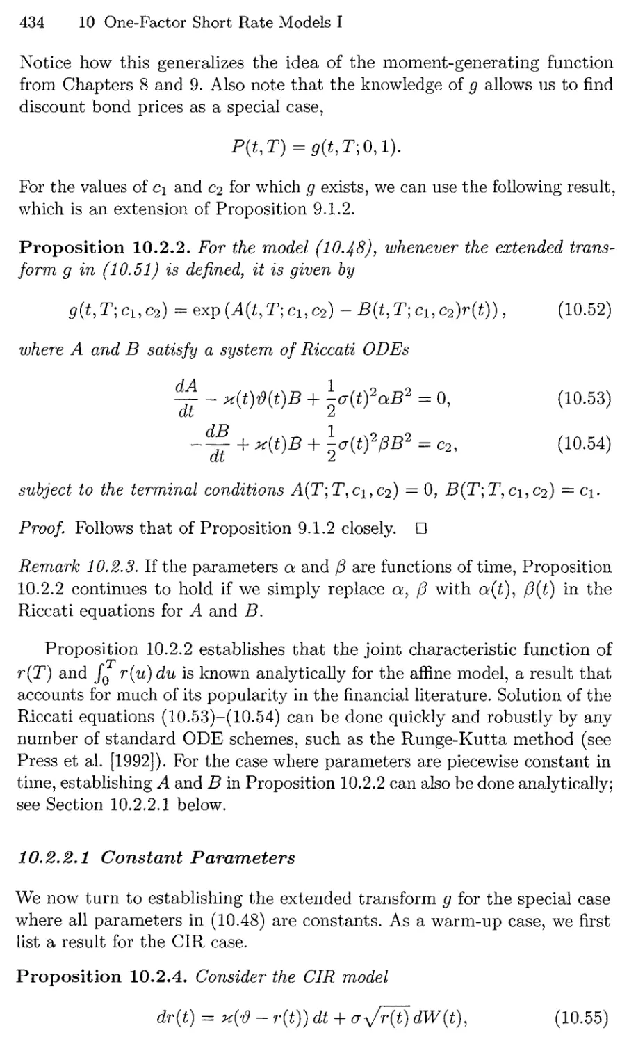
Notice how this generalizes the idea of the moment-generating function
from Chapters 8 and 9. Also note that the knowledge of g allows us to find
discount bond prices as a special case,
P(t,T) = g(t9T;Q,l).
For the values of c\ and c2 for which g exists, we can use the following result,
which is an extension of Proposition 9.1.2.
Proposition 10.2.2. For the model (10.48), whenever the extended
transform g in (10.51) is defined, it is given by
g(t,T;cuC2) ^ exp(A{t,T;cuc2) - B(t,T;cuc2)r(t)), (10.52)
where A and B satisfy a system of Riccati ODEs
HA 1
^p - x(t)${t)B + -a{t)2aB2 = 0, (10.53)
-^r + K(t)B + -o{tfpB2 = c2, (10.54)
at z
subject to the terminal conditions A(T;T,Ci,c2) = 0, B(T;T,ci,c2) = c\.
Proof Follows that of Proposition 9.1.2 closely. □
Remark 10.2.3. If the parameters a and ft are functions of time, Proposition
10.2.2 continues to hold if we simply replace a, (5 with a(£), /3(t) in the
Riccati equations for A and B.
Proposition 10.2.2 establishes that the joint characteristic function of
r{T) and JQ r{u) du is known analytically for the affine model, a result that
accounts for much of its popularity in the financial literature. Solution of the
Riccati equations (10.53)-(10.54) can be done quickly and robustly by any
number of standard ODE schemes, such as the Runge-Kutta method (see
Press et al. [1992]). For the case where parameters are piecewise constant in
time, establishing A and B in Proposition 10.2.2 can also be done analytically;
see Section 10.2.2.1 below.
10.2.2.1 Constant Parameters
We now turn to establishing the extended transform g for the special case
where all parameters in (10.48) are constants. As a warm-up case, we first
list a result for the CIR case.
Proposition 10.2.4. Consider the CIR model
dr(t) = x{<d - r(t)) dt + ay/r{fydW(t), (10.55)

10.2 The Affine One-Factor Model 435
and let g(t,T]C\,C2) be defined as in (10.51). Set
7 = 7 (c2, <t) = V'x1 + 2(j2c2.
Then
#(£, T; ci, c2) = exp (ACir(£, T; tf, a, cx, c2) - BCm{t, T; tf, cr, cx, c2)r(£)),
Acm(t,T;$,a,cuc2) = xtia-2{x + 7(c2,<j))(T~t)
2*cda~2 In
/ (x + 7 (c2, *) - c^x2) (e-r(c2,*)(r-*) - i) \
V + 27(c2,a) J'
and
(2c2 - xci) (1 - e-^^2^)^-^) + 7 (C2, a) ci (l + e^*02'^"'))
(* + 7 (C2, a) + ClCr2) (1 - e-fte.'Xr-t)) + 27 (C2, a) e-7(c2,cr)(T-t) '
Proof. The result is a small extension of Proposition 8.3.8, and follows by
direct solution of the ODEs (10.53)-(10.54). □
Armed with this result, it is straightforward to extend it to the general
constant-parameter case
dr(t) = x(d- r{t)) dt + ay/a + Pr(t)dW(t)9 f3 > 0. (10.56)
In particular, we notice that if y(t) = a + (3r(t), then y(t) follows the SDE
dy(t) =pdr(t) = x (f3ti + a - y{t)) dt + payfyfydW(t),
which is of the form (10.55). We also have
g{t,T;cuc2) = Et (exp ( -dr{T) - c2 f r{u)du\ J
= e^^c^C-'WE, (exp (~jV(T) - | j\(u)duX) .
The expectation involved in the last equality can here be evaluated directly
from Proposition 10.2.4, leading to the following lemma.

436 10 One-Factor Short Rate Models I
Lemma 10.2.5. The extended transform for the constant parameter afpne
model (10.56) is
g(t)T:cuo2) = exp (A(£,T; Cl,c2) - B(i,T; cu c2)r{t)),
A(£, T; d, c2) - <W/3 + c2a(T - *)//} + ylCiR (t, T; /3tf + a, /3a, j, j
B(t,T;c1,c2)=J9SCiR^,T;i9T9 + a,^,^-,^ ,
and i/ie functions Aqir and Bqir are given in Proposition 10.2.4-
10.2.2.2 Piecewise Constant Parameters
We can use the results established in Section 10.2.2.1 to compute extended
transforms for the case where we are given a time grid 0 — to < t\ < to < ...,
on which all model parameters h and a can be assumed piecewise constant.
The resulting recursive routine is a robust and efficient9 alternative to
Runge-Kutta solvers.
For simplicity of notation, let us define y(ti,tj]Ci,c2) = gij{ci,C2),
A(ti,tj]Ci,C2) = Aij(c\,C2), and so on. Then, from Proposition 10.2.2,
9ij{cuc2) = e^./-(ci,c2)-r(t/)Bi.;(ci.c2)j J > it (10>57)
and, using the law of iterated conditional expectations,
/ \ t^ / ~"cir(t,) — c-2 f, ' , r(u)du
(Ji-ij{cuc2) =E4|_1 I e J/'-i
= Et I e~C2^»-ir^dME. ( e~Cir(t')~C2///rMdu
T7 / —c2 f, ' r(u)du ( v \
= £*,_! I e J''-i 9ij(ci,C2)j .
Inserting (10.57) into the last equation then yields
9As pointed out in Section 9.1, depending on the level of accuracy required,
the Runge-Kutta numerical solution of the ODEs can sometimes have higher
computational efficiency.

10.2 The Affine One-Factor Model 437
gl-ltj(cuC2)=Eti_1 U-C2^irWdtte^.j(ci,C2)-r(t4)B;,;(ci,c2)
= eA^c^gi-lti(Bij(cuC2)tc2).
Applying (10.57) to the right-hand side of this equation leads to
pAi-i j(ci,c2)-r(t,_i)B,_i._,(ci,C2)
_ eA,./(ci)c2)eA;_i.i(^J(ci)C2),c2)-r(t/_i)JB^1.i(JBt.j(ci,C2),C2)
or, finally,
Ai-ij (ci,c2) =Aitj (ci,c2) + Ai-iii(Bitj (ci,c2) ,c2), (10.58)
B,_i^(ci, c2) =Bi-hi (Bij (ci, c2), c2). (10.59)
As parameters are constant on the time grid, the functions ^_i^ and Bi-i^
can be computed in closed form from the results of Lemma 10.2.5. For a
fixed j, (10.58)-(10.59) can be used in backward fashion to establish Aij
and Bij for i = j — 1, j — 2,..., 0; the recursion starts with an application
of Lemma. 10.2.5 to compute Aj-ij and Bj-ij.
10.2.3 Discount Bond Calibration
10.2.3.1 Change of Variables
In the affine SDE (10.48), the role of the mean reversion level $(t) is to
calibrate the model to the initial term structure of discount bonds. As
we discussed in the context of the GSR. model, &(t) will depend on the
derivative df(0,t)/dt which may, for many curve construction algorithms,
be irregular. For practical applications of affine models, it is therefore strongly
recommended to follow the advice of Section 10.1.2.2 and rewrite the model
in terms of a variable that measures the difference between r(i) and /(0, t).
Let this variable be x(i), defined as
x{t)=r(t)-f(0,t).
The SDE for x(t) becomes
dx(t) =dr(t) - ^J^dt
= (cu(t) - x(t)x{t)) dt + <r{t)y/£{t) + px{t)dW(t), (10.60)
where x(0) = 0, £(t) = a + /3/(0} t), and
uj{t) - x{t)0(t) - df(0,t)/dt - x(i)/(0,t).
The deterministic function u(t) is likely to be smooth even if the forward
curve is not.

438 10 One-Factor Short Rate Models I
Written in terms of x(i), the extended transform in Proposition 10.2.2
becomes
g(t, T; ci, c2) ^e-Cl/(0^-C2 ^ f^u)duEt (VC^T)"C2 ^ x{u)du)
P(0,t^
e"Cl/(0'T)^Srexp(C(i,T;Cl,c2) ~ x(t)B(t,T;cuc2)),
(10.61)
where 5 solves (10.54) and C can, after suitable translation of the results
in Proposition 10.2.2 to the process (10.60), be written as the solution to
the Riccati ODE:
dC 1
^--u(t)B + -a{tfmB2=^ (10.62)
10.2.3.2 Algorithm for uj(t)
We now assume (but see Section 10.2.5) that a and j3 have been fixed, and
that x(t) and a(t) are known for all values of t > 0. In the SDE (10.60) for
x(t), it only remains to establish the function oj(t), which shall be done to
match observed discount bond prices at time 0.
To make matters more concise, let us set b(t,T) = B(£,T;0,1) and
c(t,T) = C(£,T; 0,1) such that, from the definition of C(i,T),
P(t,T) = fl(*,T;0,1) = ^^e<^'^b^. (10.63)
The functions b and c obviously satisfy a Riccati system,
dr 1
Tt-co(t)b+-a(tfat)b2 = 0) (10.64)
~Jt + ^(^ + ^a(t)2/3/)2 = lj (10'65)
where c(T,T) = b{T,T) =0.
Setting £ = 0 in equation (10.63) establishes the fundamental calibration
requirement that c(0,T) = c(0,T;w(-)) — 0 for all T which, combined with
(10.64), defines a so-called Volterra integral equation for u;(-). We can solve
it on a time grid to < t\ < t2 < .. - < £/v by iterative bootstrapping of the
equation c(0,^;o;(-)) = 0. Assuming that oj(-) is piecewise constant at a
level uji over the time bucket (£i,£$+i], we can use the following algorithm.
1. As a pre-processing step, find b(t^ tj) for all z, j, j > i, by solving (10.65).
This does not depend on cj(-).
2. For a given 2, assume that ujj is known for j < i.
3. Compute 0{U) = ~ JQt+1 cr(s)2£(s)Ks,^+i)2 ds - JQl uj(s)b(s,ti+i) ds.

10.2 The Affine One-Factor Model 439
4. Compute u>i as the solution to 0(U) — cj-i Jt l~rl b(s. U+i) ds = 0.
5. Repeat steps 2-4 for alii = 0,1,..., N - l/
Notice that no numerical root search is needed and that the computational
complexity of the scheme is 0(N2). By modifying Steps 3 and 4, other
interpolation techniques can be supported, although stability issues might
come into play. See also Press et al. [1992] for more general schemes to solve
Volt err a equations.
We should note that there may be cases where the algorithm above will
fail, in the sense that the basic regularity condition (10.49) will prevent
a valid solution for aj(-) from existing. This is a fundamental issue with
non-Gaussian afRne short rate models, but is rarely observed as very strongly
downward-sloping yield curves are required to trigger the problem (see the
discussion in Hull and White [1994a]).
10.2.4 European Option Pricing
The short rate volatility function a(t) in the affine model (10.60) will normally
be determined through calibration against swaptions and caps/floors. For
such calibration to be computationally feasible it is, of course, important to
establish fast methods for pricing European interest rate options.
For simple options such as caplets or, equivalently, options on zero-
coupon bonds, the availability of the moment-generating function for the
logarithm of the bond (see Proposition 10.2.2) allows for application of the
Fourier methods10 of Section 8.4. Extensions to swaption pricing through
the Jamshidian approach of Section 10.1.3.1 is possible in principle, but
the need to perform Fourier integration of a large number of Riccati ODE
solutions makes this approach impractical. Several approximation techniques
have been proposed in the literature; see, for instance, Collin-Dufresne and
Goldstein [2002a] for a survey and details on a method based on Gram-
Charlier expansions. Our preferred approach to swaption pricing in the
affine model borrows the techniques of Section 10.1.3.2 to work out an
approximation for the swap rate martingale dynamics. We shall outline one
straightforward and quite accurate approach here; as was the case for the
GSR model, we again will stop short of the full-blown projection techniques
that will be introduced later in this book for more realistic candidates for
actual trading applications.
Let us, as in Section 10.1.3.2, start out by rewriting the swaption payout
as
Kwaption(To) = A(T0) (5(T0) - C)+ , (10.66)
where
10For time-homogeneous models, closed-form pricing formulas for options on
discount bonds exist for some models, including the CIR model (see Cox et al.

440 10 One-Factor Short Rate Models I
N-l
A(t) = t riP(t,Ti+l), S(t) = P^)-mTN)
Let QA be the measure induced by using A(t) as the numeraire; in this
measure S(t) is a martingale. By the reconstitution result (10.63) we have
dS(t) = ?^(T(t)y/Z(t) + Px(t) dWA(t), (10.67)
where WA(t) is a Q^-Brownian motion and
8S(t) = 6(t, r0)P(t, r0) - 6(t, TN)P{t, TN)
dx A(t)
+ f®E^(*,ri+1)p(t,ri+1).
^ ' t=o
The dynamics (10.67) are generally intractable, but S(t) can — as was
the case for the GSR model — be verified to often be well approximated by
a linear function of x(t), with slope and intercept being functions of time.
Using a Taylor expansion around some point x (e.g. x = 0, but see the
discussion in Section 10.1.3.2), we can find £(£), x(t) such that
s(t)*C(t) + x(t)x(t),
and then (10.67) approximately reduces to an affine SDE for S(t):
- x(t)a(tJm+p (s(t)Xft)C(t)) dwr>tw
= ^WV^W+AWS^d^W. (10.68)
While valuation of the payout (10.66) cannot be accomplished in closed
form when S(t) follows the time-dependent affine SDE (10.68), we can
always rely on transform-based methods. Indeed, it is evident that the
characteristic function of S(Tq) can be constructed by applying Proposition
10.2.2 and R,emark 10.2.3 to (10.68), whereafter Theorem 8.4.3 gives us a
way to calculate the required expected value in
V(0) = ^(0)EQ^ ((S(Tq) - c)+) . (10.69)
We trust that the reader can see how this would work, so we omit the details.
Instead, we proceed to further simplify matters, through time averaging of
parameters.
First, we wish to reduce (10.68) to the simplified form

10.2 The Affine One-Factor Model 441
dS(t) = *(t)y/ffii)y/xl> + S(t) dWA(t), (10.70)
where ip is a some constant. One approach for setting tp is to simply match
quadratic variance of S(t) over [0,Tq], i.e.
/ °a(t)2p8(t)il>dt= [ ° a(t)2ps(t)£s(t)dt
Jo Jo
or
f?°a{t)*0.(t)Ut)dt
f?°a(t)*l3s(t)dt
A more sophisticated alternative would be to rely on a small-noise expansion,
as in Chapter 7. In any case, for the SDE (10.70), the expectation in (10.69)
can be evaluated in closed form. To see this, simply define y(t) = ifc -f S(t)
and note that
dy(t) = a(t)y/M^y/^jdWA(t), y{0)=tl> + S(0), (10.71)
and
V(0) = A(0)E^A ((5(T0) - c)+) = A{0)EQA ((l/Cft) - cy)+) , (10.72)
with cy = ^ -f- c. Since y(i) in (10.71) is simply a (time-dependent) CEV
process with CEV power 1/2, computation of the call option expectation in
(10.72) can be carried out by the formulas in Section 7.2. Swaption prices
produced this way are, in our experience, accurate and robust, and much
more convenient to compute than by competing methods.
10.2.5 Swaption Calibration
As we showed in Section 10.1.4, calibration of the GSR model volatility to
swaption prices is a matter of straightforward bootstrapping. Unfortunately,
matters are more complicated for general affine models.
10.2.5.1 Basic Problem
To gain insight, let us first consider the simple problem of calibrating the
model volatility function a(t) in (10.60) to match the time 0 price of a
Z\-tenor zero-coupon bond option maturing at T. Assuming that the initial
yield curve is known at time 0, how much volatility information is needed to
price this option? The answer to this question depends on the specification
of £ and /3.
If ft — 0, we know that the function 6(T, T+A) in the bond reconstitution
formula (10.63) is independent of a; see Proposition 10.1.7 (and adjust
notation accordingly). It can also be verified that while c(T,T + A) in

442 10 One-Factor Short Rate Models I
(10.G3) depends on the initial discount curve all the way to time T -f A, it
only requires the specification of a(t) to time T. Further, the state of x(T)
only depends on a(i), t < T. In total, when /3 = 0, the discount bond option
payout is only affected by {o"(£)}o<t<T> irrespective of the magnitude of the
bond tenor A. This is also obvious from the reconstitution formula (10.18).
If p ^ 0, however, we see from (10.65) that 6(T, T + A) depends11 on the
volatility {<x(t)}o<t<T+z^ This again makes c(t,T+A) depend on volatilities
in [t,T + A], requiring the full knowledge of {cr(t)}o<t<T+A to price the
option at time 0. This fact has implications for calibration to, say, swaption
prices as regular bootstrapping techniques cannot be employed.
10.2.5.2 Calibration Algorithm
Consider now the situation where we wish to calibrate our volatility function
a(t) to a swaption strip defined on a maturity grid 0 — To < T\ < ... < T/v.
Recall that a swaption strip consists of N — 1 swaptions expiring at times
T/, i = 1,..., iV - 1; we here assume that all swaptions are written on swaps
that mature at time Tm (coterminal strip). According to the discussion
above, pricing any one of these swaptions —■ even the short-dated ones —
in an affine model will require knowledge of {cr(t)}o<t<rN- As it would be
too slow to calibrate volatilities by simultaneous, multi-dimensional root
search on all levels <r(T;), i — 0,1,..., AT, we instead notice that while, say,
the swaption maturing on date T% depends on volatilities everywhere on
[0,T/v], its dependence on the volatilities in [0,7*] is much stronger than
on the volatilities in the interval (Ti^x}. Assuming that a(t) is piecewise
constant on the maturity grid — with a\ denoting the flat value on (Tj,T$+i]
— we can use this observation to propose the following iterative calibration
approach.
1. Start out by setting all a.;, i — 0,..., N — 1, equal to a reasonably chosen
constant, or equal to values approximated from a calibrated GSR12
model.
2. Compute co(-) to match time 0 prices of the N discount bonds maturing
on T\,T'2, -.. ,Tn. One can use the algorithm in Section 10.2.3.2 for this.
3. Set the value do — but leave all other volatilities c^, i — 1,..., N — 1,
unchanged — such that the swaption maturing at time 7\ is priced
correctly. We can use the pricing techniques in Section 10.2.4 for this.
4. Repeat Step 3 for <7i,<T2, ... •)^n-2^ always leaving future (but not past)
points on the volatility curve unchanged.
5. R.epeat Step 2 and recompute all swaption prices.
0. Repeat Steps 3-5 until all swaptions are priced within given tolerances.
11 Recall that we solve b{t/f + A) backward in time from the known boundary
condition at t = T + A.
12For instance, if crg(t) is the volatility function in the Gaussian model, then we
can extract an estimate for a(t) from the relation a(t)y^a + f(0A)j3 ~ crg(t).

10.2 The Affine One-Factor Model 443
Notice that in Step 4, altering &i will slightly distort the prices of
swaptions maturing at dates earlier than T^; this necessitates the iteration
in Step 6.
We (re-)emphasize that the algorithm above, when applied to the
Gaussian model, will converge within one iteration in Step 6. Finally, we note that
the calibrated model needs to be checked against the regularity conditions
discussed in Section 10.2.1.2; if conditions are violated, the problem may
potentially be remedied by increasing a.
10.2.6 Quadratic One-Factor Model
In conclusion, let us consider an interesting special case of an affine class.
A quadratic Gaussian one-factor model is obtained by specifying the short
rate to be a quadratic function of a linear Gaussian process,
r(t) = a(t) + p{t)v{t) + -r(t)y(t)2, (10.73)
where
dy(t) = -x{t)y{t)dt + a(t) dW(t), y(0) = 0. (10.74)
While this is not immediately obvious, the model is indeed of affine type,
albeit in two factors. If we denote u(t) = y(t)2, we see that r(t) is a linear
function of the state vector (y(t),u(t)), which follows the SDEs
which is affine.
We consider multi-dimensional quadratic Gaussian models in a fair
amount of detail in Chapter 12, so we shall be suitably brief here. The affine
connection makes it unsurprising that bond reconstruction formulas exist
for the quadratic model. In fact, we have that zero-coupon discount bonds
are exponentials of a quadratic function of y(t),
P(t,T) = P{t,T\y{t)) = e«(*.r)-6(t,r)y(t)-c(*lT)y(t)2
with the coefficients a, 6, c satisfying Riccati ODEs.
In some ways the parameterization (10.73)-(10.74) is more convenient
than the general affine specification. For example, with the discount bonds
known functions of a Gaussian factor y(t), a swap rate — or a swap value —
is a known function of a Gaussian random variable, which allows us to price
a swaption by a simple one-dimensional Gaussian integration. We return to
this topic in Chapter 12.

444 10 One-Factor Short Rate Models I
10.2.7 Numerical Methods for the Affine Short Rate Model
Much of the material on numerical methods for the GSR model applies to
the affine short rate processes, so we shall be brief. Turning first to finite
difference methods, let us again emphasize that the spatial variable should
be set to be x(t) = r(t) — /(0,t) rather than r(t) itself. The dynamics for
x(t) can be found in (10.60) and lead to the general derivatives pricing PDE
dV dV 1 d2V
— + (co(t) - x(t)x) -^ + -a(tf ^(t) +px)^ = (x + mt)) V,
which can be solved by standard methods, given appropriate terminal
and boundary conditions. We refer to Section 10.1.5 for general guidelines.
Dimensioning of the spatial dimensions of the finite difference grid by
probabilistic means will require estimates for the mean and variance of
x(T), with T being the terminal horizon. We can compute these from the
moment-generating functions established earlier, or, perhaps more easily, by
approximating the SDE for x(t) as being approximately Gaussian. If r(t)
is close to a CIR process, we can also use the analytical moment results
established in Corollary 8.3.3. When establishing the terminal boundary
function (i.e. the option payout), we can rely on the reconstitution formulas
in (10.63) to turn values of x in the finite difference lattice into the discount
bond prices that are required to evaluate the payout.
As for Monte Carlo methods, many of the principles of Section 10.1.6
continue to apply, and we can draw on material in Chapter 8 to design
schemes to advance x(t) through time. To elaborate a bit on this, suppose
that we are interested in advancing x(t) from time ii to time £i+i. Assume
that all parameters in (10.60) are piecewise constant, such that
dx(t) &Xi(qi-x(t)) dt + aiy/ti + px{t) dW{t), t £ [£i,*i+i],
where13 ^ = xfc), qi = u(ti)/x(ti), a* = <j(tt), and & = £(U). Defining
2/(0 ~ & + fi%(t), it follows that we can approximate x(ti+i) « (y(ti+i) —
£i)//3, where
dy(t) = Ki {f3qi + & ~ y(t)) dt + Pai^tijdWit), y(ti) = & + 0x(ti).
(10.76)
Simulation of this SDE, however, was discussed in detail in Section 9.5 where
a number of practical algorithms were introduced. We should notice that
typical parameterizations of (10.76) will rarely violate the Feller condition,
making this SDE considerably easier to deal with numerically than the
stochastic volatility applications in Section 9.5. Additional material on
Monte Carlo simulation of generic short rate processes — most of which
also applies to affine processes — can be found in Section 11.3.3.
13Alternatively, we can also set >a = (x(U) + x(^+i))/2, and so forth.

11
One-Factor Short Rate Models II
While the affine specification (including the Gaussian case) of Chapter 10
is, without doubt, the most popular one-factor short rate model in practice,
quite a few other models have been proposed in the literature. In this chapter
we cover the most important of these models, paying special attention to
the case where the short rate is log-normal. We also briefly discuss some
issues in the econometric estimation of short rate models, and introduce the
important concept of unspanned stochastic volatility.
As most of the models introduced in this chapter have no analytical
bond reconstitution formulas, their calibration to the initial term structure
requires numerical work. Accordingly, the second half of this chapter is
dedicated to numerical methods for pricing and, especially, calibration of
models based on generic short rate SDE. Particularly useful in this regard
is the discussion in Section 11.3.2 on efficient finite difference schemes based
on the important concept of forward induction.
11.1 Log-Normal Short Rate Models
Given the pervasiveness of the log-normal Black-Scholes model in
derivatives pricing theory, it should come as no surprise that many authors have
attempted to specify one-factor short rate models where the dynamics of
r(t) are of the form dr(t) = 0(dt) + ar(t)r(t)dW(t) with deterministic ar(t).
This section reviews this class of models which, somewhat surprisingly, turns
out to have a number of rather severe drawbacks.
11.1.1 The Black-Derman-Toy Model
The Black-Derman-Toy (BDT) model was originally specified in a discrete-
time binomial setting in Black et al. [1990], but subsequent research has
shown the continuous-time limit of the model to be

446 11 One-Factor Short Rate Models II
r(t) - U(t)eaAt)W{t\ (11.1)
where U(t) and crr(t) are deterministic functions, and W(t) is a scalar
Brownian motion in the risk-neutral measure. Notice that r(t) is here an
outright function of W(i), a property sometimes known as path independence
in the short rate dynamics. The following lemma rewrites the BDT model
in more familiar terms.
Lemma 11.1.1. Let r(t) be given by (11.1), and let the prime denote a time
derivative. Then
dlnr(t)= (tf(t) + ^hnr(J) J dt + ar(t)dW(t), (11.2)
dr(t)/r(t) - (ti(t) + l<Tr(t)2 + ^\ lnr(t)] dt + ar(t) dW(t),
\ 2 ar(t) J
where
#(*) = U'(t)/U(t) - HU{t))Gfr{t)/ar{t).
Proof. Set y(i) = In r(t) = In [/(£) + a(t)W(t) and apply Ito's lemma to get
dy(t) = (dlR^^ + *r(*) W^(*)) * + °r{t) dW(t)
= {U\t)/U{t) + (j/(*) - In [/(*)) tj;(t)/(7r(t)) dt + <7r(*) dW(t),
so that (11.2) follows. A second application of Ito's lemma to r(t) = ey^
then gives the result for dr(t). Q
Of the various specifications of the BDT model, the most convenient is
probably (11.2) which describes the logarithm of r(t) as a mean-reverting
Gaussian process with a mean reversion speed
As lnr(t) is Gaussian, r(t) is log-normal. In the formulation (11.2), #(£)
can be considered a free parameter, the value of which can — for a fixed
volatility function ar(t) — be determined by calibrating the model to the
initial yield curve. As the BDT model has no known bond reconstitution
formula, this fit must be done numerically. The original presentation in
Black et al. [1990] outlines such a routine, based on brute-force backward
induction in a binomial tree; this algorithm is, however, computationally
inefficient and should not be used. For a much faster approach, see Sections
11.3.2.1 and 11.3.2.2.
Besides the lack of the bond reconstitution formula, the BDT model
is plagued by a number of issues that makes it unsuitable for practical
applications. One of the issues is explained in Section 11.1.3. In addition, it

11.1 Log-Normal Short Rate Models 447
is problematic that the mean reversion speed of the model is beyond user
control and is fully determined from the short rate volatility and its time
derivative. In particular, for those values of t where ar{t) grows in t, the
mean reversion will be negative, i.e. the model will imply "mean-fleeing"
behavior. It should be obvious that this feature of the model is undesirable.
11.1.2 Black-Karasinski Model
In order to rectify the problems surrounding the mean reversion in the
BDT model, Black and Karasinski [1991] (BK) took the obvious step of
introducing a model where mean reversion for In r(t) is exogenously specified.
In other words, we write
dlnr(t) - x{t) (tf(t) - lnr(i)) dt + ar{t) dW(t). (11.3)
Equivalently, we may write
r(t)=ex{t\
where x(t) is a standard mean-reverting Gaussian process; accordingly, the
BK short rate dynamics are straightforward to simulate in the Monte Carlo
method. The BK dynamics generalize and improve those of the BDT model
but still do not allow for a closed-form discount bond reconstitution formula.
11.1.3 Issues in Log-Normal Models
The BK model — and its special case, the BDT model — have short rates
that are log-normally distributed. A similar distribution of rates would arise
for risk-neutral dynamics of geometric Brownian motion type
dr{t) = Hr{t)r(t) dt + ar(t)r(t) dW(t). (11.4)
A time-homogeneous version of this model was considered in Rendleman and
Bartter [1980]; for the time-homogeneous case (very complicated) formulas1
for discount bond prices exist, see Dothan [1978] and Hogan and Weintraub
[1993]. The model (11.4) has no mean reversion, and cannot be recommended
for practical applications, however.
A common problem shared by all the log-normal short rate models (11.2),
(11.3), (11.4) is the fact that the expected value of the inverse of future
discount bond price is infinite, i.e.
Et{w7r))=0°' t<t><T- (1L5)
1A computationally efficient recursive procedure for bond pricing can be found
in Hansen and J0rgensen [1998].

448 11 One-Factor Short Rate Models II
This result is formally shown in Hogan and Weintraub [1993], but is hardly
surprising since the expectation of ecX, c > 0, is well-known to be infinite
when X is a log-normal random variable2. An important corollary of this
result is listed below, originally due to Sandmann and Sondermann [1997].
Corollary 11.1.2. Define a forward Libor rate
where r > 0 is some accrual factor. Assuming thai (11.5) holds, then also
Et(L(T,T)) -co, T>ty (11.6)
and
Et (eN rlu)du) =oo. (11.7)
Proof As 1 + tL(T,T) = 1/P(T,T + r), equation (11.6) follows directly
from (11.5). To show (11.7), we use Jensen's inequality3 to show
= - < e,/ (ef>' r{u)dv) (11 8)
P{t\T) Ei,(e-firing "M* )' {n*>
Taking expectations conditional on the time t filtration yields (11.7). □
Both (11.6) and (11.7) have unfortunate economic consequences. Formula
(11.7) predicts that the expected return of investing in the continuously
compounded money market account for a finite period of time is infinite;
and (11.6) predicts that all Libor futures rates should be infinite4. A related
problem was discussed in the context of log-normal HJM models in Section
4.5.3.
11.1.4 Sandmann-Sondermann Transformation
The problems outlined in Corollary 11.1,2 are a significant drawback of
log-normal short rate models, and one that should disqualify their use in
many applications. On the other hand, market data may dictate that interest
rates should, in fact, be log-normal. This is not as big a dilemma as it may
appear, as there are ways to build models with a strong log-normal flair, yet
avoiding (11.5). One way is to use HJM models of the type
df{t,T) = 0(dt)+a(t)r{t)dW{t),
' Even though the log-normal distribution has finite moments of all orders, the
moment-generating function is infinite at any positive argument.
3For details on Jensen's inequality, see the proof of Proposition 11.1.3.
4Recall from Section 4.1.2 that the risk-neutral expectation of a random variable
must, in the absence of arbitrage, equal its traded futures price.

11.1 Log-Normal Short Rate Models 449
where / is, as always, the instantaneous forward rate. We return to this
type of models in Chapter 13. An interesting alternative was proposed by
Sandmann and Sondermann [1997] and in essence involves writing the log-
normal dynamics for a discretely compounded rate r^(i), rather than the
infinitesimal (continuously compounded) rate r(t). Specifically, we relate rd
and r through the expression
erW* = 1 + rd{t)5 => r{t) = (T1 In (1 + rd(t)S), (11.9)
where 6 > 0 is some finite compounding interval. Sandmann and Sondermann
[1997] set S = 1, but any finite positive value will, in fact, do.
The effect of working with discretely compounded rates is summarized
in the following result.
Proposition 11.1.3. Letr<i(t) be log-normal for allt. Then, fort < tf < T,
E,(L(T,T))<oo, (11.10)
Et (e& r{u)du) <oo. (11.11)
Proof. As the proof of Proposition 11.1.3 is quite instructive, we give full
details. From (11.8), to prove both (11.10) and (11.11) it suffices to show
that the expectation of e^' r^du is finite. For this, let us recall that Jensen's
inequality for integrals states that for a real-valued function g and a concave
function (p
iplj 9(u)f(u)du\>J <p(g(u))f(u)du, (11.12)
rp
provided that f(u) is non-negative and ft, f(u)du = 1. If <p is convex, the
inequality is reversed. Now write
S'1 I In (1 + rd(u)5) du = 5'1 f —L; In ((1 + rd(u)<5)T-J') du
and apply (11.12) to the right-hand side with f(u) = l/(T—t'), (p(u) = ln(w),
and g(u) = (1 + rci(u)5)T~t to show that
(T1 In ( / —^ t1 + rd(«)«)T"'' du j > r1 / In (1 + rd{u)5) du.
(11.13)
From (11.13) it then follows immediately that

450 11 One-Factor Short Rate Models II
Et I exp [ / r(u) du
= Et I exp ( / 8'1 In (1 + rd(u)8) du j j
< Ej (exp U"1 In (J ^-^ (1 + uWSf-*' du
= Et ((t^7 [{l + rd{u)5)T~t'du
Assume that 0 < 8 < 1, and set f(u) = 1/(T - t'), ip(u) = u1/s, and
g(u) = (1 + rd(u)S)T~t . By Jensen's inequality (here (11.12) is reversed,
since <p is now convex) we must have
1/5
rT \ ' i i-T
\T~t< l (l + r^)Sf-t'du) <j^~pjti {l+rd(u)6)(T-tr>/sdu.
(11.14)
Therefore
Et (e/,Tr(U)rf«) < _1_E( ||^ (1 + rd(w)d-)(^-0/* du j , 0 < 8 < 1.
(11.15)
Since finite powers of log-normal random variables have finite expected
values, (11.11) has been shown for 0 < 8 < 1. For 8 > 1 we have 1/8 < 1,
and
// i rT , V'r'
Et
-i^^l+r^f-^uj
1/<5
-— / CI -n-.^i.U^-*' A, \ \
T-
^(E'(^/, (l+rd(«M)T-*'d«
and (11.11) follows from the same arguments. □
Comparison of Corollary 11.1.2 and Proposition 11.1.3 shows that models
of the BK type
dlnrd(t) = x(t) (ti(t) - lnrd(t)) dt + a(t) dW{t) (11.16)
and geometric Brownian motion models
drd(t)/rd{t) = ii{t) dt + a{t) dW(t), (11.17)
become significantly more reasonable when the dynamics are written in
rd(t), rather than r(t). We invite the reader to apply Ito's lemma to the

11.2 Other Short Rate Models 451
transformation (11.9) to uncover the r-dynamics for the models (11.16)-
(11.17).
Remark 11.1,4- When applied to the HJM model class, the "trick" of shifting
from continuously compounded to discretely compounded rates lays the
foundation for the class of so-called Libor market models. We return to these
models in Chapters 14 and 15.
11.2 Other Short Rate Models
11.2.1 Power-Type Models and Empirical Model Estimation
A natural extension of the Gaussian and affine short rate SDEs involves
retaining the linear mean-reverting drift term of these models, but using a
general power function in the diffusion term. That is, we write
dr{t) = x(t) (#(i) - r(t)) dt + a(t)r(t)pdW(t), p > 0. (11.18)
The time-inhomogeneous Gaussian and CIR models correspond to the choices
p = 0 and p — 1/2, respectively. The special case of (11.18) where p = 1
was suggested in Brennan and Schwartz [1980] and Courtadon [1982], and is
quite similar to the BK model — to the extent that the case p = 1 shares5
the unfortunate properties of the BK model listed in Corollary 11.1.2.
The general model (11.18) is similar to the CEV model described in
Chapter 7, and manipulation of the parameter p may allow for a better fit
of the model to observed volatility smiles in interest rate options. Due to
its intractability — no bond reconstitution formula exists for p £ {0,1/2} —
the model is, however, rarely used in derivatives pricing applications. (For
related, but significantly more tractable, models with power-type diffusion
terms, see Chapter 13.) Starting with the influential article by Chan et al.
[1992] (CKLS), the specification (11.18) has, however, been quite popular in
econometric work. As the CKLS paper is one of the most frequently cited
references on estimation of one-factor short rate models, let us make a (very)
brief foray into econometrics, to review the CKLS conclusions and some of
the criticism their work has subsequently drawn.
The CKLS estimation procedure is based on US Treasury bond data
from the period 1964-1989. Assuming that r(t) can be approximated by
the one-month yield on US Treasury bonds, they estimate eight models
with parameter restrictions, and one model with no restrictions. Generally
speaking, the empirical results indicate that the value of the parameter p is
the most important in determining whether a model is accepted or rejected.
5The proof of this statement is straightforward, and follows from a standard
comparison theorem for SDEs (see p. 293 of Karatzas and Shreve [1997]).

452 11 One-Factor Short Rate Models II
The unrestricted estimate of p is close to 1.5, and values less than around
p — 1 are rejected in their tests. The Vasicek and CIR models are, for
instance, rejected, whereas the Brennan-Schwarz/Courtadon model (with
p = 1) is accepted.
The fact that the CKLS estimates suggest that p > 1 is surprising in
light of the generally downward-sloping volatility skews in fixed income
derivatives, and also raises considerable questions about model regularity,
as one would expect from Corollary 11.1.2. Indeed, as shown in Honore
[1998b], r(t) will a.s. explode (i.e. reach oo) in finite time if p > 1. Beyond
this, we notice that the CKLS analysis has received criticism on a number
of procedural and data-related fronts. For instance, Honore [1998a] (and
quite a few others) point out that the 1 month Treasury yield may be an
unreliable proxy for the short rate. Repeating the analysis with a carefully
computed value of r(t) (obtained by exploiting the fact that a one-factor
model implies a one-to-one correspondence between any discount yield
and the short rate), Honore revises the CKLS estimate for p significantly
downward, to around p = 0.8. Bliss and Smith [1997] also point out that
the data used by CKLS covers the period October 1979 — September 1982,
when the US Federal Reserve followed unusual monetary policies ("The
Fed Experiment"). Properly accounting for this, Bliss and Smith revise the
CKLS estimate for p down to around 1.0. Applying different estimation
methods and different data sets, Andersen and Lund [1997] and Christensen
et al. [2001] estimate p to around 0.7 and 0.8, respectively.
Moving away from observations of only a short rate proxy, Gibbons and
Ramaswamy [1993] test the ability of the CIR model to simultaneously
describe the evolution in four zero-coupon rates; with data covering the
same period as the CKLS study, they accept the hypothesis p = 1/2. Finally,
to muddy waters even further, Ait-Shalia [1996] points out (in an analysis
that has subsequently been criticized as lacking robustness in Chapman and
Pearson [2000]) that the simple linear drift term in (11.18) is fundamentally
misspecified and should be adjusted to include non-linear terms such as
l/r(t) and r(t)2.
By now, it should be clear to the reader that the problem of estimating
short rate models is not close to being conclusively solved, despite an
impressively long list of papers associated to it. In much contemporary
empirical research, the importance of the choice of p is generally downplayed,
with the affine class (p = 1/2) enjoying considerable current popularity due
to its analytical tractability.
11.2.2 The Black Shadow Rate Model
As described in Chapter 10, one drawback of the Gaussian short rate
model class is the implication that interest rates can become negative with
positive probability. As long as investors can stuff their mattresses with
currency, (nominal) interest rates must, however, always remain non-negative

11.2 Other Short Rate Models 453
to preclude arbitrage. In practice, the probability of negative rates may be
small enough to ignore, but as argued in Rogers [1996] prices of certain
contingent claims may be highly sensitive to even a remote probability
of negative rates, in which case the Gaussian model should obviously be
avoided. Possible model alternatives with non-negative rates include the
log-normal models in Section 11.1, as well as the affine models in Section
10.2.
Rather than altering the underlying model, an alternative "fix" of the
Gaussian model involves simply taking the positive part of the Gaussian
short rate process, i.e. writing
r(t) = (r*(t))+ , (11.19)
where r*(t) is a Gaussian process
dr*(t) = x{t) (#(t) - r*(t)) dt + ar(t) dW(t). (11.20)
This approach was first proposed in Black [1995] and Rogers [1995]. The
form of (11.19) suggests an analogy where the interest rate r(t) is an option,
granting a choice between an underlying shadow short rate r*(t) and zero.
In other words, whenever an interest rate product has a negative rate, we
invest our money in currency instead.
The truncation in (11.19) may at first glance appear rather crude. For
instance, the process for r(t) retains full volatility ar(t) as long as r(t) > 0,
and can then suddenly get extinguished completely for potentially long
stretches of time. In contrast, alternative models with non-negative rates
such as BDT, BK, and CIR generally all imply that the interest rate volatility
will gradually vanish (linearly for BDT/BK, as a square-root for CIR.) as
the short rate tends to zero. Interestingly, there is some empirical evidence
(from the US in the 1930's and Japan in the 1990's) that suggests that very
low interest rates are often accompanied by higher absolute rate volatility
than standard models would predict, see Goldstein and Keirstead [1997].
Such evidence may lend some credibility to models such as (11.19).
The process (11.19) is not analytically tractable, and numerical methods
(such as those of Section 11.3) must be applied to price discount bonds and
other fixed income securities. For the case where all parameters in (11.20)
are constants — i.e. r*(t) follows a Vasicek model — Gorovoi and Linetsky
[2004] list6 a complicated eigenfunction expansion series for discount bond
prices. Of course, as the constant-parameter model will not be able to match
the current yield curve, the result in Gorovoi and Linetsky [2004] has limited
uses in practical applications.
Finally, the reader may very well ask whether perhaps (11.19) could be
replaced by a reflecting or absorbing barrier at zero, or by the application of
6 The authors also develop eigenfunction expansions for cases where the shadow
rate r* (t) follow time-homogeneous diffusions more complicated than the Vasicek
model.

454 11 One-Factor Short Rate Models II
a suitable transformation such as r(t) = r*(t)2. The latter idea was discussed
in Section 10.2.6 and the former is investigated in Goldstein and Keirstead
[1997] where eigenfunction expansions are derived for the time-homogeneous
case. In Black [1995], the author objects to reflecting barriers on economic
grounds.
11.2.3 Spanned and Unspanned Stochastic Volatility: the Fong
and Vasicek Model
In previous chapters, we demonstrated how to incorporate stochastic
volatility as a mechanism to model the volatility smile in vanilla models. One
wonders how to proceed with such a construction for term structure models.
We postpone much of this discussion to later chapters, but shall here take the
opportunity to discuss what constitutes a true stochastic volatility model for
interest rate evolution, and why the short rate framework is not particularly
amendable to stochastic volatility extensions. More specifically, we shall
introduce the notion of spanned and unspanned stochastic volatility For con-
creteness, our discussion focuses on a model proposed by Fong and Vasicek
[1991] which, despite initial appearances, is in fact not a true stochastic
volatility model.
The Fong-Vasicek (FV) model is characterized by risk-neutral SDEs
dr(t) = xr (tfr - r(t)) dt + s/zJt)dWi{t),
dz(t) = xz (tiz - z(t)) dt + vy/^)dW2(t),
where Wx and W2 are correlated Brownian motions, (dWi(t), dW'2(t)) = pdt,
and Xr,$r,Xz>$z,V are positive constants. We recognize the FV model as
being essentially a time-homogeneous GSR model augmented by a stochastic
variance process z(t)\ the process for z(t) is identical to that of the Heston
model (see Chapter 8). Bond prices in the FV model can be shown to satisfy
p^t + S)=eA(6)+r(t)B(6nZ(t)C(6)^ (1L21)
for deterministic functions A,B,C satisfying a coupled system of ODEs.
Details about these ODEs' and their rather complicated analytical solution
can be found in Selby and Strickland [1995]. For our purposes here, what
matters is not the precise form of A, jB, and C, but rather the fact that
P(t> T) in the FV model is a deterministic function of the two state variables
r(t) and z(t). As a consequence, one can theoretically hedge out exposure
to both r(t) and z(t) by simply taking positions in two discount bonds with
different maturities. Equivalently, given observations at time t of the prices
of two discount bonds with different maturities, we can invert (11.21) to
uncover the current values of the two variables r{t) and z(t).
7The ODEs are easily derived by substituting the right-hand side of (11.21)
into the no-arbitrage PDE for P(t,T) in the FV model.

11.3 Numerical Methods for General One-Factor Short Rate Models 455
When a "stochastic volatility" variable z(t) can be hedged by positions
in discount bonds, we say that z(t) is spanned by the discount curve. If all
stochastic volatility variables are spanned by the discount curve, moves in,
say, implied volatilities of caps and swaptions would always be accompanied
by moves in the yield curve, making vega hedging theoretically unnecessary.
In reality, however, there is much evidence that interest rate option volatilities
cannot be perfectly hedged by trading only discount bonds; see Casassus
et al. [2005] for a review of the literature. Formally, this implies that the
volatilities of discount bond prices depend on a vector of random state
variables {z\{t),..., zn(t)) that are not included in the state variables used
in reconstitution formulas for the discount curve. That is,
w=o' *=i-•••'■• <il22)
yet, for Q(t,T) = Et(d(P(t,T))2)/dt,
dQ(t,T)
dzi(t)
^0, i = l,...,n. (11.23)
Random variables satisfying (11.22)—(11.23) are said to represent unspanned
stochastic volatility (USV). Whenever we talk about true stochastic volatility
in this book, we always refer to models with USV, i.e. to models that prescribe
moves in rate volatility that cannot be inferred from moves in the level and
the shape of the discount curve.
A detailed, and highly recommended, account of USV can be found in
Collin-Dufresne and Goldstein [2002b]. Among many results, the authors
prove that in a time-homogeneous setting, bivariate affine models for the
term structure of interest rates cannot exhibit USV. This explains our
results for the FV model, and also demonstrates that several other classical
stochastic-volatility models (e.g. Longstaff and Schwartz [1992]) are not in
the USV class. Further analysis of a number of stochastic volatility models
proposed in the literature (a surprising number of which do not, in fact,
allow for USV) can be found in Collin-Dufresne and Goldstein [2002b] and
Casassus et al. [2005].
11.3 Numerical Methods for General One-Fact or Short
Rate Models
The models described in Sections 11.1 and 11.2 all (with the exception of
the Fong-Vasicek model) involve risk-neutral SDEs for the short rate of the
type
dr(t) = nr(tir(t))dt + <rr(t,r(t)) dW(t), (11.24)
for certain user-specified deterministic functions fir(t,r) and ar(t,r). As
discussed, many of these models do not allow for closed-form expressions

456 11 One-Factor Short Rate Models II
relating discount bonds to the state of r(£), necessitating the application of
numerical methods for even simple tasks such as calibrating the model to the
initial yield curve. While this issue ultimately should make one pause when
it comes to deciding whether a model is suited for practical applications, we
still want to cover some techniques that are useful in handling generic models
such as (11.24). Some of the techniques we shall discuss, e.g. calibration
through forward induction, have broad applicability.
11.3.1 Finite Difference Methods
As always, we set x(t) = r(t) — /(0,t), such that the generic pricing PDE
for a derivative V = V(t,x) becomes
dV dV 1 nd2V
— + ^x(t,x)— + -ax(t,x)2^ = (x + f(0,t))V, (11.25)
where we have defined
M*,aO=M*,s + /(0,t))- ^ > (rx(t,x)=<jr(t,x + f{0,t)).
(11.26)
Given terminal conditions for V(T, x), as well as suitable boundary conditions
in the x-domain, we can solve this equation by the generic finite difference
methods of Chapter 2. For later use, let us quickly recall that a standard
^-method finite difference scheme on an equidistant x-grid {xj}™^1 would
result in a matrix scheme of the type
[1-0 At A ((1 - 9)ti+l + 0ti)] V(U) =
[1+ (1 - 0)AtA ((1 - 9)tl+l + 0U)] V(*i+1) + B(*<, *i+1), (11.27)
where V(i) = (V(£,xi),..., V(t,xrn))T with V(t,x) denoting the
approximation to the true solution V(t,x), A(t) is a tri-diagonal matrix, and
~B(ti,ti+i) is a vector representing any boundary conditions that cannot be
folded into the matrix A. We solve the matrix system (11.27) backward
in time, starting from a given value of V(T). Determination of the spatial
boundaries in the x-domain — that is, the values of xo and xm+i — can, as
always, be set by probabilistic arguments, through estimation of the first
and second moment of x(T). While these estimates should be targeted to
the specifics of the model at hand, if all else fails we can always rely on
Gaussian estimate, e.g. something like
xo = fix (0,0) T ~ aax (0, 0) y/f, xm+1 - fix (0,0) T + aax (0,0) VT,
where a is some confidence interval multiplier (e.g. 4 or 5).
The discussion in Section 10.1.5.2 about x-domain boundary conditions
apply to (11.27) as well, but determining the terminal condition V(T) can

11.3 Numerical Methods for General One-Factor Short Rate Models 457
be problematic8, as option payouts will often involve several discount factors
at time T (e.g. to price a swap or to compute a Libor rate). As there is
generally no way of computing such discount bonds analytically for the
model (11.24), we are forced to compute the discount bond prices themselves
by finite difference methods. To compute the value of the discount bond
P(T>T*yx), T* > T, at time T we:
1. Extend the finite difference grid to time T*.
2. Set the boundary condition P(T*,T*,Xj) = 1, j = 0,... ,m + 1.
3. On some suitable time grid, use (11.27) on P to step backward to time
T.
4. Use the finite difference estimates P(T, T*,Xj), j = 0,..., rn + 1, to fill
in V(T).
To the extent that V(T) involves multiple discount bonds, we perform
the algorithm above on all of the required discount bonds; the grid must
then be extended to the maturity of the longest-dated discount bond needed
in the payout computation. In some cases this can dramatically increase
computation times relative to models where closed-form discount bond
reconstitution formulas exist. For instance, for a 3 month option on a 30
year swap, a model with an analytical formula for discount bonds (e.g. the
affine short rate model) would require us only to build the finite difference
grid out to 3 months; when such a formula does not exist, we are forced to
use a 30 year finite difference grid.
11.3.2 Calibration to Initial Yield Curve
Assume that the volatility function ar(t,r) has been fixed, but jj,r(t,r) =
/ir(£,r;#(£)) has a free time-dependent parameter #(£), the value of which
we wish to set in such a way that the initial discount curve P(0, T), T > 0,
is correctly recovered by the model. Suppose that we assume, as is common,
that $(t) is piecewise constant on some time grid 0 = to < t\ < .. - < t^,
with di-\ denoting the value of d that applies on the interval [£j_i,^). A
brute force approach to the calibration of $(£) could proceed as follows.
1. Assuming that $o> ■ • • >$i-2 are known, make a guess9 for $i_i.
2. Setting the terminal boundary value to V(ti,x) = 1 for all x, use the
backward finite difference grid algorithm (11.27) to compute the value
of P(0,t<).
3. If the computed value of P(0, ti) equals that quoted in the market stop;
otherwise return to Step 1.
8The same holds for exercise values of callable securities.
9An initial guess for ^_i could be dx-\ = dx-2> Subsequent guesses would be
performed by a root-search algorithm.

458 11 One-Factor Short Rate Models II
This approach is similar to an algorithm proposed in Black et al. [1990]
(albeit the authors worked only with binomial trees) and involves very
high computational costs as the numerical search for each of the parameters
r?o> ^i> ■ • • involves solving a full finite difference grid in each loop. Specifically,
assume that on average each search for ^ involves M iterations over steps
1-3 above. With TV tf-values to find, the computational effort of a finite
difference grid with m spatial steps (say) is O(Nm); it follows that the total
computational cost for the calibration of d(t) is
O (MN2m) ,
which is often prohibitively expensive in practice.
11.3.2.1 Forward Induction
In the setting of binomial and trinomial trees, the brute-force BDT algorithm
was markedly improved upon in Jamshidian [1991a], using a technique known
as forward induction. The basic idea is to work with a forward equation,
rather than with the backward equation (11.27). Two varieties of this
approach are feasible in a finite difference setting, depending on whether the
forward equation is developed by direct discretization of the continuous-time
Fokker-Planck equation, or by rearrangement of a discretized backward
equation. We cover the former approach here, and the latter in Section
11.3.2.2 below.
Let G(t,x;s,y), s > ty denote the time t value of a security that pays
out a Dirac delta amount iff x(s) = y, given that x(t) = x. Clearly then
/oo
G(0,0;T,y)dy. (11.28)
■OO
We already saw this financial contract, the so-called Arrow-Debreu security,
at the end of Section 1.8. Its price G — being the value of a perfectly valid
derivative contract — certainly satisfies a backward Kolmogorov equation
dG dG 1 d^G
— + nx(t,x; m)~Q^ + 2ax(t'X)2~cW = (X + /(°' ^ G' (S'V) fixed'
(11.29)
with the terminal value condition G(s, y\ s, y) = 5(y). Clearly G(t, z\ 5, y) is
closely related to the transition density p{t<>z\s,y) defined in Section 1.8,
and can be expected to satisfy a forward Kolmogorov equation, too. The
correct equation is
- a7 " -dy- 0**('>v,*('))G) + 5^2 {°At.y?G)
= {y + f(0,t))G, (t,x) fixed, (11.30)

11.3 Numerical Methods for General One-Factor Short Rate Models 459
subject to the initial condition G{t,x\t,x) = 8(x). This PDE is identical to
the Fokker-Planck equation listed in Section 1.8, except for the fact that
the right-hand side is not zero, but contains a discounting term.
Fixing (tyx) = (0,0), the PDE (11.30) can be discretized by finite
difference methods in standard fashion, although we keep in mind that the
PDE is to be solved forward in time from its initial (Dirac) condition, rather
than backward. In most cases10, the appropriate spatial boundary conditions
for the finite difference solution G are
g(0,0;5,y0)-5(0,0;5,ym+1)=:0,
which assumes that yo and ym+i have been set such that the probability
density at these levels is negligible. In a discrete setting, the initial condition
G(t,x\t,x) = 5(x) is translated to G(0,0;0,y) = (Ay)~ll{y^o} for Ay
suitably defined, in agreement with the averaging principles of Section 2.5.2.
Due to the strongly discontinuous initial condition, Rannacher stepping (see
Section 2.5) should always be used.
We are now ready to state our revised algorithm for calibration of $(£),
working again with the assumption that t?(t) is piecewise constant on a time
grid 0 — to <t\ < ... < ttf. We assume that #o> • • • ^i~2 have been found,
as has been G(0,0;^_i,y) for all y E {2/j}^=i *n the finite difference grid.
1. Make a guess for #i_i.
2. Solve (11.30) one time step forward, to time tZi and save (?(0,0:^,?/j),
j = l,...,ra.
3. Compute the discount bond price P(0,^) = J^j ^(0> 0> U> Vj)(yj ~ Vj-i)-
4. If the computed value of P(0,t^) equals that quoted in the market stop;
otherwise return to Step 1.
The cost of Steps 2 and 3 in this algorithm is 0(m), where m is the
number of points in the ^-direction of the finite difference grid. The total
computational effort of this algorithm is therefore
O(MmN),
where M is the average number of root search iterations over Steps 1-4 above.
We recall that the effort of the brute-force backward equation approach was
0(MmN2), so the use of forward induction saves us a factor of N. As N is
often of the order of N — 100, these savings can be considerable. In typical
applications, M is often in the order M = 2 to 4, so calibration of the model
(11.24) to the initial discount curve should only be a few times slower than
pricing by finite difference methods a single option maturing at time £jv (the
cost of which we recall to be 0(mN)).
10For some models, the density can grow to infinity at the boundary, notably in
the CIR model for x —> 0+ when the Feller condition is violated. Should that be
the case, a more careful analysis of boundary conditions is required, see e.g. Lucie
[2008].

460 11 One-Factor Short Rate Models II
11.3.2.2 Forward-from-Backward Induction
The backward and forward Kolmogorov equations (11.29)—(11.30) are
consistent in the continuous-time limit, but not necessarily so when discretized,
finite difference style. As a result, the function d{t) uncovered from the
algorithm in Section 11.3.2.1 will generally not allow a finite difference grid
based on the backward equation (11.25) to recover the initial term structure
of discount bonds without errors, even if discretized on t- and x-grids that
are identical to those used for the calibration of #(£). As long as the time
line is sufficiently finely spaced, the errors tend to be very small, however,
and rarely a cause for concern. Nevertheless, it should be noted that it is, in
fact, possible to restate the forward induction algorithm in such a way that
the algorithm becomes precisely compatible with the brute-force backward
equation approach we discussed earlier.
To develop this approach, we start out with the discretized backward
equation (11.27) and rearrange it to yield
V(ti) = Tl+1V(ti+1) + G)+\ (11.31)
where, with A;+l = A((l - 6)ti+1 + 0tt),
T*+l 4 [l-9AtA'+l]~l [l+(l-0)AtAt+1]
= I+[l-6AtAii+1y1A,i+1At,
and
GJ+1 = [l-0AAj+1]~1B(4xlii+1).
Repeated application of (11.31) yields, for some /,
V(0) = Tl0V{ti) + Gl (11.32)
where Tq and Gq can be found iteratively from the equations
T*>+1 =TJTJ+1, Tg = I, (11.33)
G*>+1 - T^G;+1 + Gj, G°0 = 0. (11.34)
Before we proceed, let us introduce some notation. First, we let lj denote
an ??i-dimensional column vector with j-th element equal to 1 and all other
elements equal to zero. Also we set 1 to mean a column vector with all
elements equal to 1. Consider now the zero-coupon bond maturing at time
tz. and assume that for the grid {xj}™^ the initial value of x = 0 sits in
position (3, i.e. xp = 0. By the definition of a discount bond, (11.32) allows
us to write
P(<M,-) = lj (Tjl + Gl0) = lTD'0+(y0, (11.35)
where Dq is an //^-dimensional vector and cjq is a scalar:

11.3 Numerical Methods for General One-Factor Short Rate Models 461
D<
(T?))Tl/3, 9l0
(GiVu
Assuming that the influence from the finite difference grid boundary is small,
we evidently have
m
P(0,^£(Do)i'
J=l
where (Dq)^ denotes the j-th element of Dq. Comparison with (11.28) shows
that Do can be interpreted as the discrete-time Arrow-Debreu security vector
for maturity ti (up to the scaling Ax). From (11.33)-(11.34) we have
D<+1 = (T*Ti+1) 10 = (T*1) Dj, Dg = 10
g?1 = (T'G|+I + G^)T 10 = (Gj+1)T D< + g<0,
Recalling the definition of T*+1, it follows that
9°o
0.
(11.36)
(11.37)
D*+1 = (TJ+1) D^
)4tA*+1l
= [I+(1
i-9At a:
r0'
l+\\
D^
where Yg is a vector satisfying a tri-diagonal matrix equation
I-04t(AJ+1)' Y$=D*.
(11.38)
(11.39)
With this, we are ready to state our revised fitting algorithm for d(t). We
i-l
assume that #o> • • • > $i-2 have been found, as has D0 and glQ
1. Make a guess for i^i.
2. Solve (11.39) for Yj"1.
3. Compute Dj from (11.38); and gl0 from (11.37).
4. Compute the discount bond price P(0,£?) from (11.35).
5. If the computed value of P(0,£$) equals that quoted in the market, then
stop; otherwise return to Step 1.
The computational efforts for Steps 2, 3, and 4 are all O(ra), so the
algorithm above is of the same computational complexity as the algorithm
in Section 11.3.2.1.
11.3.2.3 Yield Curve and Volatility Calibration
Volatility calibration of a general short rate model of the type (11.24) is
a rather involved affair. The typical scheme — moving model volatilities
around until the prices of calibration targets match the market — is beset
with complications such as

462 11 One-Factor Short Rate Models II
• Bond reconstitution formulas are unavailable so the model needs to be
numerically recalibrated to the initial yield curve after each update of
the model volatilities.
• All bonds used in the payoffs of calibration targets need to be computed
numerically for each volatility update.
• Bond and calibration target values depend on the entire volatility
function, making decoupling of individual target calibrations difficult.
These difficulties, however, have not prevented some major investment
banks from risk-managing large derivatives portfolios with such a setup. As
we cannot possibly do justice to ail the tricks that would be required to
make this operational, we content ourselves with presenting a mere outline
of a possible algorithm.
We consider the model of the type (11.24) but, for notational convenience,
write the volatility term in a separable form
dr(t) = Hr(tyr(t);ti(t))dt + (Tr(t)1>(r(t)) dW(t). (11.40)
Here, the purely-time-dependent function ar(t) is used to calibrate to swap-
tions, and #(£) is used to match the initial yield curve. Implicitly, $(t)
depends on ar(t).
As in Section 10.1.4, we assume that we are given a collection of N — 1
swaptions defined on a maturity grid 0 = Tq < T\ < ... < Tjy such that the
i-th swaption expires at times T{, i = 1,..., iV — 1. For concreteness assume
that all underlying swaps mature on T/y. We further assume that ar(t) is
discretized in a piecewise constant manner on the maturity grid, with Oi
denoting the flat value on [TiyTi+1).
Before discussing calibration, let us outline an efficient algorithm for
pricing all swaptions in the calibration set given a collection of volatilities
Go,..., <7Ar_i.We implicitly assume that the model is rewritten using a state
variable x as in (11.25), and the x-domain is discretized with {^j}?^1- As
the algorithm involves both forward and backward induction, it is important
to follow the approach of Section 11.3.2.2 and use a forward algorithm that
is fully compatible with the backward one.
1. Update the volatility function of the model with the new values
cr0, . . . , <7tv_i.
2. Using the forward induction algorithm from Section 11.3.2.2, calibrate
tf(*) for alHe [0,TN].
3. On Step 2, Arrow-Debreu prices G(0,0;Ti,-) are calculated; save them
for alH = l,...,iV-1.
4. For each n = iV,..., 2:
a) Create a new copy of the finite difference grid.
b) Populate a payoff P(Tn,Tn) — 1 at time Tn.
c) Calculate P{T^Tn) from P(T^+i,Tn) by backward induction for
i = n — 1,..., 1.

11.3 Numerical Methods for General One-Factor Short Rate Models 463
5. For each i — 1,..., N - 1:
a) Create the T^-expiry swaption payoff from P(Ti, Tn), n = i 4-1,..., N,
calculated on Step 4.
b) Integrate the payoff against G(0,0;T^, •) stored on Step 3.
c) This gives the value of the T*-expiry swaption.
This algorithm describes how to map a set of model volatilities
do,... ,<Tjv-i into model prices of calibration targets. In principle, one can
now perform a multi-dimensional optimization to match swaption prices
from the model to the market. Given that the number of swaptions could
be large — 30 or 40 would not be uncommon — and each valuation is
rather expensive, the resulting algorithm, while not necessarily completely
impractical, would require significant computational resources.
A further improvement entails adopting the iterative bootstrap algorithm
outlined in Section 10.2.5. We recall that the main premise of this algorithm
approach was that the value of the T^-expiry swaption depended on ar(s)
for s € [0,7*] in a much stronger way than on ar(s) for s e [7^,7^]; this
tends to also be true for the model of the type (11.40) for a wide range of
volatility specifications. To incorporate this observation into the algorithm
above, we would work our way forward from i = 0 and determine oi by
one-dimensional root-search to match the market value of the T^+i-expiry
swaption; all values o^ j / i would be kept constant in the root search. The
bootstrap loop would work its way from i = 0 to i = N~ 1 and would be
repeated a few times until convergence, in the manner described in Section
10.2.5. We trust that the reader gets the idea and can fill in remaining
details.
11.3.2.4 The Dybvig Parameterization
In some models, it may be the case that the SDE (11.24) can be reformulated
as
r(t) = s(t) + tf(J), (11.41)
where $(t) is a free time-dependent function to be fitted against discount
bond prices, and s(t) satisfies an SDE
ds(t) = il8 (t, s{t)) dt + as (*, s(t)) dW(t). (11.42)
We notice that
P(0,T) = E (e~f« r(u)du) = e~f»^iu)duE (e~^s{u)du) ,
such that
rT /E (e~$' s(u)du
P(0,T)
/ d{u)du = In j v n/n ^—'- I . (11.43)

464 11 One-Factor Short Rate Models II
To the extent that the numerator in the right-hand side of (11.43) is easy
to compute — e.g. if the SDE for s(t) permits a closed-form solution —
calibration of #(£) can conveniently be found by direct differentiation, see
(11.44).
The specification in (11.41) was proposed in Dybvig [1997] and is, as
we have already seen in Section 10.1.1.2, quite natural in the context of
Gaussian models. For non-Gaussian models, a "fudge" approach in (11.41)
may be less desirable, as the domain of r(t) is hard to control. For instance,
suppose that s{t) is a time-homogeneous CIR process
ds(t) = x(s0- s(t)) dt -f ayfs{£) dW(t),
which is guaranteed to produce only non-negative values of s(t). The
combined process11 r(t) — s(i)+ $(£), however, will have domain r(t) € [$(£), oo)
which is rather awkward as d(t) is largely out of the user's control. This is
reflected in the SDE for r(£), where now $(t) enters into the volatility term:
dr(t) = k (5o + tf(t) + $'{t)/x - r(t)) dt + <ry/r(t) - ti(t)dW(t),
where #'(£) = d$(t)/dt. By affecting the short rate volatility, the
interpretation of $(t) as only serving to fit the yield curve can no longer be maintained.
This conclusion holds not only for CIR models, but for all models where as
depends on s(t), since
dr{t) = il8 (t, r{t) - d(t)) dt + $\t) dt + as (t, r(t) - ti(t)) dW(t).
While sometimes very convenient, the Dybvig parameterization should
consequently be approached with considerable care.
11.3.2.5 Link to HJM Models
By construction the Dybvig parameterization in Section 11.3.2.4 ensures
that the model is calibrated to the initial forward curve /(0,£), t > 0. As
the resulting model is driven by Brownian motions, we know that it must
be in the HJM class. An interesting question arises: what is the type of an
HJM model that is defined through the Dybvig procedure. To answer this,
let s(t) satisfy (11.42) and define
Q(£,2» = E (e-f?*Md»\ s(t) - s
From (11.43), we then get
11 This model has been advocated by Brigo and Mercurio [2001] as an easy-to-
implement alternative to a true time-dependent CIR process. For reasons explained
above, this model has certain drawbacks that require careful evaluation.

11.3 Numerical Methods for General One-Factor Short Rate Models 465
«<«>-i-(Vi
and
As
/(t,r) = -^lnP(t,T) = -^Q(«)T,*(t)) + tf(T),
it follows that
df{t,T) = 0{dt) + af(t, T) dW(t),
where
<9T<9s
At time £, the forward rate volatility structure generated by the short rate
model evidently depends on the forward curve at time t (through f(t,t)) as
well as the function tf(£). As fl(t) depends (through (11.44)) on the forward
curve at time 0, it follows that the HJM dynamics here generally have
"memory" of the initial condition at time 0. If one were to alter these initial
conditions, the form of HJM dynamics would fundamentally change.
Looking back to Section 10.1.2.2 where the Gaussian short rate model
was developed from a separable HJM model, no dependence in the HJM
dynamics on initial conditions arose. Hence, it is clear that not all short rate
models generate "memory" in the HJM dynamics. This raises the obvious
question: under which circumstances will a finite-dimensional Markov HJM
model have no dependence in its dynamics of the initial forward curve at
time 0? The answer to this is listed in Filipovic and Teichmann [2004]
which shows that "essentially" all such models must be time-inhomogeneous
affine models. There are considerable technical details involved in the exact
statement of the result, all of which can be found in Filipovic and Teichmann
[2004].
11.3.2.6 The Hagan and Woodward Parameterization
Many of the short rate models considered so far have a free time-dependent
parameter in the drift of the state variable dynamics; the forward induction
algorithm can then be used to set this parameter to match the initial yield
curve. Hagan and Woodward [1999a] propose an interesting twist on the
idea, where the free parameter is introduced into the numeraire.
Hagan and Woodward [1999a] start with an observation that only two
ingredients are required to create an interest rate model:

4GG 11 One-Factor Short Rate Models II
• A set of stochastic processes that drive the evolution of interest rates.
• A positive-valued process that is used as a numeraire.
Once the numeraire is specified, the values of all instruments are recovered
by the standard pricing formula, see Chapter 1. Critically, the numeraire
does not need to be the money market account, or any other "identifiable"
security such as a discount bond or an annuity — a positive process is all
that is required (so in fact we need not a numeraire but a deflator' as defined
in Section 1.3, but in this section we use the two terms interchangeably).
We define the stochastic process that drives interest rates by a general
one-dimensional12 process
dx(t) = nx (t,x(t)) dt + <jx (t,x{t)) dW{t), x(0) = 0. (11.45)
Furthermore, we choose the deflator to be a function of the state variable
x(t). Without loss of generality, we specify
N(t) = ^_eMM(t))+a(t)t (1L46)
Here h{t,x) is user-specified, and a(t) is used to fit the model to the initial
yield curve. It is often natural to normalize the parameters such that
k(t,0) -0, a(0) -0.
Once the deflator is specified, we assume that (11.45) is, in fact, given under
the measure Q^ associated with this deflator.
Let E^ denote expectations in measure Q^. The time t price of a
Immaturity discount bond in this model, as a function of the state variable x,
is given by
P(t,T,;r) - N(t)EN (^(T)"1] x(t) = x)
= P (°> T) ch(t,x)+a(t)-a(T)EN /^-/i(T,x(T))\ # (11.47)
Consistency with the initial yield curve requires
P(0,T,x(0)) = P(0,T), T>0,
and we obtain the following condition on a(T),
a{T) = lnEN(e-h™T»), T > 0. (11.48)
Hagan and Woodward [1999a] show that if the model (11.45)-( 11.46) is
consistent with the initial yield curve, i.e. the condition (11.48) is satisfied,
the model is in fact arbitrage free.
12Multi-dimensional extensions are possible.

11.3 Numerical Methods for General One-Factor Short Rate Models 467
To obtain a(t) from (11.48), one should not solve for EN(e~h<^T^T^) with
a backward PDE. Instead, similarly to Section 11.3.2, one should use forward
PDE to obtain p(t,x), the density QN(x(t) e dx)/dx, for (t,x) £R+ xR.
The forward Kolmogorov equation states that
Once p(t,x) is determined, we obtain
a(T) = In / e~h{T>x)p (T, x) dx, T > 0,
where the integral is taken over the range of the random variable x(T).
Interestingly, the calibration of a(t) is independent of the initial yield curve
P(0,T), T > 0. The calibration is somewhat faster than the forward
induction algorithm of Section 11.3.2.1 for general short rate models as it requires
only a single forward pass of the finite difference scheme.
Zero-coupon discount bonds are obtained via (11.47), i.e., generally,
numerically. For special choices of//x(£,#), ax(t,x) and h(t,x), closed-form
formulas could be available.
Let us define 7(£, x; T) by
7(t,ar(t);r) = Eff(e-h^r»),
so that
P(t,T,x) = ^leh^+^-^Th^x;T).
Then instantaneous forward rates are given by
d\nj(t,x;T)
f(t,T,x) = f(0,T)+a'(T)
ot
Applying Ito's lemma to e /l(T^(T)) and setting T — i, we observe that the
short rate r(t) = f(t,t,x(t)) = r (£,#(£)) is given by
r(t,x) = /((M) + a (t) - -
dT
(11.49)
/. ,~ x // x dh(t.x) , .dh(t.x)
= / (0, t) + af(t) + KQt } + /za(t,x) ^ ;
+r*(i^ (-a^-Hr1) J- (1L50)
To make matters more concrete, let us now specialize to the case where
h(t,x) = h(t)x and fix(t,x) = 0 in the general framework (11.45)-(11.46).
One can show that this class of models includes the one-factor Gaussian

468 11 One-Factor Short Rate Models II
short rate model and the affine models. If one relaxes the requirement that
fjtx(t,x) = 0, then the BK model is also in the class. With this restricted
parameterization (11.50) yields, after ignoring small convexity terms,
r(t) « / (0, t) + a\t) + ti(t)x(t), (11.51)
and, approximately,
dr{t) « (tir(t) - xr{t)r{t)) dt + ar (t, r(t)) dW(t),
where
*«>=-£$. <»■»>
with #r(£), ar(t,r) appropriately defined. Hence, the numeraire scaling h(t)
can be conceptually linked to the mean reversion parameter for the short
rate.
As a practical example of the general approach, Hagan and Woodward
[1999a] propose the following class of "ft — 77" models:
dx{t) = X(t) (1 + ftx{t))v dW(t),
l\f(i\ - 1 rh(t)x(t)+a(t)
"w-p(o,t)e
For this specification, the transition density of x(t) is known in closed form,
allowing for (more or less) analytical calibration to the initial yield curve.
The parameters ft, rj are used to match the skew of the volatility smile.
Note the resemblance between the volatility term in this model and that
of a vanilla displaced-CEV model in Section 7.2.4. As pointed out in that
section, adding a displacement to the CEV function does not significantly
alter the range of available volatility smiles. Hence, should this approach be
pursued, we recommend the specialization of the ft — r) model with 77 == 1,
and perhaps an extension of the skew parameter ft to be time dependent.
Specifying a constant mean reversion xr{t) ~ xr and solving (11.52) for
h(t) (which we normalize, conveniently and without loss of generality, by
ft(0) = 0 and ti(0) = l), we obtain
dx(t) = \(t) (1 + ft(t)x{t)) dW(t),
In conclusion, we note a fairly strong resemblance between the Dybvig
parameterization and the approach of Hagan and Woodward. Indeed,
comparing (11.51) and (11.41) we see that a!{t) in the former plays pretty much
the same role as $(t) in the latter. The initial yield curve fit conditions,
(11.48) and (11.43), are also rather similar. Hence, our words of caution with
regards to the Dybvig parameterization apply here as well.

11.3 Numerical Methods for General One-Factor Short Rate Models 469
11.3.3 Monte Carlo Simulation
11.3.3.1 SDE Discretization
For the purposes of securities pricing by Monte Carlo methods, we are
generally interested in advancing not only r(t) through time, but also the
inverse of the money market numeraire
exp (- f r{u)du\ = P(0,t)exp (- f x{u)du\ ~ P(0,t)Y(t), (11.53)
where we recall that x(t) = r(t) - /(0,£). Our starting point can be13 the
vector SDE
ir%) - (^(!10* + ("V")*"<"• (IL54)
where the functions \ix and ax were defined in (11.26) above.
In general, simulation of (11.54) requires usage of discretization methods,
several of which were introduced in Chapter 3. For instance, the Eider
scheme for (11.54) would advance the SDE for time ti to ti+\ according to
t\)=(iM^fe'') ^{'-vy^- *—-•
where X{ = x(^), Yi = Y(ti), and Zi ~ Af(0,1) is a sample from a standard
Gaussian distribution. The Euler scheme is of (weak) convergence order
one in the time step. To improve this, a second-order Milstein scheme can
be constructed by Ito-Taylor expanding (11.54) to second order, using the
technique in Section 3.2.6.3. The construction is tedious but straightforward
(see Chapter IV in Andersen [1996] for the details), so we skip it and only
show the final result
Xi+i =Xi+ lfjLx(ti,Xi) ~ -Ci(Tx(ti,Xi)\ Ai + Ox{tl,Xl)Zx^/~Ai
+ ~ (CifjLx (tuXi) + Co<Tx (tuXi)) ZtAiy/Zl
1 1
+ -CoiJLx(tiixi)A? + -Ci<jx(ti,Xi)Z?Au (11.55)
Yi+1 =Yill- XiAi + - (x?2 - (ix faxi)) At - -ax (**,£<) ZiA^A,
(11.56)
where we have introduced differential operators
13Instead of discretizing Y(t), we could also discretize I(t) — In Y(t), as in
Section 10.1.6.1. For variation we use Y(t) in this section.

470 11 One-Factor Short Rate Models II
The Milstein scheme (11.55)—(11.56) is rather formidable-looking, and
its practical efficiency tends to be quite model-dependent. Still, using an
affine model as a test case Andersen [1996] shows that the Milstein scheme
outperforms the Euler scheme handily, even after taking the additional
computational burden of (11.55)-(11.56) into consideration. Schemes with
order higher than two can be constructed along similar principles, but will,
in our experience, rarely be worth the hassle. We also remind the reader
that higher-order schemes can be constructed by Richardson extrapolation,
as discussed in Section 3.2.7. Andersen [1996] reports modest gains for a
third-order scheme constructed by Richardson extrapolation of the Milstein
scheme above.
At this point, let us note that for European-style securities paying a
single cash flow at time T, the ideas of Section 10.1.6.3 can be applied
here, and the burden of simulating Y(t) could be avoided by a change to
the T-forward measure QT. For securities that pay intermediate cash flows,
however, matters are more complicated as these flows must effectively be
future-valued to time T. For instance, a random coupon c paid at time Tf <T
will require us to compute the numeraire-deflated value c/P(T'\T). But here,
unfortunately, the quantity P(T\T) is generally not known analytically
at time Tf as a function of the model state variables. Of course, without
affecting the economics of the trade one could invest the proceeds c into a
money market account ft at time T", yielding the payout c/3(T)//3(T/) at
time T. Evaluating this payout, however, would again require us to keep
track of Y(t), at least on the interval [T\T], This problem, however, can
be avoided by using the spot measure instead of the forward measure, as
outlined in Section 10.1.6.3. Much more material about numeraire simulation
strategies can be found in Chapter 14.
Finally, a note on variance reduction for short rate model simulation.
A systematic discussion of variance reduction techniques for short rate
models can be found in Chapter IV of Andersen [1996] and Andersen and
Boyle [2000]. Most of the methods discussed in these sources can be found
in the survey of Section 3.4 and shall not be repeated. We do, however,
highlight here the particularly useful idea of applying importance sampling
based on information extracted from a tractable (e.g. Gaussian or affine)
approximation to the short rate SDE. We postpone the discussion of this
technique, which relies on the material in Section 3.4.4.3, to Chapter 25.
11.3.3.2 Practical Issues with Monte Carlo Methods
As was the case for finite difference methods (see discussion in Section
11.3.1), whenever an explicit bond reconstitution formula is lacking, the
effort and complexity required to price derivatives by Monte Carlo methods

11.3 Numerical Methods for General One-Factor Short Rate Models 471
increase significantly. For instance, consider applying Monte Carlo methods
to the pricing of short-dated expiry T call option on a long-dated maturity
T* discount bond. This price (V) is computed as a risk-neutral expectation
V(0) = P(0,T)E (V(T)"1 (P(T,T*) - K)+)
= P(0,T)E ( r(T)"1 (et (e~ $* x{u)du-jf f(o,u)du\ __ K
= P(0,T*)E (V(T)"1 (et (e'Sr *(«>*«) - ^~^
An immediate problem is here the fact that the inner time T expectation
ET (e~ $* x(u)duS\
is not explicitly known as a function of x(T), but must itself be computed
by numerical methods. A brute-force approach involves estimating the
expectation by Monte Carlo methods, launching a "simulation-wit hin-a-
simulation" at time T. The computational expense involved in such a scheme
would most likely be prohibitive. Alternatives involve using a regression on
a space of basis functions to estimate the function
Q(T,T*,x) = E (V St* *(«)**! X(T) = x) ;
we discuss this approach in some detail in Chapter 18.
Alternatively, we can always estimate Q(T,T*,x) by finite difference
methods, as in Section 11.3.1. Combining finite difference methods and
Monte Carlo methods for the purposes of pricing a European option on a
discount bond makes little practical sense, of course, as we would always
prefer finite difference methods for this payout. For path-dependent options,
however, this idea may in fact be the best way of computing option prices.
Loosely, such a scheme would use a finite difference grid to pre-compute
zero-coupon bond prices P(t^ -,x) on a grid x € {xj}™^1, at all dates tiy
i = 1, 2,..., TV, required by the path-dependent payout function considered.
When paths for x(t) in a subsequent step are generated by Monte Carlo
simulation, interpolation of the N discount bond price vectors of dimension
m -f- 2 available in the finite difference grid would allow us to compute rapidly
discount bond prices Q{ti, -,x(^)), i = 1, 2,..., at all relevant dates. We can
use the schemes in Section 11.3.3.1 for the purpose of drawing paths of x(t). If,
however, we wish to make the dynamics for x(t) perfectly consistent with the
finite difference grid, we can use the forward induction techniques of Sections
11.3.2.1 and 11.3.2.2 to work out the (discrete) transition probabilities for
x(t) implied by the finite difference grid. Paths for x(t) can then be generated
directly from these probabilities. With this approach, we only draw values of
x(t) on the spatial grid {xj}™^1 of the finite difference grid, and therefore
never have to apply interpolation methods when looking up discount bond
prices.

472 11 One-Factor Short Rate Models II
11.A Appendix: Markov-Functional Models
The purpose of this appendix is to give a brief account of the class of Markov-
functional (MF) models. We only consider the one-factor case. Extensions to
higher dimensions are possible, but practical implementation challenges tend
to increase substantially for dimensions higher than one. MF models were
introduced in Kennedy et al. [2000] and while their popularity is generally
waning, they are still used in some banks.
ll.A.l State Process and Numeraire Mapping
We have already observed in Section 11.3.2.6 that to define an arbitrage-free
interest rate model we really only need two ingredients: a stochastic process
that drives the evolution of interest rates, and a functional form that maps
that process into a numeraire. The development of Markov-functional models
normally starts with specializing this setup to a numeraire taken to be the
discount bond P{-,T*) to the final maturity of interest T*, and a Markov
stochastic process that is Gaussian in the corresponding terminal measure
Q* (see Section 4.2.4). Assuming arbitrarily that x(t) is a Q*-martingale,
we write
dx{t) = <r(t)extdW*(t), x{0) = 0, (11.57)
where W* is a one-dimensional Brownian motion in the terminal measure,
and where we for simplicity have assumed that the mean reversion x is
constant. The role of x is to control inter-temporal correlations in the model;
see Section 13.1.8.1 for the importance of this. The transition density of x(t)
in Q* is, trivially,
p (y, t;z,s) = Q* (x{s) G [z, z + dz] \x(t) = y) /dz
i (-{z-y)2\
= ~F= exp —~—~- , s>t,
y/2^v(t,s) \ 2v(t,s)2 J
where
v(t,s)2 = I a(u)2e2xudu.
In the spirit of Section 11.3.2.6, we define P(t,T*) to be a deterministic
function of the state variable process x(t).
P{t,T*) - P{t,T\x(t)), P{t,T*,x) = H(t,x), (11.58)
for some exogenously given function H : E2 —> [0,1]. As we recall, this is
sufficient to define all discount bonds in the model since, for any 0 < t <
rp ^ rp*
P(t,T) = P(t,r)E*t( ^ y (11.59)

11.A Appendix: Markov-Functional Models 473
where E* denotes expectation in measure Q*. This allows us to express all
discount bonds as functions of x(t):
P(t,T) = P{t,T,x{t)),
P(t,T,x) ^P(t,T*,x)E*
x{t) = x
P(T,T*,x{T))\
TT, , f°° p(x,t;z,T) ,
=H{t'x)LwMdz- (1L60)
The formula (11.59) can be specialized to t = 0, yielding
P(0,T) = P(0,T*)E* (—L—) = P(0,T*)E* ( l
P(T,T*)J x ' ' \H{T,x(T))
(11.61)
which constitutes a no-arbitrage condition on the mapping function #(•,•)•
This condition is often used to choose a particular function #(•,•) from
a given parametric family; compare this to condition (11.48) in Section
11.3.2. G.
In practice, the numeraire mapping function H(t,x) in (11.58) is often
specified only indirectly, through definition of functional forms for market
rates, such as Libor or swap rates. The following two sections explore
variations on this idea.
11.A.2 Libor MF Parameterization
Let us assume that a tenor structure
0 — To < Xi < ... < Tyv = T*, rn = Tn+i — Tn,
is given, and define spanning forward Libor rates by
Ln(t) 4 L(t, Tn,Tn+1) = (p^y^) ~ l) ?n\ n = 0,..., N - 1,
(11.62)
(see (4.2)). It turns out that, if we can specify the mapping of the state process
x(-) into Libor rates on their fixing dates, Ln(Tn), for all n = 1,..., N — 1:
Ln(Tn)=ln(x(Tn)), n = l,...,iV-l,
then this is sufficient to recover the numeraire-mapping function H(Tn, ■),
n = 1,..., iV, on tenor dates14 and consequently define the MF model by
14With this approach, the numeraire-mapping function is undefined for times
that are not in the tenor structure. The "discrete" nature of the resulting model is
one of the common criticisms of the MF approach. Pragmatically, it means that all
dates of interest for a particular derivative security should be added to the tenor
structure, or interpolation schemes not unlike those considered in Section 15.1
need to be designed.

474 11 One-Factor Short Rate Models II
(11.59). We show this by induction on the fixing time Tn, for n = N — 1,..., 1.
The starting point of the induction follows directly from (11.62) as we have
H(TN^x) = P(TV_i,T*,x) - P(TN-lyTN,x) = (1 + tn^In-^x))"1 .
(11.63)
For the induction step, let us assume that H(Ti,x) are known for i =
n + l,...,JV-1. By (11.59) we have
P(Tn,T*) J» \P(Tn+uT*)
which implies that
1 (l + rnln{x))E*T/
x{Tn)=x), (11.64)
H{Tn,x) x nnK" ^ \H{Tn+ux{Tn+{))
and the statement follows.
The consistency condition (11.61) is often used to select a particular
function ln(-) from a parametric family, for each n. To explain this, let us
first consider what functional forms for ln(-) are typically used. Suppose we
desire to build a model where Libor rates on the tenor structure are close
to log-normal15. Then, with vn = v(0,Tn), we fundamentally would want
something like
Ln(Tn) « Ln(0) exp (knx(Tn) - ~k2nv2nJ , (11.65)
e-xT17 _ e — xT,, + i
where
fcn
to hold for all n. The particular form of /cn's, as well as the volatility
parameterization (11.57), are strongly inspired by the Gaussian short rate
model, see Proposition 10.1.7. (To see the connection more clearly the
reader should note that the state variable x(t) here is related to x{t) in
Proposition 10.1.7 by a multiplicative scaling of ex*; compare (11.57) to
(10.16) and disregard y(t) in the latter.) Note that the quantity
after calibration should be close to the implied Black volatility of a caplet
maturing at time Tn. To preclude arbitrage, (11.65) cannot be used as is for
all n (since only Ljv-i(£) is a martingale in Q*), so we could, for instance,
add a "convexity multiplier" cn and write
ln(x\ Cn) = cnLn(0) exp l knx - -knvn
15It is straightforward to extend the arguments to the case of displaced log-
normal Libor rates, say. We leave this to the reader.

11.A Appendix: Markov-Functional Models 475
While vn's (or, equivalently, the mean reversion k and the model volatility
c(t)) can be treated as free constants to be calibrated to option prices, we
would use (11.61) to set cn's such that the initial yield curve is replicated
by the model. It is trivial to see that cn-i = 1 and
HN-i(TN-i,x) = (1 +TAr_iijv-i(ar;l)r1,
wherefore other cn's may be obtained as solutions to
E?Kt ((l + rnln(x(Tn);cn))E^ (— \
for n = N -2,...,l.
11.A.3 Swap MF Parameterization
Defining an MF model in terms of Libor rates is especially convenient if
the model is meant to price a security that depends primarily on Libor
rates (on their fixing dates), e.g. a TARN (see Section 5.15 and Chapter
20). In particular, the Libor MF parameterization allows one direct control
over volatilities and other distributional characteristics of Libor rates, which
makes it fairly straightforward to set up a calibration scheme that is suitable
for the security (see e.g. Section 20.1.3). Libor rates, however, are not always
the primary driving factors; for example, prices of Bermudan swaptions are
arguably more directly linked to distributions of swap rates (see Section
19.2). Fortunately, MF models can be formulated in terms of swap rates as
well, as we shall now demonstrate. It is worth noting that the relationship
between Libor and swap MF models is similar to that between Libor and
swap market models which we explore in Section 15.4.
For concreteness let us consider a set of so-called "core" swap rates,
Sn(t) — SniN-n(t)
n = 1,..., AT — 1, where we used the notations (4.8), (4.10) for A/»>m and
Sk,m- We assume that the core swap rates on their fixing dates are specified
as deterministic functions sn(x) of the state process,
Sn(Tn) = sn(x(Tn)), n = 1,..., N - 1.
As for the Libor-based specification above, we claim that the knowledge of
the functions {Sn{*)}n=i (together with the dynamics of the state process
x(t)) is sufficient to define the numeraire mapping if (♦, •) and, therefore, an
arbitrage-free model of interest rates.
\x(Tn)
P(0,Tn)
P(t,Tn) - P(t,T*)
An(t)
(11.66)
N-l
J]r,P(t,Ti+1),

476 11 One-Factor Short Rate Models II
The proof also proceeds by induction. As we have that Sjv-i(Tfv-i)
Ln-i(Tn-i), the starting point of induction is given by (11.63), i.e.
H (Tjv-1, X) = (1 + TAr-lSiV-l^))"1 •
For the induction step n -f 1 —>• n, we note from (11.66) that
1 =l + 5n(Tn)-y4n(T")
P(Tn,T*) "v n'P{Tn,T*)
N-l
z—n
x(Tn) = x
and so we have (compare to (11.64))
1 N-i
Wr^c) = X + S"(X) g ^ V H(Ti+1,x(TW))
As in the Libor specification, we can choose functions {sn(-)} to
approximate log-normal (or displaced log-normal) distribution of swap rates. Also
in direct analogy to the Libor case, we typically have some no-arbitrage
conditions to satisfy, usually by means of setting some parameters in the
specific functional form of {sn(-)}. We leave these details for the reader to
explore.
11.A.4 Non-Parametric Calibration
So far we defined Markov-functional models by specific parametric mappings
of the state process into Libor and swap rates. Originally, however, the class
of models was introduced in a non-parametric way (see Hunt and Kennedy
[2000] for a typical treatment), where mapping functions are deduced from
market prices of caplets or swaptions across all strikes. While we typically
prefer the parametric approach (for reasons we touch upon below), let us
nevertheless quickly review the non-parametric method for completeness.
Through equation (11.60), we can turn the payout of any T-maturity
security that depends on the state of the yield curve into a function of x(T),
g(x(T);K,T) say, where K is some payout parameter (virtually always a
strike). The time 0 price of this security is
V(Q;K,T) = P(0,T*)E* (~^y)
P(0,r*)y°° p(0,0;z,T)j^^dz. (11.67)
Assuming that H(T,x) is invertible in x, we may write (11.67) as

ll.A Appendix: Markov-Functional Models 477
/oo
V(0,0;z,T)q(H(T,z);K,T) dz, (11.68)
-OO
where
If V(0; if, Tn) is known16 for a continuum of parameters (strikes) K, (11.68)
defines an integral equation that may allow one to uncover the function
H(Tn,-) (or, often more conveniently, ln(-) or sn{-)).
Solution of (11.68) is typically done for a fixed number of M strikes, with
H(T, x) solved for on a grid {xj}^Lv In practice, this procedure is difficult to
make fully robust, and the numerical solution is often prone to instabilities at
long maturities, even if sophisticated special-purpose numerical techniques
are employed (see Hunt and Kennedy [2000] for such techniques, many of
which rely on the fact that polynomials can be integrated exactly against
the Gaussian density). Even when numerically stable, a non-parametric
solution for #(•,♦) may imply unrealistic evolution of the volatility smile
through time, a general feature of local volatility models as explained in
Section 7.1.3. To avoid these issues we may either pre-smooth the option
prices used for calibration purposes (e.g. by best-fitting a CEV or a displaced
log-normal model to the market smile), or, preferably in our opinion, we
may use a low-dimensional parametric form for H{t,x) as in Sections 11.A.2
and 11.A.3.
11.A,5 Numerical Implementation
Numerical securities valuation in an MF model is typically quite simple
as the state process is Gaussian. Let us assume that the function H(t, x)
has been established, and consider, say, implementation of the model in a
finite difference grid. Let the derivative value function be V(£, #(£)), and
set V*(t,x) = V(t,x)/H(t,x) (such that V(0,0) = P(0,T*)Vr*(0,0)). As
V*(t,x) must be a Q*-martingale, we can write
subject to appropriate terminal and intermediate jump payout conditions. In
evaluating terminal and intermediate payout conditions, we would typically
need to apply the numerical expression (11.60) to establish the state of
the yield curve. We should note that the MF literature generally prefers to
use Gaussian integration methods (rather than standard PDE solvers) to
evaluate the PDE (11.69), see Hunt and Kennedy [2000] for details.
We could use market prices for this, or we could use option prices computed
from a vanilla model that we wish for the MF model to emulate.

478 II One-Factor Short Rate Models II
11.A.6 Comments and Comparisons
The one-factor MF model competes with a number of models in this book,
especially the quasi-Gaussian class in Chapter 13. The quasi-Gaussian
model allows for arbitrary local volatility (as does the MF model), but
has closed-form formulas that allow for reconstituting the term structure
of discount bonds analytically from the underlying state variable, rather
than through numerical integration (see (11.60)). In addition, the quasi-
Gaussian model is substantially more "direct" in its modeling of the forward
curve and has an easy-to-state term structure of instantaneous forward rate
volatilities. This, in turn, makes the model more transparent in its causality
structure — especially when it comes to the evolution of the volatility term
structure and smile — and often makes it easy to devise good closed-form
approximations for swaption and cap prices. As a consequence, calibration
of quasi-Gaussian models to option and bond prices is virtually always much
faster than for MF models. In addition, quasi-Gaussian models are quite
straightforward to extend to high dimensions and to stochastic volatility
dynamics; these extensions are far more difficult17 for MF models. On the
flip side, a quasi-Gaussian model involving a single Brownian motion involves
a two-dimensional state vector process, which makes derivatives pricing by
finite difference methods slower than for MF models18. For most applications,
total computation time of calibration and valuation is, however, less for the
quasi-Gaussian model.
Due to its flexibility, extensibility, transparency, and ease of numerical
implementation (no integration tricks are required), we generally prefer the
quasi-Gaussian model over the MF model, and consequently dedicate an
entire chapter to the former -— and only this appendix to the latter. For
those interested in learning more about MF models than what we offered
here, Kennedy et al. [2000] and Hunt and Kennedy [2000] are good starting-
points.
1 Indeed, we are unaware of the existence of any published MF models with
stochastic volatility.
18As we shall see in Chapter 13, one component in the state vector is locally
deterministic (i.e. it involves no Brownian motion term), so in a sense the quasi-
Gaussian model has a state process dimension of "one-and-a-half", allowing for
significant speed-ups in the numerical implementation.

12
Multi-Factor Short Rate Models
Short rate models with only a single driving Brownian motion imply that
the instantaneous correlation between forward rates at different maturities
is one, a prediction that is demonstrably contrary to reality, as we show in
Chapter 14. While many standard securities are, as it turns out, only weakly
affected by correlations across the term structure of forward rates, this may
not be the case for exotic securities, especially the ones that depend in a
non-linear way on the spread between rates of different maturities. Indeed,
as a general rule all derivatives that have payouts1 exhibiting significant
convexity to non-parallel moves of the forward curve must not be priced in
a one-fact or model.
In this chapter, we proceed to extend the material from Chapters 10 and
11 to cover the case of multiple driving Brownian motions. This will allow us
to properly deal with securities that depend on non-parallel forward curve
moves, and will also entail more subtle benefits, including the ability to model
non-monotonic volatility term structures in fully time-stationary fashion. The
role of the traditional multi-factor short rate models in modern derivatives
pricing is, even more so than for the one-factor models, increasingly limited,
as more sophisticated multi-factor frameworks have emerged over the last
decade. We shall have ample opportunity to address these developments in
future chapters, but a brief treatment here of the multi-factor short rate
model class is still worthwhile.
As multi-factor short rate models are typically substantially more
demanding to handle numerically than are one-fact or models, analytical
tractability is key to making multi-factor models operational. For instance,
a completely generic SDE specification of a multi-factor model (along the
lrrhe judgment of whether a security is convex in forward rate twists and
tilts can often be quite difficult. Some securities that one might guess should
be sensitive to forward rate correlation in fact only display material sensitivity
to forward rate aiito-correlation. Bermudan swaptions are a good example; see
Chapter 19 for more details.

480 12 Multi-Factor Short Rate Models
lines of Section 11.3) will require significant computational effort to calibrate
to market yields and volatilities, rarely leading to a usable result. As a
consequence, we here elect to stay entirely in the realm of models that will
allow discount bonds to be priced in closed form from the state variables of
the model.
This chapter is broken into three parts. The first part develops the multi-
factor Gaussian model in considerable generality, in the process
demonstrating a number of features and techniques that apply to all short rate
models. The second, much shorter, part provides a brief description of the
multi-factor affine class, and the third part considers a particular class of
quadratic-afflne models that are well-suited for practical applications. For a
fuller treatment of the multi-factor affine and affine-quadratic models, we
refer the reader to Duffie et al. [2000], Duffle and Kan [1996], Duffle et al.
[2003], Leippold and Wu [2002] and Ahn et al. [2002].
12.1 The Gaussian Model
As was the case for the one-factor Gaussian model, the multi-factor Gaussian
model can be developed in two different ways: the "classical" way (from
the bottom up) and the "modern" way (from a separability condition). As
either technique leads to useful insights, we here show both.
12.1.1 Development from Separability Condition
A general d-factor Gaussian model can be written as
dP(t, T)/P(t, T) = r(t) dt - aP(t, T)T dW(t),
where ap(t,T) is a bounded d-dimensional function of time, and W{t) a
d-dimensional Brownian motion in the risk-neutral measure Q. Written
in terms of instantaneous forward rates, we get, from the HJM results in
Chapter 4,
d/(t,T) - af(tyT)T<jp(t,T) dt 4- crf(t,T)T dW{t)
= af(t,T)T / af(t,u)dudt + af(t,T)T dW(t). (12.1)
This model is generally not Markovian, unless we impose additional
restrictions. A relevant result is the following.
Proposition 12.1.1. Assume that af(t,T) is "separable", in the sense that
it can be written as
af{t,T)=g{t)h{T), (12.2)
where g is a d x d deterministic matrix-valued function, and h is a d-
dimensional deterministic vector. Then

12.1 The Gaussian Model 481
f(t,T) = /(0,T) + n(t,T) + h(T)Tz(t),
where Q{t,T) is a deterministic scalar given in (12.6) and z(t) is a d-
dimensional random vector satisfying
dz{t) = g{t)T dW(t), *(0) = 0. (12.3)
In particular, we have
r(t) = /(0, t) + Q{t, t) + h(t)Tz{t). (12.4)
Proof. Inserting (12.2) into (12.1) and integrating over time, we get
f(t,T) = f(0,T) + n(t,T) + h(T)Tz(t),
where z(t) = fQ g(u)T dW(u) and
(12.5)
f2(t,T) = h(T)T I g{s)Tg(s) f h(u)duds. (12.6)
J0 Js
□
Notice that the discount bond price volatility for the model in Proposition
12.1.1 becomes simply
aP(t,T) =g(t) / h(u)du.
12.1.1.1 Mean-Reverting State Variables
Proposition 12.1.1 demonstrates that if (12.2) is satisfied, then the forward
curve can be reconstructed from d Gaussian martingale variables Zi(t),
i = l,...,d, with joint SDE (12.3). The choice of d state variables is,
however, not unique, and may in fact have disadvantages in a numerical
implementation since often the components of g(t) grow exponentially with
time. As a result, it is common to shift variables to explicitly have a mean-
reverting drift. To demonstrate one particular construction, set
ff(*) = diag (fc(*))
hx(t) 0 '.0
0 h2(t) •■- ■"-.
'•. "-. "-. o
V o ■•. o hd(t)J
(12.7)
Assuming that for all t we have hi(t) ^ 0, i = 1,..., d, then H(t) is invertible,
and we can define a diagonal d x d matrix x(t) by

482 12 Multi-Factor Short Rate Models
dH(t)
*(<) = -
dt
H{ty\
(12.8)
Let us also set
x(t) = H(t) f g(s)Tg(s) [ h(u)duds + H(t)z(t)} (12.9)
A) J s
y(t) = H(t) ( jT g(s)Tg(s) ds^j H(t). (12.10)
Notice that x(t) is a ^-dimensional random vector, and y(t) is a deterministic
d x d symmetric matrix. It is easily verified that y(t) solves the ODE
dy(t)/dt = H(t)g(t)T g{t)H{t) - x{t)y{t) - y{t)x{t).
Proposition 12.1.2. Let the forward rate volatility be separable, as in
Proposition 12.1.1. Let x{t), x(t) and y(t) be defined as in (12.8)-
(12.10), and assume that H(t) = diag(/i(t)) is invertible. Also define
1- (1,1,..., 1)T eRd. Then
dx(t) = (y(t)l - x(t)x(t)) dt + ax(t)TdW(t), <rx(t) = g(t)H(t),
and, with M{t,T) 4 H^Hit)-1!,
(12.11)
/(t, T) = /(0, T) + M(t, T)T I x(t) + y(t) j M(t, u) du
In particular, we have
d
r(t) = /(M) = /(0,t) + lTx(t) = /(0,t) + £>*(*).
i=l
Proof Applying the Leibniz integration rule to the definition of x(i) yields
\dH(t) rt rt
dx(t)
dt
/ g(s)Tg(s) / h(u)duds
dt +
dt
dH(t)
z(t) dt + H(t) dz(t)
+ \H(t)J g(s)Tg(s)h(t)ds\ w , ^
^HQlI(t)-1x(t)dt+ W{t)(f g{s)Tg{s)ds\ H(t)l\ dt
dt
±H(t)g(t)TdW(t)
= (y(t)l - x(t)x(t)) dt + ax(t)TdW(t).
Using the forward curve reconstitution formula in Proposition 12.1.1, we get

12.1 The Gaussian Model 483
/(*, T) = /(0, T) + h(T)T J g{s)Tg{s) j h{u) du ds + h(T)Tz(t)
= /(0,T)-j-lT#(T) f g(s)Tg(s) f h(u)duds + 1TH(T)z(t)
= /(0,T)-flT Ih{T) J"g{s)Tg{s) J h{u)duds\
+ 1T (H{T)H{t)~lx{t) - H{T) j g{s)Tg(s) f h{u)duds
= f(0,T) + lTH(T)H(t)-1x(t)
+ lTH(T)H(t)-1y{t)H(t)-1 f h{u)du.
The result (12.11) follows from the definition of M(i,T), the symmetry of
H(t), and the fact that H{t)~lh{u) = M{t,u). D
If H(t) fails to be invertible, it must be because one or more of the
elements in h(t) are (locally) equal to zero. From Proposition 12.1.1, if this
is the case it follows that some of the 2^'s must be locally redundant, in
turn demonstrating that the model is not truly d-dimensional for all t. As
this strongly hints at a mis-specification, the invertibility condition in the
proposition above is not a strong one.
In Propositions 12.1.1 and 12.1.2, reconstitution of the discount curve
from the Markov state variables is done through the instantaneous forward
curve. Obviously, we can also proceed to write explicit expressions for
discount bond prices. For instance, using Proposition 12.1.2 we get:
Corollary 12.1.3. In the setting of Proposition 12.1.2, define
G(t,T)= f M(t,u)du.
Then
P(t,T) = ^^exp (-G(t,T)Tx(t) - ±G(t,T)ry(t)G(t,T)
Proof. From the expression (12.11) for f(t,T), we get
P(t,T) = exp (-J f(t,u)du)
= exp j - / /(0, u)du- I M(t, u)T du J x{t) ]
x exp I - / M(t,u)Ty(t) / M(t,s)dsdu I ,

484 12 Multi-Factor Short Rate Models
so that
P(0,T)
P(tyT)
P(0,t)
x exp [ -G^ T)Tx(t) - / M(ty u)Ty(t) / M{t, s) ds du j .
But here
/ M(t,u)Ty(t) I M(t,s)dsdu= I ——^ y(t)G(t,u)du.
As y(t) is symmetric, standard matrix calculus shows that
^ (G(t,u)Ty(t)G(t,u)) = ^^1Ty(t)G(t,u) + G(t,u)Ty(t)^^
dG{t,u)T . . _, ,
= 2 ^ ' y(t)G(t,u),
such that, finally,
'■T dG(t,u)T 1 /T <9
y(t)<?(«, u)du=- — (G(t, u)Ty(t)G(t,«)) d«
C'ti A Jf CJ'Uj
= ±G(t,T)Ty(t)G(t,T).
D
Let us examine some of the matrices involved in the multi-dimensional
Gaussian model. As x(t) is diagonal, we must have
x(i) = diag ((*!(*), *2(*), • • • > ^dW)T) ,
in which case (12.8) implies that
h(t)= L-fa^^)ds^e-J^2(s)ds^^e~fil^l(s)ds\ _ (12.12)
Each element in the forward volatility vector aj{t,T) is a time-weighted
average of these d exponentiated integrals. Also, we note that
M(t,T) =H(T)H(t)-1l
T
— (e~ 1/ *i(s)ds e~ J/ ><2(s)ds >##4g-// x<i{s)ds
and

12.1 The Gaussian Model 485
y(t)= I i/(t)i7(s)-1(7rc(s)T(7a;(s)ff(s)-1£r(t)ds
Jo
diag (M(s, t)) ax(s)T ax(s)di&g (M(s, t)) ds.
As all quantities in the dynamics for x(t) and in the reconstitution formula
for f(t,T) and P{t,T) evidently can be computed from knowledge of the d
deterministic mean reversions xi(t), X2 (£),..., >Cd{j) and the dx d volatility
matrix ax(t), it follows that specification of x(t) and ax(t) fully determines
our d-dimensional Gaussian model.
A brief comment about computing the bond reconstitution formula in
Corollary 12.1.3 is in order. The vector G(t,T) takes the form
G{t,T)=(l e~$"^{s)dsdu,...J e-$;L«'l{s)dsdu\ ,
where the individual components can, importantly, be rewritten as
e-fl'"Md8du= I f e-ti"Md3du- f e~ &' ^{s) ds du) e& X*Wlds
± (At{T) -Ai(t))eti*i{8)da. (12.13)
In implementations, we would typically pre-cache the 2d scalar functions
Ai(t),A2(t)i...yAd(t)iexpl xi(s)ds\ ,...,exp I / xd(s)ds
on a suitable time grid, allowing subsequent discount bond pricing to be
done quickly and conveniently for arbitrary t and T.
Remark 12.1.4- The risk-neutral process for the discount bond P{t,T) is
log-normal
dP(t,T)/P(t, T) = r{t) dt - G{t, T)Tax(t)T dW(t).
12.1.1.2 Further Changes of Variables
Going back to Proposition 12.1.2, we note that its form is rather convenient
as it writes the short rate r(t) as its forward value f(Q>t) plus a straight
sum of d Gaussian mean-reverting variables, with each variable having a
drift depending only on itself (since x(t) is diagonal). This representation
is, however, just one of many. If we allow the expression for r(t) to be
somewhat more complicated, then we are, for instance, free to use any mean
reversion matrix — diagonal or not — that we would like. Before stating

486 12 Multi-Factor Short Rate Models
this result, we need a little extra notation. Specifically, let us consider the
generic homogeneous ODE system
where Q(t) is a deterministic d x d matrix and p a d-dimensional (column)
vector. It is well-known that the solution to this equation can always be
represented as
p(T) = Jq(T)P(0), (12.14)
where Jq(T) is a d x d deterministic matrix satisfying
dJQ(t)
dt
Q(t)JQ(t). (12.15)
The matrix Jq(1) is computable by classical ODE methods2 and satisfies
the boundary condition Jq(0) = /, where / is the identity matrix. For the
special case where Q is independent of time, we have
JQ(t) = ex.p{-Qt),
as one would expect3. For later use, let us notice that, in general,
dijQ^~1] =(JQ(t)-1)Q(t). (12.16)
Lemma 12.1.5. In the setup of Proposition 12.1.1, let us introduce some
d x d mean reversion matrix k(t) and assume that Jk(t) (see (12.15)) exists
and is invertible for all t. Then
r(t) = /(0,t) + Q{t,t) + h(t)TJk(tylx(t),
where
dx(t) - -k(t)x(t) dt + ax(t)T dW(t), ax{t) = g{t)Jk{t)T.
Proof Set
x{t)^Jk(t)z{t),
such that z(t) = Jk(t)~lx(t) and, from (12.15),
dx(t) = -k(t)x(t) dt + Jk{t)g(t)T dW(t).
2Some readers may recognize Jq(T) as the product integral of —Q{t) on [0, T];
see Dollard and Friedman [1979]. In the probability literature, the product integral
is often referred to as the fundamental matrix^ see Arnold [1974] or Karatzas and
Shreve [1997].
3Recall that the exponential of a square matrix A is defined as e =

12.1 The Gaussian Model 487
The result for r(t) follows directly from Proposition 12.1.1. D
The lemma shows that we can incorporate essentially any mean reversion
matrix k into the basic martingale setup in Proposition 12.1.1 by proper
scaling of i) the weighting of the state variables in the expression of r{t)\
and ii) the volatility matrix gT. For numerical applications, the best choice
of mean reversion is typically one that leaves both k(t) and ax(t) close to
constant.
12.1.2 Classical Development
The traditional approach to specification of a multi-dimensional short rate
model does not go through a separability condition, but instead involves
postulating that r(t) is an afflne function of a set of state variables satisfying
a linear system of SDEs. That is, one would write
r(t) = bg(t) + cq(t)Tq(t), (12.17)
where bg(t) G R and cq(t) G Rd are deterministic, and the d-dimensional
vector-valued process q(t) satisfies the risk-neutral SDE
dq{t) - k(t) (m{t) - q(t)) dt + a(t) dW(t), (12.18)
with m(t) G Rd and k(t)ya(t) G Rdxd all being deterministic. Using the
definition of Jk(t) given above, we can solve (12.18) explicitly.
Lemma 12.1.6. Let q(t) be as given in (12.18). Then
q(t) = Mt) (q(Q) + J Jk(s)-1k(s)m(s)ds + J Jk(s)-1a(s)dW(s)Y
(12.19)
i.e. q(t) has a d-dimensional Gaussian distribution, with mean
fjLg(t) = Jk(t) (q(0) + / Jk(s)-lk(s)m(s)dsj ,
and covariance matrix
2q(t) = Jk(t) (J Jk(sy1a(s)<r(s)T {Ms)-1)"7 ds) Jk(t)T.
Proof. Set
u(t) = Jk(t)-lq(t),
and observe, from (12.16), that
du(t) = Jk{t)~lk(t)m(t)dt + Jk{t)-la{t)dW{t).
Setting q(t) = Jk(t)u(t) and observing that u(0) = q(0) leads to the result
in the lemma. □

488 12 Multi-Factor Short Rate Models
Given Lemma 12.1.5 above, we would expect the class of models spanned
by specification (12.17)-(12.18) to be identical to that of the separability
condition in Proposition 12.1.1. For completeness, let us make this connection
explicit.
Lemma 12.1.7. Let r(i) and q(t) be as in (12.17) and (12.18), and define
the martingale process
dz(t) - o&) TdW(t), z(Q) = g(0), az(t) = a(t)T (Jk(t)-1)T .
Then
r(t) = bz(t)+cz{t)Tz(t),
where
bz{t) = bq(t) + cq(t)T Jk(t) [ Jk(s)-lk(s)m(s)ds,
Jo
Cz(t) = Jk(t)TCq(t).
Proof. If we set
z(t) = Jk(t)~lq(t) - w(t), w(t) = I Jkisyi-k^mis) ds,
Jo
then Ito's lemma shows that
dz{t) = Jk{tylo-(t)dW{t).
Notice that
q{t) = Jk{t){z{t)+w{t))i
insertion of this expression into (12.17) proves the lemma. □
We emphasize that the form of the expression for r(t) in Lemma 12.1.7
is identical to Proposition 12,1.1 once we align notation:
bz{t) = f{0,t) + f){t,t), cz(t) = h(t), g(t) = az(t) = a(t)r (Jk(t)-1)T .
Besides confirming that the classical approach is, indeed, equivalent to the
approach in Section 12.1.1, we also note from Proposition 12.1.1 and Lemma
12.1.5 that we are free to change state variables to something other than
q(t) or z(t).
12A.2.1 Diagonalization of Mean Reversion Matrix
While we are looking at the traditional approach to multi-factor Gaussian
models, let us for later use consider a standard question about this model
class: if the model for r(t) is time-homogeneous and the mean reversion
matrix k(t) — k is non-diagonal, can we transform the state variables in

12.1 The Gaussian Model 489
such a way that the model remains time-homogeneous but has a diagonal
mean reversion matrix? We know from Lemma 12.1.5 that such a change
of variables is always possible if we can accept that the resulting model is
not time-homogeneous. To retain time-homogeneity, however, we need to
impose some regularity on A;, as we show below.
Proposition 12.1.8. Consider the model (12.17) and (12.18) with
parameters cq,kya being independent of time. Assume that k is diagonalizable,
k = LKL~\
where K is a d x d diagonal matrix. Set cq = LTcQ and gq = L~la. Then
r{t) = bq{t) + cTQQ{t),
where
dQ(t) = K (L^mit) - Q(tj) dt + aQ dW{t).
Proof. Follows immediately from the variable transformation Q(t) =
L~lq{t). D
In Proposition 12.1.8, we emphasize that the new mean reversion matrix
K, as well as the volatility oq and the scaling vector cq all are independent
of time. We also remind the reader that a sufficient condition for k to be
diagonalizable is that k has d distinct real eigenvalues Ai, A2, •. ., A^; in this
case K = diag((Ai, A2,..., A^)T). See also Section 3.1.3.
A closely related question is as follows: if the model (12.17) for r{t) has
a constant, non-diagonal mean reversion matrix k (but is otherwise not
necessarily time-homogeneous), under which circumstances can we write
r(t) — /(0, £) + lTx(t) where x(t) has a constant diagonal mean reversion
matrix >cl From Proposition 12.1.2, we know that this re-write is generally
possible if we allow x to depend on t. For x to additionally be constant, the
following result suffices.
Proposition 12.1.9. Consider the model (12.17) and (12.18) with k
independent of time and diagonalizable, i. e.
k = LKL~\
where K is a constant d x d diagonal matrix. Assume that B{t) =
diag(e~KtLJcq) is invertible. Then
r(t) = f(0,t) + lTx(t),
where
dx(t) = (y(t)l - Kx(t))dt + ax(t)TdW(t),
with
ax{t) = <?(t)T (L~1)T diag(LTcg) ,
y(t) = [ e~K^-^ax(s)Tax(s)e-K^-sUs.
Jo

490 12 Multi-Factor Short Rate Models
Proof. Using the same steps as in Proposition 12.1.8 above, we know that
r(t) = bq{t) + clQ(t),
dQ{t) = K (L-lm{t) - Q{t)) dt + L~la{t) dW(t).
An application of Ito's lemma to eKtQ(t) reveals that, in the notation of
Section 12.1.1, this model is characterized by
h(t) = e-I<TtcQ = e-KtLTcg, g(t) = a(t)T (L"1)T eKt.
As K is diagonal, x{t) in (12.8) becomes
x{t) = diag (Ke-KtLTcq) diag (e"KtLTcgyl = K,
and
g(t)H(t) = a(t)T (L~l)T eKtdmg(e-KtLT cq) = a(t)T(L^1)Tdmg(LTcq).
The result follows from Proposition 12.1.2. □
12.1.3 Correlation Structure
As discussed earlier, one important motivation for the introduction of a
multi-factor interest rate model is the ability to control correlations among
various points on the forward curve. Let p(£,T\,T2) denote the time t
instantaneous correlation between the forward rates f{t,T\) and f(t1T2).
From the representation in Proposition 12.1.1, we get the following result,
the proof of which is straightforward.
Lemma 12.1.10. Let the model for r(t) be as in Proposition 12.1.1. Then
^h{T,y g{tY g^hiT^y/hiT^ g{tV cj{t)h(T2)
In a practical model, we generally would strongly prefer for this
correlation structure to be time-stationary, in the sense that p does not depend
outright on £, but only on time to maturity Ti — t and T2 - t, i.e.
p{t,T1,T2) = p(T1-t,T2-t).
This restriction, if enforced, imposes a number of constraints on the model
parameters; we return to this topic in Section 12.1.4.2 below.
While on the topic of correlation, let us remark that multi-factor Gaussian
models are sometimes specified with the use of correlated Brownian motions.
This setup, of course, can be translated to our setting quite easily. Specifically
suppose that we start with a setup similar to that of (12.17) and (12.18),
but now write

12.1 The Gaussian Model 491
dq(t) = k(t) (m{t) - q(t)) dt + a{t) dW*{t),
where W* is a d-dimensional vector of correlated Brownian motions. Let
R(t) be the relevant correlation matrix of increments to W*(t) and let
R(t) = C(t)C(t)T.
for a square root matrix C(t). Then, from results in Section 3.1.2.1, we
may write dW*(t) — C{t) dW(t) for a standard (uncorrelated) vector-valued
Brownian motion W(t), and thereby
dq(t) = k(t) (m(t) - q(t)) dt + a{t) C(t) dW(t).
It follows, not surprisingly, that we can incorporate correlation in Brownian
increments by a simple rotation of the volatility matrix (by C(t)).
12.1.4 The Two-Factor Gaussian Model
Having now outlined the general theory, let us make matters more concrete
(and more practical) by focusing on the important case of d = 2.
12.1.4.1 Some Basics
In practical applications, a reasonable way to specify a two-dimensional
model would be to set, in the notation of Proposition 12.1.1,
/e~ /(! *i («)<*<* \ _ (aii{t)eti*l{rtdu a12(t)e^ ^u)du\
}l{t) ~[e~ /d **<">**) ' 9{t) " \a2l(t)eti *i (<*>** *22(t)eft «>Wdu J '
We may, without loss of generality, assume that g(t) is lower diagonal4, i.e.
we can set (J\2{t) = 0 always. In this case, from Proposition 12.1.2 we have
r(t) = f(0yt) + x1(t)+x2(t),
where x(t) = (xi(t),x2(t))T satisfies (with x(0) = 0)
dx(t) = (y(t)l - x{t)x{t))dt + ax(t)TdW(t), ax(t) = (^jjj J^)) ,
(12.20)
and where x(t) = diag((^i(i), K2(t))T) and y(t) is a deterministic 2x2
matrix.
We notice that the instantaneous correlation between xi(t) and x2(t) is
n m _ cr22(t)a2i(t)
fJx\y)
V<rn(t)* + V2i(t)*yfcriiF'
4If g(t) is not lower diagonal, we can always change variables (via a Cholesky
decomposition, say) to make it so.

492 12 Multi-Factor Short Rate Models
so for convenience we may, as in Section 12.1.3, rewrite our model as
dx(t) = (y(t)l - x(t)x(t)) dt + ox(t) dW*(t), (12.21)
where (dW*(t), dW£(t)) = px(t)dt and o*(t) is diagonal with non-negative
elements,
•JW - ( ^"{t)\+'-{'r ^ = «* ((^ W.«(0)T) ■
The term y(t) in (12.21) can be computed by numerical integration from
the results in Proposition 12.1.2.
From Corollary 12.1.3, the reconstitution formula for the yield curve is
f(t,T) = /(0,T) + M(t,T)T (x(t) + y(t)G(t,T)), (12.22)
P(t,T) = ^y exp (-G{t,T)Tx{t) - l-G{UT)Ty{t)G{t,T)^ ,
where
M(t,u)du, M{t,T)= L-f;rxiMdu^e-tfx2(u)du\ ^
The specification (12.21)-(12.22) is, we feel, the most intuitive
representation of the two-factor Gaussian short rate model. For a complete model
specification, we evidently must specify 5 functions of time: px(t), xi{t),
^2(^)5 &\{t), and crzit)- As discussed earlier, however, we may want to ensure
that the model has a time-stationary correlation structure, in the sense
defined in Section 12.1.3. We turn to this in Section 12.1.4.2 below.
12.1.4-2 Variance and Correlation Structure
According to Proposition 12.1.1, it follows that the model (12.21) has the
forward rate process
df(t,T) = 0(dt) + (2lJ)e-fr«2{u)duj dW*(t), (12.23)
where we recall that {dW* (t), dWg (t)) = px(t)dt. From this representation,
or from the results in Section 12.1.3, we get the following lemma.
Lemma 12.1.11. For the model (12.21), let
oi(t) V J

12.1 The Gaussian Model 493
Then
Var, (4f(t,T))=<n(t)V2 f "*M<H(t,T,T),
p(t,T^T2) - CorrtCd/^TO.d/^Ta)) -
6(t,r!,r2)
76(^,^)6(^2,^)'
(12.24)
In particular, p(£,Ti,T2) «5 time-stationary z/ p^i), ^2(£) — ^i(£)> anG^
0*2(£)/ot(£) fl^ a^ constant.
We emphasize that if we chose to make our correlation structure time-
stationary, then Lemma 12.1.11 shows that only two functions of time (<T\(t)
and >c\(t), say) and three constants (px, ^(t) - >*i(£), an<^ ^(O/^iOO) may
be specified freely. Notice that if either i) px — 1; ii) x2(t) — xi(t) = 0; or
hi) cr2(t)/cri(t) = 0; then p(£,Ti,T2) = 1, i.e. the model is reduced to having
only one factor.
Figure 12.1 below shows some examples of the types of correlation term
structures that can be generated in our two-factor Gaussian model.
Fig. 12.1. Forward Rate Correlation Term Structure
Ti-T\
Notes: For the model (12.21), the figure graphs p(0,7i,7'2) from Lemma 12.1.11
against rl\ — Ti, using four different values of the parameter px. Other parameters
were: Tx = 0.1, xx = 0.1, x2 = 0.25, <n = 0.025, and a2 = 0.02.
Note the fact that the forward rate correlation is not necessarily a
monotonic function of px. For parameterization purposes, it is often helpful

494 12 Multi-Factor Short Rate Models
to consider p(i,£,oo), the correlation between the short rate and a (very)
long-dated forward rate. From (12.24) we get, assuming time-homogeneity
in the correlation structure,
p(t,t, oo) = PxC<7==, ca =a2[t)/(j1{t),
an expression that does not depend on mean reversion speeds. Given either
px or c<j, an exogenous specification of p(t,t, oo) allows us to back out ca or
pXy respectively.
12A.4.3 Volatility Hump
Besides allowing us to properly model the correlation between various points
of the forward curve, the use of a two-factor Gaussian model has another
benefit relative to a one-factor model: the ability to produce a time-stationary,
non-monotonic term structure of forward rate volatilities. We recall from
Section 10.1.2.3 that this was not possible in a one-factor model, where non-
constant mean reversion was required to produce a caplet volatility "hump".
To provide some details, assume that x\ and K2 are fixed at non-negative
constant values, with at least one being positive. Also assume that o\ and
(72 are fixed at constant positive values. From Lemma 12.1.11 we have
Vart (df(t,T)) = ale-2^T-V+ale-2^T-V + 2px<71a2e-(*1+^T-t>
= 9(T-t),
where
For positive values of pXi the forward rate variance term structure will
thus always be downward-sloping (dg(r)/dr < 0). However, if we set px
sufficiently negative, there may be intermediate values for r — T — t for
which the variance will increase in r; Figure 12.2 shows an example.
12.1.4-4 Another Formulation of the Two-Factor Model
To round off our treatment of the two-factor Gaussian model, we note that
the model traditionally has been developed and presented in a manner quite
different from ours. Indeed, a common starting point (e.g. Hull and White
[1994b]) for the model is the doubly mean-reverting form:
dr(t) = xr (d(t) + e(t) - r(t)) dt + ar dWr(t), (12.25)
ds(t) = -xee(t) dt + a€ dW£(t),

12.1 The Gaussian Model 495
Fig. 12.2. Forward Rate Volatility Term Structure
0.05 n
0 5 10 15 20 25
T
Notes: For the model (12.21), the figure graphs >/Var(c//(0, T)) against 2\ using
four different values of the parameter px. Other parameters were: h\ — 0.1,
x2 = 0.25, <ti = 0.025, and a2 = 0.02.
where $(t) is deterministic and (dWr(t),dWe(t)) — pdt, for some constant
p. The model can be extended to time-dependent ar and <re, but we omit
this for the sake of simplicity.
To write (12.25) in terms that are more compatible with our notation,
let q(t) = (qi(t),q2(t))T be defined by
*)=(o'^)((T)-«w)^(;«;.t^)^»
= k (m{t) - q(t)) dt + a{t) dW{t\ (12.26)
where the elements of W(t) = (Wi(t), W2{t))T are independent. Clearly, if
we set
r(t)=qi(t), e(t) = q2(t), (12.27)
we replicate the model (12.25) above. But (12.26)-(12.27) is of the form in
Section 12.1.2, with bq(t) — 0 and cg(t) = (1, 0)T, so we can use Propositions
12.1.8 and 12.1.9 to re-write the model in alternative formats. Some relevant
characterizations are listed below.
Lemma 12.1.12. Assume that kt ^ xe. The model (12.25) can be written
as
r(t)=Q1(t) + Q2(t)—2—,

496 12 Multi-Factor Short Rate Models
where
*<»-('?•)((?)-««»*
\ PCT£ (7£ v/l - p2 J
Proof. If xr ^ xe, the matrix /c can be diagonalized as k = LKL~l, where
1 ^-\ „ xr 0 r_, /l
'-U ^rj- M» *J- '"' = 1. r
The lemma then follows from Proposition 12.1.8. □
Lemma 12.1.13. Assume that xr ^ x£ and let K be given in Lemma
12.1.12. The model (12.25) can be written as
r{t) = f%t)+x1{t)+x2{t).
where
dx(t) = (y(t)l - Kx{t)) dt + aJdW(t), (12.28)
and
y(t)= (' e-K^'^a1axe-K^^ds.
Jo
The forward rate volatility is
aA ' } ~ { (e-^T-» ~ e-"r(T-t)) ^fae^_ - ) ■
Proof. The representation for dx(t) follows directly from Proposition 12.1.9,
after applying Lemma 12.1.12. The forward rate volatility can be recovered
from Proposition 12.1.1. Q
In Lemma 12.1,13, we note that y(t) can be written in closed form; we
leave this as an exercise to the reader. We also point out that in the dynamics
for x(t), we may translate back to the original correlated Brownian motions
Wr and W£ by an inverse Cholesky decomposition, writing
*(%<$] = ( \ ? \d(w*®
Inserting this expression into (12.28) gives the simpler expression

12.1 The Gaussian Model 497
dx(t) = (y(oi -Kxmdt+(j* j£:v?)d (w$j) ■ (12-29)
By the same token, we can write
(12.30)
The discount bond reconstitution formula for the model (12.25) can
be recovered from Corollary 12.1.3, using the representation in Lemma
12.1.13. The reconstitution formula can, of course, be re-stated in terms of
the original q-h variables, should we desire to do so.
Finally, let us note that the special case of ar = 0 may be useful as a way
to model the fact that central bank activities (which govern the dynamics
of the short end of the forward curve) are often largely predictable. For the
case ar = 0, notice that we get, from (12.29),
dx(t) = 0(dt) + —^—a£ f^1) dWe(t), (12.31)
Hv - XE \ 1 J
df(t,T) - 0(dt) + ^— aE (e-*«<T-» - e-*^-*)) dWe(t).
In other words, the two state variables X\ and x^ here become perfectly
anti-correlated, and the forward curve dynamics are reduced to depending on
only one Brownian motion. Despite this, notice that the model still requires
two state variables [x\ and x<i)\ this is a consequence of having two mean
reversions in the forward rate volatility
12.1.5 Multi-Factor Statistical Gaussian Model
The single-Brownian-mot ion, two-state model discussed at the end of
Section 12.1.4 highlights an interesting and important interpretation of the
model parameters. Let us re-write the model slightly to make our point. We
have, from (12.31), that
df(t, t + r) = 0 (dt) + l(r) dz{t),
where we have denoted
Z(r) = Xr (e~^r - e-H'-r) , (12.32)
dz(t) =a£dW£(t).
We can interpret z(t) as the (single) factor that affects the movements of the
forward rate curve {/(£,£ + t)}t>o> and the function l(r) as the response
function, or a loading, whose value at time r determines the impact of the

498 12 Multi-Factor Short Rate Models
factor shock on a rate of tenor r. Note that in this parameterization, the
loading is a function of the tenor r only, i.e. is time-homogeneous. This
opens up the possibility of linking it to the statistically-estimated properties
of the movements of the yield curve, the connection that we shall explore
momentarily5. First, however, let us develop some technical tools.
The exponential functions {e-^7"}*^ are dense in the space of all
continuous functions. Hence, any continuous function l(r) can be approximated
by a linear combination of exponential functions to an arbitrary degree of
precision. Assume such a function (recycling the notations) l(r) is given.
Then, we can find a set of coefficients {^}£=1 and exponents {x^}f=1 such
that, approximately,
Kr)&YlVie~
(12.33)
2=1
A moment of reflection on (12.32) and (12.33) shows that a model with the
loading (12.33) could be represented as an ?i-state, single-Brownian-motion
Gaussian model; we formalize this result as a proposition.
Proposition 12.1.14. Let
df {t,t + r) = 0 {dt) 4- 1{t) dz(t), (12.34)
J(r) = X>
dz(t) = al(t)dW1(t),
where Wi(t) is a one-dimensional Brownian motion and o~i(t) is a one-
dimensional function of time. Then this model admits a Markovian
representation in n state variables
*(t) = /(o,*)+5><W'
where, with x(t) = (xi(£),...
have
dx(t) = (y(t)l
fvi v2
.00-
<Tx(t) =<Tl(t)
,xn(t))T and x = diag((^i,..., xn)T), we
xx(t)) dt + ax{t)T dW{t),
0
W(t) = (W1(t)A
•,0)T,
and
\ 0 0 ••• 0 /
y(t) = H(t) (J a1(S)2H(s)-1C///(S)-1ds) H(t),
ff(t) = diag((e-^t,...,e-"»t)T),
5The material in this section is largely inspired by Balasanov [1996].

12.1 The Gaussian Model 499
Proof. From (12.34),
n
df(t,T) = 0(dt) + ^Te~"iT (e^crityvidW^t)) .
Hence the model can be written in a separable form with
h(t) = ((e-"lt,..., e—"t)T) , 5(t) = ox(t)H{t)~\
where H{t) and crx(£) are given in the statement of the proposition. The
result follows from Proposition 12.1.2, definition (12.10) for y(t), and the
fact that
M*)T<7*(*)=<7i(*)2tf>
where U is the n x n matrix defined above. □
The model (12.34) allows for an essentially arbitrary loading l(r)) but
employs only one factor to describe the dynamics of the yield curve, a
restriction that we can easily relax. Suppose we believe that in factors are
needed to describe the dynamics of an interest rate curve. Also assume
that we are given m loadings, each describing the (linear) response of the
forward rate curve to a given factor. Approximating each loading by a linear
combination of exponentials, we arrive at a model of the form
m
df(t,t + r) ^0(dt) + J2h(T) dzj(t), (12.35)
lj(r) = ^vjiie-"->-'T, dzj(t) = v^dW^t),
where W/s are independent Brownian motions. By a simple (but laborious,
.and left as an exercise to the reader) extension of Proposition 12.1.14, the
model (12.35) can be shown to be Markovian in a total of
m
state variables.
Proposition 12.1.15. The model (12.35) admits a Markovian
representation
r(t) = f(0,t) + lTx(t),
where x(t) = (xi(t),... ,xn(t))T satisfies
dx(t) = (y(t)l ~ Kx(t)) dt + ax(t)T dW(t),
with

500 12 Multi-Factor Short Rate Models
K = diag ((^1,1, • . • , XitUl, X2,i, . . . , ^2,n2 > • • • » ^m,^)7) ,
a(t) = diag ((c^(*),..., <7i(*), cr2(i),..., a2(i), • • • > ^m(*))T) »
/i(t) = (c
-*i,it
,...,e
-*l,rM* «--^2.1*
,...,e
"^2,not
,...,e
and
where
ax(t) =va(t),
(viti ••• vi>ni 0 ••• 0 ••
0 . . • 0 V2,l • • • V2,n2 ' ■
o \
::::::: 0 ••• 0
V 0 • • • 0 0 0 0 • • • vma • • • vm,nm )
Here W(t) is an m-dimensional vector of independent Brownian motions
W(t) = (W1(t),W2(t),...,Wm(t))T,
and
y(t)=H(t)(f H{s)-1a(s)vTva(s)H{s)-1ds) H(t), H(t) = diag (h(t)).
The representation (12.35) allows us to link the interest rate model
parameterization to statistical properties of the movements of the yield
curve. To demonstrate, let us fix JVr, the number of tenors of interest, and
specify a set of tenors {ti, ... ,r^}. Then we can observe from history how
the vector of rates f(t) = (/(£, t 4- ti), ..., f(t, t -f Tivr ))T changed over time.
With the application of principal components (PC) analysis6 we can identify
a set of m, m < NTi factors ((t) = (Ci(*)>••• >Cm(0)T? an(^ m loadings
Aj = (Aj(ri),..., Aj(tjvt))t, j = 1,... ,m, that we can use to represent
4f(0«X>;4C,-(t);
(12.36)
j'=i
here A is a time-differencing operator, i.e. the day-to-day change of a given
quantity. The PC analysis guarantees that the m factors will be optimal in
the sense that the m factors will explain the largest possible variability of
the vector of rates. As we shall see in Chapter 14, we can typically use a
value m that is much smaller than JVr, allowing for a significant reduction
in dimension of the model. The loading vectors Xj here define the shapes of
the forward curve shocks associated with each factor.
6PC analysis was introduced in Section 3.1.3; its application to statistical
analysis of interest rate curve movements will be described in details later, in
Chapter 14.

12.1 The Gaussian Model 501
Once we have identified loading vectors Xj, j = 1,..., m, the transition
from (12.36) to (12.35) is merely an interpolation exercise where the functions
lj(r) are extracted from the vectors Xj by tenor-interpolation and a best-fit
approximation with a linear combination of exponentials. After this step,
the model can be represented, and efficiently implemented, in Markovian
state variables as outlined in Proposition 12.1.15. The remaining factor
volatility parameters <Jj(£), j — 1,... ,m, may, for instance, be found by
calibrating the model to market prices of caps/swaptions; see Section 12.1.6
for swaption pricing formulas that would be needed for such a calibration.
As we demonstrate later in Chapter 14, in the model (12.35) it is often
sufficient to choose m to be 3 or 4, i.e. the yield curve movements through
time are usually well explained by 3 to 4 factors. For each loading, the number
of exponential terms required to match its shape is, typically, between 2 and
4 — the higher the loading number, the more complicated its shape typically
is, and the more exponential terms are required. So, the overall number of
state variables in the Markovian representation is typically around 10 or so.
The combination of statistical and risk neutral calibration, where some
parameters (loadings) are obtained from historical data and others
(factor volatilities) are market-implied, is an appealing characteristic of the
model (12.35) and the parameterization strategy outlined above. Ultimately,
however, (12.35), being nearly time-homogeneous, does not constitute a
setup flexible enough for a precise calibration to all, or the majority of,
market-quoted swaptions. In particular, historical loading shapes are often
at odds with those consistent with the implied swaption volatilities. While,
perhaps, not fully suitable as a model for interest rate exotics, (12.35) is still
useful in settings where incorporation of historical information into pricing
is of primary importance, such as risk management applications (such as
VaR calculations, see Section 22.3), proprietary trading, or mortgage bonds
valuation.
Remark 12A .16. As an implementation note, we observe that working with
instantaneous forward rates in the historical setting is inconvenient.
Fortunately, (12.35) can be integrated in r to obtain a similar linear representation
for continuously compounded forward yields (see (4.1)), for which historical
analysis can be performed more easily.
12.1.6 Swaption Pricing
While the parameterization (12.35) is just one of many for multi-factor
interest rate models, it demonstrates a common strategy of specifying forward
rate correlations exogenously and then calibrating the overall levels of model
volatilities to European swaptions. We elaborate more on such calibration
ideas in Section 12.1.7 and in Chapter 14. To make these ideas operational,
we need to establish efficient pricing formulas for European swaptions. For

502 12 Multi-Factor Short Rate Models
eoncreteness, we consider a payer swaption maturing at time Tq > 0, with the
underlying swap paying an annualized coupon c at times T\ < T2 < ... < T^.
The swaption payout at time To is thereby
N-l
+
Swaption (To) = f 1 - P(T0)TN) - C J] TiP{T0jTi+l) 1,7*= Ti+i - 7*.
(12.37)
12.1.6.1 Two-Dimensional Jamshidian Decomposition
Let us consider to what extent we can use the Jamshidian decomposition in
Section 10.1.3.1 in the multi-dimension case. For simplicity, we focus on the
two-factor case, and later indicate how to extend our arguments to higher
dimensions. Throughout we work with the parameterization7 in Section
12.1.1.1, i.e. r(t) — f(0,t) + xi(t) + X2(t), where x\ and X2 are state variables
satisfying8
dx1{t) = ($i{t)-Mt)x1{t))dt + an{t)dlV1{t)+a12(t)dW2{t), (12.38)
dx2(t) = (tf2(*) - Mt)x2(t))dt + a2i{t)dW1(t)+a22(t)dW2(t). (12.39)
Expressions for d1(t) = yn(t) + yi2(t) and d2{t) = y2\{t) + 2/22W can be
found in Section 12.1.1.1. We recall, in particular, the reconstitution formula
P(T T+ A\- P(°^ T + A) rA(T,T+A)-x, (T)Gi (T,T+A)-x-2(T)G?(T,T+A)
{' ' P(0,T)
(12.40)
where A, Gj, G2 are known deterministic functions given in Corollary 12.1.3.
We shall first need to establish the following result.
Lemma 12.1.17. Consider a put option on a discount bond, i.e. a derivative
with Tq payout
Pi(To;K) = (K - P(T0,T,))+ , T{ > T0.
Let ET[) denote expectation in the To-forward measure QT<>, and define the
X2-conditional option price
Pi(0; K,x2) = P(0, T0)ET(> (Pi(T0; K)\x2(T0) = x2).
Then
7This choice is made largely for reasons of familiarity. We indicate later (at the
very end of this section) how the choice of different state variables may streamline
the method.
8We here use a(t) = ax(t)T.

12.1 The Gaussian Model 503
Pi(0;K,x2) = P(o,T,-)e^To'T;>-*2G2(Tu'Ti>
x (K*$(-d+) - efi(Tu'T"a!l>#(-d_)) ,
where
^ n(T0,Ti,x2) -ln/r- ± ^;(ro,Tt)8i(ro,g2)2
± G1(T0,Tl)s1(To,x2)
K* __ ^(0»7b) -A(T,uTi)+X2G2(T(uTi) K
P(0,Ti)e
/2(T0,T,x2) = -/x1(T0).x2)G1(To,Tl) + ^G21(T0,Ti)s1(T0,x2)2y
and n\(To,:r2) andsi(To,£2) are given in (12.41)-(12.42) below.
Proof. A discount bond P(i, T) has risk-neutral dynamics of the form (see
Remark 12.1.4)
dP(t, T)/P{t, T) = r(t) dt - <tPi1 (t, T) d\Vl (t) - aP>2(t, T) dW2(t),
where
ap,i(t,T) = G1(t,T)a11{t) + G2(t,T)a21(t),
<7p,2(£,T) = G1(t,T)a12{t) + G2(t,T)a22(t).
From standard results (see Chapter 4), we know that dWT"(t) = dW(t) +
ap(t,To)dt, where ap(t,To) = (ap,i(t,To),apt2(t,To))T, is a Brownian
motion in QT". The QTu dynamics for x\(t) and x2(t) therefore are
dxi(t) = (<°(t) - xi{t)xx{t)) dt + an{t)dW?n(t)+a12(t)dW?°(t),
dx2{t) = (dl°{t) - x2{t)x2{t)) dt + <j2i{t) dW?°(t) + a22{t) dW%°(t),
where
til0{t) = i?i(«) ~ an(t)o-P>1{t,T0) -a12(t)aPt2(t,T0),
0%>(t) = ti2(t) - <72i(t)ap,i(t,r0) - <722(i)ap,2(i,To).
In measure QT", £i(To) and x2(To) are jointly Gaussian, with moments
rTa
ET"(Xi(T0))= e-f>"»'^dutfj"(s)ds, i = 1,2,
Jo
VarT" (xi(T0)) = f" e" ^" 2"'<")d« (<7n(s)2 + a12(5)2) ds,
Jo
VarT» (x2(T0)) = T' e" /"" 2^"> rf« (a21(S)2 + a22(s)2) ds,
Jo
CovT<' (a:1(T0),a;2(To))= / ° e"
/T() (tnTT^ r<^Tn^ — / p~ L {){x\{u)+x2{u))du
/o
X (0ll(s)a2i{s) +^12(5)^22(5)) ti5.

504 12 Multi-Factor Short Rate Models
E*» (xl(T0)|,2(ro) = x2) = E*> (xl(T0)) + ™J2™£T)}*2
Conditional upon £2(To), xi(Tq) must therefore be Gaussian with moments
CovT"(xi(T0),x2(To))
Varr» (i2(T0))
= Hi(To,x2), (12.41)
and
Var^o (xl(T„)|xa(r„) = x2) = Var* (,l(To)) - ^'ff)*f '^
VarJ° (z2(T0))
= si(T0,x-2)2. (12.42)
Using (12.40) we get, after a little rearrangement,
Pi(0;K,x2) = P(0,r0eA<Tu>Ti>-**G»<To'Ti>
x ET» ( (k* - e-^T'>>Gl(T«'T<>) + L(T0) = x2) ,
where K* was defined above. The result of the lemma now follows from the
standard results for log-normal random variables. □
Conditional on a value for £2(To), the payer swaption payout is mono-
tonically increasing in a?i(To), allowing for application of the Jamshidian
decomposition to break the (conditional) swaption price into a sum of
(conditional) discount bond options. A subsequent numerical integration against
the density of £2(To) will then uncover the unconditional swaption price.
To formally state our result for the swaption price, define a function
x\{x2) as the solution to the equation Vswaption(T0,xl(x2),X2) — 0, or
N-l
1 - P(T0,Tjv;*t(x2),x2) - c ]T t^T^T^ x\(x2),x2) = 0,
where the functions P(To,T;;a;|(£2),£2) are given in Corollary 12.1.3. Given
x\{x2)) we also define ^-dependent strikes
/^(x2) = P(T0,Tr,x?(x2),x2), i = l,...,JV. (12.43)
Proposition 12.1.18. In the two-factor Gaussian model (12.38)-(12.39),
let Ki be given by (12.43), and let x2-conditional discount bond put prices
be given as in Lemma 12.1.17. Then, the swaption in (12.37) has price
r
vaption (0) =
J — c
v (cx\ _ / Piv(Q;^iv(^2)^2) + c^-IQ1r^+i(0;Ki+l{x2),x2)
''swaption V
yVarT" (x2(T0))
'x2 - ET» (x2(T0))
^Vea?" (x2(T0))
dx2,

12.1 The Gaussian Model 505
where cj)(x) is the standard Gaussian density. The moments ET°(a^C^o)) &nd
VarT°(x2(To)) are given in Lemma 12.1.17.
Proof. Let V(Tq,X2) denote the swaption price at time T0, conditional on
^Po) — x2- If ^2(^0) = x2> we note that the swaption only pays out a
positive amount if xi(Tq) > x*(a?2). Following the argument in Section
10.1.3.1, we can then easily decompose the swaption payout as follows,
V(T0,x2) = U~P(To,TAr;x1(To),.x2)-c^T,P(To,^i;2;1(To),x2)j
X 1{xl(TQ)>x*1(x2)}
= (KN(x2) - P(r0,rN;x1(T0),X2)) +
N-l
+ cj^n (^+1(^2) - P(To,T,+1;x1(To),x2))+ .
Clearly, then
v;WaPtion(o) = p(o,t0)eT(> (v;waption(T0))
= F(0,T0) / ET« (T/(T0,x2(T0)))QT« (x2(T0) € dx2),
and the result follows from the observation that £2(To) is Gaussian in
measure QT°, with moments given in Lemma 12.1.17. □
The technique behind Proposition 12.1.18 extends in straightforward
fashion to dimension d > 2, with the "unconditioning" step involving
numerical integration against a [d — l)-dimensional Gaussian density. This
is rarely practical — especially since the integrand involves root-search to
establish trigger levels for exercise — so in a real application we would
typically never use Jamshidian decomposition, but instead introduce fast
approximations. We list one such approximation in the next section.
As indicated earlier (in footnote 7), it is possible to make the derivation of
the two-dimensional Jamshidian decomposition a little smoother by choosing
another set of Markov state variables. To sketch how one might proceed,
notice that, in the To-forward measure,
dP(t, To, T)/P(t, To,T) = - (G(*, T) - G(t, T0))T ax(t)T dWT«(t)
= - (A(T) - A(T0)))T H(t)ax(t)T d\VT« (i),
(12.44)
where A(t) — (yli(t), A2(t))T is the two-dimensional vector given in (12.13),
and H(t) is the 2x2 diagonal matrix
H(t) = diag f exp ( / x\{$) ds j ,exp I / x2(s) ds

506 12 Multi-Factor Short Rate Models
Defining the two-dimensional Gaussian process
dz(t) = H(t)ax{t)TdWTo(t),
it follows from (12.44) that we can express forward bonds as closed form
expressions of the QT°-martingale process z(t). The QT°-dynamics for z(t)
are simpler than those of x(t) (listed in the proof of Lemma 12.1.17), making
subsequent manipulations easier.
12.1.6.2 Gaussian Swap Rate Approximation
We now return to the d-dimensional setting of Section 12.1.1. As in Section
5.10, we start by rewriting the swaption payout to
Caption (To) = A(T0) (5(T0) - C)+ ,
where A(t) = i4o,jv(£) and S(t) = 5o,at(£) are the swap annuity and par rate,
respectively:
Let QA be the measure induced by using A(t) as the numeraire, such that
Kwaption(O) = A(0)EA ((5(T0) - c)+) , (12.45)
where EA denotes expectation in measure QA. We know that S(t) is a
martingale in QA and, due to our Markov setting, a deterministic function
of x(t)y i.e. S(t) = S(t,x(t)). It follows from Ito's lemma that
dS(t) =q(t,x(t))T(jx(t)TdW{t), (12.46)
where q(t, x) is a d-dimensional column vector with elements
8S(t) d P(t,T0,x)-P(t,TN,x) .
9i (*.*) = -g—- = — —, j = l,...,d.
axj ax, J2i=0 TiP{t,Ti+i,x)
From the reconstitution formula in Corollary 12.1.3 we can evaluate the
partial derivatives explicitly, yielding
P(t,T0,x)Gj(t,Tp) - P(t,TN,x)Gj(t,TN)
q^x)~ A(t,x)
S(t,x)Y,£01TiP(t,Ti+1,x)GJ(t>Ti+1)
A(t,x)
where we recall that

12.1 The Gaussian Model 507
Gj(t,T)= / e-K*Md8du.
The functions qj can be experimentally verified to be close to a constant9
so, as a good approximation, we can write
qj(t,x(t)) » qjit.xit)), j = 1,...,TV, (12.47)
where x{t) is some deterministic proxy for the random vector x(t). A
reasonable approach is to set x(t) = 0, but see Chapter 13 for refinements. In
any case, with the approximation (12.47), the following swaption pricing
formula is easily proven.
Lemma 12.1.19. Letx(t) be a deterministic function of time, and assume
that (12.47) holds. Then
Swaption(0) = A(0) [(5(0) - C) *(d) + yfi4>{d)\ ,
where
d
5(0)
V*
T0
\q(t,x(t))T*z(t)T
dt.
Proof. Follows directly from the Bachelier pricing formula (7.16), expression
for the swap rate volatility (12.46), and approximation (12.47). D
12,1.7 Calibration and Parameterization via Benchmark Rates
With the swaption formulas developed in the previous sections, we have
reached a point where we can entertain ideas of how to calibrate a multi-
factor Gaussian model. As one would expect, the basic principles of such a
calibration are, for the most part, identical for all multi-factor models, and
a detailed discussion is best postponed to later chapters when our model
catalog is more complete. Nevertheless, it is useful to present here a few
ideas that will align the Gaussian multi-factor model with later material,
particular that in Chapter 14.
Using the fundamental model setup from Section 12.1.1, we first observe
that the parameters g(t) and h{t) of the Gaussian model (in the
parameterization from Proposition 12.1.1) affect both volatilities and correlations
of market rates. Thus, should we desire to recover g(t) and h(t) via
calibration to market instruments, we would need both caplet/swaptions (for
overall level of volatility) and spread options10 (for correlation) as calibration
targets. The former are much more liquid than the latter, so it would be
9Reflecting a rather intuitive fact that in a Gaussian model a swap rate is
approximately Gaussian.
10Or other derivatives with first-order correlation dependence. See Chapter 17
for details on yield curve spread options.

508 12 Multi-Factor Short Rate Models
beneficial to be able to separate volatility and correlation calibration; such
separation of different model parameters is a good idea anyway, for any
model. The parameterization of Proposition 12.1.1 is somewhat awkward
for this purpose, so let us attempt to reparameterize the model in quantities
that are more closely related to market observations.
It is intuitively obvious that a model with d stochastic factors is fully
specified by volatilities and correlations of d (different) forward rates. Let
us select d benchmark tenors 5\ < ... < Sd, and define d benchmark rates
fi{t) — f{t, t -f Si), i = 1,..., d. Notice that these forward rates are defined
with "sliding" tenors, to encourage time-homogeneity. Let Xi(t) be the
instantaneous volatility of the rate ft(t), i = 1,... ,d, and let Xi,j($) De the
instantaneous correlation between rates fi(t) and fj(t). To recover model
parameters from this data, we first observe that the instantaneous covariance
matrix of the vector
f(t) = (h(t),...jd(t))T
is given by R/(t) = {Ai(t)Aj(t)xi,j(t)}i%j=i- On the other hand, in the model
parameterized as in Proposition 12.1.1, the instantaneous covariance matrix
is given by (see (12.5))
H'(t)g(t)Tg(t)H'(t)T,
where the d x d matrix H^(t) is obtained by "stacking" vectors h(t + St)
together,
hit + SifX
h(t + 5d)TJ
Let us assume that the vector li(t) is directly parameterized, for instance
by the specification of d different (and typically constant) mean reversion
parameters k^ i = l,...,d, to be applied in (12.12). It follows that the
matrix g(t) can then be recovered by solving
Hf(t)g(t)T = Cf(t)T, (12.48)
where C^(t) is such that
Bf(t)=Cf(t)TCf(t).
While this completely determines the model parameterization, (12.48) is not
the only way to specify g(t). For computational reasons we could, for example,
decide to determine g(t) by fitting correlation rather than covariance, as
suggested in Andreasen [2005]. Defining Xf(t) = {Xi,j(t)} and Df(t) by
Xf(t) — Df(t)TDf(t), we then obtain the matrix g(t) by solving
Hf(t)g(t)T - diag ((A!(t),..., Xd(t))T) D?{t)T. (12.49)
Hf(t) =

12.1 The Gaussian Model 509
The computational advantage of (12.49) over (12.48) is that the matrix D*(t)
does not depend on Aj(£)'s and, hence, does not need to be recomputed
after each update of the volatilities Xi(t). (Such frequent updates happen,
for example, during volatility calibration to quoted option prices.) The
disadvantage of (12.49) is that the true instantaneous correlation matrix of
the vector f(t) is not going to be exactly equal to X^(t). (Similar issues are
discussed at length in Section 14.3.4.) This is less of a concern if X^(t) itself
is fit to the observed prices of correlation-dependent instruments such as
spread options.
The ruminations above can be used to design a relatively straightforward
calibration routine, a sketch of which is listed below. For full details, we
again refer to Chapter 14.
1. Specify h(t) via the mean reversion parameterization of Section 12.1.1.1,
using d different constant mean reversions. The choice of mean reversions
defines the interpolation of volatilities and correlations, i.e. how the
volatilities/correlations of non-benchmark rates are obtained from those
of the benchmark ones. As such, mean reversions have rather limited
impact on prices of exotic derivatives, as volatilities and correlations of
benchmark rates — presumably chosen not at random but to represent
the primary risk factors for a given pricing problem — are controlled
directly in our setup. With that in mind, we advocate choosing mean
reversions in such a way as to improve the numerical properties of
the algorithm. In particular, as an inversion of the matrix H^(t) is
implicit in (12.48) (or (12.49)), we suggest using mean reversions that
are sufficiently different from each other so that the matrix H^(t) has
a better-behaved inverse. Besides stable numerics, a good choice of
mean reversions will generate volatility factors that are fundamentally
consistent with observed swaption quotes, in the sense that calibrated
volatilities X(t) will be close to time-stationary. Working with a four-
factor model, Andreasen [2005] suggests the following values:
x(t) =diag((0.015,0.15,0.30,1.20)T),
{5i,52,53,S4} = {6m,2i/,10y,302/},
which gives us a good example to follow.
2. Populate the correlation matrix {Xi,j(t)} °f benchmark rates. This may
be done through a smooth functional form, as described in Chapter
14. Most often a time-homogeneous specification should be used. The
parameters of the functional form may be found from historical analysis
or through calibration to market prices of spread options.
3. Calibrate benchmark rate volatilities against swaptions, using the results
of Section 12.1.6. For a discussion of optimization techniques and relevant
calibration norms, see Chapter 14.
4. Recover g(t), the diffusion matrix of factors, using (12.48) or (12.49).

510 12 Multi-Factor Short Rate Models
With the function h(t) and the correlation matrix {xi,j(t)} pre-specified,
the model has enough parameters to calibrate d swaption strips (see
Section 10.1.4). In most applications, we recommend choosing d strips with
constant swap tenors matching benchmark tenors <$i, ..., 5d> An alternative
would be to do a best-fit calibration to all available options (i.e., a global
calibration).
12.1.8 Monte Carlo Simulation
Monte Carlo methods for the ^-dimensional Gaussian model are
straightforward, as all state variables are jointly Gaussian. To demonstrate, we adopt
the parameterization in Section 12.1.1.1 and consider pricing a security that
pays an amount V(T) at time T, where V(T) may be a function of the entire
path of the discount curve on [0,T]. Working in the risk-neutral measure,
we must compute
V(0) = EQ (v(T)e- £ r(u)cM
= P(0, T)EQ (V(T; {x(t) :0<t< T})e~ & iT*(*)<M , (12.50)
where we have used the relation r(t) = /(0,i) + lTx(t)y and also have
emphasized the dependence of V(T) on the entire path of x(-). We assume
that the determination of V(T) involves observations of the yield curve on a
discrete schedule {ti}fL0 with to = 0 and tyv = T.
We recall from Proposition 12.1.2 that the risk-neutral dynamics for
x(t) = {xi{t),...,xd{t))T are
dx(t) = (y(t)l - >c{t)x(t)) dt + ax(t)TdW(t), x{0) = 0,
for deterministic vectors/matrices y(t), x{t), ax(t). Observe that x(ti+x),
conditional on x(ti), is ^-dimensional Gaussian with mean
EQ (xiU^Mu)) = e~ £+1 *Wd"x(U) + jtl+1 e~ /-"+1 ^duy{s)l ds,
and covariance matrix
Vzr(x(ti+1)\x(U)) = J ' + 1 e~f»i+l ^duax(s)ax(s)Te~^i+1 *MT*«ds.
(12.51)
Let the square root of the covariance matrix be denoted C.
Advancement of x(-) from ti to ti+i can now proceed in an obvious
fashion:
1. Draw d independent Gaussian samples Z — (2q, Z2,..., Z^)T.
2. Compute Z* = CZ.

12.1 The Gaussian Model 511
3. Set x{ti+1) = E^(x(tz+i)\x(U)) + Z*.
At each time on the simulated path x(to),...,x(tjv), we can use the
reconstitution formula in Corollary 12.1.3 to reconstruct the entire discount
curve, in turn allowing us to compute V(T) on the path. To evaluate (12.50),
it remains to simulate the quantity
fT
I(T) = - / lTx(u)du
Jo
on the path. Clearly I(t) is a Gaussian process, so we can work out the
moments of I(ti+\) conditional on I(t%) and x(ti), allowing for bias-free
joint time-stepping of x(t) and I(t) on the schedule {ti}^LQ. The analysis
proceeds as in Section 10.1.6.1, and is omitted for brevity. In practice, we
find that it is often more convenient to change the measure (as in Section
10.1.6.3) or to compute I(T) by numerical integration, i.e.
n
7(T)«-1T $>(*,).
2=1
While the last method obviously introduces some amount of bias, this is
generally of little concern and can be controlled as needed through the
insertion of extra dates in the schedule.
Finally, we remind the reader once again that all time integrals involved
in the Monte Carlo discretization scheme above should be pre-computed
before actual path simulations commence.
12.1.9 Finite Difference Methods
We finish our treatment of the multi-factor Gaussian short rate model with
a brief discussion of finite difference applications. For this, let us consider a
claim V the terminal payout of which can be computed solely from knowledge
of the yield curve at time T. We assume that the yield curve is driven by a
multi-factor Gaussian model, in the form described in Section 12.1.1.1. In
this model, the discount curve at time T can be reconstituted solely from
knowledge of the Markovian state variable vector x(T), so we may write
V(T) = V(T,x(T)). By standard results from Chapter 1, for t < T we then
have V(t) = V(t,x(t)) where V(t,x) satisfies a d-dimensional PDE:
CV - (/(0, t) + lTx) V - 0, (12.52)
where £ is a partial differential operator,
CV = Vt + x(t) (y(t)l - x(t))T Vx + itr {Vxxax(t)Tax(t)) .

512 12 Multi-Factor Short Rate Models
In the definition of £, tr(-) is the matrix trace operator, Vx is a d-dimensional
vector of first-order spatial derivatives, and Vxx a d x d matrix of second-
order spatial derivatives. The d-dimensional PDE (12.52) is subject to a
given terminal condition V(T,x), the computation of which typically would
involve usage of the discount bond reconstitution formulas in Corollary
12.1.3.
Numerical solution of (12.52) is practically feasible provided that d does
not exceed 3 or 4, say. We recommend the Craig-Sneyd scheme in Section
2.12. As this is a splitting scheme with only one dimension being computed
non-explicitly in each split step, applications of the one-dimensional side-
boundary conditions of Section 10.1.5 carry over in straightforward fashion.
A similar comment holds for the application of upwinding in the edges of
the finite difference grid.
12.2 The Affine Model
12.2.1 Introduction
In Section 10.2, we introduced the one-factor affine short rate model through
the short rate SDE
dr(t) = [i (t, r(t)) dt + a (t, r(t)) dW(t)
= x{t) (d{t) - r(t)) dt + y/a +Pr(t)dW(t),
for deterministic parameters x(t), #(£), a, /?, subject to certain regularity
conditions. The fact that both fi(t,r) and cr{t,r)2 were linear (that is, affine)
in r allowed for a discount bond price formula that was exponentially affine
in r. We are now interested in examining how we can extend this one-factor
setup to a multi-dimensional one. Our discussion of this extension shall
be quite brief though, as the general multi-factor affine class is of fairly
limited practical relevance in securities pricing applications. A subset of
affine models — those that can be rewritten as linear-quadratic interest rate
models — have some uses in practice and shall receive a fuller treatment in
Section 12.3.
12.2.2 Basic Model
Let us consider a time-homogeneous11 Markov system of state variables
dx(t) = fi (x(t)) dt + a (x(t)) dW{t)y (12.53)
11 As is standard practice in much of the literature on multi-factor arnne models,
for notational simplicity we here assume that fi and a do not depend on time t.
See the comments at the end of Section 12.2.4 for extensions to time-dependent
parameters.

12.2 The Affine Model 513
where x(t) — (xi(t),... ,Xd(t))T has state space D C Rd] W is a d-
dimensional Brownian motion in the risk-neutral probability measure Q;
and where ji : D —> Rd and a : D -> Rd x Rd have sufficient regularity for
(12.53) to have a unique solution. We further write
r(t) = F(x(t)) (12.54)
for some deterministic function F : D —» M.
For the one-dimensional affine model in Section 10.2, we concluded that
discount bonds were exponential affine in the underlying state variables.
It is of interest to establish the circumstances for which something similar
holds for (12.53)-(12.54) That is, we wish to determine the form that /z, a,
and F must take such that P(t, T) can be written12
P(t,T) = E [ exp | / F(x(u))du)) = exp{A(T -t)-B(T- t)Tx(t)),
for deterministic functions A : R —> R and B : M —> Rd. The following result
is shown in Duffle and Kan [1996].
Proposition 12.2.1. Suppose that in (12.53)-(12.54) V, o~aT and F are
affine functions of x. Then discount bond prices are exponential affine.
Remark 12.2.2. Under additional non-degeneracy assumptions, Duffle and
Kan [1996] show that the converse of Proposition 12.2.1 holds. However, many
interesting models, including those of Chapter 13, violate these conditions.
The proof of Proposition 12.2.1 follows the line of attack of Proposition
10.2.2 and is omitted for brevity.
Duffle and Kan [1996] demonstrate that if aaT is affine one may, under
some mild non-degeneracy conditions, rearrange the dynamics for x(t) such
that a(t) is diagonal. That is, we may write
(yfcWffi 0 ■■• 0 ^
dx{t) = ia-bx(t))db + E\ ° >A>2 (*(*))"-. "■•
0
\ 0 0 y/vd(x(t))J
where a e Rd and b,EeRdxRd and
Vi(x) = cxi +pjx, 2 = l,...,d, (12.56)
dW(t),
(12.55)
2Throughout this section, E denotes expectation in the risk-neutral measure

514 12 Multi-Factor Short Rate Models
with c\i scalar and pi G W1. The representation (12.55) is convenient in
practical work and going forward shall, together with an affine short rate
specification
d
r(t) = Zo+ fx(t) = £o + Yl &*."(*)> (12.57)
constitute our working definition for a multi-factor affine model.
12.2.3 Regularity Issues
As was the case for the one-factor affine model, there are strong restrictions
on which values of Z^a^/i,-,a,b allow for valid solutions to (12.55). To state
these restrictions, we first establish the process for Vi(x(t)) to be
d {Vi{x{t))) = pjdx{t) = pj (a - bx(t)) dt + pjEv (x(t)) dW(t), (12.58)
where v(x(t)) is the diagonal matrix in (12.55). It is clear that the volatility
process Vi(x(t)) must be non-negative for all i and i, i.e. the valid domain
for x(t) is
D= {x eRd :vt(x) >0, i = l,...,d}. (12.59)
Clearly, when x(t) is on the boundary dhD — {x E D : Vi(x) = 0}, we must
ensure that i) the drift of Vj(x(t)) is positive; and ii) the instantaneous
variance is zero. The first condition implies that, for all i,
Pj (a - bx) > 0, Vx G dtD.
The second condition requires that, for all i,
Pj£v(x) = 0, VxediD.
This evidently requires that for j = 1,... ,d either Vj(x) = kvt(x) for some
constant A:; or the j-th element of the row vector Pj £ is zero, i.e. (Pj E)j = 0.
As the constant k can be absorbed into the definition of U) we may simplify
the first condition to Vj(x) = Vi(x). These results motivate the following
theorem, the detailed proof of which can be found in Duffle and Kan [1996].
Theorem 12.2.3. Consider the SDE (12.55) with domain D given in
(12.59) and assume that for all i = 1,..., d,
1. Pj (a — bx) > 0 for all x such that vi(x) = 0.
2. For allj = l,...yd, if {Pj£)j ^ 0 then vt(x) = Vj(x).
Then there exists a unique strong solution to (12.55) with x(t) G D. If
additionally x(0) is such that Vi(x(0)) > 0 for all i, then also Vj(x(t)) > 0
provided that we replace Condition 1 with the stronger criterion
1*. Pj{a - bx) > pjEETpi/2 for all x such that vt(x) = 0.

12.2 The Affine Model 515
B.emark 12.2.4- We recognize the criterion 1* above as a multi-variate
generalization of the Feller condition, first encountered in Section 8.3.
We should emphasize that the regularity conditions outlined in Theorem
12.2.3 for the affine state variable SDE to be well-defined are quite strong
and rule out many seemingly reasonable model specifications. Section 12.2.5
list some concrete models that satisfy the conditions of the theorem.
12.2.4 Discount Bond Prices
As advertised earlier, the main advantage of affine multi-factor models is
the existence of discount bond reconstitution formulas that involve only the
solution of ordinary Riccati ODEs. To develop this result, let
P(t, T, x) = E (V //r'(«)**I x{t) = x\ ,
with r(t) computed from (12.57) and the dynamics of the state variable
vector x(t) given in (12.55). From the Feynman-Kac result, we must have
£P ~ (fo + £Tz) P = 0, (12.60)
where, using the same notation as in Section 12.1.9, £ is a partial differential
operator
LP = Pt + (a - bx)T Px + ±tr {PxxEv{x)v{x)T ET) .
Earlier results from Section 10.2.2 strongly hint that we should look for a
solution of the form
P(t, T, X) = eMT-t)-B(T-t)T^ {U61)
where A : R —» R and B : R —> Rd are unknown deterministic functions.
Inserting this solution into (12.60) and using the "matching principle"13 we
get the following result.
Proposition 12.2.5. The solution to (12.60) is
P(t, T, x) = exp (A(T -t)-B(T- t)Tx),
where the real-valued function A(r) and the vector-valued function B[r)
satisfy the system of Riccati ODE equations
j-B{r) = -bTB(r) - hr dmg(ST B (t)) ST B (t) +£,
ar 2
±A{t) = -aTB{r) + iaTdiag(rTB(T))rTB(r) - &,
13If a + bT x = c + dTx holds for a non-empty open set, then a = c and b = d.

516 12 Multi-Factor Short Rate Models
with initial conditions A(0) = 0; B(0) = 0, where a ~ (ai,... ,o^)T and
the i-th row of matrix (5 is given by fij, i = 1, ♦ ♦., d. The ODE system can
be written component-wise as
d d
—Bi(r) = -J2hiBj(r)
3 = 1
+ &, i = l,...,d,
d did \
j=i &=i \j=i /
2
^(r) = ->>iBi(r) + ^>>fc| y]EjtkB5{r) | - £o.
While analytical solution of the ODEs in Proposition 12.2.5 is sometimes
possible (see Sections 12.2.5.2 and 12.2.5.3), in general one has to rely on
numerical solution. The Runge-Kutta algorithm is a good choice for this.
An application of Proposition 12.2.5 reveals that discount bond price
dynamics are
dP(t} T)/P(t, T) = r(t) dt - B(T - t)J'Ev {x(t)) dW{t),
and that forward rate dynamics are
df(t,T) = 0(dt) + dB{Td~l) Ev{x(t)) dW(t),
where the drift term can be computed from the HJM results in Section 4.4.
It follows that
Corr^TiM/^Ts))
= y(T1-^,x(t))Ty(r2-t,x(t))
Vy(T\ - t, x(t))TY(Ti - t, x{t)) ^Y{T2 - t, x(t))TY(T2 - t, x(t))'
where
YiT-Ux) = v{x)E-d-^F^.
Unlike the forward rate correlations computed earlier for the multi-factor
Gaussian model, we notice that in the affine model Corr(d/(£,Ti),a!/(£,T2))
generally depends on the random variable x(t) and hence is stochastic.
Before moving on to concrete model examples, let us note that it is
possible to extend the affine model to have time-dependent coefficients. In
this case, the bond price equation would be
P(t, T, x) = exp A(t, T) - ]T Bi(t, T)a
i=l

12.2 The Affine Model 517
where, for i = 1,2,..., d,
d d
+ 5 !>,<(*) \i^shk{t)B3{t,T)\ -at),
, d
-A{t,T)=J2«i(t)Bj(t,T)
j = l
^E^wiE^w^^T) +6>w,
subject to A(TyT) = Bi(T,T) = ... = Bd(TyT) = 0. A certain amount of
time-dependence would always be required in order to calibrate the model
to the initial yield curve and to observed option prices.
12.2.5 Some Concrete Models
12.2.5.1 Fong-Vasicek Model
In Section 11.2.3 we encountered the two-factor model
dr(t) = kt (tfr - r{t)) dt + y/zfydW^t),
dz{t) = kz (r?2 - z(t)) dt 4- vVW) (pdW^t) + y/l-p2dW2(t)>) .
This model can be folded into the framework in Section 12.2.2 by writing
r(t) = Xl(t) (i.e., f0 = f2 = 0, ft = 1 in (12.57)), *(£) - x2(*), and
«-((3:)-(?».)(*$»*
Clearly this is of the form (12.55). It is easy to verify that the restrictions
in Theorem 12.2.3 are all satisfied here.
12.2.5.2 Longstaff-Schwartz Model
Longstaff and Schwartz [1992] have proposed a two-factor extension of the
CIR model we encountered in Section 10.2. In the language of (12.55)—(12.57),

518 12 Multi-Factor Short Rate Models
the Longstaff-Schwartz (LS) model can be written as r(t) = xi(t) -f X2(t)
(£o = 0, f i = £2 = 1) with risk-neutral dynamics of the form
^o-(C&)-(o:)®:!'»*
Again, it is easy to verify that the regularity conditions of Theorem 12.2.3
hold for (12.62). We notice that here the two state variables x\(t) and X2{t)
are independent and both are time-homogeneous CIR. The independence
assumption ensures that the analytical results from Section 10.2.2.1 can
be used to solve the Riccati ODEs in Proposition 10.2.4 analytically. For
completeness, we list the result below.
Lemma 12.2.6. For the LS model (12.62), discount bond prices can be
computed by
P(t,T) = exp (Ai(T -t)+ A2(T - t) - BX{T - t)xx{t) - B2(T - t)x2(t)),
where, for i = 1,2,
Ai(r) = Xitii*-2 {k, + 70 r - 2*0^* In (l + i^i±Ji^l^A\ ,
R M = 2(l-e-*T)
,l } (^ + 7.)(l-e-^)+27,e-^'
with ji = y/xf + 2(7?.
Proof. From independence
P(t,T) = E fe~ftrMdu) = E (e~ftXl^dv\ E (e~ ftx*(u)du\ .
Application of the result in Proposition 10.2.4 (with c\ = 0 and C2 = 1) then
proves the lemma. □
We should note that it is common to reparameterize the LS model in
terms of r(t) and v(t) = dVa,rt(dr(t))/fdt, particularly when performing time
series estimation. To quickly demonstrate the basic idea, notice that
dr(t) = X! (t?i - xi(t)) dt + x2 (#2 - x2(t)) dt •
+ axy/xxtydWtit) + <J2^/x2{t)dW2{t),
such that
v(t) = <7jfri(*) + <rlx2{t). (12.63)
Combining (12.63) with the equation r(t) = xi(t) + x2(t) allows us to write,
provided <n ^ o<i,

12.2 The Affine Model 519
From this, it is possible to eliminate x\{t) and X2(t) from the SDEs for r(t)
and v(t), resulting in a Markov model with r(t) and v(t) being the only state
variables. We leave the details to the reader (or see Longstaff and Schwartz
[1992]).
As shown in Longstaff and Schwartz [1992], the two-factor time-
homogeneous specification (12.62) allows one to produce a substantially
richer set of yield curve shapes than an ordinary one-factor CIR model.
Of course, without the introduction of time-dependence in one or more
parameters14 (or application of the Dybvig "trick" from Section 11.3.2.4),
the model will still never be able to perfectly fit the market-observed yield
curve. The question of how to make an LS model acceptable for derivatives
pricing purposes (which would necessarily involve further time-dependence
and a scheme to allow for calibration to option prices) is of limited interest
to us here, so we skip it and just point to Sections 10.2 and 12.3 for some
general ideas. See also Clewlow and Strickland [1994] where some practical
issues in parameter estimation for the LS model are discussed.
As a final remark, let us mention that the time-homogeneous LS model
allows for an analytical pricing formula for European options on discount
bonds. As both x\{t) and X2(t) are non-central chi-square random variables
(see Section 8.3), the pricing formulas involve a two-dimensional non-central
chi-square distribution, the practical computation of which is discussed in
Chen and Scott [1992]. As time-homogeneous specifications are of little
interest to the applications in this book, we do not list the pricing formulas,
but simply refer to Longstaff and Schwartz [1992] for the details.
12.2.5.3 Multi-Factor CIR Models
A d-factor extension of the two-factor model in Section 12.2.5.2 would involve
a system of decoupled SDEs of the form
dxi(t) = >a {$i - Xi{t)) dt 4- Giy/x^)dWi{t), i = 1,..., d, (12.64)
with r(t) = J2i xi{t) and all Brownian motions W\(t),..., Wd{t) mutually
independent. The model satisfies the regularity conditions in Theorem 12.2.3
and it is clear from results in Section 8.3 that the resulting model will imply
a non-negative short rate process. In fact, the short rate process will be
strictly positive provided that there exists at least one i G {1,... ,d} for
which the Feller condition 2xirdi > a\ is satisfied. Discount bond pricing
in the model (12.64) can be done analytically by re-using the one-factor
results in Section 10.2.2.1, in the same manner as in Lemma 12.2.6. We
leave the details to the reader. The uncoupled nature of the SDEs for the
Longstaff and Schwartz [1993] suggest making X2 a function of time.

520 12 Multi-Factor Short Rate Models
various xi(t) in (12.64) is rather convenient as it allows us to reuse analytical
and numerical techniques from Section 10.2. For instance, Monte Carlo
simulation of (12.64) can proceed by simply simulating each xh(t) according
to the scheme discussed in Section 10.2.7.
12.2.6 Brief Notes on Option Pricing
Pricing of contingent claims with no path-dependence can be done via the
PDE (12.60), the solution of which would often proceed by finite
difference methods, at least if the dimension d is modest. See Section 12.1.9
for further details. When model dimension is high or the payout is path-
dependent, Monte Carlo methods are required. In some cases (as in Section
12.2.5.3 above), Monte Carlo discretization of d-dimensional affine models is
a straightforward application of one-dimensional schemes.
To calibrate affine models to market option data, it is, as always,
important to have fast schemes for swaption pricing. Without going into details,
we note that the ideas laid out earlier in Section 10.2 for the one-factor
models may be applied to the multi-factor affine models as well. As our
treatment of (and interest in) affine models is rather cursory, we just refer
the reader to material in Section 12.3 and Chapter 13. We should also note
the existence of several dedicated swaption approximations in the literature
for affine models; see Collin-Dufresne and Goldstein [2002a] for an example
and further references.
12.3 The Quadratic Gaussian Model
A sub-class of affine models called quadratic Gaussian (QG) models is
particularly attractive for practical applications. While currently more familiar
to academics than to practitioners (see Chen et al. [2004], Aim et al. [2002],
Assefa [2007]) the quadratic Gaussian models have several appealing
properties: they are Markovian in a finite number of state variables, the state
variables are Gaussian facilitating fast simulation, and the models in this
class are capable of generating volatility smiles that can be parameterized
in an intuitive waj'.
A QG model is obtained by generalizing (12.4) to include a quadratic
term:
r(t) = z(t)Tj(t)z{t) + h{t)Tz(t) + a(t), (12.65)
where j(t) is a d x d symmetric matrix and, as before, h{t) is a d-dimensional
vector. The scalar function a(t) is used to fit the initial yield curve. The
state variable vector z{t) follows (12.3), i.e.
dz(t) = g{t)T dW{t), z(0) = 0, (12.66)

12.3 The Quadratic Gaussian Model 521
with W(t) a Brownian motion under the risk-neutral measure. Just like
a linear Gaussian model, a quadratic model can be expressed in terms of
mean-reverting state variables:
r(t) = x(t)T:y{t)x(t) + lTx(t) + a(t), (12.67)
where
m = H(t)-iJ(t)H(t)-\
and the transformed state variables x(t), defined by x(t) = H(t)z(t), follow
dx(t) = -x(t)x(t) dt + {g(t)H(t))T dW{t\
with H(t) defined by (12.7) and x(t) defined by (12.8). Other linear
transformations, along the lines of Section 12.1.1.2, are also possible. Such
representations may provide certain advantages for model implementation and
numerical methods, as we often prefer to keep the diffusion term as constant
in time as possible. Nevertheless, to reduce notational clutter we here stick
to the driftless form (12.65)-(12.66).
We briefly saw a one-dimensional quadratic Gaussian model in Section
10.2.6; here, following Piterbarg [2009a], we study the multi-dimensional
version.
12.3.1 Quadratic Gaussian Models are Affine
To show that the model defined by (12.65)-(12.66) is indeed affine, we
introduce a vector of extra state variables u(t) of length d2, whose elements
are pairwise products of the coordinates of z(t), i.e.
u(t) - (zl(t)z1(t),z1{t)z2{t)yz1(t)z3(t),... ,zd(t)zd(t))T .
Then, clearly, r(t) is a linear function of (z(t),u(t)), and the coefficients of
the SDE for the matrix z(t)z(t)T are linear in z(t):
d {z(t)z(t)T) = g(t)T dW(t) z(t)T + z{t) dW(t)Tg(t) + (g(t)Jg(t)) dt.
As we can write u(t) by "unwrapping" the rows of z(t)z(t)T into a vector,
it follows that the coefficients of the SDE for du(t) are linear in z(t).
The analysis above makes it clear that the combined state variable vector
(z(t),u(t)) has multi-factor affine dynamics. Represented as a standard affine
model, the quadratic model would evidently require a total of d(d + 1)
state variables (rather than just d), so there is often good reason not to
use such a representation explicitly. We note in passing that the quadratic
parameterization satisfy the regularity constraints from Section 12.2.3 by
construction.

522 12 Multi-Factor Short Rate Models
12.3.2 The Basics
Since the QG model (12.65)-(12.66) is affine, it should come as no surprise
that bond reconstruction formulas are available.
Proposition 12.3.1. In the quadratic Gaussian model (12.65)-(12.66)1
zero-coupon discount bonds are exponentials of quadratic forms,
- In P(*,T)
= z{t)T1 (t, T) z(t) + h (t, T)T z(t) + a (t, T) - In (P (0, T) /P (0, t)),
with 7(t,T), h(t,T) satisfying Riccati equations
—J (t, T) + 27 (t, T) <7(%(*)T7 («, T) = 7(t). (l2-68)
-^ (*, T) + 27 (t, T) 5(t)5(t)T/i (*, T) = h(t),
with terminal conditions y(T,T) = 0, h(T,T) = 0.
Proof. By the same arguments as Proposition 12.2.5. □
Remark 12.3.2. The function a(t,T) also satisfies a Riccati equation;
however, we find that it is better to determine it from the no-arbitrage condition
P(0,*)E*(jP(t,r)) = P(0,T), where E* is the expected value operator under
the ^-forward measure Q*, so that
a{t,T) = InE' (exp (-z(£)T7(*,T) z(t) - h{t,T)T z(t))) . (12.69)
To calculate a(-yT) in (12.69), we need to know the distribution of z(t)
under the ^-forward measure Q*; this distribution will also be of general use
in option pricing. From Proposition 12.3.1,
dP{t,T)
= 0{dt) - (*z(t)T1 (t,T) + /x(t,T)T) g{t)T dW(t),
so by Girsanov's theorem (Theorem 1.5.1),
dWT{t) = dW(t) + g(t) (27 (i, T) z(t) + /i (t, T)) dt (12.70)
is a Brownian motion under the T-forward measure QT. We use this fact to
obtain the following result.
Proposition 12.3.3. In the quadratic Gaussian model (12.65)-(12.66), the
dynamics of the state process z(t) in the T-forward measure QT are given by
dz(t) = (mT(t) - kT(t)z{t)) dt + g(t)T dWT(t), (12.71)

12.3 The Quadratic Gaussian Model 523
where
kT(t) = 2g(t)Tg(t)1(t,T), mT(t) = -g(t)T g(t)h(t,T),
and WT(t) is a QT-Brownian motion. In particular, z(t) is a Gaussian
process under any T-forward measure, and is given in the integrated form
by
z(s) = Jkr(s)
JkT{t)~lz(t)+ \ JkT(u)~lmT(u)du
+ f' Jk'r{u)-lg(u)TdWT(u)
, (12.72)
where the matrix-valued function Jkr(t) is defined by (12.15), i.e. satisfies
an ODE
jtJk-r{t) = -29(t)T9(th(t,T)JkT(t), Jfcr(0) = I. (12.73)
Proof The equation (12.71) follows from (12.70). Integrating a linear
Gaussian SDE (12.71) we obtain (12.72), see Lemma 12.1.6 or Karatzas and
Shreve [1997]. □
As z(t) is Gaussian under any forward measure, its distribution is fully
specified by its first and second moments.
Proposition 12.3.4. In the quadratic Gaussian model (12.65)-(12.66), the
conditional moments of the Gaussian state process z(t) under the T-forward
measure QT;
mT (t, s, z) = ET (z(s)\ z{t) - z), (12.74)
vT (i, 5, z) = VarT (z(s)\ z(t) = z) (12.75)
= ET Uz(s) -mT (£,s,z)) (z(s) -mT (t,s,z))T\z(t) = z) ,
are given by
mT (t,s,z) = Jkr{s)JkT{t)"lz- Jkr(s) / Jkr (u)~lg(u)Tg(u)h (u,T) du,
(12.76)
VT(t,S,z) = Jkr(s) (J* Jk,(u)-lg(u)Tg{u) (Jkr(u)-1)T du^J Jkr(s)T,
(12.77)
where Jkr(t) is defined by (12.73).
Proof. Follows immediately from (12.72). D
To compute the function a(t, T) via (12.69) we need to know the moment-
generating function of a quadratic form of a Gaussian vector.

524 12 Multi-Factor Short Rate Models
Proposition 12.3.5. Let Z be a K-dimensional Gaussian vector with mean
m and variance v. Let Q be a symmetric K x K matrix and u a K-
dimensional vector. Define
9 (u, Q; m, v) = InE (exp (ZTQZ + uTZ)) .
If det(I - 2Qv) >0, then
& (u,Q',m,v) — - (2mTQ -f uT) v{I~ 2Qv)~x (2Qm + u)
4 mTQm + wTm - - In (det (I - 2Qu)).
Proof. In Appendix 12.A. D
In addition to the proof of Proposition 12.3.5, Appendix 12. A contains
a number of technical results useful for working with quadratic forms of
Gaussian vectors.
The QG model is Markovian in d state variables (the vector z) and it
should not be surprising that, with the help of the quadratic term, it can
generate a genuine U-shaped volatility smile (see Figure 12.3). The state
vector follows a Gaussian process, and it can be simulated at minimal
computational cost (see Section 12.3.7). While these properties make the quadratic
model both flexible and numerically efficient, its practical usefulness
ultimately hinges on our ability to parameterize it in a sensible and intuitive way.
Such a task is not trivial given that the generic time-dependent quadratic
term j(t) is, essentially, unconstrained. While the richness of the model
allows for a potentially large number of parameterization strategies, we here
have little interest in exhaustive classification and content ourselves with
presenting just one possible — and quite reasonable, we think — approach.
12.3.3 Parameterization
12.3.3.1 Smile Generation
To devise a parameterization strategy for the QG model, it is useful to
understand the mechanism by which it generates a volatility smile. As the
one-factor case is somewhat degenerate, we first look at the two-factor case
for inspiration. We find it convenient to parameterize the quadratic term in
such a way that we can identify one state variable as a "curve" factor and
the other as a "volatility" factor (see Tezier [2005]). With that in mind, we
set d = 2, glt2(t) = g2>l(t) = 0, hx(t) = e~"\ h2(t) = 0,
7i,i(t) = r^/n(£)2, 7i,2(0 = |t*M*), 72,2(*) = 0, (12.78)
where xz = y/1 — vj2. According to (12.65), the short rate is then given by

12.3 The Quadratic Gaussian Model 525
r(t) = (1 + riv{t)) /ii(t)zi(t) 4- a(t), (12.79)
where
V(t) = Whi(t)zi(t) + WZ2(t).
If r] = 0, the expression for the short rate reduces to
r(*)=M*)*i (*) + *(*).
and the model then becomes a one-factor (linear) Gaussian,
dr(t) = x(tf(t) - r(t)) dt + e"^i,i(t) dH^i(t), #(t) - a(*) + a'{t)/x.
Fittingly, we can identify hi(t)zi(t) as a curve factor, i.e. as the factor that
drives the state of the yield curve. If 77 ^ 0, the short rate is given by the
curve factor times 1 -f rjv(t). As high values of v(t) imply high volatility of
r(t), rjv(t) plays the role of15 "stochastic volatility". Consequently, rj may
be interpreted as a volatility of volatility parameter. We notice that the
volatility factor v(t) is a linear combination of the curve factor hi(t)zi(t)
and a process 22 CO which is independent of the curve factor. The parameter
w therefore determines the correlation between the curve factor and the
volatility factor.
As one would intuitively guess, the model outlined above is capable
of producing volatility smiles that are similar to those of the stochastic
volatility models we encountered in Chapter 8. Figure 12.3 shows a sample
fit of the QG model to a market-implied volatility smile.
The parameterization (12.78) not only serves to identify one of the
state variables as a curve factor and the other as a volatility factor, it also
conceptually separates parameters that affect the volatility structure of
the model (/ii(£), <7i,i(£)), and those that affect the volatility smile (77, zu).
Such separation is very convenient for building intuition for model dynamics
and for the development of efficient European option approximations and
practical calibration algorithms. Consequently, we seek to impose a similar
structure as we build QG models of dimensions higher than two.
12.3.3.2 Quadratic Term
Given a budget of d curve factors and 1 volatility factor, we follow the
example from the previous section and use a linear function of the d curve
factors to define the yield curve dynamics, and the volatility factor to drive
multiplicative scaling.
Let z(t) be a (d + l)-dimensional column vector of factors, with the first
d coordinates, denoted by z\:(i(t), being curve factors and Zd+\(t) being the
15In the language of Section 11.2.3, the stochastic volatility driver is here
evidently of the spanned type. See also Section 12.3.6.

526 12 Multi-Factor Short Rate Models
Fig. 12.3. Implied Volatility Smile
-2%
-1%
0%
Strike Offset
Model
Market
1%
Notes: Fit of a four-factor quadratic Gaussian model to the volatility smile of
lOy x lOy swaptions as observed in the summer of 2007. The swaption strike ("Strike
Offset") is set as an oifset to the forward swap rate.
single volatility factor. Let the (d+ 1) x (d -h 1) matrix-valued function g(t)
in (12.66) be of the block form,
git)
gi-.d(t) o
0 9d+i,d+i{t)
with gi:d(t) being a d x d diffusion matrix for curve factors, and gd+i4+i{t)
being a scalar diffusion coefficient for the volatility factor Zd+x(t). We write
(12.66) as
dz{t) =g{t)TdW(t),
where
W(t)
( W1:d(t)
\Wd+i(t)
is a (d + l)-dimensional Brownian motion in the risk-neutral measure Q.
Notice that we assume that the volatility factor is independent of the curve
factors. In (12.65), let the linear term h(t)) a (d+ l)-dimensional column
vector, have a last clement 0 so that the volatility factor has no first-order
effect on the short rate,
h(t) =
hl:d{t)
0
(12.80)

12.3 The Quadratic Gaussian Model 527
Finally, in (12.65) the quadratic term j(t) is specified to have the block
form,
<v(t\-( 7i:d(*) 7i:d,d+i(*A Mo«n
7W-\,7i:^iWT 0 J' ( }
where the d x d matrix 7i:c*(£) is given by
7i:d(0 = V&hi:d{t)h1:d(t)T,
and the dxl vector 71^+1 (£) is given by
7i:d,d+i(*) = 2#i:dW> ^ = vl-^,
where ^7 E [—1,1].
Combining everything above, our model for the short rate is given by
r{t) = (1 + 77 (tu x (/i(£)Tz(£)) + w x zd+i(*))) x (/i(t)Tz(£)) + o(t),
(12.82)
and we obtain a representation of the short rate as a curve factor times one
plus a volatility process, similar to (12.79).
12.3.3.3 Linear Term
To understand the volatility structure of the QG model better, let us
momentarily set r; — 0 in (12.82). The model then reduces to a multi-factor
(linear) Gaussian model,
r(t) = h{t)Tz(t)+a{t), (12.83)
for which we can use the tools and intuition we developed earlier in this
chapter. In particular, the ideas of Section 12.1.7 could be fruitfully
applied. Without repeating ourselves, we assume that d benchmark rates are
specified, and the volatility structure is parameterized by their
instantaneous volatilities A*(£), i = 1,... ,d, and instantaneous correlations {Xij(t)}i
i,j — 1,..., d. Assuming, for concreteness, that the loadings vector h(t) is
specified through a series of d constant mean reversions,
h(t) = (e"Xlt, ...,e"Xdt, 0)T , (12.84)
we see that the "curve" part of the diffusion coefficient, i.e. the matrix g\:d(t),
can be obtained by the algorithm from Section 12.1.7. Together with the
quadratic form parameterization in (12.81), this completely specifies the
model. Of course, it still remains to set the various model parameters in
such a way that market prices for interest rate options are matched, a topic
that we turn to next.

528 12 Multi-Factor Short Rate Models
12.3.4 Swaption Pricing
12.3.4-1 State Vector Distribution Under the Annuity Measure
Adopting the notation employed in Section 12.1.6, we consider a swaption
that fixes at To > 0 and has fixed payments at 7\ < ... < T/v, n = T^+i — T^.
We remind the reader that the relevant swap rate and the annuity are given
by
S(t) = P{t'To)-*{t>TN\ A(t) = NfTiP(t,Ti+1). (12.85)
The corresponding annuity measure is the measure QA for which A(t) is the
numeraire. As exploited on numerous occasions already, in QA the swap rate
S(t) is a martingale and the swaption price may be obtained as a European
option on 5(T0).
The term distribution of the state vector on the fixing date To of the
swap rate, z(To), is easily characterized.
Lemma 12.3.6. The distribution of z(To) in the annuity measure QA is a
Gaussian mixture, with the density i/ja(z) of z(Tq) given by
N-l
ijjA{z) = Y. wt<t> &™Ti+1 (0,T0,0) y^ (0,T0,0)) , (12.86)
r,P(0,Ti+1)
W% A(0) ' u,...,iv i,
where c/)(z;myi/) is a (d+1)-dimensional Gaussian density with mean m and
covariance matrix v. The mean mTi+1(0,To,0) and the covariance matrix
z/T;+1(0,To,0) are given in Proposition 12.3.4-
Proof. For an arbitrary scalar function g(z) we have, from standard measure
change arguments,
E^ (g(z(T0))) = ^JpET (g(z(T0))A(T0))
^^ £ E^ (g(z(T0))TiP (To, Ti+1))
AW i=0
N-l
tTiP%o)+l)ET'+i{9{z{To)))-
i=0
The lemma follows directly from Proposition 12.3.4. D
It follows from Lemma 12.3.6 that the mean and the covariance matrix
of 2(To) in the annuity measure QA are given by

12.3 The Quadratic Gaussian Model 529
N-l
EA(z(T0)) = Yl ^r'+1(0,r0l0), (12.87)
N-l
VarA(z(T0)) = £ w? (uT^(0,To,0) + mT^(0,T0,0)2) - (E^(z(T0)))2.
We emphasize that z(Tq) is not Gaussian under the annuity measure,
although it is tempting to use the approximation
z(T0) «AA(E-4(2(T0)))Va^(z(To))) . (12.88)
In practical uses of either (12.86) or (12.87), we need an efficient way to
compute the moments mTl+1 (0, T0, 0) and z/T*+1 (0, T0,0) of z(T0). The results
in Proposition 12.3.4 require an integration in the time domain for each
i = 0,..., N—ly and, with N being potentially large, the computational effort
would therefore often be quite high. Fortunately, a much faster alternative
is available. Once mT°(0,To,0) and ^r°(0,Tb,0) are on hand — and they
are always known as both are required for yield curve fitting via (12.69) —
the moments of the factors observed on the same date, but under all other
forward measures, can be calculated by a measure-change formula:
m (0,T0,0) - E (2(T0)) - et„ (P(TojT.+l)) • (12'89)
The expression on the right-hand side is obtained in closed form in Corollary
12.A.3 of Appendix 12.A, utilizing the fact that the discount bond is an
exponential of a quadratic form of a Gaussian vector.
12.3.4-2 Exact Pricing of European Swaptions
The result of Lemma 12.3.6 that shows that the distribution of the state
vector in the annuity measure is a mixture of Gaussian distributions leads
us to one possible European swaption pricing method. To elaborate, let us
define S(T0)z) to be the value of the swap rate S(T0) when z(T0) = z. It
follows from (12.86) that the value of a European swaption with strike c can
be represented as
Caption(0) = A(0)EA (5(T0,Mc + o,:X) - c)+ , (12.90)
where £ is an integer-valued random variable with distribution
Q(Z = i)=v>t i = 0,...,JV-l,
X is a standard Gaussian (d -f l)-dimensional random variable, and
Mz
mTi+* (0,T0,0), a* = ^T'+l(0,T0,0), i = 0,... ,7V - 1.

530 12 Multi-Factor Short Rate Models
Evaluation of (12.90) may, for instance, proceed by a simple one-step Monte
Carlo simulation
1 L
E^(5(To)-c)+^z^(5(T0,^+^X/)-c)+,
where {£}/Li is an i.i.d. sample from the distribution of £, and {Xi\iL1 is
an i.i.d. sample from the standard (d + l)-dimensional Gaussian distribution.
While this scheme still requires a Monte Carlo simulation to compute a
swaption value, we emphasize that it is simple and fast: one only needs to
draw a sample of the variable £ (which essentially defines what mean/variance
to use) and one sample of a standard Gaussian vector, in order to sample
directly the terminal distribution of the swap rate. When combined with
quasi-random numbers as in Section 3.2.10.1, the method could be seen as a
type of outright (d + l)-dimensional numerical integration.
12.3.4-3 Approximations for European Swaptions
As the short rate and all continuously compounded forward rates are
quadratic forms of the state vector, it seems reasonable to assume that
swap rates are approximately of this form as well. We can use this
observation to develop analytically tractable approximations for swaptions. Let us
define
hs = VrS(T0,z*), ls = ±VTVS(T0,z*), (12.91)
where V is the gradient operator, V = (d/dz\,... ,d/dzd+i) (row vector).
In essence, hs is the first, and 75 is the (half of the) second-order derivative
of the swap rate function 5(To, •) at a specific point z*. Both are easily
computed by a numerical finite difference algorithm. The expansion point
z* could be 0 or, for a slightly more accurate approximation,
z* = EA(z(T0))
as computed by (12.87). Applying Taylor's expansion,
S(T0, *)«(*- z*)T 7s (z -z*) + h];(z-z*) + s (z*).
To ensure that the forward swap rate is repriced correctly under this
approximation, we adjust the constant term accordingly, and define the quadratic
approximation to the swap rate by
S(T0,z)*Sq(T0,z),
Sg(T0, z) = zTlsz + hTsz - EA (z(T0)Tjsz(T0) + hJz(T0)) + 5(0),
(12.92)
where the required expected value is calculated in Corollary 12.A.1.

12.3 The Quadratic Gaussian Model 531
Under the quadratic approximation to the swap rate and Gaussian
approximation to the distribution of 2(To) (see (12.88)), it becomes possible
to price options on the swap rate using Fourier integration methods. For
this, we need the moment-generating function
q(u) ± E (e«sv(T0,*(To))^ ?
where E is the expected value operator under the assumption that z(To)
is Gaussian. This expression is indeed available in closed form, thanks to
Proposition 12.3.5:
q(u) = exp (# {uhs,uls; EA (z(T0)), VarA (z(T0)))).
Given q(u), we can compute the option price
E((59(To,z(To))-c)+)
by Theorem 8.4.3. A suitable control variate as in Theorem 8.4.4 is essential
for improving numerical performance.
It should be noted here that the application of Fourier methods to
swaption pricing does not hinge on the Gaussian approximation (12.88), as
the true moment-generating function of Sq(Tq, 2:(To)) is readily available
under QA. Indeed, from the mixing formula (12.86) we get
;v-i
7V-1
= £ wfexV (V(uhs,ujs;mTi+1 (0,T0,0),z/T^ (0,To,0))).
i=0
We can use this formula in option pricing instead of the Gaussian
approximation;; however, we find that the resulting increase in computational cost —
for each value of u we now require N evaluations of the function &, instead
of just one — is rarely justified by the (slight) improvements of accuracy.
While we find the Fourier integration method to be robust and efficient16,
we can further explore the specifics of our parameterization to design even
faster valuation algorithms. In particular, from (12.82) we notice that the
quadratic form defining the short rate is not of full rank, as the short rate is a
quadratic function of only two "aggregate" quantities, h(t)T z(t) and Zd+i(t).
We can expect that this rank-2 structure is preserved, at least approximately,
in swap rates. The linear term in the quadratic approximation for the swap
rate, h^z, will be one of the two aggregate factors to use in re-parameterizing
16 Contrary to some claims in the literature, see e.g. Boyarchenko and Levendorski
[2007].

532 12 Multi-Factor Short Rate Models
the quadratic part zTn/sz- The other one, naturally, will be the stochastic
volatility factor. In summary, we seek to approximate
zTlsz ~ (h~sz, zd+i) 75 (ftj2, Zd+x) , (12.93)
where 75 is a 2 x 2 (symmetric) matrix.
To formalize the idea outlined above, let us define a two-dimensional
stochastic vector z{T0) = (?i(T0), z2(T0))T by
2i(T0) = /^(T0), ?2(r0) = ^+i(r0),
or, in matrix notation,
(zi{Tq) \ _ p^fTx p /%■•• ^5,d ^rf+i ^
U(T0)J (To)' V 0 ••• 0 1 )'
Then (12.93) can be re-written as
zTjsz « zTBTysB.z.
Formally, we set 75 to be a solution to the following minimization problem
VarA (z(T0)T (75 - iJ!T7s*) *(To)) -+ min; (12.94)
we then call this 75 a rank-2 quadratic approximation. The problem (12.94)
can be solved explicitly (if rather tediously) using Corollary 12.A. 1, resulting
in the following approximation to the value of an option on the swap rate.
Theorem 12.3.7. Under the rank-2 quadratic approximation (12.94) to the
swap rate defined by (12.85), and Gaussian approximation to the distribution
of the state vector z(Tq) under QA. the value of a European swaption with
strike c is approximately given by
Kwaption(O) « A(0) / (?Tjs2 + ?x + as + 5(0) - c) <f> (z; m, V) dz,
(12.95)
where 2 — (Ji,^)"1" and </)($: fh,V) a two-dimensional Gaussian density with
mean fh and covariance matrix v. Also, as is defined by
as = -EA (z(T0)TBTjsRz(To) + hTsz(T0)) , (12.96)
with
js = (2mmT + d)~ B (2mmT + v) 7s W?."1"?"1,
where
m = EA {z{T0)), v - Var^ (z(T0)), m - Bm, V = B,vBJ,

12.3 The Quadratic Gaussian Model 533
As in Section 12.1.6.1, the two-dimensional integral in (12.95) can be
computed efficiently by conditioning on one of the integration variables,
evaluating the resulting sub-expression in closed form, and performing the
outer integration using, say, Gauss-Hermite quadrature (see Press et al.
[1992]). We omit straightforward details. Table 12.1 demonstrates typical
quality of various approximations. Data in the table represent lOyxlOy
swaption volatilities, computed from the same model settings as those used
to construct Figure 12.3.
Strike ATM-2% ATM-1% ATM ATM+1% ATM+2%
Model exact
Gauss approx
Gauss+Quadratic
Gauss+Quadratic-I-Rank 2
15.84
15.84
15.89
15.89
13.17
13.17
13.17
13.17
11.54
11.55
11.51
11.51
11.12
11.12
11.06
11.07
11.09
11.09
11.00
10.99
Table 12.1. Implied Black Volatilities in a Quadratic Gaussian Model. "Exact"
is defined by (12.90). "Gauss approx" is defined by (12.88). "Quadratic" is defined
by (12.92). "Rank 2" is denned by (12.95). Results for a lOyxlOy swaption in %.
12.3.5 Calibration
While a number of viable approaches to calibration exist, we recommend
organizing it as a multi-pass bootstrap algorithm, an approach that should
be familiar to the reader by now (see e.g. Section 10.2.5.2). First, the
parameters w and r? are fixed to the desired shape of volatility smile. Next,
the correlation matrix of the benchmark rates {Xij(t)} ls parameterized by
a convenient functional form (see the discussion in Section 14.3.2), generally
to either match historical correlations of the relevant rates or to fit market-
implied prices of CMS spread options. After that, the calibration problem is
reduced to the problem of matching at-the-money swaption volatilities by
manipulating the benchmark rate volatilities A^(t), i — 1,... ,d (the reader
will recall from Sections 12.3.3.3 and 12.1.7 that they are used to construct
the state vector diffusion matrix g(t)). Having d time-dependent volatilities
allows us to calibrate to d swaption strips. While not strictly necessary, we
find it convenient to choose the swaption strips to be of constant tenor, with
the tenors matching those of the benchmark rates. Denoting £i < ... < t/<-
to be the expiry dates of the swaptions in the calibration set, we break
the calibration into K subproblems, where in the j-ih. sub-calibration we
match the j-th row of the swaption matrix by tweaking \i{tj), i = 1,..., d.
In the linear case, i.e. when the quadratic term is zero, only one pass for
j = 1,..., K is required, as swaption prices with expiry tj depend on X(s)
for s £ [0, tj] only. In the general quadratic case, this is no longer the case,
and prices of swaptions with expiry tj depend on A (s) for all s (for s > tj

534 12 Multi-Factor Short Rate Models
through bond reconstruction formulas). However, this "tail" dependence is
minor, and we can still calibrate sequentially by performing multiple passes
(typically two or three). For a more performant algorithm, we could use fast
swaption approximations for initial pass(es), saving a more accurate one for
the final pass. The specifics of such a multi-pass calibration should follow
closely the ideas discussed in more details in the context of afhne models in
Section 10.2.5.
12.3.6 Spanned Stochastic Volatility
While we have used the term "stochastic volatility" throughout to describe
our parameterization of the QG model, the model clearly does not involve
true unspanned stochastic volatility, of the type defined in Section 11.2.3. In
particular, the discount bond reconstitution formulas in Proposition 12.3.1
depend on the full vector of state variables z(t). However, in parameterizing
the model we were careful to assign zero weight to Zd+i, the "volatility"
factor, in the linear part of the quadratic form for the short rate (see (12.80)),
ensuring that discount bonds have rather small (second order) dependence on
it. Hence, we expect the model to exhibit some traits of stochastic volatility
models. Lending some credibility to this observation, Piterbarg [2009a] (and,
with more details, Piterbarg [2008]) analyzes the dynamics of volatility
smiles in two-factor quadratic Gaussian models and concludes that these
models lie somewhere between local volatility and true stochastic volatility
models (which we introduce in Chapter 13 below).
12.3.7 Numerical Methods
We round out our discussion of quadratic Gaussian models with a quick
review of numerical methods available for derivatives pricing. The discussion
is mercifully brief because the state variables in a quadratic Gaussian model
follow the same process as the state variables in a linear Gaussian model,
making the material of Section 12.1.8 directly applicable. This fortunate
circumstance is, in fact, one of the key attractions of the quadratic Gaussian
models, as we mentioned earlier. For instance, PDE methods for the quadratic
Gaussian model carry over unchanged from the linear Gaussian case, as the
state variables in both classes of models follow essentially identical processes.
We refer to Section 12.1.9 for details.
As for Monte Carlo simulation, we can reuse results from Section 12.1.8,
and emphasize that the state vector can be simulated at low cost and bias-
free over a period of time of any length without adding any intermediate
dates. As a result, the performance of the Monte Carlo method for the
quadratic Gaussian model is on par with the linear Gaussian model, and far
ahead of any alternative multi-factor model with volatility smile, such as the
Libor market model (Chapter 14) or even the multi-factor quasi-Gaussian
model (Chapter 13).

12.A Appendix: Quadratic Forms of Gaussian Vectors "3T
12.A Appendix: Quadratic Forms of Gaussian Vectors
First, we prove Proposition 12,3.5. We have,
We have,
2TQz 4- uTz — ((z -m) Q(z - ?n) + 2mTQz - mTQm -f wTz J ,
so the integrand is equal to
exp [--(z - m) (y~l - 2Q) (z - m) ) exp {2mJ Qz — mTQm + ttT^) .
Define
i/Q 4 (z,-1 - 2Q)"1 =i/(J- 2Qiy)~1.
Let Q'yQ be a measure under which Z has mean m and variance i/q, and
El/Q the corresponding expected value operator. Then
9 (w, Q; m, i/) = exp (-mTQm) Vdet(^E"Q (exp (2?7iTQZ + uTZ)) .
Vdet(^)
By the standard results for exponents of Gaussian linear forms (see e.g. Kotz
et al. [2000]),
E^(exp((2mTQ-f uT)Z))
= exp ((2mTQ + uT)m + -(2mTQ 4- uT)v(I - 2Qv)-l{2Qm + u) J .
Thus we get
lnE(exp(ZTQZ + uTZ)) = i(2mTQ + uT)v(I - 2Qu)~l{2Qm + u)
-f mTQm + wTm -f - lndet(V-1^Q).
The proposition has been proven.
Once the moment-generating function is available, other characteristics
of the distribution follow. For example, we can easily calculate the mean
and the variance of a quadratic form of a Gaussian vector.

536 12 Multi-Factor Short Rate Models
Corollary 12. A.1. Let Z be a K-dimensional Gaussian vector with mean m
and variance v. Let Q be a symmetric KxK matrix and u a K-dimensional
vector. Then
E (ZTQZ + uTZ) = (mTQm 4- uTm) + tr (Qu),
Var (ZTQZ 4- uTZ) = (2mTQ 4- uT) v (2Qm 4 u) 4 2tr (QvQv).
Proof. Clearly,
E(ZTQZ + uTZ) = —#(eu,eQ;m,i/):
de |
Vnr(ZTQZ + uTZ) = -^!P(eu,eQ;ro,i/)
€=Q
€=0
Recall
e ~i
^ (eu, eQ; m, v) = — (2mTQ 4 wT) (z/"1 - 2eQ) (2Qm 4 u)
4 e (mTQm 4 uTm) ~ - lndet (I - 2eQv).
By Jacobi's formula,
d_
de
det (I - 2eQu) = - det (I - 2eQv) tr (2 (I - 2eQi/) * QiA ,
so
Then
de
lndet (I - 2eQu) = -tr (2 (J ~ 2tQv)~l QiA .
—& (cu,eQ;m,i/) = e (2mTQ 4 uT) (z/-1 - 2Qe) * (2Qra + u)
ae
so that
Furthermore,
^ (eifc, e<2; m, ^)
4 (mTQm 4 uTm) 4 tr ((/ - 2eQz/) * Qz/) ,
= {in Qm 4 uTm) 4 tr (Qz/).
e=0
^tr ((/ - 2eO^)-x Q^ = tr (£ ((/ - 2eQ^)"1 Qi/))
= 2tr ((/ - 2eQ^)~1 Qu (I - 2cQv)~l Qv) ,

12.A Appendix: Quadratic Forms of Gaussian Vectors 537
So,
d2 -1
—^f (ett, eQ; m, v) = (2mTQ + uT) {v~l - 2eQ) (2Qm + u)
+ ex(...)
+ 2tr ((J - 2eQu)~l Qv (I - 2eQu)"1 Qi/) ,
thus
^2
2-#(eu,eQ;m,i/)
= (2mTQ 4- nT) i/ (2Qm 4- u) 4- 2tr (QvQv).
e=0
D
Interestingly, we can obtain covariances or, indeed, any cross-moments
of multiple quadratic forms of the same vector Z using the same idea as in
the previous corollary
Corollary 12.A.2. Let Z be a K-dimensional Gaussian vector with mean
m and variance v. Let Qi, Q2 be symmetric K x K matrices and u\, u2 be
K-dimensional vectors. Then
E ((ZTQXZ + ujz)n (ZTQ2Z + t^)m)
de^deV?
In particular,
exp ($ (dui + e2u2, eiQi + e2Q2; m, 1/))
€i=e2=0
Cov (ZrQ1Z + u[Z, ZTQ2Z + uJZ)
= (2mTQi + uj) 1/ (2Q2m 4- u2) + 2tr [QiuQ2u).
The next corollary helps with calculating moments of the state vector
under different forward measures in quadratic Gaussian models, see (12.89).
Corollary 12. A.3. Let Z be a K-dimensional Gaussian vector with mean m
and variance v. Let Q be a symmetric K x K matrix and u a K-dimensional
vector. Denote
^ E (Zexp (- (ZTQZ + uTZ)))
777 — ^ 1 ^ LLL
E(exp(-(ZTQZ + uTZ))) '
_ E(ZZTexp(-(ZTQZ + uTZ))) _T
]/ — —^ 2 ^ LLL — mm
E(exp(-(ZTQZ + uTZ)))
Then
fh = m-i>{I + 2Qv) 1(2Qm + u), (12.97)
\-i
v = v(I + 2Qis)~\ (12.98)

538 12 Multi-Factor Short Rate Models
Proof. First, we note that
fh = - — \P (-w, -Q; m,i/),
du
V = --77^ (-w, -Q\m,v) - mmT.
From Proposition 12.3.5,
#(-u,-Q;m,i/) = -(2?uTQ + uT) (/y_I + 2Q)"1 (2<2?rc + u)
— mTQm ~ uTm — - In det (/ -j- 2Qz/).
Then
— ( - (2?/2T(5 4- uT) u(I + 2Qu)~l (2Qm + u)- mTQm - uTm
= */(/ + 2(5z/)~1 (2(5?n + u) - m,
and (12.97) follows.
The proof of (12.98) proceeds along similar lines, using the fact that for
any matrix A
^detA-(detA)(A-L)T
and, in particular,
dQ
a
det (J + 2Qu) = 2 det (I + 2Qv) v{I + 2Qu)~l

13
The Quasi-Gaussian Model with Local and
Stochastic Volatility
In this chapter we consider extensions to one- and multi-factor Gaussian
short rate models (Chapters 10, 11 and 12) with local and stochastic
volatility. The extensions come at additional computational cost, as extra state
variables are required to preserve the Markovian structure of the model.
Following the pioneering work of Jamshidian [1991b], we use the term quasi-
Gaussian1 for the models in this chapter; their development for practical
applications was undertaken in Andreasen [2001], Andersen and Andreasen
[2002] and Andreasen [2005], building on early work by Jamshidian [1991b],
Babbs [1990], Cheyette [1991] and Ritchken and Sankarasubramanian [1995].
Low-dimensional versions of quasi-Gaussian models are, in our opinion,
among the best — if not the best — low-factor short rate models, as they
combine flexibility of volatility smile specification, relative ease of calibration,
and efficient numerical implementation. Higher-dimensional quasi-Gaussian
models, while not yet mainstream, provide an alluring alternative to the
better-established Libor market models (see Chapter 14).
We start this chapter by developing a one-factor quasi-Gaussian model
with a local volatility function. The problems of volatility and mean
reversion calibration are given considerable attention, and are followed by a
discussion of various numerical methods used for model implementation. A
straightforward extension to stochastic volatility is presented next, followed
by development of multi-factor quasi-Gaussian models.
13.1 One-Factor Quasi-Gaussian Model
13.1.1 Definition
Recall that any HJM model is defined by a volatility structure of
instantaneous forward rates. In particular, for any "reasonable" random function
crf(t,T) = af{t,T,cj), the following SDE defines a valid HJM model,
1Also known as pseudo-Gaussian or Cheyette models.

540 13 The Quasi-Gaussian Model
df (t,T) = af (t,T) (([<?/ (t,u) du\dt + dW(t) J , 0 < t < T < oo.
(13.1)
Here W(t) is a one-dimensional Brownian motion in the risk-neutral measure,
and {f(t,T)}T>t Is a collection of instantaneous forward rates.
It is shown in Section 4.5.2 that a one-factor Markovian Gaussian model is
obtained by imposing a separability condition on the deterministic volatility
structure of instantaneous forward rates, see (4.44). A general class of one-
factor quasi-Gaussian (qG)2 models is obtained by retaining the separability
condition, but relaxing the deterministic requirement in a specific way. In
particular, the component of the volatility structure that is a function of
calendar time (the function g), is now allowed to be stochastic:
(Tf(t,T,u) = g(t,w)h(T). (13.2)
In line with the notations of Section 10.1.2.2, we define
C(tT\- ^h^ds
G^T>~ h(t) '
o~r (t, u>) — a/ (£, t,w) = g (£, lj) h(t).
The proof of Proposition 10.1.7 carries through unchanged even for stochastic
g(t,cu), and we obtain the following result.
Proposition 13.1.1. Consider a general one-factor qG model, i.e. the HJM
model (13.1) with the separable volatility condition (13.2). Define stochastic
processes x(t) and y(t) by
dx(t) = (y(t) - x(t)x(t)) dt + oT (i, w) dW(t), (13.4)
dy(t) = [ar (t,uj)2 - 2x(t)y(t)) dt,
x(0) = y(Q) = 0.
In the general qG model all zero-coupon discount bonds are deterministic
functions of the processes x(t) and y(t),
P(t,T)=P(t,T,x(t)>y(t))>
where
P (t, T, x,y) = ^M exp (-G (t,T)x-l-G{t,T)2y^j , (13.5)
2We use a small q in the abbreviation qG to avoid notational conflict with the
quadratic Gaussian (QG) models of Chapter 12.

13.1 One-Factor Quasi-Gaussian Model 541
the instantaneous forward rates are given by
f (t, T) = f (0, T) + ^ (x(t) + G (t, T) y(t)), (13.6)
and the short rate is
r(t)=f(t,t) = f(0,t)+x(t). (13.7)
The proposition demonstrates that the evolution of the whole interest
rate curve, as parameterized by either forward rates or discount bonds, in the
model can be reduced to the evolution of just two state variables x(t) and y(t),
with dynamics given by (13.4). Unlike many of the models in Chapter 11, the
qG model has a closed-form bond reconstitution formula for arbitrary choices
of g(t,uj)\ this tractability comes at the cost at requiring two state variables
(x and y), even though the Brownian motion W(t) is only one-dimensional.
Observe that in general, the function y(t) is not deterministic, except in
the case of pure Gaussian dynamics, i.e. when crr(t,u) is a deterministic
function of t. However, even when it is not deterministic, y(t) does not have
the diffusion term; we call such processes locally deterministic.
The roles of the two state variables x(t) and y(t) in the qG model are
rather different. The variable x(t) constitutes the main yield curve driver,
as evidenced in (13.7), whereas y[t) is an auxiliary "convexity" variable
required to uphold the no-arbitrage condition; in general, it is convenient to
think of the model as having "one and a half" factors.
13.1.2 Local Volatility
A one-factor qG model with local volatility is obtained by requiring g(-) to
be a deterministic, time-dependent function of the state variables,
g(t)=g(t,x(t),y(t)). (13.8)
Then, the short rate volatility or{-) is also a function of the state variables,
ar(t) - or (t,x(t),y(t)) = g (£,x{t)yy(t)) h(t), (13.9)
and the dynamics of the state variables in the local volatility qG model are
given by
dx{t) = (y(t) - x(t)x(t)) dt + or (t,x(t),y{t)) dW(t), (13.10)
dy(t) = (ar{t,x(t),y(t))2 ~-2x{t)y{t)) dt. (13.11)
Clearly, (13.10)—(13.11) define a two-dimensional Markovian process. As all
zero-coupon discount bonds are functions of these two state variables by
Proposition 13.1.1, the local volatility qG model is Markovian in two state
variables.

542 13 The Quasi-Gaussian Model
For future use, we denote
a»(t)±ar(t,0,0). (13.12)
If ar(t,x, y) is independent of rr, y, the model reduces to a purely Gaussian
model with the deterministic short rate volatility c{?(£).
13.1.3 Swap Rate Dynamics
For the purpose of European swaption pricing in the qG model, we shall need
to establish swap rate dynamics in an annuity measure. For this purpose,
let us fix a tenor structure
0<T0<T1<T2<...<TN,
with
Consider a forward swap rate S(t) with the first fixing To and the last
payment T^ (see Section 4.1.3), i.e.
S{t) = S0jN{t) = — , (13.13)
JV-l
A(t)±A0iN(t)='52TnP{tyTn+1). (13.14)
n=0
It follows from Proposition 13.1.1 that all zero-coupon bonds P(t,-) are
deterministic functions of x(t) and y(t), and hence so is the forward swap
rate; accordingly we define
s(t,x,y) 4 rKZN-i LZJ: :- (13-15)
P(t,T0,x,y)-P(t,TN,x,y)
Z:=o rnP(t >Tn+ux,y)
The following proposition, a simple extension of the results from Section
10.1.3.2, determines the dynamics of the swap rate under its corresponding
annuity measure, i.e. the measure QA for which A(t) is a numeraire.
Proposition 13.1.2. We have
dS(t) = (^ (t, x(t), y(t))\ ar (t, x(t), y{t)) dWA(t), (13.16)
where WA(t) is a Brownian motion in measure QA. Here
dS 1
— (t,x,y) = -A (P(t,T0,x,y)G(t,T0) - P(t,TN,x,y)G(t,TN))
A(t,x,y)^0

13.1 One-Factor Quasi-Gaussian Model 543
Proof. By definition
S(t) = S(t,x(t),y(t)).
The statement of the proposition follows by applying Ito's lemma and
dropping dt terms from the expression, as justified by the fact that the swap
rate is a martingale in the annuity measure, per Lemma 4.2.4. D
13.1.4 Approximate Local Volatility Dynamics for Swap Rate
The SDE (13.16) shows that a swap rate follows a local volatility process
where the volatility is a function of the short rate state x and the auxiliary
variable y. Since the model is essentially one-factor, it is reasonable to assume
that there is a strong linkage between a swap rate and the state of the short-
rate. Hence, it seems plausible that the dynamics for a swap rate could be
written with a diffusion term that is just a function of the swap rate itself.
Such a simplification would be convenient in many applications, as methods
from Chapter 7 could be called upon to solve the resulting SDE or to price
options. The following proposition proven by the methods of Markovian
projection (see Appendix A) makes matters precise.
Lemma 13.1.3. The values of all European options on the swap rate S{t)
in the model (13.16) are identical to values computed in a vanilla model with
time-dependent local volatility function:
dS(t) = <p (*, S(t)) dWA(t), (13.1*
where
x2 _vA
p(t,sy = EA ( r^{t,x(t)yy{t))ar(t,x(t),y(t))
S(t) = s . (13.19)
While evaluating conditional expectations such as (13.19) is often rather
difficult, here we are aided considerably by the essentially one-dimensional
structure of the problem. If we assume that y(t) is well approximated by a
deterministic function y(t) — an approximation we shall use repeatedly in
this chapter — then S(t) would just be a deterministic function of x(t) and
time t. The opposite would also be true, i.e. x(t) would be a deterministic
function of £(£), x(t) = X(t,S(t)). If this function were available, the
evaluation of the conditional expected value in (13.19) would boil down to
evaluating ^(t,x(t),y(t))ar(t,x(t),y(t)) at x(t) = X(t,s) and y(t) = y(t),
dS
<p(t,s) « — (t,X (M) ,y{t))ar (t,X (t,s) ,y(t)),
where dS/dx is given by (13.17).
Before presenting various methods for approximating y and the function
X, let us emphasize again that once the volatility function </?(£, s) is
determined, swaption values can be computed from (13.18) by methods developed
for local volatility vanilla models in Chapter 7.

544 13 The Quasi-Gaussian Model
13.1.4-1 Simple Approximation
A simple approximation for the function ip is obtained by slightly extending
the idea from Section 10.1.3.2. Setting
y(t) = o,
and applying a linear approximation
dS
S (t, x, 0)^S (t, 0,0) + — (*, 0,0) x, (13.20)
-(i),,0)«-M,0),
we obtain
__S(t,x,0)-S(t,0,0) mon
as(t,o,o)/dx • [ '
Hence we arrive at the approximation
"'■"^"■'■'"-('■w'iM' (i322)
13.1.4-2 Advanced Approximation
The approximation (13.22) is quite accurate provided that volatility is low
or moderate. For an approximation with a greater range of applicability,
we can consider improving (13.20) by using a higher-order expansion and
by taking greater care in selecting the expansion point. Starting with the
latter, we note that the conditional expectation in (13.19) is taken in the
annuity measure, suggesting that the expected values of x(t) and y(t) under
QA provide a good expansion point.
Proposition 13.1.4. Let
y(t)=EA(y(t)).
Then, approximately,
y(t) « h(t)2 [ <j°r(s)2h(s)~2ds, t e [0,T0], (13.23)
Jo
where, per (13.3),
h{t) — exp ( - / x(u) du

13.1 One-Factor Quasi-Gaussian Model 545
Proof. Recall the dynamics of y(i) in the quasi-Gaussian model (Proposition
13.1.1),
dy(t) = (o-r (t, x(t), y{t))2 - 2x(*)y(*)) dt, y(0) = 0.
Taking expected values, we obtain
dEA (y(t)) = (EA (ar (t,x(t),y(t))2) - 2x(t)EA (j/(«))) dt, (13.24)
subject to EA(y(0)) = 0. Approximating, for the purposes of this calculation,
EA{ar(t,x(t),y(t)f)^a°r(t)2,
the equation (13.24) yields
dEA (y(t)) « (<r?(i)2 - 2*(*)EA (y(t))) dt, E^4 (y(0)) = 0.
Solving this ODE leads to (13.23). □
As above, let X(t,s) be the function inverse, in x, to S(t,x,y(t)), i.e.
5(t,X(«,s),y(t)) = 3, (13.25)
and let x0(t) be given as the solution of
S(t,x0(t),y(t)) = S(0), (13.26)
where 5(0) is the forward swap rate at time 0.
Remark 13.1.5. The function 5(£,x,y(t)) is known in closed form from
(13.15) and is smooth and monotonic in x. As such, (13.26) can be solved
for xo(t) in just a few iterations of the Newton algorithm. A good starting
point for the search is x — 0.
It turns out that xo(t) in (13.26) is a good expansion point itself, and
can also be used to calculate an even better one:
Lemma 13.1.6. The function xo(t) is a first-order approximation to
EA(x(t)). An approximation to second order is given by
x(t) = x0(t) + ^ (*, 5(0)) VarA (S(t)), t G [0, T0).
Proof Expanding X(t, s) around s = 5(0) to first order, we obtain
8X 1
x(t)-xQ(t)= -7r-(M) (5(*)-5(0)) + O((5(£)-5(0))2). (13.27)
OS \s = S(Q)
Taking expected values and using the fact that S(t) is a martingale in
measure QA, we get

546 13 The Quasi-Gaussian Model
EA (x(t)) - x0(t) = O {EA ((5(0 - S(0))2)),
i.e. Xo(t) is an approximation to EA(x(t)) to first order. The approximation
x(t) is obtained by expanding (13.27) to second order,
8X
x(t) - x0(t) = — (*, S(0)) (S(t) - S(0))
+ \^{t>S{0)) {S{t) ~ 5(°))2 + ° ({S{t) " 5(°))3) '
Then
EA (x(t)) = x0(t) + ~ (t, 5(0)) Var^ (S(t)) + O (E^4 ((S(t) - S(0))3)) .
□
Remark 13.1.7. As high precision is not required when calculating the
variance VaxA(S(t)) in Lemma 13.1.6, it can be evaluated by considering a
simple Gaussian approximation to the dynamics of S(t), i.e. using x(t) = 0,
y(t) = 0 in (13.16),
dS(t) « —(t,0,0)a°r(t)dWA(t)y
which would yield
VzrA (S(t)) « jT (g(S,0,0)<Tr°(S)) d*.
The second derivative d2X(t,s)/ds2 can be computed by differentiating the
implicit definition (13.25) twice.
Having now established an expansion point, let us proceed to determine
an approximation to X(t,s) with higher accuracy than the linear one in
(13.21). Empirically, it can be observed that S(t,x) is closely approximated
as a quadratic function of x across a wide range of the argument x. This
suggests a second-order expansion of (13.25) around x(t), and approximating
X(t, s) with £ = £(£, s), the solution of the following quadratic equation in
dS
s (t, x(t),v(t)) + ■{£ (t, m,v(t)) (£ - *(*))
+ \^§ (t,x(t),m) (S-*(t)f = s. (13.28)
With S(t,x{t),y(t)), dS(t,x(t),y{t))/dx and d2S(t,x{t),y(t))/dx2 pre-
computed, the evaluation of £(£,s) for any s is essentially instantaneous,
and we obtain the following efficient approximation for <p(t,s).

13.1 One-Factor Quasi-Gaussian Model 547
Proposition 13.1.8. An approximation to tp(tys) in (13.19) is given by
dS
V&s) & ^ (t,£(t,s) ,y(t))ar(t,€(t,s) ,y(t)),
where £(£,$) is the solution to the quadratic equation (13.28), withx(t) given
by Lemma 13.1.6 andy(t) given by Proposition 13.1.4-
13.1.5 Linear Local Volatility
As demonstrated above, the local volatility qG model (13.9) has the flexibility
to generate essentially arbitrary local volatility dynamics for swap rates.
Using the results of Lemma 13.1.3 and Proposition 13.1.8, the function
crr(£, ir,y) could therefore, in principle, be calibrated non-parametrically (see
Dupire [1994] and the discussion in Section 7.1.3) to the implied volatilities
of a collection of swaptions across all strikes. However, as explained in
Section 7.1.3, we recommend the volatility function ar(t,x,y) to be chosen
from a parametric family of monotone, downward sloping functions of state
variable(s). While power functions that give rise to models with CEV-type3
dynamics could be used, as explained in Remark 7.2.14 linear functions
provide a less-involved alternative capable of producing essentially the same
range of volatility smiles as CEV models.
With the above in mind, let us consider the following short rate local
volatility function
or (t,x,y) = Xr(t) (ar(t) + br(t)x). (13.29)
The scale function ar(t) is redundant (as it can be absorbed in Xr(t)) and
may be set exogenously; Section 13.1.6 discusses a convenient choice. The
functions Xr(t) (volatility) and br(t) (skew) are calibrated to the market.
Under (13.29), the local volatility of the swap rate S is given, approximately,
by
dS
<p (t, s) « K{t)— (*,i (*, s) ,y(t)) {ar(t) + br(t)£ (t, s)), (13.30)
with £(£, s) as in Proposition 13.1.8. As the local volatility of the short rate
is linear in x, it seems reasonable that the local volatility of the swap rate
would be well approximated by a linear function as well. To exploit this, let
ip be given as in (13.30) and notice that
<p(t,5(0)) « K{t) — {t,^ S(0)),y(t))(Mt) + WW, 5(0))),
^(t,S(0)) ^ Xr(t)^(t,at,S(0)),y(t))fs%S(0))
0(*>flt,S(O)),y(O),
■(t,$(t,S(0)),y(t))
S-sTrrn nMl^u-K(() + br{t)S(t,S(0))) + br(t)
3Constant Elasticity of Variance, see Section 7.2.

548 13 The Quasi-Gaussian Model
Clearly
e(t,S(0))«3?(t),
and, with £(£, •) being an approximate inverse to 5(t, ♦,!/(£)),
^(^(0))«i(<)-W)_(i))-
It follows that
dS
V(t,S(0)) « Ar(t)— (t,x(t),V(t)) (ar(t) + br(t)x(t)), (13.31)
^(*,5(0))«Ar(i)
%£ {t,x(t),y(t))
^(t,m,y(t)){arit) + brmt)) + bAt\
(13.32)
The following corollary to Proposition 13.1.8 holds.
Corollary 13.1.9. Under the assumption of linear local short rate volatility
(13.29) for the quasi-Gaussian model (13.10), the dynamics of the swap rate
S(t) are approximated by
dS(t) « Xs(t) (bs(t)S(t) + (1 - bs(t)) 5(0)) dWA(*), (13.33)
where
1 dS
*s(t) = MO^y^ (t,x(t),V(t)) (ar(t) + br(t)x(t)), (13.34)
, () = 5(0) br(t) 5(0)0 (t,5f(*),y(t))
S[ (M*) + M«)) f (t,x{t),y(t)) (|f (i,x(0,FW))2 '
(13.35)
Proof. Under a linear approximation to the local volatility function of the
swap rate we have, with ip defined in (13.30),
dS(t) « (p (t, 5(0)) + |£ (t, 5(0)) (S(t) - 5(0))) <WA(t)
which, after rearranging the terms, yields
dS(t) « ^» (5(0) + S(o)^ff (5W - 5(0))) ^(t).
Defining
A ¥>(t,g(0)) A d<p(t,S(0))/ds
AsW = _5(0)-' 6sW = 5(0) V(t,5(0)) '

13.1 One-Factor Quasi-Gaussian Model 549
the result follows from (13.31)-(13.32). □
We recognize (13.33) as a displaced log-normal SDE with time-dependent
volatility Xs(t) and skew bs{t). Using averaging techniques from Section 7.6.2,
we can convert it into a displaced log-normal SDE with time-constant
parameters Xs and bs, see Proposition 7.2.12. For convenience, we list the
resulting swaption pricing formula below.
Proposition 13.1.10. Consider a payer swaption with strike (i.e., coupon)
c and expiry To on the swap rate S(t) defined in (13.13). In the quasi-
Gaussian model (13.10) with linear short rate volatility (13.29), the swaption
price can be approximated by the displaced log-normal option formula
Kwaption(O) « A(0) [(5(0) + S(0) (1 - bS) /Is) <P(d+)
- (c + S(0)(l-55)/E5)*(d_)],
d±
ln{ c+5(o)(iU)/i )±2bsxsn
bsXs
where
(i rT- V'2
bs= / bs{t)ws(t)dt,
Jo
(13.36)
(13.37)
tf>(\s(u)if0u\s(s)Zds)du'
with Xs{t), bs{t) given by Corollary 13.1.9.
13.1.6 Linear Local Volatility for a Swaption Strip
The quasi-Gaussian model (13.10) is typically calibrated to a swaption strip
(recall the definition in Section 10.1.4) on a maturity grid 0 = To < ... < T/v,
i.e. a collection of N — 1 swaptions with the n-th swaption expiring on Tn,
n = 1,..., iV — 1. Let us suppose a swaption strip is specified, and that the
n-th swaption has an underlying swap with ji{n) periods. For each n, we
denote the corresponding swap rate and the annuity by
Sn(t) = SnMn)(t), An{t) ± AnMn){t)y n = 1,..., N - 1.
For the model with the linear volatility specification (13.29), Proposition
13.1.10 will, after proper adjustment of maturities (see footnote 6 in Chapter
10), allow us to value all swaptions of all strikes in the strip by using the

550 13 The Quasi-Gaussian Model
displaced log-normal model with the effective parameters computed from
the local volatility function of the model.
As mentioned earlier, in the specification (13.29) the function ar(t) is
only included for convenient scaling. To find a good value for it, let us
consider the relationship between the local swap rate skews bsn (t) and the
local short rate skew br(t) in (13.35). Ignoring small terms,
h (t\ - 5"(0) br{t) rnitt
DsAt) ~ ar(t) dSn (t,x(t),y(t))Idx- [l6-M>
It is often convenient to parametrize the model in such a way that the
values of model parameters (here br(i)) are roughly of the same order of
magnitude as the output parameters (here bs„ (£))■ This allows one to quickly
check whether model parameters are sensible, and may well lead to better
numerical properties of the calibration algorithm. Based on (13.38), we elect
to set ar(t) equal to 5n(0) (of course we need to account for different values
of ?i), and rescale br(t) to incorporate the term dSn/dx (again, for different
?i). In summary, we specialize the definition (13.29) to be
N-l
<rr(t,x,y) = Yl Xn(Sn(0) + bnDnx)lmT„-ltT„]}> (13-39)
where the skew scalings Dn are given by
Z?n = ^f(t,0,0).
This definition recognizes the fact that the behavior of Ar(£) and br(t)
between the knot dates {Tn} is of no consequence, wherefore these functions
can be taken to be piecewise constant,
n=l
N-l
®r{t) = ]T Sn(0)l[te{Tii_uTn]},
n=l
N-l
br(t) = /J bnDnl{te(Ttt_ltTn]y.
n=l
13.1.7 Volatility Calibration
Let us assume that a swaption strip is given, and the model is parameterized
with the local volatility of the form (13.39). The model parameters An and
6n, n — 1,..., N — 1, need to be determined by calibrating the model to

13.1 One-Factor Quasi-Gaussian Model 551
market prices of swaptions in the swaption strip. For now, let us suppose
that the mean reversion function >c{t) in (13.10) is specified externally —
we will return to its calibration later in the chapter.
As each swap rate has an approximately displaced log-normal distribution
in the model, the calibration objective could be expressed as the problem of
matching displaced log-normal parameters, as given by the model for each
swap rate, to a similar set of market-implied parameters. We already saw a
similar approach in Section 9.3.4 and recall that performing the calibration
in model parameter space, rather than in the space of calibration instrument
values, avoids the expense of invoking option pricing formulas within the
calibration loop.
Accordingly, assume that a collection of market parameters, i.e. displaced
log-normal volatilities and skews {Xs„»bslt), n = l,...,iV — 1, is given. In
practice, these parameters are obtained by fitting a series of constant-
parameter displaced log-normal vanilla models to the observed swaption
volatility smiles at all expiries T\,..., TV- i . A best-fit model calibration
across swaption strikes is possible (at the expense of using a numerical
optimizer), or we may simply set the volatility \sn to match at-the-money
swaption volatilities, while the skew b$a is fit to the slope of the volatility
smile at-the-money, or to the volatility at some relevant non-ATM strike.
It is clear from the swaption pricing formula in Proposition 13.1.10 that
the value of a swaption with expiry Tn depends on model parameters (A*, bi)
for i — 1,..., n only. Hence, the qG model can be calibrated by a bootstrap
method, similarly to the pure Gaussian case from Section 10.1.4. In the
bootstrap method, the equations (13.36)-(13.37) are solved sequentially for
n — 1,..., AT — 1, with the two equations on step n used to determine two
unknown model parameters (An,6n). For example, the following algorithm
could be used.
1. Set (An, bn), n = 1,..., N — 1, to some reasonable starting values, e.g.
set An's to (properly scaled) volatilities obtained by calibrating a pure
Gaussian model as in Section 10.1.4, and bn = bsn.
2. Set 71 = 1.
3. For given n, (A*, b*) are known for i = 1,... ,n — 1. Note we use a star
to denote calibrated values of the model parameters.
4. Calculate x(t) (Lemma 13.1.6) and y(t) (Proposition 13.1.4) for t G
[0,Tn] using (A*, &*), i = 1,... , n - 1, and the initial guess for (An,6n)
from Step 1. Note that x(t),y(t) implicitly depend on n as their definition
depends on the swap rate/annuity measure used.
5. Calculate A5„(t), bs„(t) for t € [0,Tn_i] from(A*,6*)5 i = l,...,n- 1,
using (13.34)-(13.35).
6. Make another guess for (An,6n).
7. Update As„ (t)> bs„ (t) fortG (Tn_i,Tn] from (A*, 6*), i = 1,... ,n - 1,
using (13.34)-(13.35).
8. Calculate Xs„, bs„ using Proposition 13.1.10.

552 13 The Quasi-Gaussian Model
9. Compare (^sri^sr1) to (Asn,&srt). If not equal within given tolerance,
go to Step 6. Otherwise, proceed to Step 10.
10. As we have reached acceptable convergence between (Asn,6s,J and
(Asv^&svJ, set the calibrated model parameter values to the latest trial
values, (A;,6*) = (A„,6n).
11. Update n —v n + I. l£ n < N — I go to Step 3. Otherwise, conclude.
It may appear more accurate to make Step 4 a part of the calibration loop
(for each n), with x(t), y{t)> t £ (Tn_!,Tn], and dependent quantities such
as dSn(t,x(t),y(t))/dx, etc. computed using the current guess for (An,fcn)
in each loop iteration (together with already-calibrated values (A*, &*),
i = 1,..., n — 1). While such extensions are relatively straightforward, our
experience shows that the quality of the calibration is rarely improved
enough to justify the additional complexity.
It is possible to add regularity terms to Step 9 of the algorithm above,
to ensure that the resulting model parameters do not behave irregularly as
functions of t. See Section 13.1.8.2 below for an example of this.
13.1.8 Mean Reversion Calibration
With the volatility calibration out of the way, let us discuss what to do with
the remaining model parameter, the mean reversion function x(t) in (13.10).
We start with a short review of the effects of mean reversion.
13. 1.8.1 Effects of Mean Reversion
Let us first consider a few simple examples as a way of building intuition
about the effects of mean reversion on market values of various securities.
For simplicity, we use continuously compounded rates as convenient proxies
for Libor and swap rates, and consider a pure Gaussian model with constant
volatility and mean reversion,
ar{t) = <7r, x{t) = x.
A continuously compounded forward yield over a period [T> M], observed
at time t, is given by4
4We normally use y(t/l\M) for continuously compounded forward yield, see
Section 4.1.1, and F(t/I\M) for a futures rate, see Section 4.1.2, but for the
remainder of this chapter only we allow ourselves a slight notational inconsistency
to avoid the possibility of confusion between y, the state variable, and ?/, the
forward yield.

13.1 One-Factor Quasi-Gaussian Model 553
According to Proposition 10.1.7, the forward yield can be expressed as a
function of the state variables and parameters of the model,
F{t,T,M) . ^.MH^r)^ + ^.Mf-O^Tf,^
1 _ p-x{u-t)
G(t,u) = .
Recall that y{t) is deterministic in the Gaussian case, so the standard
deviation of F(T, T, M) is equal to
Stdev (F(T,T.M)) = G{T'MJf ~_ °{T'T) (Var (X(T))f>
i _ -x(M-T)
= :iM-T) (v"(^r)))i/2-
For two maturities Mi, M2, T < M\ < M2) we therefore observe that
Stdev (F (T, T, M2)) /1 - e-^(M^T) \ / /1 - e—(^1-^) ^
Stdev (F(T,T,MX)) V x(M2-T) )/ \ x(Mi-T)
i.e. the ratio of standard deviations of two forward yields with the same
expiry T but different tenors is independent of the volatility parameter <rr,
and solely determined by the mean reversion parameter x. Since standard
deviations of forward yields can loosely be thought of as proxies for implied
swaption volatilities, we observe that the mean reversion parameter changes
the relative levels of implied volatilities of swaptions with the same expiry but
different underlying swap tenors. Specifically, for a fixed level of volatility crr,
an increase in mean reversion makes the volatility of a longer-tenor swaption
decrease relative to the volatility of a shorter-tenor swaption, assuming both
have the same expiry date.
With the mean reversion effect above in mind, consider (say) a caplet
and a swaption with the same expiry, and imagine an experiment in which
the mean reversion is changed, but the volatility ar is adjusted to keep
the implied volatility of the caplet unchanged. It should be clear from the
discussion above that as mean reversion increases, the swaption volatility will
decrease. If, instead, the market volatility of the swaption is kept constant
by adjusting ar for each level of mean reversion, then the caplet volatility
will increase when the mean reversion increases. Such complementarity of
effects of the mean reversion h and volatility <jr allows us, in principle, to
set both in such a way that we match the market-implied volatilities of both
the caplet and the swaption.
For an alternative look at the effect of mean reversion, let us consider two
forward rates with different fixing dates, F{TUTUMX) and F(T2yT2,M2)
with Ti<T2. Observing that

554 13 The Quasi-Gaussian Model
x(t)=ar f e-^*-u>dW(w),
Jo
it is easy to establish that
Cow (F(T1,T1,M1),F(T2,T2,M2))
This correlation, which we can call inter-temporal correlation as the forward
yields are observed at different times, depends only on x, i.e. on the
autocorrelation properties of the process x(t). At a level of h = 0, the
intertemporal correlation is (T1/T2)1/2 and decreases to 0 as yt —> 00.
The dependence of inter-temporal correlation on mean reversion is
potentially useful for calibration purposes. To see this, consider a hypothetical
security, a basket option on a set of rates with different expiry dates, with a
payoff
max{F(Tn,Tn,Mn), n = 1,... ,JV - 1}.
It is well-known (and intuitively obvious) that prices of basket options are
decreasing functions of correlation, hence we expect the price of the contract
above to be increasing in the mean reversion x, ceteris paribus. If such
a basket option were traded in the market, the mean reversion could in
principle be implied from its price.
While basket options on forward yields are, of course, not traded outright,
the example above is not as far-fetched as it might seem since a Bermudan
swaption (see Section 5.12) gives the holder a right to exercise into one of
several different swaps that, critically, are observed on different exercise
dates. The Bermudan swaption is therefore conceptually similar to a basket
option on a strip of swap rates, with each rate fixing on its own fixing
date. The implications of this analogy, and the effect of mean reversion on
inter-temporal correlations, will be exploited later in developing the local
projection method for Bermudan swaptions (see Chapter 19).
13.1.8.2 Calibrating Mean Reversion to Volatility Ratios
We consider the qG model with the volatility function (13.39). In Section
13.1.7 we developed the volatility calibration algorithm for this model
under the assumption that the mean reversion function x(t) was already
available. Since it is often beneficial to calibrate different model parameters
separately, the calibration of mean reversion should then ideally not require
the knowledge of the volatility ov(£, x, y) of the model.
As presented earlier, the qG model volatility calibration involves a strip
of swap rates {Sn(')}n=ii with the rate Sn(-) fixing on Tn and having fx(n)
periods; these swap rates define the volatility function ar(t,x,y) in (13.39)

13.1 One-Factor Quasi-Gaussian Model 555
and serve as volatility calibration targets. As indicated in Section 13.1.8.1,
the ratio of volatilities of two swaptions with the same expiry date is more-
or-less independent of volatility, suggesting the usage of a second strip5 of
swap rates to define targets for mean reversion calibration as the ratios
between these rates and the original ones.
We assume that a second strip of swap rates is given, with the n-th rate
fixing on Tn and having i/(n) periods, where v{n) ^ /i(rc). We use extended
notations to distinguish the two strips, with
{#n,M(n)(-)}n=i
used for the original strip and
{Sn,v(n)(-)}n=1
used for the additional one. The mean reversion is then calibrated to
the pairwise ratios of implied volatilities of SnyU^(Tn) and 5n>M(n)(Tn),
n = 1,...,iV — 1. The following result forms the basis of mean reversion
calibration.
Proposition 13.1.11. In the quasi-Gaussian model with local short rate
volatility function (13.9), the ratio of variances of two swap rates fixing on
Tn with mi and m2 periods, respectively, is approximately given by either
Var(gn,mi(rn)) rj if (*?(«)%* M.O))2 dt
Var(5n,m2(T„)) ~ £„ (ffo(t)^p. (*,0,0))2 dt
where cr{?(£) is defined in (13.12), or
Var (Sn,m, (Tn)) ^ Jo " (~i^ (<» °* °)j dt
Var(5n,m2(T„)) ~ fTn ^es^ ^^ ^
Proof The first formula is obtained by using x(t) = 0, y(t)
see also Remark 13.1.7. The second one follows from the first under the
approximation of the time-dependent volatility <J®(t) by a constant,
<7?(0«<r?(0). (13.42)
□
5 Note that it is also possible to calibrate mean reversion to a whole collection of
European swaptions (i.e. more than two) sharing the same expiry; the motivation
for such calibration and an outline of the algorithm are presented in Section 19.4.4.
(13.40)
(13.41)
= 0 in (13.16);

556 13 The Quasi-Gaussian Model
Remark 13A.12. In practice, using the simpler approximation (13.41) instead
of (13.40) does not reduce the accuracy of mean reversion calibration much.
However, if the more accurate formula (13.40) is preferred, one can use an
estimate of o®(t) obtained from, for example, a pre-calibration of a pure
Gaussian model.
Proposition 13.1.11 suggests an algorithm for mean reversion calibration.
Recalling formulas (13.17), (13.3) we notice that the ratios
( f \\} N~l
J Var(5n,/y(n)(rn)) {
Vax(5n>Mn)(Tn))
71=1
as computed in (13.41) depend on the mean reversion parameter x{t) only,
allowing us to set up an optimization problem in which k(1) is chosen to
match the ratios (13.43) to their market-implied values.
For a possible calibration algorithm, suppose that we discretize x{t) on
the time grid,
N-\
x(0 = 2J Xn X ^^(^-iX.]) +XAr X 1{t€(TN-Uoc)}-
n=l
It is generally not advisable to find these mean reversions only by best-
fitting to variance ratios, as the function x(t) would likely end up being
quite irregular. To prevent this, we suggest the inclusion of a regularization
term penalizing non-stationary behavior. While there are multiple ways of
doing this, one simple approach would be to set optimal mean reversion
levels {x*}^=1 as the solution to the following optimization problem,
{^}=ar§mmiS(va,(5„„l(n)(rn))(^})
Var(Sw,y(n)(rn))'
Var(5n>M(n)(Tn))/
Af-l
+ w J3K+1-x„)2L (13.44)
n=l
where
rT„ /as,,.,,,.)
Var(gw„(n)(rB)) /o-(^^(^0,0)j clt
Var(5„,M(n)(r„)) ({Xni) fT„ (as^{tMy df
Here w > 0 is a user-specified regularization weight, and the Var(5n>m),s
are market-implied variances of swap rates. This minimization problem is
easily solved by standard non-linear optimization methods, to be discussed
in some detail later (in particular in Section 14.5).

13.1 One-Factor Quasi-Gaussian Model 557
At this point the reader might, of course, wonder whether target variances
of swap rates, as required for the mean reversion calibration, could indeed
be observed in the market. The answer is yes: in general, a market-implied
variance of a swap rate can be calculated directly from values of options
on the swap rate (i.e. swaptions) across a collection of strikes, as discussed
in detail in Chapter 16. In the most commonly used linear local short rate
volatility (13.29) case, we may simplify matters further. Indeed, in this
model the market volatility parameters of swap rates are the displaced
log-normal volatilities As#ltMl (see (13.33) and Section 13.1.7), in which case
the market-implied variance of a swap rate can be approximated by
VaJ(S„,m(Tn)) « (5n,m(0)A5r);rJ2Tn. (13.45)
Hence, in this case the mean reversion calibration targets could be specified
directly in terms of market-implied displaced log-normal volatilities. In any
case, when paired up with the volatility calibration procedure from Section
13.1.7, numerical solution of the optimization problem (13.44) ultimately
allows us to calibrate the model to market-implied values of two separate
swaption strips.
13.1.8.3 Calibrating Mean Reversion to Inter-Temporal
Correlations
In the previous section, we took advantage of the observation from Section
13.1.8.1 that a ratio of standard deviations of two rates with the same
expiry in a one-factor constant-volatility Gaussian model is independent of
volatility. In this section, we develop a different calibration method for mean
reversion, based on our earlier observation that inter-temporal correlations
between forward yields are also nearly independent of volatility.
We focus on correlations (for the rest of this section, we omit the
"intertemporal" qualifier for brevity) of the original strip of swap rates {5,n(-)}^T11.
While a different swap rate strip could be used, the practical importance of
such a generalization is limited.
Proposition 13.1.13. Let a^(t) be given by (13.12). The correlation
between two rates Sni(Tni) and 5n2(Tn2), n\ < n2, in the quasi-Gaussian
model with the general local volatility function (13.9) can be approximated
by either

558 13 The Quasi-Gaussian Model
Corr(5ni(Tni),5n2(Tn2))
r (:
dx J \ dx
((,0,0) ^(t,0,0) UJW <*
X"(^('-o'°>)^«^)~"2
"'^gM*,0,0)J ^(*)2* , (13-46)
r e
or
Corr(5ni(Tni),5n2(Tn2))« / "' (^l(*,0,0)) (^-(t,0,0)) dt
(13.47)
Proo/. By Proposition 13.1.2,
dSni(t) = -£- (t,x(t),y(t)) or (t,x(t),y(t)) dWA»<(t)
in QAn^ 2 = 1,2. In the risk-neutral measure, the SDE for Sni(t) will have
a stochastic drift; however, for the purposes of calculating the correlations
in question, we ignore drift contributions. Thus, in the risk-neutral measure
Q we have approximately that
E(5ni (Tni)Sn2 (TnJ) - 5ni(0)5n2(0)
= E(5ni (Tni) Sn2 (Tni)) - 5ni(0)5n2(0)
Jo
ni (t,x(t),y(t))^(t,x(t),y(t)Wr(t,x(t),y(t)f dt.
dx ' dx
Using (13.12) and approximating all functions of state variables with their
values at x = y — 0, we obtain
E(5ni (Tni)Sn2 (Tn2)) - Sni(0)Sn2(0)
rTui fdSni ,± „ A (8S,
r a
dx (''0»°) ^(t'0'°))WA
Similar formulas hold for E(Sn,(Tn,)2), i = 1,2, and (13.46) follows. The
result (13.47) follows from (13.46) by approximating the deterministic volatility
function a{!(£) with a constant,
a?(t)*a°(0).

13.1 One-Factor Quasi-Gaussian Model 559
□
If a "market-implied" correlation matrix
Xnun2 = Corr (Sni (Tni) ,Sn2 (TnJ), 1 < m < n2 < N - 1,
is somehow known — extracted, for example, from Bermudan swaption
prices that, per discussion in Section 13.1.8.1, depend strongly on such
correlations — then Proposition 13.1.13 can be used to calibrate the mean
reversion function x(t) to this matrix. The formula (13.47) is independent of
the volatility term o> (£, x, y), and the mean reversion calibration can precede
volatility calibration. Alternatively, the more accurate formula (13.46) could
be used with the volatility obtained from a pre-calibration of a pure Gaussian
model.
13.1.8.4 Final Comments on Mean Reversion Calibration
The reader has undoubtedly noticed that the formulas for mean reversion
calibration were derived using rather crude approximations. Refinements are
certainly possible, but achieving a high level of accuracy for mean reversion
calibration was never our objective. Indeed, while it is possible to execute
a global calibration to vanilla option in which the mean reversion and the
volatility function are calibrated together using numerical valuation methods
(such as the PDE method, see later in the chapter), we believe that in
setting mean reversion, market information should be a rough guide rather
than a "hard" calibration target. For this reason, we recommend using
mean reversion calibration to match ratios of volatilities or inter-temporal
correlations in an approximate sense only; subsequently, we can apply much
more precise volatility calibration to recover our main targets, namely the
implied volatilities of the primary swaption strip.
Calibrating a model with relatively limited set of parameters to market
inevitably leads to time-dependent parameters and, subsequently, questions
about the stationarity of the resulting volatility structure. In most
applications, a completely time-stationary model would yield a clearly unacceptable
fit to market data, and a certain degree of non-stationarity is unavoidable.
However, as far as mean reversion calibration is concerned, we often
advocate using a constant mean reversion function x{t) = k in the calibration
routines developed previously. For example, we can use a constant mean
reversion x to roughly match the volatility ratios of cap lets and swaptions,
and then calibrate a time-dependent volatility function to match the
volatilities of swaptions in the swaption strip exactly. To encourage even more time
stationarity in the model, it is also possible to set (through an optimizer)
the mean reversion x in such a way that the volatility parameters of the
calibrated model (i.e. the An's) are as close to constant as possible.
Let us note that there is one instance of the application of the model
where we recommend time-dependent mean reversion, namely when the

560 13 The Quasi-Gaussian Model
model is used as part of the local projection method.. The method is developed
in detail later in the book (see e.g. Sections 18.4, 19.2, 20.1.3, 20.2.1), but it
can loosely be described as using a "small" model, such as the qG model,
as a local or instrument-specific proxy for a "big" model, such as a Libor
market model (see Chapter 14). In this case the dynamics of the volatility
structure are defined by the "big" and, hopefully, realistic model, and the
local model is effectively just a mechanism to reduce numerical complexity
of valuation.
Finally, we note that it is, of course, also possible to use the qG model
without explicitly calibrating the mean reversion parameter. For example, it
could be exposed as an "exotic risk" parameter and set exogenously by a
trader to reflect his estimation of the market prices of Bermudan swaptions
or other exotic securities. Such practice is, we believe, quite common.
13.1.9 Numerical Methods
13A,9.1 Direct Integration
We start the discussion of numerical methods for pricing derivatives in the
quasi-Gaussian model by deriving an approximation to the density of the
state variables x(T) and y(T), T > 0. Our approximation is constructed to
be suitable for small T; we find that it has good accuracy for T around 1-2
years or less, depending on the level of volatility. While usable for valuing
European-style derivatives by direct integration — a method generally
preferable to PDE or Monte Carlo methods when available — the real utility
of having a probability density comes in improving the accuracy of the PDE
method, as described in Sections 2.8.2 and 2.8.3.
Consider a contract with a payoff V(x(T)}y(T)) at time T. Its value at
time 0 is given by
V0 = P(0,T)ET(V(x(T),y(T))),
where ET (as always) denotes expectation in the T-forward measure QT.
Accordingly, we seek the density of x(T),y(T) in the T-forward measure.
As we focus on short times to maturity, it suffices to replace y(T) with
a deterministic approximation y(T) from Proposition 13.1.4. The local
volatility (13.9) and mean reversion x[t) are, as a rule, piecewise constant
in time; thus, in the small-T regime, they can be assumed to be independent
of t. It is also safe to ignore the dependence of the volatility function on y.
With this in mind, we define
*=x(0), (13.48)
v(x) = ar(0,x,0)/(7°(0).
The following result holds.

13.1 One-Factor Quasi-Gaussian Model 561
Theorem 13.1.14. Let us define tt(x) by the ODE
v{x) (tt'O))2 + 2kG2{T)tt{x) (x/7t(x))' -1 = 0, x 6 R, tt(0) = 0,
xo/iere G2{T) is defined by (see (13.S) for the definition of h(t))
G2{T)^ f h{s)2ds, (13.49)
Jo
and the prime denotes differentiation with respect to x. Set
w(x) = x/tt(x),
and let ]P(T,x) be the CDF of x(T) in the T-forward measure. Then
${T,x)^<P
+ a0^^G^T)wf(x)4>[--
^(0)^Wv^(T)j '
where ${z), 4>(z) are the standard Gaussian CDF and PDF, respectively.
Proof. While lengthy and somewhat technical, the proof is instructive as it
shows a general approach to deriving short-time densities for local volatility
term structure models. Full details are shown in Appendix 13.A of this
chapter. D
Remark 13.1.15. If crr(0,x,0) = const (pure Gaussian case), then v(x) = 1,
and 7r(x) = x is a solution to the ODE. Therefore, m(x) — 1, and we
recover the Gaussian CDF of x(T) as expected. The function w{x) — x/tt(x)
measures the deviation of the model from the Gaussian case; ct^(0)vj(x) can
be thought of as an "effective term volatility" at x.
Equipped with Theorem 13.1.14, we can recover an approximation for
the density
^(T,x) = — (T,x),
which allows us to value (short-dated) derivative contracts by numerical
integration. Specifically, the value of a contract with a payoff V(x(T),y(T))
at time T in the quasi-Gaussian local volatility model is approximately equal
to
/oo
V(x,y(T))^(T,x)dx,
-co
where y(T) is given in Proposition 13.1.4. Again, the primary use of the
results in Theorem 13.1.14 is to improve on the finite difference method,
using the results of Sections 2.8.2 and 2.8.3.

562 13 The Quasi-Gaussian Model
13.1.9.2 Finite Difference Methods
We consider the model in its general local volatility form (13.10),
dx(t) = (y(t) - x{t)x{t)) dt + ar(t,x(t),y(t)) dW{t),
dy(t) = [ar{t,x{t),y{t))2 ~2x{t)y(t)) dt.
Using methods from Chapter 2, a PDE for the value of a security as a
function of x, y can be easily derived from these SDEs. We find it more
convenient, however, to transform the variables first to replace y(t) with a
locally deterministic process u{t) that is drift-free on average.
Recall the definition (13.12), and define the deterministic function y(t)
by (as in Proposition 13.1.4)
dy{t) = (a°r(t)2 - 2x{t)y{t)) dt, y{Q) = 0,
or
y(t) = h(tf ( a°r(s)2h(s)-2ds.
Jo
We define a new, normalized auxiliary variable u(t) by
u(t) = y(t)-y(t), (13.50)
so that the state process (x(t),u(t)) satisfies
dx(t) = (u(t) + y(t) - x{t)x(t)) dt + ar (i, x(t),u(t) + y(t)) dW(t),
(13.51)
du(t)= ((ar (t,x(t),u(t) + y(t))2 - a°r{t)2^ -2*(t)u(t))dt, (13.52)
subject to x(0) = it(0) = 0. Values of zero-coupon discount bonds can easily
be re-expressed in terms of the new state variables,
P(t,T,x,u) = ^-^exp (-G{t,T)x-l-G(t,T)2u - l-G(t,T)2y(t)
The new parameterization of the qG model reduces nicely to the
(Gaussian) case of deterministic volatility, in the following sense. If or(t,x,y) is
independent of x and y, then
ar(t,a;,2,)=<7°(*), (13.53)
and the SDE for the state variable u(t) becomes
du{t) = ~2x{t)u(t) dt, u(0) = 0,
with the unique solution

13.1 One-Factor Quasi-Gaussian Model 563
u(t) = 0. (13.54)
Thus, in the pure Gaussian case, the system of SDEs (13.51) reduces to a
single SDE, in line with the way a one-factor Gaussian model was developed
in Section 10.1.2.2.
Aesthetic reasons aside, the change of variable from y(t) to u{t) improves
the numerical properties of a discretization of the PDE. Specifically, the
variable y (or u) does not have a diffusion term so, at least in the y direction,
the PDE is convection-dominated, in the sense described in Section 2.6.
Removing most of the drift outside of the time-stepping scheme alleviates
some of the numerical issues associated with such PDEs6.
The PDE associated with the dynamics (13.51) is derived in the standard
way. Let V(t>xyu) be the value, at time £, of a derivative with a payoff
V(x(T),u(T)) at time T, given that x(t) = x, u{t) = w,
V(t, x, u) = E (e~ tf r^s) dsV(x(T),u{T))I x(t) = x, u{t) = u) .
Then the function V(£, x1 u) satisfies the PDE
dV
^(t,x,u) + (£V)(t,x,u) = (f(0,t)+x)V(t,x,u)i 0<t<T,
(13.55)
where
and
V{T,x,u) - V(xyu),
d 1 d2
At = (u + y(t) - x{t)x) — + -(Jr (t, x, u + y(t)f -—-j,
£tt= ^ar(t,xyu + y(t)f-a°r(t)2^ - 2x(t)u) ^.
The PDE (13.55) has two space dimensions and no mixed derivatives, and
can be solved numerically by the Douglas-Rachford ADI method outlined in
Section 2.10. The fact that u(t) has no diffusion term does not complicate the
situation much; even without upwinding (which we nevertheless recommend),
we have observed no noticeable deterioration in the stability or accuracy of
the scheme. There is some evidence that a 5-point discretization in the u
direction may improve precision slightly, as may semi-Lagrangian schemes
(see e.g. Chen and Forsyth [2007]); as standard methods produce adequate
results, we consider such improvements optional and leave them to the reader
to explore.
6 Removing deterministic drift components from variables before discretizing a
PDE is a useful trick for any model.

564 13 The Quasi-Gaussian Model
The simple nature of the process for u(t) typically allows one to use
a rather coarse discretization in the u direction. For instance, a typical
setting might involve nt = 100 time steps, nx — 150 steps in x direction,
and nu = 10 steps in the u direction. With these settings, most instruments
are priced to basis point precision. It should be noted that nu can be chosen
to reflect the degree to which the model deviates from the pure Gaussian
case. To elaborate, consider a volatility term of the form (13.29). If b = 0
the model is Gaussian, in which case only one discretization point (uo = 0)
is required, as is clear from (13.54). As b is increased, the model becomes
increasingly non-Gaussian, and an ever larger number of points in u direction
are required to maintain adequate precision. In other words, a practical
scheme would set u as an increasing function of the skew parameter b.
The choice of the domain for (x(t)yu(t)) follows standard prescriptions
from Chapter 2. Boundaries in the x dimension are most easily obtained
under the Gaussian approximation to the short rate state dynamics
dx(t) « (y(t) - x(t)x{t)) dt + a°(t) dW(t), x(0) = 0, (13.56)
using the formula (10.31) for the size of the grid while calculating E(rr(T)),
Var(x(T)) from (13.56) (see also footnote 7 in Chapter 10). For a slightly
more refined approach, we note that with the linear local volatility (13.29) (or
under a linear approximation in x to the general volatility function ar(£, x, y))
the distribution of x(T) is closer to a displaced log-normal than to a Gaussian;
we can then set the boundaries by moment-matching a displaced log-normal
variable to the distribution of x{T) and using appropriate quantiles. We
leave it to the reader to fill in missing details.
A slightly more interesting question is how to dimension the grid in the
u direction. As u(t) does not have its own diffusion term, the randomness
in u{T) comes from the stochasticity of the drift in (13.52) which, to first
order, is driven by x(t). To extract this dependence, we apply a linear
approximation to the volatility function <jr(t,x,y) ,
ar (*, x, u 4- y{t))2 - a°(t)2 « 2<r°(t) (dar (t, 0,0) /dx) x,
in the SDE (13.52), which allows us to integrate (13.52) in an approximate
sense,
u{T) w 2h(T)2 f x(t)a°(t) (dar (*, 0,0) /dx) h{t)-~2 dt.
Jo
Then, under the Gaussian approximation (13.56) to the dynamics of x(t),
we see that u(T) is also Gaussian with an easily calculated variance, which
allows us to set the boundaries in the u direction using an analog to the
formula (10.31).
Once the grid boundaries are determined, appropriate spatial boundary
conditions need to be specified. This is straightforward, with the ideas from

13.1 One-Factor Quasi-Gaussian Model 565
Section 10.1.5 easily transferable to the quasi-Gaussian model. For instance,
a reasonable boundary specification is to assume linearity in V as a function
of u at the u-boundaries (as in Section 2.2.2), while using the PDE itself (as
in Section 10.1.5.2) to establish the boundary conditions at the ^-boundaries.
13.1.9.3 Monte Carlo Simulation
Application of the Monte Carlo method to the quasi-Gaussian model is
straightforward and can follow general guidelines from Chapter 3. As with
the PDE method, there may be some accuracy gains associated with using
the state variable u(t) in (13.50) instead o£y(t).
Consider the problem of computing the value of a derivative with the
payoff V(x(T),u(T)) at time T. Let
0 = to < t\ < ... < tjsf ~ T, An = tn — £n-i>
be the discretization of the time domain. By applying a standard Euler
discretization (see Section 3.2.3) to (13.51), the following stepping scheme is
obtained,
Xn = Xn_i -J- (Sn-1 +y{tn-l) ~ ^ {tn-l)xn-i) An
+ ar (tn-l,£n-l,Wn-l +2/(*n-l)) Zn\/^Xi->
Un = Sn_i + An
x (ar{tn-uxn-uun-i +y {tn-i)f - a® (tn^if -2x(t
where x$ = So = 0, {Zn}^=zi is a collection of i.i.d. standard Gaussian
random variables, and {xn,wn}^=0 is an approximation to {x(tn), u(tn)}^0.
Of course, more advanced discretization schemes are possible, as explained
in Chapter 3. Some of the ideas of Section 10.1.6 are also applicable here,
including the observation that the model can be simulated under either the
terminal measure or the spot measure to avoid the bias involved in time-
discretizing the continuously compounded money market account e->» r^ ds
in the risk-neutral measure.
13.1.9.4 Single-State Approximations
The extra state variable, and the resultant requirement of a ^^-dimensional
PDE scheme (see (13.55)) for an essentially one-factor model, is the price one
has to pay for the flexibility of volatility specification in the qG model. This
price is relatively modest in practice, but does make the model slightly slower
than a classical one-factor short rate model, and also makes it somewhat
more challenging to use as a building block for more complicated models,
such as equity or FX-linked interest rate hybrid models. In this section we

566 13 The Quasi-Gaussian Model
briefly outline a few ideas for reducing the dimensionality of the model to
one state only.
A very simple idea that can be traced to Hagan and Woodward [1999a] (in
the multi-dimensional setting) is to force the y(t) variable to be deterministic
in the SDE for x(t):
dx(t) = (y(t) - x(t)x{t)) dt + crr (t,x(t)) dW(t), x(0) = 0,
where now y(t) is deterministic. Then, using generic machinery of Section
11.3, we can fit y(t) to the initial yield curve via forward induction. Of
course, tractability of bond reconstruction formulas is then largely lost,
although much of the intuition behind the model is retained and we still
maintain separate control over the at-the-money volatility structure (via
mean reversion) and the volatility smile (via the local volatility function).
Also, the bond reconstruction formulas from Proposition 13.1.1 can be
considered as approximations in the new model, and potentially could be
used to speed up volatility calibration.
A straight deterministic approximation is a rather blunt tool and would
most likely not deliver the level of accuracy we require. A more refined
approach for replacing the stochastic variable y(t) in the qG model involves
using its projection on the variable x(t), as proposed in Kramin [2008].
To develop this idea in a bit more detail, consider a qG model with local
volatility (13.10). Focusing first on calculating the following one-dimensional
risk-neutral expectation
E(V(x(T))),
with the payoff V(x) is a function of x(T) only, the ideas behind Markovian
projection (Gyongy's theorem, see Theorem A. 1.1) give us the following
exact result.
Proposition 13.1.16. The undiscounted expected value ofapayoffV(x(T))
in the model (13.10) is equal to
E(V(x(T))) = E(V(Z(T))), (13.57)
where the process x(t) satisfies
dx(t) = (y(t, x{i)) - x{t)x{t)) dt + 5r (*, x(t)) dW{t), (13.58)
with
y(t,x) =E{y(t)\x{t) = x), ar {t,xf = E (crr {t,x(t),y{t)f\x{t) = x) .
(13.59)
The equality (13.57) does not hold for the more realistic, and useful,
case of calculating discounted expected values of a payoffs that depend
on both x and y. Nor is there much theoretical justification for using this

13.1 One-Factor Quasi-Gaussian Model 567
projection when calculating expected values of payoffs that depend on values
of the state variables at multiple times. Nevertheless, there is some empirical
evidence that the approximations work reasonably well in practice. With
that in mind, let us define a generic one-state approximate quasi-Gaussian
local volatility model by
dx(t) = (y{t,x(t)) -x(t)x{t)) dt + ar{t,x(t)) dW(t), (13.60)
P{t,T) = ^^y exp (~G(tyT)x(t) - l-G{t,T)2y{t,x{t))
r(t) =/((),*)+*(*),
with y(t,x), ar(t)X) given by (13.59). Then, the value V(t,x) of a given
security at time t in state x satisfies the following one-dimensional PDE
dV dV 1 o d2V
— + (y(t,x) - x(t)x) -^ + ~ar (t,xf — = (/(0,t) + x) V. (13.61)
Assuming that we can evaluate all terms efficiently, solving the one-
dimensional PDE (13.61) is typically quicker than solving the PDE (13.55) for
the real model. There is little, if any, benefit in applying the approximation
to the Monte Carlo method.
Needless to say, the PDE (13.61) should only be considered for problems
inside the domain of applicability of the approximation (13.60). In general,
we would expect the approximation to work reasonably well for low to
moderate volatilities and maturities (up to, say, 20 years), and deteriorate
for longer maturities and/or for large volatilities. Kramin [2008] reports
good results across a wide maturity spectrum.
To effectively use (13.60), we need to compute/approximate y(t,x) and
ar(t,x). Typically the volatility term ar(£,x, y) either does not depend on
y at all (see e.g. (13.29)), or depends on y in a close-to-linear fashion, due
to the low variance of y(t) compared to x(t). In both cases, the following
simple approximation
5y (t,x) = ar (t,xyy(t,x))
appears to be justified.
To calculate y(t,x), we recall the definition of y(£),
h(tf f
Jo
2 utn\-2
y(t) = h(ty / ar(s,x(s),y(s)yh(s)-Ads.
Jo
Conditioning on x(t) and replacing y(s) with y(s) in the argument of <rr,
where y(-) is defined in (13.23), we obtain
y(t,x)^h{t)2 I E(ar(s,x(s),y{s))2\x(t) = x)h(s)-2ds.

568 13 The Quasi-Gaussian Model
Invoking approximate linearity of ar(s,x,y)2 in x we obtain
y{t,x)^h{t)2 j crr(s,E(x(s)\x{t) = x) ,y(s)f Ii(s)-'2 ds.
Jo
Under the Gaussian approximation
e(,Mm,) . x). Mf»,» "{s)2 WW')-'*;. Mx,
VarWt)) /i(t)2/0'<7»(u)2/i(ur2*' »(')
so we obtain
y(t,x)vh(t)2 I <Tr(s,(v(3)/y(t))x,y(s))2h(s)-2ds. (13.62)
Jo
A direct application of (13.62) is rather costly: with nt discretized points
in t direction and nx points in x direction, the cost of computing ?/(•,•) for
all i, x on the grid is 0(n2nx), i.e. higher than for solving the PDE (13.61)
itself. One remedy for this issue is to approximate ar(s,x,y(s))2 by a first-
or second-order polynomial in x for each 5, to obtain a polynomial
approximation to y{s,x) with the coefficients computed at 0(nt) cost. Alternatively,
we can derive a recursive update equation for y(t, x) with the additional
advantage that it does not rely on approximate linearity of ar{s,x,y)2 in
x (unlike (13.62)), a condition that, although generally desirable as we
pointed out before, is not necessarily satisfied in all applications. We recall
the equation (13.11) satisfied by y(t), and discretize it for the time step
[tn,tn+i]. Using short-hand notations xn = x(tn), etc., we obtain
2/n+l = Vn + \°r (*n+l > Zfi+1> Vn+l) ~ 2^)?7nj 4, , A* = tn+l ~ *n>
where ar(t,xyy)2 is evaluated at the right point of the interval for reasons
that will be clear momentarily. Next, conditioning on xn, xn+i, we obtain
E{yn+1\xn,xn+1) =E(yn|xn,xn+1)
+ \ar (tn+uxn+i,yn+iy - 2x(t)E(yn\xnixn+L)) An.
By the Markov property
E (yn| xn,xn+i) = E (yn\ xn),
so
E(2/n+l|£n,Sn+l) = E (tjn\ Xn)
+ (ar (tn+uxn+uyn+l) -2x(t)E{yn\xn)j An,

13.2 One-Factor Quasi-Gaussian Model with Stochastic Volatility 569
which gives us a way to obtain E(yn+i|xn,o:n+i) from E(yn|xn). To get at
the quantity that we want, namely E(yn+i|.xn+i), we average over xn,
E(yn+1\xn+1)
= / E(yn+1\xn ^x,xn+i)Q(xn G dx\xnjri)
= / \E(yn\xn = x)
+ \0r (tn+i,xn+i,yn+1) -2x{t)E{yn\xn =x)j AnJ
x Q{xn G dx\xn+i)
and, after rearranging some terms, we obtain a recursive formula for
E(Vn+i\xn+i)>
E(2/n+i|sn+i) = (1 -2x(t)An) / E(yn\xn = x)Q(xn Gdx\xn+1)
For small Z\n, the density
Q(xn G dx\xn+i)
is approximately Gaussian, and the required integral can be quickly computed
numerically with just a few terms, giving us an algorithm of numerical
complexity 0(ntnx).
Finally, we point out that the model (13.60) could be made exactly
arbitrage-free by introducing a time-dependent deterministic component in
its drift that is fit numerically to the initial yield curve, in line with the
discussion at the beginning of this section — but of course at the cost of
losing analytical tractability.
13.2 One-Factor Quasi-Gaussian Model with Stochastic
Volatility
The most general one-factor quasi-Gaussian model specification allows for
the short rate volatility to be a stochastic process, see (13.2). While so far
we only considered the case of deterministic dependence of the volatility
on state variables of the model, we now proceed to generalize the setup to
include stochastic volatility.
13.2.1 Definition
Introduction of a stochastic variance process (see Chapter 8) in the
specification of <?(•) in (13.2) leads to a stochastic volatility quasi-Gaussian model.
In particular, defining z(t) to be the familiar CIR process,

570 13 The Quasi-Gaussian Model
dz(t) =6(zq- z(t)) dt + rj(t)y/z(j)dZ(t)9 {dZ{t),dW(t)} = 0,
we obtain a stochastic volatility qG model by specifying the volatility
structure of the form
g (*, uj) - yfz~{t)g (*, x(t), y(t)), (13.63)
where g(t, x, y) is a function of £, x, y only. With the standard definition
ar(t,x,y) =g(t,x,y)h(t),
the model is defined by the collection of SDEs
dx{t) = (y(t) - x{t)x{t)) dt + y/z{£)<Tr (t,x(t),y(t)) dW(t), (13.64)
dy(t) = (z(i)ar (t,x(0,y(t))2 - 2x(i)y(*)) dt,
dz(t) = 0(z0-z(t)) dt + r}(t)^/z(j)dZ(t),
subject to
x(0) = y(0) - 0, z(0) - z0 = 1, (dZ(t),dW{t)} = 0.
When specifying the local volatility function, it was natural to use piecewise
constant functions for various parameters (see (13.39)), and we do the same
with the volatility of variance,
N-l
V(t) = ]T Vnl{te(Tn.ltTn]}- (13.65)
n=l
The bond reconstitution formulas in the model (13.64) are the same as for
the local volatility case j as follows from Proposition 13.1.1, they are the same
for any quasi-Gaussian model. In particular, the zero-coupon discount bond
formulas do not depend on the stochastic volatility process z(t), and thus the
model is a "true" stochastic volatility model, i.e. its stochastic volatility is
unspanned and cannot be hedged by discount bonds. We remind the reader
of the discussion of this topic in Section 11.2.3 and note that the model
(13.64) has the lowest possible number of state variables — three — for an
unspanned stochastic volatility term structure model, see Collin-Dufresne
and Goldstein [2002b].
We note in passing that the assumption of zero correlation
(dZ(t), dW'(£)} = 0 is a technical restriction helpful for developing efficient
calibration formulas. It does not, however, restrict the range of available
volatility smiles in the model, as the local volatility term can be used to
control the slope of the smile. See also our discussion in Section 13.2.5.

13.2 One-Factor Quasi-Gaussian Model with Stochastic Volatility 571
13.2.2 Swap Rate Dynamics
Many results obtained in the local volatility case extend naturally to
incorporate stochastic volatility, including Proposition 13.1.2, Lemma 13.1.3 and
Proposition 13.1.8. The following analog to Corollary 13.1.9 is particularly
useful for calibration.
Proposition 13.2.1. Under the assumption of linear local short rate
volatility (13.29), the dynamics of a swap rate S{t) in the stochastic volatility
quasi-Gaussian model (13.64) are given approximately by
dS(t) - V^WAs(t) (bs(t)S(t) + (1 - bs(t)) 5(0)) dWA(t),
dz(t) = 9{z0- z(t)) dt + rj^y/z^dZ^),
z(0) = z0 = 1, (dZ(t),dWA(t)) = 0,
where \s(t) and bs{t) are given by (13.34)-(13.35).
The dynamics in Proposition 13.2.1 are easily recognized to be those
of a time-dependent SV model, see Chapter 9. As time averaging methods
are available for stochastic volatility models (see Section 9.3), the following
proposition, an analog to Proposition 13.1.10, should not come as a surprise.
See also Theorem 9.3.1, Corollary 9.3.5, and Theorem 9.3.6.
Proposition 13.2.2. In the setting of the stochastic volatility quasi-
Gaussian model (13.64) with the linear local volatility (13.29), consider
a T-maturity swaption on a swap rate S(T). For the purpose of European
option pricing, the dynamics of S(t) in its annuity measure can be
approximated by the following time-homogeneous stochastic volatility model,
dS(t) = V^As (bsS(t) + (1 - bs(t)) 5(0)) dWA(t),
dz(t) = e(zQ-z(i)) dt + rjsy/z(ijdZ(t),
where
• The effective volatility of variance rjs is given by
—2 JO ^' hj\~j — f-\o ar\
Vs = -J:L7t———, (13-66)
Jo Ps(t)dt
with the weight function ps(t) given by
PS
(r)= f f Xs(t)2Xs(s)2e-^-^e-2e^-rUtds.

572 13 The Quasi-Gaussian Model
•
•
The effective skew 65 is given by
bs= [ bs(t)ws(t)dt, (13.67)
Jo
with the weight function ws(t) given by
Ws(t) — —f ,
J0 vs{u)2Xs{u)2du
vs{t)2 = zl [ Xs{s)2ds + z0e-0t f Xs(s)2e-°s frj(u)2e2eududs.
Jo Jo Jo
The effective volatility Xs is given by the solution to the equation
^(t777^4,0;T)=^(T7^,0;T)1 (13.68)
h"«s)j2 0.T\_v {h"(Cs)
WMXs,0,T)-^{Ws)
where (see Theorem 9.3.1)
Cs = zo I Xsitfdt,
Jo
S^(v,0;r) = E (explv f Xs(t)2z(t)dt)
^(v,0;T) = E(exp(t; /" z(t)dt\V
/i(x) = M(2*(55Vi/2)-l).
os
The functions Xs(t), bs(t) are given by (13.34)-(13.85).
13.2.3 Volatility Calibration
With a swaption strip {Sn(-)}^~i given as in Sections 13.1.6 and 13.1.7,
the volatility calibration algorithm can proceed along the same principles as
in Section 13.1.7, where swap rate distributions in the stochastic volatility
qG model can be found from the constant-parameter displaced SV SDEs
in Proposition 13^2.2. As before, we assume that a collection of market
parameters (As7i,frsri,?7srJ, n = l,...,iV — 1, is given; in practice, these
parameters may be obtained by fitting a vanilla SV model to swaptions of a
given expiry/tenor across strikes, a procedure described in more detail in
Section 16.1.4.
While it is easy to modify the algorithm of Section 13.1.7 to introduce one
more variable to solve for (rjn) in Step 6 for each n, the calibration algorithm

13.2 One-Factor Quasi-Gaussian Model with Stochastic Volatility 573
is typically more stable if we first solve for the volatility of variance function
rj(t), i.e. find {r/*} for all n, and then follow the algorithm from Section
13.1.7 to solve recursively in n for (A*,6£), using slightly modified formulas
from Proposition 13.1.10 as given in Proposition 13.2.2. For completeness,
we repeat the algorithm with the necessary modifications.
1. Set (An, 6n), n = 1,..., iV — 1, to some reasonable starting values, e.g.
set An's to (properly scaled) volatilities obtained by calibrating a pure
Gaussian model as in Section 10.1.4, and bn = bs„ •
2. Solve for tj^ for n = 1,..., N — 1, using (13.66). For weights psri (£), use
As7) (t) as computed from the first guess for An's (using (13.34)) obtained
on Step 1.
3. Set n = 1.
4. For given n, (A*, b*) are known for i = 1,..., n — 1. Note we use a star
to denote calibrated values of the model parameters.
5. Calculate x(t) (Lemma 13.1.6) and y(t) (Proposition 13.1.4) for t G
[0,Tn] using (A*, &*), i = 1,... , n — 1, and the initial guess for (An,6n)
from Step 1. Note that x(t), y(t) implicitly depend on n as their definition
depends on the swap rate/annuity measure used.
6. Calculate ASn(i), bSn{t) for t G [0,Tn_i] from (A*,6*), i = 1,... ,n - 1,
using (13.34)-(13.35).
7. Make another guess for (An,6n).
8. Update As„(t), bSn(t) for t G (Tn-i,Tn] from (AJ,6J), i = 1,... ,n - 1,
using (13.34)-(13.35).
9. Calculate Xsni bsTI using Proposition 13.2.2.
10. Compare (As7, ,6srj) to (A^7, bsr,)- If not equal within given tolerance,
go to Step 7. Otherwise, proceed to Step 11.
11. As we have reached acceptable convergence between (A^,^) and
(\s„, bsn), set the calibrated model parameter values to the latest trial
values, (A*,6*) = (An,6n).
12. Update n —> n + 1. If n < N — 1 go to Step 4. Otherwise, conclude.
As in Section 13.1.7, Step 5 can be performed inside of the calibration
loop with some positive impact on the quality of calibration at a (moderate)
cost of extra complexity.
13.2.4 Mean Reversion Calibration
The stochastic variance scaling z(t) has some impact on the inter-temporal
correlations or volatility ratios of swaptions of different maturities, an effect
we discuss further in Section 20.2.4. Still, as mean reversion calibration is
not meant to be overly precise, we can continue to use formulas developed
in Section 13.1.8 that, in the context of a stochastic volatility qG model,
imply that we roundly ignore any such effects.

574 13 The Quasi-Gaussian Model
While on the topic of mean reversions, let us not forget the parameter <9,
the mean reversion of the variance process. The parameter 9 fundamentally
determines the decay of volatility smile curvature as a function of option
maturity T; a good setting of this parameter will help keep the parameter
rj(t) from depending excessively on calendar time t. In general, we inherit the
same 9 as used for the vanilla SV model calibration to European swaptions.
a subject we discuss in depth in Section 16.1.4.
13.2.5 Non-Zero Correlation
A question sometimes arises whether it is too restrictive to assume (as we
do) that the correlation between the Brownian motions driving the curve
factor and the stochastic volatility is zero. Empirical evidence from all major
fixed income markets generally suggests that correlations between interest
rates and their (short-dated) volatilities are small; see e.g. the analysis in
Chen and Scott [2001]. Moreover, the assumption of zero correlation has
little impact on the range of volatility smiles that the model can produce,
as the skew term in the local volatility can produce the necessary tilting of
the smile. Nor does it affect hedging implications of the model as long as
minimum variance hedging is employed; see our discussion in Section 8.9. In
our view, the zero-correlation constraint has little consequence in practice,
but brings substantial technical benefits, particularly the ability to shift
pricing numeraires without affecting the form of the stochastic variance
process. If desired, non-zero correlation can still be accommodated, as most
numerical schemes — including averaging formulas — are easy to adapt,
as we briefly explain in Remark 9.3.7. One should be mindful, however, of
the fact that under non-zero correlation, measure changes introduce a rate-
dependent term in the drift of the stochastic variance (see Proposition 8.3.9),
which requires additional considerations when deriving approximations for
European swaptions, say. If interested, the reader can attack the problem
along the same lines as in Chapter 15, where the case of non-zero correlation
is considered in a context of a different model (the Libor market model).
13.2.6 PDE and Monte Carlo Methods
The PDE method of Section 13.1.9.2 can be extended to cover the stochastic
volatility case, using the techniques of Section 9.4 for the stochastic volatility
part. The resulting PDE will involve three spatial dimensions, which can be
handled by the Craig-Sneycl scheme. The same is true for the Monte Carlo
method, where a combination of ideas from Sections 13.1.9.3 and 9.5 cover
most practical issues.

13.3 Multi-Factor Quasi-Gaussian Model 575
13.3 Multi-Factor Quasi-Gaussian Model
13.3.1 General Multi-Factor Model
Multi-factor quasi-Gaussian models combine the flexibility of volatility
specification of multi-factor models (see Chapter 12) with the ability to
generate volatility skews and smiles. Practical multi-factor quasi-Gaussian
models are relatively new (see Andreasen [2005]), but could provide a
compelling alternative to the Libor market model in Chapter 147, the
current de-facto market standard for multi-factor models.
Following the steps that lead to the one-factor quasi-Gaussian model,
the multi-factor qG model is obtained by imposing a separability condition
on the volatility structure of a multi-factor HJM model. Specifically, let us
consider the forward rate process
df{t,T) = <Tf(t,T,uj)
uj) du\ dt + dW(t)
(13.69)
where a/(£, T,u;) is a d-dimensional stochastic process, and W{i) a d-
dimensional Brownian motion in the risk-neutral measure. Let us assume
that af(t,T,(jj) is separable, in the sense that it can be written as
<rf(t,T,uj) = g(t,u)h(T),
(13.70)
where g(t,u) is a d x d stochastic matrix-valued process, and h(t) is a
d-dimensional deterministic vector-valued function of time. Then we define
H(t) =diag (h(t)) =
hi(t) 0
0 h2(t)
0
0
\
V o
0 hd(t)J
Let us assume further that hi{t) ^ 0, i — 1,..., d, for all t, whereby H(t) is
then invertible, and so we can define a diagonal d x d matrix ?c(t) by
x(t) = -dJ^rH{tyl
(13.71)
(this is the same as in (12.7)-(12.8)). Moreover, let us define
T
G{t,T)= f H(u)H(tylldu, ar(t,u)) = g(t,u))H(t),
where we use the notation 1 — (1,1,...,1)T from Section 12.1.1.1.
7For readers not fully familiar with Libor market models, we recommend
reading Chapters 14 and 15 before proceeding with this section.

576 13 The Quasi-Gaussian Model
Proposition 13.3.1. Consider a general multi-factor quasi-Gaussian model,
i.e. an HJM model (13.69) with the separable volatility condition (13.70).
Define stochastic processes x(t), y(t) by
dx(t) = (y(t)l - K{t)x{t)) dt 4- ar{t)uj)TdW(t), (13.72)
dy(t) = (ar(t,u>)Tar(t,u>) - x(t)y(t) - y{t)x(t)) dt,
where x(t) € Rd, y(t) € Rdxd, and x(0) = 0, y(0) = 0. Then, zero-coupon
discount bonds are given by
P(t,T)=P(t,T,x(t),y(t)),
with
P(*,T,x,y) = ^-^ exp (-G(t,T)Tx -l-G{t,T)TyG(t,T)) .
In addition, the instantaneous forward rates are given by
f(t,T)=f(0,T) + lTH(T)H(t)-1(x(t) + y(t)G(t,T)), (13.73)
with the short rate
r(t)=f(0,t) + lTx(t).
Proof. Follows closely that of Proposition 12.1.2. D
13.3.2 Local and Stochastic Volatility Parameterization
While a pure local volatility specification of the multi-factor qG model is
certainly possible, for brevity let us proceed directly to a more general
setting where we have both local and stochastic volatility. Following Section
13.2, we start by specifying a one-dimensional process z(t) by
dz(t) =0(z0- z{t)) dt + 7i(t)y/z~(i)dZ(t), *(0) = *o = 1, (13.74)
with (dZ'(t), dW(t)) — 0. Inspired by the one-dimensional case, we would
like to specify a model with the volatility structure of the type
ar(t,w)T = VW*x(t,x(t),y(t))T , (13.75)
where ax(t,x,y) is a multi-dimensional local volatility function responsible
for inducing the skews in volatility smiles of swaptions. However, it is not
entirely obvious how to parametrize ax(t,x,y) sensibly, as the volatility
function is not only responsible for skews but also for the general volatility
structure of the model, including volatilities and correlations of all the rates.
Fortunately, the ideas of Section 12.1.7 could be fruitfully recycled and
extended here, as suggested by Andreasen [2005] (see also Cheyette [1991]).

13.3 Multi-Factor Quasi-Gaussian Model 577
Recalling the definition of benchmark rates from Section 12.1.7, we take
d benchmark tenors Si < ... < Sd^ and define d "rolling" benchmark rates
fi(t) — fit, t + Si), i = 1,..., d. Ideally, it would be convenient if the qG
model specification was such that the dynamics of the benchmark rates fi(t),
i = 1,..., d, were of the familiar form
dfi(t) = y^)A{(£) (a{(t) + b{(t)fi(t)) dUi(t) + O (dt), i = 1,..., d,
(13.76)
where {Ui(t)}f=1 is a d-dimensional vector of Brownian motions with the
correlation matrix X^(t) = {Xz,iW}- The following proposition shows how
model parameters need to be set for these dynamics to hold.
Proposition 13.3.2. Let us define the d x d matrix-valued process H? by
\h{t + Sd)T
and a? by
°f(t,f(t))
= diag ((\{(t)(a{(t) + bi(t)Mt)),..., \fd(t)(afd(t) + b^(t)fd(t)))T
where f(t) = {fi(t),... ,fd(t))T. Also, let D^(t) be specified by X*{t) =
Df(t)TDf(t). In (13.72), let us set
<rr(t,u>)r = y/z(i)ax(t,x(t),y(t))r, (13.77)
ax(t,x(t),y(t))r = H{t)Hf{t)-lof{t,}\t))Df{t)T,
where ax is a function ofx(t), y(t) because fi 's are, see (13.73). Then the qG
model in Proposition 13.3A is consistent with the benchmark rate dynamics
of equation (13.76).
Proof. From (13.73) and using the definition of the vector /(£), we obtain
f(t) = /(0) + H^t)H{t)~\x(t) + y(t)G(t,T)).
Then, with the help of (13.72),
df(t) = 0{dt) + Hs{t)H(t)-1 dx(t)
= O(dt) + H1\t)H(t)-l<jr{t,io)TdW{t).
Using (13.77), we obtain

578 13 The Quasi-Gaussian Model
df(t) = 0{dt) 4- ^/I(^Hf(t)H(t)-1H(t)Hf(t)-1af{tJ(t))Df(t)TdW(t)
= O(dt) + ^/^{t)af{t, f(t))Df{t)T dW(t).
The statement of the proposition follows once we set dll(t) = D^(t)T dW(t).
U
With the parameterization outlined in Proposition 13.3.2, the benchmark
rates follow "SV-like" dynamics (13.76), and we can reasonably expect
Libor and swap rates to follow similar dynamics, at least approximately.
Besides reducing the generic qG model to a familiar class of dynamics,
the parameterization in Proposition 13.3.2 also achieves a clear distinction
between the effects of the various model parameters: we now have volatility
parameters {A^(t)}, rate correlation parameters {Xij(t)}i skew parameters
{b{(t)}, and the volatility of variance r){t).
As was the case for the model in Section 12.1.7, the qG model above has
enough flexibility to calibrate to d swaption strips, if we assume that the
mean reversions x(t) and the correlation matrix X^(t) are specified prior
to volatility calibration. If the swaption strips are of constant-tenor type
— a sensible choice for d > 1 — then it is natural to set the tenors of the
swaptions we want to use in calibration equal to the benchmark tenors <5^,
i — 1,..., d. With the stochastic volatility parameterization (13.74), (13.77),
we can calibrate
1. At-the-money volatilities for d swaption strips.
2. Slopes of the volatility smiles for d swaption strips.
3. Curvature of the smile for one swaption strip.
The last point is not as restrictive as it may appear, since the curvatures
of the smiles for swaptions of the same expiry but different tenors tend to
be fairly similar.
To parametrize the model in a suitable way, let us choose a tenor structure
0 = To < ... < Tjsi and denote the swap rates/annuities for the i-th swaption
strip, i = 1,..., d, in the calibration set by
(i, x{t),y{t)), -VMi(n) (*, x(t), y(t)), n = 1,..., N - 1.
Extending (13.39), it is natural to define, for i = 1,..., d,
iV-l JV-l
A/(0 = X^ A^^1{t€(T7?_1)r?,]}, a{{t) = ^ Sn)M.(n)(0)l{tG(Tn_1>TTr]},
n=l n=l
N-l N-l
bi(f) = Y^ hnDiinl{te(Tr,.1,Tr,]}, V{t) = ^ ^1{^(Tr,„1)Tri]},
n=l n=l
where the skew scalings D^n are given by an approximate (as we ignore dy
terms) derivative of Sn,^.(n) "in the direction" of /$,

13.3 Multi-Factor Quasi-Gaussian Model 579
A,n - 1T#(* + Sz)H{t)-1 (VSn>Mn)) ,
with
VS=(dS/dxu...,dS/dxd).
In summary, the volatility smile parameters in the model are the (2d + l)x
(N - 1) parameters {Xifn}9 {bi>n} and {r)n}.
13.3.3 Swap Rate Dynamics and Approximations
The swap rate dynamics in the multi-factor qG model can be derived and
simplified by techniques similar to those we applied earlier in the one-factor
case. First, we establish a multi-dimensional counterpart to Proposition
13.1.2, i.e. the exact dynamics of a given swap rate S(t) in the annuity
measure corresponding to its annuity A(t)> see (13.13)-(13.14).
Proposition 13.3.3. In a multi-factor stochastic volatility quasi-Gaussian
model with volatility parameterization (13.75), the dynamics of a swap rate
S(t) defined by (13.13) are given by
dS(t) = V^) ((V5)aJ(Tx(V5)TV/2 dUA(t), (13.78)
where all functions are understood to be evaluated at (t,x(t),y(t)), and UA(t)
is a one-dimensional Brownian motion in the annuity measure QA.
Proof. By standard arguments of using Ito's lemma on S(t) and a martingale
property of S(t). U
Using the Markovian projection method (see Appendix A), the dynamics
of (13.78) can be approximated, for the purposes of pricing European options,
with
dS(t) = yJW)^p (*, S(t)) dUA(t), (13.79)
where
<p (t, sf = EA ((VS) cx (VS)T [ 5(t) = s) ,
and we have denoted
cx = cx (t, x, y) = ax (t, x, y) ax (t, x, y). (13.80)
We expect the local volatility term in (13.79) to mostly control the
slope of the volatility smile, hence we look for a linear approximation to
^(t, s) in s. First, we need to choose the point for expansion. One can use
x(t) = 0, y(t) = 0 as a decent choice; however, using EA(x(t)), EA(y(t)) or
approximations thereof is, as always, preferable.

580 13 The Quasi-Gaussian Model
Proposition 13.3.4. Let
a°x{t)=ax{t,0,0). (13.81)
Then
VA (y(t)) « y(t) ± H(t) ^ i/(s)-V°(S)Ta°(.S)tf (s)"1 ds^j H(t).
An approximation x(t) to EA(x(t)) is given by
x(t) = H(t) Q H(s)-1 (V(s)l - a°x(s)ra°x(s)GA(s)) ds^, t€ [0,7\],
where (recall that S(t) = So,iv(£), A(t) = Aq^^))
AT-1
Ga(s) = jt^ Y, rnP(0,Tn+1)G(s,Tn+1).
^ ' n=0
Proof. The result for EA(y(t)) follows after approximating Gr(t,u) in (13.72)
by &x(t) and then proceeding as in the proof of Proposition 13.1.4 (see also
Section 12.1.1.1).
Using the same approximation and replacing y(t) with y(t), we obtain
from (13.72) the following SDE for xg(t), a Gaussian approximation to x(t)<
dxg(t) = (y(t)l - x{t)xg(t)) dt + a°x(t)T dW (t).
For a given T > 0, in the T-forward measure,
dxg(t) = (y(t)l-a°x(t)Ta°x{t)G(t,T) - x(t)xg(t)) dt-h al{t)TdWT(t),
where dWT is a driftless Brownian motion; hence
ET (Xg(t)) = H{t) Qf* H(s)-1 (Tj(s)l - a0x(s)Ta0x(s)G (s,T)) ds) .
Then,
EA(x(t))^EA(xg(t))
= -^-)E(P(t)-1Mt)xg(t))
1 N~x
= T?m E TnE{xg(t)p{ty1P(t,Tn+1))
\ ' n=0
_ y. TnP(0,rn+l) T
N'1TnP{Q,Tn+1)
X
/ H(S)-l{y(s)l-a0x(s)Ta0x(s)G(s,Tn+l)) ds,
Jo

13.3 Multi-Factor Quasi-Gaussian Model 581
and the result follows. D
In preparation for our next result, let us define Sg(t) to be the Gaussian
approximation to S(t), i.e. a process with the dynamics given by (13.78)
where all functions are evaluated at (£, 0,0) and there is no stochastic
volatility,
dS9(t)= ((V5)K)T^(V5)T)
1/2
dUA{t).
(t,0,0)
The dynamics of Sg(t) can alternatively be represented using a
multidimensional Brownian motion,
dSg{t) = VS (*, 0,0) (a°x)T dWA(t).
(13.82)
Theorem 13.3.5. Letx(t) andy(t) be as given in Proposition 13.3.4, and
let cx(t) be defined as in (13.80). For pricing European swaptions, the
dynamics of the swap rate S(t) (defined by (13.13)) in the multi-factor
quasi-Gaussian model with the volatility structure given by (13.77) can be
approximated by the following time-dependent Heston dynamics,
where
dS(t) « y/^)Xs(t) (bs(t)S(t) + (1 - bs(t)) S(0)) dUA(t),
Xs(t) = sk ({vs) Cx (V5)T)V2 (t' *®>vW'
bs(t) = S(0)
+
(vs)dx(vsy
(V5)(cT(V5)T(V5)cx)(V5)T
(VS) (cx (V2S) cx) (VS)T
(V5)(c,(V5)T(VS)c,)(VS)T
(t,x(t),y(t))
Here we have denoted
dx
£(*(™>T),
i=i
del .Td°.
ax + a.
dx.
dxr
g-*(.)*'(«>-'d^{<otfW^..
and
...,A^(^(t)^M)^(t)T, (13-83)
V25^{a25/^5x,}^.=1.

582 13 The Quasi-Gaussian Model
Proof. In (13.79), consider the conditional expected value
EA((X7S)cx(VS)T\s(t) = s).
Expanding the integrand (VS)cx(X7S)r around (tyx(t),y(t)) to first order
in x, we obtain
(V5)Ccc(V5)T) (t,x(t),y(t)) * ((V5)c,(V5)T) (t,x(t),y(t))
+ V ((VS) cx (V5)T) I (x(t) - x(t)) ■
\ / \(t,x(t),v(t))
Then
EA ((VS)cx(VS)T\s(t) = s) « ((V5)c,(V5)T) (i,3:(i),S7(*))
+ v((V5)cx(V5)T)| EA(x(i)-x(i)|5(0 = s).
Using a Gaussian approximation for the conditional expected value,
EA(x(t) - x(t)\S(t) = s)kEa (xg(t) - x(t)\ Sg(t) = s)
_ Cov(Sg(t),xg(t))
v.M) {S-Sm
(ax)Tax(VS(t,0,0))T
(V5(t,0,0))(crO)Tffo(v5(t)o,o))
T(S - 5(0))
Cx (V5)'
(VS)cx(VS)'
(s-S(O)).
(t,x(t),j/(t))
For any I, I = 1,..., d, we have
9
9xj
(V5)c,(V5)T
((V2S),)TcI(VS)T + (V5) (^ ) (V5)T + (V5)c3;(V25)i
(V5)
9xj x x dxi I
Tdax)(VS)T + 2(VS)cx(V2S)h
where (V25)j is the l-th column of the matrix V2^. Thus
v((V5)c:c(V5)T)ca;(V5)T
= (VS) dx (V5)T + 2 (V5) (c* (V25) cx) (V5)T ,
where the matrix dx is given in the statement of the theorem, and

13.3 Multi-Factor Quasi-Gaussian Model 583
vf(V5)cs(V5)T)| _ _ EA(x(t)-x(t)\S(t) = s)
(t,x(t),y(t))
T
(VS)dx(VS)
' \(VS)cx(VS)T
| 2 (V5) (cx (V25) cx) (V5)1
(V5)Cl(V5)T
(5-5(0)).
(t,x(t),j7(t))
Thus, we obtain (all terms on the right-hand side evaluated at (t,x(t),y(t)))
<p(M)2«(VS)cx(VS)T
/(V5K(VS)T + 2(V5)(cg(V25)cT)(VS)T'
V(V5)cx(V5)T (VS)c,(VS)'
+ pj::: x:;;T+2v ; ;r ^;^ («-g(o)),
so that, linearizing around 5 ~ S(0),
1/2
^(t7s)^((V5)cx(V5)T) +
2((V5)c,(V5)T)
v 1/2
x Av5)^(V5r 2(V^)(e4V^)c^)T\ (fl _ 5(Q)).
V(V5)Ca;(V5)T (VS)cx(VS)T yv
Setting
y(f,S(0)) M|M0))
AsW = ^(0T-' 5s(i) = 5(0)^(^5(0))'
the main statement of the theorem follows. Finally, from the definition of
ax(t,x,y) (see (13.77)),
del
I = ffWH'W^diag f A{(t)6{(t)^, ■ • ■, A^M^) D<(t)
Bxi w w °V l ' dxi ' dV ' dV ' dxi
and the expression (13.83) follows from
dfi(t)
dxi
= M* + **)/M*)-
Remark 13.3.6. Using averaging techniques, the time-dependent Heston
dynamics could be easily translated into time-independent ones. The derivation
and the result essentially mimic those for the one-dimensional case, see
Proposition 13.2.2.

584 13 The Quasi-Gaussian Model
13.3.4 Volatility Calibration
As explained in Section 13.3.2, the model (13.72), (13.74), (13.77) has
enough degrees of freedom to calibrate to the smiles of d swaption strips if
the vector function /i(£), as well as the time-dependent correlation matrix of
benchmark rates Xf(t), are specified exogenously. For multi-factor quasi-
Gaussian models, the strips are usually taken to be const ant-tenor strips
with swap tenors matching benchmark rate tenors. With d = 4 or 5 factors
being a typical choice of dimensionality, a calibration to 4 or 5 swaption
strips essentially recovers the whole universe of swaption volatilities, so there
is little need to choose calibration targets in a product-specific way.
As with the one-factor stochastic volatility qG model, we favor splitting
the calibration into two main steps. First, we calibrate the volatility of
volatility curve rj(t) to the market-implied curvatures of the smiles or, better
yet, to average curvatures of volatility smiles across swap tenors, as we only
have the flexibility of making rj(t) time-specific, not tenor-specific. After that,
the main calibration is performed, matching the overall levels and slopes
of volatility smiles of d swaption strips. We omit the details as they follow
closely the algorithm of Section 13.2.3, with the only difference being that on
each time step, the calibration problem involves d swaptions and not 1. Since
all formulas are closed-form, the calibration is essentially instantaneous.
13.3.5 Mean Reversions, Correlations, and Numerical Schemes
In the multi-factor context, the time-dependent "loadings" vector h(t)
essentially defines the interpolation rule, i.e. how the volatilities and correlations
of non-benchmark rates are obtained from those of the benchmark rates.
We advocate choosing d fixed values of mean reversions and using them for
all cases — note that they should all be different, since the inverse of matrix
Hf(t) is required to exist. For example, a reasonable choice is to span the
interval [0,1] with mean reversions while always including the point 0, i.e.
set
x{t) = diag ((0.015,0.15,0.30,1.20)T)
for a 4-dimensional model, corresponding to benchmark tenors
{51,...,54} = {6m, 2y,10y,30y}.
However, in principle at least, the mean reversions can be calibrated as well,
giving us additional d strips to calibrate to. Formulas for mean reversion
calibration could be derived in the same way as for the one-dimensional case,
see Section 13.1.8.
Additionally, the correlation matrix between benchmark rates, X^(t),
could in principle be used in calibration, particularly when valuing products
with strong correlation sensitivity. In this case, to capture market-implied
correlation information in the model, one sometimes chooses to best-fit

13.A Appendix: Density Approximation 585
market-observed prices of CMS spread options by tweaking benchmark rate
correlations. We discuss this in more details in the context of LM models
in Section 14.5.9. For now we just note that spread option values exhibit a
correlation smile, i.e. the dependence of implied correlation on the strike of
the spread option (see Section 17.4.2), so the choice of the strike to calibrate
to should be carefully considered.
Finally, some brief words on numerical implementation. For d > 1, PDE
methods quickly become impractical — even for the simple case of d = 2,
there are 3 auxiliary (y) variables to take care of, pushing the dimension of
the PDE to 5 which is prohibitively expensive in virtually all applications.
However, by using tricks such as "freezing" or projecting some of the auxiliary
variables, as in Section 13.1.9.4, a PDE scheme for d = 2 or d = 3 could
possibly be made viable.
With Monte Carlo methods, the usual considerations apply, and no
special tricks beyond those for a one-dimensional stochastic volatility model
are required.
13.A Appendix: Density Approximation
We prove Theorem 13.1.14 in a number of steps. Denoting for brevity
a = ff°(0),
and using the notations of Section 13.1.9.1, we can write down the
approximate risk-neutral model dynamics as
dx(t) = (y(t) - xx(t)) dt + av (x(t)) dW(t), (13.84)
dy(t) = (a2 - 2xy(t)) dt. (13.85)
13.A.1 Simplified Forward Measure Dynamics
As a first step we simplify the dynamics of the state process.
Proposition 13.A.1. For small time T, the distribution of x(T) in the
T-forward measure can be approximated by the distribution ofx{T)y with
the dynamics ofx(t) given by
dx(t) = -Kx{t) dt + av (x(t)) dWT(t), (13.86)
where WT(t) is a Brownian motion in the T-forward measure, and v(x) is
the same as in (13.84) (and defined by (13.48)).
Remark 13. A.2. Note that the statement is only about approximating the
marginal distribution of x(T) with a?(T), not the dynamics of x(-) with x(-)
in the T-forward measure.

586 13 The Quasi-Gaussian Model
Proof. The process
dWT{t) = dW(t) + ay (x(t)) G (t, T) dt
is a driftless Brownian motion in the T-forward measure, hence
cb(t)= (Tj(t)-a2v{x{t))2G{t,T)-xx(t)^ dt + av{x{t))dWT{t).
Also,
y(t) = a2 I e-2"{t-s^ds - a2G2{t),
Jo
using notation introduced in (13.3). Thus
x(T) =a2 I e-^T-l) (G2{t) - v {x{t)f G (t, T)) di
-f a / e-x(r-t)t;(x(t)) dWT(£).
Jo
On the other hand, the instantaneous forward rate /(t,T) is a martingale
in the T-forward measure,
ET (f (T,T)) = f (0,T),
which implies that
ET(x(T)) = 0.
Therefore
ET ( f e-^T"l) (G2{t)-v{x{t))2G(t,T)} dt) =0,
where the equality is only approximate as we replaced y(t) with y(t), but is
as accurate as the approximation of y(t) with y(t). We replace the equality
with a somewhat stronger condition
/ e'^T-V (G2(t)-v(x(t))2G{tyT)} dt = Q,
leading to
x{T) = a / e-^T~^v {x(t)) dWT{t),
Jo
which is equivalent to (13.86). D

13.A Appendix: Density Approximation 587
13.A.2 Effective Volatility
From now on we consider the distribution of x(T) to be given by (13.86),
and we drop the tilde to simplify the notations. The (undiscounted) value
of a call option on x(t) with strike k is denoted by
c(t,k)^ET(x(t)-k)+ . (13.87)
By the Bachelier formula (Remark 7.2.9), this function is known explicitly
for v(x) = 1 (since (13.86) is a Gaussian SDE then), and we denote it cq:
co (i,M) - (*o - k)4> (J^=) + <rVGtf)<t> (J^^) >
\<y^G2{t)J \G^G2{t)J
where <fi(z) is the standard Gaussian PDF, $>(z) is the standard Gaussian
CDF, xo — x(0) — 0, and G2(t) is defined in (13.49). Using this expression as
the base case, we look for the approximate value of c(£, fc), for x(t) governed
by (13.86), of the form (compare to the methods of Section 7.5)
c (£, k) = c0 (t, fc, aw(k)). (13.88)
Here zu(k) has the meaning of the effective term volatility. For notational
convenience, we also define
C(*»*)= Z~!?m- (13-89)
Then
c (t, fc) = (z0 - fc) * (C (*, *)) + <7w{k)y/G2(t)<t> (C (*, A;)). (13.90)
In the next few sections, we obtain an expression for £(£, k) in the small-cr
limit. To do so, we, firstly, derive a PDE for c(t, k) defined by (13.87). Then,
we substitute the expression (13.90) into the PDE to derive an equation
on £(£,&). We drop the terms of order 0(a2) and smaller, and solve the
simplified equation for £(£, &). Finally, we obtain a CDF and a PDF of x(t)
by differentiating c(£, k) in strike.
13.A.3 The Forward Equation for Call Options
In this section we derive a PDE for c(t, k) in the variables t (time to expiry)
and k (strike), just as we did in Proposition 7.4.2 for vanilla local volatility
models. Let ip{t,k) be the density of x(t) and &(t,k) its CDF. We use
subscripts to denote partial derivatives, and primes to denote derivatives of
functions of a single variable.

588 13 The Quasi-Gaussian Model
Proposition 13.A.3. The function c{t,k) defined by (13.87) for x(t)
following (13.86) satisfies
2
ct (t, k) = -x [c (t, k) - kck (t, k)] + ~v{k)2ckk (t, k) (13.91)
with the initial condition
c(0,Jfc) = <J(fc),
where 6(k) is the Dirac delta function at 0.
Proof Follows that of Proposition 7.4.2 closely, with the use of the following
identity
E (x(t)l{x(t)>k}) - E ((x(t) - *) l{x(t)>k}) + kE (1
= c(t,k) - kck (t,k).
D
13.A.4 Asymptotic Expansion
Lemma 13.A.4. The following holds for c(t,k) as defined by (13.90),
0(0
avj(k) (y/G2(t)y, (13.92)
C-^ = (tu(k) - kwf{k)) a^G^T), (13.93)
fffi = -& + vVG^T) (t*"(*) - *7'(*)C*C) i (13.94)
w/iere tu, C are defined by (13.88), (13.89).
Proof. Follows by straightforward differentiation of c(t, k) defined by (13.90)
with the help of the identities
<t>f(z) - -z<t>{z\ 4>"{z) = (z2 - 1) 4>{z). (13.95)
D
Proposition 13. A.5. If the function zu(k) is such that
satisfies the ODE
v{k)2 (Tr'(fc))2 + 2xG2{t)n{k) (Jnr) -1=0, * G R,

13.A Appendix: Density Approximation 589
with the boundary condition
7T(0) = 0,
then
c(t,k) = co(t,k,azu(k)) + 0(a2),
i.e. c0(t,k1aw(k)) is an approximation to c(t,k) (given in (13.90)) to the
first order in a, a —> 0.
Proof Substituting (13.92)-(13.94) into the PDE (13.91) and keeping only
the terms of order 0(a2) we obtain,
(Jw{k)~JG2{t) = -x{w{k) - kw'(k))a^G2(t)
at
Dividing by a and using the fact that
aw{k)y/G2(t)Z{k) = -fc, (13.96)
we obtain
w(k)-^G2{t) - -x {w{k) - kw'{k)) y/G2(t)
By definition of 7r(/c), with the help of (13.96), and using the definition of
which, substituted into (13.97), gives us, after some simplifications,
In addition,
kwf(k) /1S / k V
— 7r(k) ' *
w(k) \7r(^)
so, finally,
v{kf (Tr'(fc))2 + 2HG2(t)n(k) (-±-r\ -1=0.
To obtain the boundary conditions on n(k), we recall that w(k) — k/-n(k)
and, as vo(k) has to be bounded at k = 0, we must have 7r(k) = 0. D

590 13 The Quasi-Gaussian Model
13.A.5 Proof of Theorem 13.1.14
The statement of the theorem follows by using Proposition 13.A.3 to simplify
the model dynamics to (13.86), and then differentiating Co(T, x, aw(x))
with w(x) from Proposition 13.A.5 once with respect to x to obtain the
approximate CDF of x(T),
*(T,X) = dCoiT>X>aw{x))+l.
ox
We omit tedious but straightforward details.

14
The Libor Market Model I
Many of the models considered so far describe the evolution of the yield curve
in terms of a small set of Markov state variables. While proper calibration
procedures allow for successful application of such models to the pricing
and hedging of a surprising variety of securities, many exotic derivatives
require richer dynamics than what is possible with low-dimensional Markov
models. For instance, exotic derivatives may be strongly sensitive to the
joint evolution of multiple points of the yield curve, necessitating the usage
of several driving Brownian motions. Also, most exotic derivatives may not
be related in any obvious way to vanilla European options, making it hard
to confidently identify a small, representative set of vanilla securities to
which a low-dimensional Markovian model can feasibly be calibrated. What
is required in such situations is a model sufficiently rich to capture the full
correlation structure across the entire yield curve, and to allow for volatility
calibration to a large enough set of European options that the volatility
characteristics of most exotic securities can be considered "spanned" by
the calibration. Candidates for such a model include the multi-factor short
rate models in Chapter 12 and the multi-factor quasi-Gaussian models in
Section 13.3. In this chapter, we shall cover an alternative approach to
the construction of multi-factor interest rate models, the so-called Libor
market (LM) model framework. Originally developed in Brace et al. [1997],
Jamshidian [1997], and Miltersen et al. [1997], the LM model class enjoys
significant popularity with practitioners and is in many ways easier to grasp
than, say, the multi-factor quasi-Gaussian models in Chapter 13.
This chapter develops the basic LM model and provides a series of
extensions to the original log-normal framework in Brace et al. [1997] and
Miltersen et al. [1997] in order to better capture observed volatility smiles.
To facilitate calibration of the model, efficient techniques for the pricing of
European securities are developed. We provide a detailed discussion of the
modeling of forward rate correlations which, along with the pricing formulas
for caps and swaptions, serves as the basis for most of the calibration

592 14 The Libor Market Model I
strategies that we proceed to examine. Many of these strategies are generic
in nature and apply to multi-factor models other than the LM class, including
the models discussed in Chapters 12 and 13. We wrap up the chapter with
a careful discussion of schemes for Monte Carlo simulation of LM models. A
number of advanced topics in LM modeling is postponed to Chapter 15.
14.1 Introduction and Setup
14.1.1 Motivation and Historical Notes
Chapter 4 introduced the HJM framework which, in its most general form,
involves multiple driving Brownian motions and an infinite set of state
variables (namely the set of instantaneous forward rates). As argued earlier,
the HJM framework contains any arbitrage-free interest rate model adapted
to a finite set of Brownian motions. Working directly with instantaneous
forward rates is, however, not particularly attractive in applications, for a
variety of reasons. First, instantaneous forward rates are never quoted in
the market, nor do they figure directly in the payoff definition of any traded
derivative contract. As discussed in Chapter 5, realistic securities (swaps,
caps, futures, etc.) instead involve simply compounded (Libor) rates,
effectively representing integrals of instantaneous forward rates. The disconnect
between market observables and model primitives often makes development
of market-consistent pricing expression for simple derivatives cumbersome.
Second, an infinite set of instantaneous forward rates can generally1 not be
represented exactly on a computer, but will require discretization into a finite
set. Third, prescribing the form of the volatility function of instantaneous
forward rates is subject to a number of technical complications, requiring
sub-linear growth to prevent explosions in the forward rate dynamics, which
precludes the formulation of a log-normal forward rate model (see Sandmann
and Sondermann [1997] and the discussion in Sections 4.5.3 and 11.1.3).
As discovered in Brace et al. [1997], Jamshidian [1997], and Miltersen et al.
[1997], the three complications above can all be addressed simultaneously
by simply formulating the model in terms of a non-overlapping set of simply
compounded Libor rates. Not only do we then conveniently work with a
finite set of directly observable rates that can be represented on a computer
but, as we shall show, an explosion-free log-normal forward rate model also
becomes possible. Despite the change to simply compounded rates, we should
emphasize that the Libor market model will still be a special case of an HJM
model, albeit one where we only indirectly specify the volatility function of
the instantaneous forward rates.
xAs we have seen in earlier chapters, for special choices of the forward rate
volatility we can sometimes identify a finite-dimensional Markovian representation
of the forward curve that eliminates the need to store the entire curve. This is not
possible in general, however.

14.2 LM Dynamics and Measures 593
14.1.2 Tenor Structure
The starting point for our development of the LM model is a fixed tenor
structure
0-T0 <Ti < ... <TN. (14.1)
The intervals rn = Tn+1 — Tn, n = 0,...,JV — 1, would typically be set to
be either 3 or 6 months, corresponding to the accrual period associated with
observable Libor rates. Rather than keeping track of an entire yield curve,
at any point in time t we are (for now; but see Section 15.1) focused only
on a finite set of zero-coupon bonds P(t,Tn) for the set of n's for which
Tjv > Tn > t; notice that this set shrinks as t moves forward, becoming
empty when t > Tyv- To formalize this "roll-off" of zero-coupon bonds in
the tenor structure as time progresses, it is often useful to work with an
index function </(£), defined by the relation
Tq(t)^<t<Tq(t). (14.2)
We think of q(t) as representing the tenor structure index of the shortest-
dated discount bond still alive.
On the fixed tenor structure, we proceed to define Libor forward rates
according to the relation (see (4.2))
L(t,Tn,Tn+l) = Ln(t) = - {^In\ - l) , N - 1 > n > q(t).
We note that when considering a given forward Libor rate Ln(t), we always
assume n > q(t) unless stated otherwise. For any Tn > t,
n-l
P(t,Tn) = P(t,rg(t)) n (l + iitort)-1. (14.3)
Notice that knowledge of Ln(t) for all n > q(t) is generally not sufficient to
reconstruct discount bond prices on the entire (remaining) tenor structure;
the front "stub" discount bond price P(t,Tq^) must also be known.
14.2 LM Dynamics and Measures
14.2.1 Setting
In the Libor market model, the set of Libor forward rates
Lq(t)(t)iLq(t)+i(t),..., Ljv-i(t) constitutes the set of state variables for
which we wish to specify dynamics. As a first step, we pick a probability
measure P and assume that those dynamics originate from an m-dimensional
Brownian motion W(t), in the sense that all Libor rates are measurable with

594 14 The Libor Market Model I
respect to the filtration generated by W(t). Further assuming that the Libor
rates are square integrable, it follows from the martingale representation
theorem that, for all n > q(t),
dLn(t) = an(t)T (j^M dt + dW(t)), (14.4)
where fin and an are m-dimensional processes, respectively, both adapted
to the filtration generated by W[t). From the diffusion invariance principle
(see Section 1.5) we know that an(t) is measure invariant, whereas {in{t) is
not.
As it turns out, for a given choice of an(t) in the specification (14.4), it-
is quite straightforward to work out explicitly the form of nn(t) in various
martingale measures of practical interest. We turn to this shortly, but let us
first stress that (14.4) allows us to use a different volatility function an for
each of the forward rates Ln(t), n — q(t),..., N — 1, in the tenor structure.
This obviously gives us tremendous flexibility in specifying the volatility
structure of the forward curve evolution, but in practice will require us to
impose quite a bit of additional structure on the model to ensure realism
and to avoid an excess of parameters. We shall return to this topic later in
this chapter.
14.2.2 Probability Measures
As shown in Lemma 4.2.3, Ln(t) must be a martingale in the Tn+1-forward
measure QT"+1, such that, from (14.4),
dLn{t) = an{t)TdWn+\t), (14.5)
where Wn+l(t) = WTr'+1(t) is an m-dimensional Brownian motion in QT,i+1.
It is to be emphasized that only one specific Libor forward rate — namely
Ln — is a martingale in the Tn+1-forward measure. To establish dynamics
in other probability measures, the following proposition is useful.
Proposition 14.2.1. Let Ln(t) satisfy (14-5). In measure QT" the process
for Ln(t) is
dLn(t) = an(t)T f-^fL-dt + dVTit)) ,
where Wn(t) is an m-dimensional Brownian motion in measure QTrl.
Proof. From Theorem 1.4.2 we know that the density s(t) relating the
measures QT?'+1 and QTn is given by
p(*,Tn)/p(o,rw) P(o,rw+1)
p(*,Tn+1)/p(o,rn+1) ^+Tn^l» p(o,r„) •

14.2 LM Dynamics and Measures 595
Clearly, then,
*(t) - W^rT"dLJt)' ^fM'""^ dW""m-
1 +TnLn(t)
From the Girsanov theorem (Theorem 1.5.1), it follows that the process
dWn(t) = dWn+1(t) - rn(7n^\ dt (14.6)
1 -f rnLn(t)
is a Brownian motion in QT?'. The proposition then follows directly from
(14.5). D
To gain some further intuition for the important result in Proposition
14.2.1, let us derive it in less formal fashion. For this, consider the forward
discount bond P(t,Tn,Tn+1) = P(£,Tn+1)/P(i,Tn) = (1 + rnLn(t))-\ An
application of Ito's lemma to P(£,T„,Tn+i), with the help of (14.5), shows
that
dP(t,Tn,Tn+1)
= r2n (1 + rnLn{t)y3 an(t)Tan{t) dt
- rn (1 + rnLn(t))'2 an(t)T dWn+1{t)
= rn (1 + rnLn(t))-2 an(t)T [rn (1 + rnLn{t))~l an{t) dt - dWn+l(t)} .
As P(t,Tn,Tn+i) must be a martingale in the QT"-measure, it follows that
-dWn{t) = rn (1 + rnLn{t))-1 an{t) dt - dWn+l(t)
is a Brownian motion in QTr', consistent with the result in Proposition 14.2.1.
While Proposition 14.2.1 only relates "neighboring" measures QT"+1 and
QTt\ it is straightforward to use the proposition iteratively to find the drift
of Ln in any of the probability measures discussed in Section 4.2. Let us
give some examples.
Lemma 14.2.2. Let Ln(t) satisfy (14-5)- Under the terminal measure QTyv
the process for Ln(t) is
dLn(t)=an(t)T I- £ 1TJL)(t)dt + dWN{t)) '
where WN(t) is an m-dimensional Brownian motion in measure QTn .

596 14 The Libor Market Model I
Proof. From (14.6) we know that
1 +TN-iLN-i{t)
dw»-\t) + l"-^-*\ dt + ™-™-«\ dt.
1 + rN-2LN-2{t) 1 4- TN-iLN-i{t)
Continuing this iteration down to Wn+l, we get
dwN(t) = dwn+i(t)+ y -Hzm
*±li l + TiLi
j=n+1 - • j-A1)
The lemma now follows from (14.5). D
Lemma 14.2.3. Let Ln(t) satisfy (14-5). Under the spot measure QB (see
Section 4-2.3) the process for Ln(t) is
dLn(t) = an(t)T I J2 . ?gf Ldt + dWB(t)) , (14.7)
where WB(t) is an m-dimensional Brownian motion in measure QB.
Proof Recall from Section 4.2.3 that the spot measure is characterized by a
rolling or "jumping" numeraire
q(t)-l
B(t) = P (t,Tq{t)) J] (l+rnLn(Tn)). (14.8)
n=0
At any time t, the random part of the numeraire is the discount bond
F(t,Tg(t)), so effectively we need to establish dynamics in the measure
QT'/('). Applying the iteration idea shown in the proof of Lemma 14.2.2, we
get
dwn+1(t) = dw*M(t)+ T 1 Tj(Tjf\.
■dt,
as stated. D
The spot and terminal measures are, by far, the most commonly used
probability measures in practice. Occasionally, however, it may be beneficial
to use one of the hybrid measures discussed earlier in this book, for instance
if one wishes to enforce that a particular Libor rate Ln(t) be a martingale.
As shown in Section 4.2.4, we could pick as a numeraire the asset price
process
Pn+^-\B(t)/B(Tn+1),t>Tn+1, <14-9>

14.2 LM Dynamics and Measures 597
where Bit) is the spot numeraire (14.8). Using the same technique as in the
proofs of Lemmas 14.2.2 and 14.2.3, it is easily seen that when i > n, then
dLi{t)
^(t)T (Ej-„+i j^&i)dt + dWn+1(t)). * < r„+i,
^(*)T (E;=,(*) iffl* + dW^\t)\ , t > Tn+1,
where Wn+1(£) is a Brownian motion in the measure induced by the
numeraire Pn+i(t). Note in particular that Ln(t) is a martingale as desired,
and that we have defined a numeraire which — unlike P(£,Tn+i) — will be
alive at any time t.
We should note that an equally valid definition of a hybrid measure will
replace (14.9) with the asset process
tt+llJ -\B(Tn+1)P(t,TN)/P(Tn+uTN), t > Tn+1. [i^W)
This type of numeraire process is often useful in discretization of the LM
model for simulation purposes; see Section 14.6.1.2 for details.
14.2.3 Link to HJM Analysis
As discussed earlier, the LM model is a special case of the general HJM class
of diffusive interest rate models. To explore this relationship a bit further,
we recall that HJM models generally have risk-neutral dynamics of the form
df(t
T)^af{t,T)T / <Tf{t,u)dudt + <Tf(t,T)T dW{t),
where /(t,T) is the time t instantaneous forward rate to time T and aj(t,T)
is the instantaneous forward rate volatility function. Prom the results in
Chapter 4, it follows that dynamics for the forward bond P(£,Tn,Tn+i) are
of the form
dpHnrn+1l = °W ~ (<rp(t,Tn+1)T - aP(t,Tn)T) dW(t),
where 0(dt) is a drift term and
ap(t,T) — / af(t,u)du.
By definition Ln(t) = T-l(P(t,Tn,Tn+i)-1 - 1), so that
dLn{t)=0(dt) + T~1(l+TnLn(t)) f + <7f(t,u)T dudW{t).

598 14 The Libor Market Model I
By the diffusion invariance principle, it follows from (14.5) that the LM
model volatility an(t) is related to the HJM instantaneous forward volatility
function a/(tyT) by
(t)) / <Tf(t,u)du. (14.11)
Note that, as expected, an(t) —>> <j/(i,Tn) as rn -> 0.
It should be obvious from (14.11) that a complete specification of <7/(£, T)
uniquely determines the LM volatility an(t) for all t and all n. On the other
hand, specification of an(t) for all t and all n does not allow us to imply a
unique HJM forward volatility function a/(t,T) — all we are specifying is
essentially a strip of contiguous integrals of this function in the T-direction.
This is hardly surprising, inasmuch as the LM model only concerns itself
with a finite set of discretely compounded forward rates and cannot be
expected to uniquely characterize the behaviors of instantaneous forward
rates and their volatilities. Along the same lines, we note that the LM model
docs not uniquely specify the behavior of the short rate r(t) = f(t,t)', as a
consequence, the rolling money market account f3(t) and the risk-neutral
measure are not natural constructions in the LM model2. Section 15.3
discusses these issues in more detail.
14.2.4 Separable Deterministic Volatility Function
So far, our discussion of the LM model has been generic, with little structure
imposed on the N — 1 volatility functions an(t), n — 1,2,..., TV — 1. To
build a workable model, however, we need to be more specific about our
choice of an(t). A common prescription of an(t) takes the form
an(t)=\n(t)<p{Ln{t)), (14.12)
where Xn(t) is a bounded vector-valued deterministic function and (p :
1R -> R is a time-homogeneous local volatility function. This specification
is conceptually very similar to the local volatility models in Chapter 7,
although here crn(-) is vector-valued and the model involves joint dynamics
of multiple state variables (the N — 1 Libor forward rates).
At this point, the reader may reasonably ask whether the choice (14.12)
in fact leads to a system of SDEs for the various Libor forward rates that
is "reasonable", in the sense of existence and uniqueness of solutions. While
we here shall not pay much attention to such technical regularity issues, it
should be obvious that not all functions (p can be allowed. One relevant
result is given below.
2In fact, as discussed in Jamshidian [1997], one does not need to assume that
a short rate process exists when constructing an LM model.

14.2 LM Dynamics and Measures 599
Proposition 14.2.4. Assume that (H.12) holds with (p(0) = 0 and that
Ln{G) > 0 for all n. Also assume that tp is locally Lipschitz continuous and
satisfies the growth condition
<p(x)2 < C (l + x2) , x > 0,
where C is some positive constant* Then non-explosive, pathwise unique
solutions of the no-arbitrage SDEs for Ln(t), q(t) < n < N — 1, exist under
all measures QT\ q(t) < i < N. If Ln(0) > 0, then Ln(t) stays positive at
all t.
Proof. (Sketch) Due to the recursive relationship between measures, it
suffices to consider the system of SDEs (14.7) under the spot measure QB:
dLn(t) = <p (Ln(t)) Xn(t)T (/*„(*) dt + dWB{t)), (14.13)
<*«> = ± TJ^&T- (14")
Under our assumptions, it is easy to see that each term in the sum for \xn
is locally Lipschitz continuous and bounded. The growth condition on ip in
turn ensures that the product (p(Ln(t))Xn(t)Tfin(t) is also locally Lipschitz
continuous and, due to the boundedness of /xn, satisfies a linear growth
condition. Existence and uniqueness now follow from Theorem 1.6.1. The
result that 0 is a non-accessible boundary for the forward rates if started
above 0 follows from standard speed-scale boundary classification results;
see Andersen and Andreasen [2000b] for the details. D
Some standard parameterizations of (p are shown in Table 14.1. Of those,
only the log-normal specification and the LCEV specification directly satisfy
the criteria in Proposition 14.2.4. The CEV specification violates Lipschitz
continuity at x = 0, and as a result uniqueness of the SDE fails. As shown
in Andersen and Andreasen [2000b], we restore uniqueness by specifying
that forward rates are absorbed at the origin (see also Section 7.2.3). As
for the displaced log-normal specification (f(x) = ax -f 6, we here violate
the assumption that ip(0) — 0, and as a result we cannot always guarantee
that forward rates stay positive. Also, to prevent explosion of the forward
rate drifts, we need to impose additional restrictions to prevent terms of the
form 1 + rnLn{t) (in the denominator) from becoming zero. As displaced
log-normal models are of considerable practical importance, we list the
relevant restrictions in Lemma 14.2.5 below.
Lemma 14.2.5. Consider a local volatility Libor market model with local
volatility function (p(x) = bx -\- a, where 6 > 0 and a ^ 0. Assume that
bLn(0) + a > 0 and a/b < r~l for all n = 1, 2,..., N - 1. Then non-
explosive, pathwise unique solutions of the no-arbitrage SDEs for Ln(t),
q(t) <n<N-l, exist under all measures QT?:, q(t) <i<N. All Ln(t) are
bounded from below by —a/b.

600 14 The Libor Market Model I
Name ip(x)
Log-normal x
CEV xp, 0 < p < 1
LCEV xmin(ep-1}xp'1), 0<p<l,e>0
Displaced log-normal bx + a, 6 > 0, a ^ 0
Table 14.1. Common DVF Specifications
Proof. Define Hn(t) = bLn(t) -f a. By Ito's lemma, we have
dHn(t) = bdLn(t) = bHn(t)Xn(t)T (fin(t) dt + dWB(t)) ,
_ ^ r^-^A^)
From the assumptions of the lemma, we have Hn(0) > 0 for all n, allowing
us to apply the result of Proposition 14.2.4 to Hn{t), provided that we can
guarantee that iij{t) is bounded for all positive Hj, j — q(t),... ,n. This
follows from 1 — Tja/b > 0 or a/b < r"1. □
We emphasize that the requirement a/b < r~l implies that only in
the limit of r3-, —> 0 — where the discrete forward Libor rates become
instantaneous forward rates — will a pure Gaussian LM model specification
(b — 0) be meaningful; such a model was outlined in Section 4.5.1. On the flip-
side, according to Proposition 14.2.4, a finite-sized value of Tj ensures that a
well-behaved log-normal forward rate model exists, something that we saw
earlier (Section 11.1.3) was not the case for models based on instantaneous
forward rates. The existence of log-normal forward rate dynamics in the
LM setting was, in fact, a major driving force behind the development and
popularization of the LM framework, and all early examples of LM models
(see Brace et al. [1997], Jamshidian [1997], and Miltersen et al. [1997]) were
exclusively log-normal.
We recall from earlier chapters that it is often convenient to specify
displaced log-normal models as (p(Ln(t)) = (1 — b)Ln(0) + 6Ln(i), in which
case the constant a in Lemma 14.2.5 is different from one Libor rate to the
next. In this case, we must require
(1 - b)/b < (Ln(0)rn)-\ n = 1,..., N - 1.
As Ln(0)rn is typically in the magnitude of a few percent, the regularity
requirement on b in (14.2.4) is not particularly restrictive,
14.2.5 Stochastic Volatility
As discussed earlier in this book, to ensure that the evolution of the volatility
smile is reasonably stationary, it is best if the skew function cp in (14.14)

14.2 LM Dynamics and Measures 601
is (close to) monotonic in its argument. Typically we are interested in
specifications where ip{x)/x is downward-sloping, to establish the standard
behavior of interest rate implied volatilities tending to increase as interest
rates decline. In reality, however, markets often exhibit non-monotonic
volatility smiles or "smirks" with high-struck options trading at implied
volatilities above the at-the-money levels. An increasingly popular mechanism
to capture such behavior in LM models is through the introduction of
stochastic volatility. We have already encountered stochastic volatility models
in Chapters 8, 9 and, in the context of term structure models, in Sections 13.2
and 13.3; we now discuss how to extend the notion of stochastic volatility
models to the simultaneous modeling of multiple Libor forward rates.
As our starting point, we take the process (14.14), preferably equipped
with a <p that generates either a flat or monotonically downward-sloping
volatility skew, but allow the term on the Brownian motion to be scaled
by a stochastic process. Specifically, we introduce a mean-reverting scalar
process z(t)) with dynamics of the form
dz(t) ^0(z0- z(t)) dt + rjip (z(t)) dZ(t), z(0) = z0i (14.15)
where <9, zq> an(l V are positive constants, Z is a Brownian motion under
the spot measure QB, and ip : M+ —>> E+ is a well-behaved function. We
impose that (14.15) will not generate negative values of z(t), which requires
^(0) = 0. We will interpret the process in (14.15) as the (scaled) variance
process for our forward rate diffusions, in the sense that the square root of
z(t) will be used as a stochastic, multiplicative scaling of the diffusion term
in (14.14). That is, our forward rate processes in QB are, for all n > q(t),
dLn(t) - v^(% (MO) An(0T (y^f)!*n(t) dt + dWB{t)) , (14.16)
__ ^ r^(Lj(Q)Ajft)
where z(t) satisfies (14.15). This construction naturally follows the
specification of vanilla stochastic volatility models in Chapter 8, and the specification
of stochastic volatility quasi-Gaussian models in Chapter 13. As we
discussed previously, it is often natural to scale the process for z(t) such that
z{0) = zo = l.
Let us make two important comments about (14.16). First, we emphasize
that a single common factor y/z{t) simultaneously scales all forward rate
volatilities; movements in volatilities are therefore perfectly correlated across
the various forward rates. In effect, our model corresponds only to the
first principal component of the movements of the instantaneous forward
rate volatilities. This is a common assumption that provides good balance
between realism and parsimony, and we concentrate mostly on this case —
although we do relax it later in the book, in Chapter 15. Second, we note

602 14 The Libor Market Model I
that the clean form of the z-process (14.15) in the measure QB generally
does not carry over to other probability measures, as we would expect from
Proposition 8.3.9. To state the relevant result, let (Z(t),W(t)} denote the
vector of quadratic covariations between Z(t) and the m components of
W(t) (recall the definition of covariation in Remark 1.1.7). We then have
Lemma 14.2.6. Let dynamics for z(t) in the measure QB be as in (14-15).
Then the SDE for z(t) in measure QTr,+1, n > q(t) — 1, is
dz(t) = 0{z0- z{t)) dt + r)i) (z(t))
x (-\f4t)Vn{t)T (dZ(t),dWB{t)) + dZn+1(*)) , (14.17)
where fj,n(t) is given in (14-16) and Zn+l(t) is a Brownian motion in measure
QTn+1.
Proof. From earlier results, we have
dWn+1{t) = y/zJt)fJLn{t)dt + dWB(t).
Let us introduce the m-dimensional vector
a{t) = {dZ(i),dWB{t)) /dt,
so that we can write
dZ(t) = a(t)T dWB(t) + ^Jl-\\a(t)\\2dW(t),
where W(t) is a scalar Brownian motion independent of WB(t). In the
measure QT"+1, we then have
dZ(t) = a{t)T (dWn+1(t) - y/zl$)iLn(t) dt) + y/l-\\a(t)\\2dW(t)
= dZn+l{t) - a(t)Ty/z~(t)fin(t) dt,
and the result follows. D
The process (14.17) is awkward to deal with, due to presence of the drift
term fj,n(t)T{dZ(t)ydWB(t)) which will, in general, depend on the state of
the Libor forward rates at time t. For tract ability, on the other hand, we
would like for the ^-process to only depend on z(t) itself. To achieve this,
and to generally simplify measure shifts in the model, we make the following
assumption3 about (14.15)-(14.16):
Assumption 14.2.7. The Brownian motion Z(t) of the variance process
z(t) is independent of the vector-valued Brownian motion WB(t).
3We briefly return to the general case in Section 15.6.

14.3 Correlation 603
We have already encountered the same assumption in the context of
stochastic volatility quasi-Gaussian models, see Section 13.2.1, where we
also discussed the implications of such a restriction.
The diffusion coefficient of the variance process, the function ip, is
traditionally chosen to be of power form, tj){x) = xa,a > 0. While it probably
makes sense to keep the function monotonic, the power specification is likely
a nod to tradition rather than anything else. Nevertheless, some particular
choices lead to analytically tractable specifications, as we saw in Chapter 8;
for that reason, a = 1/2 (the Heston model) is popular.
B,emark 14-2.8. Going forward we shall often use the stochastic volatility
model in this section as a benchmark for theoretical and numerical work.
As the stochastic volatility model reduces to the local volatility model in
Section 14.2.4 when z(t) is constant, all results for the stochastic volatility
model will carry over to the DVF setting.
14.2.6 Time-Dependence in Model Parameters
In the models we outlined in Sections 14.2.4 and 14.2.5, the main role of
the vector-valued function of time Xn(t) was to establish a term structure
"spine" of at-the-money option volatilities. To build volatility smiles around
this spine, we further introduced a universal skew-function <p> possibly
combined with a stochastic volatility scale z(t) with time-independent process
parameters. In practice, this typically gives us a handful of free parameters
with which we can attempt to match the market-observed volatility smiles
for various cap and swaption tenors. As it turns out, a surprisingly good
fit to market skew data can, in fact, often be achieved with the models
of Sections 14,2.4 and 14.2.5. For a truly precise fit to volatility skews
across all maturities and swaption tenors it may, however, be necessary
to allow for time-dependence in both the process parameters for z(t) and,
more importantly, the skew function <p. The resulting model is conceptually
similar to the model in Section 14.2.5, but involves a number of technical
intricacies that draw heavily on the material presented in Chapter 9. To
avoid cluttering this first chapter on LM models with technical detail, we
postpone the treatment of time-inhomogeneous <p and z-process parameters
to Chapter 15.
14.3 Correlation
In one-factor models for interest rates — such as the ones presented in
Chapters 10 and 11 — all points on the forward curve always move in the
same direction. While this type of forward curve move indeed is the most
commonly observed type of shift to the curve, "rotational steepenings" and

604 14 The Libor Market Model I
the formation of "humps" may also take place, as may other more complex
types of curve changes. The empirical presence of such non-trivial curve
movements is an indication of the fact that various points on the forward
curve do not move co-monotonically with each other, i.e. they are imperfectly
correlated. A key characteristic of the LM model is the consistent use of
vector-valued Brownian motion drivers, of dimension ?n, which gives us
control over the instantaneous correlation between various points on the
forward curve.
Proposition 14.3.1. The correlation between forward rate increments
dLk{t) and dLj(t) in the SV model (14-16) is
Corr (dLk(t),dL3(t)) - Xk^XjW
lAfctollllAjWir
Proof. Using the covariance notation of Remark 1.1.7, we have, for any j
and fc,
d{Lk(t),L3(t)} = z{t)<p (Lfc(t)) <p {L3(t)) Afc(t)TAj(t) dt.
Using this in the definition of the correlation,
Con-(dLk(tULj{t))= <«*M«).«*M*)> ,
which gives the result of the proposition. □
A trivial corollary of Proposition 14.3.1 is the fact that
Corr(dLk(t),dLj(t)) = 1 always when in = 1, i.e. when we only
have one Brownian motion. As we add more Brownian motions, our ability
to capture increasingly complicated correlation structures progressively
improves (in a sense that we shall examine further shortly), but at a cost of
increasing the model complexity and, ultimately, computational effort. To
make rational decisions about the choice of model dimension ??i, let us turn
to the empirical data.
14.3.1 Empirical Principal Components Analysis
For some fixed value of r (e.g. 0.25 or 0.5), let us define "sliding" forward
rates4 l(t,x) with tenor x as
l{t,x) = L(t,t + x,t + x + r).
4The use of sliding forward rates, i.e. forward rates with a fixed time to
maturity rather than a fixed time of maturity, is often known as the Musiela
■parameterization.

14.3 Correlation 605
For a given set of tenors x\,... ,xtvx and a given set of calendar times
£o,ii, ■ • • ,£yv,, we can use market observations5 to set up the Nx x Nt
observation matrix O with elements
l{tj,Xj) - /(^•_1,Xj) _
<A,j — /, _ , 5 2 — 1, . . . ,l\Xi J — 1, . . . , JVt.
Notice the normalization with yjtj — £j-i which annualizes the variance
of the observed forward rate increments. Also note that we use absolute
increments in forward rates here. This is arbitrary — we could have used,
say, relative increases as well, if we felt that rates were more log-normal
than Gaussian. For small sampling periods, the precise choice is of little
importance.
Assuming time-homogeneity and ignoring small drift terms, the data
collected above will imply a sample Nx x Nx variance-covariance matrix
equal to
For our LM model to conform to empirical data, we need to use a sufficiently
high number m of Brownian motions to closely replicate this variance-
covariance matrix. A formal analysis of what value of m will suffice can
proceed with the tools of principal components analysis (PCA), as established
in Section 3.1.3.
14-3.1.1 Example: USD Forward Rates
To give a concrete example of a PCA run, we set Nx = 9 and use tenors
of {xu...,x9} = {0.5,1,2,3,5,7,10,15,20} years. We fix r - 0.5 (i.e., all
forward rates are 6 months discrete rates) and use 4 years of weekly data
from the USD market, spanning January 2003 to January 2007, for a total of
Nt — 203 curve observations. The eigenvalues of the matrix C in (14.18) are
listed in Table 14.2, along with the percentage of variance that is explained
by using only the first m principal components.
m 12345678 9
Eigenvalue 7.0 0.94 0.29 0.064 0.053 0.029 0.016 0.0091 0.0070
% Variance 83.3 94.5 97.9 98.7 99.3 99.6 99.8 99.9 100
Table 14.2. PCA for USD Rates. All eigenvalues are scaled up by 104.
As we see from the table, the first principal component explains about 83%
of the observed variance, and the first three principal components together
5 For each date in the time grid tj we construct the forward curve from market
observable swaps, futures, and deposits, using the techniques from Chapter 6.

606 14 The Libor Market Model I
explain nearly 98%. This pattern carries over to most major currencies, and
in many applications we would consequently expect that using m — 3 or
m = 4 Brownian motions in a LM model would adequately capture the
empirical covariation of the points on the forward curve. An exception to
this rule-of-thumb occurs when a particular derivative security depends
strongly on the correlation between forward rates with tenors that are close
to each other; in this case, as we shall see in Section 14.3.4, a high number
of principal components is required to provide for sufficient decoupling of
nearby forward rates.
The eigenvectors corresponding to the largest three eigenvectors in Table
14.2 are shown in the Figure 14.1; the figure gives us a reasonable idea
about what the (suitably scaled) first three elements of the A&(£) vectors
should look like as functions of Tf~ — t. Loosely speaking, the first principal
component can be interpreted as a near-parallel shift of the forward curve,
whereas the second and third principal components correspond to forward
curve twists and bends, respectively.
Fig. 14.1. Eigenvectors
First Eigenvector
Second Eigenvector
Third Eigenvector
Forward Rate Maturity (Years)
Notes: Eigenvectors for the largest three eigenvalues in Table 14.2.
14.3.2 Correlation Estimation and Smoothing
Empirical estimates for forward rate correlations can proceed along the lines
of Section 14.3.1. Specifically, if we introduce the diagonal matrix

VcU o
14.3 Correlation 607
\
0 y/C^'--
0
then the empirical Nx x Nx forward rate correlation matrix R becomes
R = c~1Cc-1.
Element i?i0 of R. provides a sample estimate of the instantaneous correlation
between increments in l{t,Xi) and l(t,Xi), under the assumption that this
correlation is time-homogeneous.
The matrix R. is often relatively noisy, partially as a reflection of the fact
that correlations are well-known to be quite variable over time, and partially
as a reflection of the fact that the empirical correlation estimator has rather
poor sample properties with large confidence bounds (see Johnson et ah
[1995] for details). Nevertheless, several stylistic facts can be gleaned from
the data, as demonstrated in Figure 14.2 where we have graphed a few slices
of the correlation matrix for the USD data in Section 14.3.1.1.
1
0.9 H
0.8
0.7 -\
0.6
0.5
0.4
Fig. 14.2. Forward Rate Correlations
• 5 Years
2 Years
- 6 Months
0
5 10 15
Forward Rate Maturity (Years)
20
Notes: For each of three fixed forward rate maturities (6 months, 2 years, and 5
years), the figure shows the correlation between the fixed forward rate and forward
rates with other maturities (as indicated on the x-axis of the graph).

608 14 The Libor Market Model I
To make a few qualitative observations about Figure 14.2, we notice that
correlations between forward rates /(-,£&) and l(-,Xj) generally decline in
\xk — Xj\i this decline appears near-exponential for Xk and Xj close to each
other, but with a near-flat asymptote for large \xk — Xj\. It appears that the
rate of the correlation decay and the level of the asymptote depend not only
on \xk — Xj\, but also on mm(xk,Xj). Specifically, the decay rate decreases
with min(xk,Xj), and the asymptote level increases with min(xkyXj).
In practice, unaltered empirical correlation matrices are typically too
noisy for comfort, and might contain non-intuitive entries (e.g., correlation
between a 10 year forward and a 2 year forward might come out higher than
between a 10 year forward and a 5 year forward). As such, it is common
practice in multi-factor yield curve modeling to work with simple parametric
forms; this not only smoothes the correlation matrix, but also conveniently
reduces the effective parameter dimension of the correlation matrix object,
from NX(NX — l)/2 distinct matrix elements to the number of parameters
in the parametric form.
Several candidate parametric forms for the correlation have been proposed
in the literature, see Schoenmakers and Coffey [2000], Jong et al. [2001],
and Rebonato [2002], among many others. Rather than list all of these, we
instead focus on a few reasonable forms that we have designed to encompass
most or all of the empirical facts listed above. Our first parametric form is
as follows:
Corr (dL* (*),<*£;(*)) = qi (T* - t,Tj - t),
where
Qi(x,y) = Poo + (l -Poo)exp(-a(min(:z,y))|y-a;|), (14.19)
a(z) = aoo + (ao - a00)e~ftZ,
subject to 0 < poo < 1, ao,aoo,tt > 0. Fundamentally, qi(x,y) exhibits
correlation decay at a rate of a as \y — x| is increased, with the decay rate a
itself being an exponential function of min(a;,y). We would always expect
to have ao > aco, in which case
dQlQXx,y) = (1 - Poo)e-a{x)(y-x) [a{x) + (y- x)K(a0 - a00)e—] , x < y,
is non-negative, as one would expect.
Variations on (14.19) are abundant in the literature — the case ao = «oo
is particularly popular — and q\ generally has sufficient degrees of freedom
to provide a reasonable fit to empirical data. One immediate issue, however,
is a lack of control of the asymptotic correlation level at \x — y\ —>> co which,
as we argued above, is typically not independent of x and y. As the empirical
data suggests that p^ tends to increase with min(:r,y), we could introduce
yet another decaying function
Ax>(z) = froo + (&o ~ &oo)e az,
(14.20)

14.3 Corre:.v,:c *3»
and extend q\ to the "triple-decaying" form
q2{x, y) = poo (min(x, y)) + (1 - Poo (min(a;, y))) exp (-a (min(a\ t_ : - r
with a(z) given in (14.19), and where 0 <bo,boo < l,a> 0. Empir;: i_ sua
suggests that normally bo < 6qo5 in which case we have
M|^ = _a(6o _ 6oo)e— (i _ e-W(H)
+ (1 - poo W) e"flWM [a(s) + (y - x)^(a0 - a^e"^} , a: < ,
which remains non-negative if 6o < fr<x> and ao > aoo-
In a typical application, the four parameters of q\ and the six parameters
of #2 ar^ found by least-squares optimization against an empirical
correlation matrix. Any standard optimization algorithm, such as the Levenberg-
Marquardt algorithm in Press et al. [1992], can be used for this purpose. Some
parameters are here subject to simple box-style constraints (e.g. p^ £ [0,1]),
which poses no particular problems for most commercial optimizers. In any
case, we can always use functional mappings to rewrite our optimization
problem in terms of variables with unbounded domains. For instance, for
the form <?i, we can set
1 arctan('u)
Poo = x + , uG (-00,00),
Z 7T
and optimize on the variable u instead of p^. Note that we sometimes may
wish to optimize correlation parameters against more market-driven targets
than empirical correlation matrices, an idea that we shall investigate further
in Section 14.5.9.
14.3.2.1 Example: Fit to USD Data
Let R be the 9x9 empirical correlation matrix generated from the data
in Section 14.3.1.1, and let i?2(£)> £ ~ (ao>Goo> «, &o>&oo>^)T> be the 9x9
correlation matrix generated from the form 92, when using the 9 specific
forward tenors in 14.3.1.1. To determine the optimal parameter vector f*.
we minimize an unweighted Frobenius (least-squares) matrix norm, subject
to a non-negativity constraint
C = argmin (tr ((i? - i?2(£)) (i? - i?2(0)T)) , subject to <£ > 0.
The resulting fit is summarized in Table 14.3; Figure 14.3 in Section 14.3.4.1
contains a 3D plot of the correlation matrix i?2(£*)-
The value of the Frobenius norm at £* is 0.070, which translates into an
average absolute correlation error (excluding diagonal elements) of around

610 14 The Libor Market Model I
ao aoo k bo boo a
0.312 0.157 0.264 0.490 0.946 0.325
Table 14.3. Best-Fit Parameters for q2 in USD Market
2%. If we use the four parameter form r/i instead of qi in the optimization
exercise, the Frobenius norm at the optimum increases to 0.164. As we
would expect from Figure 14.2, allowing correlation asymptotes to increase
in tenors thus adds significant explanatory power to the parametric form.
14.3.3 Negative Eigenvalues
While some functional forms are designed to always return valid correlation
matrices (the function in Schoenmakers and Coffey [2000] being one such
example), many popular forms — including our q\ and qo above — can, when
stressed, generate matrices R, that fail to be positive definite. While this
rarely happens in real applications, it is not inconceivable that on occasion
one or more eigenvalues of R, may turn out to be negative, requiring us
to somehow "repair" the matrix. A similar problem can also arise due to
rounding errors when working with large empirical correlation matrices.
Formally, when faced with an B. matrix that is not positive definite, we
would ideally like to replace it with a modified matrix R* which i) is a valid
correlation matrix; and ii) is as close as possible to i?,, in the sense of some
matrix norm. The problem of locating R* then involves computing the norm
{\\R — X|| : X is a correlation matrix}
and setting R* equal to the matrix X that minimizes this distance. If || • || is
a weighted Frobenius norm, good numerical algorithms for the computation
of R* have recently emerged, see Higham [2002] for a review and a clean
approach.
If the negative eigenvalues are small in absolute magnitude (which is
often the case in practice), it is often reasonable to abandon a full-blown
optimization algorithm in favor of a more heuristic approach where we
simply raise all offending negative eigenvalues to some positive cut-off value.
To present one obvious algorithm, let us start by writing
R = EAET,
where A is a diagonal matrix of eigenvalues, and E is a matrix with the
eigenvectors of R in its columns. Let A* be the diagonal matrix with all-
positive entries
A*j = max(e, Ai4), 2 = 1,...,^,
for some small cut-off value e > 0. Then set

14.3 Correlation
C* = EA*ET,
which we interpret as a covariance matrix, i.e. of the :::—
C* = c*R*c*,
where c* is a diagonal matrix with elements c.*7 = y/C*{ aiii p" if the valid,
positive definite correlation matrix we seek. R* is then coir.r::ei as
/?* = (c*)-1^^*)-1. 14.22)
We emphasize that R* as defined in (14.22) will have l's in i:s diagonal.
whereas C* will not. Both C* and R* are, by construction, positive infinite.
14.3.4 Correlation PCA
We now turn to a problem that arises in certain important applications,
such as the calibration procedure we shall discuss in Section 14.5. Consider _-.
p-dimensional Gaussian variable Y, where all elements of Y have zero mean
and unit variance. Let Y have a positive definite correlation matrix i?, given
by
i? = E(yyT).
Consider now writing, as an approximation,
Y «DA\ .14.23
where A' is an m-dimensional vector of independent standard Gaussian
variables, m < p, and D is a (p x ra)-dimensional matrix. We wish to strictly
enforce that DX remains a vector of variables with zero means and unit
variances, thereby ensuring that the matrix DDT has the interpretation of
a valid correlation matrix. In particular, we require that DD has ones on
its diagonal.
Let v{D) be the ;>dimensional vector of the diagonal elements of DD .
i.e. vt = (DDT)UU i = l,...,p. Working as before with an unweighted-
Frobenius norm, we set
h(D; R) = tr ((R - DDT) (R - DDT)T^j , , 14.24
and define the optimal choice of D, denoted D*, as
D* = argmmh(D;R), subject to v(D) = 1, 14.25
D
where 1 is a p-dimensional vector of l's.
6The introduction of user-specified weights into this norm is a straightforward
extension.

612 14 The Libor Market Model I
Proposition 14.3.2. Let (j, be a p-dimensional vector, and let D^ be given
as the unconstrained optimum
D^ = argmin/i(D; R 4- diag(/x)),
D
with h given in (14-24). Define D* as in (14-25) and let p* be the solution
to
v{D^) -1 = 0.
Then D* = D^.
Proof. We only provide a sketch of the proof; for more details, see Zhang
and Wu [2003]. First, we introduce the Lagrangian
Of (D, p) = h(D; R) - 2pT (v(D) - 1).
(The factor 2 on pT simplifies results.) Standard matrix calculus shows that
dD \ dDi9J J
We can use this result to compute the derivative of the Lagrangian with
respect to D, which in turn yields the following condition for an optimum
- (R -f diag(/j)) D + DDTD = 0, (14.26)
where we still must enforce the condition v(D) = 1.. Equation (14.26)
identifies the optimum as minimizing the (unconstrained) optimization norm
h(D\R + dia,g(fjL)). □
Remark 14-3.3. For any fixed value of /x, DM can be computed easily by
standard PCA methods provided we interpret R -f diag(/z) as the target
covariance matrix.
With Proposition 14.3.2, determination of D* is reduced to solving the
p-dimensional root-search problem v{Dll) ~ 1 = 0 for p. Many standard
methods will suffice; for instance, one can use straightforward secant search
methods such as the Broyden algorithm on p. 389 of Press et al. [1992].
As is the case for ordinary PCA approximations of covariance matrices,
the "correlation PCA" algorithm outlined so far will return a correlation
matrix approximation D*(D*)T that has reduced rank (from p down to m),
a consequence of the PCA steps taken in estimating D^.
Computation of optimal rank-reduced correlation approximations is a
relatively well-understood problem, and we should note the existence of
several recent alternatives to the basic algorithm we outlined above. A
survey can be found in Pietersz and Groenen [2004] where an algorithm

14.3 Correlation 613
based on majorization is also developed7. A recent paper by Li and Qi
[2009] not covered in the survey of Pietersz and Groenen [2004] develops an
approach based on representing the problem as a non-convex semi-definite
programming problem. The authors show how a numerical algorithm that
is highly efficient for large scale problems can be constructed. We should
also note that certain heuristic (and non-optimal) methods have appeared
in the literature, some of which are closely related to the simple algorithm
we outlined in Section 14.3.3 for repair of correlation matrices. We briefly
outline one such approach below (in Section 14.3.4.2), but first we consider
a numerical example.
14.3.4 A Example: USD Data
We here consider performing a correlation PC analysis on the correlation
matrix R generated from our best-fit form #2 in Section 14.3.2.1. The 3D
plots in Figure 14.3 below show the correlation fit we get with a rank-3
correlation matrix.
Fig. 14.3. Forward Rate Correlation Matrix in USD
Notes: The left-hand panel shows the correlation matrix R for form q^ calibrated
to USD data. The right-hand panel shows the best-fitting rank-3 correlation matrix,
computed by the algorithm in Proposition 14.3.2. In both graphs, the x- and y-axes
represent the Libor forward rate maturities in years.
Looking at Figure 14.3, the effect of rank reduction is, loosely, that the
exponential decay of our original matrix R, away from the diagonal has been
TIn our experience, the majorization method in Pietersz and Groenen [2004] is
faster than the method in Proposition 14.3.2 but less robust, at least for large and
irregular correlation matrices.

614 14 The Libor Market Model I
replaced with a "sigmoid" shape (to paraphrase Riccardo Rebonato) that
is substantially too high close to the matrix diagonal. As the rank of the
approximating correlation matrix is increased, the sigmoid shape is — often
rather slowly — pulled towards the exponential shape of the full-rank data.
Intuitively, we should not be surprised at this result: with the rank m being
a low number, we effectively only incorporate smooth, large-scale curve
movements (e.g. parallel shifts and twists) into our statistical model, and
there is no mechanism to "pull apart" Libor forward rates with maturities
close to each other.
Analysis of this difference — rather than the simple PCA considerations
of Section 14.3.1 — often forms the basis for deciding how many factors m
to use in the model, especially for pricing derivatives with strong correlation
dependence. For the reader's guidance, we find that m = 5 to 10 suffices to
recover the full-rank correlation shape in most cases.
14.3.4.2 Poor Man's Correlation PCA
For the case where the p x p correlation matrix R is well-represented by a
rank-ra representation of the form (14.23), it may sometimes be sufficiently
accurate to compute the loading matrix D by a simpler algorithm based
on standard PCA applied directly to the correlation matrix. Specifically,
suppose that we as a first step compute
where Am is an m x m diagonal matrix of the m largest eigenvalues of i?,
and Em is a p x m matrix of eigenvectors corresponding to these eigenvalues.
While the error Rm~R minimizes a least-squares norm, Rm itself is obviously
not a valid approximation to the correlation matrix R as no steps were taken
to ensure that Rm has a unit diagonal. A simple way to accomplish this
borrows the ideas of Section 14.3.3 and writes
R^r^R^1, (14.27)
where rm is a diagonal matrix with elements (rm)^ = y{R-m)i,u fc = 1,... ,P-
We note that this approximation sets the matrix D in (14.23) to
D = rm1Em</Am~.
It is clear that the difference between the "poor man's" PCA result
(14.27) and the optimal result in Proposition 14.3.2 will generally be small if
Rm is close to having a unit diagonal, as the heuristic step taken in (14.27)
will then have little effect. For large, complex correlation matrices, however,
the optimal approximation in Proposition 14.3.2 will often be quite different
from (14.27) unless m is quite large.

14.4 Pricing of European Options 615
14.4 Pricing of European Options
The previous section laid the foundation for calibrating an LM model to
empirical forward curve correlation data, a topic that we shall return to
in more detail in Section 14.5. Besides correlation calibration, however, we
need to ensure that the forward rate variances implied by the LM model are
in line with market data. In most applications — and certainly in all those
that involve pricing and hedging of traded derivatives — this translates
into a requirement that the vectors \k(t) of the model are such that it
will successfully reproduce the prices of liquid plain-vanilla derivatives, i.e.
swaptions and caps. A condition for practical uses of the LM model is thus
that we can find pricing formulas for vanilla options that are fast enough to
be embedded into an iterative calibration algorithm.
14.4.1 Caplets
Deriving formulas for caplets is generally straightforward in the LM model,
a consequence of the fact that Libor rates — which figure directly in the
payout formulas for caps — are the main primitives of the LM model itself.
Indeed, the word "market" in the term "Libor market model" originates
from the ease with which the model can accommodate market-pricing of
caplets by the Black formula.
As our starting point here, we use the generalized version of the LM
model with skews and stochastic volatility; see (14.15) and (14.16). Other,
simpler models, are special cases of this framework, and the fundamental
caplet pricing methodology will carry over to these cases in a transparent
manner. We consider the price of a c-strike caplet Vcap\et(-) maturing at
time Tn and settling at time Tn+\. That is,
Caplet C^rM-l) = Tn (Ln(Tn) - CJ .
For the purpose of pricing the caplet, the m-dimensional Brownian motion
Wn+1{t) can here be reduced to one dimension, as shown in the following
result.
Proposition 14.4.1. Assume that the forward rate dynamics in the spot
measure are as in (14.15)-(14-16), and that Assumption 14-2.7 holds. Then
Kaplet(O) = P(OiTn+1)rnET^ ((Ln(T„) - C) + ) ,
where
dLn(t) = V^ (Ln(t)) \\Xn(t)\\ dYn+\t), (14.28)
dz(t) = 6(z0- z{t)) dt + r]ip (z(t)) dZ{t\

616 14 The Libor Market Model I
and Yn+1(t) and Z(t) are independent scalar Brownian motions in measure
QT"+1, Specifically, Yn+l(t) is given by
JO \\Xn{s)\\
Proof. Fn+1(£) is clearly Gaussian, with mean 0 and variance \/t,
identifying Yn+1(t) as a Brownian motion such that ||An(i)||dYn+1(i) =
\n(t)TdWn+l(t). The remainder of the proposition follows from the
martingale property of Ln(t) in Q7,,+1, combined with the assumed independence
of the forward rates and the process for z(t). □
While rather obvious, Proposition 14,4.1 is useful as it demonstrates
that caplet pricing reduces to evaluation of an expectation of (Ln(Tn) — c)+,
where the process for Ln(t) is now identical to the types of scalar stochastic
volatility diffusions covered in detail in Chapters 8 and 9; the pricing of
caplets can therefore be accomplished with the formulas listed in these
chapters. In the same way, when dealing with LM models of the simpler
local volatility type, we compute caplet prices directly from formulas in
Chapter 7.
14.4.2 Swaptions
Whereas pricing of caplets is, by design, convenient in LM models, swaption
pricing requires a bit more work and generally will involve some amount
of approximation if a quick algorithm is required. In this section, we will
outline one such approximation which normally has sufficient accuracy
for calibration applications. A more accurate (but also more complicated)
approach can be found in Section 15.2.
First, let us recall some notations. Let Kwaption(^) denote the time t value
of a payer swaption that matures at time Tj > t, with the underlying security
being a fixed-for-floating swap making payments at times T^+i,..., T^, where
j < k < N. We define an annuity factor for this swap as (see (4.8))
k-\
A(t) ± A^-jit) = £P(*,Tn+1)rn, rn =Tn+i -Tn. (14.29)
n=j
Assuming that the swap underlying the swaption pays a fixed coupon of c
against Libor, the payout of Kwaption at time Tj is (see Section 4.1.3)
Vs^uon{Tj) = A(Tj)(S(Tj)-c)+,
where we have defined a par forward swap rate (see (4.10))
<?m ^9 m- p^Tj)-P{t,Tk)
b{t) - bj,k-j{t) - — .

14.4 Pricing of European Options 617
Assume, as in Section 14.4.1, that we are working in the setting of a
stochastic volatility LM model, of the type defined in Section 14.2.5; the
procedure we shall now outline will carry over to simpler models unchanged.
Proposition 14.4.2. Assume that the forward rate dynamics in the spot
measure are as in (14.15)-(14-16). Let QA be the measure induced by
using A(t) in (14-29) as a numeraire, and let WA(t) be an m-dimensional
Brownian motion in QA. Then, in measure QA,
fc-i
dS(t) - ^/4t)^(S(t))Y,^n(t)Xn(t)T dWA(t),
(14.30)
n=j
where the stochastic weights are
wn(t)
<p(Ln(t)) dS(t) =<p(Ln(t))
tp(S(t)) X dLn(t) <p{S(t))
PfrTk)
PfaTj) - P(t,Tk) *
y S{t)rn
1 +TnLn(t)
YltZlnnP{t,Tl+l)
A(t)
(14.31)
Proof. It follows from Lemma 4.2.4 that S(t) is a martingale in measure
QA, hence we know that the drift of the process for S(t) must be zero in this
measure. From its definition, S(t) is a function of Lj(t)y Lj+i(t),..., Lk-i(t),
and an application of Ito's lemma shows that
dS{t)
z(t)^(Ln(t))^^Xn(t)TdWA(ty
Evaluating the partial derivative proves the proposition. □
It should be immediately obvious that the dynamics of the par rate in
(14.30) are too complicated to allow for analytical treatment. The main
culprit are the random weights wn(t) in (14.31) which depend on the entire
forward curve in a complex manner. All is not lost, however, as one would
intuitively expect that S(t) is well-approximated by a weighted sum of its
"component" forward rates Lj(t), Lj+i(£),..., Lfc_i(£), with weights varying
little over time. In other words, we expect that, for each n, 8S(t)/dLn(t) is
a near-constant quantity.
Consider now the ratio cp(Ln(t))/(f(S(t)) which multiplies dS(t)/dLn(t)
in (14.31). For forward curves that are reasonably flat and forward curve
movements that are predominantly parallel (which is consistent with our
earlier discussion in Section 14.3.1.1), it is often reasonable to assume that
the ratio is close to constant. This assumption obviously hinges on the
precise form of (/?, but tends to hold well for many of the functions that
we would consider using in practice. To provide some loose motivation for
this statement, consider first the extreme case where <p(x) = const (i.e. the

618 14 The Libor Market Model I
model is Gaussian) in which case the ratio <p(Ln(t))/(p(S(t)) is constant, by
definition. Second, let us consider the log-normal case where (p(x) = x. In
this case, a parallel shift h of the forward curve at time t would move the
ratio to
r..Jt\4-h T...(t\ ^ll/f _„,„,
+ h euvtW+0(/l2),
Ln(t) + h = Ln(t) S(t)~Ln{t) ( ^i2n
S(t) + h S(t) + S(t)2
which is small if the forward curve slope (and thereby S(t) — Ln(t)) is small.
As the <pys that we use in practical applications are mostly meant to produce
skews that lie somewhere between log-normal and Gaussian ones, assuming
that cp(Ln(t))/(p(S(t)) is constant thus appears reasonable.
The discussion above leads to the following approximation, where we
"freeze" the weights wn(t) at their time 0 values.
Proposition 14.4.3. The time 0 price of the swaption is given by
^waption(O) = A(0)EA ((5(7)) - c)+). (14.32)
Let wn(t) be as in Proposition 14-4-% &nd set
k-i
A5(0 = £>n(0)An(0,
71=7
The swap rate dynamics in Proposition 14-4-^ can be approximated as
dS(t) « v^)^ (S(t)) \\Xs(t)\\ dYA(t)y (14.33)
dz(t) =0(z0- z(t)) dt + r)il) (z(t)) dZ{t),
where YA(t) and Z(t) are independent scalar Brownian motions in measure
QA, and
fe-i
||A5(0II dYA(t) = ^wn(0)\n(t)T dWA(t).
n=j
Proof. Equation (14.32) follows from standard properties of QA. The
remainder of the proposition is proven the same way as Proposition 14.4.1,
after approximating wn(t) « wn(0). D
We emphasize that the scalar term ||As(£)|| is purely deterministic,
whereby the dynamics of S(t) in the annuity measure have precisely the same
form as the Libor rate SDE in Proposition 14.4.1. Therefore, computation
of the QA-expectation in (14.32) can lean directly on the analytical results
we established for scalar stochastic volatility processes in Chapter 8 and,
for simpler DVF-type LM models, in Chapter 7. We review relevant results
and apply them to LM models in Chapter 15; here, to give an example, we
merely list a representative result for a displaced log-normal local volatility
LM model.

14.4 Pricing of European Options 619
Proposition 14.4.4. Let each rate Ln(t) follow a displaced log-normal
process in its own forward measure,
dLn(t) = {bLn(t) + (1 - 6)Ln(0))An(t)T dWn^{t), n = 1,..., N - 1.
Then the time 0 price of the swaption is approximated by
Vswaptio„(0) « X(0)cB(0,S(0)/6;Tj)C- S(0) + S(0)/b;b\s),
where cb(£, ^T, X; a) is the Black call option formula with volatility a, see
B,emarh 7.2.8, and the term swap rate volatility Xs is given by
A5=f^jTT,||As(t)||2d*
with \s{t) defined in Proposition 14-4-3.
Proof By Proposition 14.4,3, the approximate dynamics of S(t) are given
by
dS(t) « (bS(t) + (1 - 6)5(0)) ||A5(t)|| dYA(t).
The result then follows from Proposition 7.2.12. D
While we do not document the performance of the approximation (14.33)
in detail here, many tests are available in the literature; see e.g. Andersen and
Andreasen [2000b], Glasserman and Merener [2001], and Rebonato [2002].
Suffice to say that the approximation above is virtually always accurate
enough for the calibration purposes for which it is designed, particularly if
we restrict ourselves to pricing swaptions with strikes close to the forward
swap rate. As mentioned earlier, should further precision be desired, one
can turn to the more sophisticated swaption pricing approximations that
we discuss in Chapter 15. Finally, we should note the existence of models
where no approximations are required to price swaptions; these so-called
swap market models are reviewed in Section 15.4.
14.4.3 Spread Options
When calibrating LM models to market data, the standard approach is to fix
the correlation structure in the model to match empirical forward rate
correlations. It is, however, tempting to consider whether one alternatively could
imply the correlation structure directly from traded market data, thereby
avoiding the need for "backward-looking" empirical data altogether. As it
turns out, the dependence of swaptions and caps on the correlation structure
is, not surprisingly, typically too indirect to allow one to simultaneously back
out correlations and volatilities from the prices of these types of instruments
alone. To overcome this, one can consider amending the set of calibration
instruments with securities that have stronger sensitivity to forward rate
if *

620 14 The Libor Market Model I
correlations. A good choice would here be to use yield curve spread options, a
type of security that we encountered earlier in Section 5.13.3. Spread options
are natural candidates, not only because their prices are highly sensitive to
correlation, but also because they are relatively liquid and not too difficult
to value in an LM model setting.
14-4-3' 1 Term Correlation
Let S\{t) = Sjl^l-j1(t) and S2OO = Sj2^2~j2{t) be two forward swap rates,
and assume that we work with a stochastic volatility LM model of type
(14.15)-( 14.16). Following the result of Proposition 14.4.3, for i = 1,2 we
have, to good approximation,
dSi(t) « O(dt) + V<t)<P{Si{t))\Si(t) dWB{t),
ki-l
A*(*)= £ t"s,,n(0)An(*),
n=ji
where WB(t) is a vector-valued Brownian motion in the spot measure, and
we use an extended notation wsi,n to emphasize which swap rate a given
weight relates to. Notice the presence of drift terms, of order O(dt). The
quadratic variation and covariation of Si(t) and 62 (t) satisfy
d(S1(t),S2(t)) = z(t)<p(S1(t))p(S2(t))\Sl(t)T\s2(t) dt,
d{Si(t)) = z(t)V(Si(t)f\\\Si(t)f dt, * = 1,2,
and the instantaneous correlation is
^^'"■■^"'-I^WM^WI- (1434)
Instead of the instantaneous correlation, in many applications we are
normally more interested in an estimate for term correlation pterm(T',T)
of 5i and 52 on some finite interval [T',T]. Formally, we define this time 0
measurable quantity as
Pterm(T',T) ^ Corr(5!(T) - Sl(T'),S2(T) - S2(T')).
Ignoring drift terms and freezing the swap rates at their time 0 forward
levels, to decent approximation we can write
lT, T, <P(Si(0))<p(S2(0))fi,EB(z(t))\Sl(t)T\s2(t)dt
<P (5i(0)) ip (52(0)) n?=i yj& EB (z(t)) \\XsMf dt
(14.35)
ff,XSl(t)r\S2(t)dt
yl&WXsMf dty/f£\\*sa(t)\\2 &

14.4 Pricing of European Options 621
wliere in the second equality we have used that fact that the parameterization
(14.15) implies that, for all t > 0,
EB(z(t))=z<>.
14-4-3'% Spread Option Pricing
Consider a spread option paying at time T < min(T:7l,T:?-2)
^spread(T) = (S^T) - S2(T) - K)+ ,
such that
Vspread(0) = P(0,T)ET ((5i(T) - S2(T) - K)+^j ,
where, as always, ET denotes expectations in measure QT. An accurate
(analytic) evaluation of this expected value is somewhat involved, and we
postpone it until Chapter 17. Here, as a preview, we consider a cruder
approach which may, in fact, be adequate for calibration purposes. We
assume that the spread
e(T) = S^T) - S2(T)
is a Gaussian variable with mean
ET(£(T))=ET(51(T))-ET(52(T)).
In a pinch, the mean of e(T) can be approximated as 5i(0) — £2(0), which
assumes that the drift terms of Si(t) and £2(0 m the T-forward measure
are approximately identical. For a better approximation, see Chapter 16. As
for the variance of e(T), it can be approximated in several different ways,
but one approach simply writes
VarT(e(T))«^^(^(°))2^ / HWOfd*
2 / fr \ V2
-2pterm(0,T)^n^(^(0))(j/o UsMfdt) . (14.36)
With these approximations, the Bachelier formula (7.16) yields
Spread (0) = P(0, T) Jv*rT (£(T)) (d<P(d) + 0(d)) , d = ^ ^T)) ~ K .
^/Varr(e(T))
(14.37)

622 14 The Libor Market Model I
14.5 Calibration
14.5.1 Basic Principles
Suppose that we have fixed the tenor structure, have decided upon the
number of factors m to be used, and have selected the basic form (e.g. DVF
or SV) of the LM model that we are interested in deploying. Suppose also, for
now, that any skew functions and stochastic volatility dynamics have been
exogenously specified by the user. To complete our model specification, what
then remains unanswered is the fundamental question of how to establish the
set of m-dimensional deterministic volatility vectors A^(-), k — 1,2,..., N — 1,
that together determine the overall correlation and volatility structure of
forward rates in the model.
As evidenced by the large number of different calibration approaches
proposed in the literature, there are no precise rules for calibration of LM
models. Still, certain common steps are nearly always invoked:
• Prescribe the basic form of ||Afc(£)||, either through direct parametric
assumptions, or by introduction of discrete time- and tenor-grids.
• Use correlation information to establish a map from ||Afc(£)|| to A&(£).
• Choose the set of observable securities against which to calibrate the
model.
• Establish the norm to be used for calibration.
• Recover Xk(t) by norm optimization.
In the next few sections, we will discuss these steps in sequence. In doing
so, our primary aim is to expose a particular calibration methodology that
we personally prefer for most applications, rather than give equal mention
to all possible approaches that have appeared in the literature. We note
up front that our discussion is tilted towards applications that ultimately
involve pricing and hedging of exotic Libor securities (see e.g. Chapters 18
and 19).
14.5.2 Parameterization of |[Afc(£)||
For convenience, let us write
Xk(t) = h(t,Tk-t), \\\k(t)\\=9(t,Tk-t), (14.38)
for some functions h : M+ —> Rm and g : R^_ —> M+ to be determined. We
focus on g in this section, and start by noting that many ad-hoc parametric
forms for this function have been proposed in the literature. A representative
example is the following 4-parameter specification, due to Rebonato [1998]:
g (t, x) = g(x) = {a + bx)e~cx + d, a, 6, c, d G R+. (14.39)

14.5 Calibration 623
We notice that this specification is time-stationary in the sense that ||Afc(£)||
does not depend on calendar time £, but only on the remaining time to
maturity (T& — t) of the forward rate in question. While attractive from a
perspective of smoothness of model volatilities, assumptions of perfect time
stationarity will generally not allow for a sufficiently accurate fit to market
prices. To address this, some authors have proposed "separable" extensions
of the type
g(t,x)=gl(t)g2(x), (14.40)
where g\ and g2 are to be specified separately See Brace et al. [1997] for an
early approach along these lines.
For the applications we have in mind, relying on separability or parametric
forms is ultimately too inflexible, and we seek a more general approach. For
this, let us introduce a rectangular grid of times and tenors {t{\ x {xj},
i = 1,..., Nt, j = 1,. ♦., Nx; and an (Nt x TV^-dimensional matrix G. The
elements Gij will be interpreted as
9(1^x3)= Gitj. (14.41)
When dimensioning the grid {ti} x {xj}, we would normally8 require that
t\ + xnx > TV, to ensure that all forward rates on the Libor forward curve
are covered by the table; beyond this, there need not be any particular
relationship between the grid and the chosen tenor structure, although we
find it convenient to ensure that t% + Xj € {Tn} as long as U -f- Xj < T/v — a
convention we adopt from now on. Note that the bottom right-hand corner
of the grid contains Libor maturities beyond that of our tenor structure and
is effectively redundant.
A few further comments on the grid-based approach above are in order.
First, we notice that both time-stationary and separable specifications along
the lines of (14.39) and (14.40) can be emulated closely as special cases of
the grid-based approach. For instance, the parametric specification (14.39)
would give rise to a matrix G where
Gity = (a + bXj)e~CXj + d,
i.e. all rows would be perfectly identical. We also point out that free
parameters to be determined here equate all non-superfluous elements in G.
In practice Nt and A^ would often both be around 10-15, so even after
accounting for the fact that the bottom-right corner of G is redundant, the
total number of free parameters to be determined is potentially quite large.
To avoid overfitting, additional regularity conditions must be imposed — an
important point to which we return in Section 14.5.6.
8An alternative would be to rely on extrapolation.

624 14 The Libor Market Model I
14.5.3 Interpolation on the Whole Grid
Suppose that we have somehow managed to construct the matrix G in
(14.41), i.e. we have uncovered ||A/.(£)|| = g(t,Tk -1) for the values of t and
x ^Tk—t on the grid {ti} x {xj}. The next step is to construct ||A/~(t)|| for
all values of t and k, k = 1,..., N — 1.
It is common9 to assume that for each fc, the function ||Afc(£)|| is piecewise
constant in i, with discontinuities at Tn, n = 1,..., k — 1,
k k
W)\\ = J2 l{Tn-i<t<Tn) \\Kk\\ = £ l{,W=n} ||An,fc|| • (14-42)
n=l n=\
In this case, we are left with constructing the matrix ||Anjfc|| from G) for
alll<n<fc<iV — 1. This is essentially a problem of two-dimensional
interpolation (and, perhaps, extrapolation if the {U} x {xj} grid does not
cover the whole tenor structure). Simple, robust schemes such as separate t-
and ^-interpolation of low order seem to perform well, whereas high-order
interpolation (cubic or beyond) may lead to undesirable effects during risk
calculations. In practice, one would normally use either piecewise constant
or piecewise linear interpolation.
Suppose, for concreteness, that linear interpolation in both dimensions of
G is chosen. Then for each n, fc (1 <n<k < N — 1) we have the following
scheme
||An>fc|| = w++Gitj + w+^Gij-x + iy_+Gt_i}j + w—Gi-itj-iy (14.43)
where, denoting rn^ = Tk ~ Tn_i, we have
= min {a : ta > Tn_i} , j = min {b : xb > rnM} ,
_ (Tn-i ~ U-i) (Tn,fc ~ arj-i) _ (Tn-i -tj-i)(xj -rn?fe)
++ {ti-U-i){xj-Xj-.i) ' +~ (U-t%^i)(xj -Xj-i)
_ (ti -Tn-i)(rn>fe -Xj-i) _ fo -rn-i)(^- -Tn,fc)
W l — — r—. —, W — — r~: r*.
(ti ~ ti-l) (Xj ~ Xi"l) (^ ~ ^-l) \X3 ~ X3-l)
Apart from the order of interpolation, we can also choose which type of
volatilities we want to interpolate. To explain, let us recall from Chapters 7
and 8 that we often normalize the local volatility function in such a way that
p(Ln(0)) « Ln(0). Then, ||Afc(-)||'s have the dimensionality of log-normal,
or percentage, volatilities, and (14.43) defines interpolation in log-normal
Libor volatilities. This is not the only choice, and using volatilities that are
scaled differently in the interpolation will sometimes lead to smoother and
more robust results, as was the case during much of the 2007-2009 financial
9A more refined approach, especially for low values of time-to-maturity, is
advisable for some applications where the fine structure of short-term volatilities
is important. See the discussion in Remark 15.1.1.

14.5 Calibration 625
crisis. To demonstrate the basic idea, let us fix p, 0 < p < 1. Then we can
replace (14.43) with
MO)1"*5 ||An,fc|| = w^L^Oy-VGij +^+_Ln(,J_1)(0)1-^J_1
+ W;_+Ln(2_1,i)(0)1-^_1J + w.-Ln^j-viOf-PGi-xj-u (14.44)
where the indexing function n(i,j) is defined by Tn^^ — t{ + £?• For
p = 0, this can be interpreted as interpolation in Gaussian volatilities (see
Remark 7.2.9). For arbitrary p, the formula (14.44) specifies interpolation
in "CEV" volatilities.
Finally, note that even if we use linear interpolation between the knot
points (either in t or x or both), it is normally better to use constant
extrapolation before the initial t\ and X\ and after the final t^ and xnx.
14.5.4 Construction of Afc(t) from ||Afe(£)||
Suppose the values of volatility norm ||An>fc|| are known on the full grid
1 < n < k < N — 1. For each Tn, the components of the m-dimensional Afc(Tn)
vectors may now be obtained from instantaneous Libor rate volatilities
||Anjfc|| for k > n, and instantaneous correlations of Libor rates fixing on
or after Tn. The procedure is similar in spirit to the one we employed
previously for parameterizing multi-factor Gaussian short rate models in
Section 12.1.7. So, with the calendar time fixed at some value Tn, we
introduce an (N — n) x (JV — n) instantaneous correlation matrix R(Tn),
with elements
(R(Tn))itj = Corr (dLz (Tn-) ,dL5 (Tn~)), ij = n,... ,iV - 1.
The correlation matrix would, in many applications, be computed from
an estimated parametric form, such as those covered in Section 14.3.2.
Furthermore, we define a diagonal volatility matrix c(Tn) with elements
l|An,n||, ||Anjn+i]|,..., ||An)iv-i|| along its diagonal. That is,
(c(Tn))jd - HAn.n+^iH , j = 1, . . . ,N - 71,
with all other elements set to zero. Given R(Tn) and c(Tn), an instantaneous
covariance matrix10 C(Tn) for forward rates on the grid can now be computed
as
C(Tn) = c(Tn)R(Tn)c(Tn). (14.45)
Let us define H(Tn) to be an (N — n) x m matrix composed by stacking
each dimension of h(Tn, Tn+j_i ~Tn) (see 14.38) side by side, with j running
on the grid:
10Earlier results show that the true instantaneous covariance matrix for forward
rates may involve DVF- or SV-type scales on the elements of c. For the purposes
of calibration of A^, we omit these scales.

626 14 The Libor Market Model I
(H(Tn))jti = h (Tn, rn+i_i - Tn), j = 1,..., iV - n, i = 1,..., ro.
Then, it follows that we should have
C(Tn) = H(Tn)H(Tn)T. (1446)
Equations (14.45) and (14.46) specify two different representations of the
covariance matrix, and we want them to be identical, i.e.
H(Tn)H(Tn)T = c(Tn)R(Tn)c(Tn), (14.47)
which gives us a way to construct the H(Tn) matrix, and thereby the
vectors ft(Tn,Tn+j_i) for all values of n, j on the full grid 1 < n < N — 1,
1 < J < A/" — n. Assuming, as before, piecewise constant interpolation of
Ajfc(t) for t between knot dates {T^}, the full set of factor volatilities A^(t)
can be constructed for all t and T^.
As written, equation (14.47) will normally not have a solution as the left-
hand side is rank-deficient, whereas the right-hand side will typically have
full rank. To get around this, we can proceed to apply PCA methodology, in
several different ways. We discuss two methods below, but first quickly note
that for n close to N (in particular for N - n < m), the equation (14.47) will
have too many solutions. A pragmatic approach here is to zero out the last
few (namely, m — (N — ri)) columns of the matrix H(Tn) before solving the
equation, in effect "forbidding" Brownian motions with high index affecting
remaining Libor rates. We trust the reader can fill in the details of this
scheme, and will ignore this slight complication going forward.
14*5.4*1 Covariance PCA
In this approach, we apply PCA decomposition to the entire right-hand side
of (14.47), writing
c{Tn)R(Tn)c(Tn) « em{Tn)Am{Tn)em{Tn)T,
where Am(Tn) is an m x m diagonal matrix of the m largest eigenvalues
of c{Tn)R(Tn)c(Tn), and em(Tn) is an (N — n) x m matrix of eigenvectors
corresponding to these eigenvalues. Inserting this result into (14.47) leads to
H(Tn) = em(Tn)^Am(Tn). (14.48)
As discussed in Chapter 3, this approximation is optimal in the sense of
minimizing the Frobenius norm of the covariance matrix errors.
14.5.4.2 Correlation PCA
An attractive alternative to the approach in Section 14.5.4.1 uses the
correlation PCA decomposition discussed in Section 14.3.4. Here we write

14.5 Calibration 627
R(Tn) = D(Tn)D(Tn)T, (14.49)
for an (N — n) x m matrix D found by the techniques in Section 14.3.4.
Inserting this into (14.47) yields
H(Tn) = c(Tn)D(Tn). (14.50)
In computing the matrix D, we would normally use the result from
Proposition 14.3.2, which would minimize the Frobenius norm on correlation matrix
errors.
14-5.4-3 Discussion and Recommendation
Several papers in the literature focus on the method in Section 14.5.4.1
(e.g. Sidenius [2000], and Pedersen [1998]), but we nevertheless strongly
prefer the approach in Section 14.5.4.2 for calibration applications. Although
performing the PCA decomposition (as in Proposition 14.3.2) of a correlation
matrix is technically more difficult than the same operation on a covariance
matrix, the correlation PCA is independent of the c matrix and as such will
not have to be updated when we update guesses for the G matrix (on which
c depends) in a calibration search loop. When the correlation matrix R(Tn)
originates from a parametric form independent of calendar time (which we
recommend), the matrix D in (14.49) will, in fact, need estimation only
once per tenor date11 Tn, at a minimal computational overhead cost. In
comparison, the covariance PCA operation will have to be computed at each
Tn every time G gets updated in the calibration loop. We also notice that
D(Tn)D(Tn)T having a unit diagonal will automatically ensure that the
total forward rate volatility will be preserved if m is changed; this is not
the case for covariance PCA, where the total volatility of forward rates will
normally increase as m is increased, ceteris paribus.
If the complexity of the optimal PCA algorithm in Proposition 14.3.2 of
Section 14.3.4 is deemed too egregious, the simplified approach of Section
14.3.4.2 could be used instead. It shares the performance advantages of the
"true" correlation PCA as it only needs to be run once outside the calibration
loop, but its theoretical deficiencies suggest that its use should, in most
circumstances, be limited to the case where the correlations are themselves
calibrated, rather than exogenously specified by the user. We return to the
concept of correlation calibration in Section 14.5.9.
14.5.5 Choice of Calibration Instruments
In a standard LM model calibration, we choose a set of swaptions and caps
(and perhaps Eurodollar options) with market-observable prices; these prices
11 Since the matrix D shrinks in Tn, we need to repeat the PCA analysis at each
tenor date. Alternatively, but suboptimally, we can do the PCA analysis only once
at time 0, pruning the results as needed for other values of Tn.

628 14 The Libor Market Model I
serve as calibration targets for our model. The problem of determining
precisely which caps and swaptions should be included in the calibration
is a difficult and contentious one, with several opposing schools of thought
represented in the literature. We shall spend this section12 outlining the
major arguments offered in the literature as well as our own opinion on
the subject. Before commencing on this, we emphasize that the calibration
algorithm we develop in this book accommodates arbitrary sets of calibration
instruments and as such will work with any selection philosophy.
One school of thought — the fully calibrated or global approach —
advocates calibrating an LM model to a large set of available interest options,
including both caps and swaptions in the calibration set. When using grid-
based calibration, this camp would typically recommend using at-the-money
swaptions with maturities and tenors chosen to coincide with each point in
the grid. That is, if Ts is the maturity of a swaption and Te is the end date of
its underlying swap, then we would let Ts take on all values in the time grid
{ti}, while at the same time letting Te — Ts progress through all values13 of
the tenor grid {x3}. On top of this, one would often add at-the-money caps
at expiries ranging from T — t\ to T = t^t.
The primary advantage of the fully calibrated approach is that a large
number of liquid volatility instruments are consistently priced within the
model. This, in turn, gives us some confidence that the vanilla option market
is appropriately "spanned" and that the calibrated model can be used on
a diverse set of exotic securities. In vega hedging (see Section 8.9.1 for
definition and Chapter 26 for much more on vega hedging in LM models) of
an exotic derivative, one will undoubtedly turn to swaptions and caps, so
mispricing these securities in the model would be highly problematic.
Another school of thought — the parsimonious or local approach
—judiciously chooses a small subset of caps and swaptions in the market, and puts
significant emphasis on specification of smooth and realistic term structures
of forward rate volatilities. Typically this will involve imposing strong time-
homogeneity assumptions, or observed statistical relationships, on the Afc(-)
vectors. The driving philosophy behind the parsimonious approach (besides
the desire for calibration speed) is the observation that, fundamentally, the
price of a security in a model is equal to the model-predicted cost of hedging
the security over its lifetime. Hedging profits in the future as specified by the
model are, in turn, directly related to the forward rate volatility structures
that the model predicts for the future. For these model-predicted hedging
profits to have any semblance to the actual realized hedging profits, the
dynamics of the volatility structure in the model should be a reasonable
1 We also revisit the subject in the context of callable Libor exotics in
Section 18.1.
13One would here limit Ts to be no larger than Tjv, so the total number of
swaptions would be less that Nt • Nx. See our discussion of redundant grid entries
in Section 14.5.2.

14.5 Calibration 629
estimate of the actual dynamics. In many cases, however, our best estimate
of future volatility structures might be today's volatility structures (or those
we have estimated historically), suggesting that the evolution of volatility
should be as close to being time-homogeneous as possible. This can be
accomplished, for instance, by using time-homogeneous mappings such as
(14.39) or similar.
The strong points of the parsimonious approach are, of course, weak
ones of the fully calibrated approach. Forward rate volatilities produced
by the fully calibrated model can easily exhibit excessively non-stationary
behavior, impairing the performance of dynamic hedging. On the other
hand, the inevitable mispricings of certain swaptions and/or caps in the
parsimonious approach are troublesome. In a pragmatic view of a model as
a (sophisticated, hopefully) interpolator that computes prices of complex
instruments from prices of simple ones, mispricing of simple instruments
obviously does not inspire confidence in the prices returned for complex
instruments. As discussed, the parsimonious approach involves an attempt
to identify a small enough set of "relevant" swaptions and caps that even
a time-homogeneous model with a low number of free parameters can fit
reasonably well, but it can often be very hard to judge which swaption and
cap volatilities are important for a particular exotic security. In that sense, a
fully calibrated model is more universally applicable, as the need to perform
trade-specific identification of a calibration set is greatly reduced. Notice
also that the risk profile of a given security may change greatly over time
as market rates move around, potentially necessitating the use of different
calibration instruments over time. Changing the calibration instrument set
will obviously trigger a discontinuity in the hedge strategy, which is not
ideal.
It is easy to imagine taking both approaches to the extremes to generate
results that would convincingly demonstrate the perils of using either of them.
To avoid such pitfalls we recommend looking for an equilibrium between the
two. While we overall favor the fully calibrated approach, it is clear that, at
the very least, it should be supplemented by an explicit mechanism to balance
price precision versus regularity (e.g. smoothness and time-homogeneity) of
the forward rate volatility functions. In addition, one should always perform
rigorous checks of the effects of calibration assumptions on pricing and
hedging results produced by the model. These checks should cover, at a
minimum, result variations due to changes in
• Number of factors used (ra).
• Relative importance of recovering all cap/swaption prices vs. time-
homogeneity of the resulting volatility structure.
• Correlation assumptions.
A final question deserves a brief mention: should one calibrate to either
swaptions or caps, or should one calibrate to both simultaneously? Followers
of the parsimonious approach will often argue that there is a persistent

630 14 The Libor Market Model I
basis between cap and swaption markets, and any attempt to calibrate
to both markets simultaneously is bound to distort the model dynamics.
Instead, it is argued, one should only calibrate to one of the two markets,
based on an analysis of whether the security to be priced is more cap- or
swapt ion-like. Presumably this analysis would involve judging whether either
caps or swaptions will provide better vega hedges for the security in question.
The drawback of this approach is obvious: many complicated interest rates
securities depend on the evolution of both Libor rates as well as swap rates
and will simultaneously embed "cap-like" and "swaption-like" features.
To avoid discarding potentially valuable information from either swaption
or cap markets, we generally recommend that both markets be considered in
the calibration of the LM model. However, we do not necessarily advocate
that both types of instruments receive equal weighting in the calibration
objective function; rather, the user should be allowed some mechanism to
affect the relative importance of the two markets. We return to this idea in
the next section.
14.5.6 Calibration Objective Function
As discussed above, several issues should be considered in the choice of a
calibration norm, including the smoothness and time-stationarity of the
Afc(-) functions; the precision to which the model can replicate the chosen set
of calibration instruments; and the relative weighting of caps and swaptions.
To formally state a calibration norm that will properly encompass these
requirements, assume that we have chosen calibration targets that include
Ns swaptions, V;waption}i,
^swaption,25 •••> ^swaption,Ns ■>
and Nc caps, KaP,i>
^cap,2> • • •> K:ap,7Vc- Strategies for selecting these instruments were discussed
in the previous section. We let V denote their quoted market prices and,
adopting the grid-based framework from Section 14.5.2, we let V(G) denote
their model-generated prices as functions of the volatility grid G defined in
Section 14.5.2. We introduce a calibration objective function X as
Ns
waption,^
X{G) — -j— ^ ( Vgwaption.^G) — Vs.
Nc
+ ^E(Fcap,*(G)-KaPl
NxNt ^^\ dti J NxNt
N* N- / rtn \ 2 N( N* (^n \ 2

14.5 Calibration 631
where ws^wc^wot^dx^d^^dx2 £ ^+ are exogenously specified weights.
In (14.51) the various derivatives of the elements in the table G are, in
practice, to be interpreted as discrete difference coefficients on neighboring
table elements — see (14.52) below for an example definition14.
As we have defined it, 1(G) is a weighted sum of i) the mean-squared
swaption price error; ii) the mean-squared cap price error; iii) the mean-
squared average of the derivatives of G with respect to calendar time; iv)
the mean-squared average of the second derivatives of G with respect to
calendar time; v) the mean-squared average of the derivatives of G with
respect to forward rate tenor; and vi) the mean-squared average of the
second derivatives of G with respect to forward rate tenor. The terms in
i) and ii) obviously measure how well the model is capable of reproducing
the supplied market prices, whereas the remaining four terms are all related
to regularity. The term iii) measures the degree of volatility term structure
time homogeneity and penalizes volatility functions that vary too much over
calendar time. The term iv) measures the smoothness of the calendar time
evolution of volatilities and penalizes deviations from linear evolution (a
straight line being perfectly smooth). Terms v) and vi) are similar to iii)
and iv) and measure constancy and smoothness in the tenor direction. In
(14.51), the six weights ws,wc,Wdt^dx^dt2,wdx2 determine the trade-off
between volatility smoothness and price accuracy, and are normally to be
supplied by the user based on his or her preferences. In typical applications,
the most important regularity terms are those scaled by the weights WQt and
wqx2 which together determine the degree of time homogeneity and tenor
smoothness in the resulting model.
We should note that there are multiple ways to specify smoothness
criteria, with (14.51) being one of many. For example, as we generalized the
basic log-normal interpolation scheme (14.43) to allow for interpolation in
"CEV" volatilities in (14.44), we can adjust the definition of smoothness to
be in terms of compatible quantities. In particular, instead of using
as implicit in (14.51) for the tenor-smoothness term, we could use
for some p, 0 < p < 1. The case of p — 0 would then correspond to smoothing
basis-point Libor volatilities rather than log-normal Libor volatilities.
As written, the terms of the calibration norm that measure precision
in cap and swaption pricing involve mean-squared errors directly on prices.
14Depending on how table boundary elements are treated, notice that the range
for i and j may not always be as stated in (14.51).

632 14 The Libor Market Model I
In practice, however, the error function is often applied to some transform
of outright prices, e.g. implied volatilities. For an SV-type LM model, for
instance, we could institute a pre-processing step where the market price
of each swaption Kwaption,* would be converted into a constant implied
volatility A^., in such a way that the scalar SDE for the swap rate Si
underlying the swaption V^^ion,*,
dSi{t) = yffifiXsiViSiifydYiit),
would reproduce the observed swaption market price. Denoting by As^ (G)
the corresponding model volatility of the swap rate Si (as given by, for
example, Proposition 14.4.4) and repeating this exercise for all caps and
swaptions in the calibration set, we obtain an alternative calibration norm
definition where the cap and swaption terms in (14.51) are modified as
follows:
Ns 2 Na 2
I(G) = j^T,fct(G)-\Si) +^£(Ac,(G)-ACi) +•••• (14.54)
i=l i=l
The advantage of working with implied volatilities in the precision norm is
two-fold. First, the relative scaling of individual swaptions and caps is more
natural; when working directly with prices, high-value (long-dated) trades
would tend to be overweighed relative to low-value (short-dated) trades15.
Second, in many models computation of the implied volatility terms A^
and Xd can often be done by simple time integration of (combinations of)
Afc(-) (see e.g. Proposition 14.4.4) avoiding the need to apply a possibly
time-consuming option pricing formula to compute the prices Vswaption,i and
^cap,i- Considerable attention to this particular issue was paid in Section 9.3
(for SV models) and Section 7.6.2 (for DVF models), and we review relevant
results and apply them to LM models in Chapter 15.
The quality-of-fit objective can be expressed in terms of scaled volatilities,
which sometimes improves performance. Following the ideas developed for
interpolation (14.44) and smoothing (14.53), we could express the fit objective
as
2(G) = S§ E (^(0)1_P (*s,(G) - ASi))2 + • • • ,
for a given p, 0 < p < 1. Taking this idea further we note that a more
refined structure of mean-squared weights in the definition of calibration
norm is possible. For instance, rather than weighting all swaptions equally
with the term ws, one could use different weights for each swaption in the
calibration set. Similarly, by using node-specific weights on the derivatives
of the entries in G one may, say, express the view that time homogeneity is
more important for large t than for small t.
15Another approach to producing more equitable scaling involves using relative
(^percentage) price errors, rather than absolute price errors.

14.5 Calibration 633
14.5.7 Sample Calibration Algorithm
At this point, we are ready to state our full grid-based calibration algorithm.
We assume that a tenor structure and a time/tenor grid {^} x {xj} have been
selected, as have the number of Brownian motions (m), a correlation matrix
i?, and the set of calibration swaptions and caps. In addition, the user must
select the weights in the calibration norm 1 in (14.51) or (14.54). Starting
from some guess for G, we then run the following iterative algorithm:
1. Given G, interpolate using (14.43) or (14.44) to obtain the full norm
volatility grid ||An>fc|| for all Libor indices k — 1,..., N — 1 and all expiry
indices n — 1,..., k.
2. For each ra = 1,..., iV — 1, compute the matrix H(Tn), and ultimately
volatility loadings Afc(Tn), from ||An>jt||, k > n, by PCA methodology,
using either (14.48) or (14.50).
3. Given Afc(-) for all k = 1,..., N — 1, use the formulas in Sections 14.4.1
and 14.4.2 to compute model prices for all swaptions and caps in the
calibration set.
4. Establish the value of 1(G) by direct computation of either (14.51) or
(14.54).
5. Update G and repeat Steps 1-4 until 1(G) is minimized.
Step 5 in the above algorithm calls for the use of a robust high-dimensional
numerical optimizer. Good results can, in our experience, be achieved
with several algorithms, including the Spellucci algorithm16, the Levenberg-
Marquardt algorithm, and the downhill simplex method (the last two can
be found in Press et al. [1992]). These, and many alternative algorithms, are
available in standard numerical packages, such as IMSL17 and NAG18. On
a standard PC, a well-implemented calibration algorithm should generally
complete in about 10 seconds from a cold start (i.e. where we do not have a
good initial guess for G) for, say, a 40 year model with quarterly Libor rolls.
14.5.8 Speed-Up Through Sub-Problem Splitting
An LM model calibration problem involves a substantial number of free
input variables to optimize over, namely all elements of the matrix G. In
a typical setup, the number of such variables may range from a few dozen
to a few hundred. As the number of terms, or "targets", in the calibration
norm is of the same order of magnitude, we are dealing with a fairly sizable
optimization problem. While modern optimization algorithms implemented
on modern hardware can successfully handle the full-blown problem, it is still
16donlp2 SQP/ECQP algorithm, available on www.mathematik.
tu-darmstadt.de:8080/ags/ag8/Mitglieder/spellucci_de. html.
17www.imsl.com.
1 www.nag.com.

634 14 The Libor Market Model I
of interest to examine whether there are ways of to improve computational
efficiency. For instance, if we could split the optimization problem into a
sequence of smaller sub-problems solved separately and sequentially, the
performance of the algorithm would typically improve. Indeed, imagine for
illustrative purposes that we have an optimization problem with m — m\mo
variables and computational complexity of the order19 0(m2) = O^ifm^).
However, if we could find the solution by sequentially solving mi problems of
??7,2 variables each, then the computational cost would be miOijiio), yielding
savings of the order O(rai).
Our ability to split the problem into sub-problems typically relies on
exploring its particular structure, i.e. the relationship between input variables
and targets. If, for example, target 1 depends on variable 1 but not — or only
mildly — on other variables, then it makes sense to find the optimal value
for the variable 1 by optimizing for target 1 while keeping other variables
constant, and so on. Fortunately, the LM model optimization problem
presents good opportunities for this type of analysis. First, recall that the
main calibration targets for the problem are the differences in market and
model prices (or implied volatilities) of caps and swaptions. Let us consider
a swaption with expiry Tj and final payment date Tn\ let i be such that
Tj = t[. Then, as follows from the swaption approximation formula (14.33),
the model volatility for this swaption depends on A/j^'s for t £ [0,^] and
for k — j,... ,n — 1. Hence, the part of the calibration norm associated with
the price fit of the swaption will depend on the first i rows of the matrix
G only. This observation suggests splitting the calibration problem into a
collection of "row by row" calibration problems.
To simplify notations, we assume that the set of fit targets consists of all
swaptions with expiries ti and tenors #/, i ~ 1,..., Nti I = 1,... ,NX. In a
row-by-row calibration algorithm, the first row of the matrix G is calibrated
to all Nx swaptions with expiry t\, then the second row of G is calibrated
to the swaptions with expiry *2> and so on.
As we emphasized earlier, having regularity terms in the calibration norm
is important to ensure a smooth solution. Fortunately, regularity terms can
generally be organized in the same row-by-row format as the precision terms.
For instance, the regularity terms in the tenor direction naturally group
into row-specific collections. As for the terms controlling the regularity of
the matrix G in calendar time t, when optimizing on time slice t%, we would
only include in the norm the terms that involve rows of G with an index
less than or equal to i. We trust that the reader can see how to arrange this,
and omit straightforward details.
19As many of the algorithms we have in mind compute, at the very least, the
sensitivity of each calibration target to each input variable, the computational
complexity is at least 0(m2); if the order of complexity is higher, the case for
problem splitting is even more compelling.

14.5 Calibration 635
Computational savings from the row by row scheme could be substantial
— for a 40 year model with quarterly Libor rolls, a well-tuned algorithm
should converge in less than a second or two. There are, however, certain
drawbacks associated with problem splitting. In particular, as the calibration
proceeds from one row to the next, the optimizer does not have the flexibility
to adjust previous rows of the matrix G to the current row of swaption
volatilities. This may result in a tell-tale "ringing" pattern of the Libor
volatilities in the time direction, as the optimizer attempts to match each
row of price targets through excessively large moves in the elements of G,
in alternating up and down directions. Judicious application of regularity
terms in the optimization norm can, however, help control this behavior, and
overall the row-by-row scheme performs well. We recommend it as the default
method for most applications, but note that sometimes a combination of
full-blown and row-by-row calibration is the best choice.
Returning to the row-by-row calibration idea, one can try to take it
further and split the calibration to an ever-finer level, eventually fitting
each individual price target — a given caplet or swaption volatility, say —
separately, by moving just a single element of the matrix G. This should
seemingly work because the (^,a^+i)-swaption volatility depends on the
same elements of matrix G as the (^,x/)-swaption volatility plus 6^,/+i.
(This is not entirely true due to some grid interpolation effects, but the
general idea is correct). So, in principle, Gij+i can be found by just solving
a quadratic equation, i.e. in closed form. For full details we refer the reader
to Brigo and Mercurio [2001] where this bootstrap, or cascade, algorithm
is described in detail. While this may appear to be a strong contender for
practical LM calibration — full calibration is performed by just solving NtNx
quadratic equations — the scheme generally does not work for practically-
sized problems. The cascade calibration suffers strongly from the ringing
problem discussed above, and the quadratic equations typically fail to have a
solution for swaption targets with just a few years of total maturity (i.e. from
today to the final payment date). While it is possible to include regularity
terms that preserve the closed-form nature of the solution, the ringing
problem is difficult to remedy and calibration to long-dated options is rarely
feasible. We find this to be true, even if one applies ad-hoc remediation
methods proposed by various authors (see e.g. Brigo and Morini [2006]).
We should note that bootstrap calibration does have certain uses. For
instance, one could use full-blown (or row by row) optimization to
fundamentally calibrate G, and then use some version of bootstrap calibration to
examine the effect of making small perturbations to input prices, e.g. when
computing vegas. We discuss this idea in Chapter 26.
14.5.9 Correlation Calibration to Spread Options
In the calibration algorithm in Section 14.5.7, the matrix R, was specified
exogenously and would typically originate from an empirical analysis similar

636 14 The Libor Market Model I
to that in Section 14.3.2. As we discussed in Section 14.4.3, an alternative
approach attempts to imply R, directly from market data for spread options.
Less is known about the robustness of calibrations based on this approach,
but this shall not prevent us from listing a possible algorithm.
First, to make the problem tractable, we assume that the matrix R is time-
homogeneous and specified as some parametric function of a low-dimension
parameter-vector £,
R = i?.(0-
Possible parameterizations include those listed in Section 14.3.2. We
treat £ as an unknown vector, to be determined in the calibration
procedure along with the elements of the volatility matrix G. For
this, we ^introduce a set of market-observable spread option prices
^spread,i, ^pread^, • • •, Kpread,nsr » ^ieir corresponding model-based prices
^spread,l(G')0)^/spread,2(G',£),"^^/spread,7V.s-y^(G'^)5 and Update the norm
X in (14.51) (or (14.54)) to the norm X*(G,0, where20
Nsr _ 2
r (G,0 = X(G,0 + ^ E (^spread,i(G,0 - Spread,*) - (14.55)
SP i=l
The algorithm in Section 14.5.7 proceeds as before with a few obvious
changes; we list the full algorithm here for completeness.
1. Given G, interpolate using (14.43) or (14.44) to obtain the full norm
volatility grid ||An^|| for all Libor indices k = 1,..., N — 1 and all expiry
indices n = 1,..., k.
2. Given £, compute R = R(£).
3. For each n = 1,..., JV — 1 and using i?.(£), compute the matrix H,
and ultimately volatility loadings A^(Tn), from ||An)jt||, k > n, by PCA
methodology, using either (14.48) or (14.50).
4. Given Afc(-) for all k — 1,..., N — 1, use the formulas in Sections 14.4.1,
14.4.2 and 14.4.3 to compute model prices for all swaptions, caps and
spread options in the calibration set.
5. Establish the value of X*(G, £) by direct computation of (14.55).
6. Update G and £ and repeat Steps 1-5 until X(G, £) is minimized.
When using a correlation PCA algorithm in Step 3, in practice one may
find that it is most efficient to use the "poor man's" approach in Section
14.3.4.2, rather than the slower expression listed in Proposition 14.3.2. Indeed,
as long as the spread option prices ultimately are well-matched, we can be
confident that our model has a reasonable correlation structure, irrespective
of which PCA technique was used.
As was the case for our basic algorithm, let us note that it may be useful
to transform spread option prices into implied volatilities or, even better,
20Note that our original norm X now also is a function of £, since cap and
swaption prices depend on the correlation matrix R.

14.6 Monte Carlo Simulation 637
into implied term correlations when evaluating the mean-squared error. For
spread options, a definition of implied term correlation can be extracted from
the simple Gaussian spread approach in Section 14.4.3, equations (14.36)
and (14.37) or, for more accurate formulas, using the results of Chapter 17
and in particular Sections 17.4.2 and 17.9.1.
Finally, we should note that the optimization problem embedded in the
algorithm above can be quite challenging to solve in practice. To stabilize
the numerical solution, it may be beneficial to employ a split calibration
approach, where we first freeze correlation parameters £ and then optimize
G over the parts of the calibration norm that do not involve spread options.
Then we freeze G at its optimum and optimize £ over the parts of the
calibration norm that do not involve caps and swaptions. This
alternating volatility- and correlation-calibration is then repeated iteratively until
(hopefully) convergence. A similar idea can be employed when calibrating
models to a volatility smile; see Section 15.2.3 for LM model applications
and Section 16.2.3 for applications to vanilla models.
14.5.10 Volatility Skew Calibration
The calibration algorithm we have discussed so far will normally take at-the-
money options as calibration targets when establishing the Xk{t) functions.
Establishing the volatility smile away from at-the-money strikes must be
done in a separate step, through specification of a DVF skew function <p
and, possibly, a stochastic volatility process z(i). For the time-stationary
specifications of these two mechanisms that we considered in Section 14.2.5,
best-fitting to the volatility skew can be done relatively easily — in fact, it
is probably often best to leave the parameters22 of the skew function (p as a
free parameter for trader's input. We study the problem of volatility skew
calibration for LM models in more detail in Chapter 15.
14.6 Monte Carlo Simulation
Once an LM model has been calibrated to market data, we can proceed to use
the parameterized model for the pricing and risk management of non-vanilla
options. In virtually all cases, pricing of such options will involve numerical
methods. As the LM model involves a very large number of Markov state
21 By representing spread options through implied term correlations, the
information extracted from spread options is more "orthogonal" to that extracted from
caps and swaptions, something that can help improve the numerical properties of
the calibration algorithm, particularly if split calibration approach is used.
22Assuming that there are only a few parameters that define the shape of
the function. We generally recommend using simple skew functions that can be
described by a single-parameter family, such as linear or power functions.

638 14 The Libor Market Model I
variables — namely the full number of Libor forward rates on the yield
curve plus any additional variables used to model stochastic volatility —
finite difference methods are rarely applicable (but see the brief discussion in
Section 15.3 for a special case), and we nearly always have to rely on Monte
Carlo methods. As we discussed in Chapter 3, the main idea of Monte Carlo
pricing is straightforward: i) simulate independent paths of the collection
of Libor rates through time; ii) for each path, sum the numeraire-deflated
values of all cash flows generated by the specific interest rate dependent-
security at hand; iii) repeat i)-ii) many times and form the average. Proper
execution of step i) is obviously key to this algorithm, and begs an answer
to the following question: given a probability measure and the state of the
Libor forward curve at time t, how do we move the entire Libor curve (and
the numeraire) forward to time t + Ay A > 0, in a manner that is consistent
with the LM model dynamics? We address this question here.
14,6.1 Euler-Type Schemes
Assume that we stand at time £, and have knowledge of forward Libor
rates maturing at all dates in the tenor structure after time t. We wish
to devise a scheme to advance time to t 4- A and construct a sample of
Lq(t+£){t 4- A),..., Ljv"-i(£ 4- A). Notice that q(t 4- A) may or may not
exceed q(t); if it does, some of the front-end forward rates expire and "drop
off" the curve as we move to t 4- A.
For concreteness, assume for now that we work in the spot measure QB
in which case Lemma 14.2.3 tells us that general LM model dynamics are of
the form
dLn(t) - an{t)T (f,n(t) dt + dWB(t)) , ixn{t) = T /fj{r\^
(14.56)
where the an(t) are adapted vector-valued volatility functions and WB(t)
is an /n-dimensional Brownian motion in measure QB. The simplest way
of drawing an approximate sample Ln(t 4- A) for Ln(t 4- A) would be to
apply a first-order Euler-type scheme. Applying results from Section 3.2.3,
Euler (14.57) and log-Euler (14.58) schemes for (14.56) are, for n = q(t 4-
4),...,JV-1,
Ln(t 4- A) - Ln{i) + an(t)T (fin(t)A + VAZ^J , (14.57)
(14.58)

14.6 Monte Carlo Simulation 639
where Z is a vector of m independent A/^O, 1) Gaussian draws23. For
specifications of crn(t)T that are close to proportional in Ln(t) (e.g. the log-
normal LM model), we would expect the log-Euler scheme (14.58) to produce
lower biases than the Euler scheme (14.57). As discussed in Chapter 3, the
log-Euler scheme will keep forward rates positive, whereas the Euler scheme
will not.
As shown, both schemes (14.57), (14.58) advance time only by a single
time step, but creation of a full path of forward curve evolution through
time is merely a matter of repeated application of the single-period stepping
schemes on a (possibly non-equidistant) time line to,^i, When working
in the spot measure, it is preferable to have the tenor structure dates
Ti,T2,... ,T/v_i among the simulation dates, in order to keep track of the
spot numeraire B(-) without having to resort to extrapolations. In fact,
it is common in practice to set U = T^, which, unless accrual periods T{
are unusually long or volatilities unusually high, will normally produce
an acceptable discretization error for many types of LM models. See e.g.
Andersen and Andreasen [2000b] and Glassernian and Zhao [2000] for some
numerical investigations of the Euler bias.
Remark H.6.1. When t coincides with a date in the tenor structure, t = X^,
say, q(t) will equal Tk+\ due to our definition of q being right-continuous.
As a result, when stepping forward from time t = T^, Lk(Tk) will not be
included in the computation of the drifts ^un, n > k + 1. As it turns out, this
convention reduces discretization bias, a result that makes sense when we
consider that the contribution from Lk(t) to the drifts drops to zero at time
Tk -f dt in a continuous-time setting.
While Euler-type schemes such as (14.57) and (14.58) are not very
sophisticated and, as we recall from Chapter 3, result in rather slow convergence of
the discretization bias (0(A)), these schemes are appealing in their
straightforwardness and universal applicability. Further, they serve to highlight
the basic structure of an LM simulation and the computational effort in
advancing the forward curve.
14*6.1.1 Analysis of Computational Effort
Focusing on the straight Euler scheme (14.57), a bit of contemplation reveals
that the computational effort involved in advancing Ln is dominated by the
computation of /in(0 which, in a direct implementation of (14.56), involves
m • (n — q(t) -f 1) = 0(mn)
23 In addition to these time-stepping schemes for the forward rates, it may be
necessary to simultaneously evolve stochastic volatility variables if one works with
models such as those in Section 14.2.5.

640 14 The Libor Market Model I
operations for a given value of n. To advance all N — q(t + A) forward rates,
it follows that the computational effort is 0(mN2) for a single time step.
Assuming that our simulation time line coincides with the tenor structure
dates, generation of a full path of forward curve scenarios from time 0
to time T/v-i will thus require a total computational effort of 0(?7iiV3).
As N is often big (e.g., a 25 year curve of quarterly forward rates will
have N — 100), a naive application of the Euler scheme will often require
considerable computing resources.
As should be rather obvious, however, the computational order of
0(mN3) is easy to improve on, as there is no need to spend 0(mN)
operations on the computation of each /in. Instead, we can invoke the recursive
relationship
MnW = Mn-lW + Tn(Jn^\ x , (14.59)
1 + TnLn{t)
which allows us to compute all fin, n = q{t-\-A),..., N — 1, by an 0(?niV)-step
iteration starting from
q{t+A)
In total, the computational effort of advancing the full curve one time step
will be 0(mN), and the cost of taking N such time steps will be 0(mN2) —
and not 0(mNz).
We summarize this result in a lemma.
Lemma 14.6.2. Assume that we wish to sim.ulate the entire Libor forward
curve on a time line that contains the dates in the tenor structure and has
O(N) points. The computational effort of Euler-type schemes — such as
(14.57) and (14.58) ~ is 0(mN2).
B.emark 14-6.3. The results of the lemma can be verified to hold for any of
the probability measures we examined in Section 14.2.2.
We note that when simulating in other measures, the starting point of
the iteration for \xn will be measure-dependent. For instance, in the terminal
measure,
and the equation (14.59) still holds. Now, however, the iteration starts at
fiN-i{t) = 0,
and proceeds backwards through fiN-2, M/v~3; • • • >/A?(t+4)- We leave it to
the reader to carry out the analysis for other probability measures.

14.6 Monte Carlo Simulation 641
14.6.1.2 Long Time Steps
Most exotic interest rate derivatives involve revolving cash flows paid on a
tightly spaced schedule (e.g. quarterly). As our simulation time line should
always include dates on which cash flows take place, the average time spacing
used in path generation will thus normally, by necessity, be quite small. In
certain cases, however, there may be large gaps between cash flow dates,
e.g. when a security is forward-starting or has an initial lock-out period.
When simulating across large gaps, we may always choose to sub-divide the
gap into smaller time steps, thereby retaining a tightly spaced simulation
time line. To save computational time, however, it is often tempting to
cover large gaps in a small number of coarse time steps, in order to lower
overall computation effort. Whether such coarse stepping is possible is, in
large part, a question of how well we can keep the discretization bias under
control as we increase the time step, something that is quite dependent
on the magnitude of volatility and the particular formulation of the LM
model under consideration. Section 14.6.2 below deals with this question
and offers strategies to improve on the basic Euler scheme. Here, we instead
consider the pure mechanics of taking large time steps, i.e. steps that skip
past several dates in the tenor structure.
Assume that we stand at the j-th date in the tenor structure, t =
Tj, and wish to simulate the forward curve to time T^, k > j + 1, in a
single step. As noted earlier, the mere notion of skipping over dates in the
tenor structure makes usage of the spot measure QB inconvenient, as the
numeraire B{Tk) cannot be constructed without knowledge of the realizations
of Lj+i(Tj+i),L:?-+2(T:/+2)v • • > Lk-i{Tk-i)\ in turn, numeraire-deflation of
cash flows is not possible and derivatives cannot be priced. Circumventing
this issue, however, is merely a matter of changing the numeraire from B(t)
to the price of an asset that involves no roll-over in the interval [Tj,Tfc]. One
such asset price is P(£,T/v), the choice of which corresponds to running our
simulated paths in the terminal measure. In particular, we recognize that
N-l
P{TkyTN) = H (14.60)
which depends only on the state of the forward curve at time T&. Another
valid numeraire asset would be Pj(t), as defined in Section 14.2.2:
^jW \ B(Tj)P(t,TN)/P(TjyTN)y t > Tj.
The numeraire Pj{Tk) can always be computed without knowledge of
Lj+i(Tj+i), ..., Lfc_i(Tfc_i), as long as B(Tj) is known24. In the measure
induced by this asset, the LM model dynamics are
24This precludes the existence of other large gaps in the simulation time line
prior to time Tj. When using a hybrid measure such as Pj, we would need to

642 14 The Libor Market Model I
dL (t) = { Gn{t)J (" E^+1 ™^ + f^(*)) . * > ^
\^{ty{^=q(t)T^Br)^ + dw\t)), t<Tj.
H.6.1.3 Notes on the Choice of Numeraire
Given our discussion above, the terminal measure may strike the reader as
an obvious first choice for simulating the LM model — after all, simulations
in the terminal measure will never fail to be meaningful, irrespective of
the coarseness of the simulation time line. Other issues, however, come in
play here as well. For instance, updating the numeraire P(t,Tjy) from one
time step to the next is generally a more elaborate operation that updating
the spot numeraire B(t): the former requires multiplying together O(N)
terms (see (14.60)), whereas the latter only involves multiplying B(t) at the
previous time step with a single discount bond price. Also, the statistical
sample properties of price estimators in the terminal measure may be inferior
to those in the spot measure, in the sense that the Monte Carlo noise is
larger in the terminal measure. Glasserman and Zhao [2000] list empirical
results indicating that this is, indeed, often the case for many common
interest rate derivatives. A formal analysis of this observation is complex,
but we can justify it by considering the pricing of a very simple derivative
security, namely a discount bond maturing at some arbitrary time Tk in the
tenor structure. In the spot measure, we would estimate the price of this
security by forming the sample average of random variables
P{Tk,Tk)/B(Tk) = Bin)'1 = nk.1(* . fTW (14-61)
whereas in the terminal measure we would form the sample average of
random variables
N-l
P(Tk,Tk)/P(Tk,TN) = P(TkyTN)-1= [] (l+TnLn(Tk)). (14.62)
n=k
Assuming that Libor rates stay positive, the important thing to notice is
that the right-hand side of (14.61) is bounded from above by 1, whereas
the right-hand side of (14.62) can grow arbitrarily large. For moderate to
high Libor rate volatilities, we would thus intuitively expect price estimators
based on (14.62) to have higher sample error.
As discussed in Section 14.6.1.2, sometimes it is mechanically inconvenient
to simulate in the spot measure, due to a desire to take large time steps. In
these cases, usage of a hybrid numeraire P{i) that switches from B(t) to
P(tyTjy) at the latest possible date may be a useful strategy.
position T3 at the start of the first simulation time step that spans multiple dates
in the tenor structure.

14.6 Monte Carlo Simulation 643
14.6.2 Other Simulation Schemes
When simulating on a reasonably tight time schedule, the accuracy of the
Euler or log-Euler schemes is adequate for most applications. However, as
discussed above, we may occasionally be interested in using coarse time steps
in some parts of the path generation algorithm, requiring us to pay more
attention to the discretization scheme. Generic techniques for these purposes
were introduced in detail in Chapter 3; we proceed to discuss a few of these in
the context of LM models. We also consider the case where special-purpose
schemes happen to exist for the discretization of the stochastic integral in
the forward rate dynamics.
14-6.2.1 Special-Purpose Schemes with Drift
Predictor- Corrector
In integrated form, the general LM dynamics in (14.56) become
Ln(t + 4) = Ln{t) + / an{u)Tfin(u) du+ an{u)TdWB{u)
4 Ln{t) + Dn(t,t + A) + Mn(t,t + A), (14.63)
where Mn(t,t + A) is a zero-mean martingale increment and Dn(t,t + A) is
the increment of a predictable process. In many cases of practical interest,
high-performance special-purpose schemes exist for simulation of Mn(£, t-\-A).
This, for instance, is the case for the SV-LM model specification (Section
14.2.5), as discussed in detail in Section 9.5. In such cases, we obviously will
choose to generate Mn(t,t + A) from the special-purpose scheme, and it
thus suffices to focus on the term Dn(t,t + A). A simple approach is to use
Euler stepping:
Ln(t + A)= Ln(t) + <rn(t)Titn(t) A + Mn(t, t + A), (14.64)
where Mn(t, t + A) is generated by a special-purpose scheme.
The drift adjustments in (14.64) are explicit in nature, as they are based
only on the forward curve at time t. To incorporate information from time
t + A, we can use the predictor-corrector scheme from Section 3.2.5, which
for (14.64) will take the two-step form
Ln{t + A) = Ln(t) + an(tX(t)) fin(tX(t)) A + Mn{tyt + A),
(14.65)
Ln(t + A) = Ln{t) + 0pC<Tn (tX(tj) {In (tX{t)) A
+ (1 - #pcK (t + AL(* 4- ^))T [in (t + AL{t + A)) A
+ Mn{t,t + A), (14.66)

644 14 The Libor Market Model I
where #pc is a parameter in [0,1] that determines the amount of implicitness
we want in our scheme (Ope ™ 1: fully explicit; Ope = 0: fully implicit).
In practice, we would nearly always go for the balanced choice of 0pc =
1/2. In (14.65)-(14.66), L denotes the vector of all Libor rates, L(t) =
(Li(t),... ,Ljv_i(£))T (with the convention that Li(t) = L{(Ti) for i <
q{t)), and L, L denned accordingly. In particular, the short-hand notation
/in(t, L(t)) is used to indicate that fin (and an) may depend on the state of
the entire forward curve at time t.
The technique above is based on a standard (additive) Euler scheme. If
one is more inclined to use a multiplicative scheme in the vein of (14.58),
we may replace the explicit scheme (14.64) with
Ln(t + A)= Ln(t) exp J ^L-^^A 1 Mn(t, t + A), (14.67)
where Mn(t, t+A) now has been redefined to be a unit-mean positive random
variable, often a discretized multiplicative increment of an exponential
martingale. The construction of a predictor-corrector extension of (14.67)
follows closely the steps above, and is left for the reader.
While the weak convergence order of simulation schemes may not be
affected by predictor-corrector schemes (Section 3.2.5), experiments show
that (14.65)-(14.66) often will reduce the bias significantly relative to a
fully explicit Euler scheme. Some results for the simple log-normal LM
model can be found in Hunter et al. [2001] and Rebonato [2002]. As the
computational effort of applying the predictor step is not insignificant, the
speed-accuracy trade-off must be evaluated on a case-by-case basis. Section
14.6.2.3 below discusses a possible modification of the predictor-corrector
scheme to improve efficiency.
14-6.2.2 Euler Scheme with Predictor-Corrector
In simulating the term Mn{t,t + A) in the predictor-corrector scheme above,
we can always use the Euler scheme, i.e. in (14.64) we set
Mn(t,t + A)=an(t)Ty/AZ,
where Z is an m-dimensional vector of standard Gaussian draws. As we
recall from Chapter 3, however, it may also be useful to apply the predictor-
corrector principle to the martingale part of the forward rate evolution itself,
although this would involve the evaluation of derivatives of the LM volatility
term with respect to the forward Libor rates; see Chapter 3 for details.
14-6.2.3 Lagging Predictor-Corrector Scheme
Drift calculations, as was pointed out earlier, are the most computationally
expensive part of any Monte Carlo scheme for a Libor market model. The

14.6 Monte Carlo Simulation 645
predictor-corrector scheme of (14.65)-(14.66) requires two calculations of
the drift and is thus considerably more expensive than the standard Euler
scheme. We often prefer to use a "lagging" modified predictor-corrector
scheme which, as it turns out, allows us to realize most of the benefits of the
predictor-corrector scheme, while keeping computational costs comparable
to the standard Euler scheme.
Recall the definition of the drift of the ?z-th Libor rate under the spot
measure,
^ I + TjLjW
Unit) =
3=q{t)
Note that the drift depends on the values of the Libor rates of indices less
than or equal to n. Let us split the contributions coming from Libor rates
with an index strictly less than n, and the n-th Libor rate,
MnW .^t)l+rjLj(t) + l + rnLn(ty
Denoting tf = t -f A, we observe that if we simulate the Libor rates in the
order of increasing index, then by the time we need to simulate Ln(tf), we
have already simulated Lj{t'), j = <?(£),..., n — 1. Hence, it is natural to use
the predictor-corrector technique for the part of the drift that depends on
Libor rates maturing strictly before Tn, while treating the part of the drift
depending on the n-th Libor rate explicitly. This idea leads to the following
scheme (compare to (14.64) or (14.65)-(14.66) with 0PC = 1/2),
Ln(t') = Ln(t)+an{t)T
Vf(r
V^ / Tj^j{t) _l rjaj(tf) \ j rn<?n{t)
3=Q{t)
-hTjLjit) l+rjLj(t,)l 1 +
Importantly, the drifts required for this scheme also satisfy a recursive
relationship, allowing for an efficient update. Defining
we see that, clearly,
^{l + TjLtf) l+rjLj(tf)/
an(t ) =an_i(£ ) +
l + rnLn(*) l+TnLn(t')'
and (14.68) can be rewritten as

646 14 The Libor Market Model I
Ln(t') = Ln(t) + an(t)T ( Jon-xCO + Tn<Tn® ) A + Mn(t, tf).
\z 1 +TnLn{t)J
(14.69)
The scheme above can easily be applied to other probability measures.
In fact, since in the terminal measure the drift
Ai1 + T^W
does not depend on Ln(t) in the first place, no "lag" is required in this
measure. Indeed, we simply redefine
^i(*')
and, starting from n = N — 1 and working backwards, use the scheme
£n(0 - £«(*) + o-™(t)T|3n(t/)^ + Mn{tj). (14.70)
Notice that Sn now satisfies the recursion
sn«1(0 = sn(0-
l+r„Ln(t) l+rnLn(t')
to be started at 3jv-i(£) = 0.
The modifications of (14.69) and (14.70) to accommodate log-Euler
stepping are trivial and left to the reader to explore. The lagging predictor-
corrector scheme in the spot Libor measure has, as far as we know, not
appeared in the literature, and its theoretical properties are not well-known
(although the terminal measure version was studied in Joshi and Stacey
[2008]). Still, its practical performance is very good and we do not hesitate
recommending it as the default choice for many applications.
14-6.2,4 Further Refinements of Drift Estimation
For large time steps, it may be useful to explicitly integrate the time-
dependent parts of the drift, rather than rely on pure Euler-type
approximations. Focusing on, say, (14.63), assume that we can write
vn{u)Tfin{u) w g (u, L(t)), u>t, (14.71)
for a function g that depends on time as well as the state of the forward
rates frozen at time t. Then,
rt+A »t+A
Dn(t, t + A)= / <rn(u)Tnn(u) du « / g (u, L(t)) dxi. (14.72)

14.6 Monte Carlo Simulation 647
As g evolves deterministically for u > t, the integral on the right-hand size
can be evaluated either analytically (if g is simple enough) or by numerical
quadrature. If doing the integral numerically, a decision must be made on
the spacing of the integration grid. For volatility functions that are piecewise
flat on the tenor-structure — which is a common assumption in model
calibration — it is natural to align the grid with dates in the tenor structure.
To give an example, consider the DVF LM model, where we get (in the
terminal measure, for a change)
an(u) Vn{u) = -<p{Ln(u))\n(uy > J\ v J\
.^—' l+TjLj(u)
*-HLn(t))Xn(u)-NfT>Y:\iL(f\ u>t,
.^ l+TjLj(t)
which is of the form (14.71). For stochastic volatility models we might, say,
additionally assume that the process z(i) would stay on its expected path,
i.e. z{u) « E^r(z(u)) which can often be computed in closed form for models
of interest. For instance, for the SV model in (14.15) we have
Ef (z(u)) = z0 + (z(t) - z0)e-^).
The approach in (14.72) easily combines with predictor-corrector logic, i.e.
we could write
ft+A
Dn(t,t + A)^ePC / g(uMt))du
ft+A _
+ (l-0pc)/ g{uM* + A)) d^ (14-73)
where Li{t + A) has been found in a predictor step using (14.72) in (14.64).
The "lagged" schemes in Section 14.6.2.3 work equally well. Formula (14.72)
also applies to exponential-type schemes such as (14.67), with or without
predictor-corrector adjustment; we leave details to the reader.
14-6.2.5 Brownian-Bridge Schemes and Other Ideas
As a variation on the predictor-corrector scheme, we could attempt a further
refinement of taking into account variance of the Libor curve between the
sampling dates t and t + A. Schemes attempting to do so by application
of Brownian bridge techniques25 were proposed in Andersen [2000b] and
Pietersz et al. [2004], among others. While performance of these schemes is
25See Section 3.2.9 for an introduction to the Brownian bridge, albeit for a
somewhat different application.

648 14 The Libor Market Model I
mixed — tests in Joshi and Stacey [2008] show rather unimpressive results
in comparison to simpler predictor-corrector schemes — the basic idea is
sufficiently simple and instructive to merit a brief mention. In a nutshell, the
Brownian bridge approach aims to replace in (14.72) all forward rates L(t)
with the expectation of L(ti), conditional upon the forward rates ending
up at L(t -f A)y where L(t + A) is generated in a predictor step. Under
simplifying assumptions on the dynamics of Ln(t), a closed-form expression
is possible for this expectation.
Proposition 14.6.4. Assume that
dLn(t)^an(t)TdW(t),
where an(t) is deterministic and W(t) is an m-dimensional Brownian motion
in some probability measure P. Let
Vn(t,T)=j |K(s)||2d5, T>t.
Then, foru e [t,t + A],
E (Ln(t*)|Ln(t), Ln(t + A)) = Ln(t) + V^\, {Lnit + A) - Ln(t)).
Proof. We first state a very useful general result for multi-variate Gaussian
variables.
Lemma 14.6.5. Let X — (Xi,X2)T be a partitioned vector of Gaussian
variables, where Xi and X2 are themselves vectors. Assume that the covari-
ance matrix between Xi and Xj is Eij such that the total covariance matrix
of X is
E = (^ljl ^'1'2
(where, of course, E2,i = £-[2)- Let the vector means of Xi be fi{, i — 1,2,
and assume that £2,2 ^ invertible. Then Xi\X2 = x is Gaussian:
{X1\X2 =x)~M(imx + Elt2Ell(x - M2), A,i " ^1,2^2^2,1) .
In Lemma 14.6.5, now set X\ = Ln(u)—Ln(t) and X2 = Ln(t+A)—Ln(t).
Note that /xi = \x2 = 0 and
£1,2 = E2ti = Eiti = vn(t, u)y £2,2 = vn(t, t + A).
The result of Proposition 14.6.4 follows. □
We can use the result of Proposition 14.6.4 in place of the ordinary
corrector step. For instance, in (14.73) we write

14.6 Monte Carlo Simulation 649
rt+A
Dn(t, t + A)& g(u,m(u)) du,
where, for m(u) = (mi(u),..., mjv-i(u)),
mt(u) = EB (LiMlLiifyLiit + A))
is computed according to Proposition 14.6.4 once Li(t + A) has been sampled
in a predictor step.
In some cases, it may be more appropriate to assume that Ln is roughly
log-normal, in which case Proposition 14.6.4 must be altered slightly.
Lemma 14.6.6. Assume that
dLn(t)/Ln(t)^an(t)TdW(t),
where an(t) is deterministic and W(t) is an m-dimensional Brownian motion
in some probability measure P. Then, for u G [t,t -f A],
E(Ln(u)\Ln(t),Ln(t + A)) = Lnpl nK ^ }
x exp
Ln(t)
Vn(t,u) (Vn(t,t + A) - Vn(t,u))
2vn{t,t + A)
where vn(t,T) is given in Proposition 14-6.4-
Proof. Apply Lemma 14.6.5 to X\ — InLn(u) — ln Ln(t) and X<i — In Ln(t +
A) — In Ln(t). To translate back to find the conditional mean of eXl, one
may use the fact that E(ea+by) = ea+f>2/2 if Y is Gaussian A/"(0,1). □
Joshi and Stacey [2008] investigate a number of other possible
discretization schemes for the drift term in the LM model, including ones that attempt
to incorporate information about the correlation between various forward
rates. In general, many of these schemes will result in some improvement of
the discretization error, but at the cost of more computational complexity
and effort. All tilings considered, we hesitate to recommend any of these
methods (and this goes for the Brownian bridge scheme above) for general-
purpose use, as the bias produced by simpler methods is often adequate.
If not, it may, in fact, often be the case that we can insert a few extra
simulation dates inside large gaps to bring down the bias, yet still spend
less computational time than we would if using a more complex method of
bridging the gap in a single step. Finally, we should note that most authors
(including Joshi and Stacey [2008]) exclusively examine simple log-normal
models where the martingale component (Mn in the notation of Section
14.6.2.1) can be simulated completely bias-free. When using more
realistic models, this will not always be the case, in which case high-precision
simulation of the drift term Dn will likely be a waste of time.

650 14 The Libor Market Model I
14.6.2.6 High-Order Schemes
Even with predictor-corrector adjustment, all Euler-type discretization
schemes are limited to a convergence order of A To raise this, one possibility
is to consider higher-order schemes, such as the Milstein scheme and similar
Taylor-based approaches; see Section 3.2.6 for details. Many high-order
schemes unfortunately become quite cumbersome to deal with for the type
of high-dimensional vector-SDE that arises in the context of LM models
and, possibly as a consequence of this, there are currently very few empirical
results in the literature to lean on. One exception is Brotherton-Ratcliffe
(Brotherton-Ratcliffe [1997]) where a Milstein scheme was developed for the
basic log-normal LM model with piecewise flat volatilities. The efficacy of
this, and similar high-order schemes, in the context of the generalized LM
model would obviously depend strongly on the particular choice of model
formulation.
A simple alternative to classical Taylor-based high-order schemes involves
Richardson extrapolation based on prices found by simulating on two separate
time lines, one coarser than the other (see Section 3.2.7 for details). Andersen
and Andreasen [2000b] list some results for this scheme, the efficacy of which
seems to be rather modest.
14.6.3 Martingale Discretization
Consider again the hybrid measure induced by the numeraire Pn+i> defined
in Section 14.2.2. As discussed, one effect of using this measure is to render
the process for the n-th forward Libor rate Ln(t) a martingale. When time-
discretizing the LM model using, say, an Euler scheme, the martingale
property of Ln(t) is automatically preserved, ensuring that the expectation
of the discretized approximation Ln(t) will have expectation I/n(0), with no
discretization bias. Also, when using Monte Carlo to estimate the price of
the zero-coupon bond maturing at time Tn+i, we get
P(0,Tn+1) = Pn+1(0)E"+1(l),
which will (obviously) be estimated bias-free as well.
As the discussion above highlights, it is possible to select a measure such
that a particular zero-coupon bond and a particular FRA will be priced bias-
free26 by Monte Carlo simulation, even when using a simple Euler scheme.
While we are obviously rarely interested in pricing zero-coupon bonds by
Monte Carlo methods, this observation can nevertheless occasionally help
guide the choice of simulation measure, particularly if, say, a security can
be argued to depend primarily on a single forward rate (e.g. caplet-like
securities). In practice, matters are rarely this clear-cut, and one wonders
26 But not error-free, of course — there will still be a statistical zero-mean error
on the simulation results. See Section 14.6.4 below.

14.6 Monte Carlo Simulation 651
whether perhaps simulation schemes exist that will simultaneously price
all zero-coupon bonds P(t,Ti), P(£,T2),..., P(t,Tpf) bias-free. It should be
obvious that this cannot be accomplished by a simple measure-shift, but
will require a more fundamental change in simulation strategy.
H.6.S.1 Deflated Bond Price Discretization
Fundamentally, we are interested in a simulation scheme that by construction
will ensure that all numeraire-deflated bond prices are martingales. The
easiest way to accomplish this is to follow a suggestion offered by Glasserman
and Zhao [2000]: instead of discretizing the dynamics for Libor rates directly,
simply discretize the deflated bond prices themselves. To demonstrate, let
us consider the spot measure, and define
^,Tra+1)=P(^+l). (14.74)
Lemma 14.6.7. Let dynamics in the spot measure QB be as in Lemma
H.2.3. The dynamics for deflated zero-coupon bond prices (14-74) are given
by
dU{t,Tn+i) ^ U(t9Tj+i) MT jwBn\ „ nu\ AT 1
tf(i,Tn+1) ~~^{t)3 UfrTj) aj{t) dW W' n = ^"-N~1'
(14.75)
Proof. We note that, by definition,
P{^Tq{t))\\j=q(t) l+TjLj{t) _ rij=9(t) l+TjLj{t)
U(t,Tn+1)
P(t9Tq{t))B(Tm^) BiT^.,)
where B(Tq(t)-i) is non-random at time t. We have that E/(£, Tn+i) must,
by construction, be a martingale in QB. An application of Ito's lemma to
the diffusion term of U gives
di/(*,rn+1)=:-^(t,rn+1) £ J^^-dwB(t),
J=Q(t) 3 3\ )
and the lemma follows once we note that
U(t,Tj+1) 1
UfrTj) 1+TjLjit)
□
Discretization schemes for (14.75) that preserve the martingale property
are easy to construct. For instance, we could use the log-Euler scheme

652 14 The Libor Market Model I
U(t + A,Tn+l) = U(t,Tn+1)exp (~ hn+iWf ^ + 7n+i(*)TZ\/Z) .
(14.76)
where, as before, Z is an m-dimensional standard Gaussian random variable,
and ^
7n+1(0 = - E ^i^T^T^W. (14.77)
We have several remarks to the log-Euler scheme (14.76). First, for
models where interest rates cannot become negative, U(t,Tn+i)/U(t,Tn) —
P(t,Tn+i)/P(t,Tn) cannot exceed 1 in a continuous-time model, so it might
be advantageous to replace (14.77) with
j=q(t) \ U\t^1J) J
as recommended in Glasserman and Zhao [2000]. Second, for computational
efficiency we should rely on iterative updating,
7n+i(*) =7n(0-Tnmin ' "+1 ,1 an(i),
using the same arguments as those presented in Section 14.6.1.1. Third, once
U(t + A,Tn) has been drawn for all possible n, we can reconstitute the Libor
curve from the relation
£.(« + 4)-g(' + *;r-)-ft' + ^r-"), » = ,<. + 4) *-,.
rnC/(t + ATn+i)
(14.78)
For completeness, we note that dynamics of the deflated bond prices in
the terminal measure QTv can easily be derived to be
dU(t,Tn+i) 5T-r U(t,T3+i) T /tt/n/,n /-I, 7Q-,
c/(t,Tn+l) = .L^-^r^ dW <*>• <14-79>
where we must now (re-)define U(t,Tn) as
I/(£,Tn) = P(i,Tn)/P(t,TN).
Equation (14.79) can form the basis of a discretization scheme in much the
same manner as above.
14-6.3.2 Comments and Alternatives
The discretization scheme presented above will preserve the martingale
property of all deflated bonds maturing in the tenor structure, and in this

14.6 Monte Carlo Simulation 653
sense can be considered arbitrage-free. The resulting lack of bias on bond
prices, however, does not necessarily translate into a lack of bias on any
other derivative security price, e.g. a caplet or a swaption. In particular,
we notice that nothing in the scheme above will ensure that bond price
moments of any order other than one will be simulated accurately.
The extent of the bias induced by the scheme in Section 14.6.3.1 is
specific to the security and model under consideration. For instance, using a
log-Euler scheme for deflated bonds might work well in an LM model with
rates that are approximately Gaussian, but might work less well in a model
where rates are approximately log-normal. If results are disappointing, we
can replace (14.76) with another discretization of (14.75) (see Chapter 3
for many examples), or we can try to discretize a quantity other than the
deflated bonds U(t,Tn). The latter idea is pursued in Glasserman and Zhao
[2000], where several suggestions for discretization variables are considered.
For instance, one can consider the differences
U(t,Tn)-U(t,Tn+1) (14.80)
which are martingales since the C/'s are. As follows from (14.78), discretizing
U(t,Tn) — U(t, Tn+i) is, in a sense, close to discretizing Ln(t) itself which may
be advantageous. Joshi and Stacey [2008] contains some tests of discretization
schemes based on (14.80), but, again, only in a log-normal setting. Additional
tests in Beveridge et al. [2008] (in a displaced log-normal case) find (14.80)
inferior to the standard predictor-corrector scheme and demonstrate that
the scheme can lead to negative (path realizations of) bond prices.
14.6.4 Variance Reduction
We recall from the discussion in Chapter 3 that the errors involved in Monte
Carlo pricing of derivatives can be split into two sources: the statistical Monte
Carlo error (the standard error), and a bias unique to the discretization
scheme employed. So far, our discussion has centered exclusively on the latter
of these two types of errors and we now wish to provide some observations
about the former. We should note, however, that it is difficult to provide
generic prescription for variance reduction techniques in the LM model, as
most truly efficient schemes tend be quite specific to the product being priced.
We shall offer several such product-specific variance reduction schemes in
later chapters, and here limit ourselves to rather brief suggestions.
We recall that Chapter 3 discussed three types of variance reduction
techniques: i) antithetic sampling; ii) control variates; and iii) importance
sampling. All have potential uses in simulation of LM models.
14-6.4-1 Antithetic Sampling
Application of antithetic sampling to LM modeling is straightforward. Using
the Euler scheme as an example, each forward rate sample path generated

654 14 The Libor Market Model I
from the relation
Ln(t + A) - Ln{t) + an(t)T [fin{t)A + VZz)
is simply accompanied by a "reflected" sample path computed by flipping
the vector-valued Gaussian variable Z around the origin, i.e.
Lia\t + A) = L<£\t) + an(t)T (^\t)A - VZz) .
The reflection of Z is performed at each time step, with both paths having
identical starting points, l4 (0) = Ln(0) = Ln(0). Using antithetic variates
thus doubles the number of sample paths that will be generated from a
fixed budget of random number draws. In practice, the variance reduction
associated with antithetic variates is often relatively modest.
14-6.4-2 Control Variates
As discussed in Chapter 3, the basic (product-based) control variate method
involves determining a set of securities (control variates) that i) have payouts
close to that of the instrument we are trying to price; and ii) have known
expected values in the probability measure in which we simulate. Obvious
control variates in the LM model include (portfolios of) zero-coupon bonds
and caplets. Due to discretization errors in generation of sample paths, we
should note, however, that the sample means of zero-coupon bonds and
caplets will deviate from their true continuous-time means with amounts
that depend on the time step and the discretization scheme employed. This
error will nominally cause a violation of condition ii) — we are generally able
only to compute in closed-form the continuous-time expected values — but
the effect is often benign and will theoretically be of the same order27 as the
weak convergence order of the discretization scheme employed. Swaptions
can also be included in the control variate set, although additional care must
be taken here due to the presence of hard-to-quantify approximation errors
in the formulas in Section 14.4.2. See Jensen and Svenstrup [2003] for an
example of using swaptions as control variates for Bermudan swaptions.
An alternative interpretation of the control variate idea involves pricing
a particular instrument using, in effect, two different LM models, one of
which allows for an efficient computation of the instrument price, and one
of which is the true model we are interested in applying. We shall return to
this in Chapter 25.
Finally, the dynamic control variate method, based on the idea that an
(approximate) self-financed hedging strategy could be a good proxy for the
value of a security, is available for LM models as well. The method was
developed in Section 3.4.3.2.
27Suppose that we estimate E{X) « E(X'+y'-/*y), where \iY = E(Y')+0(Ap)
and E(X') = E(X) + 0(AP). Then clearly also E(X' + Y' - fly) = E(X) + 0(AP).

14.6 Monte Carlo Simulation 655
14-6.4-3 Importance Sampling
Importance sampling techniques have so far found relatively limited use in
the simulation of LM models, although Capriotti [2007] demonstrates that
least-squares importance sampling (see Section 3.4.4.4) gives good results
when pricing simple European options (caps and swaptions) in a three-factor
log-normal LM model. As the variance reduction efficiency of importance
sampling depends strongly on the payout, it is, however, unclear to what
extent the results in Capriotti [2007] carry over to more complex security
payouts (and models, for that matter).
Probably the most fruitful application of importance sampling in LM
modeling is in the pricing of securities with a knock-out barrier. The basic
idea is here that sample paths are generated conditional on a barrier not
being breached, ensuring that all paths survive to maturity; this conditioning
step induces a change of measure. We will expose the details of this technique
in Chapter 20, where we discuss the pricing of the TARN product introduced
in Section 5.15.2.

15
The Libor Market Model II
For the sake of cohesion, our discussion of LM models in Chapter 14 silently
skipped over a number of practical issues. Chief amongst these is the problem
of how to construct an entire (continuous) discount curve from knowledge
of only a finite set of simply compounded Libor rates. This surprisingly
subtle issue shall be discussed in this chapter, along with a select set of
other advanced pricing and calibration topics in LM modeling. For instance,
we provide a number of extensions to the stochastic volatility setup of
Chapter 14 and also show how to construct swaption pricing formulas more
accurate and more general than those in Chapter 14. We cover the generic
problem of evolving separate discount and forward curves, and also include
brief discussions of the so-called swap market models and of LM models
with "near-Markov" structure. The latter topic shall be taken up again in
Chapter 25.
15.1 Interpolation
The simulation schemes that we developed so far (see Section 14.6) allow us
to obtain at any time t a vector of forward Libor rates on a pre-specified
tenor structure. As should be obvious, and as pointed out previously in
Sections 14.1.2 and 14.2.3, this information is not sufficient to recover the
full interest rate yield curve at time t. At the very least, to be able to
compute P(t,Tn) for all n (see (14.3)), we need to additionally establish the
front stub discount factor P(tyTq^). In addition, as many actual security
payoffs dictate that we calculate P(t, T) for an arbitrary T, the back stub
(forward) discount factor P{t,T,Tq{T)) = P(t,Tq(T))/P{t,T) will also be
required, since
/<?(T)-i \
P(t,T) = P(t,rff(t))x J] (l+nLiit))-1 \/P(t,T,Tq(T)).
\ i=q(t) J

658 15 The Libor Market Model II
Both the front and back stubs cannot, in general, be expressed as a function
of Libor rates on a fixed tenor structure.
There are a number of approaches that could be employed to obtain the
front and back stub in a simulation. We start with the back stub as it is
somewhat easier to handle.
15.1.1 Back Stub, Simple Interpolation
Let us fix the discount factor maturity time T, and set m = q(T) such that
Tm-i < T < Tm.
Observe that as T -+ Tm-\ the back stub P(t,T,Tm) = P(t,Tm)/P(t,T)
converges to P(£,Tm_i,Tm), a discount factor that can be calculated from
Libor rates as P(t,Tm_i,Tm) = (1 + Lm„i(t)rm_i)_1. At the other limit,
when T —> Tm, the back stub converges to 1. Hence, it seems reasonable to
approximate P(t,T, Tm) by interpolating between these two known extremes.
This idea gives rise to a number of plausible schemes that we now proceed
to describe.
A particularly simple idea is to apply linear interpolation directly to
bond prices, resulting in the scheme
P{t,T,Tm)=T~Tin-i + Tm-T p{t>Tm_ltTmy (15.1}
-*m -*ra—1 J-m -*m—1
Using P{t,Tm_i,T) = P(t,Tm-UTm)fP(t,T,Tm) as the interpolation
variable instead, another linear interpolation scheme arises:
P(t,Tm_i,T) = ———— 1- __ P(£,Tm_i,Tm),
•*-m -Lin—I -Lin -*ra — 1
or
P^T-) = T...-T ^T-l:::^T T)- (15-2)
T',„—T,„_i Tnl— T„,_i * \ "> J-rn—li 1rn)
Alternatively, we can apply piecewise constant interpolation to
continuously compounded instantaneous forward rates f(t,u) for u G [Tm_i,Tm],
yielding
- —L-lnP(t,T,rm) = --—i- lnP(t,Tm_l7Tm),
-*m -L -Lrn -Mn—1
or, in terms of forward bond prices,
P(*,T,rm) - P^Trn-uTrn)''-''"^'^ . (15.3)
Yet another interpolation scheme is obtained by constant interpolation
of simply compounded rates,

15.1 Interpolation 659
resulting in the scheme
P(t,T,Tm) = (*-_Ib-1 +Jm~T P(tTl TY- (15-4)
While the interpolation schemes (15.1), (15.2), (15.3), and (15.4) are
all simple to understand and to apply, they are ultimately flawed as they
violate the basic no-arbitrage conditions
P(0,Tm-.1,T)=ET-1(P(t,Tm_1,T)), (15.5)
P(0,Tm_i,Tm)=ET'-1(P(t,rm_i,Tm)). (15.6)
Any interpolation scheme, once we apply the expected value operator,
imposes a certain relationship on discount bonds at time 0, a relationship
that, in general, will not be satisfied by actual market prices. Taking as an
example (15.2), applying the expectation operator E7"'-1 and using (15.5),
we obtain
P(0,Tm^,T) = TmjJ + r~J™~1 P(0,Tm^,Tm).
-Lrn -*m—1 -*-m -*-m—l
a relationship between time 0 discount bond prices that is unlikely to be
satisfied a priori
15.1.2 Back Stub, Arbitrage-Free Interpolation
To ensure that observable relationships between time 0 discount bond prices
are respected, consider choosing an arbitrary constant ot(T) and setting
P(t,Tm_i,T) = P(0,Tm_i,r)+a(T)(P(* i-Lm—li-t-m) * \U, J-rn—1> -* m)) •
(15.7)
Clearly, the additive scheme (15.7) will preserve (15.5) as long as (15.6) is
satisfied — and (15.6) is essentially a no-arbitrage condition for discount
bonds maturing on the tenor structure and is guaranteed by the LM model
construction itself.
We can regard a(-) as a function of maturity time1; for consistency (^{T^)
must equal 1 and a(Tm_i) = 0, but beyond this there are few restrictions on
a{T). Yet it is not advisable to specify a(T) arbitrarily, as this may affect
model dynamics in unintended ways. To devise a reasonable approach to
the definition of a(T), we note from (15.7) that
dP(t,Tm_1,T) = 0(dt) + «(r)dP(t1Tm_1,Tm).
2And, implicitly, calendar time, which we ignore here as we work with a fixed t.

660 15 The Libor Market Model II
On the other hand, in an HJM model we have
dP(t,Tm^uT)/P(t,Tm^,T)
= O (dt) + (<rp(*,Tm-i) " oP (t, T))T dW(t),
and
dP(tyTm-i,Tm) /P(t,Tm_i,Tm)
= O (dt) + (op(£,Tm_i) — <jp (t,Tm))r dW(t),
from which we conclude that a(T) is linked to the ratio of forward discount
bond volatilities. Exploiting this link, we may define a(T) from, for instance,
the equation
P(*,Tm_i,T)||<Tp(t,Tro_i)-<rp(«,r)||
= a(T)P(t,Tm.uTm) \\aP(tyTm-i) - aP (i,rro)||.
Then2
P(t,Tm„lyT) \\ap(t,Tm^)-ap(t,T)\\
a(T)
P(0,rro_i,r) \\ap(t,Tm^)-ap(t,T)\\
P(0,Tm^,Tm)\\ap(t,Tm^)-ap(t,Tm)W
(15.8)
As we have seem in Chapter 14, the LM model does not uniquely define
all the bond volatilities in (15.8) and we would need to interpolate
available volatilities to compute (15.8). Note that (15.8) turns the problem of
interpolating bond prices into a problem of interpolating bond volatilities
instead. This point of view is advantageous as there are few, if any, arbitrage
restrictions on interpolating the volatilities of bonds, as opposed to the
bonds themselves. One can, for example, choose a linear interpolation to
obtain <jp(t,T) from <7p(£,Tm_i) and £>(£, Tm) or, for a more sophisticated
scheme, draw inspiration from the shape of forward volatilities in a mean-
reverting one-factor Gaussian model. To explore the latter idea, recall that in
the one-dimensional Gaussian model with constant mean reversion (Section
10.1.2),
crp(t,T) - a(t) , (15.9)
K
where x is the mean reversion and a(t) is the short rate volatility. Plugging
into (15.8) and rearranging we get
2As discount bond volatility vectors ap(t,T) are generally non-deterministic,
a suitable approximation is required to make sense of this formula. This is most
easily done by freezing any state variables appearing in bond volatilities, such as
Libor rates, at their time 0 values.

15.1 Interpolation 661
a{1} ~ PfrTm-i,^) 1 - e—(rm-rm_o •
The mean reversion parameter x could be either set as part of the user
input, or obtained by best-fitting the Gaussian parametric form (15.9) to
the volatility structure of the LM model.
15.1.3 Back Stub, Interpolation Inspired by the Gaussian Model
Above, we used a volatility parameterization inspired by the Gaussian model
to construct an interpolation scheme for bond prices. An alternative, more
direct, approach to extracting information from a Gaussian model in the
interpolation exercise is to let the bond reconstitution formulas from the
Gaussian model form the basis for interpolation. To demonstrate, recall that
in the one-factor Gaussian model with constant mean reversion k and short
rate volatility a(t) (see Section 10.1.2.2),
P(t,Tm_1,T) = P(0,Tm_1,T)exp(-G(rm_1,T)e-^r-1-^x(t)
x exp f~ (G{t,Tf ~ G(i,Tm_!)2) y(t)) , (15.10)
and
P(t,Tm^Tm) = P(0,Tm^,Tm)exp (-G(Tm_1,Tm)e-"(T'"-1-f)x(0)
x exp (-± (G(t,Tm)2 - G(t,Tm^)2) y(t)\ , (15.11)
where
G(t,T)=—Z , (15.12)
y(t) = e~2^ f e2*sa{s)2ds, (15.13)
Jo
and x(t) is the short rate state. Eliminating x(i) in (15.10) and (15.11)
defines a relationship between bond prices,
G(Tr
or, after a few additional manipulations,

662 15 The Libor Market Model II
P(()Tm.1,T) = P(0,Tra_1)T)^(O)ViiTm)j
x exp (-i (G(t,T)2 - G(i,Tm_i)2) y(i)) . (15.14)
In (15.14), the volatility a(t) and the mean reversion x can be obtained,
for example, by fitting the Gaussian volatility structure to the volatilities
of Libor rates generated by the LM model itself. High level of precision is
not required here; we can take, say, >c — 0 and a(t) = ||<rm(£)|| where am(t)
is the vector of volatilities for the m-th Libor rate Lm(t) (the comment of
footnote 2 applies here as well, to Libor volatilities).
The scheme (15.14) would be arbitrage-free in the context of a Gaussian
model, i.e. if the expected value in (15.5) were computed in the Gaussian
model. In the LM model the equality (15.5) would not hold exactly, but
would be a good approximation as long as the choice of the volatility/mean
reversion in the scheme is reasonably consistent with the actual LM model
volatility structure. While we have no strong opinions on the matter, on the
whole (15.14) tends to be our preferred choice for the back-stub interpolation
as it is nearly arbitrage-free and is perhaps somewhat easier to implement
and maintain than other schemes from Section 15.1.2.
15.1.4 Front Stub, Zero Volatility
Having considered various options for the back stub, let us now focus on
the front stub. The simplest way to "complete" the LM model volatility
specification is to specify that the front stub bond has no volatility, i.e.
aP(t,Tm)=0 (15.15)
in the notation of Section 14.2.3. This automatically specifies the front stub
interpolation scheme, as
p{t>Tq(t)) =P(T9(t)_i,i,r9(t)),
where the right-hand side can be computed from the previous results on
back stub interpolation.
The choice (15.15) was first proposed in Brace et al. [1997] and implies
that the continuously rolling money market account fi(t) coincides with the
discrete numeraire B(t), whereby the risk-neutral measure is identical to the
spot Libor measure. The bond volatilities for "core" bonds — that is, the
bonds paying on the dates in the tenor structure — are explicitly given by
n-l /,s
^(t,T„)= ^
3=Q{t) J JW

15.1 Interpolation 663
While certainly technically convenient, (15.15) leads to unrealistic
dynamics of the yield curve. To give an example, assume that the LM model
is specified with a 6 month tenor; i.e. rn's are all approximately 0.5 and
T\ — 0.5. For a 3 month option on a 3 month rate, i.e. a caplet with the
payoff
(L (0.25,0.25,0.5) - K)+ , (15.16)
(15.15) implies that the rate L(t,0.25,0.5) has no volatility for t € [0,0.25],
i.e. the option with the payoff (15.16) will be priced at its intrinsic value.
Clearly, this is unrealistic and will not be consistent with an actual market
price. This example is not as contrived as one might think, as many complex
derivatives have at least some exposure to short-expiry, short-tenor
volatility. The specification (15.15) forces such volatility to zero, and cannot be
recommended.
The analysis of the shortcomings of (15.15) puts into focus the
requirements that one would wish to impose on all "good" front-stub interpolation
schemes. In particular, we will be looking for schemes that recover both
market-implied forward rates, as well as volatilities for rates with
nonstandard expiries and tenors. With "non-standard", we here refer to rates
that are not aligned with the tenor structure. For example, for a 6 month
tenor LM model, we can examine the dynamics and values of 3 month tenor
forward rates maturing in 1 month, 2 months, ..., or, in 3 months time,
we can look at rates with 3 month, 6 month, 9 month, ..., tenors. Note
that such an analysis will also help uncover problems with the back-stub
interpolation, should there be any.
15.1.5 Front Stub, Exogenous Volatility
At a fundamental level, the volatilities ap(t^Tq^) for all t constitute
extra information that is required to specify the model behavior between
tenor dates. This information would define the dynamics of the stub bonds
P(£, Tg(t)) (for all t) which, in principle, is all that is required to define the
values of all bonds, as for any 0 < s < t>
P(s,t) = P(s,Tqi$))P(s,Tq{s),Tq(t))Ej"^ ( ^ ) . (15.17)
As this formula specifies the values of all discount bonds, in principle it makes
back-stub interpolation methods from earlier in the section redundant. In
practice, however, calculation of the expected value in (15.17) is non-trivial,
especially for s <C i, so the application of (15.17) is best left for the case of
t — s being small, when accurate approximations are easier to obtain.
The information on the stub bond volatilities ap(t,Tq^) should be
supplied in addition to the basic Libor rate volatility structure of the
LM model. To make such exogenous volatility specification easier on the
model user, we recommend that some additional structure is added through

664 15 The Libor Market Model II
simplifying assumptions. For instance, an obvious simplification is to assume
that the stub volatilities are both time-homogeneous and identical for all
periods in the tenor structure; in other words, ap(t,u) = crstub('ii — t) for
some chosen astub(r), t <u < Tq(ty This reduces the problem to specifying
a stub volatility function of only one argument; this function could be
calibrated to short-dated options on short-tenor rates.
In the scheme above, we notice that crstub Is vector-valued. To reduce the
specification burden further, we can inherit the correlation structure from
that of the core Libor forward rates, and set
I* +\ hstub (u-t)\\ , .
"*«» ("-*>= |M*)|| ^'
where <J\{t) is the vector of volatilities for the front Libor rate L\{i). With
this scheme, we only need to specify a scalar function ||crstub(r)||-
The dimensionality of the additional model inputs could be further
reduced by using a particular parametric form. Drawing inspiration — yet
again — from the one-factor Gaussian model, we could for instance specify
Ikstub (r)|| - a8tub (15.18)
><stub
for given constants astu\y and xstub. With this, we have reduced the
specification of the front-stub volatility function to just two constants.
Once the stub volatility function is specified, it needs to be incorporated
into a Monte Carlo simulation. Suppose we need to perform a time step
from t to t' where t is one of the tenor dates, t — Tm_i and tf < Tm. Then,
in addition to the standard MC step (see (14.64))
Ln(0 = Ln(t) + an(t)Tfin(t) (t' -t) + Mn(t, 0, n = m,..., W - 1,
we also need an update equation for P(tf,Tm). Over the period s €
lTm-i,Tm}y the spot numeraire coincides, up to a constant, with the bond
price P(t,Tm) (see (14.8)). Hence, in spot measure, the forward bond price
P(.s,t',Tm), t<s< t\ satisfies
dP(5,^Tm)/P(s,t/,Tm) = Ktub(s,t/,Tm)||2ds
+ <Tstub(s,t\Tm)T dWB(s),
where we have defined
Gstub (S> t\ Tm) = CTstub (Tm - s) - <7stllb {t' - s) .
A simple log-Euler scheme for the bond is given by
P(t\Tm) -P(t,t/,Tm)exp^stub(t,^,Tm)1 VF=iZ)
x exp Q ||astub (M',Tm)||2 (tf - t)) , (15.19)

15.1 Interpolation 665
where Z is a draw from the standard one-dimensional Gaussian distribution.
This scheme, together with the update equations for {Ln(t)}^~^ defines the
Monte Carlo step. Extensions to more sophisticated discretization schemes
for P{t', Tm) are straightforward, but rarely needed.
Since we assumed that t ~ Tm_i, the term P(t,t\Tm) in (15.19) is
available at time t from Libor rates using 6adb-stub interpolation methods
discussed earlier in the section. If we, in addition, need to calculate P(t/;,Tm)
for some £", tr < t" < Tm, we can either apply (15.19) to step from t to t"
directly, or to suitably modify (15.19) to step from tf to t". In the latter
case we will, however, need to be able to simulate other short-dated discount
bond values, i.e. P(t\u) for u < Tm (something that may be required for
other purposes as well); this can be incorporated into the time-stepping
algorithm in the same way as for P(£',Tm).
More pragmatically, instead of simulating a whole collection of short-
tenor bonds P(-,ui),... ,P(-,iifc), t' < u\ < ... < Uk < Tm, that maybe
required at time t', we may choose to propagate a single discount bond with
the shortest time to maturity, i.e. P(-,ui), with other bond prices
subsequently obtained by one of the back-stub interpolation schemes discussed
earlier. Alternatively we could propagate the stub bond P(-,Tm) and use
(15.17) to approximate all P(t/,ui),..., P(i/,u/c_1) (with, perhaps, some
approximation to calculate the expected values):
Proceeding by either of these methods, the yield curve at time t', as well as
the spot numeraire, are then fully defined by the augmented state vector
(P(t/,T(?^/)),L(?(t/)(t/),... ,Ljv-i(£')}• Moreover, by construction, the Monte
Carlo scheme recovers the expected values of short-tenor rates and their
volatilities, as specified by the stub volatility function (within Monte Carlo
error and up to discretization bias, of course). The disadvantage of the
scheme is the need to carry an extra state variable for each time step.
Remark 15.1.1. Parameterizations such as (15.18) introduce volatility
functions (of stub bonds) that are not constant between tenor dates. A similar
idea could be applied to core Libor rate volatilities as well, as an extension
of the simple piecewise constant interpolation we discussed in Section 14.5.3.
This could be required to be able to match shorter-dated options on Libor
rates, e.g. a 3 month option on a 6 month Libor rate in an LM model
with 6 months between dates in the tenor structure. For example, drawing
inspiration from a Gaussian model we could amend (14.42) by a final-period
Libor volatility specification of the form
||A,(i)|| = e^'"»(t-:r*-'>||Afc(Tfc_1)|| = e^-(*-^-'»||Afc,fc||, t e [rfe_,,Tfc),
where xshort is user-specified or calibrated to short-dated options.

666 15 The Libor Market Model II
15.1.6 Front Stub, Simple Interpolation
As an alternative to the scheme in the previous section, one could contemplate
avoiding simulation of the stub bond altogether by interpolating it from
the original state vector of Libor rates. To demonstrate, let us assume the
same setup as in the previous section. Then, at time £', simulated forward
bond prices P(£',Tn,Tn+1), n > m = q(t'), are available; the goal is to
construct P{t',Tm) from these. A simple interpolation scheme could, for
example, specify that the simulated instantaneous forward rates f(t\u) are
constant over u £ [£',Tm+1]. This would link P(t\Tm) to P(£',Tm,Tm+1)
in the following way:
P(f,Tm) = P(t\Tm,Tm+i)''W»"-V- . (15.20)
This scheme, while simple, does not satisfy our notion of a "good" one. In
particular, it does not recover the time 0 forward discount bond value, as
generally
P(0,t',Tm) ^ E*' ('p(t^Tm,Tm+1)^;V-^ V
Nor does the scheme recover the market volatility of P(t',Tm), as now
\nP{t',Tm) = J"1'* lnP(t',Tm,Tm+1),
-* ra-f 1 -L in
and the volatilities of In P(t\Tm) and InP(tf,Tm,Tm+i) are then linked in
a specific way that does not necessarily hold in the market.
Both of the shortcomings above can be addressed in a more sophisticated
interpolation scheme, to be discussed in the next section. Before proceeding,
however, we note that a similar, albeit somewhat more general, scheme has
been proposed by Schlogl [2002]:
_L_ = i + (Tm - *') (Z(t)Lm-i(Tm-i) + (1 - at'))Lm(t')),
where an essentially arbitrary deterministic function £(£) is chosen so that
1 - f (Tm_i) > f (£') > f (Tm) = 0. While the volatility of the stub bond
P(£', Tm) could be manipulated by the choice of the function £(£), the forward
discount bond value is still not recovered by the model.
15.1.7 Front Stub, Interpolation Inspired by the Gaussian Model
The idea of employing a bond reconstitution formula from a Gaussian model,
already used for the back stub, can be applied to the front stub as well. Here
we assume that for short tenors, the LM model can be locally approximated
by a one-factor Gaussian model. Recall that in the latter,

15.2 Advanced Swaption Pricing via Markovian Projection 667
P(*',Tm) = P(0,t\Tm)exp f-G(*',Tm)x(?) -±G(t\Tmf y (*'))
and
xexp(-(G(t',rm+1)-G(*',rm))a;(0)
x exp f-± (<?(*', Tm+1)2 - G(i',Tm)2) y(f;
Solving the second equation for x(t') and substituting into the first one, we
obtain
i"»T:T™\+;G(W2y(0= G(f',Tm)
P(0,f,Tm) '2 ^ ' "*' »v ' G(t',Tm+1)-G(t',Tm)
In
P(f,Tm,Tm+i) 1 /„,., „ x2
-P(0,TTO,Tm+i)
so that
+ -(G(<',Ttn+1)2-G(*',rm)2)y(0),
P(*',Tm) = P(CU')T, ^ ,'P^Tm,Tm+1)\^.r:^,rM)
x exp Qg (*', Tm) G (*', Tm+i) y(*')) • (15.21)
The interpolation scheme depends on two parameters, the mean reversion
k in (15.12) and the short rate volatility <j(t) in (15.13) of the Gaussian
model. The latter could be approximated by the volatilities of the front
Libor rate, ensuring that the forward price of the front-stub discount bond
is approximately recovered by the model. The mean reversion plays an
important role here as it defines the relative magnitude of the volatility of
(log) P(tf,Tm) in relationship to (log) P(t',Tm,Tm+i). As such, k can be
used to set the stub bond volatility to, or near, its market-implied value.
Empirical evidence shows a close fit between time 0 market-observed
short-tenor rates and those computed from the model in the manner described
above. Also, with the right choice of mean reversion, the market-implied
front-stub volatility is recovered as well. We recommend this scheme for
most applications.
15.2 Advanced Approximations for Swaption Pricing
via Markovian Projection
Having wrapped up the topic of interpolation, let us now go back to the
problem of approximate pricing of vanilla options — such as swaptions

668 15 The Libor Market Model II
— in LM models. While the pricing approximation for swaptions derived
in Section 14.4.2 has proved to be remarkably successful for calibration
purposes, it does have limitations, especially for longer-dated options on
longer-dated swaps and for swaptions that are not at-the-money. There are
several improvements that could be made to the basic approximation. For
instance, in (14.33) the skew of a swap rate is taken to be the same as
the (common) skew of all Libor rates, yet numerical simulation shows that
this is not the case. For instance, in a log-normal LM model, a long-expiry,
long-tenor swap rate would have a "super log-normal" skew, i.e. implied
log-normal swaption volatilities would trend up with the strike. Hence, a
more accurate estimate of the swap rate skew from Libor rate skews would
be useful. Moreover, the accuracy of the swap rate volatility calculations
can be improved by a more careful analysis than that of Section 14.4.2.
Before proceeding, let us first enlarge the model setup from Section 14.2.5
somewhat. Specifically, we wish to address the fact that the specification
of the model in Section 14.2.4 (or Section 14.2.5) uses the same time-
homogeneous local volatility function for all Libor rates. Such a setup
implies that swaptions of all tenors and expiries have essentially the same
volatility skew, a model feature that is inconsistent with current market-
reality. For the Libor market model to be able to match the swaption
volatilities for all expiries, tenors and strikes, it is necessary to assume that
different Libor rates have different local volatility functions, and that those
functions explicitly depend on time. In the stochastic volatility model, it may
also be necessary to assume that the volatility of variance is time-dependent,
so that the curvatures of smiles of different swaptions are allowed to differ.
More advanced methods are then required to derive approximations to swap
rate volatilities in such a, more generic, specification. In total, we therefore
consider the following generalization3 of the specification (14.15)-(14.16):
dz{t) =0(zo- z(t)) dt + r)(t)i/) (z(t)) dZ(t)y (15.22)
dLn(t) = y/tffiipn (*, Ln(t)) Xn{t)TdWT^(t), n = 1,..., N - 1.
(15.23)
In particular, the volatility of variance parameter rj(t) depends on t, and the
DVFs y?n(£,a;) are now specific to each Libor rate (i.e. depend on n) and
may also depend on time t. Without loss of generality, we assume
<pn(t,Ln(0)) = l.
As in other applications of DVF modeling, we assume that the functions
ipn(t,x) are well-approximated by their first-order expansions,
3As before, we here assume zero correlation between Z(t) and W(t), but relax
this assumption in Section 15.6.

15.2 Advanced Swaption Pricing via Markovian Projection 669
tpn (t, x) « 1 + bn(t) {x - L„(0)), (15.24)
^nW-^n(Un(0)).
In practical applications, this usually means that (pn(t,x)ys are either linear
or power functions, see Table 14.1.
As we did in Section 14.6.2.1, let us denote by L(t) the vector of all
Libor rates, i.e. L(t) = (Li(t),..., Ljv-i(t))T, with the convention that
Li(t) = LiiTi) for i < q(t). Continuing with the notations of Section 14.4.2,
let S(t) = Sj,k-j(t) be a particular swap rate. The dynamics of S(t) in the
model (15.22)-(15.23) are easy to write down,
dS{t) = y/^\s{tMt))T dWA{t), (15.25)
where
k — 1
As (t, L(i)) = £ §TlTfn (t, Ln{t)) An(£), (15.26)
n=j
and WA(£) is a Brownian motion in the annuity measure QA for S(t).
Moreover, the dynamics can be written in a one-dimensional form,
dS(t) = ^ ||As(t,L(t))|| dYA(t), (15.27)
where YA(t) is a one-dimensional Brownian motion in QA.
The following result serves as a starting point for various useful
approximations.
Proposition 15.2.1. For the purposes of European swaption valuation, the
dynamics of the swap rate S(t) in QA are approximately given by the following
displaced log-normal stochastic volatility SDE
dS(t) « y/z{t)ps(t) (1 + bs(t) (S(t) - 5(0))) dYA(t), (15.28)
with
Ps(t) = \\\s(t,EA(L(t)))\\, (15.29)
b 1 y^1 d [JA5 (t, EA (L(t))) || Jo (An(^)TA5 (u, L(0))) du
Vs{t)^3 dLn(t) /J||As(u,L(0))||2^
(15.30)
Proof The proof relies on standard results on Markovian projection, see
Appendix A. From (A.18), the European options on S(t) in the model (15.27)
have the same values as in the Markovian model
dS(t) = v^) (EA (||As (i,L(S))||2| £(£))) V2 dYA{t).

670 15 The Libor Market Model II
First, we approximate
(ea (\\Xs(t, L(t))f\ S(t)))1/2 « E* (||AS(«,L(t))|| | S(t)),
and then linearize ||As(£,L(£))|| around EA(L(t))y
||As(«,L(0)||«||As(t,EA(L(t)))||
+ (V ||As (t, EA (L(t))) ||) (L(t) - EA (L(t))),
where V = (507T, • • •, 9L a (t>) is the (row-vector) gradient.
Let us introduce the Gaussian approximation
dln(t) = Xn(t)TdWA(t), dS{t) = As (t, L(0))T dWA(t), (15.31)
so that we can approximate
EA (L(t) - EA (L(t))| S(t) = s) w EA (£(i) - L(0)| 5(t) = 5)
E" ((£(«)-L(0)) (5(t)-5(0)))
E>»((5(«)-5(0))(5(t)-5(0)))
(S - 5(0)),
where we have defined L(t) = (Li,..., Ln-i)T• The result follows. D
The price of a European swaption is given by the value of the option on
S(Tj) (times the annuity). The model (15.22) and (15.28) is a stochastic
volatility model with time-dependent parameters. Using the methods of
Chapter 9, effective, time-constant parameters can be derived, to facilitate
fast pricing of European swaptions, as well as calibration of the model
parameters to their market values. We do not repeat the relevant formulas
here, but simply note that the total volatility, skew and volatility of variance
of any swap rate are available as functions of the model parameters.
15.2.1 Advanced Formula for Swap Rate Volatility
In this section, we use the results of Proposition 15.2.1 to derive useful
formulas for the swaption volatility. Recall (15.28), the approximate SDE
for the swap rate used for European option pricing. The function ps{t) in
(15.29) is the (time-dependent) swap rate volatility,
Ps(*) = ||A5(t,E*(L(«)))||
|fc_1 ds(t)
E
n% 9Ln{t)
L(t)=E'HL(t))
<Pn(t,EA(Ln{t)))\n(t)

15.2 Advanced Swaption Pricing via Markovian Projection 671
where we have used (15.26). The equivalent quantity in the standard
approximation of Section 14.4.2 is given by (compare to (14.33))
<Pn(t,Ln(Q))\n(t) .
L(t)=L(0) [I
Hence, the improvements over the standard approximation come from
evaluating the actual volatility function of the swap rate (As(t,L(t))) at
L(t) = EA(L(t)) rather than at L(t) — L(0); this is similar to the
improvements obtained for the quasi-Gaussian model in Section 13.1.4.2. Clearly
EA(L(t)) =^ L(0); the difference can be approximated with the help of the
following proposition.
Proposition 15.2.2. For j < n < k — 1, the expected value of the n-th
Libor rate in the annuity measure is approximately given by
EA(Ln(t)) = Ln(0)(l+cn(t)),
where
*<"" «5) g if i' W"*-"') *• *■<«> - p$h>-
with A(t) defined in (14.29).
Proof. We have,
EA (Ln(t)) = Q;1(0)ET^1 (Qn(t)Ln(t)).
Both Qn(t) and Ln(t) are martingales in QTn+1. Applying Gaussian
approximations,
dQn(t) ~ \Qn(t)TdWT^{t), dln{t) « \Tn{t)dWT^{t),
where
A (f] vMwrt
we obtain
ET"^(Qn(t)Ln(t))*Qn(0)Ln(0)+ f (\Qn(s)T\n(s))ds,
Jo
and the statement follows. □
The idea of employing EA(L(t)) instead of L(0) in the standard swap
rate volatility approximation can be used independently of any
considerations involving time-dependent skews. In particular, the more accurate
approximation can be applied directly in the statement of Proposition 14.4.3
when defining the value of Xs(t) in (14.33). The differences between the
two formulas are small, but become noticeable for swaptions of longer-dated
expiries and tenors.
PS,standard (*) =
ft— ±
dS(t) I
dLn(t)\

672 15 The Libor Market Model II
15.2.2 Advanced Formula for Swap Rate Skew
In the approximate SDE (15.28) for the swap rate used for European option
pricing, the parameter bs(t) controls the skew of the volatility smile. Define
dSlt) . , ,
Vn{t) = dL^fy » = *—*-!.
(compare to (14.31)), and
32sW / - , ,
Vntn'(t) = „T . , 72,71 = J,...,fc-l.
dLn{t)dLn,(t)
Proposition 15.2.3. The time-dependent swaption skew bs{t) is
approximately given by
bs(t)= 52 r^«t,n(0)&(t) + £&i(t)«i(0)&(i),
where
rsM = Ai(t)TA5 (*,L(0)), rs(t) = ||As (t,L(0))||
rsAt)SorsAu)du
rs(t)f0rs{u)du
Proof. Recall from Proposition 15.2.1,
fc-i
1 ^a||As(t,L(t))||
/ors,i(«)o!w
L(0=E/,(L(t)) /0rs(u)du
P5(0 ^ ait(t)
= y ain ||AS(£,. L(t))|| | /o rs,i(n)du
dLz{t)
1=3
L(t)=E^(L(t)) J0r5(w)du
We have
31n||A5(*,L(0)||
dLi(t) ||AS(*,L(*))
|2
X I] (AnWTV(t))(v»WM^
n,n'=j
While using EA(L(£)) instead of L(0) in the calculations of the swaption
volatility (see the previous section) results in noticeable improvements in the
approximation quality, this turns out to not be the case for approximations to
the skew. Furthermore, as (/?n(£,Ln(0)) = 1 for any n, the formulas resulting

15.2 Advanced Swaption Pricing via Markovian Projection 673
from evaluating the expression for bs(t) above at Ln(0) are compact and
convenient, which in practice will justify any slight deterioration in precision.
With this in mind, we note that
■(vn'{t)<Pn' (t,Ln<(t)))
= ^,n'(0) + l{t=n'}On'(0)&„'(*)
L(*)=L(0)
dU(t)
(recall (15.24) for the definition of &n's). Hence,
k-l
"777 £ (Xn(t)TK>(t))vn(0)Vi,n>(0)
dIn \\Xs(tMt))\\
dLi(t)
L(t)=L(0) rs(t) n^/==:j
k-l
rs(t)
+ -L-biftViiO) £ (An(*)TAi(0) Vn(0).
n==7
We recognize
jfc-i
£ (K(t)T\n>(t)) vn(0) = An^)TA5 (*,L(0)) = rs,n>(t),
so that
91n||As(t,L(t))|||
9Li(t) lL(t)=L(0)
/k-l
fS,i(0
The result follows. D
B.emark 15.2.4- The swaption skew consists of two parts, one that involves
second-order derivatives of the swap rate with respect to Libor rates and
captures overall convexity of a swap rate with respect to Libor rates, and
the other being a weighted average of Libor skews.
Remark 15.2.5. Even with Libor rates sharing a common skew, i.e. in the
"classic" LM model of Sections 14.2.4, 14.2.5, the swaption skew is not exactly
equal to the (shared) Libor skews. If bi(t) — b for all i and t, then
k-l ... k-l
Even if the convexity term is ignored, we have
bs(t) = bj2Mm(t)^b.

674 15 The Libor Market Model II
15.2.3 Skew and Smile Calibration in LM Models
With pricing issues out of the way, let us now turn our attention to calibration,
and see what modifications to the calibration algorithm of Section 14.5
are required by the more general model specification (15.22)-(15.23). We
assume a typical set of swaption volatilities is given, and we have available
a collection of market-implied volatility smiles across strikes for swaptions
of different expiries and tenors. The model (15.22)-(15.23) has enough
parameter flexibility to match
• At-the-money volatilities of all European swaptions, using the volatility
structure ||An(£)||.
• Slopes of volatility smiles (skews) of all European swaptions, using the
skew structure bn(t) (see (15.24)).
• Curvatures of smiles for swaptions of different expiries, for a given tenor,
using term structure of volatilities of variance rj(t).
Of course, all these parameters are in addition to the correlation structure
of Libor rates, as in the standard LM model case. Note that, for the last
point, technically there is no flexibility in the model to change the volatility
smile curvature for swaptions of the same expiry but different tenors. This
is not really a serious limitation as the curvature of the smile tends to be
constant across tenors for a given expiry.
Assume, as in Section 14.5, that we have chosen calibration targets
that include Ns swaptions, VsyJaptiOTlyU T4waption,2, ♦ ♦ •, Swaption,ns> and let
us ignore caps; the considerations below extend trivially to cover them as
well. Unlike previously, however, let us assume that each target includes not
one swaption, but a collection of them of different strikes. Hence, we redefine
the calibration as the goal to match volatility smiles of Ns swaptions.
Having chosen a (vanilla) stochastic volatility model for European
swaptions such as (8.3)-(8.4), the target volatility smiles can be summarized
by a collection of market-implied SV parameters, namely volatilities A^,
skews bsi and volatilities of variance rjsi for i = 1,..., Ns (a common mean
reversion of volatility parameter is assumed). Recall that in Section 14.5.2
we denoted by G a grid of the Libor volatilities ||An(£)||. To be able to
generalize, redefine G\ = G and, in the same spirit, define G& to be the grid
of Libor skews bn (t), and Gv (a vector) to be the discretized term structure
of volatilities of variance rj(t). The formulas from the previous section allow
us to compute term volatilities, skews and volatilities of variance from the
model. We denote them by
As7 {G\,Gfe,Gv), bSi {G\,Gfe,Gv), rjSi (Ga, G*>,Gv).
One can incorporate the skew and smile calibration in the algorithm of
Section 14.5 by adding extra terms to the calibration norm, replacing (14.54)
with

15.2 Advanced Swaption Pricing via Markovian Projection 675
Ns _ 2
l(Gx,Gb,Gn) = ^Y,{Xs^G^G^G^~^,) (15-32)
+ !^£(>(Ga,G6,G?7)-&s,
Ns *
Ns
+ 7gIE(%(GA,G6,Gn)-%i)
1=1
with dots denoting various regularization terms for Ga, G&, and Gv. This,
however, is not necessarily the best approach, as it increases the number of
degrees of freedom in the non-linear optimization problem quite substantially,
thus potentially significantly reducing the speed at which it could be solved.
It is much better to take advantage of the structure of the problem and
solve for volatilities, skews and volatilities of variance separately rather than
all at the same time.
To motivate the method, we note that the impact of changes in the Libor
skews G\) on term swaption volatilities, or their volatilities of variance, is
rather small. Likewise, changes in Libor volatilities G\ have only a small
impact on term swaption skews, and so on. This near-orthogonality allows
us to solve for various parameters sequentially. To facilitate this approach,
we define three norms
Z\ (G\,Gb,Gv) = —— 2^ i^Si (Gx,Gb,Grj) - XSi) + ••.,
i=l
Xb(Gx,Gb,Gv) = ~fl &< (Gx,Gb,Gv) -6S,)2 + ...,
i=l
Ns
Ns
ln(Gx,Gb,Gv) = ^J2(rJsAGx,Gb,GT,)~fjs,)2 + ---,
i=l
and modify the algorithm from Section 14.5.7 as such.
1. First, make a guess for Gb and G„, denoted by G°b and G°. The guesses
could be quite approximate. For example the grid G® could be set to
the same value, an average of swaption term skews Ng1 Yli=i &st> and
the same for G®.
2. Perform steps 1-5 from Section 14.5.7 with 1 - ZA(GA, Gg, G°) until
G\, the solution, is found. Note that we keep the skew and volatility of
variance grids constant throughout
3. Minimize lb(G\, G&, G®) by iterating over G&; denote the solution by
G\.
4. Minimize 2^(Gj;, G\^GV) by iterating over Gv; denote the solution by

676 15 The Libor Market Model II
Typically, the triple of parameters (G\y G\, G}7) provides a good overall
solution. If a better fit is desired, the steps could be iterated, starting with
(G£,G*) on Step 1. If the number of iterations is more than 1, it could
be beneficial to stop after Step 2 (of the second or subsequent iterations)
in order to have the best possible fit to the volatilities, usually the most
important target.
15.3 Near-Markov LM Models
The LM model, even if driven by a single Brownian motion, is not Markovian
in a low number of state variables. Rather, the state vector comprises all Libor
rates and whatever state variables are needed for the stochastic volatility, if
present. This is readily seen from the expression for the drift of each Libor
rate (see e.g. (14.7)) which involves multiple other rates.
This state of affairs, however, has not stopped some researchers from
attempting to approximate an LM model with a low-dimensional Markovian
one. These attempts mostly involve i) restricting the volatility structure to
a "separable" form, similar to that used to specify Markovian models in
Chapters 12 and 13; and ii) removing path dependence in the Libor drifts
by either "freezing" them at time 0 values or by employing various tricks
not unlike those discussed previously in the context of drift estimation for
large time steps in Monte Carlo.
The practical usefulness of such approximations for pricing and risk
managing of derivatives is limited. The imposed restrictions on the volatility
structure remove many of the main LM advantages in terms of calibration
flexibility, and the necessity of approximating the Libor rate drifts makes
the model arbitrageable and problematic to use for anything other that
short-dated derivatives. Fundamentally, there is also something misplaced
about trying to force LM models into a low-dimensional Markovian setting:
if such a setting is desired, there are really no appealing reasons to use an
LM model in the first place. Instead, one should from the outset pick one of
the many perfectly good low-dimensional Markovian models we have covered
earlier in the book. The models in Chapter 13 are particularly appealing,
we think.
That said, a low-dimensional Markov approximation to an LM model
can, however, still find use as a type of a model-based control variate. We
discuss this application in more detail in Chapter 25; this chapter also covers
the mechanics of the various steps involved in creating near-Markov LM
models.
15.4 Swap Market Models
In a nutshell, the LM modeling principle revolves around using models for
simple forward rates (Libor) that become tractable in properly selected

15.4 Swap Market Models 677
martingale measures. Longer-dated swap rates can be constructed iteratively
by, in effect, adding up the individual forward rates that constitute the
LM model primitives. As we have seen in Section 14.4.2, the swap rates
constructed in this manner rarely have tractable dynamics, and swaption
pricing formulas will nearly always involve approximations and/or numerical
methods.
An alternative modeling approach due to Jamshidian [1997] turns the LM
philosophy on its head by using forward swap rates as the fundamental model
primitives, and constructing individual Libor rates as differences of such
swap rates. This is similar to the idea behind swap Markov-functional model
construction that we briefly discussed in Appendix 11.A.3 of Chapter 11.
By specifying tractable dynamics for forward swap rates, swaption pricing
formulas now often can be done exactly, whereas cap pricing must be done
by approximation. While this so-called swap market model framework has
some proponents (e.g. Galluccio and Hunter [2003], Galluccio et al. [2005]),
it is fair to say that the approach has attracted much less interest from
practitioners and academics than has the LM model. Our treatment of swap
market models shall therefore be brief.
Given a tenor structure 0 = To < T\ < ... < T/v, our market primitives
are now the swap rates
Sj(t) = SjtN-j(t), l<j<N,
where the notation is similar to that used in Section 14.4.2:
S>(t) = P^T^~^Tn\ Ajit) = A^it) = ^ P(t,Tn+1)rn.
We emphasize that all forward swaps here have identical terminal maturity,
namely Tm- We also emphasize that the information content of the primitives
of a swap market model is identical to that of an LM model, as the forward
Libor rates curve can be uniquely constructed from knowledge of Si(t), for
all i € [q(t),N — 1]. To show this, write for any j
Lj-iit)
g3--1(t)A7-.1(t)-.S3-(t)A,-(t)
= Sj(t) + (Sj-iit) - Sj(t))
As
P(t,Tn+1) _ P(t,TJ+1) P(t,Tj+2) P(t,Tn+l) A. w rl
P^Tj) ~ P(t,Tj) P(t,Tj+1)--- P(t,Tn) 1H1* WW ,
k=j

678 15 The Libor Market Model II
it follows from the definition of Aj-i(t) that
(N-l n \
n=j k=j J lJ
(15.33)
Starting from L^-i(t) = Stf-i(t), equation (15.33) gives us an iterative
formula to construct the Libor forward curve at time t, as claimed.
In the swap market model framework, the modeler specifies dynamics
on the swap forward rates in their respective annuity measures. Let WAj (t)
be an m-dimensional Brownian motion in the annuity measure induced by
Aj(t). As shown earlier, Sj(t) is a martingale in this measure, and we can
write
dSjW^asAt^dW^it), j = </(*),... ,i\T-l, (15.34)
for some adapted volatility function as (t) specific to the j-th swap rate. As
for an LM model, we could now proceed to specialize the model by using
DVF or SV type specifications for as (£), generally keeping an eye out for
models that allow construction of easy-to-compute expressions for payer
swaption prices
TWionjto = Mm?' ((5j(T,-) -c)+) .
As we mentioned earlier, no exact pricing formulas for caplets will normally
exist (as should be obvious from the complicated form of (15.33)), a situation
that also holds for any swaption that does not involve a swap maturing at
time T/v- For these instruments, approximative formulas must be devised if
a quick calibration of the model is desired. See Galluccio et al. [2005] for
some details on this.
In the context of the LM models, Section 14.2.2 derived relations between
the different forward martingale measures, allowing us to describe the
dynamics of all forward rates in a single measure, as required in Monte Carlo
simulations, say. For the swap market models, starting with the specification
(15.34) we can derive similar relations between the different annuity measures,
ultimately allowing for simulation of all swap rates Si, S2,..., Sjv-i in a
common measure. For details, the reader is referred to Jamshidian [1997]
and Section 14.4 of Musiela and Rutkowski [1997].
15.5 Evolving Separate Discount and Forward Rate
Curves
A single yield curve for discounting and calculating Libor rates is not always
compatible with no-arbitrage constraints of cross-currency markets, nor is it

15.5 Evolving Separate Discount and Forward Rate Curves 679
particularly realistic in stressed marked conditions, such as those experienced
during the subprime crisis of 2007-2009. As explained in Section 6.5.2.2,
separating the discounting curve from the forward, or index, curve will
ensure that linear instruments (i.e. swaps and bonds) are correctly priced
at time 0. In this section we consider how to incorporate the idea of curve
separation into a dynamic model of interest rates. While we use an LM
setting for some of the material in this section, the basic ideas are generic
and can be applied to virtually all models in this book.
15.5.1 Basic Ideas
Suppose two yield curves are given at time 0, the discount curve P(0, T),
T > 0, and the index curve P(0, T), T > 0 (note the change of notation from
P^ in Section 6.5.2.2 to P for convenience). The index curve corresponds
to a particular Libor tenor r, and is defined through the requirement that
forward Libor rates of tenor r must equal the conditional expected values of
the future spot Libor rates,
I (t,T,T + t)= Ej+t (L (T,T,T + t)) , (15.35)
where Et +r denotes expectation in the (T 4- r)-forward measure and, by
definition,
L(t,TyT + r) = - (^ 1 ] . (15.36)
For emphasis, we have added a tilde to the regular Libor rate notation to
highlight the link to the index curve. Note that we take (15.35) to hold for
arbitrary values of T > t.
It is important to point out that using different Libor tenors r in the
equation above would lead to different models of two-curve evolution, and
our first choice shall focus on what tenor we actually want to use. In the
next section we will be looking at extending the HJM instantaneous forward
rate formalism, so our choice will be influenced by that fact. Later, in
Section 15.5.3, we will consider Libor market models that, not surprisingly,
lead to a somewhat different choice.
As we initially focus on adding a second curve evolution in the HJM
setting, it is convenient to consider a specific choice of r = 0 that corresponds
to instantaneous forward rates. In particular, we note that for r —» 0,
L(t,T,T-hr) converges to /(£,T), so according to (15.35), for the next
section we shall require that
/(t,T) = Ef(/(T,T)). (15.37)
As discussed in Chapter 6 (see (6.44)-(6.45)), it is convenient to represent
the index curve through an additive spread e in continuously compounded
forward rates. Specifically, at time 0 we write

680 15 The Libor Market Model II
p (0, T) = P (0, T) ef* £(0'u) du, T > 0. (15.38)
We already hinted in Section 6.5.2.4 that a standard way of including the
spread in a dynamic model is to assume that it evolves deterministically. We
will ultimately make the same recommendation here, but it is still instructive
to develop a generic dynamic model of two-curve evolution first. In developing
such a model, we have several possible choices for the model primitives. For
example, we could impose dynamics on the index and discount curves in
separation. Alternatively, we could impose dynamics on the spread and just
one of the two curves, deriving the remaining curve from these two primitives.
It is often desirable to have direct control of the spread process — e.g. to
ensure that its dynamics and range are in line with historical observations
— so we adopt the latter approach here. As for the choice of which yield
curve to use as a direct model ingredient, this is largely a matter of taste
and convenience. We shall demonstrate both approaches below, using the
discount curve as the primary curve in the HJM model setting of Section
15.5.2; and the index curve as the primary curve in the LM model setting of
Section 15.5.3.
15.5.2 HJM Extension
The framework for discount bonds is unchanged by the presence of an index
curve, and we can therefore start with the standard HJM dynamics for the
discount factors (see Section 4.4.1) in the risk-neutral measure Q,
dP(t, T)/P(t, T) = r(t) dt - <7P(t, T)T dW(t),
where W(t) is a d-dimensional Brownian motion and ap(t,T) is a d-
dimensional discount bond volatility function. Importantly, the T-forward
measure QT is determined solely by the dynamics of the discount curve
because the numeraire, the zero-coupon discount bond P(t,T), is just a
particular point on the time t discount curve. In particular, the T-forward
measure is defined by the familiar requirement that
dWT(t) = dW(t) + aP (t,T) dt
be a driftless Brownian motion.
As for the instantaneous forward rates f(t,T), the standard HJM result
(see Lemma 4.4.1) shows that their dynamics are given by
df(t,T) = af(t,T)TaP{t,T)dt + af(t,T)T dW(t). (15.39)
Let e(t,u) be the forward rate spread defined by extending (15.38) to
arbitrary t,
P(t, T) = P(t, T)etf £(t'u) du, T>t. (15.40)

15.5 Evolving Separate Discount and Forward Rate Curves 681
Treating z as a forward rate spread is justified by considering /(£, T), the
instantaneous forward rates calculated from the index curve f(t,T) =
-dInP(t,T)/dT, and observing that
/(t,T) = /(t,r)-£(*,T), 0<t<T. (15.41)
Let us endow e(t>T) with the following dynamics4,
de(t, T) = a£(t, T) dt + ce(t, T)T dW(t), (15.42)
for some, yet unspecified, adapted processes ae(t,T) and a£(t,T), the latter
d-dimensional. Not surprisingly, the drift term in (15.42) cannot be set
arbitrarily.
Proposition 15.5.1. To satisfy the martingale restrictions of (15.37), the
drift of s{t,T) in (15.42) must obey
ae{t,T) = a€(t,T)Tap(t,T). (15.43)
Proof According to (15.37), f(t,T) must be a martingale in the T-forward
measure. Its dynamics in that measure follow from (15.39)-(15.42),
df(t,T) = (vf(t,T)T*P(tyT)-a£(t,T))dt
+ (<rf(t,T) -<re(t,T))r dWT(t) - (af(t,T)-as(t,T))TaP(UT)dty
and the result in the proposition follows by setting the dt term to zero. □
The SDEs for various quantities related to the index curve can now be
derived from the discount and spread parameters.
Proposition 15.5.2. Define
5/(t,T)^a/(t,T)TaP(^T), af(t,T) ± <rf(t,T)-oe(t,T).
The dynamics of f(tyT) in the risk-neutral measure are then
df(t,T) - S/(*,T) dt + af(t,T)T dW(t).
Further, set r(t) = f{t,t) and
4Arguably, diffusive dynamics do not reflect the observed movements of the
spread particularly well, as the spread between discount and index curves tends
to remain stable for extended period of times, followed by sometimes violent
dislocations. On the other hand, our needs in capturing the distribution of the
spread within a model are usually quite modest, rarely exceeding the requirement
to capture an overall level of its dispersion. As long as the volatility of the spread
is reasonable, this requirement will be satisfied by a diffusion model.

682 15 The Libor Market Model II
aP(t,T) = / af(t,u)T(ap(t,u)-aP(t,u))du:
cfp(t,T) = / aj(tyu)du.
Then
dP (i, T) jP (t, T) = r(t) <ft + 5F(*, T) d* - oP(t, T)T dV7(£).
Proof. The result for df(t,T) follows directly from (15.39) and (15.41)-
(15.43). From the equation
P(t,T) = e-^T^tt)du,
it follows that Y(t,T) = ln(P(t,T)) satisfies
rT
dY(t,T) = f(t,t)dt- / af(t)u)dudt-aP(t,T)T dW(i)
= r(t)dt-ap{t,T)T dW{t) - I af{t,u)TaP{t,u) dudt.
An application of Ito's lemma (to eY) then shows that
dP (t, T) jP (t, T) = r(t) dt + aP(t, T) dt - aP(t, T)T dW(t),
where
aP(t,T) = - j a/(t,n)TaP(^n)^+i5p(t,T)T3:p(i5T).
Integration by parts shows that
<jp(t,T) o~p(tyT) = 2 / <jf(tyu) ap(t1u)du,
and the result follows. D
B.emark 15.5.3. Note the presence of an "extra" drift term ap(t,T) in the
dynamics for the pseudo-bonds P(t,T); sometimes, in an analogy with
foreign exchange markets, this term is called a quanto correction.
For future use, let us define
Z{t,T)^e-^e^u)du, (15.44)
so that
P{t,T) = P(tyT)/Z(t,T)y 0<t<T. (15.45)

15.5 Evolving Separate Discount and Forward Rate Curves 683
The drift and diffusion terms in the process for Z(t),
dZ{t,T)/Z{t,T) = (r(t)-r(t)) dt+az(t,T)dt-oz(t,T)T dW(t), (15.46)
are given by
az(tyT) = -ap(t,T)-<jz(t,T)Tap(t,T), az(t,T) = f o£(t,u)du.
(15.47)
Options linked directly to the spread between the index and discount
curves are rarely, if ever, traded, so a high level of sophistication in basis
spread dynamics is seldom required. A simple one-factor Gaussian model for
the spread, say, is more than sufficient for most applications. Nevertheless,
richer dynamics are possible. Recall that if the forward rate volatility function
is of separable form,
vf(t,T) = g(t)h(T),
where g(-) is a d x d matrix-valued process and h(-) is a d-dimensional
deterministic vector-valued function (see e.g. (4.44), (12.2) or (13.70)), then
the discount curve admits a d-dimensional Markovian representation, see,
for example, Proposition 13.3.1. If, in addition, the forward rate spread
volatility function a£(t,T) is also of separable form with the same g(t) but
a different h£(T),
o£(t,T)=g(t)h£(T),
then the forward rate spread curve e{t,T) and, by extension, the index
curve also admit Markovian representations with the same Markovian state
variables. This fact opens up a possibility of building efficient Markovian
models of joint evolution of the discount and the index curve with non-
deterministic spread. We leave this line of inquiry for the reader to explore,
and instead move on to the changes required to extend the LM model
framework to support two-curve dynamics.
15.5.3 Applications to LM Models
We now return to the LM framework, and continue with the notations of
Section 14.2. In particular, we assume that a tenor structure (14.1) has been
specified. Clearly, in the LM setup, it is natural to assume that (15.36) is
satisfied for the Libor tenor used in the definition of the LM model. This
would correspond to extending the LM model to drive both the discounting
curve and the index curve that corresponds to the Libor tenor used in LM
model definition. We remind the reader that if multiple index curve dynamics
are required, each will have to be driven by its own LM model (of a given
Libor tenor).
As discussed earlier, we here choose as our primary model variables (in
addition to the spread) the set of "regular" Libor rates Ln(t) = L(t,Tn,Tn+i),

684 15 The Libor Market Model II
n — 0,..., N — 1, as defined off the index curve in (15.36). Apart from
giving ourselves a chance to present a slightly different twist on the material
of the previous section, the choice^of the index Libors as building blocks
allows us to use the volatilities of {Ln(t)}^~Q tnat are more directly related
to the market-observable volatility information, i.e. the volatilities of swap
rates of various maturities and tenors. Conveniently, for each n, Ln(t) is a
martingale in Tn+i-forward measure by construction, see (15.35). Therefore,
in close analogy to (14.5), we can define the dynamics by
dLn(t) = an(t)T dWn+\t), (15.48)
where Wn+1(t) is an ?n-dimensional Brownian motion in QTr,+1 and an(t)
is an m-dimensional adapted process.
The discrete money market account B(t), see (14.8), induces a useful
common measure for all Libor rates in the single-curve case. The extension
to the two-curve framework is straightforward: we apply (14.8) literally, i.e.
use simply compounded forward rates computed off the discount curve in the
definition of B(t). This corresponds exactly to the actual trading strategy
of re-investing into deposits of a given tenor, with the value of the strategy
solely determined by the discount curve:
B(t) = P(t,Tq(t)) [] P(T T y (15.49)
We define the spot measure QB accordingly. Interestingly, a measure change
from any T-forward measure to the spot measure is determined by the
dynamics of discount factors P{t,T) only, and we see that if Ln's satisfy
(15.48), then in the spot measure Qs, the process for Ln is given by
dln(t) = an(t)T f £ ^M-dt + dWB(t) J , (15.50)
where WB(t) is an m-dimensional Brownian motion in measure QB. Here
Lj(t) are simply compounded forward rates calculated off the discount curve,
and (Tj(t) are their volatilities. It would, however, be more convenient to
have the drift in terms of the Libor rate model primitives Lj(t) and the
process for the spread.
Before deriving the result for the drifts, let us decide what variables
to use to represent the spread evolution. Using the instantaneous forward
spread curve e(t, T) is not convenient in the LM framework, and we settle
on forward bond ratios Zn(t), n — 0,..., N — 1, as state variables, defined
by
Zn(t) ± Z(t,Tn+1)/Z(t,Tn), (15.51)
with the Z(t,T)'s given in (15.44). This choice of state variables keeps the LM
framework in line with (but not exactly equivalent to!) the HJM extension

15.5 Evolving Separate Discount and Forward Rate Curves 685
from Section 15.5.2, although other choices are possible; we comment on
that at the end of the section.
Let us assume that forward bond ratios follow the dynamics
dZn(t)/Zn(t) = 0(dt) - oz» (*)T dWB{t) (15.52)
in the spot measure, with az" (£)'s being their volatilities. Note that az« (t) =
ez(t,Tn+i) - <rz{t,Tn), where az(t,T) are defined in (15.4G). The drifts of
forward bond ratios, not surprisingly, are not free parameters. We have the
following result on the dynamics of Libor rates and forward bond ratios.
Proposition 15.5.4. If the Libor rates Ln(t) satisfy (15.48), and forward
bond ratios Zn(t) follow the dynamics of (15.52), then in the spot measure
QB, the process for the state variables of the model is given by
dLn{t) = an(t)T (Jin(t) dt + dWB(t)) , (15.53)
dZn(t)/Zn(t)=*z«(t)T
- ' ' 7VJn(*)- + Gz„ (t) - Jln(t)) dt - dWB(t)) ,
\\1 +rnLn(t)
(15.54)
where
and WB(t) is an m-dimensional Brownian motion in measure QB.
Proof Clearly
Vtt = ^ Zj(t). (15.55)
Differentiating (15.55) and matching the dW terms, we obtain that
l+r3L3{t) 1 +rjL.it)
+ <?z>{t),
and (15.53) follows.
To derive the drift in (15.54), we note that (1 4- rnLn(t))Zn{t) = 1 +
rnLn(t) is a Qn+1-martingale. Hence, in Tn+1-forward measure we have the
following dynamics,
dZn(t)/Zn{t) = vz«(t)T f1 ^""^di-dUT*1®
\1 +TnLn{t)
Switching to the spot measure, we obtain (15.54). D

686 15 The Libor Market Model II
The simulation scheme for the two-curve LM model is similar to the
one-curve case, with obvious^ modifications. The initial values of the model
primitives, the Libor rates Ln(0) and the forward bond ratios Zn(t), n =
0,..., N — 1, are derived from the initial values of the discount and index
curves. Having specified the Libor rate volatilities an(t) and forward bond
spread volatilities cr^« (£), n = 1,..., N — 1, we simulate the Libor rates and
the bond spreads using SDEsJxom Proposition 15.5.4. At each time t, we
may construct an index curve P(t, T),T >t, from the simulated Libor rates
Ln(i), n = 0,..., N — 1, as in the one-curve case in Chapter 14. From the
simulated index curve and the simulated bond spread curve Z(t,T),T > t,
the discount curve P(t, T), T > t, is calculated via (15.40). The discount
curve is used to update the numeraire by (15.49) and, together with the index
curve, to calculate market rates needed for evaluating derivative payoffs. In
particular, forward swap rates are calculated by projecting Libor rates off
the index curve and discounting them off the discount curve (compare to
(6.39)), so a rate fixing at Tj covering k - j periods is calculated by
In the two-curve setup, the derivation of swaption pricing approximations
for model calibration can proceed as for the single-curve case. For this
purpose, first rewrite (15.56) in terms of model primitives, to obtain
s _(t)= S*=7 nZ(t,Ti+l) P(t,Ti+l) Zj(t)
T^}rtZ(t,Tt+1)P(t,Tt+1)
Proceeding as in the standard single-curve case and ignoring contributions
from the Z(t,Ti+1) terms in the swap rate dynamics — a respectable
approximation even with stochastic spreads — we obtain the following
dynamics in the appropriate annuity measure
N-l
^{ dLn(t)
an{t)TdWAi>k->(t). (15.57)
=o
This formula can be used as the starting point for the usual European
swaption approximations. Compared to earlier results in Section 14.4.2, the
presence of the basis spread leads to slightly altered expressions for the
weights dS{t)/dLn{t)\t=$\ the exact form of these weights is left for the
reader to derive.
To conclude our discussion of dynamic two-curve modeling in the LM
framework, we note that our decision to use forward bond spreads Zj(t) as
variables driving the spread between the index and discount curves is not the
only choice. For example, we could have used the spreads between the simply
compounded forward rates computed off the index and discount curves,

15.6 SV Models with Non-Zero Correlation 687
Lj(t) — Lj(t), j = 0,..., JV — 1, instead. This would lead to a somewhat
different, but equally tractable, extension. As this area of interest rate
modeling is still rapidly evolving, consensus on what are the right variables
to use has not emerged yet.
15.5.4 Deterministic Spread
It is not hard to see that the values of derivative securities that do not
directly reference the spread between the index and the discount curve —
which is the majority of them — respond approximately linearly to this
spread. For one, the spread is usually confined to a rather tight range,
ensuring that a linear approximation may be adequate. Moreover, changes
in the spread will normally affect the discount curve substantially more than
the index curve, as the latter is predominantly calibrated to linear market
instruments such as FRAs and swaps. Values of most securities, even exotic
ones, tend to be approximately linear to changes in discounting.
A fairly self-evident rule states that if the dependence of a value of a
security on a given market factor is approximately linear, there is little
reason to model that factor with a stochastic process for the purposes of
valuation and hedging of that security. As a consequence, it is not uncommon
to assume deterministic evolution for the spread between the discount and
index curves. In the framework we developed, this may be achieved by
setting the volatility of the spread cre(£, T) to zero. The two-curve LM model
simplifies accordingly. Obviously, one does not need to simulate e(t,T)
anymore, as
e(t,T) = e(0,T), Z (t,T) = Z (0,T)/Z (0,t)
for all t,T such that 0 < t < T. Furthermore, the drift term in (15.53)
reduces to the standard single-curve expression, and discount factors P(t, T)
are obtained from pseudo-discount ones by
Derivation of swaption pricing expressions proceeds as in Section 15.5.3
where the randomness in the spreads was already ignored in (15.57).
15.6 SV Models with Non-Zero Correlation
Let us return to the SV-type LM model we considered in Section 14.2.5. In
the spot measure, we recall that forward rate dynamics are postulated to be
of the form

688 15 The Libor Market Model II
dLn{t) = y/^t)v(Ln(t))\n(t)T (^z~ttjpn{t)dt + dWB{t)^} ,
^W" 2L, l + r^-W '
3=Q{t) 3 3K J
with
dz(t) = 0(zo- z(t)) dt + -qijj (z(t)) dZ(t).
See Section 14.2.5 for further details on the notation.
In previous work, we assumed that the scalar Brownian motion Z(t) was
independent of all components of the 7n-dimensional Brownian motion W(t),
This assumption allowed us to switch from the spot measure into more
convenient forward measures, without altering the form of the process for
z(t). We shall now briefly consider relaxing this assumption. In particular,
let us assume a non-zero deterministic correlation vector p(t) between Z(t)
and WB(t). In this case, Lemma 14.2.6 tells us the dynamics of z(t) in the
forward measure QTn+1. As we defined (dWB(t), dZ'(£)} = p(t)dt, then
dz(t) = 0 (zo - z(t) - y (z(t)) VW)p(t)T)in(t)) dt + •# (z(t)) dZn+l(t),
where Zn+i(t) in a QT,,+1-Brownian motion. In certain important cases, this
expression can be simplified and approximated somewhat, as demonstrated
in the following corollary
Corollary 15.6.1. When rt/j(z(t)) — y/z{t), we have
dz{t) =9{zo- a(t)z(t)) dt + T)y/z{i)dZn^1(t), (15.58)
where
.7=0(0 3 3\ J
Notice that in Corollary 15.6.1 we have used an approximation under
which the multiplier a(t) in the drift term of (15.58) is approximately
deterministic. The approximation is based on the same "freeze along forwards"
idea as was used in Section 14.4.2 and elsewhere, and makes the SDE for
z(t) affine. As such, from the results in Chapter 8 we would expect that a
Fourier-based approach would allow for (approximate) caplet pricing if the
dynamics for Ln(t) are themselves affine, e.g. if ip(x) = ax + b. We verify this
below for the log-normal case ((f(x) = x); for displaced log-normal dynamics
the result follows along similar lines.
Proposition 15.6.2. Define Xn(t) = InLn(t) where
dLn(t)/Ln(t) = ^zJF)\n(t)TdWn+l(t),
dz{t) = 8(z0- a{t)z{t))dt + ■n^/z~(t)dZn+1(t),

15.6 SV Models with Non-Zero Correlation 689
for a deterministic function a(t) and (dWn+l(t),dZn+l(t)} = p(t)dt. The
moment-generating function
can be written as
$x„{v) = eA{0'T)+x"(0)B{0<T)+z{0')C<-0'T\
where A, B, and C solve a system of Riccati ODEs
0 = A' (t,T) + 0zoC {t,T),
0 = B'{t,T),
0 = C'(t,T) - l- ||An(£)||2B(t,r) + \ \\Xn(t)f B (t,Tf
- da(t)C (t,T) + l-v2C (t, Tf + VXn(t)Tp(t)B (t, T) C (t, T),
with the terminal conditions
A{T,T) = 0, B{T,T) = u, C(T,T) = 0.
Proof. Positing the form
ET„ + 1 (e»X„(T„)\Xn{t) = x^(t) = \ eA{ttT)+xB(ttT)+vC(ttT)
and substituting it into the Feynman-Kac PDE that corresponds to the
dynamics of (Xn(t), zn(t)), we obtain the following equation
0 = A' (*, T) + xB' (t, T) + vC (t, T)
- \v \\K{t)\\2 B (t, T) + \v \\Xn(t)\\2 B (t,Tf
+ d{z0- a(t)v) C (*, T) + ±v2vC (t, Tf
+ vri\n(t)Tp(t)B(t,T)C(t,T).
Combining the terms in x and v together, the result follows. Q
The result of the proposition above can be combined with Theorem 8.4.1
to allow for analytical pricing of capiets by Fourier methods. Pricing of
swaptions follows a similar line of attack. To start, we write down the drift
of z(t) under the corresponding annuity measure; while somewhat more
complicated in appearance, it will still be linear in z after application of the
"freezing" technique. Then, the moment-generating function for the logarithm
of the swap rate is available, allowing for analytic pricing of swaptions via
Fourier methods. We trust the reader to fill in missing details.

690 15 The Libor Market Model II
15.7 Multi-Stochastic Volatility Extensions
15.7.1 Introduction
In the specification (15.22)-(15.23) of the LM model, a single stochastic
volatility process \/z(t) is used to scale the diffusion coefficients of all forward
rates. As such, the volatility structure of the model is only allowed (nearly)
parallel moves up and down. While sufficiently rich to introduce the volatility
smile for all European swaptions, one has to wonder about the limitations
of this one-factor specification.
The value of many exotic interest rate derivatives, sometimes called "first
generation" exotics, is primarily linked to the overall level of the interest
rate curve. This class includes, for example, Bermudan swaptions, callable
inverse floaters, or callable range accruals on a Libor or CMS rate. For such
instruments, having a single stochastic volatility factor applied to all rates
is typically adequate.
On the other hand, interest rate exotics linked to the spread of two CMS
rates, such as CMS spread callable swaps (see Section 5.13.3) or CMS spread
TARNs (see Section 5.15.2) derive their value from the distribution of the
slope of the interest rate curve. Just like a single-factor model is unsuitable
for pricing such exotics — being unable to represent the changes in the
slope of the curve — a common stochastic volatility factor applied to all
rates does not always allow for sufficient control over the distribution of the
slope of the interest rate curve. In particular, such a specification does not
typically allow for much control over the finer features of the volatility smile
of the spread, e.g. its slope or curvature.
We will have quite a bit more to say about modeling the smile of a
CMS spread later on in Chapter 17, but let us take these observations as a
rationale (or excuse) for sketching an extension of the LM model that allows
for some de-correlation in stochastic volatility factors applied to different
rates. While many roads could be taken, the route we shall suggest here
• Incorporates the features necessary for realistic CMS spread modeling.
• Remains relatively parsimonious.
• Can still be calibrated using analytical approximations to prices of caps
and swaptions.
We must point out that the whole area of multi-dimensional stochastic
volatility interest rate modeling is quite new, so we keep the discussion
suitably brief, with details to be filled by future research.
15.7.2 Setup
One can take a view, admittedly not inconsistent with the philosophy of
LM modeling, that each Libor rate should be driven by its own stochastic
variance process. However, it should be obvious that such specification

15.7 Multi-Stochastic Volatility Extensions 691
would be quite unwieldy, and would likely not lend itself easily to closed-
form approximations for swaption prices. With the point of our proposed
extension focused primarily on controlling the smiles of CMS spreads, we
instead consider a parsimonious extension that involves only two stochastic
variance processes.
We define
dzl{t) = 9i (4 - z\t)) dt + ^y/z^jdZ^t), i = l,2. (15.60)
Note the time-independence of parameters; while a more general specification
is certainly possible, we keep our focus on more important details. Moreover,
we require
(dZl(t),dZ2{t)) = 0.
For the applications we have in mind, we need to allow for non-zero
correlation between Brownian motions driving the Libor rates and those driving
the stochastic variances. Hence, (15.60) is understood to hold under QB,
the spot Libor measure only. Under the same measure, we assume that the
Libor rates follow
dLn(t)/<p(Ln(t)) = ^Ht)\ln{t)T (dWl{t) + ^ln{t)dt)
+ ^{t)X2n(t)T (dW2(t) + ^2n(t)dt), n=l,...,JV-l. (15.61)
Here, W1^) and W2(t) are two independent copies of a d-factor Brownian
motion. Moreover, we assume that
(dWi(t),dZi(t))=xi, * = 1,2, (15.62)
but also
{dWx{t),dZ2{t)) = (dW2(t),dZ1{t)) = 0. (15.63)
Under the T^+i-forward measure, the Libor rate Ln(t) is a martingale,
dLn(t)/cp(Ln(t)) = ^it)Xln(t)TdW^T^(t)
+ y/^)\2n{t) dW2'T"+l (*), n = 1,..., JV - 1. (15.64)
15.7.3 Pricing Caplets and Swaptions
Following the same techniques used in Section 15.6 above, it is
straightforward to show that in the Tn+i-forward measure, the dynamics of the
stochastic variance processes are
dz\t) = 6l (zj - z\t)) dt - ?7V'n+1 (*, L(t)) z\t) dt + r?^/zHf) dZ^T"+l (t),
i = 1, 2, where

692 15 The Libor Market Model II
, ,T A T7-(p (£,-(*)) Aj(«)
^(*,L(t)) = (x') E i4i(* •
Freezing the drifts, in the same manner as in Corollary 15.6.1, we get
dz\t) - ff1 (4 - z\tj) dt-rfv1^1 (t,L(0))^(Odt + 77<v^*W^i,Tw+1(*)J
(15.65)
and we obtain that (15.64), (15.65) constitute an affine specification (thanks
to (15.63)). Hence, the moment-generating function could be represented in
a quasi-closed form of an exponential of coefficients computable from Riccati
equations, and prices of caplets could be obtained by Fourier inversion of
the moment-generating function. We omit straightforward details.
As far as swaptions are concerned, as is the case in many other LM model
specifications, we could derive the dynamics of a swap rate of essentially the
same form as that of the Libor rates. Then, the same arguments as above
can be applied to compute European swaption prices.
15.7.4 Spread Options
The intention of introducing two stochastic variance processes above is to
be able to control the volatility smile5 of the spread option, while keeping
the smiles of individual swap rates fixed and in calibration with observed
swaption values. As shown later in Chapter 17, such control can be achieved
if we have a mechanism to affect i) the correlation of the stochastic variance
processes affecting the two rates in the spread; and ii) the "cross" correlations
between a forward rate and the variance process of the other forward rate
in the spread. The specification outlined above allows for this, as we shall
now demonstrate.
Consider two forward Libor rates, Ln(t) and Lm(t)y n ^ m. For simplicity
we assume that in (15.61) <p(x) = 1 and Aj^(£) = Xlk, i = 1,2, k — n,ra.
Focusing on the diffusion terms only, we have (drifts and probability measure
are irrelevant),
dLk(t) = 0(dt) + ^/zT(t) (Xl)T dW\t) + ^(t) (X2k)T dW2(t), fc = n, ro,
(15.66)
dz\t) = Oid^+^y/zHijdZ^t), i = 1,2. (15.67)
In the following easily proven result, we rewrite the dynamics in the form
convenient for correlation analysis.
Proposition 15.7.1. Assume that Ln and Lm satisfy (15.66)-(15.67) above,
with the correlation structure as in (15.62) and (15.63). The joint dynamics
5One way to define such a smile is in terms of the implied Bachelier volatility
of the spread itself; see Sections 14.4.3 and 17.4.1 for more details.

15.7 Multi-Stochastic Volatility Extensions 693
of the two Libor rates and their stochastic variance processes can then be
written as
dLk{t) = 0{dt) + ^uk{t)dUk{t), duk{t) = 0(dt) + ^r]k(t)dXk{t), k = n,m,
where
uk(t)=zHt)\\\l\\2 + zHt)\\Ai\\\
Vk(t)=z1(t)\\\l\\4tf)2 + z\t)\\\i\\4(VZ)2>
and
dUk(t) = -i= (^W) (Xi)T dW\t) + y/*V){\2k)T dW\t)) ,
dxk(t) = -J— (y/^\\x1k\\2vldz1(t) + VW)\\x2k\\2v2dz2(t)
VW) v
It follows from Proposition 15.7.1 that our model setup allows for essentially
independent control of the correlations between the variance processes un
and um, as well as the correlations between Lm and un and Ln and um as
should be clear from the expression for one of the correlations (others are
similar):
Con(dLn(t),dum(t))= *
y/un(t)vm(t)
x (z'mMWWi^X1 + A0I|A^|| V(A£) V).
The results extend to swap rate spreads in a predictable, and largely
mechanical, fashion, allowing us to set up an LM calibration that targets quantities
linked to the shape of smile of various CMS spread options of interest. As
the reader might expect, the formulas become rather cumbersome and we
do not list them here.
At this point we have gathered enough results for our later discussion on
spread option pricing, so we conclude the analysis here. We return to spread
options in stochastic volatility models in Chapter 17.
15.7.5 Another Use of Multi-Dimensional Stochastic Volatility
In models for foreign exchange or for equity prices, multi-dimensional
stochastic volatility is typically used not as a way to refine spread option pricing,
but rather as i) a mechanism to induce multiple6 time-scales in the mean-
reverting behavior of volatility; or ii) to control the evolution of the volatility
smile through time. A discussion of multiple time-scales in empirical data
6Basically this means that k\ is either much larger or much smaller than AC2-

694 15 The Libor Market Model II
can be found in Perello et al. [2004], and Kainth and Saravanamuttu [2007]
(among others) discuss applications specific to foreign exchange, with an
emphasis on smile dynamics. We also note that Andersen and Brotherton-
Ratcliffe [2005] introduce a tractable alternative to (15.61) that has perfect
correlation between the variances of all Libor forwards, but still introduces
multiple time-scales in the variance dynamics; this setup (the details of which
we omit) is mainly useful for applications where the correlation between
variances of different forwards is thought to be high.