FRACTALS AND CHAOS IN
SOLID STATE PHYSICS
Dmitri A. Parshin
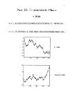
PART I: Fractals Around Us
How Long Is the Coast of Britain?
Figure 1: How to find the lenght L of the coast between A and B?
Approximations of Britain
Polygonal approximation of the
coast of Britain.
Compass Setting	Length
500 km	2600 km
100 km	3800 km
54 km	5770 km
17 km	8640 km
2
L°Sio (Total Length in Kilometers)
Figure 4.32 : Count all boxes that intersect (or even touch) the coastline of Great Britain, including Ireland.
Box-Counting	As an example let us reconsider the classic example, the coastline of
Dimension of the Great Britain. Figure 4.32 shows an outline of the coast with two underlying
Coast of Great Britain grids. Having normalized the width of the entire grid to 1 unit, the mesh
sizes are 1/24 and 1/32. The box-count yields 194 and 283 boxes that
intersect the coastline in the corresponding grids (check this carefully, if
you have the time). From these data it is now easy to derive the box-
counting dimension. When entering the data into a log/log-diagram, the
slope of the line that connects the two points is
_ log 283 - log 194 ~ 2.45 - 2.29 _
log 32 - log 24 ~ 1.51 - 1.38 “ L3 '
This is in nice agreement with our previous result from the compass dimen-
sion.
4
Figure 6. (a) The coast ofNorway. Note the fractal, hierarchical
geometry, with fjords, and fjords within fjords, and so on. Mandelbrot
has pointed out that landscapes often are fractals. (From Feder, 1988.)
Figure 6. Continued (b) The length L of tha coast measured by cover-
ing the coast with boxes, like the ones shown in (a), of various lengths S.
The straight line indicates that the coast is fractal. The slope of the line
yields the fractal dimension" of the coast of Norway. D— 1.52.
5
River’s Basin
The Amazon.
6
Diameter Distribution of Craters and Asteroids
Diameter distribution of craters on the Moon
7
The distribution of meteorite mass follows a power law with
D = 2.3 for meteorites larger than 100 kg. Most smaller meteorites
are burnt up by friction with the atmosphere and those arriving
on Earth fail to follow the power law.
The size distribution of asteroids is also known to be goverened
by a fractal distribution of estimated dimension D = 2.1.
In the study of brittle fracture the distribution of splinters is
known to follow a power law. For example, when a rock is shattered
with a gun, the distribution of splinter size is a power law with
D~2.
Metabolic Rate
Metabolic Rate As Power
Law
The reduction law of metabolism,
demonstrated in logarithmic coordi-
nates, showing basal metabolic rate
as a power function of body mass.
Q oc A/0'75 ex L2-25
8
Distribution of Blood Vessels
Figure 2: Diameter distribution of blood vessels in a bat’s wing.
9
Zipf’s Law
Figure 3: Frequency of words (X) and the order (N) in log-log plot.
10
Figure 8. (a) Ranking of cities by size around the year 1920 (Zipf,
1949). The curve shows the number of cities in which the population
exceeds a given size or, equivalently, the relative ranking of cities versus
their population.
Figure 8. Continued (b) Ranking of words in the English language.
The curve shows how many words appear with more than a given fre-
quency.
11
Gutenberg-Richter Law
Figure 2. (a) Distribution of earthquake magnitudes in the New
Madrid zone in the southeastern United States during the period
1974—1983. collected by Arch Johnston and Susan Nava of
Memphis State University. Ths points show the number of earthquakes
with magnitude larger than a given magnitude m. The straight line indi-
cates a power law distribution of earthquakes. This simple law is known
as the Gutenberg—Richter law. (b) Locations of the earthquakes used in
the plot The size of the dots represent the magnitudes of the earthquakes.
12
Discharge Patterns
Fig. 8.1. Discharge pattern in a block of polymethyl-methacrylate (PMMA). The material
is charged with 2 MeV electron beam and subsequently discharged through a point contact.
The sample was prepared by A. Miller
FIG. 1. Time-integrated photograph of a surface
leader discharge (Lichtenberg Figure) on a 2-mm glass
plate in 0.3-MPa SF^. Applied voltage pulse: 30 kV x 1
/is (Ref. 5). This experiment corresponds to an equipo-
tential channel system growing in a plane with radial elec-
trode.
13
The Lightning
Experimental set up for the study of Lichtenberg figures
14
Mass Dimension
7И(г) ос rD
Counting the number of points within a sphere of radius
15
Electrochemical Deposition
In the Petri-dish a solution of zinc sulfate Is covered by a thin
layer of n-butyl-acetate.
Sample Result
This dendritic growth pattern was
produced in only about 15 minutes
by Peter Plath, University of Bre-
men. The reproduction here is in
about the original size. The real
zinc dendrite looks very attractive
due to its metallic shiny character.
16
Diffusion-limited aggregation.
Figure 10.14. Representative picture of a forest of einc metal
trees deposited along a linear carbon cathode. The actual size of
this part of the sample is about 6cm (Matsushita et al 1985).
17
Simulation of the
Electrochemical Aggregation
Experiment
Simulation of Brownian motion in
two dimensions is used for the paths
of the zinc ions in the liquid. Par-
ticles move from pixel to pixel un-
til they ‘attach’ to the existing den-
drite.
N oc R1-7
Simulation Results
Result of the numerical simulation
of DLA based on Browman motion
of single particles.
18
Viscous Fingers
Viscous Fingering
If a less-viscous fluid is injected slowly into a more viscous fluid, then
the less-viscous fluid will tend to penetrate the other fluid, forming
long thin “fingers,” often with branches developing out from the fin-
gers. A typical viscous fingering pattern is shown in Fig. 11.19.
The physical processes underlying viscous fingering are important
in several applied areas. For example, water is often injected into oil
(petroleum) fields to enhance the recovery of oil by using the water
pressure to force the oil to flow toward a well site. However, the
recovery attempt may be frustrated by the tendency of the less-viscous
water to form viscous fingers through the oil. See WON88 for a wider
discussion of applications of viscous fingering.
11.19. On the left is a sketch of a Hole—Shaw cell used in the study of viscous
fingering. A thin layer of viscous fluid lies between two flat plates. A less-viscous
fluid is slowly injected through a small hole in the center of the cell. On the right is
a typical viscous fingering pattern for water and glycerin. (From WON88.)
19
(b)
FIG. 1. (a) Schematic illustration of the lateral and radial
cells, (b) typical radial viscous finger, and (c) analysis of the
fractal dimension by method (i).
N ос Г1-7
20
Romanesco
The new bread romanesco, a crossing between cauliflower and
broccoli, exhibits striking self-similarity:
21
Brownian Motion^
grid size 3.2 /1
22
Self-similarity of the Brownian Trace
Trace of Brownian Motion in
the Plane
Shown is the trace of the Brown-
ian motion of a particle. The boxed
detail of the trace (magnified in the
upper left portion of the figure) sug-
gests an invariance of scale or self-
similarity: the detail looks like the
whole.
N<xR2
23
Coordinate of a Brownian Particle
24
Turbulence
25
Turbulence. Shapes of Clouds
Figure 2.13 Area (S) and perimeter length (L) of clouds [26].
S oc L2/p,
D - 1.35
26
Saturn Ring System
27
Distribution of galaxies in the sky
TV oc Rd = 7?1-23
TV ос В? for homogeneous distribution
28
Second Order Phase Transitions
29
Percolation Ciasters
30
Fractal Dimension of the
Incipient Percolation Cluster
The fractal dimension D of the in-
cipient percolation cluster in a tri-
angular lattice is determined here
in a log-log diagram of the cluster
size M(L) versus the grid size L.
The percolation threshold is pc =
0.5. The slope of the approximating
line confirms the theoretical value
D = 91/48. (Figure adapted from
D. Stauffer, Introduction to Per-
colation Theory, Taylor & Francis,
1985.)
31
Three Body Problem
Typical orbit in a three body problem of celestial mechanics.
The upper part shows the beginning, the lower part the sequel of
the chaotic motion of a small planet around two suns of equal mass.
32
Chaos in Dissipative Systems
Lorenz Attractor
X = (j{y — x)
у = px — у — xz
z = xy — flz
(J = 10, p = 28, /3 = 8/3, ж(0) = 3/(0) = г(0) = 1
33
Ueda Attractor
4
2
0
-2
-4
0.5 1.0	1.5	2.0	2.5 3.0
x + 0.05ж + ж3 =4.1 cos(0.7t)
34
Henon Attractor
^n+l
= 1 - ax% + yn
Уп+i — bxn
(6 = o.3, a = 1.4)
Figure 4: The Henon attractor for 104 iterations. Some successive iterates have been
numbered to illustrate their erratic movement on the attractor, b), c) Enlargements of
the squares in the preceding figure, d) The height of each bar is the relative probability
to find a point in one of the six leaves ib c).
35
Basin Boundaries
The Pendulum Setup
The metal ball of the pendulum
swings over three magnets.
pendulum
magnet
Basins of Attraction
Basins of attraction for the pen-
dulum over three magnets. For
each of the three magnets, one of
the above figures shows the basin
shaded in black. The fourth pic-
ture displays the borders between
the three basins. This border is not a
simple line; but within itself it has
a Cantor-like structure, as the en-
largement in figures 12.79 and 12.80
show (see also the color plates 27
and 28).
36
37
Blowup of Basin Boundaries
This enlargement of a portion of fig-
ure 12.75 reveals the Cantor-set like
structure of the boundaries of the
basins of attraction in the pendulum
experiment.
38
Haos in Hamiltonian Systems
The Chirikov Standard Map
Уп+i = Уп~^ sin(27ra?n)
Уп-\-1
Figure 5: Islands around islands for the standard map at к = 1.20141333. The bottom-
right figure has the bounds [-0.5,0.5] for x and [0,0.6] for y.
39
The Web Map
Fig. 3.5.1. Self-similar structure of islands for the web map with К = 6.349972: (a)
the phase space with islands of the accelerator mode; (b) magnification of the bottom
right part of (a); (c) magnification of the top right island of (b); and (d) magnification
of the bottom left island of (c).
(d)
^n+1 — Vn
Vn+1 = -un- К sin vn
40
Wave Functions in Disordered Systems
Figure 6: Local density IV’(r) |2 of an eigenstate at the center of the lowest Landau level
of a lattice system with 150 x 150 sites
41
Fractal Dimension
Vl.4.2 FRACTAL DIMENSIONS
Consider a set of points in a p-dimensional space. We seek to cover this set by
(hyper) cubes of linear dimension s. Let N (e) be the smallest number of cubes necessary
to accomplish this (see fig. VI.33). The Hausdorff (also called Hausdorff-Besicovitch)
dimension D is defined to be the limit, if it exists, of the ratio In N(e)/ln (1/e) as the
length e of the hypercubes tends to zero. That is:
„ r lnN(s)
D = lim------—
»-»o In (1/s)
Figure VI.33 Illustration of the covering of an object (a set of points) by cubes of
linear dimension s.
N(e) <x jg
О
42
Figure VI.36 Illustration of the method
of calculating the fractal dimension of a
set of points located in a two-dimensional
space.
We draw a circle (a sphere or hypersphere
in higher dimensional cases) of radius r,
centered about an arbitrary point of the
set We then determine the number of
points N(r) located inside the circle and its
dependence on r.
a) general case 7V(r) ~ r*
Л) line (dimension one) N(r) ~ r1
c) surface (dimension two) N(r) ~ r2
d) Cantor set N(r) ~ r0-63.
43
The Similarity Dimension
1-0	N	parts, scaled by	ratio r = 1 /N N r1 = 1
2-D	N	parts, scaled by	ratio r = 1/N1/2 N r2 = 1
3-0	N	parts, scaled by	ratio r = 1/N1/3 N r3 = 1
GENERALIZE
for an object of N parts, each scaled down
by a ratio r from the whole
N r D = 1
defines the fractal (similarity) dimension D
n _ log N
r
log 1/
44
Fractal Dimension of the Cantor Dust.
N«1
N«2
N«4
n	E	Me)
0	1	1
1	1/3	2
2	1/9	4
• • •	. . .	• • •
n	1/3"	2n
In N(e) In 2™
ln(l/g) In 377
In 2
ln3
= 0.6309...
45
6.4.3 A curious property of the Cantor set
The Lebesgue measure of the Cantor set is 0 but it contains uncountably
many points. Thus the Cantor set has the following curious property. Let
X] and x2 be points in a Cantor set. It has been proved that the distance
between the two points, Ixi — x2l, can take any value from 0 to 1 if we
choose suitable xt and x2 [105]. In 2-dimensional space, this implies that a
set (E x [0,1] U ([0,1] x E) contains any rectangle whose sides have
length less than 1. Thus it is possible to find any size of rectangles in
Figure 6.6.
A strange Cantor mesh. There are rectangles of every size.
46
Cantor Curtains
47
Devil’s Staircase
48
Devil’s Staircase:
Construction
The column construction of the
devil’s staircase.
The Complete Devil’s
Staircase
Self-Affinity
49
The Koch Curve
Koch Curve Construction
The construction of the Koch curve
proceeds in stages. In each stage the
number of line segments increases
by a factor of 4.
n	e	W(e)
0	1	1
1	1/3	4
2	1/9	16
• • •		• • •
n	1/3"	
InTV(e) ln4n
ln(l/e) ln3n
In 4
ln3
= 1.2618...
50
The Length of the Koch Curve
1	ln(l/e)
e = —, hence n = —;----------
3"’	ln3
n = enln4 = Д$>1п4 = е!ЙМ1Л) = e
1\л
Triadic Koch Island or Snowflake
Figure 7: Infinite perimeter but finite area.
51
A Quadric Koch Island
52
Generalized Koch Curves.
Self-Similarity With Unequal Parts
(D - 1.4490, D ~ 1.8797.)
= 1
i—< m
m
53
Sierpinski Gasket
54
Sierpinskii Arrowhead
Figure 8: Initiator and generator.
Figure 9: 2 and 3 steps.
Figure 10: Next two steps.
In3
In 2
= 1.5849...
55
Pascal Triangle
Pascal’s Triangle
The first eight rows of Pascal’s tri-
angle in a hexagonal web.
Color Coding
Color coding of even (white) and
odd (black) entries in the Pascal tri-
angle with eight rows.
Blaise Pascal, 1623-1662
(d И- — a? 2(16 4~ 62
(a 4- 6)3 = a3 4- 3a26 4- 3a62 4- 63
(a 4- 6)4 = a4 4- 4a36 4- 6a262 4- 4a63 4- 64
(a 4- 6)5 = a5 4- 5a46 4- 10a362 4- 10a263 4- 5a64 4- 65
56
Color coding, of even and odd entries in the Pascal triangle with 16, 32, and 64 rows.
57
Color coding the Pascal triangle. Black cells denote divisibility by 3 (top left), by 5 (top right)
and by 9 (bottom).
58
The Hexagonal Gasket
Figure 11: Durer pentagon (Albrecht Durer 1471-1528).
59
Sierpinski Carpet
60
The Menger Sponge
In 20
ln3
2.7268...
61
A Sierpinski Tetrahedron
62
Peano Curves
Peano Curve Construction
Construction of a plane filling curve
with initiator and generator. In each
step one line segment is replaced by
9 line segments scaled down by a
factor of 3. For reasons of clarity
the comers in these polygonal lines,
where the curve may intersect itself,
have been slightly rounded.
63
Hilbert Space Filling Curve
64
Gosper Island (TV = 7, r = l/\/7)
Figure 12: Algorithm for Gosper curve.
Figure 13: Next 3 steps.
Figure 14: Fractal boundary of Gosper island.
65
Gosper Island’s Boundary
N=3
l/r=/7
D=dog3/log (/7)~1.1291
66
Plane Tiling with Gosper Islands
67
The Harter-Heightway Dragon
Figure 15: Initiator and generator for Harter-Heightway dragon.
Figure 16: 12 and 16 generations.
68
Twindragon
A twindragon can be tiled by reduced size replicas of itself
D-1.5236
Twindragon Skin
69
Cesaro’s Triangle Sweep (0 = 85°).
70
Fournier Universe
N(R2) = 77V(/?!)
if
лг(л) <x rd
then
In 7
ln(7?2/-Ri)
2.3 Space science
2.3.1 Distribution of mass
Stars are not uniformly distributed in the universe - they form galaxies
and the galaxies form clusters. Mass in the universe seems to have a
tendency to cluster.
A cluster of galaxies may contain from one hundred to several
thousand galaxies. A typical diameter would be about 20 million light
years. It is known that clusters of galaxy tend to form super-clusters; and
there are some regions, which are called voids, of size several hundred
million light years where no galaxy exists.
The correlation function for galaxy distribution is found to follow a
power law. The fractal dimension of mass distribution estimated from
this power law is about 1.2 [1, 9]. This value is much smaller than 3. the
dimension of the space. No theory has yet succeeded in explaining this
value.
71
The Korcak Empirical Law
List all the islands of a region, or of the whole Earth, by de-
creasing size. The total number of islands of size above a is to be
written as Nr (A > a). В and F' being two positive constants,
to be called exponent and prefactor, the following striking and
elementary area-number relation is given in Korcak 1938
Nr(A > a) = F'a~B
N=16
r=l/8
D=4/3
72

Fractal Trees
73
\
74
Dry Earth and Leaf
75
San Francisco
»>tH
 Г- Й»*л
owh
•-< - „ -

76
Viscous Fingers
Viscous Fingering
If a less-viscous fluid is injected slowly into a more viscous fluid, then
the less-viscous fluid will tend to penetrate the other fluid, forming
long thin “fingers,” often with branches developing out from the fin-
gers. A typical viscous fingering pattern is shown in Fig. 11.19.
The physical processes underlying viscous fingering are important
in several applied areas. For example, water is often injected into oil
(petroleum) fields to enhance the recovery of oil by using the water
pressure to force the oil to flow toward a well site. However, the
recovery attempt may be frustrated by the tendency of the less-viscous
water to form viscous fingers through the oil. See WON88 for a wider
discussion of applications of viscous fingering.
11.19. On the left is a sketch of a Hole—Shaw cell used in the study of viscous
fingering. A thin layer of viscous fluid lies between two flat plates. A less-viscous
fluid is slowly injected through a small hole in the center of the cell. On the right is
a typical viscous fingering pattern for water and glycerin. (From WON88.)
19