/


Author: Ashcroft Neil W.(Neil W. Ashcroft) Mermin N. David
Tags: physics
ISBN: 0-03-083993-9
Year: 1976


Text
, ASHCROFT MERMIN
" .
'"
,
I
SOLID STATE P CS
- -
a ;:; - S
. w -, w a w . - u . w - .
fj < ! < '" <
- < '" D '" JJ < '" '" i;;' n r: I ;:
::' n n C- n '" n n x - .
£! n 2.: n n n -
- - - -
i; - -
a 8 iii 8 .. "
" :Ii - . !:: .. . :: > w a -
" . ii 5 ; - >
w N .
- - a
f '" " .. - .. i ! - N
n g> n !(' " n r " g> »
n It n n t x x w
w w W
, -
g: .' . :;: ,. a :'! , ;: . "
iji w
w - w . N .
f ! L
.. F -
n 0. < 0. :; -< 0. g> W c:;
n X X 0. X '" 0,
It t 3.
..- w w & ..- 3:<
» . -;, o_
n » '"' g: N . :;: ,
.... z f.j n3
....
Z :I: & "'.. -.... <"
» - J. nnn ,," I !1
z ! .... nn -I
j c > - I I I I
== <::' ::! " .. "'..
x X 0. - X Q '" n z
S If: - Iii t r t ;" 7
;j < ,. ::: "
:I> u i - <
» . .. E .. .
q "';" a ;;; . - w N .
> ! nn ()
:] .. .. m '" c '" " '" c '" g. - ! 2'
-1 n -I n Q » n E ;} < n 2 n < < '" ir n "'
n Q ;r n :I> n n C- n x
.... 0. , \ 1
;: 0:1:0
J Ii! 8 g: is tj n -m:l> n a; ;:
. . - - ..- »xn ,.
e < I I I I 1 1 \ I
d f c fi . . .. 0 ij . if "U
,- a ! i f "
-J , " ! 0:-
j 0 '" z '" s: a '" - '"
:1 ;;? :1' n { n z n !;' < '" g :I> 3 3
x 0 0 0 c n , i n' n
,- 0. < n' -iJ. 0' z
- "!:.. It n 0 I
w :i: .
- a ;I I:; . a \I 8 .... t"
!! . . 8 b . :: .. I .-
. f w w r ! . g"
z > "
0 " 2 :J: 0 :I>
:I> C m C Q '"
n X 0- X X '" :J:
Q ..-
- l -<
w ::: E g . U\ 8 [)I t
- w ---'
I
w .. . f) .. c ii 0 ' ::!
f " a; z
- ! 0"
0 2 1. ." S? JJ C '" ;r .
:I> " n
n "C 3 X X 0. " < n I ..
a [OJ :I>
? : . U\ a t e :;: 0' 0'
. i: a "
f . iJ 6 .. 0 .
0 0 !:
n
;: :I> '" C .. .. JJ (') ;;
> i!: 3 < 0 n 0. ;r 0. 0
% % 0 " X .
'" It a f, 1
'<Ii :; a ::j I!; t::
. . 8 .
c
» '" m ,
3 , n "
0
:!i " . e
8 - i
, :
(') C>
3 X [ 0-
o. It
w :Ii . " Iii Ii: :
0
-
'" -I
Q "" X C-
;
- g: '.
f 0
s: "5 0
.. , X -< ,
'" ,
:i: " " g:
.., ;
w " " :
- I
X 0
.,'
:g L . 0
" ;
:
3 X
8 g:
0
. - ..
s: -I ,
0- X 3
{
0 0 :::
.
w
2 : .. " -<
0 n ,
n C-
-,
" " "
. - .
,
.- - .-
, X "
a ,:
w S w CO
* . .. S b .' w . E
"
.. u
.. l ." ?
n Jl n Q < g
n n 0-
5
0 0: c 0
ii ;; " " .
" !
L
.. » .. .. Q (') ;;;
n n n "
0 " n n
a ;;: - !:: Ii! .'
< ii c l-
. . 0 c w ii ! .
w <
:I> l J' (') : w N N
i!: X 0. 0- X 0. " '"
c- " - ,
8 I); a Ii :: - Ii :;
w X = 9 a . 0
w 0
! 0
E 0. 0 .. .. W
Q ::! " :I> g> n !:: '" »
X .... n n ....
:Ii i > . i'i
- '- a W -
x = a . i: F .
- .. w - ! i:J
0 - w ! .
a
.. Q Q Z
." .... go 0 c 0 0 ..
g C- m ;; i ;; ;; (') »
....
g: a :!: a ::: a -
. X : :;: L . - X Z
- - W ;
, w ! i
:I> ! .. :I> .. F :J: '1"
:I> '" " l: n " '"
i!: i!: i!: i :i m 2
C- ." X »
" " .
8 0
a " e . 0 ;; ::: .. ! w
x . !! \:
w . ! . w
! c c,
.. . - . n
'" ." : ;1 0. W < 0 '"
0 : :I> '" 0 »
0 X X 0
i ! I - ;;
- ..
II: 0 , ;;; : . m
x t .
t ! " '"
! " c,
i - 0 .. 0 "- 0 ;:
:I> - :I> i :I> Q
" 0 n »
"
g: !: t: ,; k
.. ;;; , .
- - ! - w w 0 .
w , ! g
- -
.. JJ .. .. 0. < .. ..
n g " 1:' n i ;:' n 0 Eo ;:, if
£! " n n n 0 I X
0 .
8i . Ii: >, - !<: g: ;;; e ;; . N
m
..-
mZ
;:0
m'"
z"-
;;jm
. ; .j7:: '.::""....:;"'f"' .. ...:f:> =..,. \.!. -'r.
=""-'" '"If'
I
.
Fs. .;: 1S
Harcourt
College Publishers
A Harcourt Higher Learning Company
Now you will find Saunders College
Publishing's distinguished innovation,
leadership, and support under a different
name. . . a new brand that continues our
unsurpassed quality, service, and
commitment to education.
-,
!
!
We are combining the strengths of our
college imprints into one worldwide
brand: m1Harcourt
Our mission is to make learning
accessible to anyone, anywhere,
anytime-reinforcing our commitment
to lifelong learning.
We are now Harcourt College Publishers.
Ask for us by name. r
J1r\lher2 '...earrd:1
(om(!S to LifE."
i\HN\'1f.: a arc;:; . !0$(K:clle 2.com
Yolid State
Physics
Neil w. Ashcroft
N. David M ermin
Cornell University
Saunders College Publishing
Harcourt College Publishers
Fort Worth Philadelphia San Diego
New York Orlando Austin San Antonio
Toronto Montreal London Sydney Tokyo
f 'SH
Copyright @ 1976 by Harcourt, Inc.
All rights reserved. No part ofthis publication may be
reproduced or transmitted in any fonn or by any means,
electronic or mechanical, including photocopy, recording, or
any infonnation storage and retrieval system, without pennission
in writing from the publisher.
Requests for pennission to make copies of any part of the work
should be mailed to: Pennissions Department, Harcourt, Inc.,
6277 Sea Harbor Drive, Orlando, FL 32887-6777.
This book was set in Times Roman
Designer: Scott Chelius
Editor: Dorothy Garbose Crane
Drawings: Eric G. Hieber Associates, Inc.
Library of Congress Cataloging in Publication Data
Ashcroft, Neil W
Solid state physics.
\. Solids. I. Mermin, N. David, joint author.
II. Title.
QC176.A83 530.4'1 74-9772
ISBN 0-03-083993-9 (College Edition)
Printed in the United States of America
SOLID STATE PHYSICS
ISBN # 0-03-083993-9 (College Edition)
o 1 2 3 4 5 6 7 8 9 076 35 34 33 32 31 3029 28 27
I \) \
\ J J....
for Elizabeth, Jonathan, Robert, and Ian
Pleface
We began this project in 1968 to fill a gap we each felt acutely after several
years of teaching introductory solid state physics to Cornell students of physics,
chemistry, engineering, and materials science. In both undergraduate and graduate
courses we had to resort to a patchwork array of reading assignments, assembled
from some half dozen texts and treatises. This was only partly because of the great
diversity of the subject; the main problem lay in its dual nature. On the one hand an
introduction to solid state physics must describe in some detail the vast range of real
solids, with an emphasis on representative data and illustrative examples. On the
other hand there is now a well-established basic theory of solids, with which any
seriously interested student must become familiar.
Rather to our surprise, it has taken us seven years to produce what we needed: a
single introductory text presenting both aspects of the subject, descriptive and ana-
lytical, Our aim has been to explore the variety of phenomena associated with the
major forms of crystalline matter, while laying the foundation for a working under-
standing of solids through clear, detailed, and elementary treatments of fundamental
theoretical concepts,
Our book is designed for introductory courses at either the undergraduate or
graduate level. 1 Statistical mechanics and the quantum theory lie at the heart of solid
state physics. Although these subjects are used as needed, we have tried, especially in
the more elementary chapters, to recognize that many readers, particularly under-
graduates, will not yet have acquired expertise. When it is natural to do so, we have
clearly separated topics based entirely on classical methods from those demanding a
quantum treatment. In the latter case, and in applications of statistical mechanics, we
have proceeded carefully from explicitly stated first principles, The book is therefore
suitable for an introductory course taken concurrently with first courses in quantum
theory and statistical mechanics. Only in the more advanced chapters and appendices
do we assume a more experienced readership.
The problems that follow each chapter are tied rather closely to the text, and are of
three general kinds: (a) routine steps in analytical development are sometimes
relegated to problems, partly to avoid burdening the text with formulas of no intrinsic
interest, but, more importantly, because such steps are better understood if completed
by the reader with the aid of hints and suggestions; (b) extensions of the chapter
(which the spectre of a two volume work prevented us from including) are presented
as problems when they lend themselves to this type of exposition; (c) further numerical
and analytical applications are given as problems, either to communicate additional
I Suggestions for how to use the text in courses of varying length and level are given on pp, xviii-xxi,
vii
"Hi Preface
information or to exercise newly acquired skills. Readers should therefore examine
the problems. even if they do not intend to attempt their solution,
Although we have respected the adage that one picture is worth a thousand words.
we are also aware that an uninformative illustration, though decorative, takes up the
space that could usefully be filled by several hundred. The reader will thus encounter
stretches of expository prose unrelieved by figures, when none are necessary, as well as
sections that can profitably be perused entirely by looking at the figures and their
captions,
We anticipate use of the book at different levels with different areas of major
emphasis. A particular course is unlikely to follow the chapters (or even selected
chapters) in the order in which they are presented here, and we have written them in a
way that permits easy selection and rearrangement. 2 Our particular choice of sequence
follows certain major strands of the subject from their first elementary exposition to
their more advanced aspects, with a minimum of digression.
We begin the book 3 with the elementary classical [I] and quantum [2] aspects of
the free electron theory of metals because this requires a minimum of background and
immediately introduces, through a particular class of examples, almost all of the
phenomena with which theories of insulators. semiconductors. and metals must come
to grips. The reader is thereby spared the impression that nothing can be understood
until a host of arcane definitions (relating to periodic structures) and elaborate
quantum mechanical explorations (of periodic systems) have been mastered,
Periodic structures are introduced only after a survey [3] of those metallic prop-
erties that can and cannot be understood without investigating the consequences
of periodicity. We have tried to alleviate the tedium induced by a first exposure
to the language of periodic systems by (a) separating the very importan conse-
quences of purely translational symmetry [4. 5] from the remaining but rather less
essential rotational aspects [7], (b) separating the description in ordinary space [4]
from that in the less familiar reciprocal space [5], and (c) separating the abstract
and descriptive treatment of periodicity from its elementary application to X-ray
diffraction [6].
Armed with the terminology of periodic systems, readers can pursue to whatever
point seems appropriate the resolution of the difficulties in the free electron model of
metals or. alternatively, can embark directly upon the investigation of lattice vibra-
tions. The book follows the first line. Bloch's theorem is described and its implications
examined [8] in general terms, to emphasize that its consequences transcend the
illustrative and very important practical cases of nearly free electrons [9] and tight
binding [I 0]. Much ofthe content ofthese two chapters is suitable for a more advanced
course, as is the following survey of methods used to compute real band structures
[II]. The remarkable subject of semiclassical mechanics is introduced and given
elementary applications [12] before being incorporated into the more elaborate semi-
classical theory of transport [13]. The description of methods by which Fermi surfaces
are measured [14] may be more suitable for advanced readers, but much of the survey
2 The Table on pp, xix-xxi lists the prerequisites for each chapter, to aid those interested primar-
ily in one aspect of the subject. or those preferring a different order of presentation,
3 References to chapter numbers are given in brackets,
Preface ix
of the band structures of actual metals [15] is readily incorporated into an elementary
course,
Except for the discussion of screening, an elementary course might also bypass the
essays on what is overlooked by the relaxation-time approximation [16] and by the
neglect of electron-electron interactions [17].
Work functions and other surface properties [18] can be taken up at any time
after the discussion of translational symmetry in real space. Our description of the
conventional classification of solids [19] has been separated from the analysis of
cohesive energies [20]. Both have been placed after the introduction to band structure,
because it is in terms of electronic structure that the categories are most clearly
distinguished,
To motivate the study of lattice vibrations (at whatever point after Chapter 5
readers choose to begin the subject) a summary [21] lists those solid properties that
cannot be understood without their consideration. Lattice dynamics is given an
elementary introduction, with the classical [22] and quantum [23] aspects of the
harmonic crystal treated separately, The ways in which phonon spectra are measured
[24], the consequences of anharmonicity [25], and the special problems associated
with phonons in metals [26] and ionic crystals [27] are surveyed at an elementary
level. though some parts of these last four chapters might well be reserved for a more
advanced course, None of the chapters on lattice vibrations rely on the use of normal
mode raising and lowering operators; these are described in several appendices for
readers wanting a more advanced treatment.
Homogeneous [28] and inhomogeneous [29] semiconductors can be examined at
any point after the introduction of Bloch's theorem and the elementary discussion of
semiclassical mechanics, Crystalline defects [30] can be studied as soon as crystals
themselves have been introduced, though parts of earlier chapters are occasionally
referred to,
Following a review of atomic magnetism, we examine how it is modified in a solid
environment [31], explore exchange and other magnetic interactions [32], and apply
the resulting models to magnetic ordering [33]. This brief introduction to magnetism
and the concluding essay on superconductivity [34] are largely self-contained. They
are placed at the end of the book so the phenomena can be viewed, not in terms of
abstract models but as striking properties of real solids,
To our dismay, we discovered that it is impossible at the end ofa seven year project,
labored upon not only at Cornell, but also during extended stays in Cambridge,
London, Rome, Wellington, and Jiilich, to recall all the occasions when students,
postdoctoral fellows, visitors, and colleagues gave us invaluable criticism, advice,
and instruction. Among others we are indebted to V, Ambegaokar, B. W. Batterman,
D. Beaglehole, R. Bowers, A. B. Bringer, C. di Castro, R. G. Chambers. G, V.
Chester, R, M. Cotts, R. A. Cowley, G. Eilenberger, D. B. Fitchen, C. Friedli,
V. Heine, R. L. Henderson, D. F. Holcomb, R. 0. Jones, B. D. Josephson, J. A,
Krumhansl, C. A. Kukkonen, D. C. Langreth, W, L. McLean, H. Mahr, B. W.
Maxfield, R. Monnier, L. G. Parratt, 0, Penrose, R, 0, Poh\. J. J. Quinn. J. J.
Rehr, M. V. Romerio, A. L. Ruoff, G, Russakoff, H. S. Sack, W. L. Schaich, J. R.
Schrieffer. J. W. Serene, A. J, Sievers, J, Silcox, R. H. Silsbee, J. P. Straley, D. M.
Straus, D. Stroud, K, Sturm, and J. W. Wilkins.
x Preface
One person, however, has influenced almost every chapter. Michael E. Fisher,
Horace White Professor of Chemistry, Physics, alld Mathematics, friend and neigh-
bor, gadfly and troubadour, began to read the manuscript six years ago and has
followed ever since. hard upon our tracks, through chapter, and, on occasion,
through revision and re-revision. pouncing on obscurities, condemning dishonesties,
decrying omissions, labeling axes, correcting misspellings, redrawing figures, and
often making our lives very much more difficult by his unrelenting insistence that we
could be more literate. accurate, intelligible, and thorough. We hope he will be
pleased at how many of his illegible red marginalia have found their way into our text,
and expect to be hearing from him about those that have not.
One of us (NDM) is most grateful to the Alfred p, Sloan Foundation and the
John Simon Guggenheim Foundation for their generous support at critical stages of
this project, and to friends at Imperial College London and the Istituto di Fisica
"G, Marconi," where parts of the book were written. He is also deeply indebted to
R, E, Peierls, whose lectures converted him to the view that solid state physics is a
discipline of beauty, clarity, and coherence, The other (NW A), having learnt the
subject from J. M. Ziman and A. B. Pippard, has never been in need of conversion,
He also wishes to acknowledge with gratitude the support and hospitality of the
Kernforschungsanlage Jiilich. the Victoria University of Wellington, and the
Cavendish Laboratory and Clare Hall. Cambridge.
Ithaca
June 1975
N. W, Ashcroft
N. D. Mermin
CrJntents
Preface vii
Important Tables xiv
Suggestions for Using the Book xviii
1. The Drude Theory of Metals 1
2. The Sommerfeld Theory of Metals 29
3. Failures of the Free Electron Model 57
4. CrY.'ital Lattices 63
5. The Reciprocal Lattice 85
6. Determination of Crystal Structures by X-Ray
Diffraction 95
7. Classification of BraJ'ais Lattices and Crystal
Structures 111
8. Electron Le.'els in a Periodic Potential:
General Properties 131
9. Electrolls in a Weak Periodic Potential 151
10. The Tight-Binding Method 175
11. Other Methods for Calculating Band
Structure 191
12. The Semiclassical Model of Electron
Dynamics 213
13. The Semiclassical Theory of Conduction in
Metals 243
14. Measuring the Fermi Surface 263
15. Band Structure of Selected Metals 283
16. Beyond the Relaxation-Time
Approximarion 313
17. Beyond the Independent Electron
Approximation 329
18. Surface Effects 353
xi
xii Contents
19. Classification of Solids 373
20. Cohesive Energy 395
21. Failures of the Static Lattice Model 415
22. Classical Theory of the Harmonic
Crystal 421
23. Quantum Theory of the Harmonic
Crystal 451
24. Measuring Phonon Dispersion
Relations 469
25. Anharmonic Effects in Crystals 487
26. Phonons in Metals 511
27. Dielectric Properties of Insulators 533
28. Homogeneous Semiconductors 561
29. Inhomogeneous Semiconductors 589
30. Defects in C,.ystals 615
31. Diamagnetism and Paramaglletism 643
32. Electron Interactions and Magnetic
Structure 671
33. Magnetic Orderillg 693
34. Superconductivity 725
APPENDICES
A. Summary of Importallt Numerical Relations ill
the Free Elect,.on Theory of Metals 757
B. The Chemical Potential 759
C. The Sommerfeld Expansioll 760
D. Plane-Wave Expansions of Periodic Functiolls
in More Than One Dimension 762
E. The Velocity and Effective Mass of Bloch
Electrons 765
F. Some Identities Related to Fourier Allalysis
of Periodic Systems 767
G. The Variational Principle for Schrodinger's
Equation 769
Contents xiii
H. Hami/tonian Formulation of the
Semiclassical Equations of lvlotion, and
Liom'i/le's Theorem 771
I. Green's Them'emfor Pe,.;odic
Functions 772
J. Conditions for the Absence of Interband
T,'ansitions in Uniform Electric or
Magnetic Fields 773
K. Optical Properties of Solids 776
L. Quantum Theory of the Harmonic
Crystal 780
M. Conse,'vation of Crystal Momentum 784
N, Theory of the Scatte,.;ng of Neutrons by a
Crystal 790
O. Anharmonic Terms and n-Phonon
Processes 796
P. Evaluation of the Lande g-Factor 797
INDEX 799
Important T ahle
The more important tables of data 1 or theoretical results are listed below.
To aid the reader in hunting down a particular table we have grouped them into
several broad categories. Theoretical results are listed only under that heading, and
data on magIietic and superconducting metals are listed under magnetism and super-
conductivity, rather than under metals. Accurate values ofthe fundamental constants
are given in the end paper and on page 757.
Theoretical Results
The noncubic crystallographic point groups 122
The cubic crystallographic point groups 121
Comparison of properties of Sommerfeld and Bloch
electrons 214
Comparison of the general treatment of collisions
with the relaxation-time approximation 318
Lattice sums of inverse nth powers for the cubic
Bravais lattices 400
Madelung constants for some cubic crystal structures 405
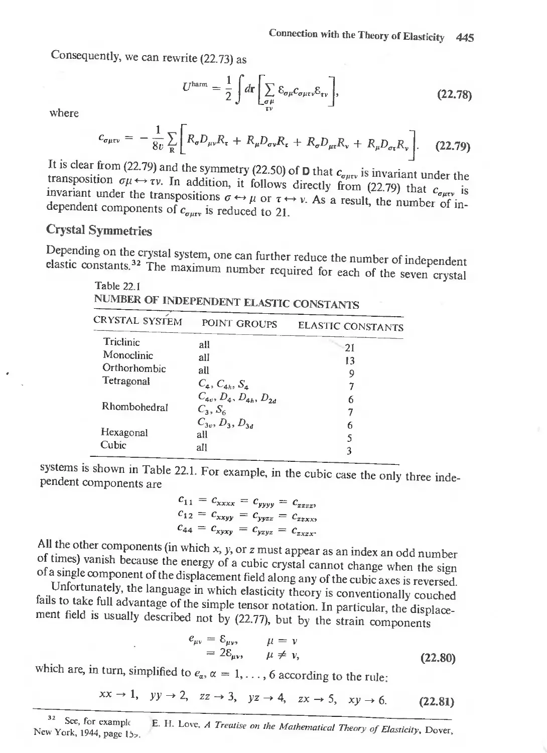
Numbers of independent elastic constants for the seven
crystal systems 445
Values of the Debye specific heat 461
Comparison of phonons and photons 466
Comparison of a gas of molecules and a gas of phonons 506
Characteristic lengths in a p-n junction 607
Ground states of ions with partially filled d- or
f-shells 652
Comparison of exact and mean field critical temperatures
for several Ising models 717
Major numerical formulas of free electron theory 757
I The data in the tables are presented with the aim of giving the reader an appreciation for orders of
magnitude and relative sizes, We have therefore been content to quote numbers to one or two significant
places and have not made special efforts to give the most precise values, Readers requiring data for funda-
mental research should consult the appropriate sources,
xiv
Crystal Structure
The face-centered cubic elements 70
The body-centered cubic elements 70
The trigonal (rhombohedral) elements 127
The tetragonal elements 127
The hexagonal close-packed elements 77
Elements with the diamond structure 76
Some compounds with the sodium chloride structure 80
Some compounds with the cesium chloride structure 81
Some compounds with the zincblende structure 81
Metals
Free electron densities and rs/ao 5
Electrical resistivities 1\
Some typical relaxation times 10
Thermal conductivities 21
Fermi energies, temperatures, wave vectors, and
velocities 38
Bulk moduli 39
Low temperature specific heats 48
Work functions 364
Elastic cOnstants 447
Debye temperatures 461
Linear expansion coefficients 496
InslilatOl's and Semiconductors
Alkali halide ionic radii 384
Ionic radii of II - VI compounds 386
Lattice constants of some III - V compounds 389
Important Tables xv
x\'i Important Tables
Radii of metallic ions compared with nearest-neighbor
distances in the metal 391
Cohesive energies of the alkali halides 406
Bulk moduli of the alkali halides 408
Debye temperatures of some alkali halides 459
Griineisen parameters and linear expansion coefficients
for some alkali halides 494
Atomic polarizabilities of the noble gas atoms and
the alkali halide ions 544
Static and optical dielectric constants and transverse
optical phonon frequencies of the alkali halides 553
Lennard-Jones parameters for the noble gases 398
Lattice constants, cohesive energies, and bulk moduli
of the solid noble gases 401
De Boer parameters for the noble gases 412
Elastic constants 447
Debye temperatures 459,461
Static dielectric constants for covalent and
covalent-ionic crystals 553
Ferroelectric crystals 557
Energy gaps of semiconductors 566
Impurity levels in silicon and germanium 580
Magnetism
Molar susceptibilities of the noble gas atoms and alkali
halide ions 649
Effective Bohr magneton numbers for the rare earth
ions 657
Effective Bohr magnet on numbers for the iron group
ions 658
Pauli susceptibilities of the alkali metals 664
Some dilute alloys with (and without) local moments 686
Critical temperatures and saturation magnetizations
of ferromagnets 697
Critical temperatures and saturation magnetizations
of ferrimagnets 698
Critical temperatures of antiferromagnets 697
Superconductivity
The superconducting elements 726
Critical temperatures and critical fields of the
superconducting elements 729
Energy gaps of selected superconducting elements 745
Specific heat discontinuities of selected superconducting
elements 747
Important Tables x\'ii
Suggestions fur
Using the Book
It is in the nature of books that chapters must be linearly ordered. We
have tried to select a sequence that least obscures several interwoven lines of develop-
ment. The accompanying Table (pp. xix-xxi) is designed to help readers with
special interests (in lattice vibrations, semiconductors, or metals, for example) or
teachers of courses with particular constraints on time or level.
The prerequisites for each chapter are given in the Table according to the following
conventions: (a) If"M" is listed after Chapter N, then the contents of Chapter M (as
well, of course, as its essential prerequisites) are essential for understanding much or
all of Chapter N; (b) If "(M)" appears after Chapter N, then Chapter M is not an
essential prerequisite: either a small part of Chapter N is based on Chapter M, or a
few parts of Chapter M may be of some help in reading Chapter N; (c) The absence of
"M" or "(M)" after Chapter N does not mean that no reference back to Chapter M
is made; however, such references as may occur are primarily because N illuminates
the subject of M, rather than because M aids in the development of N.l
The rest of the Table indicates how the book might be used in a one semester
(40 to 50 lectures) or two-semester (80 to 100 lectures) introductory undergraduate
course, Chapters (or selections from a chapter) are listed for reading 2 if they are
almost entirely descriptive, or, alternatively, if we felt that an introductory course
should at least make students aware of a topic. even if time was not available for its
careful exploration, The order of presentation is, of course, flexible, For example,
although a two-semester course could follow the order of the book, one might well
prefer to follow the pattern of the one-semester course for the first term, filling in the
more advanced topics in the second.
An introductory course at the graduate level. or a graduate course following a one-
semester undergraduate survey, would probably make use of sections omitted in the
two-semester undergraduate course, as well as many of the sixteen appendices.
I Thus to proceed to Chapler 12 with a mmimum of digression it is necessary to read Chapters 8. 5, 4,
2. and I
2 Students would presumably be asked to read the chapters bearing on the lectures as well,
X\jjj
I::
.... C
.., "-
....
i::
t:
.:;
I::
.... C
.., "-
....
i::
I C
.!
..,
....
:
s
'=="
....
e
d
Z
25
.(
c.:
<11
c.:
;J
E-<
U
....:I
d
Z
25
.(
c.:
<11
c.:
;J
E-<
U
....:I
:;;;:
:;;;:
cu
s:::
o
Z
cu
"0
o
:;;;:
:;;;:
"0
....
cu
E
E
o
tJ')
N
:;;;:
:;;;:
N
s:::
o
b
u
cu
cu
cu
<t:
'-
o
'"
cu
....-
.2
"- 0
E
..,.;
:;;;:
:;;;:
:;;;:
cu
N
';::
E
E
tJ')
'<t
C
:;;;: I
I
cu
s:::
o
Z
'<t
'"
cu
.
]
]
'"
»
....
U
, I ,g
u
I '"
]
....
,3' I
I
vi I",
i
-.i-
:;;;:
V)
I:;;;:
I
:;;;:
<">
'<t
I
<">
I
I
I
'<t V)
'"
cu
"5
Q)
E
E
»
en
en
»
....
U
'"
s:::
o
b
E u
cu cu
I
oS tt
I
co z
r-:
00 do
I
0\
00
-
I
'<t
00
'<t
00
-
:;;;:
I
'D
r--
,
I
'D
r--
-
'D'
'D ,
I
N
V)
-
,..,
,
00
€
00 00
cu
....
8
u
b
'"
"0
s:::
OJ)
s::: .D
:.a I OJ)
s::: ,5
15 "5
0.
..r: E
OJ) 0
E= u
c
:;;;:
<">
0\
I
N
0\
-
I
-
-
'D
'<t
N
I
N
<">
<">
N
I
'<t
N
I
N
I
'<t
N
00
N
N
-
'"
u
'8
s:::
»
"0
c;
u
";;;
'"
u
"8
cu
tJ')
pJ
....
o
0.
'"
s:::
b
c;
,S!
en
'"
u
'8
cu
tJ')
N
-
..,.;
-
xix
One-Semester Two-Semester
Chapter Prerequisites Introduction Introduction
LECTURES READING LECTURES READING
14, Measuring the Fermi surface 12 264-275 264-275
- -- - -
15. Band structure of metals 8 (2, 9, 10,
II, 12) All All
-- - -
16, Beyonc. relaxation-time
approximation 2 (13) All
- - - -
17. Beyond independent
electron approximation 2 337-342 330-344 345-351
i---- -- - -- - - - - - - - - -
18_ Surface effects 2, 4 (6, 8) 354- 364 354-364
- - - - - - -
19. Classification of solids 2, 4 (9, 10) All All
- --
20. Cohesive energy 19 (17) 396-410 All
- - - - - -I-
2L Failures of static lattice
model (2,4) All All
-- - --- -
22. Classical harmonic
crystal 5 422-437 All
- - - -
23. Quantum harmonic
crystal 22 452-464 All
- - - - -- - -
- - - - -
24. Measuring phonons 2,23 470-481
25. Anharmonic effects 23 499-505
- - - - - - -'-
26. Phonons in metals 17,23 (16) 523-526
- - -
27. Dielectnc properties 19,22 . 542
-
28. Homogeneous
semiconductors 2, 8, (12) 562-580
- - - -
29. Inhomogeneous
, semiconductors 28 590-600
l - - - -
[30. Defects 4 (8, 12, 19, I I
22, 28, 29) 628 -636 I
------ -
I 31. Diamagnetism,
I Paramagnetism (2,4, 14) 1 661 -665 1
- -- ,-- -
32. Magnetic interactions 31 (2,8, 10,
I 16,17) 672 682
i - - - 1
I 3 M agn:tic o ering 4,5,32 694- 700
- - - - 1- -
34_ Superconductivity I. 2 (26) I I 726- 736 I
I
- - - - - - - - - I
.
-AI
AI _ _ -+-
512-519
523-526
All
AI i
All
All
All
672-684
All
All
'1
The Drude Theory
of Metals
Basic Assumptions of the Model
Collision or Relaxation Times
DC Electrical Conductivity
Hall Effect and Magnetoresistance
AC Electrical Conductivity
Dielectric Function and Plasma Resonance
Thermal Conductivity
Thermoelectric Effects
2 ( hapler I The Drude TheoQ' of \1elal_
Metals occupy a rather special po ition in the stud of solids. sharing a \ ariepy of
striking properties that other solids (such as quartz. sulfur. or common salt) lack,
They are excellent conductors of heat and electricit . are ductile and malleable. and
display a striking luster on freshly exposed surfaces, The challenge of accounting for
these metallic features gave the starting impetus to the modern theory of solids,
Although the majority of commonly encountered solids are nonmetallic. metals
ha\ e continued to playa prominent role in the theory of solids from the late nineteenth
century to the present day. Indeed. the metallic statc has proved to be one of the great
fundamental states of matter. The elements. for example. definitely favor the metallic
state: over two thirds are metals, Even to understand nonmetals one must also
understand metals. for in explaining why copper conducts so welL onc begins to
learn why common salt does not.
During the last hundred years ph sicists ha\e tried to construct simple models of
the metallic state that account in a qualitative. and even quantitative, way for the
characteristic metallic properties, In the course of this search brilliant successes ha\'e
appeared hand in hand with apparently hopeless failures. time and again, E\'en the
earliest models, though strikingly wrong in some respects. remain. when properly
used. of immense value to solid state physicists today,
In this chapter we shall examine the theory of metallic conduction put forth by
p, Drude 1 at the turn of the century, The successes of the Drude model \\'ere con-
siderable. and it is still used today as a quid, practical way to form simple picture
and rough estimates of properties \\ hose more precise comprehension may require
analysis of considerable complexity, The failures of the Drude model to account for
some experiments. and the conceptual puzzles it raised. defined the problems \\'ith
which the theory of metals was to grapple over the next quarter century. Thes found
their resolution only in the rich and subtle structure of the quantum theory of solids,
BASIC ASSUMPTIONS OF THE DRl'DE :\10DEL
J. J, Thomson"s discovery of the electron in 1897 had a vast and immediate impact
on theories of the structure of matter. and suggested an obvious mechanism for con-
duction in metals, Three years after Thomson's discovery Drude constructed his
theory of electrical and thermal conduction by applying the highly successful kinetic
theory of gases to a metal, considered as a gas of electrons.
In its simplest form kinetic theory treats the molecules of a gas as identical solid
spheres. which move in straight lines until they collide with one another. 2 The time
taken up by a single collision is assumed to be negligible. and. except for the forces
coming momentarily into play during each collision. no other forces are assumed to
act between the particles.
Although there IS only one kind of particle present in the simplest gases. in a metal
there must be at least two. for the electrons are negati\'ely charged. yet the metal is
electrically neutral. Drude assumed that the compensating positive charge was at-
l1l1alen der Ph...,,;k t. 566 and 3. 369 (1900),
Or wilh the walls or the \ essel cont.lining them. a pos<ibility generally ignored in discussing meuls
unlc l'nc is inlt:rc lcd in \ ef) fine Wlft S. ttun :-ohccts. or effects l the urface.
Basic ,\ssumplions of Ihe Drude :\Iodcl 3
- -eZ -
{'
D Nudeus
D Core electrons
Valence electrons
{ D Nucleus
ton
D Core
Conduction electrons
(aJ
(b)
Figure 1.1
(a) Schemmic picture of an i,olaled alom (nOI to scale), (b) In a melal Ihe nueleus and ion
core relam their configuration in Ihe free alom. bUI Ihe valence eleclrons leave Ihe atom 10
form Ihe eleclron gas,
tached to much heavier particles, which he considered to be immobile. At his time,
however, there was no precise notion of the origin of the light, mobile electrons and
the heavier, immobile, positively charged particles. The solution to this problem is
one of the fundamental achievements of the modern quantum theory of solids. In
this discussion of the Orude model. however, we shall simply assume (and in many
metals this assumption can be justified) that when atoms of a metallic element are
brought together to form a metal. the valence electrons become detached and wander
freely through the metal, while the metallic ions remain intact and play the role of the
immobile positive particles in Orude's theory. This model is indicated schematically
in Figure 1.1. A single isolated atom of the metallic element has a nucleus of charge
eZ o . where Zo is the atomic number and e is the magnitude of the electronic charge 3 :
e = 4.80 x 10- 10 electrostatic units (esu) = 1.60 x 10- 19 coulombs. Surrounding
the nucleus are Zo electrons of total charge - eZ o . A few of these, Z, are the relatively
weakly bound valence electrons. The remaining Zo - Z electrons are relatively tightly
bound to the nucleus, play much less of a role in chemical reactions, and are known
as the core electrons. When these isolated atoms condense to form a metal, the core
electrons remain bound to the nucleus to form the metallic ion, but the valence
electrons are allowed to wander far away from their parent atoms. In the metallic
context they are called conduction electrons. 4
, We shall al"'ays take e to be a positive number.
4 When. as in the Drude model. the core electrons playa pa»ive role and the ion acts as an indivisible
inert entity. one orten refers to the conduction electrons simply as nthe electrons," sa\ ing Ihe fullterm for
times when the distinction between conduction and core electrons is to be emphasized,
4 Chapter 1 The Drude Theory of Metals
Drude applied kinetic theory to this "gas" of conduction electrons of mass m, which
(in contrast to the molecules of an ordinary gas) move against a background of heavy
immobile ions. The density of the electron gas can be calculated as follows:
A metallic element contains 0.6022 x 10 24 atoms per mole (Avogadro's number)
and PmiA moles per em 3 , where Pm is the mass density (in grams per cubic centimeter)
and A is the atomic mass of the element. Since each atom contributes Z electrons,
the number of electrons per cubic centimeter, n = N/V, is
n = 0.6022 x 10 24 Zpm (1.1)
A
Table 1.1 shows the conduction electron densities for some selected metals.
They are typically of order 10 22 conduction electrons per cubic centimeter, varying
from 0.91 x 10 22 for cesium up to 24.7 X 10 22 for beryllium. 5 Also listed in
Table 1.1 is a widely used measure of the electronic density. r,. defined as the
radius of a sphere whose volume is equal to the volume per conduction electron,
Thus
V
N n
4nr, 3
3
r, = ( ) L3
4nn
(1.2)
Table 1.1 lists r, both in angstroms (10- 8 cm) and in units of the Bohr radius ao =
h 2 jme 2 = 0.529 x 10- 8 cm; the latter length, being a measure of the radius of a
hydrogen atom in its ground state, is often used as a scale for measuring atomic
distances. Note that r.lao is between 2 and 3 in most cases. although it ranges between
3 and 6 in the alkali metals (and can be as large as 10 in some metallic compounds).
These densities are typically a thousand times greater than those of a classical gas
at normal temperatures and pressures. In spite of this and in spite of the strong
electron-electron and electron-ion electromagnetic interactions, the Drude model
boldly treats the dense metallic electron gas by the methods of the kinetic theory of
a neutral dilute gas, with only slight modifications. The basic assumptions are these:
1. Between collisions the interaction of a given electron, both with the others
and with the ions, is neglected. Thus in the absence of externalIy applied electro-
magnetic fields each electron is taken to move uniformly in a straight line, In the
presence of externally applied fields each electron is taken to move as determined
by Newton's laws of motion in the presence of those external fields, but neglecting
the additional complicated fields produced by the other electrons and ions. 6 The
neglect of electron-electron interactions between collisions is known as the indepen-
dent electron approximation. The corresponding neglect of electron-ion interactions
is known as the free electron approximation. We shalI find in subsequent chapters that
, This is the range for metallic elements under nonnal conditions, Higher densities can be attained
by application of pressure (which tends to favor the metallic state), Lower densities are found in com-
pounds,
o Strictly speaking, the electron-ion interaction is not entlrel) Ignored, for the Drude model im-
plicitly assumes that the electrons are confined to the interior of the metal. Evidently this confinement is
brought about by their attraction to the positively charged ions, Gross effects of the electron-ion and
electron-electron interactIOn like this are often taken into account by adding to the external fields a sUItably
defined internal field representing the average effect of the electron-electron and electron-ion interactions,
Basic Assumptions of the Drude Model 5
Table 1,1
FREE ELECTRON DENSITIES OF SELECTED METALLIC ELE-
MENTS"
ELEMENT Z n (1022/ cm 3) rs(A) rs/a o
Li (78K) I 4,70 1.72 3.25
Na (5 K) I 2,65 2.08 3.93
K (5K) I 1.40 2.57 4.86
Rb (5 K) 1 U5 2.75 5,20
Cs (5K) I 0.91 2.98 5.62
Cu I 8,47 1.41 2.67
Ag I 5.86 1.60 3.02
Au I 5.90 1.59 3.01
Be 2 24.7 0,99 1.87
Mg 2. 8,61 1.41 2.66
Ca 2 4.61 1.73 3.27
Sr 2 3,55 1.89 3.57
Ba 2 3.15 1.96 3,71
Nb I 5,56 1.63 3,07
Fe 2 17.0 U2 2.12
Mn(C{) 2 16,5 Ll3 2,14
Zn 2 13,2 1.22 2.30
Cd 2 9.27 1.37 2,59
Hg (78 K) 2 8.65 1.40 2.65
AI 3 18.1 1.10 2.07
Ga 3 15.4 1.16 2.19
In 3 11.5 1.27 2,41
TI 3 10,5 L31 2.48
Sn 4 14,8 Ll7 2,22
Pb 4 13.2 1.22 2.30
Bi 5 14.1 Ll9 2.25
Sb 5 16.5 Ll3 2.14
"At room temperature (about 300 K) and atmospheric pressure, unless
otherwise noted. The radius rs ofthe free electron sphere is defined in Eq. (1.2),
We have arbitrarily selected one value of Z for those elements that display
more than one chemical valence, The Drude model gives no theoretical
basis for the choice, Values of n are based on data from R, W, G, Wyckoff,
Crystal Structures, 2nd ed., Interscience, New York, 1963.
although the independent electron approximation is in many contexts surprisingly
good, the free electron approximation must be abandoned if one is to arrive at even
a qualitative understanding of much of metallic behavior.
2. Collisions in the Drude model, as in kinetic theory, are instantaneous events
that abruptly alter the velocity of an electron, Drude attributed them to the electrons
bouncing off the impenetrable ion COres (rather than to electron-electron collisions.
the analogue of the predominant collision mechanism in an ordinary gas). We shall
find later that electron-electron scattering is indeed one of the least important of the
several scattering mechanisms in a metal, except under unusual conditions. However,
6 Chapter I The Drude Theory of 'tetals
Figure 1.2
Trajectory of a conduction electron scattering off the
ions. according to the naive picture of Drude,
the simple mechanical picture (Figure 1.2) of an electron bumping along from ion to
ion is very far off the mark. 7 Fortunately. this does not matter for many purposes:
a qualitative (and often a quantitative) understanding of metallic conduction can
be achieved by simply assuming that there is sOllie scattering mechanism, without
inquiring too closely into just what that mechanism might be. By appealing, in our
analysis. to only a few general effects of the collision process. we can avoid committing
ourselves to any specific picture of how electron scattering actually takes place. These
broad features are described in the following two assumptions,
3. We shall assume that an electron experiences a collision (i.e.. sutTers an abrupt
change in its velocity) with a probability per unit time liT. We mean by this that the
probability of an electron undergoing a collision in any infinitesimal time interval of
length dt is just dt /T. The time T is variously known as the relaxation time, the collision
time, or the mean free time. and it plays a fundamental role in the theory of metallic
conduction. It follows from this assumption that an electron picked at random at a
given moment will, on the average, travel for a time T before its next colIision, and
will. on the average, have been traveling for a time T since its last collision. s In the
simpIest applications of the Drude model the collision time T is taken to be inde-
pendent of an electron's position and velocity, We shall see later that this turns out
to be a surprisingly good assumption for many (but by no means all) applications.
4, Electrons are assumed to achieve thermal equilibrium with their surroupdings
only through collisions. 9 These collisions are assumed to maintain local thermo-
dynamic equilibrium in a particularly simple way: immediately after each collision
an electron is taken to emerge with a velocity that is not related to its velocity
just before the collision, but randomly directed and with a speed appropriate to the
temperature prevailing at the place where the colIision occurred. Thus the hotter the
region in which a collision occurs. the faster a typical electron wiII emerge from the
collision.
In the rest of this chapter we shall illustrate these notions through their most
important applications. noting the extent to which they succeed or fail to describe
the observed phenomena.
DC ELECTRICAL CONDUCTIVITY OF A METAL
According to Ohm's law, the current I flowing in a wire is proportional to the potential
drop Valong the wire: V = I R, where R, the resistance of the wire, depends on its
7 For some time people were led into difficult but irrelevant problems connected ....ith the proper
aiming of an electron al an ion in each collision. So titeral an interpretation of Figure 1,2 is strenuously
to be avoided.
· See Problem I,
· Given the free and independent electron approximation. this is the only possible mechanism left.
DC Electrical Conducthity of a Metal 7
dimensions, but is independent of the size of the current or potential drop. The Orude
model accounts for this behavior and provides an estImate of the size of the resistance.
One generally eliminates the dependence of R on the shape of the wire by intro-
ducing a quantity characteristic only of the metal of which the wire is composed. The
resistivity p is defined to be the proportionality constant between the electric field
E at a point in the metal and the current density j that it induces 10 :
E = pj.
(1.3)
The current density j is a vector. parallel to the flow of charge, whose magnitude is
the amount of charge per unit time crossing a unit area perpendicular to the flow,
Thus if a uniform current 1 flows through a wire of length L and cross-sectional area
A, the current density will be j = 1. A. Since the potential drop along the wire will be
V = EL, Eq.(1.3) gives V = 1pLlA, and hence R = pLIA.
If n electrons per unit volume all move with velocity v, then the current density
they give rise to will be parallel to v. Furthermore, in a time dt the electrons will
advance by a distance rdt in the direction of v, so that n(t'dt)A electrons will cross
an area A perpendicular to the direction of flow. Since each electron carries a charge
-e. the charge crossing A in the time elt will be -l1erA dt, and hence the current
density is
j = -/lev.
(1.4)
At any point in a metal, electrons are always moving in a variety of directions
with a variety of thermal energies. The net current density is thus given by (1.4),
where v is the average electronic velocity. In the absence of an electric field, electrons
are as likely to be moving in anyone direction as in any other, v averages to zero,
and, as expected, there is no net electric current density. In the presence of a field E,
however, there will be a mean electronic velocity directed opposite to the field (the
electronic charge being negati\'e), which we can compute as follows:
Consider a typical electron at time zero. Let t be the time elapsed since its last
collision. Its velocity at time zero will be its velocity Vo immediately after that collision
plus the additional velocity -eEtlm it has subsequently acquired. Since we assume
that an electron emerges from a collision in a random direction, there will be no
contribution from V o to the average electronic velocity, which must therefore be given
entirely by the average of - eEtlm. However, the average of t is the relaxation time
T. Therefore
, = _ eET . . = ( "e 2 T ) E
'"s m ' Jill'
(1.5)
This result is usually stated in terms of the inverse of the resistivity, the conductivity
(J = lip:
I
j = (JE;
ne 2 r
(J=-.
m
(1.6)
10 In general, E andJ need not be parallel One then defines a resistivity tensor, See Chapters 12 and 13,
8 Chapter 1 The Drude Theory of Metals
This establishes the linear dependence of j on E and gives an estimate of the
conductivity (J in terms of quantities that are all known except for the relaxation
time T. We may therefore use (1.6) and the observed resistivities to estimate the size
of the relaxation time:
m
T=-
pne 2 '
Table 1.2 gives the resistivities of several representative metals at several temper-
atures. Note the strong temperature dependence. At room temperature the resistivity
is roughly linear in T, but it falls away much more steeply as low temperatures are
Table 1.2
ELECfRICAL RESISTIVITIES OF SELECfED ELEMENTS.
(1.7)
ELEMENT 77K 273 K 373 K
Li 1.04 8.55 12.4
Na 0,8 4,2 Melted
K 1.38 6.1 Melted
Rb 2,2 11.0 Melted
Cs 4,5 18,8 Melted
Cu 0,2 1.56 2.24
Ag 0.3 1.51 2.13
Au 0.5 2,04 2,84
Be 2,8 5.3
Mg 0.62 3,9 5,6
Ca 3.43 5.0
Sr 7 23
Ba 17 60
Nb 3,0 15.2 19.2
Fe 0,66 8,9 14.7
Zn 1.1 5.5 7,8
Cd 1.6 6,8
Hg 5,8 Melted Melted
AI 0.3 2,45 3,55
Ga 2,75 13,6 Melted
In 1.8 8,0 12.1
TI 3,7 15 22.8
Sn 2,1 10,6 15.8
Pb 4,7 19,0 27,0
Bi 35 107 156
Sb 8 39 59
(pITh?3 K
(plTb3 K
1.06
1.05
1.03
1.02
1.39
1.05
1.07
0,92
1.21
1.04
1.06
1.11
1.11
1.09
1.04
1.07
LII
. Resistivities in microhm centimeters are given at 77 K (the boiling point ofliquid
nitrogen at atmospheric pressure). 273 K, and 373 K, The last column gives the
ratio of PiT at 373 K and 273 K to display the approximate linear temperature
dependence of the resistivity near room temperature,
Source: G, W, C. Kaye and T. H, Laby, Table of Physical and Chemical Conslanls,
Longmans Green, London, 1966,
DC' Electrical Conduct;.'it}" of a Metal 9
reached. Room temperature resistivities are typically of the order of microhm centi-
meters (/lohm-cm) or. in atomic units, of order 10- 18 statohm-cm. lI If p" is the
resistivity in microhm centimeters, then a convenient way of expressing the relaxation
time implied by (1.7) is
( 0.22 ) ( rs ) 3 14
T = p; 00 x 10- sec,
Relaxation times calculated from (1.8) and the resistivities in Table 1.2 are displayed
in Table 1.3. Note that at room temperatures T is typically 10- 14 to 10- 15 sec. In
considering whether this is a reasonable number. it is more instructive to contemplate
the mean free path, f = VOT, where V o is the average electronic speed. The length l
measures the average distance an electron travels between collisions. In Orude's time
it was natural to estimate V o from classical equipartition of energy: tmvo 2 = ik B T.
Using the known electronic mass, we find a 1'0 of order 10 7 cm/sec at room tem-
perature, and hence a mean free path of I to 10 A. Since this distance is comparable
to the interatomic spacing, the result is quite consistent with Orude's original view
that collisions are due to the electron bumping into the large heavy ions,
However, we shall see in Chapter 2 that this classical estimate of V o is an order
of magnitude too small at room temperatures. Furthermore, at the lowest tempera-
tures in Table 1.3, T is an order of magnitude larger than at room temperature, while
(as we shall see in Chapter 2) 1"0 is actually temperature-independent. This can raise
the low-temperature mean free path to 10 3 or more angstroms, about a thousand
times the spacing between ions, Today, by working at sufficiently low temperatures
with carefully prepared sam pies, mean free paths of the order of centimeters (i.e" 10 8
interatomic spacings) can be achieved, This is strong evidence that the electrons do
not simply bump off the ions, as Orude supposed,
Fortunately. however, we may continue to calculate with the Orude model without
any precise understanding of the cause of collisions. In the absence of a theory of the
collision time it becomes important to find predictions of the Drude model that are
independent of the value of the relaxation time T. As it happens, there are several
such ,-independent quantities, which even today remain offundamental interest, for
in many respects the precise quantitative treatment of the relaxation time remains
the weakest link in modern treatments of metallic conductivity. As a result, ,-inde-
pendent quantities are highly valued, for they often yield considerably more reliable
information.
Two cases of particular interest are the calculation of the electrical conductivity
when a spatially uniform static magnetic field is present, and when the electric field
..
(1.8)
II To convert resistivities from microhm cenlimeters to statohm centimeters note that a resiSlivlty of
I JlOhm-cm yields an electric field of 10- 6 vol! cm in the presence of a current of I amp cm', Since I amp
is 3 x 10 9 esu sec. and I volt IS ] O statvol!. a resistivity of I JlOhm-cm yields a field of I stalvoh 'cm "hen
Ihe current densil} is 300 x 10 6 X 3 X 10 9 esu-cm -l_sec-I, The statohm-centimcler is Ihe electrostatic
unit of resistivity. and therefore gives I statvol! cm with a current density of only I esu-cm - '-sec- l Thus
I JlOhm-cm is eqUIvalent 10 ! x 10-" statohm-cm, To avoid using the statohm-centimeler. one may
evaluate (1,7) taking p in ohm meters, m in kilograms, /I in eleclrons per cubic meter. and e in coulomb"
(Nole: The most important formulas, constants, and comersion factors from Chapters I and are sum-
marized in Appendix A,)
to Chapter I 1 he Drude Theory of '\lctal
Table 1,3
DRLDE RELAXATION TI:\lES IN l"NITS OF 10 14 SECO:'\D"
ELBfENT 77K 273 K 373 K
Li 7,3 0.88 061
Na 17 3.2
K 18 4,1
Rb 14 2.8
Cs 8,6 2.1
Cu 21 2.7 1.9
Ag 20 4,0 2,8
Au 12 3,0 2,1
Be 0,51 0,27
Mg 6,7 I.l 0,74
Ca 2,2 1.5
Sr 1.4 0,44
Ba 0,66 0,19
Nb 2,1 0,42 0,33
Fe 3.2 0,24 0,14
Zn 2.4 0.49 0.34
Cd 2,4 0.56
Hg 0,71
AI 6.5 0.80 0,55
Ga 0,84 0,17
In 1.7 0,38 0,25
TI 0,91 0.22 0.15
Sn 1.1 0,23 0,15
Pb 0,57 0,14 0,099
Bi 0,072 0,023 0,016
Sb 0,27 0,055 0,036
a Relaxation times are calculated rrom the data in Tables 1.1 and 1.2.
and Eq. (1.8). The slight temperature dependence or II is ignored.
is spatially uniform but time-dependent. Both of these cases are most simply dealt
with by the following observation:
At any time l the average electronic velocity v is just p(t)/m, where p is the total
momentum per electron. Hence the current density is
j =
lIep(t)
--
m
(1.9)
Given that the momentum per electron is pIt) at time t, let us calculate the momentum
per electron p(t + dl) an infinitesimal time dllater. An electron taken at random at
time t will have a col1ision before time t + dl, with probability dt/r, and will therefore
survive to time l + dl without suffering a col1ision with probability 1 - dt/1:. If it
experiences no collision, however, it sImply evolves under the influence of the force
f(t) (due to the spatially uniform electric pnd/or magnetic fields) and will therefore
Hall Effect and :\lagnetoresistance II
acquire an additional momentum l2 f(r)dr - o (dr)2. The contribution of all those
electrons that do not collide between rand r + dr to the momentum per electron at
time t + dt is the fraction I I - dt/!) they constitute of all electrons, times their a\'erage
momentum per electron, p(t) + f(t)dt + Oldl}2.
Th us neglecting for the moment the contribution to p( t + dt) from those electrons
that do undergo a collision in the time between t and t + dt, we have l3
pet + dt) = (I - )[pitl + f{t)dt + Oldt)2]
= p(t) - ( r) pIt) + f(r)elr + O(elr) .
11.10)
The correction to (1.10) due to those ele.:trons that ha\'e had a collision in the
interval t to t + dt is only of the order of(dtf To see this, first note that such electrons
constitute a fraction dt/! of the total number of electrons, Furthermore, since the
electronic velocity (and momentum) is randomly directed immediately after a col-
lision, each such electron will contribute to the average momentum PIt + drl only
to the extent that it has acquired momentum from the force f since its last collision.
Such momentum is acquired over a time no longer than dt. and is therefore of order
flr)dt. Thus the correction to (LIOI is of order Idt,',)f(tldr. and does not aff .:! the
terms of linear order in dt. We may therefore write:
( dt ) ,
p(t + dt) - pIt) = - pit) + f!t)dt -r- Oldrl-.
(1.11)
where the contribution of all electrons to pI t + dt) is accounted for. Dividing this
by dt and taking the limit as dt -+ 0, we find
dp(t) = _ pili + fIr),
dt !
( 1.12)
This simply states that the effect of individual electron collisions is to introduce a
frictional damping term into the equation of motion for the momentum per electron.
We now apply (1.12) to several cases of interest.
HALL EFFECT AND MAGNETORESISTANCE
In 1879 E. H. HaIl tried to determine whether the force experienced by a current
carrying wire in a magnetic field was exerted on the whole wire or only upon (what
we would now call) the moving electrons in the wire. He suspected it was the latter,
and his experiment was based on the argument that "if the current of electricity in a
fixed conductor is itself attracted by a magnet, the current should be drawn to one
side of the wire, and therefore the resistance experienced should be increased:' I" His
12 By O(d!)2 we mean a tenn of the order of (m)2 ,
13 If the force on the electrons is not the same for every electron, (1.10) will remain valid pro\'ided
that we interpret f as the a"erage force per electron,
14 Am, J, Math. 2, 287 (1879),
12 Chapter l The Drude Theory of Metals
efforts to detect this extra resistance were unsuccessful, 15 but Hall did not regard this
as conclusive: "The magnet may tend to deflect the current without being able to do
so. It is evident that in this case there would exist a state of stress in the conductor,
the electricity pressing, as it were, toward one side of the wire:" This state of stress
should appear as a transverse voltage (known today as the Hall voltage), which Hall
was able to observe.
Hall's experiment is depicted in Figure 1.3. An electric field E" is applied to a wire
extending in the x-direction and a current density I" flows in the wire. In addition, a
magnetic field H points in the positive z-direction. As a result the Lorentz force 16
e
- -v x H
c
(1.13)
acts to deflect electrons in the negative .v-direction (an electron's drift velocity is
opposite to the current flow). However the electrons cannot move very far in the
y-direction before running up against the sides of the wire. As they accumulate there,
an electric field builds up in the .v-direction that opposes their motion and their
further accumulation, In equilibrium this transverse field (or Hall field) Ey will balance
the Lorentz force, and current will flow only in the x-direction.
"'7 '
-ev X H
H
---
Ex
+ + + + +
/Ey
ix
Figure 1.3
Schematic view of Hall's experiment.
There are two quantities of interest. One is the ratio of the field along the wire
Ex to the current density jx'
Ex
p(RI = .
lx
This is the magnetoresistance,17 which Hall found to be field-independent. The other
is the size of the transverse field Ey. Since it balances the Lorentz force, one might
expect it to be proportional both to the applied field H and to the current along the
(1.14)
" The increase in resistance (knov. n a, the magnetoresistance) does occur, as \\e shall see in Chapters
12 and 13, The Drude model. however. predicts HaIrs null result.
10 When dealing with nonmagnetic (or weakly magnetic) materials. we shall always call the field "-
the difference between Band H being extremely small.
P More precisely. It is the transverse magnetoresistance, There is also a longitudinal magneto-
resistance. measured with the magnetic field parallel to the current,
Hall Effect and Magnetoresistance 13
wire jx' One therefore defines a quantity known as the .Hall coefficient by
Ey
R H - - (1.15)
- jx H '
Note that since the Hall field is in the negative y-direction (Figure 1.3), R H should
be negative. If, on the other hand, the charge carriers were positive, then the sign of
their x-velocity would be reversed, and the Lorentz force would therefore be un-
changed. As a consequence the Hall field would be opposite to the direction it has for
negatively charged carriers. This is of great importance, for it means that a measure-
ment of the Hall field determines the sign of the charge carriers. Hall's original data
agreed with the sign of the electronic charge later determined by Thomson. One of
the remarkable aspects of the Hall effect, however, is that in some metals the Hall
coefficient is positive, suggesting that the carriers have a charge opposite to that of
the electron. This is another mystery whose solution had to await the full quantum
theory of solids. In this chapter we shall consider only the simple Drude model
analysis, which though incapable of accounting for positive Hall coefficients. is often
in fairly good agreement with experiment.
To calculate the Hall coefficient and magnetoresistance we first find the current
densities jx and jy in the presence of an electric field with arbitrary components Ex
and Ey, and in the presence of a magnetic field H along the z-axis. The (position
independent) force acting on each electron is f = -e(E + " x H/e), and therefore
Eq. (1.12) for the momentum per electron becomes'8
dp = -e ( E + x H ) - . (1.16)
dt me !
In the steady state the current is independent of time, and therefore Px and py will
satisfy
Px
o = -eEx - WcPy - -,
!
(1.17)
Py
o = -eEy + WcPx - -,
!
where
eH
W c =-'
me
(1.18)
We multiply these equations by - neT/m and introduce the current density com-
ponents through (1.4) to find
aoEx = Wc!jy + jx.
aoEy = -Wc!jx + j.,
(1.19)
where ao is just the Drude model DC conductivity in the absence of a magnetic
field, given by (1.6),
18 Note that the Lorentz force is not the same for each electron since it depends on the electronic
velocity v, Therefore the force f in (1.12) is to be taken as the average force per electron (see Footnote 13),
Because, however, the force depends on the electron on which it acts only through a term linear in the
electron's velocity, the average force is obtained simply by replacing that velocity by the average velocit}.
p!m,
14 Chapter I The Drude TheoQ' of :\letals
The Hall field E, is determined by the requirement that there be no transverse
current j". Setting j, to zero in the second equation of (1,19) we find that
( WeT ) . ( H ) ,
E, = - --;;;; lx = - Ilee lr
(1.20)
Therefore the Hall coefficient (1.15) is
RJI =
(1.21 )
lIee
This is a \'ery striking result. for it asserts that the Hall coefficient depends on no
parameters of the metal except the density of carriers. Since we have already calcu-
lated 11 assuming that the atomic valence electrons become the metallic conduction
electrons. a measurement of the Hall constant provides a direct test of the validity
of this assumption.
In tr)- ing to extract the electron density II from measured Hall coefficients one is
faced with the problem that. contrary to the prediction of (\.21 I. they generally do
depend on magnetic field. Furthermore, they depend on temperature and on the care
with which the sample has been prepared. This result is somewhat unexpected, since
the relaxation time T. which can depend strongly on temperature and the condition
of the sample. does not appear in (\.21). However. at very low temperatures in very
pure. carefully prepared samples at very high fields. the measured Hall constants do
appear to approach a limiting value. The more elaborate theory of Chapters 12 and 13
predicts that for many (but not all) metals this limiting value is precisely the simple
Drude result (1.21).
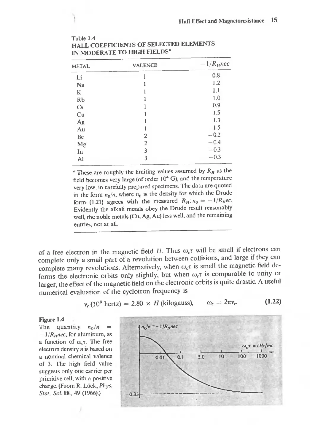
Some Hall coefficients at high and moderate fields are listed in Table lA'. Note
the occurrence of cases in which RJI is actually positive, apparently corresponding
to carriers with a positive charge. A striking example of observed field dependence
totally unexplained by Drude theory is shown in Figure lA.
The Drude result confirms Hall's observation that the resistance does not depend
on field, for whenj}, = 0 (as is the case in the steady state when the Hall field has been
established), the first equation of (1.19) reduces to jx = uoEx, the expected result for
the conductivity in zero magnetic field. However, more careful experiments on a
variety of metals have revealed that there is a magnetic field dependence to the re-
sistance, which can be quite dramatic in some cases. Here again the quantum theory
of solids is needed to explain why the Drude result applies in some metals and to
account for some truly extraordinary deviations from it in others.
Before leaving the subject of DC phenomena in a uniform magnetic field, we note
for future applications that the quantity WeT is an important, dimensionless measure
of the strength of a magnetic field. When WeT is small, Eq. (1.19) gives j very nearly
parallel to E, as in the absence of a magnetic field. In general, however. j is at an
angle cjJ (known as the Hall angle) to E. where (1.19) gives tan cjJ = WeT. The quantity
{')e. known as the cyclotron frequency. is simply the angular frequency ofrevolution '9
10 In a uniform magnetic field Iheoorbil of an electron is a spiral along the field whose projection in a
plane perpendicular 10 the field IS a circle. The angular frequency w, is determined by Ihe condilion that Ihe
centripelal ccelera[ion w/r be prO\ided by [he Lorentz force. (e,d«,J,r)Il,
Hall Effect and MagnelOresistance IS
Table 1.4
HALL COEFFICIENTS OF SELECTED ELEMENTS
IN MODERATE TO HIGH FIELDS.
METAL VALENCE -ljRlfllec
Li I 0.8
Na I 1.2
K I I.I
Rb 1 1.0
Cs I 0.9
Cu I 1.5
Ag I I.3
Au I 1.5
Be 2 -0.2
Mg 2 -0,4
In 3 -0.3
AI 3 -0.3
. These are roughly the limiting values assumed by RII as the
field becomes very large (of order 10 4 G), and the temperature
very low, in carefully prepared specimens. The data are quoted
in the form no/n, where no is the density for which the Orude
form (1.21) agrees with the measured R Il : no = -1/Rllec.
Evidently the alkali metals obey the Orude result reasonably
well, the noble metals (Cu, Ag, Au) less well, and the remaining
entries, not at aIL
of a free electron in the magnetic field H. Thus We' will be small if electrons can
complete only a small part of a revolution between collisions, and large if they can
complete many revolutions. Alternatively, when We' is small the magnetic field de-
forms the electronic orbits only slightly, but when We' is comparable to unity or
larger, the effect of the magnetic field on the electronic orbits is quite drastic. A useful
numerir.al evaluation of the cyclotron frequency is
V e (10 9 hertz) = 2.80 x H (kilogauss),
We = 2nv e .
(1.22)
Figure 1.4
The quantity no/n
-1/Rllllec, for aluminum, as
a function of We'!:. The free
electron density n is based on
a nominal chemical valence
of 3. The high field value
suggests only one carrier per
primitive cell, with a positive
charge. (From R. Luck, Phys.
Stat. Sol. IS, 49 (1966),)
"rJ" = - I/R H "ec
"'e" = eHr/me
100 1000
-033 --------------------
16 Chapter I The Drude Theory of Metals
AC ELECTRICAL CONDUCTIVITY OF A METAL
To calculate the current induced in a metal by a time-dependent electric field, we
write the field in the form
E(l) = Re (E(w)e-' w, ).
(1.23)
The equation of motion (1.12) for the momentum per electron becomes
tip p
- = - - - eE,
dc ,
(1.24)
We seek a steady-state solution of the form
pel) = Re (p(ro)e- iw ,).
(1.25)
Substituting the complex p and E into (1.24), which must be satisfied by both the
real and imaginary parts of any complex solution, we find that p(co) must satisfy
pew)
- iwp(ro) = - - - eE(w).
,
(1.26)
Since j = - nep/m, the current density is just
j(C) = Re (j(w)e-' w ,),
. nep(w) (ne 2 /m)E(w)
J(w) = - - = .
m (I/!) - iw
One customarily writes this result as
ifw) = O'(w)E(w),
(1.27)
(1.28)
where O'(w). known as the frequency-dependent (or AC) conductivity, is given by
0'0 ne 2 ,
O'(w) = 1 . , 0'0 = -.
- IW, m
(1.29)
Note that this correctly reduces to the DC Drude result (1.6) at zero frequency.
The most important application of this result is to the propagation of electro-
magnetic radiation in a metal. It might appear that the assumptions we made to
derive (1.29) would render it inapplicable to this case, since (a) the E field in an electro-
magnetic wave is accompanied by a perpendicular magnetic field H of the same
magnitude,20 which we have not included in (1.24), and (b) the fields in an electro-
magnetic wave vary in space as well as time. whereas Eq, (1.12) was derived by
assuming a spatiaIly uniform force.
The first complication can always be ignored. It leads to an additional term
-ep!mc x H in (1.24), which is smaller than the term in E by a factor ,'/c, where
'" is the magnitude of the mean electronic velocity. But even in a current as large as
I amp/mm 2 . v = j/ne is only of order 0.1 em/sec. Hence the term in the magnetic
field is typically 10- 10 of the term in the electric field and can quite correctly be
ignored.
20 One of the more appealing features of CGS units,
AC Electrical ('onducth'it , of a !\letal 17
The second point raIses more serious questions. Equation (1.12) was derived by
assuming that at any time the same force acts on each electron, which is not the case
if the electric field varies in space, Note, however, that the current density at point
r is entirely determined by what the electric field has done to each electron at r since
its last collision. This last collision, in the overwhelming majority of cases, takes place
no more than a few mean free paths away from r. Therefore if the field does not vary
appreciably over distances comparable to the electronic mean free path, \\e may
correctly calculate j(r, r). the current density at point r, by taking the field everywhere
in space to be given by its value E(r, t) at the point r. The result,
j(r. (I)) = O"(w)F(r, w). (1.30)
is therefore valid whenever the wavelength;' of the field is large compared to the
electronic mean free path {, This is ordinarily satisfied in a metal by visible light (whose
wavelength is of the order of 10 3 to 10" AI, When it is not satisfied, one must resort
to so-called nonlocal theories, of greater complexity,
Assuming, then, that the wavelength is large compared to the mean free path, we
may proceed as follows: in the presence of a specified current density j we may write
Maxwell's equations as 1
V' E = 0: V' H = 0: V x E =
I (-H
c ?t
4rr . I ?E
V x H = - J + - .
c c ct
(1.31)
We look for a solution \\'ith time dependence e- iur . noting that in a metal we can
write j in terms of E \ iJ (1,28). \\ e then find
. iw iw ( 4 rrO" iW )
V x IV x EI = - V-E = - V x H = - - E - - E .
(" (" (" C
(1.32)
or
. w ( 4rriO" )
- V-E = ---z I + - E,
c w
( 1.33)
This has the form of the usual \\ ave equation.
.
.., ('J-
- V-E = --,-E(('})E.
c-
(1.34)
\\ith a complex dielectric constant given by
4rriO"
E(W) = I + - .
w
( 1.35)
If\\e are at frequencies high enough to satisfy
(1)[ » I.
(1.36)
" We are considering here an electromagnelic W3\'e. in which the induced charge density I' \anishes,
Bek", we e' mine the posSlbllit} of oscllI !lon' In the charge densl!},
18 Chapter I The Drude Theof)' of :\ letal
then, to a first approximation, Eqs. (1.35) and (1.29) give
W 2
E(W) = I - --;-,
OT
(1.37)
where Wp, known as the plasma frequency. is given by
, 4Tme 2
(')p- = ---;;-.
( 1.38)
When E is real and negative (w < wpl the solutions to (1.34-) decay exponentially in
space; i.e" no radiation can propagate, However. when E is positive (co > w p ) the
solutions to (1.341 become oscillatory. radiation can propagate, and the metal should
become transparent. This conclusion is only valid, of course. if our high-frequency
assumption (1.36) is satisfied in the neighborhood of w = wp,lfwe express T in terms
of the resistivity through Eq. (1.8), then \\'e can use the definition (1.38) of the plasma
frequency to compute that
W p ' = 1.6 X 10 2 G: Y 2 CJ
Since the resisti\ ity in microhm centimeters, Pw is of the order of unity or less, and
since I"s:oo is in the range from 2 to 6. the high frequency condition (1.36) will be well
satisfied at the plasma frequency.
The alkali metals have. in fact, been observed to become transparent in the ultra-
violet. A numerical evaluation of (1.381 gives the frequency at which transparency
should set in as
( 1.39)
W ( I" ) -32
" = --.£ = 11,4 x x 10 15 Hz
p 2n 00
(1.40)
or
C ( I" ) 3,2
i,p = - = 0.26 x 10 3 A.
"p 00
(1.41 )
In Table 1.5 we list the threshold wa\elengths calculated from (1.41), along with the
Table 1.5
OBSERVED A:\"D THEORETICAL \VA VELE:\"GTHS BELOW
WHICH THE ALKALI :\lETALS BECO:\IE TRA:\SPARENT
Li
Na
K
Rb
Cs
1.5
2,0
2,1;
3.1
3,5
OBSERVED },
(103 A)
2,0
2.1
3,1
3,6
4.4
ELEME:>iT
THEORETICAL a i.
(10 3 A)
a From Eq, (1.41),
Source: M, Born and E. Wolf. Principles orOp/ies, Pergamon. New York.
1964,
AC Electrical Conducth'ity of a :\1etal 19
observed thresholds, The agreement between theory and experiment is rather good.
As we shall see, the actual dielectric constant of a metal is far more complicated than
(1.37) and it is to some extent a piece of good fortune that the alkali metals so strikingly
display this Orude behavior. In other metals different contributions to the dielectric
constant compete quite substantially with the "Orude term" (\.37).
A second important consequence of (\.37) is that the electron gas can sustain
charge density oscillations, By this we mean a disturbance in which the electric charge
density22 has an oscillatory time dependence e- iv ". From the equation of continuity,
i'p
ir'
V' j =
v . j([I)) = ;wp(w).
( 1.42)
and Gauss's law,
v . E(w) = 4np(w),
we find, in view of Eq. (1,30). that
;wp(w) = 4nO"(w)p(w).
This has a solution provided that
( 1.43)
(1.44)
+ 4n;0"(w) = 0,
w
( 1.45)
which is precisely the condition we found above for the onset of propagation of
radiation. In the present context it emerges as the condition the frequency must meet
if a charge density wave is to propagate.
The nature of this charge density wave, known as a plasma oscillation or plasmon,
can be understood in terms of a very simple model. 23 Imagine displacing the entire
electron gas, as a whole. through a distance d with respect to the fixed positive back-
ground of the ions (Figure 1.5).24 The resulting surface charge gives rise to an electric
field of magnitude 4nO", where 0" is the charge per unit area 25 at either end of the slab.
Figure 1.5 (J = + nde
Simple model of a plasma oscillation.
N electrons
+ -
+ -
+ E= 2,,,,+ 2,,,, = 41Tnde -
+ -
+ -
N,Z ions
o = - nde
__ The charge density p should not be confused with the resistivity, also generally denoted by p,
The context will always make it clear which is being referred to.
23 Since the field of a uniform plane of charge is independent of the distance from the plane. this crude
argument. which places all of the charge density on two opposite surfaces. is not as crude as it appears at
first glance,
,. We observed earlier that the Drude model docs take the electron-ion interactIOn into account by
acknowledging that the attraction to the positively charged ions confines the electrons to the interior of the
metal. In this simple model of a plasma oscillation it is precisely this attraction that provides the restoring
force,
25 The surface charge density a should not be confused with the conductivity. also generally denoted
by a,
20 Chapter I The Drude Theory of Metals
Consequently the electron gas as a whole will obey the equation of motion:
Nmd = -NeI47!al = -Ne(47!l1de) = -47!l1e 2 Nd. (1"'6)
which leads to oscillation at the plasma frequency.
Few direct observations have been made of plasmons, Perhaps the most notable
is the observation of energy losses in multiples of fw)p when electrons are fired through
thin. metallic films. 26 Nevertheless, the possibility of their excitation in the course
of other electronic processes must always be borne in mind.
THERMAL CONDUCTIVITY OF A METAL
The most impressive success of the Orude model at the time it was proposed was its
explanation of the empirical law of Wiedemann and Franz (1853). The Wiedemann-
Franz law states that the ratio, Kia, of the thermal to the electrical conductivity of
a great number of metals is directly proportional to the temperature, with a propor-
tionality constant which is to a fair accuracy the same for all metals. This remarkable
regularity can be seen in Table 1.6, where measured thermal conductivities are given
for several metals at 273 K and 373 K. along with the ratios KfaT (known as the
Lorenz number) at the two temperatures.
In accounting for this the Orude model assumes that the bulk ofthe thermal current
in a metal is carried by the conduction electrons. This assumption is based on the
empirical observation that metals conduct heat much better than insulators do, Thus
thermal conduction by the ions 27 (present in both metals and insulators) is much
less important than thermal conduction by the conduction electrons (present only
in metals).
To define and estimate the thermal conductivity, consider a metal bar along which
the temperature varies slowly, If there were no sources and sinks of heat at the ends
of the bar to maintain the temperature gradient, then the hot end would cool and the
cool end would warm, i.e,. thermal energy would flow in a sense opposite to the
temperature gradient. By supplying heat to the hot end as fast as it flows away, one
can produce a steady state in which both a temperature gradient and a uniform flow
ofthermal energy are present. We define the thermal current density jq to be a vector
parallel to the direction of heat flow, whose magnitude gives the thermal energy per
unit time crossing a unit area perpendicular to the flow. 28 For small temperature
gradients the thermal current is observed to be proportional to VT (Fourier's law):
jq = -KVT.
(1047)
The proportionality constant K is known as the thermal conductivity. and is positi\e.
since the thermal current flows opposite to the direction of the temperature gradient.
00 C. J, Pm,ell and J. B, Swan. PhI'S, Re\', 115.869 (1959),
0' Although the metallic ions cannot "ander through the metal. there i, a way in "hich they can
transport thermal energy (though not electric charge): the ions can vibrate a little about their mean posi-
tions. leading to the transmission of thermal energy in the form of elastic "aves propagatll1g through the
network of ions, See Chapter 25,
08 Note the analogy to the definition of the electrical current density j, as "ell as the analog) bet"een
the la"s of Ohm and Fourier.
Thermal Conductivity of a Metal 21
Table 1.6
EXPERIMENTAL THERMAL CONDUCTIVITIES AND LORENZ NUMBERS
OF SELECTED METALS
273K 373 K
ELEMENT K K/aT K K/aT
(watt/cm-K) (watt-ohm/K 2 ) (watt/cm-K) (watt-ohmjK 2)
Li 0.71 2,22 x 10- 8 0,73 2.43 x 10- 8
Na 1.38 2.12
K 1.0 2.23
Rb 0.6 2.42
Cu 3.85 2,20 3,82 2,29
Ag 4.18 2.31 4.17 2.38
Au 3.1 2.32 3.1 2.36
Be 2,3 2,36 1.7 2,42
Mg 1.5 2,14 1.5 2.25
Nb 0.52 2,90 0.54 2,78
Fe 0.80 2,61 0.73 2.88
Zn 1.13 2.28 1.1 2.30
Cd 1.0 2.49 1.0
AI 2,38 2.14 2,30 2.19
- In 0,88 2.58 0.80 2,60
TI 0,5 2,75 0.45 2.75
Sn 0,64 2.48 0,60 2.54
Pb 0.38 2.64 0,35 2.53
Bi 0,09 3,53 0,08 3.35
Sb 0.18 2.57 0.17 2.69
Source: G. w, C. Kaye and T. H. Laby, Table of Physical and Chemical Constants, Longmans
Green, London, 1966
As a concrete example let us examine a case where the temperature drop is uniform
in the positive x-direction. In the steady state the thermal current will also flow in
the x-direction and have a magnitude l = -K dT/dx. To calculate the thermal
current we note (assumption 4, page 6) that after each collision an electron emerges
with a speed appropriate to the local temperature; the hotter the place of the collision,
the more energetic the emerging electron. Consequently, even though the mean
electronic velocity at a point may vanish (in contrast to the case when an electric
current flows) electrons arriving at the point from the high-temperature side will have
higher energies than those arriving from the low-temperature side leading to a net
flow of thermal energy toward the low-temperature side (Figure 1.6),
To extract a quantitative estimate of the thermal conductivity' from this picture,
consider first an oversimplified "one-dimensional"' model, in which the electrons can
only move along the x-axis, so that at a point x halfthe electrons come from the high-
temperature side of x, and halffrom the low. If 6(T) is the thermal energy per electron
in a metal in equilibrium at temperature T, then an electron whose last collision was
at x' will, on the average, have a thermal energy 6(T[ x 'J). The electrons arriving at
x from the high-temperature side will, on the average, have had their last collision at
22 Chapter I The Drude Theory of Metals
High T
lowT
Figure 1.6
Schematic view of the relation between temperature
gradient and thermal current. Electrons arriving at the
center of the bar from the left had their last collision
in the high-temperature region. Those arriving at the
center from the right had their last collision in the
low-temperature region, Hence electrons moving to
the right at the center of the bar tend to be more
energetic than those moving to the left, yielding a net
thermal current to the right.
*--*
x - Fr, and will therefore carry a thermal energy per electron of size £(T[ x - v'(]).
Their contribution to the thermal current density at x will therefore be the number of
such electrons per unit volume, 11/2, times their velocity, v, times this energy, or
(11/2)v8( T[ x - V'f]). The electrons arriving at x from the low-temperature side, on
the other hand, will contribute (11/2)( - v)[£(T[ x + V'f])], since they have come from
the positive x-direction and are moving toward negative x. Adding these together gives
l = im{B(T[x - V'f]) - S(T[x + V'f])].
(1.48)
Provided that the variation in temperature over a mean free path (t = V'f) is very
small,29 we may expand this about the point x to find:
}"l = I1V2'( df, ( _ dT ) . (1.49)
dT dx
To go from this to the three-dimensional case we need only replace v by. the x-
component V x of the electronic velocity v, and average over all directions. Since 30
(v/> = (v/> = (v/> = tv 2 , and since 11 df,/dT = (N/V)df,/dT = (dE/dT)fV =
c v ' the electronic specific heat, we have:
jq = tv 2 'fC v ( - VT)
(1.50)
or
K = tv 2 'fC v = ttvc v ,
(1.51)
where v 2 is the mean square electronic speed.
We emphasize the roughness ofthis argument. We have spoken rather glibly about
the thermal energy per electron carried by a particular group of electrons, a quantity
one might be hard pressed to define with precision. We have also been quite careless
about replacing quantities, at various stages of the calculation, by their thermal
averages. One might object, for example, that if the thermal energy per electron
depends on the direction the electrons come from, so will their average speed, since
this too depends on the temperature at the place of their last collision. We shall note
below that this last oversight is canceled by yet another oversight, and in Chapter 13
29 Its change in (is (IlL) times its change in the sample length L.
30 In equilibrium the velocity distribution is isotropic. Corrections to this due to the temperature
gradient are exceedingly small,
Thermal Conducth'ity of a Metal 23
we shall find by a more rigorous argument that the result (1.51) is quite close to (and,
in special circumstances, precisely) the correct one,
Given the estimate (1.51), we can derive another result independent of the mysteries
buried in the relaxation time T, by dividing the thermal conductivity by the electrical
conductivity (1.6):
K
a
1 2
'3 C v l1lV
----,- .
l1e-
(1.52)
It was natural for Orude to apply the classical ideal gas laws in evaluating the
electronic specific heat and mean square velocity. He therefore in effect took c" to
be il1k B and tmv 2 to be ikBT, where k B is Boltzmann's constant, 1.38 x 10- 16 ergjK.
This leads to the result
= ( kB ) 2 T.
a 2 e
(1.53)
The right side of (1.53) is proportional to T and depends only on the universal con-
stants k B and e, in complete agreement with the law of Wiedemann and Franz.
Equation (1.53) gives a Lorenz number 31
a = ( y
1.24 x 10- 13 (ergjesu-K)2
1.11 X 10- 8 watt-ohm'K2,
(1.54)
which is about half the typical value given in Table 1.6. In his original calculation
of the electrical conductivity, Orude erroneously found half the correct result (1.6),
as a result of which he found a value KjaT = 2.22 x 10- 8 watt-ohmjK 2. in extraor-
dinary agreement with experiment.
This success, though wholly fortuitous, was so impressive as to spur further in-
vestigations with the model. It was, however, quite puzzling, since no electronic
contribution to the specific heat remotely comparable to }lIk B was ever observed.
Indeed, at room temperature there appeared to be no electronic contribution to the
specific heat measured at all. In Chapter 2 we shall find that the classical ideal gas
laws cannot be applied to the electron gas in a metal. Orude's impressive success,
aside from his factor-of-two mistake, is a consequence of two errors of about 100 that
cancel: at room temperature the actual electronic contribution to the specific heat
is about 100 times smaller than the classical prediction, but the mean sq uare electronic
speed is about 100 times larger.
We shall examine the correct theory of the equilibrium thermal properties of the
free electron gas in Chapter 2, and shall return to a more correct analysis of the thermal
conductivity of a metal in Chapter 13. Before leaving the subject of thermal transport,
however, we should correct one oversimplification in our analysis that obscures an
important physical phenomenon:
We calculated the thermal conductivity by ignoring all manifestations of the
temperature gradient except for the fact that the thermal energy carried by a group
31 Since (joule/coulomb)' = (watt/amp)' = watt-ohm, the practical units in which Lorenz numbers
are quoted are often called watt-ohm/K2, instead of (joule/coulomb-KjZ,
24 Chapter 1 The Drude Theory of Metals
of electrons depends on the temperature at the place of their last collision. But if
electrons emerge from a collision with higher energies when the temperature is higher,
they will also have higher speeds. It would therefore appear that we should let the
electron's speed v as well as its contribution to the thermal energy depend on the place
of the last collision. As it turns out such an additional term only alters the result
by a factor ofthe order of unity, but we were in fact quite right to ignore such a correc-
tion. It is true that immediately after the temperature gradient is applied there will be
a nonvanishing mean electronic velocity directed toward the low-temperature region.
Since the electrons are charged, however, this velocity will result in an electric current.
But thermal conductivity measurements are performed under open-circuit conditions,
in which no electric current can flow. Therefore the electrIc current can continue only
until enough charge has accumulated at the surface of the sample to build up a re-
tarding electric field that opposes the further accumulation of charge, and hence
precisely cancels the effect of the temperature gradient on the electronic mean ve-
locity.32 When the steady state is reached there will be no electric current flow, and
we were therefore correct in assuming that the mean electronic velocity at a point
vanished,
In this way we are led to consider another physical effect: A temperature gradient
in a long, thin bar should be accompanied by an electric field directed opposite to
the temperature gradient, The existence of such a field, known as the thermoelectric
field, has been known for some time (the Seebeck effect). The field is conventionally
written as
E = QVT,
(1.55)
and the proportionality constant Q is known as the thermopower. To estimate the
thermo power note that in our "one-dimensional" model the mean electronic velocity
at a point x due to the temperature gradient is
dr
vQ = ![r(x - t'T) - rex + rT)] = -TV-
dx
= -T :. ( }
( 1.56)
We can again generalize to three dimensions 33 by letting t. 2 -> r/, and noting that
(v/> = (t\2> = (v/> = }r 2 . so that
T dt,2
\'Q = - 6" dT (VT), (1.57)
The mean velocity due to the electric field is 34
eET
m
( 1.58)
\'E =
J2 See the analogous discussIOn of the genesIs of the Hall field on page 12,
B Cf. the discussion leading from Eq, (1.49) to Eq, (1.50),
34 See the discussion on page 7,
Problems 25
To have vQ + VE = 0, we require that
Q = - Ge ) :T m;2 =
C"
3ne
(1.59)
This result is also independent of the relaxation time. Drude evaluated it by another
inappropriate application of classical statistical mechanics, setting Cc equal to 3nk B /2
to find that
Q=
k B
2e
-0.43 X 10- 4 volt/K.
(1.60)
Observed metallic thermopowers at room temperature are of the order of microvolts
per degree, a factor of 100 smaller. This is the same error of 100 that appeared twice
in Drude's derivation of the Wiedemann-Franz law, but being now uncompensated,
it offers unambiguous evidence of the inadequacy of classical statistical mechanics in
describing the metallic electron gas.
With the use of quantum statistical mechanics one removes this discrepancy.
However, in some metals the sign of the thermopower the direction of the thermo-
electric field--is opposite to what the Drude model predicts, This is as mysterious as
the discrepancies in the sign of the Hall coefficient. The quantum theory of solids can
account for a sign reversal in the thermopower as well, but one's sense of triumph
is somewhat tempered in this case, for a really quantitative theory of the thermo-
electric field is still lacking, We shall note in later discussions some of the peculiarities
of this phenomenon that make it particularly difficult to calculate with precision.
These last examples have made it clear that we cannot proceed very far with a
free electron theory without a proper use of quantum statistics. This is the subject of
Chapter 2.
PROBLEMS
1. Poisson Distribution
In the Orude model the probability of an electron suffering a collision in any infinitesimal interval
dt is just dt/T.
(a) Show that an electron picked at random at a given moment had no collision during the
preceding t seconds with probability e- r /,. Show that it will have no collision during the next
t seconds with the same probability,
(b) Show that the probability that the time interval between two successive collisions of an
electron falls in the range between t and t + dt is (dtJ-r)e- r ;,.
(c) Show as a consequence of (a) that at an} moment the mean time back to the last collision
(or up to the next collision) averaged over all electrons is -r.
(d) Show as a consequence of (b) that the mean time between successi\'e collisions of an
electron is -r.
(e) Part (c) implies that at any moment the time T between the last and next coll1sion
averaged over all electrons is 2-r. Explain why this is not inconsistent with the result in (d), (A
26 Chapter I The Drude Theory of 'Ietals
thorough explanation should include a derivation of the probability dIstribution for T.) A failure
to appreciate this subtlety led Drude to a conductivity only half of (1.6). He did not make the
same mistake in the thermal conductivity, whence the factor of two in his calculation of the
Lorenz number (see page 231,
2. Joule Heating
Consider a metal at uniform temperature in a static uniform electric field E, An electron expe-
riences a collision, and then, after a time c, a second collision. In the Drude model, energy is not
conserved in collisions, for the mean speed of an electron emerging from a collision does not
depend on the energy that the electron acquired from the field since the time of the preceding
collision (assumption 4. page 6).
(a) Show that the average energy lost to the ions in the second of two collisions separated
by a time C is (eEC)2/2m. (The average is over all directions in which the electron emerged from
the first collision,)
(b) Show, using the result of Problem I(b), that the average energy loss to the ions per
electron per collision is (c£orf /11\, and hence that the average loss per cubic centimeter per second
is (IIC 2 -r/I1IIE2 = aE 2 . Deduce that the power loss in a wire of length L and crOss section A is
]lR, where] is the current flowing and R is the resistance of the wire.
3. Thom.mn Effect
Suppose that in addition to the applied electric field in Problem 2 there is also a uniform tem-
perature gradient VTin the metal. Since an electron emerges from a collision at an energy deter-
mined by the local temperature, the energy lost in collisions will depend on how far down the
temperature gradient the electron travels between collisions, as well as on how much energy it
has gained from the electric field, Consequently the power lost will contain a term proportional
to E. VT(which is easily isolated from other terms since it is the only term in the secontl-order
energy loss that changes sign when the sign of E is reversed), Show that this contribution is given
in the Drude model by a term of order (ne-r/m) (df,/dT) (E . VT), where f, is the mean thermal
energy per electron, (Calculate the energy lost by a typical electron colliding at r, which made its
last collision at r - d, Assuming a fixed (that is, energy-independent) relaxation time -r, d can be
found to linear order in the field and temperature gradient by simple kinematic arguments, which
is enough to give the energy loss to second order.)
4. Helicon Wat'es
Suppose that a metal is placed in a uniform magnetic field H along the z-axis, Let an AC electric
field Ee- iw ' be applied perpendicular to H.
(a) If the electric field is circularly polarized (E y = :t iEx) show that Eq. (1.28) must be
generalized to
. ( 0"0 ) E . +.. , 0
}x = 1 . ( - ) x,}y = _l}x, }. = .
- C W + We !
(1.61)
(b) Show that, in conjunction with (1.61), Maxwell's equations (1.31) have a solution
Ex = Eoe ilk .- w ." Ey = :J:iEx, E. = 0,
provided that Pe 2 = EW 2 . where
(1.62)
E(W)
w- (
l-
w W + We
+ if! ).
(1.63)
Problems 27
(c) Sketch E(W) for W > 0 (choosing the polarization E, = iE,} and demonstrate that solu-
tions to J.. 2e 2 = EO} exist for arbitrar k at frequencies w > w. and W < We' (Assume the
high field condition (WI» I. and note that even for hundreds of kilogauss, w.fwe » 1.1
(d) Show that when w « We the relation between k and w for the low-frequency solution is
(J) = We ( k1C: ) .
W p -
This low-frequency wave, known as a helicon, has been observed in many metals.'s Estimate
the helicon frequency if the wavelength is I cm and the field is 10 kilogauss, at typical metallic
densities,
(1.64)
5. Surface Plasmons
An electromagnetic wave that can propagate along the surface of a metal complicates the obser-
vation of ordinary (bulk) plasmons. Let the metal be contained in the half space z > 0, Z < 0
being vacuum. Assume that the electric charge density p appearing in Maxwell's equations
vanishes both inside and outside the metal. (This does not preclude a surface charge density
concentrated in the plane z = 0,) The surface plasmon is a solution to Maxwell's equations of
the form:
Ex = Aeiqxe- K ., E" = 0, E= = Beiqxe- K :.
Ex = Ceiqxe K ", E}, = 0, E: = Deiqxe K '=,
q, K, K' real. K, K' positive.
z > 0;
z < 0;
(1.65)
(a) Assuming the usual boundary conditions (Ell continuous, (EE).l continuous) and using
the Drude results (1.35) and (1.29) find three equations relating q, K, and K' as functions of w.
(b) Assuming that WT » I, plot q 2 e 2 as a function of w 2 .
(c) In the limit as qc» w, show that there is a solution at frequency w = w.lft. Show
from an examination of K and K' that the wave is confined to the surface. Describe its polarization,
This wave is known as a surface plasmon,
"
R, Bowers et al.. Phys, Rel'. Letters 7,339 (1961),
2
The Sommerfeld
Theory of
Metals
Fermi-Dirac Distribution
Free Electrons
Density of Allowed Wave Vectors
Fermi Momentum, Energy, and Temperature
Ground-State Energy and Bulk Modulus
Thermal Properties of a Free Electron Gas
Sommerfeld Theory of Conduction
Wiedemann-Franz Law
30 Chapter 2 The Sommerfeld Theor)' of :\Ictals
In Drude's time, and for many years thereafter, it seemed reasonable to assume that
the electronic velocity distribution, like that of an ordinary classical gas of density
II = .'II' V. was given in equilibrium at temperature T by the Maxwell-Boltzmann
distribution. This gives the number of electrons per unit volume with velocities in the
range l dv about v as!B(\')dv, where
r ( , ) _ ( /11 ) 3,2 -m.,2'2kBT ( 2.1)
.IB" -II 2nk B T e -
We saw in Chapter I Ihat in conjunction with the Drude model this leads to good
order of magnilude agreement with the Wiedemann-Franz law, but also predicts a
contribution to the specific heat of a metal of kR per electron that was not observed. 2
This paradox cast a shadow over the Drude model for a quarter of a century, which
was only removed by the advent of the quantum theory and the recognition that for
electrons 3 the Pauli exclusion principle requires the replacement of the Maxwell-
Boltzmann distribution (2.1) \\ith the Fermi-Dirac distribution:
, (111;11)3
I(v)=-
, 4n 3 exp [HIIW 2
I
k B To)fk B T] + I'
(2.2)
Here Ii is Planck's constant divided by In, and To is a temperature that is determined
by the normalization condition 4
II = jdV!(V),
(2.3)
and is typically tens of thousands of degrees, At temperatures of interest (that is.
less than 10 3 K) the Maxwell-Boltzmann and Fermi-Dirac distributions are spectacu-
larly different at metallic electronic densities (Figure 2.1).
In this chapter we shall describe Ihe theory underlying the Fermi-Dirac distribution
(2.2) and survey the consequences of Fermi-Dirac statistics for the metallic electron
gas,
Shortly after the discovery that the Pauli exclusion principle was needed to account
for the bound electronic states of atoms, Sommerfeld applied the same principle to
the free electron gas of metals, and thereby resolved the most flagrant thermal anoma-
lies of the early Drude model. In most applications Sommerfeld's model is nothing
more than Drude's classical electron gas with Ihe single modification that the elec-
tronic velocity distribution is taken 10 be the quantum Fermi-Dirac distribution
1 We use standard vector notation, Thus by,' we mean the magnitude of the vector >; a velocity is in
the range ,Iv about v if its ith component lies between ", and r, + d,',. for i = x. '.. z; we also use dv to
denote the volume of the region of"elocny space in the range dv about v: dv = d",dl',dl', (thereby following
the practice common among physicists of failing to distinguish notationally between a region and its
volume, the significance of the symbol being clear from context),
, Because. as we sh,,11 see. ,he actual electronic contribu,ion is about 100 times smaller at room
temperature. becommg smaller still as the temperature drops,
3 And any other particles obeying Fermi-Dirac statistics,
. Note that the constants in the Maxwell-Boltzmann distribution (2.1) have already been chosen so
that (23) is satisfied, Equation (2,2) IS derived below; see Eq, (2,89), In Problem 3d the prefactor appearing
in Eq, (2,2) is cast in a form that facilitates direct comparison with Eq, (2.1),
F enni- Dirac Distribution 31
.....of'.,
f
1.0
Ij.'i
0.8
0:-" !HB f FD
{)(;
'-05
0.4
'0.3
0.2
0.1 x = Inv2/2ksT
Q , ,10 20 30 40 50 60 70 80 90 100 110
f (a)
700
J
600 I
500
400
300
200
100,
:t = mv2/2ksT ..
4 5 6 7 8 9
(b)
,r :' '....,. >;.' .......)
Figure 2.1
(a) The Maxwell-Boltzmann and Fenni-Dirac distributions for typical metallic densities
at room temperature. (Both curves are for the density given by T = 0,01 To,) The scale
is the same for both distributions, and has been nonnalized so that the Fenni-Dirac
distribution approaches 1 at low energies. Below room temperature the differences between
the two distributions are even more marked. (b) A view of that part of (a) between x = °
and x = 10, The x-axis has been stretched by about a factor of 10, and the/-axis has been
compressed by about 500 to get all of the Maxwell-Boltzmann distribution in the figure.
On this scale the graph of the Fermi-Dirac distribution is indistinguishable from the x-axis,
32 (hapler 2 The Sommerfeld rheor of J\lt'tal
rather than the classical Maxwell-Boltzmann distribution. To justify both the use of
the Fermi-Dirac distribution and its bold grafting onto an otherwise classical theory,
we must examine the quantum theory of the electron gas. s
For simplicity we shall examine the ground state (i,e" T = 0) of the electron gas
before studying it at nonzero temperatures, As it turns out. the properties of the
ground state are of considerable interest in themselves: we shall find that room tem-
perature. for the electron gas at metallic densities, is a very low temperature indeed.
for many purposes indistinguishable from T = O. Thus many (though not all) of the
electronic properties of a metal hardly differ from their values at T = 0, even at room
temperature.
GROl!ND-ST A TE PROPERTIES OF THE ELECTRON GAS
We must calculate the ground-state properties of N electrons confined to a volume
Because the electrons do not interact with one another (independent electron
approximation) we can find the ground state of the N electron system by first finding
the energy levels of a single electron in the volume V, and then filling these levels up
in a manner consistent with the Pauli exclusion principle. which permits at most one
electron to occupy any single electron leveI. b
A single electron can be described by a wave function !/J(r) and the specification of
which oftwo possible orientations its spin possesses, Ifthe electron has no interactions.
the one electron wave function associated with a level of energy C satisfies the time-
independent Schrodinger equation 7:
III ( ("2 (12 £'2 ) 112 ,
- - - -;;- + -;;- + -;;- I/t(r) = - - V-I/t(r) = C!/J(r).
2111 (x 2 ( .1'2 (":2 2m
We shall represent the confinement of the electron (by the attraction of the ions)
to the volume V by a boundary condition on Eq. (2.4). The choice of boundary
condition. whenever one is dealing with problems that are not explicitly concerned
with effects of the metallic surface. is to a considerable degree at one's disposal and
can be determined by mathematical convenience. for if the metal is sufficiently large
we should expect its hulk properties to be unaffected by the detailed configuration of
its surface. 8 In this spirit we first select the shape of the metal to suit our analytic
convenience, The time-honored choice is a cube 9 of side L = V I ,3.
!':ext we must append a boundary condition to the Schrodinger equation (2,4).
(2.4)
. Throughout this ch,'pter \\ e ,hall take "eleclron gas' 10 mean .I gas offree ,md independen! eleclrons
bee page 41 unl ... \\c an: c\phcill} considering correclions due to electron-eleclron or clectrrm-ion
intcr..lclion'3
n Null' Ihal here and 1,lIer "e shall resene Ihe lerm "sidle" for Ihe Sidle oflhe j\'-eleclron syslem, and
Ihe lerm "Ie\el h for a one-eleclron Sidle,
, We .,Iso m"ke Ihe rree ekclron appro\imalion. so Ih.\1 no pOlenual energy lerm appears m Ihe
Schrodinger eqmuion,
" This is the dpproaeh Ih.111S .lImoS! uni\e"ally follm>,ed in Iheones of macroscopic mdlter. Rigorous
proofs Ihdl bulk propenies .Ire indeP<'ndent oflhe boundar} conditions can no" be conslrucled m a vdnelY
of contexls, The "ork most pert men! 10 solid slate ph}sics IS b) J L Lebm>"ilz and F, H, Lieb, Phys.
Rei", Lm, 22. 631 (1969),
Q We shdll sub"quentl} find il far more comeniem 10 lake nOl a cube bUI a parallelepIped wllh
Ground-State Properti("; of the [lectron Gas 33
reflecting the fact that the electron is confined to this cube, We also make this choice
in the belief that it will not affect calculated bulk properties, One possibility
is to require the wave function I/;(r) to vanish whenever r is on the surface of the cube,
This, however, is often unsatisfactory, for it leads to standing-wave solutions of ( .4),
while the transport of charge and energy by_ the electrons is far more comeniently
discussed in terms of running waves. A more satisfactory choice is to emphasize the
inconsequence of the surface by disposing of it altogether. We can do this by imagining
each face of the cube to be joined to the face opposite it. so that an electron coming
to the surface is not reflected back in, but leaves the metal. simultaneously reentering
at a corresponding point on the c,pposite surface. Thus, if our metal were one-dimen-
sional, we would simply replace the line from 0 10 L 10 which the electrons were
confined, by a circle of circumference L. In three dimensions the geometrical embodi-
ment of the boundary condition, in which the three pairs of opposite faces on the cube
are joined, becomes topologically impossible to construct in three-dimensional space,
Nevertheless, the analytic form of the boundary condition is easily generalized. In
one dimension the circular model of a metal results in the boundary condition
I/;(x + L) = I/;(x), and the generalization to a three-dimensional cube is evidently
I/;(x, y, z + L) = I/;(x. y. =),
I/;(x, y + L. z) = I/;(x. y. =).
1/;('( + L, y,.:) = I/;I'\:. y. =).
Equation (2.5) is known as the Born-von Karman lor periodic) boundary ,condition,
We shall encounter it often (sometimes in a slightly generalized 9 form),
We now solve ( .4) subject to the boundary condition 1 ,5), One can verify by
differentiation that a solution, neglecting the boundary condition, is
(2.5)
I
I/;d r ) = - = e'L"
....1 V
(2.6)
with energy
11 2 k 2
f,(k) = .
_III
(2.7)
where'" is any position independent vector. We have picked the normalization con-
stant in (2,6) so that the probability of finding the electron olllel\'he,.e in the whole
volume Vis unity:
I = fdr II/;(r)!2,
(2.8)
To see the significance of the vector k. note that the Icvell/;Llrl is an eigenstate of
the momentum operator.
h? h ( IIi' )
p = -: -:;- = -: , . p,\ = -:;- . etc, .
I cr, I ex
(2.9)
edges nOi nece.s.uily equ,ll or perpendICul.u, F-or the momem \\e use a cube to a'Old mm'" genmetriml
comple,ities. bUi it is a usdul exercise to \erir\ that .,11 the results or thi, .eeti,'n rem..in \.llld ror t' .
p.uallelepiped,
3-t ("haptl'r 2 I hl' "mml'rfl'ld I hcur ' of \ letal,
\\'ith eige/1\'alue p = 11 k. for
11 .-
-:---::-(:"11...... = like""'""'.
I I r
(2.10)
Since a particle III an eigenstate of an operator has a definite value of the corre-
sponding obscn ,lble gi\ en b the eigel1\ alue, an electron in the le\ d Ij; (r) has a
definite momentum proportional to k:
p = ilk.
(2.11)
and,l\eloclt \ = plllof
I1k
\ =
III
(2.12)
In \'iew of thi the enagy (2.7) can be written in the familiar classical form.
pl
f = - = lIlrl.
2m -
(2.13)
We can also interpret k as a w.we vector. The plane wave l" ' r is constant in any
pl,lI1e perpendicular to k (sinee such planes arc defined by the equation k . r = con-
stant) and it is periodic along lines parallel to k. with wavelength
21!
I. = k'
(2.14 )
kno\\ n as the de Broglie \\"avelength,
We now invoke the boundar condition (2.5), This permits only certain discrete
\alues of k. since (2,51 will be satisfied by the general wave function (2,6) only if
('iI,xl. = eik)"L = eik=L = I.
(2.15)
Since e= = I onl if = = 21!;1I. \\'here II is an integer,IO the components of the wave
\ector k must be of the form:
.,
k = .;.ml x
x L
k = 2;;:HI"
\' L .
.,
k = 1!H=
= L .
"x. H,., H" integers,
(2.16)
Thus in a three-dimensional space with Cartesian axes kx. k,., and k= (known as
k-space) the allowed wave vectors are those whose coordinates along the three a:\es
arc given by integral multiples of 21! L. This is illustrated (in two dimensions) in
Figure 2,2.
Generally the only practical use one makes of the quantization condition (2.16)
is this: One often needs to know how many allowed values of k are contained in
a region of k-space that is enormous on the scale of 21!, L, and that therefore contains
a vast number of allowed points, If the region is very large. II then to an excellent
approximation the number of allo\\ed points is just the volume of k-space contained
within the region. divided by the volume of k-space per point in the network of
III \\"c shall al\\a\s U'\e the \\ord "integer" 10 me ln the negali\'e integers and zero. as well as lhe
pO ltl\.C: integers.
" ,\nd nolloo orregul rl shaped: only ,\ neghgihlc fraclion of the points should he \\ilhin O(2n L)
of the ,urfacc.
G rouud-Stat Prop rtil' of the Electron (;a 35
Figurc 2.2
Point, in a t\\o-dimensional k-space of the form 1-., =
21111x L. k" = 21111, L Note thaI Ihe arca pcr poinl is just
(211 Ll2, [11 cl dimensIOns the H11ume pcr point is (211 Lid,
ky
k,
I
allowed values of k, That latter volume (see Figure 2,2) is just (2re L)3. We therefore
conclude that a region of k-space of volume Q will contain
Q
ere, L)3
Q[/
8re 3
(2.17)
allowed values of k. lJr. equivalently. that the number of allowed k-values per unit
volume of k-space (also known as the k-space density of levc\st is just
v
8 n 3 '
In practice we shall deal with k-space regions so large (- 10 points) and so regular
(typically spheres) that to all intents and purposes (2.17) and (2,18) can be regarded
as exact. We shall begin to apply these important counting formulas shortly.
Because we assume the electrons are non interacting we can build up the N-electron
ground state by placing electrons into the allowed one-electron levels we have just
found. The Pauli exclusion principle plays a vital role in this construction (as it does
in building up the states of many electron atoms): we may place at most one electron
in each single electron level. The one-electron levels are specified by the wave vectors
k and by the projection of the electron's spin along an arbitrary axis, which can take
either of the two values '1/2 or -h 2, Therefore associated with each allowed wave
vector k are two electronic levels, one for each direction of the electron's spin.
Thus in building up the N-electron ground state we begin by placing two electrons
in the one-electron level k = 0, which has the lowest possible one-electron energy
f, = O. We then continue to add electrons, successively filling the one-electron levels
of lowest energy that are not already occupied, Since the energy of a one-electron
level is directly proportional to the square of its wave vector (see (2.7)), when N is
enormous the occupied region will be indistinguishable from a sphere. I The radius
of this sphere is called k F (F for Fermi), and its volume Q is 4rek F 3 /3. According to
(2.17) the number of allowed values of k within the sphere is
(2.18)
( 4rek F 3 ) ( ) = k F 3 V,
3 8re 3 6re 2
(2.19)
" Ifil "ere nOl sphcrical il would nol be the ground state. for we could then conslrucl .. stale of lower
energy by 111'" '-I! Iheclectrons in Ic\ cis fanhesl away from k = 0 into unoccupied le\els closeno the origin,
36 Chapter 2 The Sommerfeld Theory of Metals
Since each allowed k-value leads to two one-electron levels (one for each spin value),
in order to accommodate N electrons we must have
k F 3 k F 3
N=2'- 6 2V= V.
n 3n
(2.20)
Thus if we have N electrons in a volume V(i.e" an electronic density n = N /V),
then the ground state of the N-electron system is formed by occupying all single-
particle levels with k less than k F , and leaving all those with k greater than k F un-
occupied, where k F is given by the condition:
I n :: I (W)
This free and independent electron ground state is described by some rather
unimaginative nomenclature:
The sphere of radius k F (the Fermi wave vector) containing the occupied one
electron levels is called the Fermi sphere,
The surface of the Fermi sphere, which separates the occupied from the unoccupied
levels is called the Fermi surface. (We shall see, starting with Chapter 8, that the
Fermi surface is one of the fundamental constructions in the modern theory of metals;
in general it is not spherical.)
The momentum hk F = PF of the occupied one-electron levels of highest energy
is known as the Femli momentum; their energy, f,F = h2k//2m is the Fermi energy;
and their velocity, VF = PF/m, is the Fermi velocity. The Fermi velocity plays a role
in the theory of metals comparable to the thermal velocity, v = (3k B T/m)I/2, in a
classical gas,
All these quantities can be evaluated in terms of the conduction electron density,
via Eq. (2,21). For estimating them numerically it is often more convenient to express
them in terms of the dimensionless parameter r./ao lsee page 4), which varies from
about 2 to 6 in the metallic elements. Taken together, Eqs. (1.2) and (2.21) give
(9n/4)1/3 1.92
k F = (2.22)
rs rs
or
k F = 3.63 A -I.
r./ao
(2.23)
Since the Fermi wave vector is of the order of inverse angstroms, the de Broglie
wavelength of the most energetic electrons is of the order of angstroms,
The Fermi velocity is
VF = ( ) kF = 4,20 X 10 8 cm/see.
m ,./ao
(2.24)
This is a substantial velocity (about I percent of the velocity of light). From the
viewpoint of classical statistical mechanics this is quite a surprising rpo"lt, for we are
Ground-State Properties of the Electron Gas 37
describing the ground state (T = 0), and all particles in a classical gas have zero
velocity at T = O. Even at room temperature the thermal (i.e., average) velocity for
a classical particle with the electronic mass is only of order 10 7 cmjsec.
The Fermi energy is conveniently written in the form (since ao = h 2 jme 2 )
h 2 k 2 ( e2 )
OF = = - (k F a o)2.
2m 2ao
Here e2j2ao, known as the rydberg (Ry), is the ground-state binding energy of the
hydrogen atom, 13.6 electron voItsY The rydberg is as convenient a unit of atomic
energies as the Bohr radius is of atomic distances. Since kFao is of the order of
unity, Eq. (2.25) demonstrates that the Fermi energy has the magnitude of a typical
atomic binding energy. Using (2.23) and ao = 0.529 x 10- 8 cm, we find the explicit
numerical form:
(2.25)
50.1 eV
OF = ,
(rsjao)
(2.26)
indicating a range of Fermi energies for the densities of metallic elements between
1.5 and 15 electron volts.
Table 2.1 lists the Fermi energy, velocity, and wave vector for the metals whose
conduction electron densities are given in Table LL
Td calculate the ground-state energy of N electrons in a volume Vwe must add
up the energies of all the one-electron levels inside the Fermi sphere '4 :
E = 2 I k2. (2.27)
k<kF 2m
Quite generally, in summing any smooth function F(k) over all allowed values of
k, one may proceed as follows:
Because the volume of k-space per allowed k value is k = 8n 3 jV(see Eq. (2.18»
it is convenient to write
v
I F(k) = _ 8 3 I F(k) k,
k n k
(2.28)
for in the limit as k -+ 0 (i,e., V -+ (0) the sum F(k) k approaches the integral
J dk F(k), provided only that F(k) does not vary appreciably I S over distances in k-space
of order 2njL. We may therefore rearrange (2.28) and write
I f dk
lim - I F(k) = _ 8 3 F(k).
v-x V k n
(2.29)
In applying (2,29) to finite, but macroscopically large, systems one always assumes
that (ljV) F(k) differs negligibly from its infinite volume limit (for example, one
13 Suictly speaking, the rydberg is the binding energy in the approximation of infinite proton mass,
An electron volt is Iheenergy gained by an electron crossing a potential ofl volt; 1 eV = 1.602 x 10- 12 erg
= 1.602 x 10- 19 joule,
14 The factor of 2 is for the two spin levels allowed for each k.
" The most celebrated case in which F fails to satisfy this condition is the condensation of the ideal
Bose gas, In applications to metals the problem never arises,
38 Chapter 2 The Sommerfeld Theory of Metals
Table 2.1
FERMI ENERGIES, FER.I\1I TE!\1PERATL'RES, FERMI WAVE VECTORS, AI'Iil)
FERMI VELOCITIES FOR REPRESENTATIVE METALS"
ELEME l r.lao E F T F k F v F
Li 3.25 4,74 eV 5.51 x 10 4 K 1.12 x J08 cm- 1 1.29 x J08 em/see
Na 3.93 3.24 3,71 0.92 1.07
K 4.86 2,12 2,46 0,75 0.86
Rb 5,20 1.85 2.15 0.70 0,81
Cs 5,62 1.59 1.84 0,65 0.75
Cu 2,67 7,00 8.16 1.36 1.57
Ag 3,02 5,49 6.38 \.20 \.39
Au 3,01 5,53 6.42 \.21 1.40
Be 1.87 14,3 16,6 1.94 2.25
Mg 2,66 7,08 8,23 1.36 1.58
Ca 3.27 4.69 5,44 1.11 1.28
Sr 3,57 3,93 4,57 1.02 1.18
Ba 3.71 3.64 4,23 0,98 1.13
Nb 3,07 5.32 6.18 U8 \.37
Fe 2.12 ILl \3,0 1.11 1.98
Mn 2,14 10,9 12.7 1.70 1.96
Zn 2,30 9.47 11.0 1.58 1.83
Cd 2,59 7.47 8,68 1.40 1.62
Hg 2.65 7,\3 8,29 1.37 1.58
AI 2.07 11.7 \3,6 1.75 2,03
Ga 2.19 10.4 12.1 1.66 1.92
In 2.41 8,63 10,0 1.51 1.74
11 2.48 8.15 9,46 1.46 1.69
Sn 2,22 10,2 11.8 1.64 1.90
Pb 2.30 9,47 11.0 1.58 1.83
Bi 2.25 9,90 11.5 1.61 1.87
Sb 2.14 10.9 12,7 1.70 1.96
"The table entries are calculated from the values of rJao given in Table Ll using m =
9,lI x 10- 28 grams.
assumes that the electronic energy per unit volume in a I-em cube of copper is the
same as in a 2-cm cube).
Using (2.29) to evaluate (2.27), we find that the energy density of the electron gas is:
E 1 r h 2 k 2 I h 2 k/
V = 4n 3 Jk<kF dk 2m = n 2 10m ' (2.30)
To find the energy per electron, EIN, in the ground state, we must divide this by
NIV = k F 3 /3n 2 , which gives
E 3 h 2 k/ 3
N = 10 ----;;;- = 5" E F .
(2.31)
, We can also write this result as
E 3
- = - k B T F
N 5
(2.32)
Ground-State Properties uf the Electron Gas 39
where T F , the Fermi temperature, is
T F = E F = 58.2 2 x 10 4 K,
k B (rs/ao)
(2.33)
Note, in contrast to this, that the energy per electron in a classical ideal gas, j;k B T,
vanishes at T = 0 and achieves a value as large as (2.32) only at T = ! T F 10 4 K,
Given the ground-state energy E, one can calculate the pressure exerted by the
electron gas from the relation P = -(iJE/iJV)N. Since E = jNE F and E F is propor-
tional to k/, which depends on V only through a factor n 2/3 = (N/V)2/3, it follows
that 16
2E
P = 3V"
(2.34)
One can also calculate the compressibility, K, or bulk modulus, B = I/K, defined
by:
1 OP
B = - = - V-.
K iJV
(2.35)
Since E is proportional to V- 2 /3, Eq.(2,34) shows that Pvaries as V- 5 / 3, and therefore
5 IOE 2
B = - P = -- = -nE F
3 9 V 3
(2.36)
or
( 613 ) 5
B = ......:-... x 10 10 dynes/cm 2 ,
rs/ao
In Table 2.2 we compare the free electron bulk moduli (2.37) calculated from rs/ao,
with the measured bulk moduli, for several metals, The agreement for the heavier
alkali metals is fortuitously good, but even when (2.37) is substantially off, as it is in
(2.37)
Table 2,2
BULK MODl"LI IN 10. 0 DYNES/CM2 FOR SOME
TYPICAL METALS.
METAL FREE ELECTRON B MEASURED B
Li 23,9 11.5
Na 9,23 6.42
K 3,19 2.81
Rb 2,28 1.92
Cs 1.54 1.43
Cu 63,8 134.3
Ag 34.5 99,9
AI 228 76.0
G The free electron value is that for a free electron gas at the observed
density of the metal, as calculated from Eq, (2,37),
.6 Atno
temperatures the pressure and energy density continue to obey this relation, See (2, 10 I),
40 Chapter 2 The Sommerfeld Theory of Metals
the noble metals, it is still of about the right order of magnitude (though it varies from
three times too large to three times too small, through the table), It is absurd to expect
that the free electron gas pressure alone should completely determine the resistance
of a metal to compression, but Table 2.2 demonstrates that this pressure is at least as
important as any other effects,
THERMAL PROPERTIES OF THE FREE ELECTRON GAS:
THE FERMI-DIRAC DISTRIBUTION
When the temperature is not zero it is necessary to examine the excited states of the
N-electron system as well as its ground state, for according to the basic principles
of statistical mechanics, if an N-particle system is in thermal equilibrium at tem-
perature T, then its properties should be calculated by averaging over all N-particle
stationary states, assigning to each state of energy E a weight PN(E) proportional to
e- E / kBT :
e- E / kBT
PN(E) = -E N/k T '
1:e a B
(2.38)
(Here E/ is the energy of the ath stationary state of the N-e1ectron system, the sum
being over all such states.)
The denominator of (2.38) is known as the partition function, and is related to
the Helmholtz free energy, F = U - TS (where U is the internal energy and S, the
entropy) by
1:e-EaN/kBT = e-FN/kBT.
(2.39)
We can therefore write (2.38) more compactly as:
PN(E) = e-(E-FNJ/kBT.
(2.40)
Because of the exclusion principle, to construct an N-electron state one must fill
N different one-electron levels. Thus each N-electron stationary state can be specified
by listing which of the N one-electron levels are filled in that state, A very useful
quantity to know is ft, the probability of there being an electron in the particular
one-electron level i, when the N-electron system is in thermal equilibrium. I7 This
probability is simply the sum of the independent probabilities of finding the N-
electron system in anyone of those N-electron states in which the ith level is occupied:
(summation over all N-electron
It = 'LPN(Ea N ) states ain which there is an elec- (2.41)
tron in the one-electron level i),
We can evaluatej;N by the following three observations:
1. Since the probability of an electron being in the level i is just one minus the
probability of no electron being in the level i (those being the only two possibilities
17 In the case we are interested in the level i is specified by the electron's wave vector k and the pro-
jection s of its spin along some axis,
Derivation of the Fermi-Dirac Distribution 41
allowed by the exclusion principle) we could equally well write (2.41) as
(summation over all N-electron
states)' in which there is no elec-
tron in the one-electron level i), _
f/''' = 1 - I P",(E/)
(2.42)
2. By taking any (N + I)-electron state in which there is an electron in the one-
electron level i, we can construct an N-electron state in which there is no electron
in the level i, by simply removing the electron in the ith level, leaving the occupation
of all the other levels unaltered, Furthermore, any N -electron state with no electron
in the one-electron level i can be so constructed from just one (N + 1 )-electron state
with an electron in the level LIS Evidently the energies of any N-e1ectron state and
the corresponding (N + I)-electron state differ by just 0j, the energy of the only
one-electron level whose occupation is different in the two states_ Thus the set of
energies of all N-e1ectron states with the level i unoccupied is the same as the set of
energies of all (N + I)-electron states with the level i occupied, provided that each
energy in the latter set is reduced by 0i' We can therefore rewrite (2.42) in the peculiar
fonn
(summation over all (N + I)-electron
states (J, in which there is an electron (2.43)
in the one-electron level i).
But Eq. (2.40) permits us to write the summand as
ft = 1 - IPN(E:+ I - 0d
PN(E:+ I - 0;) = e(Cj-"J'kBTPN+I(E:+ I ),
where p, known as the chemical potential, is given at temperature T by
p = F N +1 - FN'
Substituting this into (2.43), we find:
(2.44)
(2.45)
(summation over all (N + I)-electron
ft = I - e(Cj-"J/kBT I PN+I(E:+ I ) states (J, in which there is an electron (2.46)
in the one-electron level i),
Comparing the summation in (2.46) with that in (2.41) one finds that (2.46) simply
asserts that
ft = 1 - e(Cj-"J/kBT fiN+I,
(2.47)
3. Equation (2,47) gives an exact relation between the probability of the one-
electron level i being occupied at temperature Tin an N-electron system, and in an
(N + I)-electron system, When N is very large (and we are typically interested in
N of the order of 10 22 ) it is absurd to imagine that by the addition of a single extra
electron we could appreciably alter this probability for more than an insignificant
handful of one-electron levels. 19 We may therefore replacef +1 by it in (2,47), which
IS Namely the one obtained by occupying all those le\<els occupied in the .V-electron state plus the
ith level.
,. For a typical level, changing N by one alters the probability of occupation by order I tV, See
Prohlem 4,
42 Chapter 2 The Sommerfeld Theory of Metals
makes it possible to solve for It:
rN 1
Ji = e(&j-,.)/kBT + 1.
(2.48)
In subsequent formulas we shall drop the explicit reference to the N dependence
of/;. which is. in any event, carried through the chemical potential p; see (2.45). The
value of N can always be computed, given theJi, by noting thatIj is the mean number
of electrons in the one-electron level 20 i. Since the total number of electrons N is
just the sum over all levels of the mean number in each level,
1
N = Ii = e(&j-,.)/kBT + l '
I I
(2.49)
which determines N as a function of the temperature Tand chemical potential p. In
many applications, however, it is the temperature and N (or rather the density,
n = NjV) that are given. In such cases (2.49) is used to determine the chemical
potential p as a function of nand T, permitting it to be eliminated from subsequent
formulas in favor of the temperature and density. However the chemical potential
is of considerable thermodynamic interest in its own right. Some of its important
properties are summarized in Appendix B. 21
THERMAL PROPERTIES OF THE FREE ELECTRON GAS:
APPLICATIONS OF THE FERMI-DIRAC DISTRIBUTION
In a gas of free and independent electrons the one-electron levels are specified by
the wave vector k and spin quantum number s, with energies that are independent
of s (in the absence of a magnetic field) and given by Eq. (2.7); i,e"
h 2 k 2
0(k) = 2m .
(2.50)
We first verify that the distribution function (2.49) is consistent with the ground-state
(T = 0) properties derived above. In the ground state those and only those levels are
occupied with 0(k) 0F, so the ground-state distribution function must be
I.. = 1, 0(k) < 0F;
= 0, 0(k) > 0F'
(2.51)
2e Proof: A level can contain either 0 or I electron (more than one being prohibited by the exclusion
principle). The mean number of electrons is therefore I times the probability of I electron plus 0 times the
probability of 0 electrons, Thus the mean number of electrons in the level is numerically equal to the
probability of its being occupied, Note that this would not be so if multiple occupation of levels were
permitted,
21 The chemical potential plays a more fundamental role when the distribution (2,48) is derived in
the gTand canonical ensemble, See, for example, F, Reif, Statistical and Thermal Physics, McGraw-Hill,
New York, 1965, p, 350, Our somewhat unorthodox derivation, which can also be found in Reif, uses only
the canonical ensemble,
Thermal Properties of the Free Electron Gas 43
On the other hand, as T -> O. the limiting form of the Fermi-Dirac distribution
(2.48) is
lim k = I, 0(k) < p;
T-O = 0, 0(k) > p.
(2.52)
For these to be consistent it is necessary that
lim p = 0F' (2.53)
T-O
We shall see shortly that for metals the chemical potential remains equal to the
Fermi energy to a high degree of precision, all the way up to room temperature. As
a result, people frequently fail to make any distinction between the two when dealing
with metals, This, however, can be dangerously misleading. In precise calculations
it is essential to keep track of the extent to which p, the chemical potential, differs
from its zero temperature value. 0F'
The most important single application of Fermi-Dirac statistics is the calculation
of the electronic contribution to the constant-volume specific heat of a metal,
C v = (: )v = (:; \:
U
II = V '
(2.54)
In the independent electron approximation the internal energy U is just the sum
over one-electron levels of 0(k) times the mean number of electrons in the level 22 :
U = 2L0(k)f(0(k». (2.55)
k
We have introduced the Fermifiil1ctio/lfl0} to emphasize thatfk depends on k only
through the electronic energy 0(k):
I
f(0) = e(& I'J/kBT +
(2.56)
If we divide both sides of (2.55) by the volume V, then (2,29) permits us to write the
energy density !I = U / Vas
f dk
!I = 4n 3 0(k)flE(k».
(2.57)
Ifwe also divide both sides of(2.49) by V, then we can supplement (2.57) by an equation
for the electronic density /I = N IV, and use it to eliminate the chemical potential:
f dk
/I = f(qk».
4n
In evaluating integrals like (2.57) and (2.58) ofthe form
f 4 3 F(0(k»,
(2.58)
(2.59)
22 As usual. the factor of 2 reflects the fact that each k-Ievel can contain two electrons of opposite
spin orientations,
44 OJapter 2 The Sommerfeld Theory of Metals
one often exploits the fact that the integrand depends on k only through the electronic
energy f, = h 2k 2 j2m, by evaluating the integral in spherical coordinates and changing
variables from k to f,:
f dk f ro k2 dk f ro
F(f,(k» = -z F(f,(k» = df,g(f,)F(f,),
41! 0 n - ro
(2.60)
Here
m J2mf,
g(0) = h2n2 h2' f, > 0;
= 0, f, < O. (2.61)
Since the integral (2.59) is an evaluation of (ljV) bs F(f,(k», the form in (2.60)
shows that
g(0) df, = (- ) x [the number of one-electron
V levels in the energy range
from f, to f, + df,).
(2.62)
For this reason g(0) is known as the density oflevels per unit volume (or often simply
as the density of levels). A dimensionally more transparent way of writing 9 is
3 n ( f, ) 1/2
g(f,) = -- -
2 f,F f,F
= 0,
f, > 0;
f, < 0,
(2.63)
where f,F and k F are defined by the zero-temperature equations (2,21) and (2.25). A
quantity of particular numerical importance is the density of levels at the Fermi
energy, which (2,61) and (2,63) give in either of the two equivalent forms:
mk F
g(f,F) = h 2 n 2
(2.64)
or
3 n
g(f,F) = --.
2 f,F
(2.65)
Using this notation, we rewrite (2.57) and (2.58) as:
II = f:ro df, g(0)f,f(f,)
(2.66)
and
n = f:ro df,g(f,)f(f,).
We do this both for notational simplicity and because in this form the free electron
approximation enters only through the particular evaluation (2.61) or (2,63) of the
density ofIevels g. We can define a density ofIevels, via (2.62), in terms of which (2,66)
(2.67)
Thermal Properties of the Free Electron Gas 45
1
,
t
..
Figure 2.3
The Fenni function, feE) =
1/[eP(£- ) + I] versus E for
given /1, at (a) T = ° and
(b) T 0,01/1 (of order room
temperature, at typical me-
tallic densities), The two
curves differ only in a regi n
of order k B T about /1,
p
{a}
1
\
E
.
It
(b)
p
(to E "" Tj
and (2.67) remain valid for any set of noninteracting (that is, independent) electrons. 23
Thus we shall later be able to apply results deduced from (2.66) and (2.67) to con-
siderably more sophisticated models of independent electrons in metals,
In general, the integrals (2,66) and (2,67) have a rather complex structure. There
is, however, a simple systematic expansion that exploits the fact that at almost all
temperatures of interest in metals, T is very much smaller than the Fermi tempera-
ture (2.33). In Figure 2.3 the Fermi function f(f,) is plotted at T = 0 and at room
temperature for typical metallic densities (kBT//1 ::::: 0.01), Evidently f differs from its
zero temperature form only in a small region about /1 of width a few kBT. Thus
the way in which integrals of the form J'::oo H(f,)f(f,) df, differ from their zero tem-
perature values, J oo H(f,) df" will be entirely determined by the form of H(f,) near
f, = J-l. If H(f,) does not vary rapidly in the energy range of the order of kBT about /1,
the temperature dependence of the integral should be given quite accurately by
replacing H(f,) by the first few terms in its Taylor expansion about f, = /1:
H(f,) = f d n n H(f,) I (f, - /1)n
n=O df, E=,. n!
(2.68)
This procedure is carried out in Appendix C. The result is a series of the form:
f oo H(f,)f(f,) df, = roo H(f,) df, + Jl (k B 1)2n an :::n-_ 1 l H(f,) IE=,. (2.69)
which is known as the Sommerfeld expansion. 24 The'a n are dimensionless constants
of the order of unity. The functions H one typically encounters have major variations
on an energy scale of the order of /1, and generally (d/df,Y' H(f,)k=,. is of the order of
H(/1)//1n. When this is the case, successive terms in the Sommerfeld expansion are
23 See Chapter 8,
24 The expansion is not always exact, but is highly reliable unless H(t) has a singularity very close to
t = p., I for example, H is singular at f, = 0 (as is the free electron density of levels (2,63» then the expan-
sion will neglect terms of the order of exp (- p./k B T), which are typica1\y of order e- 1OO _ 10- 43 , See also
Problem 1.
46 Chapter 2 The Sommerfeld Theory of Metals
smaller by O(kBT/pl which is 0(10- 4 ) at room temperature. Consequently, in
actual calculations only the first and (very occasionally) the second terms are retained
in the sum in (2,69). The explicit form for these is (Appendix C):
f:"" H(f,)f(f,) elf,
f " 1[2 7 4 ( k T ) 6
= _ "" H(f,) elf, + (; (k B T)2 H'(p) + 3 (k B T)4 H"'( p) + 0 -;- .
(2.70)
To evaluate the specific heat of a metal at temperatures small compared with T F
we apply the Sommerfeld expansion (2,70) to the electronic energy and number
densities (Eqs, (2,66) and (2.67»:
i " 1[2
u = f,g(f,)df, + - (k B T)2[pg'(p) + getl)] + 0(T 4 ),
o 6
i " 1[2
/I = g(f,)df, + -(kBT)V(p) + 0(T 4 ),
o 6
(2.71)
(2.72)
Equation (2.72) as we shall presently see in detail, implies that p differs from its T = 0
value, f,F, by terms of order T 2 . Thus, correctly to order T 2 , we may write
r" rrF
Jo H(f,) elf, = Jo H(f,) df, + (p - EF)H(f,F)'
(2.73)
If we apply this expansion to the integrals in (2,71) and (2.72), and replace p by f,F
in the terms already of order T 2 in these equations, we find
C"F { 1[2 }
U = Jo f,g(f,)df, + f,F (Il - f,F)g(f,F) + (;(k B T)2 g '(f,F)
1[2
+ - (k B T)2 g (f,F) + O( T 4 ),
6
rrF { 1[2 }
/I = Jo g(f,)df, + (p - f,F)g(f,F) + (;(k B T)2 g '(f,F) ,
(2.74)
(2.75)
The temperature-independent first terms on the right sides of (2.74) and (2,75) are
just the values of u and /I in the ground state. Since we are calculating the specific
heat at constant density, /I is independent of temperature, and (2,75) reduces to
1[2
o = (Il - f,F)g(E F ) + (; (k B T)2 g '(E F ),
which determines the deviation of the chemical potential from f,F:
1[2 2 g'(f,F)
Il = f,F - (; (kBT) g(E F ) ,
(2.76)
(2.77)
Thermal Properties of the Free Electron Gas 47
Since for free electrons g(f,) varies as f,1/2 (see Eq, (2.63), this gives
p = f,F[1 - (n::F0 ]
(2.78)
which is, as we asserted above, a shift of the order of T 2 and typically only about
0,01 percent, even at room temperature.
Equation (2.76) sets the term in braces in (2,74) equal to zero, thereby simplifying
the form of the thermal energy density at constant electronic density:
n 2
II = 110 + 6 (k B T)2 g (f,F)
(2.79)
where "0 is the energy density in the ground state. The specific heat of the electron
gas is therefore
( ell ) n2
C v = aT n = 3 k B 2 Tg(f,F)
(2.80)
or, for free electrons (see (2,65»,
C v =' 2 e:!) nk B . (2.81)
Comparing this with the classical result for an ideal gas, C t , = 3nk B /2, we see that the
effect of Fermi-Dirac statistics is to depress the specific heat by a factor of (n 2 /3)
(k B T/f,F), which is proportional to the temperature, and even at room temperature is
only of order 10- 2. This explains the absence of any observable contribution of the
electronic degrees of freedom to the specific heat of a metal at room temperature.
If one is willing to dispense with the precise numerical coefficient, one can under-
stand this behavior of the specific heat quite simply from the temperature dependence
of the Fermi function itself. The increase in energy of the electrons when the tem-
perature is raised from T = ° comes about entirely because some electrons with
energies within O(k B T) below f,F (the darkly shaded region of Figure 2.4) have been
excited to an energy range of O(k B T) above f,F (the lightly shaded region of Figure 2.4),
The number of electrons per unit volume that have been so excited is the width, k B T,
of the energy interval times the density of levels per unit vol ume g(f,F)' Furthermore,
the excitation energy is of order k B T, and hence the total thermal energy density is
of order g(f,F)(k B T)2 above the ground-state energy. This misses the precise result
(2,79) by a factor of 1[2/6, but it gives a simple physical picture, and is useful for rough
estimates.
Figure 2.4 1
The Fermi function at nonzero T, The 1.0
distribution differs from its T = 0 form
because some electrons just below E F (darkly
shaded region) have been excited to levels
just above f., (lightly shaded region).
L
I-------i
(AE ""kBT)
48 Chapter 2 The Sommerfeld Theory of Metals
The prediction of a linear specific heat is one of the most important consequences
of Fermi-Dirac statistics, and provides a further simple test of the electron gas theory
of a metal, provided one can be sure that degrees of freedom other than the electronic
ones do not make comparable or even bigger contributions. As it happens, the ionic
degrees offreedom completely dominate the specific heat at high temperatures. How-
ever, well below room temperature their contribution falls off as the cube of the
Table 2,3
SOME ROUGH EXPERIMENTAL VALUES FOR THE COEFFICIENT
OF THE LINEAR TERM IN T OF THE MOLAR SPECIFIC HEATS
OF METALS, AND THE VALUES GIVEN BY SIMPLE FREE
ELECTRON THEORY
ELEMENT FREE ELECTRON Y MEASURED Y RATIoa
(in 10- 4 cal-mole- 1 -K-2) (m* 1m)
Li 1.8 4,2 2.3
Na 2,6 3.5 1.3
K 4,0 4,7 1.2
Rb 4,6 5.8 1.3
Cs 5,3 7,7 1.5
Cu I.2 1.6 1.3
Ag 1.5 1.6 1.1
Au 1.5 1.6 \.I
Be I.2 0,5 0,42
Mg 2.4 3,2 1.3
Ca 3.6 6.5 1.8
Sr 4.3 8.7 2,0
Ba 4,7 6.5 1.4
Nb 1.6 20 12
Fe 1.5 12 8,0
Mn 1.5 40 27
Zn 1.8 1.4 0,78
Cd 2,3 1.7 0,74
Hg 2.4 5,0 2.1
AI 2,2 3,0 1.4
Ga 2.4 1.5 0,62
In 2,9 4.3 1.5
TI 3.1 3,5 \.I
Sn 3,3 4.4 1.3
Pb 3,6 7,0 1.9
Bi 4.3 0,2 0.047
Sb 3,9 1.5 0,38
a Since the theoretical value of l' is proportional to the density of levels at
the Fermi level, which in turn is proportional to the electronic mass m, one
sometimes defines a specific heat effective mass m* so that m* 1m is the ratio
of the measured l' to the free electron 1'- Beware of identifying this specific heat
effective mass with any of the many other effective masses used in solid-state
theory. (See, for example, the index entries under "effective mass,")
The Sommerfeld Theory of Conduction in Metals 49
temperature (Chapter 23), and at very low temperatures it drops below the electronic
contribution, which only decreases linearly with T. In order to separate out these two
contributions it has become the practice to plot cvlT against T 2 , for if the electronic
and ionic contributions together result in the low-temperature form,
C v = yT + A T 3 , (2.82)
then
C v 2
T = Y + AT .
(2.83)
One can thus find y by extrapolating the cvlT curve linearly down to T 2 = 0, and
noting where it intercepts the cvIT-axis. Measured metallic specific heats typically
contain a linear term that becomes comparable to the cubic one at a few degrees
Kelvin. 2s
Specific heat data are usually quoted in joules (or calories) per mole per degree
Kelvin. Since a mole offree electron metal contains ZN A conduction electrons (where
Z is the valence and N A is Avogadro's number) and occupies a volume ZN ...In, we must
multiply the heat capacity per unit volume, C v by ZN Aln, in order to get the heat
capacity per mole, C:
n 2 k B Tg(f,F)
C = - ZR ,
3 n
(2.84)
where R = kBN A = 8.314 joules/mole = 1.99 calories/mole-K. Using the free elec-
tron density of levels (2.65) and the evaluation (2.33) of EF!k B , we find a free
electron contribution to the heat capacity per mole of C = yT, where
1 Z ( r ) 2
y = - 2 n2R - = 0.169Z -..!... x 1O- 4 cal-mole- 1 -K- 2 .
T F 00
Some rough, measured values of yare displayed in Table 2.3, together with the free
electron values implied by (2.85) and the values of r.lao in Table 1.1. Note that the
alkali metals continue to be reasonably well described by free electron theory, as do
the noble metals (Cu, Ag, Au). Note also, however, the striking disparities in Fe and
Mn (experiment ofthe order of 10 times theory) as well as those in Bi and Sb (experi-
ment of the order of 0.1 times theory). These large deviations are now qualitatively
understood on fairly general grounds, and we shall return to them in Chapter 15.
(2.85)
THE SOMMERFELD THEORY OF CONDUCTION IN METALS
To find the velocity distribution for electrons in metals, consider a small 26 volume
element of k-space about a point k, of volume dk. Allowing for the twofold spin
" Since constant density is hard to arrange experimentally, one generally measures the specific heat
at constant pressure, c p ' However, one can show (Problem 2) that for the metallic free electron gas at room
temperature and below, cplc. := I + O(k B T/E p )2, Thus at temperatures where the electronic contribution
to the specific heat becomes observable (a few degrees Kelvin) the two specific heats differ by a negligible
amount.
26 Small enough that the Fermi function and other functions of physical interest vary negligibly
throughout the volume element, but large enough that it contains very many one-electron levels,
50 Chapter 2 The Sommerfeld Theory of Mctals
degeneracy, the number of one-electron levels in this volume element is (see (2.18»
(4 3) dk.
(2.86)
The probability of each level being occupied is just f(0(k», and therefore the total
number of electrons in the k-space volume element is
V h 2 k 2
4n3 f(0(k» dk, 0(k) = 2m . (2.87)
Since the velocity of a free electron with wave vector k is v = hk/m (Eq. (2.12»,
the number of electrons in an element of volume dv about v is the same as the number
in an element of volume dk = (m/h)3 dv about k = mv/h. Consequently the total
number of electrons per unit volume of real space in a velocity space element of volume
dv about v is
f(v) dv,
(2.88)
where
(m/h) 3 1
f(v) = -
4n 3 exp [(!mt,2 - J.I)/kBT] + 1.
Sommerfeld reexamined the Drude model, replacing the classical Maxwell-Boltz-
mann velocity distribution (2.1) by the Fermi-Dirac distribution (2.89). Using a
velocity distribution constructed from quantum-mechanical arguments in an other-
wise classical theory requires some justification. 27 One can describe the motion of an
electron classically if one can specify its position and momentum as accurately as
necessary, without violating the uncertainty principle. 28 .
A typical electron in a metal has a momentum ofthe order of M F , so the uncertainty
in its momentum, I'1p, must be small compared with fJk F for a good classical descrip-
tion. Since, from (2.22), k F - l/r.. the uncertainty in position must satisfy
(2.89)
h 1
I'1x - - » - - r
I'1p k F so
where, from (1.2), r. is of the order of the mean interelectronic distance-i.e., ang-
stroms. Thus a classical description is impossible if one has to consider electrons
localized to within atomic distances (also of the order of angstroms). However, the
conduction electrons in a metal are not bound to particular ions, but can wander
freely through the volume of the metal. In a macroscopic specimen, for most purposes
there is no need to specify their position to an accuracy of 10- 8 cm. The Drude model
assumes a knowledge of the position of an electron primarily in only the two following
contexts:
(2.90)
27 A detailed analytical justification is fairly complicated to construct, just as it is a fairly subde
maUer 10 specify with generality and precision when the quantum theory can be replaced by its classical
limit. The underlying physics, however, is straightforward,
28 There is also a somewhat more specialized limitation on the use of classical mechanics In describing
conduction electrons, The energy of motion of an electron in the plane perpendicular to a uniform applied
magnetic field is quantized in multiples of hw, (Chapter 14), Even for fields as large as to 4 gauss. this is a
very small energy, but in suitably prepared samples at temperatures of a few degrees Kelvin, these quantum
effects become observable, and are, in fact, of great practical imporlance.
The Sommeneld Thcof) of Conduction in Metals 51
1. When spatially varying electromagnetic fields or temperature gradients are ap-
plied, one must be able to specify the position of an electron on a scale small
compared with the distance i. over which the fields or temperature gradients vary.
F or most applications the applied fields or temperature gradients do not vary
appreciably on the scale of angstroms, and the necessary precision of definition
in the electron's position need not lead to an unacceptably large uncertainty in
its momentum. For cxample, the electric field associated with visible light varies
appreciably only over a distance of order 10 3 A. If, however, the wave length is
very much shorter than this (for example, X rays), one must use quantum me-
chanics to describe the electronic motion induced by the field.
2. There is also an implicit assumption in the Drude model that one can localize an
electron to within substantially less than a mean free path t, and one should
therefore be suspicious of classical arguments when mean free paths much shorter
than tens of angstroms occur. Fortunately, as we shall see below, mean free paths
in metals are of the order of 100 A at room temperature, and become longer still
as the temperature drops,
There is thus a wide range of phenomena in which the behavior of a metallic
electron is well described by classical mechanics. It is not, however, immediately
evident from this that the behavior of N such electrons can be described by classical
mechanics. Since the Pauli exclusion principle so profoundly affects the statistics of
N electrons, why should it not have similarly drastic effects on their dynamics'! That
it does not follows from an elementary theorem, which we state without proof, since
the proof, though simple, is notationally rather cumbersome:
Consider a system of N electrons whose interactions with one another are ignored,
and which are exposed to an arbitrary space- and time-dependent electromagnetic
field. Let the N-clectron state at time 0 be formed by occupying a particular group of
N one-electron levels, 1/1 I (0), ..., I/IN(O). Let 1/1 j(t) be the level 1/1 j(O) would evolve into
in time t under the influence of the electromagnetic field if there were only a single
electron present, which was in the leveil/lj(O) at time zero. Then the correct N-electron
state at time t will be the one formed by occupying the set of N one-electron levels
I/It(t), ..., I/IN(t).
Thus the dynamical behavior of N noninteracting electrons is completely deter-
mined by considering N independent one-electron problems. In particular, if the
classical approximation is valid for each of these one-electron problems, it will also
be valid for the whole N-electron system. 29
The use of Fermi-Dirac statistics affects only those predictions of the Drude model
that require some knowledge of the electronic velocity distribution for their evalua-
tion. If the rate l/r at which an electron experiences collisions does not depend on its
energy, then only our estimate of the electronic mean free path and our calculation of
the thermal conductivity and thermopower are at all affected by a change in the
equilibrium distribution function.
29 Note that Ihis implies that any classical configuration consislent wilh the exclusion principle at
time t = 0 (i,e" having less than one electron of each spin per unit volume. in any momentum space region
of volume dp = (27rll)3 IV) will remain consistent with the exclusion principle al all future limes. This result
can also be provp<'i by purely classical reasoning as a direct corollary of Liouville's theorem, See Chapler 12,
52 Chapter 2 The Sommerfeld Theory of Metals
Mean Free Path Using VF (Eq. (2.24)) as a measure of the typical electronic speed,
we can evaluate the mean free path (, = VFL from Eq. (1.8) as follows':
( = (rJ a o)2 x 92 A.
p"
(2,91)
Since the resistivity in microhm centimeters, p", is typically 1 to 100 at room tem-
perature, and since r Ja o is typically 2 to 6, mean free paths of order a hundred
angstroms long are possible even at room temperature. 30
Thermal Conductivity We continue to estimate the thermal conductivity by Eq. (1.51):
K = j-V 2 LC V '
(2.92)
The correct specific heat (2.81) is smaller than the classical guess of Drude by a factor
of order k B TISF; the correct estimate of v 2 is not the classical thermal mean square
velocity of order k B Tim, but VF 2 = 2S F lm, which is larger than the classical value by
a factor of order SF/k B T. Inserting these values in (2.92) and eliminating the relaxation
time in favor of the conductivity through (1.6), we find
K n 2 ( k ) 2
- = _.-!!. = 2.44 X 10- 8 watt-ohmjK2.
aT 3 e
This is remarkably close to Drude's fortuitously good value, thanks to the two
compensating corrections of order k B TISF, and in exceIlent agreement with the data
in Table 1.6. We shall see (Chapter 13) that this value of the Lorenz number is a far
better one than the very rough derivation of (2.93) would suggest.
(2.93)
Thermopower Drude's overestimate of the thermo power is also resolved by the use
of Fermi-Dirac statistics. Substituting the specific heat, from Eq. (2.81), into Eq. (1.59)
we find
n 2 k B ( kB T ) ( kB T ) 4
Q = --- - = -1.42 - x 10- volt/K,
6 e SF SF
which is smaller than Drude's estimate (Eq. (1.60)) by O(kBTISF) - 0.01 at room
temperature.
(2.94)
Other Properties Smce the form of the electronic velocity distribution did not play
a role in the calculation of the DC or AC conductivities, the Hall coefficient, or the
magnetoresistance, the estimates given in Chapter 1 remain the same whether one
uses MaxweIl-Boltzmann or Fermi-Dirac statistics.
This is not the case, however, if one uses an energy-dependent relaxation time. If,
for example, one thought the electrons collided with fixed scattering centers, then it
would be natural to take an energy-independent mean free path, and hence a relaxa-
tion time L = (Iv - f/Sl/2. Shortly after Drude set forth the electron gas model of a
30 It is perhaps just as well that Drude estimated fusing the very much lower classical thermal velocity,
or he might have been sufficiently baffled by such long mean free paths to abandon further investigation.
Problems 53
metal, H. A. Lorentz showed, using the classical Maxwell-Boltzmann velocity dis-
tribution, that an energy-dependent relaxation time would lead to temperature depen-
dence in the DC and AC conductivities, as well as to a nonvanishing magnetoresis-
tance and a field- and temperature-dependent Hall coefficient. As one might now
expect from the inappropriateness of the classical velocity distribution, none of these
corrections were in any way able to bring the discrepancies of the Drude model into
better alignment with the observed facts about metals. 31 Furthermore, we shall see
(Chapter 13) that when the correct Fermi-Dirac velocity distribution is used, adding
an energy dependence to the relaxation time has little significant effect on most of
the quantities of interest in a metal. 32 If one calculates the DC or AC conductivities,
the magnetoresistance, or the Hall coefficient assuming an energy-dependent ,(S), the
results one finds are the same as those one would have calculated assuming an energy-
independent " equal to ,(SF)' In metals these quantities are determined almost entirely
by the way in which electrons near the Fermi level are scattered. 33 This is another
very important consequence of the Pauli exclusion principle, the justification of which
will be given in Chapter 13.
PROBLEMS
1. The Free and Independent Electron Gas in Two Dimensions
(a) What is the relation between n and k F in two dimensions?
(b) What is the relation between k F and r. in two dimensions?
(c) Prove that in two dimensions the free electron density oflevels g(8) is a constant indepen-
dent of 8 for 8 > 0, and 0 for 8 < O. What is the constant?
(d) Show that because g(8) is constant, every tenn in the Sommerfeld expansion for n vanishes
except the T = 0 tenn, Deduce that Ji. = 81' at any temperature.
(e) Deduce from (2.67) that when geE) is as in (c), then
J1 + kBTln (1 + e-lLfkBT) = SF'
(2.95)
(f) Estimate from (2,95) the amount by which Ji. differs from 81" Comment on the numerical
significance of this "failure" of the Sommerfeld expansion, and on the mathematical reason for
the "failure,"
2. Thermodynamics of the Free and Independent Electron Gas
(a) Deduce from the thennodynamic identities
c,. = ( u ) T ( S ) ,
cT " cT "
(2.96)
Jl The Lorentz model is, however, of considerable importance In the descnption of semiconductors
(Chapter 29),
Jl The thermopower is a notable exception,
J3 These assertions are correct to leading order in kBTfEF' but in metals this is always a good expansion
parameter,
54 Chapter 2 The Sommerfeld Theory of Metals
from Eqs. (2.56) and (2.57), and from the third law of thennodynamics (s --+ 0 as T --+ 0) that the
entropy density, s = S/Vis given by:
s = -k B f dk 3 [Jln J + (1 -f)ln(1 -f)],
4n
where f(S(k)) is the Fenni function (Eq. (2.56)),
(b) Since the pressure Psatisfies Eq. (B,5) in Appendix B,P = -(u - Ts - Jln),deducefrom
(2.97) that
(2.97)
P = k B T f ::3 In (I + exp [ - (h 2 k 2 'i - P J}
Show that (2,98) implies that P is a homogeneous function of JI and T of degree 5/2; that is,
(2.98)
P(Ap, }.T) = A 5/2 pep, T)
(2.99)
for any constant L
(c) Deduce from the thermodynamic relations in Appendix B that
( : )T = n,
( P ) = s.
cT"
(2.100)
(d) By differentiating (2.99) with respect to I. show that the ground-state relation (2.34) holds
at any temperature, in the form
P = ju.
(2.101)
(e) Show that when kBT « EF' the ratio of the constant-pressure to constant-volume specific
heats satisfies .
( c p ) _ 1 = n 2 ( k B !\ 2 + 0 ( k B !\ 4.
c v 3 8 F -j 8 F -j
(0 Show, by retaining further tenns in the Sommerfeld expansions of u and n, that correct
to order T 3 the electronic heat capacity is given by
n 2
c v = 3 k B 2 Tg(8 F )
_ n 4 k 4T 3 ( 8 ) [ 15 ( g'(f,F ) ) 2 - 21 g"(8 F ) J .
90 B g F g(8 F ) g(8 F )
(2.102)
3. The Classical Limit of Fermi-Dirac Statistics
The Fenni-Dirac distribution reduces to the Maxwell-Boltzmann distribution, provided that the
Fenni function (2.56) is much less than unity for every positive f" for in that case we must have
J(f,) e-(E-"J/kB T .
The necessary and sufficient condition for (2.103) to hold for all positive f, is
(2.103)
e-,,/kB T » 1.
(2.104)
(a) Assuming that (2.104) holds, show that
rs = e-,,/3kB T 3If3nl/6h(2mkBT)-1/2.
(2.105)
Problems 55
In conjunction with (2.104) this requires that
( h2 ) 1/2
rs» - ,
2mk B T
(2.106)
which can also be taken as the condition for the validity of classical statistics.
(b) What is the significance of the length rs must exceed?
(c) Show that (2.106) leads to the numerical condition
rs ( 105 K ) 1/2
-» -
Go T
(d) Show that the nonnalization constant m 3 /41C 3 h 3 appearing in the Fermi-Dirac velocity dis-
tribution (2.2) can also be written as (3..!n/4)n(m/21Ck B T f"!3/2 so that 1 B(O)/ 1(0) = (4/3.../1r.)( TdT)3/2.
(2.107)
4. Insensitivity of the Distribution Function to Small Changes in the Total Number
of Electrons
In deriving the Fenni distribution (page 41) we argued that the probability of a given level being
occupied should not change appreciably when the total number of electrons is changed by one.
Verify that the Fenni function (2.56) is compatible with this assumption as follows:
(a) Show, when kBT« f,F, that when the number of electrons changes by one at fixed tem-
perature, the chemical potential changes by
1
1'1J1 = V g(SF) '
(2.108)
where g(f,) is the density oflevels.
(b) Show, as a consequence of this, that the most the probability of any level being occupied
can change by is
1 SF 1
M= 6 k B TN "
(2.109)
[Use the free electron evaluation (2,65) of g(SF)'] Although temperatures of millidegrees Kelvin
can be reached, at which f,F/k B T 10 8 , when N is of order 10 22 then I is still negligibly small.
3
Failures of
the Free Electron
Model
58 Chapter 3 Failures or the Free Electron Model
Free electron theory successfully accounts for a wide range ofmetalIic properties. In
the form originally put forth by Drude the most striking deficiencies of the model
were due to Ihe use of classical statistical mechanics in describing the conduction
electrons. As a result, predicted thermoelectric fields and heat capacities were hun-
dreds of times too large, even at room temperature. The difficulty was obscured by
the fact that classical statistics fortuitously gave a form for the Wiedemann-Franz
law that was not in such gross error. Sommerfeld's application of Fermi-Dirac sta-
tistics to the conduction electrons eliminated this class of difficulties while retaining
all of the other basic assumptions of the free electron model.
However, the Sommerfeld free electron model still makes many quantitative pre-
dictions that are quite unambiguously contradicted by observation, and leaves many
fundamental questions of principle unresolved. We list below those inadequacies of
the free electron model that have emerged from the applications made in the preceding
two chapters. l
DIFFICULTIES WITH THE FREE ELECTRON MODEL
1. Inadequacies in the Free Electron Transport Coefficients
(a) The Hall Coefficient Free electron theory predicts a Hall coefficient which
at metallic densities of electrons has the constant value R H = -l/nec, inde-
pendent of the temperature, the relaxation time, or the strength of the mag-
netic field. Although observed Hall coefficients have this order of magnitude,
generally speaking they depend on both the magnetic field strength .and the
temperature (and presumably on the relaxation time, which is rather harder
to control experimentalIy). Often this dependence is quite dramatic. In alumi-
num, for example, R H (see Figure 1.4) never gets within a factor ofIhree of
the free electron value, depends strongly on the strength of the field, and at
high fields does not even have the sign predicted by free electron theory.
Such cases are not atypical. Only the Hall coefficients of the alkali metals
come even close to behaving in accordance with the predictions of free elec-
tron theory.
(b) The Magnetoresistance Free electron theory predicts that the resistance of
a wire perpendicular to a uniform magnetic field should not depend on the
strength of the field. In almost all cases it does. In some cases (notably the
noble metals, copper, silver, and gold) it can be made to increase apparently
without limit as the field increases. In most metals the behavior of the resis-
tance in a field depends quite drastically on the manner in which the metallic
specimen is prepared and, for suitable specimens, on the orientation of the
specimen with respect to the field.
1 These examples and the remarks making up the rest of this brief chapter are not intended to give
a detailed picture of the limitations of the free electron model. That will emerge in the chapters that follow,
together with the solutions to the difficulties posed by the model. Our purpose in this chapter is only to
emphasize how varied and extensive the shortcomings are, thereby indicating why one must resort to a
considerably more elaborate analysis,
Failures of the Free Electron Model 59
(c) The Thermoelectric Field The sign of the thermoelectric field, like the sign
of the Hall constant, is not always what free electron theory predicts it should
be. Only the order of magnitude is right.
(d) The Wiedemann-Franz Law That great triumph of free electron theory, the
Wiedemann-Franz law, is obeyed beautifully at high (room) temperatures
and also quite probably at very low (a few degrees K) temperatures. At inter-
mediate temperatures it fails, and K/aT depends on the temperature.
(e) Temperature Dependence of the DC Electrical COllductit'ity Nothing in free
electron theory can account for the temperature dependence of the DC con-
ductivity (revealed, for example, in Table 1.2). It has to be mechanically
inserted into the theory as an ad hoc temperature dependence in the relaxa-
tion time !.
(f) Directional Dependence of the DC Electl"ical Conductivity In some (but by
no means all) metals the DC conductivity depends on the orientation of the
specimen (if sUitably prepared) with respect to the field. In such specimens the
current j need not even be parallel to the field.
(g) AC Conductit'ity There is a far more subtle frequency dependence to the
optical properties of metals than the simple free electron dielectric constant
can hope to produce. Even sodium, in other respects a fairly good free electron
metal, appears to fail this test in the detailed frequency dependence of its
reflectivity. In other metals the situation is far worse. We cannot begin to
explain the colors of copper and gold in terms of reflectivities calculated from
the free electron dielectric constant.
2. Inadequacies in the Static Thermodynamic Predictions
(a) Linear Term in the Specific Heat The Sommerfeld theory accounts reason-
ably well for the size of the term linear in T in the low-temperature specific
heat of the alkali metals. rather less well for the noble metals. and very
poorly indeed for transition metals such as iron and manganese (much too
small a prediction) as well as for bismuth and antimony (much too large a
prediction).
(b) Cubic Te,'", ill the Specific Heat There is nothing in the free electron model
to explain why the low-temperature specific heat should be dominated by
the electronic contribution. However, it is evident from experiment that the
T J correction to the linear term is very definitely dominated by something
else, since the simple Sommerfeld theory for the electronic contribution to the
T J term has the wrong sign and is millions of times too small.
(c) The Compressibility of Metals Although free electron theory does miracu-
lously well in estimating the bulk moduli (or compressibilities) of many metals,
it is clear that more attention must be paid to the ions and to electron-
electron interactions if one is to achieve a more accurate estimate of the
equation of state of a metal.
3. Fundamental Mysteries
(a) What Dete,mines the Number of Conduction Electrons? We have assumed
th" '} valence electrons become conduction electrons, while the others
60 Chapter 3 Failures of the Free Electron Model
remain bound to the ions. We have given no thought to the question of why
this should be, or how it is to be interpreted in the case of elements, like
iron, that display more than one chemical valence.
(b) Why Are Some Elements Nonmetals'! A more acute inadequacy of our rule
of thumb for determining the number of conduction electrons is posed by the
existence of insulators. Why, for example, is boron an insulator while its
vertical neighbor in the periodic table, aluminum, an excellent metal? Why
is carbon an insulator when in the form of diamond and a conductor when
in the form of graphite? Why are bismuth and antimony such very poor
conductors?
REVIEW OF BASIC ASSUMPTIONS
To make further progress with any of these problems we must reexamine the basic
assumptions on which free electron theory rests. The most notable are these:
1. Free Electron Approximation 2 The metallic ions playa very minor role. In be-
tween collisions they have no effect at all on the motion of an electron, and though
Orude invoked them as a source of collisions, the quantitative information we
have been able to extract about the collision rate has made no sense when inter-
preted in terms of electrons colliding with fixed ions. The only thing the ions
really seem to do properly in the models of Orude and Sommerfeld is to maintain
overall charge neutrality.
2. Independent Electron Approximation 3 The interactions of the electrons with one
another are ignored.
3. Relaxation-Time Approximation 4 The outcome of a collision is assumed not to
depend on the configuration of the electrons at the moment of collision.
All these oversimplifications must be abandoned if we are to achieve an accurate
model of a solid. However, a remarkable amount of progress can be made by first
concentrating entirely on improving some aspects ofthe free electron approximation
while continuing to use the independent electron and relaxation time approximations.
We shall return to a critical examination ofthese last two approximations in Chapters
16 and 17, limiting ourselves here to the following general observations:
There is a surprisingly wide range of circumstances in which the independent
electron approximation does not drastically diminish the validity of the analysis. In
resolving the problems of free electron theory listed above, improving on the inde-
pendent electron approximation plays a major role only in the calculation of metallic
compressibilities (2C).5.6 An indication of why we apparently ignore electron-electron
interactions is given in Chapter 17, together with further examples in which electron-
electron interactions do playa direct and crucial role,
2 See page 4,
3 See page 4,
4 See page 6,
5 Numbers in parentheses refer to numbered paragraphs at the beginning of thIs chapter.
o There are also some cases where a failure of the independent electron approximation (Chapter 10.
p, 186 and Chapter 32) invalidates the simple distinction between metals and insulators that we shall
draw in Chapters 8 and 12,
Review of Basic Assumptions 61
As for the relaxation time approximation, even in Orude's time there were methods
in kinetic theory for correcting this oversimplification. They lead to a much more
complex analysis and in many cases are primarily important in understanding metallic
phenomena with greater precision. Of the difficulties described previously, only the
problem of the Wiedemann-Franz law at intermediate temperatures (Id) has a resolu-
tion that requires abandoning the relaxation time approximation even at the most
gross qualitative level of explanation. 7 In Chapter 16 we shall describe the form a
theory must take ifit is to go beyond the relaxation time approximation, together with
further examples of problems requiring such a theory for their resolution,
The free electron approximation is the major source ofthe difficulties in the theories
of Orude and Sommerfeld. It makes several simplifications:
(i) The effect of the ions on the dynamics of an electron between collisions is ignored.
(ii) What role the ions playas a source of collisions is left unspecified.
(iii) The possibility that the ions themselves, as independent dynamical entities,
contribute to physical phenomena (such as the specific heat or thermal con-
ductivity) is ignored.
The failures of assumptions (ii) and (iii) play an essential role in accounting for
deviations from the Wiedemann-Franz law at intermediate temperatures (I d) and the
temperature dependence of the electrical conductivity (Ie). The failure of assumption
(iii) accounts for the cubic term in the specific heat (2b). Relaxing these two assump-
tions is also essential in accounting for a variety of phenomena yet to be discussed,
Such phenomena are briefly described in Chapter 21, and the consequences of
abandoning assumptions (ii) and (iii) are explored in detail in Chapters 22 to 26.
It is assumption (i), that the ions have no significant effect on the motion of electrons
between collisions, that is responsible for most of the deficiencies of the Orude and
Sommerfeld theories described above. The reader may well be perplexed at how one
can distinguish between assumptions (i) and (ii), for it is far from clear that the effect
of the ions on the electrons can be unambiguously resolved into "collisional" and
"noncollisional" aspects. We shall find, however (especially in Chapters 8 and 12),
that a theory that takes into account the detailed field produced by an appropriate
static array of ions but ignores the possibility of ionic motion (the "static ion approxi-
mation") reduces under a wide range of circumstances to a relatively simple modifica-
tion of the Orude and Sommerfeld free electron theories, in which collisions are
entirely absent! It is only when one allows for ionic motion that their role as a source
of collisions can be properly understood.
We shall therefore relax the free electron approximation in two stages. First we
shall examine the wealth of new structure and the subsequent elucidation that emerges
when the electrons are considered to move not in empty space, but in the presence of a
specified static potential due to a fixed array of stationary ions. Only after that (from
Chapter 21 onward) will we examine the consequences of the dynamical deviations of
the ionic positions from that static array.
The single most important fact about the ions is that they are not distributed at
random, but are arranged in a regular periodic array, or "lattice," This was first
7 It must also be abandoned to explain the detailed temperature dependence of the DC conductivity
(Ie).
62 Chapter 3 Failures of the Free Electron Model
suggested by the macroscopic crystalline forms assumed by many solids (including
metals), first directly confirmed by X-ray diffraction experiments (Chapter 6) and
subsequently reconfirmed by neutron diffraction, electron microscopy, and many
other direct measurements.
The existence of a periodic lattice of ions lies at the heart of modern solid state
physics. It provides the basis for the entire analytic framework of the subject, and
without it comparatively little progress would have been made. If there is one
reason why the theory of solids is so much more highly developed than the theory
of liquids, even though both forms of matter have comparable densities, it is that
the ions are arranged periodically in the solid state but are spatially disordered in
liquids. It is the lack of a periodic array of ions that has left the subject of amorphous
solids in so primitive a state compared with the highly developed theory of crystalline
solids. s
To make further progress in the theory of solids, whether metallic or insulating,
we must therefore turn to the subject of periodic arrays. The fundamental properties
of such arrays are developed in Chapters 4, 5, and 7, without regard to particular
physical applications. In Chapter 6 these concepts are applied to an elementary
discussion of X-ray diffraction, which provides a direct demonstration ofthe period-
icity of solids and is a paradigm for the wide variety of other wave phenomena in
solids we shall subsequently encounter. Chapters 8 to II explore the direct con-
sequences of the periodicity of the array ofions on the electronic structure of any solid,
whether insulating or metallic, In Chapters 12 to 15 the resulting theory is used to
reexplore the properties of metals described in Chapters 1 and 2. Many of the anoma-
lies of free electron theory are thereby removed, and its mysteries are in I,!rge part
resolved.
8 Although there has been a great burst of interest in amorphous solids (starting in the late 1960s),
the subject has yet to develop any unifying principles of a power even remotely comparable to that provided
by the consequences of a periodic array of ions. Many of the concepts used in the theory of amorphous
solids are borrowed, with little if any justification, from the theory of crystalline solids, even though they
are only well understood as consequences oflattice periodicity. Indeed, the term "solid state physics," if
defined as the subject matter of solid state physics textbooks (including this one) is currently confined
almost entirely to the theory of crystalline solids. This is in large part because the normal condition of
solid matter is crystalline, and also because in its present form the subject of amorphous solids still lacks
the kind of broad basic principles suitable for inclusion in an elementary text.
4
Crystal Lattices
Bravais Lattice and Primitive Vectors
Simple, Body-Centered, and Face-Centered
Cubic Lattices
Primitive Unit Cell, Wigner-Seitz Cell, and
Conventional Cell
Crystal Structures and Lattices with Bases
Hexagonal Close-Packed and Diamond Structures
Sodium Chloride, Cesium Chloride, and
Zincblende Structures
64 Chapter 4 Crystal Lattices
Those who have not wandered amidst the mineralogical departments of natural
history museums are often surprised to learn that metals, like most otl}er solids, are
crystalline, for although one is used to the very obvious crystalline features of quartz,
diamond, and rock salt, the characteristic plane faces at sharp angles with one another
are absent from metals in their most commonly encountered forms. However, those
metals that occur naturally in the metallic state are quite often found in crystalline
forms, which are completely disguised in finished metal products by the great mal-
leability of metals, which permits them to be fashioned into whatever macroscopic
shape one wishes.
The true test of crystallinity is not the superficial appearance of a large specimen,
but whether on the microscopic level the ions are arranged in a periodic array.!
This underlying microscopic regularity of crystalline matter was long hypothesized
as the obvious way to account for the simple geometric regularities of macroscopic
crystals, in which plane faces make only certain definite angles with each other. It
received direct experimental confirmation in 1913 through the work of W. and
L. Bragg, who founded the subject of X-ray crystallography and began the inves-
tigation of how atoms are arranged in solids.
Before we describe how the microscopic structure of solids is determined by X-ray
diffraction and how the periodic structures so revealed affect fundamental physical
properties, it is useful to survey some of the most important geometrical properties
of periodic arrays in three-dimensional space. These purely geometrical consider-
ations are implicit in almost all the analysis one encounters throughout solid state
physics. and shall be pursued in this chapter and in Chapters 5 and 7. The first of
many applications of these concepts will be made to X-ray diffraction in Chapter 6.
BRAVAIS LATTICE
A fundamental concept in the description of any crystalline solid is that of the B,.avais
lattice, which specifies the periodic array in which the repeated units of the crystal
are arranged. The units themselves may be single atoms, groups of atoms, molecules,
ions, etc., but the Bravais lattice summarizes only the geometry of the underlying
periodic structure, regardless of what the actual units may be. We give two equivalent
definitions of a Bravais lattice z :
(a) A Bravais lattice is an infinite array of discrete points with an arrangement and
orientation that appears exactly the same, from whichever of the points the
array is viewed.
(b) A (three-dimensional) Bravais lattice consists of all points with position vectors
R of the form
R = ni3i + nz3z + n333,
(4.1)
1 Often a specimen is made up of many small pieces, each large on the microscopic scale and con-
taining large numbers of periodically arranged ions. This "polycrystaIline" stale is more commonly
encountered than a single macroscopic crystal, in which the periodIcity is perfect, extending through the
entire specimen.
2 Why the name Bravais appears is explained in Chapter 7,
Bravais Lattice 65
where 3 10 31, and 33 are any three vectors not all in the same plane, and n10
nl, and n3 range through all integral values. 3 Thus the point 1:lli3i is reached by
moving n i steps4 of length ai in the direction of 3 i for i = 1, 2, and 3.
The vectors 3 i appearing in definition (b) of a Bravais lattice are called Pl'imitive
vectors and are said to generate or span the lattice.
It takes some thought to see that the two definitions of a Bravais lattice are equiva-
lent. That any array satisfying (b) also satisfies (a) becomes evident as soon as both def-
initions are understood. The argument that any array satisfying definition (a) can
be generated by an appropriate set of three vectors is not as obvious. The proof
consists of an explicit recipe for constructing three primitive vectors. The construction
is given in Problem 8a.
Figure 4.1
A general two-dimensional Bravais lattice of no
particular symmetry: the oblique net. Primitive
vectors a. and a z are shown. All points in the net are
linear combinations of these with integral coefficients;
for example. P = a l + 2a 2 , and Q = -a. + a.-
.
-p
Q-
.L"
"
Figure 4.1 shows a portion of a two-dimensional Bravais lattice. S Clearly definition
(a) is satisfied, and the primitive vectors 3 1 and 31 required by definition (b) are
indicated in the figure. Figure 4.2 shows one of the most familiar of three-dimensional
Bravais lattices, the simple cubic. It owes its special structure to the fact that it can
be spanned by three mutually perpendicular primitive vectors of equal length.
Figure 4.2
A simple cubic three-dimensional Bravais lattice. The three
primitive vectors can be taken to be mutually perpendicular,
and with a common magnitude.
, We continue with the convention that "integer" means a negative integer or zero, as well as a
positive Integer.
· When n is negative, n steps in a direction means n steps in the opposite direction, The point reached
does not. of course, depend on the order in which the n, + n 1 + n, steps are taken,
, A two-dimensional Bravais lattice is also known as a net
66 Chapter 4 CQ'staI Lattices
Figure 4.3
The vertices of a two-dimensional honeycomb
do 1101 form a Bravais lattice. The array of
points has the same appearance whether \'iewed
from point P or point Q, However, the view
from point R is rotated through 180 .
It is important that not only the arrangement, but also the orientation must
appear the same from every point in a Bravais lattice, Consider the vertices of a
two-dimensional honeycomb (Figure 4.3). The array of points looks the same when
viewed from adjacent points only if the page is rotated through 180 0 each time one
moves from one point to the next. Structural relations are clearly identical, but 110t
orientational relations, so the vertices of a honeycomb do not form a Bravais lattice.
A case of more practical interest, satisfying the structural but not the orientational
requirements of definition (a), is the three-dimensional hexagonal close-packed lattice,
described below.
INFINITE LATTICES AND FINITE CRYSTALS
Since all points are equivalent, the Bravais lattice must be infinite in extent. Actual
crystals are, of course, finite, but if they are large enough the vast majority of points
will be so far from the surface as to be unaffected by its existence. The fiction of an
infinite system is thus a very useful idealization. If surface effects are of interest the
notion of a Bravais lattice is still relevant, but now one must think of the physical
crystal as filling up only a finite portion of the ideal Bravais lattice.
Frequently one considers finite crystals, not because surface effects are important,
but simply for conceptual convenience, just as in Chapter 2 we placed the electron
gas in a cubical box of volume V = L 3 . One then generally picks the finite region
of the Bravais lattice to have the simplest possible fonn. Given three primitive
vectors at. 32, and a3, one usually considers the finite lattice of N sites to be the set
of points of the fonn R = nta. + n232 + n3a3, where 0 nl < N.. 0 n2 < N 2,
o 113 < N 3, and N = N IN 2N 3. This artifact is closely connected with the general-
ization to the description of crystalline systems 6 of the periodic boundary condition
we used in Chapter 2.
FURTHER ILLUSTRATIONS AND IMPORTANT EXAMPLES
Of the two definitions of a Bravais lattice, definition (b) is mathematically more
precise and is the obvious starting point for any analytic work. It has, however, two
6 We shall make particular use of it in Chapters 8 and 22.
Further Illustrations and Important Examples 67
minor shortcomings. First, for any given Bravais lattice the set of primitive vectors
is not unique-indeed, there are infinitely many nonequivalent choices (see Figure
4.4)-and it is distasteful (and sometimes misleading) to rely too heavily on a defi-
nition that emphasizes a particular choice. Second, when presented with a particular
array of points one usually can tell at a glance whether the first definition is satisfied,
although the existence of a set of primitive vectors or a proof that there is no such
set can be rather more difficult to perceive immediately.
. .
.
Figure 4.4
Several possible choices of pairs of
primitive vectors for a two-dimen-
sional Bravais lattice. They are
drawn, for clarity, from different
origins.
.
.
.
.
.
.
.
.
.L
..;?
.
.
.
.
.
\
v.
.
.
.
.
.
.
.
.
.
.
.
. .-------- -------
. .
Consider, for example, the body-centered cubic (bee) lattice, formed by adding to
the simple cubic lattice of Figure 4.2 (whose sites we now label A) an additional point,
B, at the center of each little cube (Figure 4.5). One might at first feel that the center
points B bear a different relation to the whole than the corner points A. However,
the center point B can be thought of as corner points of a second simple cubic array.
Figure 4.5
A few sites from a body-centered cubic Bravais
lattice, Note that it can be regarded either as a simple
cubic lattice formed from the points A with the points
B at the cube centers, or as a simple cubic lattice
formed from the points B with the points A at the
cube centers. This observation establishes that it is
indeed a Bravais lattice.
B
B
A
In this new array the corner points A of the original cubic array are center points.
Thus all points do have identical surroundings, and the body-centered cubic lattice
is a Bravais lattice. If the original simple cubic lattice is generated by primitive vectors
a5\., ay, az,
(4.2)
68 Chapter 4 Crystal Lattices
where , y, and 2 are three orthogonal unit vectors, then a set of primitive vectors
for the body-centered cubic lattice could be (Figure 4.6)
a
3 1 = a , 32 = ay, 33 = "2 ( + y + 2).
(4.3)
Figure 4.6
P Three primitive vectors, specified in Eq. (4.3),
for the body-centered cubic Bravais lattice, The
lattice is formed by taking all linear combina-
tions of the primitive vectors with integral
coefficients. The point P, for example, is P =
Z -a. - a z + 2a3.
,)
y
A more symmetric set (see Figure 4.7) is
a a a
31 = "2 (y + 2 - ), 32 = "2 (2 + - y), 33 = "2 ( + y - 2). (4.4)
It is important to convince oneself both geometrically and analytically that these
sets do indeed generate the bcc Bravais lattice.
Figure 4.7
A more symmetric set of primitive vectors,
specified in Eq. (4.4), for the body-
centered cubic Bravais lattIce. The point
P, for example, has the form P = 2a. +
a 2 + a 3 ,
Another equally important example is the face-centered cubic (fcc) Bravais lattice,
To construct the face-centered cubic Bravais lattice add to the simple cubic lattice
of Figure 4.2 an additional point in the center of each square face (Figure 4.8). For
ease in description think of each cube in the simple cubic lattice as having horizontal
bottom and top faces, and four vertical side faces facing north, south, east, and west.
It may sound as if all points in this new array are not equivalent, but in fact they are.
One can, for example, consider the new simple cubic lattice formed by the points added
Further Illustrations and Important Examples 69
Figure 4.8
Some points from a face-centered
cubic Bravais lattice,
Up
w
E
Down
to the centers of all the horizontal faces. The original simple cubic lattice points are
now centering points on the horizontal faces of the new simple cubic lattice, whereas
the points that were added to the centers of the north-south faces of the original cubic
lattice are in the centers of the east-west faces of the new one, and vice versa.
In the same way one can also regard the simple cubic lattice as being composed
of all points centering the north-south faces of the original simple cubic lattice, or
all points centering the east-west faces ofthe original cubic lattice. In either case the
remaining points will be found centered on the faces of the new simple cubic frame-
work.-Thus any point can be thought of either as a corner point or as a face-centering
point for any of the three kinds offaces, and the face-centered cubic lattice is indeed
a Bravais lattice.
A symmetric set of primitive vectors for the face-centered cubic lattice (see Figure
4.9) is
a a
3) = 2 ()' + 2), 32 = 2 (2 + ),
Figure 4.9 r
A set of primitive vectors, as given in Eq, (4,5),
for the face-centered cubic Bravais lattice, The
labeled points are P = 3, + a 2 + a 3 , Q = 2a 2 ,
R = 3 2 + a 3 , and S = -a) + a 2 + a 3 -
z
k(,
x
a
33 = 2 ( + n
(4.5)
s
The face-centered cubic and body-centered cubic Bravais lattices are of great
importance, since an enormous variety of solids crystallize in these forms with an
atom (or ion) at each lattice site (see Tables 4.1 and 4.2). (The corresponding simple
cubic form, however, is very rare, the alpha phase of polonium being the only known
example among the elements under normal conditions.)
70 Chapter 4 Crystal Lattices
Table 4.1
ELL'\1ENTS WITH THE MONA TO!\fiC FACE-CENTERED
CUBIC CRYSTAL STRUCTURE
ELEMENT a (A) ELDfENT a (A) ELEMENT a (A)
Ar 5.26 (4,2 K) Ir 3.84 Pt 3.92
Ag 4.09 IV 5.72 (58 K) l)-Pu 4.64
AI 4.05 La 5.30 Rh 3.80
Au 4.08 Ne 4.43 (4.2 K) Sc 4.54
Ca 5.58 Ni 3.52 Sr 6,08
Ce 5.16 Pb 4.95 Th 5.08
p-Co 3.55 Pd 3.89 Xe (58 K) 6,20
Cu 3.61 Pr 5.16 Yb 5,49
Data in Tables 4.1 to 4.7 are from R. W. G. Wyckoff, Crystal Structures, 2nd ed.,
Interscience, New York, 1963, In most cases, the data are taken at about room tem-
perature and normal atmospheric pressure. For elements that exist in many forms the
stable room temperature form (or forms) is given. For more detailed information, more
precise lattice constants, and references, the Wyckoff work should be consulted.
)
Table 4.2
ELEMENTS WITH THE MONATO!\HC BODY-CENTERED
CUBIC CRYSTAL STRUCTURE
ELEMENT a (A) ELEME:-IT a (A) ELEMENT a ( )
Ba 5.02 Li 3.49 (78 K) Ta 3.31
Cr 2,88 Mo 3.15 11 3.88
Cs 6.05 (78 K) Na 4.23 (5 K) V 3.02
Fe 2.87 Nb 3.30 W 3.16
K 5.23 (5 K) Rb 5.59 (5 K)
A NOTE ON USAGE
Although we have defined the term "Bravais lattice" to apply to a set of points, it
is also generally used to refer to the set of vectors joining anyone of these points
to all the others. (Because the points are a Bravais lattice, this set of vectors does not
depend on which point is singled out as the origin.) Yet another usage comes from
the fact that any vector R determines a translation or displacement, in which everything
is moved bodily through space by a distance R in the direction of R. The term "Bravais
lattice" is also used to refer to the set of translations determined by the vectors, rather
than the vectors themselves. In practice it is always clear from the context whether
it is the points, the vectors, or the translations that are being referred to. 7
7 The more general use of the term provides an elegant definition of a Bravais lattice with the pre-
cision of definition (b) and the nonprejudicial nature of definition (a): A Bravais lattice is a discrete set
of vectors not all in a plane, closed under vector addition and subtraction (i.e., the sum and difference of
any two vectors in the set are also in the set).
Primitive Unit Cell 71
COORDINA TION NUMBER
The points in a Bravais lattice that are closest to a given point are called its nearest
neighbors. Because of the periodic nature of a Bravais lattice, each point has the same
number of nearest neighbors. This number is thus a property of the lattice, and is
referred to as the coordination number of the lattice. A simple cubic lattice has co-
ordination number 6; a body-centered cubic lattice, 8; and a face-centered cubic
lattice, 12. The notion of a coordination number can be extended in the obvious way
to some simple arrays of points that are not Bravais lattices, provided that each point
in the array has the same number of nearest neighbors.
PRIMITIVE UNIT CELL
A volume of space that, when translated through all the vectors in a Bravais lattice,
just fills all of space without either overlapping itself or leaving voids is called a
primitive cell or primitive unit cell of the lattice. 8 There is no unique way of choosing
a primitive cell for a given Bravais lattice. Several possible choices of primitive cells
for a two-dimensional Bravais lattice are illustrated in Figure 4.10.
.
.
.
.
.
.
.
Figure 4.10
Several possible choices of primitive cell for a single two-dimensional Bravais lattice,
A primitive cell must contain precisely one lattice point (unless it is so positioned
that there are points on its surface). It follows that if n is the density of points in
the lattice 9 and v is the volume of the primitive cell, then nv = 1. Thus v = l/n. Since
8 Translations of the primitive cell may possess common surface points; the nonoverlapping proviso
is only intended to prohibit overlapping regions of nonzero volume.
· The density n of Bravais lattice points need not, of course, be identical to the density of conduction
electrons in a metal. When the possibility of confusion is present, we shall specify the two densities with
different symb r "
72 Chapter 4 Crystal Lattices
this result holds for any primitive cell, the volume of a primitive cell is independent
of the choice of cell.
It also follows from the definition of a primitive cell that, given any two primitive
cells of arbitrary shape, it is possible to cut the first up into pieces, which, when
translated through appropriate lattice vectors, can be reassembled to give the second.
This is illustrated in Figure 4.11.
Figure 4.11
Two possible primitive cells for a two-dimen-
sional Bravais lattice. The parallelogram cell
(shaded) is obviously primitive; additional
hexagonal cells are indicated to demonstrate
that the hexagonal cell is also primitive. The
parallelogram can be cut into pieces, which,
when translated through lattice vectors, re-
assemble to form the hexagon. The translations
for the four egions of the p allelogram are:
gion I-CO; Region II-BO; Region III-
AO; Region IV-no translation.
The obvious primitive cell to associate with a particular set of primitive vectors,
31. 32, 33, is the set of all points r of the form
r = X131 + X232 + X3 3 3
(4.6)
for all Xi ranging continuously between 0 and 1; i.e., the parallelipiped spanned by the
three vectors 31> 32, and 33. This choice has the disadvantage of not displaying the
full symmetry of the Bravais lattice. For example (Figure 4.12), the unit cell (4.6) for the
choice of primitive vectors (4.5) of the fcc Bravais lattice is an oblique parallelipiped,
which does not have the full cubic symmetry of the lattice in which it is embedded.
It is often important to work with cells that do have the full symmetry oftheir Bravais
lattice. There are two widely used solutions to this problem:
Figure 4.12
Primitive and conventional unit cells for the face-
centered cubic Bravais lattice, The conventional cell is
the large cube. The primitive cell is the figure with six
parallelogram faces, It has one quarter the volume of
the cube, and rather less symmetry.
ii
,I
, ----
--- !"\..
I
iI' ...
.l l- ---
I
Wigner-Seitz Primitive Cell 73
UNIT CELL; COl\"'VENTIONAL UNIT CELL
One can fill space up with nonprimitive unit cells (known simply as unit cells or
conventional unit cells). A unit cell is a region that just fills space without any over-
lapping when translated through some subset of the vectors of a Bravais lattice. The
conventional unit cell is generally chosen to be bigger than the primitive cell and to
have the required symmetry. Thus one frequently describes the body-centered cubic
lattice in terms of a cubic unit cell (Figure 4.13) that is twice as large as a primitive
bcc unit cell, and the face-cent<tred cubic lattice in terms of a cubic unit cell (Figure
4.12) that has four times the volume of a primitive fcc unit cell. (That the conventional
cells are two and four times bigger than the primitive cells is easily seen by asking
how many lattice points the conventional cubic cell must contain when it is so placed
that no points are on its surface.) Numbers specifying the size of a unit cell (such as
the single number a in cubic crystals) are called lattice constants.
Figure 4.13
Primitive and conventional unit cells for the body-
centered cubic Bravais lattice, The primitive cell
(shaded) has half the volume of the conventional
cubic cell,
WIGNER-SEITZ PRIMITIVE CELL
-t,"
One can always choose a primitive cell with the full symmetry of the Bravais lattice.
By far the most common such choice is the Wigner-Seitz cell. The Wigner-Seitz cell
about a lattice point is the region of space that is closer to that point than to any
other lattice point. 1o Because of the translational symmetry of the Bravais lattice,
the Wigner-Seitz cell about anyone lattice point must be taken into the Wigner-Seitz
cell about any other, when translated through the lattice vector that joins the two
points. Since any point in space has a unique lattice point, as its nearest neighbor ll
it will belong to the Wigner-Seitz cell of precisely one lattice point. It follows that a
10 Such a cell can be defined for any set of discrete points that do not necessarily form a Bravais
lattice, In this broader context the cell is known as a Voronoy polyhedron, In contrast to the Wigner-Seitz
cell, the structure and orientation of a general Voronoy polyhedron will depend on which point of the
array it encloses.
11 Except for points on the common surface of two or more Wigner-Seitz cells.
74 Chapter 4 CQ,stal Lattices
Wigner-Seitz cell, when translated through all lattice vectors, will just till space
without overlapping; i.e., the Wigner-Seitz cell is a primitive cell.
Since there is nothing in the detinition of the Wigner-Seitz cell that refers to any
particular choice of primitive vectors, the Wigner-Seitz cell will be as symmetrical
as the Bravais lattice. 12
The Wigner-Seitz unit cell js illustrated for a two-dimensional Bravais lattice in
Figure 4.14 and for the three-dimensional body-centered cubic and face-centered
cubic Bravais lattices in Figures 4.15 and 4.16,
Note that the Wigner-Seitz unit cell about a lattice point can be constructed by
drawing lines connecting the point to all others'3 in the lattice, bisecting each line
e
e-------
. Figure 4.14
The Wigner-Seitz cell for a two-dimensional
Bravais lattice, The six sidcs of the cell bisect
the lines joining the central points to its six
nearest neighboring points (shown as dashed
lines), In two dimensions the Wigner-Seitz
cell is always a hexagon unless the lattice is
rectangular (see Problem 4a),
Figure 4.15
The Wigner-Seitz cell for the body-centered cubic Bravais
lattice (a "truncated octahedron"). The surrounding cube is a
conventional body-centered cubic cell with a lattice point at
its center and on each vertex. The hexagonal faces bisect the
lines joining the central point to the points on the vertices
(drawn as solid lines). The square faces bisect the lines joining
the central point to the central points in each of the six neigh-
boring cubic cells (not drawn), The hexagons are regular (see
Problem 4d).
'-
Figure 4.16
Wigner-Seitz cell for the face-centered cubic Bravais
lattice (a "rhombic dodecahedron"), The surrounding
cube is not the conventional cubic cell of Figure 4,12,
but one in which lattice points are at the center of the
cube and at the center of the 12 edges. Each of the 12
(congruent) faces is perpendicular to a line joining the
central point to a point on the center of an edge,
12 A precise definition of "as symmetrical as" is given in Chapter 7_
1J In practice only a fairly small number of nearby points actually y; ,Ianes that bound the cell
Cr)'stal Structure; Lattice with a Basis 75
with a plane, and taking the smallest polyhedron containing the point bounded by
these planes.
CRYSTAL STRUCTURE; LATTICE WITH A BASIS
A physical crystal can be described by giving its underlying Bravais lattice, together
with a description of the arrangement of atoms, molecules, ions, etc., within a
particular primitive cell. When emphasizing the difference between the abstract
pattern of points composing the Bravais lattice and an actual physical crystaJl4
embodying the lattice, the technical term "crystal structure" is used. A crystal structure
consists of identical copies of the same physical unit, called the basis, located at all
the points of a Bravais lattice (or, equivalently, translated through all the vectors
of a Bravais lattice). Sometimes the term lattice with a basis is used instead. However,
"lattice with a basis" is also used in a more general sense to refer to what results
even when the basic unit is llOt a physical object or objects, but another set of points.
For example, the vertices of a two-dimensional honeycomb, though not a Bravais
lattice, can be represented as a two-dimensional triangular Bravais lattice'S with a
two-point basis (Figure 4.17). A crystal structure with a basis consisting of a single
atom or ion is often called a monatomic Bravais lattice.
Figure 4.17
The honeycomb net, drdwn so as
to emphasize that it is a Bravais
lattice with a two-point basis, The
pairs of points joined by heavy
solid lines are identically placed in
the primitive cells (parallelograms)
of the underlying Bra vais lattice,
One also can describe a Bravais lattice as a lattice with a basis by choosing a non-
primitive conventional unit cell. This is often done to emphasize the cubic symmetry
of the bcc and fcc Bravais lattices, which are then described respectively, as simple
cubic lattices spanned by a1/:, ay, and a2, with a two-point basis
a
0, 2 (1/: + y + 2)
(bcc)
(4.7)
or a four-point basis
0,
a a a
2(1/: + y), 2(y + 2), 2(2 + 1/:)
(fcc).
(4.8)
14 But still idealized in being infimte in extent.
l' Spanr - by two primitive vectors of equal length. making an angle of 60°_
76 Chapter 4 Cf)"stal Lattices
SOME IMPORTANT EXAMPLES OF CRYSTAL STRlJCTCRES AND
LATTICES WITH BASES
Diamond Structure
The diamond lattice 16 (formed by the carbon atoms in a diamond crystal) consists of
two interpenetrating face-centered cubic Bravais lattices, displaced along the body
diagonal of the cubic cell by one quarter the length ofthe diagonal. I t can be regarded
as a face-centered cubic lattice with the two-point basis 0 and (a/4)(x + y + z). The
coordination number is 4 (Figure 4.18). The diamond lattice is not a Bravais lattice,
Figure 4.18
Conventional cubic cell of the diamond lattice.
For clarity, sites corresponding to one of the
two interpenetrating face-centered cubic lattices
are unshaded. (In the zincblende structure the
shaded sites are occupied by one kind of ion,
and the unshaded by another.) Nearest-neighbor
bonds have been drawn in, The four nearest
neighbors of each point form the vertices of a
regular tetrahedron.
because the environment of any point differs in orientation from the environments
of its nearest neighbors, Elements crystallizing in the diamond structure are given
in Table 4,3.
Table 4.3
ELEMENTS WITH THE DIAMO;\O CRYSTAL
STRUCfliRE
ELEMENT
CUBE SIDE a (A)
3.57
5.43
5,66
6.49
C (diamond)
Si
Ge
Cl-Sn (grey)
Hexagonal Close-Packed Structure
Though not a Bravais lattice, the hexagonal close-packed (hcp) structure ranks in
importance with the body-centered cubic and face-centered cubic Bravais lattices;
about 30 elements crystallize in the hexagonal close-packed form (Table 4,4).
.6 We use the word "lattice:' without qualifications. to refer either to a Bravais lattice or a lauice
with a basis,
Jlmportant Examples of Cr)stal Structures and Lattices with Bases 77
Table 4.4
ELEMu-.iS WITH THE HEXAGONAL CLOSE-PACKED CRYSTAL
STRUCTURE
ELEc\lENT a(A) c cIa ELEMENT a (A) c cIa
Be 2.29 3.58 1.56 Os 2.74 4.32 1.58
Cd 2,98 5.62 1.89 Pr 3.67 5.92 1.61
C.e 3.65 5.96 1.63 Re 2.76 4.46 1.62
IX-CO 2.51 4.07 1.62 Ru 2.70 4,28 1.59
Dy 3.59 5.65 1.57 Sc 3.31 5.27 1.59
Er 3.56 5.59 1.57 Tb 3.60 5,69 1.58
Gd 3.64 5.78 1.59 Ti 2.95 4,69 1.59
He(2K) 3.57 5.83 1.63 TI 3.46 5.53 1.60
Hf 3.20 5.06 1.58 Tm " 3.54 5.55 1.57
Ho 3.58 5.62 1.57 Y 3.65 5.73 1.57
La 3,75 6.07 1.62 Zn 2.66 4.95 1.86
Lu 3.50 5.55 1.59 Zr 3.23 5.15 1.59
Mg 3.21 5.21 1.62
Nd 3.66 5.90 1.61 "Ideal" 1.63
Underlying the hcp structure is a simple hexagonal Bravais lattice, given by stacking
two-dimensional triangular nets 15 directly above each other (Figure 4.19). The direc-
tion of stacking (33, below) is known as the c-axis, Three primitive vectors are
3 1 = a1/:, a ..fia 33 = c2. (4.9)
a2 = - 1/: + - )'
2 2'
The first two generate a triangular lattice in the x-y plane, and the third stacks the
planes a distance c above one another.
The hexagonal close-packed structure consists of two interpenetrating simple hex-
agonal Bravais lattices, displaced from one another by 3 1 /3 + 32/3 + 33/2 (Figure
4.20). The name reflects the fact that close-packed hard spheres can be arranged in
le'
x
\
1.,1= 1021=a
z
Figure 4.19
The simple hexagonal Bravais lattice Two-dimensional triangular nets (shown in inset) are
stacked directly abo\'p one another, a distance c apart.
78 Chapter 4 Cr)stal Lattices
Figure 4.20
The hexagonal close-packed crystal structure. It can
be viewed as two interpenetrating simple hexagonal
Bravais lattices, displaced vertically by a distance e/2
along the common e-axis, and displaced horizontally
so that the points of one lie directly above the centers
of the triangles formed by the points of the other.
such a structure. Consider stacking cannonballs (Figure 4.21), starting with a c1ose-
packed triangular lattice as the first layer. The next layer is formed by placing a ball
in the depressions left in the center of every other triangle in the first layer, thereby
forming a second triangular layer, shifted with respect to the first. The third layer is
formed by placing balls in alternate depressions in the second layer, so that they lie
directly over the balls in the first layer. The fourth layer lies directly over the second,
and so on. The resulting lattice is hexagonal close-packed with the particular value
(see Problem 5):
1 1:1
,1.
ta}.
I!c.. "
c = fl a = 1.63299a.
Figure 4.21
View from above of the first two layers in a stack
of cannonballs. The first layer is arranged in a
plane triangular lattice. Balls in the second layer
are placed above alternate interstices in the first.
If balls in the third layer are placed directly
above those in the first, at sites of the type
shown in inset (a), balls in the fourth directly
above those in the second, etc., the resulting
structure will be close-packed hexagonal. If,
however, balls in the third layer are placed
directly above those interstices in the first that
were not covered by balls in the second, at sites
of the type shown in inset (b), balls in the fourth
layer placed directly above those in the first,
balls in the fifth directly above those in the
second, etc., the resulting structure will be face-
centered cubic (with the body diagonal of the
cube oriented vertically.)
(4.10)
Because, however, the symmetry of the hexagonal close-packed lattice is independent
of the cia ratio, the name is not restricted to this case. The value cia = .j8j3 is
sometimes called "ideal," and the truly close-packed structure, with the ideal value
of cia, is known as an ideal hcp structure. Unless, however, the physical units in the
hcp structure are actually close-packed spheres, there is no :nn why cia should
be ideal (see Table 4.4).
Some Important E amples of Cr)'stal Structures and Lattices with Bases 79
Note, as in the case of the diamond structure, that the hcp lattice is not a Bravais
lattice, because the orientation of the environment of a point varies from layer to
layer along the c-axis. Note also that, when viewed along the c-axis, the two types
of planes merge to form the two-dimensional honeycomb array of Figure 4.3, which
is not a Bravais lattice.
Other Close-Packing Possibilities
Note that the hcp structure is not the only way to close-pack spheres. If the first two
layers are laid down as described above, but the third is placed in the other set of
depressions in the second-i.e., those lying above unused depressions in both the first
and second layers (see Figure 4.21}-and then the fourth layer is placed in depressions
in the third directly above the balls in the first, the fifth above the second, and so on,
one generates a Bravais lattice. This Bravais lattice turns out to be nothing but the
face-centered cubic lattice, with the cube diagonal perpendicular to the triangular
planes (Figures 4,22 and 4,23),
figure 4.22
How to section the face-centered cubic Bravais lattice to get
the layers pictured in Figure 4,21,
Figure 4.23
A cubic section of some face-centered cubic close-packed
spheres.
There are infinitely many other close-packing arrangements, since each successive
layer can be placed in either of two positions. Only fcc close-packing gives a Bravais
lattice, and the fcc (...ABCABCABC..,) and hcp (...ABABAB...) structures are by
far the me wt commonly encountered. Other close-packed structures are observed,
however. .ain rare earth metals, for example, take on a structure of the form
(.. .ABACAHACABAc.. .).
80 Chapter 4 Crystal Lattices
The Sodium Chloride Structure
We are forced to describe the hexagonal close-packed and diamond lattices as lattices
with bases by the intrinsic geometrical arrangement of the lattice points, A lattice
with a basis is also necessary, however, in describing crystal structures in which the
atoms or ions are located only at the points of a Bravais lattice, but in which the crystal
structure nevertheless lacks the full translational symmetry of the Bravais lattice
because more than one kind of atom or ion is present. For example, sodium chloride
(Figure 4.24) consists of equal numbers of sodium and chlorine ions placed at alternate
points of a simple cubic lattice, in such a way that each ion has six of the other kind
of ions as its nearest neighbors,1? This structure can be described as a face-centered
cubic Bravais lattice with a basis consisting of a sodium ion at 0 and a chlorine ion
at the center of the conventional cubic cell, (a/2)(i + y + z),
Figure 4.24
The sodium chloride structure. One type of ion is repre-
sented by black balIs, the other type by white, The black
and white balls form interpenetrating fcc lattices,
Table 4.5
SOME COMPOUNDS WITH THE SODIUM CHLORIDE STRUCTURE
CRYSTAL a (A) CRYSTAL a (A) CRYSTAL a (A)
LiF 4,02 RbF 5.64 CaS 5,69
LiCI 5.13 RbCl 6.58 CaSe 5.91
LiBr 5,50 RbBr 6,85 CaTe 6,34
LiI 6,00 RbI 7,34 srO 5,16
NaF 4.62 CsF 6,01 SrS 6.02
NaG 5,64 AgF 4,92 SrSe 6,23
NaBr 5,97 AgO 5.55 SrTe 6.47
Nal 6.47 AgBr 5,77 BaO 5.52
KF 5,35 MgO 4,21 BaS 6,39
KCI 6.29 MgS 5,20 BaSe 6.60
KBr 6,60 MgSe 5,45 BaTe 6,99
KI 7,07 CaO 4,81
The Cesium Chloride Structure
Similarly, cesium chloride (Figure 4.25) consists of equal numbers of cesium and
chlorine ions, placed at the points of a body-centered cubic lattice so that each ion
17 For examples see Table 4,5,
Important Examples of Crystal Structures and Lattices with Bases 81
has eight of the other kind as its nearest neighbors. 1s The translational symmetry
of this structure is that of the simple cubic Bravais lattice, and it is described as a
simple cubic lattice with a basis consisting of a cesium ion at the origin 0 and a chlorine
ion at the cube center (a/2)(x + y + z).
Figure 4.25
The cesium chloride structure. One type of ion is repre-
sented by black balls, the other type by white. The black
and white balls form interpenetrating simple cubic lattices,
Table 4,6
SOME COMPOUNDS WITH THE CESIUM CHLORIDE
STRUCfURE
TICI
TlBr
TII
a (A)
3,83
3.97
4,20
CsCI
CsBr
CsI
a (A)
4.12
4,29
4.57
CRYSTAL
CRYSTAL
The Zincblende Structure
Zincblende has equal numbers of zinc and sulfur ions distributed on a diamond lattice
so that each has four of the opposite kind as nearest neighbors (Figure 4.18). This
structure 19 is an example of a lattice with a basis, which must be so described both
because of the geometrical position of the ions and because two types of ions occur.
Table 4,7
SOME COMPOUNDS WITH THE ZINCBLENDE STRUCfURE
CRYSTAL a (A) CRYSTAL a (A) CRYSTAL a (A)
CuF 4,26 Zns 5.41 A1Sb 6.13
CuCl 5.41 ZnSe 5.67 GaP 5.45
CuBr 5,69 ZnTe 6,09 GaAs 5,65
CuI 6,04 CdS 5,82 GaSb 6.12
Agl 6.47 CdTe 6,48 InP 5,87
BeS 4.85 HgS 5,85 lnAs 6,04
BeSe 5,07 HgSe 6,08 InSb 6.48
BeTe 5,54 HgTe 6.43 SiC 4.35
MnS (red) 5.60 AlP 5.45
MnSe 5,82 AlAs 5,62
,. For examples see Table 4,6,
,. For exampl, ,Table 4,7,
82 Chapter 4 Crystal Lattices
OTHER ASPECTS OF CRYSTAL LATTICES
This chapter has concentrated on the description of the translational symmetry of
crystal lattices in real physical space, Two other aspects of periodic arrays will be
dealt with in subsequent chapters: in Chapter 5 we examine the consequences of
translational symmetry not in real space, but in the so-called reciprocal (or wave
vector) space, and in Chapter 7 we describe some features of the rotational symmetry
of crystal lattices.
PROBLEMS
1. In each ofthe following cases indicate whether the structure is a Bravais lattice, If it is, give
three primitive vectors; if it is not, describe it as a Bravais lattice with as small as possible a basis.
(a) Base-centered cubic (simple cubic with additional points in the centers of the horizontal
faces of the cubic cell),
(b) Side-centered cubic (simple cubic with additional points in the centers of the vertical
faces of the cubic cell),
(c) Edge-centered cubic (simple cubic with additional points at the midpoints of the lines
joining nearest neighbors),
2. What is the Bravais lattice formed by all points with Cartesian coordinates (/1 1 ' /12, 113) if:
(a) The /1, are either all even or all odd?
(b) The sum ofthe /1, is required to be even?
3. Show that the angle between any two of the lines (bonds) joining a site of the diamond lattice
to its four nearest neighbors is cos- 1 (-1/3) = 109°28'.
4. (a) Prove that the Wigner-Seitz cell for any two-dimensional Bravais lattice is either a
hexagon or a rectangle,
(b) Show that the ratio of the lengths of the diagonals of each parallelogram face of the
Wigner-Seitz cell for the face-centered cubic lattice (Figure 4.16) is .)2:1.
(c) Show that every edge of the polyhedron bounding the Wigner-Seitz cell of the body-
centered cubic lattice (Figure 4.15) is .)2/4 times the length of the conventional cubic cell,
(d) Prove that the hexagonal faces of the bcc Wigner-Seitz cell are all regular hexagons,
(Note that the axis perpendicular to a hexagonal face passing through its center has only threefold
symmetry, so this symmetry alone is not nough,)
5. (a) Prove that the ideal cia ratio for the hexagonal close-packed structure is j8i3 = 1.633,
(b) Sodium transforms from bee to hcp at about 23K (the "martensitic" transformation),
Assuming that the density remains fixed through this transition, find the lattice constant a of
the hexagonal phase, given that a = 4,23 A in the cubic phase and that the cia ratio is indistin-
guishable from its ideal, value,
6. The face-centered cubiC-is the most dense and the simple cubic is the least dense of the three
cubic Bravais lattices, The diamond structure is less dense than any of these. One measure of
this is that the coordination numbers are: fcc.12; bee, 8; sc, 6; diamond, 4, Another is the following:
Suppose identical solid spheres are distributed through space in SL way that their centers
Problems 83
lie on the points of each of these four structures, and spheres on neighboring points just touch,
\\ ithout overlapping, (Such an arrangement of spheres is called a close-packing arrangement.)
Assuming that the spheres have unit density, show that the density of a set of close-packed spheres
on each of the four structures (the "packing fraction") is:
fee:
bee:
se:
diamond:
An/6 = 0,74
J3n/8 = 0,68
n/6 = 0.52
fin/16 = 0.34.
7. Let N. be the number of 11th nearest neighbors of a given Bravais lattice point (e.g,. in a simple
cubic Bravais lattice I'l l = 6,1'1 2 = 12, etc,), Let r. be the distance to the 11th nearest neighbor
expressed as a multiple of the nearest neighbor distance (e,g" in a simple cubic Bravais lattice
rl = 1, r2 = ,j2 = 1.414), Make a table of N. and r. for II = 1, u" 6 for the fcc, bee, and sc
Bravais lattices,
8. (a) Given a Bravais lattice, let 81 be a vector joining a particular point P to one of Its nearest
neighbors, Let P' be a lattice point not on the line through P in the direction of 8 1 that is as
close to the line as any other lattice point, and let 8 2 join P to po, Let P" be a lattice point not
on the plane through P determined by 8 1 and 82 that is as close to the plane as any other lattice
point, and let 8 3 join P to p", Prove that 8 10 8 1 , and 83 are a set of primitive vectors for the
Bravais lattice.
(b) Prove that a Bravais lattice can be defined as a discrete set of vectors, not all in a plane,
closed under addition and subtraction (as described on page 70),
5
The Reciprocal
Lattice
Definitions and Examples
First Brillouin Zone
Lattice Planes and Miller Indices
86 Chapter 5 The Reciprocal Lattice
The reciprocal lattice plays a fundamental role in most analytic studies of periodic
structures. One is led to it from such diverse avenues as the theory of crystal diffraction,
the abstract study of functions with the periodicity of a Bravais lattice, or the question
of what can be salvaged of the law of momentum conservation when the full trans-
lational symmetry offree space is reduced to that of a periodic potential. In this brief
chapter we shall describe some important elementary features of the reciprocal lattice
from a general point of view not tied to any particular application.
DEFINITION OF RECIPROCAL LATTICE
Consider a set of points R constituting a Bravais lattice, and a plane wave, elk". For
general k, such a plane wave will not, of course, have the periodicity of the Bravais
lattice, but for certain special choices of wave vector it will. The set of all wave vectors
K that yield plane waves with the periodicity of a given Bravais lattice is known as its
reciprocal lattice. Analytically, K belongs to the reciprocal lattice of a Bravais lattice
of points R provided that the relation
eiKo(r+R) = eiJ{-r
(5.1)
holds for any r, and for all R in the Bravais lattice. Factoring out eil{' " we can charac-
terize the reciprocal lattice as the set of wave vectors K satisfying
e'"K'R = 1
(5.2)
for all R in the Bravais lattice.
Note that a reciprocal lattice is defined with reference to a particular Bravais
lattice. The Bravais lattice that determines a given reciprocal lattice is often referred
to as the direct lattice, when viewed in relation to its reciprocal. Note also that
although one could define a set of vectors K satisfying (5.2) for an arbitrary set of
vectors R, such a set of K is called a reciprocal lattice only if the set of vectors R is
a Bravais lattice. ·
THE RECIPROCAL LATTICE IS A BRAVAIS LATTICE
That the reciprocal lattice is itself a Bravais lattice follows most simply from the
definition of a Bravais lattice given in footnote 7 of Chapter 4, along with the fact
that if K. and K 2 satisfy (5.2), so, obviously, will their sum and difference.
It is worth considering a more clumsy proof of this fact, which provides an explicit
algorithm for constructing the reciprocal lattice, Let ah a2, and a3 be a set ofprimitive
vectors for the direct lattice. Then the reciprocal lattice can be generated by the three
primitive vectors
b _ 2 a2 x a 3
1 - n ,
a 1 . (a 2 x a3)
b _ 2 a3 x a 1
2 - 71: ,
a 1 . (a 2 x a3)
b al x a 2
3 = 271: .
a 1 . (a2 x a 3 )
(5.3)
I In particular, in working with a lattice with a basis one uses the recip' allattice detennined by
the underlying Bravais lattice, rather than a set of K satisfying (5,2) for v. ' R describing both the
Bravais lattice and the basis points,
The Reciprocal of the Reciprocal Latrice 87
To verify that (5.3) gives a set of primitive vectors for the reciprocal lattice, one
first notes that the b i satisf y 2
b i ' aj = 2n(jij,
where (jij is the Kronecker delta symbol:
(5.4)
(jij = 0,
(jij = 1,
i of-j;
i = j.
(5.5)
Now any vector k can be written as a linear combination 3 of the b i :
k = k1b l + k 2 b 2 + k3b3'
If R is any direct lattice vector, then
R = IIlal + n2a2 + 113a3,
(5.6)
(5.7)
where the l1 i are integers. It follows from (5.4) that
k. R = 2n(klnl + k2n2 + k3n3).
(5.8)
For e ik ' R to be unity for all R (Eq. (5,2» k. R must be 2n times an integer for any
choices of the integers ni' This requires the coefficients k i to be integers. Thus the
condition (5.2) that K be a reciprocal lattice vector is satisfied by just those vectors
that are linear combinations (5.6) of the b i with integral coefficients. Thus (compare
Eq. (4.1» the reciprocal lattice is a Bravais lattice and the b i can be taken as primitive
vectors,
THE RECIPROCAL OF THE RECIPROCAL LATTICE
Since the reciprocal lattice is itself a Bravais lattice, one can construct its reciprocal
lattice. This turns out to be nothing but the original direct lattice.
One way to prove this is by constructing Ch C2, and C3 out of the b i according to
the same formula (5.3) by which the b i were constructed from the ai' It then follows
from simple vector identities (Problem 1) that Ci = ai, i = 1,2,3.
A simpler proof follows from the observation that according to the basic definition
(5.2), the reciprocal of the reciprocal lattice is the set of all vectors G satisfying
eiG'K = 1
(5.9)
for all K in the reciprocal lattice. Since any direct lattice vector R has this property
(again by (5.2», all direct lattice vectors are in the lattice reciprocal to the reciprocal
lattice. Furthermore, no other vectors can be, for a vector not in the direct lattice has
the form r = Xlal + X2a2 + X3a3 with at least one nonintegral XI' For that value
of i, e ibi '. = e 2 " ix i of- I, and condition (5,9) is violated for the reciprocal lattice vector
K = bl'
1 When i -#- j, Eq. (5,4) follows because the cross product of two vectors is normal to both, When
i = j, it follows because of the vector identity
a. . (a2 x a3) = a2 . (a3 x ad = a3 . (a. x a2)'
3 This is t ,r any three vectors not all in one plane, It is easy to verify that the b; are not all in a
plane as long as the ft, are not.
88 Chapter 5 The Reciprocal Lattice
IMPORTANT EXAMPLES
The simple cubic Bravais lattice, with cubic primitive cell of side a, has as its reciprocal
a simple cubic lattice with cubic primitive cell of side 21(/a. This can be seen, for
example, from the construction (5.3), for if
a l = a)it, a2 = u5', a3 = a2. (5.10)
then
21( 21( 21( (5.11)
b l =-)it, b z = -5', b 3 = - 2,
a a a
The face-centered cubic Bravais lattice with conventional cubic cell of side a has
as its reciprocal a body-centered cubic lattice with conventional cubic cell of side
41(/a, This can be seen by applying the construction (5.3) to the fcc primitive vectors
(4.5), The result is
l l l
b l = 2: (5' + 2 - )it), b 2 = "2 (2 + )it - 5'), b 3 = "2 ()it + 5' - 2)
(5.12)
This has precisely the form of the bcc primitive vectors (4.4), provided that the side
of the cubic cell is taken to be 41(/a.
The body-centered cubic lattice with conventional cubic cell of side a has as its
reciprocal a face-centered cubic lattice with conventional cubic cell of side 41(/a. This
can again be proved from the construction (5.3), but it also follows from the above
result for the reciprocal of the fcc lattice, along with the theorem that the reciprocal
of the reciprocal is the original lattice,
It is left as an exercise for the reader to verify (Problem 2) that the reciprocal to a
simple hexagonal Bravais lattice with lattice constants c and a (Figure 5.1 a) is another
c'
.
a'
.
.
.
(d)
{bl
Figure 5.1
(a) Primitive vectors for the simple hexagonal Bravais lattice, (b) Primitive vectors for
the lattice reciprocal to that generated by the primitive vectors in (a). The c and c. axes
are parallel. The a. axes are rotated by 30 with respect to the a axes in the plane perpen-
dicular to the c or c. axes, The reciprocal lattice is also simple hexagonal.
Lattice Planes 89
simple hexagonal lattice with lattice constants 2n/c and 4nj.,/3a (Figure 5.1 b), rotated
through 30° about the c-axis with respect to the direct lattice. 4
VOLlTl\1E OF THE RECIPROCAL LATTICE PRII\IITIYE CELL
If r is the volumes of a primitive cell in the direct lattice, then the primitive cell of the
reciprocal lattice has a volume (2n)3/r. This is proved in Problem I,
FIRST BRILLOUIN ZONE
The Wigner-Seitz primitive cell (page 73) of the reciprocal lattice is known as the
first Brillouill zone. As the name suggests. one also defines higher Brillouin zones,
which are primitive cells of a different type that arise in the theory of electronic levels
in a periodic potential. They are described in Chapter 9.
Although the terms "Wigner-Seitz cell" and "first Brillouin zone" refer to identical
geometrical constructions, in practice the latter term is applied only to the k-space
cell. In particular, when reference is made to the first Brillouin zone of a particular
r-space Bravais lattice (associated with a particular crystal structure), what is always
meant is the Wigner-Seitz cell of the associated reciprocal lattice, Thus, because the
reciprocal of the body-centered cubic lattice is face-centered cubic, the first Brillouin
zone of the bcc lattice (Figure 5,2a) is just the fcc Wigner-Seitz cell (Figure 4.16).
Conversely, the first Brillouin zone ofthe fcc lattice (Figure 5,2b) isjust the bcc Wigner-
Seitz cell (Figure 4.15).
Figure 5.2
(a) The first Brillouin zone for
the body-centered cubIc I.!ttice,
(b) The first Brillouin zone for
the face-centered cubic I.mice,
(J)
(h)
LATTICE PLAl'\ES
There is an intimate relation between vectors in the reciprocal lattice and planes of
points in the direct lattice. This relation is of some importance in understanding the
fundamental role the reciprocal lattice plays in the theory of diffraction, and will be
applied to that problem in the next chapter. Here we shall describe the relation in
general geometrical terms,
· The hexagonal close-packed strl/cture is not a Bravais lanice, and therefore the reciprocal lanicc
used in the analvsis of hcp solids is that of the simpk hexagonallanice (see footnote I)
, The primitive cell volume is independent of the choice of cell, a, prmed in Chapter 4,
90 Chapter 5 The Reciprocal Lattice
Given a particular Bravais lattice, a lattice plalle is defined to be any plane con-
taining at least three noncollinear Bravais lattice points. Because of the translational
symmetry of the Bravais lattice, any such plane will actually contain infinitely many
lattice points, which form a two-dimensional Bravais lattice within the plane. Some
lattice planes in a simple cubic Bravais lattice are pictured in Figure 5.3.
(a)
(b)
Figure 5.3
Some lattice planes (shaded) in a simple cubic Bravais lattice: (a) and (b)
show two different ways of representing the lattice as a family oflattice planes,
By afamily of lattice planes we mean a set of parallel, equally spaced lattice planes,
which together contain all the points of the three-dimensional Bravais lattice. Any
lattice plane is a member of such a family. Evidently the resolution of a Bravais lattice
into a family of lattice planes is far from unique (Figure 5.3). The reciprocal lattice
provides a very simple way to classify all possible families of lattice planes, which is
embodied in the following theorem:
For any family of lattice planes separated by a distance d, there are reciprocal
lattice vectors perpendicular to the planes, the shortest of which have a length
of 2n/d. Conversely, for any reciprocal lattice vector K, there is a family of lattice
planes normal to K and separated by a distance d, where 2n/d is the length of
the shortest reciprocal lattice vector parallel to K.
The theorem is a straightforward consequence of (a) the definition (5.2) of recip-
rocallattice vectors as the wave vectors of plane waves that are unity at all Bravais
lattice sites and (b) the fact that a plane wave has the same value at all points lying in
a family of planes that are perpendicular to its wave vector and separated by an
integral number of wavelengths.
To prove the first part of the theorem, given a family of lattice planes, let fi be a
unit vector normal to the planes. That K = 2nfi/d is a reciprocal lattice vector follows
from the fact that the plane wave e,K., is constant in planes perpendicular to K and
has the same value in planes separated by). = 2n/K = d, Since one of the lattice
planes contains the Bravais lattice point r = 0, e,1(., must be unity for any point r in
any of the planes. Since the planes contain all Bravais lattice points, e,1(', = 1 for all
R, so that K is indeed a reciprocal lattice vector. Furth '.""'1ore, K is the shortest
Miller Indices of Lattice Planes 9]
reciprocal lattice vector normal to the planes, for any wave vector shorter than K
will give a plane wave with wavelength greater than 2nlK = d. Such a plane wave
cannot have the same value on all planes in the family, and therefore cannot give a
plane wave that is unity at all Bravais lattice points.
To prove the converse of the theorem, given a reciprocal lattice vector, let K be
the shortest parallel reciprocal lattice vector. Consider the set of real space planes on
which the plane wave e iK .. has the value unity. These planes (one of which contains
the point r = 0) are perpendicular to K and separated by a distance d = 2nlK. Since
the Bravais lattice vectors R all satisfy e iK . R = I for any reciprocal lattice vector K,
they must all lie within these planes; i.e., the family of planes must contain within it
a family of lattice planes. Furthermore the spacing between the lattice planes is also
d (rather than some integral multiple of d), for if only every nth plane in the family
contained Bravais lattice points, then according to the first part of the theorem, the
vector normal to the planes of length 2nlnd, i.e., the vector Kin, would be a reciprocal
lattice vector. This would contradict our original assumption that no reciprocal
lattice vector parallel to K is shorter than K.
MILLER INDICES OF LATTICE PLANES
The correspondence between reciprocal lattice vectors and families of lattice planes
provides a convenient way to specify the orientation of a lattice plane. Quite generally
one describes the orientation of a plane by giving a vector normal to the plane. Since
we know there are reciprocal lattice vectors normal to any family of lattice planes, it
is natural to pick a reciprocal lattice vector to represent the normal. To make the
choice unique, one uses the shortest such reciprocal lattice vector. In this way one
arrives at the Miller indices of the plane:
The Miller indices of a lattice plane are the coordinates of the shortest reciprocal
lattice vector normal to that plane, with respect to a specified set of primitive recip-
rocallattice vectors. Thus a plane with Miller indices h, k, 1, is normal to the reciprocal
lattice vector hb 1 + kb 2 + lb 3 .
As so defined, the Miller indices are integers, since any reciprocal lattice vector is
a linear combination of three primitive vectors with integral coefficients. Since the
normal to the plane is specified by the shortest perpendicular reciprocal lattice vector,
the integers h, k, 1 can have no common factor. Note also that the Miller indices
depend on the particular choice of primitive vectors.
In simple cubic Bravais lattices the reciprocal lattice is also simple cubic and the
Miller indices are the coordinates of a vector normal to the plane in the obvious
cubic coordinate system. As a general rule, face-centered and body-centered cubic
Bravais lattice are described in terms of a conventional cubic cell, i.e., as simple cubic
lattices with bases. Since any lattice plane in a fee or bcc lattice is also a lattice plane
in the underlying simple cubic lattice, the same elementary cubic indexing can be
used to specify lattice planes. In practice, it is only in the description of non cubic
crystals that one must remember that the Miller indices are the coordinates of the
normal in a system given by the reciprocal lattice, rather than the direct lattice.
The Miller indices of a plane have a geometrical interpretation in the direct lattice,
which is sOIT'p.times offered as an alternative way of defining them. Because a lattice
92 Chapter 5 The Reciprocal Lattice
plane with Miller indices h, k, 1 is perpendicular to the reciprocal lattice vector K =
hb l + kb 2 + lb 3 . it will be contained in the continuous plane K . r = A, for
suitable choice of the constant A. This plane intersects the axes determined by the
direct lattice primitive vectors 3 i at the points X131' X232' and X3 3 3 (Figure 5.4),
where the Xi are determined by the condition that X i 3 i indeed satisfy the equation of
the plane: K' (Xi3J = A. Since K . 31 = 2nh, K' 32 = 2nk, and K' 3 3 = 2nl, it
follows that
A
Xl = 2nh '
A
X2 = 2nk '
A
X3 = 2nl .
(5.13)
Thus the intercepts with the crystal axes of a lattice plane are inversely proportional
to the Miller indices of the plane.
Figure 5.4
33 An illustration of the crystallographic definition of the Miller indices of
a lattice plane. The shaded plane can be a portion ofthe continuous plane
X3'3 in which the points of the lattice plane lie, or any plane parallel to the
lattice plane. The Miller indices are inversely proportional to the Xi.
Crystallographers put the cart before the horse, defi11i11g the Miller indices to be a
set of integers with no common factors, inversely proportional to the intercepts of
the crystal plane along the crystal axes:
111
h:k:l = -: -:-.
XI X2 X3
(5.14)
SOME .CONVENTIONS FOR SPECIFYING DIRECTIONS
Lattice planes are usually specified by giving their Miller indices in parentheses:
(h, k, 1). Thus, in a cubic system, a plane with a normal (4, - 2, 1) (or, from the crys-
tallographic viewpoint, a plane with intercepts (1, -2,4) along cubic axes) is called a
(4, - 2, 1) plane. The commas are eliminated without confusion by writing Ii instead
of -11, simplifying the description to (421). One must know what set of axes is being
used to interpret these symbols unambiguously. Simple cubic axes are invariably used
when the crystal has cubic symmetry. Some examples of planes in cubic crystals are
shown in Figure 5.5.
A similar convention is used to specify directions in the direct lattice, but to avoid
confusion with the Miller indices (directions in the reciprocal lattice) square brackets
are used instead of parentheses. Thus the body diagonal of a simple cubic lattice lies
in the [111] direction and, in general the lattice point 11131 + 11232 + 113 3 3 lies in
the direction [111112113] from the origin.
There is also a notation specifying both a family of lattice planes and all those
other families that are equivalent to it by virtue of the symmetry of the crystal. Thus
(010)
(110)
Problems 93
(Ill)
Figure 5.5
Three lattice planes and their Miller indices in a simple cubic Bravais lattice.
the (100), (010), and (001) planes are all equivalent in a cubic Crystdl. One refers to
them collectively as the {100} planes, and in general one uses {hkl} to refer to the
(hkl) planes and all those that are equivalent to them by virtue ofthe crystal symmetry.
A similar convention is used with directions: the [100], [010], [001], [lOO], [010],
and [001] directions in a cubic crystal are referred to, collectively, as the (100)
directions.
This concludes our general geometrical discussion of the reciprocal lattice. In
Chapter 6 we shall see an important example of the utility and the power of the
concept in the theory of the diffraction of X rays by a crystal.
PROBLEMS
1. (a) Prove that the reciprocal lattice primitive vectors defined, in (5.3) satisfy
(211:)3
b, . (b2 X b 3 ) = (
a, . a2 X a3)
(Hint: Write b, (but not b 2 or b 3 ) in terms of the ai, and use the orthogonality relations (5.4).)
(b) Suppose primitive vectors are constructed from the b i in the same manner (Eq. (5.3» as
the b i are constructed from the ai, Prove that these vectors are just the a i themselves; i.e., show that
b 2 X b 3
211: b, . (b 2 X b 3 ) = a"
(5.15)
etc.
(5.16)
(Hint: Write b 3 in the numerator (but not b 2 ) in terms of the a" use the vector identity A x
(B )( C) = B(A' C) - qA' B), and appeal to the orthogonality relations (5.4) and the result
(5.15) above.)
(c) Prove that the volume of a Bravais lattice primitive ceIl is
v = la, . (a2 X a3)1,
(5.17)
where thea, are three primitive vectors, (In conjunction with (5.15) this establishes that the volume
of the reciprocal lattice primitive cell is (2n)3 Iv.)
94 Chapter 5 The Reciprocal Lattice
2. (a) Using the primitive vectors given in Eq. (4.9) and the construction (5.3) (or by any other
method) show that the reciprocal of the simple hexagonal Bravais lattice is also simple hexagonal,
with lattice constants 2nlc and 4n/.j3a, rotated through 30° about the c-axis with respect to the
direct lattice.
(b) For what value of cia does the ratio have the same value in both direct and reciprocal
lattices? If cia is ideal in the direct lattice, what IS its value in the reciprocal lattice?
(c) The Bravais lattice generated by three primitive vectors of equal length a, making equal
angles () with one another, is known as the trigonal Bravais lattice (see Chapter 7). Show that the
reciprocal of a trigonal Bravais lattice is also trigonal, with an angle ()* given by -cos ()* =
cos (}I[I + cos (}J, and a primitive vector length a*, given bya* = (2nja)(I + 2 cos () cos (}*)-1/2.
3. (a) Show that the density of lattice points (per unit area) in a lattice plane is d/v, where v is
the primitive cell volume and d the spacing between neighboring planes in the family to which the
given plane belongs.
(b) Prove that the lattice planes with the greatest densities of points are the {Ill} planes in
a face-centered cubic Bravais lattice and the {11O} planes in a body-centered cubic Bravais lattice.
(Hint: This is most easily done by exploiting the relation between families of lattice planes and
reciprocal lattice vectors.)
4. Prove that any reciprocal lattice vector K is an integral multiple of the shortest parallel
reciprocal lattice vector Ko. (Hint: Assume the contrary, and deduce that since the reciprocal
lattice is a Bravais lattice, there must be a reciprocal lattice vector parallel to K shorter than K o ,)
6
Determination of
Crystal
Structures by
X-ray Diffraction
Formulation of Bragg and yon Laue
The Laue Condition and Ewald's Construction
Experimental Methods: Laue, Rotating Crystal,
Powder
Geometrical Structure Factor
Atomic Form Factor
96 Chapter 6 Determination of Crystal Structures b) X-ray Diffraction
Typical interatomic distances in a solid are on the order of an angstrom (10- 8 em).
An electromagnetic probe of the microscopic structure of a solid must therefore have
a wavelength at least this short, corresponding to an energy of order
he he 3
hw = T = 10-8 cm 12.3 x 10 eV. (6.1)
Energies like this, on the order of several thousands of electron volts (kilovolts or
keY), are characteristic X-ray energies.
In this chapter we shall describe how the distribution of X rays scattered by a
rigid/ periodic 2 array of ions reveals the locations of the ions within that structure.
There are two equivalent ways to view the scattering of X rays by a perfect periodic
structure, due to Bragg and to von Laue. Both viewpoints are still widely used. The
von Laue approach, which exploits the reciprocal lattice, is closer to the spirit of
modern solid state physics, but the Bragg approach is still in wide use by X-ray crys-
tallographers. Both are described below, together with a proof of their equivalence.
BRAGG FORMULATION OF X-RAY DIFFRACTION BY A CRYSTAL
In 1913 W. H. and W. L Bragg found that substances whose macroscopic forms
were crystalline gave remarkably characteristic patterns of reflected X-radiation,
quite unlike those produced by liquids. In crystalline materials, for certain sharply
defined wavelengths and incident directions, intense peaks of scattered radiation
(now known as Bragg peaks) were observed.
W. L Bragg accounted for this by regarding a crystal as made out of parallel planes
of ions, spaced a distance d apart (i.e., the lattice planes described in Chapter 5). The
conditions for a sharp peak in the intensity of the scattered radiation were: (1) that
the X rays should be specularly reflected 3 by the ions in anyone plane and (2) that the
reflected rays from successive planes should interfere constructively. Rays specularly
reflected from adjoining planes are shown in Figure 6.1. The path difference between
the two rays isjust 2d sin e, where e is the angle ofincidence. 4 For the rays to interfere
constructively, this path difference must be an integral number of wavelengths, leading
to the celebrated Bragg condition:
n). = 2d sin e. (6.2)
The integer n is known as the order of the corresponding reflection. For a beam
of X rays containing a range of different wavelengths ("white radiation") many
different reflections are observed, Not only can one have higher-order reflections
from a given set of lattice planes, but in addition one must recognize that there are
1 Actually the ions vibrate about their ideal equilibrium sites (Chapters 21 26), This does not affect
the conclusions reached in this chapter (though in the early days of X-ray diffraction it was not clear why
such vibrations did not obliterate the pattern characteristic of a periodic structure)_ It turns out that
the vibrations have two main consequences (see Appendix N): (a) the intensity in the characteristic peaks
that re,-eal the crystal structure is diminished, but not eliminated; and (b) a much weaker continuous
background of radiation (the "diffuse background") is produced.
2 Amorphous solids and liquids have about the same density as crystalline solids, and are therefore
also susceptible to probing with X rays, However, the discrete, sharp peaks of scattered radiation charac-
teristic of crystats are not found,
3 In specular reflection the angle of incidence equals the angle of reflection,
4 The angle of incidence in X-ray crystallography is conventionally measurer' "-..,m the plane of
reflection rather than from the normal to that plane (as in classical optics). Note t is just half the
angle of deflection of the incident beam (Figure 6.2),
von Laue Fonnulation of X-ray Diffraction by a Crystal 97
Figure 6.1
A Bragg reflection from a particular
family of lattice planes, separated by a
distance d, Incident and reflected rays are
shown for the two neighboring planes,
The path difference is 2d sin e.
. . . . . .
. . . . . .
. . . . . .
Figure 6.2
The Bragg angle e is just half the total angle by which the incident
beam is deflected.
Figure 6.3
The same ponion of Bravais lattice shown
in Figure 6.1, with a different resolution
into lattice planes indicated. The incident
ray is the same as in Figure 6.1, but both
the direction (shown in the figure) and
wavelength (determined by the Bragg
condition (6,2) with d replaced by d') of
the reflected ray are different from the
reflected ray in Figure 6.1, Reflections
are possible, in general, for any of the
infinitely many ways of resolving the
lattice into planes,
many different ways of sectioning the crystal into planes, each of which wilI itself
produce further reflections (see, for example, Figure 5.3 or Figure 6.3).
VON LAUE FORMULATION OF X-RAY DIFFRACTION
BY A CRYSTAL
The von Laue approach differs from the Bragg approach in that no particular sec-
tioning of the crystal into lattice planes is singled out, and no ad hoc assumption of
specular reflection is imposed. s Instead one regards the crystal as composed of
· The Bragg assumption of specular reflection is, however, equivalent to the assumption that rays
scattered from individual. - within each lattice plane interfere constructively, Thus both the Bragg and
the von Laue approache. .Jased on the same physical assumptions, and their precise equivalence (see
page 99) is to be expected,
98 Chapter 6 Detennination of Crystal Structures by X-ray Diffraulon
ii'
Figure 6.4
Illustrating that the path difference for rays
scattered from two points separated by d is
given by Eq. (6.3) or (6.4).
iiL
,, . - ,.,
k'
k'
d cos e' = - d . ii'
identical microscopic objects (sets of ions or atoms) placed at the sites R of a Bravais
lattice, each of which can reradiate the incident radiation in all directions. Sharp
peaks will be observed only in directions and at wavelengths for which the rays
scattered from all lattice points interfere constructively.
To find the condition for constructive interference, consider first just two scatterers,
separated by a displacement vector d (Figure 6.4). Let an X ray be incident from
very far away, along a direction ft, with wavelength )., and wave vector k = 2nftj)..
A scattered ray will be observed in a direction ft' with wavelength 6 ). and wave vector
k' = 2nfi'/A, provided that the path difference between the rays scattered by each of
the two ions is an integral number of wavelengths. From Figure 6.4 it can be seen
that this path difference is just
d cos e + d cos eo = d' (ft - ft').
The condition for constructive interference is thus
(6.3)
d . (ft - ft') = InA,
(6.4)
for integral m. Multiplying both sides of(6.4) by 2nj). yields a condition on the incident
and scattered wave vectors:
d . (k - k') = 2mn,
(6.5)
for integral m.
Next, we consider not just two scatterers, but an array of scatterers, at the sites of
a Bravais lattice. Since the lattice sites are displaced from one another by the Bravais
lattice vectors R, the condition that al1 scattered rays interfere constructively is that
condition (6.5) hold simultaneously for all values ofd that are Bravais lattice vectors:
for integral m and
all Bravais lattice
vectors R.
R . (k - k') = 2nm,
(6.6)
This can be written in the equivalent fonn
e;{k'-kj'R = 1, for all Bravais lattice vectors R.
(6.7)
. Here (and in the Bragg picture) we assume that the incident and scattered radiation has the same
wavelength. In terms of photons this means that no energy has been lost in the scattering. i.e,. that the
scattering is elastic. To a good approximation the bulk of the scattered radiation is elastically scattered,
though there is much to be learned from the study of that small component of the radiation that is in-
elastically scattered (Chapter 24 and Appendix N). I
Equh'alence of tbe Bragg and "on Laue Formulations 99
Comparing this condition with the definition (5.2) of the reciprocal lattice, we
arrive at the Laue condition that constnlctil'e interference will occur provided that
the change in ware t,ector, K = k' - k, is a rector of the reciprocal lattice.
It is sometimes convenient to have an alternative formulation of the Laue con-
dition, stated entirely in terms of the incident wave vector k. First note that because
the reciprocal lattice is a Bravais lattice, if k' - k is a reciprocal lattice vector, so is
k - k'. CaHing the latter vector K, the condition that k and k' have the same magni-
tude is
k = Ik - KI.
Squaring both sides ?f (6.8) yields the condition
k.t( = tK;
(6.8)
(6.9)
i.e., the component of the incident wave vector k along the reciprocal lattice vector
K must be half the length of K.
Thus an incident wave vector k will satisfy the Laue condition if and only if the
tip of the vector lies in a plane that is the perpendicular bisector of a Ime joining the
origin of k-space to a reciprocal lattice point K (Figure 6.5). Such k-space planes
are caHed Bragg planes.
Figure 6.5
The Laue condition. If the sum ofk and - k'
is a vector K, and if k and k' have the same
length, then the tip of the vector k is equi- 0
distant from the origin 0 and the tip of the
vector K, and therefore it lies in the plane
bisecting the line joining the origin to the tip
ofK.
It is a consequence of the equivalence of the Bragg and von Laue points of view.
demonstrated in the following section, that the k-space Bragg plane associated with
a particular diffraction peak in the Laue formulation is paraHel to the family of direct
lattice planes responsible for the peak in the Bragg formulation.
EQUIVALENCE OF THE BRAGG AND VON LAUE FORMULA nONS
The equivalence of these two criteria for constructive interference of X rays by a
crystal foHows from the relation between vectors of the reciprocal lattice and families
of direct lattice planes (see Chapter 5). Suppose the incident and scattered wave
vectors, k and k', satisfy the Laue condition that K = k' - k be a reciprocal lattice
vector. Because the incident and scattered waves have the same wavelength,6 k' and
k have the same magnitudes. It foHows (see Figure 6.6) that k' and k make the same
angle e with the plane perpendicular to K. Therefore the scattering can be viewed
as a Bragg reflection, with Bragg angle e, from the family of direct lattice planes
perpendic r to the reciprocal lattice vector K.
100 Chapter 6 Determination of Crystal Structures by X-ray Diffraction
K: k' - k
Figure 6.6
The plane of the paper contains the incident wave
vector k, the reflected wave vector k', and their differ-
ence K satisfying the Laue condition. Since the scat-
tering is elastic (k' = k), the direction of K bisects the
angle between k and k'. The dashed line is the inter-
section of the plane perpendicular to K with the plane
of the paper.
k'
To demonstrate that this reflection satisfies the Bragg condition (6.2), note that
the vector K is an integral multiple 7 of the shortest reciprocal lattice vector Ko parallel
to K. According to the theorem on page 90, the magnitude of Ko is just 2nld, where
d is the distance between successive planes in the family perpendicular to Ko or to
K. Thus
K = 2nn
d .
(6.10)
On the other hand, it follows from Figure 6.6 that K = 2k sin e, and thus
. nn
k SIn e = d'
Since k = 2nl)., Eq. (6.11) implies that the wavelength satisfies the Bragg condition
(6.2).
Thus a Laue diffraction peak corresponding to a change in wave vector given by the
reciprocal lattice vector K corresponds to a Bragg reflection from the family of direct
lattice planes perpendicular to K. The order, n, of the Bragg reflection is just the length
of K divided by the length of the shortest reciprocal lattice vector parallel to K.
Since the reciprocal lattice associated with a given Bravais lattice is far more easily
visualized than the set of all possible planes into which the Bravais lattice can be
resolved, the Laue condition for diffraction peaks is far more simple to work with
than the Bragg condition. In the rest of this chapter we shall apply the Laue condition
to a description of three of the most important ways in which X-ray crystallographic
analyses of real samples are performed, and to a discussion of how one can extract
infonnation not only about the underlying Bravais lattice, but also about the arrange-
ment of ions within the primitive cell.
(6.11)
EXPERIMENTAL GEOMETRIES SUGGESTED BY THE
LAUE CONDITION
An incident wave vector k will lead to a diffraction peak (or "Bragg reflection") if
and only if the tip of the wave vector lies on a k-space Bragg plane. Since the set of all
7 This is an elementary consequence of the fact that the reciprocal lattice is a Bravais lattice, See
Chapter 5, Problem 4.
Experimental Geometries Suggested by the Laue Condition 101
Bragg planes is a discrete family of planes, it cannot begin to fill up three-dimensional
k-space, and in general the tip of k will not lie on a Bragg plane. Thus for a fixed
incident wave vector-i.e., for a fixed X-ray wavelength and fixed incident direction
relative to the crystaJ axes-there will be in general no diffraction peaks at all.
I[ one wishes to search experimentally for Bragg peaks one must therefore relax
the constraint of fixed k, either varying the magnitude ofk (i,e., varying the wavelength
of the incident beam) or varying its direction (in practice, varying the orientation of
the crystal with respect to the incident direction).
The Ewald Construction
A simple geometric construction due to Ewald is of great help in visualizing these
various methods and in deducing the crystal structure from the peaks so observed.
We draw in k-space a sphere centered on the tip of the incident wave vector k of radius
k (so that it passes through the origin). Evidently (see Figure 6.7) there will be some
wave vector k' satisfying the Laue condition if and only if some reciprocal lattice
point (in addition to the origin) lies on the surface of the sphere, in which case there
will be a Bragg reflection from the family of direct lattice planes perpendicular to
that reciprocal lattice vector.
Figure . 7
The Ewald construction, Given the
incident wave vector k, a sphere of
radius k is drawn about the point k.
Diffraction peaks corresponding to re-
ciprocal lattice vectors K will be ob-
served only ifK gives a reciprocal lattice
point on the surface of the sphere, Such
a reciprocallauice vector is indicated in
the figure, together with the wave vector
k' of the Bragg eflected ray,
o
In general, a sphere in k-space with the origin on its surface will have no other
reciprocal lattice points on its surface, and therefore the Ewald construction con-
firms our observation that for a general incident wave vector there will be no Bragg
peaks. One can, however, ensure that some Bragg peaks will be produced by several
techniques:
1. The Laue Method One can continue to scatter from a single crystal of fixed
orientation from a fixed incident direction fI, but can search for Bragg peaks by
using not a monochromatic X-ray beam, but one containing wavelengths from
Al up to ).0. The Ewald sphere will then expand into the region contained between
the two spheres detennined by ko = 2nflfAo and k l = 2nflj).!, and Bragg peaks
will be observed corresponding to any reciprocal lattice vectors lying within this
region (Figure 6.8), By making the spread in wavelengths sufficiently large, one
102 Chapter 6 Determination of Cf)'stal Structures by X-ray DiffractIOn
Figure 6.8
The Ewald construction for
the Laue method, The crystal
and incident X-ray direction
are fixed, and a continuous
range of wavelengths, corre-
sponding to wave vectors
between ko and k, in magni-
tude, is present. The Ewald
spheres for all incident wave
vectors fill the shaded region
between the sphere centered
on the tip of the vector ko
and that centered on the tip
of k,. Bragg peaks will be
observed corresponding to
all reciprocal lattice points
lying within the shaded re-
gion, (For simplicity in illus-
tration, the incident direction
has been taken to lie in a
lattice plane, and only recip-
rocal lattice points lying in
that plane are shown,)
can be sure of finding some reciprocal lattice points within the region; whereas
by keeping it from getting too large, one can avoid too many Bragg reflections,
thereby keeping the picture fairly simple.
The Laue method is probably best suited for determining the orientation of
a single crystal specimen whose structure is known, since, for example, if the
incident direction lies along a symmetry axis of the crystal, the pattern of spots
produced by the Bragg reflected rays will have the same symmetry. Since solid
state physicists generally do study substances of known crystal structure, the
Laue method is probably the one of greatest practical interest.
2. The Rotating-Crystal Method This method uses monochromatic X rays, but
allows the angle of incidence to vary. In practice the direction of the X-ray beam
is kept fixed, and the orientation of the crystal varied instead. In the rotating
crystal method the crystal is rotated about some fixed axis, and all Bragg peaks
that occur during the rotation are recorded on a film. As the crystal rotates, the
reciprocal lattice it determines will rotate by the same amount about the same
axis. Thus the Ewald sphere (which is determined by the fixed incident wave
vector k) is fixed in k-space, while the entire reciprocal lattice rotates about the
axis Qf rotation of the crystal. During this rotation each reciprocal lattice point
traverses a circle about the rotation axis, and a Bragg reflection occurs whenever
this circle intersects the Ewald sphere. This is illustrated in Figure 6.9 for a
particularly simple geometry.
3. The Powder or Debye-Scherrer Method This is equivalent to a rotating crystal
experiment in which, in addition, the axis of rotation is varied over all possible
orientations. In practice this isotropic averaging of the incident direction is
Experimental Geometries Suggested by the Laue Condition 103
Figure 6.9
The Ewald construction for the rotating-crystal method. For
simplicity a case is shown in which the incident wave vector lies
in a lattice plane, and the axis ofrotation is perpendicular to that
plane. The concentric circles are the orbits swept out under the
rotation by the reciprocal lattice vectors lying in the plane per-
pendicular to the axis containing k. Each intersection of such a
circle with the Ewald sphere gives the wave vector of a Bragg
reflected ray. (Additional Bragg reflected wave vectors associated
with reciprocal lattice vectors in other planes are not shown.)
achieved by using a polycrystalline sample or a powder, grains of which are still
enormous on the atomic scale and therefore capable of diffracting X rays. Because
the crystal axes of the individual grains are randomly oriented, the diffraction
pattern produced by such a powder is what one would produce by combining
the diffraction patterns for all possible orientations of a single crystal.
The Bragg reflections are now determined by fixing the incident k vector, and
with it the Ewald sphere, and allowing the reciprocal lattice to rotate through all
possible angles about the origin, so that each reciprocal lattice vector K generates
a sphere of radius K about the origin. Such a sphere will intersect the Ewald
sphere in a circle (Figure 6.1Oa) provided that K is less than 2k. The vector
joining any point on such a circle with the tip of the incident vector k is a wave
vector k', for which scattered radiation will be observed. Thus each reciprocal
lattice vector of length less than 2k generates a cone of scattered radiation at an
angle 4> to the forward direction, where (Figure 6.1Ob)
K = 2k sin t4>. (6.12)
104 Chapter 6 Detennination of Crystal Structures by X-ray Diffraction
I
!
f ..
.," \
\ k ,,:,
. - ..
'", -....
"
\
(a)
(b)
Figure 6.10
The Ewald construction for the powder method. (a) The Ewald sphere is the smaller sphere.
It is centered on the tip of the incident wave vector k with radius k, so that the origin 0 is on its
surface, The larger sphere is centered on the origin and has a radius K. The two spheres intersect
in a circle (foreshortened to an ellipse), Bragg reflections will occur for any wave vector k' con-
necting any point on the circle of ,intersection to the tip of the vector k, The scattered rays
therefore lie on the cone that opens in the direction opposite to k. (b) A plane section of (a),
containing the incident wave vector. The triangle is isosceles, and thus K = 2k sin it/!,
By measuring the angles 4> at which Bragg reflections are observed, one therefore
learns the lengths of all reciprocal lattice vectors shorter than 2k. Armed with this
information, some facts about the macroscopic crystal symmetry, and the fact that
the reciprocal lattice is a Bravais lattice, one can usually construct the reciprocal
lattice itse1f(see, for example, Problem 1).
DIFFRACTION BY A MONATOMIC LATTICE WITH A BASIS;
THE GEOMETRICAL STRUCTURE FACTOR
The preceding discussion was based on the condition (6.7) that rays scattered from
each primitive cell should interfere constructively. If the crystal structure is that of
a monatomic lattice with an n-atom basis (for example, carbon in the diamond
structure or hexagonal close-packed beryllium, both of which have n = 2), then the
contents of each primitive cell can be further analyzed into a set of identical scatterers
at positions db...' d n within the cell. The intensity of radiation in a given Bragg peak
will depend on the extent to which the rays scattered from these basis sites interfere
with one another, being greatest when there is complete constructive interference and
vanishing altogether should there happen to be complete destructive interference.
If the Bragg peak is associated with a change in wave vector k' - k = K, then the
phase difference (Figure 6.4) between the rays scattered at d i and dj will be K . (d i -
d) and the amplitudes of the two rays will differ by a factor eiK.(d,-d J ). Thus the
amplitudes of the rays scattered at d), ..., d n are in the ratios e iK . d , , l'iK.d.. The net
Diffraction b)" a Monatomic Lattice with a Basis; the Geometrical Structure Factor 105
ray scattered by the entire primitive cell is the sum of the individual rays, and will
therefore have an amplitude containing the factor
"
SK = L e,1{'d J . (6.13)
j=1
The quantity SK, known as the geometrical structure factor, expresses the extent
to which interference of the waves scattered from identical ions within the basis can
diminish the intensity of the Bragg peak associated with the reciprocal lattice vector
K. The intensity in the Bragg peak, being proportional to the square of the absolute
value of the amplitude, will contain a factor ISKI2. It is important to note that this
is not the only source of K dependence to the intensity. Further dependence on the
change in wave vector comes both from the ordinary angular dependence of any
electromagnetic scattering, together with the influence on the scattering of the detailed
internal structure of each individual ion in the basis. Therefore the structure factor
alone cannot be used to predict the absolute intensity in a Bragg peak. 8 It can,
however, lead to a characteristic dependence on K that is easily discerned even though
other less distinctive K dependences have been superimposed upon it. The one case,
in which the structure factor can be used with assurance is when it vanishes. This
occurs when the elements of the basis are so arranged that there is complete destructive
interference for the K in question; in that case no features of the rays scattered by
the individual basis elements can prevent the net ray from vanishing.
We illustrate the importance of a vanishing structure factor in two cases 9 :
1. Body-Centered Cubic Considered as Simple Cubic with a Basis Since the body-
centered cubic lattice is a Bravais lattice, we know that Bragg reflections will occur
when the change in wave vector K is a vector of the reciprocal lattice, which is face-
centered cubic. Sometimes, however, it is convenient to regard the bcc lattice as a
simple cubic lattice generated by primitive vectors ai, aJ, and a'J., with a two-point
basis consisting of d l = 0 and d 2 = (af2)(i + Y + 2). From this point of view the
reciprocal lattice is also simple cubic, with a cubic cell of side 2nfa. However, there
will now be a structure factor Sli. associated with each Bragg reflection. In the present
case, (6.13) gives
SK = 1 + exp [iK . ia(x + y + i)].
A general vector in the simple cubic reciprocal lattice has the form
2n
K = - (n1i + n2Y + n32).
a
(6.14)
(6.15)
Substituting this into (6.14), we find a structure factor
Sli. = 1 + e in (" 1 +"2+"3) = 1 + (-1)"1 +"2"'"3
= { 2, nl + n2 + n3 even, }
0, n l + n2 + n3 odd.
(6.16)
· A brief but thorough discussion of the scallering of electromagnetic radiation by crystals, including
the derivation of detailed intensity formulas for the various experimental geometries described above, is
given by Landau and Lifshitz, Elecrrodynamics of Continuous Media, Chapter IS, Addison-Wesley,
Reading, Mass" 1966,
· Further example -" given in Problems 2 and 3,
106 Chapter 6 Determination of Crystal Structures by X-ray Diffraction
Thus those points in the simple cubic reciprocal lattice, the sum of whose coor-
dinates with respect to the cubic primitive vectors are odd, will actually have no
Bragg reflection associated with them. This converts the simple cubic reciprocal lattice
into the face-centered cubic structure that we would have had if we had treated the
body-centered cubic direct lattice as a Bravais lattice rather than as a lattice with
a basis (see Figure 6.11).
Figure 6.11
Points in the simple cubic reciprocal lattice of side 2nia,
for which the structure factor (6.1 6) vanishes. are those
(white circles) that can be reached from the origin by
moving along an odd number of nearest-neighbor bonds.
When such sites are eliminated. the remaining sites
(black circles) constitute a face-centered cubic lattice
with cubic cell of side 47rfQ,
Thus if, either inadvertently or for reasons of greater symmetry in description, one
chooses to describe a Bravais lattice as a lattice with a basis, one still recovers the
correct description of X-ray diffraction, provided that the vanishing of the structure
factor is taken into account.
2. Monatomic Diamond Lattice The monatomic diamond lattice (carbon, silicon,
germanium, or grey tin) is not a Bravais lattice and must be described as a lattice
with a basis. The underlying Bravais lattice is face-centered cubic. and the basis can
be taken to be d l = 0, d 2 = (aj4)( + y + ), where , y, and 2, are along the cubic
axes and a is the side of the conventional cubic cell. The reciprocal lattice is body-
centered cubic with conventional cubic cell of side 4nja. If we take as primitive
vectors
b l = - (y + 2 - ), b 2 = - (2 + - y), b 3 = - ( + y - 2), (6,17)
a a a
then the structure factor (6.13) for K = :En;h; is
SK = 1 + exp [tin(n 1 + n2 + n3)]
1 2, . nl + n2 + n3 twice an even number, )
= 1:t I, n 1 + n2 + n3 odd,
0, nl + n2 + n3 twice an odd number.
To interpret these conditions on :En; geometrically, note that if we substitute (6.17)
into K = :En;b;, we can write the general reciprocal lattice vector in the form
(6.18)
4n
K = - (Vl + V2Y + V3 2 ),
a
(6.19)
Diffraction by a Polyatomic Crystal; the Atomic Form Factor 107
where
j
Vj = t(nl + n2 + nj) - Ilj, L Vj = !(nl + n2 + nj).
}=I
We know (see Chapter 5) that the reciprocal to the fec lattice with cubic cell of side
a is a bcc lattice with cubic cell of side 4nja. Let us regard this as composed of two
simple cubic lattices of side 4nja. The first, containing the origin (K = 0), must
have all VI integers (according to (6.19) and must therefore be given by K with
III + n2 + n3 even (according to (6.20)). The second, containing the "body-centered
point" (4nja)'H + y + 2), must have all Vi integers + t (according to (6.19) and
must therefore be given by K with n l + 112 + n3 odd (according to (6.20».
Comparing this with (6.18), we find that the points with structure factor 1 :!: i
:ire those in the simple cubic sublattice of "body-centered" points. Those whose
structure factor S is 2 or 0 are in the simple cubic sub lattice containing the origin,
where Vi is even when S = 2 and odd when S = O. Thus the points with zero struc-
ture factor are again removed by applying the construction illustrated in Figure 6.11
to the simple cubic sublattice containing the origin, converting it to a face-centered
cubic structure (Figure 6.12).
.-s= 2
.-S=lt;
O-s=o
(6,20)
Figure 6.12
The body-centered cubic lattice with cubic cell side
4rrja that is reciprocal to a face-centered cubic lattice
with cubic cell side a, When the fee lattice is that under-
lying the diamond structure, then the white circles
indicate sites with zero structure factor. (The black
circles are sites with structure factor 2, and the gray ones
are sites with structure factor 1 :J: i.)
DIFFRACTION BY A POLYATOMIC CRYSTAL;
THE ATOMIC FORM FACTOR
If the ions in the basis are not identical, the structure factor (6.13) assumes the form
n
SK = L fj(K)e,1(' d j ,
j=l
(6.21)
where h, known as the atomic form factor, is entirely determined by the internal
structure ofthe ion that occupies position d j in the basis. Identical ions have identical
form factors (regardless of where they are placed), so (6.21) reduces back to (6.13),
multiplied by the common value of the form factors, in the monatomic case.
In elementary treatments the atomic form factor associated with a Bragg reflection
108 Chapter 6 Determination of Cr)"stal Struetures by X-ray Diffraction
given by the reciprocal lattice vector K is taken to be proportional to the Fourier
transform of the electronic charge distribution of the corresponding ion lo :
fj(K) = - f dr e'!(" pir). (6.22)
Thus the atomic fonn factor fj depends on K and on the detailed features of the
charge distribution of the ion that occupies position d j in the basis. As a result, one
would not expect the structure factor to vanish for any K unless there is some for-
tuitous relation between form factors of different types. By making reasonable
assumptions about the K dependence of the different form factors, one can often
distinguish quite conclusively between various possible crystal structures on the basis
of the variation with K of the Bragg peak intensities (see, for example, Problem 5).
This concludes our discussion of the Bragg reflection of X rays. Our analysis has
exploited no properties of the X rays other than their wave nature. I I Consequently
we shall find many of the concepts and results of this chapter reappearing in sub-
sequent discussions of other wave phenomena in solids, such as electrons (Chapter 9)
and neutrons (Chapter 24).12
PROBLEMS
I. Powder specimens or three different monatomic cubic crystals are analyzed with a Debye-
Scherrer camera. It is known that one sample is face-centered cubic, one is body-centered cubic,
and one has the diamond structure, The approximate positions of the first four diffraction rings
in each case are (see Figure 6,13):
V ALVES OF I/J FOR SAI\IPLES
A B
c
42,2'
49,2
72.0
87.3
28,8°
41.0
50,8
59,6
42,8°
73,2
89,0
115,0
(a) Identify the crystal structures of A, B, and C.
(b) If the wavelength of the incident X-ray beam is 1.5 A, what is the length of the side of the
conventional cubic cell in each case?
(c) If the diamond structure were replaced by a zincblcnde structure with a cubic unit cell
of the same side, at what angles would the first four rings now occur?
10 The electronic charge density P j( r) is that of an ion of type j placed at r = 0; th us the contribution
of the ion at R + d j to the electronic charge density of the crystal is pJ(r - [R + d J ]), (The electronic
charge is usually factored out of the atomic form {actor to make it dimensionless,)
II As a result we have been unable to make precise statements about the absolute intensity of the
Bragg peaks, or about the diffuse background of radiation in directions not allowed by the Bragg condition,
12 Considered quantum mechanically, a particle of momentum P can be viewed as a wave of wave-
length l = hiP,
Problems 109
Figure 6.13
Schematic view of a Debye-Scherrer camera,
Diffraction peaks are recorded on the film strip.
Incident bedm
ISA
2. It is often convenient to represent a face-centered cubic Bravais lattice as simple cubic, with
a cubic primitive cell of side 0 and a four-point basis,
(a) Show that the structure factor (6,13) is then either 4 or 0 at all points of the simple cubic
reciprocal lattice,
(b) Show that when points with zero structure factor are removed, the remaining points of
the reciprocal lattice make up a body-centered cubic lattice with conventional cell of side 471/0.
Why is this to be expected?
3. (a) Show that the structure factor for a monatomic hexagonal close-packed crystal structure
can take on any of the six values I + e in " 3 , rz = I, ...,6, as K ranges through the points of the
simple hexagonal reciprocal lattice,
(b) Show that all reciprocal lattice points have nonvanishing structure factor in the plane
perpendicular to the c-axis containing K = 0,
(c) . Show that points of zero structure factor are found in alternate planes in the family of
reciprocal lattice planes perpendicular to the c-axis,
(d) Show that in such a plane the point that is displaced from K = 0 by a vector parallel to
the c-axis has zero structure factor.
(e) Show that the removal of all points of zero structure factor from such a plane reduces the
triangular network of reciprocal lattice points to a honeycomb array (Figure 4,3),
4, Consider a lattice with an rz-ion basis, Suppose that the ith ion in the basis, when translated
to r = 0, can be regarded as composed of mi point particles of charge - Zije, located at positions
bij,j = I".., mi'
(a) Show that the atomic form factor Ii is given by
m'
f iK'b,
i = L zije J}.
j I
(6.23)
(b) Show that the total structure factor (6.21) implied by (6,23) is identical to the structure
factor one would have found if the lattice were equivalently described as having a basis of
m, + . . . + rzI n point ions.
5. (a) The sodium chloride structure (Figure 4,24) can be regarded as an fcc Bravais
lattice of cube side 0, with a basis consisting of a positively charged ion at the origin and a negatively
charged ion at (a/2)x. The reciprocal lattice is body-centered cubic, and the general reciprocal
lattice vector has the form (6.19), wIth all the coefficients Vi either integers or integers + t. If the
atomicfonn factors for the two ions are/+ and/_, show that the structure factor is S = 1+ + 1-,
if the Vi are integers, and 1+ - 1-, if the Vi are integers + t, (Why does S vanish in the latter
case when/+ = 1- ?)
(b) The zincblende structure (Figure 4.18) is also a face-centered cubic Bravais lattice of cube
side a, with a basis consisting of a positively charged ion at the origin and a negatively charged
110 Chapter 6 Determination of Cr)stal Structures by X-ray Diffraction
ion at (a/4J(x + y + z), Show that the structure factor S is f+ :!: if- if the Vi are integers +t,
f+ + f- if the Vi are integers and I:v; is even, andf+ - f- if the Vi are integers and I:Vi is odd.
(c) Suppose that a cubic crystal is known to be composed of closed-shell (and hence spheri-
cally symmetric) ions, so thatf, (K) depends only on the magnitude ofK. The positions of the Bragg
peaks reveal that the Bravais lattice is face-centered cubic, Discuss how one might determine,
from the structure factors associated with the Bragg peaks, whether the crystal structure was
likely to be of the sodium chloride or zincblende type,
7
Classification of
Bravais Lattices
and Crystal
Structures
Symmetry Operations and the Classification of
Bravais Lattices
The Seven Crystal Systems and Fourteen Bravais
Lattices
Crystallographic Point Groups and Space Groups
Schoenfiies and International Notations
Examples from the Elements
112 Chapter 7 Classification of Bravais Lattices and Crystal Structures
In Chapters 4 and 5, only the translational symmetries of Bravais lattices were
described and exploited. For example, the existence and basic properties of the
reciprocal lattice depend only on the existence ofthree primitive direct lattice vectors
ai> and not on any special relations that may hold among them.! The translational
symmctries are by far the most important for the general theory of solids. It is never-
theless clear from examples already described that Bravais lattices do fall naturally
into categories on the basis of symmetries other than translational. Simple hexagonal
Bravais lattices, for example, regardless of the cia ratio, bear a closer resemblance
to one another than they do to any of the three types of cubic Bravais lattice we
have described.
It is the subject of crystallography to make such distinctions systematic and
precise. 2 Here we shall only indicate the basis for the rather elaborate crystallographic
classifications, giving some of the major categories and the language by which they
are described. In most applications what matters are the features of particular cases,
rather than a systematic general theory, so few solid state physicists need master the
full analysis of crystallography, Indeed, the reader with little taste for the subject can
skip this chapter entirely with little loss in understanding what follows, referring
back to it on occasion for the elucidation of arcane terms.
THE CLASSIFICATIO OF BRAVAIS LATIICES
The problem of classifying all possible crystal structures is too complex to approach
directly, and we first consider only the classification of Bravais lattices. 3 From the
point of view of symmetry, a Bravais lattice is characterized by the specification of
all rigid operations 4 that take the lattice into itself. This set of operations is known
as the symmetry group or space group of the Bravais lattice. 5
The operations in the symmetry group of a Bravais lattice include all translations
through lattice vectors, In addition, however, there will in general be rotations,
reflections, and inversions 6 that take the lattice into itself. A cubic Bravais lattice,
for example, is taken into itself by a rotation through 90" about a line oflattice points
in a (100) direction, a rotation through 120" about a line of lattice points in a (Ill)
direction, reflection of all points in a {100} lattice plane, etc.; a simple hexagonal
Bravais lattice is taken into itself by a rotation through 60" about a line of lattice
points parallel to the c-axis, reflection in a lattice plane perpendicular to the c-axis, etc.
1 An example of such a relation is the orthonormality condition H. . HJ = a 2 (j'J' holding for the
appropriate primitive vectors in a simple cubic Bravais lattice,
2 A detailed view of the subject can be found in M, J, Buerger, Elemelllary Crysral/ography. Wiley,
New York, 1963.
] In this chapter a Bravais lattice is 'iewed as the crystal structure formed by placing at each point
of an abstract Bravais lattice a basis of maximum possible symmetry (such as a sphere, centered on the
lattice point) so that no symmetries of the point BravaIS lallice are lost because of the Insertion of the basis.
4 Operations that preserve the distance between all lattice points,
, We shall avoid the language of mathematical group theory, since we shall make no use of the
analytical conclusions to which it leads,
o Reflection in a plane replaces an object by its mirror image in that plane; inversion in a point P
takes the point with coordinates r (with respect to P as origin) into - r, All Bravais lattices have inversion
symmetry in any Idttice point (Problem I),
The Classification of Bravais Lattices 113
Any symmetry operation of a Bravais lattice can be compounded out of a trans-
lation T R through a lattice vector R and a rigid operation leaving at least one lattice
point fixed.' This is not immediately obvious. A simple cubic Bravais lattice, for
example, is left fixed by a rotation through 90° about a < lOG) axis that passes through
the center of a cubic primitive cell with lattice points at the eight vertices of the
cube. This is a rigid operation that leaves no lattice point fixed. However, it can be
compounded out of a translation through a Bravais lattice vector and a rotation
CD CD
.P
CD CD
.p
o
0)
(a)
CD
o
CD (2) CD CD
0 0) rn CD CD CD 0
0 0
(b)
Figure 7.1
(a) A simple cubic lattice is carried into itself by a rotation through 90-
about an axis that contains no lattice points, The rotation axis is perpen-
dicular to the page, and only the four latticc points closest to the axis in
a singlc lattice plane arc shown, (b) Illustrating how the same final result
can be compounded out offat left) a translation through a lattice constant
and (at right) a rotation about the lattice point numbered I.
about a line oflattice points, as illustrated in Figure 7.1. That such a representation
is always possible can be seen as follows:
Consider a symmetry operation S that leaves no lattice point fixed. Suppose it
takes the origin ofthe lattice 0 into the point R. Consider next the operation one gets
by first applying S, and then applying a translation through -R, which we denote
by LR' The composite operation, which we can LRS, is also a symmetry of the lattice,
but it leaves the origin fixed, since S transports the origin to R while T... R carries R
back to the origin. Thus T...RS is an operation that leaves at least one lattice point
(namely the origin) fixed. If, however, after performing the operation T RS we then
perform the operation , the result is equivalent to the operation S alone, since the
final application of just undoes the preceding application of T...R' Therefore Scan
be compounded out of T...RS, which leaves a point fixed. and . which is a pure
translation.
, Note that translMion through a IJuice vector (other than OJ leaves no poim fixed,
114 Chapter 7 Classification of Bra\'ais Lattices and CrJstal Structures
Thus the fuII symmetry group of a Bravais lattices contains only operations of
the folIowing form:
1. Translations through Bravais lattice vectors;
2. Operations that leave a particular point of the lattice fixed;
3. Operations that can be constructed by successive applications of the operations
of type (1) or (2).
The Seven Crystal Systems
When examining nontranslational symmetries, one often considers not the entire
space group of a Bravais lattice, but only those operations that leave a particular
point fixed (i.e., the operations in category (2) above). This subset ofthe fuII symmetry
group of the Bravais lattice is calIed the poillt grol/p of the Bravais lattice.
There turn out to be only seven distinct point groups that a Bravais lattice can
have. 9 Any crystal structure belongs to one of seven crystal systems, depending on
which ofthese seven point groups is the point group of its underlying Bravais lattice.
The seven crystal systems are enumerated in the next section.
(a)
I
!.\
Jo'. .,",."
'I
'
1"
.,
I
(b)
Figure 7.2
(a) Every symmetry operation of a cube is also a symmetry operation
of a regular octahedron, and vice versa, Thus the cubic group is
identical to the octahedral group, (b) Not every symmetry operation
of a cube is a symmetry operation of a regular tetrahedron, For
example, rotation through 90 0 about the indicated vertical axis takes
the cube into itself, but not the tetrahedron.
8 We shall see below that a general crystal structure can have additional symmetry operations that
are not of types (I), (2), or (3), They are known as "screw axes" and "glide planes."
9 Two point groups are identical if they contain precisely the same operations, For example, the set
of all symmetry operations of a cube is identical to the set of all symmetry operations of a regular octahe-
dron, as can readily be seen by inscribing the octahedron suitably in the cube (Figure 7.2a), On the other
hand, the symmetry group ofthe cube is not equivalent to the symmetry group of the regular tetrahedron,
The cube has more symmetry operations (Figure 7,2b),
Bra\"ais Lattices and Crystal S)stems 115
The Fourteen Bravais Lattices
When one relaxes the restriction to point operations and considers the full symmetry
group of the Bravais lattice, there turn out to be founeen distinct space groups that a
Bravais lattice can have. 1O Thus, from the point of view of symmetry, there are
fourteen different kinds of Bravais lattice, This enumeration was first done by M, L.
Frankenheim (1842), Frankenheim miscounted, however, reporting fifteen possibili-
ties. A. Bravais (1845) was the first to count the categories correctly.
Enumeration of the Seven Crystal Systems and Fourteen Bravais Lattices
We list below the seven crysta1 systems and the Bravais lattices belonging to each.
The number of Bravais lattices in a system is given in parentheses after the name of
the system:
Cubic (3) The cubic system contains those Bravais lattices whose point group is just
the symmetry group of a cube (Figure 7.3a). Three Bravais lattices with nonequivalent
space groups all have the cubic point group, They are the simple cubic, body-centered
cubic, and face-centered cubic. All three have been described in Chapter 4.
Tetragonal (2) One can reduce the symmetry of a cube by pulling on two opposite
faces to stretch it into a rectangular prism with a square base, but a height not equal
to the sides of the square (Figure 7.3b). The symmetry group of such an object is the
tetragona1 group. By so stretching the simple cubic Bravais lattice one constructs the
simple tetragonal Bravais lattice, which can be characterized as a Bravais lattice
generated by three mutually perpendicular primitive vectors, only two of which
are of equal length. The third axis is called the c-axis. By similarly stretching the
body-centered and face-centered cubic lattices only one more Bravais lattice of the
tetragonal system is constructed, the centered tetragonal.
To see why there is no distinction between body-centered and face-centered te-
tragonal, consider Figure 7.4a, which is a representation of a centered tetragonal
Bravais lattice viewed along the c-axis. The points 2 lie in a lattice plane a distance
10 The equivalence of two Bravais lattice space groups is a somewhat more subtle notion than the
equivalence of two point groups (although both reduce to the concept of "isomorphism" in abstract group
theory). It is no longer enough to say that two space groups are equivalent if they have the same operations,
for the operations of identical space groups can differ in inconsequential ways. For example, two simple
cubic Bravais lattices with different lattice constants. a and a', are considered to have the same space
groups even though the translations in one are in steps of a, whereas the translations in the other are in
steps of a', Similarly, we would like to regard all simple hexagonal Bravais lattices as ha ving identical space
groups, regardless of the value of cIa. which is clearly irrelevant to the total symmetry of the structure.
We can get around this problem by noting that in such cases one can continuously deform a structure
of a given type into another of the same type without ever losing any of the symmetry operations along
the way, Thus one can uniformly expand the cube axes from a to a', always maintaining the simple cubic
symmetry, or one can stretch (or shrink) the c-axis (or a-axis), always maintaining the simple hexagonal
symmetry, Therefore two Bravais lattices can be said to have the same space group if It is possible con-
tinuously to transform one into the other in such a way that every symmetry operation of the first is con-
tinuously transformed into a s)mmetry operation of the second. and there are no additional symmetry
operations of the second not so obtained from symmetry operations of the first.
116 Chapter 7 Classification of Bravais Lattices and Crystal Structures
(b)
(f)
(d)
Figure 703
Objects whose symmetries
are the pomt-group symme-
tries of Bravais lattices be-
longing to the seven crystal
systems: (a) cubic: (b) te-
tragonal; (c) orthorhombic;
(d) monoclinic; (e) triclinic;
(f) trigonal; (g) hexagonal.
a
(c) (g)
cl2 from the lattice plane containing the points 1. If c = a, the structure is nothing
but a body-centered cubic Bravais lattice, and for general c it can evidently be viewed
as the result of stretching the bcc lattice along the c-axis. However, precisely the same
lattice can also be viewed along the c-axis, as in Figure 7.4b, with the lattice planes
regarded as centered square arrays of side a' = -J2a, If c = a'/2 = al fl, the struc-
ture is nothing but a face-centered cubic Bravais lattice, and for general c it can
therefore be viewed as the result of stretching the fcc lattice along the c-axis,
Putting it the other way around, face-centered cubic and body-centered cubic are
both special cases of centered tetragonal, in which the particular value of the cia
ratio introduces extra symmetries that are revealed most clearly when one views the
lattice as in Figure 7,4a (bcc) or Figure 7.4b tfcc),
O,othorhombic (4) Continuing to still less symmetric deformations of the cube, one
can reduce tetragonal symmetry by deforming the square faces of the object in Figure
7.3b into rectangles, producing an object with mutually perpendicular sides of three
unequal lengths (Figure 7.3c), The orthorhombic group is the symmetry group of
such an object. By stretching a simple tetragonal lattice along one of the a-axes
(Figure 7.5a and b), one produces the simple orthorhombic Bravais lattice. However.
by stretching the simple tetragonal lattice along a square diagonal (Figure 705c and
d) one produces a second Bravais lattice of orthorhombic point group svmmetry, the
base-centered orthorhombic.
(a)
Bravais Lattices and Crystal Systems 117
(b)
Figure 7.4
Two ways of viewing the same centered tetragonal Bravais lattice, The view is along the
c-axis, The points labeled I lie in a lattice plane perpendicular to the c-axis, and the points
labeled 2 lie in a parallel lattice plane a distance cJ2 away. In (a) the points I are viewed
as a simple square array, stressing that centered tetragonal is a distortion of body- centered
cubic, In (b) the points I are viewed as a centered square array, stressing that centered
tetragonal is also a distortion of face-centered cubic
(a)
Ie)
(b)
(d)
Figure 7.5
Two ways of defonning the same simple tetragonal Bravais lattice, The view is along
the c-axis, and a single lattice plane is shown, In (a) bonds are drawn to emphasize that
the points in the plane can be viewed as a simple square array. Stretching along a side
of that array leads to the rectangular nets (b), stacked directly above one another. The
resulting Bravais lattice is simple orthorhombic, In (c) lines are drawn to emphasize
that the same array of points as shown in (a) can also be viewed as a centered square
array, Stretching along a side of that array (i,e,. along a diagonal of the square array
emphasized in (a» yields the centered rectangular nets (d), stacked directly above one
another. The resuJ Bravais lattice is base-centered orthorhombic.
118 Chapter 7 Classification of Bravais Lattices and Cr)'stal Structun
In the same way, one can reduce the point symmetry of the centered tetragonal
lattice to orthorhombic in two ways, stretching either along one set of parallel lines
drawn in Figure 7.4a to produce body-centered orthorhombic, or along one set of
parallel lines in Figure 7.4b, producing face-centered orthorhombic.
These four Bravais lattices exhaust the orthorhombic system.
Monoclinic (2) One can reduce orthorhombic symmetry by distorting the rectan-
gular faces perpendicular to the c-axis in Figure 7.3c into general parallelograms.
The symmetry group of the resulting object (Figure 7.3d) is the monoclinic group.
By so distorting the simple orthorhombic Bravais lattice one produces the simple
monoclinic Bravais lattice, which has no symmetries other than those required by the
fact that it can be generated by three primitive vectors, one of which is perpendicular
to the plane of the other two. Similarly, distorting the base-centered orthorhombic
Bravais lattice produces a lattice with the same simple monoclinic space group. How-
ever, so distorting either the face-centered or body-centered orthorhombic Bravais
lattices produces the centered monoclinic Bravais lattice (Figure 7.6).
Figure 7.6
View along the c-axis of a centered monoclinic
Bravais lattice, The points labeled I lie in a
lattice plane perpendicular to the c-axis, The
points labeled 2 lie in a parallel lattice plane a
distance c/2 away, and are directly above the
centers of the parallelograms formed by the
poin ts I.
Note that the two monoclinic Bravais lattices correspond to the two tetragona.l
ones. The doubling in the orthorhombic case reflects the fact that a rectangular net
and a centered rectangular net have distinct two-dimensional symmetry groups, while
a square net and centered square net are not distinct, nor are a para1Jelogram net
and centered parallelogram net.
Tliclinic (1) The destruction of the cube is completed by tilting the c-axis in Figure
7.3d so that it is no longer perpendicular to the other two, resulting in the object
pictured in Figure 7.3e, upon which there are no restrictions except that pairs of oppo-
site faces are parallel. By so distorting either monoclinic Bravais lattice one constructs
the triclinic Bravais lattice. This is the Bravais lattice generated by three primitive
vectors with no special relationships to one another, and is therefore the Bravais
lattice of minimum symmetry. The triclinic point group is not, however, the group
of an object without any symmetry, since any Bravais lattice is invariant under an
inversion in a lattice point. That, however, is the only symmetry required by the
general definition of a Bravais lattice, and therefore the only operation ll in the
triclinic point group.
By so torturing a cube we have arrived at twelve of the fourteen Bravais lattices
and five of the seven crystal systems. We can find the thirteenth and sixth by returning
to the original cube and distorting it differently:
11 Other than the identity operation (which leaves the lattice where it is), which is always counted
among the members of a symmetry group,
The Crystallographic Point Groups 119
Trigonal (1) The trigonal point group describes the symmetry of the object one
produces by stretching a cube along a body diagonal (Figure 7.3f). The lattice made
by so distorting any of the three cubic Bravais lattices is the rhombohedral (or trigonal)
Bravais lattice. It is generated by three primitive vectors of equal length that make
equal angles with one another. 12
Finally, unrelated to the cube, is:
Hexagonal (1) The hexagonal point group is the symmetry group of a right prism
with a regular hexagon as base (Figure 7.3g). The simple hexagonal Bravais lattice
(described in Chapter 4) has the hexagonal point group and is the only Bravais lattice
in the hexagonal system. 13
The seven crystal systems and fourteen Bravais lattices described above exhaust
the possibilities. This is far from obvious (or the lattices would have been known as
Frankenheim lattices). However, it is of no practical importance to understand why
these are the only distinct cases. It is enough to know why the categories exist, and
what they are.
THE CRYSTALLOGRAPHIC POINT GROUPS AND SPACE GROUPS
We next describe the results of a similar analysis, applied not to Bravais lattices but
to general crystal structures. We consider the structure obtained by translating an
arbitrary object through the vectors of any Bravais lattice, and try to classify the
symmetry groups of the arrays so obtained. These depend both on the symmetry of
the object and the symmetry of the Bravais lattice. Because the objects are no longer
required to have maximum (e.g., spherical) symmetry, the number of symmetry groups
is greatly increased: there turn out to be 230 different symmetry groups that a lattice
with a basis can have, known as the 230 space groups. (This is to be compared with
the fourteen space groups that result when the basis is required to be completely
symmetric.)
The possible point groups of a general crystal structure have also been enumerated.
These describe the symmetry operations that take the crystal structure into itself
while leaving one point fixed (i.e., the nontranslational symmetries). There are thirty-
two distinct point groups that a crystal structure can have, known as the thirty-two
crystallographic point groups. (This is to be compared with the seven point groups
one can have when the basis is required to have full symmetry.)
These various numbers and their relations to one another are summarized in
Table 7.1.
The thirty-two crystallographic point groups can be constructed out of the seven
Bravais lattice point groups by systematically considering all possible ways of re-
ducing the symmetry of the objects (Figure 7.3) characterized by these groups.
Each of the twenty-five new groups constructed in this way is associated with one
12 Special values of that angle may introduce extra symmetries, in which case the lattice may actually
be one ofthe three cubic types. See, for example, Problem 2(a),
13 If one tries to produce further Bravais lattices from distortions of the simple hexagonal, one finds
that changing the angle between the two primitive vectors of equal length perpendicular to the c-axis yields a
base-centered orthorhombic lattice, changing their magnitudes as well leads to monoclinic, and tilting
the c-axis from the perpendicular leads, in general, to triclinic.
120 Chapter 7 Classification of Bravais Lattices and Crystal Structures
Table 7,1
POINT AND SPACE GROlJPS OF BRAVAIS LATIICES A:'IiD CRYSTAL STRUCTURES
Number of
point groups:
BRAVAIS LATTICE
(BASIS OF SPHERICAL SYMMETRY)
7
("the 7 crystal systems")
CRYSTAL STRUCTURE
(BASIS OF ARBITRARY SYMMETRY)
32
("the 32 crystallographic point groups")
Number of
space groups:
14
("the 14 Bravais lattices")
230
("the 230 space groups")
of the seven crystal systems according to the following rule: Any group constructed
by reducing the symmetry of an object characterized by a particular crystal system
continues to belong to that system until the symmetry has been reduced so far that
all of the remaining symmetry operations of the object are also found in a less sym-
metrical crystal system; when this happens the symmetry group of the object is
assigned to the less symmetrical system. Thus the crystal system of a crystallographic
point group is that of the least symmetric 14 of the seven Bravais lattice point groups
containing every symmetry operation of the crystallographic group.
Cubic
Hexagonal Tetragonal
Trigon!. L.ortholombic
I MonicliniC
Triclinic
Figure 7.7
The hierarchy of symmetries among the seven crystal systems,
Each Bravais lattice point group contains all those that can be
reached from it by moving in the direction of the arrows,
Objects with the symmetries of the five crystallographic point groups in the cubic
system are pictured in Table 7.2. Objects with the symmetries of the twenty-seven
noncubic crystallographic groups are shown in Table 7.3.
Crystallographic point groups may contain the following kinds of symmetry
operations:
l. Rotations through Integral Multiples of 2ft n about Some Axis The axis is called
an n-fold rotation axis. It is easily shown (Problem 6) that a Bravais lattice can
14 The notion of a hierarchy of crystal system symmetries needs some elaboration, In Figure 7,7 each
crystal system is more symmetric than any that can be reached from it by moving along arrows; i,e" the
corresponding Bravais lattice point group has no operations that are not also in the groups from which it
can be so reached, There appears to be some ambiguity in this scheme since the four pairs cubic-hexagonal,
tetragonal-hexagonal, tetragonal-trigonal, and orthorhombic-trigonal are not ordered by the arrows,
Thus one might imagine an object all of whose symmetry operations belonged to both the tetragonal and
trigonal groups but to no group lower than both of these, The symmetry group of such an object could
be said to belong to either the tetragonal or trigonal systems, since there would be no unique system of
lowest symmetry, 1 t turns out, however, both in this and the other three ambiguous cases, that all symmetry
elements common to both groups in a pair also belong to a group that is lower than both in the hierarchy,
(For example, any element common to both the tetragonal and Ihe Irigonal groups also belongs to the
monoclinic group,) There is therefore always a unique group of lowest symmetry,
The Cr)"stallographic Point Groups 121
Table 7.2
OBJECTS \\ITH THE S\;\f:\-IETRY OF THE FIVE CUBIC CRYSTALLOGR.\PHIC
POINT GROUPS"
o
J
(m3m)
432
It
:iJ3m
23
(m3)
"To the left of each object is the Schoenflies name of its symmetry group and to the right is the
international name, The unpictured faces may be deduced from the f,lct thai rotation about a
body diagonal through 120 is a symmetry operalion for all five objects, (Such an axis is sho\\n
on the undecorated cube.)
contain only 2-, 3-, 4-, or 6-fold axes. Since the crystallographic point groups are
contained in the Bravais lattice point groups, they too can only have these axes,
2. Rotation-Reflections Even when a rotation through 2TC; II is not a symmetry
element, sometimes such a rotation followed by a reflection in a plane perpen-
dicular to the axis may be. The axis is then called an II-fold rotation-reflection
axis. For example. the groups S6 and S,J (Table 7.3) have 6- and 4-fold rotation-
reflection axes.
3. Rotation-Im-ersions Similarly. sometimes a rotation through 271:, I. followed by an
inversion in a point lying on the rotation axis is a symmetry element, even though
such a rotation by itself is nor. The axis is then called an II-fold rotation-inversion
axis. The axis in S,J (Table 7.3). for example. is also a 4-fold rotation-inversion
axis. However, the axis in S6 is only a 3-fold rotation-inversion axis,
4. Reflections A reflection takes every point into its mirror image in a plane, known
as a mirror plane.
122 Chapter 7 Classification of Bravais Lattices and Cf)'stal Stmctl.
Table 7.3
THE NO:"CCBlC CRYSTALLOGRAPHIC POINT GROUPS.
SCHOEN- HEXAGONAL TETRAGOSAL TRIGO:\AL ORTHO- MONOCLINIC TRICLINIC INTER-
FLIES RHOMBIC NATIONAL
C 6 4 w , C 3 C2 C,
C n OJ 12O (j;) n
6 3 2 I
c.. "to C 3 , lTI
OJ nmm
C n , (n even)
nm
(nodd)
6mm 4mm 3m 2mm
c. "ell C 2h
@ nlm
Cnh 61m 21m
C 3h C1h (2)
OJ @
"6 m ;;
S'W_ S'[] S2
Sn (j;)
4 (C 3 ,) "3 (C i ) "I
D' D'to. D3 D?
lD Jlt n2T
Dn (n even)
-. " 422 n2
622 32 (n odd)
D 6 h "lD ""df
E.J.J.
mmm
(nlmmm)
Dnh 61mmm 41mmm <Vh) 21mmm
D 3 h
OJ "ii2m
(n even)
62m
- 2
lIJ Dw rrf n-
m
(n odd)
Dna .
(Va) 42m 3-
m
. Table caption on p. 123.
The Crystallographic Point Groups 123
Table 7.3 (continued)
The unpictured faces can be deduced by imagining the representative objects to be rotated about
the n-fold axis, which is always vertical. The Schoenfiies name of the group is given to the left
of the representative object, and the international designation the right. The groups are organized
into vertical columns by crystal system, and into horizontal rows by the Schoenfiies or inter-
national type. Note that the Schoenfiies categories (given on the extreme left of the table) divide
up the groups somewhat differently from the international categories (given on the extreme right),
In most (but not all) cases the representative objects have been made by simply decorating in the
appropriate symmetry reducing manner the faces of the objects used to represent the crystal
systems (Bravais lattice point groups) in Figure 7.3. Exceptions are the trigonal groups and two
of the hexagonal groups, where the figures have been changed to emphasize the similarity within
the (horizontal) Schoenfiies categories, For a representation of the trigonal groups by decorations
of the object in Figure 7.3f, see Problem 4.
5. Inversions An inversion has a single fixed point. If that point is taken as the
origin, then every other point r is taken into -r.
Point-Group Nomenclature
Two nomenclatural systems, the Schonflies and the international, are in wide use.
Both designations are given in Tables 7.2 and 7.3.
Schoen flies Notationfor the Noncuhic Gystallographic Point G'"OltpS The Schoen flies
categories are ilIustrated by grouping the rows in Table 7,3 according to the labels
given on the left side. They are: I 5
Cn:
C nv :
These groups contain only an n-fold rotation axis.
In addition to the n-fold axis, these groups have a mirror plane that contains
the axis of rotation, plus as many additional mirror planes as the existence of
the n-fold axis requires.
C nh : These groups contain in addition to the n-fold axis, a single mirror plane that
is perpendicular to the axis.
These groups contain only an n-fold rotation-reflection axis.
In addition to an n-fold rotation axis, these groups contain a 2-fold axis
perpendicular to the n-fold axis, plus as many additional 2-fold axes as are
required by the existence of the n-fold axis.
D nh : These (the most symmetric of the groups) contain all the elements of Dn plus
a mirror plane perpendicular to the n-fold axis.
D nd : These contain the elements of Dn plus mirror planes containing the n-fold
axis, which bisect the angles between the 2-fold axes.
H is instructive to verify that the objects shown in Table 7.3 do indeed have the
symmetries required by their Schoenflies names.
Sn:
Dn:
International Notation for the Noncuhic Crystallographic Point Groups The interna-
tional categories are illustrated by grouping the rows in Table 7.3 according to
15 C stands for "cyclic," D for "dihedral," and S for "Spiegel" (mirror), The subscripts h, v, and d stand
for "horizontal," "vertical," and "diagonal," and refer to the placement of the mirror planes with respect
to the n-fold axis, considered to be vertical. (The "diagonal" planes in Dn. are vertical and bisect the angles
between the 2-fold axes,)
124 Chapter 7 Classification of Bra\'ais Lattices and Crystal Structures
the labels given on the right side. Three categories are identical to the Schoenflies
categories:
n is the same as Cn.
nmm is the same as Cn"' The two m's refer to two distinct types of mirror planes
containing the n-fold axis. What they are is evident from the objects illustrating 6mm,
4mm, and 2mm. These demonstrate that a 2j-fold axis takes a vertical mirror plane
into j mirror planes, but in addition j others automatically appear, bisecting the
angles between adjacent planes in the first set. However, a (2j + 1)-fold axis takes a
mirror plane into 2j + 1 equivalent ones, and therefore t6 C 3 " is only called 3m.
n22 is the same as Dn' The discussion is the same as for nmm, but now perpendicular
2-fold axes are involved instead of vertical mirror planes.
The other international categories and their relation to those of Schoenflies are
as follows:
n/m is the same as C nh , except that the international system prefers to regard C 3h
as containing a 6-fold rotation-inversion axis, making it 0 (S'ee the next category).
Note also that C th becomes simply m, rather than 11m.
n is a group with an n-fold rotation-inversion axis. This category contains C 3h ,
disguised as 6. It also contains 5.., which goes nicely into 4. However, 56 becomes
"3 and 52 becomes T by virtue of the difference between rotation-reflection and
rotation-inversion axes.
fit fu , abbreviated nimmm, is just Dnh' except that the international system prefers to
regard D 3h as containing a 6-fold rotation-inversion axis, making it o2m (see the next
category, and note the similarity to the ejection of C 3h from nlm into n). Note also
that 2/ mmm is conventionally abbreviated further into mmm. The full-blown inter-
national title is supposed to remind one that Dnh can be viewed as an n-fold axis with
a perpendicular mirror plane, festooned with two sets of perpendicular 2-fold axes,
each with its own perpendicular mirror planes.
ii2m is the same as Dnd, except that D3h is included as o2m. The name is intended
to suggest an n-fold rotation-inversion axis with a perpendicular 2-fold axis and a
vertical mirror plane, The n = 3 case is again exceptional, the full name being "3fu
(abbreviated 3,11) to emphasize the fact that in this case the vertical mirror plane is
perpendicular to the 2-fold axis.
Nomenclatlll'e fo,. tI,e Cubic C,.ystallog,.aphic Point G,.oups The Schoenflies and in-
ternational names for the five cubic groups arC given in Table 7.2. Oh tS the full
symmetry group of the cube (or octahedron, whence the 0) including improper
operations/7 which the horizontal reflection plane (h) admits. 0 is the cubic (or
octahedral) group without improper operations, Td is the full symmetry group of the
regular tetrahedron including all improper operations, Tis the group of the regular
tetrahedron excluding all improper operations, and Th is what results when an
imersion is added to T.
16 In emphasizing the differences between odd- and even-fold axes, the international system, unlike
the Schoenflies, treats the 3-fold axis as a special case,
17 Any operation that takes a right-handed object into a left-handed one is called improper, All others
are proper. Operations containing an odd number of imersions or mirrorings are improper.
The Cf)stallographic Space Groups 125
The international names for the cubic groups are conveniently distinguished from
those of the other crystallographic point groups by containing 3 as a second number,
referring to the 3-fold axis present in all the cubic groups.
The 230 Space Groups
We shall have mercifully little to say about the 230 space groups, except to point
out that the number is larger than one might have guessed. For each crystal system
one can construct a crystal structure with a different space group by placing an object
with the symmetries of each of the point groups of the system into each of the Bravais
lattices of the system. In this way, however, we find only 61 space groups, as shown
in Table 7.4.
Table 7.4
ENUMERATION OF SOME SIMPLE SPACE GROUPS
SYSTHt NUMBER OF POINT GROUPS NUMBER OF BRAVAIS LATTICES PRODUCT
Cubic 5 3 15
Tetragonal 7 2 14
Orthorhombic 3 4 12
Monoclinic 3 2 6
T ricIinic 2 I 2
Hexagonal 7 1 7
Trigonal 5 I 5
Totals 32 14 61
We can eke out five more by noting that an object with trigonal symmetry yields
a space group not yet enumerated, when placed in a hexagonal Bravais lattice. t8
,. Although the trigonal point group is contained in the hexagonal point group. the trigonal Bravais
lattice cannot be obtained from the simple hexagonal by an infinitesimal distortion. (This is in contrast
to all other pairs of systems connected by arrows in the symmetry hierarchy of Figure 7.7.) The trigonal
point group is contained in the hexagonal point group because the trigonal Bravais lattice can be viewed
as simple hexagonal ",ith a three-point basis consisting of
0; !a" ja2, !c; and 1a" ja 2 , k
As a result. placing a basis \\'Ith a trigonal point group into a hexagonal Bravais lattice results in a different
space group from that obtained by placing the same basis into a trigonal lattice. In no other case is this
so, For example, a basis with tetragonal symmetry, when placed in a simple cubic lattice, yields exactly the
same space group as it would if placed in a simple tetragonal lattice (unless there happens to be a special
relation bet"een the dimensions of the object and the length of the c-axis), This is reflected physically in the
fact that there are crystals that have trigonal bases in hexagonal Bravais lattices, but none with tetragonal
bases in cubic Bravais lattices, In the latter case there would be nothing in the structure of such an object
to require the c-axis to have the same length as the a-axes; if the lattice did remain cubic it would be a
mere coincidence. In contrast, a simple hexagonal Bravais lattice cannot distort continuously into a trigonal
one, and can therefore be held in its simple hexagonal form even by a basis with only trigonal symmetry,
Because trigonal point groups can characterize a crystal structure with a hexagonal Bravais lattice,
crystallographers sometimes maintain that there are only six cr)-stal systems, This is because crystal-
lography emphasizes the point symmetry rather than the translational symmetry, From the point of view
of the Bravais lattice point groups, however, there arc unquestionably seven crystal systems: the pOlOt
groups D,. and Do. are both the point groups of Bravdis lattices, and are not equivalent,
126 Chapter 7 Classification of Bra\'ais Lattices and Crystal Structures
Another seven arise from cases in which an object with the symmetry of a given point
group can be oriented in more than one way in a given Bravais lattice so that more
than one space group arises. These 73 space groups are called symmorphic.
The majority of the space groups are Ilollsymmorphic, containing additional oper-
ations that cannot be simply compounded out of Bravais lattice translations and
point-group operations. For there to be such additional operations it is essential that
there be some special relation between the dimensions ofthe basis and the dimensions
ofthe Bravais lattice. When the basis does have a size suitably matched to the primitive
vectors of the lattice, two new types of operations may arise:
l. Screw Axes A crystal structure with a screw axis is brought into coincidence
with itself by translation through a vector not in the Bravais lattice, followed by a
rotation about the axis defined by the translation.
2. Glide Planes A crystal structure with a glide plane is brought into coincidence
with itself by translation through a vector not in the Bravais lattice, followed by
a reflection in a plane containing that vector.
The hexagonal close-packed structure offers examples of both types of operation,
as shown in Figure 7.8. They occur only because the separation of the two basis
points along the c-axis is precisely half the distance between lattice planes.
0 0
CD CD CD
0 0 0
CD CD CD CD
---------------------
0 0 0 0
CD CD CD
0 0 0
CD CD
Figure 7.8
The hexagonal close-packed structure
viewed along the e-axis, Lattic,e planes
perpendicular to the e-axis are separated
by e/2 and contain, alternately, points of
type I and points of type 2. The line parallel
to the e-axis passing through the dot in the
center of the figure is a screw axis: the
structure is invariant under a translation
through e/2 along the axis followed by a
rotation of 60 c (but it is not invariant under
either the translation or rotation alone,)
The plane parallel to the e-axis that inter-
sects the figure in the dashed line is a glide
plane: the structure is invariant under a
translation through e/2 along the e-axis
followed by a reflection in the glide plane
(but is not invariant under either the trans-
lation or reflection alone).
There are both Schoenflies and international systems of space-group nomenclature,
which can be found, on the few occasions they may be needed, in the book by Buerger
cited in footnote 2.
Examples Among the Elements 127
EXAMPLES AMONG THE ELEMENTS
In Chapter 4 we listed those elements with face-centered cubic, body-centered cubic,
hexagonal close-packed, or diamond crystal structures. Over 70 percent of the ele-
ments fall into these four categories. The remaining ones are scattered among a variety
of crystal structures, most with polyatomic primitive cells that are sometimes quite
complex. We conclude this chapter with a few further examples listed in Table 7.5,
7.6, and 7.7. Data are from Wyckoff (cited on page 70) and are for room temperature
and normal atmospheric pressure, unless stated otherwise.
Table 7,5
ELEMENTS WITH RHOMBOHEDRAL (TRIGONAL) BRAVAIS LAT-
TlCES"
A roMS IN
ELEMENT a (A) 0 BASIS
PRIMITIVE CELL
Hg (5 K) 2.99 70°45' I x=O
As 4.13 54°)0' 2 x = :to,226
Sb 4.51 57°6' 2 x = :to.233
Bi 4,75 57°14' 2 x = :to,237
Sm 9.00 23°13' 3 x = 0, :to,222
" The common length of the primitive vectors is G, and the angle between any
two of them is O. In all cases the basis points expressed in terms of these primitive
vectors have the form x(a, + a 2 + a 3 ). Note (Problem 2(b» that arsenic, antimony,
and bismuth are quite close to a simple cubic lattice, distorted along a body
diagonal.
Table 7.6
ELEMENTS WITH TETRAGONAL BRAVAIS LATTICES"
ELEMENT a (A) c (A) BASIS
In 4.59 4.94 At face-centered positions
of the conventional cell
Sn (white) 5.82 3.17 At 000, Ot!, fOi, tH,
with respect to the axes
of the conventional ceIl
" The common length of two perpendicular primitive vectors is G, and the
length of the third, perpendicular to these. is c. Both examples have centered
tetragonal Bravais lattices, indium with a one-atom and white tin with a two-
atom basis. However, both are more commonly described as simple tetragonal
with bases. The conventional cell for indium is chosen to stress that it is a
slightly distorted (along a cube edge) fcc structure. The white tin structure
can be viewed as a diamond structure compressed along one of the cube axes.
128 Chapter 7 Classification of Bravais Lattices and Crystal Structun,'S
Table 7,7
ELEMENTS WITH ORTHORHO:\IB1C BRAVAIS LATTICES"
ELEMENT a (A) b (A) c(A)
Ga 4,511 4.517 7.645
P (black) 3,31 4.38 10,50
CI (ll3 K) 6,24 8.26 4.48
Br (123 K) 6,67 8.72 4A8
I 7.27 9.79 4.79
S (rhombic) IOA7 12.87 24A9
"The lengths of the three mutuall) perpendicular primitive vectors are
a, b, and c. The structure of rhombic sulfur IS complex, with 128 atoms
per unit cell. The others can be described in terms of an eight-atom unit
cell, For details the reader is referred to Wyckoff.
PROBLEMS
I. (a) Prove that any Bravais lattice has inversion symmetry in a lattice point. (Hint: Express
the lattice translations as linear combinations of primitive vectors with integral coefficients,)
(b) Prove that the diamond structure is invariant under an inversion in the midpoint of any
nearest neighbor bond.
2. (a) If three primitive vectors for a trigonal Bra\ais lattice are at angles of90- to one another,
the lattice obviously has more than trigonal symmetry, being simple cubic, Show that if the
angles are 60' or arc cos (-i) the lattice again has more than trigonal symmetry, being face-
centered cubic or body-centered cubic,
(b) Show that the simple cubic lattice can be represented as a trigonal lattice with primitive
vectors a, at 60° angles to one another, with a two-point basis :t !(a l + a2 + a3)' (Compare
these numbers with the crystal structures in Table 7.5,)
(c) What structure results if the basis in the same trigonallaltice is taken to be :t Mal +
a2 + aJ)'!
3. If t\\O systems are connected by arrows in the symmetry hierarchy of Figure 7,7, then a
Bravais lattice in the more symmetric system can be reduced to one of lo\\er symmetry by an
infinitesimal distortion, except for the pair hexagonal-trigonal The appropriate distortions have
been fully described in the text in all cases except hexagonal-orthorhombic and trigonal-
monoclinic,
(a) Describe an infinitesimal distortion that reduces a simple hexagonal Bravais lattice to
one in the orthorhombic system.
(b) What kind of orthorhombic Bravais lattice can be reached in this way?
(c) Describe an infinitesimal distortion that reduces a trigonal Bravais lattice to one in the
monoclinic system,
(d) What kind of monoclinic Bravais lattice can be reached in this way?
Problems 129
4. (a) Which of the trigonal point groups described in Table 7.3 is the point group of the
Bravais lattice? That is, which ofthe representative objects has the symmetry of the object shown
in Figure 7.3f?
(b) In Figure 7,9 the faces of the object of Figure 7.3f are decorated in various symmetry-
reducing Yoays to produce objects with the s}mmetries of the remaining four trigonal point groups,
Referring to Table 7.3, indicate the point-group symmetry of each object,
A
Figure 7.9
Objects with the symmetnes
of the trigonal groups of
lower symmetry. Which is
which?
(a)
(b)
(e)
(d)
5. Which of the 14 Bravais lattices other than face-centered cubic and body-centered cubic do
not have reciprocal lattices of the same kind?
6. la) Sho\\ that there is a family of lattice planes perpendicular to any n-fold rotation axis
of a Bravais lattice, n 3. (The result is also true when n = 2, but requires a somewhat more
elaborate argument (Problem 7),)
(b) Deduce from (d) that an n-fold axis cannot exist in any three-dimensional Bravais lattice
unless it can exist in some two-dimensional Bravais lattice.
(c) Prove that no t""o-dimensional Bravais lattice can have an n-fold axis wilh II = 5 or n ;;. 7.
(Hilll: First show thaI the axis can be chosen to pass through a lattice point. Then argue by reductio
ad absurdum, using the set of point into which the neare t neighbor of the fixed poinl is taken by
the n rotations to find a p.Jir of points closer together than the a sumed nearest neighbor distance.
INote that the case n = 5 requires slightly different treatment from the others).)
7. (a) Show that if a Bravais lattice has a mirror plane, then there is a family oflattice planes
parallel to the mirror plane, (Him: Show from the argument on page 113 that the existence of a
mirror plane implies the existence of a mirror plane containing a lattice point. II is then enough to
prm e that that plane contains tYo 0 other lanice points not collinear with the first.)
Ib) Show that if a Bravais lattice has a 2-fold rolation axis then there is a family of lattice
planes perpendicular to the axis,
8
Electron Levels
in a Periodic
Potential:
General
Properties
The Periodic Potential and Bloch's Theorem
Born-von Karman Boundary Condition
A Second Proof of Bloch's Theorem
Crystal Momentum, Band Index, and Velocity
The Fermi Surface
Density of Levels and van Hove Singularities
132 Chapter 8 Electron Levels in a Periodic Potential
Because the ions in a perfect crystal are arranged in a regular periodic array, we are
led to consider the problem of an electron in a potential U(r) with the periodicity of
the underlying Bravais lattice; i.e.,
U(r + R) = U(r)
(8.1)
for all Bravais lattice vectors R.
Since the scale of periodicity of the potential U ( 10- 8 cm) is the size of a typical
de Broglie wavelength of an electron in the Sommerfeld free electron model, it is
essential to use quantum mechanics in accounting for the effect of periodicity on
electronic motion. In this chapter we shall discuss those properties of the electronic
levels that depend only on the periodicity of the potential, without regard to its
particular form. The discussion will be continued in Chapters 9 and 10 in two limiting
cases of great physical interest that provide more concrete iIlustrations of the general
results of this chapter. In Chapter 11 some of the more important methods for the
detailed calculation of electronic levels are summarized, In Chapters 12 and 13 we
shall discuss the bearing of these results on the problems of electronic transport
theory first raised in Chapters 1 and 2, indicating how many of the anomalies of
free electron theory (Chapter 3) are thereby removed. In Chapters 14 and 15 we shall
examine the properties of specific metals that illustrate and confirm the general theory.
We emphasize at the outset that perfect periodicity is an idealization, Real solids
are never absolutely pure, and in the neighborhood of the impurity atoms the solid
is not the same as elsewhere in the crystal. Furthermore, there is always a slight
temperature-dependent probability of finding missing or misplaced ions (Chapter 30)
that destroy the perfect translational symmetry of even an absolutely pure crystal.
Finally, the ions are not in fact stationary, but continually undergo thermal vibra-
tions about their equilibrium positions.
These imperfections are all of great importance. They are, for example, ultimately
responsible for the fact that the electrical conductivity of metals is not infinite,
Progress is best made, however, by artificially dividing the problem into two parts:
(a) the ideal fictitious perfect crystal, in which the potential is genuinely periodic, and
(b) the effects on the properties of a hypothetical perfect crystal of all deviations from
perfect periodicity, treated as small perturbations,
We also emphasize that the problem of electrons in a periodic potential does not
arise only in the context of metals. Most of our general conclusions apply to all
crystalline solids, and will play an important role in our subsequent discussions of
insulators and semiconductors.
THE PERIODIC POTENTIAL
The problem of electrons in a solid is in principle a many-electron problem, for the
full Hamiltonian of the solid contains not only the one-electron potentials describing
the interactions of the electrons with the massive atomic nuclei, but also pair potentials
describing the electron-electron interactions. In the independent electron approxi-
mation these interactions are represented by an effective one-electron potential U(r).
The problem of how best to choose this effective potential is a complicated one,
which we shall return to in Chapters 11 and 17. Here we merely observe that whatever
detailed form the one-electron effective potential may have, if the crystal is perfectly
Bloch's Theorem 133
periodic it must satisfy (8.1). From this fact alone many important conclusions can
already be drawn.
Qualitatively, however, a typical crystalline potential might be expected to have
the form shown in Figure 8.1, resembling the individual atomic potentiats as the ion
is approached closely and flattening off in the region between ions.
Figure 8.1
A typical crystalline periodic
potential, plotted along a line
of ions and along a line mid-
way between a plane of ions.
(Closed circles are the equi-
librium ion sites; the solid
curves give the potential
along the line of ions; the
dotted curves give the poten-
tial along a line between
planes of ions; the dashed
curves give the potential of
single isolated ions.)
We are thus led to examine general properties of the Schrodinger equation for a
single electron,
Ht/J = ( - ; V Z + v(r») t/J = Et/J,
that follow from the fact that the potential V has the periodicity (8.1). The free electron
Schrodinger equation (2.4) is a special case of(8.2) (although, as we shall see, in some
respects a very pathological one), zero potential being the simplest example of a
periodic one.
Independent electrons, each of which obeys a one electron Schrodinger equation
with a periodic potential, are known as Bloch electrons (in contrast to "free electrons,"
to which Bloch electrons reduce when the periodic potential is identically zero). The
stationary states of Bloch electrons have the following very important property as
a general consequence of the periodicity of the potential V:
BLOCH'S THEOREM
(8.2)
Theorem. l The eigenstates t/J of the one-electron Hamiltonian H = -h z V z /2m +
VCr), where V(r + R) = VCr) for all R in a Bravais lattice, can be chosen to have the
form of a plane wave times a function with the pe riodicity of the Bravais lattice:
I t/J"k(r) = e''''' 'u"k(r), I
(8.3)
1 The theorem was first proved by Floquet in the one-dimensional case, where it is frequently called
Floquer's rheorem.
134 Chapter 8 Electron Le\'e1s in a Periodic Potential
where
""k(r + R) = u"k(r)
(8.4)
for all R in the Bravais lattice. 2
Note that Eqs. (8.3) and (8.4) imply that
t/f"L(r + R) = e ik ' Rt/f"L(r).
(8.5)
Bloch's theorem is sometimes stated in this alternative form: 3 the cigenstates of H
can be chosen so that associated with each t/f is a wave vector k such that
IIjJ(r + R) = eik'Rt/f(r),1
(8.6)
for every R in the Bravais lattice.
We offer two proofs of Bloch's theorem, one from general quantum-mechanical
considerations and one by explicit construction. 4
FIRST PROOF OF BLOCH'S THEOREM
For each Bravais lattice vector R we define a translation operator which, when
operating on any function fer), shifts the argument by R: .
f(r) = fer + R).
(8.7)
Since the Hamiltonian is periodic, we have
HIjJ = H(r + R)t/f(r + R) = H(r)ljJ(r + R) = H t/f. (8.8)
Because (8.8) holds identically for any function t/f, we have the operator identity
TRH = HT R .
(8.9)
In addition, the result of applying two successive translations does not depend on
the order in which they are applied, since for any t/f(r)
,t/f(r) = TR, t/f(r) = t/f(r + R + R').
(8.10)
Therefore
TR ' = TRT R = +R"
(8.11)
Eq uations (8.9) and (8.11) assert that the T R for all Bravais lattice vectors Rand
the Hamiltonian H form a set of commuting operators. It follows from a fundamental
theorem of quantum mechanics 5 that the eigenstates of H can therefore be chosen
to be simultaneous eigenstates of all the :
Ht/f =Et/f,
1jJ = c(R)IjJ.
(8.12)
Z The index n IS known as the bUild index and occurs because for a given k, as we shall see, there
will be many independent eigenstates,
3 Equation (8.6) implies (8,3) and (8.4), since it requires the function u(r) = exp (- ik . r) "'(r) to have
the periodicity of the Bravais lattice,
· The first proofrelies on some formal results of quantum mechanics. The second is more elementary,
but also notationally more cumbersome.
· See, for example, D, Park, IntroductiDn tD tile Quantum TlieDry. McGraw-Hili, New York, 1964,
p.l23.
The Born-\on Karman Boundary Condition 135
The eigenvalues c(R) of the translation operators are related because of the condition
(8.1 I}, for on the one hand
T R rjJ = c(R) t/1 = c(R)c(R')rjJ,
while, according to (8,11),
T R .T R t/1 = +R t/1 = c(R + R'}t/1.
(8.13)
(8.14)
It follows that the eigenvalues must satisfy
c(R + R') = c(R)c(R').
(8.15)
Now let a i be three primitive vectors for the Bravais lattice. We can always wnte
the c(ai) in the form
c(ai) = e21tixi
(8.16)
by a suitable choice 6 of the Xi' It then follows by successive applications of (8.15)
that if R is a general Bravais lattice vector given by
R = "la, + n2a2 + "3a3,
(8.17)
then
c(R) = c(ad"lc(a2)"2c(a3)"3.
But this is precisely equivalent to
(8,18)
c(R) = e'l'R,
(8.19)
where
k = xlb\ + X2b2 + X3b3
(8.20)
and the b i are the reciprocal lattice vectors satisfying Eq. (5.4): b i . a j = 2noij.
Summarizing, we have shown that we can choose the eigenstates t/1 of H so that
for every Bravais lattice vector R,
T R t/1 = t/1(r + R) = c(R}t/1 = e'1<'Rt/1(r).
This is precisely Bloch's theorem, in the form (8.6).
(8,21)
THE BORN-VON KARMAN BOUNDARY CONDITION
By imposing an appropriate boundary condition on the wave functions we can
demonstrate that the wave vector k must be real, and arrive at a condition restricting
the allowed values of k. The condition generally chosen is the natural generalization
of the condition (2.5) used in the Sommerfeld theory of free electrons in a cubical
box. As in that case, we introduce the volume containing the electrons into the theory
through a Born -von Karman boundary condition of macroscopic periodicity (page
33). Unless, however, the Bravais lattice is cubic and L is an integral multiple of
the lattice constant a, it is not convenient to continue to work in a cubical volume
of side L. Instead, it is more convenient to work in a volume commensurate with a
· We shall see that for suitable boundary conditions the x, must be real, but for now they can be
regarded as general complex numbers,
136 Chapter 8 Electron Levels in a Periodic Potential
primitive celI of the underlying Bravais lattice. We therefore generalize the periodic
boundary condition (2.5) to
t/i(r + NiBi) = t/i(r},
i = 1,2,3,
(8.22)
where the Bi are three primitive vectors and the N i are all integers of order N 1 /3.
where N = N I N 2N 3 is the total number of primitive cells in the crystal.
As in Chapter 2, we adopt this boundary condition under the assumption that
the bulk properties of the solid will not depend on the choice of boundary condition,
which can therefore be dictated by analytical convenience.
Applying Bloch's theorem (8.6) to the boundary condition (8.22) we find that
t/ink(r + NiBi) = efNjk..,t/ink(r),
which requires that
i = 1,2, 3,
(8.23)
e'Nik-ai = 1,
i = 1, 2, 3.
(8.24)
When k has the form (8.20), Eq. (8.24) requires that
e21tiNi i = 1,
(8.25)
and consequently we must have
m.
Xi = N'. '
,
mi integral.
(8.26)
Therefore the general form for allowed Bloch wave vectors is 7
3 m,
k = j 1 N l i bi'
m i integral.
(8.27)
It follows from (8.27) that the volume k of k-space per allowed value of k is just
the volume of the little parallelepiped with edges bJN j :
b l ( b 2 b3 ) 1
k = -' - x - = - b l . (b 2 X b 3 ).
N I N 2 N 3 N
(8.28)
Since b l . (b 2 x b 3 ) is the volume of a reciprocal lattice primitive cell, Eq. (8.28)
asserts that the number of aI/owed wave vectors in a primitive cel/ of the reciprocal
lattice is equal to the number of sites in the crystal.
The volume of a reciprocal lattice primitive cell is (2n)3jv, where v = VjN is the
volume of a direct lattice primitive cell. so Eq. (8.28) can be written in the alternative
form:
I k (2.)' I
V.
(8.29)
This is precisely the result (2.18) we found in the free electron case.
7 Note that (8.27) reduces to the form (2.16) used in free electron theory when the Bravais lattice is
simple cubic, the 8i are the cubic primitive vectors, and N 1 = N 2 = N 3 = LJa,
Second Proof of Bloch's Theorem 137
SECOND PROOF OF BLOCH'S THEOREMs
This second proof of Bloch's theorem illuminates its significance from a rather dif-
ferent point of view, which we shall exploit further in Chapter 9. We start with the
observation that one can always expand any function obeying the Born-von Karman
boundary condition (8.22) in the set of all plane waves that satisfy the boundary
condition and therefore have wave vectors of the form (8.27):9
t/J(r) = >qeiq.,_ (8.30)
q
Because the potential U(r) is periodic in the lattice, its plane wave expansion wiIl
only contain plane waves with the periodicity of the lattice and therefore with wave
vectors that are vectors of the reciprocal lattice: 10
U(r) = I UKe iK .,.
K
The Fourier coefficients UK are related to U(r) byll
UK = ! f dr e-iK.'U(r).
v cell
(8.31)
(8.32)
Since we are at liberty to change the potential energy by an additive constant, we
fix this constant by requiring that the spatial average U 0 of the potential over a
primitive cell vanish:
U o = f dr U(r) = o. (8.33)
V cell
Note that because the potential U(r) is real, it follows from (8.32) that the Fourier
coefficients satisfy
U_ K = U K *. (8.34)
If we assume that the crystal has inversion symmetry12 so that, for a suitable choice
of origin, U(r) = U( -r), then (8.32) implies that UK is real, and thus
U_ K = UK = U K * (for crystals with inversion symmetry). (8.35)
We now place the expansions (8.30) and (8.31) into the Schrodinger equation (8.2).
The kinetic energy term gives
p2 h2 h2,
-t/J = - -V 2 t/J = I- q 2 ce ,q-,.
2m 2m q2m q
(8.36)
· Allhough more elementary than the first proof, the second is also notalionally more complicated,
and of importance primarily as a starting point for the approximate calculations of Chapter 9, The reader
may therefore wish to skip it at this poin!.
· We shall subsequently understand unspecified summations over k to be over all wave vectors oflhe
form (8.27) allowed by the Born-von Karman boundary condition,
10 A sum indexed by K shall always be understood to run over all reciprocal laUice vectors,
II See Appendix D, where the relevance of the reciprocal lauice to F ouner expansions of periodic
functions is discussed,
12 The reader is invited to pursue the argument of this section (and Chapter 9) without the assumption
of inversion symmetry, which is made solely to avoid messenlIal complications in the notation,
138 Chapter 8 Electron Levels in a Periodic Potential
The term in the potential energy can be written 13
UVi = ( uKe'K'') ( CQeiQ-')
= L UKcQei(K+Q)'r = L UKCQ'_Ke'Q"r.
KQ KQ'
(8.37)
We change the names of the summation indices in (8.37)-from K and q', to K'
and q-so that the Schrodinger equation becomes
e iQ ' r { (2 q2 - E) c Q + f. UK'C Q _ K } = O.
(8.38)
Since the plane waves satisfying the Born-von Karman boundary condition are
an orthogonal set, the coefficient of each separate term in (8.38) must vanish,14 and
therefore for all allowed wave vectors q,
c q2 - E) c Q + UK'C Q _ K ' = O.
(8.39)
It is convenient to write q in the form q = k - K, where K is a reciprocal lattice
vector chosen so that k lies in the first Brillouin zone. Equation (8.39) becomes
( fl2 )
_ 2 (k - K)2 - E C k _ K + L UK'C k - K - K ' = 0,
m K'
or, if we make the change of variables K' -+ K' - K,
(8.40)
( fl2 )
_ 2 (k - K)2 - E C k _ K + L UK'_KCk_K' = O.
m K'
(8.41)
We emphasize that Eqs. (8.39) and (8.41) are nothing but restatements of the
original Schrodinger equation (8.2) in momentum space, simplified by the fact that
because ofthe periodicity of the potential, Uk is nonvanishing only when k is a vector
of the reciprocal lattice.
For fixed k in the first Brillouin zone, the set of equations (8.41) for all reciprocal
lattice vectors K couples only those coefficients c k , C k _ K ' C k _ K " C k _ K ", . . . whose wave
vectors differ from k by a reciprocal lattice vector. Thus the original problem has
separated into N independent problems: one for each allowed value of k in the first
Brillouin zone. Each such problem has solutions that are superpositions of plane
waves containing only the wave vector k and wave vectors differing from k by a
reciprocal lattice vector.
13 The last step follows from making the substitution K + q = q', and noting that because K is a
reciprocal lattice vector, summing over all q of the form (8.27) is the same as summing over all q' of that
form,
14 This can also be deduced from Eq_ (D,12), Appendix D, by multiplying (8.38) by the appropriate
plane wave and integrating over Ihe volume of the crystal.
CI')"stal Momentum 139
Putting this information back into the expansion (8.30) of the wave function 1jJ,
we see that if the wave vector q only assumes the values k, k - K', k - K", . . . ,
then the wave function will be of the form
", - '" C e iCk-K)"
'l'k - L., k-K .
K
(8.42)
If we write this as
IjJk(r) = e'k" (L ck_Ke- iK ' '),
K
(8.43)
then this is of the Bloch form (8.3) with the periodic function u(r) given byl5
( ) '" -,K",
11 r = L., ck_Ke .
K
(8.44)
GENERAL REMARKS ABOUT BLOCH'S THEOREM
1. Bloch's theorem introduces a wave vector k, which turns out to play the same
fundamental role in the general problem of motion in a periodic potential that the
free electron wave vector k plays in the Sommerfeld theory. Note, however, that
although the free electron wave vector is simply p/h, where p is the momentum of the
electron, in the Bloch case k is not proportional to the electronic momentum. This
is clear on general grounds, since the Hamiltonian does not have complete trans-
lational invariance in the presence of a nonconstant potential, and therefore its
eigenstates will not be simultaneous eigenstates of the momentum operator. This
conclusion is confirmed by the fact that the momentum operator, p = (hli) V, when
acting on ljJ"k gives
h h
V 1/J"k = V (e'1<"u"k(r»
I I
h
= tlkljJ"k + e ' 1<" V U"k(r),
I
(8.45)
which is not, in general, just a constant times IjJ ok; i.e., ljJ"k is not a momentum eigen-
state.
Nevertheless, in many ways ttk is a natural extension of p to the case of a periodic
potential. It is known as the crystal momentum of the electron, to emphasize this
similarity, but one should not be misled by the name into thinking that hk is a mo-
mentum, for it is not. An intuitive understanding of the dynamical significance of
the wave vector k can only be acquired when one considers the response of Bloch
electrons to externally applied electromagnetic fields (Chapter 12). Only then does
its full resemblance to p/h emerge. For the present, the reader should view k as a
quantum number characteristic ofthe translational symmetry of a periodic potential,
just as the momentum p is a quantum number characteristic of the fuller translational
symmetry of free space.
2. The wave vector k appearing in Bloch's theorem can always be confined to
the first Brillouin zone (or to any other convenient primitive cell of the reciprocal
15 Note that there will be (infinitely) many solutions to the (infinite) set of equations (8.41) for a given
k. These are classified by the band index n (see footnote 2),
140 Chapter 8 Electron Levels in a Periodic Potential
lattice). This is because any k' not in the first Brillouin zone can be written as
k'=k+K
(8.46)
where K is a reciprocal lattice vector and k does lie in the first zone. Since e iK ' R = 1
for any reciprocal lattice vector, if the Bloch fonn (8.6) holds for k', it will also hold
for k.
3. The index 11 appears in Bloch's theorem because for given k there are many
solutions to the Schrodinger equation. We noted this in the second proof of Bloch's
theorem, but it can also be seen from the following argument:
Let us look for all solutions to the Schrodinger equation (8.2) that have the Bloch
form
I/I(r) = e ik ' 'u(r),
(8.47)
where k is fixed and u has the periodicity of the Bravais lattice. Substituting this into
the Schrodinger equation, we find that u is detennined by the eigenvalue problem
Hkllk(r) = (;': G V + k Y + u(r») uk(r)
= Skuk(r)
(8.48)
with boundary condition
uk(r) = 14«r + R).
(8.49)
Because of the periodic boundary condition we can regard (8.48) as a Hennitian
eigenvalue problem restricted to a single primitive cell of the crystal. Because the
eigenvalue problem is set in a fixed finite volume, we expect on general grounds to
find an infinite family of solutions with discrerely spaced eigenvalues,16 which we
label with the band index 11.
Note that in terms of the eigenvalue problem specified by (8.48) and (8.49), the
wave vector k appears only as a parameter in the Hamiltonian Hk' We therefore
expect each of the energy levels, for given k, to vary continuously as k varies. I 7 In
this way we arrive at a description of the levels of an electron in a periodic potential
in tenns of a family of continuous 18 functions S.(k),
4. Although the full set of levels can be described with k restricted to a single
primitive cell, it is often useful to allow k to range through all of k-space, even though
this gives a highly redundant description. Because the set of all wave functions and
energy levels for two values of k differing by a reciprocal lattice vector must be
10 Just as the problem of a free electron in a box of fixed finite dimensions has a set of discrete
energy levels, the vibrational normal modes of a fimte drumhead have a set of discrete frequencies, etc.
17 This expectation is implicit, for example, in ordinary perturbation theory, whIch is possible only
because small changes in parameters in the Hamiltonian lead to small changes in the energy levels, In
Appendix E the changes in the energy levels for small changes in k are calculated explicitly,
18 The fact that the Born -von Karman boundary condition restricts k to discrete values of the
form (8,27) has no bearing on the continuity of E.(k) as a function of a continuous variable k, for the
eigenvalue problem given by (8.48) and (8.49) makes no reference to the size of the whole crystal and is
well defined for any k. One should also note that the set of k of the form (8,27) becomes dense in k-space
in the limit of an infinite crystal.
The F enni Surface 141
identical, we can assign the indices n to the levels in such a way that for givenn, the
eigenstates and eigenvalues are periodic functions of k in the reciprocal lattice :
1/1", k+K(r) = I/Ink(r),
S"'k.,.K = Snk.
(8.50)
This leads to a description of the energy levels of an electron in a periodic potential
in terms of a family of continuous functions Snk (or Sn(k», each with the periodicity
of the reciprocal lattice. The information contained in these functions is referred to
as the band structure of the solid.
For each n, the set of electronic levels specified by Sn(k) is called an energy band.
The origin of the term "band" will emerge in Chapter 10. Here we only note that
because each s,,(k) is periodic in k and continuous, it has an upper and lower bound,
so that all the levels Sn(k) lie in the band of energies lying between these limits.
5. It can be shown quite generally (Appendix E) that an electron in a level specified
by band index n and wave vector k has a nonvanishing mean velocity, given by
1
vn(k) = h V k Sn(k).
(8.51)
This is a most remarkable fact. It asserts that there are stationary (i.e., time-
independent) levels for an electron in a periodic potential in which, in spite of the
interaction of the electron with the fixed lattice of ions, it moves forever without
any degradation of its mean velocity. This is in striking contrast to the idea of Drude
that collisions were simply encounters between the electron and a static ion. Its
implications are of fundamental importance, and will be explored in Chapters 12
and 13.
THE FERMI SURFACE
The ground state of N free electrons!9 is constructed by occupying all one-electron
levels k with energies S(k) = h Z ej2mless than SF, where SF is determined by requiring
the total number of one-electron levels with energies less than SF to be equal to the
total number of electrons (Chapter 2).
The ground state of N Bloch electrons is similarly constructed, except that the
one-electron levels are now labeled by the quantum numbers /I and k, Sn(k) does not
have the simple explicit free electron form, and k must be confined to a single primitive
cell of the reciprocal lattice if each level is to be counted only once. When the lowest
of these levels are filled by a specified number of electrons, two quite distinct types
of configuration can result:
.9 We shall not distinguish notationally between the number of conduction electrons and the number
of primitive cells when it is clear from the contex! which is meant; they are equal, however, only in a
monovalent monatomic Bravais lattice(e,g., the alkali metals),
142 Chapter 8 Electron Le\'eIs in a Periodic Potential
1. A certain number of bands may be completely filled, all others remaining empty,
The difference in energy between the highest occupied level and the lowest un-
occupied level (i.e., between the "top" of the highest occupied band and the
"bottom" of the lowest empty band) is known as the band gap. We shall find that
solids with a band gap greatly in excess of kBT (T near room temperature) are
insulators (Chapter 12). If the band gap is comparable to kBT, the solid is known
as an intrinsic semiconductor (Chapter 28). Because the number of levels in a
band is equal to the number of primitive cells in the crystal (page 136) and because
each level can accommodate two electrons (one of each spin), a configuration
with a band gap can arise (though it need 1I0t) olily if the number of electrons per
primitive cell is even.
2. A number of bands may be partially filled. When this occurs, the energy of the
highest occupied level, the Fenni energy SF, lies within the energy range of one
or more bands. For each partially filled band there will be a surface in k-space
separating the occupied from the unoccupied levels. The set of all such surfaces
is known as the Fermi swface, and is the generalization to Bloch electrons of the
free electron Fermi sphere. The parts of the Fenni surface arising from individual
partially filled bands are known as branches of the Fenni surface. 2o We shall
see (Chapter 12) that a solid has metallic properties provided that a Fenni
surface exists.
Analytically, the branch of the Fenni surface in the nth band is that surface in
k-space (if there is one) determined by21
Sn(k) = SF'
(8.52)
Thus the Fenni surface is a constant energy surface (or set of constant energy surfaces)
in k-space, just as the more familiar equipotentials of electrostatic theory are constant
energy surfaces in real space.
Since the [",(k) are periodic in the reciprocal lattice, the complete solution to (8.52)
for each n is a k-space surface with the periodicity of the reciprocal lattice. When a
branch of the Fenni surface is represented by the full periodic structure, it is said
to be described in a repeated zone scheme. Often, however, it is preferable to take
just enough of each branch of the Fermi surface so that every physically distinct level
is represented by just one point of the surface. This is achieved by representing each
branch by that portion ofthe full periodic surface contained within a single primitive
cell of the reciprocal lattice. Such a representation is described as a reduced zone
20 In many important cases the F enni surface is entirely within a single band, and generally it is found
to lie within a fairly small number of bands (Chapter 15),
21 If EF is generally defined as the energy separating the highest occupied from the lowest unoccupied
level, then it is nO! uniquely specified in a solid with an energy gap, since any energy in the gap meets this
test. People nevertheless speak of "lhe Fermi energy" of an intrinsic setTIlconductor. What they mean is
the chemical potential, which is well defined at any nonzero temperature (Appendix B), As T -+ 0, the
chemical potential of a solid with an energy gap approaches the energy at the middle of the gap (page 575),
and one sometimes finds II asserted that this is the "Fenni energy" ofa solid with a gap, With either the
correct (undetermined) or colloquia! definition of E F , Eq, (8.52) asserts that solids with a gap have no
Fermi surface,
Densit)' of Le\'els 143
scheme. The primitive cell chosen is often, but not always, the first Brillouin zone,
Fermi surface geometry and its physical implications will be illustrated in many
of the following chapters, particularly Chapters 9 and 15.
DENSITY OF LEVELS22
One must often calculate quantities that are weighted sums over the electronic levels
of various one-electron properties. Such quantities are of the form 23
Q = 2 I Qn(k),
n,k
(8.53)
where for each n the sum is over all allowed k giving physically distinct levels, i.e., all
k of the form (8.27) lying in a single primitive cell. 24
In the limit of a large crystal the allowed values (8.27) ofk get very close together,
and the sum may be replaced with an integral. Since the volume of k-space per allowed
k (Eq. (8.29)) has the same value as in the free electron case, the prescription derived
in the free electron case (Eq. (2.29)) remains valid, and we find thae s
,Q " f dk Q
q = J V = 2;- (2n)3 n(k),
(8.54)
where the integral is over a primitive cell.
If, as is often the case,26 Qn(k) depends on 11 and k only through the energy Sn(k),
then in further analogy to the free electron case one can define a density of levels
per unit volume (or "density oflevels" for short) g(S) so that q has the form (cf. (2.60)):
q = f dSg(S)Q(S).
Comparing (8.54) and (8.55) we find that
(8.55)
g(S) = I gn(S)'
(8.56)
where gn(S), the density of levels in the 11th band, is given by
f dk
gn(S) = 4n 3 o( S - Sn(k)),
(8.57)
where the integral is over any primitive cell.
22 The reader can, without loss of continuity, skip this section at a first reading, referring back to it
in subsequent chapters when necessary,
23 The factor 2 is because each level specified by nand k can accommodate two electrons of opposite
spin, We assume that Qn(k) does not depend on the electron spin s, \fit does, the factor 2 must be replaced
by a sum on s.
24 The functions Qn(k) usually have the periodicity of the reciprocal lattice, so the choice of primitive
cell is immaterial.
25 See page 37 for the appropriate cautionary remarks,
26 For example, if q is the electronic number density n, then Q(E) = feE), wherefis the Fermi function;
if q is the electronic energy density u, then Q(E) = Ef(E).
144 Chapter 8 Electron Levels in a Periodic Potential
An alternative representation ofthe density oflevels can be constructed by noting
that, as in the free electron case (Eq. (2.62»:
(the number of allowed wave vectors
gn(S) ds = (2jV) x in the nth band in the energy range
from S to S + dS).
(8,58)
The number of allowed wave vectors in the nth band in this energy range is just the
volume of a k-space primitive cell, with S ::;; Sn(k) ::;; S + dS, divided by the volume
per allowed wave vector, k = (2n)3 jV. Thus
f dk { I, S::;; S.(k) ::;; S + dS, }
gn(S) ds = 4n3 x 0, otherwise .
(8.59)
Since ds is infinitesimal, this can also be expressed as a surface integral. Let Sn(S)
be the portion of the surface Sn(k) = S lying within the primitive cell, and let ok(k)
be the perpendicular distance between the surfaces Sn(S) and Sn(S + dS) at the point
k. Then (Figure 8.2):
f dS
gn(S) ds = _ 4 3 ok(k).
Sn(E) n
(8.60)
Figure 8.2
An illustration in two dimensions ofthe construction expressed
in Eq. (8,60), The closed curves are the two constant-energy
surfaces, the required area is that lying between them (shaded),
and the distance .5k(k) is indicated for a particular k.
To find an explicit expression for ok(k) note that, since Sn(S) is a surface of constant
energy, the k-gradient of Sn(k), VSn(k), is a vector normal to that surface whose mag-
nitude is equal to the rate of change of Sn(k) in the normal direction; i.e.,
S + ds = S + IVSn(k) I ok(k),
(8.61)
and hence
dS
ok(k) = IW;n(k) ' 0
(8.62)
Substituting (8.62) into (8.60), we arrive at the form
f dS 1
gn(S) = -
Sn(g) 4n IVSn(k) I
(8.63)
which gives an explicit relation between the density of levels and the band structure.
van Hm'e Singularities 145
Equation (8.63) and the analysis leading to it will be applied in subsequent
chapters. 27 Here we only note the following quite general property of the density
of levels:
Because En(k) is periodic in the reciprocal lattice, bounded above and below for
each n, and, in general, everywhere differentiable, there must be values of k in each
primitive cell at which IVEI = O. For example, the gradient of a differentiable function
vanishes at local maxima and minima, but the boundedness and periodicity of each
En(k) insure that for each n there will be at least one maximum and minimum in
each primitive cell. 2B
When the gradient of En vanishes, the integrand in the density of levels (8.63)
diverges. It can be shown that in three dimensions 29 such singularities are integrable,
yielding finite values for gn. However, they do result in divergences of the slope,
dgn/dE. These are known as van Hove singularities. 3o They occur at values of E for
which the constant energy surface S.(E) contains points at which VEn(k) vanishes.
Since derivatives of the density oflevels at the Fermi energy enter into all terms but
the first in the Sommerfeld expansion,31 one must be on guard for anomalies in low-
temperature behavior if there are points of vanishing VE,,(k) on the Fermi surface,
Typical van Hove singularities are shown in Figure 8.3 and are examined in
Problem 2, Chapter 9.
Figure 8.3
Characteristic van Hove sin-
gularities in the density of
levels, indicated by arrows at
right angles to the 8-axis,
I;
This concludes our discussion of the general features of one-electron levels in a
periodic potential. 32 In the following two chapters we consider two very important,
but quite different, limiting cases, which provide concrete illustrations of the rather
abstract discussions in this chapter.
" See also Problem 2,
28 A very general analysis of how many points of vanishing gradient must occur is fairly complex
See, for example, G. weinreich, Solids. Wiley, New York, 1965, pp, 73-79,
29 In one dimension g.(I;) itself will be infinite at a van Hove singularity,
]0 Essentially the same singularities occur in the theory of lattice vibrations, See Chapter 23,
]1 See. for example, Problem 2f, Chapter 2,
]2 Problem I pursues the general analysis somewhat further in the tractable but somewh.rt misleading
case of a one-dimensional periodic potential.
146 Chapter 8 Electron Levels in a Periodic Potential
PROBLEMS
1. Periodic Potellt;als ;11 Olle D;mells;oll
The general analysis of electronic levels in a periodic potential, independent ofthe detailed features
of that potential, can be carried considerably further in one dimension, Although the one-dimen-
sional case is in many respects atypical (there is no need for a concept of a Fermi surface) or
misleading (the possibility-indeed, in two and three dimensions the likelihood-of band overlap
disappears), it is nevertheless reassuring to see some of the features of three-dimensional band
structure we shall describe through approximate calculations, in Chapters 9,10, and II, emerging
from an exact treatment in one dimension.
Consider, then, a one-dimensional periodic potential U(x) (Figure 8.4).11 is convenient to view
the ions as residing at the minima of U, which we take to define the zero of energy. We choose
to view the periodic potential as a superposition of potential barriers vex) of width a, centered at
the points x = :t na (Figure 8.5):
U(x)
00
L v(x - na).
13= - 00
WW:
-3a12 -a12 0 al2 3a/2
vex) v{x)
i t -L I
-
, r
x x
-a12 al2
(a) (b)
....
(8.64)
Figure 8.4
A one-dimensional periodic
potential U(x), Note that the
ions occupy the positions of
a Bravais lattice of lattice
constant a. It is convenient
to take these points as having
coordinates (n + t)a, and to
choose the zero of potential
to occur at the position of
the ion.
Figure 8.5
Illustrating particles incident
from the left (a) and right (b)
on a single one of the bar-
riers separating neighboring
ions in the periodic potential
of Figure 8,4. The incident,
transmitted, and reflected
waves are indicated by ar-
rows along the direction of
propagation. proportional to
the corresponding ampli-
tudes,
The term vex - na) represents the potential barrier against an electron tunneling between the
ions on opposite sides of the point nu. For simplicity we assume that vex) = v( - x) (the one-
dimensional analogue of the inversion symmetry we assumed above), but we make no other
assumptions about v, SO the form of the periodic potential U is quite generaL
Problems 147
The band structure of the one-dimensional solid can be expressed quite simply in terms of the
properties of an electron in the presence of a single-barrier potential L{X). Consider therefore an
electron incident from the left on the potential barrier vex) with energyB E = '1 2 K 2 t2m, Since
('(x) = 0 when Ixl al2, in these regions the wave function \/,Ax) will have the form
IjJt(x) = e'K" + ,.e- iK ",
x::::;
a
2'
= te iKx ,
a
x -.
2
(8.65)
This is Illustrated schematically in Figure 8.5a.
The transmission and reflection coefficients t and r give the probability amplitude that the
electron will tunnel through or be reflected from the barrier; they depend on the incident wave
vector K in a manner determined by the detailed features of the barrier potential v, However,
one can deduce many properties of the band structure of the periodic potential U by appealing
only to very general properties of t and r. Because v is even, 1,Itr(x) = 1,It,( - x) is also a solution
to the Schr6dinger equation with energy E. From (8.65) it follows that 1,Itr(X) has the form
IjJr(x) = te- iK ",
a
x
- -2'
= e- iKx + re iKx ,
a
x -.
2
(8.66)
Evidently this describes a particle incident on the barrier from the right, as depicted in Figure 8.5b.
Since t/t, and 1,Itr are two independent solutions to the single-barrier Schrodinger equation with
the same energy, any other solution with that energy will be a linear combination 34 of these two:
1,It = A1,It, + Bt/tr' In particular, since the crystal Hamiltonian is identical to that for a single
ion in the region - al2 x a12, any solution to the crystal Schrodinger equation with energy
o must be a linear combination oft/t, and I/Ir in that region:
ljJ(x) = AIjJI(X} + BljJr(x),
a a
-- x -
2 '" '" 2'
(8.67)
Now Bloch's theorem asserts that 1,It can be chosen to satisfy
ljJ(x + a) = eikaljJ(x),
for suitable k. Differentiating (8.68) we also find that 1,It' = d1,lt Idx satisfies
(8.68)
1jJ'(x + a) = eikaljJ'(x).
(8.69)
(a) By imposing the conditions (8,68) and (8.69) at x = - a12, and using (8.65) to (8.67),
show that the energy of the Bloch electron is related to its wave vector k by:
t 2 _,.2 . K 1 . K
coska = -e'. + -e-' a
2t 2t'
h 2 K 2
f,=-.
2m
(8.70)
Verify that this gives the right answer in the free electron case (v == 0).
33 Nore: in this problem K is a continuous variable and has nothing to do with the reciprocal lattice.
3. A special case of the generallheorem that there are n independent solutions to an nth-order linear
differential equation.
148 Chapter 8 Electron Le\'els in a Periodic Potential
Equation (8.70) is more infonnative when one supplies a little more information about the
transmission and reflection coefficients. We write the complex number l in terms of its magnitude
and phase:
t = It I ei .
(8.71)
The real number li is known as the phase shift, since it specifies the change in phase of the trans-
mitted wave relative to the incident one, Electron conservation requires that the probability of
transmission plus the probability of reflection be unity:
1 = I t l 2 + W.
(8.72)
This. and some other useful infonnation, can be proved as follows. Let 4>, and 4>2 be any two
solutions to the one-barrier Schrodinger equation with the same energy:
lzl f1 2 K l
--<p( + r<pi = -<Pi.
2m 2m
Define "{4>.. 4>2) (the "Wronskian") by
i = 1,2.
(8.73)
w{lji" ljil} = <PI'{X)<Pl(X) - <p,{x)<pz'(x).
(8.74)
(b) Prove that II' is independent of x by deducing from (8.73) thaI its derivative vanishes.
(c) Prove (8.72) by evaluating W(1/11.l/1n for x';; -a12 and x al2, noting that because vex)
is real 1/11* will be a solution to the same Schrodinger equation as 1/1"
(d) By evaluating \\'(1/1,. 1/1.*) prove that rt* is pure imaginary, so r must have the form
r = :ti Irl ei ,
(8.75)
where li is the same as in (8.71).
(e) Show as a consequence of (8.70). (8.72). and (8,75) that the energy and wave vector of the
Bloch electron are related by
cos (Ka + b) _ k
It I - cos a,
lzlK l
8=-
2m .
(8.76)
Since It I is always less than one, but approaches unity for large K (the barrier becomes in-
creasingly less effective as the incident energy grows\. the left side of (8.76) plotted against K has
the structure depicted in Figure 8,6. For a given k. the allowed values of K (and hence the allowed
energies f,(k) = 1/ 2 K 2/2m) are given by the intersection of the curve in Figure 8.6 with the hori-
zontal line of height cos (ka), Note that values of K in the neighborhood of those satisfying
Ka + b = 1111:
(8.77)
give lcos (Ka + b) Ill> I. and are therefore not allowed for any k, The corresponding regions
of energy are the energy gaps. If li is a bounded function of K (as is generally the case), then
there will be infinitely many regions of forbidden energy, and also infinitely many regions of
allowed energies for each value of k-
(f) Suppose the barrier is very weak (so that It I I, Irl 0, li 0), Show that the energy
gaps are then very narrow, the width of the gap containing K = nrr./a being
III
8 ap 2nn Irl. (8.78)
ma
(g) Suppose the barrier is very strong, so that ill 0, Irl ::: L Show that,
lowed bands
of energies are then very narrow, with widths
8max - 8 m in = O(ltl),
Problems 149
Figure 8.6
Characteristic form of the
function cos (Ka + 15)/ltl, Be-
cause It(K)1 is always less
than unity the function will
exceed unity in magnitude
in the neighborhood of solu-
tions to Ka + 15(K) = rnL
Equation (8.76) can be satis-
fied for real k if and only
if the function is less than
unity in magnitude. Conse-
quently there will be allowed
(unshaded) and forbidden
(shaded) regions of K (and
therefore of 8 = h 2 K 2 /2m).
Note that when It I is very
near unity (weak potential)
the forbidden regions will be
narrow, but if It I is very small
(strong potential) the allowed
regions will be narrow,
(8.79)
(h) As a concrete example, one often considers the case in which vex) = g15(x), where 15(x)
is the Dirac delta function (a special case of the "Kronig-Penney model"), Show that in this case
h 2 K
cot b = - -
mg'
It I = cos b.
(8.80)
This model is a common textbook example of a one-dimensional periodic potential, Note, how-
ever, that most of the structure we have established is, to a considerable degree, independent of
the particular functional dependence of It I and 15 on K.
2. Density of Levels
(a) In the free electron case the density of levels at the Fermi energy can be written in the
form (Eq, (2,64» g(8 F ) = mk F /h 2 n 2 , Show that the general form (8,63) reduces to this when
Sn(k) = h 2 k 2 /2m and the (spherical) Fermi surface lies entirely within a primitive cell.
(b) Consider a band in which, for sufficiently small k,8 n (k) = 8 0 + (h 2 /2)(k//m x + k//my +
k//m z ) (as might be the case in a crystal of orthorhombic symmetry) where mx, my, and m, are
positive constants, Show that if 8 is close enough to So that this form is valid, then gn(S) is pro-
portional to (S - SO)'12, so its derivative becomes infinite (van Hove singularity) as S approaches
the band minimum. (Hint: Use the form (8.57) for the density of levels,) Deduce from this that if
the quadratic form for Sn(k) remains valid up to SF, then gn(SF) can be written in the obvious
generalization of the free electron form (2.65):
3 n
gn(8F) = _ 2 8
SF - 0
where /I is the contri' '')n of the electrons in the band to the total electronic density,
(8.81 )
150 Chapter 8 Electron Le\'els in a Periodic Potential
(c) Consider the density of levels in the neighborhood of a saddle point, where 8.(k) = 8 0 +
(h2/2)(k//mx + k//my - k//mz! where mx> my, and m z are positive constants, Show that when
8 80, the derivat;ve of the density of levels has the form
9.'(8) constant,
(8 0 _ 8)-1/2,
f, > 8 0 ;
8 < 80,
(8.82)
-
9
Electrons in a
Weak Periodic
Potential
Perturbation Theory and Weak Periodic Potentials
Energy Levels Near a Single Bragg Plane
Illustration of Extended-, Reduced-, and
Repeated-Zone Schemes in One Dimension
Fermi Surface and Brillouin Zones
Geometrical Structure Factor
Spin-Orbit Coupling
152 Chapter 9 Electrons in a Weak Periodic Potential
One can gain substantial insight into the structure imposed on the electronic energy
levels by a periodic potential, if that potential is very weak. This approach might
once have been regarded as an instructive, but academic, exercise, We now know,
however, that in many cases this apparently unrealistic assumption gives results
surprisingly close to the mark. Modem theoretical and experimental studies of the
metals found in groups I, II, III, and IV of the periodic table (i,e., metals whose
atomic structure consists of sand p electrons outside of a closed-shell noble gas
configuration) indicate that the conduction electrons can be described as moving in
what amounts to an almost constant potential. These elements are often referred to
as "nearly free electron" metals, because the starting point for their description is the
Sommerfeld free electron gas, modified by the presence of a weak periodic potential.
In this chapter we shall examine some of the broad general features of band structure
from the almost free electron point of view, Applications to particular metals will
be examined in Chapter 15.
H is by no means obvious why the conduction bands of these metals should be
so free-electron-like, There are two fundamental reasons why the strong interactions
of the conduction electrons with each other and with the positive ions can have the
net effect of a very weak potential.
1. The electron-ion interaction is strongest at small separations, but the conduction
electrons are forbidden (by the Pauli principle) from entering the immediate
neighborhood of the ions because this region is already occupied by the core
electrons.
2. In the region in which the conduction electrons are allowed, their mobility
further diminishes the net potential any single electron experiences, for they
can screen the fields of positively charged ions, diminishing the total effective
potential.
These remarks offer only the barest indication of why the following discussion
has extensive practical application, We shall return later to the problem of justifying
the nearly free electron approach, taking up point 1 in Chapter 11 and point 2 in
Chapter 17.
GENERAL APPROACH TO THE SCHRODINGER EQUATION
WHEN THE POTENTIAL IS WEAK
When the periodic potential is zero, the solutions to SchrOdinger's equation are plane
waves, A reasonable starting place for the treatment of weak periodic potentials is
therefore the expansion of the exact solution in plane waves described in Chapter 8.
The wave function of a Bloch level with crystal momentum k can be written in the
fonn given in Eq, (8.42):
V;k(r) = I ck_Ke'(k-K) - r,
K
(9.1)
where the coefficients Ck-K and the energy of the level f, are determined by the set
of Eqs. (8.41):
[ (k - K)2 - B J Ck-K + I UK'_KCk-K' = 0,
2m K'
(9.2)
SchrOdinger Equation for a Weak Periodic Potential 153
The sum in (9.1) is over all reciprocal lattice vectors K, and for fixed k there is an
equation of the form (9,2) for each reciprocal lattice vector K. The (infinitely many)
different solutions to (9,2) for a given k are labeled with the band index n. The wave
vector k can (but need not) be considered to lie in the first Brillouin zone of k-space,
In the free electron case, all the Fourier components UK are precisely zero, Equation
(9,2) then becomes
(8 _K - 8)C k _ K = 0,
where we have introduced the notation:
(9.3)
h 2
80 = _q2
q 2m
(9.4)
Equation (9.3) requires for each K that either C k - K = 0 or 8 = 8r-K' The latter
possibility can occur for only a single K, unless it happens that some of the 8 _K
are equal for several different choices of K. If such degeneracy does not occur, then
we have the expected class of free electron solutions:
8 = 8 _K' I/Ik oc e i1k - K )',.
(9.5)
If, however, there is a group of reciprocal lattice vectors K 1 " , " Km satisfying
8 -Kl = . , , = 8 -Km'
(9.6)
then when 8 is equal to the common value of these free electron energies there are
m independent degenerate plane wave solutions. Since any linear combination of
degenerate solutions is also a solution, one has complete freedom in choosing the
coefficients C k _ K for K = K 1 , , , . , Km'
These simple observations acquire more substance when the UK are not zero, but
very small. The analysis still divides naturally into two cases, corresponding to the
nondegenerate and degenerate cases for free electrons. Now, however, the basis for
the distinction is not the exact equality' of two or more distinct free electron levels,
but only whether they are equal aside from terms of order U.
Case 1 Fix k and consider a particular reciprocal lattice vector K, such that the
free electron energy 8LK! is far from the values of 8LK (for all other K) compared
with U (see Figure 9,1)2:
18 -Kl - -KI » U,
for fixed k and all K =I- K"
(9.7)
We wish to investigate the effect of the potential on that free electron level given by:
8 = 8 _KI' Ck-K = 0,
K =I- K"
(9.8)
1 The reader familiar with stationary perturbation theory may think that if there is no exact de-
generacy. we can always make all level differences large compared with U by considering sufficiently
small U, That is indeed true for any gil'en k. However. once we are given a definite U. no matter how
small, we want a procedure valid for all k in the first Brillouin zone, We shall see that no matter how
small U is we can always find some values of k for which the unperturbed levels are closer together than
U Therefore what we are doing is more subtle than conventional degenerate perturbation theory,
2 In inequalities of this fonn we shall use U to refer to a typical Fourier component of the potential.
154 Chapter 9 £.Iectrons in a Weak Periodic Potential
K
1
K
Figure 9.1
For the range ofk within limits
indicated by the dark band the
free electron levels 8,_., and
8, K differ by an energy O(U).
k
Setting K = Kt in Eq, (9.2) (and using the short notation (9.4» we have (dropping
the prime from the summation index):
(E - 8 _KI)Ck_K! = I UK-KICk-K'
K
(9.9)
Because we have picked the additive constant in the potential energy so that UK = 0
when K = 0 (see page 137), only terms with K =I- Kt appear on the right-hand side
of(9,9), Since we are examining that solution for which C k _ K vanishes when K =I- Kt
in the limit of vanishing U, we expect the right-hand side of (9.9) to be of second
order in U. This can be explicitly confirmed by writing Eq, (9.2) for K =I- Kt as
_ UK I -KCk-KI '" UK'-KCk-K'
C k - K - 0 + L o '
8 - E k - K K'''KI E - 8 k - K
(9.10)
We have separated out of the sum in (9.10) the term containing Ck-K p since it will
be an order of magnitude larger than the remaining terms, which involve C k _ K , for
K' =I- Kl' This conclusion depends on the assumption (9.7) that the level 8 _K! is not
nearly degenerate to some other E _K' Such a near degeneracy could cause some of
the denominators in (9,10) to be of order U, canceling the explicit U in the numerator
and resulting in additional terms in the sum in (9,10) comparable to the K = Kt term.
Therefore, provided there is no near degeneracy, .
C k - K = UK!-KC -K! + O(U 2 ).
8 - 8 k - K
Placing this in (9.9), we find:
(9.11)
_ 0 ) _ '" UK-K I UK I -K O(U 3 )
(E E k - K ! Ck-K 1 - L 0 Ck-K! + .
K 8 - 8 k - K
(9.12)
Thus the perturbed energy level E differs from the free electron value 8LK! by terms
of order U 2 . To solve Eq, (9.12) for 8 to this order, it therefore suffices to replace
Schriidinger Equation for a Weak Periodic Potential 155
the 8 appearing in the denominator on the right-hand side by 8LK" leading to the
following expression 3 for 8, correct to second order in U:
8 = 80 . + '" I U K _ KI I 2 + O ( U 3 ) ,
k-K 1 L <,0 <,0
K uk-K, - <>k-K
(9.13)
Equation (9.13) asserts that weakly perturbed nondegenerate bands repel each
other, for every level 8LK that lies below 8r-K I contributes a term in (9.13) that raises
the value of 8, while every level that lies above 8 -KI contributes a term that lowers
the energy. However, the most important feature to emerge from this analysis of the
case of no near degeneracy, is simply the gross observation that the shift in energy
from the free electron value is second order in U, In the nearly degenerate case (as
we shall now see) the shift in energy can be linear in U. Therefore, to leading order
in the weak periodic potential, it is only the nearly degenerate free electron levels
that are significantly shifted, and we must devote most of our attention to this
important case.
Case 2 Suppose the value of k is such that there are reciprocal lattice vectors K I' . . . ,
Km with 8tK 1 ' . . . , 8r- K m all within order U of each other,4 but far apart from the
other 8tK on the scale of U:
18LK - 8LK.! » U,
i = 1,...,m,
K ¥- KI,.,.,Km.
(9.14)
In this case we must treat separately those equations given by (9.2) when K is set
equal to any of the m values KI'. . . ,Km. This gives m equations corresponding to
the single equation (9,9) in the nondegenerate case. In these m equations we separate
from the sum those terms containing the coefficients Ck-KJ,j = 1,..., m, which need
not be small in the limit of vanishing interaction. from the remaining Ck-K, which
will be at most of order U. Thus we have
m
(8 - 8 _K.)Ck_K' = I UK,-K,C k _ K , + I UK_K,C k _ K ,
I I j= 1 ') I J K'#KIO. _. Km
i = 1,. .. , m. (9.15)
Making the same separation in the sum, we can write Eq. (9.2) for the remaining
levels as
1 ( m
Ck-K = ° I UK J ,-KCk-K j
8 - 8 k - K '=1
+ I UK'_KCk_K' ) '
K' KI...-.Km
K ¥- K".. , , Km, (9.16)
(which corresponds to equation (9.10) in the case of no near degeneraC),
Since C k _ K will be at most of order U when K ¥- K".. ., Km, Eq. (9.16) gives
1 m
C k _ K = 0 I UK,-KCk-K, + O(U 2 ),
8 - 8k-K j= 1 J J
(9.17)
J We use Eq, (8.34), U_ K = UK'
4 In one dimension m cannot exceed 2, but in three dimensions it can be quite large,
156 Chapter 9 Electrons in a Weak Periodic Potential
Placing this in (9.15), we find that
m
(E - 8 _K)Ck_K = I U K - K C k - K
I I j= 1 J I ')
+ I ( I UK-KjUKrK ) Ck_K' + O(U 3 ). (9.18)
j=l K..K 1 .....K m E - E -K 1
Compare this with the result (9.12) in the case of no near degeneracy. There we
found an explicit expression for the shift in energy to order U 2 (to which the set of
equations (9.18) reduces when m = 1). Now, however, we find that to an accuracy
of order U 2 the determination of the shifts in the m nearly degenerate levels reduces
to the solution of m coupled equations 5 for the Ck-K( Furthermore, the coefficients
in the second term on the right-hand side of these equations are of higher order in
U than those in the first. 6 Consequently, to find the leading corrections in U we can
replace (9.18) by the far simpler equations:
m
(8 - 8LK)C k - K , = I UK,-K,C k - K " i = 1,..., m,
I I j= 1 J I J
which are just the general equations for a system of m quantum levels,7
(9,19)
ENERGY LEVELS NEAR A SINGLE BRAGG PLANE
The simplest and most important example of the preceding discussion is when two
free electron levels are within order U of each other, but far compared with U from
all other levels. When this happens, Eq. (9.19) reduces to the two equations:
(8 - 8 -K)Ck-KI = UKrKICk-K2'
(8 - 8 -K)Ck-K2 = UK1-K{k-K!' (9.20)
When only two levels are involved, there is little point in continuing with the
notational convention that labels them symmetrically. We therefore introduce vari-
ables particularly convenient for the two-level problem:
q = k - K 1 and K = K 2 - K 1 ,
(9.21 )
and write (9.20) as
(E - E )Cq = UKC q _ K ,
(8 - 8 _K)Cq_K = U _KCq = U Cq'
(9.22)
S These are rather closely related to the equations of secolld-order degenerate perturbation theory,
to which they reduce when all the E _K are rigorously equal, i = I, ' - -, m, (See L D, Landau and
E. M, Lifshitz, QuanrulIl !>-fechallics, Addi on-Wcsley. Reading Mass,. 1965, p, 134,)
6 The numerator is explicitly of order U 2 . and since only K-values different frol\! Kl"'" Km appear
in the sum, the denominator is not of order U when E is close to the EZ-K' i = 1" - - , Ill,
7 Note that the rule of thumb for going from (9,19) back to the more a urate fonn in (9.18) is simply
that U should be replaced by U', where
'" U Kj -K UK-K j
U'KrK. = U Kj - K . + L O '
K..K 1 ,.. ,Km 8 - 8k-K
Energy Levels Near a Single Bragg Plane 157
We have:
8 8 _K' 18 - 8 _K'1 » U, for K' of. K,O, (9.23)
Now 8 is equal to 8 _K for some reciprocal lattice vector only when Iql = Iq - KI,
This means (Figure 9,2a) that q must lie on the Bragg plane (see Chapter 6) bisecting
the line joining the origin of k space to the reciprocal lattice point K. The assertion
that 8 = 8q_K' only for K' = K requires that q lie only on thi Bragg plane, and on
no other.
Figure 9.2
(a) If Iql = Iq - KI, then the point q must
lie in the Bragg plane determined by K.
(b) If the point q lies in the Bragg plane,
then the vector q - tK is parallel to the
plane,
o
K
q-K
o
Thus conditions (9,23) have the geometric significance of requiring q to be close
to a Bragg plane (but not close to a place where two or more Bragg planes intersect),
Therefore the case of two nearly degenerate levels applies to an electron whose
wave vector very nearly satisfies the condition for a single Bragg scattering, B Corre-
spondingly, the general case of many nearly degenerate levels applies to the treatment
of a free electron level whose wave vector is close to one at which many simultaneous
Bragg reflections can occur. Since the nearly degenerate levels are the most strongly
affected by a weak periodic potential, we conclude that a weak periodic potential has
its major if.fecrs on only those Fee elecrroll lerels whose wat"e vectors are close to ones
at which Bragg reflections can occur.
We discuss systematically on pages 162 to 166 when free electron wave vectors
do, or do not, lie on Bragg planes, as well as the general structure this imposes on
the energy levels in a weak potential. First, however, we examine the level structure
· An incident X-ray beam undergoes Bragg reflection only if its wave vector lies on a Bragg plane
(see Chapter 6),
158 Chapter 9 Electrons in a Weak Periodic Potential
when only a single Bragg plane is nearby, as determined by (9,22). These equations
have a solution when:
I f, -* f, - U I = o.
- UK f, - f,q_K
This leads to a quadratic equation
(f, - f, )(f, - f, _K) = I U K j2.
The two roots
(9.24)
(9.25)
f, = t(f, + f, _K) :t [ e -1 f, -K r + IUK12]"2 (9.26)
give the dominant effect of the periodic potential on the energies of the two free
electron levels f, and f, _K when q is close to the Bragg plane determined by K.
These are plotted in Figure 9.3.
E
I
I
I
I
I
I
I
I
I
I
I
I
I
,'
\
\1 21 U. I
.}, K
liT
I
I
I
I
I
I
I
I
I
I
I
I
I
o
1 K
Figure 9.3
Plot of the energy bands given by Eq, (9,26) for
q parallel to K, The lower band corresponds to
the choice of a minus sign in (9.26) and the
upper band to a plus sign, When q = !K, the
two bands are separated by a band gap of mag-
nitude 21UKI, When q is far removed from the
Bragg plane, the levels (to leading order) are
indistinguishable from their free electron values
(denoted by dotted lines),
q
The result (9.26) is particularly simple for points lying on the Bragg plane since,
when q is on the Bragg plane, f, = f, _K' Hence
f, = f, :t IUKI, q on a single Bragg plane. (9.27)
Thus, at all points on the Bragg plane, one level is uniformly raised by IUKI and the
other is uniformly lowered by the same amount.
It is also easily verified from (9,26) that when f, = f, _K'
Bf, f12 1
- = - (q - zK); (9.28)
i'q In
i.e" when the point q is on the Bragg plane the gradient of f, is parallel to the plane
(see Figure 9.2b). Since the gradient is perpendicular to the surfaces on which a
Energy Bands in One Dimension 159
function is constant, the constant-energy surfaces at the Bragg plane are perpendicular
to the plane. 9
When q lies on a single Bragg plane we may also easily determine the form of
the wave" functions corresponding to the two solutions 0 = 0 :t IV,J From (9.22),
when 0 is given by (9.27), the two coefficients c q and c q _ K satisfy'O
c q = :t sgn (V K )c q _ K . (9.29)
Since these two coefficients are the dominant ones in the plane-wave expansion (9.1),
it follows that if V K > 0, then
IIjI(rW IX (cos 1K' r)2, 0 = 0 + IvKI,
IIjI(rW rx (sin 1K' r)2, 0 = 0 - IvKI,
while if V K < 0, then
IIjI(rW rx (sin 1K' r)2, 0 = 0 + IVKI,
IIjI(r)1 2 rx (cos 1K . r)2, 0 = 0 - IV KI. (9.30)
Sometimes the two types ofIinear combination are called "p-like" <l1jI1 2 - sin 2 tK . r)
and "s-like" (11jI1 2 - cos 2 tK' r) because of their position dependence near lattice
points. The s-Iike combination, like an atomic s-Ievel, does not vanish at the ion;
in the p-like combination the charge density vanishes as the square of the distance
from the ion for small distances, which is also a characteristic of atomic p-Ievels.
ENERGY BANDS IN ONE DIMENSION
We can illustrate these general conclusions in one dimension, where twofold degen-
eracy is the most that can ever occur. In the absence of any interaction the electronic
energy levels are just a parabola in k (Figure 9.4a). To leading order in the weak
one-dimensional periodic potential this curve remains correct except near Bragg
"planes" (which are points in one dimension). When q is near a Bragg "plane" cor-
responding to the reciprocal lattice vector K (i.e., the point 1K) the corrected energy
levels are determined by drawing another free electron parabola centered around K
(Figure 9.4b), noting that the degeneracy at the point of intersection is split by 21 V K I
in such a way that both curves have zero slope at that point, and redrawing Figure
9.4b to get Figure 9.4c. The original free electron curve is therefore modified as in
Figure 9.4d. When all Bragg planes and their associated Fourier components are
included, we end up with a set of curves such as those shown in Figure 9.4e. This
particular way of depicting the energy levels is known as the extended-zone scheme.
If we insist on specifying all the levels by a wave vector k in the first Brillouin zone,
then we must translate the pieces of Figure 9.4e, through reciprocal lattice vectors,
into the first Brillouin zone. The result is shown in Figure 9.4f. The representation
is that of the reduced-zone scheme (see page 142).
9 This result is often, but no1 always, true even when the periodic p01ential is not weak, because
the Bragg planes occupy positions of fairly high symmeuy,
10 For simplicity we assume here 1hat UK is real (the crystal has inversion symmetry),
160 Chapter 9 Electrons in a Weak Periodic Potential
(c)
(d)
\
k
- K
k
f,
!I-L
i 0 : 21 '"
, I
I ,
! !
I
I I
IiI
! 2IU KI
,'i
I '
I I I
' t ' ,
, , ,
I KI I
.. I I k
o K K K
k
Figure 9.4
(a) The free electron f, vs, k
parabola in one dimension,
(b) Step 1 in the construction
to determine the distortion
in the free electron parabola
m the neighborhood of a
Bragg "plane," due to a weak
periodic potential. If the
Bragg "plane" is that deter-
mined by K, a second free
electron parabola is drawn,
centered on K. (c) Step 2 in
the construction to deter-
mine the distortion in the
free electron parabola in the
neighborhood of a Bragg
"plane," The degeneracy of
the two parabolas at K/2
is split. (d) Those portions
of part (c) corresponding
to the original free electron
parabola given in (a), (e) Ef-
fect of all additional Bragg
"planes" on the free electron
parabola, This particular
way of displaying the elec-
tronic levels in a periodic
potential is known as the
extended-zone scheme, (f) The
levels of (e), displayed in a
reduced-zone scheme, (g) Free
electron levels of (e) or (f) in
a repeated-zone scheme,
(e)
(f)
-K -"iK 0
(g)
k
One can also emphasize the periodicity of the labeling in k-space by periodically
extending Figure 9,4f throughout all of k-space to arrive at Figure 9.4g, which em-
phasizes that a particular level at k can be described by any wave vector differing
from k by a reciprocal lattice vector. This representation is the repeated-zone scheme
(see page 142), The reduced-zone scheme indexes each level with a k lying in the first
zone, while the extended-zone scheme uses a labeling emphasizing continuity with
the free electron levels, The repeated-zone scheme is the most general representation,
The Energy Gap 161
but is highly redundant, since the same level is shown many times, for all equivalent
wave vectors k, k :t K, k :t 2K, . . . .
ENERGY-WAVE-VECTOR CURVES IN THREE DIMENSIONS
In three dimensions the structure of the energy bands is sometimes displayed by
plotting E vs. k along particular straight lines in k-space. Such curves are generally
shown in a reduced-zone scheme, since for general directions in k-space they are not
periodic. Even in the completely free electron approximation these curves are surpris-
ingly complex. An example is shown in Figure 9.5, which was constructed by plotting,
as k varied along the particular lines shown, the values of ELK = h 2 (k - K)2/2m for
all reciprocal lattice vectors K close enough to the origin to lead to energies lower
than the top of the vertical scale.
a:;
t.>
Figure 9.5
Free electron energy levels
for an fcc Bravais lattice. The
energies are plotted along
lines in the first BriIlouin
zone joining the points
r(k = 0), K. L, W, and X.
f,x is the energy at point X
([h 2 j2m] [2njaY). The hori-
zontal lines give Fermi
energies for the indicated
numbers of electrons per
primitive cell. The number of
dots on a curve specifies the
number of degenerate free
electron levels represented by
the curve, (From F. Herman,
in An Atomistic Approach to
the Nature and Properties of
Materials, J. A, Pask, ed"
Wiley, New York, 1967.)
.
"
co.
'"
15
<J
"
lii
Note that most of the curves are highly degenerate. This is because the directions
along which the energy has been plotted are all lines of fairly high symmetry, so
points along them are likely to be as far from several other reciprocal lattice vectors
as they are from any given one. The addition of a weak periodic potential will in
general remove some, but not necessarily all, of this degeneracy. The mathematical
theory of groups is often used to determine how such degeneracies will be split.
THE ENERGY GAP
Quite generally, a weak periodic potential introduces an "energy gap" at Bragg
planes. By this we mean the following:
162 Chapter 9 Electrons in a Weak Periodic Potential
When UK = 0, as k crosses a Bragg plane the energy changes continuously from
the lower root of (9.26) to the upper, as illustrated in Figure 9.4b. When UK =I- 0,
this is no longer so. The energy only changes continuously with k, as the Bragg plane
is crossed, if one stays with the lower (or upper) root, as illustrated in Figure 9.4c.
To change branches as k varies continuously it is now necessary for the energy to
change discontinuously by at least 2IUKI.
We shall see in Chapter 12 that this mathematical separation of the two bands
is reflected in a physical separation: When the action of an external field changes
an electron's wave vector, the presence of the energy gap requires that upon crossing
the Bragg plane, the electron must emerge in a level whose energy remains in the
original branch of G(k). It is this property that makes the energy gap of fundamental
importance in electronic transport properties.
BRILLOUIN ZONES
Using the theory of electrons in a weak periodic potential to determine the complete
band structure of a three-dimensional crystal leads to geometrical constructions of
great complexity. It is often most important to determine the Fermi surface (page 141)
and the behavior of the Gn(k) in its immediate vicinity.
In doing this for weak potentials, the procedure is first to draw the free electron
Fermi sphere centered at k = O. Next, one notes that the sphere will be deformed
in a manner of which Figure 9.6 is characteristic ll when it crosses a Bragg plane and
in a correspondingly more complex way when it passes near several Bragg planes.
When the effects of all Bragg planes are inserted, this leads to a representation of the
Fermi surface as a fractured sphere in the extended-zone scheme. To construct the
portions of the Fermi surface lying in the various bands in the repeated-zone scheme
one can make a similar construction, starting with free electron spheres centered
about all reciprocal lattice points. To construct the Fermi surface in the reduced-zone
scheme, one can translate all the pieces of the single fractured sphere back into the
first zone through reciprocal lattice vectors. This procedure is made systematic
through the geometrical notion of the higher Brillouin zones.
Recall that the first Brillouin zone is the Wigner-Seitz primitive cell of the reciprocal
lattice (pages 73 and 89), i.e. the set of points lying closer to K = 0 than to any other
o.
(3)
Figure 9.6
(a) Free electron sphere cut-
ting Bragg plane located at
! K from the origin (U K = 0).
(b) Deformation of the free
electron sphere near the
Bragg plane when UK =I- O.
The constant-energy surface
intersects the plane in two
circles, whose radii are cal-
culated in Problem 1.
o.
(b)
11 This follows from the demonstration on page 159 that a constant-energy surface is perpendicular
to a Bragg plane when they IDtersect, in the nearly free electron approximation,
Brillouin Zones 163
reciprocal lattice point. Since Bragg planes bisect the lines joining the origin to points
of the reciprocal lattice, one can equally well define the first zone as the set of points
that can be reached from the origin without crossing any Bragg planes. 12
Higher Brillouin zones are simply other regions bounded by the Bragg planes,
defined as follows:
The first Brillouin zone is the set of points in k-space that can be reached from
the origin without crossing any Bragg plane. The second Brillouill zOlle is the set of
points that can be reached from the first zone by crossing only one Bragg plane. The
(11 + l)th Brillouin zone is the set of points not in the (n - l)th zone that can be
reached from the nth zone by crossing only one Bragg plane.
Alternatively, the nth Brillouin zone can be defined as the set of points that can be
reached from the origin by crossing 11 - I Bragg planes, but no fewer.
These definitions are illustrated in two dimensions in Figure 9.7. The surface of
the first three zones for the fcc and bcc lattices are shown in Figure 9.8. Both definitions
emphasize the physically important fact that the zones are bounded by Bragg planes.
Thus they are regions at whose surfaces the effects of a weak periodic potential are
important (i.e., first order), but in whose interior the free electron energy levels are
only perturbed in second order.
Figure 9.7
I1\ustration of the definition of the BriIlouin
zones for a two-dimensional square Bravais
lattice. The reciprocal lattice is also a square
lattice of side b. The figure shows all Bragg
planes (lines, in two dimensions) that lie within
the square of side 2b centered on the origin,
These Bragg planes divide that square into
regions belonging to zones 1 to 6. (Only zones
1, 2, and 3 are entirely contained within the
square, however,)
It is very important to note that each Brillouin zone is a primitive cell of the
reciprocal lattice. This is because the nth Brillouin zone is simply the set of points
that have the origin as the nth nearest reciprocal lattice point (a reciprocal lattice
point K is nearer to a point k than k is to the origin if and only if k is separated from
the origin by the Bragg plane determined by K). Given this, the proof that the nth
Brillouin zone is a primitive cell is identical to the proof on page 73 that the Wigner-
Seitz cell (i.e., the first Brillouin zone) is primitive, provided that the phrase "nth
nearest neighbor" is substituted for "nearest neighbor" throughout the argument.
12 We exclude from consideralion poinls lying on Bragg planes, which lurn oullO be pOiDlS common
10 lhe surface of lwo or more zones. We define lhe zones in lerms of lheir iDlerior pOiDlS,
164 Chapter 9 Electrons in a Weak Periodic Potential
/'
""
./ \/'\ /1
II
----------
III
Figure 9.8
Surfaces of the first, second.
and third Brillouin zones for
(a) body-centered cubic and
(b) face-centered cubic crys-
tals. (Only the exterIOr sur-
faces are shown, It follows
from the definition on page
163 that the interior surface
of the nth zone is identical
to the exterior surface of the
(/I - l)th zone.) Evidently
the surfaces bounding the
zones become 'increasingly
complex as the zone number
increases, In practice it is
often simplest to construct
free electron Fermi surfaces
by procedures (such as those
described in Problem 4) that
avoid making use of the ex-
plicit form of the Brillouin
zones, (After R, Luck. doc-
toral dissertation, Techni-
sche Hochschule. Stuttgart.
1965,)
(a) (b)
Because each zone is a primitive cell, there is a simple algorithm for constructing
the branches of the Fermi surface in the repeated-zone schemel 3 :
\. Draw the free electron Fermi sphere.
2. Deform it slightly (as illustrated in Figure 9,6) in the immediate vicinity of every
Bragg plane. (In the limit of exceedingly weak potentials this step is sometimes
ignored to a first approximation,)
3. Take that portion of the surface of the free electron sphere lying within the nth
Brillouin zone, and translate it through all reciprocal lattice vectors. The resulting
surface is the branch of the Fermi surface (conventionally assigned to the nth
band) in the repeated-zone scheme. 14
" The representation of the Fermi surface in the repeated-zone scheme IS the most general. After
surveying each branch in its full periodic splendor, one can pick that pnmltlve cell which most lucidly
represents the topological structure of the "hole (which is often. but by no means al"ays. the first Brillouin
zone
14 An alternative procedure is to translate the pieces of the Ferm. surface in the nth zone through
those reciprocal lattice vectors that take the pieces of the nth zone in "hich they are contained. into the
first zone, (Such translations exist because the 11th zone is a primitive cell,l This is illustrated in Figure 9,9,
The Fermi surface in the repeated-zone scheme is then constructed by translating ," -esultmg first zone
structures through all reciprocal lattice vectors,
Brillouin Zones 165
rr
L
;..
----
(a)
"'
"
(c)
(d)
)
"-'
(b)
(e)
Figure 9.9
The free electron Fermi sphere for a face-centered cubic metal of valence 4 The first zone
lies entirely within the interior of the sphere, and the sphere does not extend beyond the
fourth zone, Thus the only zone surfaces intersected by the surface of the sphere are the
(exterior) surfaces of the second and third zones (cf. Figure 9,8b), The second-zone Fermi
surface consists of those parts of the surface of the sphere lying entirely within the poly-
hedron bounding the second zone (i,e" all of the sphere except the parts extending be}ond
the polyhedron in (a», When translated through reciprocal lattice vectors into the first
zone, the pieces of the second-zone surface give the simply connected figure shown in (c),
(It is known as a "hole surface"; the levels it encloses have higher energies than those
outside), The third-zone Fermi surface consists of those parts of the surface of the sphere
lying outside of the second zone (i.e" the parts extending beyond the polyhedron in (a»
that do not lie outside the third zone (i,e" that are contained within the polyhedron shown
in (b», When tr,mslated through reciprocal lattice vectors into the first zone. these pieces
of sphere give the multiply connected structure shown in (d). The fourth-zone Fermi sur-
face consists of the remaining parts of the surface of the sphere that lie outside the third
zone (as shown in (b», When translated through reciprocal lattice vectors into the first
zone they form the "pockets of electrons" shown in (e), For clarity (d) and (e) show only
the intersection of the third and fourth zone Fermi surfaces with the surface of the first
zone. (From R, Luck, op, cit,)
166 Chapter 9 Electrons in a Weak Periodic Potential
Generally speaking, the effect of the weak periodic potential on the surfaces
constructed from the free electron Fermi sphere without step 2, is simply to round
off the sharp edges and corners. If, however, a branch of the Fermi surface consists
of very small pieces of surface (surrounding either occupied or unoccupied levels,
known as "pockets of electrons" or "pockets of holes"), then a weak periodic potential
may cause these to disappear. In addition, if the free electron Fermi surface has
parts with a very narrow cross section, a weak periodic potential may cause it to
become disconnected at such points.
Some further constructions appropriate to the discussion of almost free electrons
in fcc crystals are illustrated in Figure 9.10. These free-electron-like Fermi surfaces
are of great importance in understanding the real Fermi surfaces of many metals.
This will be illustrated in Chapter 15.
First zone
Second zone
Third zone
Fourth zone
Valence
2
'/''i::>'"'' ,
J ." Ii
I , ., "
\. -' . --\
, . ' ; -- '\.
,"'" /'
, -'
...... -----,'
None
None
\
'" ,
',' ,
....... -----"
,
, ,
,
----..
/-<;.----"',
,,1'.1" "to:
" /'
i /.. 0:)
. ,,, , I
\....../'.. ')-..---'\ :
\':'.. , / .. /''1
',.\.-----/
---- ......
-'
/
...........
Valence
3
None
, "
, "
, "I;
,
Figure 9.10
The free electron Fermi surfaces for face-centered cubic metals of valence 2 and 3. (For
valence 1 the surface lies entirely within the interior of the first zone and therefore remains
a sphere to lowest order; the surface for valence 4 is shown in Figure 9.9.) All branches
of the Fermi surface are shown, The primitive cells in which they are displayed have the
shape and orientation of the first Brillouin zone. However, the cell is actually the first zone
(i,e., is centered on K = 0) only in the figures illustrating the second zone surfaces. In the
first and third zone figures K = 0 lies at the center of one of the horizontal faces, while
for the fourth zone figure it lies at the center of the hexagonal face on the upper right
(or the parallel face opposite it (hidden», The six tiny pockets of electrons constituting
the fourth zone surface for valence 3 lie at the corners of the regular hexagon given by
displacing that hexagonal face in the [111] direction by half the distance to the face op-
posite it. (After W, Harrison, Phys. Rev. 118, 1190 (1960),) Corresponding constructions
for bod}'-centered cubic metals can be found in the Harrison paper.
THE GEOMETRICAL STRUCTURE FACTOR IN MONATOMIC
LATTICES WITH BASES
Nothing said up to now has exploited any properties of the potential U(r) other
than its periodicity, and, for convenience, inversion symmetry. If we pay somewhat
Geometrical Structure Factor 167
closer attention to the form of U, recognizing that it will be made up of a sum of atomic
potentials centered at the positions of the ions, then we can draw some further con-
clusions that are important in studying the electronic structure of monatomic lattices
with a basis, such as the diamond and hexagonal close-packed (hcp) structures.
Suppose that the basis consists of identical ions at positions d j . Then the periodic
potential U(r) will have the form
U(r) = I I <jJ(r - R - d j ).
R j
(9.31)
If we place this into Eq. (8.32) for UK' we find that
UK = f dre-.K', L<jJ(r - R - d j )
V cell R.j
= f dr e- iK ', L cP(r - d j ),
v all j
space
(9.32)
or
UK = <jJ(K)SK *,
v
(9.33)
where <jJ(K) is the Fourier transform of the atomic potential,
<jJ(K) = f dr e-.K"<jJ(r),
all
space
(9.34)
and SK is the geometrical structure factor introduced in our discussion of X-ray
diffraction (Chapter 6):
SK = I eiK'd j .
j
(9.35)
Thus when the basis leads to a vanishing structure factor for some Bragg planes,
i.e., when the X-ray diffraction peaks from these planes are missing, then the Fourier
component of the periodic potential associated with such planes vanishes; i.e., the
lowest-order splitting in the free electron levels disappears.
This result is of particular importance in the theory of metals with the hexagonal
close-packed structure, of which there are over 25 (Table 4.4). The first Brillouin
zone for the simple hexagonal lattice is a prism on a regular hexagon base. However,
the structure factor associated with the hexagonal top and bottom of the prism
vanishes (Problem 3, Chapter 6).
Therefore, according to nearly free electron theory, there is no first-order splitting
of the free electron levels at these faces. It might appear that small splittings would
stilI occur as a result of second-order (and higher-order) effects. However, if the
one-electron Hamiltonian is independent of the spin, then in the hcp structure any
Bloch level with wave vector k on the hexagonal face of the first Brillouin zone
can be proved to be at least twofold degenerate. Accordingly, the splitting is rigorously
zero. In a situation like this it is often more convenient to consider a representation
of the zone structure in which those planes with zero gap are actually ignored. The
regions that one is then led to consider are known as Jones zones or large zones.
168 Chapter 9 Electrons in a Weak Periodic Potential
(,
/ ----------n , ---------- ", "
"".' - \ ;;/
. , ",-."' -------- "'(-'
""'-
(a) First zone
(b)
Second ZOne
'-
o
u
(d) Fourth zone
(c) Third zone
Figure 9.11
Free electron Fermi surface for a divalent hcp metal with ideal
cia = 1.633, Since the hcp structure is simple hexagonal with two
atoms per primitive cell, there are four electrons per primitive cell
to be accommodated. The resulting Fermi surface comes in many
pieces, whose names reveal an interesting level of imagination and
taste, (a) The cap. The first zone is almost entirely filled by the free
electron sphere, but there are small unoccupied regions in the six
upper and six lower corners. These can be assembled, by transla-
tions through reciprocal lattice vectors, into two of the objects
shown, (b) The monster. Portions of the free electron sphere in the
second zone can be translated back into the first zone to form one
of the large structures shown in the second-zone picture, The mon-
ster encloses unoccupied levels, (c) Portions of the free electron
sphere in the third zone can be reassembled into several electron-
enclosing surfaces, There is one lens, two cigars, and three butter-
flies. (d) Those few occupied free electron levels in the fourth zone
can be reassembled into three pockets of the type pictured,
These structures arise when there is significant splitting of the
free electron levels on the hexagonal faces of the first zone as a
result of spin-orbit coupling, When spin-orbit coupling is weak
(as it is in the lighter elements), there is negligible splitting on these
faces, and the appropriate structures are those shown in Figure 9.12.
(FromJ, B. Ketterson and R. W. Stark, Phys, Rev. 156,751 (1967).)
Spin-Orbit Coupling 169
IMPORTANCE OF SPIN-ORBIT COUPLING AT POINTS OF HIGH
SYMMETRY
Until now we have regarded the electron spin as being completely inert dynamically.
In fact, however, an electron moving through an electric field such as that of the
periodic potential VCr), experiences a potential proportional to the scalar product of
its spin magnetic moment with the vector product of its velocity and the electric field.
This additional interaction is referred to as the spin-orbit coupling, and is of great
importance in atomic physics (see Chapter 31). Spin-orbit coupling is important in
calculating the almost free electron levels at points in k-space of high symmetry,
since it often happens that levels that are rigorously degenerate when it is ignored
are split by the spin-orbit coupling.
For example, the splitting of the electronic levels on the hexagonal faces of the
first zone in hcp metals is entirely due to spin-orbit coupling. Since the strength of
spin-orbit coupling increases with atomic number, this splitting is appreciable in the
heavy hexagonal metals, but can be small enough to be ignored in the light ones.
Correspondingly, there are two different schemes for constructing free electronlike
Fermi surfaces in hexagonal metals. These are illustrated in Figures 9.11 and 9.12.
---------------....,
i':-:, ---':-1
I ....T --------- I
r
I
I
I
""
4-
'VI
- _" , ., --;!
", t ,
.::t I
" I
I
I
I
: I ___J
',"-__________.1---
Figure 9.12
A representation of the Fermi surface of a divalent hcp metal
obtained by reassembling those pieces in Figure 9.11 that were
severed from each other by the horizontal hexagonal faces of the
first Brillouin zone, The first and second zones together make up
the structure on the left, and the many pieces in the third and
fourth zones lead to the structure on the right. This representa-
tion ignores the spin orbit splitting across the hexagonaJ face,
(After W, Harrison. Phys. Rev. 118, 1190 (1960),)
PROBLEMS
1. Nearly Free Electron Fermi Surface Near a Single Bragg Plane
To investigate the nearly free electron band structure given by (9.26) near a Bragg plane, it is
convenient to measure the wave vector q with respect 10 the point iK on the Bragg plane, If
we write q = iK + k, and resolve k into its components parallel (k u ) and perpendicular (kcJ
170 Chapter 9 Electrons in a Weak Periodic Potential
to K, then (9.26) becomes
h Z ( hZ ) In
t; = t; !2 + 2m k Z :t 4t; :2 2m kIlZ + IUKIZ
(9.36)
It is also convenient to measure the Fermi energy f,F with respect to the lowest value assumed
by either of the bands given by (9.36) in the Bragg plane, writing:
OF = O '2 -I UK I + IJ.,
(9.37)
so that when I'J. < 0, no Fermi surface intersects the Bragg plane,
(a) Show that when 0 < I'J. < 2IUKI, the Fermi surface lies entirely in the lower band and
intersects the Bragg plane in a circle of radius
P = J2;zlJ. . (9.38)
(b) Show that if I'J. > 12UKI, the Fermi surface lies in both bands, cutting the Bragg plane
in two circles of radii PI and pz (Figure 9.6), and that the difference in the areas of the two
circles is
Z Z 4mn l I
n(pz - PI ) = V UK'
(9.39)
(The area of these circles can be measured directly in some metals through the de Haas-van
Alphen effect (Chapter 14), and therefore IUKI can be determined directly from experiment for
such nearly free electron metals,)
2. Density of Levels for a Two-Band Model
To some extent this problem is artificial in that the effects of neglected Bragg planes can lead
to corrections comparable to the deviations we shall find here from the free electron result. On
the other hand, the problem is instructive in that the qualitative features are general.
If we resolve q into its components parallel (qll) and perpendicular (q,cJ to K. then (9.26)
becomes
fl Z
t; = 2m qi + h:t(qll)'
(9.40)
where
fl Z [ Z I Z
h:t(qll) =2m qll + z(K - 2q1lK
{[ flZ J z } I/Z
:t 2m !-(K Z - 2q1lK) + IUKl z
(9.41)
is only a function of qll' The density of levels can be evaluated from (8.57) by performing the
integral in an appropriate primitive cell over wave vectors q in cylindrical coordinates with the
z-axis along K.
(a) Show that when the integral over q IS perfonned, the result for each band is
1 ( 2m ) ,
g(t;) = 4n z fl z (qjj'ax - qjj'm),
(9.42)
where, for each band, qil ax and qil;n are the solutions to t; = h:t(qll)' Verify that the familiar free
electron result is obtained in the limit IU\[I o.
g(t;)
p
p
'/'/
V
V
1
(b) Show that
Problems 171
Figure 9.13
Density of levels in the two-band approxima-
tion. The dashed line is the free electron result
Eq. (2.63). Note that in contrast to earlier
figures in this chapter, this one explicitly shows
second-order corrections to the free electron
result far from the Bragg plane,
t;
J2lnf, 2
qt n = - ---z + O(U K ), (f, > 0),
Ii
qjfax = !K
(9.43)
for the lower band, if the constant energy surface (at energy E) cuts the zone plane (that is,
E /2 -luKI E E 2 + lu K !>.
(c) Show that for the upper band (9.42) should be interpreted as giving a density of levels
g+(f,) = 4 2 G ) (qjj'ax_ !K), for f, > f,K2 + IUKI. (9.44)
(d) Show that dgjdf, is singular at f, = f,.;2 :!: I u .1, so that the density of levels has the fonn
shown in Figure 9.\3. (These singularities are not peculiar either to the weak potential or two-
band approximations. See page 145.)
3. Effect of Weak Periodic Potential at Places in k-Space Where Bragg Planes iI-feet
Consider the point W (kw = (21!ja)(I, t, 0» in the Brillouin zone of the fcc structure shown (see
Figure 9.14). Here three Bragg planes ((200), (III), (111» meet, and accordingly the free electron
energies
o f1 2 k2
8 1 = 2m '
f1 2 ( 2n ) 2
f, = - k - - (1, 1, 1) ,
2m a
1i 2 ( 2n _ ) 2
f, = - k - - (1,1,1) ,
2m a
f1 2 ( 2n ) 2
f, = 2m k - -; (2, 0, 0)
are degenerate when k = k w , and equal to f,w = 'J2kw2j2m,
(9.45)
Figure 9.14
First Brillouin zone for a face-centered cubic crystal
172 Chapter 9 Electrons in a Weak Periodic Potential
(a) Show that in a region of k-space near W, the first-order energies are given by solutions to l5
8Y - s VI VI V 2
VI 8° 8 V 2 VI
2 - =0
VI V 2 sg - 8 VI
V 2 VI VI 82 - 8
where V 2 = V 200 , VI = V lli = VllT, and that at W the roots are
8 = 8w - V 2 (twice), 8 = 8w + V 2 :t 2V I .
(9.46)
(b) Using a similar method, show that the energies at the point V (k u = (211ja)(I, i. !)) are
8 = 8u - V 2 , 8 = 8u + tV 2 :t f(V 2 2 + 8V/)1!2,
where Su = 't2ku2j2m.
(9.47)
4. Alternative Definition of Brillouin Zones
Let k be a point in reciprocal space. Suppose spheres of radius k are drawn about every reciprocal
lattice point K except the origin. Show that if k is in the interior of n - 1 spheres, and on the
surface of none, then it lies in the interior of the nth Brillouin zone. Show that if k is in the
interior of n - I spheres and on the surface of m additional spheres, then it is a point common
to the boundaries of the nth, (n + I)th,..., (n + m)th Brillouin zones.
5. Brillouin Zones in a Two-Dimensional Square Lattice
Consider a two-dimensional square lattice with lattice constant a.
(a) Write down. in units of 211,£1, the radius of a circle that can accommodate m free elec-
trons per primitive cell, Construct a table listing which of the first seven zones of the square
lattice (Figure 9.15a) are completely full, which are partially empty, and which are completely
empty for m = 1,2,..., 12, Verify that if m :;;; 12, the occupied levels lie entirely within the
first seven zones, and that when m 13, levels in the eighth and higher zones become occupied.
(b) Draw pictures in suitable primitive cells of all branches of the Fermi surface for the cases
m = 1,2,...,7, The third zone surface for In = 4, for example, can be displayed as in Figure
9.15b.
" Assume that the periodic potential U has inversion symmetry so that the UK are real.
I
.
/
/
/
/
/
/
/
/
--Jl------
/1
/
(a)
(h)
Problems 173
Figure 9.15
(a) The first seven Brillouin
zones for the two-dimensional
square lattice. Because of the
lattice symmetry it is necessary
to display only one eighth of
the figure. The rest can be
reconstructed by reflection in
the dashed lines (which are not
zone boundaries). (b) Fenni
------.._- surface in the third zone for a
square lattice with four elec-
trons per lll1it cell. (The scale
in (b) has been expanded con-
siderably.)
\
10
The Tight-Binding
Method
Linear Combinations of Atomic Orbitals
Application to Bands from s- Levels
General Features of Tight-Binding Levels
Wannier Functions
176 Chapter 10 The Tight-Binding Method
In Chapter 9 we calculated electronic levels in a metal by viewing it as a gas of nearly
free conduction electrons, only weakly perturbed by the periodic potential of the
ions. We can also take a very different point of view, regarding a solid (metal or
insulator) as a collection of weakly interacting neutral atoms, As an extreme example
of this, imagine assembling a group of sodium atoms into a body-centered cubic
array with a lattice constant of the order of centimeters rather than angstroms. All
electrons would then be in atomic levels localized at lattice sites, bearing no resem-
blance to the linear combinations of a few plane waves described in Chapter 9.
If we were to shrink the artificially large lattice constant of our array of sodium
atoms, at some point before the actual lattice constant of metallic sodium was reached
we would have to modify our identification of the electronic levels of the array with
the atomic levels of isolated sodium atoms. This would become necessary for a
particular atomic level, when the interatomic spacing became comparable to the
spatial extent of its wave function, for an electron in that level would then feel the
presence of the neighboring atoms.
The actual state of affairs for the Is, 2s, 2p and 3s levels of atomic sodium is shown
in Figure 10.1. The atomic wave functions for these levels are drawn about two nuclei
separated by 3.7 A, the nearest-neighbor distance in metallic sodium. The overlap
of the Is wave functions centered on the two sites is utterly negligible, indicating
that these atomic levels are essentially unaltered in metallic sodium. The overlap of
the 2s- and 2p-levels is exceedingly small, and one might hope to find levels in the
metal very closely related to these. However, the overlap of the 3s-levels (which hold
the atomic valence electrons) is substantial, and there is no reason to expect the
actual electronic levels of the metal to resemble these atomic levels.
The tight-binding approximation deals with the case in which the overlap of atomic
wave functions is enough to require corrections to the picture of isolated atoms, but
not so much as to render the atomic description completely irrelevant. The approxi-
mation is most useful for describing the energy bands that arise from the partially
filled d-shells of transition metal atoms and for describing the electronic structure
of insulators.
Quite apart from its practical utility, the tight-binding approximation provides an
instructive way of viewing Bloch levels complementary to that of the nearly free
electron picture, permitting a reconciliation between the apparently contradictory
features oflocalized atomic levels on the one hand, and free electron-like plane-wave
levels on the other.
GENERAL FORMULATION
In developing the tight-binding approximation, we assume that in the vicinity of
each lattice point the full periodic crystal Hamiltonian, H, can be approximated by
the Hamiltonian, Hat' of a single atom located at the lattice point. We also assume
that the bound levels of the atomic Hamiltonian are well localized; i.e., if t/I. is a
bound level of Hat for an atom at the origin,
Ha,t/I. = E.t/I.,
(10.1)
Atomic Hamiltonian 177
.---
' " ' .]
3s
Is
o
2
\
,
,
,
\
Figure 10.1
Calculaled electron wave functions for the levels of atomic sodium, ploued aboul two nuclei
separaled by Ihe nearesl-neighbor dislance in melallic sodium, 3.7 A. The solid curves are rt/J(r)
for Ihe Is, 2.1', and 3s levels. The dashed curve is r limes Ihe radial wave function for Ihe 2p levels.
Nole how Ihe 3s curves overlap extensively, Ihe 2s and 2p curves overlap only a lit lie, and Ihe Is
curves have esseniially no overlap. The curves are laken from calculalions by D, R. Harlree and
W, Harlree, Proc. Roy, Soc. AI93, 299 (1948). The scale on the r-axis is in angstroms.
then we require that I/Jn(r) be very small when r exceeds a distance of the order of
the lattice constant, which we shall refer to as the "range" of I/Jn'
In the extreme case in which the crystal Hamiltonian begins to differ from Hat
(for an atom whose lattice point we take as the origin) only at distances from r = 0
that exceed the range of I/Jn(r), the wave function I/Jn(r) wiII be an excellent approxi-
mation to a stationary-state wave function for the full Hamiltonian, with eigenvalue
En. So also will the \vave functions I/J.lr - R) for all R in the Bravais lattice, since
H has the periodicity of the lattice.
To calculate corrections to this extreme case, we write the crystal Hamiltonian
Has
H = Hat + U(r),
(10.2)
178 Chapter 10 The Tight-Binding \lethod
where 6qr) contains all corrections to the atomic potential required to produce the
full periodic potential of the crystal (see Figure 10.2). If 1jI,,(r) satisfies the atomic
Schr6dinger equation (10.1), then it will also satisfy the crystal SchrOdinger equation
(10.2), provided that 6U(r) vanishes whercver 1jI,,(r) does not. If this were indeed the
case, then each atomic levelljl,,(r) would yield N levels in the periodic potential. with
wave functions ljI"lr - R), for each of the N sites R in the lattice. To preserve the
Bloch description we must find thc N linear combinations of these degenerate wave
functions that satisfy the Bloch condition (see Eq. (8.6»:
ljI(r + R) = e'. o/J(r),
(10.3)
r
Inn
\
AU(r)
nn,
Figure 10.2
The lower curve depicts the function 6.U(r) dra\\n along a line of atomic sites, When 6.U(r) is
added to a single atomic potential localized at the origin. the full periodic potential t'(r) is re-
covered, The upper curve represents r times an atomic wave function localized at the origin.
When np(r) is large, 6.U(r) is small, and vice versa,
The N linear combinations we require are
Ij1l1k(r) = I elk' RIjI,,(r - R),
R
(10.4)
where k ranges through the N values in the first Brillouin zone consistent with the
Born-von Karman periodic boundary condition! The Bloch condition lIO.3) is
verified for the wave functions (10.4) by noting that
I Except when explicitly studying surface effects, one should avoid the temptation to treat a finite
crystal by restricting the summation on R in (10.4) to the sites of a finite portion of the Bravais lattice.
It is far more convenient to sum over an infinite Bravais lattice (the sum converging rapidly because of
the short range of the atomic wave function "'.) and to represent the finite crystal with the usual B oro-von
Karman boundary condition. which places the standard restnction (8,27) on k, \\ hen the Bloch condition
holds, With the sum taken over all sites, for example. it is pennissihle to make the crucial replacement
of the summation variable R' by R = R' - R, in the second to last line of Eq, (10.5),
Tight-Binding Bloch Functions 179
tJ;(r + R) = 1:e'1<. KtJ; n(r + R - R')
R
= eik'R[ tik'IR-RItJ;n(r - (R' - R))]
= e'1< R [ e'k' RtJ;n(r - R)]
= e'k. RtJ;(r).
(10.5)
Thus the wave functions (l0.4) satisfy the Bloch condition with wave vector k,
while continuing to display the atomic character of the levels. The energy bands
arrived at in this way, however, have little structure, f,n(k) being simply the energy
of the atomic level, En' regardless of the value ofk. To remed} this deficiency we must
recognize that a more realistic assumption is that tJ;n(r) becomes small, but not
precisely zero, before U(r) becomes appreciable (see Figure 10.2). This suggests
that we seek a solution to the full crystal Schrodinger equation that retains the
general form of(IO.4):2
tJ;(r) = L e'k' RfjJ(r - R),
R
(10.6)
but with the function fjJ(r) not necessarily an exact atomic stationary-state wave
function, but one to be determined by further calculation. If the product U(r)tJ;n(r).
though nonzero, is exceedingly small, we might expect the function fjJ(r) to be quite
close to the atomic wave function tJ;n(r) or to wave functions with which tJ;n(r) is
degenerate. Based on this expectation, one seeks a fjJ(r) that can be expanded in a
relatively small number of localized atomic wave functions: 3 ,4
fjJ(r) = L bntJ;n(r).
(10.7)
If we multiply the crystal Schrodinger equation
HI/f(r) = (Hal + U(r) )tJ;(r) = f,(k)tJ;(r)
(10.8)
by the atomic wave function tJ;m *(r). integrate over all r, and use the fact that
f I/Jm *(r)Ha,l/f(r) dr = f(Ha,tJ;m(r) )*tJ;(r) dr = Em f tJ;m *(r)tJ;(r) dr,
we find that
(10.9)
(f,(k) - E",) f tJ;m *(r)tJ;(r) dr = f tJ;m *(r) U(r)tJ;(r) dr.
(10.10)
2 It turns out (see p, 187) that any Bloch Cunction can be wrilten in the Corm (10,6), the Cunction .p
being known as a WUllI1ier function, so no generality is lost in this assumption.
] By including only localized (i,e., bound) atomic wave functions in (10.7) we make our first serious
approximation, A complete set of atomic levels includes the ionized ones as well. This is the point at which
the method ceases to be applicable to levels well described by the almost free electron approximation.
4 Because oC this method of approximating .p. the tight-binding method is somelimes known as the
method oC Ihe linear combination of atomic orbitals (or LCAO).
180 Chapter 10 The Tight-Binding Method
Placing (10.6) and (10.7) into (10.10) and using the orthonormality of the atomic
wave functions,
f tJ;m *(r)tJ;.(r) dr = Dnm,
we arrive at an eigenvalue equation that determines the coefficients bn(k) and the
Bloch energies f;(k):
(f;(k) - Em)b m = -(f;(k) - Em)L ( L f tJ;m*(r)tJ;.(r - R )e'''''Rdr ) b n
n R#O
+ (f tJ;m *(r) LlU(r)tJ;n(r) dr) b n
+ L ( L f tJ;m *(r) LlU(r)tJ;n(r - R)e''''' R dr ) bn' (10.12)
n R#O
The first term on the right of Eq. (10.12) contains integrals of the forms
(10.11)
f dr tJ;m *(r)tJ;n(r - R).
We interpret our assumption of well-localized atomic levels to mean that (10.13)
is small compared to unity. We assume that the integrals in the third term on the right
ofEq. (10.12) are small, since they also contain the product of two atomic wave func-
tions centered at different sites. Finally, we assume that the second term on the right
of (10.12) is small because we expect the atomic wave functions to become small at
distances large enough for the periodic potential to deviate appreciably from the
atomic one. 6
Consequently, the right-hand side of(IO.13)(and therefore (f;(k) - Em)b m ) is always
small. This is possible if f;(k) - Em is small whenever b m is not (and vice versa). Thus
f;(k) must be close to an atomic level, say Eo, and all the b m except those going with
that level and levels degenerate with (or close to) it in energy must be small:?
(10.13}
f;(k) Eo, b m 0 unless Em Eo.
(10.14)
If the estimates in (10.14) were strict equalities, we would be back to the extreme
case in which the crystal levels were identical to the atomic ones. Now, however, we
5 Integrals whose integrands contain a product of wave functions centered on different lattice sites
are known as ol'erlap il1tegrals, The tight-binding approximation exploits the smallness of such overlap
integrals, They also play an important role in the theory of magnetism (Chapter 32),
6 This last assumption is on somewhat shakier ground than the others, since the ionic potentials
need not fall off as rapidly as the atomic wave functions, However, it IS also less critical in determining the
conclusions we shall reach, since the term in question does not depend on k, In a sense this term simply
plays the role of correcting the atomic potentials within each cell to include the fields of the ions outside
the cell; it could be made as small as the other two terms by a judicious redefinition of the "atomic"
Hamiltonian and levels,
7 Note the similarity of this reasoning to that employed on pages 152 to 156, There. however, we
concluded that the wave function was a linear combmation of only a small number of plane waves,
whose free electron energies were very close together. Here, we conclude that the wave function can be
represented, through (10,7) and (10,6), by only a small number of atomic wave functions, whose atomic
energies are very close together.
Tight-Binding s-Band 181
can determine the levels in the crystal more accurately, exploiting (10.14) to estimate
the right-hand side of (10.12) by letting the sum over n run only through those levels
with energies either degenerate with or very close to Eo. Ifthe atomic level 0 is non-
degenerate,8 i.e., an s-Ievel, then in this approximation (10.12) reduces to a single
equation giving an explicit expression for the energy of the band arising from this
s-Ievel (generally referred to as an "s-band"). If we are interested in bands arising from
an atomic p-Ievel, which is triply degenerate, then (10.12) would give a set of three
homogeneous equations, whose eigenvalues would give the 8(k) for the three p-bands,
and whose solutions b(k) would give the appropriate linear combinations of atomic
p-Ievels making up qy at the various k's in the Brillouin zone. To get a d-band from
atomic d-Ievels, we should have to solve a 5 x 5 secular problem, etc.
Should the resulting 8(k) stray sufficiently far from the atomic values at certain
k, it would be necessary to repeat the procedure, adding to the expansion (10.7) of qy
those additional atomic levels whose energies the 8(k) are approaching. In practice,
for example, one generally solves a 6 x 6 secular problem that includes both d- and
s-Ievels in computing the band structure of the transition metals, which have in the
atomic state an outer s-shell and a partially filled d-shell, This procedure goes under
the name of "s-d mixing" or "hybridization."
Often the atomic wave functions have so short a range that only nearest-neighbor
terms in the sums over R in (10.12) need be retained, which very much simplifies
subsequent analysis. We briefly illustrate the band structure that emerges in the
simplest case. 9
APPLICATION TO AN s-BAND ARISING FROM A SINGLE ATOMIC
s-LEVEL
Ifall the coefficients b in (10.12) are zero except that for a single atomic s-Ievel, then
(10.12) gives directly the band structure of the corresponding s-band:
_ E _ f3 + :Ey(R)e'k. R
8(k) -. I + :Ecx(R)e''''' R'
(10.15)
where E. is the energy of the atomic s-level, and
f3 = - f dr U(r)Ir,b(rW,
cx(R) = f dr r,b*(r)qy(r - R),
(10.16)
(10.17)
and
y(R) = - f dr r,b*(r) U(r)r,b(r - R).
(10.18)
· For the moment we ignore spin-orbit coupling, We can therefore concentrate entirely on the orbital
parts of the levels, Spin can then be included by simply multiplying the orbital \\aVe functions by the
appropnate spinors, and doubling the degeneracy of each of the orbital levels,
· The simplest case is that of an s-band, The next most complicated case, a p-band, is discussed in
Problem 2.
182 Chapter 10 The Tight-Binding Method
The coefficients (10.16) to (10.18) may be simplified by appealing to certain sym-
metries. Since qy is an s-Ievel, qy(r) is real and depends only on the magnitude
r. From this it follows that a( - R) = a:(R). This and the inversion symmetry of
the Bravais lattice, which requires that U( -r) = U(r), also imply that 'l'( -R) =
1'(R). We ignore the terms in a in the denominator of (10.15), since they give small
corrections to the numerator. A final simplification comes from assuming that only
nearest-neighbor separations give appreciable overlap integrals.
Putting these observations together, we may simplify (10.15) to
£(k) = Es -'- f3 - I y(R) cos k . R,
(10.19)
where the sum runs only over those R in the Bravais lattice that connect the origin to
its nearest neighbors.
To be explicit, let us apply (10.19) to a face-centered cubic crystal. The 12 nearest
neighbors of the origin (see Figure 10.3) are at
G G G
R = 2 (:1::1, :I:: 1, 0), 2(:1:: 1 ,0, :1::1), "2 (0. :1::1, :t 1).
(10.20)
Figure 10.3
The 12 nearest neighbors of the origin in a face-centered cubic
lattice with conventional cubic cell of side a
If k = (k x , kp k.), then the corresponding 12 values of k . Rare
G
k'R = 2: (:l::k i , :tk), i,j = x, y; y, z; z, x. (10.21)
Now U(r) = U(x, y, z) has the full cubic symmetry of the lattice, and is therefore
unchanged by permutations of its arguments or changes in their signs. This, together
with the fact that the s-Ievel wave function qy(r) depends only on the magnitude of r,
implies that y(R) is the same constant l' for all 12 of the vectors (10.20). Consequently,
the sum in (10.19) gives, with the aid of (1O.2l),
£(k) = Es - f3 - 4y(cos !kxG cos !kyG
+ cos !kyG cos !kzG + COS !kzG COS !kxG), (10.22)
where
l' = - f dr qy*(x, y, z) U(x, y, z) fjJ(x - !G, Y - !G, z). (10.23)
Equation (10.22) reveals t,ge characteristic feature of tight-binding energy bands:
The bandwidth-i.e., the spread between the minimum and maximum energies in
the band-is proportional to the small overlap integral 1'. Thus the tight-binding
Tight-Binding s-Band 183
bands are narrow bands, and the smaller the overlap, the narrower the band. In the
limit of vanishing overlap the bandwidth also vanishes, and the band becomes N-fold
degenerate, corresponding to the extreme case in which the electron simply resides
on anyone of the N isolated atoms. The dependence of bandwidth on overlap integral
is illustrated in Figure 10.4.
VIr)
Energy levels
(Spacing)"'
Bands,
each
with
N values
ofk
(a)
,->-,
N-fold (b)
degenerate
levels
Figure 10.4
(a) SchematIc representation of nondegenerate electronic levels in
an atomic potential. (b) The energy levels for N such atoms in a
periodic array, plotted as a function of mean inverse interatomic
spacing. When the atoms are far apart (small overlap integrals)
the levels are nearly degenerate, but when the atoms are closer
together (larger overlap integrals), the levels broaden into bands.
In addition to displaying the effect of overlap on bandwidth, Eq. (10.22) illustrates
several general features of the band structure of a face-centered cubic crystal that are
not peculiar to the tight-binding case. Typical of these are the following:
1. In the limit of small ka, (10.22) reduces to:
£'(k) = Es - f3 - 121' + l'k 2 a 2 . (10.24)
This is independent of the direction of k-i.e., the constant-energy surfaces in
the neighbourhood of k = 0 are spherical. to
2. If £, is plotted along any line perpendicular to one of the square faces of the first
Brillouin zone (Figure 10.5), it will cross the square face with vanishing slope
(Problem 1).
Figure 10.5
The first Brillouin zone for face-centered cubic crystals, The point r
is at the center of the zone. The names K, L. W, and X are widely
used for the points of high symmetry on the zone boundary.
10 This can be deduced quite generally for any nondegenerate band in a cry stat with cubic symmetry,
184 Chapter 10 The Tight-Binding Method
3. If £ is plotted along any line perpendicular to one of the hexagonal faces of the
first Brillouin zone (Figure 10.5), it need not, in general, cross the face with
vanishing slope (Problem 1). t I
GENERAL REMARKS ON THE TIGHT-BINDING METHOD
1. In cases of practical interest more than one atomic level appears in the ex-
pansion (10.7), leading to a 3 x 3 secular problem in the case of three p-Ievels, a
5 x 5 secular problem for five d-Ievels, etc. Figure 10.6, for example, shows the band
structure that emerges from a tight-binding calculation based on the 5-fold degenerate
atomic 3-d levels in nickel. The bands are plotted for three directions of symmetry
in the zone. each of which has its characteristic set of degeneracies. 12
E
Eo
0,6
I
I
I
I
Doubly I
degenerale I
I
I
I
I
L
Doubly I
degenerate I
I
0,6
'K
\
-0,8
Figure 10.6
A tight-bindmg calculation of the 3d bands of nickel. (G, C. Fletcher, Proc. Phys. Soc, A65, 192
(1952),) Energies are given in units of £0 = 1.349 eV, SO the bands are about 2,7 volts wide. The
lines along which £ is plotted are shown in Figure 10.5. Note the characteristic degeneracies
along rx and rL. and the absence of degeneracy along rK, The great width of the bands indicates
the inadequacy of so elementary a treatment.
E
Eo
2. A quite general feature of the tight-binding method is the relation between
bandwidth and the overlap integrals
Yi)R) = - felr fjJ;*(r) t1U(r)fjJ)r - R),
0,0 r
,,{),6
(10,25)
11 Compare the nearI) free electron case (page 158), where the rate of ch.mge of E along a line normal
to a Bragg plane was alwa)s found to vanish as the plane was crossed at points far from any other
Bragg planes. The tight-binding result illustrates lhe more general possibility that arises because there is
no pl,me of mirror symmetry parallel to the hexagonal face,
11 The calculated bands are so wide as to cast doubt on lhe validity of the entire expansion, A more
realistic calculation would have 10 include, at the very least, the effects of the 4s-levei.
General Remarks on the Tight-Binding Method ]85
If the 'Yij are small, then the bandwidth is correspondingly small. As a rule of
thumb, when the energy of a given atomic level increases (i,e., the binding energy
decreases) so does the spatial extent of its wave function. Correspondingly, the low-
lying bands in a solid are very narrow, but bandwidths increase with mean band
energy. In metals the highest band (or bands) are very broad. since the spatial ranges
of the highest atomic levels are comparable to a lattice constant, and the tight-binding
approximation is then of doubtful validity.
3. Although the tight-binding wave function (10.6) is constructed out oflocalized
atomic levels 41, an electron in a tight-binding level will be found, with equal prob-
ability. in any cell of the crystal. since its wave function (like any Bloch wave function)
changes only by the phase factor e ik ' R as one moves from one cell to another a distance
R away. Thus as r varies from cell to cell, there is superimposed on the atomic struc-
ture within each cell a sinusoidal variation in the amplitudes of Re tJ; and 1m tJ;, as
illustrated in Figure 10.7.
JVC--M W w
- ,
-------- -- ---------
Hgure 10.7
Characteristic spatial variation of the real (or imaginary) part ofthe tight-binding wave function
(10.6).
A further indication that the tight-binding levels have a running wave or itinerant
character comes from the theorem that the mean velocity of an electron in a Bloch
level with wave vector k and energy £(k) is given by .(k) = (ljfl) o£ji'k. (See Appendix
E.) If £ is independent of k. o£j?k is zero, which is consistent with the fact that in
genuinely isolated atomic levels (which lead to zero bandwidth) the electrons are
indeed tied to individual atoms. If, however, there is any nonzero overlap in the atomic
wave functions, then £(k) will not be constant throughout the zone. Since a small
variation in £ implies a small nonzero value of c£ji'k. and hence a small but nonzero
mean velocity, as long as there is any overlap electrons will be able to move freely
through the crystal! Decreasing the overlap only reduces the velocity; it does not
eliminate the motion. One can view this motion as a quantum-mechanical tunneling
from lattice site to lattice site. The less the overlap, the lower the tunneling probability,
and hence the longer it takes to go a given distance,
4. In solids that are not monatomic Bravais lattices, the tight-binding approxi-
mation is more complicated, This problem arises .in the hexagonal close-packed
metals, which are simple hexagonal with a two-point basis. Formally, one can treat
the two-point basis as a molecule. whose wave functions are assumed to be known,
and proceed as above. using molecular instead of atomic wave functions. If the
nearest-neighbor overlap remains small, then, in particular. it will be small in each
"molecule," and an atomic s-Ievel will give rise to two nearly degenerate molecular
levels. Thus a single atomic s-Ievel yields two tight-binding bands in the hexagonal
close-packed structure.
186 Chapter 10 The Tight-Binding Method
Alternatively, one can proceed by continuing to construct linear combinations of
atomic levels centered at the Bravais lattice points alld at the basis points, generalizing
(10.6) to
tJ;(r) = Le'k' ar,b(r - R) + br,b(r - d - R»,
R
(10.26)
(where d is the separation of the two basis atoms). This can be viewed as essentially
the first approach, in which, however, approximate molecular wave functions are
used. the approximation to the molecular levels being combined with the tight-
binding approximation to the levels of the entire crystal. 13
5. In the heavier elements spin-orbit coupling (see page 169) is of great importance
in determining the atomic levels, and should therefore be included in a tight-binding
treatment of the broadening of these levels into bands in the solid. In principle the
extension is straightforward. We simply include in U(r) the interaction between the
electron's spin and the electric field of all ions except the one at the origin, incor-
porating that interaction into the atomic Hamiltonian. Once this is done we can no
longer use spin-independent linear combinations of atomic orbital wave functions,
but must work with linear combinations of both orbital and spin levels. Thus the
tight-binding theory of an s-Ievel, when spin-orbit coupling is appreciable, would
approximate r,b not by a single atomic s-level but by a linear combination (with k
dependent coefficients) of two levels with the same orbital wave fu tions and two
opposite spins. The tight-binding theory of a d-band would go from a 5 x 5 deter-
minantal problem to a 10 x 10 one, etc. As mentioned in Chapter 9, effects of spin-
orbit coupling, though often small, can frequently be quite crucial, as when they
eliminate degeneracies that would rigorously be present if such coupling were
ignored. 14
6. All the analysis of electronic levels in a periodic potential in this chapter (and
the preceding two) has been done within the independent electron approximation,
which either neglects the interaction between electrons, or, at best, includes it in some
average way through the effective periodic potential experienced by each single
electron. We shall see in Chapter 32 that the independent electron approximation
can fail when it gives at least one partially filled band that derives from well-localized
atomic levels with small overlap integrals. In many cases of interest (notably in
insulators and for the very low-lying bands in metals) this problem does not arise,
since the tight-binding bands are so low in energy as to be completely filled. However,
the possibility of such a failure of the independent electron approximation must be
kept in mind when narrow tight-binding bands are derived from partially filled
atomic shells-in metals, generally the d- and f-shells. One should be particularly
aware of this possibility in solids with a magnetic structure.
This failure of the independent electron approximation obscures the simple picture
the tight-binding approximation suggests: that of a continuous transition from the
13 The "approximate molecular wave functions" will thus be k-dependent.
14 The inclusion of spin-orbit coupling in the tight-binding method is discussed by J. Friedel, P.
Lenghart, and G, Leman, J, Phl's, Chern, Solids 25, 781 (l964),
Wannier Functions 187
metallic to the atomic state as the interatomic distance is continuously increased. 15
If we took the tight-binding approximation at face value, then as the lattice constant
in a metal increased, the overlap between all atomic levels would eventually become
small, and all bands-even the partially filled conduction band (or bands}--would
eventually become narrow tight-binding bands. As the conduction band narrowed,
the velocity of the electrons in it would diminish and the conductivity of the metal
would drop. Thus, we would expect a conductivity that dropped continuously to
zero with the overlap integrals as the metal was expanded.
In fact, however, it is likely that a full calculation going beyond the independent
electron approximation would predict that beyond a certain nearest-neighbor sepa-
ration the conductivity should drop abruptly to zero, the material becoming an
insulator (the so-called Matt transition).
The reason for this departure from the tight-binding prediction lies in the inability
of the independent electron approximation to treat the very strong additional repul-
sion a second electron feels at a given atomic site when another electron is already
there. We shall comment further on this in Chapter 32, but we mention the problem
here because it is sometimes described as a failure of the tight-binding method. 16
This is somewhat misleading in that the failure occurs when the tigh t -binding approxi-
mation to the independent electron model is at its best; it is the independent electron
approximation itself that fails.
W ANNIER FUNCTIONS
We conclude this chapter with a demonstration that the Bloch functions for any
band can always be written in the form (l0.4) on which the tight-binding approxi-
mation is based. The functions 4Y that play the role of the atomic wave functions are
known as Wannier jimctions. Such Wannier functions can be defined for any band,
whether or not it is well described by the tight-binding approximation; but if the band
is not a narrow tight-binding band, the Wannier functions will bear little resemblance
to any of the electronic wave functions for the isolated atom.
To establish that any Bloch function t/Jnk(r) can be written in the form (10.4), we
first note that considered as a function ofk for fixed r, t/Jnk(r) is periodic in the reciprocal
lattice. It therefore has a Fourier series expansion in plane waves with wave vectors
in the reciprocal of the reciprocal lattice, i.e., in the direct lattice. Thus for any fixed
r we can write
t/Jnk(r) = Ifn(R, r)e'H,
R
(10.27)
where the coefficients in the sum depend on r as well as on the "wave vectors" R,
since for each r it is a different function of k that is being expanded.
15 A difficult procedure to realize in the laboratory, but a very tempting one to visualize theoretically,
as an aid in understanding the nature of energy bands,
16 See, for example, H, Jones, The Theory of Brillouin Zones and Electron States in Crystals, North-
Holland, Amsterdam, 1960, p. 229,
188 Chapter 10 The Ti ht-Binding Method
The Fourier coefficients in (10,27) are given by the inversion formula 17
fn(R, r) = f dk e-,R'kl/lnk(r). (10.28)
V o
Equation (10.27) is of the form (10.4), provided that the functionfn(R, r) depends
on rand R only through their difference, r - R. But if rand R are both shifted by
the Bravais lattice vector Ro, thenfis indeed unchanged as a direct consequence of
(10.28) and Bloch's theorem, in the form (8.5). Thus fn(R, r) has the form:
fiR, r) = CPn(r - R)
(10.29)
Unlike tight-binding atomic functions cp(r), the Wannier functions CPn(r - R) at dif-
ferent sites (or with different band indices) are orthogonal (see Problem 3, Eq. (10.35).
Since the complete set of Bloch functions can be written as linear combinations of
the Wannier functions, the Wannier functions CPn(r - R) for all nand R form a
complete orthogonal set. They therefore offer an alternative basis for an exact
description of the independent electron levels in a crystal potential.
The similarity in form of the Wannier functions to the tight-binding functions
leads one to hope that the Wannier functions will also be localized-i.e., that when
r is very much larger than some length on the atomic scale, CPn(r) will be negligibly
small. To the extent that this can be established, the Wannier functions offer an
ideal tool for discussing phenomena in which the spatial localization of electrons
plays an important role. Perhaps the most important areas of application are these:
1. Attempts to derive a transport theory for Bloch electrons. The analog of free
electron wave packets, electronic levels in a crystal that are localized in both
rand k, are conveniently constructed with the use of Wannier functions. The
theory of Wannier functions is closely related to the theory of when and how
the semiclassical theory of transport by Bloch electrons (Chapters 12 and 13)
breaks down.
2. Phenomena involving localized electronic levels, due, for example, to attractive
impurities that bind an electron. A very important example is the theory of donor
and acceptor levels in semiconductors (Chapter 28).
3. Magnetic phenomena, in which localized magnetic moments are found to exist
at suitable impurity sites.
Theoretical discussions of the range of Wannier functions are in general quite
subtle. 18 Roughly speaking, the range of the Wannier function decreases as the band
gap increases (as one might expect from the tight-binding approximation, in which
the bands become narrower as the range of the atomic wave functions decreases).
The various "breakdown" and "breakthrough" phenomena we shall mention in
17 Here "0 is Ihe volume in k-space of the first Brillouin zone, and the integral is over the zone,
Equations (IO,27) and (lO,28) (with r regarded as a fixed parameter) arc just Eqs, (O,l) and {O,2} of
Appendix O. with direct and reciprocal space inlerchanged,
.8 A relatively simple argument, but only in one dimension, is given by W. Kohn. Phys, Rn', 115.
809 (1959), A more general discussion can be found in E. I. Blount, Solid Scarc Physics. Vol, 13, Academic
Press, New York, 1962, p, 305.
Problems 189
Chapter 12 that occur when the band gap is small find their reflection in the fact
that theories based on the localiLation of the Wannier functions become less reliable
in this limit.
PROBLEMS
1. (a) Show that along the principal symmetry directions shown in Figure 10.5 the tight-
binding expression (10,22) for the energies of an s-band in a face-cemered cubic crystal reduces
to the following:
(i) Along rx (k y = k. = 0, k. = Jl2n/a,
o Jl I)
B = E. - P - 4y(l + 2 cos Jln).
(ii) Along rL (k. = ky = k. = Jl 2n/a,
O Jl !)
./'
B = Es - P - 12y COS 2 Jl1!.
(iii) Along rK (k. = 0, k. = ky = Jl 2n/a,
O Jl i)
B = E. - P - 4y(cos 2 Jln + 2 cos Jln).
(iv) Along rw (k. = 0, k. = Jl2n/a, ky = iJl 2n/a,
O Jl 1)
B = E. - P - 4y(cos Jln + cos tJln + cos Jln cos tJln).
(b) Show that on the square faces of the zone the normal derivative of B vanishes.
(c) Show that on the hexagonal faces of the zone, the normal derivative of B vanishes only
along lines joining the center of the hexagon to its vertices.
2. Tight-Binding p-Bands in Cuhic Crystals
In dealing with cubic crystals, the most convenient linear combinations of three degenerate
atomic p-Ievels have the form xt/>(r), yt/>(r), and zt/>(r), where the function t/> depends only on
the magnitude of the vector r, The energies of the three corresponding p-bands are found from
(lO.l2) by settmg to zero the determinant
I(B(k) - E p ) flij + /3ij + Yij(k) = 0,
(10.30)
where
Yij(k) = I e il . Ryij(R),
R
Yij(R) = - f dr r/Ji*(r)r/Jj(r - R) U(r),
/3ij = Yij(R = 0).
(10.31)
(A term multiplymg B(k) - Ep, which gives rise to very small corrections analogous to those
given by the denominator of (10.15) in the s-band case, has been omitted from (l0.30).)
(a) As a consequence of cubic symmetry, show that
Pxx = /3yy = /3:z = /3,
/3XY = O.
(10.32)
190 Chapter 10 The Tight-Binding Method
(b) Assuming that the Yij(R) are negligible except for nearest-neighbor R, show that Yi)(k)
is diagonal for a simple cubic Bravais lattice, so that x,p(r), y,p(r), and z,p(r) each generate inde-
pendent bands. (Note that this ceases to be the case if the Y'j(R) for next nearest-neighbor Rare
also retained.)
(c) For a face-centered cubic Bravais lattice with only nearest-neighbor Yi} appreciable,
show that the energy bands are given by the roots of
£(k) - EO(k) +
4yo cos !kra cos !kza
-4YI sin !kxa sin !kya
-4Yl sin !kxa sin !kza
o = -4YI sin !kya sin !kxa
E(k) - EO(k) +
4yo cos !kza cos !kxa
-4YI sin !kya sin !kza
-4YI sin !kza sin !kxa
-4YI sin !kza sin !kya
E(k) - EO(k) +
4yo cos !kxa cos tkya
(10.33)
where
EO(k) = Ep - f3
- 4Y2(COS tkxa cos }k.a + cos }kxa cos }kya + cos }kfl cos }kza),
Yo = - f dr [x 2 - y(y - }a)]ljJ(r)cf>([x 2 + (y - }a)2 + (z - }a)2] 1/2) U(r),
1'1 = - J dr x(y - -ta)4>(r)<b([(x - -ta)2 + (y - -ta 2 ) + i]I/2) U(r),
Y2 = - f dr xIx - }a)cf>(r)cf>([(x - }a)2 + (y - }a)2 + Z2]1/2) U(r), (10.34)
(d) Show that all three bands are degenerate at k = 0, and that when k is directed along
either a cube axis (rx) or a cube diagonal (rL) there is a double degeneracy. Sketch the energy
bands (in analogy to Figure 10.6) along these directions.
3. Prove that Wannier functions centered on different lattice sites are orthogonal,
f cf>n *(r - R)cf>n,(r - R') dr oc fln,n' flu"
by appealing to the orthonormality of the Bloch functions and the identity (F.4) of Appendix F.
Show also that
(10.35)
f dr I cf>n(r) 1 2
(10.36)
if the integral of the IVtnk(rW over a primitive cell is normalized to unity.
11
Other Methods for
Calculating Band
Structure
Independent Electron Approximation
General Features of Valence Band Wave Functions
Cellular Method
Muffin-Tin Potentials
Augmented Plane Wave (APW) Method
Green's Function (KKR) Method
Onhogonalized Plane Wave (OPW) Method
Pseudopotentials
192 Chapter II Other Methods for Calculating Band Structure
In Chapters 9 and 10 we explored approximate solutions to the one-electron
SchrOdinger equation in the limiting cases of nearly free electrons, and tight binding.
In most cases of interest the tight-binding approximation (at least in the simple form
outlined in Chapter 10) is suitable only for the representation of bands arising from
the ion core levels, while the nearly free electron approximation cannot be directly
applied to any real solid. I The purpose of this chapter is therefore to describe some
of the more common methods actually used in the calculation of real band structures.
We remarked in Chapter 8 that in merely writing down a separate Schrodinger
equation 2
( - V 2 + Vcr» ) r/lk(r) = £(k)r/lk(r)
2m
for each electron we are already enormously simplifying the actual problem of many
interacting electrons in a periodic potential. In an exact treatment each electron
cannot be described by a wave function determined by a single-particle Schrodinger
equation, independent of all the others.
The independent electron approximation does not in fact entirely neglect electron-
electron interactions. Rather it assumes that most of their important effects can be
taken into account with a sufficiently clever choice for the periodic potential VCr)
appearing in the one-electron Schrodinger equation. Thus VCr) contains not only the
periodic potential due to the ions alone, but also periodic effects due to the interaction
of the electron (whose wave function appears in (11,1» with all the other electrons. The
latter interaction depends on the configuration of the other electrons; i.e., it depends
on their individual wave functions, which are also detennined by a Schrodinger
equation of the fonn (11.1). Thus to know the potential appearing in (11.1), one must
first know all the solutions to (11.1). Since, however, to know the solutions one must
know the potential, one is in for some difficult mathematical efforts.
The simplest (and often the most practical) procedure is to start with a shrewd
guess, V o(r), for V(r), calculate from (11.1) the wave functions for the occupied
electronic levels, and from these recompute VCr). If the new potential, V I(r) is the
same as (or very close to) V oCr), one says that self-consistency has been achieved and
takes V = V I for the actual potential. If V I differs from V 0' one repeats the procedure
starting with V I' taking V 2 as the actual potential if it is very close to V I' and other-
wise continuing on to the calculation of V 3' The hope is that this procedure will
converge, eventually yielding a self-consistent potential that reproduces itself.3
We shall assume in this chapter (as in Chapters 8-10) that the potential V(r) is a
given function; i.e" that we are either engaged in the first step of this iterative procedure
or, by a fortunate guess, are able to work with a reasonably self-consistent VCr) from
the start. The reliability of the methods we are about to describe is limited not only
by the accuracy of the computed solutions to (11.1), which can be quite high, but
also by the accuracy with which we have been able to estimate the potential VCr).
(11.1)
1 However, more sophislicaled lechnIques often yield an analysis very much like Ihe nearly free
electron approximation in a suitably modified potential, known as Ihe pseudopotential (see below).
2 We continue 10 drop explicit reference to the band index n, excepl when Ihis would Ie-dd 10 ambiguity,
) One mUSI remember. however, that even Ihe self-consislent solution is still only an dpproximate
solution 10 Ihe vastly more complex many-body problem,
General Feature of Valence-Band Wave FUnctions 193
The resulting £n(k) display a disconcerting sensitivity to errors in the construction
of the potential, and it is often the case that the final accuracy of the computed band
structure is limited more by the problem offinding the potential than by the difficulties
in solving the Schrodinger equation (I 1.1) for a given U. This is strikingly illustrated
in Figure 11.1.
Figure 11.1
Energy bands for vanadium, calculated for
two possible choices of crystal potential
U(r). Vanadium is body-centered cubic and
the bands are plotted along the [100] direc-
tion from the origin to the Brillouin zone
boundary. The atomic structure of vana-
dium is five electrons around a closed-shell
argon configuration, The bands displayed
are the 3d and 4s derived bands (and higher
bands). (a) The bands are shown as calcu-
lated in a U(r) derived from an assumed
3d 3 4s 2 configuration for atomic vanadium,
(b) The bands are shown based on an as-
sumed 3d 4 4s. atomic configuration, (From
L F. Matheiss, Phys. Rer, A970 134, (1964).)
Vanadium
1.4 3d'4s7--
i
c
'"
1.4
Vanadium
3d 4 4s'
la)
1.2
1.0
,s 0,8
'"
x
(b)
Another point to emphasize at the start is that none ofthe methods we shall describe
can be carried through analytically, except in the simplest one-dimensional examples.
AIl require modern, high-speed computers for their execution. Progress in the theo-
retical calculation of energy bands has kept close pace with development of larger
and faster computers, and the kinds of approximations one is likely to consider are
influenced by available computational techniques."
GENERAL FEATURES OF VALENCE-BAND WAVE FUNCTIONS
Since the low-lying COre levels are well described by tight-binding wave functions,
calculational methods aim at the higher-lying bands (which may be either filled,
partiaIly fiIled, or empty). These bands are referred to in this context, in contrast to
the tight-binding core bands, as the ralence bands. s The valence bands determine the
electronic behavior of a solid in a variety of circumstances, electrons in the core
levels being inert for many purposes.
The essential difficulty in practical calculations of the valence-band wave functions
and energies is revealed when one asks why the nearly free electron approximation
of Chapter 9 cannot be applied to the valence bands in an actual solid. A simple,
4 See, for example, Compurarional .\ferhods in Band Theory. P. M, Marcus. J, F. Janak. and A. R,
Williams, eds" Plenum Press, New York. 1971; and Jferhods ill ComplirariOl'ul Physics: Ellergy Bunds ill
Solids, Vol. 8, B. Alder, S, Fernbach, and t. ROlenburg. eds" Academic Pre", New York. 1968.
, Unrortunalely the same term, "valence band:' is used in the theory or semIconductors with a rather
more narrow me-dning. See Chapler 28.
194 Chapter II Other Methods for Calculating Band Structure
but superficial, reason is that the potential is not small. Very roughly we might estimate
that, at least well within the ion core, VCr) has the coulombic form
- Za e2
(11.2)
r
where Za is the atomic number. The contribution of(I1.2) to the Fourier components
V K in Eq. (9.2) will be (see p. 167 and Eq. (17.73»:
V _ ( 47rZae2 ) . (11.3 )
K K 2 v
If we write this as
IVKI;::;; 2e:0(a 3)(ao )2 87rZa' ;:0 = 13.6eV, (11.4)
we see that V K can be of the order of several electron volts for a very large number
of reciprocal lattice vectors K and is therefore comparable to the kinetic energies
appearing in Eq. (9.2). Thus the assumption that V K is small compared to these
kinetic energies is not permissible.
A deeper insight into this failure is afforded by considering the nature of the core
and valence wave functions. The core wave functions are appreciable only within the
immediate vicinity of the ion, where they have the characteristic oscillatory form of
atomic wave functions (Figure 11.2a). These oscilIations are a manifestation of the
Re 1/1:
(a)
Re 1/1."
(b)
Figure 11.2
(a) Characteristic spatial dependence of a core wave function Ijt{(r), The curve shows Re Ijt
against position along a line of ions. Note the characteristic atomic oscillations in the vicinity
of each ion. The dashed envelope of the atomic parts is sinusoidal, with wavelength A = 2n/k.
Between lattice sites the wave function is negligibly small. (b) Characteristic spatial depen-
dence of a valence wave function Ijt."(r), The atomic oscillations are still present in the core
region. The wave function need not be at all small between lattice sites, but it is likely to be
slowly varying and plane-wavelike there.
The Cellular Method 195
high electronic kinetic energy within the core,6 which, in combination with the high
negative potential energy, produces the total energy of the core levels. Since valence
levels have higher total energies than core levels, within the core region, where they
experience the same large and negative potential energy as the core electrons, the
valence electrons must have even higher kinetic energies. Thus within the core
region the valence wave functions must be even more oscillatory than the core
wa ve functions.
This conclusion can also be reached by an apparently different argument:
Eigenstates of the same Hamiltonian with different eigenvalues must be orthogonal.
In particular any valence wave function rJlk"(r) and any core wave function rJlkC(r)
must satisfy:
o = f dr rJlkC(r)*rJlk"(r).
Core wave functions are appreciable only within the immediate vicinity of the ion, so
the main contribution of this integral must come from the core region. It is enough
to consider the contribution to (11.5) from the core region of a single ion, since Bloch's
theorem «8.3» requires the integrand to be the same from cell to cell. Within this
core region rJlk"(r) must have oscillations that carefully interlace with those of all the
rJlkC(r) in order to cause the integrals (11.5) to vanish for all core levels.
Either of these arguments leads to the conclusion that a valence wave function
should have the fonn pictured in Figure 11.2b. If, however, the valence wave functions
have an oscillatory structure on the scale of the core region, a Fourier expansion such
as (9.1) must contain many short wavelength plane waves, i,e., many terms with large
wave vectors. Thus the nearly free electron method, which leads to an approximate
wave function composed of a very small number of plane waves, must be untenable.
In one way or another, all of the calculational methods now in use are attempts
to come to grips with the necessity for reproducing this detailed, atomic-like structure
of the valence wave functions in the core region, while facing the fact that the valence
levels are not of the tight-binding type, and therefore have appreciable wave functions
in the interstitial regions.
(11.5)
THE CELLULAR METHOD
The first serious attempt to calculate band structure (aside from Bloch's original use
of the tight-binding method) was the cellular method of Wigner and Seitz.? The
method begins by observing that because of the Bloch relation (8.6):
rJlk(r + R) = e'...' Rt/Jk(r), (11.6)
it is enough to solve the SchrOdinger equation (11.1) within a single primitive cell
Co. The wave function can then be detennined via (11.6) in any other primitive cell
from its values in Co.
However, not every solution to (11.1) within Co leads in this way to an acceptable
wave function for the entire crystal, since rJI(r) and VrJI(r) must be continuous as r
o The velocity operator is <hlmi)V, which means that the more rapidly a wave function varies in a
region, the greater the electronic velocity must be in that region,
7 E, p, Wigner and F, Seitz. Phys, R<-r, 43, 804 (1933); 46. 509 (1934),
196 Chapter II Other Methods for Calculating Band Structure
crosses the primitive cell boundary. 8 Because of (11.6), this condition can be phrased
entirely in terms of the values of 1/1 within and on the surface of Co. It is this boundary
condition that introduces the wave vector k into the cellular solution, and eliminates
all solutions except those for a discrete set of energies, which are just the band energies
f, = f,n(k).
Boundary conditions within Co are
(11,7)
and
l/1(r) = e- ik ' RI/1(r + R),
fi(r) . VI/1(r) = - e- ik ' Rfi(r + R) . VI/1(r + R),
(11.8)
where rand r + R are both points on the surface of the cell and fi is an outward
normal (see Problem 1).
The analytical problem is therefore to solve (11.1) within the primitive cell Co
subject to these boundary conditions. To preserve the symmetry of the crystal, one
takes the primitive cell Co to be the Wigner-Seitz primitive cell (Chapter 4) centered
on the lattice point R = O.
The foregoing is an exact restatement of the problem. The first approximation of
the cellular method is the replacement of the periodic potential VCr) within the
Wigner-Seitz primitive cell by a potential VCr) with spherical symmetry about the
origin (see Figure 11.3). One might, for example, choose VCr) to be the potential of
Actual polential U(r)
Approximate potential V(r)
Figure 11.3
Equipotentials (i.e" curves of constant U(r)) within a primitive cell, For the actual crystal potential
these will have spherical symmetry near the center of the cell where the potential is dominated by
the contribution from the central ion. However near the boundary of the cell the potential will
deviate substantially from spherical symmetry, The cellular method approximates the potential
by a spherically symmetric one everywhere within the cell. with equipotentials as shown on the
right.
. If rJt or vrJt were discontinuous al the cell boundary. then V'rJt "ould have singularities (which are
eilher o-functions or derivalives of o-functions) on Ihe boundary, Since there are no such lerms occurring
in UrJt on the boundary. the Schrodinger equalion could nol be satisfied.
The Cellular Method 197
a single ion at the origin, ignoring the fact that the neighbors of the origin wiIl also
contribute to VCr) within Co' especiaIly near its boundaries. This approximation is
made entirely for practical reasons, to render a difficult computational problem
more manageable,
Once a potential has been chosen sphericaIly symmetric inside Co. then within
the primitive ceIl a complete set of solutions to the SchrOdinger equation (11.1) can
be found of the form 9
r/J'm(r) = Y;m(e, 4> )XI(r), (11.9)
where Y;m(e, 4» are spherical harmonics and XI(r) satisfies the ordinary differential
equation
" 2, -21'1I-(, h 2 1(1 + 1) )
X, (r) + -;: X, (r) + h2 \£ - VCr) - 2m XI(r) = O. (11.10)
Given the potential VCr) and given any value of £, there is a unique X,, that solves
(11.10) and is regular at the origin,lO These XI" can be calculated numerica'I1y, ordinary
differential equations being easy to handle on machines. Since any linear combination
of solutions to Schrodinger's equation with the same energy is itself a solution,
r/J(r,£) = I A'm Y;m(e, 4»XI,,(r)
1m
(11.11)
wiIl solve (11.1) at energy £ for arbitrary coefficients A'm' However, (11.11) wiIl only
yield an acceptable wave function for the crystal ifit satisfies the boundary conditions
(11.7) and (11.8). It is in the imposition of these boundary conditions that the ceIlular
, method makes its next major approximation.
To begin with, one takes only as many terms in the expansion (11.11) as it is
calculationaIly convenient to handle. lt Since there is only a finite number of coeffi-
cients in the expansion, we can, for a general ceIl, fit the boundary condition only
at a finite set of points on its surface. The imposition of this finite set of boundary
conditions (chosen to be as many as there are unknown coefficients) leads to a set
of k-dependent linear homogeneous equations for the A'm' and the values of £ for
which the determinant of these equations vanishes are the required energies £"(k).
9 See, for example, D. Park, Introduction to ti,e Qualltum Theory, McGraw-Hili, New York, 1964,
pp. 516-519, or any other book on quantum mechanics, There is, however, this importaI1l difference
compared with the familiar atomic case: In atomic physics the boundary condition (that rJt vanishes at
infinity) is also spherically symmetric, and consequently a single term of the form (11.9) gives a stationary
state (i,e" the angular momentum is a good quantum number), In Ihe preseI1l case (except for the sphencal
cellular model described below) the boundary condition does nO! have spherical symmetry. Therefore the
stationary wave functions will be of the form (I I. II) with nonvamshing coefficients for several distinct
I and m values; i,e" angular momentum will not be a good quantum number,
10 This assertion may be somewhat jarring to those who, from atomic physics, are used to the fact
that only a discrete set of eigenvalues are found in any atomic problem. namely the energy levels of the
atom for angular momeI1lum I, This is because, in the atomic problem, we have the boundary conditIon
that x,(r) vanishes as r --+ 00, Here we are only iI1lerested in X, within the Wigner-Seitz cell, and no such
additional condition is required; ultimately the allowed values of E will be determined by the crystal
boundary condiuons (11.7) and (11.8), Imposing these does indeed lead back to a discrete set of energies:
the E,(k),
It Comforted by the assurance that eventually the expansion must converge, since for high enough
angular momeI1la Ithe wave function will be very small everywhere within the cell.
198 Chapter II Other Methods for Calculating Band Structure
In this way one can search for the eigenvalues £,.(k) for each fixed k. Alternatively,
one can fix 8, do a single numerical integration of (11.10), and then search for values
ofk for which the determinant vanishes. Provided that one has not been so unfortunate
as to choose 8 in an energy gap, such values of k can always be found, and in this
way the constant-energy surfaces can be mapped out.
Various ingenious techniques have been used to minimize the mismatch of the
wave function at the boundaries due to the fact that the boundary conditions can
only be imposed at a finite number of points; such cleverness, and the ability of
computers to handle large determinants, have led to cellular calculations of very high
accuracy,12 producing band structures in substantial agreement with some of the
other methods we shall describe.
The most famous application of the cellular method is the original calculation by
Wigner and Seitz of the lowest energy level in the valence band of sodium metal.
Since the bottom of the band is at k = 0, the exponential factor disappears from the
boundary conditions (11.7) and (11.8). Wigner and Seitz made the further approxi-
mation of replacing the Wigner-Seitz primitive cell by a sphere of radius ro with the
same volume, thereby achieving a boundary condition with the same spherical sym-
metry as the potential V(r). They could then consistently demand that the solution
rf1(r) itself have spherical symmetry, which requires that only the single term I = 0,
m = 0 be retained in (11.1 1). Under these conditions the boundary conditions reduce
to
Xo'(ro) = O. (11.12)
Thus the solutions to the single equation (11.10) for I = 0, subject to the boundary
condition (11.12), give the spherically symmetric cellular wave functions and energies.
Note that the problem has the same form as an atomic problem except that the
atomic boundary condition-that the wave function vanish at infinity-is replaced
by the cellular boundary condition-that the wave function have a vanishing radial
derivative at roo The 3s 1 atomic and celltiJar wave functions are plotted together in
Figure 11.4. Note that the cellular wave function is larger than the atomic one in
the interstitial region, but differs from it very little in the core region.
>J;
,
Cellular
, olao
------
Atomic
4 ,Ia o
Figure 11.4
Comparison of 3s t cellular (soltd curve) and atomic (dashed curve)
wave functions for sodium.
12 Notably by S, L. Ahmann and co-workers (see Proc. Ruy, Sue, A244, 141. 153 (1958».
The CelluJar Method 199
There are perhaps two major difficulties with the cellular method:
1. The computational difficulties involved in numerically satisfying a boundary
condition over the surface of the Wigner-Seitz primitive cell, a fairly complex
polyhedral structure.
2. The physically questionable point of whether a potential representing an isolated
ion is the best approximation to the correct potential within the entire Wigner-
Seitz primitive cell. In particular, the potential used in the cellular calculations
has a discontinuous derivative whenever the boundary between two cells is
crossed (Figure 11.5), whereas in actual fact the potential is quite flat in such
regions.
.
- Cellular method potentia]
------- Actual crystal potential
. . . . . . . Individual atomic potentials
-.-.- Cell boundaries
Figure 11.5
The cellular method potential has a discontmuous derivative
midway between lattice points, but the actual potential is quite
flat there.
A potential that overcomes both objections is the muffin-tin potential, which is
taken to represent an isolated ion within a sphere of specified radius ro about each lat-
tice point, and taken to be zero (i.e., constant) elsewhere (with ro chosen small enough
that the spheres do not overlap). (See Figure 11.6.) The muffin-tin potential mitigates
both problems. being flat in the interstitial regions. and leading to matching conditions
on a spherical rather than a polyhedral surface.
Formally, the muffin-tin potential can be defined (for all R) by:
U(r) = V(lr - RI>,
= V(ro) = 0,
when Ir - RI < ro
when Ir - RI > ro
(the core or atomic region),
(the imerstitial region),
(11.13)
where ro is less than half the nearest-neighbor distance. I 3
13 Frequently '0 is taken to be half the nearest-neighbor distance; i,e,. the sphere is the inscribed
sphere in the Wigner-Seitz cell, There are minor technical complications in Ihe analysis in Ihat case, which
we avoid by requiring, to be less than that distance,
200 Chapter II Other Methods for Calculating Band Structure
(a)
B Core region
olnterstitial region
(b)
Figure 11.6
(a) The muffin-tin potential, plotted along a line of ions. (b) The
muffin-tin potential is constant (zero) in the interstitial regions and
represents an isolated ion in each core region.
If we agree that the function V(r) is zero when its argument exceeds r o , then we
can write U(r) very simply as
U(r) = L V(lr - RI).
R
(11.14)
Two methods are in wide use for computing the bands in a muffin-tin potential: the
augmented plane-wave (APW) method and the method of Korringa, Kohn. and
Rostoker (KKR).
THE AUGMENTED PLAl'IE-W A VE METHOD (APW)
This approach. due to J. C. Slater,14 represents I/Ik(r) as a superposition of a finite
number of plane waves in the flat interstitial region, while forcing it to have a more
rapid oscillatory atomic behavior in the core region. This is achieved by expanding
I/Iu in a set of augmemed plane Iwt:es. 1S The APW cf>,.,E is defined as follows:
1. l/11t.,E = e'k' r in the interstitial region. It is important to note that there is no
constraint relating f, and k (such as. for example, f, = h 2 k 2 /2m). One can define
14 PI,ys, Rev, 51. 846 (1937),
" We append the energy or a level as an additional subscript when its explicit specification helps
to avoid possible ambiguil1es,
The Augmented Plane-\\ a\'e Method (AP\\ ) 201
an APW for any energy f, and any wave vector k. TIllis any single APW does
not satisfy the crystal SchriJdinger equation for energy f, in the illterstitial region,
2. Q1k.E is continuous at the boundary between atomic and interstitial regions.
3. In the atomic region about R, Q1k,g does satisfy the atomic Schrodinger equation:
h 2
- 2m V 2 Q1k,g(r) + V(lr - Ri)Q1k,g(r) = f,Q1k,g(r), Ir - RI < roo (11.15)
Since k does not appear in this equation. Q1k,g gets its k dependence only via the
boundary condition (2) and the k dependence determined by (I) in the interstitial
region. \
It can be shown that these conditions determine a unique APW Q1k,g for all 'k
and f,. Note that in the interstitial region the APW satisfies not (ILlS) but HQ1k,g =
(h 2 k 2 /2m)Q1k,g. Note also that, in general, Q1k,l; will have a discontinuous derivative on
the boundary between interstitial and atomic regions, so that V 2 Q1k£ will have delta-
function singularities there.
The APW method tries to approximate the correct solution to the crystal
SchrOdinger equation (ILl) by a superposition of APW's, all with the same energy.
For any reciprocal lattice vector K the APW Q1k+K,g satisfies the Bloch condition
with wave vector k (Problem 2), and therefore the expansion of !/Ik(r) will be of the
form
!/Ik(r) = I C K Q1k+K,g(k,(r),
K
(11.16)
where the sum is over reciprocal lattice vectors.
By taking the energy of the APW to be the actual energy of the Bloch level, we
guarantee that !/Ik(r) satisfies the crystal Schrodinger equation in the atomic regions.
The hope is that not too many augmented plane waves will suffice to approximate
the solutions to the full Schrodinger equation in the interstitial region t6 and at the
boundary. In practice, as many as a hundred APW's can be used; by the time this
stage is reached, f,(k) does not change appreciably when more APW's are added. and
one feels with some confidence that good convergence has been achieved.
Because each APW has a discontinuous derivative at the boundary of the atomic
and interstitial regions. it is best to work not with the Schrodinger equation but with
an equivalent variational principle:
Given any diflerelltiable (but not necessarily twice differentiable)t7 function !/Ifr).
define the energy functional:
£[!/I]
f (fI V !/I(r>j2 + u(rJ1!/I(r W ) dr
fl!/l(r W dr
(11.17)
16 The reader is warned not to rail into the trap orthmking that the exact solutions to _h 2 (!.mV 2 1/! =
EI/! in the region or complex shape, where the muffin-tin potential is flat, must be hnear combinations or
plane waves e'." with E = h 2 k 2 /2m.
17 The runction I/! may have a kink where VI/! is discontinuous,
202 Chapter II Other Methods for Calculating Band Structure
It can be shown 1s that a solution to the Schrodinger equation (11.1) satisfying the
Bloch condition with wave vector k and energy 8(k) makes (11.17) stationary with
respect to differentiable functions !/I(r) that satisfy the Bloch condition with wave
vector k. The value of E[ !/Ik] is just the energy S(k) of the level !/Ik'
The variational principle is exploited by using the APW expansion (11.16) to
calculate E[ !/Ik]. This leads to an approximation to S(k) = E[ !/Ik] that depends on
the coefficients C K , The demand that E[ !/Ik] be stationary leads to the conditions
fiEjcc K = 0, which are a set of homogeneous equations in the C K . The coefficients
in this set of equations depend on the sought for energy S(k), both through the S(k)
dependence of the APW's and because the value of E[ !/Ik] at the stationary point
is S(k). Setting the determinant of these coefficients equal to zero gives an equation
whose roots detennine the S(k).
As in the cellular case, it is often preferable to work with a set of APW's of definite
energy and search for the k at which the secular determinant vanishes, thereby
mapping out the constant energy surfaces in k-space. With modern computing
techniques it appears possible to include enough augmented plane waves to achieve
excellent convergence,19 and the APW method is one of the more successful schemes
for calculating band structure. 20
In Figure 11.7 we show portions of the energy bands for a few metallic elements,
as calculated by L. F. Mattheiss using the APW method. One of the interesting results
of this analysis is the extent to which the bands in zinc, which has a filled atomic
d-shell, resemble the free electron bands. A comparison of Mattheiss' curves for
titanium with the cellular calculations by Altmann (Figure 11.8) should, however,
instill a healthy sense of caution: Although there are recognizable similarities, there
are quite noticeable differences. These are probably due more to the differences in
choice of potential than to the validity of the calculation methods, but they serve to
indicate that one should be wary in using the results of first principles band-structure
calculations.
THE GREEN'S FUNCTION METHOD OF KORRINGA, KOHN, AND
ROSTOKER (KKR)
An alternative approach to the muffin-tin potential is provided by a method due to
Korringa and to Kohn and Rostoker. 21 This starts from the integral form of the
Schrodinger equation 22
\
,
18 For a simple proof ("and a more detailed statement of the variational principle) see Appendix G.
19 In some cases a very small number of APW's may suffice to give reasonable convergence for much
the same reasons as in the case of the onhogonalized plane wave and pseudopotential methods, discussed
below.
20 Complete details on the method along with sample computer programs may even be found in
textbook form: T, L. Loucks, Augmented Plane Wave Method, W, A. Benjamin, Menlo Park, California,
1967.
21 J. Korringa, Physica 13,392 (1947); W, Kohn and N. Rostoker, PI,ys, Rev, 94,1111 (1954),
22 Equation (11.18) is the starting point for the elementary theory of scattering, That it is equivalent
to the ordinary SchrOdinger equation (11.1) follows from the fact (Chapter 17, Problem 3) that G satisfies
(E + ,,'V 2 /2m)G(r - r') = l5(r - r'J. For an elementary discussion of these facts see, for example, D. S,
Saxon, Elementary Quantum Mechanics, Holden-Day, San Francisco, 1968, p, 360 et seq, In scattering
theory it is customary to include an inhomogeneous term e' " in (11.18), where "k = , to satisfy
the boundary condition appropriate to an incoming plane wave, Here, however, the boundary condition
is the Bloch relation, which is satisfied by (11.18) without an inhomogeneous term,
The Green's Function Method (KKR) 203
1.S
Iron
(bee)
,
,
Copper
(fee)
Zine
(hep)
1.0
H f'
X f'
K f'
K
I:?
"
.D
"C
S
<-:J
Q!J @ g
Figure 11.7
APW energy bands for iron, copper, and zinc, calculated by L. F.
Mattheis, Phys, Rev, 134, A970 (1964), The bands are plotted from the
origin ofk-space to the points indicated on the zone surfaces. Note the
striking resemblance between the calculated bands of zinc and the free
electron bands (pictured to the right). Zinc has two s-e1ectrons outside
of a closed-shell configuration. The horizontal dashed lines mark the
Fermi energy.
I/.tk(r) = f dr' GECk)(r - r')l:(r')l/.tk(r'),
(11.18)
where the integral is over all space and
G ( , 2m eiKjr-r'l
E r - r) = - 477jr _ r'l '
K = J2iiIfJfi" ' f, > 0,
= i J 2111( - f,)/h Z, f, < o.
(11,19)
Substituting the form (11.14) for the muffin-tin potential into (11.18), and making
the change of variables r" = r' - R in each term of the resulting sum, we can rewrite
(11.18) as
I/.tk(r) = f dr" GECk!r - r" - R)V(r")'Mr" + R).
The Bloch condition gives I/Ik(r" + R) = e,....Rl/lk(r"), and we can therefore rewrite
(11.20) (replacing r" by r'):
I/Ik(r) = f dr' 9 U1k )(r - r')V(r')l/Ik(r'), (11.21)
(11.20)
204 Chapter II Other Methods for Calculating Band Structure
(3)
1.2
K
0,8
K
/hl
'"
.c
'0
.£
K
(c)
I-'i urc 11.8
Three calculated band structures for titanium, Curves (a) and (b) were calculated by the cellular
method for two possible potentials, They are taken from S, L. Altmann, in Soft X-RlI}' BlIlld
Specll"ll. D, Fabian (ed.), AC.ldemic Press London. 1968. Curve (c) is from the APW calculation
of Mattheis,
where
Sk.f.(r - r') = I Go(r - r' - R)e'k'R.
R
(11.22)
Equation (11.21) has the pleasing feature that all of the dependence on both wave
vector k and crystal structure is contained in the function Su, which can be calculated,
once and for all. for a variety of crystal structures for specified values of 8 and k,23
It is sho\\n in Problem 3 that Eq. (11.21) implies that on the sphere of radius "0,
the values of I/1k are constrained to satisfy the following integral equation:
o = f d!Y [ Skflkl(roOcJ>, roO'cJ>') t-1/t(ro'cJ>') !
cr r=ro
- l/1(r o O'cJ>') ' S k.f,klroocJ>,ro'cJ>') 1 J . (11.23)
{'r r=,o
2J To do the R-sum one uses the same techniques as in calculations or the latllce energies or ionic
crystals (Chaptcr 20),
The Green's ."unetion Method 205
Since the function IjJk is continuous'l it retains the form determined by the atomic
problem (Eqs. (11.9) to (11.11» at '0' The approximation of the KKR method (which
is exact for the muffin-tin potential up to this point) is to assume that IjJk will be given
to a reasonable degree of accuracy by keeping only a finite number (say N) of spherical
harmonics in the expansion (11.11). By placing this truncated expansion in (11.23),
multiplying by J-;m(O, 4», and integrating the result over the solid angle dO d4> for all
I and m appearing in the truncated expansion, we obtain a set of N linear equations
for the A'm appearing in the expansion (11.11), The coefficients in these equations
depend on 8(k) and k through gk.C(k) and through the radial wave function Xl.t and
its derivative X;.E' Setting the N x N determinant of the coefficients equal to zero
once again gives an equation dctennining the relation between 8 and k. As in the
methods described earlier, one can either search for values of 8 giving a solution for
fixed k, or fix 8 and map out the surface in k-space at which the determinant vanishes,
which will then give the constant-energy surface 8(k) = 8.
Both the KKR and APW methods can be regarded as techniques which, if carried
out exactly for the muffin-tin potential, would lead to infinite-order detenninantal
conditions. These are then approximated by taking only a finite subdeterminant. In
the APW method the truncation is in K; the wave function is approximated in the
interstitial region. In KKR, on the other hand, the sum over all K is effectively per-
formed when glcE is computed. 24 Instead, the approximation is in the form of the
wave function in the atomic region. In both cases the procedure converges well if
sufficiently many terms are retained; in practice the KKR method appears to require
fewer terms in the spherical hannonic expansion than the APW technique requires
in the K expansion. When the APW and KKR methods are applied to the same
muffin-tin potential, they give resu.lts in substantial agreement.
The results of a KKR calculation for the 3s 2 and 3pl derived bands of aluminum
are displayed in Figure 11.9. Note the extraordinary resemblance of the calculated
.8
:g .6
'<::5
.4
Figure 11.9
Calculated valence bands ror
aluminum (three electrons
outside or a closed-shell neon
configuration)compared with
free electron bands (dashed
lines). The bands are com-
puted by the KKR method,
(8. Segall, Pllys, ReI', 124.
1797(1961),)
1.2
1.0
24 It is not necessary to calculate S,. for all values of r. but only the integrals
f dO. dO.' lim *(04))K.,('o04>, 'oO'4>')J-;'m,(O'4>') and
f do.llo.' l;m *(04)) f Sk,r.(r o 04>, ,0'4>') 1 l;'m.(6'4>'j.
t r r=r o
These have been tabulated for various cr}stal structures over a range of!; and k values. "ith ro usually
taken as the radius pr , sphere inscribed in a Wigner-Seitz cell,
206 Chapter II Other Methods for Calculating Band Structure
bands to the free electron levels, plotted as dashed lines in the same figure. The only
discernible effects of the interaction between electrons and ions are, as predicted by
nearly free electron theory, to split the band degeneracies. This is a striking illustration
of our observation (see page 152) that metals whose atomic configuration consists
of a small number of sand p electrons outside of a rare-gas configuration have band
structures that can be reproduced very well by the nearly free electron bands. The
next two methods to be discussed attempt to shed some light on this remarkable fact.
THE ORTHOGONALIZED PLANE-WAVE METHOD (OPW)
An alternative method of combining rapid oscillations in the ion core region with
plane-wavelike behavior interstitially, is the method of orthogonalized plane waves,
due to Herring. 25 The OPW method does not require a muffin-tin potential to make
calculations feasible, and is therefore of particular value if one insists on using an
undoctored potential. In addition, the method affords some insight into why the
nearly free electron approximation does so remarkably well in predicting the band
structures of a variety of metals.
We begin by explicitly distinguishing between the core electrons and the valence
electrons. The core wave functions are well localized about the lattice sites. The
valence electrons, on the other hand, can be found with appreciable probability in
the interstitial regions, where our hope is that their wave functions will be well
approximated be a very small number of plane waves. Throughout this and the next
section we shall affix superscripts c or v to wave functions to indicate whether they
describe core or valence levels.
The difficulty with approximating a valence wave function by a few plane waves
everywhere in space (as in the nearly free electron method) is that this hopelessly
fails to produce the rapid oscillatory behavior required in the core region. Herring
noted that this could be taken care of by using not simple plane waves, but plane
waves orthogonalized to the core levels right from the start. Thus we define the
orthogonalized plane wave (OPW) Q1k by:
Q1k = eik-r + I bel/tke(r),
(11.24)
where the sum is over all core levels with Bloch wave vector k. The core wave functions
are assumed to be known (generally they are taken to be tight-binding combinations
of calculated atomic levels), and the constants be are determined by requiring that
Q1k be orthogonal to every core level: 26
f dr 1/t *(r)Q1k(r) = 0,
(11.25)
which implies that
be = - f dr I/t *(r)e'"k...
(11.26)
2S C. Herring, Phys, Rev. 57, 1169 (1940).
26 We assume the normalization condition J dr 11/1.'1 2 = I. Note that rJ>.,is also orthogonal to 1/1.',
with k' #' k because of the Bloch condition,
The Orthogonalized Plane-Wa\e Method (OP\\') 207
The OPW Q1k has the following properties characteristic of valence level wave
functions:
1. By explicit construction it is orthogonal to all the core levels. It therefore also
has the required rapid oscillations in the core region. This is particularly evident
from (11.24), since the core wave functions I/IkC(r) appearing in Q1k themselves
oscillate in the core region.
2. Because the core levels are localized about lattice points, the second term in
(11.24) is small in the interstitial region, where Q1k is very close to the single plane
wave e'k. '.
Since the plane wave e ik " and the core wave functions I/IkC(r) satisfy the Bloch
condition with wave vector k, so will the OPW Q1k' We may therefore, as in the APW
method, seek an expansion of the actual electronic eigenstates of the Schrodinger
equation as linear combinations of OPW's:
I/Ik = L C K Q1k+K.
K
(11.27)
As in the APW method, we can determine the coefficients C K in (11.27) and the energies
S(k) by inserting (11.27) into the variational principle (11.17), and requiring that the
derivatives of the resulting expression with respect to all the cK's vanish. The crystal
potential VCr) will enter into the resulting secular problem only through its OPW
matrix elements:
f Q1:+ K(r) V(r)Q1k + K,(r) dr. (11.28)
The OPW method owes its success to the fact that although the plane-wave
matrix elements of V are large, its OPW matrix elements turn out to be much smaller.
Therefore, although it is hopeless to try to get convergence by expanding I/Ik in plane
waves, the convergence of the expansion in OPW's is very much faster.
In practice the OPW method is used in two very different ways. On the one hand,
one may carry out numerically a first principles OPW calculation, starting with an
atomic potential, calculating its OPW matrix elements, and working with large
enough secular problems (which may sometimes turn out to be remarkably small,
but which can also require as many as a hundred OPW's) to ensure good convergence.
On the other hand, one frequently encounters "calculations" of band structure
that appear to be nothing but the nearly free electron theory of Chapter 9, in which
the Fourier components V K of the potential are treated as adjustable parameters
rather than known quantities. The V K are determined by fitting the nearly free electron
bands either to empirical data or to the bands calculated in detail by one of the more
realistic methods. As an example of this, the KKR bands for aluminum, shown in
Figure 11.9, can be reproduced with remarkable precision throughout the zone by
a nearly free electron calculation that uses only four plane waves and requires only
two parameters 27 : V III and V 200'
27 B. Segall, Phys. Rev, 124, 1797 (1961), (A third parameter IS used in the form for the free electron
energy, which is written as "h 2 k 2 /2m,) As it happens, these bands do not lead to a Fermi surface with the
correct detailed structure (an illustration of the difficulty of getting precise potentials),
208 Chapter II Other Methods for Calculating Band Structure
Since nearly free electron theory surely cannot work so well, it must be that the
apparently nearly free electron secular problem is actually the final stage of a much
more complicated analysis, such as that of the OPW method, the Fourier components
UK being OPW rather than plane-wave matrix elements of the potential. One there-
fore refers to such a calculation as an OPW calculation. In this context, however,
such a designation is little more than a reminder that although the analysis is formally
identical to nearly free electron theory, it can be placed on a more secure theoretical
footing.
It is not at all clear, however, that the OPW approach is the best way to reduce
the actual problem of an electron in a periodic potential to an effectively "nearly
free" electron calculation. A more systematic way of studying this problem, as well
as a variety of additional calculational approaches, is offered by the pseudopotential
methods.
THE PSEUDO POTENTIAL
The theory of the pseudopotential began as an extension of the OPW method. Aside
from the possibility it offers of refining OPW calculations, it also provides at least a
partial explanation for the success of nearly free electron calculations in fitting actual
band structures.
We describe the pseudopotential method only in its earliest formulation,28 which
is basically a recasting of the OPW approach. Suppose that we write the exact wave
function for a valence level as a linear combination of OPW's, as in (11.27). Let
ch v be the plane-wave pan of this expansion:
4>k"(r) = L cKeifk+Kl".
K
(11.29)
Then we can rewrite the expansions (11.27) and (11.24) as
I/Ik"(r) = 4>k"(r) - (f dr' 1/I *(r')4>k"(r'») IhC(r).
(11.30)
Since I/Ik" is an exact valence wave function, it satisfies Schrodinger's equation with
eigenvalue f,k":
Hl/lk V = f,k"l/Ik v ,
Substitution of (11.30) into (11,31) gives
H4>k" - (felr' 1/I *4>k') Hl/lk c = f,k" (4)k'' - (felr. 1/I *4>k') I/Jk} (11.32)
(11.31)
If we note that Hl/lk c = f,kcl/tk c for the exact core levels, then we can rewrite (11.32) as
(H + VR)ch" = f,k"4>k'"
(11.33)
'" E, Antoncik. J, PhI's. Chem, Solids 10. 31411959); J, C. Phillips and L Kleinmdn. Ph,rs, Re{", 116,
287.880 (1959),
\
where we have buried some rather cumbersome terms in the operator V R , which is
defined by
The Pseudopotential 209
vRI/t = U; v - 0c) (f dr' 1/t *1/t ) I/t{
(11.34)
We have therefore arrived at an effective SchrOdinger equation (11.33) satisfied by
cP v, the smooth part of the Bloch function. Since experience with the OPW method
suggests that cP v can be approximated by a linear combination of a small number
of plane waves, we might expect that the nearly free electron theory of Chapter 9
could be applied to finding the valence levels of H + V R. This is the starting point
for pseudopotential calculation and analysis.
The pselldopotential is defined to be the sum of the actual periodic potential U,
and V R :
H + V R = - V 2 + Vpseudo.
2m
(11.35)
The hope is that the pseudo potential is sufficiently small to justify a nearly free electron
calculation of the valence levels, One can see a hint that this might be so from the
fact that although the actual periodic potential is attractive near the ion cores, and
thus (if;, Uif;) = J dr if;*(r)U(r)if;(r) is negative, the corresponding matrix element of
the potential V R is, according to (11.34),
(I/t, VRI/t) = (0 V - 0 C)lfdrl/t *1/t12
(11.36)
Since the valence energies lie above the core energies, this is always positive. Thus
adding V R to U provides at least a partial cancellation, and one might optimistically
hope for it to lead to a potential weak enough to do nearly free electron calculations
for cP v (the so-called pseudo wave function), treating the pseudopotential as a weak
perturbation.
There are some peculiar features to the pseudopotential. Equation (11.34) implies
that V R (and hence the pseudopotential) is nonlocal; i.e., its effect on a wave function
I/t(r) is not merely to multiply it by some function of r. In addition, the pseudopotential
depends on the energy of the level being sought, 0 ", which means that many of the
basic theorems one is used to applying without further thought (such as the orthog-
onality of eigenfunctions belonging to different eigenvalues) are no longer applicable
to HPseudo.
The second difficulty can be removed by setting 0{ in (11.34) and in VP'eudoequal
to the energy of the levels one is most interested in-generally the Fermi energy. Of
course, once this replacement has been made, the eigenvalues of H + V R are no
longer exactly those of the original Hamiltonian, except for the levels at the Fermi
energy. Since these are frequently the levels of greatest interest, this need not be too
great a price to pay. For example, one can, in this way, find the set of k for which
0 v = 0F' thereby mapping out the Fermi surface,
There turn out to be many ways other than (11.34) to define a V R such that
H + V R has the same valence eigenvalues as the actual crystal Hamiltonian H.
210 Chapter II Other Methods for Calculating Band Structure
From such choices has arisen a wealth of pseudo potential lore, whose usefulness
for anything other than justifying the nearly free electron Fermi surfaces has yet
to be convincingly established. 29
COMBINED :VIETHODS
People have, of course, exercised considerable further ingenuity in combining the
various techniques. Thus, for example, it may be useful to treat the d-bands of tran-
sition elements in a manner suggested by the tight-binding approximation and yet
allow for s-d mixing, not by adding tight-binding functions for the s-band as well,
but by combining one ofthe plane-wave methods we have described in some suitably
self-consistent way. It goes without saying that we have only scratched the surface
of several vast fields of endeavor in this survey of methods for computing the energy
bands.
This and the preceding three chapters have been concerned with the abstract
structural Features of band structure. We now turn to some of the more direct obser-
vational manifestations of the electronic energy bands. Chapters 12 and 13 discuss
the generalization of the transport theory of Drude and Sommerfeld to Bloch elec-
trons; Chapter 14 discusses some of the techniques for direct observation ofthe Fermi
surface: and Chapter 15 describes the band structures of some of the more familiar
metals.
PROBLEMS
1. Boundary Conditions on Electron WUI'e-Funct;ons in Crystals
Lei r locate a point just within the boundary of a primitive cell Co, and r' another point infini-
tesimally displaced from r just outside the same boundary. The continuity equations for "'(r) are
liIl1 [1jJ(r) - ljJ(r')] = 0,
r r
liIl1 [VIjJ(r) - VIjJ(r')] = O.
r r
(11.37)
(a) Verify that any point r on the surface of a primitive cell is separated by some Bravais
lattice vector R from another surface point and that the normals to the cell at rand r + Rare
oppositely directed.
(b) Using the fact that'" Can be chosen to have the Bloch form, show that the continuity
conditions can equaIly well be written in terms of the values of'" entirely within a primitive cell:
ljJ(r) = e-;Jo.'RIjJ(r + R),
VIjJ(r) = e-ik'RVIjJ(r + R),
( 11.38)
for pairs of points on the surface separated by direct lattice vectors R.
29 A review of the pseudopotential and its applications tan be found in Solid State Physics, Vol. 24,
D, Turnbull and F. Seitz, eds" Academic. New York, 1970:
Problems 211
(c) Show that the only mformation in the second of equations (11.38) not already contained
in the first is in the equation
n(r) . VIjI(r) = - e- ik - R n(r + R)' VIjI(r + R),
(11.39)
where the vector Ii is normal to the surface of the cell.
2. Using the fact that the APW is continuous on the surfaces defining the muffin-tin potential,
give an argument to show that the APW <Pk+K.E satisfies the Bloch condition with wave vector k.
3. The integral equation for a Bloch function in a periodic potential is given by Eq. (11.21)
where, for potentials of the muffin-tin type, the region of integration is confined to Ir'l < roo
(a) From the definition (11.22) of 9 show that
( V'2 + 0 ) Sk,E(r - r') = a(r - r'),
2m
r,r' < roo
( 11.40)
(b) Show by writing
SV'21j1 == V' . (SV'1jI - V'IjIS) + IjIV'2S,
that (1 UI), (I 1.40), and the Schr6dinger equation forr' < ro lead to
o = f. dr' V' . [Sk,Elk,(r - r')V'l/1k(r') - IjIk(r')V'Sk,Elkl(r - r')]. (11.41)
r'<ro
(c) Use Gauss' theorem to transform (HAl) to an integral over the surface of a sphere of
radius r' = ro and show that when r is also set equal to ro, Eq. (11.23) results.
12
The Semiclassical
Model of
Electron
Dynamics
Wave Packets of Bloch Electrons
Semiclassical Mechanics
General Features of the Semiclassical Model
Static Electric Fields
The General Theory of Holes
Uniform Static Magnetic Fields
Hall Effect and Magnetoresistance
214 Chapter 12 The Semiclassical ;\]odel of Electron D)'namics
The Bloch theory (Chapter 8) extends the equilibrium free electron theory of Sommer-
feld (Chapter 2) to the case in which a (nonconstant) periodic potential is present. In
Table 12.1 we compare the major features of the two theories.
Table 12,1
COMPARISON OF SOMMERFELD AND BLOCH Ol'iE-ELECTRON EQl:1LIBRIUM
LEVELS
SOM tERFELD BLOCH
QUANTUM NUMBERS k (Ilk is the k, II (Ilk is the crystal momentum
(EXCLUDING SPIN) momentum,) and II is the band index,)
RA:\GE OF QUANTUM k runs through all of k- For each II, k runs through all wave
NCMBERS space consistent with the vectors in a single primitive cell of the
Born-von Karman reciprocal lattice consistent with the
periodic boundary Born-von Karman periodic boundary
condition. condition; II runs through an infinite
set of discrete values.
ENERGY 11 2 k 2 For a given band index n, En(k) has no
E(k) =-. simple explicit form. The only general
2m
property is periodicity in the reciprocal
lattice:
En(k + K) = E.(k).
VELOCITY The mean velocity of an The mean velocity of an electron III a
electron in a level with level with band index n and wave
wave vector k is: vector k is:
Ilk ICE (k) _ cEn(k)
\' = - = -- "n - .
III Ilik' II ik
WAVE FUNCTION The wave function of an The wave function of an electron with
electron with wave vector band index n and wave vector k is:
k is: "'n,(r) = e'''''u,,(r)
eilr.-r where the function Un' has no simple
rJ.r,(r) = V 112 ' explicit form. The only general property
is periodicity in the direct lattice:
u" (r + R) = un,(r).
To discuss conduction we had to extend Sommerfeld's equilibrium theory to
nonequilibrium cases. We argued in Chapter 2 that one could calculate the dynamic
behavior of the free electron gas using ordinary classical mechanics, provided that
there was no need to localize an electron on a scale comparable to the interelectronic
distance. Thus the trajectory of each electron between collisions was calculated
according to the usual classical equations of motion for a particle of momentum nk:
hk
r=-
/11'
lJi{ = -e(E + v x H}
(12.1)
The Semiclassical Model 215
If pressed to justify this procedure from a quantum-mechanical point of view we
would argue that (12.1) actually describes the behavior of a wave packet of free
electron levels,
[ ( hk'2t )]
ljI(r, t) = g(k') exp i k', r - 2m '
g(k') :::::: 0, Ik' - kl > I'>k,
(12.2)
where k and r are the mean position and momentum about which the wave packet
is localized (to within the limitation I'>x I'>k > I imposed by the uncertainty principle).
This approach has a simple and elegant generalization to electrons in a general
periodic potential, which is known as the semiclassical model. Justifying the semi-
classical model in detail is a formidable task, considerably more difficult than jus-
tifying the ordinary classical limit for free electrons. In this book we shall not offer
a systematic derivation. Our emphasis instead will be on how the semiclassical model
is used. We shall therefore simply describe the model, state the limitations on its
validity, and extract some of its major physical consequences.!
The reader who is dissatisfied with the very incomplete and merely suggestive
bases we shall offer for the semiclassical model is urged to examine the broad array
of mysteries and anomalies of free electron theory that the model resolves. Perhaps
a suitable attitude to take is this: If there were no underlying microscopic quantum
theory of electrons in solids, one could still imagine a semiclassical mechanics (guessed
by some late nineteenth-century Newton of crystalline spaces) that was brilliantly
confirmed by its account of observed electronic behavior, just as classical mechanics
was confirmed by its accounting for planetary motion, and only very much later given
a more fundamental derivation as a limiting form of quantum mechanics.
As with free electrons, two questions arise in discussing conduction by Bloch
electrons 2 : (a) What is the nature of the collisions? (b) How do Bloch electrons move
between collisions? The semiclassical model deals entirely with the second question,
but the Bloch theory also critically affects the first. Drude assumed that the electrons
collided with the fixed heavy ions. This assumption cannot be reconciled with the
very long mean free paths possible in metals, and fails to account for their observed
temperature dependence. 3 The Bloch theory excludes it on theoretical grounds as
well. Bloch levels are stationary solutions to the Schrodinger equation in the presence
of the full periodic potential of the ions. If an electron in the levelljlnk has a mean
nonvanishing velocity (as it does unless a0 n (k)jck happens to vanish), then that
velocity persists forever. 4 One cannot appeal to collisions with static ions as a mecha-
nism to degrade the velocity, because the interaction of the electron with the fixed
periodic array of ions has beenflllly taken into account ab initio in the Schrodinger
equation solved by the Bloch wave function. Thus the conductivity of a perfect
periodic crystal is infinite.
1 For one of the more recent efforts at a systematic derivation see J. Zak, Phys, Rev, 168, 686 (1968).
References to much of the earlier work are given therein, A very appealing treatment of Bloch electrons
in a magnetic field (perhaps the most difficult area in which to derive the semiclassical model) is given
by R, G. Chambers, Proc. Phys, Soc, 89, 695 (1966), who explicitly constructs a time-dependent wave
packet whose center moves along the orbit determined by the semiclassical equations of motion.
2 We shall use the term "Bloch electrons" to mean "electrons in a general periodic potential."
3 Page 9.
4 See page 141.
216 Chapter 12 The Semiclassical Model of Electron Dynamics
This result, so disconcerting to one's classical inclination to picture the electrons
as suffering current degrading bumps with individual ions, can be understood as a
simple manifestation of the wave nature of electrons. In a periodic array of scatterers
a wave can propagate without attenuation because of the coherent constructive
interference of the scattered waves. 5
Metals have an electrical resistance because no real solid is a perfect crystal. There
are always impurities, missing ions, or other imperfections that can scatter electrons,
and at very low temperatures it is these that limit conduction. Even if imperfections
could be entirely eliminated, however, the conductivity would remain finite because
of thermal vibrations of the ions, which produce temperature-dependent distortions
from perfect periodicity in the potential the electrons experience. These deviations
from periodicity are capable of scattering electrons, and are the source of the tem-
perature dependence of the electronic relaxation time that was noted in Chapter l.
We defer a full discussion ofthe actual scattering mechanisms to Chapters 16 and
26. Here we only note that the Bloch theory now forces us to abandon Drude's naive
picture of electron-ion scattering. We shall nevertheless continue to extract conse-
quences that follow from the simple assumption that some scattering mechanism
exists, irrespective of its detailed features.
Thus the main problem we face is how to describe the motion of Bloch electrons
between collisions. The fact that the mean velocity of an electron in a definite Bloch
level 1/1 nl is 6
k _ c0n(k)
v.( ) - Ii ?k
(12.3)
is very suggestive. Consider a wave packet of Bloch levels from a given band, con-
structed in analogy to the free electron wave packet (12.2):
I/In(r, t) = g(k')l/Ink,(r) exp [ - 0.(k')J
g(k') 0, Ik' - kl > t:.k
(12.4)
Let the spread in wave vector I1k be small compared with the dimensions of the
Brillouin zone, so that 0n(k) varies little over all levels appearing in Ihe wave packet.
The formula for the velocity (12.3) can then be viewed as the familiar assertion that
the group velocity of a wave packet is cwjck = (cjck)(0jli).
The semiclassical model describes such wave packets when it is unnecessary to
specify the position of an electron on a scale comparable with the spread of the
packet.
Let us estimate how broad the wave packet (12.4) must be when the spread in
wave vector is small compared with the dimensions of the Brillouin zone. We examine
the wave packet at points separated by a Bravais lattice vector. Setting r = ro + R,
and using the basic property (8,6) ofthe Bloch function, we can write (12.4) as
I/I.(r o + R, t) = [g(k')I/I"l (roJ] exp [i (k' . R - 0.(k')t) 1
(12.5)
S For a unified view or a variety or such phenomena. see L. Brillouin, Ware Propagation in Periodic
ScrllcllIres, Dover, New York, 1953,
o See page 141. The result is proved in Appendix E.
Description of the Semiclassical Model 217
Viewed as a function of R for fixed r 0' this is just a superposition of plane waves, of
the form (12.2), with a weight function g(k) = [g(k)l/Ink(r O )]. Thus if I1k measures the
region within which g (and hence 9) is appreciable,? then I/In(r o + R), in accordance
with the usual rules for wave packets, should be appreciable within a region of
dimensions I1R :::::: 1/l1k. Since I1k is small compared with the zone dimensions, which
are of the order of the inverse lattice constant I/a, it follows that I1R must be large
compared with a. This conclusion is independent of the particular value of ro, and
we therefore conclude that a "-'Ql'e packet of Bloch leL'els with a wave vector that is
well defined on the scale of the Brillouin zone must be spread in real space over many
primitive cells.
The semiclassical model describes the response of the electrons to externally
applied electric and magnetic fields that vary slowly over the dimensions of such a
wave packet (Figure 12.1) and therefore exceedingly slowly over a few primitive cells.
Figure 12.1
Schematic view of the situation
described by the semiclassical
model. The length over which the
applied field (dashed line) varies is
much greater than the spread in
the wave packet of the electron
(solid line), which in turn is much
larger than the lattice constant,
._______- ---. f\
1A'1 '111111111111111111 j li l J 1111111 r 1111111111111 r 1111 J
........ ,.'
'....---------'""
t-- Spread of wave packet
-..; t--- Lattice constant
.
x
-----------------------------------
Wavelength of applied field
In the semiclassical model such fields give rise to ordinary classical forces in an
equation of motion describing the evolution of the position and wave vector of the
packet. The subtlety of the semiclassical model that makes it more complicated than
the ordinary classical limit of free electrons, is that the periodic potential of the
lattice varies over dimensions that are small compared with the spread of the wave
packet, and therefore cannot be treated classically. Thus the semiclassical model is
a partial classical limit: The externally applied fields are treated classically, but the
periodic field of the ions is not.
DESCRIPTION OF THE SEMICLASSICAL MODEL
The semiclassical model predicts how, in the absence of collisions, the position r
and wave vector k of each electron 8 evolve in the presence of externally applied
electric and magnetic fields. This prediction is based entirely upon a knowledge of the
band structure of the metal, i,e., upon the forms of the functions 0 n (k), and upon no
otller explicit informacion about the periodic potential of the ions. The model takes the
0n(k) as given functions, and says nothing about how to compute them. The aim of
the model is to relate the band structure to the transport properties, i.e., the response
1 If 9 is appreciable only in a neighborhood of k small compared with the dimensions of the zone,
then "".,(r o ) will vary little over this range, and as a function ofk. 9 will differ little from a constant times
g,
· Hereafter we shall speak of an electron as having both a position and a wave vector. What we are
referring to, of course, is a wave packet, as described above.
218 Chapter 12 The Semiclassical Model of Electron Dynamics
of the electrons to applied fields or temperature gradients. One uses the model both
to deduce transport properties from a given (calculated) band structure and to deduce
fearures of the band structure from the observed transport properties.
Given the functions 0 n (k), the semiclassical model associates with each electron
a position r. a wave vector k, and a band index 11. In the course of time and in the
presence of external electric and magnetic fields E(r, t) and H(r, t) the position, wave
vector, and band index are taken to evolve according to the following rules:
1. The band index 11 is a constant of the motion. The semiclassical model ignores
the possibility of "interband transitions".
2. The time evolution of the position and wave vector of an electron with band
index 11 are determined by the equations of motion:
i = v ( k ) = ! c0n(k) ( 12.6a )
n h ck '
hi< = - e [ E(r, t) + vn(k) x H(r, t)} (12.6b)
3. (This rule simply restates thQse features of the full quantum mechanical Bloch
theory that are retained in the semiclassical model.) The wave vector of an electron
is only defined to within an additive reciprocal lattice vector K. One cannot
have two distil1ct electrons with the same band index /l and position r, whose
wave vectors k and k' differ by a reciprocal lattice vector K; the labels 11, r, k
and 11, r, k + K are completely equivalent ways of describing the same electron. 9
All distinct wave vectors for a single band therefore lie in a single primitive cell
ofthe reciprocal lattice. In thermal equilibrium the contribution to the electronic
density from those electrons in the 11th band with wave vectors in the infinitesimal
volume element dk of k-space is given by the usual Fermi distribution (2.56):10
dk dk/4n 3
f(0.(k» 4 3 =
" e(Cn(kJ-j.lJ/kBT +
(12.7)
COMMENTS AND RESTRICTIONS
A Many-Carrier Theory
Because the applied fields are assumed to cause no inter band transitions, one can
consider each band to contain a fixed number of electrons of a particular type. The
properties of these types may differ considerably from band to band, since the kind
of motion electrons with band index 11 can undergo depends on the particular form
of 0n(k). In (or near) equilibrium, bands with all energies many kBTabove the Fermi
energy 0F will be unoccupied. Thus one need not consider infinitely many carrier
9 The semiclassical equations of motion (12,6) preserve this equivalence as time evolves, Ifr(I), k(l)
give a solution for the /lth band, then so will r(t), k(t) + K for any reciprocal lattice vector K, as a
consequence of .he periodicity of 8 n (k).
10 This assumes that interactions of the electron spin with any magnetic fields are of no consequence;
if they are, then each spin population makes a contribution to /I given by half (12,7) where 8n(k) must
include the interaction energy of the given spin with the magnetic field.
Comments and Restrictions 219
types, but only those in bands with energies within a few k B T of, or lower than, 0F'
Furthermore, we shall see below that bands in which all energies are many k B T less
than 0F- i . e " bands that are completely filled in equilibrium---{;an also be ignored!
As a result, only a small number of bands (or carrier types) need be considered in
the description of a real metal or semiconductor.
Crystal Momentum Is Not Momentum
Note that within each band the equations of motion (12.6) are the same as the free
electron equations (12.1) except that Eik) appears instead of the free electron energy
fl z k z f2m. Nevertheless, the crystal momentum flk is not the momentum of a Bloch
electron, as emphasized in Chapter 8. The rate of change of an electron's momentum
is given by' the total force on the electron, but the rate of change of an electron's
crystal momentum is given by Eq. (12.6), in which forces are exerted only by the
external fields and not by the periodic field of the lattice. I I
Limits of Validity
In the limit of zero periodic potential the semiclassical model must break down,
for in that limit the electron will be a free electron. In a uniform electric field a free
electron can continually increase its kinetic energy at the expense of electrostatic
potential energy. However, the semiclassical model forbids interband transitions,
and therefore requires that the energy of any electron remains confined within the
limits of the band in which the electron origimllly found itselfY Thus there must
be some minimum strength to a periodic potential before the semiclassical model
can be applied. Such restrictions are not easy to derive, but have a very simple form,
which we state here without proof. 13 At a given point in k-space the semiclassical
equations will be valid for electrons in the nth band provided that the amplitudes
of the slowly varying external electric and magnetic fields satisfy
eEa « [0 gap (k)Y
0F '
flw c « [0 gap (k)Y
0F
(12.8)
(12.9)
In these inequalities the length a is of the order of a lattice constant, 0 gap (k) is the
difference between 0n(k) and the nearest energy 0 n ,(k) at the same point in k-space
but in a different band, and We is the angular cyclotron frequency (Eq. (Ll8)).
Condirion (12,8) is never close to being violated in a metal. Even with a current
density as large as lO z amp/cm z and a resistivity as large as 100 J.l0hm-cm, the field
11 Allhough lhe periodic lalllce potential does playa crucial role 10 the semiclassical equations
(through the structure of the function S.(k) determined by that potential), the role cannot be that of a
position-dependent force. To probe a force with the periodicity of the lallice one would have to localize
an electron y,ithin a single primiti\'e cell, Such a localization is inconsistent with the structure oflhe wave
packets underlying the semiclassical model (see Figure 12.0, which are spread over many lallice sites,
12 This requirement is violated every time the free electron wave vector crosses a Bragg plane. since
the electron then jumps from the lower free electron band to the higher one,
13 A rough justification is given in Appendix J,
220 Chapter 12 The Semiclassical Model of Electron Dynamics
in the metal will only be E = pj = 10- 2 volt/em. Hence for a on the order of 10- 8
em, eEa is of order 10- 10 eV. Since 0F is of the order of an electron volt or more,
0 gap (k) must be as small as 10- 5 eV before condition (12.8) is violated. In practice,
gaps this small are never encountered except near points where two bands become
degenerate, and then only in an exceedingly small region of k-space about such
points. Typical small band gaps are of the order of 10- 1 eV, and therefore (12.8)
is satisfied with a factor of 10- 8 to spare. The condition is of practical concern only
in insulators and in homogeneous semiconductors, where it is possible to establish
immense electric fields; when the condition is violated electrons can make an inter-
band transition driven by the field, a phenomenon known as electric breakdown.
The condition (12.9) on the magnetic field strength is not as difficult to violate.
The energy flw c is of order 10- 4 eV in a field of 10 4 gauss, in which case (12.9) fails
for gaps as large as 10- 2 eV. Although this is still a small energy gap, such gaps
are not at all uncommon, especially when the gap is entirely due to a degeneracy
split by spin-orbit coupling. When condition (12,9) fails to hold, electrons may not
follow the orbits determined by the semiclassical equations of motion (12.6), a phe-
nomenon known as magnetic breakthrough (or "breakdown"). The possibility of
magnetic breakthrough must always be kept in mind in interpreting electronic
properties in very strong magnetic fields.
In addition to the conditions (12.8) and (12.9) on the amplitude of the applied
fields, one must add a low-frequency condition on the fields,
flw «0 gap ,
(12.10)
or else a single photon could supply enough energy to produce an interband transi-
tion, There is also the condition on the wavelength of the applied fields,
), »a,
that is necessary if wave packets can be meaningfully introduced at all. 14
(12.11)
Basis for the Equations of Motion
As discussed above, Eq. (I2.6a) is simply the statement that the velocity of a semi-
classical electron is the group velocity of the underlying wave packet. Equation
(12,6b) is considerably more difficult to justify. It is highly plausible in the presence
of a static electric field as the simplest way to guarantee conservation of energy, for
if the field is given by E = - V <jJ, then we should expect each wave packet to move
so that the energy
0n(k(t» - e<jJ(r(t»
(12.12)
remains constant. The time derivative of this energy is
C0 .
---'-'. k - eV..!, . r
ck '1-',
(12.13)
.4 It is also sometimes necessary 10 take into account further quantum effects due to the possibility
of closed electronic k-space orbits in a magnetic field. This can be handled by an ingenious extension of
the semiclassical model, and is therefore not a limitation in the sense of the restrictions described above,
The problem arises in the theory ofthe de Haas-van Alphen effect and related phenomena. and is described
in Chapter l,t
Consequences of the Semiclassical Equations of Motion 221
which Eq. (l2.6a) permits us to write as
vn(k) . [M:' - eV 4>].
(12.14)
This will vanish if
hk = eV4> = -eE,
(12.15)
which is Eq. (12.6b) in the absence ofa magnetic field. However, (12.15) is not necessary
for energy to be conserved, since (12.14) vanishes if any term perpendicular to vn(k)
is added to (12.15). To justify with rigor that the only additional term should be
[vn(k)fc] x H, and that the resulting equation should hold for time-dependent fields
as well, is a most difficult matter, which we shall not pursue further. The dissatisfied
reader is referred to Appendix H for a further way of rendering the semiclassical
equations more plausible. There it is shown that they can be written in a very compact
Hamiltonian form, To find a really compelling set of arguments, however, it is
necessary to delve rather deeply into the (still growing) literature on the subject. 15
CONSEQUENCES OF THE SEMICLASSICAL EQUATIONS OF
MOTION
The rest of this chapter surveys some of the fundamental direct consequences of the
semiclassical equations of motion. In Chapter 13 we shall turn to a more systematic
way of extracting theories of conduction,
In most of the discussions that follow we shall consider a single band at a time,
and shall therefore drop reference to the band index except when explicitly comparing
the properties of two or more bands. For simplicity we shall also take the electronic
equilibrium distribution function to be that appropriate to zero temperature. In
metals finite temperature effects will have negligible influence on the properties dis-
cussed below. Thermoelectric effects in metals will be discussed in Chapter 13, and
semiconductors will be treated in Chapter 28.
The spirit of the analysis that follows is quite similar to that in which we discussed
transport properties in Chapters 1 and 2: We shall describe collisions in terms of a
simple relaxation-time approximation, and focus most of our attention on the motion
of electrons between collisions as determined (in contrast to Chapters 1 and 2) by
the semiclassical equations of motion (I 2.6).
Filled Bands Are Inert
A filled band is one in which all the energies lie below 16 f,F' Electrons in a filled band
with wave vectors in a region of k-space of volume dk contribute dkf4n 3 to the total
electronic density (Eq. (12.7». Thus the number of such electrons in a region of
position space of volume dr will be dr dkf4n 3 . One can therefore characterize a filled
band semiclassically by the fact that the density of electrons in a six-dimensional
rk-space (called phase space, in analogy to the rp-space of ordinary classical me-
chanics) is 1/4n 3 .
IS See, for example, the references given in footnote l.
16 More generally, the energies should be so far below the chemical potential J1 compared with k B T
that the Fermi function is indistinguishable from unity throughout the band,
222 Chapter 12 The Semiclassical Model of Electron D}"namics
The semiclassical equations (12.6) imply that a filled band remains a filled band
at all times, even in the presence of space- and time-dependent electric and magnetic
fields. This is a direct consequence of the semiclassical analogue of Liouville's theorem,
which asserts the following: 17
Given any region of six-dimensional phase space 0" consider the point r', k' into
which each point r, k in 0, is taken by the semiclassical equations of motion between
times 18 t and t'. The set of all such points r', k' constitutes a new region Or" whose
volume is the same as the volume of Or (see Figure 12.2); i.e., phase space volumes
are conserved by the semiclassical equations of motion.
,
Figure 12.2
Semiclassical trajectories in /'k-space. The region Or' contains
at time t' just those points that the semiclassical motion has
carried from the region!1, at time t. Liouville's theorem asserts
that !1, and 0, have the same volume. (The illustration is for
a two-dimensional /'k-space lying in the plane of Ihe page, i,e.,
for semiclassical motion in one dimension,)
This immediately implies that if the phase space density is 1/4n 3 at time zero, it
must remain so at all times, for consider any region 0 at time t. The electrons in 0
at time t are just those that were in some other region 0 0 at time zero where, according
to Liouville's theorem, 0 0 has the same volume as O. Since the two regions also have
the same number of electrons, they have the same phase space density of electrons.
Because that density was 1/411: 3 , independent of the region at time 0, it must also be
17 See Appendix H for a proof that the theorem applies to semiclassical motion. From a quantum
mechanical point of view the inertness of filled bands is a simple consequence of the Pauli exclusion
principle: The "phase space density" cannot increase if every level contains the maximum number of
electrons allowed by the Pauli principle; furthermore, if interband transitions are prohibited, neither can
it decrease, for the number of electrons in a level can only be reduced if there are some incompletely filled
levels in the band for those electrons to move into, For logical consistency, however, it is necessary to
demonstrate that this conclusion also follows directly from the semiclassical equations of motion, without
reinvoking the underlying quantum mechanical theory that the model is meant to replace,
18 The time f need not be greater than r; i.e., the regions from which 0, evolved have the same volume
as 0" as well as the regions into which 0, will evolve.
Inertness of Filled Bands 223
1/4n 3 , independent of the region at time t. Thus semiclassical motion between
collisions cannot alter the configuration of a filled band, even in the presence of
space- and time-dependent external fields. t9
However, a band with a constant phase space density 1,4n 3 cannot contribute to
an electric or thermal current. To see this, note that an infinitesimal phase space
volume element elk about the point k will contribute elk/4n 3 electrons per unit
volume, all with velocity ,-(k) = (1/f!) c8(k)!ck to the current. Summmg this over all
k in the Brillouin zone, we find that the total contribution to the electric and energy
current densities from a filled band is
f dk 108
j = (-e) 4n3 h i'k '
f dk 1 c8 1 f elk 1 a 2
-8(k)- = - ---;;-(qk».
4n 3 fJ (k 2 4n 3 fJ ck
jE =
(12.16)
But both of these vanish as a consequence of the theorem 2o that the integral over
any primitive cell of the gradient of a periodic function must vanish.
Thus only partially filled bands need be considered in calculating the electronic
properties of a solid. This explains how that mysterious parameter of free electron
theory, the number of conduction electrons, is to be arrived at: Conduction is due
only to those electrons that are found in partially filled bands. The reason Orude's
assignment to each atom of a number of conduction electrons equal to its valence is
often successful is that in many cases those bands derived from the atomic valence
electrons are the only ones that are partially filled.
Evidently a solid in which all bands are completely filled or empty will be an
electrical and (at least as far as electronic transport of heat is concerned) thermal
insulator. Since the number oflevels in each band is just twice the number of primitive
cells in the crystal, all bands can be filled or empty only in solids with an even number
of electrons per primitive cel\. Note that the converse is not true: Solids with an even
number of electrons per primitive cell may be (and frequently are) conductors, since
the overlap of band energies can lead to a ground state in which several bands are
partially filled (see. for example. Figure 12.3). We have thus derived a necessary, but
by no means sufficient, condition for a substance to be an insulator.
It is a reassuring exercise to go through the ,periodic table looking up the crystal
structure of all insulating solid elements. They will all be found to have either even
valence or (e.g., the halogens) a crystal structure that can be characterized as a lattice
with a basis containing an even number of atoms, thereby confirming this very
general rule.
19 Collisions cannot alter this stability of filled bands either, provided that we retain our basic
assumption (Chapter I, page 6 and Chapter 13, page 245) that whatever else they do, the collisions cannot
alter the distribution of electrons when it has its thermal equilibrium form, For a distribution function
with the constant value 1/4n' is precisely the zero temperature equilibrium form for any band all of whose
energies lie below the Fermi energy_
20 The theorem is proved in Appendix I. The periodic functions in this case are Elk) IU the case of j,
and E(k)2 in the case of k
224 Chapter 12 The Semiclassicall\lodcl of Electron D}namics
Figure 12.3
A two-dimensional illustration of why a divalent solid
can be a conductor. A free electron circle, whose area
equals that of the first Brillouin zone (I) of a square
Bravais lattice, extends into the second zone (II), thus
producing two partially filled bands, Under the in-
fI uence of a sufficiently strong periodic potential the
pockets of first-zone holes and second-zone electrons
might shrink to zero, Quite generally, however, a weak
periodic potential will always lead to this kind of
overlap (except in one dimension),
Semiclassical Motion in an Applied DC Electric Field
In a uniform static electric field the semiclassical equation of motion for k (Eq. (12.6))
has the general solution
eEt
k(t) = keG) - h"
(12.17)
Thus in a time t every electron changes its wave vector by the same amount. This is
consistent with our observation that applied fields can have no effect on a filled band
in the semiclassical model, for a uniform shift in the wave vector of every occupied
level does not alter the phase space density of electrons when that density is constant,
as it is for a filled band. However, it is somewhat jarring to one's classical intuition
that by shifting the wave vector of every electron by the same amount we nevertheless
fail to bring about, a current-carrying configuration.
To understand this, one must remember that the current carried by an electron is
proportional to its velocity, which is not proportional to k in the semiclassical model.
The velocity of an electron at time t will be
v(k(t) = v (k(G) _ e } (12.18)
Since \'(k) is periodic in the reciprocal lattice, the velocity (12.18) is a bounded function
of time and, when the field E is parallel to a reciprocal lattice vector, oscillatory!
This is in striking contrast to the free electron case, where v is proportional to k and
grows linearly in time.
The k dependence (and, to within a scale factor, the t depcndence) of the velocity
is illustrated in Figure 12.4, where both f,(k) and 1'(/..) are plotted in one dimension,
Although the velocity is linear in k near the band minimum, it reaches a maximum
as the zone boundary is approached, and then drops back down, going to zero at the
zone edge. In the region between the maximum of v and the zone edge the velocity
actually decreases with increasing k, so that the acceleration of the electron is opposite
to the externally applied electric force!
This extraordinary behavior is a consequence of the additional force exerted by
the periodic potential, which, though no longer explicit in the semiclassical model,
lies buried in it (through the functional form of f,(k). As an electron approaches a
Figure 12.4
E(k) and r(k) vs, k (or vs.
time, via Eq, (12.17)) in one
dimension (or three dimen-
sions, in a direction parallel
to a reciprocal lattice vector
that determines one of the
first-zone faces,)
Motion in a DC Electric Field 225
k
Zone
boundary
Zone
boundary
Bragg plane, the external electric field moves it toward levels in which it is increasingly
likely to be Bragg-reflected back in the opposite direction. 2 1
Thus if an electron could travel between collisions a distance in k-space larger
than the dimensions of the zone, it would be possible for a DC field to induce an
alternating current. Collisions, however, quite emphatically exclude this possibility.
For reasonable values of the field and relaxation time the change in wave vector
between two collisions, given by (12.17), is a minute fraction of the zone dimensions. 22
But although the hypothetical effects of periodic motion in a DC field are in-
accessible to observation. effects dominated by electrons that are close enough to the
zone boundary to be decelerated by an applied field are readily observable through
the curious behavior of "holes."
Holes
One ofthe most impressive achievements of the semiclassical model is its explanation
for phenomena that free electron theory can account for only if the carriers have a
positive charge, The most notable of these is the anomalous sign of the Hall coefficient
in some metals (see page 58). There are three important points to grasp in under-
standing how the electrons in a band can contribute to currents in a manner suggestive
of positively charged carriers:
1. Since electrons in a volume element dk about k contribute - ev(k)dk/4n 3 to
the current density, the contribution of all the electrons in a given band to the current
density will be
i dk
j = (-e) _ 4 3 v(k).
oa::upied 7r
(12.19)
21 For example, il is just in the vicinity of Bragg planes that plane-w..we levels with different wave
\ectors are most strongly mixed in the nearly free electron approximation (Chapter 9),
22 With an electric field of order 10- 2 volt/cm and a relaxation time of order 10-" sec, eE! h is
of order 10 - I cm - " Zone dimensions are of order 1 'a - 10" cm - "
226 Chapter 12 The Semiclassical Model of Electron Dynamics
where the integral is over aU occupied levels in the band. 23 By exploiting the fact
that a completely fiUed band carries no current,
f, dk i dk i dk
o = v(k) = v(k) + v(k),
zone 4n oa::upled 4n unoccupied 4n
we can equaUy weU write (12.19) in the form:
(12.20)
. i dk
J = (+e) v(k).
unoccupied 4n
(12.21)
Thus the current produced by occupying with electrons a specified set of levels is
precisely the same as the current that would be produced if(a) the specified levels were
ul/occupied and (b) all other levels in the band were occupied but with particles of charge
+e (opposite to the electronic charge).
Thus, even though the only charge carriers are electrons, we may, whenever it is
convenient, consider the current to be carried entirely by fictitious particles of positive
charge that filJ all those levels in the band that are unoccupied by electrons. 24 The
fictitious particles are caUed holes.
When one chooses to regard the current as being carried by positive holes rather
than negative electrons, the electrons are best regarded as merely the absence orholes:
i.e., levels occupied by electrons are to be considered unoccupied by holes. It must
be emphasized that pictures cannot be mixed within a given band. If one wishes to
regard electrons as carrying the current, then the unoccupied levels make no con-
tribution; if one wishes to regard the holes as carrying the current, then the electrons
make no contribution. One may, however, regard some bands in the electron picture
and other bands in the hole picture, as suits one's convenience.
To complete the theory of holes we must consider the manner in which the set of
unoccupied levels changes under the influence of applied fields:
2. The unoccupied levels in a band evolve in time under the influence of applied
fields precisely as they would if they were occupied by real electrons (of charge - e).
This is because, given the values of k and r at t = 0, the semiclassical equations,
being six first-order equations in six variables, uniquely determine k and r at all
subseq uent (and aU prior) times, just as in ordinary classical mechanics the position
and momentum of a particle at any instant determine its entire orbit in the presence
of specified external fields. In Figure 12.5 we indicate schematicaUy the orbits deter-
mined by the semiclassical equations, as lines in a seven-dimensional rkt-space.
Because any point on an orbit uniquely specifies the entire orbit, two distinct orbits
can have no points in common. We can therefore separate the orbits into occupied
and unoccupied orbits, according to whether they contain occupied or unoccupied
points at t = O. At any time after t = 0 the unoccupied levels wiU lie on unoccupied
orbits, and the occupied levels on occupied orbits. Thus the evolution of both
occupied and unoccupied levels is completely determined by the structure of the
23 This need not be the set of levels with energies less than EF' since we are interested in the non-
equilibrium configurations brought about by applied fields,
24 Note that this contains as a special case the fact that a filled band can carry no current, for a
filled band has no unoccupied levels and therefore no fictitious positive carriers,
\
Figure 12.5
Schematic illustration of the time evolution
of orbits in semiclassical phase space (here
rand k are each indicated by a single co-
ordinate), The occupied region at time t is
determined by the orbits that lie in the
occupied region at time t = O.
Holes 227
orbits. But this structure depends only on the form of the semiclassical equations
(12.6), and not on whether an electron happens actually to be following a particular
orbit.
3. It therefore suffices to examine how electrons respond to applied fields to
learn how holes do. The motion of an electron is determined by the semiclassical
equation:
hk = (-e)(E + v x H)
(12.22)
Whether or not the orbit of the electron resembles that of a free particle of negative
charge depends on whether the acceleration, dvjdt, is or is not parallel to k. Should
the acceleration be opposite to k, then the electron would respond more like a
positively charged free particle. As it happens, it is often the case that dv(k)jdt is
indeed directed opposite to k when k is the wave vector of an unoccupied level,
for the following reason:
In equilibrium and in configurations that do not deviate substantially from
equilibrium (as is generally the case for nonequilibrium electronic configurations of
interest) the unoccupied levels often lie near the top of the band. If the band
energy 8(k) has its maximum value at ko, then if k is sufficiently close to ko, we may
expand 8(k) about ko' The linear term in k - ko vanishes at a maximum, and if we
assume, for the moment, that ko is a point of sufficiently high symmetry (e.g., cubic),
then the quadratic term will be proportional to (k - ko)2. Thus
8(k) :::=: 0(k o ) - A(k - ko)2,
(12.23)
where A is positive (since 8 is maximum at ko)' It is conventional to define a positive
quantity m* with dimensions of mass by:
h 2
2m* = A.
For levels with wave vectors near ko,
1 a8
v(k) = - - :::=:
h ck
(12.24)
h(k - ko)
111*
(12.25)
228 Chapter 12 The Semiclassical Model of Electron Dynamics
and hence
d h .
a = - v(k) = - - k,
dt m*
(12.26)
i.e., the acceleration is opposite to k.
Substituting the acceleration wave vector relation (12.26) into the equation of
motion (12.22) we find that as long as an electron's orbit is confined to levels close
enough to the band maximum for the expansion (12.23) to be accurate, the (negatively
charged) electron responds to driving fields as if it had a negative mass - m*. By
simply changing the sign of both sides, we can equally well (and far more intuitively)
regard Eq. (12.22) as describing the motion of a positively charged particle with a
positive mass m*.
Since the response of a hole is the same as the response an electron would have
if the electron were in the unoccupied level (point 2 above), this completes the demon-
stration that holes behave in all respects like ordinary positively charged particles.
The requirement that the unoccupied levels lie sufficiently close to a highly sym-
metrical band maximum can be relaxed to a considerable degree. 25 We might expect
dynamical behavior suggestive of positively or negatively charged particles, according
to whether the angle between k and the acceleration is greater than or less than 90°
(k . a negative or positive). Since
. . d . d I af, 1 ". a 2 f, .
k.a = k.-v = k.--- = - L..k,-k,
dt dt h ak h ij I ak j ak j J'
(12.27)
a sufficient condition that k . a be negative is that
L f:.. a 2 f,(k) f:., < 0
jj I ak j ak j J
When k is at a local maximum of f,(k), (12.28) must hold, for if the inequality was
reversed for any vector f:.o, then the energy would increase as k moved from the
"maximum" in the direction of f:.o. By continuity, (12.28) will therefore hold in some
neighborhood of the maximum, and we can expect an electron to respond in a
manner suggestive of positive charge, provided that its wave vector remains in that
neigh borhood,
The quantity m* determining the dynamics of holes near band maxima of high
symmetry is known as the "hole effective mass." More generally, one defines an
"effective mass tensor":
(for any vector f:.).
(12.28)
_ 1 I (J2[,(k) 1 GV j
[M (k)]ij = 1: h2 i'k cf.. ' = 1: Ii i'k.' (12.29)
, J J
where the sign is - or + according to whether k is near a band maximum (holes)
or minimum (electrons). Since
dv
a = - = 1: M-l(k)fII .
dt
(12.30)
25 If the geometry oflhe unoccupIed regIon of k-space becomes too complicated, however, the pIcture
of holes becomes of limited usefulness,
)
Motion in a Uniform Magnetic Field 229
the equation of motion (12.22) takes on the form
1
M(k)a = =+= e(E + - \(k) x H),
c
(12.31)
The mass tensor plays an important role in determining the dynamics of holes
located about anisotropic maxima (or electrons located about anisotropic minima),
If the pocket of holes (or electrons) is small enough, one can replace the mass tensor
by its value at the maximum (minimum), leading to a linear equation only slightly
more complicated than that for free particles. Such equations describe quite accu-
rately the dynamics of electrons and holes in semiconductors (Chapter 28).
Semiclassical Motion in a Uniform Magnetic Field
A wealth of important information on the electronic properties of metals and semi-
conductors comes from measurements of their response to various probes in the
presence of a uniform magnetic field, In such a field the semiclassical equations are
r = \'(k) = c8(k)
11 i'k '
, 1
lik = ( - e) - v(k) x H.
c
(12.32)
(12.33)
It follows immediately from these equations that the component of k along the
magnetic field and the electronic energy £(k) are both constants of the motion, These
two conservation laws completely determine the electronic orbits in k-space: Electrons
move along curves given by the intersection of surfaces of constant energy with planes
perpendicular to the magnetic field (Figure 12,6),
Figure 12.6
Intersection of a surface of constant energy with a plane
perpendicular to the magnetic field, The arrow indicates
the directIon of motion along the orbit if the levels
enclosed by the surface have lower energy than those
outside.
r. H
\
------- , U ..A .. /"
; \
k x /
---.... k y
The sense in which the orbit is traversed follows from observing that v(k), being
proportional to the k-gradient of £, points in k-space from lower to higher energies,
In conjunction with (12.33) this implies that if one were to imagine walking in k-space
along the orbit in the direction of electronic motion with the magnetic field pointing
from one's feet to one's head, then the high-energy side of the orbit would be on
one's right. In particular, closed k-space orbits surrounding levels with energies
higher than those on the orbit (hole orbits) are traversed in the opposite sense to
I
230 Chapter 12 The Semiclassical Model of Electron D)"namics
)
closed orbits surrounding levels of lower energy (electron orbits). This is consistent
with. but slightly more general than the conclusions reached in our discussion of
holes,
The projection of the real space orbit in a plane perpendicular to the field, r.l =
r - A(A . r), can be found by taking the vector product of both sides of (12.33) with
a unit vector parallel to the field. This yields
- . eH _ _
H x flk = - - (t - H(H . t» =
c
eH
--£.1'
c
(12.34)
which integrates to
flC -
r.l(t) - r.l(O) = - - H x (k(t) - k(O».
eH
Since the cross product of a unit vector with a perpendicular vector is simply the
second vector rotated through 90" about the unit vector, we conclude that the projec-
tion of the real space orbit in a plane perpendicular to the field is simply the k-space
orbit, rotated through 90° about the field direction and scaled by the factor ncjeH
(Figure 12.7).26
(12.35)
k r , H
y
""""
/ ky
k
x
(a>
(b)
Figure 12.7
The projection of the r-space orbit (b) in a plane perpendicular to the field is obtained from the
k-space orbit (a) by scaling with the factor hc/eH and rotation through 90° about the axis deter-
mined by H,
26 The component ofthe real space orbit parallel to the field is not so simply described, Taking the
field to be along the z-a is, we have
r' 1 08
z(r) = z(O) + Jo v,,(t) dr; t'" = Ii ok;
In contrast to the free electron case, V z need nOl be constant (even though k z is). Therefore the motion
of the electron along the field need not be uniform.
)
Motion in a Uniform Magnetic Field 231
Note that in the free electron case (8 = 11 2 k 2 /2m) the constant energy surfaces are
spheres, whose intersections with planes are circles. A circle rotated through 90°
remains a circle, and we recover the familiar result that a free electron moves along
a circle when its motion is projected in a plane perpendicular to the field, In the
semiclassical generalization the orbits need not be circular, and in many cases
(Figure 12,8) they need not even be closed curves.
'c A
- -_: ' > "" ;.......
\. ' -
-».,
A
\ - 0.'
- .
, .',
... y
'- ....
. ,
: o ',-y "
'\.
[001] _
[101]
'
r'
, '.
""!
/H
"
[010]
...
,
[100]
Figure 12.8
Representation in the repeated-zone schcme of a constant-energy surface with simple
cubic symmetry, capable of giving rise to open orbits in suitably oriented magnetic fields,
One such orbit is shown for a magnetic field parallel to [TOI], For another example
occurring in real metals, see page 292,
We can also express the rate at which the orbit is traversed in terms of certain
geometrical features ofthe band structure. Consider an orbit of energy 8 in a particular
plane perpendicular to the field (Figure 12.9a). The time taken to traverse that portion
of the orbit lying between k 1 and k 2 is
t 2 - t l = I2 dt = fl 2 . (12.36)
Eliminating k through Eqs. (12,32) and (12.33) we have
11 2 c f. k 2 dk
t 2 - t l = eH k l 1(08/lk)l (12.37)
where (08/ckh is the component of 08/ck perpendicular to the field, i,e., its projection
in the plane of the orbit.
The quantity 1(08jlkhl has the following geometrical interpretation: Let i\(k) be a
vector in the plane of the orbit that is perpendicular to the orbit at point k and that
joins the point k to a neighboring orbit in the same plane of energy 8 + 8 (Figure
12,9b). When N, is very small we have
c8 ( 08 )
N, = ck ' i\(k) = lk .l' i\(k).
(12.38)
232 Chapter 12 The Semiclassical Model of Electron Dynamics
I-
---- :-:::--1
1
kx
(a)
(b)
Figure 12.9
The geometry of orbit dynamics, The magnetic field H is along the z-axis, (a) Portions of
two orbits with the same kz,lyingon the constant-energy surfaces 8(k) = 8 and 8(k) = 8 +
t!.8, The time of flight between k, and k 2 is given by (12,41), (b) A section of (a) in a plane
perpendicular to H containing the orbits. The line element dk and vector ACk) are indicated,
The shaded area is (CA.,2/c8)t!.8,
Furthermore, since of,/ck is perpendicular to surfaces of constant energy, the vector
(of,lckh is perpendicular to the orbit, and hence parallel to (k)_ We can therefore
replace (12.38) by
f, = I G )J (k)
(12.39)
and rewrite (12.37):
h 2 e 1 I k 2
1 2 - 11 = -A (k) dk.
eH ilf, kl
(12.40)
The integral in Eq, (12.40)just gives the area of the plane between the two neighboring
orbits from kt to k 2 (Figure 12,9). Hence if we take the limit of (12.40) as f, -+ 0,
we have
1 2 - 11
h 2 e oA 1 ,2
eH -----as'
(12.41)
where oA I ,21of, is the rate at which the portion of the orbit between k 1 and k 2 starts
to sweep out area in the given plane as f, is increased.
The result (12.41) is most frequently encountered in the case in which the orbit is
a simple closed curve, and k 1 and k 2 are chosen to give a single complete circuit
(k 1 = k 2 ). The quantity 1 2 - 11 is then the period T of the orbit. If A is the k-space
area enclosed by the orbit in its plane, then (12.41) gives 27
27 The quantities A and T depend on the energy E of the orbit and its plane, which is specified by
k, where the z-axis is taken to be along the field,
Motion in Crossed Fields 233
h 2 c 0
T(8, k z ) = eH 08 A(8, k z ).
(12.42)
To make this resemble the free electron result 28
T = 2n = 2mnc
We eH'
(12.43)
it is customary to define a cyclotron effective mass m*(8, k z ):
* ( k ) _ h 2 oA(8, k z )
m 8, z - 2n 08 .
(12.44)
We emphasize that this effective mass is not necessarily the same as other effective
masses that it is convenient to define in other contexts, such as the specific heat
effective mass. (See Problem 2,)
Semiclassical Motion in Perpendicular Uniform Electric and Magnetic Fields
When a uniform electric field E is present in addition to the static magnetic field H,
the equation (12.35) for the projection ofthe real space orbit in a plane perpendicular
to H acquires an additional term:
he _
r,dt) - r.1(O) = - eH H x [k(t) - k(O)] + wt,
(12.45)
where
E _ _
w=c-(Ex H).
H
(12.46)
Thus the motion in real space perpendicular to H is the superposition of (a) the
k-space orbit rotated and scaled just as it would be if only the magnetic field were
present and (b) a uniform drift with velocity W. 29
To determine the k-space orbit we note that when E and H are perpendicular, the
equation of motion (12.6b) can be written in the form
hk = - ! 0"8 x H.
chok
(12.47)
where 30
8(k) = 8(k) - hk . w,
(12.48)
Equation (12.47) is the equation of motion an electron would have if only the
magnetic field H were present, and if the band structure were given by E;(k) rather
than 8(k) (c£ Eq, (12.33», We can therefore conclude from the analysis of that case
that the k-space orbits are given by intersections of surfaces of constant E; with planes
perpendicular to the magnetic field,
2" See page 14 and Eq, (1.18), Eqllltion (12.43) is derived from the general result (12.42) in Problem \.
29 The reader versed in electromagnetic theory will recognize w as the velocity of the frame of reference
in which the electric field vanishes,
30 For a free electron g is simply the electron's energy in the frame moving with velocity w (to within
a k-independent additive constant),
234 Chapter 12 The Semiclassical Model of Electron D}"namics
We have thus found an explicit geometrical construction for the semiclassical
orbits in crossed electric and magnetic fields.
High-Field Hall Effect and Magnetoresistance 31
We pursue further the analysis in crossed electric and magnetic fields when (a) the
magnetic field is very large (typically 10 4 gauss or more; the pertinent physical
condition depends on the band structure and will emerge below), and (b) f{k) differs
only slightly from 8(k). The second assumption is almost certain to hold when the
first does, since a typical wave vector k is at most of order l/a o ' Consequently
h E ( e 2 ) ( eEao )
hk'w <-c-= - -,
a o H ao hW e
(12.49)
Since eEao is at most 32 of order 10- 10 eV and fJw e is of order 10- 4 eV in a field of
10 4 gauss, hk . W is of order 10- 6 Ry, Since 8(k) is typically an appreciable fraction
of a rydberg, elk) (Eq, (12.48» is indeed close to f,(k),
The limiting behavior of the current induced by the electric field in high magnetic
fields is quite different depending on whether (a) all occupied (or all unoccupied)
electronic levels lie on orbits that are closed curves or (b) some of the occupied and
unoccupied levels lie on orbits that do not close on themselves, but are extended or
"open" in k-space. Because elk) is very close to 8(k), we shall assume that whichever
of these criteria is satisfied by the orbits determined by e is also satisfied by the orbits
determined by 8,
Case 1 When all occupied (or all unoccupied) orbits are closed, we shall take the
high magnetic field condition to mean that these orbits can be traversed many times
between successive collisions, In the free electron case this reduces to the condition
We' » 1, and we shall take this as indicating the order of magnitude required of the
field in the general case, To satisfy the condition requires not only very large fields
(10 4 gauss or more) but also very pure single crystals at very low temperatures, to
guarantee long relaxation times. With some effort values of We' as large as 100 or
more have been achieved.
Suppose then that the period T is small compared with the relaxation time L, for
every orbit containing occupied levels. 33 To calculate the current density at time
t = 0 we note 34 that j = - nev, where v is the mean velocity acquired by an electron
since its last collision, averaged over all occupied levels. Since the mean time back
31 In applying the preceding analysis of crossed E and H fields to the theory of the Hall effect and
magnetoresistance, we restrict ourselves to geometries symmetrically enough disposed \\ ith respect to
the crystal axes that both Hall and applied electric fields are perpendicular to the magnetic field, However,
similar conclusions can be reached by the more elaborate methods of Chapter 13, in the general case.
32 See the paragraph following Eq, (12.9).
33 For concreteness we assume the occupied levels all lie on closed orbits. If it is the ulloccupied
levels, we can appeal to the discussion of holes to justify essentially the same analysis, except that the
current density will be given by j = + n.ev, where ". is the density of holes, and v is the mean velocity
that an electron would acquire in time T averaged over all unoccupied levels,
34 See Eq, (1.4), The analysis that follows is quite similar in spirit to the Drude derIvation of the DC
conductivity in Chapter L We shall calculate the current carried by a single band, since the contributions
of more than one band simply add together.
Hall Effect and Magnetoresistance 235
to the last collision is T, we can conclude from (12.45) that the component of this
velocity perpendicular to the magnetic field for a particular electron is just
f.L(O) - f.L(-T) he - k(O) - k(-T)
= - - H x + w,
T elf T
(12.50)
Since all occupied orbits are closed, k = k(O) - k( - T) is bounded in time, so for
sufficiently large T the drift velocity w gives the dominant contribution to (12.50) and
we have 35
, nee-
hm h = -new = - - (E x H).
</T-oo H
(12.51)
Ifit is the unoccupied levels that all lie on closed orbits, the corresponding result is 36
, n"ee-
hm h = + - (E x H)
</T- 00 lf
(12.52)
Equations (12.51) and (12.52) assert that when all relevant orbits are closed, the
deflection of the Lorentz force is so effective in preventing electrons from acquiring
energy from the electric field that the uniform drift velocity w perpendicular to E
gives the dominant contribution to the current. The result embodied in Eqs. (12.51)
and (12.52) is usually stated in terms of the Hall coefficient, defined (see Eq, (Ll5)
as the component of the electric field perpendicular to the current, divided by the
product of the magnetic field and the current density. If the entire current is carried
by electrons from a single band, for which (12.51) or (12.52) is valid, then the high-
field Hall coefficient is simply37
R =
00
nee'
electrons;
Roo
1
+-,
1I"ce
holes.
(12.53)
3S In writing the high-field limit in this form, we are interpreting the limit to mean large -r at fixed
H, rather than large H at fixed -r, To demonstrate that the same leading term emerges in the latter case,
or to estimate the value of ill,-r at which the leading term begins to dominate, requires a somewhat deeper
analysis. We first note that if the electric field were zero, then the net contribution to the mean current
of the term in (12,50) proportional to t.k would vanish when averaged over occupied orbits (since both
j and w must vanish when E = 0), When E >I 0, t.k no longer vanishes when averaged over orbits, because
the replacement of S by E (Eq, (12.48» displaces a\1 the k-space orbits in the same general direction, This
is easily seen in the free electron case, since if S(k) = h2k2j2m, then 8(k) is given (to within a dynamica\1y
irrelevant additive constant) by E(k) = h 2 (k - mwfh)2j2m, Consequently, when averaged over a\1 orbits,
t.k will no longer give zero, but mWjh, It follows from (12,50) that the size of the contribution of t.k
to the mean velocity v, when averaged over orbits, wi\1 be (m...!h)(hcleH)(I/-r) = Wf(ill,-r), This is smaller
than the leading term w by I/ill,-r, Thus the limiting form (12,51) does indeed become valid when the orbits
can be traversed many times between co\1isions, For a general band structure the average of t.k will be
more complicated (for example, it wi\1 depend on the particular orbit), but we can expect the free electron
estimate to give the right order of magnitude if m is replaced by a suitably defined effective mass.
30 Since (12,51) and (12.52) are manifestly different, there can be no band in which a\1 orbits (occupied
and unoccupied) are closed curves, The topologica\1y minded reader is invited to deduce this directly
from the periodicity of S(k).
37 This remarkably general result is nothing but a compact way of expressing the dominance in the
current of the drift velocity W in the high-field limit. It holds for quite general band structure precisely
because the semiclassical equations preserve the fundamental role that W plays in free electron theory,
It fails (see below) when some electron and hole orbits are open, because W then no longer dominates the
high-field current.
236 Chapter 12 The Semiclassical Model of Electron Dynamics
This is just the elementary result (1.21) offree electron theory, reappearing under
remarkably more general circumstances provided that (a) all occupied (or all un-
occupied) orbits are closed, (b) the field is large enough that each orbit is traversed
many times between collisions, and (c) the carriers are taken to be holes if it is the
unoccupied orbits that are closed, Thus the semiclassical theory can account for the
"anomalous" sign of some measured Hall coefficients,38 as well as preserving, under
fairly general conditions, the very valuable information about the carrier density that
measured (high-field) Hall coefficients yield,
If several bands contribute to the current density, each of which has only closed
electron (or hole) orbits, then (12.51) or (12,52) holds separately for each band, and
the total current density in the high-field limit will be
, l1eW?C-
hm 1L = - - H (E x H). (12.54)
T/T-+ 00
where l1 eff is the total density of electrons minus the total density of holes, The high-
field Hall coefficient will then be
l1eW?C
Further aspects of the many-band case, including the question of how (12.55) must
be modified when the density of electrons is equal to the density of holes (so-called
compensated materials), are explored in Problem 4.
One can also verify (Problem 5) that since the corrections to the high-field current
densities (12.51) and (12.52) are smaller by a factor of order l/w c T:, the transverse
magnetoresistance 39 approaches a field-independent constant ("saturates") in the
high-field limit 40 provided that the current is carried by a single band with closed
electron (or hole) orbits, The many-band case is investigated in Problem 4, where
it is shown that if all electron or hole orbits are closed in each band, the magneto-
resistance continues to saturate unless the material is compensated, in which case
it grows without limit with increasing magnetic field,
Case 2 The above conclusions change drastically if there is at least one band in which
neither all occupied nor all unoccupied orbits are closed. This will be the case if at
least some orbits at the Fermi energy are open, unbounded curves (Figure 12,8),
Electrons in such orbits are no longer forced by the magnetic field to undergo a
periodic motion along the direction of the electric field, as they are in closed orbits.
Consequently the magnetic field is no longer effective in frustrating the ability of
such electrons to acquire energy from the driving electric field, If the unbounded
orbit stretches in a real space direction ii. one would therefore expect to find a con-
tribution to the current that does not vanish in the high-field limit, directed along ii,
and proportional to the projection of E along Ii:
R =
00
(12.55)
. _ (O) ( . ) (I). E dO) -+ constant as H -+ 00,
J - (J n n E + (j , (II 0 H
u -+ as -+ 00.
(12.56)
38 See Table lA, Figure lA, and p, 58,
39 See page 12,
40 In free electron theory the magnetoresistance is independent of magnetic field strength (page 14)
Magnetoresistance 237
8H
8H
"-
E
/
w
(a)
(b)
Figure 12.10
A section of constant-energy surfaces in a plane perpendicular to the magnetic field H, showing
occupied open (shaded) and closed (unshaded) orbits, In (a) no electric field is present and the
currents carried by open orbits in opposite directions cancel, In (b) an electric field E is present,
leading in the steady state to an imbalance in oppositely directed populated open orbits, and hence
a net current. (This follows from the fact that I:; (Eq, (12.48)) is conserved by the semiclassical
motion between collisions,)
This expectation is confirmed by the semiclassical equations, for the growth in
wave vector ( k) of an electron emerging from a collision on an open orbit is not
bounded in time, but grows at a rate 41 directly proportional to H, leading to a
contribution to the average velocity (12.50) that is independent of magnetic field
strength and directed along the real space direction of the open orbit in the high-field
limit. 42
The high-field form (12,56) is radically different from the forms (12.51) or (12.52)
appropriate to carriers all of whose orbits are closed, As a result the Hall coefficient
no longer has the simple high-field limit (12,53). Furthermore, the conclusion that the
high-field magnetoresistance approaches a constant is no longer valid; indeed, the
failure of the magnetoresistance to saturate is one of the characteristic signals that a
Fermi surface can support open orbits.
To understand the implications of the limiting behavior (12,56) on the high-field
magnetoresistance, consider an experiment (Figure 12,11) in which the direction of
current flow (determined by the geometry of the specimen) does not lie along the
direction ii of the open orbit in real space, Because of (12.56) this is possible in the
41 Since the rate at which the orbit is traversed is proportional to H {Eq, (12.4 I».
42 Note that when E = 0 this contribution must still give zero when averaged over all open orbits
(since j and ware zero) so there must be oppositely directed open orbits whose contributions cancel. When
an electric field is present, however, the orbits directed so as to extract energy from the field become more
heavily populated at the expense of those directed so as to lose energy (Figure 12,10), This population
difference is proportional to the projection of the drift velocity w along the k-space direction of the orbit,
or, equivalently, to the projection of E along the real space direction of the orbit. This is the source of
the fi. E dependence in (12.56),
238 Chapter 12 The Semiclassical Model of Electron Dynamics
Ex
E
Ey _,
8H,
t j
L
+
+
+
+
+
+
+
+
+
+
+
+
+
+
+
+
+
Figure 12.11
Schematic picture of the current j in a wire per-
pendicular to a magnetic field H. when an open
orbit lies in a real-space direction fi perpendicular
to the field, In the high-field limit the total electric
field E becomes perpendicular to ii, Since the
component Ex parallel to j is determined by the
applied potential, this is brought about by the
appearance of the transverse field Ey, due to the
charge that accumulates on the surfaces of the
specimen, Thus the Hall angle (the,angle between
j and E) is just the complement of the angle between
j and the open-orbit direction, It therefore fails
(in contrast to the free electron case, page 14) to
approach 90° in the high-field limit,
high-field limit only if the projection of the electric field on ii, E . ii, vanishes. 43 The
electric field therefore has the form (see Figure 12.11)
E = E(O'fl' + E(l)fl,
(12.57)
where fl' is a unit vector perpendicular to both fl and II (fl' = fl x II), E(O) is inde-
pendent of H in the high-field limit, and E(l) vanishes as H -> co.
The magnetoresistance is the ratio of the component of E along j, to j:
E')
p = --;--.
J
When the current is not parallel to the direction fi of the open orbit, this gives in the
high field-limit
p = (E;O) fl' . j. (12.59)
To find E(O'/j we first substitute the electric field (12,57) into the field-current relation
(12.56) to find, in the high-field limit, the leading behavior
(12.58)
j = a(O)fiE(l) + (j(l) . fl' E(O).
(12.60)
Since fl' is perpendicular to fl, this implies that
fl' 'j = E(O)fi' . (j(l) . fl',
(12.61)
'3 In the experiment (Figure 12,11) the component of E along j is specified, However, in the steady
state there will also be a Ha\1 field perpendicular to j (see p. 12), which makes it possible for E .jj to vanish
in the high-field limit,
Problems 239
or
E(O) ft' . j
j ft' . (T(U . ft"
(12.62)
Substituting this result into Eq. (12.59), we find that in the high-field limit the leading
term in the magnetoresistance is
(ft' . Ji
P = ft' . (T(l) . ft"
(12.63)
Since (T(l) vanishes in the high-field limit, this gives a magnetoresistance that grows
without limit with increasing field, and is proportional to the square of the sine of
the angle between the current and the real-space direction of the open orbit.
Thus the semiclassical model resolves another anomaly of free electron theory,
providing two possible mechanisms 44 by which the magnetoresistance can grow
without limit with increasing magnetic field.
We defer until Chapter 15 some illustrations of how these predictions are confirmed
by the behavior of real metals, and turn next to a more systematic method of extracting
transport coefficients from the semiclassical model.
PROBLEMS
1. For free electrons f{k) = hze /2m. Calculate i'A(S, kz)/oS and show that the general expression
(12.42) for the period in a magnetic field reduces to the free electron result (12.43).
2. For electrons near a band minimum (or maximum) s(k) has the form
11 2
E(k) = constant + 2" (k - ko) . M- I . (k - k o ),
(12.64)
where the matrix M is independent of k. (Electrons in semiconductors are almost always treated
in this approximation.)
(a) Calculate the cyclotron effective mass from (12.44) and show that it is independent of
Sand k", and given by
m* = ( !!& ) l/2,
M zz
(cyclotron)
(12.65)
where IMI is the determinant of the matrix M,
(b) Calculate the electronic specific heat (2.80) resulting from the band structure (12.64),
and by comparing it with the corresponding free electron result, show that the band structure
contribution to the specific heat effective mass (page 48) is given by
m* = IM1 1/ 3.
(specific heat)
(12.66)
3. When f{k) has the form (12.64), the semiclassical equations of motion are linear, and therefore
easily solved.
44 Open orbits or (Problem 4) compensation. In free electron theory the magnetoresistance is field-
independent.
240 Chapter 12 The Semiclassical Model of Electron Dynamics
(a) Generalize the analysis in Chapter I to show that for such electrons the DC conductivity
is given by
(J = ne 2 tM- I .
(12.67)
(b) Rederive the result (12,65) for the cyclotron effective mass by finding explicitly the time-
dependent solutions to Eq, (12.31):
M. : = -e (E + X H),
(12.68)
and noting that the angular frequency is related to m* by w = eHjm*c.
4. The free electron result (1.19) for the current induced by an electric field perpendicular to a
uniform magnetic field can be written in the form
E = p. j
(12.69)
where the resistivity tensor p has the form
P = (:H -:H)
(12.70)
(It follows from the definitions (1.14) and (1.15) that P is the magnetoresistance and R the Hall
coefficient.)
(a) Consider a metal....ith several partially filled bands, in each of which the induced current
is related to the field by En = p,jn' where the Pn have the form (12.70):45
( Pn
Pn = Rn H
- Rn H ) .
Pn
(12.71)
Show that the total induced current is given by E = p. j, with
P = (LPn-I)-I.
(12.72)
(b) Show that if there are only two bands, then the Hall coefficient and magnetoresistance
are given by:
R
RIP/ + R 2 PI 2 + R I R 2 (R I + R 2 )H 2
(PI + P2)2 + (R 1 + R 2 )2H 2
PIP2(PI + P2) + (pIR/ + p2R12)H2
P = (PI + p2f; + (R] + R 2 )2 H 2
(12.73)
(12.74)
Note the explicit dependence on magnetic field strength even if the R i and Pi are field-independent
(as they are for free electron bands).
(c) Deduce directly from (12,73) the form (12.55) ofthe high-field Hall coefficient when both
bands have closed orbits, and discuss the limiting high-field behavior in the case no" = 0 (i.e., for
a compensated two-band meta\). Show that in this case the magneto resistance increases as
H 2 with increasing field,
.. The form (12,71) does not, in general, require that each band be free-electron-like, but only that
the magnetic field lie along an axis of sufficient symmetry,
Problems 241
5. Since the correction to the high-field result (12.51) is of order H 2 , the general form for the
current induced in an electron band with closed orbits is
- nee (E x H) + 0'(1) . E,
H
(12.75)
where
lim H 2 O'(I) < GO.
H oo
(12.76)
Show that the high-field magnetoresistance IS given by
_ 1 , 2 (1)
P - - ( ) 2 hm H (lyy,
nee H oo
(12.77)
where the y-axis is perpendicular to the magnetic field and the direction of current flow, Note
that Eq, (12.76) requires the magnetoresistance to salllrare,
6. The validity of the semiclassical result kIt) = k(O) -eEtjh for an electron in a uniform
electric field is strongly supported by the following theorem (which also provides a useful starting
point for a rigorous theory of electric breakdown):
Consider the time-dependent Schrodinger equation for an electron in a periodic potential
VIr) and a uniform electric field:
if! tf; = [ - V 2 + U(r) + eE . r J tf; = Htf;.
ct 2m
Suppose that at time t = 0, !/t(r, 0) is a linear combination of Bloch levels, all of which have the
same wave vector k. Then at time t, !/t(r, t) will be a linear combination of Bloch levels,46 all of
which have the wave vector k - eEtjh.
Prove this theorem by noting that the formal solution to the Schrodinger equation is
(12.78)
I/;(r, t) = e-iHr!htf;(r, 0),
(12.79)
and by expressing the assumed property of the initial level and the property to be proved of the
final level in terms of the effect on the wave function of translations through Bravais lattice
vectors,
7. (a)
(b)
Does the orbit in Figure 12,7 enclose occupied or unoccupied levels?
Do the closed orbits in Figure 12,10 enclose occupied or unoccupied levels?
46 The semiclassical theory of an electron in a uniform electric field is not exact in spite of this theorem,
because the coefficients in the linear combination of Bloch levels will in general depend on time; thus
interband transitions may occur,
13
The Semiclassical
Theory of
Conduction in
Metals
The Relaxation-Time Approximation
General Form of the Nonequilibrium
Distribution Function
DC Electrical Conductivity
AC Electrical Conductivity
Thermal Conductivity
Thermoelectric Effects
Conductivity in a Magnetic Field
244 Chapter 13 The Semiclassical Theory of Conduction in Metals
Our discussion of electronic conduction in Chapters 1,2, and 12 was often somewhat
qualitative and frequently depended on simplifying features of the particular case
being examined. In this chapter we describe a more systematic method of calculating
conductivities, applicable to general semiclassical motion in the presence of space- and
time-dependent perturbing fields and temperature gradients. The physical approxi-
mations underlying this analysis are no more rigorous or sophisticated than those
used in Chapter 12, merely more precisely stated. However, the method by which
the currents are calculated from the basic physical assumptions is more general and
systematic, and of such a form that comparison with more accurate theories can easily
be made (Chapter 16).
The description of conduction in this chapter will employ a nonequilibrium dis-
tribution function gn(r, k, t) defined so that gn(r, k, t) dr dk/4n 3 is the number of electrons
in the nth band at time t in the semiclassical phase space volume dr dk about the point
r, k. In equilibrium g reduces to the Fermi function,
gn(r, k, t) == f(f,n(k»),
1
f(f,) = e(£-/fJ/kBT + l'
(13.1)
but in the presence of applied fields and/or temperature gradients it will differ from
its equilibrium form.
In this chapter we shall derive a closed expression for g, based on (a) the assumption
that between collisions the electronic motion is determined by the semiclassical
equations (12.6), and (b) a particularly simple treatment of collisions. known as the
relaxation-time approximation, that gives a precise content to the qualitative view
of collisions we have put forth in earlier chapters. We shall then use the nonequilibrium
distribution function to calculate the electric and thermal currents in several cases
of interest beyond those considered in Chapter 12.
THE RELAXATION-TIME APPROXIMATION
Our fundamental picture of collisions retains the general features described, in
Chapter 1, which we now formulate more precisely in a set of assumptions known
as the relaxation-time approximation. We continue to assume that an electron expe-
riences a collision in an infinitesimal time interval dt with probability dt/t, but now
aU ow for the possibility that the collision rate depends on the position, wave vector,
and band index of the electron: t = tn(r, k). We express the fact that collisions drive
the electronic system toward local thermodynamic equilibrium in the following
additional assumptions:
1. The distribution of electrons emerging from coUisions at any time does not
depend on the structure of the non equilibrium distribution function gn(r, k, t)
just prior to the collision.
The Relaxation-Time Approximation 245
2. If the electrons in a region about r have the equilibrium distribution appropriate
to a local temperature I T(r),
o 1
g.(r, k, t) = gn(r, k) = e(En(k)-,,(r)/kBTtr) + l '
(13,2)
then collisions wiIl not alter the form of the distribution function.
Assumption 1 asserts that coIlisions are completely effective in obliterating any
information about the nonequilibrium configuration that the electrons may be
carrying. This almost certainly overestimates the efficacy of coIlisions in restoring
equilibrium (see Chapter 16).
Assumption 2 is a particularly simple way of representing quantitatively the fact
that it is the role of coIlisions to maintain thermodynamic equilibrium at whatever
local temperature is imposed by the conditions of the experiment. 2
These two assumptions completely determine the form dgn(r, k, t) ofthe distribution
function describing just those electrons that have emerged from a collision near point
r in the time interval dt about t. According to assumption (1) dg cannot depend on
the particular form of the fuIl nonequilibrium distribution function gn(r, k, t). It
therefore suffices to determine dg for any particular form of g. The simplest case is
when g has the local equilibrium form (13.2), for according to assumption (2) the
effect of coIlisions is then to leave this form unaltered, We know, however, that in
the time interval dt a fraction dtj-rn(r, k) of the electrons in band n with wave vector
k near position r wiIl suffer a coIlision that does alter their band index and/or wave
vector. Ifthe form (13.2) of the distribution function is nevertheless to be unaltered,
then the distribution of those electrons that emerge from coIlisions into band n with
wave vector k during the same interval must precisely compensate for this loss. Thus:
d . dt 0 .
gn(r, k, t) = - ( k) gn(r, k),
Tn r,
(13.3)
Equation (13.3) is the precise mathematical formulation of the relaxation-time
approximation. 3
I The only case we shall discuss in which the local equilibrium distribution is not the umform
equilibrium distribution (13,1) (with constant T and fl) is when the spatially varying temperature T(r) is
imposed by suitable application of sources and/or sinks ofhea\.as in a thermal conductivity measurement.
In that case, since the electronic density n is constrained (electrostatIcally) to be constant, the local chemical
potential will also depend on position, so that fl(r) = fl".,';b (n, T(r», In the most general case the local
temperature and chemical potential may depend on time as well as position. See. for example. Problem 4
at the end of this chapter, and Problem I b in Chapter 16,
2 A more fundamental theory would derive the fact that collisions play such a role, rather than
assuming it.
3 The relaxation-time approximation is critically reexamined in Chapter 16. where it is compared
with a more accurate treatment of collisions,
246 Chapter 13 The Semiclassical Theory of Conduction in Metals
Given these assumptions. we can compute the non equilibrium distribution func-
tion in the presence of external fields and temperature gradients. 4
CALCULATION OF THE NONEQUILIBRIUM
DISTRIBUTION FUl'ICTION
Consider the group of electrons in the nth band that find themselves at time t in the
volume element dr dk about r, k. The number of electrons in this group is given in
terms of the distribution function by
drdk
dN = g,,(r, k, t) 4n 3 '
(13.4)
We can compute this number by grouping the electrons according to when they had
their last collision. Let r,,(r'), k,,(t') be the solution to the semiclassical equations of
motion for the 11th band that passes through the point r, k when t' = t:
r,,(t) = r, k,,(t) = k.
(13.5)
Electrons in the volume element dr dk about r, k at time t, whose last collision prior
to t was in the interval dt' about t', must have emerged from that last collision in
a phase space volume element dr' dk' about r,,(t'), k,,(t'), since after t' their motion
is determined entirely by the semiclassical equations, which must get them to r, k
at time t. According to the relaxation-time approximation (13.3), the total number
of electrons emerging from collisions at r,,(t'), k,,(t') into the volume element dr' dk'
in the interval dt' about t' is just:
dt' 0' ,dr dk
T,,(r,,(t'), k,,(t')) g,,(r,,(t), k,,(t)) 4n3 ,
(13.6)
where we have exploited Liouville's theorem 5 to make the replacement
dr'dk' = dr dk.
(13.7)
Of this number, only a fraction P,,(r, k, t; t') (which we shall compute below) actually
survive from time t' to time t without suffering any further collisions. Therefore dN
is given by multiplying (13.6) by this probability and summing over all possible times
t' for the last collision prior to t:
d = dr dk f t dt' g (r,,(t'), k,,(t') )P,,(r, k, t; t')
N 3 ( ' ) ( '
4n -00 T"(r,, t , k" t))
(13.8)
. Note the different roles played by the fields. which determine the electronic motion between colli-
sions. and the temperature gradient, which determines the form (13,3) taken by the distribution of electrons
emerging from collisions.
· The theorem states that volumes in rk-space are preserved by the semiclassical equations of motion.
It is pro>ed in Appendix H.
Calculation of the Nonequilibrium Distribution Function
247
Comparing this with (13.4) gives
_ f t dt' g (rn(t'), k,,(t'))Pnt r , k, t; n
gn(r, k, t) - ( r ( t' ) k ( t' )
- OCI Tn n ' n
(13.9)
The structure of the result (13.9) is somewhat obscured by the notation, which
reminds us explicitly that the distribution function is for the nth band evaluated at
the point r, k, and that the t' dependence of the integrand is determined by evaluating
g and 'n at the point rn(t'), kit') of the semiclassical trajectory that passes through
r, k at time t. To avoid obscuring the simplicity of some further manipulations on
(13,9) we temporarily adopt an abbreviated notation in which the band index n, the
point r, k, and the trajectories r", k n are fixed and left implicit. Thus
gn(r, k, t) --t g(t), g (rn(t'), kn(t')) --t gO(t'),
'n(rn(t'), kn(t'» --t ,(t'), Pn(r, k, t; t') --t P(t, t'),
(13.10)
so that (13.9) can be written: 6
f t dt'
g(t) = - ( ' ) gO(t')P(t, t').
-oo,t
(13.11)
We emphasize the simple structure of this formula. The electrons in a given phase
space element at time t are grouped according to the time of their last collision. The
number of electrons whose last collisions were in the time interval dt' about t' is the
product of two factors:
1. The total number emerging from collisions in that time interval that are aimed
so that if no further collision intervenes they will reach the given phase space
element at time t. This number is determined by the relaxation-time approxima-
tion (13.3).
2. The fraction P(t, t') of those electrons specified in (1) that actually do survive
from t' to t without collisions.
It remains to compute P(t, t'), the fraction of electrons in band n that traverse the
trajectory passing through r, k at time t, without suffering collisions between t' and
t. The fraction that survive from t' to t is less than the fraction that survive from
t' + dt' to t by the factor [1 - dt'J,(t')], which gives the probability of an electron
colliding between t' and t' + dt'. Thus
[ dt' J
P(t, t') = P(t, t' + dt') 1 - ,(t') .
(13.12)
In the limit as dt' --t 0, this gives the differential equation
a ,P(t, t')
ot, P(t,t) = '
(13,13)
6 This result and the method by which it was constructed are associated with the name of R, G,
Chambers, Proc. Phys. Soc. (London) 81, 877 (1963),
248 Chapter 13 The Semiclas. ical Theory of Conduction in Metals
whose solution, subject to the boundary condition
pet, t) = 1.
(13.14)
is
pet, t') = exp (- f , :J
We may use Eq. (13.13) to rewrite the distribution function (13.11) in the form
(13.15)
I ' 0
get) = dt' gO(t') '" pet, t').
-ex> ut
It is convenient to integrate Eq. (13.16) by parts, using Eq. (13.14) and the physical
condition that no electron can survive infinitely long without a collision: pet, - 00) =
O. The result is
(13.16)
f ' d
get) = gO(t) - dt' pet, t') - d ,go(t'),
-ex> t
(13.17)
which expresses the distribution function as the local equilibrium distribution plus
a correction,
To evaluate the time derivative of gO, note (see Eqs. (13.10) and (13.2) that it
depends on time only through E.(k.(n), T(r.(t'J), and Jl(r.(t'J), so thae
dgO( t') egO eE. dk" egO 0 T dr. ?gO OJl dr.
= (lE" ck . d( + aT cr . dt' + aJl cr . dt" (13,18)
If we use the semiclassical equations of motion (12.6) to eliminate dr,,/dt' and dk,,/dt'
from Eq, (13.18), then Eq. (13.17) can be written as
g(t) = gO + Loo dt' pet. t') [ ( - { ) v' ( -eE - VJl - (E ; Jl) VT) 1 (13.19)
where! is the Fermi function (13.1) (evaluated at the local temperature and chemical
potential), and all the quantities in the brackets B depend on t' through their arguments
r .(t' J and k,,1 n.
SIMPLIFICATION OF THE NONEQUlLIBRIUM
DISTRIBUTION FUNCTION IN SPECIAL CASES
Equation (13.19) gives the semiclassical distribution function in the relaxation-time
approximation under very general conditions, and is therefore applicable to a great
variety of problems. In many cases, however, special circumstances permit consid-
erably further simplification:
7 If we "ere interested in applications in which the local temperature and chemical potential had an
explicit time dependence, we should have to add terms in ,'Tlet and (1Wi't to (13,18), An example IS given
in Problem 4,
· Note that a magnetic field H will not appear explicitly in (13,19) since the Lorentz force is per-
pendicular to v, lIt will, of course, appear implicitly through the time dependence of r.(t') and \(,,(t'),)
Simplification of the "onequilibrium Distribution Function in Special Cases 249
I. Weak Electric Field and Temperatllre Gradients As noted in Chapter I, the
electric fields and temperature gradients commonly applied to metals are almost
invariably weak enough to permit calculation of the induced currents to linear order. 9
Since the second term in (13.19) is explicitly linear I ° in E and VI, the t' dependence
of the integrand can be calculated at zero electric field and constant T.
2. Spatially Uniform Electromagnetic Fields and Temperatllre Gradients, alld
Position-Independent Relaxation Time ,ll In this case the entire integrand in (13,19)
will be independent of fn(t'). The only t' dependence (aside from possible explicit
dependence ofE and Ton time) will be through kn(t'), which will be time-dependent
if a magnetic field is present. Since the Fermi function f depends on k only through
Sn(k), which is conserved in a magnetic field, the t' dependence of the integrand in
(13.19) will be entirely contained in P(t, t'), v(kn(t')), and (if they are time-dependent)
E and T.
3. Energy-Dependent Relaxatioll Time If, depends on wave-vector only through
Sn(k), then since Sn(k) is conserved in a magnetic field, ,(t') will not depend on t', and
(13.15) reduces to
pet, t') = e-(r-r')/<n(k).
(13.20)
There is no compelling reason why T should depend on k only through Sn(k) in
anisotropic systems, but when the nature of the electronic scattering does depend
significantly on wave vector, the entire relaxation-time approximation is probably of
questionable validity (see Chapter 16). Therefore most calculations in the relaxation-
time approximation do make this additional simplification. and often even use
a constant (energy-independent) 1. Since the distribution function (13.19) contains
a factor ef/e"S, which is negligible except within O(k B T) of the Fermi energy, only the
energy dependence of ,(C) in the neighborhood of SF is significant in metals.
Under these conditions we can rewrite (13.19) as
f ' elt' e-('-n r(f(k)) ( -
_<YO ef,)
x "(k(t')).[ -rE(t') - VJl(t') - S(k)T- JI VT(t')}
g(k, t) = gO(k) +
(B.2I)
9 The linearization can be justified directly from (13.19) by first observing that the probability of an
electron suffering no collisions in an inten'al of gi.en length prior to I becomes negligibly small when the
length of the interval is apprecIably greater than t, Consequently, only times I on the order of, contribute
apprecidbly to the integral in (13,19), Howe\er (see page 225). within such a time..n elcctric field perturbs
the dectronic k-vector by an amount tl1.lt IS minute compared with the dimensIons of the zone, This
immediately implies that the E dependence of all terms in (13,19) IS very weak, In a sImilar way. one can
justify linearizing in the temperature gradient provided th..t the change in temperature Over a mean free
path is a small fraction of the prevailing temperature, However. one cannot linearize in the magnetic field,
since it is entirely possible to produce magnetic fields in metals so strong that an electron can mOve distances
in k-space comparable to the size of the zone within d rela,ation time,
10 The chemical potential varies in space only because the temperature does (see footnote I) so VI-'
is of order VT,
II In general. one might wish to allow t to depend on position to take into account. for example.
inhomogeneous distributions of impurities, special scattering effects associated with surfaces. etc,
250 Chapter I3 The Semiclassical Theory of Conduction in Meta"
where we have continued to suppress explicit reference to the band index /1, but have
reintroduced explicitly the k and t dependence. 1 2
We conclude this chapter with applications of(13.21) to several cases of interest.
DC ELECTRICAL CONDUCTIVITY
If H = 0, the k(t') appearing in (13.21) reduces to k, and the time integration IS
elementary for static E and VT. If the temperature is uniform, we find:
g(k) = gO(k) - eE' v(k)r(8(k» ( - :0 ,
(13.22)
Since the number of electrons per unit volume in the volume element dk is g(k)
dkj4n3, the current density in a band is t3
j = -e f dk 3 v(k)g.
4n
(13.23)
Each partially filled band makes such a contribution to the current density: the total
current density is the sum of these contributions over all bands. From (13.22) and
(13.23) it can be written as j = (JE, where the conductivity tensor (J is a sum of con-
tributions from each band;14
(J = I (Jln),
n
(13.24)
(Jln) = e 2 f dk3 Tn(8n(k) )vn(k)vn(k) ( - f\ .
4n cE )t t.(k)
The following properties of the conductivity are worthy of note:
1. Anisot,.opy In free electron theory j is parallel to E, i.e. the tensor (J is diagonal:
u/l V = u(j/lv. In a general crystal structure j need not be parallel to E, and the con-
ductivity will be a tensor. In a crystal of cubic symmetry, however, j remains parallel
to E, for if the x-, y-, and z-axes are taken along the cubic axes then Un = U yy = U ZZ '
Furthermore, if a field in the x-direction induced any current in the y-direction, by
exploiting the cubic symmetry one could equally well predict that the same current
must arise in the - y-direction. The only consistent possibility is zero current, so that
u xy must vanish (and, by symmetry, so must the other off-diagonal components).
Hence u/l V = u(juv in crystals of cubic symmetry.
(13.25)
2. /,.,.elcl'unce of Filled Bunds The Fermi function has negligible derivative
except when 8 is within k B T of 8 F . Hence filled bands make no contribution to the
conductivity, in accordance with the general discussion on pages 221-223.
12 The quantity k(t') is the solullon to the semiclassical equation of motion for band n in a uniform
magnetic field H. that is equal to k when t' = t,
13 Here and elsewhere in this chapter integrations over k are assumed to be over a primitive cell
unless otherwise specified,
14 Since no current flows in equilibrium, the leading term in the distribution function, gO, makes no
contribution to (13.23). We are using a tensor notation in which A = be stands for A" = b,c,.
DC Electrical Conducth'ity 251
3. Equ;.'alellce of Part;cle and Hole Pictures ;n llfetals In a metal, to an accuracy
of order (k B T/f,F)2 \';e can evaluate 'S (13.25) at T = O. Since (-of/of,) = li(f, - f,F),
the relaxation time can be evaluated at f,F and taken outside of the integral. Further-
more, since 16
( C D
\'(k) --
28 G E"(k)
we may integrate by parts 17 to find
1 0
- fi ck f(8(k»,
(13.26)
f dk 0
(J = e 2 T(8F) 4n 3 h ck \'(k)f(8(k»
2 i dk - 1
= e ,(8 F ) M (k).
occupied 4 n
levels
Since M- 1 (k) is the derivative of a periodic function, its integral over the entire
primitive cell must vanish,18 and we may write (13.27) in the alternative form
(13.27)
f dk
(J = e 2 T(8F) (- M- 1 (k».
unoccupied 4 n
levels
Comparing these two forms, we find that the contribution to the current can be
regarded as coming from the unoccupied rather than the occupied levels, provided
that the sign of the effective mass tensor is changed, This result was already implied
by our discussion of holes (pages 225-229), but is repeated here to emphasize that
it emerges from a more formal analysis as well.
4. Recol'elY of the F,.ee Electron Result If M- t,,> = O/m*) li ,,> independent of
k for all occupied levels in the band, then (13.27) reduces to the Drude form (Eq. (1.6»:
(13.28)
l1e 2 ,
(f,,> = m* '
(13.29)
with an effective mass. If M- 1,,>
levels,19 then (13.28) reduces to
- (l/m*) li,,> independent of k for all unoccupied
l1h e2 ,
(f,,> = '
(13.30)
where l1h is the number of unoccupied levels per unit volume; i.e., the conductivity
of the band is of the Drude form, with m replaced by the effective mass m* and the
electronic density replaced by the density of holes.
15 See Appendix C.
16 We again drop explicit reference to the band index, The formulas below give the conductivity for
a solid with a single band of carriers, If there is more than one band of carriers, one must sum on n to
get the full conductivity.
17 See Appendix L
18 This follows from the identity (Ll) of Appendix I, with one of the periodic functions taken to be
unity. The mass tensor M-'(k) is defined in Eq, (12.29),
19 Since the mass tensor is negative definite at the band maximum, m* will be positive. For the relation
between k-space volumes and particle densities see page 35.
252 Chapter I3 The Semiclassical Theory of Conduction in Metals
AC ELECTRICAL CONDUCfIVITY
If the electric field is not static, but has the time dependence
E(t) = Re [E(w)e- iro ,],
(13.31)
then the derivation of the conductivity from (13.21) proceeds just as in the DC case,
except for an additional factor e-iro< in the integrand. One finds
j(t) = Re [j(w)e- iro ,]
(13.32)
where
j(w) = G(w). E(w), G(w) = L G(n)(w),
(13.33)
and
(n) _ 2 f dk vik)vik)(-of/of,)M.r..) ( 13.34 )
G (w) - e 4n3 [llr n (f,n(k»] _ iw .
Thus, as in the free electron case (Eq. (1.29», the AC conductivity is just the DC
conductivity divided by 1 - iWT, except that we must now allow for the possibility
that the relaxation time may differ from band to band. 20
The form (13.34) permits a simple direct test of the validity of the semiclassical
model in the limit WT » L where it reduces to
e 2 f dk
G(n)(w) = - -:- vn(k)vn(k)( - Of/Of,)E E IkJ'
IW 4n .
or, equivalently (as derived in the DC case),
n) _ e 2 f dk 1 o2f,n(k)
d/1.(w) - - iw 4n 3 f (f,n(k» 11 2 ok ok .
/1 v
(13.35)
(13.36)
Equation (13.36) determines the current induced to linear order in the AC electric
field in the absence of collisions, since the high WT limit can be interpreted to mean
T -+ 00 for fixed w. In the absence of collisions, however, it is an elementary quantum-
mechanical calculation to compute exactll l the change to linear order in the Bloch
wave functions induced by the electric field. Given these wave functions, one can
calculate the expectation value of the current operator to linear order in the field,
thereby arriving at a fully quantum-mechanical form for G(w) that is not based on
the approximations of the semiclassical model. Such a calculation is a straightforward
exercise in first-order time-dependent perturbation theory. It is slightly too lengthy
to include here, and we only quote the result: 22
e 2 f dk 1 [ h2
utJ(w) = - -:- _ 4 3f(f,n(k») h 2 -b/1v
IW n m
_ h: L « nkIV/1ln'k) <n'kIVvlnk) + <nkIVvln'k) <n'k!V/1l nk » )J . (13.37)
m n''fn hw + f,n(k) - f,n,(k) -hw + f,n(k) - f,n,(k)
20 Wilhin each band ,.(E) can be replaced by ,.IE F ) wilh negligible error in melals.
21 Wilhin lhe independem eleCiron approximalion,
22 The nolalion for lhe malrix elemenls of lhe gradienl operalor is as in Appendix E.
Thermal Conducth'ity 253
In general, this is quite different from (13.36). If, however, /iw is small compared
with the band gap for all occupied levels, then the frequencies in the denominators
of (13.37) can be ignored, and the quantity in brackets reduces to the expression for
ij20 n (k)/okIJ. ok. derived in Appendix E (Eq. (E.ll». Equation (13.37) then reduces to
the semiclassical result (13.36), confirming the assertion made in Chapter 12 that the
semiclassical analysis should be valid provided that /iw « 0gap (Eq. (12.10».23
THERMAL CONDUCTIVITY
In Chapters 1 and 2 we described the thermal current density as analogous to the
electrical current density, with thermal energy being carried rather than electric
charge. We can now give a more precise definition of the thermal current.
Consider a small fixed region ofthe solid within which the temperature is effectively
constant. The rate at which heat appears in the region is just T times the rate at which
the entropy of the electrons within the region changes (dQ = TdS). Thus 24 the
thermal current density jq is just the product of the temperature with the entropy
current density, jS:
jq = Tjs.
(13.38)
Since the volume of the region is fixed, changes in the entropy in the region are
related to changes in the internal energy and number of electrons by the thermo-
dynamic identity:
TdS = dU - JldN,
(13.39)
, or, in terms of current densities,
TjS = j' - Jljn
where the energy and number current densities are given by25
{ :} = f ::3 {0n k)} vn(k)gn(k).
(13.40)
(13.41)
23 As long as hw is small enough that no denominators in (13.37) vanish, the more general resuh
simply provides quantitative corrections 10 the semiclassical approximation, which could, for example,
be cast in the form of a power series in hw/E"p' However, when hw becomes large enough for denominators
10 vanish (i,e.. when the photon energy is large enough 10 cause interband transitions), then the semiclassical
resuh fails qualitatively as well, for the detailed derivation of (13,37) mcludes the stipulation that when
the denominator is singular, the resuh is to be interpreted in the limit as w approaches the real axis of
the complex frequency plane from above, (When no denominalOr vanishes, the result is independent of
any infinitesimal imaginary part w may have,) This introduces a real pari into the conductivity, providing
a mechanism for absorption in the absence of collisions, which the semiclassical model is incapable of
producing, This additional real part is of critical importance in understanding the properties of metals
at optical frequencies (see Chapter 15), in which interband transitions playa crucial role.
24 This assumeS that the entropy within the region changes only because electrons carry it in or out.
Entropy can also be generated within the region through collisions, However, such entropy production
can be shown 10 be a second-order effect in the applied temperature gradient and electric field (Joule
heating-the "J2 R loss"-being the most familiar example) and can therefore be ignored in a linear theory,
2S Note that these have the same form as the electrical current density except that the quantity carried
by each electron is no longer its charge (- e) but its energy (Eft(k» 'Or its number (unity). Note also that
the number current is just the electric current divided by the charge: j = - ej". (Do not confuse the
superscript n, indicating that i is the number current density, with the band index n,)
254 Chapter 13 The Semiclassical Theory of Conduction in l\Ietal
Combining (13.40) and (13.41) we find a thermal current density26
jq = I f dk3 [8n(k) - II ]vn(k)gn(k).
n 4n
(13.42)
The distribution function appearing in (13.42) is given by (13.21), evaluated at H = 0
in the presence of a uniform static electric field and temperature gradient 27 :
( c[\ [ 8(k) - II ]
g(k) = gO(k) + -r(8(k» - C8 )v(k)' -eS + T (-VT).
(13.43)
where
S=E+ VII .
e
(13.44)
We can construct the electrical current density (13.23) and the thermal current density
(13.42) from this distribution function:
j = LllS + L 12 (-VT),
jq = L 21S + L 22( - VT), (13.45)
where the matrices Lij are defined 28 in terms of
.c( ) = e 2 f ::3 ( - :0 -r(8(k) )v(k)v(k)(8(k) - lit
(13.46)
by
L ll = .c(0)
L 21 = TL 12 = - .c(1)
e '
L 22 _ (2)
- 2 .c .
e T
(13.47)
The structure of these results is simplified by defining 29
in terms of which
f dk
G(8) = e 2 -r(8) 4n 3 b(8 - 8(k) )v(k)v(k),
(13.48)
.c(") = f d8 ( - :0 (8 - 1I)"G(8).
(13.49)
26 Smce thermal conductivities are normally measured under conditions in which no electric current
flows, it is often enough to identify the thermal current with the energy current (as we did in Chapter 1).
When, however. heat and electric charge are carried simultaneously (as in the Peltier effect, described
below), it is essential to use (13.42),
27 See the discussion on pages 23 and 24 for why, in general, a temperature gradient will be
accompanied by an electric field,
28 To keep the notation as simple as possible the results that follow are given for the case in which
all carriers lie in a single band, and the band index is suppressed. In the many-band case, each L must
be replaced by the sum of the L's for all the partially filled bands. This generalization does not affect the
validity of the Wiedemann-Franz law, but it can complicate the structure of the thermopower.
29 Since (-cfJ,"E) = <i(E - EE) to an accuracy of order (k.TiEE)2 in metals, the notation is meant
to remind one that the DC conductivity of a metal (13,25) is essentially <rIE E ),
Thermal Conductivity 255
To evaluate (13.49) for metals we can exploit the fact that (- af/of,) is negligible
except within O(k n T) of J.t f,F' Since the integrands in £(1) and £(2) have factors
that vanish when f, = J.t, to evaluate them one must retain the first temperature
correction in the Sommerfeld expansion. 3o When this is done, one finds with an
accuracy of order (k n T/f,F)2
L II = G(f,F) = G, (13.50)
n 2
L 21 = TL 12 = - 3e (k n T)2G', (13.51)
n 2 k 2T
L 22 = - G
3 e 2 '
(13.52)
where
G' = _ a a - CJ(f,) 1 .
f, F
(13.53)
Equations (13.45) and (13.50) to (13.53) are the basic results of the theory of
electronic contributions to the thermoelectric effects. They remain valid when more
than one band is partially occupied, provided only that we interpret (Jiif,) to be the
sum of (13.48) over all partially occupied bands.
To deduce the thermal conductivity from these results, we note that it relates the
thermal current to the temperature gradient under conditions in which no electric
current flows (as discussed in Chapter 1). The first of Eqs. (13.45) determines that if
zero current flows, then
f, = - (L ll )-IL 12 (-VT).
Substituting this into the second of Eqs. (13.45), we find that
jq = K(-VT),
(13.54)
(13.55)
where K, the thermal conductivity tensor, is given by
K = L 22 _ L 21 (LLl)-lL 12 . (13.56)
It follows from Eqs, (13.50) to (13.52) and the fact that 0' is typically of order
G/f,F, that in metals the first term in (13.56) exceeds the second by a factor of order
(f,F/k n T)2. Thus
K = L 22 + O(knT/f,d. (13.57)
This is what one would have found if one had ignored the thermoelectric field from
the start. We emphasize that its validity requires degenerate Fermi statistics. In
semiconductors (13.57) is not a good approximation to the correct result (13.56).
If Eq. (13.57) is evaluated using (13.52), we find that
K = ;2 e: r TG. (13.58)
This is nothing but the Wiedemann-Franz law (see Eq. (2.93» with a vastly more
general range of validity. For arbitrary band structure, component by component,
the thermal conductivity tensor is proportional to the electrical conductivity tensor
30 See appendix C or Eq, (2_70), page 46,
256 Chapter I3 The Semiclassical Them')' of Conduction in Metals
with the universal constant of proportionality nZk/T/3e z . Thus this remarkable
experimental observation, made over a century ago, continues to reemerge from
successively more refined theoretical models in an essentialIy unaltered form.
While rejoicing that the semiclassical model preserves this elegant result, one
must not forget that deviations from the Wiedemann-Franz law are observed. 3l We
shall see in Chapter 16 that this is a failure not of the semiclassical method, but of
the relaxation-time approximation.
THE THERMOELECTRIC POWER
When a temperature gradient is maintained in a metal and no electric current is
all owed to flow, there wilI be a steady-state electrostatic potential difference between
the high- and low-temperature regions of the specimen. 32 Measuring this potential
drop is not completely straightforward for several reasons:
1. To measure voltages accurately enough to detect a thermoelectric voltage, it is
essential that the voltmeter connect points ofthe specimen at the same tempera-
ture. Otherwise, since the leads to the meter are in thermal equilibrium with the
specimen at the contact points, there would be a temperature gradient within the
circuitry of the meter itself, accompanied by an additional thermoelectric voltage
Since no thermoelectric voltage develops between points of a single metal at the
same temperature, one must use a circuit of two different metals (Figure 13.1),
connected so that one junction is at a temperature T. and the other (bridged only
by the voltmeter) at a temperature To i= Tl. Such a measurement yields the
difference in the thermoelectric voltages developed in the two metals.
T,
Figure I3.1
Circuit for measuring the differ-
ence in thermoelectric voltages
developed in twO different metals,
in each of which the temperature
varies from To to Tl.
2. To measure the absolute thermoelectric voltage in a metal, one can exploit the
fact that no thermoelectric voltage develops across a superconducting metal. 33
Hence when one of the metals in the bimetalIic circuit is superconducting, the
measurement yields directly the thermoelectric voltage across the other. 34
3, The points in the circuit joined by the voltmeter have different electrostatic
potentials and different chemical potentials. 35 If, as in most such devices, the
31 See Chapter 3,
32 The Seebeck effect, A crude bUi elementary discussion oflhe underlying physics is given on pages
23-25,
33 See page 730,
3 This makes it possible to measure the absolute thermoelectric voltage in a meml at temperatures
up 10 20 K (currently the highest lemperalUre at which superconductivity has been observed), One can
deduce it at higher temperatures from measurements of the Thomson effect (Problem 5),
3' Although electrons will flow from one metal to the other so as to equalize the chemical potentials
at the point of contact (see Chapter 18), there is still a chemical potential difference at the points joined
by the voltmeter, because Ihe temperature variation of the chemical potential differ the two metals.
The Thermoelectric Power 257
voltmeter reading is actually JR, where J is the small current flowing through a
large resistance R, then it is essential to realize that the current is driven not just
by the electric field E, but by 8 = E + (lfe)VJl. This is because the chemical
potential gradient leads to a diffusion current, in addition to the current driven
mechanically by the electric field. 36 As a result, the voltmeter reading wilI not
be - IE . dl, but - J8 . de.
The thermoelectric power (or thermopower) of a metal, Q, is defined as the pro-
portionality constant between the contribution of the metal to the reading of such a
voltmeter, and the temperature change:
- J8 . dl = Q 1:1 T
(13.59)
or
8 = Q VT.
(13.60)
Since negligible current flows when the thermoelectric voltage is measured, Eq. (13.45)
gives 37
L I2
Q = LIP
(13.61 )
or, from Eqs. (13.50) and (13.51),
n 2 k/T (J'
----
3 e (J
This has a considerably more complex structure than the free electron estimate
(2.94), which is independent 38 of the relaxation time!. We can cast (J' into a more
useful form, by differentiating (13.48):
Q=
(13.62)
o ,,'(8) f dk
08 cr(8) = ,,(8) cr(8) + e 2 "(8) 4n 3 b'( 8 - 8(k))v(k)v(k).
(13.63)
Since
I 0
v(k)b'( 8 - 8(k)) = - h iJk b( 8 - 8(k)),
(13.64)
an integration by parts gives 39
,,' e 2 " f
cr' = cr + 4n 3 dk b(8 F - 8(k) )M-1(k).
(13.65)
36 That it is this particular combination offield and chemical potential gradient that drives the electric
current follows from Eq, (13.45). This phenomenon is often summarized in the assertion that a voltmeter
measures not the electric potential but the "electrochemical potential",
37 For simplicity we limit the discussion to cubic metals, for which the tensors L U are diagonal.
38 If we take 7" to be independent of energy, then in the free electron limit u' /u = (3/2E F ), and
(13.62) reduces to Q = -( /2e)(kB2T/EF)' This is a factor of 3 larger than the rough estimate (2,94).
The disparity is due to the very crude way in which thermal averages of energies and velocities were
treated in Chapters I and 2, It indicates that it is largely a lucky accident that the analogous derivation of
the thermal conductivity gave the correct numerical factor.
]9 Although it IS tempting to try to interpret u'(E F ) as the variation of the physically measured DC
conductivity with some suitably controlled parameters, this cannot bejustified. The quantity u'(E F ) means
(within the relaxation-ti. .7proximation) no more (or less) than (13,65),
258 Chapter 13 The Semiclassical Theory of Conduction in Metals
If the energy dependence of the relaxation time is unimportant, then the sign of
the thermopower is determined by the sign of the effective mass, averaged over the
Fermi surface, i.e., by whether the carriers are electrons or holes. This is consistent
with the general theory of holes described in Chapter 12, and also provides a possible
explanation for another of the anomalies of free electron theory.4o
However, the thermopower is not a very valuable probe of the fundamental
electronic properties of a metal; the energy dependence of! is not well understood,
the validity of the form (13.65) depends on the relaxation-time approximation, and,
most important, vibrations of the lattice can affect the transport of thermal energy in
a way that makes it very difficult to achieve an accurate theory of the thermopower.
OTHER THERMOELECTRIC EFFECTS
There is a variety of other thermoelectric effects. The Thomson effect is described in
Problem 5, and we mention here only the Peltier effect. 41 If an electric current is
driven in a bimetallic circuit that is maintained at a uniform temperature, then heat
will be evolved at one junction and absorbed at the other (Figure 13.2). This is because
an isothermal electric current in a metal is accompanied by a thermal current.
To
jq = ITj,
j To
1'1'1'1
.......A
To
(13.66)
iq
Figure 13.2
The Peltier effect. A current j is
driven in a bimetallic circuit at
___ jq unifonn temperature To. To
maintain the uniform tempera-
ture it is necessary to supply
heat (via a thermal current jq at
one junction, and extract it at
the other),
where IT is known as the Peltier coefficient. Because the electric current is uniform in
the closed circuit and the Peltier coefficient differs from metal to metal, the thermal
currents in the two metals will not be equal, and the difference must be evolved at
one junction and supplied to the other if the uniform temperature is to be maintained.
If we set the temperature gradient in (13.45) equal to zero, then we find that the
Peltier coefficient is given by
...........
T /
o
L 21
IT= L ll '
Because of the identity (13.51). the Peltier coefficient is simply related to the thermo-
power (13.61) by
(13.67)
IT = TQ,
(13.68)
a relation first deduced by Lord Kelvin.
40 See Chapter 3,
4' When a magnetic field, as well as a temperature gradient, is present, the number of possible
measurements is further multiplied, The various thermomagnetic effects (Nernst, Ettingshausen, Righi-
Leduc) are compactly summarized in H. B. Callen, Thermodynamics, Wiley, New York (1960), Chapter 17.
Problems 259
SE:\-lICLASSICAL CONDUCTIVITY IN A UNIFORM MAGNETIC
FIELD
The DC electrical conductivity at uniform temperature in a uniform magnetic field
H can be cast in a form quite similar to the H = 0 result (13.25). In a magnetic field
v(k(t')) does depend on t', and the integral occurring in the nonequilibrium distribu-
tion function (13.21) can no longer be explicitly evaluated in the general case. Instead.
the zero-field result (13.25) must be replaced by
(n) - 2 f dk - ( a 0
a - e Tn(8n(k) )vik)vik) - -;;- ,
4n 08 ' '.'k)
(13.69)
where vn(k) is a weighted average of the velocity over the past history of the electron
orbit 42 passing through k:
S O dt
vn(k) = ( k ) e'.'Tn(klvn(ki t )).
-00 'I'll
(13. 70)
In the low-field limit the orbit is traversed very slowly, only points in the immediate
vicinity ofk contribute appreciably to the average in (13.70), and the zero field result
is recovered. In the general case, and even in the high field limit, one must resort to
some rather elaborate analysis, even to extract the information we arrived at in
Chapter 12 from a direct examination of the semiclassical equations of motion. We
shall not pursue such computations further here, but some of the applications of
(13.70) are illustrated in Problem 6.
PROBLEMS
1. On page 250 we argued that in a metal with cubic symmetry the conductivity tensor is a
constant times the unit matrix, i.e" that j is always parallel to E, Construct an analogous argu-
ment for a hexagonal close-packed metal, showing that the conductivity tensor is diagonal in a
rectangular coordinate system with z taken along the c-axis, with U xx = u". so that the current
induced by a field parallel or perpendicular to the c-axis is parallel to the field.
2. Deduce from (13,25) that at T = 0 (and hence to an excellent approximation at any T« T F )
the conductivity of a band with cubic symmetry is given by
e 2
(J = 12n 3 h T(8 F )vS,
(13. 71)
42 Here k.{t) is the solution to the semiclassical equations of motion (12,6) in a uniform magnetic
field that passes through the point k at time zero (k.(O) = k), (We have used the fact that the distribution
function is independent of time when the fields are time-independent, and written the integral in (13,21)
in the form it has at t = 0.)
260 Chapter 13 The Semiclassical Theory of Conduction in Metals
where S is the area of Fermi surface in the band, and v is the electronic speed averaged over the
Fermi surface:
v = f dS Iv(k)l.
(13.72)
(Note that this contains, as a special case, the fact that filled or empty bands (neither of which
have any Fermi surface) carry no current, It also provides an alternative way of viewing the fact
that almost empty (few electrons) and almost filled (few holes) bands have low conductivity,
since they wiIl have very small amounts of Fermi surface,)
Verify that (13,71) reduces to the Drude result in the free electron limit.
3. Show that the equations describing the electric and thermal currents, (13.45) and (13.50)
to (13.53), continue to hold in the presence ofa uniform magnetic field, provided that Eq, (13.48)
for a(l» is generalized to include the effects of the magnetic field by replacing the second v(k)
by v(k), defined in Eq, (13,70),
4. The response of the conduction electrons to an electric field
E(r, t) = Re [E(q, w)e;(q',-w'J],
(13,73)
which depends on position as well as time, requires some special consideration, Such a field will
in general induce a spatially varying charge density
p(r, t) = - e bn(r, t),
bn(r, t) = Re [bn(q, w)ei(q" ""JJ.
(13.74)
Since electrons are conserved in collisions, the local equilibrium distribution appearing in the
relaxation-time approximation (13.3) must correspond to a density equal to the actual instanta-
neous local density n(r, t), Thus even at uniform temperature one must allow for a local chemical
potential of the form
r(r, t) = r + br(r, t),
br(r, t) = Re [br(q, w)e"q' '-W'I],
(13. 75)
where bll(q, w) is chosen to satisfy (to linear order in E) the condition
) an (r)
un(q, w = --a;;- ur(q, w),
(13.76)
(a) Show, as a result, that at uniform temperature Eq, (13,22) must be replaced by'3
g(r, k, t) = f(G(k» + Re [bg(q, k, w)e'lq"-W'I],
( ) = ( _ cf ) (br(q, w)/.) - ev(k) . E(q, w)
ug q. W ( / ) . [ )] .
, CG 1. - I W - q . v(k
(13.77)
(b) By constructing the induced current and charge densities from the distribution function
(13,77), show that the choice (13,75) of bll(q, w) is precisely what is required to insure that the
equation of continuity (local charge conservation)
q . j(q. w) = wp(q. w)
(V'j+ =O)
(13.78)
is satisfied,
43 See foolnote 7,
Problems 261
(c) Show that if no charge density is induced, then the current is
j(r, t) = Re [O'(q. w) . E(q, w)e,(q' .-wr)].
2 f dk ( a D n
O'(q w) = e - --
. 4n 3 af, (I/r) - i[w - q' v(k)l
(13.79)
Show that a sufficient condition for (13,79) to be valid is that the electric field E be perpendicular
to a plane of mirror symmetry in which the wave vector q lies,
5. Consider a metal in which thermal and electric currents flow simultaneously, The rate at
which heat is generated in a unit volume is related to the local energy and number densities by -
(cf. (13.39)):
dq dll dll
dt = dt - J1 dt '
(13.80)
where 11 is the local chemical potentiaL Using the equation of continuity,
dn .
de = -V.t,
(13.81)
and the fact that the rate of change of the local energy density is determined by the rate at which
electrons carry energy into the volume plus the rate at which the electric field does work,
dll
de = - V . j" + E . j,
(13.82)
show that (13,80) can be written in the form
dq .
- = -V, t + f, . j,
dt
(13.83)
where jq is the thermal current (given by (13.38) and (13.40», and f, = E + O/e)Vll' Assuming
cubic symmetry, so that the tensors Lii are diagonal, show that under conditions of uniform
current flow (V' j = 0) and uniform temperature gradient (V 2 T = 0) that
dq dK dQ,
- = pf + - (VT)2 - T - d (VT)' j
dt dT T
(13.84)
where p is the resistivity, K is the thermal conductivity, and Q is the thermopower. By measuring
the change in bulk heating as the current direction is reversed for fixed temperature gradient
(known as the Thomson effect) one can therefore determine the temperature derivative of the
thermo power, and thereby compute the value of Q at high temperatures, given its low-temperature
value,
Compare the numerical coefficient of VT' j with that of the crude estimate in Problem 3,
Chapter 1.
6. The average velocity v (Eq, (13,70» appearing in the expression (13,69) for the conductivity
in a uniform magnetic field takes on a fairly simple form in the high-field limit,
(a) Show that for a closed orbit, the projection on in a plane perpendicular to H is
f1c _ ( I )
V = - eH. H x [k- <k>] + 0 H 1 '
(13.85)
262 Chapter 13 The Semiclassical Theory of Conduction in Metals
where (k) is the time average of the wave vector over the orbit:
(k) = fk dr,
(b) Show that for an open orbit the high-field limit of V is just the average velocity of motion
along the orbit (and hence parallel to the direction of the orbit),
(cl Show 44 that in the high-field limit. when E. H = O.
(13.86)
J . = -e f dk ( - Cf ) k. W ( 13.87 )
1. 4n 3 ck '
where w = c(E X H)/H z is the drift velocity defined in (12,46), Deduce the fonns (12.51) or
(12.52) from (13.87). depending on whether the band is particle- or hole-like. (Note: Because k
is not a periodic function in k-space, one cannot automatically integrate by parts in (13,87),)
(d) Deduce. from the result of (b), the limiting form (12.56) for the conductivity in the presence
of open orbits. (Hint: Observe that v is independent of the component of k parallel to the k-space
direction of the open orbit.)
(el Show from the general form of the semiclassical equation of motion in a magnetic field
(12,6) that the conductivity tensor (13,69) for a given band in a uniform magnetic field has the
functional dependence on Hand, of the form:
a = ,F(R-r).
(13.88)
Deduce from (13,88) that when the current is carried by electrons in a single band (or if the
relaxation time is the same for all bands), then
p",.,(H) - p",,,,(O)
p",AO)
(13.89)
depends on Hand, only through the product H, (Kohler's rule), for any diagonal component of
the resistivity perpendicular to H.
([) Deduce from the properties of the semiclassical equations of motion in a magnetic field
that
CJ".(H) = CJ.,,( - H).
(13.90)
This is known as an Onsager reiation,4S (Hint: Make the change of variables k(t) = k', and
appeal to Liouville's theorem in replacing the k-space integrals in (13.69) by integrals over k'.)
44 Argue that the term in (k) in (13,85) makes no contribution because it depends only on E and k z '
., Such relationships between transport coefficients were first formulated in very great generality by
L Dnsager, The first equality in Eq, (13.51) is another example of an Onsager relation,
14
Measuring the
Fermi Surface
The de Haas-van Alphen Effect
Other Oscillatory Galvanomagnetic Effects
Free Electron Landau Levels
Bloch Electrons Landau Levels
Physical Origin of Oscillatory Phenomena
Effects of Electron Spin
Magnetoacoustic Effect
Ultrasonic Attenuation
Anomalous Skin Effect
Cyclotron Resonance
Size Effects
264 Chapter 14 Measuring the Fermi Surface
There is a class of measurable quantities valued primarily because they contain
detailed information about the geometric structure of the Fermi surface. Such quan-
tities depend only on universal constants (e, h, c, or m), experimentally controlled
variables (such as temperature, frequency, magnetic field strength, crystal orientation),
and information about the electronic band structure that is entirely determined by
the shape of the Fermi surface,
We have already encountered one such quantity, the high-field Hall constant,
which (in uncompensated metals with no open orbits for the given field direction)
is entirely determined by the k-space volume enclosed by the hole-like and particle-like
branches of the Fermi surface,
Quantities yielding such Fermi surface information have a place of special im-
portance in metals physics. Their measurement almost always requires single crystals
of very pure substances at very low temperatures (to eliminate dependence on the
relaxation time) and is frequently performed in very strong magnetic fields (to force
the electrons to sample the Fermi surface geometry in the course of their semiclassical
motion in k-space).
The importance of determining the Fermi surface of metals is clear: The shape
of the Fermi surface is intimately involved in the transport coefficients of a metal
(as discussed in Chapters 12 and 13) as well as in the equilibrium and optical properties
(as will be illustrated in Chapter 15), An experimentally measured Fermi surface
provides a target at which a first-principles band structure calculation can aim. It
can also be used to provide data for fitting parameters in a phenomenological crystal
potential, which can then be used to calculate other phenomena, If nothing, else,
Fermi surface measurements are of interest as a further test of the validity of the
one-electron semiclassical theory, since there are now many independent ways of
extracting Fermi surface information,
Of the techniques used to deduce the geometry ofthe Fermi surface, one has proved
far and away the most powerful: the de Haas-van Alphen effect (and a group of closely
related effects based on the same underlying physical mechanism), This phenomenon
is almost entirely responsible for the vast and growing body of precise knowledge
of the Fermi surfaces of a great number of metals, No other technique approaches
it in power or simplicity. For this reason the bulk of this chapter is devoted to an
exposition of the de Haas-van Alphen effect. We shall conclude with brief discussions
of a selection of other effects which have been used to provide supplementary
geometrical information.
THE de HAAS-van ALPHEN EFFECT
In Figure 14,1 are shown the results of a famous experiment by de Haas and van
Alphen in 1930. They measured the magnetization M of a sample of bismuth as a
function of magnetic field in high fields at 14,2 K, and found oscillations in MIH.
On the face of it this curious phenomenon, observed only at low temperatures and
high fields, would not strike one as the extraordinary key to the electron structure of
metals it has turned out to be, The full extent of its usefulness was only pointed out
in 1952, by On sager. Since the original experiment, and especially since around 1960,
The de Haas-van Alphen Effect 265
-MIH (X 106)
. H 1 binary axis
'"' H n binary axis I.
T: 14,2K
. ..
'"' I. ..
. . ..
.
. I. .
'"' . I.
I. I.
. I.
I.
'"' I.
I e[ I"" ',.j, I
5 10 15 20 H(kG)
2,0
1.5
1.0
Figure 14.1
The data of de Haas and van Alphen, Magnetization per gram
divided by field, plotted vs, field for two orientations of a crystal of
bismuth, at 14.2 K. (\V. J, de Haas and p, M, van Alphen, Leiden
Comm, 208d, 212a (1930), and 220d (1932).)
careful observations have been made in many metals of this same oscillatory field
dependence in the magnetic susceptibility,! X = dMjdH.
The oscillations display a remarkable regularity, if the susceptibility is plotted not
against field, but against inverse field, It then becomes clear that X has a periodic
dependence on IjH, though frequently two or more periods are superposed, Some
typical data are shown in Figure 14.2.
Similar oscillatory behavior has been observed not only in the susceptibility, but
also in the conductivity (Shubnikov-de Haas effect), the magnetostriction (depen-
dence of sample size on magnetic field strength), and, when measured with sufficient
care, in almost all other quantities, Minute oscillations of this kind have even been
observed in the high-field Hall "constant," a clear indication that the effect must lie
in a failure of the semiclassical model. A variety of such effects are displayed in
Figure 14.3,
The refinement of the de Haas-van Alphen effect into a powerful probe of the Fermi
surface has been due largely to D, Shoenberg. whose history of the phenomenon 2
provides delightful and instructive reading, Two major techniques have been widely
exploited to measure the oscillations, One, based on the fact that in a field a magne-
tized sample experiences a torque proportional to its magnetic moment, 3 simply
measures the oscillations in angular position of a sample of the metal, attached to a
1 When the magnetization varies linearly with the field one need not distinguish between M,H and
oM/oH, Here, however, (and in the treatment of critical phenomena in Chapter 33) nonlinear effects are
crucial. It is now generally agreed that in such cases the susceptibility should be defined as oM/eH,
2 Proc. 9tll Internat, Conf. on Lou' Temperature Physics, Daunt, Edwards, Milford, and Yaqub, ed,
Plenum Press, New York, 1965, p, 665,
3 The torque only exists when the magnetization is not parallel to the field, Because the effect is
nonlinear, this is generally the case except when the field is in certain symmetry directions,
266 Chapter 14 Measuring the Fermi Surface
,-
,
(a)
" --
Figure 14.2
De Haas-van Alphen oscillations in (a) rhenium and (b) silver- (Courtesy of A, S, Joseph,)
filar suspension, as the magnetic field strength, and hence the magnetization M(H)
varies. The second technique, especially valuable if high fields are required, measures
the voltage induced in a pickup coil surrounding the sample when a burst 4 of field
is applied. Since this will be proportional to dMjdt = (dMjdH)(dHjdt), one can
measure the oscillations in the susceptibility as a function of field.
Even before the key to the theory of the de Haas-van Alphen effect for Bloch
electrons was pointed out by Onsager, Landaus was able to account for the oscil-
lations in free electron theory, as a direct consequence of the quantization of closed
4 This "burst" of field is, of course, slowly varying on the scale of metallic relaxation times, so that
the magnetization stays in equilibrium with the instantaneous value of the field,
5 L. D, Landau, Z_ Phys, 64, 629 (1930), Note the date. Landau predicted the oscillations without
knowing of de Hass and van Alphen's experiment, but thought that a magnetic field uniform enough to
observe them could not be achieved (see Problem 3),
The de Haas van Alphen Effect 267
10
8
"
"C
. 6
0.
.. 4
"
..
(ij
2
0
0 5
(a)
T=O.4K
20
22
11 12 13 14 15 16 17 18 19
H(kG)
21
(b)
(c)
Figure 14.3 (a). (b), (c)
The ubiquity of the oscillations, of which the de Haas-van Alphen
effect is the most celebrated example. (a) Sound attenuation in tungsten.
(c. K. Jones and J. A, Rayne,) (b) dTjdH vs, field in antimony. (B. D.
McCombe and G, Seidel.) (c) Magnetoresistance of gallium vs. field
at 1.3 K.
120
268 Chapter 14 Measuring the Fermi Surface
100
110
90
80
"0
>
g
i 70
'"
"0 60
>
"
'I:
'0
'" 50
'"iJ
0
E
'"
40
30
20
W-
Oo
.
,
. .
..
.
.
.
.
.
..'\
.
.
.
.
.....
.
...
..
.. .
.
20,8 kG
(d)
0,410
0.408
.. . -.
.... ...-..
. -.. .
.-". .-
.. ..
.
.
,.
E 0,406
!
'" ..
.
.' .
.
.
0,404
C
:E
'0
"
"C
"
o
u
<a
E
i2
0,402
.
0.400
0.398 .
0.396 . , , I ,
0 I 2 3 4 5
fl"' X 10' (G- 1 )
, I , ,
I 2 3 4 5
W' X 1O'(G- 1 )
(e) (f)
Figure 14.3 (d), (e), (f)
(d) Oscillations accompanying the Peltier effect in zinc, (e) Thermoelectric voltage of bismuth
at 1.6 K. (f) Thermal conductivity of bismuth at 1.6 K. (Sources: (a), (b), (c}--Proc. 9th
/ntemat, Conf 011 Loll' Temperature Physics, 1. G, Daunt et aI., eds., Plenum Press, New York,
1965, (d}-H, J, Trodahl and F, J. Blatt, Phys, Rev. ISO, 709 (1969), (e), (f}-M, C. Steele
and J, Babiskin, Phys, Rev, 98. 359 (1955),)
electronic orbits in a magnetic field, and thus as a direct observational manifestation
of a purely quantum phenomenon, The phenomenon became of even greater interest
and importance when Onsager 6 pointed out that the change in I/H through a single
period of oscillation, !1(l/H), was determined by the remarkably simple relation:
!1 ( ) = 2ne
H he Ae (14.1)
where Ae is any extremal cross-sectional area of the Fermi surface in a plane normal
to the magnetic field.
o L Onsager, Phil, Mag, 43, 1006 (1952),
The de Haas-van Alphen Effect 269
Some extremal areas are illustrated in Figure 14.4. If the z-axis is taken along the
magnetic field, then the area of a Fermi surface cross section at height k z is A(k z ),
and the extremal areas Ae are the values of A(k z ) at the k z where dAJdk z = O. (Thus
maximum and minimum cross sections are among the extremal ones.)
Figure 14.4
l11ustration of various extremal orbits, For H
along the k)-axis, (1) and (2) are maximum
extremal orbits and (3) is a minimum extremal
orbit. When the field is along the kraxis, only one
extremal orbit, (4), is present.
kJ
(4)
Constant-energy
surface
E(k) = E F
Since altering the magnetic field direction brings different extremal areas into play,
all extremal areas of the Fermi surface can be mapped out. This frequently provides
enough information to reconstruct the actual shape of the Fermi surface. In practice
this may be a complex task, for if more than one extremal orbit is present in certain
directions, or if more than one band is partially filled, several periods will be super-
imposed. Rather than directly disentangling the geometrical information from the
data, it is often easier to guess at what the surface is (using, for example, an approxi-
mate calculation of the band structure), later refining the guess by testing it against
the data.
The argument justifying (14.1) is simple but strikingly bold. The explanation cannot
be classical, for a theorem of Bohr and van Leeuwen (see Chapter 31) asserts that
no properties of a classical system in thermal equilibrium can depend in any way on
the magnetic field, This powerful result applies to semiclassical systems (in the sense
of Chapters 12 and 13) as well, so the de Haas-van Alphen effect is a definite failure
of the semiclassical model. The failure arises whenever the semiclassical theory pre-
dicts closed orbits for the electronic motion projected on a plane perpendicular to
the field, When this happens (as it generally does), the energies of motion perpendicular
to H are quantized. To find these energy levels one must in principle return to the
Schrodinger equation for an electron in the periodic crystalline potential in the
presence of the magnetic field, The full solution of this problem is a formidable task,
which has been accomplished only in the simple case of free electrons (i.e., zero
270 Cbapter 14 Measuring tbe Fermi Surface
periodic potential) m a magnetic field. We describe the results in the free electron case
below, referring the reader to one of the standard texts for their derivation. 7 We shall
not use the free electron results except to illustrate and test the validity of Onsager's
far more general, but somewhat less rigorous, theory of the magnetic levels in a
periodic potential.
FREE ELECTRONS IN A UNIFORM MAGNETIC FIELD
The orbital 8 energy levels of an electron in a cubical box with sides oflength L parallel
to the X-, y-, and z-axes are determined in the presence of a uniform magnetic field
H along the z-direction by two quantum numbers, v and k%:
fi2 ( 1 )
c',(k%) = 2m k% 2 + v + 2 fJwc>
eH
W c =-'
me
(14.2)
The quantum number v runs through all nonnegative integers, and k z takes on the
same values as in the absence of a magnetic field (Eq. (2.16»:
2nn z
kZ=L'
(14.3)
for any integral n z . Each level is highly degenerate. The number oflevels with energy
(14.2) for a given v and k z is (including the factor of 2 for spin degeneracy):
2e HL 2 .
hc
(14.4)
Since
he = 2068 X 10- 7 G-c m 2
2e . ,
(14.5)
in a field of a kilogauss (a typical field for a de Haas-van Alphen experiment) and a
sample 1 cm on a side, this degeneracy will be about 10 10 . The degeneracy reflects
the fact that a classical electron with a given energy and k z spirals about a line parallel
to the z-axis, which can have arbitrary x- and y-coordinates. 9
Equation (14.2) is quite plausible: Since there is no component of Lorentz force
along H, the energy of motion in the z-direction is unaffected by the field, and con-
tinues to be given by fi 2 k z 2 12m. However, the energy of motion perpendicular to the
field, which would be fi2(k/ + k/)/2m if no field were present, is quantized in steps
of fiwc-Planck's constant times the frequency of the classical motion (page 14), This
7 L D. Landau and E. M. Lifshitz, QualJtum Mecl1alJics, (2nd ed,) Addison-Wesley, Reading, Mass"
1965, pp. 424-426, or R. E, Peierls, Quantum Theory, of Solids. Oxford, New York, 1955, pp. 146-147,
Peierls gives a better discussion of the rather subtle spatial boundary condition. The energy levels are
found by reducing the problem, by a simple transformation, to that of a one-dimensional harmonic
oscillator.
8 Equation (14,2) does 110t include the interaction energy between the field and the electron spin. We
consider the consequences of this additional term below, but for the moment we ignore it.
o This is why the degeneracy (I4,4) is proportional to the cross-sectional area of the specimen,
Levels of Bloch Electrons in a Unifonn Magnetic Field 271
phenomenon is called orbit quantization. The set of all levels with a given v (and
arbitrary k z ) is referred to collectively as the vth Landau level lO .
From this information a theory of the de Haas-van Alphen effect can be con-
structed for the free electron model. Rather than reproduce that analysis 11 we turn
to a slightly modified version of Onsager's simple, but subtle, argument, which
generalizes the free electron results to Bloch electrons and bears directly on the
problem of Fermi surface determination.
LEVELS OF BLOCH ELECTRONS IN A UNIFORM MAGNETIC
FIELD
Onsager's generalization of Landau's free electron results is only valid for magnetic
levels with fairly high quantum numbers. However, we shall find that the de Haas-van
Alphen effect is due to levels at the Fermi energy which almost always do have very
high quantum numbers. In free electron theory, for example, unless almost all the
electronic energy is in motion parallel to the field, a level of energy SF must have a
quantum number v whose order of magnitude is SF/hwe = sF/[(eh/mc)H]. Now
eh h
_ = _ X 10- 8 eV/G = 1.16 x 10- 8 eV/G.
mc m
(14.6)
Since SF is typically several electron volts, even in fields as high as 10 4 G, the quantum
number v will be of order 10 4 .
Energies of levels with very high quantum numbers can be accurately calculated
with Bohr's correspondence principle, which asserts that the difference in energy of
two adjacent levels is Planck's constant times the frequency of classical motion at
the energy of the levels. Since k z is a constant of the semiclassical motion, we apply
this condition to levels with a specified k., and quantum numbers v and v + 1.
Let S.(k z ) be the energy ofthe vth allowed level 12 at the given k z . The correspon-
dence principle then gives
h
Sv+ 1(k z ) - Sv(k z ) = T(Sv(k z ), k z )'
(14.7)
10 It must be added that the above results are only valid when the radius of classical circular motion
of an electron with energy f, and momentum hk z is not comparable with the cross-sectional dimensions
ofthe box. For an electron with energy f,F and k z = 0 the condition is most stringent:
L » re = v F = hk F = ( ) kp
we mco e eH
At to' gauss, hc/eH :::: 10- 10 cm 2 . Since k F is typically about 10. cm-', the results are applicable to
samples wIth dimensions on the order of centimeters, but fail when the sample is still as large as 0,1 mm,
11 It can be found in tbe book by Peierls cited in footnote 7,
12 Throughout the discussion that follows we consider a single band, and drop explicit reference to
the band index. This is done primarily to avoid confusion between the band index n and the magnetic
quantum number v. Throughout this chapter f,,(k z ) is the ,-th allowed energy of an electron in the given
band, with wave vector k z ' Should it be necessary to deal with more than one band, we would use the
notation f,...(k z ),
272 Chapter 14 Measuring the Fermi Surface
where T(f" k z ) is the period of semiclassical motion on the orbit specified by f, and
k z (Eq. (12.42»:
( _ h 2 e oA(f" k z )
T f" k z ) - H ,
e of,
(14.8)
and A(f" k z ) is the k-space area enclosed by the orbit. Combining (14.8) and (14.7),
we may write (suppressing explicit reference to the variable k z )
o 2neH
(f,. + t - f,.) cf, A(f,.) = .
(14.9)
Because we are interested in f,. of the order of f,F' we can greatly simplify (14.9).
On the basis of the free electron results we expect that the energy difference between
neighboring Landau levels will be of order hw e , which is at least 10- 4 times smaller
than the energies of the levels themselves, It is therefore an excellent approximation
to take:
o A(f,. + d - A(f,.)
-A(f,.) = - .
of, f,d t - f,.
(14.10)
Placing this in (14,9) we find
2neH
A(f,v+ d - A(f,v) = '
(14.11)
which states that classical orbits at adjacent allowed energies (and the same k z )
enclose areas that differ by the fixed amount A, where
I_ 2"If I
ilA he'
(14.12)
Another way of stating this conclusion is that, at large v, the area enclosed by the
semiclassical orbit at an allowed energy and k= must depend on v according to:
I A(f,.(k.), k=) = (v + ).) A, I
(14.13)
where ;. is independent 13 of v, This is Onsager's famous result (which he derived by
an alternate route, using the Bohr-Sommerfeld quantization condition).
ORIGIN OF THE OSCILLATORY PHENOMENA
Underlying the de Haas-van Alphen and related oscillations is a sharp oscillatory
structure in the electronic density of levels imposed by the quantization condition
13 We shall follow the usual practice of assuming that). is also independent of k z and H. This is
verified in Problem la for free electrons, and holds for any ellipsoidal band. Although it has not been
proved in general. the reader is invited to show, as an exercise, that the conclusions reached below under
the assumption of a constant ;. are altered only if ;, is an exceedingly rapidly varying function of either
k z or H. This is most unlikely,
Origin of the Oscillator)' Phenomena 273
(14,13). The level density will have a sharp peak l4 whenever S is equal to the energy
of an extremal orbit 15 satisfying the quantization condition, The reason for this is
shown in Figure 14.5. Figure 14.5a depicts the set of all orbits satisfying (14.13) for
a given v. These form a tubular structure (of cross-sectional area (v + A) A) in
k-space. The contribution to g(S) ds from the Landau levels associated with orbits
on the vth such tube will be the number of such levels with energies between Sand
S + ds, This, in turn, is proportional to the area 16 of the portion of tube contained
between the constant-energy surfaces of energies Sand S + dE. Figure 14.5b shows
this portion of tube when the orbits of energy S on the tube are not extremal, and
Figure 14.5c shows the portion of tube when there is an extremal orbit of energy Son
the tube. Evidently the area of the portion of tube is enormously enhanced in the
latter case, as a result of the very slow energy variation of levels along the tube near
the given orbit.
Most electronic properties of metals depend on the density of levels at the Fermi
energy, g(SF).1t follows directly from the above argument 17 that g(SF) will be singular
) ) )
Figure 14.5
(a) A Landau tube, Its cross sections by planes perpendicular to H have the same area-
(v + A) L'1A for the vth tube-and are bounded by curves of con slant energy f,,(k z ) al height
k z . (b) The portion of the tube containing orbits in the energy range from f, to f, + elf, when
none of the orbits in that range occupy extremal positions on their constant-energy surfaces,
(c) Same conslruction as in (b), except that f, is now the energy of an extremal orbit. Notc
the great enhancement in the range of k z for which the tube is contained between the constant-
energy surfaces at f, and f, + df,.
14 In fact. a more delailed analysis shows Ihat the level densily becomes singular as (E - Eo) - 11 2 ,
when E is near Ihe energy Eo of an extremal orbit satisfying Ihe quanlization condition.
15 An extremal orbil of energy E is one Ihat encloses an extremal cross-seclional area of Ihe surface
E(k) = E,
10 The densily of levels contained in the tube is uniform along Ihe field direclion, allowed values of
k= being given by (14.3),
17 Striclly speaking, Ihe chemical potenlial (which is equal 10 E F at zero temperature) also depends
on magnetic field slrength, complicating Ihe argument. bullhis is a very small effect and can normally' e
ignored
274 Chapter 1-1 :\Iea urillg the Fermi Surface
whenever the value of the magnetic field causes an extremal orbit on the Fermi
surface to satisfy the quantization condItion (14.13), i,e., whenever
(v + i.1 A = A.(8 F I.
(14.14)
Using the value (14,121 for A, it follows that g(8 F ) will bc singular at regularly
spaccd intervals in 1 Ii given by
( ) 2ne (14.15)
H = fie A.(8 F I'
Thus oscillatory behavior as a function of I H v.ith period (14.15) should appear
in any quantity that depends on the level density at 8 F , which, at zero temperature,
ineludcs almost all characteristic metallic properties.
At nonzero temperatures typical metallic properties are determincd by averages
over a range of energies within "B Tof 8 F . If this range is so broad that for an.\' value
of H extremal orbits satisfying (14.13) contribute appreciably to the average, thcn the
oscillatory structure in I/H will be washed out. This will happen when kBT is greater
than the typical energy separation bct\\cen adjoining tubes of Landau levels. We
estimate this energy separation by its free electron value. tlW e (Eq. (14,2», Since
eh
- " = 1.34 X 10- 4 K/G.
/II£' 'B
(14.16)
one must use fields of the order of 10 4 G and temperatures as low as a few degrees
Kelvin to avoid the thermal obliteration of the oscillations.
Electron scattering can cause similar problems. A dctailed treatment of how this
affects the oscillations is difficult, but for a rough estimate we need only note that if
the electronic relaxation time is T, then its encrgy can be defined only to within
8 - fliT. If 8 is larger than the spacing between peaks in y(8). the oscillatory
structure will be appreciably diminished. In the free electron case this spacing is
flco e , which leads to the condition that WeT be comparable to or larger than unity for
oscillations to be observed. This is the same high-field condition that arises in the
semiclassical theory of electronic transport (Chapters 12 and 13).
THE EFFECT OF ELECTRON SPIN ON THE OSCILLATORY
PHENOMENA
Ignoring the effects of spin-orbit coupling,18 the major complication introduced by
electron spin is that the encrgy of each level will be increased or decreased by an
amount
getJH
4/11e
(14.17)
according to whether the spin is along or opposite to the field. The number g (not to
be confused with the level density y(8» IS the "clectron g-factor," which is very nearly
equal to 2. Ifwe denote the level density calculated by ignoring this additional energy
18 \\'hich arc m;jllll1 the lighter dcmcnt'\. Sl'l. page 169.
Other F cOlli Surface Probes 275
by go(8). then the result of these shifts is that the true level density g(8) is given by
1 ( getlH ) 1 ( geflH )
g(8) = _ 2 go 8 + _ 4 + - ") go 8 - _ 4 .
/IIC /IIC
Note that the shift in the peaks is comparable to the separation between peaks (as
estimated by the free electron value eflHj/llc). Cases have actually been observed in
which for appropriate field directions this shift causes the oscillations in the two
terms of (14.18) to fallI80' out of phase. leading to no net oscillation.
(14.18)
OTHER FERMI SURFACE PROBES
A variety of other experiments are used to probe the Fermi surface. In general, the
information available from other techniques is geometrically less straightforward
than the extremal areas supplied by the de Haas-van Alphen effect and related
oscillations. Furthermore. this information is often more difficult to extract un-
ambiguously from the data. We therefore confine ourselves to a brief survey of
selected methods.
The Magnetoacoustic Effect
Fairly direct information about Fermi surface geometry can sometimes be extracted
by measuring the attenuation of sound wa\'es in a metal as they propagate perpendic-
ular to a uniform magnetic field, 19 particularly if the wave is carried by displacements
of the ions that are both perpendicular to its direction of propagation. and to the
magnetic field (Figure 14.6). Since the ions are electrically charged. such a wave is
accompanied by an electric field of the same frequency, wave vector. and polarization,
The electrons in the metal can interact with the sound wave through this electric
field, thereby supporting or hindering its propagation.
If conditions permit the electrons to complete many orbits in the magnetic field
between collisions,2° then the sound attenuation can depend on wavelength in a
Figure 14.6
The instantaneous displacement from equi-
librium of the ions in a sound \la\e suitable
for the magnetoacoustic effect. Only one
row of ions is shown.
L
- q
'.:- =--=:
x = equilib-
rium position
- = instan-
taneous
position
19 A detailed theer} of this phenomenon in the case of free electrons has been gIven by M, H, Cohen
et aI., P"ys, ReI'. 117,937 (1960),
:0 This requires OJ,' » I: i,e" the specimen must be a single crystal "fhigh purity at low temper,nures
in a strong field,
276 Chapter 14 Measuring the Fermi Surface
manner reflecting the Fermi surface geometry. This is because 21 the electrons follow
real space orbits whose projections in planes perpendicular to the field are simply
cross sections of constant energy surfaces, scaled by the factor hcfeH (and rotated
through 90°). When the wavelength of the sound is comparable to the dimensions
of an electron's orbit 22 the extent to which the electric field of the wave perturbs the
electron depends on how the wavelength I matches the maximum linear dimension
Ie of the orbit along the direction of wave propagation (referred to in this context as
the orbit's "diameter"). For example, electrons on orbits with diameters equal to half
a wavelength (Figure 14.7a) can be accelerated (or decelerated) by the wave throughout
their entire orbit, while electrons with orbit diameters equal to a whole wavelength
(Figure 14.7b) must always be accelerated on parts of their orbit and decelerated on
other parts.
......
......
....
q
Figure 14.7
(a) An electron orbit with a diameter
Ie equal to half a wavelength, posi-
tioned so as to be accelerated by the
electric field accompanying the sound
wave at all points of its orbit. (b) An
electron orbit with a diameter equal
to a whole wavelength. No matter
where the orbit is positioned along
the direction Ii. the kind of coherent
acceleration (or deceleration) over the
entire orbit possible in case (a) cannot
occur.
H
'......-
...... le
(a)
H
,
....
q
......
,
....
,
'......- l ""
"-.....-- c
,
(b)
More generally, an electron will be weakly coupled to the wave when its orbit
diameter is a whole number of wavelengths, but can be strongly coupled when the
orbit diameter differs from a whole number of wavelengths by half a wavelength:
Ie = nl
Ie = (n + W
(weakly coupled),
(strongly coupled).
(14.19)
The only electrons that can affect the sound attenuation are those near the Fermi
surface. since the exclusion principle forbids electrons with lower energies from
exchanging small amounts of energy with the wave. The Fermi surface has a con-
" See pdges 229 and 230,
22 A typical orbit diameter is of order vElw" Since the angular frequency of the sound is of order
v,/I. when I ,., I, we have w ,., w,(r,lvE)' Typical sound velocities are about I percent of the Fermi velocity,
so electrons can complete many orbits during a single period of the waves of interest. In particular, during
a single revolution of an electron. the electric field perturbing it can be regarded as static,
Other Fenni Surface Probes 277
tinuous range of diameters, but the electrons on orbits with diameters near the
extremal diameters play a dominant role, since there are many more of them. 23
As a result the sound attenuation can display a periodic variation with inverse
wavelength, in which the period (d. Eq. (14.19» is equal to the inverse ofthe extremal
diameters of the Fermi surface along the direction of sound propagation:
G) = t-
By varying the direction of propagation (to bring different extremal diameters into
play) and by varying the direction of the magnetic field (to bring different Fermi
surface cross sections into play), one can sometimes deduce the shape of the Fermi
surface from this structure in the sound attenuation.
(14.20)
Ultrasonic Attenuation
Information about the Fermi surface can also be extracted from measurements of
sound attenuation when no magnetic field is present. One no longer examines a
resonant effect, but simply calculates the rate of attenuation assuming that it is
entirely due to energy being lost to the electrons. It can be shown that if this is the
case,24 then the attenuation will be entirely determined by Fermi surface geometry.
However, the geometrical information extracted in this way is, under the best of
circumstances, nowhere near as simple as either the extremal areas furnished by the
de Haas-van Alphen effect or the extremal diameters one can deduce from the
magnetoacoustic effect.
Anomalous Skin Effect
One of the earliest Fermi surface determinations (in copper) was made by Pippard 25
from measurements of the reflection and absorption of microwave electromagnetic
radiation (in the absence of a static magnetic field). If the frequency w is not too high,
such a field will penetrate into the metal a distance 00 (the "classical skin depth")
given by26
o - (14.21)
o - J2Tr(Jw .
The derivation of (14.21) assumes that the field in the metal varies little over a mean
free path: 00» f. When 00 is comparable to f a much more complicated theory is
required, and when 00 « f (the "extreme anomalous regime") the simple picture of
an exponentially decaying field over a distance 00 breaks down completely, However,
in the extreme anomalous case it can be shuwn that the field penetration and the
23 This is quite analogous to the role played by cross sections of extremal area in the theory of the
de Haas-van Alphen effect,
24 In general, an unwarranted assumption, There are other mechanisms for sound attenuatIon, See,
for example. Chapter 25,
25 A, B. Pippard, Phil. Trans, Roy, Soc. AlSO, 325 (1957),
20 See, for example, J, D. Jackson, Classical Electrodynamics. Wiley, New York, 1962, p, 225.
278 Chapter 14 Measuring the Fermi Surface
microwave reflectivity are now determined entirely by certain features of the Fermi
surface geometry that depend only on the orientation of the Fermi surface with
respect to the actual surface of the sample.
Cyclotron Resonance
This technique also exploits the attenuation of a microwave field as it penetrates a
metal. Strictly speaking, the method does not measure Fermi surface geometry. but
the "cyclotron mass" (12.44), determined by 2Aj2f,. This is done by observing the
frequency at which an electric field resonates with the electronic motion in a uniform
magnetic field. High WeT is required for the electrons to undergo periodic motion,
and the resonance condition W = We is satisfied at microwave frequencies.
Since the field does not penetrate far into the metal, electrons can absorb energy
only when they are within a skin depth of the surfaceP At microwave frequencies
and large We one is in the extreme anomalous regime, where the skin depth is quite
small compared to the mean free path. Because the dimensions of the electron's real
space orbit at the Fermi surface are comparable to the mean free path, the skin depth
will also be small compared with the size of the orbit.
These considerations led Azbel' and Kaner 28 to suggest placing the magnetic field
parallel to the surface, leading to the geometry shown in Figure 14.8. If the electron
-H _E
UOOO I
Figure 14.8
Parallel-field Azbel'-Kaner geometry.
experiences an electric field of the same phase each time it enters the skin depth, then
it can resonantly absorb energy from the field. This will be the case if the applied
field has completed an integral number of periods, T E , each time the electron returns
to the surface:
T = I1T E ,
(14.22)
where T is the period of cyclotron motion and 11 is an integer. Since frequencies
are inversely proportional to periods we can write (14.22) as
W = nw e .
(14.23)
Usually one works at fixed frequency w, and varies the strength of the magnetic field
H, writing the resonant condition as
1 2ne 1
-=--n
H '1 2 ew iJAjcf, .
Thus if the absorption is plotted vs. I/H, resonant peaks due to a given cyclotron
period will be uniformly spaced.
(14.24)
27 In semiconductors the electron density is very much lower, a microwave field can penetrate much
further, and the technique of cyclotron reSonance is much more straightforward, (See Chapter 28,)
28 M, I. Azbel' and E. A, Kaner, Sov, PI,)"s, JETP 3,772 (1956),
Analysis of the data is complicated by the question of which orbits are providing
the major contributions to the resonance, In the case of an ellipsoidal Fermi surface
it can be shown that the cyclotron frequency depends only on the direction of the
magnetic field, independent of the height. k z ' of the orbit. The method is therefore
quite unambiguous in this case, However, when a continuum of periods is present
for a given field direction, as happens whenever T(f,F' k z ) depends on k z , some care
must be exercised in interpreting the data, As usual, only orbits at the Fermi surface
need be considered, for the exclusion principle prohibits electrons in lower-lying
orbits from absorbing energy. A quantitative calculation indicates that the orbits at
which the cyclotron period T(f,F' k z ) has its extremal value with respect to k z are
very likely to determine the resonant frequencies, However, the detailed frequency
dependence of the energy loss can have quite a complicated structure, and one must
be wary of the possibility that one may not always be measuring extremal values of
T(f,F' k z ), but some rather complicated average of T over the Fermi surface, The
situation is nowhere near as clearcut as it is in the de Haas-van Alphen effect.
Some typical cyclotron resonance data are shown in Figure 14,9, Note that several
extremal periods are involved, The uniform spacing in I/H of all the peaks produced
by a single period is of great help in sorting out the rather complex structure.
Figure 14.9
Typical cyclotron resonance
peaks in aluminum at two
different field orientations,
Peaks in the field derivative
of the absorbed power due
to four distinct extremal cy-
clotron masses can be iden-
tified, (peaks due to the same
extremal mass are spaced
uniformly in IjH, as can be
verified by careful examina-
tion of the figure.) (T, W.
Moore and F. W. Spong,
Phys, Rev, 125,846 (1962).)
Othcr Fermi Surfacc Probes 279
..
>
,"'
'"
>."::
I: "
.. ::J
"0»
" ..
.9 e As
e,:E
0:'
.c
«
,4
,8
1.2 1.6 2,0 2,4 2,8
H(kG)
3,2
3,6
4,0
E.
..
>
g
'I: "
.. ::J
a ..
'e.:E
.c
«
2
3
6 7
H(kG)
B
10
9
4
280 Chapter 14 Measuring the Fermi Surface
Size Effects
Another class of Fermi surface probes works with very thin specimens with parallel
plane surfaces, looking for resonant effects produced by those electronic orbits that
just fit between the two surfaces. The most straightforward of these is the parallel-field
Gantmakher effect,29 in which a thin plate of metal is placed in a magnetic field
parallel to its surface, and exposed to microwave radiation polarized perpendicular
to the field (Figure 14,10),
Incident radiation
Direction of E
Metal slab with
parallel faces
H perpendicular
to figure
Transmitted radiation
Figure 14.10
The parallel-field Gantmalher effect. When the thickness of the
slab coincides with an extremal orbit diameter (or is an integral
multiple of an extremal orbit diameter), there will be resonant
transmission through the slab, The field can penetrate the slab only
to within the skin depth (shaded region on top), and only electrons
within a skin depth can reradiate energy out of the metal (shaded
region on the bottom),
Suppose that the slab is thick compared with the skin depth, but not compared
with the mean free path (which requires us to be in the extreme anomalous regime).
Then an electric field can influence the electrons only when they are within a skin
depth of the surface, and, conversely, electrons can radiate energy back out of the
metal only when they are within a skin depth of the surface.
Now consider those electrons whose orbits in the magnetic field carry them from
within a skin depth of the top of the slab to within a skin depth of the bottom. It can
be shown that electrons in such orbits can reproduce, on the far side of the slab, the
current induced by the driving electric field on the near side, thereby causing electro-
magnetic energy to be radiated from the far side of the slab. As a result, there is a
resonant increase in the transmission of electromagnetic energy through the slab
29 V, F, Gantmakher. SOl'. Ph)'.', JETP 15, 982 (t962). The parallel- and tilted-field Gantmakher
effects are also important sources of information about electronic relaxation times,
Problems 281
whenever the thickness and magnetic field are such that orbits can be so matched
with the surfaces, Here, again, only electrons near the Fermi surface are effective,
since only these are permitted by the exclusion principle to exchange energy with the
field, Here, too, only orbits with extremal linear dimensions will contribute to the
resonance.
Measurements of the Gantmakher effect are often made in the megahertz region
to avoid the complex situation arising when the size resonances are superimposed
on the cyclotron resonance frequencies, as might happen in the microwave regime,
It is necessary, however, that the frequency be high enough to be in the anomalous
regtme.
The Fermi surface probes described above, together with a variety of related probes,
have now been applied to a large number of metals. The information that has been
extracted in this way is surveyed m Chapter 15,
PROBLEMS
1. (a) Show that the Onsager quantization condition (14,13) (with I. = t) applied to the orbits
of a free electron leads directly to the free electron levels (14,2),
(b) Show that the degeneracy (14.4) of the free electron levels (14.2) is just the number of
zero-field free electron levels with the given k" and with kx and k, within a planar region of area
l1A (Eq. (14.12)),
2. Using the fundamental relation (14.1), deduce the ratio of the areas of the two extremal
orbits responsible for the oscillations in Figure 14,2b,
3. If there is any nonuniformity of the magnetic field over the sample of metal used in a de
Haas-van Alphen experiment, then the structure in g(£) will reflect this variation, Different regions
will have maxima in g(£) at different field strengths, and the susceptibility, which sums contribu-
tions from all regions, may lose its oscillatory structure, To avoid this, any spatial variation (jH in
the field must lead to a variation (j£. that is small compared with £" + I - £. for the extremal orbits,
Using the fact that cA(£, kz)fok z vanishes for the extremal orbits, calculate c£.(kz);i'H from (14.13)
for an extremal orbit, Deduce from this that to preserve the oscillatory structure the field in-
homogeneity must satisfy
bH t.A
H<A'
(14.25)
where L'1A is given in (14,12),
4, (a) Show that in the range of micro\>.ave frequencies (w - 10 10 sec- I ) Eq, (1.33) for the
propagation of an electromagnetic wave in a metal reduces to
2 _ ( 47tiO"W ) E
-V E - --y- ,
c
(14.26)
(b) Deduce from this the expression (14,21) for the classical skin depth,
(c) Why is this analysis incorrect when the field varies appreciably over a mean free path?
(Hint: It is necessary to reexamine Drude's derivation of Ohm's law,)
15
Band Structure of
Selected Metals
Alkali Metals
Noble Metals
Divalent Simple Metals
Trivalent Simple Metals
Tetravalent Simple Metals
Semimetals
Transition Metals
Rare Earth Metals
Alloys
284 Chapter 15 Band Structure of Selected Metals
In this chapter we describe some of the better understood features of the band
structures of specific metals, as deduced from experiment through techniques such
as those described in Chapter 14. Our primary aim is simply to illustrate the great
range and variety of band structures possessed by the metallic elements. When,
however, a particular feature of its band structure is strikingly reflected in the physical
properties of a metal, we shall point this out, In particular, we shall note examples of
Fermi surfaces that afford clearcut illustrations ofthe influence of band structure on
transport properties, as discussed in Chapters 12 and 13, as well as noting some of
the more straightforward examples of how band structure can affect specific heats
and optical properties.
THE MONOVALENT METALS
The monovalent metals have the simplest of all Fermi surfaces. They fall into two
classes, the alkali metals and the noble metals, whose atomic structures and crystal
structures are shown in Table 15.1.
Table 15.1
THE MONOVALENT METALS
ALKALI METALS
(BODY-CENTERED CUBIC)"
NOBLE METALS
(FACE-CENTERED CUBIC)
Li: Is22s'
Na: [Ne]3s'
K: [Ar]4s'
Rb: [Kr]5s 1
Cs: [Xe]6s 1
Cu: [Ar]3d 10 4s'
Ag: [Kr]4d'05s'
Au: [Xe]4f'45d 1 06s'
"The Fermi surface of lithium is not well known because it has a
so-called martensltic transformation to a mixture of crystalline phases
at 77 K. Thus the bee phase only exists at temperatures too high to
observe the de Haas-van Alphen effect, and the low-temperature
phase lacks the crystallinity necessary for a de Haas-van Alphen
study, Sodium undergoes a similar martensitic transformation at
23 K, but with care the transformation can be partially inhibited,
and good de Haas-van Alphen data on the bcc phase have been
obtained, (We have also omitted the first and the last occupants of
column IA of the periodic table from the list of alkali metals: Solid
hydrogen is an insulator (and therefore not a monatomic Bravais
lattice), though a metallic phase at very high pressures has been con-
jectured; and francium is radioactive, with a very short half-life,)
The Fermi surfaces of these metals are known with great precision (with the
exception of lithium) and enclose a volume of k-space that accommodates just one
electron per atom, All the bands are completely filled or empty except for a single
half-filled conduction band, Of the two groups the noble metals are the more com-
plicated, Their Fermi sudaces have a more complex topology and the influence on
their properties of the filled d-band can be pronounced,
The Alkali Metals 285
The Alkali Metals
The alkali metals have singly charged ions (whose core electrons form the tightly
bound rare gas configuration and therefore give rise to very low-lying, very narrow,
filled, tight-binding bands) outside of which a single conduction electron moves, If
we treated the conduction electrons in the metal as completely free, then the Fermi
surface would be a sphere of radius k F , given by (see Eq, (2.21»
k/ 2
3n2 = n = a 3 '
(15.1)
where a is the side of the conventional cubic cell (the bcc Bravais lattice has two
atoms per conventional cell). In units of 2nja (half the length of the side of the con-
ventional cubic cell of the fec reciprocal lattice) we can write:
k F = (:nr 3 C:) = 0.620 C:}
(15.2)
The shortest distance from the center of the zone to a zone face (Figure 15,1) is
rN = 2: J( W + (W + 0 2 = 0.707 C:)'
(15.3)
Therefore the free electron sphere is entirely contained within the first zone, ap-
proaching it most closely in the direction rN, where it reaches a fraction kFjrN =
0,877 of the way to the zone face,
De Haas-van Alphen measurements of the Fermi surface confirm this free electron
picture to a remarkable degree of precision, especially in Na and K, where deviations
in k F from the free electron value are at most a few parts in a thousand. I The deviations
of these Fermi surfaces from perfect spheres are shown in Figure 15,1, which reveals
both how small these deviations are, and how very precisely they are known.
Thus the alkalis furnish a spectacular example of the accuracy of the Sommerfeld
free electron model. It would be wrong to conclude from this, however, that the
effective crystalline potential is minute in the alkali metals. What it does suggest is
that the weak pseudopotential method (Chapter 11) is well suited to describing the
conduction electrons in the alkalis. Furthermore, even the pseudopotential need not
be minute, for except near Bragg planes the deviation from free electron behavior
occurs only to second order in the perturbing potential (Problem 5; see also Chapter
9), As a result, it can be shown that band gaps as large as an electron volt at the Bragg
planes are still consistent with the nearly spherical Fermi surfaces (see Figure 15,3).
1 The difficulty in observing such minute changes in the de Haas-van Alphen period as the orientation
of the crystal is changed is neatly circum\'emed by working at constant magnetic field. and observing
the change in susceptibility as the orientation ofthe crystal varies, Typical data are illustrated in Figure 15,2.
The peak-to-peak distance is now associated with a change in extremal area of ....A, which is typically
to-'A. Therefore, quite precise information can be extracted,
)
286 Chapter 15 Band Structure of Selected Metals
Sodium
Po tassium
Rubidium
Cesium
Figure 15.1
The measured Fermi surfaces of the alkali metals, Contours of constant distance from the
origin are shown for that portion of the surface lying in the first octant. The numbers
indicate percent deviation of kjko from unity at maximum and minimum deviation,
where ko is the radius of the free electron sphere, Contours for Na and K are at intervals
of 0,02 percent, for Rb at intervals ofO,2 percent, with an extra dashed one at - 0.3 percent,
and for Cs at intervals of 0,5 percent, with an extra dashed one at -1.25 percent, (From
D. Shoenberg, The Physics of Metals, vol. 1, J, M, Ziman, ed" Cambridge, 1969,)
The Alkali Metals 287
l l
(01I1 111 I]
A I
B
C
D
E
I I I I 1
100 80 60 40 20°
I
[1111
f
I I
140 120
Figure 15.2
De Haas-van Alphen oscillations produced by rotating a potassium crystal in a fixed magnetic
field, (From Do Shoen berg, Low Temperature Physics LT9, Plenum Press, New York, 1965,)
The alkali metals are unique in possessing nearly spherical Fermi surfaces lying
entirely inside a single Brillouin zone. Because of this property the detailed semi-
classical analysis of Chapter 12 reduces to the simple Sommerfeld free electron theory
of Chapter 2 when applied to the transport properties of the alkalis, Since the analysis
of free electrons is simpler than for general Bloch electrons, the alkalis provide a
most valuable testing ground for studying various aspects of electronic behavior in
metals, free of the formidable analytical complications imposed by band structure,
Figure 15.3 f.
Illustrating that a fairly substantial
energy gap at the Bragg plane (N)
is possible, even though the bands
are indistinguishable from free elec-
tron bands at k F = 0,877 rN.
f. pp }
1 I
1 I
1 I
I I
i/ @J
, I
/ , No
I'
I '
I '.....
I "
I ,_
--
k
r
I
N
k F
288 Chapter 15 Band Structure of Selected Metals
By and large the observed transport properties of the alkali metals 2 agree rea-
sonably well with the observed sphericity of their Fermi surfaces-i,e" with the
predictions of free electron theory, However, it is difficult to prepare samples suffi-
ciently free of crystalline defects to test this with any stringency. Thus, for example,
although it is clear that measurements ofthe magnetoresistance show it to be far less
field-dependent in the alkalis than in many other metals, the field-independent
behavior at large W c ! required for spherical Fermi surfaces has yet to be observed,
and measured Hall constants are still reported which deviate by a few percent from
the value -1/nec required by free electron theory (or by any simple closed Fermi
surface containing one electronic level per atom). These discrepancies have led to
some speculation that the electronic structure of the alkalis may be more complex
than described here, but the evidence for this is far from compelling, and as of this
writing the widely prevailing opinion is that the alkali metals do indeed have very
nearly spherical Fermi surfaces,
The Noble Metals
A comparison of potassium ([ Ar ]4s 1 ) and copper ([ Ar ]3d 1 04s l ) reveals the charac-
teristic important differences between the alkali and noble metals, In the metallic
state of both elements, the closed-shell atomic levels of the argon configuration
(ls22s22p 6 3s 2 3 p 6) give rise to very tightly bound bands, lying well below the energies
of any of the remaining electronic levels in the metaL The electrons in these low-lying
levels can be considered as part of the (for most purposes) inert ion cores, and the
remaining bands can be constructed by considering either a bee Bravais lattice of
K + ion cores to which is added one electron per primitive cell, or an fec Bravais
lattice of CUll + ions to which are added eleven electrons (3d I 04s l ) per primitive celL
In the case of potassium (and the other alkalis) the extra electron is accommodated
by filling half of a band that is quite free electron-like. resulting in the very nearly
spherical Fermi surfaces described above,
In the case of copper (and the other noble metals 3 ) at least six bands are required
(and six turn out to be enough) to accommodate the eleven additional electrons,
Their structure is'shown in Figure 15.4, For almost all wave vectors k the six bands
can be seen to separate into five lying in a relatively narrow range of energies from
about 2 to 5 eV below SF' and a sixth, with an energy anywhere from about 7 eV
above to 9 eV below SF'
It is conventional to refer to the set of five narrow bands as the d-bands, and the
remaining set of levels as the s-band, However, these designations must be used
cautiously, since at some values ofk all six levels are close together, and the distinction
between d-band and s-band levels is not meaningfuL The nomenclature reflects the
fact that at wave vectors where the levels do clearly group into sets of five and one,
the five are derived from the five orbital atomic d-levels, in the sense of tight binding
(Chapter 10), and the remaining level accommodates what would be the 4s electron
in the atom,
2 Excepting lithium. whose Fermi surface. for the reasons mentioned in Table 15,1, is poorly known,
3 The 4/ band in gold lies low enough for its electrons to be considered part of the ion core, along
with all those from the Xe configuration,
Figure 15.4
(a) Calculated energy bands
in copper. (After G. A. Bur-
dick, Phys. Rev. 129. 138
(1963).) The 8 vs. k curves are
shown along several lines in
the interior and on the surface
ofthe first zone:(The point r
is at the center of the zone,)
The d-bands occupy the
darkest region of the figure,
whose width is about 3.5 eV,
(b) The lowest-lying free
electron energies along the
same lines as in (a), (The
energy scales in ( a) and (b)
are not the same,)
Tbe Noble Metals 289
C
C F
r
x
w
L r
(a)
K
C
@ , -- .
X'-/ '.',
w K
C F
r X W l r K
(b)
Note that the k dependence of the s-band levels, except where they approach the
d-bands, bears a remarkable resemblance to the lowest free electron band for an fcc
crystal (plotted in Figure 15.4b for comparison), especially if one allows for the
expected modifications near the zone faces characteristic of a nearly free electron
calculation (Chapter 9). Note also that the Fermi level lies far enough above the
d-band for the s-band to intersect SF at points where the resemblance to the free
electron band is still quite recognizable. 4 Thus the calculated band structure indicates
that for purposes of Fermi surface detennination one might still hope for some
success with a nearly free electron calculation. However, one must always keep in
mind that not too far below the Fenni energy lurks a very complex set of d-bands,
which can be expected to influence the metallic properties far more strongly than
do any of the filled bands in the alkali metals. 5
The Fermi surface for a single half-filled free electron band in an fcc Bravais
lattice is a sphere entirely contained within the first Brillouin zone, approaching the
surface of the zone most closely in the < III > directions, where it reaches 0.903 of the
distance from the origin to the center of the hexagonal face. The de Haas-van Alphen
4 However, the Fermi level is close enough to the d-band to make the s-band nomenclature somewhat
dubious for conduction band levels on the Fermi surface, A more precise specification of how s-like or
d-like a level is must be based on a detailed examination of its wave function, In this senSe most, but
by no means al levels at the Fermi surface are s-like,
S The atomic ionization potentials provide a conveniem reminder of the different roles played by
filled bands in the alkali and noble metals, To remove the first (4s) and then the second 13pJ electron from
atomic potassium requires 4.34 and 31.81 eV, respectively, The corresponding figures for copper are
7,72 eV (4s) and 20,29 eV (3d),
290 Chapter 15 Band Structure of Selected Metals
effect in all three noble metals reveals that their Fermi surfaces are closely related to
the free electron sphere; however, in the (111) directions contact is actually made
with the zone faces, and the measured Fermi surfaces have the shape shown in Figure
15.5. Eight "necks" reach out to touch the eight hexagonal faces of the zone. but
otherwise the surface is not grossly distorted from spherical. The existence of these
necks is most strikingly evident in the de Haas-van Alphen oscillations for magnetic
fields in the (Ill) directions, which contain two periods, determined by the extremal
"belly" (maximum) and "neck" (minimum) orbits (Figure 15.6). The ratio of the two
periods directly determines the ratio of the maximal to minimal (Ill) cross sections: 6
(a)
x
r
(b)
Figure 15.5
(a) In the three noble metals the free electron sphere
bulges out in the < Ill) directions to make contact with
the hexagonal zone faces. (b) Detailed cross sections
of the surface for the separate metals. (D. Shoenberg
and D. J, Roaf, Pltil. Trans, Roy. 50c, 255,85 (1962).) The
cross sections may be identified by a comparison with
(a).
K
K
K
6 M. R, Halse, Phil, Trans. Roy, Soc. A26S, 507 (1969). The entry for sdver can be read directly from
the experimental curve in Figure 15,6.
fbe Monovalent Metals 291
Cu
Ag
Au
A 111 (BELL v)/ A 111 (NECK)
27
51
29
METAL
Although a distorted sphere, bulging out to make contact with the hexagonal
zone faces, is still a fairly simple structure, when viewed in the repeated-zone scheme
the noble metal Fermi surface reveals a variety of exceedingly complex orbits. Some
of the simplest are shown in Figure 15.7. The open orbits are responsible for the very
dramatic behavior of the magneto resistance of the noble metals (Figure 15.8), whose
I \<- { , ;,,'
'
". '
./
Figure 15.6
De Haas-van Alphen oscillations in silver. (Courtesy of A. S.
Joseph.) The magnetic field is along a (HI) direction. The two
distinct periods are due to the neck and belly orbits indicated in
the inset, the high-frequency oscillations coming from the larger
belly orbit. By merely counting the number of high-frequency
periods in a single low-frequency period (i.e" between the two
arrows) one deduces directly that All1(belly)/All1(neck) = 51.
(Note that it is not necessary to know either the vertical or hori-
zontal scales of the graph to determine this fundamental piece of
geometrical infonnation!)
292 Chapter 15 Band Structure of Selected Metals
Figure 15.7
Indicating only a few of the surprisingly many
types of orbits an electron can pursue in k-space
when a uniform magnetic field is applied to a
noble metal. (Recall that the orbits are given by
slicing the Fermi surface with planes perpen-
dicular to the field,) The figure displays (a) a
closed particle orbit; (b) a closed hole orbit;
(c) an open orbit, which continues in the same
general direction indefinitely in the repeated-
zone scheme.
c
\
b
, ,
",
a
Plane of gr. ph.
[0101
Figure 15.8
The spectacular direction de-
pendence of the high-field
magneto resistance in copper
that IS characteristic of a Fermi
surface supporting open orbits.
The [001] and [010] directions
of the copper crystal are as
indicated in the figure, and the
current flows in the [100]
direction perpendicular to the
graph. The magnetic field is
in the plane of the graph, Its
magnitude is fixed at 18 kilo-
gauss, and its direction varied
continuously from [001] to
[010]. The graph is a polar
plot of
[1001
p(H) - p(O)
p(O)
vs, orientation of the field. The
sample is very pure and the
temperature very low (4,2 K-
the temperature of liquid he-
lium) to insure the highest
possible value for WeT. (J, R.
Klauder and J, E. Kunzler,
The Fermi Surface, Harrison
and Webt 's., Wiley, New
York,196L...
Optical Properties of tbe Monovalent Metals 293
failure to saturate in certain directions is very neatly explained by the semiclassical
theory (see pages 234-239).
Although the topology ofthe noble metal Fermi surfaces can lead to very complex
transport properties, the Fermi surfaces have but a single branch, and therefore like
the alkali metals the noble metals can be treated as one-band metals in analyses of
their transport properties. All other known Fermi surfaces of metallic elements have
more than one branch.
Because, however, of the very shallow d-bands, a one-band model is quite likely
to be inadequate in explaining effects requiring more than a semiclassical analysis.
The d-bands are revealed especially unambiguously in the optical properties oCthe
noble metals.
Optical Properties of the Monovalent Metals
The color of a metal is determined by the frequency dependence of its reflectivity:
Some frequencies are reflected more strongly than others. The very different colors
of copper, gold, and aluminum indicate that this frequency dependence can vary
strikingly from one metal to another.
In turn, the reflectivity of a metal is determined by its frequency-dependent
conductivity, through one of the standard calculations of electromagnetic theory
(Appendix K). Substituting the free electron form (1.29) into Eq, (K.6) yields a re-
flectivity in which properties of the specific metal appear only through the plasma
frequency and the relaxation time. This free electron reflectivity lacks the structure
necessary to account for the characteristic thresholds that appear in the reflectivities
of real metals, as well as the striking variations from one metal to another.
Abrupt changes in the reflectivity are caused by the onset of new mechanisms for
the absorption of energy. The free electron model gives a relatively structureless
reflectivity because collisions provide the only mechanism for energy absorption.
Incident radiation simply accelerates free electrons, and if there were no collisions
the electrons would radiate back all the energy so acquired in the form of transmitted
and reflected radiation. Since there is no transmission below the plasma frequency
(see page 18 and also Problem 2), all radiation would be perfectly reflected in the
absence of collisions. Above the plasma frequency, transmission is possible, and the
reflectivity declines. The only effect of collisions on this is to round the sharp transition
from perfect to partial reflection. Because of collisions some of the energy acquired
by the electrons from the incident radiation is degraded into thermal energy (of the
ions or impurities, for example), thereby diminishing the amount of reflected energy
both above and below the plasma frequency. Because collisions have this effect at
all frequencies, they introduce no striking frequency-dependent structure into the
reflectivity.
For Bloch electrons the situation is quite different. A strongly frequency-dependent
mechanism for absorbing incident energy is possible, which is most simply understood
by regarding the incident radiation as a beam of photons of energy hw and momentum
hq. A photon may lose energy by exciting an electron from a level with energy f, to
one with energy f,' = f, + hw, In the free electron case momentum conservation
imposes the additional constraint p' = p + hq. which proves impossible to satisfy
(Problem 3). thereby 'Jhibiting this type of energy loss. In the presence of a periodic
potentiaL however, translational symmetry offrec space is broken, and momentum
294 Chapter 15 Band Structure of Selected Metals
conservation does not hold. Nevertheless, a weaker conservation law is still In force
because of the remaining translational symmetry of the periodic potential. This
restricts the change in electron wave vector in a manner reminiscent of momentum
conservation:
k' = k + q + K,
(15.4)
where K is a vector of the reciprocal lattice.
Equation (15.4) is a special case of "crystal momentum conservation," which is
discussed in detail in Appendix M, Here, we only note that (15.4) is a highly plausible
modification of the momentum conservation law satisfied in free space, since the
electronic levels in a periodic potential, although not the single plane-wave levels of
free space, can still be represented as superpositions of plane waves all of whose wave
vectors differ only by vectors of the reciprocal lattice (see, for example, Eq. (8.42»).
Since a photon of visible light has a wavelength of order 5000 A, the photon wave
vector q is typically of order 10 5 cm - I. Typical Brillouin zone dimensions, on the
other hand are of order k F :::; 10 8 cm -1. Thus the term q in (15.4) can shift the wave
vector k by only a fraction of a percent of the dimensions of the Brillouin zone.
Because two levels in the same band whose wave vectors differ by a reciprocal lattice
vector are, in fact, identical, the shift by K can be ignored altogether, and we reach
the important conclusion that the wave vector of a Bloch electron is essentially
unchanged when it absorbs a photon.
For the electron's energy to change by fJw, typically a few electron volts, the
electron must move from one band to another without appreciable change in wave
vector. Such processes are known as interband transitions. 7 They can occur as soon
as fJW exceeds 0 n ,(k) - 0n(k) for some k, and for two bands 11 and 11', where 0n(k) is
below the Fermi level (so that such an electron is available for excitation) and 0Ak)
is above the Fermi level (so that the final electronic level is not made unavailable by
the Pauli principle). This critical energy or frequency is called the inter band threshold. 8
The interband threshold may be due either to the excitation of electrons from the
conduction band (highest band containing some electrons) into higher unoccupied
levels, or to the excitation of electrons from filled bands into unoccupied levels in
the conduction band (lowest band containing some unoccupied levels).
In the alkali metals the filled bands lie far below the conduction band, and the
excitation of conduction band electrons to higher levels gives the interband threshold.
Since the Fermi surface in the alkali metals is so close to a free electron sphere, the
bands above the conduction band are also quite close to free electron bands, especially
7 More precisely, they are known as direCl illlerbond lronsilions, In general the analysis of optical
data is complicated by Ihe further possibility of i"direcl i"lerbond lronsilions, in which the electronic wave
vector k is not consened, the missing crystal momentum being carried away by a quantized lattice vibration
or phonon, Since pho"on energies are very much less Ihan optical phoro" energies in the monovalent metals
(Chapters 23 and 24), our general conclusions are not very sensitive to the possibililY ofmdirect transItions,
and we shall ignore them, They cannot be ignored, however, in a more precise quantitative theory,
8 Interband transitions are explicitly prohibited in the semiclassical model of Chapters 12 and 13
by condition (1210), When the frequency becomes comparable to the interband threshold, the semiclassical
AC conductivity (13.34) must be used cauliously, if at all, since corrections coming from the more general
form (13.37) may be quile important.
Optical Properties ofthe ;\ lonm'alcnt Metals 295
for values of k within the Fermi "sphere," which does not reach all the wa} to the
zone faces. A free electron estimate ofthe threshold energy IIw follows from observing
that the occupied conduction band levels with en,ergies closest to the next highest
free electron levels at the same k occur at points on the Fermi sphere nearest to a
Bragg plane; i.e., at points (Figure 15.1) where the Fermi sphere meets the lines rN.
As a result, the inter band threshold is
11 2 tz2
'1W = - ., (2ko - k F )2 - _ 2 k/.
_In In
(15.5)
Here ko is the length ofthe line rN from the center of the zone to the midpoint of one
of the zone faces (Figure 15.9), and satisfies (see page 285) k F = O.877k o ' If ko is
expressed in terms of k F , Eq. (15.5) gives
IIw = O.648 F .
(15.6)
Figure 15.9
Free electron determination of the
threshold energy for interband ab-
sorption in the alkali metals. Nu-
merically, hw = O.648 F ,
c
Tiw
/
,
, ' @J '
l:: .
I ,
I "
I "
I '....
IN ......................_
k F
ko
(2 ko - kF)-----j
Figure 15.10 shows Re a(w) as deduced from the measured reflectivities of sodium,
potassium, and rubidium. At lower frequencies the sharp decrease with increasing
frequency characteristic of the free electron model (see Problem 2) is observed. In
the neighborhood ofO.648 F , however, there is a noticeable rise in Re a(w), a striking
confirmation of the nearly free electron estimate of the interband threshold
The situation is quite different in the noble metals, due to the d-bands. Figure 15.11
shows the computed band structure of Cu, including the lowest-lying completely
empty bands. Note that these are also recognizable distortions of the free electron
bands displayed below them. The threshold for exciting an electron up from the
conduction band occurs at point b (which is where the Fermi surface "neck" meets
the hexagonal zone face (Figure 15.5a» with an energy proportional to the length
of the upper vertical arrow-about 4 eV.
However, d-band electrons can be excited into unoccupied conduction band levels
with considerably less energy than this. Such a transition occurs at the same point
b, with an energy difference proportional to the length of the lower vertical arrow-
about 2 eV. Another, somewhat lower, transition occurs at point a.
296 Chapter 15 Band Structure of Selected Metals
2,0 1
I
. I
I
,
I
I
I
J
I
. I
I
L5 I
. I
I
I
.. I
. I
il! I
I
'u I
11 .. I
. I
"0 1.0 I
I
3' . I
b I I
.
.... I .J'!
] Ii. ...
. . I ... .
. .,eA
....'" . .
. I . .
I . . Rb .
0.5 . I . ... .
I "'Na
. I . .
.1. . .
I .
, .. K
I .. . . .
I
,
I
0.64'
0 2
Izw
E;
Figure 15.10
Re a(w). deduced from reflec-
tivity measurements in three
alkali metals. The interband
threshold is evident, and occurs
quite close to O.64E F , where 8 F is
the free electron Fermi energy
given in Table 2.1, page 38.
(Courtesy of N. Smith.)
The measured absorption in copper (see Figure 15.12) does increase sharply at
about 2 eV. Thus its reddish color is a direct manifestation ofthe rather low threshold
for the excitation of d-band electrons into the conduction band, 2eV lying somewhere
in the orange part of the visible spectrum. 9
The inference of band structure from optical properties remains simple in some
of the polyvalent metals, 10 but it can be far from straightforward in others. Frequently,
for example, there are points On the Fermi surface where the conduction band is
degenerate with the next higher band, leading to interband transitions at arbitrarily
low energies and the absence of any sharp interband threshold.
9 A threshold at about the same energy also produces the yellowish color of gold, Silver. however,
is more complicated: the threshold for d-band excitation and a plasmon-like threshold apparently merge
at abou14 eV (Figure 15,12), resulting in a more uniform reflectivity throughout the visible range (about
2to4eV),
10 See, for example, the discussion of aluminum below,
Figure 15.11
Burdick's calculated bands for
copper, illustrating that the ab-
sorption threshold for transi-
tions up from the conduction
band is about 4 eV, while the
threshold for transitions from
the d-band to the conduction
band is only about 2 eV. (The
energy scale is in tenths of a
rydberg (OJ Ry = 1.36 eV).)
Note the resemblance of the
bands other than the d-bands to
the free electron bands plotted
below.
Optical Properties of the Monovalent Metals 297
C
C
b
a
@
.
x.
w K
C F
r
L
K
x
w
:
o 5 to IS 20 25
fJw(eV)
:
o 5 10 IS 20 25
fJw(eV)
Figure 15.12
The imaginary part ofthe dielectric constant, Eiw) = 1m E(W) vs. hw, as deduced from reflectivity
measurements, (H, Ehrenreich and H. R. Phillip, Phys. Rel', 128,1622 (1962),) Note the charac-
teristic free electron 1- ",ior (lfw 3 ) below about 2 eV in copper and below about 4 eV in silver.
The onset of interbal JSorption is quite apparent.
298 Chapter 15 Band Structure of Selected Metals
THE DIVALENT METALS
The divalent metals lie in the columns of the periodic table immediately to the right
of the alkali and noble metals. Their electronic structure and crystal structures are
given in Table 15.2.
Table 15,2
DIVALENT METALS
IIA METALS lIB METALS
Be: Is22s 2 hcp
Mg: [Ne]3s 2 hcp
Ca: [Ar]4s 2 fcc Zn: [Ar]3d ' 04s2 hcp
Sr: [Kr]5s 2 fee Cd: [Kr]4d l o5s 2 hcp
Ba: [Xe]6s 2 bcc Hg: [Xe]4f145dlO6s2 *
* Rhombohedral monatomic Bravais lattice.
In contrast to the [A (alkali) and IB (noble) metals, the properties of the IIA and
lIB metals are considerably less drastically affected by the presence or absence of
the filled d-band. Band structure calculations indicate that in zinc and cadmium the
d-band lies completely below the bottom of the conduction band, while in mercury
it overlaps the conduction band only in a narrow region quite near the bottom. As
a result, the d-bands are relatively inert, and the variation in metallic properties with
crystal structure is far more striking than the variation from column IIA to lIB.
The Cubic Divalent Metals
With two electrons per primitive cell, calcium, stronium, and barium could, in prin-
ciple, be insulators. In the free electron model, the Fermi sphere has the same volume
as the first zone and therefore intersects the zone faces. The free electron Fermi
surface is thus a fairly complex structure in the first zone, and pockets of electrons
in the second. From the point of view of nearly free electron theory, the question is
whether the effective lattice potential (i.e., the pseudo potential) is strong enough to
shrink the second-zone pockets down to zero volume, thereby filling up all the
unoccupied levels in the first zone. Evidently this is not the case, since the group II
elements are all metals. However, the detailed structures of the Fermi surfaces in
the group IIA metals (the "alkali earths") are not known with confidence, since they
are difficult to obtain in pure forms and the standard probes are correspondingly
ineffective.
Mercury
Mercury, having a rhombohedral Bravais lattice, requires one to embark on un-
pleasantly unfamiliar geometric constructions in k-space. However, de Haas-van
Alphen measurements have been made " indicating pockets of electrons in the second
zone and a complex extended figure in the first.
11 G, B. Brandt and J, A. Rayne, PI1ys. Rev, 148,644 (1966),
The Trh'alent :\Ietals 299
The Hexagonal Divalent Metals
Good de Haas van Alphen data are available for, beryIlium, magnesium. zinc, and
cadmium. The data suggest Fermi surfaces that are more or less recognizable dis-
tortions ofthe (extremely complex) structure found by simply drawing a free electron
sphere containing four levels per primitive hexagonal ceIl (remember that the hcp
structure has two atoms per primitive ceIl) and seeing how it is sliced up by the
Bragg planes. This is illustrated in Figure 9.1 I for the "ideal" rati o 12 cia = 1.633.
A complication characteristic of all hcp metals arises from the vanishing of the
structure factor on the hexagonal faces of the first zone, in the absence of spin-orbit
coupling (page 169). It foIlows that a weak periodic potential (or pseudopotential)
wiIl not produce a first-order splitting in the free electron bands at these faces. This
fact transcends the nearly free electron approximation: Quite generaIly, if spin-orbit
coupling is neglected, there must be at least a twofold degeneracy on these faces. As
a result, to the extent that spin-orbit coupling is smaIl (as it is in the lighter elements)
it is better to omit these Bragg planes in constructing the distorted free electron
Fermi surface, leading to the rather simpler structures shown in Figure 9.12. Which
picture is the more accurate depends on the size of the gaps induced by the spin-orbit
coupling. It may happen that the gaps have such a size that the representation of
Figure 9.1 I is valid for the analysis of low-field galvanomagnetic data. while at high
fields the probability of magnetic breakthrough at the gaps is large enough that the
representation of Figure 9. I 2 is more appropriate.
This complication makes it rather difficult to disentangle de Haas-van Alphen
data in hexagonal metals. BeryIlium (with very weak spin-orbit coupling) has perhaps
the simplest Fermi surface (Figure 15.13). The "coronet" encloses holes and the (two)
"cigars" enclose electrons, so that beryIlium furnishes a simple, if topologicaIly
grotesque, example of a compensated metal.
THE TRIVALENT METALS
Family resemblances diminish still further among the trivalent metals, and we con-
sider only the simplest, aluminum. 13
Aluminum
The Fermi surface of aluminum is very close to the free electron surface for a face-
centered cubic monatomic Bravais lattice with three conduction electrons per atom.
12 Be and Mg have cia ratios close to the ideal value, but Zn and Cd have a cia ratio about 15
percent larger.
13 Boron is a semiconductor, The crystal structure of gallium (complex orthorhombic) leads to a free
electron Fermi surface extending into the ninth zone. Indium has a centered tetragonal lattice that can
be regarded as fcc, slightly stretched along one cube axis, and many of its electronic properties are recog-
nizable distortions of those of aluminum, Thallium is the heaviest hcp metal. and therefore the one with
strongest spin-orbit coupling. Its Fermi surface appears to resemble the free electron surface of Figure 9.11,
in which the splittings on the hexagonal faces are retained (in contrast to beryllium, the lightest hcp metal),
300 Chapter IS Band Structure of Selected Metals
-- '---------- '"
f"- ----1
I ....T, ------...,.... I
I
,
-
--""
, -
'- '
-. -
, '
r ... ,
:
I
I
I
I
L..._ .----J
'''-__________1..-- ,
2X
Figure 15.13
The measured Fenni surface of beryllium. (T. L. Loucks and p, H. Cutler, Phys. Rev. A 133, 819
(1964).) The free electron "monster" (upper left) shrinks to a "coronet" (upper right) and all the
other free electron pieces (lower left) vanish except for two "cigars" (lower right), The coronet
encloses unoccupied levels. and the cigars contain electrons.
pictured in Figure 15.14. One can verify (Problem 4) that the free electron Fermi
surface is entirely contained in the second, third, and fourth zones (Figure 15.14c).
When displayed in a reduced-zone scheme the second-zone surface (Figure 15.14d)
is a closed structure containing unoccupied levels, while the third-zone surface
(Figure 15.14e) is a complex structure of narrow tubes, The amount of surface in the
fourth zone is very small, enclosing tiny pockets of occupied levels.
The effect of a weak periodic potential is to eliminate the fourth-zone pockets of
electrons, and reduce the third-zone surface to a set of disconnected "rings" (Figure
15.15). This is consistent with the de Haas-van Alphen data, which reveal no fourth-
zone electron pockets and give the dimensions of the second- and third-zone surfaces
quite precisely.
Aluminum provides a striking illustration of the semiclassical theory of Hall
coefficients. The high-field Hall coefficient should be R H = -lj(n. - nh)ec, where n.
and n h are the number of levels per unit volume enclosed by the particle-like and
hole-like branches of the Fermi surface. Smce the first zone of aluminum is completely
filled and accommodates two electrons per atom, one of the three valence electrons
per atom remains to occupy second- and third-zone levels. Thus
n lI + n llI =
· . 3'
(15.7)
(a)
(b)
The Trivalent Metals 301
(d)
(c)
(e)
Figure 15.14
(a) First Brillouin zone for an fcc crystaL (b) Second Brillouin zone for an fee
crystaL (c) The free electron sphere for a trivalent monatomic fcc Bravais lattice,
It completely encloses the first zone, passing through and beyond the second
zone into the third and (at the corners) ever so slightly into the fourth, (d) Portion
of the free electron sphere in the second zone when translated back into the first
zone, The convex surface encloses holes, (e) Portion of the free electron sphere
in the third zone when translated back into the first zone, The surface encloses
particles. (The fourth-zone surface translates into microscopic pockets of electrons
at all comer points,) (From R. Luck. doctoral dissertation, Technische
Hochschule, Stuttgart, 1965.)
/\
/
Figure 15.15
The third-zone surface of aluminum, in a reduced-zone scheme.
(From N. W. Ashcroft, Phil, Mag, 8,2055 (1963),)
302 Chapter 15 Band Structure of Selected Metals
where 11 is the free electron carrier density appropriate to valence 3. On the other
hand, since the total number of levels in any zone is enough to hold two electrons
per atom, we also have
I1 I + II I = 2 (j)-
Subtracting (15,8) from (15,7) gives
(15.8)
I1 II - 111 1
11
3'
(15.9)
Thus the high-field Hall coefficient should have a positive sign and yield an effective
density of carriers a third ofthe free electron value, This is precisely what is observed
(see Figure 1.4). From the point of view of the high-field Hall effect aluminum has
one hole per atom (the net result of slightly more than one hole per atom in the
second zone, and a small fraction of an electron per atom in the third) rather than
three electrons,
The reflectivity of aluminum (Figure 15.16a) has a very sharp minimum, which
is neatly accounted for as an interband transition in a nearly free electron model. 14
Figure 15.16b shows the energy bands in a nearly free electron calculation plotted
along the line rx (passing through the center of the square face of the zone). The
bands are plotted as a function of k within the square face in Figure 15.16c. In a
nearly free electron model the bands in Figure 15.16c are easily shown (see Eq. (9.27»
to be displaced by a constant amount 21VI, independent ofk. Because of the position
of the Fermi level it is cIearfrom Figure 15.16cthat there is a range of values ofk within
the square face for which transitions are possible from occupied to unoccupied levels,
all of which differ in energy by 21VI. This results in a resonant absorption at nw = 21VI,
and a pronounced dip in the reflectivity.
The value of IVI deduced from the position of the dip in Figure 15.16a is in good
agreement with the value deduced from de Haas-van Alphen data,15
THE TETRA V ALENT METALS
The only tetravalent metals are tin and lead, and we again consider only the simplest,
lead. 16
14 The interband thresholds in the alkali metals were explained in terms of an essentially free electron
model; i.e" it was unnecessary to take into account any of the distortions in the free electron bands produced
by the lattice potential. The example discussed here is at the next level of complexity: the pertinent transition
takes place between levels whose wave vectors lie in a Bragg plane, and the splitting between them is
therefore entirely due to the first-order perturbation of the periodic potential, in a nearly free electron
model.
" In the nearly free electron model the cross-sectional areas at a Bragg plane (which are extremal,
and therefore directly accessible from the de Haas-van Alphen data) are entirely determiDed by the matrix
element of the periodic potential!UI associated with that plane, See Eq, (9,39),
16 Carbon is an insulator or a semimetaJ (see below), depending on crystal structure, Silicon and
germanium are semiconductors (Chapter 28), Tin has both a metallic (white tin) and a semiconducting
(grey tin) phase. Grey tin has the diamond structure, but white tin is body-centered tetragonaJ with a
two-atom basis. The Fermi surface has been measured and calculated and is again a recognizable distortion
of the free electron surface,
The Trivalent Metals 303
f.k
".
f. F
I
I
I
I
I".
______1
X
k
1.0
0,95
"
u
U
..
c::
0,90
.I....... .
. .
. .
.'
0.85
o
r
2,5
'",,(e V)
(a)
to
(b)
f.k
Empty
;@
\.. 0 _-:.
"'"
(c)
Figure 15.16
(a) Reflectivity of aluminum in the energy range 0 ftW 5 eV,
(H, E. Bennet, M, Silver, and E. J. Ashley, J. Opt, Soc. Am, 53, 1089
(1963).) (b) Energy bands plotted along rx, and also in the square
zone face perpendicular to rx (dashed). (c) A second view of the energy
bands in the square zone face perpendicular to rx, For a weak pseudo-
potential these bands are nearly parallel and separated by an amount
21 Vi. When hw just exceeds this amount it becomes possible for electrons
within hw of the Fermi energy to be excited from the lower to the upper
band, This is the source of the structure in (a), (See N. W, Ashcroft
and K. Sturm, Pltys, Rev, B 3, 1898 (1971),)
Lead
Like aluminum, lead has an fcc Bravais lattice and its free electron Fermi surface is
rather similar, except that the sphere must have one third more volume and hence
10 percent greater radius, to accommodate four electrons per atom (see Figure 9,9),
The fourth-zone electron pockets are therefore rather larger than in aluminum, but
are stilI apparently eliminated by the crystal potential. The hole surface in the second
zone is smaller than in aluminum, and the extended tubular particle surface in the
304 Chapter 15 Band Structure of Selected Metals
third zone is less slender. 17 Since lead has an even valence, the second- and third-zone
surfaces must contain the same number oflevels; i,e" 11 1 = n ll. Its galvanomagnetic
properties are rather complex, however, since the orbits of the third zone Fermi
surface are not all of a single carrier type,
THE SEMI METALS
The graphite form of carbon, and the conducting pentavalent elements are semi-
metals,18 Semimetals are metals in which the carrier concentration is several orders
of magnitude lower than the 1022/cm 3 typical of ordinary metals,
Graphite
Graphite has a simple hexagonal Bravais lattice with four carbon atoms per primitive
ceIl. Lattice planes perpendicular to the c-axis have the honeycomb arrangement
(Figure IS,17), The structure is peculiar in that the separation between lattice planes
along the c-axis is almost 2.4 times the nearest-neighbor distance within planes,
There is hardly any band overlap, the Fermi surface consisting primarily of tiny
pockets of electrons and holes, with carrier densities of about 11. = I1h = 3 x 10¹⁸/ cm 3.
Figure 15.17
Crystal structure of graphite (not to scale), The distance
between the top and bottom planes is almost 4,8 times
the nearest-neighbor distance within planes,
The Pentavalent Semimetals
The noninsulating pentavalent elements, As ([Ar]3d I 04s 2 4 p 3), Sb ([Kr]4d 1 0Ss 2 Sp3),
and Bi ([Xe]4f14Sd l o6s 2 6 p 3) are also semi metals, All three have the same crystal
structure: a rhombohedral Bravais lattice with a tWo-atom basis, as described in
17 Since lead is a very heavy metal it is important to take into account spin-orbit coupling in com-
puting the Fermi surface, See E, Fawcett, Phys, Rev, LeU, 6, 534 (1961),
18 Semimetals should not be confused with semIconductors, A pure semimetal at T = 0 is a conductor:
there are partially filled electron and hole bands, A semiconductor, however, conducts only because carriers
are either thermally excited or introduced by impurities, A pure semiconductor at T = 0 is an insulator
(see Chapter 28),
The Transition Metals 305
Table 7.5, Having an even number of conduction electrons per primitive rhombo-
hedral cell, they come very close to being insulators, but there is a slight band overlap,
leading to a very small number of carriers, The Fermi surface of bismuth consists of
several quite eccentric, ellipsoidal-shaped pockets of electrons and holes; the total
density of electrons (and the total density of holes-these are compensated semi-
metals) is about 3 x 10 17 /cm 3 --down from typical metallic densities by about a
factor of 10 5 . Similar pockets have been observed in antimony, though apparently
not so perfectly ellipsoidal, and with larger electron (and hole) densities-about
5 x 10 19 /cm 3 . In arsenic the common electron or hole density is 2 x 10²°/ cm 3,
The pockets are still less ellipsoidal, the hole pockets apparently being connected by
thin "tubes" leading to an extended surface. 19
These low carrier densities explain why the pentavalent metals provide such glaring
exceptions to the data tabulated in Chapters I and 2 in rough support of free electron
theory, Small pockets of carriers imply little Fermi surface area and hence a small
density oflevels at the Fermi energy. This is wh y 20 the linear term in the heat capacity
of bismuth is only about 5 percent of the naive free electron value for a pentavalent
element, and in antimony only about 35 percent (see Table 2.3), The resistivity of
bismuth is typically 10 to 100 times larger than that of most metals, and in antimony
it is about 3 to 30 times larger (see Table 1.2),
It is interesting to note that the crystal structure of bismuth (and the other two
semimetals) is only a slight distortion of a simple cubic monatomic Bravais lattice,
for it can be constructed as follows: Take a sodium chloride structure (Figure 4.24).
stretch it out slightly along the (l II) direction (so that the cube axes make equal
angles of somewhat less than 90° with each other), and displace each chlorine site
very slightly by the same amount in the (Ill) direction, The bismuth structure has
one bismuth atom at each of the resulting sodium and chlorine sites,
As a result, the pentavalent semimetals provide a striking illustration of the crucial
importance of crystal structure in determining metallic properties, Were they exactly
simple cubic Bravais lattices, then, having an odd valence, they would be very good
metals indeed. Thus the band gaps introduced by a very slight deviation from simple
cubic change the effective number of carriers by a factor as large as 10 5 !
THE TRANSITION METALS
The three rows of the periodic table extending from the alkali earths (calcium,
strontium, and barium) to the noble metals (copper, silver, and gold) each contain
nine transition elements, in which the d-shell that is empty in the alkali earths, and
completely filled in the noble metals, is gradually filled in, The stable room tempera-
ture forms of the transition elements are either monatomic fcc or bcc Bravais lattices,
or hcp structures. All are metals, but unlike the metals we have described up to now
I. See M, G. Priestley e1 at, Phys, Re", 154. 67t (1967),
20 In unders1anding these deviations from free eleclfon 1heory i1 is also imponant to note 1hat the
effective masses in the pentavalent semimetals are generally substanlIally smaller than the free electron
mass; as a result the disparity in the conductivity is not so great as the disparity in the number of carriers
would suggest (since their velocities are higher for a given k than the velocity of a free electron),
306 Chapter 15 Band Structure of Selected Metals
(the noble metals and the so-called simple metals) their properties are to a con-
siderable degree dominated by the d-electrons.
Calculated transition metal band structures indicate that the d-band not only lies
high up in the conduction band (as in the noble metals), but in general (unlike the
noble metals) extends through the Fermi energy. When levels on the Fermi surface
are d-derived levels, the tight-binding approximation is probably a more sound
conceptual starting point for estimating the Fermi surface than the nearly free electron
(or OPW) constructions, and there is no longer any reason to expect the transition
metal Fermi surfaces to resemble slightly distorted free electron spheres, A typical
example, a suggested Fermi surface for bcc tungsten ([Xe]4f145d 4 6s 2 ), is shown in
Figure 15.18.
10,
.
....,
".."J-'
Figure 15.18
Proposed Fermi surface for bcc
tungsten, The six octahedron-shaped
pockets at the zone corners contain
holes, They are all equi\Oalent; i,e,.
anyone can be taken into any other
by a translation through a reciprocal
lattice \'ector, so that all physically
distinct levels in the group are con-
tained in anyone of them, The
twelve smaller pockets in the centers
of the zone faces (only five are
visible) are also hole pockets. They
are equivalent in pairs (from opposite
faces), The structure in the center is
an electron pocket. Tungsten has an
even number of electrons. and is
therefore a compensated metal. It
therefore follows that the volume of
\ a large hole pocket plus six times the
volume of a small hole pocket is
I. . equal to the volume of the electron
7\, pocket at the center of the zone.
. Consistent with a Fermi surface
composed entirely of closed pockets,
the magnetoresistance has been ob-
served to increase quadratically with
H for all field directions, as predicted
for a compensated metal without
open orbits, Note that the surface,
unlike those considered earlier. is not
a distortion of the free electron
surface. This is a conseq uence of the
Fermi level lying within the d-band,
and is characteristic of transition
metals, (After A. V, Gold, as quoted
in D, Shoenberg, The Physics of
Merals-l. Electrons, J, M, Ziman,
ed" Cambridge, 1969, p, 112,)
The d-bands are narrower than typical free electron conduction bands, and con-
tain enough levels to accommodate ten electrons. Since the d-bands contain more
levels in a narrower energy range, the density of levels is likely to be substantially
higher than the free electron density ofIevels throughout the energy region where the
d-band lies (see Figure 15.19). This effect can be observed in the electronic contribution
to the low temperature specific heat. This was shown in Chapter 2 to be proportional
to the density ofIeveIs at the Fermi energy (Eq. (2,80)).21 An inspection of Table 2.3
reveals that the transition metal electronic specific heats are indeed significantly
higher than those of the simple metals. 22 ,23
Fib>urc 15.19
Some qualitative features of
the d-band and s-band con-
tributions to the density of
levels of a transition metaL
The d-band is narrower and
contains more levels than the
s-band, Consequently when
the Fermi level (separating
the shaded and unshaded
regions) lies within the d-
band, the density of levels
g( SF) is very much larger than
the free-electronlike contri-
bution of the s-band alone,
(An actual density of levels
would have sharp kinks in
it; see the description of van
Hove singularities on page
145,) (From J, M, Ziman,
Electrons and Phonons, Ox-
ford, New York, 1960,)
The Transition Metals 307
gd{r,)
o
9'(f,),
o
,1
2
3
4
:5
f,F
6
&(eV)
Studies of the transition metals are complicated by the fact that the partially filled
d-bands can give rise to striking magnetic properties. Consequently, a far more subtle
treatment of electron spin interactions is required than is found in any of the methods
we have described. These points will be discussed further in Chapter 32,
The de Haas-van Alphen effect is also more difficult to measure in transition
metals, since narrow bands lead to large values of aAjaf, and therefore to low cyclotron
frequencies (Eq, (12.42)). The high Wc'f regime is therefore more difficult to reach.
Despite these complexities, de Haas-van Alphen data and the more conventional
types of band structure calculations (for what they are worth) are now available for
21 The derivation of Eq, (2.80) did not use specific properties of the free electron level density, and
the result is equally valid for Bloch electrons,
22 Note also that the specific heats ofthe semimetals are significantly lower, as their very low density
of conduction electrons would lead one to expect.
23 A detailed comparison of Eq, (2,80) with experiment is complicated by the fact that there are
corrections due to electron-electron interactions (Iypically only a few percent) as well as corrections due
to electron-phonon interactions (to be discussed in Chapter 26), which can be as large as 100 percent,
308 Chapter 15 Band Structure of Selected Metals
more than half of the transition metals, and data have been taken even in ferro-
magnetic samples,
THE RARE EARTH METALS
Between lanthanum and hafnium lie the rare earth metals. Their atomic configura-
tions are characterized by partially filled 4f shells, which, like the partially filled
d-shells of the transition metals, can lead to a variety of magnetic effects. The typical
rare earth atomic configuration is [Xe ]4f n 5d(l orO)6s Z . The solids can have many types
of crystal structure, but by far the most common room temperature form is hexagonal
close-packed.
There is currently very little Fermi surface data on the rare earth metals, for being
chemically very similar to one another, they are difficult to obtain in sufficiently pure
form, There have been a few band structure calculations, but in the absence of Fermi
surface data their reliability is not easily assessed,
The customary approach is to treat the conduction band as containing a number
of electrons per atom equal to the nominal chemical valence (three, in almost all
cases), Except for the influence of the 5d atomic levels (which can be considerable)
the conduction band is free electron-like; i,e" the 4f levels are not mixed in, in any
essential way. At first glance this appears surprising, for one might expect the 4f
atomic levels to broaden out into a partially filled z4 4f band, Such a band would,
like any partially filled band, contain the Fermi level, and therefore, conversely, at
least some levels on the Fermi surface would have a strong 4f character. This is in
obvious analogy to what indeed happens to the partially filled 3d-, 4d-, or 5d levels
in the transition metals,
In spite of the analogy this does not occur in the rare earth metals, and levels on
the Fermi surface have very little 4f character. The crucial difference is that the atomic
4f orbitals in the rare earth elements are much more localized than the highest
occupied atomic d-Ievels in the transition metal elements, As a result, it seems quite
likely that the independent electron approximation breaks down altogether for the
4f electrons, since they meet the requisite conditions (pages 186-187) of yielding
narrow partially filled bands in a tight-binding analysis, Electron-electron inter-
actions among the 4f electrons at each atomic site are in fact strong enough to yield
local magnetic moments (Chapter 32).
It is sometimes asserted that the 4f band in the rare earths splits into two narrow
parts: one fully occupied well below the Fermi level, and the other completely empty,
well above (Figure 15.20), This picture has dubious validity, but is probably the best
that can be had if one insists on applying the independent electron model to the 4f
electrons, The gap between the two portions of the 4f band is then an attempt to
represent the very stable spin configuration attained by the 4f electrons in the occupied
portion of the band, in which any additional electrons are unable to participate.
However one chooses to describe the 4f electrons, it does appear to be the case
that they can be considered as part of the ion cores in viewing the rare earth metal
band structures, in spite of the fact that the atomic 4f shells are only partially filled.
.. In mOSl of the rare earths there are fewer than t4 electrons outside of the [Xe] configuration
Alloys 309
6 6
w 00
Figure 15.20
Two hypothetical level density curves for a rare earth metal. (a) The incorrect form,
which naively superposes on a fairly broad s-p-d band a sharp f-band peak, at the Fermi
energy, (b) The partially correct fornI, which has a fairly broad s-p-d form in the neighbor-
hood of the Fermi energy, and two f-band peaks, one well below and one well above
the Fermi energy, The most realistic point of view probably abandons the independent
electron approximation (and hence the possibility of drawing simple one-electron
densities of levels) for the 4J electrons,
ALLOYS
We conclude this chapter with the important reminder that the metallic state is not
exhausted by a survey of the periodic table, The construction of alloys from the 70
or so elemental metals is an immense subject in its own right. Although there is no
guarantee that any two metals will dissolve in each other (indium, for example, will
not dissolve in gallium), most pairs do form so-called binary alloys over wide ranges
of concentration, Ternary (three-component) alloys, tertiary (four-component) alloys,
and so on, are also made and studied, Evidently we can construct in this way an
immense number of different metals,25
Alloys are conveniently grouped into two broad classes: ordered and disordered,
The ordered alloys, sometimes also called stoichiometric, have the translational
symmetry of a Bravais lattice. Their structure is given by placing at each site of the
Bravais lattice a multiatomic basis, As an example, the alloy known as p-brass has
an ordered 26 phase in which the two components (copper and zinc) have equal
2S Some alloys, like indium antimonide, are not metals, but semiconductors,
26 There is also a disordered phase, and a sharp transition temperature, above which the ordering
disappears, This order-disorder transition can be discussed in terms of the Ising model (in which copper
at a site corresponds to "spin up" and zinc at a site, to "spin down"), See Chapter 33,
310 Chapter 15 Band Structure of Selected Metals
concentrations and form a cesium chloride structure (Figure 4.25), This can be con-
sidered as a simple cubic Bravais lattice with a two-point basis: Cu at (000) and Zn
at (a/2)(111), The first Brillouin zone of a simple cubic lattice is a cube, whose surface
is intersected by a free electron sphere containing three electrons per unit cell (copper
has nominal valence one, and zinc, two). 27
However, use of the free electron model should be restricted by the requirement
that all constituents be simple metals (making its use for brass dubious). When this
is not the case, one must resort to the methods described in Chapter 11, suitably
generalized to cope with multi atomic bases.
In the disordered phase of brass, which is the stable one at sufficiently high tem-
peratures, even at compositions for which ordered geometries are possible ("stoichio-
metric" compositions), the atoms lie at (or very close to) the sites of an abstract
Bravais lattice, and the lack of order lies in the randomness of the nature of the atoms.
For example, proceeding along a (111) direction in ordered p-brass one would en-
counter copper and zinc atoms in the sequence: Cu Zn Cu Zn Cu Zn Cu Zn . . . . In
the disordered phase, a typical sequence might be Cu Zn Zn Zn Cu Zn Cu Cu . . . .
The theoretical study of disordered alloys is an altogether more difficult matter.
Because of the random assignment of atoms to sites there is no Bloch's theorem, and
without the quantum number k one is at a loss to describe any electronic properties
at all. On the other hand, such materials are clearly metals, frequently well described
by simple Drude model calculations, and their heat capacities display the charac-
teristic electronic contribution we have learned to expect from metals.
A striking difference, however, between disordered alloys and pure metals is that
no matter how pure the disordered alloy is made, the substantial decrease in resistance
with decreasing temperature characteristic of pure metals is absent. Thus the electrical
resistance of the purest disordered brass at liquid-helium temperatures has only
fallen to about half its room temperature value (as opposed to a drop of 10- 4 in
carefully prepared ordered metals). This phenomenon makes sense if we view one
constituent of the alloy as a (highly concentrated) substitutional impurity in the lattice
of the other, for the impurity scattering is then a major (temperature-independent)
source of resistance at all temperatures. In very pure metals, in contrast, impurity
scattering is onI} revealed at very low temperatures. Alternatively, one can simply
note that in a disordered alloy the periodicity is destroyed, and the semiclassical
analysis leading to un degraded currents in the absence of scattering mechanisms is
no longer valid.
Thus the problem ofthe electronic structure of disordered alloys is a very difficult
one, still largely unsolved, and of considerable current interest.
PROBLEMS
1. Verify that in a crystal with an fee monatomic Bravais lattice, the free electron Fermi sphere
for valence I reaches (16/3n2) 116 = 0,903 of the way from the origin to the wne face, in the [lIl]
direction.
27 See, for example, J. P. J an, Can. J. PI1ys, 44, 1787 (1966),
Problems 311
2. Using the general result given in Eq, (K. 6), examine the reflectivity implied by the free electron
conductivity (1.29) when WT » I. Show that the reflectivity is unity below the plasma frequency,
and that,. = [w//4w 2 ]2 when W » w p '
3. Prove that energy conservation and momentum conservation make it impossible for a free
electron to absorb a photon, (Note: If you use the nonrelativisticform f, = p2/2m for the electronic
energy, you will find that such absorption is possible, but only at an electronic energy so high
(on the scale of me 2 ) that the nonrelativistic approximation is not valid, It is therefore necessary
to use the relativistic relation, f, = (p 2 e 2 + m 2 e 4 )112, to prove that the absorption is impossible
at any electronic energy,)
4. The first Brillouin zone for a crystal with an fee Bravais lattice extends furthest from the
origin (n at the point W where the square face and two hexagonal faces meet (Figure 15.4),
Show that the free electron Fermi sphere for valence 3 extends beyond that point (specifically,
kF/fW = (1296/125n 2 )1/6 = 1.008), so that the first Brillouin zone is entirely filled,
5. In the alkali metals the free electron Fermi sphere is entirely contained in the first Brillouin
zone, and the weak pseudopotential produces only slight deformations of this sphere, without
altering the basic topology (in contrast to the noble metals), Various features of these deformations
can be investigated using the methods of Chapter 9,
(a) In a weak periodic potential in the vicinity of a single Bragg plane, the two-plane-wave
approximation (pages 156-159) may be used, Let the wave vector k have polar angles 8 and 4>,
with respect to the reciprocal lattice vector K associated with the Bragg plane, If f, < (h 2 /2m)(K/2)2
and UK is sufficiently small, show that to order U/ the surface of energy f, is given by
J211!f,
k(B, <1» = 712(1 + (j(B»,
(15.10)
where
(j B) = 111/ U KI 2 If,
( (hK)2 - 2hK cos B J2mc,
(15.11)
(b) Assuming that the result of the single Bragg plane approximation is valid through the
zone, show that the shift in Fermi energy due to the weak periodic potential is given by f,F - f, = y,
where
y = _ IUf ( 2kF ) In 1 1 + 2k F /K I ,
8 C,F K 1 - 2k F IK
(Hint: Note that the Fermi energy satisfies n = J(dk/4n 3 )8(0F - f;.), where 8 is the step
function (8(x) = I for x > 0; 8(x) = 0 for x < 0), and expand the 8 function in y,)
In the alkali metals the free electron Fermi sphere comes close to 12 Bragg planes, but since
it is never close to more than one at a time, the shift in Fermi energy is just that calculated
above, multiplied by 12,
(15.12)
16
Beyond the
Relaxation- Time
Approximation
Sources of Electronic Scattering
Scattering Probability and Relaxation Time
General Description of Collisions
The Boltzmann Equation
Impurity Scattering
Wiedemann-Franz Law
Matthiessen's Rule
Scattering in Isotropic Materials
314 Chapter 16 Belond the Relaxation-Time Approximation
The general semiclassical theory of conduction in Chapter 13 (as well as the arguments
in Chapters 1 and 2) described electronic collisions as random, uncorrelated events
that could be treated in a relaxation-time approximation, This approximation as-
sumes that the fOnTI of the nonequilibrium electronic distribution function has no
effect either on the rate at which a given electron experiences collisions or on the
distribution of electrons emerging from collisions. I
No attempt was made to justify these assumptions. They are only used because
they give the simplest representation of the fact that collisions do take place and are
ultimately responsible for thermal equilibrium. Indeed, in detail the assumptions are
certainly wrong, The rate at which an electron collides depends critically on the
distribution of the other electrons, even in an independent electron approximation,
because the Pauli exclusion principle allows an electron to be scattered only into
empty electronic levels, Furthermore, the distribution of electrons that emerge from
collisions does depend on the electronic distribution function, not only because the
exclusion principle limits the available final levels, but also because the net output
from collisions depends on the form of the input, which is determined by the dis-
tribution function.
Thus considerable restraint must be exercised in drawing conclusions from cal-
culations based on the relaxation-time approximation. In general, such results can
be used with confidence only when details of the collision process are clearly of little
consequence. For example, the high-frequency (wr » 1) conductivity and the high-
field (we' » 1) Hall coefficient are left unchanged by improvements in the relaxation-
time approximation, since they describe limiting cases in which the number of
collisions per cycle, or per period of revolution in the magnetic field, is vanishingly
small.
Results whose validity transcends the relaxation-time approximation usually in-
volve quantities that are independent of 1:. The high-field Hall coefficient, for example,
is RII = - Ijllec. However, one should not assume uncritically that all expressions in
which , fails to appear are valid beyond the relaxation-time approximation. A
noteworthy counterexample is the Wiedemann-Franz law, which predicts the uni-
versal ratio (n 2 j3)(k B je)2T for the ratio of thermal to electrical conductivities of a
metal, independe,lt 2 of the functional form of 'n(k). Nevertheless, when the relaxation-
time approximation is not made, we shall see that that the law holds only when the
energy of each electron is conserved in each collision.'
When specific features of the collision process are of importance, the relaxation-
time approximation can still be highly informative, provided that the features are
gross properties rather than fine details. Thus in describing semiconductors one often
assigns different relaxation times to electrons and holes; i.e., one uses a, that depends
on the band index but not on the wave vector. If there is reason to believe that
scattering processes are much more common in one band than the other, then such
a simplification may be quite valuable in working out the general implications of
such a disparity.
I See pages 244 and 245.
2 See page 255.
Sources of Elcctronic Scattering 315
However, results that are sensitive to detailed features of the functional form of
'n(k) are to be viewed with suspicion. If, for example, one attempts to deduce ,(k) for
a given band from a set of data and a theory based on the relaxation-time approxima-
tion, there is no reason to expect that different kinds of experimental determinations
of ,(k) will not yield entirely different functions, The relaxation-time approximation
overlooks the fact that the nature ofthe scattering does depend on the nonequilibrium
electronic distribution function, which in general will differ from one experimental
situation to another.
In this chapter we shall describe, and contrast to the relaxation-time approxi-
mation, the more accurate description of collisions used (except in the cases noted
above) for anything more accurate than a rough, qualitative description of conduction.
SOURCES OF ELECTRONIC SCATTERING
How electronic collisions are to be described depends on the particular collision
mechanisms of importance. We have already noted 3 the gross inadequacy of Drude's
idea of collisions with individual ions. According to the Bloch theory, an electron in
a perfectly periodic array of ions experiences no collisions at all. Within the indepen-
dent electron approximation collisions can only arise from deviations from perfect
periodicity. These fall into two broad categories:
1. Impurities and Crystal Defects Point defects (Chapter 30)-e,g., missing ions or
an occasional ion in the wrong place-behave in much the same way as impurities,
providing a localized scattering center. These are probably the simplest kinds of
collision mechanisms to describe. In addition, however, there may also be more
extended defects in which the lattice periodicity is violated along a line, or even
over an entire plane,4
2. Intrinsic Deviations from Periodicity in a Perfect Crystal, due to Thermal Vibra-
tions of the Ions Even in the absence of impurities or defects the ions do not
remain rigidly fixed at the points of an ideal periodic array, for they possess some
kinetic energy which increases with increasing temperature (Chapters 21-26).
Below the melting temperature this energy is rarely enough to enable the ions to
stray very far from their ideal equilibrium positions, and the primary effect of
the thermal energy is to cause the ions to undergo small vibrations about these
positions, The deviation of the ionic network from perfect periodicity due to
these vibrations is the most important source of temperature dependence in the
DC resistivity (Chapter 26), and is usually the dominant scattering mechanism
at room temperature. As the temperature declines, the amplitude of the ionic
vibrations drop , and eventually impurity and defect scattering dominates,
Aside from the scattering mechanisms due to deviations from perfect periodicity,
another source of scattering, neglected in the independent electron approximation.
3 See page l4I.
4 In this category we might include surface scaltering, which becomes important, for example. in
cryslals whose dimensions are comparable 10 a mean free path,
316 Chapter 16 Beyond the Relaxation-Time Approximation
arises from the interactions among the electrons. Electron-electron scattering 5 plays
a relatively minor role in the theory of conduction in solids, for reasons to be described
in Chapter 17. At high temperatures it is much less important than the scattering
by thermal vibrations of the ions, and at low temperatures, except in crystals of
exceptional purity and perfection, it is dominated by impurity or defect scattering.
SCATTERING PROBABILITY AND RELAXATION TIME
Instead of making the relaxation-time approxImation, more realistic descriptions of
collisions assume there is a probability per unit time (to be determined by suitable
microscopic calculations) that an electron in band n with wave vector k will, as a
result of a collision, be scattered into band n' with wave vector k'. For simplicity we
limit our discussion to a single band,6 assuming that scattering occurs only within
this band (n' = n). We also assume that the electron's spin is conserved in the
scattering.? Finally, we assume that the collisions can be well localized in space and
time, so that the collisions occurring at r, t are determined by properties of the solid
in the immediate vicinity of r, t, Since all quantities affecting collisions at r, t will
then be evaluated at that point, to keep the notation simple we suppress explicit
reference to these variables.
The scattering probability is written in terms of a quantity Wk,k" defined as follows:
The probability in an infinitesimal time interval dt that an electron with wave vector
k is scattered into anyone of the group of levels (with the same spin) contained in
the infinitesimal k-space volume element dk' about k', assuming that these levels
are all unoccupied (and therefore not forbidden by the exclusion principle) is
Wk,k' dt dk'
(2n)3
(16.1)
The particular form taken by Wk,k' depends on the particular scattering mechanism
being described. In general, Wwill have a quite complex structure, and may depend
on the distribution function g. We shall consider a particularly simple form Wmay
take below (Eq, (16.14», but for the moment the points we wish to make depend only
on the existence of W and not on its detailed structure.
Given the quantity Wk,k" and given the electronic distribution function g, we can
explicitly construct the probability per unit time that an electron with wave vector
k will suffer some collision. This quantity is, by definition, just If'r(k), (page 244) and
its structure reveals some of the limitations of the relaxation-time approximation.
Since Wk,k' dk'/(2n)3 is the probability per unit time that an electron with wave vector
k will be scattered into the group of levels (with the same spin) contained in dk'
about k', given that these levels are all unoccupied, the actual rate of transition must
S In the kinetic theory of gases, the analogue of electron-electron scattering is the sole source of
scattering, aside from collisions with tbe walls of the container. In this sense the electron gas in a metal
is quite unlike an ordinary gas,
o It is straightforward to generalize the discussion to cover the possibility of interband scattering,
All of the points we wish to make, however, are fully illustrated by the one-band case,
7 This is not the case when the scattering is due to magnetic impurities, and the lack of spin con-
servation can lead to some striking effects (pages 687 -688).
Rate of Change of the Distribution Function Due to Collisions 317
be reduced by the fraction of these levels that actually are unoccupied (since transitions
into occupied levels are forbidden by the exclusion principle). This fraction is just 8
1 - g(k'). The total probability per unit time for a collision is given by summing
over all final wave vectors k':
1 f dk'
T(k) = (2n)3 ,k,[1 - g(k')]. (16.2)
It is evident from (16.2) that, in contrast to the relaxation time approximation,
T(k) is not a specified function of k, but depends on the particular form assumed by
the nonequilibrium distribution function g.
RATE OF CHANGE OF THE DISTRIBUTION FUNCTION DUE TO
COLLISIONS
It is convenient to represent the information in (16.2) in a slightly different way. We
define a quantity (dg(k)jdt)oul so that the number of electrons per unit volume with
wave vectors in the infinitesimal volume element dk about k that suffer a collision
in the infinitesimal time interval dt is
_ ( d9(k) ) dt (16.3)
dt ou, (2n)3 '
Since dk is infinitesimal, the effect of any collision on an electron in the volume
element is to remove it from that volume element. Thus (16.3) can also be viewed as
the number of electrons scattered out of the volume element dk about k in the time
interval dt.
To evaluate (dg(k)jdt)ouI' we simply note that because dtj'r(k) is the probability
that any electron in the neighborhood of k is scattered in the time interval dt, the
total number of electrons per unit volume in dk about k that suffer a collision is just
dtjT(k) times the number of electrons per unit volume in dk about k, g(k) dkj(2n)3.
Comparing this with (16.3) we find that
( d9(k) ) g(k)
dt ou, T(k)
f dk'
= -g(k) (2n)3 ffi.,k-[l - g(k')]. (16.4)
This is not the only way in which the distribution function is affected by scattering:
Electrons not only scatter out of the level k, but are also scattered into it from other
levels. We describe such processes in terms of a quantity (dg(k)jdt)in, defined so that
( d9(k) ) dk 3 dt
dt in (2n)
(16.5)
· The contribution to the electron density from electrons (with specified spin) in the volume element
dk about k is (see page 244) g(k) dkj(2n)', Since the maximum possible contribution to tbe density from
electrons (with the specified spin) in this volume element occurs when all levels are occupied, and is equal
to dkj(2n)', g(k) can also be interpreted as the fraction of levels in the volume element dk about k that
are occupied, Hence 1 - g(k) is tbe fraction that are unoccupied
318 Chapter 16 Beyond the Relaxation-Time Approximation
is the number of electrons per unit volume that have arrived in the volume element
dk about k, as the result of a collision in the infinitesimal time interval dt.
To evaluate (dg(k)fdthn, consider the contribution from those electrons that, just
prior to the collision, were in the volume element dk' about k'. The total number
of such electrons (with the specified spin) is g(k')dk'j(2n)3. Of these, a fraction
H{',kdt dkj(2n)3 would be scattered into dk about k, if all the levels in the volume
element dk were empty; since. however, only a fraction 1 - g(k) are empty, the first
fraction must be reduced by this factor. Therefore, the total number of electrons per
unit volume arriving in the volume element dk about k from the volume element
dk' about k' as the result of a collision in the time interval dt is
[ dk' ] [ dk ]
g(k') (271)3 '.k (2n)3 dt [1 - g(k)].
Summing this over all k', and comparing the result with (16.5), we find that
(16.6)
( d9(k» ) f dk' ,
dt In = [1 - g(k)] (2n)3 H{'.ky(k ),
which has the same structure as (16.4) except for the interchange of k and k'.
It is instructive to compare these expressions with the corresponding quanti-
ties in the relaxation-time approximation, The relaxation-time approximation for
(dg(k)jdt)ou! differs from (16.4) only in that the collision rate, l/,r(k), is a definite
specified function of k that does not (in contrast to (16,2» depend on the distribution
function g. The disparity between the expression (16.7) for (dg(k)jdt);n and the corre-
sponding quantity in the relaxation-time approximation is more pronounced, for
the relaxation-time approximation asserts that the distribution of electrons emerging
from collisions in an interval dt is simply dt/,r(k) times the local equilibrium distri-
bution function gO(k) (see Eq. (13,3». These results are summarized in Table 16.1.
Table 16,1
A COMPARISON OF THE GENERAL TREATMENT OF COLLISIONS WITH
THE SIMPLIFICATIONS OF THE RELAXATION-TIME APPROXIMATION
(16.7)
RELAXA TIO:'ll- TIME
APPROXIMA nON GENERAL
ego.)r g(k) J dk'
dt coli ,(k) - (211:)3 W.,.,[l - g(k')]go.)
ego.)r gOo.) J dk'
dt roll ,0.) (211:)3 W.,..g(k')[l - go.)]
Comments ,(k) is a specified function W...' is a function of k and k', which
of k and does not depend in general may also depend on g(k),
on g(k); l(k) is the local or even on a second distribution func-
equilibrium distribution tion describing the local configuration
function, of scauerers,
It is convenient to define (dgjdt)coll as the total rate at which the distribution function
is changing due to collisions: (dg(k)jdt)coll dt dkj(2n)3 is the change in the number
Determination orlhe Distribution Function: The Boltzmann Equation 319
of electrons per unit volume with wave vectors in the volume element dk about k
in the time interval dr, due to all collisions. Since electrons can be scattered either
into or out of dk by collisions, (dg/drLll is simply the sum of (dg/dt)in and (dg/dr)oU!:
( d9(k» ) f dk' , .
- d = - - ( 3 {J1i,k.g(k)[1 - g(k )] - Uj;'.I<y(k )[1 - g(k)]}.
r coli 2n)
(16.8)
In the relaxation-time approximation (see Table 16.1) this simplifies to
( d9(k» )
dr coli
[g(k) - gO(k)]
r(k)
(relaxation-time
approximation)
(16.9)
DETERMINATION OF THE DISTRIBUTION FUNCTION:
THE BOLTZMANN EQUATION
When the relaxation-time approximation is abandoned, one cannot construct an
explicit representation of the nonequilibrium distribution function y in terms of
the solutions to the semiclassical equations of motion, as we did in Chapter 13 by
surveying all past times. One can, however, answer the more modest question of
how 9 is to be constructed at time r from its value an infinitesimal time dr earlier.
To do this we first ignore the possibility of collisions taking place between t - dr
and t, correcting for this omission later. If no collisions occurred, then the rand k
coordinates of every electron would evolve according to the semiclassical equations
of motion (12.6):
t = v(k). !Ii, = - e ( E + v x H) = F (r, k),
Since dr is infinitesimal, we can find the explicit solution to these equations to linear
order in dt: an electron at r, k at time r must have been at r - v(k)dt, k - F dt/fl, at
time r - dr. In the absence of collisions this is the only point electrons at r, k can have
come from, and every electron at this point will reach the point r, k. Consequently,9
(16.10)
g(r, k, t) = g(r - v(k) dr, k - F dt/fl, r - dt).
(16.11)
To take collisions into account we must add two correction terms to (16.11), The
right-hand side is wrong because it assumes that all electrons get from r - v dr,
k - F dt/fl to r, k in the time dr, ignoring the fact that some are deflected by collisions.
It is also wrong because it fails to count those electrons found at r, k at time t not
as a result of their unimpeded semiclassical motion since time r - dr, but as the result
· In writing (16.1 1) we must appeal to Liouville's theorem (Appendix H) that volumes in phase space
are preserved by the semiclassical equations of motion, for the argument only yields the result:
g(r, k, t) dr(r) dk(t) = g(r - v(k)t, k - F dt/h, r - dr) dr(r - dt) dk(r - dr),
which expresses the equality of the numbers of electrons in dr(r) dk(r) and dr[r - elr) elk(t - elr). Liouville's
theorem is required to permit cancellation of the phase-space volume elements from both sides,
320 Chapter 16 Beyond the Relaxation-Time Approximation
of a collision between t - dt and t. Adding these corrections, we find to leading order
in dt:
g(r, k, t) =
g(r - v(k)dt, k - F dt/h, t - dt) (collisionless evolution)
( og(r, k, t» ) d (correction: some fail to get
+ ot t there because of collisions)
out
( og(r, k, t» ) d (correction: some get there
+ ot in t. only because of collisions) (16.12)
If we expand the left side to linear order in dt, then in the limit as dt 0, (16.12)
reduces to
og + v.!g + F. 9 = ( Og ) .
ot Or h ok 0 t coli
(16.13)
This is the celebrated Boltzmann equation. The terms on the left side are often
referred to as the drift terms, and the term on the right side as the collision term,
When the form (16.8) is used for the collision term, the Boltzmann equation in general
becomes a nonlinear integrodifferential equation. This equation lies at the heart of
the theory of transport in solids. Many subtle and ingenious techniques have been
developed for extracting information about the distribution function, and hence the
various conductivities. lo We shall not pursue the subject further here, but shall refer
to the Boltzmann equation only to the extent that it illuminates the limitations of
the relaxation-time approximation,
If we replace the collision term in the Boltzmann equation by the relaxation-time
approximation (16,9), the equation simplifies to a linear partial differential equation,
It can be shown that the distribution function (13.17) that we constructed from the
relaxation-time approximation is the solution to this equation (as must be the case,
since identical assumptions underlie both derivations), We emphasize this equiva-
lence because it is widespread practice to derive results such as those we found in
Chapter 13 not directly from the explicit distribution function (13.17) given by the
relaxation-time approximation, but by the apparently quite different route of solving
the Boltzmann equation (16.13) with the collision term given by the relaxation-time
approximation (16.9). The equivalence ofthe two approaches is illustrated in Problems
2 and 3, where some typical results of Chapter 13 are rederived from the Boltzmann
equation in the relaxation-time approximation.
IMPURITY SCATTERING
We wish to compare some of the predictions of the relaxation-time approximation
with those implied by the more accurate collision term (16.8), When we require a,
specific form for the collision probability Ui.,k" we shall specialize to the case of
10 A very thorough survey is given in J, M. Ziman, Electrons and Phol1ol1s, Oxford, 1960, There
is also a remarkable series of review papers by I. M, Lifshitz and M, I. Kaganov, SOL', Phys, Usp,
2,831 (1960), 5,878 (19631, 8,805 (1966), [Usp, Fiz, Nauk 69,419 (1959), 78, 411 (1962), 87,389 (1965).]
Impurity Scattering 321
greatest analytic simplicity: elastic scattering by fixed substitutional impurities, lo-
cated at random lattice sites throughout the crystal. This is not an artificial case,
since scattering by the thermal vibrations of the ions (Chapter 26) and electron-
electron scattering (Chapter 17) become increasingly weak as the temperature drops,
whereas neither the concentration of impurities nor the electron-impurity interaction
shows any striking temperature dependence, Thus at sufficiently low temperatures
impurity scattering will be the dominant source of collisions in any real specimen.
This scattering will be elastic provided that the energy gap between the impurity
ground state and lowest excited state (typically ofthe order of electron volts) is large
compared with kBT. This will insure (a) that there are very few excited impurity
ions to give up energy to electrons in collisions and (b) that there are very few empty
electronic levels that lie low enough in energy to receive an electron after it has lost
enough energy to excite the impurity ion out of its ground state.
If the impurities are sufficiently dilute!! and the potential U(r) describing the
interaction between an electron and a single impurity at the origin is sufficiently
weak, then it can be shown that
2n
Wk. k ' = h l1i b (8(k) - 8(k'))1 < kl Ulk' > 1 2 ,
(16.14)
where l1 i is the number of impurities per unit volume,
< kl Ulk' > = f dr 1/t.;t,(r)U(r)l/tnk(r),
and the Bloch functions are taken to be normalized so that
(16.15)
r dr !l/tnk(rW = L'cell'
Jcell
(16.16)
Equation (16.14) can be derived by applying the "Golden Rule" of first-order
time-dependent perturbation th eory l2 to the scattering of a Bloch electron by each
of the impurities. It is considerably harder to construct a more fundamental derivation
by starting with the basic Hamiltonian for all the electrons and impurities, and
deriving the entire Boltzmann equation with a collision term given by (16.8) and
(16.14).13
We shall not pursue the derivation of (16,14) here, since we shall only exploit a
few very general properties of the result:
1. Because of the delta function in (16.14), W kk , = 0 unless 8(k) = 8(k'); the scat-
tering is explicitly elastic. '
2. Wk.k is independent of the electronic distribution function g. This is a con-
sequence ofthe independent electron approximation: The way in which an electron
11 They mus! be dilu!e enough !ha! one can !reat tbe electrons as interacting with one impurity at
a time,
12 See, for example, L. D, Landau and E. M, Lifshitz, Quantum Mechanics, Addison-Wesley, Reading,
Mass., 1965, Eq, (43.1),
13 One of the earliest full analyses was given by J. M, Luttinger and W, Kohn, Phys, Rev. 108,590
(1957) and 109,1892 (1958),
322 Chapter 16 Beyond the Relaxation-Time Approximation
interacts with an impurity is, aside from the restrictions imposed by the exclusion
principle, independent of the other electrons. This is the major simplifying feature
of impurity scattering. In electron-electron scattering, for example, Wk,k depends on
the distribution function g, since over and beyond the simple restrictions imposed
by the exclusion principle, the probability of an electron scattering depends on what
other electrons are available for it to interact with. The description of the scattering
by the thermal vibrations of the ions is also more complicated since W will depend
on the properties of the system of ions, which may be quite complex.
3. W has the symmetry
Wk.. k ' = ',k' (16.17)
which follows from the fact that U is Hermitian (kl Ulk') = (k'i Ulk)*). It can be
shown that this symmetry does not depend on the impurity-electron interaction being
weak, but follows generally provided only that the crystal and impurity potentials
are real and invariant under spatial inversions. The symmetry (16.17) is usually called
"detailed balancing", For more general scattering mechanisms there are related, but
more complex symmetries, which are of great importance in studies of the approach
to thermodynamic equilibrium.
The symmetry (16.17) simplifies the collision term (16.8) to
( d9(k» ) f dk' ,
----a1 coli = - (2n)3 WkJ<.[g(k) - g(k )].
(16.18)
Note that the quadratic tenns in 9 appearing in (16.8) as a consequence of the ex-
clusion principle cancel identically as a result of the symmetry (16.17).
In the remainder of this chapter we describe some typical problems whose proper
formulation requires a more accurate description of collisions than the relaxation-
time approximation can provide.
THE WIEDEMANN-FRANZ LAW
The derivation of the Wiedemann-Franz law in Chapter 13 appeared to be quite
general. When the problem is reexamined without using the relaxation-time approxi-
mation, however, it can be shown that the law holds only when the energy of each
electron is conserved in each collision. The corresponding mathematical requirement
is that for any function g(k) the scattering probability Wk..k' be such that
f dk' Wk..k,l:;(k')g(k') = I:;(k) f dk' Wu,g(k'). (16.19)
This is clearly satisfied when W has the energy-conserving fonn, (16,14), but will not
hold if Wk.. k ' can be nonzero for values of k and k' with I:;(k) =f. I:;(k').
It would take us too far afield to demonstrate analytically that the condition of
elastic scattering (16.19) is enough to insure the Wiedemann-Franz law. However,
the physical reason for this is not hard to understand. Since the charge of each
electron is pernianently - e, the only way collisions can degrade an electric current
is by changing the velocity of each electron. However, in a thermal current (Eq. (13.42»
the charge is replaced by (I:; - /l)/T. Therefore if energy is conserved in each collision
Matthiessen's Rille 323
(as charge certainly is), then thermal currents will be degraded in precisely the same
manner and to the same extent as electric currents. If, however, collisions do not
conserve the energy f, of each electron, then a second mechanism becomes available
for the degradation of a thermal current that has no electrical analogue: Collisions
can alter the electron's energy f, as well as its velocity. Since such inelastic colli-
sions will have a substantially different effect on thermal and electric currents,
there is no longer any reason to expect a simple relation to hold between electrical
and thermal conductivities. 14
Evidently the Wiedemann-Franz law will hold to a good approximation, if energy
is conserved to a good approximation. The crucial requirement is that the change
in energy of each electron in a collision should be small compared with k B T. It turns
out that the scattering by thermal vibrations of the ions can satisfy this condition at
high temperatures. Since such scattering is the dominant high-temperature source of
collisions, the Wiedemann-Franz law is generally well obeyed at both high and 10w lS
temperatures. However, in the intermediate temperature range (roughly ten to a few
hundred degrees K), where inelastic collisions are both prevalent and capable of
producing electronic energy losses of order kBT, one expects and observes failures
of the Wiedemann-Franz law.
MATIHIESSEN'S RULE
Suppose there are two physically distinguishable sources of scattering (for example,
scattering by impurities and scattering by other electrons). If the presence of one
mechanism does not alter the way in which the other mechanism functions, then the
total collision rate Wwill be given by the sums of the collision rates due to the separate
mechanisms:
W = W(1) + W(2).
In the relaxation-time approximation this immediately implies that
(16.20)
I I I
-=-+-
1: 1:(1) 1:(2) .
(16.21)
If, in addition, we assume a k-independent relaxation time for each mechanism, then,
since the resistivity is proportional to 1/1:, we will have
m m I m I (11 (2)
P = ne21: = ne2 1:(1) + ne 2 1:(2) = P + P .
(16.22)
This asserts that the resistivity in the presence of several distinct scattering mecha-
nisms is simply the sum of the resistivities one would have if each alone were present.
14 One sometimes encounters the assertion that the Wiedemann-Franz law fails because the relax-
ation time for thermal currents is different from the relaxation time for electric currents, This is, at best,
a misleading oversimplification. The Wiedemann-Franz law fails, if inelastic scattering is present, because
there are scattering processes that can degrade a thermal current without degrading an electric current.
The failure is due not to the comparative rates at which electrons experience collisions, but to the com-
parative effectiveness of each single collision in degrading the two kinds of currents.
15 At low temperatures, as we have pointed out, the dominant source of collisions is elastic impurity
scattering.
324 Chapter 16 Beyond the Relaxation-Time Approximation
This proposition is known as Matthiessen's rule. At first glance its utility might
seem questionable, since it is difficult to imagine how one might remove a source of
scattering, keeping all other things constant. However, it does make certain general
assertions of principle that are easily tested. For example, elastic impurity scattering
should proceed at a temperature-independent rate (since neither the number of im-
purities nor their interaction with electrons is appreciably affected by the temperature),
but the electron-electron scattering rate should go as T 2 (in the simplest theories: see
Chapter 17). Thus Matthiessen's rule predicts a resistivity of the form p = A + BT 2
with temperature-independent coefficients A and B, if impurity and electron-electron
scattering are the dominant mechanisms.
It is not hard to verify that Matthiessen's rule breaks down even in the relaxation-
time approximation, if T depends on k. For the conductivity (J is then proportional
to some average, T, of the relaxation time (see, for example, Eq, (13.25)). Thus the
resistivity, p, is proportional to l(i, and Matthiessen's rule requires that
1(i = I jT(1) + l jT(2) .
However, Eq, (16.21) gives only relations such as
(16.23)
(ljT) = (ljT!l») + (ljT(2») ,
(16.24)
which are not equivalent to (16.23) unless TO) and T(2 1 are independent ofk.
A more realistic picture of collisions casts even graver doubts on the general
validity of Matthiessen's rule, for the assumption that the scattering rate due to one
mechanism is independent ofthe presence ofthe second becomes much less plausible
as soon as the assumptions of the relaxation-time approximation are dropped. The
actual rate at which an electron experiences collisions depends on the configuration
of the other electrons, and this can be strongly affected by the presence of two com-
peting scattering mechanisms unless, by some good fortune, it happens that the
distribution function in the presence of each separate scattering mechanism is the
same.
It can, however, be shown without making the relaxation-time approximation,
that Matthiessen's rule holds as an inequality:16
p ): p(l) + p(2).
(16.25)
Quantitative analytic studies of the extent to which Matthiessen's rule fails are
quite complex. The rule is certainly valuable as a crude guide to what to expect, but
one must always bear in mind the possibility of gross failures-a possibility that is
obscured by the naive relaxation-time approximation,
SCATTERING IN ISOTROPIC MATERIALS
It is sometimes asserted that the relaxation-time approximation can be justified in
isotropic systems. This is an interesting and useful observation, but one must be aware
16 See, for example, J, M, Ziman, Electrolls alld PIIOIIOIIS. Oxford, 1960, p, 286. and also Problem 4
below.
Scattering in Isotropic Materials 325
of its limitations. The point arises in the description of elastic impurity scattering in
an isotropic metal. The two crucial conditions 17 are:
(a) The energy S(k) must depend only on the magnitude k of the vector k.
(b) The probability of scattering between two levels k and k' must vanish unless
k = k' (i,e., it must be elastic), and must depend only on the common value of
their energies and on the angle between k and k'.
If condition (a) holds, then in the relaxation-time approximation the nonequilibrium
distribution function in the presence of a static, spatially uniform electric field and
temperature gradient. Eq. (13.43), has the general form 18
g(k) = g0(k) + a(S) . k,
(16.26)
where the vector function a depends on k only through its magnitude-i.e., only
through S(k)-and gO(k) is the local equilibrium distribution function. When the
scattering is elastic impurity scattering and conditions (a) and (b) hold, one can show
that if the solution to the Boltzmann equation in the relaxation-time approximation
has the form (16.26),19 then it is also a solution to the full Boltzmann equation.
To demonstrate this it suffices to show that the more correct Eq. (16.18) for
(dgfdt)coll reduces to the form (16.9) assumed in the relaxation-time approximation,
whenever the distribution function 9 has the form (16.26). We must therefore show
that it is possible to find a function T(k) that does not depend on the distribution
function g, such that whenever 9 has the form (16.26) and the scattering is elastic
isotropic impurity scattering, then
f dk' 1
(211:)3 Jv..Ag(k) - g(k')] = T(k) [g(k) - gO(k)].
(16.27)
If we substitute the distribution function (16.26) into (16.27) and note that for
elastic scattering k' vanishes unless S(k) = S(k'), then the vector a(E;') can be replaced
by atE;) and removed from the integral, reducing the condition (16.27) t0 20
f dk' ,1
a(E;) . (211:)3 Wk,k.(k - k) = T(k) a(E;) . k.
(16.28)
'7 A more detailed analysis reveals that these requirements need hold only for levels within O(k B T)
of the Fermi surface. This is because the final form of the distribution function differs from the local
equilibrium form only within this energy range; see, for example Eq, (13.43). As a result, the analysis that
follows may apply not only to the ideal free electron gas, but also to the alkali metals, whose Fermi surfaces
are remarkably spherical. provided that the scattering is sufficiently isotropic near the Fermi energy,
I. This form also holds for time-dependent perturbations, and in the presence of spatially uniform
static magnetic fields, If. however, any of the external fields or temperature gradients depend on position,
then (16,26) does not hold, and the conclusion that the solution to the Boltzmann equation has the form
given by the relaxation-time approximation can no longer be drawn,
19 The distribution function constructed in Chapter 13 is a solution to the Boltzmann equation in
the relaxation time approximation. as pointed out on page 320,
20 Note that the equilibrium distribution gO depends on k only through E(k), and therefore drops
out of (16,28) when the scattering is elastic.
326 Chapter 16' Be}'ond the Relaxation-Time Approximation
We next resolve the vector k' into its components parallel and perpendicular to k:
k' = k ll + k',L = (k . k')k + k .
(16.29)
Because the scattering is elastic and ,k' depends only on the angle between k and
k', W k . k . cannot depend on k , and therefore Jdk' .k'k1. must vanish. Consequently
f dk' Wk,kk' = f dk' Wk.k,kil = k f dk' Wk,k(k' k')k'.
(16.30)
Finally, because Wk,k' vanishes unless the magnitudes ofk and k' are equal, the factor
k' in the last integrand in (16.30) can be replaced by k and brought outside the integral,
where it can be combined with the unit vector k to yield the vector k:
f dk' Wk,k,k' = k f dk' Wk,k.(k' k').
It follows from the identity (16.31) that the left side ofEq. (16.28) does indeed have
the same form as the right side, provided that T(k) is defined by21
(16.31)
1 f dk'
T(k) = (211:)3 k,(1 - I{. 1<).
(16.32)
Thus the relaxation-time approximation (with a relaxation time given by (16.32)
provides the same description as the full Boltzmann equation, when applied to
spatially homogeneous disturbances in an isotropic metal with isotropic elastic
impurity scattering.
Note that the relaxation-time given by (16.32) is a weighted average ofthe collision
probability in which forward scattering (k = 1<) receives very little weight. If 8 is the
angle between k and k', then 1 - k' k' = 1 - cos 8 8 2 /2 for small angles, It is
not unreasonable that small-angle scattering should make a very small contribution
to the effective collision rate. If collisions were only in the forward direction (i.e., if
.k' vanished unless k = k') then they would have no consequences at all. When the
possible changes in wave vector are not zero, but very small, then the distribution of
electronic wave vectors will be only slightly affected by collisions. A single collision,
for example, would certainly not obliterate all traces of the fields that accelerated the
electron, as maintained by the relaxation-time approximation, and therefore the
effective inverse relaxation time (16.32) is very much smaller than the actual collision
rate (16.2) when the scattering is predominantly forward scattering.
This point remains valid quite generally: Forward scattering will contribute less
to effective "collision rates" than wide-angle scattering, unless a property is being
measured that depends delicately on the precise direction in which certain electrons
move. We shall see in Chapter 26 that this point is of importance in understanding
the temperature dependence of the DC electrical resistivity.
21 Note that the relaxation time given by (16.32) can depend on the magnitude, but not the direction
ofk.
Problems 327
PROBLEMS
I. Let h(k) be anyone-electron property whose total density is
f dk
H = 4n 3 h(k)g(k),
(16.33)
where g is the electronic distribution function, If, for example, h(k) is the electronic energy, £(k),
then H is the energy density u; if h(k) is the electronic charge, - e, then H is the charge density,
p. The value of the density H in the neighborhood of a point changes because electrons move
into and out of the neighborhood, some as the result of the semiclassical equations of motion,
and some as a result of collisions. The change in H due to collisions is
( dH ) f dk I k ( Cg )
- - -1()-
dt coli - 4n 3 ct coli'
(16.34)
(a) Show from (16.8) that (dH/dl),oll vanishes provided that all collisions conserve h (i,e.,
provided that there is only scattering between levels k and k' with h(k) = h(k'»,
(b) Show that if(16,8) is replaced by the relaxation-time approximation (16.9), then (dH/dt),oll
vanishes only if the parameters Jl(r, I) and T(r, I), characterizing the local equilibrium distribution
f, yield an equilibrium value of H equal to the actual value (16.33),
(c) Deduce the equation of continuity, V. j + Op/CI = 0 from the Boltzmann equation
(16.13).
(d) Deduce the equation of energy flow (I 3.83) from the Boltzmann equation (16.13), assuming
that (du/dt)ron = O.
2. A metal is perturbed by a spatially uniform electric field and temperature gradient. Making
the relaxation-time approximation (16,9) (where go is the local equilibrium distribution appro-
priate to the imposed temperature gradient), solve the Boltzmann equation (16.13) to linear order
in the field and temperature gradient, and verify that the solution is identical to (13.43).
3. A metal at constant temperature and in a uniform static magnetic field is perturbed by a
uniform static electric field,
(a) Making the relaxation-time approximation (16.9), solve the Boltzmann equation (16.13)
to linear order in the electric field (treating the magnetic field exactly), under the assumption
h 2 P
S(k) = 2m* .
(16.35)
Verify that your solution is of the form (16,26),
(h) Construct the conductivity tensor from your solution, and verify that it agrees with what
one finds by evaluating (13.69) and (13,70) for a single free electron band.
4. Consider the Boltzmann equation (16.13) for a metal in a static uniform electric field, with
a collision term (16.18) appropriate to elastic impurity scattering,
(a) Assuming a nonequilibrium distribution function of the form
g(k) = f(k) + bg(k),
(16.36)
328 Chapter 16 Beyond tbe Relaxation-Time Approximation
where f is the equilibrium Fermi function and og(k) is of order E, derive to linear order in E
an integral equation obeyed by og, and show that the conductivity can be written in the form
f dk ( tJf )
0' = e 2 4n 3 - of, v(k)u(k),
(16.37)
where u(k) is a solution to the integral equation
f dk'
v(k) = (2n)3 Wk. k .[ u(k) - u(k')].
(16.38)
(b) Let ex(k) and y(k) be any two functions of k. Define
f dk ( Of )
(ex, y) = e 2 4n 3 - of, ex(k)y(k)
(16.39)
so that (16.37) can be written compactly as
(JI'V = (VI" tl v )'
(16.40)
Define
f dk ( Of ) f dk'
{ex, y} = e 2 4n 3 - of, ex(k) (2n)3 Wk.k.[y(k) - y(k')].
(16.41)
Show that {ex, y} = {y, !X}, and that Eq, (16.38) implies
{UI"y} = (VI',y),
(16.42)
so that the conductivity can also be written in the form
(J1l\! = {Up., u",}.
(16.43)
(c) Prove for arbitrary !X and y that
{ex,y}2
{ex, ex} ): - { } .
y, y
(16.44)
(Hint: Prove that {ex + AjI, ex + AY} ;;. 0 for arbitrary)" and choose a A that minimizes the
left-hand side of this inequality,)
(d) With the choice ex = u x , deduce that (Jxx satisfies the inequality
e 2 [f ( - ) Vx(k)y(k>J
(JXX): f dk ( Of ) f dk' .
4n 3 - of, y(k) (2n)3 Wk,k.[y(k) - y(k')]
(16.45)
for arbitrary functions y.
(e) Suppose that W = W(!) + W(2). Let y be u x ' where u is the solution to (16.38), Let (J(I)
and crf2) be the conductivities one would have if only WIlt or W(2) were present. Deduce from
(16.45), as it applies to crf!) and (J(2), that
1 I 1
- ;;. (1j" + (2)"'
(J xx (J xx (J xx
(16.46)
17
Beyond the
Independent
Electron
Approximation
The Hartree Equations
The Hartree-Fock Equations
Correlation
Screening: The Dielectric Function
Thomas-Fermi and Lindhard Theory
Frequency-Dependent Lindhard Screening
Screening the Hartree-Fock Approximation
Fermi Liquid Theory
330 Chapter 17 Be)'ond the Independent Electron Approximation
The proper choice of the potential U(r) appearing in the one-electron SchrOdinger
equation
h 2
- 2m V 2 t/Jlr) + U(r)t/J(r) = 8t/J(r)
(17.1)
is a subtle problem. l Underlying this problem is the question of how best to represent
the effects of electron-electron interactions, a subject we have so far altogether ignored,
by working in the independent electron approximation.
From a fundamental point of view it is impossible to describe electrons in a metal
correctl y 2 by so elementary an equation as (17.1), however ingenious the choice of
U(r), because of the enormously complicating effects of the interactions between
electrons. A more accurate calculation of the electronic properties of a metal should
start with the Schrodinger equation for the N-particle wave function of all N electrons
in the metal,3 'I'(rls h r2s2,' .., rNs N ):
N ( h2 1 ) 1 e 2
H'I' = L - - V/'I' - Ze 2 L - 'I' + - L - 'I' = E'I'.
i= 1 2m R Iri - RI 2 if-j Ir; - rjl
(17.2)
Here the negative potential-energy term represents the attractive electrostatic poten-
tials of the bare nuclei fixed at the points R of the Bravais lattice, and the last term
represents the interactions of the electrons with each other.
One has no hope of solving an equation such as (17.2). Further progress requires
some simplifying physical idea. One such idea is suggested by asking what choice of
U(r) would make the one-electron equation (17.1) least unreasonable. Evidently U(r)
should include the potentials of the ions:
lfon(r) = -Ze 2 L '
R Ir - RI
(17.3)
In addition, however, we should like U(r) to incorporate (at least approximately) the
fact that the electron feels the electric fields of all the other electrons. If we treated
the remaining electrons as a smooth distribution of negative charge with charge
density p, the potential energy of the given electron in their field would be
UeI(r) = -e f dr' p(r') .
Ir - r'l
(17.4)
Furthermore, if we persisted in an independent electron picture, the contribution of
an electron in the level 4 t/Ji to the charge density would be
pi(r) = -elt/Ji(rW.
(17.5)
1 See the discussion at the beginning of Chapter 11.
2 Even in the approximation of fixed immovable ions. We shall retain this assumption here, relaxing
it in Chapters 21-26.
3 We include explicitly the dependence of 'I' on the electron spin s, as well as the position r
4 We let i stand for both the spin and orbital quantum numbers of the one-electron level.
The Rartree Approximation 331
The total electronic charge density would then be
p(r) = -e L It/Ji(rW,
(17.6)
where the sum extends over all occupied one-electron levels in the metal. 5
Placing (17.6) in (17.4) and letting U = U iOD + U eJ we arrive at the one-electron
equation:
- : V 2 t/Ji(r) + Uion(r)t/JM + [e 2 f dr' 1t/J/r'W Ir r'IJ t/Jl r ) = 8 i t/Jlr).
The set of equations (17.7) (there is one for each occupied one-electron level t/Ji(r»
is known as the Harrree equations. These nonlinear equations for the one-electron
wave functions and energies are solved, in practice, by iteration: A form is guessed
for U e ' (the term in brackets in (17.7» on the basis of which the equations are solved.
A new U el is then computed from the resulting wave functions, t/Ji(r), and a new
Schrodinger equation is solved. Ideally, the procedure is continued until further
iterations do not materially alter the potential. 6
The Hartree approximation fails to represent the way in which the particular (as
opposed to the average) configuration ofthe other N - 1 electrons affects the electron
under consideration, for Eq. (17.7) describes the electron as interacting only with the
field obtained by averaging over the positions of the remaining electrons (with a
weight determined by their wave functions). As crude an approximation as this is to
the full Schrodinger equation (17.2), it still leads to a mathematical task of considerable
numerical complexity. To improve upon the Hartree approximation is quite difficult.
There are, however, certain other important physical features of electron-electron
interactions that cannot be treated in a simple self-consistent field approximation,
but are nevertheless fairly well understood. In this chapter we shaJI survey the
following:
(17.7)
1. The extension of the self-consistent field equations to include what is known as
"exchange."
2. The phenomenon of "screening," which is of importance in developing a still
more accurate theory of electron-electron interactions, and in accounting for the
response of metallic electrons to charged particles such as ions, impurities, or
other electrons.
3. The Fermi liquid theory of Landau, which provides a phenomenological way of
predicting the qualitative effects of electron-electron interactions on the electronic
properties of metals, as well as offering an explanation for the quite extraordinary
success the independent electron approximation has had.
We shall not discuss any of the many attempts to develop a really systematic way
of treating electron-electron interactions. Such efforts come under the general heading
S Although the electron does not interact with itself, it is not necessary to exclude its level from the
sum in (17.6), for the inclusion of one extra spatially extended level among the 10 22 or so occupied levels
results in a negligible change in the density.
6 For this reason the Hartree approximation is also known as the "self-consistent field approximation."
332 Chapter 17 Beyond the Independent Electron Approximation
of "many-body problems," and have been dealt with, in recent years, through "field
theoretic" or "Green's function" methods.
EXCHANGE: THE HARTREE-FOCK APPROXIMATION
The Hartree equations (17.7) have a fundamental inadequacy that is not at all evident
from the derivation we gave. The defect emerges if we return to the exact N-electron
Schrodinger equation and cast it into the equivalent variational form,? which asserts
that a solution to H'P = E'P is given by any state 'P that makes stationary the
quantity:
('P, H'P)
<H>,¥ = ('P, 'P) ,
(17.8)
where
('P, c1» = I ' , . I f dfl' . . dfN 'P*{fIS 1 , . . . , fNS N ) c1>{f l S h . . . , fNS N ). (17.9)
SI 5N
In particular, the ground-state wave function is that 'P that minimizes (17.8). This
property ofthe ground state is frequently exploited to construct approximate ground
states by minimizing (17,8) not over all 'P, but over a limited class of wave functions
chosen to have a more tractable form.
It can be shown 8 that the Hartree equations (17.7) follow from minimizing (17.8)
over all 'P ofthe form:
'P(flS h fzSz, . . . ,fNS N ) = '/!t{f1sl)t/!Z(rZsz). . . t/!N{rNsN),
(17.10)
where the t/!i are a set of N orthonormal one-electron wave functions. Thus the
Hartree equations give the best approximation to the full N-electron wave function
that can be represented as a simple product of one-electron levels.
The wave function (17.1O), however, is incompatible with the Pauli principle, which
requires the sign of'P to change when any two of its arguments are interchanged: 9
'P{f 1 S lo ..., ri s i ,..., rjs j ,.. ., rNsN) = -'P(rls h ..., fjSj"", fiS;,. .., fNSN)' (17.11)
Equation (17.11) cannot be satisfied for the product form (17.10) unless 'P vanishes
identically.
The simplest generalization of the Hartree approximation that incorporates the
antisymmetry requirement (17.11) is to replace the trial wave function (17.10) by a
7 See Appendix G. The discussion there is for the one-electron Schrodinger equation, but the general
case is, if anything, simpler.
· We leave this as a straightforward exercise (Problem I) for the reader.
9 The antisymmetry of the N-electron wave function is the fundamental manifestation of the Pauli
principle, The alternative statement of the principle, that no one-electron level can be multiply occupied,
can only be formulated in an independent electron approximation, There it follows directly trom the fact
that (17,13) must vanish if any oJii = oJi J , The Hartree state (17.10) is consistent (though not, like (17,13),
automatically so) with the prohibition on multiple occupation, provided that no two oJii are the same.
However, it fails the more fundamental test of antisymmetry,
Exchange: The Hartree-Fock Approximation 333
Slater determinant of one-electron wave functions. This is a linear combination of the
product (17.10) and all other products obtainable from it by permutation of the rjs j
among themselves, added together with weights + 1 or - 1 so as to guarantee condi-
tion (17.11):
'P = t/JI(rlsl)t//z(rzsz).,. t/JN(rNsN) - t/JI(rZsZ)t/JZ(rlsl)'" t/JN(rNsN) + .... (17.12)
This antisymmetrized product can be written compactly as the determinant of an
N x N matrix: lo
t/JI(rlsr)t/JI(rZs Z )
t/Jz(r I SI)t/JZ(r zSz)
t/JI(rNs N )
t/Jz(rNs N )
'P(rISh rzsz,. .., rNs N ) =
(17.13)
t/JN(rlsl)t/JN(rZs Z ) . t/JN(rNs N )
With a little bookkeeping (Problem 2) it can be shown that if the energy (17.8) is
evaluated in a state ofthe form (17.13), with orthonormal single electron wave func-
tions t/J I . . . t/J N, then the result is:
<H)'I' = f dr t/Ji*(r) ( - :: '1 Z + UiOn(r») t/Ji(r)
+ t f dr dr' Ir r'l lt/Ji(r W It/Jir'W
- t f dr dr' Ir r'l bSiSjt/J;*(r)l/Ji(r')I/J/(r')t/Jj(r).
(17.14)
Notice that the last term in (17.14) is negative and involves the product t/J;*(r)t/Ji(r')
in place ofthe usual one-electron combination I t/Ji(rW. Minimizing (17.14) with respect
to the t/J;* (Problem 2) leads to a generalization of the Hartree equations known as
the Hartree-Fock equations:
h Z
- 2m VZt/Ji(r) + U'0n(r)t/J;(r) + uel(r)t/JJr)
- f dr' Ir r'l t/J/(r')t/Ji(r')t/Jir)bsiSj = £it/Ji(r), (17.15)
where U el is defined in (17.4) and (17.6),
These equations differ from the Hartree equations (17.7) by an additional term
on the left side, known as the exchange term. The complexity introduced by the
exchange term is considerable. Like the self-consistent field U el (often referred to as
the direct term) it is nonlinear in t/J, but unlike the direct term it is not of the form
V(r)t/J(r). Instead, it has the structure JV(r, r')t/J(r') dr'-i.e" it is an integral operator.
As a result, the Hartree-Fock equations are in general quite intractable. The one
exception is the free electron gas. When the periodic potential is zero (or constant)
10 Since a determinant changes sign when any two columns are interchanged, this insures that the
condilion (17.11) holds,
334 Chapter 17 Beyood the Independent Electron Approximation
the Hartree-Fock equations can be solved exactly by choosing the t/!; to be a set of
orthonormal plane waves. 11 Although the case of free electrons has dubious bearing
on the problem of electrons in a real metal, the free electron solution suggests a further
approximation that makes the Hartree-Fock equations in a periodic potential more
manageable. We therefore comment briefly on the free electron case.
HARTREE-FOCK THEORY OF FREE ELECTRONS
The familiar set of free electron plane waves,
( e'"k;" )
t/!;(r) = JV x spin function,
in which each wave vector less than k F occurs twice (once for each spin orientation)
in the Slater determinant, gives a solution to the Hartree-Fock equation for free
electrons. For if plane waves are indeed solutions, then the electronic charge density
that determines U el will be uniform. However, in the free electron gas the ions are
represented by a uniform distribution of positive charge with the same density as
the electronic charge. Hence the potential of the ions is precisely canceled by the
direct term: U ion + U el = 0, Only the exchange term survives, which is easily
evaluated by writing the Coulomb interaction in terms of its Fourier transform l2 :
(17.16)
= 4ne 2 !" !e iq .(r-r 1 -+ 4ne 2 f e;q'(r-...). (17.17)
Ir - r'l V q2 (2n)3 q2
If (17.17) is substituted into the exchange term in (17.15) and the t/!i are all taken to
be plane waves of the form (17.16), then the left side of (17.15) assumes the form
£(kj)t/!;,
(17.18)
where
h 2 k 2 I 4ne 2
£(k) = - - - L 2
2m V k'<k F Ik - k'i
= h 2 k 2 _ 2e 2 kFF ( ) ,
2m n k F
h 2 k 2
2m
r dk' 4ne 2
J (2n)3 Ik - k'12
k'<kF
(17.19)
and
1 I - x 2 I I + X I
F(x)=-+-ln-.
2 4x 1 - x
This shows that plane waves do indeed solve (17.15), and that the energy of the
one-electron level with wave vector k is given by (17.19). The function F(x) is plotted
in Figure 17.1a, and the energy £(k) in Figure 17.1b.
Several features of the energy (17.19) deserve comment:
1. Although the Hartree-Fock one-electron levels continue to be plane waves, the
energy of an electron in the level e'"k'r is now given by h 2 k 2 f2m plus a term describing
(17.20)
] I More complicated solutions, known as spin density waves, are also possible (Chapter 32).
J2 See Problem 3.
Figure 17.1
(a) A plot of the function
F(x), defined by Eq, (17.20),
Although the slope of this
function diverges at x = I.
the divergence is logarithmic,
and cannot be revealed by
changing the scale of the plot.
At large values of x the be-
havioris F(x)_1/3x 2 , (b) The
Hartree-Fock energy (17.19)
may be written
:; = [X2 - 0.663 G:) F(X)].
where x = k/k F . This function
is plotted here for r.lao = 4,
and may be compared with
the free electron energy
(white line). Note that in
addition to depressing the
free electron energy substan-
tialIy, the exchange term has
led to a considerable increase
in the bandwidth (in these
units from 1 to 2.33), an
effect not corroborated by
experiments such as soft x-
ray emission or photoelec-
tron emission from metals,
which purport to measure
such bandwidths.
Hartree-Fock Theory of Free Electrons 335
F(x)
1.0
0.8
0.6
0.4
I 0.2
t., 0 0,2 x
(a)
--
- -
I S/&'F
BII
I
2,
'0
! -I
I
1
&r'
-2
(b)
336 Chapter 17 Be}'ond the Independent Electron Approximation
the effects ofthe electron-electron interaction, To oompute the contribution ofthese
interactions to the total energy ofthe N-electron system, we must sum this correction
over all k < k F , multiply by 2 (for the two spin levels that are occupied for each k),
and divide by 2 (because, in summing the interaction energy of a given electron over
all electrons, we are counting each electron pair twice). In this way we find that
E = 2 L h 2 k 2 _ e 2 kF L [ 1 + k/ - k 2 In I k F + k l] . (17.21)
k<kF 2m 1t k<k F 2kk F k F - k
We have already evaluated the first term in Chapter 2 (Eq. (2.31». If we transform
the second term into an integral, it can be evaluated to give:
E = N [ 8F - e 2 kF ] . (17.22)
5 4 1t
This result is conventionally written in terms ofthe rydberg (e 2 j2a o = 1 Ry = 13.6 eV)
and the parameter rJa o (page 4):
= ;:0 [ (kFao)2 - :1t (kFa o )] = [(r i )2 - ( :J Ry. (17.23)
Since r.la o in metals is in the range from 2 to 6, the second term in (17.23) is quite
comparable to the first in size, and indicates that electron-electron interactions cannot
be overlooked in any free electron estimate of the electronic energy of a metal.
2. With much labor the exact leading terms in a high-density (i.e., small r.la o )
expansion of the ground-state energy of the electron gas have been calculated: 13
E [ 2.21 0.916 ]
- = ) 2 - - ( + 0.0622 In (r.la o ) - 0.096 + O(r.la o ) Ry. (17.24)
N (r.lao r.lao)
Note that the first two terms are just the Hartree-Fock result (17.23). Since r.la o is
not small in metals, this expansion is of doubtful relevance, but its derivation marked
one of the first systematic attempts to work out a more accurate theory of electron-
electron interactions. The next two terms in (17.24) and all other corrections to the
Hartree-Fock result are conventionally referred to as the correlation energy. Note
that the correlation energy is not a quantity with physical significance; it merely
represents the error incurred in making a fairly crude first-order approximation. 14
3. The average change in the energy of an electron from h 2 k 2 /2m due to exchange
is just the second term in EIN; i.e"
3 e 2 kF
<8 cxchg > = _ --
4 1T.
_ 0.916 Ry
(r.la o ) .
(17.25)
13 M. Gell-Mann and K. Brueckner, Phys. Rev, 106,364 (1957).
14 Indeed, the name 'correlation energy" is something of a misnomer, The Hartree approximatIOn
ignores electron correlations; i,e" the N-e1ectron probability distribution factors into a product of N
one-electron distributions, The Hartree-Fock wave function (17,131 does not so factor; i,e,. electron
correlations are introduced at this next level of approximation, Nevertheless the "correlation energy" is
defined to exclude the exchange contribution, containing only further corrections beyond that provided
by Hartree-Fock theory.
Hartree-Fock Theor} of Free Electrons 337
This form led Slater 15 to suggest that in nonuniform systems and, in particular, in
the presence of the periodic potential of the lattice, one could simplify the Hartree-
Fock equations by replacing the exchange term in (17.15) by a local energy given by
twice (17.25) with k F evaluated at the local density; i.e., he proposed an equation
in which the effect of exchange was taken into account by merely adding to the
Hartree term UeI(r) an additional potential U"xchg(r), given by
Uexchg(r) = -2.95(a o 3 1l(r»1/3 Ry. (17.26)
This procedure, gross and ad hoc though it is, is actually followed in many band
structure calculations. There have been some controversies l6 over whether it is better
to average the free electron exchange over all k or to evaluate it at k = k F , but the
crude nature of the approximation makes the dispute one of limited content. It
is hard to say more for this simplification than that it approximates the effects of
exchange by introducing a potential that favors regions of high density, in a way
that roughly mimics the density dependence of the exchange term in the free electron
energy density.
4. Equation (17.19) has one rather alarming feature: The derivative c81ck becomes
logarithmically infinite l ? at k = k F . Since (ljfl) 1'8jcklk=kF is precisely the velocity
of those electrons most important for metallic properties. this is an unsettling
result. A singularity at k = k F in the one-electron energies makes the Sommerfeld
expansion (2.70) invalid, and leads in this case to an electronic heat capacity at low
temperatures going not as T, but as TIlln TI.
The singularity does not occur for a general noncoulombic potential, but can be
traced back to the divergence of the Fourier transform 4ne 2 1k 2 of the interaction
e 2 /r, at k = O. This in turn reflects the very long range of the inverse square force.
If the Coulomb interaction were replaced, for example, by one of the form e 2 (e- kor Ir),
then its Fourier transform I 8 would be 4ne 2 /(k 2 + k02), the k = 0 divergence would
be eliminated, and the un physical singularity of the Hartree-Fock energies removed.
It can be argued (see below) that the potential appearing in the exchange term should
be modified in just this way to take into account the fields of electrons other than
the two at rand r', which rearrange themselves so as partially to cancel the fields the
two electrons exert on one another. This effect, known as "screening," is offundamen-
tal importance not only for its effects on the electron-electron interaction energy, but,
more generally, in determining the behavior of any charge-carrying disturbance in
a metal. I 9
SCREENING (GEr\'ERAL)
The phenomenon of screening is one of the sin1plest and most important manifes-
tations of electron-electron interactions. We consider here only screening in a free
" J, C. Slater. Plrys, Re!". 81, 385 (\951); 82, 538 (1951); 91. 528 (1953),
10 See, for example. W, Kohn and L. J, Sham, Plrys, Re.... 140. AI193 (1965), and R, Gaspar, A('/a,
Phys. Acad. Sci. Ill/ng, 3.263 (1954),
17 See Figure \7,\.
18 Problem 3,
19 The ions in a metal are an important case and will be referred to in the contexi of dynamic screening
in Chapler 26,
338 Chapter 17 Beyond the Independent Electnm Approximation
electron gas. The detailed theory of screening in the presence of a realistic periodic
potential is much more complex, and one is often forced to use the free electron
form of the theory even in discussions of real metals.
Suppose a positively charged particle is placed at a given position in the electron
gas and rigidly held there. It will then attract electrons, creating a surplus of negative
charge in its neighborhood, which reduces (or screens) its field. In treating this
screening it is convenient to introduce two electrostatic potentials, The first, 4Ft,
arises solely from the positively charged particle itself, and therefore satisfies Poisson's
equation in the form:
- V 2 <jJcX!(r) = 4 np cxt(r),
(17.27)
where pCX!(r) is the particle's charge density.20 The second. <jJ, is the full physical
potential, produced by both the positively charged particle and the cloud ofscreening
electrons it induces. It therefore satisfies
- V 2 <jJ(r) = 4np(r),
(17.28)
where p is the full charge density,
per) = pC"(r) + pinder),
(17.29)
and pind is the charge density induced in the electron gas by the presence of the external
particle.
By analogy with the theory of dielectric media, one assumes that <jJ and <jJcX! are
linearly related by an equation ofthe form ll
<jJcn(r) = f dr' E(r. r')<jJ(r').
(17.30)
In a spatially uniform electron gas E can depend only on the separation between the
points rand r', but not on their absolute position:
E(r, r') = E(r - r').
(17.31)
Thus (17.30) assumes the form
<jJcxt(r) = f dr' E(r - r')<jJ(r'),
(17.32)
20 The term "external" and superscript "ext" used to describe the applied charge are not meant to
suggest that the charge is placed outside of the metal-it is in fact inside the metal-but refer only to its
origin from some source of charge external to the system of electrons.
2I The potential <p 1 is analogous to the electric displacement D (whose sources are the "free" charges
extrinsic to the medium); the potential <p is analogous to the electric field E, which arises from the total
charge distribution, including both the "free" charges and the "bound" charges induced in the medium,
The relatIOn D(r) = J dr'E(r - r')E(r') (or the corresponding relation (17.32)) reduces to the more familiar
local relation D(r) = EE(r), with the dielectric constant E being given by E = J drE(r), when D and E are
spatially uniform fields (or, more generally, when the fields vary slowly on the scale of some '0 for which
E(r) 0, , > '0')
Screening 339
which implies 22 that the corresponding Fourier transforms satisfy
<Pex'(q} = E(q}<P(q),
(17.33)
where the Fourier transforms are defined by
E(q) = f dr e iq'rdr),
f dq ,
E(r} = - e,q.rE(q}
(2n}3 '
(17,34)
(17.35)
with similar equations for <p and <p ex '.
The quantity E( q) is called the (wave vector dependent) dielectric constant of the
metal. 23 When written in the form
1
<P(q) = - <pext(q)
E(q)
(17.36)
equation (17.33) asserts that the qth Fourier component of the total potential present
in the electron gas is just the qth Fourier component of the external potential, reduced
by the factor I/E(q). This kind of relation is familiar in elementary discussions of
dielectrics, where, however, the fields are generally uniform so that the dependence
on wave vector does not come into play.
The quantity that turns out to be the most natural to calculate directly is not the
dielectric constant E(q) but the charge density pinder) induced in the electron gas by
the total potential <p(r). We shall examine below how this can be calculated. When
pind and <p are linearly related (as they will be for sufficiently weak <P), then their
Fourier transforms will satisfy a relation ofthe form
pind(q) = X(q)<p(q).
(17.37)
We can relate E (the quantity of direct physical interest) to X (the quantity that
emerges naturally from a calculation) as follows:
The Fourier transforms of the Poisson equations (17.27) and (17.28) are
q2 <Pex'( q) = 4 np ex'( q),
q 2 <p(q) = 4np(q).
(17.38)
Together with (17.29) and (17.37) these give
2
:n (<P(q) - <Pex'(q» = X(q)<p(q},
(17.39)
H Through the convolution theorem of Fourier analysis. We follow the usual physicists' practice of
using the same symbol for a function and its Fourier transform, distinguishing the two by the symbol
used for the argument.
23 In elementary discussions of electrostatics it is sometimes asserted that the dielectric constant of
a metal is infinite-i.e" that the charge is free to move and the medium is therefore infinitely polarizable,
We shall find that the form of E(q) is consistent with this, for in the limit of a spatially uniform applied
field (q --> 0) E(q) does indeed become infimte. (See Eq, (17.51),)
340 Chapter 17 Beyond the Independent Electroo Approximation
or
ep(q) = epu'(q) I (1 - : X(q)}
(17.40)
Comparing this with (17.36) leads to the relation
4n 4n pinll(q)
E(q) = 1 - q2 X(q) = 1 - q2 ep(q)
(17.41)
Except for the assumption that the externally applied charge is weak enough to
produce only a linear response in the electron gas, the analysis up to this point has
been exact (though little more than a series of definitions). Serious approximations
become necessary when one tries to calculate X. Two widely prevalent theories of X
are employed, both simplifications of a general Hartree calculation of the charge
induced by the impurity. The first-the Thomas-Fermi method-is basically the
classical (more precisely, the semiclassical) limit of the Hartree theory; the second-
the Lindhard method, also known as the random phase approximation (or RPA}-is
basically an exact Hartree calculation of the charge density in the presence of the
self-consistent field of the external charge plus electron gas, except that the Hartree
calculation is simplified from the start by the fact that pind is only required to linear
order in ep.
The Thomas-Fermi method has the advantage that it is applicable even when a
linear relation between pind and ep does not hold; it has the disadvantage that it is
reliable only for very slowly varying external potentials. When the Thomas-Fermi
result is linearized, it is identical to the Lindhard result at small values of q, and less
accurate than the Lindhard result when q is not small. We describe the two cases
separately below.
THOMAS-FERMI THEORY OF SCREENING
In principle, to find the charge density in the presence of the total potential ep =
epex' + epind we must solve the one-electron Schrodinger equation,24
h 2
- 2m V 2 Ij;i(r) - eep(r)I/Ii(r) = 8 i l/l i (r),
(17.42)
and then construct the electronic density from the one-electron wave functions using
(17.6). The Thomas-Fermi approach is based on a simplification in this procedure
that can be made when the total potential ep(r) is a very slowly varying function of
r. Here we mean "slowly varying" in precisely the same sense as in Chapters 2 and
Z4 Because <P is the total potential, arising from both the external charge and the charge density it
induces in the electron gas, Eq, (17.42) is implicitly treating electron-electron interactions in the Hartree
approximation, The self-consistency problem (at least in the linearized version of the theory) is contained
in the stipulation that <P is related to the electronic charge density p d determined by the solutions to
(17:42), through Eqs, (17.36) and (17.41),
Thomas-F enni Theory of Screening 341
12; i.e., we assume it is meaningful to specify the energy vs. wave vector relation of
an electron at the position r, and we take this relation to be
h 2 k 2
£(k) = 2m - ecp(r).
(17.43)
Thus the energy is modified from its free electron value by the total local potential.
Evidently (17.43) makes sense only in terms of wave packets. These will have a
typical spread in position at least of the order of 11kF' We must therefore require
that cp(r) vary slowly on the scale of a Fermi wavelength. In terms of Fourier com-
ponents this means that the calculation will be reliable only for values of X(q) with
q « k F . We shall verify this limitation explicitly when we turn to the more accurate
Lindhard approach.
Thus we assume that the solutions to Eq. (17.42) describe a set of electrons with
energies ofthe simple classical form (17.43). To calculate the charge density produced
by these electrons we place their energies into the expression (2.58) for the electronic
number density, to find (with f3 = 1Ik B T)
f dk 1
r) =
n( 4n 3 exp [f3( (h 2 k 2 12m) - ecp(r) - J.l)] + 1 .
(17.44)
The induced charge density is just - en(r) + eno, where the second term is the charge
density ofthe uniform positive background. The number density of the background
is just the density of the electronic system when cpex., and hence cp, vanishes: 25
f dk 1
no(J.l) = 4n 3 exp [f3((h 2 k 2 f2m) - J.l)] + 1 .
We combine (17.44) and (17.45) to write,
pind(r) = - e[ n o (1l + ecp(r)) - no(J.l)].
(17.45)
(17.46)
This is the basic equation of nonlinear Thomas-Fermi theory.
In the present case we assume that cp is small enough for (17.46) to be expanded
to give in leading order
, d 2 ano
pill (r) = -e - cp(r).
aJ.l
Comparing (17.47) with (17.37) we find that X(q) is given by the constant
2 ano f
x(q) = -e ap' independent 0 q.
Substituting this in (17.41) gives the Thomas-Fermi dielectric constanr2 6
4ne 2 ano
€(q) = 1 + 7ap'
(17.47)
(17.48)
(17.49)
25 The values of the chemical potential" appearing in (17.44) and (17.45) will be the same under
the assumption that ,p(r) is appreciable only in a finite region of the electron gas, outside of which the
electron density is negligibly perturbed from its equilibrium value.
26 As anticipated, this form for the dielectric constant does indeed become infinite as q --> O. (See
footnote 23.)
342 Chapter 17 Beyond the Independent Electron Approximation
It is customary to define a Thomas-Fermi wave vector ko by:
2 2 on o
ko = 4ne 73;'
(17.50)
so that
k02
E(q) = I + """2'
q
(17.51)
To illustrate the significance of k o , consider the case where the external potential
is that of a point charge:
qP'(r) = Q , qpt(q) = 4n .
r q
The total potential in the metal will then be
I ext _ 4nQ
</J(q) = E(q) </J (q) - q2 + ko 2
The Fourier transform can be inverted to give (see Problem 3)
</J(r) = f eiq', 4nQ = Q e- ko ', (17.54)
(2n)3 q2 + k02 r
Thus the total potential is of the coulombic form times an exponential damping
factor that reduces it to a negligible size at distances greater than order l/ko. This
form is known as a screened Coulomb potential 27 or (from an analogous form in
meson theory) a Yukawa potential.
We have thus extracted the anticipated result that the electrons screen out the
field ofthe external charge, In addition, we have an explicit expression for the charac-
teristic distance beyond which the disturbance is effectively screened. To estimate ko
note that for a free electron gas, when T « T F , on%ll is simply the density of levels
at the Fermi energy, g(8 F ) = mk F /h 2 n 2 (Eq. (2.64)). Therefore
(17.52)
(17.53)
k 2 4 me 2 4 1 ( 16 ) 2/3 ( r )
k;2 = -; h 2 k F = -; kFa O = 3n 2 a: ;
( r ) 1/2
ko = 0.815 k F a:
2.95 A-I
(rs/a o )1/2 .
(17.55)
Since rs/a o if. about 2 to 6 at metallic densities, ko is of the order of k F ; i.e., disturbances
are screened in 3 istance which is similar to the interparticle spacing. Thus the
electrons are highly effective in shielding external charges.
27 This form appears in the theory of electrolytes as originally given by p, Debye and E. Huckel,
Phys, Z. 24, 185, 305 (1923).
Lindhard Theory of Screening 343
LIND HARD THEORY OF SCREENING
In the Lindhard approach 28 one returns to the SchrOdinger equation (17.42) and
does not make a semiclassical approximation, requiring a slowly varying 4J. Instead,
one exploits from the outset the fact that the induced density is required only to
linear order in the total potential 4J. It is then a routine matter to solve (17.42) to
linear order by perturbation theory. Once one knows the electronic wave functions
to linear order in 4J one can also compute the linear change in electronic charge density
via (17.6). The procedure is straightforward (Problem 5) and here we quote only the
result. Equation (17.48) of linearized Thomas-Fermi theory must be generalized to
( ) - - 2 f dk fk-'i<I - fk+!<I ( 17.5 6)
X q - e 4n3 h 2 k. q/m '
where fk denotes the equilibrium Fermi function for a free electron with energy
h 2 k 2 /2m:fk = 1/{exp[{3(h 2 k 2 /2m - f-l)] + I}.
Note that when q is small compared to k F the numerator of the integrand can be
expanded about its value at q = 0:
h 2 k . q a 2
fk+!<I = fk ::t _ 2 -" fk + O(q ).
In Uf-l
The term linear in q in this expansion gives the Thomas-Fermi result (17.48). Thus,
as expected, in the limit of a slowly varying disturbance Lindhard theory reduces
to Thomas-Fermi theory.29 However, when q becomes comparable to k F there is
considerably more structure in the Lindhard dielectric constant. At T = 0 the
integrals in (17.56) can be performed explicitly to give
(17.57)
( ) = -l? ( mkF ) [ l I IJ
X\q h2n2 2 + 4x n 1 - x '
q
x=-.
2k F
(17.58)
The quantity in sq uare brackets, which is 1 at x = 0, is the Lindhard correction 30 to
the Thomas-Fermi result. Note that at q = 2k F the dielectric constant E = 1 - 4nX/q2
is not analytic. As a result it can be shown that at large distances the screened potential
4J of a point charge now has a term that goes (at T = 0) as:
1
4J(r) - 3" cos 2k F r.
r
(17.59)
Thus the screening at large distances has considerably more structure than the simple
Yukawa potential predicted by the Thomas-Fermi theory, with a much more weakly
decaying oscillatory term. Depending on the context these oscillations go under
the name of Friedel oscillations or Ruderman-Kittel oscillations. We comment on
them further in Chapter 26.
28 J. Lindhard, Kg/. Danske Videnskab, Se/skab Mat,-Fys. Medd, 28, No, 8 (1954).
29 Indeed, the Thomas-Fermi X(q) can be characterized as the limit of the Lindhard X(q) as q -+ O.
30 The function in square brackets happens to be the function F(x) appearing in the Hanree-Fock
energy (17,19) for free electrons and plotted in Figure 17,1a,
344 Chapter] 7 Beyond the Independent Electron Approximation
FREQUENCY-DEPENDEJ\il LIND HARD SCREENING
If the external charge density has time dependence e- irot , then the induced potential
and charge density will also have such a time dependence, and the dielectric constant
will depend on frequency as well as on wave vector. In the limiting case, where
collisions can be ignored, the Lindhard argument can be straightforwardly generalized
by using time-dependent rather than stationary perturbation theory. One finds that
the static result (17.56) need be modified only by the addition of the quantity hOJ to
the denominator of the integrand,31 This more general form is of considerable
importance in the theory of lattice vibrations in metals, as well as in the theory of
superconductivity. Here we note only that when q approaches zero at fixed OJ, the
Lindhard dielectric constant,
4ne 2 f dk fk-t-J - fk+t-J
E(q, OJ) = 1 + ----r- 4 3 h 2 k! h '
q n . qm + OJ
(17.60)
reduces to the Drude result (1.37), which we derived under the assumption of a
spatially uniform disturbance. Thus the more sophisticated Lindhard approach is
consistent with more elementary investigations in the regimes in which they are
applicable.
SCREENING THE HARTREE-FOCK APPROXIMA nON
We have discussed screening by metallic electrons of an externally imposed charge
distribution, However, screening will also affect the interaction of two electrons with
each other, since from the point of view of the remaining electrons these two can be
considered as external charges, If one returns to the Hartree-Fock equations and
takes this point of view, one can make an important improvement. One cannot
tamper with the Hartree self-consistent field term, since this is the term that gives
rise to the screening in the first place, However, it is tempting 32 to replace the electron-
electron interacti:m that occurs in the exchange term by its screened form, multiplying
Ij(k - kY by the inverse dielectric constant ljE(k - k') in (17.19), This eliminates
the singularity responsible for the anomalous divergence in the one electron velocity
v(k) = (ljh)(cc;(k)jck) at k = k F . for in the neighborhood of q = 0 the screened
interaction approaches not e 2 jq2 but e2jko 2 . If one now calculates the value of v(k)
at k = k F , one finds that for values of rs typical of metallic densities the velocity
differs from its free electron value by only about 5 percent. Thus screening has
characteristically reduced the importance of electron-electron interactions. 33
31 When the denominator vanishes, the integral is made unambiguous by the requirement that it
be evaluated by giving OJ a vanishingly small positive imaginary part.
32 One of the successes of the Green's function approach is the justification in a systematic way of
this apparently ad hoc introduction of screening into the exchange term,
33 In the present case the reduction is rather dramatic, from a divergence to a minor correction of
a few percent,
Fenni Liquid Theory 345
FERMI LIQUID THEORY
We conclude this chapter with a brief look at some deep and subtle arguments,
primarily due to Landau,34 that (a) explain the remarkable success of the independent
electron approximation in spite of the strength of electron-electron interactions and
(b) indicate how, in many cases, particularly in the calculation oftransport properties,
the consequences of electron-electron interactions can qualitatively be taken into
account. Landau's approach is known as Fermi liquid theory. It was designed to
deal with the liquid state of the isotope of helium of mass number 3, but is increasingly
being applied to the theory of electron-electron interactions in metals. 35
We first observe that up to this point our analysis of electron-electron interactions
has led to a substantially modified energy vs. wave vector relation for the one-electron
levels (e.g., Eq. (17.19)), but has not in any substantial way challenged the basic
structure of the independent electron model, in which the electronic properties of a
metal are viewed as arising from the occupation of a specified set of one-electron
levels. Thus even in the Hartree-Fock approximation we continue to describe the
stationary electronic states by specifying which one-electron levels t/J, are present in
the Slater determinant (17.13). The N-electron wave function therefore has exactly
the same structure as it would have for noninteracting electrons, the only modification
being that the form of the one-electron wave functions t/J, may be affected by the
interactions. 36 It is far from clear that this is a sensible way to describe the stationary
states of the N -electron system. Suppose, for example, that the net electron-electron
interaction were attractive, and so much so that pairs of electrons formed bound
states. 37 Then the natural way to describe the electrons in a metal would be in terms
, of electron pairs. Such a metal could no more be adequately described by the sta-
tionary states of a set of independent single electrons than a gas of oxygen molecules
could be described in terms of independent oxygen atoms.
Even if nothing as drastic as pair formation happens, it is still far from obvious
that an independent electron description, with suitably modified energies, will be
anywhere near the mark in describing the electrons in an actual metal. There is,
however, reason to expect that this may be the case for electrons with energies near
the Fermi energy.38 The argument, due to Landau, can be divided into two stages,
The first is fairly straightforward, but the second is very subtle indeed.
34 L. D. Landau, Sov, Phys, JETP 3,920 (1957); 5,101 (1957); and 8,70 (1959)_
35 A thorough and fairly elementary survey of the theory of charged Fermi liquids up to 1966
can be found in The Theory of Quantum Liquids I. D. Pines and p, Nozieres, W, A. Benjamin, Menlo
Park, California, 1966, .
36 For free electrons, not even this change is made, The wave functions continue to be plane waves,
37 Something like this actually happens in a superconductor. See Chapter 34_
3. There is no justification for the independent electron picture when the electronic energies are far
from the Fermi energy, but happily, as we have seen in Chapters 2, 12, and 13, many of the most interesting
electronic properties of a metal are almost completely determined by electrons within k B T of the Fermi
energy_ However, any property involving electronic levels well below or high above the Fermi energy
(such as soft X-ray emission, photoelectric emission, or optical absorption) may vel)' well be substantially
affected by electron-electron interactions,
346 Chapter 17 Beyond the Independent Electron Approximation
FERMI LIQUID THEORY: CONSEQUENCES OF THE
EXCLUSION PRINCIPLE ON ELECTRON-ELECTRON
SCATTERING NEAR THE FERMI ENERGY
Consider a set of noninteracting electrons. If we imagine gradually turning on the
interactions between electrons, they will lead to two kinds of effects:
1. The energies of each one-electron level will be modified. 39 This is the kind of
effect illustrated by the Hartree-Fock approximation and its refinements. We
shall return to it below.
2. Electrons will be scattered in and out of the single electron levels, which are no
longer stationary. This does not happen in the Hartree-Fock approximation,
where one-electron levels continue to give valid stationary states ofthe interacting
system. Whether this scattering is serious enough to invalidate the independent
electron picture depends on how rapid the rate of scattering is. If it is sufficiently
low, we could introduce a relaxation time and treat the scattering in the same way
as the other scattering mechanisms we have discussed in our theories oftransport
processes, If it should happen (and we shall see that it usually does) that the
electron-electron relaxation time is much larger than other relaxation times, then
we can safely ignore it altogether and use the independent electron model with
considerably more confidence, subject only to modifications required by the
altered energy vs, k relation. 40
One naively might expect the electron-electron scattering rate to be quite high,
since the Coulomb interaction, even when screened, is rather strong. However, the
exclusion principle comes dramatically to the rescue by reducing the scattering rate
quite spectacularly in many cases of major interest. This reduction occurs when the
electronic configuration differs only slightly from its thermal equilibrium form (as is
the case in all of the transport processes we have investigated in Chapter 13). To
illustrate the effect of the exclusion principle on the scattering rate, suppose, for
example, that the N-electron state consists of a filled Fermi sphere (thermal equilib-
rium at T = 0) plus a single excited electron in a level with 8 1 > 8 F . In order for this
electron to be scattered, it must interact with an electron of energy 8 2 , which must
be less than 8 F , since only electronic levels with energies less than 8 F are occupied.
The exclusion principle requires that these two electrons can only scatter into
unoccupied levels, whose energies 8 3 and 8 4 must therefore be greater than 8F" Thus
we require that
8 2 < 8 F , 8 3 > 8 F , 8 4 > 8 F .
In addition, energy conservation requires that
8 1 + 8 2 = 8 3 + 8 4 .
(17.61)
(17.62)
39 We defer, for the moment, the question of whether it makes sense to speak of "one-electron levels"
at all, when the interaction is turned on. (This is, of course, the central problem, which is why the argument
is so subtle,)
40 And subject to the delicate change in pomt of view assocJated with the introduction of "quasi-
particles" (see below),
Electron-Electron Scattering r\ear the Fermi Energy 347
When 8 1 is exactly 8 F , conditions (17.61) and (17,62) can only be satisfied if 8 2 ,
8 3 , and 8 4 are also all exactly 8 F . Thus the allowed wave vectors for electrons 2, 3,
and 4 occupy a region ofk space of zero volume (i.e., the Fermi surface), and therefore
give a vanishingly small contribution to the integrals that make up the cross section
for the process. In the language of scattering theory, one cay say that there is no
phase space for the process. Consequently, the lifetime of an electron at the Fermi
surface at T = 0 is irifinite.
When 8 1 is a little different from 8 F , some phase space becomes available for the
process, since the other three energies can now vary within a shell of thickness of
order \81 _ 8 F I about the Fermi surface, and remain consistent with (17.61) and
(17.62). This leads to a scattering rate of order (8 1 - 8 F )2. The quantity appears
squared rather than cubed, because once 8 2 and 8 3 have been chosen within the shell
of allowed energies, energy conservation allows no further choice for 8 4 ,
If the excited electron is superimposed not on a filled Fermi sphere, but on a
thermal equilibrium distribution of electrons at nonzero T, then there will be partially
occupied levels in a shell of width k B T about 8F" This provides an additional range
of choice of order k B T in the energies satisfying (17.61) and (17.62), and therefore
leads to a scattering rate going as (k B T)2, even when 8 1 = 8 F . Combining these
considerations, we conclude that at temperature T, an electron of energy 8 1 near
the Fermi surface has a scattering rate 1/< that depends on its energy and the
temperature in the form
1 2 2
- = a(8 1 - 8 F ) + b(kBT) ,
<
(17.63)
where the coefficients a and b are independent of 8 1 and T.
Thus the electronic lifetime due to electron-electron scattering can be made as
large as one wishes by going to sufficiently low temperatures and considering electrons
sufficiently close to the Fermi surface. Since it is only electrons within kBT of the
Fermi energy that significantly affect most low-energy metallic properties (those
farther down are "frozen in" and there are negligibly few present farther up), the
physically relevant relaxation time for such electrons goes as 1/T2.
To give a crude, but quantitative, estimate of this lifetime, we argue as follows:
Assume that the temperature dependence of < is completely taken into account by
a factor 1/T2. We expect from lowest-order perturbation theory (Born approximation)
that < will depend on the electron-electron interaction through the square of the
Fourier transform of the interaction potential. Our discussion of screening suggests
that this can be estimated by the Thomas-Fermi screened potential, which is every-
where less than 4ne 2 /ko 2 . We therefore assume that the dependence of < on temper-
ature and electron-electron interaction is completely taken into account by the form:
! ( ) 2 ( 4ne2 ) 2
oc k B T k 2 .
< 0
(17.64)
Using the form (17.55) for ko we can write this as
! ( ) 2 ( n2h2 ) 2
oc kBT k .
< m F
(17.65)
348 Chapter 17 Beyond the Independent Electron Approximation
To establish the form of the proportionality constant we appeal to dimensional
analysis. We have left at our disposal only the temperature-independent quantities
characterizing a noninteracting electron gas: k F , m, and h. We can construct a quantity
with dimensions of inverse time by multiplying (17.65) by m 3 /h 7 , to get
1 1 (k B T)2
-=A--.
t h SF
(17.66)
Since no dimensionless factor can be constructed out of k F , m, and h, (17.66) is the
only possible form. We take the dimensionless number A to be of order unity to
within a power or two of ten.
At room temperature k B T is of the order of 10- 2 eV, and SF is of the order of
electron volts. Therefore (k B T)2/S F is of the order of 10- 4 eV, which leads to a lifetime
t ofthe order of 10- 10 second, In Chapter I we found that typical metallic relaxation
times at room temperature were ofthe order of 10- 14 second. We therefore conclude
that at room temperature electron-electron scattering proceeds at a rate 10 4 times
slower than the dominant scattering mechanism. This is a sufficiently large factor to
allow for the power or two of ten error that might easily have crept into our crude
dimensional analysis; there is no doubt that at room temperature electron-electron
scattering is of little consequence in a metal. Since the electron-electron relaxation
time increases as I/T 2 with falling temperature, it is quite possible that it can be of
little consequence at all temperatures. It is certainly necessary to go to very low
temperatures (to eliminate thermal scattering by the ionic vibrations) in very pure
specimens (to eliminate impurity scattering) before one can hope to see effects of
electron-electron scattering, and indications are only just emerging that it may be
possible under these extreme conditions to see the characteristic T 2 dependence.
Therefore, at least for levels within kBT of the Fermi energy, electron-electron
interactions do not appear to invalidate the independent electron picture. However,
there is a serious gap in this argument, which brings us to the subtle part of Landau's
theory.
FERMI LIQUID THEORY: QUASIPARTICLES
The above argument indicates that if the independent electron picture is a good
first approximation, then at least for levels near the Fermi energy, electron-electron
scattering will not invalidate that picture even if the interactions are strong. However,
if the electron-electron interactions are strong it is not at all likely that the independent
electron approximation will be a good first approximation, and it is therefore not
clear that our argument has any relevance.
Landau cut this Gordian knot by acknowledging that the independent electron
picture was not a valid starting point. He emphasized, however, that the argument
described above remains applicable, provided that an independent something picture
is still a good first approximation. He christened the "somethings" quasiparticles (or
quasielectrons), If the quasiparticles obey the exclusion principle, then the argument
we have given works as well for them as it does for independent electrons, acquiring
thereby a much wider validity, provided that we can explain what a quasiparticle
might be. Landau's definition of a quasiparticle is roughly this:
Quasiparticles 349
Suppose that as the electron-electron interactions are turned on, the states (at
least the low-lying ones) of the strongly interacting N-electron system evolve in a
continuous way from, and therefore remain in a one-to-one correspondence with,
the states of the noninteracting N-electron system. We can specify the excited states
of the noninteracting system by specifying how they differ from the ground state-i.e.,
by listing those wave vectors k l , k 2 , . . . , k n above k F that describe occupied levels,
and those, k l ', k 2 ',. . ., k,.' below k F , that describe unoccupied levels. 41 We then
describe such a state by saying that m electrons have been excited out of the one-
electron levels k l ', . . . , k m ', and 11 excited electrons are present in the one-electron
levels k l , . , . , k n . The energy of the excited state is just the ground state energy plus
8(kd + . . . + 8(k n ) - 8(k l ') - . . . - 8(k m '), where, for free electrons, 8(k) = h 2 k 2 /2m.
We now define quasiparticles implicitly, by asserting that the corresponding state
of the interacting system is one in which m quasiparticles have been excited out of
levels with wave vectors k l '. . . k m ' and 11 excited quasiparticles are present in levels
with wave vectors k l . . . k.. We say that the energy of the state is the ground-state
energy plus 8(kd + ... + 8(kn) - 8(k1') - . . . - 8(k m ') where the quasiparticle 8
vs. k relation is, in general, quite difficult to determine.
It is not clear, of course, whether this is a consistent thing to do, for it implies
that the excitation spectrum for the interacting system, though numerically different
from that ofthe free system, nevertheless has a free electron type of structure. However
we can now return to the argument ofthe preceding section and point out that this is
at least a consistent possibility, for if the spectrum does have a structure like the free
electron spectrum, then because ofthe exclusion principle quasiparticle-quasiparticle
interactions will not drastically alter that structure, at least for quasi particles near
the Fermi surface.
This glimmering of an idea is a long way from a coherent theory. In particular,
we must reexamine the rules for constructing quantities like electric and thermal
currents from the distribution function, once we acknowledge that it is describing
not electrons, but quasiparticles, Remarkably, these rules turn out to be very similar
(but not identical) to what we would do if we were, in fact, dealing with electrons
and not quasiparticles. We cannot hope to give an adequate account of this extra-
ordinary subject here, and must refer the reader to the papers of Landau 34 and the
book by Pines and Nozieres 35 for a fuller description,
The term "normal Fermi system" is used to refer to those systems of interacting
particles obeying Fermi-Dirac statistics, for which the quasiparticle representation
is valid. It can be shown by a difficult and ingenious argument of Landau's based
on Green's function methods, that to all orders of perturbation theory (in the inter-
action) every interacting Fermi system is normal. This does not mean, however, that
all electronic systems in metals are normal, for it is now well known that the super-
conducting ground state, as well as several kinds of magnetically ordered ground
states, cannot be constructed in a perturbative way from the free electron ground
4. Note that if we are comparing the N-electron excited state to an N-electron ground state, then
nand m must be the same, They need not be the same if we are comparing the excited state of the N
electron system to an N'-electron ground state, Note also that although we use a language appropriate
to free electrons in describing the occupancy of levels, we could make the same points for a Fermi surface
of general shape,
350 Chapter 17 Beyond the Independent Electron Approximation
state. We can therefore o"nly say that if a Fermi system is not normal, it is probably
doing something else quite interesting and dramatic in its own right.
FERMI LIQUID THEORY: THE.f-FUNCTION
Finally, assuming we are dealing with a normal Fermi system, we comment briefly
on the remaining effects of electron-electron interactions on the electronic behavior.
If a quasiparticle picture is valid, then the primary eff ct of electron-electron inter-
actions is simply to alter the excitation energies 8(k) from their free electron values.
Landau pointed out that this has an important implication for the structure of
transport theories. When electric or thermal currents are carried in a metal, the
electronic distribution function g(k) will differ from its equilibrium form j(k). For
truly independent electrons this has no bearing on the form of the 8 vs. k relation,
but since the quasiparticle energy is a consequence of electron-electron interactions,
it may well be altered when the configuration of the other electrons is changed.
Landau noted that if the distribution function differed from its equilibrium form by
bl1(k) = g(k) - j(k), then in a linearized theory42 this would imply a change in the
quasiparticle energy of the form 43
1
b8(k) = V j(k, k') bl1(k'). (17.67)
This is precisely the state of affairs prevailing in Hartree- F ock theory, where j (k, k')
has the explicit form 4ne 2 /(k - k')2. In a more accurate screened Hartree-Fock
theory, j would have the form 4ne 2 /[(k - k')2 + ko 2]. In general neither of these
approximate forms is correct, and the exact j-function is difficult to compute. Never-
theless, the existence ofthe relation (17.67) must be allowed for in a correct transport
theory. It is beyond the scope of this book to carry out such a program. However
one of its most important consequences is that for time independent processes the
j-function drops completely out ofthe transport theory, and electron-electron inter-
actions are of importance only insofar as they affect the scattering rate. This means, in
particular, that stationary processes in a magnetic field at high WeT will be completely
unaffected by electron-electron interactions and correctly given by the independent
electron theory. These are precisely the processes that give valuable and extensive
information about the Fermi surface, so that a major stumbling block to one's faith
in the absolute validity of that information can be removed.
Although the I-function is beyond reliable computational techniques, one can try
to deduce how its mere existence should affect various frequency-dependent transport
properties. In most cases the effects appear to be small, and quite difficult to disen-
tangle from band structure effects. However, attempts have recently been made to
measure properties that do depend in a critical way on the j-function, in an effort
to extract its values from experiments. 44
42 Such as almost all the transport theories used in practice,
43 It is conventional to exclude from (17,67) the contribution to the change in energy associated with
the macroscopic electromagnetic field produced by the currents or charge densities associated with the
deviation from equilibrium; i,e., the I-function describes the exchange and correlation effects, Self-consistent
field effects are explicitly dealt with separately, in the usual way.
44 See, for example, p, M. Platzman, W, M. Walsh, Jr., and E-Ni Foo, Phys, Rev, 172, 689 (1968).
Problems 351
FERMI LIQUID THEORY: CONCLUDING RULES OF THUMB
In summary, the independent electron picture is quite likely to be valid:
1. Provided that we are dealing only with electrons within kBT of [;F.
2. Provided that we remember, when pressed, that we are not describing simple
electrons anymore, but quasiparticIes.
3. Provided that we allow for the effects of interaction on the [; vs. k relation.
4. Provided that we allow for the possibility of an j-function in our transport
theories.
PROBLEMS
1. Derivation of the Hartree Equationsfrom the Variational Principle
(a) Show that the expectation value ofthe Hamiltonian (17,2) in a state of the form (17.10) is 45
<H) = f dr I/;;*(r) ( - ; V 2 + Uinn(r)) I/;i(r)
1 " f ,e 2 I 1 2 1 ' 1 2
+ 2/;'j dr dr Ir _ r'l I/;i(r) I/;i r ),
(17.68)
provided that all the l/1i satisfy the normalization condition J dr 11/1.1 2 = 1.
(b) Expressing the constraint of normalization for each l/1i with a Lagrange multiplier f,i' and
taking Ol/1i and Ol/1i* as independent variations, show that the stationary condition
(ji<H) = 0
(17.69)
leads directly to the Hartree equations (17.7).
2. Derivation of the Hartree-Fock Equationsfrom the Variational Principle
(a) Show that the expectation value of the Hamiltonian (17,2) in a state ofthe form (17.13)
is given by (17.14).
(b) Show that when applied to Eq. (17.14) the procedure described in Problem l(b) now leads
to the Hartree-Fock equations (17.15).
3. Properties of the Coulomb and Screened Coulomb Potentials
(a) From the integral representation of the delta function,
f dk
(j(r) = - eik'r
(2n )3
(17.70)
and the fact that the Coulomb potential 4>(r) = -e/r satisfies Poisson's equation,
- V 2 </J(r) = - 4ne(j(r),
(17.71)
45 Note the restriction (somewhat pedantic when large numbers of levels appear in the sum) i i> j.
Such a restriction is not present in the more general Hartree-Fock energy ofEq, (17,14) because there the
direct and exchange terms for i = j cancel identically.
352 Chapter 17 Beyond the Independent Electron Approximation
argue that the electron-electron pair potential, VCr) = -e4>(r) = e 2 /r can be written in the form
f dk
VCr) = (2n)3 eik"V(k),
(17.72)
where the Fourier transform V(k) is given by
4ne 2
V(k) = y.
(17,73)
(b) Show that the Fourier transform of the screened Coulomb interaction V.(r) = (e 2 /r)e- kOr
is
4ne 2
V.(k) = k2 + k/'
(17.74)
by substituting (17,74) into the Fourier integral
f dk
V. ( r ) = - e ik ' rv. ( k )
. (2n)3 ·
(17.75)
and evaluating that integral in spherical coordinates. (The radial integral is best done as a contour
integral,)
(c) Deduce from (17.74) that V.(r) satisfies
(_V 2 + k o 2 )V.(r) = 4ne 2 (j(r),
(17.76)
4. Hartree-Fock Effective Mass near k = 0
Show that near the band minimum (k = 0) the Hartree-Fock one-electron energy (17.19) is
parabolic in k:
h 2 k 2
E(k) 2m* ' (17,77)
where
m* 1
1 + O.22(r./a o f (17.78)
m
5, Calculation of the Lindhard Response Function
Using the formula of first-order stationary perturbation theory,
I/Ik = I/I + L (I/I ', VI/I )I/I "
k' Ek - Ek'
(17.79)
and expressing the charge density as
per) = - e L Ik I/Ik(r) 2 = pO(r) + pinder),
(17.80)
(where f. is the equilibrium Fermi distribution), show that the Fourier transform of the charge
induced to first order in a total potential 4> is given by
pind(q) = _ e 2 f dk Ik-t<! - A+t<! </J(q).
4n 3 h 2 (k' q/m)
(Equation (17,56) then follows from the definition (17.37) of X(q).)
(17.81)
18
Surface Effects
The Work Function
Contact Potentials
Thermionic Emission
Low-Energy Electron Diffraction
Field Ion Microscopy
Electronic Surface Levels
354 Chaptcr 18 Surface Effects
Because we have been interested primarily in bulk properties, we have ignored
surfaces, working with the idealized model of an infinitely extended solid. 1 Our
justification for this was that of the 10 24 atoms in a macroscopic crystal of typically
10 8 atoms on a side, only about one in 10 8 reside near the surface.
In limiting ourselves to bulk properties we are neglecting the increasingly impor-
tant field of surface physics, which deals with phenomena such as catalysis or crystal
growth, which are entirely determined by the interaction of surface atoms with atoms
impinging on the crystal. Since the microscopic structure of the surfaces of most
specimens tends to be irregular and difficult to ascertain, the field of surface physics
is quite complex, with nothing like the variety of simple and experimentally verifiable
models available in the physics of bulk solids. We shall have nothing to say, even in
this chapter, about such surface phenomena, limiting ourselves to a description of
some of the important tools for determining surface structure.
However, even if we are interested only in bulk properties, we are still forced to
deal with the surface whenever a measurement (e.g., the application of a voltmeter)
removes an electron from the solid. The energy required to extract an electron,
although it originates deep in the interior, is determined by surface as well as bulk
conditions. This is because there are distortions in the electronic charge distribution
near the surface that, because of the long range of the Coulomb potential, affect the
energies of levels far inside. Such effects are crucial to the understanding of contact
potentials (see below), thermionic emission (the boiling of electrons out of a metal
at high temperatures), the photoelectric effect (the ejection of electrons by incident
photons), or any other phenomena in which electrons are removed from a solid or
pass from one solid to another.
In describing such phenomena a crucial role is played by the work function, defined
as the minimum energy required to remove an electron from the interior of a solid
to a position just outside. "Just outside" means a distance from the surface that is
large on the atomic scale, but small compared with the linear dimensions of the
crystal and will be given a more detailed specification in the discussion below.
EFFECT OF THE SURFACE ON THE BINDING ENERGY OF AN
ELECTRON: THE WORK FUNCTION
To illustrate how the surface affects the energy required to remove an electron, let
us compare the periodic potential Umf(r) of an idealized infinite crysta1, with the
potential Ufin(r) appearing in the one-electron Schrodinger equation for a finite
specimen of the same substance. For simplicity we consider only crystals from the
cubic system that possess inversion symmetry. In the infinite (or periodically extended
crystal) we can represent U inf as a sum of contributions from primitive Wigner-Seitz
cells about each lattice point:
Uinf(r) = L vCr - R),
R
(18.1)
1 For mathematical convenience, we have also generally replaced the infinite solid with the period-
ically repeated solid portrayed by i;le Born-von Karman boundary conditions,
Thc Work Function 355
where
vCr} = - e Ie dr' p{r'} Ir r'I '
(18.2)
The integration in (18.2) is over a Wigner-Seitz cell C centered at the origin; per) is the
total charge density, electronic and ionic. 2
At distances from the cell that are large compared with its dimensions we can
make the multipole expansion of electrostatics, writing
1 1 , 1 1, 21
----, = - - (r . V) - + - (r . V) - + . . .
Ir - r I r l' 2 l'
1 r' . £ 3(r' . W - 1',2 1 ( 1" ) 3
=-+-+ +-0 -
l' 1'2 1'3 l' 1"
(18.3)
to find that
vCr) = -e Q - e P '£ + O ( ) ,
l' 1'2 1'3
(18.4)
where
Q
L dr' per')
(18.5)
is the total charge of the cell, and
P = L dr' r' per')
(18.6)
is its total dipole moment.
Since the crystal is electrically neutral and per) has the periodicity of the Bravais
lattice, each primitive cell must be electrically neutral: Q = O. Furthermore, in a
crystal with inversion symmetry the contribution of the Wigner-Seitz cell to the dipole
moment vanishes. As a consequence of cubic symmetry the coefficient of the 1/1'3
term (the quadrupole potential) will also vanish,3 and since inversion symmetry also
requires the coefficient of 1/1'4 to vanish, we can conclude that the contribution of a
Wigner-Seitz cell to vCr) decreases as 1/r 5 -i.e., quite rapidly-at large distances from
the cell.
2 The one-electron Schr(jdinger equation we have in mind is therefore the self-consistent Hartree
equation discussed in Chapters 11 and 17.
3 This follows from the fact that Ie dr' ',',/p(r') must vanish when i i' j, and must equal its average
value, ! J dr' ,'2 p (r'), when i = j. Consequently the first term in
i ' [ 3(r' . £)2 r'2 J '
dr - - - p(r)
c 1'3 1'3
must cancel the second,
If the crystal does not have cubic symmetry our general conclusions are unaffected, but considerable
care must be exercised in dealing with the quadrupole term, A 1/T 3 dependence by itself does not diminish
quite rapidly enough with distance to insure that remote cells are without mutual influence, and the angular
dependence ofthe quadrupole potential must also be taken into account, This makes the discussion much
more technical, and is not, for our purposes, worth the trouble,
356 Chapter 18 Surface Effects
Thus the contribution to Uinf(r) from cells far (on the atomic scale) from the point
r is negligibly small, and (fnf(r) is very welI approximated by the contribution from
cells within a few lattice constants ofr.
Now consider a finite crysta1. Suppose that we could represent the ionic con-
figuration by simply occupying some finite region V of the Bravais lattice occupied
in the infinite crystal. Suppose, furthermore, that the electronic charge density in the
Wigner-Seitz cell about each ion remained completely undistorted from the form it
takes in the infinite crystal, even in cells near the surface (Figure 18.1a). Under these
assumptions each occupied cell would continue to contribute vCr - R) to the poten-
tial, and we would have:
£Fin(r) = I vCr - R).
Rin V
p
(a)
U=-e
(b)
(18.7)
Figure 18.1
(a) The electric charge density near
the surface of a finite crystal if there
were no distortion in cells near.the
surface. The density is plotted along
a line of ions, Vertical dashed lines
indicate cell boundaries, (b) The
form of the crystal potential U (or
the electrostatic potential tP =
- U Ie) determined by the charge
density in (a), along the same line,
Far from the crystal U and tP drop
to zero, The (negative) Fermi energy
is indicated on the vertical axis, The
shading below the Fermi energy is
meant to suggest the filled electronic
levels in the metal. Since the lowest
electronic levels outside the metal
have zero energy, an energy W =
-SF must be supplied to remove an
electron.
If (18.7) were correct, then at points r far inside the crystal on the atomic scale, U fin
would differ from U mf only because the finite crystal lacked cells at sites R far from
r. Since such cells make a negligible contribution to the potential at r, Ufin(r) would
be indistinguishable from Uinf(r) when r was more than a few lattice constants inside
the crystal. Furthermore, when r was more than a few lattice constants outside of the
crystal, Ufi"(r) would be vanishingly small, because of the rapidly diminishing inverse
fifth-power dependence of the contribution to U fin from each occupied cell of the
cubic crystal (Figure 18.1b).
As a result, the energy of the highest occupied electronic level well within the
crystal would still be SF' where SF is the Fermi energy calculated for the ideal infinite
crystal with the periodic potential (fnf. Furthermore the lowest energy of an electronic
level outside of the crystal would be zero (since U fin would approach zero outside of
the crystal, and the kinetic energy of a free electron can be made arbitrarily small).
The Work Function 357
Therefore if there were no distortion in the charge distribution in surface cells, the
minimum energy required to remove an electron from the interior of the crystal to
a point just outside the crystal would be 4
W = 0 - SF = - SF'
(18.8)
This conclusion is incorrect. The actual charge distribution in cells near the surface
of a finite crystal does differ from the charge distribution of cells in the interior. For
one thing the positions of the surface ions will, in general, be slightly displaced from
their ideal Bravais lattice positions. Furthermore the electronic charge distribution
in cells near the surface need not have the symmetry of the Bravais lattice (Figure
I8.2a). Such cells will, in general, have a nonvanishing electric dipole moment and
may even yield a non vanishing net electrical surface charge.
The particular way in which the charge distribution in cells near the surface differs
from that in the bulk depends on such details as whether the surface is plane or rough,
and, if plane, on the orientation of the plane with respect to the crystallographic axes.
Determining this distorted charge distribution for various types of surfaces is a
difficult problem in surface physics that we shall not explore. Our primary interest
is in the consequences of such a distortion.
We first consider the case in which the distortion of the surface cells does not
result in a net macroscopic charge per unit area of metallic surface. If we require the
metal as a whole to be electrically neutral, this will be the case if all its surfaces have
equivalent structures, either because they are crystallographically equivalent planes
or, if rough, because they have been prepared by identical processes. At distances far
(on the atomic scale) from such an electrically neutral surface, the charge distributions
of the individual distorted surface cells will continue to yield no net macroscopic
electric field. s However, within the surface layer in which the cells are distorted, this
distortion will give rise to appreciable electric fields, against which an amount of
work fY. = JeE . dl must be performed, in moving an electron through the layer.
The value of fY. is determined by the manner in which the charge distribution in
the surface cells differs from that of the bulk, which, in turn, depends on the type of
surface being considered. In some models 5 the distortion in the charge of surface cells
is represented as a uniform macroscopic surface density of dipoles, and with this model
4 Since electrons are bound to the metal, work must be done to extract them, so SF must be negative,
This is not hard to reconcile with the convention of free electron theory that SF = n 2 kl/2m, The point
is that in theories of bulk properties that use the model of an infinite metal, there is nO reason to consider
any particular value for the arbitrary additive constant in the electronic energy; we implicitly committed
ourselves to a particular choice for that constant by assigning the energy zero to the lowest electronic
level. With that convention, the potential energy for an electron outside of the crystal must be large and
positive (larger, in fact, than SF) if electrons are indeed to be bound to the metal. In the present discussion,
however, we adopted the familiar electrostatic convention of taking the potential to be zero at large
distances from a finite metallic specimen. To be consistent with this alternative convention, it is necessary
to add a large negative constant to the energy of each electronic level within the metal. One can regard
that negative constant as providing a crude representation of the attractive potential ofthe lattice of ions.
The value of that constant has no effect on the determination of bulk properties, but in comparing energies
inside and outside ofthe metal one must either introduce such a term explicitly, or abandon the convention
that the potential is zero far from the metal.
, See, for example, Problem la,
358 Chapter 18 Surface Effects
p
(a)
(b)
W;-f,F+ W ,
f,F _____J__
Figure 18.2
(a) The actual form of the electric
charge density near the surface
of a crystal (neglecting possible
slight displacements of the ions
near the surface from their sites
in the infinite crystal), Note the
electron deficiency in the two
cells nearest the surface and the
presence of electronic charge in
the first "cell" on the vacuum
side of the surface, It is this kind
of distortion that produces the
"double layer" described below
(b) The fonn of the crystal poten-
tial U detennined by the charge
density in (a), If the additive
constant is chosen so that U
resembles the potential of Fig.
18.1 b far inside the crystal, then
outside of the crystal U will not
approach zero. but the value
H equal to the work that must
be done to carry an electron
through the electric field in the
double layer. The lowest levels
outside the crystal now have an
energy I-Y,;, and therefore an
energy W = -f,F + I-y'; must be
supplied to remove an electron,
in mind, the surface layer (quite generally) is often referred to as the "double layer."
The work J¥. done by the field prevailing in the double layer must be added to the
expression (18.8) that gives the work function when the distortion of the surface cells
is ignored. The COrrect work function is therefore given by6
w = - SF + J¥.. (18.9)
The corresponding form for the crystal potential VCr) is shown in Fig. 18.2b.
If the crystal faces are not equivalent, then there is nothing to prohibit a net
macroscopic surface charge developing in each face in addition to the double layers,
provided the total charge on all surfaces of the crystal vanishes. Indeed, it is easy to
see that small but nonvanishing surface charges must arise for the following reason:
Consider a crystal with two inequivalent faces F and F'. Their work functions W
and W' need not be the same, since the contributions J¥. and J¥.' to the work functions
6 Like Eq, (1 8.8), Eq, (18,9) assumes that f,F has been calculated for the infinite crystal with a particular
choice for the additive constant in the periodIc potential, namely the one that insures that for a finite
crystal where distortion of the surface cell charge distributions is not taken into account, U vanishes at
large distances from the crystal.
The Work Function 359
will arise from double layers of different internal structures. Consider now extracting
an electron at the Fermi level through face F, and then bringing it back in through
face F' to an interior level that is again at the Fermi energy (Figure 18,3). The total
work done in such a cycle must vanish, if energy is to be conserved. However, the
work done in extracting and reintroducing the electron is IV - W', which need not
vanish if the surfaces are not equivalent. There must therefore be an electric field
outside of the metal against which a compensating amount of work is done as the
electron is carried from face F to face F'; i.e., the two faces of the crystals must be at
different electrostatic potentials cJ> and cJ>' satisfying
-e(cJ> - cJ>') = W - W'.
(18.10)
Figure 18.3
Zero total work is done in taking an electron from
an interior level at the Fermi energy over the path
shown, returning it at the end to an interior level at
the Fermi energy, That work, however, is the sum
of three contributions: W (in going from 1 to 2),
e{4> - 4>') (in going from 2 to 3, where 4> and 4>' are
the electrostatic potentials just outside faces F and
and P), and - W' (in going from 3 back to 1).
2
:h
I...........
F
\
3
Since the double layers cannot yield macroscopic fields outside of the metal these
fields must arise from net macroscopic distributions of electric charge on the surfaces. 7
The quantity of charge that must be redistributed among the surfaces to produce such
exterior fields is minute, compared with the amount of charge that is redistributed
among neighboring surface cells in establishing the double layer. 8 Correspondingly,
the electric field prevailing inside the double layer is immense compared with the
exterior electric field arising from the net surface charge. 9
When all surfaces of the solid are not equivalent, the work function is defined for
a particular surface to include only the work that must be done against the field in
its double layer (a feature intrinsic to that surface), but not the additional work that
must be done against exterior fields that may be present due to the redistribution of
surfaces charges (a quantity that depends on what other surfaces happen to be
exposed). Because such exterior fields are minute compared with the fields in the
double layers, one insures that only the latter fields contribute to the work function
of a surface by defining it to be the minimum work required to remove an electron
through that surface to a point that is far away on the atomic scale (so that the electron
7 The condition that the crystal as a whole be neutral requires only that the sum over all faces of
the macroscopic surface charge on each should vanish,
8 See Problem lb,
. The potential drop from face to face is comparable to the potential drop across the double layers
(see Eq, (18.10)), The former drop, however, takes place over macroscopic distances (of the order of the
dimensions of the crystal faces) while the latter occurs over microscopic distances (of the order of the
thickness of the double layer-i.e., a few lattice constants),
360 Chapter 18 Surface Effects
has passed through the entire double layer) but not far on the scale of the dimensions
of the macroscopic crystal faces (so that fields existing outside of the crystal do
negligible work on the electron 10).
CONTACT POTENTIALS
Suppose two metals are connected in a way that permits electrons to flow freely from
one to the other. When equilibrium is attained, the electrons in each metal must be at
the same chemical potentia1. This is achieved by a momentary flow of charge from the
surface of one to the surface of the other. The surface charge on each metal gives rise
to a potential in the interior that uniformly shifts aU of the bulk levels together with
the chemical potential (so that bulk properties in the interior remain unahered).
Because charge has been transferred, the two metals will no longer be at the same
electrostatic potentia1. The potential difference between any two faces of the two
metals can be expressed in terms of their work functions by the same argument we
used to find the potential difference between two inequivalent faces of a single metallic
specimen (Figure 18.3). One again observes that if an electron at the Fermi level ll
is extracted through a face of the first metal (with work function W), and reintroduced
through a face ofthe second metal (with work function W') at the (same) Fermi level,
then if energy is to be conserved, there must be an exterior electric field that does
work W - W' on the electron, which requires, in turn, a potential difference between
the two faces given by
-e(tj> - tj>') = W - W'.
(18.11)
The two metals (before and after their electrons have come to equilibrium) are
depicted schematically in Figure 18.4. Since some contact must be made between the
metals to permit their electrons to come to equilibrium, the potential difference
(18.11) is known as a contact potentia1.
THE MEASUREMENT OF WORK FUNCTIONS VIA THE
MEASUREMENT OF CONTACT POTE lIALS
Equation (18.11) suggests that a simple way to measure the work function of a metal 12
would be to measure the contact potential between it and a metal of known work
function. This cannot be done simply by connecting a galvanometer across two faces,
for if it could one would have produced a flow of current in a circuit without a
sustaining source of energy.
10 Even if all faces are equivalent, the interaction of the removed electron with those remaining in
the metal will induce macroscopic surface charges (giving rise to the "image charge" of electrostatics)
whose contribution to the work function is also made negligible by this definition,
11 In meta1s at room temperature and below, the chemical potential differs negligibly from the
Fermi energy, See Eq, (2,77),
12 When speaking of the work function of a metal without reference to a particular crystal face one
has in mind the value appropriate to some rough (on the microscopic scale) face, which therefore represents
some average value of the work functions for crystallographically well-defined faces.
U=-eq,
(a)
Measurement of Contact Potentials 36]
U'=-et/>'
(b)
-eq,
-e,q,'
.JTIacro-
- scopic --
distance
(c)
Figure 18.4
(a) The crystal potential V (or electrostatic potential 4> = VI( -e)) for a metal wilh
work function Wand Fermi energy f,F. (The figure is essentially that of Figure 18.2b.)
(b) A similar plot for a second metal with work function W' and Fermi energy f,/,
electrically insulated from the first, In (c) the two metals have been joined together by
a conducting wire, so that charge can pass freely from one to the other. The only result
is to introduce small amounts of net surface charge in each metal, sufficient to shift
uniformly the level structures in (a) and (b) so as to bring the two Fermi levels into
coincidence. Because of the slight surface charges on the metals the potentials outside
them are no longer strictly constant, and there is a potential drop from one metal
to the other given by -e(4) - 4>') = W - w.
However, a simple method due to Kelvin can be used to measure contact potentials.
Suppose the two samples are arranged so that the two crystal faces form a plane
parallel capacitor. If there is a potentia1 difference V between the faces, then there
will be a charge per unit area given by
E V
(J----
- 4n - 4nd'
(18.12)
where d is the distance between the faces. If the plates are connected and no externa1
voltage imposed, the potential difference will just be the contact potential V c . As the
362 Chapter 18 Surface Effects
distance d between plates is varied, the contact potential remains unchanged, and
therefore charge must flow between the faces to maintain the relation
V c
(J = 411:£
(18.13)
By measuring the flow of charge one can measure the contact potential. One can
simplify the procedure by adding to the circuit an external potential bias and
adjusting it so that no current flows when d is varied (Figure 18.5). When this is
achieved, the bias will be equal and opposite to the contact potential.
rl I A
"- 1'2 _...' ·
J,
..1\'
-\ \-- d
Figure 18.5
How to measure a contact potential. As the distance between two
parallel plane faces is varied, the capacitance will vary. Since the
potential difference is fixed at the contact potential, variable
capacitance implies variable charge density on the faces, To pennit
the charge on the faces to readjust as the separation between them
is changed, a current must flow in the wire joining them. The
measurement can be made simpler by adding an external potential
bias and adjusting it so that 110 current flows through the ammeter
A when d is varied. When this situation is achieved, the bias will
just cancel the contact potential.
OTHER WAYS TO MEASURE WORK FUNCTIONS: THERMIONIC
EMISSION
There are several other ways of measuring work functions. One method ,exploits the
photoelectric effect, measuring the minimum photon energy necessary to eject an
electron through the crystal face, and setting that equal to W.
Another method, of some importance in designing cathode-ray tubes, measures
the temperature dependence of the electron current flowing from the face of a hot
metal. To understand such thermionic emission, first consider the idealized case in
which a metal surface is in thermal equilibrium with a dilute electron gas outside
of the metal (Figure 18.6). At temperature T the electronic distribution function is
,/ \ .....-0 ?,P Figure 18.6
A simple model of thermionic
\, ....... \, emission, The current flowing
..- out of a metal when electrons
, ,P-" that escape are continually
--0 swept away is calculated by
Metal ..... Dilute electron assuming that the metal is in
I gas thermal equilibrium with a
?
...... \:, dilute gas of free electrons,
and identifying the thermion-
...... ....... ic current with that carried
I by those electrons moving
I /' I I away from the surface (solid
circles).
Thermionic Emission 363
1
f(k) = exp [(0 n (k) - Ji)/kBT] +
Inside the metal 0n(k) is determined by the band structureY Outside of the metal,
0n(k) should be taken to have the free particle form
fl 2 k 2
- - efjJ, (18.15)
2m
(18.14)
where fjJ is the local value of the electrostatic potentiaI. t4 If the additive constant in
the periodic potential is defined according to the convention of Figure 18.2b (so that
the expression (18.9) gives the work function), then outside of the double layer we
have (see Figure 18.2b):
-efjJ = W..
(18.16)
Therefore the distribution of external electrons beyond the double layer will be
f(k) = 1 .
exp [(fl 2 k 2 /2m + W. - Ji)/kBT] + 1
However, Eq. (18.9) permits this to be written in the form tS
(18.17)
1
f(k) = exp [(fl 2 k 2 /2m + W)/kBT] + l '
where W is the work function of the surface.
Since work functions are typically a few electron volts in size (see Table 18.1),
W/k B is of order 1Q 4 K. Therefore at temperatures below several thousand degrees
(18.18) reduces to:t6
(18.18)
f(k) = exp [ -(fl 2 k 2 /2m + W)/kBTJ.
(18.19)
The electronic current density flowing away from the surface is given by adding
the contributions from all electrons with positive V x = fJkx/m, where the positive
x-direction is taken to be the direction of the normal out of the surface:
j = -e r dk 3 vxf(k) = e-W/kBT(_e) r dk 3 flkx e-h2k2/2mkBT. (18.20)
Jkx>O 4n Jkx>O 4n m
The integration is elementary, giving for the current per unit area emitted by the
surface,
J . = - ( k T ) 2e-W/kBT
2n 2 fl3 B
= 120amp_cm-2_K-2(T2e-w/kBT).
(18.21)
13 The derivation given here does not require the bands to be free electron-like, The result (18,21)
is independent of the details of the band structure.
14 Ignore for the moment the contribution of the dilute electron gas itself to this potential. The current
calculated by ignoring such complications (known as space-charge effects) IS called the saturation curren!.
IS See footnote 11.
16 The experimental confirmation of the Maxwell-Bohzman form (18.191 of this distribution function
was a considerable obstruction on the road to the discovery that metallic electrons obey Fermi-Dirac
statistics.
364 Chapter 18 Surface Effects
This result, known as the Richardson-Dushman equation, asserts that if In U/T2)
is plotted against Ijk B T, the resulting curve will be a straight line with slope - W.
In this way the absolute work function can be determined.
In practice, the neglected space-charge effects are made unimportant by the ap-
plication of a small electric field that sweeps away the electrons as they are emitted.
In addition, for our model to be applicable, the flow of electrons away from the metal
must be dominated by electrons that have originated within the metal, and not by
electrons from the gas outside, which have been reflected back after striking the
surface. If surface scattering is important, the current will be less than predicted by
(18,21).
MEASURED WORK FUNCTIONS OF SELECTED METALS
In Table 18.1 we list the work functions for some typical metals as determined by
these three methods. Generally speaking, the various methods all give results that
differ by about 5 percent. Since the variation in work function over different crystal-
lographic faces can easily be of this size, it is not worth quoting the separate results.
Nor should a number for the metal as a whole be relied on to more than a few percent.
Table 18.1
WORK FUNCTIONS OF TYPICAL METALS
METAL W(eV) METAL W(eV) METAL W(eV)
Li 2.38 Ca 2,80 In 3.8
Na 2,35 Sr 2.35 Ga 3.96
K 2.22 Ba 2.49 TI 3,7
Rb 2,\6 Nb 3.99 Sn 4,38
Cs 1.8\ Fe 4.3\ Pb 4,0
Cu 4,4 Mn 3,83 Bi 4.4
Ag 4,3 Zn 4,24 Sb 4.08
Au 4.3 Cd 4,\ W 4,5
Be 3,92 Hg 4.52
Mg 3,64 Al 4.25
Source: V, S, Fomenko, Handbook of Thermionic Properties, G, V, Samsanov, ed"
Plenum Press Data Division, New York, 1966, (Values given are the author's dis-
tillation or many different experimental determinations,)
We conclude out discussion of surfaces with brief descriptions oftwo of the major
techniques used to probe surface structure.
LOW-ENERGY ELECTRON DIFFRACTION
The structure of the surface of a crystal specimen with a good plane surface (on the
microscopic level) can be studied by the technique of low-energy electron diffraction
(LEED). The basis for the method is very much the same as in the theory of X-ray
diffraction, modified to take into account the fact that the diffracting surface is only
periodic in two dimensions (i.e" in its own plane). Elastically scattered electrons are
more suitable for the study of surfaces than X rays, because they penetrate only a
Low-Energy Electron Diffraction 365
very short distance into the solid, so that the diffraction pattern is detennined almost
entirely by the surface atoms.
The energies ofthe electrons required for such a study are easily estimated. A free
electron with wave vector k has energy
h 2 k 2
E = - = (kaO)2Ry = 13.6(kao)2 eV,
2m
(18.22)
from which it follows that the de Broglie wavelength of an electron is related to its
energy in electron volts by
A 12.3 A
= (EeV)I/2 .
Since the electron wavelengths must be of the order of a lattice constant or less,
energies of some tens of electron volts or higher are necessary.
To understand qualitatively the pattern produced in an electron diffraction mea-
surement, suppose the scattering is elastic,17 and that the incident and scattered
electron wave vectors are k and k'. Suppose, furthermore, that the crystal surface is
a lattice plane perpendicular to the reciprocal lattice vector b 3 (see page 90). Choose
a set of primitive vectors including b 3 for the reciprocal lattice, and primitive vectors
B i for the direct lattice, satisfying
(18.23)
B i . b j = 2nbij.
(18.24)
If the electron beam penetrates so little that only scattering from the surface plane
is significant, then the condition for constructive interference is that the change q in
the wave vector of the scattered electron satisfy
q . d = 2n x integer,
q = k' - k,
(18.25)
for all vectors d joining lattice points in the plane of the surface (cf. Eq. (6.5».
Since such d are perpendicular to b 3 , they can be written as:
d = nlB I + n 2 B 2 .
(18.26)
Writing q in the general fonn
3
q = I qibi,
i=l
(18.27)
we find that conditions (18.25) and (18.26) require
q I = 2n x integer,
q2 = 2n x integer,
q3 = arbitrary. (18.28)
Since b 3 is normal to the surface, these conditions will be satisfied by discrete lines ls
in q-space perpendicular to the crystal surface (as opposed to discrete points in the
case of diffraction by a three-dimensional lattice). Consequently, even when the
17 In fact, however, the elastically scattered component is generally a very small fraction orthe total
reflected flux of electrons.
18 Sometimes referred to as "rods" in the literature,
366 Chapter 18 Surface Effects
energy conservation condition k = k' is added, there will always be nontrivial
solutions unless the incident wave vector is too small.
Equation (18.28) (together with an experimental arrangement that selects out
the elastically scattered component) enables one to deduce the surface Bravais lattice
from the structure of the reflected pattern. If scattering from more than one surface
layer is important, the general structure of the pattern will be unchanged, for lower-
lying planes will produce a weaker version of the same pattern (attenuated because
only a smaller fraction of the beam can penetrate to the next layer).
Much more information is contained in the detailed distribution of scattered
electrons than the mere arrangement of atoms in the surface plane, but to extract
such information is a difficult problem, whose solution remains elusive.
THE FIELD ION MICROSCOPE
Elastic low-energy electron diffraction reveals the structure ofthe Fourier transform of
the surface charge density-i.e., its shape in k-space. The structure in real space can be
seen by the technique of the field ion microscope. The surface must be that of a sharply
pointed specimen (Figure 18.7), with a point that is more or less hemispherical on
the atomic scale, and with a radius of order a few thousand angstroms. The specimen is
placed in a high vacuum facing an electrode. A large voltage is applied between the
; +
f
f'l
, ,
1:- ....
,"
Figure 18.7
Schematic representation of a field ion microscope.
The sample (pointed cone) is at a positive potential
with respect to the plate, so that field lines point radi-
ally outward. A neutral helium atom (empty circle)
will be attracted to the region of high field by the
induced dipole interaction. A helium ion (circle
with plus) will be strongly repelled along field lines.
The field will only be strong enough to ionize helium
atoms in the immediate vicinity of the tip. The basic
assumption is that most of the helium atoms are
ionized in the immediate neighborhood of surface
atoms, where the field is at its strongest. Since the
variation of the field near the surface reflects the
variation of the atomic structure, the pattern of ions
impinging on the plate should give a representation
of the atomic structure of the tip,
specimen and the electrode, with a polarity chosen to make the specimen positive,
Neutral helium atoms are then introduced into the vacuum chamber, which are
polarized by the field. The interaction of the field with this induced dipole moment
draws the helium atoms into the region of strongest field-i.e., toward the tip of the
specimen. At a few atomic spacings from the tip the field becomes so strong that an
Electronic Surface Levels 367
electron can be torn from the helium atom. When this happens, the atom becomes
a positively charged helium ion, and is energetically repelled from the tip toward the
electrode. If the field strength is adjusted so that ionization occurs only very close
to the surface, one might hope that the angular distribution of ions fleeing from the
tip would reflect the microscopic structure of the surface-via the structure of the
field in the immediate vicinity of the surface-magnified by the ratio of the radius
of the collecting electrode to the radius of the hemispherical sample.
In fact, the pictures so obtained not only reflect the detailed symmetry ofthe crystal,
but actually indicate the positions of individual atoms (Figure 18,8). The technique
can be used to study the behavior of individual atomic impurities.
Figure 18.8
A field ion micrograph of a
gold tip. In this example the
imaging gas is neon rather
than helium. (From R. S.
Averbach and D, N, Seid-
man, Surface Science 40, 249
(1973), We thank Professor
Seidman for giving us the
original micrograph,)
,JI!!I:,"'" . ,#Jt-. ....... ... '.' ''''4 ",." ''\;.;> '- .,'..
" -. ,*...#f'./fl ,::t '.t::, "" "'h ..t ...
":" ..."J;,... l'h..'i;._""" : !,.. . -,\, ''t , ,
" ,' / ' ,'<I' " tJ '1i>. .Yti' J!' ,.: ..y:.r.." :. "
. ,.' " .ftl. ,;.II 't1i1Ji.' .0.... t-
',- '"I' ' , , ":v!- ........> ' ..
..-:.:. .:or,. ;".: l .. - :. ;Jf, ':
. .\; . -,Jl ,........'I 'i'" ._
. ... "',... ...-:." 'ioI,..ioh1'!t
- .",'fj, ..«:", r "
, ...... "'! .. .., ,. .
" '!Ito f. '" ...... """3. r .
. _ : 4..: -J,. - .... 1:" ..,:...... . , ......." .
..,- .... ......."...... + ..
t.,.__-4; . ,-. ..",. . .,......... ... !"A_ .. 1Ii'..
fI" ....... ... ....... .r.. .".: -. -
-101 ........... x.. .. '. .."ti...\ ;.. Ii!t1..,
1\ : - .fI;. .. ..",...... tIi. :""...,.. ;_..
.¥- ,_.......... 111<' 1 . .,. .. .. . ,if .. ..
'*. Itr.-''''''!'... II' . <>1'i.1f- ". ............J.,. ...... ....
. l- J ' -' ...: i..-'......." ._Ik '- I
. . 'I. . ..... ' ..
.: "\' . . .' . ..... .".. .f.. 'Wit. ....
,...;;;. ..":".\I\....'. ,, c>lJ,; *..:t:-- ...-=,,,.
.", . ..v. ..... ,.... .t,... "..... "I,...., ". "''''''',"::.t''.
. I!:", "' ti .:. "" *,,' ...... .... ." "<l,-:- . "4
I'f':\. :...:.;.... !, , '-. ,,.... .,,..
.... . ill" ' " . ' .- ."....'!r. .1. ',);ir.; .,"
( {. .Jl:f? ,.t :'J Jj ;J.:i 2' t ..,:, '-' l
:. , : r -_....ti< ::::
,. " 4k'i. "'4'-l ,' .. .''iy,,
-"'S !.-' l:/t. ___:.7l' .,. It . '_ ",;,
, _ - .. :{.. . J. _' '"
i/# - .) , .... ':.t .:; .... ,,:it :. ·
ELECTRONIC SURFACE LEVELS
Any attempt to describe a solid surface in detail must use the fact that in addition
to the Bloch solutions to the one-electron Schrodinger equation for the familiar
periodically extended crystal, there are other solutions with complex wave vectors
describing electronic levels that are localized in the neighborhood of the surface of
a real crystal. We have properly neglected such levels in our earlier discussions of
bulk properties. The number of surface levels compared with the number of Bloch
levels turns out to be at most of the order of the number of surface atoms compared
with the number of atoms in the entire crystal, i.e., about one in 10 8 for a macroscopic
specimen. As a result the surface levels make negligible contribution to bulk properties
368 Chapter 18 Surface Effects
except for exceedingly small specimens. However, they are of considerable importance
in determining the structure of the crystal surface. For example, they must playa
role in any genuinely microscopic calculation of the structure of the surface dipole
layer.
To understand qualitatively how these surface levels arise, we reexamine our
derivation of Bloch's theorem in Chapter 8.
The argument leading to the Bloch form
IJ;(r) = e ik ' 'u(r),
u(r + R) = u(r),
(18.29)
did not require the wave vector k to be real. This further restriction emerged from an
application of the Born-von Karman periodic boundary condition. This boundary
condition, however, is an artifact of the infinite crystal. If it is abandoned, we can
find many more solutions to the infinite crystal Schrodinger equation, having the
form
IJ;(r) = [eik-ru(r)]e- K .'
(18.30)
where k is now the real part of the Bloch wave vector, which may also have an
imaginary part K.
The wave function (18.30) grows without bound in the direction opposite to K,
and decays exponentially in the direction of K. Since the electronic density is every-
where finite, such levels have no relevance for an infinite crystal. If, however, there
is a plane surface perpendicular to K, then one might attempt to join a solution
of the form (18.30) within the crystal, that grows exponentially as the surface is
approached, with one that is exponentially damped outside of the crystal (Figure 18.9).
Re ,jJ{x)
Vacuum
x
Figure 18.9
Wave function for a one-electron surface level plotted in a direction x, perpendicular to the
surface, Note that r/J decays exponentially outside and has an exponentially decreasing envelope
inside.
Problems 369
In general, for a fixed component of k parallel to the surface this matching will be
possible only for a discrete set OfK (as is the case for any problem concerning localized
levels).
To explore this problem further would take us well beyond the scope ofthis book,
for we should first have to reexamine the entire discussion of Bloch functions without
the restriction that the wave vector k be real, and then discuss the problem of how
such Bloch functions with complex wave vectors can be matched onto exponentially
decaying levels in empty space. Features of such solutions in the nearly free electron
approximation are explored in Problem 2.
PROBLEMS
1. Some Problems in Electrostatics Bearing on Contact Potentials and the Double
Layei.
(a) Consider a plane surface of a metal perpendicular to the x-axis, Perhaps the simplest
model of the distortion in the charge densities of the cells near the surface is one that ignores any
variation in the plane of the surface, describing the deviation in the charge density from its form
in the bulk by a function of the single variable x, lip(x), The condition that there is no net macro-
scopic charge density on the surface is
o = f dx bp(x),
The charge density lip(x) will give rise to an electric field E(x) also normal to the surface. Deduce
directly from Gauss's law (V . E = 4n lip) that if the field vanishes on one side of the double layer
(as it does inside the metal) then it must also vanish on the other side, Deduce also that the work
that must be done to move an electron through the double layer is just
(18.31)
= -4neP,
(18.32)
where P is the dipole moment per unit surface area produced by the double layer. (Hint: Write
the work as an integral and introduce a judicious integration by parts.)
(b) Show that the charge density that must be supplied to a conducting sphere of radius
1 cm to raise its potential from zero to I volt is of order 10- 10 electrons per square angstrom,
2. Electron Surface Levels for a Weak Periodic Potential 19
The method of Chapter 9 can be used to investigate electronic surface levels, Consider a semi-
infinite crystal with a plane surface, perpendicular to a reciprocal lattice vector K (crystal surfaces
are parallel to lattice planes). Taking the x-axis to lie along K and the origin to be a Bravais lattice
point, to a rough approximation we can represent the potential of the semi-infinite crystal by
V(r) = U(r), x < a: V(r) = O. x > a, Here U(r) is the periodic potential of the infinite crystal.
The distance a lies between zero and the interplanar distance in the family of planes parallel to
the surface, and should be chosen in any particular problem to give that U(r) which most resembles
the actual potential at the surface,
19 See E. T. Goodwin Proc, Camb, Phil, Soc. 35, 205 (1935),
370 Chapter 18 Surface Effects
\Ve continue to assume that the Fourier components UK are real. However, if we wish the
lowest level outside of the crystal to have energy 0, we can no longer neglect the zeroth Fourier
component U 0 within the crystal, as we did in Chapter 9, The resu]t of retaining U 0 is simply to
shift the fonnulas of Chapter 9 for the levels \vithin the crystal by that amount. Note that U 0
need not be small for the method of Chapter 9 to work, in contrast to the Fourier components
UK' with K # 0,
We examine a Bloch level for the infinite crystal with a wave vector k that is near the Bragg
plane detennined by K. but near no other Bragg plane, so that in a weak periodic potential the
wave function of the level is a linear combination of plane waves with wave vectors k and k - K,
In Chapter 9 we required k to be real, to satisfy the Born-von Karman boundary condition, In
a semi-infinite crystal, however, the component ofk nonnal to the crystal surface need not be real,
provided that it yields a decaying wave in the negative x-direction (into the metal). Outside of
the metal, the Bloch function must be joined onto a solution ofthe free-space Schrodinger equation
that decays in the positive x-direction (away from the metal). Thus, outside the metal we take
t/1(r) = e- px + ikJl ",
X> a,
(18.33)
and inside,
t/1(r) = eqX+ikox+ikJl"(Ck + ck_Ke-iKx),
x < a,
(18.34)
where k ll is the part of k parallel to the surface, and the coefficients in (18.34) are detennined by
the secular equation (9,24) (with the energy f, shifted by the constant U o ):
(0 - 0 - U o)c k - UKC k _ K = 0,
- UKC k + (0 - 0 _K - UO)ck-K = O.
(18.35)
(a) Verify that for (18.35) to yield Teal energies for q # 0 it is necessary that ko = KI2,
(b) Show that when ko = K12, the resulting energies are
f12 ( 2 1 2 2 )
o = 2m k ll +"4 K - q + U 0 ::!:
U 2
K -
( f12 ) 2
-qK.
2m
(18.36)
(c) Show that continuity of r/t and Vr/t at the surface leads to the condition
P+q= Ktan ( a+b).
(18.37)
where
= e2i .
C k _ K
(18.38)
(d) Taking the case a = 0, and using the fact that outside of the metal
f12 2 2
o = 2m (k ll - P ),
(18.39)
show that (18.35) to (18.39) have a solution:
1 UK.
q = --K-sm2b
4 00 '
Prohlems 371
where
sec 2 b =
(U o + UK)
8 0
_ ( K ) 2
8 0 -? 2 '
_1/1
(18.41)
(Note that this solution exists only when U o and U. are negative, and IUol + \U.I > So')
19
Classification of
Solids
The Spatial Distribution of Valence Electrons
Covalent, Molecular, and Ionic Crystals
The Alkali Halides
Ionic Radii
II-VI and III-V Compounds
Covalent Crystals
Molecular Crystals
Metals
Hydrogen-Bonded Solids
374 Chapter 19 Classification of Solids
In Chapter 7 we discussed the classification of solids on the basis of the symmetry of
their crystal structures. The categories described there are very important, but are
based entirely on a single aspect of the solid: its geometrical symmetries. Such a
classification scheme is blind to important structural aspects of a solid that affect its
physical (even if not its purely geometrical) properties. Thus within each of the seven
crystal systems one can find solids exhibiting the fuIl range of electrical, mechanical,
and optical proper ies.
In this chapter we describe another, less rigorous, classification scheme, which is
not based on symmetry, but emphasizes physical properties. The scheme is based on
the configuration of the valence electrons.!
The most important distinction determined by the valence electrons is that between
metals and insulators. As we have seen (Chapter 8) the difference between metals and
insulators depends on whether there are (metals) or are not (insulators) any partiaIly
fiIled energy bands. 2 In perfect crystals at zero temperature, provided that the
independent electron approximation is valid, this is a completely rigorous criterion,
leading to two unambiguous categories. 3
The basis for these two categories is the distribution of electrons, not in real space,
but in wave vector space. Nowhere near as rigorous a criterion can be found to
distinguish metals from insulators based on the distribution of electrons in real
space. One can only make the qualitative observation that the electronic distribution
in metals is generaIly not nearly so concentrated in the vicinity of the ion cores as
it is in insulators. This is illustrated in Figure 19.1, where the wave functions of the
occupied electronic levels in atomic sodium and atomic neon are plotted about two
centers whose separation is equal to the nearest-neighbor separation in the solid,
The electronic density in sodium remains appreciable even midway between the
atoms, but it is quite smaIl in neon. If one tried to construct from this an argument
that solid neon should be insulating and solid sodium conducting, the chain of
thought would be something like this: Appreciable overlap of atomic wave functions
suggests-from the point of view of tight-binding theory (Chapter lO)-the presence
of broad bands, which in turn leads to the possibility of considerable band overlap,
and, hence, metallic properties. One is thus led rather quickly back to k-space, where
the only reaIly satisfactory criterion can be given.
1 As elsewhere in this book, we take the view that solids are composed of ion cores (i.e" nuclei and
those electrons so strongly bound as to be negligibly perturbed from their atomic configurations by their
environment in the solid) and valence electrons (i,e., those electrons whose configuration in the solid may
differ significantly from that in the isolated atom.) As emphasized earlier, the distinction between core
and valence electrons is one of convenience, In metals-especially in simple metals-it is frequently enough
to consider only the conduction electrons as valence electrons, including all others in the rigid ion core.
In transition metals, however, it may be of considerable importance to consider the electrons in tbe highest
d-shells as valence rather tban core electrons, In saying that the classification scheme is based on the valence
electrons, we mean only that it depends on those aspects of the atomic electronic configuration that are
significantly altered when the atoms arc assembled together into the solid,
2 The distinction also depends on the validity of the independent electron approximation (or, less
stringently, on the validity of the quasiparticle picture (Chapter 17»,
3 At nonzero temperatures the distinction may be blurred in insulators with small energy gaps,
because of thermal excitation of electrons into the conduction band. Such solids are known as intrinsic
semiconductors, Impurities in an otherwise insulating solid may also contribute electrons that are easily
thermally excited into the conduction band, leading to extrinsic semiconductors. TIle characteristic
properties of semiconductors are discussed in Chapter 28. From the point of view of tbis chapter (which
is concerned only with perfect crystals at T = 0), all semiconductors are insulators.
Figure 19.1
The calculated radial atomic
wave functions njl(r) for (a)
neon [ls22s 2 2 p 6] and (b) so-
dium [ls22s 2 2p 6 3s']. The
wave functions are drawn
about two centers whose sep-
aration is taken to be the
observed nearest-enighbor
distance in the solid (neon,
3.1A; sodium, 3.7A.) There is
a very small overlap of the 2s
and 2p orbitals in neon. The
2s and 2p orbitals overlap
considerably less in sodium,
but there is enormous over-
lap of the 3s wave functions.
(Curves are from calculations
by D, R. Hartree and W.
Hartree, Proc. Roy. Soc.
A193, 299 (1948).)
Metals vs. Insulators 375
ts
Is
(a)
'II
Is
;
(b)
376 Chapter 19 Classification of Solids
THE CLASSIFICATION OF INSULATORS
The distinction between metals and insulators is based on the electronic distribution
in k-space, which specifies which of the possible k-levels are occupied. However, it
is of great utility to draw further distinctions, within the family of insulators, on
the basis of the spatial electronic distribution. There are three broadly recognizable
kinds of insulating solids with clearly distinguishable types of spatial electronic
distributions. 4 The categories cannot be rigorously specified, and we shall encounter
borderline cases, but the prototypes of each class are easily delineated.
1. Covalent Crystals These can be described as having spatial electronic distribu-
tions not that dissimilar from metals, but with no partially filled bands in k-space.
Thus the electrons in covalent crystals need not be sharply localized in the neighbor-
hood of the ion cores. On the other hand, covalent crystals are not likely to have
the nearly uniform distribution of electronic density in the interstitial region charac-
teristic of simple metals, whose one-electron wave functions are nearly plane waves
between ion cores. It is more likely that the interstitial electronic distribution l
be localized in certain preferred directions, leading to what are known in the language
of chemistry as "bonds". An example of a covalent crystal (also known as a valence
crystal) is diamond, an insulator with a band gap of 5.5 eV. There is an appreciable
interstitial density of electrons in diamond, which is highly concentrated in the vicinity
of the lines joining each carbon ion core to its four nearest neighbors (Figure 19.2).5
This interstitial charge density is the characteristic feature distinguishing covalent
crystals from the other two insulating types.
2. Molecular Crystals The outstanding examples of molecular crystals 6 are the
solid noble gases, neon, argon, krypton, and xenon. 7 In the atomic state they have
4 Because hydrogen is in several respects unique among atoms. a fourth type-the hydrogen-bonded
solid-is frequently added to the list. We shall briefly describe this type of solid at the end of the chapter.
S Chemists would refer to this distribution of charge as the four electronic carbon bonds, From the
point of view of Bloch theory, however, it is simply a property of the occupied electronic levels that leads
to a charge density
p(r) = -e I ItjJ(rW,
all valence
band levels
that is appreciable in certain directions far from the ion cores, in spite of there being a substantial energy
gap between occupied and unoccupied levels, so that the crystal is an insulator.
o The name "molecular crystal" reflects the fact that the entities out of which such substances are
composed differ little from the isolated individual molecules, In the case of the noble gases the "molecules"
happen to be identical to the atoms, Nevertheless, these structures are called molecular crystals. rather
than atomic crystals, to permit the inclusion of such additional substances as solid hydrogen, mtrogen,
etc, In these materials the constituent entitles are H 2 or N 2 molecules, which are weakly perturbed from
their free form in the solid. Although solid hydrogen and nitrogen are perhaps more deserving of the name
"molecular crystal" than the solid noble gases, they provide considerably less clearcut examples, since
within each molecule the electronic distribution is not localized about the two ion cores, Therefore if one
should focus one's attention on the individual ion cores as the fundamental building blocks. one would
have to describe solids such as hydrogen and nitrogen as partially molecular and partially covalent,
7 Solid helium is a somewhat pathological example of a molecular solid, because of the very light
mass of the helium atom, Even at T = 0 the liquid phase is more stable, unless considerable external
pressure is applied,
Figure 19.2
The electronic charge distri-
bution on a plane section of
the conventional cubic cell of
diamond, as suggested by
X-ray diffraction data, The
curves in (a) are curves of
constant electronic density.
The numbers along the
curves indicate electronic
density in electrons per cubic
angstrom. The plane section
of the cell that (a) describes is
displayed in (b), Note that the
electron density is quite high
(5.02 electrons per cubic ang-
strom, as compared with
0.034 in the regions oflowest
density) at the points where
the plane intersects the near-
est neighbor bonds. This is
characteristic of covalent
crystals. (Based on a figure
from Y. K. Syrkin and M. E.
Dyatkina, Structure of M ole-
clites and the Chemical Bond,
translated and revised by
M. A. Partridge and D, 0,
Jordan, Interscience, New
York, 1950,)
The Classification of Insulators 377
{ ( ) O ' 5 \ \ , \:
[ 1. -.) \ i
' . , I 034 \ I f
I ". r !
\ \ I I
A'-.../ '[
\ I
' ---- -
J32\/5 \
I I
I I
I I
.\ I
\ j,
'______ ___ I !
/;...--,--------...
-/' ....\'
I \
T\.
I I
'I \
4 31 1:5 i
" 'f .{
I f
I 1
I I
'- ' j
","-, /
e ...., ;:;;:..____,
" , IY , -=====--- - \ ,
\' {ft'\/ / "(
(a)
-;:/ "
,/
(b)
completely filled electronic shells-a highly stable configuration which is only weakly
perturbed in the solid. From the point of view of band structure the noble gases are
fine examples of extreme tight-binding solids; i.e., there is very little electronic density
between ion cores, all the electrons remaining well localized in the neighborhood of
their parent ions. For many purposes the whole theory of band structure is somewhat
beside the point for such solids, since all electrons can be considered to be core
electrons. 8 A discussion of molecular crystals must start with a consideration of
those weak perturbations on the atoms that do occur when the solid is formed.
3. Ionic Crystals Ionic crystals, such as sodium chloride are compounds composed
of a metallic and nonmetaIlic element. Like molecular crystals, ionic crystals have
· The conduction band levels have been calculated and, as expected, lie several electron volts above
the filled band that accommodates the eight atomic valence electrons,
378 Chapter 19 Classification of Solids
electronic charge distributions that are highly localized in the neighborhood of the
ion cores. However, in molecular crystals all electrons remain very close to their
parent atoms, while in ionic crystals some electrons have strayed so far from their
parents as to be closely bound to the constituent of the opposite type. Indeed, one
might consider an ionic crystal to be a molecular crystal in which the constituent
molecules (which come in two varieties) are not sodium and chlorine atoms, but Na +
and Cl- ions. whose charge distribution is only weakly perturbed in the solid from
what it would be in the isolated free ions. Because, however, the localized entities
composing an ionic crystal are not neutral atoms, but charged ions, the immense
electrostatic forces among the ions play an overbearing role in determining the
properties of ionic crystals, which are very different from those of molecular solids.
The electronic charge distributions that characterize the three basic categories of
insulators are summarized in Figure 19.3.
IBi:' IB+ \8+ IB+' l7+ 19t 't7+ 19+
tB- lB- IB- tB- IS- lB- IB- lB-
IB lB+, l8t 18+ 19+ 17+ '19+ 17+
18- 18- 18- IB- 18- 18- lB- lB-
Molecular Ionic
(a) (b)
b+ +. 6+ 6+" 19+ 19+ + )9+
....
6+ 6+ t> 6+ 19+ 191- 19+ III:!'
- -
Covalent MetaIlie
(e) (d)
Figure 19.3
Highly schematic two-dimensional representation of the electronic charge distribution in the basic
solid types, The small circles represent the positively charged nuclei, and the shaded parts,
regions in which the electronic density is appreciable (though by no means uniform). We have
(a) molecular (represented by two-dimensional "argon"): (b) ionic ("potassium chloride");
(c) covalent ("carbon"); (d) metallic ("potassium").
One frequently finds these distinctions drawn with emphasis not so much on the
spatial configuration of the electron as on the so-called bonding. This is a point of
view particularly dear to chemists, for whom the question of overwhelming impor-
tance in classifying a solid is what holds it together. The two points of view are
closely related, since the Coulomb attraction between the electrons and atomic nuclei
is the ultimate "glue" binding any solid together. Thus the nature of the binding
depends critically on the spatial arrangement of the electrons. However, from the
Ionic Crystals 379
point of view of contemporary physics, and especially in the study of macroscopic
solids, the energy required to assemble an object is not nearly as fundamental a
property as it can be for the chemist. We have therefore chosen to emphasize spatial
electronic structure in describing the categories, rather than (as has become tradi-
tional) bonding. To the physicist, bonding is only one of many properties strongly
affected by this spatial distribution.
One should nevertheless be aware of the nomenclatural implications of this
chemical point of view: One speaks of "the metallic bond," "the ionic bond," "the
covalent bond," and "the hydrogen bond" when referring to the characteristic way
in which the electrostatic forces conspire to hold solids of the corresponding types
together. We shall have more to say about the binding energies (also known as cohesive
energies) of the various solid types in Chapter 20.
In the remainder of this chapter we wish to amplify the distinctions among the
basic categories of solids, emphasizing both the very different kinds of models used
in describing the extreme types, as well as the continuity that prevails between the
different categories. The discussion that follows vastly oversimplifies each type. What
we are offering is a series of models on the level of sophistication of the Drude model
of a metal, from which to begin the analysis ofthe several categories. More quantitative
aspects of these models will be found in Chapter 20.
IONIC CRYSTALS
The most naive model of an ionic crystal treats all ions as impenetrable charged
spheres. The crystal is held together by the electrostatic attraction between posi-
tively and negatively charged spheres, and is prevented from collapsing by their
impenetrability.
The impenetrability is a consequence of the Pauli exclusion principle and the
stable closed-shell electronic configurations of the ions. When two ions are brought
so close together that their electronic charge distributions start to overlap, the
exclusion principle requires that the excess charge introduced in the neighborhood
of each ion by the other be accommodated in unoccupied levels. However, the
electronic configuration of both positive and negative ions is of the stable closed-shell
ns 2 np6 variety, which means that a large energy gap exists between the lowest un-
occupied levels and the occupied ones. As a result it costs much energy to force
the charge distributions to overlap; i.e., a strongly repulsive force exists between
ions, whenever they are so close together that their electronic charge distributions
interpenetrate.
For the qualitative points we wish to make in this chapter it is enough to consider
the ions as impenetrable spheres-i.e., to take the potential representing this repulsive
force as infinite within a certain distance, and zero beyond that distance. We stress,
though, that the ions are not rigorously impenetrable. In detailed calculations on
ionic crystals one must assume a less simplistic form for the dependence of the repul-
sive potential on interionic separation. (We shall give an elementary illustration of
this in Chapter 20.) Furthermore, in a more realistic picture the ions cannot be taken
to be rigorously spherical, since they are distorted from their (rigorously spherical)
shape in free space by their neighbors in the crystal.
380 Chapter 19 Classification of Solids
ALKALI HALIDES (I-VII IONIC CRYSTALS)
The ideal ionic crystal of spherical, charged biIliard baIls is most nearly realized by
the alkali halides. These crystals are all cubic at nonnal pressures. The positive ion
(cation) is one of the alkali metals (Li+, Na+, K+, Rb+, or Cs+) and the negative
ion (anion) one of the halogens (F-, Cl-, Br-, or 1-), They all crystallize under
nonnal conditions in the sodium chloride structure (Figure 19.4a) except for CsCl,
CsBr, and CsI, which are most stable in the cesium chloride structure (Figure 19.4b).
To understand why the basic entities in these structures are ions rather than
atoms, consider, for example, RbBr. An isolated bromine atom can actually attract
an additional electron to form the stable anion Br- , with the closed-shell electronic
configuration of krypton. The additional electron has a binding energy9 of about
(b)
Figure 19.4
(a) The sodium chloride structure; (b) the cesium chloride structure; (c) the zincblende
(sphalerite) structure, The side of the conventional cubic cell, a, and the nearest-neighbor
distance, d, are indicated in each case, Inspection of the figure reveals that they are related
by: (a) sodium chloride: d = a/2; (b) cesium chloride: d = J3a/2; (c) zincblende: d =
J3aI4. For detailed descriptions of these structures see Chapter 4,
9 This is usually put by saying that bromine has an "electron affinity" of 3,5 eV, It may at first appear
surprising that a neutral atom can bind an extra electron, The binding is possible because the cloud of
atomic electrons surrounding the nucleus is not completely effective in screening its field over the sixth
and last p-orbital (the one holding the extra electron) which penetrates rather far into the cloud,
Alkali Halides 381
3.5 eV. However, to produce the cation Rb+ (also with the closed-shell krypton
configuration) it cOsts 4.2 eV to liberate the extra electron. It might therefore appear
that a rubidium atom 3.. bromine atom together would have an energy 0.5 eV
lower than the corresponding-io,ns. This is indeed the case, provided that the ions
are very far apart. If, however, we bring the ions together, the energy of the pair is
lowered by their attractive electrostatic interaction. In crystalline RbBr the interionic
distance is about r = 3.4 A. A pair of ions at this distance has an additional Coulomb
energy of -e 2 /r = -4.2 eV, which more than compensates for the 0.5 eV favoring
the atoms over the ions at large separation.
The picture of an alkali halide as a set of spherical ions packed together is confirmed
by the electronic charge distributions inferred from X-ray diffraction data. Figure 19.5
shows the charge distribution these experiments suggest for sodium chloride.
Figure 19.5
Electronic charge density in a [100] plane of NaCl containing the ions, as inferred from X-ray
diffraction data. The numbers give the values of the density along lines of constant density, in
units of electrons per cubic angstrom. The lines perpendicular to the constant density curves are
error bars, (After G. Sc h 0knecht, Z. NaturforscllUng 12,983 (1957).)
382 Chapter 19 Classification of Solids
The idea that the alkali halides are composed of slightly distorted localized ions
is also confirmed by band structure calculations. Figure 19.6 shows the energy bands
calculated for KCI as a function of (externally imposed) lattice constant, compared
with the corresponding levels ofthe free ions. The band energies can differ by as much
as half a rydberg from the energies of the levels of the isolated ions even at large
separations, because of the interionic Coulomb interactions. However, the band
widths at the observed lattice constant are all exceedingly narrow, indicating that
there is little overlap of the ionic charge distributions.
dla o
4
COp
COp
-1.0
K'3p
:'."
" -2,0
.c
'0
S COs
'"
COs
K'3p
-3,0
K+3s
-4,0
Figure 19.6
The four highest filled energy bands of KCI, calculated as a func-
tion of the interionic distance d (measured in Bohr radii), The
vertical line is at the observed d. The energies of the free ions are
indicated by the arrows on the right. Note that although the
energies are considerably shifted in the crystalline state, the bands
remain very narrow. (From L. p, Howard. PhY'&-Re.v 109, 1927
( 1958),) ------=-------
Ionic Radii
The values of the conventional cubic cell side a given by X-ray diffraction measure-
ments on the 20 alkali halide crystals are consistent with an elementary model in
Alkali Halides 383
which the ions are regarded as impenetrable spheres of a definite radius r, known
as the ionic radius. Let d be the distance between the centers of neighboring positive
and negative ions, so that d = al2 in the sodium chloride structure, and a.J3/2 in
the cesium chloride structure (see Figure 19.4). Table 19.1 lists the values of d for the
alkali halide crystals. to If we take each of the nine ions to be a sphere of definite
radius, then in most cases we can fit the nearest-neighbor distance d xr for the alkali
halide XY to an accuracy of around 2 percent by taking d xy = "x + "y. The only
exceptions are LiCI, LiBr, and LiI, where the radius sum falls short of d by 6, 7, and
8 percent, respectively, and NaBr and NaI, where the radius sum falls short by 3 and
4 percent.
Leaving aside, for the moment, these exceptions, this shows that the observed
lattice constants can be reproduced to a few percent accuracy by assuming the ions
to be hard spheres of the specified radii, close packed into a sodium chloride (or
cesium chloride) structure. However, the choice of ionic radii is not unique, for by
adding a fixed amount /1,. to all the alkali radii and subtracting the same /1,. from
the halogen radii ("x --> r + /1,., ry --> r - /1,.) the value of,.x + "y will be unaffected. I I
This ambiguity can be resolved and the anomalous behavior of the lithium halides
can be eXplained by the following further observation:
Our assertion that the nearest-neighbor distance d is given by the sum of the radii
of the ions whose centers are separated by d assumes that such ions are in fact in
contact (Figure 19.7). This will be the case provided the radius ,.> of the larger ion
is not too much greater than the radius ,.< of the smaller. Should the disparity be
too great, however, the smaller ions may not touch the larger ones at all (Figure 19.8).
In that case d will be independent of the size of the smaller ion altogether, and be
determined entirely by the size of the larger. The relation,. + + r - = d appropriate
to the sodium chloride structure must then be replaced by .j2r> = d (Figure 19.7
and 19.8). The critical radius ratio, at which the smaller ion loses contact, occurs when
each large ion touches both the small ion centered on the nearest-neighbor site and
the large ion centered on the next nearest-neighbor site (Figure 19.9). The critical
ratio satisfies (see Figure 19.9)
r> 1
<" = .j2 = Ii + 1 = 2.41
r 2-1 yL.
(sodium chloride structure). (19.1)
From the values of r> Ir< given in Table 19,1, one finds that the critical value 2.41
is exceeded only in LiCI, LiBr, and LiLlI is thus to be expected that the value observed
for d exceeds the radial sum in these lithium halides, for in these cases d should be
compared not with r+ + r-, but with fir>. This latter quantity is listed in square
brackets after the value of ,.> Ir< for the three lithium halides. It fits the observed d
to the same 2 percent accuracy that the values of,. + + ,. - yield in the cases in which
10 By "nearest-neighbor distance" we always mean the minimum distance between ionic cenlers,
Thus (for example) in Figure 19,8 the nearest-neighbor distance is d, even though the large circles touch
each other, but not the little circles. The distance between the center of a big circle and the center of a
little circle is less than the distance between centers of neighboring big circles.
II This leads to rival schemes of ionic radii being put forth, but those quoted in Table 19.1 are still
the most widely used,
.. "
384 Chapter 19 Classification of Solids
'f
.
1
v
:;;,'
,,<
...!-.:.-t> ----
r;.- .
,
. #I
,
"'.'
a
-d
-...........,-
-- '
, "
. (, i
. , ';/'
0"',/1'
>
, . 0
/ >
"
a
-d-
l- -
".".....- ,
. >
..,.---.-' 7
'-/
,>
/
a
_d-
, <'
J.
...
Figure 19.7
A [100] plane of the sodium chloride structure
containing the centers of ions. Each large ion
makes contact only with the neighboring small
ions. Therefore the nearest-neighbor distance d
is equal to the sum of the ionic radii, r> + r<.
This is the normal state of affairs.
- 1
":"]
'
.£
. A I
A _!
"" ,
Figure 19,8
Same plane as in Figure 19.7, but now the
disparity in ionic radii is so great that each large
ion makes contact only with the nearest large
ion_ In this case the nearest-neighbor distance d
(defined to be the shortest distance between ionic
centers) is related only to the larger ionic radius
r> by d = fir>.
r:,
."
.
Figure 19.9
The state of affairs when the radius ratio has its
critical value r> jr< = fl + 1. For smaller
ratios Figure 19_7 holds; for larger ratios,
Figure 19.8 holds, The value for the critical ratio
follows from the observation that when the ratio
is criticaIthe relations d = fl r> and d = r+ +
r- = r> + r< must both hold_
they are applicable. It is not significant that one of the three errant lithium halides
can be brought into line in this way, since the free variable /1,. can be chosen to bring
this about. However, the fact that the other two are also thereby made to agree lends
great credence to the picture of the ions as impenetrable spheres, with the radii given
in Table 19.1.
A similar calculation for the cesium chloride structure yields the smaller critical
value
,. 1
2 = -(,)3 + I) = 1.37
r< 2
This value is not exceeded by the radius ratios of the three alkali halides with this
(cesium chloride).
(19.2)
Alkali Halides 385
Table 19,1
PROPOSED IONIC RADn FOR THE ALKALI HALIDES.
Li+ (0.60) Na + (0.95) K + (1.33) Rb + (1.48) Cs + (1.69)
F- (1.36)
- ..
d 2,0\ 2,31 2.67 2.82 3.00
r- + r+ 1.96 2.31 2.69 2.84 3.05
r> jr< 2.27 1.43 1.02 1.09 1.24
Cl- (1.81)
d 2.57 2,82 3.15 3.29 3.57
r- + r+ 2.41 2.76 3.14 3,29 3,50
r> jr< 3.02 [2.56] 1.91 1.36 1.22 1.07
Br- (1.95)
d 2.75 2.99 3.30 3.43 3.71
r- + r+ 2.55 2.90 3.28 3,43 3,64
r> /r< 3.25 [2.76] 2.05 1.47 1.32 1.15
1- (2.16)
-
d 3.00 3,24 353 3.67 3,95
r- + r+ 2.76 3.11 3.49 3.64 3,85
r> jr< 3,60[3,05] 2,27 1.62 1.46 1.28
. The ionic radius (in angstroms) is given in parentheses immediately following the name of each
, ion, The following additional infonnation (all in angstroms) is listed in the box corresponding
to each alkali halide:
1. The nearest-neighbor distance d. 1O In the sodium chloride structure, d = a/2, where a is
the side of the conventional cubic cell; in the cesium chloride structure (CsCI, CsBr, and CsI),
d = .)3a/2. (See Figure 19.4,)
2. The sum of the ionic radii, r- + r+.
3, The ratio of the ionic radii, r> jr<. In the three cases where this ratio is so large that d is
not given by the radius sum, the new theoretical value (.)2r» is listed in square brackets imme-
diately after the radius ratio.
Source: L. Pauling, The N alllre of the Chemical Bond, 3rd ed" Cornell University Press, Ithaca, New
York, 1960, p, 514,
structure, and the radial sums are III good agreement with the observed lattice
constants. 12
II-VI Ionic Crystals
Doubly ionized elements from columns II and VI of the periodic table may also
form ionic crystals. Except for the beryllium compounds and MgTe, these also assume
the sodium chloride structure. It can be seen from Table 19.2 that d = a/2 again
12 Agreement can be somewhat improved by increasing the ionic radii In 1he cesium chloride structure
to account for the fact that each ion has eight nearest neighbors rather than the six it is surrounded by
in the sodium chloride structure, Consequently, the Pauli principle repulsion is stronger, and the ions will
not be squeezed so closely together.
386 Chapter 19 Classification of Solids
Table 19,2
PROPOSED IONIC RADII FOR THE DOUBLY IONIZED ELEMENTS FROM
COLU\INS II AND VI OF THE PERIODIC TABLE a
Be+ + (0.31) Mg+ + (0.65) Ca + + (0,99) Sr+ + (1.l3) Ba ++ (1.35)
0- - (1.40)
d 1.64 2.\0 2,40 2.54 2.76
r- + r+ 1.71 2,05 2.39 2.53 2,75
r>,'r< 4.52 2,15 1.41 1.24 1.04
SU (1.84)
d 2,\0 2,60 2,85 3.01 3.19
r- + r+ 2.15 2.49 2.83 2,97 3.19
r> Ir < 5,94[2.25] 2.83[2.60] 1.86 1.63 1.36
Se- - (1.98)
d 2.20 2.72 2.96 3.11 3,30
r- + r+ 2,29 2.63 2,97 3.11 3,33
r> Ir< 6.39[2.42] 3,05 [2,80] 2.00 1.75 1.47
Te U (2.21)
d 2,41 2.75 3.17 3,33 3.50
r- + r+ 2.52 2,86 3.20 3.34 3.56
r> Ir< 7,13[2,71] 3.40 2.23 1.96 1.64
. The ionic radius (in angstroms) is given in parentheses immediately following the name of each
ion. In addition, the following infonnation is given in the box corresponding to each compound:
1. The nearest-neighbor distance d.
2. The sum of the ionic radii, r+ + r-
3. The ratio of the ionic radii, r> /r<.
All compounds have the sodium chloride structure except for BeS, BeSe, and BeTe (zincblende)
and BeO, MgTe (wurtzite.) In the two magnesium compounds for which the radius ratio exceeds
the critical value 2,42 for the sodium chloride structure, the corrected theoretical value d = .J2r>
is given in brackets. In the zincblende struciUres, the critical ratio 4,45 is exceeded in all cases,
and the corrected value d = ../6r> /2 is given in brackets, These (and cryslals with the wurtzite
structure) are belter Healed as covalent.
Source: L. Pauling, The Nature of the Chemical Bond, 3rd ed,. Cornell University Press. Ithaca, N,Y.,
1960, p, 514.
agrees to within a few percent with r+ + r- for the calcium, strontium, and barium
salts, and MgO. In MgS and MgSe the critical ratio r> jr< = 2.42 is exceeded; here
d = aj2 agrees with .J2r> to within about 3 percent.
However, agreement with the ionic radii is not nearly as satisfactory for MgTe
and the beryllium compounds. BeS, BeSe, and BeTe crystallize in the zincblende
(sphalerite) structure (see Chapter 4 and figure 19.4), and the other two in the
Covalent Cr)"stals 387
wurtzite structure. I 3 The critical ratio l4 r> Ir< is 2 + -J6 = 4.45, which is exceeded
in all three beryllium compounds with the zincblende structure. IS The quoted value
of d (taken to be .J314 times the measured side a of the conventional cubic cell)
should then be compared not with r+ + r-, but with .J6r> 12, which is listed in
square brackets in Table 19.2 after r> Ir<. The agreement is relatively poor compared
with the impressive agreement we found in the crystals with the sodium chloride
structure.
One reason for this is that beryllium (and to some extent magnesium) is substan-
tially more difficult to ionize than the other elements in column II. (First ionization
potentials, in electron volts: Be, 9.32; Mg, 7.64; Ca, 6.11; Sr, 5.69; Ba, 5.21.) Thus
the cost in energy to produce widely separated ions, as opposed to atoms, is quite
high in the beryllium compounds. In addition, because it is so small, the beryllium
ion cannot take full advantage of the crystal structures with high coordination num-
ber to compensate for this by maximizing the intcrionic Coulomb interaction: The
anions would be repelled by the overlap of their own charge distributions, before
they came close enough to the beryllium ion (as, for example, in Figure 19.8). These
considerations suggest that in the beryllium compounds we are already moving away
from the realm of purely ionic crystals.
As it turns out, tetrahedrally coordinated structures (such as the zincblende and
wurtzite structures) tend to be primarily covalently bonded. The tetrahedrally co-
ordinated II-VI compounds are more covalent than ionic in character. 16
III-V CRYSTALS (MIXED IONIC AND COVALEN1)
The crystals that pair elements from columns III and V of the periodic table are still
less ionic in character. They almost all assume the zincblende structure characteristic
of covalent crystals. Some examples are given in Table 19.3. Most behave as semi-
conductors rather than insulators; i.e" their band gaps are relatively small. This is
another indication that their ionic nature is quite weak, and the electrons not strongly
localized. The III-V compounds are thus good examples of substances that are
partially ionic and partially covalent. They are conventionally described as primarily
covalent, with some residual concentration of excess charge about the ion cores,
COVALENT CRYSTALS
The striking difference in interstitial charge distributions in ionic and covalent crystals
is seen by comparing Figures 19,2 and 19,5; the electron density along a nearest-
13 In the zincblende structure, a view along a [Ill] direction reveals that the atoms of a given kind
are stacked in the sequence. . . ABCABC . . . while maintaining tetrahedral bonds with those of the other
kind, The underlying Bravais lattice is cubic. There is another arrangement that preserves the tetrahedral
bonding but stacks the atoms of a given kind in the sequence, , . ABABAB . . .. This is the wurtzite
structure, whose underlying Bravais lattice is hexagonal.
14 The reader is invited to verify these numerological assertions.
15 This is also the critical ratio for the wurtzite structure, provided the cia of the underlying hcp
structure is close to ideal, as it almost always is.
,. It is possible to specify covalem radii, for use in tetrahedrally coordinated structures, which are
almost as successful in fitting their lattice constants as are the ionic radii in ionic crystals, (See L. Pauling,
The Natllre of/he Chemical Bond, 3rd ed" Cornell University Press, Ithaca, New York, 1960.
388 Chapter 19 Classification of Solids
""'\
....
""'\.
III.
:E)' e
I e
..
k,S'
,-
E)'
e\..
",,- .
G, e
(a)
....
...
''', ' 8 ""
G ,&..
. ,.
..... '
"\..
E> X:)
0)
8
(c)
(b)
8
'
;0
(d)
Figure 19.10
A highly schematic representation of the continuity from perfect covalent to perfect
ionic crystals, (a) Perfectly covalent germanium. Four electrons per unit cell are identically
distributed about the Ge4+ ion cores, The electronic density is large in certain directions
in the interstitial region. (b) Covalent gallium arsenide, The interstitial electron density
has diminished somewhat and there is a slight tendency for the cloud of electrons around
each Ass + ion core to have somewhat more charge than is necessary to compensate the
positive charge, while the electron cloud around each Ga H ion core has somewhat less,
The crystal thus has a very slight ionic character as well. (c) Ionic calcium selenide. The
Ca 2 + ion is almost denuded of valence electrons and the cloud of electrons around the
Se 6 + ion core is almost the full eight necessary to produce Se--. (It would be more
conventional, in fact, to represent the selenium as an Se - - ion core lacking a small
fraction of an electron,) The crystal is weakly covalent, to the extent that the Ca2+ is
slightly shielded by electrons in its immediate neighborhood, and the Se 6 + does not
have quite enough electrons to filled the outer eight shells completely, making Se - -.
The covalent character is also seen in the slight distortion of the charge distribution
outward along nearest-neighbor lines, (d) Perfectly ionic potassium chloride, The K +
ion is bare of excess electrons, and all eight electrons cluster around the CI H to make
CI- . (1 t would be more conventional to show no electrons at all, and simply draw a CI-
ion core for the chlorine.)
Molecular Crystals 389
neighbor line drops below 0.1 electron per cubic angstrom in NaCl, while it does
not get less than 5 electrons per cubic angstrom, in the covalent crystal par excellence,
diamond.
Diamond is typical of the crystal structures formed by the elements from column
IV of the period table: carbon, silicon, germanium, and (grey) tin (see Table 4.3).
These elements all crystallize in the tetrahedrally coordinated diamond structure. In
chemical terminology, each atom participates in four covalent bonds, by sharing an
electron with each of its four neighbors. Although the ultimate basis for the bonding
remains electrostatic, the reason why the crystal remains bound is considerably more
complex than the simple picture of oppositely charged billiard balls that suits the
ionic crystals so well. We shaIl have more to say about this in Chapter 20.
Table 19.3
SOME COVALENT m-v COMPOUNDS.
AI Ga In
P 5.45 5.45 5,87
As 5.62 5.65 6.04
Sb 6.13 6,12 6.48
. All have the zincblende structure, The side of the conventional
cubic cell (in angstroms) is given,
The continuous variation in the nature of the charge distribution as one progresses
from the extreme ionic I-VII compounds through the progressively more ambiguous
II -VI, and 111- V compounds over to the extreme covalent elements from column
IV, is indicated schematicaIly in Figure 19.10,
Covalent crystals are not as good insulators as ionic crystals; this is consistent
with the delocalization of charge in the covalent bond. The semiconductors are all
covalent crystals, sometimes (as in the III-V compounds) with a small touch of
ionic bonding.
MOLECULAR CRYSTALS
As one moves to the right in the periodic table from any of the elements in the upper
part of column IV, the solids one encounters become successively more insulating
(or, if one starts lower down in column IV, less metallic) and more weakly bound
(with, for example, lower and lower melting points). At the extreme right of the table
are the column VIII elements, which afford the best example of molecular solids. The
solid noble gases (except for helium) all cry taIlize in monatomic fcc Bravais lattices.
The electronic configuration of each atom is of the stable closed-shell type, which
is little deformed in the solid, The solid is held together by very weak forces, the
so-called van de,. Waals or fluctuating dipole forces. The qualitative physical origin
of this force is easily explained: 17
11 Note that, again, the ultimate source of the bonding must be electrostatic, However, the way in
which the electrostatic attraction now manifests itself is so different (from, for example, the ionic crystals)
that this type of binding is given a separate name of its own, A more rigorous quantum-mechanical
derivation of the van der Waals attraction is given in Problem L
390 Chapter 19 Classification of Solids
Consider two atoms (1 and 2) separated by a distance ,.. Although the average
charge distribution in a single rare gas atom is spherically symmetric, at any instant
there may be a net dipole moment (whose time-averaged value must vanish). If the
instantaneous dipole moment of atom 1 is Pi> then there will be an electric field
proportional to pJ!,.3 at a distance,. from the atom. t8 This will induce a dipole
moment in atom 2 proportional to the field:
Pt
pz = Ct.E , -,
,.3
(19.3)
where Ct. is the polarizabilityl9 of the atom. Since two dipoles have an energy of
interaction proportional to the product of their moments divided by the cube of
the distance between them, there will be a lowering of energy of order
PZPt apt Z
7 '" 7'
(19.4)
associated with the induced moment. Since this quantity depends on Pt z, its time
average does not vanish, even though the average value of PI is zero. Because this
force falls off rapidly with distance, it is exceedingly weak, whence the low melting
and boiling points of the condensed noble gases.
For a more precise treatment of molecular solids one must also consider the
fluctuating dipolar interaction between groups of three or more atoms that cannot
be represented as a sum of pair interactions. These fall off more rapidly than 1/,.6,
but are also important in arriving at an accurate theory of the solid state. 20
The elements in groups V, VI, and VII (with the exception of metallic polonium
and the semimetals antimony and bismuth) partake to varying degrees of both
molecular and covalent character. Solid oxygen and nitrogen, as we have mentioned,
are molecular crystals in which the weakly perturbed entities are not free atoms, but
Oz or N z molecules, Within these molecules the binding is covalent, so that the
electronic distribution in the crystal as a whole has a mixed molecular and covalent
structure. There are also substances (sulfur and selenium are examples) that possess
elaborate crystal structures and for which no simple categorization of their bonding
is possible.
METALS
As one moves to the left in the periodic table from column IV, one enters the family
of metals; i,e., the covalent bond expands until there is an appreciable density of elec-
trons throughout the interstitial regions, and, in k-space, appreciable band overlap.
The prime examples of metallic crystals are the alkali metals of column I, which for
_ many purposes can be accurately described by the Sommerfeld free electron model, in
18 We have in mind a distance ralher farther from the atom than ils linear dimensions, When one
gets 100 close 10 the alom the dipole approximalion is no longer valid, bUI, more importantly, Ihe slrong
core-core repulsion begins to dominate Ihe allractive flucluating dipole inleraction.
19 See Chapler 27,
20 B. M. Axilrod and E. Teller, J, C/wn. Ph)'s. 22, 1619 (1943); B. M. Axilrod, J. Chern, Ph)'s. 29,
719, 724 (1951).
Hydrogen-Bonded Crystals 391
which the valence electrons are completely separated from their ion cores and form
a nearly uniform gas.
More generally, one can find aspects of covalent and molecular bonding even in
metals, particularly in the noble metals in which the filled atomic d-shells are not
very tightly bound, and as a consequence suffer considerable distortion in the metal.
It is instructive to compare the ionic radii of the metallic elements (as calculated
from the structure of the ionic crystals they participate in) with the nearest-neighbor
distance in the metal (Table 19.4). It is evident that the concept of ionic radius is
completely irrelevant in determining the alkali metal lattice constants. This is con-
sistent with the fact that such quantities as the alkali metal compressibilities are of
the order of their electron gas values; the ions are genuinely small objects, embedded
in a sea of electrons. In the noble metals, on the other hand, as noted in Chapter 15,
the closed d-shell plays a far more important role in determining metallic properties
than do the ion cores of the alkali metals. This is reflected in the fact that in Cu,
Ag, and Au, the nearest-neighbor distances in the metal are not that much larger than
the ionic radii in ionic crystals. In both the ionic crystals and (to only a slightly lesser
degree) the metal, size is determined by the d-shells.
Table 19.4
IONIC RADIl COMPARED WITH HALF THE NEAREST-NEIGHBOR
DISTANCES 11''1 METALS
SINGLY IONIZED NEAREST-NEIGHBOR HALF
METAL IONIC RADIUS, r ian (A) DISTANCE IN METAL, rme' (A) "met/rlon
Li 0.60 1.51 2.52
Na 0.95 1.83 1.93
K 1.33 2.26 1.70
Rb 1.48 2.42 1.64
Cs 1.69 2,62 1.55
Cu 0.96 1.28 1.33
Ag 1.26 1.45 US
Au 1.37 1.44 1.05
HYDROGEN-BONDED CRYSTALS
Some classifications list hydrogen-bonded crystals as a fourth category of insulator.
This is in recognition of the fact that hydrogen is unique in three important ways:
1. The ion core of a hydrogen atom is a bare proton of order 10- 13 cm in radius,
a factor of 10 5 smaller than any other ion core.
2. Hydrogen is but one electron shy of the stable helium configuration, which,
uniquely among stable configurations, has not eight but only two electrons in the
outermost shell.
3. The first ionization potential of atomic hydrogen is unusually high (H, 13.59 eV;
Li, 5.39 eV; Na, 5.14 eV; K, 4.34 eV; Rb, 4.18 eV; Cs, 3.89 eV).
As a result of these properties hydrogen can playa role unlike any other element
in crystalline structures. Because of its large ionization potential, it is much more
difficult to remove an electron completely from hydrogen, and it therefore does not
392 Chapter 19 Oassification of Solids
behave as an alkali metal ion (of minute radius) in forming ionic crystals. On the
other hand, it cannot behave as the atoms in typical covalent crystals, for lacking
only one electron from a closed-shell configuration it can, in chemical terms, form
only one covalent bond through electron sharing. 21 Finally, because the proton has,
for all practical purposes, no size at all, it can essentially sit on the surface of the
large negative ions, resulting in a type of structure unattainable with any other
positive ion.
One manifestation of these peculiar properties is illustrated in Figure 19.11 for
the case of ice. The electron from the hydrogen atom is, like the proton, fairly well
localized in the neighborhood of the oxygen ions, The positive proton resides close
to a single oxygen ion, along the line joining it to one of its neighbors, thereby helping
to bind the two oxygen ions together. (Note the lack of regularity in the positions of
the protons. This can be observed thermodynamically in the large "residual entropy"
possessed by ice at low temperatures, corresponding to the large number of ways of
assigning a proton to either end of each bond, consistent with two protons being
close to each oxygen atom,)
Figure 19.11
The crystal structure of one of the many phases of ice, The
large circles are oxygen ions; the small circles are protons.
Ice is an example in which hydrogen bonding plays a
crucial role, (After L. Pauling, The Narure of The Chemical
Bond, 3rd, ed" Cornell University Press, Ithaca, New
York, 1960.)
This completes our descriptive survey of some of the various solid types. We now
turn to some of the elementary quantitative implications of the various structures
on bulk solid properties-particularly the binding, or cohesive, energy.
PROBLEMS
1. Origin of the van der Waals Force
Consider two noble gas atoms a distance R apart, represented by fixed nuclei of charge Ze located
at 0 and R, each surrounded by Z electrons. The electrons bound to the nucleus at 0 have co-
21 This contrasts with the four bonds that are present in tetrahedrally coordinated covalent crystals,
as the result of forming two closed shells from eight electrons.
Problems 393
ordinates r\l) and those bound to the nucleus at R have coordinates r 2), i = 1,. . . , Z. We suppose
R to be so large that there is negligible overlap between the electronic charge distributions about
the two nuclei. 22 Let HI and H 2 be the Hamiltonians for atoms 1 and 2 alone. The Hamiltonian
for the two-atom system will be H = HI + H 2 + U, where U gives the Coulomb interaction
between all pairs of charged particles, one from atom 1, and one from atom 2:
[ Z2 Z ( z Z ) Z 1 ]
V = e 2 R -.2: IR _ r!l)1 + r!21 +.?: Ir!l) - r(2)1 .
1= 1 I I I,J= 1 I J
(19.5)
To second order in perturbation theory, the interaction energy between the two atoms will be
given by:
tJ.E = <OlvIO> + 2: 1 <Olv 1 n>1 2 ,
n Eo - En
(19.6)
where 10) is the ground state of the unperturbed two-atom system, and In) its excited states.
(a) Show that the first-order term in (19.6) is just the electrostatic interaction energy between
two distributions of charge density p(I)(r) and p(2)(r), where p(l) and p(2) are the ground-state
charge distributions of atoms 1 and 2.
(b) Prove that if the charge distributions have zero overlap and are spherically symmetric,
this interaction energy is identically zero. 23
(c) The assumption that there is negligible overlap between the electronic states on the two
atoms also means that the wave functions appearing in the second order term in (19.6) are
negligibly small unless W'I and Ir?) - RI are small compared with R. Show that if (19.5) is
expanded in these quantities, the leading nonvanishing term is
- ;2 3 [ 3(r P ) . R)([r}2) - R] . R) - rl1) . (r}Z) - R) J .
',J
(19.7)
(d) Show, as a result, that the leading term in (19.6) varies as 1/R 6 and is negative,
2, Geometrical Relations in Diatomic Crystals
VeriJy that the critical ratios r> /r < are (fi + 1)/2 for the cesium chloride structure and 2 + .J6
for the zincblende structure, as asserted in the text.
22 Because of this we can ignore the Pauli principle as it affects the interchange of electrons between
atoms, and regard the electrons on atom 1 as distinguishable from those on atom 2. In particular, we need
not antisymmetrize the states appearing in (19,6),
23 If the atoms are too close together, overlap cannot be ignored. and it leads to a slrong (short-range)
repulsion, The very slighl overlap when Ihe aloms are far apar! yields correclions to the interaction that
fall off exponentially with separation,
20
Cohesive Energy
The Noble Gases: The Lennard-Jones Potential
Density, Cohesive Energy, and Bulk Modulus
of the Solid Noble Gases
Ionic Crystals: The Madelung Constant
Density, Cohesive Energy, and Bulk Modulus
of the Alkali Halides
Cohesion in Covalent Crystals
Cohesion in Metals
396 Chapter 20 Cohesh'e Energy
The cohesive energy of a solid is the energy required to disassemble it into its con-
stituent parts-i.e., its binding energy.! This energy depends, of course, on what the
constituent parts are considered to be. They are generally taken to be the individual
atoms of the chemical elements out of which the solid is composed, but other con-
ventions are sometimes used. For example, it might be convenient to define the
cohesive energy of solid nitrogen as that required to separate it into a set of isolated
nitrogen molecules, rather than atoms. Knowing the binding energy of an isolated
nitrogen molecule. one can easily convert from one definition to the other. Similarly,
in the alkali halide crystals we shall discuss the energy necessary to separate the solid
into isolated ions, rather than atoms. The link between the two energies is provided
by the first ionization potential of the alkali metal atom and the electron affinity of
the halogen atom.
In the early days of solid state physics much effort was devoted to computing
cohesive energies, and the subject pervaded the theory of solids much more than it
does today. Older discussions of the classification of solids, for example, rely heavily
on the nature of the cohesion, rather than emphasizing (as in Chapter 19) the (closely
related) spatial electronic arrangement. The importance of the cohesive energy is
that it is the ground-state energy of the solid; its sign, for example, determines whether
the solid will be stable at alL Indeed, its generalization to nonzero temperatures, the
Helmholtz free energy, if known as a function of volume and temperature, contains
all equilibrium thermodynamic information about the solid. However, solid state
physics has come to focus more and more on nonequilibrium properties (e.g., transport
properties and optical properties) and the study of cohesion no longer plays the
dominant role it once did.
In this chapter we shall discuss some elementary facts about cohesive energies at
zero temperature. We shall calculate these energies for an externally imposed lattice
constant, and shall therefore be considering solids under external pressure. By cal-
culating the rate of change of cohesive energy with lattice constant we can find the
pressure necessary to maintain a given volume, and therefore determine the equilib-
rium lattice constant as that requiring zero pressure 2 for its maintenance. In the same
way we can calculate the compressibility of the solid-i.e" the change in volume
produced by a given change in pressure. This is more accessible to physical measure-
ment than the cohesive energy itself. since it does not require dismantling of the solid
into its constituents.
Throughout this chapter we shall treat the ion cores as classical particles, which
can be perfectly localized with zero kinetic energy at the sites of a lattice, This is
incorrect, for it violates the uncertainty principle. If an ion core is confined to a
region of linear dimensions tH, the uncertainty in its momentum will be of order
hjtu, It will therefore have a kinetic energy of order h 2 jM(!1X)2, known as the zero-
point kinetic energy, whose contribution to the energy of the solid must be taken
1 It is frequently given in kilocalories per mole, A useful conversion factor is 23.05 kcal(mole = 1
e V jmolecule,
2 More correctly, atmospheric pressure, However, the difference in size between a solid at atmospheric
pressure and one in vacuum is negligible at the level of accuracy of our analysis.
Cohesive Energy 397
into account. Furthermore, since the ions are not perfectly localized (for that would
imply infinite zero-point kinetic energy), the deviations in their potential energy from
that of classical particles fixed at lattice sites must be allowed for. We shall not be
able to do this in any but the crudest way (Problem 1) until Chapter 23, where we
describe the theory of lattice vibrations. For now we only note that the lighter the
ionic mass, the larger is the zero-point kinetic energy, and the more suspect the
approximation of perfectly localized ions. We shall see some simple evidence for the
importance of zero-point motion in the lighter noble gases in our discussion below. 3
In most other cases the errors introduced by the neglect of zero-point motion are
of the order of 1 percent or less.
Having noted this oversimplification, we turn to the other, generally more impor-
tant, factors contributing to the binding energy ofthe various types ofsolids. 4 We start
with the molecular solids (the crude theory of which is particularly simple) treating
them as atoms held together by the short-range fluctuating dipole interaction, and
prevented from coming close together by the still shorter-range core-core repulsion. 5
On a similar level of sophistication, ionic crystals are somewhat more subtle, because
the basic building blocks are now electrically charged ions, and problems arise
connected with the very long range of the interionic force. On the other hand, the
electrostatic interaction energy of the ions is so large that it completely dominates
all other sources of attraction. 6 In this respect the crude theory of ionic crystals is
the simplest of alL
However, when we turn to covalent crystals and metals we find that even a crude
theory is difficult to construct. The basic problem is that the arrangement of the
valence electrons, whether in the well-localized bonds of good covalent insulators or
the electron gas of the alkali metals, is vastly different from what it is in either the
isolated atoms or the isolated ions. Our discussion in these cases will be highly
qualitative.
For simplicity we shall discuss only cubic crystals in this chapter, and consider
the energy of the solid as a function of the cubic cell side, a. In so doing we are ignoring
crystals whose energy may depend on more than one geometrical parameter (e.g., on
c and a in hcp structures). We shall also ignore deformations of cubic crystals from
their equilibrium size and shape more general than a mere uniform compression
(which preserves their cubic symmetry). The physics of more complex deformations
is no different, but the geometrical aspects of the more general defonnations can be
complicated. We shall limit our discussion of such deformations to the less funda-
mental description given in the discussion of elastic constants in Chapter 22.
3 Only in solid helium do considerations determined by zero-point motion become of really crucial
importance. The mass of helium is so light that quantum effects prevent it from solidifying at all, unless
an external pressure is imposed,
4 We emphasize again that the only attractive forces at work are electrostatic, but the way in which
they manifest themselves varies so dramatically from category to category as to require in each case
separate discussions, and even separate nomenclature,
5 Recall (page 379) that this is simply a crude way of representing classically some effects of the
Pauli exclusion principle, when applied to filled atomic shells,
OSuch as the fluctuating dipole interactions between the ions,
398 Chapter 20 Cohesive Energy
MOLECULAR CRYSTALS: THE NOBLE GASES
We consider only the simplest molecular crystals, in which the constituent entities
are noble gas atoms. We omit solid helium, because of the crucial role played by
quantum effects. 7 As described in Chapter 19, the atoms in a solid noble gas are only
slightly distorted from the stable closed-shell configuration they possess in the free
state. Such small distortion as occurs can be described by the fluctuating dipole
interaction and represented as a weak attractive potential which varies as the inverse
sixth power of the interatomic separation. It is this weak attraction that holds the
solid together.
When the atoms approach one another too closely, the repulsion of the ion core
comes into play and is crucial in determining the equilibrium size of the solid. At
short distances this repulsion must be stronger than the attraction, and it has become
conventional to represent it in the form of a power law as well. The power generally
chosen is 12, and the resulting potential then has the form
A B
Ij;(r) = - 6 + 12' (20.1)
r r
where A and B are positive constants, and r is the distance between atoms. The
potential is usually written in the dimensionally more appealing form
(J = (BfA)1 / 6,
E = A 2 f4B,
(r) = 4E[(n 12 - ( rJ.
(20.2)
and is known as the Lennard-Jones 6-12 potential. There is no reason for choosing
the exponent in the repulsive term to be 12, other than the resulting analytic simplicity
and the requirement that the number be larger than 6. With this choice, however,
the thermodynamic properties of gaseous neon, argon, krypton, and xenon at low
densities can be well reproduced by suitable choices of the parameters E and (J for
each. The values so obtained are displayed 8 in Table 20.1.
Table 20.1
VALUESOFTHELENNAR JONESPARMMETERSFORTHE
NOBLE GASES.
Ne Ar Kr Xe
£(10- 13 erg) 0.050 0.167 0,225 0.320
£(eV) 0.0031 0.01 04 0.0140 0,0200
u(A) 2.74 3.40 3.65 3.98
. As deduced from properties of the low-density gases (second virial coefficient).
Source: N, Bernardes, Phys. Rev, 112, 1534 (1958),
7 And also because solid helium (of either isotope) does not exist at zero pressure; 25 atmospheres
are required for 'He, and 33 for 3He.
S These values must be used with caution in the solid state, for at high densities the interaction cannot
be represented as a sum of pair potentials (see page 390), If one nevertheless insists on fitting data in the
solid with a sum of pair potentials of the form (20,2), the best choice of £ and (f need not be the same as
that determined by properties in the gaseous state.
The Noble Gases 399
We emphasize that the precise form of the potential (20.2) should not be taken too
seriously. It is nothing more than a simple way oftaking into account the following:
1. The potential is attractive and varies as l/r 6 at large separations.
2. The potential is strongly repulsive at small separations.
3. The parameters E and (J measure the strength of the attraction and the radius
of the repulsive core, as determined by fitting data in the gaseous state.
Note that E is only of order 0.01 eV, consistent with the very weak binding of the
solidified noble gases. The Lennard-Jones potential is shown in Figure 20.1.
Figure 20.1
The Lennard Jones 6-12
potential (Eg. (20,2)).
I 1>/4E
1 016 t
. I
0.5 f-
:' I
i ,r-
I 0.4 "
I 1--:'-
,: I
; 0.3r-
t
[,
,O.2I:'-
t, .1'
r
O,lF
9,0
2.0 ',Ia
D
Ie
Let us try to fit some of the observed properties of the solid noble gases using
only the data from the gaseous state contained in Table 20.1, and the potential (20.2).
We treat the rare gas solid as a set of classical particles, localized with negligible
kinetic energy at the points of the observed face-centered cubic Bravais lattice. To
compute the total potential energy of the solid first note that the energy of interaction
of the atom at the origin with all the others is '
L 4> (R).
R"'O
(20.3)
If we multiply this by N, the total number of atoms in the crystal, we get twice the
400 Chapter 20 Cohesh'e Energy
total potential energy of the crystal, because we have thereby counted the interaction
energy of each atom pair twice. Thus the energy per particle, u, is just:
1
u = _ 2 L 4> (R),
R" 0
(20.4)
where the sum is over all nonzero vectors in the fcc Bravais lattice.
It is convenient to write the length ofthe Bravais lattice vector R as a dimensionless
number, a(R), times the nearest-neighbor separation, r. Equations (20.2) and (20.4)
then give
u = 2E[ A 12 ( Y2 - A6 ( rl
(20.5)
where
1
An = L a ( R ) n '
R"O
The constants An depend only on the crystal structure (in this case, fcc) and the number
n. Evidently when n is very large, only the nearest neighbors of the origin will con-
tribute to the sum (20.6). Since by definition a(R) = 1, when R is a vector joining
nearest neighbors, as n 00, An approaches the number of nearest neighbors, which is
12 for the fcc Bravais lattice. As n diminishes, An increases, since next-nearest neighbors
start to contribute. When n is 12, An is given to a tenth of a percent by the contributions
from the nearest, next-nearest, and third-nearest neighbors of the origin. Values of
An have been computed for most common crystal structures and a range of values
of n. The values of An for the most common cubic structures are shown in Table 20.2.
(20.6)
Table 20,2
THE LATIICE SUMS An FOR THE THREE CUBIC BRAVAIS LA TIICES"
n SIMPLE CUBIC BODY-CENTERED CUBIC FACE-CENTERED CUBIC
3 r::IJ r::IJ r::IJ
4 16,53 22.64 25.34
5 10.38 14,76 16,97
6 8,40 12.25 14,45
7 7.47 11.05 13.36
8 6.95 10.36 12.80
9 6,63 9.89 12.49
10 6.43 9.56 12.31
11 6.29 9.31 12.20
12 6.20 9.11 12.13
13 6.14 8.95 12.09
14 6.10 8.82 12.06
15 6,07 8.70 12.04
16 6,05 8.61 12.03
n;;' 17 6 + 12(l/2f/2 8 + 6{3/4)"/2 12 + 6(1/2)"/2
" An is the sum ofthe inverse nth powers ofthe distances from a given Bravais lattice point
to all others, where the unit of distance is taken to be the distance between nearest neigh-
bors (Eq, (20,6) j, To the accuracy of the table only nearest- and next-nearest neighbors
contribute when n ;;. 17, and the given formulas may be used.
Source: J, E. Jones and A, £, Ingham, Proc, Roy. Soc, (London) AI07. 636 (1925),
The Noble Gases 401
Equilibrium Density of the Solid Noble Gases
To find the nearest-neighbor separation in equilibrium, ro, and hence the density,
we need only minimize (20.5) with respect to r, to find that aujar = 0 at
r = e1;2 Y' 6 CT = 1.09CT. (20.7)
In Table 20.3 the theoretical value r = 1.09CT is compared with the measured value,
r xP. Agreement is quite good, although r xp becomes progressively bigger than r as
the atomic mass becomes lighter. This can be understood as an effect of the zero-point
kinetic energy we have neglected. This energy becomes greater, the smaller the volume
into which the atoms are squeezed. It should therefore behave as an effectively repul-
sive force, increasing the lattice constant over the value given by (20.7). Since the
zero-point energy becomes more important with decreasing atomic mass, we should
expect (20.7) to fall short of ro xp most for the lightest masses.
Table 20,3
NEAREST-NEIGHBOR DISTANCE fo, COHESIVE ENERGY Do, AND
BULK MODULUS Bo AT ZERO PRESSURE FOR THE SOLID NOBLE
GASES"
Ne Ar Kr Xe
ro (angstroms) (Experiment) 3.13 3.75 3,99 4.33
ro = 1.090" (Theory) 2,99 3,71 3.9S 4.34
uo (eV/atom) (Experiment) -0,02 -O.OS -0.11 - 0.17
U o = -S,6€ (Theory) -0,027 -O,OS9 -0.120 - 0.172
Bo (10 10 dyne/cm 2 )b (Experiment) 1.1 2.7 3.5 3.6
Bo = 75£/0"3 (Theory) 1.S1 3.1S 3.46 3,SI
" The theoretical values are those calculated from the elementary classical theory,
b One atmosphere of pressure = 1.01 x 10 6 dynes/em 2 ; I bar of pressure = 10 6
dynes/cm 2 .
Source: Data quoted by M. L. Klein, G, K. Horton, and J, L. Feldman, Phys, Rev, 184,
968 (1969); D, N, Batchelder, et aI., Phys. Rev, 162, 767 (1967); E. R. Dobbs and
G, 0, Jones, Rep, Prog, Phys, xx, 516 (1957),
Equilibrium Cohesive Energy of the Solid Noble Gases
If we substitute the equilibrium nearest-neighbor separation (20.7) into the energy
per particle (20.5) we find the equilibrium cohesive energy:
th IOA62 20 8)
Uo = -- = - 8.6E. ( .
2A I2
If u is compared with the measured value u xp (Table 20.3), the agreement is again
found to be good, although lu 1 increasingly exceeds luoPI as the atomic mass decreases.
This again makes sense as an effect of the neglected zero-point motion. We have
ignored a positive term in the energy (kinetic energy is always positive) that decreases
the binding, and becomes more important with decreasing atomic mass.
402 Chapter 20 Cohesi\'e Energy
Equilibrium Bulk Modulus of the Solid Noble Gases
The bulk modulus B = - V(cPjiWh can also be calculated in terms of £ and a.
Since the pressure at T = 0 is given by P = -dU/dV, where U is the total energy,
we can write B in terms of the energy per particle u = U/N and volume per particle
v = V/N as
e ( eu )
B - l' - -
- . CD cv .
The volume per particle v in a fcc lattice is v = a 3 /4, where the side a of the conven-
tional cubic cell is related to the nearest-neighbor separation r by a = .J2r. We may
therefore write
(20.9)
1'3
v=
,/2'
a ,/2 a
av - 3r z Cr '
(20.10)
and rewrite the bulk modulus as
.J2 ala
B = -r---u.
9 ar r Z ar
(20.11)
The equilibrium separation 1'0 is that which minimizes the energy per particle u.
Therefore ru/er vanishes in equilibrium and (20.11) reduces to
lh _ -J2 azu l _ ( ) 5/Z _ 75£
Bo - Z - 3 All - 3 .
91'0 ar r=ro a All (j
Comparing B with the measured BgP (Table 20.3) we find good agreement in
xenon and krypton, but the experimental bulk modulus is about 20 percent larger
in argon and 60 percent larger in neon. The mass dependence again suggests that
these discrepancies are due to the neglected zero-point motion.
(20.12)
IONIC CRYSTALS
The simplest theory of cohesion in the ionic crystals makes the same physical sim-
plifications as the theory of cohesion in molecular crystals: One assumes that the
cohesive energy is entirely given by the potential energy of classical particles localized
at the equilibrium positions. 9 Because the particles in ionic crystals are electrically
charged ions, by far the largest term in the interaction energy is the interionic Coulomb
interaction. This varies as the inverse first power of the interionic distance, and
completely overwhelms the inverse sixth-power fluctuating dipole interaction 10 and
can be taken as the sole source of binding in rough calculations,
9 We shaH define the cohesive energy of an ionic crystal to be the energy required to disassemble
it into isolated ions, rather than atoms. If one wishes the cohesive energy with respect to isolated atoms,
one must supplement our analysis with calculations or measurements of ionization potentials and electron
affinities,
10 Such a term, however, is present in ionic crystals as well, and must be allowed for in more precise
calculations,
Ionic Crystals 403
In determining the equilibrium lattice parameters one must still take into account
the strong short-range core-core repulsion due to the Pauli principle. without which
the crystal would collapse. We therefore represent the total cohesive energy per ion
pair 11 in the form
u(r) = ucore(r) + uCOUI(r),
(20.13)
where r is the nearest-neigh bor distance. 12
The calculation of ucOul(r) is not as straightforward as the calculation of the attrac-
tive energy in molecular crystals, because of the very long range of the Coulomb
potential. Consider, for example, the sodium chloride structure (Figure 19.4a), which
we can represent as a fcc Bravais lattice of negative anions at sites R, and a second
Bravais lattice of positive cations displaced by d from the first, where d is a translation
through al2 along a cube side. We again measure all interionic distances in terms
of the nearest-neighbor distance r = a12:
IRI = o:(R)r,
IR + dl = o:(R + d)r.
(20.14)
It is then tempting to proceed as in the earlier case, writing the total potential energy
of a single cation (or a single anion) as
e 2 { I ( 1 I )}
- -;:- o:(d) + R O o:(R + d) - o:(R) .
(20.15)
If there are N ions in the crystal, the total potential energy will be half of N times
(20.15):
u = - {O:;d) + R O C(R 1+ d) - o:( » )}.
The energy per ion pair is this divided by the number NI2 of ion pairs:
(20.16)
ucoul(r) = - e; {O:;d) + R o C(R 1+ d) - o:( » )}.
However, l/r falls off so slowly with distance that Eq. (20.17) is not a well-defined
sum. Mathematically speaking, it is only a conditionally convergent series, and can
therefore be summed to any value whatsoever, depending on the order in which the
summation is performed!
This is not just a mathematical nuisance. It reflects the physical fact that Coulomb
interactions are of such long range that the energy of a collection of charged particles
can depend crucially on the configuration of a negligibly small fraction of them on
the surface. We have already encountered this problem in Chapter 18. In the present
case we can put the point as follows:
(20.17)
II It is customary to calculate the cohesive energy per ion pair, rather than per lon, If there are 1\'
ions, then there will be N /2 ion pairs.
12 We called the nearest-neighbor distance <I in Chapter 19 to avoid confusion with ionic radii,
Here we call it r because it is esthetically distressing to take derivatives with respect to <I, And we are
esthetes, at heart.
404 Chapter 20 Cohesive Energy
If we included only a finite set of ions in the summation there would be no
ambiguity, and the sum would give the electrostatic energy of that finite crystal.
Summing the infinite series in a particular order corresponds to constructing the
infinite crystal as a particular limiting form of successively larger and larger finite
crystals. If the interionic interactions were of short enough range one could prove
that the limiting energy per ion pair would not depend on how the infinite crystal
was built up (provided that the surface of successive finite constructions was not
wildly irregular). However, with the long-range Coulomb interaction one can con-
struct the infinite crystal in such a way that arbitrary distributions of surface charge
and/or dipolar layers are present at all stages. By judiciously choosing the form
of these surface charges one can arrange things so that the energy per ion pair u
approaches any desired value in the limit of an infinite crystal. This is the physics
underlying the mathematical ambiguity in Eq. (20.17).
The disease being thus diagnosed, the cure is obvious: 111e series must be summed
in such a way that at all stages of the summation there are no appreciable contributions
to the energy from charges at the surface. There are many ways this can be guaranteed.
For example, one can break up the crystal into electrically neutral cells whose charge
distributions have the full cubic symmetry (see Figure 20.2). The energy of a finite
sub crystal composed of n such cells will then be just n times the energy of a single
cell, plus the cell-cell interaction energy. 111e internal energy of a cell is easily cal-
culated since the cell contains only a small number of charges. But the interaction
energy between cells will fall off as the inverse fifth power of the distance between
the cells,13 and thus the cell-cell interaction energy will be a rapidly converging
summation, which, in the limit of an infinite crystal, will not depend on the order
of summation.
There are numerically more powerful, but more complex, ways of computing such
Figure 20.2
One possible way of dividing up the sodium chloride
structure into cubical cells, whose electrostatic interaction
energy falls off rapidly (as the inverse fifth power) with
intercellular distance. Each cell contains four units of
positive charge, made up of a whole unit at the center and
twelve quarter units on the edges, and four units of negative
charge, made up of six half units on the faces and eight
eighth units at the corners, For computation each sphere
can be represented as a point charge at its center. (The
energies of interaction of the surface point charges of two
adjacent cubes must not be counted,)
13 This is because the charge distribution within each cell has the full cubic symmetry, See page 355,
Note also that a minor problem arises if some ions lie on the boundary between cells, Their charge must
then be divided between cells so as to maintain the full symmetry of each ceiL Having done this, one must
be careful not to incl ude the self-energy of the divided ion in the interaction energy between the cells
sharing it,
Ionic Crystals 405
Coulomb lattice sums, which are, however, all guided by the same physical criterion.
The most famous is due to Ewald. 14
The result of all such calculations is that the electrostatic interaction per ion pair
has the form:
e 2
uCOU r) = -(1-,
r
(20.18)
where (1, known as the Madelung constant, depends only on the crystal structure.
Values of (1 for the most important cubic structures are given in Table 2004. Note that
(1 is an increasing function of coordination number; i.e., the more nearest neighbors
(of opposite charge), the lower the electrostatic energy. Since the Coulomb interaction
has so long a range this is not an obvious result. Indeed, the amount by which the
electrostatic energy of the cesium chloride structure (coordination number 8) is lower
than that of a sodium chloride structure with the same nearest-neighbor distance
r (coordination number 6) is less than 1 percent, although the nearest-neighbor
contribution is lower by 33 percent.
Table 20,4
THE MADELUNG CONSTMT"f a FOR SOME CUBIC
CRYSTAL STRUCTURES
CRYSTAL SmUCTURE
MADELUNG CONSTANT (1
Cesium chloride
Sodium chloride
Zincblende
1.7627
1.7476
1.6381
111e dominant contribution of the Coulomb energy to the cohesive energy of
the alkali halides is demonstrated in Table 20.5, where ucoul(r) is evaluated at the
experimentally observed nearest-neighbor separations, and compared with the ex-
perimentally determined cohesive energies. It can be seen that the II coul alone accounts
for the bulk of the observed binding, being in all cases about 10 percent lower than
the measured cohesive energy.
It is to be expected that the electrostatic energy alone overestimates the strength
of the binding, for Eq. (20.18) omits any contribution from the positive potential
representing the short-range core-core repulsion. 111is weakens the binding. We can
see that the resulting correction will be small by noting that the potential representing
the core-core repulsion is a very rapidly varying function of ionic separation. If we
were to represent the core as infinitely repulsive hard spheres, we should find a
cohesive energy exactly given by the electrostatic energy at minimum separation
(Figure 20.3). Evidently this is too extreme, We acquire more latitude by letting the
repulsion vary with an inverse power law, writing the total energy per ion pair as
ete 2 C
u(r) = - - + -.
r r'"
(20.19)
14 P. p, Ewald, Ann, Physik 64,253 (1921). A particularly nice discussion can be found in J. C. Slater,
Inslliators Semicondllctors alld Metals, McGraw-Hill, I"ew York, 1967, pp. 215-220.
406 Chapter 20 Cohesive Energy
Table 20.5
MEASLRED COHESIVE Ei'lERGY AND ELECTROSTATIC
ENERGY FOR THE ALKALI HALIDES
WITH THE SODIUM CHLORIDE STRUCTURE
Li Na K Rb Cs
F -1.68" - 1.49 - 1.32 - 1.26 - 1.20
-2,Olb -1.75 -1.51 -1.43 - 1.34
Cl - 1.38 - 1.27 -Ll5 -l.ll
-1.57 -1.43 - 1.28 - 1.23
Br - 1.32 -1.21 -LIO - 1.06
-1.47 - 1.35 - 1.22 -U8
I -1.23 -1.l3 - 1.04 -1.01
-1.34 - 1.24 -Ll4 -1.l0
" The upper figure in each box is the measured cohesive energy (compared with
separated ions) in units oflO- lI erg per ion pair. Source: M, P. Tosi, SolidState
Physics, vol. 16, F. Seitz and D. Turnbull, eds" Academic Press, New York,
1964, p. 54,
b The lower figure in each box is the electrostatic energy as given by Eq. (20.18),
evaluated at the observed nearest-neighbor separation ,.
The equilibrium separation '0 is then determined by minimizing u. Setting u'('o)
equal to zero gives
m-l mC
'0 = e 2 CJ: .
(20.20)
In the noble gases we used the corresponding equation to determine '0 (Eq. (20.7»,
but now, lacking an independent measurement of C, we may use it to determine
<P
t,
I'
k
r
I
I
I r
I
I
I
I
,
'I'
.,
t'
Figure 20.3
I Graph of the pair potential, which is infinitely
repulsive when , < '0 and Coulombic when
' 1 ' ,> '0. The dashed curve is the extension of the
,. Coulomb potential. The dotted curve is how the
potential would be affected if the repulsion were
I a power law, rather than being infinitely strong.
T
Ionic Crystals 407
C in terms of the experimentally measured 1'0:
ae2ro m-l
C=
m
(20.21)
We can then substitute this back into (20.19) to find that the theoretical cohesive
energy per ion pair is
ut = u(ro) =
ae 2 m-l
1'0 m
(20.22)
As expected, this is only slightly smaller than (20.18) for large In,
In the noble gases we chose In = 12, for reasons of calculational convenience,
noting that this led to reasonable agreement with the data. The motivation for
m = 12 is lacking in the alkali halides,15 and if a power law is used to represent
the repulsion, we might just as well determine the exponent by fitting the data as
closely as possible. It is not advisable to fix m by setting (20,22) equal to the observed
cohesive energy, for (20.22) is so slowly varying a function of m that small errors in
the experimental measurement will cause large alterations in In. A better procedure
is to find an independent measurement determining m. We can then use that m in
(20,22) to see whether the agreement with the experimental cohesive energies is
thereby improved over the 10 percent agreement in Table 20.5.
Such an independent determination of m is provided by the experimentally mea-
sured bulk moduli. If Bo and 1'0 are, respectively, the equilibrium bulk modulus and
nearest-neighbor separatioI1, then (see Problem 2) m has the value
18B or0 3
m = 1 + luCOU1(ro)l.
(20.23)
The values of m obtained from the measured values of Bo and 1'0 are listed in Table 20.6.
They vary from about 6 to 10. When the purely electrostatic contributions to the
cohesive energy are corrected by the factor (m - l)jln, agreement with the observed
cohesive energies is considerably improved, being 3 percent or better, except from
the troublesome 16 lithium halides and sodium iodide.
This is as much as (if not more than) one can expect from so crude a theory. A
better analysis would make several improvements:
L The core-core repulsion is probably better represented in an exponential form
(the so-called Born-Mayer potential being a popular choice) than as a power law.
2. 111e inverse sixth-power fluctuating dipole force between ion cores should be
taken into account.
3, The zero-point vibrations of the lattice should be allowed for.
However, these improvements will not alter our main conclusion, that the major
part (90 percent) of the cohesive energy in the ionic crystals is due simply to the
electrostatic Coulomb interactions among the ions, considered as fixed-point charges.
" One might expect'" to be rather less than 12 simply because the halogen ions owing to their excess
negative charge should have a rather lower density of eleclrons at their surface than the corresponding
noble gas atoms,
I. See page 383.
408 Chapter 20 Cohesive Energy
Q
C2
o
..J
:r;
U
5
s
o
[fJ
:r;
Eo-<
:r;
Eo-<
[fJ
Q
::3
-<
:I:
::J
-<
::.:
.J
-<
:I:
Eo-<
c.::
o
....
W
E:
E:
z
-<
o
Q
C2
Q
Q
Z
-<
<
Eo-<
-<
Q
Qc.::
'-O
o Eo-<
<'<[fJU
Q) -<
:E c.::
;:;t;;
-5
8;:3.
I E
II
'---'"'
E
I
00 -
+
II
'---'"'
""
o
\..
I
II
'---'"'
(")
'-'
I .@
bJJp.
:J I::
.9
,
o
..--<
'---'"'
N
'-'
I '"
I:: E.
i:q u
'0
..--<
'---'"'
r- 'V \0 V)
:
OO("fi'D'V
oar-ON
v1...or-.:r-.:
_f-r-'V
OV)'Vr<")
N"":"'; .
OOOONM
....c;
-OOOON
r--:a::r<'1r-
\,QNN
..
_\OV10
OV1r-O
NNN....)
o
?i
o
Po.
::E
o
u
- ....
U.UCQ_
o V100 0"1
:3
or-O\\O
O\f-Ooo:;t
...or-.: 0000
Vjr<")V)'V
r--: rr;
0"1 r- _ M
-:
V100\-
\0 'V 0\ V)
N "":
_NO\'V
("fj 00 0'\ t"'1
NNNrr)
- ....
U.UCQ_
cd cd cd cd
ZZZZ
NMOON
r<'1;
NO\V1M
O\'-DOO-
r-.:oo 00 0\
_OON-.::t"
V? -:
NV10-V
-;C:
- -
V) V) 00 r-
Ot--.::t"-
M....;....:
r-V)Or<i
\O_r<")V)
N MM
u.DP:i_
'-O0V100
-:; O\
_ a
I
OMOO\
'V-O
000\0\0\
MMOOO
-:
--
\0 _ \.C; .......
C'-!-;,c:c:
N\OOV1
\,QV)r<")O
N"":""";""";
t"'1 0\ ("fj r-
OOr"!
NMM("fj
u.DP:i
.D.D.D.D
""""
o
<'!
8 ,115:
5Z og",
.0 00 - t: E
X8
P: __U
- u J::' .5
oJ "E ;;- c;;- 6i)
Q)Q.) C:('"'.II-o
] "<Tog
-< II!::!.
- .8 .e:
OO 0 00
..... f.);:! Q.)
-
'" -:.0 0
- b
"'3 dJUdJ
SE a
:j ...00
c.Eo-< 1:Ji3
U' .;;; E
"'O 1S.;
O"'t;;) O""'d-
U I-I,J:::
uro Q.)O.
»N .<::.D
. +-'
d v: E.o:;
. u. Ii' 8..
::::'" E
oG- a8
Ec5 g15
0> "'-0-0
S. r.; .9 "3
..... "Ejcd o
:9
--
19 g .g ":-:
tI'J 0 0 E
:O E>
oC;S E '-
o::i I
0iJ- ::i
"a:J c5S 0 Q.) >-.
7 ._ u 3:?
t;oo .--..00::>
f: . 8
. ooEb.O
Z 0... v: "3 a .=:
...; p..;:: en 1:;>
.J a E "
g g.23
'".... ",6
"t;;) :>-.13...... >-.
] ;j "i: :
:g 5
0 Q.} g.
E E 'v; .:: 0...D
g; b.O O
"60 S 0 g;
en CQ U 6 ';;; Q)
"' ::I-'"
o 5.
-0 u "
V}
_ c...s:::'-'O
,J::: '" - u
:: i t; "ca ca
00 0 a., cd c...
J3 -"':g
,J:::'-o
!;"z .t" rf-5
<'<
V)
0\
"<T
'"
o
V)
M
N
o
M
u.
U
Cohesion in Covalent Crystals 409
COHESION IN COVALENT CRYSTALS AND METALS
The crude theories we have made of the cohesive energies of molecular and ionic
crystals are as accurate as they are, primarily because in these solids the valence
electron configuration is not appreciably distorted from what it is in the isolated
atoms (molecular crystals) or ions (ionic crystals). This ceases to be so in covalent
crystals and metals, which are characterized by distributions of valence electrons
that differ substantially from anything found either in isolated atoms or in isolated
ions of the underlying material. Consequently, to calculate the cohesive energy of
such solids one cannot merely calculate the classical potential energy of a set of
weakly or negligibly deformed atoms or ions, arranged in the appropriate crystal
structure. Instead, even the simplest calculations must include a computation of the
energy levels of the valence electrons in the presence of the periodic potential of the
IOn cores.
Thus a theory of the cohesive energy of covalent crystals and metals must contain
a computation oftheir band structure,l? For this reason there is no model of cohesion
in such solids of remotely comparable simplicity to those we have described for
molecular and ionic crystals. 111e basis for calculations of comparable accuracy must
be provided by the techniques we have described in Chapters 10, 11, and 17. We
shall limit ourselves here to a few qualitative remarks about covalent crystals, and
some crude and highly inaccurate estimates for metals, based on a free electron
picture,
Cohesion in Covalent Crystals
The theory of cohesion in good covalent insulators is quite similar to the theory of
chemical bonding in molecules,18 a subject beyond the scope of this book" 9 The
way in which the electrostatic forces conspire to hold covalent crystals together
is considerably more subtle than the simple electrostatic attraction between point
ions, which works so well in describing ionic crystals, or even the fluctuating dipole
interaction we used in describing the solid noble gases. Consider, for concreteness,
the case of diamond (carbon), Suppose that a group of carbon atoms are placed onto
the sites of a diamond lattice, but with so large a lattice constant that the energy
of the collection is just the sum of the energies of the isolated atoms (i,e" the cohesive
energy is zero), Cohesion will result if the energy of the collection can be lowered
by reducing the lattice constant to its observed value, As the lattice constant is reduced,
there will eventually be some overlap in the atomic wave functions centered on
different sites (cf. the discussion in Chapter 10). If the outermost atomic shells were
filled (as they are in the noble gas atoms or in the ions forming an ionic crystal) this
overlap would result in the short-range core-core repulsion, and would raise the
17 Indeed, cohesive-energy calculations provided the earliest motivations for accurate band structure
calculations, It was only later that it became generally recognized that the band structure itself was of
fundamental interest, independent of the problem of cohesion,
18 The basic text is L. Pauling, The Nature of the Chemical Bond, 3rd ed" Cornell University Press,
Ithaca. New York, 1960,
19 However, an elementary discussion of the hydrogen molecule is given in Chapter 32.
410 Chapter 20 Cohesive Energy
energy over that of isolated atoms. However, the core-core repulsion of filJed atomic
shells is a consequence of the Pauli exclusion principle, together with the fact that
the only available electronic levels, if the outer sheIls are fiIled, lie much higher in
energy, If the outermost electronic shells are only partiaIly filled (as in carbon), then
the electrons in the outer sheIls can rearrange themselves with considerably more
flexibility when the wave functions of neighboring atoms start to overlap, since other
levels with comparable energy in the same sheIl are available.
It turns out that under these circumstances the overlap of the outermost shells
generaIly leads to a lowering of the total electronic energy, with the electrons forming
levels that are not localized about a single ion core. There is no simple reason why
this is so. The less localized the electronic wave function, the smaller need be the
maximum electronic momentum required by the uncertainty principle, and hence
the lower the electronic kinetic energy. To this must be added estimates of the change
in potential energy in the less localized levels. The net result is generally a lowering
of the energy.20
Cohesion in Free Electron Metals
Turning to the other extreme, we can compare a solid not with a set of atoms but
with a free electron gas. In Chapter 2 we noted that the pressure of a free electron
gas at the density of the alkali metals gave their observed compressibilities to within
a factor of two or less. To go from this to a crude theory of cohesion in the alkali
metals, we must add to the electron gas kinetic energy the total electrostatic potential
energy. This contains, among other things, the energy of attraction between the
positively charged ions and the negatively charged electron gas, without which the
metal would not be bound at all.
We treat the ions in an alkali metal as point charges localized at the sites of the
body-centered cubic Bravais lattice. We treat the electrons as a uniform compensating
background of negative charge. The total electrostatic energy per atom of such a
configuration can be computed by techniques similar to those used in the elementary
theory of ionic crystals. 111e result for a bcc lattice is 21
24,35
u coul = --eV/atom
(rslao) ,
(20.24)
where rs is the radius of the Wigner-Seitz sphere (the volume per electron is 4nrs 3 13)
and a o is the Bohr radius. As expected, this term favors high densities (i.e" low I"s).
The attractive electrostatic energy (20.24) must be balanced against the electronic
kinetic energy per atom. Since there is one free electron per atom in the alkali metals,
we have (see Chapter 2, page 37):
k ' 3 30.1
u In = - C.F = -----:- eV/atom,
5 (l"sla o )2
(20.25)
20 The discussion of the hydrogen molecule in Chapter 32 provides an illustration of this in an
especially simple case.
21 See, for example, C. A, Sholl, Proc. Phys. Soc, 92,434 (1967),
Cohesion in Metals 411
If we wished to be more accurate, we should have to replace (20.25) by the complete
ground-state energy per electron of a uniform electron gas 22 at the density 3/4m' s 3 .
The computation of this is quite difficult (see Chapter 17) and, considering the crude-
ness of the electron gas model, of questionable utility for an estimate ofreal cohesive
energies. Here we shall include only the exchange correction to (20,25)(see Eq. (17.25»:
0916 125
Il CX = --RY/atom = --eV/atom.
(rslaa) (rslao)
(20.26)
Note that the exchange correction to the electron gas energy has the same density
dependence as the average electrostatic energy (20.24) and is about half its size. This
indicates the importance of electron-electron interactions in metallic cohesion and
the consequent difficulties that any adequate theory of cohesion must cope with.
Adding these three contributions, we find that
30.1 36.8
II = - -eV/atom.
(r.la o ) (rsla o )
(20.27)
Minimizing this with respect to r. gives:
r.
1.6.
(20,28)
aa
The observed values of rsla o range from 2 to 6 in the alkali metals. 23 The failure of
(20.28) even to come close is in (perhaps healthy) contrast to our earlier successes,
and indicates the difficulty in coming to terms with metallic cohesion with any simple
picture. A particularly striking qualitative failure of(20.28) is its prediction of the same
rs for all alkali metals. This result would not be affected by a more accurate deter-
mination of the total electron gas energy, for that would still have the form E(rs),
and, minimizing E(rs) - 24.35 (a oil's), would still lead to a unique equilibrium value
of rs, independent of the alkali metal.
Evidently some other scale of length must be introduced to distinguish among the
alkali metals, and it is not hard to see what that must be. Our treatment has pictured
the ions as points, even though the real ion cores have nonnegligible radii. The
approximation of point ions is not as absurd in metals as it would be in molecular
or ionic crystals, since the fraction of the total volume occupied by the ions is con-
siderably smaller in metals. However, in making that approximation we have ignored
at least two important effects. If the ion core has a nonzero radius, then the conduction
electron gas is largely prevented from entering that fraction of the metallic volume
occupied by the ion cores. Even in a very crude theory, this means that the density
of the electron gas is greater than we have estimated, and therefore its kinetic energy
is also greater. Furthermore, because the conduction electrons are excluded from the
ion core regions, they cannot get as close to the positively charged ions as the picture
II Excluding the average electrostatic energy of the electrons and ions, which is already accounted
for in (20,24). This average electrostatic energy is just the Hartree energy (Chapter 17), which vanishes
when the ions are treated as a uniform positive background of compensating charge, rather than as the
localized point charges on which the computation of (20,24) is based,
Z3 Table 1.1.
412 Chapter 20 Cohesive Energy
underlying (20,24) assumes, We should therefore expect the electrostatic energy to be
less negative than we have estimated,
Both these effects should cause the equilibrium value of r./a o to increase with
increasing ion core radius (Problem 4). This is consistent with the observed alkali
metal densities, Evidently, any even moderately accurate computation ofthis crucial
effect must be quite subtle, requiring good estimates of both the conduction electron
wave functions and the crystal potential appearing in the one-electron Schrodinger
equation.
PROBLEMS
1, A measure of the importance of quantum effects in the noble gases is the de Boer parameter,
We calculated the energy per atom tI(r) of <;i noble gas (Eq. (20.5» under the assumption tha it
was entirely potential energy, In a quantum theory, however, there will be zero-point vibrations
even at T = 0, leading to a correction to Eq, (20.5) proportional to h.
(a) Show, on purely dimensional grounds, that if the correction is strictly linear in h, then
the correction to the energy must have the form
!!u = EAf(r/a),
(20.29)
where! depends on the particular noble gas in question only through the ratio r/a, and
h
A= .
a ME
(20.30)
The quantity /\, known as the de Boer parameter, is listed in Table 20.7, Since hfa is the un-
certainty in the momentum of a particle localized to within a distance a, /\2 is roughly the ratio
of the kinetic energy of zero-point motion of an atom to the magnitude of the attractive inter-
action. The size of II is thus a measure of the importance of quantum effects (and a glance at
Table 20,7 immediately indicates why our purely classical discussion cannot hope to cope with
solid helium),
Table 20.7
THE DE BOER PARAMETER FOR THE NOBLE GASES, INCLUDl:\'G
THE TWO HELIUM ISOTOPES
3.1
2,6
Ne
0.59
Ar
0.19
Kr
0,10
Xe
0,064
3He
4He
(b) Let re be the equilibrium interparticle distance computed by minimizing the classical
energy (20.5) and re + I'1r be the value obtained by minimizing the classical energy plus the
quantum correction (20,29). Show, under the assumption I'1r « r e , that the ratio of the values of
I'1r/re for any two noble gases is equal to the ratio of their de Boer parameters.
(c) Show that the result of (b) also holds for the fractional changes in internal energy and
bulk moduli, due to quantum corrections,
These conclusions are compared with the data for neon and argon in Table 20.8, {In the cases
of krypton and xenon the deviations from the classical values are too small to be reliably extracted
from the data; in the case ofthe helium isotopes the de Boer parameter is too large for this analysis
Problems 413
to be reliable.) Chapter 25 describes how the effects of zero-point vibrations can be more accurately
taken into account.
Table 20,8
COMPARATIVE SIZE OF QUANTUM CORRECTIONS TO
THE EQUlLIBRl1JM PROPERTIES OF NEON AND ARGON
X X Ne X Ar XNe/X Ar
A 0.59 0.19 3.1
Mjr 0,047 0,011 4.3
l'1uju C 0,26 0.10 2,6
MjJ3< 0,39 0.15 2.6
2. Show that the bulk modulus for an ionic crystal with the NaCl structure is given by
1 d 2 u I
Bo = ----z '
18ro dr r=r o
where ro is the equilibrium nearest-neighbor separation, Show that the form (20,19) for the total
energy per ion pair gives
(20,31 )
B _ (m - 1) et.e 2
o - 18 ro 4 '
(20.32)
and hence that
18B or0 3
m=l+
IUeaulro)I'
(20.33)
. where ucou,(r) is the energy per ion pair ofa crystal of point charges at nearest-neighbor separation r.
3. We can use the form (20,19) of the cohesive energy per ion pair to investigate the stability of
the possible crystal structure an ionic crystal may assume, Assuming that the coupling constant
C characterizing the contribution of the short-range repulsion is proportional to the coordina-
tion number Z, show that the equilibrium cohesive energy for different lattice types varies as
(amjZ)l/(m-l), and use the values of a in Table 20,4 to construct a table of relative stability according
to the value of rn. (Hint: First examine the cases of large or small rn.)
4. (a) As a very crude model of an alkali metal, suppose that the charge of each valence electron
is uniformly distributed through a sphere of radius rs about each ion, Show that the electrostatic
energy per electron is then
9a o 24.49
l/eaul = - - RY/electron = - - ) eV/electron,
Sr s (rslao
(This is remarkably close to the result (20,24) for a bcc lattice of ions immersed in a completely
uniform distribution of compensating negative charge,)
(b) In a real metal the valence electrons are largely excluded from the ion core, If we take this
into account by uniformly distributing the charge of each electron in the region between spheres of
radius rc and rs about each ion, and then replacing the potential of each ion by the pseudopotential.
(20.34)
e 2
Yps(r) = --,
r
r> rc
= 0,
r < re,
(20.35)
414 Chapter 20 Cohesiw Energ)'
show that (20.34) must be replaced to leading order in rc/r. by
9ao 3(rc! a o)2
- _ 5 + ( j )3 Ryjelectron.
rs rs a o
(20.36)
(c) Taking the energy per particle to be the sum of the kinetic (20.25). exchange (20.26),
and potential (20.36) energies, show that the equilibrium value of rs/ao is given by
rsjao = 0,82 + 1.82(rc!a o )[1 + O(aojrY],
(20.37)
and compare this with the values given in Table 1.1 and Table 19,4,
21
Failures of the
Static Lattice
Model
416 Chapter 21 Failures of the Static Lattice Model
In Chapter 3 we reviewed the limitations of the free electron theory of metals, citing
a variety of phenomena that could only be explained by the presence of the periodic
potential arising from the lattice of ions,1 In subsequent chapters the periodic array
of ions has played a critical role in our treatment of metals and insulators. In all such
discussions we have taken the ions to constitute a fixed, rigid, immobile periodic
array.2 This, however, is only an approximation to the actual ionic configuration, 3
for the ions are not infinitely massive, nor are they held in place by infinitely strong
forces, Consequently, in a classical theory the static lattice model can be valid only
at zero temperature, At nonzero temperatures each ion must have some thermal
energy, and therefore a certain amount of motion in the vicinity of its equilibrium
position. Furthermore, in a quantum theory even at zero temperature the static
lattice model is incorrect, because the uncertainty principle (l\x l\p ;;:: h) requires
localized ions to possess some non vanishing mean square momentum,4
The oversimplified model of immobile ions has been impressively successful in
accounting for a wealth of detailed metallic equilibrium and transport properties
dominated by the behavior of the conduction electrons, provided that one does not
inquire into the source of the electronic collisions, We have also had some success
with the static lattice model in accounting for the equilibrium properties of ionic and
molecular insulators.
However, it is necessary to go beyond the static lattice model to fill in the many
gaps in our understanding of metals (some of which-for example, the theory of the
temperature dependence of the DC conductivity-are substantial) and to achieve
anything beyond the most rudimentary theory of insulators, The limitations of a
static lattice theory are particularly severe in the theory of insulators, since the
electronic system in an insulator is comparatively passive, all electrons residing in
filled bands. Except in phenomena that supply enough energy to excite electrons
across the energy gap Eg between the top of the highest filled band and the lowest
empty levels, insulators are electronically quiescent. If we adhered to the static lattice
approximation in insulators, we would have no degrees of freedom left to account
for their rich and varied properties.
In this chapter we shall summarize some of the ways in which the static lattice
model fails to cope with experimental facts, In subsequent chapters we shall turn to
the dynamical theory of lattice vibrations, which in one form or another will be the
primary subject of Chapters 22 to 27.
We have grouped the major shortcomings of the static lattice model into three
broad categories:
1 Recall that, when used in this general way, the word "ion" means ions in ionic crystals, ion cores
in metals and covalent crystals, and atoms in a rare gas solid,
2 Except in Chapter 20, where we considered a unifonn expansion of the array, and briefly considered
atomic zero-point motion in the solid noble gases.
3 We do not have in mind the fact that any real crystal has imperfections-i,e" static deviations from
perfect periodicity (see Chapter 30), These can still be described in terms of a static lattice. Our concern
here is with dynamic deviations from periodicity associated with the vibrations of the ions about theu
equilibrium positions. These always occur, even in an otherwise perfect crystal.
4 We have discussed this consequence of the uncertainty principle on page 396, and have seen some
simple evidence for it in our estimates of the cohesive energies of the rare gas solids (Problem I, Chapter 20).
Equilibrium Properties 417
1. Failures to explain equilibrium properties.
2. Failures to explain transport properties,
3, Failures to explain the interaction of various types of radiation with the solid,
EQUILIBRIUM PROPERTIES
AU equilibrium properties are affected in varying degrees by the lattice vibrations.
We list below some of the most important.
Specific Heat
The static lattice model attributes the specific heat of a metal to the electronic degrees
of freedom, It predicts a linear temperature dependence at temperatures weU below
the Fermi temperature-i.e., aU the way to the melting point. Such linear behavior
is indeed observed (Chapter 2), but only up to temperatures of order 1OK. At higher
temperatures the specific heat increases much more rapidly (as T3) and at still higher
temperatures (typicaUy between 10 2 and 10 3 K) approaches a roughly constant value,
This additional (and, above JOK, dominant) contribution to the specific heat is
entirely due to the hitherto neglected degrees of freedom of the lattice of ions,
Insulators provide further evidence that the ions contribute to the specific heat.
If static lattice theory were literaUy correct, the thermal energy of an insulator would
differ from that at T = 0 only to the extent that electrons were thermally excited
across the energy gap Eg. The number of electrons so excited can be shown (Chapter
28) to have a temperature dependence dominated by e-EgI2kBT, at temperatures
below Eg/kB (i,e., at aU temperatures of interest, if Eg is as big as an electron volt),
This exponential also dominates the behavior of C v = du/dT. However, the observed
low-temperature specific heat of insulators is not exponential, but varies, as T 3 .
Both in insulators and in metals this T 3 contribution to C v can be explained by
introducing the motion of the lattice into the theory in a quantum-mechanical way.
Equilibrium Density and Cohesive Energies
We have mentioned in Chapter 20 that zero-point vibrations must be included in a
calculation of the ground-state energy of a solid, and hence in a calculation of its
equilibrium density and cohesive energy. The contribution of the zero-point vibra-
tions of the ions is considerably smaUer than the potential energy terms in most
crystals, but, as we have seen, leads to easily observable effects in neon and argon,S
Thermal Expansion
The equilibrium density of a solid depends on the temperature, In the static lattice
model the only effect of temperature is the excitation of electrons, In insulators such
excitations are of negligible importance at temperatures below Eg/kB' The thermal
, In solid helium the zero-point vibrations are so substantial that they cannot be ignored even in a
first approximation, For this reason, the solid forms of the two helium isotopes (of mass number 3 and 4)
are often referred to as quantum solids,
418 Chapter 21 Failures of the Static Lattice Model
expansion of insulators (and, as it turns out, of metals, too) is critically related to
the ionic degrees of freedom, In a sense this is merely the T#>O version of the point
made in the preceding paragraph. but the lattice vibrations generally provide only a
small correction to the T = 0 equilibrium size, whereas they playa central role in
determining the thermal expansion,
Melting
At sufficiently high temperatures solids melt; i.e" the ions leave their equilibrium
positions and wander great distances through the resulting liquid. Here the static
lattice hypothesis fails with a vengeance; however, even below the melting point,
when the ions remain in the vicinity of their equilibrium positions, it is clear that any
adequate theory of the melting process (and only very crude ones exist) must take
into account the increasing amplitude of the lattice vibrations with increasing tem-
perature.
TRANSPORT PROPERTIES
In Chapters 1, 2, 12, and 13 we examined those transport properties of a metal that
depend almost entirely on its electronic structure, However, many aspects of transport
in metals, and all aspects of transport in insulators, can only be understood when the
vibrations of the lattice are taken into account.
Temperature Dependence of the Electronic Relaxation Time
In a perfect periodic potential an electron would suffer no collisions and the electrical
and thermal conductivities of such a metal would be infinite. We have on occasion
referred to the fact that one of the major sources of scattering in a metal is the deviation
of the lattice from perfect periodicity due to the thermal vibrations of the ions about
their equilibrium sites. This is responsible for the characteristic T 5 term in the elec-
trical resistivity at low temperatures, as well as its linear growth with T at high
temperatures (Chapter 26), The static lattice model cannot explain these facts.
Failure of the Wiedemann-Franz Law
The failure of the Wiedemann-Franz law at intermediate temperatures (page 59)
finds a simple explanation in the theory of how electrons are scattered by the lattice
vibrations,
Superconductivity
Below a certain temperature (20 K or substantially less) the resistivity of certain
metals (known as superconductors) drops abruptly to zero, A full explanation for
this was not given until 1957, It is now understood, and one of the crucial parts of
the explanation is the influence of lattice vibrations on the effective interaction
Interaction with Radiation 419
between two electrons in a metal (Chapter 34). If the lattice were rigorously static,
there would be no superconductors. 6
Thermal Conductivity of Insulators
Most metallic transport properties have no analogues in insulators. However, elec-
trical insulators do conduct heat. To be sure, they do not conduct it as well as metals:
The far end of a silver spoon dipped in coffee becomes hot much faster than the handle
of the ceramic cup. However, from the point of view of a static lattice model there is
no mechanism for insulators to conduct appreciable amounts of heat at all; there
are simply too few electrons in partially filled bands to do the job. The thermal con-
ductivity of insulators is due predominantly to the lattice degrees of freedom,
Transmission of Sound
Insulators transmit not only heat; they transmit sound as well, in the form of vibra-
tional waves in the lattice of ions, In the static lattice model electrical insulators
would also be acoustic insulators.
INTERACTION WITH RADIATION
We have discussed the interaction of radiation with solids in Chapter 6 (X radiation)
and parts of Chapters 1 and 15 (optical properties of metals). There is a wealth of
additional data on the response of solids to radiation that cannot be explained in
terms of the response of electrons in a fixed array of ions. Some important examples
are the following:
Reflectivity of Ionic Crystals
Ionic crystals exhibit a sharp maximum in their reflectivity at frequencies in the
infrared, corresponding to values of nw far below their electronic energy gap. The
phenomenon therefore cannot be due to an electronic excitation. It arises from the
fact that the electric field in the radiation exerts oppositely directed forces on the
positive and negative ions, thereby displacing them with respect to one another. The
proper explanation of this phenomenon requires a theory of lattice vibrations.
Inelastic Scattering of Light
When laser light is scattered from crystals some components of the reflected beam
have small shifts in frequency (Brillouin and Raman scattering). The explanation of
this phenomenon requires a quantum theory of lattice vibrations.
· More precisely, there might stil] be superconductors, but they would be quite different from the
ones we know today, Alternative mechanisms for superconductivity have been proposed that do not rely
on the effect of lattice vibrations on the electron-electron interaction, but examples of superconductivity
based on such mechanisms have yet to be found,
420 Chapter 21 Failures of the Static Lattice Model
Scattering of X Rays
The intensity of X radiation in the Bragg peaks predicted by the static lattice model
is incorrect. The thermal vibrations ofthe ions about their equilibrium positions (and
even the zero-point vibrations at T = 0) diminish the amplitude of the Bragg peaks.
In addition, because the lattice is not static, there is a background of scattered X
radiation in directions that do not satisfy the Bragg condition.
Scattering of Neutrons
When neutrons 7 are scattered off crystalline solids, they are found to lose energy only
in definite discrete amounts, which depend on the change of momentum suffered in
the scattering. The quantum theory of lattice vibrations gives a very simple explana-
tion of this phenomenon, and neutrons are one of the most valuable probes of a
solid we possess,
The foregoing is in no sense an exhaustive list of the ways in which lattice vibrations
make themselves felt. However, it does illustrate most of the important functions the
lattice vibrations perform:
1. The ability ofthe ions to vibrate about their equilibrium positions is essential in
determining any equilibrium property ofa solid that is not dominated by a very
much larger contribution from the electrons.
2, The lattice vibrations provide a mechanism for transporting energy through a
solid.
3. The lattice vibrations are a crucial source of electronic scattering in metals, and
can profoundly affect the interaction between electrons,
4, The lattice vibrations play a role in the response of a solid to any probe that
couples to the ions, such as visible light, X rays, or neutrons.
We shall examine these and other aspects of the lattice vibrations in Chapters 22
to 27.
7 From the quantum-mechanical point of view a beam of neutrons of energy E and momentum p
can be regarded as a beam of radiation of angular frequency (V = E/h and wave vector k = p/h,
22
Classical Theory of
the Harmonic
Crystal
The Harmonic Approximation
The Adiabatic Approximation
Specific Heat of a Classical Crystal
One-Dimensional Monatomic Bravais Lattice
One-Dimensional Lattice with a Basis
Three-Dimensional Monatomic Bravais Lattice
Three-Dimensional Lattice with a Basis
Relation to Theory of Elasticity
422 Chapter 22 Classical Theory of the Harmonic Crystal
In relaxing the artificial assumption that the ions sit without moving at the sites R
of a Bravais lattice, we shall rely extensively on two weaker assumptions:
l. We shall assume that the mean equilibrium position of each ion is a Bravais
lattice site. We can then continue to associate with each ion a particular Bravais
lattice site R, about which the ion oscillates, but the site R is now only the
mean position of the ion, and not its fixed instantaneous position.
2. We shall assume that the typical excursions of each ion from its equilibrium
position are small compared with the interionic spacing (in a sense to be made
more precise below).
Assumption 1 accounts for the observed crystalline structure of solids by asserting
that the Bravais lattice is still there in spite of ionic motion, but that it describes the
average ionic configuration rather than the instantaneous one. Note that although
this assumption permits a wide range of possible ionic motion, it does not allow
for ionic diffusion: The oscillations of each ion are assumed to be forever about a
particular Bravais lattice site R. Except when the possibility of ions interchanging
equilibrium positions becomes important (as it might, for example, near the melting
point) this assumption is not terribly restrictive.
Assumption 2, however, is not made out of any strong conviction in its general
validity. but on grounds of analytical necessity. It leads to a simple theory-the
harmonic approximation-from which precise quantitative results can be extracted.
These results are often in excellent agreement with observed solid properties. Some
properties, however, cannot be accounted for by a harmonic theory, and to explain
them it is necessary to go to an anharmonic theory (Chapter 25). Even in such cases,
however, the method of computation implicitly continues to rely on assumption 2,
although it is exploited in a more sophisticated way. When assumption 2 genuinely
fails (as appears to be the case in solid helium), one must deal from the start with
a theory of formidable analytical complexity, and it is only quite recently that any
progress has been made along these lines.!
Because of assumption 1 we may unambiguously label each ion with the Bravais
lattice site R about which it oscillates. 2 We denote the position of the ion whose
mean position is R by r(R) (see Figure 22.1). If the static lattice approximation were
valid, i.e., if each ion were stationary at its Bravais lattice site, we would have r(R) = R.
In the more realistic case, however, r(R) will deviate from its average value R, and
we may write at any given time: 3
r(R) = R + u(R),
(22.1)
1 Under the romantic name of "the theory of quantum solids," The nomenclature refers to the fact
that according to classical theory, assumption 2 holds in any solid at low enough T.1t is only the uncertainty
principle that requires some deviations from equilibrium in Ihe ionic positions no matter how low the
lemperature,
, In much of this chapler we shall deal explicitly only with monatomic Bravais lattices; i,e" solids
whose crystal slructures consist of a single ion per primitive cell located at the sites R = n I 8 I + n,8, + n 3 8 3
of a Bravais lattice, The generalization of the discussIOn to lattices with a basis of n atoms per primitive
cell, located at R + d" R + d""" R + dn' is straightforward, but the notation can be cumbersome,
3 More generally, in describing a lattice with a basis, we would let riR) describe the position of the
jth basis atom in the primitive cell about R, and write riR) = R + d j + uAR),
- --------
Lattice Potential Energy 423
. .\l<
o . .
.
.. .. ". ,. tf
". .. .. .. ..
..
t \l)
o -. -. .. ..
(b)
.
.
.
(a)
Figure 22.1
(a) The Bravais lattice of points. specified by vectors R. (b) A par-
ticular instantaneous configuration of ions. The ion whose mean
position is R is found at r(R).
where u(R) is the deviation from equilibrium of the ion whose equilibrium site is R.
(See Figure 22.2.)
To make the discussion concrete, let us reexamine our treatment of the cohesive
energy of the noble gases (Chapter 20) within this broader framework. We continue
to asswne that a pair of atoms separated by r contributes an amount cp(r) to the
potential energy of the crystal, where cp is, for example. the Lennard-Jones potential
(20.2). If the static lattice model were correct, and each atom remained fixed at its
Bravais lattice site, the total potential energy of the crystal would just be the sum
of the contributions of all distinct pairs:
u = _ 2 1 L cp(R - R') = L cp(R),
RR" - R"O
(22.2)
If, however, we allow for the fact that the atom whose average position is R will in
general be found at a position r(R) i= R, then we must replace (22.2) by
I I
U = - L cp{r(R) - r(R'») = - L cp{R - R' + u(R) - u(R'».
2 RR' 2 RR'
(22.3)
Thus the potential energy now depends on the dynamical variables u(R), and we
must come to grips with the dynamical (or statistical mechanical) problem governed
by the Hamiltonian: 4
Figure 22.2
The relation between the Bravais lattice vectDr R, the in-
stantaneous position r(R) of the ion that oscillates about R,
and the ionic displacement, u(R) = r(R) - R.
4 In lattice dynamics one generally takes the canonical coordinates to be the u(R) rather than the
r(R); j,e" each ion is referred to a different origin,
424 Chapter 22 Classical Theory of the Harmonic Crystal
P ( R ) 2
H="-+U
'i: 2M '
where P(R) is the momentum of the atom whose equilibrium position is R, and M
is the atomic mass.
(22.4)
THE HARMONIC APPROXIMATION
For a pair potential cP of the Lennard-Jones fonn the extraction of useful exact
information from this Hamiltonian is a task of hopeless difficulty. One therefore
resorts to an approximation based on the expectation that the atoms will not deviate
substantially from their equilibrium positions. If all the u(R) are small, 5 then we can
expand the potential energy U about its equilibrium value, using the three-dimen-
sional fonn of Taylor's theorem:
1 1
f(r + a) = f(r) + a' V f(r) + :2 (a. V)2f(r) + 3! (a' V)3f(r) + . . '. (22.5)
Applying this to each term of (22.3), with r = R - R' and a = u(R) - u(R'), we find:
U = N 2 L cp(R) + ! L (u(R) - u(R'»' Vcp(R - R')
2 RR'
1
+ - L [(u(R) - u(R'») . V]2cp(R - R') + O(u 3 ). (22.6)
4 RR'
The coefficient of u(R) in the linear term is just
L Vcp(R - R').
R'
(22.7)
This, however, is just minus the force exerted on the atom at R by all the other atoms,
when each is placed at its equilibrium position. It must therefore vanish, since there
is no net force on any atom in equilibrium,
Since the linear tenn in (22.6) vanishes, the first nonvanishing correction to the
equilibrium potential energy is given by the quadratic term. In the harmonic approx-
imation only this term is retained, and the potential energy is written as
U = v eq + Vh'rrn,
(22.8)
where ueq is the equilibrium potential energy (22.2) and
Vh,em = !
4
L
RR'
I1.V = X.y,z
[uJl(R) - uJl(R')]cpJliR - R')[uv(R) - uiR')],
a 2 cp(r)
cpJlv(r) = _ a a .
rJl rv
(22.9)
5 More precisely, ifu(R) - u(R') is small for all atom pairs with appreciable ,p(R - R'), The absolute
displacement of an atom can be large, What is important is that its displacement be small with respect
to those atoms with which it has any appreciable interaction.
The Adiabatic Approximation 425
Since U eq is just a constant (i.e., independent of the u's and P's), it can be ignored
in many dynamical problems,6 and one frequently acts as if the total potential energy
were just U hann , dropping the superscript altogether when no ambiguity is likely to
result.
The harmonic approximation is the starting point for all theories of lattice dy-
namics (except, perhaps, in solid helium). Further corrections to U, especially those
of third and fourth order in the II'S, are known as anharmonic terms, and are of
considerable importance in understanding many physical phenomena, as we shall
see in Chapter 25. They are generally treated as small perturbations on the dominant
harmonic term,
The harmonic potential energy is usually written not in the form (22.9), but in the
more general form
u hann = _ 2 1 L llJl(R)DJlvC R - R')ll.(R').
RR'
JlV
(22.10)
Evidently (22.9) has this structure, with
DJlv(R - R') = bRR'L cpJlv(R - R") - cpJlv(R - R').
R"
(22.11)
THE ADIABATIC APPROXIMATION
Aside from the fact that it is more compact, we use the form (22.10) rather than
(22,9) because in general the ion-ion interaction cannot be represented as a simple
sum of pair interactions of the form (22.3). Indeed, except in particularly simple cases
(such as the noble gases) the quantities D appearing in (22.10) are quite difficult to
calculate. In ionic crystals the difficulty comes from the long-range nature of the
Coulomb interaction between ions. In covalent crystals and metals the difficulty is
a more profound one, for there the ionic motion is inextricably coupled to the motion
of the valence electrons. This is because in covalent crystals and metals the electronic
arrangement, and hence the contribution of the valence electrons to the total energy
of the solid, depends in detail on the particular arrangement of the ion cores. Thus
when the solid is deformed by displacing the ion cores from their equilibrium posi-
tions, the electronic wave functions will be deformed as well, in a way that can be
quite difficult to deduce with any precision.?
One copes with this problem by making the so-called adiabatic approximation.
The adiabatic approximation is based on the fact that typical electronic velocities
are much greater than typical ionic velocities. As we saw in Chapter 2, the significant
electronic velocity is ["F 10 8 em/sec, On the other hand, typical ionic velocities
o Of course. it cannot always be ignored, As we have seen in Chapter 20, it is of crucial importance
in determining the absolute energy of the crystal, its equilibrium size, or its equilibrium compressibility.
7 This can be a problem even in ionic crystals, The outermost core electrons can be sufficiently weakly
bound for the ions to undergo significant polarization when displaced from their equilibrium positions, A
theory that takes this into account is known as the shell model (not to be confused with the shell model
of nuclear physics), See Chapter 27,
426 Chapter 22 Oassical Theory of the Harmonic Crystal
are at most of order 10 5 cm/sec. 8 One therefore assumes that because the ions move
so slowly on the scale of velocities of relevance to the electrons, at any moment the
electrons will be in their ground state for that particular instantaneous ionic con-
figuration. In computing the force constants appearing in (22.10), one must then
supplement the interaction between ion cores with terms representing the dependence
of the additional electronic energy on the instantaneous ionic configuration specified
by the u(R). In practice, this can be quite difficult to do, and a more practical approach
is to consider the quantities D as empirical parameters, to be measured directly by
experiment (Chapter 24).9
SPECIFIC HEAT OF A CLASSICAL CRYSTAL: THE LAW
OF DULONG AND PETIT
Having abandoned the static lattice approximation, we can no longer evaluate equi-
librium properties (as we did in Chapter 20) by simply assuming that each ion sits
quietly at its Bravais lattice site R. We must now average over all possible ionic
configurations, giving each configuration or state a weight proportional to e-E/kBT,
where E is the energy of the configuration.. 0 Thus if we treat the crystal classically,
its thermal energy density is given by
1 f dr e-PHH
U=-
V f dr e- PH
1
P = kBT '
(22.12)
where we have used a compact notation in which dr stands for the volume element
in crystal phase space:
dr = f1 du(R) dP(R) = f1 duiR) dp (R).
R R.
(22.13)
We can also write (22.12) in the more useful form:
u = - ln f dr e-PH
vap ,
as can be verified by explicitly differentiating the logarithm in (22.14).
(22.14)
8 This will emerge in the subsequent analysis. We shall find that typical iOnIC vibration frequencies
are at most of the order of 0.01 SF/fl. Since the amplitude of the ionic vibrations is small compared with
the size of the unit cell, a = O(I/k F ), the ionic velocity is of order less than O,OISdf.kF "" O,Olv F .
9 There is, however, a highly developed theory of how to compute D for metals, See Chapter 26.
10 This is the fundamental rule of equilibrium statistical mechanics. It applies whether the system
under consideration is treated classically or quantum-mechanically, provided that the states under dis-
cussion are states of the full N-partic/e sysrem (i,e" not single panicle levels), By a classical state we mean
a specified set of values for the 3N canonical coordinates u(R) and 3N canonical momenta P(R), i,e" a
point in phase space, By a quantum state we mean a stationary-state solution to the N-particle Schrodinger
equation: H'f! = E'f!,
Specific Heat of a Classical Crystal 427
In the harmonic approximation the temperature dependence of the integral ap-
pearing in (22.14) is easily extracted by making the change of variables:
u(R) = fJ-1/2 U (R). du(R) = 13- 3/2 dU(R),
P(R) = fJ-1/2P(R), dP(R) = 13- 3 / 2 dP(R). (22.15)
The integral in (22.14) can then be written as
fdre-PH = fdr exp[ _fJ(L P 2 + u eq + U harm )]
= e-PUeqfJ-3N { f Q dU(R) dP(R)
x exp [ - L 2 p(R)2 - L uJl(R)DJl.(R - R')U.(R')]}. (22.16)
The entire integral appearing in braces in (22.16) is independent of temperature. and
therefore makes no contribution to the fJ-derivative when (22.16) is substituted into
(22.14). The thermal energy therefore reduces simply to:
1 a u eq 3N
u = - v 013 In (e-PueqfJ-3N x const) = V + V kBT
(22.17)
or 11
u = u eq + 3nk B T.
(22.18)
Note that this reduces to the result u = u eq of static lattice theory at T = 0 (as we
expect from classical theory, which ignores zero-point motion). At nonzero tempera-
tures the static result is corrected by the simple additive term 3nk B T. Since kBT is
only a few hundredths of an electron volt. even at room temperature. this is generally
a small correction. It is far more useful to consider the specific heat, C v = (aujaT)v.
(which is also much more easily measured than the internal energy). The static lattice
contribution to u drops out of c v . which is determined entirely by the temperature-
dependent correction: 12
au
C v = aT = 3nk B .
(22.19)
11 When it is necessary to distinguish the number of ions per unit volume from the number of con-
duction electrons per unit volume we shall use subscripts (n, or n e ), In simple metals ne = Zn" where Z
is the valence,
12 Experiments measure the specific heat at constant pressure, c p , but we have calculated the specific
heat at constant volume, c v ' In a gas these differ substantially, but in a solid they are almost identical.
This is seen most intuitively from the thermodynamic identity: cplcv = (iJPliJV)sl(iJPloV)T' The two
specific heats differ to the extent that the adiabatic and isothermal compressibilities differ. Since u cq is
the dominant term in the internal energy of a solid. thermal considerations are of little consequence in
determining the compressibility. Thus the work necessary to compress a solid by a definite amount depends
very little on whether the solid is thermally insulated (adiabatic) or in contact with a heat bath at tem-
perature T (isothermal) during the compression, Ordinarily the two specific heats differ by less than a
percent at room temperature, and substantially less than a percent, at lower temperatures,
428 Chapter 22 Classical Theory of the Hannonic Crystal
This result, that the specific heat due to the lattice vibrations (i.e., the entire
specific heat of an insulator) is just 3k B per ion, is known as the law of Dulong and
Petit. In a monatomic solid in which there are 6.022 x 10 23 ions per mole, it is
most commonly encountered in the form: 13
C;:lOlar = 5.96 cal/mole-K.
(22.20)
In Figure 22,3 we display the measured specific heats of solid argon, krypton. and
xenon. At temperatures of the order of 100 K and above, the measured specific heats
are quite close to the Dulong and Petit value. However:
1. As the temperature drops, the specific heat falls well below the Dulong and Petit
value, heading toward zero at zero temperature.
2. Even as the temperature gets large, it seems fairly clear that the curve is not
approaching the precise Dulong and Petit value.
cvGoules/mole-lC)
30
20
o
Figure 22.3
Measured specific heats of argon, xenon, and krypton. The hori-
zontal line is the classical Dulong and Petit value, (Quoted in
M, L. Klein, G. K. Horton, and J, L. Feldman, Phys. Rev, 184,
68 (1969),)
Point 2 can be explained on purely classical grounds as a failure of the harmonic
approximation. According to classical theory, at very low temperatures the thermal
energies are simply insufficient to permit an ion to wander any appreciable distance
from its equilibrium site, and the harmonic approximation becomes very good as the
13 k B = 1.38 X 10- 16 ergjK; 4,184 x 10 7 ergs = 1 cal.
The Law of Dulong and Petit 429
temperature drops.t4 However, at higher temperatures the ions possess sufficient
energy to stray far enough from their equilibrium positions for the neglected anhar-
monic terms (i,e., terms beyond the quadratic ones in the expansion of U in powers
of the ionic displacements u) to become important. Thus classical statistical mechanics
indicates that the law of Dulong and Petit need not be perfectly obeyed at high
temperatures, but should become more and more closely followed as the temperature
drops.
Thus the low-temperature behavior (point 1) is completely inexplicable classically.
The quantum theory is required to account for the low-temperature specific heat of
the lattice and, except at rather high temperatures (of order 10 2 K, judging from
Figure 22.3), we cannot expect to get very far in a theory of lattice dynamics that
adheres to a purely classical picture. tS We must therefore turn to a quantum theory
oflattice dynamics to explain physical phenomena governed by the lattice vibrations.
In spite of this blatant failure of classical mechanics, however, it is essential to
understand the classical theory of lattice vibrations before attempting to construct
a quantum theory. The reason for this lies in the quadratic structure of the harmonic
Hamiltonian. Because it is quadratic in the displacements u(R) and momenta P(R) it
represents a special case of the general classical problem of small oscillations, which
can be solved exactly.t6 In the solution a general motion of the N ions is represented
as a superposition (or linear combination) of 3N normal modes of vibration, each
with its own characteristic frequency v. But it is a basic result of the quantwn theory
that the aIlowed energies of an oscillator with frequency v are given by
(/1 + t)hv,
/1 = 0,1,2,....
(22.21)
The generalization of this result to 3N independent oscillators is the obvious one:
The allowed energies of the 3N oscillator system are given by assigning to each
oscillator a half integral multiple of its frequency times h, and adding up the con-
tributions from each oscillator. In the case of the harmonic crystal the frequencies of
the 3N normal modes provide such a set of frequencies, out of which all the energy
levels of the crystal can be constructed. t 7
An analysis of the classical normal modes of a lattice of ions is therefore of great
utility, even though a purely classical theory oflattice vibrations is clearly inadequate,
We must examine the classical normal modes of the crystal before we can correct the
14 In fact, the harmonic approximation becomes asymptotically exact as T -+ 0 in a classical theory,
for at T = 0 (infinite P) only values of the u that give an absolute minimum to th'e energy (i,e" n(H) -+ 0)
contribute to the exact integral (22,12), At sufficiently small T only u(R) in the immediate vicinity of 0
will give any appreciable contribution, Thus at sufficiently small T the exact Hamiltonian is equal to its
harmonic approximation at all values of u that contribute appreciably to the integral. On the other hand,
it is also true that at very low temperatures only very small values of the u(R) give any appreciable con-
tribution 10 the integral (22.16) in which the Hamiltonian has been replaced by its harmonic approximation.
Thus in both the exact integral (22,12) and its harmonic approximation (22,16) the integrands are appre-
ciable at low temperatures only where they agree,
15 A similar problem arose in connection with the electronic contribution to the specific heat of a
metal, where the classical result (3/2)k B per electron fails at temperatures below the Fermi temperature,
16 See any text on classical mechanics.
17 We shall state this more precisely at the beginning of Chapter 23, A summary of the detailed
quantum-mechanical proof is given in Appendix L.
430 Chapter 22 Classical Theory of the Harmonic Crystal
law of Dulong and Petit and go on to describe a variety of other properties of the
dynamical lattice. The rest of this chapter is therefore devoted to a study of the
classical harmonic crystal. We approach the problem in the following stages:
1. Normal modes of a one-dimensional monatomic Bravais lattice.
2. Normal modes of a one-dimensional lattice with a basis.
3. Normal modes of a three-dimensional monatomic Bravais lattice.
4. Normal modes of a three-dimensional lattice with a basis.
In principle the analysis is the same in all four cases, but the purely notational com-
plexities of the most general case (4) tend to obscure important physical aspects,
which are revealed more clearly in the simpler cases.
We conclude the chapter by relating this analysis to the classical theory of an
elastic continuous medium.
NORMAL MODES OF A ONE-DIMENSIONAL
MONATOMIC BRAVAIS LATTICE
Consider a set of ions of mass M distributed along a line at points separated by a
distance a, so that the one-dimensional Bravais lattice vectors are just R = na, for
integraln. Let u(na) be the displacement along the line from its equilibrium position,
of the ion that oscillates about na (Figure 22.4). For simplicity we assume that only
(n - 4)a (n - 3)a (n - 2)a (n - i)a na (n + i)a (n + 2)a (n + 3)a (n + 4)a
... .. .. . .. .. .. .. .. ...
"
"
-J I--
II
II
u(na)
Figure 22.4
At any instant, the ion whose equilibrium position is na is displaced from
equilibrium by an amount u(na).
neighboring ions interact, so we may take the harmonic potential energy (22.9) to
have the form
1
u barm = - K I [u(na) - u([n + l]aW,
2 n
(where K = c/J"(a), c/J(x) being the interaction energy of two ions a distance x apart
along the line). The equations of motion are then
(22.22)
a u barm
Mi na) = - - = - K[2u(na) - u([n - l]a) - l [n + l]a)]. (22.23)
au(na)
These are precisely the equations that would be obeyed if each ion were connected
to its two neighbors by perfect massless springs with spring constant K (and equi-
librium length a, although the equations are in fact independent of the equilibrjum
length of the spring). The resulting motion is most easily visualized in terms oJ such
a model (Figure 22.5). //
/
Normal Modes of a One-Dimensional Monatomic Bravais Lattice 431
roo¥()COOli¥(ijJx5 o()@¥OOliOo¥()()@¥()olXX)¥()O()OO¥()OOooYOoooo¥fXX)oo¥[ij)1X)yo(r'
Figure 22.5
If only nearest-neighbor forces are kept, the harmonic approximation for the
one-dimensional Bravais lattice describes a model in which each ion is tied to its
neighbors by perfect springs.
If the chain of ions has only a finite number, N, then we must specify how the ions
at the two ends are to be described. We could take them to interact only with their
neighbors on the interior side, but this would complicate the analysis without materi-
ally altering the final results. For if N is large, and if we are not interested in end
effects, then the precise way in which the ions at the ends are treated is immaterial,
and we may choose the approach on grounds of mathematical convenience. As in
the case of the electron gas (Chapter 2) by far the most convenient choice is the
Born-von Kannan periodic boundary condition. In the linear chain of ions this
boundary condition is easily specified: We simply join the two remote ends of the
chain back together by one more of the same springs that connect internal ions
(Figure 22.6). If we take the ions to occupy sites a, 2a, . . . , N a, then we can use Eq.
(22.22) to describe each of the N ions (/1 = 1, 2, . . , , N), provided that we interpret
the quantities t [ N + l]a) and t O) that occur in the equations of motion for t N a)
and u(a), respectively, as 18
u([N + l]a) = u(a); u(O) = t Na).
(22.24)
, ' '
... .. .. ..
... .. ... ..
Figure 22.6
The Born-von Karman or periodic boundary condition for the linear chain.
Na
ilX)¥()1X)OOYOlW)YOoill)¥b1JX)OYOoo1X)¥()OOOOYOOOOOYOOOOOYOOOOOY01X)oo¥iXX)1X)YOill)O¥()OOOO
Figure 22.7
An alternative representation of the Born-von Karman boundary condition. The object con-
necting the ion on the extreme left with the spring on the extreme right is a massless rigid rod
of length L = Na
18 An alternative interpretation of the Born-von Karman boundary condition is to consider not
the deformation of the chain into a loop, but an explicit mechanical constraint forcing ion N to interact
with ion I via a spring of spring constant K (Figure 22.7). This picture is probably more helpful in inter-
preting the boundary condition in three dimensions, and is especially useful to keep in mind when
considering questions involving the total momentum of a finite crystal, or the question of why a crystal
assumes the equilibrium size it does,
432 Chapter 22 Classical Theory of the Hannonic Crystal
We seek solutions to (22.23) of the form:
u(na, t) cc ei(kna-wtJ.
(22.25)
The periodic boundary condition (22.24) requires that
e ikNa = 1,
(22.26)
which in turn requires k to have the form:
k = 2: ; , n an integer. (22.27)
Note that if k is changed by 2n/a, the displacement u(na) defined by (22.25) is un-
affected. Consequently, there are just N values of k consistent with (22.27) that yield
distinct solutions. We take them to be the values lying between -n/a and n/a. 19
Upon substituting (22.25) into (22.23) we find that
_Jl.1w2ei(kna-wr} = -K[2 _ e- ika _ eika]eHkna-wtJ
= -2K(1 - cos ka)ei(kna-w'J,
and thus we have a solution for a given k, provided that w = w(k), where
,..J k) 2K(1 - cos ka) $1 ' l k 1
l.U\ = =2 -Sill-za.
M M
(22.28)
(22.29)
The solutions describing the actual ionic displacements are given by the real or
imaginary parts of (22.25):
{ cos (kna - wt) }
u(na, t) cc ' (k ) .
Sill na - wt
Since w is an even function of k, it suffices to take only the positive root in (22.29),
for the solutions (22.30) determined by k and - w(k) are identical to those determined
by - k and w(k) = w( - k). We thus have N distinct values of k, each with a unique
frequency w(k), so Eq. (22.30) yields 2N independent solutions. 20 An arbitrary motion
of the chain is determined by specifying the N initial positions and N initial velocities
of the ions. Since these can always be fit with a linear combination of the 2N inde-
pendent solutions (22.30), we have found a complete solution to the problem.
The solutions (22.30) describe waves propagating along the chain with phase
velocity c = wlk, and group velocity v = ow/ok. The frequency w is plotted against
the wave vector k in Figure 22.8. Such a curve is known as a dispersion curve. When
k is small compared with n/a (i.e., when the wavelength is large compared with the
interparticle spacing), w is linear in k:
(22.30)
w = (a ) Ikl.
(22.31)
This is the type of behavior we are accustomed to in the cases of light waves and
ordinary sound waves. If w is linear in k, then the group velocity is the same as the
19 This is just the one-dimensional version of requiring k to lie in the first Brillouin zone (Chapter 8),
20 Although there are 2N solutions, there are only N "normal modes", for the sine solution is simply
the eosine solution, shifted in time by n/2w.
Figure 22.8
Dispersion curve for a mon-
atomic linear chain with
only nearest-neighbor inter-
actions. Note that w is linear
for small k, and that ew/Bk
vanishes at the boundaries
of the zone (k = i:.n/a).
Normal Modes of a One-Dimensional Lattice with a Basis 433
, [4 k , ' , ' , ) , .
Jii
'If '7n
k
,..7
-
'0,
,< 'J!'
:0:
phase velocity, and both are independent of frequency. One of the characteristic
features of waves in discrete media, however, is that the linearity ceases to hold at
wavelengths short enough to be comparable to the interparticle spacing. In the
present case w falls below ck as k increases, and the dispersion curve actually becomes
fiat (i.e" the group velocity drops to zero) when k reaches In/a.
If we drop the assumption that only nearest neighbors interact, very little changes
in these results. The functional dependence of w on k becomes more complex, but
we continue to find N normal modes of the form (22.25) for the N allowed values of
k. Furthermore, the angular frequency w(k) remains linear in k for k small compared
with n/a, and satisfies ow/ok = 0 at k = In/a. 21
NORMAL MODES OF A ONE-DIMENSIONAL LATTICE
WITH A BASIS
We consider next a one-dimensional Bravais lattice with two ions per primitive cell,
with equilibrium positions na and na + d. We take the two ions to be identical, but
take d a/2, so the force between neighboring ions depends on whether their separa-
tion is d or a - d (Figure 22.9).22 For simplicity we again assume that only nearest
-I a-d I-- -I d I-- -I a I--
.
x. X. x. x
na {n + 1)a {n + 2)a (n + 3)a
x. x. x
{n + S}a {n + 6)a {n + 7)a
x
{n + 4}a
rj)\jJ:T 1V0 rjJjJJ'I'01l!rJ:ljJJYV'0!O'JifjJII0I oW/.iJ::ljJJwv.
\)i)1Xxf G-spring
'I/V\ K -spring
Figure 22.9
The diatomic linear chain of identical atoms, connected by springs of alternating strengths.
21 See Problem L These conclusions are correct provided that the interaction is of finite range-i.e.,
provided that an ion interacts only with its first through mth nearest neighbors, where m is a fixed integer
(independent of N), If the interaction has infinitely long range, then it must falloff faster than the inverse
cube of the mterionic distance (in one dimension) if the frequencies are to be linear in k for small k.
22 An equally instructive problem arises when the forces between a1l neighboring ionic pairs are
identical, but the ionic mass alternates between M 1 and M 2 along the chain, See Problem 2
434 Chapter 22 Classical Theory of the Harmonic Crystal
neighbors interact, with a force that is stronger for pairs separated by d than for pairs
separated by a - d (since a - d exceeds d). The harmonic potential energy (22.9) can
then be written:
K G
Uh,rm = _ 2 I [ul(na) - uz{naj]l + - I [U2(na) - ul([n + I]aj]l, (22.32)
n 2 n
where we have written u l (lla) for the displacement of the ion that oscillates about the
site na, and u2(na) for the displacement of the ion that oscillates about na + d. In
keeping with our choice d ::::; a/2, we also take K G.
The equations of motion are
Mill(na) =
a u harm
OUI (na)
-K[ul(na) - U2(na)] - G[u l (lla) - U2([n - l]P)),
oUh,rm
Mil 2 (lla) =
oU 2 (lla)
-K[U2(lla) - u l (lla)] - G[U2(na) - ul([n + l]a)].
(22.33)
We again seek a solution representing a wave with angular frequency wand wave
vector k:
uI(na) = Elei(kna-wt),
u2(na) = E 2 e i (kna-w,).
(22.34)
Here El and E2 are constants to be determined, whose ratio will specify the relative
amplitude and phase of the vibration of the ions within each primitive cell. As in the
monatomic case, the Born-von Karman periodic boundary condition again leads
to the N nonequivalent values of k given by (22.27).
If we substitute (22.34) into (22.33) and cancel a common factor of ei(kna-wr) from
both equations, we are left with two coupled equations:
[Mw 2 - (K + G)]El + (K + Ge- ika )E2 = 0,
(K + Geika)El + [Mw 2 - (K + G)h = o.
(22.35)
This pair of homogeneous equations will have a solution, provided that the deter-
minant of the coefficients vanishes:
[Mw 2 - (K + G)]2 = IK + Ge- ika l 2 = K 2 + G 2 + 2KG cos ka. (22.36)
Equation (22.36) holds for two positive values of w satisfying
K+G I
w 2 = :t M K2 + G 2 + 2KGcoska,
(22.37)
with
E2
El
K + Ge ika
+: I K + Geikal"
(22.38)
For each of the N values of k there are thus two solutions, leading to a total of
2N normal modes, as is appropriate to the 2N degrees of freedom (two ions in each
Normal Modes of a Om -Dimensional Lattice with a Basis 435
of N primitive cells). The two (j) vs. k curves are referred to as the two branches of
the dispersion relation, and are plotted in Figure 22,10. The lower branch has the
same structure as the single branch we found in the monatomic Bravais lattice: (j)
vanishes linearly in k for small k, and the curve becomes fiat at the edges of the
Brillouin zone. This branch is known as the acoustic branch because its dispersion
relation is of the form (j) = ck chara cteristic of sound waves, at small k. The second
branch starts at (j) = J 2(K + G)/M at k = 0 and decreases with increasing k down
to J2K/M at the zone edge. This branch is known as the optical branch because
the long wavelength optical modes in ionic crystals can interact with electromagnetic
radiation, and are responsible for much of the characteristic optical behavior of such
crystals (Chapter 27).
Figure 22.10
Dispersion relation for the
diatomic linear chain. The
lower branch is the acoustic
branch and has the same
structure as the single branch
present in the monatomic
case (Figure 22.8). In addi-
tion, there is now an optical
branch (upper branch.)
w(k)
I
I
I
I
' m
IVM
1 m
I M
I
I
I
I
I
I
I
I
Ie
_!!
a
o
"
a
We can gain some insight into the nature of the two branches by considering some
special cases in more detail:
Case 1 k« 11/a Here cos ka 1 - (ka)2/2, and to leading order in k the roots
become:
(j) = - O(ka)2,
(j) = J 2M( G+ G) (ka).
(22.39)
(22.40)
When k is very small, (22.38) reduces to E2 = =+= El' The lower sign belongs to the
acoustic mode, and describes a motion in which the two ions in the cell move in
phase with one another (Figure 22.11). The upper sign belongs to the high-frequency
optical mode, and describes a motion in which the two atoms in the cell are 180 0
out of phase.
436 Chapter 22 Classical Theory of the Harmonic Crystal
....... -.. -.. ........ -.. -.. -..
................ ........
tf0/'-1iJjJJ:TfI0/iffJjjJj1lW ijjJJ:T I'0I\ 00iJJJ ww.
(a)
...... .......... ........... ........... ..... .....
1IWPJJJJJ YWlbWJJ 1II/V'v>
(b)
Figure 22,11
The long wavelength acoustic (a) and optical (b) modes in the diatomic linear
chain. The primitive cell contains the two ions joined by the K-spring, repre-
sented by a jagged line, In both cases the motion of every primitive cell is identical,
but in the acoustic mode the ions within a cell move together, while they move
180"' out of phase in the optical mode,
Case 2 k = n/a Now the roots are
w= $ ,
w= /tJ ,
€1 = -E2;
(22.41)
€1 = €2.
(22.42)
When k = n/a, the motions in neighboring cells are 180 0 out of phase, and therefore
the two solutions must be as pictured in Figure 22.12. In each case, only one type
of spring is stretched. Note that if the two spring constants were the same, there
would be no gap between the two frequencies at k = n/a. The reason for this is clear
from Figure 22.12.
--
........
................
1NW!Jjjj) YWlbrljjJ TJ
(a)
........... ........... ...........
........... ...........
1IWPJJJJJ YI/VI!iJJ\fJJYWlbrljjJ WO
(b)
Figure 22.12
The acoustic (a) and optical (b) modes of the diatomic linear chain, when
k = In/a, at the edges of the Brillouin zone. Now the motion changes by 180'0
from cell to cell. However, as in Figure 22.11, the ions within each cell move in
phase in the acoustic mode, and 180'0 out of phase in the optical mode. Note that
if the K - and G-springs were identical the motion would be the same in both cases,
This is why the two branches become degenerate at the edges of the zone when
K = G,
Case 3 K» G To leading order in G/K we have:
w = $ [1 + o ( ) J €1 -E 2 ;
w = /tJ Isin !kal [1 + 0 ( )J €1 €2.
(22.43)
(22.44)
Normal Modes of a Monatomic Three-Dimensional Bravais Lattice 437
The optical branch now has a frequency that is independent of k, to leading order
in Gj K, and eq ual to the vibrational freq uency ofa single diatomic molecule composed
of two mass M ions connected by a spring K. Consistent with this picture of inde-
pendent molecular vibrations in each primitive cell, the atomic motions within each
cell are 180 0 out of phase (to leading order in GjK) whatever the wavelength of the
normal mode. Because GjK is not zero, these molecular vibrations are very weakly
coupled, and the result is a small spread of order GjK in the optical band frequencies,
as k varies through the Brillouin zone. 23
The acoustic branch (22.44) is (to leading order in GjK) just that for a linear chain
of atoms of mass 2M coupled by the weak spring G (compare (22.44) with (22,29».
This is consistent with the fact that El = E2; i.e., within each cell the atoms move
in phase, and the strong K-spring is hardly stretched at all,
This case suggests the following characterization of the difference between optical
and acoustic branches :24 An acoustic mode is one in which all ions within a primitive
cell move essentially in phase, as a unit, and the dynamics are dominated by the
interaction between cells; an optical mode, on the other hand, is one in which the
ions within each primitive cell are executing what is essentially a molecular vibratory
mode, which is broadened out into a band of frequencies by virtue of the intercellular
interactions.
Case 4 K = G [n this case we are really dealing with a monatomic Bravais lattice
of lattice constant aj2, and the analysis of the preceding section is applicable. 1t is
nevertheless instructive to see how that analysis emerges in the limit K -> G. This
is the subject of Problem 3.
NORMAL MODES OF A MONATOMIC THREE-DIMENSIONAL
BRAVAIS LATTICE
We now consider a general three-dimensional harmonic potential (Eq. (22.10». To
keep from being blinded by indices it is often convenient to adopt a matrix notation,
writing a quantity like
I u/,(R)Dw(R - R')uv(R')
(22.45)
/,v
as the vector product of u(R) with the vector obtained by operating on the vector
u(R') with the matrix D(R - R'). With this convention the harmonic potential (22.10)
can be written:
u hann = ! I u(R)D(R - R')u(R').
2 RR ,
In discussing the normal modes of the crystal it is helpful to exploit some general
symmetries that must be obeyed by the matrices D(R - R'), regardless of the par-
ticular forms of the interionic forces.
(22.46)
23 Note the similarity of this case to the tight-binding theory of electronic energy levels (Chapter 10),
in which weakly coupled atomic energy levels broaden into a narrow band, In the present case weakly
coupled molecular vibrational levels broaden into a narrow band,
24 This simple physical interpretation does not hold in the general case,
438 Chapter 22 Classical Theory of the Harmonic Crystal
Symmetry I
D !'V(R - R') = DVI'(R' - R).
(22.47)
Since the D's are coefficients in the quadratic form (22.10), they can always be
chosen to have this symmetry. Alternatively, it follows from the general definition
of D I'.(R - R') as a second derivative of the exact interaction potential,
a 2 u I
DI'.(R - R') = ,
aUI'(R) aUv(R') _=0
(22.48)
because of the independence of order of differentiation.
Symmetry 2
DI'.(R - R') = DI'\,(R' - R) or D(R) = D( -R),
or, by virtue of(22.47),
,
,
(22.49)
Dl'v(R - R') = DVI'(R - R').
(22.50)
This symmetry follows from the fact that every Bravais lattice has inversion symmetry.
This implies that the energy ofa configuration in which the ion associated with site R
has a displacement u(R) must be the same as the energy of the configuration in which
the ion associated with site R has a displacement - u( - R).25 Equation (22.49) is just
the condition that (22.45) be unchanged by this replacement (u(R) - u( - R)) for
arbitrary values of the u(R).
Symmetry 3
L Dl'v(R) = 0 or L D(R) = O.
R R
(22.51)
This follows from the fact that if every ion is given the same displacement d from
equilibrium (i.e., u(R) == d), then the entire crystal will simply be displaced without
internal distortion, and u bann will have the same value as it has when all the u(R)
vanish, namely zero:
0= L dl'Dl'v(R - R')d v = L NdA(L Dl'v(R)).
RR' I'V R
I'V
(22.52)
The relation (22.51) is simply the condition that (22,52) vanish for arbitrary choices
of the vector d.
Armed with these symmetries, we may proceed as follows:
We have 3N equations of motion (one for each of the three components of the
displacements of the N ions):
MuiR) =
o U b _ nn
- L DI'.(R - R')uv(R'),
R'"
(22.53)
oui R )
25 That is, r(R) -+ - r( - R).
Normal Modes of a Monatomic Three-Dimensional Bra\'ais Lattice 439
or, in matrix notation,
Mii(R) = - L D(R - R')u(R'),
R'
(22.54)
As in the one-dimensional cases we seek solutions to the equations of motion in
the form of simple plane waves:
u(R, t) = Eei(k.R-mt J . (22.55)
Here E is a vector, to be determined, that describes the direction in which the ions
move. It is known as the polarization vector of the normal mode.
We continue to use the Born-von Karman periodic boundary condition, re-
quiring that u(R + NiaJ = u(R) for each of the three primitive vectors ai, where the
N i are large integers satisfying N = N IN 2N 3, This restricts the allowed wave vectors
k to those of the form :26
n l n2 n 3
k = - b l + - b 2 + - b 3 ,
N 1 N 2 N 3
where the b i are the reciprocal lattice vectors satisfying b i . a j = 2noij. As in our
discussion of the one-dimensional case, only k within a single primitive cell of the
reciprocal lattice will yield distinct solutions; i.e., if one adds a reciprocal lattice
vector K to the k appearing in (22.55) the displacements of all ions are left completely
unaltered, because of the basic property e iK ' R == 1, of the reciprocal lattice vectors.
As a result there will be just N nonequivalent values of k of the form (22.56) which
can be chosen to lie in any primitive cell of the reciprocal lattice. It is generally
convenient to take that cell to be the first Brillouin zone.
If we substitute (22.55) into (22,54) we find a solution whenever E is an eigenvector
of the three-dimensional eigenvalue problem:
ni integral,
(22.56)
MW 2 E = D(k)E,
Here D(k), known as the dynamical matrix, is given by
(22.57)
D(k) = LD(R)e- ik ' R .
R
(22.58)
The three solutions to (22.57) for each of the N allowed values of k, give us 3N
normal modes. In discussing these solutions it is useful to translate the symmetries
of D(R) into corresponding symmetries of D(k). It follows from (22.49) and (22.51)
that D(k) can be written in the form:
1
D(k) = - L D(R)[e- ik ' R + e ik ' R - 2]
2 R
= L D(R)[ cos (k . R) - 1]
R
= -2 L D(R) sin 2 (tk. R).
R
(22.59)
26 Compare the discussion on page 136, where identical restrictions were imposed on the allowed
wave vectors for an electronic wave function in a periodic potential.
440 Chapter 22 Classical Theory of the Hannonic Crystal
Equation (22.59) explicitly demonstrates that D(k) is an even function of k, and a
real matrix. In addition, Eq, (22.50) implies that D(k) is a symmetric matrix. It is a
theorem of matrix algebra that every real symmetric three-dimensional matrix has
three real eigenvectors, El' E2' E 3 , which satisfy
D(k)E.(k) = A.(k)E.(k),
(22,60)
and can be normalized so that
E.(k) . E..(k) = 0...,
s, s' = 1, 2, 3.
(22.61)
Evidently the three normal modes with wave vector k will have polarization vectors
E.(k) and frequencies w.(k), given by27
w.(k) = J ) .
(22.62)
In the one-dimensional monatomic Bravais lattice we found that w(k) vanished
linearly with k at small k. In the three-dimensional monatomic Bravais lattice this
remains the case for each of the three branches. This follows from Eq. (22.59), for
when k . R is small for all R connecting sites whose ions have any appreciable inter-
action, then we can approximate the sine by28
sin 2 (ik . R) >:::; (1k. R)2
(22.63)
and therefore
k 2
D(k) >:::; - - L (k . R)2D(R),
2 R
k
k=-
k'
(22.64)
Consequently, in the long-wavelength (small k) limit we can write
w.(k) = c.(k)k,
where the c.(k) are the square roots of the eigenvalues of the matrix
(22.65)
- L (k . R)2D(R).
2M R
Note that, in general, the c. will depend on the direction Ii of propagation of the
wave as well as on the branch index s.
Typical dispersion curves for a three-dimensional monatomic Bravais lattice are
shown in Figure 22.13.
(22.66)
27 It can be shown that ifD(k) has any negative eigenvalue, then there will be an ionic configuration
for which Uh"m is negative, contradicting the assumption that U" is the minimum energy, Consequently,
the frequencies w.Jk) are reaL As in the one dimensional case, it suffices to take only the positive square
root in (22,62),
28 If the interaction does not decrease rapidly enough with distance, this procedure may be imper-
missible, A sufficient condition for its validity is that
L R 2 D(R)
R
converge, which is guaranteed provided that D(R) decreases faster than in three dimensions (cf. footnote
21). R
Normal Modes of a Monatomic Three-Dimensional Bravais Lattice 441
!
I
I
..- I .
. . I .. .
2,0 . . .. '£ 10. . .
. . . ! .. .", L
. L I . .,
. + .,
I .
j ....
:E 1.5 . I . ..
N I . .
a . I . .
. , . .
:::; .. .. I . .
. t
17 T . . .
I.' . ... I ,
" 1.0 ';'J .'...1 . . I
.,. l ,.! ' -.=. . . rI'. I T. '"
" I . - .
It .. . f
i I .
. I 11 . "
I
0.5 ,.- I . . .
I . '.
I
. I .
I .
J
j f
r q x w X K q r
(a)
''''-,
Figure 22.13
(a) Typical dispersion curves for the normal-mode frequencies in a monatomic Bravais lattice.
The curves are for lead (face-centered cubic) and are plotted in a repeated-zone scheme along the
edges of the shaded triangle shown in (b), Note that the two transverse branches are degenerate
in the [100] direction, (After Brockhouse et a!., Pilys, Rel'. 128, 1099 (1962),)
In the three-dimensional case it is important to consider not only the behavior of
the frequencies w.(k), but also the relations between the directions ofthe polarization
vectors Es(k) and the direction of propagation k. In an isotropic medium, one can
always choose the three solutions for a given k so that one branch (the longitudinal
branch) is polarized along the direction of propagation (E II k), and the other two
(the transverse branches) are polarized perpendicular to the direction of propagation
(E.l k),
In an anisotropic crystal the polarization vectors need not be so simply related
442 Chapter 22 Classical Theory of the Harmonic Crustal
to the direction of propagation unless k is invariant under appropriate symmetry
operations of the crystal. If, for example, k lies along a 3-.4-. or 6-fold rotation axis,
then one mode will be polarized along k and the other two will be polarized per-
pendicular to k (and degenerate in frequency).29 One can then continue to use the
nomenclature of the isotropic medium, referring to longitudinal and transverse
branches, In crystals of high symmetry (e,g., cubic) such symmetry directions are
quite common, and since the polarization vectors are continuous functions of k, the
branch that is longitudinal when k is along a symmetry direction tends to have a
polarization vector fairly close to being along k, even when k is not along a symmetry
direction. Similarly, the branches that are transverse when k is along a symmetry
direction have polarizations not too far out of the plane perpendicular to k, even
when k lies in a general direction, One therefore continues to speak of longitudinal
and transverse branches, even though they are strictly longitudinal or transverse
only for special directions of k.
NORMAL MODES OF A THREE-DIMENSIONAL LATTICE
WITH A BASIS
The calculation for a three-dimensional lattice with a basis is not sufficiently different
from the case we have just described to bear repeating, Just as in one dimension,
the chief effect of introducing a polyatomic basis is to produce optical branches.
The description of these is made notationally more complicated by the introduction
of an index to specify which of the ions in the basis is being referred to, The main
results of the analysis are by and large the obvious extrapolations of the cases we
have already considered:
For each value of k there are 3p normal modes, where p is the number of ions
in the basis, The frequencies w.(k) (s = 1,..., 3p) are all functions of k, with the
periodicity of the reciprocal lattice, corresponding to the fact that plane waves whose
wave vectors k differ by reciprocal lattice vectors K describe identical lattice waves.
Three of the 3p branches are acoustic; i,e" they describe vibrations with frequencies
that vanish linearly with k in the long-wavelength limit. The other 3(p - 1) branches
are optical; i,e., their frequencies do not vanish in the long-wavelength limit. One
can think of these modes as the generalizations to the crystalline case of the three
translational and 3(p - 1) vibrational degrees of freedom of a p-atomic molecule,
Typical dispersion curves, for the case p = 2, are shown in Figure 22.14.
The polarization vectors of the nomal modes are no longer related by orthogo-
nality relations as simple as (22.61). If in normal mode s the displacement of ion i in
the cell about R is given by
u/(R, t) = Re [E'/(k)ei(k'R-W,,{k)IJ], (22.67)
then it can be shown that the polarization vectors can be chosen to satisfy the 3p
generalized orthogonality relations:
p
I E'.i*(k)' E'/(k)M i = b...,
i=l
(22.68)
29 See Problem 4, Note, however, that the three polarization vectors are orthogonal for general
directions of k lEq, 22,61),
Figure 22.14
Typical dispersion curves
along a general direction
in k-space for a lattice with a
two-ion basis, The three lower
curves (acoustic branches)
are linear in k for small k. The I
three upper curves (optical
branches) will be quite flat
if the intracellular interac-
tions are much stronger than
those between cells, Note
that the direction of k is not
one of high symmetry, since
there is no degeneracy,
where M j is the mass of the ith type of basis ion, In general the polarization vectors
need not be real,30 nor does the orthogonality relation (22.68) lend itself to a simple
general geometrical interpretation,
Connection with the Theory of Elasticity 443
.....
=,
w(k)
k
CONNECTION WITH THE THEORY OF ELASTICITY
The classical theory of elasticity ignores the microscopic atomic structure of a solid,
and treats it as a continuum. A general deformation of the solid is described in terms
of a continuous displacement field u(r), specifying the vector displacement of the part
of the solid that in equilibrium occupies position r. The fundamental assumption of
the theory is that the contribution to the energy density of the solid at point r depends
only on the value ofu(r) in the immediate vicinity ofr, or, more precisely, only on the
first derivatives of u(r) at the point r.
We can derive the continuum theory of elasticity from the theory of lattice vibra-
tions, by considering only lattice defonnations that vary slowly on a scale determined
by the range of the interionic forces. We must also assume that one can specify the
defonnation of the basis ions within each primitive cell entirely in terms of the vector
field u(r), specifying the displacement of the entire cell. For simplicity we restrict our
discussion to monatomic Bravais lattices, where this assumption is trivially valid.
To derive the classical theory of elasticity we first note that the symmetries (22.49)
and (22.51) permit us to write the harmonic potential energy (22.10) in the form:
1
Uha,m = - - I {u(R') - u(R)}C(R - R'){u(R') - u(R)} ,
4 HR'
(22.69)
We only consider displacements u(R) that have a very slight variation from cell to
cell. We can then consider a smooth continuous function u(r), which is equal to u(R)
when r is a Bravais lattice site. Hu(r) varies little over the range of C(R - R'), then to
an excellent approximation (which becomes exact in the limit of very long-wavelength
disturbances) we can make the replacement
u(R') = u(R) + (R' - R)' Vu(r)I'=R
(22.70)
30 That is, perpendicular components of the displacement in the normal mode will not be in phase,
and the mode will have an elliptical polarization.
444 Chapter 22 Classical Theory of the Harmonic Crystal
in (22,69), to find that
harm l, ( a )( a )
u = _ 2 L.. ,,- uJL(R) -;- uv(R) EU/LTV'
RjlW1t vX a uX't
(22.71)
The quantities E UJLTV ' which constitute a tensor of the fourth rank, are given in terms
of D b y 3!
1
EuJL,v = - 2" L RuDJLv(R)R"
R
(22.72)
Since the u(r) are slowly varying, we can equally well write (22,71) as an integral,
harm_1' f ( a ( a ) _
u - 2" dr ax u uJL(r ax, uv(r) EuJL,v,
JLV
(22.73)
where
1
EaJ.LTV = - Ec;J.L'tV'
V
(22.74)
and v is the volume ofthe primitive cell.
Equation (22.73) is the starting point in the analysis of classical elasticity theory.
We pursue the subject further, to extract the symmetries of the tensor E UJLTV that the
theory exploits,
First note that it follows directly from (22,72) and (22.50) that E UJLTV is unaltered by
the interchange (}l <--+ v) or the interchange (a <--+ -r), Thus it is enough to specify the
value of E UJLTV for the six values:
xx, yy, ZZ, yz, ZX, xy (22.75)
of the pair }lV, and the same six values of the pair aT. This indicates that 6 x 6 = 36
independent numbers are required to specify the energy for a given deformation. A
further general argument reduces their number to 21; it can be reduced still further
by exploiting the symmetry of the particular crystal at hand,
Further Reduction in the Number of Independent Elastic Constants
The energy of a crystal is unaffected by a rigid rotation, However, under a rotation
through the infinitesimal angle bw about an axis n passing through the origin, each
Bravais lattice vector will be shifted by
u(R) = bro x R,
bro = bwn,
(22,76)
If we substitute (22.76) into (22.71), we must find that u harm = 0 for arbitrary bro, It
is not difficult to show that this implies that u harm can depend on the derivatives
(a/axu)u JL only in the symmetrical combination (the strain tensor):
SUI' = (a u uJL + a JL U u } (22.77)
31 Evidently our theory will make sense only if OCR) vanishes rapidly enough at large R for the sum
in (22,72) to converge, This will be satisfied trivially if D(R) vanishes for R greater than some Roo and also
for OCR) of infinitely long range, provided it vanishes faster than lfR 5 ,
Connection with the Theory of Elasticity 445
Consequently, we can rewrite (22,73) as
U harm = f dr [ Su Cu nSnJ,
where
(22.78)
n
Cu n = - 8 1 v [RuD vR. + R DuvR. + RuD TRv + R Du.RvJ (22.79)
It is clear from (22.79) and the symmetry (22,50) of D that CU TV is invariant under the
transposition (J/1 <--> TV. In addition, it follows directly from (22,79) that cu n is
invariant under the transpositions (J <--> /1 or T <--> v. As a result, the number of in-
dependent components of cu n is reduced to 21.
Crystal Symmetries
Depending on the crystal system, one can further reduce the number of independent
elastic constants,32 The maximum number required for each of the seven crystal
Table 22.1
NUMBER OF INDEPENDENT ELASTIC CONSTANTS
CRYSTAL SYSTEM
ELASTIC CONSTANTS
Triclinic
Monoclinic
Orthorhombic
Tetragonal
Rhombohedral
Hexagonal
Cubic
POINT GROUPS
all
all
all
C 4 , C 4h , S4
C 4v , D4' D 4h , Du
C 3 , S6
C 3v , D 3 , D3d
all
all
21
13
9
7
6
7
6
5
3
systems is shown in Table 22.1. For example, in the cubic case the only three inde-
pendent components are
C ll = c xxxx = C yyyy = c zzzz ,
C l2 = C xxyy = C yyzz = c zzxx ,
C 44 = C xyxy = C yzyz = c zxzx .
All the other components (in which x, y, or z must appear as an index an odd number
of times) vanish because the energy of a cubic crystal cannot change when the sign
of a single component of the displacement field along any of the cubic axes is reversed,
Unfortunately, the language in which elasticity theory is conventionally couched
fails to take full advantage of the simple tensor notation. In particular, the displace-
ment field is usually described not by (22.77), but by the strain components
eJ.L\i = BJ1.v,
= 2S v>
/1=v
J1. # v,
(22.80)
which are, in turn, simplified to e a , ex = 1,.,.,6 according to the rule:
xx --> 1, yy --> 2, zz --> 3, yz --> 4, zx --> 5, xy --> 6,
(22.81)
32 See, for exampl, E, H. Love, A Treatise 011 the Mathematical Theory of Elasticity, Dover,
New York, 1944, page I):>,
446 Chapter 22 Classical Theory of the Harmonic Crystal
Instead ofEq, (22.78), one writes:
U = L f dr eaCafJefJ,
2 afJ
where the elements of the 6 x 6 matrix of C's are related to the components of the
tensor c"".. by
(22.82)
Cap = c apT \",
where ex <-> (J 11
and fJ <-+ LV,
as specified in (22,81),
(22.83)
The quantities CafJ are called the elastic stiffness constants (or the elastic moduli),
The elements of the 6 x 6 matrix S that is inverse to C are called the elastic compliance
constants (or simply the elastic constants).
Given the potential-energy density (22.78), the macroscopic theory of elasticity
goes on to construct a wave equation for u(r, t). The neatest way to do this is to note
that the kinetic energy associated with a given deformation field u(r) can be written
in the form
T = p f dr ti(r, t)2,
(22.84)
where p is the mass density oflhe lattice: p = MNjV. W n then write a Lagrangian
for the medium in the form:
L = T - U = f dr [fl ti (r)2
- C"""T ( a " u,,(r) + a " u,,(r») ( a T u,(r) + a v lI T (r») J (22.85)
"T
Hamilton's principle,
(j f dt L = 0,
then implies the equations of motion: 33
a 2 11
pii" = L C""VT '
G\''[ vX a (IX"
(22.86)
If a solution is sought of the form
u(r, t) = E'e;(k'r-wt J
(22.87)
3J These can also, of course, be derived in a more elementary and picturesque way by considering
the forces acting on small volume elements, The superiority of the Lagrangian derivation is only evident
when tensor notation is used,
Connection witb tbe TbeoQ' of Elasticity 447
then w will have to be related to k through the eigenvalue equation
PW 2 €p. = I ( I Cp.ankak., ) €T'
T av
(22.88)
This has the same structure as (and through (22,79) can be shown to be identical to)
the results (22.65) and (22,66) derived in the long wavelength limit of the general
harmonic theory. Thus in the limit of long wavelengths the normal modes of the
discrete crystal reduce to the sound waves of the elastic continuum, Conversely, by
measuring the velocities of sound in the solid, one can extract information about the
force constants via (22.88) and the microscopic definition of the CaP.VT in (22.79).
In Table 22,2 we list the elastic constants for some representative cubic solids.
Table 22,2
ELASTIC CONSTANTS FOR SOME CUBIC CRYSTALS.
SUBSTANCE C ll C l2 C 44 REFERENCE h
Li (78 K) 0.\48 0.125 0.\08 1
Na 0,070 0,061 0,045 2
Cu 1.68 1.21 0,75 3
Ag 1.24 0,93 0.46 3
Au 1.86 1.57 0.42 3
AI 1.07 0,61 0,28 4
Pb 0.46 0,39 0.\44 5
Ge 1.29 0.48 0,67 I
Si 1.66 0,64 0,80 3
V 2.29 1.19 0.43 6
Ta 2.67 1.61 0,82 6
Nb 2.47 1.35 0,287 6
Fe 2,34 1.36 1.18 7
Ni 2.45 1.40 1.25 8
LiCl 0.494 0,228 0,246 9
NaCI 0.487 0.\24 0.\26 9
KF 0,656 0.\ 46 0.\25 9
RbCl 0.361 0,062 0,047 10
a Elastic constants in 10 12 dynes-cm- 2 at 300 K,
h References are as follows:
1. H, B. Huntington, Solid State Phys, 7, 214 (1958),
2, p, Ho and A. L. Ruoff, J, Phys, Chon, Solids 29, 2101 (1968),
3. J, deLaunay, Solid State Phys, 2, 220 (1956).
4, p, Ho and A, L. Ruoff, J. Appl. Phys, 40, 3 (1969),
5, p, Ho and A, L. Ruoff, J, Appl. Phys, 40.51 (1969).
6. D. I. Bolef, J, Appl. Phys. 32, 100 (1961),
7, J, A, Rayne and B. S. Chandrasekhar, Phys, Rev. 122. 1714 (1961),
8, G, A, Alers et al.. J, Phys, Chem, Solids 13, 40 (1960),
9, J, T. Lewis et aI., Phys, Rev, 161,877 (1969),
10, M, Ghafelebashi et aI., J, Appl. Phys, 41, 652, 2268 (1970),
448 Chapter 22 Classical Theory of the Harmonic Cr)"stal
PROBLEMS
1. Linear Chain with mth Nearest-Neighbor Interactions
Reexamine the theory of the linear chain, without making the assumption that only nearest
neighbors interact, replacing Eq, (22,22) by
1
Uharm = I I 2: Km[u(na) - u([n + m]a)y.
n m>O
(22.89)
(a) Show that the dispersion relation (22,29) must be generalized to
'co=2
(sin 2 !mka)
L. Km .
m>O M
(22.90)
(b) Show that the long-wavelength limit of the dispersion relation, (22.3 I), must be generalized
to:
( ) 1/2
co = a I m 2 Km/ M Ikl,
m>O
(22.91)
provided that m2 Km converges,
(c) Show that if Km = limP (1 < p < 3), so that the sum does not converge, then in the
long-wavelength limit
co OC k(p-1J/2,
(22.92)
(Hint: It is no longer pennissible to use the small-k expansion ofthe sine in (22.90), but one can
replace the sum by an integral in the limit of small k,)
(d) Show that in the special case p = 3,
co k5kl.
(22.93)
2. Diatomic Linear Chain
Consider a linear chain in which alternate ions have mass M 1 and M 2' and only nearest neighbors
interact,
(a) Show that the dispersion relation for the nonnal modes is
K
co 2 = - (Ml + M 2 :t J M/ + M/ + 2M 1 M 2 CDS ka),
M 1 M 2
(22.94)
(b) Discuss the fonn of the dispersion relation and the nature of the nonnal modes when
M 1 » M2'
(c) Compare the dispersion relation with that of the monatomic linear chain (22,29) when
Ml"" M2'
3. Lattice with a Basis Viewed as a Weakly Perturbed Monatomic Bravais Lattice
It is instructive to examine the dispersion relation (22.37) for the one-dimensional lattice with a
basis, in the limit in which the coupling constants K and G become very close:
K = Ko + ll, G = Ko - ll,
II « Ko.
(22.95)
(a) Show that when D. = 0, the dispersion relation (22.37) reduces to that for a monatomic
linear chain with nearest-neighbor coupling, (Warning: lfthe length of the unit cell in the diatomic
Problems 449
chain is a, then when K = G it will reduce to a monatomic chain with lattice constant 0/2;
furthermore, the Brillouin zone (-n/a < k < n/a) for the diatomic chain will be only half the
Brillouin zone (-n/(a/2) < k < n/(a/2}} of the monatomic chain, You must therefore explain
how two branches (acoustic and optical) in half the zone reduce back to one branch in the full
zone, To demonstrate the reduction convincingly you should examine the behavior of the ampli-
tude ratio, Eq, (22.38), when!J. = 0,)
(b) Show that when D. -# 0, but!J.« Ko, then the dispersion relation differs from that of the
monatomic chain only by terms of order (D.jKO}2, except when In - kal is of order D./Ko, Show
that when this happens the distortion of the dispersion relation for the monatomic chain is linear
in D./KO,34
4. Polarization of the Normal Modes ofa Monatomic Bravais Lattice
(a) Show that ifk lies along a 3-,4-, or 6-fold axis, then one normal mode is polarized along
k, and the other two are degenerate and polarized perpendicular to k.
(b) Show that if k lies in a plane of mirror symmetry, then one nonnal mode has a polariza-
tion perpendicular to k, and the other two have polarization vectors lying in the mirror plane,
(c) Show that if the point k lies in a Bragg plane that is parallel to a plane of mirror symmetry,
then one nonnal mode is polarized perpendicular to the Bragg plane, while the other two have
polarizations lying in the plane, (Note that in this case the modes cannot be strictly longitudinal and
transverse unless k is perpendicular to the Bragg plane,)
To answer these questions, one must note that any operation that leaves both k and the
crystal invariant must transform one nonnal mode with wave vector k into another. In particular,
the set of three (orthogonal) polarization vectors must be invariant under such operations. In
applying this fact one must remember that if two normal modes are degenerate, then any vector
in the plane spanned by their pol;1;ization vectors is also a possible polarization vector.
5. Normal Modes of a Three-Dimensional Crystal
Consider a face-centered cubic monatomic Bravais lattice in which each ion interacts only with
its (twelve) nearest neighbors, Assume that the interaction between a pair of neighboring ions is
described by a pair potential q, that depends only on the distance r between the pair o(ions.
(a) Show that the frequencies of the three normal modes with wave vector k are given by
w = .,filM
(22.96)
where the A are the eigenvalues of the 3 x 3 matrix:
D = L sin 2 (1'k' R)[AI + ERR].
R
(22.97)
Here the sum is over the twelve nearest neighbors ofR = 0:
a ( )
2" :!:x:!: y,
a ( _ _ )
2" :!:y:t z,
a ( _ _ )
2" :!:z:t x;
(22.98)
1 is the unit matrix «l}p> = (jp», and RR is the diadic fonned from the unit vectors R = R/R
(i,e" (RR)p. = RpR.). The constants A and B are: A = 2q,'(d)/d, B = 2[q,"(d} - q,'(d)/d], where
34 Note the analogy to the nearly free electron model of Chapter 9: The free electron gas corresponds
to the monatomic linear chain; the weak periodic potential corresponds to the small change in coupling
between alternate nearest-neighbor pairs,
450 Chapter 22 Classical Theory of the Hannonic Crystal
d is the equilibrium nearest-neighbor distance, (This follows from Equations (22,59) and (22.11),)
(b) Show that when k is in the (100) direction (k = (k, 0, 0) in rectangular coordinates),
then one normal mode is strictly longitudinal, with frequency
J8A + 4B . 1
WL = M sm "4 ka ,
(22.99)
and the other two are strictly transverse and degenerate, with frequency
J8A + 2B . 1
WT = M sm "4 ka ,
(22.100)
(c) What are the frequencies and polarizations of the normal modes when k is along a [111]
direction (k = (k, k, k)f )?
(d) Show that when k is along the [110] direction (k = (k. Ie. O)f-J2). then one mode is
strictly longitudinal, with frequency
8A + 2B . 2 ( 1 ka ) 2A + 2B , 2 ( 1 ka )
M sm "4 fl + M sm "2 .)2 '
one is strictly transverse and polarized along the z-axis (E = (0,0, I)), with frequency
WL =
(22.101)
W (1)_
T -
8A + 4B . 2 ( 1 ka ) 2A. 2 ( 1 ka )
sm - - + - sm - -
M 4.)2 : M 2.)2 ,
(22.102)
and the third is strictly transverse and perpendicular to the z-axis, with frequency
W (2)_
T -
8A + 2B . 2 ( 1 ka ) 2A. 2 ( 1 ka )
sm - - + - sm --
M 4.)2 M 2.)2 .
(22.103)
(e) Sketch the dispersion curves along the lines rx and rKX, (Figure 22,13), assuming that
A = 0, (Note: The length ofrX is 2nfa,)
23
Quantum Theory of
the Harmonic
Crystal
Normal Modes and Phonons
High-Temperature Specific Heat
Low-Temperature Specific Heat
Models of Debye and Einstein
Comparison of Lattice and
Electronic Specific Heats
Density of Normal Modes (Phonon Level Density)
Analogy with Theory of Blackbody Radiation
452 Chapter 23 Quantum Theory of the Harmonic Crystal
In Chapter 22 we found that the contribution of the lattice vibrations to the specific
heat of a classical harmonic crystal was independent of the temperature (the law of
Dulong and Petit). However, as the temperature drops below room temperature, the
specific heat of all solids starts to decline below the classical value, and eventually is
observed to vanish as T 3 (in insulators) or AT + BT 3 (in metals). The explanation
of this behavior was one of the earliest triumphs of the quantum theory of solids.
In a quantum theory of the specific heat of a harmonic crystal, the classical ex-
pression (22,12) for the thermal energy density u must be replaced by the general
quantum-mechanical result
u = Eie-PEi / e-PEi,
. .
f3 = l/k B T,
(23.1)
where E j is the energy of the ith stationary state of the crystal, and the sum is over an
stationary states.
The energies ofthese stationary states are given by the eigenvalues ofthe harmonic
Hamiltonian: 1
H harm = I 2M 1 p(R)2 + _ 2 1 I u,JR)Dl'v(R - R')uv(R').
R RR'
(23.2)
The detailed procedure by which these eigenvalues are extracted is summarized in
Appendix L. The result of this calculation is so simple and intuitively plausible that
we simply state it here, unencumbered by its straightforward, but rather lengthy,
derivation.
To specify the energy levels of an N-ion harmonic crystal, one regards it as 3N
independent oscillators, whose frequencies are those ofthe 3N classical normal modes
described in Chapter 22. The contribution to the total energy of a particular normal
mode with angular frequency ws(k) can have only the discrete set of values
(nkS + t)hws(k),
(23.3)
where nk<> the excitation number of the normal mode, is restricted to the values 0, 1,
2, . . . . A state of the entire crystal is specified by giving the excitation numbers for
each of the 3N normal modes. The total energy is just the sum of the energies of the
individual normal modes:
E = I (nk,' + t)hws(k).
ks
(23.4)
The thermal energy (23,1) can be evaluated from (23.4) straightforwardly, Before
doing so, however, we digress to describe the language in which the excited states of
the harmonic crystal are customarily discussed.
1 See Eqs, (22,8) and (22,10). We display only the fonn appropriate to a monatomic Bravais lattice,
but the discussion that follows is quite general. We have added the kinetic energy, which no longer
disappears from the problem at an early stage, (as it does in classical statistical mechanics), We drop, for
the moment, the additive constant U"'. This has the effect of subtracting U"'jV from the energy density
(23.1), Since U'Q does not depend on temperature, this has no effect on the specific heat. Should we require,
however, the volume dependence of the internal energy, it would be necessary to retain U'Q.
General Form of the Lattice Specific Heat 453
NORMAL MODES vs. PHONONS
We have described the result (23.4) in terms ofthe excitation number n k , ofthe normal
mode with wave vector k in branch s. This nomenclature can be quite clumsy, es-
pecially when describing processes in which energy is exchanged among the normal
modes, or between the normal modes and other systems, such as electrons, incident
neutrons, or incident X rays. Usually the language of normal modes is replaced by
an equivalent corpuscular description, which is analogous to the terminology used
in the quantum theory ofthe electromagnetic field. In that theory the allowed ener-
gies of a normal mode of the radiation field in a cavity are given by (n + t)liw,
where w is the angular frequency of the mode. It is the universal practice, however,
to speak not of the quantum number of excitation of the mode, n, but of the number,
n, of photons of that type that are present. In precisely the same way, instead of saying
that the normal mode of branch s with wave vector k is in its nksth excited state, one
says that there are n ks phonons of type s with wave vector k present in the crystal.
The term "phonon" stresses this analogy with photons. The latter are the quanta
of the radiation field that (in the appropriate frequency range) describes classical
light; the former are the quanta ofthe ionic displacement field that (in the appropriate
frequency range) describes classical sound. Although the language of phonons is
more convenient than that of normal modes, the two nomenclatures are completely
equivalent.
GENERAL FORM OF THE LATIICE SPECIFIC HEAT
To calculate the contribution of the lattice vibrations to the internal energy, we
substitute the explicit form (23.4) of the energy levels into the general formula (23.1).
To expedite the calculation we introduce the quantity
The identity
f = In( e-PE}
of
of3
(23.5)
u=
(23.6)
can be verified by explicit differentiation of(23.5). To evaluate f, note that e- PE occurs
exactly once for every energy E of the form (23.4) in the expansion of the product
n (e-P w,1k)/2 + e-Jp ws(k)/2 + e-5P ws(k)/2 + .. . ).
b
(23.7)
The individual terms in this product are just convergent geometric series, that can
be explicitly summed, to give
1 e - phwj.k)j2
f = II In (I 1 _ e-phw,1k) '
(23.8)
454 Chapter 23 Quantum Theory of the Harmonic Crystal
Differentiating f, as required by (23.6), we find that the internal energy density is given
by
1
V t fuu.(k) [ n.(k) + t],
(23.9)
where
1
/I.(k) = ph," jk) 1 .
e . -
(23.10)
Comparing Eq. (23.9), for the mean thermal energy density of the crystal at tem-
perature T, with Eq. (23.4), for the energy in a particular stationary state, leads one
to conclude that IIs(k) is simply the mean excitation number of the normal mode ks
at temperature T. In the phonon language, /ls(k) is the mean number of phonons of
type ks present in thermal equilibrium 2 at temperature T.
Thus the simple classical expression for the energy density of a harmonic crystal
at temperature T, Eq. (22.18), must be generalized t0 3 ,
"
_ cq '" 1.liw ( k '" liws(k)
u - u + V -i;' 2 .) + V -i;' ePhCJ, k) - l'
(23.11 )
As T -+ 0 the third term vanishes, but, in contrast with the classical result (22.18),
there remains not only the energy ueq of the equilibrium configuration, but also a
second term, giving the energy of the zero-point vibrations of the normal modes. All
the temperature dependence of u (and hence the entire contribution to the specific
heat) comes from the third term, whose variation with temperature is far more complex
than the simple linear form of the classical result. In the quantum theory of the
harmonic solid the specific heat is no longer constant, but is given by
1 a liw.(k)
C v = v t aT ePhCJ, k) - l'
which now depends in a detailed way on the frequency spectrum of the normal modes.
Certain general features of the specific heat (23.12) emerge in limiting cases, which
we now examine.
(23.12)
HIGH-TEMPERATURE SPECIFIC HEAT
When kBT/1i is large compared with all the phonon frequencies (i.e., when every
normal mode is in a highly excited state), then the argument of the exponential will
be small in each term of (23.12) and we can expand:
2 Those familiar with the ideal Bose gas will recognize Eq. (23.10) as a special case ofthe Bose-Einstein
distribution function, giving the number ofbosons with energy hru,(k) in thermal equilibrium at temperature
T, when the chemical potential J1. is taken to be zero. The lack of freedom in selecting J1. comes from the
fact that the total number of bosons in thermal equilibrium is not an independent variable at our disposal
in the case of phonons (as it is. for example. in the case of 4He atoms) but is entirely detennined by the
temperature,
3 For comparison with Eq. (22.18) we reintroduce the constant giving the potential energy of the
static equilibrium distribution,
Low-Temperature Specific Heat 455
1
eX _ 1 x + !X2 + ix 3 + . . .
hw
x = kBT « 1.
If we keep only the leading term in this expansion, then the summand in (23,12)
reduces to the constant k B T, and the specific heat reduces to k B times the density of
normal modes, 3N/V. This is just the classical law of Dulong and Petit (22.19).
Additional terms in the expansion (23.13) yield the high-temperature quantum
corrections to the Dulong and Petit law. The linear term in x (in the square brackets)
gives a temperature-independent term in the thermal energy (which is precisely equal
to minus the zero-point energy) and therefore does not affect the specific heat. The
leading correclion is thus given by the term in square brackets quadratic in x. When
this is substituted into (23.12) it gives a correction to the Dulong and Petit specific
heat c of the form:
1 [ X x 2 3 ]
1 - - + - + O(x ) ,
x 2 12
(23.13)
C v = C + !J.C v ,
!J.C v
--0=
C v
h 2 1
12(k B T)2 3N L w.(W,
(23.14)
At temperatures high enough for this expansion to be valid, the anharmonic
corrections to the classical specific heat, which are not included in the Dulong and
Petit value,4 are likely to be of significance, and will tend to mask the quantum
correction (23.14). 5
LOW-TEMPERATURE SPECIFIC HEAT
To discuss the specific heat more generally, we first observe that in the limit of a
large crystal the set of discrete wave vectors summed over in Eq. (23.12) becomes
dense on the scale over which the summand has appreciable variation. We can there-
fore replace the sum by an integral according to the general prescription (2.29) for any
set of wave vectors satisfying the Born-von Karman boundary conditions, rewriting
(23.12) as
a f dk flw s (k)
C v = aT (211:)3 e ",;k)/kBT - l '
where the integral may be taken over the first Brillouin zone,
At very low temperatures, modes with hw.(k) » kBT will contribute negligibly to
(23.15), since the integrand will vanish exponentially. However, because w.(k) -+ 0 as
k -+ 0 in the three acoustic branches, this condition will fail to be satisfied by acoustic
modes of sufficiently long-wavelength, no matter how low the temperature. These
modes (and only these) will continue to contribute appreciably to the specific heat.
Bearing this in mind, we can make the following simplifications in (23.15), all of which
result in a vanishingly small fractional error, in the zero-temperature limit:
(23.15)
4 See point 2, page 428, and the discussion following it.
S Indeed, at such high temperatures real crystals are likely to have melted-a rather extreme form
of anharmonic behavior.
456 Chapter 23 Quantum Theory of the Harmonic Crystal
1. Even if the crystal has a polyatomic basis, we may ignore the optical modes in
the sum over s, since their frequencies are bounded below. 6
2. We may replace the dispersion relation w = ws(k) for the three acoustic branches
by its long-wavelength form (22.65) w = cs(k)k. This will be valid provided that
kBT/h is substantially less than those frequencies at which the acoustic dispersion
curves begin to differ appreciably from their long-wavelength linear forms.
3. We may replace the k-space integration over the first Brillouin zone by an integra-
tion over all of k-space. This is because the integrand is negligibly small unless
hcs(k)k is of order kBT, which happens only in the immediate vicinity of k = 0
at low temperatures.
These three simplifications are illustrated in Figure 23.1.
.........,
1
Co>
w
w = kaT ,
II
k
Figure 23.1
The simplifications that can be made in evaluating the low-temperature specific heat of a harmonic
crystaL (a) Typical normal-mode dispersion relations for a diatomic crystal along a particular
direction in k-space (taken to be a direction of high enough symmetry for two ofthe acoustic and
two of the optical branches to be degenerate), (b) The spectrum that replaces (a) in evaluating the
integral (23.15), The acoustic branches are replaced by linear branches, extending over all k (i.e"
the integral is extended from the first zone to all of k-space) and the optical branches are ignored,
This is justified because frequencies large compared with kBTJfz (those pans of the dispersion
curves in (a) and (b) above the horizontal dashed line) make negligible contributions to (23.15),
and because the parts of the dispersion curves describing modes that do contribute (the parts
below the horizontal dashed line) are identical in (a) and in (b),
Thus at very low temperatures (23.15) may be simplified to
a f dk hcs(k)k
Co = aT (2n)3 e cs(f;.)klkBT - l '
(23.16)
where the integral is over all of k-space. We evaluate the integral in spherical coor-
o Under certain special conditions (usually associated with an imminent change in crystal structure)
an optical branch may dip down almost to zero frequency (acquiring what is known as a "soft mode"),
When this happens, there will be an additional contribution to the low-temperature specific heat from
that optical branch,
Low Temperature Specific Heat 457
dinates, writing dk = k 2 dk dD. If we make the change of variables fihes(k)k = x in
the k integration, then (23.16) becomes
a (k B T)4 3 roo x 3 dx
e v = aT (he)3 2n 2 Jo eX _ I ' (23.17)
where l/e 3 is the average of the inverse third power of the long-wavelength phase
velocities of the three acoustic modes:
1 1 J dD 1
e 3 - "3 4n e.(k)3 .
The definite integral in (23.17) can be evaluated by writing 7
f oo X3 dx 00 f oo 00 1
---x-- = I x 3 e- nx dx = 6 I 4:
oe-l n=10 n=l n
Therefore, at very low temperatures 8
n 2 (k B T)4 _ 2n 2 k ( kBT ) 3
e v aT 10 (he)3 - 5 B he '
This relation can be checked by comparing the measured low-temperature specific
heat with the measured elastic constants, which are directly related to the phase
velocities appearing in the definition (23.18) of e. In the alkali halides, for example,
the disagreement has been found to be less than the experimental errors in the
measurements (typically about a percent).9
Since (23.20) remains valid only as long as k B Tltl is small compared with all phonon
frequencies that are not in the linear part of the spectrum, we might expect that this
would require k B Tit! to be a small fraction ofthe frequencies near the zone edge. This
requires Tto be well below room temperature, Since the Dulong and Petit law starts
to fail as the'temperature drops below room temperature, there is a considerable
temperature'range over which neither the high- nor low-temperature evaluations of
the specific heat are valid, and one must work with the general form (23.15). However,
it is quite common to use an approximate interpolation scheme for this intermediate
temperature range.
(23.18)
n 4
15
(23.19)
(23.20)
INTERMEDIATE-TEMPERATURE SPEOFIC HEAT:
THE MODELS OF DEBYE AND EINSTEIN
The earliest quantum theories ofIattice specific heats, due to Einstein and Debye, did
not use phonon spectra of the general form we have been considering, but assumed
7 See also Appendix C, Eqs. (e. 11) to (e. 13),
. We reemphasize that this result becomes asymptotically exact (within the harmonic approximation)
as T -> 0; i.e., it can be written as an equality:
Iim = 2n 2 k B 4
T O T 3 5 h 3 c3"
o J, T. Lewis et aI., Phys, Rev. 161, 877 (1967),
458 Chapter 23 Quantum Theory of the Harmonic Crystal
normal-mode dispersion relations of an especially simple structure. Their results,
based on crude approximations to the normal-mode dispersion relations, are still of
use as interpolation formulas. Debye's theory has had a considerable impact on the
nomenclature of the subject, and even on the way in which data are presented.
The Debye Interpolation Scheme
The Debye model replaces all branches of the vibrational spectrum with three
branches, each with the same linear dispersion relation: tO
W = ck.
(23.21)
In addition, the integral in (23.15) over the first Brillouin zone is replaced by an
integral over a sphere of radius k D , chosen to contain precisely N allowed wave
vectors, where N is the number of ions in the crystal. Since the volume of k-space
per wave vector is (2n)3jV (see page 37), this requires (2n)3NjV to equal 4nk D 3 j3,
so that k D is determined by the relation ll
I" :::I
(23.22)
As a result of these simplifications Eq. (23.15) reduces to
a 3hc r kD k 3 dk
C v = aT 271 2 Jo eP ck - l'
(23.23)
In evaluating the integral (23.23) it is convenient to define a Debye frequency by
I WD = kDc I
(23.24)
and a Debye temperature by
k B 8 D = hWD = hCkD.1
Evidently k D is a measure of the inverse interparticle spacing, WD is a measure of the
maximum phonon frequency, and 8 D is a measure of the temperature above which
all modes begin to be excited, and below which modes begin to be "frozen out.',12
(23.25)
10 In the case of a lattice with a polyatomic basis. the representation of the 3p branches of the phonon
spectrum by only three is compensated by the volume of the Debye sphere being p times the volume of
the first Brillouin zone, This point is elaborated in the discussion of the Einstein model.
11 When, in applications to metals, there is a danger of confusing the density of ions with the density
of conduction electrons, we shall denote the fonner by ni and the latter by n.. The two are related by
n. = Zni, where Z is the nominal valence. Since the free electron Fermi wave vector k F satisfies k F 3 /3,,2 =
n.. k n is related to k F in a metal by k n = (2/Z)l/3k F .
12 One can also regard en and run as measures of the "stiffncss" of the crystal.
The Model of Debye 459
If we make the change of variables Fzck/kBT = x, then (23.23) can be written in
terms of the Debye temperature:
_ ( T ) 3 reDIT x 4 e x dx
c v - 9nk B e D Jo (eX - If.
(23.26)
This formula expresses the specific heat at all temperatures in terms of a single
empirical parameter, eD. One reasonable way to pick e D (though it is by no means
the only way used) is by making (23.26) agree with the observed specific heat at low
temperatures. This will be assured (at least in the harmonic approximation) if the
speed c in (23.21) or (23.25) is related to the exact phonon spectrum through (23,18).
The resulting form for the low-temperature specific heat is!3
12n4 ( T ) 3 ( T ) 3
C v = -nk B - = 234 - e IIkB'
5 e D D
(23.27)
Values of e D for some of the alkali halides,- determined by fitting the T 3 term in
their low-temperature specific heats, are quoted in Table 23.1.
Table 23,1
DEBYE TEMPERATURES FOR THE ALKALI HALIDE
CRYSTALS.
Li
Na
K
Rb
F
730
492
336
Cl
Br
I
422
321
231
165
224
173
131
164
131
103
. Given in degrees kelvin. All values were obtained by comparing the
constant in the T 3 fit to the low-temperature specific heat to Eq
(23,27), except for NaF, KF, and NaBr, where e D was deduced from
the measured elastic constants through (23.18), and (23.25). (In cases
where values were obtained by both methods, they agree to within a
percent or two, which is about the size of the experimental uncertainty
in the numbers,)
Source: J. T. Lewis et aI., Phys, Rev, 161, 877 (1967),
Unfortunately e D is not always chosen by this convention. Partly because the
Debye result (23.26) was viewed by some as far more general than a rough inter-
polation formula, the practice arose of fitting observed heat capacities with (23.26)
by allowing e D to depend on temperature. There is no good reason for doing this,
13 This can be derived directly from (23.26) by noting that for T < en. the upper limit of the integral
can be extended to infinity with exponentially small error. It is also equivalent to the exact result (23.20),
provided c is eliminated in favor of en and the ionic density via (23.22) and (23.25).
L05
460 Chapter 23 Quantum Theory of the Harmonic Crystal
8: 0.95
co
h
0,90
<D
LOO
Figure 23.2
Debye temperature as a func-
tion oftemperature for argon
and krypton. This is a widely
used way of presenting spe-
cific heat data. (L. Finegold
and N. Phillips, Phys. Rev.
177,1383 (1969),)
0,85
0,80
o
0,20
0,05
0,\0
TieD (0)
but the practice has persisted down to the present day-to the extent that results
of heat-capacity measurements are sometimes reported in terms of 8 D (T) rather than
the data themselves. 14 It is helpful, in converting such information back to specific
heats, to have a graph of the Debye C v as a.function of8 D IT, This is shown in Figure
23.3, and some numerical values of the function are given in Table 23.2. In Table 23.3
we give some Debye temperatures for selected elements that were determined by
fitting the observed heat capacity with the Debye formula (23.26) at the point where
the heat capacity is about half the Dulong and Petit value.
Figure 23.3
Specific heat in the Debye approximation (in
cal(mole-K) vs. Tje D , (From J. de Launay,
op, cit.; see Table 23.2.)
6
5
4
<; 3
2
0 0,7 0,8 0.9 1.0
Note that at temperatures well above 8 D we can replace the integrand in (23.26)
by its form for small x, and the Dulong and Petit result emerges. (This is to be expected,
since it was built into the formula through the definition of k D .) Thus the Debye
temperature plays the same role in the theory of lattice vibrations as the Fermi
temperature plays in the theory of electrons in metals: Both are a measure of the
temperature separating the low-temperature region where quantum statistics must
be used from the high-temperature region where classical statistical mechanics is
valid. However, in the electronic case actual temperatures are always well below T F ,
whereas 8 D (see Table 23.3) is typically of the order of 10 2 K, so both classical and
quantum regimes can be encountered.
14 See, for example, Figure 23.2.
The Model of Debye 461
Table 23,2
TEMPERATURE DEPENDENCE OF THE DEBYE SPECIFIC HEAT"
TieD c v l3nk B TieD c.J3nkB TieD cJ3nkB
0.00 0 0.35 0.687 0.70 0.905
0.05 0,00974 0,40 0.746 0.75 0,917
0.10 0.0758 0.45 0.791 0.80 0.926
0,15 0,213 0.50 0,825 0,85 0.934
0,20 0.369 0.55 0.852 0.90 0.941
0.25 0.503 0.60 0,874 0,95 0.947
0.30 0,608 0.65 0.891 1.00 0.952
" The table entries are the ratios of the Debye to the Dulong-Petit specific heats,
that is, c v /3nk B , with C v given by (23,26).
Source: J, de Launay, Solid Slale Physics, vol. 2, F. Seitz and D. Turnbull, eds., Academic
Press, New York, 1956,
Table 23,3
DEBYE TEMPERATURES FOR SELECfED ELEMENTS"
ELEMENT e D (K) ELEMENT e D (K)
Li 400 A 85
Na L50 Ne 63
K 100
Cu 315
Be 1000 Ag 215
Mg 318 Au 170
Ca 230
Zn 234
B 1250 Cd 120
Al 394 Hg 100
Ga 240
In 129 Cr 460
TI 96 Mo 380
W 310
C (diamond) 1860 Mn 400
Si 625 Fe 420
Ge 360 Co 385
Sn (grey) 260 Ni 375
Sn (white) 170 Pd 275
Pb 88 Pt 230
As 285 La 132
Sb 200 Gd L52
Bi L20 Pr 74
. The temperatures were determined by fitting the observed specific
heats C v to the Debye fonnula (23.26) at the point where C v = 3nk B /2.
Source: J, de Launay, Solid Stale Physics, vol, 2, F, Seitz and D, Turnbull,
eds., Academic Press, New York, 1956,
462 Chapter 23 Quantum Theory of the Hannonic Crystal
The Einstein Model
In the Debye model of a crystal with a polyatomic basis, the optical branches of the
spectrum are represented by the high k values of the same linear expression (23.21)
whose low k values give the acoustic branch (Figure 23.4a). An alternative scheme
is to apply the Debye model only to the three acoustic branches of the spectrum.
The optical branches are represented by the "Einstein approximation," which replaces
the frequency of each optical branch by a frequency WE that does not depend on k
(see Figure 23.4b). The density n in (23,22), (23.26), and (23.27) must then be taken
as the number of primitive cells per unit volume of crystal, and (23.26) will give only
(11)
L
1<
k,
(b)
I
f
i
- ..
Figure 23.4
Two different ways of approximating the acoustic and optical branches of a diatomic crystal
(illustrated in two dimensions along a line of symmetry). (a) The Debye approximation. The first
two zones of the square lattice are replaced by a circle with the same total area, and the entire
spectrum is replaced by a linear one within the circle. (b) Debye approximation for the acoustic
branch and Einstein approximation for the optical branch. The first zone is replaced by a circle with
the same area, the acoustic branch is replaced by a linear branch within the circle, and the optical
branch is replaced by a constant branch within the circle,
Comparison of Lattice and Electronic Specific Heats 463
nnWE
ehroElkBT _
the contribution of the acoustic branches to the specific heatY Each optical branch
will contribute
(23.28)
to the thermal energy density in the Einstein approximation, so if there are p such
branches there will be an additional term
optical _ (nwE/k B T)2ehroElkBT
C v - pnk B (ehroElkBT _ 1)2
(23.29)
in the specific heat. 16
The characteristic features of the Einstein term (23.29) are that (a) well above the
Einstein temperature 0 E = hWE/k B each optical mode simply contributes the constant
kB/V to the specific heat, as required by the classical law of Dulong and Petit, and
(b) at temperatures well below the Einstein temperature the contribution of the optical
modes to the specific heat drops exponentially, reflecting the difficulty in thermally
exciting any optical modes at low temperatures.
Figure 23.5
A comparison of the Debye and Einstein ap-
proximations to the specific heat of an insulating
crystal. 8 is either the Debye or the Einstein
temperature, depending on which curve is being
examined. Both curves are normalized to ap-
proach the Dulong and Petit value of 5,96
calfmole-K at high temperatures. In fitting to a
solid with an m-ion basis, the Einstein curve
should be given m - 1 times the weight of the
Debye one. (From J. de Launay, op. cit; see
Table 23.2.)
6
Q
4
E
"] 3
2
COMPARISON OF LATTICE AND ELECTRONIC SPECIFIC HEATS
It is useful to have a measure of the temperature at which the specific heat of a
metal ceases to be dominated by the electronic contribution (linear in T) rather than
the contribution from the lattice vibrations (cubic in T). If we divide the electronic
I> Note that in Eq. (23.27) for the low-temperature specific heat this redefinition of 11 is precisely
comp nsated by the redefinition of eD, so that the coefficient of T 3 is unchanged. This reflects the fact
that the optical branches do not contribute to the Jow-temperature specific heat, the form of which must
therefore be independent of how they are treated.
16 The first application of quantum mechanics to the theory of the specific heats of solids was made
by Einstein, who proposed a total specific heat of the form (23,29), Although this form did produce the
observed decline from the high-temperature form of DuJong and Petit, it fell far too rapidly to zero at
very low temperatures (see Figure 23,5). Debye subsequently observed that because a solid could support
elastic waves of very long-wavelength, and hence very low frequency, the picture of a solid as a set of
identical oscillators, on which Einstein's formula was based, could not be correct, Nevertheless, the Einstein
model does apply fairly well to the contribution of a relatively narrow optical branch to the specific heat,
and in that role the model is still used,
464 Chapter 23 Quantum Theory of the Harmonic Crystal
contribution to the specific heat (Eq, (2.81» by the low-temperature form (23.27) of
the phonon contribution, and note that the electronic density is Z times the density
of ions, where Z is the nominal valence, we find
eel 5 e 3
=-Z
e h 24n 2 T 2 '4 .
(23.30)
Thus the phonon contribution begins to exceed the electronic contribution at a
temperature To, given by
( Ze D ) 1/2
To = 0.145 TeD'
(23.31)
Since Debye temperatures are of the order of room temperature, while Fermi tem-
peratures are several tens of thousands of degrees Kelvin, the temperature To is
typically a few percent of the Debye temperature-i.e" a few degrees Kelvin. This
explains why the linear term in the heat capacity of metals is only observed at low
temperatures.
DENSITY OF NORMAL MODES (pHONON-LEVEL DENSITY)
One frequently encounters lattice properties that, like the specific heat (23.15), are
of the form
1 f dk
V t Q(w.(k» = (2n)3 Q(w.(k».
(23.32)
It is often convenient to reduce such quantities to frequency integrals, by introducing
a density of normal modes per unit volume,17 g(w), defined so that g(w) dw is the
total number of modes with frequencies in the infinitesimal range between wand
w + dw, divided by the total volume of the crystal. In terms of g, the sum or integral
in (23.32) takes on the form
f dw g(w)Q(w).
(23.33)
By comparing (23.33) with (23.32) it is clear that the density of normal modes can
be represented in the form
f dk
g(w) = (2n)3 b(w - w.(k».
(23.34)
The density of normal modes is also called the phonon density of levels, for if we
describe the lattice in the phonon rather than the normal-mode language, each normal
mode corresponds to a possible level for a single phonon,
By following precisely the same steps that led to the representation (8.63) for the
17 Compare the quite analogous discussion of the electronic density of levels on pages 143-145,
Generally g(w) is taken to give the contributions of all branches of the phonon spectrum, but one can also
define separate g,(w) for each branch,
Densit)' of Normal Modes (Phonon-Le.el Density) 465
electron density of levels, one can represent the phonon density of levels in the
alternative form
f dS 1
g(w) = (2n)3I Vw .(k)I '
where the integral is over that surface in the first zone on which w.(k) == w. Just as
in the electronic case, because w.(k) is periodic there will be a structure of singularities
in g(w), reflecting the fact that the group velocity appearing in the denominator of
(23.35) must vanish at some frequencies. As in the electronic case, the singularities
are known as van Hove singularities. 18 A typical density of levels displaying these
singularities is shown in Figure 23.6, and a concrete illustration of how the singularities
arise in the linear chain is given in Problem 3.
Figure 23.6
Phonon density oflevels in aluminum,
as deduced from neutron scattering
data (Chapter 24). The highest curve
is the full density of levels. Separate
level densities for the three branches
are also shown, (After R. Stedman,
L. Almqvist, and G, Nilsson, Phys.
Rev. 162,549 (1967).)
0.4
-
I
-c
!:Jf:. 0.3
I
a
::.
3' 0.2
(23.35)
0.5
0,1
6
o
4
w00 13 rad/sec)
The Debye approximation and its limitations are quite compactly expressed in
terms of the density of levels. If all three branches of the spectrum have the linear
dispersion relation (23.21), and if the wave vectors of the normal modes are assumed
to lie within a sphere of radius kv rather than the first Brillouin zone, then (23.34)
becomes simply:
gv(w) = 3 f ( dk 3 b(w - ck) = fk V k 2 dk b(w - ck)
Jk<k V 2n) 2n Jo
= j 2 2 ;3 2 , W < Wv = kv c ;
0, w > w v. (23.36)
This simple parabolic behavior is clearly a rather gross approximation to the form
characteristic of real solids (Figure 23.6). The choice of kv does guarantee that the
IB The singularities were in fact first noted in the context of the theory of lattice vibrations.
466 Chapter 23 Quantum Theory of the Harmonic Cr)'stal
area under the curve gD(W) will be the same as under the correct curve, and if, in
addition, the velocity c is chosen according to (23.18), then the curves will be in
agreement in the neighborhood of co = O. The former property is sufficient to produce
the Dulong and Petit law at high temperatures, and the latter guarantees the correct
specific heat at low temperaturcs. 19
In a similar way, an Einstein model for an optical branch amounts to the approx-
imation:
f dk < " (
gdw) = (2n)3 (J(w - WE) = no w - wd,
zone
(23.37)
which can be expected to give reasonable results provided that the frequency variation
of the property Q being calculated is not appreciable over the width of the actual
optical branch.
ANALOGY WITH THE THEORY OF BLACKBODY RADIATION
The photon-phonon analogy we described on page 453 carries over to a correspon-
dence between the theory of electromagnetic radiation in thermal equilibrium (so-
called blackbody radiation) and the theory of the vibrational energy of a solid that
we have just discussed. Both subjects were a source of mystery in the context of the
classical physics prevailing at the turn of the century. The failure of the Dulong and
Petit law to explain the very low specific heats of solids at low temperatures was
mirrored by the failure of the classical theory to predict an energy density for
blackbody radiation that did not yield an infinite answer when summed over all
frequencies-the Rayleigh-Jeans catastrophe. In both cases the problem came from
the classical result that all normal modes should contribute kBT to the energy. The
Dulong and Petit law was saved from the self-contradiction afflicting the corre-
sponding result for the radiation field because the discrete nature of the solid allowed
for only a finite number of degrees of freedom. The two theories are compared in
Table 23.4.
Table 23.4
A COMPARISON OF PHONONS AND PHOTONS
PHONONS PHOTONS
Number of 3p modes for each k, Two modes for each k,
normal modes w = w.(k) w = ck (c :::: 3 x 10 10 em/see)
Restriction on k confined 10 k arbitrary
wave vector first Brillouin zone
Thermal f dk hw.(k) f dk tIck
energy density (2n)3 e 'w,(k) - 1 2 (2n)3 efJhck _ 1
(integral over first (integral over all k)
Brillouin zone)
10 One can somewhat improve the overall fit with a refinement of the Debye model that uses three
different sound velocities for the three branches.
Problems 467
Because of the simple general form for the photon dispersion relation, the exact
expression for the thermal energy of blackbody radiation is very similar to the Debye
approximation to the thermal energy of a harmonic crystal. The differences are:
1. The sound velocity is replaced by the velocity of light.
2. The formula for blackbody radiation has an extra factor of j, corresponding to
the fact that there are only two branches to the photon spectrum (electromagnetic
radiation must be transverse: there is no longitudinal branch).
3. The upper limit of the integral is not kv but (j), since there is no restriction on
the maximum allowed photon wave vector.
Point 3 means that the formulas for blackbody radiation always assume the form
appropriate to the extreme low-temperature limit in the crystalline case. This is
reasonable, since no matter what the tcmperature the vast majority (infinitely many)
of the normal modes of the radiation fle1d will have hck greater than k B T. Together
with the exact linearity in k of the photon dispersion relation, this means that we
are always in the region where the heat capacity is rigorously cubic. As a result, we
can read off the exact thermal energy density for blackbody radiation from Eq. (23.20)
for the low-temperature speciflc heat C v = cujcT due to lattice vibrations, by inter-
preting c to be the velocity of light and multiplying by t (to remove the contribution
of the longitudinal acoustic branch), The result is the Stefan-Boltzmann law:
n 2 (k B T)'
U = _ _ (23.38)
15 (hC)3 .
Similarly, the thermal energy density in the frequency range from w to w + dw is
IIwg(w) dw
eP ro - 1 .
(23.39)
The appropriate level density is just two thirds of the Debye form (23.36), without
the cutoff at Wv. This yields
Ii w 3 dw
n 2 2 eP ro - l'
(23.40)
which is the Planck radiation law.
PROBLEMS
1. High TempeI"ature Specific Heat of a Hat'monic Oystal
(a) Show that Eq. (23.\4). for the leading high-temperature quantum corrections to the law
of Dulong and Petit, can also be written in the form:
Cv 1 f ( "W ) 2 / f
--0 = - - dw g(w) - dw g(w)
C v 12 kBT
(23.41)
where g(w) is the density of normal modes,
468 Chapter 23 Quantum TheOl")' of the Harmonic Crystal
(b) Show that the next term in the high-temperature expansion of cv!c is
2 O f dw g(w) (:: r I f dw g(w).
(23.42)
(c) Show that if the crystal is a monatomic Bravais lattice of ions acting only through pair
potentials ct>(r), then (within the harmonic approximation) the second moment of the frequency
distribution that appears in (23.41) is given by
f dW w2g(W) = L V 2 tjJ(R).
M R"O
(23.43)
2. Low Tempel'atUl'e Specific Heat in d-Dimensions, and fOl' Nonlinear Dispel'sion
Laws
(a) Show that Eq, (23.36), for the density of normal modes in the Debye approximation,
gives the exact (within the harmonic approximation) leading low-frequency behavior of g(w),
provided that the velocity c is taken to be that given in Eq, (23.18).
(b) Show that in a d-dimensional harmonic crystal, the low-frequency density of normal
modes varies as W d - 1 .
(c) Deduce from this that the low-temperature specific heat of a harmonic crystal vanishes
as T d in d dimensions.
(d) Show that if it should happen that the normal mode frequencies did not vanish linearly
with k, but as k', then the low-temperature specific heat would vanish as Tdl', in d dimensions,
3. van Hove Singu/at'ities
(a) In a linear harmonic chain with only nearest-neighbor interactions, the normal-mode
dispersion relation has the form (d Eq. (22.29)) w(k) = wolsin (kaf2)j, where the constant Wo is
the maximum frequency (assumed when k is on the zone bo'undary). Show that the density of
normal modes in this case is given by
2
g(w) = J 2 2 '
na W o - w
The singularity at w = Wo is a van Hove singularity.
(b) In three dimensions the van Hove singularities are infinities not in the normal mode
density itsel but in its derivative. Show that the normal modes in the neighborhood of a maximum
of w(k), for example, lead to a term in the normal-mode density that varies as (wo - W)112.
(23.44)
24
Measuring Phonon
Dispersion
Relations
Neutron Scattering by a Crystal
Crystal Momentum
Zero-, One-, and Two-Phonon Scattering
- Electromagnetic Scattering by a Crystal
X-Ray Measurements of Phonon Spectra
Brillouin and Raman Scattering
Wave Interpretation of the Conservation Laws
470 Chapter 24 Measuring Phonon Di persion Relations
It is possible to extract the detailed form of the normal-mode dispersion relations
ws(k) from experiments in which the lattice vibrations exchange energy with an
external probe, The most informative of such probes is a beam of neutrons. One can
view the energy lost (or gained) by a neutron while interacting with a crystal as being
due to the emission (or absorption) of phonons, and by measuring the emergent angles
and energies of the scattered neutrons one can extract direct information about the
phonon spectrum. Similar information can be obtained when the probe is electro-
magnetic radiation, the two most important cases being X rays and visible light.
The broad, general principles underlying these experiments are much the same,
whether the incident particles are neutrons or photons, but the information one
extracts from electromagnetic probes is generally more limited or more difficult to
interpret. On the other hand. electromagnetic probes-particularly X-ray analyses-
are of crucial importance for those solids that are not susceptible to analysis through
neutron scattering. One example' is solid helium-3, in which neutron spectroscopy
is made impossible by the enormous cross section for a helium-3 nucleus capturing
a neutron,
Neutrons and photons probe the phonon spectrum in different ways primarily
because of their very different energy-momentum relations:
p2
Neutrons: En = 2M '
n
Aln = 1838,65m e = 1.67 X 10- 24 gm, (24.1)
Photons: E = pc,
e = 2.99792 x 10' 0 em/sec. (24.2)
Throughout the energy ranges of interest for the measurement of phonon dispersion
relations, these two energy-momentum relations are spectacularly different (see Figure
24.1). However, the part of the general analysis that does not exploit the particular
form of the E vs. p relation of the probe is much the same in either case. Therefore,
although we shall start with a discussion of neutron scattering, we shall be able to
apply to photons those aspects of the discussion that do not depend on the particular
form (24.1) of the neutron energy-momentum relation.
NEUTRON SCATTERING BY A CRYSTAL
Consider a neutron, of momentum p and energy E = p2/2M n , that is incident upon
a crystal. Since the neutron interacts strongly only with the atomic nuclei in the
crysta1. 2 it will pass without difficulty into the crystal 3 and subsequently emerge with
momentum p' and energy E' = p'2/2Mn.
1 A more subtle example is vanadium, in which the natura! relative abundances of the vanadium
isotopes conspire numerically with the isotopic variation in neutron scattering amplitude, in such a way
as to cancel out almost completely the informative (so-called cO/lerem) part of the scattering, The com-
bination of scattering amplitudes can be changed by isotope enrichment.
2 The neutron has no electric-charge, so it interacts with electrons only through the relatively weak
coupling of its magnetic moment to the magnetic moment of the electrons, This is of considerable impor-
tance in the study of magnetically ordered solids (Chapter 33), but is of little consequence in determining
phonon spectra,
3 Typical nuclear radii are of order 10- '3 em, and typical internuclear distances in the solid are of
order 10- 0 cm, Hence the nuclei occupy only 10- 15 of the total volume of the solid,
Neutron Scattering b)' a Crystal 471
Figure 24.1 E(eV)
Neutron (II) and photon ()') 10'
energy-momentum relations.
When k = 10" em-I. En = 10'
2,07 X IOln-1g e Vand E:, =
1.97 X 10"-5 eV. Typical 10 2
thermal energies lie in or
near the white band. 10°
10-.
10- 2
10'"
10-6
10- 10
10- 12
10- 1 .
10- 1 .
10- 18
k(cm- I )
10 2
10'
10'
10.
We assume that the ions in the crystal are well described by the harmonic ap-
proximation, Later we shall indicate how our conclusions must be modified by the
inevitable anharmonic terms in the ion-ion interaction. Suppose that at the start of
the experiment the crystal is in a state with phonon occupation numbers 4 111<" and
after the experiment, as a result of its interaction with the neutron, the crystal is in
a state with phonon numbers n s. Conservation of energy requires that
E' - E = - L hwk.' llllks'
les
.6.ll ks = n \ - Ilks;
(24.3)
i.e., the change in the energy of the neutron is equal to the energy of the phonons
it has absorbed during its passage through the crystal. minus the energy of the phonons
it has emitted,5
Thus the change in neutron energy upon passage through the crystal contains
information about the phonon frequencies. A second conservation law is required
to disentangle this information from the scattering data, The second law is known
as the conservation of crystall11omelJttlm. It is a very general consequence of a symmetry
of the neutron-ion interaction,
Hn-i = L w(r - R - u(R».
R
(24.4)
. By a slate with phonon occupation numbers n., we mean one in which "., phonons of Iype ks are
present-i.e" one in "hich the ks-th normal mode is in its 1I",lh exciled slate,
S A neutron may lose energy or gain it, depending on the balance bel ween the energies of the emitted
and absorbed phonons,
472 Chapter 24 Measuring Phonon Dispersion Relations
Here w is the (very short-ranged) potential of interaction between a neutron and
an atomic nucleus of the crystal, and r is the neutron coordinate. The interaction
(24.4) is unaffected by a transformation that shifts the neutron coordinate r by any
Bravais lattice vector Ro and also permutes the ion displacement variables u(R) by
u(R) -> u(R - Ro), for if we make both replacements, then (24.4) becomes:
Hn-i -> I w(r + Ro - R - u(R - Ron
R
= I w(r - (R - Ro) - u(R - Ro)). (24.5)
R
Since we are summing over all vectors in the Bravais lattice, (24.5) is precisely the
same as (24.4).6
One of the fundamental results of quantum theory is that symmetries of the
Hamiltonian imply conservation laws. It is shown in Appendix M that this particular
symmetry implies the conservation law:
p' - p = - I hk nk' + (reciprocal lattice vector x h).
k;
(24.6)
If we define the crystal momentum of a phonon to be h times its wave vector, then
(24.6) makes an assertion strikingly similar to momentum conservation: The change
in neutron momentum isjust the negative of the change in total phonon crystal momentum,
to within an additive reciprocal lattice vector.
We emphasize, however, that the crystal momentum of a phonon is not, in general,
accompanied by any real momentum of the ionic system. "Crystal momentum" is
simply a name for h times the phonon wave vector.' The name is intended to suggest
that hk frequently plays a role quite similar to that of a momentum, as it evidently
does in Eq. (24.6). Since a crystal possesses translational symmetry, it is not surprising
that there should be a conservation law rather like momentum conservation;8 but
because this symmetry is only that of a Bravais lattice (as opposed to the fuIl trans-
lational symmetry of empty space), it is also not surprising that the conservation law
is weaker than r.tomentum conservation (i.e., crystal momentum is only conserved
to within an additive reciprocal lattice vector).
Because there are two conservation laws, it turns out to be possible to extract the
explicit forms of the ws(k) from the neutron scattering data in a simple way. To
show this we examine the distribution of scattered neutrons emerging from the crystal,
classifying the types of scattering that can take place according to the total number
o This is strictly the case only for a neutron interacting with an infinite crystaL To the extent that
surface scattering is important (and in neutron scattering it is not), crystal momentum will not be conserved,
7 The nomenclature is quite analogous to that used in Chapter 8, where we defined the crystal
momentum of a Bloch electron with wave vector k, to be "II. The identical terminology is deliberate, for
in processes in which phonon and electronic transitions occur together, the total crystal momentum of
the electron-phonon system is conserved (to within a reciprocal lattice vector x "), (See Appendix M and
Chapter 26.)
8 The law of momentum conservation follows from the complete translational invariance of empty
space,
Neutron Scattering by a Cr}stal 473
of phonons that a neutron has exchanged energy with while passing through the
crystal.
Zero-Phonon Scattering
In this case the final state of the crystal is identical to its initial state. Energy con-
servation (Eq. (24.3» implies that the energy of the neutron is unchanged (i.e" the
scattering is elastic) and crystal momentum conservation (Eq. (24.6» implies that
the neutron momentum can only change by hK, where K is a reciprocal lattice vector.
If we write the incident and scattered neutron momenta as:
p = hq, p' = hq',
(24.7)
then these restrictions become:
q' = q, q' = q + K.
(24.8)
Equations (24.8) are precisely the Laue conditions that the incident and scattered
X-ray wave vectors must satisfy in order for elastically scattered X rays to produce
a Bragg peak (see page 99). Since a neutron with momentum p = hq can he viewed
as a plane wave with wave vector q, this emergence of the Laue condition is to be
expected, We conclude that elastically scattered neutrons, which create or destroy
110 phonons, are found only in directions that satisfy the Bragg condition, and give
precisely the same structural information about the crystal as descrihed in the dis-
cussion of elastic X-ray scattering in Chapter 6.
One-Phonon Scattering
It is the neutrons that absorb or emit precisely one phonon that convey the most
important information, In the case of absorption (which is generally the more im-
portant) conservation of energy and crystal momentum implies that
E' = E + hwsCk),
p' = p + f7k + hK,
(24.9)
where k and s are the wave vector and branch index of the absorbed phonon, In the
case of emission we have;
E' = E - hw.(k),
p' = p - hk + hK,
(24.10)
where the phonon has been emitted into branch s, with wave vector k.
In either case we can use the crystal momentum law to represent k in terms of
the neutron momentum transfer, p' - p. Furthermore, the additive reciprocal lattice
vector that appears in this relation can be ignored, when the resulting expression for
k is substituted into the energy conservation law. for each w.(k) is a periodic function
in the reciprocal lattice;
w.(k :t K) = w.(k).
(24.11 )
474 Chapter 24 Measuring Phonon Dispersion Relations
As a result, the two conservation laws yield one equation:
p'2 p2 ( p' _ P )
2M. = 2M. + hw s -----,;- ,
phonon absorbed,
(24.12)
or
p'2 = L _ h ( p - p' )
2M. 2M. W s h '
phonon emitted.
(24.13)
In a given experiment, the incident neutron momentum and energy are usually
specified. Thus for a given phonon dispersion relation ws(k) the only unknowns in
(24.12) and (24.13) are the three components of the final neutron momentum p',
Quite generally, a single equation relating the three components of a vector p' will
(if it has any solutions at all) specify a surface (or surfaces) in three-dimensional
p'-space. If we only examine neutrons emerging in a definite direction we will specify
the direction ofp', and can therefore expect to find solutions at only a single point on
the surface (or a finite number of points on the surfaces).9
If we select a general direction we will see neutrons scattered by one-phonon
processes only at a few discrete values of p', and correspondingly only at a few discrete
energies E' = p'2/2M.. Knowing the energy and the direction in which the scattered
neutron emerges, we can construct p' - p and E' - E, and can therefore conclude
that the crystal has a normal mode whose frequency is (E' - E)/h and wave vector
is ::!::(p' - p)/h. We have therefore measured a point in the crystal's phonon spectrum.
By varying all the parameters at our disposal (incident energy, orientation of the
crystal, and direction of detection) we can collect a large number of such points, and
quite effectively map out the entire phonon spectrum (Figure 24.2). This can be
accomplished. however, only if it is, possible to distinguish the neutrons scattered in
one-phonon processes from the others. We consider explicitly the case oftwo-phonon
processes.
Two-Phonon Scattering
In a two-phonon process a neutron can absorb or emit two phonons, or emit one
and absorb another (which can also be described as the scattering of a single phonon).
To be concrete we discuss the case oftwo-phonon absorption. The conservation laws
will then have the form:
E' = E + hws(k) + hw..(k'),
p' = p + fIk + hk' + hK.
If we eliminate k' through the crystal momentum conservation law, we arrive at a
single restriction:
(24.14)
, ( p'-p )
E = E + hws(k) + hw s ' -----,;- - k .
(24.15)
· Alternatively, by specifying the direction of p' we leave a single unknown variable (the magnitude
p') in (24.12) or (24,13) and therefore expect at most a finite number of solutions.
Neutron Scattering by a Cl)stal 475
7
Aluminum at 300 K
11001 direction
Aluminum at 300 K
1110] direction
&
& &
6
6
&
&
...-
..'
.'
....
-u
1;\4
:0
'0
;:::,3
3
A","'''''''''',...
&
& L
&&
&
&
&&
&
&
&
&
&
&
&
.
&
&
&
&
&
&
&
&
u
J!4
& L
aT
a 2
&
&
&&
&
&
&
&
o
a
o
o .'
0 0 ...- TJ
.'
o .
- ..-
o
;:::'3
3
&
&
&
&
&
&
T
2
0,'
A o. .
..'
".
o
Zone
boundaIY
0.4 1.0
K X
(b)
2
.""
o
['
o
0.4
0,6
x
['
(a)
Figure 24.2
Phonon dispersion relations in aluminum, measured along the k-space lines rx and rKX by
neutron scattering. The estimated error in frequency is I to 2 percent. Each point represents an
observed neutron group. (After J. Yarnell et aI., Lattice Dynamics, R. F. Wallis, ed" Pergamon,
New York, 1965.) Note that the two transverse branches are degenerate along rx (4-fold axis),
but not along rK (2-fold axis), See Chapter 22.
For each fixed value of k, the discussion we gave in analyzing the one-phonon case
can be repeated: For a given direction of detection, scattered neutrons will occur
only at a small set of discrete energies. However, k can now be varied continuously
throughout the first Brillouin zone, since the wave vector of the absorbed phonons
476 Chapter 24 Measuring Phonon Dispersion Relations
is not at our disposal. As k varies, the discrete energies of the emergent neutron will
also vary. Therefore the totality of neutrons emerging from the process in a specified
direction will have a continuous distribution of energies,
Evidently this conclusion is not restricted to the particular type of two-phonon
process we have considered, nor even to two-phonon processes. Only in one-phonon
processes are the conservation laws restrictive enough to forbid all but a discrete set
of energies for the neutrons scattered in a given direction, If a, neutron has exchanged
energy with two or more phonons, the number of degrees of freedom sufficiently
exceeds the number of conservation laws that a continuum of scattered neutron
energies can be observed ill any direction.
As a result it is possible to distinguish the one-phonon processes from the rest
(known as the multiphonon background) not by any characteristics of a single scat-
tered neutron, but by the statistical structure of the energy distribution ofthe neutrons
scattered in a given direction, The one-phonon processes will contribute sharp peaks
at isolated energies, whereas the multi phonon processes will give a continuous back-
ground (Figure 24.3). The energy and momentum transfer of the one-phonon processes
can therefore be identified as those at which the sharp peaks occur.
,I
,. "
,I, I
J \.1 \
,
Figure 24.3
Relative numbers of scat-
tered neutrons in a given
direction as a function of
neutron energy, The smooth
curve is the background due
to multiphonon processes. In
an ideal harmonic crystal the
one-phonon processes would
contribute sharp peaks, In a
real crystal these peaks are
broadened (dashed curves)
due to phonon lifetime ef-
fects,
Number
of
counts
E'-E (neutron energy gain)
Widths of One-Phonon Peaks
Some typical neutron distributions are shown in Figure 24,4. Note that although
the one-phonon peaks are generally quite unambiguous, they are not perfectly sharp,
as our analysis has suggested. This is because real crystals are not perfectly harmonic.
The stationary states of the harmonic approximation are only approximate stationary
states: Even if the real crystal is in such a state (characterized by a specific set of
phonon occupation numbers) at one time, it will eventually evolve into a superposition
of other such states (characterized by different phonon occupation numbers). If,
however, the harmonic stationary states are reasonably good approximations to the
exact ones, this decay may be slow enough to permit one to continue to describe
processes occurring within the crystal in terms ofphonons, provided that one assigns
Neutron Scattering by a Crystal 477
Figure 24.4
Some typical experimental
neutron groups. In all cases
the number of neutrons
emerging in a fixed direction
for a fixed incident energy is
plotted against a variable
that distinguishes scattered
neutron energies, (a) Copper.
(G. Gobert and B. Jacrot,
j, Ph}'s, Radium 19 (1959).) oS
(b) Germanium. (1, Pelah et
a\., Ph}'s. Rev. 108, 1091
(1957),)
.
.
.
.
.
..
.
.. .. . ,.
. .
.. .... . .... . .
. .- ..- .. .- . ...
.... ... ..
I I I I
1 1.5 2 2,5
.
(a)
Neutron wavelength (A)
.
.
.
E
.:;
(b)
.
.
.
.
........,.. ,.
."eIe. .
. . ..........."V...........
..
.., V....:..
.....r. .
-Neutron energy (eV)
to the phonons finite lifetimes, reflecting the eventual decay of the approximate
harmonic stationary state. Associated with a phonon of lifetime '!", there wiII be an
uncertainty hi'!" in the phonon energy. The energy conservation law determining the
one-phonon peaks will then be correspondingly weakened,
These points wilI be taken up in more detail in Chapter 25. Here we merely note
that the one-phonon peaks, though broadened, are stilI clearly identifiable. The fact
that they are indeed due to one-phonon processes is strikingly confirmed by the
consistency of the ws(k) curves inferred from their positions, for there is considerable
redundancy in the data furnished by the one-phonon peaks. One can extract infor-
478 Chapter 24 Measuring Phonon Dispersion Rclations
mation about a particular phonon in several ways, by considering scattering events
with the same energy exchange, and momentum transfers that differ by a reciprocal
lattice vector. IO
It is important to emphasize that there are indeed solutions to the one-phonon
conservation law (24.12) for a range of energy and momentum transfers sufficient to
permit a systematic mapping out of the phonon spectrum, To see this, suppose first.
for simplicity, that the incident neutron energy E is negligibly small on the scale of
phonon energies. Since the maximum phonon energy is of order k B 0 D , and 0 D is
typically somewhere from 100 to 1000 K, this means we are dealing with so-caIled
cold-neutron scattering,
Conservation Laws and One-Phonon Scattering
If E = 0, then Eq. (24.13) will have no solutions at all (a zero-energy neutron cannot
emit a phonon and conserve energy), However, the conservation law for phonon
ahsorptiol1 (24.12) reduces to
p'l ( p' )
liw (24.16)
2/1/ = sr;'
which must have solutions for any direction of p'. This is evident from Figure 24.5.
.Iiw(K).
En (Flk)
E.
"
--ii
!!
a
k
Figure 24.5
One-dimensional demonstration of the fact that the conservation laws for one-phonon absorption
can always be satisfied ,for zero-energy incident neutrons. The equation tl 2 k 2 f2M n = hw(k) is
satisfied wherever the two curves intersect.
10 It is also possible to extract information about the polarization vectors, This follows from the fact
(derived in Appendix N) that the cross section for a given (me-phonon process is proportional to
lE"s(k) . (p - p'W,
where fi,(k) is the polarization veclor for the phonon involved, and p' - p is the neutron momentum transfer.
Neutron Scattering by a Crystal 479
It follows analytically from the fact that the neutron energy vanishes quadratically
for small p', while fIw,(p'jfI) either vanishes linearly (acoustic branch) or approaches
a constant (optical branch), Hence for small enough p' the neutron energy is always
less than that of the phonon for any direction of p'. However, as p' increases, the
neutron energy can increase without bound, while fIws(p'/fI) is bounded above by the
maximum phonon energy in the branch, By continuity there is therefore at least one
value of p' for each direction of p' for which the left and right sides of (24,16) are
equal. There must be at least one such solution for each branch s of the phonon
spectrum. Usually there is more than one solution (Figure 24.5). This is because the
final neutron energy is comparatively smaIl (even when p';t. is at the surface of the
BriIlouin zone), for a neutron of wave vector q (measured in inverse angstroms) has
an energy
EN = 2.1 (q[A -IW x 10- 3 eV,
:N = 24(q[A - 1])2 K.
n
(24.17)
Thus E"/kn is smaIl compared with typical eD' even when q is at a zone boundary.
When the incident neutron energy is not zero. there win continue to be solutions
corresponding to the absorption of a phonon in each branch (Figure 24.6). If a
,
I
I
I
I"
k
k
k{
k O
Figure 24.6
Graphical solution to the one-phonon conservation laws when the incident neutron has wave
vector k i . The conservation law for phonon absorption can be written
EN(flk + flki) - EN(flk i ) = flW(k),
where fzk is the momentum of the scattered neutron, and EN(p) = p2/2MN' To draw the left-hand
side of this equation, one displaces the neutron energy-momentum curve horizontally so that it
is centered at k = -k l rather than k = O. and di places it downward by an amount EN(hk i ),
Solutions occur wherever this displaced CUrve intersects the phonon dispersion curve flw(k). In
the present case there are solutions for four different scattered neutron wave vectors, k/ . . . k./.
480 Chapter 24 Measuring Phonon Dispersion Relations
certain threshold energy is exceeded, additional solutions will become possible
corresponding to the emission of a phonon. Therefore there is no lack of one-phonon
peaks, and ingenious techniques have been developed for mapping out the phonon
spectrum of a crystal along various directions in k-space with considerable accuracy
(a few percent) and at a large number of points,
ELECTROMAGNETIC SCATTERING BY A CRYSTAL
Precisely the same conservation laws (energy and crystal momentum) apply to the
scattering of photons by the ions in a crystal, but because ofthe very different quan-
titative form of the photon energy-momentum relation, simple direct information
about the entire phonon spectrum is much more difficult to extract than from neutron
scattering data. The two most commonly employed electromagnetic techniques, each
with its limitations, are the inelastic scattering of X rays and of visible light.
X-Ray Measurements of Phonon Spectra
Our discussion of X-ray scattering in Chapter 6 was based on the model of a static
lattice (which is why it is equivalent to the zero-phonon elastic scattering described in
our discussion of neutron scattering), When the assumption of a rigid static lattice
of ions is relaxed, it is possible for X-ray photons, like neutrons, to be inelastically
scattered with the emission and/or absorption of one or more phonons. However,
the change in the energy of an inelastically scattered photon is extremely difficult to
measure. A typical X-ray energy is several keY (10 3 eV), whereas a typical phonon
energy is several me V (10- 3 eV), and at most a few hundredths of an eV, for E>D of
order room temperature. In-.general the resolution of such minute photon frequency
shifts is so difficult that one can only measure the total scattered radiation of all
frequencies, as a function of scattering angle, in the diffuse background of radiation
found at angles away from those satisfying the Bragg condition. Because of this
difficulty in energy resolution, the characteristic structure ofthe one-phonon processes
is lost and their contribution to the total radiation scattered at any angle, cannot
be simply distinguished from the contribution of the multi phonon processes.
Some information can be extracted along different lines, however. It is shown in
Appendix N that the contribution of the one-phonon processes to the total intensity
of radiation scattered at a given angle is entirely determined by a simple function of
the frequencies and polarizations ofthose few phonons taking part in the one-phonon
events. Therefore one can extract the phonon dispersion relations from a measurement
of the intensity of scattered X radiation as a function of angle and incident X-ray
frequency, provided that one can find some way of subtracting from this intensity
the contribution from the multi phonon processes, Generally one attempts to do this
by a theoretical calculation of the multi phonon contribution, In addition, however,
one must allow for the fact that X rays, unlike neutrons, interact strongly with
electrons. There will be a contribution to the intensity due to inelastically scattered
electrons (the so-called Compton background), which must also be corrected for.
As a result of these considerations X-ray scattering is a far less powerful probe
of the phonon spectrum than neutron scattering. The great virtue of neutrons is
Electromagnetic Scattering by a Crystal 481
that good energy resolution is possible, and once the scattered energies have been
resolved, the highly informative one-phonon processes are clearly identifiable.
Optical Measurements of Phonon Spectra
If photons of visible light (usually from a high intensity laser beam) are scattered
with the emission or absorption of phonons, the energy (or frequency) shifts are
still very small, but they can be measured, generally by interferometric techniques.
Therefore one can isolate the one-phonon contribution to the light scattering, and
extract the values of ws(k) for the phonons participating in the process. Because,
however, the photon wave vectors (of order 10 5 cm -1) are small compared with the
Brillouin zone dimensions (of order 10 8 cm -1), information is provided only about
phonons in the immediate neighborhood of k = O. The process is referred to as
Brillouin scattering, when the phonon emitted or absorbed is acoustic, and Raman
scattering, when the phonon is optical.
In examining the conservation laws for these processes, one must note that the
photon wave vectors inside the crystal will differ from their free space values by a
factor of the index of refraction of the crystaln (since the frequencies in the crystal
are unchanged, and the velocity is cjn). Therefore if the free space wave vectors of
the incident and scattered photons are q and q', and the corresponding angular
frequencies are wand w', conservation of energy and crystal momentum in a one-
phonon process requires
hw' = hw 'I hws(k)
(24.18)
and
hnq' = hnq I hk + hK.
(24.19)
Here the upper sign refers to processes in which a phonon is absorbed (known as
the anti-Stokes component of the scattered radiation) and the lower sign refers to
processes in which a phonon is emitted (the Stokes component). Since the photon
wave vectors q and q' are small in magnitude compared with the dimensions of the
Brillouin zone, for phonon wave vectors k in the first zone the crystal momentum
conservation law (24.19) can be obeyed only if the reciprocal lattice vector K is zero.
The two types of process are shown in Figure 24.7, and the constraint imposed
nq
nq
w W
Figure 24.7
The scattering of a photon through an angle e from free space wave vector q
to free space wave vector q' with (a) the absorption of a phonon of wave vector
k (anti-Stokes) and (b) the emission of a phonon of wave vector k (Stokes).
The photon wave vectors in the crystal are nq and nq', where n is the index of
refraction.
482 Chapter 24 Measuring Phonon Dispersion Relations
by crystal momentum conservation in Figure 24,8, Since the energy of any phonon
is at most, of order f1wv 10- 2 eV, the photon energy (typically a few eV), and
hence the magnitude of the photon wave vector, is changed very little-i,e" the
triangle in Figure 24,8 is very nearly isosceles, It [ollows immediately that the mag-
nitude k of the phonon wave vector is related to the angular frequency of the light
and the scattering angle 8 by
k = 2/Jq sin t8 = (2w/Jje) sin t8.
(24.20)
The direction ofk is determined by the construction in Figure 24.8, and the frequency,
w.(k) by the measured (small) change in photon frequency,
Figure 24.8
Geometrical derivation of Eq, (24,20),
- Anti-Stokes (phonon absorbed) Because the photon energy is virtually
unchanged, the triangle is isosceles,
Because the process takes place within
the crystal, the photon wave vectors
are nq and nq', where n is the index of
refraction of the crystal. The figure is
drawn for the case of phonon absorp-
tion (anti-Stokes), It also describes the
case of phonon emission (Stokes) if
-the direction of k is reversed,
nq
In the case of Brillouin scattering, the phonon is an acoustic phonon near the
origin of k-space, and w.(k) has the form w.(k) = e.(1{)k (Eq, (22,65)). Equation (24.20)
then relates the sound velocity e.(k) to the scattering angle and shift in photon energy
I1w by
(: I1we I
e.(K) = - - (ese 18).
2w /J
(24.21)
Some typical data are shown in Figure 24,9.
WAVE PICTURE OF THE INTERACTION OF RADIATION WITH
LATTICE VIBRATIONS
In the above discussion we have regarded both neutrons (or photons) and phonons
as particles, for which the crucial equations (24,3) and (24,6) express the conservation
of energy and crystal momentum, However, the same constraints can be derived by
viewing the phonons and the incident radiation not as particles, but as waves, For
electromagnetic scattering this is the natural classical approach, and was the point
of view from which the subject was originally developed by Brillouin. For neutron
scattering, the wave picture remains quantum mechanical, since although the phonon
is no longer considered a particle, the neutron is regarded as a wave, This alternative
point of view cannot contain any new physics, but is nevertheless worth keeping in
mind for the additional insights it sometimes affords.
\
Main
laser
beam
'.
TA,
\ "
TA .
. \' .
.' _\:.
Tf'.
TA. I
.. I .
.#.
.. I
LA,
.:
.....
/LA
.i
.,
' .I""
.'
: -:...J::.....
."
.'
,... ..:;...
.'.
. - '. ...:: ...,:..
(a)
CdS
CdSe
,r
3 5 9
I
I , ' " f ,', ,
300 250
Shift (em-I)
(b)
I
200
I
150
Figure 24.9
(a) Characteristic structure of a Brillouin spectrum, Intensity is plotted vs, frequency, There are
clearly identifiable peaks at frequencies above and below the frequency of the main laser beam,
corresponding to one longitudinal and two transverse acoustic branches, (S, Fray et aI., Light
Scattering Spectra of Solids, G, B. Wright, ed., Springer, New York, 1969.) (b) The Raman spectra
of CdS and CdSe, revealing peaks determined by the longitudinal and transverse optical phonons.
(R. K, Chang et aI., ibid.)
484 Chapter 24 Measuring Phonon Dispersion Relations
Consider, then, the interaction of a wave with angular frequency E/h and wave
vector q = pjh, with a particular normal mode of the crystal with angular frequency
wand wave vector k. We suppose that only this particular normal mode is excited;
i,e" we consider the interaction ofthe wave with one phonon at a time. We also ignore
for the moment the microscopic structure of the crystal, regarding the normal mode
of interest as a wavelike disturbance in a continuous medium, If the disturbance did
not move it would present to the incident radiation a periodic variation in density,
which would act as a diffraction grating (Figure 24.10), the scattered wave being
dt,:termined by Bragg's law. However, the disturbance is not stationary, but is moving
Figure 24.10
Scattering of a neutron by a phonon
in a frame of reference in which the
phonon phase velocity is zero, The
phonon appears as a static diffrac-
tion grating; i,e" it results in regions
of alternating high and low ionic
density. The Bragg condition (p.
97), m}, = 2d sin e (m an integer),
can be written as
= 2W
k
../'\"
A<
2nm 4n,
= - sm e
q k
or
mk = 2q sin e
or
mk = (q' - q) . k.
Since Bragg reflection is specular
(angle of incidence equals angle of
reflection) and since the magnitude
q' equals the magnitude q, it follows
that q. - q must be parallel to k,
and therefore q' - q = mk.
with the phonon phase velocity which is directed along k and has magnitude w/k:
w-
v = Tk.
(24.22)
This complication can be dealt with by describing the diffraction in the frame of
reference that moves with the phase velocity v, In that frame the disturbance will be
stationary, and the Bragg condition can be applied, The wave vectors (of both the
lattice wave and the incident and scattered waves) are unaltered by a change of
frame, since this affects neither the distance between planes of constant phase nor
their orientation, II However, the frequencies undergo a Doppler shift:
11 More precisely, the change in waVe vector is a relativistic effect, which we ignore because the phase
velocity v is small comp,:,red with c, The Doppler shift formulas (24.23) are also used in their nonrelativistic
forms,
t
Wave Picture of the Interaction of Radiation with Lattice Vibrations 485
(jj = 0) - k' v,
E E
h = h - q . v,
E' E'
h = h - q' . v.
(24.23)
Since Bragg reflection by a stationary grating leaves the frequency orthe incident
wave unaltered, E' must be equal to E. The transformation law (24.23) then implies
that in the original frame the frequency of the scattered wave must be shifted:
E' E
h = h + (q' - q) . v.
(24.24)
The change in wave vector under a Bragg reflection has the form:
,
/ q' = q + mk,
(24.25)
where the integer m is the order of the Bragg reflection (as demonstrated in Figure
24,10).12 This relation holds in either frame, since wave vectors are invariant under
change of frame.
Substituting (24,25) into (24.24), we find that the frequency shift in the original
frame is given by
E' E
- = - + mk . v,
h h
(24.26)
If we substitute into (24,26) the explicit form (24.22) for the phase velocity v, we find
that
E' = E + mhO),
(24.27)
Equations (24.25) and (24.27) reveal that an mth-order Bragg reflection in the
moving frame corresponds to a process that we would describe in the laboratory
frame as the absorption or emission of m phonons of a given type, Multiphonon
processes involving several normal modes evidently will correspond to successive
Bragg reflections from the corresponding moving diffraction gratings,
The wave vector condition (24,25) might appear to lack the arbitrary additive
reciprocal lattice vector that is present in the crystal momentum conservation law
(24,6). Actually, it is implicit in (24,25) as well, as soon as we acknowledge that the
crystal is not a continuum, but a discrete system, Only in a continuum is it possible
to assign a unique wave vector k to each normal mode. In a discrete lattice the normal
mode wave vector is defined only to within an additive reciprocal lattice vector
(see page 439),
Thus from the wave point of view the law of energy conservation is simply a state-
ment of the Doppler shift for a wave reflected from a moving diffraction grating; the
law of crystal momentum conservation is the Bragg condition for that grating, the
additive reciprocal lattice vector expressing the variety of orientations that the grating
12 Note that m can have either sign, depending on the side of the grating from which the wave is
incident.
)
486 Chapter 24 Measuring Phonon Dispersion Relations
)
may be considered to have, due to the discrete periodic nature of the underlying
crystaL
PROBLEMS
1. (a) Draw diagrams showing some possible two-phonon processes in which a neutron enters
with momentum p and leaves with momentum p', In labeling the diagrams take due account of
the conservation laws,
(b) Repeat (a) for three-phonon processes,
2. (a) Repeat the method of graphical solution given in Figure 24,6 for the case of phonon
emission,
(b) Verify that when the incident neutron energy is zero, no solutions are possible.
(c) In qualitative terms, how does the number of solutions depend on the incident wave
vector k j ?
3. This problem is based on Appendices Land N,
(a) Using the definition of W given in Eq, (N.l7) and the expansion (L.14) for u(R), show
that the Debye-Waller factor has the form:
e- 2W = exp {-v f ( d 2M: s (k) (q . Es(k))2 coth t J3 !JW s (k)}
(24.28)
where v is the appropnate cell volume,
(b) Show that e- 2W = 0 in one and two dimensions. (Consider the behavior of the integrand
for small k.) What are the implications ofthis for the possible existence of one- or two-dimensional
crystalline ordering?
(c) Estimate the size of the Debye- Waller factor for a three-dimensional crystal.
\
25
Anharmonic
Effects in
Crystals
Fundamental Inadequacy of Harmonic Models
General Aspects of Anharmonic Theories
Equation of State and
Thermal Expansion of a Crystal
The Griineisen Parameter
Thermal Expansion of Metals
Phonon Collisions
Lattice Thermal Conductivity
Umklapp Processes
Second Sound
488 Chapter 25 Anharmonic Effects in Crystals
In Chapter 21 we reviewed the evidence forcing us to abandon the model of a static
lattice of ions!, and in subsequent chapters we have cautiously relaxed this oversimpli-
fication, We have, however, relied on two less restrictive simplifying assumptions:
1. Assumption of Sma]) Oscillations We have assumed that although the ions are
not rigidly confined to their equilibrium sites, their displacements from those
equilibrium sites are small.
2. Hannonic Approximation We have assumed that we can calculate accurately
the properties of solids by retaining only the leading non vanishing term in the
expansion of the ionic interaction energy about its equilibrium value,
The assumption of small oscillations appears to be reasonable in most solids (with
the important exception or solid helium) for temperatures well below the melting
point. In any event, it is forced on us by computational necessity. When it fails, one
must resort to very complex approximation schemes whose validity is far from clear.
When the assumption of small oscillations does hold, one might be tempted to
conclude that corrections to the harmonic approximation are of interest only in
calculations of high precision. This is incorrect. There are many important physical
phenomena that cannot be explained in a purely harmonic theory because they are
entirely due to the neglected higher-order terms in the expansion or the ionic inter-
action energy about its equilibrium value,
In this chapter we shall survey some of those phenomena whose explanation
requires the presence of such anharmonic terms, We have already encountered two
examples:
1. The quantum theory of the harmonic crystal predicts that the specific heat should
obey the classical law or Dulong and Petit at high temperatures (T » 0 D ), The
failure of the high-temperature specific heat to approach this value is an anhar-
monic effect (see page 428 and also page 455),
2, In our discussion or neutron scattering (Chapter 24) we argued that the inelastic
neutron scattering cross section should have sharp peaks at energies allowed by
the conservation laws governing one-phonon processes. However, the observed
peaks, though quite clearly peaks, have a measurable width (see Figure 24.4), We
interpreted this broadening to be a consequence of the fact that the eigenstates
of the harmonic Hamiltonian were not true stationary states of the crystal-i,e"
that anharmonic corrections to the harmonic approximation were significant.
The width of the one-phonon peaks is a direct measure or the strength of the
anharmonic part of the ionic interaction energy,
Additional phenomena dominated by the anharmonic terms can be grouped into
equilibrium and transport properties:
1. Equilibrium Properties There is a large class of equilibrium properties in
crystals, observable at any temperature, whose consistent explanation requires
I We continue to use the word "ion" in the broadest sense, including in the term, for example, the
neutral atoms or molecules making up a molecular solid,
General Aspects of Anharmonic Theories 489
the presence of anharmonic terms in the ionic interaction energy, The most
important of these is thermal expansion, In a rigorously harmonic crystal the
equilibrium size would not depend on temperature. The existence of anharmonic
terms is also implied by the fact that the elastic constants depend on volume and
temperature, and by the fact that the adiabatic and isothermal elastic constants
are not the same.
2. Transport Properties The thermal conductivity of an insulating solid is limited
in a perfect crystal only by the anharmonic terms in the ionic interaction energy.
A rigorously harmonic crystal would have an infinite thermal conductivity, This
is probably the most important transport property determined by the anharmonic
terms, but they also play essential roles in almost any of the processes by which
the lattice vibrations transmit energy.
GENERAL ASPECTS OF ANHARMONIC THEORIES
The standard description of anharmonic terms is simple in principle, though plagued
in practice by notational complexities. The small-oscillation assumption is retained
which permits one to keep only the leading corrections to the harmonic terms in the
expansion of the ionic interaction energy, V, in powers of the ionic displacements u,
Thus one replaces (22.8) and (22.10) by:
V = v eq + v harm + vanh,
(25.1)
where (see (22.10» the anharmonic correction terms have the form:
v anh = f I D :.. 'I'n (R 1 .. , Rn)Ul'l(Rd' , , ul'n(R n ),
n=3/1, R(""'Rn
(25.2)
where
D n:.. 'I'n(R 1 ' , , Rn) = onV/oUI'1(R 1 ) , . . oUl'n(Rn)lu=,o'
(25.3)
In the spirit of the assumption of small oscillations one might be tempted 'to retain
only the leading terms (cubic in the u) in v anh , and this is frequently done. However,
there are two reasons for retaining the quartic terms as well:
1. The Hamiltonian that retains only the cubic anharmonic terms is unstable: The
potential energy can be made as large and negative as desired by assigning suitable
values to the u's (see Problem 1), This implies that the cubic Hamiltonian has no
ground state,2 so by replacing the full Hamiltonian with one truncated at the
cubic anharmonic terms, we have replaced a well-defined physical problem by
one with spectacular, but artificial, mathematical pathologies. Nevertheless, the
additional cubic terms are frequently treated as a small perturbation, and physi-
cally sensible results are found in spite of the formal absurdity of the procedure,
If one insists, however, on dealing with a well-defined problem, one must retain
the quartic terms as well.
2 See, for example, G. Baym, Phys, Rev, 117,886 (1960),
490 Chapter 25 Anharmonic Effects in Crystals
)
2. Contributions from the cubic terms often behave anomalously not for the
reason given above but because of the rather stringent requirements the con-
servation laws impose on processes mediated by these terms, When this happens
quartic terms can be of comparable importance even when the small oscillations
assumption is a good one,
It is the almost universal practice to retain no terms beyond the quartic anharmonic
terms in detailed calculations, unless one is engaged in proving very general types of
results, or dealing with crystals (notably solid helium) for which the entire assumption
of small oscillations is of doubtful validity. Furthermore, there is a tendency in practice
to keep only the cubic anharmonic terms, though one must always keep in mind the
pitfalls described above.
EQUATION OF STATE AND THERMAL EXPANSION OF A CRYSTAL
To calculate the equation of state, we write the pressure as P = -(iJFjiJVh, where F,
the Helmholtz free energy, is given by F = V - TS, Since the entropy S and internal
energy V are related by
T (: ) v = G ) v'
(25.4)
we can express the pressure entirely in terms of the internal energy, in the form:3
a [ i T dT' iJ ]
P= -- u- T --U ( T' V ) .
av 0 T' aT' '
If the small-oscillations assumption is valid, then the internal energy of an insu-
lating crystal should be accurately given by the result (23.11) of the harmonic approxi-
mation:
(25,5)
eq 1 " "hws(k)
V = V +"2 L, hws(k) + L, fihws(kJ _ l '
ks ks e
(25.6)
Substituting this into the general form, (25.5), one finds that 4
p = - a [Ueq + Ithwik)] + t ( - a (hWs(k))) efihWs( _ 1 .
This result has a very simple structure: The first term (which is all that survives at
T = 0) is the negative volume derivative of the ground-state energy. At nonzero
temperatures this must be supplemented with the negative volume derivative of the
phonon energies, the contribution of each phonon level being weighted with its mean
occupation number.
According to (25.7), the equilibrium pressure depends on temperature only because
the normal-mode frequencies depend on the equilibrium volume of the crystal. If,
(25.7)
3 We use the fact that the entropy density vanishes at T = 0 (third law of thermodynamics) to dispose
of an integration constant,
4 See Problem 2,
Equation of State and Thermal Expansion of a Crystal 491
however, the potential energy of the crystal were rigorously of the harmonic form
(Eqs. (22.46) and (22.8) )
u eq + t I u(R)D(R - R')u(R'),
RR'
(25.8)
with force constants D that were independent of the u(R), then the normal mode
frequencies could have no volume dependence at all. 5
To see this, note that to determine the volume dependence of the normal-mode
frequencies, we must examine the small-oscillations problem not only for the original
Bravais lattice given by vectors R, but also for the expanded (or contracted) lattices
given by the vectors 6 R = (1 + E)R, whose volumes differ by the factor (1 + E)3
from the volume of the original lattice. If the potential energy is rigorously of the
form (25,8) even when the u(R) are not small, then the new small-oscillations problem
is easily reduced back to the old one, For the ionic positions r(R) = R + u(R) can
also be written as r(R) = R + u(R), provided that the displacements u with respect
to the original lattice are related to the displacements u with respect to the expanded
(or contracted) lattice by
u(R) = ER + u(R),
(25.9)
If the potential energy is rigorously given by (25,8), then to evaluate the energy of the
configuration given by r(R) = R + u(R) we need not perform a new expansion of U
about the new equilibrium positions R, but may simply substitute the equivalent
displacements u given by (25.9) into (25.8), The resulting expression for the potential
energy of the configuration in which the ions are displaced by u(R) from equilibrium
positions at R is 7
u eq + t E 2 I RD(R - R')R' + t I u(R)D(R - R')u(R'), (25.10)
RR' RR'
The first two terms in (25.10) are independent of the new displacements u and give
the potential energy of the new equilibrium configuration, The dynamics are deter-
mined by the term quadratic in the u. Since the coefficients in this term are identical
to the coefficients of the corresponding term in (25,8), the dynamics ofthe oscillations
about the new equilibrium positions will be identical to those ofthe old, The normal-
mode frequencies are therefore unaffected by the change in equilibrium volume.
Because the normal-mode frequencies of a rigorously harmonic crystal are un-
affected by a change in volume, the pressure given by (25,7) depends only on volume,
but not on temperature. Thus in a rigorously harmonic crystal the pressure required
to maintain a given volume does not vary with temperature. Since
( a V ) (aPjaT)v
aT p = - (aPjiJV)r'
(25.11)
5 This is a generalization of the familiar observation that the frequency of a harmonic osciIIator
does not depend on the amplitude of vibration.
o For simplicity we consider only monatomic Bravais lattices whose symmetry is such that a uniform
isotropic expansion (or contraction) yields a new equilibrium configuration (as opposed, for example, to
a crystal of orthorhombic symmetry, where the scale factor (1 + £) would differ along different crystal
axes). The final result, however, is quite general.
7 Terms linear in the jj must vanish if the new sites R. do indeed give an equilibrium configuration
of the crystal.
492 Chapter 25 Anharmonic Effects in Crystals
it also follows that the equilibrium volume cannot vary with temperature at fixed
pressure, Thus the coefficient of thermal expansion,8
1 ( af ) 1 ( av ) 1 ( ap )
Ct. = T aT p = 3 V aT p = 3B aT v'
(25.12)
must vanish,
The absence of thermal expansion in a rigorously harmonic lattice implies ther-
modynamically several other anomalies, The constant-volume and constant-pressure
specific heats are related by:
T(ap/aT)
c p = C" - V(ap/avh
and must therefore be identical in such a solid, So must the adiabatic and isothermal
compressibilities, since
(25.13)
C p
C"
(ap/av)s
(ap/avh'
(25.14)
Results such as these are anomalous, because in real crystals the force constants D
in the harmonic approximation to the potential energy do depend on the equilibrium
lattice about which the harmonic expansion is made, Implicit in this dependence is
the fact that in real crystals the harmonic approximation is not exact. Indeed, it is
possible to express the amount by which the normal-mode frequencies change when
the equilibrium lattice vectors are changed from R to (1 + E)R, in terms of the
coeffi,cients of the anharmonic terms appearing in the expansion of the potential
energy9 about the equilibrium positions R. In this way, measurements ofthe thermal
expansion coefficient can be made to yield information about the magnitude of the
anharmonic corrections to the energy,
THERMAL EXPANSION; THE GRUNEISEN PARAMETER
Having recognized that the phonon frequencies of a real crystal do depend on the
equilibrium volume, we may continue with the analysis of the equation of state (25,7),
Substituting this form ofthe pressure into (25.12), we find that the coefficient ofthermal
expansion may be written as
1 ( a ) a
CJ. = _ 3 L - _ a hWks _ a n.(k).
B k, V T
where ns(k) = [eP1r",lk) - 1]-1, If we compare this with the formula (23.12) for the
specific heat, which can be written in the form
(25.15)
_ '" hws(k) k )
c" - L. V aT ns( ,
k.,
(25.16)
the following representation is suggested for the thermal expansion coefficient ex:
8 We continue to assume a symmetric enough crystal that all linear dimensions scale in the same
way with temperature, Crystals of noncubic symmetry have direction-dependent expansion coefficients.
We have introduced the bulk modulus B, defined (Eq, (2,35) by B = - V(CP/CV)T'
9 See Problem 4,
Thermal Expansion; The Griineisen Para eter 493
First, define a quantity
, hcus(k) c
cvs(k) = - - IJ s (k),
V aT
(25.17)
which is the contrihution of the normal-mode k, s to the specific heat. Next, define
a quantity y"" known as the GriilJeiselJ parameter for the mode ks, as the negative
logarithmic derivative of the frequency of the mode with respect to volume; i,e.,
V ccu.(k) cOn cus(k) )
y", = - cus(k) cV = - cOn V) .
(25.18)
Finally, define an overall GriilJeisen parameter
L y",cv.(k)
k"
y = L cv.(k) ,
k,s
(25.19)
as the weighted average of the Yks' in which the contribution of each normal mode
is weighted by its contribution to the specific heat. Using these definitions, we may
write (25.15) in the simple form:
YC v
fJ. = 3B '
(25.20)
The coefficient of thermal expansion is represented in this rather peculiar way
because in the simplest models the volume dependence of the normal-mode fre-
quencies is contained in a universal multiplicative factor, and therefore the Yks are
the same for all normal modes, Under these circumstances. (25.15\ reduces directly
to (25.20) without need for the intervening definitions, In a Debye model, for example,
all the normal-mode frequencies scale linearly with the cutoff frequency CUD' and
therefore
cOn CUD)
Yk, == - cOn V) ,
Since the bulk modulus appearing in the denominator of (25,20) is only weakly
temperature-dependent/ o theories with constant JIk" predict that the coefficient of
thermal expansion should have the same temperature dependence as the specific
heat. In particular, it should approach a constant at temperatures large compared
with eD' and should vanish as T 3 as T O.
The representation (25,20) preserves these two limiting forms, In any real solid
the Yks will not be the same for all normal modes, and Y will therefore depend on
temperature, Nevertheless, Eq. (25.19) implies that Y approaches a constant value
as T 0, and a (different) constant value at temperatures large compared with
eD' Consequently, the limiting temperature dependence of the thermal expansion
coefficient, even in the general case, will be
CJ. T 3 , T 0;
CJ. constant, T » eD' (25.22)
(25.21)
Some Gruneisen parameters and their variation with temperature are given in
Table 25.1 and Figure 25,1.
10 In any event, B is directly measurable, so ItS slight temperature dependence can be allowed for.
494 Chapter 25 Anharmonic Effects in CQ'stals
Table 25.1
LI EAR EXPA,,"SIO:\' COEFFICIENTS AND
GRliNEISE:\' PARAMETERS FOR SO\IE ALKALI HALIDES
T(K) LiF NaCl NaI KCl KBr KI RbI CsBr
° CI. ° ° ° ° ° ° ° °
y 1.70 0,90 1.04 032 0,29 0,28 -0.\8 2,0
20 'l. 0,063 0.62 5.1 0,74 2,23 4.5 6.0 10.0
y 1.60 0.96 1.22 0.53 0.74 0,79 0,85
65 CI. 3.6 15,8 27.3 17.5 22.5 26,0 28,0 35,2
y 1.59 1.39 1.64 \.30 1.42 \.35 1.35
283 CI. 32,9 39.5 45.\ 36,9 38.5 40,0 39,2 47,1
y 1.58 1.57 1.71 1.45 1.49 1.47 2,0
a The units of the linear expansion coefficient CI. are in 10- 6 K -I.
Source: G, K, While. Proc, Roy Soc, London .40286, 204 (1965),
-0,2
0,01
l'
2.0
1.5
1.0
0,5
°
01
TieD
Figure 25.1
Griineisen parameter vs, TieD
for some alkali halide crystals,
(From G, K. White, Proc, Roy
Soc, London A286,204 (1965),)
Lattice Thermal Conductivity: General Approach 495
THERMAL EXPANSION OF METALS
The above discussion assumes that the only degrees of freedom are ionic-i,e" that
the solid is an insulator. In the case of a metal, we can estimate the effects of the
additional electronic degrees of freedom through Eq, (25.12), Again, the bulk modulus
is very weakly temperature-dependent and can be replaced by its value at T = 0,
For a rough estimate of the electronic contribution to (aPjaT)y we simply add to
the contribution from the lattice vibrations that of a free electron gas. Since the free
electron gas equation of state is (see Eq. (2.101»
2U
P="3v
(25.23)
it follows that
( aPe' ) = c\
aT y 3 c"
(25.24)
and therefore the coefficient of thermal expansion becomes
_ 1 ( ion + 2 e, )
ct. - 3B yc" "3 c" '
(25.25)
Since the Grilneisen parameter is typically of order unity, the electronic contri-
bution to the temperature dependence of the expansion coefficient will be appreciable
only at temperatures at which the electronic contribution to the specific heat is
comparable to that of the ions-i,e" at temperatures of the order of 10 K or less
(see Eq. (23.30) ).11 Thus the most striking predicted difference between the expan-
sion coefficient of metals and insulators is that at very low temperatures ct. should
vanish linearly in T in metals but as T 3 in insulators. This behavior is confirmed
by experiment. 12
Some characteristic thermal expansion coefficients for metals are given in Table
25,2.
LATTICE THERMAL CONDUCTIVITY: THE GENERAL APPROACH
As we have noted in Chapters 22 and 23, thermal energy can be stored in the vibra-
tional normal modes of the crystal. Since these modes are elastic waves, one can
also transport thermal energy through the lattice of ions by setting up suitable wave
packets of normal modes, just as one can send impulses down a stretched elastic
string by plucking one end. At low temperatures the fact that the allowed energies
of a normal mode are quantized is of critical importance, and it is much more con-
venient to describe this transport of energy in the phonon language.
11 The electrons will, of course, make a substantial contribution to the (roughly temperature inde-
pendent) bulk modulus (see pp, 39,40),
12 See G, K, White, Proc, Roy Soc, London, A286, 204 (1965), and K, Andres, Phys, Kondens, Marer,
2, 294 (1964).
496 Chapter 25 Anharmonic Effects in Crystals
Table 25,2
LINEAR EXPANSION COEFFICIENTS FOR
SELECTED METALS AT ROOM TEMPERATURE
METAL COEFFICIENT ° METAL COEFFICIENT °
Li 45 Ca 22.5
Na 71 Ba 18
K 83 Nb 7.1
Rb 66 Fe 11.7
Cs 97 Zn 61 <Ii)
Cu 17,0 14 (.1)
Ag 18,9 AI 23,6
Au 13,9 In - 7.5 <Ii)
Be 9,4(\1) 50 (.1)
11.7(.1) Pb 28.8
Mg 25.7 (,,) Ir 6,5
24.3 (.1)
a The units are 10- 6 K -1, In the noncubic cases separate coefficients are listed
for expansion parallel and perpendicular to the axis of highest symmetry,
Source: W, B, Pearson, A Handbook of Lallice Spacings and Structures of J,,[etals
and Alloys, Pergamon, New York, 1958.
In using the phonon picture to describe energy transport one considers phonons
whose positions are localized within a definite region. which is small on the scale of
the macroscopic dimensions of the crystal, though it must be large on the scale of the
inter ionic spacing, Since a single normal mode with a definite wave vector k involves
the motion of ions throughout the entire crystal, a state consisting of a single phonon
with wave vector k cannot describe a localized disturbance of the crystal. However,
by superposing states of the crystal in each of which a normal mode with wave vector in
some small neighborhood t.k of k is excited, one can construct localized phonon-like
disturbances. The justification for the change from wave to particle language relies
on the properties of wave packets, Rather than exploring the detailed and relatively
unilluminating mathematics of wave packets, we simply stress the analogy with the
electronic case,13 and allow ourselves the same liberty with phonons: By sacrificing
some precision in the specification of phonon wave vector we can construct phonon
wave functions '4 that are localized on a scale t.x :::::0 l/t.k,
In a perfectly harmonic crystal the phonon states are stationary states, Therefore,
if a distribution of phonons is established that carries a thermal current (for example,
by having an excess of phonons with similarly directed group velocities) that dis-
13 See pages 50 and 216, The point at issue here is completely parallel to that we discussed in replacing
the wave-mechamcal description of electrons with the classical picture oflocalized particles, The transport
of energy by thermal currents can be viewed in the same way as the transport of charge by electrical currents,
The carriers are now phonons and the quantity carried by each phonon is its energy hw,rk),
14 Note that the uncertainty in wave vector must be small compared with the dimensions of the
Brillouin zone if we are to assign a wave vector with the conventional properties to the phonon, Since
the zone dimensions are on the order of the inverse lattice constant, !'.x must be large compared with the
interionic spacing, and as one might have guessed the phonons are not localized on the microscopic scale,
Lattice Thermal Conducthity: General Approach 497
tribution will remain unaltered in the course of time, and the thermal current will
remain forever undegraded. A perfectly harmonic crystal would have an infinite thermal
conductivity,15
The thermal conductivity of real insulators 16 is not infinite for several reasons:
1. The inevitable lattice imperfections, impurities, isotopic inhomogeneities, and the
like (Chapter 30) that affiict real crystals act as scattering centers for the phonons,
and help to degrade any thermal current.
2. Even in a perfect, pure crystal, the phonons would eventually be scattered by the
surface of the sample, and this would limit the thermal current.
3. Even in a perfect, pure, and infinite crystal, the stationary states of the harmonic
Hamiltonian are only approximate stationary states of the full anharmonic
Hamiltonian, and therefore a state with a definite set of phonon occupation
numbers will not remain unchanged in the course of time.
In the present discussion we are primarily interested in the last point, which is the
only intrinsic source of thermal resistance that cannot in principle be systematically
reduced by making bigger and better crystals.
The point of view generally taken in discussing this effect of anharmonicity is to
view the anharmonic corrections to the harmonic Hamiltonian H 0, as perturbations
which cause transitions from one harmonic eigenstate to another-i.e., which lead
to the creation, destruction, or scattering of phonons. Thus the anharmonic part of
the ionic interaction plays the same role in the theory of heat transport in an insulator
as impurities or the electron-phonon interaction do in the theory of the transport
of charge in a metal.
If the anharmonic terms are sma1l 17 compared with the harmonic part of the
Hamiltonian, then it should suffice to calculate their effects in perturbation theory,
and this is what is generally done, It can be shown (Appendix 0) that in lowest-order
perturbation theory an anharmonic term of degree n in the ionic displacements u
can cause transitions between two eigenstates ofthe harmonic Hamiltonian, precisely
n of whose phonon occupation numbers differ, Thus the cubic anharmonic term can
cause the following kinds of transitions:
1. All phonon occupation numbers in the initial and final states are unchanged
except that n k ", -+ n ks - 1, nk,s, -+ nk,s, + 1, and IJk"s" -+ nk"s" + 1. Evidently such a
transition can be thought of as an event in which a phonon from branch s with
wave vector k decays into two with wave vectors and branch indices k's' and k"s",
2. All phonon occupation numbers in the initial and final states are unchanged
except that n k ", -+ n ks - 1, IJk,s' -+ nk,s' - 1, and nk"s" -+ nk"s" + 1. Such a transition
can be viewed as an event in which two phonons with wave vectors and branch
1> This is analogous to the fact (see page 141) that electrons in a perfect periodic potential (without
defects or lattice vibrations) would be perfect electrical conductors,
10 We speak of insulators, though our remarks also apply to the ionic contribution to the thermal
conductivity of metals, The latter, however, is generally masked by an electronic contribution that is one
or two orders of magnitude larger.
17 The fact that one-phonon peaks are clearly identifiable in the scattering of neutrons from crystals
is some indication of this (see Chapter 24),
498 Chapter 25 Anharmonic Effects in Crystals
indices ks and k's' merge to form a single phonon in branch s" with wave vector
k",
Such processes are often depicted schematically as in Figure 25,2.
k's'
k< /
ks
k"s"
/
k"s"
k's'
(a)
(b)
k',
ks k''',''
/
/
k', k"s"
k"s"
k"'s'"
k7
k '" '"
, s
"s"
ks
(e) (d) (e)
Figure 25.2
Processes produccd in lowest-order perturbation theory by cubic and quartic anharmonic tcrms,
(a) Cubic: one phonon decays mto two, (b) Cubic: two phonons merge into one. (c) Quartic: one
phonon decays into three, (d) Quartic: two phonons turn into two others (phonon-phonon
scattering), (e) Quartic: three phonons merge into one,
The two other cubic processes that come to mind (three phonons disappearing or
three new phonons being created) are forbidden by energy conservation. Since the
total energy of the three phonons must be positive, energy would be lost in a three-
phonon annihilation, and found from nowhere in a three-phonon creation,
In a similar vein, the quartic terms can yield transitions which are simply charac-
terized as ones in which one phonon decays into three, three merge into one, or two
of a given kind are replaced by two others (see Figure 25,2),
Higher-order anharmonic tcrms contribute transitions as well, but, in the spirit
of the assumption of small oscillations, the cubic and quartic terms are expectcd to
be the most important, Frequently, only transitions caused by the cubic terms are
considered, However, as we have mentioned, the conservation laws often impose very
stringent restrictions on the processes produced by the cubic terms, As a result, even
though the quartic terms are smaller than the cubic, so few cubic processes may be
allowed that the both types of process may yield comparable transition rates.
In the discussion that follows we shall not appeal to any detailed features of the
anharmonic terms, other than those embodied in the conservation laws of energy
and crystal momentum,18 If the phonon occupation numbers are IJ k ", before the
transition and n;;' after, then energy conservation requires
L fJ(Vs(k)n k ", = L f1(VJk)n s'
(25.26)
.8 Equation (M,18). A full discussion of cryslal momentum conservdtion is given in Appendix M,
See also page 471.
Lattice Thermal Conducth'ity: Elementary Kinetic Theory 499
and crystal momentum conservation requires
L knits = L kn , + K.
(25.27)
where K is some reciprocal lattice vector.
These transitions are usually referred to by the term "collisions" to emphasize the
analogy with electronic transport. Here, however, the term includes processes in
which a single phonon decays into several, several merge into one, and similar
generalized "collisions" that a theory without number conservation permits, To the
extent that the small oscillations assumption is valid and high-order anharmonic
terms are unimportant, only a small number ofphonons will participate in any given
"collision," One can then treat the transport of energy by phonons with a Boltzmann
equation (Chapter 16) containing collision terms describing those processes in which
phonons can be scattered with appreciable probability, For a more elementary quali-
tative theory, one may even introduce a single phonon relaxation time 'f, which
specifies the probability per unit time of a phonon suffering any of the various types
of collision. 19
LATTICE THERMAL CONDUCTIVITY: ELEMENTARY
KINETIC THEORY
We shall not explore hcre the detailed approach to lattice thermal conductivity
embodied in the phonon Boltzmann equation, but shall, instead, illustrate some of
the important physical features of the problem using an elementary relaxation-time
approximation, analogous to that used in our discussion of electronic transport in
metals in Chapters 1 and 2,
For simplicity, we continue to treat only monatomic Bravais lattices, where the
phonon spectrum has only acoustic branches, Since we are concerned primarily with
qualitative features of thermal conduction rather than precise results, we shall also
make the Debye approximation, when it is convenient, letting the phonon dispersion
relation be OJ = ck for all three acoustic branches.
Suppose a small temperature gradient is imposed along the x-direction in an
insulating crystal (Figure 25,3), As in the Drude model (cf, page 6) we assume that
collisions maintain local thermodynamic equilibrium in a particularly simple way.
Those phonons emerging from collisions at position x are taken to contribute to the
nonequilibrium energy density an amount proportional to the equilibrium energy
density at temperature T(x): u(x) = ueq[T(x)]. Each phonon at a given point will
contribute to the thermal current density in the x-direction an amouilt equal to the
product of the x-component of its velocity with its contribution to the energy den-
sity.20 However, the average contribution of a phonon to the energy density depends
on the position of its last collision, There is thus a correlation between where a phonon
19 In precise analogy with the electron relaxation time introduced in the discussion of the Drude
model. The argument that follows is also analogous to the electronic case except that the phonons are
uncharged (no thermoelectric field), the phonon number density depends on temperature. and phonons
need not be conserved, particularly at the ends of specimens,
20 For a more detailed description of this procedure see the quite analogous discussion of the elec-
tronic contribution to the thermal conductivity of a metal on pages 20-22,
500 Chapter 25 Anharmonic Effects in Crystals
High T
x
LowT
,
r
!
.
1cos8
dT
-liX
Figure 25.3
Heat propagation by phonons in the presence of a uniform temperature gradient along the
x-axis. The thermal current at Xo is carried by phonons whose last collision was, on the
average, a distance t = cr away from x o , Phonons with velocities making an angle e with
the x-axis at Xo collided last at a point P a distance t cos e up the temperature gradient, and
therefore carry an energy density u(xo - t cos 8) with x-velocity c cos e, The net thermal
current is proportional to the product of these quantities averaged over all solid angles,
has come from (i.e" the direction of its velocity) and its contribution to the average
energy density, which results in a net thermal current.
To estimate this thermal current we average the product of the energy density
and the x-velocity over all the places where the phonon's last collision might have
occurred, Assuming, in the spirit of the Drude model, that the collision occurred a
distance l = c, from the point Xo (at which the current is to be calculated), in a
direction making an angle 8 to the x-axis (Figure 25,3) we have
r" 211 d8 ,
j = <cxu(xo - (cos 8»0 = Jo c cos 8 u(xo - l cos 8) SIn 8,
1 I I
= - jJ.djJ. cu(xo - (jJ.),
2 -1
(25.28)
To linear order in the temperature gradient we then have
, au 1 I I 2 1 au ( aT )
] = - cl- . - jJ. djJ. = - cl- - - ,
ax 2 -1 3 aT ax
(25.29)
or
j = K ( - aT ) ,
ax
(25.30)
where the thermal conductivity K is given by
K = tc"cf = tc"c 2 ,.
(25.31)
Here C v is the specific heat ofthe phonons and is one of the quantities that determines
the temperature dependence of K. The other 21 is the phonon collision rate, ,-I. We
21 In the Debye model the phonon speed c is a temperature-independent constant. Even in a more
accurate model, in which c 2 should be replaced by some suitable average, it will not make a strong con-
tribution to the temperature dependence of K. in contrast to a classical gas, where c 2 - k B T,
Lattice Thermal Conductivity: Elementary Kinetic Theory 501
have discussed cv(T) III Chapter 23, but the question of the temperature dependence
of 1:- 1 is one of great subtlety and complexity, which took many years to understand
fully, The problems that arise depend on whether the high-temperature (T» 0 D ) or
low-temperature (T « On) regime is considered.
Case 1 (T » 0 D ) At high temperatures the total number of phonons present in the
crystal is proportional to T because the thermal equilibrium phonon occupation
numbers reduce to:
IJ ( k ) = 1 kBT
S e""f,kJ!kBT - 1 hws(k)'
Since a given phonon that contributes to the thermal current is more likely to be
scattered the more other phonons there are present to do the scattering, we should
expect the relaxation time to decline with increasing temperature, Furthermore, since
at high temperatures the phonon specific heat obeys the law of Dulong and Petit
and is temperature-independent, we should expect the thermal conductivity itself to
decline with increasing temperature, in the high-temperature regime,
This is confirmed by experiment. The rate of decline is generally given by
(25.32)
1
K......... T X '
(25.33)
where x is somewhere between 1 and 2. The precise theory of the power law is quite
complex, having to do with competition between scattering processes produced by
cubic and quartic anharmonic terms,22 This is a case where processes governed by
the cubic terms are so stringently limited by the conservation laws that the quartic
terms, even when very much smaller, can produce enough processes to even up the
balance,
Case 2 (T « 0 D ) At any temperature T, only phonons with energies comparable to
or less than kBT will be present in appreciable numbers. In particular, when T « 0 D ,
the phonons present will have w.(k) « WD, and k « k D . With this in mind, consider
a phonon collision mediated by the cubic or quartic anharmonic terms. Since only
a small number of phonons are involved, the total energy and total crystal momentum
of those phonons about to participate in the collision must be small compared with
hWD and k D . Since energy is conserved in the collision, the total energy of the phonons
emerging from the collision must continue to be small compared with hWD' This is
only possible if the wave vector of each, and hence their total wave vector, is small
compared with k D . However, both initial and final total wave vectors can be small
compared with k D (which is comparable in size to a reciprocal lattice vector) only if
the additive reciprocal lattice vector K appearing in the crystal momentum conserva-
tion law is zero, Thus, at very low temperatures, the only collisions occurring with
appreciable probability are those that conserve the total crystal momentum exactly,
and not just to within an additive reciprocal lattice vector.
This very important conclusion is sometimes stated in terms of a distinction
between so-called lJormal and umklapp processes: A normal process is a phonon
collision in which the total initial and final crystal momenta are strictly equal; in an
zz See, for example, C. Herring, Phys, Rev. 95,954 (1954), and references cited therein,
umklapp process they differ by a nonzero reciprocal lattice vector. Evidently this
distinction depends on the primitive cell in which one chooses to specify the phonon
wave vector (Figure 25.4). That cell is almost always taken to be the first Brillouin
zone,23 The effect of low temperatures on crystal momentum conservation is some-
times summarized in the assertion that at sqfficiently low temperatures the only scat-
tering processes that can occur at an appreciahle rate are 1I0rmal processes: umklapp
processes are "ji-ozen out."
The freezing out of umklapp processes is of critical significance for the low-
Figure 25.4
An umklapp process (il1ustrated in the two-
dimensional square lattice). The points are re-
ciprocal lattice points, the square region in
(a) is the first Bril10uin zone, and the parallelo-
gram in (b) is an alternative primitive cell. Two
phonons with wave vectors k and k' are allowed
by crystal momentum conservation to merge
into a single phonon of wave vector k", If all
phonon wave vectors are specified in the first
Bril10uin zone, then k" differs from k + k' by
the nonzero reciprocal lattice vector Ko, and the
process is an umklapp process, If, however, all
phonon wave vectors are specified in the primi-
tive cell shown in (b), then k" = k + k', and the
process is a normal process. Given the primitive
cel1 in which phonon wave vectors are to be
specified, the distinction between umklapp and
normal processes is unambiguous, for every
phonon level has a unique wave vector in that
cell, and the sums of the initial and final wave
vectors are uniquely determined. The process is
normal if the two sums agree, and umklapp if
they differ by a nonzero reciprocal lattice vec-
tor. However, by changing to another primitive
cell, one can make some umklapp processes
normal, and vice versa. (Note that the vectors
k and k' are the same in (a) and (b),)
502 Chapter 25 Anharmonic Effects in Crystals
.
.
Ko
.
.
(a)
".- -.
.
".
"
f'
'.
-
.
(b)
.
.
.
.'
.,
23 The rarity of collisions that add a reciprocal lattice vector to the total crystal momentum at low
temperatures can be unambiguously described in terms of the freezing out ofumklapp processes, provided
that the primitive cell contains a neighborhood of the point k = 0 that is large enough to include all
phonon wave vectors k wIth /jw,(k) large compared with knT. The first Brillouin zone is obviously such
a choice,
Lattice Thermal Conducth'ity: Elementary Kinetic Theory 503
temperature thermal conductivity, If only normal processes occur, then the total
phonon wave vector
I I kn.(k)
s ISl Bz
(25.34)
will be conserved. However, In the thermal equilibrium state, with mean phonon
occupation numbers:
1
n.(k) = eW'",.lk) _ l '
(25.35)
the total phonon wave vector (25.34) vanishes, since w.( -k) = w.(k). Thus if one
should start with a phonon distribution with nonvanishing total crystal momentum,
then normal collisions alone cannot bring about full thermodynamic equilibrium,
even if there is no temperature gradient present. In fact, it can be shown 24 that in the
absence of a temperature gradient, if all collisions conserve crystal momentum, then
the phonon distribution function will relax to the steady-state form:
1
n;'(k) = PI"", (k)-w' kl 1 '
e' -
(25.36)
where w is a constant determined by the condition that
I kn.W(k)
(25.37)
be equal to the initial total crystal momentum.
Evidently the distribution function (25.36) is not symmetric
general, support a nonvanishing thennal current density:25
In k and will, In
h 1 I cw.(k) w
j' = V nw.(k) ----;;-- n. (k) # O.
k.s ck
This is tantamount to the assertion that in the absence of1l11Jklapp processes the thermal
conductivity of an insulating crystal is il'ifinite. 26
(25.38)
24 Equation (25.36) can be derived with the aid of a phonon Boltzmann equation; see, for example,
J. M. Ziman, Electrons and P/JOnons, Oxford, 1960, Chapter Vl11. We shall not derive it here, since the only
point we wish to draw from it is intuitively quite plausible: If the steady-state distribution function leads
to a nonzero total crystal momentum, then it must violate the symmetry leading to vanishing thermal
current. The thermal current will therefore also be nonzero, barring fortuitous cancellations. A similar
point arises in the theory of the low temperature electrical resistivity of a metal. See pps. 527, 528,
25 That current will be parallel to the total crystal momentum, in crystals of cubic symmetry, and,
more generally, will flow in a direction not too far from the direction of the total crystal momentum.
26 Implicit in this discussion is the fact that phonons can appear and disappear at the ends of the
sample. This becomes clear when one tries to apply the same argument to a dilute classical gas, in which
collisions conserve real momentum, Such a gas, contained in a long cylindrical vessel, does not have
infinite thermal conductivity, Our argument fails in this case because the gas cannot penetrate the ends
of the vessel, and the resulting accumulation of molecules at the ends leads to diffusion currents which
reduce the total momentum back to zero. Phonons, however, though they can be reflected, can also be
absorbed at the ends of a cylindrical crystalline sample by transferring their energy to the heat baths at
either end. There is therefore no Inconsistency in assuming a steady-state distribution with net non vanishing
crystal momentum throughout the specimen, The thermal current in a crystal in the absence of umklapp
processes is more analogous to the transport of heat by convection in a gas flowing through an open-ended
cylinder.
504 Chapter 25 Anharmonic Effects in Crystals
A perfect infinite anharmonic crystal has a finite thermal conductivity at low
temperatures only because there will still be some small probability of crystal-
momentum-destroying umklapp processes that do degrade the thermal current. Since
the change in total crystal momentum in an umklapp process is equal to a non-
vanishing reciprocal lattice vector (of a size comparable to k D ), this means that at
least one of the phonons involved in a cubic or quartic umklapp collision must itself
have a crystal momentum that is not small compared with k D . That same phonon
must also have an energy that is not small compared with hWD' and energy conserva-
tion therefore requires at least one phonon with an energy not small compared with
hWD to be present before the collision. When T is small compared with eD' the mean
number of such phonons is
1
n.(k) = e hC9 ,(k J !kB T _
-eDIT
eeDIT _ 1 e .
(25.39)
Thus, as the temperature drops, the number of phonons that can participate in
umklapp processes drops exponentially. Without the umklapp processes the thermal
conductivity would be infinite, and we therefore expect that the effective relaxation
time appearing in the thermal conductivity must vary as
1" e TolT
(25.40)
at temperatures well below eD' where To is a temperature of order e D . Determining
To precisely requires analysis of great complexity, an analysis which also leads to
powers of T multiplying the exponential. But these are small corrections to the
dominant exponential behavior, the qualitative form of which is a straightforward
consequence of the freezing out of umklapp processes.
When the temperature reaches a point where the exponential increase in the
thermal conductivity sets in, the conductivity increases so rapidly with decreasing
temperature that the phonon mean free path soon becomes comparable to the mean
free path due to the scattering of phonons by lattice imperfections or impurities, or
even to the mean free path describing the scattering of phonons by the sides of the
finite specimen. Once this happens, the mean free path in (25.31) ceases to be the
intrinsic one due to the anharmonic terms, and must be replaced by a temperature-
independent length determined by the spatial distribution of imperfections or the
size 27 of the specimen. The temperature dependence of K then becomes that of the
specific heat, which declines as T 3 at temperatures well below e D - 28
Surveying the full temperature range, we expect the very low temperature thermal
conductivity to be limited by temperature-independent scattering processes deter-
mined by the geometry and purity of the sample. It will therefore rise as T 3 with
the phonon specific heat. This rise continues until a temperature is reached at which
umklapp processes become frequent enough to yield a mean free path shorter than
27 This regime is known as the Casimir limit, See H. B. G, Casimir, Pllysica 5,595 (t938),
28 The degree to which this result is dependent on crystallinity is indicated by experiments on glasses
and amorphous materials, where, for T:S I K. the thermal conductivity rises roughly as T 2 , See
R. C. Zeller and R, 0, Po hi, Pllp. Ref. B-t, 2029 (1971),
Lattice Thermal Conductivity: Elementary Kinetic Theory 505
the temperature-independent one. At this point the thermal conductivity will reach
a maximum, beyond which it will decline rapidly due to the factor e T ofT, reflecting the
exponential increase in the frequency of umklapp processes with rising temperature.
The decline in I( continues up to temperatures well above eD, but the drastic expo-
nential decline is quickly replaced by a slow power law, reflecting simply the increasing
number of phonons available to participate in scattering at high temperatures.
Some typical measured thermal conductivities that illustrate these general trends
are displayed in Figure 25.5.
Figure 25.5
Thermal conductivity of iso-
topicaJly pure crystals ofLiF,
Below about to K the con-
ductivity is limited by surface
scattering. Therefore the tem-
perature dependence comes
entirely from the T 3 depen-
dence of the specific heat,
and the larger the cross-
sectional area of the sample,
the larger the conductivity.
As the temperature rises,
umklapp processes become
less rare, and the conductivi-
ty reaches a maximum when
the mean free path due to
phonon-phonon scattering is
comparable to that due to
surface scattering, At stiJl
higher temperatures the con-
ductivity falls because the
phonon-phonon scattering
rate is rapidly increasing,
while the phonon specific
heat is starting to level off,
(After P. D, Thatcher, Phys.
Rev. 156, 975 (1967),)
200
100
50
20
10
k
's
u
c
"
'0
"
o
u
'"
E
(B)-C:-
(D)
'--..,,(C)
(A)
0.5
Crystal dimensions:
'(A) 7.55 X 6.97 mm
(B) 4,24X 3.77 mm
(C) 2.17 X2,1O mm
(D) J,23 X 0,91 mm
0,2
0.1
0'05 [ _
0,02 _ " " I
2
r '.
5
I
10
T(K)
I
20
I
50
100
506 Chapter 25 Anharmonic Effects in Crystals
SECOND SOUND
As we have had occasion to note, there is an analogy between the phonons in an
insulator and the molecules of an ordinary classical gas, Like the molecules of a gas,
phonons can exchange energy and (crystal) momentum in collisions, and can transport
thermal energy from one region to another. Unlike the molecules in a gas, however,
the number of phonons need not be conserved in a collision or at the surfaces of
the containing vessel (the container, in the case of phonons, being the crystal itself).
Finally, though momentum is always conserved in intermolecular collisions in a gas,
phonon crystal momentum is conserved only in normal rollisions, and therefore
crystal momentum conservation is a good conservation law only to the extent that
the temperature is low enough to freeze out umklapp processes. These similarities
and differences are summarized in Table 25.3.
Table 25.3
THE CLASSICAL GAS vs. THE PHONON GAS
CLASSICAL GAS OF MOLECULES PHONON GAS
Container A vessel with A crystal, which is the
impenetrable walls medium that sustains the phonons
Collisions Molecules collide with each Phonons collide with each other,
other and with walls of vessel with surface of crystal,
and with impurities
Energy conserved in
collisions Yes Yes
(Oystal) momentum Yes (except at walls) Yes (except at surfaces and in
conserved in collisions collisions with impurities),
provided that T « eD' so that
umklapp processes are frozen out
Number conserved in
collisions Yes No
One of the most striking phenomena observed in an ordinary gas is sound, a
wavelike oscillatory disturbance in the local density of molecules. According to
elementary kinetic theory sound can propagate in a gas provided that:
(a) Collisions between the molecules conserve number, energy, and momentum.
(b) The collision rate, II., is large compared with the frequency of the sound wave,
v = wl2n:
1
w« -.
.
(25.41)
Condition (b) insures that at any instant in the oscillatory cycle collisions occur
rapidly enough to bring about a local state of thermodynamic equilibrium, in which
the instantaneous local density, pressure, and temperature are related by the equi-
librium equation of state for the uniform gas. The conservation laws (condition (a))
Second Sound 507
are essential for the establishment of this equilibrium. The momentum conservation
law is of critical importance, in requiring the instantaneous local equilibrium con-
figuration to have a net nonvanishing momentum (sometimes referred to as "local
equilibrium in a moving frame of reference"), which is the kinematical basis for the
oscillation.
In considering whether sound has an analogue in the phonon gas, one must
recognize that the phonon gas differs in two relevant ways from an ordinary gas:
1. Number is not conserved in collisions.
2. Crystal momentum is not conserved exactly, although it becomes conserved to
increasingly greater accuracy as the temperature drops and umklapp processes
are "frozen out."
The first point presents no serious problems: The loss of one of the conservation
laws reflects the fact that the equilibrium phonon distribution function
e',"',1 k Jf k BT _ I
(25.42)
is determined entirely by the temperature, while the equilibrium distribution func-
tion in an ideal gas depends on both temperature and density. Since local equilibrium
is specified by one less variable in the phonon gas, one less conservation law is required
to maintain it.
However, momentum conservation is quite essential for the propagation of sound,
and this means that the rate of umklapp collisions, which destroy crystal momentum,
must be small compared with the frequency of the oscillation:
1
- « OJ.
T.
(25.43)
This condition has no analogue in the theory of sound in an ordinary gas. However,
the analogue of Eq. (25.41) must continue to hold, where the relevant relaxation time
is that describing the momentum-conserving normal collisions, TN,
1
OJ«-
TN'
(25.44)
for it is still essential that local thermodynamic equilibrium be maintained on a time
scale short compared to the period of an oscillation, Combining conditions (25.43)
and (25.44), we find that the frequency must lie in the "window"
I 1
- « OJ « -.
Tu TN
(25.45)
Therefore the analogue of sound in the phonon gas will exist at temperatures low
enough for the rate of normal collisions to be substantially greater than the rate of
umklapps and at frequencies intermediate between the two collision rates. The
phenomenon, known as second sound, can be regarded as an oscillation in the local
phonon number density (just as ordinary sound is an oscillation in the local density
of molecules) or, perhaps more pertinently for phonons (since their chief attribute
508 Chapter 25 Anharmonic Effects in Crystals
is that they carry energy), as an oscillation in the local energy density. Since the local
equilibrium number and energy densities of the phonon gas in a crystal are uniquely
determined by the local temperature, second sound will manifest itself as a wavelike
oscillation in the temperature. Its observation is most favorable in solids of very high
isotopic purity (since any deviation from a perfect Bravais lattice, including the
presence of occasional ions of different isotopic mass, will lead to collisions in which
crystal momentum is not conserved) and with fairly large anharmonic terms (since
a high rate of normal phonon collisions is required to maintain local thermodynamic
equilibrium), These considerations make solid helium and the ionic crystal sodium
fluoride promising media for the observation of second sound, In both crystals heat
impulses have indeed been observed to propagate at the velocity predicted by the
second-sound wave equation, rather than in the diffusional manner associated with
ordinary thermal conduction,29 The prediction and detection of second sound is one
of the great triumphs of the theory of lattice vibrations.
PROBLEMS
1. Instability of a Theory lIIith Dilly Cubic Anharmonicity
Show that if only cubic corrections to the harmonic potential energy are retained, then that
potential energy can be made negative and arbitrarily large in magnitude by a suitable choice
of the ionic displacements u(R). (Him: Take an arbitrary set of displacements and consider the
effect on the total potential energy of multiplying them all by a scale factor and changing all
of their signs,)
2. Equation of State of the Harmonic Crystal
Derive the fonTI (25.7) for the pressure in the harmonic approximation, by substituting the
, harmonic form (25,6) of the internal energy U into the genera1 thermodynamic relation (25.5),
(Hint: Change the integration variable from T to x = Ilws(k)/T, and integrate by parts with
respect to x, taking due care of the integrated tenTIs.)
3. G,'Uneisen Parameters in One Dimension
Consider a one-dimensional array of N atoms interacting through pair potentials cP{r) and
constrained to have a length L = Na (i,e" the equilibrium lattice constant is constrained to be a),
(a) Show that if only nearest-neighbor interactions are appreciable, then the k-dependent
Griineisen parameters are in fact independent of k and given by
1-
a f/J"'(a)
-2" f/J"(a) '
(25.46)
(b) Show that if next-nearest-neighbor interactions are retained, the Griineisen parameters
for the individual normal modes wiII, in general, depend on the wave vector.
20 The observation of second sound in solid 4He is reported by Ackerman et a!., Pltys, ReI', Let1- 16,
789 (19661. and in solid 'He by C. C Ackerman and W, C Overton. Jr., PitY-', ReI', Leu, 22, 764 (1969),
The onset of second sound m NaF is reported by T. F. McNelly et a!., Phys, ReI', Leu, 24. 100 (1970). The
subject is reviewed by C C Ackerman and R. A, Guyer. Annals oJ Pltysics SO. 128 (I968),
Problems 509
4. Gel/eral Form of the Griine;Jen ParameterJ
If the harmonic approximation is not made, the full ionic potential energy of a monatomic Bravais
lattice will have the form
u eq + t I uiR)u,(R')D",,(R - R')
",.
RR
+ t I u"(R)tdR')t,.{R")D,,,iR. R', R") + 0 0 " (25.47)
In).
RRR'
where u(R) gives the displacement from the equilibrium position R.
(a) Show that if the expansion is made not about the equilibrium positions R, but about
sites R = (1 + I])R, then the coefficients of the quadratic term in the new expansion are given to
linear order in I] by
D,,,(R - R') = D",,(R - R') + 'l t5D",(R - R'),
(25.48)
where
t5D",(R - R') = I D",,;(R, R', R")R/,.
i.R'
(25.49)
Note that only the cubic term in (25.47) contributes to this order in '7,
(b) Show that the Griineisen parameter for the nonna1-mode ks is given by
£(ks)t5D{k)£{ks)
6Alw s {k)2
5. T1tree-Phonon ProceJJeJ in One DimenJion
Consider a process in which two phonons combine to give a third (or one phonon decays into
two others), Let all phonons be acoustic, assume thaI the two transverse branches lie below the
longitudinal branch, and assume that {Pwidk 2 ,;;; 0 for all three branches,
(a) Interpreting the conservation laws graphically (as, for example, in Figure 24.5), show
that there can be no process in which all three phonons belong to the Same branch,
(b) Show that the only possible processes are those in which the single phonon is in a branch
higher than at least one of the members of the pair; ioe"
}'ks =
(25.50)
Transverse + transverse +-+ longitudinal
or
Transverse + longitudinal +-+ longitudinaL
26
Phonons in Metals
Elementary Theory of the
Phonon Dispersion Relation
Velocity of Sound
Kohn Anomalies
Dielectric Constant of a Metal
Effective Electron-Electron Interaction
Phonon Contribution to the One-Electron Energy
Electron-Phonon Interaction
Temperature- Dependent Electrical
Resistivity of Metals
Effect of Umklapp Processes
512 Chapter 26 Phonons in Metals
The general theory oflattice vibrations expounded in Chapters 22 and 23 is applicable
to both metals and insulators. However, its detailed application to metals is compli-
cated by two aspects of the metallic state:
1. The Ions Are Charged This leads to difficulties associated with the very long
range of the direct electrostatic interaction between ions. l
2. Conduction Electrons Are Present Even the simplest theory oflattice vibrations
in a metal must acknowledge the presence of a set of electrons that cannot be
considered rigidly bound up in the ion cores, The conduction electrons interact
with the ions through electrostatic forces which are just as strong as the direct
Coulomb forces between ions, and it is therefore essential to know what they
too are doing in the course of a lattice vibration.
As it turns out, these mobile conduction electrons provide just the mechanism
required to remove the problems connected with the long range ofthe direct electro-
static interaction between ions.
ELEMENT ARY THEORY OF THE PHONON DISPERSION
RELATION
Suppose that we were to ignore the forces the conduction electrons exert on the
ions. Then the theory of metallic lattice vibrations would be just the theory of the
normal modes of a set of N charged particles of charge Ze and mass M in a volume
V. In the limit of long wavelengths, except for the difference in particle mass and
charge,2 this is just the problem we analyzed in Chapter I (pages 19,20), where we
found that an electron gas could sustain density oscillations at the plasma frequency
w p ' given by
2 4nn e e 2
w =-
p m
(26.1)
Making the substitutions e -> Ze, IJl -> M, fie -> ni = ne/Z, we can conclude in the
same way that a set of charged point ions should undergo long-wavelength vibrations
at an ionic plasma frequency !lp, given by
!l 2 = 4mlj(Ze)2
p M
= ( 1) w/.
(26.2)
This contradicts the conclusion in Chapter 22 that the long-wavelength normal-
mode frequencies of a monatomic Bravais lattice should vanish linearly with k, That
result is inapplicable because the approximation (22,64) leading to the linear form
1 This problem also arises in ionic crystals, as we have seen in Chapter 20, We will discuss the theory
of their lattice vibrations III Chapter 27,
2 We also ignore the fact that, unlike an electron gas, the ions are distributed at lattice sites in equi-
librium, and have short-range repulsive interactions, A more careful analysis is given in Problem L
Elementary Them")' of the Phonon Dispersion Relation 513
for w(k) at small k is only valid if the forces between ions separated by R are negligibly
small for R of order Ilk, But the inverse square force falls off so slowly with distance
that no matter how small k is, interactions of ions separated by R ;C; Ilk can con-
tribute substantially to the dynamical matrix (22.59).3 Nevertheless, the phonon
spectra of metals clearly possess branches in which w vanishes linearly with k. This
can be seen directly from neutron scattering, and also from the y3 term in the specific
heat,4 characteristic of such a linear dependence. 5
To understand why the phonon dispersion is linear at small k it is essential, when
considering ionic motion, to take the conduction electrons into account.
The response of the electrons is treated in the adiabatic approximation (see
Chapter 22, p, 425) which assumes that at any time the electrons take on the con-
figurations they would have if the ions were frozen into their instantaneous positions.
Furthermore we have seen in Chapter 17 that in the presence of an external charge
distribution (in this case the instantaneous distribution of the ions) the electron gas
distributes itself so as to shield or screen the fields produced by that distribution.
Thus as the ions execute their comparatively sluggish vibrations, the nimble con-
duction electrons are continually redistributing themselves so as to cancel out the
long-range part of the ionic field, yielding an effective ionic field that is short-ranged,
and therefore capable of leading to a phonon dispersion relation that is linear in k
at long wavelengths,
One often refers to the original direct Coulomb interaction between ions as the
"bare" ion-ion interaction, and the short-range effective interaction produced by
conduction electron screening as the "dressed" interaction.
To estimate the actual phonon frequencies from this picture we consider the ionic
configuration in a phonon of wave vector k, to constitute, as far as the conduction
electrons are concerned, an external charge densi ty 6 with wave vector k. According
to (I7.36) the field associated with such a distribution is reduced (by virtue of the
screening action of the electrons) by ljE(k), where E(k) is the electron gas dielectric
constant. Since the square of the phonon frequency, w(k)2, is proportional to the
restoring force, and henee to the field, we must reduce (26,2) by ljE(k), for it was
derived without taking screening into account. This yields a "dressed" phonon
frequency given by
2 !\2
w(k) = E(k) '
(26.3)
As k -> 0 the dielectric constant is given by the Thomas-Fermi form (17.51):
k02
E(k) = I + k2'
(26.4)
3 Consider, for example, a plane sheet of charged particles, which gives rise to an electric field
independent of the distance from the sheet. See also Chapter 22, footnote 28,
4 See Problem 2,
, See Problem 2. Chapter 23,
o This ignores complications stemming from the discreteness of the lattice (and hence the ambiguity
of k to within an additive reciprocal lattice vector),
514 Chapter 26 Phonons in Metals
and therefore, as k -> 0,
c 2 _!1/ _ 2/11 ro/
- k/ - M ko 2 .
To see that this gives a reasonable value for the phonon velocity, we estimate ko by
its free electron value 7 (17.55) given by
roCk) ck,
(26.5)
4ne 2 h 2 n 2
ko2 = mkf"
and evaluate the electron plasma frequency using (2.21),
kf'3
ne = 3n 2 '
(26.6)
(26.7)
Thus the velocity of sound is given by
I m
c 2 = "3 2 M t./,
(26.8)
which is known as the Bohm-Staver relation. B
Since the electron-ion mass ratio is typically of order 10- 4 or 10- 5 , this predicts
a sound velocity about a hundredth of the Fermi velocity, or of order 10 6 cmjsec,
in agreement with observed orders of magnitude. Alternatively, since
0 D
T F
hckDjk B 2k D C C
thkFvE/k B = k; VF v/
(26.9)
7 Alternatively, one can use the exact long-wavelength relation (17.50)
4ne 2 1
k02 aneja/t '
together with the thermodynamic identity
n ap
anjap an'
to write (26,5) in the form
2 a Pel
c -
- apion '
Pion
Mne
Z
Since continuum mechanics predicts (ignoring anisotropy) that the sound velocity of any medium is
given by the square root of the derivative of pressure with respect to maSS density, (26,5) is as good as
the approximation that the compressibility of a metal is dominated by the electronic contribution (the
mass density, of course, is dominated by the ionic contribution) and (26,8) is as good as the approximation
that the compressibtlity is dominated by the free electron contribution, By coincidence, this is very nearly
the case in the alkali metals (see page 39), However, it is evident that (26,8) overlooks, at the least, both
electron-electron interactions and ionic core-core repulsion,
8 D, Bohm and T. Staver, Phys, Rev, 84,836 (1950).
Dielectric Constant of a Metal 515
Eq. (26,8) accounts for the fact that the Debye temperature in a metal is typically
of order room temperature, while the Fermi temperature is several tens of thousands
of degrees Kelvin.
KOHN ANOMALIES
The assumption that the Coulombic part of the effective ion-ion interaction is reduced
by the electronic dielectric constant also has implications for normal modes of short
wavelength, At wave vectors that are not small compared with k F , the Thomas-Fermi
dielectric constant (26.4) must be replaced by the more accurate Lindhard result,9
which is singular lO when the wave vector q of the disturbance has magnitude 2k F .
W, Kohn pointed out ll that this singularity should be conveyed, via the screened
ion-ion interaction, into the phonon spectrum itself, resulting in weak but discernible
"kinks" (infinities in awjaq) at values of q corresponding to extremal diameters of the
Fermi surface.
Highly accurate neutron measurements of w(q) are required to reveal these
anomalies. Such measurements have been performed l2 and indicate a structure of
singularities that is consistent with the Fermi surface geometry deduced from quite
unrelated data.
DIELECTRIC CONSTANT OF A METAL
Our discussion of screening in Chapter 17 was based on the electron gas model, which
treats the ions as an inert uniform background of positive charge. This overlooks
the fact that an external source of charge can induce fields in a metal by distorting
the charge distribution of the ions, as well as that of the electrons. There are circum-
stances in which one is legitimately interested in the screening action of the electrons
alone. 13 However, one also often wishes to consider the screening of an external
source by all the charged particles in the metal-ions and electrons. We are now in
a position to consider an elementary treatment of this additional ionic source of
screenmg.
We define, in the usual way (see Chapter 17), the total dielectric constant of the
metal as the proportionality constant relating the Fourier transform of the total
potential in the metal to the Fourier transform of the potential of the external charge:
€l/Jlotal = <jJext.
(26.10)
It is instructive to relate the total dielectric constant E to the dielectric constant
E"I of the electron gas alone, the dielectric constant E a e of the bare ions alone, and
9 See Chapler t 7, page 343,
10 lis derivative has a logarilhmic divergence.
1] W, Kohn, Ph)'s, Rev, LeU, 2, 393 (1959).
12 R. Sledman el aI., Ph)'s. Rev, 162,545 (1967),
13 For example, in our derivalion of Ihe Bohm-Slaver relalion (26.8), In Ihal argumenl Ihe ions
were trealed as a source of charge eXlernallo Ihe eleclron gas, and not as addilional consliluenls of Ihe
screening medium.
516 Chapter 26 Phonons in Metals
the dielectric constant E ssed appropriate to the dressed ions-i.e., describing a set
of "particles" (ions with their clouds of screening electrons) interacting through a
screened interaction V elf .
H we were to consider the medium to be the electrons alone, incl uding the ions in
with the explicitly external sources through a total "external" potentiall/Jert + l/J ion ,
then we could write
€ell/Jtotal = l/Jcxt + l/J ion .
(26.11)
On the other hand, we could also consider the medium to consist of the bare ions
alone, regarding the electrons as an additional source of external potential. We
should then have
€ e<ptotal = rjJext + l/Jel.
(26.12)
Adding these last two equations together and subtracting the definition (26.10) of I"
we find
(Eel + € a e _ €)cJ>lotal = l/Jexl + rjJel + l/J ion ;
(26.13)
but since l/J'ot = l/Jext + l/Jel + l/J ion , we have deduced that l4
I I" = Eel + E ion - 1 I
bare'
(26.14)
Equation (26.14) gives the dielectric constant of the metal in terms of those of the
electrons and the bare ions. However, it is often more convenient to deal not with
bare, but with the dressed ions. By dressed ions one means the ions together with
their cloud of screening electrons; i.e" particles that give rise to an effective potential
that is the bare ionic potential screened by electrons. The dielectric constant E:r, sed
describes the total potential that would be established by such a set of particles in
the presence of a given external potential. To describe the response of a rrtetal (as
opposed to a set of dressed ions) to an external potential we must note that in addition
to "dressing" the ions, the electrons also screen the external potential; i.e., the "external
potential" to be screened by the dressed ions is not the bare external potential, but
the electronically screened one.
Thus the response of a metal to a potentiall/Jext can be viewed as the response of
a set of dressed ions to a potential (\/EeI)l/Jext, and we have
l/J,otal = -2-- l/Jex,.
E 5sed Eel
(26.15)
Comparing this with the definition (26.10) of 1", we have:
€ € ssed Eel
(26.16)
14 In lerms of the polarizabilily " = (e - I) '4n. Ihis is simply a special case of Ihe asserlion Ihat
the polarizability of a medium composed of several types of carriers is the sum of the polarizabilities of
the individual carriers,
Dielectric Constant of a Metal 517
which should be used in place of (26.14) if we wish a description based on dressed,
rather than bare, ions. The two formulations must, of course, be equivalent. Writing
(26.14) in the form:
E
Eel 1 + (E a e - I}/E el
(26.17)
we see that consistency with (26.16) requires that lS
1 '
1 + c' (E::'a c - 1),
€ ssed
(26.18)
To study the rough quantitative significance of the ionic contribution to the
dielectric constant, we use the simplest expressions available for Eel and E ;:e' For
the former we use the Thomas-Fermi result (26.4).16 For the latter we can simply
transcribe the result (1.37) for the dielectric constant of a gas of charged particles,
provided that we replace the electronic plasma frequency (26.1) by that of the ions
(26,2).17 Thus with
Q2
Ei b o a e = 1 -
. w 2 '
(26.19)
the total dielectric constant (26,14) becomes
k02 Q/
E= I +---
l/ w 2 '
(26.20)
and the dielectric constant (26.18) of the dressed ions becomes
€ sscd =
Q//E el
-
W(g)2
- '
(26.21)
where we have used the screening relation (26.3) to introduce the dressed phonon
frequency w(g), Note that E : "ed has the same form as E::'a e' with the bare phonon
frequency Qp replaced by the dressed frequency,
15 In terms of polarizabilities this is the reasonable assertion that
C(ion
. Ion b:.tre
Ctdresscd = 7 1 "
16 By using the static electronic dielectric constant we are restricting our attention to disturbances
of wave vector q whose frequencies are low enough to satisfy w « 'II'"
17 Equation (26,19) (like (1.37). from which it is taken), ignores the dependence on wave vector q,
This is valid if the characteristic panicle velocity carries one a distance small compared with a wavelength
of the disturbance, in a period of the disturbance: I'/w« 1/'1, or w »'11', Since a typical ionic velocity
is very much smaller than "" there is a large range of frequencies and wave vectors for which one may
consistently use e(q, w) e(q. w = 0) for the electrons (cf. footnote 16) and e(q, w) e(q = 0, w) for the
bare ions,
518 Chapter 26 Phonons in Metals
We may substitute (26,21) into the form (26.16) for the total dielectric constant,
to find:
= C + 02/q2) C 2 (q)2).
(26.22)
which is, of course, equivalent to (26,20).
The most important consequences of the form (26.22) of the total dielectric constant
arise in treating the effective electron-electron interaction in a metal. We therefore
continue our discussion from this point of view.
EFFECTIVE ELECTRON-ELECTRON INTERACTION
In Chapter 17 we argued that for many purposes the Fourier transform of the electron-
electron Coulomb interaction should be screened by the electronic dielectric constant,
4ne 2 4ne 2 4ne 2
7 ---> kV' = k 2 + k/ ' (26.23)
to represent the effect of the other electrons in screening the interaction between a
given pair. However, the ions also screen interactions, and we should have used not
Eel but the full dielectric constant. Using the form (26.22) we find that (26.23) should
be replaced by
4ne 2 4ne 2 4ne 2 ( W(k)2 )
7 ---> k 2 E = e + k/ 1 + w2 _ W(k)2 . (26.24)
Thus the effect of the ions is to multiply (26.23) by a correction factor that,depends
on frequency as well as wave vector. The frequency dependence reflects the fact that
the screening action of the ions is not instantaneous, but limited by the (small on the
scale of vp) velocity of propagation of elastic waves in the lattice. As a result the
part of the effective electron-electron interaction mediated by the ions is retarded.
In using (26.24) as an effective interaction between a pair of electrons, one needs
to know how wand k depend on the quantum numbers of the pair. From the anal-
ysis of Chapter 17 we know that when the effective interaction is taken to have the
frequency-independent form (26.23), then k is to be taken as the difference in the wave
vectors of the two electronic levels. By analogy, when the effective interaction is
frequency-dependent, we shall take w as the difference in the angular frequencies
(i.e., the energies divided by h) of the levels. Thus, given two electrons with wave
vectors k and k' and energies E and E " we take their effective interaction to be lB
4ne 2 [ w(qf ]
,eff _ .
( ,k' - q2 + k02 1 + w2 _ W(q)2 '
q = k - k',
E - E ,
w = -,;-. (26.25)
1 B This form was arrived at through the work of Frohlich and of Bardeen and Pines (H, Frohlich,
Phys, Rev, 79,845 (1950); J, Bardeen and D, Pines, Ph:"s, Re,', 99,1140 (1955)). The argument we have given
should be viewed more as an indication of the plausibility of (26,25) than as a derivation, A systematic
derivation of (26,25), together with a specification of the circumstances under which it Can be used as an
effective interaction, requires the use of field theoretic ("'Green's function") methods,
Phonon Contribution to the Electronic Energy-Waye Vector Relation 519
There are two important qualitative features 19 of t-'ff:
1. The dressed phonon frequency w(q) is of order WD or less. Thus when the energies
of the two electrons differ by much more than IW)D' the phonon correction to
their effective interaction is negligibly small. Since the range of variation of
electronic energies, 8 F , is typically 10 2 to 10 3 times ItWD, only electrons with
energies quite close together have an interaction appreciably affected by the
phonons.
2. When, however, the electronic energy difference is less than 11WD, the phonon
contribution has the opposite sign from the electronically screened interaction,
and is larger in magnitude; i.e" the sign of the effective electron-electron inter-
action is reversed. This phenomenon, known as "overscreening" is a crucial
ingredient in the modern theory of superconductivity. We shall return to it in
Chapter 34.
PHONON CONTRIBUTION TO THE ELECTRONIC
ENERGY-WAVE VECTOR RELATION
Aside from its crucial role in the theory of superconductivity, the effective interaction
(26.25) has important implications for the less dramatic properties of conduction
electrons. In Chapter 17 we noted that the simplest correction to the electronic
energy 8k due to electron-electron interactions was the exchange term of Hartree-Fock
theory:
f dk' 4ne 2 ,
M k = - (2n)3 I k _ k'12 I(k ).
(26.26)
We observed that this correction led to a spurious singularity in o8/ ak at k = k F ,
which we removed by screening the interaction in (26.26) with the electronic dielectric
constant. In a more accurate treatment the screening should be described not by the
electronic dielectric constant alone, but by the full dielectric constant of the metal.
This suggests in conjunction with (26.25) that the screened modification of the
Hartree-Fock exchange term should be taken to be
M - f dk' 4ne 2
k - - (2n)3I k _ k'12 + ko2
{ w(k - k')2 }
x 1 + [(8 k _ 8k.)I'tJ2 _ w(k _ k')2 I(k').
(26.27)
Because the ionic contribution to the screening depends on the electronic energy,
this is a rather complicated integral equation for 8k' However, by exploiting the fact
that the phonon energy hw(k - k') is very small compared with 8 F , it is possible to
19 The vanishing of (26.25) at w = 0 should not be taken seriously, It would mean that for very
slowly varying disturbances the ions have time to adjust themselves so as to cancel perfectly the field of
the electrons, This cannot be so, if only because electrons are point particles, while ions have impenetrable
cores. This was ignored in the derivation of the bare ionic dielectric constant, which took into account
only the Coulomb interactions between ions, r.,'10re accurate calculations that take finite core effects into
account eliminate the perfect cancellation,
520 Chapter 26 Phonons in Metals
extract the most important information from (26.27) without solving the full integral
equation (see Problem 3). The most important conclusions are:
1. The value of 8 F and the shape of the Fermi surface are unaffected by the ionic
correction to the screening; i.e., they are correctly given by ignoring the second term
within the braces in (26.27).
2. When 8k is close to 8 F on the scale of hWD, one finds that
8lF - 8 F
8k - 8 F = 1 + A '
(26,28)
where 8lF is the energy calculated in the absence of the ionic correction to the
screening, and A is given by an integral over the Fermi surface:
f dS' 4ne 2
A = 8n3hv(k')(k _ k')2 + k/ '
(26.29)
In particular, this means that the phonon correction to the electronic velocity and
density of levels at the Fermi surface are given by20
1 a8 1 °
v(k) = h ak = (1 + A) v (k),
g(8 F ) = (I + ).)go(8 F ).
(26.30)
These corrections apply only to one-electron energy levels well within hWD of 8 F .
However, at temperatures well below room temperature (k B T« hWD) these are pre-
cisely the electronic levels that determine the great bulk of metallic properties, and
therefore corrections due to ionic screening must be taken into account. This becomes
particularly clear when we estimate the size of A.
Since ko is of order k F (see (17.55», we have that
4ne 2 f dS'
A:S ko2 8n3hv(k')'
However, from (17.50) and (8.63), we find:
4ne 2 an I [ f dS' J -1
k02 = a/t = g(8 F ) = 4n 3 hv(k')
(26.31)
(26.32)
Thus). in this simple model is less than, but of order, unity. As a result, in many
metals the correction due to ionic screening of the electron-electron interaction (more
commonly known as the phonon correction) is the major reason for deviations of
the density of levels from its free electron value, being more important than either
band structure effects or corrections due to direct electron-electron interactions. 21
10 We assume a spherical Fenni surface, so A is constanl. The superscript 0 indicates the Thomas-
Fenni value,
21 In determining the effect of the electron-phonon interaction on various one-electron properties
it is not enough simply to replace the uncorrected density of levels by Eq, (26,30), One must, in general,
reexamine the full derivation III the presence of the effective interaction (26,27). One finds, for example,
that the specific heat (Eq, (2,80» should be corrected by the factor (1 + A), but that the Pauli susceptibility
(Eq, (31.69» should not (see Chapter 31, page 663, footnote 29),
The Electron-Phonon Interaction 521
3. When 8k is several times hwv from 8 F , then
TF [ ( hwv ) 2 J
8k - 8 F = (8 k - 8 F ) I - 0 - ,
8k - 8 F
and the phonon correction rapidly becomes insignificant.
These results are summarized in Figure 26,1.
Figure 26.1
Correction to the electronic
f, vs. k relation due to
screening by the ions (elec-
tron-phonon correction), The
correction (lighter curve) is
appreciable only within liw n
of f,F' where the slope of the
uncorrected curve can be
considerably reduced. Sk
(26.33)
SF --- ------------------- -
k F
k
THE ELECTRON-PHONON INTERACTION
According to (26.27) the ionic screening adds to the energy of an electron with wave
vector k an amount
ef! I ( 4ne2 ) ( [hw(k - k'W )
Vk,k' = V (k - kY + k02 [hw(k - k'W - (8 k - 8d 2
for each occupied electronic level k' (with the same spin). There is, however, an
alternative way of deriving the effect of lattice deformations on the electronic energy.
Without making any explicit reference to screening, one can simply calculate the
(26.34)
522 Chapter 26 Phonons in Metals
change in the total energy of the metal due to the fact that the electrons (charged
particles) can interact with the phonons (density waves in the charged lattice of ions).
If this interaction is described by some interaction Hamiltonian yep, then the change
in the energy of the metal due to the interaction will be given in second-order per-
turbation theory by an expression of the form:
1<01 vepli>12
L1E = I
I Eo - E j
(26.35)
The most important excited states Ii> are taken to be those in which an electron,
which had wave vector k in the ground state, has emitted a phonon with wave vector
q. ending up itself with wave vector k' in the excited state. (Processes in which a
phonon is absorbed cannot occur at T = ° since no phonons are present. Multi-
phonon transitions can be shown to be of considerably less importance,)
Since total crystal momentum must be conserved,22 it follows that k' + q = k,
to within a reciprocal lattice vector. The energy of the intermediate state differs from
that of the ground state by the energy of the extra phonon and the new electronic
level, minus the energy of the old electronic level:
E j - Eo = f,k' + hw(k - k') - ,
(26.36)
One such intermediate state is possible for every pair of occupied and unoccupied
one-electron levels in the original ground-state configuration. If we let gk,k' be the
matrix element of yep between the ground state and such an excited state, then
the sum on i in (26.35) is just a sum over all pairs of wave vectors of occupied and
unoccupied levels, and we have:
'" !gk,kY
L1E = fk- nk(l - n k ,) f,k - f,k' - hw(k - k')'
It is natural 23 to identify the v elf in (26,34) with
a 2 L1E
v ,=-.
an k an k ,
(26.37)
(26.38)
Equation (26,37) then gives:
p , = - Igk,kY ( f,k - f,k' - IhW(k - k') + , - f,k - IhW(k' - k» )
2 [ 2hw(k - k') ]
= Igk,k,1 [hw(k - k')y - (f,k _ .)2 .
(26.39)
22 See Appendix M, page 788,
23 This argument (which is not rigorous) is in the spirit of the Landau approach (Chapter 17),
which holds that the appropriate quasiparticle energies follow from the first derivative (with respect to
occupation number) of (26.37) and the modification of those energies due to the occupation of those levels,
from the second derivative,
The Temperature-Dependent Electrical Resistivity of Metals 523
By requiring this form of the effective interaction to agree with the result (26,34),
we can deduce the electron-phonon coupling constant:
I 1 2 1 4ne 2 1 fi
gk,k' = V Ik _ k'12 + ko2:2 IWk_k"
(26.40)
The most important feature of this result is that, in the limit of small Ik - k'l,
g2 vanishes linearly with Ik - k'i. If we write the free electron estimate (26.6) for ko
in the form:
4ne 2 28 F
ko 2 3ne
(26.41)
we find that
I 1 2 hw{k - k')8 F _ hw{k - k')8 F
gk,k' 3n V - 3NZ '
e
Ik - k'i « ko.
(26.42)
The fact that the square ofthe electron-phonon coupling constant vanishes linearly
with the wave vector of the phonon has important consequences for the theory of
the electrical resistivity of a metal.
THE TEMPERATURE-DEPENDENT ELECTRICAL RESISTIVITY
OF METALS
We have noted 24 that Bloch electrons in a perfect periodic potential can sustain an
electric current even in the absence of any driving electric field; i,e" their conductivity
is infinite. The finite conductivity of metals is entirely due to deviations in the lattice
of ions from perfect periodicity. The most important such deviation is that associated
with the thermal vibrations of the ions about their equilibrium positions, for it is an
intrinsic source of resistivity, present even in a perfect sample free from such crystal
imperfections as impurities, defects, and boundaries.
The quantitative theory of the temperature dependence ofthe resistivity provided
by the lattice vibrations starts from the observation that the periodic potential of a
set of rigid ions,
uper(r) = I V(r - R),
R
(26.43)
is only an approximation to the true, aperiodic potential:
U(r) = I V[r - R - u(R)] = [JPer(r) - L u(R) . VV(r - R) + . . '. (26.44)
R R
The difference between these two forms can be considered as a perturbation that acts
on the stationary one-electron levels ofthe periodic Hamiltonian, causing transitions
among Bloch levels that lead to the degradation of currents.
24 See, for example, Chapter 12, page 215,
524 Chapter 26 Phonons in Metals
As is generally the case with transitions caused by lattice vibrations, they can be
considered here as processes in which an electron absorbs or emits a phonon (or
phonons), changing its energy by the phonon energy and its wave vector (to within
a reciprocal lattice vector) by the phonon wave vector. Indeed, this picture of the
scattering of electrons by lattice vibrations is very similar to the picture in Chapter 24
of the scattering of neutrons by lattice vibrations,
The simplest theories of the lattice contribution to the resistivity of metals assume
that the scattering is dominated by processes in which an electron emits (or absorbs)
a single phonon, If the electronic transition is from a level with wave vector k and
energy 8k to one with wave vector k' and energy 8 k " then energy and crystal momentum
conservation 25 require that the energy of the phonon involved satisfy
f,k = 8 k , :t hw(k - k'),
(26.45)
where the plus (minus) sign is appropriate to phonon emission (absorption) (and
where we assume that w( - q) = w(q)). This equation can be viewed as a constraint
on the wave vectors q of phonons capable of participating in a one-phonon process
with an electron with wave vector k, namely
1
w(q) = :t h [f,k+q - f,kJ.
(26,46)
As in the case of neutron scattering, this constraint, being a single restriction, deter-
mines a two-dimensional surface of allowed wave vectors in the three-dimensional
phonon wave vector space. Indeed, since hw(q) is a minute energy on the electronic
energy scale, the surface of allowed q for a given k is very close to the set of vectors
connecting k to all other points on the constant energy surface f,k' = 8k (Figure 26.2),
Figure 26.2
Construction of the wave vectors of those phonons
allowed by the conservation laws to participate in a
one-phonon scattering event with an electron with wave
vector k. Because the phonon energy is at most hwv « SF'
the surface containing the tips ofthe phonon wave vectors
originating from k differs only slightly from the Fermi
surface. At temperatures well below 0v the only phonons
that can actually participate in scattering events have
wave vectors whose tips lie within the small sphere of
size kBTjhc about the tip of the wave vector k.
25 See Appendix M,
The Temperature-Dependent Electrical Resisth-ity of Metals 525
At high temperatures (T » en) the number of phonons in any normal mode is
given by
1 kBT
n(q) = ePhw(qj _ 1 hOJ(q) ,
Thus the total number of phonons on the surface of allowed wave vectors for the
scattering of a given electron is directly proportional to T. Since the number of
scatterers increases linearly with T, so will the resistivity:
(26.47)
I p T,
I
T »e n , I
I
(26.48)
At low temperatures (T« en) things are rather more complicated. We first note
that only phonons with hOJ(q) comparable to or less than kBT can be absorbed or
emitted by electrons. In the case of absorption this is immediately obvious, since
these are the only phonons present in appreciable numbers, It is also true in the
case of emission, for in order to emit a phonon an electron must be far enough above
the Fermi level for the final electronic level (whose energy is lower by hOJ(q) to be
unoccupied; since levels are occupied only to within order kBT above C,F, and un-
occupied only to within order kBT below, only phonons with energies hOJ(q) of order
kBT can be emitted.
Well below the Debye temperature, the condition hOJ(q) :S kBT requires q to be
small compared with k n , In this regime OJ is of order cq so the wave vectors q ofthe
phonons are of order kBT/hc or less, Thus within the surface of phonons that the
conservation laws permit to be absorbed or emitted, only a subsurface of linear
dimensions proportional to T, and hence of area proportional to T 2 , can actually
participate.
We conclude that the number of phonons that can scatter an electron declines
as T 2 well below the Debye temperature, However. the electronic scattering rate
declines even faster, for when q is small the square of the electron-phonon coupling
constant (26.42) vanishes linearly with q, Well below en the physically relevant
phonons have wave vectors q of order k B T/hc, and therefore the scattering rate
(which is proportional to the square of the coupling constant) for those processes
that can take place, declines linearly with T,
Combining these two features, we conclude that for T well below en the net
electron-phonon scattering rate declines as T3:
T 3
,el-ph
T« e n -
(26.49)
However, low-temperature electron-phonon scattering is one of those cases in
which the rate at which the current degrades is not simply proportional to the scat-
tering rate, This is because well below en any given one-phonon process can change
the electronic wave vector by only a very small amount (namely the wave vector of
the participating phonon, which is small compared with kv or k F ), Provided that the
electronic velocity v(k) does not undergo large variations between Fermi surface
points separated by very small q, the velocity will also not change very much in a
526 Chapter 26 Phonons in Mctals
single scattering event. Thus as the temperature declines, the scattering becomes more
concentrated in the forward direction and is therefore less effective in degrading a
curren t.
The quantitative consequences of this for the low-temperature phonon resistivity
are suggested by the analysis of Chapter 16 (pages 324-326). There we showed, in
the case of elastic scattering in an isotropic metal, that the effective scattering rate
appearing in the resistivity is proportional to an angular average of the actual scat-
tering rate. weighted with the factor 1 - cos O. where 0 is the scattering angle (Figure
26,3), At very low temperatures phonon scattering is very nearly elastic (the energy
change being small compared with tlcod, and we can apply this result with some
confidence. at least in metals with isotropic Fermi surfaces, Since sin (0/2) = q/2k F
(Figure 26,3), I - cos 0 = 2 sin 2 (0/2) = -!(q/k F )2, But q = O(kBT/tlc) for T well
below eD, and this introduces a final factor of T 2 into the low-temperature resistivity,
Iq J= 2k F sinf
Figure 26.3
Small-angle scattering on a spherical Fermi
surface, Since the scattering is nearly elastic,
k ;::: k' "" k F , When the phonon wave vector
q (and hence OJ are small, we have 0/2 ;::::
q/2k F ,
q
The additional factor of T 2 , expressing the growing predominance of forward
scattering with declining temperature, arises even in anisotropic metals (with certain
exceptions noted in the following section), When combined with the T 3 dependence
of the scattering rate, it leads to the "Bloch T S law":
I p - TS,
T «e D . I
(26.50)
MODIFICATION OF THE P LAW BY UMKLAPP PROCESSES
The factor of T 2 in the low-temperature resistivity due to the dominance offorward
scattering depends on the assumption that electronic levels with nearly the same
wave vectors have nearly the same velocities, For sufficiently complex Fermi surfaces,
or when interband scattering is possible this need not be so. In such cases the current
can still be efficiently degraded even though the change in wave vector (but not
velocity) is small in each scattering event, and the low-temperature resistivity need
not decline as rapidly as T S .
One of the most important examples of a small change in wave vector causing
Phonon Drag 527
a large change in velocity arises when a nearly free electron Fermi surface approaches
a Bragg plane lFigure 26.4). A small wave vector q can then join Fermi surface
levels on opposite sides of the plane, with nearly oppositely directed velocities, Such
events are called "umklapp processes."26 Within the nearly free electron point of
view, one can regard the large change in velocity as due to a phonon-induced Bragg
reflection. 27
Figure 26.4
A simple umklapp process, The wave
vectors k and k + q differ by an amount
small compared with kF(or k D ), but the
velocities \ik) and \'(k + ql are not close
together.
PHONON DRAG
Peierls 28 pointed out a way in which the low temperature resistivity might decline
more rapidly than T S . This behavior has yet to be observed, owing, presumably, to
2. Compare the discussion in Chapter 25. pages 501-502,
27 If the Fermi surface IS displayed in the first zone rather than in an extended-zone scheme, then the
change in wave vector is only small modulo a reciprocal lattice vector. Umklapp processes are sometimes
said to be those in which the additive reciprocal lattice vector appearing in the crystal momentum con-
servation law is nonzero, As emphasized in Chapter 25, this distinction is not independent of the choice
of primitive cell, The crucial point for electron-phonon scattering is whether small changes in ele.::tron
crystal momentum (to within a possible additive reciprocal lattice vector) can result in large ehanges in
electron veJocity, When put this way. the criterion is independent of primitive cell,
2. R_ E. Peierls. AIlIl, Ph)'s, (5) 12. 154 (1932),
528 Chapter 26 Phonons in Metals
its being masked by temperature-independent scattering by defects (which eventually
dominates the resistivity at low enough temperatures),
The derivation of the T51aw assumes that the phonons are in thermal equilibrium,
whereas in fact the nonequilibrium nature of the current-carrying electronic distri-
bution should lead, through electron-phonon scattering, to a phonon distribution
that is also out of equilibrium, Suppose (to take a simple case) that the Fermi surface
lies within the first Brillouin zone. We define umklapp processes as those in which
total crystal momentum is not conserved, under the convention that the primitive
cell in which individual electron and phonon wave vectors are specified is the first
zone, If the total crystal momentum of the combined electron-phonon system were
initially nonzero then in the absence ofumklapp processes, it would remain nonzero at
all subsequent times, even in the absence of an electric field,29 and the electron-phonon
system could not come to complete thermal equilibrium, Instead, the electrons and
phonons would drift along together, maintaining their nonzero crystal momentum
and also a nonzero electric current.
Metals (free from defects) have finite conductivities only because umklapp pro-
cesses can occur, These do degrade the total crystal momentum and make it possible
for a current to decay in the absence of a driving electric field. If however, the Fermi
surface is within the interior of the zone, then there is a minimum phonon wave
vector and energy (Figure 26.5) below which umklapp processes cannot occur. When
k B T is well below this energy, the number of phonons available for such events should
become proportional to exp ( - fJwrninlk B T), and therefore the resistivity should drop
exponentially in liT.
Figure 26.5
Extended-zone picture of a metal whose Fermi surface is
completely contained in the first zone, Here qm;n is the
minimum wave vector for a phonon that can participate in
an umklapp process, At temperatures below those corre-
sponding to the energy of this phonon, the contribution
from umklapp scattering should drop exponentially,
qrnin
29 Compare the very similar discussion of the thermal conductivity of an insulator in Chapter 25,
Problems 529
PROBLEMS
1. A More Detailed Treatment of the Phonon Dispersion Relation in Metals
In deriving the Bohm-Staver relation (26,8) we regarded the ions as point particles, interacting
only through Coulomb forces, A more realistic model would take the ions as extended distribu-
tions of charge, and allow for the impenetrability ofthe ion cores by an effective ion-ion interaction
in additional to the Coulomb interaction, Since the core-core repulsion is short-ranged, it leads
to no difficulties in the usual treatment of lattice vibrations, and can be described by a dynamical
matrix DC in the manner described in Chapter 22, We can therefore treat lattice vibrations in
metaJs by the methods of Chapter 22, provided that we take the full dynamical matrix D to be
D' plus a term arising from the Coulomb interactions between the ionic charge distributions, as
screened by the electrons.
Let us take the ion at position R + u(R) to have a charge distribution pEr - R - ufR)], so
that the electrostatic force on such an ion is given by J dr E(r)p[r - R - u(R)], where E(r) is the
electric field reduced by electronic screening,30 due to all the other ions (whose charge density is
LR''''R pEr - R' - u(R')]),
(a) Expand this additional electrostatic interaction to linear order in the ionic displacements
u, and, assuming that the electronic screening is described by the static dielectric constant 31 e(q),
show that the dynamical matrix appearing in Eq, (22,57) must now be taken to be
DpvCk) = D ,.(k) + v"v(k) +
V (q) = 4nnqpq,lp(q)1 2
p' le(q)
I [v",.(k + K) - v"v(K)],
K,..O
(26.51)
(b) Show that if the electronic screening is not taken into account (e =" 1), Eq, (26,51) predicts
in the long-wavelength limit a longitudinal normal mode at the ionic plasma frequency (26,2),
(c) Show that when screening is taken into account via the Thomas-Fermi dielectric function
(26.4), all phonon frequencies vanish linearly with k at long wavelengths, though the dispersion
relation is not of the simple Bohm-Staver form (26,5),
2. Electronic vs. Ionic Contributions to the Specific Heat of Metals
(a) Estimating the sound velocity in a metal by the Bohm-Staver relation (26.8), show that
flWD = ( 2 8 ;3 ZIl3m ) t/2
8 F 3 AI
(26.52)
30 The screening theory of Chapter 17 was based on the assumption that the external potential was
a weak perturbation On the electron gas. Since this is not the case for the potential of the ions, a relation
of the form <I>'ota1 (q) = (I, e)<I>'on(q) is not strictly valid, One can find a linear relation between the deviations
of the total and ionic potentials from their equilibrium values, To derive it, however, One must take the
system penurbed by the ions to be not a free electron gas. but a gas of electrons in the presence of the
full equilibrium periodic potentiaL The formula describing the screening is then morC complex, These
extra difficulties are referred to as band structure effects, We ignore them in this problem,
31 More precisely, we should use the frequency-dependent dielectric function e(q, (0), where (0 is the
frequency of the normal mode being examined, When, however, w is less than (OD, the frequency dependence
of the dielectric function (17.60) is quite negligible, This observation is the analytic justification of the
adiabatic approximation,
530 Chapter 26 Phonons in Metals
(b) Using this result and Eq, (23.30), show that the low temperature electronic and ionic
contributions to the specific heat are related by
C ,I = ( ) Z ( 4Z I / 3 m ) 3/2 ( E F )2
c on 127? 3M kBT
(26.53)
(C) Estimating the mass oflhe ion by AMp, where A is the mass number and M p is the proton
mass (M p = 1836 m) show that Ihe eleclronic specific heat exceeds the ionic conlribution when
the temperature falls below
( Z ) 3 1 4- ( ) 2
To = 5.3Z I / 2 A :: x 10 2 K.
(26.54)
(d) Evaluate To for sodium. aluminum, and lead,
(e) Show that the magnitude of the leading (cubic) term in the lattice specific heat is bigger
than the magnitude of the cubic correction to the electronic specific heat (Eq. (2.102), evaluated in
the free electron approximation) by a factor
( ) 3/2
Z ZI/3m
(26.55)
3. Phonon Corrections to the Elect/'Onic Energy
In the limit W v -> 0, the correction (26.27) to the electronic energy reduces to that of the Hartree-
Fock approximation as modified by Thomas-Fermi screening (Chapter 17, page 344):
TF 0 r dk' 4ne 2
f,k = f,k - Jk' <kF (2n)3 Ik - k'12 + ko 2 '
(26.56)
When the phonon frequencies are not considered vanishingly small, (26,27) differs appreciably
from (26,56) only for those values of the integration variable k' for which S.' is within O(nw v ) of
S.. Since hw v is small compared with SF' the region of k' for which the correction is appreciable
is a shell about the surface S.' = S. that is thin (on the scale of the dimensions of the zone), We
may exploit this fact to simplify the correction term by writing the integral over k' as an integral
over energy S', and an integral over the constant-energy surfaces 8,., = s'. As S' varies, the variation
of the term in (S. - sY in the denominator of (26.27) is very important, since the denominator
vanishes within this range, However, the remaining s' dependence of the integrand (due to the
fact that k' is constrained to a surface of energy S') leads to very little variation as s' varies within
O(hw v ) of SF' It is thus a good approximation to replace the k' integrations over the surfaces
S.' = s' by integrations over the single surface S.' = S.' After this replacement, the only S' depen-
dence left comes from the explicit term in S' in the denominator. The integral over S' is then easily
performed,
(a) Show that under this approximation,
f,k = f,[F -
r dS' 4ne 2
J4<' Ek 8n31t3f,/t3kllk - k'12 + ko2
x ! flW(k _ k') In I f,F - f,k - hw(k - k') \
2 f,F - f,k + flw(k - k') .
(26.57)
Problems 531
(b) Show that (26.57) immediately implies that the phonon-corrected Fermi surface Sk = SF
is identical to the uncorrected Fermi surface, S F = SF'
(c) Show that when Sk is several times hwv from SF- the phonon correction is smaller than
the Thomas-Fermi correction by O(hWV/SF)(hwv/[Sk - SF])'
(d) Show that when Sk - SF is small compared with hwv, (26,57) reduces to (26,28) and
(26,29),
27
Dielectric
Properties of
Insulators
Macroscopic Electrostatic Maxwell Equations
Theory of the Local Field
Clausius- Mossotti Relation
Theory of the Polarizability
Long-Wavelength Optical Modes in Ionic Crystals
Optical Properties of Ionic Crystals
Reststrahlen
Covalent Insulators
Pyroelectric and Ferroelectric Crystals
534 Chapter 27 Dielectric Properties of Insulators
Because charge cannot flow freely in insulators, applied electric fields of substantial
amplitude can penetrate into their interiors, There are at least three broad contexts
in which it is important to know how the internal structure of an insulator, both
electronic and ionic, readjusts when an additional electric field is superimposed on
the electric field associated with the periodic lattice potential:
I. We may place a sample of the insulator in a static electric field such as that
existing between the plates of a capacitor. Many important consequences of the
resulting internal distortion can be deduced if one knows the static dielectric
constant Eo of the crystal, whose calculation is therefore an important aim of any
microscopic theory of insulators.
2, We may be interested in the optical properties of the insulator-i,e" in its response
to the AC electric field associated with electromagnetic radiation, In this case the
important quantity to calculate is the frequency-dependent dielectric constant
E(W), or, equivalently, the index of refraction, 11 = .)E.
3. In an ionic crystal, even in the absence of externally applied fields, there may be
long-range electrostatic forces between the ions in addition to the periodic lattice
potential, when the lattice is deformed from its equilibrium configuration (as,
for example, in the course of executing a normal mode). Such forces are often
best dealt with by considering the additional electric field giving rise to them,
whose sources are intrinsic to the crystal.
In dealing with any of these phenomena the theory of the macroscopic Maxwell
equations in a medium is a most valuable tool. We begin with a review of the electro-
static aspects of this theory.
MACROSCOPIC MAXWELL EQUATIONS OF ELECTROSTATICS
When viewed on the atomic scale, the charge density pmicro(r) of any insulator is a very
rapidly varying function of position, reflecting the microscopic atomic structure of
the insulator. On the same atomic scale the electrostatic potential q;micro(r) and the
electric field Em>ero(r) = - Vq;micro(r) also have strong and rapid variations since they
are related to pmicro(r) by
v . Emicro(r) = 4 np micro(r),
(27.1)
On the other hand, in the conventiond mQcroscopic electromagnetic theory of an
insulator the charge density p(r), potential q;(r), and electric field E(r) show no such
rapid variation,l Specifically, in the case of an insulator bearing no excess charge
beyond that of its component ions (or atoms or molecules), the macroscopic electro-
static field is determined by the macroscopic Maxwell equation: 2
v . D(r) = 0,
(27.2)
1 Indeed, in an insulating medium in the absence of any externally applied fields, </i(r) is zero (or
constant).
2 More generally, one writes V' D = 4np, where p is the so-called free charge-i,e., that part of the
macroscopic charge density due to excess charges not intrinsic to the medium, Throughout the following
discussion we assume that there is no free charge, so that our macroscopic charge density is always the
so-called bound charge of macroscopic electrostatics, The mclusion of free charge is straightforward, but
not relevant to any of the applications we wish to make here,
Macroscopic Maxwell Equations of Electrostatics 535
in conjunction with the equation giving the macroscopic electric field E in terms of
the electric displacement D and polarization density P,
D(r) = Elr) + 4nP(r),
(27.3)
These imply (in the absence offree charge) that the macroscopic electric field satisfies
v . E(r) = - 4nV . P(r),
(27.4)
where P (to be defined in detail below) is generally a very slowly varying function of
position inside an insulator.
Although it is very convenient to work with the macroscopic Maxwell equations,
it is also essential to deal with the microscopic field acting on individual ions. 3 One
must therefore keep the relation between macroscopic and microscopic quantities
clearly in mind. The connection, first derived by Lorentz, can be made as follows: 4
Suppose we have an insulator (not necessarily in its equilibrium configuration)
that is described (at an instant) by a microscopic charge density pmicro(r), which reflects
the detailed atomic arrangement of electrons and nuclei and which gives rise to the
rapidly varying microscopic field, Emic<O(r), The macroscopic field E(r) is defined to be
an average of Emlcro over a region about r that is small on the macroscopic scale, but
large compared with characteristic atomic dimensions Q (Figure 27.1), We make the
averaging procedure explicit by using a positive normalized weight function f,
satisfying:
f(r) 0; f(r) = 0,
r> 1"0; f drf(r) = I; f( -r) = f(r),
(27.5)
The distance 1"0 beyond whichf vanishes is large compared with atomic dimensions
Figure 27.1
The value of a macroscopic quantity at
a point P is an average of the microscopic
quantity over a region of dimensions ro
in the neighborhood of P, where ro is
large compared to the interparticle
spacing Q.
1 a 1.
.... ....
........
.........
3 We continue with our convention of using the single term "ion" to refer to the ions in ionic crystals,
but also the atoms or molecules making up molecular crystals,
4 The following discussion is very similar to a derivation of all the macroscopic Maxwell equations
by G. Russakoff, Am, J, Ph)'s, 10, U88 (1970),
536 Chapter 27 Dielectric Properties of Insulators
a, but small on the scale over which macroscopically defined quantities vary, S We also
require that f vary slowly; i,e" IVfl/f should not be appreciably greater than the
minimum value, of order 1/"0_ required by Eqs, (27,5). Beyond these assumptions,
the form of the macroscopic theory is independent of the properties of the weight
function f.
We can now give a precise definition of the macroscopic electric field E(r) at the
point r: it is the average of the microscopic field in a region of radius "0 about r, with
points displaced by -r' from r receiving a weight proportional to f(r'); i.e.,
E(r) = f dr' Ernicro(r - r')f(r').
(27.6)
Loosely speaking, the operation specified by (27.6) washes out those features of the
microscopic field that vary rapidly on the scale of ro, and preserves those features
that vary slowly on the scale of,.o (Figure 27.2). Note, for example, that if E rniero should
happen to vary slowly on the scale of "0 (as would be the case if the point r were in
empty space, far from the insulator), then E(r) would equal ErnicrO(r).
'0
Figure 27.2
The lighter rapidly oscillatory curve illustrates the characteristic spatial variation of a micro-
scopic quantity. The heavier curve is the corresponding macroscopic quantity, Only spatial
variations that occur on a scale comparable to or larger than "0 are preserved in the macroscopic
quantity.
Equations (27,6) and (27,1) immediately imply that
V . E(r) = f dr' V . EmicrO(r - r')f(r')
= 411: f dr' prniero(r - r')f(r').
Therefore, to establish (27.4) we must show that
f dr' pmiero(r - r')f(r') dr' = - V . per),
where per) is a slowly varying function that can be interpreted as a dipole moment
density,
(27.7)
(27.8)
, More precisely, the macroscopic Max"ell equations are valid only when the variation in the
macroscopic fields is sufficiently slow that their minimum characteristic wavelength allows a choice of
'0 satisfying). » '0 » a. This condition can be satIsfied by the field associated with visible light (A - 10 4 a),
but not by the field associated with X rays (A - a).
Macroscopic Maxwell Equations of Elecrrostatics 537
We shall discuss only the case in which the microscopic charge density can be
resolved into a sum of contributions from ions (or atoms or molecules) located at
positions r i characterized by individual charge distributions pir - r):
pmicro(r) = I pAr - r i ),
i
(27.9)
Such a resolution is quite natural in ionic or molecular solids, but is rather more
difficult to achieve in covalent crystals, where important parts of the electronic charge
distribution are not readily associated with a particular site in the crystal. Our dis-
cussion is therefore primarily applicable to the former two insulating categories, Quite
a different approach is required to calculate the dielectric properties of covalent
crystals. We shall return to this point below,
We are interested in nonequilibrium configurations of the insulator in which the
ions are displaced from their equilibrium positions rJ and are deformed from their
equilibrium shapes,6 which are described by charge densities pJ. Thus pmicro(r) will
not, in general, be equal to the equilibrium microscopic charge density,
pg'icro(r) = I pJ(r - r ). (27.10)
j
Using (27,9) we can write (27.7) as:
V . E(r) = 4n f dr' pir - r j - r')f(r')
= 4n f df plf)f(r - rJ - (f + A), (27.11)
where Aj = r j - r . The displacement Ai of the jth ion from its equilibrium position
is a microscopic distance of order a or less, Furthermore the charge density plf)
vanishes when r exceeds a microscopic distance of order a, Since the variation in the
weight function f is very small over distances of order a, we can expand (27.11) in
what is effectively a series in powers of alro by using the Taylor expansion:
ro 1 [ I n
f(r - rJ - (I' + A j » = I, -(I' + Aj)'V f(r - rJ).
n O n.
If we substitute the first two terms 7 from (27,12) into (27.11) we find that
V . E(r) = 4n [ ed(r - rJ) - (Pi + ei A )' Vf(r - r >J
(27.12)
(27.13)
where
ei = f df pli'), Pj = f df pAi')i',
(27.14)
· We have in mind applicarions (a) to monatomic Bravais lattices (in which the rJ are just the Bravais
lattice vectors R and all of the functions pJ are identical. and (bl to lattices with a basis, in which the rJ
run through all vectors R, R + d, etc,. and there are as many distinct functional forms for the pJ as there
are distinct types of ions in the basis,
7 We shall find that the first (n = 0) term makes no contribution to (27,ll), and we must therefore
retain the next (n = 1) term to get the leading contribution,
538 Chapter 27 Dielectric Properties of Insulators
The quantities e j and Pj are simply the total charge and dipole moment ofthejth ion.
In the case of a monatomic Bravais lattice the charge of each "ion" must be zero
(since the crystal is neutral and all "ions" are identical), In addition the equilibrium
positions rJ are the Bravais lattice sites R, so (27.13) reduces to
v . E(r) = -4nV' I f(r - R)p(R),
R
(27.15)
where P(R) is the dipole moment of the atom at site R.
With a straightforward generalization of the definition of peR), this result remains
valid (to leading order in alro) even when we allow for ionic charge and a polyatomic
basis. To see this, suppose that the rJ now run through the sites R + d of a lattice
with a basis. We can then label Pj and ej by the Bravais lattice vector R and basis
vector d specifying the equilibrium position of the jth ion: 8
Pj -> peR, d), ej -> e(d), rJ -> R + d, Aj -> n(R. d). (27.16)
Since d is a microscopic length of order a, we can perform the further expansion:
fer - R - d) fer - R) - d . V f(r - R).
(27.17)
Substituting this into (27,13) and dropping terms of higher than linear order in alro,
we again recover (27.15), where peR) is now the dipole moment ofthe entire primitive
cel1 9 associated with R:
peR) = I [e(d)u(R, d) + peR, d)].
d
(27.18)
Comparing (27.15) with the macroscopic Maxwell equation (27.4), we find that
the two are consistent if the polarization density is defined by
Per) = I fer - R)p(R).
R
(27.19)
If we are dealing with distortions from equilibrium whose form does not vary much
from cell to cell on the microscopic scale, then peR) will vary only slowly from cell
to cell, and we can evaluate (27.19) as an integral:
1 1 f
Per) = - I vf(r - R)p(R) - dF f(r - r)p(r),
v R v
(27.20)
where per) is a smooth, slowly varying continuous function equal to the polarization
of the cells in the immediate vicinity of r, and v is the volume of the equilibrium
primitive cell,
8 Ions separated by Bravais lattice vectors have the same total charge, so ej depends only on d, and
not on R.
· In deriving (27,18) we have used the fact that the total charge of the primitive cell, 1:e(d), vanishes,
We have also neglected an additional term, 1: de(d), which is the dipole moment of the primitive cell in
the undistorted eq uilibrium crystal. In most crystals this term vanishes for the most natural choices of
primitive cell. If it did not vanish, the crystal would have a polarization density in equilibrium in the
absence of distorting forces or external electric fields, Such crystals do exist, and are known as pyroelectrics.
We shall discuss them later in this chapter, where we shall also make clearer what is meant by "most
natural choices of primitive cell" (see page 554).
Theory of the Local Field 539
We shall restrict our use of the macroscopic Maxwell equations to situations in
which the variation in cellular polarization is appreciable only over distances large
compared with the dimensions 1"0 of the averaging region; this is certainly the case
for fields whose wavelengths are in the visible part of the spectrum or longer. Since
the integrand in (27.20) vanishes when c is more than 1"0 from r, then if per) varies
negligibly over a distance 1"0 from c, we can replace per) by per), and bring it outside
the integral to obtain:
per) f
per) = dr fer - f).
Since J dr' fer') = I, we finally have
(27.21)
1
per) = - per);
v
(27.22)
i.e., provided the dipole moment of each cell varies appreciably only on the macro-
scopic scale, then the macroscopic Maxwell equation (27.4) holds with the polarization
density per) defined to be the dipole moment of a primitive cell in the neighborhood
of r, divided by its equilibrium volume. 10
THEORY OF THE LOCAL FIELD
To exploit macroscopic electrostatics, a theory is required relating the polarization
density P back to the macroscopic electric field E. Since each ion has microscopic
dimensions, its displacement and distortion will be determined by the force due to
the micl"oscopic field at the position of the ion, diminished by the contribution to the
microscopic field from the ion itself. This field is frequently called the local (or effective)
field, E1oc(r).
We can exploit macroscopic electrostatics to simplify the evaluation of E10C(r) by
dividing space into regions near to and far from r. The far region is to contain all
external sources of field, all points outside the crystal, and only points inside the
crystal that are far from r compared with the dimensions 1"0 of the averaging region
used in (Eq. (27.6», All other points are said to be in the near region (Figure 27.3),
The reason for this division is that the contribution to E10C(r) of all charge in the
far region will vary negligibly over a distance 1"0 about r, and would be unaffected
if we were to apply the averaging procedure specified in (27.6). Therefore the con-
tribution to E1oc(r) of all charge in the far region is just the macroscopic field, Efa cro(r),
that would exist at r if only the charge in the far region were present:
E10C(r) = E ';.,.(r) + Er.:;cro(r) = Et .rCr) + Efu;'cro(r).
(27.23)
Now E(r), the full macroscopic field at r, is constructed by averaging the microscopic
field within ro of r due to all charges, in both the near and the far regions; i.e.,
E(r) = Efu;'CfO(r) + E:=O(r),
(27.24)
10 The derivation of this Intuitive result permits us to estimate corrections when required,
540 Chapter 27 Dielectric Properties of Insulators
External
Source
I'
,>
,
f--r 0 -1
. . .
r .
. :T
:1
External
Source
Figure 27.3
In calculating the local field at a point r it is convenient to consider separately contributions from
the far region (i,e., all the crystal outside the sphere of radius r 1 about r and all external sources
offield) and from the near region (i,e" all points within the sphere about r). The far region is taken
to be far from r on the scale of the averaging length ro, to insure that the microscopic field due
to charges in the far region is equal to its macroscopic average,
where E: '"(r) is the macroscopic field that would exist at r if only the charges in
the near region I I were present. We can therefore rewrite Eq, (27.23) as:
EOC(r) = E(r) + Oe lr) - E :'':O(r),
(27.25)
Thus we have related the unknown local field at r to the macroscopic electric field 12
at r and additional terms that depend only on the configuration of charges in the
near region,
We shall apply (27,25) only to nonequilibrium configurations of the crystal with
negligible spatial variation from cell to cell over distances of order r 1, the size of the
near region. 13 In such cases E '"(r) will be the macroscopic field due to a uniformly
polarized medium, whose shape is that of the near region. Ifwe choose the near region
11 Including, of course, the ion on which we are calculating the force,
12 A further complication of a purely macroscopic nalure is peripheral to the argument here, in which
E(r) is assumed to be given. If the inlernal field and polarization are produced by placing the sample in
a specified field E"', then an additional problem in macroscopic electrostatics must be solved to delermine
Ihe macroscopic field E in the interior of the sample, since the discontinuity in the polarization density
P at the surface of the sample acts as a bound surface charge, and contributes an additional term to the
macroscopic field in the interior. For certain simply shaped samples in uniform external fields the induced
polarization P and the macroscopic field E in the interior will both be constant and parallel to E'" , and
one can write: E = E'" - NP, where N, the "depolarization factor;" depends on the geometry of the
sample, The most important elementary case is the sphere, for which N = 41[/3. For a general ellipsoid
(in which P need not be parallel to E) see E. C. Stoner, Phil, Mag, 36, 803 (\945),
13 Note that we are now very macroscopic indeed, requiring that A » r 1 » ro » a,
Theory of the Local Field 541
to be a sphere, then this field is given by the following elementary result of electro-
statics (see Problem 1): The macroscopic field anywhere inside a uniformly polarized
sphere is just E = -4nPJ3, where P is the polarization density, Therefore if the
near region is a sphere over which P has negligible spatial variation, then Eq. (27,25)
becomes
E10C(r) = E(r) + M + 4n:(r) _
(27.26)
We are thus left with the problem of calculating the microscopic local field E r<r)
appropriate to a spherical region whose center is taken to be the ion on which the
field acts, Inside this region the charge density is the same in every cell (except for
the removal of the ion at the center on which we are calculating the force). In most
applications this calculation is done under the following simplifying assumptions:
1. The spatial dimensions and the displacement from equilibrium of each ion are
considered to be so small that the polarizing field acting on it can be taken to
be uniform over the whole ion and equal to the value of E10c at the equilibrium
position of the ion,
2. The spatial dimensions and the displacement from equilibrium of each ion are
considered to be so small that the contribution to the local field at the equilibrium
position of the given ion, from the ion whose equilibrium position is R + d, is
accurately given by the field of a dipole of moment e(d)u(R + d) + p(R + d),
Since the dipole moments of ions at equivalent sites (displaced from each other
by Bravais lattice vectors R) are identical within the near region over which P has
negligible variation, the calculation ofE r at an equilibrium site reduces to the type
of lattice sum we described in Chapter 20, Furthermore, in the special case in which
every equilibrium site in the equilibrium crystal is a center of cubic symmetry, it is
easily shown (Problem 2) that this lattice sum must vanish; i,e" r(r) = 0 at every
equilibrium site, Since this case includes both the solid noble gases and the alkali
halides, it is the only one we consider. For these crystals we may assume that the
field polarizing each ion in the neighborhood ofr is 14
E10C(r) = E(r) + 4n:(r) .
(27.27)
This result, sometimes known as the Lorentz relation, is widely used in theories of
dielectrics, It is very important to remember the assumptions underlying it, par-
ticularly that of cubic symmetry about every equilibrium site,
Sometimes (27,27) is written in terms of the dielectric constant E of the medium,
using the constitutive relation 15
D(r) = EE(r),
(27.28)
14 Note that implicIt in this relation is the fact that the local field acting on an ion depends only
on the general location of the ion but not (in a lattice with a basis) on the type of ion (i,e" it depends on
R but not on d), This convenient simplification is a consequence of our assumption that every ion occupies
a position of cubic symmetry,
U In noncubic crystals P, and therefore D, need not be parallel to E, so E is a tensor.
542 Chapter 27 Dielectric Properties of Insulators
together with the relation (27.3) between D. E, and P, to express P(r) in terms ofE(r):
E - 1
P(r) = E(r).
(27.29)
Using this to eliminate P(r) from (27.27), one finds that
E+2
E1oc(r) = - E(r),
3
(27.30)
Yet another way of expressing the same result is in terms of the polarizability, a,
of the medium. The polarizability a(d) of the type of ion at position d in the basis
is defined to be the ratio of its induced dipole moment to the field actually acting
on it. Thus
p(R + d) + eu(R + d) = a(d) E1OC(r) I,,, R .
(27.31)
The polarizability a of the medium is defined as the sum of the polarizabilities of
the ions in a primitive cell:
a = La(d).
d
(27.32)
Since (cf. (27.18) and (27.22».
P(r) = ! L [ P(R, d) + e(d)u(R, d) ] ,
v d R'"
(27.33)
it follows that
a
P(r) = - E'OC(r).
v
(27.34)
Using (27.29) and (27.30) to express both P and E10c in terms ofE, we find that (27.34)
implies that
E - 1 4na
E + 2 3v
(27.35)
This equation, known as the Clausius-Mossotti relation, t6 provides a valuable
link between macroscopic and microscopic theories. A microscopic theory is required
to calculate a, which gives the response of the ions to the actual field E10c acting on
them. The resulting E can then be used, in conjunction with the macroscopic Maxwell
equations, to predict the optical properties of the insulator.
THEORY OF THE POLARIZABILITY
Two tenns contribute to the polarizability a. The contribution from p (see Eq. (27.31»),
the "atomic polarizability," arises from the distortion of the ionic charge distribution.
16 When written in terms of the index of refraction, n = ..fE, the Clausius-Mossotti relation is known
as the Lorentz-Lorenz relation, (In the recent physics and chemistry literature of England and the United
States it has become the widespread practice to misspell the last name of O. F, Mossotti with a single
"s," and/or to interchange his initials,) ,
Atomic Polarizability 543
The contribution from eu, the "displacement polarizability," arises from ionic dis-
placements. There is no displacement polarizability in molecular crystals where the
"ions" are uncharged, but in ionic crystals it is comparable to the atomic polarizability.
Atomic Polarizability
We allow the local field acting on the ion in question to be frequency-dependent,
writing
E10c = Re (Eoe - 'W'),
(27.36)
where Eo is independent of position (assumption 1, page 541). The simplest classical
theory of atomic polarizability treats the ion as an electronic shell of charge Zie
and mass Z;»1 tied to a heavy, immobile, undeformable ion core, by a harmonic
spring, of spring constant K = ZinlWO 2 (Figure 27.4). If the displacement of the shell
Figure 27.4
Crude classical model of atomic polarizability.
The ion is represented as a charged shell of
charge Zie and mass Zim tied to an immobile
nucleus by a spring of force constant K =
Zi mw /,
from its equilibrium position is given by
r = Re (roe- iw '),
then the equation of motion of the shell,
(27.37)
implies that
Z,mi' = -Kr - ZieE10C,
(27.38)
eEo
ro = - m(w02 _ w 2 )"
Since the induced dipole moment is P = - Z,er, we have
P = Re (poe- iW '),
with
(27.39)
(27.40)
Z,e 2
Po = 2' 2 Eo.
m(w o - w )
Defining the frequency-dependent atomic polarizability by
Po = O(at(w)Eo,
(27.41)
(27.42)
544 Chapter 27 Dielectric Properties of Insulators
we have
Z,e 2
a"'(w) = (2' 2)" (27.43)
mwo - w
The model leading to (27.43) is, of course, very crude. However, for our purposes
the most important feature of the result is that if w is small compared with wo, the
polarizability will be independent of frequency and equal to its static value:
I Z j e 2
a" = -----"2'
mwo
(27.44)
We would expect wo, the frequency of vibration of the electronic shell, to be of the
order of an atomic excitation energy divided by h. This suggests that, unless hw is
of the order of several electron volts, we can take the atomic polarizability to be
independent of frequency. This is confirmed by more accurate quantum-mechanical
calculations of a.
Note that we can also use (27.44) to estimate the frequency below which a"1 will
be frequency-independent, in terms of the observed static polarizabilities:
h Z,e 2
--1-
ma"'
_ J4a o 3Z j
- a"1 2ao'
J ( 10-24 em 3 )
= Zj aat x 10.5 eV. (27.45)
Since the measured polarizabilities (see Table 27.1) are of the order of 10- 24 cm 3 , we
conclude that the frequency dependence of the atomic polarizability will not come into
play (in all but the most highly polarizable of ions) until frequencies corresponding
to ultraviolet radiation.
hwo
h 2
Go = me 2 '
Table 27.1
ATOMIC POLARIZABILITIES OF THE HALOGEN IONS,
NOBLE GAS ATOMS, AND ALKALI METAL IONS"
HALOGENS NOBLE GASES ALKALI METALS
He 0.2 Li+ 0,03
F- 1.2 Ne 0.4 Na+ 0,2
0- 3 Ar 1.6 K+ 0,9
Br- 4.5 Kr 2.5 Rb+ 1.7
1- 7 Xe 4.0 Cs+ 2,5
" In units of 10- 24 cm 3 , Note that entries in the same row have the
same electronic shell structure, but increasing nuclear charge,
Source: A, Dalgarno. Advallces Phys, 11. 281 (\962),
Displacement Polarizability
In ionic crystals we must consider the dipole moment due to the displacement of the
charged ions by the electric field, in addition to the atomic polarization resulting
Displacement Polarizability 545
from the deformation of their electronic shells by the field. We begin by ignoring
the atomic polarization (rigid-ion approximation), To simplify the discussion we also
consider only crystals with two ions per primitive cell, of charges e and -e. If the
ions are undeformable, then the dipole moment of the primitive cell is just
p = ew,
w = u+ - u-,
(27.46)
where u:t is the displacement of the positive or negative ion from its equilibrium
position.
To determine w(r) we note that the long-range electrostatic forces between ions
are already contained in the field E'o c . The remaining short-range interionic forces
(e.g., higher-order electrostatic multipole moments and core-core repulsion) will fall
off rapidly with distance, and we may assume that they produce a restoring force
for an ion at r that depends only on the displacement of the ions in its vicinity. Since
we are considering disturbances that vary slowly on the atomic scale, in the vicinity
of r all ions of the same charge move as a whole with the same displacement, u+(r)
or u-(r). Thus the short-range part of the restoring force acting on an ion at r will
simply be proportional to l7 the relative displacement w(r) = uT(r) - u-(r) of the
two oppositely charged sublattices in the neighborhood of r.
Consequently in a distortion of the crystal with slow spatial variation on the
microscopic scale, the displacements of the positive and negative ions satisfy equations
of the form:
M +u+
M _u-
-k(u+ - u-) + eE1o<,
-k(u- - u+) - eE 'o <,
(27.47)
which can be written
e k
w=_E1oc__w
M M'
(27.48)
where M is the ionic reduced mass, M- I = (M+)-I + (M_)-I. Letting E'oc be an
AC field of the form (27.36), we find that
w = Re(woe- iwt ),
eEo/M
wo = {jj2 _ ai'
(27.49)
where
k
(jj2 = _
M.
(27.50)
Accordingly,
dis Po ewo e 2
0: = Eo = E;; = M(w 2 _ a/). (27.51)
Note that thc displacement polarizability (27.51) has the same form as the atomic
polarizability (27.43), However the resonant frequency {jj is characteristic of lattice
vibrational frequencies, and therefore nw nW D 10- 1 to 10- 2 eV, This can be
10 2 to 10 3 times smaller than the atomic frequency wo, and therefore, in contrast
to the atomic polarizability, the displacement polarizability has a significant frequency
dependence in the infrared and optical range.
17 The proportionality constant in general will be a tensor, but it reduces to a constant in a crystal
or cubic symmetry, the only case we consider here,
546 Chapter 27 Dielectric Properties of Insulators
Note also that because the ionic mass M is about 10 4 times the electronic mass
m, the static (w = 0) ionic and displacement polarizabilities may well be of the
same size. This means that the rigid-ion model we have used is unjustifiable, and
(27.51) must be corrected to take into account the atomic polarizability of the ions
as well. The most naive way to do this is simply to add the two types of contribution
to the polarizability:
e 2
(1. = (:x+ + (1.-) + M(O'/ _ w 2 )'
(27.52)
where (1.+ and (1.- are the atomic polarizabilities of the positive and negative ions.
There is no real justification for this, since the first term in (27.52) was calculated
on the assumption that the ions were immobile but polarizable, while the second
was calculated for ions that could be moved, but not deformed. Evidently a more
reasonable approach would combine the models that lead on the one hand to (27.43)
and, on the other, to (27.51), calculating in one step the response to the local field
of ions that can be both displaced and deformed, Such theories are known as shell
model theories. They generally lead to results that differ considerably in numerical
detail from those predicted by the more naive (27.52), but have many of the same
basic structural features. We therefore explore the consequences of (27.52) further,
indicating later how it should be modified in a more reasonable model.
In conjunction with the Clausius-Mossotti relation (27.35), the approximation
expressed by (27.52) leads to a dielectric constant E(W) for an ionic crystal, given by
E(W) - 1 4n ( + _ e 2 )
=- (1. +(1. + .
E(W) + 2 3v M(w 2 _ w 2 )
(27.53)
In particular, the static dielectric constant is given by
::: = : (:x+ + (1.- + :2).
while the high-frequency18 dielectric constant satisfies
(W « w),
(27.54)
E", - 1 470 +
-=-(:x +(1.-),
E", + 2 3v
(w « W « w o ).
(27.55)
It is convenient to write E(W) in terms of EO and E"" since the two limiting forms
are readily measured: Eo is the static dielectric constant of the crystal, while E", is
the dielectric constant at optical frequencies, and is therefore related to the index of
refraction, n, by 1)2 = E",. We have
E(w) - 1 E", - 1 1 ( Eo - 1 E"" - 1 )
E(W) + 2 = E"" + 2 + 1 - (W 2 j{jj2) Eo + 2 - Eoo + 2 '
(27.56)
18 In this context, by "high frequencies" we shall always mean frequencies high compared with lattice
vibrational frequencies, but low compared with atomic excitation frequencies. The frequency of visible
light generally satisfies this condition.
Optical Modes in Ionic Crystals 547
which can be solved for E(W):
Eoo - Eo
E(W) = Ero + (w2 Jw/) _ l '
(27.57)
where
2 _ -2 ( ) _ -2 (1 _ Eo - Eoo )
WT-W -W .
EO + 2 EO + 2
(27.58)
Application to Long-Wavelength Optical Modes of Ionic Crystals
To calculate the normal mode dispersion relations in an ionic crystal we could proceed
by the general techniques described in Chapter 22. However, we would encounter
severe computational difficulties because of the very long range of the interionic
electrostatic interactions. Techniques have been developed for dealing with this
problem, similar to those exploited in calculating the cohesive energy of an ionic
crystal (Chapter 20). However, for long-wavelength optical modes one can avoid
such calculations by stating the problem as one in macroscopic electrostatics:
In a long-wavelength (k 0) optical mode the oppositely charged ions in each
primitive cell undergo oppositely directed displacements, giving rise to a non-
vanishing polarization density P. Associated with this polarization density there will
in general be a macroscopic electric field E and an electric displacement D, related by
D = EE = E + 4nP.
(27.59)
In the absence of free charge, we have
V.D = O.
(27.60)
Furthermore, Emicro is the gradient of a potential. 19 It follows from (27.6) that E is
also, so that
v x E = V x (- V cp) = O.
(27.61)
In a cubic crystal D is parallel to E (i.e., E is not a tensor) and therefore, from (27.59),
both are parallel to P. If all three have the spatial dependence,
{:} = Re{;H e'k",
(27.62)
then (27.60) reduces to k . Do = 0, which requires that
D = 0 or D, E, and P 1.. k,
while (27.61) reduces to k x Eo = 0, which requires that
E = 0 or E, D, and P II k
(27.63)
(27.64)
In a longitudinal optical mode the (nonzero) polarization density P is parallel to k,
19 Al oplical frequencies one might worry about keeping only electrostatic fields, since the right
side of Ihe full Maxwell equalion, V x E = -(Ijc) oBjot need not be negligible. We shall see shortly,
however, that a full electrodynamic treatment leads to very much the same conclusions.
548 Chapter 27 Dielectric Properties of InsuJators
and Eq. (27.63) therefore requires that D must vanish. This is consistent with (27.59)
only if
E = -4nP, I' = 0
(longitudinal mode).
(27.65)
On the other hand, in a transverse optical mode the (nonzero) polarization density
P is perpendicular to k, which is consistent with (27.64) only if E vanishes. This,
however, is consistent with (27.59) only if
E = 0, I' = 00 (transverse mode). (27.66)
According to (27.57), I' = 00 when o} = w/, and therefore the result (27.66)
identifies W T as the frequency of the long-wavelength (k --> 0) transverse optical
mode. The frequency WL of the longitudinal optical mode is determined by the
condition I' = 0 (Eq. (27.65», and (27.57) therefore gives
2 EO 2
WL = - W T .
1'""
(27.67)
This equation, relating the longitudinal and transverse optical-mode frequencies to
the static dielectric constant and index ofrefraction, is known as the LyddalJe-Sachs-
Teller relation, Note that it follows entirely from the interpretation that (27.65) and
(27.66) lend to the zeros and poles of E(W), together with the functional form of
(27.57}--i.e" the fact that in the frequency range of interest I' as a function of w 2 is
a constant plus a simple pole. As a result, the relation has a validity going well beyond
the crude approximation (27.52) of additive polarizabilities, and also applies to the
far more sophisticated shell model theories of diatomic ionic crystals.
Since the crystal is more polarizable at low frequencies 20 than at high, W L exceeds
W T . It may seem surprising that W L should differ at all from W T in the limit of long
wavelengths, since in this limit the ionic displacements in any region of finite extent
are indistinguishable. However, because of the long range of electrostatic forces, their
influence can always persist over distances comparable to the wavelength, no matter
how long that wavelength may be; thus longitudinal and transverse optical modes
will always experience different electrostatic restoring forces. 21 Indeed, if we use the
Lorentz relation (27.27) we find from (27.65) that the electrostatic restoring force in
a long-wavelength longitudinal optical mode is given by the local field
4nP SnP
(E10C)L = E + - = --
3 3
(longitudinal),
(27.68)
while (from (27.66)) it is given in a long-wavelength transverse optical mode by
(EIOC)T = 4nP
3
(transverse).
(27.69)
20 At frequencies well above the natural vibrational frequencies of the ions, they fail to respond to
an oscillatory force, and one has only atomic polarizability, At low frequencies both mechanisms can
contribute,
21 This argument, based on instantaneous action at a distance, must be reexamined when the electro-
static approximation (27,61) is dropped (see footnotes 19 and 25).
Optical Modes in Ionic Crystals 549
Thus in a longitudinal mode the local field acts to reduce the polarization (i.e., it
adds to the short-range restoring force proportional to k = M( 2 ) while in a transverse
mode it acts to support the polarization (i.e., it reduces the short-range restoring
force). This is consistent with (27.58), which predicts that W T is less than w (since
EO - 1'"" is positive), It is also consistent with (27.67). which, with the aid of (27.58),
can be written:
WL 2 = (0 2 ( I + 2 Eo - 1'"" )
Eo + 2 1'"" '
(27.70)
which indicates that W L exceeds w.
The Lyddane-Sachs-Teller relation (27.67) has been confirmed by comparing
measurements of W L and W T from neutron scattering, with measured values of the
dielectric constant and index of refraction. In two alkali halides (Nal and KBr),
WL/WT and (1'0/1'",,)1/2 were found to agree to within the experimental uncertainty of
the measurements (a few percent).22
However, because it is merely a consequence of the analytic form of E(W), the
validity of the Lyddane-Sachs-Teller relation does not provide a very stringent test
of a theory. A more specific prediction can be constructed from Eqs. (27.54), (27.55),
and (27.58), which combine together to give
9 (EO - 1'",,) 2
WT
470 (I'", + 2)2 Mv
Since e 2 /Mv is determined entirely by the ionic charge, the ionic reduced mass. and
the lattice constant, the right side of (27.71) is known. However, measured values of
Eo, 1'00' and W T in the alkali halides lead to a value for the left side of (27.71) that can
be expressed in the form (e*)2/Mv, where e* (known as the Szigeti charge) ranges
between about O.7e and O.ge, This should not be taken as evidence that the ions are
not fully charged, but as a telling sign of the failure of the crude assumption (27.52) that
atomic and displacement polarizabilities simply add to give the total polarizability.
To remedy this defect, one must turn to a shell model theory in which atomic and
displacement polarizations are calculated together, by allowing the electronic shell
to move relative to the ion core (as done above in calculating the atomic polariz-
ability) at the same time as the ion cores are themselves displaced,23 The general
structural form (27.57) of E(W) is preserved in such a theory, but the specific forms
for the constants Eo, 1'"", and WT can be quite different.
e 2
(27.71)
Application to the Optical Properties of Ionic Crystals
The above discussion of the transverse optical mode is not completely accurate, based
as it is on the electrostatic approximation (27.61) to the Maxwell equation: 24
lOB
VxE=
c ot .
(27.72)
22 A. D. B. Woods et aL Phys. Rer. 131.1025 (1963).
23 An early and par1icularly simple modells given by S, Roberts, Phys, Rei', 77,258 (1950).
24 Our discussion of the longitudinal optical mode is founded entirely on the Maxwell equation
V . D = 0 and remains valid in a fully electrodynamic analysis,
550 Chapter 27 Dielectric Properties of Insulators
When (27.61) is replaced by the more general (27.72), the conclusion (27,66) that the
transverse optical mode frequency is determined by the condition E(O» = :JJ must be
replaced by the more general result (Eq. (1.34)) that transverse fields with angular
frequency (!) and wave vector k can propagate only if
ec 2
1'«(1)) = --yo
(I)
(27.73)
Thus for optical modes with wave vectors satisfying kc » (I). the approximation
E = 00 is reasonable. The frequencies of optical phonons are of order (l)D = kDs,
where s is the speed of sound in the crystal, so this requires that
k s
-» -.
k D c
(27.74)
Since k D is comparable to the dimensions of the Brillouin zone, while sIc is of order
10- 4 to 10- 5 , the electrostatic approximation is fully justified except for optical
modes whose wave vectors are only a small fraction ofa percent of the dimensions of
the zone from k = O.
We can describe the structure of the transverse modes all the way down to k = 0,
by plotting E vs. (I) (Eq. (27.57)) (Figure 27.5). Note that I' is negative between (l)T and
(l)v so Eq. (27,73) requires kc to be imaginary. Thus no radiation can propagate in
the crystal between the transverse and longitudinal optical frequencies. Outside this
forbidden range (I) is plotted vs. k in Figure 27.6. The dispersion relation has two
branches, lying entirely below CUT and entirely above W L . The lower branch has the
form W == W T except when k is so small as to be comparable to wTlc. It describes the
electric field accompanying a transverse optical mode in the constant-frequency
region. However, when k is of order wTlc the frequency falls below WT> vanishing as
kcl.JEo, a relation characteristic of ordinary electromagnetic radiation in a medium
with dielectric constant EO'
(£(-w) =€(w»
I
€(w) I
I
I
I
I
I
J
I
------ -- ---------
I
lWT
£(0)
£(00)
Figure 27.5
Frequency-dependent dielec-
tric constant for a diatomic
ionic crystal.
w
Figure 27.6
Solutions to the dispersion
relation w = kc/ for
transloerse electromagnetic
modes propagating in a di-
atomic ionic crystal. (The
relation to Figure 27,5 is
most readily seen by rotating
the figure through 90° and
considering it to be a plot of
k = w.jB{(,j)!c. vs. w,) In the
linear regions one mode is
clearly photonlike and one
clearly optical phononlike,
In the curved regions both
modes have a mixed nature,
and are sometimes referred
to as "polaritons,"
Optical Properties of Ionic Crystals 55]
w
WL
./"
././ kr
.// W = JEO
:I' ././
/ ./
/--;7"---------
w= // ././
..r€::/ "./
----/-;r-
/ "
/ "
/
/
/
/.
W r
k
The upper branch, on the other hand, assumes the linear form W = kc/ ,
characteristic of electromagnetic radiation in a medium with dielectric constant 10"",
when k is large compared with WT/C, but as k approaches zero, the frequency does not
vanish linearly, but levels off to WV 25
Finally, note that if the dielectric constant is a real number, then the reflectivity of
the crystal is given by (see Eq. (K.6) in Appendix K)
,. = ( : r
(27.75)
As 10 -+ 00, the reflectivity approaches unity. Thus all incident radiation should be
perfectly reflected at the frequency of the transverse optical mode. This effect can be
amplified by repeated reflections of a ray from crystal faces. Since n reflections will
diminish the intensity by t', after very many reflections only the component of radia-
tion with frequencies very close to W T will survive. This surviving radiation is known
as the reststrahl (residual ray). Such repeated reflections provide a very precise way
of measuring Wr. as well as a method for producing very monochromatic radiation
in the infrared.
2S Thus as k .... 0 a transverse mode does occur at the same frequency as the longitudinal mode
(see page 548), The reason this behavior emerges in an electrodynamic, but not an electrostatic, analysis
is basically the finite velocity of signal propagation in an electrodynamic theory, Electromagnetic signals
can only propagate with the speed of light, and therefore no matter how long their spatial range, they
can be effective in distinguishing longitudinal from transverse modes only if they can travel a distance
comparable to a wavelength in a time small compared with a period (i,eo, kc » w), The argument on
page 548, which explains why W L and W T differ, implicitly assumes that Coulomb forces act instantaneously
at a distance, and becomes invalid when this assumption fails,
552 Chapter 27 Dielectric Properties of Insulators
To the extent that the lattice vibrations are anharmonic (and therefore damped)
E will also have an imaginary part. This broadens the reststrahl resonance. The typical
behavior of observed frequency-dependent dielectric constants in ionic crystals, as
deduced from their optical properties, is shown in Figure 27.7. Alkali halide dielectric
properties are summarized in Table 27:2.
'SO
i
::r
ZnS'
25
KCI
o
'2
;\
o
20
-20
v (1 ! Hz)
I
o
I I
3 6
dlO l2 Hz)
I
9
-40
Re (w)
IrtH(W)
-60
(a)
(b)
Figure 27.7
(a) Real (solid line) and imaginary (dashed line) parts of the dielectric constant of zinc sulfide,
(After F. Abeles and J, P. Mathieu, Am/ales de Physique 3, 5 (1958); quoted by E. Burstein, PllOnons
and Phonon Interactions, T, A. Bak, ed., W, A, Benjamin, Menlo Park. California. 1964,) (b) Real
(solid line) and imaginary (dashed line) parts of the dielectric constant of potassium chloride,
(After G. R. Wilkinson and C. Smart; quoted by D. H. Martin, Adwnces Phys, 14, 39 (1965),)
COVALENT INSULATORS
The above analysis of ionic and molecular crystals has relied on the possibility of
resolving the charge distribution of the crystal into contributions from identifiable
ions (atoms, molecules) as in (27.9). In covalent crystals, however, appreciable elec-
tronic charge density resides between ions (forming the so-called covalent bonds).
This part of the total charge distribution is uniquely a property of the condensed
state of matter, bearing no resemblance to the charge distribution of single isolated
ions (atoms, molecules). Furthermore, since it comes from the most loosely bound
atomic electrons, it !llakes a very important contribution to the polarizability of the
crystal. Therefore, in calculating dielectric properties of covalent crystals one must
deal with the polarizability of the crystal as a whole, either invoking band theory
from the start or developing a phenomenology of "bond polarizabilities."
We shall not pursue this subject here, except to point out that covalent crystals
can have quite large dielectric constants, reflecting the relatively delocalized structure
of their electronic charge distributions. Static dielectric constants for selected covalent
crystals are listed in Table 27.3. As we shall see (Chapter 28), the fae' t the dielectric
Covalent Insulators 553
Table 27.2
STATIC DIELECTRIC CONSTANT, OPTICAL DIELECTRIC
CONSTANT, AND TRANSVERSE OPTICAL PHONON
FREQUENCY FOR ALKALI HALIDE CRYSTALS
COMPOUND EO E", hwdk B a
LiF 9.01 1.96 442
NaF 5,05 1.74 354
KF 5.46 1.85 274
RbF 6.48 1.96 224
CsF 2.16 125
LiO 11.95 2,78 276
NaO 5.90 2,34 245
KO 4.84 2.19 215
RbO 4.92 2.19 183
CsO 7,20 2.62 151
LiBr 13,25 3,17 229
NaBr 6,28 2,59 195
KBr 4.90 2.34 166
RbBr 4,86 2,34 139
CsBr 6,67 2.42 114
Lil 16.85 3.80
Nal 7.28 2.93 167
KI 5.10 2.62 156
RbI 4.91 2,59 117,5
CsI 6.59 2,62 94.6
"From the reststrahl peak; in degrees Kelvin.
Source: R. S, Knox and K. J. Teegarden, Physics of C%r Centers, w. B,
Fowler, ed" Academic Press, New York, 1968, page 625,
Table 27.3
STATIC DIELECTRIC CONSTANTS FOR SELECTED COVALENT AND
CO V ALENT-IONIC CRYSTALS OF THE DIAMOND, ZINCBLENDE,
AND WURTZITE STRUCTURES"
CRYSTAL STRUCTURE Eo CRYSTAL STRUCTURE Eo
C d 5,7 ZnO w 4.6
Si d 12,0 ZnS w 5.1
Ge d 16,0 ZnSe z 5,8
Sn d 23,8 ZnTe z 8.3
SiC z 6,7 CdS w 5,2
GaP z 8.4 CdSe w 7.0
GaAs z 10,9 CdTe z 7.1
GaSb z 14.4 BeO w 3.0
InP z 9,6 MgO z 3,0
lnAs z 12,2
InSb z 15,7
a Quoted by J, r Phillips, Phys, Rev. Lett. 20, 550 (1968).
554 Chapter 27 Dielectric Properties of Insulators
constants can be quite substantial is a point of considerable importance in the theory
of impurity levels in semiconductors.
PYROELECTRICITY
In deriving the macroscopic equation
V . E = - 4nV . P
(27.76)
for ionic crystals, we assumed (see footnote 9) that the equilibrium dipole moment of
the primitive cell,
Po = I de(d),
d
(27.77)
vanished, and therefore ignored a term
L'.P = Po
v
(27.78)
in the polarization density p, As Figure 27.8 demonstrates, the value of the dipole
moment Po is not independent of the choice of primitive cell. However, since only the
divergence of P has physical significance, an additive constant vector L'.P does not
affect the physics implied by the macroscopic Maxwell equations.
$ +-1 + -1+ -1+ -1+ -1+ -1+ -1+ -1+ -1+ -1+ -I+
(a)
)+1- +1- +1- +1- +1- +1- +1- +1- +1- +1- +1- +
(b)
Figure 27.8
The dipole moment of the primitive
cell depends on the choice of primi-
tive cell, This is illustrated for a
one-dimensional ionic crystal.
There would be nothing more to say if all crystals were infinite in extent. However,
real crystals have surfaces, at which the macroscopic polarization density P drops
discontinuously to zero, thereby contributing a singular term on the right side of
(27,76). This term is conventionally interpreted as a bound surface charge per unit
area, whose magnitude is the normal component of P at the surface, p.. Thus an
additive constant in P is far from inconsequential in a finite crystal.
In a finite crystal, however, we must reexamine our assumption that each primitive
cell has zero total charge:
I e(d) = O.
d
(27.79)
In an infinite crystal of identical cells this is merely the statement that the crystal as
a whole is neutr!1 , but in a crystal with surfaces, only the interior cells are identically
occupied, and charge neutrality is perfectly consistent with partially filled, and there-
fore charged, surface cells (Figure 27.9). Should one's choice of cell lead to surface
cells containing net charge, an additional term would have to be added to (27.76) to
represent this bound surface charge, P.. When the choice of cell is changed, both p.
and P. will change, in such a way that the total net macroscopic surface charge density,
p. + P., is unchanged.
-+-+-+-+-
+-+-+-+-+
-+-+-+-+-
+-+-+-+-+
-+-+-+-+-
+-+-+-+-+
-+-+-+-+-
+-+-+-+-+
-+-+-+-+-
(a)
(b)
Pyroelectricity 555
- + -+ - + - + -
+ - + - +- + - +
- + -+ - + - +-
+ - + - + - + - +
- + -+- + - +-
+ - + -+ - + - +
- + - +- + - +-
+ - + - + - + - +
- + - +- + - +-
(c)
Figure 27.9
The "natural" choice of primitive cell is one that leads to uncharged cells at the surface, The
cells chosen in (a) and (b) violate this criterion, and their contribution to the polarization density
is cancelled by the contribution from the charged surface cells, The cell in (c) (which is non-
primitive) leads to uncharged surface cells and has no dipole moment.
Thus the "natural" choice of cell for which (27.76) is valid without an additional
term representing the unbalanced charge in surface cells, is a cell whose neutrality is
maintained even at the surfaces of actual physical specimens,26
Crystals whose natural primitive cells have a nonvanishing dipole moment Po are
called pyroelectric. 27 In equilibrium a perfect specimen of a pyroelectric crystal has
a total dipole moment of Po times the number of cells in the crystal,28 and thus a
polarization density P = Po/v throughout the crystal, even in the absence of an
external field. This immediately implies some severe restrictions on the point-group
symmetries of a pyroelectric crystal, for a symmetry operation must preserve all
crystalline properties and, in particular, the direction of p, Thus the only possible
rotation axis is one parallel to P, and furthermore there cannot be mirror planes
perpendicular to that axis, This excludes all point groups except (Table 7.3) C n and
C nv (n = 2,3,4,6) and C 1 and C 1h . A glance at Table 7.3 reveals that these are the
only point groups compatible with the location of a directed object (an arrow, for
example) at each site. 29
26 This often requires a cell that is not primitive (see Figure 27,9), but it is easily verified that the
earlier analysis in this chapter is in no way affected by using a larger microscopic cell,
27 The name (pyro = fire) reflects the fact that under ordinary conditions the moment of a pyroelectric
crystal will be masked by neutralizing layers of ions from the atmosphere that collect on the faces of the
crystal. If, however, the crystal is heated, then the masking will no longer be complete, since the polarization
will change due to thermal expansion of the crystal, neutralizing ions will be evaporated, etc. Thus the
effect was first thought to be the production of an electric moment by heat. (Sometimes the term "polar
crystal" is used instead of "pyroelectric crystaL" However, "polar crystal" is also widely used as a synonym
for "ionic crystal" (whether pyroelectric or not), and the term is Iherefore best avoided,) The net polarization
can also be masked by a domain structure, as in ferromagnets (see Chapter 33).
28 The dipole moment of the surface cells need not be Po, but in the limit of a large crystal this will
have a negligible effect on the total dipole moment, since the overwhelming majority of cells will be in
Ihe interior,
29 Some crystals, though nonpyroelectric in the absence of external stresses can develop a spontaneous
dipole moment when mechanically suained; i,e., by suitable squeezing, their crystal structures can be
distorted to ones that can sustain a dipole moment. Such crystals are called piezoelectric, The point group
of a piezoelectric crystal (when unstrained) cannot contain the inversion.
556 Chapter 27 Dielectric Properties of Insulators
FERROELECTRIOTY
The most stable structure of some crystals is nonpyroelectric above a certain tem-
perature Tc (known as the Curie temperature) and pyroelectric below it. 30 Such
crystals (examples are given in Table 27.4) are called ferroelectrics. 31 The transition
from the unpolarized to the pyroelectric state is called first order if it is discontinuous
(i.e" ifP acquires a nonzero value immediately below Tc) and second or higher order,
if it is continuous (i.e" if P grows continuously from zero as T drops below Tc),32
Just below the Curie temperature (for a continuous ferroelectric transition) the
distortion of the primitive cell from the unpolarized configuration will be very small,
and it is therefore possible, by applying an electric field opposite to this small polariza-
tion, to diminish and even reverse it. As T drops farther below Tc> the distortion of
the cell increases, and very much stronger fields are required to reverse the direction
or-po This is sometimes taken as the essential attribute of ferroelectrics, which are
then defined as pyroelectric crystals whose polarization can be reversed by applying
a strong electric field. This is done to include those crystals one feels would satisfy
the first definition (existence of a Curie temperature), except that they melt before
the conjectured Curie temperature can be reached. Well below the Curie temperature,
however, the reversal of polarization may require so drastic a restructuring of the
crystal as to be impossible even in the strongest attainable fields,
Immediately below the Curie temperature of a continuous ferroelectric transition,
the crystal spontaneously and continuously distorts to a polarized state. One would
therefore expect the dielectric constant to be anomalously large in the neighborhood
of Tc> reflecting the fact that it requires very little applied field to alter substantially
the displacement polarization of the crystal. Dielectric constants as large as 10 5 have
been observed near ferroelectric transition points, In an ideal experiment the dielectric
constant should actually become infinite precisely at Tc- For a continuous transition
this simply expresses the fact that as Tc is approached from above, the net restoring
force opposing a lattice distortion from the unpolarized to the polarized phase
vanishes,
If the restoring force opposing a particular lattice distortion vanishes, there should
be a zero-frequency normal mode whose polarization vectors describe precisely this
distortion. Since the distortion leads to a net dipole moment and therefore involves
a relative displacement between ions of opposite charge, the mode will be an optical
mode, In the vicinity of the transition, relative displacements will be large, anharmonic
terms will be substantial, and this "soft" mode should be rather strongly damped,
These two observations (infinite static dielectric constant and a zero-frequency
optical mode) are not independent. One implies the other by the Lyddane-Sachs-
Teller relation (27.67), which requires the transverse optical-mode frequency to vanish
whenever the static dielectric constant is infinite.
30 Transitions back and forth are also known: e,g" there can be a range of temperatures for the
pyroelectric phase, above and below which the crystal is unpolarized,
31 The name stresses the analogy with ferromagnetic materials, which have a net magnetic moment.
It is not meant to suggest that iron has any special relation to the phenomenon,
32 Sometimes the term "ferroelectric" is reserved for crystals in which the transition is second order.
Perhaps the simplest type of ferroelectric crystal (and the one most widely studied)
is the perovskite structure, shown in Figure 27.10. Other ferroelectrics tend to be
substantially more complex, Some characteristic examples are given in Table 27.4,
Figure 27.10
The perovskite structure, characteristic of the barium
titanate (BaTi0 3 ) class of ferroelectrics in the unpolarized
phase, The crystal is cubic, with Ba + + ions at the cube
corners, 0- - ions at the centers of the cube faces, and
Ti4+ ions at the cube centers, The first transition is to a
tetragonal structure, the positive ions being displaced
relative to the negative ones, along a [100] direction, The
perovskite structure is an example of a cubic crystal in
which every ion is /lOt at a point of full cubic symmetry,
(The Ba + + and Ti 4 + are, but the 0- - ions are not,) There-
fore the local field acting on the oxygen ions is more com-
plicated than that given by the simple Lorentz formula,
This is important in understanding the mechanism for the
ferroelectricity,
Table 27.4
SELECTED FERROELECTRIC CRYSTALS
Problems 557
?
::
Tc P at T
NAME FORMULA (K) (flC/cm 2 ) (K)
Potassium dihydrogen phosphate KHzP04 123 4,75 96
Potassium dideuterium phosphate KDzP04 213 4,83 180
Rubidium dihydrogen phosphate RbH z P0 4 147 5,6 90
Rubidium dideuterium phosphate RbDzP04 218
Barium titanate BaTi0 3 393 26.0 300
Lead titanate PbTi0 3 763 >50 300
Cadmium tItanate CdTi0 3 55
Potassium niobate KNb0 3 708 30.0 523
e 9 T
Rochelle salt NaKC 4 H 4 0 6 .4D z O 0,25 278
255
eOT
Deuterated Rochelle salt NaKC 4 H z D z 0 6 . 4D z O 0.35 279
251
a Has upper and lower Tc.
Source: F. Jona and G, Shirane, FerroelectrIc Crystals, Pergamon, New York, 1962, p, 389,
PROBLEMS
1. Electric Field of a Neutral Uniformly Polarized Sphere of Radius a
Far from the sphere, the potential cf> will be that of a point dipole of moment p = 4nPa 3 /3:
.A, = P cas e
'P 2'
r
(27.80)
558 Chapter 27 Dielectric Properties of Insulators
(where the polar axis is along PI. Using the fact that the general solution to V 2 cf> = 0 proportional
to COs e is
Acos8
+ Brcos8,
r
(27.81)
use the boundary conditions at the surface of the sphere to show that the potential inside the
sphere leads to a uniform field E = -47IP/3,
2. Electric Field of all AlTay of [delltical Dipoles with [delltical O,.;elltatiolls,
at a Poillt with Respect to Which the Army Has Cubic Symmetry
The potential at r due to the dipole at r' is
1
cP = -p'V-,
Ir - r'l
(27.82)
By applying the restrictions of cubic symmetry to the tensor
1
I tV"- 1 ' I '
... r - r
and noting that V 2 (1/r) = 0, r #- 0, show that E(r) must vanish, when the positions r' of the
dipoles have cubic symmetry about r.
(27.83)
3. Polarizability of a Sillgle Hydrogell Atom
Suppose an electric field E is applied (along the x-axis) to a hydrogen atom in its ground state
with wave function
1/10 oc e- r / uo ,
(27.84)
(a) Assume a trial function for the atom in the field of the form
1/1 oc 1/10(1 + yx) = 1/10 + bl/1,
(27.85)
and determine l' by minimizing the total energy.
(b) Calculate the polarization
p = felr (-e) x (1/10 bl/1* + I/1PI/1),
(27.86)
using the best trial function, and show that this leads to a polarizability ex = 4a o 3 , (The exact
answer is 4,Sa o 3 ,)
4. Odelltatiollal Poladzatioll
The following situation sometimes arises in pure solids and liquids whose molecules have per-
manent dipole moments (such as water or ammonia) and also in solids such as ionic crystals with
some ions replaced by others with permanent moments (such as OH- in KCl),
(a) An electric field tends to align such molecules; thermal disorder favors misalignment.
Using equilibrium statistical mechanics, write down the probability that the dipole makes an
angle in the range from e to e + de with the applied field. If there are N such dipoles of moment
p, show that their total dipole moment in thermal equilibrium is
Np<cos8> = NPL ( }
(27.87)
\
I
Problems 559
where L(x), the "Langevin function," is given by
L(x) = coth x - G}
(b) Typical dipole moments are of order 1 Debye unit (10- 18 in esu). Show that for an electric
field of order 10 4 volts/cm the polarizability at room temperature can be written as
(27.88)
p2
a=-.
3k B T
(27.89)
5. Generalized Lyddane-Sachs-Teller Relation
Suppose that the dielectric constant E(W) does not have a single pole as a function of w 2 (as in
(27.57)) but has the more general structure:
B,
E(W) = A + L 2 I 2 .
.=1 W - Wi
(27.90)
Show directly from (27.90) that the Lyddane-Sachs-Teller relation (27,67) is generalized to
= Il ( W? ) 2,
EX) Wi
(27,91)
where the w are the frequencies at which Evanishes. (Hillt: Write the condition E = 0 as an nth-
degree polynomial in w 2 , and note that the product of the roots is simply related to the \'alue of the
polynomial at w = 0.) What is the significance of the frequencies Wi and w??
28
Homogeneous
Semiconductors
General Properties of Semiconductors
Examples of Semiconductor Band Structure
Cyclotron Resonance
Carrier Statistics in Thermal Equilibrium
Intrinsic and Extrinsic Semiconductors
Statistics of Impurity Levels in Thermal
Equilibrium
Thermal Equilibrium Carrier Densities
of Impure Semiconductors
Impurity Band Conduction
Transport in Nondegenerate Semiconductors
562 Chapter 28 Homogeneous Semiconductors
In Chapter 12 we observed that electrons in a completely filled band can carry no
current. Within the independent electron model this result is the basis for the dis-
tinction between insulators and metals: In the ground state of an insulator all bands
are either completely filled or completely empty; in the ground state of a metal at
least one band is partially filled.
We can characterize insulators by the energy gap, Eg, between the top of the highest
filled band(s) and the bottom of the lowest empty band(s) (see Figure 28.1). A solid
with an energy gap will be nonconducting at T = 0 (unless the DC electric field is
so strong and the energy gap so minute that electric breakdown can occur (Eq. (12.8))
or unless the AC field is of such high frequency that ftw exceeds the energy gap).
Unoccupied D
Occupied D
E
E
Eg
T
g(E}
- - g(E}
(b)
(a)
Figure 28.1
(a) In an insulator there is a
region of forbidden energies
separating the highest occu-
pied and lowest unoccupied
levels. (b) In a metal the
boundary occurs in a region
of allowed levels. This is
indicated schematically by
plotting the density of levels
(horizontally) vs, energy (ver-
tically)'
However, when the temperature is not zero there is a nonvanishing probability
that some electrons will be thermally excited across the energy gap into the lowest
unoccupied bands, which are called, in this context, the conduction bands, leaving
behind unoccupied levels in the highest occupied bands, called valence bands. The
thermally excited electrons are capable of conducting, and hole-type conduction can
occur in the band out of which they have been excited.
Whether such thermal excitation leads to appreciable conductivity depends criti-
cally on the size of the energy gap, for the fraction of electrons excited across the gap
at temperature T is, as we shall see, roughly of order e-EgI2kBT. With an energy gap
of 4 eV at room temperature (kBT ;::: 0.025 eV) this factor is e- 80 10- 3 5, and
essentially no electrons are excited across the gap. If, however, Eg is 0.25 eV, then the
factor at room temperature is e- 5 ::::; 10- 2 , and observable conduction will occur.
Solids that are insulators at T = 0, but whose energy gaps are of such a size that
thermal excitation can lead to observable conductivity at temperatures below the
melting point, are known as semiconductors. Evidently the distinction between a
semiconductor and an insulator is not a sharp one, but roughly speaking the energy
gap in most important semiconductors is less than 2 eV and frequently as low as a
few tenths of an electron volt. Typical room temperature resistivities of semicon-
ductors are between 10- 3 and 10 9 ohm-em (in contrast to metals, where p ::::; 10- 6
ohm-em, and good insulators, where p can be as large as 10 22 ohm-cm).
Since the number of electrons excited thermally into the conduction band (and
therefore the number of holes they leave behind in the valence band) varies exponen-
tially with liT, the electrical conductivity of a semiconductor should be a very rapidly
Homogeneous Semiconductors 563
increasing function of temperature. This is in striking contrast to the case of metals.
The conductivity of a metal (Eq. (1.6)),
ne 2 -r
(J=-
/11'
(28.1 )
declines with increasing temperature, for the density of carriers n is independent of
temperature, and all temperature dependence comes from the relaxation time -r,
which generally decreases with increasing temperature because of the increase in
electron-phonon scattering. The relaxation time in a semiconductor will also decrease
with increasing temperature, but this effect (typically described by a power law) is
quite overwhelmed by the very much more rapid increase in the density of carriers
with increasing temperature.!
Thus the most striking feature of semiconductors is that, unlike metals, their
electrical resistance declines with rising temperature; i,e., they have a "negative coeffi-
cient of resistance." It was this property that first brought them to the attention of
physicists in the early nineteenth century.2 By the end of the nineteenth century a
considerable body of semiconducting lore had been amassed; it was observed that
the thermopowers of semiconductors were anomalously large compared with those
of metals (by a factor of 100 or so), that semiconductors exhibited the phenomenon
of photoconductivity, and that rectifying effects could be obtained at the junction of
two unlike semiconductors. Early in the twentieth century, measurements of the Hall
effect 3 were made confirming the fact that the temperature dependence of the con-
ductivity was dominated by that of the number of carriers, and indicating that in
many substances the sign of the dominant carrier was positive rather than negative.
Phenomena such as these were a source of considerable mystery until the full
development of band theory many years later. Within the band theory they find
simple explanations. For example, photoconductivity (the increase in conductivity
produced by shining light on a material) is a consequence of the fact that if the band
1 Thus the conductivity of a semiconductor is not a good measure of the collision rate, as it is in a
metaL It is often advantageous to separate from the conductivity a term whose temperature dependence
reflects only that of the collision rate, This is done by defining the mobility, p, of a carrier, as being the
ratio of the drift velocity it achieves in a field E, to the field strength: Vd = pE, If the carriers have density
n and charge q, the current density will be j = IlqVd, and therefore the conductivity is related to the mobility
by (J = Ilqp. The concept of mobility has little independent use in discussions of metals, since it is related
to the conductivity by a temperature-independent constant. However, it plays an important role in
descriptions of semiconductors (and any other conductors where the carrier density can vary, such as ionic
solutions), enabling one to disentangle two distinct sources of temperature dependence in the conductivity,
The useFulness of the mobility will be illustrated in our discussion of inhomogeneous semiconductors in
Chapter 29,
2 M, Faraday, Experimental Researches 011 Electricity, 1839, Facsimile Reprint by Taylor and Francis,
London, R. A, Smith, Semicolldllctors. Cambridge University Press, 1964, provides one ofthe most pleasant
introductions to the subject available. Most of the inFormation in our brief historical survey is drawn
from It.
3 One might expect that the number of excited electrons would equal the number of holes left behind,
so that the Hall effect would yield little direct information on the number of carriers. Howevcr, as we
shall see, the number of electrons need not equal the number of holes in an impure semiconductor, and
these were the only ones available at the time of the early experiments.
564 Chapter 28 Homogeneous Semiconductors
gap is small, then visible light can excite electrons across the gap into the conduction
band, resulting in conduction by those electrons and by the holes left behind, The
thermopower, to take another example, is roughly a hundred times larger in a semi-
conductor than in a metal. This is because the density of carriers is so low in a
semiconductor that they are properly described by Maxwell-Boltzmann statistics (as
we shall see below). Thus the factor of 100 is the same factor by which the early
theories of metals (prior to Sommerfeld's introduction of Fermi-Dirac statistics)
overestimated the thermo power (page 25).
The band theoretic explanations of these and other characteristic semiconducting
properties will be the subject of this chapter and the next.
Compilation of reliable information on semiconductors in the early days was
substantially impeded by the fact that data are enormously sensitive to the purity
of the sample. An example of this is shown in Figure 28.2, where the resistivity of
germanium is plotted vs. T for a variety of impurity concentrations. Note that con-
centrations as low as parts in 10 8 can lead to observable effects, and that the resistivity
can vary at a given temperature by a factor of 10 12 , as the impurity concentration
changes by only a factor of 10 3 . Note also that, for a given impurity concentration,
the resistivity eventually falls onto a common curve as the temperature increases.
This latter resistivity which is evidently the resistivity of an ideal perfectly pure
sample, is known as the intrinsic resistivity, while the data for the various samples,
except at temperatures so high that they agree with the intrinsic curve, are referred
to as extrinsic properties. Quite generally, a semiconductor is intrinsic if its electronic
properties are dominated by electrons thermally excited from the valence to the con-
duction band, and extrinsic if its electronic properties are dominated by electrons
contributed to the conduction band by impurities (or captured from the valence band
by impurities) in a manner to be described below. We shall return shortly to the
question of why semiconducting properties are so very sensitive to the purity of the
specImen.
EXAMPLES OF SEMICONDUCTORS
Semiconducting crystals come primarily from the covalent class of insulators. 4 The
simple semiconducting elements are from column IV of the periodic table, silicon
and germanium being the two most important elemental semiconductors. Carbon,
in the form of diamond, is more properly classified as an insulator, since its energy
gap is of order 5.5 eV. Tin, in the allotropic form of grey tin, is semiconducting, with
a very small energy gap. (Lead, of course, is metallic.) The other semiconducting
elements, red phosphorus, boron, selenium, and tellurium, tend to have highly com-
plex crystal structures, characterized, however, by covalent bonding,
In addition to the semiconducting elements there is a variety of semiconducting
compounds, One broad class, the III -V semiconductors, consists of crystals of the
zincblende structure (page 81) composed of elements from columns III and V of the
4 Among the various categories of insulating crystals, the covalent crystals have a spatial distribution
of electronic charge most similar to metals, (See Chapter 19,)
Specimen
I
2
5
7
8
10
12
15
17
18
20
21
22
23
24
25
26
27
29
Donor concentration
(em- 3 )
5.3 x lOt.
9.3 x 10 1 '
1.6 X 10"
2.3 X 10"
3,0 X IO IS
5,2 X 10"
8.5 X 10"
1.3 X 10 1 "
2,4 X 10 1 "
3.5 X 10 1 "
4.5 X 10 1 "
5.5 X 10 1 "
6.4 X 10 1 "
7.4 X 10 1 "
8,4 X 10 1 "
1.2 X 10 17
1.3 X 10 17
2.7xI0 17
9.5 X 10 17
E
u IO s
e
""
s
c
'"
10'
Examples of Semiconductors 565
,P
0
.0 2
lOll ,Q
; .
.'0
'.Q "
8:
10" -'oee
e
'"
10 7
.. -,_v
.. , FVV
v .0
/'. <>.o
v OO
,__ .. v,
.'-
-'0 ."a". '
'....
:: ' v
. V Vvv <>
:''1'1
v
:v cn fD
::' \f fD
v«> .
. '" .
(1) ._ +
'111. +,
",. +
-$.+ .
v. -i+ ·
y.+ ..
_.. /:. t:.
.. 1:. G . Y
v' G .. ·
v-.c..- 't' · 0 0
v ""o " 0 Ii "
"" 0
.... x x xx?<,x x x )(
v o 00
J' . ...
"
v
,'v. V
.9
10
'.
.
\(
.,
-
-.
-
-- +
+
..
>G
5
.,
-
.-
+
-
+
..
v
'" 7
to
'ii, "
o. v.12
.. v
" 'v
v ., j5
'{
'"
'" -
.-. 17
..
.
.
J:.
J:.
t:.
,.
,. ,.
"
" ,0
" x "
0 ,0 25
. . .
J:.
t:.
(> (>(> '" '" '" '" '"
. + + + +
10- 3
0 0.4
I!HK- 1 )
+
18
'+
,,' .
.- .:20'
-..
"A
'J:. ,21
22
,.
0"
,0°
23
x
x
24
.
6
,4
27.
+
+
'29
0,6
0,8
Figure 28.2
The resistivity of antimony-doped germanium as a function of liT for several impurity con-
centrations, (From H, J. Fritzsche, J, Phys, Chern, Solids 6,69 (1958),)
periodic table. As described in Chapter 19, the bonding in such compounds is also
predominantly covalent. Semiconducting crystals made up of elements from columns
II and VI begin to have a strong ionic as well as a covalent character. These are
known as polar semiconductors, and can have either the zincblende structure or, as
in the case of lead selenide, telluride, or sulfide, the sodium chloride structure more
566 Chapter 28 Homogeneous Semiconductors
characteristic of ionic bonding. There are also many far more complicated semi-
conducting compounds.
Some examples of the more important semiconductors are given in Table 28.1.
The energy gaps quoted for each are reliable to within about 5 percent. Note that
the energy gaps are all temperature-dependent, varying by about 10 percent between
o K and room temperature. There are two main sources of this temperature de-
pendence. Because of thermal expansion the periodic potential experienced by the
electrons (and hence the band structure and the energy gap) can vary with temperature.
In addition, the effect of lattice vibrations on the band structure and energy gapS will
also vary with temperature, reflecting the temperature dependence of the phonon
distribution. In general these two effects are of comparable importance, and lead to
an energy gap that is linear in T at room temperature and quadratic at very low
temperatures (Figure 28.3).
Table 2R.I
ENERGY GAPS OF SELECTED SEMICONDVCTORS
Eg Eg Eo (LI:\"EAR LINEAR
MATERIAL EXTRAPOLA nON
(T = 300 K) (T = 0 K) TO T = 0) DOWN TO
Si 1.I2 eV 1.17 I.2 200 K
Ge 0,67 0,75 0.78 150
PbS 0.37 0,29 0,25
PbSe 0,26 0.1 7 0.14 20
PbTe 0.29 0.19 0.1 7
InSb 0.16 0,23 0,25 100
GaSb 0,69 0.79 0,80 75
AISb 1.5 1.6 I.7 80
InAs 0.35 0.43 0,44 80
InP 1.3 1.4 80
GaAs 1.4 1.5
GaP 2,2 2,4
Grey Sn 0.1
Grey Se 1.8
Te 0.35
B 1.5
C (diamond) 5.5
Sources: C. A. Hogarth, ed" MUlerials Used in Semiconduclor Derices, Interscience, New York,
1965; 0. Made1ung, Physics of III-V Compounds. Wiley, New York. 1964; R, A. Smith, Semi-
conducrors, Cambridge University Press. 1964.
The energy gap can be measured in several ways. The optical properties of the
crystal are one of the most important sources of information. When the frequency
of an incident photon becomes large enough for f1w to exceed the energy gap, then,
just as in metals (see pages 293, 294) there will be an abrupt increase in the absorption
S Via, for example, the kinds of effects described in Chapter 26,
The Energy Gap 567
Figure 28.3
Typical temperature depen-
dence of the energy gap of a
semiconductor. Values of Eo,
£.(0), and £pOO K) for
several materials are listed
in Table 2Kl.
Eg
Eo
Eg(O)
E g (300 K) ----------------
I
I
I
I
I
I
I
I
I
I
I
300
T(K)
of incident radiation. If the conduction band minimum occurs at the same point in
k-space as the valcnce band maximum, then the energy gap can be directly determined
from the optical threshold. If, as is often the case, the minima and maxima occur at
different points in k-space, then for crystal momentum to be conserved a phonon
must also participate in the process,6 which is then known as an "indirect transition"
(Figure 28.4). Since the phonon will supply not only the missing crystal momentum
f,
1
:jt
VaJence band
I
f,
' k
, k
(a)
(b)
Figure 28.4
Photon absorption via (a) direct and (b) indirect transitions. In (a) the optical threshold is at
w = E./tJ; in (b) it occurs at E./tJ - w(q), since the phonon of wave vector q that must be absorbed
to supply the missing crystal momentum also supplies an energy tlw(q).
6 At optical frequencies the crystal momentum supplied by the photon itself is negligibly smaiL
568 Chapter 28 Homogeneous Semiconductors
hk, but also an energy hw(k), the photon energy at the optical threshold will be less
than Eg by an amount of order hWD' This is typically a few hundredths of an electron
volt, and therefore of little consequence except in semiconductors with very small
energy gaps. 7
The energy gap may also be deduced from the temperature dependence of the
intrinsic conductivity, which is predominantly a reflection of the very strong tem-
perature dependence of the carrier densities. These vary (as we shall see below)
essentially as e-Eg/2kBT, so that if -In (0-) is plotted against 1/2k B T, the slopes should
be very nearly the energy gap, Eg.
TYPICAL SEMICONDUCTOR BAND STRUCTURES
The electronic properties of semiconductors are completely determined by the com-
paratively small numbers of electrons excited into the conduction band and holes left
behind in the valence band. The electrons will be found almost exclusively in levels
near the conduction band minima, while the holes will be confined to the neighbor-
hood of the valence band maxima. Therefore the energy vs. wave vector relations for
the carriers can generally be approximated by the quadratic forms they assume in
the neighborhood of such extrema: 9
h 2
S(k) = Sc + 2 I k (M-l) vkv (electrons),
v
11 2
S(k) = Sv - 2 I k (M-t) vkv (holes). (28.2)
,"v
Here Sc is the energy at the bottom of the conduction band, Sv is the energy at the top
of the valence band, and we have taken the origin of k-space to lie at the band maxi-
mum or minimum. If there is more than one maximum or minimum, there will be
one such term for each point. Since the tensor M- t is real and symmetric, one can
find a set of orthogonal principal axes for each such point, in terms of which the
energies have the diagonal forms
( 12 k2 k 2 )
Slk) = Sc + 11 2 _ 2 1 + _ 2 2 + _ 2 3
1111 1112 1113
( k 2 k 2 k 2 )
S(k) = Sv - h 2 + +
2ml 21112 21113
(electrons),
(holes).
(28.3)
7 To extract a really accurate band gap from the optical absorption data. however. it is necessary
to determine the phonon spectrum and use it to analyze the indirect transllIons,
B In deducing the energy gap in this way, however, one must remember that at room temperature
the gaps of most semiconductors have a linear variation with temperature, If Eg = Eo - AT, then the slope
of the graph will be not Eg but Eo, the linear extrapolation of the rOom temperature gap to zero temperature
(Figure 28.3), Values of Eo extracted from this linear extrapolation procedure are also given in Table 28.1.
9 The inverse of the matrix of coefficients in (28,2) is called M because it is a speeial case of the general
effective mass tensor introduced on page 228. The electron mass tensor will not, of course, be the same
as the hole mass tensor, but to avoid a multiplicity of subscripts we use the single generic symbol M for
both,
Typical Semiconductor Band Structures 569
Thus the constant energy surfaces about the extrema are ellipsoidal in shape, and
are generally specified by giving the principal axes ofthe ellipsoids. the three "effective
masses," and the location in k-space of the ellipsoids, Some important examples are:
Silicoll The crystal has the diamond structure, so the first Brillouin zone is the
truncated octahedron appropriate to a face-centered cubic Bravais lattice. The con-
duction band has six symmetry-related minima at points in the (100) directions,
about 80 percent of the way to the zone boundary (Figure 28.5). By symmetry each
Figure 28.5
Constant-energy surfaces near the conduction band minima in
silicQn, There are six symmetry-related ellipsoidal pockets, The
long axes are directed along (100) directions.
of the six ellipsoids must be an ellipsoid of revolution about a cube axis. They are
quite cigar-shaped, being elongated along the cube axis. In terms of the free electron
mass /11, the effective mass along the axis (the longitudinal effective mass) is /11L
1.0/11 while the effective masses perpendicular to the axis (the transverse effective mass)
are /11T 0,2/11. There are two degenerate valence band maxima, both located at
k = 0, which are spherically symmetric to the extent that the ellipsoidal expansion
is valid, with masses of 0.49/11 and 0,16/11 (Figure 28.6).
Figure 28.6
Energy bands in silicon, Note the conduction band minimum along
[100] that gives rise to the ellipsoids of Figure 28.5. The valence
band maximum occurs at k = 0, where two degenerate bands with
different curvatures meet, giving rise to "light holes" and "heavy
holes." Note al o. the third band. only 0,044 eV below the valence
band maximum, This band is separated from the other two only
by spin-orbit coupling, At temperatures on the order of room
temperature (kBT = 0,025 eV) it too may be a significant source of
carriers, (From C. A, Hogarth, ed" Materials Used in Semiconductor
Devices, Interscience, New York, 1965,)
;;-
>,
::.0
<U
"
[J III
[0001
[100)
Gemlallium The crystal structure and Brillouin zone are as in silicon. However, the
conduction band minima now occur at the zone boundaries in the (111) directions.
Minima on parallel hexagonal faces of the zone represent the same physical levels,
so there are four symmetry-related conduction band minima. The ellipsoidal constant
energy surfaces are ellipsoids of revolution elongated along the (111) directions,
with effective masses /11L "" 1.6m, and mT ;:::; 0,08/11 (Figure 28.7). There are again two
570 Chapter 28 Homogeneous Semiconductors
Figure 28.7
Constant-energy surfaces near the conduction band minima in germa-
nium, There are eight symmetry-related half ellipsoids with long axes
along (Ill) directions centered on the midpoints of the hexagonal
zone faces, With a suitable choice of primitive cell in k-space these can
be represented as four ellipsoids, the half ellipsoids on opposite faces
being joined together by translations through suitable reciprocal
lattice vectors,
degenerate valence bands, both with maxima at k = 0, which are spherically sym-
metric in the quadratic approximation with effective masses of 0.28m and O,044m
(Figure 28,8).
, -l---i8------
0,67 j '
l'
6;J__t.-_
0.3
---
[III]
k
Figure 28.8
Energy bands in germanium. Note the conduction band
minimum along [111] at the zone boundary that gives rise to
the four ellipsoidal pockets of Figure 28.7. The valence band
maximum, as in silicon, is at k = 0, where two degenerate
bands with different curvatures meet, giving rise to two pockets
of holes with distinct effective masses, (From C. A. Hogarth,
ed., Afaterials Used in Semiconductor Devices, Interscience,
New York, 1965.)
[110]
11ldium a1ltimo1lide This compound, which has the zincblende structure, is interesting
because all valence band maxima and conduction band minima are at k = O. The en-
ergy surfaces are therefore spherical. The conduction band effective mass is very small,
m* 0.015m. Information on the valence band masses is less unambiguous, but there
appear to be two spherical pockets about k = 0, one with an effective mass of about
0.2m (heavy holes) and another with effective mass of about 0.015/11 (light holes).
CYCLOTRON RESONANCE
The effective masses discussed above are measured by the technique of cyclotron
resonance. Consider an electron close enough to the bottom of the conduction band
(or top of the valence band) for the quadratic expansion (28.2) to be valid. In the
Cyclotron Resonance 571
presence of a magnetic field H the semiclassical equations of motion (12.32) and
(12.33) imply that the velocity v(k) obeys the single set of equations
dv e
M = :+ - v x H.
dt c
(28.4)
Ina constant uniform field (taken along the z-axis) it is not difficult to show (Problem 1)
that (28.4) has an oscillatory solution
v = Re voe- iW ',
(28.5)
provided that
eH
w=-
l11*c'
(28.6)
where 111*, the "cyclotron effective mass," is given by
111* = ( det M ) 1/2
M zz
(28.7)
This result can also be written in terms of the eigenvalues and principal axes of the
mass tensor as (Problem 1):
111* =
111111121113
H121111 + H/1112 + H3 2111 3'
(28.8)
where the Hi are the components along the three principal axes of a unit vector
parallel to the field, ,
Note that the cyclotron frequency depends, for a given ellipsoid, on the orientation
of the magnetic field with respect to that ellipsoid, but not on the initial wave vector
or energy of the electron. Thus for a given orientation of the crystal with respect to
the field, all electrons in a given ellipsoidal pocket of conduction band electrons
(and, by the same token, all holes in a given ellipsoidal pocket of valence band holes)
precess at a frequency entirely determined by the effective mass tensor describing
that pocket. There will therefore be a small number of distinct cyclotron frequencies.
By noting how these resonant frequencies shift as the orientation of the magnetic
field is varied, one can extract from (28.8) the kind of information we quoted above.
To observe cyclotron resonance it is essential that the cyclotron frequency (28.6)
be larger than or comparable.t0 the collision frequency. As in the case of metals,
this generally requires working with very pure samples at very low temperatures,
to reduce both impurity scattering and phonon scattering to a minimum. Under
such conditions the electrical conductivity of a semiconductor will be so small that
(in contrast to the case of a metal (page 278)) the driving electromagnetic field can
penetrate far enough into the sample to excite the resonance without any difficulties
associated with a skin depth. On the other hand, under such conditions of low
temperatures and purity the number of carriers available in thermal equilibrium
to participate in the resonance may well be so small that carriers will have to be
created by other means such as photoexcitation. Some typical cyclotron resonance
data are shown in Figure 28.9.
572 Chapter 28 Homogeneous Semiconductors
.
o
J;::
u
"
Eij
v=2.4x 10 10 Hz
T=4K
Silicon
'"
"
o
J;::
v = 2.4 x 10¹⁰Hz
T=4K
Germanium
';;
"
:e
-::.
';;
"
:e
-::.
" "
.9 .2
B B
< <
o 1000 2000 3000 4000
Magnetic field (gauss)
(a)
Magnetic field (gauss)
(b)
Figure 28.9
Typical cyclotron resonance signals in (a) germanium and (b) silicon. The field lies in a (110)
plane and makes an angle with the [001] axis of60' (Ge) and 30' (Si), (From G, Dresselhaus eta!.,
Phys. Rev. 98, 368 (1955).)
NUMBER OF CARRIERS IN THERlVIAL EQUILIBRIUlVI
The most important property of any semiconductor at temperature Tis the number
of electrons per unit volume in the conduction band, n e , and the number of holes tO
per unit volume in the valence band, Pl" The determination of these as a function
of temperature is a straightforward. though sometimes algebraically complicated,
exercise in the application of Fermi-Dirac statistics to the appropriate set of one-
electron levels. ;
The values of ne(T) and p"(T) depend critically, as we shall see, on the presence of
impurities. However, there are certain general relations that hold regardless of the
purity of the sample, and we consider these first. Suppose the density of levels
(page 143) is ge([,) in the conduction band and g"(8) in the valence band, The effect
of impurities, as we shall see below, is to introduce additional levels at energies
between the top of the valence band, ["" and the bottom of the conduction band, 0c>
without, however, appreciably altering the form of ge([,) and g,,([,). Since conduction
is entirely due to electrons in conduction band levels or holes in valence band levels,
regardless of the concentration of impurities the numbers of carriers present at
temperature T will be given by
f o;: 1
ncC T ) = d[, ge([,) e(E- )!kBT + l '
Ee
f E" ( 1 )
Pv(T) = -0;: d[, g,,([,) 1 - e(C- )/kBT + 1
f EV 1
= _ '" d[, gJ[,) e(rE)/kBT + 1"
(28.9)
10 Hole densities are conventionally denoted by the letter p (for positive), This widely used notation
exploits the coincidence that the" denoting the 11l1mber density of electrons can also be regarded as standing
for "negative,"
Number of Carriers in Thennal Equilibrium 573
Impurities affect the determination of nc and Pv only through the value of the
chemical potentiaP t J1 to be used in Eq, (28.9), To determine J1 one must know
something about the impurity levels, However, one can extract some useful informa-
tion from (28.9) which is independent of the precise value of the chemical potential,
provided only that it satisfies the conditions:
0 c - J1 » kBT,
J1 - 0 v » kBT.
(28.10)
There will be a range of values of J1 for which (28.10) holds even for energy gaps
Ey = 8c - 0 v as small as a few tenths of an electron volt and temperatures as high
as room temperature. Our procedure will be to assume the validity of (28.10), use it
to simplify (28.9), and then, from the values of nc and Pv so obtained and the appro-
priate information about possible impurity levels, compute the actual value of the
chemical potential to check whether it does indeed lie in the range given by (28.10).
If it does, the semiconductor is described as "non degenerate," and the procedure is
a valid one, If it does not, one is dealing with a "degenerate semiconductor" and must
work directly with Eq. (28.9) without making the simplifications implied by (28.10),
Given Eq. (28.10), then since every conduction band level exceeds f,c and every
valence band level is less than 8v, we may simplify the statistical factors in (28.9):
e(C-IlJ/kBT +
e-(C-IlJ/kBT,
8> 8 c ;
e(Il-CJ/kBT +
e-(Il- C J/k B T,
8 < 8 v '
(28.11)
Equations (28,9) thereby reduce to
niT) = N c (T)e-(oc- Il J/k B T,
Pv(T) = P v (T)e-(Il- C v J/k B T,
(28.12)
where
Nc(T) = C'XJ d8 gA8)e-(o-C c J/kBT,
Joc
Pv(T) = J:v oo d8 gv(8)e-(C v -CJ/kBT,
Because the ranges of integration in (28.13) include the points where the arguments
of the exponentials vanish, Nc(T) and Pv(T) are relatively slowly varying functions
(28.13)
11 11 is the widespread practice to refer to the chemical potential of a semiconductor as "the Fermi
level," a somewhat unfortunate terminology. Since the chemical potential almost always lies in the energy
gap, there is no one-electron level whose energy is actually at "the Fermi level" (in contrast to the case
of a metal), Thus the usual definition of the Fermi level (that energy below which the one-electron levels
are occupied and above which they are unoccupied in the ground state of a metal) does not specify a unique
energy in the case of a semiconductor: Any energy in the gap separates occupied from unoccupied levels
at T = 0, The term "Fermi level" should be regarded as nothing more than a synonym for "chemical
potential," in the context of semiconductors.
574 Chapter 28 Homogeneous Semiconductors
of temperature, compared with the exponential factors they multiply in (28,12). This
is their most important feature. Usually, however, one can evaluate them explicitly.
Because of the exponential factors in the integrands of (28.13) only energies within
kBTofthe band edges contribute appreciably, and in this range the quadratic approx-
imation, (28,2) or (28.3), is generally excellent. The level densities can then be taken
to be (Problem 3):
m 3/2
ge,,,(8) = J 218 - 8e,vl f;3 : '
(28.14)
and the integrals (28.13) then give
_ ( 2m e k BT ) 3/2
Ne(T) - 4 nh 2 '
( ) = ( 2m V k BT ) 3 / 2
Pv T 4 nl12
(28.15)
Here me 3 is the product of the principal values of the conduction band effective mass
tensor (i.e., its determinant),12 and m,,3 is similarly defined
Equation (28,15) can be cast in the numerically convenient forms:
( m ) 3/2 ( T ) 3/2
Ne(T) = 2,5 me 300 K X IO J9 jcm 3 ,
( m ) 3/2 ( T ) 3/2
P.(T) = 2.5 ,: 300 K X 1019/cm 3 ,
(28.16)
where T is to be measured in degrees Kelvin, Since the exponential factors in (28.12)
are less than unity by at least an order of magnitude, and since me/m and m,,/m are
typically ofthe order of unity, Eq. (28.16) indicates that 10 18 or 10 19 carriers/cm 3 is an
absolute upper limit to the carrier concentration in a nondegenerate semiconductor.
We still cannot infer l1 e (T) and p..(T) from (28.12) until we know the value of the
chemical potential 11. However, the 11 dependence disappears from the product of the
two densities:
l1ePv = NePve-(Ee-Ev)/kBT
= NePve-EolkBT.
(28.17)
This result (sometimes called the "law of mass action"13) means that at a given
temperature it suffices to know the density of one carrier type to determine that of
the other. How this determination is made depends on how important the impurities
are as a source of carriers.
12 If Ihere IS more Ihan one conduclion band minimum one must add together terms of the form
(28.14) and (28,15) for each minimum. These sums will continue 10 have the same forms as (28.14) and
(28,15), provided that the definition of me is altered to me'J2 -+ L m/,2,
13 The analogy with chemical reactIOns is quite precise: A carrier is provided by the dissociation
of a combined electron and hole,
]\" umber of Carriers in Thermal Equilibrium 575
Intrinsic Case
If the crystal is so pure that impurities contribute negligibly to the carrier densities,
one speaks of an "intrinsic semiconductor," In the intrinsic case. conduction band
electrons can only have come from formerly occupied valence band levels, leaving
holes behind them, The number of conduction band electrons is therefore equal to
the number of valence band holes:
lIe(T) = Pc(T) == I1.(T),
(28.18)
Since l1e = Pc, we may write their common value l1i as (l1ep,,)1/2. Equation (28.17)
then gives
lIi(T) = [Ne(T)Pc(T)J1!2e-Egi2k8T,
or, from (28.15) and (28.16):
(28.19)
I ( 2k T ) 3/2
l1i(T) = 4 1[;2 (memv)3/4e-EgI2k8T
( m ) 3/4 ( 111 ) 3/4 ( T ) 3:2
= 2,5 --" - e- E g, 2k 8 T x
m m 300 K
10 19 /cm 3 .
(28.20)
We may now establish in the intrinsic case the condition for the validity of as sump-
tion (28.1 0) on which our analysis has been based. Defining Pi to be the value of the
chemical potential in the intrinsic case, we find that Eqs, (28.12) give values of l1e and
Pv eq ual to l1i (Eq. (28.19», provided that
1 1. ( Pv )
P = Pi = 0v + zEg + z k 8 Tln N e '
(28.21)
or, from Eq. (28.15),
1 3 ( lI1e )
Pi=0v+z E g+"4k 8 Tln -,
me
(28.22)
This asserts that as T -+ 0, the chemical potential Pi lies precisely in the middle
of the energy gap. Furthermore, since In (mv/me) is a number of order unity, Pi will
not wander from the center ofthe energy gap by more than order k8T. Consequently,
at temperatures k8 T small compared with Eg, the chemical potential will be found
far from the boundaries of the forbidden region, 0e and 0" compared with k 8 T(Figure
28.10), and the condition for non degeneracy (28.10) will be satisfied. Therefore (28.20)
is a valid evaluation of the common value of l1e and Pc in the intrinsic case, provided
only that Eg is large compared with k8T, a condition that is satisfied in almost all
semiconductors at room temperature and below,
Extrinsic Case: Some General Features
If impurities contribute a significant fraction ofthe conduction band electrons and/or
valence band holes, one speaks of an "extrinsic semiconductor." Because of these
576 Chapter 28 Homogeneous Semiconductors
/l
E.+!E g
E
Figure 28.10
In an intrinsic semiconductor
with an energy gap Eg large
compared with kBT, the
chemical potential J1 lies
wi thin order k B T ofthe center
of the energy gap, and is
therefore far compared with
kBTfrom both boundaries of
the gap at f,c and E,..
E.
E.
g(f,)
added sources of carriers the density of conduction band electrons need no longer
be equal to the density of valence band holes:
n. - Pv = n # o.
(28.23)
Since the law of mass action Eq, (28.17) holds regardless of the importance of
impurities, we can use the definition (28.19) of nj(T) to write quite generally,
ncpv = n/.
(28.24)
Equations (28.24) and (28.23) permit one to express the carrier densities in the extrinsic
case in terms of their intrinsic values nj and the deviation n from intrinsic behavior:
{ n } 1 [ J 1/2
P: = 2" ( n)2 + 4n/ :t t n.
(28.25)
The quantity n/nj, which measures the importance of the impurities as a source
of carriers, can be given a particularly simple expression as a function of chemical
potential J1, if we note that Eqs, (28.12) have the form 14
Therefore
n. = e P1 1'-l'j)nj; Pv = e- P1 1'-l'j)nj'
(28.26)
n
- = 2 sinh /J(p - pj).
nj
(28.27)
14 To verify these relations one need not substitute the explicit definitions of 11, and 1[,; it is enough
to note that "c and P. are proportional to exp ({3Jl) and exp (- (3Jl), respectively, and that both reduce to
n i when JL = l1i-
Impurity Levels 577
We have noted that if the energy gap Ey is large compared with kBT, then the
intrinsic chemical potential fli will satisfy the assumption (28.10) of nondegeneracy,
But Eq. (28.27) requires that if fli is far from Cc or 0v on the scale of k B T, then fl must be
as well, unless n is many orders of magnitude larger than the intrinsic carrier density
ni' Thus the nondegeneracy assumption underlying the derivation of (28.27) is valid
when Ey » k B T, unless we are in a region of extreme extrinsic behavior.
Note also that when n is large compared with ni, then Eq. (28.25) asserts that
the density of one carrier type is essentially equal to n, while that of the other type
is smaller by a factor of order (n;/ n)2. Thus when impurities do provide the major
source of carriers, one of the two carrier types will be dominant. An extrinsic semi-
conductor is called "n-type" or "p-type" according to whether the dominant carriers
are electrons or holes.
To complete the specification of the carrier densities in extrinsic semiconductors
one must determine n or fl. To do this we must examine the nature of the electronic
levels introduced by the impurities and the statistical mechanics of the occupation
of these levels in thermal equilibrium.
IMPURITY LEVELS
Impurities that contribute to the carrier density of a semiconductor are called donors
if they supply additional electrons to the conduction band, and acceptors if they
supply additional holes to (i.e., capture electrons from) the valence band. Donor
impurities are atoms that have a higher chemical valence than the atoms making
up the pure (host) material, while acceptors have a lower chemical valence.
Consider, for example, the case of substitutional impurities in a group IV semi-
conductor. Suppose that we take a crystal of pure germanium, and replace an
occasional germanium atom by its neighbor to the right in the periodic table, arsenic
(Figure 28.11). The germanium ion has charge 4e and contributes four valence
electrons, while the arsenic ion has charge 5e and contributes five valence electrons,
If, to a first approximation, we ignore the difference in structure between the arsenic
and germanium ion cores, we can represent the substitution of an arsenic atom for
O=Ge
11 11.11 II _. II -110
=O O=O= =0=0=0=
If If I! n II II
=0=@=0=--=O=8=0=--
II .II II It ,II II
=0=0=0= =0=0=0=
II' II II II II II
(a)
(b)
(c)
Figure 28.11
(a) Schematic representation of a substitutional arsenic (valence 5) donor impurity in a
germanium (valence 4) crystal. (b) The arsenic (As) can be represented as a germanium
atomp/us an additional unit of positive charge fixed at the site of the atom (circled dot), (c)
In the semiclassical approximation, in which the pure semiconductor is treated as a homo-
geneous medium, the arsenic impurity is represented as a fixed point charge +e (dot).
578 Chapter 28 Homogeneous Semiconductors
a germanium atom by a slightly less drastic modification, in which the germanium
atom is not removed, but an additional fixed positive charge of e is placed at its
site, along with an additional electron.
This is the general model for a semiconductor doped with donor impurities.
Distributed irregularly 15 throughout the perfect pure crystal are N D fixed attractive
centers of charge + e, per unit volume, along with the same number of additional
electrons. As expected, each such center of charge + e can bind l6 one of the additional
electrons of charge - e, If the impurity were not embedded in the semiconductor,
but in empty space, the binding energy of the electron would just be the first ionization
potential of the impurity atom, 9.81 eV for arsenic, However (and this is of crucial
importance in the theory of semiconductors), since the impurity is embedded in the
medium of the pure semiconductor, this binding energy is enormously reduced
(to 0,013 eV for the case of arsenic in germanium). This happens for two reasons:
1. The field of the charge representing the impurity must be reduced by the static
dielectric constant E of the semiconductor. 17 These are quite large (E:::::; 16 in
germanium), being typically between about 10 and 20 but ranging in some cases
as high as 100 or more. The large dielectric constants are consequences of the
small energy gaps. If there were no overall energy gap, the crystal would be a
metal instead of a semiconductor, and the static dielectric constant would be
infinite, reflecting the fact that a static electric field can induce a current in which
electrons move arbitrarily far from their original positions. If the energy gap is
not zero, but small, then the dielectric constant will not be infinite, but can be
quite large, reflecting the relative ease with which the spatial distribution of
electrons can be deformed. 18
2. An electron moving in the medium of the semiconductor should be described
not by the free space energy-momentum relation, but by the semiclassical relation
(Chapter 12) 0(k) = 0c(k), where hk is the electronic crystal momentum, and 0c(k)
is the conduction band energy-momentum relation; i,e" the additional electron
introduced by the impurity should be thought of as being in a superposition of
conduction band levels of the pure host material, which is appropriately altered
by the additional localized charge +e representing the impurity, The electron
can minimize its energy by using only levels near the bottom of the conduction
band, for which the quadratic approximation (28.2) is valid. Should the conduction
band minimum be at a point of cubic symmetry, the electron would then behave
very much like a free electron, but with an effective mass that differs from the free
15 Under very special circumslances it may be possible for the impurities themselves to be regularly
arranged in space. We shall not consider this possibility here,
16 As we shall see, the binding is quite weak, and the electrons bound to the center are readily liberaled
by thermal excitation,
17 This use of macroscopic electrostatics in describing the binding of a single electron is justified by
the fact (establisbed below) that the wave function of the bound electron extends over many hundreds
of angstroms,
18 The connection between small energy gaps and large dielectric constants can also be understood
from the point of view of perturbation theory': The size of the dielectric constant is a measure of the extent
to which a weak electric field distorts the electronic wave function. But a small energy gap means there
will be small energy denominators, and hence large changes, in the first-order wave functions,
Impurity Levels 579
electron mass m. More generally, the energy wave vector relation will be some
anisotropic quadratic function of k. In either case, however, to a first approxi-
mation, we may represent the electron as moving in free space but with a mass
given by some appropriately defined effective mass 111*, rather than the free
electron mass, In general, this mass will be smaller than the free electron mass,
often by a factor of 0,1 or even less.
These two observations suggest that we may represent an electron in the presence
of a donor impurity of charge e within the medium of the semiconductor, as a particle
of charge - e and mass m*, moving in free space in the presence of an attractive
center of charge e/E. This is precisely the problem of a hydrogen atom, except that
the product - e 2 of the nuclear and electronic charges must be replaced by - e1/E, and
the free electron mass m, by 111*. Thus the radius of the first Bohr orbit, a o = ft2/me 2 ,
becomes
m
ro = m* Ea o ,
(28.28)
and the ground-state binding energy, l11e 4 /2li 2 = 13,6 eV becomes
m* 1
0= -2 x 13.6eV.
m E
For reasonable values of m*/m and E, the radius ro can be 100 A or more. This
is very important for the consistency of the entire argument, for both the use of the
semiclassical model and the use of the macroscopic dielectric constant are predicated
on the assumption that the fields being described vary slowly on the scale of a lattice
constant.
Furthermore, typical values of m* /m and E can lead to a binding energy 0 smaller
than 13.6 eV by a factor of a thousand or more. Indeed, since small energy gaps are
generally associated with large dielectric constants, it is almost always the case
that the binding energy of an electron to a donor impurity is small compared with the
energy gap of the semiconductor. Since this binding energy is measured relative to
the energy of the conduction band levels from which the bound impurity level is
formed, we conclude that donor impurities introduce additional electronic levels
at energies 0d which are lower than the energy 0c at the bottom of the conduction
band by an amount that is small compared with the energy gap E. (Figure 28.12).
(28.29)
Figure 28.12
Level density for a semiconductor contammg both
donor and acceptor impurities. The donor levels Sd are
generally close to the bottom of the conduction band,
Se compared with E., and the acceptor levels, Sa, are
generally close to the top of the valence band, Sv'
E
Ee__
Ed
Eg
Ea__
E._
g(E)
580 Chapter 28 Homogeneous Semiconductors
A similar argument can be applied to acceptor impurities, whose valence is one
less than that of the host atoms (e.g" gallium in germanium). Such an impurity can
be represented by the superimposition of a fixed charge - e on top of a host atom,
along with the presence of one less electron in the crystal. The missing electron can
be represented as a bound hole, attracted by the excess negative charge representing
the impurity, with a binding energy that is again small 19 on the scale of the energy gap,
Ey, In terms ofthe electron picture this bound hole will be manifested as an additional
electronic level at an energy 0a lying slightly above the top of the valence band
(Figure 28.12). The hole is bound when the level is empty. The binding energy of the
hole is just the energy 0a - 0v necessary to excite an electron from the top of the
valence band into the acceptor level, thereby filling the hole in the vicinity of the
acceptor and creating a free hole in the valence band,
Table 28,2
LEVELS OF GROUP V (DONORS) AND GROUP III (ACCEPTORS)
Il\iIPURITIES IN SILICON AND GERMANIUM
GROUP III ACCEPTORS (TABLE ENTRY IS C a - 0v)
B Ga
Si
Ge
0,044 eV
0,0120
0,049
0,0127
0,039
0,0096
In Tl
0.16 0,26
0,0112 0,01
Bi
0,069
Si
Ge
0,046 eV
0.0104
0,057
0,0102
0.065
0.0108
GROUP V DONORS (TABLE ENTRY IS 0c - 0 d )
P As Sb
ROOM TEMPERATURE ENERGY GAPS (Ey = 0c - 0v)
Si 1.12 eV
Ge 0,67 eV
Source: p, Aigrain and M. Balkanski, Selected Constants Relative to Semiconductors,
Pergamon, New York, I96J.
The single most important fact about these donor and acceptor levels is that they
lie very close to the boundaries of the forbidden energy region,20 It is far easier
thermally to excite an electron into the conduction band from a donor level, or a
hole into the valence band from an acceptor level. than it is to excite an electron
across the entire energy gap from valence to conduction band, Unless the concentra-
tion of donor and acceptor impurities is very small, they will therefore be a far more
important source of carriers than the intrinsic mechanism of exciting carriers across
the full gap,
19 For the same reasons as in the case of donor impurities, the binding energy of lhe hole is quite
weak; i,e,> valence band electrons are readily lifted into the acceptor level by thermal excltation,
20 Some measured donor and acceptor levels are given in Table 28,2,
Population of Impurity Le\'els in Thennal Equilibrium 581
POPULA nON OF IMPURITY LEVELS IN THERMAL EQUILIBRIUM
To assess the extent to which carriers can be thermally excited from impurity levels,
we must compute the mean number of electrons in the levels at a given temperature
and chemical potential. We assume that the density of impurities is low enough
that the interaction of electrons (or holes) bound at different impurity sites is negligible,
We may then calculate the number density of electrons I1d (or holes Pa) bound to
donor (or acceptor) sites by simply multiplying by the density of donors N d (or
acceptors N a) the mean number of electrons (or holes) there would be if there were
only a single impurity. For simplicity we assume that the impurity introduces only
a single one-electron orbital level. 2 I We calculate its mean occupancy as follows:
Donor Level If we ignored electron-electron interactions the level could either be
empty, could contain one electron of either spin, or two electrons of opposite spins.
However, the Coulomb repulsion of two localized electrons raises the energy of the
doubly occupied level so high that double occupation is essentially prohibited,
Quite generally, the mean number of electrons in a system in thermal equilibrium
is given by:
'" N ,e-P(Erl'N}
< 11 ) - L. J
- I e-P(Erl'N} ,
(28.30)
where the sum is over all states of the system, Ej and N j , are the energy and number
of electrons in state j, and 11 is the chemical potential. In the present case the system
is a single impurity with just three states: one with no electrons present which makes
no contribution to the energy, and two with a single electron present of energy Ed,
Therefore (28,30) gives
2e- P ([rl')
<11) = I + 2e-P([rl') teP(6rl') + l '
(28.31)
so that 22
N d
11 =
d teP(6rl') + l'
(28.32)
Acceptor Lel'el In contrast to a donor level, an acceptor level, when viewed as an
electronic level, can be singly or doubly occupied, but not empty, This is easily seen
from the hole point of view, An acceptor impurity can be regarded as a fixed, negatively
charged attractive center superimposed on an unaltered host atom. This additional
charge -e can weakly bind one hole (corresponding to one electron being in the
21 There is no general reason why a donor site cannot have more than one bound level. and we assume
a single one only to simplify our discussion, Our qualitative conclusions, however, are quite general
(see Problem 4c).
22 Some insight into the curious factor of t that emerges in (28,32) in contrast to the more familiar
distribution funclion of Fermi-Dirac statistics can be gained by examining what happens as the energy
of the doubly occupied level drops from +ac down to 2Ed' See Problem 4,
582 Chapter 28 Homogeneous Semiconductors
acceptor level). The binding energy of the hole is Ea - E", and when the hole is
"ionized" an additional electron moves into the acceptor level. However, the con-
figuration in which no electrons are in the acceptor level corresponds to two holes
being localized in the presence of the acceptor impurity, which has a very high
energy due to the mutual Coulomb repulsion of the holes. 23
Bearing this in mind, we can calculate the mean number of electrons at an acceptor
level from (28.30) by noting that the state with no electrons is now prohibited, while
the two-electron state has an energy that is Ea higher than the two one-electron states.
Therefore
2e{J" + 2e-{J(E a -2"J e{J(,,-E a } + 1
(II) - -
- le P " + e-{J(E a -2,,) - te{J(,,-E a ) + l'
The mean number of holes in the acceptor level is the difference between the
maximum number of electrons the level can hold (two) and the actual mean number
of electrons in the level «II»: (p) = 2 - (II), and therefore Pa = No(p) is given by
(28.33)
N a
Pa = teP(,,-Ea) + l'
(28.34)
THERMAL EQUILIBRIU\l CARRIER DENSITIES OF IMPURE
SEMICONDUCTORS
Consider a semiconductor doped with N d donor impurities and No acceptor impurities
per unit volume, To determine the carrier densities we must generalize the constraint
l1e = P., (Eq. (28.18» that enabled us to find these densities in the intrinsic (pure)
case. We can do this by first considering the electronic configuration at T = O.
Suppose N d No. (The case N d < N a is equally straightforward and leads to the
same result (28,35),) Then in a unit volume of semiconductor No of the N d electrons
supplied by the donor impurities can drop from the donor levels into the acceptor
levels. 24 This gives a ground-state electronic configuration in which the valence
band and acceptor levels are filled, N d - N a of the donor levels are filled, and the
conduction band levels are empty. In thermal equilibrium at temperature T the
electrons will be redistributed among these levels, but since their total number remains
the same, the number of electrons in conduction band or donor levels, lie + lid, must
exceed its value at T = 0, N d - N a , by precisely the number of empty levels (i.e.,
holes), Pv + Pa, in the va lence band and acceptor levels:
Ille + lid = N - No + Pv + Po' I
(28.35)
23 When describing acceptor levels as electronic levels one usually ignores the electron that must be
in the level. considering only the presence or absence of the second electron, One describes the level as
empty or filled according to whether Ihe second electron is absent or present,
,. Since gd is just below the conduction band minimum g" and g. is just above the valence band
maximum, g", we have gd > g. (see Figure 8.12),
Thermal Equilibrium Carrier Densities of Impure Semiconductors 583
This equation, together with the explicit forms we have found for ne, Pv, I1d, and na
as functions of J-L and T. permits one to find J-L as a function of T, and therefore to
find the thermal equilibrium carrier densities at any temperature. A general analysis
is rather complicated, and we consider here only a particularly simple and important
case:
Suppose that
Ed - J-L » kBT,
J-L - Ea » kBT.
(28.36)
Since Ed and Ea are close to the edges of the gap, this is only slightly more restrictive
than the nondegeneracy assumption (28.10). Condition (28.36) and the expressions
(28.32) and (28.34) for I1d and Pu insure that thermal excitation fully "ionizes" the
impurities, leaving only a negligible fraction with bound electrons or holes: nd « N d ,
Pu « N a . Equation (28.35) therefore becomes
11 = l1e - Pv = N d - N a ,
(28.37)
so Eqs. (28.25) and (28,27) now give the carrier densities and chemical potential as
explicit functions of the temperature alone:
{ l1e } 1 [ 2 2 ] 1/2 1 [ ]
Pv ="2 (Nd-N a ) +4/1i :1:2: Nd-N a
(28.38)
N d - N a ' {3 )
= 2 smh (J-L - J-Li'
I1j
(28.39)
If the gap is large compared with kBT, the assumption (28.36) we began with
should remain valid unless J-L is quite far from J-Lj on the scale of kBT. According to
Eq. (28.39), this will only happen when IN d - Nal is several orders of magnitude
greater than the intrinsic carrier density /1j. Therefore Eq. (28.38) correctly describes
the transition from predominantly intrinsic behavior (11; » IN d - Nal) wen into the
region of predominantly extrinsic behavior (l1j « IN d - Nul). Expanding (28.38),
we find that at low impurity concentrations the corrections to the purely intrinsic
carrier densities are
{;:} I1 j :!: !{N d - N a ),
while for a considerable range of carrier concentrations in the extrinsic regime,
(28.40)
l1e N d - Na }
/1.2 N d > N a ;
Pv N d N a
l1e Nal Nd } N N
a> d,
Pv N a - N d
(28.41)
584 Chapter 28 Homogeneous Semiconductors
Equation (28.41) is quite important in the theory of semiconducting devices
(Chapter 29), It asserts that the net excess of electrons (or holes) N d - No introduced
by the impurities is almost entirely donated to the conduction (or valence) band;
the other band has the very much smaller carrier density n//(N d - N.J, as required
by the law of mass action, (28,24),
If the temperature is too low (or the impurity concentration too high), condition
(28,36) eventually fails to hold, and either nd/Nd or Pa/Na (but not both) ceases to be
negligible, i,e., one of the impurity types is no longer fully ionized by thermal excitation,
As a result, the dominant carrier density declines with decreasing temperature
(Figure 28.13).25
Figure 28.13
Temperature dependence of
the majority carrier density
(for the case N d > N a ), The
two high-temperature re-
gimes are discussed in the
text; the very low-tempera-
ture behavior is described in
Problem 6.
lnne
Slope = -! (; -&d)
-----
I
i
IlkBT,
\
\
\Slope =_1£
\ 2 .
\
IMPURITY BAND CONDUCTION
As the temperature approaches zero, so does the fraction of ionized impurities, and
therefore also the density of carriers in the conduction or valence bands. Nevertheless,
some small residual conductivity is observed even at the lowest temperatures. This
is because the wave function of an electron (or hole) bound to an impurity site has
considerable spatial extent, and therefore the overlap of wave functions at different
impurity sites is possible even at fairly low concentrations. When this overlap is
not negligible, it is possible for an electron to tunnel from one site to another. The
resulting transport of charge is known as "impurity band conduction."
The use of the term "band" in this context is based on an analogy with the tight-
binding method (Chapter 10), which shows that a set of atomic levels with a single
energy can broaden into a band of energies, when wave function overlap is taken
into account. The impurities, however, are usually not situated at the sites of a Bravais
lattice, and one must therefore be cautious in attributing to the impurity "bands"
features associated with electronic bands in periodic potentials,26
25 This behavior is described more quantitatively in Problem 6,
26 The problem of electronic behavior in aperiodic potentials (which'anses nO! only in connection
with impurity bands, but also, for example, in the case of disordered alloys) is still in its infancy, and is
one of the very lively areas of current research in solid state physics.
Problems 585
THE THEORY OF TRANSPORT IN NONDEGENERATE
SEMICONDUCTORS
It is a straightforward consequence (Problem 7) of Fermi-Dirac statistics and the
nondegeneracy assumption (28.10) that the thermal equilibrium velocity distribution
for electrons near a particular conduction band minimum (or holes near a particular
valence band maximum) has the form:
Idet M 1 1/ '2 { f3 }
f(v) = n (2nk B T)3/2 exp - 2" t vuMuvvv ,
where n is their contribution to the total carrier density,
This is just the form assumed by the thermal equilibrium
distribution in a classical gas, with two exceptions:'
1. In a classical gas, the density of molecules n is specified; in a semiconductor,
n is an extremely sensitive function of temperature.
2. In a classical gas the mass tensor M is diagonal.
(28.42)
molecular velocity
As a result, the theory of transport in a nondegenerate semiconductor is similar
to the theory oftransport in a classical gas of several charged components, 27 and many
results of the classical theory can be applied directly to semiconductors, when
allowance is made for the temperature dependence of the carrier densities and tensor
character of the mass. For example, the anomalously high thermopower of a semi-
, conductor (page 563) is only anomalous in comparison with the thermopower of
metals; it is quite in accord with the properties of a classical charged gas, Indeed,
the thermopower of metals was considered anomalously low in the early days of
electron theory, before it was realized that metallic electrons must be described by
Fermi-Dirac, rather than classical, statistics,
PROBLEMS
1. Cyclotron Resonance in Semiconductors
(a) Show that the formulas (28,6) and (28,7) for the cyclotron resonance frequency follow
from substituting the oscillatory velocity (28.5) into the semiclassical equation of motion (28.4),
and requiring that the resulting homogeneous equation have a nonzero solution,
(b) Show that (28,7) and (28.8) are equivalent representations of the cyclotron effective mass
by evaluating (28,7) in the coordinate system in which the mass tensor M is diagonal.
2. Interpretation of Cyclotron Resonance Data
(a) Compare the cyclotron resonance signal from silicon in Figure 28,9b with the geometry
of the conduction band ellipsoids shown in Figure 28,5, and explain why there are only two
electron peaks although there are six pockets of electrons,
27 Such a theory was extensively developed by Lorentz, as an attempt at refining the Drude model
of metals, Although Lorentz's theory requires substantial modification to be applicable to metals (i,e" the
introduction of degenerate Fermi-Dirac statistics and band structure), many of his results can be applied
to the description of nondegenerate semiconductors with very little alteration,
586 Chapter 28 Homogeneous Semiconductors
(b) Verify that the positions of the electron resonances in Figure 28,9b are consistent with
the electron effective masses given for silicon on page 569 and the formulas, (28,6) and (28,8),
for the resonance frequency.
(c) Repeat (a) for the resonance in germanium (Figure 28,9a), noting that Figure 28.7 shows
four electron pockets,
(d) VerifY that the positions of the electron resonances in Figure 28,9a are consistent with
the electron effective masses given for germanium on page 569,
3. LeJ'el Density for Ellipsoidal Pockets
(a) Show that the contribution of an ellipsoidal pocket of electrons to the conduction band
density of levels gc(8), is given by (d/d8)h(8), where h(f,) is the number of levels per unit volume in
the pocket with energies less than 8.
(b) Show, similarly, that the contribution of an ellipsoidal pocket of holes to the valence
band density of levels gv!8) is given by (d/d8)h(8), where h(8) is the number of electronic levels per
unit volume in the pocket with energies greater than 8,
(c) Using the fact that a volume 0 of k-space contains 0/411 3 electronic levels per cubic centi-
meter and the formula V = (411/3)abc for the volume of the ellipsoid x 2 ja 2 + y2/b 2 + Z2/C 2 = 1,
show that formulas (28.14) follow directly from (a) and (b), when the conduction (or valence) band
has a single ellipsoidal pocket.
4. Statistics of Donor Levels
(a) Show that if the energy of a doubly occupied donor level is taken to be 28d + /1, then
Eq, (28.32) must be replaced by
1 + e-fJ([rl'+">
li d = N d
tefJ([rl'> + I + te-fJ([rl'+W
(28.43)
(b) Verify that Eq, (28.43) reduces to (28.32) as /1 -> 00, and that it reduces to the expected
result for independent electrons as /1 -> 0,
(c) Consider a donor impurity with many bound electronic orbital levels, with energies 8"
Assuming that the electron-electron Coulomb repulsion prohibits more than a single electron
from being bound to the impurity, show that the appropriate generalization of (28.32) is
N d
1 + t( ::e-fJ([i-I'»)-l
(28.44)
Indicate how (if at all) this alters the results described on pages 582-584.
5. Constraint on Carrier Densities in p-Type Semiconductors
Describe the electronic configuration of a doped semiconductor as T -> 0, when N a > N d ,
Explain why (28.35) (derived in the text when N d ;;;. N a ) continues to give a correct constraint on
the electron and hole densities at nonzero temperatures, when N a > N d ,
6. Carrier Statistics in Doped Semiconductors at Low Tempe/'Utures
Consider a doped semiconductor with N d > N a . Assume that the nondegeneracy condition
(28.10) holds, but that (N d - N a )/II, is so large that (28.39) does not necessarily yield a value of J1
compatible with (28.36).
(a) Show under these conditions that Pc is negligible compared with lie> and Pa is negligible
compared with N a , so that the chemical potential is given by the quadratic equation
Nce-fJ([c-I'> = N d - N a -
N d
tefJ([r I'J +
(28.45)
Problems 587
(b) Deduce from this that if the temperature drops so low that ne ceases to be given by
N d - No (Eq, (28.41», then there is a transition to a r egime in which
_ J Ne(N d - No) -P(C e -Cd)/2
ne - 2 e .
(28.46)
(c) Show that as the temperature drops stilI lower, there is another transition to a regime
in which
_ Ne(N d - No) -P(Ee-Ed>
ne - N e .
Q
(28.47)
(d) Derive the results analogous to (28.45)-(28.47) when N. > N d ,
7. Velocity Distributionfor Carriers in an Ellipsoidal Pocket
Derive the velocity distribution (28.42) from the k-space distribution function
f (k) ct: eP(E(k) -:) + l '
(28.48)
by assuming the nondegeneracy condition (28.10), changing from the variable k to the variable
v, and noting that the cohtribution of the pocket to the carrier density is just n = J dv f(v),
29
Inhomogeneous
Semiconductors
The Semiclassical Treatment of
Inhomogeneous Solids
Fields and Carrier Densities in
the Equilibrium p-n Junction
Elementary Picture of Rectification by
a p-n Junction
Drift and Diffusion Currents
Collision and Recombination Times
Fields, Carrier Densities, and Currents in
the Nonequilibrium p-n Junction
590 Chapter 29 Inhomogeneous Semiconductors
As used by music lovers, the term "solid state physics" refers only to the subject of
inhomogeneous semiconductors, and it would be more accurate if it were this latter
phrase that festooned the brows of countless tuners and amplifiers. The prevailing
usage reflects the fact that modern solid state physics has had its most dramatic
and extensive technological consequences through the electronic properties of semi-
conducting devices. These devices use semiconducting crystals in which the concen-
trations of donor and acceptor impurities have been made nonuniform in a carefully
controlled manner. We shall not attempt to survey here the great variety of semi-
conducting devices, but will only describe the broad physical principles that underlie
their operation. These principles come into play in determining how the densities and
currents of electrons and holes are distributed in an inhomogeneous semiconductor,
both in the absence and in the presence of an applied electrostatic potential.
The inhomogeneous semiconductors of interest are, ideally, single crystals in which
the local concentration of donor and acceptor impurities varies with position. One
way to make such crystals is to vary the concentration of impurities in the "melt"
as the growing crystal is slowly extracted, thus producing a variation in impurity
concentration along one spatial direction. Delicate methods of fabrication are needed
because it is generally important, for efficient operation, that there be no great increase
in electronic scattering associated with the variation in impurity concentration.
We shall illustrate the physics of inhomogeneous semiconductors by considering
the simplest example, the p-n junction. This is a semiconducting crystal in which the
impurity concentration varies only along a given direction (taken to be the x-axis)
and only in a small region (taken to be around x = 0). For negative x the crystal has
a preponderance of acceptor impurities (i,e., it is p-type) while for positive x it has a
preponderance of donor impurities (i.e" it is n-type) (Figure 29.1), The manner in
which the densities of donors and acceptors N .Ix) and N.(x) vary with position is
!\TIP\loty deE tx
ii-type"
p-tYpe
Nil
+
+
+ +
+
+ +
+
-N.
+
+
+
+
+
+
):
x=O
'j;. ;:,,' ,,>'
:>',, :.G .< .....
!
I
i
I
I
,j
Figure 29.1
The impurity densities along
a p-n junction in the case of
an "abrupt junction," for
which donor impurities dom-
inate at positive x, and
acceptor impurities at nega-
tive x. The donors are repre-
sented by (+) to indicate
their charge when ionized,
and the acceptors by (-),
For a junction to be abrupt,
the region about x = 0 where
the impurity concentrations
change must be narrow com-
pared with the "depletion
layer" in which the carrier
densities are nonuniform,
(Typical plots of the carrier
densities are superimposed
on this figure in Figure 29.3,)
The Semiclassical Model 591
called the "doping profile," The term "junction" is used to refer both to the device
as a whole and, more specifically, to the transition region about x = ° in which the
doping profile is nonuniform.
As we shall see below, the nonuniformity in impurity concentrations induces a
non uniformity in the densities flc(X) and Pv(x) of conduction band electrons and
valence band holes, which in turn gives rise to a potential cp(x), The region in which
these carrier densities are nonuniform is known as the "depletion layer" (or "space-
charge region"). The depletion layer can extend for a range of about 10 2 to 10 4 A
around the (generally more narrow) transition region in which the doping profile
varies, as we shall see below, Within the depletion layer, except near its boundaries,
the total density of carriers is very much less than it is in the homogeneous regions
farther away from the transition region, The existence of a depletion layer is one of
the crucial properties of the p-lijunction. One of our main concerns will be to explain
why such a layer is induced by the variation in impurity concentrations, and how its
structure changes with the application of an external potential V.
For simplicity we shall consider here only "abrupt junctions," in which the tran-
sition region is so sharp that variation in impurity concentrations l can be represented
by a single discontinuous change at x = 0:
Nix) = { N d , x > O }
0, x < ° '
Nix) = { 0, x > O } . (29.1)
N a , x < °
Abrupt junctions are not only conceptually the simplest, but also the type of greatest
practical interest. How sharp the actual transition region must be made for (29.1) to
give a reasonable model of a physical junction will emerge in the analysis below. We
shall find that a junction may be regarded as abrupt if the transition region in the
actual doping profile is small in extent compared with the depletion layer. In most
cases this permits the transition region to extend for 100 A or more. A junction that
cannot be treated as abrupt is called a "graded junction."
THE SEMICLASSICAL MODEL
To calculate the response of an inhomogeneous semiconductor to an applied electro-
static potential, or even to compute the distribution of electric charge in the absence
of an applied potential, one almost always uses the semiclassical model of Chapter 12.
When a potential cp(x) is superimposed on the periodic potential of the crystal, the
semiclassical model treats the electrons in the 11th band as classical particles (i.e., as
wave packets) governed by the Hamiltonian
H. = 8. ( ) - ecp(x). (29.2)
] It is not essential that there be only donor impurities in the n-type region and only acceptor im-
purities in the p-type region, It suffices for each impurity type to be the dominant one in its own region,
In what follows N d may be viewed as the excess density of donors over acceptors and No as the excess
density of acceptors over donors.
592 Chapter 29 Inhomogeneous Semiconductors
Such a treatment is valid provided that the potential q;(x) varies sufficiently slowly.
How slow this variation must be is, in general, a very difficult question to answer.
At the very least, one requires that the change in electrostatic energy eb.q; over a
distance of the order of the lattice constant be small compared with the band gap
Eg, but the condition may well be even more stringent than this,2 In the case of the
P-/J junction the potential q; has almost all of its spatial variation within the depletion
layer. There, as we shall see, the energy eq; changes by about Eg, over a distance that
is typically a few hundred angstroms or more (so that the field in the depletion layer
can be as large as 10 6 volts per meter), Although this satisfies the minimum necessary
condition for the validity of the semiclassical model (the change in eq; over a lattice
constant is no more than a fraction of a percent of E g ), the variation is strong enough
that one cannot exclude the possibility that the semiclassical description may break
down in the depletion layer. Thus one should bear in mind the possibility that the
field in the depletion layer may be strong enough to induce tunneling of electrons
from valence band to conduction band levels, leading to a conductivity considerably
in excess of the semiclassical prediction,
Having issued this warning, however, we shall follow the general practice of
assuming the validity of the semiclassical description, so that we may explore its
consequences. Before describing the semiclassical theory of the currents that flow in
a P-/J junction in the presence of an applied potentiaL we first examine the case of the
P-/J junction in thermal equilibrium, in the absence of applied potentials and current
flow.
THE p-n JUNCTION IN EQUILIBRIUM
We wish to determine the carrier densities and the electrostatic potential q;(x) induced
by the nonuniform doping. We assume that nondegenerate conditions hold through-
out the material, so that the carrier densities at each position x have the "Maxwellian"
forms analogous to the densities (28.12) we found in the uniform case. [n the non-
uniform case, to derive the carrier densities at position x along the junction in the
presence of a potential q;(x), the semiclassical procedure is simply to repeat the
analysis for the uniform case, but using the semiclassical one-electron energy (29.2),
in which each level is shifted by - eq;(x). Using the forms (28.3) of the 8(k) appropriate
to levels near the conduction band minimum or valence band maximum, we see that
the effect of this is simply to shift the constants 8, and 8" by -eq;(x). Thus Eq, (28.12)
for the equilibrium carrier densities is generalized to
{ [8, - eq;(x) - 11 J }
/Jb) = N,(T) exp - kBT '
( ) = P (T) { _ [11 - 8" + eq;(x)] }
p" x "exp kBT .
(29.3)
The potential q;(x) must be determined self-consistently, as that potential arising
(via Poisson's equation) when the carrier densities have the forms (29.3). We examine
2 A crude argument appropriate to metals is given in Appendix J, Analogous arguments (of com-
parable crudity) can be developed for semiconductors,
The p-n Junction in Equilibrium 593
this problem in the special case (again, the case of major practical interest) in which
far from the transition region on either side extrinsic conditions prevail, in which
the impurities are fully "ionized" (see pages 583-584). Thus far away on the n-side
the density of conduction band electrons is very nearly equal to the density N d of
donors, while far away on the p-side the density of valence band holes is very nearly
equal to the density No of acceptors:
{ [8e - eq;(oo) - pJ }
N d = ne(oo) = Ne(T) exp - kBT '
{ [p - 8v + eq;( - oo)J }
No = Pv( - 00) = PvCT) exp - kBT .
Since the entire crystal is in thermal equilibrium, the chemical potential does not
vary with position. In particular, the same value of P appears in either of Eqs. (29.4);
this immediately requires that the total potential drop across the junction be given by3
(29.4)
eq;(oo) - eq;( -00) = 8e - 8v + kBTln [ NdNo J ,
NePv
(29.5)
or
[ N dN O J
eb.q; = Eg + kBTln - .
NePv
(29.6)
An alternative way of representing the information in (29.3) and (29.6) is sometimes
helpful. If we define a position-dependent "electrochemical potential" pix) by
Pe(X) = P + eq;(x),
then we may write the carrier densities (29.3) as
(29.7)
{ [8e - PiX)] }
ncCx) = Ne(T) exp - kBT '
{ [,ue(x) - 8 v J }
Pv(x) = Pv(T) exp - kBT .
These have precisely the form of the relations (28.12) for a homogeneous semi-
conductor, except that the constant chemical potential P is replaced by the electro-
chemical potential pix). Thus pioo) is the chemical potential of a homogeneous
n-type crystal whose properties are identical to those of the inhomogeneous crystal
far on the n-side of the transition region, while Pe( - 00) is the chemical potential of
a homogeneous p-type crystal identical to the inhomogeneous crystal far on the
p-side. The relation (29.6) can equally well be written as 4
(29.8)
e b.q; = pioo) - ,ui - 00).
(29.9)
3 The derivation of (29,5) requires the validity of(29.3) only far from the depletion layer, where'" is
indeed slowly varying. ft thereFore holds even when the semiclassical model fails in the transition region.
4 This follows directly from (29.7). Equation (29.9) is sometimes summarized in the rule that the total
potential drop is such as to bring the "Fermi levels at the two ends of the junction" into coincidence, This
point of view is evidently inspired by the representation of Figure 29,2b.
594 Chapter 29 Inhomogeneous Semiconductors
Figure 29.2a shows the electrochemical potential plotted as a function of position
along the p-n junction. We have assumed (as will be demonstrated below) that q;
varies monotonically from one end to the other. Figure 29.2b shows an alternative
representation of the same information in which the potential q; giving the position
dependence in (29.3) is regarded as shifting 8e (or 8v) rather than fl. In either case,
the significance of the diagrams is that at any particular position x along the junction,
the carrier densities are those that would be found in a piece of homogeneous material
with the impurity concentrations prevailing at x, and with a chemical potential that
is positioned with respect to the band edges as shown in the vertical section of the
diagrams at x.
Figure 29.2
Two equivalent ways of repre-
senting the effect of the internal
potential 4>(x) on the electron and
hole densities of a p-11 junction.
(a) The electrochemical potential
pix) = p + e4>(x) is plotted along
C e the p-11 junction. The carrier den-
- ------- ----j.l.(x) sities at any point x are those that
---------------/ would be found in a uniform
semiconductor characterized by
the fixed band and impurity
energies 0" 0", 0d' and ° 0 , at a
chemical potential equal to P.(x),
(b) Here 0Ax) = 0 e - e4>(x) is the
energy of an electron wave packet
localized about x formed from
levels very near the conduction
band minimum, and similarly for
Cd (X) -... Ce(X) 0,(X). The energies of the local
------------- ----------------- j.I impurity levels are 0d(X) = 0d -
c"(x)"< ,, ,': :::-- CO(X) e4>(x) and 00(X) = ° 0 - e4>(x). The
(constant) chemical potential is
._ . '.f--,t'!-- -:-..:.::- also shown. The carrier densities
at any point x are those that
would be found in a uniform
semiconductor characterized by
band and impurity energies equal
to 0 e (X), 0ix), 00(X), and 0,,(X) at
the fixed chemical potential /1,
Cd
C II _
C a
'....., ,"
-" ,
',-'-,'"
(a)
(b)
Equation (29.6) (or its equivalent form, (29,9)) serves as the boundary condition
in a differential equation determining the potential q;(x). The differential equation
is simply Poisson's equation,S
_ V 2 q; = _ d 2 q; _ 4np(x)
dx 2 - EO '
(29.10)
5 Here € is the static dielecrric constant of the semiconductor. The use of the macroscopic equation
is possible because'" vanes over the depletion layer, which is large on the interatomic scale,
The p-n J unction in Equilibrium 595
relating the potential cP(x) to the charge distribution p(x) giving rise to it. To express
p(x) in terms of cP and get a closed equation, we first note that if (as we have assumed)
the impurities are fully ionized far from the junction, then they will remain fully
ionized 6 at all x. Consequently the charge density due to the impurities and the
carriers is 7
pix) = e[Nix) - Nix) - nc(x) + Pc(x)J. (29.11)
When the carrier and impurity densities (29.3) and (29.1) are substituted into the
form (29.11) for the charge density, and the result is substituted into Poisson's equation
(29.10), one finds a nonlinear differential equation for cP(x) whos<: exact solution
usually requires numerical techniques. 8 However, a quite reasonable description of
cP(x) may be had by exploiting the fact that the total change in ecP is of order Eg » kBT.
The relevance of this fact emerges when we combine (29.3) and (29,4) to write
nc(x) = Nde-d<!>(x)-<!>(x)]/kBT,
Pv(x) = Nae-e[<!>(X)-<!>C-x)]/kBT.
(29.12)
Suppose that the change in cP occurs within a region -d p x dn" Outside of this
region, cP has its asymptotic value, and therefore nc = N d on the n side, Pv = N. on
the p side, and p = O. Within the region, except quite near the boundaries, ecP differs
by many kBT from its asymptotic value, so nc « N d , Pv « N.. Thus, except in the
vicinity of x = -d p and x = d m the charge density (29.11) between -d p and d n is
quite accurately given by p(x) = e[ N ,Ax) - Nix)), there being no appreciable carrier
charge to cancel the charges of the "ionized" impurities. The points x = - d p and
x = d n therefore mark the boundaries of the depletion layer.
Combining these observations, and using the form (29.1) for the impurity densities,
we find that except for x just greater than - d p or just less than d m Poisson's equation
is well approximated by
0, x> dn'
-4neN d d n > x > 0,
cP"(x) = E (29.13)
4neN. O>x> -d p ,
E
0, -d p > x.
6 If '" is monotonic (as we shall find below) this follows from the fact that the degree of ionization of
an impurity increases, the farther the chemical potentIal is from the impurity leveL See Figure 29.2 and
Eqs. (28.32) and (28.34),
7 The density of holes on the far n-side has the very small value p,{ 00) = n.'l ,'II, required by the law
of mass action. However, the density of electrons on the far n-side actually exceeds ,'II, by this same small
amount so as to insure that '1,(00) - pv(oo) = ,'II,. In computing the total charge density, if we ignore this
small correction in n, (as we have done in writing (29.4». then we should also ignore the small compensating
density of holes on the far n-side. Similar remarks apply to the small concentration of electrons on the far
p-side. These "minority carrier densities" have negligible effect on the total balance of charge, We shall see
below, however, that they play an important role in determining the flow of currents in the presence of an
applied potentiaL
B Some aspects of that equation are investigated in Problem 1.
596 Chapter 29 Inhomogeneous Semiconductors
This immediately integrates to give
cjJ(oo), x> dn,
cjJ(oo) - Cn:N d ) (x - d n )2, d n > x> 0,
=
cjJ(-oo) + Cn:N a ) (x + d p )2, 0> X > -d p ,
cjJ(-oo), x < -d p .
The boundary conditions (continuity of cjJ and its first derivative) are explicitly obeyed
by the solution (29.14) at x = -d p and x = dn. Requiring them to hold at x = 0
gives two additional equations that determine the lengths d n and d p . Continuity of
cjJ' at x = 0 implies that
Ndd n = Nad p ,
(29.15)
which is just the condition that the excess of positive charge on the n-side of the
junction be equal to the excess of negative charge on the p-side. Continuity of cjJ at
x = 0 requires that
( 2ne )
E (Ndd/ + Nad/) = cjJ(oo) - cjJ(-oo) = D.cjJ.
(29.16)
Together with (29.15) this determines the lengths d n and d p :
d _ _ { (Na/Nd)H ED.cjJ } 1/2
(29.17)
n,p (N d + N a ) 2ne
To estimate the sizes of these lengths we may write Eq, (29.17) in the numerically
more convenient form
{ (Na/Nd)"kI } I/2 0
d np = 105 18 [Ee D.cjJ]eV A.
, 10- (N d + N a )
The quantity Ee D.cjJ is typically of order 1 eV, and since typical impurity concentra-
tions are in the range from 10 14 to 10 18 per cubic centimeter, the lengths d n and d p ,
which give the extent of the depletion layer, will generally be from 10 4 to 10 2 A. The
field within the depletion layer is of order D.cjJ/(d n + d p ), and for d's of this size is
therefore in the range from 10 5 to 10 7 volts per meter, for an energy gap of 0.1 eV.
The resulting picture of the depletion layer is shown in Figure 29.3. The potential
cjJ varies monotonically through the layer, as asserted above. Except at the boundaries
of the layer, the carrier concentrations are negligible compared with the impurity
concentrations, so the charge density is that of the ionized impurities. Outside of the
depletion layer the carrier concentrations balance the impurity concentrations, and
the charge density is zero.
The mechanism establishing such a region of sharply reduced carrier densities is
relatively simple. Suppose that one initially were able to impose carrier concentrations
that gave charge neutrality at every point in the crystal. Such a configuration could
not be maintained, for electrons would begin to diffuse from the n-side (where their
concentration was high) to the p-side (where their concentration was very low), and
(29.18)
Figure 29.3
(a) Carrier densities, (b) charge den- 'I
sity, and (c) potential 4>(x) plotted
vs. position across an abrupt p-n
junction, In the analysis in the text
the approximation was made that
the carrier densities and charge den-
sity are constants except for discon-
tinuous changes at x = - d p and
x = d n , More precisely (see Problem
1), these quantities undergo rapid
change over regions just within the
depletion layer whose extent is a
fraction of order (k n T/E.)1/2 of the
total extent of the depletion layer.
The extent of the depletion layer is
typically from 10 2 to 10 4 A.
Elementary Picture of Rectification by a p-n Junction 597
Carrier density
p - type
x
N d
N
.<-Q
(a)
DepletIon layer
-
Charge deilsity
'(b)
x
eN.
Potential
x
4>(_00) ;4>(0) - 2:e Nadp'
(0)
holes would diffuse in the opposite direction. As this diffusion continued, the result-
ing transfer of charge would build up an electric field opposing further diffusive
currents, until an equilibrium configuration was reached in which the effect of the
field on the currents precisely canceled the effect of diffusion. Because the carriers
are highly mobile, in this equilibrium configuration the carrier densities are very low
wherever the field has an appreciable value. This is precisely the state of affairs
depicted in Figure 29.3.
ELEMENTARY PICTURE OF RECTIFICATION BY Ap-n JUNCTION
We now consider the behavior of a p-n junction when an external voltage V is applied,
We shall take V to be positive if its application raises the potential of the p-side with
respect to the n-side. When V = 0 we found above that there is a depletion layer
some 10 2 to 10 4 A in extent about the transition point where the doping changes
from p-type to n-type, in which the density of carriers is reduced greatly below its
value in the homogeneous regions farther away. Because of its greatly reduced carrier
598 Chapter 29 Inhomogeneous Semiconductors
density, the depletion layer will have a much higher electrical resistance than the
homogeneous regions, and the whole device can therefore be viewed as a series circuit
in which a relatively high resistance is sandwiched between two relatively low resis-
tances, When a potential V is applied across such a circuit, almost all of the potential
drop will occur across the region of high resistance. Thus even in the presence of an
applied potential V, we expect that the potential cP(x) along the device will vary
appreciably only within the depletion layer. When V = 0 we found that cP(x) rose
from the p-side of the depletion layer to the n-side by the amount (which we now
denote by (.1cP)o) given by Eq. (29.6), so we conclude that when V f= 0 the change in
potential across the depletion layer is modified to
.1cP = (.1cP)o - V.
(29.19)
Associated with this change in potential drop across the depletion layer, there is a
change in the size of the layer. The lengths d. and d p giving the extent of the layer on
the n- and p-sides of the junction are determined by Eqs. (29.15) and (29.16), which
use only the value of the total potential drop across the layer, and the assumption
that the carrier densities are greatly reduced throughout almost all of the layer. We
shall find below that this assumption remains valid when V f= 0, and therefore d ll
and d p continue to be given by Eq. (29.17) provided that we take the value of .1cP to be
(.1cP)o - V. Since d. and d p vary as (.1cP)1/2 according to Eq. (29.17), we conclude that
when V f= 0,
[ V J 1/2
d.,p( V) = d.,p(O) 1 - (.1cP )0
(29.20)
This behavior of cP and the extent of the depletion layer are illustrated in Figure 29.4.
To deduce the dependence on V of the current that flows when a p-n junction is
"biased" by the application of an external voltage, we must consider separately the
currents of electrons and holes, Throughout the discussion that follows we shall use
the symbol J for number current densities and j for electrical current densities, so that
je = -eJ e , jh = eJ h .
(29.21)
When V = 0, both J e and J h vanish. This does not, of course, mean that no individual
carriers flow across the junction, but only that as many electrons (or holes) flow in
one direction as in the other. When V f= 0, this balance is disrupted. Consider, for
example, the current of holes across the depletion layer. This has two components:
1. A hole current flows from the n- to the p-side of the junction, known as the hole
generation current. As the name indicates, this current arises from holes that are
generated just on the n-side of the depletion layer by the thermal excitation of
electrons out of valence band levels. Although the density of such holes on the
n-side ("minority carriers") is minute compared with the density of electrons
("majority carriers"), they play an important role in carrying current across the
junction. This is because any such hole that wanders into the depletion layer is
immediately swept over to the p-side of the junction by the strong electric field
Elementary Picture of Rectification by a p-n Junction 599
Figure 29.4
The charge density p and potential rP in the depletion
layer (a) for the unbiased junction, (b) for the junction
with V > 0 (forward bias), and (c) for the junction
with V < 0 (reverse bias), The positions x = d n and
x = -d p that mark the boundaries of the depletion
layer when V = 0 are given by the dashed lines. The
depletion layer and change in rP are reduced by a
forward bias and increased by a reverse bias.
(a)
v=o
(unbiased)
x
x
v?,o
(forward bias)
, (b)
v<o
(reverse bia )
x
_x
(c)
that prevails within the layer. The resulting generation current is insensitive to
the size of the potential drop across the depletion layer, since any hole, having
entered the layer from the n-side, will be swept through to the p-side. 9
2. A hole current flows from the p- to the n-side of the junction, known as the hole
recombination clirrent. lO The electric field in the depletion layer acts to oppose
such a current, and only holes that arrive at the edge of the depletion layer with
a thermal energy sufficient to surmount the potential barrier will contribute to
9 The density of holes giving rise to the hole generation current will also be insensiti ve to the size of
V, provided that eV is small compared with E., for this density is entirely determined by the law of mass
action and the density of electrons. The latter density differs only slightly from the value N c outside of the
depletion layer when eV is small compared with E., as will emerge from the more detailed analysis below,
10 So named because of the fate suffered by such holes upon arriving on the IJ-side of the junction,
where one of the abundant electrons will eventually drop into the empty level that constitutes the hole.
600 Chapter 29 Inhomogeneous Semiconductors
the recombination current. The number of such holes is proportional to e-el>4>/kBT,
and therefore!!
J ec cc e-e[(l>4»o-V]/kBT.
(29.22)
In contrast to the generation current, the recombination current is highly sensitive
to the applied voltage V. We can compare their magnitudes by noting that when
V = 0 there can be no net hole current across the junction:
J '"c I - J gen
h v=o - h.
(29.23)
Taken together with Eq. (29.22), this requires that
J ec = Jl!eneeV/kBT.
(29.24)
The total current of holes flowing from the p- to the n-side of the junction is given by
the recombination current minus the generation current:
J h = .!h ec - J en = J en(eeV/kBT - 1). (29.25)
The same analysis applies to the components of the electron current, except that
the generation and recombination currents of electrons flow oppositely to the corre-
sponding currents of holes. Since. however, the electrons are oppositely charged, the
electrical generation and recombination currents of electrons are parallel to the
electrical generation and recombination currents of holes. The total electrical current
density is thus:
j = e(J en + J en)(eeV/kBT - 1),
(29.26)
This has the highly asymmetric form characteristic of rectifiers, as shown in Figure
29.5.
Figure 29.5
Current vs, applied voltage V for a
p-n junction, The relation is valid
for eV small compared with the
energy gap, Eg, The saturation
current (eJ '" + eJ:"') varies with
temperature as e-EglkBT, as estab-
lished below,
j(V) = e(Jl en + Jrn)(eeYlkBT -1)
' IN
Reverse bias
l411 1 1.-=-J
Forward bias
.V
11 In assuming that (29.22) gives the dominant dependence of the hole recombination current on V,
we are assuming that the density of holes just on the p-side of the depletion layer differs only slightly from
N u- We shall find that this is also the case provided that e V is small compared with the energy gap E.,
Diffusion and Drift 601
GENERAL PHYSICAL ASPECTS OF THE NONEQUILIBRIUM CASE
The foregoing discussion provides no estimate of the size of the prefactor e( J en + J eo)
appearing in (29.26). In addition, in the nonequilibrium (V i= 0) case the local carrier
densities will not in general be determined by the local potential cjJ through the simple
equilibrium Maxwellian relations (29.3). In the nonequilibrium case it requires further
analysis to construct a picture of the carrier densities in the neighborhood of the
transition region that is comparable in detail to the picture we gave for the equilibrium
case.
In this more detailed approach it is not especially helpful to resolve the electron
and hole currents across the junction into generation and recombination currents.
Instead, at each point x (both inside and outside the depletion layer) we shall write
equations relating the total electron and hole currents, Jix) and Jh(x), the electron
and hole densities, ne(x) and Pv(x), and the potential cjJ(x) (or, equivalently, the electric
field, E(x) = - dcjJ(x)/dx). We shall find five such equations, which will enable us, in
principle, to find these five quantities. This method is a direct generalization of the
approach we followed in our analysis of the equilibrium (V = 0) case. In equilibrium
the electron and hole currents vanish, there are only three unknowns, and the three
equations we used were Poisson's equation, and the two equations (29.3) that relate
ne(x) and Pv(x) to cjJ(x) in thermal equilibrium. Thus the nonequilibrium problem can
be viewed as that of finding the appropriate equations to replace the equilibrium
relation (29.3), when V i= 0 and currents flow.
We first observe that in the presence of both an electric field and a carrier density
gradient, the carrier current density can be written as the sum of a term proportional
to the field (the drift cWTent) and a term proportional to the density gradient (the
diffusion current):
dll e
J e = -/loneE - D n - d '
x
dpv
J h = /l p p"E - D p -'
dx
(29.27)
The positive 12 proportionality constants /l" and /lp appearing in Eq. (29.27) are
known as the electron and hole mobilities. We have introduced the mobilities, rather
than writing the drift current in terms of conductivities, to make explicit the manner
in which the drift current depends on the carrier densities. If only electrons at uniform
density are present, then aE = j = -eJ e = e/lnnE. Using the Drude form a =
ne 2 ,/m for the conductivity (Eg. (1.6» we find that
e1 oll
/In = -,
m n
(29.28)
12 The signs in Eq. (29,27) have been chosen to make the mobilities positive; the hole drift current is
along the field, and the electron drift current IS opposite to the field,
602 Chapter 29 Inhomogeneous Semiconductors
and, similarly,
_ e, OIl
f.1 p --'
mp
where Inn and Inp are the appropriate effective masses, and , oll and , Oll are the carrier,
collision times. 13
The positive 14 proportionality constants Dn and Dp appearing in Eq. (29.27) are
known as the electron and hole diffilsion constants. They are related to the mobilities
by the Einstein relations: 15
(29.29)
eD n eD p
f.1n = kBT ' f.1 p = kBT .
(29.30)
The Einstein relations follow directly from the fact that the electron and hole currents
must vanish in thermal equilibrium: Only if the mobilities and diffusion constants
are related by (29.30) will the currents given by (29.27) be zero when the carrier
densities have the equilibrium form (29.3)16 (as is easily verified by direct substitution
of (29.3) into (29.27)).
The relation (29.27) giving the currents in terms ofthe density gradients and field,
together with the forms (29.28)-(29.30) ror the mobilities and diffusion constants,
can also be derived directly from the kind of simple kinetic argument used in Chapter 1
(see Problem 2).
Note that in thermal equilibrium, Eq. (29.27) and the conditions J e = J h = 0
contain all information necessary to determine the carrier densities, for when the
currents vanish we may integrate Eq. (29.27) to rederive (with the aid of the Einstein
relations (29.30)) the thermal equilibrium densities (29.3). When V # 0 and currents
flow, we require a further equation, which can be viewed as the generalization to
the nonequilibrium case of the equilibrium conditions of vanishing currents. If the
numbers of carriers were conserved, the required generalization would simply be
the equations of continuity,
one
at
apv
at
aJe
ax'
aJ h
-8;'
(29.31)
which express the fact that the change in the number of carriers in a region is entirely
determined by the rate at which carriers flow into and out of the region. However,
carrier numbers are not conserved. A conduction band electron and a valence band
13 In semiconductors there is another lifetime of fundamental importance (see below), the recom-
bination time, The superscript "coll" has been affixed to the collision mean free times to distinguish them
from the recombination times.
14 They are positive because the diffusion current flows from high- to low-density regions. In zero
field, Eq, (29,27) is sometimes known as Fick's law.
15 The Einstein relations are very general, arising in any treatment of charged particles that obey
Maxwell-Boltzmann statistics, such as the ions in 'an electrolytic solution, '
16 The generalization of (29.30) to the degenerate case is described in Problem 3,
Generation and Recombination 603
hole can be generated by the thermal excitation of an electron out of a valence band
level. Furthermore a conduction band electron and a valence band hole can recombine
(i.e., the electron can drop into the empty level that is the hole), resulting in the
disappearance of one carrier of each type. Terms must be added to the continuity
equations describing these other ways in which the number of carriers in a region
can change:
aile _ ( dne ) aJ e
at - dt g_' - ax '
apv _ ( d P v ) aJh
at - dt g_' - a;:
(29.32)
To detennine the forms of (dnJdt)g_r and (dpJdt)g_r we note that generation and
recombination act to restore thermal equilibrium when the carrier densities deviate
from their equilibrium values. In regions where lie and Pv exceed their equilibrium
values, recombination occurs faster than generation, leading to a decrease in the
carrier densities, while in regions where they fall short of their equilibrium values,
generation occurs faster than recombination, leading to an increase in the carrier
densities. In the simplest models these processes are described by electron and hole
lifetimes,17 Tn and Tp. The rate at which each carrier density changes due to recom-
bination and generation is set proportional to its deviation rrom the form determined
by the other carrier density and the law of mass action (28.24):
(lie - n )
( dne )
dt g_' =
eX: t , =
Tn
(Pv - p3
(29.33)
Tp
where n = IIf /Pv, and p = IIf /ne.
, To interpret these equations, note that the first, for example, expresses the change
in electron carrier density due to generation and recombination in an infinitesimal
time dt as
nit + dt) = (1 - :) nit) + ( :) n .
The first term on the right of Eq. (29.34) expresses the destruction, through recom-
bination, of a fraction dt/Tn of the electron carriers; i.e., Tn is the average electronic
lifetime before recombination occurs. The second term on the right expresses the
creation through thenna! generation of liD/Tn electron carriers per unit volume, per
unit time. Note that, as required, Eqs. (29.33) give carrier densities that decrease
when they exceed their equilibrium values, increase when they are less than their
equilibrium values, and do not change when they are equal to their equilibrium I
values.
The lifetimes Tn and Tp are generally much longer than overall electron or hole
collision times, T oll and T OIl, for the recombination (or generation) of an electron
(29.34)
17 Also known as "recombination times," Conservation of total electric charge requires that the
recombination rates be proportional to the densities of the other carrier type: (l/T.}/(l/T.) = p.!n c '
604 Chapter 29 Inhomogeneous Semiconductors
and a hole is an interband transition (electron goes from valence to conduction
band (generation) or conduction band to valence band (recombination». Ordinary
collisions, which conserve the number of carriers, are intraband transitions. Reflecting
this, typical lifetimes range between 10- 3 and 10- 8 second, while the collision times
are similar to those found in metals-i.e" 10- 12 or 10- 13 second.
In the presence of a static external potential the p-n junction, though not in thennal
equilibrium, is in a steady state; i,e., the carrier densities will be constant in time:
dncjdt = dpvJdt = O. Using this fact and the forms (29.33) for the rates at which
recombination and generation change the carrier densities, we find that the continuity
equation (29.32) requires
dJ e + nc - n = 0
dx 'n '
dJ h + Pv - p = O.
dx 'p
(29.35)
These are the equations that replace the equilibrium conditions J e = J h = 0, when
V* O.
One very important application of Eqs. (29.35) and (29.27) is in regions where
tht; electric field E is negligibly small and the majority carrier density is constant.
In that case the minority carrier drift current can be ignored compared with the
minority carrier diffusion current, and Eqs. (29.27) and (29.35) reduce to a single
equation for the minority carrier density with a constant recombination time:
d 2 n nc - n
Dn dx; 'n
d 2 0
D - Pv - Pv
p dx 2 - 'p
(E :::; 0)
(29.36)
The solutions to these equations vary exponentially in xjL, where the lengths
Ln = (D n 'n)1/2, Lp = (D p 'p)1/2, (29.37)
are known as the electron and hole difjilsion lengths. Suppose, for example, (to take
a case that will be of some importance below) that we are in the region of uniform
potential on the n-side of the depletion layer, so that the equilibrium density p has
the constant value Pv( 00) = n/ IN d' If the density of holes is constrained to have the
value p,,(x o ) * Pv(oo) at a point Xo, then the solution to Eq. (29,36) for x Xo is
Pv(x) = Pv(oo) + [Pv(x o ) - pv(oo)]e-(X-xoJ/L P . (29.38)
Thus the diffusion length is a measure of the distance it takes for the density to relax
back to its equilibrium value.
One would expect that the distance L over which a deviation from equilibrium
density can be maintained would be roughly the distance a carrier can travel before
undergoing recombination. This is not immediately obvious from the forms (29.37)
for the diffusion lengths Ln and Lp, but it is revealed when one rewrites \29.37) using
(a) the Einstein relations (29.30) between the diffusion constant and the mobility,
Theory of the Nonequilibrium p-n Junction 605
(b) the Drude form (29.28), or (29.29), for the mobility, (c) the relation -!-mv th 2 = kBT
between the mean square carrier velocity and the temperature under nondegenerate
conditions, and (d) the definition l = VthLcoll of the carrier mean free path between
collisions. Making these substitutions one finds:
( L ) 1/2
Ln = 3L OIl ln,
( L ) 1/2
Lp = 3L oll lp.
(29.39)
Assuming that the direction of a carrier is random after each collision, a series of
N collisions can be viewed as a random walk of step length l. It is easily shown 18
that in such a walk the total displacement is N 1 /2f. Since the number of collisions a
carrier can undergo in a recombination time is the ratio of the recombination time
to the collision time, Eq. (29.39) does indeed show that the diffusion length measures
the distance a carrier can go before undergoing recombination.
Using the typical values given on page 604 for the collision time and the (very
much longer) recombination time, we find that (29.39) gives a diffusion length that
can be between 10 2 and 10 5 mean free paths.
We can estimate the size ofthe generation currents that appear in the 1- V relation
(29.26), in terms of the diffusion lengths and carrier lifetimes. We first note that, by
definition of the lifetime, holes are created by thermal generation at a rate p /L p per
unit volume. Such a hole stands an appreciable chance of entering the depletion layer
(and then being swiftly swept across to the n-side) before undergoing recombination,
provided that it is created within a diffusion length Lp of the boundary ofthe depletion
layer. Therefore the flow ofthermally generated holes per unit area into the depletion
layer per second will be of order Lpp /L P" Since p = n/ IN d, we have
( n2 ) L
J en = -E
N d Lp
(29.40)
and, similarly,
J cn = ( n/ ) Ln .
N a Ln
(29.41)
The sum of the currents appearing in (29.40) and (29.41) is known as the satura-
tion current, since it is the maximum current that can flow through the junction
when V is negative ("reversed bias"). Because the temperature dependence of n/ is
dominated by the factor e-EglkBT (Eq. (28,19)), the saturation current is strongly
temperature-dependent.
A MORE DETAILED THEORY OF THE NONEQUILIBRIUM p-n
JUNCTION
Using the concepts of drift and diffusion currents we can give a more detailed
description of the behavior of the p-n junction when V#- 0, The equilibrium p-n
IS See for example, F. Reif, Fundamentals of Statistical and Thermal Physics, McGraw-Hill. New
York, 1965, p. 16,
606 Chapter 29 Inhomogeneous Semiconductors
junction has two characteristic regions: the depletion layer, in which the electric
field, space charge, and carrier density gradients are large, and the homogeneous
regions outside of the depletion layer, in which they are quite small. In the non-
equilibrium case the position beyond which the electric field and space charge are
small differs from the position beyond which the carrier density gradients are small.
Thus when V#- 0, the p-n junction is characterized not by two, but by three different
regions (described compactly in Table 29.1):
1. The Depletion Layer As in the equilibrium case, this is a region in which the
electric field, space charge, and carrier density gradients are all large. When V#- 0,
according to Eq. (29.20) the depletion layer is narrower than or wider than
is the case for V = 0 depending on whether V is positive (forward bias) or
negative (reverse bias).
2. The Difl'usion Regions These are regions (extending a distance of the order of
a diffusion length out from the boundaries of the depIction laycr) in which the
electric field and space charge are small. but the carrier density gradients remain
appreciable (though not as large as in the depletion layer),
3. The Homogeneous Regions Beyond the diffusion regions the electric field, space
charge, and carrier density gradients are all very small, as in the equilibrium
homogeneous regions.
The diffusion region (2) is not present in the equilibrium case, It arises when V#-O
for the following reason:
In equilibrium (V = 0) the change in carrier densities across the depletion layer
is just enough to join the homogeneous equilibrium values on the high-density sides
(nkD) = N d , Pv( - (0) = N a ), to the homogeneous equilibrium values on the low-
density sides t9 (ni-oo) = n//N., p,,(+oo) = n//N d ). When V*" 0, however, we
have noted that the extent of the depletion layer and the size of the potential drop
across the layer differ from their equilibrium values, Consequently (as we shall see
explicitly below) the change in carrier densities across the layer can no longer fit
the difference in the homogeneous equilibrium values appropriate to the two sides,
and a further region must appear in which the carrier densities relax from their values
at the boundaries ofthe depletion layer to the values appropriate to the more remote
homogeneous region (Figure 29.6),
Table 29.1 summarizes these properties. and also indicates the characteristic
behavior of the electron and hole drift and diffusion currents in each of the three
regions, when a current j flows in the junction 20 :
1. In the depletion layer there are both drift and diffusion currents. In the equilibrium
case they are equal and opposite for each carrier type, yielding no net currents of
19 In discussing the equilibrium case above, we approximated the minority carrier densities (i,e" the
homogeneous equilibrium values on the low-density side) by zero (d. note 7), This was appropriate because
We were describing only the space-charge density, to which the minority carriers make a minute contribu-
tion compared with the majority carriers, The contribution of the minority carriers to the current, however,
is not negligible, and it is necessary for us to use the values quoted here (determined by the values
of the majority carrier densities and the law of mass action).
20 In the steady state the total electric current is uniform along the junction: j cannot depend on x.
Theory of the Nonequilibrium p-n Junction 607
.
Z
o
1=
u
z
;:)
....
en
::J
0 '"
'" ..J
Z Q.,
'" >- ..J 0 0 0 '--,
0 « /I II /I /I
::<
0 en
::0
0
:c
..J '"
..J f-- 0
« ::.:
:;; «
en ..J
Z
0
(3
"
Z ...:J 0
..J a ::::> ::::>
0 a .J 1/ a a
u; «
:;;
::J '"
is
0:
'"
>-
j ""=i
Z ! '" '"
0 0 '--' '--, '--, '--,
8i ::.: 0:
« « >I
'" "- ..J .J
C:""=i
""
Q
-
Z ..J
0 ..J
(3 «
"" ...
en
"- S S
Z...:J ::::> 0
o a a a II
",Q
::J ..J
..J
«
is :;; '"
'" 0
0:
«
f-- ..J
..J
..J '--' 0 0 0
« II II II II
:;;
en en
::J
0
'"
Q.,
'" >-
0 E-
o
::0 CJ '"
0 ..J "
:c '" 0:
u: « 0
U 0: :I: c
<2 0 u "'- :;: c ..
.:: .c.c ih i;.
t; '" '--, '--, '--, '--,
u
'" «
..J c..
'" en
:::
Q
10<
en
<
-
CQ
<
en
Z
o
-
10<
Q::
U
;
10<
t;
<
Q::
<
:c
u
10<
10<
Q::
o\:C
<'IE-
Io<
"':C
E-E-
'0
'"
-0
.3
'a
0.0
'"
E
'0
'"
...
'"
-0
...
o
'"
-5
'"
'"
;>
'50
c
o
'50
'"
...
u
'"
'"
.<:
0::;
.0
C
E
::s
(3
u
'"
.<:
f-
eU
:D
;g
-5
'0
0.
£
-0
u
'13
.=:
'"
...
'"
'"
c
o
'50
'"
...
'" 00
-5 :
'- -
o c
- '"
-
><: '"
'" u
"'0 . u;
c '"
"'.<:
0.
'"
c -
o c
,- '"
- -
.- ...
'" 0
o 0.
:7E
.-
f: '"
..c:
. -
608 Chapter 29 Inhomogeneous Semiconductors
x
Figure 29.6
The density of holes (heavy
curve) along a p-n junction
with V > 0 (forward bias),
The vertical solid lines give
the boundaries of the deple-
tion layer and diffusion re-
gions. Note the break in
vertical scale. For compari-
son, the density of holes when
V = 0 (unbiased junction) is
shown as a light curve,
together with the boundaries
of the depletion layer in the
unbiased case (dashed verti-
cal lines), The density of
electrons behaves in a similar
manner. When V is negative
(reverse bias), the density of
holes falls below its asymp-
totic value in the diffusion
region, Note that although
the excess density in the
biased case over the unbiased
case has the same size in both
diffusion regions, on the p-
side it represents a minute
percentage change in the
carrier density, while on the
n-side it is a very large per-
centage change.
v > 0 (forward bia s)
III \ II J
p,(-d p ) = N" + n, (-d p )
I
I
I
I
I
I
I
I
I
I
n.'l
P,(oo) =,...!-
N d
electrons or holes. In the nonequilibrium case the net current flowing across the
depletion layer results from a slight imbalance between the drift and diffusion
currents of each carrier type; i.e., the drift and diffusion currents are separately
quite large compared with the total current. Once we have constructed a complete
picture of the currents flowing in the junction it is easy to verify this explicitly
(Pro blem 4). It is a consequence ofthe very large electric field and density gradients
in the diffusion layer (which more than compensate for the very low carrier
densities).
2. In the diffilsion regions, the carrier densities are nearer to the values they have
in the homogeneous regions, The majority carrier density has become so large
that its drift current is appreciable, even though the field is now very small;
the minority carrier drift current is quite negligible in comparison. Because the
carrier densities continue to vary in the diffusion regions, both diffusion currents
(proportional not to the density, but its gradient) are appreciable. Typically,
all currents in the diffusion region except the negligible minority carrier drift
curre t are of order j,
3. In the homogeneous regions the diffusion currents are negligible, and the entire
current is carried by the majority carrier drift current.
Theory of the Nonequilibrium p-n Junction 609
Given this picture of the individual carrier drift and diffusion currents, we can
readily calculate the total current j flowing in the junction for a given value of V. To
simplify the analysis we make one further assumption: 21 We assume that the passage
of carriers across the depletion layer is so swift that negligible generation and
recom bination occur within the layer. If this is so, then the total currents of electrons
and holes, J e and J h , will be constant across the depletion layer in the steady state.
Consequently, in the expression j = -eJ e + eJ h for the total current, we may
separately evaluate J e and J h at whatever points along the depletion layer it is most
convenient to do so. The most convenient point for the electron current is at the
boundary between the depletion layer and the diffusion region on the p-side, and the
most convenient point for the hole current is at the other boundary.l2 We therefore
write
j = - eJ e( - d p ) + eJh(d n ). (29.42)
This representation is useful because at the boundaries between the depletion
layer and the diffusion regions the minority carrier currents are purely diffusive
(see Table 29.1). Consequently, if we could calculate the position dependence of the
minority carrier densities within the diffusion regions, we could immediately compute
their currents, using Eq. (29.27) (with E = 0):
J e( - d p ) = - D dnc l
n dx x= -d p '
Jh(d n ) = -D dPv l (29.43)
p dx X=d n .
Because, however, the minority carrier drift currents are negligible in the diffusion
regions, the minority carrier densities satisfy the diffusion equation (29.36). If we
let Pv(d n ) be the density of holes at the boundary of the depletion layer on the n-side,
and if we note that far from that boundary on the n-side Pv approaches the value
Pv(oo) = n//N d , then the solution (29.38) to the diffusion equation (29.36) is
, Pv(x) = : + [Pidn) - ] e-(X-dnJ/L p , x d n . (29.44)
Similarly, the electron density within the diffusion region on the p-side is given by
nc(x) = : + [nc( -d p ) - ] e(x+dp)/L n , x .:;; -dp- (29.45)
Substituting these densities into (29.43) we find that the minority carrier currents
at the boundaries of the depletion layer are
Dn [ ( d ) n/ ]
J (-d) = - - n - -_
e p Ln c p No'
D p [ d ) nil ]
JMn) = Lp Pv( n - N d '
(29.46)
21 Also generally the case, When the assumption fails, the full set of equations must be integrated
across the depletion layer.
22 The more elementary picture of rectification given above also focused on the electron current
originating on the hole sio p r the junction, and vice versa,
610 Chapter 29 Inhomogeneous Semiconductors
so that the total current, (29.42), is
. eD" [ n? ] eDp [ Il? ]
] = L: ne( -d p ) - N a + L; p,,(d,,) - N d .
It only remains for us to find the amounts by which the minority carrier densities
differ from their homogeneous equilibrium values at the boundaries of the depletion
layer. [n equilibrium we found the variation in carrier densities across the depletion
layer by using the equilibrium expression (29.3) for the variation ofthe carrier densities
in a potential </;(x). We have noted above that this expression follows from the fact
that in equilibrium the drift currents are equal and opposite to the diffusion currents.
[n the general nonequilibrium case (e.g., in the diffusion region) the drift and diffusion
currents are not in balance, and Eq. (29.3) does not hold. However, in the depletion
layer there is a near balance between drift and diffusion currents,23 and therefore
to a reasonable approximation the carrier densities do obey Eq. (29.3), changing by
a factor e-eMlkBT as the depletion layer is crossed:
ne( - d p ) = ne(dn)e -el\,p/kBT = [ne(dn)e -e(MJo/kBT]eev/kBT,
Pv(d n ) = Pv( _dp)e-el\,p/kBT = [Pv( _dp)e-e(MJo/kBT]eeV/kBT. (29.48)
When e V « Eg, then V will be small compared with (1::.</;)0' and the carrier densities
on the minority side [ne( - d p ) and Pv(d n )] will continue to be very small compared
with their values of the majority side [nMn) and Pv( - d p )], just as they are when
V = O. Consequently, the conditions that the space charge vanish at the boundaries
of the depletion layer,
(29.47)
nAd n ) - Pv(d n ) = N d ,
pJ -d p ) - nA -d p ) = N.,
(29.49)
give values for the majority carrier densities ne(d n ) and Pv( - d p ) that differ from their
equilibrium values N d and N a only by factors that are very close to unity. Thus, to
an excellent approximation, when e V « Eg,
ne( -d p ) = [Nde-e(l\,pJo/kBT]eev/kBT,
Pv(d n ) = [Nae-e(MJo/kBT]eeV/kBT, (29.50)
or, equivalently,24
2
n (-d) = eeV/kn T
e p N. '
2
P ( d ) = ni eeV/kn T
v n N d .
(29.51)
Substituting these results into the expression (29.47) for the total current, we find
that
j = eni2 ( + ) (eeV/kBT - 1).
LnN. LpN d
(29.52)
23 This is verified in Problem 4.
24 This follows from the form (29,6) of (lIlMo and the form (28,19) of n,. It also follows directly from
(29,50) by requiring that it yield the correct equilibrium values nJ. -d p ) = n,'/Nn and p.(d.) = n//N e ,
when V = o.
\
I
Problems 611
This has the form (29.26) with the generation currents given explicitly by
JBen = ( : ) : '
.
J en = ( :) : . (29.53)
If we eliminate the diffusion constants appearing in (29,53) with the aid of (29,37),
the expressions for the generation currents agree with the rough estimates (29.40)
and (29.41).
PROBLEMS
1. The Depletion Layer in Thermal Equilibrium
(a) Show that if the exact (nondegenerate) form (29.3) is retained for the carrier densities,
then Poisson's equation (which we approximated by Eq. (29,13) in the text) becomes the following
differential equation for the variable t/t = (et/> + J1 - 1I;)/k B T:
d 2 1jt 2 ( . N(X» )
dX2 = K smh Ijt - '
where K 2 = 8mJ;e 2 jk B Te, N(x) is the doping profile, N(x) = Nix) - No(x), and /I; and III
are the carrier density and chemical potential for an impurity-free sample at the same temperature.
(b) The text discussed the case of a p-/I junction made of highly extrinsic material. with
N d , No » II;. In the opposite case of a lightly doped nearly intrinsic semiconductor, with
(29.54)
ni » N d , No,
(29.55)
we can find the electrostatic potential to high precision for an arbitrary doping profile, as follows:
(i) Assume that t/t « 1, so that sinh t/t "" t/t. Show that the solution to (29.54) is then given
by:
Ijt(x) = K f ot:) dx' e-K1x-x'l N(X') .
2 -<tJ 2ni
(ii) Show that this solution and (29.55) imply that t/t is indeed much less than 1, justifying
the initial ansatz,
(iii) Show that if N varies along more than one dimension, then in the nearly intrinsic
(29.56)
case:
f e-Klr-r'l
<p(r) = e dr' N(r') Ir - rl
(29.57)
(iv) The above result is identical in form to the screened Thomas-Fenni potential produced
by impurities in a metal [Eq. (17,54)]. Show that the Thomas-Fenni wave vector [Eq, (17,50)]
for a free electron gas has precisely the form of K, except that l"F must be replaced by the thermal
velocity appropriate to Boltzmann statistics, and the carrier density must be taken as 2/1,. (Why
this last factor of 2?) The quantity K is the screening length of Debye-Hiickel theory.
612 Chapter 29 Inhomogeneous Semiconductors
(c) Some insight into the general solution to (29.54) may be gained by the simple expedient
of changing the names of the variables:
t/J -+ u, x -+ t,
1
K 1 --->-
m
(29.58)
The equation then describes the displacement u of a particle of mass m moving under the influence
of a force that depends upon position (u) and time (t). In the case of an abrupt junction this force
is time-independent before and after t = 0, Sketch the "potential energy" before and after t = 0,
and deduce from your sketch a qualitative argument that the solution to (29,54) that becomes
asymptotically constant as x -> :t 00 can vary appreciably only in the neighborhood of x = 0,
(d) Show that conservation of "energy" before and after t = 0 in the mechanical model for
the abrupt junction described above permits one to show that the exact potential at x = 0 is
that given by the approximate solution (29.14) plus a corre ction llf/J, giv en by:
kT ( I N 1 + 4n,l - I N 1 + 4n,l )
114J = _ _ V d I V a "
e N d + N a
(29.59)
Comment on how important a correction to f/J this is, and how reliable the carrier densities
(29,12) given by the approximate solution (29,14) are likely to be in the depletion region,
(e) As in (d), find and discuss the approximate and exact electric fields at x = 0,
2. Derivation of the Einstein Relationsfrom Kinetic Theory
Show thar the phenomenological equations (29.27) relating the carrier currents to the electric
field and carrier density gradients. follow from elementary kinetic arguments such as were used
in Chapter 1, with mobilities of the form (29,28) and (29,29), and diffusion constants of the form
D = t(V1),colI.
(29.60)
Show that the Einstein relations (29.30) are satisfied provided the mean square thermal velocity
<v 2 ) is given by Maxwell-Boltzmann statistics,
3. Einstein Relations in the Degenerate Case
When dealing with degenerate inhomogeneous semiconductors one must generalize the equi-
librium carrier densities (29.3) to
nAx) = n (p + e4J(x)).
Pv(x) = P (p + e4J(x)),
(29.61)
where n (JI), and p (p) are the carrier densities of the homogeneous semiconductor as a function
of chemical potentia!."
(a) Show that the expression {19,9} for llf/J and the interpretation that precedes it continue
to follow directly from (29,61),
(b) Show by a slight generalization of the argument on page 602 that
1 an
f1n = eDn - -;:;-,
n 0/1
1 ap
pp= -eD pp a /1 '
(29.62)
25 Note that the functional forms of n (I') and p (1') do not depend on the doping (though of course
the value of I' does),
Problems 613
(c) In an inhomogeneous semiconductor, nor in equilibrium" with carrier densities nc(x). and
and P.(x), one sometimes defines electron and hole qllasichemical potentials 26 ".(x) and "h(X) by
requiring the carrier densities to have the equilibrium fonn (29,61):
nc(x) = n (Pe(x) + e4J(x», p,,(x) = p (Ph(X) + e4J(x».
(29.63)
Show that, as a consequence of the Einstein relations (29,62), the total drift plus diffusion currents
are just
d 1
J e = - /1nnc - d - p.(x),
xe
d 1
J h = /1pP" - d - Ph(X).
xe
(29.64)
Note that these have the form of pure drift currents in an electrostatic potential f/J = (-lje),!,
4. Drift and Diffusion Currents in the Depletion Layer
Noting that the electric field in the depletion layer is of order l1<Pfd, d = d" + d p , and that the
carrier densities there exceed their minority values substantially (except at the edges of the layer),
show that the assumption that the drift (and hence diffusion) currents in the depletion layer greatly
exceed the total current is very well satisfied,
5. Fields in the Diffusion Region
Verify the assumption that the potential r/J undergoes negligible variation in the diffusion region,
by estimating its change across the diffusion region as follows:
(a) Find the electron drift current at d" by noting that the total electron current is continuous
across the depletion layer and calculating explicitly the electron diffusion current at do.
(b) Noting that the electron density is very close to N d at do, find an expression for the electric
field at d" necessary to produce the drift current calculated in (a),
(c) Assuming that the field found in (b) sets the scale for the electric field in the diffusion
region, show that the change in f/J across the diffusion region is of order (kBTje)(nJNdJ>,
(d) Why is this indeed negligible?
6. Saturation Current
Estimate the size of the saturation electric current in a p-n junction at room temperature, if the
band gap is 0.5 eV, the donor (or acceptor) concentrations 1018jcm 3 , the recombination times
10- 5 second, and the diffusion lengths 10- 4 cm,
26 Since we are not in equilibrium, ii, need not eq ual Ph'
30
Defects in Crystals
Thermodynamics of Point Defects
Schottky and Frenkel Defects
Annealing
Electrical Conductivity of Ionic Crystals
Color Centers
Polarons and Excitons
Dislocations
Strength of Crystals
Crystal Growth
Stacking Faults and Grain Boundaries
616 Chapter 30 Defects in Crystals
By a crystalline defect one generally means any region where the microscopic arrange-
ment of ions differs drastically from that of a perfect crystal. Defects are called surface,
line, or point defects, according to whether the imperfect region is bounded on the
atomic scale in one, two, or three dimensions,
Like human defects, those of crystals come in a seemingly endless variety, many
dreary and depressing, and a few fascinating. In this chapter we shall describe a few
of those imperfections whose presence has a profound effect on at least one major
physical property of the solid, One could argue that almost any defect meets this
test; for example, isotopic inhomogeneity can alter both the phonon spectrum and
the character of the neutron scattering, The examples we will consider, however,
are somewhat more dramatic. I The two most important kinds of defects we shall
mention are:
1. Vacancies and Interstitials These are point defects, consisting of the absence
of ions (or presence of extra ions), Such defects are entirely responsible for the
observed electrical conductivity of ionic crystals, and can profoundly alter their
optical properties (and, in particular, their color), Furthermore, their presence
is a normal thermal equilibrium phenomenon, so they can be an intrinsic feature
of real crystals.
2. Dislocations These are line defects which, though probably absent from the
ideal crystal in thermal equilibrium, are almost invariably present in any real
specimen, Dislocations are essential in explaining the observed strength (or
rather, the lack of shear strength) of real crystals, and the observed rates of
crystal growth.
POINT DEFECTS: GENERAL THERMODYNAMIC FEATURES
Point defects are present even in the thermal equilibrium crystal, as we can illustrate
by considering only the simplest kind: a vacal1cy or Schottky defect in a monatomic
Bravais lattice. A vacancy occurs whenever a Bravais lattice site that would normally
be occupied by an ion in the perfect crystal has no ion associated with it (Figure 30.1),
If the number, 11, of such vacancies at temperature Tis an extensive thermodynamic
variable (i.e" if it is proportional to the total number of ions, N, when N is very large),
o 0 000 0 0 0 0 0 0 0 0 000
o 0 0 0 0 0 0 000 000 000
o 0 000 000 000 000 0 0
000000 000000000
o 0 0 0 0 0 0 0 000 000 0 0
o 0 0 0 0 0 0 0 0 0 000 000
o 0 0 0 0 0 0 0 0 0 0 0 0 000
Figure 30.1
A portion of a monatomic Bravais lattice
containing a vacancy or Schottky defect.
I Not only is our choice of defects highly selective, but we have also included in the chapter some
phenomena (polarons and excitons) that are not generally regarded as defects at all. This is because they
bear strong resemblances to other phenomena that are regarded as defects, and thereFore arise rather
naturally in such a discussion,
Point Defects: General Thermodynamic Features 617
then we can estimate its size by minimizing the appropriate thermodynamic potentiaL
If the crystal is at constant pressure P, this will be the Gibbs free energy,
G = U - TS + pv.
To see how G depends on n, it is simplest to think of an N-ion crystal containing
n vacant sites, as an (N + n)-ion perfect crystal, from which n ions have been removed,
Thus the volume, V(n), will to a first approximation be just (N + n)v o , where Vo is
the volume per ion in the perfect crystaL
For any particular choice of the n sites to be deprived of their ions, we can, in
principle, calculate F o(n) = U - TS for that particular imperfect crystaL If n is
very small 2 compared with N, then we might expect this to depend only on the number
of vacancies but not on their spatial arrangement. 3 We must add to the entropy S
for a fixed configuration of vacancies, a further contribution sconfig expressing the
disorder arising from the (N + n)!/N!n! ways of choosing the n vacant sites out of
the N + n:
sconfig = k In (N + n)!
B N!n!.
(30.1)
Thus the full Gibbs free energy is
G(n) = F o(n) - TSconfig(n) + P(N + n)vo,
Using Stirling's formula, valid for large X,
In X! ::::: X(In X - 1)
(30.2)
(30.3)
we can evaluate
asconfig ( N + n ) ( N )
-=kBln - :::::kBln -;
an n n
n« N,
(30.4)
and therefore
aG aF o ( N )
an = a;;- + Pvo - k B Tin -;;- ,
(30.5)
When n « N, we can write
aF o cFo I
= 8, (30.6)
a;;- en n=O
where 8 is independent of n. Therefore (30,5) tells us that G is minimized by
n = Ne-(c+Pco)/kBT.
(30.7)
2 This is not inconsistent with our assertion that n is an extensive variable of order N, Extensivity
requires limN_ (n/N) of- 0, However, n being small compared with N requires not that the limit vanish,
but only that it be much less than unity, This is always the case for point defects in crystals, Indeed, if the
number of defects were close to the number of ions, We would have no business speaking of a crystal at
all.
J This will certainly not be true for configurations in which appreciable numbers of vacancies lie
close together, since the presence of one can then affect the energy required to form another. However,
when n « N, such configurations will be quite rare,
618 Chapter 30 Defects in Crlstals
To calculate 8 we could (as in Chapter 22) write the total potential energy of a
typical (N + /1) ion lattice with /1 vacancies as U = U eq + Uha,m (see (22.8». We
could then calculate F 0 from the partition function
e- PFo = L e- PE = e- pueq L e-PEha,m,
E Eharm
I
f3 = kET '
(30.8)
where Eha,m runs through the eigenvalues of the harmonic part of the Hamiltonian,
Evidently this will yield an F 0, which is the equilibrium potential energy ofthe lattice
with vacancies plus the free energy of the phonons
F 0 = ueq + ph, (30.9)
The second term is generally small compared with the first, so that to a first approxi-
mation 8 is just
aueq I
8 0 =-
a/1 n=o'
the temperature-independent potential energy required to remove one ion, At normal
(e,g., atmospheric) pressures PVo is negligible in comparison, and therefore
/1 = Ne-P'o,
(30.10)
(30.11)
Since 8 0 can be expected to be of the order of electron volts, 4 11/ N will indeed be
small, but not zero,
The phonon correction to (30.11) from the second term in (30.9) generally increases
n somewhat. This is because the introduction of vacancies tends to lower some of
the normal-mode frequencies (and hence the associated phonon energies), thereby
leading to a negative Cph/ CII , A simple model ofthis effect is discussed in Problem L
The analysis above has assumed that only one kind of point defect can occur:
a vacancy at a Bravais lattice site. In general, of course, there can be more than one
kind of vacancy (in polyatomic lattices). There is also the possibility of extra ions
occupying regions not occupied in the perfect crystal, a type of point defect known
as an interstitial. Thus we should generalize our analysis to allow for /1j point defects
of the jth type. If all nj are small compared with N, each type of defect will occur in
numbers given by the obvious generalization of (30,7) (ignoring the small correction
Pv o ):
_ _pO' _aFo l
n, - N ,e 1 8, - - ,
J J ' J anj n ,=0
J
where N j is the number of sites where a defect of type j can occur.
The 8j are generally quite large compared with k E T and if, in addition, the smallest
two values of 8j (say 8 1 and 8 2 ) are, themselves far apart compared with kET, then n l
will be very much greater than all the other n j ; i,e., the defect with the smallest 8j
will be overwhelmingly the most abundant type.
However, (30.12) is only correct if the numbers of each kind of defect are inde-
pendent, since it follows from minimizing the free energy independently with respect
(30.12)
. We would expect it to be roughly the size of the cohesive energy per particle, See Chapter 20,
Point Defects: General Thermodynamic Features 619
to all the n j. Should there be constraints among the n j, we must reexamine the problem.
The most important such constraint is charge neutrality. We cannot have a set of
defects consisting entirely of positive ion vacancies in an ionic crystal, without creating
unbalanced positive charge, with its prohibitively large Coulomb energy, This excess
charge must be balanced either by positive ion interstitials, negative ion vacancies,
or some combination of these. 5 Thus the free energy must be minimized subject to
the constraint:
o = qjnj,
(30.13)
where qj is the charge of the jth defect type (qj = + e for a negative ion vacancy or
positive ion interstitial, and qj = - e for a positive ion vacancy or negative ion
interstitial). If we introduce a Lagrange multiplier A, then we can take the constraint
into account by minimizing not G, but G + (A qflj). This leads to the replacement
of (30.12) by
nj = Nje-P(Ej+J.qjJ,
(30.14)
where the unknown A is determined by requiring that (30,14) satisfy the constraint
(30.13),
Usually the lowest 8j for each charge type is separated in energy by many kBT
from the next lowest. 6 Consequently there will be one dominant type of defect of
each charge, whose numbers are given by
n+ = N +e- PtE + +J.e)
n_ = N _e- II (E- -J.e),
8:!: = min (8 j )
(qj :!: e)
(30.15)
Since the densities of all the other defect types satisfy
nj «n+, qj = +e,
nj «n_, qj = -e,
(30.16)
charge neutrality requires to high precision that
n+ = n_,
(30.17)
Since (30.15) also requires
n+n_ = N +N _e- II (E+ +E_),
(30.18)
we find that
n+ = n_ = IN +N _ e- PtE + H_)/2.
(30.19)
Thus the constraint of charge neutrality reduces the concentration of the most
abundant defect type and raises the concentration of the most abundant type of
the opposite charge. It does so in a manner that changes the values they would have
in the absence of the constraint to the geometric mean of those values.
Even in simple diatomic ionic crystals, there are several ways in which charge
neutrality can thus be achieved (Figure 30.2). There can be essentially equal numbers
5 We ignore the possibility of color center formation, See below,
6 When this is not the case, then the distinction developed below between Schottky and Frenkel
defects cannot be made, See Problem 2.
620 Chapter 30 Defects in Crystals
+ - + - +
+ - +
Figure 30.2
(a) A perfect ionic crystal. (b) An ionic crystal with point
defects of the Schottky type (equal numbers of positive and
negative ion vacancies), (c) An ionic crystal with defects of
the Frenkel type (equal numbers of positive ion vacancies
and interstitials),
+ - + - + - + - +
+ - +
+ - + - +
+ - + - + - + - +
+ - + - + - + - +
+ - + - + - + - +
(3)
+ - + - + - + + -
- + + - + + - +
+ - - + - + +-
- +
+
+
+ - +
+ - + - +
+ -
+ - + - + - + - +
(b)
+ - + - + - + - +
- + +
+ - + - +
- +
+ - +
+
+
+ - + - + - + - +
+
+ - + + - - +
+ - +
+ - + - +
(c)
of positive and negative ion vacancies, known, in this context, also as Schottky
defects, On the other hand, there can be essentially equal numbers of vacancies and
interstitials of the same ion, known as Frenkel defects. Alkali halides have defects
of the Schottky type; silver halides, of the Frenkel type. (The third possibility, equal
numbers of positive and negative ion interstitials, does not seem to occur, interstitials
being generally more costly in energy than vacancies of the same ion,)
DEFECTS AND THERMODYNAMIC EQUILIBRIUM
It is most unlikely that line or surface defects can. like point defects, have a non-
vanishing concentration in thermal equilibrium. The energy of formation of one of
these more extended defects will be proportional to the linear dimensions (N l /3)
or cross-sectional area (N 2 /3) of the crystal. However, the number of ways of intro-
ducing one (provided that it is not excessively "wiggly" (lines) or "wobbly" (surfaces))
does not appear to be more than logarithmic in N, as for point defects, Thus although
the cost in energy of a single point defect (independent of N) is more than compen-
sated for by the gain in entropy (of order In N), this is probably not the case for the
line and surface defects,
Line and surface defects are, in all likelihood, metastable configurations of the
crystal. However, thermal equilibrium may well be approached so slowly that for
Electrical Conducth'ity of Ionic Crystals 62]
practical purposes the defects may be considered to be frozen in, It is also easy to
arrange non equilibrium concentrations of point defects, which can have considerable
permanence (for example, by quickly cooling a crystal that had been in equilibrium),
The equilibrium concentration of point defects can be brought back to the Maxwell-
Boltzmann form, and the density ofline and surface defects correspondingly reduced
toward zero by the slow application and removal of heat. The restoration of
equilibrium defect concentrations in this way is known as annealing.
POINT DEFECTS: THE ELECTRICAL CONDUCTIVITY OF IONIC
CRYSTALS
Ionic crystals, those electronic insulators par excellence, have a nonvanishing
electrical conductivity. Typical resistivities depend sensitively on temperature and
purity of the specimen, and can range, in alkali halide crystals, from 10 2 to 10 8 ohm-em
(which should be compared with typical metallic resistivities, which are of order
microhm centimeters). Conduction cannot be due to the thermal excitation of
electrons from the valence to the conduction bands, as in semiconductors (eq. (28.20)),
for the band gap is so large that few if any of the 10 23 electrons can be so aroused.
There is direct evidence that the charge is carried not by electrons, but by the ions
themselves: After the passage of a current, atoms corresponding to the appropriate
ions are found deposited at the electrodes in numbers proportional to the total
charge carried by the current.
The ability of the ions so to conduct is enormously enhanced by the presence of
vacancies, It requires far less work to move a vacancy through a crystal than to force
an ion through the dense ionic array of a perfect crystal (Figure 30.3).
There is abundant evidence that ionic conduction depends on the movement of
vacancies. The conductivity is observed to increase with temperature exponentially
in liT, reflecting the temperature dependence of the thermal equilibrium vacancy
concentration (30,14),7 Furthermore, at low temperatures, the conductivity of a
monovalent ionic crystal doped with divalent impurities (e,g" Ca in NaCI) is found
to be proportional to the concentration of divalent impurities, in spite of the fact
that the material deposited at the cathode continues to be the monovalent atom,
As shown in Figure 30.4, the important function ofthe impurity is to force, via charge
neutrality, the creation of a Na + vacancy for each Ca + + ion incorporated substi-
tutionally into the lattice at an Na+ site,8 Thus the more Ca introduced. the greater
the number of Na+ vacancies. and the greater the conduction,9
7 This by itself is not completely convincing. since the ionic diffusion constant, which depends on the
probability ofthe ion having enough thermal energy to cross a potential barrier will also vary exponentially
in liT. Consequently, so will the mobilIty and conductivity, (See Chapter 29 for definitions of diffusion
constant and mobility,)
· Direct evidence for this is that the density of the doped crystal is less than that of the pure crystal,
even though a calcium atom has a greater mass than one of sodium,
9 This phenomenon is quite analogous to the impurity doping of semiconductors, See Chapter 28.
and Problem 3,
622 Chapter 30 Defects in Crystals
+
+ - +
+ - + - +
Figure 30.3
(a) It is very difficult to pass an extra positively
charged ion through a perfect crystal. However, by
successive motion of positively charged ions into
neighboring vacancies, (b)-(d), a unit of positive
charge can be moved with relative ease across the
whole crystal.
+ - + - + - + - +
+ - + - +
+ - + - +
+ - +-- +
(+)
+ - + - + - + -+ - +
+ - +
- + - +
+ - + - + -
(a)
+ - + - - + - + - +
"-
+ - + - + - + - +
+ - +
+ - +
+ - +
- + + - + - + - +
+ - + + - + - + - +
- + + - + + +
(b)
+ - + - - +
"-
+ + - + +
+ - + - + - +
+ - + - + - + - + - +
- +
+ - +
- + - +
(c)
+ - +
+ - +
- +
+ - +
+ - + - +
+ - + + - + - + +
- + + - + - + +
+ - + - + + - +
+ + - + -'+ +
+ - + - + + + - +
+ + - + - + + -
(d)
COLOR CENTERS
We have indicated that charge neutrality requires vacancies of one constituent of
a diatomic ionic crystal to be balanced, either by an equal number of interstitia Is
of the same constituent (Frenkel) or by an equal number of vacancies of the other
constituent (Schottky). It is also, however, possible to balance the missing charge
of a negative ion vacancy with an electron localized in the vicinity of the point defect
whose charge it is replacing.
Such an electron can be regarded as bound to an effectively positively charged
center, and will, in general, have a spectrum of energy levels. Io Excitations between
10 See Problem 5,
Color Centers 623
Na' er Na' er Na' n- Na' er Na' n- Na'
-,
Na' ' \
er n- Na' er Na' er {,: } er Na' n-
Na' el- Na+ n- Na' er Na+ CI- Na+ n- Na+
er Na' n- Na' n- Na' eC Na' er Na' n-
Na' t ....-..\ Na' Na+ er Na+ Na+
er , I n- er CI-
I '- /
n- Na' er Na' n- Na+ el- Na' er Na' n-
,,----,
Na+ n- Na' el- f Ca++ er Na+ CI- Na+ n- Na+
'--..,/
n- Na' n- Na' Cl- Na' el- Na+ er Na' er
Na' Cl- Na+ n- Na' Cl- Na' Cl- Na' Cl- Na'
/--
t \ Na'" Na' Na' Na'
Cl- , , Cl- Cl- el- Cl- Cl-
\....-..... t
Na' n- Na+ n- Na' Cl- Na' Cl- Na' el- Na'
Cl- Na' Cl- Na' n- Na' Cl- Na' Cl- Na+ Cl-
Figure 30.4
The introduction of 11 Ca + + ions into NaCI results in 11 Na + ions
being replaced by Ca + + and the creation of an additional 11 Na +
vacancies to preserve charge neutrality.
these levels produce a series of optical absorption lines quite analogous to those of
single isolated atoms. These excitation energies occur in the optically forbidden band
between hWT and hwv for the perfect crystal (see Chapter 27), and therefore stand
out as quite striking peaks in the optical absorption spectrum (Figure 30.5). These
and other such defect-electron structures are known as color centers, since their
'presence imparts a strong color to the otherwise transparent perfect crystal.
Color centers have been extensively studied in the alkali halides, which can be
colored by exposure to X- or )I-radiation (with the ensuing production of defects
by the very high-energy photons) or, more instructively, by heating an alkali halide
crystal in a vapor of the alkali metal. In this last case excess alkali atoms (whose
'numbers can range from one in 10 7 to as high as one in 103) are incorporated into
the crystal, as subsequent chemical analysis demonstrates. However, the mass density
of the colored crystal diminishes in proportion to the concentration of excess alkali
Figure 30.5
The absorption spectrum of
KCI, showing peaks asso-
ciated with the various com-
binations of F-centers; e,g.,
the F-center itself, the M-
center, and the R-center.
R. H. Silsbee, Phys. Rev.
AlSO, 138 (1965).)
Abs()rption
MA.)
4000
624 Chapter 30 Defects in Crystals
+ - + - +
- + - -4- - +
+ + - + -
- + - + - +
plus
+ - + - +
+ - + - +
+ - + + -
- + - + - +
Perfect crystal
+ - ,+ - + - +
+ +. +
. +
-+
EB EB
EB
EB
+ - +
+ - + - +
+ - + - + - +
+ . + +-
Vapor
+ - +
+ . +
+ - + - + -
. =e-
Colored crystal
Figure 30.6
Heating a perfect alkali ha-
lide crystal in the vapor of the
alkali metal can produce a
crystal with an excess of
alkali ions. There is a corre-
sponding concentration of
negative ion vacancies whose
sites are now occupied by
the (highly localized) excess
electrons.
atoms, demonstrating that the atoms are not absorbed interstitially. Instead, the alkali
metal atoms are ionized and assume positions in the sites of a perfect positively
charged sublattice, and the excess electrons are bound to an equal number of negative
ion vacancies (Figure 30.6).
Striking evidence for the validity of this picture is provided by the fact that the
absorption spectrum so produced is not substantially altered if, for example, we heat
potassium chloride in a vapor of sodium, rather than potassium metal. This confirms
the fact that the primary role of the vapor of metal atoms is to introduce negative
ion vacancies and to supply the neutralizing electron, whose energy levels produce
the absorption spectrum.
An electron bound to a negative ion vacancy (known as an F-center lt ) is capable
of reproducing many of the qualitative features of ordinary atomic spectra, with the
added complication that it moves in a field of cubic, rather than spherical, symmetry.
This permits one to exercise one's knowledge of group theory (e.g" how angular
momentum multiplets are split by cubic fields). Indeed, by stressing the crystal, one
can reduce the cubic symmetry, producing diagnostic perturbations, which are
helpful in disentangling a wealth of additional structure in the absorption spectrum.
The extra structure is present because the simple F-center is not the only way the
electrons and vacancies,can conspire to color the crystal. J2 Two other possibilities
are: (a) The M-center (Figure 30,7a), in which two neighboring negative ion vacancies
in a (100) plane bind two electrons. (b) The R-center (Figure 30.7b), in which three
neighboring negative ion vacancies in a (111) plane bind three electrons.
- + + - + -
+ : + + to to - -,,-
+ - + - + - +
- + + - +
(a) (b)
Figure 30.7
(a) The M-center, in which
two neighboring negative ion
vacancies in a (100) plane
bind two electrons. (b) The
R-center, in which three neg-
ative ion vacancies in a (111)
plane bind three electrons.
11 An abbreviation for the German Farb eI1t1"llm.
12 It is, however, the most abundant of the centers
Color Centers 625
It took considerable ingenuity to demonstrate that these various categories of
defects were indeed responsible for the observed spectra. Identification is made
possible by noting that each has a characteristic response to the effects of stress or
electric fields on its level structure.
The resonances in the optical absorption produced by color centers are not nearly
so sharp as those produced by the excitation of isolated atoms. This is because the
linewidth is inversely proportional to the excited-state lifetime, Isolated atoms
can only decay radiatively, a relatively slow process, but the "atom" represented
by an F -center is strongly coupled to the rest of the solid, and can lose its energy by
the emission of phonons.
One might think that by heating an alkali halide crystal in halogen gas, one could
also introduce alkali metal vacancies to which holes could be bound, but these
antimorphs to the F-center and its cousins have not been observed. Holes can be
bound to point imperfections, but the imperfections have not been observed to be
positive ion vacancies. Indeed, the most studied hole center, the VK-center is based
on no vacancies at all, but only on the possibility of a hole binding two neighboring
negative ions (e.g. chlorine) into something which has a spectrum rather like Cl 2
Figure 30.8
Color centers involving the binding of
holes do not involve positive ion vacancies.
The Vrcenter is based on the possibility
ofa hole binding two neighboring negative
Ions.
+ + - + - + - + -
+ - +
+ - + - +
+ - + r-+ + - +
'Pi"\,
+ - +"' + - + - +
+ - + - + - + - +
VI( center
+ - + - + + - +
+ - + - + + - + -
(Figure 30,8). A similar "hole center," the H-center, apparently results from an
interstitial chlorine ion being so bound to a (symmetrically situated) lattice ion by
a hole (Figure 30.9); i.e., the singly ionized chlorine molecule is forced to occupy
a single negative ion site. The spectra of the V K - and H-centers are similar enough to
have greatly impeded efforts to make definitive classifications.
Figure 30.9 + - + + - + - + - +
The H-center, which is thought to result + - + - + + + -
from the binding (by a hole) of an inter- + - + - + + - + - +
stitial chloride IOn to a symmetrically
situated lattice ion. The result is a singly - + + clt+ - + + - H-center
ionized chlorine molecule that is forced + - + + - + - + - +
to occupy a single negative ion site, - + + - + - + - +
+ + + - + - + - +
Having started upon the diagnosis and construction of color centers, one can
continue at some length. For example, one can look for, or make, a simple F-cemer
in which one of the six nearest neighboring positive ions has been replaced by an
626 Chapter 30 Defects in Crystals
+ - + EB - + + - +
+ - + .. + - + - +
+ - + - + + + - +
+ - + - + - + +
+ - + - + - + + +
. =e-
EB = impurity
ion
Figure 30.10
The FA-center, in which one of the
six nearest-neighbor positive ions
surrounding a negative ion vacancy
is replaced by an impurity ion, there-
by lowering the symmetry of the
levels of the bound electron, This
type of conjunction of impurity and
vacancy is often energetically favor-
able,
+ - +
+
+ - + - +
+ - + - + - + - +
impurity (Figure 30.10). One then has an FA-center, whose reduced symmetry
delights spectroscopists.
Finally, pursuing the search for opposites we might inquire whether the antimorph
of the VK-center has been observed: a localized electron, serving to bind two neigh-
boring positively charged ions together. Because (for example) Cl 2 molecules exist
(covalently bonded) and Na 2 molecules in general do not, the answer is no. Indeed,
the asymmetry between electron and hole centers is precisely due to the crucial
difference in the sodium (s-level) and chlorine (p-level) valence electrons, which form
covalent bonds only in the latter case. However, something rather less localized
than the V K antimorph does exist, and is known as the polaroll.
POLARONS
When an electron is introduced into the conduction band of a perfect ionic crystal,
it may be energetically favorable for it to move in a spatially localized level, accom-
panied by a local deformation in the previously perfect ionic arrangement (i.e., a
polarization of the lattice) that serves to screen its field and reduce its electrostatic
energy. Such an entity (electron plus induced lattice polarization) happens to be far
more mobile than the defects we have described up to now, and is generally not viewed
as a defect at all, but rather as an important complication in the theory of electron
mobility in ionic or partially ionic crystals. Theories of polarons are quite intricate,
since one is required to consider the dynamics of an electron that is strongly coupled
to the ionic degrees of freedom. 13
EXCITONS
The most obvious point defects consist of missing ions (vacancies), excess ions
(interstitials), or the wrong kind of ions (substitutional impurities). A more subtle
possibility is the case of an ion in a perfect crystal, that differs from its colleagues only
by being in an excited electronic state. Such a "defect" is called' a Frenkel exciton.
13 Two general references on polarons are C. G. Kuper and G. D, Whitfield, eds" Po/arolls alld
Excitons, Plenum Press, New York, 1963, and the article by J. Appel, in Solid State Physics, voL 21, Academic
Press, New York, 1968, page 193, (The reader should be wamed that our introduction of the polaron as a
mobIle antimorph of the V K center reflects only our own desperate efforts at literary contInuity, It is not
the orthodox point of view,)
Excitons 627
Since any ion is capable of being so excited, and since the coupling between the ions'
outer electronic shells is strong, the excitation energy can actually be transferred
from ion to ion. Thus the Frenkel exciton can move through the crystal without the
ions themselves having to change places, as a result of which it is (like the polaron)
far more mobile than vacancies, interstitials, or substitutional impurities, Indeed,
for most purposes it is better not to think of the exciton as being localized at all,
It is more accurate to describe the electronic structure of a crystal containing an
exciton, as a quantum-mechanical superposition of states, in which it is equally
probable that the excitation is associated with any ion in the crystal. This latter
view bears the same relation to specific excited ions, as the Bloch tight-binding levels
(Chapter 10) bear to the individual atomic levels, in the theory of band structures.
Thus the exciton is probably better regarded as one of the more complex mani-
festations of electronic band structure than as a crystal defect. Indeed, once one
recognizes that the proper description of an exciton is really a problem in electronic
band structure, one can adopt a very different view of the same phenomenon:
Suppose we have calculated the electronic ground state of an insulator in the
independent electron approximation. The lowest excited state of the insulator will
evidently be given by removing one electron from the highest level in the highest
occupied band (the valence band) and placing it into the lowest-lying level of the
lowest unoccupied band (conduction band).14 Such a rearrangement of the dis-
tribution of electrons does not alter the self-consistent periodic potential in which
they move (Eqs. (17.7) or (17.15)). This is because the Bloch electf0ns are not localized
(since !Vtnk(r)1 2 is periodic), and therefore the change in local charge density produced
by changing the level of a single electron will be of order I/N (since only an Nth
of the electron's charge will be in any given cell), i,e. negligibly small. Thus the
electronic energy levels do not have to be recomputed for the excited configuration
and the first excited state will lie an energy Be - Bv above the energy of the ground
state, where Be is the conduction band minimum and Bv the valence band maximum.
However, there is another way to make an excited state. Suppose we form a one-
electron level by superposing enough levels near the conduction band minimum to
form a well-localized wave packet. Because we need levels in the neighborhood of
the minimum to produce the wave packet, the energy Be of the wave packet will be
somewhat greater than Be. Suppose, in addition, that the valence band level we
depopulate is also a wave packet. formed oflevels in the neighborhood of the valence
band maximum (so that its energy Bv is somewhat less than B v ), and chosen so that the
center of the wave packet is spatially very near the center of the conduction band
wave packet. Ifwe ignored electron-electron interactions, the energy required to move
an electron from valence to conduction band wave packets would be Be - 8v > Be - Bv,
but because the levels are localized, there will, in addition, be a non-negligible amount
of negative Coulomb energy due to the electrostatic attraction of the (localized)
conduction band electron and (localized) valence band hole.
This additional negative electrostatic energy can reduce the total excitation energy
to an amount that is less than Be - B,.. so the more complicated type of excited
state, in which the conduction band electron is spatially correlated with the valence
14 We use the nomenclature introduced on page 562,
628 Chapter 30 Defects in Crystals
band hole it left behind, is the true lowest excited state of the crystal. Evidence for
this is (a) the onset of optical absorption at energies below the inter band continuum
threshold (Figure 30.11) and (b) the following elementary theoretical argument,
indicating that one always does better by exploiting the electron-hole attraction:
Let us consider the case in which the localized electron and hole levels extend
over many lattice constants, We may then make the same type of semiclassical
argument that we used to deduce the form of the impurity levels in semiconductors
(Chapter 28). We regard the electron and hole as particles of masses me and m" (the
conduction and valence band effective masses (see (28.3», which we take, for simplicity,
to be isotropic). They interact through an attractive Coulomb interaction screened
by the dielectric constant E of the crystal. Evidently this is just the hydrogen atom
problem, with the hydrogen atom reduced mass fl (l/fl = l/Mpro,on + l/melectroo
l/me'ectron) replaced by the reduced effective mass m* (l/m* = lime + limo), and the
electronic charge replaced by e 2 /E. Thus there will be bound states, the lowest of
which extends over a Bohr radius given by:
1'z2 m
a ex = m*(e 2 /E) = E m* aQ.
(30.20)
The energy of the bound state will be lower than the energy (£e - £0) of the non-
interacting electron and hole by
_ (e 2 jE) _ m* 1 e 2
Eex- --2"-
2ao m E 2ao
m* I
= - 2" (13.6) eV. (30.21)
mE
The validity of this model requires that a ex be large on the scale of the lattice
(i.e" a ex » ao), but since insulators with small energy gaps tend to have small effective
masses and large dielectric constants, that is not difficult to achieve, particularly
in semiconductors. Such hydrogenic spectra have in fact been observed in the optical
absorption that occurs below the interband threshold.
The exciton described by this model is known as the Mott-WatJl1ier exciton.
Evidently as the atomic levels out of which the band levels are formed become more
tightly bound, E will decrease, 111* will increase, ao * will decrease, the exciton will
become more localized, and the Mott-Wannier picture will eventually break down.
The Mott-Wannier exciton and the Frenkel exciton are opposite extremes of the
same phenomenon. In the Frenkel case, based as it is on a single excited ionic level,
the electron and hole are sharply localized on the atomic scale, The exciton spectra
of the solid rare gases fall in this class. 15
LINE DEFECTS: DISLOCATIONS
One of the most spectacular failures of the model of a solid as a perfect crystal is its
inability to account for the order of magnitude of the force necessary to deform a
IS For a general reference on excitons, see R, S, Knox, Excitons, Academic Press, New York, 1963,
Xl
(,!
tV
5
o
Lie
eXi
L2
(a)
L
r
x
r exciton,
1.5
E
5 1.0
'0
C.
0
0.5
(b)
8 (eV)
Figure'30.11
(a) The band structure of KI as inferred by J, C. Phillips (Phys. Rev. 136, AI705 (1964) from its
optical absorption spectrum. (b) The exciton spectrum associated with the various valence and
conduction band maxima and minima, (After J. E. Eby, K. J. Teegarden, and D, B. Dutton,
Phys, Rev. 116, 1099 (1959), as summarized by J, C. Phillips, "Fundamental Optical Spectra of
Solids," in Solid State Physics, vol 18, Academic Press, New York, 1966,)
629
)
630 Chapter 30 Defects in Crystals
crystal plastically (i.e., permanently and irreversibly). Assuming the solid is a perfect
crystal, this force is easily estimated:
Suppose, as in Figure 30.12, that we resol.l/e the crystal into a family of parallel
lattice planes, separated by a distance d, and consider a shear deformation of the
crystal in which each plane is displaced parallel to itself in a specified direction ii
by an amount x, with respect to the plane immediately below it. Let the extra energy
per unit volume associated with the shear be II(X). For small x, we expect II to be
quadratic in x (x = 0 corresponds to equilibrium) and given by the elasticity theory
described in Chapter 22. For example, if the crystal is cubic, the planes are (100)
planes, and the direction is [010], then (Problem 4)
U = 2 ur C 44 . (30.22)
More generally we will have a relation of the form:
I ( X ) 2
U=- - G
2 d '
(30.23)
where G is the size of a typical elastic constant, and therefore (Table 22.2) of order
1011 to 10 12 dynesjcm 2 .
The form (30.23) will certainly fail when x is too large. To take an extreme case,
if x is as large as the shortest Bravais lattice vector a parallel to ii, then the displaced
a
Figure 30.12
An undeformed crystal undergoes
progressively increasing shear strain.
(a) Perfect crystal. (b) Deformed
crystal. In (c) the crystal is deformed
so far that the new interior configura-
tion is indistinguishable from the
undeformed crystal.
.
d
(a)
.
Shear strain
=x/d
.
:p
(b)
-. .
Direction of
stress Ii
(e)
Dislocatioffi 631
u(x)
;
I \
/ \.
/
x
0 a
u(x) = d (du)
1 G -"
II
I I
U C -TT:--
;' I
l : \
/ : \
o
a/2\ t a
V
(b)
x
(a)
Figure 30.13
(a) The behavior of the additional energy per unit volume, u(x), due to a shear strain x. Note
that u(x + a) = u(x), (b) A plot of the force per unit area per plane necessary to maintain the
strain x. In this simple model the order of magnitude of the maximum or critical stress a c can be
estimated by taking the value of a at x = a/4, or alternatively by extrapolating the linear region
of a(x) to this value of x,
configuration (ignoring small surface effects) will be indistinguishable from the
undeformed crystal, and u(a) will be O. Indeed, as a function of x, u will be periodic
with period a: u (x + a) = u(x), reducing to the form (30.23) only when x « a
(Figure 30.13a). As a result, starting from the perfect crystal the force O'(X) per unit
area of plane (per plane) necessary to maintain the displacement x, known as the
shear stress, will not increase indefinitely with x. We estimate its maximum size as
follows:
If the crystal is made up of N planes of area A. then the volume is V = ANd,
and the shear stress is given by
1 d ( dU )
O'=--(Vu)=d -.
N A dx dx
(30.24)
This will be maximum at some displacement xo between 0 and a/2 (Figure 30.13b).
If we roughly estimate the value at maximum by extrapolating the linear region of
O'(X) (valid for small x) out to x = a/4, then we find that the critical shear stress is
of order:
d 1 x 2 1 1 a 11 2
O' c --G- = --G 10 dynes/em.
dx 2 d x=o:4 4 d
If a shear greater than O' c is applied, there is nothing to prevent one plane from
sliding over another; i.e., the crystal undergoes slip. It is evident from Figure 30.13b
that (30,25) gives only a rough estimate of the critical shear stress. However, the
observed critical shear stress in apparently well-prepared "single crystals" can be
less than the estimate (30.25) by as much as a factor ofl0 4 ! An error ofthis magnitude
(30.25)
632 Chapter 30 Defects in Crystals
suggests that the description of slip, on which the estimate (30.25) is based, is simply
incorrect.
The actual process by which slip occurs in most cases is far more subtle. A crucial
role is played by a special kind of linear defect known as a dislocation. The two
simplest kinds, screw dislocations and edge dislocations, are illustrated in Figure 30.14,
and described in more detail below. Dislocation densities in actual crystals depend
on the preparation of the specimen/ 6 but can range from 10 2 to 1012jcm 2 . Along
a linear dislocation the crystal is in so high a state oflocal distortion that the additional
distortion required to move the dislocation sideways by one lattice constant requires
relatively little additional applied stress. Furthermore, the net effect of moving a
dislocation through many lattice constants is a displacement by a lattice constant t7
of the two halves of the crystal separated by the plane of motion,t8
One can imagine constructing an edge dislocation (Figure 30.14a) by removing
from the crystal a half plane of atoms terminating in the dislocation line, and then
carefully joining back together the two planes on either side of the missing plane
Direction of
dislocation
motion
/
/'
(direction of slip)
(.)
(b)
Figure 30.14
(a) Slip in a crystal via the motion of an edge dislocation, (b) Slip in a crystal via the motion of
a screw dislocation.
10 As mentioned above linear defects are not a thermodynamic equilibrium phenomenon, There is
therefore no intrinsic value [0 the dislocation density (which can be considerably reduced by annealing),
17 There is another kind of slip, mediated by dislocations, in which the slipped portion of the crystal
bears a more complex relation [0 the unslipped part. See [he description of "twinning," below,
18 The analogy is of [en made to the passage of a linear ripple across a carpet. The effect is a slight
displacement of [he carpet, made far more easily than by sliding the entire undeformed carpet [he same
distance,
)
Dislocations 633
in a way that restores the basic order of the perfect crystal everywhere except in the
vicinity of the dislocation line. 19
Similarly, a screw dislocation (Figure 30.14b) can be "constructed" by imagining
a plane terminating at the dislocation line, above which the crystal has been displaced
by a lattice vector parallel to the line, and then rejoined to the part of the crystal
below in a way that preserves the basic crystalline order everywhere except near the
line itself.
More generally, dislocations need not be rectilinear. One can describe a general
Figure 30.15
Ambiguities in the "construc-
tive" definition of a disloca-
tion, One plane of a crystal is
shown, perpendicular to a
single edge dislocation, (The
point where the dislocation
intersects the plane is most
easily perceived by viewing
the figure at a low angle
along either of the families of
parallel lines,) One can de-
scribe the dislocation as
being produced by the inser-
tion of the extra plane of
atoms that intersects the
upper half of the figure in the
line 6. or, equally well, by the
insertion of the extra plane
of atoms that intersects the
upper half of the figure in the
line F. Alternatively, the dis-
location can be viewed as
produced by the removal of
a plane from the lower half
of the figure, and that plane
can either have been the one
that was between 5 and 7 or
between E and G. The figure
is based on the "bubble raft"
photographs of Bragg and
Nye, (Proe. Roy. Soe., A190.
474 (1947),)
ABCDE
I J K
1234567891011
i,.I...i ,
Q.,)
j..; .),JI -
i.>_e
t-.- .C
J J (. .., .
t.:nii
() ') "
t - -"
e .
e
23457891011
ABCDEGHIJK
19 Only the dislocation line itself has an absolute significance. however. G1\ en an edge dislocation,
there are any number of places from which the "removed plane" might have been taken, Indeed, one may
also think of the dislocation as having been constructed by the insertIOn of an extra plane (Figure 30,15).
The same is true of SCrew dislocations,
634 Chapter 30 Defects in Crystals
dislocation as any linear region in the crystal (either a closed curve or a curve that
terminates on the surface) with the following properties:
1. A way from the region the crystal is locally only negligibly different from the
perfect crystal.
2. In the neighborhood of the region the atomic positions are substantially different
from the original crystalline sites.
3. There exists a nonvanishing Burgers vector.
The Burgers vector is defined as follows: Consider a closed curve in the perfect
crystal passing through a succession ofIattice sites, which therefore can be traversed
by a series of displacements by Bravais lattice vectors (Figure 30,16, lower curve).
Now traverse the same sequence of Bravais lattice displacements in the putatively
dislocated crystal (upper curve in Figure 30.16). The test path should be far enough
away from the dislocation that the configuration of the crystal in its neighborhood
hardly differs from the undistorted crystal, giving an unambiguous meaning to the
phrase "same sequence of Bravais lattice displacements." If the series of displacements
now fails to bring one back to one's starting point, then the curve has surrounded
a dislocation. The Bravais lattice vector b by which the endpoint fails to coincide
with the starting point is called the Burgers vector of the dislocation. 20
to....-e'U......-.-.-.-.-.-.-.-..- -.-.....-.....-..,....,
e......................
.............. .........
...... p. .........
...... - , , "", .... ...
...... - . ...... .......
...... ...... ........
..... ....o ........
t..g. . ... 1"] .........
..... " . ..n .
............ . '..'. , ..
.......0.... .....
............ .... ' ..
........... ... ..
........... ' . "I. . ...
........... . "-, ....
............... .......
Figure 30.16
Two paths in a lattice plane,
The lower path is in a dis-
location free region. If one
starts at A and moves five
steps down, six to the right,
five up, and six to the left,
one returns to A. The upper
path surrounds a dislocation,
(The dislocation line is per-
pendicular to the lattice
plane.) If one starts at Band
moves through the same se-
quence of steps (five down,
six to the right, five up, and
six to the left) one does not
return to the starting point B,
but to C. The vector from B
to C is the Burgers vector b,
(The dislocation that the
second path surrounds is
seen most readily by viewing
the page at a very low angle.)
20 Ifb = 0, the linear dcfcct is not a dislocation (unless it happens that the path has surrounded two
dislocations with Burgers vectors of cqual magmtudes and opposite directions), A linear array of vacancies,
for example. satisfies criteria I and 2, but is not a dislocation, (If an ion in the interior of the lower curve
in Figure 30.16 is withdrawn, the path still closes,)
Crystalline Strength 635
Some thought should convince one that the Burgers vector of a given dislocation
does not depend on the path around the dislocation chosen for the test. The Burgers
vector is perpendicular to an edge dislocation, and parallel to a screw dislocation.
Dislocations more complex than edge or screw dislocations can still be described by
a single path-independent Burgers vector, though the relation between the direction
of the Burgers vector and the geometry of the dislocated region will not be as simple
as it is for edge and screw dislocations.21
CRYSTALLINE STRENGTH
The weakness of good crystals was a mystery for many years, in part, no doubt,
because the observed data easily led one to the wrong conclusion. Relatively poorly
prepared crystals were found to have yield strengths close to the high value we first
estimated for the perfect crystaL However, as the crystals were improved (for example,
by annealing) the yield strengths were found to drop drastically, falling by several
orders of magnitude in very well prepared crystals. It was natural to assume that the
yield strength was approaching that of a perfect crystal as specimens were Improved,
but, in fact, quite the opposite was happening.
Three people independently came up with the explanation in 1934,22 inventing 23
the dislocation to account for the data. They suggested that almost all real crystals
contain dislocations. and that plastic slip occurs through their motion as described
above. There are then two ways of making a strong crystal. One is to make an
essentially perfect crystal, free of all dislocations. This is extremely difficult to
achieve. 24 Another way is to arrange to impede the flow of dislocations, for although
dislocations move with relative ease in a perfect crystal, if they encounter interstitials,
impurities, or even other dislocations crossing their paths, the work required to move
them can increase considerably.
Thus the poorly prepared crystal is hard because it is infested with dislocations
and defects, and these interfere so seriously with each other's motion that slip can
occur only by the more drastic means described earlier. However, as the crystal is
purified and improved, dislocations largely move out of the crystal, vacancies and
interstitials are reduced to their (low) thermal equilibrium concentrations, and the
unimpeded motion of those dislocations that remain makes it possible for the crystal
to deform with ease. At this point the crystal is very soft. If one could continue the
process of refinement to the point where all dislocations were removed, the crystal
21 If one imagines making a closed dislocation with scalpel and glue, cutting a surface bounding a
circuit in the crystal, displacing the surfaces on either side of the cut, and then regluing them together after
removing or adding any atoms that arenow required to restore perfect order, then the Burgers vector is the
amount by which the surfaces have been displaced, The topological definition (which is equivalent) is
perhaps more intuitive since it does not require contemplation of these abstruse operations,
22 G, 1. Taylor, E, Orowan, and G. Polyani. (G, 1. Taylor, Proc, Roy. Soc, A145, 362 (1934);
E, Orowan, Z. Phys. 89, 614 (1934); G. Polyani, Z. Phys, 98, 660 (1934),) Dislocations were introduced
into the continuum theory of elasticity, some 30 years earlier, by V, Volterra.
23 Dislocations were not directly observed for almost another 10 years,
24 See, however, the description of "whiskers" below,
636 Chapter 30 Defects in Crystals
would again become hard. In certain cases this has actually been observed, as we shaH
see below.
WORK HARDENING
It is a familiar fact that a bar of soft metal, after repeated bendings back and forth,
eventually refuses to be bent, and breaks, This is an example of work hardening.
With every bending, more and more dislocations flow into the metal, until there are
so many that they impede each other's flow. Then the crystal is incapable of further
plastic deformation, and breaks under subsequent stress.
DISLOCATIONS AND CRYSTAL GROWTH
The problem of plastic (i.e., irreversible) flow was unraveled by attributing it to the
motion of dislocations. An equally perplexing problem was that of crystal growth,
which was solved by invoking the existence of screw dislocations, Suppose we grow
a large crystal by exposing a small piece of crystal to a vapor of the same atoms.
Atoms from the vapor will condense into lattice positions more readily if neighbors
surrounding the site are already in place. Thus an atom is relatively weakly attracted
to a perfect crystal plane, more strongly attracted to a step between two planes,
and most strongly attracted to a corner (Figure 30.17). If one assumes that grown
crystals are perfect, and that growth takes place plane by plane, then whenever a
new plane is required, atoms must condense onto the plane below as in Figure 30.17a.
Because of the relatively weak binding in this case, such processes (known as
"nucleating the next layer") occur far too slowly to account for the observed rate of
crystal growth. If, however, the crystal contains a screw dislocation, it is never
necessary to nucleate a new plane, for the local planar structure can wind endlessly
about the screw dislocation like a spiral ramp (as in Figure 30.17d).
..
, , ; ':;' -..
.<,.
r
t
"
(b)
, ,
':",:"
(d)
(c) '"
Figure 30.17
Atoms are relatively weakly at-
tracted to perfect crystal planes
(a), are more strongly attracted
to a step between two planes (b),
and are most strongly attracted
to a corner (c), If the crystal
contains a screw dislocation, as
in (d), then by adding atoms as
shown, the local planar structure
can spiral endlessly around the
dislocation, Crystals can grow
much more rapidly in this way,
since the nucleation of new
planes by the process shown in
(a) is never required,
Stacking Faults 637
WmSKERS
The type of crystal growth described above can lead to a very long, thin, whisker-
shaped crystal winding about and extending a single screw dislocation. Such whiskers
may contain only a single dislocation (the nucleating screw dislocation itselO and
are observed to have yield strengths comparable to those predicted by the perfect
crystal model.
OBSERVATION OF DISLOCATIONS AND OTHER DEFECTS
One of the earliest confirmations that dislocations (and other varieties of defects)
can indeed exist in naturally formed crystals was provided by the observations of
Bragg and Nye 25 on rafts of identical bubbIes floating on the surface of soap solutions.
The bubbles are held together by surface tension and a two-dimensional array of
them approximate very well a section of crystal. Point defects, dislocations, and grain
boundaries were all found to occur in the bubble arrays,
Direct observations in solids have since been made by the technique oftransmission
electron microscopy, Chemical etching also reveals the intersection of dislocations
with solid surfaces. At such points the solid is in a state of considerable strain, and
the nearby atoms may be preferentially dislodged by chemical action.
SURFACE IMPERFECTIONS: STACKING FAULTS
There is a more complex kind of slip, mediated by dislocations, in which the applied
stress causes the coherent formation of dislocations in successive crystal planes.
As each dislocation moves through the crystal it leaves in its wake a lattice plane
displaced by a non-Bravais lattice vector, and the result of the passage of the family
of dislocations is a region in which the crystalline ordering is the mirror image (in
the plane of slip) of the original crystal. Such processes are known as "twinning,"
and the inverted region is known as a "deformation twin."
For example, in a perfect face-centered cubic, successive (Ill) planes are arranged
in the pattern
, .. AOCAOCAOCAOC , .. ,
(30.26)
as in Figure 4,21. After slip giving rise to a deformation twin, the pattern will be
/>--. ---"- />--. ft,n,
. , , ABCABCABCABCBACBACBACBA _ . , , (30.27)
where the double arrow indicates the boundary of the slipped region,
Misplaced planes of atoms such as these are known as "stacking faults." Another
example is the arrangement
/>--. ____ ,n, ____ />--.
, . , ABCABCABABCABCABC ' , , .
(30.28)
25 W, L Bragg and J, F. Nye, Proc, Roy, Soc., Al90, 474 (1947)_
638 Chapter 30 Defects in Crystals
in which a given plane (indicated by the double arrow) is out of step, falling into the
hexagonal close-packed sequence rather than that appropriate to face-centered cubic,
after which the regular (un mirrored) fcc arrangement is resumed.
LOW-ANGLE GRAIN BOUNDARY
A grain boundary is formed by the junction of two single crystals of different orienta-
tion along a common planar surface. When the difference in orientations is small,
the boundary is referred to as a low-angle grain boundary. An example known as a
tilt boundary is shown in Figure 30.18. It is formed from a linear sequence of edge
dislocations. There is also a twist boundary, which is formed from a sequence of
screw dislocations. In general, low-angle grain boundaries are composed of a mixture
of both types.
A
B
-€-
Figure 30.18
A low-angle tilt boundary (a type of low angle grain
boundary) can be regarded as formed from a sequence
of edge dislocations, If the section B of the crystal is
twisted relative to A about the axis shown by a small
amount, we may generate (in addition) a twist component
in the boundary, A twist boundary, if of small angle,
may be viewed as composed of a sequence of screw
dislocations.
Unless very carefully prepared, most real crystals consist of many slightly mis-
aligned grains, separated by low-angle grain boundaries. The misalignmenf is little
enough for X-ray diffraction to reveal sharp Bragg peaks, but the existence of the
grains has an important effect on the intensity of the peaks.
PROBLEMS
t. Phonon Correction to the Density of Vacancies
A more accurate treatment of the equilibrium number of vacancies in a monatomic Bravais
lattice would multiply (30.11) by a phonon correction (see (30.9»:
n = Ne-{JGoe-/i(i'FPh/<'n) ,
(30.29)
Make a simple Einstein theory of the normal modes of the crystal with vacancies, i.e., treat each
ion as an independent oscillator, but let the oscillator frequency be either WE or WE, according
to whether the ion has or does not have one of its (z) nearest neighboring sites vacant. Show
that in this model (30.29) becomes:
[ I - e- PhWE ] 3Z
n = Ne- PEo Ph-
I - e- WE
(30.30)
Problems 639
Since WE < WE (why?) the phonon correction favors vacancy formation. Discuss its form when
T » BE and when T« BE.
2. Mixed Schottky and Frenkel Defects
Consider a diatomic ionic crystal in which the energies of formation for positive and negative
ion vacancies and interstitials are given by S".-, 8"-, 8 , 8 i _, If negative ion interstitials are pro-
hibited (i.e., if 8 i _ is much larger than the others on the scale of kBT), then positive ion vacancies
will be the only possible negatively charged defects. Their charge can be balanced either by
negative ion vacancies (Schottky) or positive ion interstitials (Frenkel) depending on whether
8 - 8"- » kBT or 8"- - 8 i + » kBT, respectively. In the Schottky case Eq. (30.19) gives
(n".-)s = (n'.:.)s = [N".-N'.:.e-P( '+H'!.-)]1/2,
(30.31)
and in the Frenkel case,
(n".-)f = (ni+)f = [N".-Ni+e-P( ,++ i+)]1/2.
(30.32)
Show that if neither case applies (i.e" if 8 i + - 8"- = O(kBT), then the concentrations of the three
defect types will be given by
n".- = [(n".-)/ + (n"..)/]1/2,
(n i +)/
--,,-- ,
n+
(11'.:. )/
n
11'.:.
n V
+
(30,33)
Verify that these reduce back to (30.31) and (30.32) in the appropriate limits.
3. Point Defects in Calcium-Doped Sodium Chloride
Consider a crystal of Ca-doped NaCL with nc. calcium atoms per cubic centimeter. Noting that
pure NaCl has defects of the Schottky type with concentrations
11".- = 11'.:. = ni = (N+N_)1/2e-P( ++L)/2,
(30.34)
show that the defect densities in the doped crystal are given by
11".- = [ 411/ + nCa 2 + ncaJ.
IlV= [4 2 + 2 ]
- 2 ni IlCa - nCa .
(30.35)
(Note the similarity to the theory of doped semiconductors; see Eq. (28.38),)
4. Shear Stress of a Perfect Crystal
Show from (22.82) that (30,22) is valid for a cubic crystal.
5. Simple Model of an F-Center
Figure 30.19b shows the positions of the maxima of F-center bands (illustrated for the chlorides
in Figure 30.19a) as a function of lattice constant Q, Take as a model of the F-center an electron
640 Chapter 30 Defects in Crystals
Wavelength (mjl)
4
3
2
2
Energy, eV
(a)
8'
'"
"
$J 6
'"
0
"
"
:3
3
4
RbI=--.
: Kl ' . .
.. " '. ;;:;--- , '..., . , " .. . ,
'RbBr?--X' 2 '>'. ·
RbCr:,.. " '7 / ' · .
..... "'KC , l , I
Kl\r" .
. NaBr 'J
NaCI KF
.
'/
.LiCI i
NaF.
i
LiF
2
4
6
Position of the maximum o(the F-band(eV)
(b)
Figure 30.19
(a) Absorption bands of F-centers in some alkali chlorides, (b) The dependence on lattice
constant of the maximum in the F-center absorption band. (From Schulman and Compton,
Color Centers in Solids, Pergamon, New York, 1962,
trapped by a vacancy potential of the form VCr) = 0, r < d; VCr) = CIJ, r > d, where d IS pro-
portional to the lattice constant u. Show that the spectrum scales as lId', so that if the peaks
are associated with the same types of excitation,
Amax ex a 2 (30.36)
where ).max is the wavelength corresponding to the observed maximum in the F-band absorption,
(Equation (30.36) is known as the Mollwo relation.)
6. Burgers Vectol"
What is the smallest Burgers vector parallel to a [111] direction that a dislocation may have in
an fcc crystal?
7. Elastic Energy of a Screw Dislocation
Consider a region of crystal of radius r about a screw dislocation with Burgers vector b (Figure
30,20), Provided r is sufficiently large, the shear strain is bI27!r. (What happens close to the dis-
Problems 641
Figure 30.20
A screw dislocation and its Burgers vector b,
,
I
j
"
I
J
i
I
I
-I
b/
location?) Assuming that stress and strain are related by Eq. (30.23), show that the total elastic
energy per unit length of the screw dislocation is
b 2 R
G-In-
411: ro'
(30.36)
where Rand ro are upper and lower limits on r. What physical considerations determine reasonable
values for these quantities?
31
Diamagnetism and
P aramagnetisln
The Interaction of Solids with Magnetic Fields
Larmor Diamagnetism
Hund's Rules
Van-Vleck Paramagnetism
Curie's Law for Free Ions
Curie's Law in Solids
Adiabatic Demagnetization
Pauli Paramagnetism
Conduction Electron Diamagnetism
Nuclear Magnetic Resonance: The Knight Shift
Electron Diamagnetism in Doped Semiconductors
644 Chapter 31 Diamagnetism and Paramagnetism
In the preceding chapters we have considered the effect of a magnetic field only on
metals, and only insofar as the motion of conduction electrons in the field revealed
the metal's Fermi surface, In the next three chapters we turn our attention to some
of the more intrinsically magnetic properties of solids: the magnetic moments they
exhibit in the presence (and sometimes even in the absence) of applied magnetic
fields.
In this chapter we shall first review the theory of atomic magnetism. We shall
then consider those magnetic properties of insulating solids that can be understood
in terms of the properties of their individual atoms or ions with, if necessary, suitable
modifications to take into account effects of the crystalline environment. We shall
also consider those magnetic properties of metals that can be at least qualitatively
understood in the independent electron approximation.
In none of the applications of this chapter shall we discuss at any length electron-
electron interactions. This is because in the case of insulators we shall base our
analysis on results of atomic physics (whose derivation depends critically, of course,
on such interactions), and because in the case of metals the phenomena we shall
describe here are at least roughly accounted for in an independent electron model.
In Chapter 32 we shall turn to an examination of the physics underlying those
electron-electron interactions that can profoundly affect the characteristically mag-
netic properties of metals and insulators, In Chapter 33 we shall describe the further
magnetic phenomena (such as ferromagnetism and antiferromagnetism) that can
result from these interactions.
MAGNETIZATION DENSITY AND SUSCEPTIBILITY
At T = 0 the magnetization density M(H) of a quantum-mechanical system of
volume V in a uniform magnetic field! H is defined to be 2
( _ _ 8Eo(H)
M H) - V 8H '
(31.1)
where Eo(H) is the ground-state energy in the presence of the field H. If the system
is in thermal equilibrium at temperature T, then one defines the magnetization
density as the thermal equilibrium average of the magnetization density of each
excited state of energy E.(H):
I Mn(H)e-EnlkBT
M(H, T) = n
I e-EnlkBT
(31.2)
1 We shall take H to be the field that acts on the individual microscopic magnetic moments
within the solid, As in the case of a dielectric solid (cL Chapter 27). this need not be the same as the
applied field, However. for the paramagnetic and diamagnetic substances to be discussed in this chapter
the local field corrections are very smaiL and will be ignored,
2 For simplicity we assume that 1\1 is parallel to H, More generally one should write a vector equation:
1>1. = -(lfV)cEo/i' H., and the susceptibility (defined below) will be a tensor. In Problem I it is shown
that this definition is equivalent to the more familiar one of Ampere encountered in the conventional
formulations of classical macroscopic electrodynamics,
Calculation of Atomic Susceptibilities 645
where
Mn(H) = 1 aE.(H)
- v ail"
(31.3)
This can also be written in the thermodynamic form
1 aF
M = ---
VaH'
(31.4)
where F, the magnetic Helmholtz free energy, is defined by the fundamental statistical
mechanical rule:
e- F / kBT = L e-En(H)/kBT.
n
(31.5)
The susceptibility is defined as 3
aMI a 2 F
x = aH = - VaH2 "
(31.6)
The magnetization can be measured by recording the force exerted on a specimen
by an inhomogeneous field that varies slowly over the sample, for the change in free
energy on moving the specimen 4 from x to x + dx will be: 5
aF aH aH
dF = F(H(x + dx)) - F(H(x)) = -- dx = - VM - dx,
aH ax ax
(31.7)
and therefore the force per unit volume f exerted on the specimen by the field is
1 dF aH
f= ---=M-.
V dx ax
(31.8)
CALCULATION OF ATOMIC SUSCEPTIBILITIES:
GENERAL FORMULATION
In the presence of a uniform magnetic field the Hamiltonian of an ion (or atom) is
modified in the following major ways:6
Often, as we shall see, M is very accurately linear in H for attainable field strengths, in which case
the definition reduces to X = MJH, Note also that X is dimensionless (in CGS units) since H 2 has the
dimensions of energy per unit volume,
4 Equal to the mechanical work done on the specimen if the temperature is held constant.
We take the field to be along the z-direction and move the sample in the x-direction,
6 Note the following ways in which, generally, one does not bother to modify it. One almost always
neglects the effects of the magnetic field on the translational motion of the ion; i,e., one does not make
the replacement (31.9) for the momentum operators describing the ionic nuclei, Furthermore, unless one
is explicitly interested in nuclear spin effects (as in the case of magnetic resonance experiments) one ignores
the analogue of (31.12) for the nuclear spins, In both cases these simplifications are Justified by the very
much greater nuclear mass, which makes the nuclear contribution to the magnetic moment of"the solid,
some 10 6 to 10 8 times smaller than the electronic contribution. Finally, the replacement (31.9) in the
electron momentum operators that appear in the terms describing spin-orbit coupling leads to very
small corrections compared with the direct coupling of the electron spin to the magnetic field, and is also
generally ignored,
646 Chapter 31 Diamagnetism and Paramagnetism
1. In the total electronic kinetic energy, To = I p//2m, the momentum of each
electron (of charge - e) is replaced by 7
e
P; --> Pi + - A(r i ),
e
(31.9)
where A is the vector potential. In this chapter we shall take A in a uniform field
H to have the form:
A = -tr x H,
(31.10)
so that the conditions
H = V x A and V' A = 0
(31.11 )
are both satisfied.
2. The interaction energy of the field with each electron spm Si = to'; must be
added to the Hamiltonian: 8
f"JC = goJ.1 B HS z ,
( Sz = t s/).
(31.12)
Here J.1B, the Bohr magneton, is given by
en
J.1B = - = 0.927 x 10- 20 erg/G
2me
= 0.579 X to- 8 eV/G,
and go, the electronic g-faetor, is given by
(31.13)
go = 2 [ 1 + 2: + 0(a 2 ) + . . . J
= 2.0023,
e 2 1
ct.=- -
he 137
(31.14)
which, to the accuracy of most measurements of interest in solids, can be taken
to be precisely 2.
As a result of (31.9) the total electronic kinetic energy operator must be replaced by
1 [ e J 2 1 ( e ) 2
T=-I p;+-A(r i ) =-I Pi--r;xH ,
2m i e 2m i 2e
(31.15)
7 In a purely classical theory (taking the electron's spin to be a quantum phenomenon) this would
be the only effect of the field, It can then easily be demonstrated from classical statistical mechanics that
the thermal equilibrium magnetization must always vanish (Bohr-von Leeuwen theorem) for the sum
defining the fi-ee energy becomes an integral over a 6N-dimensional N-electron phase space:
e- PF = fl dp; elr i exp [ -fJH(rI...., r N ; PI...., PN)].
Since the magnetic field enters only in the form Pi + eA(r,)/c it can be eliminated entirely by a simple shift
of origin in the momentum integrations (the limits of which run from - 00 to 00 and are therefore unaffected
by the shift), But if F does not depend on R, then the magnetization, being proportional to of/cR, must
vanish. Thus a quantum theory is required from the start to explain any magnetic phenomena.
'. In magnetic problems we use script 3C for the Hamiltonian to avoid confusion with the magnetic
field strength H. We also Use dimensionless spins (with integral or half-integral values) so that the angular
momentum is h times the spin.
Calculation of Atomic Susceptibilities 647
which can be expanded to give
e 2
T = To + PBL . H + _ 8 2 H 2 I (x/ + y/),
me i
where L is the total electronic orbital angular momentum: 9
(31.16)
hL = "r, x P '
I I"
(31.17)
The spin term (31.12) combines with (31.16) to give the following field-dependent
terms in the Hamiltonian:
e 2
f1JC = PB(L + goS) . H + _ 8 2 H 2 I (x/ + y/).
me i
(31.18)
We shall see below that the energy shifts produced by (31.18) are generally quite
small on the scale of atomic excitation energies, even for the highest presently attain-
able laboratory field strengths. Therefore one can compute the changes in the energy
levels induced by the field with ordinary perturbation theory. To compute the
susceptibility, a second derivative with respect to the field, one must retain terms up
to the second order in H, and must therefore use the famous result of second-order
perturbation theory:Io
E. --> E. + f1E.;
f1E. = (nlf1JCln) + I l(nlf1JCln' 12
n''f. E. - E.
(31.19)
Inserting (31.18) into (31.19) and retaining terms through those quadratic in H,
we find that to second order, 1 1
f1E = H. ( I L S l ) + " l(nIPBH. (L + goS)ln')1 2
. PB n + go n L.., E _ E '
n'tn n n
e 2 2 2 2
+ _ 8 2 H (nII(Xi + Yi )In).
me i
(31.20)
Equation (31.20) is the basis for theories ofthe magnetic susceptibility of individual
atoms, ions, or molecules. It also underlies theories of the susceptibilities of those
solids that can be represented as a collection of only slightly deformed individual
ions, i.e., ionic and molecular solids. In such cases the susceptibility is computed
ion by ion.
9 We measure L in the same dimensionless units as the spin, so that each component of L has IDtegral
eigenvalues, and the orbital angular momentum in conventional units is hL We also use sans serif boldface
type to denote angular momentum operators. Note also 'that by L we shall mean the yeClOr operator
whose components are Lx> L" and Lz' (Similar remarks apply to the spin operator S, and the total angular
momentum operator J,)
10 D, Park, Introduction to the Quantum Theory. McGraw-Hili, New York, 1964, Chapter 8. Note
that if the nth level is degenerate, as is often the case, the states n must be chosen so as to diagonalize 3C
in the degenerate subspace. This is not hard to arrange, as we shall see,
11 The quantity e 2 /mc 2 may be written as ",2 ao ,
648 Chapter 31 Diamagnetism and Paramagnetism
Before applying (31.20) to particular cases, we first observe that unless the term
that is linear in H vanishes identically (as it sometimes does), it will almost always
be the dominant term even when the field is very strong ( 10 4 gauss). If it does
not vanish, (nl(lz + goSz)ln) will be of order unity so that
lieH
PBU. (nl(l + goS)ln) = O(PBH) - - liw c . (31.21)
me
This is of order 10- 4 eV when H is of order 10 4 gauss (thereby substantiating our
earlier assertion that the energy shifts are small). To estimate the size of the last
term in JC, we note that (nl(x/ + y/)In) will be of the order of the square of a
typical atomic dimension, so that
H2(nII (x/ + y/)In) = 0 [ ( eH ) 2 ma02 J (liwJ ( W j c ) . (31.22)
8mc i me e a o
Since e 2 ja o is about 27 eV, this term is smaller than the linear term (31.21) by a
factor of about 10- 5 , even at fields as high as 10 4 gauss. The second term in (31.20)
can also be shown to be smaller than the first by a factor of order liwJ , where
= min IEn - En'l is a typical atomic excitation energy. In most cases will be
large enough to make this factor quite small.
SUSCEPTIBILITY OF INSULATORS WITH ALL SHELLS FILLED:
LARMOR DIAMAGNETISM
The simplest application of these results is to a solid composed of ions 12 with all
electronic shells filled. Such an ion has zero spin and orbital angular momentum in
its ground stateD 10)
JIO) = qO) = SIO) = 0.
(31.23)
Consequently only the third term in (31.20) contributes to the field-induced shift in
the ground-state energy:14
e 2 e 2
Eo = _ 8 2 H2(01I (x/ + y/)IO) = _ 12 2 H2(01I r;210).
me; me
(31.24)
If (as is the case at all but very high temperatures) there is negligible probability of
the ion being in any but its ground state in thermal equilibrium, then the susceptibility
of a solid composed of N such ions is given by
N 82 Eo e 2 N
X = - _ v 8H 2 - _ 6 2 _ V (OII r/IO). (31.25)
me ;
12 As in earlier chapters we continue to use the term "ion" to mean ion or atom, the latter being
an ion of charge O.
13 This is because the ground state of a closed-shell ion is spherically symmetric, It is also an especially
simple consequence of Hund's rules (see below),
.. The last form follows from the spherical symmetry of the closed-shell ion:
(Ol x/IO) = (Ol y/IO) = (Ol z/IO) = (01 r;210)
Larmor Diamagnetism 649
This is known as the Larmor diamagnetic susceptibility. I 5 The term diamagnetism
is applied to cases of negative susceptibility-i.e., cases in which the induced moment
is opposite to the applied field,
Equation (31.25) should describe the magnetic response of the solid noble gases
and of simple ionic crystals such as the alkali halides, since in these solids the ions
are only slightly distorted by their crystalline environment. Indeed, in the alkali
halides the susceptibilities can be represented, to within a few percent, as a sum of
independent susceptibilities for the positive and negative ions. These ionic suscep-
tibilities also give accurately the contribution of the alkali halides to the susceptibility
of solutions in which they are dissolved.
Susceptibilities are usually quoted as molar susceptibilities, based on the magneti-
zation per mole, rather than per cubic centimeter. Thus X mo1a . is given by multiplying
X by the volume of a mole, N A/[ N/V], where N A is Avogadro's number. It is also
conventional to define a mean square ionic radius by
1
(r 2 ) = z, I (Olr/IO),
.
(31.26)
where Z; is the total number of electrons in the ion, Thus the molar susceptibility
is written:
e 2 ( e 2 ) 2 N a 3
Xmo1a. = -Z;N A - (r 2 ) = -Z; - «r/a o )2).
6mc 2 nc 6
Since a o = 0.529 A, e 2 /hc = 1/137, and N A = 0.6022 X 10 24 ,
X mol "< = -0.79Z; x 1O- 6 «r/ao)2) cm 3 /mole. (31.28)
The quantity «rfao)2) is of order unity, as is the number of moles per cubic centimeter
(by which the molar susceptibility must be multiplied to get the dimensionless suscep-
tibility defined in (31.6». We conclude that diamagnetic susceptibilities are typically
of order 10- 5; i.e., M is minute compared with H.
Molar susceptibilities for the noble gases and the alkali halide ions are given in
Table 31.1.
(31.27)
Table 31.1
MOLAR SUSCEPTIBILITIES OF NOBLE GAS ATOMS AND ALKALI
HALIDE IONS.
ELEJI,lENT SUSCEPTIBILITY ELEMENT SUSCEPTIBILITY ELEMENT SUSCEPTIBILITY
F- -9.4
CI- -24.2
Br- -34.5
r -50.6
He - 1.9
Ne -7.2
A -19.4
Kr -28
Xe -43
Li+ -0.7
Na+ -6.1
K+ -14,6
Rb+ -22,0
Cs+ -35,\
. In units of 10- 6 cm 3 /mole.lons in each row have the same electronic configuration,
Source: R, Kubo and T. Nagamiya, eds" Solid State PI,ysics, McGraw-Hili, New York, 1969, p, 439,
15 It is also frequently referred to as the Langevin susceptibility,
650 Chapter 31 Diamagnetism and Paramagnetism
When a solid contains some ions with partially filled electronic shells, its magnetic
behavior is very different. Before we can apply the general result (31.20) to this case,
we must review the basic facts about the low-lying states of such ions.
GROUND STATE OF IONS WITH A PARTIALLY FILLED SHELL:
HUND'S RULES
Suppose we have a free I6 atom or ion in which all electronic shells are filled or
empty except for one, whose one-electron levels are characterized by orbital an-
gular momentum I. Since for given I there are 21 + 1 values Iz can have (I, I - 1,
I - 2,. . . , -I) and two possible spin directions for each I z ' such a shell will contain
2(21 + 1) one-electron levels. Let n be the number of electrons in the shell, with
o < n < 2(21 + 1). If the electrons did not interact with one another, the ionic
ground state would be degenerate, reflecting the large number of ways of putting
n electrons into more than n levels. However, this degeneracy is considerably (though
in general not completely) lifted by electron-electron Coulomb interactions as well
as by the electron spin-orbit interaction. Except for the very heaviest ions (where
spin-orbit coupling is very strong) the lowest-lying levels after the degeneracy is
lifted can be described by a simple set of rules, justified both by complex calculations
and by the analysis of atomic spectra. Here we shall simply state the rules, since we
are more interested in their implications for the magnetic properties of solids than
in their underlying justification. I7
1. Russel-Saunders Coupling To a good approximation I B the Hamiltonian of the
atom or ion can be taken to commute with the total electronic spin and orbital
angular momenta, Sand L, as well as with the total electronic angular momentum
J = L + S. Therefore the states of the ion can be described by quantum numbers
L, Lz, S, Sz, J, and J z, indicating that they are eigenstates of the operators L 2 , Lz,
S2, Sz, J2, and Jz with eigenvalues L(L + 1), Lz, S(S + 1), S.. J(J + 1), and Jz,
respectively. Since filled shells have zero orbital, spin, and total angular momentum,
these quantum numbers describe the electronic configuration of the partially filled
shell, as well as the ion as a whole.
2. Hund's First Rule Out of the many states one can form by placing 11 electrons
into the 2(21 + 1) levels of the partially filled shell, those that lie lowest in energy
have the largest total spin S that is consistent with the exclusion principle. To see
what that value is, one notes that the largest value S can have is equal to the largest
magnitude that Sz can have. If n 21 + 1, all electrons can have parallel spins
without multiple occupation of anyone-electron level in the shell, by assigning them
levels with different values of Iz. Hence S = tn, when n 21 + 1. When n = 21 + 1,
16 We shall discuss how the behavior of the free atom or ion is modified by the crystalline environment
on pages 656-659.
17 The rules are discussed in most quantum mechanics texts. See, for example, L. D, Landau and
E. M, Lifshitz. Qualltum Mechanics, Addison Wesley, Reading, Mass" 1965,
18 The total angular momentum J is always a good quantum number for an atom or ion, but Land
S are good quantum numbers only to the extent that spin-orbit coupling is unimportant.
Hood's Rules 651
S has its maximum value, I + t. Since electrons after the (21 + l)th are required by
the exclusion principle to have their spins opposite to the spins ofthe first 21 + I, S is
reduced from its maximum value by half a unit for each electron after the (21 + l)th.
3. Hund's Second Rule The total orbital angular momentum Lofthe lowest-lying
states has the largest value that is consistent with Hund's first rule, and with the
exclusion principle, To determine that value, one notes that it is equal to the largest
magnitude that Lz can have. Thus the first electron in the shell will go into a level
with IIzl equal to its maximum value l. The second, according to rule 2, must have the
same spin as the first, and is therefore forbidden by the exclusion principle from
having the same value of Iz. The best it can do is to have IIzl = I - I, leading to a
total L of I + (l - I) = 21 - 1. Continuing in this way, if the shell is less than half
filled, we will have L = I + (I - I) + . . . + [I - (n - I)]. When the shell is pre-
cisely half filled, all values of Iz must be assumed, and therefore L = 0, The second
half of the shell is filled with electrons with spin opposite to those in the first half,
and therefore the exclusion principle allows us again to go through the same series
of values for L we traversed in filling the first half.
4. Hund's Third Rule The first two rules determine the values of Land S assumed
by the states of lowest energy. This still leaves (2L + 1)(2S + 1) possible states.
These can be further classified according to their total angular momentum J, which,
according to the basic rules of angular momentum composition, can take on
all integral values between IL - SI and L + S. The degeneracy of the set of
(2L + 1)(2S + I) states is lifted by the spin-orbit coupling, which, within this set of
states, can be represented by a term in the Hamiltonian of the simple form I.(L 'S),
Spin-orbit coupling will favor maximum J (parallel orbital and spin angular momenta)
if A is negative, and minimum J (antiparallel orbital and spin angular momenta) if
A is positive. As it turns out, A is positive for shells that are less than half filled and
negative for shells that are more than half filled. As a result, the value J assumes in
the states of lowest energy is:
J = IL - SI,
J = L + S,
n (21 + I),
n (21 + I).
(31.29)
In magnetic problems one usually deals only with the set of (2L + 1)(2S + I)
states determined by Hund's first two rules, all others lying so much higher in energy
as to be of no interest. Furthermore, it is often enough to consider only the 2J + 1
lowest lying of these specified by the third rule.
The rules are easier to apply than their description might suggest; indeed, in
determining the lowest lying J-multiplet (known as a term) for ions in a solid, one
really encounters only 22 cases of interest: 1 to 9 electrons in a c/-shell (l = 2) or
1 to 13 electrons in an I-shell (I = 3).19 For unfortunate historical reasons the
ground-state multiplet in these cases is not described by the simple triad of numbers
19 Partially filled p-shells contain valence electrons, and invariably broaden into bands in the solid.
Thus the configuration of the electrons they contain in the solid is in no sense a slight distortion of the
configuration in the free atom, and the analysis of this chapter is inapplicable,
652 Chapter 31 Diamagnetism and Paramagnetism
SLJ, Instead, the orbital angular momentum L is given by a letter, according to
the hallowed spectroscopic code:
L=0123456
X=SPDFGHI
(31.30)
The spin is specified by affixing the number 2S + 1 (known as the multiplicity) to
the letter as a superprefix, and only J is given as the number J, affixed as a right
subscript. Thus the lowest lying J-multiplet is described by the symbol: (2S+I)X J o
The cases of major interest for the study of magnetism in solids are given in
Table 31.2.
Table 31.2
GROUND STATES OF IONS WITH PARTIALLY FILLED d- ORf-SHELLS,
AS CONSTRUCTED FROM HUND'S RULES"
d-shell (l = 2)
n /z = 2, 1, 0, -1, -2 S L = II:/zi J SYMBOL
1 ! 112 2 3 P } 2D3/2
2 ! ! 1 3 2 J = IL - sl 3F 2
3 ! ! t 3/2 3 4F3/2
4 ! ! ! ! 2 2 sD o
5 ! ! ! ! ! 5/2 0 5/2 6S S/2
6 !t t t t t 2 2 2}H + S sD 4
7 !t !t t t t 3/2 3 4F 9 / 2
8 !t !t !t t t I 3 3F 4
9 !t !t !t !t t 1/2 2 5/2 2D s / 2
10 !t !t !t !t !t 0 0 0 'So
f -shell (l = 3)
n /z = 3, 2, I, 0,-1,-2, -3 S L = II:/zi J
1 ! 112 3 Sp } 2F s / 2
2 ! ! 1 5 /2 J = IL - SI 3H 4
3 ! ! ! 3/2 6 4[9/2
4 ! ! ! ! 2 6 S[4
5 ! ! ! ! ! 5/2 5 5/2 6H s / 2
6 ! ! ! ! ! ! 3 3 0 7FO
7 ! ! ! ! ! ! ! 7/2 0 7/2 8S 7 / 2
8 !t t t t t t t 3 3 6 } 7F 6
9 !t !t t t t t t 5/2 5 1512 6 H IS/2
10 !t !t !t t t t t 2 6 !5/2 J = L + S S[8
II !t !t !t !t t t t 3/2 6 4[ IS/2
12 !t !t !t !t !t t t I 5 3H 6
13 !t !t !t !t !t !t t 1/2 3 7/2 2F 7 / 2
14 !t !t !t !t !t !t !t 0 0 0 'So
a f = spin!; ! = spin -1-
Ions with a Partially FiIled SheIl 653
SUSCEPTIBILITY OF IN"SULATORS CONTAINING IONS WITH A
PARTIALLY FILLED SHELL: PARAMAGNETISM
There are two cases to distinguish:
1. If the shell has J = ° (as is the case for shells that are one electron short of
being half filled) then the ground state is nondegenerate (as in the case of a filled shell)
and the linear term in the energy shift (31.20) vanishes. 20 However (in contrast to
the case of a filled shell), the second term in (31.20) need not vanish, and the shift
in the ground-state energy due to the field will be given by
!1E = H2 < 0 1 "" ( .2 ,2 )1 0 ) _ "" I<OIPn H ' (l + goS)ln)1 2
o 8 2 L.. XI + YI L.. E E .
me i n n- 0
(31.31)
When the solid contains N/V such ions per unit volume, the susceptibility is
N {PEo
X = - V oH 2
_ N [ e 2 2 <01 L (x/ + y/)IO) - 2pn 2 L I<OI(lz + goSzln)12 J . (31.32)
V 4mc i n En - Eo
The first term is just the Larmor diamagnetic susceptibility discussed above. The
second term has a sign opposite to that of the first (since the energies of excited states
necessarily exceed that of the ground state). It therefore favors alignment of the
moment parallel to the field, a behavior known as paramagnetism. This paramagnetic
correction to the Larmor diamagnetic susceptibility is known as Van Vleck para-
magnetism. 21 The magnetic behavior of ions with a shell one electron short of being
half filled is determined by a balance between Larmor diamagnetism and Van Vleck
paramagnetism, provided that only the ground state is occupied with appreciable
probability in thermal equilibrium, so the free energy isjust the ground-state energy.
In many such cases, however, the next lowest J-multiplet is close enough to the J = °
ground state that its contribution to the free energy (and hence to the susceptibility)
is appreciable, and a more complicated formula than (31.32) is required.
2. If the shell does not have J = ° (i,e" in all cases except for closed shells and
shells one electron short of being half filled), then the first term in the energy shift
(31.20) will not vanish and, as we indicated above. will almost always be so much
larger than the other two that they can safely be ignored, In this case the ground state
is (2J + I)-fold degenerate in zero field, and we are faced with the problem of
evaluating and diagonalizing the (2J + I)-dimensional square matrix 22
(JLSJzl(lz + goS=)IJLSJ':);
J=. J=' = -J,..., J.
(31.33)
20 This follows from the symmetry of states with J = 0, as shown in Problem 4,
21 Van Vleck paramagnetism also arises in the susceptibilities of molecules of a more complex
structure than the single ions we consider here,
22 See the remark in footnote 10,
654 Chapter 31 Diamagnetism and Paramagnetism
This task is made simple by a theorem (Wigner-Eckart),23 which states that the matrix
elements of any vector operator in the (2J + I)-dimensional space of eigenstates of
J2 and Jz with a given value of J, are proportional to the matrix elements of J itself:
<JLSJz!(L + goS)IJLSJ/) = g(JLS)<JLSJzIJIJLSJ.').
(31.34)
The significant feature of this result is that the proportionality constant g(JLS) does
not depend on the values of Jz or Jz',
In particular, since the matrix elements of Jz are
it follows that
(JLSJzIJ:IJLSJ.') = J/'llz,I:'
(31.35)
<JLSJzl(L z + goS:)!JLSJ.') = g(JLS)J/'llzl.'
(31.36)
This solves the secular problem: i.e., the matrix is already diagonal in the states of
definite Jz, and the (2J + I)-fold degenerate ground state is therefore split into states
with definite values of Jz whose energies are uniformly separated by g(JLS)/ln H .
The value of g(JLS)(known as the Lande g-factor) is easily computed (Appendix P):
t I L(L + 1) - S(S + 1)
g(JLS) = 1{go + 1) - ¥go - 1) J(J + 1) ,
(31.37)
or, taking the electron g-factor go to be exactly 2,
( ) _ [ S(S + 1) - L(L + I) J
9 JLS - 2 + 2 J(J + 1) .
(31.38)
One sometimes encounters the result (31.34), which can be written in the equivalent
form,
<JLSJzl(L + goS)lJLSJ/) = <JLSJzlg(JLS)JIJLSJ/),
(31.39)
written without the surrounding state vectors:
L + goS = g(JLS)J.
(31.40)
We stress that this relation is valid only within the (2J + 1) dimensional set of states
that make up the degenerate atomic ground state in zero field; i.e., (31.40) is obeyed
only for matrix elements taken between states that are diagonal in J, L, and S. If
the splitting between the zero-field atomic ground-state multiplet and the first excited
multiplet is large compared with knT(as is frequently the case), then only the (2J + 1)
states in the ground-state multiplet will contribute appreciably to the free energy. In
that case (and only in that case) Eq. (31.40) permits one to interpret the first term in
the energy shift (31.20) as expressing the interaction (-J1' H) of the field with a
magnetic moment that is proportional to the total angular momentum of the ion,24
J1 = -g(JLS)/ln J ,
(31.41)
23 For a proof see, for example, K. Gottfried, Quantum Mechanics, vol. I, W. A. Benjamin, Menlo
Park, Calif., 1966, pp. 302-304,
24 Within the ground-state multiplet the energy of the ion in a field H is then given by the operator
-11' H. This is a very simple example of a "spin Hamiltonian" (see pages 679-681),
Curie's Law 655
Because the zero-field ground state is degenerate, it is never permissible to calculate
the susceptibility by equating the free energy to the ground-state energy (as we did
in the case of the nondegenerate shells with J = 0), for as the field goes to zero, the
splitting of the (2J + 1) lowest-lying states will be small compared with k B T. To
obtain the susceptibility we must therefore do an additional statistical mechanical
calculation.
Magnetization of a Set of Identical Ions of Angular
Momentum J: Curie's Law
If only the lowest 2J + 1 states are thermally excited with appreciable probability,
then the free energy (31.5) is given by:
J
e- PF = L e- PyHJ .,
Jz= -J
y = g(JLS)/lB,
fJ= .
kBY.
(31.42)
This geometric series is easily summed to give:
ePyH(J+l/2) _ e- PyH (J+l/2\
-PF _
e - ePyH/2 _ e- PyH / 2
(31.43)
The expression (31.4) for the magnetization of N such ions in a volume V then gives
N of N
M = - -- = -yJBAj3yJR)
VoR V '
(31.44)
where the Brillouin function BAx) is defined by
2J + 1 2J + IlL
BAx) = -----zJ coth -----zJ x - 2J coth 2J x.
(31.45)
This is plotted in Figure 31.1 for several values of J.
Note that as T --> 0 for fixed R, M --> (NIV)yJ; i.e., each ion is compLetely aligned
by the field, IJ.I having its maximum (or "saturation") value J. However, this case
Figure 31.1
Plot ofthe Brillouin function BJ{x)
B ix) for various values of
the spin J.
0.6
0.4
0.2
0,0 x
2 3 4
656 ampler 31 Diamagnetism and Paramagnetism
arises only when kBT « yH; since yH/k B hWc/kB 1 K in a field of 10 4 gauss,
one normally encounters the opposite limit except at the lowest temperatures and
highest fields.
When yH« kBTthe small-x expansion,
1 1 3 J+l 3
coth x + ;rX + O(x), BAx) ----y- x + O(x ),
(31,46)
gives
N (gJlB)2 J(j + 1)
X = V kBT
(kBT» gJlBH),
(31.47)
or
molar _ N (gJlB)2 J(J + 1)
X - A 3 kBT.
(31.48)
This variation of the susceptibility inversely with the temperature is known as Curie's
law. It characterizes paramagnetic systems with "permanent moments" whose align-
ment is favored by the field, and opposed by thermal disorder. Although the condition
kBT» gJlBH for the validity of Curie's law is satisfied for an enormous range of
fields and temperatures, it is important to remember that the "law" is subject to
this restriction. 2 5
The paramagnetic susceptibility (31.47) is larger than the temperature-independent
Larmor diamagnetic susceptibility (31.25) by a factor of order 500 at room tempera-
ture (Problem 7) and, therefore, when an ion is present that has a partially filled shell
with nonzero J, the contribution of the shell to the total susceptibility of the solid
completely dominates the diamagnetic contribution from the other (filled) shells,
From our estimate that diamagnetic susceptibilities are of order 10 - 5 (see page 649)
we conclude that room temperature paramagnetic susceptibilities should be of order
10- 2 to 10- 3 .
Curie's Law in Solids
We now examine the extent to which the above theory of the paramagnetism offree
ions continues to describe the behavior of the ions when they are part of the structure
of a solid.
Insulating crystals containing rare earth ions (which have partially filled electronic
fshells) are found to obey Curie's law quite well. One frequently writes the law in
the form:
1 N JlB 2 p 2
X = "3 V kBT '
(31.49)
where p, the "effective Bohr magneton number," is given by
p = g(JLS)[J(J + 1)]1/2.
(31.50)
25 On the other hand the law does hold at very high temperatures even when there are appreciable
magnetic interactions among the ions, See Eq, (33,50).
Curie's Law in Solids 657
In Table 31.3 the value of p determined by the coefficient of liT in the measured
susceptibility, is compared with that given by (31.50) and the Lande g-factor (31.38),
Table 31.3
CALCULATED AND MEASURED EFFECTIVE MAGNETON NUMBERS P FOR
RARE EARTH IONS"
ELEMENT
(TRIPLY BASIC ELECTRON GROUND-STATE
IONIZED) CONFIGURATION TERM CALCULATEDbp MEASUREDc p
La 4fo 's 0.00 diamagnetic
Ce 4f' 2F 5/2 2.54 2.4
Pr 4F 3H 4 3.58 3.5
Nd 4j3 4/ 9 / 2 3.62 3.5
Pm 4f4 5/ 4 2.68
Sm 4j5 6H s / 2 0.84 1.5
Eu 4f6 7FO 0.00 3.4
Gd 4r SS7/2 7,94 8.0
Tb 4fs 7F 6 9.72 9.5
Dy 4f9 6 H "/2 10,63 10.6
Ho 4f1O sl s 10,60 10.4
Er 4f" 4/,5/2 9.59 9.5
Tm 4f'2 3H 6 7.57 7.3
Yb 4f'3 2F 7 / 2 4.54 4,5
Lu 4f'4 'S 0.00 diamagnetic
a Note the discrepancy in Sm and Eu having its origin in low-lying J-multiplets assumed absent
in the theory,
b Equation (31.50).
C Equation (31.49),
Source: J, H, Van Vleck. The Theory of Elecrric and Magnetic Susceptibilities, Oxford, 1952, p, 243;
see also R, Kubo and T. Nagamiya, eds" Solid State Physics, McGraw-Hill, New York, 1969, p, 451.
The agreement is excellent, except for samarium and europium. In the latter case we
have J = 0, and our analysis is clearly not applicable. In both cases, however, the
discrepancy has been accounted for by recognizing that the J-multiplet lying just
above the ground state is so close in energy that (a) the energy denominators in the
second term in the energy (31.20) (neglected in the derivation of Curie's law) are small
enough for it to be important, and (b) the probability of some ions being thermally
excited out of the staters) of lowest J (also neglected in deriving Curie's law) can be
appreciable.
Thus in all cases the magnetism of rare earth ions in an insulating solid is well
described by treating them as isolated ions, This is not the case, however, for transition
metal ions in an insulating solid. Indeed, for transition metal ions from the iron group
one finds that although Curie's law is obeyed, the value of p determined from it is
given by (31.50) only if one assumes that although S is still given by Hund's rules,
Lis zero and hence J is equal to S, (See Table 31.4.) This phenomenon is known as
the quenching of the orbital angular momentum, and is a particular example of a
general phenomenon known as crystal field splitting,
658 Chapter 31 Diamagnetism and Paramagnetism
Table 31.4
CALCULATED AND MEASURED EFFECTIVE MAGNETON ]\;UMBERS p FOR
THE IRON (3d) GROUP IONS"
ELEMENT BASIC GROU D-
(AKD ELECTRON STATE CALCULATEDbp
IONIZATION) CONFIGURATION TERM (J = S) (J = IL :t Sj) MEASUREDc P
Ti3+ 3d 1 20,/2 1.73 1.55
V4+ 3d 1 20'/2 1.73 1.55 1.8
V'+ 3d 2 'F 2 2.83 1.63 2,8
V 2 + 3d' 4F'/2 3,87 0,77 3.8
Cr 3 + 3d 3 4F 312 3,87 0,77 3,7
Mn 4 + 3d 3 4F3/2 3,87 0,77 4.0
Cr 2 + 3d 4 sOo 4,90 0 4.8
Mn 3 + 3d 4 sOo 4.90 0 5.0
Mn 2 + 3d s 6S S / 2 5.92 5.92 5,9
Fe H 3d s 6S S/2 5.92 5.92 5.9
Fe 2 + 3d 6 S04 4.90 6.70 5.4
Co2+ 3d 7 4F 9 / 2 3.87 6.54 4.8
Ni2+ 3d B 3F 4 2.83 5.59 3.2
Cu 2 + 3d 9 20 S/2 1.73 3.55 1.9
" Because of quenching, much better theoretical values are obtained by taking J equal to S, the
total spin, than by taking the value J = IL i: SI appropriate to the free ion,
b Equation (31.50). In the case J = S, one takes L = O.
c Equation (31.49).
Source: J, H. Van Vleck, fhe Theory of Electric alld Maglletic SU$ceptibilities, Oxford, 1952, p. 285;
R. Kubo and T. Nagamiya. eds" Solid State P/lysics, McGraw-Hili, New York, 1969, p. 453,
Crystal field splitting is unimportant for rare earth ions, because their partially
filled 4f shells lie deep inside the ion (beneath filled 5s and 5p shells). In contrast
to this, the partially fillcd d-shells of transition metal ions are the outermost electronic
shells, and are therefore far more strongly influenced by their crystalline environment.
The electrons in the partially filled d-shells are subject to nonnegligible electric fields
that do not have spherical symmetry, but only the symmetry of the crystalline site at
which the ion is located. As a result, the basis for Hund's rules is partially invalidated.
As it turns out, the first two of Hund's rules can be retained, even in the crystalline
environment. The crystal field must, however. be introduced as a perturbation on
the (2S + 1 )(2L + 1 )-fold set of states determined by the first two rules. This per-
turbation acts in addition to the spin-orbit coupling. Therefore Hund's third rule
(which resulted from the action of the spin-orbit coupling alone) must be modified.
In the case of the transition metal ions from the iron group (partially filled 3d
shells) the crystal field is very much larger than the spin-orbit coupling, so that to
a first approximation a new version of Hund's third rule can be constructed in which
the perturbation of spin-orbit coupling is ignored altogether, in favor of the crystal
field perturbation. This latter perturbation willllot split the spin degeneracy, since
it depends only on spatial variables and therefore commutes with S, but it can com-
Adiabatic Demagneti7ation 659
pletely lift the degeneracy of the orbital L-multiplet, if it is sufficiently asymmetric. 26
The result will then be a ground-state multiplet in which the mean value of every
component of L vanishes (even though L 2 still has the mean value L(L + 1». One
can interpret this classically as arising from a precession of the orbital angular
momentum in the crystal field, so that although its magnitude is unchanged, all its
components average to zero.
The situation for the higher transition metal series (partially filled 4d or 5d shells)
is more complex, since in the heavier elements the spin-orbit coupling is stronger.
The multiplet splitting due to spin-orbit coupling may be comparable to (or greater
than) the crystal field splitting. In general cases like these, considerations of how the
crystal fields can rearrange the levels into structures different from those implied by
Hund's third rule, are based on fairly subtle applications of group theory. We shall
not explore them here, but mention two important principles that come into play:
1. The less symmetric the crystal field, the lower the degeneracy one expects the
exact ionic ground state to have. There is, however, an important theorem (due
to Kramers) asserting that no matter how unsymmetric the crystal field, an ion
possessing an odd number of electrons must have a ground state that is at least
doubly degenerate, even in the presence of crystal fields and spin-orbit inter-
actions.
2. One might expect that the crystal field would often have such high symmetry (as
at sites of cubic symmetry) that it would produce less than the maximum lifting
of degeneracy allowed by the theorem of Kramers. However, another theorem,
due to Jahn and Teller, asserts that if a magnetic ion is at a crystal site of such
high symmetry that its ground-state degeneracy is not the Kramers minimum,
then it will be energetically favorable for the crystal to distort (e.g" for the equi-
librium position of the ion to be displaced) in such a way as to lower the symmetry
enough to remove the degeneracy. Whether this lifting of degeneracy is large
enough to be important (i.e., comparable to k B T or to the splitting in applied
magnetic fields) is not guaranteed by the theorem. If it is not large enough, the
Jahn-Teller effect will not be observable.
THERMAL PROPERTIES OF PARAMAGNETIC INSULATORS:
ADIABATIC DEMAGNETIZATION
Since the Helmholtz free energy is F = U - TS, where U is the internal energy, the
magnetic entropy S(H, T) is given by
2 aF 1
S = knfJ ofJ ' fJ = knT '
(31.51)
26 If one adds the spin-orbit coupling to the Hamiltonian, as an additional perturbation on the
crystal field, even the remaining (2S + I)-fold degeneracy of the ground stale will be split, However this
additional splitting may well be small compared with both k B T and the splitting in an applied magnetic
field, in which case it can be ignored, Evidently this is the case for the transition metal ions from the
iron group,
660 Chapter 31 Diamagnetism and Paramagnetism
(since U = (Cfcf3)f3F). The expression (31.42) for the free energy of a set of non-
interacting paramagnetic ions reveals that f3F depends on f3 and H only through
their product; i.e., F has the form
1
F = <1J(f3H).
(31.52)
Consequently the entropy has the form
S = k n [ - <1J(f3H) + f3H<1J'(f3H)],
(31.53)
which depends only on the product f3H = Hlk n T. As a result, by adiabatically (i,e"
at fixed S) lowering the field acting on a spin system (slowly enough so that thermal
equilibrium is always maintained) we will lower the temperature of the spin system
by a proportionate amount, for if S is unchanged then HIT cannot change, and
therefore
T T ( H fiDal )
final = initial .
_ InItial
(31.54)
This can be used as a practical method for achieving low temperatures only in a
temperature range where the specific heat of the spin system is the dominant con-
tribution to the specific heat of the entire solid. In practice this restricts one to tem-
peratures far below the Debye temperature (see Problem 10), and the technique has
proved useful for cooling from a few degrees Kelvin down to a few hundredths (or, if
one is skillful, thousandths) of a degree,
The limit on the temperatures one can reach by adiabatic demagnetization is set
by the limits on the validity of the conclusion that the entropy depends only on HIT.
If this were rigorously correct one could cool all the way to zero temperature by
completely removing the field. But this assumption must fail at small fields, for
otherwise the zero-field entropy would not depend on temperature. In reality the
entropy in zero field must depend on temperature, so that the entropy density can
drop to zero with decreasing temperature, as required by the third law of thermo-
dynamics. The temperature dependence of the zero-field entropy is brought about
by the existence of magnetic interactions between the paramagnetic ions, the increased
importance of crystal field splitting at low temperatures, and other such effects that
are left out of the analysis leading to (31.53), When these are taken into account,
the result (31.54) for the final temperature must be replaced by the general result
S(Himtial, T.mtial) = S(O, '1;;nal) and one must have a detailed knowledge ofthe tempera-
ture dependence of the zero-field entropy, to compute the final temperature (see
Figure 31.2),
Evidently the most effective materials are those where the inevitable decline with
temperature of the zero-field entropy sets in at the lowest possible temperature.
One therefore uses paramagnetic salts with well-sheltered (to minimize crystal field
splitting), well-separated (to minimize magnetic interactions) magnetic ions, Coun-
tering this, of course, is the lower magnetic specific heat resulting from a lower
density of magnetic ions. The most popular substances used at present are of the type
Ce 2 Mg 3 (N0 3 )12 . (H 2 0b,
Figure 31.2
Plots of the entropy of a
system of interacting spins
for various values of external
magnetic field, H. (The
dashed line represents the
constant Nk B In (21 + 1) for
independent spins in zero
field.) The cooling cycle is
this: Starting at A (1;, H = 0),
we proceed isothermally to
B, raising the field in the
process from zero to H4. The
next step is to remove the
field adiabatically (constant
S), thereby moving to C and
achieving a temperature Tf.
Pauli Paramagnetism 661
"
s
S (H = 0) according to
the simple theory
-HI. <H, <If. <: H.
'T
!t
1;
"""
"
SUSCEPTIBILITY OF METALS: PAULI PARAMAGNETISM
None of the above discussions bear on the problem ofthe contribution of conduction
electrons to the magnetic moment of a metal. The conduction electrons are not
spatially localized like electrons in partially filled ionic shells, nor, because of the
stringent constraints of the exclusion principle, do they respond independently like
electrons localized on different ions.
However, within the independent electron approximation the problem of con-
duction electron magnetism can be solved. The solution is quite complicated, owing
to the intricate way in which the electron orbital motion responds to the field.
If we neglect the orbital response (i.e., consider the electron to have only a spin
magnetic moment, but no charge), then we may proceed as follows:
Each electron will contribute - JlBiV (taking go = 2) to the magnetization density
if its spin is parallel to the field H, and Jln/V, if antiparallel. Hence if nt is the number
of electrons per unit volume with spin parallel (+) or anti parallel (-) to H, the
magnetization density will be
M = - JlB(I1+ - 'L).
(31.55)
If the electrons interact with the field only through their magnetic moments, then
the only effect of the field is to shift the energy of each electronic level by I JlB H ,
according to whether ,the spin is parallel (+) or antiparallel (-) to H, We can express
this simply in terms of the density oflevels for a given spin. Let 9 + (8) d8 be the number
of electrons of the specified spin per unit volume in the energy-range 8 to 8 + d8. 27
In the absence of the field we would have
g",(8) = tg(8),
(H = 0),
(31.56)
'7 To avoid confusing the density oflevels with the g-factor, we shall always make the energy argument
of the level density explicit, A subscript distinguishes the Bohr magneton /1B from the chemical potential /1,
)
662 Chapter 31 Diamagnetism and Paramagnetism
)
where geE) is the ordinary density of levels. Since the energy of each electronic level
with spin parallel to the field is shifted up from its zero field value by JlBR, the number
of levels with energy £ in the presence of R is the same as the number with energy
£ - JlBR in the absence of R:
g+(£) = !g(£ - JlBR).
Similarly,
g-(£) = !g(£ + JlBR).
The number of electrons per unit volume of each spin species is given by
11:!: = fd£9:!:(£)f(£),
where f is the Fermi function
1
feE) = eP(t-ll) + 1 .
(31.57)
(31.58)
(31.59)
(31.60)
11 = 11+ + 11_.
The chemical potential Jl is determined by noting that the total electronic density is
given by
(31.61)
Eliminating Jl through this relation we can use (31.59) and (31.55) to find the mag-
netization density as a function of the electronic density /J. In the nondegenerate case
(f;:::; e- P(t- Il ) this leads back to our earlier theory of paramagnetism, giving precisely
(31.44) with J = 1/2. (See Problem 8,)
However, in metals one is very much in the degenerate case. The important
variation in the density of levels geE) is on the scale of £F, and since JlBR is only of
order 1O-4£F even at 10 4 gauss, we can, with negligible error, expand the density
of levels:
g:!: (£) = !g(£::!:: JlB R ) = !g(£) ::!:: 1JlB R g'(f,).
In conjunction with (31.59) this gives
11:!: = ! f geE) feE) d£ =+= 1 JlBR f d£ g'(£)f(f,),
so that, from (31.61),
(31.62)
(31.63)
11 = f geE) feE) df,.
This is precisely the formula for the electronic density in the absence of the field, and
thus the chemical potential Jl can be taken to have its zero field value, Eq. (2.77):
Jl = £F [ 1 + 0 e::r l
In conjunction with Eq. (31.55), Eq. (31.63) gives a magnetization density
M = Jli R f g'(f,) feE) df"
(31.64)
(31.65)
(31.66)
Pauli Paramagnetism 663
or, integrating by parts,
M = P B 2 H f g(£) ( - ) dE. (31,67)
At zero temperature, -of/eS = 15(£ - £F), so that
M = piHg(£F)' (31.68)
Since (see Chapter 2) the T f= 0 corrections to -of/o£ are of order (k B TI£F)2, Eq.
(31.68) is also valid at all but the very highest temperatures (T 10 4 K).
It follows from (31.68) that the susceptibility is
I "J. = Jli9(£F).1
(31.69)
This is known as the Pauli paramagnetic susceptibility. In contrast to the susceptibility
of paramagnetic ions given by Curie's law, the Pauli susceptibility of conduction
electrons is essentially independent of temperature. In the free electron case the density
of levels has the form g(£F) = mk F lh 2 n 2 , and the Pauli susceptibility takes on the
simple form
XPauh = (2:J (aOk F ),
where ex = e 2 1hc = 1/137. An alternative form is
"J.P,uli = (:j :) x 10- 6 .
These expressions reveal that "J.Pauli has the minute size characteristic of diamagnetic
susceptibilities, in contrast to the strikingly larger paramagnetic susceptibilities .of
magnetic ions. This is because the exclusion principle is far more effective than thermal
disorder in suppressing the tendency of the spin magnetic moments to align with the
field. Another way of comparing Pauli paramagnetism with the paramagnetism of
magnetic ions is to note that the Pauli susceptibility can be cast into the Curie's law
form (Eq. (31.47), but with a fixed temperature of order T F playing the role of T, Thus
the Pauli susceptibility is hundreds of times smaller, even at room temperatures. 28
Values of the Pauli susceptibility, both measured and theoretical (from Eq. (31.71»
are given in Table 31.5 for the alkali metals. The rather significant discrepancy between
the two sets of figures is mainly a result of the neglected electron-electron interactions
(see Problem 12).29
(31.70)
(31.71)
28 Until Pauli's theory, the absence of a strong Curie's law paramagnetism in metals was another
of the outstanding anomalies in the free electron theory of metals; as in the case of the specific heat, the
anomaly was removed by observing that electrons obey Fermi-Dirac, rather than classical, statistics.
29 The reader who recalls the large correction to the electronic density of levels appearing in the
electronic specific heat, which arises from the electron-phonon interaction. may be surprised to learn
that a similarly large correction does not arise in the Pauli susceptibility, There is an important difference
between the two cases, When the specific heat is computed, one calculates a fixed temperature-independent
correction to the electronic density of levels, and then inserts that fixed density of levels into formulas
(such as (2.79» telling how the energy changes as the temperature varies. When a magnetic field is
varied, however, the density of levels itself changes, We have already noted, for example (ignoring phonon
664 Chapter 31 Diamagnetism and Paramagnetism
Table 31.5
COMPARISON OF FREE ELECfRON AND MEASURED PAULl
SUSCEPTIBILITIES
10 6 Xpauli 10 6 XPauli
METAL r./ao (from Eq, (31.71» (measured)"
Li 3.25 0,80 2.0
Na 3,93 0,66 1.1
K 4.86 0.53 0.8,
Rb 5,20 0.50 0.8
Cs 5,62 0,46 0.8
. The measured values are taken from the following sources: Li: R, T. Schuma-
cher and C. p, Slichter, Phys, Rev, 101, 58 (1956); Na: R. T, Schumacher and
W. E, Vehse, J, Phys, Chern, Solids 24, 297 (1965); K: S. Schultz and G, Dunifer,
Phys, Rev, LeU. 18,283 (1967); Rb. Cs: J, A. Kaeck, Phys, Rev, 175, 897 (1968),
CONDUCTION ELECTRON DIAMAGNETISM
In the foregoing discussion of conduction electron magnetism we considered only
the paramagnetic effects arising from the coupling of the intrinsic spin of the electrons
with the applied field H. There are also diamagnetic effects arising from the coupling
of the field to the orbital motion of the electrons. We discussed this at some length in
Chapter 14, where we found that at very low temperatures, high fields, and high
purities «(WI: = eHT./mc » 1) there was a complicated oscillatory structure to the
dependence of M on H, In ordinary specimens the condition of high WeT. is not met,
and the oscillatory structure is not perceptible. However, the dependence of M on
H does not average out to zero: There is a net nonvanishing magnetization anti-
parallel to H, known as the Landau diamagnetism, that is due to the orbital electronic
motion induced by the field, For free electrons it can be shown 30 that
XLaudau = -!XPauli'
(31.72)
If the electrons move in a periodic potential but are otherwise independent, the
analysis becomes quite complicated, but again results in a diamagnetic susceptibility
of the same order of magnitude as the paramagnetic susceptibility. In practice, of
corrections), that the density oflevels for each spin population is shifted up or down in energy with changing
field, The phonon correction to this result occurs in a neighborhood (of width hWn, which is large compared
with the shift hw, due to the field) of the Fermi level. But the Fermi level does not shift with field, in
contrast to the uncorrected density of levels, Consequently, one cannot simply substitute a phonon-
corrected density of levels into (31.68) as one can in (2,79) because the corrected density of levels varies
with field in an intrinsically different way from the uncorrected one, A careful analysis reveals that because
the phonon correction is tied to the Fermi level, it has very little effect on the magnetization as the field
varies, leading to a correction factor in the susceptibility that is only of order (mIM)"2 (in contrast to
the correction of order unity in the specific heat),
30 See, for example, R. E, Peierls, Quantum Theory of Solids, Oxford, 1955, pp, 144-149, An analysis
that takes band structure into account can be found in p, K, Misra and L. M, Roth, Phys, Rev, 177,
1089 (1969) and references therem,
Measurement of Pauli Paramagnetism by Nuclear Magnetic Resonance 665
course, it is the total susceptibility that is revealed by a measurement of the bulk
moment induced by a field, and this is a combination of the Pauli paramagnetic
susceptibility, the Landau diamagnetic susceptibility, and the Larmor diamagnetic
susceptibility (of the closed-shell ion cores), As a result, it is not at all a straightforward
matter to isolate experimentally a particular term in the susceptibility. Thus the Pauli
susceptibilities quoted in Table 31.5 were obtained by quite indirect methods, one of
which we now describe.
MEASUREMENT OF PAULI PARAMAGNETISM BY
NUCLEAR MAGNETIC RESONANCE
To distinguish the electron spin paramagnetic contribution to the susceptibility of a
metal from the other sources of magnetization, one requires a probe that couples
much more strongly to the spin magnetic moments of the conduction electrons than
it does to fields arising from electronic translational motion. The magnetic moments
of the ionic nuclei provide such a probe,
A nucleus of angular momentum 1 possesses a magnetic moment m N = yNI (which
is typically smaller in order of magnitude than the electronic magnetic moment by
the electron to nuclear mass ratio). In an applied magnetic field the (21 + 1) de-
generate nuclear spin levels are split by an amount yNH. This splitting can be detected
by observing the resonant absorption of energy at the angular frequency y N H/n,31,32
The field determining the frequency of the nuclear magnetic resonance is, of course,
the field acting directly on the nucleus, In nonparamagnetic substances the field at
the nucleus differs by small diamagnetic corrections (known as the chemical shift)
from the externally applied field. In metals, however, there is a more important 33
source offield at the nucleus:
The conduction electrons (whose wave functions are generally derived, at least in
part, from atomic s-shells) have nonvanishing wave functions at the ionic nuclei,
When an electron actually overlaps the nucleus, however, there is a direct magnetic
coupling of their moments proportional to me . m N ,34 lfthe conduction electron gas
had no net paramagnetic moment, this coupling would yield no net shift in the nuclear,
resonance since electrons of all spin orientations would be found, with equal prob-
ability, at the nuclear position,35 However, the same field in which the nuclei precess
also produces the Pauli paramagnetic imbalance in the electronic spin populations,
31 In practical nuclear magnetic resonance experiments the resonance is observed by fixing the
frequency of the perturbing radio-frequency (RF) field, and varying the applied magnetic field,
32 An excellent introduction to nuclear magnetic resonance is given by C. Slichter, Principles of
!I-[agneric Resonance, Harper Row, New York, 1963.
33 Since isolated nuclei are hard to work with, one generally deals only with relative shirts, One
knows that the shift in metals is more important because it differs from the shift in salts of the same metal
by far more than the shift from One salt to another.
34 Known, variously, as the hyperfine interaction, the Fermi interaction, or the contact interaction.
35 This picture assumes, of course, that the nucleus experiences the average electron field-ie" that
each nucleus interacts with many electron spins in the time it takes 10 complete a single period of precession,
Since this time is typically 10- 6 second in a strong field, the condition is very well satisfied, for a conduction
electron moves with velocity CF (of order 10 8 cm/sec) and therefore takes about 10- 21 second to cross
an atomic nucleus (whose radius is of order 10- 13 cm),
666 Chapter 31 Diamagnetism and Paramagnetism
There is therefore a net electronic moment leading to an effective field at the nucleus
that is proportional to the conduction electron spin susceptibility.
The shift produced by this field, known as the Knight shift, is measured by noting
the difference in resonant frequency between the metallic element in (for example) a
nonparamagnetic salt, and in the metallic state, Unfortunately the Knight shift is
proportional not only to the Pauli susceptibility, but also to the magnitude squared of
the conduction electron wave function at the ionic nucleus, It is therefore necessary to
have some estimate of this (usually from a calculation) to extract the Pauli suscep-
tibility from the measured Knight shift.
ELECTRON DIAMAGNETISM IN DOPED SEMICONDUCTORS
Doped semiconductors provide an example of a conducting material in which the
conduction electron diamagnetism can be substantially larger than the paramag-
netism. One first measures the susceptibility of the intrinsic material at very low
temperatures, where it is almost entirely due to the diamagnetism of the ion cores.
This contribution will also be present in the doped material, and by subtracting it
from the total susceptibility one can extract the contribution to the susceptibility of
the doped material due to the carriers introduced by the doping. 36
Consider the case in which the carriers go into bands with spherical symmetry,
so that £(k) = fi 2 k 2 /m*. (For concreteness we consider donor impurities, and measure
k with respect to the conduction band minimum.) According to (31.69), the para-
magnetic susceptibility is proportional to the density oflevels. 37 Since this is propor-
tional to m for free electrons, the Pauli susceptibility of the carriers will be reduced 38
by a factor /11* /m, On the other hand, the Landau susceptibility is enhanced by a
factor 111/111*, since the coupling of the electron orbital motion to the fields is pro-
portional to e(v/c) x H, which is inversely proportional to 111*. As a result,
XLandau ( ) 2
XPauh 111*
(31.73)
Thus there are semiconductors in which the electron Landau diamagnetism com-
pletely dominatt:s the Pauli spin paramagnetism, and can therefore be directly
extracted, by measuring the amount by which the susceptibility exceeds that of the
undoped material. 39
This completes our survey of those magnetic properties of solids that can be
understood without taking into explicit account the interactions between the sources
of magnetic moment. In Chapter 32 we shall turn to the theory underlying such
interactions, and in Chapter 33 we shall return to the examination of further magnetic
properties of solids, which depend on them crucially.
36 The change in the diamagnetic susceptibility due to the different closed-shell structure of the donor
ions gives a very small correction.
37 These considerations can be shown to remain valid even if the conduction band electrons are not
degenerate.
38 The ratio rn*/rn is typically 0_1 or smaller,
39 For a review, see R. Bowers, J. Phys, Chern, Solids 8,206 (1959),
Problems 667
PROBLEMS
1. The classical definition of the magnetic moment m ofa particle of charge -e, due to its orbital
motion, was given by Ampere as the average over the orbit of
e
- 2e (r x v).
(31.74)
Show that our definition, m = -cE/cH, reduces to this form by showing from (31.15) that
m=
- --=- I r j x ( pj - -=- r j X H )
2me j 2e
(31,75)
and
oR
Vj = -;;-- =
CPi
( Pi - -=- rj X H ) ,
m 2e
(31.76)
2. The Pauli spin matrices satisfy the simple identity
(a . (T)(b ' (T) = a' b + ita X b)' (f
(31.77)
provided all the components of a and b commute with those of G, If the components of a commute
among themselves, a x a = 0, Since the components ofp so commute, in the absence ofa magnetic
field we could equally well write the kinetic energy of a spin-t particle in the form (G' p)'/2I1l,
However when a field is present, the components of p + eA/c no longer commute among them-
selves, Show, as a result, that (31.77) implies:
1 [ ( eA )J 2 1 ( eA ) 2
- (T' p+- =- p+-
2m e 2m e
en 1
+--(f'H
me 2 '
(31.78)
which thus gives both the spin and orbital contributions to the magnetic part of the Hamiltonian
in one compact formula (provided that go = 2),
3. (a) Show that Hund's rules for a shell of angular momentum I containing 11 electrons can
be summarized in the formulas:
S = H(2l + 1) - 12/ + 1 - nl],
L = SI2l + 1 - nl,
J = 12/ - IllS.
(31. 79)
(b) Verify that that the two ways of counting the degeneracy of a given LS-multiplet give the
same answer; i,e" verify that
L+S
(2L + 1)(2S + 1) = I (2J + 1),
IL-SI
(c) Show that the total splitting of an LS-multiplet due to the spin orbit interaction ) L . S) is
(31.80)
EJ - EJ.' = AS(2L + 1),
max mm = AL(2S + 1),
L> S,
S> L,
(31.81 )
668 Chapter 31 Diamagnetism and Paramagnetism
and that the splittings between successive J-multiplets within the LS-multiplet is
E H1 - EJ = }.(J + 1),
(31.82)
4. (a) The angular mOffiemum commutation relations are summarized in the vector operator
idemities
L X L = iL, 5 X 5 = is,
(31.83)
Deduce from these identities and the fact that all components oIL commute with all components
of5 that
[L + 90S, fi . J] = ifi x (L + 90 S ),
(31.84)
for any (e-number) unit Vector 6,
(b) A state 10) with zero total angular momentum satisfies
JxIO) = JyIO) = JzIO) = 0,
(31.85)
Deduce from (31.84) that
<OI(L + 905)1°) = 0,
(31.86)
even though L 2 and 52 need not vanish in the state 10), and (L + 905)1°) need not be zero,
(c) Deduce the Wigner-Eckart theorem (Eq. (31.34) in the special case J = 1/2, from the
commutation relations (31.84),
5. Suppose that within the set of (2L + 1)(2S + I) lowest-lying ionic states the crystal field
can be represented in the form aL/ + bL/ + cL/, with a, b, and c all different, Show in the
special case L = I that ifthe crystal field is the dominant perturbation (compared with spin-orbit
coupling), then it will yield a (2S + I)-fold degenerate set of ground states in which every matrix
element of every component of L vanishes,
6. The susceptibility of a simple metal has a contribution X" from the conduction electrons and
a contribution x'"" from the diamagnetic response of the closed-shell core electrons, Taking the
conduction electron susceptibility to be given by the free electron values of the Pauli paramagnetic
and Landau diamagnetic susceptibilities, show that
Xc,e,
1 Zc 2
- "3 z «k F /") ),
t'
(31.87)
lion
where Zv is the valence, Zc is the number of core electrons, and (r 2 ) is the mean square ionic
radius defined in (31.26),
7. Consider an ion with a partially filled shell of angular momentum J, and Z additional electrons
in filIed shells, Show that the ratio of the Curie's law paramagnetic susceptibility to the Larmor
diamagnetic susceptibility is
Xpar =
X d;a
lJeJ + 1) t1 2
ZkBT 111</"2) '
(31.88)
and deduce from this the numerical estimate on page 656,
Problems 669
8. Show that the magnetization of a nondegenerate electron gas is precisely given by the result
(31.44) for independent moments (with J set equal to Ij2), by inserting the low-density expansion
of the Fermi function,! e-P(E-,,) into (31.59),
9. If one writes the free energy (31.5) in the fonn
e- fJF = I e- fJEn = I <nle-fJ""ln) = Tr e- fJ ,"',
(31.89)
then it is easy to deduce Curie's law directly at high temperature without going through the algebra
of Brillouin functions, for when 3C « kBT, we can expand e- P "" = 1 - f33C + (f33Cfj2 _ ' , ,
Evaluate the free energy to second order in the field, using the fact that
Tr(J"J v ) = tb"v Tr Jl,
and extract the high-temperature susceptibility (31.47),
10. Show that for an ideal paramagnet whose free energy has the form (31.52), the specific heat
at constant field is simply related to the susceptibility by
CH = T (:;t
H2Z
T'
(31.90)
or, in the regime where Curie's law is valid,
1 N ( 9PBH ) 2
CH = 3VkBJ(J + 1) kBT '
(31.91)
Estimating the lattice vibrational contribution to the specific heat by Eq, (23,27), show that the
lattice contribution drops below that of the spins at a temperature To of order
( N ) 1/5 ( 9PBH ) 2'S _
To N i k B 0 D 0 D ,
(Here N i is the total number of ions, and N is the number of paramagnetic ions,) What is a typical
size for gp B Hjki2J D in a field of l(f gauss?
(31.92)
11, Show that if T is small compared with the Fermi temperature, the temperature-dependent
correction to the Pauli susceptibility (31.69) is given by
( n2 [( 9' ) 2 9" J)
X(T) = x(O) I - 6 (k B 1)2 9 - 9
(31.93)
where g, g', and g" are the density of levels and its derivatives at the Fermi energy, Show that for
free electrons this reduces to
( n2 ( k T ) 2 )
X(T) = X(O) 1 - 12 F '
(31.94)
12. Because of electron-electron interactions, the shift in an electron's energy due to the inter-
action of its spin magnetic moment with a field H win have an additional term expressing the
670 Chapter 31 Diamagnetism and Paramagnetism
change in the distribution of electrons with which a given electron interacts, In the Hartree-Fock
approximation (see, for example, Eq, (17.19)) this will be of the form
f dk'
£:!:(k) = £o(k) :t /lBH - (2n)3 v(lk - k'l)f(£:t(k».
(31.95)
Show that when kBT « £F this leads to an integral equation for £+ - £_ that has the solution:
2J1 B F
[£,(k) - £- (k)]k=kF = 1 (8 )'
- vog F
(31.96)
where V o is an average of v over all solid angles,
1 f l
V o = 2: dx v( J 2kF2(1 - x».
-I
(31.97)
By what factor is the Pauli susceptibility now modified?
32
Electron
Interactions and
Magnetic
Structure
Electrostatic Origins of Magnetic Interactions
Magnetic Properties of a Two-Electron System
Failure of the Independent Electron
Approximation
Spin Hamiltonians
Direct, Super, Indirect, and Itinerant Exchange
Magnetic Interactions in the Free Electron Gas
The Hubbard Model
Local Moments
The Kondo Theory of the Resistance Minimum
672 Chapter 32 Electron Interactions and Magnetic Structure
The simple theory of paramagnetism in solids, described in Chapter 31, assumes that
the discrete sources of magnetic moment (e.g., the ionic shells of nonzero angular
momentum in insulators, or the conduction electrons in simple metals) do not interact
with one another. We have seen that this assumption must be dropped in order, for
example, to predict the lowest temperatures attainable by adiabatic demagnetization,
or to estimate accurately the Pauli spin paramagnetism of metallic conduction
electrons.
There are, however, more spectacular consequences of magnetic interactions. l
Some solids. known as ferromagnets, have a nonvanishing magnetic moment, or
"spontaneous magnetization," even in the absence of a magnetic field. 2 If there were
no magnetic interactions, in the absence of a field the individual magnetic moments
would be thermally disordered, would point in random directions, and could not sum
to a net moment for the solid as a whole (Figure 32.1a). The net parallel orientation
of the moments in a ferromagnetic (Figure 32.1 b) must be due to interactions between
them. In other solids, known as antiferromagnets, although there is no net total
moment in the absence of a field, there is a far from random spatial pattern of the
individual magnetic moments, due to magnetic interactions favoring anti parallel
orientations of neighboring moments (Figure 32.1c).
The theory of the origin of magnetic interactions is one of the less well developed
of the fundamental areas of solid state physics. The problem is best understood in
t I t '\. \ , f t t , t J t
I \ "- \ t t t , t f I J t I
"- \ ""- \ f , f r f , , I t
'\ l ./ ¥'" f 1 I , t I I \ \
/' '\ \ /' t \ , t t t f l f
(a) (b) (c)
Figure 32.1
Typical distribution of directions for the local magnetic moments when no magnetic field is
present (a) in a solid with inconsequential magnetic interactions, (b) in a ferromagnetic solid
below its critical temperature, and (c) in an antiferromagnetic solid below its critical temperature.
Cases (b) and (c) illustrate magnetically ordered states,
1 We use the term "magnetic interaction" to describe any dependence of the energy of two or more
magnetic moments on their relative directions, We shall see that the most important contribution to this
energy dependence is usually electrostatic rather than magnetic in origin, The nomenclature can be mis-
leading if one forgels that "magnetic" refers only to the effects of the interactions. and not necessarily their
sources.
2 The spontaneous magnetization decreases with increasing temperature, and vanishes above a
certain critical temperature (see Chapter 33). When we use the term "ferromagnet" we shall mean a ferro-
magnetic material below its cntlcal temperature, We use the term "anti ferromagnet" with the same
understanding,
Dipolar Interaction Energies 673
insulators, where the magnetic ions are well separated, though even here the theory
is quite complex. To keep things as simple as possible we shall illustrate some of
the basic physics applicable to insulators (and, with considerable modifications and
embellishments, to metals as well) only in the simple case of a single hydrogen mole-
cule, which the charitable reader will be asked to regard as a solid with N = 2,
rather than 0(10 23 ), We shall then indicate how the ideas suggested by the hydrogen
molecule are generalized to real solids containing large numbers of atoms. FinalIy,
we shall illustrate some of the further complexities one encounters in the theory of
magnetic moments and their interactions, in metals.
Readers who wish to be spared the rather uncomfortably compromised exposition
forced on us by the difficulty and incompleteness of the subject might merely want
to note the following two major points, which the remainder of the chapter will
serve to illustrate in rather more detail:
1. One's first expectation might be that the magnetic interactions between discrete
moments arise from their magnetic fields, either directly through magnetic dipole-
dipole interactions, or, less directly, through spin-orbit coupling. These, however,
are not often the dominant magnetic interaction. By far the most important
source of magnetic interaction is the ordinary electrostatic electron-electron
interaction. Indeed, to a first approximation many theories of magnetism ig-
nore dipole-dipole and spin-orbit coupling altogether, retaining only Coulomb
interactions,
2, To explain magnetic ordering in solids, in the great majority of cases it is necessary
to go well beyond the independent electron approximation, upon which band
theory, with its impressive successes in accounting for nonmagnetic properties,
is based. It is rarely enough merely to introduce electron-electron interactions
into band theory in the form of self-consistent fields. Indeed, the development
of a tractable model of a magnetic metal, capable of describing both the charac-
teristic electron spin correlations as well as the electronic transport properties
predicted by simple band theory, remains one of the major unsolved problems
of modem solid state theory.
ESTIMATE OF MAGNETIC DIPOLAR INTERACTION ENERGIES
Before explaining how magnetic interactions can arise from purely electrostatic cou-
plings, we estimate the direct dipolar interaction energy of two magnetic dipoles fi l
and fib separated by r:
v = 13 [mt . m 2 - 3(mt . i')(m 2 . 1')].
r
(32.1)
Atomic magnetic dipole moments have a magnitude 111 1 ;:::: 1112 ;:::: gPB ;:::: eh/mc (pages
646 and 654), Hence the size of V (ignoring its angular dependence) will be
(gPB)2 ( e 2 ) 2 ( 00 ) 3 e2 1 ( 00 ) 3
U - - - - - Ry.
r 3 hc r 00 (137)2 r
(32.2)
674 Chapter 32 Electron Interactions and :\Iagnetic Structure
In a magnetic solid, moments are typically about 2 A apart, and hence U is no more
than 10- 4 eV. This is minute compared with electrostatic energy differences between
atomic states, which are typically a fraction of an electron volt. Therefore, if we can
find a reason why the electrostatic energy of a pair of magnetic ions (or electrons)
depends on the direction of their moments (and such a reason is supplied by the
Pauli exclusion principle, as we shall see below), then we should expect that source
of magnetic interaction to be far more important than the dipolar interaction. 3
One can also generally rule out spin-orbit coupling as a major source of magnetic
interaction. To be sure, it is quite important in determining the total magnetic moment
of individual atoms, and is therefore a significant intraatomic source of magnetic
interaction. Even in this case, however, the first two Hund rules (page 650) are deter-
mined purely by electrostatic energy considerations. Only the third rule, giving the
final splitting within the LS-multiplet is based on spin-orbit coupling. [n those para-
magnetic insulators in which crystal field splitting quenches the orbital angular
momentum (page 657) even this consequence of spin-orbit coupling is superseded
by purely electrostatic effects.
MAGNETIC PROPERTIES OF A TWO-ELECTRON SYSTEM:
SINGLET AND TRIPLET STATES
To illustrate how the Pauli principle can lead to magnetic effects even when there
are no spin-dependent terms in the Hamiltonian, we consider a two-electron system
with a spin-independel1t Hamiltonian. Because H does not depend on spin, the general
stationary state '¥ will be the product of a purely orbital stationary state whose wave
function ljI(r b r 2 ) satisfies the orbital SchrOdinger equation,
/12 2 2
HIjI = -7(V 1 + V 2 )1jI + V(r b r 2 )1jI = EIjI, (32.3)
_/11
with any linear combination of the four spin states 4
, 1ft), Iti), .
(32.4)
We can choose these linear combinations to have definite values of the total spin S,
and its component Sz along an axis. The appropriate linear combinations can be
tabulated as follows: 5
3 A strong hint that the dipolar interaction is far too weak is provided by the ferromagnetic critical
temperatures in Iron, cobalt, and nickel, which are many hundreds of degrees K. If the spins were aligned
by magnetic dipolar interactions, one would expect ferromagnetic alignment to be thermally obliterated
above a few degrees K (I K - 10- 4 eV). On the other hand, in solids with widely separated magnetic
moments the dipolar interactions may dominate those of electrostatic origin. Dipolar interactions are also
of crucial importance in accounting for the phenomenon of ferromagnetic domains (page 718),
4 These symbols denote spin states with both electrons in levels of definite Sz- In the state If!), for
example, electron 1 has s, = 1/2, and electron 2, s, = -1/2,
5 See, for example, D. Park, Introduction to the Quantum Theory, McGraw-HilI, New York, 1964,
pp. 154-156,
Magnetic Properties of a Two-Electron S}'stem 675
STATE
S Sz
0 0
0
-I
1
J2 <lit) - i»)
]ii)
1
J2 <lit) + Ili»)
IJ.J.)
Note that the one state with S = 0 (known as the singlet state) changes sign when
the spins of the two elections are interchanged, while the three states with S = 1
(known as the triplet states) do not. The Pauli exclusion principle requires that the
total wave function 'P change sign under the simultaneous interchange of both space
and spin coordinates. Since the total wave function is the product of its spin and
orbital parts, it follows that solutions to the orbital Schrodinger equation (32,3) that
do not change sign under interchange ofr I and r 2 (symmetric solutions) must describe
states with S = 0, while solutions that do change sign (antisymmetric solutions) must
go with S = 1. 6 There is thus a strict correlation between the spatial symmetry of
the solution to the (spin-independent) orbital Schrodinger equation and the total
spin: Symmetric solutions require singlet spin states; and antisymmetric, triplets.
If Es and E, are the lowest eigenvalues of (32.3) associated with the singlet (sym-
metric) and triplet (anti symmetric) solutions, then the ground state will have spin
zero or one, depending only on whether Es is less than or greater than E" a question,
we stress again, that is settled completely by an examination of the spin-independent
Schrodinger equation (32.3).
As it happens, for two-electron systems there is an elementary theorem that the
ground-state wave function for (32.3) must be symmetric. 7 Thus Es must be less than
E" and the ground state must have zero total spin. However, the theorem holds only
for two-electron systems,8 and it is therefore important to find a way to estimate
Es - E, that can be generalized to the analogous problem for an N-atom solid. We
continue to use the two-electron system to illustrate this method (in spite of the
theorem assuring us that the singlet state has the lowest energy) because it reveals
most simply the inadequacy of the independent electron approximation in magnetic
problems.
6 All solutions to (32.3) can be taken to be symmetric or antisymmetric, because of the symmetry of
V (which contains all electrostatic interactions among the two electrons and two protons fixed at R, and
Rz), See Problem I.
7 See Problem 2,
. In Olle spatial dimensIOn it has been proved that the ground state of allY number of electrons with
arbitrary spin-independent interactions must have zero total spin (E. Lieb and 0, Mattis, Ph)'s, Rev, 125,
164 (l962». The theorem cannot be generalized to three dimensions (where, for example, Hund's rules
(see Chapter 31) provide many counterexamples),
676 Chapter 32 Electron Interactions and Magnetic Structure
CALCULATION OF THE SINGLET-TRIPLET SPLITTING:
FAILURE OF THE INDEPENDENT ELECTRON APPROXIMATION
The singlet-triplet energy splitting measures the extent to which the antiparalIel
(S = 0) spin alignment of two electrons is more favorable than the paralIel (S = 1).
Since E. - E, is the difference between eigenvalues of a Hamiltonian containing only
electrostatic interactions, this energy should be of the order of electrostatic energy
differences, and therefore quite capable of being the dominant source of magnetic
interaction, even when explicitly spin-dependent interactions are added to the Hamil-
tonian. We shalI describe some approximate methods for calculating E. - E,. Our
aim is not to extract numerical results (though the methods are used for that purpose),
but to illustrate in the very simple two-electron case the very subtle (especially
when N is large) inadequacies of the independent electron approximation, in dealing
with electron spin correlations.
Suppose, then, we begin by trying to solve the two-electron problem (32.3) in the
independent electron approximation; i.e., we ignore the electron-electron Coulomb
interaction in V(r 1 , r2), retaining only the interaction of each electron with the two
ions (which we take to be fixed at RI and R 2 ). The two-electron Schrodinger equation
(32.3) then assumes the form
(hI + h 2 )IjI(r 1 , r 2 ) = EIjI(r], r 2 ),
(32.5)
where 9
h 2
hi = __V,2_
2m' Ir; - RII
e 2
e 2
i = 1,2.
(32.6)
Ir; - Rl
Because the Hamiltonian in (32.5) is a sum of one-electron Hamiltonians, the solution
can be constructed from solutions of the one-electron Schrodinger equation:
hljl(r) = 81j1(r).
(32.7)
If IjI oCr) and IjI I (r) are the two solutions to (32,7) oflowest energy, with energies 8 0 <
8 1 , then the symmetric solution of lowest energy to the approximate two-electron
Schrodinger equation (32,5) is
IjJ.(r], r2) = ljIo(r.)ljIo(r 2 ), E. = 28 0 ,
(32.8)
and the lowest antisymmetric solution is
1jI,(r 1 ,r 2 ) = IjIO(rdljll(r 2 ) - IjIO(r 2 )IjII(r 1 ), E, = 8 0 + 8 1 ,
The singlet-triplet energy splitting is then
(32.9)
E. - E, = 8 0 - 8 1 ,
(32.10)
which is consistent with the general theorem E. < E, for two-electron systems.
In arriving at the ground-state energy 28 0 , we have merely followed the steps of
9 The following discussion would apply unchanged if one were to approximate the electron-electron
interaction by a self-consistent field which modified the bare electron-ion Coulomb interaction, (See
page 192,)
Calculation of the Singlet-Triplet Splitting 677
band theory, specialized to the case of an N = 2 "solid," first solving the one-electron
problem (32.7), and then filling the lowest NI2 one-electron levels with two electrons
(of opposite spin) per level. In spite ofthis pleasing familiarity, the wave function (32.8)
is manifestly a very bad approximation to the ground state of the exact Schrodinger
equation (32.3) when the protons are very far apart, for in that case it fails quite
disastrously to deal with the electron-electron Coulomb interaction. This becomes
evident when one examines the structure of the one-electron wave functions 1/10(r)
and 1/1 I (r). For well-separated protons these solutions to (32.7) are given to an excellent
approximation by the tight-bIDding method (Chapter 10) specialized to the case in
which N = 2. The tight-binding method takes the one-electron stationary-state wave
functions of the solid to be linear combinations of atomic stationary-state wave
functions centered at the lattice points R. When N = 2 the correct linear combinations
are 10
1/10(r) = 1;l(r) + 1;z(r),
I/1I(r) = 1;l(r) - 1;2(r),
(32.11)
where 1;,{r) is the ground-state electronic wave function for a single hydrogen atom
whose proton is fixed at R i . If the one-electron levels have this form (which is essen-
tially exact for well-separated protons), then the two-electron wave functions (32.8)
and (32.9) (given by the independent electron approximation) become
nrb r2) = 1;1(r 1 )1;z(r 2 ) + 1;2(rd1;1(r 2 )
+ 1;1(rd1;1(r 2 ) + 1;2(rdcPz(r2),
(32.12)
and
1/1,(rb r z ) = 2[ 1;Z(rl)1;1(r 2 ) - 1;1(rd1;2(r Z )].
(32.13)
Equation (32.12) gives an excellent approximation to the ground state of the
Schrodinger eq uation (32.5), in which electron-electron interactions are ignored. How-
ever, it gives a very bad approximation to the original Schrodinger equation (32.3),
in which electron-electron interactions are retained. To see this, note that the first
and second terms in (32,12) are quite different from the third and fourth. In the first
two terms each electron is localized in a hydrogenic orbit in the neighborhood of a
different nucleus. When the two protons are far apart the interaction energy of the
two electrons is small, and the description of the molecule as two slightly perturbed
atoms (implied by the first two terms in (32.12» is quite good. However, in each of
the last two terms in (32.12) both electrons are localized in hydrogenic orbits about
the same proton. Their interaction energy is therefore considerable no matter how
far apart the protons are, Thus the last two terms in (32.12) describe the hydrogen
molecule as a H- ion and a bare proton-a highly inaccurate picture when electron-
electron interactions are allowed fOr. 11
10 See Problem 3, If we choose phases so that the <Pi are real and positive (which can be done for
the hydrogen atom ground state), then the linear combination with the positive sign will have the lower
energy since it has no nodes,
11 This failure of the independent electron approximation to describe accurately the hydrogen mole-
cule is analogous to the failure of the independent electron approximation treated in our discussion of
the tight-binding method in Chapter 10, The problem does not arise in the case of a filled band (or, in
the molecular analogue, two nearby helium atoms) because a more accurate wave function also must place
two electrons In each localized orbital.
678 Chapter 32 Electron Interactions and Magnetic Structure
The ground state (32.12) of the independent electron approximation therefore gives
a 50 percent probability of both electrons being together on the same ion. The in-
dependent electron triplet state (32,13) does not suffer from this defect. Consequently,
when we introduce electron-electron interactions into the Hamiltonian, the triplet
(32.13) will surely give a lower mean energy than the singlet (32.12), when the protons
are far enough apart.
This does not mean, however, that the true ground state is a triplet. A symmetric
state which never places two electrons on the same proton, and is therefore of much
lower energy than the independent electron ground state, is given by taking only the
first two terms in (32.12):
lfJ.(r" r z ) = 1J1(r1)1Jz(r Z ) + 1JZ(rd1J1(r Z )'
(32.14)
The theory that takes its approximations to the singlet and triplet ground states of
the full Hamiltonian (32.3) to be proportional to (32.14) and (32.13) is known as the
Heitler-London approximation. 12 Evidently the Heitler-London singlet state (32.14)
is far more accurate for widely separated protons than the independent electron
singlet state (32,12), When appropriately generalized, it should be more suitable
for discussing magnetic ions in an insulating crystal.
On the other hand, when the protons are very close together the independent
electron approximation (32.8) is closer to the true ground state than the Heitler-
London approximation (32.14), as is easily seen in the extreme case in which the two
protons actually coincide. The independent electron approximation starts with two
one-electron wave functions appropriate to a single doubly charged nucleus, whereas
the Heitler-London approximation works with one-electron wave functions for a
singly charged nucleus. These are far too extended in space to form a good starting
point for the description of what is now not a hydrogen molecule, but a helium atom.
The foregoing analysis was intended primarily to emphasize, through the simple
example of a two-electron system, that one cannot apply the concepts of band theory,
based as it is on the independent electron approximation, to account for magnetic
interactions in insulating crystals. As for the Heitler-London method itself, it too has
shortcomings, for although it gives very accurate singlet and triplet energies for large
spatial separations,13 its prediction for the very small singlet-triplet energy splitting
is considerably less certain when the ions are far apart. The method is therefore
quite treacherous to use uncritically.14 We nevertheless give below the form of the
12 In the context of molecular physics, the description based on the independent electron ground
state (32.12) is known as the Hund-Mulliken approximation, or the method of molecular orbitals. Other
terminology is associated with the fact that the Heitler-London approximation to the ground state can be
written as a linear combination of two independent electron approximation two-electron states:
!F(r1, rz) = 1/10(r1)1/10(C Z ) - I/1t(rdI/11(CZ)'
a simple example of a state of affairs referred to as "configuration mixing," The Heitler-London states
/!is and 0/1, are known as the "bonding" and "anti-bonding" states.
13 Unlike the independent electron approximation,
14 A thorough critique of the Heitler-London method has been given by C. Herring, "Direct ExchalJge
Between Well Separated A lams," in Magnetism, vol. 2B, G, T, Rado and H, Suhl, eds" Academic Press,
New York, 1965.
The Spin Hamiltonian and the Heisenberg Model 679
Heider-London result for E. - E" because it is both a starting point for more refined
treatments and the source of a nomenclature that pervades much of the subject of
magnetism:
The Heider-London approximation uses the singlet and triplet wave functions
(32,14) and (32.13) to estimate the singlet-triplet splitting as
E _ E = (IF.. HIF.) _ (1/1" HIjI,)
. , (IF.. 1jI.) (1/1,,1/1,) ,
(32.15)
where H is the full Hamiltonian (32.3). In the limit of large spatial separations this
splitting can be shown (Problem 4) to reduce simply to
1 f ( eZ eZ
7 (E. - E,) = dr l drz [4>I(rl)4>2(r 2 )] I 1 + IR R!
_ rl - r2 I - 2
e 2 e 2 )
Ir l - R I I- !r2 - R21 [4>z{ r d4>l(r2)].
(32,16)
Because this is a matrix element between two states that differ solely through the
exchange of the coordinates of the two electrons, the singlet-triplet energy difference
is referred to as an exchange splitting or, when viewed as a source of magnetic inter-
action, an exchange interaction. ls
Since the atomic orbital 4>i(r) is strongly localized in the neighborhood of r = R i ,
the factors 4>1(r l )4>2(r l ) and 4>1(r 2 )4>2(r 2 ) in the integrand of (32.16) insure that the
singlet -triplet energy splitting will fall off rapidly with the di tance I R 1 - R21 between
protons.
THE SPIN HAMILTONIAN AND THE HEISENBERG MODEL
There is a way to express the dependence of the spin of a two-electron system on the
singlet -triplet energy splitting, which, though unnecessarily complicated in this simple
case, is of fundamental importance in analyzing the energetics of the spin configura-
tions of real insulating solids. One first notes that when the two protons are far apart,
the ground state describes two independent hydrogen atoms and is therefore fourfold
degenerate (since each electron can have two spin orientations). One next considers
the protons to be brought a bit closer together, so that there is a splitting (E. #- E,)
ofthe fourfold degeneracy due to interactions between the atoms, which is, however,
small compared with all other excitation energies of the two-electron system. Under
such conditions these four states will play the dominant role in determining many
important properties of the molecule,16 and one often simplifies the analysis by
ignoring the higher states altogether, representing the molecule as a simple four-state
system. If we do represent a general state of the molecule as a linear combination of the
four lowest states, it is convenient to have an operator, known as the spin Hamiltonian,
15 One should not. however. be lulled by this nomenclature into forgetting that underlying the
exchange imeraction are nothing but electrostatic interaction energies, and the Pauli exclusion principle,
16 For example, the thermal equilibrium properties when kBT is comparable to E. - E., but small
enough that no states other than the four are thermally excited.
680 Chapter 32 Electron Interactions and Magnetic Structure
whose eigenvalues are the same as those of the original Hamiltonian within the four-
state manifold, and whose eigenfunctions give the spin of the corresponding states.
To construct the spin Hamiltonian for a two-electron system, note that each
individual electron spin operator satisfies 8/ = Ht + 1) = t so that the total spin
8 satisfies
8 2 = (8 1 + 8 2 )2 = + 28 1 . 8 2 , (32.17)
Since 8 2 has the eigenvalue S(S + 1) in states of spin S, it follows from (32.17) that
the operator 8 1 . 8 2 has eigenvalue -i in the singlet (S = 0) state and +i in the
triplet (S = 1) states. Consequently the operator
x,pin = iCEs + 3E,) - (E. - E,)8 1 . 8 2 (32.18)
has eigenvalue E. in the singlet state, and E, in each of the three triplet states, and is
the desired spin Hamiltonian.
By redefining the zero of energy we may omit the constant (E. + 3E,)/4 common
to all four states, and write the spin Hamiltonian as
X,pin = -J8 1 . 8 2 , J = E. - E,.
(32.19)
Since x,pin is the scalar product of the vector spin operators 8 1 and 8 2 , it will favor
parallel spins if J is positive and anti parallel if J is negative. 1 ? Note that in contrast
to the magnetic dipolar interaction (32.1), the coupling in the spin Hamiltonian
depends only on the relative orientation of the two spins, but not on their directions
with respect to R 1 - R2' This is a general consequence of the spin independence of
the original Hamiltonian and (one should note) holds without any assumption about
its spatial symmetry. One must include terms that break rotational symmetry in spin
space (such as dipolar interactions or spin-orbit coupling) in the original Hamiltonian,
in order to produce a spin Hamiltonian with anisotropic coupling. 18
When N is large, rather than merely reexpressing some known results (as when
N = 2), the spin Hamiltonian contains in highly compact form some exceedingly
complex information about the low-lying levels. 19 When N ions of spin S are widely
separated,20 the ground state will be (2S + I)N-fold degenerate. The spin Hamiltonian
describes the splitting of this vastly degenerate ground state when the ions are some-
what closer together, but still far enough apart that the splittings are small compared
with any other excitation energies. One can (in a variety of ways) construct an operator
function of the 8 i whose eigenvalues give the split levels: What is remarkable, how-
ever, is that for many cases of interest the form of the spin Hamiltonian is simply that
17 Since J is positive or negative depending on whether E, or E, is lower. this simply restates the fact
that the spins are parallel in the triplet state and antiparallel in the singlet.
18 Such anisotropy is of critical importance in understanding the existence of easy and hard directions
of magnetization and plays a role in the theory of domain formation, (See page 720,)
19 In general, this information is not easily extracted, even from a spin Hamiltonian, In contrast to
the case N = 2 one does not know the low-lying levels from the start, and finding a spin Hamiltonian is
only half the problem. There remains the highly nontrivial problem of finding the eigenvalues of that spin
Hamiltonian, (See, for example, pages 701-709).
20 For simplicity we assume that for each ion J = S (i,e" L = 0), This restriction is not essential to
the development of a spin Hamiltonian,
Exchange 681
for the two-spin case, summed over all pairs of ions:
Hspin = - '\' J..S,' S,
l) 1 J"
(32.20)
We shall not go into the question of when (32.20) can be justified, which is quite a
complex matter. 21 However one should note:
1. For only products of pairs of spin operators to appear in (33.20) it is necessary
that all magnetic ions be far enough apart that the overlap of their electronic
wave functions is very smaIL
2. When the angular momentum of each ion contains an orbital as well as a spin
part, the coupling in the spin Hamiltonian may depend on the absolute as well as
the relative spin orientations.
The spin Hamiltonian (32.20) is known as the Heisenberg 22 Hamiltonian, and the
J ij are known as the exchange coupling constants (or parameters or coefficients).
Extracting information even from the Heisenberg Hamiltonian is, in general, so
difficult a task, that it by itself is taken as the starting point for many quite profound
investigations of magnetism in solids. One must remember, however, that much subtle
physics and quite complex approximations must be delved into before one can even
arrive at a Heisenberg Hamiltonian.
DIRECT EXCHANGE, SUPEREXCHANGE,
INDIRECT EXCHANGE, AND ITINERAl\'T EXCHANGE
The magnetic interaction we have just described is known as direct exchange, because
it arises from the direct Coulomb interaction among electrons from the two ions. It
often happens that two magnetic ions are separated by a nonmagnetic ion (i.e., one
with all electronic shells closed). It is then possible for the magnetic ions to have a
magnetic interaction mediated by the electrons in their common nonmagnetic neigh-
bors, which is more important than their direct exchange Interaction. This type of
magnetic interaction is called superexchange. (See Figure 32.2.)
Yet another source of magnetic interaction can occur between electrons in the
partially filled f-shells in the rare earth metals, In addition to their direct exchange
coupling, the f-electrons are coupled through their interactions with the conduction
electrons. This mechanism (in a sense the metallic analogue of superexchange in
insulators) is known as indirect exchange. It can be stronger than the direct exchange
coupling, since the f-shells generally overlap very little.
There are also important exchange interactions in metals among the conduction
electrons themselves, often referred to as itinerant exchange. 23 To emphasize the great
generality of exchange interactions, we give below a brief discussion of itinerant
exchange in the case farthest away from the well-localized electrons for which the
Heitler-London theory of direct exchange was devised: the free electron gas.
21 A very thorough discussion is given by C. Herring (see footnote 14),
22 In the older literature it is known as the Heisenberg-Dirac Hamiltonian.
23 A discussion of itinerant exchange is given by C. Herring in lHagnetism, vol. 4, G, T. Rado and
H, Suhl. eds" Academic Press, New York, 1966,
682 Chapter 32 Electron Interactions and Magnetic Structure
Figure 32.2
Schematic illustrations of (a) direct exchange,
in which the magnetic ions interact because
their charge distributions overlap; (b) super-
(a) exchange, in which magnetic ions with non-
overlapping charge distributions interact
because both have overlap with the same non-
magnetic ion; and (c) indirect exchange, in
which in the absence of overlap a magnetic
interaction is mediated by interactions with
the conduction electrons.
(b)
MAGNETIC INTERACTIONS IN THE FREE ELECTRON GAS
The theory of magnetism in a free electron gas is hopelessly inadequate as an approach
to the problem of magnetism in real metals. However, the subject is not without
interest because (a) it provides another simple model in which magnetic structure is
implied in the absence of explicitly spin-dependent interactions, (b) its complexity
indicates the magnitude of the problem one faces in real metals, and (c) a correct
(currently nonexistent) general theory of magnetism in metals will undoubtedly have
to find a way of dealing simultaneously with both the localized (as described above)
and itinerant (as described below) aspects of exchange.
F. B1och 24 first pointed out that the Hartree-Fock approximation can predict
ferromagnetism in a gas of electrons interacting only through their mutual Coulomb
interactions. Within this approximation we showed in Chapter 17 that if every one-
electron level with wave vector less than k F is occupied by two electrons of opposite
spin, then the ground-state energy of N free electrons is (Eq. (17.23)):
[ 3 2 3 J
E = N "5 (kJ'Clo) - 2n (kFao) Ry
(1 Ry = ;;J .
(32.21)
The first term in (32.21) is the total kinetic energy, and the second, known as the
exchange energy, is the Hartree- F ock approximation to the effect of electron-electron
Coulomb interactions.
In deriving (32.21), however, we assumed that every occupied one-electron orbital
level would be occupied by two electrons of opposite spin. A more general possibility,
leading to a net spin imbalance, would be to fill each one-electron level with k less
than some k l with spin-up electrons, and each with k < k , with spin-down electrons.
24 Z, Physik 57, 545 (1929),
Magnetic Interactions in the Free Electron Gas 683
Since (see Eq. (17.15)) the exchange interaction in Hartree-F ock theory is only between
electrons of the same spin, we will have an equation of the form (32.21) for each spin
population:
[ 3 2 3 ]
E T = NT "5 (kTao) - 2n (kTao) Ry,
[ 3 2 3 ]
E j = N j 5 (kjao) - 2n (kpo) Ry,
(32.22)
where the total energy and total number of electrons are
E = E T + Eb
N NT N j k T 3 k/ k/
V = V + V = 6n 2 + 6n 2 = 3n 2 '
(32.23)
Equation (32.21) is the form E takes if NT = N j = N12, but we may now ask whether
one cannot get a lower energy by dropping this assumption. If so, then the ground
state will have a nonvanishing magnetization density,
NT - N j
M = -gP8 V '
(32.24)
and the electron gas will be ferromagnetic.
F or simplicity, we consider only the opposite extreme,25 taking N j = N and NT =
O. Then E will be Ej, and k j will be 2 1 / 3 k F (according to (32.23), and therefore
E = N [ 22/3(kFao)2 - :n 2 1f3 (k F a o )]. (32.25)
Compared with the nonmagnetic case (32.21), the positive kinetic energy in (32.25)
is larger by 2 2/3 , and the magnitude of the negative exchange energy is larger by 2 1/3 .
Hence the energy ofthe fully magnetized state is lower than that ofthe unmagnetized
state when exchange energy dominates kinetic energy. This happens for smaIl kr- i . e .,
at low densities. As the density decreases, the transition from nonmagnetic to fully
magnetic ground states occurs when the energies (32.21) and (32,25) become equal-
i.e., when
5 1
kFao = 2n 21/3 + l '
(32.26)
or (see Eq. (2.22)) when
= 2n (2 1/3 + 1) ( 9n ) 1 / 3 = 5.45. (32.27)
ao 5 4
C sium is the only metallic element with so Iowa conduction electron density that
rs exceeds this value, but there are metallic compounds 26 with r.lao > 5.45. In none
25 It can be shown that values of NT and NI between the extremes Nt = N lo and Nt (or N.J = N,
NI (or Nt) = 0, give a higher energy than one or the other limiting case,
26 For example, the metal amines, See J, J, Lagowski and M, J, Sienko, eds., Metal Ammonia Soll/tions,
Butterworth, London, 1970,
684 Chapter 32 Electron Interactions and Magnetic Structure
of these cases, however, are the materials ferromagnetic, even though their band
structures are reasonably welI described by the free electron model.
The simple criterion (32.26) for low-density ferromagnetism is invalidated by fur-
ther theoretical considerations as welI:
1. Even within the Hartree-Fock approximation there are still more complicated
choices of one-electron levels that lead to a lower energy than either the fulIy
magnetized or nonmagnetic solutions, These solutions, called spin density waves,
were discovered by Overhauser 27 and give an anti ferromagnetic ground state,
at densities in the neighborhood of that given by (32.27).
2. The Hartree-Fock approximation is improved if one lets the electrons screen
the exchange interaction (page 344), and thereby reduce its spatial range. This
improvement alters the Hartree-Fock prediction quite drasticalIy. For example,
in the extreme short-range case of a delta function potential, it predicts ferro-
magnetism at high densities and a nonmagnetic state at low densities.
3. At very low densities the true ground state of the free electron gas bears no
resemblance to any of the forms described above, In the low density limit the
free electron gas can be shown to crystallize, taking on a configuration (the
Wigner crystal) whose description is quite outside the reach of the independent
electron approximation. 2 8
Thus the best Hartree-Fock ground state is by no means obvious and, worse stilI,
simple attempts to improve Hartree-Fock theory can drasticalIy alter its predictions.
It is currently thought that the free electron gas is probably not ferromagnetic at any
density, but a rigorous proof of this is lacking. Certainly ferromagnetism has only
been observed experimentalIy in metals whose free ions contain partially filIed d- or
f-shelIs, a state of affairs hopelessly beyond the range of competence of the free
electron model. To account for magnetic ordering in metals, itinerant exchange
interactions must be combined with specific features of the band structure 29 and/or
the kinds of atomic considerations leading to Hund's rules.
17 A, W, Overhauser, Phy"" Rev, LeU, 4, 462 (1960); Phys, Rev, 128. 1437 (1962); see also C. Herring
(footnote 23), Introducing screening eliminates the spin density wave, However, certain special features of
the band structure of chromium make it possible to resurrect the spin density wave by introducing band
structure into the theory in a fairly simple way, and it is currently believed that such a theory accounts for
the anti ferromagnetism of chromium, See, for example, T. M. Rice, Pltys, Rec B2, 3619 (1970) and references
cited therein
2' E, Wigner, Trans, Farad, Sac, 34, 678 (1938),
29 A widely held view of the ferromagnetism of nickel, for example, simply combines the free electron
picture of itinerant ferromagnetism with the band theory, Thus the energy bands of nickel are calculated
in the usual way except that one allows for a self-consistent exchange field (frequently taken to be simply a
constant) that can differ for electrons of opposite spins when the two spin populations differ. By suitably
choosing the exchange field one can construct a ground state for nickel (which has a total of ten electrons
in 3d and 4s levels in the atomic state) in which one d-band is filled (five electrons per atom) with spin-up
electrons, The second d-band contains spin-down electrons, but is displaced (relative to the first) upward
in energy across the Fermi level. so that it is somewhat short of being filled (containing only 4.4 electrons
per atom), The missing 0,6 electron per atom resides in a free electron band, with randomly oriented spins,
Since the population of the spin-up band exceeds that of the spin-down band by 0,6 electron per atom, the
solid has a net magnetization, See E, C. Stoner, Rept, Pro!!, Phys, It, 43 (1947) for a review of early work
along these lines, and C. Herring (footnote 23) for a more up-to-date survey.
Localized Moments in Alloys 685
THE HUBBARD MODEL
J. Hubbard 30 has proposed a highly oversimplified model that attempts to come to
grips with these problems, containing the bare minimum of features necessary to
yield both bandlike and localized behavior in suitable limits. In the Hubbard model
the vast set of bound and continuum electron levels of each ion is reduced to a single
localized orbital level. The states of the model are given by specifying the four possible
configurations of each ion (its level can either be empty, contain one electron with
either of two spins, or two electrons of opposite spin). The Hamiltonian for the
Hubbard model contains two types ofterms: (a) a term diagonal in these states, that
is just a positive energy U times the number of doubly occupied ionic levels (plus an
(unimportant) energy E times the number of electrons); and (b) a term off-diagonal in
these states that has non vanishing matrix elements t between just those pairs of states
that differ only by a single electron having been moved (without change in spin) from
a given ion to one of its neighbors. The first set of terms, in the absence of the second,
would favor local magnetic moments, since it would suppress the possibility of a
second electron (with oppositely directed spin) at singly occupied sites, The second
set of terms in the absence of the first, can be shown to lead to a conventional band
spectrum and one-electron Bloch levels in which each electron is distributed through-
out the entire crystal. When both sets of terms are present, even this simple model has
proved too difficult for exact analysis, although much interesting information has
been extracted in special cases. If, for example, the total number of electrons is equal
to the total number of sites, then in the limit of negligible intrasite repulsion (t » U)
one has an ordinary half-filled metallic band. In the opposite limit l U » t), however,
one can derive an antiferromagnetic Heisenberg spin Hamiltonian (having an ex-
change constant IJI = 4t 2 jU) to describe the low-lying excitations, No one, however,
has given a rigorous solution to how the model changes from a nonmagnetic metal to
an antiferromagnetic insulator as tjU is varied.
LOCALIZED MOMENTS IN ALLOYS
We have pointed out the perils in treating magnetism in conductors from a purely
itinerant point of view. On the other hand, in metals for which the magnetic ions have
a partially filled d-shell in the free atom, one's natural inclination might be to go to
the other extreme, treating the d-electrons with the same techniques used in magnetic
insulators-i.e., with the concept of direct exchange (supplemented by the indirect
exchange that can also arise in metals).31 This approach is also perilous, An ion that
in isolation has a magnetic electronic shell may retain only a fraction of its magnetic
moment, or none at all, when placed in a metallic environment. This is very well
illustrated by the properties of dilute magnetic alloys.
When small amounts of transition metal elements are dissolved in a nonmagnetic
(often free electronlike) metal, the resulting alloy mayor may not display a localized
30 J, Hubbard, Froc. Roy, Soc. A276, 238 (t963); A277, 237 (1964), A281. 40t (1964), The model is
applied to the hydrogen molecule in Problem 5.
31 With the I-shells in rare earth metals this is probably a reasonable procedure,
686 Chapter 32 Electron Interactions and Magnetic Structure
moment (Table 32.1).32 The moment of the free ion is determined by Hund's rules
(pages 650-652), which in turn are based on considerations ofthe intraionic Coulomb
(and, to a lesser degree, spin-orbit) interactions. A theory of localized moments in
dilute magnetic alIoys must determine how these considerations are modified when
the ion is not free, but embedded in a metaI. 33
Table32.1
PRESENCE OR ABSENCE OF WCALIZED MOMENTS WHEN
TRAL"ISITION METAL IMPURITIES ARE DISSOLVED IN
NO:\"MAGNETIC HOSTS"
HOST
IMPURITY Au Cu Ag AI
Ti No No
V ? No
Cr Yes Yes Yes No
Mn Yes Yes Yes ?
Fe Yes Yes No
Co ? ? No
Ni No No No
"Presence is indicated by a "Yes" entry, absence, by "No," A question
mark indicates that the situation is uncertain, For some combinations
of host and impurity there are metallurgical difficulties in achieving
reproducible dilute alloys, due chiefly to problems of insolubility. These
account for the majority of blank entries,
Source: A. J, Heeger, Solid Slale Physics 23, F, Seitz and D, Turnbull, eds"
Academic Press, New York, 1969.
Even if we were to ignore all interactions between the electrons on the magnetic
ion, and the electrons and ions of the host metal, there would still be a simple mecha-
nism by which the net moment of the ion could be altered. Depending on the position
of the levels of the ion relative to the metallic Fermi level, electrons might leave the
ion for the conduction band of the host, or drop from the conduction band into
lower-lying ionic levels, thereby altering or, in some cases, even eliminating the
moment of the ion. In addition to this, because levels of the ion are degenerate with
the continuum of conduction band levels in the host, there will be a mixing of levels,
in which the ionic ones become spatially less localized, while nearby conduction band
levels have their charge distributions altered in the neighborhood of the magnetic
32 The criterion for a localized moment is a term in the magnetic susceptibility inversely proportional
to the temperature, with a coefficient proportional to the density of magnetic ions as predicted by Curie's
law, Eq, (31.47),
33 In Chapter 31 we considered the analogous problem arising when the ion was embedded in an
insulator, and found that effects of the crystal field could easily be more important than the Hund's rules
couplings, with a corresponding alteration in the net magnetic moment.
The Kondo Theory of the Resistance Minimum 687
ion. This, in turn, will radically alter the intra-ionic energetics that determine the net
spin configuration of those electrons that are localized near the ion. For example,
as the ionic levels become less and less localized, the intra-ionic Coulomb repulsion
will become of progressively less importance.
In short, the problem is one of considerable complexity. Some insight has been
provided by a model due to P. W, Anderson,34 in which all the levels of the magnetic
ion are replaced by a single localized level (as the ions are treated in the Hubbard
model), and the coupling between localized and band levels is reduced to a bare
minimum. It is a measure of the complexity of problems in which both localized and
band features play an important role that even the highly oversimplified Anderson
model has failed to yield an exact solution, in spite of its having been subject to an
onslaught of theoretical analysis.
THE KONDO THEORY OF THE RESISTANCE MINIMUM
The existence of localized moments in dilute alloys that couple to the conduction
electrons has important consequences for the electrical conductivity. The magnetic
impurities act as scattering centers, and if they are the predominant type of impurity
or lattice imperfection, then at low enough temperatures the scattering they cause
will be the primary source of electrical resistance. 35 In Chapter 16 we found that
nonmagnetic scatterers lead to a temperature independent term toward which the
resistivity monotonically drops with decreasing temperature (the so-called residual
resistivity). In magnetic alloys, however, it has been known since 1930 36 that instead
of dropping monotonically the resistivity has a rather shallow minimum occurring
at a low (0(10 K) ) temperature that depends weakly on the concentration of magnetic
impurities (Figure 32.3),
It was not until 1963 that this minimum was shown by J. Kond0 37 to arise from
some unexpected features of the scattering of conduction electrons that arise only
when the scattering center has a magnetic moment. In such a case the exchange
interaction between the conduction electrons and the local moment leads to scattering
events in which the electronic spin is flipped (with a compensating change of spin on
the local moment). Prior to Kondo's analysis, this scattering was treated only to
leading order in perturbation theory and was found not to differ qualitatively from
nonmagnetic scattering, such as we described in Chapter 16. Kondo discovered,
however, that in all higher orders of perturbation theory the magnetic scattering
cross section is divergent, yielding an infinite resistivity.
The divergence depends critically on there being a sharp cutoff in the conduction
electron wave vector distribution, as there is at T = O. Subsequent analysis by Kondo
and others has shown that the thermal rounding of the electron distribution removes
34 p, W. Anderson, Phys, Rev, 124,41 (1961), See also A. J, Heeger, Solid State Physics, vol. 23, F. Seitz
and D, Turnbull, eds" Academic Press, New York, 1969, p, 293.
3S Recall that the contribution due to phonon scattering decreases as T',
36 W, Meissner and B. Voigt, Ann. Phys, 7, 761. 892 (1930),
37 J, Kondo, Prog, Theoret, Phys, 32, 37 (1964); Solid State Physics, vol. 23, F. Seitz and D, Turnbull,
eds" Academic Press, New York, 1969, p, 183,
688 Chapter 32 Electron Interactions and Magnetic Structure
_ 0_64
.
.
0,63
0,61
.
.
.
.
0,59
.
.
{},2% 'Fe iuCu
.
. it. I
'.
. . ........ .
'.
<>::
.
.'
.
o
<>:: 0.49
.
.
0.47
.
0.33
.
.
.
0,1% fein Cu
.
0,45
.
0.31
.'
.. I
-. - .
... ... . .
.
0.43
0,29
,.
0,27
.
.
.
0,05% Fe in Cu
.
.
0,25
.
.
.
.
°
.
60
80°,23
Temperature (K)
Figure 32.3
The resistance minimum for various dilute alloys of iron in cOpper. (R o is the resistivity at G°e.)
The position of the minimum depends on the concentration of iron, (From J, P. Franck et aI.,
Proc, Roy, Soc. A263, 494 (1961),)
the divergence, yielding instead a term in the impurity contribution to the resistivity
that increases with decreasing temperature. It is the balancing of this term against the
phonon contribution, which decreases as the temperature falls, that results in the
resistance minimum.
The foregoing has offered little more than a glimpse into the difficult, subtle, often
fascinating questions that one encounters in almost any attempt to account for
magnetic interactions. It is, however, only half the problem. Even if one is given a
suitably simplified model of the important magnetic interactions (for example, the
Problems 689
Heisenberg Hamiltonian (32.20», one must stilI face the task of extracting information
of physical interest from the model. In general this turns out to be as difficult, subtle,
and fascinating as the problem of deriving the model in the first place, A view of
this aspect of magnetism is given in Chapter 33,
PROBLEMS
1. Symmetl)' of Two-Electl'on Ol'hital Wave Functions
Prove that the stationary states of the orbItal SchrlJdinger equation for a two-electron system
with a symmetric potential-i.e" Eq. (32.3) with Vtrl> r 2 ) = V(rl> r[)-can be chosen to be either
symmetric or antisymmetric. (The proof is quite analogous to the first proof of Bloch's theorem
in Chapter 8.)
2. Pl'oof Tllat tile Two-Electron G/"Ound State of a Spin-Independent Hamiltonian
Is a Singlet
(a) The mean energy of a two-electron system with Hamiltonian (323) in the state f can
be written (after an integration by parts in the kinetic energy tenn) in the fonn:
E = f dr[ drl [ {IV[t/Jll + IV 1 t/J1 2 } + V(rr, r2MI2 J ,
2m
(32.28)
Show that the lowest value (32,28) assumes over all normalized antisymmetric differentiable wave
functions t/t that vanish at infinity is the triplet ground-state energy E" and that when symmetric
functions are used the lowest value is the singlet ground-state energy Es'
(b) Using (i) the result of (a), (ii) the fact that the triplet ground state t/t, can be taken to be
real when V is real, and (iii) the fact that 1t/t,1 is symmetric, deduce that Es :;;; E"
3. Symmetry of One-Electron Orhital Wm'e Functions fOl' tile Hydrogen Molecule
Prove (in much the same way as in Problem I) that if a one-electron potential has a plane of
mirror symmetry. then the stationary one-electron levels can be chosen so that they are either
invariant or change sign under reflection in that plane. (This establishes that Eq, (32.11) gives
the correct linear combinations of atomic orbitals for the two-proton potentia!.)
4. Heitlel'-London Singlet-Tl'iplet Splitting
Derive the Heitler-London estimate (32,16) for the difference in singlet and triplet ground-state
energies for the hydrogen molecule, (In showing that (32.15) reduces to (32.16) for well-separated
protons, it is essential to take into account the following points: (a) The one-electron wave func-
tions cp, and cp2 out of which (32:13) and (32.14) are constructed are exact ground-state wave
functions for a single electron in a hydrogen atom at R, and R 2 , respectively. (b) The criterion
for well-separated protons is that they be far apart compared with the range of a one-electron
hydrogenic wave function, (c) The electrostatic field outside of a spherically symmetric distribution
of charge is precisely the field one would have if all the charge were concentrated in a smgle
point charge at the center of the sphere, It is also convenient to include in the Hamiltonian the
(constant) interaction energy e 2 /IR[ - R21 of the two protons,)
5. Hubbard Model of tile Hydrogen Molecule
The Hubbard model represents an atom at R by a single orbital electronic level IR), If the level
is empty (no electron on the atom) the energy is zero, if one electron (of either spin) is in the level
the energy is 8, and if two electrons (of necessarily opposite spins) are in the level the energy
690 Chapter 32 Electron Interactions and :\-1agnetic Structure
is 28 + U, the additional positive energy U representing the intra-atomic Coulomb repulsion
between the two localized electrons. (The exclusion principle prevents more than two electrons
from occupying the leveL)
The Hubbard model for a two-atom molecule consists of two such orbital levels, IR) and
IR'), representing electrons localized at R and R'. respectively. For simplicity, one takes the two
levels to be orthogonal:
<RIR') = 0,
(32.29)
We first consider the problem of two "protons" and one electron (i,e.. H 1 +). If the one-electron
Hamiltonian h were diagonal in IR) and IR'), the stationary levels would describe a hydrogen
atom and a proton. We know, however, that if the protons are not too far apart, there will be
a probability for the electron tunneling from one to the other, which leads to an ionized hydrogen
molecule. We represent this amplitude for tunneling by an off-diagonal term in the one-electron
Hamiltonian:
<RlhIR') = <R'lhIR) = - t,
(32.30)
where we may choose the phases of JR) and JR') to make the number t real and positive, This,
in conjunction with the diagonal tenns
<R/hIR) = <R'lhIR') = 8,
(32.31 )
defines the one-electron problem,
(a) Show that the one-electron stationary levels are
1
J2 (IR) =+= IR'»
(32.32)
with corresponding eigenvalues
8:tt.
(32.33)
As a first approach to the two-electron problem (the hydrogen molecule) we make the inde-
pendent electron approximation for the singlet (spatially symmetric) ground state, putting both
electrons into the one-electron level of lowest energy, to get a total energy of 2(8 - t). This
ignores entirely the interaction energy U arising when two electrons are found on the same proton,
The crudest way to improve upon the estimate 2(8 - t) is to add the energy U, multiplied by
the probability of actually finding two electrons on the same proton, when the molecule is in
, the ground state of the independent electron approximation.
(b) Show that this probability is t. so that the improved independent electron estimate of
the ground-state energy is
E ie = 2(8 - t) + tV.
(32.34)
(This result is just the Hartree (or self-consistent field) approximation, applied to the Hubbard
model. See Chapters II and 17,)
The full set of singlet (spatially symmetric) states of the two-electron problem are:
1
11>0 = J2 (IR)IR') + IR')IR»,
11>1 = IR)IR), 11>2 = IR')IR'),
(32.35)
where JR)IR') has electron 1 on the ion at R, and electron 2 on the ion at R', etc,
Problems 691
(c) Show that the approximate ground state wave function in the independent electron
approximation can be written in tenns of the states (32.35) as
1 1
<1>ie = -Ii <1>0 + "2 (<1>1 + <1>2)
(32.36)
The matrix elements of the full two-electron HamiJtonian.
H = hI + h 2 + V 12 ,
(32.37)
in the space of singlet states are Hi; = (<1>i' H<1>j), where
( HOO
HlO
H 2o
H 01
H"
H 21
H02 ) ( 28 -fi t
H 12 = -fi t 28 + U
H 22 -fit 0
-{it )
28 + U
(32.38)
Note that the diagonal elements in the states <1>, and <1>2 that place two electrons on the same
proton contain the extra Coulomb repulsion V; the Coulomb repulsion is not present in the
diagonal element in the state <1>0' since in <1>0 the electrons are on different protons, This appearance
of V is the only effect of the electron-electron interaction V 12 . Note also that the one-electron
tunneling amplitude t connects only states in which a single electron has been moved from one
proton to the other (it would take a further two-body interaction to give a nonvanishing matrix
element between states in which the positions of two electrons are changed). Convince yourself
that the factor of in (32.38) is correct.
The Heider-London approximation to the singlet ground state is just <1>0' and therefore the
Heider-London estimate of the ground-state energy is just H oo , so
E HL = 28.
(d) Show that the exact ground-state energy of the Hamilto nian (32.38) is
E = 28 +!U - J 4t 2 + ;\:U 2 .
(32.39)
(32.40)
Plot this energy, the independent electron approximation (32.34) to the ground-state energy, and
the Heider-London approximation to the ground-state energy as functions of U (for fixed 8 and
t). Comment on the behavior for large and small Vir and why it is physically reasonable. How
do these three energies compare when U = 2r?
(e) Show that the exact ground state ofthe Hamiltonian (32.38) is (to within a normalization
constant)
<1> = Jz <1>0 + ( J 1 + ( r - ) (<1>1 + <1>2)
(32.41)
What is the probability in this state of finding two electrons on the same ion? Plot your answer
as a function of U (for fixed 8 and t) and comment on its behavior for small and large U Ir,
,33
Magnetic Ordering
Types of Magnetic Structure
Observation of Magnetic Structure
Thermodynamic Properties at
the Onset of Magnetic Ordering
Ground State of the
Heisenberg Ferro- and Antiferro-magnet
Low-Temperature Properties: Spin Waves
High-Temperature Properties:
Corrections to Curie's Law
Analysis of the Critical Point
Mean Field Theory
Effects of Dipolar Interactions:
Domains, Demagnetization Factors
694 Chapter 33 Magnetic Ordering
In the preceding two chapters we were primarily concerned with how magnetic
moments can be established in solids, and how electron-electron Coulomb interac-
tions, together with the Pauli exclusion principle, can give rise to effective interactions
among moments, In this chapter we shaIl start from the existence of such interacting
moments, without further inquiry into the theory of their origin. We shall survey the
types of magnetic structure such moments are observed to yield, and shall examine
some typical problems encountered in trying to deduce the behavior of these struc-
tures, even when one's starting point is not the fundamental Hamiltonian of the
solid, but a "simple" phenomenological model of interacting moments.
In describing observed properties of magnetic structures we shall avoid committing
ourselves to a particular model of the underlying magnetic interactions. In most of our
theoretical analysis, however, we shall use the spin Hamiltonian (32,20) of Heisen berg.
As it turns out, even starting from the Heisenberg model, it is an exceedingly difficult
task to deduce the magnetic properties of the solid as the temperature and applied field
vary. No systematic solution has been found even to this simplified model problem,
although much partial information has been extracted in a variety of important cases.
We shall discuss the following representative subjects:
1. The types of magnetic ordering that have been observed,
2. The theory of the very low-lying states of magnetically ordered systems.
3. The theory of high-temperature magnetic properties.
4. The critical region of temperatures in which magnetic ordering disappears.
5. A very crude phenomenological theory of magnetic ordering (mean field theory).
6. Some important consequences of magnetic dipolar interactions in ferromagnet-
ically ordered solids.
TYPES OF MAGNETIC STRUCTURE
We shall use the language appropriate to solids in which the magnetic ions are
localized at lattice sites, indicating below how the discussion may be generalized to
itinerant electron magnetism.
If there were no magnetic interactions, individual magnetic moments would, in
the absence of a field, be thermaIly disordered at any temperature, and the vector
moment of each magnetic ion would average to zero.! In some solids, however,
individual magnetic ions have nonvanishing average vector moments below a critical
temperature Tc. Such solids are caIled magnetically ordered.
The individual localized moments in a magnetically ordered solid mayor may
not add up to a net magnetization density for the solid as a whole. If they do, the
microscopic magnetic ordering is revealed by the existence of a macroscopic bulk
magnetization density (even in the absence of an applied field) known as the spon-
taneous magnetization, and the ordered state is described as ferromagnetic.
More common is the case in which the individual local moments sum to zero total
moment. and no spontaneous magnetization is present to reveal the microscopic
ordering. Such magnetically ordered states are called antiferromagnetic.
1 This was demonstrated in Chapter 31. Equation (31.44) gives M = 0 when H = 0 at any T.
Types of Magnetic Structure 695
In the simplest ferromagnets all the local moments have the same magnitude and
average direction, The simplest anti ferromagnetic state arises when the local moments
fall on two interpenetrating sublattices of identical structure. 2 Within each sublattice
the moments have the same magnitude and average direction, but the net moments
of the two sublattices are oppositely directed, summing to zero total moment (see
Figure 33.1),
Figure 33.1
Some simple antiferromagnetic spin
arrangements, (a) Antiferromagnetic
ordering on a body-centered cubic
lattice. Spins of the same kind form
two interpenetrating simple cubic lat-
tices. (b) Antiferromagneuc ordering
on a simple cubic lattice. Spins of the
same kind form two interpenetrating
face-centered cubic lattices,
(a)
(b)
The term "ferromagnetic" is also used in a more restrictive sense, when one
distinguishes among the varieties of ferromagnetic states that can occur when there
are many (not necessarily identical) magnetic ions per primitive cell. In such contexts
the term "ferromagnetic" is often reserved for those magnetic structures in which all
the local moments have a positive component along the direction of spontaneous
magnetization, Solids possessing a spontaneous magnetization that fail to satisfy this
criterion are called ferrimagnets. 3 In a simple ferrimagnet the exchange coupling
between nearest neighbors may favor antiparaIlel alignment, but because neighboring
magnetic ions are not identical their moments will not cancel, leaving a net moment
for the solid as a whole.
Some of the many types of magnetic ordering are illustrated schematically in
Figure 33.2. Many magnetic structures are so complex that it is better to describe
them explicitly rather than using one of the above three categories.
Similar distinctions can be made for magnetically ordered metals, even though the
concept of a localized magnetic ion may be inapplicable. One specifies the ordering
in terms of the spin density, which is defined so that at any point r and along any
direction z, sz(r) = t[n,(r) - nl(r)], where n,(r) and nl(r) are the contributions of the
two spin populations to the electronic density when the spins are resolved into
components along the z-axis. In a magnetically ordered metal the local spin density
fails to vanish. In a ferromagnetic metal J drsz(r) is also nonvanishing for some
direction z, while it is zero for any choice of z in an antiferromagnetic metal, even
though s.(r) itself does not vanish.
The magnetic structures observed in metals can also be complex. Antiferromagnetic
chromium, for example, has a nonvanishing periodic spin density, whose period is
Z For example, a simple cubic lattice can be viewed as two interpenetrating face-centered cubic
lattices; a body-centered cubic lattice can be viewed as twO'interpenetrating simple cubic lattices, A face-
centered cubic lattice, however, cannot be so represented,
3 After the ferrites. See W. p, Wolf, Reprs, Prog, Phys. 24, 212 (1961) for a review.
696 Chapter 33 Magnetic Ordering
ttttttttttttt
ttttttttt t t
Figure 33.2
Linear arrays of spins illus-
trating possible (a) ferromag-
netic, (b) antiferromagnetic,
and (c) ferrimagnetic orderings,
/ '-./ '-./ '-./'-./
(a)
t!t!t !t!t!t!
; -T- - J_L_- ,,--r
(b)
t
J
J
t
t
t
t
t
t
t
t
t
t
(c)
unrelated to the periodicity of the lattice under normal conditions, being determined
instead by the Fermi surface geometry,
Some exampl;:s of magnetically ordered solids are listed in Tables 33.1 to 33.3.
OBSERVATION OF MAGNETIC STRUCTURES
The magnetic ordering of a solid with a spontaneous magnetization is clearly revealed
by the resulting macroscopic magnetic field. 4 However the magnetic ordering in
anti ferromagnetic solids yields no macroscopic field, and must be diagnosed by
more subtle means, Low-energy neutrons are an excellent probe of the local moments,
for the neutron has a magnetic moment that couples to the electronic spin in the
solid. This leads to peaks in the elastic neutron scattering cross section in addition to
those due to the nonmagnetic Bragg reflection of the neutrons by the ionic nuclei (see
page 473), The magnetic reflections can be distinguished from the nonmagnetic ones
because they weaken and disappear as the temperature rises through the critical
4 A caveat: This is often masked by a domain structure, See pages 718-722.
Observation of Magnetic Structures 697
Table 33,1
SELECTED FERROMAGNETS, WITH CRITICAL
TEMPERATURES TcAND SATURATION
MAGNETIZATION Mo
MATERIAL 1;: (K) M 0 (gauss)a
Fe 1043 1752
Co 1388 1446
Ni 627 510
Gd 293 1980
Dy 85 3000
CrBr, 37 270
AUzMnAl 200 323
CUzMnAl 630 726
CUzMnIn 500 613
EuO 77 1910
EuS 16,5 1184
MnAs 318 870
MnBi 670 675
GdCl, 2.2 550
a At T = O(K),
Source: F. Keffer. Ha/1dbuch der Physik. vol. 18, pI. 2, Springer,
New York, 1966: P. Heller, Rep. Progr, Phys., 30, (pl. II), 731 (1967).
Table 33,2
SELECTED ANTIFERROMAGNETS, WITH CRITICAL
TEMPERATURES 1;,
MATERIAL Tc (K) MATERIAL 1;: (K)
MnO 122 KCoF, 125
FeO 198 MnFz 67,34
CoO 291 FeF z 78.4
NiO 600 CoFz 37,7
RbMnF, 54,5 MnCl z 2
KFeF, 115 VS 1040
KMnF, 88,3 Cr 311
Source: F. Keffer, Ham/buch der Physik, vol. 18, pI. 2, Springer, New York, 1966,
temperature at which the ordering vanishes, and also by the way they vary with
applied magnetic fields,5 (See Figure 33.3.)
Nuclear magnetic resonance 6 offers another way to probe the microscopic spin
structure. The ionic nuclei feel the dipolar magnetic fields of nearby electrons, Nuclear
magnetic resonance in magnetically ordered solids can therefore be observed even
, A comprehensive survey of both theoretical and experimental aspects of neutron scattering from
magnetically ordered solids can be found in y, A.lzyumov and R. P. Ozerov, lWag/1etic Neutro/1 Diffractioll,
Plenum Press, New York, 1970,
6 See page 665,
698 Chapter 33 1agnetic Ordering
Table 33,3
SELECTED FERRIMAGNETS, WITH CRITICAL
TEMPERATURES X AND SATURATION
MAGNEflZATION Mo
MATERIAL 1;(K) M 0 (gauss)"
Fe 3 0 4 (magnetite) 858 510
Co Fe 2 0 4 793 475
NiFe 2 0 4 858 300
CuFe 1 0 4 728 160
MnFe 2 0 4 573 560
Y 3Fe s O u (YIG) 560 195
a At T = O(K),
Source: F. Keffer. Ham/buch del' Physik, vol. 18, pI, 2, Springer. New York,
1966,
.' MnV 2 0 4
T = 45K
(220)
.
: y(l1l)
. /. (200)
...... I.............
e.l_
.....
(220)
c
"
:s
c
[::
:5
"
z
.. . .. .
" .
(a)
'.
.
c
"
:s
c
[::
:5
"
z
... . .
.....'..--... ..
. . ',.' (Ill)
'.
".
... ....
to 20 30 40 50 60 70
T(K)
(b)
Figure 33.3
(a) Neutron Bragg peaks in manganese vanadite IMnV 1 0 4 ), an antiferromagnet wIth 1;, = 56 K.
The intensity of the peaks decreases as T rises to 1;,. (b) Intensity of the (220) and (I II) peaks vs,
temperature, Above 1;, the temperature dependence is very slight. (From R. Plumier, Proceedings
of the International Conference on Magnetism, Nottingham, 1964,)
Thermodynamic Properties at the Onset of Magnetic Ordering 699
in the absence of applied fields, the field at the nucleus (and hence the resonance
frequency) being entirely due to the ordered moments. Thus nuclear magnetic reso-
nance can be used, for example, to measure the macroscopically inaccessible net
magnetization of each anti ferromagnetic sublattice (see, for example, Figure 33.4),
THERMODYNAMIC PROPERTIES AT THE ONSET OF
MAGNETIC ORDERING
The critical temperature Tc above which magnetic ordering vanishes is known as
the Curie temperature in ferromagnets (or ferrimagnets) and the Neel temperature
(often written TN) in antiferromagnets. As the critical temperature is approached
from below, the spontaneous magnetization (or, in antiferromagnets, the sublattice
magnetization) drops continuously to zero, The observed magnetization just below
Tc is well described by a power law.
M(T) - (Tc - T)P,
(33.1)
where {3 is typically between 0,33 and 0.37 (see Figure 33.4).
The onset of ordering is also signaled as the temperature drops to Tc from above,
most notably by the zero-field susceptibility. In the absence of magnetic interactions
the susceptibility varies inversely with T at all temperatures (Curie's law, page 656).
In a ferromagnet, however, the susceptibility is observed to diverge as T drops to
To following the power law:
x(T) ('{ - Tc)- Y,
(33.2)
where y is typically between 1.3 and 1.4 (see Figure 33,5), In an antiferromagnet the
susceptibility rises to a maximum a little above To and then drops toward Tc, with
a large maximum in its slope at the critical point (see Figure 33.6).
There is also a characteristic singularity in the zero-field specific heat at a magnetic
critical point:
c(T) (T - Tc)-a.
(33.3)
The singularity is not nearly so strong as in the susceptibility, the exponent ex being
of order 0,1 or less. 7
The critical region of temperatures is probably the most difficult to handle theoret-
ically. We shall comment further on the theory of the critical region below, but shall
first turn our attention to the regimes oflow (T« TC> and high (T » Tc) temperatures,
which are more amenable to analysis.
7 A variety of other critical exponents can also be defined and measured, Excellent reviews of magnetic
and other critical points have been given by M, E, Fisher, Rep, Progr. Phys, 30 (pt. II), 615 (1967); p,
Heller. Rep. Progr. Phys, 30 (pt, II), 731 (1967); and L. P. Kadanoff et a!., Rev. Mod. Ph)'s, 39, 395 (l967),
A theory of the critical point that permits the numerical calculation of critical exponents has been devel-
oped by K. G. Wilson. It is based on the methods of the renormalization group and has been given an
elementary review by S, Ma, Rev, Mod. Phys. 45. 589 (1973), See also M. E. Fisher, Rev, Mod, Phys, 46.
597 (I 974),
110 .
.
90 .
.
.
N
;r:: 70
6 .
»
u
"
"
" .
if 50 .
30 .
.
10 .
.
(a) 52 54 56 58 66 68 T(K)
(b) 20
.
M
N
:z::
:;;;
Co 15
;,;
"
.
.::
"
u .
"
" 10
"
.s:
;:; .
"
Of)
"
E
"
" 5 .
u Tc = 67.336 K
I
I
I
.... I
I
I
I
I
65,500 66.000 66.500 67.000 T(K)
Figure 33.4
(a) The temperature dependence of the zero field 19F nuclear magnetic resonance frequency in
the anti ferromagnet MnF2' The resonance frequency vanishes at the antiferromagnetic critical
temperature I;, = 67.336 K.(From p, HeUer and G, B. Benedek. Phys, ReI:. LeU, 8,428 (1962).)
(b) Temperature dependence of the cube of the zero-field 19F nuclear magnetic resonance fre-
quency in MnF 2 in the immediate vicinity of I;, (note that the temperature scale is much expanded
compared with that in (a), If the frequency is proportional to the sublattice magnetization, this
demonstrates that the magnetization vanishes as (I;, - T)1/3 to very high accuracy,
700
Ground State of the Heisenberg Ferromagnet 701
Figure 33.5
The susceptibility of iron
(with a small amount of dis-
solved tungsten) above the
critical temperature Tc =
1043 K. A power law is very
closely obeyed in this range,
and the slope gives X
(T - '()-1.33, (From J, E.
Noakes et aI., J, Appl, Phys.
37, 1264 (1966), Note that
loglo X = 0.4343 In X,)
.
4
3
.
.
2
.
In X I
0.02
.
.
.
...\.
.
.
.
.
.
.
.
..,
,
\.
.
.
o
-I
-2
-3
ZERO-TEMPERATURE PROPERTIES: GROUND STATE OF THE
HEISENBERG FERROMAGNET
We consider a set of magnetic ions at Bravais lattice sites R, whose low lying excita-
tions can be described by a ferromagnetic Heisenberg Hamiltonian (Eq, (32.20». 8
1
JC = - - L S(R) . S(R')J(R - R') - gflBH L Sz(R),
2 R
J(R - R') = J(R' - R) O.
(33.4)
We describe this Hamiltonian as ferromagnetic because a positive exchange inter-
action J favors parallel spin alignment. Effects due to magnetic dipolar coupling
between the moments are not included in the interaction J, but can be taken into
account by suitable definition of the field H (whose direction we take to define the
z-axis) that acts on the local spins, We shall elaborate on this below (p. 722), but
B It is the widespread practice to refer to the operators in the Heisenberg Hamiltonian as spin
operators, even though the spin operator for each ion here represents its total angular momentum which,
in general, has both a spin and an orbital part. It is also the usual practice to take these tictitious spins to
be parallel to the magnetic moment of the ion, rather than to its tOlal angular momentum: i,e.. the term
in H in (33.4) is preceded by a minus sign (for positIve gilD), when H IS along the positive z-axis.
702 Chapter 33 Magnetic Ordering
x
T
Figure 33.6
Characteristic temperature
dependence of the suscepti-
bility of an antiferromagnet
near the critical temperature.
Below 7;, the susceptibility
depends very much on
whether the field is applied
parallel or perpendicular to
the direction of sublattice
magnetization, Note that if
the antiferromagnet were
perfectly isotropic this would
not be the case: Whatever
the direction of the applied
field, the sublattice magneti-
zation would rotate into the
energetically most favorable
orientation with respect to
the field (presumably per-
pendicular) and there would
be only one susceptibility
(Xl)' The orientation depen-
dence below 7;, is due to
crystalline anisotropy. The
anisotropy is also responsible
for the slight difference in XII
and Xl above 7;" where
parallel and perpendicular
now refer to the axis along
which (because of anisotropy)
the sublattice magnetization
below 7;, prefers to lie, (See
M. E. Fisher, Phil. Mag. 7,
1731 (1962).)
merely note for now that H is the local field (in the sense of Chapter 27) acting on
each magnetic ion, which is not necessarily equal to the externally applied field.
If we were to regard the spins appearing in the Hamiltonian (33.4) as classical
vectors, we should expect the state of lowest energy to be the one with all spins
aligned along the z-axis, parallel to the magnetic field and to each other. This suggests,
as a candidate for the quantum-mechanical ground state 10), one that is an eigenstate
of Sz(R) for every R with the maximum eigenvalue, S:
10) = flIS)R,
R
where
Sz(R)IS)R = SIS)R'
(33.5)
(33.6)
)
Ground State of the Heisenberg Ferromagnet 703
To verify that 10) is indeed an eigenstate of x, we rewrite the Hamiltonian (33.4)
in terms of the operators
St (R) = S,,(R) :t iSiR),
(33,7)
which have the property9
S:t(R)ISz)R = .j (S + Sz)(S + 1 :t Sz) IS. :t lh.
(33.8)
Separating the terms in Sz from those containing S+ or S_, we may write
X=
1
- - I J(R - R')Sz(R)Sz(R') - g/lBH I S.(R)
2R R
1
- - I J(R - R')S_(R')S+(R).
2 R,R'
(33.9)
Since S+(R)ISz)R = ° when Sz = S, it foIlows that when X acts on 10), only the
terms in Sz contribute to the result. But 10) is constructed to be an eigenstate of each
Sz(R) with eigenvalue S, and therefore
XIO) = EoIO),
(33.10)
where
Eo = - ! S2 I J(R - R') - Ng/lBHS.
2 R.R'
(33.11)
Thus 10) is indeed an eigenstate of X. To prove that Eo is the energy of the ground
state, we consider any other eigenstate 10') of X with eigenvalue Eo'. Since
Eo' = <O'IXIO'),
it foIlows that when all the J(R - R') are positive, Eo' has the lower bound
1
- _ 2 I J(R - R') max <S(R) . S(R') - g/lBH I max <Sz(R) (33.13)
R
(33.12)
where max <X) is the largest diagonal matrix element that the operator X can assume
(in any state whatsoever). In Problem 1 it is shown that lO
<S(R) . S(R') .:;;; S2,
<SiR) .:;;; S.
R # R',
(33.14)
Combining these inequalities with the bound (33.13) for Eo' and comparing the
resulting inequality with the form (33.11) of Eo, we conclude that Eo' cannot be less
than Eo, and therefore Eo must be the energy of the ground state.
See, for example, A. Messiah. Quanrum Mechanics, Wiley, New York, p. 512,1962,
10 These results may seem "obvious" to one's classical intuition, but one should reflect on the
fact that min (S(R) , S(R'J> is not _S2, but -S(S + 1) (Problem 1), And, of course, if R = R', then
max (S(R) . S(R'» is not S2, but S(S + I).
704 Chapter 33 Magnetic Ordering
ZERO-TEMPERATURE PROPERTIES:
GROUND STATE OF THE HEISENBERG ANTIFERROMAGNET
Finding the ground state of the Heisenberg antiferromagnet is an unsolved problem
except in the special case of a one-dimensional array of spin 1/2 ions with coupling
only between nearest neighbors. I I The difficulty is illustrated by the case in which
the spins reside on two sublattices, each spin interacting only with those on the
other sub lattice. In the absence of an applied field the Hamiltonian is
3r = L IJ(R - R')IS(R) . S(R').
2 R.R"
An obvious guess for the ground state is to put each sublattice into a ferromagnetic
ground state of the form (33.5), with oppositely directed stiblattice magnetizations,
If the spins were classical vectors this would take maximum advantage of the anti-
ferromagnetic coupling between sublattices, and would yield a ground-state energy
(33.15)
I
Eo = - - L IJ(R - R')IS2.
2 R,R'
In contrast to the ferromagnetic case, however, the terms S_(R)S+(R') in the Hamilto-
nian (33.9), when acting on such a state do not always give zero, but also yield
a state in which a spin in the "up" sublattice has had its z-component reduced by
unity and a spin in the "down" sublattice is correspondingly raised, Thus the state
is not an eigenstate.
All that can easily be established is that (33.16) is an upper bound to the true
ground-state energy (Problem 2). A lower bound can also be found (Problem 2)
leading to the inequality:
(33.16)
1 1
- - S(S + 1) L IJ(R - R')I :::; Eo :::; - - S2 L IJ(R - R')I.
2 R.R 2 R.R
In the limit of large spin (when the spins become, in effect, classical vectors) the
ratio of these bounds approaches unity. However, they are far from restrictive when
S is small, In the one-dimensional nearest-neighbor spin 1/2 chain, for example,
the bounds give -O.25NJ :;;. Eo :;;. -O.75NJ, while Bethe's exact result is Eo =
_ NJ[ln 2 - (1/4)] = -O,443NJ. Thus more elaborate analysis is needed to estimate
accurately the antiferromagnetic ground-state energy.
(33,17)
LOW-TEMPERATURE BEHAVIOR OF THE HEISENBERG
FERROMAGNET: SPIN WAVES
We can not only exhibit the exact ground state of the Heisenberg ferromagnet, but
can also find some of its low-lying excited states, The knowledge of these states
underlies the theory of the low-temperature properties of the Heisenberg ferromagnet.
11 H, A, Bethe, Z, Physik, 71,205 (1931),
Spin Waves 705
At zero temperature the ferromagnet is in its ground state (33.5), the mean "spin"
of each ion is S, and the magnetization density (known as the saturation magnetization)
IS
N
M = gPBV"S,
(33.18)
When T # 0, we must weight the mean magnetization of all states with the Boltzmann
factor e-ElkBT. Very near T = 0, only low-lying states will have appreciable weight.
To construct some ofthese low-lying states we examine a stateI2IR) differing from the
ground state 10) only in that the spin at site R has had its z-component reduced from
8t08-1:
I
IR) = fiS S_(R)IO).
The state JR) remains an eigenstate of the terms containing Sz in the Hamiltonian
(33.9). Because, however, the spin at R does not assume its maximum z-component,
S+(R)IR) will not vanish, and S_(R')S+(R) simply shifts the site at which the spin
is reduced from R to R'. Thus l3
(33.19)
S_(R)S+(R)IR) = 2SjR').
(33.20)
If in addition we note that
Sz(R')IR) = SiR),
= (S - I)IR),
R' oIR,
R' = R,
(33.21)
then it follows that
XIR) = EoIR) + gpBHIR) + 8 L J(R - R')[IR) - IR')],
R'
(33.22)
where Eo is the ground-state energy (33.1 I).
Although IR) is therefore not an eigenstate of x, XIR) is a linear combination
of IR) and other states with only a single lowered spin. Because J depends on Rand
R' only in the translation ally invariant combination R - R', it is straightforward to
find linear combinations of these states that are eigenstates. 14 Let
I
Ik) = - L e'k'RIR).
fiR
(33.23)
Equation (33.22) implies that
Xlk) = Eklk),
Ek = Eo + gpBH + S L J(RHI - e'k'R),
R
(33.24)
12 Exercise: Verify Ihat IR) is normalized to unity,
13 Exercise: Verify that the numerical factor 2S is correct,
14 The analysis that follows closely parallels the discussion in Chapter 22 of normal modes in a
harmonic crystal. In particular. the state Ik) can be formed for just IIi distinct wave vectors lying in the
first Brillouin zone, if we invoke the Born-von Karman boundary condition. Since values of k that differ
by a reciprocal lattice vector lead to identical states, it suffices to consider only these tv values, The reader
should also verify, using the appropriate identities from Appendix F, that the states Ik) are orthonormal:
(k!k') = ,5,...,
706 Chapter 33 Magnetic Ordering
;
Taking advantage of the symmetry, J( - R) = J(R), we can write the excitation energy
8(k) of the state Ik) (i.e" the amount by which its energy exceeds that of the ground
state) as
8(k) = Ek - Eo = 25 L J(R) sin 2 (tk . R) + g/lBH.
R
(33.25)
To give a physical interpretation of the state Ik) we note the following:
1. Since jk) is a superposition of states in each of which the total spin is diminished
from its saturation value NS by one unit, the total spin in the state Ik) itself has
the value N5 - 1.
2. The probability of the lowered spin being found at a particular site R in the state
Ik) is l<kIR)1 2 = I/N; i.e., the lowered spin is distributed with equal probability
among all the magnetic ions,
3. We define the transverse spin correlation function in the state Ik) to be the
expectation value of
S.l(R). S.l(R') = S.r(R)SAR') + Sy(R)SiR').
A straightforward evaluation (Problem 4) gives
, 25
<kjS.l(R). S.l(R')lk) = N cos [k. (R - R')],
(33,26)
R *- R'_
(33.27)
Thus on the average each spin has a small transverse component, perpendicular to
the direction of magnetization, of size (25/1\;)1/2; the orientations of the transverse
components of two spins separated by R - R' differ by an angle k . (R - R').
The microscopic magnetization in the state Jk) suggested by these facts is pictured
in Figure 33,7. One describes the state Ik) as a state containing a spin wave (or
"magnon") of wave vector k and energy 8(k) (Eq. (33.25».
11111! I! 11
(a)
11vvlr
(b)
Figure 33.7
Schematic representations of the orientations in a row of spins in (a) the ferromagnetic
ground state and (b) a spin wave state,
These one-spin-wave states are exact eigenstates of the Heisenberg Hamiltonian.
To calculate the low-temperature properties, one often makes the assumption that
additional many-spin-wave eigenstates with excitation energies 8(k 1 ) + 8(k 2 ) + ... +
8(k NO ) can be constructed by superposing No spin waves with wave vectors k 1 ,..., k NO .
On the basis ofthe analogy with phonons in a harmonic crystal (where many-phonon
states are exact stationary states, just as one-phonon states are) this appears to be a
reasonable assumption, However, in the case of spin waves it is only an approximation.
Spin waves do IlOt rigorously obey the superposition principle. Nevertheless, it has
Spin Waws 707
been shown that this approximation correctly reproduces the dominant term in the
low-temperature spontaneous magnetization. We therefore pursue the approximation
further, using it to calculate M(T), with the warning that if one wishes to go beyond
the leading correction to the T = 0 result, one must resort to a far more sophisticated
analysis.
If the low-lying excited states of the ferromagnet have excitation energies of the
form
L 8(kh,
I1 k = 0, 1,2, . , . ,
(33.28)
then the mean number of spin waves with wave vector k at temperature T will be
given b y 15
1
n(k) = <nk> = (ef(kJ/kBT _ 1)"
Since the total spin is reduced from its saturation value NS by one unit per spin
wave, the magnetization at temperature T satisfies
(33,29)
Ir,..
M(T) = M(O) [ 1 - L n(k) ] ,
NS k
(33.30)
or
M(T) = M(O) [1 - :S f (; 3 (e f (k J /k B1 T - 1) ].
The spontaneous magnetization is evaluated from (33.31) using the form (33.25)
assumed by the 8(k), in the limit of vanishing magnetic field:
(33.31)
8(k) = 2S L J(R) sin 2 (tk ' R),
R
(33.32)
At very low temperatures we can evaluate (33.31) in the same way as we extracted
the low-temperature lattice specific heat in Chapter 23. As T --> 0, only spin waves
with vanishingly small excitation energies will contribute appreciably to the integral.
Since we have taken all the exchange constants J(R) to be positive, the energy of a
spin wave is vanishingly small only in the limit as k --> 0, when it becomes:
8(k) J(R)(k . R)2.
We may insert this form into (33.31) for all k, for when the approximation (33.33)
ceases to be valid, both the exact and approximate 8(k) will be so large that they
will give a negligibly small contribution to the integral as T --> O. For the same reason
we may extend the integration over the first Brillouin zone to all of k-space with
negligible error at low temperatures. If, finally, we make the change of variables
k = (k B T)I/2 q , we arrive at the result:
(33.33)
M(T) = M(0)[1 - :S (k B T)3/2 f(; 3 {exP[S J(R) (q.2R)2] - lr] (33.34)
15 See the analogous discussion for phonons on pages 453-454,
708 Chapter 33 Magnetic Ordering
This asserts that as the temperature rises from Y = 0, the spontaneous magneti-
zation should deviate from its saturation value by an amount proportional to y3/2,
a result known as the Bloch y3/2 law. The y 3/2 law is well confirmed by experiment 16
(Figure 33.8), The result (33.34) has also been shown I 7 to be the exact leading term
in the low-temperature expansion ofthe deviation of the spontaneous magnetization
from saturation.
1.0 x-
x
x
0,9
8: x
x
5 0,8 x
::; x
0,7 x
x
0.6
0
Figure 33.8
The ratio of the spontaneous magnetization at
temperature T to its saturation (T = 0) value as a
function of (TjT,j3/ 2 for ferromagnetic gadolinium
(1; = 293 K). The linearity of the curve accords
with the Bloch T 3/2 1aw. (After F. Holtzberg et aI.,
J, Appl. Phys, 35.1033 (1964).)
Another implication of (33.34) has also been rigorously verified. In one and two
spatial dimensions the integral in (33.34) diverges at small q. One generally interprets
this to mean that at any nonzero temperature so many spin waves are excited that
the magnetization is completely eliminated. This conclusion, that there can be no
spontaneous magnetization in the one- and two-dimensional isotropic Heisenberg
models, has been proved directly without making the spin wave approximation. 18
Spin waves are not peculiar to the isotropic Heisenberg ferromagnet. There is a
spin wave theory of the low-lying excitations of the anti ferromagnet which is rather
more complex, as one might guess from the fact that even the antiferromagnetic
ground state is unknown. The theory predicts a spin wave excitation energy that, in
contrast to the ferromagnetic case, is linear in k at long wavelengths. 19
Spin wave theories have also been constructed for itinerant models of magnetism,
Quite generally, one expects spin waves to exist whenever there is a direction asso-
ciated with the local order that can vary spatially in a continuous manner at a cost
in energy that becomes small as the wavelength of the variation becomes very long.
We noted above that elastic magnetic neutron scattering can reveal magnetic
16 In isolropic ferromagnels; if there is significanr anisolropy in Ihe exchange coupling, the spin
wave excilalion energy will nol vanish for small k, and the T3/2 law fails, See Problem 5,
17 F. Dyson, Phys, Re,', 102,1230 (1956), Dyson also calculaled several or the higher-order corrections,
Thai his calculalion was somelhing of a tOllr de force is indicated by the facl that.prior to his work there
were almost as many disagreeing "corrections" to the T3/2 term as there were published papers on the
subject.
18 The proof(N, D, Mermin and H, Wagner, Phys, Rev, Lett. 17,1133 (1966» is based on an argument
of P. C. Hohenberg, See N, D, Mermin, J, Phys, Soc. Japan 26 Supplement, 203 (1969) for a review and
for other applications of the method in solids,
19 An elementary phenomenological analysis is given by F. Keffer et aI., Am, J, Phys, 21, 250 (1953),
High-Temperature Susceptibility 709
structure,just as elastic nonmagnetic neutron scattering can reveal the spatial arrange-
ment of the ions. The analogy extends to inelastic scattering: Inelastic magnetic
neutron scattering reveals the spin wave spectrum in the same way as inelastic
nonmagnetic neutron scattering reveals the phonon spectrum. Thus there are "one-
spin-wave" peaks in the magnetic part of the inelastic scattering cross section, in
which the change in neutron energy and wave vector are given by the excitation
energy and wave vector of a spin wave, Observation of these peaks confirms the k 2
dependence of the spin wave excitation energy in ferromagnets (and also the linear
dependence on k in antiferromagnets). (See Figure 33.9.)
. [HI] 100
. [110] . PropagationJn a (00 I> direction
,0S .. [100] 0-0--< . Propagation in a <I 00) direction
;> .....-.
" ->1-< g
;;;- ,04
...
,03 >--<0-, "
"
" "
£ .......... :>
» .......
,02 "
'is.
" U1
LU
,0]- M"'
--
" I I
0,1 0,2 °
aq Wave veclor q/qrnax
2"
(a) (b)
Figure 33.9
Characteristic spin wave spectra as measured by inelastic neutron scattering in (a) a
ferromagnet and (b) an antiferromagnet. (a) Spin wave spectrum for three crystallographic
directions in an alloy of cobal1 with 8 percent iron, (R. N, Sinclair and B. N. Brockhouse,
Phys, Rer. 120. 1638 (1960),) The curve is parabolic, as expected for a ferromagnet, with
a gap at q = 0 due to anisotropy (see Problem 5), (b) Spin wave spectrum for two
crystallographic directions in MnF2' (G. G. Low et aI., J. Appl, Phys, 35,998 (1964).)
The cune exhibits the linear smaII-q behavior characteristic of an antiferromagnet. The
gap at q = 0 is again due to anisotropy,
HIGH-TEMPERATURE SUSCEPTIBILITY
Except in artificially simplified models, no one has succeeded in calculating the zero-
field susceptibility X(T) of the Heisenberg model in closed form, when magnetic
interactions are present. It has, however, been possible to compute many terms in
the expansion of the susceptibility in inverse powers of the temperature. The leading
term is inversely proportional to T, independent of the exchange constants, and by
itself gives the Curie's law susceptibility (page 656) characteristic of noninteracting
moments. Subsequent terms give corrections to Curie's law.
710 Chapter 33 Magnetic Ordering
1
The high-temperature expansion starts from the exact identity20
9llB a" I
x(T) = _ v ' H (L.. SiR» H=O
C R
= k T (9IlB)2([ siR)Y)H=O.
(33.35)
Here the angular brackets denote an equilibrium average in the absence of an applied
field:
I (C(IXlcx)e-PE
(X)H=O = a I pE
e- a
a
TrXe- PJCo
Tr e- P '1C O '
(33.36)
where
:!Co =
l:R' J(R - R')S(R) . S(R').
(33.37)
It is convenient to express the mean square z-component of spin in the form:
([I SAR)y> = I r(R, R'),
R RR
(33.38)
where r is the spin correlation function,
r(R, R') = (Sz(R)SiR'»H=O'
(33.39)
The leading term in the susceptibility at high temperatures is found by evaluating
r in the limit as T --> 00 (i.e., e-JCo/kBT --> 1). In the limit of infinite temperature,
interactions are inconsequential (formally, e- J / kBT --> 1 is both the high-temperature
and the zero-interaction limit) and therefore spins at different sites are completely
uncorrelated. Thus 21
but
(SiR)Sz(R'»o = (Sz(R»o(S.(R'»o = 0,
(SiR)S.(R»o = t«(S(R»2)o = t8(8 + 1).
R i'R',
(33.40)
(33.41)
Combining these, we have
(Sz(R)Sz(R'»o = t8(8 + 1) DR.R'
(33.42)
The leading correction to the behavior of r for T --> 00 is given by retaining the
first term in the expansion of the statistical weight:
e-P,>:o = 1 - f3:!C o + O(f3:!C O )2.
(33.43)
20 If the spins in the Hamiltonian (33.4) were classical vectors, this would follow directly from
the definition (31.6), The fact that they are operators does not invalidate the derivation, provided that
the component of the total spin along the field commutes with the Hamiltonian,
21 We introduce the notation (X)o = limT-r, (X). Note that (X)o = Tr XtTr1,
High-Temperature Susceptibility 711
Inserting this into (33.39) we find that
r(R, R') is(S + 1) DRR' - P(Sz(R)Sz(R')3C o )o .
1 - P(3C o )o
At infinite T (i.e., in the absence of interactions) we have
(33.44)
(S(R) . S(R'»o = 0,
(3C o )o = 0,
R* R',
(33.45)
so the denominator in (33.44) remains unity. The correction to the leading term in
the numerator, however, is
P L J(R 1 - R 2 )(S.(R)Sz(R') S(Rd' S(R 2 »0.
RI.R2
(33.46)
Because the spins at different sites are independent in the T --> 00 limit, (33.46) fails
to vanish only when Rl = R, R 2 = R', or vice versa. It therefore reduces to
pJ(R - R') L (Sz(R)S,,(R»o(S.(R')S,JR'»o.
(33.47)
Il=X,y.2:
Since different components of a given spin are uncorrelated, this further simplifies to
pJ(R - R')(S/(R»o(S/(R'»o = pJ(R - R') C(S 3+ 1) r
Collecting these results, we find that the high-temperature expansion (33.44) yields
(33.48)
r(R, R') = S(S 3+ 1) [DR.R' + S(S 3+ 1) pJ(R - R') + O(PJ)2]. (33.49)
Thus at high temperatures the correlation function for two distinct spins is simply
proportional to the exchange interaction itself. This is reasonable, since one expects
a positive (i.e., ferromagnetic) exchange coupling between two spins to favor their
parallel alignment (and hence lead to a positive value of their inner product), while
a negative (i.e., antiferromagnetic) coupling should favor anti parallel alignment. The
result neglects, however, the possibility that two distinct spins may be more strongly
correlated by their common coupling to other spins than by their direct coupling.
Terms that can be so interpreted do appear when one carries the high-temperature
expansion to still higher orders in JfkBT.
Inserting the correlation function (33.49) into the susceptibility (33.35), using Eg.
(33.38), we find the high-temperature susceptibility:
x(T) = N (gfJ.B)2 S(S + 1) [ 1 + ! + 0 ( ! ) 2 ] (33.50)
V 3k B T T T'
where
8 = S(S + 1)10
3 k B '
J o = L J(R),
R
(33.51)
The susceptibility (33.50) has the form of Curie's law (Eg. (31.47» multiplied by the
correction factor (1 + 8fT), which is greater than or less than unity, according to
712 Chapter 33 Magnetic Ordering
whether the coupling is predominantly ferromagnetic or antiferromagnetic,22 Thus
even well above the critical temperature one can obtain a clue as to the nature of the
ordering that sets in below T.: from the temperature dependence ofthe susceptibilityP
ANALYSIS OF THE CRITICAL POI T
Quantitative theories of magnetic ordering have proved most difficult to construct
near the critical temperature T.: at which the ordering disappears. The difficulty is not
peculiar to the problem of magnetism. The critical points of liquid-vapor transitions,
superconducting transitions (Chapter 34), the superfluid transition in liquid He 4 , and
order-disorder transitions in alloys, to name just a few, present quite strong analogies
and give rise to quite similar theoretical difficulties.
One computational approach 24 has been to calculate as many terms as possible
in the high-temperature expansion of (for example) the susceptibility, and extrapolate
down in T to the singularity, thereby obtaining the critical temperature as well as
the exponent y (Eq. (33.2». Highly sophisticated extrapolation techniques have been
developed 2 5 and the value of y thereby obtained is quite compatible with the observed
divergence. Unfortunately, a similar approach cannot easily be used for the sponta-
neous magnetization of the Heisenberg model. If the series expansion for M(T) were
known about T = 0, one could extrapolate upward to the singularity, obtaining
both a check on the T.: evaluated by extrapolating the susceptibility downward, as
well as the critical exponent {3 (Eq. (33.1». Unfortunately, however, low-temperature
expansions of M(T) require calculating corrections to the spin wave approximation,
Although this is possible to a limited extent. it cannot be carried to anywhere near
the level of the systematic procedure available for calculating high-temperature ex-
pansIOns.
Another approach is to simplify the Hamiltonian still further. The price that one
pays is a model that bears only a generic resemblance to the original physical problem,
except occasionally in peculiar cases that happen (generally ex post facto) to resemble
the new models. What one gains is a model that is considerably more tractable
analytically. The detailed theoretical analyses of such models are of value both for
what they suggest about the more realistic Heisenberg model, and also as a prelimi-
nary testing ground for various approximation techniques.
By far the most important simplification of the Heisenberg model is the Ising
22 Whcn this analysis is generalized to more complex crystal structures (which is straightforward).
the result (33.51) provides a way to distinguish simple ferromagnetic solids from simple fern magnetic
ones; if a spontaneous magnetization (below T,) is due to a positive exchange interaction (ferromagnetism),
then the term in IIT z in the high-temperature susceptibility should bc positive; if it is due to a negative
(antiferromagnetic) coupling between unlike spins, then the term in IIT2 in the high-temperature suscep-
tibility should be negative.
23 This is the most important content of a phenomenological modification of Curie's law, known
as the Curie-Weiss law. See the discussion of mean field theory below,
24 This is reviewed by M, E. Fisher, Rep, Progr. Pl1ys, 30 (pI. Il), 615 (1967).
2> The most important is the method of Padeapproximants, This is reviewed by G, A. Baker, Adrances
ill Tl1eoretiwl Pl1ysics I, K. A, Brueckner, ed" Academic Press, New York, ]965,
Analysis of the Critical Point 713
model, in which the terms in S+ and S_ are simply dropped from the Heisenberg
Hamiltonian (33.9), leaving
1
;Jelsm E = - - L J(R - R')SiR)SiR') - gpBH L SiR),
2 R,R' R
(33.52)
Since all the S.(R) commute, JC lsing is explicitly diagonal in the representation in which
each individual S.(R) is diagonal; i.e., all the eigenfunctions and eigenvalues of the
Hamiltonian are known, In spite of this, calculating the partition function is still a
task of formidable difficulty. However, the high-temperature expansion is more easily
evaluated and can be cartied out to more terms than in the Heisenberg model, and
the profound difficulties in the low-temperature expansion disappear (together, un C
fortunately, with the Bloch T312 law).
Near the critical point, however, one can still do little more than extrapolate the
high-temperature (and low-temperature) expansions. except in the case of the two-
dimensional Ising model with only nearest-neighbor interactions. 26 In that one case,
for several simple lattices (e.g" square, triangular, honeycomb) the exact free energy
is known 27 in zero magnetic field, together with the spontaneous magnetization. It is
sobering to note that the calculation of these results is among the most impressive
tours de force achieved by theoretical physicists, in spite of the extensive oversimpli-
fications that have had to be made to construct a model even this tractable.
According to the exact Onsager solution, the specific heat of the two-dimensional
Ising model has a logarithmic singularity in zero magnetic field, as the critical tem-
perature 7;, is approached from either above or below. The spontaneous magnetiza-
tion vanishes as (Tc - n 118 , and the susceptibility diverges as (T - 7;,)-7 1 4. Note
that these exponents are quite different from the observed values described on page
699, except, perhaps, for the specific heat singularity (a very small power law diver-
gence being hard to distinguish from a logarithmic singularity), This is a consequence
of the two-dimensional structure of the model. Series expansions in three dimensions
indicate singularities much closer to those observed,
Finally, we note another approach to the critical region arising from the hypothe-
sis 28 that in the neighborhood of T = Tc and H = 0 the magnetic equation of state
should have the form
H ( M )
ITc - TI P +1 = f:t ITc - TIP'
T Tc,
(33.53)
which is known as a scaling equation of state. Given such a form, one can deduce
certain relations between the exponents describing the critical point singularities-
for example (see Eqs, (33.1), (33.2), and (33.3), rJ. + 2fJ + Y = 2-that can only be
20 See, however, the remark on renormalization group methods III footnote 7, The model can also
be analyzed completely in one dimension, but for any finite range of interaction there is no magnetic
ordering at any temperature,
27 The solutIOn was found by L Onsager, Phys, Re,', 65. 117 (1944), The first published calculation
of the spontaneous magnetization (Onsager reported the result but never published his calculation) is by
C. N, Yang, Phys, Ref, 85, 808 (1952), A relatively accc,sible version of the Onsager calculation of the free
energy has been given by T, Schultz et aI., Ref. Mod, Ph.'s, 36. 856 (1964),
2. B. Widom, J, Chell!, Phys, 43,3898 (1965); L p, Kadanoff, Physics 2,263 (1966).
714 Chapter 33 Magnetic Ordering
proved 29 as inequalities, but appear to be satisfied in real systems as strict equalities.
The scaling concept has been applied to the static correlation function 30 and even
to the time-dependent correlation function. 3t It has set the direction to many ex-
periments on the critical point, which have, in turn, confirmed the original conjec-
ture (see, for example, Figure 33.10). It is only with the recent theoretical work of
K. G. Wilson, however, that a firm basis has been given to the scaling hypothesis. 32
28 X IOJ
0
0
24 b 615.0 K
0611,5 i< 0
. 620.0K
20 0
. 622.5 K 0
o 625.0 K 0
T<Tc .
N 16 .
0 0
Ihf .
0
/ fjo 0
12
/ .
I
.
0 T>Tc
. o 630.0 i<
0,
. . 632.5 K
o 635.QK
. 637,5 K
" 640.0 1(
0
0
H/II - T/Te If! + ')'
111/11 - T/Te If!
Fignre 33.10
The magnetic equation of state
of nickel near 7; = 627,4 K.
If the scaling hypothesis is
correct, there should be two
temperature-independent ex-
ponents f3 and y such that
HilT - 7;l fJ +r depends on M
and T only in the combination
MilT - 7;l fJ . (The functional
relations will not be the same,
however, above and below 7;,)
By plotting [Mill - (TI7;)jfiY
vs, [Hill - (TI7;)jfi+']/[MI
11 - (T/7;)jfi], one can demon-
strate the extent to which the
hypothesis is satisfied. For five
different temperatures above
7; the points so plotted all
lie on one universal curve;
the same behavior is found
for five different temperatures
below 7;. The exponents used
are p = 0.378 and y = 1.34.
(The scales are based on H
in gauss and M in emu/gm.)
(From J. S. KouveI and J. B.
Comly, Phys. Rev. Lett. 20,
1237 (1968).)
29 R. B. Griffiths (J. Cl1em, Pl1ys.43, 1958 (1965)) gives a large number of thermodynamic inequalities
that can be proved about singular quantities near the critical point.
30 In its simplest form, scaling asserts (M, E. Fisher, J, Macl1. Pl1ys, 5,944 (1964)) that the correlation
function has the form
r(R) = p f( ).
where .;(T), known as the correlation length, diverges at the critical temperature, It is clear, from the fact
that the susceptibility diverges at the critical point, that the correlation function should acquire a very
long spatial range at T, (see Eqs, (33.35) and (33.38)), The scaling hypothesis makes the additional assump-
tions that the correlation function falls off as a simple power of R at Too and that it depends on temperature
only through the variable Rff,(T),
31 B. I. Halperin and p, C. Hohenberg, Pl1ys. Rev, Leu. 19,700(1967).
32 See footnote 7, and also F, J, Wegner, Pl1ys. Rev, B5, 4529 (1972).
Mean Field Theory 715
MEAN FIELD THEORY
The earliest attempt at a quantitative analysis of the ferromagnetic transition was put
forward by P. Weiss and is known as mean (or molecular) field theory.33 Mean field
theory gives a grossly inadequate picture of the critical region, fails to predict spin
waves at low temperatures, and even at high temperatures reproduces without error
only the leading correction to Curie's law. We nevertheless mention it here because
(a) the theory has been so widely used and quoted that one must learn to recognize
it and be aware of its inadequacies; (b) when one is confronted with a new situation
(e.g., a particular complicated arrangement of spins on a crystal structure with several
types of coupling), mean field theory probably offers the simplest rough way of sorting
out the types of structures one might expect to arise; and (c) mean field theory is
sometimes taken as a starting point for more sophisticated calculations.
Suppose that in the Heisenberg Hamiltonian (33,4) we focus our attention on a
particular site R and isolate from :JC those terms containing S(R):
:JC = -S(R). ( L J(R - R')S(R') + 9PBH ) .
R"R'
(33.54)
This has the form of the energy of a spin in an effective external field:
1
H eff = H + - L J(R - R')S(R'),
gPB R'
but the "field" H eff is an operator, depending in a complicated way on the detailed
configuration of all the other spins at sites different from R. The mean field approxi-
mation evades this complexity by replacing Heff with its thermal equilibrium mean
value. In the case of a ferromagnee 4 every spin has the same mean value, which can
be represented in terms of the total magnetization density as
(33.55)
VM
<S(R) = --.
N gPB
If we replace each spin in Eq. (33.55) by its mean value (33.56) we arrive at the effective
field,
(33.56)
H eff = H + i.M,
(33.57)
where
A= V
N (gpBf'
J o = L J(R).
R
(33.58)
The mean field theory of a ferromagnet assumes that the only effect of interactions
is to replace the field each spin feels by H..,ff' This is rarely justified in cases of practical
33 The theory is readily generalized to describe all vaneties of magnetic ordering, is closely analogous
to the van der Waals theory of the liquid-vapor transition, and is a particular example of a very general
theory of phase transitions due to Landau,
34 For other cases see Problem 7. In general, one makes an initial al1satz for the equilibrium average
of each SIR), uses that to construct the average mean field, and then requires (self-consistency) that the
equilibrium average of each spin SIR), computed as if it were a free spin in the average mean field, agree
with the initial al1satz,
716 Chapter 33 Magnetic Ordering
interest, since it requires either that individual spin directions do not deviate dras-
tically from their average values, or that the exchange interaction is of such long range
that many spins contribute to (33.55), with individual spin fluctuations about the
average canceling among themselves,
If we nevertheless make the mean field approximation, then the magnetization
density is given by the solution to
M = M ( Hetr )
o T '
(33.59)
where Mo is the magnetization density in the field H at temperature T, calculated in
the absence of magnetic interactions. We computed Mo in Chapter 31, where we
found (Eq. 31.44) that it depended on Hand T only through their ratio, as Eq. (33.59)
takes explicitly into account. If there is a spontaneous magnetization M(T) at a
temperature T, then it will be given by a nonzero solution to (33.59) when the applied
field vanishes. Since Hetr = AM when H = 0, we must have
( AM )
M(T) = Mo T .
(33.60)
The possibility of solutions to Eq, (33,60) is most easily investigated graphically.
If we write it as the pair of equations
then solutions will occur whenever the graph of MaCx) intersects the straight line
(T/}.)x (see Figure 33.11). This will happen at a nonzero value of x if and only if the
Figure 33.11
Graphical solution to the
mean field equations (33,61),
When T has a value exceed-
ing Tc (for example, T = To)
there is no solution except
M = o. When T is less than
7; (for example, T = T",.,
T 4 ) there are solutions with
nonzero M, The critical value
of T. 7;, is determined by the
geometrical condition that
the slope of Mo(x) at the
origin be 7;/ L
M(T) = Mo(x),
T
M(T) = TX'
M To x "Fe x
}, },
T,
-x
},
T 2 X
},
T3 x
},
M (T.)
M(T 3 )--
M(T 2 )
M(T,)
(33.61 )
T.
AX
x
slope of the straight line. Tp, is less than the slope of M o(x) at the origin, M 0'(0). The
latter slope, however, can be expressed in terms of the zero-field susceptibility Xo
calculated in the absence of interactions. for
( OM O )
Xo= -
aH H O
M 0'(0)
T
(33.62)
Mean Field Theory 717
Comparing this with the explicit form (31.47) of Curie's law, we can read off the value
of M 0'(0), and conclude that the critical temperature Tc below which a nonzero
spontaneous magnetization can be found is given by
T = N (9PB)2 S ( S + 1 ) ;. = S(S + 1) J
c V 3k B 3k B O.
(33.63)
In Table 33.4 this prediction is compared with the exact critical temperatures for
several two- and three-dimensional Ising models. 35 The actual critical temperatures
are lower than the mean field prediction by as much as a factor of 2. However, agree-
ment does improve with increasing lattice dimensionality and coordination number,
as one might expect.
Table 33.4
RATIO OF THE EXACf CRffiCAL TEMPERATURES TO THOSE PREDICTED
BY MEAN FIELD THEORY (MFT) FOR SEVERAL NEAREST NEIGHBOR ISING
MODELS"
LATTICE DIMENSIONALITY COORDINATION NUMBER TcjTc mft
Honeycomb 2 3 0,5062173
Square 2 4 0.5672963
Triangular 2 6 0.6068256
Diamond 3 4 0.67601
Simple cubic 3 6 0.75172
Body-centered cubic 3 8 0,79385
Face-centered cubic 3 12 0,8162
" The two-dimensional values of I; are known in closed form; the values in three dimen-
sions have been computed by extrapolation techniques to the accuracy quoted.
Source: M, E, Fisher, Repts, Prog, Phys, 30 (pt. II), 615 (1967),
Just below Tc, Eq. (33.60) gives a spontaneous magnetization that varies as
(Tc - T)112, regardless of the dimensionality of the lattice (see Problem 6). This is in
striking contrast to the known results M (Tc - T)P, with fJ = t for the two-
dimensional Ising model, and fJ t for most three-dimensional physical and model
systems. Note, though, that the agreement with mean field theory again improves as
the dimensionality increases,36
Near zero temperature mean field theory predicts that the spontaneous magne-
tization deviates from its saturation value by a term of order e-JoS/kBT (Problem 9).
This is in striking contrast to the T 3 / 2 dependence that a more accurate analysis of
the isotropic 3 ? Heisenberg model predicts and experiments have confirmed.
35 When applying (33,63) to the Ising model. jS(S + I) must be replaced by the lerm from which
it arose: the mean value of S, 2 for a randomly oriented spin,
36 It is believed that in more than four dimensions the mean field critical indices are correct.
37 The spontaneous magnetization of Ihe anisotropic Heisenberg model does deviale only expo-
nentially from saturation, However, J O/kB T is replaced by !1J/k B T, where !1J is a measure of Ihe anisotropy
in the exchange coupling, which is very much smaller than J 0 when the anisotropy is weak. See Problem 5,
718 Chapter 33 Magnetic Ordering
The susceptibility in the mean field approximation is given by differentiating
(33.59) :
aM aM o aH eff
x = aH = aH eff aH = Xo(1 + AX).
(33.64)
Hence
Xo
X=
I - AXo '
where Xo is evaluated in the field HCff' Above 7;; in the limit of zero applied field, H eff
vanishes and the susceptibility Xo assumes the Curie's law form (31.47). Equation
(33.65) then gives a zero-field susceptibility
(33.65)
Xo
X = I - (7;;/T)"
(33.66)
This result is identical in form to Curie's law for an ideal paramagnet (Eq. (31.47)),
except that the T in the denominator has been replaced by T - To a modification
known as the Curie-Weiss law. The term "law" is an unfortunate one, since near
Tc the measured and calculated susceptibilities of three-dimensional ferromagnets
diverge as an inverse power of T - 7;; somewhere between i and 1-, rather than as
the simple pole that (33.66) predicts. 38 However, the dominant (order I/T2) correc-
tion to the high-temperature Curie's law susceptibility given by (33.66) does agree
with the exact result (33.50), and this is the only real content ofthe Curie-Weiss law:
the high-temperature correction to the susceptibility of a ferromagnet makes it
larger than the value predicted by Curie's law. 39 Corrections beyond the dominant
one at high temperatures disagree with the prediction of (33.66), and therefore once
one leaves the high-temperature regime the Curie-Weiss law is little more than a
particularly simple and not very reliable way of extrapolating the high-temperature
susceptibility series down to lower T.
CONSEQUENCES OF DIPOLAR INTERACTIONS IN
FERROMAGNETS: DOMAINS
Although the critical temperature of iron is over 1000 K, a piece of iron picked from
the shelf normally appears to be "un magnetized." The same piece of iron, however,
is attracted by magnetic fields far more strongly than a paramagnetic substance, and
can be "magnetized" by stroking it with a "permanent magnet."
To explain these phenomena it is necessary to consider the hitherto neglected
magnetic dipolar interactions between the spins. We stressed in Chapter 32 that this
interaction is very weak, the dipolar coupling between nearest neighbors being typi-
cally a thousand times smaller than the exchange coupling. However, the exchange
38 In the two-dimensional Ising model the susceptibility diverges as (T - T,)-7/4, an even wider
departure from the Curie-Weiss prediction, Note once again, however, that the mean field prediction
improves with increasing dimensionality,
3. In antiferromagnets mean field theory leads above T, to a susceptibility of the form (33,66), but
with a pole at negative T (see Problem 7), Here, again, this result is not reliable except for its prediction
about the sign of the high-temperature correction to Curie's law.
Domains 719
interaction is quite short-ranged (falling off exponentially with spin separation in a
ferromagnetic insulator) whereas the dipolar interaction is not (falling off only as the
inverse cube of the separation), As a result, the magnetic configuration of a macro-
scopic sample can be quite complex, for the dipolar energies become significant when
enormous numbers of spins are involved, and can then considerably alter the spin
configuration favored by the short-range exchange interactions.
In particular, a uniformly magnetized configuration such as we have used to
characterize the ferromagnetic state is exceedingly uneconomical in dipolar energy.
The dipolar energy can be substantially reduced (Figure 33.12) by dividing the speci-
men into uniformly magnetized domains of macroscopic size, whose magnetization
vectors point in widely different directions. Such a subdivision is paid for in exchange
energy, for the spins near the boundary of a domain will experience unfavorable
exchange interactions with the nearby spins in the neighboring misaligned domain.
Because, however, the exchange interaction is short-ranged, it is only the spins near
the domain boundaries that will have their exchange energies raised. In contrast, the
gain in magnetic dipolar energy is a bulk effect: because of the long range of the
interaction, the dipolar energy of every spin drops when domains are formed. There-
fore. provided that the domains are not too small, domain formation will be favored
in spite of the vastly greater strength of the exchange interaction. Every spin can
lower its (small) dipolar energy, but only a few (those near domain boundaries) have
their (Jarge) exchange energy raised.
---
t t t t
t t t I
t I
I t I t
1
t t t t
---
(a) (b) (c)
Figure 33.12
A ferromagnetically ordered solid can reduce its magnetic dipolar
energy by breaking up into a complex structure of domains, Thus
the single-domain structure (a) has a much higher dipolar energy
than the structure (b) consisting of two domains. (To see this
think of the two halves of (b) as being two bar magnets, To form
the single domain (a), one of the magnets in (b) must be reversed,
thereby changing a configuration in which opposite poles are
near one another to one in which like poles are near one another.)
The two-domain structure (b) can lower its dipolar energy still
further by producing the additional domains shown in (c).
The ease with which a ferromagnet below 7;, retains or loses (by breaking up into
domains) its spontaneous magnetization, as well as the process by which application
of a field forces the spontaneous magnetization to reappear, is intimately tied to the
physics of how domains alter their size and orientation. The structure ofthe boundary
between two domains (known as the domain wall, or Bloch wall) plays an important
720 Chapter 33 Magnetic Ordering
role in these processes. An abrupt boundary (Figure 33.13a) between two domains is
unnecessarily costly in exchange energy. One can lower the surface energy of a domain
wall by spreading out the reversal of spin direction over many spins. 40 For if the spin
reversal is spread over n spins, then as one passes through the wall each spin will be
seen to differ in orientation from its neighbor by an angle n/n (Figure 33.l3b). In a
crude classical picture the exchange energy of successive pairs will therefore be not
the minimum value -JS 2 , but rather -JS 2 cos (n/n) -JS 2 [1 - t(n/n)2] Since
it takes n steps to reverse the spin, the cost of achieving a 180 0 spin reversal down a
line of n spins will be
!!.E = n [ -JS 2 cos ( ) - (-JS 2 )] = ;: JS 2 ,
(33.67)
which is lower than the cost of an abrupt (one-step) reversal by the factor n 2 /2n.
I I
I I
J; J I <_I
I,V\
I t tt t !JI j 1 . t i/ _,x \ j
t Ut I I I t 1/ _ ,,\ '
H t t I H . . , t // -s\\.
tttt I I J ! t 1/ _ '" \\'1
I J " I " I
tt I /_' I
I I
I I
(a) (b)
Figure 33.13
Detailed view of a portion of domain wall showing (a) an abrupt
boundary and (b) a gradual boundary, The latter type is less costly
in exchange energy,
If this were the only consideration, the domain wall would broaden out to a
thickness limited only by dipolar interactions. However, the above analysis assumed
that the exchange coupling between neighboring spins was perfectly isotropic, de-
pending only on the angle between them. Although interactions in the Heisenberg
Hamiltonian (33.4) have this isotropy, this is only because spin-orbit coupling was
neglected in its derivation. In a real solid the spins will be coupled to the electronic
charge density via spin-orbit coupling, and their energy will therefore depend to some
extent on their absolute orientation with respect to the crystal axes, as well as on their
relative orientation with respect to one another. Although this dependence of the spin
energy on absolute orientation (known as anisotropy energy) may be quite weak, it
will, on the average, contribute a fixed energy per spin to the energy of a line of
deviant spins, and will therefore eventually outweigh the increasingly small reduc-
tions in exchange energy made possible by successive extensions of the domain wall
40 We consider the case where the wall is not so very thick that the dipolar energy of the boundary
itself is consequential
Domains 721
thickness. Thus in practice the thickness of a domain wall is determined by a balance
between exchange and anisotropy energies. 4t
The "magnetization" of a piece of "unmagnetized" iron by application of a field
(well below 7;,) is a process in which domains are rearranged and reoriented. When a
weak field is applied, domains oriented along the field can grow at the expense of
adversely oriented domains by smooth motion of the domain walls (Figure 33.14).. 2
The magnetization process in weak fields is reversible: As the aligning field returns
to zero, the domains revert to their original forms (with zero bulk magnetization for
the entire specimen). If, however, the aligning field is not weak, favorably aligned
domains may also extend themselves by irreversible processes, For example, the
Figure 33.14
The magnetization process.
(a) An unmagnetized speci-
men. (b) The specimen in a
weak field that favors spin up,
The domain of up spins has
grown at the expense of the (a)
domain of down spins by
motion of the domain wall to
the right. In (c) the applied
field is stronger, and domain
rotation is starting to take
place, The magnetization
curve (convell1ionally plotted
as B = H + 4nM vs. H)
from zero magnetization
(configuration (a) in zero
field) up to saturation is
shown in the inset. If one sub-
sequently reduces the field,
the magnetization does not
return to zero with the field,
and a hysteresis curve (d)
results, At the field - He> B
vanishes. Sometimes this is
taken as an alternative defi-
nition of the coercive force,
'-.
/
! I
I
!
i
I
'-
(b)
(c)
Domain'
rotation
B=H+4rrM
H
H
(d)
41 Anisotropy energy is also responsible for the observed phenomenon of "easy" and "hard" axes
of magnetization.
42 The gradual reversal of spins in the wall is important for the smoothness of the wall's motion,
To move an abrupt wall by a series of 180 0 flips of individual spins would require moving each spin through
a large (exchange) energy barrier.
)
722 Chapter 33 Magnetic Ordering
reversible low-field motion of domain walls may be hindered by crystalline imper-
fections through which the wall will pass only if the gain in external field energy is
sufficiently large. When the aligning field is removed, these defects may prevent the
domain walls from returning to their original unmagnetized configuration. It then
becomes necessary to apply a rather strong field in the opposite direction to restore
the un magnetized configuration. This phenomenon is known as hrsteresis, and the
field necessary to restore zero magnetization (usually from saturation) is known as
the coercire force. Evidently the value of the coercive force depends on the state of
preparation of the specimen.
At very large fields it may become energetically favorable for entire domains to
rotate as a whole, in spite of the cost in anisotropy energy. Once magnetized in this
way, it may be quite difficult for a substance to reform into domains unless some
remnant of domain structure is left to provide nucleation centers for the less cata-
strophic sort of domain growth through motion of the walls.
CONSEQUENCES OF DIPOLAR INTERACTIONS:
DEMAGNETIZATION FACTORS
Finally we note that the dipolar magnetic interactions can result in strong internal
fields acting on each spin site, causing the local field H a spin actually experiences to
differ substantially from the applied external field. The analogous electrical phenom-
enon in insulators was discussed in some detail in Chapter 27. Here we merely note,
in addition, that the effect in ferromagnetic materials can be quite large: The internal
local field in a ferromagnet can be thousands of gauss in zero external field. As in the
case of dielectrics, the value of the internal field depends in a complicated way on the
shape of the specimen. One often introduces a "demagnetization factor" to convert
the applied field to the true local field.
PROBLEMS
1. BOllnds for P,'odllcts of Spin Operators
(a) From the fact that the eigenstates ofa Hermitian matrix form a complete orthonormal
set, deduce that the largest (smallest) diagonal matrix element a Hermitian operator can have is
equal to its largest (smallest) eigenvalue.
(b) Prove that the largest diagonal matrix element S(R) . S(R') can have when R # R' is S2.
(Hint: Write the operator in terms of the square ofS(R) + S(R').)
(c) Prove that the smallest diagonal matrix element S(R). S(R') can have is -S(S + I),
2. BOllnds for the Grollnd-State Energy of an Antiferromagnet
Derive the lower bound in (33,17) for the ground state energy of a Heisenberg antiferromagnet
from one ofthe results in Problem L Derive the upper bound in (33,17) from a variational argu-
ment, using as a trial ground state the one described on page 704.
3. Exact Grollnd-State Energy of a Simple" Antiferromagnet"
Show that the ground-state energy ofthe four spin antiferromagnetic nearest-neighbor Heisenberg
linear chain,
JC = J(8 1 . 8 2 + 8 2 . 8 3 + 8 3 . 8 4 + 8 4 . 8r>,
(33.68)
Problems 723
is
Eo = -4JS 2 [1 + 2 1 S].
(33.69)
(Hint: Write the Hamiltonian in the form
JC = 1J[(51 + 52 + 53 + 5 4 )2 - (51 + 5 3 )2 - (52 + 5 4 )2].) (33.70)
4. Propel,ties of Spin Wal'e States
(a) Confirm the normalization in Eqs, (33.19) and (33.20),
(b) Derive Eq, (33.27),
(c) Show that <kISdR)lk) = 0, i,e" that the phase of the spin wave is unspecified in the
state Ik),
5. Anisotropic Heisenberg i'l1.odel
Consider the anisotropic Heisenberg spin Hamiltonian
JC = - 1 L (J.(R - R')5.(R)5.(R') + J(R - R')5dR)' 5.l(R')] (33.71)
RR'
with 1z(R - R') > 1(R - R') > 0,
(a) Show that the ground state (33,5) and one-spin-wave states (33.23) remain eigenstates of
:JC, but that the spin wave excitation energies are raised by
S L (J.(R) - J(R)].
R
(33.72)
(b) Show that the low-temperature spontaneous magnetization now deviates from saturation
only exponentially in -liT.
(c) Show that the argument on page 708, that there can be no spontaneous magnetization
in two dimensions, no longer works,
6. Mean Field Theory Near the Critical Point
For small x, the Brillouin function BJ(x) has the form Ax - Bx3, where A and B are positive.
(a) Deduce that as T approaches 1;, from below, the spontaneous magnetization of a ferro-
magnet vanishes as (1;, - T)1/2 according to mean field theory.
(b) Deduce that at 1;" the magnetization density M(H, Tc) vamshes as H1/3 in mean field
theory. (Observations and calculations indicate an exponent closer to 1/5 for three-dimensional
systems, The exponent for the two-dimensional Ising model is 1/15.)
7. Mean Field Theory of Ferrimagnetism and Antiferromagnetism
Consider a magnetic structure made up of two types of spins that occupy two interpenetrating
sublattices. Let spins within sublattice 1 be coupled by exchange constants 11> within sublattice 2,
by 1 2 , and between sublattices 1 and 2, by 13'
(a) Generalize the mean field theory ofa simple ferromagnet to this structure, showing that
Eq. (33,59) for the spontaneous magnetizatIon generalizes to two coupled equations for the two
sublattice magnetizations of the fonn:
M 1 = Mo[(H + A1M1 + A3 M 2)/T],
M 2 = Mo[(H + }'2M2 + A3 M 1)/T].
(33.73)
(b) Deduce from this that above 1;, the zero-field susceptibility is the ratio of a polynomial
linear in T to one quadratic in T.
724 Chapter 33 Magnetic Ordering
(c) Verify that the susceptibility reduces back to the Curie-Weiss fonn when the ions in the
two sublattices are identical and ferromagnetically coupled (AI = Az > 0, A3 > 0),
(d) Verify that when the ions in the two sublattices are identical (A) = A 2 > 0) and anti-
ferromagnetically coupled (A3 < 0) with IA 3 1 > lAd. the temperature in the Curie-Weiss "law"
becomes negative.
8. High-Temperature Susceptibility of Ferrimagnets and Antiferromagnets
Generalize the high-temperature susceptibility expansion to the case of the structure described
in Problem 7, and compare the exact leading (O(IIT Z )) correction to Curie's law to the mean
field res uI t.
9. Low-Temperature Spontaneous Magnetization in Mean Field Theory
Show that when T is far below Tn the mean field theory of a ferromagnet predicts a spontaneous
magnetization that differs from its saturation value exponentially in -liT.
34
Superconductivity
Critical Temperature
Persistent Currents
Thermoelectric Properties
The Meissner Effect
Critical Fields
Specific Heat
Energy Gap
The London Equation
Structure of the BCS Theory
Predictions of the BCS Theory
The Ginzburg-Landau Theory
Flux Quantization
Persistent Currents
The Josephson Effects
..
726 Chapter 34 Superconducti\"ity
,
In Chapter 32 we found that the independent electron approximation cannot ade-
quately describe most magnetically ordered solids. In many metals without any
magnetic ordering a still more spectacular failure ofthe independent electron approxi-
mation sets in abruptly at very low temperatures, where another kind of electronically
ordered state is established, known as the superconducting state. Superconductivity
is not peculiar to a few metals. More than 20 metallic elements can become super-
conductors (Table 34.1). Even certain semiconductors can be made superconducting
under suitable conditions, I and the list of alloys whose superconducting properties
have been measured stretches into the thousands,2
Table 34,1
SUPER CONDUCTING ELEMENTS u
- -
H He
.
Li Be S C N 0 F Ne
.
Na Mg AI Si P S CI Ar
" ',; " --, . .
K Ca Sc Ti V Cr Mn 1'8 Co Ni Cu Zn Ga Ge As Sa Sr Kr
. .
Rb Sr Y Zr Nb Mo Tc Ru Rh Pd Ag Cd In Sn Sb Te I Xe
. . .
Cs Ba Lu Hf Ta W Re Os Ir Pt Au Hg TI Pb Bi Po At Rn
Fr Ra
La
AcTh Pa U NpPu
UElements that are superconducling only under special conditIOns are indicated separately. Note the
incompatibility of superconducting and magnetic order. After G. Gladstone. et aL Parks op_ dr, note 6.
Legend:
o Super conducting
o Superconductmg under high pressure or in thin filins
G Metallic but not yet found to be superconducting
o Nonmetallic elements
1;;FiJ' j Elements with magnetic order
The characteristic properties of metals in the superconducting state appear highly
anomalous when regarded from the point of view of the independent electron approxi-
mation. The most striking features of a superconductor are:
Such as application of high pressure, or preparation of the specimen in very thin films, A striking
example of the unexpected ways in which superconductivity can be enhanced is provided by bismuth:
Amorphous bismUlh is a superconductor at higher temperatures than crystalline bismuth, which makes
no sense at all in the independent electron approximation,
See B. W, Roberts, Progr, Cryog, 4, 161 (1964).
Superconductivity 727
1 A superconductor can behave as ifit had no measurable DC electrical resistivity.
Currents have been established in superconductors which, in the absence of any
driving field, have nevertheless shown no discernible decay for as long as people
have had the patience to watch. 3
2. A superconductor can behave as a perfect diamagnet. A sample in thermal
equilibrium in an applied magnetic field, provided the field is not too strong,
carries electrical surface currents. These currents give rise to an additional mag-
netic field that precisely cancels the applied magnetic field in the interior of the
superconductor.
3. A superconductor usually behaves as if there were a gap in energy of width 2L'1
centered about the Fermi energy, in the set of allowed one-electron levels. 4 Thus
an electron of energy 8 can be accommodated by (or extracted from) a super-
conductor 5 only if 8 - 8 F (or 8 F - 8) exceeds L'1. The energy gap L'1 increases in
size as the temperature drops, leveling off to a maximum value L'1(O) at very low
temperatures.
The theory of superconductivity is quite extensive and highly specialized. Like the
theories we have described elsewhere in this book, it is based on the nonrelativistic
quantum mechanics of electrons and ions, but beyond that its similarity to the other
models and theories we have examined diminishes rapidly. The microscopic theory
of superconductivity cannot be described in the language of the independent electron
approximation. Even comparatively elementary microscopic calculations for super-
conductors rely on formal techniques (field theoretic methods) which, while concep-
tually no more sophisticated than the ordinary methods of quantum mechanics,
require considerable experience and practice before they can be used with confidence
and understanding.
Consequently, to a greater degree than in other chapters we shall limit our survey
of the theory of superconductivity to qualitative descriptions of some of the major
concepts, together with statements of a few of the simpler predictions. The reader
who wishes to acquire even an elementary working knowledge of the subject must
consult one of the many available books. 6
3 The record appears to be 2! years; S. C. Collins, quoted in E. A. Lynton, Superconductivity, Wiley,
New York, 1969.
4 Under a variety of special conditions superconductivity can also occur without an energy gap.
Gapless superconductivity can be produced, for example, by introducing a suitable concentration of
magnetic impurities, A review is given by K. Maki in Superconductivity, R, D, Parks, ed" Dekker, New
York, 1969, In the context of superconductivity, the term, "energy gap" always refers to the quantity ll,
S This is most directly observed in electron tunneling experiments, which are described below along
with other manifestations of the energy gap,
o Two fundamental references on the phenomenological theory are F, London, Superfiuids, vol. I,
Wiley, New York, 1954, and Dover, New York, 1954, and D, Shoenberg, Superconductivity, Cambridge,
1962. A very brief survey is given by E. A. Lynton, Superconductivity, Methuen, London, 1969, The micro-
scopic theory is expounded in J. R. Schrielfer, Superconductivity, W, A. Benjamin, New York, 1964, and
in the final chapter of A. A. Abrikosov, L p, Gorkov, and L E. Dzyaloshinski, Methods of Qua/1tum
Field Theory in Statistical Physics, Prentice-Hall, Englewood Cliffs, N,J., 1963. A detailed survey of the
theoretical aspects of the subject has been given by G, Rickayzen, n,eory of Superconductivity, Intersclence,
New York, 1965, and in somewhat less detail by p, de Gennes, Superconductivity of Metals and Alloys,
W, A. Benjamin, Menlo Park, Calif., 1966, A survey of all aspects of the subject, theoretical and experi-
mental, by many of the leading expens in the field is Superconductivity, R. D. Parks, ed" Dekker, New
York, 1969,
728 Chapter 34 Superconductivity
This chapter is organized as follows:
1. A survey of the basic empirical facts about superconductivity.
2, A description of the phenomenological London equation and its relation to
perfect diamagnetism.
3. A qualitative description of the microscopic theory of Bardeen, Cooper, and
Schrieffer.
4. A summary of some of the fundamental equilibrium predictions of the microscopic
theory and how they compare with experiment.
5. A qualitative discussion of the relationship between the microscopic theory, the
concept of an "order parameter," and the transport properties of superconductors,
6. A description ofthe remarkable tunneling phenomena between superconductors
predicted by B. D. Josephson.
CRITICAL TEMPERATURE
The transition to the superconducting state is a sharp one in bulk specimens. Above
a critical temperature 7 Tc the properties of the metal are completely normal; below
T.: superconducting properties are displayed, the most dramatic of which is the absence
of any measurable DC electrical resistance. Measured critical temperatures range
from a few millidegrees Kelvins up to a little over 20 K. The corresponding thermal
energy kBT.: varies from about 10- 7 eV up to a few thousandths of an electron volt.
This is quite minute compared with the energies we have become accustomed to
regarding as significant in solids,9 Transition temperatures of the superconducting
elements are listed in Table 34,2,
PERSISTENT CURRENTS
Figure 34.1 displays the resistivity of a superconducting metal vs. temperature as the
critical temperature T.: is crossed. Above T.: the resistivity has the form characteristic
of a normal metal, p(T) = Po + BT 5 , the constant term arising from impuritylO and
defect scattering, and the term in T 5 arising from phonon scattering, Below T.: these
mechanisms lose the power to degrade an electric current and the resistivity drops
abruptly to zero. Currents can flow in a superconductor with no discernible dissipa-
tion of energy. 11 There are, however, some limitations:
1. Superconductivity is destroyed by application of a sufficiently large magnetic
field (see below).
7 The critical temperature is that at which the transition occurs in the absence of an applied magnetic
field, When a magnetic field is present (see below) the transition occurs at a lower temperature, and the
nature of the transition changes from second order to first order; i,e" there is a latent heat in nonzero field,
· The lowest temperatures at which superconductivity has been sought, to date,
9 Thus SF - 10 eV, liw n - 0.1 eV.
10 We assume there are no magnetic impurities present; see page 687,
II When Ampere first proposed that magnetism could be understood in terms of electric currents
flowing in individual molecules, it was objected that no currents were knov.n to flow without dissipation,
Ampere persisted in his view and was vindicated by the quantum theory, which permits stationary molec-
ular states in which a net current flows (see Chapter 31), A solid in the superconducting state is behaving
like one enormous molecule, The presence of an electric current without dissipation in a superconductor
is a dramatic macroscopic manifestation of quantum mechanics.
Persistent Currents 729
Table 34,2
V ALVES OF 4 AND He FOR THE
SUPER CONDUCTING ELEMENTS"
Te He
ELEMENT (K) (GAUSS)b
AI 1.196 99
Cd 0,56 30
Ga 1.091 51
Hf 0,09
Hg ex (rhomb) 4,15 411
f3 3,95 339
In 3.40 293
Ir 0,14 19
La ex (hep) 4,9 798
f3 (fee) 6.06 1096
Mo 0.92 98
Nb 9.26 1980
Os 0.655 65
Pa 1.4
Pb 7.19 803
Re 1.698 198
Ru 0.49 66
Sn 3.72 305
Ta 4.48 830
Tc 7,77 1410
Th 1.368 162
Ti 0.39 100
TI 2,39 171
U ex 0.68
y 1.80
V 5.30 1020
W 0,012 1
Zn 0.875 53
Zr 0,65 47
a For type II superconductors, the zero-temperature
critical field quoted is obtained from an equal-area
construction: The low-field (H < He.> magnetiza-
tion is extrapolated linearly to a field He chosen to
give an enclosed area equal to the area under the
actual magnetization curve,
b At T = 0 (K),
Sources: B. W, Roberts, Progr, Cryog, 4, 161 (1964);
G, Gladstone, M. A. Jensen, and J, R. Schrieffer,
Slipercondlictirity, R, D, Parks, ed" Dekker, New York,
]969; Handbook of Chemistry and Physics, 55th ed"
Chemical Rubber Publishing Co" Cleveland, 1974-] 975,
730 Chapter 34 Superconductivity
Po
Figure 34.1
(a) Low-temperature resistivity of a nonnal
metal (p(T) = Po + BT5) containing nonmag-
netic impurities (b) Low-temperature resistivity
of a superconductor (in zero magnetic field)
containing nonmagnetic impurities, At 1;, P
drops abruptly to zero,
pen
T
(a)
p(1)
(H O)
Tc
T
(b)
2. If the current exceeds a "critical current," the superconducting state will be
destroyed (Silsbee effect). The size of the critical current (which can be as large
as 100 amp in a I-mm wire) depends on the nature and geometry ofthe specimen,
and is related to whether the magnetic field produced by the current exceeds the
critical field at the surface of the superconductor. 1z
3. A superconductor well below its transition temperature will also respond without
dissipation to an AC electric field provided that the frequency is not too large.
The change from dissipationless to normal response occurs at a frequency OJ of
order Nh, where t1 is the energy gap.
THERMOELECTRIC PROPERTIES
In the independent electron approximation good electrical conductors are also good
conductors of heat, since the conduction electrons transport entropy as well as
electric charge. 13 Superconductors, contrary to this, are poor thermal conductors
(Figure 34.2).14 They also exhibit no Peltier effect; i.e., an electric current at uniform
temperature in a superconductor is not accompanied by a thermal current, as it
would be in a normal metal. The absence of a Peltier effect indicates that those
electrons that participate in the persistent current carry no entropy. The poor thermal
12 See Problem 3,
13 See page 253,
14 This property is exploited to make thennal switches,
Magnetic Properties: Perfect Diamagnetism 731
Figure 34.2
The thermal conductivity of lead, Below T.o the
lower curve gives the thermal conductivity in
the superconducting state, and the upper curve,
in the normal state. The normal sample is pro-
duced below T.o by application of a magnetic
field. which is assumed otherwise to have no
appreciable affect on the thennal conductivity,
(Reproduced by permission of the National
Research Council of Canada from 1. H. p,
Watson and G, M, Graham, Can, ], Phys. 41,
1738 (1963),)
7,0
6,0
Q
E
5,0
'"
4,0
.
"'..
.
..
.
..
.
.
....
..
: -
" .,
.r ....
.
.
3,0
.1
,
",."
...
.,
Pb
.
.
6,0
T(K)
conductivity indicates that even when a superconductor is not carrying an electric
current, only a fraction of its conduction electrons are capable of transporting
entropy. I 5
MAGNETIC PROPERTIES: PERFECT DIAMAGNETISM
A magnetic field (provided that it is not too strong) cannot penetrate into the interior
of a superconductor. This is most dramatically illustrated by the Meissner-Ochsenfeld
effect: If a normal metal in a magnetic field l6 is cooled below its superconducting
transition temperature, the magnetic flux is abruptly expelled. Thus the transition,
when it occurs in a magnetic field, is accompanied by the appearance of whatever
surface currents are required to cancel the magnetic field in the interior of the
specimen.
Note that this is not implied by perfect conductivity (i.e., (J = (0) alone, even
though perfect conductivity does imply a somewhat related property: If a perfect
conductor, initially in zero magnetic field, is moved into a region of nonzero field (or
if a field is turned on), then Faraday's law of induction gives rise to eddy currents that
cancel the magnetic field in the interior. If, however, a magnetic field were established
in a perfect conductor, its expulsion would be equally resisted. Eddy currents would
be induced to maintain the field if the sample were moved into a field-free region (or
if the applied field were turned off). Thus perfect conductivity implies a time-inde-
pendent magnetic field in the interior, but is noncommittal as to the value that field
must have. In a superconductor, the field is not only independent of time, but also
zero.
IS Presumably the efficacy of the phonons in conducting heat remains undiminished, but this is
generally a less important contribution to the thermal conductivity than that of the conduction electrons,
16 A normal metal is only weakly paramagnetic or diamagnetic (no magnetically ordered metals are
superconductors) and an applied magnetic field can penetrate it,
732 Chapter 34 Superconductivity
We shall examine the relation between perfect conductivity and the Meissner effect
somewhat more quantitatively in our discussion of the London equation below.
MAGNETIC PROPERTIES: THE CRITICAL FIELD
Consider a superconductor at a temperature T below its critical temperature Te. As
a magnetic field H is turned on, a certain amount of energy is expended to establish
the magnetic field of the screening currents that cancels the field in the interior of the
superconductor. If the applied field is large enough it will become energetically
advantageous for the specimen to revert back to the normal state, allowing the field
to penetrate. For although the normal state has a higher free energy than the super-
conducting state below 1;, in zero field, at high enough fields this increase in free
energy will be more than offset by the lowering of magnetic field energy that occurs
when the screening currents disappear and the field is allowed to enter the specimen.
The manner in which penetration occurs with increasing field strength depends
in general on the geometry of the specimen. However, for the simplest geometry-
long, thin, cylindrically shaped samples with their axes parallel to the applied magnetic
field-there are two clearly distinguishable kinds of behavior:
Type I Below a critical field He(T) that increases as T falls below To, there is no
penetration of flux; when the applied field exceeds He(T) the entire specimen reverts
to the normal state and the field penetrates perfectly.17 The resulting phase diagram
in the H- T plane is pictured in Figure 34.3. 18 One often describes this type of field
penetration by plotting the macroscopic diamagnetic magnetization density M vs.
the applied field H (Figure 34.4a).
H
Normal
Figure 34.3
The phase boundary between the supercon-
ductmg and normal states of a type I super-
conductor in the H-T plane. The boundary is
given by the curve HAT).
Superconducting
T
Type II Below a lower critical field Hcl(T) there is no penetration of flux; when the
applied field exceeds an upper critical field HdT) > Hcl(T), the entire specimen
reverts to the normal state and the field penetrates perfectly. When the applied field
strength is between Hcl(T) and HdT), there is partial penetration of flux, and the
1- Except for the small diamagnetic and paramagnetic effects characteristIc of normal metals,
IS Some quantitative thermodynamic consequences of this behavior are explored in Problem 1.
Figure 34.4
(a) Magnetization curve of a
type I superconductor. Below
He no field penetrates: B = 0
(or !vI = - Hj4n), (See foot-
note 30 for the distinction
between Band H in a super-
conductor.) (b) Magnetiza-
tion curve of a type II super-
conductor. Below Hel be-
havior is as in the type I case.
Between Hc1 and H e2 .!vI
falls smoothly to zero, and
B rises smoothly to H,
Magnetic Properties: The Critical Field 733
(a) Type I
4"M
r
H
H
He
He
(b) Type II
4,,1J1
B
H
H
H e2
sample develops a rather complicated microscopic structure of both normal and
superconducting regions, known as the mixed state. 1 9 The magnetization curve corre-
sponding to type II behavior is shown in Figure 34.4b.
It was proposed by A. A. Abrikosov, and subsequently confirmed by experiment
(Figure 34.5), that in the mixed state the field partially penetrates the sample in the
form of thin filaments of flux. Within each filament the field is high, and the material
is not superconducting. Outside of the core of the filaments, the material remains
Figure 34.5
Triangular array of vortex lines
emerging through the surface of a
Pb,9sIn 02 superconducting foil in
a field of 80 gauss normal to the
surface, (Courtesy of J, Silcox and
G, Dolan.) The vonices are re-
vealed by the coagulation of fine
ferromagnetic particles, Neigh-
boring vortices are about half a
micron apart.
19 Not to be confused with the inrermediare srare, a configuration a type I superconductor may assume
when its shape is more complex than a cyhnder parallel to the field, in which macroscopic superconducting
and normal regions are interleaved in such a way as to lower the magnetic field energy by more than the
cost in free energy of the normal regions,
734 Chapter 34 Superconductivity
superconducting, and the field decays in a manner determined by the London equa-
tion (see below). Circulating around each filament is a vortex of screening current. 20
Typical critical fields in type I superconductors are about 10 2 gauss well below
the transition temperature. However, in so-called "hard" type II superconductors the
upper critical field can be as high as 10 5 gauss, which makes type II materials of
considerable practical importance in the design of high-field magnets.
Low temperature critical fields. for the elemental superconductors are given III
Table 34.2,
SPECIFIC HEAT
At low temperatures the specific heat of a normal metal has the form AT + BT 3 ,
where the linear term is due to electronic excitations and the cubic term is due to
lattice vibrations. Below the superconducting critical temperature this behavior is
substantially altered. As the temperature drops below T.: (in zero magnetic field) the
specific heat jumps to a higher value and then slowly decreases, eventually falling
well below the value one would expect for a normal metal (Figure 34,6). By applying
Figure 34.6
Low-temperature specific
heat of normal and super-
conducting aluminum. The
normal phase is produced
below 4 by application of a
weak (3OG-gauss) magnetic
field, which destroys the
superconducting ordering
but has otherwise negligible
effect on the specific heat. The
Debye temperature is quite
high in aluminum, so the
specific heat is dominated by
the electronic contribution
throughout this temperature
range (as can be seen from
the fact that the normal-state
curve is quite close to being
linear). The discontinuity at
4 agrees well with the theo-
retical prediction (34,22)
[c. - cn]/c n = 1.43. Well be-
low Te, c. drops far below
Cn, suggesting the existence
of an energy gap. (N, E.
Phillips, Phys. Rev. 114, 676
(1959),)
4
I
I
.II
. I
I
3 1 I
Cf . I
I .
. I .
Q I
I .
,
" .r I
'0 I .
I .
I . ..
2 . I
:; . I... . .
0
.
." .. I
.. I
" . .- I
. . I
. .. I
. I
. .. :
...
'" c n _I
.,"1 I
... . I
.- . I
/ .. I
I
0
0 0,5 1.0 Te 1.5 2.0
T(K)
20 The term "vortex" is often used to refer to the filaments themselves, as well as to the structure of
the current in the vicinity of each filament, It can be shown that the magnetic flux enclosed by each vortex
is just equal to the magnetic flux quantum, hel2e (see footnote 60),
Other Manifestations of the Energy Gap 735
a magnetic field to drive the metal into the normal state, one can compare the specific
heats of the super conducting and normal states below the critical temperature. 21
Such an analysis reveals that in the superconducting state the linear electronic con-
tribution to the specific heat is replaced by a term that vanishes much more rapidly
at very low temperatures, having a dominant low-temperature behavior of the form
exp (-l1fk B T). This is the characteristic thermal behavior of a system whose excited
levels are separated from the ground state by an energy 2l1. 22 Both theory (see
Eq. (34,19)) and experiment (see Table 34.3) indicate that the energy gap l1 is of
order kBTc.
OTHER MANIFESTATIONS OF THE ENERGY GAP
Normal Tunneling
The conduction electrons in a superconductor and a normal metal can be brought
into thermal equilibrium with one another by placing the metals into such close
contact that they are separated only by a thin insulating layer,23 which the electrons
can cross by quantum-mechanical tunneling. In thermal equilibrium enough electrons
have passed from one metal to the other to make the chemical potentials of electrons
in both metals equaJ.l4 When both metals are normal, application of a potential
difference then raises the chemical potential of one metal with respect to the other,
and further electrons tunnel through the insulating layer. Such "tunneling currents"
at normal metal junctions have been observed to obey Ohm's law. However, when
one of the metals is a superconductor well below its critical temperature, then no
current is observed to flow until the potential V reaches a threshold value, e V = 11
(see Figure 34.7). The size of 11 is in good agreement with the value inferred from
low-temperature specific heat measurements, confirming the picture of a gap in the
density of one-electron levels in the superconductor. As the temperature is raised
toward Tn the threshold voltage declines,25 indicating that the energy gap itself is
declining with increasing temperature.
Frequency Dependent Electromagnetic Behavior
The response of a metal to electromagnetic radiation (for example the transmission
through thin films or the reflection from bulk samples) is determined by the frequency
dependent conductivity. This in turn depends on the available mechanisms for energy
absorption by the conduction electrons at the given frequency. Because the electronic
excitation spectrum in the superconducting state is characterized by an energy gap t..,
one would expect the AC conductivity to differ substantially from its normal state
form at frequencies small compared with l1fh, and to be essentially the same in the
superconducting and normal states at frequencies large compared with l1/h. Except
21 The normal specific heat is not appreciably affected by the presence of a magnetic field.
22 See point 3, page 727,
23 For example, the thin layer of oxide on the surfaces of the two specimens,
2' Sce page 360.
25 The threshold also becomes blurred, due to the presence of thermally excited electrons, which
require less energy to tunnel.
736 Chapter 34 Superconducthity
v
[ ----+-
-
v
Insula ting
laye,
(a)
[-
-
v
Insulating
/ layer
Superconductor
Normal metal
V th",hoJd = %
(b)
Figure 34.7
(a) Current-voltage relation for electron tunneling through a thin insulating barrier
bet\':een t\':o normal metals, For small currents and voltages the relation is linear.
(b) Current-voltage relation for electron tunneling through a thin insulating barrier
bet\':een a superconductor and a normal metaL The relation is strongly temperature-
dependent, At T = 0 there is a sharp threshold, which is blurred at higher tempera-
tures due to the thennal excitation of electrons across the energy gap within the
superconductor.
quite near the critical temperature (see p. 744).l1fh is typically in the range between
microwave and infrared frequencies, In the superconducting state an AC behavior
is observed which is indistinguishable from that in the normal state at optical fre-
quencies, Deviations from normal state behavior first appear in the infrared, and only
at microwave frequencies does AC behavior fully displaying the lack of electronic
absorption characteristic of an energy gap become completely developed,
Acoustic Attenuation
When a sound wave propagates through a metal the microscopic electric fields due
to the displacement of the ions can impart energy to electrons near the Fermi level,
thereby removing energy from the wave. 26 Well below Tc the rate of attenuation is
markedly lower in a superconductor than a normal metal, as one would expect for
sound waves, where hw < 2.1..
>0 See pages 275 277.
The London Equation 737
THE LONDON EQUATION
F. London and H, London first examined in a quantitative way the fundamental fact
that a metal in the superconducting state permits no magnetic field in its interior. 2 7
Their analysis starts with the two-fluid model of Gorter and Casimir. 28 The only cru-
cial assumption ofthis model that we shall use is that in a superconductor at tempera-
ture T < 1;, only a fraction n.(T)/n of the total number of conduction electrons are
capable of participating in a supercurrent. The quantity niT) is known as the density
of superconducting electrons. It approaches the full electronic density n as T falls
well below 1;, but it drops to zero as Trises to 1;. The remaining fraction of electrons
are assumed to constitute a "normal fluid" of density n - n. that cannot carry an
electric current without normal dissipation. The normal current and the supercurrent
are assumed to flow in parallel; since the latter flows with no resistance whatever, it
will carry the entire current induced by any small transitory electric field, and the
normal electrons will remain quite inert. Normal electrons are therefore ignored in
the discussion that follows.
Suppose that an electric field momentarily arises within a superconductor. The
superconducting electrons will be freely accelerated without dissipation so that their
mean velocity v. will satisf y 29
dv.
md( = -eE.
(34.1)
Since the current density carried by these electrons is j = - ev.n., Eq. (34.1) can be
written as
j = n.e 2 E,
dt m
(34.2)
Note that the Fourier transform of (34.2) gives the ordinary AC conductivity for an
electron gas of density n. in the Drude model, Eq. (1.29), when the relaxation time,
becomes infinitely large:
j(w) = O"(w)E(w),
n e 2
O"(w) = i .
mw
(34.3)
Substituting (34.2) into Faraday's law of induction,
VxE=
- -;; (It '
1 aB
(34.4)
27 F. London and H, London, Proc, Roy. Soc. (London), A149. 71 (1935), Physico 2, 341 (1935);
F, London. SI/pe fll/ids vol. 1, Wiley. New York. 1954. and Dover, New York, 1954,
2. The two-fluid model is also used to describe superfluid helium-4, and is described in both of the
volumes by F. London, SI/perfillids, vols, 1 and 2, Ibid,
29 We ignore band structure effects throughout this chapter and describe the electrons with free
electron dynamics,
738 Chapter 34 Superconductivity
gives the following relation between current density and magnetic field:
C ( . ne 2 )
-:;- VXJ+ B =0.
ct me
(34.5)
This relation, together with the Maxwell equation 30
4n.
VxB=-J,
e
(34.6)
determines the magnetic fields and current densities that can exist within a perfect
conductor.
Note in particular that any static field B determines a static current density j
through Eq. (34,6). Since any time-independent Band j are trivially solutions to
(34.5), the two equations are consistent with an arbitrary static magnetic field. This
is incompatible with the observed behavior of superconductors, which permit 110
fields in their interior. F. London and H. London discovered that this characteristic
behavior of superconductors could be obtained by restricting the full set of solutions
of (34.5) to those that ob ey 31
v x j
2
_ nse B
me '
(34.7)
which is known as the London equation, Equation (34.5), which characterizes any me-
dium that conducts electricity without dissipatIOn, requires that V x j + (n s e 2 jme)B
be independent of time; the more restrictive London equation, which specifically
characterizes superconductors and distinguishes them from mere "perfect conduc-
tors," requires in addition that the time-independent value be zero,
30 We assume that the rate of time variation is so slow that Ihe displacement current can be neglected,
We also take the field in (34,6) to be B rather than H; this is because j represents the mean microscopic
current flowing In the superconductor. The field H would appear only if we represented j by an effective
magnetization density satisfYIng V x M = j/c, and defined H In the usual way as H = B - 4,,1\'1, In
that case Eq. (34,6) would be replaced by the equation V x H = O. Given the definitions of Hand 1\1.
this would be a completely equivalent formulation,
31 This is a local relatIOn; i,e" the current at the point r is related to the field at the same point.
A. B. Pippard pointed out that, more generally, the current at r should be determined by the field within
a neighborhood of the point r according to a relation of the form
V x j(r) = - f dr'K(r - r')B(r'),
where Ihe kernel K(r) is appreciable only for r less than a length ';0' The distance ';0 is one of several
fundamental lengths characterizing a superconductor, all of which, unfortunately, are indiscriminately
referred to as "the coherence length:' In pure materials well below the critical temperature all such co-
herence lengths are the same, but near T, or in materials with short impurity mean free paths, the "coherence
length" may vary from one context to another. We shall avoid this tangle of coherence lengths by restricting
our comments on its significance to the low-temperature pure case, where all coherence lengths agree,
It turns out that in such cases the criterion for whether a superconductor is type I or type II is that the
coherence length be large (type I) or small (type II) compared with the London penetration depth A
(Eq, (34,9)).
;\'licroscopic Theory: Qualith'e Features 739
The reason for replacing (34,5) by the more restrictive London equation is that the
latter leads directly to the Meissner effect. 32 Equations (34.6) and 134.7) imply that
VZB = 4nllse z B
I11C 2 '
<7Z" 4n/l s e 2 " (34.8)
v J = ------y- J.
/lIC
These equations, in turn, predict that currents and magnetic fields in superconductors
can exist only within a layer of thickness A of the surface, where A, known as the
London penetration depth, is given by33
_ ( mcz ) I/Z _ ( l"s ) 3/2 ( /I ) 1/2
A - - 41.9 - - A.
4nllse ao /Is
Thus the London equation implies the Meissner effect, along with a specific
picture of the surface currents that screen out the applied field. These currents occur
within a surface layer of thickness lO z _10 3 A (well below Tc-the thickness can be
considerably greater near the critical temperature, where /Is approaches zero), Within
this same surface layer the field drops continuously to zero, These predictions are
confirmed by the fact that the field penetration is not complete in superconducting
films as thin as or thinner than the penetration depth A.
(34.9)
MICROSCOPIC THEORY: QUALITATIVE FEATURES
The microscopic theory of superconductivity was put forth by Bardeen, Cooper, and
Schrieffer in 1957. 34 In a broad survey such as this we cannot develop the formalism
necessary for an adequate description of their theory, and can only describe in a
qualitative way the underlying physical principles and the major theoretical predic-
tions.
The theory of superconductivity requires, to begin with, a net attractive interaction
between electrons in the neighborhood of the Fermi surface. Although the direct
electrostatic interaction is repulsive, it is possible for the ionic motion to "overscreen"
the Coulomb interaction, leading to a net attraction. 35 We described this possibility
32 We shall see below that the London equation is also suggested by certain features oCthe microscopic
electronic ordering,
33 Consider, for example, the case of a scmiinfinite superconductor occupying the half space x > 0,
Then Eq, (34,8) implies that the physical solutions decay exponentially:
B(x) = B(O)e- xIA .
Other geometries are examined in Problem 2,
34 J, Bardecn, L. N. Cooper, and J. R. Schrieffer, Pllys. ReI', 108, 1175 (1957). The theory is generally
referred to as the BCS theory.
35 Direct evidence that the ionic motion plays a role in establishing superconductivity is provided
by the isotope effect: The critical temperature of different isotopes of a given metallic element varies from
one isolope to another, frequently (but not always) as the inverse square root of the ionic mass, The facl
that there is any dependence on ionic mass demonstrates that the ions cannot playa merely static role
in the transition, but must be dynamically involved,
740 Chapter 34 Superconducthity
in Chapter 26, where we found, in a simplified model, that allowing the ions to
move in response to motions ofthe electrons led to a net interaction between electrons
with wave vectors k and k' of the form 36
4ne 2 (1)2
Vk ,(k, k') = 2 k 2 ' 2 2 '
q + 0 (I) - (l)q
where nw is the difference in electronic energies, ko is the Thomas-Fermi wave vector
(17,50), q is the difference in electron wave vectors. and w q is the frequency of a phonon
of wave vector q.
Thus screening by the ionic motion can yield a net attractive interaction between
electrons with energies sufficiently close together (roughly, separated by less than
nWD, a measure of the typical phonon energy). This attraction 3 ? underlies the theory
of superconductivity.
Given that electrons whose energies differ by O(nwD) can experience a net attrac-
tion, the possibility arises that such electrons might form bound pairs. 38 This would
appear to be doubtful, since in three dimensions two particles must interact with a
certain minimum strength to form a bound state, a condition that the rather limited
effective attraction would be unlikely to meet. However, Cooper 39 argued that this
apparently implausible possibility was made quite likely by the influence of the
remaining N - 2 electrons on the interacting pair, through the Pauli exclusion
principle,
Cooper considered the problem of two electrons with an attractive interaction that
would be far too weak to bind them if they were in isolation. He demonstrated,
however, that in the presence of a Fermi sphere of additional electrons 4o the exclusion
principle radically altered the two-electron problem so that a bound state existed no
matter how weak the attraction. Aside from indicating that the net attraction need
not have a minimum strength to bind a pair, Cooper's calculation also indicated how
the superconducting transition temperature could be so low compared with all other
characteristic temperatures of the solid, This followed from the form of his solution,
which gave a binding energy that was very small compared with the potential energy
of attraction when the attraction was weak.
Cooper's argument applies to a single pair of electrons in the presence of a normal
Fermi distribution of additional electrons, The theory of Bardeen, Cooper, and
(34.10)
36 See pages 518-519, That such an attraction was possible and might be the source of supercon-
ductivity was first emphasized by H, Frohlich,
37 Any other mechanism leading to a net attractive interaction between electrons near the Fermi
surface would also lead to a superconducting state at low enough temperature, However, no cases of
superconductivity due to other mechanisms have been convincingly established in metals,
" More generally, one might inqUIre lUte the possibility of n electrons binding together, but the weak
interaction and the Pauli exclusion principle make the case n = 2 the most promising,
39 L. N, Cooper. Phys, ReL 104. 1189 (1956),
40 The degenerate FermI dIstribution of additional electrons was taken to play no role other than
prohibiting the two electrons from occupying any levels with wave vectors less than k F , Thus the Cooper
calculation was basically a two-electron calculation except that analysis was restricted to states built out
of one-electron levels from which all plane waves with wave vectors less than k F had been excluded, See
Problem 4,
Microscopic Theory: Qualitative Features 741
Schrieffer took an essential further step, constructing a ground state in which all
electrons form bound pairs. This is a considerable extension of the Cooper model,
for each electron now plays two roles: It provides the necessary restriction on allowed
wave vectors (via the exclusion principle) that makes possible the binding of other
pairs in spite of the weakness of the attraction; at the same time, the electron itself is
participating in one of the bound pairs.
The BCS approximation to the electronic ground state wave function can be
described as follows: Group the N conduction electrons into NI2 pairs 4t and let each
pair be described by a bound-state wave function qy(rs, r's'), where r is the electronic
position and s is the spin quantum number. Then consider the N-electron wave
function that is just the product of NI2 identical such two-electron wave functions:
'P(rt s t ",., rNsN) = qy(rts., r2 s 2)'" qy(rN-tSN-t, rNsN)'
(34.11)
This describes a state in which all electrons are bound, in pairs, into identical two-
electron states. However, it lacks the symmetry required by the Pauli principle. To
construct a state that changes sign whenever the space and spin coordinates of any
two electrons are interchanged, we must antisymmetrize the state (34.11). This leads
to the BCS ground state: 42
'P BCS = a'P. (34.12)
It may seem surprising that the state (34.12) satisfies the Pauli principle even though
all the pair wave functions qy appearing in it are identical. Indeed. if we had constructed
a product state analogous to (34.1 1) out of N identical one-electron levels, subsequent
antisymmetrization would cause it to vanish. The fundamental requirement of anti-
symmetry implies that no one-electron level can be doubly occupied when the states
are antisymmetrized products of one-electron levels. However, the requirement of
antisymmetry does not imply a corresponding restriction on the occupancy of two-
electron levels in states that are antisymmetrized products of two-electron levels. 43
It can be demonstrated that ifthe state (34.12) is taken as a trial state in a variational
estimate of the ground-state energy, then the optimum choice of qy must lead to a
lower energy than the best choice of Slater determinants (i.e., the best independent
electron trial function) for any attractive interaction, no matter how weak.
In the BCS theory the pair wave functions qy are taken to be singlet states;44 i.e.,
41 The odd electron (if N is odd) is of no significance in the limit of a large system,
42 The antisymmetrizera simply adds to the Cunction it acts upon each oCthe N! - I other functions
obtained by all possible permutations oC the arguments, weighted with + I or -1 according to whether
the permutation is constructed out of an even or odd number of pair interchanges,
43 This is why it is possible for a pair oC Cermions to behave statistically like a boson, Indeed, if the
binding energy of each pair were so strong that the size oC the pair were small compared with the inter-
particle spacing rs. then the ground state would consist oC NI2 bosons, all condensed into the same two-
electron level. As we shall see, however, the size of a Cooper pair is large compared with rs' and it can be
highly misleading to view the Cooper pairs as independent bosons.
44 IC the pair states were triplets (spin 1) this would imply characteristic magnetic properlles that
are not observed, Triplet pairing has, however, been observed in liquid helium-3, a degenerate Fermi
liquid that bears many resemblances to the electron gas in metals, See, for example, Nobel Symposium 24,
Colleclil'e Properties of Physical Syslems, 8, Lundqvist and S, Lundqvist, eds,. Academic Press, New York,
1973, pages 84-120,
742 Chapter 34 Superconductivity
the two electrons in the pair have opposite spin and the orbital part of the wave
function, <p(r, r') is symmetric, If the pair state is chosen to be translationally invariant
(ignoring possible complications due to the periodic potential of the lattice) so that
<p(r, r') has the form x(r - r'), then one can write:
x(r - r') = Xkeik "e-'''' "',
Thus X can be viewed as a superposition of products of one-electron levels in each
term of which electrons with equal and opposite wave vectors are paired. 45
One result of the variational calculation of'P Bcs is that the spatial range C;o of the
pair wave function 46 is very large compared with the spacing between electrons r s ,
A crude estimate of C;o can be constructed as follows: The pair wave function <p(r) is
presumably a superposition of one-electron levels with energies within O( ) of GF,
since outside of that energy range tunneling experiments indicate that the one-electron
level density is little altered from the form it has in a normal metaL The spread in
momenta of the one-electron levels making up the pair state is therefore fixed by the
condition
(34.13)
= oG = 0 G,:) = e:) op V F op.
The spatial range of <p(r) is thus of order
): h fWF 1 GF
\'0 op 71 k F t;,. (34.15)
Since GF is typically 10 3 _10 4 times , and k F is of order 10 8 cm -1, C;o is typically 10 3 A.
Thus within the region occupied by any given pair will be found the centers of
many (millions, or more) pairs. This is a very crucial feature of the superconducting
state: The pairs cannot be thought of as independent particles, but are spatially
interlocked in a very intricate manner, which is essential to the stability of the state.
The above description summarizes the essential features of the electronic ground
state in a superconductor. To describe the excited states, or the thermal or transport
properties of a superconductor, one must resort to more sophisticated formalisms.
We shall not go into these here, except to emphasize that the underlying physical
picture remains that of a system of paired electrons. In nonequilibrium processes the
pair state can be more complex. At nonzero temperatures a fraction of the pairs are
thermally dissociated, and the density of superconducting electrons ns is determined
by the fraction that remain paired. Furthermore, because of the intricate self-con-
sistent nature of the pairing, the thermal dissociation of some of the pairs at nonzero
(34.14)
4S This aspect of the ground state is often emphasized, and the assertion is made that electrons with
opposite spins and wave vectors are bound in pairs, This is no more (or less) accurate than the assertion
that any translationally invariant bound state of two identical particles pairs them with equal and opposite
momenta; i,e" the assertion correctly focuses attention on the fact that the total momentum ofthe bound
pair is zero, but it misleadingly distracts attention from the fact that the state is a superposition of such
pairs, and therefore localized in the relative position coordinate (unlike a single product of plane waves),
46 In pure superconductors well below T, this turns out to be the same as the coherence length,
described in footnote 3 I. It is therefore denoted by the same symbol.
Quantitative Predictions of the Elementary Microscopic Theory 743
temperatures results in a temperature dependence in the characteristic properties
(for example, the range of the pair function) of those pairs that remain bound, As T
rises through Tc all pairs become dissociated, and the ground state reverts con-
tinuously back to the normal ground state ofthe independent electron approximation.
QUANTITATIVE PREDICTIONS OF THE ELEMENTARY
MICROSCOPIC THEORY
In its simplest form the BCS theory makes two gross oversimplifications in the basic
Hamiltonian that describes the conduction electrons:
1. The conduction electrons are treated in the free electron approximation; band
structure effects are ignored,
2. The rather complicated net attractive interaction 47 (34,10) between electrons near
the Fermi energy is further simplified to an effective interaction V. The matrix
element of V between a two-electron state with electronic wave vectors k 1 and
k 2 , and another with wave vectors k3 and k 4 , is taken in a volume n to be
(ktk21V!k3k4> = - VoiD., when k 1 + k 2 = k3 + k 4 ,
10(k j ) - 0FI < fJw. i = 1,. . . , 4,
= 0, otherwise,
(34.16)
The restriction on wave vectors is required for any translationally invariant potential;
the significant aspect of the interaction (34,16) is the attraction experienced when-
ever all four free electron energies are within an amount fJw (usually taken to be of
order fJWD) of the Fermi energy.
Equation (34.16) is a gross oversimplification of the actual net interaction, and any
results depending on its detailed features are to be viewed with suspicion. Fortunately,
the theory predicts a number of relations from which the two phenomenological
parameters V o and fJw are absent. These relations are rather well obeyed by a large
class of superconductors, with certain notable exceptions (such as lead and mercury).
Even these exceptions, known as "strong coupling superconductors" have been con-
vincingly brought into the more general framework of the BCS theory, provided
that the simplifications inherent in the approximate interaction (34.16) are abandoned,
along with certain other overly simple representations of the effects of phonons. 48
From the model Hamiltonian (34.16), the BCS theory deduces the following major
equilibrium predictions:
47 One must not forget that even Eq, (34.10) is a comparatively crude representation of the detailed
dynamic interaction induced among the electrons by the phonons. In so-called strong coupling super-
conductors (see below) even Eq. (34,10) is inadequate,
48 In the theory of strong-coupling superconductors one treats the full electron-phonon system,
without at the start trying to eliminate the phonons in favor of an effective interaction of the form (34,16),
or even (34,10). As a result, the net interaction between electrons is more complicated and no longer instan-
taneous but retarded. Furthermore, the lifetimes due to electron-phonon scattering of the electronic levels
within hWD from the Fermi level may be so short that the picture of well-defined one-electron levels out of
which pairs are formed also requires modification.
744 Chapter 34 Superconductivity
Critical Temperature
In zero magnetic field, superconducting ordering sets in at a critical temperature
given by
kBTc = l.13fJwe-l/NoVo,
(34.17)
where No is the density of electronic levels for a single spin population in the normal
metal 49 and wand V o are the parameters ofthe model Hamiltonian (34.16), Because of
the exponential dependence, the effective coupling V o cannot be determined precisely
enough to permit very accurate computations of the critical temperature from (34.17),
However, this same exponential dependence accounts for the very low critical tem-
peratures (typically one to three orders of magnitude below the Debye temperature),
for although fJw is of order k B 0 D , the strong dependence on NoVo can lead to the
observed range of critical temperatures with NoVo in the range from 0,1 to 0.5, i,e"
with Yon in the range 50 0.10F to O,50F' Note also that no matter how weak the
coupling Yo, the theory predicts a transition, though the transition temperature
(34.17) may be unobservably low.
Energy Gap
A formula similar to (34.17) is predicted for the zero-temperature energy gap:
£\(0) = 2fJwe-l/NoVo. (34.18)
The ratio of (34.18) to (34,17) gives a fundamental formula independent of the
phenomenological parameters:
£\(0) = 1.76.
k B 4
This result appears to hold for a large number of superconductors to within about
10 percent (Table 34.3). Those for which it fails (for example, lead and mercury,
where the discrepancy is closer to 30 percent) tend systematically to deviate from
other predictions of the simple theory as well, and can be brought closer into line with
theoretical predictions by using the more elaborate analysis of the strong-coupling
theory.
The elementary theory also predicts that near the critical temperature (in zero
field) the energy gap vanishes according to the universallaw 51
(34.19)
£\(T) ( T ) 1/2
£\(0) = 1.74 1 - Tc '
T Tc'
(34.20)
49 The quantity No is simply 9(0 F )/2, This notation for the density of levels is widely used in the
literature of superconductivity,
50 The quantity No is of order 11/0 F , See Eq. (2,65),
51 Equation (34.20) is a characteristic result of mean field theory (cf. the prediction of mean field theory
that the spontaneous magnetization vanishes as (1; - T)'!2, Chapter 33, Problem 6), Mean field theory is
known to be wrong in ferromagnets sufficiently near the critical temperature, Presumably it fails suffi-
ciently near 1; in a superconductor as well. but arguments have been advanced that the region inside of
which mean field theory fails is exceedingly small (typically (1; - T)/1; ,., 10- 8 ), Superconductors provide
a rare example of a phase transition that is well described by a mean field theory quite near the critical
point.
Quantitative Predictions of the Elementary Microscopic Theory 745
Table 34,3
MEASURED VALVES. OF 2"'-(O)/k B T c
AI
Cd
Hg(c>:)
In
Nb
Pb
Sn
Ta
Tl
V
Zn
2!J.(O)/k B T.:
3.4
3,2
4,6
3,6
3,8
4,3
3.5
3,6
3,6
3,4
3,2
ELEMENT
a "'-(0) is taken from tunneling experiments,
Note that the BCS value for this ratio is 3.53,
Most of the values listed have an uncertainty
of :to.1,
Source: R, Mersevey and B, B. Schwartz, Super-
conductivlIy, R, D. Parks, ed" Dekker, New York,
1969,
Critical Field
The elementary BCS prediction for Hc(T) is often expressed in terms of the deviation
from the empiricallaw: 52
Hc(T) 1 ( T ) 2
- - - (34.21)
Hc(O) Tc .
The quantity [Hc(T)/Hc(O)J - [1 - (T/TYJ is shown for several superconductors
in Figure 34,8, along with the BCS prediction, The departure is small in all cases,
but note that the strong-coupling superconductors lead and mercury are more out
of line than the others,
Specific Heat
At the critical temperature (in zero magnetic field) the elementary BCS theory predicts
a discontinuity in the specific heat that can also be put in a form independent of the
parameters in the model Hamiltonian (34,16):53
C s - c" l = 1.43. (34.22)
C n Tc
52 The BCS prediction can again be cast in a parameter independent form. At low temperatures it is
H,(T)fH,(O) :>; I - 1.06(TfT,,)', while near 7; it is H,(T)fH,(O) = 1.74[1 - (Tf7;)].
53 A specific heat discontinuity at 7; is also a characteristic mean field theory result, Presumably,
very close to 7; the specific !'eat may diverge.
746 Chapter 34 Superconductivity
0,03
B
,
::.
--'-
s
o
:t:
E
o
Figure 34.8
The deviation from the crude empirical relation
Hc(T)jHc(O) ::::: 1 - [Tn]2, as measured in
several metals and as predicted by the simple
BCS theory, Deviations from the simple BCS
prediction are more pronounced in the "strong-
coupling" superconductors, lead and mercury,
(J, C. Swihart et aI., Phys, Rev, LeU, 14, 106
(1965),)
The agreement of this prediction with experiment is again good to about 10 percent
except for the strong-coupling superconductors (Table 34.4),
The low-temperature electronic specific heat can also be cast in a parameter
independent form,
= 1.34 ( ""'(0) ) 3/2 e-t-,(OJ/T, (34.23)
yT c T
where y is the coefficient of the linear term in the specific heat of the metal in the
normal state (Eq. (2.80)), Note the exponential drop, on a scale determined by the
energy gap ""'(0).
MICROSCOPIC THEORY AND THE MEISSNER EFFECT
In the presence of a magnetic field, diamagnetic currents will flow in the equilibrium
state of a metal, whether it is normal or superconducting, although the currents are
vastly greater in a superconductor. In a free electron model the current will be
determined to first order in the field by an equation of the form s4
V x j(r) = - f dr' K(r - r')B(r'), (34.24)
If it happens that the kernel K(r) satisfies
f dr K(r) = Ko =1= 0, (34.25)
then in the limit of magnetic fields that vary slowly over the range of K(r), Eq. (34.24)
reduces to
5' This is the same kernel K mentioned in foomote 3 I.
V X j(r) = - KoB(r),
(34.26)
The Ginzburg-Landau Theory 747
Table 34,4
MEASURED VALUES OF THE RATIO.
[(c, - cn)/Cn]T c
ELEMENT
[ cs - c n ]
e rJ Tc
Al
Cd
Ga
Hg
In
La (HCP)
Nb
Pb
Sn
Ta
TI
V
Zn
1.4
1.4
1.4
2.4
1.7
1.5
1.9
2,7
1.6
1.6
1.5
1.5
1.3
. The simple BCS prediction is [(c, - cn)/Cn]T c =
1.43,
Source: R, Mersevey and B, B. Schwanz, Superco/!-
ductivity, R, D, Parks, ed" Dekker, New York, 1969,
which is nothing but the London equation (34.7), with ns given by
. me
ns = --y Ko,
e
(34.27)
Since the London equation implies the Meissner effect, it follows that in normal
metals the constant Ko must vanish, To demonstrate that BCS theory implies the
Meissner effect, one calculates the kernel K(r) by perturbation theory in the applied
field, and verifies explicitly that Ko =1= O.
The actual demonstration that Ko =1= 0 is a fairly complex application of BCS
theory. However, a more intuitive explanation for the London equation was offered
at the time the equation was first put forth, by the Londons. This explanation can
be made somewhat more compelling through a phenomenological theory of V, L.
Ginzburg and L. D. Landau,55 which, though proposed seven years prior to the BCS
theory, can be quite naturally described in terms of some of the fundamental notions
of the microscopic theory,
THE GINZBURG-LANDAU THEORY
Ginzburg and Landau asserted that the superconducting state could be charac-
terized by a complex "order parameter" t/t(r), which vanishes above Tc and whose
55 V. L Ginzburg and L D, Landau, Zh, Eksp. Tear, Fiz, 20, 1064 (1950),
748 Chapter 34 Superconductivity
magnitude measures the degree of superconducting order at position r below Tc 56
From the perspective of the BCS theory the order parameter can be viewed as a
one-particle wave function describing the position of the center of mass of a Cooper
pair. Since all Cooper pairs are in the same two-electron state, a single function
suffices. Because the order parameter does not refer to the relative coordinate of the
two electrons in the pair, the description of a superconductor in terms of t/J(r) is
valid only for phenomena that vary slowly on the scale 57 of the dimensions of the
pair.
In the ground state of the superconductor each pair is in a translationally invariant
state that does not depend on the center of mass coordinate; i,e" the order parameter
is a constant. The order parameter develops interesting structure when currents flow,
or when an applied field appears. A fundamental assumption of the Ginzburg-Landau
theory is that the current flowing in a superconductor characterized by order para-
meter t/J(r) in the presence of a magnetic field given by the vector potential A(r) is
given by the ordinary quantum-mechanical formula for the current due to a particle
of charge - 2e and mass 2m (i.e" the Cooper pair itself) described by a wave function
t/J(r), namely
e [ {( fJ 2e ) } {( fJ 2e ) } * J
j = - 2m t/J* i V + -: A t/J + i V + -: A t/J t/J,
(34.28)
The London equation (34,7) follows from (34.28), provided one also assumes that
the significant spatial variation of the order parameter t/J = 1t/Jli<P is through the
phase <p, and not the magnitude It/JI, Since the magnitude of the order parameter
measures the degree of superconducting ordering, this assumption restricts consider-
ation to disturbances in which the density of Cooper pairs is not appreciably altered
from its uniform thermal equilibrium value, This should be the case in phenomena
in which the pairs can flow, but not accumulate or be destroyed. 58
Given this assumption, the relation (34.28) for the current simplifies to
. [ 2e 2 efl J 2
J = - - A + - V<p 11/11.
me m
(34.29)
56 It is sometimes helpful to bear in mind an analogy to a Heisenberg ferromagnet, where the order
parameter may be viewed as the mean value of the local spin s(r). Above T" sfr) vanishes; below, it gives
the local value of the spontaneous magnetization, In the ground state s(r) is independent of r (and, corre-
spondingly, in a uniform superconductor that carries no current, \li(r) is constant). However, one can
consider more complicated configurations of the ferromagnet. in which, for example. the magnetization
is constrained by applied fields to point in different directions at two ends of a bar. A position-dependent
s(r) is also useful in investigating aspects of domain structure, In a similar way, a position-dependent \li(r)
is used to investigate current-carrying configurations of a superconductor,
57 Well below 7; this is just the length o' described on page 742,
5a More generally, when the degree of superconducting order does have significant spatial variation,
one must use a second Ginzburg-Landau equation in conjunction with (34,28) to determine both I/t and
the current. The second equation relates the spatial rate of change of the order parameter to the vector
potential, and bears a (to some extent deceptive) resemblance to a one-particle Schrodinger equation, The
use of the full set of Ginzburg-Landau equations is essential, for example, in the description of vortices in
type II superconductors. for in the cor of the vortex the magnitude of the order parameter drops rapidly
to zero, yielding a region in which the magnetic flux is appreciable,
Flu.x Quantization 749
Since the curl of any gradient vanishes, and since ItJtl 2 is essentially constant, we
immediately deduce the London equation (34,7) provided that we identify the super-
fluid density ns with 21tJt1 2 , which is reasonable in view of the interpretation of tJt as
a wave function characterizing particles of charge 2e.
FLUX QUANTIZATION
Equation (34,29) has an even more striking implication than the London equation.
Consider a superconductor in the shape of a ring (Figure 34.9), If we integrate (34,29)
Figure 34,9
A ring of superconducting material, showing a path encircling the
aperture and lying weIl within the interior of the superconductor.
over a path deep inside the superconducting material enclosing the hole in the ring,
then, since appreciable currents can flow only near the surface of the superconductor,
we find that
f . f ( 2e2 eh )
o = r dt = - A + - V</J . dt.
me m
(34.30)
Stokes theorem gives
fA' dt = f V x A. dS = f B . dS = <1>,
where <1> is the flux enclosed by the ring. 59 Furthermore, since the order parameter
is single-valued, its phase must change by 2n times an integer n when the ring is
encircled:
(34.31)
fV</J . dt = f1</J = 2nn,
Combining these results, we conclude that the magnetic flux enclosed by the ring
must be quantized:
(34.32)
nhe
1<1>1 = 2; = n<1>o.
The quantity <1>0 = he/2e = 2,0679 x 10- 7 gauss-cm 2 is known as the fluxoid, or
flux quantum. Flux quantization has been observed and is one of the most compelling
pieces of evidence for the validity of the description of a superconductor by means
of a complex order parameter. 60
(34.33)
59 Since the magnetic field cannot penetrate the superconducting material, the enclosed flux will not
depend on the choice of path. as long as the path is deep inside the material.
60 B. S_ Deaver and W, M, Fairbank, Phys. Rev, LeU, 7, 43 (1961); R. Doll and M, Niibauer, Phys.
Rev. Lett. 7, 51 (1961), The Ginzburg-Landau theory also predicts, and experiments have confirmed, that
each vortex in a type II superconductor contains a single quantum of magnetic flux.
750 Chapter 34 Superconductivity
MICROSCOPIC THEORY AND PERSISTENT CURRENTS
The property for which superconductors are named is unfortunately one of the most
difficult to extract from the microscopic theory, In a sense perfect conductivity is
implied by the Meissner effect, for macroscopic currents must flow without dissipation
in order to screen macroscopic magnetic fields in equilibrium. Indeed, the direct
microscopic derivation of persistent currents is not dissimilar to that of the Meissner
effect. One calculates to linear order the current induced by an electric field, and
demonstrates that there is a piece in the AC conductivity that has the form (34.3)
appropriate to an electron gas without dissipation. For this it suffices to prove that61
lim w 1m a(w) i= O.
"'-0
(34.34)
The value of the nonzero constant determines, by comparison with (34.3), the value
of the density of superconducting electrons n.,
Demonstrating that (34.34) holds is more complicated than demonstrating the
condition (34,25) for the Meissner effect, because it is essential to include the effects
of scattering: If there were no scattering any metal would obey (34.34), but even in
the absence of scattering a calculation of diamagnetism in a normal metal reveals
no Meissner effect. However, the calculation has been done 62 and the value of 11.
deduced from the low-frequency conductivity is found to agree with that deduced
from the calculation of the Meissner effect. The calculation is unfortunately quite
formal, and does not provide any intuitive explanation for the remarkable fact that
none of the familiar scattering mechanisms are effective in degrading a current, once
it has been established in a superconducting metal. Such an intuitive explanation is
at least suggested by the following line of reasoning: 63
Suppose that we use an electric field to establish a current in a metal, and then
turn off the field and ask how the current can decay. In a normal metal the current
can be degraded one electron at a time; i.e., scattering processes can reduce the total
momentum of the electronic system by a series of collisions of individual electrons
with impurities, phonons, imperfections, etc., each of which, on the average, drives
the momentum distribution back to its equilibrium form, in which the total current
vanishes, When a current is established in a superconductor, all the Cooper pairs
move together: The single two-electron state describing each of the pairs is one with
6' Equation (34,34) is not dissimilar in structure to the condition (34,25) for a Meissner effect. The
integral over all space of the kernel K is equal to the k = 0 limit of its spatial Fourier transform, In both
cases one must establish the failure of a certain electromagnetic response function to vanish, in an appro-
priate long-wavelength or low-frequency limit,
62 See, for example, A. A. Abrikosov, L. p, Gorkov, and I. E, Dzyaloshinski, Methods of Quantum
Field Theory in Statistical Physics, Prentice-Hall, Englewood Cliffs, N,]" 1963, pp, 334-34L
63 A variety of "intuitive" arguments have been offered on this point, many of them quite spurious,
There is, for example, an argument (based on an old argument of Landau's to explain superfluidity in 4He)
purporting to deduce persistent currents from the existence of a gap in the one-electron excitation spectrum,
But this merely explains why currents cannot be degraded by one-electron excitations, leaving open the
possibility of degrading the current pair by pair, The argument we indicate here can be found under many
guises, associated with the notions of "rigidity of the wave function," "off-diagonal long-range order," or
"long-range phase coherence."
Supercurrent Tunneling; The Josephson Effects 751
a nonzero center of mass momentum,64 One might expect that such a current could
be degraded by single-pair collisions, analogous to the one-electron collisions in a
normal metal, in which individual pairs have their center of mass momenta reduced
back to zero by collisions. Such a suggestion, however, fails to take into account the
delicate interdependence of the pairs,65 Essential to the stability of the paired state
is the fact that all the other pairs exist and are described by identical pair wave
functions. Thus one cannot change the pair wave functions individually without
destroying the paired state altogether, at an enormous cost in free energy,
The supercurrent-degrading transition that is least costly in free energy depends,
in general, on the geometry of the specimen, but it usually requires destruction of
the pairing in some macroscopic portion of the sample. Such processes are possible,
but the cost in free energy will in general be so large that the lifetime of the super-
current is infinite on any practical time scale,66
SUPERCURRENT TUNNELING; THE JOSEPHSON EFFECTS
We ha ve described (page 735) the tunneling of single electrons from a superconducting
metal through a thin insulating barrier into a normal metal, and indicated how
measurements of the tunneling current give information about the density of one-
electron levels in the superconductor. Measurements can also be made of the tunneling
currents when both metals are superconductors, and the results are fitted well by
assuming that both metals have one-electron-level densities of the form predicted by
the BCS theory (Figure 34.10). In 1962 Josephson 67 predicted that in addition to this
"normal tunneling" of single electrons there should be another component to the
tunneling current carried by paired electrons: Provided that the barrier is not
too thick, electron pairs can traverse the junction from one superconductor to the
other without dissociating.
One immediate consequence of this observation is that a supercurrent of pairs
should flow across the junction in the absence of any applied electric field (the DC
Josephson effect). Because the two superconductors are only weakly coupled (i.e.,
because the paired electrons must cross a gap of nonsuperconducting material), the
typical tunneling current across the junction will be far smaller than typical critical
currents for single specimens.
64 That a supercurrent is very well described by regarding all paired electrons as occupying a single
quantum state is confirmed by the absence of thermoelectric effects in a superconductor (see page 730),
If a supercurrent resembled the disorderly flow of electrons that constitutes a current in a normal metal,
then there would be an accompanying thermal current (Peltier effect).
65 Recall (page 742) that within the radius of a given pair will be found the centers of millions of
other pairs,
66 Thus. in principle. supercurrent-carrying states are only metastable, For suitable geometries (i,e.,
specimens that are very small In one spatial dimension or more) the fluctuations necessary to destroy a
supercurrent need not be overwhelmingly improbable, and one can observe the decay of the "persistent
current." A very appealing microscopic picture of such processes has been given by V. Ambegaokar and
J. S, Langer, Phys. Rev, 164.498 (l967),
67 B. D, Josephson. Phys, Let!, 1,251 (1962), See also the articles by Josephson and Mercereau in
Supercollductirity, R, D, Parks, cd,. Dekker, New York, 1969,
752 Chapter 34 Superconductivity
Calculated curve
. Experimental points
fitted at the point
marked by the arrow
Figure 34.10
Normal tunneling current between two super-
conductors (tin and lead). The solid curve is the
prediction of BCS theory. (S, Shapiro et aI.,
IBM J. Res. Develop, 6,34 (1962),)
Sn-Pb: T=3.70K
c
t
:J
U
.
",-
.
.
.
o
... .
.. ..
.
..
Voltage (millivolts)
Josephson predicted a variety of further effects by assuming that the supercon-
ducting ordering on both sides of the junction could be described by a single order
parameter JjJ(r), He showed that the tunneling current would be determined by the
change in phase of the order parameter across the junction. Furthermore, by using
gauge invariance to relate the phase of the order parameter to the value of an applied
vector potential, he was able to show that the tunneling current would depend in
a sensitive way upon any magnetic field present in the junction. Specifically, the
tunneling current in the presence of a magnetic field should have the form
sin n<PI<Po
I = 10 n<PI<Po '
(34.35)
where <P is the total magnetic flux in the junction, <Po is the flux quantum he/2e, and
10 depends on the temperature and the structure of the junction, but not upon mag-
netic field, Such effects were subsequently observed (Figure 34.11), thereby providing
impressive further confirmation of the fundamental validity of the order parameter
description of the superconducting state, as well as vindicating Josephson's highly
imaginative application of the theory.68
Similar considerations led Josephson to predict further that if a DC electric
potential were applied across such a junction the induced supercurrent would be
oscillatory (the AC Josephson effect) with angular frequency
2eV
OJ} = T' (34.36)
This remarkable result-that a DC electric field should induce an alternating cur-
rent-was not only observed, but has been made the basis for highly accurate
techniques for measuring voltages as well as the precise value of the fundamental
constant elh. 69
68 The value of the flux quantum is exceedingly small, making the effect of practical Importance as
an highly sensitive way to measure magnetic field strengths,
69 W. H. Parker et aI., Phys, Rev, 177,639 (1969),
Problems 753
T,:, }:90K
5" - SnO - Sn'
"
:s
"
"
o
11
'"
-4,0
-3,0
-2,0
-1.0
o
1.0
3,0
4,0
Magnetic field (gauss)
Figure 34.11
Josephson tunneling current as a function of magnetic field in an Sn-SnO-Sn junction.
(R, C. Jaklevic, quoted in James E. Mercereau, Superconductivity, vol. I, R. D, Parks, ed.,
Dekker, New York, 1969, p, 393,)
It is fitting that this volume should conclude with this sketchy and tantalizingly
incomplete survey of superconductivity. The rich and highly original theories, both
microscopic and phenomenological, that have successfully evolved over the past two
decades to cope with superconducting phenomena are indicative of the fundamental
health and future promise of the contemporary theory of solids, In spite of the
novelty and, at times, the forbidding complexity of the concepts upon which the
theory of superconductivity is based, one must not forget that it rests on a broad
foundation extending over almost all the important areas of the theory of solids we
have examined in earlier chapters, In no other subject are the two fundamental
branches of solid state physics-the dynamics of electrons and the vibrations of the
lattice of ions-so intimately fused, with such spectacular consequences.
PROBLEMS
1. Thermodynamics of the Slipercondlicting State
The equilibrium state of a superconductor in a uniform magnetic field is determined by the
temperature T and the magnitude of the field H. (Assume that the pressure P is fixed, and that
the superconductor is a long cylinder parallel to the field so that demagnetization effects are
754 Chapter 34 Superconductivity
unimportant.) The thermodynamic identity is conveniently written in terms of the Gibbs free
energy G:
dG = - S dT - mL dH
(34.37)
where S is the entropy and mI, the total magnetization (mI = !'I1v, where M IS the magnetization
density), The phase boundary between the superconducting and normal states in the H-Tplane
is given by the critical field curve, H,(T) (Figure 34.3).
(a) Deduce, from the fact that G is continuous across the phase boundary, that
dHe(T)
dT
Sn - Ss
mLs - mL n '
(34.38)
(where the subscripts sand n indicate values in the superconducting and normal phase,
respectively),
(b) Using the fact that the superconducting state displays perfect diamagnetism (B = 0),
while the normal state has negligible diamagnetism (M 0), show from (34.38) that the entropy
discontinuity across the phase boundary is
V dHe
Sn - Ss = - 4n He dT '
(34.39)
and thus the latent heat, when the transition occurs in a field, is
Q = _ TV H , dH e .
4n dT
(34.40)
(c) Show that when the transition occurs at zero field (i.e.. at the critical point) there is a
specific heat discontinuity given by
T ( dH ) 2
(Cp)n - (Cp)s = - 4n d;
(34.41)
2. The LOlldon Equation for a Supercollducting Slab
Consider an infinite superconducting slab bounded by two parallel planes perpendicular to the
y-axis at y = :td, Let a uniform magnetic field of strength Ho be applied along the z-axis,
(a) Taking as a boundary condition that the parallel component of B be continuous at the
surface, deduce from the London equation (34,7) and the Maxwell equation (34,6) that within
the superconductor
B = B(y)z,
cosh (yjA)
B(y) = Ho cosh (djA)'
(34.42)
(b) Show that the diamagnetic current density flowing in equilibrium is
. , . C sinh (yjA)
J = J(Y)x, J(Y) = 4nA Ho cosh (djA)"
(c) The magnetization density at a point within the slab is M(y} = (B(y) - Ho)f4n, ,Show
that the average magnetization density (averaged over the thickness of the slab) is
- H 0 ( Ad )
M = - - l - - tanh-
4n d A '
(34.43)
and give the limiting form for the susceptibility when the slab is thick (d »A) and thin (d « A),
Problems 755
3. Critical Current in a Cylindrical Wiloe
A current of I amperes flows in a cylindrical superconducting wire of radius r cm. Show that when
the field produced by the current immediately outside the wire is He (in gauss), then
I = 5rHc-
(34.44)
4. The Cooper Problem
Consider a pair of electrons in a singlet state, described by the symmetric spatial wave function
cfJ(r - r') = f x(k)e'k.(r-r')
(2n)3 ' '
(34.45)
In the momentum representation the Schrodinger equation has the form
( h2k2 ) f dk'
E - 2 2m X(k) = (2n)3 V(k, k')x(k').
(34.46)
We assume that the two electrons interact in the presence of a degenerate free electron gas, whose
existence is felt only via the exclusion principle: Electron levels with k < k F are forbidden to each
of the two electrons, which gives the constraint:
X(k) = 0, k < k F .
(34.47)
We take the interaction of the pair to have the simple attractive form (cr. Eq. (34,16»:
h 2 k- 2
C,F C,F + hw, i = 1, 2;
2m
V(k 1 k 2 ) == - V,
= 0,
otherwise, (34.48)
and look for a bound-state solution to the Schrodinger equation (34.46) consistent with the
constraint (34.47). Since we are considering only one-electron levels which in the absence of the
attraction have energies in excess of 28 F , a bound state will be one with energy E less than 28 F ,
and the binding energy will be
/1 = 28 F - E.
(34.49)
(a) Show that a bound state of energy E exists provided that
i £F+hW N(8) dc,
1 = V 2 _ E '
£F c,
where N(8) is the density of one-electron levels of a given spin,
(b) Show that Eq, (34.50) has a solution with E < 28 F for arbitrarily weak V, provided that
N(8 F ) oF O. (Note the crucial role played by the exclusion principle: If the lower cutoff were not
8 F , but 0, then since N(O) = 0, there would /Jot be a solution for arbitrarily weak coupling),
(c) Assuming that N(8) differs negligibly from N(8 F ) in the range 8 F < 8 < 8 F + hw, show
that the binding energy is given by
(34.50)
e - 2jN(£F W
/1 = 2hw 1 _ e-2jN(£FW '
(34.51)
or, in the weak-coupling limit:
/1 = 2hwe- 2jN(BF)V,
(34.52)
Appendix A
Summary of Important Numerical
Relations in The Free Electron
Theory of Metals
We collect here those results of free electron theory from Chapters 1 and 2 that
are useful in making rough numerical estimates of metallic properties, We use the
following values of the fundamental constants: 1
Electronic charge:
e = 1.60219 x 10- 19 coulomb
= 4.80324 x 10- 10 esu
c = 2,997925 X 10 10 em/see
h = 6.6262 X 10- 27 erg-see
h/2n = h = 1.05459 X 10- 27 erg-see
m = 9.1095 x 10- 28 gm
k B = 1.3807 X 10- 16 erg/K
= 0.8617 x 10- 4 eV/K
ft2/me 2 = ao = 0,529177 A
e2/2ao = 13.6058 eV
leV = 1.60219 x 10- 12 erg
= 1.1604 x 10 4 K
Speed oflight:
Planck's constant:
Electronic mass:
Boltzmann's constant:
Bohr radius:
Rydberg:
Electron volt:
IDEAL FERMI GAS:
k F = [3.63 A -I] X [rs/ao]-I
V F = [4.20 X 10 8 em/see] x [rs/ao]-I
OF = [50.1 eV] x [rsfa o ]-2
T F = [58.2 X 10 4 K] x [rs/ao]-2
(2.23)
(2.24)
(2.26)
(2.33)
The quantity rs(Eq, (1.2» is listed for selected metals in Table 1.1, and is numerically
given by
= 5,44[nn]-1;3,
ao
where the electronic density is n = nn x lO n /cm 3 ,
RELAXATION TIME AND MEAN FREE PATH:
-r = [2.2 x 10- 15 see] x [(r s /a o )3/ p ,,]
1 = [92 A] x [(r s /a o )2/ p ,,]
(1.8)
(2.91)
Here PI' is the resistivity in microhm centimeters. listed for selected metals in Table 1.2,
1 B. N, Taylor, W. H. Parker. and D. N, Langenberg, Rer, Mod. Ph)"s, 41, 375 (1969), We quote the
values to far greater precision than it is meaningful to use in free electron calculations, Other constants
are given on the back i' ,cover.
I
757
758 Appendix A
j
CYCLOTRON FREQUENCY:
V e = w/2n = 2.80H x 10 6 Hz
I1w e = I.16H X 10- 8 eV
= 1.34H x 10- 4 K
(1.22)
Here We = eH/mc (Eq, (1.18» and H (above) is the magnetic field in gauss.
PLASMA FREQUENCY:
\'p = w p /2n = [11.4 x 10 15 Hz] x (r s /ao)-3/2
I1wp = [47,1 eV] x (r s /a o )-3/2
(1.40)
Here W p = [4nne 2 /m]1-'2 (Eq, (1.38».
n.ppendix B
The Chemical Potential
One believes I that in the limit of a large system the Helmholtz free energy per unit
volume approaches a smooth function of density and temperature:
lim F(N, V, T) = fen, T),
N.Y-+co V
N/Y -+n
(B.t)
or, to an excellent approximation for large N and V,
F(N, V, T) = Vf(n, T).
Since (Eq. (2.45» the chemical potential is defined by
Il = F(N + I, V, T) - F(N, V, T),
(B.2)
(B.3)
we have, for a large system,
Il = V[f (N; 1 , T) -f ( , T)] = V[f(n + , T) -fen, T)J.
v oo (Z\ . (B.4)
The pressure is given by P = -(oFjoV)T, which (B.2) and (B.4) reduce to P =
- f + Iln. Since F = U - TS, where U is the internal energy and S is the entropy,
it follows that the chemical potential is just the Gibbs free energy per particle:
G
Il = -, G = U - TS +PV.
N
(B.5)
Since T = (oujos)n (where the energy density u = UjV and entropy density
s = SjVare defined in the same way as the free energy density f was defined in (B.l»,
it follows from (B.4) that Il can also be written in the forms
Il = (: ).. (B.6)
or
Il = - T Cs) . (B. 7)
on u
I In many cases it can be proved. See, for example, J, L. Lebowitz and E, H. Lieb, Phys. Rev, Leu,
22, 631 (1969),
759
Appendix C
The Sommerfeld Expansion
The Sommerfeld expansion is applied to integrals of the form
f oo 1
-00 df, H(f,)f(f,), f(f,) = e(t-/l)/kBT + l '
where H(f,) vanishes as f, -+ - 00 and diverges no more rapidly than some power of
f, as S -+ + 00. If one defines
(C.!)
so that
K(f,) = roo H(f,') df,',
H ( f, ) = dK(f,)
df, ,
( C.2)
(C.3)
then one can integrate by parts t in (C.1) to get
f:oo H(f,)f(f,) df, = f:oo K(f,) (- ) df"
Since f is indistinguishable from zero when f, is more than a few k B T greater
than /1, and indistinguishable from unity when f, is more than a few k B T less than
p, its f,-derivative will be appreciable only within a few k B T of /1. Provided that H
is nonsingular and not too rapidly varying in the neighborhood of f, = /1, it is very
reasonable to evaluate (C4) by expanding K(f,) in a Taylor series about f, = /1, with
the expectation that only the first few terms will be of importance:
(C.4)
K(f,) = K(p) + n t [<f, :! /1)"] [d" f,)l =/l.
When we substitute (CS) in (C4), the leading term gives just K(p), since
f-oooo (- af/af,)df, = 1.
Furthermore, since af/af, is an even function of f, - p, only terms with even n in
(C.S) contribute to (C4), and if we reexpress K in terms of the original function H
through (C2), we find that:
f:oo df, H(f,)f(f,) = roo H(f,) df,
00 f oo (f, - p)2n ( af ) d2n-t
+ n l -00 (211)! - as df, df,2n-t H(f,)lt=w (C.6)
(C.S)
I The integrated term vanishes at w because lhe Fermi function vanishes more rapidly than K
diverges, and al - w because the Fermi function approaches unity while K approaches zero,
760
The Sommerfeld Expansion
Finally, making the substitution (S - 11)/k B T = x, we find that
f oo f " 00 d 2n - 1
-00 H(S)j(S)ds = -00 H(s)ds + n 1 anCk B T)2n ds2n-1 H(S)lc=",
where the an are dimensionless numbers given by
an = Loooo ( :;! ( - d e 1) dx,
By elementary manipulations one can show that
an = 2 (1 - 2 n + 3 n - 4 n + 5 n - ...).
This is usually written in terms of the Riemann zeta function, ,en), as
an = (2 - 22( -1) ((2n),
where
vII 1
(,(n) = 1 + 2n + 3n + 4 n + .,. ,
For the first few n. '(2/1) has the values 2
n 2n
[ ( 2/1 ) = 2 2n - 1 _B
- (2n)! n
where the Bn are known as Bernoulli numbers, and
I 1 1 1 5
BI = 6' B 2 = 30 ' B3 = 42 ' B4 = 30 ' B5 = 66 '
761
(c. 7)
(C.8)
(C.9)
( C.W)
(C.ll)
(C.l2)
(C.B)
In most practical calculations in metals physics, one rarely needs to know mOre
than '(2) = n 2 /6, and never goes beyond '(4) = n 4 /90, Nevertheless, if one should
wish to carry the Sommerfeld expansion (2,70) beyond 11 = 5 (and hence past the
values of the Bn listed in (C.13», by the time 2/1 is as large as 12 the an can be eval-
uated to five-place accuracy by retaining only the first two terms in the alternating
series (C.9),
2 See, for example, E, Jahnke and F. Emde, Tables oj FUllctiolls, 4th ed" Dover, New York, 1945,
p, 272.
Appendix D
Plalle- Wave Expallsiolls of Periodic
FUllctiolls ill More Thall Olle Dilnellsioll
We start from the general observation that the plane waves e ik " form a complete set
of functions in which any function (subject to suitable conditions of regularity) can be
expanded.! If a function fer) has the periodicity of a Bravais lattice, i,e., if fer + R) =
fer) for all r and all R in the Bravais lattice, then only plane waves with the periodicity
of the Bravais lattice can occur in the expansion. Since the set of wave vectors for
plane waves with the periodicity of the lattice is just the reciprocal lattice, a function
periodic in the direct lattice will have a plane wave expansion of the form
fer) = 'iJKe'x",
K
(D.I)
where the sum is over all reciprocal lattice vectors K.
The Fourier coefficients fK are given by
fK = r dr e-,X"f(r)
v Jc
(D.2)
where the integral is over any direct lattice primitive cell C, and v is the volume of
the primitive cell. 2 This follows from multiplying (D.I) by e-'x., Iv and integrating
over the primitive cell C, provided thae we can show
I dr e iK " = 0 (D.3)
for any nonvanishing reciprocal lattice vector K.
To establish (D.3) we merely note that since e iK " has the periodicity of the lattice
(K being a recipocallattice vector) its integral over a primitive cell is independent of
the choice of cell. 2 In particular, it will not be changed if we translate the primitive
cell C through a vector d (not necessarily a Bravais lattice vector). However, the
integral over the translated cell C' can be written as the integral of e'x, i,+d) over the
I No attempt at mathematical rigor is made here, The mathematical subtleties in three dimensions
are no more difficult than they are in one, since the function can be considered one variable at a time,
Our concern is more one of bookkeeping and notation: how most compactly to express the basic formulas
of three-dimensional Fourier series, quite aside from how they can be rigorously derived.
2 The choice of cell is immaterial, since the integrand is periodic. That the integral of a periodic
function over a primitive cell does not depend on the choice of cells is most easily seen by recalling that
any primitive cell can be cuI up and reassembled into any other, by translating its pieces through Bravais
lattice vectors. But translating a periodic function through a Bravais lattice vector leaves it unchanged.
3 In our mathematically lax manner, we ignore possible difficulties in interchanging orders of integra-
tion and summation.
762
PI ,Wave Expansions of Periodic Functions in More Than One Dimension 763
original celL Thus
r dr eiK'(r+d) = r dr e iK " = r dr e iK "
Jc JC' Jc
(0.4)
or
(eiK'd - 1) L dr e iK " = O. (0.5)
Since e iK ' d - 1 can vanish for arbitrary d only if K itself vanishes, this establishes
(D.3) for nonzero K.
These formulas have several kinds of application. They can be applied directly to
functions with the real-space periodicity of a crystal Bravais lattice. They can also
be applied to functions that are periodic in k-space with the periodicity of the recip-
rocallattice. In that case, noting that the reciprocal of the reciprocal is the direct
lattice and that the volume of a reciprocal lattice primitive cell is (2n)3 Iv, we can
transcribe (D.l) and (D.2) to read:
tfy(k) = Le+iR-ktfyR
R
(0.6)
for any tfy(k) with the periodicity of the reciprocal lattice (tfy(k + K) = cP(k) for all k
and all reciprocal lattice vectors K), where the sum is over all direct lattice vectors
Rand
f dk
tfyR = v (2n)3 e- iR ' ktfy(k),
(0.7)
where v is the volume of the direct lattice primitive cell, and the integral is over any
reciprocal lattice primitive cell (such as the first Brillouin zone).
Another important application is to functions in real space whose only periodicity
is that imposed by the Born-von Kannan boundary condition (Eq. (8.22)):
f(r + Nia i ) = f(r),
i = 1,2,3.
(D,S)
Such functions are periodic in a very large (and unphysical) Bravais lattice generated
by the three primitive vectors Nia i , i = 1, 2, 3. The reciprocal to this lattice has
primitive vectors b,/N i , where the b i are related to the a i by Eq. (5.3). A vector of this
reciprocal lattice has the form
3 m,
k = L --.!.b.
i=l N i I'
mi integral.
(0.9)
Since the volume of the primitive cell associated with the Born-von Karman peri-
odicity is the volume V of the entire crystal, (D. 1) and (D.2) now become
f(r) = L J..eik-r
k
(0.10)
for any f satisfying the Born-von Karman boundary condition (D,8), where the
764 Appendix D
sum is over all k of the form (D.9) and
fk = : fdr e-ik.'f(r), (0.11)
where the integral is over the entire crystal. Note also the analogue of (D.3):
Iv dr e ik " = 0 (0.12)
for any k of the form (D.9) different from 0,
Appendix E
The Velocity and Effective Mass of
Bloch Electrons
One may evaluate the derivatives 08"/ak j and c 2 f,"/okJ}k j by noting that they are
the coefficients of the linear and qu'adratic terms in q, in the expansion
( _ '" 08" ] '" 0 2 8" 3
8" k + q) - 8"(k) + L,- ok, qj + 2 ok, ok, qjqj + O(q ).
I I I) I J
(E.l)
Since, however, 8"(k + q) is the eigenvalue of H k + q (Eq. (8A8)), we can calculate the
required terms from the fact that
11 2 ( I ) 112
H k + q = Hk + m q. i V + k + 2m q2,
(E.2)
as an exercise in perturbation theory.
Perturbation theory asserts that if H = H ° + Vand the normalized eigenvectors
and eigenvalues of Ho are
Hot/i" = E I/J",
then to second order in V, the corresponding eigenvalues of Hare
(E.3)
- ° f * '" II dr t/i:Vt/i".1 2 ..
E" - E" + elr t/i" Vt/i" + f-- (EO _ EO.) +
n t" II n
(E.4)
To calculate to linear order in q we need only keep the term linear in q in (E.2)
and insert it into the first-order term in (EA), In this way, we find that
'" 08" _ '" f * 11 2 ( I )
L _ ok qj - L elr lI"k- -: V + k qjll"k'
i i i 1n 1 i
(E.5)
(where the integrations are either over a primitive cell or over the entire crystal,
depending on whether the normalization integral J elr IlI n kl 2 has been taken equal to
unity over a primitive cell or over the entire crystal). Therefore
08" _ 11 2 f * ( I )
_ 0 - - elr link -: V + k link'
k m I
If we express this in terms of the Bloch functions t/ink via (8.3), it can be written as
(E.6)
08 11 2 f I
k " = - elr I/J:k -: VljJnk'
c m I
(E.7)
Since (l/m)(l1/i)V is the velocity operator, 1 this establishes that (1/11)(08"(k)jok) is the
mean velocity of an electron in the Bloch level given by II, k,
I The velocity operator is v = dr/dt = (l/ih)[r, H] = p/m = hV/mi,
765
766 Appendix E
To calculate iJ2f,n/ckj ck j we need 8n(k + q) to second order in q. Equations (E2)
and (E4) give 2
I o28n h 2 2 I f dr U: k q . G V + k) Un'kl 2
I--q;qj = -q + I (E.8)
jj 2 ok j ok j 2m n'" n 8nk - 8 n 'k
Again using (8.3), we can express (E.8) in terms of Bloch functions:
:>2 Ji 2 I (lIkJ h 2 . q . V In'k) / 2
'" 1 u 8n I 2 '" ml
L--qjqj = -q + L ,
jj 2 ok; ok j 2m n'"n 8nk - 8 n 'k
where we have used the notation:
(£.9)
Consequently,
f dr rjJ,!XrjJn'k = (lIkIXln'k).
(E.1O)
o28n(k) h 2
-=-b,,+
ok j ak j m IJ
I I I I
( 2 ) 2 (nkl-=- V;jn'k)(n'kl-=- Vjlnk) + (nkl-=- Vjln'k)(n'kl-=- Vdllk)
h '" I I I I
+ - L
m n''/'n 8ik) - 8 n ,(k)
(E.1l )
The quantity on the right side of (Ell) (times a factor l/h2) is the inverse "effective
mass tensor" (page 228) and the formula (E.II) is often called "the effective mass
theorem."
2 The first term on the right of (£.8) comes from placing the second-order term in Hk+q(Eq. (E.2»
into the first-order term in the perturbation theory formula (Eq. (E,4», The second term on the right comes
from placing the first-order term in Hk+qinto the second-order term in the perturbation tbeory formula.
Appendix F
SOlne Identities Related to
Fouriel. Analysis of Periodic Systems
To derive Fourier inversion formulas it suffices to establish the identity
I e,k-R = N ,o' I
(F.l)
where R runs through the N sites of the Bravais lattice
3
R = "I1,a-
L I I'
i=l
o ni < Nj, N 1 N 2 N 3 = N,
(F.2)
and k is any vector in the first Brillouin zone consistent with the Born-von Karman
boundary condition appropriate to the N points specified by (F.2).
The identity is most simply proved by noting that because k is consistent with
the Born-von Kannan periodic boundary condition, the value of the sum in (F.I)
is unchanged if every R is displaced by the same Ro, where Ro is itself any vector
of the form (F.2):
Le ik . R = Leik'IR+RoJ = eik.ROLe,J<'R.
R R R
(F.3)
Consequently the sum must vanish unless e'k. RO = I, for all Ro of the form (F.2),
i.e" for all vectors Ro of the Bravais lattice. This is possible only if k is a reciprocal
lattice vector, But k = 0 is the only reciprocal lattice vector in the first Brillouin
zone.! Hence the left side of (F. I) does indeed vanish ifk :f. 0, and is trivially equal
to N, when k = o.
A closely related identity of similar importance is
I eik'R = N ,o, I
(F .4)
where R is any vector of the form (F.2), and the sum on k runs through all sites in
the first Brillouin zone consistent with the Born-von Karman boundary condition
The sum in (FA) is now unchanged if every k is translated by the same vector ko
lying in the first zone and consistent with the Born-von Karman boundary condition,
for the primitive cell constructed by shifting the entire first zone by ko, can be re-
assembled into the first zone by shifting appropriate pieces of it through reciprocal
lattice vectors. Since no term of the form eik'R is changed when k is shifted by a
I If k is not restricted to the first zone, the sum in (EI) will therefore vanish unless k is a reciprocal
lattice vector K, in which case it wilI be equal to N,
767
768 Appendix F
reciprocal lattice vector, the sum over the shifted zone is identical to the sum over
the original zone, Thus:
Ie ik ' R = Lei{k+ko)'R = e iko - R I e ik ' R ,
k k k
(F.5)
and therefore the sum on the left side of (FA) must vanish unless eik,). R is unity for
all ko consistent with the Born-von Karman boundary condition, The only R of
the form (F.2) for which this is possible is R = o. And when R = 0, the sum in (FA)
is trivially equal to N.
Appendix G
The Variatiollal Prillciple for
S chrodillger' s Equatioll
We wish to show that the functional E[IJt] (Eq. (11.17)) is made stationary over all
differentiable functions IJt satisfying the Bloch condition with wave vector k, by the
IJtk that satisfy the Schrodinger equation:
h 2
- _ 2 V21Jtk + U(r)lJtk = 8r.lJtk.
111
(G.!)
By this we mean the following: Let IJt be close to one of the IJtk, so that
IJt = IJtk + blJt,
(G,2)
where blJt is small. Let IJt satisfy the Bloch condition with wave vector k, so that blJt
does as welL Then
E[IJt] = E[lJtk] + O(blJt)2.
(G.3)
To keep notation simple in the proof it helps to define
F[ qy, X] = f dr G: VcP*. Vx + u(r)qy*x).
(G.4)
, and to use the standard notation
(qy, X) = f dr qy*X.
Note that E[ 1Jt] is then given by
(G.5)
E[IJt] = F[IJt, 1Jt]
(1Jt, 1Jt) .
(G.6)
The variational principle follows directly from the fact that
F[ qy, IJtk] = 8 k (qy, IJtk)'
F[!/Jk' qy] = 8 k (lJt k , qy),
(G.7)
for arbitrary qy that satisfy the Bloch condition with wave vector k. This is because
the Bloch condition requires the integrands in (G.7) to have the periodicity of the
lattice, Consequently, one can use the integration-by-parts formulas of Appendix I
to transfer both gradients onto IJtk; (G.7) then follows at once from the fact that IJtk
satisfies the Schrodinger equation (G.!).
\Ve can now write
F[IJt, 1Jt] = F[lJtk + blJt, IJtk + blJt]
= F[lJtk' I}Jk] + F[bl}J, IJtk] + F[lJtk, blJt] + O(blJtf
= 8 k {(lJtk, IJtk) + (1Jtk> blJt) + (blJt, IJtd} + O(blJt)2. (G.8)
769
770 Appendix G
Furthermore,
(1/1,1/1) = (I/Ik, I/Ik) + (I/Ik, bl/l) + (brjJ, I/Ik) + O(bl/l)2.
Dividing (G.8) by (G.9), we have
E[I/I] = ' ] = 8k + O(brjJf,
(G.9)
(G. 10)
which establishes the variational principle. (The fact that E[I/Ik] = 8k follows at once
from (G.lO) by setting bl/l equal to zero.)
Note that nothing in the derivation requires rjJ to have a continuous first derivative.
Appendix H
Hamiltonian Formulation oftlze
Senliclassical Equations of Motion,
and Liouville's TlzeOJ'eln
The semiclassical equations of motion (12.6a) and (l2.6b) can be written in the
canonical Hamiltonian form
cH
r=- p=
cp'
i'H
, ,
cr
(H.l)
where the Hamiltonian for electrons in the nth band is
H(r. p) = 0. G [p + A(r, r)]) - ecfJ(r, t),
the fields are given in terms of the vector and scalar potentials by
leA
H = V x A E = -Vcfi ---
, c 2c'
(H,2)
(H.3)
and the variable k appearing in (12.6a) and (12,6b) is defined to be
e
r,k = p + -A(r,c).
c
(H.4)
To verify that (12.6a) and (12.6b) follow from (H.l) through (H.4) is a somewhat
complicated, but conceptually straightforward. exercise in differentiation Uust as it
is in the free electron case).
Note that the canonical crystal momentum (the variable that plays the role of the
canonical momentum in the Hamiltonian formulation) is not hk, but (from Eq. (H.4) ),
e
p = r,k - -A(r, r).
c
(H.5)
Because the semiclassical equations for each band have the canonical Hamiltonian
form, Liouville's theorem 1 implies that regions of six-dimensional 'T-space evolve in
time in such a way as to preserve their volume. Because, however, k differs from p
only by an additive vector that does not depend on p, any region in IT-space has the
same volume as the corresponding region in rk-space. 2 This establishes Liouville's
theorem in the form used in Chapters 12 and 13,
1 The proof depends only on the equations of motion having the form (H.I), See, for example, Keith
R. Symon, Mechanics, 3rd ed" Addison-Wesley, Reading, Mass, 1971, p.395.
2 Formally, the Jacohian c(r, p)jiJ(r, k) is unity.
771
Appendix I
Green's Theoremfor Periodic Functions
If u(r) and vCr) both have the periodicity of a Bravais lattice, l then the following
identities hold for integrals taken over a primitive cell c:
I dr 11 VV = - I dr v Vu, (I. 1)
I dr 11 V 2 v = I dr v v 2 u. (I.2)
These are proved as follows:
Let fer) be any function with the periodicity of the Bravais lattice. Since C is a
primitive cell, the integral
I(r') = Idr fer + r')
is independent ofr'. Therefore, in particular,
V'I(r') = I dr V'f(r + r') = I dr VIer + r') = 0, (1.4)
V'2I(r') = I dr V'2f(r + r') = I dr V 2 f(r + r') = O. (1.5)
(1.3)
Evaluating these at r' = 0 we find that any periodic f satisfies
I dr V fer) = 0, (1.6)
I dr V 2 f(r) = O. (1.7)
Equation (1.1) follows directly from (1.6) applied to the case f = uv. To derive (1.2)
set f = uv in (1.7) to find
I dr (V 2 u)v + I dr u(V 2 v) + 2 L dr Vu . Vv = O. (I.8)
We can apply (1.1) to the last term in (1.8), taking the two periodic functions in (1.1)
to be v and the various components of the gradient of u. This gives
2 I dr Vu . Vv = - 2 I dr uV 2 v, (I.9)
which reduces (1.8) to (1.2).
1 We use a real-space notation, although the theorem, of course, also holds for periodic functions in
.k-space.
772
Appendix J
Conditions for the Absence of
Interband Transitions in
Uniform Electric or Magnetic Fields
The theories of electric breakdown and magnetic breakthrough that underly the
conditions (12.8) and (12,9) are quite intricate. In this appendix we present some
very crude ways of understanding the conditions.
In the limit of vanishingly small periodic potential, electric breakdown occurs
whenever the wave vector of an electron crosses a Bragg plane (page 219). When
the periodic potential is weak, but not zero, we can ask why breakdown might still
be expected to occur near a Bragg plane, and how strong the potential must be for
this possibility to be excluded.
In a weak periodic potential, points near Bragg planes are characterized by 8(k)
having a large curvature (see, for example, Figure 9.3). As a result, near a Bragg
plane a small spread in wave vector can cause a large spread in velocity, since
aV 1 ( a 2 8 )
t.v(k) = ak . t.k R; h ak 2 t.k.
(J.l)
For the semiclassical picture to remain valid, the uncertainty in velocity must remain
small compared with a typical electronic velocity V F . This sets an upper limit on t.k:
hVF
t.k « a 2 8/ae .
(J.2)
Since the periodic potential is weak, we can estimate the maximum value of
a 2 8/ak 2 by differentiating the nearly free electron result (9.26) in a direction normal
to the Bragg plane, and evaluating the result on the plane:
a 2 8 (h 2 K/mf
ak 2 IUKI .
(J.3)
Since hK/m R; V F , and 8 gap R; I UKI (see Eq. (9.27», Eq. (J.2) becomes
t. k 8gap
«- h '
V F
(J.4)
which sets a lower limit on the uncertainty in the electron's position,
1 hV F
t.x -»-.
t.k 8g;tp
As a result of this uncertainty in position the potential energy of the electron in
the applied field is uncertain by
eEhvF
e t.cp = eE t.x » -. (J.6)
8 gap
(J.5)
773
774 Appendix J
If this uncertainty in potential energy becomes comparable to the band gap, an
interband transition can occur without violating energy conservation. To prohibit
this we must have
eEhv F
E gap » -,
Egap
(J.7)
Since hl'F/a ::::: EF' when a is the lattice constant, (J.7) can also be written in the form
E 2
» eEa.
E F
(J.8)
A similarly rough argument gives the condition for magnetic breakthrough. Since
energy cannot be gained from a magnetic field, breakthrough requires a lack of
definition in an electron's wave vector comparable to the distance between points
of equal energy on two different branches of the Fenni surface. The k-space distance
to be bridged is of order Egap/laE/ckl (Fig. Jl). which is of order E lt4p /hvF' A condition
-- Figure J.l
When two bands come close together, the
separation in k-space of points with the same
energy is roughly Ilk = Egap/laE/ckl. Here E gap is
6gap the minimum vertical separation between the
two bands.
k
Ilk
, prohibiting breakthrough is therefore
E
!:"k« .
hVF
(J.9)
On page 230 we found that in a magnetic field the semiclassical orbit in real
space is given by rotating the k-space orbit through 90° about the field direction
and scaling it with the factor he/eH. Consequently the uncertainty relation
!:"ky!:"y > 1
implies a k-space uncertainty relation:
(J.lO)
eH
!:"ky /:,.kx > .
(J.ll)
Thus in a magnetic field an electron cannot be localized in k-space to better than a
region of dimensions
( eH ) I/2
!:"k::::: -
he
(J.12)
Conditions for the Absence of Interband Transitions 775
In conjunction with (J.9) this means that to avoid breakthrough it is necessary that
( eH ) I/2 « Sga p .
he hVF
Taking SF = tmv/, we can rewrite this condition as
S2
hw c « .
SF
(J.B)
(J.14)
Appendix K
Optical Properties of Solids
Consider a plane electromagnetic wave with angular frequency OJ propagating along
the z-axis through a medium with conductivity O"(OJ) and dielectric constant 1 EP(OJ).
(We ignore in this discussion the case of magnetic media, assuming that the magnetic
permeability J1 is unity; i.e., we take B equal to H in Maxwell's equations.) If we define
D(z, OJ), E(z, OJ), and j(z, OJ) in the usual way:
j(z, t) = Re [j(z, OJ)e- iro ,], etc., (K.l)
then the electric displacement and current density are related to the electric field by:
j(z, OJ) = O"(OJ)E(z, OJ); D(z, OJ) = eO(OJ) E(z, OJ).
(K.2)
ASSUMPTION OF LOCALITY
Equation (K.2) is a local relation; i.e., the current or displacement at a point is entirely
determined by the value of the electric field at the same point. This assumption is
valid (see pages 16-17) provided that the spatial variation of the fields is small
compared with the electronic mean free path in the medium. Once the fields have
been calculated assuming locality, the assumption is easily checked and found to be
valid at optical frequencies.
ASSUMPTION OF ISOTROPY
For simplicity we assume the medium is sufficiently simple that O"ij(OJ) = O"(OJ)(jij'
eB(OJ) = eO(w)Oij: i.e., D and j are parallel to E. This wilI be true, for example, in any
crystal with cubic symmetry or in any polycrystalline specimen. To study birefringent
crystals the assumption must be dropped.
CONVENTIONAL NATURE OF THE
DISTINCTION BETWEEN (;:O(m) AND O'(m)
The dielectric constant and conductivity enter into a determination of the optical
properties of a solid only in the combination:
° 4niO"(w)
e(w) = e (w) + -.
OJ
(K.3)
As a result, one is free to redefine EO by adding to it an arbitrary function offrequency,
provided one makes a corresponding redefinition of 0" so that the combination
(K.3) is preserved:"
O ( ° < W
E w) -> e (w) + UE(W), O"(w) -> O"(OJ) - oe(w). (K.4)
4m
I We use Gaussia'l- units, in which the dielectric constant of empty space is unity. We use EO for the
dielectric constant of the medium.
776
Optical Properties of Solids 777
This freedom of choice reflects a genuine ambiguity in the physical definitions of
EO and u, which describe distinguishable physical processes only in the DC case,
where u describes the "free charges" (those that can move freely over arbitrary
distances in response to the DC field) and EO describes the "bound charges" (those
that are bound to equilibrium positions and only stretched to new equilibrium
positions by the DC field; see Figure K.1).
. . v=eET{m
(Drude)
E
Before
field
C____e
Bound
charge
In presence
offield
Free charge
Figure K.t
The response of "free" and "bound" charges to a DC electric field, The
free charge moves for as long as the field acts, but the bound charge is
constrained by restoring forces, and can be displaced ("polarized")
only to a new equilibrium position,
In the case of an AC field the distinction blurs. The free charges do not move
arbitrarily far, but oscillate back and forth with the frequency of the field, whereas
the bound charges no longer come to rest at new equilibrium positions, but also
oscillate at the field frequency,
If the frequency of the field is sufficiently low (OJ « Ilr) the distinction can still
be preserved, but on rather different grounds: The free charge velocities will respond
in phase with the field (i.e" u(w) will be predominantly real) while the bound charge
velocities will respond out of phase with the field (i.e., EO(W) will be predominantly
real). At higher frequencies even this distinction disappears: The free charges can
have a substantial out-of-phase response (indeed in metals, at optical frequencies,
u(OJ) is predominantly imaginary) and the bound charges can have a considerable
in-phase response (which mayor may not be present at optical frequencies, depending
on the material).
Thus at high frequencies the distinction between free and bound charges (and
hence between u(OJ) and EO(OJ)) is entirely a conventional one. In discussing metals,
at least two different conventions are widely used:
1. u is reserved for the response of electrons in partially filled bands (i.e., the con-
duction electrons) and EO describes the response of the electrons in completely
filled bands (e.g., the core electrons),2
2. The response of all electrons (core and conduction) is lumped into the single
dielectric constant,
4niu(w)
E(OJ) = EO (OJ) + -,
OJ
(K.5)
where E(OJ) now includes the contributions of both partially filled and filled
bands to the current. This convention enables the optical theories of metals to
2 From the point of view of the semiclassical theory of Chaplers 12 and 13, the filled bands are inert,
and do not respond to the fields, However, corrections to the semiclassical theory do predict some core
polarization,
778 Appendix K
use the same notation as is used for insulators, where, by universal convention,
all charge is considered bound.
THE REFLECTIVITY
When a plane wave is normally incident from vacuum on a medium with dielectric
constant € (in the sense of Eq. (K.5» the fraction r of power reflected (the reflectivity)
is given by3
r = 1E'12 = 1 1 2
IEil2 1 + K
(1 - 11)2 + k 2
(1 + 11)2 + k 2
(K.6)
where
K = JE, n = Re K, k = 1m K.
(K. 7)
DETERMINATION OF E(oo) FROM THE
MEASURED REFLECTIVITY
To determine nand k (and hence E = (n + ik)2) from the reflectivity (K.6), more
information is required. Two approaches are followed:
1. One can exploit the fact that nand k are related by the Kramers- Kronig relations: 4
f '" dol k(w')
n(w) = 1 + P _ --
......., 1t OJ' - OJ'
k(w) = _ P f- "' dw' n( ') - 1
......,1t OJ-OJ
(K.8)
Either of these equations, plus a knowledge of r(w) at all frequencies, permits one,
in principle, to disentangle the separate values of II(W) and k(w). In practice the
numerical analysis can be quite complicated, and the method has the disadvantage
of requiring measurements to be made at enough frequencies to give reliable
extrapolations to the entire frequency range, as required in (K.8).
2. One can use the generalization of (K.6) to nonnormal angles of incidence. 5 One
then obtains a second expression for the reflectivity at angle of incidence e,
involving e, II(W), k(w), and the polarization of the incident radiation. By com-
paring this with the measured reflectivity at angle e, one obtains a second equation
involving II(W) and k(w), and the two can then be extracted,
THE RELATION BETWEEN E AND THE INTERBAND
ABSORPTION IN A METAL
In a metal the core polarization generally leads to a real contribution to EO, and
Eq. (K.5) gives, for the imaginary part,
4n
1m € = - Re (J. (K.8)
w
3 This result is proved in most texts on electromagnetism, See, for example. L. D, Landau and E, M,
Lifshitz, EleccmdYl1amics of Colltil1uouS Media, Addison-Wesley, Reading, Mass" 1960, p, 274 The quan-
tities E' and E' are the amplitudes of the incident and reflected electric fields. The square root in (K.7) is
the one yielding non-negative 11.
4 Landau and Lifshitz, op, cil., p. 259. (The" P" indicates a princIpal value integraL)
S Ibid" pp, 272-277.
Optical Properties of Solids 779
In the semiclassical theory the AC conductivity (13.34) has a real part only by virtue
of collisions. In the absence of collisions the semiclassical conductivity is purely
imaginary and E entirely real, signifying no dissipation of electromagnetic energy
within the metal. If, however, we use the correction to the semiclassical result (13.37),
then the conductivity has a real part even in the absence of collisions, and we find
that 6
1m E = 4n e2 L: 3 D"",(k)c5 (S,,(k) S".(k) - OJ ). (K.9)
where
D"",(k) = f(S",(k» - f(S"(k» L l(n k lvil n 'k)1 2 .
S,,(k) - S",(k) 3 i
(K.1 0)
The quantity D"",(k) is nonnegative, and negligibly small (when kBT« SF) unless
one of the pair of levels nk, n'k is occupied and the other is unoccupied. Therefore
the additional contribution to the real (absorptive) part of the conductivity arises
whenever rlill is equal to the energy difference between two levels with the same k,
one occupied and the other empty. This is precisely the condition for interband
absorption suggested by intuitive arguments about photons (see page 293).
o We specialize to the case of a metal with cubic symmetry, The frequency appearing in the denomi-
nator of (13,37) is to be evaluated in the limit of a vanishingly small positive Imaginary part , and we
use the identity:
. 1
hm 1m - = -nc5(x).
-o x + it]
Appendix L
Quantum Theory of the
Harmonic Crystal
We first slUTImarize the quantum theory of a single (one-dimensional) harmonic
oscillator with Hamiltonian
p2
h = 2m + tmoiq2.
(L.l)
The structure of this Hamiltonian is simplified by defining the "lowering" operator
rmw f1
a = 'II 2h q + i 'II p,
and its adjoint, the "raising" operator
(L.2)
rmw f1
at = '112h q - i 'II p.
(L.3)
The canonical commutation relations [q, p] = ih imply that
[a, at] = 1.
(LA)
If the Hamiltonian is expressed in terms of a and at rather than q and p, it takes on
the simple form:
h = hw(ata + t). (L.S)
It is not difficult to show l that the commutation relations (L.4) imply that the
eigenvalues of (L.5) are of the form (n + t)hw, where n = 0, 1, 2, . . . . If the ground
state of h is denoted by 10), then the nth excited state In) is
In) = (d)"IO),
(L.6)
and satisfies
ataln) = nln),
hln) = (n + t)hwln).
(L. 7)
The matrix elements of a and at in this complete set of states are given by:
(n'lall1) = 0, n' i= 11 - 1,
(n-ll a ln) = ,
(n'latln) = (nlall1').
(L.8)
All these results follow in a straightforward way from Eqs. (LA) and (L.5).
The procedure in the case of a harmonic crystal is similar. The Hamiltonian is now
given by Eq, (23.2),2 Let w.(k) and E.(k) be the frequency and polarization vector for
1 See, for example, D. Park, Inrroduccio/J to ,he QualIlum Theory, McGraw-Hill New York, 1964,
p, \10,
2 We summarize the derivation only for monatomic Bravais lactices, stating below how the conclusions
are to be generalized when there is a polyatomic basis.
780
Quantum Theory of the Hannonic Crystal 781
the classical normal mode with polarization s and wave vector k, as described on
page 439. In analogy to (L.2) we now define 3 the "phonon annihilation operator"
1 [ Mw (k)
aks = - L e-ik.RE (k)' u(R) +
.IN R s 2h
2hM .(k) peR)}
(L.9)
and its adjoint, the "phonon creation operator"
at. = .P eik'RE.(k)' [ JM h(k) u(R) - i
The canonical commutation relations
2h W.(k) P(R)}
(L.I0)
[u,,(R), Pv(R')] = ih D"v DR,R"
[uiR), uv(R')] = [P,,(R), Pv(R')] = 0,
(L.ll)
the identity4
, { Ok not a reciprocal lattice vector, }
L e ,k - R = '
R N, k a reciprocal lattice vector,
and the orthonormality of the polarization vectors (Eq. (22.61» yield the commutation
relations
(L.l2)
[aks> aL] = Dkk' D s ,"
[ aks' ak"] = [at" aL] = 0,
(L.l3)
which are analogous to (LA).
One can invert (L.9) to express the original coordinates and momenta in terms of
the aks and at,:
1
u(R) = .IN t -v2MW:(k) (aks + a!.k,}E.(k)eik'R,
-i JhMW.(k) ,
peR) = IN L 2 (a ks - a!.ks)E.(k)e'k'R.
V 1.'1 ks
Equation (L.l4) can be verified by direct substitution of (L.9) and (L.IO), and by use
of the "completeness relation" that holds for any complete set of real orthogonal
vectors,
(L.14)
3
L [Es(k)]" [Es(k)]v = D"v>
5=1
(L.IS)
together with the identity4,5
L e ik ' R = 0,
k
R # O.
(L.16)
3 If w,(k) = 0, this definition fails, The problem occurs for only three of the normal modes out of N
(the k = ° acoustic modes) and can usually be ignored. It is a reflection of the fact that the three degrees
offreedom describing translations of the entire crystal as a whole cannot be described as oscillator degrees
of freedom, Only in problems in which one wishes to consider translations of the crystal as a whole, or
the total momentum of the crystal, does it become important to treat these degrees of freedom correctly
as well. The problem is discussed further in Appendix M.
· See Appendix F,
S Use has also been made ofthe fact that in a monatomic Bravais lattice cu,(k) = cu,! - k), and €,(k) =
€,(-k),
782 Appendix L
We can express the harmonic Hamiltonian in terms of the new oscillator variables
by substituting (L.14) into (23.2). If the identity (L.16) and the orthonormality of the
polarization vectors of a given k, are used, it can be shown that the kinetic energy
is given by:
I" 2 I" t t
_ 2 L... P(R) = 4 - L... f1w s (k)(aks - a_d(a.., - a_k,).
M R ks
(L.17)
The potential energy takes on a similar structure when one exploits the fact that the
polarization vectors are eigenvectors of the dynamical matrix D(k) (see (22.57):
I" t t
U = - L... f1w S (k)(a ks + lI_k,)(a_ k , + aks)' (L.t8)
4 ks
Adding these together, we find that
1 " t t
H = - L... tlw.(k)(aksaks + aLA,),
2
(L.t9)
or, using the commutation relations (L.13),
H = L tlws(k)(a ,ak' + !),
(L.20)
This is nothing more than the sum of 3N independent oscillator Hamiltonians,
one for each wave vector and polarization. When a Hamiltonian separates into a
sum of commuting sub-Hamiltonians. its eigenstates are simply all products of the
eigenstates of each of the separate sub-Hamiltonians, and the corresponding eigen-
values are the sum of the individual eigenvalues of the sub-Hamiltonians, We can
therefore specify an eigenstate of H by giving a set of 3N quantum numbers I1k" one
for each of the 3N independent oscillator Hamiltonians hws(k)(al,aks + !). The energy
of such a state is just
E = L (l1 ks + !)hw.(k).
(L.2t)
In many applications (such as those in Chapter 23) it is necessary to know only
the form (L.21) of the eigenvalues of H. However, in problems involving the inter-
action oflattice vibrations with external radiation or with each other (i.e., in problems
where anharmonic terms are important) it is essential to use the relations (L.14), for
it is the u's and P's in terms of which physical interactions are simply expressed, but
the a's and ahs that have simple matrix elements in the harmonic stationary states.
A similar procedure is used to transform the Hamiltonian for a lattice with a
polyatomic basis. We quote here only the final result:
The definitions (L.9) and (L.1O) (which now define the aks and at for s = I,... 3p,
where p is the number of ions in the basis) remain valid provided one makes the
replacements
u(R) --+ ui(R),
P(R) --+ pi(R),
M --+ 1H i ,
Es(k) --+ J!ifiE/(k) in (L.9),
Es(k) --+ JNfE/(k)* in (LlG),
(L.22)
and sums over the index i (which specifies the type of basis ion). The E/{k) are now
the polarization vectors of the classical normal modes as defined in Eq. (22,67),
obeying the orthonormality relation (22.68), the completeness relation
Quantum Theory of the Hannonic Crystal 783
3p, ' 1
s t [E:(k)*]" [E/(k)J., = M i bij b".,
(L.23)
and the condition 6
E/( -k) = E:(k)*.
(L.24)
The inversion formulas (L.14) remain valid provided the replacements 7 specified in
(L.22) are made, and the commutation relations (L.13) and the form (L.20) of the
harmonic Hamiltonian are unchanged.
6 Together with the conditIOn w,(k) = (0,( - k) this holds quite generally, However in the polyatomic
case the polarization vectors are not, in general, real.
1 The first of the two prescriptions for the polarization vectors is to be used in generalizing both of
equations (L.14).
Appendix M
Consel'vation of CI]Jstal Momentum
Associated with every symmetry of a Hamiltonian is a conservation law. The Hamil-
tonian of a crystal possesses a symmetry, closely related to the translational symmetry
of the Bravais lattice, that leads to a very general conservation law known as the
conservation of crystal momentum. Consider the Hamiltonian:
P(Rf I
H = L - + - L cP[R + u(R) - R' - u(R')]
R 2M 2 RR'
n p,2 I
+ L ---'- + - L vjj(r j - r j )
i=12111j 2 j"j
+ L wj(r j - R - u(R)).
R.i
(M.I)
The first two terms are the Hamiltonian of the ion cores. Note that we have not
made the harmonic approximation, 1 but have represented the ion-ion interaction by
a general sum of pair potentials. 2 The next two terms are the Hamiltonian of n
additional particles, and the last term gives the interaction of these particles with
the ions. To keep the discussion general, we do not specify the nature ofthe n particles,
though the following possibilities are of interest:
I. If /1 = 0, we are discussing an isolated insulating crystal.
2. If n = I, we can apply the discussion to the scattering of a single particle, say
a neutron, by an insulating crystal.
3, Ifwe wish to discuss an isolated metal, we can let the n particles be the conduction
electrons (n 1023). in which case all the m j \\ould be the electron mass m and
the vij(r) would all be the same function of r,
4, We can let the /1 particles be the conduction electrons and an incident external
particle, if we wish to discuss neutron scattering by a metaL
Note that the Hamiltonian (M.l) is invariant under the uniform translation:
r j -> rj + ro,
u(R) -> u(R) + ro,
i = 1,.. , n,
for all R.
(M.2)
This familiar symmetry leads to conservation of the total momentWll of the ions and
particles, and is not the symmetry we are interested in. Crystal momentum conservation
arises from the fact that when the translation vector ro is a Bravais lattice vector Ro,
then it is possible to simulate the translation ofthe ions by a simple permutation ofthe
I We shall, however, be introducing operators defined in terms of the phonon operators a and at
(Appendix L), These will nO! be well defined. if the system is so unlike a -harmonic crystal with Bravais
lattice {R} as to lie in a completely different Hilbert space, Thus although the procedure we shall follow
makes formal sense for any system (e,g,. a liquid, or a crystal with a Bravais lattice different from that
specified by the {R }). the conclusions can be meaningfully applied only to the case of a crystal with the
Bravais lattice {R}.
2 Even the assumption of pair interactions is unnecessary, It is made only to give H a concrete form
that is not too complex to obscure the argument.
784
Conservation of Cr}"staI Momentum 785
ionic variables; i.e., the Hamiltonian (M.I) is also invariant under the transformation:
f i -+ fj + Ro, i = I,..., n,
u(R) -+ u(R - R o ), peR) -+ peR - R o ), for all R,
(1\1.3)
as can be verified explicitly by direct substitution into (M.I).
To emphasize the difference between symmetry (M.2) (with f 0 = Ro) and symmetry
(M.3), consider the following two symmetry-breaking terms one might add to the
Hamiltonian (M.I):
1. We might add a term:
I
- K L [u(R)y,
2 R
which ties each ion to its equilibrium site with a harmonic spring. This term destroys
the translational symmetry (M.2) of the Hamiltonian, and momentum will not be
conserved in its presence. However, the term (M.4) is invariant under the permuta-
tion symmetry (M.3), so its addition will not destroy the conservation of crystal
momentum.
2. Suppose, on the other hand, we alter the Hamiltonian (M,!) so as to maintain
the translational symmetry but destroy the permutation symmetry. We might, for
example, give each ion a different mass, replacing the ionic kinetic-energy term by:
(M.4)
P(R)2
2M(Rj"
(M.5)
The resulting Hamiltonian will continue to be invariant under the spatial translation
(M.2) so total momentum will continue to be conserved. However, it will no longer be
invariant under the permutation (M.3), and crystal momentum will not be conserved.
Of the two conservation laws, crystal momentum conservation is by far the more
important. In practice, crystals are not free to recoil as a whole, and even if they were,
the minute changes in the total momentum of the entire crystal produced by the
scattering of a single neutron would be impossible to measure directly.
DERIVATION OF THE CONSERVATION LAW
To derive the conservation law implied by the symmetry (M.3) we must describe the
quantum-mechanical operators that produce this transformation, That part of the
transformation affecting the particle coordinates, fj -+ fj + Ro, is effected by the
particle translational operator T Rn (see Chapter 8), It is a fundamental result of
quantum mechanics that this transformation can be written as a umtary transforma-
tion involving the total momentum operator for the particles: 3
fj -+ fj + Ro = T R" f i T R,,-l = e,j/dP' R.. f i e-I"hlP' R".
n
P = L Pi'
;=1
(i\J.6)
j Sec. for ex..mpk. K, Gottfried, QULllI/llm .\fec/ILlIlII'"" vol. I, W, A, Benjamin, Menlo Park. Calif.,
1966, p, 245
786 Appendix M
In addition, we need the operator that produces the transformation (M,3) on the ionic
variables. Crystal momentum conservation takes on a simple form primarily because
this transformation has a structure very much like Eq. (M.6):
u(R) --> u(R - Ro) = J R , u(R) J Ro -( = eiX'Ro u(R) e- iX ' R "
P(R) --> peR - Ro) = J Ro P(R) J R , -( = e'x, Ro P(R) e-<X' Ro.
(M.7)
The operator X is not related in any way to the total momentum operator P = LP(R)
for the ions, but is specified 4 by taking the eigenstates of X to be the eigenstates of
the harmonic part of the ion-ion Hamiltonian, and its eigenvalue in a state with
phonon occupation numbers Ilks to be given by
xlhJ) = (t kllks) j{l1 ks }).
(M.8)
To verify that the operator X defined by (M.8) does produce the transformation
(M.7), we must use the representation (L14) that gives u(R) and P(R) in terms of the
oscillator raising and lowering operators for each normal mode:
1
u(R) = iN L
V" ks
h t R
2Mw.(k) (a ks + a_kJe' ' Es(k).
(M.9)
(We consider explicitly only the u(R). The argument for the P(R) is virtually the
same.) Since the only operators in (M,9) are ak., and a ks' we have
eiX'R'u(R) e-,X'R o
= L
vfN ks
h ( eiX'R'a e-,X'R" + e'X'R'at,e-'X,Rc ) e'k'RE ( k ) , ( M.JO )
2 Mw.(k) ks -ks s
We will therefore have established (M.7) when we prove that
eix' - Ro Qks e- i3C . Ro = e- ik - ROOks,
e i3C - Ro a!&;s e-' X - Ro = e- ik - RCa!kS'
(M.ll)
for substitution of(M.l!) into (M.JO) reduces it back to the form (M.9) with R replaced
byR - Ro.
Both results in (M.ll) will follow if we can establish the single identity:
e iX ' Ro a(s e- i3C . Ro = e ik ' Rna[s,
(M.12)
for the first of(M.ll) is just the adjoint of(M.12) and the second follows from letting
k --> - k. Equation (M.12) will be established if we can demonstrate that the operators
on both sides of the equation have the same effect on a complete set of states, for
they will then have the same effect on any linear combination of states from the
complete set, and thus on any state whatsoever. We again choose the complete set to
be the eigenstates of the harmonic Hamiltonian. The operator at" being an oscillator-
4 An operator is defined by giving a complete set of eigenstates and the corresponding eigenvalues,
since any state can be written as a linear combination of eigenstates. Note that here the subtle assumption
that the solid is actually crystalline with Bravais lattice {R} appears; if it were not, its states could not be
written as linear combinations of eigenstates of a harmonic crystal with Bravais lattice {R},
Conservation of Crystal Momentum 787
raising operator for the ks normal mode, simply acts on a state with a particular set
of phonon occupation numbers to produce (to within a normalization constant) a
state in which the occupation number for the ks normal mode is increased by one,
and all other occupation numbers remain the same. We may, to begin with, write
e iX ' Roat, e-'x, Rol{l1k'}) = exp ( -i I k'nk'" Ro ) eiX' R'aWl1ks}), (M.B)
k',
which simply exploits (M.8). Since the state aLl{l1ks}} differs from 1{l1ks}} only in that
the occupation number of mode ks is increased by one, it will also be an eigenstate of
x with eigenvalue Lk'l1k's + k. Therefore every term in the eigenvalue of e ik . Ro can-
cels the corresponding term in the eigenvalue of e-ik'Ro except for the single extra
term eik'Ro, and we have:
exp ( - i k'l1 k ,,' RO ) e'x, R oa t,I{l1k'}) = e ik - Roa {l1ks})' (M.I4)
k,
Equations (M.14) and (M.13) establish (M.12), and therefore X gives the desired
transformation, The operator fiX is called the crystal momentum operator.
APPLICATIONS
We illustrate the workings of crystal momentum conservation in several cases:
1. Isolated Insulator If only the ions are present, then the invariance (M.3)
implies that the Hamiltonian commutes with the operator e'x, R o , since
cJX. R'H({u(R), P(R)})e-'x. Ro = H({u(R - Ro), peR - Ro)}) == H,
or eix.RoH = Heix'Ro. (M.IS)
This means that the operator :iRo = e'x' Ro is a constant of the motion; i.e., if the
crystal is in an eigenstate of :iRo at time t = 0, it will remain in an eigenstate at all
subsequent times. In particular, suppose that the crystal is in an eigenstate of the
harmonic Hamiltonian at t = 0 with phonon occupation numbers Ilk,. Because the
full Hamiltonian is not harmonic this will not be a stationary state. However, crystal
momentum conservation requires that it remain an eigenstate of :iRo for all Bravais
lattice vectors Ro. This means that the state at future times can only be a linear
combination of eigenstates of the harmonic Hamiltonian with phonon occupation
numbers 11 , leading to the same eigenvalue of :iRo as the original state:
exp (i I kl1'k,' Ro) = exp (i I kl1ks' Ro).
(M.I6)
Since this must hold for arbitrary Bravais lattice vectors Ro (the :iRo commute with
one another for different Ro) we have
exp {i[I (kl1ks - kl1 ,) . Ro]} = 1
which requires that
for all Ro,
(M.I7)
I knks = I kn;" + reciprocal lattice vector,
(M.I8)
788 Appendix M
Thus the total phonon wave vector in an anharmonic crystal is conserved to within
an additive reciprocal lattice L'ector.
2. Scattering of a Neutron by an Insulator Suppose that at the start of the ex-
periment the crystal is in an eigenstate of the harmonic Hamiltonian with phonon
occupation numbers nksand the neutron is in a state with real momentum p, satisfying:
TRol/1(r) = e(i/hjp' Rol/1(r)
(i.e"I/1(r) = elilhjp'Ro),
(M.19)
where T Ro is the neutron translation operator. The invariance of the total neutron-ion
Hamiltonian under (M.3) implies that the product of the neutron translation and ion
permutation operators commutes with H for any Ro:
[TR"J Ro ' H] = O.
(M.20)
In the initial state <1> we have:
T Ro 'J Ro <1> = exp [i(p/h + Lkn",) . Ro]<1>,
(M.21)
and therefore subsequent states must continue to be eigenstates with the same eigen-
value. They can therefore be represented as linear combinations of states in which
the neutron has momentum p' and the crystal has occupation numbers nks with the
restriction that
p' + h I kn s = p + hI knks + h x reciprocal lattice vector.
(M.22)
Thus the change in the momentum of the ne!Jtron must be balanced by a change in
the crystal l1wmentum 5 of the phonons, to within a/1 additive reciprocal lattice vector
times h,
3. Isolated !'vletal If the particles are conduction electrons then we can consider
at t = 0 a state in which the electrons are in a specified set of Bloch levels. Now each
Bloch level (see Eq. (8.21» is an eigenstate of the electron translation operator:
T R"l/1nk(r) = e ik ' R"l/1nk(r). (M.23)
If, in addition, the crystal is in an eigenstate of the harmonic Hamiltonian at t = 0,
then the combined electron translation and ion permutation operator T R" 'J R " will have
the eigenvalue
exp [i(k e + nnk.') . Ro],
(M.24)
where ke is the sum of the electronic wave vectors of all the occupied Bloch levels
(i,e., hke is the total electronic crystal momentum). Since this operator commutes
with the electron-ion Hamiltonian, the metal must remain in an eigenstate at all
subsequent times, Therefore the change in the total electronic crystal momentum must
be compensated for by a change in the total ionic crystal momentum to within an additive
reciprocal lattice rector.
4. Scattering of a Nellt/'On by a Metal In the same way. we can deduce that
when /1e!Jtrol1S are scattered by a metal, the change in the neutron momentwn nmst be
S The eigenvalue hLknks of the crystal momentum operator h3\., is called the crystal momentum,
(cr. page 472),
Conservation of Crystal Momentum 789
balanced by a change in the total crystal momentum of the electrons and ions, to within
an additive reciprocal lattice vector times h. Neutrons, however, interact only weakly
with electrons, and in practice it is only the lattice crystal momentum that changes.
This case is therefore essentially the same as case 2, Note, however, that X rays do
interact strongly with electrons, so crystal momentum can be lost to the electronic
system in X-ray scattering.
Appendix N
TIleory of tile Scattering of
Neutrons by a Crystal
Let a neutron with momentum p be scattered by a crystal and emerge with momentum
p'. We assume that the only degrees of freedom of the crystal are those associated with
ionic motion, that before the scattering the ions are in an eigenstate of the crystal
Hamiltonian with energy Eh and that after the scattering the ions are in an eigenstate
of the crystal Hamiltonian with energy Ef' We describe the initial and final states
and energies of the composite neutron-ion system as follows:
Before scattering:
'Pi = I/fp(r)<I>i,
I" _ 1 ip"rlh
'f --iJje ,
p "V
f,i = E i + pZf2M n ;
After scattering:
'P f = I/fp,(r)<I> f>
I/fp' = Jv eip'-r,h,
f,f = Ef + p,zf2M n . (N.t)
It is convenient to define variables wand q in terms of the neutron energy gain and
momentum transfer:
p'Z pZ
l1W = - - -,
2M n 2M n
llq=p'-p.
We describe the neutron-ion interaction by
(N.2)
1
V(r) = I v(r - r(R» = - I vkeik'[r-rtRJI.
R V k.R
Because the range of v is of order 10- 13 cm (a typical nuclear dimension), its Fourier
components will vary on the scale of k ;::::: 10 13 cm -1, and therefore be essentially
independent of k for wave vectors of order 10 8 cm -1, the relevant range for experi-
ments that measure phonon spectra. The constant V o is conventionally written in
terms of a length a, known as the scattering length, defined so that the total cross
section for scattering of a neutron by a single isolated ion is given in Born approxi-
mation by 4na Z . 1 Eq. (N.3) is thus written
V(r) = 2nh Z a I eik'[r-rt R )). (N.4)
MnV k.R
(N.3)
1 We assume that the nuclei have spin zero and are of a single isotope, In general, one must consider
the possibility of Q depending on the nuclear state, This leads to two types of terms in the cross section:
a coherent term, which has the form of the cross section we derive below, but with Q replaced by its
mean value, and an additional piece. known as the incoherent term, which has nO striking energy dependence
and contributes, along with the multiphonon processes, to the diffuse background,
790
Theory of the Scattering of Neutrons by a Crystal 791
The probability per unit time for a neutron to scatter from p to p' by virtue of its
interaction with the ions is almost always calculated with the "golden rule" oflowest-
order time-dependent perturbation theory:2
P = I 2 h n D(0i - 0f)j('P i' V'll 1 W
f
2n I I f ' , 1 2
= hD(Ef - E i + hw) V dre,q"(<1>i' V(r)<1>f)
= ( : ;2 a 2 D(E f - E i + hw) I (<1>b e,q'(RI<1>ff
(N.S)
The transition rate P is related to the measured cross section, dajdo. dE, by the fact
that the cross section, transition rate, and incident neutron flux, j = (pjM n )ll/JpI2 =
(ljV)(pjM n ) satisf y 3 .
. da p da PV dp'
] dO. dE dO. dE = MnV dO. dE dO. dE = (2nli)3
PVp'2 dp' dO. PVMnP' dE dO.
(2nW (2nh)3
(N.6)
For a given initial state i (and all final states! compatible with the energy-conserving
D-function), Eqs. (N.5) and (N.6) give
da p' Na 2
dO. dE = ph S;(q, w), (N.7)
where
S;(q, w) = 15 ( Ef ; E i + W )I (<1>i' e,q'r(RI<1>ff
To evaluate Si we use the representation
f "" dt '
D(W) = - e''''',
- "" 2n
(N.8)
(N.9)
and note that any operator A obeys the relation e,(Er , E;I'I"(cD 1 A<1>J = (<1>/' A(t)<l>J,
where A(t) = eilI./I'Ae-;Hr/l'. Furthermore for any pair of operators A and B,
I (cD i , AcD f )(<1>f, B<1>J = (<1>;, AB<1>i)' (N.lO)
f
Therefore
Si(q, w) = N I f2 dt eiro'I e- iq ' (R-R')(<1>b exp [iq . u(R')] exp [ - iq . ulR, t)]<1>J (N.ll)
n RR'
2 See, for example, D. Park Incroduction co rile Quanillm Theory McGraw-Hili, New York, 1964,
p, 244, The analysis of neutron scattering data relies heavily on this use of lowest-order perturbation
theory-i,e" on the Born approximation, Higher order perturbation theory produces so-called multiple
scactering corrections,
3 We use tbe fact that a volume element dp' contains V dp'/l27tt.)3 neutron slates of a given spin, (The
argument is identical to that given in Chapter 2 for electrons,)
792 Appendix N
Generally the crystal will be in thermal equilibrium, and we must therefore average
the cross section for the given i over a Maxwell-Boltzmann distribution of equi-
librium states. This requires us to replace Si by its thermal average
S(q, w) = I e-,q'{R-R') f dt eimr <exp [iq 'u(R')] exp [-iq 'u(R, t)]),
N RR' 2n
(N.12)
where
" e-EilkBT ( <I>, A<I>, )
< A ) - L, '"
- I e-EilkBT
(N.B)
Finally,
da p' Na 2
dQdE = ph S(q, w).
(N.14)
S(q, w) is known as the dynamical structure factor of the crystal, and is entirely
determined by the crystal itself without reference to any properties of the neutrons. 4
Furthermore, our result (N.14) has not even exploited the harmonic approximation,
and is therefore quite general, applying (with the appropriate changes in notation)
even to the scattering of neutrons by liquids. To extract the peculiar characteristics
of neutron scattering by a lattice of ions, we now make the harmonic approximation.
In a harmonic crystal the position of any ion at time t is a linear function of the
positions and momenta of all the ions at time zero. It can be proved,5 however, that
if A and B are operators linear in the u(R) and P(R) of a harmonic crystal, then
<eAeB) = e{l/2)(A2+2AB+B2>.
(N.IS)
This result is directly applicable to (N.12):
< exp [iq . u(R')] exp [ - iq . u(R, t)]) =
exp (-t<[q' u(R'W) - t<[q' u(R, t)Y) + <[q' u(R')][q' u(R, t)]»). (N.16)
This can be further simplified from the observation that the operator products depend
only on the relative positions and times
<[q' u(R'W) = <[q' u(R, tW) = <[q' u(OW) == 2W,
<[q' u(R')][q' u(R, t)]) = <[q' u(O)][q' u(R-R', t)]), (N.17)
and therefore:
S(4,w) = e- 2W f : eimt e-iq'Rexp<[q'U(O)][q'U(R,t)]). (N.18)
Equation (N.18) is an exact evaluation of S(q, w), Eq. (N.12), provided that the
crystal is harmonic.
4 It is simply the Fourier transform oflhe density aUlocorrelation function,
, N. D, Mermin. J, Math, Phys, 7, 1038 (l966) gives a particularly compact proof.
Theory of the Scattering of Neutrons by a Crystal 793
In Chapter 24 we classified neutron scatterings according to the number, m, of
phonons emitted and/or absorbed by the neutron, If one expands the exponential
occurring in the integrand of S,
OOI ( ) m
exp ([q' u(O)][q. u(R. t)]) = n o m! ([q' u(O)][q' u(R, t)]) ,
(N.19)
then it can be shown that the mth term in this expansion gives precisely the contri-
bution of the m-phonon processes to the total cross section. We limit ourselves here
to showing that the m = 0 and m = 1 terms give the structure we deduced on less
precise grounds for the zero- and one-phonon processes of Chapter 24,
1. Zero-Phonon Contribution (m = 0) If the exponential on the extreme right of
(N.18) is replaced by unity, then the sum over R can be evaluated with Eq, (L.12),
the time integral reduces to a ()-function as in (N.9), and the no-phonon contribution
to S(q, w) is just
S(O)(q, w) = e- 2W ()(w) N I ()q,K'
K
(N.20)
The ()-function requires the scattering to be elastic, Integrating over final energies,
we find that:
da f da -2W 2'"
dO. = dE dO. dE = e (Na) 'i' ()q,K'
This is precisely what one expects for Bragg-reflected neutrons: The scattering is
. elastic and occurs only for momentum transfers equal to h times a reciprocal lattice
vector. The fact that Bragg scattering is a coherent process is reflected in the cross
section being proportional to N 2 times the cross section a 2 for a single scatterer,
rather than merely to N times the single ion cross section, Thus the ampliwdes combine
additively (rather than the cross sections). The effect of the thermal vibrations of the
ions about their equilibrium positions is entirely contained in the factor e- 2W , which
is known as the Debye-Waller factor. Since the mean square ionic displacement from
equilibrium ([u(O)]2) will increase with temperature, we find that the thermal vibra-
tions of the ions diminish the intensity of the Bragg peaks but do not (as was feared
in the early days of X-ray scattering) eliminate the peaks altogether. 6
(N.2l)
2. One-Phonon Contribution (m = 1) To evaluate the contribution to du/dQ dE
from the m = 1 term in (N.19) one requires the form of
([q' u(O)][q' u(R, t)]),
This is readily evaluated from Eq. (L.14) and the fact thae
(N.22)
a...J:t) = akse-iWS<k1t, a Jt) = a eie)sl.k)l,
(aL,ak') = n s (k)<5kk'()ss" (a:,ats) = 0,
(ak,aL) = [I + ns(k)] ()kk'()ss" (ak,ak',) = O.
(N.23)
6 This is a mark of the long-range order that always persists in a true crystal,
7 Here, as in (23,10), n,(q) is the Bose-Einstein occupation factor for phonons in mode s with wave
vector q and energy hro,(q),
794 Appendix N
We then find that
S(l)(q, w) = e- 2W I 2M fJ ( ) [q . E,(q)]2 ( [1 + n,(q)] 6[w + w.(q)]
, OJ, q
+ n,(q) b[w - W,(q)]). (N.24)
Substituting this into (N.14) we find that the one-phonon cross section is:
da 2W p' ' I 1 ] 2 ([ ]
f A fE = Ne- -a- _ 2 ' 1 - [q' E,(q) 1 + n.(q)] b[w + w.(q)
'H' P. NOJ,(q)
+ 1I.(q) b[w - w.(q)]). (N.25)
Note that this does indeed vanish unless the one-phonon conservation laws (24.9) or
(24.10) are satisfied; thus, as a function of energy, dajdQ dE is a series of sharp deIta-
function peaks at the allowed final neutron energies.
This structure makes it possible to distinguish the one-phonon processes from all
the remaining terms in the multiphonon expansion of S or the cross section, all of
which can be shown to be smooth functions of the final neutron energy. Note that
the intensity in the one-phonon peaks is also modulated by the same Debye-Waller
factor that diminishes the intensity ofthe Bragg peaks, Note also the factor [q . E,(q)]2,
which enables one to extract information about the phonon polarization vectors.
Finally, the thermal factors n.(q) and 1 + 1I.(q) are for processes in which phonons
are absorbed or emitted, respectively. These factors are typical for processes involving
the creation and absorption of Bose-Einstein particles, and indicate (as is reasonable)
that at very low temperatures processes in which phonons are emitted will be the
dominant ones (when they are allowed by the conservation laws),
APPLICATION TO X-RAY SCATTERING
Aside from the factor (p'/p)a 2 , peculiar to the dynamics of neutrons, the inelastic
scattering cross ection for X rays should have precisely the same form as (N.14).
However, one can generally not resolve the small (compared wi'th X-ray energies)
energy losses or gains occurring in one-phonon processes, and must therefore, in
effect, integrate the cross section over all final energies:
CI:. fdW S(q, w) ex e- 2W e-ig'R exp <[q' u(O)][q' u(R)]).
(N.26)
This result is simply related to our discussion of X-ray scattering in Chapter 6, in
which we relied on the static lattice model. In that chapter we found that the scattering
for a monatomic Bravais lattice was proportional to a factor:
II e ig ' R I2.
R
(N.27)
Equation (N.26) generalizes this result by allowing for the ions to be displaced from
their equilibrium positions, R -> R + u(R), and taking a thermal equilibrium average
over ionic configurations.
Theory of the Scattering of Neutrons by a Crystal 795
Making the multiphonon expansion in (N,26) will yield the frequency integrals of
the individual terms in the multiphonon expansion we made in the neutron case, The
no-phonon terms continue to give the Bragg peaks, diminished by the Debye-Waller
factor - an aspect of the intensity of the Bragg peaks that was not taken into account
in our discussion of Chapter 6. The one-phonon term yields a scattering cross section
proportional to
f -2W I ft 2 I
dw S(I)(q, w) = e s 2Mw s (q) (q . E.(q)) coth 2f3fzw s (q),
(N.28)
where q is the change in X-ray wave vector. Since the change in photon energy is
minute, q is entirely determined by the incident X-ray energy and the direction of
observation. The contribution to (N.28) of the terms arising from the various branches
of the phonon spectrum may be disentangled. by doing the experiment at several
values of q differing by reciprocal lattice vectors. However the major problem is
distinguishing the contribution (N,28) of the one-phonon processes to the total scat-
tering cross section, from the contribution of the multiphonon terms, since the
characteristic structure of the one-phonon terms lies entirely in their singular energy
dependence, which is lost once the integral over w has been performed. In practice,
one can do little better than to try to estimate the multiphonon contribution from
the general result (N.26). Alternatively, one can work at temperatures so low, and
momentum transfers q sufficiently small, as to make the expansion (N,19) rapidly
convergent. If crystals were strictly classical this would always be possible. since the
deviations from equilibrium of the ions would vanish as T -> O. Unfortunately, how-
ever, the zero-point ionic vibrations are present even at T = 0, and there is therefore
an intrinsic limit to the rate at which the multiphonon expansion can converge.
Appendix 0
Anharmonic Terms and
n-Phonon Processes
An anharmonic term of nth degree in the ionic displacements u can be written in
terms of the normal mode lowering and raising operators a and at, through Eq.
(L.14). Such a term will consist of linear combinations of products containing m
lowering operators, a k S I ' . . . a k S , and n - m raising operators, at s , . . . at,
I mm m+1 m+1 frn
(0 m n). Each such product, when acting on a state characterized by a definite
set of phonon occupation numbers, produces a state in which the n ks are all un-
changed except for being reduced by one when ks = kts t ,. . . kms m , and increased
by one when ks = km+1Sm+l,'" knsn- Thus an anharmonic term of the nth degree
has non vanishing matrix elements only between states in which just n phonon
occupation numbers differ. t
1 The overwhelming majority of terms in the expansion of any anharmonic term will have all the
k,s, different, unless the crystal is microscopically small. Terms in which the occupation number of a
given normal mode changes by two or more make a negligible contribution in the limit of a large crystal.
796
Appendix P
Evaluation of the Lande g-Factor
We take the vector product of both sides of (31.34) with (JLSJ IJIJLSJ z ) and sum
over J , for fixed J. Since the matrix elements of J vanish between states with differing
values of J, we may as well sum over all states in the (2L + 1)(2S + 1) dimensional
manifold with given Land S. Having noted this, however, we can use the completeness
relation
I IJLSJ ) ULSJ I = 1,
JJz
(P.I)
to replace the sums of products of matrix elements by matrix elements of the operator
products:
(JLSJzl(L + goS). JIJLSJ z ) = g(JLS)<JLSJzIJ2IJLSJz)' (p.2)
Now we simply observe that the operator identities:
S2 = (J - L)2 = J2 + L 2 - 2L. J,
L 2 = (J - S)2 = J2 + S2 - 2S. J,
(JLSJzl ! : } IJLSJz) = { : ! ,
S2 S(S + 1)
(p.3)
permit one to evaluate (P.2) as
g(JLS)J(J + 1) = (JLSJzl(L. J)IJLSJ z ) + go(JLSJzl(S. J)IJLSJ z )
1
= 2 [J(J + 1) + L(L + 1) - S(S + 1)]
+ go [J(J + 1) + S(S + 1) - L(L + 1)], (P.4)
2
which is equivalent to the result (31.37) quoted in the text.
797
.lfndex
av, see Bohr radius
Abrupt junction, 591
Acceptor impurities, 577
See also Impurities in semiconductors; p-n
junction; Semiconductors
Acoustic modes, 435
vs, optical modes, 437
and polyatomic bases, 442
See a/so Lattice vibrations; Phonons
Adiabatic approximation, 425-426
analytic justification of, 529n
in metals, 513
Adiabatic demagnetization, 659-661, 669
Alkali earths, 298
Alkali halides, 380-385
band structure, 382
bulk moduli, table of, 408
charge distribution, 381
cohesive energy, 402-407
table of, 406
color centers, 622-626, 640
conductivity, 621
Debye temperatures, table of, 459
defects, 620
diamagnetic susceptibilities, table of, 649
dielectric constants, table of 553
Griineisen parameters, table of, 494
ionic radii, 382-385
lattice constants, table of, 80, 81
nearest-neighbor distances, table of, 408
optical modes, 547 -552
optical phonon frequencies, table of, 553
polarizabilities, table of, 544
Alkali metals, atomic configurations, 284
band structure and Fermi surface, 284- 288
bulk moduli, table of, 39
cohesion, 410-412, 413-414
conduction electron densities, table of, 5
density and size of ion, 413-414
free electron parameters, table of, 38
Hall coefficients, 15, 288
ionization potentials, 391
lattice constants, table of, 70
optical properties, 18,293-296
Pauli paramagnetism, 664
resistivities, table of, 8
r.. table of, 5
specific heats, table of, 48
thermal conductivities, table of, 21
transparency in ultraviolet, 18
Alloys, 309-310
dilute magnetic, 685 -687
Amorphous solids, 62
anomalous thermal properties, 504n
X-ray diffraction, 96n
Anderson model, 687
Angular momentum, notational convention, 647n
Anharmonic terms, 422, 487-509
cubic terms and conservation laws, 490, 509
instability of, 489, 508
transitions resulting from, 497-499
and crystal momentum conservation, 498-499
and elastic constants, 489
and Griineisen parameter, 508, 509
and n-phonon processes, 796
and one-phonon widths, 476-478
quartic vs. cu bic terms, 489 -490, 498
and reststrahl resonance, 552
and scattering of phonons, 497 - 499
and second sound, 506-508
and soft modes, 556
and specific heat at high temperature, 428-429,
455
and thermal conductivity, 495-505
and thermal expansion, 490-492, 495
and thermodynamic properties, 490-492
and umklapp processes, 501 - 505
Anion, 380
Anisotropy energy, 720-721
Annealing, 621
Annirulation operator (phonon), 781
Anomalous skin effect, 277 -278
Antibonding states, 678n
Antiferromagnetism, 672, 694-696
energy of ground state, 704, 722
of free electrons, 684
Heisenberg model, 704
in Hubbard model, 685
linear chain (Bethe solution), 704
mean field theory, 718n, 723-724
susceptibility, 699, 702, 718n
table, 697
Antimorph of color center, 625
Anti-Stokes component, 481
APW, see Augmented plane-wave method
Atomicform factor, 107-108
Atomic Hamiltonian, 176, 180n
Atomic levels broadened into bands, 182-183
Atomic orbitals, linear combination of (LCAO),
179
Atomic wave functions and interatomic distance
in sodium, 177
of neon, compared with sodium, 375
Augmented plane-wave method (APW), 200-202
800 Index
Augmented plane-wave method (col1wllled)
compared with Green's function (KKR)
method, 205
Avogadro's number (N A ). 4, 49
Band gap, 142
at Bragg planes, 161 -162, 172
in insulators, 562
in one dimension, 148
in semiconductors, 562
measurement of, 566-568
table of, 566
temperature dependence of, 566-567
Band index, 134n, 140
for nearly free electrons, 153
Band overlap, 146, 223
Band repulsion, 155
Band structure, 141
of alkali halides, 382
and distinction between insulators and metals,
223
and ferromagnetism, 684n
methods for calculating, 192-21 I
augmented plane-wave (APW) method, 200-
202
cellular method, 195-200
Green's function (KKR) method, 202-206
orthogonalized plane-wave (OPW) method,
206-208
pseudopotential method, 208-210
See also Nearly free electron approximation;
Tight-binding method
in one dimension, 146-149
of selected metals, 284-311
of selected semiconductors, 568-570
See also Bloch electrons; Density of levels;
Fermi surface
Band width, d compared WIth 5, 307
free electron. in Hartree-Fock approximation,
335
in one dimension, 148-149
in tight-binding method, 182-183
Bands, vs, atomic levels, 182-183
"bending" of, 594
filled, 221-224, 250
partially filled, 223
Bardecn, Cooper, Schrieffer theory, 739-747
and Cooper pairs, 740-743
critical field, 745
critical temperature, 744
effective interaction, 743
energy gap, 744
excited states, 742-743
ground state, 741
and Meissner effect, 746-747
and persistent currents, 750-75 I
Bardecn, Cooper. Schrieffer theory (conti1ZlIed)
specific heat discontinuity, 745
specific heat (electronic) at low temperature, 746
See also Cooper pairs; Superconductivity
Bare ions, 513
Base-centered orthorhombic Bravais lattice, 117
Basis, 75
bcc, see Body-centered cubic Bravais lattice
BCS, see Bardeen, Cooper, Schrieffer theory
Biased junction. 598
Binding energy, see Cohesive energy
Birefringence, 776
Blackbody radiation, 466-467
Bloch electrons, density ofIevels, 143-145
dynamics of, 214-241
effective mass (dynamic), 227-229
effective mass theorem, 765-766
vs, free electrons, 214
holes, 225-229
no collisions with static lattice, 215, 418
in one dimension, 146-149, 159-161
orbits in a magnetic field, 229-233
period, 232-233
quantization, 271 -272
s- and p-like. 159
in static electric field, 224
at surfaces, 367-369, 369-371
velocity, 141, 765
wave vector, 136, 139
See also Band gap; Band structure; Density of
levels; Effective mass; Fermi surface;
Nearly free electrons; Semiclassical model;
Tight-binding method
Bloch T 3 ;2 law, 708
Bloch T 5 law, 526
Bloch's theorem, 133
first proof, 134
second proof, 137
and surface levels, 367-369
Bloch wall, 719-721
Body-centered cubic Bravais lattice, 67-68
conventional cell, 75
coordination number, 71
elements with, 70
first Brillouin zone, 89
higher Brillouin zones, 164
lattice sums of inverse powers, 400
packing fraction, 83
primitive vectors, 68
reciprocal of, 88
relation to centered tetragonal Bravais lattice,
117
as simple cubic with structure factor, 105
Wigner-Seitz cell, 74
Body-centered orthorhombic Bravais lattice, 118
Bohm-Staver relation, 514
Bohr magneton, 646
effective number, 656-658
Bohr radius (ao), 4
accurate numerical value, 757
of impurity level in semiconductor, 579
Bohr-van Leeuwen theorem, 269, 646
Boltzmann's constant (k B ), 23
accurate numerical value, 757
Boltzmann distribution, see Maxwell-Boltzmann
distribution
Boltzmann equation, 319-328
and conservation laws, 327
derivation of relaxation-time approximation
for isotropic elastic impurity scattering,
324-326
solution to in relaxation-time approximation,
320
variational principle, 327-328
See also Relaxation-time approximation
Bonding, 378-379, 389
Bond polarizability, 552
Bonding states, 678n
Born-Mayer potential, 407
Born-Oppenheimer method, see Adiabatic ap-
proximation
Born-von Karman boundary condition, see
Boundary conditions
Bose-Einstein condensation, 37n
Bose-Einstein distribution, 454n
Bose gas, ideal, 454
Bound charge vs, free charge, 534n, 777
Boundary conditions, 32
Born-von Karman (periodic) for Bloch elec-
trons, 135
for free electrons, 33
for linear chain, 431
for spin waves, 705n
for tight-binding method, 178n
for free electron gas, 32
at surfaces, 368
Bragg condition, 97
Bragg formulation of X-ray diffraction, 96-97
equivalence to formulation of von Laue, 99-100
Bragg peaks. 96
and Debye-Waller factor, 795
and magnetic reflections, 696-697
as zero-phonon scattering, 473
Bragg planes, 99
and nearly free electrons, 156-159
Bragg reflection, 100
order of, 97
Bravais lattice, 64-75
of average positions in dynamic system, 422
definitions of, 64-65, 70n
and finite crystals, 66
inversion symmetry of, 128
Index 801
Bravais lattice (continued)
nontranslational symmetries of, 112 -129
number of, 120
origin of name, 115
symmetry group of, 112, 114, 116
symmetry operations, 113, 120-123
allowed rotation angles, 121, 129
types enumerated, 115-119
base-centered orthorhombic, 117
body-centered cubic, 67 -68
body-centered orthorhombic, 118
centered monoclinic, 118
centered tetragonal, 115
face-centered cubic, 68-69
face-centered orthorhombic, 118
rhombohedral (trigonal), 119
simple cubic, 65
simple hexagonal, 77, 119
simple monoclinic, 118
simple orthorhombic, 117
simple tetragonal, 115
triclinic, 118
Use of term, 70
See a/so Crystal Systems; Reciprocal lattice
Breakdown, electric, 220
conditions for absence in semiclassical model,
219-220,773-775 .
in inhomogeneous semiconductors, 592
and Wannier functions, 188
Breakthrough, magnetic, 220
conditions for absence in semiclassical model,
219-220,773-775
in hexagonal divalent metals, 299
and spin-orbit coupling, 220
and Wannier functions, 188
Brillouin function, 655
Brillouin scattering. 419, 481-486
classical picture of, 482-486
Stokes and anti-Stokes components, 481
Brillouin zone, first, 89
for face-centered and body-centered cubic
lattices, 89
and reduced zone scheme, 142-143
Brillouin zones, higher, 162-166, 171-173
for face-centered and body-centered cubic
lattices, 164
as primitive cells, 163
for square lattice, 163, 171
Bulk modulus, 39
of alkali halides, 407 -408
table, 408
free electron, 39-40
of noble gas solids, 401-402
table, 401
of selected metals, 39
Burgers vector, 634-635
802 Index
e/a ratio, hexagonal close-packed elements, table
for, 77
in hexagonal rcciprocallanice. 88 -89
ideal value, 78
ca]ories/mole to eV/molecule conversion, 396n
Carrier densities in semiconductors. 572-577,
58] -584,586 587
in cquilibrium p-II junction, graph, 597
extrinsic, 575-577
intrinsic, 575
minority, 595n, 598, 606n
position dependence, 609
in nonequilibnum p-l1junetion, graph, 597
thermal generation, 603
Carrier types, 218-219
Cart, before horse, 92
Casimir limit, 504
Cation, 380
c-axis, hexagonal systems, 77
tetragonal systcms, ]]5
Cell, see Conventional unit cell; Primitive cell
Cellular method, ]95-200
difficulties with, ] 99
Cellular wave function vs. atomic, 197-]98
Centered monoclinic Bravais laniee, ] 18
Centered tetragonal Bravais bnice, ] 15
relation to face-centered and body-eentered
cubic, 117
Cesium chloride strueture, 80
in a]ka Ii halides, 380
compounds with, table of, 81
Chambers' path integral, 247n
Charge density in alkali halides, 381
near surface of crystal, 358
Chemical potential, 41
e]ectrochemical potentIal, 257n, 593-594
of electron gas at zero temperature, 43
vs, Fermi energy, 43. 46, 142n, 573n
of intrinsic semiconductor, 575-576
local, 245
in A C eleetric field, 260
quasichemieal potential, 613
temperature dependenee in metals, 46-47
thermodynamic treatment of, 759
Chemical shift, 665n
C]assical limit, 50-51
C]ausius-Mossoni relation, 542
spelling, 542n
Close packing of spheres, 77-79
and face-centered cubic structure, 79
and hexagonal close-packed structure, 78
and other struetures, 79
packing fraetion, 82-83
Coercive force, 72], 722
Coherence length in superconduetors. 738n
and size of Couper pair, 742
Cohesion in covalent crystals, 409-410
in free electron metals, 410-412, 413
in noble gas solids, 398-402
Cohesive energy, 396-414
of ionic crystals, 402-407
table, 406
of noble gas solids, 401
table, 401
Collisions, of Bloch electrons, 2] 5
in Drude modcl, 6
effect on nonequilibrium distribution function,
317-319
electron-phonon, 523-528
with magnetic impurities, 687-689
with nonmagnetic impurities (elastic). 320- 322
bet ween phonons. 499
See also Anharmonic terms; Second sound
probability of, 316-317
sources of, 216,315-316
and thermal equilibrium, 6, 245
See also Relaxation time; Relaxation-time
approximation; Scanering
Collision term, 320
Collision time, see Relaxation lime
Color centers, 622-626
F-center, 624
F,.-center, 626
H-center, 625
,"I-center, 624
R-center, 624
VK-center, 625
width of optical absorption line, 625
Compensated materials, 236
Hall coefficient, 237, 240
magnetoresistance, 236. 240
Compressibility, isothermal vs, adiabatic, 492
See also Bu]k modulus
Compton scanering, 480
Conduction band in metals, 223
in semiconductors, 562
Conduction electrons, 3
See also Bloch electrons; Electron gas; Free
electron approximation; Independent elec-
tron approximation
Conductivity, AC electrical, vs, dielectric con-
stant, 776-778
in Drude model, 16, 59
at finite wavelengths, 260-261
and interband transitions, 253n
non]oca]. 17
quantum mechanical, 252
and reflectivity, 778
in semiclassical model, 252-253
Conductivity, DC electrical, anisotropy, 59, 250
Bloch T' law, 526
conversion of units, 9
Conductivity, DC electrical (comilll/ed)
of disordered dlloys, 310
Drude formula for. 7
and energy gap of intrinsic semiconductors, 568
and Fermi surface area. 259-260
and holes, 251
and impurities in semiconductors, 564- 565
of ionic crystals. 621-622
and lanice vibrations, 418, 523-528
in perfect cryslals, 216
perfect, distinguished from superconductivity,
731, 738
resistance minimum, 687-689
in semiclassical model, 251
of semiconductors, 563
tcmperaturc dependence. 59,418,526,563
in uniform magnetic field. 259. 261-262
Conductivity tensor, 240
in cubic systems, 250
in hexagonal systems, 259
Conductivity, thermal, of insulators, 495-505
Casimir limit, 504
high temperature, 501
infinite in harmonic approximation, 497
infinite without umklapp processes, 503
and lattice vibrations, 419
low temperature, 501-505
vs, metals, 20, 497n
and umklapp processes, 503
Conductivity, thermal, of metals, 20-24
Drude formula for, 22
vs, insulators, 20, 497n
in semiclassical model, 253-256
in Sommerfeld model. 52
in superconductors, 730-731
table, 21
See a/so Wiedemann-Franz law
Conservation laws and relaxation-time approxi-
mation, 327
COntdct (Fermi. hyperfine) interaction. 665n
Contact potentials, 360, 369
Kel\in's method for measuring, 361-362
See a/so Work function
Continuity, literary, 626n
Conventional unit cell, 73
for face-ccntered and body-centered cubic
Bravais lattices, 75
Cooper pairs, 740-743
vs, bosons, 741
crude calculation, 755
size of, 741n. 742
Coordination number, 71
Core-core repulsion, 379, 397
Born-Mayer potential, 407
in ionic crystdls, 405
in Lennard-Jones potential, 398
Index 803
Core-core repulsion (camillI/cd)
and phonons in metals. 529
and polarizability of ionic crystals, 545
Core electrons, 3, 374
wave function. 194
compared with valence, 195
Correlation energy. 336
See 0/.<0 Electron-electron interactions
Correlation length, 714
Corrcspondence principle, 271
Coulomb potential, and cohesive energy of ionic
crystals. 403 -407
and constraiut in defect concentrations, 619
Fourier transform of, 334, 351-352
the "glue" of solids. 378
and ionic plasma, 513
and lattice sums, 403-405
Madelung constants, 405
and optical modes in ionic crystals, 547
screened, 342
and surface effects, 354
See also Long range interactions; Screening
Covalent bond, 379, 389, 552
bond polarizability, 552
in metals, 391
Covalent crystals, 376, 387-389
compared with ionic, 388
dielectric constant, 553
electronic charge distribution, 377
polarizability of, 552-553
semiconducting, 564-566
Covalent radii. 387n
Creation operator (phonon), 781
Critical current, 730
in cylindrical wire, 755
Silsbee elfect, 730
Critical field (H,), 728-729, 732-734
lower (H,,), 732-734
relation to latent heat, 754
relation to specific heat discontinuity, 754
in type I superconductors. 732
in type II superconductors, 732-734
upper (H,,), 732-734
See a/so Meissner effect; Superconductivity
Critical point, 699n, 712-714
exponents, 699-701
mean field theory, 723
two-dimensional Ising model, 713
mean field theory, 715-718, 723
scaling equation of state, 713-714
scaling form of correlation function, 714n
See a/so Mean field theory
Critical temperature, ferroelectric, 556-557
table, 557
See a/so Ferroelectricity
Critical temperature, magnetic, 694. 699
804 Index
Critical temperature, magnetic (comillued)
antiferromagnets, table for, 697
ferrimagnets, table for, 698
ferromagnetic and strength of dipolar inter-
action, 674n
ferromagnets, table for, 697
mean field '-s, exact, 717
See also Antiferromagnetism; Ferrimagnetism;
Ferromagnetism; Magnetic ordering
Critical temperature, superconducting, 728
BCS prediction, 744
in magnetic field, 728, 732
table, 729
See also Superconductivity
Crossed fields, electron motion in, 233-239
Crystal field splitting, 657-658
Crystallinity, criterion for, 64
Crystallographic point groups, 114, 119-125
cubic, 121
international nomenclature, 121-124
noncubic, 122
number of, 119-120
operations, 120-123
relation to crystal systems, 119-120
Schoenflies nomenclature, 121-123
See also Crystal systems
Crystal momentum, classical view of conserva-
tion, 482-486
conservation of, in electron-phonon scattering,
524, 788
in neutron scattering, 471-473, 788-789
in phonon-phonon scallering, 499, 787
of electrons, 139
general theory of, 784-789
and interband transitions, 294
vs_ momentum, 139,219,472,784 785
operator, 787
and optical properties of semiconductors, 567
and umklapp processes, 502
and vector potentials, 771
See also Umklapp processes
Crystal structure, 75
cesium chloride structure, 80-81
table, 81
determination by neutron scallering, 473
determination by X-ray scattering, 96-110
diamond structure, 76
table, 76
hexagonal close-packed structure, 76-79
table, 77
perovskite structure, 557
sodium chloride structure, 80
table, 80
white tin structure, 127
wurzite structure, 387n
Crystal structure (continued)
zincblende structure, 76, 81
table, 81
Crystal systems, 114-120
as Bravais lattice point groups, 114, 116, 120
cubic, 115
hexagonal, 119
hierarchy of, 120
monoclinic, 118
number of, 119-120
orthorhombic, 117
tetragonal, 115
triclinic, 118
trigonal, 119
Crystals, growth of, 636-637
strength of, 630, 635-636
Cubic Bravais lallices, See Body-centered cubic;
Face-centered cubic; Simple cubic Bravais
lattices
Cubic crystal system, 115
point group, nomenclature, 124-125
table, 121
relation to trigonal system, 119
See also Body-centered cubic; Face-centered
cubic; Simple cubic Bravais lattices
Curie's law, 655-656
corrections to, 709-712
and effective Bohr magneton number, 656-657
rare earth ions, table of, 657
transition metal ions, table of, 658
free ions vs, solids. 656-659
from high temperature expansion, 669, 711
See also Susceptibility
Curie temperature, see Critical temperature,
ferroelectric; Critical temperature, magnetic
Curie-Weiss law, 712n, 718
Current density, electrical, 7
thermal, 254
Cyclotron frequency, 14
numerical formulas for. 15,758
in semiconductors, 571
Cyclotron mass, 233, 239
in metals. 278
in semiconductors, 571
See also Etfective mass
Cyclotron resonance in metals, 278-279
in semiconductors, 278n, 570-571
d-bands, 181
in noble metals, 288-289
in transition metals, 306-307
de Boer parameter, 412-413
table, 412
de Broglie wavelength, 34
numerical relation to energy of electrons, 365
Debye frequency (roD)' 458
compared with Fermi energy, 529
Debye-Hiickel theory, 342n
of depletion layer, 611
Debye model of phonon spectrum, 457-461,
465-466
density of levels, 465 -466
vs, Einstein model, 462-463
Griineisen parameter, 493
specific heat interpolation formula, 459-461
graph, 460
table, 461
See also Specific heat (lattice)
Debye-Scherrer method, 102 -104
Ewald construction for, 104
Debye T 3 law, 457
See also Specific heat (lattice)
Debye temperature (e D )
of alkali halides, 459
dependence on temperature, 459-460
of selected elements, 461
Debye unit, 559
Debye-Waller factor, 486, 793
Debye wave vector (k D ), 458
relation to Fermi wave vector, 458n
Defects in crystals, 616-641
annealing, 62]
and charge neutrality, 619
and color centers, 622-626
and conductivity of ionic crystals, 621-622
dislocations, 628 -638
Frenkel type, 620
grain boundaries, 638
magnetic impurities, 687-689
and magnetization process, 722
mixed Frenkel and Schottky type, 639
point, line, and surface, 616
Schottky type, 616
as source of scattering, 216, 315
stacking faults, 637
surface defects, 637-638
thermodynamics of line and surface defects,
620-621
thermodynamics of point defects (Frenkel,
Schottky, or mixed), 616-620, 638
See also Color centers; Dislocations
Deformation twin, 637
Degenerate semiconductors, 573
See also Semiconductors
de Haas-van Alphen effect, 264-275
in alkali metals. 285-287
and density of levels, 272-274
and electron spin, 274-275
and field uniformity, 281
measurement of, 265-266
Index 805
de Haas-van Alphen effect (continued)
minimum specimen size, 271n
in noble metals, 289-291
quantization of orbit area, 271-272
and scauering, 274
thermal broadening, 274
in transition metals, 307
Delta, Kronecker, 87
Dell1aE:>i;, tization factor, 722
Density of levels (electron), Bloch electrons,
143-145, 149
and electron spin, 143n
free electron, 44-45
and Pauli paramagnetism, 661-662, 663n
phonon correction to, 520
in rare earth metals, 308-309
in semiconductors, 574, 586
graph for impure case, 579
graph for pure case, 576
singularities in strong magnetic field. 272-274
and specific heat, 47
in transition metals, 307
in two band nearly free electron model. 170
in two dimensions, 53
van Hove singularities, 145, 150
Density of levels (k-space), 35, 136
Density of levels (phonon), 464-466
in Debye model, 465
in Einstein model, 466
Density of normal modes, see Density of levels
(phonon)
Density of states, see Density of levels
Depletion layer (space charge region), 591
See also p-n junction
Depolarization factor, 540n
Detailed balancing, 322
Diamagnetism, atomic (Larmor), 648-652
compared with conduction electron magne-
tism in metals, 668
compared with Curie law paramagnetism,
668
in ionic crystals, 649
in noble gas solids, 649
in doped semiconductors, 666
Landau, 664-665
perfect (Meissner effect), 727, 731, 739
See also de Haas-van Alphen effect; Suscep-
tibility
Diamond structure, 76
bond angle, 82
elements, table of, 76
and inversions, 128
pack ing fraction, 83
structure factor. 106
Dielectric constant, alkali halides, table for, 553
806 Index
Dielectric constant, (conrinued)
Clausius-Mossotti relation, 542
and conductivity, 776-778
of covalent crystals, 553
of electron gas, 338-344
Drude, 17
Lindhard, 343 - 344, 352
Thomas-Fermi, 341-342
of ferroelectrics, 556
"high frequency," 546n
and index of refraction, 534
in ionic crystals, 548 - 550
Lyddane-Sachs- Teller relation, 548-549
of a metal, 17,515-518
and optical modes, 548
quantum mechanical form, 779
and reflectivity, 778
of semiconductors, 578-579
See also Polarizability
Diffraction, see Electron diffraction; Neutron
scattering; X-ray diffraction
Diffusion constant, 602
Diffusion current, 601
Diffusion lengths, 604-605
Diffusion region (p-njunction), 606-610
Dipolar interaction, see Magnetic dipolar inter-
action
Dipole moment (electric), see Ferroelectricity;
Polarizability; Pyroelectricity
Dipole moment (magnetic), see Magnetic mo-
ment
Direct exchange, 681-682
Direct lattice, 86
Direct optical transition, 567
( Direct term in Hartree-Fock equation, 333
"'--- Directions, conventions for specifying, 92-93
Dislocations, 616, 628-638
Burgers vector, 634-635
densities of, 632
edge, 632
elastic energy, 640
general dislocation, 633-635
and grain boundaries, 638
and growth of crystals, 636-637
observation of, 637
screw, 632
and slip, 632-633
and stacking faulls, 637
and strength of crystals, 635-636
and twinning, 637
and work hardening, 636
See also Defects in crystals
Disordered alloys, 309-310, 584n
Dispersion curve, 432
for linear chain with basis, 434-435
Dispersion curve (conti/wed)
for monatomic linear chain with nearest-neigh-
bor interactions, 432-433
with mth nearest-neighbor interactions, 448
for three-dimensional lattice with basis, 443
for three-dimensional monatomic Bravais lat-
tice, 441
See also Lattice vibrations; Phonons
Dispersion relation (Kramers-Kronig), 778
Displacement, electric, 534-535, 541
Displacement (translation) of Bravais lattice, 70
Distribution function, Bose-Einstein, 454
equilibrium electronic, 40-43
Fermi-Dirac, 30-31, 40-42
Maxwell-Boltzmann, 30-31
nonequilibrium, electronic, 244
calculation of in relation-time approxima-
tion, 246- 250
linearization of, 249
phonon, 454
rate of change due to collisions, 317-319
in relaxation-time approximation, 318-319
See also, Bollzmann equation; Fermi-Dirac
distribution; Relaxation-time approxima-
tion
Divalent metals, 298-299
Domains, 718-722
and anisotropy energy, 720-721
Bloch wall, 719-720
and dipolar energy, 718-720
Donor impurities, 577
See also Impurities in Semiconductors; p-n
junction; Semiconductvrs
Doping of semiconductors, 590-591
doping profile, 59 I
Doppler shift of scattered waves, 484
Double layer, 358
Dressed ions, 513
and dielectric constant of metals, 515-518
Drift current, 60 I
Drift term, 320
Drift velocity in crossed fields, 233
Drude model, 2-27
basic assumptions, 4-6
shortcomings arising from classical statistics,
23, 25, 30, 58
Dulong and Petit law, 426-429
failure o 429
quantum corrections at high temperature, 455,
467-468
and Rayleigh-Jeans catastrophe, 466
See also Specific heat (lattice)
Dynamical matrix, 439
for face-centered cubic crystal, 449
symmetries of, 438
Dynamical structure factor, 792
in harmonic approximation, 792 -794
Edge dislocation, 632
See also Dislocations
Effective Bohr magneton number, 656-658
Effective mass, cyclotron (metals), 233-239
measurement of, 278-279
cyclotron (semiconductors), 239, 568
and DC conductivity, 251
in Harlree-Fock approximation, 337, 352
of holes, 227
phonon contribution to, 520, 530
witb screened exchange, 344
of semimetals, 305n
specific heat, 239
table, 48
tensor, 228-229, 568n, 766
theorem, 765-766
Einstein model of phonon spectrum, 462-463
vs, Debye model, 462-463
density of levels, 466
formula for specific heat, 463
graph,463
Einstein relation, 602
derived from kinetic theory, 6]2
in nondegenerate case, 6]2
Einstein temperature (8£!, 463
Elasticity, theory of, 443-447
elastic constants, 444-447
and anharmonic tenns, 489
compliance constant, 446
number of independent, for seven crystal
systems, 445
stiffness constant (modulus), 446
tabulated for cubic crystals, 447
related to theory of lattice vibrations, 443-447
See also Bulk modulus
E]astic scattering and Wiedemann-Franz law,
322- 323
E]ectric breakdown, see Breakdown, electric
Electric displacement, 534-535, 541
E]ectric field, local, 539-542
Electrochemical potentia], 257n
in semiconductors, 593-594
Electron affinity, 380n
Electron, Bloch, see Bloch electrons
Electron charge, sign convention, 3n
E]ectron, core, see Core electrons
Electron density, 4
and classification of solids, 374-379
in covalent crystals, 377
in ionic crystals, 381
table (conduction) for selected metals, 5
Electron diffraction, 364- 366
Index 807
Electron-electron interaction, 330-352
in Drude model, 4-5
and exclusion principle, 346-348
and Fermi liquid theory, 345-351
and ground state energy of free electron gas, 336
Hanree approximation, 743
Hartree-Fock approximation, 334-337
and Hubbard model, 685
lifetime, 347 -348
and magnetic structure, 672-691
and Pauli paramagnetism, 669-670
and periodic potential, 132, 192, 330-331
via phonons, 518-519
scallering, 5, 316, 346-348
and superconductivity, 739-740
and tight-binding method, 1&6
See also Fermi liquid theory; Hanree-Fock
equation; Independent electron approxi-
mation; Screening
Electron, free, see Free electron approximation
Electron gas. 2- 6, 316n
See also Free electron approximation
Electron g-factor, 646
Electron, independent, see Independent electron
approximation
E]ectron-ion interaction (static), in Drude model,
4
and negative Fenni energies, 357n
See also Periodic potential
E]ectron, nearly free, see Nearly free electron
approximation
Electron-neutron interaction (magnetic), 470
Electron-phonon interaction, 519-528
coupling constant, 523
and electron effective mass, 520
and magnetic susceptibility, 663n
and one electron energy, 519-521
and resistivity, 523-528
and superconductivity, 739-740
Electron spin, see Spin
Electron, tight-binding, see Tight-binding ap-
proximation
Electron. valence, see Valence electrons
Electron volt (eV), 37n
accurate conversion factors, 757
eV/molecu]e to calories/mole conversion, 396n
E]ectrostatic approximation, S47n, 548n, 551n
Electrostatic field of array of dipoles, 558
of uniformly polarized sphere, 557
Energy band, 141
See also Band gap; Band structure; Band width;
Density of levels
Energy, binding, see Cohesive energy
Energy gap (norma] materials), see Band gap
Energy gap (superconducting materials), 727
808 Index
Energy gap (superconductivity) (conrinued)
and acoustic attenuation, 736
BCS, relation to Teo 744
and electromagnetic energy absorption, 735
and magnetic impurities, 727n
measured values, 745
and tunneling, 735
Entropy, current of, 253
of free electron gas, 54
generation of, 253n
of ice, 392
lack of in persistent currents, 730
ofspin system, 659-661
Equation of state of insulators, 490-494
and volume dependence of norma] mode
frequencies, 490-492
Equipartition of energy, 9
Estheticism, 403n
Ettingshausen effect, 258n
Ewald construction, 101
for Laue method, 102
for powder method, 103
for rotating crystal method, 102
Ewald sphere, 101
Exchange energy, 334- 337
and cohesion in metals, 41]
Exchange interaction, 679
coupling constants, 681
direct, indirect. itinerant, and super. 681-682
Exchange term in Hartree-Fock equation, 333
approximated by one electron potential, 337
screening or. 344, 518
and conduction electron magnetism, 684
Excitons, 626- 628
Frenkel, 626
Mott-Wannier, 628
Exclamation marks, 61.185,219,224 (twice!),
291,305,403,631,808
Exclusion principle, see Pauli exclusion principle
Expansion, thermal, see Thermal expansion
Extended zone schemc, 159-160
Extremal orbits, in cyclotron resonance, 279
and de Haas-van Alphen effect, 268-269, 273
and density of levels, 273
and Gantmakher effect, 280
and magnetoacoustic effect, 277
Extrinsic semiconductors, 564
carrier densities, 575-577
See also Semiconductors
Face-centered cubic Bravais lattice, 68-69
and close-packed spheres, 79
conventional cell, 75
coordination number, 71
Face-centered cubic Bravais lattice (continued)
elements with, 70
first Brillouin zone, 89
nomenclature for symmetry points, 183
free electron Fermi surface, ]65-166
free electron levels in, 161
vs, hexagon a] close-packed structure, 78
higher Brillouin zones, 164
lattice sums of inverse powers, 400
packing fraction, 83
primitive reciprocal lattice vectors, 88
primitive vectors, 69
reciprocal of, 88
relation to centered tetragonal, 117
tight-binding p-bands, 189-]90
tight-binding s-bands, 18]-184
Wigner-Seitz cell, 74
Face-centered orthorhombic Bravais lattice, \18
F,.-center, 626
f-bands, 308-309
fcc, see Face-centered cubic Bravais lattice
F-center (Farbzenrrum), 624
simple model, 639-640
Fermi-Dirac distribution, 30-3], 40-42
classical limit, 54
compared with Maxwell-Boltzmann distribu-
tion, 30-31
derived,40-42
graph, 31
in thermionic emissIOn. 363
in velocity space, 30, 50
Fermi energy, Bloch electrons, ]42
vs, chemical potential, 43, 46, 573n
compared with Debye frequency, 529
free electron, 36
table, 38
negative values, 357n
of semiconductor, 142n, 573n
See also Chemical potential
Fermi function, 43
See also Fermi-Dirac distribution
Fermi gas, see Free electron approximation
Fermi (contact, hyperfine) interaction, 665n
Fermi level of semiconductor, 573n
See also Chemical potential
Fermi liquid theory, 345-351
electron-electron scattering, 346-348
f-function, 350
quasiparticles, 348-350
summary, 351
Fermi momentum, 36
Fermi sphere, 36
and alkali metals, 285-288
in bcc monovalent metal, 285
Fermi sphere (continued)
in fcc monovalent meta], 289, 310
in fec tetravalent m,ta], 165
in fcc trivalent metal, JUI, 1]
Fermi surface, 14] - ]43
of alkali metals, 286
of aluminum, 301
of beryllium, 300
at Bragg planes, 162
extend.,p zone scheme, 159-160
extremal, cross-sectional areas, 268
free electron, SEe Fermi sphere
importance of, 264
of lead, 303 -304
measurement of, 264 -28]
nearly free electron construction, ]62- ]66, ]69,
172-173
of noble metals, 290-292
reduced zone scheme, 142
repeated zone scheme, ] 42
Fermi temperature, 38-39
table, 38
Fermi velocity, 36
table offree electron values, 38
Fermi wave vector, 36
and free electron density, 36
relation to Debye wave vector, 458n
table, 38
in terms of r" 36
Ferrimagnetism, 695-696
critical (Curie) temperature, 699
table, 698
distinguished from ferromagnetism, 695-696,
712n
mean field theory, 723 -724
susceptibility, 7I2n
table, 698
See also Magnetic ordering
Ferroe]ectricity,556-557
table, 557
Ferromagnetism, 672, 694-696
anisotropy energy, 72]
in band theories, 684n
conventions on use of term, 672n, 695
coercive force, 72] - 722
critical exponents, 699
critical temperature, 672n, 699
table, 697
and dipolar interactions, 674, 718-722
distinguished from ferrimagnetism, 695-696,
712n
domains, 718-722
easy and hard axes, 721
in free electron gas, 682-684
Index 809
Ferromagnetism (continued)
Heisenberg model, 701-709
hysterisis, 722
low temperature spontaneous magnetization,
707 - 709
magnetization process, 72] - 722
mean field theory, 715-7]8
spin waves, 704-700
susceptibility, 699, 711-712, 718
table, 697
See also Magnetic interactions; Magnetic
ordering; Spontaneous magnetization
I-function, 350
Fick's law, 602
Field ion microscope, 366-367
Field theoretic methods, 332, 349, 727
First Brillouin zone, see Brillouin zone
Floquet's theorem, 133n
Fluctuating dipole (van der Waals) force, 389-390
in ionic crystals, 402
and Lennard-Jones potential, 398 )
origin of, 392-393
Fluxoid, 749
Flux quantization, 734n, 749
Force constants, 426
Form factor, atomic, 107-108
Fourier's law, 20
Fourier transform, of Coulomb interaction, 334,
351-352
inversion formulas, 762- 764
notational convention, 339n
of screened Coulomb interaction, 342, 351-352
Frankenheim, M, L., and enumeration of
Bravais lauices, 115, 119
Free charge vs. bound charge, 534n, 777
Free electron approximation, 4, 60-6]
and alkali metals, 285-288
basic formulas (noninteracting) summarized,
757-758
bulk modulus, 39-40
chemical potential, 47
and cohesion in metals, 410-4]2, 413
correlation energy, 336
density of conductIon electrons, 4, 59
tab]e,5
in terms of k F , 36
diamagnetism, 664-665
dielectric constant, ] 7,338-344
Drude model, 2-27
energy density, ground state, interacting, 336
noninteracting, 38
thermal, 47
equation of state, 39, 54
exchange energy, 336
810 Index
Frce electron approximation (continl/ed)
failure of, 58- 60 '
Fermi liquid theory. 345-351
ground state properties. 32-40
Hartree-Fock approximation, 334-337
high density limit. 336
vs, independent electron approximation, 4,
60-61
and interactions among electrons, 330-352
levels in fee laltice, 161
Icvel quantization in magnetic field, 270-271,
281
paramagnetism, 661-664
nondegenerate C'dse. 669
and screening, 337- 344
Sommerfeld model, 30-55
specific heat, 47-49
table. 48
spin density wave, 684
thermal properties. 40-49
in two dimensions, 53
Wigner crystal, 684
Free energy, Gibbs, 754
Free energy. Helmholtz. 40, 490
magnetic, 645
Frenkel defect, 620
See also Defects in crystals
Frenkel exciton, 626
Friedel oscillations, 343
Gantmakher effects, 280-281
Gap, see Band gap; Energy gap (superconducting
materials)
Gapless superconducti\'ity, 727n
Gas, classical, compared \\ ith electrons in nonde-
gencrate semicondnctors, 585
compared ",ith phonon gas, 500n, 503n.
506-507
sound propagation in, 506-507
Gas, electron, see Electron gas; Free electron
approximation
Galvanomagnetic effects, see Hall effect; Magne-
toresistance
Generation current, 598
formula for, 605, 611
See also p-n junction
Generation of carriers, 603
See also Semiconductors
Geometrical structure factor. see Structure factor
g-factor, electron, 274, 646
Lande, 654, 797
Gibbs free energy (superconductor), 754
Ginzburg-Landau theory. 747-749
current, 748
and flux quantization, 749
Ginzburg-Landau theory (cominl/ed)
and London equation, 748-749
and vortices, 748n
Glasses, specific heats and thermal conductivity,
504n
Glide plane, 114n, 126
Graded junction, 591
Grain boundary, 638
Graphite structure, 304
Green's function method (KKR), 202-206
compared with augmented plane-wave (APW)
method, 205
Green's function (field theoretic) techniques, 332
and Fermi liquid theory, 349
and phonons in metals, 518n
and screened exchange, 344n
and superconductivity, 727
Green's theorem (for periodic functions), 772
Ground state energy of free electron gas, 336
Group, see Point group; Space group
Growth of crystals, 636-637
GrUneisen law. see Bloch T 5 law
Griineisen parameter, 492-494, 508-509
alkali halides, table for, 494
in Debye model, 493
See also Thermal expansion
Hall angle, 14
in materials with open orbits, 238
Hall coefficient, 13
Drude form for, 14
hIgh field, from semiclassical model, 235
quantum oscillations in high field, 265
sign of, 13-14
table, 15
in two band model, 240
Hall effect, 11-13
in aluminum, 15,300-302
in compensated materials, 240
and density of carriers, 14, 235-236
in Drude model, 11-15
high field, from semiclassical model, 234-236
problems with free electron theory of, 58
in semiconductors, 563
and sign of carriers, 13-14. 235-236
in two band model, 240
Hall field, 12
HaIl voltage, 12
Harmonic approximation, 424-425, 488
applied to lattice vibrations, 422-450
distinguished from small oscillations assump-
tion, 488
dynamical structure factor in, 792-794
energy levels of N-ion crystal, 452
failure of, 488-489
')
-_/
Harmonic approximation \,-ontilllledj
form in general, 425
form for pair potentials, 424
and infinite thermal conductivity, 497
quantum theory of, 780-783
and theory of specific beats, 452-468
and volume dependence of normal mode fre-
quencies, 49 I 492
See a/so Anharmonic terms; Lattice vibrations;
Phonons
Harmonic oscillator (quantum), 780
Hartree equations, 33]
from variational principle, 332, 35 I
See also Periodic potential
Hartree-Fock equations, 344-519
approximation by one electron potential, 337
and effective mass, 337, 352
for free electrons, 334-337
and free electron '"band width;" 335
and free electron ferromagnetism, 682-684
one electron levels, 334- 335
and Landau I-function, 350
and Pauli susceptibility of free electrons,
669-670
and specific heat, 337
and spin density waves, 684
H-center, 625
hcp, see Hexagonal close-packed structure
Heat capacity, see Specific heat
Heisenberg model. 679-681
anisotropic, 723
anti ferromagnetic ground state, 704, 722
anti ferromagnetic spin waves, 708
ferromagnetic ground state, 701-703
ferromagnetic spin waves, 704-709
Hamiltonian, 681
high temperature susceptibility, 709-712
lack of ordering in isotropic one and two
dimensional, 708
See a/so Magnetic interactIOns; Spin Hamil-
tonian
Heitler-London approximation, 678-679, 689
formula for exchange splitting in hydrogen
molecule, 679
in Hubbard model of hydrogen molecu]e,
689-691
limitations of, 678
He]icons, 26-27
Helium, solid, and harmonIc approximation, 425
and neutron scattering ('He), 470
patho]ogical, 376n
and small oscillations assumption, 488, 490
solidification pressure (T = 0), 398n
and theory of quantum solids. 422
He]mholz free energy, see Free energy, Helmholtz
Index 8]]
Hexagonal close-packed structure, 76-79
c/a ratio, ideal, 78
table, 77
and close-packed spheres, 78
elements with, 77
vs, face-centered cubic Bravais lattice, 78
and nearly free electrons, 167-168,299-300
spin-orbit coupling in, 169,299
structure factor, 109
See a/so Simple hexagonal Bravais lattice
Hexagona] crystal system, 119
Holes, 225 - 229
and conduction in semiconductors. 562
and DC conductivity, 251
effective mass, 227
and Hall effect, 235-236
and thermopower. 258
See a/so Semiclassica] model; Semiconductors
Hole orbits, 229
in noble metals, 292
Hole surface, 165
in aluminum, 301
in lead, 303-304
Honeycomb network, 66
and hexagonal close-packed structure, 79
as lattice with hasis, 75
Horse, after cart, 92
Huhbard mode], 685
of hydrogen molecule, 689-691
Hund-Mulliken approximation, 678n
Hund's rules, 650-651
applied to rare earth ions, 657
applied to transition meta] ions, 658
formula for, 667
tahle, 652
Hyhridization, 181
Hydrogen hond 376n, 379, 391-392
and ice, 392
Hydrogen molecule, 674-681
in Hubhard mode], 689-691
Hyperfine (contact, Fermi) interaction, 665n
Hysteresis (magnetic), 722
Ice, 392
Ideal hexagonal close packed structure, 78
Image charge and work function, 360n
Improper operations. 124
Impurities, elastic scattering hy, 320-3n
and electrical conductivity, 2]6, 3]5
and gapless superconductivity, 727n
and Kondo effect, 687-689
magnetic, 685-689
See a/so Defects in crystals
Impurities in semiconductors, Bohr radius, 579
812 Index
Impurities in semiconductors (continued)
and carrier densities, 573, 575-577, 582-584,
586-587
donors and acceptors, 577
doping, 590-591
importance of, 564
impurity band conduction, 584
levels, 586-587
table of binding energies, 580
population of levels in thermal equilibrium,
581-582
and resistivity (graph), 565
See a/so Semiconductors
Independent electron approximation, 4, 60, 132,
192
failure of, in low density electron gas, 684
in magnetic problems, 673, 676-679
in partially filled tight-binding bands, 186-
187
in rare earth metals, 308
in superconductors, 726
vs. free electron approximation, 4, 60-61
justification for, 345-348
representation of electron-electron interactions
in, 330-337
See also Electron-electron interaction; Fermi
liquid theory; Hartree-Fock equations
Index of refraction, 534
Kramers-Kronig relations, 778
See a/so Dielectric constant
Indirect exchange, 681-682
and rare earth metals, 685n
Indirect optical transitions, 567
Inelastic scattenng and Wiedemann-Franz law,
322-323
Inert gas, see Noble gas
Infrared absorption and reststrahl resonance, 551
in superconductors, 735-736
Inhomogeneous semiconductors, see Semicon-
ductors
Insulator-metal (Mott) transition, 187, 685
Insulators, distinguished from metals, 60, 223,
562
distinguished from semiconductors, 562
Integer, convention on use oft<;rm, 34
Interactions, see Electron-electron interaction;
Electron-ion interaction; Electron-phonon
interaction; Magnetic dipolar interaction;
Magnetic interactions; Phonon-phonon in-
teraction
Interband transitions, 218
condition for absence in semiclassical motion,
219-220,773-775
and conductivity, 253n
and dielectric constant, 778-779
Interband transitions (continued)
direct, 294n
indirect, 294n
and recombination in semiconductors, 603-604
threshold, 294
Intermediate state in superconductors, 733n
International nomenclature for crystallographic
point groups, 123-125
tables, 121, 122
Interstitials, 616, 618
See a/so Defects in crystals
Intrinsic semiconductors, 564
See also Semiconductors
Inversion in a point, 112, 123
Inversion symmetry and Fourier coefficients of
periodic potential, 137
Ion, convention on use of term, 416n
Ion cores, 374n
See also Core-core repulsion; Core electron (J
Ionic bond, 379, 388 J
Ionic conduction, 621-622
Ionic crystals, 377-379
I-VII (alkali halides), 380-385
II-VI, 385 -387
III-V (mixed ionic-covalent), 387-389
cohesive energy, 402-407
color centers in, 622-626
conductivity of, 621
compared with covalent, 388
Madelung energy, 403-405
optical modes in, 547-552
optical properties, 549-552
reflectivity, 551
reststrahl, 551
shell model of, 425n, 546, 549
stability of crystal structure, 413
See a/so Alkali halides; Color centers; Ionic
radii
Ionic displacement variables, 423
Ionic plasma frequency in metals, 512
Ionic radii, 382-387
in alkali halides, 382 -385
table, 385
in II-VI compounds, 385-387
table, 386
compared with half nearest-neighbor distances
in metals, 391
Ion-ion interactions, "bare" and "dressed," 513
Ionization energies of alkali metal and hydrogen
atoms, 391
of copper compared with potassium, 289n
Ising model, 712-713
and order-disorder transition, 309n
Isotope effecl, 739
Itinerant exchange, 681-682
Jahn-Teller theorem, 659
Jones zone, 167
Josephson effects, 751-753
Joule heating, 26, 253n
Junction, 590-591
abrupt, 590
biased, 592
sign convention, 597
graded, 591
p-n, 590
See a/so p-n junction
k B (Boltzmann's constant), 23
accurate numerical value, 757
KKR, see Korringa, Kohn, Rostoker method
k F ,35
See also Fermi wave vector
Kelvin's method, 361-362
Kilocalories per mole to eVJmolecule conversion,
396n
Kinetic theory of gases, applied to metals, 2-27
applied to phonons, 499-501, 506-508
Knight shift, 666
Kohler's rule, 262
Kohn anomalies, 515
Kondo theory, 687-689
Korringa, Kohn, and Rostoker method (KKR),
202 - 206
compared with augmented plane-wave (APW)
method, 205
Kramers degeneracy, 659
Kramers-Kronig relations, 778
Kronecker delta, 87
Kronig-Penney model, 149
k-space, 34
density of levels. 35, 136
Landau diamagnetism, 664-665
Landau-Ginzburg theory, see Ginzburg-Landau
theory
Landau levels for free electrons, 270-271
Landau theory of a Fermi liquid, see Fermi liquid
theory
Landau tube, 273
Lande g-factor, 654
evaluation of, 797
Langevin function, 559
Langevin susceptibility, 649n
See also Diamagnetism
LA (longitudinal acoustic) phonons, see Acoustic
modes
Large zone, 167
Larmor diamagnetism, 648-652
See a/so Diamagnetism
Index 813
Lasers and measurement of phonon spectrum,
481
Lattice, 61-62, 76n
Lattice, Bravais, see Bravais lattice
Lattice conductivity, see Thermal conductivity
Lattice constant, 73
table, cesium chloride structure, 81
diamond structure, 76
fcc monatomic Bravais lattice, 70
hexagonal close-packed structure, 77
orthorhombic crystals, 128
rhombohedral (trigonal) crystals, 127
sodium chloride structure, 80
tetragonal crystals, 127
Lattice, direct, 86
Lattice dynamics, see Lattice vibrations
Lattice planes, 89-93
convention for specifying, 92-93
correspondence with reciprocal lattice vectors,
90-91
families of, 90
Miller indices, 91-92
Lattice potential, see Periodic potential
Lattice, reciprocal see Reciprocal lattice
Lattice sums of inverse powers, table, 400
for Coulomb potentials, 403-405
table, 405
Lattice specific heat, see Specific heat (lattice)
Lattice vibrations, acoustic branch, 435,437,442
adiabatic approximation, 425-426
and anharmonic effects, 422, 487-509
classical theory of, 422 -450
crystal momentum, 482-486, 784-789
Debye model of spectrum, 457-461, 465-466
density of normal modes, 464-466
determination of spectrum by light scattering,
481-486
by neutron scattering, 470-480, 793-794
by X-ray scattering, 794-795
and dielectric constant of metals, 515-518
dynamical matrix, 439
Einstein model of spectrum, 462-463, 466
and elasticity theory, 443-447
and electrical resistivity, 315, 418, 523-528
harmonic approximation, 422-425
interaction of radiation with, 470-486
in ionic crystals, 534, 547-549
ionic displacements and momenta and normal
mode raising and lowering operators,
781-783
Kohn anomalies, 515
and long range interactions, 443n, 440n, 448
ill metals, 512-531
Bohm-Staver relation, 514
detailed dispersion relation, 529
814 Index
Lal1ice vibrations (continucd)
of one-dimensionallal1ice with basis, 433-437,
448
of one-dimensional monatomic Bravais lattice.
430-433, 448
optical branch, 435, 437, 442
polarization, 440-442, 449,781,783
quantum theory of, 452-453, 780-783
and scattering of electrons, 216,315,524-526
and specific heat, 426-429, 453--464
summary of major physical consequences,
417-420
and superconductivity, 739-740
and thermal conductivity, 495-505
thermal energy density, 454
and thermal expansion, 490-492. 495
and thermopower, 258
of three-dimensional lattice with basis, 442-443
of three-dimensional monatomic Bravais lat-
tice, 437-442, 449-450
van Hove singularities, 465-468
volume dependence of frequencies, 490- 492
wave packets of, 496
and X-ray diffraction, 96n, 794-795
See also Anharmonic terms: Crystal momen-
tum; Debye model; Harmonic approxI-
mation; Phonons; Polarization
Lattice with a basis, 75
reciprocal lattice for, 86n
Laue condition, 99
Laue formulation of X-ray diffraction, 97-99
equivalence to formulation of Bragg, 99-100
and reciprocal lattice, 97-99
Laue method, 101-102
Ewald construction for, 102
Law of mass action, 574
LCAO (linear combination of atomIc orbitals),
see Tight-binding method
LEED, see Low energy electron diffractIOn
Lennard-Jones 6- I 2 potential, 398
graph, 399
parameters for noble gases, 398
Level vs, state, 32n
Light, scattering of, see Brillouin scattering;
Raman scattering
Lindhard dielectric constant, 343-344, 352
compared with Thomas Fermi, 340-343
See also Dielectric constant; Screening
Line defects, 616
See also Defects in crystals; Dislocations
Linear chain, 43 I -433
with basis. 433-437
diatomic, 448
and GrUneisen parameter, 508
with mth nearest-neighbor interactions, 448
Liouville's theorem, 222, 771
and derivation of Boltzmann equation, 319n
Liquids, theory of, vs, theory of solids, 62
Liquid 'He and triplet pairing, 741
Local field theory, 539-542
Locality assumption, 16- 17,277, 776
Localized moments, 685-689
criterion for, 686
and resistance minimum, 687-689
London equation. 737-739
applied to slab, 754
and Ginzburg-Landau equation, 748-749
London penetration depth, 739
Longitudinal, see Polarization
Long range interactions, and lattice sums, 403-
405
and lattice vibrations, 433n, 440n, 448
in ionic crystals. 547-548
in metals, 513
and work function, 354
See a/so Coulomb potential
LO (longitudinal optical) phonons, see Optical
modes
Lorentz force, 12
Lorentz-Lorenz relation, 542n
Lorentz relation, 541
Lorentz theory of metals, 63. 585n
Lorenz number, 20
table, 21
theoretical value, 52
See also Wiedemann-Franz law
Low angle grain boundary, 638
Low energy electron diffraction, 364-366
Lower critical field, 732-733
Lyddane-Sachs-Teller relation, 548-549
in ferroelectrics, 556
generalization of, 559
and soft modes, 556
Macroscopic electric field 35-536
of uniformly polarized sphere, 541, 557-558
Macroscopic electrostatic Maxwell equations,
534-539
Madelung constant, 405
table, 405
Madelung energy, 403-405
Magnetic alloys (dilute), 685-687
Magnetic anisotropy and domain formation
720- 721
and easy and hard axes, 72ln
energy, 720
and spin Hamiltonian, 680
and spin waves, 708!}, 723
Magnetic breakthrough, see Breakthrough,
magnetic
Magnetic cooling, 659-661, 669
Magnetic dipolar interactions, 673-674
and demagnetization factors, 722
and domain formation, 718 - 722
vs. exchange (Coulomb) interactions, 673-674,
680
Magnetic flux quantum (he/2e), 734n, 749
Magnetic impurities in normal metals, 685-689
in superconductors, 727n
Magnetic interactions, 672 691
and adiabatic demagnetization, 660
and band theory, 684n
convention on use of term, 672n
electrostatic origin of, 672-673, 674-675
in free electron gas, 682- 684
and Hubbard model, 685
and Hund's rules, 650
and local moments, 685-689
and Pauli principle, 674
and resistance minimum, 687-689
and spin-orbit coupling, 674
in two electron system, 674-681, 689-691
See also Heisenberg model; Magnetic dipolar
interactions; Magnetic ordering; Spin
Hamiltonian
Magnetic moment, classical definition, 667
effective, 654
effective Bohr magneton number, 656
electronic, 646
of iron group ions, 658
localized,685-687
nuclear, 665
of rare earth ions, 657
See also Susceptibility
Magnetic ordering, 672, 694-724
critical point, 712-714
critical temperature, 694
Heisenberg model, 701-711
Ising model, 712 - 713
lack of in one- and two-dimensional isotropic
Heisenberg model, 708
and mean field theory, 715-718, 723-724
and neutron scattering, 696-699
and nuclear magnetic resonance, 697-699
types o( 672, 694-696
See also Antiferromagnetism; Critical point;
Ferrimagnetism; Ferromagnetism; Hei-
senberg model; Magnetic interactions;
Mean field theory; Susceptibility
Magnetic properties of superconductors, see Cri-
tical field; Meissner effect; Superconductivity
Magnetic reflections of neutrons, 696
Magnetic susceptibility, see Susceptibility
Magnetization density, 644-645
Magnetization process, 721-722
Index 815
Magnetoacoustic effect, 275-277
Magnetoresistance, 12
in compensated materials, 236, 240
Drude theory of, 11-15
longitudinal, 12n
of noble metals. 58, 291-293
and open orbits, 236-237
problems with free electron theory of, 58
saturation, 236
semiclassical theory of, 234-239
transverse, 12n
in two band model, 240
Magnetostriction, 265
Magneton, Bohr, 646
Magnons, see Spin waves
Majority carriers, 598
Many body problem, 332
Martensitic transformation of lithium, 284
sodium, 82, 284
Mass action, law of, 574
Mass, effective, see Effective mass
Matthiessen's rule, 323-324, 328
failure of, 323
Maxwell-Boltzmann distribution, 30-32
compared wIth Fermi-Dirac distribution, 30-
31
graph, 31
and nondegenerate semiconductors, 585
Maxwell's equations in free space, 17
macroscopic electrostatic. 534-539
M -center, 624
Mean field theory, 715-718
comparison of critical temperature with exact,
717
near critical point, 723-724
critique of, 715
Curie-Weiss law, 718
graphical solution for spontaneous magnetiza-
tion, 716
low temperature spontaneous magnetization,
717
susceptibility, 718, 724
validity offor superconducting transition, 744n,
745n
Mean free path in metals, 9
expressed in terms of resistivity, 52
See also Relaxation time
Mean free time, see Relaxation time
Mechanical equivalent of heat, 428n
Meissner (Meissner-Ochsenfeld) effect, 731
and BCS theory, 746-747
and London equation, 739
See also Critical field; Superconductivity
Melting, 418
Metallic bond, 379, 388
816 Index
Metal-insulator (Mott) transition, 187, 685
Metals, distinguished from insulators, 60, 223, 562
Miller indices, 91-92
in cubic crystals, 91
Minority carriers, 595n, 598
curren ts, 609
position dependence of densities, 609
See a/so p-n junction; Semiconductors
Mirror plane, 121
Mixed state in superconductors, 733
compa ed with intermediate state, 733n
Mobility, 563n, 601-602
Molecular crystals, 376-378
bonding, 398-402
convention on use of term, 376n
intermolecular interaction, 389-390,398-399
See a/so Noble gas solids
Molecular field theory, see Mean field theory
Mollwo relation, 640
Momentum conservation, contrasted to crystal
momentum conservation, 784-785
See a/so Crystal momentum
Monatomic Bravais lattice, 75
Monoclinic crystal system, 118
Mott transition, 187
in Hubbard model, 685
Mott-Wannier exciton, 628
Muffin tin potential, 199
Multiphonon background, 476
Multiphonon processes, and anharmonic terms,
796
Multiplet, 652
Multiplicity, 652
Multipole expansion, 355
N a ,581
n" 572
N" 573
n d ,581
N d ,581
"" 575
Nearest neighbor, 71
Nearly free electron approximation, 152-173
analogy in theory of lattice vibrations, 449n
band index, 153
contrasted with conventional perturbation
theory, 153n
eigenvalue problem near Bragg planes, 156
energies far from Bragg planes, 155
energies near one Bragg plane, 156-159,
169-172
geometrical structure factor, 166-168
illustrated with selected metals, 284-305
and interband optical threshold in alkali
metals, 294-295
in aluminum, 302-303
Nearly free electron approximation (continl/ed)
levels in face-centered cubic lattice, 161
levels in extended; reduced, and repeated zone
schemes, 160
in one dimension, 159-161
relation to orthogonalized plane-wave method,
208
relation to pseudopotentlal method, 208-210
similarity to theory of lattice vibrations, 449n
s-like and p-like bands, 159
and spin-orbIt coupling, 169
theory of surface levels, 369-371
Nearly free electron (simple) metals. 152, 306
Neel temperature, 699
table, 697
Nemst effect, 258n
Net 65n
Neutron, cold (thermal), 478
energy momentum relation, 470-471
compared with photon, 471
groups, 477
interaction with electrons, 470n. 696
mass, 470
Neutron scattering, 420, 470-480, 790-795
coherent, 470n, 790n
conservation laws in one-phonon processes,
478-480
and crystal momentum, 471-472, 788-789
and Debye-Waller factor, 486, 793
and determination of crystal structure, 473, 793
general theory, 790-795
and magnetic ordering, 470n, 696-697
magnetic reflections, 696
one-phonon scattering, 473-474. 793-794
and phonon lifetimes, 476-478
and phonon polarizations, 478, 794
scattering length, 790
and spin waves, 709
two-phonon scattering, 474-476
viewed as a waVe phenomenon, 482-486
zero-phonon scattering, 473, 793
Noble gas solids, 389-390,498-402
bulk moduli, cohesive energies, and nearest-
neighbor distances, table of, 401
de Boer parameter, 412-413
diamagnetic susceptibilities, table of, 649
ionic zero point motion, 401, 402
Lennard-Jones parameters, 398
polarizabilities, table of, 544
specific heats, 428
See a/so Helium, solid; Molecular crystals
Noble metals, band structure and Fermi surface,
288 -293
bulk moduli, table of, 39
conduction electron densities, table of, 5
Hall coefficients, 15
Noble metals (continlled)
hole orbits in, 292
lattice constants, table of, 70
magnetoresistance, 58, 291 293
optical properties, 297
specific heats, table of, 48
Nondegenerate semiconductors, 573
See a/so Semiconductors
Nonlocal effects, see Locality assumption
Nonsymmorphic space groups, 126
Normal Fermi system, 349
Normal modes of harmonic crystal, 429
See a/so Harmonic approximation; Lattice
vibrations; Phonons
Normal process (N-process), 501
and thermal equilibrium, 503
vs, umklapp process, 502
See a/so U mklapp process
Nuclear magnetic resonance, 665-666
and antiferromagnetism. 697, 699
and Pauli paramagnetism, 666
Nuclear size, 470n
II-type semiconductor, 577
See a/so Semiconductors
Ohm to electrostatic units conversion, 9n
Ohm's law, 6 7
One electron potential, 132, 192,330-331
effect of surface on, 354-357
representation of exchange as, 337
See a/so Hartree equations; Hartree-Fock
equations; Periodic potential
Onsager relations, 262
Open orbits, see Orbits
Optical measurement of phonon spectra, 481-486
Optical modes, 435, 442
vs, acoustic modes, 437
Debye and Einstein models of, 462
in ionic crystals 547 - 552
and Raman scattering, 481
See a/so Lattice vibrations; Phonons
Optical properties, 293-294, 776-779
Brillouin scattering, 481-482
and distinction between dielectric constant
and conductivity, 776-778
of ionic crystals, 549 - 552
of metals, 16-19,293-294
alkali metals, 294-296
aluminum, 302-303
and independent electron approximation,
345n
noble metals, 295-297
Raman scattering. 481,-482
of semiconductors, 566-568
OPW, see Orthogonalized plane-wave method
Orbital angular momentum, quenching of, 657
Index 817
Orbitals, Linear combination of atomic, .<ee
Tight-binding method
Orbits of Bloch electrons in a magnetic field,
229-233
hole, 229
open, 231
and magnetoresistance, 236-239
in noble metals, 291-293
period,231-233
quantization, 271- 272
relation between k-space and ,-space orbits, 230
See a/so Extremal orbits; Semiclassical model
Order of Bragg reflection, 97
relation to Laue condition, 100
.Order-disorder transition, 309n
Order parameter (superconductivity), 747
analogy to ferromagnetism. 748n
See a/so Ginzburg-Landau theory
Orthogonalized plane-wave method, 206-208
applied to selected metals, 284-305
and nearly free electron approximation, 208
and pseudopotential, 208
Orthorhombic crystal system. 117
examples among the elements, 128
Oscillator raising and lowering operators, 780,
781
Overlap integrals, 180n
and bandwidth, 184-185
Overscreening, 519
Pa. 581
P,',572
P",573
Packing fraction, 83
Pade approximants. 712n
Pairing, .<ee Bardeen, Cooper, Schrieffcr theory;
Cooper pairs
Paramagnetism, 653-659
compared with diamagnetism in metals, 668
compared with Larmor diamagnetism, 668
Curie's law, 655-659
in doped semiconductors, 666
Pauli,661-664
effect of electron-electron interactions on.
669-670
effect of electron-phonon interactions on.
663n
susceptibilities, table of, 664
thermal corrections to, 669
van Vleck, 653
See a/so Curie's law; Hund's rules; Suscepti-
bility
Pauli exclusion principle, 32, 332n
and classical electron dynamics, 51
and Cooper pairs, 755
and electron-electron scattering, 346-348
818 Index
Pauli exclusion principle (comilll/ed)
and electron scattering rate, 314
and free electron ground state, 35
and impenetrability of ions, 379
and inertness of filled bands, 222n
irrelevance offor impurity scattering, 322
and magnetic interactions, 674-675
Pauli paramagnetism, see Paramagnetism
Pauli spin matrices, algebraic properties, 667
p-band, 181
tight-binding in simple and face-centered cubic
lattices, 189-190
Peltier coefficient, 258
Peltier effect, 258
lack of in superconductors, 256,730, 751n
Penetration depth, 739
See a/so London equation; Superconductivity
Periodic boundary condition, See boundary
conditions
Periodic functions, Green's theorem for, 772
plane-wave expansions of, 762-764
Periodic potential, 132-133, 192-193, 330-331
See a/so Hartree equations; Hartree-Fock
equations; Bloch's theorem
Perovskite structure, 557
Persistent currents, 727, 728-730
decay of, 751 n
theory of, 750-751
See a/so Superconductivity
Perturbation theory, and electron levels in mag-
netic field, 647
uk, p", 765-766
and nearly free electron approximation, 153n,
156n
Phase shift, 148
Phase space, 221
Phase transitions, order of, 556
See a/so Critical point; Critical temperature
Phonon drag, 527 - 528
Phonons, acoustic, 435,437,442
annihilation and creation operators (Bravais
lattice), 781
lattice with a basis, 782-783
and band gap in semiconductors, 566
collisions among, 499
compared with classical gas, 500n, 503n,
506-507
compared with photons, 453, 466-467
creation, destruction, and scattering of, 497-499
crystal momentum, 472, 784-789
Debye model of spectrum, 457-461. 465-466
density oflevels, 464-466
and density of vacancies, 618, 638
and dielectric constant of metals, 515-518
Einstein model of spectrum, 462-463, 466
Phonons (colltinued)
and electrical resistivity, 523-528
and electron effective mass, 519-521, 530
energies compared with X-ray, 480
interactions with electrons, 519-528
and interband transitions, 294
in ionic crystals, 534, 547-549
ionic displacements and momenta 10 terms of
annihilation and creatIon operators (Bra-
vais lattice), 781
lattice wi th a basis. 782 - 783
Kohn anomalies, 515
lifetimes, 477
and linewidths of color centers, 625
mean number in thermal equilibrium, 454
measurement of spectrum by light scattering,
481-486
by neutron scattering, 470-480, 793-794
by X-ray scattering, 794-795
in metals, 512-531
normal processes, 501-502
occupation numbers, 471n
opticaL 435, 437, 442
and optIcal properties of semiconductors,
567- 568
and Pauli susceptibility, 663n
polarization, 440-442, 449, 781, 783
and neutron scattering. 478n
processes, O-phonon, 473, 793
I-phonon, 473-474, 793-794
2-phonon, 474-476
Il-phonon, 796
as quantized normal modes, 453
quantum mechanics of, 780-783
second sound, 506-508
and specific heats, 453-464
summary of major physical effects. 417-420
and superconductivity, 739-740
and thermal conductivity, 495-505
thermal energy density, 454
and thermal expansion, 490-492, 495
and thermopower, 258
umklapp processes, 501-505
van Hove singularities, 465-468
wave packets, 496
See a/so Anharmonic terms; Crystal momen-
tum; Debye model; Electron-phonon
linteraction; Harmonic approximation;
Lattice vibrations; Polarization: Umklapp
process
Photoconductivity, 563
Photoelectric effect, and independent electron
approximation, 345n
and measurement of work function, 362
and surfaces of solids, 354
Photons, compared with phonons, 453, 466-467
energy-momentum relation, 470-471
compared with neutrons, 471
Piezoelectricity, 555n
Planck radiation law, 467
Plane waves. 34
lattice sum of, 767-768
sum over first Brillouin zone, 767
Plasma frequency. 18
ionic, 512
numerical formulas for, 758
and optical properties of metals, 18-19, 293
Plasma oscillation (plasmon), 19
observation of, 20
surface, 27
Plastic defonnatlOn, 630
p-like nearly free electron Bloch function, 159
P-II junction, 590-613
"bending of bands" in, 594
biased, sign convention for, 597
carrier densities, equilibrium. 592 - 597
graph, 597
nonequilibrium, 606-611
charge density, equilibrium. 597
nonequilibrium, 608
depletion layer (space charge region), 590-597,
606-610,611-612
currents in, 606-608, 613
in equilibrium 592-597
size of, equilibrium, 596
nonequilibrium, 598
diffusion current, 601
diffusion region, 606-610
fields in, 613
drift current, 60 I
fabrication of, 590-591
generation current, 598, 605, 611
homogeneous region, 606-610
1- V curve, 600
minority carrier currents, 609
densities, 609
potential drop across, equilibrium, 593-596
graph, 597
nonequilibrium. 598
graph, 599
recombination current, 599
related to generation current, 600
rectification by, 597-600, 605-611
reverse bias, 605
saturation current, 600, 605
See a/so Semiconductors
Pockets of electrons and/or holes, 166
Point defects. 616
See a/so Defects in crystals
Point groups, see Crystallographic point groups
Index 819
Poisson distribution, 25-26
Polar crystals, 555n
Polariton, 551
Polarizability, 542-552
of alkali metal ions, 544
atomic, 542-544
bond, 552
of covalent crystals, 552-553
and dielectric constant (Clausius-Mossotti
relation), 542
displacement, 543. 544-545
of halogen ions, 544
of hydrogen atom, 558
of noble gas atoms, 544
shell model of, 546, 549
See a/so Dielectric constant
Polarization density, 535
Polarization of lattice vibrations, 439
completeness relations, 781-783
in lattice with a basis, 442
and lattice symmetries, 449
longitudinal vs. transverse, 441-442
"strictly," 442
and neutron scattering, 478n, 794
Polarons, 626
Polar semiconductors, 565
Polycrystalline state, 64n
in X-ray diffraction, 103
Polyvalent metals, 298 - 309
band structure, of rare earth metals, 308-309
of simple metals, 298-305
of transition metals, 305-308
Potential, periodic, see Periodic potential
Powder method, 102-104
Ewald construction for, 104
Primitive (unit) cell, 71-72
volume of, 71
in reciprocalla ttice, 89, 93
Primitive vectors, 65
algorithm for construction of, 83
Prose, page of unrelieved, 627
p-type semiconductor, 577
See a/so Semiconductors
Pseudopotential methods, 208-210
relation to nearly free electron method, 208-210
relation to orthogonalized plane-wave method.
208
Pyroelectric crystals, 538n, 554-555
symmetries of, 555
Quadrupole interactions in crystals of low sym-
metry,355n
Quantum effects in noble gas solids, see Zero
point energy
Quantum of flux, 734n, 749
820 Index
Quasichemical potential, 613
Quasiparticles (quasielectrons), 348-350
Quantization of orbits, 271-272
Quantum solids, 417n, 422n
Quenching of orbital angular momentum, 657
rs,4
numerical formula for, 757
table, 5
Radius, covalent, 387n
Radius, ionic, see Ionic radii
Raman scattering, 419, 481-486
anti-Stokes and Stokes components. 481
classical view of, 482 -486
Range of atomic wave functions, 177
Rare earth ions, effective magneton numbers, 657
metals, band structure, 308-309
and indirect exchange, 685n
Rare gas, see Noble gas
Rayleigh-Jeans catastrophe, 466
R-center, 624
Reciprocal lattice, 86-94
of body-centered cubic Bravais lattice, 88
construction of basis vectors, 86
of face-centered cubic Bravais lattice, 88
and lattices with bases, 86n
and Miller indices, 91-91
proof that it is a Bravais lattice, 86
reciprocal of, 87
rods (surface), 365
of simple cubic Bravais lattice, 88
of simple hexagonal Bravais lattice, 88, 94
of rhombohedral (trigonal) Bravais lattice, 94
volume of primitive cell, 89,93
See also Bravais lattice; Brillouin zones; Lattice
planes
Recombination current, 599
relation to generation current, 600
See also p-II junction
Recombination time, 603
Rectification by p-II junction, 597-600, 605-611
Reduced zone scheme, 142. 159-160
Reflection, Bragg, 100
order of, 97
Reflection coefficient (barrier penetration), 147
Reflection in a plane, ll2n, 121
Reflection, specular, 96n
Reflectivity and complex dielectric constant, 778
and real dielectric constant, 551
Relaxation time, 6
and collision probability, 317
for electron-electron scattering, 347 -348
for electron-phonon scattering, 525
energy dependent, 53. 249
expressed in terms of resistivIty, 9
ta ble, 10
Relaxation tIme (colllinued)
for isotropic, elastic, electron-impurity scat-
tering, 326
for phonons, 499-501
normal and umklapp, 507
and Poisson distribution, 25-26,
generalized,247-248
position dependent, 249n
in semiconductors, collision, 602
recombination, 603
Relaxation-time approximation, 6, 244-246
compared with more general formulation, 318
and conservation laws, 327
critique of, 314-328
to general nonequilibrium electronic distribu-
tion function, 246-250
and local charge conservation, 260
and Matthiessen's rule, 323-324
validity of for isotropic, elastic impurity scat-
tering, 324-326
and Wiedemann-Franz law, 322-323
See also Boltzmann equation; Collisions;
Scattering
Renormalization group, 699n
Repeated zone scheme, 142, 160
Residual ray (Reststrahlj, 551
Residual resistivity, 687
Resistance, electrical, 6-7
See also Conductivity
Resistance minimum, 687 -689
Resistivity, DC electrIcal, 7-8
table, 8
tensor, 7n
in magnetic field, 240
See also Conductivity
Resonance, nuclear magnetic, see Nuclear mag-
netic resonance
Reststrahl (residual ray), 551
Rhombohedral (trigonal) Bravais lattice, 119
examples among the elements, 127
reciprocal of, 94
relation to cubic Bravais lattices, ll9n, 128
Richardson-Dushman equation, 363-364
Rigid ion approximation, 545
failure of, 546, 549
Righi-Leduc effect, 258n
Rods, 365
Rotating crystal method. 102
Ewald construction for, 103
Rotation axis, 120-121
allowed angles in Bravais lattice, 121, 129
Rotations and elastic energy. 444
Rotation-inversIOn axis, 121
Rotation-reflection axis, 121
Ruderman-Kittel oscillations, 343
Russel-Saunders coupling, 650
Rydberg (Ry), 37
accurate numerical value, 757
Saturation current, in p-n junction, 600, 605
in thermionic emission, 363
Saturation magnetization. in ferromagnet. 705
in paramagnet, 655
s-band,181
tight-binding in face-centered cubic lattice,
181-184
sc, see Simple cubic Bravais lattice
Scattering. elastic isotropic impurity, 320-322
electron-electron, 5-6, 346-348
electron-phonon, 523-528
forward (small angle) and temperature depen-
dence of resistivity. 526
inelastic and failure of Wiedemann-Franz law,
322-323
by magnetic impurities, 687-688
and persistent currents, 750-751
phonon-phonon. 497-499
sources of electronic, 315-316
See a/sa Anharmonic terms; Brillouin scatter-
ing; Collisions; Neutron scattering; Raman
scattering; Relaxation time; Relaxation-
time approximation; X-ray diffraction
Scattering length, 790
Schoenflies nomenclature for crystallographic
point groups, 121-123
tables, 121-122
Schottky defect, 616
See a/so Defects in crystals
Screening, 337-345, 515-519
and electron gas ferromagnetism, 684
of Hartree-Fock approximation, 344, 519-521
of ion-ion interaction, 513
Lindhard, 343 -344
overscreening, 519
and superconductivity, 739-740
in p-n junction, 611
screened Coulomb potential, 342
oscillations in, 343
Thomas-Fermi,340-342
Screening current, 734
Screw axis, I 14n, 126
Screw dislocation, 632
See a/so Dislocations
s-d mixing, 181
Second sound, 506-508
Seebeck effect, 24, 256
lack of in superconductors, 256, 730, 751n
Self-consistent field (Hartree) approximation, see
Periodic potential
Semiclassical model, 214-241
AC electrical conductivity, 252-253
and carrier types, 218-219
Index 82]
Semiclassical model (co1lTinlled)
DC electrical conductivity, 250-251
in uniform magnetic field. 259, 261-262
equations of motion, 216
and excitons, 628
and filled bands, 221-223
vs, free electron model, 214
and Hall effect, 234-236
Hamiltonian formulation, 771
and holes, 225-229
and impurity levels in semiconductors, 577 -580
and inhomogeneous semiconductors. 591-592
possibility of failure, 592
limits of validity, 219-221, 252, 773-775. 779
Liouville's theorem, 222, 771
and magnetoresistance, 234-239, 240, 241
and motion in crossed fields, 233
and orbit quantization, 269. 271-272
phase space, 221
in static electric field, 224, 241
and thermal conductivity, 253-256
and thermoelectric effects, 257 - 258
transport theory, 244-262
in uniform magnetic field, 229-233
See a/so Bloch electrons; Orbits
Semiconductors, 562-613
band structure, examples of. 568-572
germanium, 569-570
indium antimonide, 570
silicon, 569
carrier densities, 572-577, 581-584, 586-587
See a/so Carrier densities in semiconductors
chemical potential. 573, 575-577
vs, Fermi energy, 142n, 573n
conduction bands, 562
conductivity. 563-565
cyclotron resonance, 570-572
degenerate, 573
density of levels. 562, 574. 586
with impurities, 579
diamagnetism (doped), 666
diffusion constant, 602
diffusion length, 604-605
doping of, 590-591
electrochemical potential, 593-594
energy gap (band gap), 562 - 564
measurement of, 566-568
table, 566
temperature dependence of, 566-567
examples, 564-566
extrinsic, 564
carrier densities. 575-577
Fermi level, 573n
generation of carriers, 603
impurities. >ee Impurities in semiconductors
vs, insulators. 562
822 Index
Semiconductors {cominued!
intrinsic, 564
carrier densities, 572-575
law of mass action, 574
majority carriers, 598
minority carriers, 595n, 598
mobility, 563n, 601 602
nondegenerate, 573
transport in, 585
n-type, 577
optical properties of, 566-568
paramagnetism (doped), 666
photoconductivity, 563
p-" junction, 590
See also p-'I junction
polar, 565
p-type, 577
recombination of ca rriers, 603
rccombination time, 603
resistance, 562-564
graph, 565
scmiclassical model, 591 - 592
vs, scmimetals, 304n
thermopower, 563
valence bands, 562
Semimetals, 304-305
effective mass. 305n
vs, semiconductors, 304n
specific heat, 307n
Shear strain. 630
Shear stress, 631
Shell model (ionic crystals), 425n, 546, 549
Shown, it can be, 167,277,280,320,322,324,333,
343, 442, 503, 664, 683, 685, 707, 708, 734n,
741,782,792,793,794
Shubnikov-de Haas effect, 265
Silsbee effect, 730
Simple cubic Bravais lattice, 65
coordination number. 71
example among elements, 69
lattice sum of inverse powcrs, 400
packing fraction. 83
reciprocal of, 88
Simple hexagonal Bravais lattice, 77
reciprocal of, 88-89
relation to orthorhombic, 119n
relation to rhombohedral (trigonal), 125n
See also Hexagonal close-packed struct ure
Simple metals (nearly free electron metals), 152,
306
Simple monoclinic Bravais latticc, 118
Simple orthorhombic Bravais lattice, 117
Simple tetragonal Bravais lattice, 115
Singlet states, 675
Singlet-triplet splitting, 676-679
Size effects, 280-281
Skin dcpth, 277, 281
Slatcr approximation to exchange term, 337
Slater determinant, 333
s-like nearly free electron Bloch function, 159
Slip, 631
Small oscillations approximation, 422, 488
Sodium chloride structure, 80
in alkali halides, 390
compounds with, table of, 80
structure factor, 109-110
Soft modes, 456n
in ferroelectrics, 556
Soft X ray cmission, see X ray
Sommerfeld expansion. 45-46, 53
derivation, 760-761
Sommerfeld theory of metals, 30-55
See also Free electron approximation
Sound, Bohm-Staver relation for veloctty in
metals, 514
in classical gas. 506-507
and continuum mechanics, 514n
as long wavelength limit of lattice vibrations,
440
in metals, 513-515
attenuation of, and Fermi surfacc, 275-277
and superconductivity, 736
second,506-508
See also Elasticity, theory of
Space charge effects in thermionic emission, 363
Space chargc region (depletion layer), 591
See also p-n junction
Space groups, 112
equivalence of, 115n
number of, 119-120
related to point groups and Bravais lattices,
125-126
symmorphic vs, nonsymmorphic, 126
Specific heat (electronic), compared with lanice,
463-464,530
constant volume vs. constant pressurc, 49n
cubic term, 54, 59, 530
and density oflevels, 47
failure of classical theory, 22-23
free electron theory, 43, 46-49
tablc, 48
linear term, 47, 48, 59
phonon correction to, 520n
in superconductors, 734-735
low temperature, 746
relation to critical field, 754
at transition, 745
measured values of discontinuity, 747
Specific heat (lattice), 417, 453-464
compared with electronic, 463-464,530
Specific heat (laUice) (continued)
compared with magnetic, 669
constant volume vs, constant pressure, 427n,
492
in d-dimensions, 468
Debye model, 457-461
interpolation formula, 459
graph, 460
table, 461
Einstein model, 462-463
compared with Debye model, 462-463
graph, 463
failure of classical theory, 426-429
high temperature form, 454-455, 467-468
general form in harmonic approximation, 454
low temperature form, 452, 455-457
for nonlinear (small k) dispersion, 468
See also Dulong and Petit law
Specific heat, magnetic, compared with lauice, 669
singularity at critical point, 699
Spectroscopic code, 652
Specular reflection, 96n
Spheres, close packing of, see Close packing of
spheres
Spin correlation function, 706
high temperature form, 710-711
scaling form near critical temperature, 714n
Spin density wave, 684
Spin of electron, 35
and density of levels, 143n
Spin entropy, 659-661
Spin Hamiltonian, 679-681
vs, dipolar interaction energy, 680
isotropy of, 680
See also Heisenberg model; Magnetic inter-
actions
Spin-orbit coupling, in divalent hexagonal metals,
299
in hexagonal close-packed metals, 169,299
and magnetic anisotropy, 680, 720
and magnetic breakthrough, 220
and magnetic interactions, 674
in nearly free electron calculations, 169
in tight-binding method, 186
Spin waves, in anisotropic Heisenberg model,
708n, 723
in antiferromagnets, 708
in ferromagnets, 704-709
and low temperature spontaneous magne-
tization,707-709
observation of, 709
superposition of, 706-707
See also Heisenberg model
Spontaneous magnetization, 672, 694
general mean field form, 716
[ndex 823
Spontaneous magnetization Iconti"uetl)
low temperature form, Heisenberg model,
707-709
mean field theory, 716
singularity at critical point, 699
See also Ferrimagnetism; Ferromagnetism
Stacking faults, 637-638
State vs, level, 32n
Static lattice model, 61, 416-420
Statistical mechanics, fundamental rule of, 426n
Stefan-Boltzmann law, 467
Stoichiometric alloys, 309
Stokes component, 481
Strain components, 445
Strain tensor, 444
Strength of crystals, perfect, 630
real, 635 -636
See also Dislocations
Strictly longitudinal or transverse modes, 442
See also Polarization of lattice vibrations
Structure factor, 104-107
for bcc Bravais lattice, considered as simple
cubic with a basIs, 105
for diamond structure, 106
in divalent hexagonal metals, 299
dynamical, 792
for hexagonal close-packed structure, 109
in nearly free electron approximation, 166-168
for sodium chloride structure, 109-110
for zincblende structure, 109
Sublattices, magnetic, 695
See also Antiferromagnetism; Ferrimagnetism
Superconductivity, 726-755
and acoustic attenuation, 736
coherence length, 738n, 742
critical current, 730
in cylindrical wire, 755
critical temperature, 728
table, 729
density of superconducting electrons, 737
destruction of by applied field, 728
See also Critical field
elements, table of, 726
flux quantization, 734n, 749
and infrared absorption, 735-736
gapless, 727n
ground state, 741
hard superconductors, 734
intermediate state, 733n
isotope effect, 739
Josephson effects, 751-753
latent heat in magnetic field, 754
magnetization curves, 733
Meissner (Meissner-Ochsenfeld) effect, 731, 739,
746-- 747
824 Index
Superconductivity (continued)
and microwave absorption, 735
mixed state, 733
vs, intermediate state, 733n
order parameter, 747
vs. perfect conductivity, 731, 738
perfect diamagnetism, 727
phase diagram, 732
specific heat, discontinuity, 745, 747
low temperature electronic, 746
relation to critical field, 754
strong coupling, 743, 744, 745
thermal conductivity, 730-731
thermodynamics of, 753-754
thermoelectric properties, 256, 730, 751n
and triplet pairing, 741
type I vs, type II, 732-733
vortex lines, 733-734
See also Bardeen, Cooper, Schrieffer theory;
Cooper pairs; Critical field; Energy gap;
Ginzburg-Landau theory; London equa-
tion; Persistent currents; Tunneling
Superexchange, 681-682
Surface corrections to bulk one-electron potential.
354-357
Surface defects, 617, 637-638
See also Defects in crystals
Surface dipole layer, 358
Surface levels, 367-371
and Bloch's theorem, 368
nearly free electron theory, 369-371
Surface plasmons, 27
Susceptibility, magnetic, 645
alkali halide ions, table for, 649
of antiferromagnet, 699, 702
atomic, 645-650. 653-656
high temperature (Heisenberg model), 709-712
and calculation of critical temperature, 712
of ions with partially filled shells, 653-659
Landau diamagnetic, 664-665
Larmor diamagnetic, 648-650
mean field (Curie-Weiss law), 718
molar, 1>49
noble gas atoms, table for, 649
Pauli paramagnetic, see Paramagnetism
singularity at T" 699
See also Critical point; Curie's law
Symmetry operations of Bravais lattice, 113-114
Symmorphic space groups, 126
Szigeti charge, 549
T A (transverse acoustic) phonon. see Acoustic
modes
Tetragonal crystal system, 115
examples among the elements, 127
Tetravalent metals, 302-304
Thermal conductivity, see Conductivity, thermal
Thermal equilibrium, and collisions, 6, 245
local, 6,244-245
Thermal expansion, 490-495
and band gaps of semiconductors, 566
coefficient of, 492
alkali halides, table of. 494
metals, table of, 496
and GrUneisen parameter, 493
of metals, 495
temperature dependence, 493
and volume dependence of normal mode
frequencies, 490-492
See also GrUneisen parameter
Thermionic emission, 362-364
Thermoelectric effects, 24-25, 26, 52, 253-259,
261
measurement of, 256-257
in superconductors, 256, 730-731, 751n
Thermoelectric field, 24-25
Thermomagnetic effects, 258n, 260
Thermopower (thermoelectric power), 24, 257
failure of classical theory, 25
free electron theory of, 52
and lattice vibrations, 258
and Peltier effect, 258
in semiclassical model, 256-258
in semiconductors, 563, 585
and sign of charge carriers, 258
of superconductors, 256, 730-731, 751n
and Thomson effect, 261
Third law of thermodynamics, 490n
and adiabatic demagnetization, 660
Thomas-Fermi method, 340-342
dielectric constant, 341
vs. Lindhard method, 340, 343
nonlinear, 341
wave vector, 342
See also Dielectric constant; Screening
Thomson effect, 26, 258, 261
Tight-binding method, 176-190
"failure" of, 187, 308, 677n
in lattices with bases, 185-186
and Mott transition, 187
vs, nearly free electron method, 179n
p-bands, 189-190
s-bands, 181-184
similarity to theory of lattice vibrations, 437n
spin-orbit coupling in, 186
and transition metals, 306
Tilt boundary, 638
Tin, white vs, grey, 302n, 564
TO (transverse optical) phonons, see Optical
modes
Transition metals, 305-308
ions, magnetic moment of, 658
specific heats, 59
Translations of Bravais lattice, 70
Translation operator, 134
in terms of momentum operator, 785
Transmission coefficient (barrier penetration), 147
Transverse, see Polarization
Triclinic Bravais lattice, 118
Triclinic crystal system, 1\8
Trigonal Bravais lattice, see Rhombohedral
Bravais lattice
Trigonal crystal system, 119
examples among the elements, 127
relation to cubic, 119
relation to hexagonal, 125n
Triplet pairing in liquid 'He, 741n
Triplet-singlet splitting, 676-679
Triplet states, 675
Trivalent metals, 299-302
Tube, Landau, 273
Tunneling interpretation of Bloch electron mo-
tion, 185
Tunneling, between superconductors, Josephson
effects, 751-753
normal, 751
from normal metal to superconductor, 735
and energy gap, 735
Twinning, 632n, 637
Twist boundary, 638
Two fluid model, 737
Ultrasonic attenuation, and Fermi surface, 277
in superconductors, 736
Umklapp process (U-process), 501 -502
and choice of primitive cell, 502
and crystal momentum conservation, 502
and electrical resistivity, 526-528
"freezing out" of, 502
vs, normal process, 502
and phonon drag, 527-528
and thermal conductivity, 503-505
Unit cell, see Conventional unit cell; Primitive
cell
Upper critical field, 732-733
Vacancies, 616
See also Defects in crystals
Valence bands, in metals, 193
Wave function, 194
compared with core, 195
in semiconductors, 562
Valence crystals, see Covalent crystals
Valence electrons, 3
mystery, 59-60
Index 825
Valence electrons (continued)
solution of mystery, 223
Van der Waals force, see Fluctuating dipole force
Van Hove singularities, in electronic density of
levels, 145, 150
in nearly free electron model, 17 I
in phonon density of levels, 465, 468
Van Leeuwen theorem, 269, 646
Van Vleck paramagnetism, 653
Variational principle, for Boltzmann equation.
327-328
for Schrodinger equation in periodic potential,
769-770
Vector potential, and electron magnetism, 646
in semiclassical equations of motion, 771
Velocity of Bloch electrons, 141,765
in tight-binding model, 185
V rcenter, 625
Voltmeter, what it measures, 256-257
Von Laue condition, 99
Von Laue formulation of X-ray diffraction, 97-99
equivalence to formulation of Bragg, 99-100
and reciprocal lattice, 97 -99
Von Laue method, 101-102
Ewald construction for, 102
V oronoy polyhedron, 73n '
Vortex lines in superconductors, 733-734
and Ginzburg-Landau theory, 748n
and magnetic flux quantum, 734n
Wannier functions, 187-189
orthonormality relations, 190
uses of, 188
Wave packets, electron, 215-217
phonon, 496
Wave vectors, density of, 35, 136
Whiskers, 637
White tin structure, 127
Wiedemann-Franz law, 20-21
classical theory, 23
accidental success of, 23, 52
failure for inelastic scattering, 323
in free electron theory, 52
in semiclassical model, 255-256
See also Conductivity, thermal, of metals;
Lorenz number
Wigner crystal, 684
Wigner-Eckart theorem, 654. 668
Wigner-Seitz cell, 73-75
algorithm for construction of, 74
for body-centered cubic Bravais lattice, 74, 82
for face-centered cubic Bravais lattice, 74, 82
proof of primitive nature, 74
in reciprocal space, see Brillouin zone, first
in two dimensions, 82
826 Index
Work function, 354-360
and contact potentials, 360
for inequivalent surfaces, 359
table, 364
and thcrmionic emission, 362-364
Work hardening, 636
Wronskian, 148
Wurtzitc structure, 387n
X rays, characteristic energies, 96
compared with phonon energies, 480
X-ray difTraclion, 96-110, 794-795
atomic form factor, 107 -1 08
Bragg condition, 97
Bragg formulation, 96-97
Bragg peaks, 96
Bragg reflection, 100
Compton background, 480
convention for angle of incidence, 96n
Debye- Waller factor, 486, 792
diffuse background, 96n
effect of laltice vibrations on, 420, 794-795
equivalence of Bragg and Laue formulations,
99 100
Ewald construction, 101
Laue formulation, 97 -99
Laue method, 101
nearly elastic nature of scattering, 98n
,
X-ray diffraction (cDmilll/ed)
from particle point of view, 473
and phonon spectrum, 480, 794-795
powder method, 102
rotating crystal method, 102
structure factor, 104-107
X ray, soft emission, and independent electron
approximation, 345n
and measurement of bandwidth, 335
Yukawa potential, 342
Zener breakdO\Hl, set' Breakdown, electric
Zero point motion of ions, 416
contribution to thermal energy dcnsity, 454
and de Boer parameter, 412-413
and inadequacy of classical thcory of lattice
vibrations, 422n
manifestations of in lighter noble gas solids.
401-402
Zincblcnde structure, 76, 81
compounds with, tables of, 81
and 11- VI ionic crystals, 386
and III-V mixed ionic covalent crystals, 387,389
relation to wurzite structure. 387n
structure factor, 109
Zone, see Brillouin LOne; Extended zone scheme:
Jones zone; Large zone; Reduced zone
scheme; Repea ted zone scheme