COUNTEREXAMPLES IN PROBABILITY (TOC)
Preface to the Second Edition
Preface to the First Edition
Basic Notation and Abbreviations
Part 1. Classes of Random Events and Probabilities 1
Section 1. Classes of Random Events 3_
1.1. A Class of Events Which Is a Field but Not ст-Field 3_
1.2. A Class of Events Can Be Closed under Finite Unions and 4
Finite Intersections but Not under Complements
1.3. A Class of Events Which Is a Semi-Field but Not a Field 4
1.4. ст-Field of Subsets of Q Need Not Contain All Subsets of Q 4
1.5. Every ст-Field of Events Is a D-System, but the Converse Does 5_
Not Always Hold
1.6. Sets Which Are Not Events in the Product ст-field 5_
1.7. The Union of a Sequence of ст-Fields Need Not Be ст-Field. 6
Section 2. Probabilities 6
2.1. A Probability Measure Which Is Additive but Not ст-Additive 7
2.2. The Coincidence of Two Probability Measures On a Given 8
Class Does Not Always Imply Their Coincidence On the ст-Field
Generated by This Class
2.3. On the Validity of the Kolmogorov Extension Theorem in 8

2.4. There May Not Exist a Regular Conditional Probability with K)
Respect to a Given a-Field
Section 3. Independence of Random Events j_j_
3.1. Random Events with a Different Kind of Dependence J_2
3.2. The Pairwise Independence of Random Events Does Not Imply J_3
Their Mutual Independence

3.3. The Relation V(ABC) = PD)P(S)P(C) Does Not Always Imply 14
the Mutual Independence of the Events А, В, С
3.4. A Collection of n + 1 Dependent Events Such That Any n of J_5
Them Are Mutually Independent
3.5. Collections of Random Events with 'Unusual' Jj5
Independence/Dependence Properties
3.6. Is There a Relationship between Conditional and Mutual 18
Independence of Random Events?
3.7. Independence Type Conditions Which Do Not Imply the ^9
Mutual Independence of a Set of Events
3.8. Mutually Independent Events Can Form Families Which Are ^9
Strongly Dependent
3.9. Independent Classes of Random Events Can Generate a-fields 20
Which Are Not Independent
Section 4. Diverse Properties of Random Events and Their Probabilities 2J_
4.1. Probability Spaces Without Non-Trivial Independent Events: 2J_
Totally Dependent Spaces
4.2. On the Borel-Cantelli Lemma and Its Corollaries 22
4.3. When Can a Set of Events Be Both Exhaustive and 23
Independent?
4.4. How Are Independence and Exchangeability Related? 24
4.5. A Sequence of Random Events Which Is Stable but Not Mixing 2_5
Part 2. Random Variables and Basic Characteristics 27
Section 5. Distribution Functions of Random Variables 29
5.1. Equivalent Random Variables Are Identically Distributed but 3J_
the Converse Is Not True

5.2. If X, Y, Z Are Random Variables on the Same Probability 3J_
Space, Then X ±Y Does Not Always Imply That XZ = YZ
5.3 Different Distributions Can Be Transformed by Different 32
Functions to the Same Distribution
5.4 A Function Which Is a Metric on the Space of Distributions but 3_3
Not on the Space of Random Variables
5.5. On the n-Dimensional Distribution Functions 3_3
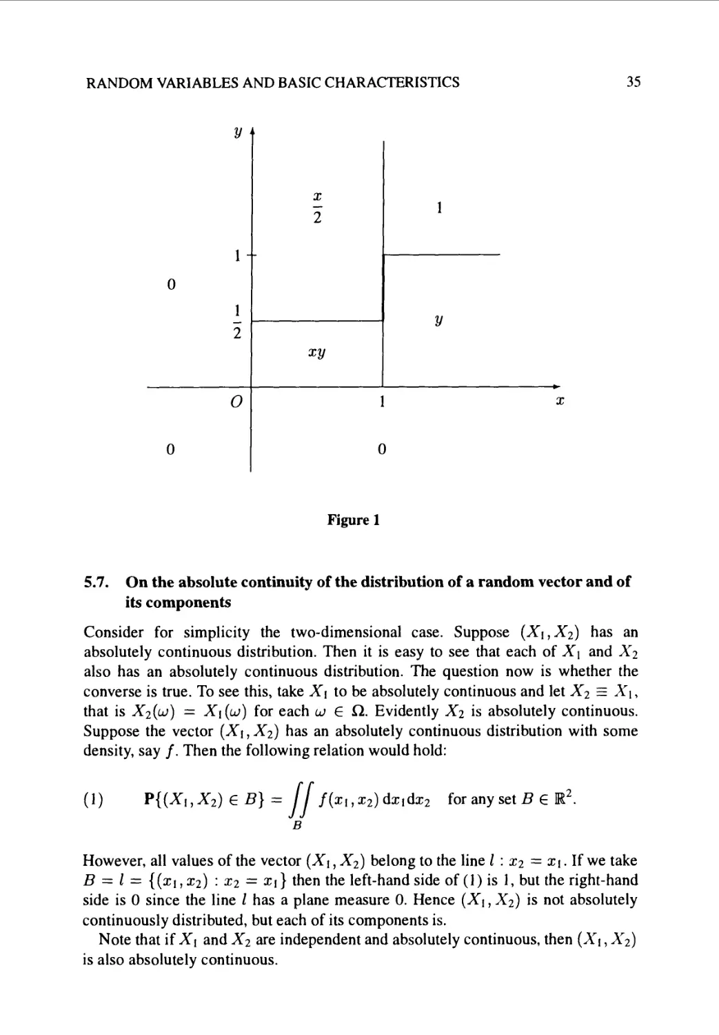
5.6. The Continuity Property of One-Dimensional Distributions 34
May Fail in the Multi-Dimensional Case
5.7. On the Absolute Continuity of the Distribution of a Random 3_5
Vector and of Its Components
5.8. There Are Infinitely Many Multi-Dimensional Probability 36
Distributions with Given Marginals
5.9. The Continuity of a Two-Dimensional Probability Density 37
Does Not Imply That the Marginal Densities Are Continuous

5.10. The Convolution of a Unimodal Probability Density Function 3J5
with Itself Is Not Always Unimodal
5.11. The Convolution of Unimodal Discrete Distributions Is Not 40
Always Unimodal
5.12. Strong Unimodality Is a Stronger Property Than the Usual 40
Unimodality
5.13. Every Unimodal Distribution Has a Unimodal Concentration 4J_
Function, but the Converse Does Not Hold
Section 6. Expectations and Conditional Expectation 42
6.1. On the Linearity Property of Expectations 44
6.2. An Integrable Sequence of Non-Negative Random Variables 4_5
Need Not Have a Bounded Supremum
6.3. A Necessary Condition Which Is Not Sufficient for the 4_5
Existence of the First Moment
6.4. A Condition Which Is Sufficient but Not Necessary for the 46
Existence of Moment of Order (-1) of a Random Variable
6.5. An Absolutely Continuous Distribution Need Not Be 47
Symmetric Even Though All Its Central Odd-Order Moments
Vanish
6.6. A Property of the Moments of Random Variables Which Does 47
Not Have an Analogue for Random Vectors
6.7. On the Validity of the Fubini Theorem 48
6.8 A Non-Uniformly Integrable Family of Random Variables 48
6.9 On the Relation E[E(X|F)] = EX 49
6.10. Is It Possible to Extend One of the Properties of the 49
Conditional Expectation?
6.11. The Mean-Median-Mode Inequality May Fail to Hold 50

6.12. Not All Properties of Conditional Expectations Have 5J_
Analogues for Conditional Medians
Section 7. Independence of Random Variables 5J_
7.1. Discrete Random Variables Which Are Pairwise but Not 53^
Mutually Independent
7.2. Absolutely Continuous Random Variables Which Are Pairwise 52
but Not Mutually Independent
7.3. A Set of Dependent Random Variables Such That Any of Its 54
Subsets Consists of Mutually Independent Variables
7.4. Collection of и Dependent Random Variables Which Are 56
да-Wise Independent
7.5. An Independence-Type Property for Random Variable 57
7.6. Dependent Random Variables Xand Y Such That X2 and Y2 Are 58
Independent
7.7. The Independence of Random Variables in Terms of 59
Characteristic Functions

7.8. The Independence of Random Variables in Terms of 61
Generating Functions
7.9. The Distribution of a Sum Can Be Expressed by the 62
Convolution Even If the Variables Are Dependent
7.10. Discrete Random Variables Which Are Uncorrelated but Not 63
Independent
7.11. Absolutely Continuous Random Variables Which Are 64
Uncorrelated but Not Independent
7.12. Independent Random Variables Have Zero Correlation Ratio, 64
But the Converse Is Not True
7.13. The Relation Е[Щ] = E7 Almost Surely Does Not Imply 65
That the Random Variables X and 7 Are Independent
7.14. There Is No Relationship between the Notions of 65
Independence and Conditional Independence
7.15. Mutual Independence Implies the Exchangeability of Any Set 67
of Random Variables, but Not Conversely
7.16. Different Kinds of Monotone Dependence between Random 67
Variable
Section 8. Characteristic and Generating Functions 68
8.1. Different Characteristic Functions Which Coincide on a Finite 70
Interval but Not On the Whole Real Line
8.2. Discrete and Absolutely Continuous Distributions Can Have 71
Characteristic Functions Coinciding On the Interval [-1, 1]
8.3. The Absolute Value of a Characteristic Function Is Not 72
Necessarily a Characteristic Function
8.4. The Ratio of Two Characteristic Functions Need Not Be a 72
Characteristic Function

8.5. The Factorization of a Characteristic Function into 73
Indecomposable Factors May Not Be Unique
8.6. An Absolutely Continuous Distribution Can Have a 74
Characteristic Function Which Is Not Absolutely Integrable
8.7. A Discrete Distribution Without a First-Order Moment but with 75
a Differentiable Characteristic Function
8.8. An Absolutely Continuous Distribution Without Expectation 75
but with a Differentiable Characteristic Function
8.9. The Convolution of Two Indecomposable Distributions Can 76
Even Have a Normal Component
8.10. Does the Existence of All Moments of a Distribution 77
Guarantee the Analyticity of Its Characteristic and Moment
Generating Functions?
Section 9. Infinitely Divisible and Stable Distributions 78
9. 1. A Non-Vanishing Characteristic Function Which Is Not 79
Infinitely Divisible

9.2. If |ф| Is an Infinitely Divisible Characteristic Function, This 80
Does Not Always Imply That ф Is Also Infinitely Divisible
9.3. The Product of Two Independent Non-Negative and Infinitely 8j_
Divisible Random Variables Is Not Always Infinitely Divisible
9.4. Infinitely Divisible Products of Non-Infinitely Divisible 82
Random Variables
9.5. Every Distribution Without Indecomposable Components Is 83_
Infinitely Divisible, but the Converse Is Not True
9.6. A Non-Infinitely Divisible Random Vector with Infinitely 83_
Divisible Subsets of Its Coordinates
9.7. A Non-Infinitely Divisible Random Vector with Infinitely 84
Divisible Linear Combinations of Its Components
9.8. Distributions Which Are Infinitely Divisible but Not Stable 85
9.9. A Stable Distribution Which Can Be Decomposed into Two 86
Infinitely Divisible but Not Stable Distributions
Section 10. Normal Distribution 87
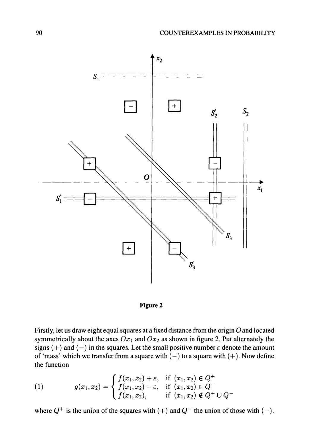
10.1. Non-Normal Bivariate Distributions with Normal Marginals 8^
10.2. If (Xi, X2) Has a Bivariate Normal Distribution Then Д X2 and 89
X\ + X2 are Normally Distributed, but Not Conversely
10.3. A Non-Normally Distributed Random Vector Such That Any 91
Proper Subset of Its Components Consists of Jointly Normally
Distributed and Mutually Independent Random Variables
10.4. The Relationship between Two Notions: Normality and 92
Uncorrelatedness
10.5. It Is Possible ThatX, 7, X+ 7, X- 7 Are Each Normally 94
Distributed, X and Y Are Uncorrelated, but (X, 7) Is Not Bivariate
Normal

10.6. If the Distribution of (Xu..., Xn) Is Normal, Then Any Linear 94
Combination and Any Subset of Xh..., Xn is Normally Distributed,
but There Is a Converse Statement Which Is Not True
10.7. The Condition Characterizing the Normal Distribution by 96
Normality of Linear Combinations Cannot Be Weakened
10.8. Non-Normal Distributions Such That All or Some of the 97
Conditional Distributions Are Normal
10.9. Two Random Vectors with the Same Normal Distribution Can 98
Be Obtained in Different Ways from Independent Standard Normal
Random Variables
10.10. A Property of a Gaussian System May Hold Even for 99
Discrete Random Variables
Section 11. The Moment Problem Ш
11.1. The Moment Problem for Powers of the Normal Distribution 101
11.2. The Lognormal Distribution and the Moment Problem 102

11.3. The Moment Problem for Powers of an Exponential 105
Distribution
11.4. A Class of Hyper-Exponential Distributions with an 105
Indeterminate Moment Problem
11.5. Different Distributions with Equal Absolute Values of the 107
Characteristic Functions and the Same Moments of All Orders
11.6. Another Class of Absolutely Continuous Distributions 108
Which Are Not Determined Uniquely by Their Moments
11.7. Two Different Discrete Distributions on a Subset of 109
Natural Numbers Both Having the Same Moments of All Orders
11.8. Another Family of Discrete Distributions with the Same 110
Moments of All Orders
11.9. On the Relationship between Two Sufficient Conditions 111
for the Determination of the Moment Problem
11.10. The Carleman Condition is Sufficient but Not Necessary 113
for the Determination of the Moment Problem
11.11. The Krein Condition is Sufficient but Not Necessary for 114
the Moment Problem to Be Indeterminate
11.12. An Indeterminate Moment Problem and Non-Symmetric 115
Distributions Whose Odd-Order Moments All Vanish
11.13. A Non-Symmetric Distribution with Vanishing 115
Odd-Order Moments Can Coincide with the Normal
Distribution Only Partially
Section 12. Characterization Properties of Some Probability 116
Distributions
12.1. A Binomial Sum of Non-Binomial Random Variables 117
12.2. A Property of the Geometric Distribution Which Is Not Its Д8
Characterization Property

12.3. If the Random Variables X, Y and Their Sum X+ 7Each П8
Have a Poisson Distribution,This Does Not Imply That Xand Y
Are Independent
12.4. The Raikov Theorem Does Not Hold Without the Д9
Independence Condition
12.5. The Raikov Theorem Does Not Hold for a Generalized 120
Poisson Distribution of Order k, & > 2
12.6. A Case When the Cramer Theorem Is Not Applicable 121
12.7. A Pair of Unfair Dice May Behave Like a Pair of Fair Dice 121
12.8. On Two Properties of the Normal Distribution Which Are 122
Not Characterizing Properties
12.9. Another Interesting Property Which Does Not Characterize the 125
Normal Distribution

12.10. Can We Weaken Some Conditions under Which Two 126
Distribution Functions Coincide?
12.11. Does the Renewal Equation Determine Uniquely the 127
Probability Density?
12.12. A Property Not Characterizing the Cauchy Distribution 128
12.13. A Property Not Characterizing the Gamma Distribution 128
12.14. An Interesting Property Which Does Not Characterize 129
Uniquely the Inverse Gaussian Distribution
Section 13. Diverse Properties of Random Variables 130
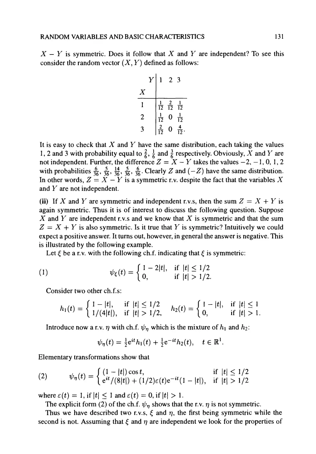
13.1. On the Symmetry Property of the Sum or the Difference of 130
Two Symmetric Random Variables
13.2. When Is a Mixture of Normal Distributions Infinitely 132
Divisible?
13.3. A Distribution Function Can Belong to the Class IFRA but Д3_
Not to FR
13.4. A Continuous Distribution Function of the Class NBU Which 134
Is Not of the Class IFR
13.5. Exchangeable and Tail Events Related to Sequences of Д4
Random Variables
13.6. The de Finetti Theorem for an Infinite Sequence of 136
Exchangeable Random Variables Does Not Always Hold for a
Finite Number of Such Variables
13.7. Can we Always Extend a Finite Set of Exchangeable Random 137
Variables?
13.8. Collections of Random Variables Which Are or Are Not 138
Independent and Are or Are Not Exchangeable
13.9. Integrable Randomly Stopped Sums with Non-Integrable
Stopping Times

Part 3. Limit Theorems 141
Section 14. Various Kinds of Convergence of Sequences of Random 143
Variables
14.1. Convergence and Divergence of Sequences of Distribution 144
Functions
14.2. Convergence in Distribution Does Not Imply Convergence in 145
Probability
14.3. Sequences of Random Variables Converging in Probability 146
but Not Almost Surely
14.4. On the Borel-Cantelli Lemma and Almost Sure Convergence 147
14.5. On the Convergence of Sequences of Random Variables in 148
Zr-Sense for Different Values of r
14.6. Sequences of Random Variables Converging in Probability 148
but Not in Lr"Sense

14.7. Convergence in Zr-Sense Does Not Imply Almost Sure 149
Convergence
14.8. Almost Sure Convergence Does Not Necessarily Imply 150
Convergence in Zr-Sense
14.9. Weak Convergence of the Distribution Functions Does Not 151
Imply Convergence of the Densities
14.10. The Convergence Xn —* % and У» —* ^ Does Not Always 152
Imply That X„ + Y* -Л X + Y
14.11. The Convergence in Probability ^« —* X Does Not Always 152
Imply That s(xn) —* JPO.for Any Function g
14.12. Convergence in Variation Implies Convergence in 153
Distribution but the Converse Is Not Always True
14.13. There Is No Metric Corresponding to Almost Sure 155
Convergence
14.14. Complete Convergence of Sequences of Random Variables 155
Is Stronger Than Almost Sure Convergence
14.15. The Almost Sure Uniform Convergence of a Random 156
Sequence Implies Its Complete Convergence, but the Converse Is
Not True
14.16. Converging Sequences of Random Variables Such That the J_56
Sequences of the Expectations Do Not Converge
14.17. Weak b'-Convergence of Random Variables is Weaker Than 157
Both Weak Convergence and Convergence in L1 -Sense
14.18. A Converging Sequence of Random Variables Whose 158
Cesaro Means Do Not Converge
Section 15. Laws of Large Numbers 159
15.1. The Markov Condition is Sufficient but Not Necessary for the 161
Weak Law of Large Numbers

15.2. The Kolmogorov Condition for Arbitrary Random Variables 162
is Sufficient but Not Necessary for the Strong Law of Large
Numbers
15.3. A Sequence of Independent Discrete Random Variables Jj53_
Satisfying the Weak but Not the Strong Law of Large Numbers
15.4. A Sequence of Independent Absolutely Continuous Random 164
Variables Satisfying the Weak but Not the Strong Law of Large
Numbers
15.5. The Kolmogorov Condition ?^i аУп* < °° Is the Best 165
Possible Condition for the Strong Law of Large Numbers
15.6. More on the Strong Law of Large Numbers Without the 165
Kolmogorov Condition
15.7. Two 'near' Sequences of Random Variables Such That the Jj56
Strong Law of Large Numbers Holds for One of Them and Does
Not Hold for the Other

15.8. The Law of Large Numbers Does Not Hold If Almost Sure 167
Convergence Is Replaced by Complete Convergence
15.9. The Uniform Boundedness of the First Moments of a Tight 167
Sequence of Random Variables Is Not Sufficient for the Strong
Law of Large Numbers
15.10. The Arithmetic Means of a Random Sequence Can Converge 168
in Probability Even If the Strong Law of Large Numbers Fails to
Hold
15.11. The Weighted Averages of a Sequence of Random Variables 169
Can Converge Even If the Law of Large Numbers Does Not Hold
15.12. The Law of Large Numbers with a Special Choice of 170
Norming Constants
Section 16. Weak Convergence of Probability Measures and 171
Distributions
16.1. Defining Classes and Classes Defining Convergence 173
16.2. In the Case of Convergence in Distribution, Do the 174
Corresponding Probability Measures Converge for All Borel Sets?
16.3. Weak Convergence of Probability Measures Need Not Be 175
Uniform
16.4. Two Cases When the Continuity Theorem Is Not Valid 176
16.5 Weak Convergence and Levy Metric 177
16.6 A Sequence of Probability Density Functions Can Converge in 178
the Mean of Order 1 Without Being Converging Everywhere
16.7. A Version of the Continuity Theorem for Distribution 179
Functions Which Does Not Hold for Some Densities
16.8. Weak Convergence of Distribution Functions Does Not Imply 180
Convergence of the Moments

16.9. Weak Convergence of a Sequence of Distributions Does Not 182
Always Imply the Convergence of the Moment Generating
Functions
16.10. Weak Convergence of a Sequence of Distribution Functions 182
Does Not Always Imply Their Convergence in the Mean
Section 17. Central Limit Theorem 183
17.1. Sequences of Random Variables Which Do Not Satisfy the 184
Central Limit Theorem
17.2. How is the Central Limit Theorem Connected with the Feller 186
Condition and the Uniform Negligibility Condition?
17.3. Two 'Equivalent' Sequences of Random Variables Such That 186
One of Them Obeys the Central Limit Theorem While the Other
Does Not

17.4. If the Sequence of Random Variables {Xn} Satisfies the 187
Central Limit Theorem, What Can We Say about the Variance of
17.5. Not Every Interval Can Be a Domain of Normal Convergence 188
17.6. The Central Limit Theorem Does Not Always Hold for 189
Random Sums of Random Variables
17.7. Sequences of Random Variables Which Satisfy the Integral 189
but Not the Local Central Limit Theorem
Section 18. Diverse Limit Theorems 192
18.1. On the Conditions in the Kolmogorov Three-Series Theorem 192
18.2. The Independency Condition is Essential in the Kolmogorov 193
Three-Series Theorem
18.3. The Interchange of Expectations and Infinite Summation Is 195
Not Always Possible
18.4. A Relationship between a Convergence of Random Sequences 195
and Convergence of Conditional Expectations
18.5. The Convergence of a Sequence of Random Variables Does ^96
Not Imply That the Corresponding Conditional Medians Converge
18.6. A Sequence of Conditional Expectations Can Converge Only 196
on a Set of Measure Zero
18.7. When Is a Sequence of Conditional Expectations Convergent 197
Almost Surely?
18.8. The Weierstrass Theorem for the Unconditional Convergence 198
of a Numerical Series Does Not Hold for a Series of Random
Variables
18.9. A Condition Which Is Sufficient but Not Necessary for the 199
Convergence of a Random Power Series

18.10. A Random Power Series Without a Radius of Convergence 200
in Probability
18.11. Two Sequences of Random Variables Can Obey the Same 201
Strong Law of Large Numbers but One of Them May Not Be in the
Domain of Attraction of the Other
18.12. Does a Sequence of Random Variables Always Imitate 202
Normal Behaviour?
18.13. On the Chover Law of Iterated Logarithm 204
18.14. On Record Values and Maxima of a Sequence of Random 205
Variables
Part 4. Stochastic Processes 207
Section 19. Basic Notions on Stochastic Processes 209
19.1. Is It Possible to Find a Probability Space on Which Any 210
Stochastic Process Can Be Defined?

19.2. What Is the Role of the Family of Finite-Dimensional 211
Distributions in Constructing a Stochastic Process with Specific
Properties?
19.3. Stochastic Processes Whose Modifications Possess Quite 212
Different Properties
19.4. On the Separability Property of Stochastic Processes 213
19.5. Measurable and Progressively Measurable Stochastic 214
Processes
19.6. On the Stochastic Continuity and the Weak b'-Continuity of 217
Stochastic Processes
19.7. Processes Which are Stochastically Continuous but Not 2J9
Continuous Almost Surely
19.8. Almost Sure Continuity of Stochastic Processes and the 219
Kolmogorov Condition
19.9. Does the Riemann or Lebesgue Integrability of the Covariance 220
Function Ensure the Existence of the Integral of a Stochastic
Process?
19.10. The Continuity of a Stochastic Process Does Not Imply the 223
Continuity of Its Own Generated Filtration, and Vice Versa
Section 20. Markov Processes 224
20.1. Non-Markov Random Sequences Whose Transition Functions 226
Satisfy the Chapman-Kolmogorov Equation
20.2. Non-Markov Processes Which Are Functions of Markov 227
Processes
20.3. Comparison of Three Kinds of Ergodicity of Markov Chains 229
20.4. Convergence of Functions of an Ergodic Markov Chain 232
20.5. A Useful Property of Independent Random Variables Which 233
Cannot be Extended to Stationary Markov Chains

20.6. The Partial Coincidence of Two Continuous-Time Markov 234
Chains Does Not Imply That the Chains Are Equivalent
20.7. Markov Processes, Feller Processes, Strong Feller Processes 235
and Relationships between Them
20.8. Markov but Not Strong Markov Processes 236
20.9. Can a Differential Operator of Order к > 2 Be an Infinitesimal 238
Operator of a Markov Process?
Section 21. Stationary Processes and Some Related Topics 239
21.1. On the Weak and the Strict Stationary Properties of Stochastic 240
Processes
21.2. On the Strict Stationarity of a Given Order 24J_
21.3. The Strong Mixing Property Can Fail If We Consider a 242
Functional of a Strictly Stationary Strong Mixing Process

21.4. A Strictly Stationary Process Can Be Regular but Not 243
Absolutely Regular
21.5. Weak and Strong Ergodicity of Stationary Processes 244
21.6. A Measure-Preserving Transformation Which Is Ergodic but 246
Not Mixing
21.7. On the Convergence of Sums of ф-mixing Random Variables 248
21.8. The Central Limit Theorem for Stationary Random Sequences 248
Section 22. Discrete-Time Martingales 250
22.1. Martingales Which Are L^Bounded but Not L^Dominated 251
22.2. A Property of a Martingale Which Is Not Preserved Under 252
Random Stopping
22.3. Martingales for Which the Doob Optional Theorem Fails to 254
Hold
22.4. Every Quasimartingale Is an Amart, but Not Conversely 255
22.5. Amarts, Martingales in the Limit, Eventual Martingales and 256
Relationships between Them
22.6. Relationships between Amarts, Progressive Martingales and 257
Quasimartingales
22.7. An Eventual Martingale Need Not Be a Game Fairer with 258
Time
22.8. Not Every, Martingale-Like Sequence Admits a Riesz 258
Decomposition
22.9. On the validity of Two Inequalities for Martingales 259
22.10. On the Convergence of Submartingales Almost Surely and in 260
L^Sense

22.11. A Martingale May Converge in Probability but Not Almost 261
Surely
22.12. Zero-Mean Martingales Which Are Divergent with a Given 263
Probability
22.13. More on the Convergence of Martingales 264
22.14. A Uniformly Integrable Martingale with a Nonintegrable 265
Quadratic Variation
Section 23. Continuous-Time Martingales 267
23.1. Martingales Which Are Not Locally Square Integrable 268
23.2. Every Martingale Is a Weak Martingale but the Converse Is 269
Not Always True
23.3. The Local Martingale Property Is Not Always Preserved under 270
Change of Time
23.4. A Uniformly Integrable Supermartingale Which Does Not 271
Belong to Class (D)
23.5. L^-Bounded Local Martingale Which Is Not a True Martingale 272
23.6. A Sufficient but Not Necessary Condition for a Process to Be 274
a Local Martingale

23.7. A Square lntegrable Martingale with a Non-Random 275
Characteristic Need Not Be a Process with Independent Increments
23.8. The Time-Reversal of a Semimartingale Can Fail to Be a 276
Semimartingale
23.9. Functions of Semimartingales Which Are Not 276
Semimartingales
23.10. Gaussian Processes Which Are Not Semimartingales 277
23.11. On the Possibility of Representing a Martingale As a 279
Stochastic Integral with Respect to Another Martingale
Section 24. Poisson Process and Wiener Process 280
24.1. On Some Elementary Properties of the Poisson Process and 281
the Wiener Process
24.2. Can the Poisson Process Be Characterized by Only One of It 283
Properties?
24.3. The Conditions under Which a Process Is a Poisson Process 284
Cannot Be Weakened
24.4. Two Dependent Poisson Processes Whose Sum Is Still a 286
Poisson Process
24.5. Multidimensional Gaussian Processes Which Are Close to the 287
Wiener Process
24.6. On the Wald identities for the Wiener process 288
24.7. Wald identity and a non-uniformly integrable martingale 290
based on the Wiener process
24.8. On Some Properties of the Variation of the Wiener Process 291
24.9. A Wiener Process with Respect to Different Filtrations 293
24.10. How to Enlarge the Filtration and Preserve the Markov 294
Property of the Brownian Bridge

Section 25. Diverse Properties of Stochastic Processes 295
25.1. How Can We Find the Probabilistic Characteristics of a 296
Function of a Stationary Gaussian Process?
25.2. Cramer Representation, Multiplicity and Spectral Type of 297
Stochastic Processes
25.3. Weak and strong Solutions of Stochastic Differential 300
Equations
25.4. A Stochastic Differential Equation Which Does Not Have a 302
Strong Solution but For Which a Weak Solution Exists and Is
Unique
Supplementary Remarks 305
References 317
Index 339

PREFACE TO THE SECOND EDITION
A large amount of newly collected and created material and the lively interest in the first edition of this book
(CEP-1) motivated me towards the second edition (CEP-2). Actually, I have never stopped looking for new
counterexamples or thinking about how to achieve completeness and clarity as far as possible in this work.
My strategy was to keep the best from CEP-1, replace some examples by new and more attractive ones and
add entirely new examples taken from recent publications or invented especially for CEP-2. Thus the reader
will find several original topics well supplementing the material in CEP-1.
Among the topics essentially extended are independence/dependence/exchangeability properties of sets of
random events and random variables, characterization of probability distributions, the moment problem,
martingales and limit theorems. Clearer interpretations of many statements and improvements in presentation
have been made in all sections. The text of CEP-2 is more compact. However, much material has remained
unused in order to keep the book a reasonable size. The Index, Supplementary Remarks and the References
have been updated and extended accordingly.
My work on CEP-2 took a long time and, as always, my enthusiasm was based on my strong belief about the
importance of the role of counterexamples to everyone teaching or learning probability theory. Additional
stimuli came from the positive reactions of so many colleagues in so many countries. Like many others I
experienced difficulties during this time and first had to solve the problem of how to survive in this changing
and unpredictable world. I now use this opportunity to express sincere thanks to many colleagues and friends
for their attention and support during my visits to several universities in The Netherlands, Great Britain,
Russia, Italy, Canada, USA, France and Spain. In particular, large portions of CEP-2 were prepared when I
was visiting Queen's University (Kingston, Ontario) and Miami University (Oxford, Ohio). The last stages of
this work were undertaken during a recent visit to Universite Joseph Fourier (Grenoble) and in Sofia just
before my trip to Kentucky.
I am very grateful for my collaboration with John Wiley & Sons (Chichester). The attention, the patience and
the help of Helen Ramsey and Jenny Smith were much appreciated. My thanks go to them and to all the staff
at Wiley.

Finally, I hope that you, the reader, will benefit from this edition and my belief that new counterexamples
will be created as an essential part of the further development of probability theory. As before, any new
suggestions are welcome!
July/August 1996
Europe/America
Jordan Stoyanov

PREFACE TO THE FIRST EDITION
General comments. We have used the term counterexample in the same sense as generally accepted in
mathematics. Three previous books related to counterexamples: on analysis (Gelbaum and Olmsted 1964), on
topology (Steen and Seebach 1978) and on graph theory (Capobianco and Molluzzo 1978), have been and
still are popular among mathematicians. The present book is a collection of counterexamples covering
important topics in the field of probability theory and stochastic processes.
It is not only traditional theorems, proofs and illustrative examples, but also counterexamples, which reflect
the power, the width, the depth, the degree of nontriviality and the beauty of the theory.
If we have found necessary and sufficient conditions for some statement or result, then any change in the
conditions implies that the result is false and accordingly the statement has to be modified. Our attention is
focused on interesting questions concerning: (a) the necessity of some sufficient conditions; (b) the
sufficiency of certain necessary conditions; (c) the validity of a statement which is the converse to another
statement. However, we have included some useful and instructive examples which can be interpreted as
counterexamples in a generalized sense.
Purpose of the book. The present book is intended to serve as a supplementary source for many courses in
the field of probability theory and stochastic processes. The topics dealt with in the book, and the level of
counterexamples, are chosen in such a way that it becomes a multi-purpose book. Firstly, it can be used for
any standard course in probability theory for undergraduates. Secondly, some of the material is suitable for
advanced courses in probability theory and stochastic processes, assuming that the students have had a course
in measure theory and function theory. Thirdly, young researchers and even professionals will find the book
useful and may discover new and strange results. The wide variety of content and detail in the discussions of
the counterexamples may also help lecturers and tutors in their teaching.
It should be noted that some of the examples considered in the book give the reader an opportunity to become
more familiar with standard results in probability and stochastic processes and to develop a better
understanding of the subject. However, there exist some examples which are more difficult and their
mastering requires a considerable amount of additional work.

Content and structure of the book. The present book includes a relatively large number of
counterexamples. Their choice was not easy. We have tried to include a variety of counterexamples
concerning different topics in probability theory and stochastic processes. Though we have avoided trivial
examples, we have nonetheless included some which cover elementary matters. Pathological examples have
been completely avoided. The examples which are most useful and interesting fall in between these two
categories.
The material of the book is divided into 4 chapters and 25 sections. Each section begins with short
introductory notes giving basic definitions and main results. Then we present the counterexamples related to
the main results, the motivation for questions and the counter-statements. Some notions and results are given
and analysed in the counterexamples themselves. All counterexamples are named and numbered for the
convenience of readers.
The counterexamples range over various degrees of difficulty. Some are elementary and well known
counterexamples and can be classified as a part of a probabilistic folklore. Also the style of presentation
needs to vary. Some of the counterexamples are only briefly described to economize on space and to provide
the reader with a chance for independent work.
Readers of the book are assumed to be familiar with the basic notions and results in probability theory and
stochastic processes. Some references are given to textbooks and lecture notes which provide the necessary
background to the subject.
At the end of the book, Supplementary Remarks are included providing references and some additional
explanations for the majority of the counterexamples. For most of the examples we have given at least one
relevant early reference. Many of the counterexamples originate from individual probabilists and statisticians
and we have cited them fully. Other sources are also indicated where the reader can find new
counterexamples, ideas for such examples or some questions whose answers would lead to interesting and
useful counterexamples. The Supplementary Remarks give readers the opportunity for further work.
Note about references. References Dudley A972) and (Dudley 1976) indicate a paper or book published by
Dudley in 1972 or 1976 respectively. For convenience we have devised abbreviated names for the principal
journals in the field of probability theory, stochastic processes and mathematical statistics. In all other cases
standard international abbreviations are used.
History of the book. The book is a result of 16 years of my study in the field of probability theory and
stochastic processes. I started to collect counterexamples in 1970 when I was a student at Moscow University
and later it became an intriguing preoccupation. As a result I increased the number of counterexamples to 500
or so. Many of the counterexamples or different versions of them belong to other authors. Some new and
fresh counterexamples were created by colleagues and friends especially for this book. During the
preparation of the book I have been guided by my own experience in lecturing on these topics in several
European and Canadian universities and in giving special seminars in recent years for students of Sofia

University.
The international character of the book is obvious. It is not only my opinion that the present book is an
example, not a counterexample, of a successful collaboration and friendship among mathematicians from
different countries. Acknowledgements. The selection and presentation of the material in the book, aimed at
covering the wide field of probability theory and stochastic processes, has not been an easy task. I was
grateful for the opportunity to discuss the project with my many colleagues and friends whose advice and
valuable suggestions were extremely helpful. I wish to express my thanks to all of them.
My special thanks are addressed to my teachers Prof. B. V. Gnedenko, Prof. Yu. V. Prohorov and Prof. A. N.
Shiryaev for their attention, general and specific suggestions and encouragement. Among colleagues and
friends I have to mention N. V. Krylov, R. Sh. Liptser, A. A. Novikov, Yu. M. Kabanov, S. E. Kuznetsov, A.
M. Zubkov, O. B. Enchev and S. D. Gaidov with whom I had very useful discussions on several concrete
topics.
My thanks are directed to all colleagues who were so kind as to send me their specific suggestions. The
names of these colleagues are included in the list of references.
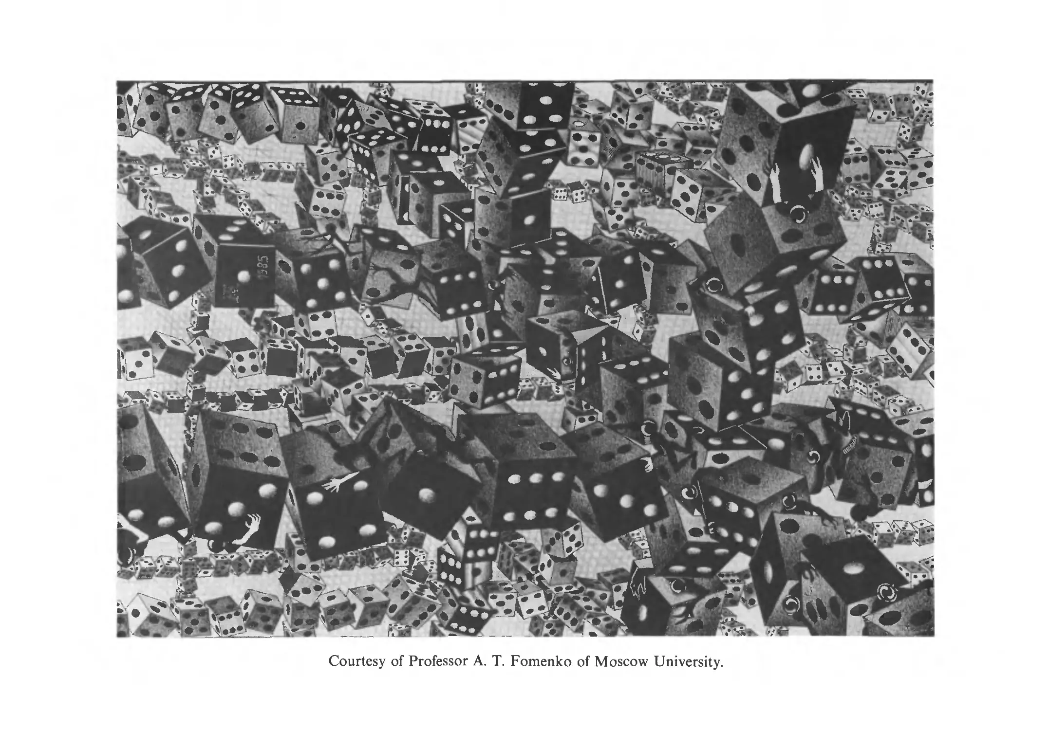
I use the opportunity to express my special grateful to Prof. A. T. Fomenko for providing five of his
extraordinary drawings especially for this book.
I wish to thank Prof. D. G. Kendall for his interest to my work and for his constructive suggestions and
encouragement.
The comments of the anonymous referees and the editor helped me to improve both the content and the style
of the presentation. I express my appreciation to them.
Finally I should like to thank the collaborators of John Wiley & Sons (Chichester) for their patience and for
their precise and excellent work. It is my pleasure to mention the names of Charlotte Farmer and Ian
Mclntosh.
Suggestions and comments from readers are most welcome and will, if appropriate, be reflected in any
subsubsequent editions of the book.
JUNE 1986, SOFIA
JORDAN STOYANOV

Part 1
Classes of Random Events and
Probabilities

Courtesy of Professor A. T. Fomenko of Moscow University.

CLASSES OF RANDOM EVENTS AND PROBABILITIES 3
SECTION 1. CLASSES OF RANDOM EVENTS
Let Q, be an arbitrary non-empty set. Its elements, denoted by u>, will be interpreted
as outcomes (results) of some experiment. As usual, we use A U В and An В (as
well AB) to represent the union and the intersection of any two subsets A and В of
Q. respectively. Also, Ac is the complement of А С Q. In particular, Qc — 0 where 0
is the empty set.
The class Л of subsets of Q. is called a field if it contains Q and is closed under the
formation of complements and finite unions, that is if:
(a) QeA;
(Ъ)АеЛ=>АсеЛ;
(с) AUA2 е Л => Л, U Аг е А.
Taking into account the so-called de Morgan laws, (A\Ai)c = A] U A\ and
(A\ U A2)c = A^A^, we easily see that (c) can be replaced by the condition
(c') A\, A2 e Л => A\ A2 e Л.
Thus Л is closed under finite intersections.
The class 3~ of subsets of Q, is called a <7-field if it is a field and if it is closed under
the formation of countable unions, that is if:
Again, as above, condition (d) can be replaced by
(d')AuA2,...,e 7=>f]^=]Ane 7
and clearly the <7-field 7 is closed under countable intersections.
Recall that the elements of any field or <j-field are called random events (or simply,
events). Other classes of events, such as the semi-field, D-system, and product of
(j-fields, will be defined and compared with each another in the examples below.
Any textbook on probability theory contains a detailed presentation of all these
basic ideas (see Kolmogorov 1956;Breiman 1968; Gihman and Skorohod 1974/1979;
Chung 1974;Neveu 1965; Chow andTeicher 1978; Billingsley 1995;Shiryaev 1995).
The examples given in this section concern some of the properties of different classes
of random events and examine the relationship between notions which seem to be
close to one another.
1.1. A class of events which is a field but not a cr-field
Let Q. — [0, oo) and J\ be the class of all intervals of the type [a, b) or [a, oo) where
0 < a < b < oo. Denote by 72 the class of all finite sums of intervals of J\. Then
7\ is not a field, and J2 is a field but not a <7-field.
Take arbitrary numbers a and b, 0 < a < b < oo. Then A = [a, b) G 3~i. However,
Ac = [0, a) U [b, oo) ф Ji and thus Jj is not a field.

4 COUNTEREXAMPLES IN PROBABILITY
It is easy to see that: (i) the finite union of finite sums of intervals (of J\) is again
a sum of intervals; (ii) the complement of a finite sum of intervals is also a sum of
intervals. This means that 3 is a field. However, J2 is not a <7-field because, for
example, the set An = [0,1/n) G 3\ for each n = 1,2,..., and the intersection
iXLi An = {0} does not belong to 7\.
Let us look at two additional cases.
(ai)LetQ = R1 and 3" be the class of all finite sums of intervals of the type ( — сю, a],
F, c] and (d, oo). Then 3*is a field. But the intersection H^Li (^ ~ Vn> cl 's e4ua't0
[6, c] which does not belong to 3". Hence the field 3" is not a <j-field.
(a2) Let Q. be any infinite set and Л the collection of all subsets A e Q such that
either A or its complement Ac is finite. Then it is easy to see that Л is a field but not
a G-field.
1.2. A class of events can be closed under finite unions and finite intersections
but not under complements
Let Q. = E1 and the class Л consist of intervals of the type (x, oo), x G П. Then
using the notations и = х А у := min{:r, y} and v — x V у :— тах{ж, у} we have:
(x, oo) U (у, oo) = (и, oo) G Л
(x, oo) П (j/, oo) = (v, oo) G Л.
However, (ж, oo)c = ( — oo, x] ? Л.
1.3. A class of events which is a semi-field but not a field
Let Q be an arbitrary set. A non-empty class 0 of subsets of Q. is called a semi-field
if Q G 0, 0 G 3, 3 is closed under the formation of finite intersections, and the
complement of any set in 0 is a finite sum of disjoint sets of 0. It is easy to see that any
field of subsets of Q. is also a semi-field. However, the following simple examples
show that the converse is not true.
(ai)LetQ = [-oo, oo) and^i contain Q, {oo} and all intervals of the type [a, b) where
-oo < a < b < oo.Then0 G 3\, Q G 3\, [ab b{ n[a2,b2) = [aj Va2,b, Л b2) G 3\
and [a, b)c = [—oo, a) U [b, oo). So 0\ is a semi-field. Obviously 3\ is not a field.
(a2) Take Q = E1 and denote by 32 the class of all subsets of the form AB (= A n B)
where A is a closed and Б is an open set in Q. Then again, 32 is a semi-field but not
a field.
1.4. A G-field of subsets of Q, need not contain all subsets of Q,
Recall that the set Л G Q is called a co-finite set if its complement Ac is finite. Let
J\ consist of the finite and co-finite subsets of Q. Then J\ is a field. It is a a-udd iff
Q is finite.

CLASSES OF RANDOM EVENTS AND PROBABILITIES 5
Further, the set A G Q is called a co-countable set if Ac is countable. Let 72 consist
of the countable and the co-countable subsets of Q. Then it is easy to check that "Jj
is a (j-field.
Suppose now that Q. is uncountable. Then Q. contains a subset A such that A and
Ac are both uncountable. This shows that in general a <j-field of Q. need not contain
all subsets of Q. and need not be closed under the formation of arbitrary uncountable
unions.
1.5. Every (j-field of events is a D-system, but the converse does not always
hold
A system D of subsets of a given set Q. is called a D-system (Dynkin system) in Q. if the
following three conditions hold: (i)Q G V;(n)A,B eVandAc В ^ B\A G T>;
(Hi) An G ?>, n = 1,2,... and Ax С А2 С ... => ЦГ=1 An е ?•
It is obvious that every <j-field is a D-system, but the converse may not be true, as
can be seen in the following example.
Take Q. = {u>\,u>2, ¦ ¦. ,u>2n}, n G N. Denote by De the collection of all subsets
D G Q. consisting of an even number of elements. Conditions (i), (ii) and (iii)
above are satisfied, and hence De is a D-system. However, if n > 1 and we
take A = {uj\,uj2} and В = {uj2,u>t,}, we see that A G De, В е T)e and
А В = {ujj} ? T>e. Thus De is not even a field and hence not a (j-field.
Note that a D-system V is a a-field iff the intersection of any two sets in D is again
in T> (see Dynkin 1965; Bauer 1996).
1.6. Sets which are not events in the product <j-field
Given two arbitrary sets Q] and Q2. we denote their product by Q.\ x Q2-
Qi x Q.x := {(ыьЫг)} : uj\ G Qi,W2 ^ ^2- For any set A G Qi x fl2 we denote
by Au)] the section of A at uj\\ Au)] — {0^2 G Q2 : (^1,^2) G ^4}- Analogously,
АШ2 = {uji G п\ : (wi,?J2) G Л} .
A rectangle in Q.\ x Q2 is a subset of the form
A\ x A2 = {(^1,ы2) : ал G A,uj2 G Л2}, Ai G Пь Л2 G Q2-
Л] x Ai is called a measurable rectangle (with respect to J\ and Э"г) if Ai G 3"i
and Л2 G Э~2 where Ji and J2 are <j-fields of subsets of Q.\ and Q2 respectively.
The measurable rectangles form a semi-field of subsets in Q.\ x Q2- Thus the
field generated by the measurable rectangles consists of all finite sums of disjoint
measurable rectangles. The <j-field generated by this field is denoted by "J\ x "Ji and
is called the product <j-field of "J\ and J2-
Let us note the following result (see Neveu 1965; Kingman and Taylor 1966). For
every measurable set A in (Q] хЙ2Д| xJ2) and every fixed u>\ G O.\ and u>2 G П2,
the sections Au)i and АШ2 are measurable sets in (Q2, ^2) and (Q\, 7\) respectively.
However, the converse is not true. To see this, let Q. be any uncountable set and

6 COUNTEREXAMPLES IN PROBABILITY
3" the smallest ст-field of subsets of Q. containing all one-point elements. Then the
diagonal D = {{u>,u>) : u> G Q.} of Q. x Q. does not belong to the product ст-field
JxJ, although all its sections belong to J. In other words, for each u> G Q, the
section -Dw G 3" and is an event but D ? 3" x 3" and is not an event.
1.7. The union of a sequence of cr-fields need not be a cr-field
Let 3"i, 3,... be a sequence of ст-fields of subsets of the set Q. Then their intersection
n^Li 3"n is always a ст-field and it is natural to ask whether the union (J^Li 3"n is a
ст-field. We shall now show that the answer to this question is negative.
Consider the set Q. = {uj\,uj2,u>j} and the following two classes of its subsets:
?, = {0, {uji},{uj2,uj3},u}, ?2 = {0,{ы2},{^ь^з},"}. Then ?, and J2 are
fields and hence ст-fields. Obviously the intersection 3"i П Э"г = {0,^}. the trivial
ст-field. However, the union
is not a field, and hence not a ст-field because the element {o^i} U [uj] = {u>\,
3".
SECTION 2. PROBABILITIES
Let Q be any set and Л be a field of its subsets. We say that P is a probability on
the measurable space (Q, Л) if P is defined for all events A e Л and satisfies the
following axioms.
(a) Р(Л) > 0 for each A e Л; P(Q) = 1.
(b) P is finitely additive. That is, for any finite number of pairwise disjoint events
A\,..., An G Л we have
n
(c) P is continuous at 0. That is, for any events A\, Л2,... € Л such that
An+l С Лп and flJLi ^n = 0, it is true that
lim Р(Л„) = О.
n—>oo
Note that conditions (b) and (c) are equivalent to the next one (d).
(d) P is ст-additive (countably additive), that is
for any events A\,A2,... € Л which are pairwise disjoint.

CLASSES OF RANDOM EVENTS AND PROBABILITIES 7
According to the Caratheodory theorem (see Kolmogorov 1956; Loeve 1977;
Shiryaev 1995), if Po is a <7-additive probability on (Q, A) andJ= <т(Л) denotes the
smallest <j-field generated by the field A, then there is a unique probability measure
P on (Q, 7) which is an extension of Po in the sense that P(A) — Po(^4) for A e A.
In this case we also say that Po is a restriction of P over A and write P\A = Po-
The ordered triplet (Q, J, P) is called a probability space if:
Q. is any set of points called elementary events (outcomes);
7 is a (j-field of subsets of Q; the elements of 3" are events;
P is a probability on J, that is P satisfies conditions (a), (b) and (c) above, or,
equivalently, (a) and (d).
Thus we have described the axiomatic system which is generally accepted in
probability theory. This system was suggested by A. N. Kolmogorov in 1933 (see
Kolmogorov 1956).
In this section we present a few examples characterizing some of the properties of
probability measures. The important notion of conditional probability is introduced
and treated in Example 2.4.
2.1. A probability measure which is additive but not cr-additive
Let Q. be the set of all rational numbers г of the unit interval [0,1] and Jj the class
of the subsets of Q. of the form [a, b], (a, b], (a, b) or [a, b) where a and b are rational
numbers. Denote by 7i the class of all finite sums of disjoint sets of 7\. Then 3*2 is
a field. Let us define the probability measure P as follows:
P(A) = b-a,
n
Consider two disjoint sets of 3*2. say
i and B'
i=\ j=\
where Ai,Aj G 7\ and all Ai,A!j are disjoint. Then В + В' - Ylki\ c* where
either Ck = A± for some i = 1,..., n, or Ck = A'j for some j = 1,..., m.
Moreover,
= ? P(Cfc) =

8 COUNTEREXAMPLES IN PROBABILITY
and hence P is an additive measure.
Obviously every one-point set {r} G 3 and P({r}) = 0. Since Q is a countable
set andQ = X^iir«}> we
oo
This contradiction shows that P is not <7-additive.
2.2. The coincidence of two probability measures on a given class does not
always imply their coincidence on the сг-field generated by this class
Let Q be a set and С a class of events such that A,B e G => AB e С (that is, С is
closed under intersection). Denote by У = <j(C) the <j-field generated by C. Let Qj
and Q2 be two probabilities on the measurable space (Q, 3). The following result is
well known (see Breiman 1968):
Q, = Q2 on e => Q, = Q2 on J.
It is not surprising that results of this kind depend essentially on the structure of
the class С By an example we show the importance of the hypothesis that С is closed
under intersection by an example.
Take Q, = {a, b, c, d} and two measures Qj and Q2 defined as follows:
Let 3" be the class of all subsets of Q and С = {a U b, d U c, a U c, b U d}. Here
and below xU у denotes the two-element set {x,y}. Then it is easy to check that
Qj = Q2 on С For example,
and thus Q\(d U c) — Q2(d U c). Analogously, Qi(-) = Q2(-) for all remaining
elements of С However, it is evident from the definition of Q, and Q2 that the
equality Q^-) = Q2O) does not hold for all elements of J; for example, it is false
for each of a, b, с and d. The reason for this is that C, as taken, is not closed under
intersection.
2.3. On the validity of the Kolmogorov extension theorem in (R°°, Ъ°°)
Recall that the probability measures in the space Rn, n > 1 are constructed in the
following way: first for elementary sets (rectangles of the type (a, b]), then for sets

CLASSES OF RANDOM EVENTS AND PROBABILITIES 9
A ¦=¦ ^2(a,i,bi], and finally, by using the Caratheodory theorem (see Loeve 1977;
Shiryaev 1995), for sets in Ъп.
A similar construction can be used for the space (К00,^00). Let Cn(B) = {iG
R°° : (x{,... ,xn) e В}, В е Ъп denote a cylinder set in R°° with base В e Ъп.
It is natural to take the cylinder sets as elementary sets in R°° with their probabilities
defined by the probability measure on the sets of Ъ°°.
Suppose P is a probability measure on (K°°, Ъ°°). For n = 1,2,... we put
pn(B) = p(Cn(B)), веъп.
Thus we obtain a sequence of probability measures P\, Pz, • • ¦ defined respectively
on(K1,31), (Ш2,Ъ2), ....Forn= 1,2, ...and В е Ъп the following consistency
(or compatibility) property holds:
A) Pn+l(BxRl)=Pn(B).
We now formulate a fundamental result.
Kolmogorov theorem. Let P\,P2,... be a sequence of probability measures
respectively on (M.1,ЪХ), (R2, Ъ2), ... satisfying the consistency property (I). Then
there is a unique probability measure P on (R°°, 3°°) such that its restriction on Ъп
coincides with Pn, that is, P(Cn(B)) = Pn(B), В G Ъп, n = 1,2,....
The proof of this theorem can be found in many textbooks (see Kolmogorov 1956;
Doob 1953;Loeve 1977;Neveu 1965;Feller 1971; Billingsley 1995;Shiryaev 1995).
Let us note that it uses several specific properties of Euclidean spaces. However, this
theorem may fail in general (without any hypotheses on the topological nature of
measurable spaces and on the structure of the family of measures {Pn})- This is seen
from the following example.
Consider the space Q. = @, 1]. (Clearly Q is not complete.) We shall construct a
sequence of <7-fields 3"i, Э"г, - - - and a sequence of probability measures {Pn} where
Pn is defined on (Q, Jn). Let 3" = cr(U3"n) be the smallest <7-field containing all Jn.
Then we shall show that there is no probability measure P on (Q, 3) such that its
restriction P|Jn on Jn coincides with Pn,n = 1,2,
For n = 1,2,... define the function hn(u>) = 1 if 0 < u> < \/n and hn(u>) = 0
if 1/n < ш < 1. Let en = {A e Q. : A = {u : hn{u>) G В}, В е Ъ1} and
Jn = a{Q\,..., en} be the smallest <7-field containing the sets G\,...,Gn. Clearly
7\ С Зг С On the measurable space (Q, 7n) define a probability measure Pn
as follows:
where Bn e Ъп. It is easy to see that the family {Pn} is consistent: if A e "Jn then
Suppose now that there exists a probability P on the measurable space (Q, 3) such
that P| Jn = Pn. If so, then for n = 1, 2,...
B) F{u-Mu>) = ... = hn(uj) = 1} = Рп{ш-Мш) = ... = hn(cj) = 1} = 1.

10 COUNTEREXAMPLES IN PROBABILITY
However, {u>:hi(u>) = ... = hn(u>) = 1} = @,1/rc) | 0, which contradicts B)
and the requirement for the set function P to be cr-additive (or, equivalently, to be
continuous at the 'zero' set 0).
2.4. There may not exist a regular conditional probability with respect to a
given cr-field
Let (Q., 7, P) be a probability space and 7\ a cr-field such that 7\ с 7. Recall that
the conditional probability P(^|3"i) is defined P-a.s. as an 3"i-measurable function
of и such that
Р(ЛВ) = / Р(Л\7\) dP(w) for each
The conditional probability P(^|3"i), Л G 3" is said to be regular if there exists a
function Р(Л, wj^G^wGii, which satisfys the following two properties:
(i) Р(Л,ы) = Р(Л|У0 P-a.s. for an arbitrary Л е 3";
(ii) for fixed w, P(-, w) is a probability measure on 7.
If condition (ii) is satisfied and condition (i) holds for all u) (not only for P-almost
all u>), then P(.4|3"i) is called a proper regular conditional probability. (In terms of
distributions we speak about regular and proper regular conditional distributions.)
Regular conditional probabilities exist in many cases, but proper regular conditional
probabilities do not always exist, as can be seen below.
Let (?1,7, A) be a probability space with Q. = [0,1], 7 the cr-field of the Lebesgue
measurable sets in [0,1 ] and A the Lebesgue measure. It is well known that in the
interval [0,1] there is a non-measurable (in Lebesgue sense) set, say TV, such that its
outer measure is A* (TV) = 1 and its inner measure is A* (TV) = 0 (for details see
Halmos 1974).
Define a new cr-field 7 which is generated by 7 and the set N. Thus 7 consists of
sets of the form TVZ?| U TVCBi where В\,Вг € 7. Define also the measure P on the
measurable space ([0, 1], 7, P) by
P(TV?, U TVCZ?2) = >[A(B,) + A(B2)].
It is easy to check that P is well defined and defines a probability on 7, so the
triplet ([0, 1], 7, P) is a probability space. For every В е 7 we have
U /VеB2) = ?{B) = X(B)
and hence P coincides with A on 7, that is P|3" = A. Moreover,
P(TV) = i.
Now we shall prove the following statement: on the probability space ([0, 1], 7, P)
there is no regular conditional probability Р(Л|7), A € 7 with respect to the cr-field
7.

CLASSES OF RANDOM EVENTS AND PROBABILITIES 11
Suppose such a probability exists: that is, there is a function, say J*(A,u>), which
satisfies the above conditions (i) and (ii). If so, then for any Borel (and Lebesgue) set A,
Р(Л,и>) = 1 a(<*>). Therefore if A is a one-point set, A = {u>}, then P({oj},u>) = 1.
Now take the set TV. From the definition of a conditional probability and the equality
P(TV) = |we get
i=P(TV)= /p(TV,u/)A(du/).
Jn
On the other hand, if P(-, cj) is a measure for each uj, then
P(JV,w) > V({oj},oj) = 1 for all w e TV =» P(JV,w) = 1 for all и е TV.
Consider the set С = {oj-V({cj},cj) = 1}. Since P(-,u>) is a Borel function in uj,
then the set С is Borel measurable with P(C) = 1. Let ?> = {u : P(TV,w) = 1}. It
is clear that ?) is Borel-measurable and D D CN, which implies that D U Cc D TV.
However, the set ?) U Cc is Borel and covers the (non-measurable!) set TV which has
A* (TV) = 1. Therefore P(?> U Cc) = 1 andP(?>) = 1. In other words, for almost all
uj we get P(TV, ш) = 1, which implies the following equality
/ P(TV,u/)A(du;) = 1.
However, this contradicts the relation fa P(TV, w) A (da>) = ^ obtained above.
Therefore a regular conditional probability need not always exist.
Let us note that in this counterexample the role of the non-measurable set TV is
essential. Recall that the construction of TV relies on the axiom of choice. Using a
weakened form of the axiom of choice, Solovay A970) derived several interesting
results concerning the measurability of sets, measures and their properties.
General results on the existence of regular conditional probabilities can be found
in the works of Pfanzagl A969), Blackwell and Dubins A975) and Faden A985).
SECTION 3. INDEPENDENCE OF RANDOM EVENTS
Let (Q., 7, P) be a probability space. The events A and В of 7 are said to be
independent (with respect to P) if
V(AB) = Р(Л)Р(В).
More generally, two classes of events (for example fields, cr-fields), say A\ and Л2,
A\,A\ € 7 are called independent if any two events A\ and Ai where A\ ? A\,
A2 € A2 are independent.
The concept of independence of two events or two classes of events can be extended
to any finite number of events or classes. We say that the events A\,..., An ? 7 are
mutually independent if the following relation (product rule)
A) V(AilAi2...Aik)=V(Ail)V(Ail)...V(Aih)

12 COUNTEREXAMPLES IN PROBABILITY
is satisfied for all к and i\, B,. ¦ ¦, ik where к = 2,..., n and 1 < i\ < ij < .. ¦ <
ik < n. Thus for the mutual independence of n events all 2n - n — 1 relations A)
must be satisfied. If at least one relation does not hold, the events are dependent. If all
the relations A) fail to hold, we say that the events A1,..., An are totally dependent.
If the product rule A) holds only for к ~ 2, the events are pairwise independent.
Finally, if A) holds for all k, 2 < к < m for some m < n, we have a set of n
events which are m-wise independent (pairwise independent if m = 2 and mutually
independent if m = n).
When considering the independence/dependence properties of collections of
random events it is natural to speak about the product rule A) at level k, that is,
that A) holds or does not hold for any of the (?) possible combinations (fc-tuples) of
events. Thus we can characterize each level к, к — 2,..., n, as being independent
or dependent. Some interesting (and even unusual) possibilities will be illustrated in
the examples below.
It is obvious how to define the independence of a finite number of classes of events.
If А, В e Jand V(B) > 0 we denote by V(A\B) the conditional probability of A
given В and put
P(A\B) =
The independence of two events can easily be expressed through conditional
probabilities. Another notion, that of conditional independence, is considered in
one of the examples.
The examples included in this section aim to help the reader understand the meaning
of the fundamental notion of independence more clearly.
3.1. Random events with a different kind of dependence
In a Bernoulli scheme with a parameter p we shall consider two events which,
according to the value of p, are either independent or dependent.
Let H = {heads} and T — {tails} be the outcomes at tossing a coin with
Р(Я) = р, Р(Т") = 1 - p, 0 < p < 1. Toss the coin three times independently
and consider the events A = {at most one tails} and В — {all tosses are the same}.
Obviously A = {HHH,HHT,HTH,THH},B = {HHH,TTT}. Hence
= p3 + (I -p)\ V{AB)=p\
It is easy to see that the product rule
V(AB) =
holds in the trivial cases p — 0 and p — 1 and in the symmetric case p — \. Hence
the events A and В are independent if p = 0, or p — 1, or p — \. For all other values
of p in the interval [0,1], A and В are dependent events.

CLASSES OF RANDOM EVENTS AND PROBABILITIES 13
3.2. The pairwise independence of random events does not imply their
mutual independence
It is natural to start with the first ever known examples showing the difference between
the mutual and pairwise independence of random events.
The two examples (i) and (ii) below, first presented by Bohlmann A908) and
Bernstein A928), were created in a period of active studies in probability theory and
its establishment as a rigorous branch of mathematics.
(i) (Bohlmann 1908). Suppose we have at our disposal 16 capsules with no difference
between them. In each capsule we insert three small balls labelled a, b, с and each
ball is either white or black. The capsules are put in an urn, mixed well, and we
choose randomly one capsule. We open this capsule to see what is inside, that is
what is the outcome of our experiment. We are interested in the property denoted by
(ai, «2, «з) where aj — 1 if a white ball is at position j and aj = 0 if that ball is
black, j — 1,2, 3. The question is: what kind of dependence exist between qi, «2
and a3 ?
Clearly, this original and illuminating description is equivalent to considering an
urn with 16 capsules marked (inside) as follows: three capsules by 111; three capsules
by 100; three capsules by 010; three capsules by 001, and each of the marks 110,
101,011 and 000 is used just once among the remaining four capsules. We choose
one capsule at random and consider the following events:
Aj = {" at jth position}, j = 1,2,3
(equivalently Aj = {aj = \},j = 1,2,3).
We easily find that P(A,) = ±, P(A2) = \, P(A3) = \ and then
P(A,A2) = J, P(A,A3) = |,P(A2A3) = I
implying that the events A\, A2, A3 are (at least) pairwise independent.
However
P(A,A2A3) = ±^1П = P(A,)P(A2)P(A3)
and hence these events are not mutually independent.
(ii) (Bernstein 1928). Suppose a box contains four tickets labelled 112, 121, 211,
222. Choose one ticket at random and consider the events A\ = {1 occurs in the first
place}, A2 = {1 occurs in the second place} and A3 = {1 occurs in the third place}.
Obviously P(Ai) = P(A2) = P(A3) = i and
This means that the three events A\, Аг, A3 are pairwise independent. However,
P(A, A2A3) = 0 ф А = P(A,)P(A2)P(A3)

14 COUNTEREXAMPLES IN PROBABILITY
and hence these events are not mutually independent.
(iii) Consider the six permutations of the letters a, b, с as well as the triplets (a, a, a),
(b, b, b) and (с, с, с). Let Q. consist of these nine triplets as points, and let each have
probability ^. Define the events Ak = {the kth place is occupied by the letter a},
к = 1,2,3. Then obviously
and hence the events A\, Ai, At, are pairwise independent. However, they are not
mutually independent, since А\Аг С A3, which implies that
P(AXA2A3) = \ф ±.
The same idea can be generalized as follows. Let Q. contain n\ + n points, namely
the n\ permutations of the symbols a\,... ,an and the n repetitions of the same
symbol а*, к — 1,... ,n. Suppose that each of the permutations has probability
1/[712(ti - 2)!] while each of the repetitions has probability 1/ra2. Then it is not
difficult to check that the events Ak = {a\ occurs at the kth place}, к = 1,..., n,
are pairwise independent, but no three of them are mutually independent.
(iv) Let A\, A2, At, be independent events each of probability \ and put
Aij = (A{ Л Aj)c where Л denotes the symmetric difference of two sets:
A{ Л Aj - AiAcj + A\Aj or, equivalently, A{ Л A,- = (Ai\ Aj) U {A3,\ A,-).
(In particular, we could consider the following simple experiment: three symmetric
coins numbered 1, 2, 3 are tossed; then Ai = {coin i falls heads}, A^ — {coins i
and j agree}.) Then the events An, А\з, Агъ are not mutually independent, though
they are independent in pairs.
(v) Let ? be the set of all v? three-letter words s of a language and all words are
equally likely. Define the events А, В and С as follows:
A = {s 6 ?: s begins with a specified letter, say x},
В = {s 6 ?: s has the letter x in the middle},
С = {s e ?: s has two of its letters the same}.
Then А, В and С are pairwise but not mutually independent.
3.3. The relation P( ABC) = P(A)P(B)P(C) does not always imply the
mutual independence of the events А, В, С
(i) Let two dice be tossed, Q. = all ordered pairs ij,i,j = 1,..., 6 and each point
of Q. has probability 1/36. Consider the events:
A = {firstdie = 1, 2or3},
В = {first die = 3, 4 or 5},
С = {the sum of two faces is 9}.

CLASSES OF RANDOM EVENTS AND PROBABILITIES 15
Obviously we have AB = {31,32,33,34,35,36}, AC = {136}, ВС =
{36,45,54}, ABC = {36}. Then Р(Л) = \, P(B) = i, P(C) = \ and
P(ABC) = ± = П1 =
Nevertheless the events А, В, С are not mutually independent, since
P(AB) = I^i
In other words, independence at level 3 does not imply independence at level 2.
(ii) Let Q. = {1,2,3,4,5,6,7,8} where each outcome has probability 1/8.
Consider the events Bx = {1,2,3,4}, B2 = Въ - {1,5,6,7}. Then P(B,) =
P(B2) = P(B3) = i, B,B2B3 = {1} and thus P(?,?2?3) = | = \ ¦ \ ¦ \ =
P(^i)P(^2)P(^3). However, the events Вг and Вт, are not independent and hence
the three events are not mutually independent.
(Hi) Let the space Q. be partitioned into five events, say A\, Аг, Аз, At, As, such
that P(Xi) = Р(Л2) = Р(Л3) = 15/64, Р(Л4) = 1/64, Р(Л5) = 18/64. Define
three new events, namely В = A\ U A4, С = Аг U A4, D = A3 U A*. Then P(B) =
P(C) = P(D) = 1/4, P(#C?>) = 1/64: that is, V(BCD) = P(B)P(C)P(D).
However, P(BC) = Р(Л4) = 1/64 ^ 1/16 = P(B)P(C) and hence the events ?,
C, ?) are not mutually independent.
3.4. A collection of n + 1 dependent events such that any n of them are
mutually independent
(i) A symmetric coin is tossed independently n times. Consider the events
Ak = {heads at the fcth tossing}, for к = l,...,n and An+\ = {the sum of
the heads in these n tossings is even}. Then obviously
It is easy to see that the conditional probability Р(Лп+1 \A\ ... An) = 1 if n is even,
and 0 if n is odd. This implies that the equality
... AnAn+x) = Р(Л,) • • • Р(Лп)Р(Лп+1)
is impossible because the right-hand side is 2~(n+1) and the left-hand side
P(i4i ...AnAn+i) = P(i4i ...i4n)P(i4n+i|i4i ...An) = 2~n if n is even, and 0 if
n is odd. Therefore A\,..., An, An+\ cannot be a collection of mutually independent
events.

16 COUNTEREXAMPLES IN PROBABILITY
Now take any n of these events. If we have chosen A\,...,An, they are
independent, since for any A^,... ,Aih, 2 < к < n we have Р(Лг, .. .A{k) =
P(i4i,)... P(i4jfc). It remains to consider the choice of n events including An+\ and
n - 1 events taken from A\,..., An, for example Аг,Аз,. ..,An, An+\. For their
mutual independence it suffices to check that
A) Р(Л,, . ..AimAn+i) = Р(Л;,).. .Р(Л,т)Р(Лп+1)
where 1 < m < n — 1, i\,..., im are among 2,..., n. We have P(At, ) = ...=
P(i4im) =P(i4n+i) = \ and thus the right-hand side of A) is 2-(m+1). Further,
... AimAn+x) = P(AU ... Aim)P(An+l\Ait ...
Thus A) is satisfied and therefore any n events among the given n + 1 events are
mutually independent. In other words, the dependent n + 1 events A\,..., An+\ are
rc-wise independent.
We can conclude that if we have n + \ events and any n of them are
mutually independent, this does not always imply that the given events are mutually
independent. Clearly this is a generalization of the Bernstein example (see Example
(ii) We are given n + 1 points in the plane, say M\,..., Mn+\, which are in a
general position (no three of them lie in a straight line). Join up the points in pairs
and obtain (n^) segments. Then we put a pointer to each of the segments by tossing
a symmetric coin (n^"') times (that is, if we consider the segment MiMj and the
result of the tossing is heads, we put a pointer from Мг to My, if tails, the pointer
goes from Mj to Мг. Consider n + 1 events A\,..., An+\, where
Ak = {the number of pointers going to Mk is even}, к = l,...,n+ 1.
Then for each k, 2 < к < n and any 1 < i\ < ii < ... < ik < n + 1, the events
Aix, Ai2,..., Aik are mutually independent. However A\,..., An+\ are dependent
and so we have another collection of n + 1 dependent events which are n-wise
independent.
3.5. Collections of random events with 'unusual' independence/dependence
properties
Let us describe a few probability models and collections of random events with
specific properties.
(i) Suppose that the sample space of an experiment is Q. = {1,2,3,4,5,6,7,8} with
probabilities pk = P({fc}) defined as follows:
pi =q, p2 =P3 =p4 = G - 16q)/24, p5 =pe =Pi = A +8c*)/24, p8 = 1/8

CLASSES OF RANDOM EVENTS AND PROBABILITIES 17
where a is an arbitrary number in the interval @,7/16). Consider the events
Ax = {2,5,6,8}, A2 = {3,5,6,8}, A3 = {4,6,7,8}.
We easily find that P(A\) = Р(Л2) = Р(Л3) = \ and then
Р(Л,Л2) = Р(Л,Л3) = Р(Л2Л3) = i^s, Р(Л,Л2Л3) = I.
Hence the events Л i, Л2, Л3 are independent at level 3 for any value of a e @,7/16).
If a = 1/4 they are independent at level 2 and this is the only case when these three
events are mutually independent.
(ii) Let Q. = {1,2, 3,4,5,6} with p, = ^, p2 = p3 = p4 = p5 = J, p6 = Ц-
Consider the following events:
Л, - {1,2,3,4}, A2 = {1,2,3,5}, Лз - {1,2,4,5}, Л4 = {1,3,4,5}.
Then P(Xi) = Р(Л2) = Р(Л3) = Р(Л4) = \ and we find further that
% AjAl) = ±, all i ( ^
Therefore these four events are independent at level 4 but they are dependent at level
2 and dependent at level 3.
(iii) Take a sample space Q. containing \?l\ = 16 outcomes denoted by 1,2,... ,16
each having the same probability ^. Consider the events:
A = {2,3,4,5,6,9,13,16}, В = {4,7,8,10,11,13,14,16},
C= {4,6,7,8,10,11,13,14}, D = {3,4,5,6,9,10,15,16}.
Then Р(Л) = P(B) = P(C) = P(D) = \ and since ABCD = {4} we have
and hence the product rule is satisfied at level 4. Further, ABC = {4, 13} implying
that
| = Р(ЛВС) = Р(Л)Р(В)Р(С)
and similarly the product rule holds for any of the remaining five possible triplets
of events. It turns out, however, that the product rule does not hold for any 6 = (*)
possible pairs of events. In particular, CD = {4,6, 10} and
1.
Thus the events А, В, С, D are independent at level 4, independent at level 3 and
(completely) dependent at level 2.

18 COUNTEREXAMPLES IN PROBABILITY
(iv) Suppose the space Q. consists of \?l\ = 12 outcomes, say 1,2,... ,12 with the
following probabilities:
P\ = tz> P2 - Pi ~ P* ~ P* = i'
Рь = Pi = P% - P9 = pio = Pn = ^, P12 = i-
Define the events B\,B2, B3, B4 as follows:
B, ={1,2,3,4,6,7,8}, B2 = {1,2,3,5,6,9,10},
B3 = {1,2,4,5,7,9,11,}, B4 = {1,3,4,5,8,10,11}.
Standard reasoning leads to the following conclusion: the events B\, B2, Вт,,В4 are
independent at level 4, dependent at level 3 and independent at level 2. (The details
are left to the reader.)
3.6. Is there a relationship between conditional and mutual independence of
random events?
The random events A\, A2,..., An are called conditionally independent given event
В with P(B) > 0 if
, A2 ...An\B) = P(A,|B)P(A2|B)... V(An\B).
We want to examine the relationship between the two concepts mutual independence
and conditional independence.
(i) Suppose we have at our disposal two coins, say a and b. Let pa and рь, ра Ф Ръ,
be the probabilities of heads for a and b respectively. Select a coin at random and
toss it twice. Consider the events A\ = {heads at the first tossing}, A2 = {heads
at the second tossing} and В = {coin a is selected}. Then J*(A\A2\B) — рарь,
P(A,|#) = pa, P(A2|B) = pa. Hence P(AiA2|B) = P(Ai|?)P(A2|?), and the
events A\ and A2 are conditionally independent given B. However,
P(A,A2) = \p\ + \p2b, P(Ai) = {(Pa+Pb), P(A2) = \{pa +Рь)
and since pa ф рь the equality ?(A\A2) — P(Ai)P(A2) is not satisfied.
Therefore the events A\ and A2 are not independent, despite their conditional
independence.
(ii) A symmetric coin is tossed twice. Consider the events A* = {heads at A;th
tossing}, к = 1,2 and В = {at least one tails}. Then P(Ai) = P(A2) = i,
P(Aj A2) = \ and hence the events A\ and A2 are independent. Further, it is easy to
see that P(Ai|B) = P(A2|B) = \. However P(A,A2|B) = 0 and A) fails to hold.
Therefore the independent events A\ and A2 are not conditionally independent given
B.
The final conclusion is that there is no relationship between conditional
independence and mutual independence, that is neither one of these properties implies
the other. (See also Example 7.14.)

CLASSES OF RANDOM EVENTS AND PROBABILITIES 19
3.7. Independence type conditions which do not imply the mutual
independence of a set of events
Suppose the random events A\,A2,...,An satisfy the conditions
A) P(Afc) = pfc, J>(AlA2...Ak)=pip2...pk, fc=l,2,...,n
which could be called independence-type conditions. In A) p\,... ,pn are arbitrary
numbers in the interval @,1).
Obviously, if n = 2 and A) is satisfied, this is merely the definition of the
independence of two random events A\ and A2. We ask the following question:
does A) imply, in the general case when n > 3, that the given events are mutually
independent? Of course, it is clear that A) is much less than the standard condition
for mutual independence. Thus we can expect that the answer to this question is
negative. Let us illustrate the truth of this with the following example, considering
for simplicity the case n = 3.
Suppose A\, A2, A3 are random events such that
P(A, A2A3) = P(A,A2Al) = I, P(A,AC2A3) = P(A<A2A3) = J - ?,
l А3) = ± + 2e,
АЩ) - I - 2e
where 0 < e < |. We can easily check that
P(A,) = P(A2) = P(A3) = {, P(A,A2) = I, P(A,A2A3) = ±
and thus the conditions in A) hold. For the mutual independence of A), A2, A3
the equalities P(Aj A3) = P(Aj)P(A3) and P(A2A3) = P(Ai)P(A3) must also be
satisfied. However,
Hence the independence-type conditions A) are satisfied for the events A\, A2,
A3, but these events are not mutually independent.
3.8. Mutually independent events can form families which are strongly
dependent
Choose a number x at random in the interval [0,1 ] and consider the expansions of x
(к)
in bases 2, 3, Denote by Л^, к = 2, 3,..., the family of sets Am', m = 1,2,...,
containing all points x whose nth digit in the expansion in base к is equal to zero.
Then for every fixed к the events A™, rn = 1,2,..., are mutually independent. This
is easily checked, but for details see Neuts A973) or Billingsley A995).
We want to know whether the families Ak, к = 2, 3,..., are independent. To see
this, take the events
4B) 4C) 4D)

20 COUNTEREXAMPLES IN PROBABILITY
which are representatives of the families Л2, A3,Л4,... respectively. On the one
hand, for any n > 2,
n i n
because the first digit in the number base к is 0 iff x < \/k for к = 2,3,... ,n.
However, on the other hand,
n
fc=l k=2
Therefore the families Л&, к = 2,3,..., are not independent, although they are
generated by mutually independent events.
3.9. Independent classes of random events can generate ст-fields which are not
independent
Let (?1,3", P) be the standard probability space: Q. = [0,1], 3" is the Borel a-field
!B[o,i] generated by the subsets of Q. and P is the Lebesgue measure. Consider the
following two classes of random events: A\ = {Ац,А\2} and Ai — {A{\ where
Then Р(Лц) = i, Р(Л12) - |, Р(Л2) = \. Hence
4 ~ 2 2
Therefore the classes A \ and Л2 are independent.
It is easy to see that the сг-fields <j(A\) and а(Аг) generated by A\ and A2 are not
independent. E.g. if A\ — А\\А\г, then P(Ai) = |, А1Л2 = [0, |) and
A similar example can be given in the discrete case. It is enough to take e.g. the
sample space Q. = {1,2,3,4} with equally likely outcomes and two classes A\ and
Ai where A\ contains one of the outcomes of O. and Ai contains two of them. A
simple calculation leads to a conclusion like that presented above.
Let us note finally that <j{A\) and ^(Лг) would be independent if each of A\ and
Аг were a тг-system, i.e. He Ai and Ai, i = 1,2, is closed under intersection.

CLASSES OF RANDOM EVENTS AND PROBABILITIES 21
SECTION 4. DIVERSE PROPERTIES OF RANDOM EVENTS
AND THEIR PROBABILITIES
Here we introduce and analyse some other properties of random events and
probabilities. The corresponding definitions are given in the examples themselves.
This section is a natural continuation and an extension of the ideas treated in the
previous sections.
4.1. Probability spaces without non-trivial independent events: totally
dependent spaces
Let (?2,3", P) be a probability space. Recall that the events А, В е 7 are non-trivial
and independent if 0 < Р(Л) < 1, 0 < P(B) < 1 and V(AB) = P(A)P(B).
One might think that every probability space contains non-trivial independent events.
However, this conjecture is false.
(i) Let Cl be a finite set, Cl = {u\,..., un} and
= 1 - (n - l)e, Р({ы2}) = Р({ы3}) = ... = Р(Ю) = e
where e is an irrational number, 0 < e < (n — I). Suppose there exists a pair
А, В of non-trivial independent events. We have the following three possibilities: A)
lo\ $l A, lj\ $l B; B) lj\ ? A,LJ\ e B, or conversely; C) u>\ G A, lj\ e B. We can
easily verify that the independence condition is not satisfied in any of the cases A),
B) or C). For example, consider case B). Here A contains some к outcomes taken
from Ш2, ¦ • •,un and В consists of u\ and some / outcomes taken from uJ,--.,u)n-
Then the intersection AB contains elements taken only from W2,... ,con. Let their
number be m, m < k. We obtain the following equality:
me = [1 - (n - \)e + le]ke.
It follows that e — (k — m)/[k(n — 1 — /)], which contradicts the assumption that e
is irrational.
Similar reasoning can be used in cases A) and C). Therefore, in this example
non-trivial independent events do not exist. Moreover, it can be shown that more than
two non-trivial events also do not exist. Notice that here Cl is a finite set.
(ii) In case (i) Cl was a finite set. Let now Cl be a countably infinite set,
Cl = {u\,LJ2, ¦..}, and let
oo
V({ujk}) =2~k], к = 2,3,..., P({^i}) =e with s= 1 -
fc=2
Note that the latter infinite series is convergent and its sum e is a number in @,1)
and it is crucial for further reasoning that e is an irrational number (in fact, e is also

22 COUNTEREXAMPLES IN PROBABILITY
transcendental; e is a Liouville number). It can be shown that any finite or infinite
collection of arbitrarily composed random events is totally dependent.
(iii) In cases (i) and (ii) above we have described probability spaces with total
dependence of their events, no matter how they are defined. In such a case we use the
term totally dependent probability space. Notice, however, that in (i) and (ii) Q. is a
discrete set and the probability measure P is purely discrete. Hence there are purely
discrete probability spaces which are totally dependent. This immediately leads to
the question: is it possible for a non-purely discrete probability space to be totally
dependent?
Recall that 'non-purely discrete' means that P is not just a sum of 'atoms', as in
cases (i) and (ii) above. Now we assume that there is a subset Clc С ?2withP(?2c) > 0
and such that the restriction P|?2C of P on ?lc is non-atomic: P({^}) = 0 for each
и G ?lc- Let P(?2C) = с where obviously 0 < с < 1. Let us clarify if such a space can
be totally dependent. For this we need the following result known as the Lyapunov
theorem (Rudin 1973): For any 6, 0 < 6 < с there is a subset (event) D С Qc such
that P{D) = b.
Let now p be a fixed number, 0 < p < c. As a consequence of the above cited
result we can find three events, say D\, Di, Dj,, which are pairwise disjoint and such
that
P(Z?,) =p\ P(D2)=p(l-p), P(D3)=p(l -p)
(the measure of D\ U D2 U D^ is p — p2 < c). Define the events
A = Dx U D2 and В = Dx U D3.
Obviously P(A) = p, P(B) = p and since AB = D\ where P{D\) = p2, we get
P(AB) = P(A)P(B)
and A and В are non-trivial events.
Therefore a non-purely discrete probability space (the measure Phas a 'continuous'
part) cannot be totally dependent.
Notice that the examples of Bernstein, Bohlmann and their inverses (Example 3.2)
are purely discrete. They all can be realized on probability spaces which are non-
purely discrete, that is, on spaces with at least a partially 'continuous' part.
4.2. On the Borel-Cantelli lemma and its corollaries
Let {An,n > 1} be a sequence of events in the probability space (?1,3", P). Define
the event A* = fl^Li UJbLn ^*- '^ien ^* = i^n io.}: that is, infinitely many An
occur (i.o. means infinitely often). The following result (the Borel-Cantelli lemma)
can be found in almost all textbooks on probability theory.
(a) If ES=i p(^n) < oo, then P[An i.o.] = 0.
(b) If J2™=\ P(^n) = oo and A\, Аг, ¦ ¦ ¦ are independent, then P[An i.o.] = 1.

CLASSES OF RANDOM EVENTS AND PROBABILITIES 23
We show by an example that in general the converse of (a) is not true, and that the
independence condition in (b) is essential.
Let Cl = [0,1], 3" = ?[o,i] and let P be the Lebesgue measure. Consider the
following sequence of events: An = [0,1/n], n = 1,2, — Then obviously we have
An I in n as n -» oo, [An i.o.] = f|^Li ^n = ®> so l^at **Ип '°] = ®- However,
53JILi p(^n) = 53JS=iO/n) - °°- II follows that the converse of (a) is not true.
Looking at (b), we see that the condition 53^Li P(Ai) = oo does not imply that
P[An i.o.] = 1 and thus the independence of A\, A2,.. ¦ is essential.
4.3. When can a set of events be both exhaustive and independent?
Let (Q., 3", P) be a probability space and {Ai,i G Л} a non-empty set of events. (Л
denotes some non-empty index set.) This set is called independent if for any k > 2
and any subset Aik,..., Aik, i\,..., ik G Л,
The set is called exhaustive if
The following question arises naturally: is it possible for the set {Ai} to be both
exhaustive and independent? The answer will be given for two cases: when the set
{Ai} consists of a finite or of an infinite number of events.
(i) Let the index set Л be finite. Suppose {Ai, i G Л} is an independent set. Then so
is the set {Ac{, i G Л}, and
=x -p (П V) = 1 - П пач).
)
Obviously, if for all i G Л, P(A?) > 0, then the right-hand side of A) becomes
less than 1 and {Ai,i G Л} cannot be exhaustive. However, if for some i we have
P(A^) = 0, this means that P(Ai) = 1 and Ai = ?1. Therefore in this trivial case
only (compare Example 4.1) the finite set of independent events can be exhaustive.
Of course, a finite set {Ai, i € Л} can be exhaustive without being independent.
(ii) Here the index set Л = N. We shall construct two different sets of independent
events such that one of them is exhaustive and the other is not.
Choose at random a number x G [0,1]. Let Ai be the event that the ith bit in the
binary expansion of x is zero. It is easy to check that A\, Aj,... are independent and

24 COUNTEREXAMPLES IN PROBABILITY
er P( A») = | for each г. Thus ^^j P(Л») = oo and, according to the Вorel-
i lemma (see Example 4.2), P(U^i A%) = L Hence the set {Ai,i > 1} is
dependent and exhaustive
moreover
Cantelli ( p
both independent and exhaustive.
Consider now another set {Bi, г > 1} defined by
Aj where г = ^i(i -1L-1, s — \i{i 4-1).
j=r
B\ is the event that the first bit in the binary expansion of x is zero, B2 that the
second and the third bits are zero, Вт, that the next three bits are zero, and so on. Since
P(Bi) = 2~\ we have YSLi p(#0 < °° and P(L& Bi) < l- Hence {B{,i > 1}
is a set of independent events which, however, is not exhaustive.
4.4. How are independence and exchangeability related?
Let us consider a finite collection of random events An = {A\,..., An}, n > 2 in
probability spaces. An is said to be exchangeable (also symmetrically dependent) if
the probability P(Aix ... A{k) is the same for all possible choices of A; events, к > 1,
1 < i\ < i2 < ... < ik < n. In other words, there are numbersp\,p2,... ,pk-i, all
in @,1), such that
P{Aj) - p\ for all j; P(A, A,) = p2 for all i < j;
P(AiAjAi) = рз for all i < j < I etc.
Like the independence property we can introduce the term exchangeability at level к
for a fixed к meaning that Р(Д, ... Aik) is the same for all choices of just к events
from An regardless of what happens at levels higher than k, and lower than k. It
turns out the collection An can be such that exchangeability property does not hold
for others. Thus An is totally exchangeable (or simply exchangeable) if it obeys this
property at all levels к, к = 1,2,..., n — 1 (for к = п we have only one event,
AiA2...An).
It is easy to see that if An is exchangeable at level 1 (P(^4i) = ... = P(An) — p\)
and An is mutually independent, then obviously An is totally exchangeable (now
P(AiAj) = p\, all i < j; P(AiAjAi) = p], all i < j < I etc.). If, however, An
is mutually independent but there are different numbers among P(A\),...,P(An),
then An is not exchangeable at all.
We can return back to Example 3.5 and derive additional conclusions about the
validity of the exchangeability property (total or partial, only at some levels).
Let us turn to another example.
Suppose we have at our disposal 192 cards on which in a special way numbers are
written such that: 110 cards are marked by a 'triplet' (each of 123, 124, 125, 134,
135, 145, 234, 235, 245, 345 is written 11 times); 30 cards are marked by a 'quartet'
(each of 1234, 1235, 1245, 1345, 2345 is written six times); six cards are marked by

CLASSES OF RANDOM EVENTS AND PROBABILITIES 25
the 'quintet' 12345; the remaining 46 cards are blank. All 192 cards are put into a
box and well mixed. We are interested in the following five events:
Ai = {randomly chosen card contains the number г}, г = 1,2,3,4,5.
It is easy to check that for all possible indices i, j, I, s we have:
Р(Л,) = P(A2) = Р(Л3) = P(A4) = P(A5) = I;
iAj) = g, i < j; P(AiAjAi) = ^, г < j < I;
AiAs) = ±, i < j < I < s;
Thus we arrive at the following two conclusions for these five events, namely:
(a) they are dependent at level 2, dependent at level 3, independent at level 4 and
independent at level 5; (b) they are totally exchangeable.
The final conclusion is that these two properties of random events, independence
and exchangeability, are not related.
4.5. A sequence of random events which is stable but not mixing
Let (Q.,3", P) be a probability space and {Ai, i > 1}, Лп G 3" a sequence of events
such that for every В G 3,
lim P(AnB) = XP(B)
n—юо
where Л is a constant not depending on B, 0 < Л < 1. Then {An} is called a mixing
sequence with density Л (see Renyi 1970). In this case it is usual to speak about
mixing in the sense of ergodic theory (see Doukhan 1994).
The mixing property can be extended as follows. The sequence {An} is called a
stable sequence of events if for any В G 3 the following limit exists
lim P(AnB) = Q(B).
n—юо
According to Renyi A970), Q is a measure on 3 which is absolutely continuous with
respect to P. The Radon-Nikodym derivative dQ/dP = а(ш) exists and for every
В G 7, Q(B) = fB a(u) dP. Here 0 < a(u) < 1 with probability 1. The r.v. a is
called a (local) density of the stable sequence {An}.
If a = Л = constant a.s., 0 < Л < 1, clearly the stable sequence {An} is mixing
and has density Л. However, if a is not a constant, the stable sequence {An} cannot
be mixing. Let us illustrate this statement by an example.
In the probability space (П,У,Р) let B{ G Э", 0 < P(B,) < 1 and B2 = B\.
Consider two spaces, (?2,3", Pi) and (?1,3, P2) where
Р,(Л) = P(A|Bi), P2{A) = P{A\B2) for each A G 7.

26 COUNTEREXAMPLES IN PROBABILITY
Suppose that {A'n} is a mixing sequence in (?2,7, Pj) with density Ai and
a mixing sequence in (?1,7, P2) with density Л2 where 0 < Ai < A2 < 1. Put
An = A'nB{ + A'^B2. Then for every В e Jwe have
P{AnB) = P(Bl)Pl(AlnB)+P(B2)P2(AtJlB)
and hence
lim P(AnB) = Q(B) where Q(B) = A1P(BB1) + A2P(BB2).
П—ЮО
Define the r.v. a = a(u)) as follows: a(u)) = Ai if и G B\, and Q:(w) = A2 if
w 6 B2. Then
Q(B)= [ a{u>)dP.
Jb
It follows that the sequence {An} is stable but not mixing, since its density is not
constant but takes two different values with positive probabilities.
As noted by Renyi A970), in a similar way we can construct a stable sequence of
events such that its density has an arbitrarily prescribed discrete distribution.

Part 2
Random Variables and Basic
Characteristics

Courtesy of Professor A. T. Fomenko of Moscow University.

RANDOM VARIABLES AND BASIC CHARACTERISTICS 29
SECTION 5. DISTRIBUTION FUNCTIONS OF RANDOM
VARIABLES
Let F(x), x € I1 be a function satisfying the conditions:
(a) F is non-decreasing, that is x\ < xi => F(x\) < F(x2);
(b) F is right-continuous and has left-hand limits at each x G M1, that is
F(x+) :=l\muix F(u) = F(x);
(c) lim:c^_ooF(x) =0,
Any function F satisfying conditions (a), (b) and (c) above is said to be a
distribution function (d.f.).
Now let (?2,3", P) be a probability space. Denote by Ъ1 the Borel cr-field of the real
line M1 = (-oo, oo). Recall that any measurable function X : (ft, T) к> (M1, Ъ1) is
called a random variable (r.v.). By the equality Px{B) = P(X~l(B)), В е Ъ1 we
define a probability measure on Ъ1. Using the properties of the probability P (see the
introductory notes to Section 3 we can easily show that the function
satisfies the above conditions (a), (b) and (c) and hence F\ is a d.f. In such a case we
say that Fx is the d.f. of the r.v. X.
If there is a countable set of numbers x\,X2,.-. (finite or infinite) such that
Fx(xn) - Fx(xn-) := pn > 0, ?npn = 1, then the d.f. Fx is called discrete.
The probability measure Px is also discrete, that is Px is concentrated at the
points xi,x2,..., called atoms, and Px({xn}) = Fx(xn) - Fx(xn-) > 0,
Y^n Px{{xn}) = 1. The set {pi,P2, • • •} is called a discrete probability distribution
and X a discrete r.v. with values in the set {xi,x2,...} and with a distribution
{pi,P2, • • •}- Clearly P[X = xn] = pn, n = 1,2,....
The d.f. Fx is said to be absolutely continuous if there is a non-negative and
integrable function /(x),iEi' such that
ГХ
Fx(x)= /
J — О
f(u)du for all z el1
Here / is called a probability density function (simply, density) of the d.f. Fx as well
as of the r.v. X and of the measure Px ¦
Let us note that there are measures whose d.f.s are continuous but have their points
of increase on sets of zero Lebesgue measure. Such measures and distributions are
called singular. They will not be treated here. The interested reader is referred to the
books by Feller A971), Rao A984), Billingsley A995) and Shiryaev A995).
Now we shall define the multi-dimensional d.f. For the n-dimensional random
vector (X\,..., Xn), consider the function
G(xu...,xn) = P[Xl <xu...,Xn<xn], (x,,...,xn) 6ln.
It is easy to derive the following properties of G:

30 COUNTEREXAMPLES IN PROBABILITY
G(x\,... ,xn) is non-decreasing in each of its arguments;
G(x\,... ,xn) is right-continuous in each of its arguments;
G(x\,... ,xn) —t 0 as xj —t — oo for at least one j;
G(x\,..., xn) —> 1 as Xj —t oo for all i = 1,..., n;
(d) if ai < bi,i = 1,..., n and
,... ,xn)
= G(X\ ,..., Xi-i, bi,Xi+i, . . . , Xn) - G{X\ ,..., Хг_1, u
then
Aai ,ь, Аа2,ь2 • - • Aan,ьп G{x\,..., xn) > 0.
Any function G satisfying conditions (ai), (bj), (cj) and (d) is called an
n-dimensional d.f. Actually G is the d.f. of the given random vector.
Analogously to the one-dimensional case we can define the notion of a discrete
multi-dimensional d.f. Further, we say that the d.f. G and the random vector
(X\,..., Xn) are absolutely continuous with density g(x\,..., xn), (x\,..., xn) G
Rnif
G(x{,...,xn) = ... j д(щ,...,ип)йщ ...dun
J— oo J— oo
for all (x\,..., xn) e Ш.п. Here g is non-negative and its integral over Rn is 1.
The marginal d.f. G%{xi) = P[Xi < xi\ is obtained from G in an obvious
way, putting Xj = oo for j ф i. If we integrate g(x\,... ,xn) in the arguments
x\,...,xi-\,xi+\,... ,xn each in R1, we obtain the function gi(xi) which is the
marginal density of X{, i = 1,..., n.
We say that the r.v.s X\ and Xj are independent if
P[X, евих2е в2] = P[x, e вхщх2 е в2]
for any Borel sets B\ and B2 (that is, B\,B2 € Ъх). Analogously to the case of
random events we can introduce the notion of mutual and pairwise independence of a
finite collection of r.v.s. If X\,..., Xn are n r.v.s with d.f.s F\,..., Fn respectively,
and F{x\,..., xn) is their joint d.f., then these variables are mutually independent
(simply independent) iff
F(xu...,xn) = Fi(n)...Fn(xn), xu...,xn еШ1.
In terms of the corresponding densities the independence of the r.v.s X\,..., Xn
is expressed in the form
f(x\,...,xn) = f\(x\)...fn(xn), x\,...,xneRl.
Let us now define the unimodality property for an absolutely continuous d.f.
F: F(x), x G M1 is said to be unimodal with its mode (or vertex) at the point xq G Ш1
if F(x) is convex for x < x0 and concave for x > xq.
For a detailed description of the properties of one-dimensional and multi-
multidimensional d.f.s we refer the reader to the works of Feller A971), Chow and Teicher
A978), Laha and Rohatgi A979) and Shiryaev A995).

RANDOM VARIABLES AND BASIC CHARACTERISTICS 31
5.1. Equivalent random variables are identically distributed but the converse
is not true
Consider two r.v.s X and Y on the same probability space (?1,3", P) and suppose
they are equivalent, that is P{uj:X(uj) ф Y(u>)} = 0. Hence
Fx{x) = P{lj:X(uj) <x} = P{lj:Y(uj) < x] = FY(x) for each x G R1.
Thus X and Y are identically distributed. In such a case we use the following notation:
X = Y.
To see that the converse is not true, take the r.v. X which is absolutely continuous
and symmetric with respect to the origin. Let Y = —X. Then the symmetry of X
implies that Fx = Fy. Further, as a consequence of the absolute continuity of X,
we obtain
P{u : X(u) = Y(u)} = P{u : X{uj) = -X{uj)} = P{uj : X{uj) = 0} = 0.
Therefore X = Y, however X and Y are not equivalent.
The same conclusion can be drawn if X is any discrete r.v. which is symmetric
with respect to 0 and such that P{X = 0} < 1. (The last condition excludes
the trivial case.) This means that X takes a finite or infinite number of values
..., — X2, — x\,xo = 0,x\,x2,... with probabilities po = P{X — 0} < \,pj =
P{X = Xj} = P{X = -Xj}, j = \,2,...,po + 2ZjPj = 1.
5.2. If X, Y, Z are random variables on the same probability space, then
X = Y does not always imply that XZ = YZ
Let X and Y be r.v.s (defined, perhaps, on different probability spaces). It is well
known that if X = Y and g(x), x G Ш1 is а Ъ1 -measurable function, then g(X) and
g(Y) are also r.v.s and g(X) = g(Y). This fact could suggest the following conjecture.
If X, Y and Z are defined on the same probability space, then
X = Y => XZ = YZ for any r.v. Z.
A simple example will show that in general this is not true. Let the r.v. X have
a symmetric distribution and let Y — —X. Then X = Y. Now take Z — Y, that
is Z = —X. Then the equality XZ = YZ is impossible because XZ = —X2 and
YZ = (—X)(—X) = X2. It suffices to note that all values of XZ are non-positive
while those of YZ are non-negative. The trivial case P{X = 0} = 1 is of no interest.

32 COUNTEREXAMPLES IN PROBABILITY
5.3. Different distributions can be transformed by different functions to the
same distribution
Suppose ? is a r.v. in E and g\ (x) ф дг(х), lEl1 are Borel-measurable functions.
d
Then g\ (?) and <7г(?) are rvs vvith different distributions, i.e. g\ (?) ф дг{?) (except
trivial cases involving symmetry-type properties).
Further, if ^i and ?2 are r.v.s and g(x), x e E1 is a Borel-measurable function, then
d d
?1 ф ?2 implies that g{?\) ф #(?2) (again except easy cases).
These two facts make the possibility to describe explicitly two r.v.s ?1 and ?2 and two
d d
Borel-measurable functions g\ and дг such that ?1 ф ?2, 9\ ф #2. but g\ (?1) = <?2(?г)
interesting. The multi-dimensional case is also of interest.
(i) Consider the r.v. ?1 ~ N@, ^), normally distributed with zero mean and variance
j and the r.v. ?2 ~ т(а)> о > 0, i.e. ?2 has a gamma distribution with density
A/Г(а))ха~'е~х, if x > 0 and 0 otherwise. Take also the functions g\{x) = |a;|p
and <72(z) = \x\0, x e E1, where p > 0 and /5 > 0 are arbitrary numbers. Let us see
how the two r.v.s 771 = <?i(?i) — 16 |p and 772 = ^2(^2) = l&l^ = ^ are connected.
If/i and /2 are the densities of 771 and 772 respectively, we find that f\ (x) = /г(ж) = О
if x < 0 and, for x > 0,
/() ^^1
Now let us keep p fixed and take а = ^ and /5 = p/2. Hence ?1 ~ N@, |) as
before, ?2 ~ 7E) and taking into account that Г(^) = y/n and comparing f\ and /2,
we conclude that the r.v.s 771 and 772 have the same distribution.
Therefore two different r.v.s ?1 ~ 7sf@, 5) and ?2 ~ 7E) can be transformed by
different functions to identically distributed r.v.s:
(ii) Here is another case involving more than two variables. Take three r.v.s ?, r) and
9 where ? ~ N@, 1), 77 ~ ?-*/?( 1) (exponential distribution with parameter 1) and
в follow the arcsine law, that is, the density of в is \/GГ\/х(\ — х)) on [0,1] and в
otherwise. Consider now three new r.v.s, namely
^2), logfa), log@)
and denote by ф\, гр2, Фъ their ch.f.s, respectively. Then
i/;i(t) = Щ + И)/уД, -02@ = ГA + г*), -0з(О = ГA + Щ
By using the obvious identity ф\ (t)ip2{t) — Фъ{1) f°r all t and assuming that ту and
9 are independent, we easily arrive at the relation

RANDOM VARIABLES AND BASIC CHARACTERISTICS 33
Note that the same conclusion can be derived directly by writing
where ? ~ N@,1) is independent of ? and showing that the two factors (?2 -I- ?2) and
?2/(?2 + ?2) are independent and follow exponential and arcsine laws respectively.
The final remark is that all r.v.s considered in cases (i) and (ii) are absolutely
continuous. Similar examples for discrete variables can also be constructed. This is
left to the reader (try to avoid some trivial cases).
5.4. A function which is a metric on the space of distributions but not on the
space of random variables
Let us define the distance r(X, Y) between any two r.v.s X and Y by
r(X, Y) = sup \P{X <x}- P{F < x}\ = sup \Fx(x) - FY(x)\, xeR1.
X X
(r is called the uniform distance or Kolmogorov distance).
Another suitable notation for r(X,Y) is r(Fx,Fy), where F\ and Fy are
d.f.s of X and Y respectively. The function r, considered on the space of all
distribution functions on E1, is a metric. Indeed, it is easy to see that: (i)
r(X,Y) > 0 and r(X,Y) = 0 iff Fx = FY\ (ii) r(X,Y) = r(Y,X); (iii)
r(X, Y) < r(X, Z) + r(Z, Y). In (i)-(iii), X, Y and Z are arbitrary r.v.s.
Suppose now that the function r is considered on the space of the r.v.s on the
underlying probability space. Then, referring to Example 5.1 above, we conclude
that r is not a metric because it violates the condition that r(X,Y) = 0 implies
X a= Y.
5.5. On the n-dimensional distribution functions
Comparing the definitions of one-dimensional and multi-dimensional d.f.s, we see
that in the one-dimensional case condition (d) is implied by (ai). However, if n > 1
then (d) is no longer a consequence of (ai) and even for n = 2 it is easy to construct
a function F(x,y) satisfying (aj), (b|) and (ci) but not (d). For example, take the
function
p( \ _ / °» ^ x < Oorx + y < 1 or у < 0
{.Х,У) - | |^ otherwise.
Obviously (aj), (b|) and (C|) are satisfied. Suppose F is a d.f. of some random vector,
say (X, Y). Then for every parallelepiped Q = [a\, b\] x [аг, Ъг] (here a rectangle)
we might have P{(X,Y) G Q} > 0. However, if Q = [i, 1] x [i, 1] then
, Y)eQ} = F(\, 1) -

34 COUNTEREXAMPLES IN PROBABILITY
which is impossible. Therefore conditions (aj), (bj) and (cj) are not sufficient for F
to be a d.f. in the n-dimensional case when n > 2.
Let us suggest one additional example. Define
Г0, ifz<0or</<0
^ '^ 1 min[l,max[x,y]], otherwise.
It can be checked that G satisfies conditions (aj), (bi) and (cj) but not (d). It is sufficent
here to take the rectangle R = [x\, X2] x [y\, t/г]. where 0 < x\ <y\ < X2 < у 2 < 1
and calculate the probability P{(X, Y) G R).
5.6. The continuity property of one-dimensional distributions may fail in the
multi-dimensional case
Let X be a r.v. on the probability space (Cl, 3", P) and F its d.f. Suppose the values
of X fill some interval (finite or infinite) in E1 and for each x of this interval,
P{uj:X(uj) = x} = 0, that is the probability measure P has no atoms. Then F(x) is
continuous in x everywhere in this interval. Thus we come naturally to the following
question: does an analogous property hold in the multi-dimensional case? By an
example for n = 2 we show that in general the answer is negative. Indeed, consider
the following function in the plane:
F(x,y) =
xy, if 0< x< 1,0 < у < \
f
y, if 1 < x < 00, 0 < у < 1
1, if x > \,y > 1
k 0, otherwise.
It is easy to check that F is a two-dimensional d.f. Denote by (X, Y) the random vector
whose d.f. is F. We shall also use the notation in figure 1, where we have indicated
the domains in E2 and the corresponding values of F. Note that the vector (X, Y)
takes values in the quadrant Q = {(x, y) : 0 < x < 00,0 < у < oo}, and moreover
each point (x, y) G Q has zero probability. Following the one-dimensional case we
could expect that F(x, y) is continuous everywhere in Q. But this conjecture is false.
Indeed, it is easily seen that every point with coordinates (\,y) where 5 < у < oo
is a discontinuity point of F. If ДA, у) : = F( 1, у) - F( 1 - 0, у - 0) is the size of
the jump in F at the point (l,y), we find that A(l,y) —y — jforj<y<\ and
A(\,y) = j for 1 < у < oo. The reason for the existence of this discontinuity of
the d.f. F is that there is a 'hyperplane' with strongly positive probability, namely
P{X =\,\<Y<\} = \ (see the bold vertical segment in figure 1).

RANDOM VARIABLES AND BASIC CHARACTERISTICS
35
0
0
У
1 -
1
2
0
X
2
xy
1
С
1
У
X
)
Figure 1
5.7. On the absolute continuity of the distribution of a random vector and of
its components
Consider for simplicity the two-dimensional case. Suppose (X\, X2) has an
absolutely continuous distribution. Then it is easy to see that each of X\ and X2
also has an absolutely continuous distribution. The question now is whether the
converse is true. To see this, take X\ to be absolutely continuous and let X2 = X\,
that is X2(u>) = X\(uj) for each ш 6 fl. Evidently X2 is absolutely continuous.
Suppose the vector (X\, X2) has an absolutely continuous distribution with some
density, say /. Then the following relation would hold:
A)
P{(Xi,X2)eB}= fff{xi,x2)dxidx2 for any set В €
в
However, all values of the vector (X\, X2) belong to the line / : x2 = x\. If we take
В = I = {(x\,X2) : x2 = x\} then the left-hand side of A) is 1, but the right-hand
side is 0 since the line / has a plane measure 0. Hence {X\, X2) is not absolutely
continuously distributed, but each of its components is.
Note that if X\ and X2 are independent and absolutely continuous, then (X\, X2)
is also absolutely continuous.

36 COUNTEREXAMPLES IN PROBABILITY
5.8. There are infinitely many multi-dimensional probability distributions
with given marginals
If the random vector (X\,... ,Xn) has a d.f. F(x\,... ,xn) then the marginal
distributions Fk{xk) = P[X& < z&], к = l,...,n are uniquely determined. By
a few examples we show that the converse is not true. It is sufficient here just
to consider the two-dimensional case. The examples treat the discrete, absolutely
continuous and the general cases.
(i) Let p = {pij,i,j = 1,2,...} be a two-dimensional discrete distribution. Select
two points, say (x\,y\) and (x\,x2), each with positive probability and such that
x\ ф Х2, у\ ф Уг- We can choose a small e satisfying the relations 0 < e < p\ \, and
0 < e < p22- Consider the set q = {qij,i,j — 1,2,...} defined as follows:
911 = PlI -?, ЯП = P\2 + ?| 921 = P21 + ?, 922 = P22- ?
and for all i,j ф 1,2, we put qij = pij. Then it is easy to check that q is a
two-dimensional distribution. Moreover, the marginal distributions of q are the same
as those of p for each e as chosen above, even though p ф q.
(ii) Consider the following two functions:
\ _ 1 4A+^1^2), if—1<Xi<1,—1<X2<1
'Xl' ~ \ 0, otherwise,
\ 0, otherwise.
Then / and g are both two-dimensional probability density functions. For the marginal
densities we find
\, if-1 < xi < 1
0, otherwise,
if-1 <xi < 1
0, otherwise,
i
2'
i
2'
if-1 <x2 < 1
0, otherwise,
2'
if-1 <x2 < 1
0, otherwise
thus /1 = ^i and /2 = 52, but obviously / ф д.
(Hi) Here is another specific but interesting example. For arbitrary positive constants
a, b, с consider the functions
f(x,y) = < Г(а)ГF)Г(с)Х У V1 x У) > 4 U4J,!
[ 0, otherwise
and
f(x,y)
0 otherwise.

RANDOM VARIABLES AND BASIC CHARACTERISTICS 37
Here Г() and B(-, •) are the well known gamma and beta functions of Euler. Both /
and / are two-dimensional probability density functions. Note that / is the density of
the so-called Dirichletdistribution. Denote by (X, Y) and (X, Y) the random vectors
whose densities are / and / respectively. Direct computations show that X and X
have beta distribution with parameters (a, b + c) and Y and Y have beta distribution
with parameters F, a -I- c). Thus, again, the marginal densities of the vectors (X, Y)
and (X, Y) are identical, but obviously f Ф f.
(iv) Suppose F\ and F2 are d.f.s obeying densities f\ and f2 respectively. Consider
the function
/(x,,x2) = /i(x,)/2(x2)[l + eBF,(x,) - l)BF2(x2) - 1)], (x,,x2) G R2
where e is an arbitrary number, |e| < 1. Then / is a density function and for each e
the marginal densities are f\ and /2 respectively.
The answer to the question formulated at the beginning of this example can be also
given in terms of the d.f.s only. Indeed, let F\, F2 be any d.f.s and e any real number,
|e| < 1. Then by direct computation we see that
F{x1,x2)=Fl{xl)F2{x2)[\+e{\-F1(xl)){\-F2(x2))], (x,,x2)€R2
is a two-dimensional d.f. whose marginals are just F\ and F2.
(v) Let F and G be arbitrary d.f.s. in R1. Define
Я,(x,y) = max{0,F(x) + G(y) - 1}, Я2(х,у) = min{F(x),G(y)}.
For any c\, c2 > 0 with C| -I- c2 = 1 let
H(x,y) = C|#i(z,y) + c2H2{x,y).
Then it is not difficult to check that H(x, y), (x, y) G 1R2 are two-dimensional d.f.s
{Frechet distributions). Moreover, any d.f. of this class has F and G as its marginals.
Hence there are infinitely many multi-dimensional distributions with the same
marginal distributions. In other words, the marginal distributions do not uniquely
determine the corresponding joint distribution. The only exception is the case when
the random vector consists of independent components. In this case, the joint
distribution equals the product of the marginals.
5.9. The continuity of a two-dimensional probability density does not imply
that the marginal densities are continuous
Let f(x,y), (x,y) E IK be a probability density function which is continuous.
Denote by f\(x), x G M1 and f2{y), J/бЕ1 the corresponding marginal densities.
There are problems which require the use of the marginal densities f\ and /2 and their
continuity properties. Intuitively we might expect that /1 and f2 are continuous if /

38 COUNTEREXAMPLES IN PROBABILITY
is. However, such a conjecture is not generally true. Indeed, consider the following
function:
A) /(x,y) = Bv^F)-INexp(-H-ia:V), (x,!/)eR2.
It is easy to check that / is a probability density function. For the first marginal
density /i we find
°> if x = 0
ixl), ifx^O.
Clearly /i is discontinuous at x = 0 despite the fact that / is continuous.
Notice that the marginal density f\ is discontinuous at one point only. Now, using
A), we construct a new probability density function which will be continuous, but
one of whose marginal densities will have infinitely many points of discontinuity.
Let n, r2,... be rational numbers in some order and let
oo
Since / given by A) is bounded on R2, the series on the right-hand side of C) is
uniformly convergent on R2. Moreover, g is a probability density function which is
everywhere continuous. The marginal density g\ of g is
oo
(А) а,(т) — \^ 2~n ft(r - r )
with /i given by B). The boundedness of f\ implies the uniform convergence of D).
It follows from D) that g\ is discontinuous at all rational points r\, r2, ¦ ¦., though it
is continuous at every irrational point of R1.
5.10. The convolution of a unimodal probability density function with itself is
not always unimodal
We present two examples and then discuss them briefly,
(i) Consider the following function:
{0, if x < — Jq and x > |
э> 1Г зо — — u
1, if 0 <x < |.
1 — о
It is easy to see that / is a probability density function which is unimodal. Direct

RANDOM VARIABLES AND BASIC CHARACTERISTICS
39
calculation shows that the convolution f (x) := (/ * f)(x) is
0,
25z
if x < — ^ and x > |
f,
if -^
< -^
-15ж+ }, if -jq < x <0
x+\, ifO<x<|
-9х+Ц, if # < x < g
if | < x < f.
Obviously/*2 has two local maxima at x = —l/30andx = 4/5,/*2(-1/30)
/*2D/5) = 17/15 and one minimum equal to 1/3 at the point x = 0.
Hence the convolution operation does not preserve unimodality.
= 5/6,
(ii) Suppose a and b are positive numbers. Denote by ua and va the densities of
uniform distributions on @,a) and (— ^a, ^a) respectively. Let / = |(ua + щ),
g = j(va + Уь). Then each of / and g is a unimodal density and, moreover, g is
symmetric. We want to know whether the convolution / * g is unimodal. To see this
we use the equality
f*9= \[(Ua * Va) + (Щ * Vb) + (Ua * Vb) + (life *
Considering separately each of the terms on the right-hand side of this representation
we arrive at the following conclusions:
A) ua * va linearly decreases on (\a, |a) with slope (—a~2) and vanishes on
(|a,oo);
-2.
B) щ * Vb linearly increases on (— jb, jb) with slope b
C) ua * Vb is constant on (a — | b, | b);
D) щ * va is constant on (|a, b — \a) and then decreases linearly.
Now choose the parameters a, b such that b > 3a. From A )-D) it follows that f *g
is decreasing in the interval (|a, |a) and is increasing in (|a, jb), but this means
that / * g is not unimodal.
Let us note that in case (i) the density / is unimodal but not symmetric, while in
case (ii) both densities / and g are unimodal, g is symmetric and / is not symmetric.
We have seen that the convolutions/ * / and f *g are not unimodal. Thus in general
the convolution operation does not preserve the unimodality property. Note that if /
and g are unimodal densities and both are symmetric then their convolution / * q is
unimodal (Lukacs 1970; Dharmadhikari and Joag-Dev 1988).

40 COUNTEREXAMPLES IN PROBABILITY
5.11. The convolution of unimodal discrete distributions is not always
unimodal
Recall first the definition of unimodality. Let У = {pn,n € No} be a probability
distribution on the set of the non-negative integer numbers No or on some subset (or
even on a countable subset of E1). We say that У is unimodal if there is an integer
ко such that pk is non-decreasing for к < к0 and non-increasing for к > ко. The
value ко is called a mode. We wish to know if the unimodal property is preserved
under the convolution operation. Example 5.9 shows that the answer is negative in
the absolutely continuous case. Let us find the answer in the discrete case.
Consider two independent r.v.s., say ? and 77 with values in the sets {0,1,..., m}
and {0, 1,..., n} respectively. For the probabilities pi = P[? = г] and qj — P[r] — j]
we suppose that
m + 2 1 n + 2 1
Pi =---=Pm =
f\J л . n 1 f I • - fill — — > 1U — , л 5 Ml • • • МП ,-, , ,-» •
2m + 2 2m + 2 2n + 2 2n + 2
Then each of the distributions У$ = {pi,i = 0, l,...,m} and Ул = {q^j =
0, I,... ,n} is unimodal. The sum 9 = ? + 77 is a r.v. with values in the set
{0, I,... ,m + n} and its distribution У в = {г к, к = 0, I,... ,m + n}, in view of
the independence of ? and 77, is equal to the convolution of У^ and Уп: У в =У^*У71.
This means that
гк = Р[0 = к] = Р[? + 77 = к] = ^2P»9i> fc = 0, l,...,m + n
where the summation is over all г € {0, 1,..., m} and j e {0, 1,..., n} with
i + j = к. In particular we can easily find that
(m + 2)(n + 2) m + n + 4
ro = Po + <?o = ,„ . . ,ч,„——rr, П = ромЧ + - - -
Bm + 2)Bn + 2) Bm + 2)Bn + 2)
m + n + 5
Comparing ro, n and Г2 we see that ro > r\ but ri < rj. Even without additional
calculations this is enough to conclude that the distribution У в, that is the convolution
У$ * Уп is not unimodal even though both У^ and Уп are unimodal.
5.12. Strong unimodality is a stronger property than the usual unimodality
The d.f. G is called strongly unimodal if the convolution G * F is unimodal for every
unimodal F. (This notion was introduced by I. Ibragimov in 1956.)
Note that several useful distributions are indeed strongly unimodal: the normal
distribution N(a,cr2); the uniform distribution on the interval [a, b]\ the gamma
distribution with a shape parameter a > 1; the beta distribution with parameters
(a,b),a>\,b> l.etc.
However we have seen (see Example 5.9) that the convolution of two unimodal
distributions is, in general, not unimodal. This implies that strong unimodality is
a stronger property than (usual) unimodality. Obviously, Example 5.9 deals with

RANDOM VARIABLES AND BASIC CHARACTERISTICS
41
absolutely continuous distributions. Hence it is of interest to consider such a case
involving discrete distributions.
Let Fk denote the uniform distribution on the finite set {0, l,...,fc} and let
F = j(Fo + Fm+i) for a fixed m > 3. Then F is unimodal and our goal is to
look at the convolution G = F * F. The distribution G is concentrated on the set
{0, 1,2,... ,2m — 2} and if git i = 0,1,2,... ,2m —2, are the masses of its 'atoms',
then we easily find that
4g0 =
2m
~l
m
~2
~2
, 4g\ = 2m~x + 2m~2, 4g2 = 2m
~l
3m
~2
It follows immediately that
9i-92 = j (~
0.
Thus #i < minfgo, 92] and therefore the distribution G = F * F is not unimodal. In
other words, F is unimodal but not strongly unimodal.
5.13. Every unimodal distribution has a unimodal concentration function,
but the converse does not hold
Let X be a r.v. with a d.f. F and /xF be the measure on (E1, Ъ1) induced by F. Recall
that the function
A)
0,
if / < 0
QF{L)= { SUP fjLF([-il,U]+ x), if I > 0
xGR
is said to be a concentration function (of P. Levy) corresponding to F and also to
(Here the sum of sets is defined in the usual sense: A + B — {a + b : a 6 A,b G B}.)
Important results concerning concentration functions and their applications have been
summarized by Hengartner and Theodorescu A973). From A) we can easily derive
that QF{l)J € K1 is a d.f.
Let us mention the following result (Hengartner and Theodorescu 1973). If F(x),
x €
IE
By a concrete example we can show that the converse is not always true. We give
below the d.f. F and its concentration function Qp calculated by A), namely:
il is a unimodal d.f. with mode x* — 0, then the concentration function Qf{1),
1 is unimodal with mode /* = 0.
F(x) =
о,
-X
l
4'
I (X
- 1),
+ 2),
if
if
if
if
if
x <
o<
1 <
2<
4<
0
x <
x <
X <
X <
С 1
C2
С 4
С 6
QfA) =
if / <0
if 0 < I < 2
if 2 < / < 6
if / > 6.
1, if x > 6,
Clearly Qf is unimodal but F is not unimodal.

42 COUNTEREXAMPLES IN PROBABILITY
SECTION 6. EXPECTATIONS AND CONDITIONAL
EXPECTATIONS
For any r.v. X on a given probability space (ft, 3", P) we can define an important
characteristic which is called an expectation, or an expected value, and is denoted by
EX. If X > 0 and P[X = oo] > 0 we put EX = oo, while if P[X = oo] = 0 we
define
A) EX = lim V — P [— < X <
P [ < X <
AC — 1
For an arbitrary r.v. X let X+ = max{X,0} and X~ = max{-X,0}. Since X+
and X~ are non-negative, their expectations E[X+] and E[X~] can be obtained by
A), and if either E[X+] < oo or E[X~] < oo then
EX = E[X+] - E[X~].
The expectation EX is also called the Lebesgue integral of the J-measurable
function X with respect to the probability measure P. We say that the expectation
of X is finite if both E[X+] and E[X~] are finite. Since |X| = X+ + X~, the
finiteness of EX is equivalent to E[|X|] < oo. In this case the r.v. X is said to be
integrable. If X is absolutely continuous with a density /, then X is integrable iff
jToo \x\fix) dx < oo and EX = /^ xf(x) dx. If X is discrete, P[X = xn] — pn,
pn > 0, n = 1, 2,..., Y^nPn - Ь then X is integrable iff J^n \xn\pn < oo and
For some purposes it is necessary to consider the integral of X over the set A G Э".
In such a case /л X dP = /a X (u) \a (w) dP(w).
It is convenient to introduce here the space Lr(ft, Э", P), or simply Lr, of all
r-integrable r.v.s where r > 0 and X ehr iff E[|X|r] < oo.
In addition to the expectation EX, important characteristics of the r.v. X are the
numbers (if defined)
E[{X -c)% E[\X-c\% k= l,2,..,cel'
which are known as the kth non-central moment and kth non-central absolute moment
of X about с respectively. If с = EX these moments are called central. In this section
and later we use the notation a* = E[Xfc] for the kth moment of X. In the particular
case when к = 2 and с = EX we get the quantity E[(X — EXJ] which is said to be
the variance of X and is denoted by \X : \X = E[{X - EXJ}.
The expectation possesses several properties. We mention here only a few of them.
If X\ and X2 are integrable r.v.s and cj,C2 G Ш1 then X\ + X2 and C{Xi are also
integrable and
E[ciA"i + c2X2] = C1EX1 + c2EX2 (linearity),
< EX2 if Xi < X2 (monotonicity).

RANDOM VARIABLES AND BASIC CHARACTERISTICS 43
Other properties such as additivity over disjoint sets and different kinds of
convergence theorems can be found in the literature (Chung 1974; Chow and Teicher
1978; Laha and Rohatgi 1979; Shiryaev 1995).
The family {Xn : n > 1} of r.v.s is said to be uniformly integrable if
sup/ \Xn\dP(u>)
n J\\X\>a]
sup / |An| ar{u)) 4Uasfl4oo
'W>a}
or, in another equivalent form, if
supE[|Xn|/[|^n|>a]] 4 0 as a ->oo.
n
Suppose now that X is a r.v. on the given probability space and D is a sub-cr-field
of Э". Following the same steps as for the definition of the expectation EX, we can
define the conditional expectation E[X|D] of the r.v. X with respect to the сг-field T>.
So, if X is an integrable r.v., then E[X|D] is a D-measurable r.v. such that for every
A € T> we have
/ E[X\V]dP= / XdP a.s.
JA JA
The existence of E[X|D], up to equivalence, is a consequence of the Radon-Nikodym
theorem (Chow and Teicher 1978; Shiryaev 1995). Here are some properties of
conditional expectations:
(i) if X = с a.s. where с = constant, then E[X|D] = с a.s.;
(ii) Xx < X2 => ЩХ\\Ъ] < E[X2\V] a.s.;
(iii) if X\ and X2 are integrable r.v.s and c\,c2 € Ш1, then
+ c2X2\V) = С1Е[Х,|Т»] + c2E[X2\V] a.s.;
(iv) E{E[X\V]} = EX;
(v) if D, С D2 С J, then E{E[X|D2]|T>i} = E[X|D,] a.s.;
(vi) if X is independent of the сг-field Ъ (that is, X is independent of I a , A € T>),
then E[X\V] = EX a.s.;
(vii) if X is Immeasurable and Е[|ХУ|] < оо, then
a.s.
Finally, let us mention an important particular case of the conditional expectation.
For any event A ? Э" the conditional expectation E[Ia\T>] is denoted by P(A|D) and
is called the conditional probability of the event A with respect to the сг-field V (also
see Example 2.4).
This section includes examples devoted to various properties of expectations,
conditional expectations and moments (in both one-dimensional and multi-
multidimensional cases). The Fubini theorem is introduced and analysed in Example 6.6,
and conditional medians are considered in Example 6.10.

44 COUNTEREXAMPLES IN PROBABILITY
6.1. On the linearity property of expectations
If one operates with expectations such as E[X + Y] and E[X + Y + Z] it is generally
accepted that E[X + Y] = EX + EY and E[X + Y + Z]=EX + EY + EZ.
(Analogous relations can be written for more than three terms.) This is just the
so-called linearity property of expectations. Its meaning is that the value of E[]
depends on the variables in [•] only through their marginal distributions.
Recall that in the case of two r.v.s the linearity holds if E[X + Y] is defined (in the
sense that E[(X + Y)+] and/or E[(X + Y)~] are finite). Of course, if EX and ЕУ
both exist then E[X + Y] exists and equals their sum. Moreover, the linearity holds
even when EX and EY are not defined, or if one of them equals +00 and the other
equals -00 (Simons 1977).
Now the question is: what happens if we consider three variables? Does the linearity
property of expectations still remain valid? The answer will follow from the example
below.
Let ? denote a r.v. distributed uniformly on [0,1]. Then I - ? and 77 = |2? - 11 have
the same distribution as ?. Define three new r.v.s, say X, Y and Z, in two different
ways.
Case I. X = У = 1ап(тг?/2), Z = -2?.
Case II. X' = tanGrf/2), У = 1ап(тгA - 0/2), Z' = -21ап(тгт7/2).
It is evident that X = X',Y = Y',Z = Z'. Our purpose now is to find the expectations
E[X + Y + Z) and E[X' + У + Z'\. In Case I, X + У + Z = 0 and hence
E[X+Y+Z) = 0. In Case II we have: У = со1(тг?/2), Z' = 1ап(тг?/2) - со1(тг?/2)
if 0 < ? < i and Z' = со1(тг?/2) - 1ап(тг?/2) if \ < ? < I. Thus X' + Y' + Z' =
21ап(тг?/2) = 2X if 0 < ? < 1 and X' + У + Z' = 2cotGr?/2) = 2У if
\ < ? < 1. Hence P[X' + У + Z' > 0] = 1. Moreover, it is easy to calculate that
Е[Х''+У+ Z'] = D/7r)log2.
Comparing the results from Cases I and II we see that the linearity property
described above for two r.v.s can fail for three variables. Note that if one considers
X = X + Y and У = Z then E[X + Y + Z] = E[X + У] and E[X + У], when
defined, depends on X and У only through the distribution of X and the distribution
of У. But X = X + Y and thus the value of the expectation E[X + Y + Z], when
defined, depends on X, Y, Z through the bivariate distribution of X and Y, and the
distribution of Z.
The reader could try to clarify how the linearity property of expectations is
expressed when considering more than three variables. In general we have to be
careful when taking expectations of even such simple expressions like sums of r.v.s.

RANDOM VARIABLES AND BASIC CHARACTERISTICS 45
6.2. An integrable sequence of non-negative random variables need not have
a bounded supremum
Let {Xn, n > 1} be a sequence of non-negative r.v.s such that for some p > 0, X?
is integrable for each n, and, moreover, let supn E[X?] < oo. Then intuitively we
could expect that the variables Xn as well as supn Xn are bounded. Let us show that
such a conjecture need not be true.
Consider the sequence X\, X2,... of i.i.d. r.v.s whose common d.f. is F(x) = 0
if x < 0 and F(x) = 1 — e~x if x > 0 (exponential distribution with parameter 1).
Then for any p > 0 we have E[X?] = Г(р + 1) < oo and thus supn E[X?] < 00.
Further, for x > 0 and m = 1,2,... we find
P[ max Xj <x) = (P[Xj < x])m = A - e"x)m.
Passing to the limit in both parameters m and x we get
lim Pf max X, < x] = Pfsup X7 < x] = 0 for all x > 0
m-юо Ll<j<m J * J j
and
lim P[sup Xj <x) = P[sup Xj < 00] = 0.
X —> OO A A
Therefore we have shown that in general the integrability of any order p > 0 of
members of the sequence {Xn, n > 1} does not imply boundedness of the supremum
of this sequence.
6.3. A necessary condition which is not sufficient for the existence of the first
moment
Let X be a r.v. with d.f. F. It is well known and easy to check that the condition
limx_>oo x( 1 — F(x)) = 0 is necessary for the existence of the expectation EX. Thus
we arrive at the inverse question: if F is such that x(\ — F(x)) -> 0 as x -> 0, does
this imply that EX exists? The example below shows that in general the answer is
negative. To see this take the following d.f.:
_ f 0, if x < 1
> ~ \ 1 - \/{kx), if e*-1 < x < ck, к = 1,2,....
Direct reasoning shows that x( 1 — F(x)) -> 0 as x -> 0 while Jo A - F(x)) dx =
00 and since EX = /0°°(l — F(x)) dx, then EX does not exist.
We can say even more: if E[|X|a] < 00 for some a > 0, then necessarily
naP[|X| > n] ->¦ 0 as n -> 00 (e.g. see Rohatgi 1976).
Let us take a = 1 and illustrate once again that a condition like nP[X > n] ->• 0 as
n —> 00 is not significant for the existence of EX. Indeed, let us consider the following
discrete r.v. X defined by P[X = n) = c/(n2 log n), n = 2, 3,..., с is a norming

46 COUNTEREXAMPLES IN PROBABILITY
constant. We can then show that for large n, P(X > n) ~ c/(n logn) implying that
nP[X > n] -> 0 as n -> oo. However EX should be equal X)^=2 c/(n l°gn) and
the divergence of this series shows that the expectation EX does not exist.
Finally, note that if na+sP[\X | > n] -> 0 as n -> oo for some 5 > 0, thenE[|X|a]
does exist.
6.4. A condition which is sufficient but not necessary for the existence of
moment of order (— 1) of a random variable
The moments of negative orders of r.v.s are used in some probabilistic problems and
it is of interest to know the conditions which ensure their existence.
If X is a r.v. with a discrete distribution having positive mass at 0, then E[X~'] is
infinite. The same holds if X is absolutely continuous and its density / satisfies the
condition /@) > 0. The following useful result is proved by Piegorsch and Casella
A985): let X be a r.v. with density f{x), x € @, со) which is continuous and satisfies
the condition
(I) lim xaf(x) = 0 for some a > 0
x—>0
thenE[X-'] < oo.
By an example we aim to show that E[X~'] can be finite even if A) fails: that is, in
general, condition (I) is sufficient but not necessary for the moment of order minus
one to be finite. Indeed, define the family of functions {/n, n > I} by
B)
where с = constant, с € @, I). It is easy to check that for each n, /„ is a probability
density function of some r.v., say Xn. Since
log и ' du , 0 < x < с
|lognu| ' du < oo, lim fn(x) = 0, lima; afn(x) =
x—>0 x4,0
for every a > 0, it follows that (I) is not satisfied. It then remains for us to determine
whether E[X~l] exists. By B) we find that E[X~!] is finite iff
/
./o
C) / (rrllog^p-'drr < oo.
./o
For n = I the integral in C) diverges for all с € @,1), but if n = 2, 3,..., this
integral is finite for any с € @, I). Consequently E[X~'] < oo iff n > 2. So, for
n > 2, E[X~'] < oo but condition A) does not hold.

RANDOM VARIABLES AND BASIC CHARACTERISTICS 47
6.5. An absolutely continuous distribution need not be symmetric even
though all its central odd-order moments vanish
Let F(x), i 6 I1 be an absolutely continuous d.f. with a density /. Suppose F
is symmetric, that is F(—x) = 1 — F(x), or, equivalently, f(—x) = f(x) for all
i6t'. Suppose F has moments of all orders. Then the central odd-order moments
ofX
/.OO
a2n+i = E[X2n+1] = / x2n+lf(x)dx
J — OO
are zero for all n = 0, 1,... since the integrand x2n+lf(x) is an odd function and
the integral is taken over the interval (—со, со), which is symmetric with respect to
the origin 0.
Suppose now that the distribution G(x), x 6 Ш1 has all its central odd-order
moments vanishing. The question is: does it follow from this condition that G is
symmetric? The answer is negative as illustrated by the following example.
Let the function g(x), x 6 Ш1 be defined by
ifx<0
exp(_xi/4A _ sin xi/4M ifx > 0
It is easy to verify that g is a probability density function. Denote by У a r.v. with
this density. Then we can calculate explicitly the moments an = Е[УП] for each n,
n = 0, 1, The result is
1
О
Thus all central odd-order moments of У are zero, but obviously the distribution of
У defined by the density A) is not symmetric. (Also see Example 11.12.)
6.6. A property of the moments of random variables which does not have an
analogue for random vectors
Let (Xj,..., Xn) be a random vector on a given probability space (ft, Э", P). Let
ki,..., kn be non-negative integers. If E[|Xi|'C| • • • IXn^"] exists, then the number
is called a (k\,..., kn)th mixed central moment of the random vector (Xi,..., Xn)
and к = k\ + ¦ • • + kn is its order.
If n — 1 we have one r.v. Xi only, and it is well known that the existence of the
kth moment a^ implies the existence of all moments otj for 0 < j < k. It suffices to
recall the Lyapunov inequality (E[|Xi |J])'/J < (E[|Xi|*]I/fc, 0 < j < k, or to use
the elementary inequality |xp < 1 + \x\k, x e E1, 0 < j < k. This observation in
the one-dimensional case leads to the following question: does a similar statement

48 COUNTEREXAMPLES IN PROBABILITY
hold in the multi-dimensional case? The answer is negative and can be expressed as
follows: in the case n > 1 the existence of a moment aklt...,kn does not imply the
existence of all moments aju...jn for 0 < jm < km, m = 1,..., n. To see this, take
Q, = @, 1), Э" = $(o,i) and P the Lebesgue measure. For fixed numbers c\ and C2,
0 < c\ < c2 < 1, define the following r.v.s:
v-Jw, ifO<w<c2 y_J0' ifO<w<ci
10, ifc2<w<l, 2~\{\-u)-\ ifc, <w<l.
It is easy to check that the product X\ ¦ X2 is integrable, but neither X\ nor X2 is.
Thus the moment a\t\ of the vector (X\, X2) exists, but ao,i and ot\}o do not exist.
Obviously, if ci < C2, then a\t\ > 0 and if c\ = c2, then a\y\ = 0.
6.7. On the validity of the Fubini theorem
Let {Q.\, 7\, Pi) and (^2, ^, P2) be two probability spaces. Then there exists only
one probability P on the product {Cl\ x ?&2, 9"i x J2) such that
P(A, x A2) = Pi(Ai)P2(A2), Ax € Ji, A2 e J2-
Further, for every non-negative (or quasi-integrable)r.v. X defined on (?2i x ?&2, J\ x
J2, P). the following formula is both meaningful and valid:
=/Q2P2(dw2)/Q|XW2(w,)P,(da;,)
(for the proof see the books of Gihman and Skorohod A974/1979) and Neveu A965)).
Our purpose now is to show that the assumption that J X dP exists is essential for
the validity of A). Let Z > 0 be a non-integrable r.v. on (?l\, 7\, Pi) and define the
variable X on the product of this space with the discrete space {0, 1}, both points
having equal probabilities, by
Х{ш,О) = Z(u),
Then it is elementary to check that the second equality in A) is violated.
6.8. A non-uniformly integrable family of random variables
Consider the sequence of r.v.s {Xn, n > 1} where
P[Xn = 2n] = 2~n, P[Xn = 0] = 1 - 2~n.
({Xn} arises in the so-called St. Petersburg paradox, see e.g. Szekely 1986.) Then
the following relation clearly holds:
/
\x 1 dp - /°' ifa>2n
\Xn\>a I '1 1IaS*

RANDOM VARIABLES AND BASIC CHARACTERISTICS 49
This means that J,x >a \Xn\ dP does not tend to zero uniformly in n as a —> oo.
However, for each n, Xn is integrable since EXn = 1.
Hence {Xn} is an integrable but not uniformly integrable family of r.v.s.
6.9. On the relation E[E(X|Y)] = EX
The definition of the conditional expectation of the r.v. X given another r.v. Y or
some cr-field, requires X to be integrable: E[|X|] < oo. In this case the equality
E[E(X|Y)] = EX holds. However, the following 'reasoning' appears to contradict
this result.
Let У be a positive r.v. whose density gu{y) is given by
A) ^^(HhnHrV^'e'K y>0, v>0
(compare this with a gamma distribution). Suppose the conditional distribution of X
given Y = у is specified for у > 0 by the following probability density function:
B) /(*|у) = Bтг)-Ме-*»х\ хеШ'.
Therefore
/•OO
E[X\Y = y]= xf{x\y) dx = 0 => E[X\Y] = 0 => E[E(X|Y)] = 0.
./ — oo
On the other hand, A) and B) imply that the marginal density of X is
C) hv{x) = Щ{1У +
that is, X has a Student distribution with ^ degrees of freedom. In particular, for
v = 1, X has a Cauchy distribution. In this case EX does not exist and hence
E[E(X|Y)] ф EX.
The reason for this 'contradiction' is in the approach used above: we started from
B), which yields E(X|Y) = 0, then from A) and B) derived C) which is a density
of a r.v. without expectation.
6.10. Is it possible to extend one of the properties of the conditional
expectation?
Consider three r.v.s, say X, У, Z. Suppose X is integrable and, moreover, X and Z
are independent. Then E[X|Z] = EX a.s. Having this property we can assume that
A) E[X\Y,Z] = E[X\Y]a.s.
Our purpose now is to show that in general such an 'extension' is impossible.
To see this, take D. = [0, 1], 1 = 23[o,i] and P the Lebesgue measure. Define the

50 COUNTEREXAMPLES IN PROBABILITY
following r.v.s:
fi, ifwe[o,i)
; \ o, if w e [\, l],
) = U if^e^i],
^7 / \ J ' ^™ 14 ' 4 /
Then we can check that X and Z are independent. Furthermore,
{„ , ( 0, if oj € [t, 11
2 if , . с [Л 21 I , fi
•, , II Ш С |W, ,J СГ VIV 71 /I ;f ,,c f 3\
A u • Hi IЛ У, ZJ = < 2? II Wt 17, jj
0, otherwise, r!* ?.
^ l, if и e [0, i).
Therefore Е[Х|У, Z] ^ Е[Л"|К] and in general A) does not hold.
6.11. The mean-median-mode inequality may fail to hold
Suppose X is a r.v. with mean ц. A number m is called a median of X if
P(A" > m) > | and P(A" < m) > |. It is easy to see that such m always
exists, but in general X may have several medians. If X is unimodal and M is its
mode, then the median m is unique and for M, m and \i we have either M < m < \i
or M > m > /i—the median falls between the mean and the mode. A result of this
kind is referred to as a mean-median-mode inequality.
Recall that the symbol >s is used to denote a stochastic domination: for two r.v.s
f and 7],?>sr} <=$> P[f > x] > P[r] > x] for all x.
Let us cite the following statement (Dharmadhikari and Joag-Dev 1988): if X is a
unimodal r.v. with mode M, median m and mean fi and (X - m)+ >s (X — m)~,
then M < m < \i.
Our goal now is to describe a case when the mean-median-mode inequality does
not hold. Consider a r.v. X with density
Г 0, if x < 0
f(x) = I x, if 0 < x < с
[ce-x(x~c\ if x >c.
Here с and A are positive constants and / is density iff c2/2 + c/A = 1. We can easily
find the mean, the median and the mode of X:
с3 с2 с t ,,
^~ 3 + A +A2' '
Now let с —> 1. Then A —> 2, /i -> || > 1 and if с is sufficiently close to 1 but с > 1,
then [i > с and M = с > 1. Here the median m (= 1) does not fall between the
mean ц (> 1) and the mode M (> 1), i.e. the mean-median-mode inequality does
not hold despite the fact that the density / is unimodal.

RANDOM VARIABLES AND BASIC CHARACTERISTICS 51
6.12. Not all properties of conditional expectations have analogues for
conditional medians
Recall that the conditional median of the r.v. X with respect to the u-field V is
defined as a D-measurable r.v., say m, such that
P[X > m|D] > | < P[X < m|D].
By using the notation [л(Х\Ъ) for the conditional median we want to see if the
properties of conditional expectations can be extended to conditional medians.
In the examples below X and У are r.v.s, D is a сг-field, Jo is the trivial u-field
(Jo = {0, ^}) and /(•) is the indicator function.
1. It is not always possible to find conditional medians satisfying
Indeed, let Xx and X2 be i.i.d. r.v.s with P[X, = 0] = I = 1 - P[Ar, = 1] and
put X = XiX2, Y = Xx - XXX2. Then /i(A"|J0) = 0, n(Y\J0) = 0 and even
XY = 0 while ц{Х + Y\70) = ^{Х\\70) = 1. Thus the linear property of the
conditional expectation (E[X + Y\V] = E[X\V] + E[y|D]) does not in general
hold for conditional medians.
2. It is not always possible to find conditional medians satisfying
»(»(Х\Ъ)\Ъ1) = »{Х\Ъ), D, CD.
Consider the r.v.s X and Y where P[Y = к] = |, к = 0,1,2; Р[Л" = l\Y = к] =
= k],k = 0, l,andP[X= \\Y = 2] = | = 1-
2]. Let D be the ст-field generated by У. Since P[X = 1] = || then ц{Х\%) = 1.
However, ц(Х\Ъ) = n{X\Y) = I(Y = 2) so /i(/i(X|D)|J0) = 0. Therefore the
smoothing property (E[E(X|D)|Dij = E[X|Di]) also does not in general hold for
conditional medians.
3. If the r.v. X is independent of the сг-field D, it does not necessarily follow that
every conditional median fi(X\T>) is constant. To see this we need the following
result (Tomkins 1975a): if X is independent of D, then every median [i(X\ Jo) of Ar
is a conditional median of X with respect to D.
Now consider two independent r.v.s X and У, each taking the values 1 and 0 with
probability \. Let D = T)Y be the сг-field generated by Y. Then X is independent
of D but the conditional median of X with respect to D is equal to Y, that is it is
not constant.
SECTION 7. INDEPENDENCE OF RANDOM VARIABLES
Two r.v.s X\ and X2 on a given probability space (Q, J, P) are called independent if
(l) P[x, € bx,x2 e в2] = P[*i € ?i]P[*2 e в2)

52 COUNTEREXAMPLES IN PROBABILITY
for any BUB2 в &AfF{xi,x2), (x\,x2) € E2 is the joint d.f. of Xx and X2 and
F\{x\), x e E1 and ^2C:2), #2 б M1 are their respective marginal d.f.s then A) is
expressed as
B) F{x\,x2) = Fi{x\)F2(x2) for all zj, z2 € E1.
In the absolutely continuous case the independence of X\ and X2 can be written in
terms of the corresponding densities by
C) f{x\,x2) = /i(zi)/2(z2) for all xux2 € E1.
If X\ and X2 are discrete r.v.s with P[X\ — хц] = рц, рц > 0, i > 1, ^2{pu — 1
andP[X2 = ^2j] = P2j,P2j > 0,j > Uj2jP2j — l.thenXi and X2 are independent
iff
D) P[X, - xu,X2 = x2j] = P[X, = xu)P[X2 = x2j)
or, equivalently, pij=pup2j for all possible i,j, wherepij:=Y?[X\ —хц, X2=x2j].
We say that X\,..., Xn is a family of mutually independent r.v.s if for every k,
2 < к < n and 1 < i\ < i2 < ... < ik < n the following relation holds:
E) p[^, eBh,...,xikeBik} = p[xix ев,,]...P[xtfc e в1к]
for arbitrary Borel sets B\x,..., B{k. If E) is valid only for к = 2, the variables
X\,..., Xn are called pairwise independent. It is clear how mutual independence
and pairwise independence of r.v.s can be expressed through the corresponding d.f.s
(see B)), and how to do this in the absolutely continuous case (see C)) and in the
discrete case (see D)).
Parallel to the notion of independence we can introduce the closely related notion
of conditional independence. Let D be a cr-field, Be? and Dj, V2 be classes of
events. Then Ъ\ and T>2 are said to be conditionally independent given T> if, for all
D\ 6 D) and D2 € TJ, the following relation holds:
P(D,D2\V)=P(Dl\T))P(D2\V) a.s.
Obviously this definition includes the conditional independence of random events
and of random variables.
Let X and Y be r.v.s with 0 < \X < 00, 0 < \Y < 00. The quantity
P{X'Y) -
is said to be a correlation coefficient between X and Y (simply, a correlation of X
and Y). If p(X, Y) = 0, the variables X and Y are called uncorrelated.
We refer the reader to the books by Feller A968, 1971), Chung A974), Chow and
Teicher A978), Laha and Rohatgi A979), Shiryaev A995) for a detailed treatment
of the notion of independence and several related topics.
The examples in this section examine the relationship between independence,
dependence and related properties of r.v.s.

RANDOM VARIABLES AND BASIC CHARACTERISTICS 53
7.1. Discrete random variables which are pairwise but not mutually
independent
Using some of the examples in Section 3 we can easily construct sets of r.v.s with
different independence/dependence properties.
(i) Let {X,Y,Z) take each of the values A,0,0), @,1,0), @,0,1), A,1,1) with
probability |. Then X, Y and Z are pairwise independent. For example, P[Ar =
1, Z = 0] = J = \ ¦ \ = P[X = l]P[Z = 0]. However,
P[X = 1, Y = 1, Z = 1] = I ф I = P[X = \}P[Y = 1]P[Z = 1],
and hence the three variables are not mutually independent.
(ii) Let Cl consist of nine points: the permutations of 1, 2, 3 and the triplets A,1,1),
B,2,2), C,3,3). Each has probability ^. Introduce three r.v.s, say X\, X2, A'3, where
Xk equals the number appearing at the fcth place. The possible values of these
variables are 1,2,3 and we can easily show that
A) P[Xk =»] = }, P[Xk = i,Xi = j] = J, k,l = 1,2,3, ij = 1,2,3.
It follows immediately from A) that X\, X2, X3 are pairwise independent. Since X\
and X2 uniquely determine X$, the three variables are not mutually independent.
(Hi) Let us continue the construction in case (ii). Consider new triplets
(X4,X5,Xe), (X-j,Xg,X9),..., similar in structure to (X\,X2,Xi) and each
independent of (X\,X2,X3). Thus we obtain an infinite sequence of r.v.s
Х\,Хг,...,Xn, Clearly, any two members Xk, Xi of this sequence satisfy
relations A). However the product rule does not hold for any к, к > 3, of these
variables. Thus the r.v.s {Xn, n > 1} are only pairwise independent.
7.2. Absolutely continuous random variables which are pairwise but not
mutually independent
Let ? and 77 be two independent r.v.s uniformly distributed in the interval (О,тг).
Define the variables X\ = tanf, X2 = tan 77, A = - tan(f + 77). The variables
X\ and X2 are independent, as a consequence of the independence of ? and r\. By
finding the distribution of Хл, we can establish that Хъ and X\ are independent, as
are Xt, and AY However, these variables are functionally dependent by the relation
X\ + X2 + АГ3 = X\ АГ2АГ3 and thus they cannot be mutually independent.
Thus we have constructed a triplet of r.v.s which are pairwise but not mutually
independent (equivalently, independent at level 2 and dependent at level 3).

54 COUNTEREXAMPLES IN PROBABILITY
7.3. A set of dependent random variables such that any of its subsets consists
of mutually independent variables
If X\,..., Xn are r.v.s, n > 3, and we know that they are mutually independent,
then any proper subset of them consists of mutually independent variables. However,
in general the converse statement is not true (see Examples 7.1 and 7.2, or construct
analogues to some of the examples in Section 3). Here we shall consider two examples
covering the discrete and the absolutely continuous cases.
(i) Let n > 3 and А С Шп~1 be the set of all (n - l)-dimensional vectors of the type
a — (qj, ... ,gan-i) where a* = 1 or 0, г = 1,... ,n — 1. Obviously A contains
2n~l elements (vectors): \A\ = 2n~l. Let I (a) = щ Н + an_b so I (a) takes
values 0, 1,..., n — 1. Let В С Ш.п be the set of all vectors b where
b _ f (ai,...,an_i, 1), if /(a) is even
\ (ai,...,an_i,0), if /(a) is odd.
Then T : a (-> 6 is a one-one mapping of A onto B, so \B\ = 2n~l and, moreover,
В is permutation invariant.
Let a^ be an (n - l)-dimensional vector obtained from b by eliminating the jth
component of b. Denote by A^ the set of all such vectors a^. Thus we have defined
the mapping T~l : В »-» A^J\ Clearly, A^ = A and since В is permutation
invariant, we have A^ — A^ for all j = 1,..., n — 1 and hence A^ — A for all
j = l,...,n.
Now define the n-dimensional random vector X — (X\,..., Xn) taking values in
the set В and with a distribution given by
(I) Р[ЛГ х] (
v ' L J \0, otherwise.
Let XW = ТГ1(Х) = (Xu...,Xj-i, Xj+i,..., Xn). Since Tfl are one-one
mappings of В onto A, we find easily that the distribution of X^ is given by
B) P[* *]
v ' l \0, otherwise.
The next step is to use relation B) in order to find the marginal distribution of each
of the components X{ of the vector X. We have
C) P[Xi Xi] {
y ' l J \0, otherwise.
Now, comparing A), B) and C) we arrive at the following conclusion: we
have constructed n dependent discrete r.v.s X\,...,Xn which are (n — l)-wise
independent, that is any proper subset of which consists of mutually independent
variables being in this case even identically distributed.

RANDOM VARIABLES AND BASIC CHARACTERISTICS 55
(ii) Let X be a r.v. with density function / and mean /i = EX. Let X\, ..., Xn,
n > 3, be r.v.s and take a function of the following type as their joint density:
n
D) 9n{xi,...,xn)= [П/(^)][1 + П^-^)/(^)]' each z .,¦ €
We consider gn only for those Xj € E , j = 1,..., n, for which \xj — n\f(xj) < 1.
Otherwise we put <?n() — 0- Then gn is a non-negative function. In order for A)
to be a density function, the integral of gn over the range of (x\,..., xn) described
above must be equal to 1. This leads to the condition
/¦OO
E) / {x - fi)f2{x)dx = 0.
J — OO
Notice that E) is satisfied if, for example, the density / is symmetric about its mean
value [i.
Let the density / satisfy E), gn be defined by D), and X\,..., Xn be r.v.s with
density gn. Our purpose now is to establish what dependence there is between these
n variables.
By direct integration of D) we find that each of the r.v.s X\,..., Xn has as
its density the given function /. Suppose we have chosen к of the Xs, without
restriction we can choose A"i,... ,Л"*, 2 < к < п. Denote by hk{x\,... ,Xk),
(xi,..., Xk) € Mfc the joint density of X\,..., Xk. Then from D) and E) we can
easily show that
hk{xu...,xk) = f{xi)...f{xk).
Obviously this relation implies that X\,..., Xk are mutually independent. Of course,
the same holds for any fc-subset of X\,..., Xn where 2 < к < п. Nevertheless
all n r.v.s X\,..., Xn are not mutually independent because D) implies that
gn(xi,...,xn) ф f(xi)...f(xn).
It is useful to consider the following case. Let X be distributed uniformly on the
interval @, c),0 < с < oo. Its density is f(x) = 1/c for 0 < x < с and 0 otherwise.
Then [i = EX — jc and E) is satisfied. Take the random vector X\,..., Xn with
density
, v ic-n[l+YlU(xi~l2c)c'll if 0<Si<c,t=l,...,n
[ 0, otherwise.
Clearly gn is not the uniform density on the n-dimensional cube @, c)n in Rn and
X\,..., Xn cannot be mutually independent. However, any к of them, 2 < к < n,
will be distributed uniformly in the cube @,c)fc in Rk and these к variables are
mutually independent.
Hence we have described collections of n dependent absolutely continuous r.v.s
which are (n — l)-wise independent.

56 COUNTEREXAMPLES IN PROBABILITY
(Hi) Consider the following function
f( , _ ГBтг)-П[1 -cosz1...coszn], if (xu...,xn) eQn
Hx*>-->x»>-\0t otherwise
where Qn is the n-dimensional cube [0,2тг]п in IRn. It is easy to check that / is
non-negative and the integral of / over IRn equals 1. Hence / is a probability density
function of a random vector in IRn, say of (X\,..., Xn).
Denoting by fk{xk) the marginal density of the component Xk, we find that
_/1/Bтг), if 0<xk<2n
- <y0 otherwise
implying that Xk is uniformly distributed on the interval [0,2тг] and this holds for
any (single) r.v. X\, X%, ¦ ¦ ¦, Xn. The form of their joint density / shows that these
variables are not independent. If, however, we take any к of them, we conclude that
for 2 < к < n — 1 they are independent (their joint density is equal to l/B7r)fc on
the cube Qk = [0,27r]fc in Жк).
Therefore X\,..., Xk is another collection of n dependent r.v.s which are
(n — l)-wise independent. (Compare with case (ii) above.)
7.4. Collection of n dependent random variables which are m-wise
independent
In Example 7.3 we have described collections of n dependent r.v.s which are
(n - l)-wise independent. Thus it is of a general interest to see collections of n
dependent r.v.s which are m-wise independent with m < n — 1.
We present two examples: in the first n = 4, m = 2, while in the second n = 5,
m = 3.
(i) Leti^i^i^i^bed.f.sonlR1 (or on its subsets). Denote Gj = 1 -F3^ and define
the functionH\234B:1, xi, ?3,2:4), (х\,хг, 2:3,?4) 6 IR4 as follows (forsimplicity we
omit the arguments but we know they are real):
#,234 = FiFjF^il + eiG2G3G4 + e2GiG3G4 + e3GiG2G4
Our first claim is that if e\, ?2, ?3, ?4, are non-zero numbers in the interval
(—1,1) and |ei| 4- |ег| + кз| + \?4 < 1> then #1234 is a four-dimensional d.f.
Let (?1, ?2, ?3, ?4) be a random vector whose d.f. is just #1234- We are interested in
the independence/dependence properties of the components of this vector, so we need
to know its fc-dimensional marginal distributions for к — 3, 2 and 1. For example, if
#123, #12 and #1 are the d.f.s of (?1,616). F,6) and 6 respectively, we easily
find that
#123 = FiFjFiH+etGxGjGi}, Hn = FXF2 and #, =

RANDOM VARIABLES AND BASIC CHARACTERISTICS 57
It is quite clear how to write down the d.f. of any possible subset of components of
the vector (&,&,&,&)•
Thus we arrive at the following conclusions:
(a) f j has a d.f. equal to F,, j = 1,2,3,4;
(b) any two of the r.v.s ?i, ?2, 6, ?4 are independent;
(c) any three of them as well as all four are dependent.
Therefore {6^2,6^4} 's a collection of dependent r.v.s which are twice-wise
(=pairwise) independent.
(ii) Now we have five d.f.s Fi,F2,F3,F4,F5 and as above we use the notation
Gj = 1 — F,, j = 1,...,5. Define the function #12345(^1??2, ?3,^4? ?5),
(a; 1,3:2, ?3,^4, ?5) € К as follows:
#12345 — F1F2F3F4 2*5A + eiGiGiG^G*, +
-f- e^GxGiG^G^ +
If ?1,?2,?3,^4,?5 are non-zero numbers in the interval (—1,1) and \e\\ + |?г| +
кз| + |?Ч| + ksl < 1. then #12345 is a five-dimensional d.f. of a random vector in R5,
say G71,772,773,774,7/5). In order to clarify what kind of independence/dependence there
exists between the components of this vector, we have first to find all fc-dimensional
marginal distributions for к = 4, 3, 2, 1. In particular, if #1234, #123. #12 and H\ are
the d.f.s of G71,772,773,774), G71,772,773), G71,772) and 771 respectively, we find that
Similarly we can write the d.f.s in all the remaining cases, thus arriving at the
following conclusions:
(a) 77j has a d.f. equal to Fj, j = 1,2, 3,4,5;
(b) any two of the r.v.s 771,772,773,774,775 are independent;
(c) any three of them are independent;
(d) any four, as well as all five, variables are dependent.
Hence G71,772,773,774,775} is a collection of dependent r.v.s which are three-wise
independent.
Note finally that a similar idea can be used when describing n dependent r.v.s
which are m-wise independent. In cases (i) and (ii) above, as well as in the general
case, the description can be done in terms of probability density functions.
7.5. An independence-type property for random variables
Let Xj, X2,... be positive integer-valued r.v.s and Sk = X\ + • • • + A^. Suppose
that Y\,Y2,... is another sequence of i.i.d. positive integer-valued r.v.s with
P[Yj = i] = Pi, Pi > 0, ?°^, р{ = 1, and for all к > 1 and г > 1 the following
relation holds:
A)

58 COUNTEREXAMPLES IN PROBABILITY
For various purposes one needs to find P[Si = ii,S2 — i2, ¦ • ¦,Sk = u]. Taking
into account A), the equalities S2 = i\ + X2, S3 — i2 + Xi, ..., Sk = ik-i + Xk
and the independence of Ys, we can suppose that
B) P[S\ - ii,S2 = i2,. -.,Sk = ik] =Pi,Pi2-ii • •¦Pik-ik-\-
Obviously B) is satisfied if the variables X\,X2,... are independent. Thus we
want to know whether or not relation B) holds for any choice of the sequence {Xk}-
Letpi,p2,P3 be positive numbers with pi -\-р2-\-ръ = 1- Denote by Y ar.v. taking
the values 1, 2, 3 with probabilitiesp\,pi,p3 respectively, and let [Yk,k > 1} be a
sequence of independent copies of Y.
Now define the pair of r.v.s (X\, X2) as follows:
=i,X2 = j] =PiPj +?ij, i,j =1,2,3
with ?ц = ?22 = ?33 = 0, ?2i = ?32 = ?43 = ? and en — ?23 = ?^31 =
—e where the real number e is chosen so that |e| < min{pip2,P2P3,PiP3}-
Let(X3,Xt), (Xs,Xb),... be independent copies of the pair (Л^Лг). Thus we
obtain the sequence X\, X2, ¦ • •, Xn,
We want to determine whether the sequences {Xk} and {У*} just defined satisfy
conditions A) and B). Evidently, for all i,j we have
P[X, = i] = Pi and P[Xi +X2= j] = Р[У, + F2 = j]
and A) holds. Furthermore, if e ф 0 then
P[5i = 2,S2 = 3] = P[X, = 2,X2 = \] = P2P1 + e ф Р2Р1
and hence B) is not satisfied. Therefore the independence property for the sequence
k} is essential for the validity of B).
7.6. Dependent random variables X and Y such that X2 and Y2 are
independent
It is well known that if X and Y are independent r.v.s, then for any continuous
functions g and h, the r.v.s g{X) and h(Y) are also independent (see Gnedenko
1962; Feller 1971). The converse statement is true if the functions g and h are one-
one mappings of R to R1. However, we can choose functions g and h without this
condition such that g(X) and h(Y) are independent r.v.s but X and Y themselves
are not. We present two examples treating the discrete and the absolutely continuous
cases.
(i) Consider the two-dimensional random vector (X, Y) with
i,Y = j}, ij = -1,0,1

RANDOM VARIABLES AND BASIC CHARACTERISTICS 59
i,! = p-i,i = l/32,p-l}-l = Pi,—i =Pi,o=Po,i = 3/32,p_i,o = po,-i =
5/32, pofl = 8/32. It is easy to check that X2 and Y2 are independent r.v.s but X
and Y are not.
(ii) Let X\ and X2 be two independent absolutely continuous r.v.s. Take another
r.v. Y which is independent on X\, X2 and assumes the values +1 and —1 with
probability j each. Define two new r.v.s, say Z\ and Z2, by
Zl=YXu Z2 = YX2.
The absolute continuity of X\ and X2 implies that Z\ and Z2 are absolutely
continuous. Obviously, Z\ and Z2 are functionally connected and thus they cannot be
independent. However, Z\ = X2, Z\ = X2 and, since X\ and X2 are independent,
Z\ and Z\ are independent.
(Hi) Here is another illustration. Let the random vector (X, Y) have the following
density (compare with Example 5.8(ii)):
f(xv) l if kl < 1 and |г/| <
JK ' У \0, otherwise.
We easily find the marginal densities f\ (x) of X and f2(y) of Y:
J u ' \0, otherwise, nyy) \ 0, otherwise.
Obviously f(x, y) 7^ /1 (x)f(y) for all a: and г/, hence X and У are dependent.
Each of the variables X2 and Y2 takes values in @,1) and for x 6 @,1) and
у 6 @,1) we find
P[X2 < x, Y2 < y) = ?[-
= - / A + uv)dudv
= yfcy/y = P[X2 < x]P[Y2 < y].
Thus X2 and Y2 are independent r.v.s.
7.7. The independence of random variables in terms of characteristic
functions
If X is a r.v. defined on a given probability space (Cl, J, P), then the function
0(г) = E[eliX], t ? Ш1, г = \/-f is called a characteristic function (ch.f.) of
X. An extensive treatment of ch.f.s is given in Section 8. Here we illustrate the
independence property of r.v.s in terms of the corresponding ch.f.s.

60 COUNTEREXAMPLES IN PROBABILITY
Let X\,X2 be independent r.v.s and ф\,ф2 their characteristic functions (ch.f.s)
respectively. Then the ch.f. ф of the sum X\ + Xj is ф\фг-
A) 0(t) =0^H2 (t) forallteE1.
We can pose the converse question: if ф\,фг and ф are the ch.f.s of X\, Xi, and
X\ + X2 and A) holds, does it follow that X\ and X2 are independent? Let us show
that the answer to this question is negative.
(i) Let the random vector (X\, X2) have density
B) Нтг х-,) - / И1 +X^x2\ -xl)l if |a?i|< land|a?2| < 1
B) nxi,*2)-\Qj otherwise.
First, we find from B) the marginal densities f\ and /2 of X\ and X2, namely
{ f2(X2)
lO, otherwise, M 2J \ 0, otherwise.
Since /(arj, #2) 7^ /1 (arj)/2B:2), the r.v.s Xi and X2 are not independent.
Second, the variables X\ and X2 are identically distributed and for their ch.f.s ф\
and Ф2 we can easily show that
Third, denote by g the density of the sum X\ + X2. Then g is expressed by / from
B) as g(x) = /^ f(x\ ,x — x\) dx\ and a direct integration yields
(\B + x), if-2<x<0
g(x)= I iB-ar), if 0<ar<2
[0, if|ar|>2.
Having ^, we find that the ch.f. ф of X\ + X2 is
Therefore ф(г) = ф\(г)ф2{г), that is relation A) is satisfied, but, as we saw above,
the variables X\ and X2 are dependent.
(ii) Take X\ = X2 = X where X has a Cauchy distribution with density
1/[тгA + ж2)], x G R1. If 0i, 02 and ф are the ch.f.s of Xx, X2 and Xx + X2
respectively, we have 0i (t) = ф2(г) — е~1*',0(<) = e"'*'. Hence 0(i) = 0i(tH2(t)
for all t G R1, but clearly Xi and X2 are not independent.
Finally, let us recall that the r.v.s X\,..., Xn with ch.f.s ф\,..., фп are independent
iff for all real ?1,... ,tn
E[exp(i(tiXi + • • • + tnXn))\ =
Comparing A) with this general condition enables us to explain the conclusions
obtained in the examples above.

RANDOM VARIABLES AND BASIC CHARACTERISTICS 61
7.8. The independence of random variables in terms of generating functions
If X is a non-negative integer-valued r.v., then the function p(z) — E[zx] is
called a probability generating function (p.g.f.). Recall that p(z) is defined for all
complex numbers z with \z\ < 1. Further, if X is an arbitrary r.v., then the function
M(z) = E[e2*], z complex, is called a moment generating function (m.g.f.) of
A". More on p.g.f.s and m.g.f.s is included in Section 8. Here we are interested
in expressing the independence property of r.v.s by the corresponding generating
functions.
(i) Let X and Y be independent non-negative integer-valued r.v.s. Denote by px,
Py, and px+y the probability generating functions of X, Y and X + Y respectively.
Then
A) Px+y{z) =px{z)pY(z).
It is natural to ask the following question: if X and Y are non-negative, integer-
valued r.v.s such that A) is satisfied, does it follow that X and Y are independent?
We show by an example that in general the answer is negative.
Let ? and r\ be independent r.v.s such that ? takes the values 0, 1 and 2 with
probability ^ each, and 77 takes the values 0 and 1 with probabilities ^ and |
respectively. Define X — ? and Y — ? + 77 (mod 3). Then Y takes the values
0, 1 and 2 with probability | each. Further, the sum X + Y takes the values 0, 1,
2, 3 and 4 with probabilities 5, |, |, | and ? respectively. Obviously relation A) is
satisfied for the p.g.f.s of X, Y and X + Y. However, the variables X and Y are not
independent; they are functionally dependent.
In addition, we can show that X and Y are uncorrelated (for this property see
Examples 7.9 and 7.10 below).
(ii) If X and Y are arbitrary r.v.s which are independent and Mx, My and Mx+y
are the m.g.f.s of X, Y and X + Y respectively, then
B) Mx+y(z) = Mx(z)My(z).
As in case (i) we want to know if B) implies the independence of X and Y. The
answer will follow from the example below.
Let (X, Y) be a two-dimensional random vector defined by the table:
Y
X
1
1
2
1
2
18
3
18
1
18
2
1
18
2
18
3
18
3
3
18
1
18
2
18

62 COUNTEREXAMPLES IN PROBABILITY
We can easily find that X and Y are identically distributed r.v.s taking each of the
values 1, 2, 3 with probability ^. The sum Z = X + Y is a r.v. taking the values 2,
3, 4, 5, 6 with probabilities ^, |, |, |, ^ respectively. Since X, У and X + Y are
non-negative and integer-valued, we can study their properties in terms of the p.g.f.s.
But in all cases we can use m.g.f.s. Thus for the m.g.f.s we get
Mx{z) = E[e2*] = Mr(z) =Е[е2Г] = i(e2 + e22 + e32),
Mz{z) = Mx+y{z) = ?(e22 + 2e32 + 3e42 + 2e52 + e62).
Clearly Mx+y{z) = Mx(z)My(z), i.e. relation B) is satisfied. However, the
r.v.s X and Y are not independent as can be seen easily from the table above:
P[X = i, Y = j] ф P[X = i]P[Y = j] for all i ф j.
Finally, let us comment on both cases (i) and (ii). The independence of two (or
more) r.v.s can be expressed in terms of the p.g.f.s or the m.g.f.s. Let us illustrate this
for two variables.
If (X\, X2) is a random vector whose components X\ and X2 are non-negative
integer-valued r.v.s, then its p.g.f., say p{z\, z2), is defined as
p{zl,Z2)=E[z?iz*1]1 complex 21, 22, Ы < 1,Ы < L
Denote by p\(z\) the p.g.f. of X\ and P2{zi) the p.g.f. of X2. Then X\ and X2
are independent iff p(zi,z2) = p](z\)p2(z2) for all z\ and z2. For z\ = z2 = z,
the function p(z,z) = E[zXl+Xl] is the p.g.f. of the sum X\ + X2 in which
case p{z,z) = p\(z)p2{z). This is exactly case (i) above where we do not have
p{z\,Z2) = p(z])p(z2) for all z\, 22, i.e. we do not have independent X\ and X2.
For an arbitrary random vector (X\, X2) the m.g.f. is defined by
M(zi,Z2) =E[exp(ziX\ +22X2)], z\,z2 complex.
Denote by M\{z\) and M2{z2) the m.g.f.s of X\ and X2 respectively, and
\z\\ < r and I22I ? r» given r > 0. Then X\ and X2 are independent iff
M(z\,Z2) = M\(z\)M2{z2) for all 21,22. If we take z\ = z, 22 = z we get the
function MB, z) which is the m.g.f. of the sum X\ -f- X2. Obviously in this case
M(z, z) = M] (z)M2(z). We met this equality in case (ii) above. However, in this
case M{z\, z2) = Mj {z\ )M2{z2) does not hold for all z\ and 22. This explains why
X\ and X2 are not independent.
7.9. The distribution of a sum can be expressed by the convolution even if the
variables are dependent
If X\ and X2 are r.v.s with d.f.s F\ and F2 respectively, and X\, X2 are independent,
the distribution of the sum X\ 4-X2is.F1 *F2.IfXi andX are absolutely continuous
with densities f\ and /2 respectively, then the density of X\ + X2 is /1 * /2.

RANDOM VARIABLES AND BASIC CHARACTERISTICS 63
Now we are interested in the converse: what is the connection between the r.v.s X\
and X2 if we know that the sum X\ + X2 has distribution F\ * F2 or density f\ * /2?
The answer will follow from an example based on the Cauchy distribution.
Let/a(ar) = а/[тт(а2+х2)],х 6 К1 bethedensity of a Cauchy distribution, where
a > 0. It is easy to check, for example by using ch.f.s, that the family of Cauchy
densities is closed under convolutions. Consider two independent r.v.s ? and 77 each
with density fa. Let X = a? + /З77, Y = y? + Sr] where a, C, 7, S are arbitrary real
numbers. Then the sum X + Y has density f(a+p+J+s)a> which is the convolution
of the densities f(a+p)a of X ar»d f(j+S)a °f Y. Nevertheless, X and Y are not
independent.
7.10. Discrete random variables which are uncorrelated but not independent
It is a well known result that if X and Y are integrable and independent r.v.s, they
are uncorrelated. The property of uncorrelatedness is weaker than independence.
This will be demonstrated by a few examples. Here we consider discrete r.v.s; the
absolutely continuous case is treated in Example 7.11.
(i) Let X and Y be r.v.s such that pij = P[X = i, Y = j] are given by
Pi,i = P-i.i = Pi,—1 = P—1,—1 = Je, Po,i = Po,-i = Pi,o = P-1,0 = 5A - e)
where 0 < e < 1. It is easy to find the marginal distributions of X, Y and compute
that EX = 0, ЕУ = 0. Moreover, we also find that E[XY] = 0 and hence the
variables X and Y are uncorrelated. However,
P[X = 0, Y = 0] = 0 ф P[X = 0]P[Y = 0] = JA - eJ
and thus X and Y are not independent.
(ii) Let Q. = {1,2,3} and let each w6fl have probability |. Define two r.v.s X and
У by
\, if w= 1 @, if o;= 1
O, if o; = 2 Y(u) = ll, if w = 2
-l, if o; = 3, lo, if o; = 3.
Then EX = 0, E[XY] = 0, so X and Y are uncorrelated. But
P[X = 1, Y = 1] = 0 ф \ ¦ \ = P[X = 1]Р[У = 1]
and therefore X and Y are not independent.
(Hi) Let X and Y be r.v.s each taking the values -1,0,1. The joint probability
Pij = P[X = i, Y = j] is given by
Pi,o = P-1,0 = Po,i = Po,-i = 4-

64 COUNTEREXAMPLES IN PROBABILITY
Then obviously EX = 0, EY = 0 and E[XY] = 0. Thus X and Y are uncorrelated.
Further,
Р[У=1] = Р[У = -l] = |,
and clearly the relation P[X = г,У = j] = P[X = г]Р[У = j] is not valid for all
pairs (i,j). So the variables X and Y are dependent.
(iv) Let ? be a r.v. taking the values 0, ^vr and тг with probability | each. Then it is
easy to see that X — sin ? and Y — cos ? are uncorrelated. However, they are not
independent. Moreover, X and Y are functionally connected: X2 + Y2 — 1.
7.11. Absolutely continuous random variables which are uncorrelated but not
independent
(i) Let X\ and X2 have a joint probability density function / where f(x\, X2) = тг if
x2 + x\ < 1 and f(x\,X2) = 0 otherwise (uniform distribution on the unit disk).
Simple computation shows that E[X"iX] = 0. Thus the variables X\ and X2 are
uncorrelated. It is very easy to find the marginal densities f\ and /2 and see that
f{x\,xi) Ф /1 (ж 1)/2(^2). This means that Xj and Xj are not independent.
(ii) If ? is uniformly distributed on the interval @,2тг) then X\ = sin ? and X2 = cos ?
satisfy the relations:
EXi=0, EX2 = 0, E[XiX2] = 0.
Therefore X\ and X2 are uncorrelated but not independent. They are functionally
dependent: X2 + X\ — 1. (See case (iv) of Example 7.10.)
(iii) Recall that the r.v. X is said to be normally distributed with parameters a
and a2, where a 6 IR1, a1 > 0, if X is absolutely continuous and has a density
(y/27ra)~l e\p[-j(x — aJ/a2], x 6 IR1. In such a case we use the following
standard notation: X ~ N(a,cr2). Several properties of the normal distribution will
be discussed further in Section 10.
Let X ~ N@,1) and X2 = X\ - 1. Then EX2 = 0, E[X,X2] = 0. Hence Xx
and Xi are uncorrelated. However they are functionally dependent.
7.12. Independent random variables have zero correlation ratio, but the
converse is not true
Let X and Y be r.v.s such that EY and \Y exist. As usual, Е[У|Х] denotes the
conditional expectation of Y given X. The quantity
= \[E(Y\X)]/\Y

RANDOM VARIABLES AND BASIC CHARACTERISTICS 65
is called a correlation ratio of Y with respect to X. Obviously 0 < K\ (Y) < 1 and
Kx{Y) is defined for Y with \Y > 0 (see Renyi 1970). Note that KX{Y) gives us
information about the mutual dependence of X and Y.
Obviously, if X and Y are independent and 0 < \Y < oo then K\{Y) = 0, but
not conversely. To see this, take (X, Y) to be uniformly distributed on the unit disk
x2 + y2 < 1. Let g(y\x) be the conditional density of Y given X = x. We have
9(y\x) = \/[2(\-x2)i] for |y|<(l-ar2)i and \x\ < 1.
Hence Е[У|Х] = 0 and consequently KX{Y) = 0, though the variables X and Y
are not independent.
7.13. The relation Е[У|Х] = EY almost surely does not imply that the
random variables X and Y are independent
If X and Y are independent r.v.s on a given probability space and Y is integrable,
then E[Y\X] = EY a.s. Now the question is whether or not the converse is true.
Let Z be any integrable r.v. which is distributed symmetrically with respect to zero,
and let X be a r.v. independent of Z and such that X > 1 a.s. Let Y = Z/X. Then
Y is integrable and the conditional expectation Е[У|Х] is well defined. Obviously
we have
EZ = 0, EY = 0, E[Y\X] = 0.
Therefore the relation Е[У|Х] = ЕУ a.s. is satisfied but the variables X and У are
dependent.
7.14. There is no relationship between the notions of independence and
conditional independence
Intuitively the notions of independence and conditional independence are close to
each other (see the introductory notes to this section). By a few examples we can
show that neither of them implies the other one. (Also see Example 3.6.)
(i) Let Xn,n > 1 be independent Bernoulli r.v.s, that is Xn are i.i.d. and each
takes two values, 1 and 0, with probabilities p and 1 — p respectively. As usual, let
Sn = X\ + ... + Xn. Then obviously for S2 = 0 or 2, we have P[X\ = 1 \S2) > 0
and P[X2 = 1 \S2] > 0, whereas for S2 = 0, P[X, = 1, X2 = 1 \S2] = 0; that is, the
equality
= \,X2=\\S2} = P[X, = 1|52]P[X2 = 1|52]
is not satisfied. Therefore the independence property of r.v.s can be lost under
conditioning.
(ii) LetXn,n > 1 be independent integer-valued r.v.s and Sn = X\+.. . + Arn.Then
clearly the r.v.s Sn, n > 1 are dependent. However, given that the event [S2 = k] has

66 COUNTEREXAMPLES IN PROBABILITY
a positive probability and occurs, we can easily show that
_ P[5i = i]P[X2 = k- i]P[X3 =j-k]
P[S2 = k]
-pre .|<?
- p[5' -г|5
= P[5, =i|52]P[53=j|52].
Therefore there are dependent r.v.s which are conditionally independent.
(Hi) Consider three r.v.s, X, Y and Z, with the following joint distribution:
P[X = k,Y = m,Z = n] = p3qm-2
where 0 < p < l,q = 1 — p, к = l,...,m— 1, m = 2,... ,n — l,n = 3,4,....
Firstly, we can easily find the distributions of the pairs (X, Y), (X, Z) and (Y, Z),
then the marginal distribution of each of X, Y and Z and see in particular that the
r.v.s Z and X are dependent.
Further, we have
P[X = k,Y = m]=p2qm-2, k= l,...,m- 1, m = 2, 3,...,
P[Z = n\X = k,Y = m] =pqn~m-\ к = 1,... ,m - 1, m = 2,...,n-l.
Hence for к = 1,..., m - 1 and m = 2,3,... we can obtain that
E[Z\X = k,Y = m] =
and write the relation
OO
n=m+l ^
OO
E[Z\X,Y] = Y+- a.s.
P
Moreover, for any measurable and bounded function g,
E[3(Z)|X - k,Y = m) =
so that
OO
i,(y + j)p^-1 a.s.
Obviously the right-hand side of the last equality does not depend on X, which
means that Z is conditionally independent of X given Y despite the fact (mentioned
above) that Z and X are dependent r.v.s.

RANDOM VARIABLES AND BASIC CHARACTERISTICS 67
7.15. Mutual independence implies the exchangeability of any set of random
variables, but not conversely
Let X\,... ,Xn be i.i.d. r.v.s. Clearly for any permutation (ij,... ,in) of A,... , n),
the random vectors (X\,..., Xn) and (X^,..., Xin) have the same distribution.
Thus X\,..., Xn is a set of exchangeable variables. However, the converse is not
generally true and this is illustrated by the following examples.
(i) Let 9 be an arbitrary r.v. with values in the interval @, 1). Let Fi, Y2,... be
r.v.s which, conditionally on 9, are independent and take the values 1 and 0 with
probabilities 9 and 1 — 9 respectively. Then for any sequence u\,..., un of 0s and
1 s, we have
A) P[Yl=uuY2 = u2,...,Yn = un\9} = 9k{\ - 9)
\п—к
where к = u\ + ... + un and n is an arbitrary natural number. We are interested in
the properties of the set of r.v.s Yj,..., Yn. Taking the expectation of both sides of
A) we find that the probability
Р[Г, = u,,..., Yn = un] = E[P(F, = u,,..., Yn = un\9)} = E[0*A - *)""*]
depends only on the sum u\ + ... + un, which is k, and on n of course. Therefore
Y\,..., Yn, for any n, is a set of exchangeable variables. However, Y\,..., Yn are not
mutually independent. Indeed, P[Yj = \] = E9 for each j > 1. Further, A) implies
that P[Yi = 1,..., Yn = 1] = E[0n]. On the other hand П"=1 P[*j = Ц = (Щп-
But 9 is an arbitrary r.v. with values in @,1). If, for example, 9 is uniformly distributed
on @, 1), then (E0)n = (i)n ф l/(n + 1) = E[0n]. This justifies our statement that
Y\,..., Yn are not mutually independent.
(ii) Suppose that an urn containing balls of two colours, say w white and b black,
is used, and after each draw the chosen ball is returned, together with s balls of the
same colour. Introduce the r.v.s Y\,..., Yn such that
'"to.
if the ith draw is black
if the uh draw is white.
It can be shown that the variables Yj,..., Yn are not independent but they are
exchangeable. The last statement follows from the fact that Р[ПГ=1 (^ = ?/«)] depends
only on the sum Х1Г=1 У* ^or details we refer the reader to Johnson and Kotz A977)).
7.16. Different kinds of monotone dependence between random variables
Recall that the r.v. Y is said to be completely dependent on the r.v. X if there exists
a function д such that

68 COUNTEREXAMPLES IN PROBABILITY
Another measure of dependence between two non-degenerate r.v.s X and Y is that
of sup correlation, defined by
p(X,Y) = supp(f(X),g(Y))
where the supremum is taken over all measurable / and g such that 0 < V[/(X)] <
oo, 0 < V[<7(K)] < oo and p is the ordinary correlation coefficient.
Let X and Y be absolutely continuous r.v.s. They are called monotone dependent
if there exists a monotone function g for which P[Y = g(X)] = 1.
The quantity
Y) = supp(f(X),g(Y))
where the supremum is taken over all monotone functions / and g with 0 <
\[f(X)] < oo and 0 < V[g(K)] < oo, is said to be a monotone correlation.
Let us try to compare these kinds of monotone dependence. It is clear that if X
and Y are monotone dependent, then their monotone correlation is 1. However, the
converse statement is false. Indeed, let (X, Y) have a uniform distribution over the
region [@,1) x @,1)] U [A,2) x A,2)]. Then
but X and Y are not monotone dependent.
Further, it is obvious that
A) \p(X,Y)\<p*(X,Y)<p(X,Y).
For a bivariate normally distributed (X,Y), it is well known that |р(Х,У)| =
p(X, Y), and in this case we should have equalities in A). On the other hand, it can
easily be seen that in general p* is not equal to p. Indeed, take (X, Y) with a uniform
distribution on the region
[@, 1) x @,1)] U [@,1) x B,3)] U [A,2) x A,2)] U [B,3) x B,3)].
Let/(i) = /(o,i)(x) + /B,3)(*)¦ Thenp*(X,K) < 1, but
P(X,Y)>p(f(X)tf{Y)) = l.
SECTION 8. CHARACTERISTIC AND GENERATING
FUNCTIONS
Let X be a r.v. defined on the probability space (?2Д,Р). The function
A) <P(t)=E[eitx], teR\ i = >/=T
is said to be a characteristic function (ch.f.) of A'. If F(x), x G Ш}, is the
d.f. of X then 0(i) = J^q^ dF{x). Thus 0(t) = J^ Qitx f {x) dx if X is

RANDOM VARIABLES AND BASIC CHARACTERISTICS 69
absolutely continuous with density / and ф(Ь) = J2n QltXnPn if X is discrete with
P[X = xn] — pn, pn > 0, J2nPn ~ 1- Recall some of the basic properties of a
ch.f.
(i) 0@) = 1, 0(-t) = 0(t), |0(t)| < 1, t 6 E1.
(ii) If E[Xn] exists, then 0<n)(O) exists and E[Xn] = rn0<n)(O).
(iii) If 0(n>(O) exists and n is even, then E[Xn] exists; if n is odd, then E[Xn-']
exists,
(iv) If E[Xn] exists (and hence E[Xk] exists for к < п) then
k=0
in the neighbourhood of the origin.
(v) 0(t), t 6 E1 is a ch.f. iff 0@) = 1 and ф is positive definite,
(vi) If X\ and X2 are r.v.s with ch.f.s ф\ and 02, and X\ and X2 are independent,
then the ch.f. ф of the sum X\ + X2 is given by
(vii) If we know the ch.f. ф of a r.v. X then we can find the d.f. F of X by the
so-called inversion formula and, moreover, if ф is absolutely integrable over
E1 then X is absolutely continuous and its density is the inverse Fourier
transform of ф.
Let us introduce two other functions which, like the ch.f. ф, are essentially used in
probability theory. For an arbitrary r.v. X with a d.f. F denote
B) M(z) = E[ezX] = I e2x dF(x), z a complex number.
Suppose for some real r > 0 the function M(z) is well defined for all z, \z\ < r.
In such a case M is called a moment generating function (m.g.f.) of X and also
of F. The relationship between the m.g.f. M and the ch.f. ф, see A), is obvious:
M(it) = 0(t) for real t.
If X is a non-negative integer valued r.v. we can introduce the function
C) p(z) = E[zx], z complex
which is called a probability generating function (p.g.f.) of X. (Note that the
m.g.f. and p.g.f. were briefly introduced in Example 7.8 and used to analyse the
independence property.)
Some of the properties of ф listed above can be reformulated for the generating
functions M and p. However, note that the ch.f. of a distribution always exists while
the m.g.f. need not always exist (excluding the trivial case when t = 0).

70 COUNTEREXAMPLES IN PROBABILITY
The ch.f. ф is called analytic if there is a number r > 0 such that ф can
be represented by a convergent power series in the interval (—r,r), that is if
0@ = S*Loa***I'^'» * e (~~"r)r)> with some complex coefficients a*. The
following important result is often used (see Lukacs 1970; Chow and Teicher 1978).
If F and фаге а pair of a d.f. and a ch.f., then the following conditions are equivalent:
(а) ф is r-analytic; (b) the moments a* = J xk dF(x), к > 1 are finite and ф admits
the representation 0@ = ??=oa*(l'O*/H t G (-r,r); (c) Jel^dF{x) < oo,
0 < * < r.
Clearly, the m.g.f. M does exist iff the corresponding ch.f. ф is analytic.
We say that the ch.f. ф is decomposable (or factorizable) if
where 0i and 02 are both ch.f.s of non-degenerate distributions. If ф admits only a
trivial product representation (that is, if ф\ or фг is of the form etat, a=constant), it is
called indecomposable.
We refer the reader to the books by Lukacs A970), Ramachandran A967), Feller
A971), Chow and Teicher A978), Rao A984), Shiryaev A995) and Bauer A996)
where the theory of characteristic functions and related topics can be found in detail.
In this section we have included various counterexamples which explain the
meaning of some of the properties of ch.f.s and of generating functions.
8.1. Different characteristic functions which coincide on a finite interval but
not on the whole real line
Suppose ф\, фг are ch.f.s such that ф\ @ = 02@ f°r * ? [~^ ^] where / is an arbitrary
positive number. Does it then follow that ф\ @ coincides with фг @ f°r a'l t ? ^ ?
This important problem was considered and solved almost 60 years ago by Gnedenko
A937). Let us present his solution.
Consider the function h(x) = 0 if \x\ > тг/2 and h(x) — x, if \x\ < n/2. If
c@ = /^ h(x)h(x 4- t)dx, then the ratio ф\(?) — c(t)/c{0) is a ch.f. An easy
calculation shows that
{4-27г-3г3, if —7Г < * < 0
Н + 2п-Н\ if 0 < f < 7Г
if \t\ > тт.
Now introduce another function, say фг, as follows:
02@=01@, i
02(О, if*
Let us show that фг is a ch.f. Obviously фг is an even function with the Fourier

RANDOM VARIABLES AND BASIC CHARACTERISTICS 71
expansion
j OO
A) -Qq + /J Qn COSnt.
n=l
A standard calculation shows that
a0 = 0, an = 6тг~2[п~2A + cosn7r) +4тг~2п~4A - cosnTr)], n = 1,2,... .
sum equals фг@) = 1. Hence фг(t) = f™ eltx dF(x) for some d.f. F. This means
Thus the series A) converges uniformly, its coefficients are non-negative and their
) = 1. Hence фг(t) = f™ eltx
that фг is a ch.f.
Therefore we have that ф2{г) - ф\{г) for t G [—тг,тг] but not for all iel'.In
a similar way we can construct two ch.f.s ф\ and фг which coincide on the interval
[—/, /] for large enough / but not for all ielR1.
Note finally that at the end of the Gnedenko's paper we can find a very important
remark made by A. Ya. Khintchine concerning the above result. Let F\ and F2 be the
d.f.s corresponding to ф\ and фг. The above reasoning implies the equality
{t) = фх (г)ф2(г) for all t G K1
which is equivalent to the relation
B) F]*Fi=F]* F2.
Equation B) states that there exists a d.f. whose convolutions with two different d.f.s
coincide. In other words, the convolution equality B) does not in general imply that
F, = F2.
8.2. Discrete and absolutely continuous distributions can have characteristic
functions coinciding on the interval [-1,1]
Let X be a r.v. whose ch.f. ф\ is given by
rn ^.m-l1*1' if|'1-1
[) 0lW-\O, otherwise.
Obviously ф\ is absolutely integrable on K1 and the density / of X is
/•OO
/(z) = B7Г)-1 / е-ихф](г)(И = {\ -cosx)/(ttx2), iGl1.
J —OO
Consider now the r.v. Y where
= 0] = ±, P[F = BА;-1)тг] = 2/[BА;-1J7г2], к = 0,±1,±2,... .

72 COUNTEREXAMPLES IN PROBABILITY
If 02 is the ch.f. of F, then
4
Л — 1
Let us show that ф\ given by A) equals 02 given by B) for each t G [— 1,1].
The function h(t) = \t\ has the following Fourier expansion: h(t) = \uq 4-
X^^Li anCosn7ri, |?| < 1, where a0 = 1, on = 2(cosn7r - 1)/(п2тг2). For even n,
on = 0 and for odd n, that is for n = 2k - 1, we have a,2k-i = —4/(Bk — 1Jтг2).
Now comparing ф\ (t) and фгA) we conclude that ф\ (t) = фг{г) for each t G [— 1,1].
Nevertheless ф\ and фг correspond to quite different distributions, one of which
is absolutely continuous while the other is purely discrete. Note additionally that
8.3. The absolute value of a characteristic function is not necessarily a
characteristic function
If 0 is a ch.f., then it is of general interest to know whether |0| is also a ch.f. Consider
the function
#t) = i(l+7e«), teR1.
Obviously 0 is a ch.f. of a r.v. taking two values. We now want to know whether
- 7е~г< 4-
is a ch.f. If the answer were positive then ф := \ф\ must be of the form
-A -p)eitX2
where 0 < p < 1 and x\, хг are different real numbers. Comparing |z/>|2 and |0|2 we
see that p should satisfy the relations
p2 =r A — pJ = -?j, 2p( 1 — p) = Ш
which are obviously incompatible. Hence |0| is not a ch.f. although 0 is.
8.4. The ratio of two characteristic functions need not be a characteristic
function
Let 0i and 02 be ch.f.s. Is it true that the ratio 0i/02 is also a ch.f.? The answer is
based on the following result (see Lukacs 1970). A necessary condition for a function,
analytic in some neighbourhood of the origin, to be a ch.f., is that in either half-plane
the singularity nearest to the real axis is located on the imaginary axis.
Consider the following two functions
, , , Г/ it\ Л it \ / it M
0i (t) = 1 - - 1 1 -
V a I \ a + ibj \ a-ibl

RANDOM VARIABLES AND BASIC CHARACTERISTICS 73
= i-- ,te
where a > b > 0. One can check that both ф\ and 02 are analytic ch.f.s. Furthermore,
their quotient ip(t) = ф\{?)/фгЦ) satisfies some of the elementary properties of
ch.f.s, namely ф(-Ь) = ф{г), \ф{Ь)\ < ф{0) = 1 for all t € R1. However, the
condition in the result cited above is violated since ф has no singularity on the
imaginary axis while it has a pair of conjugate complex poles ±b — ia.
Therefore in general the ratio of two ch.f.s is not a ch.f.
8.5. The factorization of a characteristic function into indecomposable
factors may not be unique
We shall give two examples concerning the discrete and the absolutely continuous
case respectively.
(i) The function ф{г) = | Y^k=o &tih 's ^e ch.f. of a discrete uniform distribution on
the set {0, 1,2, 3,4, 5}. Take the functions
фх{1) = |A +ew +e2i<),' ^(*) = 1A +e3l<).
Obviously we have
1
0(?) = ф\{у)ф2^ь) — ф\{1)ф2{1'), t G К .
It is easy to see that ф\, ф%, ф\, ф% are all ch.f.s of some (discrete) distributions.
Moreover, 02 and фг correspond to two-point distributions and hence they are
indecomposable (see Gnedenko and Kolmogorov 1954; Lukacs 1970). Thus it
only remains to show that ф\ and ф\ are also indecomposable. Suppose that
ф\{г) = фц{Ь)ф12^), where ф\\ and ф\г are non-trivial factors. Clearly ф\
corresponds to a distribution, say G\, concentrated at three points, 0, 1, 2 each
with probability \. However, the discontinuity points of G\ are of the type Xj + у к
where Xj and yk are discontinuity points of the distributions corresponding to the
ch.f.s ф\\ and ф\2 respectively (see Lukacs 1970).
Since G\ has three discontinuity points and фи, фп are non-trivial, we conclude
that
Фи (t) =pcitXl + A ~p)eitx\ фп(г) = q?tvi + A - qyty2
whereO < p < 1,0 < q < 1. But^i(t) = ф\\{г)фп{^) implies that p, q must satisfy
the relations
pq = A -p)(\ -q)= p(l -q) + q(\ - p) = \.
Clearly this is not possible.

74 COUNTEREXAMPLES IN PROBABILITY
We have therefore shown that ф\ is indecomposable and, since ф\ (i) = ф\ Bt),
we conclude that ф\ is also indecomposable.
(ii) Consider now a uniform distribution over the interval (-1,1). The ch.f. ф of this
distribution is
Ф{г) = r1 sin г, tel1.
Using the elementary formula t~' sin t = cos(?/2)(t/2)~' sin(?/2) we obtain
l-l
n
П
U=i
Passing to the limit in n, as n ->• oo, we get the following well known representation:
oo
A)
k=i
Now it only remains for us to show that cos(t/2k) is an indecomposable ch.f. This
is a consequence of the equality cos(t/2k) = j(e%t/2 + e~lt/2 ) which implies
that cos(t/2k) is a ch.f. of a distribution concentrated at two points and hence it is
indecomposable.
Another factorization can be obtained by using the formula
t~x sin* = {t/3)~l sin(t/3)[2cosBt/3) -
In this case we have
oo
B) фЦ) = Г' sin t = \[2cosB?/3) - 1] JJ cos(t/3 • 2k).
k=\
It follows from B) that ф is a product of indecomposable factors and obviously A)
and B) are different factorizations of the ch.f. ф.
8.6. An absolutely continuous distribution can have a characteristic function
which is not absolutely integrable
Let 0 be a ch.f. and F be its d.f. Recall that if ф is absolutely integrable on K1, then F
is absolutely continuous and the density f = F' is the inverse Fourier transform of ф
(see Feller 1971; Lukacs 1970; Loeve 1977/1978). Let us now clarify if the converse
statement holds. For this purpose we shall use the following theorem of G. Polya (see
Lukacs 1970; Feller 1971).
Let tj)(t), t e K1 be a real-valued continuous function such that: (i) ф@) = 1; (ii)
ф{-г) = ф{Ь); (hi) ф{Ь) is convex for t > 0; (iv) lim^oo ф{Ь) = 0. Then ф is a
ch.f. of a distribution which is absolutely continuous.

RANDOM VARIABLES AND BASIC CHARACTERISTICS 75
Take for example the following two functions:
According to the result cited above we conclude that ф\ and фг are ch.f.s which
correspond to absolutely continuous distributions. However, it is easy to check that
ф\ and ф% are not absolutely integrable.
Finally, suppose X is a r.v. exponentially distributed, X ~ Exp(X). By definition
X is absolutely continuous (its density is Ле~Лх, x > 0). However its ch.f. is equal
to A/(A — it), and obviously this function is not absolutely integrable on IK1.
Therefore the absolute integrability condition for the ch.f. is sufficient but not
necessary for the corresponding d.f. to be absolutely continuous.
8.7. A discrete distribution without a first-order moment but with a
differentiable characteristic function
This and the next example are given to show that the existence of the derivative
0(»)(O) for odd n does not necessarily imply that the moment an = E[Xn] exists.
To see this, consider the r.v. X with
,2
= ±n] = c/(n2logn), n = 2,3,..., c =
oo
2 1Л \-l
2 ^ (n2 logn)
. n=2
Then the ch.f. ф of X is
oo
A) ф{г) = 2c^2(cosnt)/{n2logn), f G M1.
n=2
Since the partial sums of the series ^2™-2 sin n?/n are uniformly bounded, the series
12^=2 sinnt/(n logn) obtained from A) by differentiation is uniformly convergent
(see Zygmund 1968). This implies the uniform differentiability of the ch.f. ф(г) for
alH € IK1. In particular, if t = 0, ф'@) = О but the expectation EX does not exist
because the series ]Г)п^2 ^ /(n l°8n) ^s divergent.
8.8. An absolutely continuous distribution without expectation but with a
differentiable characteristic function
(i) Let X be a r.v. with the following density.
\ _ / °' if \x\ < 2
nx)-\c/(x2\og\x\), if|ar|>2

76 COUNTEREXAMPLES IN PROBABILITY
where с is a norming constant, 0 < с < oo (the exact value is not essential). Since
J2°° (x log x) ~' dx = oo, the expectation EX does not exist. Nevertheless we can ask
whether the ch.f. ф(Ь) of X is differentiable at t = 0. Since
„ f°° coste
J2 хг\щх
2 хг\
we can write the difference [1 - ф(Ь)]/Bс) in the following way:
+ / -y- dx.
foc\-cost
/ -y-
71/t xMogx
Obviously 1 — ф(Ь) is a real-valued, non-negative and even function. For an arbitrary
it € E1 we have 0 < 1 — cost/ < min{2, it2}. This implies that 1 -ф{Ь) is not greater
than some constant multiplied by the function h(t) where
r\/t rOC
h{t)=t2 (logx)-'dx + 2 / (x2logx)-'dx.
J2 J\/t
A/t roc
h/t
However, since h(t) = O(—t/ logt) = o(t) as t ->• 0, we find that
ф{Ь) = 1 + o(<) as t->0.
Therefore the ch.f. ф{?) is differentiable at t = 0 and 0'(O) = 0.
(ii) Let us extend case (i). Suppose now that X is a r.v. with the following density
(K is a norming constant):
K/(xUog\x\), if|x|>2.
It can be shown that the ch.f. ф{Ь) = J^°ooQitxf(x)dx, t € I1 is differentiable at
t — 0 three times and e.g. 0C)(O) = 0 @D)(?) does not exist at t = 0). However
EflA7"!3] = J^ |x|3/(x) dx = oo, i.e. Q3, the third-order moment of X, does not
exist. (For details see Rao 1984.)
8.9. The convolution of two indecomposable distributions can even have a
normal component
Let F\, F2 be d.f.s and ф\, фг their ch.f.s respectively. If at least one of ф\, фг
is decomposable, then the convolution F\ * F2 has a ch.f. ф\фг which is also
decomposable. If F\ and F2 are both indecomposable, is it true that F\ * F2 is
indecomposable? Regardless of our intuition we shall show that F] * F2 can contain
a decomposable component which in particular can be chosen to be normal. To see
this, let us consider the d.f. F with the following ch.f.: ф(г) = A - t2)e~t2/2,

RANDOM VARIABLES AND BASIC CHARACTERISTICS 77
t € R1. According to Linnik and Ostrovskii A977) any ch.f. of the form
A - b2t2)exp[ict - b2t2/2] where b,c € R1, b ф 0, is indecomposable. So,
ф is indecomposable. Denote by ф the ch.f. of the d.f. G := F * F. Then
ф{г) = 02(t) = A - ?2Je-<2. Write ^(*) in the form фЦ) = ф\{Ь)ф2^) where
ф1Ц) = A- t2Jexp(-3t2/4), ф2{1) = exp(-t2/4).
It is then not difficult to check that the integral /f^ ф\ (t) exp(-itx) dt is real-valued
and non-negative for all x € R1. This implies that ф\ is a ch.f. of some distribution
(it is not important which one). On the other hand, ф2 can be identified as the ch.f. of
the normal distribution X@, j) since in general the normal distribution N(a, a2) has
a ch.f. equal to exp[iat - \cr2t2), t e R1.
Hence the indecomposability property is not preserved under convolution.
The same example considered above can be interpreted as follows. Let X\, Хг be
independent r.v.s with a common d.f. F. Then the sum X\ 4- Хг has a d.f. G and,
moreover, the following relation holds:
where Y\, Y2 are independent r.v.s such that Y\ has a ch.f. ф\, Y2 ~ X@, j).
8.10. Does the existence of all moments of a distribution guarantee the
analyticity of its characteristic and moment generating functions?
Let X be a r.v. with ch.f. ф and m.g.f. M. Then if 0(?) and M(z) are analytic functions
for t <toox\z\ <tq with to > 0, tq > 0, the r.v. X possesses moments of all orders.
Thus we come to the question of whether the converse of the statement is true.
Suppose Z is a r.v. with density
JO, if x < 0
J[x)~ ]Jexp(-v^), if z>0.
Then a* = E[Zk] = ГBк 4- 1), к = 0,1,..., and hence Z possesses moments
of any order. For clarifying the properties of the ch.f. of Z we need the following
result (see Laha and Rohatgi 1979). The ch.f. ф of the r.v. X is analytic iff: (a) X
has moments a* of any order к, к > 1; (b) there exists a constant с > 0 such that
\ak\ < k\ck for а\\ к > 1.
Since in our example a* = Bk 4- 1)! we can easily find that
= *<*+»/*
i/*
>k
and clearly condition (b) in the above result is not satisfied. Therefore the ch.f. ф of
Z cannot be analytic. It follows that the m.g.f. M does not exist. Note that the last

78 COUNTEREXAMPLES IN PROBABILITY
statement can be derived directly. Indeed, M(z) can be written in the form
M(z) = - I exp(
2 Jo
If e > 0 is small enough then for every z with 0 < z < e we have zx — \fx —>• oo
as x ->• oo. This implies that /0°° ехр(,г:г - -у/ж) da: = oo. Therefore M(z) does not
exist in spite of the fact that all moments of Z do exist.
Finally, let us show a case which is an extension of the above example. Suppose
U is a r.v. with density
g{x) =сехр(-|я:|7), хеШ.1
where 0 < 7 < 1 and с is a norming constant, c~x := J_ooexp(—|:r|7)d:r. Then
E[|f/|fc] < 00 for every к > 1, so U possesses moments of any order. Nevertheless,
the ch.f. of U is not analytic and consequently the m.g.f. off/ does not exist.
SECTION 9. INFINITELY DIVISIBLE AND STABLE
DISTRIBUTIONS
Let X be a r.v. with d.f. F and ch.f. ф. We say that X, as well as F and ф, are
infinitely divisible if for each n > 1 there exist i.i.d. r.v.s Xn\,..., Xnn such that
ь-ПП
or equivalently, if for a d.f. Fn and a ch.f. фп,
F = Fn*---*Fn = (Fn)*n and ф = (фп)п.
Let us note the following properties.
(i) A distribution F with bounded support is infinitely divisible iff it is degenerate.
(ii) The infinitely divisible ch.f. does not vanish,
(iii) The product of a finite number of infinitely divisible ch.f.s is a ch.f. which is
again infinitely divisible,
(iv) The r.v. X can be a limit of sums Sn ~ YTk-=\ -^пк iff X is infinitely divisible.
Fundamental in this field is the following result (see Feller 1971; Chow and Teicher
1978; Shiryaev 1995). The r.v. X with ch.f. ф is infinitely divisible iff ф admits the
following canonical representation known as the Levy-Khintchine representation:
A) фA) = exp \ilt + j (e«» - 1 - J?_) !±? dG(u)

RANDOM VARIABLES AND BASIC CHARACTERISTICS 79
where 7 € K1, and G(x), x € R1, is non-decreasing left-continuous function of
bounded variation and G(—00) = 0.
Now let us introduce another notion. The r.v. X, its d.f. F and its ch.f. ф are called
stable if for every n > 1 there exist constants on and bn > 0 and independent r.v.s
X\,..., Xn distributed like X such that
or, equivalents F (^f-) = [F(x)]*n, or [0(*)]n - 0(M)eie"<.
The basic result concerning stable distributions is as follows (see Chow and Teicher
1978; Zolotarev 1986). The r.v. X with ch.f. ф is stable iff ф admits the following
canonical representation:
B) ф{1) = exp ji7t - c\t\" [l + *0щ«>& a)] J
where 7 eR1,0<a< 2,\0\ < l,c>0and
,. ч Г tan lira, if a 7^ 1
Recall that B) is also known as the Levy-Khintchine representation. In particular,
if 7 = 0, 0 = 0, we obtain the symmetric stable distributions. They have ch.f.s of the
type ехр(-ф|а) where с > 0, 0 < а < 2.
A detailed investigation of the infinitely divisible distributions and the stable
distributions can be found in the books by Gnedenko and Kolmogorov A954), Lukacs
A970), Feller A971), Linnik and Ostrovskii A977), Loeve A978), Chow and Teicher
A978) and Zolotarev A986).
The next examples illustrate different properties of infinitely divisible and stable
distributions. Two examples deal with random vectors.
9.1. A non-vanishing characteristic function which is not infinitely divisible
Let the r.v. X with ch.f. ф{г), t € K1, be infinitely divisible. Then ф does not vanish.
The example below shows that in general the converse is not true.
Consider the discrete r.v. X which takes the values -1,0, 1 with probabilities \,
|, I respectively. The ch.f. ф of X is
ф{1) = ?е-« + leit0 + Je* = JC + cost).
Obviously ф(г) > 0 for all t € R1, so ф does not vanish. Nevertheless, X is not
infinitely divisible. To see this, let us assume that X can be written as
A) X = X,+X2

80 COUNTEREXAMPLES IN PROBABILITY
where X\ and Хг are i.i.d. r.v.s. Since X has three possible values, it is clear that
each of X\ and Xj can take only two values, say a and 6, a < 6. Let P[Xj = a] = p,
P[Xi = b] — 1 — p for some p, 0 < p < 1. Then X\ + Хг takes the values 2a,a + b
and 26 with probabilities p2, 2p(l — p) and A - pI respectively. Thus we should
have the relations
2a = — 1, a + 6 = 0, 26=1, p2 = |, 2p(p+l) = |, A — pJ = ^
which are clearly incompatible. Hence the representation A) is not possible, implying
that X is not infinitely divisible.
9.2. If |0| is an infinitely divisible characteristic function, this does not always
imply that 0 is also infinitely divisible
Recall that if ф is an infinitely divisible ch.f. then its absolute value \ф\ is so. It is
not so trivial that in general the converse statement is false. This was discovered by
Gnedenko and Kolmogorov A954) and we present here their example of a ch.f. ф
such that \ф\ is infinitely divisible, but ф is not.
Consider the function
A)
where 0 < a < 6 < 1. Obviously ф is continuous, 0@) = 1 and
oo
0(O=[(l-6)/(l-a)]
Jfc=0
It follows that 0 is the ch.f. of a r.v. X with
P[X = -1] = A -b)a/(l -a), P[X = fc] = A -6)A +ab)bk/(\ -a),
A: = 0, 1,2,... .
Let us show that 0 is not infinitely divisible. Indeed, we find that
oo
B) log0@ = > [(-l)*-lk-lak(e-%tk- l) + bkk~Ucttk - 1I.
We can also write log 0@ in its canonical form (see the introductory notes to this
section; the Levy-Khintchineformula)by taking7 = Yl'kLi (bk + (-\)kak)/(k2+l)
and G(x) to be a function of bounded variation with jumps of size kbk/(k2 + 1) at
x = к and (-\)к~1как/(к2 + 1) at x = -к for к - 1,2,.... However, G is not
monotone, which automatically implies that 0 cannot be infinitely divisible.
Furthermore, the function
= [A -6)/(l -a)][(l +ae")/(l -be-')]

RANDOM VARIABLES AND BASIC CHARACTERISTICS 81
is also a ch.f. but not infinitely divisible. Our next step is to show that the function
= \ФШ2 = Ш
is infinitely divisible. Note that ф is a ch.f. as a product of two ch.f.s. It is easy to
write firstly log</>(?) in the form B) and then obtain \og\jj{t), namely
oo oo
k=\ k-\
Thus in the Levy-Khintchine formula for log^(t) we can take 7 = 0 and G(x) to
be a non-decreasing function with jumps of size k(k2 + I) [bk + (—l)k~lak] at
the points x = ±k, к = 1,2, Since this representation of logip(t) is unique,
we conclude that the ch.f. ф is infinitely divisible. Moreover \ф\ — (|</>|2M is
also infinitely divisible despite the fact that ф given by A) is not. Another interesting
observation is that the infinitely divisible ch.f. ф is the product of the two non-infinitely
divisible ch.f.s ф and </>.
9.3. The product of two independent non-negative and infinitely divisible
random variables is not always infinitely divisible
(i) Define two independent r.v.s X and Y having values in the sets {0,1,2,3,...}
and {1,1 + c, 1 + 2c, 1 + 3c,...} respectively where 1 < с < \. The corresponding
probabilities for X and Y are {po,P\,Pi, ¦ ¦ ¦} and {qo,q\,q2, ¦ ¦ •} where pj > 0,
Z,pj = 1, qi > 0, b?j: = 1.
Consider the product Z = XY and suppose it is infinitely divisible. Then
where Z\ and Zj are i.i.d. r.v.s. Evidently, the 'first' six possible values of Z are 0,
1, 2, 1 + c, 3, 1 + 2c. It follows that 0, 1 and 1 + с are among the values of Z\ (and
hence of Z2). But this implies that 2 + с is a possible value of Z. Since 2 + с < 1 + 2c
we get a contradiction. Consequently a relation similar to A) is not possible. Thus Z
cannot be infinitely divisible.
Notice that X and Y take their values from different sets. The same answer
concerning the non-infinite divisibility of the product XY can be obtained in the case
of X and Y taking values in the same space.
(ii) Let us exhibit now an example in which the reasoning is based on the following
(see Katti 1967). Suppose {pn,n € N0} is a distribution with po > 0 and p\ > 0.
Then {pn} is infinitely divisible iff the numbers г^, к = 0,1,..., defined by
n
B) {n + l)pn+i =?\fcpn_fc, n = 0,1,2,...
fc=0

82 COUNTEREXAMPLES IN PROBABILITY
are all non-negative.
Let us use this result to prove a new and not too well known statement: let ? and 77
be independent r.v.s each having a Poisson distribution 7о(\). Then both ? and r] are
infinitely divisible, but the product X = ?77 is not.
Indeed, take n > 1 such that n + 1 is a prime number. Then
pn+1 =
= P[? = l,r? = n + 1] + P[? = n + l,r? = 1] = 2An+le~2A/(n + 1)!.
The number n itself is even and hence n has at least two (integer) factorizations:
n = 1 • n = 2 • (n/2). Therefore
pn = p[X = n] > 2 • (A2e~A/2!) • (Ап/2е~А/(п/2)!) = An/2+2e-2A/(n/2)!.
Obviously po = V[X = 0] = 1 - A - e~AJ > 0, p, = A2e~2A > 0, and so
ro = P\/Po > 0. Further, suppose that п,Г2,... ,rn_i in B) are all non-negative.
Let us check the sign of rn. We have
rnpo < (n + l)pn+, - ropn < 2An+2e~2A/n! - r0An/2+2e-2A/(n/2)!
= e-2AAn/2+2 [2An/2/n! - ro/(n/2)!] .
Since A > 0 is fixed and \/n\ goes to zero as n -> 00 faster than l/(n/2)!, we
conclude that for sufficiently large n the number rn becomes negative. This does not
agree with the property in B) that all rn are non-negative. Hence the product г)? of
two independent Poisson r.v.s is not infinitely divisible.
9.4. Infinitely divisible products of non-infinkely divisible random variables
There are many examples of the following kind: if X is a r.v. which is absolutely
continuous and infinitely divisible and X\, X2 are independent copies of X, then the
product Х\Хг is again infinitely divisible.
As a first example take X ~ X@, 1). Then X\X2 has a ch.f. equal to 1/A+ t2)l/2
and hence X\X2 is infinitely divisible.
As a second example, take X ~ 6@, 1), i.e. X has a Cauchy density f(x) =
1/GгA +x2)), x G 1R1. If X\ andX2 are independent copies of X, it can be checked
that the ch.f. of the product X\X2 is infinitely divisible.
These and other examples (discussed by Rohatgi etal{\ 990)) lead to the following
question. Suppose X\ and Xi are independent copies of the absolutely continuous
r.v. X. Suppose further that the product Y = X\X2 is infinitely divisible. Does this
imply that X itself is infinitely divisible?
Let У be a r.v. distributed N@, 1). Then there exists a r. v. X such that by taking two
independent copies, X\ and X2, we obtain X\X2 = Y (for details see Groeneboom
and Klaassen A982)). Thus P[|F| > x2] > (P[|X| > z]J which implies that
P[|X| > x) < (P[|F| > x2]I/2 = О(е-*4/4) as x -)- 00.

RANDOM VARIABLES AND BASIC CHARACTERISTICS 83
Referring to the paper of Steutel A973) for details we conclude that X cannot be
infinitely divisible. Hence the answer to the above question is negative.
9.5. Every distribution without indecomposable components is infinitely
divisible, but the converse is not true
Following tradition, denote by Iq the class of distributions which have no
indecomposable components. Recall that F G Iq means that the ch.f. ф of F cannot
be represented in the form ф — ф\фг where ф\ and фг are ch.f.s of non-degenerate
distributions. Detailed study of the class Iq is due to A. Ya. Khintchine. In this
connection see Linnik and Ostrovskii A977) where among a variety of results, the
following theorem is proved: the class Iq is a subclass of the class of infinitely
divisible distributions.
Our purpose now is to show that this inclusion is strong. Indeed, take the following
ch.f.:
A) 0(t) = (l-a)(l-ae")-', 0<a<l, t e
The representation
= exp[log(l - a) - log(l - aelt)] = exp
oo
.fi-_ — 1 {~itn
.n~\
ann'\titn - 1)
shows that ф is a limit of products of ch.f.s corresponding to Poisson distributions.
Then (see Gnedenko and Kolmogorov 1954; Loeve 1977/1978) the ch.f. ф is infinitely
divisible.
Further, the identity 1/A - x) = FlfcLoO + z2*)' N < 1 implies that
oo
fc=0
Recall that A + a2 cltl )/(l + a2 ) is a ch.f. of a distribution concentrated at
two points, namely 0 and 2k. However, such a distribution is indecomposable (see
Example 9.1). Hence the ch.f. ф defined by A) is infinitely divisible but ф does not
belong to the class Iq.
9.6. A non-infinitely divisible random vector with infinitely divisible subsets
of its coordinates
Let (X\, X2, Xi) be a random vector and ip(t\, ?2, fa), t\, ?2, fa € Ш1 its ch.f.:
't\X\ + t2X2 H
The vector (Х\,Х2,Хз) is said to be infinitely divisible if for each a > 0,
ipa(t\,t2,fa) is again a ch.f. Obviously this notion can be introduced for random

84 COUNTEREXAMPLES IN PROBABILITY
vectors in lRn with n > 3. We confine ourselves to the three-dimensional case for
simplicity.
Let us note that if {X\,X2,Xi) is infinitely divisible, then each subset of its
coordinates X\, X2, X3 is infinitely divisible. This follows easily from the properties
of the usual one-dimensional infinitely divisible distributions. Thus it is natural to
ask whether the converse statement is true.
Consider two independent r.v.s X and Y each N@,1). Let
Z, = X2, Z2 = XY, Z3 = Y2.
It is easy to check that each of Z\, Z2, Z3 is infinitely divisible. Moreover, any of
the two-dimensional random vectors (Zj, Z2), [Z\, Z3) and (Z2, Z3) is also infinitely
divisible. However, the vector {Z\, Z2, Z3) is indecomposable, it has trivariate gamma
distribution which is not infinitely divisible. For details we refer the reader to works
by Levy A948), Griffiths A970) and Rao A984).
9.7. A non-infinitely divisible random vector with infinitely divisible linear
combinations of its components
If (X,Y) is an infinitely divisible random vector, then any linear combination
Z = a\X + a2Y, ct\, a2 G Ш1 is an infinitely divisible r.v. The question to be
considered is whether the converse is true. This problem, posed by C.R. Rao, has
been solved by Ibragimov A972). The following example shows that the answer is
negative.
Fora; = (xux2) G Ш2, \x\ = (x\ + xlI/2 and 0 < e < J, define the function
{1, if \x\ < \ -e or \ +e < \x\ < 1
0, if \x\ > 1
-e, if \ - e < \x\ < \ +e.
Let At ([/), U G 1R2, be the signed measure with density aE, that is
Ae(JJ) = f a?{x)dx
Ju
'с/
and also introduce the function
A) xp?(t) = exp / (el(t>x) - l)dAe(x
Uu2
For all sufficiently small e > 0, гре is positive definite and hence гр? is the ch.f. of
some d.f. Fe in Ш2. Indeed, from A)
00

RANDOM VARIABLES AND BASIC CHARACTERISTICS 85
where с = exp[—A?(R )]. Thus F? can be written in the form F? = c(Go + G?)
where Go is a probability measure with Go({O}) = 1 and G? is a measure with
density j?(x) = Y^=i o^{x)/n\. Furthermore we can check that for all small e,
al(x) — I a?(x — u)a?(u) du > 0 and al(x) > 0.
Hence for n > 4 we have a"(x) = a?n~ ' * a2e(x) > 0. For small e, a?(x) is close to
the function Oq(x). It is easy to see that for | < x < | we have infx uq(x) = c\ > 0.
Thus for small e, a2e{x) > 2e if j — e < \x\ < | + e. Evidently this implies that
Je(x) > 0 for all x G M . Therefore F? described above is a probability measure in
IR2.
Denote by (X\ ,Xj) a random vector with d.f. F?. Since A? is a signed measure
(its values are not only positive), F? cannot be infinitely divisible.
It remains to be shown that any linear combination ot\X\ + ajXj, c*i, c*2 G E1,
has a distribution which is infinitely divisible. Indeed, for s G Ш1
0a(s) := E{exp[is(a{Xi + a2X2)}} = ^?{ot\s,a2s)
= exp| / (eis(a'x) - \)dA?(x)] .
Denoting (a, x) = и where и G Ш] we can write 0a(s) in the form
<?a(s) = exp f / (eisu - l)d#a(u)| , dHa(u) = f dA?{x)du.
U-oo J J(a,x)<u
Since for sufficiently small ? every strip {x : u\ < (a,x) < u2} has positive Ad-
Admeasure, we conclude (again see Ibragimov 1972) that the function Ha(u), и G E1,
is a d.f. and moreover, (f>a(s) = i{>?(a\s,a2s), s G R1, is a ch.f. of a distribution
which is infinitely divisible.
Thus we have established that any linear combination a.\ X\ + a2X2 is an infinitely
divisible r.v. but (X\, X2) is not an infinitely divisible vector.
9.8. Distributions which are infinitely divisible but not stable
Usually we introduce and study the class of infinitely divisible distributions and then
the class of stable distributions. One of the first observed properties is that every
stable distribution is infinitely divisible. Let us show that the converse is not always
true.
(i) Let X be a r.v. with Poisson distribution, X ~ ^(A), that is
P[X =n] = Ane~A/n!, n = 0,1,2,...
where the parameter A > 0 is given. If ф is the ch.f. of X then
A) 0(O=exp[A(e"-l)], teR1.

86 COUNTEREXAMPLES IN PROBABILITY
Since ф(?) = [фп{1)]п for фп{1) — exp[An~'(elt — 1)] and фп is again a ch.f.
(of 3>o(A/n)) then X is infinitely divisible. However, ф from A) does not satisfy
any relation of the type ф(Ь\1)ф(Ь21) = ф{Ы)сг1Ь (see the introductory notes to this
section). This means that the Poisson distribution is not stable despite the fact that it
is infinitely divisible.
(ii) Let У be a r.v. with Laplace distribution, that is, its density g is
g(x) = A/2Л) exp[-|* - /x|/A], iGl1
where ^Gi',A>0. For the ch.f. t/)ofFwe have
B) </>@ = е^/A + *2А2), tern1.
It is not difficult to verify that ip is infinitely divisible. But -ф from B) does not
satisfy any relation of the type ip(b\t)ip(b2t) = ip(bt)eliyt and hence tp is not stable.
Therefore the Laplace distribution is an example of an absolutely continuous
distribution which is infinitely divisible without being stable.
(iii) Suppose the gamma distributed r.v. Z has a density
g(x) = (l/y/2^)x-l/2e-x, x>0
(and g(x) = 0 for x < 0). Then by using the explicit form of the ch.f. of Z we can
show that Z is infinitely divisible but not stable.
An additional example of a distribution which is infinitely divisible but not stable
is given in Example 21.8.
9.9. A stable distribution which can be decomposed into two infinitely
divisible but not stable distributions
Let X be a r.v. with Cauchy distribution C( 1,0), that is, its density is
f(x) = 1/[тгA + ж2)], хе m1.
If ф denotes the ch.f. of X, then ф(г) = e~l*l, t e I1. It is well known that this
distribution is stable. Let us show that X can be written as
A) X = X,+X2
where X\ and X2 are independent r.v.s whose distributions are infinitely divisible but
not stable. For introduce the following two functions:
ф{ {t) = exp[-|*| + 1 - e-l'l], фг{Ь) = exp[e-l" - 1].
We claim that ф\ and фг are ch.f.s of distributions which are infinitely divisible.
This follows from the fact that each of ф\, фг can be expressed in the form

RANDOM VARIABLES AND BASIC CHARACTERISTICS 87
exp[- /0* Jq ^(v) &v&u] with a suitable integrand ¦ф and the only assumption is that
¦ф is a ch.f. Then our conclusion concerning ф\ and фг is a consequence of a result of
LukacsA970,Th. 12.2.8).
It is easy to verify that ф\ and фг are not stable ch.f.s. Thus we have
B) 0(O=eH"=0i(O02(t).
Now take two independent r.v.s, say X\ and Xj, whose ch.f.s are ф\ and фг
respectively. It only remains to see that B) implies A).
Therefore we have constructed two r.v.s X\ and X2 which are independent, both
are infinitely divisible but not stable and they are such that the sum X\ + Xj has a
stable distribution.
SECTION 10. NORMAL DISTRIBUTION
We say that the r.v. X has a normal distribution with parameters a and a2, a ? Ш1,
a > 0, if X is absolutely continuous and has a density
In such a case we use the notation X ~ N(a, a2). It is easy to write explicitly the d.f.
corresponding to A).
Consider the particular case when a = 0, a = 1. We obtain the functions
B) <p(x) = {X/y/bH) ехр(-^х2), хеШ1
and
C) Ф(х) = {\/у/Ът) [ exp(-±u2)du, x e Rl.
— 00
These two functions, <p and Ф, are called a standard normal density function, and a
standard normal d.f. respectively. They correspond to a r.v. N@,1).
Recall that the r.v. X ~ Ща,а2) has EX = a, \X = a2 and a ch.f
ф(г) = exp(iat — \a2t2). If a = 0, then all odd-order moments are zero, that
is, ct2n+\ = E[X2n+1] = 0, while the even-order moments are a2n = E[X2n] =
a2nBn- 1)!!.
Consider now the random vector X — {X\,..., Xn). If EXi — ai, i = 1,..., n,
then a = (aj,..., an) is called a mean value vector (or vector of the expectation)
of X. The matrix С = (cij) where C{j = E[(X» — ai)(Xj — a.j)], i,j = 1,..., n
is called a covariance matrix of X. We say that X has an n-dimensional normal
distribution if X possesses a density function

88 COUNTEREXAMPLES IN PROBABILITY
D) f(xu...,xn) =
Here the matrix D — (dij) is the inverse matrix to C. Clearly, D exists if С is positive
definite and \D\ :=det?>.
Note that we could start with the vector a = (aj,..., an) G Шп and the symmetric
positive definite matrix С = (cjj), then invert С to yield matrix D, and finally use
the vector a and the matrix D to write the function / as in D). This function / is an
n-dimensional density and thus there is a random vector, say (X\,..., Xn), whose
density is /. By definition this vector is called normally distributed, and D) defines
an n-dimensional normal density.
For some of the examples below we need the explicit form of D) when n = 2. The
two-dimensional (or bivariate) normal density can be written as
E) f(xux2) =
2iX(T\O2 \J\ —
1
2A -V)
(x\ - a\J (x\ - ai)(x2 - a2) (x2 ~ a2J
\
a2 o\o2 a\
where a\, a2 > 0 and \p\ < 1. If (X\, X2) is a random vector with density E) then
EXi = a\,EX2 = a2,YX\ = <J2,\X2 — a\ and p equals the correlation coefficient
p{Xx,X2).
The normal distribution over 1R1 and Шп is considered in almost all textbooks
and lecture notes. We refer the reader to the books by Anderson A958), Parzen
A960), Gnedenko A962), Papoulis A965), Thomasian A969), Feller A971), Laha
and Rohatgi A979), Rao A984), Shiryaev A995) and Bauer A996).
In this section we have given various examples which clarify the properties of the
normal distribution.
10.1. Non-normal bivariate distributions with normal marginals
(i) Take two independent r.v.s ?i and ?2. each distributed N@,1). Consider the
following two-dimensional random vector:
X2)~l(C.,-|6l), if Ci < 0.
Obviously the distribution of (X\,X2) is not bivariate normal, but each of the
components X\ and X2 is normally distributed.
(ii) Suppose h(x), a; 6 I1, is any odd continuous function vanishing outside the
interval [—1, 1] and satisfying the condition |/i(x)| < B7re)~'/2. Using the standard

RANDOM VARIABLES AND BASIC CHARACTERISTICS 89
normal density <p we define the function
A) f(x,y) = <p(x)<p(y) + h(x)h(y).
It is easy to check that f(x,y), (x,y) G Ш2, is a two-dimensional density function
and f(x,y) is not bivariate normal, but the marginal densities f\(x) and fi{y)
both normal.
The function h in A) can be chosen as follows:
h{x) = Bne)-l/2x3I[_
where /[_)!](•) is the indicator function of the interval [-1, 1].
(Hi) For any number e, \e\ < 1, define the function
Н(х,у)=Ф(х)Ф(у)[1 + ?(\ - Ф(
(Ф is the standard normal d.f.). It is easy to check that Я is a two-dimensional d.f.
with marginal distributions Ф(х) and Ф(у) respectively. Obviously, if e Ф 0, H is
non-normal.
Another possibility is to take the function
h(x,y) = фМу)[1 +?BФ(х) - 1)BФ(у) - 1)].
Then h(x,y) is a two-dimensional density function with marginals ^p(x) and
respectively, and h(x, y) is non-normal if e ф 0.
(iv) Consider the following function:
^V y2)}, if xy > 0
fix v) - I
where p G (—1, 1). It is easy to verify that / is a two-dimensional density function.
Denote by (X,Y) the random vector whose density is f(x,y). Obviously the
distribution of (X,Y) is not normal, but each of the components X and Y is
distributed N@,1).
10.2. If (X], X2) has a bivariate normal distribution then X\, X2 and
X\ + X2 are normally distributed, but not conversely
Let (X\, X2) have a bivariate normal distribution and f(x\, X2), (x\, X2) G Ш2 be its
density. Then each of the r.v.s X\, X2 and X\ + X2 has a one-dimensional normal
distribution. We are interested in whether the converse is true.
Suppose X\, X2 are independent r.v.s each distributed N@, 1). Then their joint
density is f(x\, X2) = ip{x\ )</?(хг) (</? is the standard normal density). The function
f(x\,X2) which is symmetric in both arguments x\, X2 will be changed as follows.

90
COUNTEREXAMPLES IN PROBABILITY
.5
1
v
|+ 1
-1
N
N
О
+
+
N
—
с
s
»' S
2 *
1
I
s
Ч^з
V
Figure 2
Firstly, let us draw eight equal squares at a fixed distance from the origin О and located
symmetrically about the axes Ox\ and Ox2 as shown in figure 2. Put alternately the
signs (+) and (—) in the squares. Let the small positive number e denote the amount
of 'mass' which we transfer from a square with (-) to a square with (+). Now define
the function
A)
f{x\,x2)+e, if {xux2) G Q+
g(xux2) - { f{xux2) -e, if {x\,x2) G Q~
f{x{,x2), if (xbx2) ?Q+
where Q+ is the union of the squares with (+) and Q the union of those with (-).

RANDOM VARIABLES AND BASIC CHARACTERISTICS 91
For such squares we can choose e > 0 sufficiently small such that g(x\, x2) > О
for all (x\, x2) € Ш2. From A) we find immediately that f JR2 g(xi,x2)dxi dx2 = 1-
Hence g is a density function of a two-dimensional random vector, say (Yi, Y2). Next
we want to find the distributions of Y\, Y2 and Y\ + Y2. The strips drawn in figure 2
will help us to do this. These strips can be arbitrarily wide and arbitrarily located
but parallel to Ox\ or Ox2 or to the bisector of quadrants II and IV. Evidently the
strips either do not intersect any of the squares, or each intersects just two of them,
one signed by (+) and another by (—). Since the total mass in any strip remains
unchanged and we know the distribution of (Xj, X2) (recall it is normal), then we
easily conclude that Yx ~ Щ0,1), Y2 ~ Щ0, 1), Yx + Y2 ~ Щ0, 1). For example,
look at the pairs of strips Ei,5{), (S^,^), (^З'^з)- However it is clear that the
distribution of (Yj, Y2) given by the density A) is not bivariate normal.
Therefore the normality of Y\, Y2 and Y\ + Y2 is not enough to ensure that (Y\, Y2)
is normally distributed.
10.3. A non-normally distributed random vector such that any proper subset
of its components consists of jointly normally distributed and mutually
independent random variables
We present here two examples based on different ideas. The first one is related to
Example 7.3.
(i) Let the r.v. X have a distribution N(a, a2) and let / be its density. Take n r.v.s,
say X\,..., Xn, n > 3, and define their joint density gn as follows:
(xu...,xn)
Firstly we have to check that gn is a probability density. Since in this case we
know / explicitly, f(x) = Bтта2)~1/2 exp[-(x - aJ/2a2], we can easily find that
/^(x — a)f2(x) dx = 0. Then we can derive that gn is non-negative and its integral
over Rn is 1. Thus qn, given by A), is a density and, as we accepted, gn is the density
of the vector (X{,..., Xn).
Let us choose к of the variables X\,..., Xn, 2 < к < n — 1. Without loss of
generality assume that X\,..., Xk is our choice. Denote by gk the density function
of (X\,..., Xk). From A) we obtain
B) 9k{xu---,Xk) = f{xi)...f(xk)
(recall that / is the density of X and X ~ Ж(а,а2)). Therefore the variables
X\,..., Xk are jointly normally distributed and, moreover, they are independent.
This conclusion holds for all choices of к variables among X\,..., Xn and, let us
repeat, 2 < к < n — 1. It is also clear that each Xj, j = 1,... ,n has a normal
distribution N(a, a2).

92 COUNTEREXAMPLES IN PROBABILITY
Therefore we have described a set of n r.v.s which, according to A), are dependent
but, as it follows from B), are (n - l)-wise independent.
(ii) Let (Xi,..., Xn) be an n-dimensional normally distributed random vector.
Then its distribution is determined uniquely if we know the distributions of all
pairs (Xi, Xj), i,j = 1,... , n. This observation leads to the question of whether
(X\,... ,Xn) is necessarily normal if all the pairs (X{,Xj) are two-dimensional
normal vectors. We shall show that the joint normality of all pairs and even of all
(n - 1)-tuples does not imply that (X\,..., Xn) is normally distributed. (Look at
case (i) above.)
Firstly, let n > 3 and (?i,..., ?n) be such that ?j = ±1 and any particular sign
vector (y\,..., yn) is taken with probability p if П?=1 Уз' = +1 an<^ w^h probability
q _ 2-("-i) -pif П"=, J/j = -l.HereO<p< 2 -("-О. Ц is not difficult to see
that all subsets of n — 1 of the r.v.s ?i,..., ?n are independent (that is, any n — 1
of them are mutually independent). Moreover, if p ф 2~n, all n variables are not
mutually independent. Indeed, if 1 < к < n the vector (y^,..., yik) can be extended
in 2n~k~x ways to a vector (y\,..., yn) with П/=1 Уз = 1 an<^ ш as тапУ ways to
one for which П?=1 Уз = ~~' • Thus
P[6, = Ум, • • • ,U = Vik] = 2n~k-lp + 2n'k~xq = 2-k
and this equality holds for any к < n — 1. Hence ^i,... ,?n. are (n - l)-wise
independent. Since P[^i = 1,..., ?n — 1] = p it is obvious that ?i,..., ?n are not
independent when p ф 2~п.
Now take Z\,..., Zn to be n mutually independent standard normal r.v.s which
are independent of the vector (?i,..., ?n). Define a new vector (Xi,..., Xn) where
Xj = ?j\Zj\, j = 1,... ,n. Then clearly the Xj are again standard normal. The
independence of the Zj together with the above reasoning concerning the properties
of the vector (?i,..., ?n) imply that all subsets of n — 1 of the variables X\,..., Xn
are independent. Thus any (n— l)-tupleoutofXi,... ,Xnhasan (n— l)-dimensional
normal distribution. It remains for us to clarify whether all n variables X\,..., Xn
are independent. It is easy to see that
P[X, > 0,...,Xn > 0] = P[6 = l,... ,{n = l] = p.
We conclude from this that if p ф 2~п then the variables X\,...,Xn are not
independent and not normally distributed.
Let us note finally that in both cases, (i) and (ii), the joint normality and the mutual
independence of any n — 1 of the variables X\,..., Xn do not imply that the vector
(X\,..., Xn) is normally distributed.
10.4. The relationship between two notions: normality and uncorrelatedness
Let (X, Y) be a random vector with normal distribution. Recall that both X and Y
are also normally distributed, and if X and Y are uncorrelated, they are independent.

RANDOM VARIABLES AND BASIC CHARACTERISTICS 93
The examples below will show how important the normality of (X, Y) is.
(i) Let X ~ N@, 1). For a fixed number с > 0 define the r.v. Y by
/X, if|X|<c
~ \ -X, if JXJ > с
It is easy to see that Y ~ N@, 1) for each с Further,
E[XY] = E[X2I{\X\ < c)} - E[X2/(|X| > c)].
This implies that E[XY] = -1 if с = 0 and E[XY] -> 1 as с -> oo. Since E[XY]
depends continuously on c, then there exists Co for which p(X, Y) = E[XY] = 0. In
fact, Co « 1-54 is the only solution of the equation Е[ХУ] = 4 J^0 x2ip(x) dx- 1 = 0
(</? is the standard normal density). For this cq the r.v.s X and Y are uncorrelated.
However, P[X > с, У > с] = 0 ф Р[Х > c]P[Y > с] and hence X and Y are not
independent.
(ii) Let ip\(x,y) and ip2(x,y), (x,y) E 1 be standard bivariate normal densities
with correlation coefficients p\ and pi respectively. Define
f(x,y) = clipi(x,y) + c2(p2{x,y), (x,y) <E Ш2
where c\, сг are arbitrary numbers, c\, cj > 0, c\ 4- ci — 1.
One can see that / is non-normal if p\ Ф pi- If we denote by (X,Y) a random
vector with density / then we can easily find that A' ~ N@, 1), Y ~ N@, 1).
Moreover, the correlation coefficient between X and Y is p = c\p\ 4- сгрг- Choosing
ci, сг, pi, P2 such that c\p\ 4- C2P2 = 0, we obtain two normally distributed and
uncorrelated r.v.s X and Y. However, they are not independent.
(Hi) Let (X, Y) be a two-dimensional random vector with density
f{x,y) = B7ГХ/3)-1 {exp [-§{x2 4- xy + y2)} 4- exp [-§{x2 - xy + y2)] } ,
(x,y)em2.
Obviously the distribution of (X, Y) is not bivariate normal. Direct calculation shows
that X ~ N@,1), Y ~ N@, 1) and Е[ХУ] = 0. Thus X and Г are uncorrelated but
dependent.
(iv) Let X = ?1 4- г^2 and Y = ?3 4- г& where г = V-l and (?1, ?2,6,61) is a
normally distributed random vector with zero mean and covariance matrix
C =
10 0-1
0 1-10
0-110
-10 0 1

94 COUNTEREXAMPLES IN PROBABILITY
The reader can check that С is a covariance matrix. Since X and Y are complex-
valued, their covariance is
E[XY] = E[66 + Ш + t'E[66 - 6&] = 0 + t(-1 + 1) = 0.
Hence X and Y are uncorrelated. Let us see if they are independent. If so, then
?1 and ?4 would be independent, and thus uncorrelated. But E[?i?i] = — 1. This
contradiction shows that X and Y are dependent.
10.5. It is possible that X,Y,X -\-Y,X — Y are each normally distributed, X
and Y are uncorrelated, but (X, Y) is not bivariate normal
Consider the following function:
where (x, y) e IR2 and the constant e > 0 is chosen in such a way that
\xy{x2 - y2) exp [-{{x2 + y2 + 2e)] | < 1.
In order to establish that / is a two-dimensional probability density function
and then derive some other properties, it is best to find first the Fourier transform ф
of /. We have
= //
JJr
exp(isx+ ity)f(x,y)dxdy
+ ±st{s2 -t2)exp[-e- 4-(s2 + ?2)] , (s,t) € M2
From this we deduce the following conclusions.
A) Since 0@,0) = 1, f(x, y) is the density of a two-dimensional vector (X, Y).
B) 0(t,O) - ф@, t) = exp(-ii2) => X ~ N@,1), Y ~ Щ0,1).
C) 0(t, t) = exp(-t2), that is X + Y ~ N@,2).
D) X - У is also normally distributed.
E) X and У are uncorrelated.
However, the random vector (X, Y) as defined by the density /(x, y) is not bivariate
normal despite the fact that properties B)-E) are satisfied.
10.6. If the distribution of {X\,..., Xn) is normal, then any linear
combination and any subset of X\,..., Xn is normally distributed, but
there is a converse statement which is not true
This example can be considered as a natural continuation of Examples 10.2 and 10.5.
Let us introduce the function

RANDOM VARIABLES AND BASIC CHARACTERISTICS 95
A) f?(xu...,xn) =
where (xi,... ,xn) G Ш.п, щ{х) = exp(— \x2), I(-\,\) is the indicator function of
the interval (—1,1) and the constant e is chosen such that
n
\ф2 - xl) П
Under this condition we can check that fe is a density of some n-dimensional random
vector, say (X{,..., Xn). Evidently the density f? defined by A) is not normal.
Now let us derive some statements for the distributions of the components of
(X\,..., Xn). For this purpose we find the ch.f. ф of f? explicitly, namely
n Г n 1
0*,,...,*n -\l<potk +е[фЬ t2 *i V*2) 11^ ** J
where
_ f Bi/t2)(sint-tcost), if t Ф О
~ 1 0, if t = 0,
if гФ о
if t = 0.
From B) one can draw the following conclusions.
(a) Each of the components X\,..., Xn is distributed N@,1).
(b) For each к, к < n, the vector (Xi{,..., Xik) is normally distributed.
(c) If U = X\ ± Хг and V is any linear combination of the variables X3,..., Xn,
then ?/ + V is normally distributed.
(d) If ai,...,an are real numbers such that ak Ф 0 for A; = l,...,n and
|ai I ф \аг\, then Y^k-i ak-^k is not normally distributed.
(e) Е[ГК=1 Хк] = 0.
For the particular case n — 2 (which can be compared with Example 10.5) we
obtain that: (a) =>¦ X\ and Хг have standard normal distribution; (c) =>¦ X\ 4- X2
and X\ — Хг are normally distributed; (e) =>¦ Xi and X2 are uncorrelated. However
{X\ ,Хг) is not normal, which follows from (d).
Return again to the general case. Let U = X\ ± Хг, U\ be a linear combination of
any к of the variables Xj,, X4,..., Xn, 0 < к < n — 2, and У be a linear combination
of the remaining n — к — 2 of these variables. Then the r.v.s X = U + U\ and У are
independent and normally distributed. Indeed, X and Y are uncorrelated and normal
r.v.s and (c) implies that a countably infinite number of distinct linear combinations
of them are distributed normally.

96 COUNTEREXAMPLES IN PROBABILITY
10.7. The condition characterizing the normal distribution by normality of
linear combinations cannot be weakened
Let us start with the formulation of the following result (Hamedani and Tata 1975).
Suppose {(ak,bk), к = 1,2,...} is a countable'distinct' sequence in IR2 such that for
each к, a^X + b^Y is a normal r.v. Then (X, Y) has a bivariate normal distribution.
(Here 'distinct' means that the parametric equations t\ — a^t, ?2 = b^t represent an
infinite number of lines in IR2.)
We are now interested in whether the condition of this theorem can be weakened.
More precisely, let X and Y be r.v.s satisfying the following condition:
for given N pairs (а&, 6&), к = 1,..., N, N a fixed natural number, the
linear combinations аД 4- ^K, fc = 1,..., N are normally distributed.
The question is of whether (Cn) implies that (X, Y) has a bivariate normal
distribution. To see this, consider the following function:
¦ N
0(s t) = exp — its 4-1 )+ exp — e — *c{s + t )\ I I (ofs — ait
Jfc=l
where s,t G R'.EjCG R+.
Firstly, we shall show that for a suitable choice of e and c, 0(s, ?) is the ch.f. of
some two-dimensional distribution. Indeed, denoting by f(x,y) the inverse Fourier
transform of 0(s, t), we obtain:
f(x,y) = Bтг)~2 // exp(—isx — ityH(s, t) dsdt
J Ju2
+ he,c(x,y),
hefC(x,y) := Bтг)~2е~е // exp(-isx - ity) exp [-{c{s2 + t2)]
Further, we need an estimate for the function /iec which has just been introduced. It
can be shown (Hamedani and Tata 1975) that for suitably chosen constants e and с
(О \ЪЛ*,У)\ < Bк)~1 exp [-1(з? +у2)] for all (x,y) <E Ш2.
Since ф(в, t) is a continuous function, 0@,0) = 1 and f(x, y) is real-valued, we
conclude that / and ф is a pair of functions where / is a two-dimensional density
and ф its corresponding ch.f. Denote by (?, 77) the random vector whose density is /.
Further, the definition of ф immediately implies that
4>(akt,bkt) = exp[-i(a2 + 62)t2] , k=l,...,N.
Obviously, this means that the r.v. а^+ЬкГ] is normally distributed as N@, a\+b\),
к = 1,... N. However, ф itself is not the ch.f. of a bivariate normal distribution.

RANDOM VARIABLES AND BASIC CHARACTERISTICS 97
Therefore we have constructed a pair of r.v.s, ? and r), for which condition (Cjsj) is
satisfied, but (?, 77) is not normal. Thus (Cn) is not enough for normality of (?, 77). It
should be noted that condition A) holds only if N is finite.
10.8. Non-normal distributions such that all or some of the conditional
distributions are normal
(i) Let f(x, y), (x, y) G Ш be a bivariate normal density. Then it is easy to check
that each of the conditional densities f\ (x\y) and fi{y\x) is normal. This observation
leads naturally to the question of whether the converse statement is true. We shall
show that the answer is negative.
Consider the following function:
A) g{x,y) = Cexp[-A +x2)(\ + y2)], (x,y) <E Ш2.
Here С > 0 is a norming constant such that ffR2 g(x, y) dx Ay — 1.
A standard calculation shows that the conditional densities g\{x\y) and gi{y\x) of
g(x, y) are expressed as follows:
gi(x\y) =
92(y\x) =
where a2y = 1/BA + У2)), <r2x = 1/BA + x2)), igK'.jgK1.
Obviously g\{x\y) and дг{у\х) are normal densities of 7^@, a2) and N@,a2x)
respectively. However, g(x, y) given by A) is not a two-dimensional normal density.
Therefore the normality of the conditional densities does not imply that the
two-dimensional density is normal. Let us note that similar properties hold for any
density (non-normal) of the type
-
g(x,y) = Cexp
L i,j=0
(for details see Castillo and Galambos A987, 1989)).
One particular case of g is the function g given by A).
(ii) Consider now another interesting situation. Let ? be a r.v. distributed uniformly
on the interval [0, 1] and 771, 7/2,773, щ, щ be independent r.v.s each with distribution
N@, 1). Suppose additionally that ? and щ,к = 1,... 5 are independent. Define the
r.v.s
It is then not difficult to check that each of X\, X%, Xj, has a standard normal
distribution X@,1). Further, if фъ\\,г{?) denotes the conditional ch.f. of X$ given Arb

98 COUNTEREXAMPLES IN PROBABILITY
X2, then we find
= E{E[eitx>\Xl,X2,t]} = e"^
and hence X?, conditionally on X\ and X2, has a normal distribution N@, 1). So,
given these properties we conjecture that the vector {Х\,Хг,Х-$) has a trivariate
normal distribution. Let us check whether or not this is correct. For this purpose we
compute the joint ch.f. ф{Ь\, ?2) of X\ and Xi as follows
tl>(tut2) = E{exp(it,X, +U2X2)} = E{E[exp(it,Xi
- E{exp[-it^ _ Ify _ 1 (tl + t2JA _
= exp[-i(t, +t2J]E[exp(t1t20] = («i^
This form of the ch.f. ip(t\, t2) shows that the distribution of (X\, X2) is not bivariate
normal. Therefore the vector (X\, X2, X3) cannot have a trivariate normal distribution
despite the normality of each of the components Xi, X2, X3 and the conditional
normality of Хт, given X\, X2.
Note that under some additional assumptions the conditional normality of the
components of a random vector will imply the normality of the vector itself (see
Ahsanullah 1985; Ahsanullah and Sinha 1986; Bischoffand Fieger 1991; Hamedani
1992).
10.9. Two random vectors with the same normal distribution can be obtained
in different ways from independent standard normal random variables
Recall that there are a few equivalent definitions of a multi-variate normal distribution.
According to one of them a set of r.v.s X\,..., Xn with zero means is said to
have a multi-variate normal distribution if these variables are linear combinations of
independent r.v.s, say ?1,..., ?м. where ?, ~ N@, 1), j — 1,..., M. That is, we
have
м
A) *i = ?cyu' i =!,•¦¦,^.
3=1
Note that there is no restriction on M. It may be possible that M < N, M = N or
M > N.
Suppose we are given the r.v.s ?1,..., ?м which are independent and distributed
N@, 1). Any fixed matrix (cjj) generates by A) a random vector with a multi-variate
normal distribution. Then the natural question which arises is whether different
matrices generate random vectors with different (multi-variate normal) distributions.
To find the answer we need the following result (see Breiman 1969): if both random
vectors (Xi,... ,Xn) and(Yi,... ,Удт) have a multi-variate normal distribution with
the same mean and the same covariance matrix, then they have the same distribution.

RANDOM VARIABLES AND BASIC CHARACTERISTICS 99
Now we shall use this result to answer the above question. According to A) each
of the vectors (X\,..., X^) and {Y\,..., Yn) is a transformation of independent
N@, 1) r.v.s obtained by using a matrix. Thus the question to be considered is whether
this matrix is unique for both vectors. By a simple example we can show that the
answer is negative.
Take ?i and ?2 to be independent N@, 1) r.v.s and let
Define also
У, = >/%,, Y2 = C/V2) 6 + (l/>/2) 6-
Thus we obtain two random vectors, (Х\,Хг) and (Y\,Yi). It is easy to see that
B 3\
B 3\
{Х\,Хг) has zero mean and covariance matrix ( - j . Further, (У\, 5^) has zero
mean and the same covariance matrix.
Moreover, both vectors, {X\,Xi) and (Y\,Yi) are multi-variate normal. By the
above result, (X\, X2) and {Y\, Yz) have the same distribution. However, as we have
seen, these identically distributed vectors are obtained in quite different ways from
independent N@, 1) r.v.s.
10.10. A property of a Gaussian system may hold even for discrete random
variables
A set of r.v.s {? i> • • • > fn} is said to be a Gaussian system if any of its subsets has a
Gaussian (normal) distribution. Suppose for convenience that each ?j has zero mean
and denote Cij = Cov(?{, ?,) = E[?i?j]. Then for an arbitrary choice of four indices
i,j,k,l (including any possible number of coincidences) the following relation holds:
Note that a similar property is satisfied also for a larger even number of variables
chosen from the given Gaussian system (including coincidences of indices). To prove
such a property it is enough to use the ch.f. of the random vector whose components
are involved in the product.
The above property has some useful applications but it is also of independent
interest. It is natural to ask if this property holds for Gaussian systems only. If the
answer were positive, then A) would be a property characterizing the given system
of r.v.s as Gaussian. It turns out, however, this is not the case. Here is a simple
illustration.
Consider the sequence 771,772,... of i.i.d. r.v.s such that
Pfo, = -V3] = Pfoi =y/3} = 1/6, P[t7, = 0] = 2/3.
It is easy to see that for all choices of indices (including possible coincidences)
i = 0, E[T]iT]j] = Cij and Щщгцщ] - 0,

100 COUNTEREXAMPLES IN PROBABILITY
where cij = 1, if j = i and c»j = 0,if j ф i. Direct calculations show that
цгцъъ] = 3, ElrjiTjiTjjrjj] = 1 for j ф г and Щчщг)кщ] = 0
for all other choices of indices. All these facts taken together justify the following
relation (compare with A)):
= CijCki + CikCji + CuCjk
which is valid for arbitrary indices i, j, к, I.
Hence A) is satisfied for a collection of r.v.s whose distribution is very far from
Gaussian.
SECTION 11. THE MOMENT PROBLEM
Let {ao = 1, ot\, a.2, • • •} be a sequence of real numbers and / be a fixed interval,
/CM1. Suppose there is at least one d.f. F{x), x ? I such that
an = JxndF(x),
If F is uniquely specified by {an} we say that the moment problem is determinate
(the distribution is uniquely determined by its moments). Otherwise the moment
problem is indeterminate. Note that the moment problem in the case / = [0, oo) is
called the Stieltjes moment problem, while in the case / = (-oo, oo) we speak of the
Hamburger moment problem.
There are sufficient conditions for the moment problem to be determinate or
indeterminate. Let us formulate the following three criteria.
Criterion (Q). Let F(x), x e M1 be a d.f. whose ch.f. ф{1), t e 1R1 is r-analytic
for some г > 0. Then F is uniquely determined by its moment sequence {an} where
an = J^° xn dF(x). Further, the ch.f. ф is r-analytic for some г > 0 iff
(a2n)l/i2n
lim ^^ < oo.
n-too 2fl
(Equivalently, the m.g.f. M(t) - E[etx] exists for \t\ < *0. t0 > 0.)
Criterion (C2). Let {ao = 1, ai, a2,...} be the moments of a d.f. F(x), x € Ш1
and let
A) У*(«2n)~'/Bn) = 00 (Carleman condition).
n-\
Then F is uniquely determined by {an}. If the d.f. F has as support the
interval [0, 00) (instead of (—00,00)) then a sufficient condition for uniqueness

RANDOM VARIABLES AND BASIC CHARACTERISTICS 101
Criterion (C3). (a) Suppose the d.f. F(x), x 6 M1 is absolutely continuous with
density f(x) >0,i6l' and let F have moments of all orders. If
»oo
Ba) / da; < oo (Krein condition)
— oo
then the distribution F is indeterminate.
(b) Let the d.f. F(x), x € R+ (F@) = 0) be absolutely continuous with density
f(x) > 0, x > 0 (f{x) = 0, x < 0) and let F have moments of all orders. If
f°° - loe f(x2)
{2b) / eJ\ ' dx<oo (Krein condition)
then the distribution F is indeterminate.
The proof of criteria (C\) and (C2) can be found in Shohat and Tamarkin A943).
Criterion (C3) was suggested by Krein A944) and discussed intensively by Akhiezer
A965) and Berg A995). In these sources, as well as in Kendall and Stuart A958),
Feller A971), Chow and Teicher A978) and Shiryaev A995), the reader will find
discussions of these and other related topics.
The examples in this section clarify the role of the conditions which guarantee the
uniqueness of the moment problem and reveal the relationships between different
sufficient conditions.
11.1. The moment problem for powers of the normal distribution
If ? is a r.v., ? ~ N(a, a2), then the distribution of ? (the normal distribution) as well
as that of ?2 (^-distribution) are uniquely determined by the corresponding moment
sequences. These facts are well known but also they can be easily checked by, e.g.
the Carleman criterion. Thus a reasonable question is: what can we say about higher
powers of ?? It turns out 'the picture' changes even for ?3. The first observation is
that all moments E[(?3)*], к = 1,2,..., exist, however E[exp(<?3)] exists only if
t = 0. Hence the m.g.f. does not exist and we can conclude (see Criterion (CO) that
the distribution of ?3 is indeterminate.
The case ?3 allows us to make a more detailed analysis. For let us take a r.v.
r) ~ N@, j) whose density is тг~1/2ехр(-а;2), x € Ш1. Then the new r.v. X — ry*
has the following density:
f{x) = (l/3v^)N-2/3exp(-W2/3), x 6 R1.
By using some standard integrals (/0°°(l + a;2) da; = тг/2, /0°c[(loga;)/(l +
a;2)] da; = 0, f?°[xs/(l + a;2)] da; = 7r/2cos(<57r/2), -1 < S < 1) we can easily
conclude that
/•00
J —00
[-log/(a;)/(l+a;2)]da;<oo.

102 COUNTEREXAMPLES IN PROBABILITY
Hence, according to the Krein criterion (C3), the distribution of the r.v. X — ry1 is
not determined uniquely by the moment sequence {ak = E[Xk], к = 1,2,...}.
In a similar way we can show that the moment problem is indeterminate for the
distribution of any r.v. rj2n+x, n = 1,2,....
Let us return to the r.v. X = ry1. Knowing that the distribution of 773 is indeterminate,
we should like to describe explicitly another r.v. with the same moments as those of
ry1. One possible way to do this is to consider the following function:
f?(x) = f(x) { 1 + e [cos(\/3>|2/3) - \/3 sin(\/3>|2/3)] } , 16I1.
It can be shown that for e € [— \, \], f?(x),x e R1, is a probability density function.
Denote by X? a r.v. having f? as its density. Obviously f? / /, except for the trivial
case ? = 0. Our further reasoning is based on the equality
roo
I тк f (т\\гпч(\/^\т\2/^} — \P\ cinf x/IItI^'H Ht — О к — 1 9
I X J ^X I ItUb IV-J|X| J \ J Ъ1\\\\ 3 \*L \ J\ <JX — V/, tx — 1 , Zr, . . . .
J —CO
This immediately implies that
E[X*]=E[X*], Л =1,2,...
despite the fact that X? and X are r.v.s with different distributions since for their
densities one holds: f? //,?6 [—|, ^] (except ? = 0).
It is interesting (and even curious) to note that the distribution of the absolute value
\X\ is determinate! Indeed, the r.v. \X\ — \r]S^', where ц ~ N@, 5), has a density
B/3V7r)a;/3exp(-a;2/3) for x > 0 (and 0 for a; < 0). Then for the moment
ak = E[\X\k] of order к, к = 1,2,..., we have ak = {l/y/n)T{Ck + l)/2).
For large k, ak ~ cfc3/2, с = constant, implying that Y^T=\(a^)~]^2k^ = °°' '-e-
the Carleman condition is satisfied. Therefore in this case the moment problem is
determinate.
11.2. The lognormal distribution and the moment problem
Let X be a r.v. such that log X ~ N@,1). In this case we say that X has a (standard)
lognormal distribution. The density / of X is given by
The moments an = E[Xn], n > 1, can be calculated explicitly, namely an = en I2.
It is easy to check that the moments {an} do not satisfy the Carleman condition
S^Li l^nl^2^ = oo- Since this condition is only sufficient, we cannot say
whether the sequence {&n} determines uniquely the d.f. F of Ar. Further, we have

RANDOM VARIABLES AND BASIC CHARACTERISTICS 103
the following relations:
/OO /-OO
(\+x2)~l\\ogx\kdx= / (\+e2v)-l\y\kevdy
J-oo
/•0 /-oo
< \y\kcydy+ \y\keydy<oo, k = Q,l,2,....
J — oo J 0
From this we conclude that the density A) does satisfy the Krein condition Bb).
According to Criterion (C3) the lognormal distribution is not determined uniquely by
its moments. Alternatively, the same conclusion is derived by referring to Criterion
(Ci) after showing that E[etX] = 00 for each t > 0 meaning that the m.g.f. of X
does not exist.
Thus we come to the following interesting question: is it possible to find explicitly
other distributions with the same moments as those of the lognormal distribution?
Two possible answers are given below.
(i) Let {f?(x),x E Ш1 ,t e [-1, 1]} be a family of functions defined as:
,^\ ft \ _ / f(x)[l +e sinB7rlogx)], if x > 0
where / is given by A). Obviously, f?{x) > 0 for all lei1 and any e G [-1, 1]. In
order to establish other properties of f?, we have to prove that
fx
C) Jk .= xkf(x)sinBnlogx)dx = 0, к = 0, 1,2,... .
Jo
Indeed, by the substitution log x = и = у + к we reduce J* to the integrals
B7г)~1/2 / exp f - -u2 + ku ) sinB7ru) du
A \ f°° ( 1 \
-k2) / expl--y2)sinBny)dy.
^ / J—00 \ ^ /
The last integral is zero since the integrand is an odd function and the interval
(—00,00) is symmetric with respect to 0.
So, based on C) we draw the following conclusions concerning the family B). If
к = 0 then for any e e [-1,1], /e(z), a; G M1 is a probability density function of
some r.v., say X?. Obviously, if e = 0, f? and X? are respectively / and X defined
at the beginning of this section. Moreover, we have
E[Xk] = E[Xk] for any А;, к = 1,2,...
despite the fact that f? ф f for e / 0.
Therefore we have described explicitly the family {X?} containing infinitely many
absolutely continuous r.v.s having the same moments as those of the r.v. X with

104 COUNTEREXAMPLES IN PROBABILITY
lognormal distribution. This example, after the paper by Heyde A963a) appeared,
became one of the most popular examples illustrating the classical moment problem.
(ii) Now we shall exhibit another family of d.f.s {Ha,a > 0} having the same
moments as the lognormal distribution A). Let us announce a priori that Ha, for each
a > 0, will correspond to some discrete r.v. Ya.
For a > 0 consider the function
oo
D) ha{i) = V a-ne~n/2exp(iaen0, * €
n=—oo
It is easy to see that the series in D) is convergent for all (e I1 and all a > 0.
Moreover, the functions ha(t), t € E1 are continuous and positive definite in the
standard sense: Ylj к zjZkha{tj — tk) > 0, tj, tk 6 E1, Zj, zk are complex numbers.
By the Bochner theorem (see Feller 1971) the function
WO =ha{t)/ha{0), t€M!
is a ch.f. Denote respectively by Ha and Ya the d.f. and the r.v. whose ch.f. is фа.
The explicit form D) of the function ha allows us to describe explicitly the r.v. Ya.
We have
Р[Га = ae*] := pa(k) = a^e"*2/2/ha(Q), к = 0, ±1, ±2,... .
The next step is to find the moments an = Е[Уап] = J2T=-oo(aek)nP
n— 1,2, — Since
oo
— к i zna.k\n^ — kl)
a-*(me*)ne
r={) k=-cx>
we can easily obtain
It follows from this that
) 2/2 ], n=\,2,....
Therefore there is an infinite family {Ya} of discrete r.v.s such that Ya has the same
moments as the r.v. X with lognormal distribution. We refer the reader to papers by
Leipnik A981) and Pakes and Khattree A992) for more comments about this example
and other related topics.

RANDOM VARIABLES AND BASIC CHARACTERISTICS 105
11.3. The moment problem for powers of an exponential distribution
Let? be ar.v., ? ~ Exp(l). The density of ? is e~x fora; > Oand Ofora: < 0, so the
moment of order к is a* = E[?*] = k\, к = 1,2, The distribution of ?, i.e. the
exponential distribution is uniquely determined by the moment sequence {a*}. This
follows from the Carleman criterion as well as from the existence of the m.g.f. of ?
and referring to Criterion (Cj).
Now we want to clarify whether powers of ? have determinate distributions. For
let S > 0 and let X = ?s. If / is the density of X, we easily find that
x>0
(of course, f(x) = 0 for x < 0). The moments of X exist, E[Xk] = T(Sk +
1), к = 1,2,— The explicit form of the density / allows us to find that
/Ooc[-(log/(a;2))/(l + a;2)] da; < oo iff S > 2. Hence for S > 2 the distribution of
the r.v. X = ?s is indeterminate.
Let us show that in this case, ?s with S > 2, there is a family of r.v.s all having the
same moments as those of ?<5. Indeed, consider the function:
f?{x) = f{x){l+e[cos(csx]/s) - (l/cE)sin(cEa;1/<5)]}, x > 0
where cs = tanGr/<5) and |e| < sinGr/<S). The equality
/•OO
/ xkf(x)[cos{c5x^s) - (l/c5)sin(c5x]/s)]dx = 0, к = 0,1,2,...
Jo
shows that f? is a probability density function of a r.v. X? and
E[X*} = E[X% Л =1,2,...
even though f? Ф f (except the trivial case e = 0).
For completeness we have to consider the case S e @,2]. Since а к = E[(?5)fc] =
T(Sk + 1), we can use the properties of the gamma function Г() and show that the
Carleman condition is satisfied. Thus we conclude that if ? ~ ?xp(\) andO < S < 2,
then the distribution of ?s is uniquely determined by its moment sequence (also see
Example 11.4).
11.4. A class of hyper-exponential distributions with an indeterminate
moment problem
Recall first that the one-sided hyper-exponential distribution Ji+(a, b, c), where a, b,
с are positive numbers, is given by the density function
A)
- I сЪ-а/с(Г(а/с)Г1ха-] ехр(-хс/Ъ), if x > 0

106 COUNTEREXAMPLES IN PROBABILITY
(Notice that the gamma distribution ^(a, b), and the exponential distribution ?лр(А)
are special cases of the hyper-exponential distributions.)
It can be shown (for details see Hoffmann-Jorgensen 1994) that if X is a r.v.,
X ~ Ji+(a, b, c), then the quantity E[X*] does exist for any к > 0 (not just for
integer k) and, moreover,
E[Xk) = Ък'сГ (^p) /Г Q
Hence the r.v. X has finite moments a* = E[X*], к = 1,2,..., and the question
is whether or not the moment sequence {a* } determines uniquely the distribution of
X.
Let us take some a > 0, b > 0 and 0 < с < j. Then we can choose p > 0 such
that m := a + /9 is an integer number, set г = р/с, A = r + 1//3, s = tan(c7r) and
introduce the function
ф(и) = up exp(-rwc) sin(Aswc), и > 0.
Since e~x < rrx~r for all a; > 0, we easily see that |^»(и)| < 1, и > 0. Let к be
a fixed non-negative integer. Then n = к + m is an integer, v = en € @, |) and
substituting a; = wc yields
/•OO /-OO
с / и*+а-^(и) exp{-uc/b) du= x(n*h)-iQ-\x sin(Asa.) da. = 0.
Jo Jo
This implies that for any non-negative integer к and any real e the following relation
holds:
/¦OO /-OO
/ ukf?(u)du= / ukf(u)du
Jo Jo
where / is the hyper-exponential density A) and
Since 10(x) < 1, x > 0, it is easy to see that for any e 6 [— 1,1], /e is a probability
density function of a r.v. Xe and
E{Xk] = E[Xk], к =1,2,...
despite the fact that f? Ф f (except the trivial case e = 0).
Therefore for a > 0, b > 0 and с € @, j) the hyper-exponential distribution
<K+(a,b,c) is not determined uniquely by its moment sequence. It can be shown,
however, that for a > 0, b > 0 and с > \, the moment problem for 2C1" (o, b, c) has a
unique solution (Berg 1988).

RANDOM VARIABLES AND BASIC CHARACTERISTICS 107
Since for the exponential distribution Exp(X), the gamma distribution 7(a, b) and
the hyper-exponential distribution <H+{a, b, c) we have
Exp(X) = 7A, I/A), 7(a,b) = !K^(a,b, 1)
it follows that if X ~ ?лр(А) or X ~ 7(a, b), where A > 0, a > 0 and b > 0 are
arbitrary, then the distribution of Xs for <S > 2 is not determined uniquely by the
corresponding moment sequence. (Also see Example 11.3.)
11.5. Different distributions with equal absolute values of the characteristic
functions and the same moments of all orders
Let us start with the number sequence {аь,к = 1,2,...} where a* > 0 and
a := Y1T=\ a* < °°- ^e sna" consider a special sequence of distributions and
study the corresponding sequence of the ch.f.s.
The uniform distribution on [—ak,ak] has a ch.f. sin(akt)/(akt). Denote by fk (x),
x G [—2ak,2ak] the convolution of this distribution with itself. Then the ch.f. фк
of fk is фк{г) = [sin(akt)/{akt)]2, к = 1,2,..., t € R1. The product Ц™=1 ф3-{1)
converges, as m —> сю, to the function ф(г) where
00
A)
Using the Taylor expansion of sin x for small x, we find that
ф({) « exp (-jat2) as t -> 0
where а = ^^ a]. Therefore according to Lukacs A970, Th. 3.6.1), ф(Ь), t б Ш]
is a ch.f. The d.f. corresponding to ф is absolutely continuous. Let its density be
denoted by /. Clearly / is an infinite convolution: that is, / = /i * /2 * • • •.
By the inversion formula (Feller 1971; Lukacs 1970; Shiryaev 1995) we find that
/@) = Bтг)-' X!^ 0@ d*. Since tf>(t) > 0, for all t € Ш\ we can construct the
density /o by setting fo(x) = Bж/@))-1ф(х), x € R1. If ф0 denotes the ch.f. of/0
then
^oD) = /Ло exp(ite)/0(a;) da;
= Bтг/@))-» JZo схр(-Их)ф(х) dx = /@//@).
Note especially that the support of фо is contained in the interval [—2a, 2a]. Using
the function фо and the function ф from A) we define the following four functions:
•Ф\ it) = <Ш + \[<hit + 4a) + <!>o(t - 4a)],
Mt) = <M0 " j[^o(* + 4a) + фоA - 4a)],
9l{x) = Bп/@))-]ф(х)A+со*4ах),
дг{х) = {2тх1{0))-*ф{х){\ -cos4aa;).

108 COUNTEREXAMPLES IN PROBABILITY
The above reasoning shows that g\ (x), x ? M1 and дг(х), x € Rl are probability
density functions. Moreover, tp\ and ^2 given by B) and C) are just their ch.f.s. Also
\*Pi{t)\ = \ipi(t)\ for each t € R1.
Denote by X\ and Xj r.v.s with densities g\ and g2 respectively. If c~x : =
7г/@) П/к=1 а\ ^en xi *s easy t0 derive from D) that |<?i(x)| < cn|x|~2n for each
n € N. The same estimation holds for gj. Hence both variables X\ and Хг possess
moments of all orders. As a consequence we obtain (see Feller 1971) that the ch.f.s
ф\ and ipj have derivatives of all orders, and, since \ip\ (t)| = №i(t)\,ipi(t) — ipi(t)
for t in a small neighbourhood of 0. This implies that the moments of X\ and Xj
of all orders coincide. Looking again at the pairs (<?i, дг), (ф\, fa) an^ (-^i, Xj) we
conclude that \ф\(г)\ = |^@l for all t 6 R1, E[Xf] = E[X?] for each A; € N but
nevertheless 51 / ^2-
11.6. Another class of absolutely continuous distributions which are not
determined uniquely by their moments
Consider the r.v. X with the following density:
tt \ _ I с ехр(-аа;л), if a; > 0
/l3:;~\0, ifa;<0.
Here а > 0,0 < X < \ and с is a norming constant.
For ?€(-1,1) and ,в = a tan Лтг define the function f? by
t < \ _ / c ехр(-аа;л)A + e sin(/foA)), if x > 0
MX)'\0, ifar<0.
Obviously /e(x) > 0, x 6 R1. Next we shall use the relation
rOO
A) / xn exp(-axA)sin(#rA)dx=:0.
Jo
Let us establish the validity of A). If p > 0 and q is a complex number with
> 0, then we use the well known identity
/>OO
/ tp-lc-qtdt
Jo
Denotingp= (n + l)/\,q = a + ib,t = xx,Vi/e find
/>OO />OO
/ xAKn+1>/A-1Uxp[-(a + t6)xA]AxA-1dx = A / xnexp[-(a + ib)xx]dx
Jo Jo
/>OO />OO
= A/ xnexp(-axn)cos(bxx)dx-i\ xn exp(-axx)sin(bxx)dx
Jo Jo
= Г((п+ 1)/A) [a(n+')/A(l +i tanA7r)(n+1)/A] .

RANDOM VARIABLES AND BASIC CHARACTERISTICS 109
The last ratio is real-valued because sin[7r(n + 1)] = 0 and
sin
= (cosA7r)-(n+1)/Acos7r(n+1).
Thus A) is proved. Taking n = 0 we see that f? is a probability density function.
Denote by Xe a r.v. whose density is f?. The relationship between f? and /, together
with A), imply that
E[Xen] = E[Xn] for each n = 1,2 ... .
Therefore we have constructed infinitely many r.v.s Xe with the same moments as
those of X though their densities f? and / are different (f? = f only if e = 0). So in
this case the moment problem is indeterminate. However, this fact is not surprising
because the density / does satisfy criterion (Сз).
11.7. Two different discrete distributions on a subset of natural numbers both
having the same moments of all orders
Let q > 2 be a fixed natural number and Mq = {qm : m = 0, 1,2,...}. Clearly
Mq С N for q — 2, 3, If n e Mq then n has the form qm and we can define pn
by pn — Q~qqm/m\. It is easy to see that {pn} is a discrete probability distribution
over the set Mq. Denote by X a r.v. with values in Mq and a distribution {pn}. In
this case we say that X has a log-Poisson distribution. Then the fcth-order moment
aifc of X is
ak = E[Xk] = ^ Q'qqkmqm/m\ = exp[q{qk - 1)] < oo.
m=0
Our purpose now is to construct many other r.v.s with the same moments. Consider
the function h{z) := f]?Li A - zq~k). Since Yfk=\ Я~к < °° for Я > 1 then h(z)
is an analytic function in the whole complex plane. Let h(z) = Y^=QcmZm be its
Taylor expansion around 0. Taking into account the equality h(qz) = A — z)h(z)
we have the relation cm/cm_i = — (qm — I) where Co = 1 and form > 1 we find
Setting am = m\cm we see that \am\ < 1 for all m. This implies that
oo
A) e-q^2qkmamqm/m\ = Q-4h(qk+l) = 0 for all k = 0,1,2,....

110 COUNTEREXAMPLES IN PROBABILITY
Now introduce the number set {pn ,n G Mq} where
Pn] := PnO +eam)
2 - 1)... {qm - I))], n = gm.
Here ? is any number in the interval [-1,1]. Obviously pn > 0 and A) implies that
J2n€M P™ — * f°r anv e ? [~ * > !]• Therefore {pn } defines a discrete probability
distribution over the set Mq. Let Xe be a r.v. with values in Mq and a distribution
{p{n}}. Using A) again we conclude that E[X*] = E[X*] for each к = 1,2,...,
?6 [-1,1].
So, excluding the trivial case e = 0, we have constructed discrete r.v.s X and Xe
whose distributions are different but whose moments of all orders coincide.
11.8. Another family of discrete distributions with the same moments of all
orders
Let N = {0, ± 1, ±2,...} and X be a r.v. with the following distribution:
P[X = e8m] = ce~m2, meN, c~x = ? *Q-m\
2
Here and below ^ *e m *s ше sum over all m 6 N. For any positive integer к we
can calculate explicitly the moment a* = E[Xfc] of order k, namely
<*k = E *e8bnce-m2 = e16*2 ? *cexp[-(m + 4A:J] = e16*\
Now we shall construct a family consisting of infinitely many r.v.s with the same
moments.
For any e e @,1) define the function
• 0, if m = 0 (mod 4)
J ?i if m = 1 (mod 4)
0, ifm = 2 (mod 4)
. —e, if m = 3 (mod 4).
In the sequel we use the evident properties: for any fixed e, he(m) is an odd
function of m, that is h?(—m) = —he(m); he{m) is a periodic function of period 4;
he(m + 4k) is an odd function in m for each integer k.
The next crucial step is to evaluate the sum S^ where
Sk = Y,*eSkmh?(m)ce-m\ * = 0,1,2,... .
We have
и"* = с J]*/i?:(m)exp(8A;m — m2)

RANDOM VARIABLES AND BASIC CHARACTERISTICS 111
The last sum is zero because he(u + 4k) is an odd function of и for all к = 0,1,2,
Thus we have established that
A) Sk=0 for all k = 0,1,2,... and all ее @,1).
As a consequence of A) we derive that
qe{m) = ct-m\\ - h?{m)) > 0
for each m € N and any e e @,1) and moreover ?] *qe (m) = 1. This means that the
set {qe(m),m € N} can be regarded as a discrete probability distribution of some
r.v. which will be denoted by Xe.
Thus we have constructed a r.v. X? whose values are the same as those of X but
whose distribution is
P[X? = e8m] = ce-m2(l - he(m)).
Since A) is satisfied for any к — 1,2,... we find that
d
Therefore for any e € @, 1) we have ХефХ but nevertheless Xe and X have the
same moments of all orders.
11.9. On the relationship between two sufficient conditions for the
determination of the moment problem
(i) Let Z — X log(l + Y) where X and Y are independent r.v.s each distributed
exponentially with parameter 1. Obviously Z is absolutely continuous and takes
non-negative values. The nth moment an of Z is
f°°
cxn=n\vn with vn = / [log(l +x)]ne x dx.
Jo
It can be shown (the details are left to the reader) that
A) e~4og(l +n) < v\ln < clog(l +n), с = constant
Thus
(an/n!I/n = v\ln > e log(l + n) -> oo as n -> oo
which implies that the series X^Li antn/n\ does not converge for any t ф 0.
Therefore we cannot apply Criterion (CO (see the introductory notes to this section)
to decide whether the d.f. of Z is determined by its moments.

112 COUNTEREXAMPLES IN PROBABILITY
From A) we obtain that for large n,
a\ln йе-'ш/У" < ce-'nlogO + n)
and hence Xln a" =00 because the series Xlm=i l/(ml°80 + m)) 's
divergent.
Therefore, according to Criterion (C2), the d.f. F of the r.v. Z is determined
uniquely by its moments. Note, however, that we used the Carleman criterion (C2)
whereas Criterion (Q), based on the existence of the m.g.f. does not help in this case.
(ii) In case (i) we considered an absolutely continuous r.v. Here we take a discrete
r.v. and tackle the same questions as raised in case (i).
So, let Z be a r.v. whose set of values is {3,4,5,...} and whose distribution is
given by
P[Z — m] = cexp(-m/logm), m = 3,4,...
where с is a norming constant obtained from the condition P[Z > 3] = 1.
Our purpose is to verify whether Criteria (Ci) and (C2) apply. Firstly we derive
suitable upper and lower bounds for the moment ct2n of order 2n.
Introducing the function
h(x) = xn exp(-x/ log x)
where x > 3, n > 4, we can easily show that
h'(x) n 1 1
v I -— _ I Q
h(x) x logx log2x
iff x = xn where
logxn V logxnj logxn
Since n and xn tend to infinity simultaneously, we have (n logxn)/xn —У 1 whence
^n log n < xn <2n log n for n > щ. If we define Mn by
Mn = max[xn exp(-x/ logx)] = x" exp(-xn/ logxn)
then for n > щ we obtain the following estimate:
00 00
a2n = с Y, m2ne-m/l0*m < cM2n+2^(l/m2)
m=3 m=3
< cM2n+2 < c[Dn + 4) logBn + 2)]2n+2e"-2.
Therefore for all sufficiently large n
(«2nI/Bn) < 4c1/Bn)[Bn
B)
< 8Bn + 2)logBn

RANDOM VARIABLES AND BASIC CHARACTERISTICS 113
On the other hand,
C) (ct2nI/Bn) > (cM2nI/Bn) > e-^nlogn) for all large n.
Now using B) and C) we easily find that
oo
lim [(ct2nI/Bn)/Bra)] = oo and V(ct2n)~1/Bn) = oo.
n—too t—J
n=\
Therefore the ch.f. of the r.v. Z is not analytic and we cannot apply Criterion (Ci)
to say whether the moment sequence {a*} determines uniquely the distribution of Z.
However, the Carleman criterion (C2) guarantees that the distribution of Z is uniquely
determined by its moments.
11.10. The Carleman condition is sufficient but not necessary for the
determination of the moment problem
In two different ways we now illustrate that the Carleman condition is not necessary
for the moment problem to be determined.
(i) Let Fh be a symmetric distribution on (—00,00) and Fs a distribution on [0, 00).
(The subscripts H and S correspond to the Hamburger and the Stieltjes cases.) By the
relations
we can define a one-one correspondence between the set of symmetric distributions
on (—00,00) and the set of distributions on [0,00). It is clear that Fh possesses
moments {an} of all orders iff Fs possesses moments {an} of all orders. In this case
OC2n=Ocn, &2n+l = 0, П = 0,1,2,....
Thus we conclude that the Hamburger problem for {an} is determinate iff the
corresponding Stieltjes problem is determinate. Moreover the Carleman condition
= 00 for the determination of the Hamburger case becomes
= 00 in the Stieltjes case. We shall use this result later but let us
now formulate the following result (see Heyde 1963b): if a set {an} of moments
corresponds to a determinate Stieltjes problem, the solution of which has no point
of discontinuity at the origin, then the set {an} also corresponds to a determinate
Hamburger problem.
Consider the r.v. X with density / given by
JV ' 0 if x <0
where 0 < /? < 1. One can show that an = E[Xn] = Г((п + \)/C)/T{\/C), n =
0,1,2,..., so that al/n ~ Kn1/0 for some constant K. Then ?(an)~1/Bn) = oo

114 COUNTEREXAMPLES IN PROBABILITY
for | < C < 1, and by the Carleman criterion (for the Stieltjes case) the Stieltjes
problem for these moments is determinate for \ < C < 1. Since the distribution with
density / has no discontinuity at the origin, from the above result we conclude that
the Hamburger problem corresponding to the moments an = Г((п+ 1)//?)/ГA//3),
n = 0, 1,2,..., | < /3 < 1 is also determinate. However, it is easy to check that
Yl(a2n)~l^2n^ < oo for 0 < C < 1. Hence the Carleman condition is not necessary
for the determination of the moment problem (on (—oo, oo)).
(ii) Now we shall use the following interesting and intuitively unexpected result
(see Heyde 1963b): let the moments {I,ct\,ct2,...} correspond to a determinate
Stieltjes problem. After a mass e, 0 < e < 1, has been added at the origin and
the distribution has been renormalized, it is possible for the new set of moments
{1, a\ A +e) ~l, aj( 1 +e)~l,...} to correspond to an indeterminate Stieltjes problem.
So, let{l,ai,a2,.. •} ап6{\,а\{1+е)~1,агA+е)~1,.. .},0 < e < 1, be sets of
moments corresponding respectively to a determinate and an indeterminate Stieltjes
problem. Suppose the Carleman condition is necessary for the determination of the
moment problem. Then we should have ХХа^пI^2™^ — oo, which is impossible
because ?(a2n)-I/BnH +eI/Bn) < oo.
11.11. The Krein condition is sufficient but not necessary for the moment
problem to be indeterminate
As shown in the introductory notes to this section, the Krein condition is sufficient
for the moment problem to be indeterminate. Thus it is useful to consider examples
showing that this condition is not necessary.
(i) Let X be a r.v., X ~ X@, ±), and S > 0. Then the density of the r.v. |X|* is
fs{x) = {2/S^)x1/6-1 exp{-x2/6), x>0
(fs{x) = 0, if x < 0) and it is easy to see that all moments Е[(|Х|*)*], к = 1,2,...,
exist. Berg A988) has shown that the distribution of \X\S is determinate for
5 < 4 and indeterminate for <5 > 4. However for the density fs we find that
/0°°{log fs(x)I\\fx{\ + x))}dx = —00, i.e. the Krein condition is not satisfied,
and hence it is not necessary for the moment problem to be indeterminate.
(ii) Take the function h(x) = ехр(-ж7), if x > 0 and h(x) = ехр(ж), if x < 0. Here
7 G @, j) and let с be a constant such that g-y(x) = c^h(x), x € E1 is a probability
density. If Y is a r.v. with density #7, then all moments E[Ffc], к = 1,2,..., exist.
Moreover, Jf° {log07(a;)/(l + x2)} dx = —00. Hence the Krein condition is not
satisfied but the distribution of Y is indeterminate as follows from Example 11.6.

RANDOM VARIABLES AND BASIC CHARACTERISTICS 115
11.12. An indeterminate moment problem and non-symmetric distributions
whose odd-order moments all vanish
In Example 6.5 we described a r.v. Y such that a2n+i = Е[У2п+1] = О for all
n — 0,1,2,... but the distribution of Y is non-symmetric. However, we did not
discuss the reason for this fact. Let us note that the distribution of the r.v. Y in
Example 6.5 is not determined uniquely by its moments. Now we shall show that
the vanishing of the odd-order moments of a non-symmetric distribution is closely
related to indeterminate Stieltjes problems.
From Example 11.7 we know that there are indeterminate Stieltjes problems. Let
the d.f.s F\ and Fj be two distinct solutions of such a problem for a given set of
moments {I,ai,a2,...}. Then
F(x) = \Fx{x) + \[\ - F2(-x - 0)], xeR1
is a d.f. which evidently is non-symmetric. Moreover, F has the following moments:
1, 0, ct2, 0, ct4, 0, ... . Therefore any odd-order moment of F is zero despite its
non-symmetry.
Finally, let us present one additional example based on the lognormal distribution
considered in Example 11.2. Once again, let
f{x) = i2n)-l/2x-] exp[-!(logzJ], /,(z) = f(x)[\ - sinB7r logz)], x > 0.
Denote by Z a r.v. whose density g is defined as follows:
~ I 5/1 (~x)» if a: < 0.
Then one can check that all the moments of Z are finite, all odd-order moments
E[Z2n+1] are zero but Z is non-symmetric.
11.13. A non-symmetric distribution with vanishing odd-order moments can
coincide with the normal distribution only partially
Let us recall that in general no probability distribution is determined by a finite
number of moments. The previous examples show that the distribution cannot be
determined uniquely even if we know all (and hence an infinite number of) its
moments. However, if we specify the class of distributions, then a member of this
class could be determined by a finite number of moments. For example, a member
of the so-called class of Pearson distributions is specified by a knowledge of at
most four moments (Feller 1971; Heyde 1975). Certainly we have to indicate the
normal distribution N(a, a2) which is determined uniquely by its first two moments
only. Thus we come to the following question: does there exist a r.v. X such that for
infinitely many k, but not for all Л: > 1, we have E[Xk] = E[Zk] where Z ~ X(a, a2)
d
but nevertheless X Ф Zl

116 COUNTEREXAMPLES IN PROBABILITY
Let Z be a r.v. distributed N@,1). We shall construct a r.v. X such that
A) E[X2fc+1] =E[Z2fc+1], A; = 0,1,2,...,
E[X2] = E[Z2], E[X4] = E[Z4] but X ? Z.
If A) holds we can speak about a partial, but not full, coincidence of the distributions
of X and Z.
So, let Y\ be a r.v. with density
g{x) = ^с4ехр(-с|ж|1/4)[1 - esigna:sin(c|a:|1/4)], zGl1
where с > 0, e ф 0, \e\ < 1. Obviously g is non-symmetric. The moments
a* = E[y,fc] can be calculated explicitly, namely
=0, а2к = 1с-*к{Ы + 3)\, А: = 0,1,2,...
(see also Example 6.5). By choosing с = A1 !/6)'/8 we get аг = E[Y2] = 1.
Take now a r.v. Y% which is independent of Y\ and takes the values 1 and — 1 with
probability ^ each. For some constant C, 0 < C < 1 which will be specified later, put
X = {l-py/2Y{ +CX/2Y2.
Clearly the distribution of X is non-normal and non-symmetric,
E[X2fc+1] =0 = E[Z2fc+1] foreachfe = 0,l,2,..., E[X2] = 1 = E[Z2].
Finally we find
E[X4] = 02 + 6/3A - 0) + A - 0JE[Yf).
It remains to choose/? such that E[X4] = 3 = E[Z4]. Indeed, if the kurtosis coefficient
of the r.v. Y\ is 72 = E[F,4] - 3, then take C = G2 - \/2т*) /G2 - 2) since c was
already fixed (c = A11/16I/8) then 72 and hence /? have definite values.
Thus we have constructed a r.v. X which coincides partially but not fully with the
standard normal r.v. Z in the sense of A).
SECTION 12. CHARACTERIZATION PROPERTIES OF SOME
PROBABILITY DISTRIBUTIONS
There are probability distributions which can be characterized uniquely by some
properties. In such cases it is natural to use the term 'characterization properties'.
Let us formulate two important results connected with the most popular
distributions, the normal distribution and the Poisson distribution.

RANDOM VARIABLES AND BASIC CHARACTERISTICS 117
Cramer theorem. If the sum X\ + Хг of the r.v.s X\ and Хг is normally distributed
and these variables are independent, then each ofX\ and Хг is normally distributed
(Cramer 1936).
Raikov theorem. If X\ and Хг are non-negative integer-valued r.v.s such that
X\ + Хг has a Poisson distribution and X\ and Хг are independent, then each of
X\ and Хг has a Poisson distribution (Raikov 1938).
These important theorems, several useful corollaries and other characterization
theorems can be found in the books by Fisz A963), Moran A968), Feller A971),
Kagan et al A973), Chow and Teicher A978) and Galambos and Kotz A978).
Let us note that some of the examples dealt with in Section 10 can be compared
with the Cramer theorem. In particular this comparison shows that the assumption of
the independence of X\ and Хг is essential.
We present below various examples of discrete and absolutely continuous
distributions and clarify whether or not some properties are characterization
properties.
12.1. A binomial sum of non-binomial random variables
Let the r.v.s. X and Y be non-negative integer-valued and let their sum Z = X +Y
have a binomial distribution with parameters (n,p), Z ~ Ъ1(п,р). Then the
probability generating function of Z is E[sz] = (ps + q)n. If additionally we suppose
that X and Y are independent, then (ps + q)n = E[sx]E[sY]. Since all factors of the
polynomial (ps + q)n have the form (ps + q)k, к = 0,1,..., n, it follows that each
of the variables X and Y is also binomially distributed. This observation leads to the
following question: does this conclusion hold without the hypothesis of independence
between X and Yl Let us show that the answer is negative.
Let C, be any non-negative integer-valued r.v. Suppose ? takes more than two
different values. Define the r.v.s ? and 77 by
where [x] denotes the 'integer part' of x. Obviously
С = e + 77-
Moreover, knowing the distribution of ? we can easily compute P[? = k] and
P[r] — m] for all possible values of k, m. Since P[? = k, 77 = m] = 0 for those к, т
satisfying the relation \k — m\ > 1, we see that the r.v.s С and 77 are not independent.
Note that this property holds irrespective of the distribution of ?. In particular, suppose
С is binomially distributed. Then neither ? nor 77 is binomial, but their sum ? + 77,
which is equal to (, has a binomial distribution. Recall that ? and 77 are dependent.

118 COUNTEREXAMPLES IN PROBABILITY
12.2. A property of the geometric distribution which is not its
characterization property
Recall that the r.v. X has a geometric distribution with parameter p, 0 < p < 1, if
P[X = n]= pqn, q = 1 - p, n = 0, 1,....
Let X\ and X% be independent r.v.s each distributed as X. From the definition of
a conditional probability we can easily derive that
A) P[X, = k\Xx +X2 = n] = -i-, к = 0,1,... ,n.
We are interested now in whether A) is a characterization property of the geometric
distribution. More precisely: suppose X\, X2 are integer-valued independent r.v.s
which satisfy relation A), does it follow that X\, X% are geometrically distributed?
To find the answer let us consider the set ?1 = {u>kn '¦ к = 0,1,..., n,
n = 1,2,...} and let pn, n = 0, 1,... be positive numbers with Yl^LoPn = 1-
Define a probability P on fl as follows:
This means that ?2 = (J^Lo ^" where ?ln = {ujkn, к = 0, 1,... n}, P(?2n) = Pn
and each of the outcomes Ukn has probability pn/(n+ 1). Introduce two r.v.s, Y\ and
I2, such that Y\ (шкп) = к, Yi{u)kn) = n — к. Then for к = 0,1,..., n,
РЦп) Pn/(n+l) 1
P(O.) Pn П+l'
Thus relation (I) is true for the r.v.s Y\ and Yj. However, the distribution of Y\ is
CO
Р[Г, = k) = P[{u;fcn : n = M + 1, ...}] = У>п/(п + 1)
and since the pn are arbitrary (with 22npn = 1), P[^i = к], к = 0, 1,... can be
very different from the geometric distribution.
Therefore A) is not a characterization property of the geometric distribution.
Note, however, that if additionally we suppose that X\ and Xi are independent and
identically distributed, it can be proved that each of these variables has a geometric
distribution.
12.3. If the random variables X, Y and their sum X + Y each have a Poisson
distribution, this does not imply that X and Y are independent
(i) Let X and Y be independent r.v.s each with a Poisson distribution. Then their
sum X + Y also has a Poisson distribution. We want to know whether the converse

RANDOM VARIABLES AND BASIC CHARACTERISTICS 119
of the above statement is true: if X and Y are integer-valued and each of X, Y and
X + Y has a Poisson distribution, are the variables X and Y independent? It turns
out that the answer to this question is negative.
Take two r.v.s, ? and 77 each with a Poisson distribution of a given rate. Denote
their individual distributions by {qi,i = 0,1,...} and {rj,j = 0,1,...} where
Qi = p[f = i] and tj - P[t7 = j]. Introduce the sets Лi = {@, 1), A,2), B,0)} and
Л2 = {@,2), B, l),(l,0)}.The joint distribution of f and 77, p{j :=P[f = 2,77 = j]
will be defined in the following way:
Г qtrj+e, if (ij) e Л,
A) pij = < qiTj -e, if (i,j) e Л2
[ qiTj, otherwise.
Here ? is a real number such that \e\ < min^ ^rj, (i,j) e A\ U Л2.
It is easy to check that {pij, i = 0, 1,.. ¦ ,j = 0, 1,...} is a two-dimensional
discrete probability distribution. Moreover, using A) we find that the sum ? + rj has a
Poisson distribution. By definition ? and 77 also have Poisson distributions. However,
A) implies that the r.v.s ? and 77 are not independent.
(ii) Here is another case slightly similar to case (i). For fixed Л > 0 let e be an
arbitrary number in the interval @, е~2лЛ4/6). Define pij, i = 0,1,..., j = 0,1,...,
as follows:
p,, = е-2лA2 + e, p,3 = е~2ЛЛ4/6 - е, рЪ\ = е~2лЛ4/6 - е,
рзз = е~2ЛА6/36 + ?} Pij = e-2xXi+j/i\j\ for all other i and j.
Direct calculations lead to the following conclusions:
1) {p^, i, j = 0, 1,...} is a two-dimensional distribution of a random vector, say
2) X
3) X + Y ~ 3>oBA).
However the two components X and F are not independent.
12.4. The Raikov theorem does not hold without the independence condition
Recall that the independence of the variables X and Y is one of the hypotheses in the
Raikov theorem (see the introductory notes). We are now interested in what happens
if we do not assume that X and Y are independent. Our reasoning is similar to that
used in Example 12.1.
Let ? be a r.v. with a Poisson distribution. Define the r.v.s ? and 77 by
(here [x] denotes the integer part of x). It is easy to verify that each of ? and 77 is
an integer-valued r.v., neither ? nor 77 has a Poisson distribution, ? and 77 are not
independent, but the sum ? + 77 = С has a Poisson distribution.

120
COUNTEREXAMPLES IN PROBABILITY
Therefore, as expected, the independence condition in the Raikov theorem cannot
be dropped.
12.5. The Raikov theorem does not hold for a generalized Poisson
distribution of order к, к > 2
We say that the integer-valued non-negative r.v. X has a generalized Poisson
distribution of order к and parameter A, A > 0, if
A)
P[X=n] =
e-fcAAmi+-+mfc/(m1!...mfc!)
where the summation is taken over all non-negative integers mi,..., nik such that
m\ + 2m2 -I \- ктпк = п. Obviously, if к = 1, then A) defines the usual Poisson
distribution. By using A) we find explicitly the p.g.f. g(s) — E[sx] (see Philippou
1983):
B)
g{s) - exp
Suppose now that Y\, Yi are independent r.v.s taking values in the set {0,1,2 ...}
and such that the sum Y\ + Yi has a generalized Poisson distribution of order к. The
question is: does it follow from this that each of the variables Y\, Yi has a generalized
Poisson distribution of order fc?
Note that in the particular case к = \ the usual Poisson distribution is obtained
and it follows from the Raikov theorem that the answer to this question is positive
(see Example 12.4). We have to find an answer for к > 2.
Consider two independent r.v.s, Z\ and Zi where Z\ has a generalized Poisson
distribution of order (fc — 1) and a parameter A, and Zi has the following distribution:
P[Z2 = m] =
m = 0,fc,2fc, 3fc,... .
We shall use the explicit form of the p.g.f.s g\(s) and g2(s) of Z\ and Z2
respectively. Taking B) into account we find that
fc-i
On the other hand, direct computation shows that
Since Z\ and Zi are independent, the p.g.f. 53 of the sum Z\ + Z2 is the product of
<?i and 52- Thus
gi(s) = exp
-a u-

RANDOM VARIABLES AND BASIC CHARACTERISTICS 121
But, looking at B), we see that 53 is the p.g.f. of a generalized Poisson distribution
of order k. Therefore the r.v. Z = Z\ + Z2 has just this distribution. Moreover, Z
is decomposed into a sum of two independent r.v.s Z\ and Z2, neither of which has
a generalized Poisson distribution of order k. The Raikov theorem is therefore not
valid for generalized Poisson distributions of order к > 2.
12.6. A case when the Cramer theorem is not applicable
Recall first that the Cramer theorem can be reformulated in the following equivalent
form. Let F\(x), x € M1 and F2(x), x E M1 be non-degenerate d.f.s satisfying the
relation
A) (F, * F2)(x) = Фа Ax) for all xel1
where Фаа is a d.f. corresponding to N(a, a2). Then each of F\ and F2 is a normal
d.f.
Suppose now that the condition A) is satisfied only for x < xq, where xq is a fixed
number, xq < 00 (i.e. not for all 1 G I1). Is it true in this case that F\ and F2 are
normal d.f.s? The answer follows from the next example.
Denote by Ф = Фо,1 the standard normal d.f. and define the function:
— 1)пФ(х-п), if x < О
n=0
v(x), if x > 0
where u(x) is an arbitrary non-decreasing function defined for x G @, oo) and such
thatu@+) = Fi@) andu(oo) = 1.
It is easy to check that F\ is a d.f. and let ?i be a r.v. with this d.f. Further, let F2
be the d.f. of the r.v. ?> taking two values, 0 and 1, each with probability \. Then we
find that
(F, * F2)(x) = {[Fi(x) +Fi{x-\)] = Ф(х) for all x < 0
i.e. condition A) is satisfied for x < xq with жо = 0. However if x > 0, then
(F\ * F2)(x) ^ Ф(х). Obviously F\ and F2 are not normal d.f.s.
Hence condition A) in the Cramer theorem cannot be relaxed.
12.7. A pair of unfair dice may behave like a pair of fair dice
Recall first that a standard and symmetric die (a fair die) is a term used for a 'real'
material cube whose six faces are numbered by 1,2, 3, 4, 5, 6 and such that when
rolling this die each of the outcomes has probability \.
Suppose now we have at our disposal four dice: white, black, blue and red. The
available information is that the white and the black dice are standard and symmetric.

122 COUNTEREXAMPLES IN PROBABILITY
Then the sum X + Y of the numbers of these two dice is a r.v. which is easy to
describe. Clearly, X + Y takes the values 2, 3, 4, 5, 6, 7, 8, 9, 10, 11 and 12 with
probabilities ^, ^, ^, ^, ^, ^, ^, ^, ^, ^ and ^, respectively.
Suppose we additionally know that the blue and the red dice are such that the sum
? + г] of the numbers on these two dice is exactly as the sum X + Y obtained when
rolling the white and the black dice (i.e. ? + r] takes the same values as X + Y with
the same probabilities shown above). Does this information imply that the blue die
and the red die are fair, i.e. that each is standard and symmetric?
It turns out the answer to this question is negative as can be seen by the following
physically realizable situation. Take a pair of ordinary dice changing, however, the
numbers on the faces. Namely, the faces of the blue die are numbered 1, 2, 2, 3, 3 and
4 while those of the red die are numbered 1, 3,4,5,6 and 8. If ? and 77 are the numbers
appearing after rolling these two dice, we easily find that indeed ? +r) = X + Y.
Hence, despite the facts that the sum X + Y comes from a pair of fair dice and
that X + Y has the same distribution as ? + 77, this does not imply that the blue and
the red dice are fair.
The practical advice is: do not rush to pay the same for a pair of dice with fair
sums as for a pair of fair dice!
12.8. On two properties of the normal distribution which are not
characterizing properties
Let X and Y be independent r.v.s distributed N@, 1). Then the ratio X/Y has a
distribution
?[X/Y <z} = B7г)-' Л exp (-
x/y<z
It is easy to check that
Hence X/Y has a Cauchy distribution. Let us call this property (N/N->C).
The presence of the property (N/N-»C) leads to the following question. Suppose
X and Y are i.i.d. r.v.s with zero means such that X/Y has a Cauchy distribution. Is
it true that X and Y are normally distributed? By examples we show that the answer
to this question is negative.
(i) Consider two i.i.d. r.v.s ? and 77 having the density
/(*)= (\/2/7r)/(l+x4), xeR1.

RANDOM VARIABLES AND BASIC CHARACTERISTICS 123
If g(z), z e Ж1 denotes the density of the ratio ?/77 then we easily find
g(z) = ( B/7Г2)
Therefore the ratio ?/77 has a Cauchy distribution but obviously the variables ? and
77 are non-normally distributed.
Thus we have established that the property (N/N->C) is not a characterization
property of the normal distribution.
(ii) Let us consider another case on the same topic. It can be checked that
is a density function. Take two independent r.v.s X\ and Y\ each with density f\.
Then the ratio Z\ = X\/Y\ has a Cauchy distribution (for details see Steck 1959).
Clearly X\ and Y\ are not normally distributed. It should be noted that the variables
X and Y above are independent and this condition is essential for X/ Y to be Cauchy
distributed.
(iii) It turns out the ratio X/Y has a Cauchy distribution for some cases when X
and Y are dependent. (We can guess that now the reasoning is more complicated.)
Indeed, consider the function
It can be shown that ф is the ch.f. of a two-dimensional random vector, say (?, 77)
such that: 1) each of ? and 77 is not normally distributed (look at the marginal ch.f.s
of ? and 77); 2) ? and 77 are dependent; 3) the ratio ?/77 has Cauchy distribution. (For
details see Rao 1984.)
(iv) Let X\,... ,Xn be n independent r.v.s each distributed normally N(O,cr2),
n > 2. Define
1 n 1 n
n 4-f n - 1 4-f
t— 1 1= 1
It is well known (see Feller 1971) that T has a Student distribution with n—\ degrees
of freedom. (Recall that T is often used in mathematical statistics.)
Let us consider the converse. Suppose Xj,... ,Xn are i.i.d. r.v.s with density f(x),
xGR1, and we are given that the variable T has a Student distribution. Does it follow
from this that / is a normal density? The example below shows that for n = 2 the
answer is negative.

124 COUNTEREXAMPLES IN PROBABILITY
Let X], Xi be independent r.v.s each with density / and let
, T=y/2X/s.
Our assumption is that T has a Student distribution. Thus the problem is to find the
unknown density /.
Firstly, let us introduce the functions h\ {x\, ж2), /i2(z, у) and hj(z, у) which are
the densities of the random vectors (X\, X2), (X, s) and (T, s) respectively. We find
that
hi(xux2) = /(x,)/(x2), x, e R\ rr2 <= R1,
hofr ?Л — 23/2 fir 4- 2~'/2?Л /"(r — 2~'/2?Л r P 1Й1 11 G 1R+
/13(г,у) = 2/ [у(г + 1)/V^] / [у(г - 1)/ч/2"] , 2 <= R1, у G М+.
By the assumption above T has a Student distribution and clearly in this case
(of two variables X\ and X2) T has a Cauchy distribution, that is the density of T
is 1/[ттA + г2)], г G R1. But the density of T can be obtained from /13B,1/) by
integration. Thus we come to the following relation:
A) 2тт /* / [y(z+ 1)/V2J /[у(г- 1)/л/5] dy = 1/A +г2).
It can be shown (see Mauldon 1956) that / is an even function and that the general
solution of A) is of the form f(x) = ir~1/2g(x2), x e R1, where
r 00
B) / g{u)g(au)du= l/(l+a), a > 0.
./0
Furthermore, the integral equation B) has an infinitely many solutions. However, for
our purpose it is enough to take e.g. only two solutions, namely:
(a) 9(u)=e~u, /(z) = tT'/V*2, x e
1
(b) g(u)=y/2fa(\+u2)t /(х)=
Obviously in case (a) the variables X\ and X2 are distributed normally N@, |),
while in case (b) the distributions of X\ and Xi are both non-normal. Therefore we
have constructed two i.i.d. r.v.s X\ and X2 whose distribution is non-normal but the
variable T has a Student distribution.
Finally it is interesting to note that the probability density function f(x) =
(%/2/7г)/A 4- ж4) has appeared in both cases (i) and (ii).
(v) Recall the definition of the so-called beta distribution of the second kind
denoted by pW(a,b). We say that the r.v. X ~ ^2\a,b) if its density equals
жа-'A + x)~a-b/B(a,b),ifx >0and0, if ж < 0. Here a > 0, 6 > 0.

RANDOM VARIABLES AND BASIC CHARACTERISTICS 125
The following result being of independent interest (see Letac 1995) is used for
the reasoning below: Z has a Cauchy distribution C@,1) ^=?> Z is symmetric and
Consider now two independent and symmetric r.v.s X\ and X2 such that
\Xi\2~pM{\,b) and |X2|2~/3B)(i,i+b) for some b > 0.
Then, referring again to the book by Letac A995) for details, we can show that the
quotient X2/X\ has a Cauchy distribution C@,1).
Hence we have described another case of independent r.v.s X\ and X2 such
that their quotient X2/X\ follows a Cauchy distribution. Obviously, neither X\
nor X2 is normally distributed. Note, however, that here we did not make the advance
requirement that X\ and X2 have the same distribution.
12.9. Another interesting property which does not characterize the normal
distribution
Let us start with the following result (for the proof see Baringhaus et al 1988).
If X and Y are independent r.v.s, Z = XY/{X2 + Y2I/2 and X ~ Щ0,о2),
Y ~ N@, al), then Z ~ Щ0, a2) with a2 = а}аЦ{ах + а2J.
It is interesting to poit out that Z is a non-linear function of two normally distributed
r.v.s and, as stated, Z itself has also a normal distribution. This leads to the inverse
question: if X and Y are independent r.v.s and Z is normally distributed, does it
follow that X ~ N and Y ~ N?
Assume the answer to this question is positive. Thus we can suppose that
Z ~ N@,1). The definition of Z implies that
l/X2 + l/r2=l/Z2.
It is easy to find that the distribution of 1/Z2 has a Laplace transform ф(г) =
exp(—y/li), t > 0, which means that 1/Z2 has a stable distribution with parameter
j. Let us show that 1/Z2 admits the representation
\/Z2 = Ux +U2
where U\ and U2 are independent non-negative r.v.s such that the distribution of each
of them does not have an 'atom' at 0 and does not belong to the class of stable
distributions with parameter \. For this we write ф in the form
~f
V 2тг Jo
V 2тг
and introduce the following two functions of x G
~1/2/() h2(x) = hx{x)

126 COUNTEREXAMPLES IN PROBABILITY
(as usual I a (•) is the indicator function of the set A). Denoting
/•OO
4>j(t)= / (\-e-tx)x-xhj(x)dx, j = 1,2
Jo
we see that the integrals ff° x~xhj(x) dx, j — 1,2, are convergent and both
•фх (t) = exp[-y>, (i)], t e Шх and ^(t) = ехр[ 1
are Laplace transforms of an infinitely divisible distribution with support [0, oo) (see
Feller 1971). Since ij>j(t) -> oo as t -» oo, j = 1,2, these distributions do not have
'atoms' at 0.
Suppose now that Uj is a r.v. having ipj as its Laplace transform, j = 1,2. We can
take U\ and U2 to be independent. Then the Laplace transform of the distribution of
U\ + U2 equals ф\ {г)фг (t). However ф\A)ф2A) = фA). This fact and the reasoning
above imply that \/Z2 is the sum of U\ and Ui which are independent but, obviously,
the distributions of \/U\ and X/Uj are not normal as they might be if the answer to
the above question were positive.
The interesting property described at the beginning is therefore not a characterizing
property for a normal distribution.
12.10. Can we weaken some conditions under which two distribution
functions coincide?
Let us formulate the following result (see Riedel 1975). Suppose F\ (x), x G M'.isan
infinitely divisible d.f. and ^(ж) = Ф(ж), х € M1, where Ф is the standard normal
d.f. Then the condition
A) lim Fl(x)/F2(x) = \
x—t — oo
implies that
B) F, = F2.
It is interesting to show the importance of the conditions in this result. In particular,
the following question is discussed by Blank A981): does A) imply that F\ = Fi if
we suppose that F\ and Fi are arbitrary infinitely divisible d.f.s, ^(ж) > 0, x G Ш1 ?
By an example we show that the answer is negative.
Introduce the functions
G,(x):=e-'^l/fc!, G2(x) := e ? 1/fc!
k<x 2k<x
and define F\ and F2 as convolutions by
G,)(x), F2(x) = (Ф*С2)(х), x e R1.

RANDOM VARIABLES AND BASIC CHARACTERISTICS 127
Then both Fj and F2 are infinitely divisible and F^ix) >0,iGR'. Let us now
estimate the quantity [F\ (x)/Fi(x)] — 1 in two ways. We have
^ " 2*)
On the other hand,
Thus lima;_>_00[Fi (x)/F2(x)] = 1, that is relation A) is satisfied, but F\ ф F2.
12.11. Does the renewal equation determine uniquely the probability density?
Let us start with a sequence {X{,i = 1,2,...} of non-negative i.i.d. r.v.s with a
common d.f. F and density /. It is accepted to interpret Xi as a lifetime, or renewal
time and it is important to know the probability distribution, say Ht, of the variable
Nt defined as the number of renewals on the time interval [0, t]. In some cases it is
even more important to find U(t) = ENt, the average number of renewals up to time
t without asking explicitly for Ht. We have
f F(t -
Jo
A) U(t) = F(t)+ F(t-s)dU(s)
Jo
and hence the function u(t) = dU(t)/dt (which exists since f = F' exists), called a
renewal density, satisfies
/ /(* - s)u(
Jo
B) u(t) = f(t) + / f(t- s)u{s) ds for t > 0.
Jo
The term renewal equation is used for both A) and B) and we are interested in
how to find U (or u) in terms of F (or /), and conversely. If/* and u* are the Laplace
transforms of / and и (/*(«) = /0°°е"а'/@dt, u*(a) = /0°°e~atu{t)dt), we
easily find from B) that
Obviously, C) and B) imply that / determines и uniquely. Consequently F
determines U uniquely. E.g. if F ~ ?xp(\), then f*(a) = A/(A + a), u*(a) =
A/a =?> u(t) — A for all t =^ [/(t) = At, a well known result.

128 COUNTEREXAMPLES IN PROBABILITY
Let us now answer the inverse question: does и determine / uniquely? It turns out
the answer is negative.
Recall first that the classical renewal theorem (Feller 1971) states that in general
lim^oo u(t) = \//jL, where \l — E[Xi] is the average lifetime.
Let us show that there is a renewal density u(t) with u(t) ->• 1 //z as t ->• oo for
same /л > 0 and such that f*{a) = u*(a)/[\ + u*(a)] found from C) leads to a
function f(t) which may not be a probability density.
Indeed, take u(t) = A - е~^1)/ц for t > 0 and fixed /z. Obviously, u(t) -> \/ц
as t ->• oo. The Laplace transform u* (a) of this u(t) is
u*{a) = \/[а{а + ц)] =* f*(a) = \/{а2+ац+\).
Suppose now that ц < 2 (by assumption ц > 0). Inverting /* we find that
f(t) = e-^/2(cl2)-x sin(ct/2), 0 < t < oo, where с = ^/4 — ^t2 and that
/o°° /@ dt = 1. However the function / is not a probability density.
12.12. A property not characterizing the Cauchy distribution
Suppose the r.v. X has a Cauchy distribution with density f(x) = 1/[тгA + ж2)],
x G Ш1. Then it is easy to check that the r.v. l/X has the same density. This
property leads naturally to the following question. Let X be a r.v. which is absolutely
continuous and let its d.f. be denoted by F(x), iGE1. Suppose the r.v. 1 /X has the
same d.f. F. Does it follow that F is the Cauchy distribution?
Clearly, if the answer to this question is positive, then the property X = 1 /X would
be a characterizing property of the Cauchy distribution. It turns out, however, that in
general the answer is negative. Let us illustrate this by the following example.
Suppose X is a r.v. with density
9[X)-\\/Dx2), if |*| >1.
Thus X is absolutely continuous and it is not difficult to check that 1 /X has the same
density g. He
distribution.
density g. Hence X — 1 /X. It is obvious, however, that X does not enjoy the Cauchy
12.13. A property not characterizing the gamma distribution
Let X and Y be independent r.v.s each with a gamma distribution y(p, a), p > 0,
a > 0; that is, the common density is
v 4 J Vх; ~ 1 („p 1Г(*Л\<тР-\е-ах if x > 0.

RANDOM VARIABLES AND BASIC CHARACTERISTICS 129
Then the ratio Z = X/Y has the following density:
/ °' if z °
(beta distribution of the second kind; see Example 12.8).
This connection between gamma and beta distributions leads to the next question.
Let X and Y be positive independent r.v.s such that the ratio Z = X/Y has a density
given by B). Does this imply that each of X and Y has gamma distribution?
Let us show that the answer to this question is negative. To see this, introduce the
following two functions, where a > 0, p > 0:
f / ч _ Г 0, if x < 0
1 /** Ф P P* (XIX .4- rj* "^ jl
I 1>|X С j 11 Jb s* \Jy
Г 0, if x < 0
M > ~ \ c2xP/[(\ + x2y+l/2], if x > 0.
It is easy to check that with
and Co -
/i and /2 are density functions. Take two independent r.v.s, say ?1 and 7/1, each with
density /1. Then we can establish that the density g\ of the ratio ?1 = ?1 /7/1 coincides
with the density g given by B). Clearly, however, in this case, /1 does not have the
form(l).
The same conclusion can be derive if we start with two independent r.v.s, ?2 and
7/2, each having the density /2. In this case again the density of ?2 = ?2/7/2 coincides
with B) while /2 is not of the form described by A).
12.14. An interesting property which does not characterize uniquely the
inverse Gaussian distribution
We say that the r.v. X has an inverse Gaussian distribution with parameters /z > 0
and Л > 0 if the density / of X is given by
f?/ У/2 Г A
@ {{) [
0, if x < 0.
It is easy to see that all moments an = E[Xn], n = 1,2,..., exist. Moreover, it
can be shown that this distribution is determined uniquely by its moment sequence
{an,n - 1,2,...}.
It is interesting to note that all negative-order moments of X are also finite, that is
E[X~n] exists for each positive integer n. Further, a standard transformation leads
to the following interesting relation:
B) E[X-n] = E[Xn+1]/(EXJn+1, n= 1,2,... .

130 COUNTEREXAMPLES IN PROBABILITY
This relation and the uniqueness of the moment problem mentioned above motivate
the conjecture: if X is a positive r.v. such that all moments E[Xn] and E[X~n],
n = 1,2,..., exist and satisfy B), then X has an inverse Gaussian distribution. It
turns out, however, that this conjecture is not correct.
Note firstly that EX = fi and let for simplicity fi = 1. Then B) has the form
E[X~n] = E[Xn+1]. Further, the density A) satisfies the relation
C) xf(x) = (l/x2)/(l/x), x>0.
Thus the density / of the inverse Gaussian distribution can be considered as a solution
of the functional equation C).
Let Y be a r.v. whose density g satisfies C). Then it is easy to check that the relation
B) is fulfilled for Y. So it is clear that if C) has a unique solution, namely / by A),
then our conjecture will be true; otherwise it will be false. To clarify this consider the
function g given by
D) ^JW
I if rr < 0.
It can be verified directly that g is a probability density function which satisfies C).
As a consequence, Y satisfies B).
Therefore we have found two r.v.s, X and Y, whose densities A) and D) are
different, and nevertheless both satisfy relation B). Thus the relation B) is not a
characterizing property of the inverse Gaussian distribution.
Finally we suggest that the reader considers equation C) and tries to find other
solutions to it which will provide new r.v.s satisfying relation B).
SECTION 13. DIVERSE PROPERTIES OF RANDOM VARIABLES
In this section we consider examples devoted to different properties of r.v.s and their
numerical characteristics. Some notions are defined in the examples themselves.
13.1. On the symmetry property of the sum or the difference of two
symmetric random variables
Recall first that the r.v. X is called symmetric about 0 if X =(—X). In terms of
the d.f. F, the density / and the ch.f. <p this property is expressed as follows:
F(-x) = 1 - F(x) for all x > 0; /(-re) = f(x) for all x € R1; <p(t), t € Rl
takes only real values. By the examples below we analyse the symmetry and the
independence properties under summation or subtraction.
(i) If X and Y are identically distributed and independent r.v.s, then their difference
X — Y is symmetric about 0. Suppose we know that X = Y and that the difference

RANDOM VARIABLES AND BASIC CHARACTERISTICS 131
X — Y is symmetric. Does it follow that X and Y are independent? To see this
consider the random vector (X, Y) defined as follows:
У
X
1
1
2
3
1
l
12
1
12
2
12
2
2
12
0
0
3
1
12
1
12
4
12'
It is easy to check that X and Y have the same distribution, each taking the values
1, 2 and 3 with probability equal to |, g and | respectively. Obviously, X and Y are
not independent. Further, the difference Z = X — Y takes the values —2, —1,0, 1,2
with probabilities ^, j^, ||, ^, ^. Clearly Z and (-Z) have the same distribution.
In other words, Z = X — Y is a symmetric r.v. despite the fact that the variables X
and Y are not independent.
(ii) If X and F are symmetric and independent r.v.s, then the sum Z = X + Y is
again symmetric. Thus it is of interest to discuss the following question. Suppose
X and Y are independent r.v.s and we know that X is symmetric and that the sum
Z — X + Y is also symmetric. Is it true that Y is symmetric? Intuitively we could
expect a positive answer. It turns out, however, in general the answer is negative. This
is illustrated by the following example.
Let ? be a r.v. with the following ch.f. indicating that ? is symmetric:
=f
=fl-2|t|, if И < 1/2
0, if |*| > 1/2.
Consider two other ch.f.s:
\l/D|*|), if |*| > 1/2, Л2^-\0, ' if|*|>l.
Introduce now a r.v. 77 with ch.f. ф„ which is the mixture of h\ and /12:
Elementary transformations show that
-Л1-1*1)cost, if 1*1 < 1/2
I « « if |*| > 1/2
where e(t) = 1, if |*| < 1 ande(*) = 0, if |*| > 1.
The explicit form B) of the ch.f. фп shows that the r.v. 77 is not symmetric.
Thus we have described two r.v.s, ? and 77, the first being symmetric while the
second is not. Assuming that ? and 77 are independent we look for the properties of

132 COUNTEREXAMPLES IN PROBABILITY
the sum ( = ? + 77. Since for the ch.f.s ф$, фп and ф^ we have ф^ = ф$фп, in view
of A) and B), it is not difficult to find that
_/0-2M)(l-|*|)cos*, if |t| < 1/2
~ \0, if |«|>
Obviously V>c takes only real values which means that the r.v. ( is symmetric.
Therefore the symmetric property of two variables, ? and С = ? + 77, together with
the independence of ? and 77, do not imply that 77 is symmetric.
Here is another equivalent interpretation—the difference, and hence the sum, of
two dependent r.v.s both symmetric, need not be symmetric.
13.2. When is a mixture of normal distributions infinitely divisible?
Let G(u), и G R+ be a d.f. Then the function xf>(t), t € R1 where
A)
/•OO
Jo
is a ch.f. The d.f. F with ch.f. ф is called a mixture of normal distributions and G a
mixing distribution. Note that the density f of F corresponding to A) has the form
(see Kelker 1971):
/•OO
f(x)= / B7ru)-1/2exp(-a:2/Bu))dG'(u).
Jo
Since the normal distribution is infinitely divisible it is natural to ask whether such
a mixture preserves the infinite divisibility. It is easy to check that if G is an infinitely
divisible d.f. then ф is an infinitely divisible ch.f. Now we want to answer the converse
question: if ф is an infinitely divisible ch.f., does it follow that the mixing distribution
G is infinitely divisible?
Consider the function H(x), x € R1 where
H{x) = 0, 0.26, 0.52, 0.48, 0.74 and 1
respectively in the intervals
(-00,1], A,2], B,3], C,4], D,5] and E,00).
Clearly H is not a d.f. However, we obtain the interesting and unex-
unexpected fact that the convolution H * H is a d.f. Moreover, the function
$™{2тхи)~х/2 exp(-rc2/Bu)) dH(u) is a density. Define G as follows:
00
B)

RANDOM VARIABLES AND BASIC CHARACTERISTICS 133
We can verify that G given by B) is a d.f. and find that
/•OO / J \ °^ Г f°° / I \
/ exp I --t2u) dG(u) =¦ e 2J(^!)-1 / exp f --t2u) dH(u)
exp --fu) dH(u)- 1
к
Uoo roo
[cos(te) - 1]Bтг)-1/2 / u
The last expression in this chain of equalities coincides with the
Kolmogorov canonical representation for an infinitely divisible ch.f. provided
that /0oou-1/2exp(-rc2/Bu))dF(u) > 0 for all x > 0 (see Gnedenko and
Kolmogorov 1954). But H satisfies this condition by construction.
Therefore ф defined by A), with G given by B), is an infinitely divisible ch.f.
It remains for us to show that G in B) is not infinitely divisible. This follows from
the Levy-Khintchine representation for the ch.f. of G and from the fact that H is not
non-decreasing.
13.3. A distribution function can belong to the class IFRA but not to IFR
Let F(x), x > 0 be a d.f. with density /. We say that F is an increasing failure
rate distribution and write F G IFR, if its failure rate r(x) := f(x)/(l — F(x))
is increasing in x, x > 0. In this case — log[l — F(x)] is a convex function in
the domain where — log[l — F(x)] is finite. This observation motivates the more
general definition: F G IFR if — log[l — F(x)] is convex where finite. However,
for some problems it is necessary to introduce a considerably weaker restriction on
F. For example, if F has density / and failure rate r such that (l/x) f? r(u) du is
increasing in x, we say that F has an increasing failure rate average. In this case we
write F e IFRA. More generally, F G IFRA if (-l/x) log[l - F(x)] is increasing
where finite.
Thus we have introduced two classes of distributions, IFR and IFRA, and it is
natural to ask what the relationship between them is.
According to Barlow and Proshan A966), if F G IFR and F@) = 0 then F G
IFRA. We are interested now in whether the converse is true. To see this, consider
the function
1 l(l-e"I)(l-e"h), ifx>0, A; >
It is easy to check that F G IFRA but F $. IFR.

134 COUNTEREXAMPLES IN PROBABILITY
13.4. A continuous distribution function of the class NBU which is not of the
class IFR
A d.f. F (of a non-negative r.v.) is said to belong to the class NBU (new and better
than used) if for any x, у > 0 we have
A) F(x + y) < F(x)F(y) where F = 1 - F.
If for any у > 0 the function [F(x + y) — F(x)]/F(x) is increasing in x, we say
that F is of the class IFR (compare this definition with that given in Example 13.3).
It is well known that F € IFR =$> F € NBU, but in general the converse implication
is not true (see Barlow and Proshan 1966).
The d.f. F € IFR has the property that it is continuous o'n the set {x : F(x) < 1}
and, moreover, h(x) = — log F(x) is a convex function. However, the elements of
the class NBU need not be continuous. This follows from a simple example. Indeed,
Consider the function
F(x)=\-2-k for xe{k,k+\], к = 0,1,2,....
It is easy to check that A) is satisfied and hence F € NBU. Obviously F is
discontinuous and hence F ^ IFR.
Suppose now that F € NBU and F is continuous. Does it follow from these
conditions that F € IFR? It turns out that the answer is negative. To see this consider
the function
x, if x € [0, \n)
It is easy to check that F(x) — 1 — e h^x\ x > 0 is a d.f. and, moreover, that
h(x + y)>h(x) +h(y), x,y>0.
Therefore F € NBU and clearly F is continuous. Nevertheless F ? IFR since
h(x) — - log F(x) is not a convex function.
13.5. Exchangeable and tail events related to sequences of random variables
Let {Xn,n > 1} be an infinite sequence of r.v.s defined on the probability
space (Q, jF, P). Denote by cr{X\,..., Xn} the ст-field generated by X\,..., Xn.
Then clearly \J™=] a{Xn,Xn+l,... ,Xn+k} is a field and let a{Xn,Xn+\,...}
be the G-field generated by this field. The sequence of ст-fields a{Xn,Xn+\,...},
a{Xn+\,Xn+2,...},... is non-increasing, its limit exists and is a ст-field. This limit
is denoted by
oo
7= f]a{Xn,Xn+l,...}.

RANDOM VARIABLES AND BASIC CHARACTERISTICS 135
T is called the tail a-field of the sequence {Xn, n > 1}. Any event A € T is called a
tail event, and any function on Q. which is measurable with respect to T is said to be
a tail function.
Let us formulate the basic result concerning the tail events and functions.
Kolmogorov 0-1 law. Let {Xn } be a sequence of independent r.v.s and 7 be its tail
a-field. Then for any tail event A, A € 1, either P(A) = OorP(A) = 1. Moreover,
any tail function is a.s. constant, that is, ifY is a r.v. such that cr{Y} С Т then
Р[У = c] = I with с — constant
We now introduce another notion. (Also see Example 7.14). We say that the
r.v.s X\,..., Xn are exchangeable (another term is symmetrically dependent) if for
each of the n! permutations {i\,ii, ¦ ¦ ¦ ,in} of {1,2,...,n}, the random vectors
(Xj,, Xi2,..., Xin) and (X\, Хг,..., Xn) have the same distribution. Further, an
infinite sequence {Xn,n > 1} is said to be exchangeable if for each n the
r.v.s X\,...,Xn are exchangeable. The 23°°-measurable function д{Х\,Хг, ¦. ¦)
is called exchangeable if it is invariant under all finite permutations of its
arguments: g(X\,... ,Xn,Xn+u ...) - g(Xilt... ,Xin,Xn+\,...). In particular,
A € o{X\, Xj, ¦. ¦} is called an exchangeable event if its indicator function I (A) is
an exchangeable function.
Let us formulate a result concerning the exchangeability.
Hewitt-Savage 0-1 law. Let {Xn,n > 1} be a sequence of r.v.s which
are independent and identically distributed. Then for any exchangeable event
A e a{X], X2,...} either Р(Л) = 0 or P(A) = 1.
Note that a detailed presentation of the notions and results given briefly above can
be found in the books by Feller A971), Laha and Rohatgi A979), Chow and Teicher
A978), Aldous A985) and Galambos A988).
Obviously tailness and exchangeability are close notions and it would be useful to
illustrate by a few examples the relationships between them.
(i) The first question concerns the tail and exchangeable events. Let {Xn,n > 1}
be a sequence of (real-valued) r.v.s and T its tail cr-field. If A € T, then for
any permutation {i\,..., in} of {1,..., n}, n > 1, we can write A in the form
{(Xn+i,Xn+2,...) € Bn+i} where Bn+i isaBorelsetinR00, that is, Bn+i G Ф°°.
Thus for each n,
and since Д» := Rn x Bn+\ is a Borel set in R°°, this implies that the tail event A
is also an exchangeable event.
However, there are exchangeable events which are not tail events. The simplest
example is to take A = {Xn = 0 for all n > 1}. Obviously A is an exchangeable
event. But Л ^ a{Xn,Xn+\,...} for every n > 1. So Л is not a tail event.
(ii) Now let us clarify the possibility of changing some of the conditions in the
Hewitt-Savage 0-1 law. Consider the sequence {Xn,n > 1} of independent r.v.s

136 COUNTEREXAMPLES IN PROBABILITY
where P[X, = 1] = P[X, = -1] = \ and P[Xn = 0] = 1 for n > 2. The event
A = {]Cji=i X-i > ^ ^or шг*п^е1у many n) is clearly an exchangeable (but not
tail!) event with respect to the infinite sequence of r.v.s {Xn,n > 1}. Moreover,
P(A) = P[Xi > 0] = \ and hence P(A) is neither 0 nor 1 as we could expect. Here
the Hewitt-Savage 0-1 law is not applicable since the independent r.v.s Xn, n > 1
are not identically distributed.
(Hi) Let Xn, n > 1 be independent r.v.s such that
P[Xn = 1] = 2~n, P[Xn = 0] = 1 - 2'n, n - 1,2,...
and let A = {Xn = 0 for all n > 1}. Then A is an exchangeable but not a tail event.
Further, we have
oo oo
n-\ n=\
Since X^n^=i ^-~n ^ °°' ^e infinite product П^=1 (^ ~ 2~n) converges to a positive
limit which is strictly less than 1 and hence P( A) is neither 0 nor 1.
Therefore again, as in case (ii), the Hewitt-Savage 0-1 law does not hold. Note
that here the variables Xni n > 1, are independent and take the same values but with
different probabilities.
13.6. The de Finetti theorem for an infinite sequence of exchangeable random
variables does not always hold for a finite number of such variables
Let {Xn, n > 1} be an infinite sequence of exchangeable r.v.s each taking two values,
0 and 1. Then according to the de Finetti theorem (see Feller 1971) there is a unique
probability measure fi on the Borel ст-field 3[0)i] of the interval [0, 1] such that for
each n we have
A) J>[Xl=ei,X2 = e2,...,Xn = en}= f p*(l-p)n"V(dpj
./[0,1]
where Ej = 0 or 1 and к = e\ + ... + en.
In other words, the distribution of the number of occurrences of the outcomes 0 and
1 in a finite segment of length n of the infinite sequence X\, X2, ¦ ¦ ¦ of exchangeable
variables is always a mixture of a binomial distribution with some proper distribution
over the interval [0, 1]. Thus we come to the question of whether this result holds for
a fixed finite exchangeable sequence. The answer can be found from the following
two examples.
(i) Consider the case n — 2 and the r.v.s X\ and X2.
P[X, = 0, X2 = 1] = P[X, = 1, X2 = 0] = L

RANDOM VARIABLES AND BASIC CHARACTERISTICS 137
P[X, = 0, X2 = 0] = P[X, = 1, X2 = 1] = 0.
It is easy to see that X\ and X2 are exchangeable. Suppose a representation like A)
holds. Then it would follow that
,i ,i
/ р2ц (dp) =0 and / A - pJ/i (dp) = 0.
This means that /i puts mass one both at 0 and at 1, which is not possible.
(ii) Let Y\,..., Yn be n independent r.v.s with some common distribution. Let
Sn — Y\ + ... + Yn and Zk = Yk — n~' Sn for к = 1,..., n — 1. Then it is easy to
check that the r.v.s Z\,..., Zn-\ are exchangeable but their joint distribution is not
of the form A). Therefore the de Finetti theorem does not always hold for a finite
exchangeable sequence.
13.7. Can we always extend a finite set of exchangeable random variables?
If {Xn} is a finite or an infinite sequence of exchangeable r.v.s then any subset
consists of r.v.s which are exchangeable.
Suppose now we are given the set X\,..., Xm of exchangeable r.v.s.
We say that X\,..., Xm can be extended exchangeable if there is
a finite set X\,... ,Xm,Xm+i,... ,Хт+^, к > 1, or an infinite set
X\,..., Xm,Xm+\, Xm+2,... of r.v.s which are exchangeable. Thus the question
to consider is: can we extend any fixed set of exchangeable r.v.s to an infinite
exchangeable sequence? Let us show that in general the answer is negative.
Consider the particular case of three r.v.s X\, X2, X$ each taking the values 0 or
1 withPfX; = 1] =P[Xj =0] = i, j = 1,2,3.Let
P[X, = l,X2 = 1] = P[X, = 1,X3 = 1] = P[X2= 1,X3 = 1] =0.2.
It is easy to see that (Х\,Х2,Хз) is an exchangeable set. Assume this set can be
extended to an infinite exchangeable sequence X\, X2, X3, X4, X>, This would
mean that for each n > 4 the set X\, X2, X3, X4,..., Xn consists of exchangeable
variables. Then we can easily show that
0 < e [(e;=1 i{x3 = 1)J] - (e [??=1 i(x3 = i)])
= и - w
= \n + @.2)n(n - 1) - \n2 - @.3)n - @.05)n2.
Obviously it follows from this that n must satisfy the restriction n < 6. However,
this contradicts the definition of an infinite exchangeability and therefore the desired
extension of a finite to an infinite exchangeable sequence is not always possible.

138 COUNTEREXAMPLES IN PROBABILITY
Interesting results on exchangeability of finite or infinite sequences of random
events or r.v.s can be found in the works of Kendall A967) and Galambos A988).
Finally let us mention that the variables in an infinite exchangeable sequence are
necessarily non-negatively correlated. This follows directly from an examination of
the terms of the variance \[X\ + ... + Xn]. However, in the above specific example
we have p{X\, X2) < 0.
13.8. Collections of random variables which are or are not independent and
are or are not exchangeable
Let X := {Xn,n > 2} be a finite or infinite sequence of r.v.s which are
independent and identically distributed. Then X is exchangeable, that is both
properties independence and exchangeability hold for X in this case. If, however,
Xn (at least two of them) have different distributions then X is not exchangeable
regardless of whether X is independent or dependent.
Our goal now is to describe a sequence of r.v.s which are totally dependent and
exchangeable. For consider a sequence X = {Xn,n > 2} of i.i.d. r.v.s each with
zero mean and finite variance. Let ? be another r.v. independent of X. Assume that
? is non-degenerate with finite variance, that is, 0 < V? < 00. Let us define a new
sequence
V:={Yn,n>2} where Yn = Xn + ?.
It is easily seen that У is exchangeable. Let us clarify whether or not У is
independent.
The distribution of Fj,,..., Yik is the same for any possible choice of к variables
from У, к = 1,2,.... Taking к = 2 we conclude that У is characterized by a common
correlation coefficient, say po where
po =
for any two representatives Y{ and У} of У. A simple reasoning shows that
where \X\ (= E[X,2]) is the common variance of the sequence X. The assumption
0 < V? < 00 implies that po ф 0 (in fact po > 0) and hence Fj and Yj cannot
be independent because they are not even uncorrelated. In other words, У is totally
dependent in the sense that there is no pair of variables in У which is independent.
Hence the sequence У, finite or infinite, is dependent and exchangeable.
The final conclusion is that these two properties, independence and exchangeability,
are incompatible.
13.9. Integrable randomly stopped sums with non-integrable stopping times
Let X and X\, X2,... be i.i.d. r.v.s defined on the probability space (Q., 2F, P) and
{3~n,n > 0} where 1q — {0,^} is an increasing sequence of sub-cr-fields of jF.

RANDOM VARIABLES AND BASIC CHARACTERISTICS 139
Recall that the r.v. r with possible values in the set {1,2,... ,00} is said to be a
stopping time with respect to {7п} if the set [и : т(и) = п] denoted further simply
by [r = n] belongs to jFn for each n. If So = 0, Sn = X\ + ... + Xn then ST is
the sum of the first r of the variables X\, X2, ¦ • ., that is ST = X\ + ... + XT. For
many problems it is important to have conditions under which the r.v.s X, т and ST
are integrable. Let us formulate the following result (see Gut and Janson 1986). Let
r > 1 and EX ф 0. Then E[|X|r] < 00 and E[|Sr|r] < 00 imply that E[rr] < 00.
Our aim now is to show that the condition EX ф 0 is essential for the validity
of this result. So, let the r.v. X have EX = 0. In particular, take X such that
P[X = 1] = P[X = -1] = \ and r = min{n : Sn = 1}. Clearly r is a stopping
time with respect to {2Fn} where 1n = o{X\,..., Xn}. It is easy to check that the
r.v. X and the random sum ST have moments of all orders, that is, for any r > 0 we
have E[|X|r] < 00 and E[|Sr|r] < 00. However, E[r1/2] = 00 and therefore E[rr]
does not exist for any r > I.

Part 3
Limit Theorems

Courtesy of Professor A. T. Fomenko of Moscow University.

LIMIT THEOREMS 143
SECTION 14. VARIOUS KINDS OF CONVERGENCE OF
SEQUENCES OF RANDOM VARIABLES
On the probability space (Q., 3", P) we have a given r.v. X and a sequence of r.v.s
{Xn, n > 1}. Important probabilistic problems require us to find the limit of Xn as
n —>• oo. However, this limit can be understood in a different way. Let us define basic
kinds of convergence considered in probability theory.
(a) We say that {Xn} converges almost surely (a.s.), or with probability 1, to X as
a.s.
n —>• oo and write Xn —4 X if
P[w: lim Xn(w) = X(w)]= 1.
n—юо
(b) The sequence {Xn} is said to converge in probability to X as n ->• сю if for any
? > 0 we have
lim P[w : |Xn(w) - X(u)\ > e] = 0.
n—юо
p
In this case the following notation is used: Xn —> X or P — Игг^-юо Xn = X.
(c) Let F and Fn be the d.f.s of X and Xn respectively. The sequence {Xn} is called
convergent in distribution to X if
lim Fn(x) = F(x)
n—юо
for all x € E1 for which F(x) is continuous. Notation: Fn —> F, and Arn —> X.
(d) Suppose X and Xn, n > 1, belong to the space Lr for some r > 0 (that is
E[|X|r] < oo, E[|Xn|r] < oo). We say that the sequence {Xn} converges to X in
Lr-sense, and write Xn —> X, if
lim E[\Xn - X\r] = 0.
n—too
In particular, the Lr-convergence with r = 2 is called square mean (or quadratic
mean) convergence and is used so often in probability theory and mathematical
statistics.
Note that the convergence in distribution defined in (c) is closely related to the
weak convergence treated in Section 16 (see also Example 14.1(iii)). Some notions
(complete convergence, weak L1 -convergence and convergence of the Cesaro means)
are introduced and analysed in Examples 14.14-14.18.
Practically all textbooks and lecture notes in probability theory deal extensively
with the topics of convergence of random sequences. The reader is advised to consider
the following references: Parzen A960), Neveu A965), Lamperti A966), Moran
A968), Ash A970), Renyi A970), Feller A971), Roussas A973), Neuts A973),
Chung A974), Petrov A975), Lukacs A975), Chow and Teicher A978), Billingsley
A995), Laha and Rohatgi A979), Serfling A980) and Shiryaev A995).

144 COUNTEREXAMPLES IN PROBABILITY
It is usual for any course in probability theory to justify the following scheme.
convergence a.s.
convergence in
probability
convergence in
distribution
convergence in I/-sense
In this section we consider examples which are different in their content and level
of difficulty but all illustrate this general scheme clearly. In particular, we show that
the inclusions shown above are all strong inclusions. The relationship between these
four kinds of convergence and other kinds of convergence of random sequences is
also analysed.
14.1. Convergence and divergence of sequences of distribution functions
We now summarize a few elementary statements showing that a sequence of d.f.s
{Fn,n > 1} can have different behaviour as n —> сю. In particular it can be divergent,
or convergent, but not to a d.f.
(i) Let F(x), x € K1 be a d.f. which is continuous. Consider two sets of d.f.s,
{Fn,n > 1} and {Gn,n > 1} where
Fn(x) = F(x + n), Gn(x) = F(x + (-\)nn).
Obviously Fn (x) -> 1 as n -»• сю for each x € Ш1. But a function equal to 1 at all
points is not a d.f. Hence {Fn} is convergent but the limit Нтп_юо Fn{x) is not a d.f.
Further, G2n(x) -> 1 whereas Gin-\-\{x) -> 0 as n -> сю for all x € K1. Clearly
the family {Gn} does not converge.
(ii) Consider the family of d.f.s {Fn, n > 1} where
Г 0, if x < ?
Then Fn{x) -> F(x) if x ф 0 and Fn@) = 0 for each n > 1, where F is the d.f. of
a degenerate r.v. which is zero with probability 1. Thus Нтп_юо Fn(x) exists but is
not a d.f. because it is not right-continuous at x = 0.
(Hi) The following basic result is always used when considering convergence in
distribution (see Lukacs 1970; Feller 1971; Chow and Teicher 1978; Billingsley
1995; Shiryaev 1995):
A) Fn^F <^> / g(x)dFn(x)-> f g(x)dF(x)
for all continuous and bounded functions g(x), x € Ш1.

LIMIT THEOREMS 145
Despite the fact that A) contains a necessary and sufficient condition it is useful
to show that the assumptions for g cannot be weakened. For example take g bounded
and measurable (but not continuous), say
_ Г 0, if x < 0
Denote by F and Fn the d.f.s of the r.v.s X = 0 and Xn = \/n respectively. Then
Fn —У F and obviously f gdFn = 1 for each n > 1 but / gdF = 0. Therefore A)
does not hold, as we of course expected.
Finally, recall that the integral relation A) can be used as a definition of the weak
convergence of d.f.s (see Example 14.9 and the topics discussed in Section 16).
14.2. Convergence in distribution does not imply convergence in probability
We show by a few specific examples that in general as n -> сю,
Xn —у X ф- Хп —у Х.
(i) Let X be a Bernoulli variable, that is X is a r.v. taking the values 1 and 0 with
probability \ each. Let {Xn, n > 1} be a sequence of r.v.s such that Xn — X for any
n. Since Xn = X then Xn A X as n -> oo. Now let Y = 1 - X. Thus Xn A Y
because Y and X have the same distributions. However, Xn cannot converge to Y in
any other mode since \Xn — Y\ = 1 always. In particular,
P[|Xn - Y\ > e) A 0
p
for an arbitrary e € @, 1) and therefore Xn -/-> Y as n -» сю.
(ii) Let Q. = {lji, 0^2,^3, W4}, 3 be the <r-field of all subsets of Q. and P the discrete
uniform measure. Define the r.v.s Xn, n > 1, and X where
Xniux) = Xn(Lj2) = 1, Xn(u3) = Xn(cj4) = 0, n > 1,
^l(wi) = ЛТ(Сс>2) — 0, X\UJT,) = ЛТ(Сс>4) = 1.
Then |Xn(w) — X(w)| = 1 for all и € Q. and n > 1. Hence as in case (i), Xn
cannot converge in probability to X as n -» сю. Further, if F and Fn,n> 1, are the
d.f.s of Ar and Xn, n > 1, we have
0, if x < 0 Г 0, if x < 0
- * j, if0<x<l Fn(x) = I |, if0<x<l
1, if x > 1, I 1, if x > 1.
Thus Fn(x) = F(x) for all x € M1 and trivially Fn(x) -» F(x) at each continuity
d p
point of F. Therefore Xn —> X but, as was shown, Xn -/-* X.

146 COUNTEREXAMPLES IN PROBABILITY
(Hi) Let X be any symmetric r.v., for example X ~ K@,1), and put Xn = —X
d d P
for each n > 1. Then Xn = X and Xn —> X. However, Xn -/->¦ X because for an
arbitrary e > 0 we have
P[\Xn -X\>e] = P[\X\ > ]-e] A 0 as n -> oo.
14.3. Sequences of random variables converging in probability but not almost
surely
(i) Let Q. = [0, 1], 7 = #[o,i] an<^ ** ^e ^e Lebesgue measure. For every number
n e N there is only one pair of integers, m and k, where m > 0, 0 < A; < 2m — 1,
such that n - 2m + k. Define the sequence of events An — [fc2"m, (A: + lJ~m)
and put Xn = Xn(cj) — l^n(c<;). Thus we obtain a sequence of r.v.s {Xn,n > 1}.
Obviously
l>H/2"m' if °<?< !
Since n -» сю iff m -> сю, we can conclude that
p
A) Xn—>0 as n -> сю.
Now we want to see whether in A) the convergence in probability can be replaced
by almost sure convergence.
It is easy to show that for each fixed lj € Q there are always infinitely many
n for which Хп{ш) — 1 and infinitely many n such that Xn(w) = 0. Indeed,
w e {kl-m, (jfc 4- lJ~m) for exactly one к where к = 0,1,... ,2m - 1, that is
w e A2m+i. Obviously, if к < 2m - 1 then also из € A2m+k+\ and if к = 2m - 1
(and m > 1) then also w € A2m+i. In other words, и € An i.o., and also w e Q\An
i.o. which means that lim supn_4.oo Xn — 1 and lim infn^oo Xn = 0. Therefore
a.s.
Xn -/+ 0 as n -> oo.
(ii) Consider the sequence {Xn, n > 1} of independent r.v.s where
V{Xn = 1] = -, P[Xn = 0] = 1 - -, n > 1.
n n
Obviously for any e, 0 < e < 1 we have
V[\Xn - 01 > e] = P\Xn = 1] = - -> 0 as n->oo
n
and thus Xn —^ 0 as n -» сю. It turns out, however, that the convergence Xn —4 0
fails to hold. Let us analyse a more general situation. For given r.v.s X, Xn, n > 1,

LIMIT THEOREMS
147
define the events
An{e) = {\Xn -X\> e}, Bm{e) = U^=
Then
B) Xn
Indeed, let
С = {lj €
P(Bm(e)) -> 0 as m-> ooforalle > 0.
: Xn{w) -» X(uj) asn-4 oo},
Then P(C) = 1 iff P(A(e)) = 0 for all e > 0. However {Bm(e)} is a decreasing
sequence of events, Bm(e) \. A(e)asTn -> c«andsoP(A(?:)) = OiffP(Bm(?)) -> 0
as m -4 oo. Thus B) is proved.
Using statement B) for our specific sequence {Xn} yields
V(Bm(e)) = 1 - lim P[Xn = 0 for all n such that m < n < M].
M-^oo
By the independence of Xn,
1
and since the product IlfcLmO ~ ^') ls zero f°r eac^ ш G N we conclude that
P(Bm(?)) = 1 for all m, that is P(Bm(?)) does not tend to zero as B) indicates.
Therefore the sequence {Xn} does not converge almost surely.
14.4. On the Borel-Cantelli lemma and almost sure convergence
Let {Xn, n > 1} be a sequence of r.v.s such that for each e > 0,
oo
A)
n=l
According to the Borel-Cantelli lemma, if {An, n > 1} is an arbitrary sequence of
events and Y^=i P(-^n) < oo. then P[An i.o.] = 0 (see also Example 4.2). This
lemma and condition A) immediately imply that Xn -^> 0 as n -» сю. Moreover, the
same conclusion, Xn —4 0 as n -> сю, holds if for any sequence of numbers {еп}
with en I 0, we have
oo
B)
n=\

148 COUNTEREXAMPLES IN PROBABILITY
We now want to clarify whether the converse of the statement is true. For this
purpose consider the probability space (Q., 3", P) where Q = [0, 1], 7 = $[o,i] and P
is the Lebesgue measure. Define the sequence of r.v.s {Xn, n > 1} by
/О, if 0<lj < 1 -n
~x
a.s.
Obviously Xn —4 0 as n -> oo. However, for any en > 0 with en X 0 we have
P[|Arn| > en] = P[Xn = 1] = n~l for sufficiently large n. Thus
oo
Therefore condition B) is sufficient but not necessary for the almost sure
convergence of Xn to zero.
14.5. On the convergence of sequences of random variables in Lr-sense for
different values of r
Suppose X and Xn, n > 1 are r.v.s in I/ for some fixed r, r > 0. Then X, Xn € Ls
for each s, 0 < s < r. This follows from the well known Lyapunov inequality (see
Feller 1971; Shiryaev 1995), (E[|X|S])'/S < (E[|X|r])'/r, 0 < s < r, or from the
elementary inequality |x|s < 1 + |x|r, 16 l',0< s<r (used once before in
Example 6.5). In other words
Xn -^ X =J> Xn -^ X for 0 < s < r.
Let us illustrate the fact that in general the converse is not true. Consider the
sequence of r.v.s {Xn,n > 1} where
V[Xn = n] = rT(r+s)/2 = 1 - P{Xn = 0], n > 1, 0 < s < r.
Then we find
E[Xsn] = n(s"r)/2 -> 0 as n->oo
which implies that Xn —> 0 as n -> oo. However,
E[X^] = n(r-s)/2 -> oo as n -> oo
and therefore Х„ —^ 0 ф- Xn —> 0 for all r > s.
14.6. Sequences of random variables converging in probability but not in
Lr-sense
(i) Let {Xn,n > 1} be r.v.s such that
P[Xn = en] = i, P{Xn = 0] = 1 - i, n > 1.

LIMIT THEOREMS 149
Then for any e > 0 we have
P[\Xn\ <e] = ?[Xn = 0] = 1 - - -> 1 as n -> oo
and hence Xn —> 0 as n -» oo. However, for each r > 0,
E[Xrn] = ern- -> oo as n -> oo
V
and therefore Xn -/-> 0 as n -> oo.
(ii) Consider the sequence {Xn, n > 1} where Xn has a density
fn(x) = (l/ir)n/(l+n2x2), хеШ\ n>\
(that is, Xn has a Cauchy distribution). Since for any e > 0,
/"? 2
P[|Xn| < e] = / /п(я) dx = — arctan(ne) -» I as n -> oo
p
we conclude that Xn —»0 as n -> oo. But for any r > I, E[|Xn|r] = oo and
thus the sequence {Xn} cannot converge to zero as n -» oo in Lr-sense for r > I.
Moreover, since Xn, n > I, do not belong to the space Lr it is not sensible to speak
about Lr -convergence.
(Hi) Define the sequences {Yn, n > 2} and {Zn, n > I] as follows:
P[Yn = \] = l/logn = I - P[Yn = 0],
P[Zn = 0] = I - n-a, P[Zn = ±n] = l/Bna), 0 < a < 2.
p Lr p La
Then, as n -» oo, Уп —> 0 but У„ -/^ 0 for any > 0; Zn —> 0 but Zn -/^ 0.
14.7. Convergence in Lr-sense does not imply almost sure convergence
(i) Consider again the sequence {Xn,n > 1} defined in Example 14.3(i): namely,
Xn = Xn(u) = 1лп(^) torn = 2m + k and An = [A:2~m, (k + lJ~m). Since
ш e Q. = [0, 1] and P is the Lebesgue measure then E[|Xn|] = E[Xn] = 2~m -> 0
as n -» oo. Thus
Xn —> 0 as n -» oo.
a.s.
Nevertheless, as was shown in Example 14.3(i), Xn -/+ 0 as n -> oo.
(ii) Let {Xn, n > 1} be a sequence of independent r.v.s defined by
P[Xn = n'/<2r)] = 1/n, P[Xn = 0] = 1 - 1/n, n>\

150 COUNTEREXAMPLES IN PROBABILITY
where r > 0 is arbitrary. It is easy to see that
E[|Xn|r] = ЩХгп] = (n'/Br))rn-' = n~x'2 40 asruoo.
Lr
Therefore for any r > 0, Xn —> 0 as n -> сю.
Let M < iV be positive integers. Since Xn are independent, we find
N
P[all Xn = 0 for M < n < N] = Л A - l/n).
The continuity of P (BN jB0^ Р(#лг) 4 P(#o)) imPlies that
Р[П~=м(ы:Х„М<е)]= lim J] A - l/n)
N—voo
n=M
for arbitrary ? > 0 and integer M. Separately we can check that for arbitrary M,
П~=20 - V") = Oand П~=м(» - V") = 0- Thus
Since the r.v.s Xn are non-negative this relation means that the sequence {Xn) cannot
converge almost surely.
(Hi) Let {Yn, n > 1] be a sequence of independent r.v.s given by
p[Yn = 0] = 1 - l/n1/4, P[Yn = ±1] = l/Bn'/4), n > 1.
^a a.S.
Then it can be shown that Yn —> 0 but Yn -/-> 0 as n —> сю.
(iv) Let {Sn,n > 1} be a symmetric Bernoulli walk, that is Sn = 6 + ¦ • • + ?n
where ^j are i.i.d. r.v.s each taking the values (+1) or (—1) with probability |. Define
Xn = Xn(cj) — 1 [sn=o] (^), n > 1. Then for every r > 0 we have
lim E[Xri = 0.
n—voo
Thus Arn —» 0 as n -> сю for r > 0. However, the symmetric random walk {Sn} is
recurrent in the sense that Sn crosses the level zero for infinitely many values of n
(for details see Feller 1968; Chung 1974; Shiryaev 1995). This means that Xn = 1
a.s.
i.o. and therefore Xn -/-> 0 as n —> сю.
14.8. Almost sure convergence does not necessarily imply convergence in
Lr-sense
(i) Define the sequence of r.v.s {Xn, n > 1} as follows:
Г„ = 0] = 1 - \/na, P[Xn = n] = P[Xn =-n] = \/{2na), a >0.

LIMIT THEOREMS 151
Since E[|Xn|'/2] = l/na-'/2 we find that ?^, E[|Xn|'/2] < oo for any a > §.
According to the Markov inequality we have P[|Xn| > e] < e~l/2E[\Xn\1/2] and
hence Xl^Li P[l-^n| > e] < oo for every e > 0. Using the Borel-Cantelli lemma as
a.s.
in Example 14.4 we conclude that Xn -/-10 as n -> oo.
La
Further, E[|Xn|2] = l/na~2 and hence for any a < 2, Xn -/» 0 as n ->• oo.
Therefore, if a G [§, 2], then Xn ^ 0 but Xn -f+ 0 as n ->• oo.
(ii) Let {Уп,п > 1} be a sequence of r.v.s where Yn takes the values en
and 0, with probability n~2 and 1 — n~2 respectively. Since for any ? > 0,
| > e) = V[Xn >e} = P[Xn = en] = n~2 and
oo oo
n=l n=\
we conclude as in case (i) above that Xn -^> 0 as n ->• oo. Obviously,
E[|Xn|r] = ЕЩ = enr/n2 -к» as n -)¦ oo
for any г > 0. Therefore, as n 4 oo, Xn -^4 0 but Xn -/->• 0 for all г > 0.
14.9. Weak convergence of the distribution functions does not imply
convergence of the densities
Let F, Fn, n > 1 be d.f.s such that their densities /, fn, n > 1 exist. According to
the well known Scheffe theorem (see Billingsley 1968), if fn{x) -> f(x) as n -> oo
for almost all x G M1 then Fn —> F as n -t oo. It is natural to ask whether or not
the converse is true. The example below shows that in general the answer is negative.
Consider the function
Fn{x) =
f 0, if x < 0
/ sin2n7rx\ .„ л
x 1 , if 0 < x < 1
\ 2птгх )
I 1, if x > 1.
Then Fn is an absolutely continuous d.f. with density
, / \ Г 1 — cos2n7r:r, if ж G [0, 1]
In{X)~~ \0, otherwise.
Also introduce the functions

152 COUNTEREXAMPLES IN PROBABILITY
Obviously F and / are the d.f. and the density corresponding to a uniform distribution
on the interval @, 1] respectively. It is easy to see that
Fn(x) -»¦ F(x) as n -юо for all x G Ш1,
However,
fn(x) A f(x) as n ->¦ oo.
Therefore we have established that in general Fn —> F ^ fn ->• /.
14.10. The convergence Xn —»¦ X and Kn —>• Y does not always imply that
Let X, Xn, n > 1 and K, Yn, n > 1 be r.v.s defined on the same probability
space. Suppose Xn —> X and Yn —>• У as n -> oo. Does it follow from this that
Xn + Yn —> X + Y asn —> oo? There are cases when the answer to this question is
positive, for example if Xn and Yn,n > 1 are independent, or if the joint distribution
of Xn, Yn converges to that of X, Y (see Grimmett and Stirzaker 1982). The examples
below aim to show that the answer is negative if we drop the independence condition.
(i) Let {Xn, n > 1} be i.i.d. r.v.s such that Xn = 1 or 0 with probability j each and
put Yn = 1 — Xn. Then Xn —у X and Yn —> Y as n —> oo where each of X and
Y takes the values 1 and 0 with equal probabilities. Further, since Xn + Yn = 1, it
is obvious that Xn + Yn does not tend in distribution to the sum X + Y which is a
r.v. with three possible values, 0, 1 and 2, with probabilities |, j and | respectively.
(ii) Suppose now the sequences of r.v.s {Xn,n > 1} and {Yn,n > 1} are such
that Xn -i» X and Yn -±> Y where X ~ Щ0,1), Y ~ N@,1). If for each n, Xn
and Kn are independent, then Xn + Yn —> Z with Z ~ >f@,2). Moreover, in this
case the distribution of (Xn, Yn) converges to the standard two-dimensional normal
,..,.., л . . ( 1 0 \
distribution with zero mean and covanance matrix I _ 1 .
Let us now drop the condition that Xn and Yn are independent. Again take
{Xn,n > 1} such that Xn-^X with X ~ N@,1) and let Yn = Xn for all
n G N. Then Уп -^ Г where Y ~ N@,1). Obviously the sum Xn + Гп = 2Xn and
it converges in distribution to a r.v. Z where Z ~ >f@,4) but not to a r.v. distributed
N@,2) as expected.
p
14.11. The convergence in probability Xn —> X does not always imply that
p
g{Xn) —> g(X) for any function g
The following result is well known and is used in many probabilistic problems (see
Feller 1971; Billingsley 1995; Serfling 1980).

LIMIT THEOREMS 153
P 1
If X, Xn, n > 1 are r.v.s such that Xn —> X as n ->• 0 and g(x), x G Ш is a
continuous function, then g(Xn) —> g(X) as n ->• oo.
By a specific example we show that the continuity of g is an essential condition in
the sense that it cannot be replaced by measurability only. To see this, consider the
function
Г 0, if x < 0
The sequence {Xn, n > 1} can be taken arbitrarily but so as to satisfy the properties
p
Xn > 0 for all n G N and Xn —> 0 as n ->• oo. For example, let Xn take the values 1
and n~l with probabilities n~1 and 1 — n~l respectively. Then obviously Xn —у X
where X = 0 a.s. Moreover, for each n we have g(Xn) = 1. However, g{X) — 0
and hence g(Xn) cannot converge in any reasonable sense to g{X). In particular,
p p
g(Xn) -pt g(X) as n -^ oo despite the fact that Xn —> X.
We come to the same conclusion by considering the function g defined above and
the sequence of r.v.s {Xn,n > 1} where Xn ~ N@, a2/n), a2 > 0. Obviously
p
Xn —> X as n ->• oo with X = 0 a.s. Since Xn is symmetric, we have for each n,
. . _ Г 0, with probability ^
5( nj~ \l, with probability i.
p
However, g(X) = 0 a.s. and hence g(Xn) -/-* g(X) as n ->• oo.
14.12. Convergence in variation implies convergence in distribution but the
converse is not always true
Let X and Y be discrete r.v.s such that
P[X = ak)=pk, P[Y = ak) = qk
where
ak e R\ p* >0, дл >0, A:= 1,2,..., ^kPk = 1, Ел <7* = 1-
If F and G are the d.f.s of X and У respectively, then the distance in variation,
v(F, G), is defined by
A) v(F,G)=Zk\Pk-qk\.
If X and Y are absolutely continuous r.v.s whose d.f.s and densities are F, G and
/, ^, then v(F, G) is defined by
/¦OO
B) v(F,G)= \f(x)-g(x)\dx.
J — oo

154 COUNTEREXAMPLES IN PROBABILITY
Suppose F, Fn, n > 1, are the d.f.s of the r.v.s X, Xn, n > 1, respectively.
If v(Fn,F) -y 0 as n -y oo we write Fn -^ F and also Xn -^ X and say that
the sequence {Xn} converges in variation to X as n —у oo. It is easy to see that
convergence in variation implies convergence in distribution, that is, Fn —v—y F =>¦
Fn —у F. However, as we shall now see, the converse is not true.
(i) Let Fn be the d.f. of a r.v. Xn concentrated at the point 1/n. Then Fn —у Fo
as n -y oo where Fo is the d.f. of the r.v. Xq = 0, while the quantity v(Fn,Fo)
calculated by A) does not tend to zero as n -y oo.
(ii) Let F(x), x € Ш1 be a d.f. with density f(x), igR1. Our goal is to construct a
v
sequence of d.f.s {Fn,n > 1} such that Fn -^ F but Fn -/-y F as n -y oo. Denote
/¦OO />O0
In = f (x) cos2 nx dx, Jn = f (x) sin2 nx dx, n > 1.
J — oo J — oo
-oo
-oo
-oo
The obvious identity In + Jn = /^ /(x) dx = 1 implies that the numerical
sequences {In,n > 1} and {Jn)n > 1} cannot simultaneously tend to zero as
n -У oo. Thus, we can assume that e.g. In -fy 0 as n -y oo. In such a case we
introduce the function
fn(x) = cnf(x)(\ + cosnx), x€Rl
where c~' = j^° f(x)(\+ cos nx) dx. Then for each n the function fn is a density
and let Fn be the corresponding d.f. Let us try to find the limit of the sequence {Fn}
as n -y oo. Since / is a density, then the well known Riemann-Lebesgue lemma (see
e.g. Kolmogorov and Fomin 1970)
/ /(x) cosnx dx —У 0 as n —у oo
Jb
holds for any Borel set В € Ъ1. Hence
/ /n(x)dx -y / /(x)dx, as n -y oo => F,, -^-> F as n-^ oo.
Ув Ув
Let us now calculate the distance in variation v(Fn,F). We have
v(Fn,F) = JZclfnix) - f(x)\dx
- S^L \cnf(x) cosnx - A -cn)/(x)|dx
> I J^jcn/Hcosnxldx-/^J(l -cn)/(x)|dx|.
We find that cn —У 1 as n —У oo and
¦oo roo
/¦oo roo
/ /(x)|cosnx|dx > / f (x) cos2 nx dx = In -ft 0.
./ —oo J —oo
Therefore v(Fn,F) -ft Oasn -У oo, i.e. the sequence of d.f.s {Fn} does not converge
in variation to F despite the weak convergence established above.

LIMIT THEOREMS 155
14.13. There is no metric corresponding to almost sure convergence
It is well known that each of the following kinds of convergence: (i) in distribution;
(ii) in probability; (iii) in Lr-sense, can be metrized (see Ash and Gardner 1975;
Dudley 1976). It is therefore natural to ask whether almost sure convergence can be
metrized. Let us show that the answer is negative.
Let Л denote a set of r.v.s defined on the probability space (?2, Э", P) and
d : Л x Л -> Ш+ a metric on Л, that is, d is non-negative, symmetric and satisfies
the triangle inequality. Let us check the correctness of the following statement:
ForX, Xu X2,...e% d(Xn,X)->0 iff Xn^X.
Suppose such a function d does exist. Let {Xn,n > 1} be a sequence of r.v.s
converging to some r.v. X in probability but not almost surely (see Example 14.3).
Then for some 5 > 0 the inequality d(Xn,X) > 5 will be satisfied for infinitely
many n. Let Л denote the set of these n. However, since Xn —у X there exists a
subsequence {ХПк,Пк G Л} of {Xn,n G Л} converging to X almost surely. But
this would mean that d(Xnk, X) ->• 0 as n& -> oo, which is impossible because
d(Xnk ,X)>6for each nk G Л.
Thus the statement given above is incorrect and we conclude that a.s. convergence
is not metrizable. Note, however, that this type of convergence can be metrized iff
the probability space is atomic (see Thomasian 1957; Tomkins 1975a).
14.14. Complete convergence of sequences of random variables is stronger
than almost sure convergence
The sequence of r.v.s {Xn, n > 1} is called completely convergent to 0 if
oo
A) lim Г P[|Iffl| > e] = 0 for every e > 0.
m=n
In this case the following notation is used: Xn -% 0.
In order to compare this mode of convergence with a.s. convergence, recall that
B) Xn ^0 «=> lim P[u?=n{l*m| > e}] = 0.
n—>oo
Since the probability P is semi-additive, we obtain
| > 6}} < ?~=„Р[|*т| > 6}
which immediately implies that Xn —> 0 =$• Xn —'-+ 0. However, the converse is not
always true. To see this, consider the probability space (?2, Э", P) where Q, = [0, 1],
Э" = "Bfo,!] and P is the Lebesgue measure. Take the sequence {Xn, n > 1} where
w<

156 COUNTEREXAMPLES IN PROBABILITY
Then clearly this sequence converges to zero almost surely but not completely.
These two kinds of convergence are equivalent if the r.v.s Xn, n > 1, are
independent (Hsu and Robbins 1947).
14.15. The almost sure uniform convergence of a random sequence implies its
complete convergence, but the converse is not true
Recall that the sequence of r.v.s {Xn,n > 1} is said to converge almost surely
uniformly to a r.v.X ifthere exists a set A € JwithP(A) = 0 such that Xn = Xn(u)
converge uniformly (in u) to X on the complement Ac. Note that almost sure uniform
convergence implies complete convergence discussed in Example 14.14 (see Lukacs
1975). Thus we come to the question of the validity of the converse statement. To
find the answer we consider an example.
Let the probability space (Q, Э", P) be given by Q. = [0, 1], Э" = ?[0,1] and P is the
Lebesgue measure. Consider the sequence {Xn, n > 1} of r.v.s such that
{ if 0<u < l/Bn2)
0, if \/{2п2)<и< \-\/{2n2)
2n2uj, if 1 - l/Bn2) <co < 1.
For arbitrary e > 0, 0 < Xn < e iff и G (A - e)/Bn2), 1 - A - e)/Bn2)). Hence
so that
This means that the sequence {Xn} converges completely to zero.
Now let us introduce the sets Bn = [0, \n2) U A - \n2, 1], n > 1. Clearly
P(Bn) = l/Bn2). Suppose for some set A with P(A) — 0, Xn converges to zero
almost surely uniformly on Ac. Then there exists a number ne G N (independent of
uj) such that |Arn| < e < | on Ac provided n > n?. However, we have Bn П Ac = 0
and ВПс С A. Hence P(A) > Р(ВПе) = \nj2. This contradiction shows that the
sequence {Xn} defined above does not converge almost surely uniformly to zero.
14.16. Converging sequences of random variables such that the sequences of
the expectations do not converge
If the sequence of r.v.s {Xn} converges in probability or a.s. to some r.v. X, then
under additional assumptions we can show that the sequence of the expectations
{EvYn} will tend to EX. However, in general such a statement is not true without
appropriate assumptions.

LIMIT THEOREMS 157
(i) Let {Xn,n > 1} be r.v.s defined by
P[Xn = -n - 4] = l/(n + 4), P[Xn = -1] = 1 - 4/(n + 4),
Obviously for any e > 0 we have
P[|Xn-(-l)|>e]=4/(n + 4)
and hence Xn —>•(— 1) as n ->• oo. On the other hand,
EXn = 1 + 4/(n + 1) and lim EXn = 1.
п-юо
Therefore
lim EXn = 1 ^ -1 = E |P - lim Xn]
п—Юо L n—>oo J
and the convergence in probability of Xn to X is not sufficient to ensure that
EXn ->• EX. This can be explained by referring to the standard result (see Lukacs
1975; Chow and Teicher 1978): if Xn, n > 1 and X are U r.v.s and Xn -^» X then
E[\Xn\k] ->¦ E[\X\k] for each 0 < к < г.
(ii) Consider the sequence {Yn, n > 1} of r.v.s where
улл-/п2> if 0 < w < n~l
Yn{UJ)-\0, if n < w < 1
and also the r.v. ^(w) = 0, со G [0,1]. Then for every u> G [0, 1] we have
Yn(u>) ->¦ ^(w) as n -> сю. However, ЕУП = n and ЕУП у^ ЕУ = 0 as n ->¦ со.
Let us note that in case (ii) ЕУП is unbounded, while in case (i) EXn is bounded.
According to Billingsley A995), if {Zn} is uniformly bounded and Нтп_юо Zn = Z
on a set of probability 1, then EZ = Нтп_юо EZn. Both cases (i) and (ii) show that
uniform boundedness is essential.
14.17. Weak L1 -convergence of random variables is weaker than both weak
convergence and convergence in L1-sense
Recall that the sequence {Xn,n > 1} of r.v.s in the space L1 is said to converge
weakly in L1 to the r.v. X iff for any bounded r.v. Y we have
A) lim E[XnY] = E[XY].
n—>oo
w L1
In this case the following notation is used: Xn -^ X as n -> oo.
Clearly the limit X belongs to L1 and it is unique up to equivalence (see Neveu
1965; Chung 1974).

158 COUNTEREXAMPLES IN PROBABILITY
It is of general interest to clarify the connection between this mode of convergence
w L1
and the others discussed in the previous examples. In particular, if Xn -L-> X, does
it follow that Xn -^ X or that Xn -Ьц- XI
Remark. Here the notation —> is used to denote the so-called weak convergence of
Xn to X as n —> oo which in this case is equivalent to convergence in distribution.
In a more general context weak convergence will be considered in Section 16.
To answer these questions consider the probability space (?2, Э", P) where Q, =
[0, 1], 7 = Ъ[0,\] and P is the Lebesgue measure, and take the following sequence
of r.v.s Хп(и) = sin2nnuj, n > 1. Note that {Xn} is not convergent in either
i w L1
sense—weak or L -sense. Nevertheless we shall show that Xn -L-> 0 in the sense of
definition A).
Let Y be any bounded r.v., that is Y — Y(u>), ш G [0, 1] is an ^-measurable
function. Then there is a sequence of stepwise functions {Y^m\u),m > 1} such that
y(m) JLI^ у as m -> oo (see Loeve 1978). By the Egorov theorem (see Kolmogorov
and Fomin 1970; Royden 1968) for any e > 0 we can find an open set A? С [0, 1]
such that the convergence Y^m^ -> Y as m -> oo is uniform forw e Л? = [0, 1]\Ле.
Here we can also use the Lusin theorem (see Kolmogorov and Fomin 1970) on the
existence of a continuous function Y* coinciding with Y on the complement of a set
of e-measure. In both cases, for stepwise or continuous Y, we have
E[XnY*]= / Y*(lj) sin27rnwdw->0 as n -> oo.
./o
Since Y and Y* are bounded and Y* is close to Y, the difference
can be made arbitrarily small. Hence E[XnF] -> 0 as n -> oo for any bounded r.v.
w L1
Y. Therefore Xn -L-> 0 as n -> oo. However, as noted above, neither of the relations
w Ll
Xn —> 0 or Xn —> 0 is true.
14.18. A converging sequence of random variables whose Cesaro means do
not converge
Let {Xn,n > 1} be a sequence of r.v.s. Then the following implication holds:
a.s.
A) Xn —-4 0 as n —? oo =>¦ — (Xj + ... + Xn) —4 0 as n —> oo.
n
This follows from the standard theorem in analysis about the Cesaro means.
Our aim now is to show that almost sure convergence in A) cannot be replaced
by convergence in probability. Indeed, consider the sequence of independent r.v.s
{?n, n > 1} where ?n has a d.f. Fn given by
- / °' if x < 0

LIMIT THEOREMS 159
Then for every fixed e > 0 we have
p
which means that ?n —> 0 as n -> oo. Let us show that the Cesaro means
1 p
n
Denoting Mn = max{?i,..., ?n} and taking into account the independence of the
variables ?,- we can easily show that for any x > 0
р[мп < x] = (i - -^-A (i - -±-A... ^i - —?-^ < Л - -I-^ .
Therefore
B) P[Mn/n<e]< fl —) .
Since [Mn/n > б] С [?7n > s],
P[Mn/n > e] < P[r]n > e) or P[Mn/n<e]>P[f/n<e].
Combining the last relation with B) we see that
and hence
lim P[f]n > e] > 1 - lim P[r)n < e] > 1 - exp(-(e + I)) > 0.
This means that r\n does not converge to zero in probability. Therefore in general
?n A 0 j> x- (^ + • • • + in) -^ 0 as n -)> oo.
Finally, let us indicate one additional case leading to the same result. Let
{Xn, n > 1} be independent r.v.s, Xn taking the values 2n and 0, with probabilities
p
n~' and l—n~l respectively. Then Xn —> 0 but ^ (X\ -\ f- Xn) -/-? 0 as n -> oo
(the details are left to the reader).
SECTION 15. LAWS OF LARGE NUMBERS
Let {Xn, n > 1} be a sequence of r.v.s defined on the probability space (Q., Э", P).
Define Sn = X\ -\ h Xn, ak = EXk, An = ESn = щ -\ h an-

160 COUNTEREXAMPLES IN PROBABILITY
We say that the sequence {Xn} satisfies the weak law of large numbers (WLLN)
i P
(or that {Xn} obeys the WLLN) if -^Sn — ^ An —> 0 as n -> oo, that is if for any
e > 0 we have
lim P
n—>oo
n n
>C\ =0.
Further, if ^Sn - ^An —4 0 as n -> oo, that is if
pL: lim f-Sn(uj)--An) = o] = 1
n-юо \n П I \
we say that the sequence {Xn} satisfies the strong law of large numbers (SLLN)
(or that {Xn} obeys the SLLN).
Let us formulate some of the basic results concerning the WLLN and the SLLN.
It is obvious that either {^n} is a sequence of identically distributed r.v.s or these
variables are arbitrarily distributed.
Khintchine theorem. Let {Xn,n > 1} be a sequence of i.i.d. r.v.s with
E[| A"i |] < oo. Then this sequence satisfies the WLLN and -^Sn —>a as n ->• oo
where a = EX\.
Kolmogorov theorem 1. Let {Xn, n > 1} be a sequence of i.i.d. r.v.s. The existence
o/E[|Xi|] is a necessary and sufficient condition for the sequence {Xn} to satisfy
the SLLN and ^Sn —> a as n -^ oo where a = EX\.
Markov theorem. Suppose {Xn,n > 1} is an arbitrary sequence of r.v.s such
that the following condition holds:
A) (\/n2)\[Xi -\ h Xn] -> 0 as n -»¦ oo (Markov condition).
Then {Xn} satisfies the WLLN.
Kolmogorov theorem 2. Let {Xn, n > 1} be a sequence of independent r.v.s with
a^ = \Xn < oo, n > 1. Suppose the following condition is fulfilled:
oo
B) 2_.ali/n < oo (Kolmogorov condition).
n=\
Then the given sequence satisfies the SLLN.
In the examples below we refer to A) and B) as the Markov condition and the
Kolmogorov condition respectively.
A detailed presentation of the laws of large numbers can be found in the books by
Doob A953), Gnedenko A962), Fisz A963), Revesz A967), Feller A971), Chung
A974), Petrov A975), Laha and Rohatgi A979), Billingsley A995) and Shiryaev
A995).
In this section we consider examples which illustrate the importance of the
conditions ensuring the validity of the WLLN or of the SLLN as well as the
relationship between these two laws and some other related topics.

LIMIT THEOREMS 161
15.1. The Markov condition is sufficient but not necessary for the weak law of
large numbers
(i) Let {Xn,n > 1} be a sequence of independent r.v.s such that Xn has a xn~
distribution with n degrees of freedom: that is, Xn has a density
f (x) = [ [Щп/2)]-1(х/2)(п-2^2 exp(-x/2), if x > 0
\ 0, otherwise.
Then EXn = n, \Xn = 2n and clearly the Markov condition is not satisfied. Hence
we cannot apply the Markov theorem to determine whether the sequence {Xn}
satisfies the WLLN.
We use the following result (see Feller A971) or Shiryaev A995)).
If {?n, n > 1} is a sequence of r.v.s and ?n has a ch.f. фп, then
?n—>0 as n —У oo <$=>¦ Фп\ч —> 1 as n —>• oo for all teR .
The ch.f. фп of Xn is ipn{i) = A - 2^)-"/2. Then calculating the ch.f. фп of
(Sn - ESn)/n where Sn = X\ H (- Xn and E5n = \n{n + 1) we find that
$n —>• 1 as n —>• oo for all t G M1 and in view of the above result we conclude that
the sequence {Xn } does satisfy the WLLN.
Note that analogous reasoning leads to the same conclusion if we consider the
sequence of discrete independent r.v.s {Yn,n > 1} where P[Yn = ±1] = |A— 2~n)
andP[rn = ±2n] = 2~(n+1l
Therefore the Markov condition is not necessary for the WLLN.
(ii) Let {Уп, п > 1} be independent r.v.s where Yn has a density
fn(x) = (V2an)-1 exp(-\/2|s|/(xn), iGR1.
It is easy to show that EYn = 0 and \Yn = а„. Let us choose огп in the following
special way: a\ — n1+s where 0 < S < 1. Then the Markov condition is not fulfilled.
Nevertheless, as will be shown, the sequence {Yn} satisfies the WLLN. However,
to prove this statement we need the following result (see Feller 1971): let r)n be
independent r.v.s and let
(О Р^Ы>е]<<5
for any positive e, S, к = 1,2,..., n and all sufficiently large n. Denote by {fjn} the
truncated sequence with some constant с > 0, that is щ = r)k if \r}k\ < с and щ = с
if \г)к\ > с. Then {r)k} obeys the WLLN iff the following two conditions hold for
any e > 0 and с > 0:
B) lim 5>[-|Ubl>el =°

162 COUNTEREXAMPLES IN PROBABILITY
and
n
C) lim п-2У^\щ = 0.
Jk=l
Now for any fixed e > 0 we can easily show that
], fc = l,2,...,n
and for sufficiently large n the right-hand side can be made arbitrarily small. Thus
condition A) holds.
For given e > 0 and constant с > 0 let N be an integer satisfying the relations:
eN <c and e(N + 1) > с Choose n > N. Then
D) lim > P[\Yk\ >en]= lim
n—юо * ^ n—юс
Since the sum on the right-hand side of D) contains a finite number of terms and each
term tends to zero as n —>¦ oo, D) implies B).
It then remains for us to check condition C). A direct calculation shows that
Using a Taylor expansion we find
where t^ includes higher-order terms (their exact expressions are not important).
From this we can easily derive C).
Therefore according to the Feller theorem cited above the sequence {Yn} satisfies
the WLLN. Again, as in case (i), the Markov condition is not satisfied.
15.2. The Kolmogorov condition for arbitrary random variables is sufficient
but not necessary for the strong law of large numbers
Consider the sequence {Xn, n > 1} of independent r.v.s where
P[Xn = ±1] = 1A - 2-n), P[Xn = 2n] = P[Xn = -2n) = 2-(n+1>.
Obviously EXn = 0,al = \Xn = 1 - 2~n + 2n so that ?^=1 a2n/n2 diverges.
Thus the Kolmogorov condition, Y^=i an/n2 < °° ls not satisfied. Nevertheless we
shall show that {Xn} obeys the SLLN.
Recall that two sequences of r.v.s {?n} and {r)n} are said to be equivalent in the
sense of Khintchine if YL^=\ P[?n Ф Vn] < со. According to Revesz A967) two
such sequences simultaneously satisfy or do not satisfy the SLLN.

LIMIT THEOREMS 163
Introduce the sequence {Yn,n > 1} where
P[Yn = 1] = P[Yn = -1] = 1A - 2-"), P[Yn = 0] = 2~n.
Clearly EXn = EYn and P[Xn ф Yn] = 2~n, n e N. Since the series
E"=i p[^n Ф Yn] = Zn=i 2~n is convergent, the sequences {Xn} and {Yn}
are equivalent in the sense of Khintchine. Further, \Yn = 1 - 2~n so that
Yln°=\ VFn/n2 < oo. Thus the Kolmogorov condition is satisfied for the sequence
{Yn} and therefore {Yn} obeys the SLLN. By the above result it follows that the
sequence {Xn} also obeys the SLLN.
Thus we have shown that the Kolmogorov condition for arbitrarily distributed r.v.s
is not necessary for the validity of the SLLN.
15.3. A sequence of independent discrete random variables satisfying the
weak but not the strong law of large numbers
Let {Xn, n > 2} be independent r.v.s such that
P[Xn = ±n] = l/Bnlogn), P[Xn = 0]= l-l/(
Consider the events An — \\Xn\ >n},n>2. Then
The divergence of the series Х)^=2Р(^п)' the mutual independence of the
variables Xn and the Borel-Cantelli lemma allow us to conclude that the event
[An i.o.] has probability 1. In other words,
P[\Xn\ > n i.o.] = 1 => P [ lim Snln ф ol = 1.
Intoo J
[
In—too
Therefore the sequence {Xn, n > 2} cannot satisfy the SLLN.
Now we shall show that {Xn} obeys the WLLN. Obviously \Xk = k/\ogk.
Since the function x/ log x has a local minimum at x = e and ?)а=з к/ log к is a
lower Riemann sum for the integral J3n (x/ log x) dx, we easily obtain that
n
n2 *-^ n2
fC— Z,
log 2
rn+l
/ (a;
J3
nl
+ ^ =-P——!- -> 0 as n -> oo.
l l
nl log n nl log n
Thus the Markov condition for {Xn} is satisfied and therefore the sequence {Xn}
obeys the WLLN.

164 COUNTEREXAMPLES IN PROBABILITY
Finally, let us indicate another sequence whose properties are close to those of
n}. Let {Yn, n > 2} be a sequence of i.i.d. r.v.s such that
= C/(n2/ logn), n = 2,3,..., С = - I >(n2 logn) I
\n=2 /
It can be shown that this sequence obeys the WLLN but does not satisfy the SLLN.
The easiest way to do this is to use ch.f.s showing, for example, that ipn(t) —> 1 as
n -> oo where фп is the ch.f. of ^(Yi + • • • 4- Yn+\).
15.4. A sequence of independent absolutely continuous random variables
satisfying the weak but not the strong law of large numbers
Let {Xn,n > 1} be independent r.v.s where the density of Xn is given by
fn(x) = (V2anyl exp(-V2\x\/an), x <E Rl.
It is easy to show that \Xn = o^. Let us define a1^ in the following special way:
a2n = 2n2/(lognJ,n>2.
First we shall establish that {Xn} does not obey the SLLN. In fact, if An =
{\Xn\ > n) then
exp(-V2x/an)dx = exp
1
Since (log nJ/n —> 0 as n —> сю, Xl^Lz^^n) — °°- Using similar reasoning to
that in Example 15.3, we conclude that {Xn} does not obey the SLLN.
Our purpose now is to show that {Xn} satisfies the WLLN. However, one can
check that the Markov condition for {Xn} does not hold. Then the proof uses the
Feller theorem cited in Example 15.1. Indeed, we can see that
A) p\-\Xk\>e\=exp{-ne\ogk/k), k = 2,3,...,n
and clearly this probability can be made arbitrarily small for large n.
For any truncation level с > 0 and e > 0 we introduce the variables Xk where
Xk = Xk, if |A"jfc| < с and Xk = c, if |Л*| > с. Using A) we obtain
П [1 - 1
* -1-Х*I > в -> 0 as n -> oo.
n
Jk=2 L J
Similarly to Example 15.1 we can verify that
k ->0 as n->oo.
k=2
Thus, by the Feller theorem, the sequence {Xn} satisfies the WLLN.

LIMIT THEOREMS 165
15.5. The Kolmogorov condition Yl^Li an/n2 < oo is the best possible
condition for the strong law of large numbers
Let {Xn,n > 1} be a sequence of independent r.v.s with finite variances cr2
and {6n,n > 1} be a non-decreasing sequence of positive constants with bn ->
oo. We say that the sequence {Xn} obeys the SLLN with respect to {bn} if
b~lSn - b~lESn -^ 0 as n ->¦ oo where Sn = X\ H + Xn.
According to the Kolmogorov theorem the condition ?)nJLi an/^n < °° implies
that {Xn} satisfies the SLLN with respect to {bn}. Note that in the classical
Kolmogorov theorem bn = n,n > 1.
It is of general interest to understand the importance of the condition
S^Li an/bn < oo in the SLLN. We shall now show that this condition is the
best possible in the following sense. For simplicity we confine ourselves to the case
bn = n,n > 1. So, let {<т„} be a sequence of positive numbers with
oo
A) ?<r2/n2 = oo.
n=l
We aim to construct a sequence {Yn, n > 1} of independent r.v.s with \Yn = cr2
such that {Yn} does not satisfy the SLLN. Let us describe the sequence {Yn}.
If (Tn/n2 < 1 then the r.v. Yn takes the values (—n), 0 and n with probabilities
cr2/Bn2), 1 - ст^/п2 andcr2/Bn2) respectively. If cr2/n2 > 1 then Yn = ±an with
probability \ each.
Clearly EYn = 0, \Yn = cr2. For any e > 0 we have
Suppose the sequence {Yn} does obey the SLLN. Then necessarily Yn/n -^> 0 as
n -» oo. From A) it is easy to derive that Yl^Li P[|^n| > en] = oo. By the Borel-
Cantelli lemma the events [\Yn\ > en] occur infinitely often, so the convergence
Yn/n -^> 0 as n ->¦ oo is not possible.
Therefore {Yn} does not obey the SLLN.
15.6. More on the strong law of large numbers without the Kolmogorov
condition
Consider the sequence {Xn, n > 2} of independent r.v.s where
A)
It is easy to check that the Kolmogorov condition Y^-i^liI711 < oo is not
satisfied. However, Example 15.2 shows that the SLLN can also hold without this
condition. In our specific case the most suitable result which can be applied is the

166 COUNTEREXAMPLES IN PROBABILITY
following theorem (see Revesz 1967): let {?n} be independent r.v.s with E?n = 0
and let for some r > 1
oo
E[Kn|2r]<oo and YlEl\tn\2r}/nr+l < oo.
n=l
Then the sequence {?n} satisfies the SLLN.
Clearly for the sequence {Xn} defined by A) it is sufficient to take r = 2 and
verify directly the conditions in the Revesz theorem. Thus we arrive at the conclusion
that {Xn} obeys the SLLN.
15.7. Two 'near' sequences of random variables such that the strong law of
large numbers holds for one of them and does not hold for the other
Consider two sequences of r.v.s, {Xn, n > 2} and {Yn, n > 2} where
P[Xn = n/logn] = P[Xn = -n/logn] = logn/Bn), P[Xn=0] = 1 - logn/n,
P[Yn = 0n] = P[Yn = -0n} = l/B/?2nlogn), P[Yn=O] = 1 - l/(/?2nlogn)
with 0 < C < 1. Obviously Xn and Yn are symmetric r.v.s with
EXn = EYn = 0, \Xn = \Yn = n/ log n
and both satisfy the inequalities
\Xn\ < n a.s., |Fn| < n a.s., n = 3,4,....
We are interested to know whether or not these sequences satisfy the SLLN. We
shall show that {Xn} obeys the SLLN while {Yn} does not. For this purpose we
introduce Hr where
n=2r + \
For any choice of e > 0 we have exp(—e/Hr) < exp(—er log 2/2) implying
oo
ехр(-е/Яг) < oo.
However, this condition is sufficient to conclude that the sequence {Xn} obeys the
SLLN (see Prohorov 1950).
Suppose now that {Yn} also satisfies the SLLN. Then necessarily
Р[Уп/п->0]= 1.

LIMIT THEOREMS 167
It can easily be seen from the definition of {Yn} that
oo
n=2
Then by the Borel-Cantelli lemma, the events [\Yn\ = n0\ occur infinitely often.
This, however, contradicts the above relation, namely that Yn/n -^4 0 as n ч oo,
and therefore the sequence {Yn} does not obey the SLLN.
15.8. The law of large numbers does not hold if almost sure convergence is
replaced by complete convergence
Let {Xn, n > 1} be a sequence of i.i.d. r.v.s, F(x), x ? E1 their common d.f. and
EX\ = /^ xdF(x) = 0. Suppose that {Xn} satisfies the SLLN. Then
-oo
A) Yn:=-(Xi+---+Xn)^>0 as n -> oo.
n
It is natural to ask whether the conditions for the SLLN could guarantee that in
A) almost sure convergence can be replaced by a stronger kind of convergence, in
particular by complete convergence (see Example 14.14).
Under the conditions
/•OO rOO
B) / xdF(x) = 0, a1 = / x2dF(x) < oo
J— oo J— oo
Hsu and Robbins A947) have shown the convergence of the series Yl^Li P[|^n| > e]
for any ? > 0. Therefore if condition B) is satisfied, the sequence {Yn} converges
completely. Thus instead of A) we have Yn -^-> 0 as n -> oo.
Suppose now that condition B) is relaxed a little as follows:
/•oo roo roo
C) / xdF{x)=0, / \x\a dF(x) < oo, / a;2dF(a;) = oo
J— oo J— oo J— oo
where a = constant and 5A -f л/5) < a < 2. Then the sequence {Xn} satisfies the
SLLN. However, the series Yl^Li P[l^n| > e] diverges for every e > 0 and hence the
relation Yn -—> 0 fails to hold. Therefore there are sequences of i.i.d. r.v.s such that
the corresponding arithmetic means {Yn} converge almost surely but not completely.
Finally, it remains for us to indicate a particular case when conditions C) are
satisfied. For example, take X\ to be absolutely continuous with density f(x) = |ж|~3
for |a;| > 1 and f(x) = 0 otherwise.
15.9. The uniform boundedness of the first moments of a tight sequence of
random variables is not sufficient for the strong law of large numbers
Recall firstly that the sequence {Xn, n > 1} of real-valued r.v.s is said to be tight if
foreache: > 0 there exists a compact interval K? С Е1 such that P[Xn ? K?] > 1-е

168 COUNTEREXAMPLES IN PROBABILITY
for all n.
Let {Xn, n > 1} be a sequence of independent r.v.s. According to a result derived
by Taylor and Wei A979), if {Xn} is a tight sequence and the rth moments with
r > 1 are uniformly bounded (E[|An|r] < M = constant < oo) then {Xn} satisfies
the SLLN. Is it then possible to weaken the assumption for r, r > 1, replacing it by
r = 1 in the above result?
By a specific example we show that the answer to this question is negative. Let
{Xn, n > 1} be a sequence of independent r.v.s such that
P[Xn = ±n] = \[n\og{n + 2)]~\ P[Xn = 0] = 1 - [nlog(n + 2)]-1.
Then EXn = 0, E[|Xn|] = l/log(n + 2). So E[|Xn|] are uniformly bounded,
and indeed, E[|Xn|] —> 0. Taking into account the relation P[|-ATn| > n] —
l/[n log(n + 2)], we conclude that the sequence {Xn} is tight.
Further, Yl^Li P[|-^n| > n] = oo and the Borel-Cantelli lemma implies that the
event [\Xn\ > n i.o.] has probability 1. However, this means that the SLLN cannot
be valid for the sequence
15.10. The arithmetic means of a random sequence can converge in
probability even if the strong law of large numbers fails to hold
Let {Xn, n > 1} be a sequence of i.i.d. r.v.s such that E[|A"i|] = oo. According to
the Kolmogorov theorem this sequence does not satisfy the SLLN, i.e. Yn = Sn/n,
where Sn = X\ + • • ¦ + Xn, is not a.s. convergent as n -> oo. However we can still
ask about the convergence of Yn, the arithmetic means, in a weaker sense, e.g. in
probability. This possibility is considered in the next example.
Consider the sequence {?n, n > 1} of i.i.d. r.v.s where
РК1=(-1)*-1*] = 6/(Л2I к =1,2,...
The divergence of the harmonic series implies that E[|?i|] = oo. Hence {?n} does
not satisfy the SLLN.
Let us show now that the arithmetic means (?i H l-?n)/n converge in probability
to a fixed number as n —>¦ oo. Our reasoning is based on the following general and
very useful result (see e.g. Feller 1971 or Shiryaev 1995): if the ch.f. фЦ) = E[e"*'l,
t G IR1 of ?i is differentiable at t = 0 and ^'@) = ic, where i = y/-[ and с G R ,
p
then (?i + • • • + ?n)/n —> с as n -> oo. Thus we first have to find the ch.f. ф of the
r.v. ^i defined above. We have
(e»«J*
If we introduce the functions
U2j-l
Bji)|ц|-1 and

LIMIT THEOREMS 169
we easily find that they both are differentiable and
Hence h\(u) — h'2{u) = (l/u) ln(l + u) which implies that^'(O) exists and
7Г"
Thus we arrive at the final conclusion that
1 re , , с \ p 61о§2
n it
Note that in this case the sequence {?n} satisfies the so-called generalized law of
large numbers (see Example 15.12).
15.11. The weighted averages of a sequence of random variables can converge
even if the law of large numbers does not hold
Let {Xk,k > 1} be a sequence of non-degenerate i.i.d. r.v.s, {ck,k > 1} a sequence
of positive numbers and let Sn = /^*=i CkXk and Cn = Yl^-i c*> n — 1 • The rati°s
Sn/Cn, n > 1 are called weighted averages generated by {Xk,Ck, к > 1}. We say
that the weak (strong) law holds for the weighted averages of {Xk,Ck,k > 1} iff
Sn/Cn converges in probability (a.s.) to some constant as n —> oo.
Without any loss of generality we can suppose that EXk = 0 for all к > 1. We
now want to see whether Sn/Cn converges to 0 as n —У oo.
Obviously if all cjt = 1 then Sn = X\ + • • • + Xn, Cn = n and we are in the
framework of the classical laws of large numbers.
Our aim now is to show that there is a sequence of i.i.d. r.v.s {Xk} and a sequence
of weights {cn} such that
Sn/Cn^-^O while — (X\ + ¦ • • + Xn) —/-*0 as n —У oo.
n
In other words, the strong law holds for weighted averages but the classical SLLN is
not valid. An analogous conclusion can be drawn about the weak law for weighted
averages and the classical WLLN.
Firstly, consider the strong law. By assumption the variables Xn are identically
distributed and in this case the SLLN does not hold iff E[|A"i |] = oo. Further, we
need the following result (see Wright et at): let д(х), х € E+ be a non-negative
measurable function with g{x) —У oo as x —>¦ oo. Then there exists a sequence
{Xk, Ck, к > 1} whose weighted averages Sn/Cn, n > 1, satisfy the strong law and
E\g(X+)] = E\g(XD] = oo.
Actually this result contains all that we wanted, namely a sequence of i.i.d. r.v.s
{Xk,k > 1} with E|A"i| = oo and a sequence of weights {ck,k > 1} such that

170 COUNTEREXAMPLES IN PROBABILITY
Sn/Cn —4 0 as n -> oo, although the sequence {Xk} does not obey the classical
SLLN.
A similar conclusion can be obtained by using a result of Chow and Teicher A971)
which states that there is a r.v. X with Е|Л"| = oo such that the sequence {Xk} of
independent copies of A" together with a suitable sequence of weights {c*} generates
weighted averages Sn/Cn which converge a.s. as n —> oo. Obviously it is impossible
in this case to take c* = 1 since the classical SLLN for {Xk} is not satisfied. In this
connection Chow and Teicher A971) give two specific examples. The first one arises
in the so-called St Petersburg game (Xk = 2k with probability 2~k, and 0 otherwise),
while in the second case X has a Cauchy distribution.
It is of general interest to compare some consequences of the results cited above. In
particular, let us look at the value of E[|X |r] for different r. Both examples considered
by Chow and Teicher are such that
lim xrP[\X\ > x] = 0 for all 0 < r < 1
X—tOO
which implies that E[|X|r] < oo for all 0 < r < 1. In the result of Wright et al
A977) we can take the function g{x) = (loga;) + and choose a sequence {Xk} of
i.i.d. r.v.s such that E[|A"|r] = oo for all r > 0 and find weights {c*} such that
Sn/Cn -^ constant. Clearly the SLLN fails to hold.
Consider now the weak law. It is easy to see that if the weak law holds for the
weighted averages of {Xk, c*} then {c*} must satisfy the condition
A) Cn —> oo, cn/Cn -> 0 as n -> oo.
According to Jamison et al A965), the weak law holds for any sequence of weights
{с*;} satisfying A) if J,,<TxdF(x) -> a = constant as T -> oo and
B) lim TP[\X\>T} = 0
Т-юо
where F is the d.f of X. This result and a statement by Loeve A978) allow us to
conclude that if X has a fixed distribution (we consider only the case of i.i.d.) then
the weak law holds for {Xk, c*} for any {c*} iff {Xk} satisfies the classical WLLN
(when all c* = 1).
However, using the result of Wright et al with g{x) = xr and 0 < r < 1, one
can obtain a sequence {Xk,Ck} for which the weak law holds but condition B) is
not satisfied. In such a case the weak law does not hold for the sequence {Xk, 1}.
Obviously this means that the sequence {Xk} does not obey the classical WLLN in
spite of the fact that for some weights {c*}, the weighted averages Sn/Cn converge
in probability.
15.12. The law of large numbers with a special choice of norming constants
Let {Xn, n> 1} be a sequence of independent r.v.s and Sn = X\ H (- Xn. If for
some number sequences {an, n > 1} and {bn, n > 1}, with all bn > 0, the following

LIMIT THEOREMS 171
relation holds:
A) En - an)/bn -> 0 as n -> oo
and we say that {Xn} satisfies a generalized law of large numbers (LLN). This law
is weak or strong depending on the type of convergence in A). If an = E5n and
bn = n we obtain the scheme of the classical LLN. There are sequences of r.v.s for
which the classical LLN does not hold, but for some choice of {an} and {bn} the
generalized LLN holds. Let us consider an example.
In the well known St Petersburg game (also mentioned in Example 15.11), a
player wins 2k roubles if heads first appears at the kih toss of a symmetric coin,
к = 1,2,.... Thus we get a sequence of independent r.v.s {Хь,к > 1} where
P[Xk = 2k] = 2~k = 1 - P[Xk = 0]. It is easy to check that {Xk} does not obey
the WLLN. However, we can hope that a relation like A) will hold.
Using game terminology, suppose that a player pays variable entrance fees with a
cumulative fee bn = n logn for the first n games. Then the game becomes 'fair' in
the sense that
B) lim Sn/bn = 1 in probability.
П-4ОО
It is natural to ask whether this game is 'fair' in a strong sense, that is, whether B)
is satisfied with probability 1. Actually we shall show that the St Petersburg game
with bn — nlogn is 'fair' in a weak but not in a strong sense. In other words, it
will be shown that {Xk} obeys the weak but not the strong generalized LLN with
an = bn = n log n, n > 2.
p
The result that Sn/bn —>• 1 as n -» oo is left to the reader as a useful exercise.
Further, it is easy to see that P[Xn > c] > \/c for any с > 1 and every n > 2. Hence
for с = constant > 1 and n > 2 we have
oo
P[Xn > cbn) > l/{cbn) = 1/(enlogn) and ^P[Xn > cbn] = oo.
n=2
This and the Borel-Cantelli lemma imply that J*[Xn/bn > с i.o.] = 1. Thus
Р[ПтХп/6п = oo] = 1 and P[IimSn/&n = oo] = 1.
Therefore
P[ lim Sn/bn = 1] = 0
П-4ОО
showing that B) is satisfied for convergence in probability but not a.s.
SECTION 16. WEAK CONVERGENCE OF PROBABILITY
MEASURES AND DISTRIBUTIONS
In Section 14 we introduced the notion of convergence in distribution and illustrated
it by examples. In particular, we mentioned that this kind of convergence is close to

172 COUNTEREXAMPLES IN PROBABILITY
so-called weak convergence. In this section we define weak convergence and clarify
its relationship with other kinds of convergence.
Let Fn,n > 1, and F be d.f.s over the real line E1. Denote by Pn and P the
probability measures over (Ш\Ъ1) generated by Fn and F respectively. Recall
that Pn and P are determined uniquely by the relations Pn(-oo,x] = Fn(x) and
P(-oo,x] = F(x), xeM.1. Since F is continuous at the point x iff P({x}) = 0,
then convergence in distribution Fn —> F means that Pn(-oo, x] -> P(-oo, x] for
every x such that P({x}) = 0. Let us consider a more general situation.
For any Borel set A in E1 (that is A G Ъ1), дА will denote the boundary of A.
Suppose P and Pn, n > 1, are probability measures on (E1,^1). We say that the
sequence {Pn} converges weakly to P and write Pn -^-> P, if for any A € Ъ1 with
Р(дА) = 0 we have
Pn(A) -> P(A) as n -> oo.
Now we formulate the following fundamental result.
Theorem 1. The following statements are equivalent:
(a) Pn^> P;
(b) lim Р„ (A) < P(A) for any closed set A € Ъ1;
n—>oo
(c) Hm Р„(Л) > P(A) for any open set A G B1;
n—>oo
(d) For every continuous and bounded function g on E1 we have
f
iR1
g(x)J*n(dx) -» / g(x)J*(dx) as n -» oo.
Weak convergence can be studied in much more general situations not just for
probability measures defined on the real line E1. However, convergence in distribution
treated in Section 14 is equivalent to weak convergence discussed above. If we work
with probability measures, the term weak convergence is preferable, while for d.f.s
both terms, weak convergence and convergence in distribution, are used, as well as
both notations, Fn —? F and Fn —> F.
We now formulate another fundamental result connecting the weak convergence
of d.f.s with the pointwise convergence of the corresponding ch.f.s.
Theorem 2. (Continuity theorem.) Let {Fn,n > 1} be a sequence of d.f.s on E
and {фп,п > 1} be the corresponding sequence of the ch.f.s.
(a) IfFn^F where F is a d.f, then <f>n{t) -> (j>(t), t € E1 where ф is the ch.f of
F.
(b) //linin-юо 0n(O exists for each t G E1 aпdф{t) := Птп_юо фп{1) is continuous
at t — 0, then ф is the ch.f. of a d.f. F and Fn —? F as n -> oo.
We refer the reader to the books by Billingsley A968, 1995), Chung A974) or
Shiryaev A995) for a detailed proof of Theorems 1 and 2 and of several others.
In this section we have included examples illustrating some aspects of the weak
convergence of probability measures, distributions, and densities.

LIMIT THEOREMS 173
16.1. Defining classes and classes defining convergence
Let (Q, 3) be a measurable space and P, Q probabilities on this space. The class of
events Л С 7 is said to be a defining class, if
P = Q on Л => P = Q on Э".
We say that Л С 5F is a c/ass defining convergence if
Р„(Л) -> P(A) for all sets Л G Л with P(&4) = 0
=> Pn(A) -» P(A) for all sets A G 7 with P@A) = 0
that is, that Pn -—* P as n -> oo.
Let us illustrate the relationship between these two notions.
(i) Obviously every class defining convergence is a defining class. However, the
converse is not always true.
Let Q = [0,1), 3" = $[o,i) and Л С 3 be the field of all finite sums of disjoint
subintervals of the type [a, b) where 0 < a < b < 1. Then Л is a defining class but
not a class defining convergence. To see this it is enough to consider the probabilities
Pn and P concentrated at the points 1 — 1/n and 0 respectively.
(ii) Let {Pn,n > 1}, P and Q be probabilities on (Q, Tj where Q = K1, 3 = Ъ]
and let Л С 3" be a defining class. Suppose two conditions are satisfied:
A) Pn(A)->Q(A) as n-+oo forall АеЛ
and
B) Pn -^ P as n -> oo.
Since Л is a defining class, from A) and B) we could expect that P = Q. However,
this is not the case. Define Pn, P and Q as follows:
It is easy to see that Pn —ъ P as n -> oo. Further, let В consist of the points 0, 1,
?, 1 + ^ where n > 1. Denote by Л the field containing all A G 3" such that either
AB is finite and 0 ^ A, or Ac?? is finite and 0 ^ Ac. Then Л is a defining class and
Pn(A) -» Q(A) as n -> oo for every A G Л. So A) and B) are satisfied, but P ф Q.
(iii) Let C[0,1] be the space of all continuous functions on [0,1] and С its Borel
cr-field. For к G N and t\,..., tk e [0,1] let
irt]...tk : C[0,1] h—у Rk

174 COUNTEREXAMPLES IN PROBABILITY
map the point (function) x e C[0, 1] into the point (x(ti),.. .,x(tk)) в Шк. The
finite-dimensional sets (cylinders) in C[0,1] are defined as sets of the form 7rt~' tk H
where H E Ъ . Denote by Л the class of all such sets. Since the er-field С is generated
by Л, Л is a defining class. This leads to the following question: does Л form a class
defining convergence? The answer is positive if we consider the space (R°°, Ъ°°)
and the class Л consisting of the finite-dimensional sets in E°°.
However, as we shall show now, in the space C[0, 1], Л need not be a class
defining convergence. To see this, consider the probability measures P and Pn where
P is concentrated on the function x = 0 (that is, x(t) — 0, t e [0,1]) and Pn is
concentrated on the function xn defined by
nt, if 0 < t < i
x<t<\
xn(t) = {2-nt, if ±<t< I
Since xn does not converge to 0 uniformly in C[0,1], the measures Pn cannot
converge weakly to P as n -> oo. For example, if A = 5@, ^) is the ball in C[0, 1]
with centre at 0 and radius \, then P{dA) - 0 but Pn(A) = 0 -/> P(A) = 1.
The relation Pn(-4) -» P(A) holds for any finite-dimensional set A in C[0, 1] with
P(dA) = 0. This follows from the equality Pn{A) = P(A) which is satisfied for
any A of the form ir^1 tkH, H e Ък and n > щ where n0 = [2/tmia] + 1 with
^min = VCl\n{tj,tj ф 0}.
This example shows that weak convergence in the space C[0,1] cannot be
characterized by convergence for all finite-dimensional sets (as in K°°).
16.2. In the case of convergence in distribution, do the corresponding
probability measures converge for all Borel sets?
Let Fo(a:), Fn(x), n > 1, be d.f.s and fio, цп, n > 1, their probability measures on
(E1, Ъх). Suppose Fn -^ Fo as n -> 0. It follows that
fin((-oo,x]) -
for every iGl' which is a continuity point of Fo. However this is a convergence of
fin to /xo but for a special kind of sets, namely for infinite intervals which of course
belong to Ъ]. Thus we arrive at the following question.
Is it true that Fn -^ Fo imply цп{В) -* цо(В) for all В е Ъ[1
In fact, the negative answer to this question is contained in the definition of
convergence in distribution. Perhaps the easiest illustration is to take Fn(x) =
1[1/п,оо)(я)>™ > l,andF0(x) = \[otOC){x),x e Ш1. Then obviously Fn(x) -> F0(x)
as n -> oo for all x except the only point x — 0 where Fo has a jump (of size 1).
Thus in this completely degenerate case we obviously have Fn —> Fo as n -> oo.
Taking, for example, the Borel set ( —oo, 0], we find
oo,0]) =F0@) = 1 as n-> oo.

LIMIT THEOREMS 175
In the above case the limiting function Fo is discontinuous. Let us assume now
that Fo is continuous everywhere on E1. Of course, if Fn —> Fo and Б is a Borel
set with fiO(dB) = 0, then цп{В) -> Цо{В) as n -> oo. Let us illustrate what we
expect if fiO(dB) ф 0.
Consider the r.v.s Xq and Xn, n > 1, where Xq is uniformly distributed on the
interval @,1) and Xn is defined by P[Xn = ?] = ? for к = 0,1,..., n - 1, n > 1
(uniform discrete distribution). If Fo and Fn are the d.f.s of Xq and Xn respectively,
we have (by [a] standing for the integer part of a)
@, if x < 0 @, if x < 0
F0(z) = I x, if 0 < x < 1 Fn(x) = ] [м]/п, if 0 < x < 1
I 1, if x > 1, I 1, if x > 1.
Since |[nx]/n — x\ < \/n for any a: G M1 and any n > 1 we conclude that
Xn —> Xq as n -» oo (equivalently, that Fn —^ Fo). Denote by Pq and Pn the
measures on E induced by Fo and Fn and let Q be the set of all rational numbers in
E1. Then Pn{Q) = 1 for each n, P0(Q) = 0 and hence
lim Pn(Q) = ljL0 = P0(Q).
In this example Po(dQ) = 1, that is the crucial condition Po(dB) = 0 is not satisfied
for В = Q.
Note that the limiting function Fo is not only continuous, it is absolutely continuous
with a finite support (uniform distribution on @,1)). A conclusion similar to the above
concerning the eventual convergence of Pn to Pq can also be derived for absolutely
continuous Fo having the whole real line E1 as its support. Consider a sequence of
independent Bernoulli r.v.s ?ь?г, • • - P[& = 1] = P, P[& = 0] = q, q = 1 - p,
0 < p < 1. Denote by Gn the d.f. of the quantity Sn = (Sn — np)/(npq)]/2 where
Sn — ?i + • • • + ?n and let 0 be a r.v. distributed normally N@,1). Then Sn —> в,
or equivalently, Gn —> Ф as n -> oo (Ф is the standard normal d.f.). If Pq and Pn
are the measures on Ш1 induced by Ф and Gn and the Borel set В is defined by
В = Ulfc=o{(^ ~ nP)/(nPQI/2}> men obviously
pn(B) = P[Sn e b] = l ¦/> P0(B) = Р[веВ} = 0юп-+оо.
Once again this is due to the fact that the condition PqCB) — 0 is not satisfied.
16.3. Weak convergence of probability measures need not be uniform
Let Fo(a:), Fn(x), x ? E1, n > 1 be d.f.s and /xo, A*n> n > 1, their corresponding
probability measures on (E1, Ъх). Let us suppose that
A) lim un(B) = 1
П-4ОО

176 COUNTEREXAMPLES IN PROBABILITY
It is natural to ask if A) holds uniformly in B. The example below shows that in
general the answer is negative even for absolutely continuous d.f.s. Indeed, if Fq, Fn,
n > 1, have densities /o, /n, n > 1, respectively, then A) can be written in the form
B) lim / fn(xNx = f fo(x)dx, ВеЪ1.
n-*ooJB Jb
f
b
Consider now the following functions:
f (\ _ / ! + sinB7rna;), if a; € [0,1] , . , _ f 1, if a: € [0,1]
;n[X)-\0, if x^ [0,1], MX)~\0, if x^ [0,1].
It is easy to see that /o and fn for each n > 1 are density functions. Clearly /0 is
a uniform density on [0,1]. If Fo and Fn,n > 1, are the d.f.s of /o and /n, n > 1,
then Fn —> Fo as n -> oo. Moreover, applying the Riemann-Lebesgue theorem (see
Rudin 1966; Royden 1968), we conclude that relation B), and hence A), is satisfied
for this choice of /o, /n, n > 1, and for all В е Ъ1.
Consider now the sets Bn = {x e [0, 1] : fn(x) > 1}, n > 1. Then
/
/o(a:)da:= -, / fn(x)dx = - + -,
Bn 2 JBn 2 7Г
Therefore in general the convergence in A) and B) can be non-uniform.
16.4. Two cases when the continuity theorem is not valid
Let Fo, Fn, n > 1, be d.f.s with ch.f.s фо, фп, п > 1, respectively. The continuity
theorem states that
Fn —> Fq <=> фп{^) -> 0о(О where 0o is continuous at 0.
Let us show that the continuity of 0o at 0 is essential.
(i) Consider the sequence of r.v.s {Xn, n > 1} where Xn ~ N@, n). Then the ch.f.
фп oiXn is given by 0n(O = exp(— jnt2),t G E1. Obviously we have 0n(?) —У ф(г)
as n —> oo where
J/*\ _ / °» if * ^ °
0(i)-\l, if * = 0.
Thus the limiting function ф is discontinuous at 0 and hence the continuity theorem
does not hold. On the other hand, we have
Fn{x) = P[Xn <x] = P[n~l/2Xn < n-x'2x] = Ф{п-Х'2х) -у \ as n -> oo.
Clearly limn-^oo Fn(a:) = F(a:) exists for all iGl1 but F(x) = | is not a d.f.

LIMIT THEOREMS 177
(ii) Consider the family of functions {Fn, n > 1} where
0, if x < -n
x)/Bn), if -n<x <n
if x > n.
Then for each n, Fn is a d.f. and obviously for all г 6 I1 we have liirin^oo Fn(x) —
^. Thus the sequence {Fn} is convergent but its limit, the constant ^, is not a d.f. A
simple explanation of this fact can be given if we consider the ch.f. фп of Fn. Since
фп(г) = (sin nt)/(nt) then
Again, as in case (i), the limiting function ф is discontinuous at 0 and therefore the
continuity theorem cannot be applied.
16.5. Weak convergence and Levy metric
For given two d.f.s F(x), lei1 and G(x), x ? M1 the following quantity
L(F, G) = inf {e > 0 : F(x - e) - e < G(x) < F(x + e) + e, x G M1}
is called a Levy metric (distance) between F and G. Note that L(-, ¦) is a metric in the
space of all d.f.s and plays an essential role in probability theory; e.g. the following
result is frequently used. Let F and Fn,n> 1 be d.f.s. Then, as n -> oo
w
Consider now the sequence {Xn,n > 1} of independent r.v.s. Denote Sn =
X] + ¦ • • + Xn, s^ = \Sn and let Fn be the d.f. of Sn/sn. Suppose the variables
Xn are such that Fn -—> G as n ч oo, where G is a d.f. (Actually, G belongs to
the class of infinitely divisible distributions.) This is equivalent to saying that for
any e > 0 there is an index ne such that for all n > n? we have L(Fn,G) < e.
Since the quantity L(Fn, G) is 'small', we can suggest that another related quantity,
L(Fn,Gn), is also 'small'. Here Fn is the d.f. of Sn (without normalization!) and
Gn(x) = G(xsn). In several cases such a statement is true, but not always, as in the
next example.
Let Xnj, j = 1,..., n, n > 1 be independent r.v.s where
P[Xnj = ±1] = i (l - ^ , P[Xnj = ±m/5] - i, j = l,...,n.
If 5n = Xn\ + h Xnn, then E5n = 0 and s2n - V5n = 5n2 + n - 1 -»¦ oo
as n -> oo. For the normalized variable t]n = 5n/(n\/5) we have Щп — 0 and

178 COUNTEREXAMPLES IN PROBABILITY
\r)n — 1 -f [n — l)/En2) implying that \r)n -» 1 as n -» oo. Let us find the limit
of the d.f. Fn(x) = P[r)n < x] as n —»• oo. In this case the best way is to find the ch.f.
ipn(t) = E[eltT}n]. By using the structure of the variables Xnj and the properties of
ch.f.s we find that
lim i)n(t) = \[){t) = exp(cosi - 1), t E Ш].
n—+oo
However ip(t) = exp(cos t — 1) is a ch.f. corresponding to a concrete r.v., say 770 and
770 = ?1 - ?2 with ?1 and ?2 independent r.v.s each having a Poisson distribution with
parameter ^. Hence by the continuity theorem, we have
Fn —> G as n —> 00
with G(x) = Pfao < x), x e R1, or equivalently limn-^o L(Fn, G) = 0.
Thus the quantity L(Fn,G) is 'small' and we want to see if L(Fn,Gn) is also
'small'. Recall that Fn is the d.f. of Sn itself, while Gn(x) = G(xsn). Note first that
Fn and Gn correspond to discrete r.v.s. Specifically, the values of Sn are in the set
{±j, ±k\/5 ± I : j, k, I = 1,..., n) and the d.f. Fn has jumps at all points of this
set. Further, Gn{x) = P[?n < x], where ^n = r)o-n\/5 and it is obvious that C,n takes
its values in the set {0, ±k-n\/5 : к = 1,2,...} at each point of which Gn has a
jump. In particular, Р[щ = 0] > 0 which implies that for an odd index n we can find
a number с > 0 (expressed through P[r)o = 0]) such that L(Fn, Gn) > c. Hence we
conclude that in this case the quantity L(Fn, Gn) is not small.
16.6. A sequence of probability density functions can converge in the mean of
order 1 without being converging everywhere
Let fo(x), f\(x), /2A),..., x 6 I1 be probability density functions. Here we
consider two kinds of convergence of /n to /0: convergence almost everywhere
and convergence in the mean of order 1 which are expressed respectively by
n—>oo
A) lim /n(x) =/o(x) almost every where
n>oo
and
B) lim / |/n(x)-/o(*)|dx = O.
Let us compare A) and B). According to a result by Robbins A948), A)=>B).
However, the converse is not always true. Indeed, let
f ( \ _ / n/in - 1)) if (* - 0/n < x < k/n - 1/n2, к = 1,2,.. .,n
0, otherwise

LIMIT THEOREMS 179
and let /o be the uniform density on the interval @,1). It is easy to see that for every
n, fn is a density and if Bn = {x G @, 1) : fn(z) > 0}, then
\f (Г)- fn(r\\ - / 1/(П ~ ^' ^ X E ВП
'П
Since the sets Bn and ???@,1) have Lebesgue measures (n — l)/n and 1/n
respectively, we obtain the relation
/ \fn(x) - fo(x)\ dx = - => lim / \fn(x) - fo(x)\dx = 0
Уо ™ no° Уо
that is, fn converges to /o in the mean of order 1. It now remains to show that
/„(*) ,&/o(s) = 1, x 6@,1).
For any fixed irrational number z there exist infinitely many rational numbers m/k
such that m/k — l/k2 < z < m/k. This fact and the definition of /n imply that
fn(x) — 0 for infinitely many n and for any fixed irrational a: € @, 1). Furthermore,
if a: is a rational number in @,1), then x — m/k for some positive integers m and к
with m < k, and moreover
fn(x) =0 for n = lk, 1= 1,2,... .
Thus for any x G @, 1) the densities /n(a:) cannot converge to fo(x) = 1.
16.7. A version of the continuity theorem for distribution functions which
does not hold for some densities
Let Xn be a r.v. with d.f. Fn, density /n and ch.f. фп, n > 1. The continuity theorem
provides necessary and sufficient conditions for the weak convergence of {Fn} in
terms of {фп}- Now we want to find conditions which relate the ch.f.s {фп} and the
densities {/n}-
For some r.v. Xq with d.f. Fq, density /o and ch.f. 0o we introduce the following
three conditions:
A) lim fn(x) = fo(x) for almost all iGl1,
П-4ОО
B) Fn —? Fq as n -> oo,
C) lim 0n(O = 0o(O for alH G К and фо is continuous at 0.
П-4ОО
By the continuity theorem we have B) ¦$=$¦ C). According to the Scheffe theorem
(see Example 14.9), A )=K2). Example 14.9 also shows that in general B)^( 1). Thus

180 COUNTEREXAMPLES IN PROBABILITY
we conclude that A)=>C) and can expect that in general C)^A). Let us illustrate by
an example that indeed C)^A).
Consider the standard normal density <?>(x) = B7r)~1//2exp(—|z2) and its ch.f.
0o(O = exp(-^?2). Define the functions
D) /A(x) = ф)(\ - cosAx)/(l - 0o(A)), x G R1,
E) Va@ = [2tfo(t) - <h(t + A) - <h(t ~ A)]/[2A - 0o(A))], * € I1
where A is any real number (e.g. take A = n). It is not difficult to check that for
each A, f\(x), x G Ш[ is a probability density function, ф\{г), t G Ш1 is a ch.f., and
moreover, ^a corresponds to Д. Further, we find
F) lim фхи) = </>o(t) = exp(-U2) for all t G I1
A->oo z
where the limiting function фо is continuous at 0 and thus C) is satisfied.
However,
G) lim fx(x) ф <p(x) - B7r)-'/2exp(-Ix2)
A->oo z
and hence condition A) does not hold.
Comparing F) and G) we see that in general the pointwise convergence of the
ch.f.s^n given by C) is not enough to ensure the convergence A) of the densities fn.
At this point the following result may be useful (see Feller 1971).
Let фп and ф be absolutely integrable ch.f.s such that
OO
(8) lim
Then the corresponding d.f.s Fn and F have bounded continuous densities fn and /
respectively, and (8) implies that
(9) lim /n(x) = f(x) uniformly in x, x G R1.
Obviously, in the above specific example, condition (9) is not satisfied (see G)). It
is easy to see that the pointwise convergence given by F) does not imply the integral
convergence (8).
16.8. Weak convergence of distribution functions does not imply convergence
of the moments
Let F and Fn, n > 1 be d.f.s. Denote by a* and ak their fcth moments:
ak= Г xkdF(x), a[n) = Г xkdFn(x), к =1,2,....
J— oo J— oo

LIMIT THEOREMS 181
According to the Frechet-Shohat theorem (see Feller 1971), if a^1 —> a* as
n —> oo for all к and the moment sequence {a*} determines F uniquely, then
A) Fn^+F asn-^oo.
(For such results also see the works of Kendall and Rao 1950, Lukacs 1970.)
Now let us answer the converse question: does the weak convergence A) imply
convergence of the moments a^' to a^ ? By two examples we show that A) can hold
even if a(k -ft a* as n —> oo for any k.
(i) Consider the family of d.f.s {Fn,n > 1} where
n(x) = (\ - ^Bn)-1/2 J
It is easy to see that
Fn(x) (\ ^Bn) J edw+
lim Fn(x) = Ф(х) for all x € R
n—юо
where Ф is the standard normal d.f., that is Fn —> Ф as n —У oo.
However, the moments a^ of any order к of Fn tend to infinity as n —> oo
and hence a^ cannot converge to the moments a* of N@,1). Recall that here
<*2*-i =0,a2* = Bfc-l)!!,A:= 1,2,....
(ii) Let Fn be the d.f. of a r.v. Xn distributed uniformly on the interval [0, n] and Fo
be the d.f. of a degenerate r.v. Xo, for example, Xo = 0. Define
Gn(x) = -Fn(x) + A - - J F0(a;), a; e R1, n > 1.
n \ n/
Then {Gn, n > 1} is a sequence of d.f.s. The limit behaviour of {Gn} can easily be
investigated in terms of the corresponding ch.f.s {фп}. Since
f°° 1 / 1 \
фпA) = / eitx dGn(x) = -(e"n - \)/(itn) + ( 1 - -
we find that limn-^oo ijjn(t) = \, t ? Ш] which implies that
nOr) =F0{x)
for all iel' except x = 0 (the value of Xo; the only point of jump of Fo).
It remains for us to clarify whether the moments a^ of Gn converge to the
moments a* of Fo. We have
/•OO
a[n) = / a;* dGn(x) = nk/{k + 1) -> oo as n -> oo
»/— oo
for every к, к = 1,2,..., while the moments a* of Fq are all zero.

182 COUNTEREXAMPLES IN PROBABILITY
16.9. Weak convergence of a sequence of distributions does not always imply
the convergence of the moment generating functions
Recall first a version of the continuity theorem. Suppose {Fn,n = 1,2,...} are d.f.s
and {Mn,n — 1,2,...}, the corresponding m.g.f.s Mn(z) exist for all \z\ < r0 and
all n. If F and M is another pair of a d.f. and m.g.f. such that Mn(z) -> M(z) as
n —у oo for all \z\ < r\ where r\ < ro, then Fn -^> F.
Thus under general conditions the convergence of the m.g.f.s implies the weak
convergence of the corresponding d.f.s and this motivates us to ask the inverse
question: if Fn -^-> F, does it follow that Mn -> M as n -> oo?
Intuitively we may guess that the answer is 'no' rather than 'yes', simply because
when talking about a m.g.f. we assume at least the existence of moments of any order.
The latter is not necessary for the weak distribution.
A simple example shows that the answer to the above question is negative. Consider
the d.f.s F and Fn, n = 1,2,..., defined by
Г 0 f < 0 f ^' if x < -n
F(x) — < ' .. „ Fn(x) = < \ +cnarctan(na;), if -n < x < n
1 - U, if x > n
where cn = l/[2arctan(n2)].
It is easy to check that Fn(x) -> F(x) as n -> oo at all points of continuity of
F. Hence Fn -^> F. Since F is a degenerate distribution concentrated at 0, then its
m.g.f. Mn(z) = 1 for all z. Further, the m.g.f. Mn(z) of Fn,
fn n
Mn(z)= спегх——5-rda;
7_n 1 +nzxz
exists for all z. It is almost obvious that Mn(z) -> M(z) as n -> oo only for z = 0.
If г ^ 0, Mn(z) 7^ M(г) as n -> oo since |Mn(z)| -> oo as n ->• oo.
16.10. Weak convergence of a sequence of distribution functions does not
always imply their convergence in the mean
Let Fo, Fi, F2, ¦ ¦. be d.f.s. Suppose for some C > 0 the following relation holds:
/•00
A) lim / \Fn(x) - Fo(x)\0 dx = 0.
From here it is easy to derive that Fn -^> F as n -> 00.
Now let us analyse A) but in the opposite direction. Firstly, suppose that Fn -^» Fo.
The question is, under what additional assumptions we can obtain a relation like A)
with a suitable C > 0? One possible answer is contained in the following result (see
Laube 1973). If Fn -^ Fo and for some 7 > 0,
roc
B) sup/ |a;|7dFn(a;) < 00
n>l J — oo

LIMIT THEOREMS 183
then Fn tends to Fo in the mean of order 0 > 1 /7, that is B) and the weak convergence
of Fn to Fo imply A) with {3 > 1 /7.
Our aim now is to show that A) need not be true if we take C = 1 /7. To see this,
consider the following d.f.s:
Fo{x) = l[0,oo)(z), x <ER\
Fn{x) = -l[_n>O)(a:) + 1 [0,00)(ж), x в Ш1, n = 1,2,... .
Then it can be easily seen that
\x\dFn(x) = 1, lim Fn(x) = l[0tOO)(x) = F0(x), хв
rOO
J — oo
Obviously condition B) is valid for 7 = 1. However, relation A) does not hold for
0 = 1, that is, for 0 = 1 /7, since
rOO
J — 00
\Fn(x) - F0(a:)|da; = 1 for all n.
Finally, note that relations like A) can be used to obtain estimates for the global
convergence behaviour in the central limit theorem (CLT) (see Laube 1973).
SECTION 17. CENTRAL LIMIT THEOREM
Let {Xn, n > 1} be a sequence of independent r.v.s defined on the probability space
(Q, Э', Р). As usual, denote
Sn = X\+---+Xn, ak=EXk, An = ESn = ai + ¦ ¦ ¦ + a
n,
We say that the sequence {Xn} satisfies the central limit theorem (CLT) (or, that
{Xn} obeys the CLT) if
rx
lim P[(Sn - An)/sn <x]= Ф(х) = A/v^tt) / e~u /2du for all iGl1.
^°° У-00
Let Fk denote the d.f. of Xk- Clearly, we can suppose that EXk = 0 for all к > 1.
Now introduce the following three conditions:
n
4
(L) lim A/4) y^/ u2dFk(u) = 0 for cache >0
(Lindeberg condition);
2
(F) lim max Ц- = 0
n->ool<Kn Sn

184 COUNTEREXAMPLES IN PROBABILITY
(Feller condition);
(UAN) lim max P[\Xkn > e] = 0 where Xkn = Xk/sn.
n->ool<fc<n ~~
(uniform asymptotic negligibility condition (u.a.n. condition)).
Now we shall formulate in a compact form two fundamental results.
Lindeberg theorem.
(L) => (CLT)
Lindeberg-Feller theorem. If (F), then
(L) «=> (CLT)
or if (UAN), then
(L) «=> (CLT).
The proof of these theorems and several other related topics can be found in many
books. We refer the reader to the books by Gnedenko A962), Fisz A963), Breiman
A968), Billingsley A968,1995), Thomasian A969), Renyi A970), Feller A971), Ash
A972), Chung A974), Chow and Teicher A978), Loeve A978), Laha and Rohatgi
A979) and Shiryaev A995).
The examples below demonstrate the range of validity of the CLT and examine the
importance of the conditions under which the CLT does hold. Some related questions
are also considered.
17.1. Sequences of random variables which do not satisfy the central limit
theorem
(i) Let X\,X2,... be independent r.v.s defined as follows: P[X\ = 1] = P[Xi
I
2
¦ 1] = I and for к > 2 and some c, 0 < с < 1,
P[Xk = ±1] = 1A - c), P[Xk = ±k] = ±c, P[Xk = 0] = (l - 1) с
First let us check if the Lindeberg condition is satisfied. We have
4E / x2dFk{x) = -
Sn fc=, J\x\>ean П fc=1
If n is large enough and such that E\fn > 1, e > 0 is fixed, then we find
1 n 1
V Jk2№| Jfe]
| ]
n t—^ n
k=[ey/n\

LIMIT THEOREMS 185
Therefore the given sequence {Xk} does not satisfy the Lindeberg condition.
However, this does not mean that the CLT fails to hold for the sequence {Xk}
because the Lindeberg condition is only a sufficient condition. Actually the sequence
{Xk} does not obey the CLT. This follows from the fact that Xk/sn satisfy the u.a.n.
condition. Indeed,
Thus
max Y\\Xklsn\ > e] < -z—c —у 0 as n —у оо.
\<k<n — ~ e2n
Now Sn/sn —>? where ? ~ N@, 1); this and the u.a.n. condition would imply
the Lindeberg condition which, as we have seen above, is not satisfied.
Thus our final conclusion is that the Lindeberg condition is not satisfied and the
CLT does not hold.
(ii) Let the r.v. Y take two values, 1 and —1, with probability j each, and let
{Ук,к > 1} be a sequence of independent copies of Y. Define a new sequence
{Хк, к > 1} where Xk = \fl5Yk/4k and let 5n = X\ + ¦ ¦ ¦ + Xn. Since ЕУ = 0
and \X = 1 we easily find that
E5n = 0 and s2n = \Sn = 1 - (l/16)n.
Thus s^ « 1 for large n (this is why the factor VT5 was involved).
On the other hand it is obvious that
P[|5n| < i] = 0 for every n > 1.
Therefore the probabilities P[5n < x] cannot converge to the standard normal
d.f. Ф(х) for all x, so the sequence {Xk} does not obey the CLT. Note that in this
example X\ 'dominates' the other terms.
(iii) Suppose that for each n,
Sn = Xn\ + Xn2 + • • • + Xnn
where Xn\,..., Xnn are independent r.v.s and each has a Poisson distribution with
mean l/Bn). We could expect that the distribution of the quantity (Sn-ESn)/\/YSn
will tend to the standard normal d.f. Ф. However, this is not the case, in spite of the
fact that
P[Xnk =0] = e-1^2") « 1 for large n
that is each Xnk is 'almost' zero. It is enough to note that for each n the sum 5n has
a Poisson distribution with parameter ^. In particular, P[5n = 0] = e~1//2 implying
that the distribution of (Sn - ESn)/\/\Sn cannot be close to Ф.

186 COUNTEREXAMPLES IN PROBABILITY
17.2. How is the central limit theorem connected with the Feller condition
and the uniform negligibility condition?
Let {Xn,n > 1} be a sequence of independent r.v.s such that Xn ~ N@, a^) where
a2 = 1 and a\ = 2k~2 for к > 2. Then 5n = X\ + ¦ ¦ • +Xn has variance s2n = 2n~'.
Since Xk/sk ~ N@, i) we find that
Sn/Sn ~ Щ0,1) for each n
and therefore the CLT for {Xk} is satisfied trivially. Further,
a2 2n~2 1
lim max -?• = lim _] = - ф О
and moreover
1 fe
тиР[|1*|/«„ > e] > P[|Xn|/sn >e) = \--j= I e" du > 0.
Hence neither the Feller condition nor the u.a.n. condition holds. This implies that
the Lindeberg condition also does not hold. However, despite these facts the sequence
{Xn} obeys the CLT.
17.3. Two 'equivalent' sequences of random variables such that one of them
obeys the central limit theorem while the other does not
Consider again the sequence {Xn,n > 1} from Example 17.1: namely, P[X\ =
1
2
± 1] = \ and for к > 2 and 0 < с < 1,
P[Xk = ±1] = 1A - c), P[Xk = ±k] = JLc, P[Xk = 0] = (l - 1) с
Using truncation we define the sequence {Xnk, к = 1,..., n, n > 1} by
_(Xk, if \Xk\
Denote Sn = Xni H + Xnn, s2n = \Sn. Since \Xnk = 1 if к < л/п and
\Xnk = 1 - с if к > л/п, we find that s2^ = [y/n\ + A - c)(n- [y/n\) « n(l - c)
and thus
4- J2 E[^n^(l^nt| > еёп)] w -Tjl-rCv^ - ev^O - c))c -> 0.
sn k=l Щ1 C)
Therefore the Lindeberg condition holds and Sn/sn—>rj where rj is a r.v.
distributed N@,1). So the sequence {Xnk} obeys the CLT.

LIMIT THEOREMS 187
We shall show that the sequences {Sn} and {§n} (not {Xn} and {Xnk}) are
'equivalent' in the following sense:
A) P[Sn /5п]ч0 as п-юо.
Indeed,
n
n ^ Sn] <
*=1 k=[y/Z\
Therefore
л / л \ OO -
рptn^5«]-+Oasn->°°-
However (see Example 17.1) the sequence {Xn} does not obey the CLT.
Thus we have constructed two sequences, {Xn} and {Xnk}, which are equivalent
in the sense of A) and such that the CLT holds for {Xnk} but does not hold for {Xn}.
Note again that the Lindeberg condition is valid for {Xnk} but not for {Xn}.
17.4. If the sequence of random variables {Xn} satisfies the central limit
theorem, what can we say about the variance of Sn/y/\Sn1
Consider two sequences, {Xk,k > 1} and {Yk,k > 1}, each consisting of
independent r.v.s and such that
P[Xk = ±1] = |A - k~2), P[Xk = ±k] = {k~2,P[Yk = ±1] = \.
Denote
Sn = Yx + ¦ ¦ • + Yn, Sn=Xl+--- + Xn.
Obviously the sequence {Yn} obeys the CLT: that is, Sn/>/n—>? where ? ~
N@,1). The truncation principle (see Gnedenko 1962; Feller 1971), when applied to
the sequence {Xk}, shows that Sn/>/n has the same asymptotic behaviour as that of
Sn/y/n. Thus we conclude that ?>п/л/п—>ij as n -> oo where r\ ~ N@,1).
Then we can expect intuitively that
y[Sn/Vn\ -> 1 and \[Sn/y/n\ -> 1 as n -> oo.
For the sequence {Yk } we have EYk — 0, VYk — 1. Thus for each n,
1 = V[Sn/y/n\ -> 1 as n ч oo.

188
COUNTEREXAMPLES IN PROBABILITY
On the other hand, for {Xk} we find EXk = 0, \Xk =2- l/k2 and
(since ^SkliUA2) < °°)' mat is V[Snl\fn\ A 1 as we assumed.
Therefore the CLT does not ensure in general the convergence of the moments of
the normed sum Sn/\/n to the moments of the normal distribution N@,1). For the
convergence of the moments we need some additional integrability conditions. In
particular,
Е[|5п/чА|2+<5] < oo, S > 0 => \[Sn/sM -
17.5. Not every interval can be a domain of normal convergence
Suppose {Xn,n > 1} is a sequence of i.i.d. r.v.s which satisfies the CLT. Denote
by Fn the d.f. of E„ - E5n)/(V5nI/2 where Sn = X, + • • ¦ + Xn. The uniform
convergence Fn(x) —> Ф(х), iGl1 implies
A)
lim ^7—г
п-юо 1 - ф(х)
lim
= 1 uniformly in x on any finite interval of M1.
Note that A) will hold uniformly on intervals of the type [0,6n] whose length
6n increases with n. In general, intervals for which A) holds are called domains of
normal convergence. Obviously such intervals exist, but we now show that not every
interval can be a domain of normal convergence.
Consider X\,X2,--- independent Bernoulli r.v.s with parameter p: that is,
P[X] = 1] = p = 1 - P[Xi = 0]. Obviously the sequence {Xn} obeys the CLT. If
Sn = Xi + ¦ ¦ ¦ + Xn then ESn = np, s2 = V5n = np(l - p) and
1 - Fn(x) = P
n
>x
= p
Hence for an arbitrary x > (n(l — p)/pI//2 we obtain the equality
[1 - Fn{x)]/[l -Ф{х)} =0
which clearly contradicts A). Therefore A) cannot hold for any interval of the type
[О,0(л/п)]. In particular the interval [0,cpA/n], where cp > (A - p)/pI//2 (p is
fixed), cannot be a domain of normal convergence.
Finally note that intervals of the type [0, o{yjn)\ are domains of normal
convergence. This follows from the well known Berry-Esseen estimates in the CLT
(see Feller 1971; Chow and Teicher 1978; Shiryaev 1995).

LIMIT THEOREMS 189
17.6. The central limit theorem does not always hold for random sums of
random variables
Let {Xn,n > 1} be a sequence of r.v.s which satisfies the CLT. Take another
sequence {vn,n > 1} of integer-valued r.v.s such that vn —4 oo as n —> oo and
define Tn = Svn = Xi + ¦ ¦ ¦ + XVn and 62 = VTn. If
lim P[(Tn - ETn)/bn <x] = Ф(х), i6l'
n—юо
we say that the CLT holds for the random sums {SUn } generated by {Xn} and {un}.
In the next two examples we show that the CLT does not always hold for {SUn }.
In both cases {Xn, n > 1} is a sequence of i.i.d. r.v.s such that P[X\ = 1] = P[X\ =
— 1] = ^. Obviously if vn = n a.s. for each n, then Tn = Sn = X\ + • • • + Xn,
b2 = n and Tn/bn -A ? where f ~ N@, 1).
(i) Define the sequence {vn, n > 0} as follows:
vq = 0 and vn = min{k > vn_\ : Sk — (-I)*} forn > 1.
Then vn -^> oo as n -> oo, 6^ = VTn = n2 and clearly
It follows that the distribution of Tn/bn does not have a limit as n -> oo and hence
the CLT cannot be valid for the random sums {5^n }.
(ii) Let {vn,n > 1} be independent r.v.s such that vn takes the values n and 2n,
with probabilities p and q = 1 — p respectively. Suppose additionally that {vn} is
independent of {Xn}. Then
62n = \Tn = pE[S2n] + qE[S2n] = A + q)n.
It is easy to check that Tn/bn does not converge in distribution to a r.v. ? ~ N@, 1).
More precisely, P[Tn/6n < x] converges to the mixture of the distributions of two
r.v.s, ?i ~ N@,A + q)~2) and ?2 ~ N@,2A + q)~2) with weights p and q
respectively.
17.7. Sequences of random variables which satisfy the integral but not the
local central limit theorem
Let {Xn, n > 1} be asequence of independent r.v.s. Denote by Fnand /n respectively
the d.f. and the density of (Sn — ESn)/sn where as usual Sn = X\ + ¦ ¦ • + Xn,
4 = vsn.
Let us set down the following relations:
A) lim Fn(x) = Ф(х) = Bтг)-1/2 / e~u2/2du, iGl1;
— oo

190 COUNTEREXAMPLES IN PROBABILITY
B) lim fn(x) = <p(x) = Bтг)-1/2е-х2/2, хеШ1.
n—>oo
Recall that if A) holds we say that the sequence {Xn} obeys the integral CLT,
while in case B) we say that {Xn} obeys the local CLT (for the densities). It is
easy to see that B)=>A). However, in general weak convergence does not imply
convergence of the corresponding densities (see Example 14.9). Note that in A) and
B) the limit distribution is N@, 1). Hence in this particular case we could expect that
the implication A)=>B) is true. Two examples will be considered where (\)ф-B).
In the first example the variables are identically distributed while in the second they
have different distributions.
(i) Let X be a r.v. with density
m /W = |0, if |ж| > e-1
1 l/B|a;|log2|a;|), if jarj < e-1.
Since X is a bounded r.v., the sequence {Xn, n > 1} of independent copies of X
satisfies the (integral) CLT. So the aim is to study the limit behaviour of the density
/„ of (Xi + ¦ • ¦ + Хп)/(<ту/п) where a2 = \X = /oe~' (x/ log2 x) dx.
If gi is the density of the sum X\ + Xi then gi is expressed by the convolution
g2(x) - I f(u)f(x-u)du.
Let us now try to find a lower bound for дг- It is enough to consider i in a
neighbourhood of 0; in particular we can assume that \x\ < e, and, even more,
that 0 < x < e. Then gi{x) > f*x f(u)f(x — u) du. Since f(x — u) reaches its
minimum in the domain |u| < x at и — 0, we have
Г
/
J-
1 Г !
Q2(x) > т— / ^ du =
K ' ~ 2 log2 J 2\\ log2 \u\
2x log2 x J-x 2\u\ log2 \u\ 2x\ log3 x\
Analogously we establish that in a neighbourhood of 0 the density <?з of the sum
X\ + Xi + Хз satisfies the inequality
9ъ(х) > 't~i сз — constant > 0.
a; log x
In general, if gn is the density of X\ + ... + Xn we find that around 0,
= constant > 0.
a;I log ^ a;I
Thus for each n, gn(x) takes an infinite value at x = 0. Since the density /n is
obtained from gn by suitable norming, we conclude that fn(x) cannot converge to
ip(x) asn-4 00.

LIMIT THEOREMS 191
Therefore the sequence {Xn} defined by the density C) does not obey the local
CLT although the integral CLT holds.
(ii) Let {Xn,n > 1} be independent r.v.s where Xn has density
D) f (x) = l ^"' *f "^ n~~ < x < 2~n~ or 1 - 2 n < |x| < 1 + 2
v ) Jn\ ) |0^ otherwise.
It is easy to see that EXn = 0, \Xn = \ + 5/C-22*+7). Then for an arbitrary
к > 1, \ < VXfc < 1, the Lindeberg condition is satisfied and hence the sequence
{Xn} obeys the (integral) CLT.
Denote by gk(x), x € IR1 the density of the sum Sk = X\ + ¦ ¦ ¦ + Xk- Then for
к = 2, g2 is the convolution of f\ and /2, that is
/*OO
дг(х) = (/i * /2)(ж) = / /, {u)f2{x - u) dw.
J—00
Let us find the value of gi{x) at the point x = j. By D) we have
/i(w)^0, if - ! < « < ! or {f < |w| < ||,
^0, if j? < и < j? or || < |w| < 55.
Comparing the intervals where/1 ф Oand/г Ф 0weseethat^2E) = 0. Analogously
we find that
•OO
and, more generally, that gn(\) = 0 for all n > 2. It is not difficult to see that
\
\Bm + I) +
gn(x) = 0 for all x of the form x = \{2m + 1), m = 0, ±1, ±2,... and finally that
gn(x) =0 for all x = \Bm + I) + б where m = 0,±l,±2,... and \6\ < \.
Thesum5n = X\ + - ¦ - + XnhasESn = 0andV5n = s2n = ^ + ^A -2-2n).
Since the density gn of Sn and the density pn of Sn/sn satisfy the relation
pn(x) = sngn(xsn), we have to study the behaviour of the quantity sngn(xsn)
as n ->• 00. Again, take x = ^. Then
.-ft. (i»n) = [i« + ТШ(' - 2-г
If n is of the form n = 2BiV + IJ, then the argument of gn becomes
\{2N + 1)[1 + тЙгA - 2~2-2BAr+1J)BiV + I)-2].
For large iV this expression takes the form \{2N + \) + 6 with \S\ < |. From the
properties of gn established above we conclude that
sngn {{sn) =0 for sufficiently large n.

192 COUNTEREXAMPLES IN PROBABILITY
This implies that
lim pn(i) =0.
However, </э(|) ф 0 and thus relation B) is not possible. Therefore the sequence
{Xn} defined by the densities D) does not obey the local CLT.
General conditions ensuring convergence of both the d.f.s and the densities are
described by Gnedenko and Kolmogorov A954).
SECTION 18. DIVERSE LIMIT THEOREMS
In this section we have collected examples dealing with different kinds of limit
behaviour of random sequences. The examples concern random series, conditional
expectations, records and maxima of random sequences, versions of the law of the
iterated logarithm and net convergence. The definitions of some of the notions are
given in the examples themselves. For convenience we formulate one result here and
give one definition.
Kolmogorov three-series theorem. Let {Xn,n > 1} be a sequence of
independent r.v.s andXn = XnI[\xn\<c]forsome c> 0. A necessary condition for
the convergence ofY^=\ Xn with probability 1 is that the series
oo oo oo
n=\ n=\ n=\
converge for every с > 0. A sufficient condition is that these series are convergent
for some с > 0.
The proof of this theorem and some useful corollaries can be found in the books
by Breiman A968), Chow and Teicher A978), Shiryaev A995).
Now let us define the so-called net convergence (see Neveu 1975). Let T be the set
of all bounded stopping times with respect to the family {3n, n G N). Here {1n) is
a non-decreasing sequence of sub-cx-fields of 1 and a stopping time r is a function
with values in [0, oo] such that [т = n] e 9"n for each n e N. The family (ат,т G T)
of real numbers, called a net, is said to converge to the real number b provided for
every e > 0 there is то G T such that for all т G T with т > то we have \aT -b\ < e.
Each of the examples given below contains appropriate references for further
reading.
18.1. On the conditions in the Kolmogorov three-series theorem
(i) Let {Xn, n> 1} be independent r.v.s with EXn =0,n> 1. Then the condition
S^Li VXn < oo implies that Y1^L\ Xn converges a.s. Note that this is one of the
simplest versions of the Kolmogorov three-series theorem.

LIMIT THEOREMS 193
Let us show that the condition Yln=\ VXn < oo is not necessary for the
convergence of Yl^=\ Xn- Indeed, consider the sequence {Xn,n > 1} of
independent r.v.s where
P[Xn = -n4} = P[Xn = n4] = n~2, P[Xn = 0] = 1 - 2n~2.
Obviously X^^Li VXn = oo but nevertheless the series X^^Li Xn is convergent a.s.
according to the Borel-Cantelli lemma.
(ii) The Kolmogorov three-series theorem yields the following result (see Chow and
Teicher 1978): if {Xn, n > 1} are independent r.v.s with EXn = 0, n > 1 and
oo
A) У ^ E[XnI\\xn\<\] "Ь l-^nK[|xn|>i]] < °°
n=I
then the series X^^Li xn converges a.s.
Let us clarify the role of condition A) in the convergence of Y^=\ Xn. For
this purpose consider the sequence {?n,n > 1} of i.i.d. r.v.s with P[?i = 1] =
P[?i = — 1] = \ and define Xn = ?n/\/n, n > 1. It is easy to check that for any
r > 2 the following condition holds:
oo
V / /^j LI ^1 J
n=\
Condition B) can be considered in some sense similar to A). However the series
Yl^L i Xn diverges a.s. This shows that the power 2 in the first term of the summands
in A) is essential.
Finally let us note that if condition B) is satisfied for some 0 < r < 2 then the
series Y1^L\ Xn does converge a.s. (see Loeve 1978).
18.2. The independency condition is essential in the Kolmogorov three-series
theorem
Let us start with a direct consequence of the Kolmogorov three-series theorem
(sometimes called the 'two-series' theorem). If Xn,n > 1 are independent r.v.s
and the series Yl™=\ an and Y1^L\ an> w^^ an = EXn, a2n = \Xn, are convergent,
then the random series X^^Li Xn is convergent with probability 1.
Our goal is to show that the independency property for Xn, n > 1, is essential for
this and similar results to hold.
(i) Let ? be a r.v. with E? = 0 and 0 < V? = b2 < oo (i.e. ? is non-degenerate).
Define Xn = ?/n,n > 1. Then an = EXn = 0, a2n = \Xn = b2/n2 implying
that
oo oo oo
n=\ n=\ n—\

194 COUNTEREXAMPLES IN PROBABILITY
Hence two of the conditions in the above result are satisfied and one condition, the
independence of Xn, n> 1, is not. Nevertheless the question about the convergence
Yln°=\
of the random series Yln°=\ Xn is reasonable. Since
oo oo
n=\ n=\
the series Yln°=\ Xn{u) is convergent on the set {u>: ?@0) = 0} and divergent on the
set Ac = {00 : ?(uj) ф 0}. If the non-degenerate r.v. ? is such that P(A) = p where p
is any number in [0,1), we get a random series ]C^Li Xn which is convergent with
probability p (strictly less than 1) and divergent with probability 1 - p (strictly greater
than 0).
(ii) In case (i) the dependence among the variables Xn,n > 1, is'quite strong'—any
two of them are functionally related. Let us see if the independence of Xn, n > 1, can
be weakened and replaced e.g. by the exchangeability property. We use the following
modification of the Kolmogorov three-series theorem. If Xn, n > 1, are i.i.d. r.v.s
with EX\ = 0, E[Xf] < 00 and cn,n > 1 are real numbers with Y1^L\ cn < °°>
then the random series Yln°=\ cnXn is convergent with probability 1.
Let us now consider the sequence of i.i.d. r.v.s ?n,n > 1 with E?j = 0 and
E[?f] < 00 and let 77 be another r.v. with E77 = 0, 0 < E[q2] < 00 and independent
of {?m n > !}• Define the sequence Xn, n > 1, by
Xn = in + Г}, П > 1.
Thus Xn, n > 1, is a sequence of identically distributed r.v.s with EX\ — 0 and
E[Xf] < 00. Obviously the variables Xn,n > 1, are not independent. However Xn,
n > 1, is an exchangeable sequence. (See also Example 13.8.) Our goal is to study
the convergence of the series Yln°=\ cnXn where cn, n > 1, satisfy the condition
Yln°=i cn < °°- Choose cn, n > 1, such that cn > 0 for any n and Yln^-i cn-°°
(an easy case is cn = 1 /n). Since cnXn = cn?n + cnr], we have
oo
п=\
спХп
oo
oo
n=\
The independence of ?„, n > 1, implies that the series J2n°=\ c«^n is convergent a.s.
Hence, in view of Yln^-i c" = °°' l^e series S^Li cnXn is convergent on the set
A — {uj : f){<jj) = 0} and divergent on Ac = {00 : г){и) ф 0}. For preliminary given
p,pE [0, 1), take the r.v. 77 such that P(A) = p. Then the random series X^^Li °nXn
of exchangeable (but not independent) variables is convergent with probability p < \
and divergent with probability 1 — p > 0.
We have seen in both cases (i) and (ii) the role of the independence property
for random series to converge with probability 1. The same examples lead to
one additional conclusion. According to the Kolmogorov 0-1 law, if Xn,n > 1,

LIMIT THEOREMS 195
are independent r.v.s, then the set {uj : J2^L\ Xn(u) converges} has probability
0 or 1. Hence, if Xn,n > 1, are not independent we can obtain P[u :
5Z^Li Xn(u>) converges] = p for arbitrarily given p € [0,1).
18.3. The interchange of expectations and infinite summation is not always
possible
Let us start with the formulation of a result showing that in some cases the operations
of expectations and summation can be interchanged (see Chow and Teicher 1978). If
{Xn, n> 1} are non-negative r.v.s then
A) E
oo
E*.
Ln=i
oo
n=\
Our aim now is to show that A) is not true without the non-negativity of the
variables Xn even if the series Yl^Li Xn is convergent.
Consider {?n,n > 1} to be i.i.d. r.v.s with P[?i = ±1] = j and define the stopping
time r = inf {n > 1 : Y^k=i ?* — 1} where inf{0} = oo. Then it is easy to check
that P[t < oo] = 1. Setting Xn = ?п1[т>п]' we get fr°m the definition of т that
oo oo
Е
n=\ n—\ n=l
oo
E*«
.n=l
However, the event [r > n] e cr{?\, ¦. ¦ ,^n_i}, the r.v.s ?n and /[r>n] are
independent and from the properties of the expectation we obtain
EXn = E?nE/[T>n] = 0, n> 1.
Thus X^^Li ЕХ„ = 0 and therefore A) is not satisfied.
18.4. A relationship between a convergence of random sequences and
convergence of conditional expectations
On the probability space (?1, Э", P) we have given r.v.s X and Xn, n > 1, all in the
space Lr (i.e. r-integrable) for some r > 1. Suppose Xn —> X as n ->• oo. Then for
I Г
any sub-cr-field Л С Э* we have Е[Х„|Л] —> Е[Х|Л] as n ->• oo (e.g. see Neveu
1975 or Shiryaev 1995). This statement is a consequence of the Jensen inequality
for conditional expectations. Obviously, we can ask the inverse question and the best
way to answer it is to consider a specific example.
Let Xn, n > 1 be i.i.d. r.v.s with P[X = 2c] = P[X = 0] = \, с ф 0 is a fixed
real number. Take also (a trivial) r.v. X = с : P[X = c] = 1. Then, if Л = ст{
the trivial cr-field, we obviously get
Е[ХП|Л] = EXn = 2c-\ + 0\ = с = Е[Х\Л] for any n > 1.

196 COUNTEREXAMPLES IN PROBABILITY
Moreover because X, Xn are bounded, then for any r > 1, one has
-^ Е[Х|Л] as n ч oo.
However E[|Xn - X\r] = E[\Xn - c\r] = \cr + \cr = cr for all n > 1, с # 0 and
hence Xn -/-* X as n —)¦ oo.
18.5. The convergence of a sequence of random variables does not imply that
the corresponding conditional medians converge
Let (?1,7, P) be a probability space, 1q = {0,П} the trivial ст-field and T> a
sub-<7-field of 3". If X is a r.v., then the conditional median of X with respect to
D is defined as a Immeasurable r.v. M such that
P[X > M\V] > \ < P[X < M\V] a.s.
Usually the conditional median is denoted by ц(Х\Т>) (see Example 6.10).
If {Xn, n > 1} is a sequence of r.v.s which is convergent in a definite sense, then
it is logical to expect that the corresponding sequence of the conditional medians
also will be convergent. In this connection let us formulate the following result (see
Tomkins 1975a). Let {Xn, n > 1} and {Mn, n > 1} be sequences of r.v.s such that
for a given a-ueld T> we have Mn = ц(Хп\Т>) a.s. and there exist r.v.s X and M
such that Xn -^ X and Mn —> M as n ->• oo. Then M = ц(Х\Т>) a.s. We can
now try to answer the question of whether the convergence of {Xn} always implies
convergence of the conditional medians {Mn}.
Let ? be a r.v. distributed uniformly on the interval {—\,\),Ъ = % (the trivial
o--field) and define the sequence {Xn} by
Xn =
a.s.
It is easy to see that Xn —> X as n ->• oo. Moreover, Xn has a unique median Mn
and Mn = 0 or 1 accordingly as n is odd or even. But clearly the sequence {Mn}
does not converge. (It would be useful for the reader to compare this example with
the result cited above.)
18.6. A sequence of conditional expectations can converge only on a set of
measure zero
If (П, 9", P) is a complete probability space, (9Vi,ft 6 N) an increasing family of
sub-o--fields of 3", 3oo = limn-^oo 3n and X a positive r.v., the following result holds
(seeNeveu 1975):
A) E[X|7n] -^E[X|7oo] outside the set {и : Е[Х|У„] = oo for all n}.

LIMIT THEOREMS 197
We shall show that this result cannot be improved. More precisely, we give an example
of an a.s. finite 9oo-measurable r.v. X such that E[X"|9*n] = oo a.s. for all n 6 N.
Clearly in such a case the convergence in A) holds only on a set of measure zero.
Let Q. = [0,1], 1 = ?[o,i] and P be the Lebesgue measure. Consider the increasing
sequence (?„) of sub-a-fields of Э* where 9*n is generated by the dyadic partitions
{[2~nik,2~n(A; + l)),0 < Jt < 2n,n e N}. For each n 6 N choose a positive
measurable function fn : [0,1) i-» IR+ of period 2~n with
/ /n(w)dw=l and /
Jo Jo
= 2
~n
Since the sum Yln°=\ '[/„>o] *s integrable, and hence a.s. finite, then X — J2n°=\ fn
is a positive r.v. which is finite a.s. Thus the series ]C^Li fn contains no more than
a finite number of non-zero terms for almost all ил On the other hand, for all n e N
and all A;, 0 < A; < 2", we have
(k+\) f2-n{k+l)
m.
by the periodicity of /
Therefore we have shown that E[X 17п] = ooforalln 6 N and the a.s. convergence
in A) holds only on a set of measure zero.
18.7. When is a sequence of conditional expectations convergent almost
surely?
Let (Q, Э", P) be a probability space and {?„, n > 1} an independent sequence of
sub-o--fields of 9, that is, for A; = 1,2,... and Aj e 1j, 1 < j < k, we have
P(A, A2...Ak) = P(A, )Р(Л2)... P(Afc).
Let X be an integrable r.v. with EX = a and let Xn = E[X\Jn). The following
result is proved by Basterfield A972):
if E[|X| log+ \X\] < oo then P[X -> a as n -> oo] = 1
(log ж is defined for x > 0 and log" x = log ж if x > 1, and 0 if 0 < x < 1).
We aim to show that the assumption in this result cannot be weakened, e.g. it
cannot be replaced by E[|X|] < oo. To see this, consider a sequence {An, n > 1} of
independent events with P(An) = 1/n. Define the r.v. Ar by
сю
v-
m=I

198 COUNTEREXAMPLES IN PROBABILITY
where ?m is the indicator function of the event A\ Ai... Am. Since
Щт = P(A, ...Am) = P(A,)... P(Am) = I/ml
we obtain
oo oo , 1 \ 1
Ц) 1
EX =
lm +
m=l m=l x
Moreover, it is not difficult to verify that
E[Xlog+X] = oo.
Consider now $n = {$,Ап,Асп,С1} and Xn = E[X|!yn]. We need to check if
In^iasn -4 oo. Since Е[Л"|ЛП] = (\/P(An)) JAn XdP = n JAn XdP,
replacing X by Ylm=i w'?m+2 we arrive at the equality
E[A"|An] = \.
However, X^^Li P(^«) — °o and, by the Borel-Cantelli lemma, almost all u) belong
to infinitely many An. Therefore
Hm sup Xn = l ф \ = a = EX.
n—>сю
Thus the condition E[\X\ log+ \X\] < oo cannot be replaced by E[|X|] < oo so as
to preserve the convergence Xn = EfXI^] -^> a — EX as n ->• oo.
18.8. The Weierstrass theorem for the unconditional convergence of a
numerical series does not hold for a series of random variables
Let Yln-\ a" ^e an infinite series of real numbers. This series is said to converge
unconditionally if YlT-\ а"* < °° f°r evei7 rearrangement {n\,ri2,...} of
{1,2,...}. (By rearrangement we understand a one-one map of N onto N.) We
say that the series X^^Li a« converges absolutely if X^^Li lan| < °°- According to
the classical Weierstrass theorem these two concepts, unconditional convergence and
absolute convergence, are equivalent.
Thus we arrive at the question: what happens when considering random series
S^Li Xn(u), that is series of r.v.s?
Let {Xn,n > 1} be a sequence of r.v.s defined on some probability space
(Q, 9", P). The series Yl^Li Xn is said to be a.s. unconditionally convergent if for
every rearrangement {rik} of N we have Yl'kLi Xnk < °° a-s- If S^Li l-^nl < °°
a.s., the given series is a.s. absolutely convergent.
So, bearing in mind the Weierstrass theorem, we could suppose that the concepts
a.s. unconditional and a.s. absolute convergence are equivalent. However, as will be
seen later, such a conjecture is not generally true.

LIMIT THEOREMS 199
Consider the sequence {rn,n = 0,1,2,...} of the so-called Rademacher
functions, that is rn(u>) = signsinBrc<j), 0 < u) < 1, n = 0, 1,... (see Lukacs
1975). Actually rn can also be written in the form
if 2fc/2" <uj <Bk+ \)/2n
if Bk + l)/2n < и < Bk + 2)/2n
if uj = k/2n,k = 0,\,...,2n.
Then {rn} is a sequence of independent r.v.s on the probability space (?1, Э", Р)
with Q = [0,1], Э* = ^[o,i] and P the Lebesgue measure. Moreover, rn takes the
values 1 and —1 with probability \ each, Ern = 0, \rn = 1.
Now take any numerical sequence {an} such that
oo oo
2^ttn < oo but N^ la^l = oo.
n=\ n=\
For example, an = (—l)n/(n+ 1). Using the sequence {rn} of the Rademacher
functions and the numerical sequence {an} we construct the series
oo
Applying the Kolmogorov three-series theorem we easily conclude that this series is
a.s. convergent. If {n^} is any rearrangement of N then the series YlT=i ankfnk (w)
is also a.s. convergent. However, Y^?=\ апГп(ш) is not absolutely convergent since
\rn(u)\ = 1 and Y,™=\ \an\ = oo-
Therefore the series A) is a.s. unconditionally convergent but not a.s. absolutely
convergent, and so these two concepts of convergence of random series are not
equivalent.
18.9. A condition which is sufficient but not necessary for the convergence of
a random power series
Let an = an(u>), n = 0,1,2,..., be a sequence of i.i.d. r.v.s. The random power
series, that is a series of the type X^^o an(uj)zn, is defined in the standard manner
(see Lukacs 1975). As in the deterministic case (when an are numbers), one of the
basic problems is to find the so-called radius of convergence r = r(io). This r is a
r.v. such that for all \z\ < r the series Yl'^=oan(u')zn 's as- convergent. Moreover,
ф) = (limsup^^
Among the variety of results concerning random power series, we formulate here
the following (see Lukacs 1975). If {an,n > 0} are i.i.d. r.v.s and the d.f. F(x),
x 6 IR+ of \a\ | satisfies the condition
• oo
A) / logxdF(x) <oo

200 COUNTEREXAMPLES IN PROBABILITY
then the random power series ]C^Lo an{u)zn has a radius of convergence r(w) such
thatP[r(w) > 1] = 1.
Let us show by a concrete example that condition A) is not necessary for the
existence of r with P[r > 1] = 1. Take ? as a r.v. distributed uniformly on the interval
[0,1]. Define an by an(oo) — exp(l/?(w)). Then the common d.f. of an is
„, \ _ ( 0, if ж < е
^ ' ~ \ 1 — (logx)", if x > e.
Clearly
/•OO
/ logxdF(x) = oo
and condition A) is not satisfied. However, for any e > 0 we have
P[limsup[|an| > A + e)n]] = P[limsup[0, l/(nlog(l + e))]] = 0.
n—>oo n—>oo
This relation, the definition of a radius of convergence and a result of Lukacs A975)
allow us to conclude that P[r(u>) < x] = 0 for all x € @,1]. For x — 1 we get
P[r(u>) > 1] = 1. Thus condition A) is not necessary for the random power series
S^Lo an{u)zn to have a radius of convergence r > 1.
18.10. A random power series without a radius of convergence in probability
As before consider a random power series and its partial sums
oo N
where the coefficients ап(оо), n — 0, 1,..., are given r.v.s. If Un(z) are convergent
in some definite sense as N —> oo then the random power series is said to converge
in the same sense. There are several interesting results about the existence of the
radii of convergence if we consider a.s. convergence, convergence in probability and
Lr-convergence. Note that a.s. convergence was treated in Example 18.9.
Now we aim to show that no circle of convergence exists for convergence in
probability of a random power series. For this let {ап(оо), п > 0} be independent
r.v.s with
P[a0 = 0] = 1, P[an = nn] - l/n, P[an = 0] = 1 - l/n, n > 1.
It is easy to check that the power series S^Lo0"^J" is a.s. divergent, that is its
radius of convergence is tq = 0. Clearly, this series cannot converge in probability
or in Lr-sense.
From the definition of an we find that
Р[|ап(и;)гп| >e} = P[an(u) > ФГ"] = l/n =» an(u)zn A 0 as n -^ oo.

LIMIT THEOREMS 201
Define another power series, say J2^Lo bn{u)zn, whose coefficients bn are given by
bo = ao and bn = an — an-\ for n > 1. Obviously,
N
P- lim S^bn\n = V- lim aN = 0.
N-уоо *-~* N-yoo
n=0
Furthermore, we have
N N-\
N
A) Yl Ь»И*" = aN(u)zN + A - z)
n=0 n-0
It is clear that the series Yl™=o bn{u)zn converges in probability at least at two points,
namely z = 0 and z = 1. If we suppose that it is convergent for a point z such that
2^0 and z ф 1, we derive from A) that
n=0
1 -z
N
r,bn(u>)zn-
.n=0
which must also converge in probability as N -> oo. However, this contradicts the
fact that ro = 0.
Therefore in general the random power series has no circle of convergence in
probability.
Finally, note that Arnold A967) characterized probability spaces in which every
random power series has a circle of convergence in probability. Such a property holds
iff the probability space is atomic.
18.11. Two sequences of random variables can obey the same strong law of
large numbers but one of them may not be in the domain of attraction
of the other
Let {Xk,k > 1} and {Yk,k > 1} each be a sequence of i.i.d. r.v.s. Omitting
subscripts, we say that X and Y obey the same SLLN if for each number sequence
{an,n > 1} with 0 < an | oo either
n n
A) ^Хк= o(an) and ^Y*=o(an) a.s.
k=l k=\
or
n n
B) limsup(l/an) y^ Xk = oo and limsup(l/an) / Y* = сю a.s.
We also need the following result of Stout A979): X and Y obey the same SLLN
iff
C) P[|Y| > x]/V[\X\ >x] = O(x) as x -> oo.

202 COUNTEREXAMPLES IN PROBABILITY
Note that the statement that two r.v.s X and Y, or more exactly two sequences
{Xk,k > 1} and {Yk,k > 1}, obey the same SLLN is closely related to another
statement involving the so-called domain of attraction. Let U and V be r.v.s with
d.f.s G and H and ch.f.s ф and ф respectively. Suppose H is a stable distribution with
index 7 (see Feller 1971; Zolotarev 1986). We say that U belongs to the domain of
normal attraction of У if for suitable constants bn and cn:=cn1^ the distribution of
(\/cn) ]C?=i Uk — bn tends to H as n ->• oo, or in terms of the corresponding ch.f.s:
lim exp{itbn)<t)n{t/cn) = ф{Ь), t e R1.
n—юо
We write U G N(-y) to denote that U is in the domain of normal attraction of a
stable law with index 7. Now let X e N(yx) and Y e N{yy) where jx < 2, yy < 2.
Then, as a consequence of a result by Gnedenko and Kolmogorov A954), we obtain
that X and Y obey the same SLLN iff 7^ = 7y.
Thus we come to the question: Can a r.v. Y fail to be in the domain of normal
attraction of a stable law X and yet obey the same SLLN as XI By an example we
show that the answer is positive. Consider a r.v. X with a Cauchy distribution and a
r.v. Y whose d.f. F is given by
f , if x >0
\, ifa;<0.
It is easy to check that X and Y satisfy condition C) and hence X and Y obey
the same SLLN in the sense of A) and B). According to a result by Gnedenko and
Kolmogorov A954) the r.v. Y is in the domain of attraction of a Cauchy distribution
only if
E)
for some a — constant > 0 and E{x) -> 0 as x -> 00. However, the d.f. F given by
D) does not satisfy E).
Therefore Y is not in the domain of normal attraction of the Cauchy-distributed
r.v. X despite the fact that X and Y obey the same SLLN.
18.12. Does a sequence of random variables always imitate normal
behaviour?
Let F(x), x ? 1R1 be a d.f. with zero mean and variance 1. Consider the sequence
{Xn,n > 1} of i.i.d. r.v.s whose d.f. is F, and another sequence of independent
r.v.s {Yn,n > 1} each distributed N@,1). We also have a non-decreasing sequence
{an, n > 1} of real numbers. As usual, let Sn — X\ + ¦ • ¦ + Xn. We say that the
sequence {Sn,n > 1} (generated by {Xn}) imitates normal behaviour to within
{an} if there is a probability space with r.v.s {Xn} and {Yn} defined on it such that
{Xn} are i.i.d. with a common d.f. F, {Yn} are independent N@,1) and
A) —[(Xl + --- + Xn)-(Yl+--- + Yn)]^0 as n->oo.

LIMIT THEOREMS
203
Note that the first result of this type was obtained by Strassen A964), who showed
that every sequence {Sn} with EX\ = 0 and E[Xf] = 1 imitates normal behaviour to
within {an} withan = (n log log nI/2. He used this result to prove the law of iterated
logarithm (LIL) for all such sequences. The question now is whether it is possible to
choose a sequence {an} 'smaller' than {(nloglognI/2} and preserve the property
described by A). Some results in this direction can be found in Breiman A967). Our
aim now is to show that the condition on {an}, that is an — (n log log nI/2, cannot
be weakened too much. More precisely, let us show that the sequence {Sn} defined
above does not imitate normal behaviour to within {bn} where Ьп — пх1г.
Firstly, define the sequence {nk, к > 2} by
- nk = nk+l/g(nk+l) where g(nk) = /3\ogk, /3 > 2.
Thus the differences n^+i — nk, к > 2, are increasing.
Suppose now that {Sn} imitates normal behaviour to within {bn}. Then for
Zn — i\ + • • • + in sums of independent N@,1) r.v.s, the series
oo
oo
bnh+l] and
6nfc+1
k=2
k=2
must converge or diverge simultaneously as a consequence of A). Take Хк — щвк
where 771, #1,772, #2, ••• are all mutually independent, вк ~ N@,1), E771 = 0,
E[t72] = 1 and the distribution of 771 will be specified later. We have
B) P[Znfc+1_nfc
For the sequence {Sn} we find
{uk/nk+iy/2exp[-nk+l/Buk)]
where uk = 772 + • • • + т]Пк+]_Пк. We can take 771 distributed such that
D)
n
> пд(п)
> P
n
U (rfc > пд(п))
.к=\
g(n)h(n)
where h(n) = (logn)(loglognI+5 and 5 > 0. From C) and D) it follows that
E)
Taking B) into account we find that
00
k=2

204 COUNTEREXAMPLES IN PROBABILITY
On the other hand, since logn^+i ~ k/(C\ogk), for any fixed S, 0 < S < |, we
obtain from E) that
oo
k=2
However, these two series must converge or diverge together. This contradiction
shows that the sequence {Sn} does not imitate normal behaviour to within {bn}
where bn = y/n. Therefore in the result of Strassen A964) the sequence an =
(n log log nI/2 cannot be replaced by bn = n1/2.
18.13. On the Chover law of iterated logarithm
Let {Xn,n > 1} be a sequence of i.i.d. r.v.s with ad.f. F. Denote
where {bn, n > 1} are norming constants, bn > 0, n > 1. It is interesting to study the
asymptotic behaviour of r\n asn —> oo. For example, Vasudeva( 1984) has proved the
following result. Suppose there exists a sequence {bn} such that ?n —t ? as n -> oo
where ? is a stable r.v. with index 7, 0 < 7 < 2. Then r\n -^ p where p is a definite
number in the interval [0, 00).
Let us note that the a.s. convergence of {т]п} is known as the Chover law of iterated
logarithm (for references and details see Vasudeva 1984).
One can ask whether it is necessary to assume the weak convergence of {?„} in
order to get the a.s. convergence of {т]п}. Our aim now is to describe a sequence
of r.v.s {Xn,n > 1} such that ?n = (X\ + • • • + Xn)/bn, for given {bn}, fails to
converge weakly, but nevertheless
r,n = |^|'/iogiogn ^ constant =
For this take the function F(x), 16I1 where
^ ^ if x > 1.
It is easy to see that F is a d.f. Let {Xn,n > 1} be i.i.d. r.v.s whose common d.f. is
F. Choose bn = n1/^, n > 1, as a sequence of norming constants. Note that for all
x > 0 we have
{lx-^<\-F{x) + F{-x)<f2x-^.
Then for T)n = \Sn/bn\l^oglogn, n > 3, (with 6n = n1/^) we find the following
two relations:
Р[|5„| > ^„(logn)^-5)/^] > c/CnO
< C2/(n(lognI+?)

LIMIT THEOREMS 205
valid for any e G @, 1) and all n > щ, where no is a fixed natural number. By the
Borel-Cantelli lemma and a result by Feller A946) we find that
Mg^] ,[|„| n(g).o.] =0.
Therefore
P[ lim т]п =
n—Юо
Applying a result of Zolotarev and Korolyuk A961) we see that the sequence {?n}
cannot converge weakly (to a non-degenerate r.v.) for any choice of the norming
constants {bn}.
18.14. On record values and maxima of a sequence of random variables
Let {Xn, n > 1} be a sequence of i.i.d. r.v.s with a common d.f. F. Recall that Xk
is said to be a record value of {Xn} iff Xk > max{Xi,..., Xk-\}. By convention
X\ is a record. Define the r.v.s {rn, n > 0} by
то = 0, тп = min{k : к > тп-\,Хк > ХГп_,}.
Obviously the variables rn are the indices at which record values occur. Further, we
shall analyse some properties of two sequences, {XTn, n > 1} and the sequence of
maxima {Mn, n > 1} where Mn = max{Xi,..., Xn}.
The sequence of r.v.s {?n, n > 1} is called stable if there exist norming constants
{bn, n > 1} such that t,n/bn —> 1 as n ->• oo. If the convergence is with probability
1, then {?n} is a.s. stable, while if the convergence is in probability, we say that {?„}
is stable in probability.
Let us formulate a result connecting the sequences {XTn } and {Mn} (see Resnik
1973): if {XTn } is stable in probability, then the same holds for {Mn}.
Note firstly that the function h(x) = — log(l — F(x)) and its inverse h~x{x) =
inf{y : h(y) > x) play an important role in studying records and maxima of
random sequences. In particular the above result of Resnik has the following precise
formulation: as n —У oo
This naturally raises the question of whether the converse is true. By an example
we show that the answer is negative. Take the function h(x) — (log жJ, x > 1,
and let {Xn} be i.i.d. r.v.s with d.f. F corresponding to this h. As above, {A/n}
and {XTn } are the sequences of the maxima and the records respectively. Since
the function /i (logy) = exp[(logy)'/2] is slowly varying, according to Gnedenko
A943), {Mn} is stable in probability. Moreover, from a result by Resnik A973),
{Mn} is a.s. stable. Nevertheless, the sequence of records {Arrrv} is not stable in
probability since the function /i~'((logyJ) = у (compare with the result cited
above) is not slowly varying and this condition (see again Resnik 1973) is necessary
for {XTn } to be stable.

Part 4
Stochastic Processes

№
7 •
Courtesy of Professor A. T. Fomenko of Moscow University.

STOCHASTIC PROCESSES 209
SECTION 19. BASIC NOTIONS ON STOCHASTIC PROCESSES
Let (Q, 3", P) be a probability space, T a subset of E+ and (E, ?) a measurable space.
The family X = (Xt,t ? T) of random variables on (Q, 3, P) with values in (E, ?)
is called a stochastic process (or a random process, or simply a process). We call T
the parameter set (or time set, or index set) and (E, ?) the state space of the process
X. For every и G Q, the mapping from T into E defined by t ¦-»• X((o;) is called a
trajectory (path, realization) of the process X. We shall restrict ourselves to the case
of real-valued processes, that is processes whose state space is E = E1 and ? = Ъ .
The index set T will be either discrete (a subset of N) or some interval in E+.
Some classes of stochastic processes can be characterized by the family У of the
finite-dimensional distributions. Recall that
...,вп), n> i, tu...,tneT, ви...,впеъ1}
where
The following fundamental result (Kolmogorov theorem) is important in this
analysis. Let У be a family of finite-dimensional distributions,
У= {#,,..,*„(si,.--,*n), n> 1, tu...,tn?T, xu...,xn?R1}
and У satisfies the compatibility (consistency) condition (see Example 2.3). Then
there exists a probability space (Cl, У, P) with a stochastic process X = (Xt, t G T)
defined on it such that X has У as its family of the finite-dimensional distributions.
Let T be a finite or infinite interval of E+. We say that the process X = {Xt,t G T)
is continuous (more exactly, almost surely continuous) if almost all of its trajectories
Xt(ui),t G T are continuous functions. In this case we say that X is a process in
the space C(T) (of the continuous functions from T to E1). Further, X is said to be
right-continuous if almost all of its trajectories are right-continuous functions: that
is, for each t, Xt = Xt+ where Xt+:= limS|t X8. In this case, if the left-hand limits
exist for each time t, the process X is without discontinuity of second kind and we say
that X is a process in the space D(T) (the space of all functions from T to E1 which
are right-continuous and have left-hand limits). We can define the left-continuity of
X analogously.
Let (S't, t G E+) be an increasing family of sub-<r-fields of the basic <r-field J,
that is 3t С 3" for each t G E+ and 3"8 С 3~t if s < t. The family {7ut G E+) is
called a filtration of Q. For each t G E+ define
(Recall that \/s<t 3~s denotes the minimal <r-field including all 3~8,s < t.) For
t = 0 we set %- = % and J^ = V«er+ ft- The filtration {3t,t G E+) is

210 COUNTEREXAMPLES IN PROBABILITY
continuous if it is both left-continuous and right-continuous. We say that the process
X = (Xt, t G M+) is adapted with the filtration Ct, t G M+) if for each ? G M+ the
r.v. Xf is 5"rmeasurable. in this case we write simply that X is C^) adapted.
The quadruple (Q, 3, (Jt, ? G K+),P) is called a probability basis. The phrase
'X = (X(,? G E+) is a process on (Q, 3, Ct, t G E+),P)'means that (Q,J,P) is
a probability space, Ct, t G M+) is a filtration, X is a process on (Q, 3, P) and X
is C^)-adapted. If the filtration Ct,t G E+) is right-continuous and is completed
by all subsets in Q. of P-measure zero, we say that this filtration satisfies the usual
conditions.
Other important notions and properties concerning the stochastic processes will be
introduced in the examples themselves.
The reader will find systematic presentations of the basic theory of stochastic
processes in many books (see Doob 1953, 1984; Blumenthal and Getoor 1968;
Gihman and Skorohod 1974/1979; Ash and Gardner 1975; Prohorov and Rozanov
1969; Dellacherie 1972; Dellacherie and Meyer 1978, 1982; Loeve 1978; Wentzell
1981; Metivier 1982; Jacod and Shiryaev 1987; Revuz and Yor 1991; Rao 1995).
19.1. Is it possible to find a probability space on which any stochastic process
can be defined?
Let (Q., 3, P) be a fixed probability space and X = (Xt, t G T С Ш+) be a stochastic
process. It is quite natural to ask whether X can be defined on this space. Our motive
for asking such a question will be clear if we recall the following result (see Ash 1972):
there exists a universal probability space on which all possible random variables can
be defined.
By the two examples considered below we show that some difficulties can arise
when trying to extend this result to stochastic processes.
(i) Suppose the answer to the above question is positive and (Q, 3, P) is such a
space. Note that Q. is fixed, 3 is fixed and clearly the cardinality of 3 is less than or
equal to Iй. Choose the index set T such that its cardinality is greater than that of
3 and consider the process X = (Xt,t G T) where Xt are independent r.v.s with
P[Xt = 0] = P[Xt = 1] = 5 for each t G T. However, if t\ ф t2, t\, t2 G T, the
events [Xtt = 1] and [Xtl = 1] cannot be equivalent, since this would give
\ = Y[Xtx = \) = P[Xtl = \,Xt2 = 1] ф P[Xtl = \)P[Xt2 = 1] = J.
This contradiction shows that 3 must contain events whose number is greater than or
at least equal to the cardinality of T. But this contradicts the choice of T.
(ii) Let Q — [0, 1], 3 — $[o,i] and P be the Lebesgue measure. We shall show that
on this space (Q, 3, P) there does not exist a process X = (Xt, t G [0, 1]) such that
the variables Xt are independent and Xt takes the values 0 and 1 with probability j
each. (Compare this with case (i) above.)

STOCHASTIC PROCESSES 211
Suppose X does exist on (U, J, P). Then E[Xt) < oo for every t G [0, 1]. Let
3 be the countable set of simple r.v.s of the type ^Г,к Ск1лк where e* are rational
numbers and {A^} are finite partitions of the interval [0,1] into subintervals with
rational endpoints. Since E[Xt] < oo then according to Billingsley A995) there is a
r.v. Yt G 0 with E[\Xt - Yt\] < \. (Instead of \ we could take any e > 0.) However,
for arbitrary s, t we have E[|X, - Xt\] = \ implying that E[\Ya - Yt\] > 0 for all
s фг. But there are only countably many variables Yt.
19.2. What is the role of the family of finite-dimensional distributions in
constructing a stochastic process with specific properties?
Let 9 = {Pn:=Ptu...,tn,n G N,tu ... ,tn G T,T С R+} be a compatible family
of finite-dimensional distributions. Then we can always find a probability space
(Q., 3", P) and a process X = (Xt,t ? T) defined on it with just У as a family
of its finite-dimensional distributions. Note, however, that this result says nothing
about any other properties of X. Now we aim to clarify whether the compatibility
conditions are sufficient to define a process satisfying some preliminary prescribed
properties.
We are given the compatible family У and the family of functions {Xt{uj),uj G
Q, t G T}. Denote by Л and A respectively the smallest Borel field and the smallest
сг-field with respect to which every Xt is measurable.
Since every set in Л has the form A = {и;: (Xtl {to),..., Xtn (uj)) G B} where
В G Ъп, by the relation
A)
= f dPu tn(Xl,...,xn)
Jb
we define a probability measure P on (?2, A) and this measure is additive. However,
it can happen that P is not сг-additive and in this case we cannot extend P from (Q, A)
to (Q., A) (recall that A is the сг-field generated by A) to get a process (Xt, t G T)
with the prescribed finite-dimensional distributions.
Let us illustrate this by an example. Take Г = [0, ljandQ = C[0, 1] the space of all
continuous functions on [0,1]. Let Xt{uj) be the coordinate function: Xt{u) = uj(t)
where ш = {u(t), t G [0, 1]} G C[0, 1]. Suppose the family У = {Рп} is defined as
follows:
B) Pt, t
where <?(u),w G M is any probability density function which is symmetric with
respect to zero. It is easy to see that this family У is compatible. Further, the measure
P which we want to find must satisfy the relation
P[Xt > e, Xs < -e] = ( g(u) du J for any e > 0.

212 COUNTEREXAMPLES IN PROBABILITY
Since Cl = C[0,1], the sets An = {u>:Xt(u>) > e,Xt+l/n(u>) < -e) must tend to
the empty set 0 as n —> oo for every e > 0. However,
»¦ Cf
fOO
Urn Р(ЛГ
n—>oo
Hence the measure P defined by A) and B) is not continuous at 0 (or, equivalently,
P is not cr-additive) and thus P cannot be extended to the cr-field A. Moreover, for
any probability measure P on (?l,A) we have P{Gl) = 1 which means that with
probability 1 every trajectory would be continuous. However, as we have shown, the
family У is not consistent with this fact despite its compatibility.
In particular, note that B) implies that (Xt,t G [0,1]) is a set of r.v.s which are
independent and each is distributed symmetrically with density g. The independence
between Xt and Xs, even for very close s and t, is inconsistent with the desired
continuity of the process.
This example and others show that the family, even though compatible, must satisfy
additional conditions in order to obtain a stochastic process whose trajectories possess
specific properties (see Prohorov 1956; Billingsley 1968).
19.3. Stochastic processes whose modifications possess quite different
properties
Let X — (Xt,t G T) and У = (Yt,t G T) be two stochastic processes defined
on the same probability space (Cl, 3", P) and taking values in the same state space
(E, ?). We say that Y is a modification of X (and conversely) if for each t G T,
P[u: Xt(u) ф Yt(u)] = 0. If we have
then the processes X and Y are called indistinguishable.
The following examples illustrate the relationship between these two notions and
show that two processes can have very different properties even if one of the processes
is a modification of the other.
(i) Note firstly that if the parameter set T is countable, then X and Y are
indistinguishable iff У is a modification of X. Thus some differences can arise
only if T is not countable.
So, define the probability space (Q,7,P) as follows: Q. = R+, 7 = Ъ+ and P
is any absolutely continuous probability distribution. Take T = Ш+ and consider
the processes X = (Xt,t G R+) and Y - (Yt,t G R+) where Xt(u) = 0
and Yt{ijj) = \{t}{<jj). Obviously, У is a modification of X and this fact is a
consequence of the absolute continuity of P. Nevertheless the processes X and
У are not indistinguishable, as is easily seen.
(ii) Let O. — [0,1], 3" = S[o,i], P be the Lebesgue measure and T = R+. As usual,
denote by [t] the integer part of t. Consider two processes X — {Xt,t G Ш+) and

STOCHASTIC PROCESSES 213
Y = (Yute R+) where
Xt(u) = 0 for all wand all t, Yt{uj) = S.0' X*\ " $ ^ ^
t ! > it t - [tj — w.
It is obvious that У is a modification of X. Moreover, all trajectories of X are
continuous while all trajectories of У are discontinuous. (A similar fact holds for the
processes X and У in case (i).)
(iii) Let r be a non-negative r.v. with an absolutely continuous distribution. Define
the processes X = (Xt, t e 1R+) and У = (Yt, t e 1R+) where
Xt = Xt{u>) = l[T(w)<t]M> Yt = Yt(u>) = l[T(w)<t]M, Xq = 0, Yq — 0.
It is easy to see that for each t G IR+ we have
P[oj : Xt{uj) ф Yt{oj)} = V[uj : t{uj) = t] = 0.
Hence each of the processes X and У is a modification of the other. But let us look
at their trajectories. Clearly X is right-continuous with left-hand limits, while У is
left-continuous with right-hand limits.
19.4. On the separability property of stochastic processes
Let X = (Xt,t G T С IR1) be a stochastic process defined on the probability space
(ft, Э", P) and taking values in the measurable space (IR1, Ъ1). The process X is said
to be separable if there exists a countable dense subset So С Т such that for every
closed set В Е Ъ] and every open set / G IR1,
{oj: Xtifjj) G В for all teTI} = {u: Xs(oj) G В for all s G S0I}.
Clearly, if the process X is separable, then any event associated with X can
be represented by countably many operations like union and intersection. The last
situation, as we know, is typical in probability theory. However, not every stochastic
process is separable.
(i) Let r be a r.v. distributed uniformly on the interval [0,1]. Consider the process
X = (Xt,te [0,1]) where
fl, if r{u) =t
If S is any countable subset of [0,1] we have
P[Xt = 0 for * G 5] = 1, P[Xt =0 forte [0,1]] = 0.
Therefore the process X is not separable.

214 COUNTEREXAMPLES IN PROBABILITY
(ii) Consider the probability space (ft, 1, P) where ft = [0,1], Э* is the сг-field of
Lebesgue-measurable sets of [0,1] and P is the Lebesgue measure. Let T = [0,1]
and Л be a non-Lebesgue-measurable set contained in [0,1] (the construction of such
sets is described by Halmos 1974). Define the function X = (Xt, t G T) by
( 1,
= < „
[0,
v v , , ( 1, if t G A and и = t
At = AAuJ) = < „ .,
v ' [0 otherwise.
Then for each t € T, t & A, we have Xt{uj) =¦ 0 for all weft. Further, for each
t G T, t G Л, we have Xt(uj) = 0 for all u> G ft except for и — t when Xt(u>) — 1.
Thus for every t G T, Xt(o;) is У-measurable and hence X is a stochastic process.
Let us note that for each u> G ft, u> & A, we have Xt (w) = 0 for all t G T, and
for each u) G ft, a; G Л, we have Xt (w) = 0 except for t = ш when Xt (w) = 1.
Therefore every sample function of X is a Lebesgue-measurable function. Suppose
now that the process X is separable. Then there would be a countable dense subset
So С T such that for every closed В and open /,
{u: Xt(u) G В for all * G 17} = {u: Xs{u) G В for all s G 50/}
and both events belong to the сг-field Э*. Take in particular В = [0, |] and I = Rl.
Then the event
{uj: Xt{uj) G [0,1] for all * € Г} = [0, 1] \ Л
does not belong to 1. Hence the process X is not separable.
The processes considered in cases (i) and (ii) have modifications which
are separable. For very general results concerning the existence of separable
modifications of stochastic processes we refer the reader to the books by Doob
A953, 1984), Gihman and Skorohod A974/1979), Yeh A973), Ash and Gardner
A975) and Rao A979, 1995).
19.5. Measurable and progressively measurable stochastic processes
Consider the process X = (Xt,t > 0) defined on the probability basis (ft, У, (Jt),P)
and taking values in some measurable space (E, ?). Here (Э*$) is a filtration satisfying
the usual conditions (see the introductory notes). Recall that if for each t, Xt is 3"t-
measurable, we say that the process X is (S't)-adapted. The process X is said to
be measurable if the mapping (t,u>) »->• Xt(u>) of IR+ x ft to E is measurable with
respect to the product сг-field !B+ x Э*. Finally, the process X is called progressively
measurable (or simply, a progressive process) if for each t, the map (s, uj) »->• Xs (w)
of [0, t] x ft to E is 33[O,t] x ^-measurable.
Now let us consider examples to answer the following questions, (a) Does every
process have a measurable modification? (b) What is the relationship between
measurability and progressive measurability?

STOCHASTIC PROCESSES 215
(i) Let X = (Xt,t G [0,1]) be a stochastic process consisting of mutually
independent r.v.s such that EXt = 0 and E[Xf] = 1, t G [0,1]. We want to know
if this process is measurable. Suppose the answer is positive: that is there exists a
(?,u;)-measurable family (Xt(u>)) with these properties: EXt = 0 for t G [0,1],
E[XsXt] = 0 if s ф t and E[XsXt] = 1 if s = t. It follows that for every subinterval
/ of [0,1] we should have
f f f \Xs(oj)Xt(uj)\P{duj)dsdt<oo.
JnJi Ji
Hence using the Fubini theorem we obtain
Xt(w)dt) >=e| Г f Xs{u)Xt{uj)dsdt\= f IE[XsXt]dsdt = 0.
Thus for a set Nr with P(iV/) = 0 we have Jr Xt{u>) dt = 0 if и & TV}. Consider
now all subintervals / = [r',r"] with rational endpoints r', r" and let N = UiNj.
Then PGV) = 0 and for all oj in the complement № of N we have /fl6 Xt {oj) dt = 0
for any subinterval [a, ft] of [0,1]. This means that for u> G №, Xt{w) = 0 for all
t except possibly for a set of Lebesgue measure zero. Applying the Fubini theorem
again we find that
JnJo
However, this is not possible, since
[ X}{uj)P{duj)dt= [ E[X}}dt=l.
o Jo
This contradiction shows that the process X is not measurable. Moreover, the same
reasoning shows that X does not have a measurable modification.
(ii) Consider now a situation which could be compared with case (i). Let
X = {Xt,t 6 Г с I1) be a second-order stochastic process (E[Xt2] < oo for
all t e T) and let C(s, t) = E[XsXt] be its covariance function. If X is a measurable
process, then it follows from the Fubini theorem that C(s, t) is а Ът х S^-measurable
function. This fact leads naturally to the question: does the measurability of the
covariance function C{s, t) imply that the process X is measurable? The example
below shows that the answer is negative.
Let T = [0,1] and X = (Xt,t G [0,1]) be a family of zero-mean r.v.s of unit
variance and such that Xs and Xt for s ф t are uncorrelated: that is, EXS = 0 for
* e [0,1], and C{s,t) = E[XsXt] =Oifs^t, C{s,t) = \ if s = t,s,t e [0,1].
Since С is symmetric and non-negative definite, there exists a probability space
(Cl, Э", P) and on it a real-valued process X = (Xt,t G [0,1]) with С as its covariance
function. Obviously, the given function С is 33[O)i] x !B[Oii]-measurable. Denote by

216 COUNTEREXAMPLES IN PROBABILITY
H(X) the closure in L2 = L2(?2,2F,P) of the linear space generated by the r.v.s
{Xt,t G [0,1]}; H{X) is called a linear space of the process X. According to
Cambanis A975) the following two statements are equivalent: (a) the process X has
a measurable modification; (b) the covariance function С is Ъ[ x !B/-measurable and
H(X) is a separable space.
Now, since the values of J\T are orthogonal in L2, that is E[J\TSJ\^] = 0 for s ф t,
s,t G [0,1], the space H(X) is not separable and therefore the process X does not
have a measurable modification.
The same conclusion can be derived in the following way. Suppose X has a
measurable modification, say Y = (Yt, t G [0,1]). Then
A) E{ Yt dt} = / C{t,t)dt= 1
and this relation implies that /0 Yt2dt < oo a.s. Let {v?n," > 1} be a complete
orthogonal system in the space L2[0,1] = L2([0, \],Ъ[Оц,ЬеЬ) of all functions f(t),
t G [0,1] which are !B[0,i]-measurable and square-integrable: /0 f2(t) dt < oo. Then
(see Loeve 1978)
oo
in L2[0,1] where ?n = /0 Yt(pn{t) dt a.s. Further, we have
[
)= [ [ C(s,t)ipn(s)<pn(t)dsdt = O
Jo Jo
that is P[?n = 0] = 1, and hence
/1 oo
which contradicts equality A). Therefore the process X with the covariance function
С does not have a measurable modification.
(iii) Here we suggest a brief analysis of the usual and the progressive measurability
of stochastic processes.
Let X = (Xt,t > 0) be an (У4)-progressiveprocess. Obviously X is BFt)-adapted
and measurable. Is it then true that every (^)-adapted and measurable process is
progressive? The following example shows that this is not the case.
Let Q. — IR+, 1 = Ъ+ and P(dx) = e~z dx where dx corresponds to the Lebesgue
measure. Define A = {(x,x),x G Ш+) and let 2ft for each t G K+ be the cr-field
generated by the points of IR+ (this means that A G 3t iff Л or Ac is countable).
Consider the process X = (Xt, t G Ш+) where

STOCHASTIC PROCESSES 217
Then the process X is BFt)-adapted and Ъ+ x У-measurable but is not progressively
measurable.
It is useful to cite the following result: if X is an adapted and right-continuous
stochastic process on the probability basis (Cl, Э", BF<), t > 0, P) and takes values in
the metric space (E, ?), then X is progressively measurable. The proof of this result
as well as a detailed presentation of many other results concerning measurability
properties of stochastic processes can be found in the books by Doob A953, 1984),
Dellacherie and Meyer A978, 1982), Dudley A972), Elliott A982), Rogers and
Williams A994) and Rao A995).
19.6. On the stochastic continuity and the weak L1 -continuity of stochastic
processes
Let X = (X(t), t ? T) be a stochastic process where T is an interval in IR1. We say
that X is stochastically continuous (P-continuous) at a fixed point to ? T if for t ? T,
X(t) —> X(to) as t ->• to. The process X is said to be stochastically continuous if
it is P-continuous at all points of T.
A second-order process X = (X(t),t ? T С IR1) is called weakly L1 -continuous
if for every t € T and every r.v. ? with E[?2] < oo we have
We now consider two specific examples. The first one shows that not every process
is stochastically continuous, while the second examines the relationship between the
two notions discussed above.
(i) Let the process X = (X(t),t e [0, 1]) consist of i.i.d. r.v.s with a common
density g(x),x e Ш1. Let to,t e [0, l],t ф ioande > 0. Then
p?:=P[\X(t)-X(t0)\>e}= Л g(x)g(y)dxdy.
\x-y\>?
Obviously, if e ->• 0 then
r r rOO rOO
Pe -> // 9{x)g(y) dxdy = / / g(x)g(y) dxdy = 1.
J J J — OO J — OO
This means that for some ?o > 0> Pe0 > |> anc^ hence
P[\X(t) - X(to)\ > so) A 0 as * -+ t0.
Therefore the process X is not stochastically continuous at each ? ? [0,1].
(ii) Let the probability space (ft,7,P) be defined by Cl = [0,1], Э" = S[0,i]
with P the Lebesgue measure. Take the sequence of r.v.s {r]n,n > 1} where

218 COUNTEREXAMPLES IN PROBABILITY
r)n{oj) = n3/4l[o,i/n](u;). Then for sufficiently small e > 0 we have
РМТ/„М| >?] = --> 0
and hence т/п—^0 as n —> oo. However, Е[т/^] = n1/2, the sequence {т/п} is
not bounded and consequently {т/п} is not weakly L1-convergent (see Masry and
Cambanis 1973).
Our plan now is to use the sequence {//„} to construct a stochastic process which
is stochastically but not weakly L1-continuous.
Define the process X = {X{t),te [0,1]) by X{t) = 0 for t = 0, uj e ?1 and
X(t) = (n + 1)A - nt)r)n+l{uj) + n{{n + \)t -
for t в [^,;-] andw6(i,n> 1. Thus X{0) = 0, X{\/n) = rjn, n > 1, and
for all w€ii, X(-,u;) is a linear function on every interval [^j, ^], ^ > 1. Since
X(^) — rjn and the sequence {qn} does not converge weakly in L1-sense, then the
process X is not weakly L1-continuous at the point t = 0.
It is easy to see that for all uj G O. the process X is continuous on @,1] and hence
X is stochastically continuous on the same interval @,1]. Clearly, it remains for us
to show that X is P-continuous at t = 0. Fix e > 0 and 6 > 0. Since rjn —> 0,
there exists N - N(e,6) such that for all n > JV, P[|r7n| > e] < \8. Now for all
t G @, N~l] we have t G [^j, ^] for some concrete n > N and it follows from the
definition of X that
0<|Л"(*)|<тах{Ы,|тм+,|} for all uj e ?1.
Thus
P[uj:\X(t)\ >e]< P[uj
< P[uj:\r]n\ >e) + P[uj:\r]n+l\>e}
implying that
as
and hence the process X is stochastically continuous on the interval [0,1].
Note that in this example the weak L1 -continuity of X is violated at the point
t = 0 only. Using arguments from the paper by Masry and Cambanis A973) we can
construct a process which is stochastically continuous and weakly L1-discontinuous
at a finite or even at a countable number of points in [0,1].

STOCHASTIC PROCESSES 219
19.7. Processes which are stochastically continuous but not continuous almost
surely
We know that convergence in probability is weaker than a.s. convergence (see
Section 14). So it is not surprising that there are processes which are stochastically
but not a.s. continuous. Consider the following two examples.
(i) Let X = (Xt,t G [0,1]) be a stochastic process defined on the probability space
(ft, 3", P) where ft = [0,1], 3" = !B[o,i], P is the Lebesgue measure and
The state space of X consists of the values 1 and 0, and the finite-dimensional
distributions are expressed as follows:
P[Xtl =0,...,Хи_, =0,Xti = l,...,Xtn = 1] = *«-*«_,
ift\ < tj < ... < tn and 1 < i < n;
P[Xtl =0,...,Xtn = 0] =l-tn, P[Xtl = l,...,Xtn = 1] = «,.
In all other cases P[Xt, = k\,..., Xtn = kn] = 0 where ki = 0 or 1. Clearly, the
process X is stochastically continuous since for any eg @,1) we have
P[\Xt2 -Xti\>e] = P[Xti = 0,Xt2 = \} = t2- tx.
However, almost all trajectories of X are discontinuous functions.
(ii) Consider the Poisson process X = (Xt,t > 0) with a given parameter Л. That
is, Xo — 0 a.s., the increments of X are independent, and Xt — Xa for t > s has a
Poisson distribution: P[Xt - X8 = k) = e"*<*-•) [Л(* - s)]k/k\, A; = 0,1,2,....
The definition immediately implies that for each fixed to > 0
p
Xt —> XtQ as t —> to.
Hence X is stochastically continuous. However, it can he shown that every trajectory
of X is a non-decreasing stepwise function with jumps of size 1 only. This and other
results can be found e.g. in the book by Wentzell A981).
Therefore the Poisson process is stochastically continuous but not a.s. continuous.
19.8. Almost sure continuity of stochastic processes and the Kolmogorov
condition
Let X = (Xt,t e T с IR+) be a real-valued stochastic process defined on some
probability space (ft, 3", P). Suppose X satisfies the following classical Kolmogorov
condition:
A) E[|Xt-Xs|p] <K\t-s\l+q, К = constant, p > 0,q > 0, t,s € Г.

220 COUNTEREXAMPLES IN PROBABILITY
Then X is a.s. continuous. In other words, almost all of the trajectories of X are
continuous functions. The same result can be expressed in another form: if condition
A) is valid a process X = (Xt,t G T) exists which is a.s. continuous and is a
modification of the process X.
Since A) is a sufficient condition for the continuity of a stochastic process, it is
natural to ask whether this condition is necessary.
Firstly, if we consider the Poisson process (see Example 19.7) again we can easily
see that condition A) is not satisfied. Of course, we cannot make further conclusions
from this fact. However, we know by other arguments that the Poisson process is not
continuous.
Consider now the standard Wiener process w = (wt, t > 0). Recall that wq = 0
a.s., the increments of w are independent, and wt - ws ~ N@, \t — s\). It is easy to
check that w satisfies A) withp = 4 and q — 1. Hence the Wiener process w is a.s.
continuous.
Now based on the Wiener process we can construct an example of a process
which is continuous but does not satisfy condition A). Let Y = (Yt,t > 0) where
Yt — ехр(м;^). This process is a.s. continuous. However, for any p> 0 the expectation
E[\Yt — Ys\p] does not exist and thus condition A) cannot be satisfied. This example
shows that the Kolmogorov condition A) is not generally necessary for the continuity
of a stochastic processes.
Important general results concerning continuity properties of stochastic processes,
including some useful counterexamples, are given by Ibragimov A983) and
Balasanov and Zhurbenko A985).
19.9. Does the Riemann or Lebesgue integrability of the covariance function
ensure the existence of the integral of a stochastic process?
Suppose X — (Xt,t G [a, b] С К1) is a second-order real-valued stochastic
process with zero mean and covariance function T(s,t) — E[XsXt], s,t G [a,b].
We should like to analyse the conditions under which the integral J = fa Xt dt
can be constructed. As usual, we consider integral sums of the type J^ =
Ylk-\ XSk{tk —tk-i), Sk G (tk-i,tk) and define J as the limit of {Jn} in a definite
sense. One reasonable approach is to consider the convergence of the sequence { J^v}
in L2-sense. In this case, if the limit exists, it is called an L2-integral and is denoted
as (L2)/ab Xt dt.
According to results which are generally accepted as classical (see Levy
1965; Loeve 1978), the integral (L2)fa Xtdt exists iff the Riemann integral
(R)/a /a F(s,?)dsd? exists. Note however that a paper by Wang A982) provides
some explanations of certain differences in the interpretation of the double Riemann
integral. As an important consequence Wang has shown that the existence of
(R)/a Ja T(s,t)dsdt is a sufficient but not necessary condition for the existence
of (L2)/a Xt dt. Let us consider this situation in more detail.

STOCHASTIC PROCESSES 221
Starting with the points a = xo < x\ < ... < xm = b on the axis Ox and
a = y0 < У\ < ¦ ¦ ¦ < Уп = Ь on the axis Oy we divide the square [a, b] x [a, 6] into
rectangles in the standard way. Define
Ai = max Ax{, Axi — X{ — Zi-ь A2 = max Ayj, Ayj — yj — yj-\.
\<i<m 1<JS"
Introduce the following two conditions:
m n
A) lim }] y^^ r(ui,Vj)AxjAyj exists;
m n
\4*) 11111 7 7 Ж I CX«2 ^ , ^ 17 / *-***^ X ^^M 7 vAldla.
It is important to note that the Riemann integral (R)/a /a F(a:,t/)dxdt/ exists
iff condition B) is fulfilled (not condition A)). On the other hand, the integral
(L2)f^Xtdt exists iff condition A) is fulfilled. Since B) => A), then obviously
the existence of (R)/a /a T(x, y) dx dy is a sufficient condition for the existence of
Following Wang A982) we describe a stochastic process X = (Xt,t e [0,1])
such that its covariance function F(s,?) is not Riemann-integrable but the integral
(L2)/a Xt dt does exist. In particular, this example will show that in general
A) ф B), that is conditions A) and B) are not equivalent.
For the construction of the process X with the desired properties we need some
notation and statements. Suppose that [a, b] = [0,1]. Let
A = {(x,y) :\<x<y<\],
B = {x:xe{\,\) wherex = B2" + j)/22"+1,0 < j < 22\j,A; e Щ
and j{2k) = 2k (mod j), 1 < j{2k) < 2k. Clearly, if j is odd, then jBk) is odd.
For x G B, x = B2 + j)/22 +1 we define the function
g(x) = jBk)/2k+ j
Let us now formulate four statements numbered (I), (II), (III) and (IV). (For detailed
proofs see Wang A982).)
(I)Ifxba:2 e Bandxi ф х2, then g(x\) ф g{x2).
Now let
B'={x:x e B,g{x) <? B,x < g(x)}, D={{x,y):x e B\y = g{x), {x,y) € A}.

222 COUNTEREXAMPLES IN PROBABILITY
(II) We have D С A and for arbitrary 6 > 0 and (xo, yo) € A there exists (x, y) ? D
such that d[(xo, yo), (ж, у)] < 6. (Here d[-, •] is the usual Euclidean distance in the
plane.)
Introduce the set
В" = {у:у=д(х),хеВ'}ПA\).
Then B"B' = 0. In the square [i, 1] x [i, 1] we define the function ~/(x, y) as follows.
1) If (x,y) G A = {{x,y) : \ < x <y < 1} we put 7B;, y) = 1, if (x,y) G D
and 7(x, y) = 0, otherwise.
2) If \ < x = у < 1, let 7(x,y) = 1, if x = у G B' U B" and 7B;, y) = 0,
otherwise.
3) If \ < у < x < 1 we take 7(x,y) = 7B/, x). For the boundary points of A,
x = I,x = l, у = i, у = I,let7(x,y) =0.
(III) The Riemann integral (R)/i /1 7(x, y) dx dy does not exist.
(IV) 1ш1д,_ю,д2-ю ThL\ Z)"=i 7("i» Vj)AxiAyj exists and is zero.
So, having statements (I) and (II) we can now define a stochastic process whose
covariance function equals 7(s, t). For t in the interval [5, 1] and t € B', let & be
a r.v. distributed N@, 1). If t G 1?" then there exists a unique s € B' such that
t = #(s); let ?t = 6- If t $¦ B' U Б", let & = 0. Then it is not difficult to find that
where 7(s, t) is exactly the function introduced above.
It remains for us to apply statements (III) and (IV). Obviously, (IV) implies the
existence of (L2)/i & dt. However, (III) shows that the integral (R)/i /1 7(s, t) ds dt
does not exist.
Therefore the Riemann integrability of the covariance function is not necessary for
the existence of the integral of the stochastic process.
As we have seen, the existence of the integral (L2)/a Xt dt is related to the Riemann
integrability of the covariance function of X. Thus we arrive at the question: is it
possible to weaken this condition replacing it by the Lebesgue integrability ? The next
example gives the answer.
Define the process X — (Xt,t G [0,1]) as follows:
_ Г 0, if t is irrational
' [ 77, if t is rational
where r\ is a r.v. distributed N@,1).
It is easy to see that F(s, t) = E[X8Xt] = 1 if both s and t are rational,
and T(s,t) = 0 otherwise. Since T(s,t) -fi 0 over a set of plane Lebesgue
measure zero, then V(s,t) is Lebesgue-integrable on the square [0,1] x [0, 1] and

STOCHASTIC PROCESSES 223
J
Jo Jo l"(s' *) **s ^ = Q' However, the function F(s, t) does not satisfy condition A)
which is necessary and sufficient for the existence of (L2) JQ Xt At. Hence the integral
(L2) Jo Xt dt does not exist.
Therefore the Lebesgue integrability of the covariance function Г of the process
X is not sufficient to ensure the existence of the integral (L2) Jo Xt dt.
19.10. The continuity of a stochastic process does not imply the continuity of
its own generated filtration, and vice versa
Let X = (Xt,t > 0) be a stochastic process defined on the probability space
(?l,3,P). Denote by 3? = a{Xs,s < t\ the smallest ст-field generated by the
process X up to time t. Clearly, 3?c3*ift<t\. The family Cf ,t > 0) is
called the own generated filtration of the process.
It is of general interest to clarify the relationship between the continuity of the
process X and the continuity of the filtration (9"*). Recall the following well known
result (see Liptser and Shiryaev 1977/78): if X = w is the standard Wiener process,
then the filtration C^, t > 0) is continuous.
Let us answer two questions, (a) Does the continuity of the process X imply that
the filtration {3?) is continuous? (b) Is it possible to have a continuous filtration
{3*) which is generated by a discontinuous process XI
(i) Let €1 = Ш1, 3 = Ъх and P be an arbitrary probability measure on Ъх. Consider
the process X = {Xt,t > 0) where Xt = Xt(u;) = t?(u;) and f is a r.v. distributed
N@,1). Obviously, the process X is continuous. Further, it is easy to see that for
t = 0, 3* is the trivial ст-field {0, П}. If t > 0, we have 3? = Ъ1. Thus 3* ф 3q+.
Therefore the filtration Ct ) is not right-continuous and hence not continuous despite
the continuity of X.
(ii) Let Q, = [0,1], 3 = 25[o,i] and P be the Lebesgue measure. Choose the function
+ \ and for x > \,
[]
h e C°°(R+) so that h{x) = 0 for x < \ and for x > \, h{x) > 0, and h is strictly
increasing on the interval [|,oo). (It is easy to find examples of such functions.)
Consider the process X = {Xt,t > 0) where Xt = Xt(uj) =¦ uh{t), uj € П, t > 0
and let C?, t > 0) be its own generated filtration: 3* = a{Xa, s < t}. Then it is
easy to check that
хГ{0П} ifO<t<±
ift>i.
Hence the filtration Ct ) is discontinuous even though the trajectories of X are in
the space C°°.
(iii) Now we aim to show that the filtration C?) of the process X can be continuous
even if X has discontinuous trajectories.
Firstly, let h : Ш+ (->• R1 be any function. Then a countable dense set DcE+
exists such that for alH > 0 there is a sequence {tn, n > 1} in D with tn ->¦ t and

224 COUNTEREXAMPLES IN PROBABILITY
h(tn) —t h(t) as n —> oo. The reasoning is as follows. Let (Q, 1, P) be a one-point
probability space. Define Xt (ш) = h(t) for w 6 О and all t > 0. Since the extended
real line E1 is a compact, the separability theorem (see Doob 1953, 1984; Gihman
and Skorohod A974/1979); Ash and Gardner 1975) implies that (Xt,t > 0) has a
separable version (Yt,t > 0) with Yt : О ->¦ E1, t > 0. But Yt = Xt a.s. and so
Yt{u)) =Xt(u>) =h(t),t>0.
Thus we can construct a class of stochastic processes which are separable but
whose trajectories need not possess any useful properties (for example, X can
be discontinuous, and even non-measurable; of course, everything depends on the
properties of the function h which, let us repeat, can be chosen arbitrarily).
Now take again the above one-point probability space (Q, 1, P) and choose any
function h : E+ »-> E1. Define the process X = (Xt,t> 0) by Xt = Xt{ui) = h{t),
и G Q, t > 0. Then for all t > 0, Ijf = a{Xs,s < t) is a P-trivial ст-field in the
sense that each event A G $? has either P(A) = 1 or P(A) = 0. Therefore the
filtration {if, t > 0) is continuous. By the above result the process X is separable
but its trajectories are equal to h, and h is chosen arbitrarily. It is enough to take h as
discontinuous.
Finally we can conclude that in general the continuity (and even the infinite
smoothness) of a stochastic process does not imply the continuity of its own generated
filtration (see case (i) and case (ii)). On the other hand, a discontinuous process can
generate a continuous filtration (case (iii)).
The interested reader can find several useful results concerning fine properties
of stochastic processes and their filtrations in the books by Dellacherie and Meyer
A978, 1982), Metivier A982), Jacod and Shiry aev A987), Revuz and Yor A991) and
Rao A995).
SECTION 20. MARKOV PROCESSES
We recall briefly only a few basic notions concerning Markov processes. Some
definitions will be given in the examples considered below. In a few cases we refer
the reader to the existing literature.
Firstly, let X = (Xt,t G T С К+) be a family of r.v.s on the probability space
(Q, Э", P) such that for each t, Xt takes values in some countable set E. We say
that X is a Markov chain if it satisfies the Markov property: for arbitrary n > 1,
t\ < t2 < .. ¦ < tn < t, tj, t G T,i\,... ,in, j € E,
A) V[Xt=j\Xtl =i],...,Xtn_l =in-UXtn = in) = P[Xt = j\Xtn =in).
The chain X is finite or infinite accordingly as the state space E is finite or infinite.
IfT = {0, 1,2,...} we write X = (Xn,n>0)orX = (Xn,n = 0,1,...) and say
that X is a discrete-time Markov chain. If T = E+ or T = [a, b] С Е+ we say that
A' = (Xt, t > 0) or X = [Xt,t G [a, b]) is a continuous-time Markov chain.

STOCHASTIC PROCESSES 225
The probabilistic characteristics of any Markov chain can be found if we know the
initial distribution (rj,j G E) where r, = P[Xq = j], Tj > 0, Y^j^Eri ~ * anc*
the transition probabilities pij(s, t) = P[Xt = j\Xs = i], t > s,i,j G E. The chain
X is called homogeneous if ptj(s, t) depends on s and t only through t — s. In this
case, if X is a discrete-time Markov chain, it is enough to know (rj, j G E) and the
1-step transition matrix P = (pij) where pij = P[Xn+\ = j\Xn = i], n > 0. The
n-step transition probabilities form the matrix P^ = (p\j) and satisfy the relation
(m) (n)
which is called the Chapman-Kolmogorov equation.
Note that the transition probabilities Pij(t) or pij(s,t) of any continuous-time
Markov chain satisfy the so-called forward and backward Kolmogorov equations.
In some of the examples below we assume that the reader is familiar with basic
notions and results in the theory of Markov chains such as classification of the states,
recurrence and transience properties, irreducibility, aperiodicity, infinitesimal matrix
and Kolmogorov equations.
Now let us recall some more general notions. Let X = (Xt, t > 0) be a real-valued
process on the probability space (Q, 1,P) and ($t,t > 0) be its own generated
filtration. We say that X is a Markov process with state space (R1, Ъх) if it satisfies
the Markov property: for arbitrary Г € Ъ{ and t > s,
C) P[Xt G Г| Js] = P[Xt G Г\Ха] a.s.
This property can also be written in other equivalent forms.
The function P(s,x; ?,Г) defined for s,te R+,s <t,x еШ1,Г е Ъх is said to be
a transition function if: (a) for fixed s, t and x, P(s, x\ t, ¦) is a probability measure on
B1; (b) P(s, x; t, Г) is B1-measurable in x for fixed s, t, Г; (с) P(s, x; s, Г) = 6Х(Г)
where 6Х(Г) is the unit measure concentrated at x; (d) the following relation holds:
P(s,x;t,r)= I P(s,x;u,dy)P(u,у;Ь,Г), s<u<t.
Jr1
This relation, called the Chapman-Kolmogorov equation, is the continuous analogue
of B).
We say that X = (Xt,t > 0) is a Markov process with transition function
P(s, x; t, Г) if X satisfies C) and
X] = P(s,Xs;t,r) a.s.
The Markov process X is called homogeneous if its transition function P(s, x\ t, Г)
depends on s and t only through t — s. In this case we can introduce the function
P(t, x, Г) = P@, x; t, Г) of three arguments, t > 0, x G R1, Г G B1 and to express
conditions (a)-(d) in a simpler form.

226 COUNTEREXAMPLES IN PROBABILITY
Note that the strong Markov property will be introduced and compared with the
usual Markov property C) in one of the examples.
Complete presentations of the theory of Markov chains in discrete and continuous
time can be found in the books by Doob A953), Chung A960), Gihman and Skorohod
A974/1979), Isaacson and Madsen A976) and Iosifescu A980). Some important
books are devoted to the general theory of Markov processes: see Dynkin A961,
1965), Blumenthal and Getoor A968), Rosenblatt A971, 1974), Wentzell A981),
Chung A982), Ethier and Kurtz A986), Bhattacharya and Waymire A990) and
Rogers and Williams A994).
In this section we have included examples which examine the relationships between
some similar notions or illustrate some of the basic properties of the Markov chains
and processes. Note especially that many other useful results and counterexamples
can be found in the recent publications indicated in the Supplementary Remarks.
20.1. Non-Markov random sequences whose transition functions satisfy the
Chapman—Kolmogorov equation
Here we consider a few examples to illustrate the difference between the Markov
property, which defines a Markov process, and the Chapman-Kolmogorov equation,
which is a consequence of the Markov property.
(i) Suppose an urn contains four balls numbered 1, 2, 3, 4. Randomly we choose
one ball, note its number and return it to the urn. This procedure is repeated many
times. Denote by ?n the number on the nth chosen ball. For j — 1,2,3 introduce
the events Aj = {either ?n = j or ?n = 4} and let Хцт_^+^ = 1 if Aj
occurs, and 0 otherwise, m = 1,2, Thus we have defined the random sequence
(Xn,n > 1) and want to establish whether it satisfies the Markov property and the
Chapman-Kolmogorov equation.
If each of k\, k2, fc3 is 1 or 0, then
P[Xn = fei] = P[Xn = k2\Xm = fc3] = i, n > m.
Therefore for / < m < n we have
I = p[Xn = ki\Xi = k{\
= P[Xn = k2\Xm = 0]P[Xm = 0\Xi = *,]
+ P[Xn = k2\Xm = \}P[Xm = l\Xt = fci] = i ¦ i + i ¦ i = ?.
This means that the transition probabilities of the sequence {Xn, n > 1} satisfy the
Chapman-Kolmogorov equation. Further, the event [Xj,m = l,X3m_i = 1] means
that ?„ = 4 which implies that X3m = 1. Thus
P[X3m= l|X3m-2= l»*3m-l = 1]= 1, ГП= 1,2,... .

STOCHASTIC PROCESSES 227
This relation shows that the Markov property does not hold for the sequence
{Xn, n > 1}. Therefore {Xn, n > 1} is not a Markov chain despite the fact that its
transition probabilities satisfy the Chapman-Kolmogorov equation.
(ii) In Example 7.1(iii) we constructed an infinite sequence of pairwise i.i.d r.v.s
{Xn,n > 1} where Xn takes the values 1, 2, 3 with probability | each. Thus we
have a random sequence such thatpjj = P[-^n+i = j\Xn = г] = | for all possible
i, j. The Chapman-Kolmogorov equation is trivially satisfied with p?' = j, n > 1.
However, the sequence {Xn,n > 1} is not Markovian. To see this, suppose that at
time n = 1 we have X\ — 2. Then a transition to state 3 at the next step is possible iff
the initial state was 1. Hence the transitions following the first step depend not only
on the present state but also on the initial state. This means that the Markov property
is violated although the Chapman-Kolmogorov equation is satisfied.
(iii) Every N x N stochastic matrix P defines the transition probabilities of a
Markov process with discrete time. Its n-step transition probabilities satisfy the
Chapman-Kolmogorov equation which can be written as the semigroup relation
pm+n _ pmpn jsjow we ^.g gOing to show that for N > 3 there is a non-Markov
process with N states whose transition probabilities satisfy the same equation.
Let Qj be the sample space whose points (x^\... ,x^N^) are the random
permutations of A,..., N) each with probability 1 /N\. Let i and v be fixed numbers
of the set {1,..., N} and Q2 be the set of the N points (x^l\.. .,x(N^) such
that x^ = v. Each point in Q2 has probability \/N. Let Q be the mixture of Qt
and Q2 with Qj carrying weight 1 — \/N and Q2 weight 1/iV. More formally, D.
contains N\ + N arrangements (x^\ ... ,x(N^) which represent either a permutation
of A,..., N) or the iV-fold repetition of the integer u, v = 1,..., N. To each point
of the first class we attribute probability A — N~])/N\; to each point of the second
class, probability N~2. Then clearly
p[a:@ = U] = N~\ P[x^ = u,x^ = fi] = N~2, i ф j.
Thus all transition probabilities of the sequence constructed above are the same,
namely
If x^ = 1, xW = 1, then P[x^ ф 1] = 0 which means that the Markov property
is not satisfied. Nevertheless the Chapman-Kolmogorov equation is satisfied.
20.2. Non-Markov processes which are functions of Markov processes
If X =¦ (Xt,t > 0) is a Markov process with state space (E, ?) and g is a one-one
mapping of E into E, then Y = (g(Xt),t > 0) is again a Markov process. However,
if g is not a one-one function, the Markov property may not hold. Let us illustrate
this possibility by a few examples.

228
COUNTEREXAMPLES IN PROBABILITY
( °
3
2
\ 3
1
2
1
4
1
4
I \
2
5
12
1
12 /
(i) Let {Xn,n = 0, 1,2,...} be a Markov chain with state space E = {1,2, 3},
transition matrix
P =
and initial distribution r = (j, j, j)- It is easy to see that the chain {Xn} is stationary.
Consider now the new process {Yn,n = 0,1,2,...} where Yn = g(Xn) and g
is a given function on E. Suppose the states i of X on which g equals some fixed
constant are collapsed into a single state of the new process Y called an aggregated
process. The collection of states on which д takes the value x will be called the set
of states Sx. It is obvious that only non-empty sets of states are of interest.
For the Markov chain given above let us collapse the set of states 5 consisting of
1, 2 into one state. Then it is not difficult to find that
m
P[xm+2 e S,xm+l e S\xm e s] = g ф [P[xm+, e S\x g
This relation implies that the new process Y is not Markov.
(ii) Let {Xn,n = 0,1,...} be a stationary Markov chain with state space
E = {1,2, 3,4} and n-step transition matrices
pin) = 1
(\ 11 1\
1111
1111
+ (А'/\/2ГA/\/2)
/0 1 -1 0\
0 0 0 0
0-1 10
v0 0 00/
/1-11 -1\
0 0 0 0
0 0 0 0
-1 1 -1 \)
where n — 1,2,... and A, A' are real numbers sufficiently small in absolute value.
Take the function g: E ^ {1,2} such that g(\) = g{2) = 1, g{3) = gD) = 2,
and consider the aggregated process {Yn,n = 0,1,...} where Yn = g(Xn). ^
denotes the n-step transition matrix of Y, we find
It turns out that Q(n) does not depend on A' and it is easy to check that Q^n\ n > 1,
satisfy the Chapman-Kolmogorov equation. However, the relation
DPI/" i V 1 V il 1/
"l>o — 1,л — 1,^2 — ij — g(

STOCHASTIC PROCESSES 229
implies that the sequence {Yn, n > 0} is not Markov when Л ^ A'.
(iii) Consider two Markov chains, X\ and Xj, with the same state space E and
initial distribution r, and with transition matrices P\ and Pi respectively. Define a
new process, say X, with the same state space E, initial distribution r and n-step
transition matrix P^ = jP^ + \P[2\ • Then it can be shown that the process Л',
which is called a mixture of X\ and X2, is not Markov.
(iv) Let w = (wt,t > 0) be a standard Wiener process. Consider the processes
\w\ = (\wt\,t>0), M = (Mt:=maxws,t>0), Y = M-w.
0<s<t
Then obviously the process M is not Markov. According to a result by Freedman
A971), see also Revuz and Yor A991), Y is a Markov process distributed as |ги|
where \w\ is called a Wiener process with a reflecting barrier at 0. Since the Wiener
process w itself is a Markov process, we have the relation
M = Y + w.
Here the right-hand side is a sum of two Markov processes but the left-hand side is a
process which is not Markov. In other words, the sum of two Markov processes need
not be a Markov process. Note, however, that the sum of two independent Markov
processes preserves this property.
20.3. Comparison of three kinds of ergodicity of Markov chains
Let X = {Xn,n = 0, 1,...} be a non-stationary Markov chain with state space
E (E is a countable set, finite or infinite). The chain X is described completely by
the initial distribution /(°) = {ff\j € E) and the sequence {Pn,n > 1} of the
transition matrices.
If Нтп_юоР^-' +n' = -Kj exists for all j € E independently of i, 7Tj > 0 and
YljzE^i = 1» we say that the chain X is ergodic and (kj, j € E) is its ergodic
distribution.
Introduce the following notation:
f(m) = /@)Pip2 pm; f{k,m) =
pik'm)=Pk+lPk+2...Pm.
The Markov chain X is called weakly ergodic if for all к € N,
m,
A) lim sup
т-юо
where /(°) = {ff\j € ?)and#(°) = (gf\j € E) are arbitrary initial distributions
ofX.

230 COUNTEREXAMPLES IN PROBABILITY
The chain X is called strongly ergodic if there is a probability distribution
q = (qjJ e E) such that for all к € N,
B) lim
m-юо
(In A) and B) the norm of the vector x = (xj,j € E) is defined by ||x|| =
Now we can easily make a distinction between the ergodicity, the weak ergodicity
and the strong ergodicity in the case of stationary Markov chains.
For every Markov chain we can introduce the so-called ^-coefficient. If P = (pij)
is the transition matrix of the chain we put
6(P) = 1 - i.i
This coefficient is effectively used for studying Markov chains and will be used in
the examples below.
Our aim is to compare the three notions of ergodicity introduced above. Obviously,
strong ergodicity implies weak ergodicity. Thus the first question is whether the
converse is true. According to a result by Isaacson and Madsen A976), if the state
space E is finite, the ergodicity and the weak ergodicity are equivalent notions. The
second question is: what happens if E is infinite? The examples below will answer
these and other related questions.
(i) Let {Xn} be a non-stationary Markov chain with
Ргп-i =
We can easily see that 6(P2n) = 1 and 6(P2n~i) = \- Hence for all к,
m
< JJ S(Pj) < (l/2)Km-*)/2l ->0 as m->0.
j=k+\
However, the condition J(p(fc-m)) -> 0 for all к asm -> oo is necessary and sufficient
for any Markov chain X to be weakly ergodic (see Isaacson and Madsen 1976).
Therefore the Markov chain considered here is weakly ergodic. Let us determine
whether X is strongly ergodic. Take /@) = @,1) as an initial distribution. Then
fBk) = f(*)(P]P2)(P3P4)...(P2k_lP2k)
= №i,: J |

STOCHASTIC PROCESSES
231
and
= (о, i)
1 I
2 2
О 1
= (o, 0-
Hence \\fW> - /Bi+1)|| = 2 for j = к, к + 1,... and the sequence {/<*)} does not
converge. Therefore the chain X is not strongly ergodic.
(ii) Again, let {Xn} be a non-stationary Markov chain with
Pln-l =
1 -
1 -
2n-l 2n-l
2n
'-?
2n-l 2n-l
Then for any initial distribution /(°) we have
_L 1 _ _L
2n 2n
f(k,m) _ / A ~ m' m)' li
\ (-J-, 1 --J-), ii
Г A —-, —), if m is odd
if m is even.
It is not difficult to check that condition A) is satisfied while condition B) is violated.
Therefore this Markov chain is weakly, but not strongly, ergodic.
(iii) Let {Xn} be a stationary Markov chain with infinite state space E and transition
matrix
\
P =
I
It can be shown that this chain is irreducible, positive recurrent and aperiodic. Hence
it is ergodic (see Doob 1953; Chung 1960), that is independently of the initial
distribution /(°\ limn_>oo f^P^ = 7Г exists and 7Г = (ttj, j € E) is a probability
distribution. However, S(P^) = 1 for all m which implies that the chain is not
weakly ergodic.
f i
2
1
2
0
0
^ . .
1
2
0
3
4
0
0
1
2
0
7
8
0
0
1
4
0
0 ..
0 ..
0 ..
1
8 • •
(iv) Since the condition J(p(fc-m)) -» 0 for all к as m —> oo is necessary and
sufficient for the weak ergodicity of non-stationary Markov chains, it is natural to ask
how this condition is expressed in the stationary case.
Let {Xn} be a stationary Markov chain with transition matrix P. Then p(fcm) =
p{m-k) ancj for t^e ^-coefficient we find
m — k

232 COUNTEREXAMPLES IN PROBABILITY
This means that the condition 6(P) < 1 is sufficient for the chain to be weakly
ergodic. However, this condition is not necessary. Indeed, let
P-
/ 0 1 0 \
1 0 -1
2 U 2
111.
\ 3 3 3 /
The Markov chain with this P is irreducible, aperiodic and positive recurrent.
Therefore (see Isaacson and Madsen 1976) the chain is weakly ergodic. At the
same time 8{P) = 1.
20.4. Convergence of functions of an ergodic Markov chain
Let X — (Xn, n > 0) be a Markov chain with countable state space E and n-step
transition matrix (p\j ). Let тг,- := limn_>oop^ be the ergodic distribution of X
and g :: E t-> IR1 be a bounded and measurable function. We are interested in the
conditions under which the following relation holds:
A)
One of the possible answers, given by Holewijn and Hordijk A975), can
be formulated as follows. Let X be an irreducible, positive recurrent and
aperiodic Markov chain with values in the space E. Denote by (nj,j ? E) its
ergodic distribution. Suppose that the function g is non-negative and is such that
YljeE KjdU) < °°- Additionally, suppose that for some г'о G E, P[X0 = г'о] = 1.
Then relation A) does hold.
Our aim now is to show that the condition Xq = г'о is essential. In particular, this
condition cannot be replaced by the assumption that X has some proper distribution
over the whole space E at the time n = 0.
Consider the Markov chain X — (Xn,n > 0) which takes values in the set
E = {0, 1,2,...} and has the following transition probabilities:
Poj = qJP, if j =0,1,2,..., pi,i-i = 1, if t = 1,2,..., Pij =0, otherwise
where 0<p<l,q=l— p. A direct calculation shows that
P^n-\+k,k-\ - !> if Л = 1,2,... and pj"' = 0, otherwise.
The chain X is irreducible, aperiodic and positive recurrent and its ergodic distribution
(itj ,j e E) is given by
*j '¦= JimM? = <1JP-
n—too

STOCHASTIC PROCESSES 233
Suppose now g is a function on E satisfying the following condition:
YLT=Q4J\dU)I <• °°- Suppose also that (rj,j G E) is the initial distribution of
the chain X. Then
= (r0 + ... + rn_i) Т,Т=о %
Clearly, E[g(Xn)} will converge to E^LoP^O) as rc -> со iff
lim Vrn+i(/(i) =0.
n—Юо *-—'
i=o
Now we can make our choice of g and (rj, j G 2?). Let
<»w)=j2, if,-=0,1,2,... and ^ = {°;_2.л
Then Sj^o QJ\9(J)\ ^ °° an<^ obviously for all n > 0 we get
j=o
Hence a relation like A) is not possible.
Therefore in general we cannot replace the condition P[Xo — г'о] = 1 by another
one assuming that Xq is a non-degenerate r.v. with an arbitrary distribution over the
whole state space E.
20.5. A useful property of independent random variables which cannot be
extended to stationary Markov chains
It is well known that sequences of independentr.v.s obey several interesting properties
(see Chung 1974; Stout 1974a; Petrov 1975). It turns out that the independence
condition is essential for the validity of many of these properties.
Let us formulate the following result: if {Xn,n > 1} is a sequence of i.i.d. r.v.s.
and EX\ = oo then limsupn_^oo(An/rc) = oo a.s.
This result is a consequence of the Borel-Cantelli lemma (see Tanny 1974; O' Brien
1982). Our aim now is to clarify whether a similar result holds for a 'weakly'
dependent random sequence. We shall treat the case of {Xn,n > 0} forming a
stationary Markov chain.
Let X = (Xn,n > 0) be a stationary Markov chain with state space E =
P[Xn = k}= l/(fc(fc+l)), k= 1,2,..., n = 0,1,2,...
, k= 1,2,..., n= 1,2,

234
COUNTEREXAMPLES IN PROBABILITY
It is easy to see that EXn = oo for each n. However, we have Xn < Xq + n a.s. for all
n which implies that P[\imsupn_^QO(Xn/n) < 1] = 1. Hence \\ms,\ipn^oo(Xn/n)
is not infinity as in the case of independent r.v.s. Using a result by O'Brien A982) we
conclude that lim supn_^QO(Xn/n) = 0 a.s.
Therefore we have constructed a stationary Markov chain such that for each n,
EXn = oo but with lim supn_^oo(Xn/n) = 0 a.s.
20.6. The partial coincidence of two continuous-time Markov chains does not
imply that the chains are equivalent
Let X = (Xt,t > 0) and X — (Xt,t > 0) be homogeneous continuous-time
Markov chains with the same state space E, the same initial distribution and transition
probabilitiespjj(t) andpij(t) respectively. If Pij(t) = pij(t), i,j G E for infinitely
many t, but not for all t > 0, we say that X and X coincide partially. If moreover
we have Pij(t) = pij(t), i,j G E for all t > 0, then the processes X and X are
equivalent (stochastically equivalent) in the sense that each one is a modification of
the other (see Example 19.3).
Firstly, let us note that the transition probabilities of any continuous-time Markov
chain satisfy two systems of differential equations which are called Kolmogorov
equations (see Chung 1960; Gihman and Skorohod 1974/1979). These equations are
written in terms of the corresponding infinitesimal matrix Q = (qij) and under some
natural conditions they uniquely define the transition probabilities Pij(t), t > 0.
Let X and X be Markov chains each taking values in the set {1,2, 3}. Suppose
X and X are defined by their infinitesimal matrices Q = (q^) and Q = (qij)
respectively, where
Q =
(-\ i <Л
0 -i i
1 о — i у
Thus, knowing Q and Q and using the Kolmogorov equations, we can show that
the transition probabilities pij (t) and pij (t) have the following explicit form:
Pn(t) = P2i(t) -
) = P2i(t) = pb
Pn(t) =P2i(t) =Ы
= 5
= 5
= 5
27Г/3),
= 1,2,3.
(The details are left to the reader.)

STOCHASTIC PROCESSES 235
Obviously, Pij{t) = pij{t) for every t = 4Ьг/л/3, к G N, but for all other t we
have Pij(t) ф Pij(t). Therefore the processes X and X are not equivalent, though
they partially coincide.
20.7. Markov processes, Feller processes, strong Feller processes and
relationships between them
LetX = (Xt,t > s,Ps,z) be a Markov family: that is (Xt,t > s) is a Markov process
with respect to the probability measure Ps,z, Ps,x[xs = x] = 1 and P(s,x;t,T),
t>s,xeR\Te Ъ1 is its transition function. As usual, 1 = 1(IR1) and С = C(R')
will denote the set of all bounded and measurable functions on Ш1, and the set of all
bounded and continuous functions on IR1 respectively. By the equality
Patg(x)=E8,x[g(Xt)]= f g(y)P(s,x;t,
JR*
we define on 1 a semigroup of operators {Pst}. Obviously we have the inclusion
P8il С 1 and, moreover, PatC С 1. A Markov process for which PstC С С is
called a Feller process. This means that for each continuous and bounded function g,
the function Patg(x) is continuous in x. In other words,
/ g(y)P(s,x;t,dy) ->• / g(y)P(s,xo;t,dy) as x-?xo,xoeRl
which is equivalent to the weak continuity of P(-) with respect to the second argument
(the starting point of the process).
Let us now introduce another notion. If for each g G 1 the function Pstg(x) is
continuous in x, the Markov process is called a strong Feller process. Clearly, the
assumption for a process to be strong Feller is more restrictive than that for a process
to be Feller. Thus, every strong Feller process is also a Feller process. However
the converse is not always true. There are Markov processes which are not Feller
processes, although the condition for a process to be Feller seems very natural and
not too strong.
(i) Let the family X = (Xt,t > s, Pa,x) describe the motion for t > s of a particle
starting at time s from the position Xs = x: if Xs < 0, the particle moves to the left
with unit rate; if X8 > 0 it moves to the right with unit rate; if Xa = 0, the particle
moves to the left or to the right with probability \ for each of these two directions.
Formally this can be expressed by:
Pa<x[Xt = x + (t-s),t>s]=l, if x>0
PsAXt=x-(t~s),t>s] = l, if x<0
PsAXt =t-S,t>s] = PsAXt = ~(t-s),t> S] = \.

236 COUNTEREXAMPLES IN PROBABILITY
It is easy to see that X = (Xt, t > s, Ps,x) is a Markov family. Further, if g is a
continuous and bounded function, we find explicitly that
{g(x + (t-s)), ifz>0
g(x-(t-s)), \fx<0
Since Pstg(x) has a discontinuity at x = 0, it follows from this that X is not a Feller
process even though it is a Markov process.
(ii) It is easy to give an example of a process which is Feller but not strong Feller.
Indeed, by the formula
P(t,x,T) = Ir{x + vt), t >0, x G R1, Ге Ъ\ v = constant > 0
we define a transition function which corresponds to a homogeneous Markov process.
Actually, this P describes a motion with constant velocity v. All that remains is to
check that the process is Feller but is not strong Feller.
20.8. Markov but not strong Markov processes
In the introductory notes to this section we defined the Markov property of a stochastic
process. For the examples below we need another property called the strong Markov
property. For simplicity we consider the homogeneous case.
Let X = {Xt,t > 0) be a real-valued Markov process defined on the probability
space (Q., 7, P) and Gt, t > 0) be its own generated filtration which is assumed to
satisfy the usual conditions. Let r be an (Э^)-stopping time and Э> be the ст-field of
all events A e 7 such that А П [r < t] G 7t for all t > 0.
Suppose the Markov process X is (J^-progressive, and let r] be an Э>-measurable
non-negative r.v. defined on the set [u> : t(uj) < oo]. Then X is said to be a strong
Markov process if, for any Г G Ъ ,
P[XT+V G r|3V] = P[XT+V G Г|ХГ] a.s.
This relation defines the strong Markov property. In terms of the transition function
P{t,x, Г) it can be written in the form
A) P[Xr+f|er|3V] = Pfa,Xr,r) a.s.
If (Xt, t > 0, Px) is a homogeneous Markov family (also see Example 20.5), the
strong Markov property can be expressed by
B) Px{An[XT+v G Г]} = / P(V,XT,T)Px(duj),
Ja
АсЭ"П{ш: t(co) < oo,t](uj) < oo}.

STOCHASTIC PROCESSES 237
Two examples of processes which are Markov but not strong Markov are now
given. Case (i) is the first ever known example of such a process, proposed by A. A.
Yushkevich (see Dynkin and Yushkevich 1956).
(i) Let w = (wt, t > О, Рж) be a Wiener process which can start from any point
iGI1. Define a new process X = (Xt,t > 0) by
У Ut, if w0 ф 0
1 \ 0, if w0 = 0.
Then X is a homogeneous Markov process whose transition function is
Pit xD-l (ZTTt)^/ exp[-(u-xJ/Bt)]du, if x ф 0
Kh ' j" 1<5о(Г), if x = 0.
(Here 6o() is a unit measure concentrated at the point 0.)
Let us check the usual Markov property for X. Clearly, P satisfies all the conditions
for a transition function. We then need to establish the relation
C) Px{An[Xt+h G Г]} = / P(h,Xt,T)Px(du)
JA
for t,h >0, A e 7t and Г G IB1. (Note that by equation C) we express the Markov
property of the family (Xt, t > 0, Рж), while the strong Markov property is given by
B).) If x ф 0, then Xt = Wt a.s. and C) is reduced to the Markov property of the
Wiener process. If x = 0, C) is trivial since both sides are simultaneously either 1 or
0. Hence X is a Markov process.
Let us take x ф 0, r = inf{t : Xt = 0}, r\ = A - r) V0, A = {r < 1} and
Г = IR^fO}. Then obviously r < oo a.s., rj < oo a.s. Suppose X is strong Markov.
Then the following relation would hold (see B)):
D) Px{AD[XT+ri G Г]} = f P(r,,XT,r)Px(duj).
JA
However, the left-hand side is equal to
Px[t < 1,X, ф 0] = Px[t < 1] = 2A - Ф(|х|)) > 0
while the right-hand side is 0. Thus D) is not valid and therefore the Markov process
X is not strong Markov.
(ii) Let r be a r.v. distributed exponentially with parameter 1, that is P[r > t] — e~l.
Define the process X — (Xt,t > 0) by
Xt = Xt(u)) = max{0, t - r(co)}
and let Jt = a{Xs,s < t], t > 0 be its own generated filtration.

238 COUNTEREXAMPLES IN PROBABILITY
It is easy to see that if Xt = a > 0 for some t, then Xt+S = a + s for all s > 0. If
for some t we have Xt = 0, then Xs must be zero for s < t, so it does not provide
new information. Thus we conclude that X is a Markov process. Denote its transition
function by P(t, x, Г). Let us show that X is not a strong Markov process. Indeed,
the relation [u : t{uj) > t] = [oj : Xt(oj) = 0] G 7t shows that the r.v. r is an
(^)-stopping time. For a given r we have P[Xr+s = s] = 1. Therefore
If X were strong Markov, then the following relation would hold:
F) V[XT+S < x\7r] = P[XT+S < x\Xr] a.s.
and the conditional probability on the right-hand side could be expressed according
to A) by the transition function P(t, x, Г), namely
P[XT+S < x\XT] = P(s,XT,rx) where Гя = (-oo.x].
However,
G) P(s,XT,rx) = P(s,0,Гх) = P[Xt+s < x\Xt = 0]
A, if x > s
q-(s-x)^ if x < S.
From E) and G) it follows that F) is not satisfied. The process X is therefore Markov
but not strong Markov.
20.9. Can a differential operator of order к > 2 be an infinitesimal operator
of a Markov process?
Let P(t, x, Г), t > 0, x G R1, Г G Ъ] be the transition function of a homogeneous
Markov process X = (Xt,t > 0) and {Pl, t > 0} be the semigroup of operators
associated with P: Plu(x) = JR) u(y)P(t,x,dy). The infinitesimal operator
corresponding to {P1} (and also to P and to X) is denoted by A and is defined
by:
A) Au{x) = lim(l/t) / u(y)P(t,x,dy) -u(x)\ .
tiO L-/R1 J
Let D(A) be the domain of A, that is D(A) contains all functions u(x), x e Ш1
for which the limit in A) exists in the sense of convergence in norm in the space
where {P1} is considered.
Several important results concerning the infinitesimal operators of Markov
processes and related topics can be found in the book by Dynkin A965). In

STOCHASTIC PROCESSES 239
particular, Dynkin proves that under natural conditions the infinitesimal operator
Л is a differential operator of first or second order. In the latter case D(A) = C2(IR1),
the space of twice continuously differentiable functions. So we come to the following
question: can a differential operator of order к > 2 be an infinitesimal operator?
Suppose the answer to this question is positive in the particular case к = 3 and
let Au(x) = u'"(x) with D(A) = C^IR1), the space of three times continuously
differentiable functions u(x), x G Ш1. However, if Л is an infinitesimal operator,
then according to the Hille-Yosida theorem (see Dynkin 1965; Wentzell 1981) Л
must satisfy the minimum principle: if и G D(A) is minimum at the point xo, then
Au(x0) > 0.
Take the function u(x) = 2(sin27ra:J - (sin27ra:K. Obviously и G C3(R') and
it is a periodic function with period 1. It is easy to see that и takes its minimal
value at x = 0 and, moreover, u'"@) < 0. This implies that the minimum principle
is violated. Thus in general a differential operator of order к = 3 cannot be an
infinitesimal operator. Similar arguments can be used in the case к > 3.
SECTION 21. STATIONARY PROCESSES AND SOME RELATED
TOPICS
Let X = (Xt,t G T С К1) be a real-valued stochastic process defined on the
probability space (?1, 2F, P). We say that X is strictly stationary if for each n > 1
and tk,tk + h G T,k = 1,..., n, the random vectors
(Xti,...,Xtn) and (Xti+h,...,Xtn+h)
have the same distribution.
Suppose now that X is an L2-process (or second-order process), that is E[X?] < oo
for each t G T. Such a process X is said to be weakly stationary if EXt — с —
constant for allt G T and the covariance function C(s, t) = E[XsXt] depends on s
and t only through t — s. This means that there is a function C(t) of one argument t,
t G T, such that C(t) = E[XsXs+t] for all s, s + t G T.
On the same lines we can define weak and strict stationarity for multi-dimensional
processes and for complex-valued processes. The notions of strict and weak
stationarity were introduced by Khintchine A934).
Let us note that the covariance function С of any weakly stationary process admits
the so-called spectral representation. If T = Ш1 or T = IR+ we have a continuous-
time weakly stationary process and its covariance function С has the representation
/•oo
C(t) = / eitx dF(A)
J —oo
where F(X), X G Ш is a non-decreasing, right-continuous and bounded function. F
is called a spectral d.f., while its derivative /, if it exists, is called a spectral density

240 COUNTEREXAMPLES IN PROBABILITY
function. If T = N or T = N we say that X = (Xn) is a discrete-time weakly
stationary process (or a weakly stationary sequence). In this case the covariance
function С of X has the representation
Г
etnA dF(A)
— 7Г
where F(X), A G [—тг, тг] possesses properties as in the continuous case.
Note that many useful properties of stationary processes and sequences can be
derived under conditions in terms of C, F and /. It is important to note that stationary
processes themselves also admit spectral representations in the form of integrals of
the type J^ ettx dZ\ with respect to processes with orthogonal increments.
Let X = (Xn,n G N) be a strictly stationary process. Denote by Mba the ст-field
generated by the r.v.s. Xa,Xa+\,... ,Хь. Without going into details here we note
that in terms of probabilities of events belonging to the ст-fields M^ and M™+n we
can define some important conditions, such as v>mixing strong mixing, regularity
and absolute regularity, which are essential in studying stationary processes. In the
examples below we give definitions of these conditions and analyse properties of the
processes.
A complete presentation of the theory of stationary processes and several related
topics can be found in the books by Parzen A962), Cramer and Leadbetter A967),
Rozanov A967), Gihman and Skorohod A974/1979), Ibragimov and Linnik A971),
Ash and Gardner A975), Ibragimov and Rozanov A978) and Wentzell A981).
In this section we consider only a few examples dealing with the stationarity
property, as well as properties such as mixing and ergodicity.
21.1. On the weak and the strict stationary properties of stochastic processes
Since we shall be studying two classes of stationary processes, it is useful to clarify
the relationship between them.
Firstly, if X = (Xt, t € Ш1) is a strictly stationary process, and moreover X is an
L2-process, then clearly X is also a weakly stationary process. However, X can be
strictly stationary without being weakly stationary and this is the case when X is not
an L2-process. It is easy to construct examples of this.
Further, let в be a r.v. with a uniform distribution on [0,2тг] and let Zt = sinOt.
Then the random sequence (Zn = sin6n,n = 1,2,...) is weakly but not strictly
stationary, while the process (Zt = sinOt,t € К ) is neither weakly nor strictly
stationary. If we take another r.v., say (, which has an arbitrary distribution and does
not depend on 6, then the process Y = (Yt, t G IR1) where Yt = cos((t -f 9) is both
weakly and strictly stationary.
Let us consider two other examples of weakly but not strictly stationary processes.
Let ?i and щ be r.v.s each distributed X@,1) and such that the distribution of (?i, rj\)
is not bivariate normal, and ?i and щ are uncorrelated. Such examples exist and

STOCHASTIC PROCESSES 241
were described in Section 10. Now take an infinite sequence of independent copies
of F,771), that is
which in this order are renamed X\, X2, ¦ ¦., that is,
X\ = 6
It is easy to check that the random sequence (Xn, n = 1,2,...) is weakly stationary
but not strictly stationary.
Finally, it is not difficult to construct a continuous-time process X = (Xt ,t G Ш])
with similar properties. For t > 0 take Xt to be a r.v. distributed Щ1, 1) and for t < 0
let Xt be exponentially distributed with parameter 1. Suppose also that for all s ф t
the r.v.s. Xs and Xt are independent. Then X is a weakly but not strictly stationary
process.
21.2. On the strict stationarity of a given order
Recall that the process X = (Xt, t G T С IR1) is said to be strictly stationary of order
m if for arbitrary t\,... ,tm G T and t\ + h,...,tm + h G T the random vectors
(Xtx, • • •, Xtm) and (Xtx+h, ¦ • • 1 Xtm+h) have the same distribution. Clearly, the
process X is strictly stationary if it is so of any order m, m > 1. It is easy to see that
the m-order strictly stationary process X is also fc-order strictly stationary for every
k, 1 < к < т. The following example determines if the converse is true.
Let ^ and r\ be independent r.v.s with the same non-degenerate d.f. F(x), x G IR1.
Define the sequence (Xn, n = 1,2,...) as follows:
Xi = 4, X2 = 4, X3 = ?, X4 = r), X5 = r), X6 = 4, X-i = 4, Xg = 4,
Xg = Г), X\o = 77, Л"ц =?,••••
This means that
x f?, if n = 5k + 1, 5k+ 2, 5k + 3
\t], if n = 5k + 4, 5k + 5, for к = 0,1,2,....
It is obvious that the sequence (Xn, n = 1,2,...) is strictly stationary of order 1.
Let us check if it is strictly stationary of order 2. E.g. the random vectors (X\, X2),
(X2,X)), (X4,X5), (X6,X7), ... are identically distributed. However, (X3,X4),
that is, (X\+2, -^2+2) has a distribution which differs from that of (X\, Xj). Indeed,
since X\ = ?, X2 = 4, X^ = ? and X4 = 77 we have
<xuX2< x2] = P[? < xx,4 < x2] = P[? < min{zi,x2}}
= F(mm{xux2}) Ф F(xl)F(x2) = P[Z<xuri< x2] = P[X3 <xuX4< x2].
Therefore the sequence (Xn, n = 1,2,...) is not strictly stationary of order 2. It is
clear what conclusion can be drawn in the general case.

242 COUNTEREXAMPLES IN PROBABILITY
21.3. The strong mixing property can fail if we consider a functional of a
strictly stationary strong mixing process
Suppose X = (Xn,n € N) is a strictly stationary process satisfying the strong
mixing condition. This means that there is a numerical sequence a(n) \, 0 as n -4 oo
such that
sup \P(AB) - Р(Л)Р(В)| < a(n)
A,B
where sup is taken over all events A 6 M^, В б M^_n.
This condition is essential for establishing limit theorems for sequences of weakly
dependent r.v.s (see Rosenblatt 1956, 1978; Ibragimov 1962; Ibragimov and Linnik
1971; Billingsley 1968). _
Let g(x), x € Ш1, be a measurable function and ? = (?n,rc 6 N) a strictly
stationary process. Then the process (Xn,n e N) where Xn — g(?n) is again
strictly stationary (see e.g. Breiman 1968). Suppose now ? = (?n, n € N) is strongly
mixing and g (x), x 6 K°° is a bounded and Ъ°°-measurable function. If we define
the process X — (Xn, n € N) by Xn = g(?n, ?n+] >•••)' the question to consider is
whether the functional g preserves the strong mixing property. In general the answer
is negative and this is shown in the next example.
Let {ej, j € N} be a sequence of i.i.d. r.v.s. such that P[?j = 1] = P[ej = 0] = ^.
Define the random sequence (Xj, j e N) where
Xj = 2-]?j + 2~2e3+] +...+ 2-k~x?j+k + ..., j e N.
Since {?j} consists of i.i d. r.v.s, then {?j} is a strictly stationary sequence. This
implies that the sequence (Xj,j € N) is also strictly stationary. However, {?j}
satisfies the strong mixing condition and thus we could expect that (Xj,j 6 N)
satisfies this condition. Suppose this conjecture is right. Then according to Ibragimov
A962) the sequence of d.f.s
Fn(z)=P[(X, + ... + Xn)/bn - an < z], zeR\ n= 1,2,...
where an and bn are norming constants, can converge as n -4 oo only to a stable
law. (For properties of stable distributions see Section 9.) Moreover, if the limit law
of Fn has a parameter a, then necessarily bn = (V[X\ + ... -f- Xn])x/2 = n^ah(n)
where h(n) is a slowly varying function.
Consider the random sequence
oo
k=\
where г* (ж), к = 1,2,... are the Rademacher functions :г*(Х]) = signsinBfc7rX])
orrfc = -1 +2ek (ек as above). Since rfc, к > 1 are i.i.d. r.v.s, P[r* = ±1] = i, we

STOCHASTIC PROCESSES 243
can easily see that
oo
k=l
and
>n5/\\+o(l)).
Moreover, as a consequence of our assumption that {Xj} is strongly mixing, the
sequence {gj } must satisfy the CLT, that is
P[@i + ... + дп)/<7п < z] -4 O(z), z e K1 as n -4 oo.
However, as the variance a^ is greater than n5/4( 1 -f-o(l)) it cannot be represented in
the form nh(n) with h(n) a slowly varying function. This contradiction shows that
the strictly stationary process (Xj,j 6 N) defined above does not satisfy the strong
mixing condition. This would be interesting even if we could only conclude that not
every strictly stationary process is strongly mixing. Clearly, the example considered
here provides a little more: the functional (Xj) of a strictly stationary and strong
mixing process (?j) may not preserve the strong mixing property.
21.4. A strictly stationary process can be regular but not absolutely regular
Let X = (Xt,t 6 K1) be a strictly stationary process. We say that X is regular if
the G-field
OO || —oo
is trivial, that is if M_oo contains only events of probability 0 or 1. This condition
can be expressed also in another form: for all В б M^ and A 6 М!_оо we have
sup |P(AB) - P(A)P(B)| -4 0 as t -4 oo.
A
Further, define p(t) := supE^]^] where sup is taken over all r.v.s r}\ and 772 such
that 771 is Mi oo-measurable, 772 is M^j_rmeasurable, E^] = О, Е772 = 0, ЩгЦ) — 1,
E[772] = 1. The quantity p(t), t > 0 is called a maximal correlation coefficient
between the <r-fields Mi^ and M^_t. The process X is said to be absolutely regular
(completely, strictly regular) if p(t) -4 Oast -4 00. Note that for stationary processes
which are also Gaussian, the notion of absolute regularity coincides with the so-called
strong mixing condition (see Ibragimov and Rozanov 1978).
It is obvious that any absolutely regular process is also regular. We now consider
whether the converse is true.

244 COUNTEREXAMPLES IN PROBABILITY
Suppose X is a strictly stationary process and /(A), A € R1, is its spectral density
function. Then X is regular iff
r>00
A) / A-f A2)-'log/(A)dA<oo.
J — oo
For the proof of this result and of many others we again refer the reader to the book
by Ibragimov and Rozanov A978).
Consider now a stationary process X whose spectral density is
B) /(A) = (sin2A2 + l)(A-'sinAJp
with p any positive integer. Then it is not difficult to check that / given by B)
satisfies A). Hence X is a regular process. However, the process X and its spectral
density / do not satisfy another condition which is necessary for a process to be
absolutely regular (Ibragimov and Rozanov 1978, Th. 6.4.3). Thus we conclude that
the stationary process X with spectral density / given by B) is not absolutely regular
even though it is regular.
21.5. Weak and strong ergodicity of stationary processes
Let X — (Xn, n > 1) be a weakly stationary sequence with EXn = 0, n > 1. We
say that X is weakly ergodic (or that X satisfies the WLLN) if
1 n
A) — У^ Xk—>0 as n -4 oo.
If A) holds with probability 1, we say that X is strongly ergodic (or that X satisfies
the SLLN).
If X = (Xt,t > 0) is a weakly stationary (continuous-time) process with EXt — 0
and
1 fT
B) - / ItdiAo as T-4oo
1 J
then X is said to be weakly ergodic (to obey the WLLN); X is strongly ergodic if B)
is satisfied with probability 1 (now X obeys the SLLN).
There are many results concerning the ergodicity of stationary processes. The
conditions guaranteeing a certain type of ergodicity can be expressed in different
terms. Here we discuss two examples involving the covariance functions and the
spectral d.f.
(i) Let X — (Xn,n > 1) be a weakly stationary sequence such that EXn = 0,
E[X2] = 1 and the covariance function is C(n) = E[XkXk+n]. Then the condition
C) lim C{n) = 0
n—>oo

STOCHASTIC PROCESSES 245
is sufficient for the process X to be weakly ergodic (see Gihman and Skorohod
1974/1979; Gaposhkin 1973). Note that C) also implies that A/n) Y?=\ xk^0
which means that C) is a sufficient condition for X to be L2-ergodic. Moreover,
if we suppose additionally that X is strictly stationary, then it can be shown that
condition C) implies the strong ergodicity of X. Thus we come to the question: if
X is only weakly stationary, can condition C) ensure that X is strongly ergodic? It
turns out that in general the answer is negative. It can be proved that there exists a
weakly stationary sequence X = (Xn,n > 1) such that its covariance function C(n)
satisfies the condition
C(n) = O[(loglogn)~2] as n -> oo
(hence C(n) -4 0) so that X is weakly ergodic but A/n) X^_, Хк diverges almost
surely. Note that the construction of such a process as well as of a similar continuous-
time process is given by Gaposhkin A973).
(ii) We now consider a weakly stationary process X = (Xt,t € R+) with EXt = 0,
EXt = 1 and covariance function C(t) = E[XsXs+t] and discuss the conditions
which ensure the strong ergodicity of X.
Firstly let us formulate the following result (see Verbitskaya 1966). If the covariance
function С satisfies the condition
/•OO
/ r'C(*)(IogtJd* < oo
then the process X is strongly ergodic. Moreover, if the process X is bounded, then
the condition ff° t~lC(t) dt < oo is sufficient for the strong ergodicity of X.
Obviously this result contains conditions which are only sufficient for strong
ergodicity. However, it is of general interest to look for necessary and sufficient
conditions under which a stationary process will be strongly ergodic. The above
result and other results in this area lead naturally to the conjecture that eventually
such conditions can be expressed either as restrictions on the covariance function С at
infinity, or as restrictions on the corresponding spectral d.f. around 0. The following
example will show if this conjecture is true.
Consider two independent r.v.s, say ? and в, where ? has an arbitrary d.f. F(x),
x € Ш1, and в is uniformly distributed on [0,2тг]. Let
Ь0), te
Then the process X — [Xt, t € R+) is both weakly and strictly stationary,
/•00
=0, and C(t)= cos(tx)dF(x).
J -oo
In particular this explicit form of the covariance function of X shows that the d.f.
F of the r.v. С is just the spectral d.f. of the process X. Obviously fact this is very
convenient when studying the ergodicity of X.

246 COUNTEREXAMPLES IN PROBABILITY
Suppose F satisfies only one condition, namely it is continuous at 0:
D) F{0) - F{0-) = 0.
Recall that D) is equivalent to the condition limr-юо /0 C(t) dt = 0 which implies
that X is weakly ergodic (see Gihman and Skorohod 1974/1979). Let us show that
X is strongly ergodic. A direct calculation leads to:
1 f y/2 f
T Jo l T Jo
and
-I'
if < = 0.
However, D) implies that P[? = 0] = 0. From E) we can then conclude that X is
strongly ergodic.
Note especially that D) is the only condition imposed on the spectral d.f. F of the
process X. This example and other arguments given by Verbitskaya A966) allow us
to conclude that in general no restrictions on the spectral d.f. at a neighbourhood of
0 (excluding the continuity of F at 0) could be necessary conditions for the strong
ergodicity of a stationary process.
21.6. A measure-preserving transformation which is ergodic but not mixing
Stationary processes possess many properties such as mixing and ergodicity which
can be studied in a unified way as transformations of the probability space on which
the processes are defined (see Ash and Gardner 1975; Rosenblatt 1979; Shiryaev
1995). We give some definitions first and then discuss an interesting example.
Let (?2, 7, P) be a probability space and T a transformation of ?2 into itself. T is
called measurable if T~\A) = {uj : Tuj € A} € 7 for all A € 7. We say that
T : i2 и Й is a measure-preserving transformation if P(T~]A) — P(A) for all
A € 7. If the event A 6 7 is such that T~x A = A, A is called an invariant event.
The class of all invariant events is a a-field denoted by 0. If for every A € 0 we have
P(A) = 0 or 1, the measure-preserving transformation T is said to be ergodic. The
function д : (Q, 7) »->• (R1, Ъ1) is called invariant under T iff д(Ти>) = д{ш) for all
uj. It can easily be shown that the measure-preserving transformation T is ergodic
iff every T-invariant function is P-a.s. constant. Finally, recall that T is said to be a
mixing transformation on (Q, 7, P) iff for all A,Be7,
lim P(A П T~nB) = P(A)P{B).
п—юо
We now compare two of the notions introduced above—ergodicity and mixing.
Let T be a measure-preserving transformation on the probability space A2, 7, P).
Then: (a) T is ergodic iff any T-invariant function is P-a.s. constant; (b) T mixing

STOCHASTIC PROCESSES 247
implies that T is ergodic (see Ash and Gardner 1975; Rosenblatt 1979; Shiryaev
1995).
Let ?1 = [0, 1], 7 = $[o,i] and P be the Lebesgue measure. Consider the
transformation Tu) = (a; -f- A)(mod 1), a; € ?1. It is easy to see that T is measure
preserving. Thus we want to establish if T is ergodic and mixing.
Suppose first that A is a rational number, A = k/m for some integer к and m. Then
the set
2m-2
A =
U J к к + 1 I
u_n \ 2m- 2m j
is invariant and P(A) = \. This implies that for A rational, the transformation T
cannot be ergodic.
Now let A be an irrational number. Our goal is to show that in this case T is
ergodic. Consider a r.v. ? = ?(u) on (Q, 7, P) with E[?2] < oo. Then (see Ash 1972;
Kolmogorov and Fomin 1970) the Fourier series Xl^L-oo cne27rtnu> of the function
?(ш) is L2-convergent and Xl^-oo lc«l2 < °°- Suppose that ? is an invariant r.v.
Since T is measure preserving we find for the Fourier coefficient cn that
cn =
This implies that cn{\ — e~27rmA) = 0. However, as we have assumed that A is
irrational, e-2™A ф \ for all n ф 0. Hence cn = 0 if n ф 0 and ?(u>) = Co a.s.,
со = constant. From statement (a) we can conclude that the transformation T is
ergodic.
It remains for us to show that T is not mixing. Indeed, take the set A = {u : 0 <
u) < 1 /2} and let В — A. Since T is measure preserving and invertible, then for any
n we get
P(A П T~nB) = P(A П T~nA) = P(TnA П A).
Let us fix a number e € @, 1). Since A is irrational, then for infinitely many n the
difference between e27rinA and ег0 = 1, in absolute value, does not exceed e. The
sets A and Tn A overlap except for a set of measure less than e. Thus
ПТ~пВ) >Р(А)-е
and for 0 < e < | we find
Р(АПТ~ПВ) > |.
If the transformation T were mixing, then
P(A П T~nB) -4 P{A)P{B) as n -4 oo

248 COUNTEREXAMPLES IN PROBABILITY
and P(A)P(B) > §. On the other hand, since P(A) = \,
P(A)P(B) = [P{A)f = I.
Thus we come to a contradiction, so the mixing property of T fails to hold. Therefore,
for measure-preserving transformations, mixing is a stronger property than ergodicity.
21.7. On the convergence of sums of (^-mixing random variables
It is well known that in the case of independent r.v.s {Xn,n > 1} the infinite
series Y^n°=i Xn is convergent simultaneously in distribution, in probability and with
probability 1. This statement, called the Levy equivalence theorem, can be found in a
book by Ito A984) and leads to the question: does a similar result hold for sequences
of 'weakly' dependent r.v.s?
Let {Xn,n > 1} be a stationary random sequence satisfying the so-called
ip-mixing condition. This means that for some numerical sequence </?(n) \. 0 as
n -4 oo we have
\P{AB) - P(A)P(B)\ < v>(
where A € M™, В € M™+n, m > 1, n > 1 and P(A) > 0.
Note that there are several results concerning the convergence of the partial sums
Sn = X] + ... + Xn as n -4 oo of a ^-mixing sequence (see Stout 1974a, b). Let
us formulate the following result from Stout A974b).
The conditions (a) and (b) below are equivalent:
(a) Y^=\ Xn converges in distribution and Xn —у 0 as n -4 oo;
(b) Yln°=i Xn converges in probability.
Recall that for independent r.v.s a condition like Xn —>0 is not involved. Since
for </>mixing sequences conditions (a) and (b) are equivalent it is clear that removal
of the condition Xn —> 0 will surely make the series Yln°=\ ^n not convergent in
probability. An illustration follows.
Consider the sequence {?n,n > 1} of i.i.d. r.v.s with P[?] = ±1] = \ and let
Xn = ?n+i — in- It is easy to see that the new sequence {Xn,n > 1} is </>mixing
with ip(n) — 0 for all n > 2. Clearly Sn — Y^=\ ^k = ?«+] — f i • It follows from
here that Sn is convergent in distribution because Sn has the same distribution for all
n, namely Sn takes the values 2, 0 and —2 with probabilities |, \ and ? respectively.
Obviously {Sn} is not convergent in probability as n -4 oo.
21.8. The central limit theorem for stationary random sequences
The classical CLT deals with independent r.v.s (see Section 17). Thus if we suppose
that {Xn,n > 1} is a sequence of 'weakly' dependent r.v.s we cannot expect that
without additional assumptions the normed sums Sn/sn will converge to the standard
normal distribution. As usual, Sn = X\ + ... 4- Xn, sn = VSn. There are works

STOCHASTIC PROCESSES 249
(see Rosenblatt 1956; Ibragimov and Linnik 1971; Davydov 1973; Bradley 1980)
where under appropriate conditions the CLT is proved for some classes of stationary
sequences (see Ibragimov and Linnik 1971; Bradley 1980) and for stationary random
fields (see Bulinskii 1988).
We present below a few examples which show that for stationary sequences the
normed sums Sn/sn can behave differently as n -4 oo. In particular, the limit
distribution, if it exists, need not be the normal distribution K@, 1).
(i) Let ? be a r.v. distributed uniformly on [0, 1]. Consider the random sequence
{Xn, n = 0, ± 1,...} where Xn = cosB7m?). It is easy to see that the variables Xn
are uncorrelated (but not independent), so {Xn} forms a weakly stationary sequence.
If Sn = X\ + ... + Xn we can easily see that ESn = 0 and VSn — \n. Moreover,
= 1 1 sinB7r(n
" 2 2 i(
According to a result by Grenander and Rosenblatt A957), we have
Sn—>Y := - + - , ' as n -4 oo
2 2 2 sinGr?)
where tj is another r.v. uniformly distributed on [0, 1] and independent of ?. Note
especially that Sn itself, not the normed quantity Sn/sn, has a limit distribution.
Moreover, it is obvious that Sn/sn does not converge to a r.v. distributed K@,1).
(ii) Consider the sequence of r.v.s {Xn,n = 0, ±1,...} such that for an arbitrary
integer n and non-negative integer m, the random vector (Xn, Xn+\,..., Xn+Tn)
has the following density:
1 / 1 m
/() B)~n/2~n "
2 ¦ - *=o
m
.2
k=0
Here o\ > 0, 672 > 0 and we assume that 67] ф ог- Obviously {Xn} is a strictly
stationary sequence. If Sn = X\ + ... + Xn it is not difficult to see that
lim P[Sn/sn < x] := G(x) = \Ф(с\х) + ^Ф(а2х).
n—foo
Thus the limit distribution G of Sn/sn is a mixture of two normal distributions and,
since о"] ф oi, G is not normal.
(Hi) Let {Xn, n — 0, ±1,...} be a strictly stationary sequence with E[X2] < oo
for all n. Denote by p(n), n> 1, the maximal correlation coefficient associated with
this sequence (see Example 21.4). Recall that in general
p(n) = sup{E[fo, -

250 COUNTEREXAMPLES IN PROBABILITY
where rj\ is M™^-measurable, 772 is M^+n-measurable, 0 < \t]\, V772 < 00, m is
any integer and n > 1. Note that the condition
p(n) -4 0 as n -4 00
plays an important role in the theory of stationary processes. In particular, the ip-
mixing condition implies that p(n) -4 0 and, further, p(rf) -4 0 implies the strong
mixing condition (for details see Ibragimov and Linnik 1971).
Suppose {Xn, n = 0, ±1,...} is a strictly stationary sequence with EXn = 0 and
E[Xl] < 00 for all n. Using the notation Sn = Xx + ... + Xn and s2n = E[S2]
we formulate the following result of Ibragimov A975). If p(n) -4 0 then either
supn s2 < 00 or s2n = nh(n) where h(n) is a slowly varying function as n -4 00. If
s2 -> 00, p(n) -4 0 and for some 8 > 0, E[|X0|2+E] < 00, then Sn/\/n -U Y as
n -4 00 for a r.v. Y distributed K@,1).
Our aim now is to see whether the conditions for this result can be weakened
while preserving the asymptotic normality of Sn/\/n. In particular, an example
will be described in which instead of the condition E[|Xo|2+(J] < 00 we have
E[|X0|2+<5] = 00 for each 5 > 0 but E[|X0|2] < 00. This example is the main
result in a paper by Bradley A980) and is formulated as follows.
There exists a strictly stationary sequence {Xn, n = 0, ± 1,...} of real-valued r.v.s
such that: (a) EXn = 0 and 0 < \Xn < 00; (b) s2n -4 00 as n -4 00; (c) p(n) -4 0
as n -4 00; (d) for each A > 0 there is an increasing sequence of positive integers
{n(k)} such that A1/25n(fc)/sn(fc) —^?a as к -4 oo where ^л is a r.v. with ad.f. F\
defined by
00 ,x
Fx(x) = e-Xl[0,oo)(x) + ^(Ат/т!)е-АBтгш)-1/2 / e~u /2mdu, x <E R1.
m=l ^-°°
Note that for each fixed A > 0 the limit distribution F\ is a Poisson mixture of
normal distributions and has a point-mass at 0. Thus Fa is not a normal distribution.
Therefore the stationary sequence constructed above does not satisfy the CLT.
It is interesting to note that F\ is an infinitely divisible but not a stable distribution.
(Two other distributions with analogous properties were given in Example 9.7.)
Let us note finally that Herrndorf A984) constructed an example of a stationary
sequence (not m-dependent) of mutually uncorrelated r.v.s such that the strong mixing
coefficient tends to zero 'very fast' but nevertheless the CLT fails to hold. For more
recent results on this topic see the papers by Janson A988) and Bradley A989).
SECTION 22. DISCRETE-TIME MARTINGALES
Let (Xn,n > 1) be a random sequence defined on the probability space (Q, J, P).
We are also given the family (Jn, n > 1) of non-decreasing sub-cr-fields of Э\ that

STOCHASTIC PROCESSES 251
is 7n С 7 for each n and 7n С 3n+\- As usual, if we write {Xn,Jn,n > 1),
this means that the sequence (Xn) is (Jn)-adapted: Xn is Jn-measurable for each
n. The sequence (Xn,n > 1) is integrable if E|Xn| < oo for every n > 1.
If supn>1 E|Xn| < oo we say that the given sequence is L1 -bounded, while if
E[supn>1 \Xn\] < oo the sequence (Xn,n > 1) is L1 -dominated.
The system (Xn, 3n,n> 1) is called a martingale if ЩХп\ < oo, n > 1 and
A) E[Xn|Jm] = Xm a.s.
for all m < n. If in A) instead of equality we have E[Xn|Jm] < Xm or
E[Xn | 3"m] > Xm, then we have a supermartingale or a submartingale respectively.
A stopping time with respect to (Э~п) is a function r : Л i—^ N U {oo} such that
[r = n] e Jn for all n > 1. Denote by T the set of all bounded stopping times.
Recall that the family (aT, r € T) of real numbers (such a family is called a net) is
said to converge to the real number b if for every ? > 0 there is To € T such that for
all r € T with г > то we have \aT — b\ < e.
Some definitions of systems whose properties are close to those of martingales but
are in some sense generalizations of them are listed below. The random sequence
(Xn, 7n, n > 1) is said to be:
(a) a quasimartingale if ?~=I E[\Xn-E{Xn+1\Jn)\] < oo;
(b) an amart if the net (E[Xr],r € T) converges;
(c) a martingale in the limit if supm>n |E(Xm|Jn) — Xn\ -^>0 as n -4 oo;
p
(d) a game fairer with time if supm>n |E(Xm|Jn) - Xn\ —>•() as n -4 oo;
(c) a progressive martingale if An С An+\ for n > 1 and Р[и^,Ап] = 1
whereAn = [E(Xfl+I|Jfl)=Xfl];
(f) an eventual martingale if P[E(Xn+1|Jn) ф Хп i.o.] = 0.
Random sequences which possess the martingale, supermartingale or
submartingale properties are of classic importance in the theory of stochastic
processes. Complete presentations of them have been given by Doob A953), Neveu
A975) and Chow and Teicher A978).
The martingale generalizations (a)-(f) given above have appeared in recent years.
Many results and references in this new area can be found in the works of Gut and
Schmidt A983) and Tomkins A984a, b).
In this section we have included examples which illustrate the basic properties
of martingales and martingale-like sequences (with discrete time) and reveal the
relationships between them.
22.1. Martingales which are L1 -bounded but not L1 -dominated
Let X = (Xn,Jn,n > 1) be a martingale. The relation supn>1 E|Xn| <
E[supn>1 \Xn\] implies that every L'-dominated martingale is also L'-bounded. This

252 COUNTEREXAMPLES IN PROBABILITY
raises the question of whether the converse is true. The answer is negative and will
be illustrated by a few examples.
(i) Consider the discrete space Q. = {1,2,...} with probability P on it defined by
P({rz}) = ~ — ^p n 6 N. Let C~n,n > 1) be the increasing sequence of a-fields
where 7n is generated by the partitions {{1}, {2},..., {n},[n+ l,oo)}. Define the
sequence (Xn,n > 1) of r.v.s by
Xn = Xn(cv) = (n + 1) x l[n+i,oo)H, n e N.
Then X = (Xn,7n,n > 1) is a positive martingale such that EXn — 1 for all
n e N and hence X is L1-bounded. However, supne^ Xn(u>) — ш and clearly it is
not integrable. Therefore the martingale X is not L1-dominated.
(ii) Let ?2 = [0,1], 7 = 23[o,i] an(* P be the Lebesgue measure. Define
_ /0, if \/n<uj< 1
лп-лш-^ _пгш + n^ if о < ^ < !/n
and Un = cr{X\,..., Xn}. Then (Xn, Jn, n > 1) is a martingale. Since EXn — \
for each n e N this martingale is L1-bounded. However, its supremum, supnGj^ \Xn\,
is not integrable and the L1-domination property fails to hold.
(iii) Let w = {w(t), t > 0) be a standard Wiener process, 7t = a{ws,s < t}. Take
any numerical sequence {nk, к > 1} such that 0 < rzi <rz2<-->ooasA;->oo.
Denote Mk — ехр[и;(п^) — \nk\- Then it can be shown that M = (Мк,7Пк, к > 1)
is a non-negative martingale (and even that Mk —> 0 as к —> oo) which is integrable
but E[supfc>1 Mk] = oo. Hence in this case the L'-domination property again does
not hold, despite the integrability of M. One additional example of an L1-bounded
but not L1-dominated martingale will be given at the end of Example 22.2.
22.2. A property of a martingale which is not preserved under random
stopping
Let X = (Xn,Jn,n > 1) be a martingale and Yn — ^(X\ + • • • 4- Xn). Denote
by T the set of all bounded (Jn)-stopping times and introduce the following four
conditions:
A) supE|Xn|<oo,
B) supE|rn|<oo,
n>\
C) supE|XT|<oo,
rGT
D) supE|rr|<oo.
rGT

STOCHASTIC PROCESSES 253
Obviously, conditions C) and D) can be considered as 'random stopped versions'
of A) and B) respectively. It is well known (see Yamazaki 1972) that conditions A)
and B) are equivalent; moreover, conditions A) and C) are also equivalent. Thus it
is natural to assume that C) and D) are equivalent. However, as we shall now see,
this conjecture is wrong.
Let тбТ, that is r is a positive integer-valued r.v. such that P[r < oo] = 1 and
let P[r > n] > 0 for every n > 1. Denote by 3~n the u-field generated by the events
[r = 1], [r = 2],..., [r = n]. Clearly, r is an Gn)-stopping time. Let {bn,n > 1}
be a non-increasing sequence of positive numbers such that bk-\ — bk = 0 for those
к for which P[r = к] = 0, and in such cases we also put (bk-\ — 6fc)/P[r = к] = 0.
Define the sequence (Xn, n > 1) of r.v.s by
E) Xn(u) = ?>*-• - Ь*)/Р[т = *]]1[г=*]И + (Ь„/Р[т > n])
k=\
Then it is not difficult to check that X = (Xn,7n,n > 1) is a non-negative
martingale. Indeed, taking into account that [r = 1],..., [r = n — 1] and [r > n — 1]
are atoms of Jn, we can easily see that
=k]
= (&„_! - bn) + (bn - bn-i) = 0.
These relations imply the martingale property of X. We can check directly that
condition A) is satisfied and hence B) and C) hold. It then remains for us
to clarify whether condition D) is satisfied. To do this, consider the variable
Yt = (\/t)(Xi+... + Xt). Clearly,
r-l r-1
YT > A/r) ? Xk = A/r) 5>*/P[r > *])l[r>Jk] := V.
Here 77 is a r.v. which takes the value A/n) Z^i'^fc/Pf7" > к]) with probability
equal to P[r = n]. This implies that EYT > Erj. So our aim is to estimate the
expectation E77. However, we need the following result from analysis (the proof is
left to the reader): if {an,n > 1} is a positive non-increasing sequence converging
to zero and {bn,n > 1} is a non-negative and non-increasing sequence, then
oo
E
n-2
1
П
n-\
3=1
>I
00
Now let an = P[r > n], and take the sequence {bn,n > 1} used to define X
by E) to be non-increasing and bounded from below by some positive constant, that

254 COUNTEREXAMPLES IN PROBABILITY
is bn > с = constant > 0 for all n > 1. Then these two sequences, {an,n > 1}
and {bn,n > 1}, satisfy the conditions required for the validity of F). After some
calculations we find that E77 = 00 and hence
Е|УГ| = EYT >Er) = oo.
Therefore condition D) does not hold in spite of the fact that A), B) and C) are
satisfied.
Finally, let us look at the following possibility. It is easy to see that the martingale
(Xn, 1n,n > 1) defined by E) is uniformly integrable. If in particular we choose
bn = l/(n + 1) and P[r = n] = 2~n, then we can check that E[supn>, Xn] = 00.
Thus we obtain another example of a martingale which is L1-bounded but not
L1-dominated (see also Example 22.1).
22.3. Martingales for which the Doob optional theorem fails to hold
Let X = (Xn, 7n,n > 0) be a martingale and r be an Crn)-stopping time. Suppose
the following two conditions are satisfied:
(а) Щ\ХГ\] < oo; (b) lim /
п^°°У[г>п]
Then EXT = EX0.
This statement, called the Doob optional theorem, is considered in many books
(see Doob 1953; Kemeny et al 1966; Neveu 1975). Conditions (a) and (b) together
are sufficient conditions for the validity of the relation EXT = EXo. Our purpose
now is to clarify whether both (a) and (b) are necessary.
(i) Let {r]n,n > 1} be a sequence of i.i.d. r.v.s. Suppose t?i takes only the values
-1,0, 1 and Et?i = 0. Define Xn = r)\ + • • -4- т?п and Jn = a{rj\,..., т?п} for
n > 1 and Xo = 0, Jo = {0,Ф- Clearly X = (Xn, Jn,n > 0) is a martingale.
If r = inf{n : Xn = 1}, then r is an Crn)-stopping time such that P[r < 00] = 1
and XT = 1 a.s. Hence EXo = 0^1= EXT which means that the Doob optional
theorem does not hold for the martingale X and the stopping time r. Let us check
whether conditions (a) and (b) are satisfied.
It is easy to see that E\XT\ < 00 and thus condition (a) is satisfied. Furthermore,
0= [ XndP= [ XndF+ f XndF:=Ji+J2.
Jil J[r<n] J[t>ti]
The term J\ is equal to the probability that level 1 has been reached by the martingale
X in time n and this probability tends to 1 as n -> 00. Since J\ 4- Ji — 0 we see that
Ji tends to -1, not to 0. Thus condition (b) is violated.
(ii) Let ?1,^2, ••• be independent r.v.s where ?n ~ N@,bn). Here the variances
bn,n > 1, are chosen as follows. We take b\ = 1 and 6n+) = a^+1 — a2n for n > 1

STOCHASTIC PROCESSES 255
where an = (n — IJ/ logC -f n). The reason for this special choice will become
clear later.
DefineXn = ?, + • • • +?n and Jn = a{?,,... ,Ц.ТЬепХ = (Xn, Jn,n > 0)
is a martingale. Let g be a measurable function from E to N with P[#(?i) = n] = pn
where pn = n~2 — (n + l)~2,n > 1. Thus r := g(?i) is a stopping time and
moreover its expectation is finite. It can be shown that the relation EXT = EX\ does
not hold. So let us check whether conditions (a) and (b) are satisfied.
Denote by F the d.f. of ?i and let 5i = 0, 5„ = & + •••+ ?n for n > 2. Thus
?i is independent of S\,S2, ¦ ¦ • and Xn = ?1 + Sn where Sn ~ N@,a2). Now we
have to compute the quantities E\XT\ and JJr>ni |^n| dP. We find
/ |Xn|dP = f E[\y + Sn\}dF(y)
J[r>n] •'[9>n]
< f {\y\+E\Sn\}dF(y)
= I \y\dF(y)+canF[g>n]
where с = E[|?i|]. It is easy to conclude that Jjr>ni |-X"n| dP -> 0 as n -> 00 and
hence condition (b) is satisfied. Furthermore,
E\XT\ = jE[\y + Sg{y)\}dF(y)>jE[\S9{y)\}dF(y)
= с ag(y)dF(y) =
00
pnan = 00
n=l
and condition (a) is not satisfied.
Examples (i) and (ii) show that both conditions (a) and (b) are essential for the
validity of the Doob optional theorem.
22.4. Every quasimartingale is an amart, but not conversely
It is easy to show that every quasimartingale is also an amart (for details see Edgar
and Sucheston 1976a; Gut and Schmidt 1983). However, the converse is not always
true. This will be illustrated by two simple examples.
(i) Letan = (-l)nn~',n > l.TakeXn = an a. s. and choose an arbitrary sequence
{тп,п > 1} of bounded stopping times with the only condition that r | 00 as
n —> 00. Since an -> 0 as n -> 00, we have XTn -^> 0 as n -> 00. Moreover,
an\ < 1 implies that EXTn —> 0 as n —> 00. Hence for any increasing family of
a-fields Gn,n > 1) to which (rn) are related, the system (Xn,7n,n > 1) is an
amart. However, ?JJL, E\Xn - E(Xn+{\3rn)\ = Y^=i la« - an-i| = 00 and the
amart (Xn, !Jn, n > 1) is not a quasimartingale.

256 COUNTEREXAMPLES IN PROBABILITY
(ii) Let (Xn,n > 1) be a sequence of i.i.d. r.v.s such that P[Xn = \] = P[Xn =
— 1] = 5 and let (cn,n > 1) be positive real numbers, cn | 0 as n -> oo and
S^Li cn — oo. Consider the sequence (Уп,гс > 1) where Уп = cnXi ... Xn and
the (T-fields 7n = <7{Xi,... ,Xn}. Clearly, Yn is 7n-measurable for every n > 1.
Since a.s. \Yn\ < cn I 0, YTn -^> 0 as n —> oo for any sequence of bounded stopping
times (rn, n > 1) such that rn t oo as n —> oo. Applying the dominated convergence
theorem, we conclude that ЕУГп —> 0 as n —> oo, so К = (Kn,Jn,n > 1) is an
amart. However,
oo oo oo
n=l n=l n=l
and therefore the amart Y is not a quasimartingale.
22.5. Amarts, martingales in the limit, eventual martingales and relationships
between them
(i) Let ?i,?2i-- be a sequence of positive i.i.d. r.v.s such that E?i < oo and
E[?i log+ ?1] = oo. Consider the sequence X\, Xi,... where Xn = ?n/n and the
family (Jn, n > 1) with 7n = a{?\,..., ?n}- It is easy to check that Xn -^ 0 as
n —> oo. Moreover, EXn —> 0 as n —> oo and E[supn>1 Xn] = oo. It follows that
X — (Arn,7n,n > 1) is a martingale in the limit, buf X is not an amart because
the net (EXT, т 6 T) is unbounded where T is the set of all bounded Crn)-stopping
times.
(ii) Consider the sequence (rjn,n > 1) of independent r.v.s, P[rjn = 1] = n~2 =
1 — P[rjn = 0]. Let Jn = a{rj\,..., r)n} and Xn = rj\ + • ¦ • + r)n. Since
k'1 => lim {E(Xn\Jm) - Xm) = 0 a.s.
n>m—>oo
we conclude that X = (Xn, 7n,n > 1) is a martingale in the limit. Moreover,
oo " oo oo
E ^ \rjk\ — / k~~ < oo and |^n| < / l^fcl) n > \
imply that X is even uniformly integrable. Despite these properties, X is not an
eventual martingale. This follows from the relation
E(Xn |3n_ i) = Xn-1 + n~2 ф Xn-1 for all n > 2
and definition @ (see the introductory notes in this section).

STOCHASTIC PROCESSES 257
22.6. Relationships between amarts, progressive martingales and
quasimartingales
(i) Let (?n,n > 1) be independent r.v.s such that P[?n = 1] = n/(n + 1) =
1 — P[?n = 0], n > 1. Define 771 = 1 and for n > 2, rjn = (-l)n~'?i?2 ¦ • ?n-i-
Further, let Xn — 77 H h rjn and Jn = cr{?\,..., ?n}. Obviously, for every n, Xn
is either 0 or 1. Moreover, by the Borel-Cantelli lemma, P[?n = 0 i.o.] = 1 which
implies that P[7?n ф 0 i.o.] = 0. However, E[77n|7n_i] = r)n-\ a.s. and г)п+\ = О if
rjn = 0. Hence X = (Xn,7n, n > 1) is a progressive martingale. Let us check if X
is a quasimartingale. We have
n-l
и = (-I)" Ц(к/(к + 1)) = (-
k=i
and
oo oo
n=l n-l
Therefore the progressive martingale X is not a quasimartingale.
(ii) Let us now discribe a random sequence which is a progressive martingale but
not an amart.
Consider the sequence (?n,n > 1) of independent r.v.s where P[?n = 1] =
n/(n + 1) = 1 - P[?n = 0] (case (i) above). Let Xo = 1 and for n > 1,
Xn = n2?i?2---?n-i,and 7n = ^{?i, • • • ,?n}> n > 1-Clearly,
E[Xn\У„_,] = Xn = [п2/(гг - lJ]^n_,Xn_, a.s.
By the Borel-Cantelli lemma P[?n = 0 i.o.] = 1 and since Xn-\ = 0 implies that
Xn = 0, we conclude that P[Xn ф 0 i.o.] = 0. Consequently X - (Xn, Jn, n > 1)
is a progressive martingale. However, EXn = n->ooasn-^oo which shows that
X cannot be an amart.
(iii) Recall that every quasimartingale is also an amart and a martingale in the limit.
Let us illustrate that the convers is false.
Consider the sequence (Xn,n > 1) given by Xn = Y^k=i(~l)klk~l and let
Jn = Jq for all гг > 1. Then X = (Xn,7n,n> 1) is an amart and also a martingale
in the limit. Further, we have 0 < Xn < 1 + J2T=\(~^)klk~{ < °°- However,
oo oo
n-l n=l
and therefore X is not a quasimartingale.

258 COUNTEREXAMPLES IN PROBABILITY
22.7. An eventual martingale need not be a game fairer with time
Let (?n,n > 1) be independent r.v.s such thatP[?n = -1] = 2~n = 1 - P[?n = 1],
n > l.LetJn = a{fi,...,fn},?7i =fi,»?n+i = 2n?n+iJ(?n = -l)forn > 1 and
Xn = t?i 4-. • • 4- f]n, n > 1. Then for к > 1 we find
Hence
-i = -1] - ЕГ=22-*+1 < oo.
Therefore X = (Xn, 3~n,n > 1) is an eventual martingale.
Now take m > 2. Then
E(X2m - Xm|Jm) - E
? -i = -1] + Bm - \)Щт = -1)
Hence if 0 < e < | we obtain
P[|E(X2m| Jm) -Xm\>e] = \ for all m > 2.
This means that X is not a game fairer with time.
22.8. Not every martingale-like sequence admits a Riesz decomposition
Recall that the random sequence (Xn,7n,n > 1) is said to admit the Riesz
decomposition if Xn = Mn 4- Zn, n > 1, where (Mn,Jn,n > 1) is a martingale
and EfZn/^] -> oo as n -> oo for every A e U^.jJn. If this property holds then
the sequence (EXn) must converge since
EXn = EMn 4- EZn = EMi 4- E[ZnJn] -> EMi as n -)• oo.
There are of course martingale-like sequences which admit the Riesz
decomposition. However, this property does not always hold.
Consider the sequence (?n, n > 1) of i.i.d. r.v.s such that P[?i = 4] = P[?i = 0] =
i.LetXn =(,B...^andJn = a{^,... ,?„}, n > 1. Since EXn = 2n -> oo,
(Xn, 3"n, n > 1) does not admit a Riesz decomposition. It remains for us to show
that (Xn, Jn, n > 1) is a martingale-like sequence in the sense of at least one of the
definitions (a)-(f) given in the introductory notes. In particular, it is easy to see that
E[Xn+1|Jn] = 2Xn. Also we have Xn+l = 0 if Xn = 0. By the Borel-Cantelli
lemma we conclude that T*[Xn ф 0 i.o.] = 0 and therefore (Xn,Jn,n > 1) is a
progressive martingale.

STOCHASTIC PROCESSES
259
22.9. On the validity of two inequalities for martingales
Here we shall consider two important inequalities for martingales and analyse the
conditions under which they hold or fail to hold.
(i) Let (Xn, Jn, n > 1) be a martingale and g : E1 ь-> Е1 be a measurable function
which is: (a) positive over E+; (b) even; and (c) convex; that is, for any x, у е Е1,
g(\(x + y)) < \g{x) + \g{y). Then for an arbitrary e > 0,
0)
sup \Xk\>e
0<k<n
< E[g(Xn)]/g(e).
Note that this extension of the classical Kolmogorov inequality was obtained by
Zolotarev A961). Now we should like to show that the convexity of д is essential for
the validity of A).
Suppose д satisfies conditions (a) and (b) but not (c). Since д is not convex in this
case, there exist a and h, 0 < h < a, such that
B)
g(a)
Consider the r.v.s X\ = ?i and X2 = ?\ + ?2 where ?1 and ?2 are independent,
?1 takes the values ±a with probability ^ each, and ?2 takes the values ±h also
with probability \ each. It is easy to check that E[X2|Xi] = X\ a.s. Thus letting
?! = a{?{}, T2 = ^{?ьЫ we find that the system {Xk,Jk,k = 1,2) is a
martingale. Since g is an even function, taking B) into account we obtain
E[g(X2)] = \[g{-a -h)+ g(-a + h) + g(a - h) + g(a + h)]
= \[g(a -h)+ g(a + h)] < g(a)
and
sup \Xk\ > a
Kk<2
= 1>Е[д(Х2)]/д(а).
Therefore inequality A) does not hold for the martingale constructed above, taking
e = a.
(ii) Let X = {Xn,3n,n > 1) be a martingale and [X]n = ?"=I(AX,J,
AXj = Xj — Xj-\, Xq = 0 be its quadratic variation. Then for every p > 1
there are universal constants Ap and Bp (independent of X) such that
C)
< \\Xn\\p <
where \\Xn\\p = (E(\Xn\P)y/P.
Note that inequalities C), called Burkholder inequalities, are often used in the
theory of martingales (for details see Burkholder and Gundy 1970; Shiryaev 1995).

260
COUNTEREXAMPLES IN PROBABILITY
We shall now check that the condition on p, namely p > 1, is essential. By a simple
example we can illustrate that C) fails to hold if p = 1.
Let ?i> ?2, • • • be independent Bernoulli r.v.s with P[?j = 1] = P[& = -1] = j and
let Xn = Z"=Uj whe'e r = inf{n > 1 : ??=1 (, = 1}. If Jn = *{?,,... ,?n}
then it is easy to see that the sequence X = (Xn, 3"n, n > 1) is a martingale with the
property
|LYn||, =ELYn| = 2E[X+]-+2 as n -> 00.
However,
= Е{у/т An} —> 00 as n —> 00.
Therefore in general inequalities C) cannot hold for p = 1.
22.10. On the convergence of submartingales almost surely and in L1 -sense
Let (Arn, 3"n,n > 1) be a submartingale satisfying the condition
A) supE|Xn| < 00.
Then, according to the classical Doob theorem, the limit X^ := limn^.oo Xn exists
a.s. and E|Xoo| < 00. Moreover, if (Xn,yn,n > 1) is a uniformly integrable
submartingale, then there is a r.v. Xqq with E|Xoo| < 00 such that Xn -^ Xqq and
Xn —> Xqq as n -> 00. The proof of these and of many other close results can be
found in the books by Doob A953), Neveu A975), Chow and Teicher A978) and
ShiryaevA995).
Let us now consider a few examples with the aim of illustrating the importance of
the conditions under which the above results hold.
(i) Let {?mn > 1} be i.i.d. r.v.s with P[f, = 0] = P[ft = 2] = \. Define
Xn = ?i---?n and ?„ = a{f!,...,?„}, n > 1. Then (Х„,У„,п > 1) is
a martingale with EXn = 1 for all n > 1. Hence condition A) implies that
Xn -^> Xqq as n -> 00 where X^ is a r.v. with E|Xoo| < 00. Clearly we
have P[Xn = 2n) = 2~n, P[Xn = 0] = 1 - 2~n and Xoo = 0 a.s. However,
Ll
E\Xn - Xoo| = EArn = 1. Therefore Xn -/-> Xqq despite the a.s. convergence of
Xn toXoo.
(ii) Let (Q, J, P) be a probability space defined by Q. = [0,1], J = Ъ[о< ц and let P be
the Lebesgue measure. On this space we consider the random sequence (Xn, n > 1)
where Xn = Xn{u) = 2n if и G [0,2""] and Xn = Xn(cv) = 0 if и е B~n, 1]
and let Jn = a{X\,..., Xn}. Then (Xn, Jn, n > 1) is a martingale with EXn = 1

STOCHASTIC PROCESSES 261
for all n > 1. Hence by A), Xn -^ X^ as n -> oo with Xqo = 0. Again, as above,
Xn -/-* 0 as n -> oo.
So, having examples (i) and (ii), we conclude that the Doob condition A)
guarantees a.s. convergence but not convergence in the L1-sense. In both cases we
have E|Xn| = 1, n > 1, which means that the corresponding martingales are not
uniformly integrable.
(Hi) Let us consider this further. Recall that the martingale X = (Xn,3n,n > 1)
is said to be regular if there exists an integrable r.v. ? such that Xn = E[^\7n] a.s.
for each n > 1. Clearly, if the parameter n takes only a finite number of values, say
n — 1,..., N, then such a martingale is regular since Xn = Е[Х#|7П]. However, if
n 6 N, the martingale need not be regular.
Note first the following result (see Shiryaev 1995): the martingale X is regular iff
X is uniformly integrable. In this case Xn = Epfool^n] where Xqq —\ limn_>oo Xn.
Consider the sequence (?&, к > 1) of i.i.d. r.v.s each distributed N@,1) and let
Sn = ?i 4- • • • 4- ?n, Xn = ехрE„ - \ri), 7n = &{&,..., ?„}. Then we can easily
check that X = (Xn,Jn,n > 1) is a martingale. Applying the SLLN to the sequence
(?k,k > О we find that
Xqq := lim Xn = lim exp n ( —Sn ) =0 a.s.
n-+oo п-юо L \n 2/J
Therefore a.s.
Thus we have shown that the martingale X is not regular and it can be verified that
it is not uniformly integrable.
22.11. A martingale may converge in probability but not almost surely
Recall that for series of independent r.v.s the two kinds of convergence, in probability
and with probability 1, are equivalent (see e.g. Loeve 1978, Ito 1984, Rao 1984). This
result leads to the following question for the martingale M = (Mn, 7n, n > 1). If we
know that Mn converges in probability as n -> oo, does this imply its convergence
with probability 1 ? (The converse, of course, is always true.)
(i) Let (?n, n > 1) be a sequence of independent r.v.s where
?n = 0]= \-n~\ n>\.
Consider a new sequence (Xn, n > 0) given by Xq — 0 and
if Xn-{ =0
f
n>\.
Let Jn = <?{?i, • • • ,?n}- We can easily verify that the following four statements
hold:

262 COUNTEREXAMPLES IN PROBABILITY
(a) X = (Xn, Jn, n > 1) is a martingale;
(b) for each n > 1, Xn = 0 iff ?n = 0;
(c)
(d) [] K]
Note that statement (d) follows from the relation Yln°-i P[l?n| = 1] = oo.
We are interested in the behaviour of Xn as n —> oo. Obviously, (c) implies that
p
Xn —vQ as n —> oo. However, (d) shows that P[u> : Xn(u>) converges] = 0. Thus
the martingale X converges in probability but not with probability 1.
(ii) Let (?n,n > 1) be a sequence of i.i.d. r.v.s each taking the values ±1 with
probability ^. Define Jn = <t{?i, ... ,?n} and let (Bn,n > 1) be a sequence of
events adapted to the family (Jn), that is Bn € Jn for each n > 1 and such that
limn_>oo P(Bn) = 0 and P(limsupn_>oo Bn) = 1. Consider the random sequence
(Xn,n > 1) where X{ = 0 and
Xn+i — Xn{\ +^n+i) + 1вп^п4-ь n>\.
It is easy to check that X = (Xn, 3"n, n > 1) is a martingale. Since
P[Xn+l ф 0] < \Y\Xn ф 0] + P(Bn)
we conclude that
lim P(Xn = 0) = 1, P[uj : Xn{u) converges] = 0.
П-+ОО
Therefore the martingale X is a.s. divergent despite the fact that it converges in
probability.
(iii) The existence of martingales obeying some special properties can be proved by
using the following result (see Bojdecki 1977). Let the probability space (Q., 9", P)
consist of Q. — [0,1], 7 = ?[o,i] and P the Lebesgue measure. For any sequence
Fi)n > 1) °f simple r.v.s (?, is simple if it takes a finite number of values) there
exists a martingale (Xn, Jn, n > 1) such that
P[?n = Xn for all sufficiently large n] = 1.
Recall that there are sequences of simple r.v.s converging in probability but not a.s.,
and other sequences which are bounded but not converging. Thus in these particular
cases we come to the following two statements.
(a) There exists a martingale (Xn, Jn, n > 1) such that
p
Xn —> 0 as n -> oo but P[uj : Xn(u>) converges to 0] = 0.
(b) There exists a martingale (Xn, Jn, n > 1) such that
P[u> : (Xn,n > 1) is bounded] = 1 but P[u> : Xn(u) converges] = 0.

STOCHASTIC PROCESSES 263
22.12. Zero-mean martingales which are divergent with a given probability
(i) Let (?n, n > 1) be a sequence of i.i.d. r.v.s with E?i = 0 and E|?i | > 0. Take
another sequence (r)n,n > 1) of independent r.v.s with Er)n = 0, E[^] = n~2,
n > 1, and consider the two series, Y^=\ 6» and Y^=\ Vn- According to Chung
and Fuchs A951), the series Y^=i 6» diverges a.s. On the other hand, the series
S^Li Vn converges by the Kolmogorov three-series theorem.
Assume that (?n, n > 1) and (r)n, n > 1) are independent of each other and take
another r.v. Xq which is independent of both sequences (?n) and (r)n) and is such
that P[Xo = 1] = p = 1 — P[Ao = — 1] where p is any fixed number in the interval
[0,1]. Define the new sequence (Xn,n > 1) as:
Xn=tnI(Xo=l)+TlnI(Xo=-l).
Let Jn = a{Xi,...,Xn} and put Sn = ?*=i **¦ Then (Sn,3n,n > 1) is a
martingale with E5n = 0,n > 1. The question of obvious interest is what happens
to the sequence (Sn) when n —> сю. Since
n n
sn = i(x0 = i) 53 e*+/(*<> = -о E^
k-l k=l
it follows that
P[5n converges] = P[X0 = -1] = 1 - p, P[Sn diverges] = P[X0 = 1] = p.
(ii) Let (wt, t > 0) be a standard Wiener process on (?2, J, P) which is adapted to
the given filtration (Jf, t > 0) where Jo = {0> ^} and J = V*>o ^' ^et us ta^e an
event A e Э' with 0 < Р(Л) < 1. Define the random sequence
X - x (ш\ - I °' if ^ e Л
nv ; \wn(w), if w e Ac, n>l.
Then (A'n, n > 1) is a martingale with respect to the filtration (Jn, n > 1). This is
a simple consequence of the martingale property of the Wiener process. Indeed, for
any n > m we have a.s.
E[Xn\ Jm] = EK/(^c)|Jm] = I(Ac)E[wn\ Jm] =
Furthermore, it is well known (see Freedman 1971) that
P limsuptUn = oo = 1, P liminf wn = —oo = 1.
L n-foo J L n^°° -I
From these relations we conclude that
P[uj : Xn(uj) converges as n —> oo] =
where, to repeat, P(^4) is a fixed number between 0 and 1.

264 COUNTEREXAMPLES IN PROBABILITY
22.13. More on the convergence of martingales
Here we present three examples of martingales X = (Xn,3n,n > 1) which satisfy
the condition supn>1 \Xn\ < oo a.s. but have quite different behaviour as n -у oo. It
will be shown that^Y may not be convergent, or convergent with a given probability
(as in Example 22.12), or a.s. divergent.
(i) Let (tk,k > 1) be independent r.v.s with P[?A = 2* - 1] = 2~k and
= -l] = l - 2~k. Defining r = inf{ifc : ?k ф -1} we find that
k=\
Consider the sequence (Xn,n > 1) and the family (Jn,n > 1) defined by
n
k=l
Then (Xn, Jn, n > 1) is a martingale and for X* = supn>1 \Xn\ we have
oo
P[X* >2n]< ^ 0/2*) = 2~n-
Hence for all n > 1, we have 2nP[X* > 2n] < 1 and \P[X* > X] < 2 for arbitrary
A>0.
Thus we have shown that X* < сю a.s. However, on the set [r = сю] which
has positive probability, Xn alternates between 1 and 0, and hence {Xn) does not
converge as n -y oo.
(ii) Let (?n>rc > 1) be independent r.v.s such that
P[6n = 1] = 1 - П-2 = 1 - P[6n - -{П1 ~ 1)],
-1 =П2-1], П> 1.
Obviously E^n = 0 for all n > 1. By the Borel-Cantelli lemma
P[6n+i + Ы ф 0 i.o.] - 0 and Р[|е„|#П.о.] = 0.
Let 5n = ^i 4- • • • + in and Jn = cr{?i,..., ?n}. Define the stopping time
r = inf{n > m : \in\ ф 1}
where m = m(p) is chosen so that P[UJ?-m{|?n| ф 1}] < 1 - p for some fixed p,
0 < p < 1. Finally, let A"n = 5TAn. Then it is easy to check that (Xn,Jn, n> 1) is
a martingale and
Xn = SnI(T >n)+ SrI{r < n).

STOCHASTIC PROCESSES 265
Let us note that SnI(r > n) is either 0 or +1 or — 1, and so for each n >m
\Xn\<\ + \ST\I(T<oo).
However, Xn — Sn on the set [r = сю] and thus Sn diverges a.s. since its summands
?k alternate between 1 and — 1 for all large n. Therefore
P[Xn diverges as n —> oo] > P[r = сю] > p.
(Hi) Let Q. = [0, 1], 3" — ^[o,i] and P be the Lebesgue measure. Consider the random
sequence (Xn, n > 1) and the family C"n, n > 1) defined as follows:
(|, if"€[o,i;
з
2>
=
2, и и/ с и» 4;
2, ifw€[|,l],
Similarly we can express Хп(и>) explicitly for n > 4 as well as Зп. Further, we can
easily check that (Xn,3n,n > 1) is a martingale on the probability space (Q., Эп, P).
Obviously
Xn|<§ for all we [0,1].
However,
P[o>: Xn(uj) converges as n —> сю] = О.
22.14. A uniformly integrable martingale with a nonintegrable quadratic
variation
Suppose M = (Mn, n = 0,1,...) is a uniformly integrable martingale. Then the
series Yln>\ &nM of the successive differences AnM = Mn — Mn-\ (Mo = 0) is
L1-convergent. A natural question is if L1-convergence also holds for all subseries
Yln>\ vnAnM called Burkholder martingale transforms. Here vn € {0,1}, n > 1.
Dozzi and Imkeller A990) have shown that the integrability of the quadratic
variation S(M) := {^2n>i(AnMJ}1/2 implies that all series ^2n>lvnAnM are
L1-convergent. Moreover, if S(M) is not integrable, then there is a sequence
{vn,n > 1} such that Yln>\ vnAnM is not integrable.
Let us describe an explicit example of a uniformly integrable martingale M with
a nonintegrable quadratic variation S(M) and construct a nonintegrable martingale
transform ?n>1 vnAnM.

266 COUNTEREXAMPLES IN PROBABILITY
Consider the probability space (Q, J, P) where D, = [1, oo), Jis the сг-field of the
Lebesgue-measurable sets in Q and P(du>) = ce^du;. Here с = e is the norming
constant and P corresponds to a shifted exponential distribution ?xp(l). Introduce
the r.v. Mqo and the filtration (J*, к = 1,2,...) as follows:
Moo=eu>u~2, wefl; ?k = a{[l,k])V{[k,oo)}, k> 1.
Since Mqo is integrable, the conditional expectation E[Moo| J*] is well defined and
is У*-measurable for each к > 1. Hence with M* := E[Moo|Jfc] we obtain the
martingale M = (M*, J*, к > 1). Let us derive some properties of M. For this we
use the following representation of M:
Мк(ш) = ewu,-2l[liA)(u,) +е*АГ11[А)Оо)(и/), к > 1.
For A € cr([l, A;]) this is trivial, and
/ MoodP = c/ eu>w-2e~u'duj = ekk-lP{[k,oo)) = / Mk dP.
J[k,oo) J[k,oo) J[k,oo)
Similar reasoning shows that M is uniformly integrable. The next property of M is
based on the variable
М*И := sup|MA(u;)| =e^
Obviously M* is not integrable, that is M* $ L^Q, J, P), and the Davis inequality
(see e.g. Dellacherie and Meyer A982) or Liptser and Shiryaev A989)) implies that
Thus we have described a uniformly integrable martingale whose quadratic
variation is not integrable.
It now remains for us to construct a sequence (vk,k > 1), Vk G {0, 1}, such
that the partial sums Nn := ^Ук=\ vk&kM are a.s. convergent as n —> сю but not
L1-convergent.
Since Mo := 0, then А\М(и>) = M\(w) = e and choosing Vk = \{1 + (—l)k),
к > 1, and using the above representation of M we easily find that
f/eu e2*-1 \ /e2* e2* \ 1
{( ) }
К — i
This shows in particular that iVoo := limn^oo iVn exists a.s. If we write explicitly
¦N2n(a>)l[2/,2/+i)(a>) for / < n and denote В = U/>i[2/,2/ + 1), then we see by a
direct calculation that
2l+l

STOCHASTIC PROCESSES 267
Therefore the martingale transform (Nn, n > 1) is not L1 -convergent.
It is interesting to note the case when Mn = S?_i-X"*, n > 1, with Xk
independent r.v.s, EX к = О, к > 1. Here uniform integrability of (Mn,n > 1)
implies integrability of the quadratic variation S(M).
SECTION 23. CONTINUOUS-TIME MARTINGALES
Suppose we have given a complete probability space (Q., J, Р) and a filtration
(J*,? > 0) which satisfies the usual conditions: J( С J for each t; if s < t,
then Js С J*, (J*) is right-continuous; each J* contains all P-null sets of J As
usual, the notation (Xt, J*, ? > 0) means that the stochastic process (Xt, t > 0) is
adapted with respect to (Jt), that is for each t, Xt is J* -measurable.
The process X = (Xti5ut > 0) with E\Xt\ < сю for alH > 0 is called a
martingale, submartingale or supermartingale, if s < t implies respectively that
E[Xt\Js] = X8 a.s., E[Xt\Js] > X8 a.s., orE[Xt\Js] < Xs a.s.
We say that the martingale M = (Mt, ft,t > 0) is an Lp-martingale, p > 1, if
< oo for alH > 0. If p = 2 we use the term square integrable martingale.
A r.v. Г on fl with values in R+ U {сю} is called a stopping time with respect to
(?t) (or that T is an (Jt)-stopping time) if for all t e Ш+, [Т <t]e?t.
Let X = (Xt,ft,t > 0) be a right-continuous process. X is said to be a local
martingale if there exists an increasing sequence (Tn, n > 1) of (Jt)-stopping times
with Tn -^ oo as n —> сю such that for each n the process (XtATn ,&t,t > 0) is
a uniformly integrable martingale. Further, X is called locally square integrable
if (XtATn, &t,t > 0) are square integrable martingales, that is if for each n,
FIX2 1 ^ nn
If M = (Mt,7t,t > 0) is a square integrable martingale, then there exists a unique
predictable increasing process denoted by (M) = ((Mt) ,&t,t > 0) and called a
quadratic variation of M, such that (Mt2 — (M)t, J*, t > 0) is a martingale.
Suppose X = (Xt, &t, t > 0) is a cadlag process (that is, X is right-continuous
with left-hand limits) where the filtration (Jt) satisfies the usual conditions, and
assume for simplicity that Jo- = Jo, Joo- = J The process X is said to be a
semimartingale if it has the following decomposition:
hMt+At, t>0
where M = (Mt,^, t > 0) is a local martingale with Mo = 0, and A = (At, Jt, t >
0) is a right-continuous process, Aq = 0, with paths of locally finite variation.
A few other notions will be introduced and analysed in the examples below.
A great number of papers and books devoted to the theory of martingales and
its various applications have been published recently. For an intensive and complete
presentation of the theory of martingales we refer the reader to books by Dellacherie
and Meyer A978, 1982), Jacod A979), Metivier A982), Elliott A982), Durrett

268 COUNTEREXAMPLES IN PROBABILITY
A984), Kopp A984), Jacod and Shiryaev A987), Liptser and Shiryaev A989), Revuz
and Yor A991) and Karatzas and Shreve A991).
For the present section we have chosen a few examples which illustrate the
relationship between different but close classes of processes obeying one or another
martingale-type property. In general, the examples in this section can be considered
jointly with the examples in Section 22.
23.1. Martingales which are not locally square integrable
We now introduce and study close subclasses of martingale-like processes. This makes
it necessary to compare these subclasses and clarify the relationships between them.
In particular, the examples below show that in general a process can be a martingale
without being locally square integrable. We shall suppose that the probability space
(Q, J, P) is complete and the filtration Gt,t > 0) satisfies the usual conditions.
(i) Let us construct a uniformly integrable martingale X = (Xt, 7t,t > 0) such
that for every (J^-stopping time T, T is not identically zero, we have E[A"^] = oo.
Obviously such an X cannot be locally square integrable.
Let Q. — R+, У = Ъ+ and 7t be the сг-field generated by г Л t where r is a r.v.
distributed exponentially with parameter 1 : P[r > x] = e~x, x > 0. Moreover, 7
and 7t are assumed to be completed by all P-null sets of Q. According to Dellacherie
A970) the following two statements hold.
(a) Gt) is an increasing right-continuous sequence of cr-fields without points of
discontinuity.
(b) The r.v. T is a stopping time with respect to Gt) iff there exists a number
uGl+U {oo} such that T > r a.s. on the set [r < u] and T = и a.s. on the
set [r > u].
Thus for each stopping time T with P[T = 0] < 1 there exists и € Ш+ U {0} such
that т Аи = T a.s.
Consider now the r.v. Z = т~1^2ет^21[О<т<ц. Obviously we have
EZ = х~1/2сх/2е-х6х= x~l/2e-x/2dx<oo.
Jo Jo
So Z is an integrable r.v. Take the process X = (Xt,t > 0) where
Xt =
Then A" is a right-continuous martingale which is uniformly integrable.
The next step is to check whether X is locally square integrable. To see this, we
use the following representation found by Doleans-Dade A971):
E[ZI[T>t]]
Xt ' ZI№ + P[r > t] I[T>tV

STOCHASTIC PROCESSES 269
Further, for every a € @,1) we have
X2TAa > Z2I[T<TAa] = r-Vj[0<r<a] =» E[X2TAa}> fax-lcxc-xdx = oo.
Jo
Now let T be a stopping time such that P[T = 0] < 1 and a e @,1) so that
г Л a < T a.s. Then the inequality E[X^] < сю, which is necessary for square
integrability, is not possible because this would imply that Е[Л"*Ла] < E[X?] < сю
which leads to a contradiction.
Therefore the martingale X is not locally square integrable.
(ii) Let the r.v. r be the moment of the first jump of a homogeneous Poisson
process N = (Nt, t > 0) with parameter 1. Define the filtration Ct, t > 0) where
3"t = a{Ns,s < t} and the process m = (mt,t > 0) by
mt = r~1/2/[T<t] - 2у/т Л t.
According to Kabanov A974), the process m has the following representation as a
Stieltjes integral:
rt
mt= / s-l/2I[T>s](dNs-ds).
Jo
It can be derived from here that (mt, 7t, t > 0) is a martingale. It also obeys other
properties but the question to ask is whether m is locally square integrable. To answer
this we again use the result of Dellacherie A970) cited above. So, take any Gt)-
stopping time T. Then T Л г = с Л r for some constant с and for any с > 0 we have
Efr J[r<c]] = oo. Hence E[m^] = oo and the martingale m is not locally square
integrable.
(Hi) Let ? be a r.v. defined on (?2, J, P). Consider the process M = (Mt,t > 0) and
the filtration C"t, t > 0) given by
Г0, if 0 < * < 1 Т_
'~UE? if * > 1. '~
In addition, suppose that E|?| < oo but E[?2] = oo. Then it is easy to verify that
(Mt, 3~t, t > 0) is a martingale. Following the definition we see that this martingale,
which is also a local martingale, is not locally square integrable.
23.2. Every martingale is a weak martingale but the converse is not always
true
Let M = (Mt,7t,t > 0) be a stochastic process. We say that M is a weak
martingale if for each n there exists a right-continuous and uniformly integrable
martingale Mn = (M?, 2fut > 0) such that Mt = M? for 0 < t < Tn, where
(Tn,n > 1) is an increasing sequence of (J^-stopping times with Tn -^ oo as

270 COUNTEREXAMPLES IN PROBABILITY
n —)¦ oo. It is convenient to say that a stopping time T reduces a right-continuous
process M = (M*, J*,? > 0) if there exists a uniformly integrable martingale
H = (Ht,Jt,t > 0) such that Mt = Ht for 0 < t < T.
It is obvious from the above definition that every martingale and every local
martingale are also weak martingales. This observation leads naturally to the question
of whether or not the converse statement is correct. The answer is contained in the
next example.
Let тг = (tti, t > 0) be a Poisson process with parameter Л > 0, тго = 0 and
{It, t > 0) be its own generated filtration: J* = 3^ = a{irs,s < t}. Let r be the
first jump time of тг so т is an exponential r.v. with parameter Л. An easy computation
shows that
E[r-A-'|yT] = (f- ._, *'<T
L ' J [ r — A , if t > т.
This relation will help us to construct the example we require. Indeed, for a
suitable probability space, consider a sequence of such independent Poisson processes
тг" = (тг", * > 0),n > 1, where тг" has parameter An and suppose that An —> 0
as n —> oo. Let тп be the first jump time of the process 7rn. Denote by Jt the
cr-field generated by the r.v.s тг" for all n and s < t and including all sets of
measure zero. Thus the family (J~t, t > 0) is right-continuous. Consider the process
M = (Mt,3t,t > 0) where Mt — t. Using the independence of the processes тг"
we obtain analogously that
Fr, х-1.т1_1Ч if t<rn
This relation shows that тп reduces M. If we take, for instance, An = п~ъ then the
series J2n ^t7"" — nl = ^2n(^ ~ е~"Лп) converges and the Borel-Cantelli lemma
says that тп -^ oo as n -^ oo. This and a result of Kazamaki A972a) imply that
the process M is a weak martingale. However, M is not a martingale, which is seen
immediately if we stop M at a fixed time u.
Therefore we have described an example of a continuous and bounded weak
martingale which is not a martingale.
23.3. The local martingale property is not always preserved under change of
time
Again, let (Q., J,P) be a complete probability space and (J<,? > 0) a filtration
satisfying the usual conditions. All martingales considered here are assumed to be
(^)-adapted and right-continuous.
By a change of time (rt, 7t, t > 0) we mean a family of C"t)-stopping times (r<)
such that for all w € Q. the mapping r.(a>) is increasing and right-continuous.
If X = {Xt,7t,t > 0) is a stochastic process, denote by X = (XTt, JT(, t > 0)
the new process obtained from X by a change of time. So if X obeys some useful

STOCHASTIC PROCESSES 271
property, it is of general interest to know whether the new process X obeys the
same property. In particular, if A" is a martingale or a weak martingale we want to
know whether under some mild conditions the process A" is a martingale or a weak
martingale respectively (see Kazamaki 1972a, b). Thus we come to the question: does
a change of time preserve the local martingale property?
Let M = (Mt, 7t, t > 0), Mo = 0 be a continuous martingale with
P[lim sup Mt = oo] = 1.
t—>oo
In particular, we can choose M to be a standard Wiener process w. The r.v. rt
defined by rt = inf{u : Mu > t} is a finite C"t)-stopping time. Clearly, то = 0 and
Too = oo a.s. It is easy to see that the change of time (rt,t > 0) satisfies the relation
MTt = t which is a consequence of the continuity of M. However, the process
M = (t, 3Tt,t > 0) is not a local martingale.
Therefore in general the local martingale property is not invariant under a change
of time. Dellacherie and Meyer A982) give very general results on semimartingales
when the semimartingale property is preserved under a change of time.
23.4. A uniformly integrable supermartingale which does not belong to class
(D)
Let X = {Xt,t € M+) be a measurable process. We say that X is bounded in L1
with respect to a given filtration {7t,t € Ш.+) if the number
\\X\U = supE[\XT\I[t<oo]]
T
where sup is taken aver all (Jt)-stopping times r, is finite. If, moreover, all the
r.v.s Л"т/[т<оо] are uniformly integrable, X is said to belong to class (D). Several
results characterizing this class can be found in the book by Dellacherie and Meyer
A982). In particular, it is shown there that every discrete-time uniformly integrable
supermartingale belongs to class (D). This leads naturally to the question of the
validity of a similar result for continuous-time supermartingales. The example below
shows that in the continuous case such a result does not hold.
Let w = (wt,t € Ш+) be a standard Wiener process in M3 starting at t = 0 at
a point x different from the origin. Take the superharmonic function h(y) = l/\y\,
у € Ш3 (this is just the so-called Newtonian potential) and consider the stochastic
process X = (Xt,t € Ш+) where Xt = h(wt). Our purpose now is to study the
properties of the process X. Since h is a superharmonic function and the process
u; is a martingale, we conclude that A" is a positive supermartingale with respect to
the filtration {3t,t € Ш+) with 7t = cf{ws,s < t}. Moreover, X has continuous
trajectories. As the trajectories of w in Ш3 diverge to infinity as t —> сю (see Freedman
1971), Xt -^0 as t —> oo and we get Aoo = 0. Using the explicit form of the
distribution of w, we find that the expectation E[Xt] is a continuous function of t

272 COUNTEREXAMPLES IN PROBABILITY
on [0, oo]. Moreover, for every sequence (tn) of elements of [0, oo] converging to
t G [0, oo] we have Xtn —> Xt. So the mapping t t-t Xt of [0, oo] into the space
L1 is continuous and since [0, oo] is compact, the r.v.s Xt, t G [0, oo] are uniformly
integrable (see Dellacherie and Meyer 1978).
Therefore the process X is a uniformly integrable supermartingale which is even
continuous. It remains for us to check if X belongs to class (D). For this purpose
we use the following result (see Johnson and Helms 1963). Let Z be a positive
right-continuous supermartingale and let
тп = Tn{uj) = inf{? : Zt{yj) > n}.
Then Z belongs to class (D) iff Нтп_юо E[ZTn I[Tn <ooj] = 0.
In our case the process X is continuous, XTn = n on the set [rn < oo] where
тп = inf{t : Xt > n} and obviously /, <oo, XTn dP = nP[rn < oo]. On the other
hand, тп — \nf{t :\wt\ < 1/n} and we have
{i :c i_l i /_
I 111 T^ I ^. I / 71
Hence nP[rn < oo] = l/|x| for sufficiently large n, nP[rn < oo] does not tend to 0
as n —У oo and according to the result of Johnson and Helms A963) quoted above,
the process X does not belong to class (D).
23.5. Lp-bounded local martingale which is not a true martingale
Recall that the process M = (Mt, 7t, t > 0) is called an Lp-martingale, p > 1, iff
it is a martingale and Mt G Lp for each t > 0. If supt E[|Mt|p] < oo we say that
M is U3-bounded. For simplicity, let Mq = 0. For p G [0, oo), M is called a local
Ц*-martingale if there is a sequence {тп,п > 1} of (^)-stopping times such that
tn t °° as n —* °° anc* for each n the process Mn = (Мглгп>^>? > О) is an
Lp-martingale.
In Example 23.1 we established that there are martingales and local martingales
which are not locally square integrable. Similarly, we shall show below that an
Lp-bounded local martingale need not be a true martingale.
(i) Letu; = (wt,t > 0) be a standard Wiener process in R3. Let h : R3\{0} >-)• R1 be
a function defined by h(x) = \x\~l forx G R3\{0} and let rn = inf{t > 0 : \wt\ <
n}. Then {тп,п > 1} is an increasing sequence of (^)-stopping times, $t = 3"^,
with тп —> oo a.s. as n —> oo. The function h is harmonic in the domain R3 \ {0}
which obviously contains the domain Dn = {x : |x| > n} for each n > 1. Define
a function gn on the closure Dn of Dn by gn(x) = Ex[h(wTn)], x G Dn where Ex
denotes the expectation given wq = x a.s. Since w is a strong Markov process (see
Dynkin 1965; Freedman 1971; Wentzell 1981) with spherical symmetry, gn possesses
the mean-value property that its average value over the surface of any sufficiently

STOCHASTIC PROCESSES 273
small ball about x G Dn equals its value at x (see Dynkin 1965). This implies that
gn is a harmonic function in Dn and it can be shown that gn is continuous in Dn
with boundary values equal to those of the function h. By the maximum principle for
harmonic functions we conclude that gn = h in Dn for all n. Moreover, for n > 1,
x € Dn and each fixed t we have the following relation:
Ex[h{wTn)\7t} = l[Tn<t)h{wtATn) + l[Tn>t]Ex[h(wTn)\7t] a.s.
The strong Markov property of w gives
= EWt[h{wTn)] = gn(wt) a.s.
on the set [rn > t]. So if we combine these two relations and take into account that
gn = h in Dn we have the equality
Ex[h{wTn)\7t] = ЦЩлТп) a.s.
Recall now that the initial state of the Wiener process is wq ф @,0,0) and let
wq = xo. Then for all sufficiently large n we have xo G Dn. Thus we conclude that the
process (h(wtATn), ? > 0) is a bounded martingale. This implies that (h(wt),t > 0)
is a local martingale. So it remains for us to clarify whether this local martingale is a
true martingale. We have
EXQ[h(w0)] = x0
and we want to undEXo[h(wt)]. If t > Oandc > 2|xo| then
< B7rt)-3/2
Here c\ > 0 and сг > 0 are constants not depending on с and t. Obviously, if t —>• oo,
с -)• oo and ct~3/4 ->• 0 then EXo[h(wt)] ->• 0. Hence for all sufficiently large t we
obtain
Exo[h(wt)) ф Exo[h(vo)}-
This relation means that the process (h(wt),t > 0) is not a true martingale despite
the fact that it is a local martingale.
A calculation similar to the one above shows that h(wt) e L2 for each t and also
supt E[h2(wt)] < oo. Therefore (h(wt),t > 0) is an L2-bounded local martingale
although, let us repeat, it is not a true martingale. It would be useful for the reader to
compare this case with Example 23.4.

274 COUNTEREXAMPLES IN PROBABILITY
(ii) Let us briefly consider another interesting example. Let X = {Xt, t > 0) be a
Bessel process of order /, / > 2. Recall that X is a continuous Markov process whose
infinitesimal operator on the space of twice differentiable functions has the form
Id2 /-Id
2dx2 2x dx'
Note that if I is integer, X is identical in law with the process (|iu(?)|, t > 0) where
\w(t)\ = {w2(t) + ••• + wj(t)I/2 and ((wi(t),...,wi(t)),t > 0) is a standard
Wiener process in Ш.1 (see Dynkin 1965; Rogers and Williams 1994).
Suppose X starts from a point x > 0, that is Xq = x a.s., and consider the process
M = (Mt,t> 0) where
Mt=l/Xlt~2.
If tJt = a{Xs,s < t} then it can be shown that (Mt, 3"t, t > 0) is a local continuous
martingale which, however, is not a martingale because EMt vanishes when t —>• oo
(compare with case (i)). On the other hand, E[Mf] < oo for any p such that
p < I/(I-2). Thus, if Z is close to 2, p is 'big enough' and we have a continuous local
martingale which is 'sufficiently' integrable in the sense that M belongs to the space
Lp for 'sufficiently'large p; despite this fact, the process M is not a true martingale.
23.6. A sufficient but not necessary condition for a process to be a local
martingale
We shall start by considering the following. Let X = (Xt, ^t,t > 0) be a cadlag
process with Xq = 0 and A = (At^t^t > 0) be a continuous increasing process
such that Aq = 0. Assume that for AgI1 the process Zx = (Zf,7t,t > 0) defined
by
ZtA = e\p{XXt - \X2At)
is a local martingale. Then X is a continuous local martingale and A = (X). Here
A = (X) is the unique predictable process of finite variation such that X2 — (X) is
a martingale. (For details see Dellacherie and Meyer A982) or Metivier A982).)
This result is due to M. Yor and is presented here in a form suggested by С Strieker.
It can also be found in a paper by Meyer and Zheng A984).
Now we shall show that the continuity of A and the condition Aq = 0 are essential
for the validity of this result.
Let Xn = (X™, 3t, t > 0) be a sequence of centred Gaussian martingales such
that Xn has the following increasing process An = (Л", 7t,t >G)\
( 0, if t < с
A1} = I 1, if t > c+ \/n
I linear in between, с = constant.
We now consider the limiting case as n —>• oo. Referring the reader to a paper by
Meyer and Zheng A984) for details, we get Л" ->• At and X? ->• Xt weakly in

STOCHASTIC PROCESSES 275
the space Ш> where At = Z[t>c] and Xt = f l[t>c] with f a rv- distributed N@,1).
It is not difficult to check that for each Л the process Zx = (Z^,7U t > 0), where
Zt = e\p(XXt — \\2At), is a martingale. However, neither A nor X is continuous.
Moreover, if с = 0, the property Xq = 0 a.s. no longer holds.
23.7. A square integrable martingale with a non-random characteristic need
not be a process with independent increments
Let V = (Xt, S't, t > 0) be a square integrable martingale defined on the complete
probability space (Q., 3,P) where the filtration {$t,t > 0) satisfies the usual
conditions. The well known Levy theorem asserts that if X is continuous and its
characteristic (X) is deterministic, then X is a Gaussian process with independent
increments (see Grigelionis 1977; Jacod 1979).
Our purpose now is to answer the following question. Is it true that any square
integrable martingale X with a non-random characteristic (X) is a process with
independent increments?
Let Q. = [0,1], P be the Lebesgue measure and the <7-field 7 be generated by the
following three r.v.s 770, r]\ and 772, where
n,-< ' ifwet°'5)
m~U ifw€[i,l],
7?2 =
= 0 for all
l'i 11 ^ ^ L2'
-2, ifw€[0,J)
0, if w e [J, i)
\-y/bj2, ifwe[^,f)
= <
\ + y/bJ2, ifwe[f,l].
Denote by 3^ the <7-field generated by the r.v. щ, i = 0,1,2, and fix the points so = 0,
s, = 1, s2 = 2, S3 = 00. Consider the stochastic process X = (Xt,t > 0) defined
by
and introduce the family (Jt, * > 0) of increasing and right-continuous sub-tr-fields
of 7 where Jt = 3k for ? e [sfc,Sfc+i), к = 0,1,2. It is easy to check that
X = (Xt,3t,t > 0) is a martingale (and is bounded). Moreover, its characteristic
(X) can be found explicitly, namely:
if 0 < t < 1
(X)t = {\, if 1 <t<2
if t > 2.

276 COUNTEREXAMPLES IN PROBABILITY
Obviously the characteristic (X) is non-random. Further, the relations
P[X, - Xo = l,X2 - X, = 1] = 0 # I = P[X, - Xo = 1]P[X2 - X, = 1]
imply that the increments of the process X are not independent.
Therefore we have constructed a square integrable martingale whose characteristic
(X) is non-random, but this does not imply that X has independent increments. It
may be noted that here the process X varies only by jumps while in the Levy theorem
X is supposed to be continuous. Thus the continuity condition is essential for this
result.
A correct generalization of the Levy theorem to arbitrary square integrable
martingales (not necessarily continuous) was given by Grigelionis A977). (See also
the books of Liptser and Shiryaev 1989 or Jacod and Shiryaev 1987.)
23.8. The time-reversal of a semimartingale can fail to be a semimartingale
Let w = (wt,t > 0) be a standard Wiener process in R1. Take some measurable
function h which maps the space C[0,1] one-one to the interval [0,1]. Define the r.v.
r = t(u) = h({ws(u),0 < s < 1}) and the process X = (Xt,t > 0) where
(wt, if 0< t < 1
Xt = < w\, if 1 < t < 1 + r
[ wt-T, if t > 1 +r.
Thus X is a Wiener process with a flat spot of length т < 1 interpolated from t = 1
to t — \ + т. Since r is measurable with respect to the <7-field a{Xs, s < t}, it is
easy to see that X is a martingale (and hence a semimartingale).
Now we shall reverse the process X from the time t — 2. Let
Xt = X2-t for 0 < t < 2.
Denote by (S't) the natural filtration of X. Note that the variable r is 3\ -measurable,
hence so is {Xt,0 < t < 1}, since it is the time-reversal h~l{r). Thus 3Tt = 3\
for 1 < t < 2. This means that any martingale with respect to the filtration Gt)
will be constant on the interval A,2) and any semimartingale will have a finite
variation there. However, the Wiener process w has an infinite variation on each
interval and therefore X has an infinite variation on the interval A,2). Hence X,
which was defined as the time-reversal of X, is not a semimartingale relative to its
own generated filtration {7t). According to a result by Strieker A977), the process
X cannot be a semimartingale with respect to any other filtration.
23.9. Functions of semimartingales which are not semimartingales
Let X — {Xt,5t,t > 0) be a semimartingale on the complete probability space
(Q, J, P) and the family of <7-fields {7tit > 0) satisfies the usual conditions. The

STOCHASTIC PROCESSES 277
following result is well known and often used. If f{x),x G R1, is a function of
the space С2(М!) or / is a difference of two convex functions, then the process
Y = (Yi,Jt,? > 0) where Yt = f(Xt) is again a semimartingale (see Dellacherie
and Meyer 1982).
In general, it is not surprising that for some 'bad' functions /the process Y = f(X)
fails to be a semimartingale. However, it would be useful to have at least one particular
example of this kind.
Take the function f(x) = \x\a, 1 < a < 2. Consider the process Y - f{X), that
is У = |X|a and try to clarify whether У is a semimartingale. In order to do this
we need the following result (see Yor 1978): if X is a continuous local martingale,
Xq = 0 a.s., then statements (a) and (b) below are equivalent:
(a) X = 0; (b) the local time of X at 0 is L° = 0.
Let us suppose that the process Y = |X|a is a semimartingale. Then applying the
Ito formula (see Dellacherie and Meyer 1982; Elliott 1982; Metivier 1982; Chung
and Williams 1990) for /3 = I/a > 1 we obtain
\xt\ = уt =
and
= f l[y.=o] d(Y0). = 0, t>0.
Jo
Thus by the above result we can conclude that X = 0. This contradiction shows that
the process Y = \X\a is not a semimartingale.
The following particular case of this example is fairly well known. If w is the
standard Wiener process, then \w\a, 0 < a < j, is not a semimartingale (see Protter
1990). Other useful facts concerning the semimartingale properties of functions of
semimartingales can be found in the books by Yor A978), Liptser and Shiryaev
A989), Protter A990), Revuz and Yor A991), Karatzas and Shreve A991) and Yor
A992, 1996).
23.10. Gaussian processes which are not semimartingales
One of the 'best' representatives of Gaussian processes is the Wiener process which is
also a martingale, and hence a semimartingale. Since any Gaussian process is square
integrable, it seems natural to ask the following questions. What is the relationship
between the Gaussian and semimartingale properties of a stochastic process? In
particular, is any Gaussian process a semimartingale?
Our aim now is to construct a family {X^} of Gaussian processes depending on
a parameter a such that for some a, X^ is a semimartingale, while for other a, it
is not. Indeed, consider the function
= \{sa +ta-\s-t\a), s,teR+, ae [1,2].

278 COUNTEREXAMPLES IN PROBABILITY
It can be shown that for each a 6 [1,2] the function K^ is positive definite. This
implies (see Doob 1953; Ash and Gardner 1975) that for each a e [1,2] there exists
a Gaussian process, say X^ = {X^a\t G M+), such that EXt(a) = 0 and its
covariance function is E[X{sa)X{ta)] = K^{s, t), s,teR+.
The next step is to verify whether or not the process X^ is a semimartingale
(with respect to its natural filtration). It is easy to see that for a = 1 we have
K^(s, t) = min{s, t]. This fact and the continuity of any of the processes X^a^
imply that l'1' is the standard Wiener process. Further, if a = 2 we obtain that
B)
XI ' = t? where f is a r.v. distributed N@,1). Therefore in these two particular
cases, a = 1 and a = 2, the corresponding Gaussian processes X^ and X^ are
semimartingales. To determine what happens if 1 < a < 2 we need the following
result of A. Butov (see Liptser and Shiryaev 1989). Suppose X = (Xt,t > 0) is
a Gaussian process with zero mean and covariance function T(s,t), s,t > 0 and
conditions (a) and (b) below are satisfied.
(a) There does not exist a non-negative and non-decreasing function F of bounded
variation such that (Г(*, t) + T(s, s) - 2T{s, t)I/2 < F(t) - F(s), s <t.
(b) For any interval [0, T] С M+ and any partition 0 = t0 < t\ < ... < tn = T
with max*(t*+i - **) -> 0 we have 5Z*=o№b+i ~ XthJ —^0 as n -> oo.
Then the process X is not a semimartingale.
Now let us check conditions (a) and (b) for the process X(a\ We have
However, the function \t — s\a/2 with 1 < a < 2 is not representable in the form
F(t) - F(s) for some non-negative and non-decreasing F of bounded variation.
So condition (a) is satisfied. Furthermore, for t > s we can easily calculate that
E[{X{ta) - X{sa)J] = \t- s\a. It follows that
n-l
which implies the validity of condition (b).
Thus the Gaussian process X^ is not a semimartingale if 1 < a < 2.
Therefore we have constructed the family {X^ ,1 < a < 2} of Gaussian (indeed,
continuous) processes such that some members of this family, those for a — 1 and
a = 2, are semimartingales, while others, when 1 < a < 2, are not semimartingales.
Consider another interpretation of the above case. Recall that a fractional standard
Brownian motion В и — (B[{(t),t G R1) with scaling parameter H, 0 < H < 1, is
a Gaussian process with zero mean, Вн@) — 0 a.s. and covariance function
r(s,t) = E[BH(s)BH(t)] = U\s\2H + \t\2H -\s- t\2H], s,teRl

STOCHASTIC PROCESSES 279
(compare r(s, t) with K^a\s, t) above) (see Mandelbrot and Van Ness 1968).
Hence for any H, \ < H < 1, the fractional Brownian motion Б# is not a
semimartingale.
A very interesting general problem (posed as far as we know by A. N. Shiryaev)
is to characterize the class of Gaussian processes which are also semimartingales.
Useful results on this topic can be found in papers by Emery A982), Jain and Monrad
A982), Strieker A983), Enchev A984, 1988) and Galchuk A985) and the book by
Liptser and Shiryaev A989).
23.11. On the possibility of representing a martingale as a stochastic integral
with respect to another martingale
(i) Let the process X = (Xt, t G [0, T]) be a martingale relative to its own generated
filtration G?, t G [0, T]). Suppose M = (Mt, t G [0, T]) is another process which is
a martingale with respect to Gt ). The question is whether M can be represented as a
stochastic integral with respect to X, that is whether there exists a 'suitable' function
ips,s G [0,7]) such that Mt = /0 ipsdXs. One reason for asking this question is
that there is an important case when the answer is positive, e.g. when X is a standard
Wiener process (see Clark 1970; Liptser and Shiryaev 1977/78; Dudley 1977).
The following example shows that in some cases the answer to the above question
is negative.
Consider two independent Wiener processes, say w = (wt,t > 0)andv = (vt,t >
0). Let Xt = Jq W8dv8 and 7? = a{X8,s < t}. Then (X)t is jf-measurable
and since (X)t = /0 w28 ds it follows that w\ is 3*-measurable. Hence the process
M = (Mt,t > 0) where Mt = iu\ — t is an L2-martingale with respect to the filtration
(-ff\ ? > 0)- Suppose now that the martingale M can be represented as a stochastic
integral with respect to X: that is, for some predictable function (Hs(u>), s > 0) with
E[Jo°° H] d(X)8] < oo we have Mt = J*o* Hs dXs, t > 0. Since by the Ito formula
we have Mt = 2 JQ ws dws, it follows that
rt rt pt
Mt = 2 w8dws = / HsdXs = / Hswsdvs.
Jo Jo Jo
These relations imply that
0 = E < 12 / гия dws
= 4E / w]ds
which of course is not possible.
Therefore the martingale M = (Mt,J*,? > 0) cannot be represented as a
stochastic integral with respect to the martingale X.

280 COUNTEREXAMPLES IN PROBABILITY
(ii) Let X be a r.v. which is measurable with respect to the <7-field У? generated
by the Wiener process w in the interval [0,1]. Clearly in this case X is a functional
of the Wiener process and it is natural to expect that X has some representation
through w. The following useful result can be found in the book by Liptser and
Shiryaev A977/78). Let the r.v. X be square integrable, that is E[X2] < oo. Suppose
additionally that the r.v. X and the Wiener process w = (w(t),t G [0,1]) form
a Gaussian system. Then there exists a deterministic measurable function g(t),
t G [0,1], with Jjj1 g2(t) dt < oo such that
A) X = EX
/ 9(t)dw(t).
Jo
We now want to show that the conditions ensuring the validity of this result cannot
be weakened. In particular, we cannot remove the condition that (X, w = (w(t),t G
[0,1])) is a Gaussian system. Indeed, consider the process
Xt = f h(w(s))dw(s), te [0,1]
Jo
where h{x) = 1 if x > 0 and h(x) = -1 if x < 0. It is easy to check that
(Xt, t G [0,1]) is a Wiener process. Therefore the r.v. X = X\ is a Gaussian and
3"]"-measurable r.v. However, X cannot be represented in the form given by A) with
a deterministic function g.
SECTION 24. POISSON PROCESS AND WIENER PROCESS
The Poisson process and the Wiener process play important roles in the theory of
stochastic processes, similar to the roles of the Poisson and the normal distributions
in the theory of probability. In previous sections we considered the Poisson and the
Wiener processes in order to illustrate some basic properties of stochastic processes.
Here we shall analyse other properties of these two processes, but for convenience
let us give the corresponding definitions again.
We say that w = (wt,t > 0) is a standard Wiener process if: (i) wq — 0 a.s.; (ii) any
increment wt — ws where s < ? is distributed normally, 7S@, t—s); (iii) for each n > 3
and any 0 < t\ < fa < ¦ ¦ ¦ < tn the increments w^-wt^w^—w^,... ,wtn -wtn_x
are independent.
The process N = (Nt, t > 0) is said to be a (homogeneous) Poisson process with
parameter Л, Л > 0, if: (i) Nq = 0 a.s.; (ii) any increment Nt — Ns where s < t
has a Poisson distribution with parameter X(t — s); (iii) for each n > 3 and any
0 < U < t2 < ¦ ¦ ¦ < tn the increments Nt2 - Ntx, Nti - Ntl,..., Ntn - Ntn_{ are
independent.
Note that the processes w and N can also be defined in different but equivalent
ways. In particular we can consider the non-standard Wiener process, the Wiener

STOCHASTIC PROCESSES 281
process with drift, the non-homogeneous Poisson process, etc. Another possibility
is to give the martingale characterization of each of these processes. The reader can
find numerous important and interesting results concerning the Wiener and Poisson
processes in the books by Freedman A971), Yeh A973), Cinlar A975), Liptser and
Shiryaev A977/78), Wentzell A981), Chung A982), Durrett A984), Kopp A984),
Protter A990), Karatzas and Shreve A991), Revuz and Yor A991), Yor A992, 1996)
and Rogers and Williams A994).
24.1. On some elementary properties of the Poisson process and the Wiener
process
(i) Take the standard Wiener process w and the Poisson process N with parameter 1
and let N = (Nt, t > 0) where Nt = Nt — t is the so-called centred Poisson process.
It is easy to calculate their covariance functions:
Cw(s,t) = min{s,t}, Cfi{s,t) = min{s,t}, s,t>0.
Therefore these two quite different processes have the same covariance functions.
Further, if we denote 3^ = a{w8, s < t} and 7^ = cr{N8, s < t} then each of
the processes (wt, 3"^, t > 0) and (Nt, ^, t > 0) is a square integrable martingale.
Recall that for every square integrable martingale M = (Mt, 3t, t > 0) we can find
a unique process denoted by (M) = ((M)t, t > 0) and called a quadratic variation
process, such that M2 — (M) is a martingale with respect to (J<) (see Dellacherie
and Meyer 1982; Elliott 1982; Metivier 1982; Liptser and Shiryaev 1977/78, 1989).
In our case we easily see that
(w)t = t and (N)t = t.
Again, two very different square integrable martingales have the same quadratic
processes. Obviously, in both cases (w) and (N) are deterministic functions
(indeed, continuous), the processes w and N have independent increments, w is a.s.
continuous, while almost all trajectories of N are discontinuous (increasing stepwise
functions, left- or right-continuous, with unit jumps only).
Therefore, neither the covariance function nor the quadratic variation characterize
the processes w and N uniquely.
(ii) The above reasoning can be extended. Take the function
C{s, t) = e-2^8"-*1, s, t > 0, Л = constant > 0.
It can be checked that C(s, t) is positive definite and hence there exists a Gaussian
stationary process with zero-mean function and covariance function equal to C. We
shall now construct two stationary processes, say X and Y, each with a covariance
function C; moreover, X will be defined by the Wiener process w and Y by the
Poisson process N with parameter Л.

282 COUNTEREXAMPLES IN PROBABILITY
Consider the process X = (Xt, t > 0) where
Here a > 0 and /3 > О are fixed constants. This process X is called the Ornstein-
Uhlenbeck process with parameters a and /3. It is easy to conclude that X is a
continuous stationary Gaussian and Markov process with EXt = 0, ? > 0 and
covariance function Cx(s,?) = ae"^8"""*'. So, if we take a = 1 and /3 = 2Л, we
obtain Cx (s, t) = е~2А1*-*1 (the function given at the beginning).
Further, let Y = (Yt, ? > 0) be a process defined by
Yt = Y0(-l)N<
where Yq is a r.v. taking two values, 1 and — 1, with probability | each and Yq does not
depend on N. The process Y, called a random telegraph signal, is a stationary process
with EYt = 0,? > 0 and covariance function Cy(s,?) = е-2л1*-<1. Obviously, Y
takes only two values, 1 and — 1; it is not continuous and is not Gaussian.
Thus using the processes w and N we have constructed in very different ways two
new processes, X and Y, which have the same covariance functions.
(iii) Here we look at other functionals of the processes w and N. Consider the
processes U = (Ut, ? > 0) and V = (Vt, t > 0) defined by
Ut = f Xsds, Vt=v(Nt)
where X is the Ornstein-Uhlenbeck process introduced above and the function v is
such that vBn) = vBn + 1) = n, n = 0, 1,
What can we say about the processes U and VI Obviously, U is Gaussian because
it is derived from the Gaussian process X by a linear operation. Direct calculation
shows that EUt = 0, ? > 0 and
Cu(s,t) = |min{s,?} +
Clearly, if we take /3 = 2, then forlarges,? and |s-?| wehaveC[/(s,?) « min{s,?}.
So we can say that, asymptotically, the process U has the same covariance structure as
the Wiener process. Both processes are continuous but some of their other properties
are very different. In particular, U is not Markov and is not a stationary process.
Consider now the process V. Does this process obey the properties of the original
process JV? From the definition it follows that V is a counting process which, however,
only counts the arrivals ?2, ?4, ?б, • • • from N. Further, for 0<t-/i<f<t
have
P[Vt+h -Vt=0] =

STOCHASTIC PROCESSES 283
which means that V is not a process with stationary increments. Moreover, it is easy
to establish that the increments of V are not independent. Finally, from the relations
HmPM+h = Щ = 1, Vt-r = 0] = P[Nh = Oor 1]
and
P[Nh = 0 or \] > P[Vt+h = \\Vt = \]
we conclude that V is not a Markov process.
Thus the process V, obtained as a function of the Poisson process N, does not
obey at least three of the essential properties of N. Actually, this is not so surprising,
since v as defined above is not a one-one function.
24.2. Can the Poisson process be characterized by only one of its properties?
Recall that we can construct a Poisson process in the interval [0,1] by choosing
the number of points according to a Poisson distribution and then distributing them
independently of each other and uniformly on [0,1] (see Doob 1953).
We now consider an example of a point process, say S, on the interval [0,1 ] such
that the number of points in any subinterval has a Poisson distribution with given
parameter Л, but the numbers of points in disjoint subintervals are not independent.
Obviously such a process cannot be a Poisson process.
Fix Л > 0, choose a number n with probability е~лЛп/п!, n = 0,1,... and define
the d.f. Fn of the n points t\,..., tn of S as follows.
Ifn^31et
1 n\'L\ i • ¦ • i "Ьп) — Л1 •••лп
and if n = 3 let
+exlx2x3(x\ - x2J{x\ - x3J(x2 - x3J(l - xj)(l - x2)(l - x3).
It is easy to see that for sufficiently small e > 0, Ft, is a d.f. Moreover, it is obvious
that the process S described by the family of d.f.s {Fn} is not a Poisson process.
Thus it remains for us to show that the number of points of 5 in any subinterval of
[0,1] has a Poisson distribution. For positive integers m < n and (a, b) С [0,1] we
have
B) Gm,n (a,b) = Pn [exactly m of 11,..., tn € (a, b)]
= I П )Pn[t\,...,tme(a,b),tm+i,...,tng(a,b)]
j=\ j=m+\

284 COUNTEREXAMPLES IN PROBABILITY
where Xa (t) = 1 if t < a and Xa (t) = 0 if t > a. Moreover, since
then in B) only terms of the form Fn (сц,..., an) appear where for each i, a, is equal
either to a, or to b, or to 1. Hence if
C) Fn(ai,...,an) = aj ••¦an
for all such values of a\,..., an, then Gmjn(a, b) in B) will be the same as in the
Poisson case. For n ф 3 this follows from the choice of Fn as a uniform d.f. For
n = 3, relation C) follows from A) and the remark before C).
The final conclusion is that the Poisson process cannot be characterized by only
one of its properties even if this is the most important property.
24.3. The conditions under which a process is a Poisson process cannot be
weakened
Let v be a point process on E1, v{I) denote the number of points which fall into the
interval / and |/| be the length of/. Recall that the stationary Poisson process can be
characterized by the following two properties.
(A) For any interval /, P[i/G) = к] = /,^ е~ХЩ, к = 0,1,2,....
(B) For any number n of disjoint intervals I\,..., In, the r.v.s v{I\),..., v(In)
are independent, n = 2,3,
In Example 24.2 we have seen that condition (B) cannot be removed if the Poisson
property of the process is to be preserved. Suppose now that condition (A) is satisfied
but (B) is replaced by another condition which is weaker, namely:
(B2) for any two disjoint intervals I\ and /2 the r.v.s v(I\) and v{Ii) are
independent.
Thus we come to the following question (posed in a similar form by A. Renyi): do
conditions (A) and (B2) imply that v is a Poisson process? The construction below
shows that in general the answer is negative.
For our purpose it is sufficient to construct the process v in the interval [0,1]. Let
v be a Poisson process with parameter Л with respect to a given probability measure
P. The idea is to introduce another measure, denoted by P, with respect to which the
process v will not be Poisson.
Define the unconditional and conditional probabilities of v with respect to P by
the relations
A) P[i/([0,1]) = k} = P[i/([0,1]) = к) = ^е-\ к = 0,1,2,...,
B) Р[-

STOCHASTIC PROCESSES 285
If j/([0, 1]) = к and we take a random permutation of the к points of a Poisson
process which fall into [0,1 ], then the distribution of the fc-dimensional vector obtained
is the same as the distribution of a vector whose components are independent and
uniformly distributed in [0,1], that is its conditional d.f. Fk given j/([0, 1]) = к has
the form
Fk(x\,...,xk) = x\---xk where 0 < Xj < 1, j = 1,... ,k.
From B) it follows that for к ф 5 the d.f. Fk of v about P satisfies the relations
C) Fk = Fk.
For к = 5 and 0 < Xj < 1, j = 1,..., 5 we define F5 as follows:
F5(x\,...,x5)=x\---x5+ex]---x5(l-x\)---(\-x5) JJ (xj - x{)
=F5(x\ ,...,x5)+ H{x\ ,...,
It is easy to check that for e positive and sufficiently small the mixed partial derivative
(д5/дх\ ¦ ¦ • dx5)Fs(x\,..., X5) is a probability density function and thus F5 is a d.f.
It is obvious that our process v, and also the measure P, are determined by A), B),
C) and D). Moreover, D) means that v is not a Poisson process.
Clearly it remains for us to verify that the probability measure P satisfies conditions
(A) and (B2). These conditions are satisfied for the measure P, so it is sufficient to
prove that for disjoint intervals I\ and h we have
P[i/(/,) = fc, ,i/(J2) = hi] = РИ7,) - fc,,i/G2) = fc2].
By the definition of P we see that we need to establish the relation
E) PH7,)=fc,>i/G2)=fc2|i/([0>l])=5] = P[i/G,)=fc,>i/G2)=fc2|i/([0>l])=5].
The probability in the left-hand side of E) is a finite sum of the form
^(±.?5@:1,..., as)) where each aj is either 0, or 1, or the endpoint of one of
the intervals I\ or Ij. So the difference between the two sides of E) is equal to
]TX±#(ai,..., as)). Obviously, each term in this sum is 0. This is clear if 0 or 1
occurs among the as; if not, then at least two of the as are the same, so H vanishes
again.
Therefore the measure P satisfies conditions (A) and (B2). This means that we
have described a process и which obeys the properties (A) and (B2), but nevertheless
v is not a Poisson process.
Condition (B2) can be replaced by a slightly stronger condition of the same type,
(Bm), which includes the mutual independence of the r.v.s v{I\),..., v(Im) for any
M disjoint intervals I\,... ,Im where, let us emphasise, M is finite. The conclusion
in this case is the same as for M = 2.

286 COUNTEREXAMPLES IN PROBABILITY
24.4. Two dependent Poisson processes whose sum is still a Poisson process
Let X — (X(t),t > 0) and Y = (Y(t),t > 0) be Poisson processes with given
parameters. It is well known and easy to check that if X and Y are independent
then their sum X + Y = (X(t) + Y(t),t > 0) is also a Poisson process. Let us
now consider the converse question. X and Y are Poisson processes and we know
that their sum X + Y is also a Poisson process. Does it follow that X and Y are
independent? The example below shows that in general the answer is negative.
Let g(x,y) = e~x~y for x > 0 and у > 0, and g(x,y) = 0 otherwise. So g is
the density of a pair of independent exponentially distributed r.v.s each of rate 1. We
introduce the function
a, if @<x< 1,3 < у <4) or A < x < 2,2 < у < 3)
or B < x < 3,0 < у < 1) or C < x < 4, 1 < у < 2)
-a, if @<x< 1,2 < у < 3) or A < x < 2,3 < у < 4)
or B < x < 3, 1 < у < 2) or C < x < 4,0 < у < 1)
0, otherwise
where a = constant, 0 < a < e~6 and define
/(x, y) = g(x, y) + /, (x, у), (х, у) € Ш2.
It is easy to check that: (a) / is a density of some d.f. on Ш ; (b) the marginals of
/ are exponential of rate 1; (c) for each non-negative measurable function h on Ш2
such that h(x, y) = h(y, x) the following equality holds:
A) / f(x,y)h{x,y)dxdy = / g(x,y)h(x,y)dxdy.
J2 J2
Now let Q. = Ш2 x Ш2 x • • • be the infinite and countable product of the space Ш2
with itself such that Q. = (M2)N. Define Wn{u) = (C/n(w), Vn(w)), n > 1, as the
nth coordinate of w € Cl. Let Л be the a-field generated by the coordinates. We shall
provide (?2, A) with two different probability measures, say P and Q, as follows:
(a) P is a measure for which {Wn, n> 1} is a sequence of independent r.v.s, W\
has density / and each Wn, n>2, has density g;
(b) Q is a measure for which {Wn, n> 1} is a sequence of i.i.d. r.v.s each having
the same density g.
Put Uq = Vq = 0 and define the processes X, Y and Z = X + Y where:
n n+1
X(t) = n, if ^?4<*<^C4,
k=0 k-0
n n+1
Y(t) = n,ifY,Vk<t<Y,Vk,
k-0 k-0
Z(t) = X(t) + Y{t).

STOCHASTIC PROCESSES 287
{Un, n > 1} is a sequence of independent exponential r.v.s of rate 1 with respect to
each of the measures P and Q. The same holds for the sequence {Vn,n > 1}. Hence
X and Y are Poisson processes with respect to both P and Q. Moreover, X and Y
are independent for Q which implies that Z is a Poisson process for Q.
The next step is to show that X and Y are not independent for P. This will follow
from the relation
P[XB) = 0,XC) > 1,УA) > 1] = P[XB) = 0,XC) > 1]Р[УA) > 1] + a.
Now let В с ?1 and В be the set of all points ((xi, y\),..., (xn,yn),...) such that
{{y\,x\),..., {yn,xn),...) € В. Using relation A) we can prove that P(B) = Q(B)
for any measurable subset В с Cl such that В = В (for details see Jacod 1975).
It remains for us to show that Z = (Z(t), t > 0) is a Poisson process for the
measure P. Note first that each event В which depends only on the process Z (this
means that В belongs to the a-field generated by Z) satisfies the equality В = B.
Since Z is a Poisson process for the measure Q, Z must also be a Poisson process for
the measure P. More precisely, if s\ < t\ < ... < sn < tn we see from the above
reasoning that
n
k=\ k=\
n
= Д exp{-2(tfc - sk)}[2(tk - sk)]nk/nk\ .
k=l
Obviously this relation illustrates the fact that Z is a Poisson process with respect to
the probability measure P.
Note that the present example is in some sense an analogue to Example 12.3 where
we considered an interesting property of dependent Poisson r.v.s.
24.5. Multidimensional Gaussian processes which are close to the Wiener
process
Recall that w = ((w\ (t),..., wn(t)), t > 0) is said to be an n-dimensional standard
Wiener process if each component Wj = (wj(t),t > 0), j = l,...,n, is a
onedimensional standard Wiener process and w\,..., wn are independent. Further,
the linear combinations
n
j=\
are often called the projections of w and it is very easy to see that
A) E[Y(s)Y(t)}=

288 COUNTEREXAMPLES IN PROBABILITY
Suppose now X = ((X\(t),... ,Xn(t)),t > 0) is a Gaussian process whose
projections Z(t) = ]C?=i \jXj(t), Xj € R1, satisfy the relation
B) E[Z(s)Z(t)}= f^A2Jmin{S,t}.
Comparing B) and A) we see that in some sense the projections of the process
X behave like those of the Wiener process w. Since in B) and A), Ai,..., An are
arbitrary numbers in R1, and s and t are also arbitrary in R+, we could conjecture
that X is a standard Wiener process in Rn. However, the example below shows that
in general this is not the case. To see this, consider for simplicity the case n = 2. Take
two independent Wiener processes, w\ = (w\(t),t > 0) and w2 = (w2(t),t > 0),
and define the process X = {(Xi (t), X2(t)), t > 0) by
Xl{t)=wl{\t)+w2{\t), X2{t)=wx(\t)-w2{\t).
Then w = ((w\(t),w2(t)),t > 0) is a standard Wiener process in R2 and for any
Ai, A2 € R1 the projections Y (t) = X\wi(t) + \2w2(t) satisfy A). Further, if we take
the same Ai, A2 we can easily show that the projections Z(t) = X\X\(t) + X2X2(t)
of the Gaussian process X satisfy B). However, this coincidence of the covariances
of the projections of X and w does not imply that X is a standard Wiener process in
R2. It is enough to note that the components X\ and X2 of X are not independent.
Note that the Gaussian process X with property B) will be a standard Wiener
process in Rn if we impose some other conditions (see Hardin 1985).
24.6. On the Wald identities for the Wiener process
Let w = {w(t), t > 0) be a standard Wiener process and r be an (97)-stopping time.
The following three relations
A) E«,(r)=0,
B) E[«,2(r)] = Er,
C) E[exp(w(r) - \t)] = 1
are called the Wald identities for the Wiener process. Let us introduce three conditions,
namely
A*)
B*) Er < 00,
C*) E[exp(Ir)] < 00.
Note that (P), B*) and C*) are sufficient conditions for the validity of A), B) and C)
respectively (see Burkholder and Gundy 1970; Novikov 1972; Liptser and Shiryaev
1977/78).

STOCHASTIC PROCESSES 289
Our purpose here is to analyse these conditions. In particular, to clarify what
happens to A), B) and C) when changing (P), B*) and C*).
Firstly, take the stopping time т\ = inf{t > 0 : w(t) > 1}. By the continuity of
the Wiener process w we have w{t\ ) = 1 and hence Ew(r\) = 1 but not 0 as in A).
However, the r.v. т\ has density Bтг^3)~1/2ехр(— l/Bt)), t > 0, and it is easy to
check that E[rf ] < oo for all S < \ but E[r,1/2] = oo, so (P) is violated. Obviously,
identity B) is also not satisfied because E[w2(ri)] = 1 Ф Ет\ = oo.
Regarding the identity A) we can go further. Among many other results Novikov
A983) proved the following statement. Let f(t),t > 0, be a positive, continuous and
non-decreasing function such that
/•OO
/ r3/2f(t)dt =
Then for any (?7)-stopping time r with E[/(r)] < oo and E[|iu(r)|] < oo we have
Ew(t) = 0. Let us show that the integrability condition for / cannot be weakened.
Suppose that / is positive, continuous and non-decreasing, /@) > 0 and
/,°° t~3/2/@ dt < oo. Consider the stopping time r2 = inf{? > 0 : w(t) >
1 - f(t)}. It can be shown (for details see Novikov A983)) that
E[|w(r2)|] < oo, E[/(r2)] < oo but Ew(t2) > 0.
Now consider condition C*) and the identity C). It is not difficult to show that
C*) cannot be essentially weakened. Indeed, define the stopping time
та = inf{t > 0 : w(t) < -1 + at}
where a is an arbitrary real number. Since ra has the density
Bтг^3)~1/2ехр[— j(— 1 + atJ/t], t>0
it is easy to verify that E[exp( ^а2га)] < oo for each a. Furthermore,
i Г 1 if a > 1
г4 Г //\ 1 \1 J ) nix ^_ i
t~j I CX.pl U/1 • д ) "^ «iq, ) J — л л * с i
Here ca is a constant depending on a. Its exact value is not important but it is essential
that ca < 1. Therefore the coefficient ^ in the exponent in condition C*) is the 'best
possible' case for which the Wald identity C) still holds.
The Wald identity C) is closely connected with a more general problem of
characterization of the uniform integrability of the class of exponential continuous
local martingales (see Liptser and Shiryaev 1977/78; Novikov 1979; Kazamaki and
Sekiguchi 1983; Liptser and Shiryaev 1989; Kazamaki 1994). (It is useful to compare
C) and C*) with the description in Example 24.7.)

290 COUNTEREXAMPLES IN PROBABILITY
24.7. Wald identity and a non-uniformly integrable martingale based on the
Wiener process
Let us formulate first the following very recent and general result (see Novikov 1996).
Suppose X = {Xti'Jti t > 0) is a square integrable local martingale with bounded
jumps (\AXt = \Xt — Xt-\ < constant a.s. for each t) and such that (X)^ < oo
a.s. and E[Xoo] exists. Then
A) liminf(VfP[(X)oo > t]) > >/2Л|Е[Хоо]|
t—too
and in particular liminft^oo(v^P[(^)oo > t\) = 0 implies E[Xoo] = 0.
From this result we can easily derive an elegant corollary for the Wiener process
w = (wt, t > 0). Let r be a C7)-stopping time such that т < oo a.s. and E[wT]
exists. Then the process Xt := wtAr, т > 0 is a square integrable local martingale
(even continuous) with {X)^ = т and Xoo = wT and in this case A) takes the form
B) liminf(VtP[r > t\) >
t->oo
In particular, liminf(^oo(v/fP[T > t\) = 0 => E[wT] = 0. Example 24.6 shows that
the Wald identity E[wT] = 0 does not hold for the stopping times та = inf{t : wt =
А}, Л is a real number. Note however that Р[тд > t] « y/2/n\A\t~1/2 for large t,
implying that liminft^oo(v/fP[r^ > t}) > 0.
Thus we arrive at the question: is there a more general martingale X satisfying the
conditions in the above result of Novikov and such that
C) YiminfiVtPKXjoc > *]) = 0 but limsup(VfP[(X)oo > t\) > 0
and, if so, what additional conclusion can be derived?
Let us show by a specific example that both relations C) are possible. Indeed, take
the increasing sequence 1 = t\ < tt < h < ... and define the function g(s), s > 0,
where
( 1, if 0<s < 1 =tu
g(s) = < \/s, if ti < s < ti+\ for odd г,
I 2, if ti < s < ti+\ for even i, i = 1,2,....
Introduce the following two stopping times:
r, = inf{t > 0 : wt = 1} and r = inf{t > т\ : wt = 0}
and define the process m = (mt, t > 0) by
/tf\T
g(s)dwa.
Then m is a square integrable local martingale which is continuous and such that
(m)t — G(t) = /0 g2(s) ds and (m)^ = G{t) < oo a.s. Moreover, the relations
moo = / g(s) dws = 2wT + / B- g(s))dws, wT - Oa.s.,
Jo Jo

STOCHASTIC PROCESSES 291
/•OO />OO
/ B - g(s)Ls < \ + / (\/sJds<2
Jo J\
imply that тю is integrable. The next step is to check that for large t we have
P[r > t] « c-t~xl2 and, since G(i), ? > 0 is strictly monotone (due to the special
choice of g above), there is an inverse function G~l and
Thus we conclude that
liminf(>/tP[(m)oo >t]) = 0 (=> Е[шоо] = О)
t—>oo
while
D) limsup(v/fP[(m)oo > t]) > 0.
?—юо
It should be noted that D) is a sufficient and necessary condition for the process m
to be non-uniformly integrable (see Azema et al 1980). Therefore we have described
a continuous square integrable local martingale m = (mt, t > 0) with E[moo] = 0
but despite these properties, m is not uniformly integrable.
24.8. On some properties of the variation of the Wiener process
(i) Let us consider the Wiener process w in the unit interval [0,1]. For any fixed
p > 1 let
n-l
Vp(w) = sup^ \w(tk+\ - w(tk)\p
^2
7r" Jfc=0
where sup is taken over all finite partitions тгп = {0 = to < t\ < ... < tn = 1}
of [0,1]. The quantity Vp(w) is called a p-variation (or maximal p-variation) of the
Wiener process in [0,1]. Let us also introduce the so-called expected p-variation of
We are interested in the conditions ensuring that Vp(w) and E[V^,(w)] take finite
values. It is better to consider an even more general situation.
Suppose X — (X(t), t € [0,1]) is a separable Gaussian process with EX(t) = 0,
t € [0,1] and let ex(s, t) = E\X(s) - X(t)\. Firstly, according to the 0-1 law for
Gaussian processes, the probability P[V^,(X) < oo] is either 1 or 0 (see Jain and
Monrad 1983). Further, it can be shown that if P[Vp(X) < oo] = 1, then it is also
true that E[VP(X)] < oo (see Fernique 1974). Since
E
n-l
7Tr
Jfc=0
> supE
П„
n-l
- X{tk)\*
U=o
n-l
> cp sup

292 COUNTEREXAMPLES IN PROBABILITY
we conclude that the condition
n-l
A) s\ip^2epx(tk,tk+\) < oo
Жп к=0
is necessary for the Gaussian process X to have trajectories of finite p-variation with
probability 1.
Take the particular case p = 1. The equality
E
n-l
n-l
= sup?
k=0
shows that if p = 1, then condition A) is also sufficient to ensure that the variation
V\(X) of order 1 is finite. If p > 1, condition A) is not sufficient to ensure that
VP(X) < oo a.s. To demonstrate this, consider the Wiener process w again. In
particular, for p = 2 we have
n-l
el>(tk,tk+\) < oo
к=0
that is, A) is satisfied. However, the Wiener process w has an infinite variation on
every interval. Therefore the finiteness of the expected p- variation, p > 1, does not in
general imply that the trajectories of the process have a.s. finite p- variation for p — 1.
(ii) Let us now consider some properties of the quadratic variation Vi (w, irn) of the
Wiener process w, which is defined by
n-l
B) V2(w,irn) = ?>(t*+i) - w(tk)]2.
It is useful to recall the following classical result (see Levy 1940). If the partition irn
is defined by {к2~п, к = 0,..., 2n} then with probability 1
asn->oo.
(Note that the limit value 1 is simply the length of the interval [0,1].) Obviously, in
this particular case the diameter of ттп is dn = 2~~n which tends to 0 'very quickly'
as n —> oo. Thus we come to the question of the limit behaviour of V2{w, irn) as
n ->• oo and dn —> 0. Dudley A973) proved that the condition dn = o(l/logn)
implies that V2{w,i:n) —>• 1 as n —> oo. Even in more general situations he has
shown that o(l/ logn) is the 'best possible' order of dn. More precisely, there exists
a sequence {ттп} of partitions of the interval [0,1] with dn = 0A/logn) and such

STOCHASTIC PROCESSES 293
that V2{w,TTn) does not converge a.s. to 1 as n ->¦ oo; V2(w,7Tn) will converge a.s. to
a number which is (strictly) greater than 1. A paper by Fernandez De La Vega A974)
gives details concerning the construction of {ттп} with dn = 0A/ logn) and proof
that the quadratic variation Vi(w, ттп) converges a.s. to a number 1 + S where S > 0.
(iii) Finally, let us mention another interesting result. It can be shown that if the
diameter dn of the partition irn of the interval [0,1] is of order less than A/ logn)Q
for any 0 < a < 1, then the quadratic variation Vi(w, тгп) of the Wiener process w
diverges a.s. as n -^ oo. For details we refer the reader to a paper by Wrobel A982).
24.9. A Wiener process with respect to different filtrations
The Wiener process w = (wt,t > 0) obeys several useful properties. One of them is
that w is a martingale which, moreover, is square integrable (see Liptser and Shiryaev
1977/78; Kallianpur 1980; Durrett 1984; Protter 1990).
Recall, however, that for some martingale M = (Mt,t > 0) we mean that M is
adapted with respect to a suitable filtration Ct,t > 0), that is for each t > 0, Mt
is ^-measurable. In the case of the Wiener process w we can start with some of
its definitions and establish that w is a martingale with respect to its own generated
filtration C^,t > 0): T^ = a{ws,s < t}. Note that in general a process can be
adapted with different filtrations; in particular, a process can be a martingale about
different filtrations. Hence it is interesting to consider the following question. What
is the role of the filtration and what happens if we replace one filtration by another?
One possible answer will be given in the example below.
Let (?2,У,Р) be a probability space and let (Xt,t > 0) and (yt,t > 0) be two
filtrations on this space. Suppose w = (wt,t > 0) is a Wiener process with respect to
each of the filtrations (X^, t > 0) and (У^, t > 0). Now let us define a new filtration,
say Gt,t > 0), where 7t = "Xt\/^t is the <r-field generated by the union of Xt with yt-
How is the process w = (wt,t > 0) connected with the new filtration Gt,t > 0)? In
particular, is it true that w is a Wiener process with respect to (9*t, t > 0)? Intuitively
we could expect that the answer to the last question is positive. However, the example
below shows that such a conjecture is false.
Suppose we have found two r.v.s, say X and Y, which satisfy the following three
conditions:
(a) X does not depend on the process w — (wt,t > 0);
(b) Y does not depend on the process w — (wt, t > 0);
(c) the process w = (wt,t > 0) and the <r-field a(X, Y) generated by the r.v.s X
and Y are dependent.
Now, denote 3^ = a{ws,s < t} and define Xt and yt as:
It is easy to see that the new filtration Gt,t > 0) where 2ft — Xt V yt is such that

294 COUNTEREXAMPLES IN PROBABILITY
Clearly w = (wt, t > 0) is a Wiener process with respect to each of the filtrations
(Xt, t > 0) and (^t,t > 0). However, w = (wt,t > 0) is not a Wiener process with
respect to Gt, t > 0) which follows from condition (c).
Hence it only remains for us to construct r.v.s X and Y satisfying conditions (a),
(b) and (c). For simplicity we consider the Wiener process w in the interval [0,1].
Let X be a r.v. with P[X = 1] = P[X = -1] = \ and suppose X is
independent of w — (wt,0 < t < 1). Define the r.v. Y by Y — j\X + sign(iwi)|.
Obviously the r.v. sign(iui) is a(X, F)-measurable and thus condition (c) is satisfied.
Condition (a) is satisfied by construction. Let us check the validity of (b). For
this, let 0 < t\ < t2 < ... < tn < 1 be any subdivision of [0,1]. Then for
arbitrary continuous and bounded functions f(x), x G Ш1, and g(x\,... ,xn),
x\,..., xn € Ш , we have
E[f(Y)g(wtn...,wtn)} = E{E[f(Y)g(wtn...,wtn)\X,wl}}
Since E[g(wtx, ¦. ¦ ,wtn)\w\] is a (measurable) function of w\ only, it is sufficient
to show that the variables Y and w\ are independent. Obviously, 1 and 0 are the
possible values of Y, and the event [Y — 0] can occur only if w\ G В where
В С (-oo,0), while [Y — 1] is possible only if t^i G В С @, oo). Further, the
relation [Y = 0] П [w\ eB] = [X=-l]n[i«i G B] holds for any set В G B1 and
hence we have
P{[F = 0] П [w{ G B]} = ±P[wi G B].
Analogously,
P{[F = 1] П [wi G B]} = \P[wi G B].
Therefore the variables Y and w\ are independent and so condition (b) is also
satisfied.
24.10. How to enlarge the filtration and preserve the Markov property of the
Brownian bridge
Let X — {Xt,t > 0) be a real-valued Markov process on the probability space
(ft, 7, P) and let E\Xt\ < oo for all t > 0. For s, t and и with 0 < s < t < u,
let us call t the 'present' time. Then, with respect to the 'present' time t, the <r-field
Us — a{Xv,v < s} is the 'past' (the 'history') of the process X up to time s, while
the (T-field 7U = a{Xv,v > u} is called the 'future' of X from time и on.
Denote by V.s V 7U, s < u, the minimal <r-field generated by the union of Hs and
7U. The Markov property of X, usually written as P[Xt G T\HS] - P[Xt G Г|Л"в]
a.s., can be expressed in the following equivalent form involving the 'past' and the
'future' in a symmetric way (see e.g. Al-Hussaini and Elliott 1989):
A) E[Xt\ns V 7U] = E[Xt\Xs,Xu] a.s.

STOCHASTIC PROCESSES 295
It is not difficult to derive from A) the corollary:
B) E[Xt\H. Va(Xu)} = E[Xt\Xs,Xu] a.s.
Our goal now is to determine if the 'information' V.s V (r(Xu) can be enlarged
whilst still keeping the Markov property B). Let us consider a standard Wiener
process w = (wt,t > 0) and let 1 < s < t < 2. By H™ = a{wv,v < s} we denote
the 'past' of w about the 'present' time t and a{w\ + w2} is the сг-field generated
by the r.v. w\ + w2. Note that the value w2 plays the role of the fixed 'future' of the
process wt at time t — 2. In such a case we speak about a Brownian bridge process.
We want to compare two conditional expectations, E[wt\U™ V a(w\ + wi)} and
E[wt \ws, w\ + wi]. In view of B) we could suggest that these two quantities coincide.
Let us check if this is true. The Markov property of w implies
+w2)] = E[wt\H? V a(w2)]
= E[wt\ws,W2] a.s.
Since w is a Gaussian process with independent increments, we can easily derive
the following two relations:
E[wt\ws,w2] = [B - t)ws + (t- s)w2]/B - s) a.s.
and
E[wt\ws,Wi + w2] = [A + s)(l + t)ws + s(l + t){wi + w2)]/[{l + sJ + 5s] a.s.
Thus we have shown that
V a(wi +w2)] ^E[wt\ws,wi +w2].
Hence the Markov property expressed by B) will not be preserved if the 'past' W.™
is enlarged by 'new information' taken strictly from the 'future'.
SECTION 25. DIVERSE PROPERTIES OF STOCHASTIC
PROCESSES
This section covers only a few counterexamples concerning different properties
of stochastic processes. All new notions are defined in the examples themselves.
Obviously, far more counterexamples could be considered here, but for various
reasons we have restricted ourselves to indicating additional sources of interesting
but rather complicated counterexamples in the Supplementary Remarks.

296 COUNTEREXAMPLES IN PROBABILITY
25.1. How can we find the probabilistic characteristics of a function of a
stationary Gaussian process?
Let X = (Xt, t e Ш ) be a real-valued stationary Gaussian process with EXt — 0,
tfR1, and covariance function C{t) = E[X8X8+t], s,t G R1. Then the finite-
dimensional distributions of X, and hence any other probabilistic characteristics,
are completely determined by C(t), t 6 E1. In other words, if X is any Gaussian
process and we know its moments of order 1 and 2 (that is, we know the mean
function EXt and the covariance function Е[ХвХ^]), then we can find all probabilistic
characteristics of X. It is interesting to clarify whether a similar fact holds for the
process Y — (Yt,t e Ш ) which is a function of X. We consider the following
particular case
Yt=Xf, teE1.
Does there exist a universal constant m such that the moments of Y of order not
greater than m are enough to determine the distributions of Yl As was mentioned
above, for Gaussian processes the answer is positive and m = 2.
For fixed ебЕ1 with |e| < 1 and integer n > 2, introduce the function
/(A) = A2A -cosA)(l+?cosnA), A el1.
It can be shown that the Fourier transform Ce,n of / has the form:
' \e{\ - \t-n\), if \t-n\ < 1
m с (t)-l l~^ if 1*1^l
[ ] 4nlt)" ie(l-|t + n|), if |t + n|<l
k 0, otherwise.
Moreover, for |e| < 1 and n > 2 the function C?<n(t), t G Ш1, is positive definite.
Therefore (see Doob 1953; Ash and Gardner 1975) there is a centred stationary
Gaussian process, say X, with covariance function equal to Ce<n.
Now take Yt — X}, t ? I1, and suppose that we know all the moments of Y
of order not greater than m where m is a fixed natural number. This means that we
know the quantities E[Ytt Ytl ¦ • • Ytk] for all к < m and arbitrary t\,t2,.--,tk€№1.
However,
B) E[YttYt2---Ytk}=E[XlXl---Xl]
and since Xft,Xj2,... ,Xjk is a product of 2k Gaussian r.v.s, applying the well
known Wick lemma we obtain
E[YtlYt2 •••Yth] = ^2CE>n(tni - tnk)C?,n(tn2 -
where the sum in B) is taken over the group of all permutations тг of the к elements
t\,h,... ,tk-

STOCHASTIC PROCESSES 297
Now we show (by an appropriate choice of k) that the information contained in B) is
not sufficient to determine the sign of the parameters. Indeed, let us first clarify which
of the terms in B) give a non-zero contribution. It is easy to see that non-zero terms
are those in which the difference \tni — t^(i_i) | is either smaller than 1 or is between
к — 1 and к + 1. This observation is based on the explicit form A) of the covariance
function Ce,n; together with the equality (tn] - tnk) H H (tnk - **(*-!)) = °.il
implies that if we choose к such that n > 2m > 2k then the number of terms in B)
whose arguments are close to n is the same as the number of terms with arguments
close to (—n). Obviously this means that the parameter e in B) has an even power
and thus its sign is lost.
We have shown that for an arbitrary positive integer m, there exists a centred
stationary Gaussian process X such that the moments of order not greater than m of
Yt = X2, t G R1, are not sufficient to determine the distributions of Y.
25.2. Cramer representation, multiplicity and spectral type of stochastic
processes
Let X = (X(t),t > 0) be a real-valued L2-stochastic process defined on a
given probability space (Q, 7,P). Denote by ^K<(X) the closed (in L2-sense) linear
manifold generated by the r.v.s {X(s), 0 < s < t} and let
ЩХ) = U Dit(X).
Suppose now that Y = (Y(t),t > 0) is an L2-process with orthogonal
increments. Then 3i(Y) coincides with the set of all integrals /0°° g(u) dY(u) where
/0°° g2{u) dF(u) < oo and dF(u) = E[dF2(w)]. Thus we come to the following
interesting and important problem. For a given process X, find a process Y with
orthogonal increments such that
A) Oit{X) =0it{Y) for each t > 0.
Regarding this problem and other related topics we refer the reader to works by
Cramer A960, 1964), Hida A960), Ivkovic et al A974) and Rozanov A977).
In particular, Hida A960) suggested the first example of a process X for which
relation A) is not possible. Take two independent standard Wiener processes, w\ =
{wi(t),t> 0) and w2 = (w2(t),t > 0), and define the process X = {X(t),t>0)
by
v(*\ _ / wi (*)» if * *s rational
\w2{t), if t is irrational.
Obviously, X is discontinuous at each t and we have the representation
t>0

298 COUNTEREXAMPLES IN PROBABILITY
where as usual the symbol © denotes the sum of orthogonal subspaces.
The general solution of the coincidence problem A) was found by Cramer A964)
and can be described as follows. Let F\,F2,... ,F^ be an arbitrary sequence of
measures on Ш+ ordered by absolute continuity, namely:
B) F, yF2y--yFN.
Here N is either a fixed natural number or infinity. Then there exists a continuous
process X and N mutually orthogonal processes Yi,... ,Y^ each with orthogonal
increments and dFn(t) = E[dY^(t)], n— 1,..., N, such that
N
n=\
This general result implies in particular that
Xlt - T С (и
i Jo
where the functions gn, n — 1,..., N, satisfy the condition
nt
\ gl(t,u)dFn(u) < oo.
n=l Jy}
The equality D) is called the Cramer representation for the process X while the
sequence B) is called the spectral type of X. Finally, the number N in B) (also in
C) and D)) is called the multiplicity of X.
Our purpose now is to illustrate the relationships between the notions introduced
above by suitable examples.
(i) Suppose Y = (Y(t),t > 0) is an arbitrary L2-process with orthogonal increments
and E[dF2(?)] = dt. Consider the process X = (X(t),t > 0),
E) X{t)= f h(t,u)dY{u)
Jo
where h is some (deterministic) function. Comparing E) and D) we see that X has
a Cramer-type representation and it is natural to expect that the multiplicity of X is
equal to 1. However, the kernel h can be chosen such that the multiplicity of X is
greater than 1. Indeed, take
h(t,u) = 0, ifO < t < t0 and a<u<b<t0
where 0 < a < b < to are fixed numbers. Since for t > 0 any increment Y(d) — Y{c)
with a < с < d < b belongs to 3it(Y) and is orthogonal to 3it(X), we conclude

STOCHASTIC PROCESSES 299
that 'Kt {X) С Jit (Y) (the inclusion is strong). Further, the function h can be chosen
arbitrarily for 0 < t < to and и $. [a, b]. Take, for example,
, , ч Г sinu, if и is ratio
h(t,u) = < '.,...
v ' у cos и, it и is irrati
rational
irrational
and suppose that b — a = 2irk for some natural number к. Then for any t > to, X(t)
is equal either to Z\ or to Z2 where Z\ and Z2 are r.v.s defined by
/b rb
sinudF(u), Z2= I cosudF(w).
_ ¦'a
Obviously,
/7-кк
sinwcosudw = 0
which means that Z\ and Z^ are orthogonal. Moreover, both Z\ and Zi are orthogonal
to the space %0(X). Thus for any t > to, Oi^X) consists ofHto(X), Z\ and Z2.
Consequently
E>0
According to a result by Cramer A960), the point to is a point of increase of the space
Oit^X) with dimension equal to 2. Therefore the multiplicity of the process X at
time to cannot be less than 2.
(ii) Let X\ = (Xi(t),t > 0) and X2 = (X2{t),t > 0) be Gaussian processes.
Denote by Pi and P2 the probability measures induced by these processes in the
sample function space. It is well known that Pi and P2 are either equivalent or
singular (see Ibragimov and Rozanov 1978). The question of whether Pj and P2 are
equivalent is closely related to some property of the corresponding spectral types of
the processes X\ and X2. The following result can be found in a book by Rozanov
A977). If the measures Pi and P2 of the Gaussian processes X\ and X2 are equivalent,
then X\ and X2 have the same spectral type. The next example shows whether the
converse is true.
Consider two processes, the standard Wiener process w = (w(t),t > 0) and the
process ? = (?(t),t > 0) defined by
?(t) = h(t)w(t), t > 0.
Here h is a function which will be chosen in a special way: h is a non-random
continuous function which is not absolutely continuous in any interval. Additionally,
let 0 < m\ < h(t) < m2 < 00 for some constants m\, m2 and all t. It is obvious
that 'KtiO = Ji-tiw) for each t > 0. This implies that the processes ? and w have
the same spectral type.

300 COUNTEREXAMPLES IN PROBABILITY
Denote by Pw and P$ the measures in the space C(E+) induced by the processes
w and ? respectively. Clearly, it remains for us to see whether these measures are
equivalent. Indeed, if Cw and C^ are the covariance functions of w and ?, then the
difference between them is
A(s,t) = Cw(s,t) - Cz(s,t) = [1 - h(s)h{t)]min{s,t}.
Since the function A(s,t), (s,t) € R2, is not absolutely continuous, using a well
known criterion (see Ibragimov and Rozanov 1978) we conclude that the measures
Pw and P^ are not equivalent despite the coincidence of the spectral types of the
processes w and ?.
25.3. Weak and strong solutions of stochastic differential equations
A large class of stochastic processes can be obtained as solutions of stochastic
differential equations of the type
A)
X(t) = X0+ f a(s,X(s))ds+ f a{s,X(s))dw(s), t>0
Jo Jo
where a and a2, the drift and the diffusion coefficients respectively, satisfy appropriate
conditions, and /0 a(-)dw(s) is a stochastic integral (in the sense of K. Ito) with
respect to the standard Wiener process.
Let us define two kinds of solutions of A), weak and strong, and then analyse the
relationship between them.
Let w = (w(t),t > 0) be a standard Wiener process on the probability space
(Q., 7, P). Suppose that w is adapted to the family Gt, t > 0) of non-decreasing sub-
(T-fields of Э*. If there exists an Gt)-adapted process X = (X(t),t > 0) satisfying
A) a.s., we say that A) has a strong solution. If A) has at most one (jF^-strong
solution, we say that strong uniqueness (pathwise uniqueness) holds for A), or that
A) has a unique strong solution. Further, if there exist a probability space (Q, Э", P),
a family {3*t,t > 0) of non-decreasing sub-a-fields of 3*, and two (^)-adapted
processes, X' = (X'(t), t > 0) and w' = {w'(t), t > 0) such that w' is a standard
Wiener process and (X', w') satisfy A) a.s., we say that a weak solution exists. If the
law of the process X' is unique (that is, the measure in the space С generated by X'
is unique), we say that weak uniqueness holds for A), or that A) has a unique weak
solution.
There are many books dealing entirely or partially with the theory of stochastic
differential equations (see Doob 1953; McKean 1969; Gihman and Skorohod 1972,
1979; Liptser and Shiryaev 1977/78; Krylov 1980; Jacod 1979; Kallianpur 1980;
Ikedaand Watanabe 1981; Durrett 1984).
The purpose of the two examples below is to clarify the relationship between the
weak and strong solutions of A), looking at both aspects, existence and uniqueness.
The survey paper by Zvonkin and Krylov A981) provides a very useful and detailed

STOCHASTIC PROCESSES 301
analysis of these two concepts (see also Barlow 1982; Barlow and Perkins 1984;
Protter 1990; Karatzas and Shreve 1991).
Let us briefly describe the first interesting example in this field. Consider the
stochastic differential equation
x(t) = I \x(s)\adw{s), t>0
Jo
where a > 0 is a fixed parameter. It can be shown that for a > j this equation has
only one strong solution (with respect to the family C^)), namely x = 0. However,
for 0 < a < j it has infinitely many solutions. For the proof of this result we refer
the reader to the original paper of Girsanov A962) (see also McKean 1969). Thus
the above stochastic equation has a strong solution for any a > 0, but this strong
solution need not be unique.
Among a variety of results concerning the properties of the solutions of stochastic
differential equations A), we quote the following (see Yamada and Watanabe 1971):
strong uniqueness of the solution of A) implies its weak uniqueness.
Of course, this result is not surprising. However, it can happen that a weak solution
exists and is unique, but no strong solution exists. For details of such an example we
refer the reader to a book by Stroock and Varadhan A979).
Let us now consider an example of a stochastic differential equation which has a
unique weak solution but several (at least two) strong solutions.
Take the function cr(x) = 1 if x > 0 and cr(x) = — 1 if x < 1 and consider the
stochastic equation
B)
x(t)=xo+ I a(x(s))dw(s), t > 0.
Jo
Firstly let us check that B) has a solution. Suppose for simplicity that xq = 0 and
let
x(t) = w(t) and w(t) = I a{x{s))dw{s), t > 0.
Jo
Then w is a continuous local martingale with (w)t = t and so w is a Wiener process.
Moreover, the pair (x(t),w(t),t > 0) is a solution of B). Hence the stochastic
equation B) has a weak solution. Weak uniqueness of B) follows from the fact
that for any solution x, the stochastic integral /0 a(x(s)) dw(s), with the function a
defined above, is again a Wiener process.
It remains for us to show that strong uniqueness does not hold for the stochastic
equation B). Obviously, <r(—x) = — a(x) forx ф Oandifxo = 0 and (x(t),t > 0)
is a solution of B), then the process (-x(t), t > 0) is also its solution.
Moreover, it is not only strong uniqueness which cannot hold for equation B)—the
stochastic equation B) does not have a strong solution at all. This can be shown by
using the local time technique (for details see Karatzas and Shreve 1991).

302 COUNTEREXAMPLES IN PROBABILITY
25.4. A stochastic differential equation which does not have a strong solution
but for which a weak solution exists and is unique
Let (Q, 3", P) be a complete probability space on which a standard Wiener process
w = (w(t),t > 0) is given. Suppose that a(t,x) is a real-valued function on
[0,1] x C([0,1]) defined as follows. Let (tk, к = 0, -1, -2,...) be a sequence
contained in the interval [0,1] and such that t0 = 1 > i_i > i_2 > ... -> 0 as
к -> oo. If for x e C([0,1]) we have a@, x) = 0 and if t > 0, let
< * < *fc+i> & = -1> -2,...
where {a} denotes the fractional part of the real number a and Xt denotes the value
of the continuous function x at the point t. Clearly, a satisfies the usual measurability
conditions, a is (Cj)-adapted where Gt = v{xs,s < t} and /0 a2(t,x)dt < oo for
each a: € C([0, 1]).
Consider the following stochastic differential equation:
\ = I a(s,
Jo
A) 6= / a(s,0ds + wt, te[O,\].
Jo
Firstly, according to general results given by Liptser and Shiryaev A977/78),
Stroock and Varadhan A979) and Kallianpur A980), equation A) has a weak solution
and this solution is unique.
Let us now determine whether equation A) has a strong solution. Suppose the
answer is positive, that is A) has a strong solution (&,0 < ? < 1) which is (Э^)-
adapted where 3^ = a{ws,s < t}. Then if tk < t < tk+i we obtain from A)
that
Using the notations
^ = 1 ~t 7 Г and ?k+l =
L tk — tk-\ )
we arrive at the relation
к = o,-i,-2,....
Since we supposed that a strong solution of A) exists, щ must be 3^k -measurable
and, moreover, the family of r.v.s {ч]т,т = к, к — 1,...} is independent of €k+\-
This independence and the equality

STOCHASTIC PROCESSES 303
easily lead to the relation
dk+l =
where we have introduced the notation dk = Е[е2пгт)к]. Thus, for any n = 0,1,...,
we get inductively that
dk+\ = dk-n exp -2тг2 ( — + • • • +
It follows that \dk+\ \ < е~2я'п for any n and so cfo+i -> 0 as n -л со. Hence
4=0 for Ar = 0,-1,-2,... .
From B) and the relation for 77^4-1 we find that
_ e2яiт;fc_n 2яi(e¦fc+l^
and also
E
where 3^fc_nitfc+1] = <y{wt - ws,tk-n < s <t < tk+\}. Since dk-n = Owe have
Now, if n -> 00, then 3^n_fcitfc ,] t 5^ , and since 77^+1 is 3^+1-measurable for
each к, we come to the equality
0 = E[e27riT"c+1|37fc+J = e27riT"c+1.
It is obvious, however, that this is not possible and this contradiction is a direct
result of our assumption that A) has a strong solution. Therefore, despite the fact that
the stochastic differential equation A) has a unique weak solution, it has no strong
solution.
In Examples 25.3 and 25.4 we analysed a few stochastic differential equations and
have seen that the properties of their solutions (existence, non-existence, uniqueness,
non-uniqueness) in the weak and strong sense depend completely on either the drift
coefficient or the diffusion coefficient.
More details on stochastic differential equations, not only theory but also examples
and intricate counterexamples, can be found in many books (e.g. Liptser and Shiryaev
1977/78 and 1989; Jacod 1979; Strook and Varadhan 1979; Kallianpur 1980; Ikeda
and Watanabe 1981; Jacod and Shiryaev 1987; Protter 1990, Karatzas and Shreve
1991; Revuz and Yor 1991; Rogers and Williams 1994; Nualart 1995).

Supplementary Remarks
Section 1. Classes of random events
Examples 1.1,1.2,1.3,1.4 and 1.7 or their modifications can be found in many books.
These examples are part of so-called probabilistic folklore. The idea of Example 1.5
is taken from Bauer A996). Example 1.6 is based on arguments by Neveu A965)
and Kingman and Taylor A966). Other interesting counterexamples and ideas for
constructing counterexamples can be found in works by Chung A974), Broughton
and Huff A977), Williams A991) and Billingsley A995).
Section 2. Probabilities
Example 2.1 could be classified as folklore. Example 2.2 belongs to Breiman A968).
The presentation of Example 2.3 follows that in Neveu A965) and Shiryaev A995).
Example 2.4 was originally suggested by Doob A953) and has since been included in
many books; see Halmos A974), Loeve A978), Laha and Rohatgi A979), Rao A979)
and Billingsley A995). We refer the reader also to works by Pfanzagl A969), Blake
A973), Rogers and Williams A994) and Billingsley A995) where other interesting
counterexamples concerning conditional probabilities can be found.
Section 3. Independence of random events
Since the concept of independence plays a central role in probability theory, it is no
wonder that we find it treated in almost all textbooks and lecture notes. Many examples
concerning the independence properties of collections of random events could be
qualified as probabilistic folklore. For Example 3.1 see Feller A968) or Bissinger
A980). Example 3.2(i), suggested by Bohlmann A908), and 3.2(ii), suggested by

306 COUNTEREXAMPLES IN PROBABILITY
Bernstein A928), seem to be the oldest among all examples included into this book.
Example 3.2(iii) is due to Feller A968) and 3.2(v) to Roussas A973). Examples
3.2(iv) and 3.3(ii) were suggested by an anonymous referee. Example 3.3(i) is given
by Ash A970) and Shiryaev A995). The idea of Examples 3.3(iii) and 3.7 was taken
from Neuts A973). Example 3.4(i) belongs to Wong A972) and case (ii) of the same
example was suggested by Ambartzumian A982). Example 3.5 is based on the papers
of Wang et al A993) and Stoyanov A995). Example 3.6 is considered by Papoulis
A965). Example 3.7 is given by Sevastyanov ef al A985). For other counterexamples
the reader is referred to works by Lancaster A965), Kingman and Taylor A966), Crow
A967), Moran A968), Ramachandran A975), Chow and Teicher A978), Grimmett
and Stirzaker A982), Lopez and Moser A980), Falk and Bar-Hillel A983), Krewski
and Bickis A984), Wang etal A993), Stoyanov A995), Shiryaev A995), Billingsley
A995) and Mori and Stoyanov A995/1996).
Section 4. Diverse properties of random events and their
probabilities
The idea of Example 4.1 came from Gelbaum A976) and, as the author noted, case
(ii) was originally suggested by E. O. Thorp. Example 4.2 is folklore. Example 4.3
belongs to Krewski and Bickis A984). Example 4.5 is from Renyi A970). Several
other counterexamples can be found in works by Lehmann A966), Hawkes A973),
Ramachandran A974), Lee A985) and Billingsley A995).
Section 5. Distribution functions of random variables
Different versions of Examples 5.1,5.3,5.6 and 5.7 can be found in many sources and
definitely belong to folklore. Example 5.2 was suggested by Zubkov A986). Examples
like 5.5 are noted by Gnedenko A962), Cramer A970) and Laha and Rohatgi A979).
Case (ii) of Example 5.8 is described by Ash A970) and case (iii) is given by Olkin
et al A980). Cases (iv) and (v) of the same example are considered by Gumbel
A958) and Frechet A951). A paper by Clarke A975) covers Example 5.9. Example
5.10(i) is treated by Chung A953), while case (ii) is presented by Dharmadhikari and
Jogdeo A974). Example 5.12 follows the presentation in Dharmadhikari and Joag-
Dev A988). The last example, 5.13, is described by Hengartner and Theodorescu
A973). Other counterexamples concerning properties of one-dimensional and multi-
multidimensional d.f.s can be found in the works of Thomasian A969), Feller A971),
Dall'Aglio A960, 1972, 1990), Barndorff-Nielsen A978), Ruschendorf A991),
Rachev A991), Mikusinski et al A992) and Kalashnikov A994).

SUPPLEMENTARY REMARKS 307
Section 6. Expectations and conditional expectations
Example 6.1 belongs to Simons A977). Example 6.2 is due to Takacs A985) and is
the answer to a problem proposed by Emmanuele and Villani A984). Example 6.4
and other related topics can be found in Piegorsch and Casella A985). Example 6.5,
suggested by Churchill A946), is probably the first example to be found of a non-
symmetric distribution with vanishing odd-order moments. Example 6.6 is indicated
by Bauer A996). Examples 6.7 and 6.8 can be classified as folklore. Example 6.9
belongs to Enis A973) (see also Rao A993)) while Example 6.10 was taken from
Laha and Rohatgi A979). The idea of Example 6.11 is taken from Dharmadhikari
and Joag-Dev A988). Finally, Example 6.12 belongs to Tomkins A975a). Several
other counterexamples concerning the integrability properties of r.v.s, conditional
expectations and some related topics can be found in works by Robertson A968),
B. Johnson A974), Witsenhausen A975), Rao A979), Leon and Masse A992), Bryc
and Smolenski A992), Zieba A993) and Rao A993).
Section 7. Independence of random variables
Examples 7.1(i), 7.8, 7.9(i) and (ii), 7.10(i), (ii) and (iii), and 7.12 can be described
as folklore. Examples 7.1(ii), (iii), and 7.8 follow some ideas by Feller A968, 1971).
Example 7.2 is due to Pitman and Williams A967), who assert that this is the first
example of three pairwise independent but not mutually independent r.v.s in the
absolutely continuous case. Example 7.3(i) is based on a paper by Wang A979), case
(ii) is considered by Han A971), while case (iii) is outlined by Ying A988). Example
7.4 is based on a paper by Wang A990). Runnenburg A984) is the originator of
Example 7.5. Drossos A984) suggested Example 7.6(i) to me and attributed it to E.
Lukacs and R. Laha. Case (ii) of the same example was suggested by Falin A985)
and case (iii) is indicated by Rohatgi A976). The description of Example 7.7(i)
follows an idea of Fisz A963) and Laha and Rohatgi A979). Examples 7.7(ii) and
7.12 are indicated by Renyi A970). The idea of Example 7.7(ii) belongs to Flury
A986). Case (iii) of Example 7.10 was suggested by an anonymous referee. Example
7.11 (iii) is taken from Ash and Gardner A975). Examples 7.14(i) and (ii) belong
to Chow and Teicher A978) while case (iii) of the same example is considered by
Cinlar A975). Case (i) of Example 7.15 follows an idea of Billingsley A995) and
case (ii) is indicated by Johnson and Kotz A977). Finally, Example 7.16 is based on
a paper by Kimeldorf and Sampson A978). Note that a great number of additional
counterexamples concerning the independence and dependence properties of r.v.s can
be found in works by Geisser and Mantel A962), Tsokos A972), Roussas A973),
Coleman A974), Chung A974), Joffe A974), Fortet A977), Ganssler and Stute
A977), Loeve A978), Wang A979), O'Brien A980), Grimmett and Stirzaker A982),
Galambos A984), Gelbaum A985, 1990), Heilmann and Schroter A987), Ahmed
A990), Dall'Aglio A990), Dall'Aglio etal A991), Durrett A991), Whittaker A991),
Liu and Diaconis A993) and Mori and Stoyanov A995/1996).

308 COUNTEREXAMPLES IN PROBABILITY
Section 8. Characteristic and generating functions
Example 8.1 belongs to Gnedenko A937) and can be classified as one of the most
significant classical counterexamples in probability theory. Example 8.2 is contained
in many books; see those by Fisz A963), Moran A968) and Ash A972). Examples
8.3, 8.4, 8.5 and 8.6, or versions of them, can be found in the book by Lukacs A970)
and in later books by other authors. Example 8.7 was suggested by Zygmund A947)
and our presentation follows that in Renyi A970) and Lamperti A966). Example
8.8 is described by Wintner A947) and also by Sevastyanov et al A985). Example
8.9 is given by Linnik and Ostrovskii A977). Finally, Example 8.10 is presented in
a form close to that given by Lukacs A970) and Laha and Rohatgi A979). Note
that other counterexamples on the topics in this section can be found in works by
Ramachandran A967), Thomasian A969), Feller A971), Loeve A977/1978), Chow
and Teicher A978), Rao A984), Rohatgi A984), Dudley A989) and Shiryaev A995).
Section 9. Infinitely divisible and stable distributions
Example 9.1 and other versions of it can be classified as folklore. Example 9.2 belongs
to Gnedenko and Kolmogorov A954) (see also Laha and Rohatgi A979)). Example
9.3(i) is based on a paper by Shanbhag et al A977) and answers a question proposed
by Steutel A973). Case (ii) of Example 9.3 as well as Example 9.4 are considered
by Rohatgi et al A990). Example 9.5 is described by Linnik and Ostrovskii A977).
Example 9.6 belongs to Levy A948), but some arguments from Griffiths A970)
are also needed (also see Rao A984)). Ibragimov A972) proposed Example 9.7.
Example 9.8 could also be considered as probabilistic folklore. The last example,
9.9, belongs to Lukacs A970). Let us note that several other counterexamples which
are interesting but rather complicated can be found in works by Ramachandran
A967), Steutel A970), Kanter A975), O'Connor A979), Marcus A983), Hansen
A988), Evans A991), Jurek and Mason A993), Rutkowski A995) and Bondesson et
al A996).
Section 10. Normal distribution
Some of the examples in this section are popular among probabilists and statisticians
and can be found in different sources. In particular, cases (ii), (iii) and (iv) of Example
10.1 are noted respectively by Roussas A973), Morgenstern A956) and Olkin et al
A980). The idea of Example 10.2 is indicated by Papoulis A965). Example 10.3(i)
is based on papers by Pierce and Dykstra A969) and Han A971). Case (ii) of the
same example is considered by Biihler and Mieshke A981). Example 10.4(i) in this
form belongs to Ash and Gardner A975) and case (iii) is treated by Ijzeren A972).
Hamedani and Tata A975) describe Examples 10.5 and 10.7, while Example 10.6
is considered by Hamedani A984). Moran A968) proposed the problem of finding

SUPPLEMENTARY REMARKS 309
a non-normal density such that both conditional densities are normal. Example 10.8
presents one of the possible answers. Case (i) is a result of my discussions with N.
V. Krylov and A. M. Zubkov, while case (ii) is due to Ahsanullah and Sinha A986).
Example 10.9 is given by Breiman A969). Finally, Example 10.10 was suggested
by Kovatchev A996). Many useful facts, including counterexamples, concerning the
normal distribution can be found in the works of Anderson A958), Steck A959),
Geisser and Mantel A962), Grenander A963), Thomasian A969), Feller A971),
Kowalski A973), Vitale A978), Hahn and Klass A981), Melnick and Tenenbein
A982), Ahsanullah A985), Devroye A986), Janson A988), Castillo and Galambos
A989), Whittaker A991) and Hamedani A992).
Section 11. The moment problem
Example 11.1 follows the presentation of Berg A988). Example 11.2(i) was originally
suggested by Heyde A963a) and has since been included in many textbooks; see Feller
A971), Rao A973), Billingsley A995), Laha and Rohatgi A979). Case (ii) of this
example belongs to Leipnik A981). Example 11.3 is considered in a recent paper
by Targhetta A990). Example 11.4 is mentioned by Hoffmann-Jorgensen A994), but
also see Lukacz A970) and Berg A988). Example 11.5 follows an idea from Carnal
and Dozzi A989). Our presentation of Example 11.6 follows that in Kendall and
Stuart A958) and Shiryaev A995). Examples 11.7 and 11.8 belong to Jagers A983)
and Fu A984) respectively. As far as we know these are the first examples of this
kind in the discrete case (also see Schoenberg A983)). Example 11.9(i) is based on a
paper by Dharmadhikari A965). Case (ii) of the same example is considered by Chow
and Teicher A978). Both cases of Example 11.10 belong to Heyde A963b). Example
11.12 is based on papers by Heyde A963b) and Hall A981). Example 11.13 is treated
by Heyde A975). Note that other counterexamples concerning the moment problem
as well as related topics can be found in works by Fisz A963), Neuts A973), Prohorov
and Rozanov A969), Lukacs A970), Schoenberg A983), Devroye A986), Berg and
Thill A991), Slud A993), Hoffmann-Jorgensen A994) and Shiryaev A995). Readers
interested in the history of progress in the moment problem are referred to works by
Shohat and Tamarkin A943), Kendall and Stuart A958), Heyde A963b), Akhiezer
A965) and Berg A995).
Section 12. Characterization properties of some probability
distributions
Example 12.1 was suggested by Zubkov A986). General characterization theorems
for the binomial distribution can be found in Ramachandran A967) and Chow and
Teicher A978). Example 12.2 is given by Klimov and Kuzmin A985). Example

310 COUNTEREXAMPLES IN PROBABILITY
12.3 belongs to Steutel A984) but, according to Jacod A975), a similar result was
proved by R. Serfling and included in a preprint which unfortunately I have never
seen. Example 12.4 is a natural continuation of the reasoning in Example 12.1.
Example 12.5 belongs to Philippou and Hadjichristos A985). Example 12.6 is given
by Rossberg et al A985). Example 12.7 is based on an idea of Robertson et al A988).
LahaA958)is the author of Example 12.8(i), while case (iv) of this example uses an
idea from Mauldon A956). Case (v) of Example 12.8 is discussed by Letac A995).
Baringhaus and Henze A989) invented Example 12.9. Example 12.10 is based on
a paper by Blank A981). The idea of Example 12.11 can be found in the book
by Syski A991). Example 12.12 is outlined by Rohatgi A976) and Example 12.14
was suggested to me by Seshadri A986). Note that other counterexamples and useful
facts concerning the characterization-type properties of different classes of probability
distributions can be found in works by Mauldon A956), Dykstra and Hewett A972),
Kagan et al A973), Gani and Shanhag A974), Huang A975), Galambos and Kotz
A978), Ahlo A982), Azlarov and Volodin A983), Hwang and Lin A984), Rossberg
et al A985), Too and Lin A989), Balasubrahmanyan and Lau A991), Letac A991,
1995), Prakasa Rao A992), Yellott and Iverson A992), Braverman A993) and Huang
and Li A993).
Section 13. Diverse properties of random variables
Example 13.1 (i) is folklore while case (ii) is due to Behboodian A989). Example 13.2
is indicated by Feller A971), but we have followed the presentation given by Kelker
A971). Example 13.3 is outlined by Barlow and Proshan A966). Example 13.4 is
based on a paper by Pavlov A978). The notion of exchangeability is intensively treated
by Feller A971), Chow and Teicher A978), Laha and Rohatgi A979) and Aldous
A985). Example 13.5 is based on these sources and on discussions with Rohatgi
A986). Diaconis and Dubins A980) suggested Example 13.6, but a similar statement
can also be found in the book by Feller A971). The idea of Example 13.7 is indicated
by Galambos A987). Example 13.8 belongs to Taylor etal A985). Example 13.9 is
considered by Gut and Janson A986). Other counterexamples classified as 'diverse'
can be found in the works of Bhattacharjee and Sengupta A966), Ord A968), Fisher
and Walkup A969), Brown A972), Burdick A972), Dykstra and Hewett A972),
Klass A973), Gleser A975), Cambanis etal A976), Freedman A980), Tong A980),
Franken and Lisek A982), Laue A983), Chen and Shepp A983), Galambos A984),
Aldous A985), Taylor et al A985), Husler A989) and Metry and Sampson A993).
For more abstract topics, see Laha and Rohatgi A979), Rao A979), Tjur A980),
Vahaniya et al A989), Gelbaum and Olmsted A990), Dall' Aglio et al A991), Ledoux
and Talagrand A991), Kalashnikov A994) and Rao A995).

SUPPLEMENTARY REMARKS 311
Section 14. Various kinds of convergence of sequences of random
variables
Examples 14.1,14.2,14.4,14.5,14.6,14.8(i), 14.10(ii), 14.12(i) or their modifications
can be found in many publications. These examples can be classified as belonging
to probabilistic folklore. Examples 14.3(i) and 14.7(i) are based on arguments by
Roussas A973), Laha and Rohatgi A979) and Bauer A996). Example 14.3(ii) is due
to Grimmett and Stirzaker A982). Examples 14.7(ii) and 14.8(ii) are considered by
Thomas A971). Fortet A977) has described Example 14.7(iii). Example 14.7(iv) is
treated by Chung A974). The idea of Example 14.9 is indicated by Feller A971),
Lukacs A975) and Billingsley A995). Cases (i) and (ii) of example 14.10 were
suggested by Grimmett A986) and Zubkov A986) respectively. Example 14.11 is
due to Rohatgi A986) and a similar example is given in Serfling A980). Case (ii) of
Example 14.12 is briefly discussed by Cuevas A987). Example 14.13 is presented in
a form which is close to that of Ash and Gardner A975). In Example 14.14 we follow
Hsu and Robbins A947) and Chow and Teicher A978). Lukacs A975) considers
Examples 14.15 and 14.18. Example 14.17 was suggested by Zubkov A986). Cases
(i) and (ii) of Example 14.16 are described following Lukacs A975) and Billingsley
A995) respectively. Note that other useful counterexamples can be found in works
by Neveu A965), Kingman and Taylor A966), Hettmansperger and Klimko A974),
Stout A974a), Dudley A976), Ganssler and Stute A977), Bartlett A978), Rao A984),
Ledoux and Talagrand A991), Lessi A993) and Shiryaev A995).
Section 15. Laws of large numbers
Example 15.1 (i) and its modifications can be classified as folklore. Examples 15.1 (ii),
15.3 and 15.4 belong to Geller A978). In Example 15.2 we follow the presentations
of Lukacs A975) and Bauer A996). The statement in Example 15.5 is contained
in many books: see those by Fisz A963) or Lukacs A975). Revesz A967) is the
author of Example 15.6. Example 15.7 is based on papers by Prohorov A950) and
Fisz A959). Example 15.8 is due to Hsu and Robbins A947). Taylor and Wei A979)
describe Example 15.9. For a presentation of Example 15.10 see Stoyanov et al
A988). For the presentation of Example 15.11 we used papers by Jamison et al
A965), Chow and Teicher A971) and Wright et al A977). The classical Example
15.12 is described by Feller A968). Finally, let us note that other counterexamples
about the laws of large numbers and related topics can be found in works by Prohorov
A959), Jamison et al A965), Lamperti A966), Revesz A967), Chow and Teicher
A971), Feller A971), Stout A974a), Wright et al A977), Asmussen and Kurtz A980),
Hall and Heyde A980), Csorgo et al A983), Dobric A987), Ramakrishnan A988)
and Chandra A989).

312 COUNTEREXAMPLES IN PROBABILITY
Section 16. Weak convergence of probability measures and
distributions
Example 16.1 and other similar examples were originally described by Billingsley
A968) and have since appeared in many books and lecture notes. Chung A974)
considered Example 16.2 and its variations can be classified as folklore. Example
16.3, suggested by Robbins A948), is presented in a form similar to that in Fisz
A963). Clearly, Example 16.4 belongs to probabilistic folklore. The idea of Example
16.5 was suggested by Zolotarev A989). Takahasi A971/72) is the originator of
Example 16.6. The idea of Example 16.7 is indicated by Feller A971). Example
16.8 is considered by Kendall and Rao A950). Example 16.9 is outlined by Rohatgi
A976). Example 16.10 is described by Laube A973). Other counterexamples devoted
to weak convergence and related topics can be found in works by Billingsley A968,
1995), Breiman A968), Sibley A971), Borovkov A972), Roussas A972), Chung
A974), Lukacs A975) and Eisenberg and Shixin A983).
Section 17. Central limit theorem
Example 17.1(i) is based on arguments given by Ash A972) and Chow and Teicher
A978). Cases (ii) and (iii) of the same example are considered by Thomasian A969).
Obviously Examples 17.2 and 17.5 can be classified as folklore. Example 17.3 is
considered by Ash A972). The idea of Example 17.4 is to be found in Feller A971).
Zubkov A986) suggested Example 17.6. Case (i) of Example 17.7 is considered by
Gnedenko and Kolmogorov A954), while case (ii) is taken from Malisic A970) and
is presented as it is given by Stoyanov et al A988). Additional counterexamples
concerning the CLT can be found in works by Gnedenko and Kolmogorov A954),
Fisz A963), Renyi A970), Feller A971), Chung A974), Landers and Rogge A977),
Laha and Rohatgi A979), Rao A984), Shevarshidze A984), Janson A988) and Berkes
etal(\99\).
Section 18. Diverse limit theorems
Example 18.1(i) is considered by Billingsley A995). Case (ii) of this example and
Example 18.3 are considered by Chow and Teicher A978). Examples 18.2 and 18.4
are covered in many sources. Tomkins A975a) is the author of Example 18.5 and
18.6 belongs to Neveu A975). Basterfield A972) considered Example 18.7 and
noted that this example was suggested by Williams. Examples 18.8 and 18.9 are
considered by Lukacs A975). Example 18.10 belongs to Arnold A966), but also
see Lukacs A975). Example 18.11 is based on a paper by Stout A979). Example
18.12 is given by Breiman A967). Vasudeva A984) treated Example 18.13. Example

SUPPLEMENTARY REMARKS 313
18.14 is due to Resnik A973). A great number of other counterexamples concerning
the limit behaviour of random sequences can be found in the literature. However,
some of these counterexamples are either very specialized or very complicated.
The interested reader is referred to works by Spitzer A964), Kendall A967), Feller
A968, 1971), Moran A968), Sudderth A971), Roussas A972), Greenwood A973),
Berkes A974), Chung A974), Stout A974a), Kuelbs A976), Hall and Heyde A980),
Serfling A980), Tomkins A980), Rosalsky and Teicher A981), Prohorov A983),
Daley and Hall A984), Boss A985), Kahane A985), Wittmann A985), Sato A987),
Alonso A988), Barbour et al A988), Hiisler A989), Adler A990), Jensen A990),
Tomkins A990, 1992, 1996), Hu A991), Ledoux and Talagrand A991), Rachev
A991), Williams A991), Adler et al A992), Fu A993), Rosalsky A993), Klesov
A995) and Rao A995).
Section 19. Basic notions on stochastic processes
Example 19.1 is based on remarks by Ash and Gardner A975) and Billingsley A995).
Examples 19.2,19.3,19.4(i), 19.6(i), 19.7,19.8 and 19.10(i) or modifications of them
can be found in many textbooks and can be classified as probabilistic folklore. Case
(ii) of Example 19.4 is considered by Yeh A973). Example 19.5(i) is described by
Kallianpur A980), case (ii) belongs to Cambanis A975), while case (iii) is given
by Dellacherie A972) and Elliott A982). Example 19.6(ii) is due to Masry and
Cambanis A973). Example 19.9 is based entirely on a paper by Wang A982). Cases
(ii) and (iii) of Example 19.10 are given in a form similar to that of Morrison and
Wise A987). For other counterexamples concerning the basic characteristics and
properties of stochastic processes we refer the reader to works by Dudley A973),
Kallenberg A973), Wentzell A981), Dellacherie and Meyer A982), Elliott A982),
Metivier A982), Doob A984), Hooper and Thorisson A988), Edgar and Sucheston
A992), Rogers and Williams A994), Billingsley A995) and Rao A995).
Section 20. Markov processes
Examples 20. l(i) and 20.2(iii) are probabilistic folklore. Example 20.1, cases (ii) and
(iii), are due to Feller A968, 1959). Case (iv) of Example 20.1 as well as Example
20.2(i) and (ii) are considered by Rosenblatt A971, 1974). Example 20.2(iv) is
discussed by Freedman A971). Arguments which are essentially from Isaacson and
Madsen A976) are used to describe Example 20.3. According to Holewijn and
Hordijk A975), Example 20.4 was suggested by Runnenburg. Example 20.5 is due
to Tanny A974) and O'Brien A982). Speakman A967) considered Example 20.6.
Example 20.7 is considered by Dynkin A965) and Wentzell A981). Example 20.8(i)
is due to A. A. Yushkevich (see Dynkin and Yushkevich 1956; and also Dynkin 1961;
Wentzell 1981). Case (ii) of the same example is based on an idea from Wong A971).

314 COUNTEREXAMPLES IN PROBABILITY
Example 20.9 is considered by Ito A963). A great number of other counterexamples
(some of them very complicated) can be found in the works of Chung A960, 1982),
Dynkin A961,1965), Breiman A968), Chung and Walsh A969), Kurtz A969), Feller
A971), Freedman A971), Rosenblatt A971,1974), Gnedenko and Solovyev A973),
D. P. Johnson A974), Tweedie A975), Monrad A976), Lamperti A977), Iosifescu
A980), Wentzell A981), Portenko A982), Salisbury A986, 1987), Ethier and Kurtz
A986), Grey A989), Liu and Neuts A991), Revuz and Yor A991), Alabert and
Nualart A992), Ihara A993), Meyn and Tweedie A993), Courbage and Hamdan
A994), Rogers and Williams A994), Pakes A995) and Eisenbaum and Kaspi A995).
Section 21. Stationary processes and some related topics
Examples 21.1 and 21.2 and other versions of them are probabilistic folklore. Example
21.3 is considered by Ibragimov A962). Example 21.4 is based on arguments
by Ibragimov and Rozanov A978). Case (i) of Example 21.5 is discussed by
Gaposhkin A973), while case (ii) of the same example can be found in the paper
by Verbitskaya A966). Example 21.6 can be found in more than one source: we
follow the presentation given by Shiryaev A995); see also Ash and Gardner A975).
Example 21.7 is due to Stout A974b). Cases (i) and (ii) of Example 21.8 are found in
the work of Grenander and Rosenblatt A957), while case (iii) is discussed by Bradley
A980). For other counterexamples we refer the reader to works by Krickeberg A967),
Billingsley A968), Breiman A969), Ibragimov and Linnik A971), Davydov A973),
Rosenblatt A979), Bradley A982, 1989), Herrndorf A984), Robertson and Womak
A985), Eberlein and Taqqu A986), Cambanis et al A987), Dehay A987a, 1987b),
Janson A988), Rieders A993), Doukhan A994) and Rosalsky et al A995).
Section 22. Discrete-time martingales
Examples 22.1 (iii), 22.4(i) and 22.10 can be classified as probabilistic folklore.
Example 22.1(i) is given by Neveu A975), while case (ii) of the same example
was proposed by Kiichler A986). Example 22.2 is based on arguments by Yamazaki
A972). Case (i) and case (ii) of Example 22.3 are considered respectively by Kemeny
et al A965) and Freedman A971). Examples 22.4(ii) and 22.5(i) were suggested by
Melnikov A983). Tomkins A975b) described Examples 22.5(ii) and 22.7. Examples
22.6 and 22.8 can be found in Tomkins A984b) and A984a) respectively. Zolotarev
A961) is the author of Example 22.9, case (i), while case (ii) can be found in Shiryaev
A984). Example 22.1 l(i) is given by Stout A974a) with an indication that it belongs
to G. Simons. Case (ii) of the same example is treated by Neveu A975), while
the general possibility presented by case (iii) was suggested by Bojdecki A985).
Examples 22.12(ii) and 22.13(iii) were suggested by Marinescu A985) and are given
here in the form proposed by Iosifescu A985). Example 22.13(i) is considered by

SUPPLEMENTARY REMARKS 315
Edgar and Sucheston A976a). The last example, 22.14, is based on a paper by Dozzi
and Imkeller A990). Other counterexamples concerning the properties of discrete-
time martingales can be found in works by Cuculescu A970), Nelson A970), Baez-
Duarte A971), Ash A972), Gilat A972), Mucci A973), Austin et al A974), Stout
A974a), Edgar and Sucheston A976a, 1976b, 1977), Blake A978, 1983), Janson
A979), Rao A979), Alvo etal A981), Gut and Schmidt A983), Tomkins A984a, b),
Alsmeyer A990) and Durrett A991).
Section 23. Continuous-time martingales
Example 23. l(i) belongs to Doleans-Dade A971). Case (ii) and case (iii) of the
same example are described by Kabanov A974) and Strieker A986) respectively.
According to Kazamaki A972a), Example 23.2 was suggested by P. A. Meyer.
Example 23.3 is given by Kazamaki A972b). Johnson and Helms A963) have given
Example 23.4, but here we follow the presentation given by Dellacherie and Meyer
A982) and Rao A979). Case (i) of Example 23.5 is treated by Chung and Williams
A990) (see also Revuz and Yor A991)) while case (ii) was suggested to me by Yor
A986) (see Karatzas and Shreve A991)). Example 23.6 is presented by Meyer and
Zheng A984). Example 23.7, considered by Radavicius A980), is an answer to a
question posed by B. Grigelionis. Example 23.8 belongs to Walsh A982). Yor A978)
has treated topics covering Example 23.9. Example 23.10 was communicated to me
by Liptser A985) (see also Liptser and Shiryaev A989)). According to Kallianpur
A980), Example 23.1 l(i) belongs to H. Kunita, and the presentation given here is
due to Yor. Case (ii) of the same example is considered by Liptser and Shiryaev
A977). Several other counterexamples (some very complicated) can be found in
works by Dellacherie and Meyer A982), Metivier A982), Kopp A984), Liptser and
Shiryaev A989), Isaacson A971), Kazamaki A974, 1985a), Surgailis A974), Edgar
and Sucheston A976b), Monroe A976), Sekiguchi A976), Strieker A977, 1984),
Janson A979), Jeulin and Yor A979), Azema et al A980), Kurtz A980), Enchev
A984,1988), BouleauA985),Merzbach and NualartA985), Williams A985), Ethier
and Kurtz A986), Jacod and Shiryaev A987), Dudley A989), Revuz and Yor A991),
Yor A992, 1996), Kazamaki A994) and Pratelli A994).
Section 24. Poisson process and Wiener process
Example 24.1 and its versions can be found in many sources and so can be classified
as probabilistic folklore. According to Goldman A967), Example 24.2 is due to L.
Shepp. We present Example 24.3 following the paper of Szasz A970). Example
24.4 belongs to Jacod A975). Hardin A985) described Example 24.5. Example 24.6,
cases (i), (ii) and (iii), was treated by Novikov A972, 1979, 1983) (but see also
Liptser and Shiryaev A977)). Example 24.7 was created recently by Novikov A996).

316 COUNTEREXAMPLES IN PROBABILITY
Case (i) of Example 24.8 is considered by Jain and Monrad A983); for case (ii) see
Dudley A973) and Fernandez De La Vega A974). Case (iii) of the same example is
the main result of Wrobel's work A982). An anonymous enthusiast from Marseille
wrote a letter describing the idea behind Example 24.9. Example 24.10 belongs to
Al-Hussaini and Elliott A989). Several other counterexamples can be found in the
works of Moran A967), Thomasian A969), Wang A977), Novikov A979), Jain and
Monrad A983), Kazamaki and Sekiguchi A983), Panaretos A983), Williams A985),
Daley and Vere-Jones A988), Mueller A988), Huang and Li A993) and Yor A992,
1996).
Finally, let us pose one interesting question concerning the Wiener process.
Suppose X = (Xt,t > 0) is a process such that: (i) Xq = 0 a.s.; (ii) any increment
Xt — Xs with s < t is distributed X@, t — s); (iii) any two increments, Xtl — Xtl
and X^ — Xti, where 0 < t\ < t>i < t$ < ?4, are independent. Question: Do these
conditions imply that X is a Wiener process? Conjecture: No.
Section 25. Diverse properties of stochastic processes
Example 25.1 belongs to Griinbaum A972). Case (i) of Example 25.2 is indicated
in the work of Ephremides and Thomas A974), while case (ii) of the same example
was suggested to me by Ivkovic A985). Example 25.3 is due to H. Tanaka (see
Yamadaand Watanabe 1971;ZvonkinandKrylov 1981;Durrett 1984). Example 25.4
was originally considered by Tsirelson A975), but the proof of the non-existence
of the strong solution given here belongs to N. V. Krylov (see also Liptser and
Shiryaev 1977; Kallianpur 1980). For a variety of further counterexamples we refer
the reader to the following sources: Kadota and Shepp A970), Borovkov A972),
Davies A973), Cairoli and Walsh A975), Azema and Yor A978), Rao A979),
Hasminskii A980), Hill et a/A980), Kallianpur A980), Krylov A980), Metivier and
Pellaumail A980), Chitashvili and Toronjadze A981), Csorgo and Revesz A981),
Follmer A981), Liptser and Shiryaev A981, 1982), Washburn and Willsky A981),
Kabanov et al A983), Le Gall and Yor A983), Melnikov A983), Van der Hoeven
A983), Zaremba A983), Barlow and Perkins A984), Hoover and Keisler A984),
Engelbert and Schmidt A985), Ethier and Kurtz A986), Rogers and Williams A987,
1994), Rutkowski A987), Kuchler and Sorensen A989), Maejima A989), Anulova
A990), Ihara A993), Schachermayer A993), Assing and Manthey A995), Hu and
Perez-Abreu A995) and Rao A995).

References
ААР = Advances in Applied Probability
AMM = American Mathematical Monthly
AmS = American Statistician
AMS = Annals of Mathematical Statistics
AP = Annals of Probability
AS = Annals of Statistics
JAP = Journal of Applied Probability
LNM = Lecture Notes in Mathematics
PTRF = Probability Theory and Related Fields
(formerly ZW)
SPA = Stochastic Processes and Their Applications
SPL = Statistics and Probability Letters
TPA = Theory of Probability and Its Applications
(transl. of: Teoriya Veroyatnostey i Primeneniya)
ZW = Zeitschrift fiir Wahrscheinlichkeitstheorie und verwandte
Gebiete (new title PTRF since 1986)
Adell, J. A. A996) Personal communication.
Adler, A. A990) On the nonexistence of the LIL for weighted sums of identically distributed
r.v.s. J. Appl. Math. Stoch. Anal. 3, 135-140.
Adler, A., Rosalsky, A. and Taylor, R. L. A992) Some SLLNs for sums of random elements.
Bull. Inst. Math. Acad. Sinica 20, 335-357.
Ahlo, J. A982) A class of random variables which are not continuous functions of several
independent random variables. ZW 60,497-500.
Ahmed, A. H. N. A990) Negative dependence structures through stochastic ordering. Trab.
Estadistica 5, 15-26.
Ahsanullah, M. A985) Some characterizations of the bivariate normal distribution. Metrika
32,215-217.
Ahsanullah, M. and Sinha, В. К. A986) On normality via conditional normality. Calcutta
Statist. Assoc. Bulletin 35, 199-202.
Akhiezer, N. I. A965) The Classical Moment Problem. Hafner, New York. (Russian edn 1961)
Al-Hussaini, A. N. and Elliott, R. A989) Markov bridges and enlarged filtrations. Canad. J.
Statist. 17, 329-332.
Alabert, A. and Nualart, D. A992) Some remarks on the conditional independence and the
Markov property. In: Stochastic Analysis and Related Topics. Eds H. Koreslioglu and A.
Ustunel. Birkhauser, Basel. 343-364.
Aldous, D. J. A985) Exchangeability and related topics. LNM 1117, 1-186.

318 COUNTEREXAMPLES IN PROBABILITY
Alonso, A. A988) A counterexample on the continuity of conditional expectations. J. Math.
Analysis Appl. 129, 1-5.
Alsmeyer, G. A990) Convergence rates in LLNs for martingales. SPA 36, 181-194.
Alvo, M.( Cabilio, P. and Feigin, P. D. A981) A class of martingales with non-symmetric
distributions. ZWSS, 87-93.
Ambartzumian, R. A. A982) Personal communication.
Anderson, T W. A958) An Introduction to Multivariate Statistical Analysis. John Wiley &
Sons, New York.
Anulova, S.V. A990) Counterexamples: SDE with linearly increasing coefficients may have
an explosive solution within a domain. TPA 35, 336-338.
Arnold, L. A966) Uber die Konvergenz einer zufalligen Potenzreihe. J. Reine Angew. Math.
222,79-112.
Arnold, L. A967) Convergence in probability of random power series and a related problem
in linear topological spaces. Israel J. Math. 5, 127-134.
Ash, R. A970) Basic Probability Theory. John Wiley & Sons, New York.
Ash, R. A972) Real Analysis and Probability. Acad. Press, New York.
Ash, R. B. and Gardner, M. F. A975) Topics in Stochastic Processes. Acad. Press, New York.
Asmussen, S. and Kurtz, T A980) Necessary and sufficient conditions for complete
convergence in the law of large numbers. AP 8, 176-182.
Assing, S. and Manthey, R. A995) The behaviour of solutions of stochastic differential
inequalities. PTRF103, 493-514.
Austin, D. G., Edgar, G. A. and Ionescu Tulcea, A. A974) Pointwise convergence in terms of
expectations. ZW 30, 17-26.
Azema, J. and Yor, M. (eds) A978) Temps locaux. Asterisque 52-53.
Azema, J., Gundy, R. F. and Yor, M. A980) Sur l'integrabilite uniforme des martingales
continues. L/VM 784, 53-61.
Azlarov, T A. and Volodin, N. A. A983) On the discrete analog of the Marshall-Olkin
distribution. LNM 982, 17-23.
Baez-Duarte, L. A971) An a.e. divergent martingale that converges in probability. J. Math.
Analysis Appl. 36, 149-150.
Bagchi, A. A989) Personal communication.
Balasanov, Yu. G. and Zhurbenko, I. G. A985) Comments on the local properties of the sample
functions of random processes. Math. Notes 37, 506-509.
Balasubrahmanyan, R. and Lau, K. S. A991) Functional Equations in Probability Theory.
Acad. Press, Boston.
Baringhaus, L., Henze, N. and Morgenstern, D. A988) Some elementary proofs of the normality
of XY/(X2 + Y2)l/2 when X and Y are normal. Сотр. Math Appl. 15, 943-944.
Baringhaus, L. and Henze, N. A989) An example of normal XY/(X2 + Y2)l/2 with non-
normal X, Y. Preprint, Univ. Hannover.
Barbour, A. D., Hoist, L. and Janson, S. A988) Poisson approximation with the Stein-Chen
method and coupling. Preprint, Uppsala Univ.
Barlow, M. T A982) One-dimensional stochastic differential equation with no strong solution.
J. London Math. Soc. B), 26, 335-347.
Barlow, R. E. andProshan, F. A966) Tolerance and confidence limits for classes of distributions
based on failure rate. AMS 37, 1593-1601.
Barlow, M. T and Perkins, E. A984) One-dimensional stochastic differential equations
involving a singular increasing process. Stochastics 12, 229-249.
Вarndorff-Nielsen, O. A978) Information and Exponential Families. John Wiley & Sons,
Chichester.
Bartlett, M. A978) An Introduction to Stochastic Processes Crd edn). Cambr. Univ. Press.,
Cambridge.

REFERENCES 319
Basterfield, J. G. A972) Independent conditional expectations and Llog L. ZW 21, 233-240.
Bauer, H. A996) Probability Theory. Walter de Gruyter, Berlin.
Behboodian, J. A989) Symmetric sum and symmetric product of two independent r.v.s. J.
Theoret. Probab. 2, 267-270.
Belyaev, Yu. K. A985) Personal communication.
Berg, С A988) The cube of a normal distribution is indeterminate. AP 16, 910-913.
Berg, С A995) Indeterminate moment problems and the theory of entire functions. J. Comput.
Appl. Math. 65, 27-55.
Berg, С and Thill, M. A991) Rotation invariant moment problem. Acta Math. 167, 207-227.
Berkes, I. A974) The LIL for subsequences of random variables. ZW30, 209-215.
Berkes, I., Dehking, H. and Mori, T. A991) Counterexamples related to the a.s. CLT Studia
Sci. Math. Hungarica 26, 153-164.
Bernstein, S. N. A928) Theory of Probability. Gostechizdat, Moscow, Leningrad. (In Russian;
preliminary edition 1916)
Bhattacharjee, A. and Sengupta, D. A966) On the coefficient of variation of the classes L and
Z.SPL27, 177-180.
Bhattacharya, R. and Waymire, E. A990) Stochastic Processes and Applications. John Wiley
& Sons, New York.
Billingsley, P. A968) Convergence of Probability Measures. John Wiley & Sons, New York.
Billingsley, P. A995) Probability and Measure Crd edn). John Wiley & Sons, New York.
Bischoff, W. and Fieger, W. A991) Characterization of the multivariate normal distribution by
conditional normal distributions. Metrika 38, 239-248.
Bissinger, B. A980) Stochastic independence versus intuitive independence. Two-Year College
Math. J. 11, 122-123.
Blackwell, D. and Dubins, L.-E. A975) On existence and non-existence of proper regular
conditional probabilities. AP 3, 741-752.
Blake, L. H. A973) Simple extensions of measures and the preservation of regularity of
conditional probabilities. Pacific J. Math. 46, 355-359.
Blake, L. H. A978) Every amart is a martingale in the limit. J. London Math. Soc. B), 18,
381-384.
Blake, L. H. A983) Some further results concerning equiconvergence of martingales. Rev.
Roum. Math. Pure Appl. 28, 927-932.
Blank, N. M. A981) On the definiteness of functions of bounded variation and of d.f.s. by the
asymptotic behavior as x —У oo. In: Problems of Stability of Stochastic Models. Eds V. M.
Zolotarev and V. V. Kalashnikov. Inst. Systems Sci., Moscow, 10-15. (In Russian)
Block, H.W., Sampson, A.R. and Savits, Т.Н. (eds) A991) Topics in Statistical Dependence.
(IMS Series, vol. 16). Inst. Math. Statist., Hayward (CA).
Blumenthal, R. M. and Getoor, R. K. A968) Markov Processes and Potential Theory. Acad.
Press, New York.
Blyth, С A986) Personal communication.
Bohlmann, G. A908) Die Grundbergiffeder Wahrscheinlichkeitsrechnung in Ihrer Anwendung
auf die Lebensversicherung. In: Atti dei 4. Congresso Internationale del Matematici, (Roma
1908), vol. 3. Ed G. Castelnuovo. 244-278.
Bojdecki, T. A977) Discrete-time Martingales. Warsaw Univ. Press, Warsaw. (In Polish)
Bojdecki, T. A985) Personal communication.
Bondesson, L., Kristiansen, G.K. and Steutel, F.W. A996) Infinite divisibility of r.v.s and their
integer parts. SPL 28, 271-278.
Borovkov, A. A. A972) Convergence of distributions of functionals of stochastic processes.
Russian Math. Surveys 27, 1-42.
Boss, D. D. A985) A converse to Scheffe's theorem. AS 13, 423-^27.

320 COUNTEREXAMPLES IN PROBABILITY
Bouleau, N. A985) About stochastic integrals with respect to processes which are not
semimartingales. Osaka J. Math. 22, 31-34.
Bradley, R. С A980) A remark on the central limit question for dependent random variables.
JAP 17, 94-101.
Bradley, R. C. A982) Counterexamples to the CLT under strong mixing conditions, I and II.
Colloq. Math. Soc. Janos Bolyai 36, 153-171 and 57, 59-67.
Bradley, R. A982) Personal communication.
Bradley, R. A989) A stationary, pairwise independent, absolutely regular sequences for which
the CLT fails. PTRF SI, 1-10.
Braverman, M. S. A993) Remarks on characterization of normal and stable distributions. J.
Theoret. Probab. 6, 407^15.
Breiman, L. A967) On the tail behavior of sums of independent random variables. ZW 9,
20-25.
Breiman, L. A968) Probability. Addison-Wesley, Reading (MA).
Breiman, L. A969) Probability and Stochastic Processes. Houghton Mifflin, Boston.
Broughton, A. and Huff, B. W. A977) A comment on unions of (j-fields. AMM 84, 553-554.
Brown, J. B. A972) Stochastic metrics. ZW2A, 49-62.
Bryc, W. and Smolenski, W. A992) On the stability problem for conditional expectation. SPL
15,41^6.
Biihler, W. J. and Mieshke, K. L. A981) On (n— l)-wise and joint independence and normality
of n random variables. Commun. Statist. Theor. Meth. 10, 927-930.
Bulinskii, A. A988) On different mixing conditions and asymptotic normality. Soviet Math.
Doklady 37, 443-^47.
Bulinskii, A. A989) Personal communications.
Burdick, D. L. A972) A note on symmetric random variables. AMS 43, 2039-2040.
Burkholder, D. L. and Gundy, R. F. A970) Extrapolation and interpolation of quasi-linear
operators of martingales. Acta Math. 124, 249-304.
Cacoullos, T. A985) Personal communication.
Cairoli, R. and Walsh, J. B. A975) Stochastic integrals in the plane. Acta Math. 134, 111-183.
Cambanis, S. A975) The measurability of a stochastic process of second order and its linear
space. Proc. Amer. Math. Soc. 47, 467-475.
Cambanis, S., Simons, G. and Stout, W. A976) Inequalities for E[fc(X, Y)} when the marginals
are fixed. ZW 36, 285-294.
Cambanis, S., Hardin, С D. and Weron, A. A987) Ergodic properties of stationary stable
processes. SPA 24, 1-18.
Candiloro, S. A993) Personal communication.
Capobianco, M. and Molluzzo, J. C. A978) Examples and Counterexamples in Graph Theory.
North-Holland, Amsterdam.
Carnal, H. and Dozzi, M. A989) On a decomposition problem for multivariate probability
measures. J. Multivar. Anal. 31, 165-177.
Castillo, E. and Galambos, J. A987) Bivariate distributions with normal conditionals. In: Proc.
Intern. Assoc. Sci.-Techn. Development (Cairo'87). Acta Press, Anaheim (CA). 59-62.
Castillo, E. and Galambos, J. A989) Conditional distributions and the bivariate normal
distribution. Metrika 36, 209-214.
Chandra, Т. К. A989) Uniform integrability in the Cesaro sense and the weak LLNs. Sankhya
A-51, 309-317.
Chen, R. and Shepp, L. A. A983) On the sum of symmetric r.v.s. AmSl, 236.
Chernogorov, V. G. A996) Personal communication.
Chitashvili, R. J. and Toronjadze, T. A. A981) On one-dimensional SDEs with unit diffusion
coefficient. Structure of solutions. Stochastics 4, 281-315.

REFERENCES 321
Chow, Y. and Teicher, H. A971) Almost certain summability of independent identically
distributed random variables. AMS 42,401-404.
Chow, Y. S. and Teicher, H. A978) Probability Theory: Independence, Interchangeability,
Martingales. Springer, New York.
Chung, K. L. A953) Sur les lois de probabilite unimodales. С R. Acad. Sci. Paris 236,583-584.
Chung, K. L. A960) Markov Chains with Stationary Transition Probabilities. Springer, Berlin.
Chung, K. L. A974) A Course in Probability Theory Bnd edn). Acad. Press, New York.
Chung, K. L. A982) Lectures from Markov Processes to Brownian Motion. Springer, New
York.
Chung, K. L. A984) Personal communication.
Chung, K. L. and Fuchs, W. H. J. A951) On the distribution of values of sums of random
variables. Memoirs Amer. Math. Soc. 6.
Chung, K. L. and Walsh, J. B. A969) To reverse a Markov process. Acta Math. 123, 225-251.
Chung, K. L. and Williams, R. J. A990) Introduction to Stochastic Integration Bnd edn).
Birkhauser, Boston.
Churchill, E. A946) Information given by odd moments. AMS 17, 244-246.
Cinlar, E. A975) Introduction to Stochastic Processes. Prentice-Hall, Englewood Cliffs (NJ).
Clark, J. M. C. A970) The representation of functional of Brownian motion by stochastic
integrals. AMS 41, 1282-1295.
Clarke, L. E. A975) On marginal density functions of continuous densities. AMM 82, 845-846.
Coleman, R. A974) Stochastic Processes. Problem Solvers. Allen & Unwin, London.
Courbage, M. and Hamdan, D. A994) Chapman-Kolmogorov equation for non-Markovian
shift-invariant measures. AP 22, 1662-1677.
Cramer, H. A936) Uber eine Eigenschaft der normalen Verteilungfunktion. Math. Z41,405-
414.
Cramer, H. A960) On some classes of non-stationary stochastic processes. In: Proc. 4th
Berkeley Symp. Math. Statist. Probab. 2. Univ. California Press, Berkeley. 57-78.
Cramer, H. A964) Stochastic processes as curves in Hilbert space. TPA 9, 169-179.
Cramer, H. A970) Random Variables and Probability Distributions. Cambr. Univ. Press,
Cambridge.
Cramer, H. and Leadbetter, M. R. A967) Stationary and Related Stochastic Processes. John
Wiley & Sons, New York.
Crow, E. L. A967) A counterexample on independent events. AMM 74, 716-717.
Csorgo, M. and Revesz, P. A981) Strong Approximations in Probability and Statistics. Akad.
Kiado, Budapest, and Acad. Press, New York.
Csorgo, S., Tandori, K. and Totik, V. A983) On the strong law of large numbers for pairwise
independent random variables. Acta Math. Hungar. 42, 319-330.
Cuculescu, I. A970) Nonuniformly integrable non-negative martingales. Rev. Roum. Math.
PureAppl. 15,327-337.
Cuevas, A. A987) Density estimation: robustness versus consistency. In: New Perspectives in
Theoretical and Applied Statistics. Ed M. L. Puri. John Wiley & Sons, New York. 259-264.
Cuevas, A. A989) Personal communications.
Daley, D. J. and Hall, P. A984) Limit laws for the maximum of weighted and shifted i.i.d. r.v.s.
AP 12, 571-587.
Daley, D. J. and Vere-Jones, D. A988) An Introduction to the Theory of Point Processes.
Springer, New York.
Dall'Aglio, G. A960) Les fonctions extremes de la classe de Frechet a 3 dimensions. Publ.
Inst. Statist. Univ. Paris 9, 175-188.
Dall'Aglio, G. A972) Frechet classes and compatibility of distribution functions. Symp. Math.
9, 131-150.

322 COUNTEREXAMPLES IN PROBABILITY
Dall'Aglio, G. A990) Somme di variabili aleatorie e convoluzioni. Preprint # 6/1990, Dip.
Statist., Univ. Roma "La Sapienza".
Dall'Aglio, G. A995) Personal communication.
Dall'Aglio, G., Kotz, S. and Salinetti, G. (eds) A991) Advances in Probability Distributions
with Given Marginals. (Proc. Symp., Roma'90). Kluwer Acad. Publ., Dordrecht.
Davies, P. L. A973) A class of almost nowhere differentiable stationary Gaussian processes
which are somewhere differentiable. JAP 10, 682-684.
Davis, M. H. A. A990) Personal communication.
Davydov, Yu. A. A973) Mixing conditions for Markov chains. TPA 18, 312-328.
De La Cal, J. A996) Personal communication.
Dehay, D. A987a) SLLNs for weakly harmonizable processes. SPA 24, 259-267.
Dehay, D. A987b) On a class of asymptotically stationary harmonizable processes. J. Multivar.
Anal. 22, 251-257.
Dellacherie, С A970) Un example de la theorie generale des processus. LNM124, 60-70.
Dellacherie, C. A972) Capacities et Processus Stochastiques. Springer, Berlin.
Dellacherie, С and Meyer, P.-A. A978) Probabilities and Potential. A. North-Holland,
Amsterdam.
Dellacherie, C. and Meyer, P.-A. A982) Probabilities and Potential. B. North-Hoi land,
Amsterdam.
Devroye, L. A986) Non-uniform Random Variate Generation. Springer, New York.
Devroye, L. A988) Personal communication.
Dharmadhikari, S. W. A965) An example in the problem of moments. AMM 72, 302-303.
Dharmadhikari, S. W. and Jogdeo, K. A974) Convolutions of a-modal distributions. ZW 30,
203-208.
Dharmadhikari, S. and Joag-Dev, K. A988) Unimodality, Convexity and Applications. Acad.
Press, New York.
Diaconis. P. and Dubins, L. A980) Finite exchangeable sequences. AP 8, 745-764.
Dilcher, K. A992) Personal communication.
Dobric, V. A987) The law of large numbers: examples and counterexamples. Math. Scand. 60,
273-291.
Dodunekova, R. D. A985) Personal communication.
Doleans-Dade, С A971) Une martingale uniformement integrable mais non localement de
carre integrable. LNM 191, 138-140.
Doob, J. L. A953) Stochastic Processes. John Wiley & Sons, New York.
Doob, J. L. A984) Classical Potential Theory and its Probabilistic Counterpart. Springer,
New York.
Doukhan, P. A994) Mixing: Properties and Examples. (Lecture Notes in Statist. 85.) Springer,
New York.
Dozzi, M. A985) Personal communication.
Dozzi, M. and Imkeller, P. A990) On the integrability of martingale transforms. Preprint, Univ.
Bern.
Drossos, С A984) Personal communication.
Dryginoff, M. B. L. A996) Personal communication.
Dudley, R. M. A972) A counterexample on measurable processes. In: Proc. Sixth Berkeley
Symp. Math. Statist. Probab. II. Univ. California Press, Berkeley. 57-66.
Dudley, R. M. A973) Sample functions of the Gaussian processes. AP 1, 66-103.
Dudley, R. M. A976) Probabilities and Metrics. Lecture Notes Ser. no. 45. Aarhus Univ.,
Aarhus.
Dudley, R. M. A977) Wiener functional as Ito integrals. AP 5, 140-141.
Dudley, R. M. A989) Real Analysis and Probability. Wadsworth & Brooks, Pacific Grove
(CA).

REFERENCES 323
Durrett, R. A984) Brownian Motion and Martingales in Analysis. Wadsworth & Brooks,
Monterey (CA).
Durrett, R. A991) Probability: Theory and Examples. Wadsworth, Belmont (CA).
Dykstra, R. L. and Hewett, J. E. A972) Examples of decompositions chi-squared variables.
AmS 26D), 42-43.
Dynkin, E. B. A961) Theory of Markov Processes. Prentice-Hall, Englewood Cliffs (NJ).
(Russian edn 1959)
Dynkin, E. B. A965) Markov Processes. Vols 1 and 2. Springer, Berlin. (Russian edn 1963)
Dynkin, E. B. and Yushkevich, A. A. A956) Strong Markov processes. TPA 1, 134-139.
Eberlein, E. and Taqqu, M. (eds) A986) Dependence in Probability and Statistics. Birkhauser,
Boston.
Edgar, G. A. and Sucheston, L. A976a) Amarts: A class of asymptotic martingales. A. Discrete
parameter. J. Multivar. Anal. 6, 193-221.
Edgar, G. A. and Sucheston, L. A976b) Amarts: A class of asymptotic martingales. B.
Continuous parameter. J. Multivar. Anal. 6, 572-591.
Edgar, G. A. and Sucheston, L. A977) Martingales in the limit and amarts. Proc. Am. Math.
Soc. 67,315-320.
Edgar, G. A. and Sucheston, L. A992) Stopping Times and Directed Processes. Cambr. Univ.
Press, New York.
Eisenbaum, N. and Kapsi, H. A995) A counterexample for the Markov property of local time
for diffusions on graphs. LNM1613, 260-265.
Eisenberg, B. and Shixin, G. A983) Uniform convergence of distribution functions. Proc. Am.
Math. Soc. 88, 145-146.
Elliott, R. J. A982) Stochastic Calculus and Applications. Springer, New York.
Emery, M. A982) Covariance des semi martingales Gaussienes. C.R. Acad. Sci. Paris Sen I
295, 703-705.
Emmanuele, G. and Villani, A. A984) Problem 6452. AMM 91, 144.
Enchev, О. В. A984) Gaussian random functional. Math. Research Report. Techn. Univ.
Rousse, Rousse (BG).
Enchev, О. В. A985) Personal communication.
Enchev, O. A988) Hilbert-space-valued semimartingales. Boll. Unione Mat. Italiana В 2G),
19-39.
Engelbert, H. J. and Schmidt, W. A985) On solutions of one-dimensional stochastic differential
equations without drift. ZW68, 287-314.
Enis, P. A973) On the relation Е[Е(Х|У)] = EX. Biometrika 60, 432-433.
Ephremides, A. and Thomas, J. B. A974) On random processes linearly equivalent to white
noise. Inform. Sci. 7, 133-156.
Ethier, S. N. and Kurtz, T. G. A986) Markov Processes. Characterization and Convergence.
John Wiley & Sons, New York.
Evans, S. N. A991) Association and infinite divisibility for the Wishart distribution and its
diagonal marginals. J. Multivar. Analysis 36, 199-203.
Faden, A. M. A985) The existence of regular conditional probabilities: necessary and sufficient
conditions. AP 13, 288-298.
Falk, R. and Bar-Hillel, M. A983) Probabilistic dependence between events. Two-Year College
Math. J. 14, 240-247.
Falin, G. I. A985) Personal communication.
Feller, W. A946) A limit theorem for random variables with infinite moments. Am. J. Math.
68, 257-262.
Feller, W. A959) Non-Markovian processes with the semigroup property. AMS30,1252-1253.
Feller, W. A968) An Introduction to Probability Theory and its Applications 1 Crd edn). John
Wiley & Sons, New York.

324 COUNTEREXAMPLES IN PROBABILITY
Feller, W. A971) An Introduction to Probability Theory and its Applications 2 Bnd edn). John
Wiley & Sons, New York.
Fernandez De La Vega, W. A974) On almost sure convergence of quadratic Brownian variation.
AP 2, 551-552.
Fernique, X. A974) Regularite des trajectories des fonctions aleatoires Gaussiennes. LNM
480, 1-96.
Fisher, L. and Walkup, D. W. A969) An example of the difference between the Levy and
Levy-Prohorov metrics. AMS 40, 322-324.
Fisz, M. A959) On necessary and sufficient conditions for the validity of the SLLN expressed
in terms of moments. Bull. Acad. Polon. Sci. Ser. Math. 7, 221-225.
Fisz, M. A963) Probability Theory and Mathematical Statistics Crd edn). John Wiley & Sons,
New York.
Flury, В. К. A986) On sums of random variables and independence. AmS 40, 214-215.
Fullmer, H. A981) Dirichlet processes. LNM 851, 476-^78.
Fullmer, H. A986) Personal communication.
Fortet, R. A977) Elements of Probability Theory. Gordon and Breach, London.
Franken, P. and Lisek, B. A982) On Wald's identity for dependent variables. ZW60, 143-150.
Frechet, M. A951) Sur les tableaux de correlation dont les marges sont donees. Ann. Univ.
Lyon 14, 53-77.
Freedman, D. A971) Brownian Motion and Diffusion. Holden-Day, San Francisco.
Freedman, D. A. A980) A mixture of i.i.d. r.v.s. need not admit a regular conditional probability
given the exchangeable <r-field. ZW 51, 239-248.
Fu, J. С A984) The moments do not determine a distribution. AmS3$, 294.
Fu, J. С A993) Poisson convergence in reliability of a large linearly connected systems as
related to coin tossing. Statistica Sinica 3, 261-275.
Gaidov, S. A986) Personal communication.
Galambos, J. A984) Introductory Probability Theory. Marcel Dekker, New York.
Galambos, J. A987) The Asymptotic Theory of Extreme Order Statistics Bnd edn). Krieger,
Malabar (FL).
Galambos, J. A988) Advanced Probability Theory. Marcel Dekker, New York.
Galambos, J. and Kotz, S. A978) Characterizations of Probability Distributions. (LNM 675).
Springer, Berlin.
Galchuk, L. I. A985) Gaussian semi martingales. In: Statistics and control of stochastic
processes. Proc. Steklov Seminar 1984. Eds N. Krylov, R. Liptser and A. Novikov.
Optimization Software, New York. 102-121.
Gani, J. and Shanbhag, D. N. A974) An extension of Raikov's theorem derivable from a result
in epidemic theory. ZW 29, 33-37.
Ganssler, P. and Stute, W. A977) Wahrscheinlichkeitstheorie. Springer, Berlin.
Gaposhkin, V. F. A973) On the SLLN for second-order stationary processes and sequences.
TPA 18, 372-375.
Geisser, S. and Mantel, N. A962) Pairwise independence of jointly dependent variables. AMS
33,290-291.
Gelbaum, B. R. A976) Independence of events and of random variables. ZW 36, 333-343.
Gelbaum, B. R. A985) Some theorems in probability theory. Pacific J. Math. 118, 383-391.
Gelbaum, B. R. and Olmsted, J. M. H. A964) Counterexamples in Analysis. Holden-Day, San
Francisco.
Gelbaum, B. R. and Olmsted, J. M. H. A990) Theorems and Counterexamples in Mathematics.
Springer, New York.
Geller, N. L. A978) Some examples of the WLLN and SLLN for averages of mutually
independent random variables. AmS 32, 34-36.

REFERENCES 325
Gihman, 1.1. and Skorohod, A. V. A972) Stochastic Differential Equations. Springer, Berlin.
(Russian edn 1968)
Gihman, 1.1. and Skorohod, A. V. A974/79) Theory of Stochastic Processes. Vols 1, 2 and 3.
Springer, New York. (Russian edns 1971/75)
Gilat, D. A972) Convergence in distribution, convergence in probability and almost sure
convergence of discrete martingales. AMS 43, 1374-1379.
Girsanov, I. V. A962) An example of nonuniqueness of the solution of Ito stochastic integral
equation. TPA 7, 325-331.
Gleser, L. J. A975) On the distribution of the number of successes in independent trials. AP 3,
182-188.
Gnedenko, B. V. A937) Sur les functions caracteristiques. Bull. Univ. Moscou, Ser. Internal.,
Sect. A 1, 16-17.
Gnedenko, B. V. A943) Sur la distribution limite du terme maximum d'une serie aleatoire.
Ann. Math. 44, 423^53.
Gnedenko, B. V. A962) The Theory of Probability. Chelsea, New York. (Russian edn 1960)
Gnedenko, B. V. A985) Personal communication.
Gnedenko, B. V. and Kolmogorov, A. N. A954) Limit Distributions for Sums of Independent
Random Variables. Addison-Wesley, Cambridge (MA). (Russian edn 1949)
Gnedenko, B. V. and Solovyev, A. D. A973) On the conditions for existence of final
probabilities for a Markov process. Math. Operationasforsch. Statist. 4, 379-390.
Goldman, J. R. A967) Stochastic point processes: Limit theorems. AMS3H, 771-779.
Golec, J. A994) Personal communication.
Goode, J. M. A995) Personal communication.
Greenwood, P. A973) Asymptotics of randomly stopped sequences with independent
increments. AP 1, 317-321.
Grenander, U. A963) Probabilities on Algebraic Structures. Almqvist & Wiksell, Stockholm
and John Wiley & Sons, New York.
Grenander, U. and Rosenblatt, M. A957) Statistical Analysis of Stationary Time Series. John
Wiley & Sons, New York.
Grey, D. R. A989) A note on explosiveness of Markov branching processes. AAP 21,226-228.
Griffiths, R. C. A970) Infinitely divisible multivariate gamma distributions. Sankhya A32,
393^04.
Grigelionis, B. A977) On martingale characterization of stochastic processes with independent
increments. Lithuanian Math. J. 17A), 52-60.
Grigelionis, B. A986) Personal communication.
Grimmett, G. A986) Personal communication.
Grimmett, G. R. and Stirzaker, D. R. A982) Probability and Stochastic Processes. Clarendon
Press, Oxford.
Groeneboom, P. and Klaassen, С A. J. A982) Solution to Problem 121. Statist. Neerlandica
36,160-161.
Griinbaum, F. A. A972) An inverse problem for Gaussian processes. Bull. Am. Math. Soc. 78,
615-616.
Gumbel, E. A958) Distributions a plusieurs variables dont les marges sont donnes. C. R. Acad.
Sci. Paris 246, 2717-2720.
Gut, A. and Schmidt, K. D. A983) Amarts and Set Function Processes. (LNM1042). Springer,
Berlin.
Gut, A. and Janson, S. A986) Converse results for existence of moments and uniform
integrability for stopped random walks. AP 14, 1296-1317.
Gyongy. I. A985) Personal communication.
Hahn, M. G. and Klass, M. J. A981) The multidimensional CUT for arrays normed by affine
transformations. AP 9, 611-623.

326 COUNTEREXAMPLES IN PROBABILITY
Hall, P. A981) A converse to the Spitzer-Rosen theorem. AP9, 633-641.
Hall, P. and Heyde, С. С. A980) Martingale Limit Theory and its Application. Acad. Press,
New York.
Halmos, P. R. A974) Measure Theory. Springer, New York.
Hamedani, G. G. A984) Nonnormality of linear combinations of normal random variables.
AmS 38, 295-296.
Hamedani, G. G. A992) Bivariate and multivariate normal characterizations. Commun. Statist.
Theory Methods 21, 2665-2688.
Hamedani, G. G. and Tata, M. N. A975) On the determination of the bivariate normal
distribution from distributions of linear combinations of the variables. A MM 82, 913-915.
Han, C. P. A971) Dependence of random variables. AmS 25D), 35.
Hansen, B. G. A988) On the log-concave and log-convex infinitely divisible sequences and
densities. AP 16, 1832-1839.
Hardin, C, Jr. A985) A spurious Brownian motion. Proc. Am. Math. Soc. 93, 350.
Hasminskii, R. Z. A980) Stochastic Stability of Differential Equations. Sijthoff & Nordhoff,
Alphen aan den Rijn. (Russian edn 1969)
Hawkes, J. A973) On the covering of small sets by random intervals. Quart. J. Math. 24,
427^32.
Heilmann, W.-R. and Schroter, K. A987) Eine Bemergung iiber bedingte Wahrschanlichkeiten,
bedinkte Erwartungswerte und bedingte Unabhangigkeit. Blatter 28, 119-126.
Hengartner, W. and Theodorescu, R. A973) Concentration Functions. Acad. Press, New York.
Herrndorf, N. A984) A functional central limit theorem for weakly dependent sequences of
random variables. AP 12, 141-153.
Hettmansperger, T P. and Klimko, L. A. A974) A note on the strong convergence of
distributions. AS 2, 597-598.
Heyde, С. С A963a) On a property of the lognormal distribution. J. Royal Statist. Soc. B29,
392-393.
Heyde, С. С. A963b) Some remarks on the moment problem. I and II. Quart. J. Math. B) 14,
91-96,97-105.
Heyde, С. С. A975) Kurtosis and departure from normality. In: Statistical Distributions in
Scientific Work. 1. Eds G. P. Patil etal. Reidel, Dordrecht. 193-221.
Heyde, С. С. A986) Personal communication.
Hida, T. A960) Canonical representations of Gaussian processes and their applications.
Memoirs Coll. Sci. Univ. Kyoto 23, 109-155.
Hill, В. М., Lane, D. and Sudderth, W. A980) A strong law for some generalized urn processes.
AP 8, 214-226.
Hoffmann-Jorgensen, J. A994) Probability witha View Toward Statistics vols 1 and 2. Chapman
& Hall, London.
Holewijn, P. J. and Hordijk, A. A975) On the convergence of moments in stationary Markov
chains. SPA 3, 55-64.
Hooper, P. M. and Thorisson, H. A988) On killed processes and stopped filtrations. Stock
Analysis Appl. 6, 389-395.
Hoover, D. N. and Keisler, H. J. A984) Adapted probability distributions. Trans. Am. Math.
Soc. 286, 159-201.
Houdre, C. A993) Personal communication.
Hsu, P. L. and Robbins, H. A947) Complete convergence and the law of large numbers. Proc.
Nat. Acad. Sci. USA 33B), 25-31.
Ни, Т. С A991) On the law of the iterated logarithm for arrays of random variables. Commun.
Statist. Theory Methods 20, 1989-1994.
Hu, Y. and Perez-Abreu, V. A995) On the continuity of Wiener chaos. Bol. Soc. Mat. Mexicana
1, 127-135.

REFERENCES 327
Huang, J. S. A975) A note on order statistics from Pareto distribution. Skand. Aktuarietidskr.
3, 187-190.
Huang, W. J. and Li, S. H. A993) Characterization of the Poisson process using the variance.
Commun. Statist. Theory Methods 22, 1371-1382.
Hiisler, J. A989) A note on the independence and total dependence of max i.d. distributions.
AAP 21, 231-232.
Hwang, J. S. and Lin, G. D. A984) Characterizations of distributions by linear combinations
of moments of order statistics. Bull. Inst. Math. Acad. Sinica 12, 179-202.
Ibragimov, I. A. A962) Some limit theorems for stationary processes. TPA 7, 361-392.
Ibragimov, I. A. A972) On a problem of С R. Rao on infinitely divisible laws. Sankhya A34,
447^48.
Ibragimov, I. A. A975) Note on the CLT for dependent random variables. TPA, 20, 135-141.
Ibragimov, I. A. A983) On the conditions for the smoothness of trajectories of random
functions. TPA 28, 229-250.
Ibragimov, I. A. and Linnik, Yu. V. A971) Independent and Stationary Sequences of Random
Variables. Wolters-Noordhoff, Groningen. (Russian edn 1965)
Ibragimov, I. A. and Rozanov, Yu. A. A978) Gaussian Random Processes. Springer, Berlin.
(Russian edn 1970)
Ihara, S. A993) Information Theory for Continuous Systems. World Scientific, Singapore.
Ihara, S. A995) Personal communication.
Ijzeren, J. van A972) A bivariate distribution with instructive properties as to normality,
correlation and dependence. Statist. Neerland. 26, 55-56.
Ikeda, N. and Watanabe, S. A981) Stochastic Differential Equations and Diffusion Processes.
North-Holland, Amsterdam.
Iosifescu, M. A980) Finite Markov Processes and their Applications. John Wiley & Sons,
Chichester and Tehnica, Bucharest.
Iosifescu, M. A985) Personal communication.
Isaacson, D. A971) Continuous martingales with discontinuous marginal distributions. AMS
42, 2139-2142.
Isaacson, D. L. and Madsen, R. W. A976) Markov Chains. Theory and Applications. John
Wiley & Sons, New York.
Ito, K. A963) Stochastic Processes. Inostr. Liter., Moscow. (In Russian; transl. from Japanese)
Ito, K. A984) Introduction to Probability Theory. Cambr. Univ. Press, Cambridge.
Ivkovic, Z. A985) Personal communication.
Ivkovic, Z., Bulatovic, J., Vukmirovic, J. and Zivanovic, S. A974) Applications of Spectral
Multiplicity in Separable Hilbert Space to Stochastic Processes. Matem. Inst., Belgrade.
Jacod, J. A975) Two dependent Poisson processes whose sum is still a Poisson process. JAP
12, 170-172.
Jacod, J. A979) Calcul Stochastique et Probleme de Martingales. (LNM 714). Springer, Berlin.
Jacod, J. and Shiryaev, A. A987) Limit Theorems for Stochastic Processes. Springer, Berlin.
Jagers, A. A. A983) Solution to Problem 650. Nieuw ArchiffVor Wiskunde. Ser. 4,1, 377-378.
Jagers, A. A. A988) Personal communication.
Jain, N. С and Monrad, D. A982) Gaussian quasimartingales. ZW 59, 139-159.
Jain, N. С and Monrad, D. A983) Gaussian measures in Bp. AP 11, 46-57.
Jamison, В., Orey, S. and Pruitt, W A965) Convergence of weighted averages of independent
random variables. ZW 4, 40-44.
Jankovic, S. A988) Personal communication.
Janson, S. A979) Л two-dimensional martingale counterexample. Report no. 8. Inst. Mittag-
Leffier, Djursholm.
Janson, S. A988) Some pairwise independent sequences for which the central limit theorem
fails. Stochastics 23, 439^48.

328 COUNTEREXAMPLES IN PROBABILITY
Jensen, U. A990) An example concerning the convergence of conditional expectations.
Statistics 21, 609-611.
Jeulin, T. and Yor, M. A979) Inegalite de Hardy, semimartingales et faux-amis. LNM 721,
332-359.
Joffe, A. A974) On a set of almost deterministic fc-dependent r.v.s. AP 2, 161-162.
Joffe, A. A988) Personal communication.
Johnson, B. R. A974) An inequality for conditional distributions. Math. Mag. 47, 281-283.
Johnson, D. P. A974) Representations and classifications of stochastic processes. Trans. Am.
Math. Soc. 188, 179-197.
Johnson, G. and Helms, L. L. A963) Class (D) supermartingales. Bull. Am. Math. Soc. 69,
59-62.
Johnson, N. S. and Kotz, S. A977) Urn Models and their Application. John Wiley & Sons,
New York.
Jurek, Z. J. and Mason, J. D. A993) Operator-Limit Distributions in Probability Theory. John
Wiley & Sons, New York.
Kabanov, Yu. M. A974) Integral representations of functional of processes with independent
increments. TPA 19, 853-857.
Kabanov, Yu. M. A985) Personal communication.
Kabanov, Yu. M., Liptser, R. Sh. and Shiryaev, A. N. A983) Weak and strong convergence of
the distributions of counting processes. TPA 28, 303-306.
Kadota, Т. Т. and Shepp, L. A. A970) Conditions for absolute continuity between a certain
pair of probability measures. ZW16, 250-260.
Kagan, A.M., Linnik, Yu. V. and Rao, С R. A973) Characterization Problems in Mathematical
Statistics. John Wiley & Sons, New York. (Russian edn 1972)
Kahane, J.-P. A985) Some Random Series of Functions Bnd edn). Cambr. Univ. Press,
Cambridge.
Kaishev, V. A985) Personal communication.
Kalashnikov, V. A994) Topics on Regenerative Processes. CRC Press, Boca Raton (FL).
Kalashnikov, V. A996) Personal communication.
Kallenberg, O. A973) Conditions for continuity of random processes without discontinuities
of second kind. AP 1, 519-526.
Kallianpur, G. A980) Stochastic Filtering Theory. Springer, New York.
Kallianpur, G. A989) Personal communication.
Kalpazidou, S. A985) Personal communication.
Kanter, M. A975) Stable densities under change of scale and total variation inequalities. AP
3, 697-707.
Karatzas, I. and Shreve, S. E. A991) Brownian Motion and Stochastic Calculus Bnd edn).
Springer, New York.
Katti, S. K. A967) Infinite divisibility of integer-valued r.v.s. AMS 38, 1306-1308.
Kazamaki, N. A972a) Changes of time, stochastic integrals and weak martingales. ZW 22,
25-32.
Kazamaki, N. A972b) Examples of local martingales. LNM 258, 98-100.
Kazamaki, N. A974) On a stochastic integral equation with respect to a weak martingale.
Tohoku Math. J. 2€, 53-63.
Kazamaki, N. A985a) A counterexample related to Ap-weights in martingale theory. LNM
1123, 275-277.
Kazamaki, N. A985b) Personal communication.
Kazamaki, N. A994) Continuous Exponential Martingales and BMO. (LNM 1579). Springer,
Berlin.
Kazamaki, N. and Sekiguchi, T. A983) Uniform integrability of continuous exponential
martingales. Tohoku Math. J. 35, 289-301.

REFERENCES 329
Kelker, D. A971) Infinite divisibility and variance mixture of the normal distribution. AMS 42,
802-808.
Kemeny, J. G., Snell, J. L. and Knapp, A. W. A966) Denwnerable Markov Chains. Van
Nostrand, Princeton (NJ).
Kendall, D. G. A967) On finite and infinite sequences of exchangeable events. Studia Sci.
Math. Hung. 2, 319-327.
Kendall, D. G. A985) Personal communication.
Kendall, D. G. and Rao, K. S.A950) On the generalized second limit theorem in the theory of
probability. Biometrika 37, 224-230.
Kendall, M. G. and Stuart, A. A958) The Advanced Theory of Statistics. 1. Griffin, London.
Kenderov, P. S. A992) Personal communication.
Khintchine, A. Ya. A934) Korrelationstheorie der stationaren stochastischen Prozesse. Math.
Ann. 109,604-615.
Kimeldorf, D. and Sampson, A. A978) Monotone dependence. AS 6, 895-903.
Kingman, J. F. С and Taylor, S. J. A966) Introduction to Measure and Probability. Cambr.
Univ. Press, Cambridge.
Klass, M. J. A973) Properties of optimal extended-valued stopping rules for Sn/n. AP 1,
719-757.
Klesov, O. I. A995) Convergence a.s. of multiple sums of independent r.v.s. TPA 40, 52-65.
Klimov, G. P. and Kuzmin, A. D. A985) Probability, Processes, Statistics. Exercises with
Solutions. Moscow Univ. Press, Moscow. (In Russian)
Klopotowski, A. A996) Personal communication.
Kolmogorov, A. N. A956) Foundations of the Theory of Probability. Chelsea, New York.
(German edn 1933; Russian edns 1936 and 1973)
Kolmogorov, A. N. and Fomin, S. V. A970) Introductory Real Analysis. Prentice-Hall,
Englewood Cliffs (NJ). (Russian edn 1968)
Kopp, P. E. A984) Martingales and Stochastic Integrals. Cambr. Univ. Press, Cambridge.
Kordzahia, N. A996) Personal communication.
Kotz, S. A996) Personal communication.
Kovatchev, B. A996) Personal communication.
Kowalski, C. J. A973) Nonnormal bivariate distributions with normal marginals. AmS 27C),
103-106.
Krein, M. A944) On one extrapolation problem of A. N. Kolmogorov. Doklady Akad. Nauk
SSSR 46(8), 339-342. (In Russian)
Krengel, U. A989) Personal communication.
Krewski, D. and Bickis, M. A984) A note on independent and exhaustive events. AmS 38,
290-291.
Krickeberg, K. A967) Strong mixing properties of Markov chains with infinite invariant
measure. In: Proc. 5th Berkeley Symp. Math. Statist. Probab. 2, part II. Univ. California
Press, Berkeley. 431^46.
Kronfeld, B. A982) Personal communication.
Krylov, N. V. A980) Controlled Diffusion Processes. Springer, New York. (Russian edn 1977)
Krylov, N. V. A985) Personal communication.
Kiichler, U. A986) Personal communication.
Kiichler, U. and Sorensen, M. A989) Exponential families of stochastic processes: A unified
semimartingale approach. Int. Statist. Rev. 57, 123-144.
Kuelbs, J. A976) A counterexample for Banach space valued random variables. AP4,684-689.
Kurtz, T. G. A969) A note on sequences of continuous parameter Markov chains. AMS 40,
1078-1082.
Kurtz, T. G. A980) The optional sampling theorem for martingales indexed by directed sets.
A P 8, 675-681.

330 COUNTEREXAMPLES IN PROBABILITY
Kuznetsov, S. A990) Personal communication.
Kwapien, S. A985) Personal communication.
Laha, R. G. A958) An example of a nonnormal distribution where the quotient follows the
Cauchy law. Proc. Nat. Acad. Sci. USA 44, 222-223.
Laha, R. and Rohatgi, V. A979) Probability Theory. John Wiley & Sons, New York.
Lamperti, J. A966) Probability. Benjamin, New York.
Lamperti, J. A977) Stochastic Processes. Springer, New York.
Lancaster, H. O. A965) Pairwise statistical independence. AMS 36, 1313-1317.
Landers, D. and Rogge, L. A977) A counterexample in the approximation theory of random
summation. AP 5, 1018-1023.
Laube, G. A973) Weak convergence and convergence in the mean of distribution functions.
Metrika 20, 103-105.
Laue, G. A983) Existence and representation of density functions. Math. Nachricht. 114,7-21.
Le Breton, A. A989, 1996) Personal communications.
Le Gall, J. and Yor, M. A983) Sur l'equation stochastique de Tsirelson. LNM 986, 81-88.
Lebedev, V. A985) Personal communication.
Ledoux, M. and Talagrand, M. A991) Probability in Banach Space. Springer, New York.
Lee, M.-L. T. A985) Dependence by total positivity. AP 13, 572-582.
Lehmann, E. L. A966) Some concepts of dependence. AMS 37, 1137-1153.
Leipnik, R. A981) The lognormal distribution and strong non-uniqueness of the moment
problem. TPA 26, 850-852.
Leon, A. and Masse, J.-C. A992) A counterexample on the existence of the L\-median. SPL
13, 117-120.
Lessi, O. A993) Corso di Probability. Metria, Padova.
Letac, G. A991) Counterexamples to P. С Consul's theorem about the factorization of the
GPD. Canad. J. Statist. 19, 229-232.
Letac, G. A995) Integration and Probability: Exercises and Solutions. Springer, New York.
Levy, P. A940) Le mouvement Brownien plan. Am. J. Math. 62, 487-550.
Levy, P. A948) The arithmetic character of Wishart's distribution. Proc. Cambr. Phil. Soc. 44,
295-297.
Levy, P. A965) Processus Stochastique et Mouvement Brownien Bnd edn). Gauthier-Villars,
Paris.
Lindemann, I. A995) Personal communication.
Linnik, Yu. V. and Ostrovskii, I. V. A977) Decomposition of Random Variables and Vectors.
Am. Math. Soc., Providence (RI). (Russian edn 1972)
Liptser, R. Sh. A985) Personal communication.
Liptser, R. Sh. and Shiryaev, A. N. A977/78) Statistics of Random Processes. 1 & 2. Springer,
New York. (Russian edn 1974)
Liptser, R. Sh. and Shiryaev, A. N. A981) On necessary and sufficient conditions in the
functional CUT for semimartingales. TPA 26, 130-135.
Liptser, R. Sh. and Shiryaev, A. N. A982) On a problem of necessary and sufficient conditions
in the functional CLT for local martingales. ZW 59, 311-318.
Liptser, R. Sh. and Shiryaev, A. N. A989) Theory of Martingales. Kluwer Acad. Publ.,
Dordrecht. (Russian edn 1986)
Liu, D. and Neuts, M. F. A991) Counterexamples involving Markovian arrival processes.
Stoch. Models 7, 499-509.
Liu, J. S. and Diaconis, P. A993) Positive dependence and conditional independence for
bivariate exchangeable random variables. Techn. Rep. 430, Dept. Statist., Harvard Univ.
Loeve, M. A977/78) Probability Theory. 1 & 2 Dth edn). Springer, New York.
Lopez, G. and Moser, J. A980) Dependent events. Pi-Mu-Epsilon 7, 117-118.
Lukacs, E. A970) Characteristic Functions Bnd edn). Griffin, London.

REFERENCES 331
Lukacs, E. A975) Stochastic Convergence Bnd edn). Acad. Press, New York.
McKean, H. P. A969) Stochastic Integrals. Acad. Press, New York.
Maejima, M. A989) Self-similar processes and limit theorems. Sugaku Expos. 2, 103-123.
Malisic, J. A970) Collection of Exercises in Probability Theory with Applications.
Gradjevinska Kniga, Belgrade. (In Serbo-Croatian)
Mandelbrot, B. B. and Van Ness, J. W. A968) Fractional Brownian motions, fractional noises
and applications. SIAM Rev. 10, 422-437.
Marcus, D. J. A983) Non-stable laws with all projections stable. ZW64, 139-156.
Marinescu, E. A985) Personal communication.
Masry, E. and Cambanis, S. A973) The representation of stochastic processes without loss of
information. SIAM J. Appl. Math. 25, 628-633.
Mauldon, J. G. A956) Characterizing properties of statistical distributions. Quart. J. Math.
Oxford 7B), 155-160.
Melnick, E. L. and Tenenbein, A. A982) Misspecification of the normal distribution. AmS 36,
372-373.
Melnikov, A. V. A983) Personal communication.
Merzbach, E. and Nualart, D. A985) Different kinds of two-parameter martingales. Israel J.
Math. 52, 193-208.
Metivier, M. A982) Semimartingales. A Course on Stochastic Processes. Walter de Gruyter,
Berlin.
Metivier, M. and Pellaumail, J. A980) Stochastic Integration. Acad. Press, New York.
Metry, M.H. and Sampson, A.R. A993) Ordering for positive dependence on multivariate
empirical distribution. Ann. Appl. Probab. 3, 1241-1251.
Meyer, P.-A. and Zheng, W. A. A984) Tightness criteria for laws of semimartingales. Ann.
Inst. H. Poincare B20, 353-372.
Meyn, S.P and Tweedie, R.L. A993) Markov Chains and Stochastic Stability. Springer,
London.
Mikusinski, P., Sherwood, H. and Taylor, M. D. A992) Shuffles of min. Stochastica 13, 61-74.
Molchanov, S. A. A986) Personal communication.
Monrad, D. A976) Levy processes: absolute continuity of hitting times for points. ZW 37,
43^9.
Monroe, I. A976) Almost sure convergence of the quadratic variation of martingales: a
counterexample. AP 4, 133-138.
Moran, P. A. P. A967) A non-Markovian quasi-Poisson process. Studia Sci. Math. Hungar. 2,
425^29.
Moran, P. A. P. A968) An Introduction to Probability Theory. Oxford Univ. Press, New York.
Morgenstern, D. A956) Einfache Beispiele zweidimensionaler Verteilungen. Mitt. Math.
Statist. 8, 234-245.
Mori, T. F. and Stoyanov, J. A995/1996) Realizability of a probability model and random
events with given independence/dependence structure (to appear).
Morrison, J. M. and Wise, G. L. A987) Continuity of filtrations of сг-algebras. SPL 6, 55-60.
Mucci, A. G. A973) Limits for martingale-like sequences. Pacific J. Math. 48, 197-202.
Mueller, C. A988) A counterexample for Brownian motion on manifolds. Contemporary Math.
73,217-221.
Mutafchiev, L. A986) Personal communication.
Negri, I. A995) Personal communication.
Nelsen, R. B. A992) Personal communication.
Nelson, P. I. A970) A class of orthogonal series related to martingales. AMS 41, 1684-1694.
Neuts, M. A973) Probability. Allyn & Bacon, Boston.
Neveu, J. A965) Mathematical Foundations of the Calculus of Probability. Holden-Day, San
Francisco.

332 COUNTEREXAMPLES IN PROBABILITY
Neveu, J. A975) Discrete Parameter Martingales. North-Holland, Amsterdam.
Novikov, A. A. A972) On an identity for stochastic integrals. TPA 17, 717-720.
Novikov, A. A. A979) On the conditions of the uniform integrability of continuous nonnegative
martingales. TPA 24, 820-824.
Novikov, A. A. A983) A martingale approach in problems of first crossing time of nonlinear
boundaries. Proc. Steklov Inst. Math. 158, 141-163.
Novikov, A. A. A985) Personal communication.
Novikov, A. A. A996) Martingales, Tauberian theorems and gambling systems. Preprint.
Nualart, D. A995) TheMalliavin Calculus and Related Topics. Springer, New York.
O'Brien, G. L. A980) Painvise independent random variables. APS, 170-175.
O'Brien, G. L. A982) The occurrence of large values in stationary sequences. ZW 61, 347-353.
O'Connor, T A. A979) Infinitely divisible distributions withunimodal Levy spectral functions.
AP 7, 494-499.
Olkin, I., Gleser, L. and Derman, C. A980) Probability Models and Applications. Macmillan,
New York.
Ord, J. K. A968) The discrete Student's distribution. AMS 39, 1513-1516.
Pakes, A.G. A995) Quasi-stationary laws for Markov processes: examples of an always
proximate absorbing state. AAP 27, 120-145.
Pakes, A. G. and Khattree, R. A992) Length-biasing, characterizations of laws and the moment
problem. Austral. J. Statist. 34, 307-322.
Panaretos, J. A983) On Moran's property of the Poisson distribution. Biometr. J. 25, 69-76.
Papageorgiou, H. A985) Personal communication.
Papoulis, A. A965) Probability, Random Variables and Stochastic Processes. McGraw-Hill,
New York.
Parzen, E. A960) Modern Probability Theory & Applications. John Wiley & Sons, New York.
Parzen, E. A962) Stochastic Processes. Holden-Day, San Francisco.
Parzen, E. A993) Personal communication.
Pavlov, H. V. A978) Some properties of the distributions of the class NBU. In: Math, and
Math Education, 4 (Proc. Spring Conf. UBM). Academia, Sofia. 283-285. (In Russian)
Peligrad, M. A993) Personal communication.
Pesarin, F A990) Personal communication.
Petkova, E. A994) Personal communications.
Petrov, V. V. A975) Sums of Independent Random Variables. Springer, Berlin. (Russian edn
1972)
Pfanzagl, J. A969) On the existence of regular conditional probabilities. ZW 11, 244-256.
Pflug, G. A991) Personal communication.
Philippou, A. N. A983) Poisson and compound Poisson distributions of order к and some of
their properties. Zap. Nauchn. Semin. LOMI AN SSSR (Leningrad) 130, 175-180.
Philippou, A. N. and Hadjichristos, J. H. A985) A note on the Poisson distribution of order к
and a result ofRaikov. Preprint, Univ. Patras, Patras, Greece.
Piegorsch, W. W. and Casella, G. A985) The existence of the first negative moments. AmS39,
60-62.
Pierce, Dv A. and Dykstra, R. L. A969) Independence and the normal distribution. AmS 23D),
39.
Pitman, E. J. G. and Williams, E. G. A967) Cauchy-distributed functions of Cauchy variates.
AMS 38, 916-918.
Pirinsky, Ch. A995) Personal communication.
Portenko, N. I. A982) Generalized Diffusion Processes. Naukova Dumka, Kiev. (In Russian)
Portenko, N. I. A986) Personal communication.
Prakasa Rao, B. L. S. A992) Identifiability in Stochastic Models. Acad. Press, Boston.

REFERENCES 333
Pratelli, L. A994) Deux contre-exemples sur la convergence d'integrales anticipative. LNM
1583, 110-112.
Prohorov, Yu. V. A950) The strong law of large numbers. Izv. Akad. Nauk SSSR, Ser. Mat. 14,
523-536. (In Russian)
Prohorov, Yu. V. A956) Convergence of random processes and limit theorems in probability
theory. TPA 1, 157-214.
Prohorov, Yu. V. A959) Some remarks on the strong law of large numbers. TPA 4, 204-208.
Prohorov, Yu. V. A983) On sums of random vectors with values in Hilbert space. TPA 28,
375-379.
Prohorov, Yu., V. and Rozanov, Yu. A. A969) Probability Theory. Springer, Berlin. (Russian
edn 1967)
Protter, P. A990) Stochastic Integration and Differential Equations. A New Approach. Springer,
New York.
Puri, M. L. A993) Personal communication.
Rachev, S. T. A991) Probability Metrics and the Stability of Stochastic Models. John Wiley &
Sons, Chichester.
Radavicius, M. A980) On the question of the P. Levy theorem generalization. Litovsk. Mat.
Sbornik 20D), 129-131. (In Russian)
Raikov, D. A. A938) On the decomposition of Gauss and Poisson laws. Izv. Akad. Nauk SSSR,
Ser. Mat. 2, 91-124. (In Russian)
Ramachandran, B. A967) Advanced Theory of Characteristic Functions. Statist. Society,
Calcutta.
Ramachandran, D. A974) Mixtures of perfect probability measures. AP 2, 495-500.
Ramachandran, D. A975) On the two definitions of independence. Colloq. Math. 32, 227-231.
Ramakrishnan, S. A988) A sequence of coin toss variables for which the strong law fails.
AMM 95, 939-941.
Rao, С R. A973) Linear Statistical Inference and its Applications Bnd edn). John Wiley &
Sons, New York.
Rao, M. M. A979) Stochastic Processes and Integration. Sijthoff & Noordhoff, Alphen.
Rao, M. M. A984) Probability Theory with Applications. Acad. Press, Orlando.
Rao, M. M. A993) Conditional Measures and Applications. Marcel Dekker, New York.
Rao, M. M. A995) Stochastic Processes: General Theory. Kluwer Acad. Publ., Dordrecht.
Regazzini, E. A992) Personal communication.
Renyi, A. A970) Probability Theory. Akad. Kiado, Budapest, and North-Holland, Amsterdam.
Resnik, S. I. A973) Record values and maxima. AP 1, 650-662.
Revesz, P. A967) The Laws of Large Numbers. Akad. Kiado, Budapest and Acad. Press, New
York.
Revuz, D. and Yor, M. A991) Continuous Martingales andBrownian Motion. Springer, Berlin.
Riedel, M. A975) On the one-sided tails of infinitely divisible distributions. Math. Nachricht.
70, 115-163.
Rieders, E. A993) The size of the averages of strongly mixing r.v.s. SPL 18, 57-64.
Robbins, H. A948) Convergence of distributions. AMS 19, 72-76.
Robertson, J. B. and Womak, J. M. A985) A pairwise independent stationary stochastic process.
SPL3, 195-199.
Robertson, L. C, Shortt, R. M. and Landry, S. S. A988) Dice with fair sums. AMM 95,
316-328.
Robertson, T. A968) A smoothing property for conditional expectations given cr-lattices. AMM
75,515-518.
Robinson, P. M. A990) Personal communication.
Rogers, L.C.G. and Williams, D. A987) Diffusions, Markov Processes and Martingales. Vol.
2: ho calculus. John Wiley & Sons, Chichester.

334 COUNTEREXAMPLES IN PROBABILITY
Rogers, L.C.G. and Williams, D. A994) Diffusions, Markov Processes and Martingales. Vol.
1: Foundations Bnd edn). John Wiley & Sons, Chichester.
Rohatgi, V. A976) Introduction to Probability Theory. John Wiley & Sons, New York.
Rohatgi, V. A984) Statistical Interference. John Wiley & Sons, New York.
Rohatgi, V. A986) Personal communication.
Rohatgi, V. K., Steutel, F. W. and Szekely, G. J. A990) Infinite divisibility of products and
quotients of iid random variables. Math. Sci. 15, 53-59.
Rosalsky, A. A993) On the almost certain limiting behaviour of normed sums of identically
distributed positive random variables. SPL 16, 65-70.
Rosalsky, A. and Teicher, H. A981) A limit theorem for double arrays. AP 9,460-467.
Rosalsky, A., Stoyanov, J. and Presnell, B. A995) An ergodic-type theorem a la Feller for
nonintegrable strictly stationary continuous time process. Stock Anal. Appl. 13, 555-572.
Rosenblatt, M. A956) A central limit theorem and a strong mixing condition. Proc. Nat. Acad.
Sci. USA 42, 43^7.
Rosenblatt, M. A971) Markov Processes. Structure and Asymptotic Behavior. Springer, Berlin.
Rosenblatt, M. A974) Random Processes. Springer, New York.
Rosenblatt, M. A979) Dependence and asymptotic independence for random processes. In:
Studies in Probability Theory. 18. Math. Assoc. of America, Washington (DC). 24-45.
Rossberg, H.-J., Jesiak, B. and Siegal, G. A985) Analytic Methods of Probability Theory.
Akademie, Berlin.
Rotar, V. A985) Personal communication.
Roussas, G. A972) Contiguity of Probability Measures. Cambr. Univ. Press, Cambridge.
Roussas, G. A973) A First Course in Mathematical Statistics. Addison-Wesley, Reading (MA).
Royden, H. L. A968) Real Analysis Bnd edn). Macmillan, New York.
Rozanov, Yu. A. A967) Stationary Random Processes. Holden-Day, San Francisco. (Russian
edn 1963)
Rozanov, Yu. A. A977) Innovation Processes. Winston & Sons, Washington (DC). (Russian
edn 1974)
Rozovskii, B. L. A988) Personal communication.
Rudin, W. A966) Real and Complex Analysis. McGraw-Hill, New York.
Rudin, W. A973) Functional Analysis. McGraw-Hill, New York.
Rudin, W. A994) Personal communication.
Runnenburg, J. Th. A984) Problem 142 with the solution. Statist. Neerland. 39, 48^t9.
Riischendorf, L. A991) On conditional stochastic ordering of distributions. AAP 23,46-63.
Rutkowski, M. A987) Strong solutions of SDEs involving local times. Stochastics 22,201-218.
Rutkowski, M. A995) Left and right linear innovation for a multivariate SaS random variables.
SPL 22, 175-184.
Salisbury, T. S. A986) An increasing diffusion. In: Seminar in Stochastic Processes 1984. Eds
E. Cinlar etal. Birkhauser, Basel. 173-194.
Salisbury, T S. A987) Three problems from the theory of right processes. AP 15, 263-267.
Sato, H. A987) On the convergence of the product of independent random variables. J. Math.
Kyoto Univ. 27, 381-385.
Schachermayer, W. A993) A counterexample to several problems in the theory of asset pricing.
Math. Finance 3, 217-229.
Schoenberg, I. J. A983) Solution to Problem 650. Nieuw Archiff Vor Wiskunde, Ser. 4, 1,
377-378.
Sekiguchi, T A976) Note on the Krickeberg decomposition. Tohoku Math. J. 28, 95-97.
Serfling, R. A980) Approximation Theorems of Mathematical Statistics. John Wiley & Sons,
New York.
Seshadri, V. A986) Personal communication.

REFERENCES 335
Sevastyanov, В. A., Chistyakov, V. P. and Zubkov, A. M. A985) Problems in the Theory of
Probability. Mir, Moscow. (Russian edn 1980)
Shanbhag, D. N., Pestana, D. andSreehari, M. A977) Some further results in infinite divisibility.
Math. Proc. Cambr. Phil. Soc. 82, 289-295.
Shevarshidze, T. A984) On the multidimensional local limit theorem for densities. In: Limit
Theorems and Stochastic Equations. Ed. G. M. Manya. Metsniereba, Tbilisi. 12-53.
Shiryaev, A. N. A985) Personal communication.
Shiryaev, A. A995) Probability Bnd edn). Springer, New York. (Russian edn 1980)
Shohat, J. and Tamarkin, J. A943) The Problem of Moments. Am. Math. Soc, New York.
Shur, M. G. A985) Personal communication.
Sibley, D. A971) A metric for weak convergence of distribution functions. Rocky Mountain J.
Math. 1, 437^40.
Simons, G. A977) An unexpected expectation. AP 5, 157-158.
Slud, E. V. A993) The moment problem for polynomial forms in normal random variables.
AP 21, 2200-2214.
Solovay, R. M. A970) A model of set theory in which every set of reals is Lebesgue measurable.
Ann. Math. 92, 1-56.
Solovyev, A. D. A985) Personal communication.
Speakman, J. M. O. A967) Two Markov chains with common skeleton. ZW1, 224.
Spitzer, F. A964) Principles of Random Walk. Van Nostrand, Princeton, (NJ).
Steck, G. P. A959) A uniqueness property not enjoyed by the normal distribution. AMS 29,
604-606.
Steen, L. A. and Seebach, J. A. A978) Counterexamples in Topology Bnd edn). Springer, New
York.
Steutel, F W. A970) Preservation of Infinite Divisibility Under Mixing. 33. Math. Centre
Tracts, Amsterdam.
Steutel, F W. A973) Some recent results in infinite divisibility. SPA 1, 125-143.
Steutel, F W. A984) Problem 153 and its solution. Statist. Neerland. 38, 215.
Steutel, F W. A989) Personal communications.
Stout, W. A974a) Almost Sure Convergence. Acad. Press, New York.
Stout, W. A974b) On convergence of «^-mixing sequences of random variables. ZW31,69-70.
Stout, W. A979) Almost sure invariance principle when EX,2 = oo. ZW 49, 23-32.
Stoyanov, J. A995) Dependency measure for sets of random events or random variables. SPL
23, 108-115.
Stoyanov, J., Mirazchiiski, I., lgnatov, Zv. and Tanushev, M. A988) Exercise Manual in
Probability Theory. Kluwer Acad. Publ., Dordrecht. (Bulgarian edn 1985; Polish edn 1991)
Strassen, V. A964) An invariance principle for the law of the iterated logarithm. ZW3,211-226.
Strieker, С A977) Quasimartingales, martingales locales, semimartingales et nitrations
naturelles. ZW 39, 55-64.
Strieker, C. A983) Semimartingales Gaussiennes—application au probleme de l'innovation.
ZW 64, 303-312.
Strieker, С A984) Integral representation in the theory of continuous trading. Stochastics 13,
249-265.
Strieker, С A986) Personal communication.
Stroock, D. W. and Varadhan, S. R. S. A979) Multidimensional Diffusion Processes. Springer,
New York.
Stroud, T F A992) Personal communication.
Sudderth, W. D. A971) A 'Fatou equation' for randomly stopped variables. AMS 42, 2143-
2146.
Surgailis, D. A974) Characterization of a supermartingale by some stopping times. Lithuanian
Math.J. 14A), 147-150.

336 COUNTEREXAMPLES IN PROBABILITY
Syski, R. A991) Introduction to Random Processes Bnd edn). Marcel Dekker, New York.
Szasz, D. О. Н. A970) Once more on the Poisson process. Studia Sci. Math. Hungar. 5,
441-444.
Szekely, G. J. A986) Paradoxes in Probability Theory and Mathematical Statistics. Akad.
Kiado, Budapest and Kluwer Acad. Publ., Dordrecht.
Takacs, L. A985) Solution to Problem 6452. AMM 92, 515.
Takahasi, K. A971/72) An example of a sequence of frequency function which converges to a
frequency function in the mean of order 1 but nowhere. /. Japan Statist. Soc. 2, 33-34.
Tanny, D. A974) A zero-one law for stationary sequences. ZW30, 139-148.
Targhetta, M. L. A990) On a family of indeterminate distributions. J. Math. Anal. Appl. 147,
477-479.
Taylor, R. L. and Wei, D. A979) Laws of large numbers for tight random elements in normed
linear spaces. AP 7, 150-155.
Taylor, R. L., Daffer, P. Z. and Patterson, R. F. A985) Limit Theorems for Sums of Exchangeable
Random Variables. Rowman & Allanheld, Totowa (NJ).
Thomas, J. A971) An Introduction to Applied Probability and Random Processes. John Wiley
& Sons, New York.
Thomasian, A. J. A957) Metrics and norms on spaces of random variables. AMS28, 512-514.
Thomasian, A. A969) The Structure of Probability Theory with Applications. McGraw-Hill,
New York.
Tjur, T. A980) Probability Based on Radon Measures. John Wiley & Sons, Chichester.
Tjur, T. A986) Personal communication.
Tomkins, R. J. A975a) On the equivalence of modes of convergence. Canad. Math. Bull. 10,
571-575.
Tomkins, R. J. A975b) Properties of martingale-like sequences. Pacific J. Math. 61, 521-525.
Tomkins, R. J. A980) Limit theorems without moment hypotheses for sums of independent
random variables. AP 8, 314-324.
Tomkins, R. J. A984a) Martingale generalizations and preservation of martingale properties.
Canad. J. Statist. 12, 99-106.
Tomkins, R. J. A984b) Martingale generalizations. In: Topics in Applied Statistics. Eds Y P.
Chaubey andT. D. Dviwedi. Concordia Univ., Montreal. 537-548.
Tomkins, R. J. A986) Personal communication.
Tomkins, R. J. A990) A generalized LIL. SPL 10, 9-15.
Tomkins, R. J. A992) Refinements of Kolmogorov's LIL. SPL 14, 321-325.
Tomkins, R. J. A996) Refinement of a 0-1 law for maxima. SPL 27, 67-69.
Tong, Y L. A980) Probability Inequalities in Multivariate Distributions. Acad. Press, New
York.
Too, Y H. and Lin, G. D. A989) Characterizations of uniform and exponential distributions.
SPL 7, 357-359.
Tsirelson, B. S. A975) An example of a stochastic equation having no strong solution. TPA
20,416-418.
Tsokos, С A972) Probability Distributions: An Introduction to Probability Theory with
Applications. Duxbury Press, Belmont (CA).
Twardowska, K. A991) Personal communication.
Tweedie, R. L. A975) Sufficient conditions for ergodicity and recurrence of Markov chains on
a general state space. SPA 3, 385-403.
Tzokov, V. S. A996) Personal communication.
Vahaniya, N. N., Tarieladze, V. I. and Chobanyan, S. A. A989) Probability Distributions in
Banach Spaces. Kluwer Acad. Publ., Dordrecht. (Russian edn 1985)
Van der Hoeven, P. С. Т. A983) On Point Processes. 165. Math. Centre Tracts, Amsterdam.
Van Eeden, С A989) Personal communication.

REFERENCES 337
Vandev, D. L. A986) Personal communication.
Vasudeva, R. A984) Chover's law of the iterated logarithm and weak convergence. Acta Math.
Hung. 44,215-221.
Verbitskaya, I. N. A966) On conditions for the applicability of the SLLN to wide sense
stationary processes. TPA 11, 632-636.
Vitale, R. A. A978) Joint vs individual normality. Math Magazine 51, 123.
Walsh, J. B. A982) A non-reversible semimartingale. LNM 920, 212.
Wang, A. A977) Quadratic variation of functionals of Brownian motion. AP5, 756-769.
Wang, Y. H. A979) Dependent random variables with independent subsets. AMM86,290-292.
Wang, Y. H. A990) Dependent random variables with independent subsets—II. Canad. Math.
Bull. 33, 24-28.
Wang, Y H., Stoyanov, J. and Shao, Q.-M. A993) On independence and dependence properties
of sets of random events. AmS 4П, 112-115.
Wang, Zh. A982) A remark on the condition of integrability in quadratic mean for second
order random processes. Chinese Ann. Math. 3, 349-352. (In Chinese)
Washburn, R. B. and Willsky, A. S. A981) Optional sampling of submartingales indexed by
partially observed sets. AP 9, 957-970.
Wentzell, A. D. A981) A Course in the Theory of Stochastic Processes. McGraw-Hill, New
York. (Russian edn 1975)
Whittaker, J. A991) Graphical Models in Applied Multivariate Statistics. John Wiley & Sons,
Chichester.
Williams, D. A991) Probability with Martingales. Cambr. Univ. Press, Cambridge.
Williams, R. J. A984) Personal communication.
Williams, R. J. A985) Reflected Brownian motion in a wedge: semimartingale property. ZW
69, 161-176.
Wintner, A. A947) The Fourier Transforms of Probability Distributions. Baltimore (MD).
(Published by the author.)
Witsenhausen, H. S. A975) On policy independence of conditional expectations. Inform.
Control 28, 65-75.
Wittmann, R. A985) A general law of iterated logarithm. ZW68, 521-543.
Wong, С. К. A972) A note on mutually independent events. AmS 26, April, 27-28.
Wong, E. A971) Stochastic Processes in Information and Dynamical Systems. McGraw-Hill,
New York.
Wright, F. Т., Platt, R. D. and Robertson, T. A977) A strong law for weighted averages of i.i.d.
r.v.s. with arbitrarily heavy tails. AP 5, 586-590.
Wrobel, A. A982) On the almost sure convergence of the square variation of the Brownian
motion. Probab. Math. Statist. 3, 97-101.
Yamada, T. and Watanabe, S. A971) On the uniqueness of solutions of SDEs. I and II. J. Math.
Kyoto Univ. 11, 115-167, 553-563.
Yamazaki, M. A972) Note on stopped average of martingales. Tohoku Math. J. 24,41-44.
Yanev, G. P. A993) Personal communication.
Yeh, J. A973) Stochastic Processes and the Wiener integrals. Marcel Dekker, New York.
Yellott, J. and Iverson, G. J. A992) Uniqueness properties of higher-order autocorrelation
functions. J. Optical Soc. Am. 9, 388-404.
Ying, P. A988) A note on independence of random events and random variables. Natural Sci.
J. Hunan Normal Univ. 11, 19-21. (In Chinese)
Yor, M. A978) Un exemple de processus qui n'est pas une semi-martingale. Asterisque 52-53,
219-221.
Yor, M. A986, 1996) Personal communications.
Yor, M. A989) De convex resultats sur l'equation de Tsirelson. C.R. Acad. Sci. Paris, Ser. 1
309,511-514.

338 COUNTEREXAMPLES IN PROBABILITY
Yor, M. A992) Some Aspects of Brownian Motion. Part 1: Some Special Functionals.
Birkhauser, Basel.
Yor, M. A996) Some Aspects of Brownian Motion. Part 11: Recent Martingale Problems.
Birkhauser, Basel.
Zabczyk, J. A986) Personal communication.
Zanella, A. A990) Personal communication.
Zaremba, P. A983) Embedding of semimartingales and Brownian motion. Litovsk. Mat.
Sbornik 23A), 96-100.
Zbaganu, G. A985) Personal communication.
Zieba, W. A993) Some special properties of conditional expectations. Ada Math. Hungar. 62,
385-393.
Zolotarev, V. M. A961) Generalization of the Kolmogorov inequality, lssled. Mech. Prikl.
Matem. (MFT1I, 162-166. (In Russian)
Zolotarev, V. M. A986) One-dimensional Stable Distributions. Am. Math. Soc, Providence
(RI). (Russian edn 1983)
Zolotarev, V. M. A989) Personal communication.
Zolotarev, V. M. and Korolyuk, V. S. A961) On a hypothesis proposed by B. V. Gnedenko.
Zubkov, A. M. A986) Personal communication.
Zvonkin, A. K. and Krylov, N. V. A981) On strong solutions of SDEs. SelectaMath. Sovietica
1, 19-61. (Russian publication 1975)
Zygmund, A. A947) A remark on characteristic functions. AMS 18, 272-276.
Zygmund, A. A968) Trigonometric Series Vols 1 and 2 Bnd edn). Cambr. Univ. Press,
Cambridge.