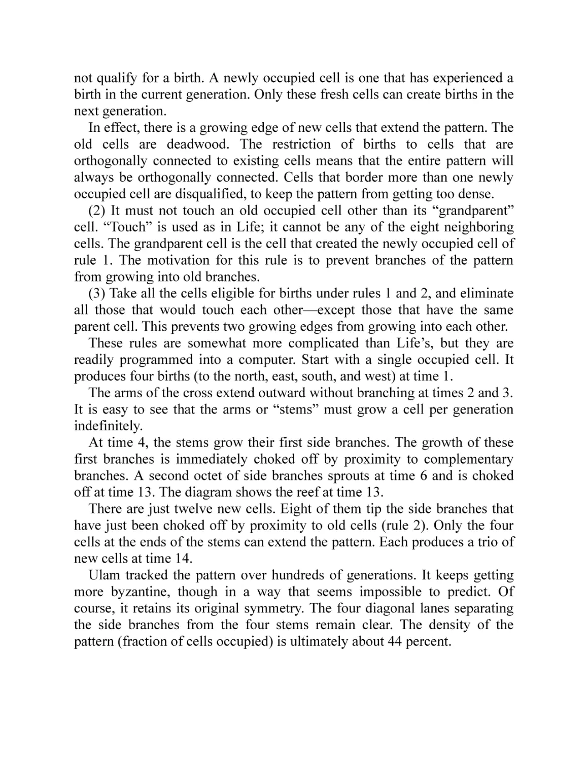
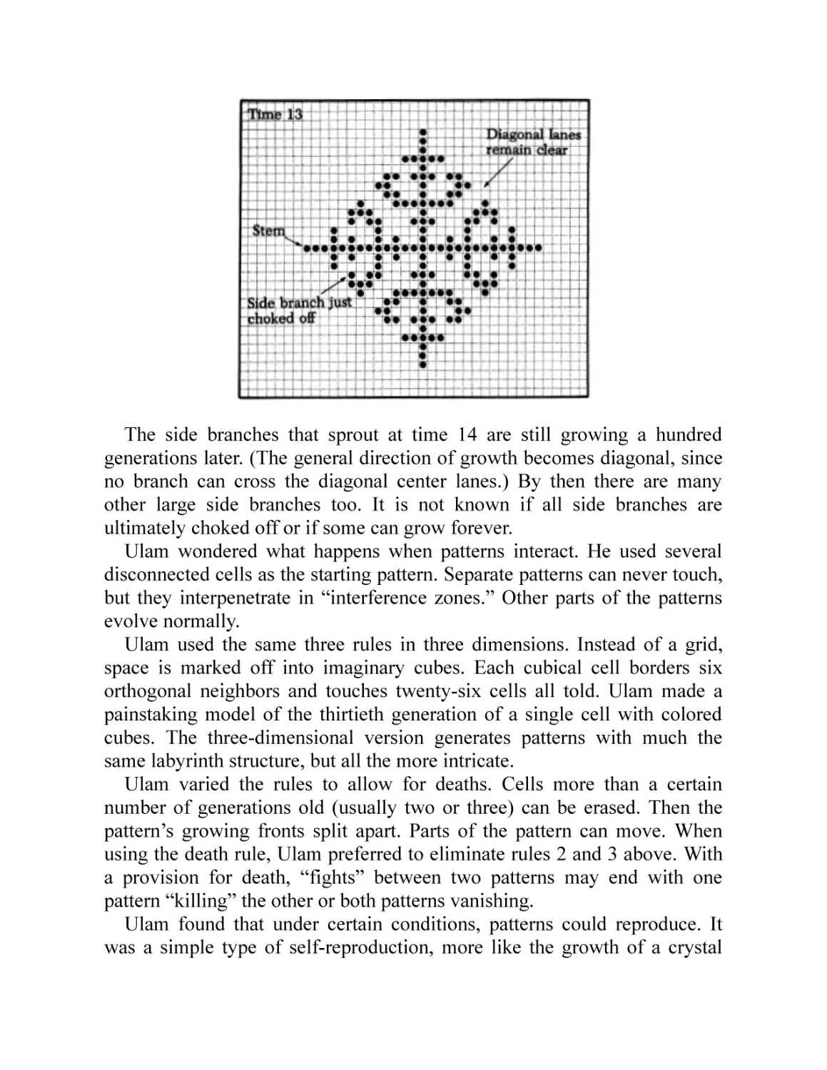
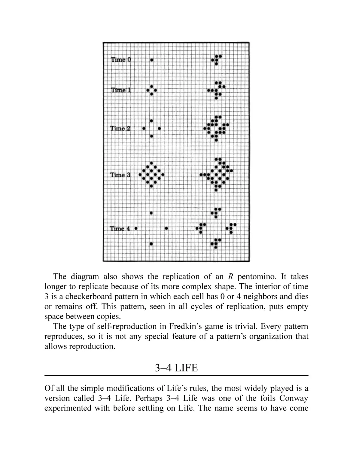
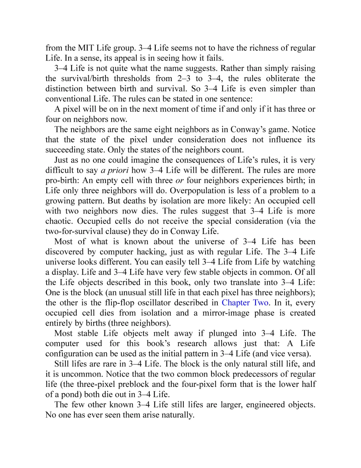
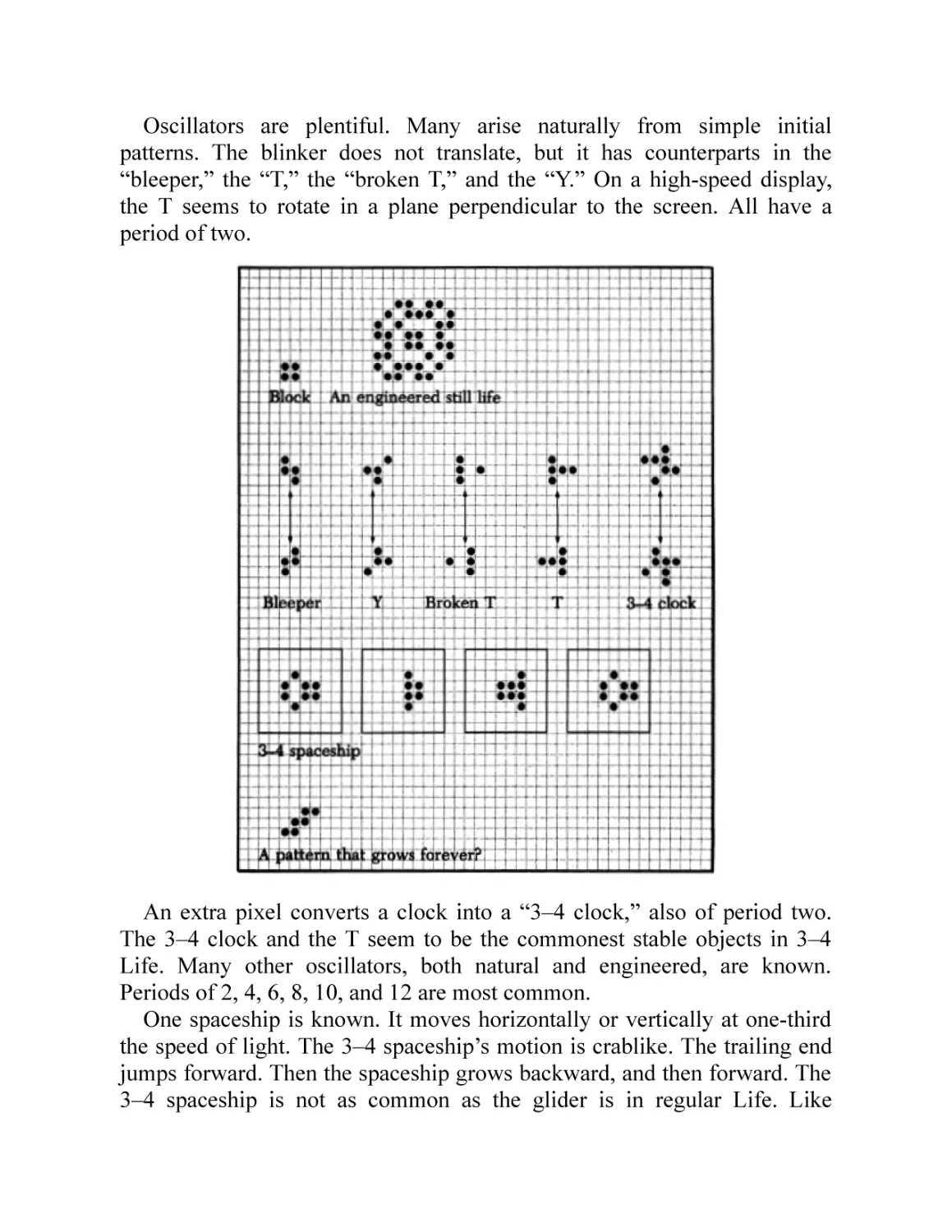
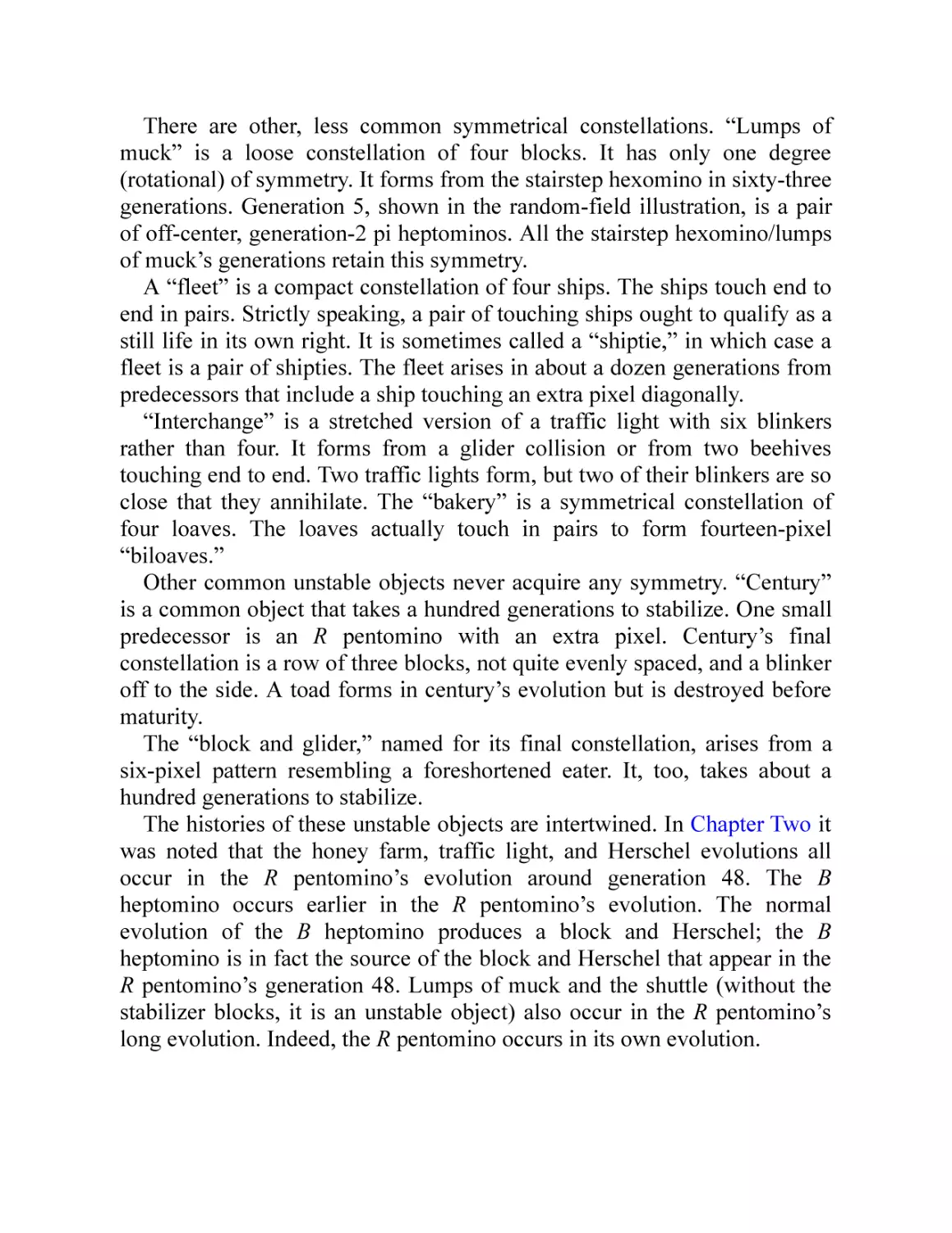
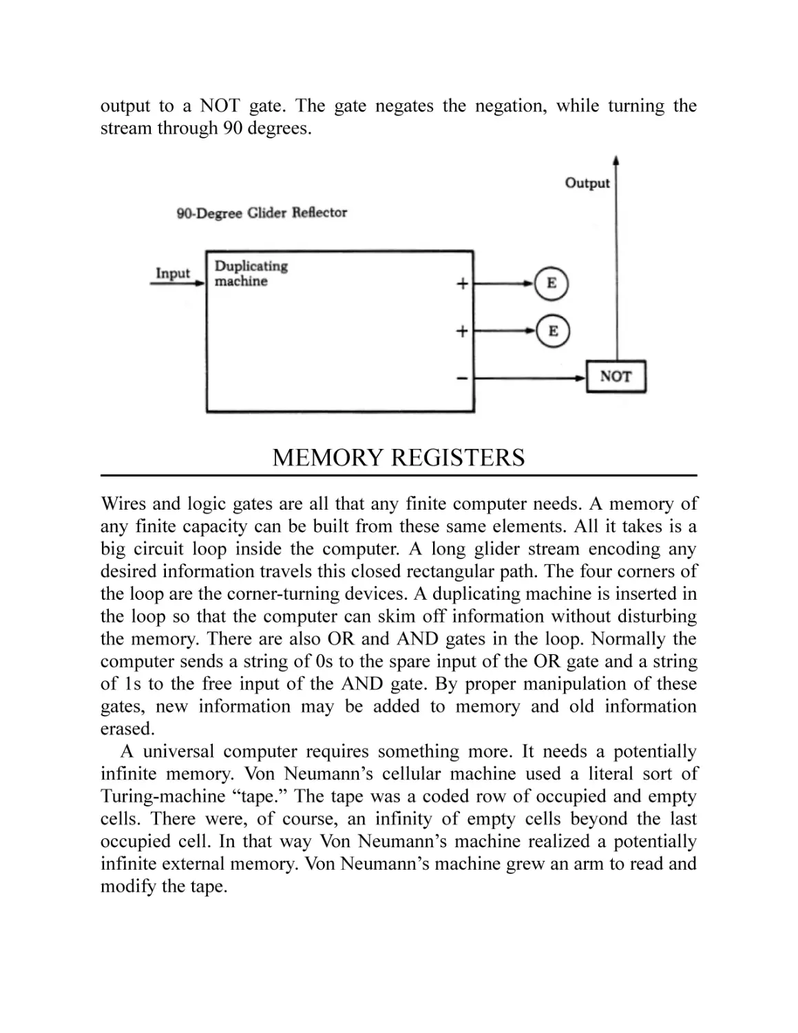
/


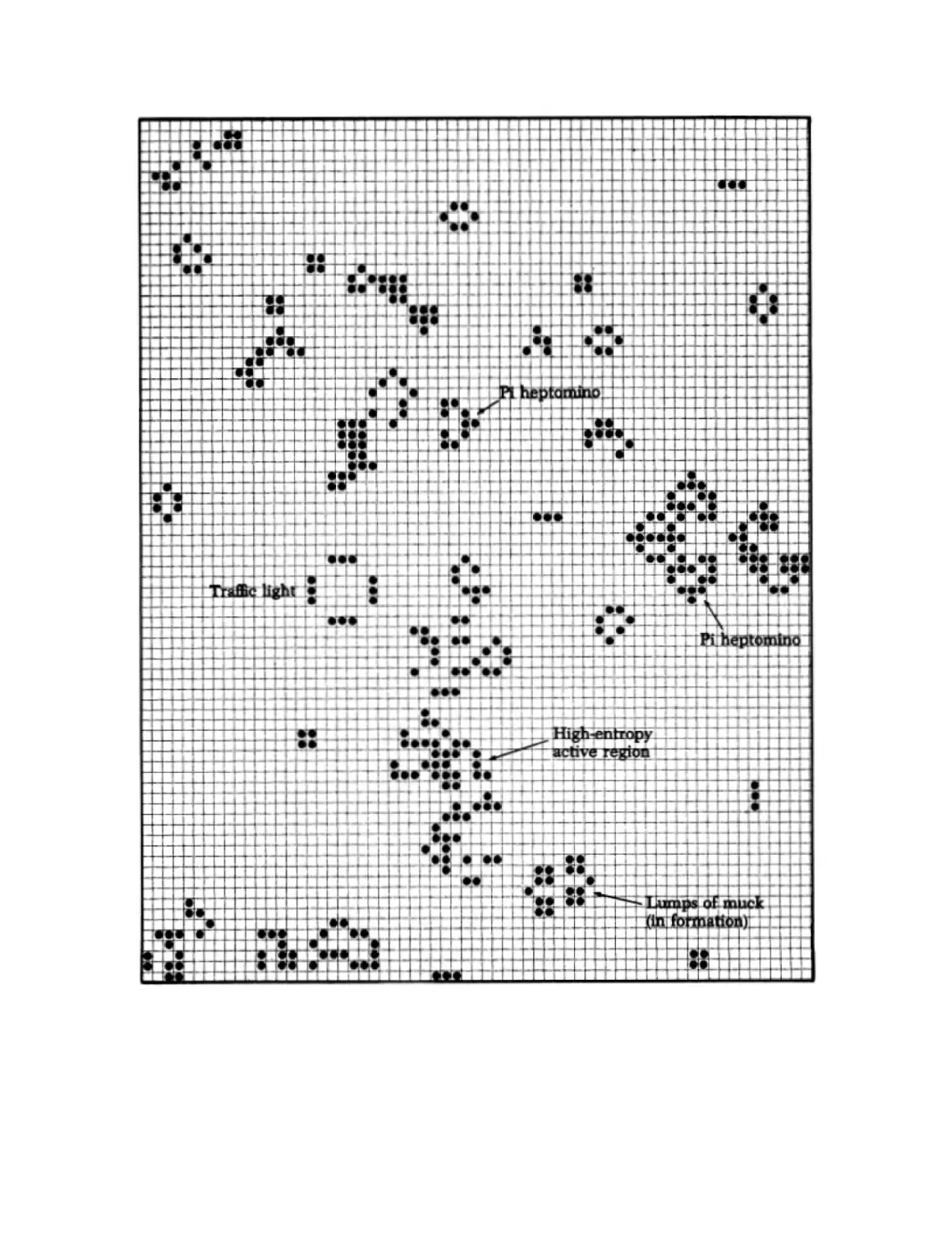
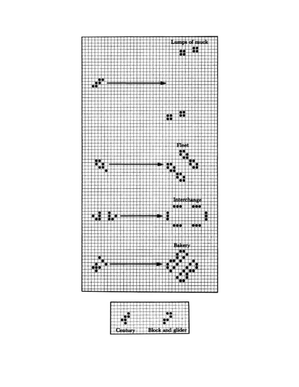
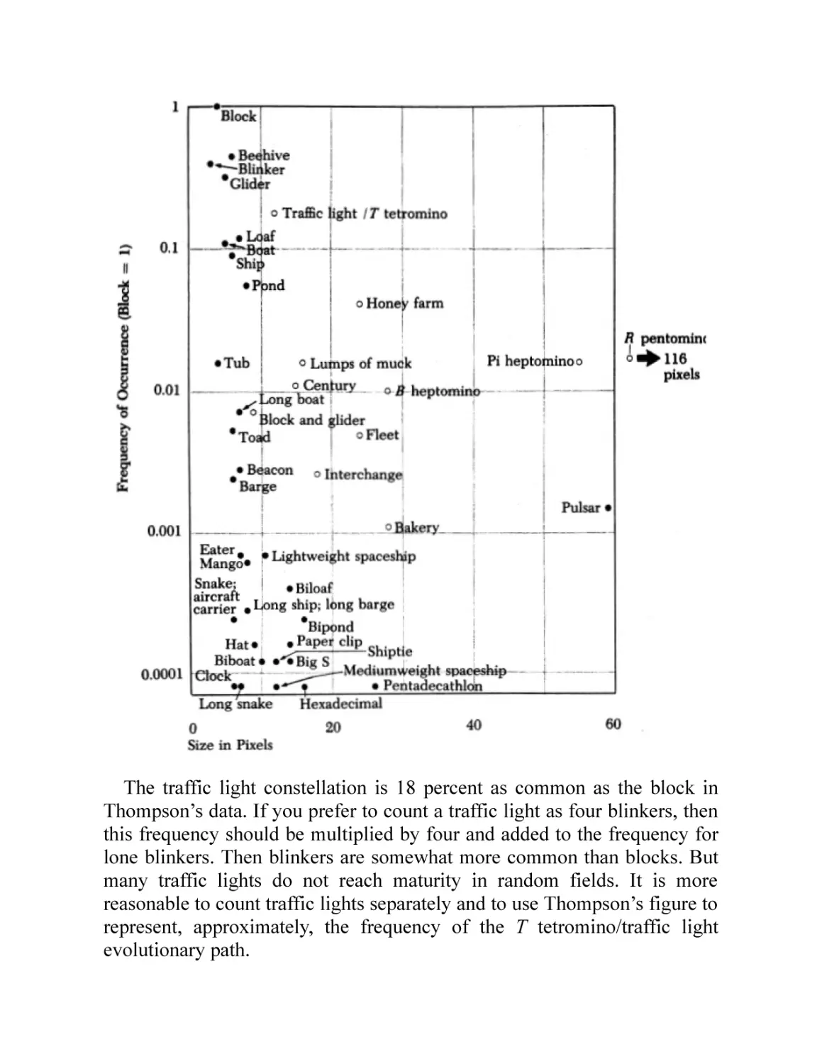
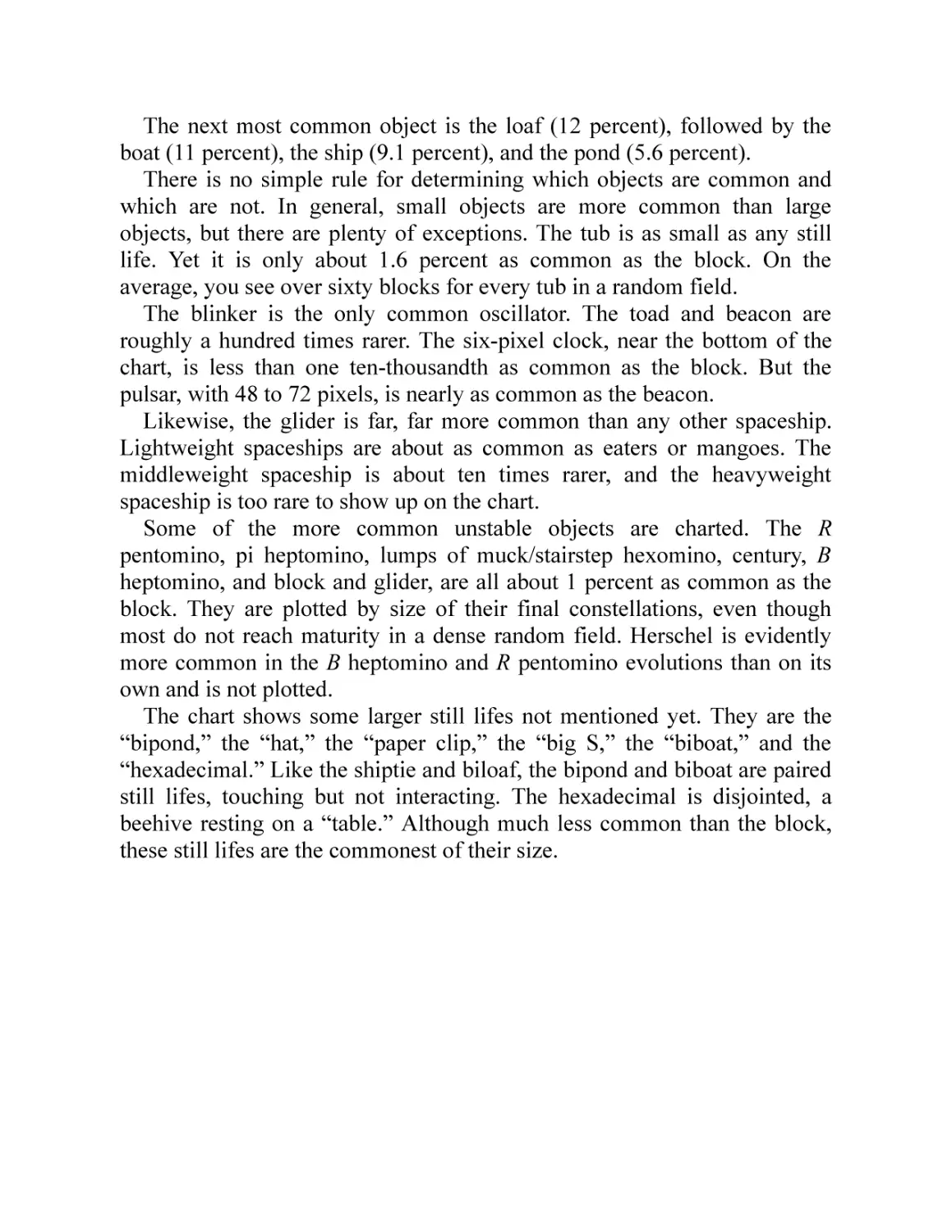
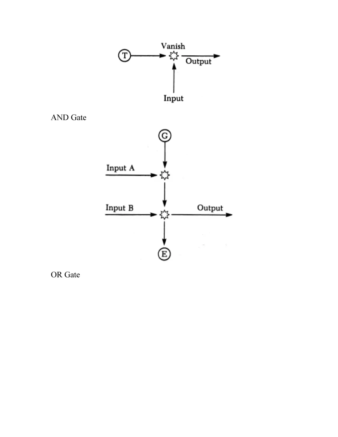
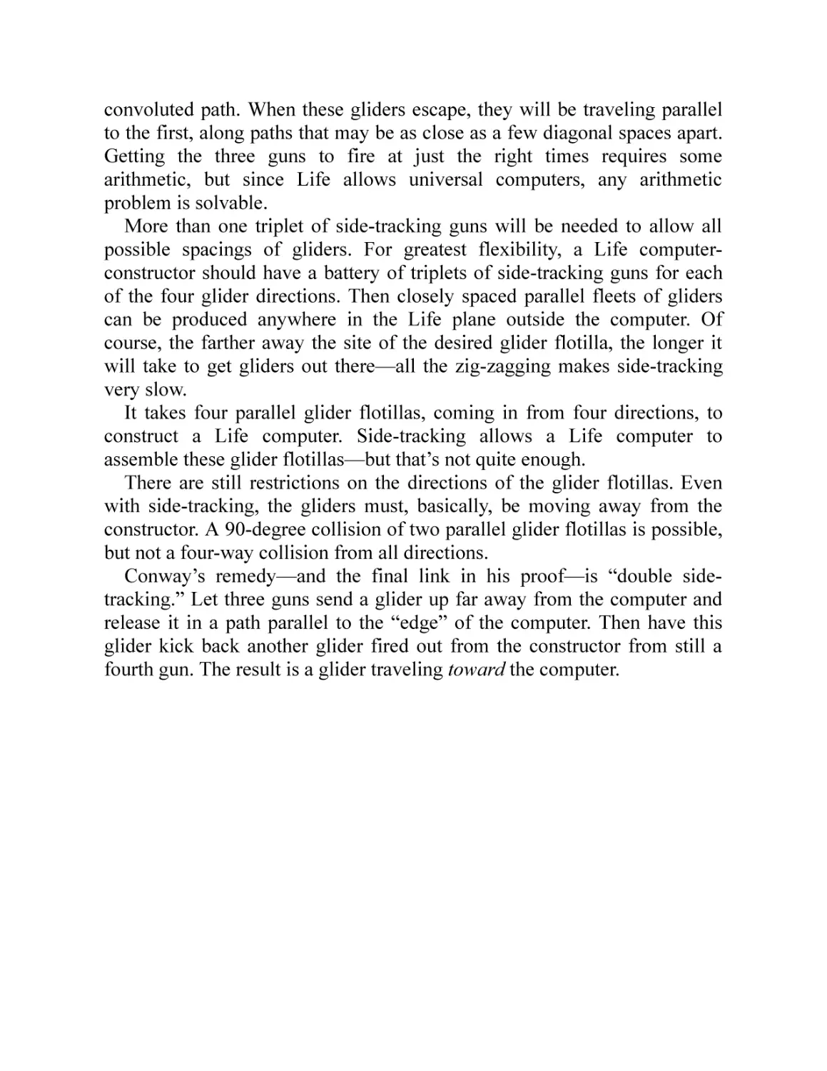
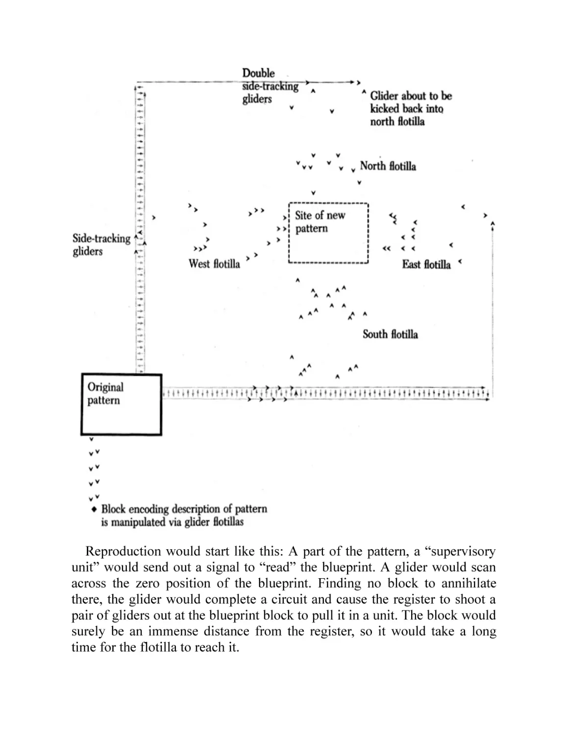
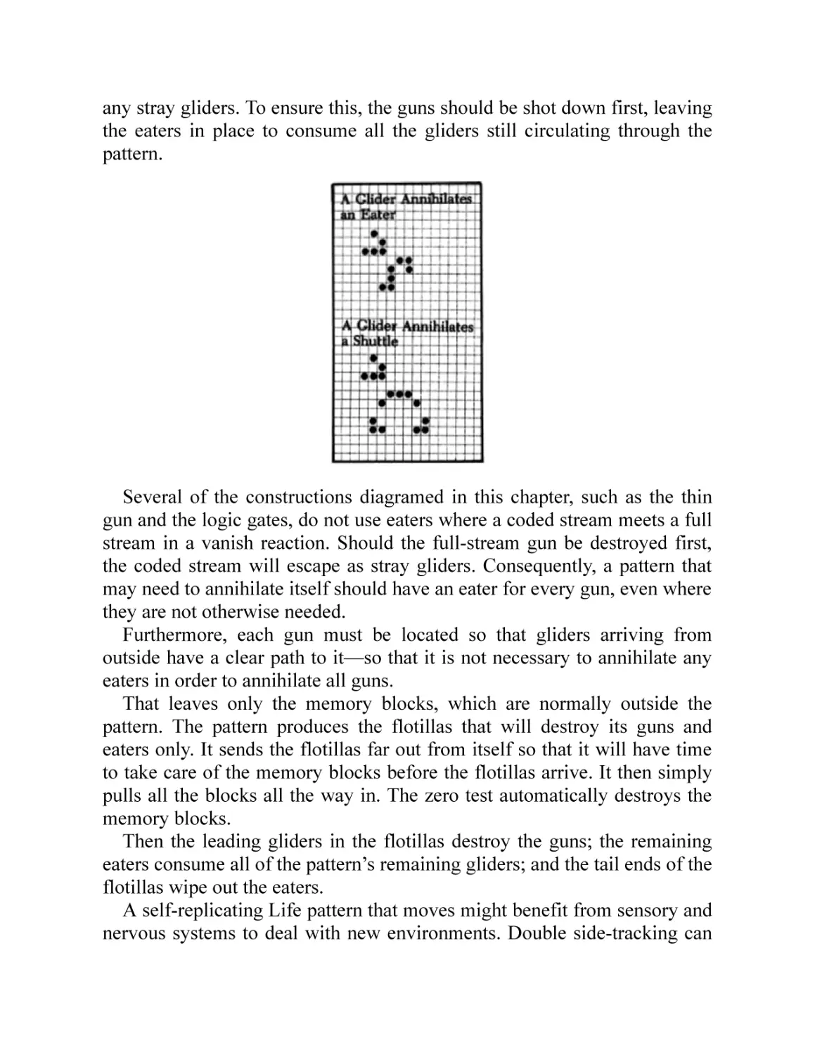


Text
The Recursive Universe
Cosmic Complexity and the
Limits of Scientific Knowledge
William Poundstone
Dover Publications, Inc., Mineola,
New York
Copyright
Copyright © 1985, 2013 by William Poundstone
All rights reserved.
Bibliographical Note
This Dover edition, first published in 2013, is a republication of
the work originally published in 1985 by William Morrow and
Company, Inc., New York. For this edition the author has proided
a new Afterword and the section Life for Home Computers has
been omitted.
International Standard Book Number
eISBN-13: 978-0-486-31579-9
Manufactured in the United States by Courier Corporation
49098X01
www.doverpublications.com
To my parents
ACKNOWLEDGMENTS
The game of Life was invented by John Horton Conway of the
University of Cambridge. Martin Gardner introduced Life through his
October 1970 Scientific American column. Interest in the game soon
spawned a newsletter, Lifeline, published by Robert T. Wainwright from
1971 to 1973. Much of what is known of the Life universe is the work of
Lifeline’s many correspondents. Among those who have contributed to this
book through their discoveries and insights are Simon Norton, Gary
Filipski, Brad Morgan, Ranan B. Banerji, D. M. Saul, Robert April,
Michael Beeler, R. William Gosper, Jr., Richard Howell, Rich Schroeppel,
Michael Speciner, Keith McClelland, Thomas Holmes, Michael Sporer,
Philip Stanley, Donald Woods, William Woods, Roger Banks, Sol
Goodman, Arthur C. Taber, Robert Bison, David W. Bray, Charles L.
Corderman, Gary Goodman, Stephen B. Gray, Maxwell E. Manowski,
Clement A. Lessner III, William P. Webb, Hugh Thompson, Robert Kraus,
Rici Liknaitsky, Bill Mann, Steve Ward, James F. Harford, Curt Gibson, Jan
Kok, Douglas G. Petrie, Philip Cohen, Paul Wilson, V. Everett Boyer, Dave
Buckingham, Mark Niemiec, Peter Raynham, Dean Hickerson, Paul Schick,
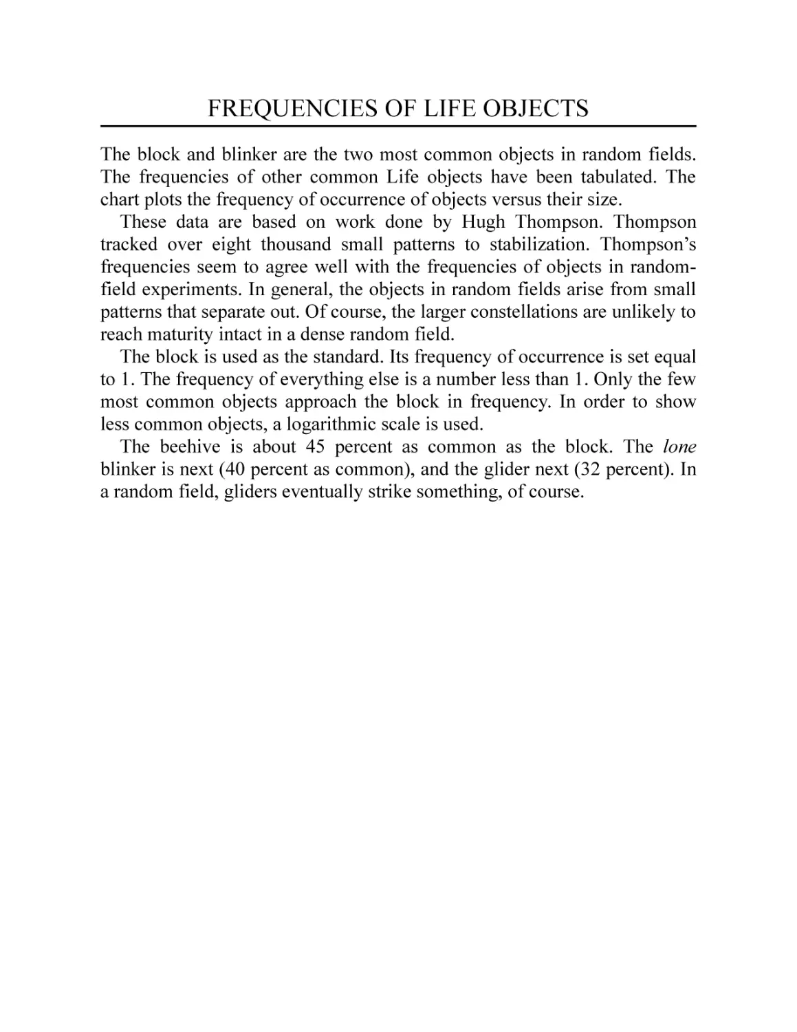
and George D. Collins, Jr. The information on relative frequencies of Life
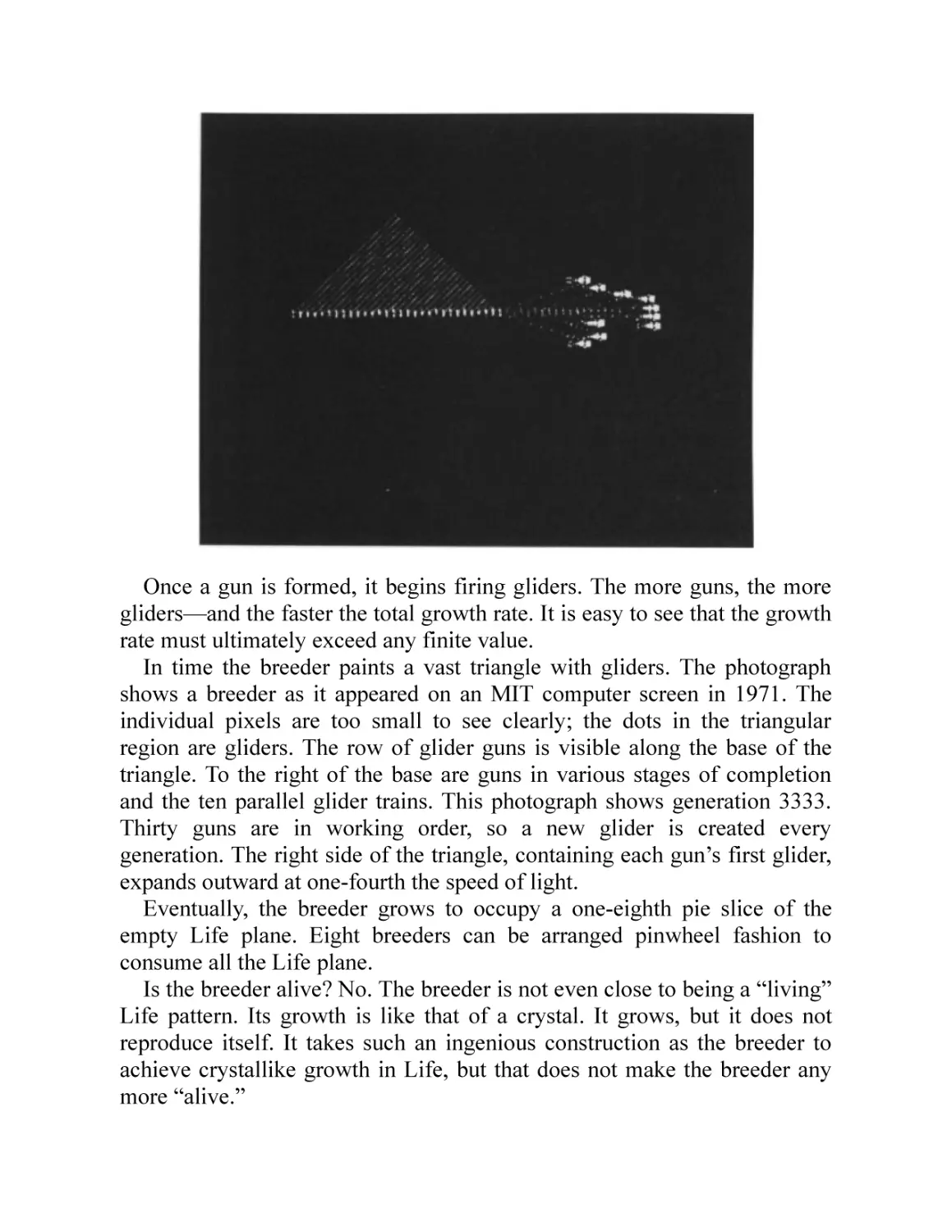
objects is largely the work of Hugh Thompson. The photograph of the
breeder is from Gosper’s group at MIT. The dedicated Life computer used
for this book’s research was constructed by George Wells.
CONTENTS
Acknowledgments
1 · Complexity and Simplicity
2 · The Life Universe
3 · Maxwell’s Demon
4 · Gliders and Spaceships
5 · Information and Structure
6 · Unlimited Growth
7 · Physics as Recursion
8 · Recursive Games
9 · Big Bang and Heat Death
10 · Random Fields
11 · Von Neumann and Self-Reproducing Machines
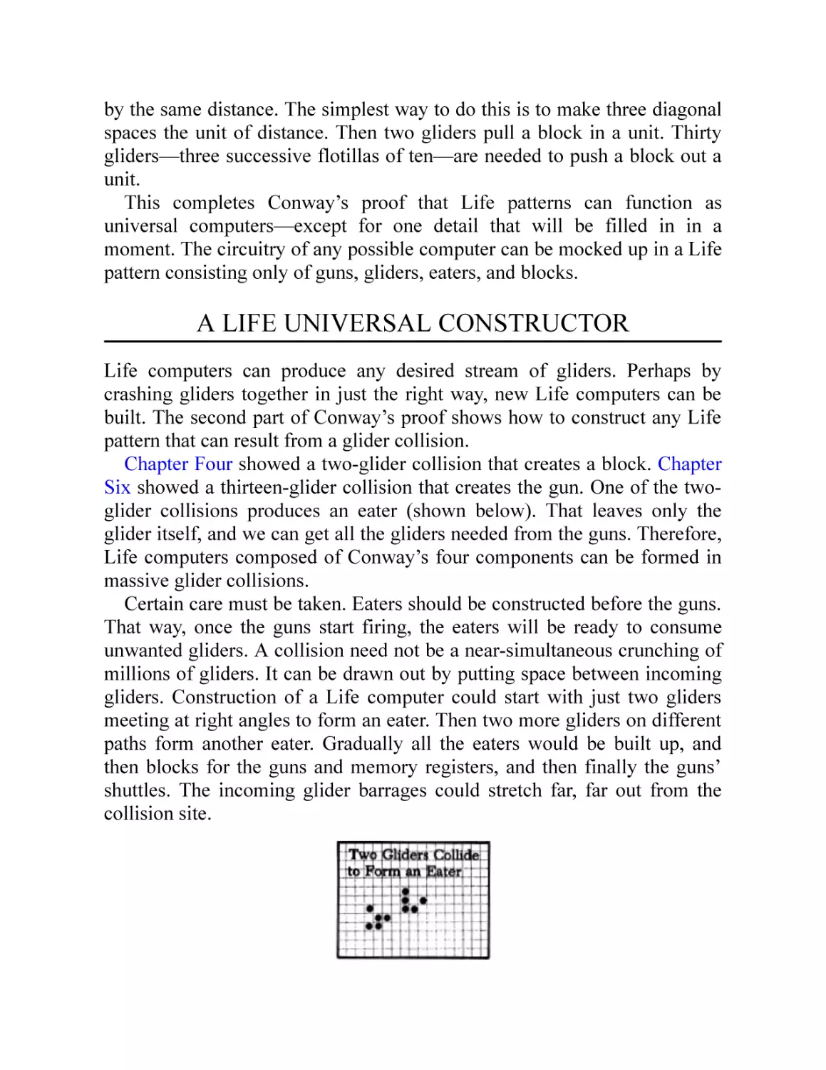
12 · Self-Reproducing Life Patterns
13 · The Recursive Universe
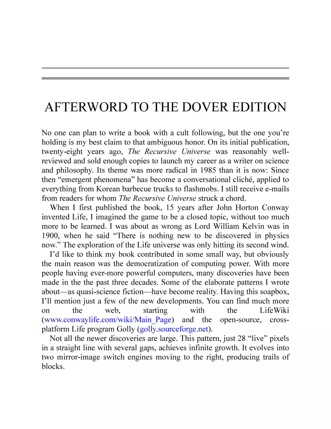
Afterword to the Dover Edition
Bibliography
Index
The Recursive Universe
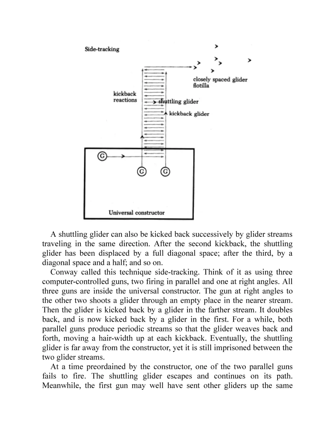
•1•
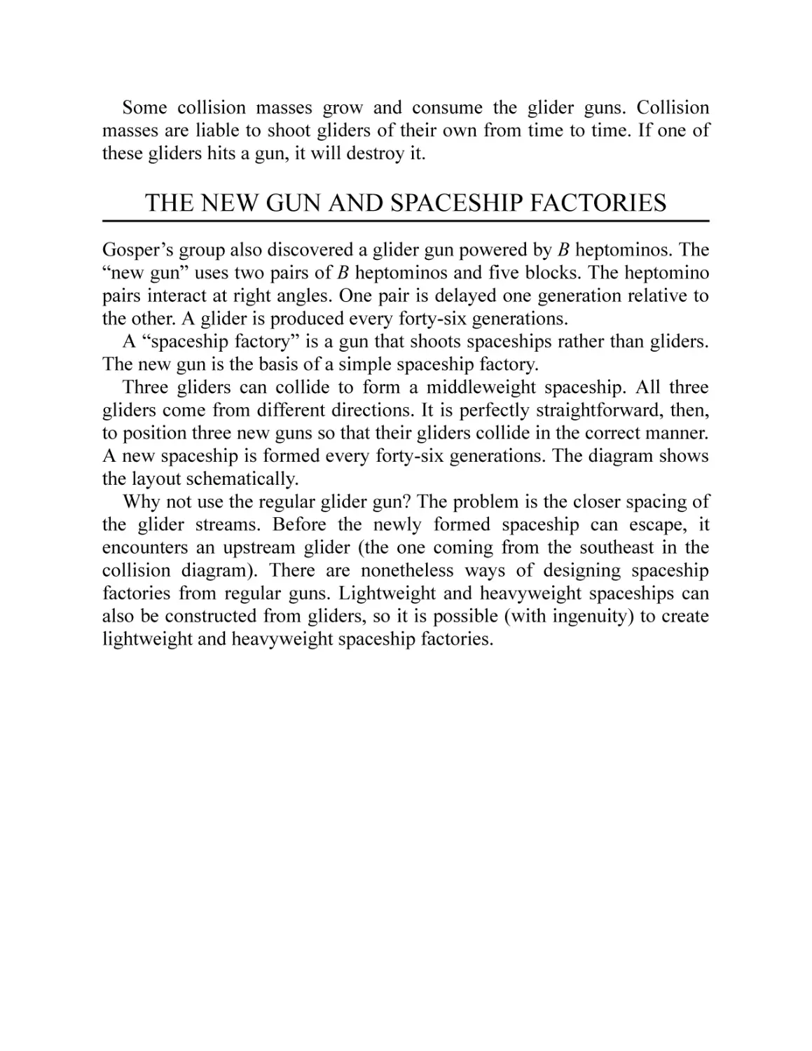
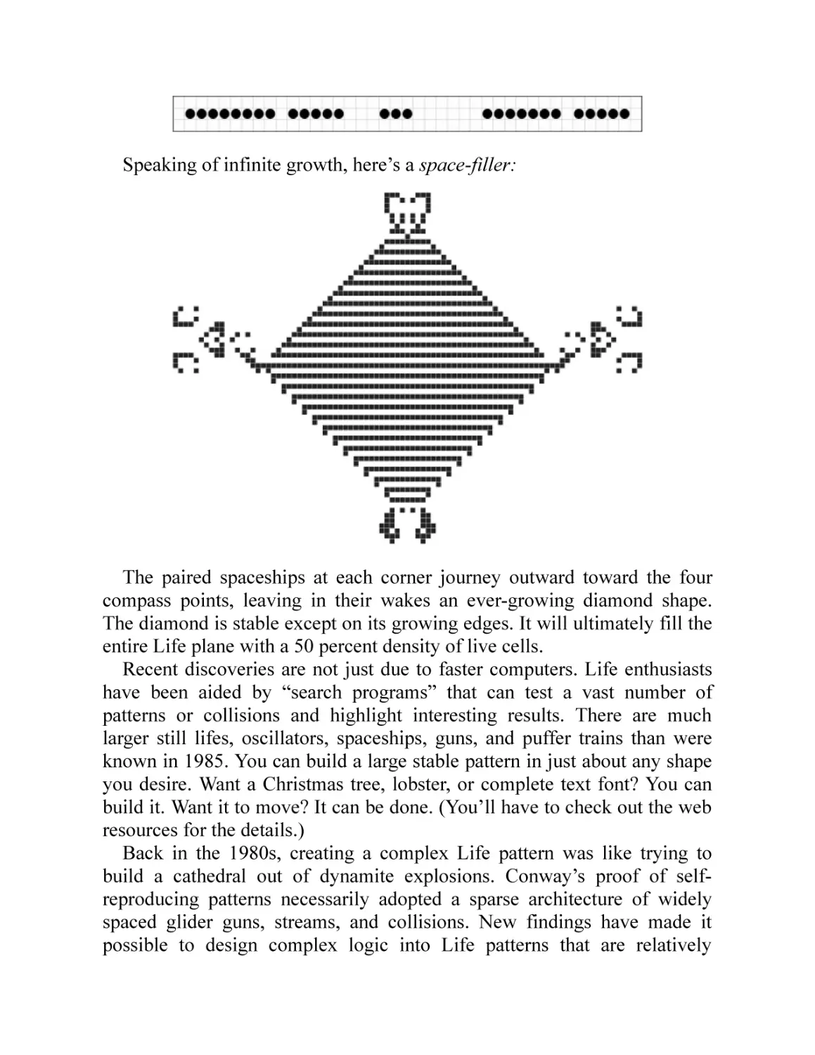
COMPLEXITY AND SIMPLICITY
In the early 1950s, the Hungarian-American mathematician John Von
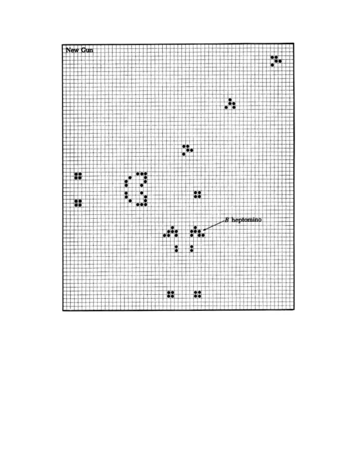
Neumann was toying with the idea of machines that make machines. The
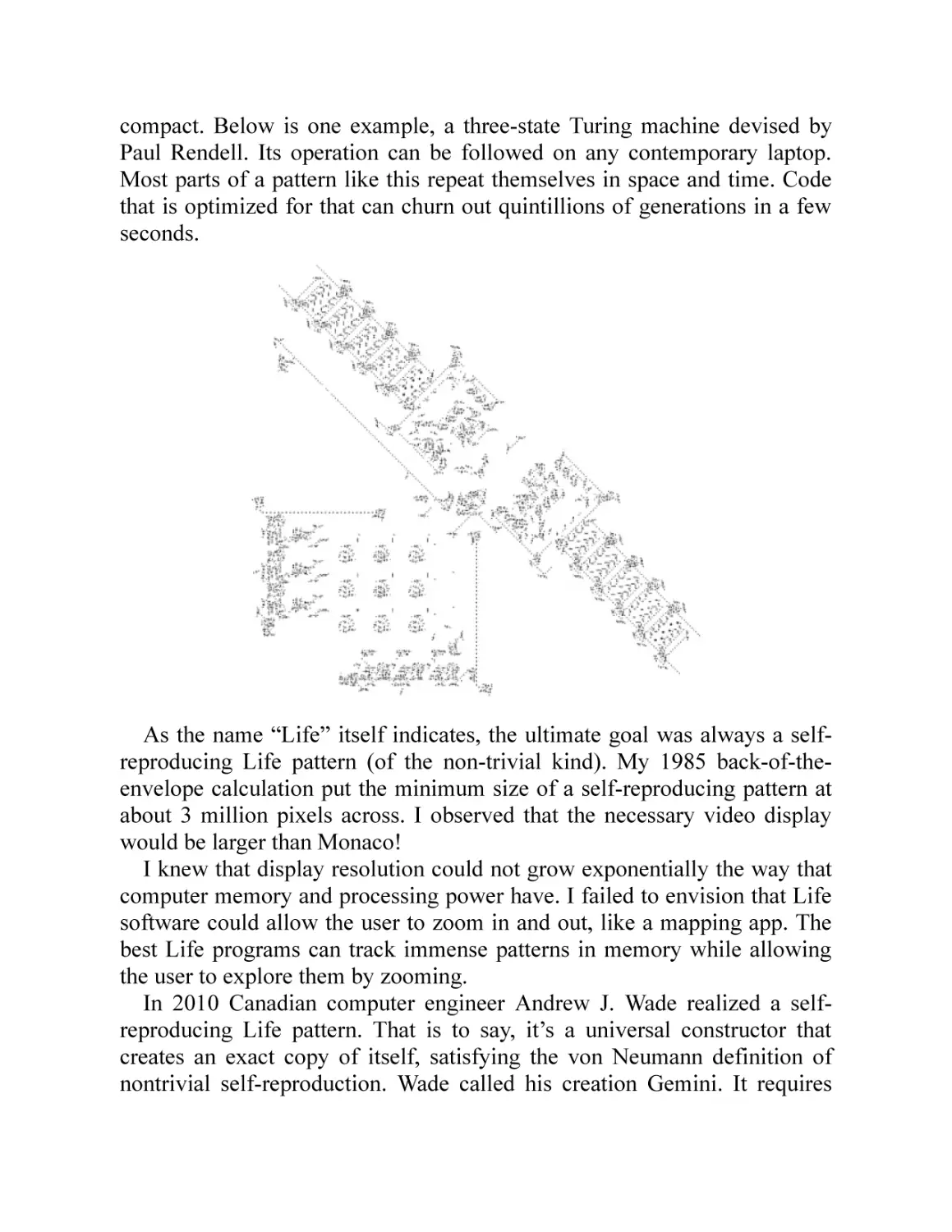
manufacture of cars and electrical appliances was becoming increasingly
automated. It wasn’t hard to foresee a day when these products would roll
off assembly lines with no human intervention whatsoever. What interested
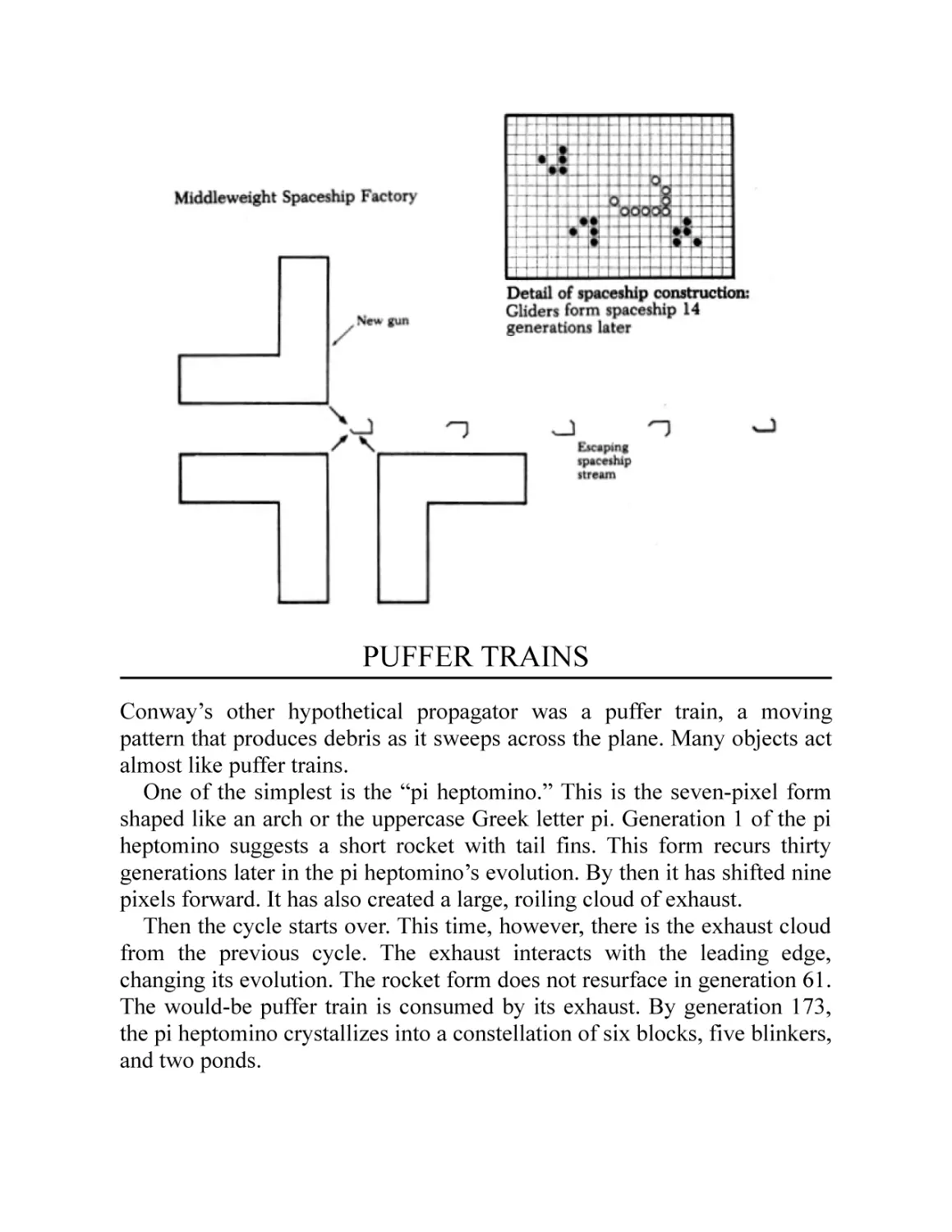
Von Neumann particularly was the notion of a machine that could
manufacture itself. It would be a robot, actually. It might wander around a
warehouse, collecting all the components needed to make a copy of itself.
When it had everything, it would assemble the parts into a new machine.
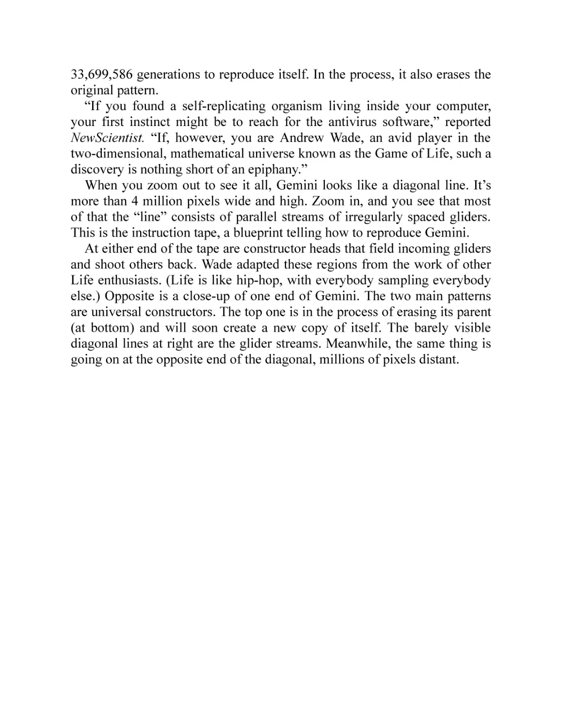
Then both machines would duplicate and there would be four . . . and then
eight . . . and then sixteen . . .
Von Neumann wasn’t interested in making a race of monster machines;
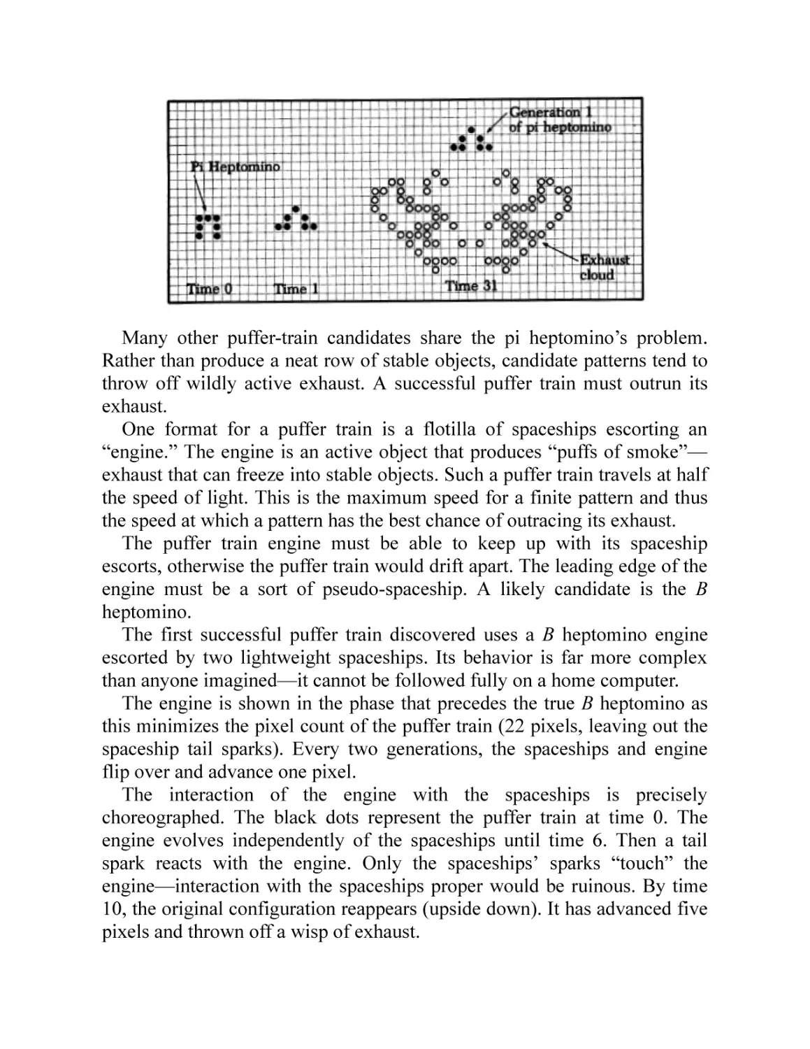
he just wondered if such a thing was possible. Or does the idea of a
machine that manufactures itself involve some logical contradiction?
Von Neumann further wondered if a machine could make a machine
more complex than itself. Then the machine’s descendants would grow ever
more elaborate, with no limit to their complexity.
These issues fascinated Von Neumann because they were so fundamental.
They were the sorts of questions that any bright child might ask, and yet no
mathematician, philosopher, scientist, or engineer of the time could answer
them. About all that anyone could say was that all existing machines
manufactured machines much simpler than themselves. A labyrinthine
factory might make a can opener.
Many of Von Neumann’s contemporaries were interested in automatons
as well. Several postwar college campuses boasted a professor who had
built a wry sort of robot pet in a vacant lab or garage. There was Claude
Shannon’s “Theseus,” a maze-solving electric rodent; Ross Ashby’s
“machina spora,” an automated “fireside cat or dog which only stirs when
disturbed,” by one account; and W. Grey Walter’s restless “tortoise.” The
tortoise scooted about on motorized wheels, reacting to obstacles in its path
but tending to become fouled in carpet shag. When its power ran low, the
tortoise refueled from special outlets.
Von Neumann’s hunch was that self-reproducing machines are possible.
But he suspected that it would be impractical to build one with 1950s
technology. He felt that self-reproducing machines must meet or exceed a
certain minimum level of complexity. This level of complexity would be
difficult to implement with vacuum tubes, relays, and like components.
Further, a self-reproducing automaton would have to be a full-fledged
robot. It would have to “see” well enough to recognize needed components.
It would require a mechanical arm supple enough to grip vacuum tubes
without crushing or dropping them, agile enough to work a screwdriver or
soldering iron. As much as Von Neumann felt a machine could handle these
tasks in principle, it was clear that he would never live to see it.
Inspiration came from an unlikely source. Von Neumann had supervised
the design of the computers used for the Manhattan Project. For the Los
Alamos scientists, the computers were a novelty. Many played with the
computers after hours.
Mathematician Stanislaw M. Ulam liked to invent pattern games for the
computers. Given certain fixed rules, the computer would print out everchanging patterns. Many patterns grew almost as if they were alive. A
simple square would evolve into a delicate, corallike growth. Two patterns
would “fight” over territory, sometimes leading to mutual annihilation.
Ulam developed three-dimensional games too, constructing thickets of
colored cubes as prescribed by computer.
Ulam called the patterns “recursively defined geometric objects.”
Recursive is a mathematical term for a repeated procedure, in this case, the
repeated rules by which the computers generated the patterns. Ulam found
the growth of patterns to defy analysis. The patterns seem to exist in an
abstract world with its own physical laws.
Ulam suggested that Von Neumann “construct” an abstract universe for
his analysis of machine reproduction. It would be an imaginary world with
self-consistent rules, as in Ulam’s computer games. It would be a world
complex enough to embrace all the essentials of machine operation but
otherwise as simple as possible. The rules governing the world would be a
simplified physics. A proof of machine reproduction ought to be easier to
devise in such an imaginary world, as all the nonessential points of
engineering would be stripped away.
The idea appealed to Von Neumann. He was used to thinking of
computers and other machines in terms of circuit or logic diagrams. A
circuit diagram is a two-dimensional drawing, yet it can represent any
conceivable three-dimensional electronic device. Von Neumann therefore
made his imaginary world two-dimensional.
Ulam’s games were “cellular” games. Each pattern was composed of
square (or sometimes triangular or hexagonal) cells. In effect, the games
were played on limitless checkerboards. All growth and change of patterns
took place in discrete jumps. From moment to moment, the fate of a given
cell depended only on the states of its neighboring cells.
The advantage to the cellular structure is that it allows a much simpler
“physics.” Basically, Von Neumann wanted to create a world of animated
logic diagrams. Without the cellular structure, there would be infinitely
many possible connections between components. The rules needed to
govern the abstract world would probably be complicated.
So Von Neumann adopted an infinite checkerboard as his universe. Each
square cell could be in any of a number of states corresponding roughly to
machine components. A “machine” was a pattern of such cells.
Von Neumann could have allowed a distinct cellular state for every
possible component of a machine. The fewer the states, the simpler the
physics, however. After some juggling, he settled on a cellular array with 29
different states for its cells. Twenty-eight of the states are simple machine
components; one is the empty state of unoccupied cells. The state of a cell
in the next moment of time depends only on its current state and the states
of its four bordering (“orthogonal”) neighbors.
Von Neumann’s cellular space can be thought of as an exotic, solitaire
form of chess. The board is limitless, and each square can be empty or
contain one of 28 types of game pieces. The lone player arranges game
pieces in an initial pattern. From then on, strict rules determine all
successive configurations of the board.
Since the player has no further say, one might as well imagine that the
game’s rules are automatically carried out from one move to the next. Then
the player need only sit back and watch the changing patterns of game
pieces that evolve.
What Von Neumann did is this: He proved that there are starting patterns
that can reproduce themselves. Start with a self-reproducing pattern, let the
rules of the cellular space take their course, and there will eventually be two
patterns, and then four, and then eight . . .
Von Neumann’s pattern, or machine, reproduced in a very general,
powerful way. It contained a complete description of its own organization.
It used that information to build a new copy of itself. Von Neumann’s
machine reproduction was more akin to the reproduction of living
organisms than to the growth of crystals, for instance. Von Neumann’s
suspicion that a self-reproducing machine would have to be complicated
was right. Even in his simplified checkerboard universe, a self-reproducing
pattern required about 200,000 squares.
Since Von Neumann was able to prove that a self-reproducing machine is
possible in an imaginary but logical world, no logical contradiction must be
inherent in the concept of a self-reproducing machine. Ergo, a selfreproducing machine is possible in our world. No one has yet made a selfreproducing machine, but today no logician—or engineer—doubts that it is
possible.
VON NEUMANN’S MACHINE AND BIOLOGY
Not only can a machine manufacture itself, but Von Neumann was also able
to show that a machine can build a machine more complex than itself. As it
happens, these facts have been of almost no use (thus far, at least) to the
designers of machinery. Von Neumann’s hypothetical automatons have
probably had their greatest impact in biology.
One of the longest running controversies in biology is whether the
actions of living organisms can be reduced to chemistry and physics. Living
matter is so different from nonliving matter that it seems something more
than mere chemistry and physics must be at work. On the other hand,
perhaps the organization of living matter is so intricate that the observed
properties of living organisms do follow, ultimately, from chemistry and
physics.
The latter viewpoint is held by virtually all biologists today, but it is not
particularly new. René Descartes believed the human body to be a machine.
By that he meant that the body is composed of substances interacting in
predictable ways according to the same physical laws that apply to
nonliving matter. Descartes felt the body is understandable and predictable,
just as a mechanical device is.
Queen Christina of Sweden, a pupil of Descartes, questioned this belief:
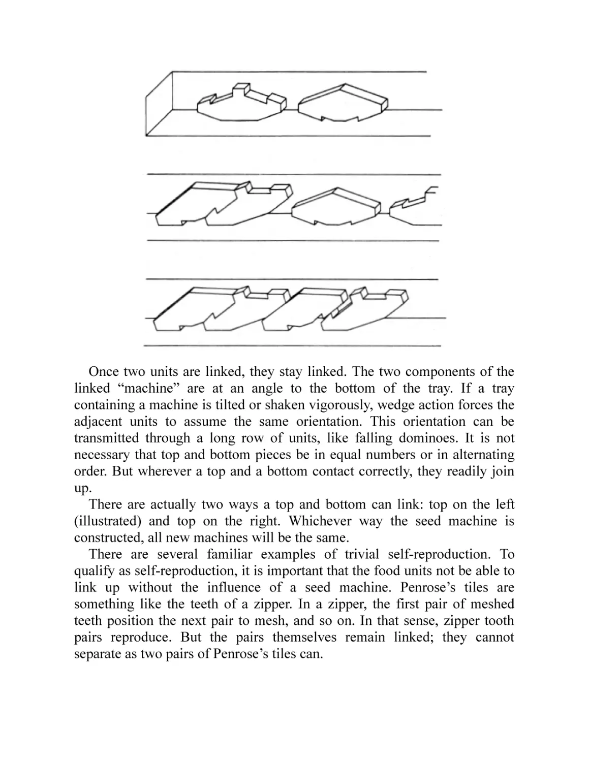
How can a machine reproduce itself? No known inanimate object
reproduced in the way that living organisms do.
Not until Von Neumann did anyone have a good rebuttal to Christina’s
objection. Many biologists postulated a “life force” to explain reproduction
and other properties of living matter. The life force was the reason that
living matter is so different from nonliving matter. It supplemented the
ordinary physical laws in living matter. Because the life force could never
apply to a mechanical device, it was pointless to compare living organisms
to machines.
At the simplest level, Von Neumann’s self-reproducing machine is
nothing like a living organism. It contains no DNA, no protein; it is not
even made of atoms. To Von Neumann such considerations were beside the
point. Von Neumann’s abstract machine demonstrates that self-reproduction
is possible solely within the context of physics and logic. No ad hoc life
force is necessary.
It became reasonable to see living cells as complex self-reproducing
machines. A living cell must perform many tasks besides reproducing itself,
of course. So it is not surprising that real cells are much more difficult to
understand than Von Neumann’s machine.
By coincidence, Watson and Crick’s work on DNA synthesis took place
concurrently with much of Von Neumann’s study of machine reproduction.
By about 1951, molecular biologists had identified structural proteins,
enzymes, nucleotides, and most other important components of cells. The
genetic information of cells was known to be encoded in observable
structures (chromosomes) composed of nucleotides and certain proteins.
Still, no one had any concrete idea how these components managed to
reproduce themselves. It might require some sort of a life force yet.
The discovery of DNA’s structure and the genetic code were first steps in
understanding how assemblages of molecules implement their own
reproduction. It is remarkable that the logical basis of reproduction in living
cells is almost identical to that of Von Neumann’s machine. There is a part
of Von Neumann’s machine that corresponds to DNA, another part that
corresponds to ribosomes, another part that does the job of certain enzymes.
All this tends to confirm that Von Neumann was successful in formulating
the simplest truly general form of self-reproduction.
Biologists have adopted Von Neumann’s view that the essence of selfreproduction is organization—the ability of a system to contain a complete
description of itself and use that information to create new copies. The life
force idea was dropped. Biology is now seen as a derivative science whose
laws can (in principle) be derived from more fundamental laws of chemistry
and physics.
IS PHYSICS DERIVATIVE TOO?
“What really interests me,” Albert Einstein once remarked, “is whether God
had any choice in the creation of the world.” Einstein was wondering if the
world and its physical laws are arbitrary or if they are somehow inevitable.
To put it another way: Could the universe possibly be any different than it
is?
In many ways, the world seems arbitrary. An electron weighs
0.00000000000000000000000000091096 grams. The stars cluster in
galaxies, some spiral and some elliptical. No one knows of any obvious
reason why an electron couldn’t be a little heavier or why stars aren’t
spaced evenly through space. It is not hard to imagine a world in which a
few physical constants are different or a world in which everything is
different.
Einstein’s statement draws a variety of reactions. One’s feelings about the
nature or reality of God are largely immaterial. The issue is whether there
can be “prior” constraints even on the creation of the world.
One reaction is that there are no such constraints. By definition, an allpowerful God can create the world any way He chooses. Everything about
the universe is God’s choice. Creation was not limited, not even by logic.
God created logic.
On the other hand, it can be argued that even God is bound by logic. If
God can lift any weight, then he is expressly prevented from being able to
create a weight so heavy that He cannot lift it. But God can do anything that
does not involve a logical contradiction.
Einstein evidently sympathized with the latter argument. He realized that
it may not be easy to recognize logical contradictions, however. Suppose
that by some recondite chain of reasoning it is possible to show that the
speed of light must be exactly 299,792.456 kilometers per second. Then the
notion of a world in which the speed of light is even slightly different would
involve a contradiction.
Conceivably, all the laws of physics could have a justification in pure
logic. Then God would have had no freedom whatsoever in determining
physics.
Taking this idea further, perhaps the initial conditions of our world were
also determined by arcane logic. The big bang had to occur precisely the
way it did; the galaxies had to form just the way they did.
In that case, God would have had no choice in creation at all. He could
not even have made a world in which forks were placed on the right side of
plates or in which New Zealand didn’t exist. This would be the only
possible world.
Some people dismiss Einstein’s statement as too metaphysical—the sort
of thing that could be argued endlessly without getting anywhere. In fact,
modern physics has much to say about choice in creation.
More and more physical laws have turned out to be derivative. If law B is
the inevitable consequence of law A, then only law A is really an
independent law of nature. B is a mere logical implication.
The chain of implication can have many links. A biological phenomenon
may be explained in terms of chemistry. The chemistry may be explained in
terms of atomic physics. The atomic physics may be explained in terms of
subatomic physics. Then the laws of subatomic physics suffice to explain
the original biology.
This is what the reductionist mode of thought seeks. To understand a
phenomenon is to be able to give reasons for it—to see the phenomenon as
inevitable rather than arbitrary. Reductionism has been a keystone of
Western science. Einstein wondered if reductionism can proceed endlessly
or whether it will reach a dead end.
Marquis Pierre Simon de Laplace, one of the founders of the reductionist
tradition, believed that everything is knowable. He illustrated his point with
a hypothetical cosmic intelligence that might, in principle, know the details
of every atom in the cosmos. Given a knowledge of the laws of physics, the
being should be able to predict the future and reconstruct the past, Laplace
felt: “Nothing would be uncertain and the future, as the past, could be
present to its eyes.”
Physicists are close to a comprehensive theory of nature in which all the
world’s phenomena are reduced to just two fundamentally different types of
particles interacting by just two types of force. This long-awaited synthesis
goes by the name of grand unified theory (GUT). Some physicists
contemplate an even broader theory in which everything is reduced to one
particle and one force. This is labeled a super-grand unified theory. It is
always dangerous to suppose that physicists have or have nearly learned
everything there is to know about physics. Laplace’s cosmic being was
evidently prompted by his belief that eighteenth-century physics was nearly
complete; late nineteenth-century physicists expressed similar beliefs just in
time to have them demolished by quantum theory and relativity.
Nonetheless, physicists are (again) facing the prospect of a comprehensive
theory of nature, one that may lie in the completion of current theoretical
projects. It is a good time to reexamine the cornerstones of reductionism.
This book cannot cover the grand and super-grand unified theories except
tangentially. Nor does it mean to endorse such theories as the last word in
natural law. Its purpose is rather to look at the explaining power of physical
law. Not since the turn of the century have physicists believed physics to be
substantially complete. The new field of information theory has grown up
in the interim. Information theory will have extensive philosophical
consequences for any future comprehensive theory of nature.
THE LIMITS OF KNOWLEDGE
Laplace, Leibniz, Descartes, and Kant popularized the idea of the universe
as a vast machine. The cosmos was likened to a watch, composed of many
parts interacting in predictable ways. Implicit in this analogy was the
possibility of predicting all phenomena. The perfect knowledge of
Laplace’s cosmic intelligence might be a fiction, but it could be
approximated as closely as desired.
Today the most common reaction to Laplace’s idea, among people who
have some feel for modern physics, is to cite quantum uncertainty as its
downfall. In the early twentieth century, physicists discovered that nature is
nondeterministic at the subatomic scale. Chance enters into any description
of quanta, and all attempts to exorcise it have failed. Since there is no way
of predicting the behavior of an electron with certainty, there is no way of
predicting the fate of the universe.
The quantum objection is valid, but it is not the most fundamental one. In
1929, two years after Heisenberg formulated the principle of quantum
uncertainty, Hungarian physicist Leo Szilard discovered a far more general
limitation on empirical knowledge. Szilard’s limitations would apply even
in a world not subject to quantum uncertainty. In a sense, they go beyond
physics and derive instead from the logical premise of observation. For
twenty years, Szilard’s work was ignored or misunderstood. Then in the late
1940s and early 1950s it became appreciated as a forerunner of the
information theory devised by Claude Shannon, John Von Neumann, and
Warren Weaver.
Information theory shows that Laplace’s perfect knowledge is a mirage
that will forever recede into the distance. Science is empirical. It is based
solely on observations. But observation is a two-edged sword. Information
theory claims that every observation obscures at least as much information
as it reveals. No observation makes an information profit. Therefore, no
amount of observation will ever reveal everything—or even take us any
closer to knowing everything.
Complementing this austere side of information theory is insight into
how physical laws generate phenomena. Physicists have increasing reason
to suppose that the phenomena of the world, from galaxies to human life,
are dictated more by the fundamental laws of physics than by some special
initial state of the world. In terms of Einstein’s riddle, this suggests that God
had little meaningful choice once the laws of physics were selected.
Information theory is particularly useful in explaining the complexity of the
world.
THE PARADOX OF COMPLEXITY
If the grand unified theories are the triumph of reductionism, they also
make it seem all the more preposterous. The GUTs postulate two types of
particles, two types of forces, and a completely homogeneous early
universe. How could any structure arise from such a simple initial state?
The world’s staggering diversity seems to preclude any simple
explanation. There is structure at all scales, from protons to clusters of
galaxies. Even before unified theories of physics, the world’s richness
seemed a paradox.
It is easy to show that the world is far, far more complex than can be
accounted for by simple interpretations of chance. Take, for instance, the
old fantasy of a monkey typing Hamlet by accident. If there are 50 keys on
a typewriter, then the chance of the monkey hitting the right key at any
given point is 1 in 50. There are approximately 150,000 letters, spaces, and
punctuation marks in a typical text of Hamlet. Once the monkey has struck
the keyboard 150,000 times, the chance that it has produced Hamlet is 1 in
50 multiplied by itself 150,000 times.
Fifty multiplied by itself 150,000 times (which can be written 50150,000)
is an unimaginably huge number. It cannot even be called an astronomical
number, for it is much larger than any number with astronomical
significance. Just writing 50150,000 out would take about 255,000 digits and
fill about half this book.
In contrast, all of the large numbers encountered in physics can be
written out easily. It is estimated that the number of fundamental particles in
the observable universe is (give or take a few zeros)
1,000,000,000,000,000,000,000,000,000,000,000,000,000,000,000,000,000,
000,000,000,000,000,000,000,000,000,000. Vast as this number is, it is
nothing compared to 50150,000.
In view of this, it may seem remarkable that anything as complex as a
text of Hamlet exists. The observation that Hamlet was written by
Shakespeare and not some random agency only transfers the problem.
Shakespeare, like everything else in the world, must have arisen
(ultimately) from a homogeneous early universe. Any way you look at it,
Hamlet is a product of that primeval chaos.
If every particle in the universe were replaced with a monkey and a
typewriter and all the monkeys had been striking keys since the big bang,
the chance of producing Hamlet would still be negligible. Yet Hamlet was
produced from a series of physical processes that (initially, at least) were
even more chaotic than monkeys banging at typewriters.
Of course, Hamlet is just one example of the complexity of the world.
The world is full of things that are too unlikely to be mere accidents. If the
GUTs are to be comprehensive, then Hamlet, Shakespeare, the earth, and
galaxies must all be consequences of simple physics.
But how? This is one of the most profound objections to the reductionist
way of thinking. It is not at all obvious that a complex world can be
constructed from simple premises. If it can’t, there is no point in looking for
a simple physical basis to our world. We all suffer from severely limited
perspective in the cosmic realm: This is the only world we know, and there
is much that we don’t know about this world.
THE GAME OF LIFE
There is a fantastic computer game called Life. It is played by collegiate
computer hackers, by distracted employees of companies with large
computers, by filmmakers experimenting with computer animation, and by
sundry others on home computers. Life was devised in 1970 by John
Horton Conway, a young mathematician at Gonville and Caius College of
the University of Cambridge. It was introduced to the world at large via two
of Martin Gardner’s columns in Scientific American (October 1970 and
February 1971). The game has had a cult following ever since. Life went
through a notorious phase in which it was often played on stolen computer
time. (In 1974, Time magazine complained that “millions of dollars in
valuable computer time may have already been wasted by the game’s
growing horde of fanatics.”) The advent of inexpensive home computers
has opened Life to a much wider audience.
Life is described as a game or, sometimes, a video art form. Neither label
quite captures the appeal of Life. Certainly Life is nothing like familiar
video games. No one ever wins or loses. Life is more like a video
kaleidoscope—a way of producing abstract moving pictures on a television
screen.
But it’s more than that. The Life screen, or plane, is a world unto itself. It
has its own objects, phenomena, and physical laws. It is a window onto an
alternate universe.
Shimmering forms pulsate, grow, or flicker out of existence. “Gliders”
slide across the screen. Life fields tend to fragment into a “constellation” of
scattered geometric forms suggestive of a Miró painting.
Much of the intrigue of Life is the suspicion that there are “living”
objects in the Life universe. Conway adapted Von Neumann’s reasoning to
prove that there are immense Life objects that can reproduce themselves.
There is reason to believe that some self-reproducing Life objects could
react to their environment, evolve into more complex “organisms,” and
even become intelligent.
Conway further showed that the Life universe—meaning by that a
hypothetical infinite Life screen—is not fundamentally less rich than our
own. All the variety, complexity, and paradox of our world can be
compressed into the two dimensions of the Life plane. There are Life
objects that model every precisely definable aspect of the real world.
Life’s rules are marvelously simple. In 1970 Conway was trying to
develop a cellular game—a game to be played in the same sort of imaginary
universe as Ulam’s games. Conway was aware of Ulam’s games and of
other cellular games inspired by them. To Conway, the most interesting
thing about these games was their unpredictability—this in spite of rather
simple rules. Conway wanted to create a game that would be as
unpredictable as possible, yet with the simplest possible rules.
Conway experimented with many sets of rules. He is said to have devised
a game he called Actresses and Bishops. After further thought, he
concluded that the rules could be more simplified yet. The simplified game
became Life.
Life is a nongame. The rules determine everything so that the game plays
itself. Life uses a checkerboard, a sheet of graph paper, or a video screen
that is, ideally, infinite. Each cell may be in one of two states. The states are
called on and off, 1 and 0, occupied and empty, or live and dead. The cells
themselves are sometimes called “bits” (in reference to the two states) or
“pixels” (the rectangular picture elements making up a video display).
Occasionally, these terms are restricted to cells in the on state: A “threepixel object” is three on pixels surrounded by off pixels.
Checkers mark on cells on a checkerboard; circles are used on graph
paper. On a video display, pixels are light to represent the on state, dark to
represent off.
At any instant, the Life universe can be described completely by saying
which cells are on. Time flows in discrete moments, digital-clock fashion.
The units of time are sometimes called “generations” or “ticks.” The
situation at one moment determines the situation in the next moment. That
situation, in turn, determines the situation in the moment after that.
Everything that happens in Life is predestined.
The rules of Life may be handled by a human player or a computer. Each
square cell has eight neighboring cells. It adjoins four cells on its edges and
touches four more at the corners. During each moment of time, the player or
computer counts the number of neighboring cells that are on for each and
every cell.
If, for a given cell, the number of on neighbors is exactly two, the cell
maintains its status quo into the next generation. If the cell is on, it stays on;
if it is off, it stays off.
If the number of on neighbors is exactly three, the cell will be on in the
next generation. This is so regardless of the cell’s present state.
If the number of on neighbors is zero, one, four, five, six, seven, or eight,
the cell will be off in the next generation.
There are no other rules. Conway’s name of Life compares the growth of
patterns to the growth of populations of living organisms—say, bacteria in a
culture. At any rate, the analogy may help you remember the rules. An on
cell with fewer than two neighbors dies of isolation. A cell with four or
more neighbors dies of overpopulation. Two or three neighbors are just
right. If an empty niche has three neighbors, trisexual mating occurs and a
new cell is born.
In most games, players make decisions throughout the course of play. In
Life, the player’s role is almost nonexistent. Life is a sort of spreadsheet
program in which each cell’s action is dictated by its neighbors. (The game
is sometimes played on financial planning software.) The player merely
decides what cells are on at the outset—at time 0. Even that role may be
abdicated by electing a random assortment of on and off cells. From then
on, the inexorable rules of Life determine everything.
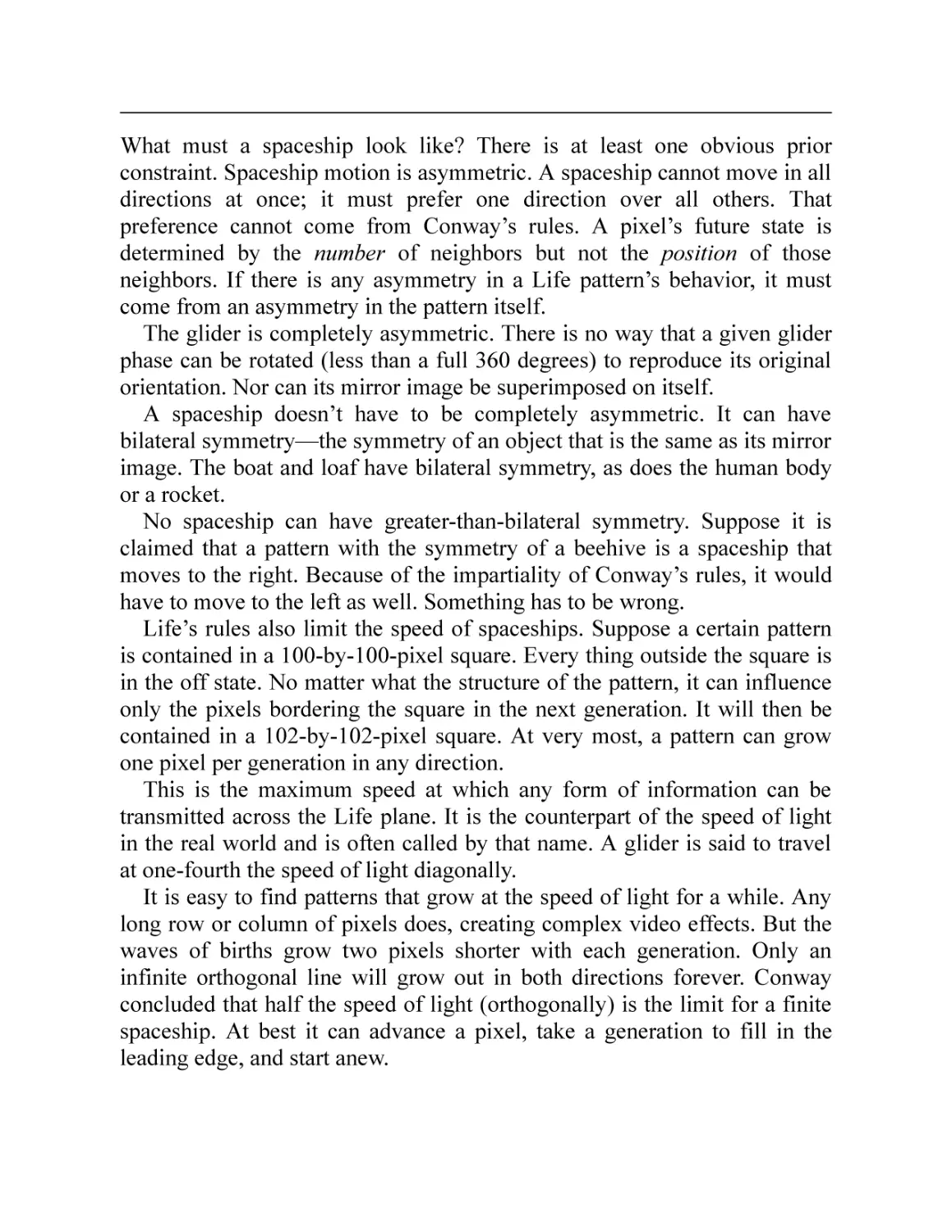
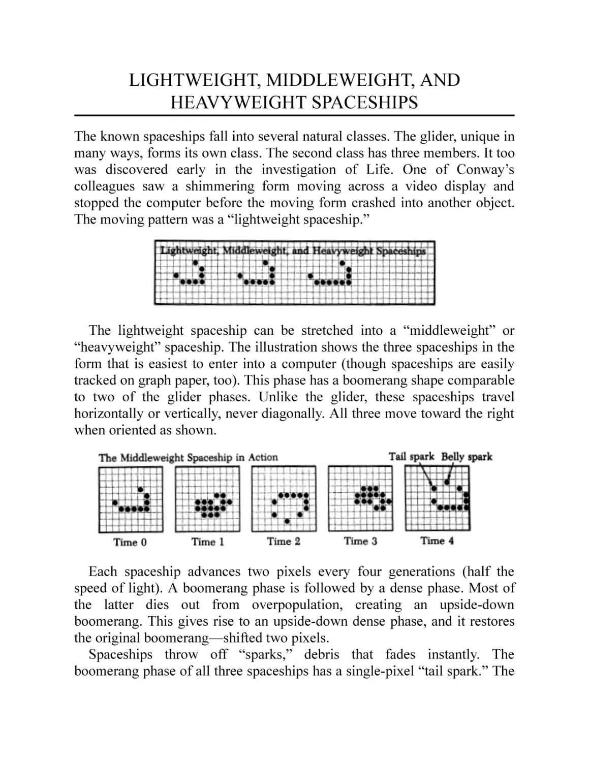
BLINKERS, BLOCKS, BEEHIVES, AND GLIDERS
The best way to get the feel of Life is to use a checkerboard or a sheet of
graph paper. Conway and colleagues played with black and white checkers.
The black checkers marked on cells. Conway identified cells due for a birth
and placed a white checker in each. A second black checker marked on
cells due to die. When all births and deaths had been identified, the double
black checkers were removed from the board and the white checkers were
replaced with black checkers. The process was repeated for each new
generation. To play on graph paper, make a new diagram for each
generation.
Try some simple configurations. If the Life universe starts out empty—
no checkers or on cells at all—every cell has zero on neighbors. By the
rules of Life, every cell remains empty in the next generation and the next
and the next. Nothing happens.
Take the opposite approach. Start with every cell occupied, an infinity of
on cells in every direction. Then every cell has eight “live” neighbors and
must die. The Life plane is empty as above a generation later.
Creation must be more subtle. Try a single live cell in an empty universe.
Now there are two cases to be considered. The live cell has zero live
neighbors, so it must die. Each of the neighboring empty cells has the one
live cell for a neighbor. That still isn’t enough to make any difference. The
configuration dies.
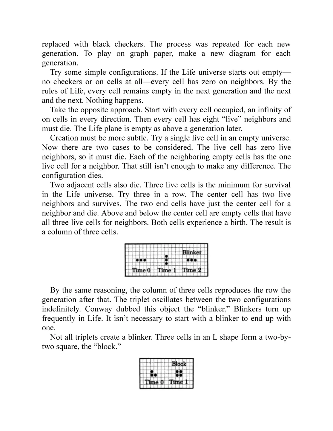
Two adjacent cells also die. Three live cells is the minimum for survival
in the Life universe. Try three in a row. The center cell has two live
neighbors and survives. The two end cells have just the center cell for a
neighbor and die. Above and below the center cell are empty cells that have
all three live cells for neighbors. Both cells experience a birth. The result is
a column of three cells.
By the same reasoning, the column of three cells reproduces the row the
generation after that. The triplet oscillates between the two configurations
indefinitely. Conway dubbed this object the “blinker.” Blinkers turn up
frequently in Life. It isn’t necessary to start with a blinker to end up with
one.
Not all triplets create a blinker. Three cells in an L shape form a two-bytwo square, the “block.”
Unlike the blinker, the block never changes. Each of the four cells has
three neighbors, so all survive. None of the surrounding empty cells has
more than two live neighbors, so there are no births. Conway’s term for
such stable patterns is “still life.” The block is the commonest still life.
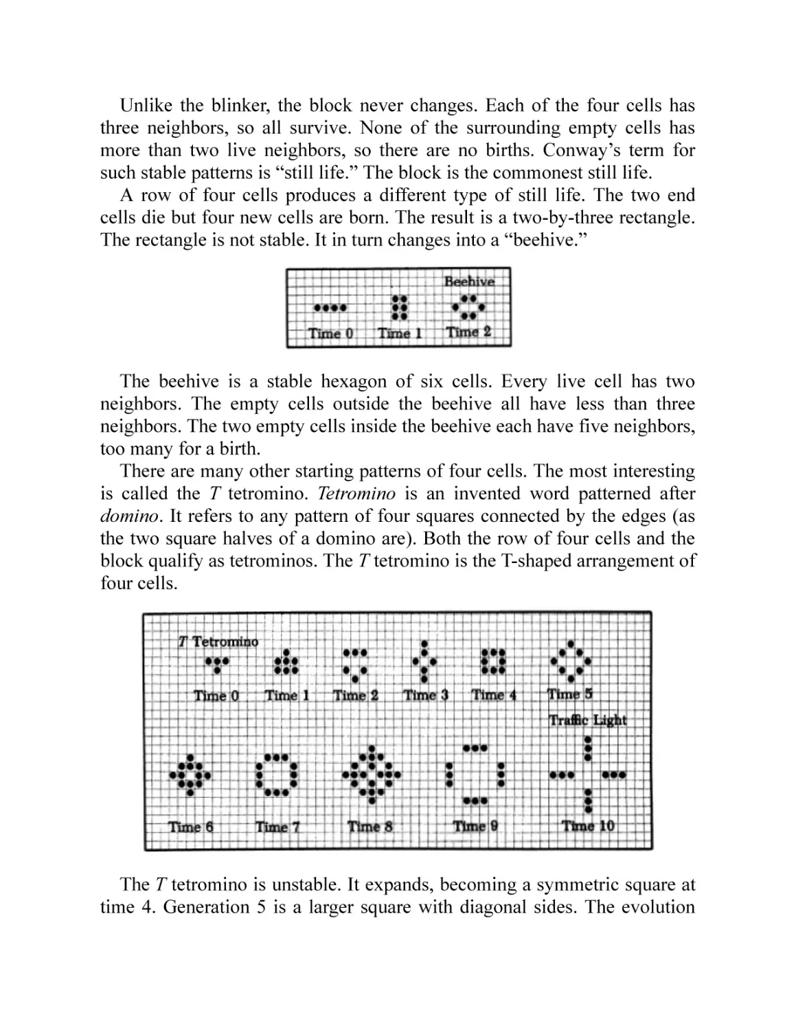
A row of four cells produces a different type of still life. The two end
cells die but four new cells are born. The result is a two-by-three rectangle.
The rectangle is not stable. It in turn changes into a “beehive.”
The beehive is a stable hexagon of six cells. Every live cell has two
neighbors. The empty cells outside the beehive all have less than three
neighbors. The two empty cells inside the beehive each have five neighbors,
too many for a birth.
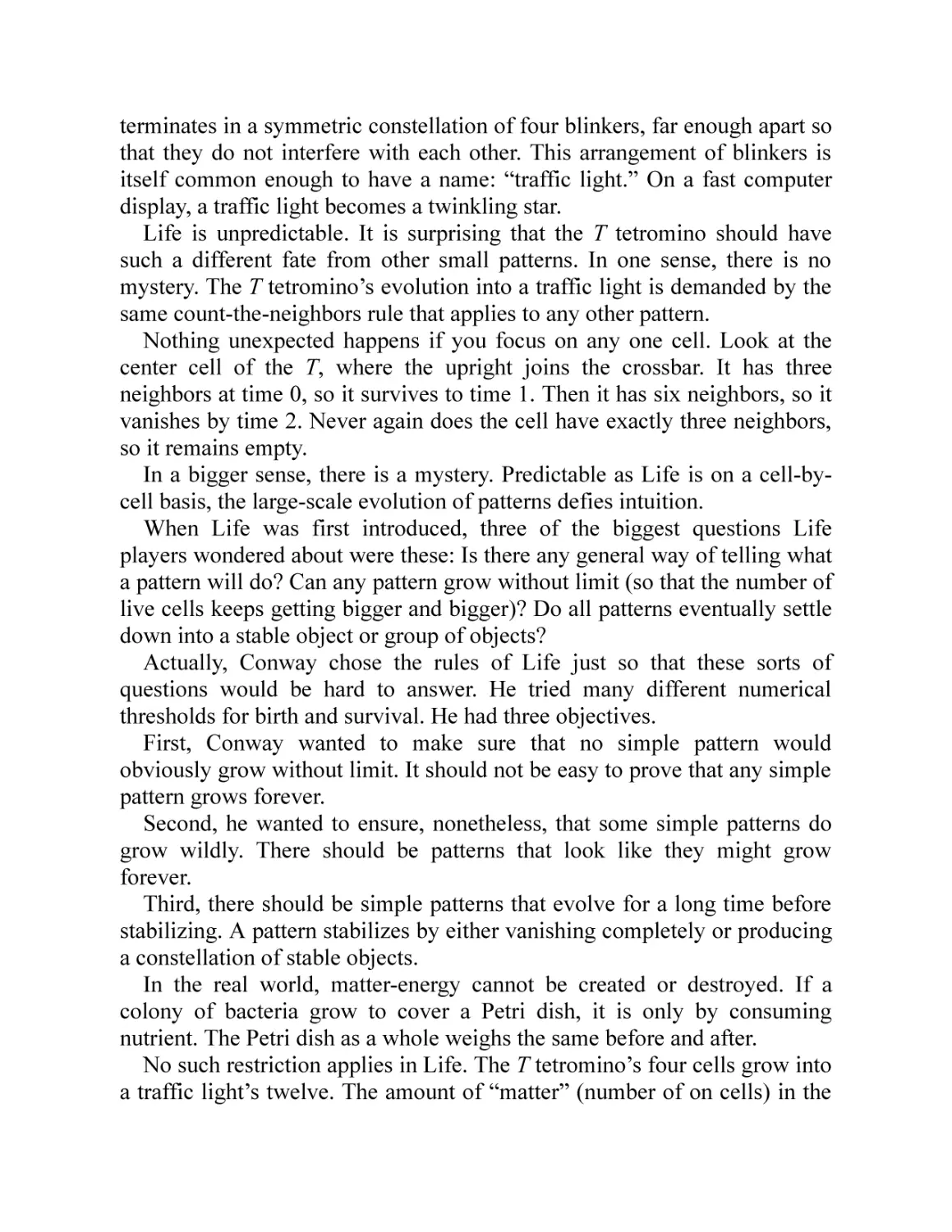
There are many other starting patterns of four cells. The most interesting
is called the T tetromino. Tetromino is an invented word patterned after
domino. It refers to any pattern of four squares connected by the edges (as
the two square halves of a domino are). Both the row of four cells and the
block qualify as tetrominos. The T tetromino is the T-shaped arrangement of
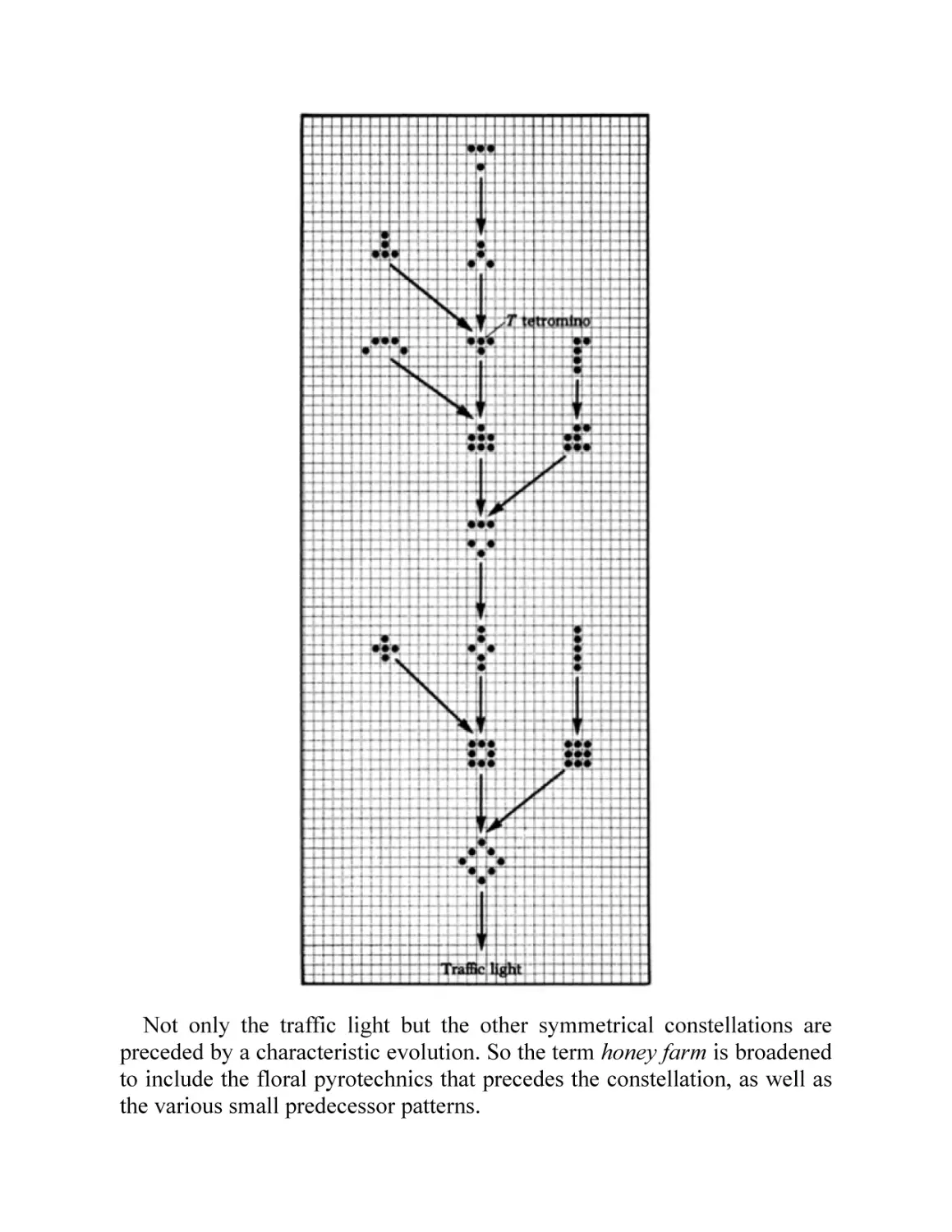
four cells.
The T tetromino is unstable. It expands, becoming a symmetric square at
time 4. Generation 5 is a larger square with diagonal sides. The evolution
terminates in a symmetric constellation of four blinkers, far enough apart so
that they do not interfere with each other. This arrangement of blinkers is
itself common enough to have a name: “traffic light.” On a fast computer
display, a traffic light becomes a twinkling star.
Life is unpredictable. It is surprising that the T tetromino should have
such a different fate from other small patterns. In one sense, there is no
mystery. The T tetromino’s evolution into a traffic light is demanded by the
same count-the-neighbors rule that applies to any other pattern.
Nothing unexpected happens if you focus on any one cell. Look at the
center cell of the T, where the upright joins the crossbar. It has three
neighbors at time 0, so it survives to time 1. Then it has six neighbors, so it
vanishes by time 2. Never again does the cell have exactly three neighbors,
so it remains empty.
In a bigger sense, there is a mystery. Predictable as Life is on a cell-bycell basis, the large-scale evolution of patterns defies intuition.
When Life was first introduced, three of the biggest questions Life
players wondered about were these: Is there any general way of telling what
a pattern will do? Can any pattern grow without limit (so that the number of
live cells keeps getting bigger and bigger)? Do all patterns eventually settle
down into a stable object or group of objects?
Actually, Conway chose the rules of Life just so that these sorts of
questions would be hard to answer. He tried many different numerical
thresholds for birth and survival. He had three objectives.
First, Conway wanted to make sure that no simple pattern would
obviously grow without limit. It should not be easy to prove that any simple
pattern grows forever.
Second, he wanted to ensure, nonetheless, that some simple patterns do
grow wildly. There should be patterns that look like they might grow
forever.
Third, there should be simple patterns that evolve for a long time before
stabilizing. A pattern stabilizes by either vanishing completely or producing
a constellation of stable objects.
In the real world, matter-energy cannot be created or destroyed. If a
colony of bacteria grow to cover a Petri dish, it is only by consuming
nutrient. The Petri dish as a whole weighs the same before and after.
No such restriction applies in Life. The T tetromino’s four cells grow into
a traffic light’s twelve. The amount of “matter” (number of on cells) in the
Life universe can fluctuate arbitrarily.
If Life’s rules said that any cell with a live neighbor qualifies for a birth
and no cell ever dies, then any initial pattern would grow like a crystal
endlessly. If on the other hand the rules were too anti-growth, then
everything would die out. Conway balanced the tendencies for growth and
death so precariously that Life is ever surprising.
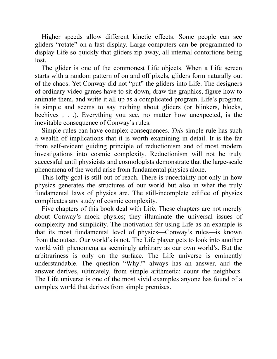
One of the first surprises was the discovery that some Life patterns move.
While following a complex pattern, one of Conway’s colleagues noticed
that a five-cell unit was “walking.” The moving unit was named the
“glider.”
The glider creeps something like an amoeba or hydra, changing its shape
as it goes. It assumes four different phases. Two phases are the shifted
mirror images of the other two. Any phase is exactly reproduced four
generations later. By then, the glider has moved one cell diagonally.
Mathematicians call a rotated mirror image a glide reflection. That and
the suggestion of motion prompted the name. A glider continues on its way
forever unless it runs into something. All gliders move diagonally, like
bishops in chess. The glider illustrated moves to the southeast, but gliders
with other orientations move in the other three diagonal directions. All
gliders move at the same speed: one cell diagonally per four generations, or
one-quarter cell per generation.
Objects such as the glider motivated Conway to program Life into a
computer. The squares of the checkerboard became the pixels of a video
screen. On a fast computer display, the motion of a glider is readily
apparent.
The most efficient Life programs for home computers typically display
two to ten generations a second. The more generations per second, the
faster things move. The appearance of gliders and other Life objects varies
with speed of display. At a few generations per second, gliders “wag their
tails” as they move—the tail being the diagonally connected trailing pixel.
Higher speeds allow different kinetic effects. Some people can see
gliders “rotate” on a fast display. Large computers can be programmed to
display Life so quickly that gliders zip away, all internal contortions being
lost.
The glider is one of the commonest Life objects. When a Life screen
starts with a random pattern of on and off pixels, gliders form naturally out
of the chaos. Yet Conway did not “put” the gliders into Life. The designers
of ordinary video games have to sit down, draw the graphics, figure how to
animate them, and write it all up as a complicated program. Life’s program
is simple and seems to say nothing about gliders (or blinkers, blocks,
beehives . . .). Everything you see, no matter how unexpected, is the
inevitable consequence of Conway’s rules.
Simple rules can have complex consequences. This simple rule has such
a wealth of implications that it is worth examining in detail. It is the far
from self-evident guiding principle of reductionism and of most modern
investigations into cosmic complexity. Reductionism will not be truly
successful until physicists and cosmologists demonstrate that the large-scale
phenomena of the world arise from fundamental physics alone.
This lofty goal is still out of reach. There is uncertainty not only in how
physics generates the structures of our world but also in what the truly
fundamental laws of physics are. The still-incomplete edifice of physics
complicates any study of cosmic complexity.
Five chapters of this book deal with Life. These chapters are not merely
about Conway’s mock physics; they illuminate the universal issues of
complexity and simplicity. The motivation for using Life as an example is
that its most fundamental level of physics—Conway’s rules—is known
from the outset. Our world’s is not. The Life player gets to look into another
world with phenomena as seemingly arbitrary as our own world’s. But the
arbitrariness is only on the surface. The Life universe is eminently
understandable. The question “Why?” always has an answer, and the
answer derives, ultimately, from simple arithmetic: count the neighbors.
The Life universe is one of the most vivid examples anyone has found of a
complex world that derives from simple premises.
•2•
THE LIFE UNIVERSE
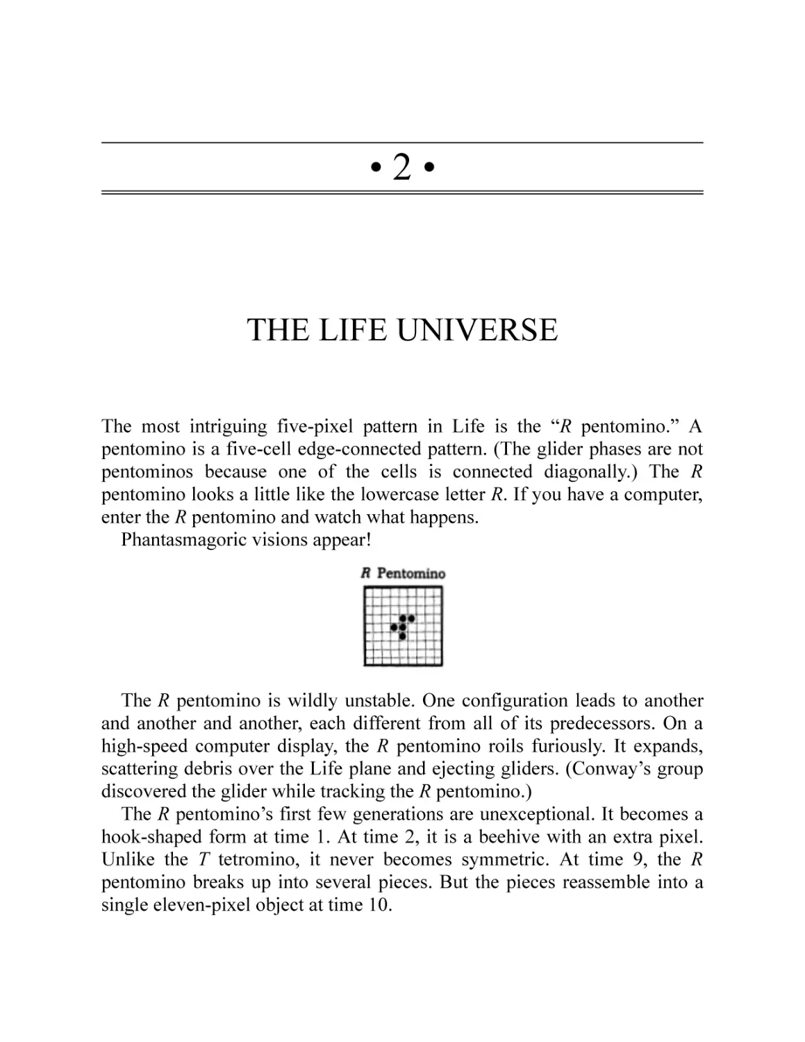
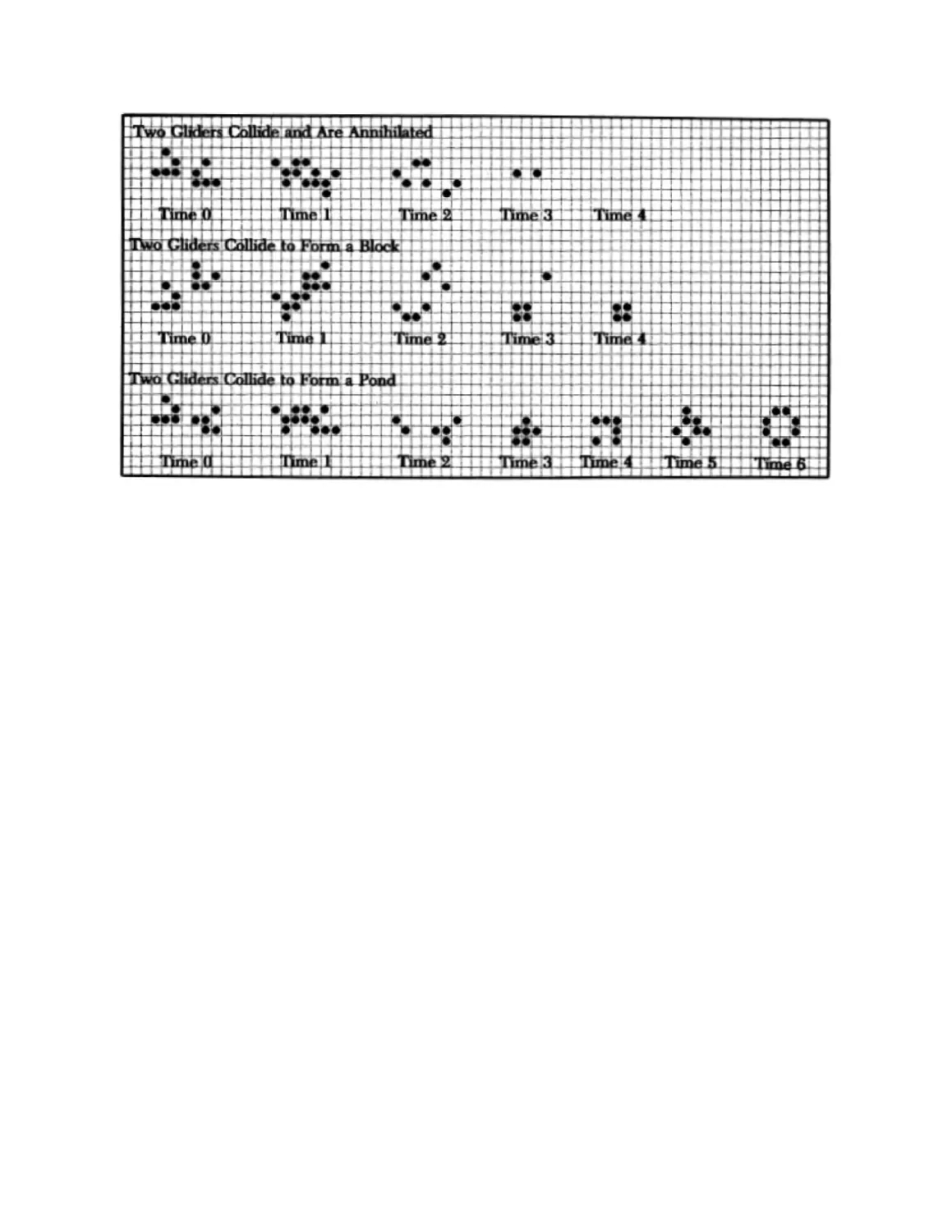
The most intriguing five-pixel pattern in Life is the “R pentomino.” A
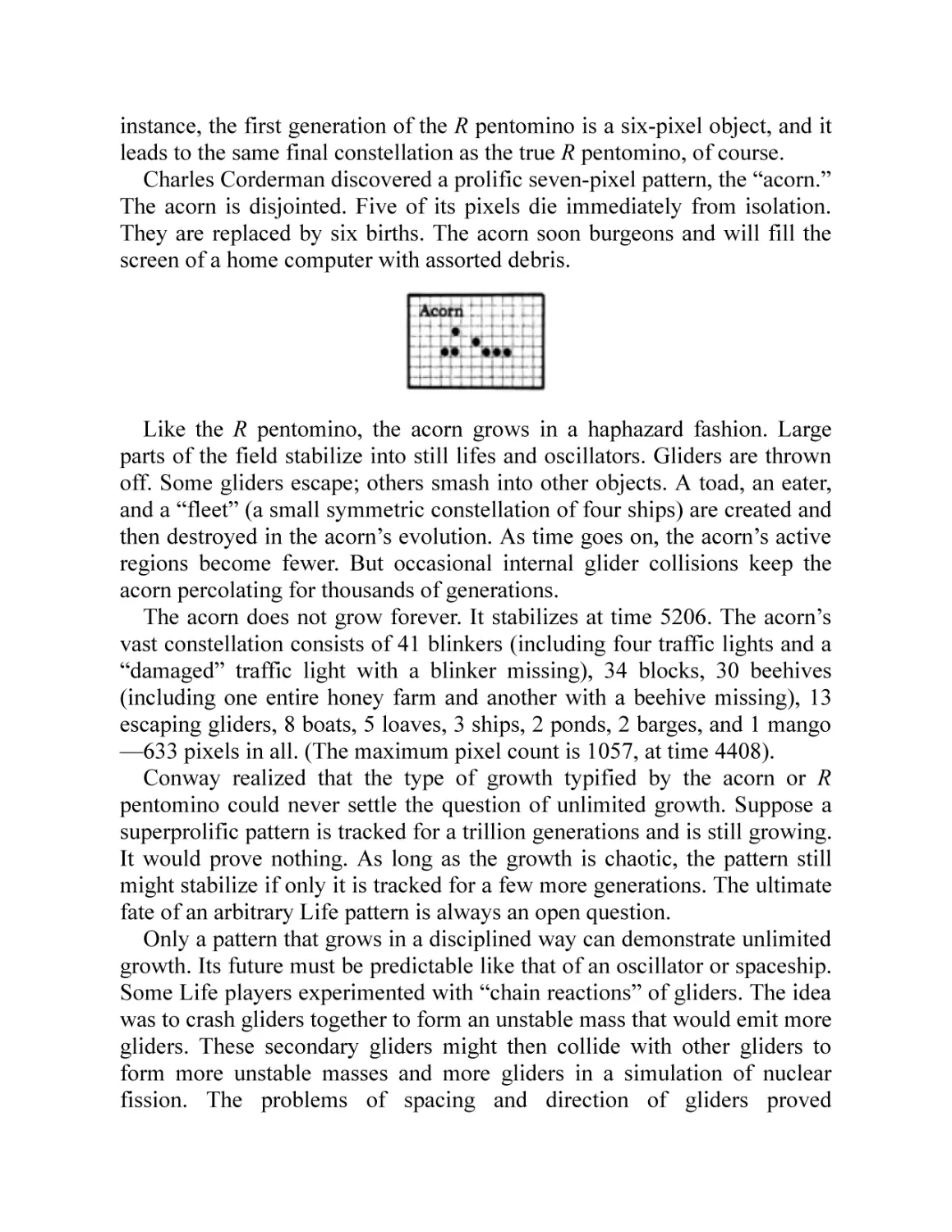
pentomino is a five-cell edge-connected pattern. (The glider phases are not
pentominos because one of the cells is connected diagonally.) The R
pentomino looks a little like the lowercase letter R. If you have a computer,
enter the R pentomino and watch what happens.
Phantasmagoric visions appear!
The R pentomino is wildly unstable. One configuration leads to another
and another and another, each different from all of its predecessors. On a
high-speed computer display, the R pentomino roils furiously. It expands,
scattering debris over the Life plane and ejecting gliders. (Conway’s group
discovered the glider while tracking the R pentomino.)
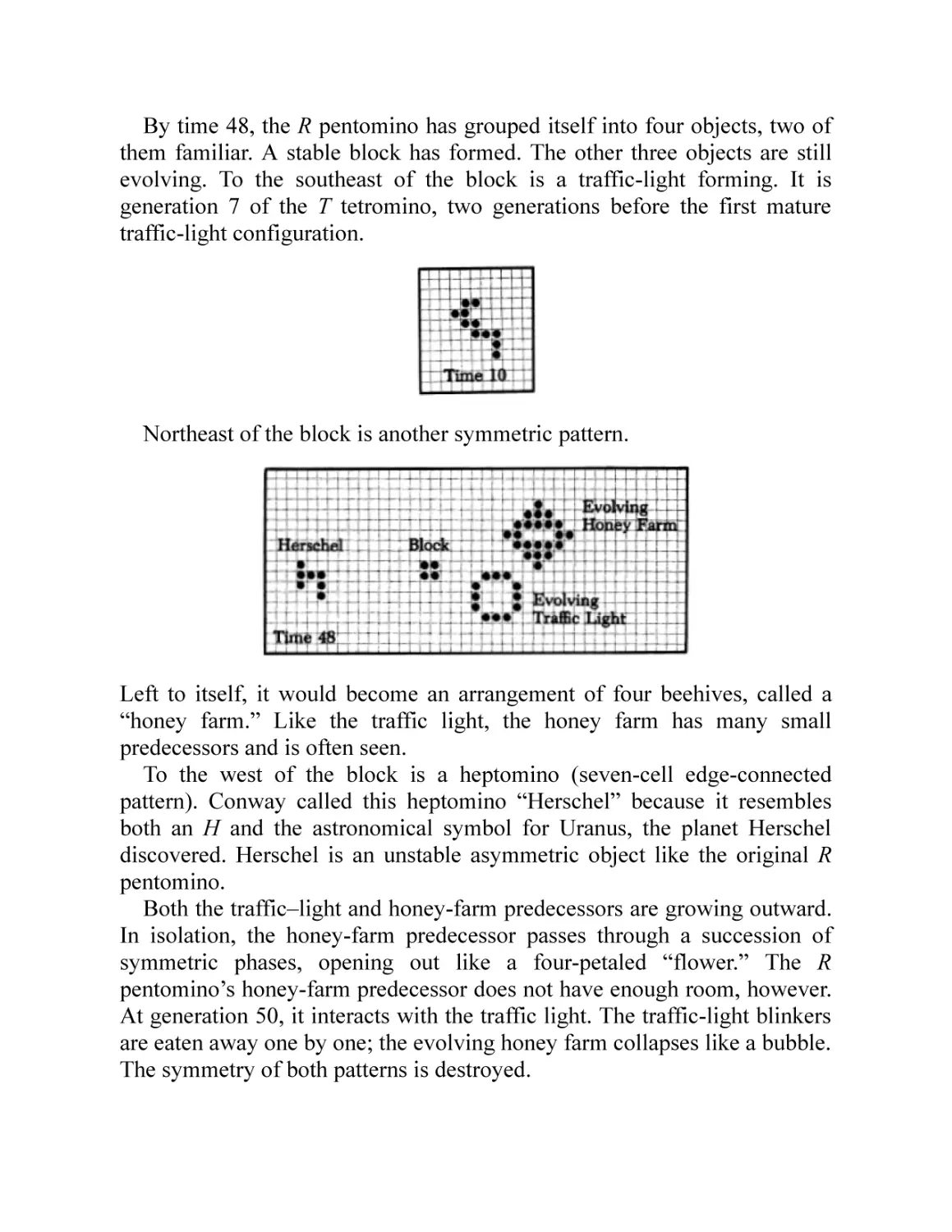
The R pentomino’s first few generations are unexceptional. It becomes a
hook-shaped form at time 1. At time 2, it is a beehive with an extra pixel.
Unlike the T tetromino, it never becomes symmetric. At time 9, the R
pentomino breaks up into several pieces. But the pieces reassemble into a
single eleven-pixel object at time 10.
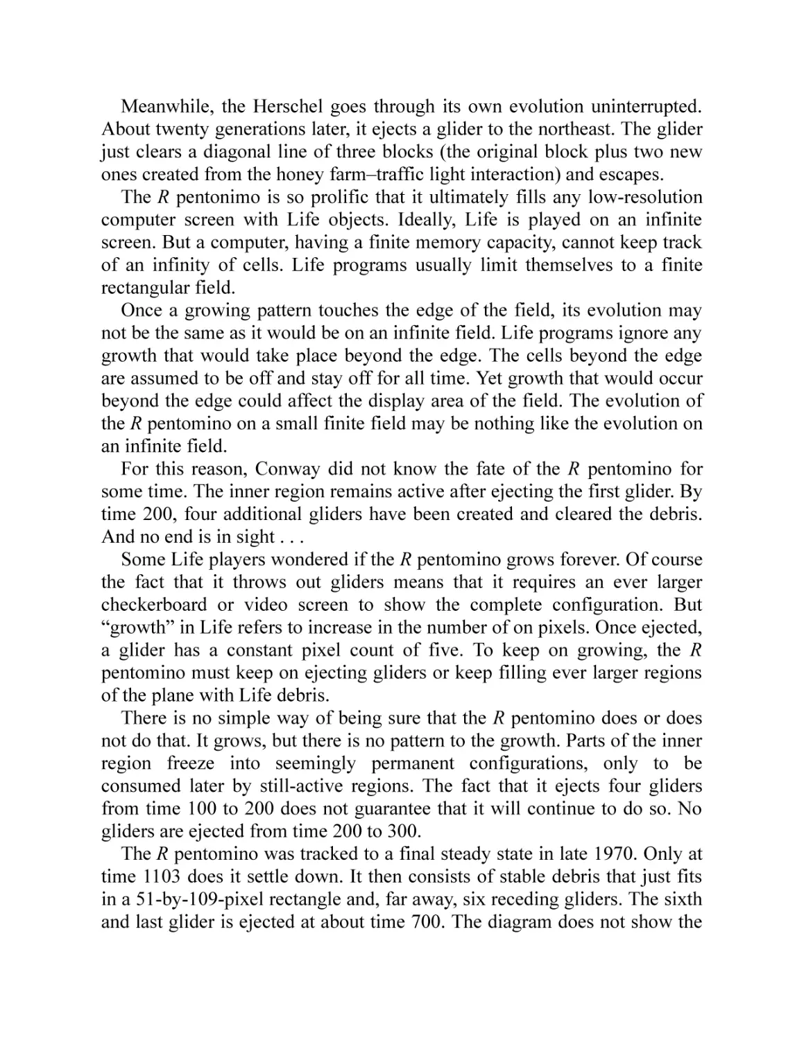
By time 48, the R pentomino has grouped itself into four objects, two of
them familiar. A stable block has formed. The other three objects are still
evolving. To the southeast of the block is a traffic-light forming. It is
generation 7 of the T tetromino, two generations before the first mature
traffic-light configuration.
Northeast of the block is another symmetric pattern.
Left to itself, it would become an arrangement of four beehives, called a
“honey farm.” Like the traffic light, the honey farm has many small
predecessors and is often seen.
To the west of the block is a heptomino (seven-cell edge-connected
pattern). Conway called this heptomino “Herschel” because it resembles
both an H and the astronomical symbol for Uranus, the planet Herschel
discovered. Herschel is an unstable asymmetric object like the original R
pentomino.
Both the traffic–light and honey-farm predecessors are growing outward.
In isolation, the honey-farm predecessor passes through a succession of
symmetric phases, opening out like a four-petaled “flower.” The R
pentomino’s honey-farm predecessor does not have enough room, however.
At generation 50, it interacts with the traffic light. The traffic-light blinkers
are eaten away one by one; the evolving honey farm collapses like a bubble.
The symmetry of both patterns is destroyed.
Meanwhile, the Herschel goes through its own evolution uninterrupted.
About twenty generations later, it ejects a glider to the northeast. The glider
just clears a diagonal line of three blocks (the original block plus two new
ones created from the honey farm–traffic light interaction) and escapes.
The R pentonimo is so prolific that it ultimately fills any low-resolution
computer screen with Life objects. Ideally, Life is played on an infinite
screen. But a computer, having a finite memory capacity, cannot keep track
of an infinity of cells. Life programs usually limit themselves to a finite
rectangular field.
Once a growing pattern touches the edge of the field, its evolution may
not be the same as it would be on an infinite field. Life programs ignore any
growth that would take place beyond the edge. The cells beyond the edge
are assumed to be off and stay off for all time. Yet growth that would occur
beyond the edge could affect the display area of the field. The evolution of
the R pentomino on a small finite field may be nothing like the evolution on
an infinite field.
For this reason, Conway did not know the fate of the R pentomino for
some time. The inner region remains active after ejecting the first glider. By
time 200, four additional gliders have been created and cleared the debris.
And no end is in sight . . .
Some Life players wondered if the R pentomino grows forever. Of course
the fact that it throws out gliders means that it requires an ever larger
checkerboard or video screen to show the complete configuration. But
“growth” in Life refers to increase in the number of on pixels. Once ejected,
a glider has a constant pixel count of five. To keep on growing, the R
pentomino must keep on ejecting gliders or keep filling ever larger regions
of the plane with Life debris.
There is no simple way of being sure that the R pentomino does or does
not do that. It grows, but there is no pattern to the growth. Parts of the inner
region freeze into seemingly permanent configurations, only to be
consumed later by still-active regions. The fact that it ejects four gliders
from time 100 to 200 does not guarantee that it will continue to do so. No
gliders are ejected from time 200 to 300.
The R pentomino was tracked to a final steady state in late 1970. Only at
time 1103 does it settle down. It then consists of stable debris that just fits
in a 51-by-109-pixel rectangle and, far away, six receding gliders. The sixth
and last glider is ejected at about time 700. The diagram does not show the
gliders. The position of the original R pentomino is indicated; these five
pixels are empty in the steady state.
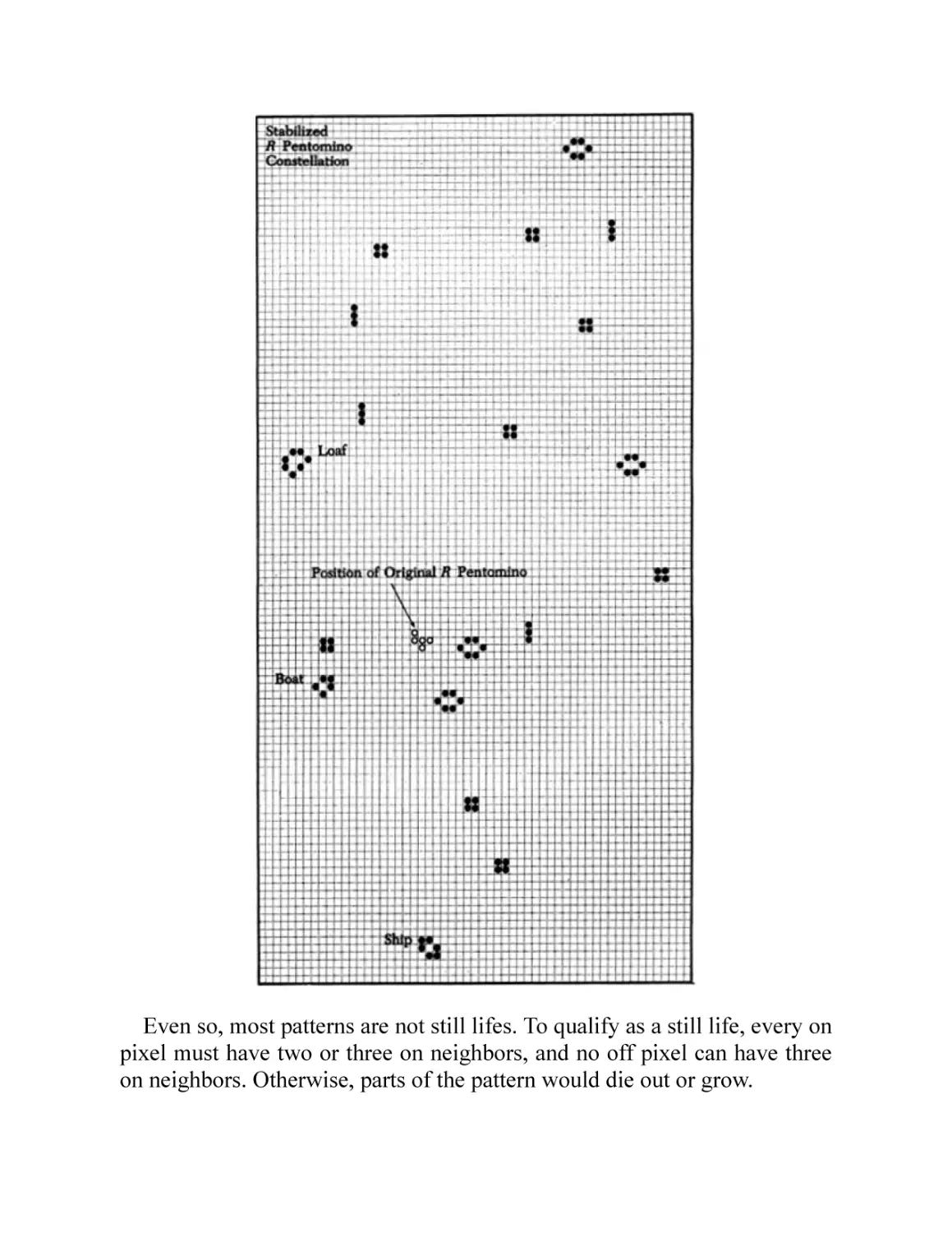
The R pentomino’s final constellation consists of twenty-five objects,
including the gliders. Three objects are new still lifes. At the bottom of the
diagram is a six-pixel object, the “ship.” The ship resembles a beehive, but
its long axis is diagonal. The constellation also includes a five-pixel “boat,”
which is a ship with one of the stern or bow pixels removed. The “loaf” is a
common half-circle form of seven pixels.
The object produced in greatest number is the simple block. The census:
8 blocks
6 gliders
4 beehives
4 blinkers
1 boat
1 loaf
1 ship
The final population is 116 on pixels. (The maximum population of 319
pixels occurs in generation 821, well before the pattern stabilizes.) Relative
to the diagram, the first glider travels northwest, the next three travel
northeast, and the last two go southwest.
To say that the R pentomino stabilizes is to say that its future is
predictable. The gliders still move, and the blinkers still blink. But nothing
in the R pentomino constellation interacts with anything else after time
1103.
The R pentomino’s evolution is incredible. Somehow all the blocks,
gliders, beehives, blinkers, and other objects are latent in the original R
pentomino—but how? The R pentomino is one of many Life objects that
defies ready analysis.
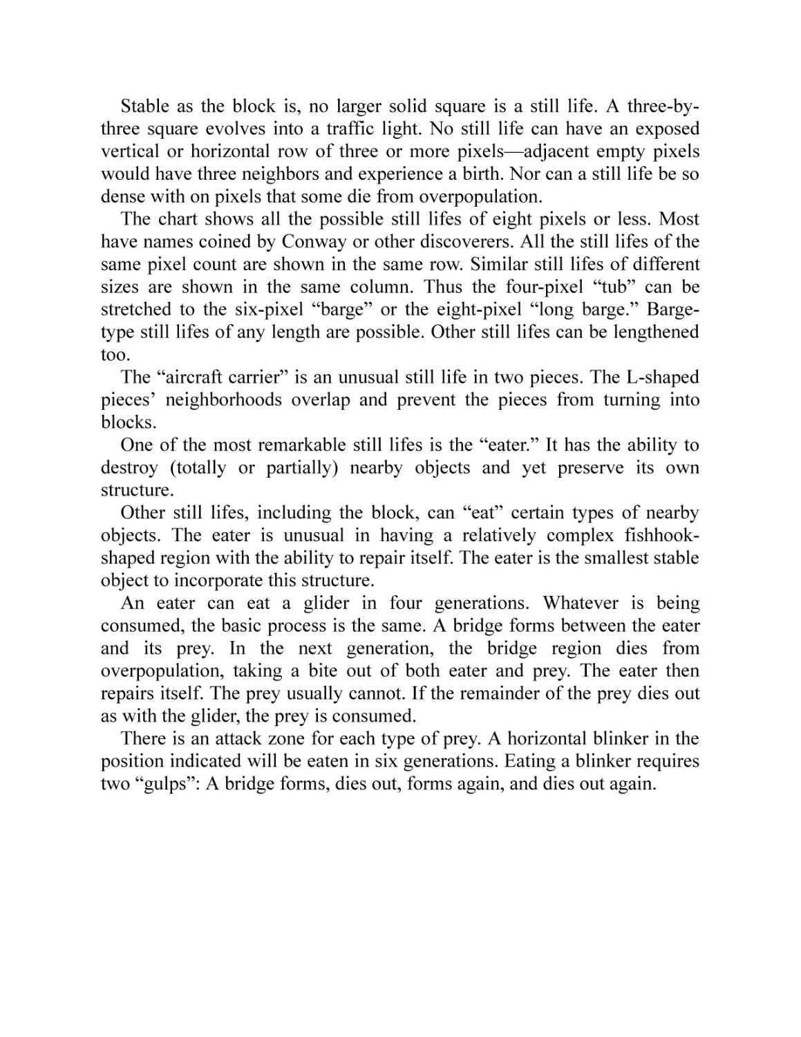
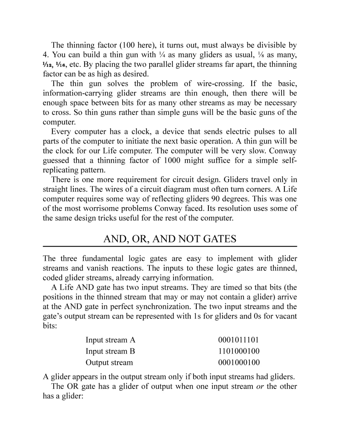
STILL LIFES AND THE EATER
The R pentomino creates five types of still lifes. There are more—infinitely
many more.
Even so, most patterns are not still lifes. To qualify as a still life, every on
pixel must have two or three on neighbors, and no off pixel can have three
on neighbors. Otherwise, parts of the pattern would die out or grow.
Stable as the block is, no larger solid square is a still life. A three-bythree square evolves into a traffic light. No still life can have an exposed
vertical or horizontal row of three or more pixels—adjacent empty pixels
would have three neighbors and experience a birth. Nor can a still life be so
dense with on pixels that some die from overpopulation.
The chart shows all the possible still lifes of eight pixels or less. Most
have names coined by Conway or other discoverers. All the still lifes of the
same pixel count are shown in the same row. Similar still lifes of different
sizes are shown in the same column. Thus the four-pixel “tub” can be
stretched to the six-pixel “barge” or the eight-pixel “long barge.” Bargetype still lifes of any length are possible. Other still lifes can be lengthened
too.
The “aircraft carrier” is an unusual still life in two pieces. The L-shaped
pieces’ neighborhoods overlap and prevent the pieces from turning into
blocks.
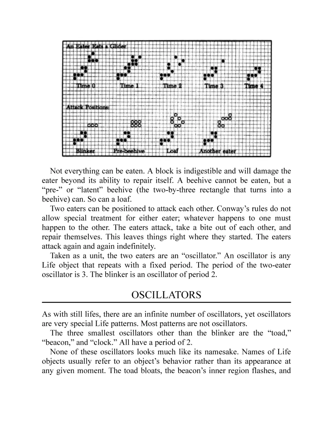
One of the most remarkable still lifes is the “eater.” It has the ability to
destroy (totally or partially) nearby objects and yet preserve its own
structure.
Other still lifes, including the block, can “eat” certain types of nearby
objects. The eater is unusual in having a relatively complex fishhookshaped region with the ability to repair itself. The eater is the smallest stable
object to incorporate this structure.
An eater can eat a glider in four generations. Whatever is being
consumed, the basic process is the same. A bridge forms between the eater
and its prey. In the next generation, the bridge region dies from
overpopulation, taking a bite out of both eater and prey. The eater then
repairs itself. The prey usually cannot. If the remainder of the prey dies out
as with the glider, the prey is consumed.
There is an attack zone for each type of prey. A horizontal blinker in the
position indicated will be eaten in six generations. Eating a blinker requires
two “gulps”: A bridge forms, dies out, forms again, and dies out again.
Not everything can be eaten. A block is indigestible and will damage the
eater beyond its ability to repair itself. A beehive cannot be eaten, but a
“pre-” or “latent” beehive (the two-by-three rectangle that turns into a
beehive) can. So can a loaf.
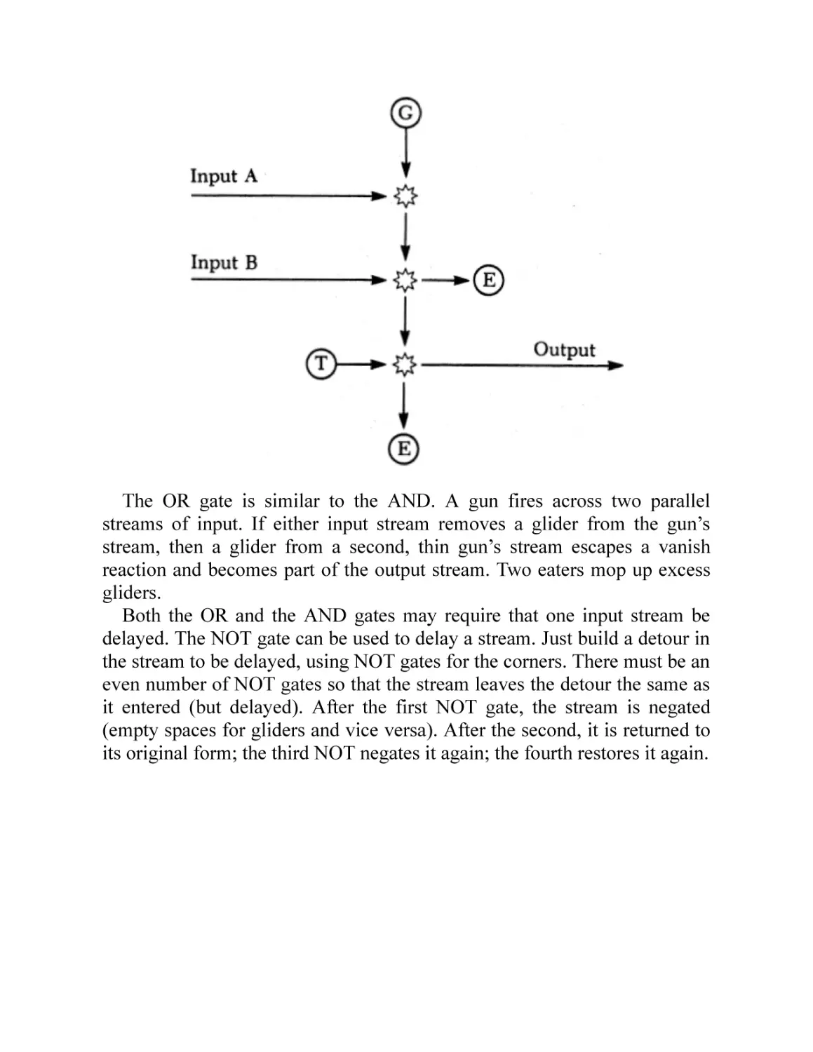
Two eaters can be positioned to attack each other. Conway’s rules do not
allow special treatment for either eater; whatever happens to one must
happen to the other. The eaters attack, take a bite out of each other, and
repair themselves. This leaves things right where they started. The eaters
attack again and again indefinitely.
Taken as a unit, the two eaters are an “oscillator.” An oscillator is any
Life object that repeats with a fixed period. The period of the two-eater
oscillator is 3. The blinker is an oscillator of period 2.
OSCILLATORS
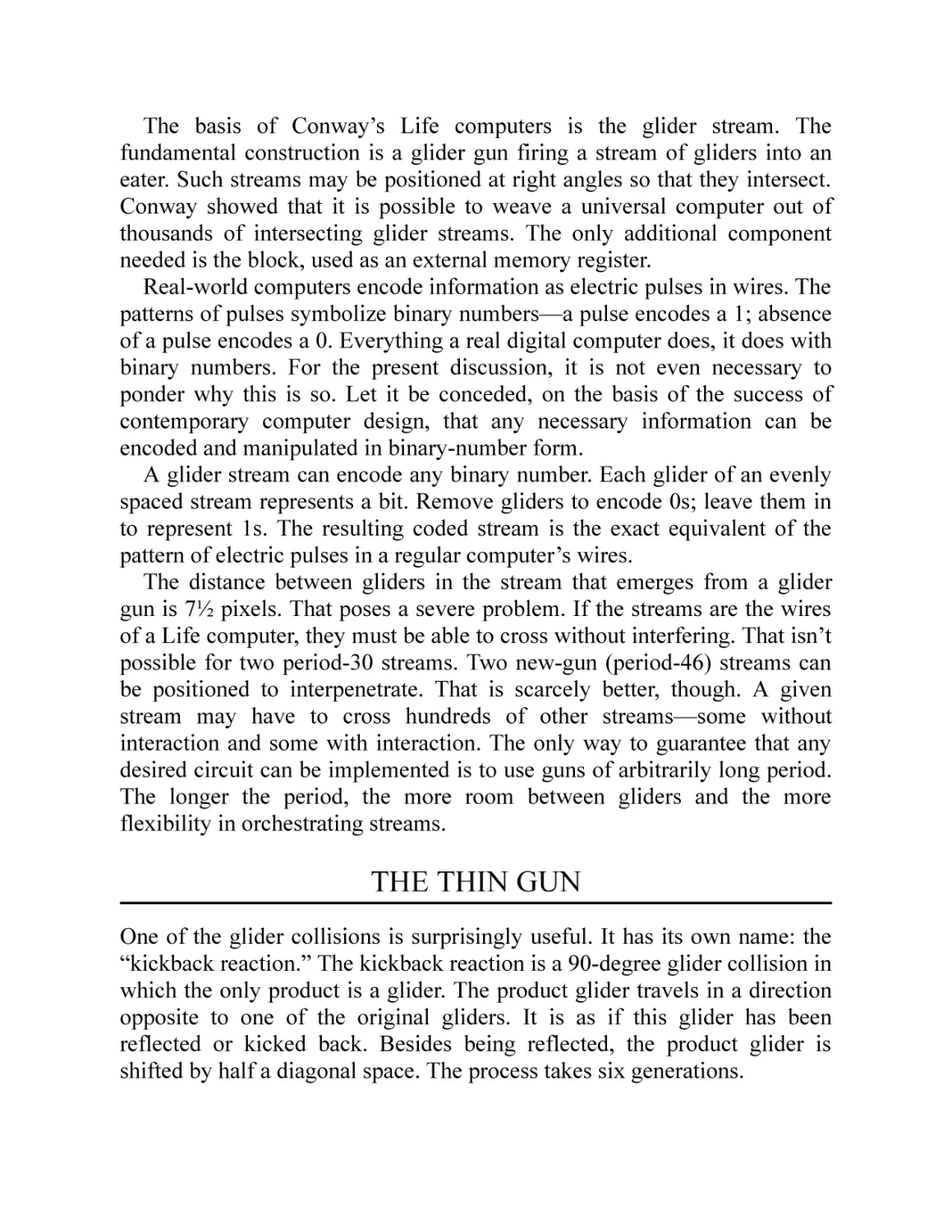
As with still lifes, there are an infinite number of oscillators, yet oscillators
are very special Life patterns. Most patterns are not oscillators.
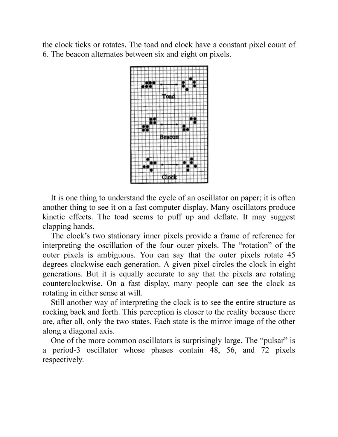
The three smallest oscillators other than the blinker are the “toad,”
“beacon,” and “clock.” All have a period of 2.
None of these oscillators looks much like its namesake. Names of Life
objects usually refer to an object’s behavior rather than its appearance at
any given moment. The toad bloats, the beacon’s inner region flashes, and
the clock ticks or rotates. The toad and clock have a constant pixel count of
6. The beacon alternates between six and eight on pixels.
It is one thing to understand the cycle of an oscillator on paper; it is often
another thing to see it on a fast computer display. Many oscillators produce
kinetic effects. The toad seems to puff up and deflate. It may suggest
clapping hands.
The clock’s two stationary inner pixels provide a frame of reference for
interpreting the oscillation of the four outer pixels. The “rotation” of the
outer pixels is ambiguous. You can say that the outer pixels rotate 45
degrees clockwise each generation. A given pixel circles the clock in eight
generations. But it is equally accurate to say that the pixels are rotating
counterclockwise. On a fast display, many people can see the clock as
rotating in either sense at will.
Still another way of interpreting the clock is to see the entire structure as
rocking back and forth. This perception is closer to the reality because there
are, after all, only the two states. Each state is the mirror image of the other
along a diagonal axis.
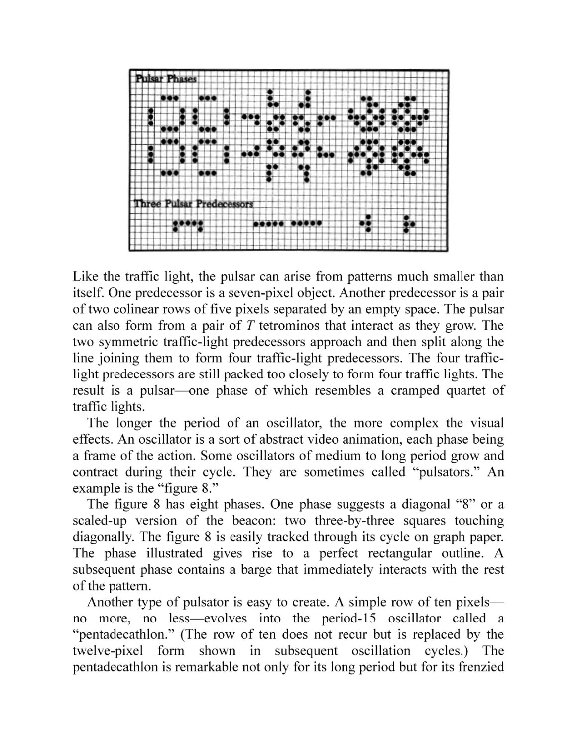
One of the more common oscillators is surprisingly large. The “pulsar” is
a period-3 oscillator whose phases contain 48, 56, and 72 pixels
respectively.
Like the traffic light, the pulsar can arise from patterns much smaller than
itself. One predecessor is a seven-pixel object. Another predecessor is a pair
of two colinear rows of five pixels separated by an empty space. The pulsar
can also form from a pair of T tetrominos that interact as they grow. The
two symmetric traffic-light predecessors approach and then split along the
line joining them to form four traffic-light predecessors. The four trafficlight predecessors are still packed too closely to form four traffic lights. The
result is a pulsar—one phase of which resembles a cramped quartet of
traffic lights.
The longer the period of an oscillator, the more complex the visual
effects. An oscillator is a sort of abstract video animation, each phase being
a frame of the action. Some oscillators of medium to long period grow and
contract during their cycle. They are sometimes called “pulsators.” An
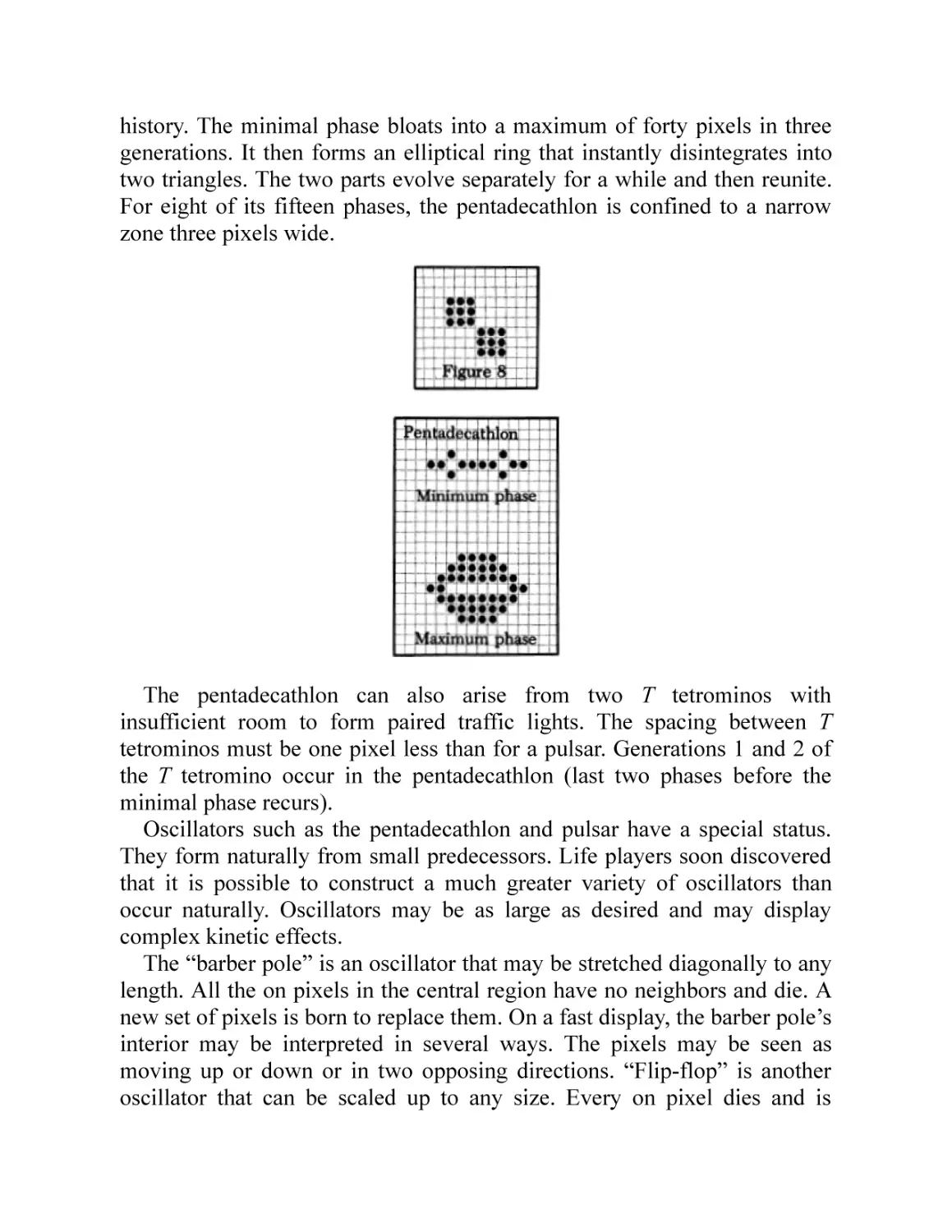
example is the “figure 8.”
The figure 8 has eight phases. One phase suggests a diagonal “8” or a
scaled-up version of the beacon: two three-by-three squares touching
diagonally. The figure 8 is easily tracked through its cycle on graph paper.
The phase illustrated gives rise to a perfect rectangular outline. A
subsequent phase contains a barge that immediately interacts with the rest
of the pattern.
Another type of pulsator is easy to create. A simple row of ten pixels—
no more, no less—evolves into the period-15 oscillator called a
“pentadecathlon.” (The row of ten does not recur but is replaced by the
twelve-pixel form shown in subsequent oscillation cycles.) The
pentadecathlon is remarkable not only for its long period but for its frenzied
history. The minimal phase bloats into a maximum of forty pixels in three
generations. It then forms an elliptical ring that instantly disintegrates into
two triangles. The two parts evolve separately for a while and then reunite.
For eight of its fifteen phases, the pentadecathlon is confined to a narrow
zone three pixels wide.
The pentadecathlon can also arise from two T tetrominos with
insufficient room to form paired traffic lights. The spacing between T
tetrominos must be one pixel less than for a pulsar. Generations 1 and 2 of
the T tetromino occur in the pentadecathlon (last two phases before the
minimal phase recurs).
Oscillators such as the pentadecathlon and pulsar have a special status.
They form naturally from small predecessors. Life players soon discovered
that it is possible to construct a much greater variety of oscillators than
occur naturally. Oscillators may be as large as desired and may display
complex kinetic effects.
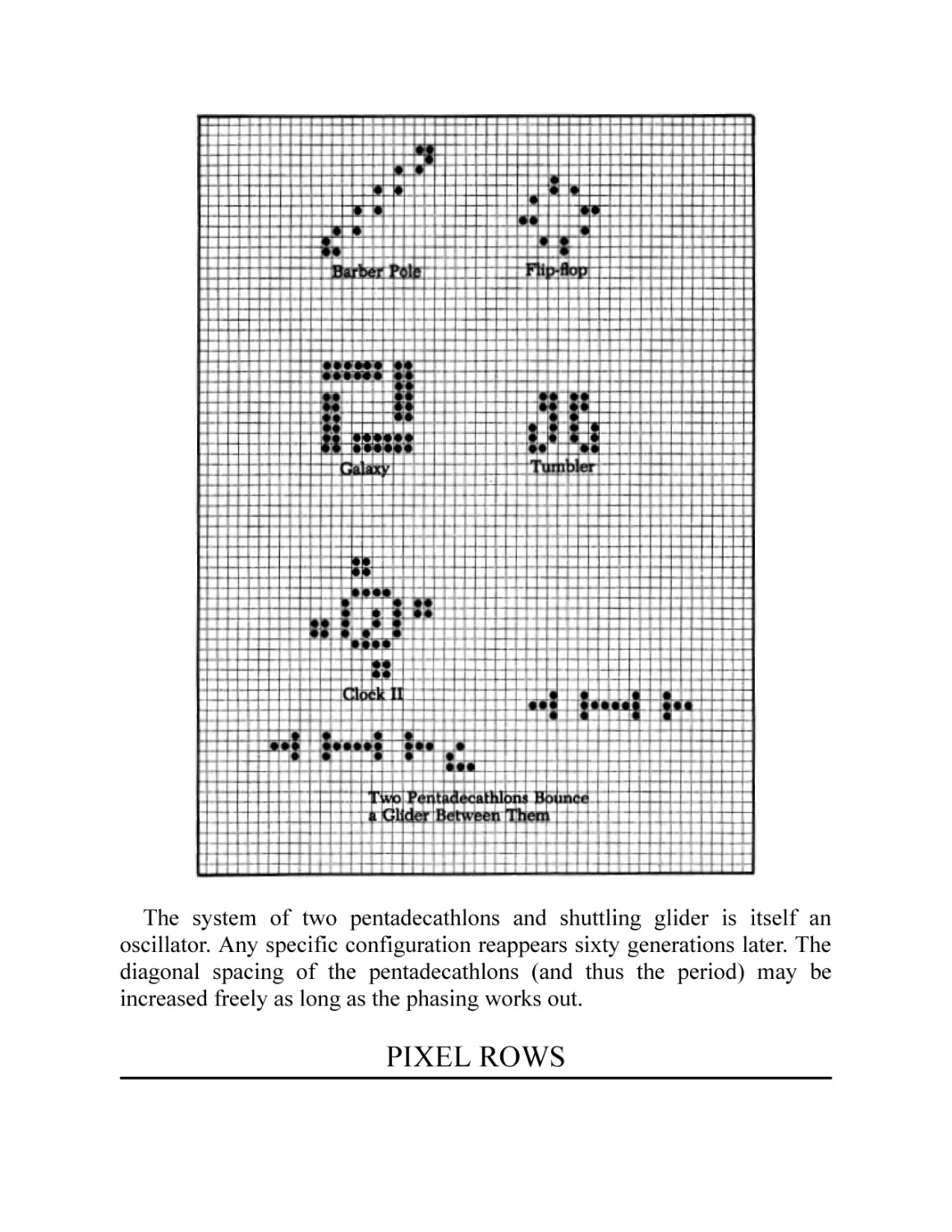
The “barber pole” is an oscillator that may be stretched diagonally to any
length. All the on pixels in the central region have no neighbors and die. A
new set of pixels is born to replace them. On a fast display, the barber pole’s
interior may be interpreted in several ways. The pixels may be seen as
moving up or down or in two opposing directions. “Flip-flop” is another
oscillator that can be scaled up to any size. Every on pixel dies and is
replaced by a birth. Like the clock, it has an ambiguous rotation. Both the
barber pole and flip-flop have a period of 2.
“Galaxy” is a period-8 pulsator. The simple geometric phase shown
becomes a four-petaled “flower” and then evolves into a spiral “galaxy,”
throwing off sparks. The fragments reassemble back into the original phase.
The “tumbler’s” symmetric halves prevent growth that would otherwise
destroy the oscillation. The four quadrants of a pulsar function similarly.
The tumbler turns itself upside down every seven generations. The full
period is 14. On a high-speed display, the tumbler suggests two snaillike
creatures climbing an invisible wall and periodically slipping back down.
The “clock II” is an example of a “billiard-table configuration.” This is
an oscillator in which the action is restricted to an enclosed region of the
Life plane. The clock’s bent hand rotates 90 degrees clockwise every
generation for a period of 4. The four blocks around the clock II’s periphery
are necessary to prevent growth on the edges. Many other billiard-table
oscillators have been designed.
The period of an oscillator can be arbitrarily long. It is possible for a
glider to collide with a pentadecathlon in just such a way that the glider is
reflected 180 degrees and the pentadecathlon is unharmed. The glider must
encounter the pentadecathlon at the proper phase of oscillation, and the
spacing must be right too.
With due attention to details, a glider can be positioned between two
pentadecathlons so that it is reflected repeatedly. The pentadecathlons
bounce the glider back and forth between them. On a high-speed display,
this is reminiscent of a Ping-Pong–type video game, though the paddles are
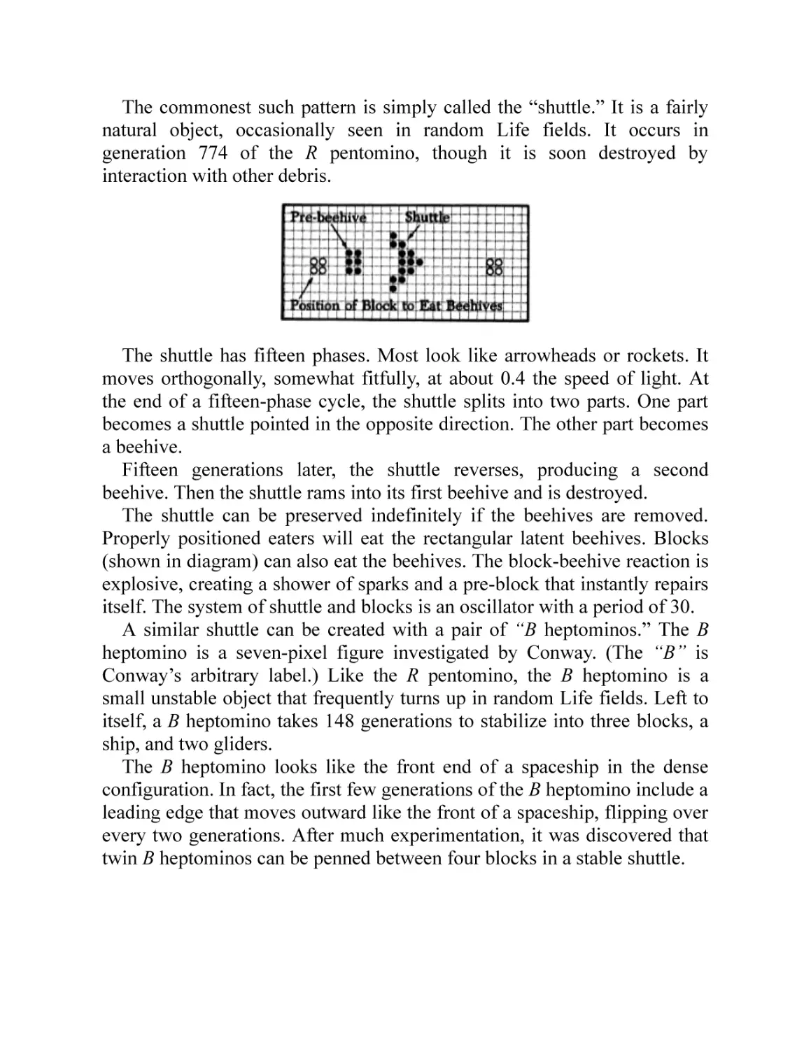
kaleidoscopic.
The shuttling glider is shifted slightly as well as reflected. Its actual
circuit is a narrow parallelogram. The diagram shows the glider in its last
normal phase before reflection. The glider, traveling to the southwest,
seems almost to have overshot the pentadecathlon. It interacts in the next
generation, and then a few generations later. The end of the pentadecathlon
that interacts with the glider dies back anyway, so the pentadecathlon is not
affected.
The system of two pentadecathlons and shuttling glider is itself an
oscillator. Any specific configuration reappears sixty generations later. The
diagonal spacing of the pentadecathlons (and thus the period) may be
increased freely as long as the phasing works out.
PIXEL ROWS
You may be wondering what a row of nine or eleven pixels creates, insofar
as a row of ten gives rise to the pentadecathlon. Conway tracked all the
small rows of cells. Surprisingly, the fate of pixel rows depends on the
precise number of pixels. One more or one less, and the fate is usually quite
different.
One or two pixels die instantly. Three is the blinker. Four becomes a
beehive in two generations. The first new case is a row of five. It becomes a
solid three-by-three square and then duplicates the later evolution of the T
tetromino, terminating with a traffic light.
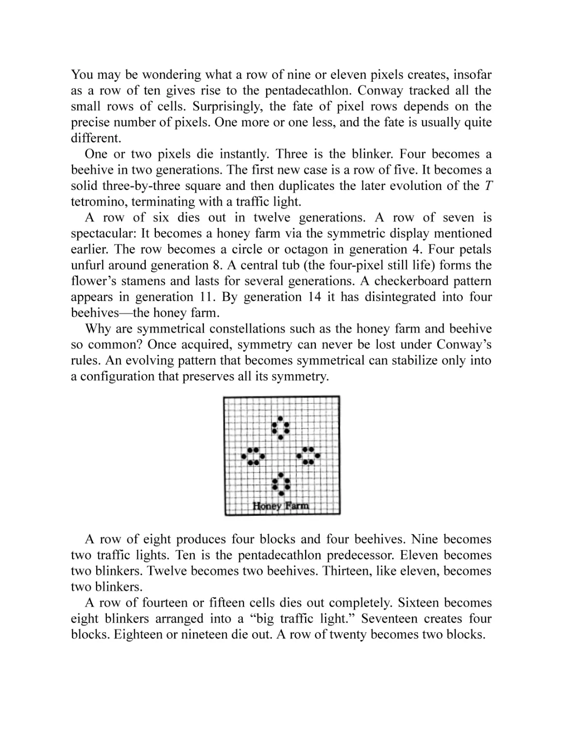
A row of six dies out in twelve generations. A row of seven is
spectacular: It becomes a honey farm via the symmetric display mentioned
earlier. The row becomes a circle or octagon in generation 4. Four petals
unfurl around generation 8. A central tub (the four-pixel still life) forms the
flower’s stamens and lasts for several generations. A checkerboard pattern
appears in generation 11. By generation 14 it has disintegrated into four
beehives—the honey farm.
Why are symmetrical constellations such as the honey farm and beehive
so common? Once acquired, symmetry can never be lost under Conway’s
rules. An evolving pattern that becomes symmetrical can stabilize only into
a configuration that preserves all its symmetry.
A row of eight produces four blocks and four beehives. Nine becomes
two traffic lights. Ten is the pentadecathlon predecessor. Eleven becomes
two blinkers. Twelve becomes two beehives. Thirteen, like eleven, becomes
two blinkers.
A row of fourteen or fifteen cells dies out completely. Sixteen becomes
eight blinkers arranged into a “big traffic light.” Seventeen creates four
blocks. Eighteen or nineteen die out. A row of twenty becomes two blocks.
NATURALISTS AND ENGINEERS
No one knows any simple way of accounting for the behavior of pixel rows,
much less for Life objects in general. There are at least two ways of looking
at Life. One is the naturalist approach, in which you are interested mainly in
seeing what objects occur naturally—what order arises from chaos. The
other is the engineer approach, in which you try to construct objects that do
complicated, clever, or surprising things.
The definition of a natural Life object is purposely open-ended.
Basically, a natural Life object is one that can occur in many different ways.
If you can expect to see an object just by playing around with a computer
programmed for Life, then it is a natural object.
An object that has many small predecessor patterns is natural. For
instance, the abundance of blocks and blinkers in Life is a consequence of
the fact that it takes only three pixels to create them. Large objects with
predecessors much smaller than themselves (such as the pulsar and honey
farm) are more natural than other large objects.
Another way of creating natural objects is to start the Life field in a
random configuration of on and off pixels. The initial ratio of on pixels to
total pixels (the density) may be any value between 0 and 1. Such random
fields (“broths”) start out being violently active. Eventually many familiar
Life objects—blocks, blinkers, beehives, gliders—appear. The more
frequently an object is seen in random fields, the more natural it is.
A third method is to experiment with collisions between gliders or of
gliders with other objects. The gliders generated in a random field
eventually strike something, so collisions are natural events. Collisions are
thoroughly unpredictable. Usually, both objects are destroyed and new
objects are created. Objects that occur frequently in collisions are natural
objects.
Life is forward-deterministic. A given pattern leads to one, and only one,
sequel pattern. Life is not backward-deterministic. A pattern usually has
many patterns that may have preceded it. In short, a configuration has only
one future but (usually) many possible pasts. This fact is responsible for one
of the occasional frustrations of playing Life. Sometimes you will see
something interesting happen, stop the program, and be unable to backtrack
and repeat it. There is no simple way you can program a computer to go
backward from a Life state—there are too many possibilities.
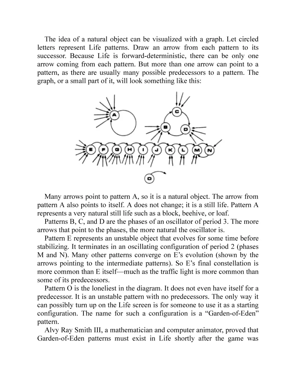
The idea of a natural object can be visualized with a graph. Let circled
letters represent Life patterns. Draw an arrow from each pattern to its
successor. Because Life is forward-deterministic, there can be only one
arrow coming from each pattern. But more than one arrow can point to a
pattern, as there are usually many possible predecessors to a pattern. The
graph, or a small part of it, will look something like this:
Many arrows point to pattern A, so it is a natural object. The arrow from
pattern A also points to itself. A does not change; it is a still life. Pattern A
represents a very natural still life such as a block, beehive, or loaf.
Patterns B, C, and D are the phases of an oscillator of period 3. The more
arrows that point to the phases, the more natural the oscillator is.
Pattern E represents an unstable object that evolves for some time before
stabilizing. It terminates in an oscillating configuration of period 2 (phases
M and N). Many other patterns converge on E’s evolution (shown by the
arrows pointing to the intermediate patterns). So E’s final constellation is
more common than E itself—much as the traffic light is more common than
some of its predecessors.
Pattern O is the loneliest in the diagram. It does not even have itself for a
predecessor. It is an unstable pattern with no predecessors. The only way it
can possibly turn up on the Life screen is for someone to use it as a starting
configuration. The name for such a configuration is a “Garden-of-Eden”
pattern.
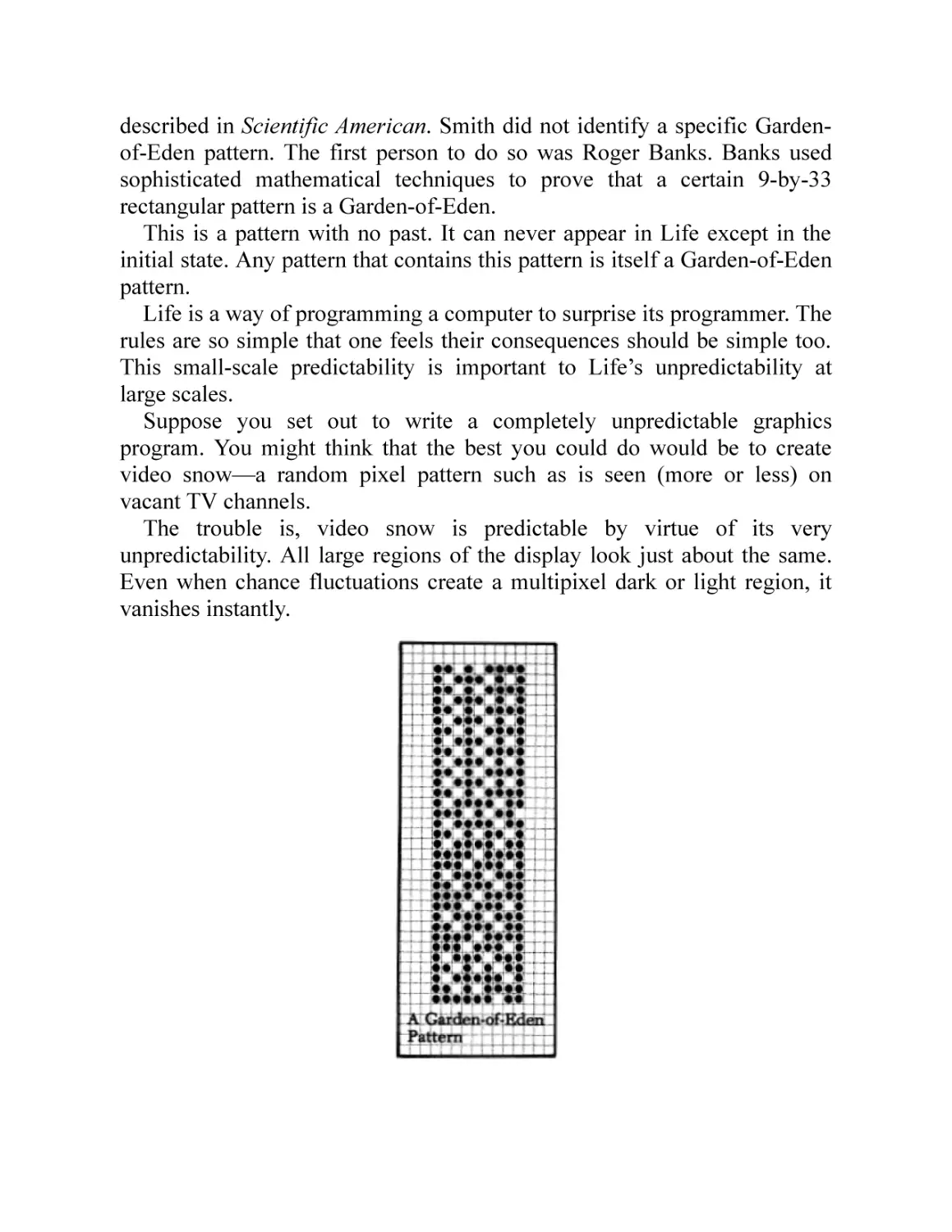
Alvy Ray Smith III, a mathematician and computer animator, proved that
Garden-of-Eden patterns must exist in Life shortly after the game was
described in Scientific American. Smith did not identify a specific Gardenof-Eden pattern. The first person to do so was Roger Banks. Banks used
sophisticated mathematical techniques to prove that a certain 9-by-33
rectangular pattern is a Garden-of-Eden.
This is a pattern with no past. It can never appear in Life except in the
initial state. Any pattern that contains this pattern is itself a Garden-of-Eden
pattern.
Life is a way of programming a computer to surprise its programmer. The
rules are so simple that one feels their consequences should be simple too.
This small-scale predictability is important to Life’s unpredictability at
large scales.
Suppose you set out to write a completely unpredictable graphics
program. You might think that the best you could do would be to create
video snow—a random pixel pattern such as is seen (more or less) on
vacant TV channels.
The trouble is, video snow is predictable by virtue of its very
unpredictability. All large regions of the display look just about the same.
Even when chance fluctuations create a multipixel dark or light region, it
vanishes instantly.
In Life, some of the fluctuations in a random field can linger. Life is
predictable enough that many types of structures survive and interact. These
interactions give Life a more profound level of unpredictability.
One of the ways in which the naturalist and engineer approaches to Life
tie together is in the perplexing question of the fate of an infinite, initially
random Life plane. Remember, a finite video screen or sheet of graph paper
is a mere window on what is supposed to be a limitless grid. Suppose you
start with an infinity of video snow and then apply the rules of Life to it.
What happens?
This is the sort of situation that concerns Life naturalists. If attention is
limited to a small part of the Life plane (that represented by a computer
screen, for instance), it isn’t too hard to give an answer. Many on cells die
out immediately. The survivors evolve frantically for a long time but
ultimately settle into a constellation of still lifes and oscillators.
Is it that simple? Conway wondered about the possibility of patterns that
grow without limit. Suppose there is some pattern that grows forever. It
needn’t even be a natural pattern. Somewhere in the tractless infinite plane,
every possible pattern—even those that would be considered engineered—
must occur.
If they exist, unlimited-growth patterns could change the history of the
Life plane. At the very least, they would grow to fill up the empty space
available to them. Eventually they would encounter other objects and
perhaps the interaction would halt their growth. But a single unlimitedgrowth pattern might stir up a vast region of the plane.
One can even wonder if some unlimited-growth patterns might be able to
preserve their mode of growth while interacting with other Life objects.
Such patterns might eventually consume the entire plane.
Evidently, the fate of a small window on an infinite Life plane could
depend on the existence or nonexistence of patterns that grow without limit
—however contrived or unlikely these patterns may be.
Conway had tried to design Life’s rules so that unlimited-growth patterns
were possible. It was not immediately obvious that he had succeeded,
though. Conway conceived of two ways of demonstrating that unlimited
growth is possible, if indeed it is.
Both ways involved finding a pattern that does grow forever, yet in a
disciplined, predictable manner. One hypothetical pattern Conway called a
“glider gun.” This would be an oscillator (almost) that creates an escaping
glider at every period. The number of pixels would grow by five every
period and never stop growing.
Conway called another type of pattern a “puffer train.” This would be a
moving object, like a glider. As it progressed, a puffer train would leave
behind stable objects such as blocks or blinkers.
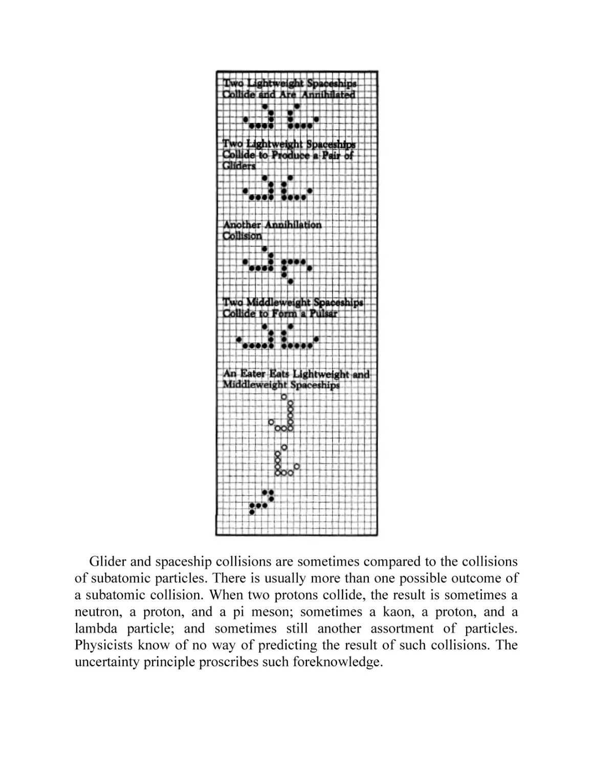
Conway was exactly right about how unlimited growth occurs. There are
glider guns, and there are puffer trains.
•3•
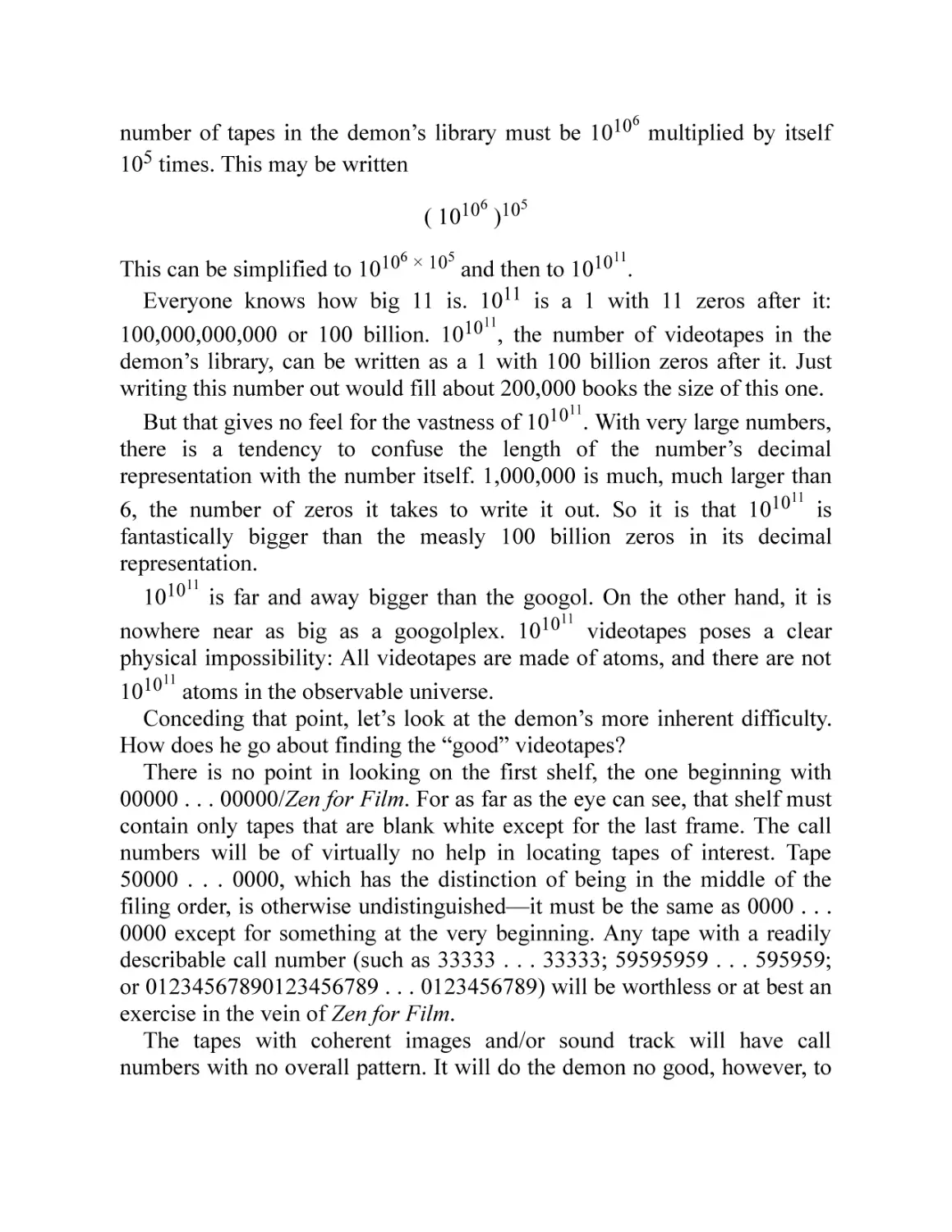
MAXWELL’S DEMON
To appreciate current thought on the origin of cosmic complexity, it is
necessary to know something of information theory. For that it is best to
start at the beginning. Information theory got its impetus from a perpetualmotion machine that doesn’t work, a fabrication presided over by
“Maxwell’s demon.”
James Clerk Maxwell was the Scottish physicist responsible for a set of
equations governing all electric and magnetic fields. He was among the first
physicists to accept the reality of atoms. In 1871, he published Theory of
Heat. One brief aside in the book is a fantasy about a remarkable device
operated by “a being whose faculties are so sharpened that he can follow
every molecule in its course.” The device is, in effect, a perpetual-motion
machine. It can extract usable energy out of thin air. By 1871 no respectable
physicist, least of all Maxwell, thought that such a thing was feasible.
Maxwell was posing a puzzle—what is wrong with this machine?
So challenging was this puzzle that the sharp-eyed being became
christened Maxwell’s demon, and the paradox was not resolved for over
half a century. It is still the subject of occasional scientific papers. Let’s
start with a version of the paradox slightly simplified from Maxwell’s
original. As background, you need know only that it is not possible to create
energy from nothing.
An airtight container is partitioned into two compartments. The wall
between the compartments has a tiny trapdoor—so tiny that it is just a little
bigger than an air molecule. Maxwell’s demon opens and shuts the trapdoor.
Whenever a molecule in the lower compartment approaches the trapdoor,
the demon opens it and lets the molecule enter the upper compartment. But
the demon keeps the trapdoor shut when molecules in the upper chamber
approach. Molecules from the lower chamber can seep into the upper
chamber, but once a molecule is in the upper chamber, it can never get out.
Eventually, Maxwell’s demon will sift all the molecules into the upper
chamber. There will be a vacuum in the lower compartment and air at twice
normal pressure in the upper. Then the demon attaches a U-shaped pipe
leading from the upper chamber to the lower. The pipe contains a turbine. A
strong wind blows through the pipe, spinning the blades of the turbine until
the pressure is equalized. The turbine can mill grain, generate electricity, or
perform any other task the demon wants. Where does the energy come
from?
CLAUSIUS AND THERMODYNAMICS
Maxwell’s demon caused great unease among physicists, since the paradox
called into doubt both the first and second laws of thermodynamics.
Both laws had been formulated by German physicist Rudolf Clausius by
1850. Clausius studied the ways that heat energy can be converted into
mechanical work. His investigation had as much the flavor of engineering
as physics to it. No one really knew what heat was, nor did Clausius’s
studies delve much into the nature of heat. He simply sought to define some
of the limitations that designers of steam engines, for instance, had
encountered in converting energy from one form to another.
It was well established that energy takes on many forms, often changing
form, both in natural processes and in man-made devices. A fire converts
chemical energy into heat; a steam engine converts heat into movement.
Just the same, there were other processes where energy seemed to vanish.
The water at the top of a dam has gravitational energy. As it falls, it can
power a mill. But if there is no water wheel, the water falls just the same
and its energy is lost.
Clausius’s first great insight was that energy never really vanishes, that
the total energy of the universe is a constant. This generalization became
the first law of thermodynamics. When energy seems to disappear, it only
changes form. Look harder and the missing energy will always be there,
Clausius argued.
In many cases, missing energy is present as heat. As water falls over a
dam, its gravitational energy is converted to motion, and its motion is
converted to heat. The water at the bottom of the dam is thus slightly
warmer than it would have been otherwise. Had the water powered a mill, it
would have been slowed. Less heat would have been created, since some of
the water’s energy was used for mechanical work.
The first law of thermodynamics also prohibits spontaneous creation of
energy. Clausius felt that the failure of engineers to build a true perpetualmotion machine is not a design problem, but an inherent limitation of
nature. No amount of ingenuity can get around that limitation. (The term
perpetual-motion machine is misleading. Nothing prohibits perpetual
motion in the absence of friction. The earth can orbit the sun indefinitely. A
perpetual-motion machine is something else, a device that creates energy.)
Clausius noted that there are restrictions on the transfer of energy above
and beyond the first law. Heat seems to have a unique status among the
forms of energy. It is usually easy to convert other forms of energy into
heat, but it is difficult—sometimes impossible—to do the reverse.
Clausius drew on the work of French engineer Sadi Carnot. In 1824,
Carnot concluded that heat can be converted to mechanical work only
where a temperature difference exists. A steam engine at a uniform
temperature cannot convert any of its heat energy into motion.
Clausius felt that Carnot’s discovery was as fundamental as the first law
of thermodynamics. Alone, the first law permitted many processes that
simply never happen. The first law would permit water to flow uphill,
becoming cooler in the process. It stipulates only that the water’s gain in
gravitational and kinetic energy be exactly offset by its loss in heat energy.
Any theory of energy transfer that does not forbid such impossibilities is
incomplete. In practice, temperature differences tend to even out. They
never increase without outside effort. To make this generalization exact,
Clausius invented a new mathematical quantity. He first called the quantity
Verwandlungsinhalt, meaning “transformation content.” Later he settled on
the shorter name entropy, Greek for “turning into.”
Clausius’s entropy was an abstract quantity residing in physical objects.
Whenever heat flowed into or out of a body, its entropy changed as well.
The entropy change was defined to be the amount of heat flowing into a
body divided by the body’s temperature.
Clausius needed the concept of entropy to state his second law of
thermodynamics succinctly: The entropy of any closed system can never
decrease.
Suppose the closed system is two adjacent reservoirs, one hot and one
cold. Heat flows from the hot water to the cold water. The first law of
thermodynamics demands that the heat loss of the hot water match the heat
gain of the cold. The hot water also loses entropy. The entropy loss is the
amount of heat transferred, divided by the hot water’s temperature.
The cold water gains entropy. Its entropy gain is the heat gain divided by
the cold water’s temperature. Although the heat gain equals the other
reservoir’s heat loss, the cold water’s temperature is lower than the hot
water’s. It follows that the cold water gains more entropy than the hot water
loses. The system as a whole has a net entropy gain.
Only processes with a net entropy gain occur in the real world. Notice
that a flow of heat from the cold water to the hot would entail an entropy
loss—and is forbidden by the second law.
But what is entropy? The second law of thermodynamics refers only to
changes in entropy. It is not necessary to define an absolute amount of
entropy for any object. Nor is it necessary to interpret entropy as anything
more than a heat transfer divided by temperature.
Perhaps the most fruitful early interpretation of entropy was this: Entropy
measures the degree to which a system’s heat energy is unavailable for
doing work. Entropy increases as temperature differences even out. Only
systems with a temperature difference can convert some of their heat energy
into mechanical work.
ENTROPY AS DISORDER
A more satisfying interpretation would explain why entropy can only
increase. Fuller understanding of entropy requires a fuller understanding of
heat. Until late in the nineteenth century, the most popular theory held that
heat was an invisible fluid that flowed from one object to another. Certain
quantitative experiments supported this view, so physicists were reluctant to
give it up.
A minority of physicists supported the view (now universally accepted)
that heat is the random motion of atoms. The motions of atoms in an object
can be broken down into two components. First, there is a motion shared by
all the atoms in the object, the observed motion of the object. Second, there
is a random atomic motion, different from atom to atom and changing
constantly. The aggregate of random atomic motions is what we call heat.
Heat is motion, but it is a collective random motion of trillions of atoms.
At any instant, there are atomic motions in every direction. Thus, heat has
no unique direction as the motion of a single atom or object does. The
higher the temperature, the more vigorous the atomic movement.
Temperature measures the average energy of motion of atoms in an object.
The modern interpretation of entropy is due largely to the Austrian
physicist Ludwig Boltzmann, one of the most outspoken proponents of the
atomic theory of heat. He became depressed and hung himself (in 1906) as
scientific opinion seemed to be rejecting his views. Shortly after his death,
experimental evidence showed that Boltzmann had been right.
Boltzmann interpreted entropy as disorder at the atomic scale. Prior to
this, the most mysterious thing about entropy had been its constant increase.
The first law of thermodynamics seemed much easier to accept on an
intuitive level than the second. There is only so much energy in the world; it
can move around, but not increase or decrease. Entropy, on the other hand,
is always being created out of thin air.
Because entropy can only increase, many processes are irreversible. A
hot bowl of soup transfers heat to its surroundings and becomes lukewarm.
Never, ever, does the reverse happen. A lukewarm bowl of soup cannot
absorb heat from its (cooler) surroundings and become hot.
Irreversibility was a novel concept in physics. All the other known laws
of physics were reversible, in the sense that if a movie of a process were
shown in reverse, the reversal would show an equally possible situation.
Newton’s gravity, for instance, would allow the planets to orbit the sun
clockwise or counterclockwise.
The atomic theory of heat pictures atoms as tiny billiard balls, colliding
and rebounding according to the same laws applying to observable
collisions. The laws governing idealized frictionless, elastic collisions are
reversible. If heat transfer is a mechanical process, why isn’t it reversible,
too?
Boltzmann realized that there are mechanical processes that are
irreversible. One example he used was the mixing of two colors of marbles.
A thousand black marbles and a thousand white marbles are placed in a
large tray. Initially, the black marbles are on one side of the tray and the
white marbles are on the other side. An experimenter shakes the tray. The
two colors mix and are soon thoroughly intermingled.
Once the marbles are randomized, no amount of further shaking will ever
restore the separation of colors. Shaking can mix the marbles, but it can
never sort them.
Any given collision of two marbles is reversible, Boltzmann noted. It is
only the aggregate of collisions that results in irreversible mixing. The
mixing is irreversible in practice rather than in principle. One can always
argue that if the tray is shaken long enough, the two colors of marbles ought
to separate just by chance. This is so unlikely, however, that it is never
observed.
Boltzmann believed the second law of thermodynamics to be a statistical
law. Entropy is a measure of the disorder of a system at the atomic level.
Individual atomic collisions neither favor nor disfavor order. But the net
effect of many random collisions is almost always to decrease order.
Molecules in a hot bowl of soup collide with molecules in the
surrounding air. The soup’s molecules are traveling faster, on the average,
than the air molecules. Any given collision is much like a collision of two
billiard balls. When a fast ball hits a ball that is standing still, the still ball
almost always gains some of the fast ball’s momentum. In consequence, the
fast ball slows down. Molecular collisions tend to even out velocity
differences too. The soup cools off, warming the air.
Boltzmann felt that Clausius’s definition of entropy could be generalized.
If entropy is disorder, then its definition should invoke some precise
definition of order and disorder.
Disorder is a difficult concept to pin down, and many obvious means of
definition fail. It is reasonable to wonder whether disorder can be
objectified at all. Disorder seems subjective—in the eye and expectations of
the beholder.
Most of the ideas about disorder can be illustrated in a familiar context.
Take two offices, one orderly and one disorderly. Both contain the same set
of objects: telephone, desk, chair, typewriter, plant, pencil sharpener, etc.
Imagine that you must explain the difference to someone who has never
seen an office before and has no idea what any of the objects are used for.
In what objective sense is the disorderly office different?
Boltzmann was faced with much the same problem. Familiar notions of
order and disorder are mostly aesthetic. All members of our culture have
seen enough interiors to recognize messy ones. Unfortunately, no one has
any preconceptions about what a system of atoms is supposed to look like.
There is nothing to fall back on. Boltzmann chose to define order in terms
of the number of ways that a system may be arranged. The more possible
arrangements, the more disorderly the system.
A very orderly office worker has a place for everything and keeps
everything in its place. If you inspected the office from time to time, you
would always find the same arrangement. In a very disorderly office, on the
other hand, any object may be anywhere at all. There are many possible
positions for each object and an even greater number of arrangements for
the entire office. If you inspected the office periodically, you would not find
the same exact arrangement twice.
Boltzmann’s definition is statistical. To determine whether an office is
orderly, you must observe it a number of times to judge how many possible
arrangements it has under its occupant. Nothing can be determined from a
single visit. But the definition is totally free of any aesthetic bias. Suppose
that the person inspecting the offices comes from a culture where chairs are
turned on end, telephones are left off the hook, and all the other furniture is
piled in the northwest corner of the room. By coincidence, he finds just
such an arrangement on his first visit to the office we think of as disorderly.
He might suspect that this office is the orderly one and that the other—
which looks to him as if a hurricane hit it—is the disorderly one. After a
few visits, though, he would be able to identify the offices as we do. The
disorderly office would almost certainly be in different arrangements on
subsequent visits. He would conclude that it had no special order and that
the arrangement he saw on the first visit was just a fluke. The orderly office
would always be in the same arrangement. Whatever he might think of that
arrangement, he would conclude that someone was taking pains to preserve
it.
In atomic systems, physicists make a distinction between “macrostates”
and “microstates.” A macrostate is an observed state of a large-scale
system: “a liter of oxygen at 1 atmosphere pressure and 0° C.,” for instance.
A microstate is a precise arrangement of atoms in a system. The molecules
in a liter of gas are always moving, so the microstate of such a system is
always changing, even when the macrostate does not.
In general, an astronomical number of microstates may correspond to the
same macrostate. All the possible arrangements of the disorderly office are
microstates. The orderly office is unusual in that it has just one allowed
microstate. As atomic systems go, gases have more microstates than liquids,
which have more than solids. A given gas molecule bounces off the walls of
its container repeatedly and may occupy any position inside the container.
Liquid molecules are confined to the volume occupied by the liquid but
may be anywhere in this volume. Solids are most orderly. Their atoms are
confined to positions in a crystal lattice. Atoms can vibrate about their
home positions in a crystal but cannot stray far (when they do, the crystal
melts).
The entropy of a macrostate is defined by its number of microstates—the
number of arrangements. It might seem that this number should always be
infinite, since even a single atom can occupy an infinite continuum of
positions. Boltzmann solved this problem by breaking down the possible
positions into discrete ranges for the purposes of calculation. He found it
easier to deal with the logarithm of the number of micro-states than with the
number itself. Boltzmann’s equation for entropy defines it as a constant
times the logarithm of the number of microstates. The use of logarithms is a
computational refinement that need not worry you. Entropy is disorder, and
disorder has to do with the number of possible arrangements.
Boltzmann’s view of entropy is reductionism at its purest. It shows that
the second law of thermodynamics is not a fundamental law but can be
reduced to the statistics of atoms obeying the simpler laws of motion. At the
heart of Boltzmann’s thesis is this realization: Practically all the microstates
for a complex system are “random” microstates. They are micro-states with
no evident pattern. Atomic positions and velocities are so evenly distributed
that large-scale properties such as temperature and pressure are uniform
throughout the system.
A system with no temperature or pressure differences is said to be in
thermodynamic equilibrium. The reason that systems tend to
thermodynamic equilibrium is simply that the vast majority of microstates
are states of thermodynamic equilibrium.
Entropy tends to increase for the same reason that offices tend to get
cluttered. Consider all the geometrically possible arrangements of the
objects in an office. It is easy to see that there are an astronomical number,
even if it is required that positions of objects must differ by at least an inch
to count as a distinct arrangement. 99.999+ % of these arrangements look
disorderly. For instance, it may not make sense to have the chair anywhere
but under the desk, yet obviously most of the possible positions for the
chair are not under the desk. Similarly, most of the possible positions for the
telephone are not on the desk, and most of the possible positions for the
files are not in the file cabinet (and certainly not in alphabetic order!). The
arrangements perceived as orderly are far, far outnumbered by those
perceived as disorderly. During the day, various objects are shifted
inadvertently. Arbitrary shifts are far more likely to produce a cluttered
microstate than another orderly one.
In a sense, it’s semantics. Out of the universe of possible arrangements,
we choose a subset and call them orderly. Everything else is called
disorderly. The tendency for offices to get cluttered is in direct proportion to
the narrowness of our definition of order.
Even so, the tendency to clutter is more general than any one definition
of order. A culture in which desks are supposed to be overturned and
furniture is piled in the northwest corner of the room would need cleaning
people as much as we do. They too would find that incidental shuffling of a
room’s arrangement would almost surely put it outside their definition of
order.
Physicists can avoid most of the subjectivity of disorder. In atomic
systems, only a few large-scale properties such as temperature and pressure
are readily measurable, so physicists deal almost exclusively with
macrostates that can be defined by these observables. One such macrostate
is the one Maxwell’s demon tries to produce: a container with air at 2
atmospheres pressure in one half and 0 pressure in the other half. Were it
not for the wall between the halves, the compressed air would rush into the
vacuum. The reason is not that nature abhors a vacuum. Individual
molecules have no way of knowing that there is a vacuum in the other end
of the container—they merely bounce about aimlessly in accordance with
the laws of motion. But of the astronomical number of ways the molecules
might be arranged, virtually all are states of maximum entropy and
thermodynamic equilibrium. Shortly after removal of the partition, the odds
favor a microstate with 1 atmosphere pressure throughout. The odds are so
overwhelming, in fact, that a compressed gas is never observed to fail to
expand into a region of lower pressure.
HEAT DEATH
Thermodynamics was the first inexact branch of physics. The details of the
atomic world are never known (as we will see). Yet is it possible to make
predictions about the behavior of systems of atoms. These predictions are
never certain, though in many cases (such as gas occupying a vacuum) they
are certain enough for any practical purpose. Thermodynamic analysis has
made it possible for cosmologists to realize much of Laplace’s dream of
surmising the past and future of the universe without inquiring into the
details of even a single atom’s position or velocity.
Thermodynamics seems incapable of explaining the complexity of the
world, however. Boltzmann puzzled over the contradiction of a rich,
ordered universe and the second law of thermodynamics. The universe is a
closed system by definition. It is also the largest possible system. Never can
the second law of thermodynamics be more statistically certain than when
applied to the entire universe. The entropy of the universe must increase
irreversibly every second.
Boltzmann’s generation of physicists was haunted by the specter of
Warmestod, heat death of the universe. It was predicted that all forms of
energy would ultimately degrade into heat and all temperature differences
would even out. Then entropy would be at a maximum.
The heat-death universe would contain just as much energy as it does
now, but all the energy would be in an unusable form. No large-scale
processes would be possible. Nothing interesting could happen. The heat
death would entail the extinction of all the stars, for stars are concentrations
of energy. It would mean the end of all life.
MAXWELL’S DEMON REBUTTED
The paradox of Maxwell’s demon plays with the idea that intelligent beings
can evade the second law of thermodynamics. A human being can sort a
mixture of black and white marbles back into two single-color piles. It
seems reasonable that a microscopic demon could do the same with
molecules. Maxwell proposed a demon sorting molecules by temperature,
not pressure as above. The demon opens and closes the trapdoor so that the
relatively fast molecules are sorted into one chamber and the relatively slow
molecules in the other. This should result in a temperature difference
between the two chambers. In principle, the temperature difference could be
harnessed by a steam engine. The paradox is not fundamentally different
whether the demon sorts by temperature or pressure. In both cases, the
demon’s actions decrease the entropy of the system. Let’s look at some of
the critiques of the demon.
The situation is too unrealistic to be relevant.
There are no atom-sized demons, so why go any further? Many physicists
felt that Maxwell’s fantasy did not really pose any threat to
thermodynamics. You can imagine a demon that makes objects fall up but
that doesn’t change the laws of gravity.
Could the demon be replaced with an automatic device?
Apparently, yes. So not all physicists were quick to dismiss the demon as a
fiction. The pressure-sorting demon is easier to simulate mechanically. Let
the trapdoor be hinged so that it opens only into the high-pressure chamber.
Molecules can push but never pull a door, so the molecules in the highpressure chamber will not be able to open the trapdoor. A spring holds the
trapdoor shut normally. Tension in the spring is adjusted so that molecules
hitting the door from the low-pressure side can open the door and enter, the
spring slamming the door shut behind them.
This is a simple model of an automated demon. Dennis Gabor and Léon
Brillouin have devised more sophisticated ones. Anything the demon can
do, a machine can be built to do (although this was not nearly so evident in
Maxwell’s time). The problem must be in the sorting operation itself and
not in the unreality of the demon.
The demon does not violate the first law of thermodynamics.
At first sight, the demon’s perpetual-motion machine seems to challenge
both the first and second laws. A little further thought shows that the first
law is inviolate—and on this, all physicists agree.
The demon’s actions do not change the basic laws of motion for any one
molecule or for the aggregate. In every collision, the energy of the colliding
molecules neither increases nor decreases. Take the version where the
demon sorts by pressure. The demon is packing a volume of gas into half its
initial volume. But he does this, ideally, without exerting any force on the
molecules. Each of the molecules is still traveling at the same average
velocity as before the compression. The temperature of the compressed air
has not changed.
In order to benefit from his efforts, the demon must allow the compressed
air to expand. The expansion of the air spins the turbine. It also lowers the
temperature of the air, as the molecules transfer some of their velocity to the
turbine. The demon does not really end up with what he started with. After
he has extracted energy from his machine, the air is at a lower temperature.
No problem. The demon can wait for the air to warm up and then start
over. Maxwell’s demon operates a “perpetual-motion machine of the second
kind.” It converts heat energy into work, in violation of the second—but not
the first—law of thermodynamics.
Does the demon’s sorting require energy?
If it did, it would explain everything. Entropy can always be decreased
locally by an outside expenditure of energy (and concurrent entropy
increase). This is what a refrigerator does. It increases the temperature
difference between its interior and exterior, at the expense of the energy it
takes to run it. If the thermodynamics of generating the electric power for
the refrigerator are taken into account, the net entropy always increases.
Opening and closing the trapdoor takes energy. This energy must be
subtracted from any generated from the temperature or pressure difference
created. Now here the simple spring valve described above looks
suspicious. In order to get into the high-pressure chamber, each molecule
must push against the force of the spring. That slows the molecules slightly,
so the molecules making it into the high-pressure chamber must have a
slightly lower effective temperature. We might decrease the tension in the
spring, but then the door would take longer to slam shut and some of the
molecules in the high-pressure chamber might escape in the meantime.
We conclude that such a simple spring valve has problems. Let’s go back
to the original demon. He merely watches the molecules and, at the right
times, opens the door. It is not necessary that the door be on any kind of
spring. The trapdoor can be as lightweight and delicately balanced as
desired. The demon can open the trapdoor for incoming molecules in
advance so no incoming molecule even touches the door. Then the energy
expended in operating the door may be arbitrarily small and need not cancel
out the energy generated. The crucial point is that the demon must know in
advance when to open the door, so that the molecules do not have to push
the door open themselves and expend energy. The demon can still be
automated, say with an electric eye to detect molecules.
The trapdoor is subject to Brownian motion.
In 1912, M. von Smoluchowski suggested that the problem is Brownian
motion, the random jostling of small objects subject to molecular collisions
from all sides. This is not exactly wrong, but neither does it much clarify
the issue. If the trapdoor is indeed big enough that molecules are likely to
be hitting it from both sides at once, then the demon cannot safely open the
door anyway. The paradox requires that the door be small enough that the
demon can deal with the collisions on a molecule-by-molecule basis. The
collisions are Brownian motion, but if the demon sees the molecules
coming he can use this Brownian motion.
The demon is foiled by quantum uncertainty.
This was suggested by J. C. Slater in 1939 and is often mentioned in
connection with the paradox. Maxwell did not know it, but atoms (and
subatomic particles) do not behave like tiny billiard balls. In certain
situations they can act like waves rather than particles. Heisenberg showed
that this mandates an inherent uncertainty in any simultaneous measurement
of a particle’s position and momentum. The more precisely the particle’s
position is known, the less precisely its velocity can be known, and vice
versa. The smaller the particle, the more overwhelming this uncertainty
becomes.
In order to operate his trapdoor, the demon must measure the position and
momentum of molecules near the door. He need not know the molecules’
trajectories precisely. If need be, he can open his trapdoor when his
measurements merely indicate it is likely a molecule will enter from the
right direction. In that case, mistakes are inevitable. Sometimes the demon
will open the door when he shouldn’t and lose ground; other times he will
fail to open the door and miss an opportunity. The demon’s sorting
operation will be slowed—but not stopped. As long as the demon can learn
something of the molecules’ positions and velocities, the odds will favor
him in the long run.
Quantum uncertainty makes the demon “near-sighted.” The smaller the
molecules he tries to sort, the worse his myopia is. But never is the demon
totally blind. Moreover, there are gas molecules massive enough that
quantum uncertainty is unimportant at low pressures (uranium hexafluoride,
for instance). The demon’s real problem lies elsewhere.
A COUNTERFEITING DEMON
Let’s consider an economic Maxwell’s demon—a situation that seems to
bear no resemblance to the original paradox. The demon sets out to attain
total wealth by acquiring everything in his home kingdom: all the land, all
the houses, all the cars, all the crops, everything. He doesn’t actually want
to steal from anyone, but neither does he want to do any work. He decides
to counterfeit. He fashions duplicates of the kingdom’s currency plates so
precise that not even treasury officials will be able to tell the difference.
That way, no one will be cheated, the demon rationalizes: The people
accepting his counterfeit bills will never know it and will be able to spend
them as freely as real money. The demon estimates the fair market value of
all the goods in his country as one billion of the local dollars. He prints up a
billion dollars and starts out on a spending spree.
The demon’s counterfeiting is a financial perpetual-motion machine. It,
too, is doomed to failure. Let’s see why.
The demon will get full value for his first bogus bill. He may be able to
spend millions before any problem is evident. It is the megalomaniacal
scale of his counterfeiting that will defeat him. The demon has printed a
dollar for every dollar’s worth of goods in the country. The amount of
money he has counterfeited can be no less than the amount of legitimate
money in circulation. It follows that the effects of the demon’s actions on
the economy cannot be ignored.
The demon’s counterfeit bills will flood the money supply, throwing the
kingdom into a galloping inflation. The demon will be forced to pay ever
higher prices. The more money he spends, the more prices will go up. The
demon’s billion dollars will run out long before he acquires everything.
Of course the demon can always print up more money. Eventually,
practically all the money in circulation will be the demon’s counterfeit bills.
The demon will have to fill wheelbarrows full of $100,000 bills (the highest
denomination) just to buy a loaf of bread. Still, the printing power of his
press is unlimited.
To print ever greater quantities of money, the demon will need ever
greater quantities of paper and ink. One day the demon will push a
wheelbarrow of $100,000 bills to the paper and ink store to replenish his
supplies. On the way home, he will find that the wheelbarrow, now
containing paper and ink, is lighter. If the paper and ink weigh less than the
money used to buy it, the demon cannot possibly print enough money to
cover its cost!
This is a problem with any sufficiently massive counterfeiting scheme.
Eventually, the counterfeiting must inflate the currency to the point where
money isn’t worth the paper it’s printed on. Then further counterfeiting does
no good. You actually lose money.
INFORMATION AND ENTROPY
The troubles of the molecule-sorting demon are cut from the same cloth. It
turns out that the demon’s sorting has effects on the system that cannot be
ignored and must ultimately confound the demon.
Leo Szilard, a colleague of Von Neumann at the University of Berlin,
offered the first modern analysis of Maxwell’s demon. Szilard critiqued the
demon in a 1929 paper, “Über die Entropieverminderung in einem
thermodynamischen System bei Eingriffen intelligenter Wesen” (Zeitschr. f.
Physik 53, 840–856). His way of looking at the paradox foreshadowed the
information theory developed twenty years later by Claude Shannon. An
experimenter’s information about a system is a vital part of the system,
Szilard found. There is no such thing as an omniscient, aloof observer. The
act of making an observation changes the system observed. As Von
Neumann commented, “An observation is an irreversible process.”
Heisenberg’s quantum uncertainty is often couched in similar phrases. It
is important to understand that quantum uncertainty is distinct from the type
of information-theoretic limitations that foil Maxwell’s demon. The latter
limitations would apply even in a universe where atoms were the tiny
billiard balls imagined in classical physics.
Szilard and those who continued his work exposed the folly of aspiring to
total knowledge of anything. Not even the position of a single gas molecule
can ever be known with total precision. Observation of a system drives up
the entropy cost of more precise observation. There comes a point at which
any observation is choked off—it ceases to yield enough information to pay
for itself.
Szilard pictured a simplified Maxwell’s demon experiment in which a
cylindrical chamber contains a single gas molecule. The molecule rebounds
off the walls of the chamber. Its complicated path traverses all parts of the
cylinder’s interior. Clearly, the molecule is somewhere at any instant.
Suppose it is in the top half of the cylinder and that the demon has
determined this fact through some observation. Then the demon need only
insert a frictionless circular piston in the middle of the cylinder. This
confines the molecule to the space above the piston. The molecule will
bounce off the piston repeatedly, each time transferring a little downward
momentum to it. In effect, the molecule is a “gas” expanding into the
vacuum below and pushing a piston as it does so. The (very, very slow!)
downward motion of the piston can be used to do work. Eventually, the
molecule will push the piston all the way down to the floor of the cylinder.
Then no more energy can be extracted.
The energy has a price, Szilard argued. Originally, the demon knew the
molecule to be in the top half of the cylinder. Afterward, he knows nothing
about the molecule’s position. It could be anywhere in the cylinder’s
volume. The demon has gained energy but sacrificed information.
To repeat the process, the demon needs more information. He needs to
observe the molecule’s position again. This is such a vital link in Szilard’s
argument that it deserves emphasis. You might wonder why the demon
cannot simply replace the piston in the middle of the cylinder.
If the demon slides the piston back to the midway point, he will be
forcing the piston against the effective pressure of the single-molecule gas.
This requires energy—the exact amount of energy he just extracted. No
good.
Instead, the demon will have to remove the piston from the bottom of the
cylinder. Perhaps the bottom screws off and the demon can take the piston
out quickly, before the molecule escapes. Perhaps, too, there is a slot in the
middle of the piston so the demon can slide the piston back in. In that case,
the demon will not have to move the piston against any resisting force and
expend energy. (The demon’s exertions while outside the cylinder are
assumed negligible.)
The demon has not observed the molecule, so he has no way of knowing
whether it is in the top or bottom half when he replaces the piston. He
consequently does not know if the piston will move up or down from the
midpoint. Say the piston is hooked up to a flywheel. The original downward
stroke of the piston has set the flywheel moving (very, very slowly)
clockwise. There is a fifty percent chance that the piston will move up this
time and slow the flywheel back to a halt. In the long run, there will be as
many downward strokes as upward strokes, so the demon cannot expect the
flywheel to pick up any speed in either direction.
It should be possible to solve the problem with two flywheels. An electric
switch is tripped when the piston starts moving down, and it engages the
piston to a clockwise flywheel. If instead the piston starts moving upward, a
different switch engages it to a counterclockwise flywheel. In the long run,
both flywheels will move faster and faster and can be used to perform
useful work. But the system of piston and switches is nothing less than a
device for measuring the approximate position (top or bottom half) of the
molecule. We conclude that the demon requires information about the
molecule’s position to make his perpetual-motion machine work.
Maxwell assumed his demon could know molecular positions and
velocities to any necessary degree of precision, but Szilard answered that
this presumed omniscience is artificial. In real life, knowledge is always the
result of observation. Szilard and such physicists as Gabor and Brillouin
examined how the demon might attain knowledge of the molecule’s
position.
Case 1: location by constraint.
Szilard’s paper considered the simplest kind of “observation,” one so crude
that it may seem to have little relevance. Picture Szilard’s system of a single
molecule in a cylinder. The simplest question the demon can ask about the
molecule’s location is whether it is in the top half or bottom half. One way
to settle the matter is to place a piston on the floor of the cylinder and raise
it to the midpoint. Then the molecule has to be in the top half. Or the piston
can be placed on the ceiling of the cylinder and lowered, forcing the
molecule to be in the bottom half.
This is the same procedure that was mentioned earlier and rejected on the
grounds that it requires energy. It seems nothing like ordinary observation.
The demon doesn’t find out anything about the molecule’s original position.
Rather, he constrains the molecule to one section of the cylinder in order
that he may know the molecule is in that section.
Surprisingly, this type of observation is not fundamentally much different
from other types. Szilard chose it for analysis because it is simple. Not only
does location of the molecule cost energy, he showed, but also increased
information about the molecule’s position is always canceled out by an
increase in entropy. Entropy, in turn, is ignorance at the molecular level.
Let the demon insert the piston at the bottom of the cylinder and raise it
to the halfway point. In effect, he is compressing a very, very thin gas to
half its volume. The rebounds of the molecule against the piston resist its
upward motion. At the same time, the piston imparts some of its momentum
to the molecule. The molecule picks up speed, which is to say its effective
temperature increases. This is nothing more than the familiar increase in
temperature when a gas is compressed.
For simplicity, Szilard supposed that the cylinder’s walls and
surroundings conduct heat so efficiently that the molecule is kept at the
same effective temperature throughout the compression. Furthermore, the
surroundings are so much bigger than the cylinder/molecule system that
they can absorb all heat generated without themselves experiencing a
measurable increase in temperature.
In that case, all the energy supplied to the piston is transferred to the
molecule and converted to heat. The heat energy flows into the cylinder’s
surroundings.
Whenever heat flows there is a change in entropy. The energy needed to
move the piston against the single-molecule gas pressure is readily
calculated. This energy is equivalent to a certain amount of heat. Take this
heat, and divide it by the cylinder’s constant temperature. The result is the
cylinder’s entropy decrease. The same amount of heat flows into the
cylinder’s surroundings, which are at the same temperature. So the
surroundings’ entropy gain equals the cylinder’s entropy loss.
The demon has succeeded in decreasing entropy in the cylinder. He
knows more about the molecule’s position than he did. Before inserting the
piston, the molecule was equally likely to be anywhere in the cylinder. It
could have any of a range of velocities determined by the temperature.
After the demon’s action, the range of velocities is the same because the
temperature has not changed. But the number of possible positions is cut by
half. The total number of possibilities (positions and velocities) for the
system is halved.
The cylinder’s surroundings include the entire universe outside the
cylinder. We know that the surroundings’ entropy gain equals the cylinder’s
entropy loss (Clausius’s definition, heat divided by temperature) and that
the cylinder’s entropy decrease represents a decrease by a factor of two in
the number of possibilities (Boltzmann’s definition, in terms of the number
of possible arrangements). It follows that the number of possible
arrangements of the surroundings—for the whole universe, in fact—must
increase by a factor of two.
This is the heart of Szilard’s thesis. Any increase in knowledge about the
lone molecule is (at least) exactly compensated by increased ignorance
about the rest of the world. If the demon raises his piston 99 percent of the
way from the bottom of the cylinder to the top, he is a hundred times surer
about where the molecule is. But the operation produces heat, which is
absorbed by the surroundings and which increases the range of possible
positions and velocities of molecules in the outside world by a factor of a
hundred.
This startling result will be examined more fully in a moment. Let’s first
look at some of the other ways the demon could observe molecules.
Szilard’s situation seems too narrow—surely the problem is with the
demon’s ham-handed way of “observing.” Maxwell had his demon watch
the molecules, but the notion of seeing a single molecule turns out to be
ambiguous, so we will consider three cases of vision at the molecular scale.
Case 2: seeing by ambient light
All matter radiates, the frequency of radiation depending on the
temperature. For objects at room temperature, the frequency is in the
infrared range. So if the demon’s eyes are sensitive to infrared light, he will
find the interior of his sealed chamber bathed in a warm glow. Infrared
photons (the fundamental “particles” of light) will bounce off the molecules
and into the demon’s eyes. He will see the molecules.
This idea is easily dispensed with. Vision does indeed involve photons
bouncing off objects and into an observer’s eyes, but just as important as
the photons themselves is the directional information they carry. The sun is
in one part of the sky. If the eye detects photons coming from other
directions, then something must be reflecting photons from those directions.
No such inferences are possible for the demon. Suppose first that the
chamber contains no molecules, just the infrared photons. The photons are
black-body radiation, which means that they are in thermodynamic
equilibrium. Photons are equally likely to be found in any part of the
chamber, traveling in any direction. The demon sees photons coming from
all directions equally.
How would the presence of a single molecule in the chamber change
things? It wouldn’t. Some of the photons the demon sees may have bounced
off the molecule. The interaction with the molecule would have changed the
photons’ course. But in the utter absence of prior knowledge about
individual photons, the demon can draw no conclusions. With the molecule
or without, photons are equally likely to come from any direction. The
demon cannot even identify photons that have interacted with the molecule
by a change in frequency, for the black-body photons are at the same
effective temperature as the molecule and the chamber walls.
The demon’s chamber can hold two molecules or a quintillion. It will still
make no difference. Black-body photons’ “message” is already as garbled
as it can be. Further garbling by molecules will be undetectable. All the
demon will ever see is a random snow of photons.
Case 3: using a flashlight.
To see anything, the demon must provide his own light. It must be a
coherent beam—light whose initial direction is known so that a change in
direction (by reflection off a molecule) is detectable. The filament of the
demon’s flashlight must be at a higher temperature than the chamber so that
reflected photons will not be confused with the black-body radiation from
the chamber itself.
This is a plausible way of gaining information about molecular positions
and velocities. Again, there is a catch. Brillouin calculated the entropy
change associated with observation. Observation of a molecule’s position
requires (at least) one photon from the flashlight striking the molecule. The
photon transfers heat from the hot filament to the molecule and thus to the
chamber and its surroundings. As in any spontaneous heat flow, there is an
increase in entropy.
Brillouin’s calculations showed that the entropy gain must at least equal,
and usually exceed, the information the demon obtains. Observation by
flashlight has the same fundamental problem as observation by Szilard’s
piston. In fact, Brillouin argued, if the demon wants to create a temperature
difference between two compartments of gas, he can do no better than to
forget sorting and use his flashlight filament to heat up one compartment.
Case 4: seeing with “sub-quantum” particles.
The problem with a flashlight seems trivial. It so happens that the particles
we use for seeing (photons) have “sizes” and energies comparable with the
molecules’. Maybe the problem would go away if smaller particles were
used for imaging.
All the known subatomic particles are bound by Heisenberg’s uncertainty
principle. The resolution of any microscope using photons, electrons, or
other quanta is limited.
One can imagine a new particle or type of particle, much smaller than the
known subatomic particles. Here “smaller” means a smaller mass and
effective diameter. Call these hypothetical particles sub-quantum particles
and assume that they are not subject to quantum uncertainty. Then subquantum particles could form the basis for a high-resolution microscope
that would allow the demon to observe and sort molecules.
The microscope would shoot a coherent stream of sub-quantum particles
at molecules to reveal their positions and velocities. The sub-quantum
particles would transfer energy to the molecules, resulting in a slight
transfer of heat to the system. But the heat transfer depends on the
momentum of the sub-quantum particles, and we’ll assume that this
momentum is negligibly small.
What’s wrong here? Nothing, really. If there were sub-quantum particles
as described, presumably they could be used to sort molecules. The sorting
of molecules observed with sub-quantum particles would not be much
different from the sorting of black and white marbles observed with
photons.
In a larger sense, sub-quantum particles would only transfer the
Maxwell’s demon paradox to the sub-quantum realm. One would end up
wondering whether a sub-demon could sort sub-quantum particles. The subdemon would run into the same problems the demon does.
Maxwell’s demon must be assumed to operate at the lowest level of
matter and energy. His difficulties are broader than any particular brand of
physics. They have to do with information. If the demon can learn about
particles and waves only by observing them with other particles and waves,
then never can he come out ahead.
THE LIMITS OF EMPIRICAL KNOWLEDGE
The moral is that there may be a great difference between omniscience and
knowledge that must be obtained through observation. The distinction is
tantalizing. For any given two-chamber container of gas, there is clearly
some sequence of openings and closings of a trapdoor that will sort the
molecules. The sequence is real and could be written out: “40 nanoseconds
open; 12 nanoseconds closed; 350 nanoseconds open; . . .” If only the
demon could know this sequence, his perpetual-motion machine would
work. Yet any attempt to learn the sequence defeats the demon in the long
run.
Szilard’s cylinder-piston single-molecule version of the paradox is a good
way of dramatizing the limitations of empirical knowledge. The demon
aspires to know the exact vertical position of the molecule. He inserts the
piston in the top of the cylinder. Initially, the molecule may be anywhere in
the cylinder’s volume. The demon pushes the piston halfway down to the
bottom. Now his uncertainty about the molecule’s position has been
decreased by a factor of two.
Since the piston offers virtually no resistance, the demon pushes it
99.99999999999999999999 percent of the way to the bottom. This confines
the molecule to a wafer-thin volume. The demon’s uncertainty about the
molecule’s vertical position is decreased by a factor of
10,000,000,000,000,000,000,000.
Now the piston is starting to push back. The molecule (which is of an
ideal gas) has about as much room as the volume per molecule in a gas at 1atmosphere pressure. The molecule bounces between the piston and the
floor so frequently that it acts like a gas at ordinary pressure. The
compression generates heat. Now the bottom of the cylinder is noticeably
warm.
Has the demon increased his total knowledge of the world? Szilard’s
analysis says no, in this sense: The demon is now at least
10,000,000,000,000,000,000,000 times less sure of the exact state of the
universe outside his cylinder.
The culprit is the heat produced. The demon had to expend mechanical
energy to compress the gas. This requires that the atoms in the demon’s arm
all move in the same direction. In return for this energy, the demon gets
back heat. Heat is chaotic motion of atoms. The hotter something is, the less
certain one is of the velocities and positions of its atoms.
To say that the demon is 10,000,000,000,000,000,000,000 times less sure
about the outside world means that the number of possible arrangements of
atoms in the surroundings warmed by the compression has increased by this
factor. This is more difficult to picture than, say, the number of
arrangements of an office, but it is the same idea.
At the beginning of the day, a wastebasket is located just right of the
desk, somewhere in a four-square-foot area. At the end of the day, it has
been moved around so much that it is equally likely to be found anywhere
in the office’s one hundred square feet of floorspace. Then the number of
possible arrangements of the office has increased twenty-fivefold. So has
the number of possible arrangements for the entire office building, or
indeed (speaking in somewhat oversimplified terms) the entire universe. We
do not have to wait for the heat produced by the demon’s compression to
diffuse to the distant galaxies. Once the cylinder and surroundings have
cooled down to their initial temperature, it can be demonstrated that the
number of atomic arrangements for the universe exclusive of the trapped
molecule is 10,000,000,000,000,000,000,000 times greater.
The demon will find himself unable ever to attain total knowledge of the
molecule’s position. As the piston is pushed to the floor, the molecule’s
effective pressure increases without limit. Soon the demon’s arm will give
out and he will have to resort to a hydraulic press or other device.
Compression becomes ever more expensive in terms of energy and entropy.
Eventually, the demon will need a refrigeration system just to prevent the
cylinder from melting. Not all the energy on earth will suffice to squash an
ideal point-sized molecule to zero volume. The best the demon can possibly
do is to harness all the available energy of the universe to his hydraulic
press. This will degrade all the world’s energy to heat, effecting the heat
death of the universe. Then the demon’s operation can go no further. He
will be out of energy.
Still the demon will have failed to banish all uncertainty in the
molecule’s vertical position—and he will be maximally uncertain about the
state of the universe.
The surprising conclusion of information theory is that experiments done
within a system can never increase total knowledge of that system at the
most fundamental level. All knowledge is counterfeit. Acquisition of
knowledge about one part of the world requires an equal sacrifice of
knowledge about other parts. Ignorance can at most be shifted around.
The limitations of science are more extreme than the most pessimistic
pre-twentieth-century philosophers would have imagined. In its most allencompassing sense, knowledge cannot be advanced at all. Nothing—not
electron microscopes, not particle accelerators, and not radio telescopes—
can take us one iota closer to Laplace’s ideal of knowing the details of
every particle in the universe.
Such statements of Szilard’s and Brillouin’s theorems should not be
misconstrued. Things aren’t totally hopeless. The apparent advancement of
knowledge hinges on the distinction between information and useful
knowledge. Useful knowledge is information that someone actually cares
about. Information theory deals with information only as an abstract
quantity.
You turn on a lamp to locate a chair in a dark room. Information theory
claims that the information gained about the chair’s location is canceled out
by the information lost about the positions and velocities of the atoms in the
light bulb and surrounding air. This is entirely true, but you probably didn’t
need the atomic information.
As long as it is possible to swap irrelevant information for useful
knowledge, there is no problem. Science is not and cannot be a quest for a
complete knowledge of the universe. Rather, it is a process whereby certain
information is selected as being more relevant to human aims and
understanding.
Economies are possible. Nothing in Szilard’s or Brillouin’s analyses
prevents us from deducing natural laws. A natural law is an induction—a
generalization from observed situations that is assumed to hold true for
unobserved situations as well. From a small number of observations, it is
possible to gain (indirect) knowledge about what is going on throughout the
universe. This is the route physics has taken.
•4•
GLIDERS AND SPACESHIPS
Heisenberg once wrote of quanta, “I would guess that the structures with
which we are confronted are beyond any objective description in
imaginable terms and that they are a kind of abstract expression of the laws
of nature rather than matter.” This idea finds its apotheosis in Life. All Life
objects are expressions of Conway’s rules. Even so, there is no simple way
of deducing the variety of Life phenomena from a mere statement of Life’s
rules. This fact likely reflects a similar difficulty of real-world physics.
The glider is not the only Life object that moves. Conway used the term
“spaceship” to describe moving patterns. Spaceships are a good example of
the convoluted relationship that may exist between object and physical law.
As simple as the notion of a moving pattern is, there is no general procedure
for finding new spaceships. Much effort has gone into finding new moving
patterns.
To qualify as a spaceship, a pattern need not shift frozen from pixel to
pixel. Remember how the glider moves. It evolves through four phases to
move one pixel diagonally. The known spaceships are oscillators that
manage to translate themselves so many pixels per cycle. A spaceship’s
speed is its shift (in pixels) divided by its cycles (in generations). It is far
easier to discover new still lifes or oscillators than spaceships. Only a few
fundamentally different types of spaceships are known, and only the glider
is common.
SPACESHIPS ARE ASYMMETRIC
What must a spaceship look like? There is at least one obvious prior
constraint. Spaceship motion is asymmetric. A spaceship cannot move in all
directions at once; it must prefer one direction over all others. That
preference cannot come from Conway’s rules. A pixel’s future state is
determined by the number of neighbors but not the position of those
neighbors. If there is any asymmetry in a Life pattern’s behavior, it must
come from an asymmetry in the pattern itself.
The glider is completely asymmetric. There is no way that a given glider
phase can be rotated (less than a full 360 degrees) to reproduce its original
orientation. Nor can its mirror image be superimposed on itself.
A spaceship doesn’t have to be completely asymmetric. It can have
bilateral symmetry—the symmetry of an object that is the same as its mirror
image. The boat and loaf have bilateral symmetry, as does the human body
or a rocket.
No spaceship can have greater-than-bilateral symmetry. Suppose it is
claimed that a pattern with the symmetry of a beehive is a spaceship that
moves to the right. Because of the impartiality of Conway’s rules, it would
have to move to the left as well. Something has to be wrong.
Life’s rules also limit the speed of spaceships. Suppose a certain pattern
is contained in a 100-by-100-pixel square. Every thing outside the square is
in the off state. No matter what the structure of the pattern, it can influence
only the pixels bordering the square in the next generation. It will then be
contained in a 102-by-102-pixel square. At very most, a pattern can grow
one pixel per generation in any direction.
This is the maximum speed at which any form of information can be
transmitted across the Life plane. It is the counterpart of the speed of light
in the real world and is often called by that name. A glider is said to travel
at one-fourth the speed of light diagonally.
It is easy to find patterns that grow at the speed of light for a while. Any
long row or column of pixels does, creating complex video effects. But the
waves of births grow two pixels shorter with each generation. Only an
infinite orthogonal line will grow out in both directions forever. Conway
concluded that half the speed of light (orthogonally) is the limit for a finite
spaceship. At best it can advance a pixel, take a generation to fill in the
leading edge, and start anew.
LIGHTWEIGHT, MIDDLEWEIGHT, AND
HEAVYWEIGHT SPACESHIPS
The known spaceships fall into several natural classes. The glider, unique in
many ways, forms its own class. The second class has three members. It too
was discovered early in the investigation of Life. One of Conway’s
colleagues saw a shimmering form moving across a video display and
stopped the computer before the moving form crashed into another object.
The moving pattern was a “lightweight spaceship.”
The lightweight spaceship can be stretched into a “middleweight” or
“heavyweight” spaceship. The illustration shows the three spaceships in the
form that is easiest to enter into a computer (though spaceships are easily
tracked on graph paper, too). This phase has a boomerang shape comparable
to two of the glider phases. Unlike the glider, these spaceships travel
horizontally or vertically, never diagonally. All three move toward the right
when oriented as shown.
Each spaceship advances two pixels every four generations (half the
speed of light). A boomerang phase is followed by a dense phase. Most of
the latter dies out from overpopulation, creating an upside-down
boomerang. This gives rise to an upside-down dense phase, and it restores
the original boomerang—shifted two pixels.
Spaceships throw off “sparks,” debris that fades instantly. The
boomerang phase of all three spaceships has a single-pixel “tail spark.” The
middleweight spaceship also has a single-pixel “belly spark.” In the
heavyweight spaceship, the belly spark is two pixels. Because the sparks
vanish without affecting the rest of the spaceship, they can be omitted when
entering a spaceship in a computer.
On a high-speed video display, these spaceships suggest a turbine. The
way the phases flip over creates a convincing illusion of 3-D rotary motion.
The apparent axis of the turbine is in line with the direction of travel.
Another unexpected video effect is a “hole” near the front of the
spaceship. The two dense phases each have an internal empty pixel. The
corresponding pixel is also off in the boomerang phases. The hole moves at
the same speed as the rest of the spaceship.
It looks as if longer spaceships can be constructed from this same design,
but they can’t be. The belly spark is the spoiler. A boomerang pattern one
unit longer than the heavyweight spaceship creates blinkers for belly sparks.
Instead of vanishing, the blinkers remain and interfere with the would-be
spaceship. Ultimately, all the debris annihilates itself. Similar problems
plague longer boomerangs.
GLIDER AND SPACESHIP COLLISIONS
What happens when a glider or spaceship collides with another object? The
results are amazingly diverse, and most of our intuitions about real-world
collisions do not translate very well. Colliding Life objects rarely bounce
back (though it can happen). Sometimes they smash into many pieces.
Rarely do the original objects survive. For simple, two-glider collisions, the
commonest outcome is mutual annihilation.
The subject of collisions is more complicated than might be thought, for
there are usually many different ways that two Life objects can collide.
Position and timing can (and almost always do) make a difference. A glider
or spaceship can encounter a target object in any of the four phases with
different results.
There are seventy-three distinct collisions of two gliders. A two-glider
collision may be head-on or at right angles. Two gliders may form a block,
blinker, beehive, pond, eater, or a single new glider. In general, two
colliding gliders form an unstable mass that evolves for some time and then
stabilizes. Parts of the collision mass may die out; other parts may give rise
to stable objects.
In one collision that produces a block, a four-pixel flattened U shape is
created at time 2. (In each diagram, time 0 is the last generation before the
gliders interact.) The U shape and the three-pixel L shape are the most
common predecessors to the block. Experienced Life players can recognize
predecessors to common stable forms. The smallest predecessor to the pond
is the four-pixel slanted Y shape that occurs at time 2 of the pond collision.
Its evolution includes the characteristic chevron of time 4.
The collisions of two spaceships, or of a glider with a spaceship, are all
the more numerous. Two lightweight spaceships can annihilate in a head-on
collision. A slight difference in spacing between the spaceships results in an
entirely different outcome: two gliders rebounding from the collision site.
When the two original spaceships are positioned as shown (mirror-image
boomerang phases), an even number of pixels between the spaceships will
result in annihilation; an odd number of pixels’ spacing will result in the
two gliders.
In another collision, two middleweight spaceships can collide to form a
pulsar. The spaceships first fragment and form a pair of T tetrominos. The T
tetrominos split into four and then coalesce into a pulsar.
Gliders and spaceships can also collide with nonmoving objects. A glider
can collide with a block and annihilate both, for instance. The eater’s
digestion of a glider is really a collision of a glider with an eater in which
only the eater survives. The eater can also eat lightweight and middleweight
spaceships. Heavyweight spaceships cause indigestion. The eater consumes
the front part only, leaving a loaf.
Glider and spaceship collisions are sometimes compared to the collisions
of subatomic particles. There is usually more than one possible outcome of
a subatomic collision. When two protons collide, the result is sometimes a
neutron, a proton, and a pi meson; sometimes a kaon, a proton, and a
lambda particle; and sometimes still another assortment of particles.
Physicists know of no way of predicting the result of such collisions. The
uncertainty principle proscribes such foreknowledge.
A common Life experiment is to position two or more gliders or
spaceships on an arbitrary collision course and watch what happens. The
results seem as unpredictable as those of subatomic collisions. Of course,
Life is deterministic, so any precisely specified collision can have only one
outcome. Nowhere does chance enter in.
One of the longstanding controversies of quantum physics is whether the
uncertainly principle allows the real world to be deterministic at some basic
level. “Surely God does not play dice with the universe,” Einstein objected.
He felt that physics must be deterministic and that the uncertainty principle
merely expresses our ignorance of the subatomic world.
Einstein postulated “hidden variables.” These would be unknown
attributes of subatomic particles and fields. The hidden variables would
determine which of the possible outcomes of a quantum collision actually
occurs. If one could uncover the hidden variables, one could predict
subatomic phenomena as accurately as planetary orbits.
In the 1930s, Von Neumann analyzed quantum theory from a
mathematical standpoint. He showed that the known behavior of quanta was
all but incompatible with hidden variables, at least of the type that most
physicists were looking for. This broke the spirit of the hidden-variables
contingent, save for diehards such as Einstein. Today physicists mostly
favor the “Copenhagen interpretation” of quantum physics (named after
Niels Bohr’s Danish institute). This links reality to the act of observation—
states of quanta do not even exist until they are observed.
In Life, at least, the two viewpoints need not be mutually exclusive. Two
distant gliders approach, collide, and form a pond. A determinist can argue
that the spacing and phase differences are the hidden variables. An equally
valid “Copenhagen interpretation” of Life can maintain that collision results
are tied to the act of collision. In isolation, all gliders are alike. Neither
glider has some hidden attribute that means “pond.”
OVERWEIGHT SPACESHIPS AND FLOTILLAS
After some thought, Conway decided that there is a way of fixing the bellyspark problem on long spaceships. The trick is to arrange for escorting
spaceships to prevent the formation of sparks longer than two pixels. A
group of spaceships traveling in parallel is called a “flotilla.” Flotillas
incorporating “overweight spaceships” are the third basic class of
spaceships. Overweight spaceships cannot travel alone, so it is the flotilla as
a unit that qualifies as a spaceship.
The simplest flotillas consist of an overweight spaceship sandwiched
between two regular (lightweight, middleweight, or heavyweight)
spaceships. All three spaceships flip over every two generations. The
escorting spaceships ensure that the margin cells of the overweight
spaceship have too many neighbors to allow long belly sparks. When all
three spaceships are in phase (all in the boomerang configuration
simultaneously), the maximum length of the base of the overweight
spaceship is twelve pixels. Then only heavyweight spaceships will work as
escorts.
A slightly longer flotilla is possible if the overweight spaceship is out of
phase with its escorts. The overweight spaceship must be in the dense phase
while the escorts are in the boomerang configuration, and vice versa.
Fourteen pixels (base of boomerang phase) is the limit.
It is not possible to escort longer overweight spaceships by a train of
regular spaceships on each side. Either the escorting spaceships are so close
that they interact with each other or problem sparks form in the chinks
between them.
Conway found a way of escorting overweight spaceships of any length.
A very long overweight spaceship can be sandwiched between two
overweight spaceships that are slightly shorter. The latter spaceships’ outer
edges can be shielded by a pair of spaceships that are slightly shorter yet.
Such a flotilla assumes the shape of a double pyramid. Lightweight,
middleweight, or heavyweight spaceships must form the apexes of the
pyramids.
All flotillas move like a single spaceship: orthogonally, at half the speed
of light. Flotillas are engineered objects—no one has ever seen one arise
naturally.
SHUTTLES
It is clear that any spaceships other than the ones already described will be
unnatural. Enough people have watched enough Life fields long enough to
rule out the possibility of any undiscovered common spaceships.
Many failed spaceships are known. These are objects that move for a
time and then run into trouble. Some patterns move a short distance and
then abruptly reverse direction. Under the right conditions, they can shuttle
between two points endlessly.
The commonest such pattern is simply called the “shuttle.” It is a fairly
natural object, occasionally seen in random Life fields. It occurs in
generation 774 of the R pentomino, though it is soon destroyed by
interaction with other debris.
The shuttle has fifteen phases. Most look like arrowheads or rockets. It
moves orthogonally, somewhat fitfully, at about 0.4 the speed of light. At
the end of a fifteen-phase cycle, the shuttle splits into two parts. One part
becomes a shuttle pointed in the opposite direction. The other part becomes
a beehive.
Fifteen generations later, the shuttle reverses, producing a second
beehive. Then the shuttle rams into its first beehive and is destroyed.
The shuttle can be preserved indefinitely if the beehives are removed.
Properly positioned eaters will eat the rectangular latent beehives. Blocks
(shown in diagram) can also eat the beehives. The block-beehive reaction is
explosive, creating a shower of sparks and a pre-block that instantly repairs
itself. The system of shuttle and blocks is an oscillator with a period of 30.
A similar shuttle can be created with a pair of “B heptominos.” The B
heptomino is a seven-pixel figure investigated by Conway. (The “B” is
Conway’s arbitrary label.) Like the R pentomino, the B heptomino is a
small unstable object that frequently turns up in random Life fields. Left to
itself, a B heptomino takes 148 generations to stabilize into three blocks, a
ship, and two gliders.
The B heptomino looks like the front end of a spaceship in the dense
configuration. In fact, the first few generations of the B heptomino include a
leading edge that moves outward like the front of a spaceship, flipping over
every two generations. After much experimentation, it was discovered that
twin B heptominos can be penned between four blocks in a stable shuttle.
This shuttle has a period of 46. The illustration shows the phase in which
the B heptominos occur in standard form. This phase includes two sparks
that need not be entered in a computer.
The B heptomino shuttle is swifter, traveling at half the speed of light. As
the twin B heptominos approach either end of their circuit, they turn around,
leaving a complicated cloud of debris. Fortuitously, it is possible to position
a pair of blocks just so that they annihilate the debris and repair themselves.
There is an unexpected degree of freedom to the B heptomino shuttle. As
many as two of the blocks may be removed, as long as they aren’t both
from the same end. The reaction is then different, but the remaining blocks
still manage to kill off the debris clouds before the B heptominos return.
•5•
INFORMATION AND STRUCTURE
Claude Shannon, the founder of information theory, was an engineer at Bell
Laboratories. He was concerned with such problems as the transmission of
television images over telephone lines. This work got him thinking about
the nature of information and about how such a subjective notion might be
defined.
To get anywhere, Shannon felt he would have to renounce all
interpretation of information. It was just as difficult to transmit a
meaningless image as a meaningful one. It seemed natural to say that they
had the same information content. By the same token, Shannon was able to
incorporate the notion of structure in his theory. A structured though
abstract image could be distinguished from a formless image. These
distinctions can be illustrated in one last version of the Maxwell’s demon
paradox.
AN INFORMATION DEMON
Videotape is a digital medium. It encodes all the information in a television
image magnetically. Each second of action is broken down into 30 still
frames, and each frame is broken down into thousands of pixels. The pixels
have a certain number of states representing color and brightness. Sound
tracks are digital too. It follows that there are only so many possibilities for
a frame of videotape—and only so many ways of stringing frames together.
Upon hearing of this, Maxwell’s demon started a new enterprise. He
called it the Universal Video Library. He built a huge warehouse and filled
it with videotapes. He took out ads in the show-business trade papers, to
this effect:
ATTENTION, PRODUCERS: Why make TV shows and movies
the old-fashioned way? Why pay millions for actors, actresses,
directors, writers, set designers, location filming, special effects,
editors, and sound mixers when all you really need is a videotape
of the final product? Whatever you’re working on, stop
production immediately. Don’t spend another penny until you
come to the Universal Video Library.
The Library is guaranteed to have a completed tape of
whatever you are working on—regardless of the stage of
production—and I will sell you the tape for a nominal price, far
less than the cost of a day of taping. How is this possible, you
ask? Why, only because the Library is a Universal Video Library!
It contains a copy of every possible videotape 100,000 frames
long (a little over 56 minutes running time). Even if two tapes
differ only by the color of a certain pixel in the 59,003rd frame,
the Library stocks both. Film producers, take note: The Library
uses such high-resolution videotape that it may be transferred to
film without any graininess. And, of course, any movie longer
than 56 minutes may be found in two or more of our standardlength tapes.
You’ll be amazed at the selection! Think a few Emmys or
Oscars would look good on your mantle? All the future winners
are somewhere on the Library’s shelves. Come in and browse—
I’ll help you separate the wheat from the chaff. One visit to the
Library, and you may never deal with a “creative” person again!
All a director does is to choose one preexisting possibility out of a
big, finite ensemble. You can do the same thing in the Library—
cheaper. But, remember: There are only so many masterpieces,
and your friends are already picking over them. Hurry in today!
THE INFORMATION DEMON REBUTTED
Maxwell’s demon will find himself as incapable of sorting good videotapes
from bad as he is of sorting fast molecules from slow. His downfall is again
that elusive concept, information. The Universal Video Library is an update
of physicist George Gamow’s playful idea of a universal printing press that
would print all possible lines of text. The library itself invokes no (logical)
impossibilities. For that reason the demon’s videotape-sorting scheme is all
the more tantalizing.
The demon could certainly build a machine to generate successively all
possible videotapes. The information in any videotape can be encoded as a
string of digits. Each digit would stand for the state (color or degree of
brightness) of a given pixel in a given frame, or for information about the
sound track accompanying a given frame. Such strings of digits would be
the “call numbers” of the demon’s library. The machine need only run
through the call numbers successively, manufacturing a tape to match each
call number.
The first tape in the library would be 0000000000 . . . 00000000. (The
full number would be billions of digits long.) Let 0 stand for a white pixel
and also for silence in the sound track. Then 00000 . . . 00000 is a silent
blank white screen for 56 minutes. As it happens, the Korean video artist
Nam June Paik made a movie called Zen for Film that is nothing but a blank
white screen. The demon’s library has a hit the first time at bat—the very
first tape contains a film that was shown in theaters.
The next tape is 00000 . . . 000001. Let 1 stand for a red pixel. This tape
is exactly the same as 0000 . . . 0000/Zen for Film except for a red dot in the
lower right corner of the very last frame. It will take the tape-generating
machine a very, very long time to come up with any tape that doesn’t start
with a blank silent screen. By the same token, its plodding progress ensures
that no possible tape will be missed. If there are ten states for each pixel or
element of sound track, then the last tape will be 999999 . . . 999999, which
might be a black screen accompanied by a monotone.
In between 0000 . . . 0000 and 9999 . . . 9999 will be a greater variety
than the demon can imagine. There will be every conceivable abstract video
animation. There will be talk shows and pornographic films from other
planets. There will in fact be movies of everything that has ever happened
or will ever happen, regardless of whether there was or will be a camera
crew there to record it.
The demon will find that substantially all forms of communication and
art are encompassed in the library. There will be tapes whose frames are the
canvases Picasso destroyed. Sound tracks will include all possible forms of
music, vocal, instrumental, or synthesized. Some tapes will be videotext, so
the demon’s library will not fail to include anything in any text library.
One obvious get-rich-quick scheme can be rejected immediately. Once
the demon’s library is complete, he can honestly claim to have tomorrow’s
TV newscasts of stock prices, racing results, and lottery numbers. But here
the library’s universality defeats him. It must also contain every possible
wrong forecast. The library is useless as a crystal ball.
As long as the demon sticks to tapes that can be appreciated on purely
aesthetic grounds, he seems to have a gold mine. All he has to do is sift
through the shelves, throwing the junk in one pile and the good tapes in
another.
Where, exactly, does the demon’s scheme falter? There is both a practical
problem and a more fundamental one. It is worthwhile to look at both.
There is not nearly enough videotape or warehouse space on earth to
support the demon’s library, of course. The number of distinct videotapes
can be estimated. In effect, Shannon’s information theory defines the
information content of a videotape using this number.
The numbers that arise in such calculations are far, far larger than any
that arise in mere physics or astronomy. It is not only convenient but
imperative that exponents be used. An expression such as 106 means 10
multiplied by itself 6 times: 10 × 10 × 10 × 10 × 10 × 10, or one million. If
you like, think of 106 as meaning the number written by putting 6 zeros
after a 1.
Likewise, 10100 means 10 multiplied by itself 100 times, or a 1 with 100
zeros
after
it:
10,000,000,000,000,000,000,000,000,000,000,000,000,000,000,000,000,00
0,000,000,000,000,000,000,000,000,000,000,000,000,000,000,000,000.
This number is called a googol. A googol is big enough that it has no direct
physical meaning. It is a fantasy number that can never come up in the
counting of real objects. By most estimates, the googol is trillions of times
bigger than the number of elementary particles in the observable universe.
Directly below the entry for googol in any big dictionary is googolplex.
A googolplex is 10 multiplied by itself a googol times. It could be written
as a 1 followed by a googol zeros, were there enough paper and ink in the
universe to write a googol zeros. More economically, the googolplex is
100
expressed as a double exponent: 1010 . The googolplex is all the further
removed from reality than the googol.
Double exponents will be needed to express the number of tapes in the
demon’s library. Consider first the possibilities for a single frame of tape.
Each frame specifies (in magnetic code) a still picture composed of a large
number of pixels. Each pixel may be in any of a small number (usually) of
states. The arithmetic is simplified if we assume ten states as above—say,
white, black, and eight colors or gray tones.
The more pixels in a frame, the sharper the image. Generally a videotape
image is less clear than a film image. Movie film is an analog medium.
Film images are not broken into pixels but are (theoretically) continuous.
The demon is justified in claiming that a digital image may be just as good,
however. The eye has a limited resolving power. Beyond a certain
approximate threshold of resolution, a videotape image will appear just as
sharp as any image. The threshold depends on the size of the screen, the
distance between the screen and the viewer, and the viewer’s eyesight.
Under typical viewing conditions, the threshold can be estimated as a
million (106) pixels.
The number of possible configurations of a million-pixel screen is 10 (the
number of pixel states) multiplied by itself a million times: 101,000,000 or
6
1010 . You can think of this number as representing, approximately, the
number of meaningfully distinct still pictures. It measures the degree of
freedom in creating a picture.
Each frame is accompanied by a -second segment of sound track. The
number of possibilities depends on the fidelity of the sound track. In all
cases, this number is far, far smaller than the possibilities for the image.
This stems from the fact that sound is one-dimensional and a TV image is
two-dimensional. It will not affect matters much to assume that the image
has slightly less than a million pixels and that the number of possibilities for
6
the image plus sound track works out to exactly 1010 .
This is just one frame. Each of the demon’s videotapes has 100,000 (105)
6
frames. The first frame of any given tape may be any of the 1010 possible
frames; there are just as many possibilities for all subsequent frames. The
6
number of tapes in the demon’s library must be 1010 multiplied by itself
105 times. This may be written
6
5
( 1010 )10
6
5
11
This can be simplified to 1010 × 10 and then to 1010 .
Everyone knows how big 11 is. 1011 is a 1 with 11 zeros after it:
11
100,000,000,000 or 100 billion. 1010 , the number of videotapes in the
demon’s library, can be written as a 1 with 100 billion zeros after it. Just
writing this number out would fill about 200,000 books the size of this one.
11
But that gives no feel for the vastness of 1010 . With very large numbers,
there is a tendency to confuse the length of the number’s decimal
representation with the number itself. 1,000,000 is much, much larger than
11
6, the number of zeros it takes to write it out. So it is that 1010 is
fantastically bigger than the measly 100 billion zeros in its decimal
representation.
11
1010 is far and away bigger than the googol. On the other hand, it is
11
nowhere near as big as a googolplex. 1010 videotapes poses a clear
physical impossibility: All videotapes are made of atoms, and there are not
11
1010 atoms in the observable universe.
Conceding that point, let’s look at the demon’s more inherent difficulty.
How does he go about finding the “good” videotapes?
There is no point in looking on the first shelf, the one beginning with
00000 . . . 00000/Zen for Film. For as far as the eye can see, that shelf must
contain only tapes that are blank white except for the last frame. The call
numbers will be of virtually no help in locating tapes of interest. Tape
50000 . . . 0000, which has the distinction of being in the middle of the
filing order, is otherwise undistinguished—it must be the same as 0000 . . .
0000 except for something at the very beginning. Any tape with a readily
describable call number (such as 33333 . . . 33333; 59595959 . . . 595959;
or 01234567890123456789 . . . 0123456789) will be worthless or at best an
exercise in the vein of Zen for Film.
The tapes with coherent images and/or sound track will have call
numbers with no overall pattern. It will do the demon no good, however, to
look for tapes with random-looking call numbers. Most such tapes are too
random.
The demon will find that any time he picks a tape off the shelves at
random, it will contain video snow and white noise—a perfectly
unstructured pattern of pixels and sound track elements—throughout every
frame. He will find by such a sampling technique that the vast majority—
99.999999999 + percent—of his tapes contain video snow and nothing else.
His job is not sorting good tapes from bad so much as finding good tapes.
He will never find a single good tape by a random search.
The library contains three classes of tapes, which the demon might
diagram as follows:
The demon is mainly interested in figurative tapes, which depict human
beings and recognizable objects and settings. By no means all figurative
tapes are good tapes. Many have banal acting, plot, and dialogue. But
clearly the demon’s task of finding good tapes would be far simpler if all he
had to sort through were figurative tapes.
Unfortunately, the figurative tapes are far, far outnumbered by abstract
tapes. Abstract tapes have structure—they aren’t just video snow—and yet
they don’t depict anything from reality. The abstract tapes include Zen f or
Film, all nonrepresentational video art, Conway’s game of Life, and all the
possible TV shows from nonexistent other worlds.
The abstract tapes in turn are dwarfed by the far larger universe of video
snow. The diagram cannot suggest the scope of the demon’s sorting
11
problem. The rectangle represents the 1010 videotapes. If the circle
representing the number of abstract tapes were drawn to the same scale, it
would be an invisible dot. Similarly, the figurative tapes are an
inconceivably small minority of the abstract tapes.
The demon could draw the same diagram for his perpetual-motion
machine, changing only the labels. The rectangle can represent all the
possible microstates of the molecules in his chamber. Replace “video snow”
with “thermodynamic equilibrium,” “abstract” with “low-entropy,” and
“figurative” with “vacuum in lower chamber.” The demon is fighting the
same sort of overwhelming statistics as before.
SHANNON AND INFORMATION THEORY
Shannon noticed the similarity between thermodynamics and information.
He came to formulate information in terms of the freedom of choice
involved. A message specifies one possibility out of a “menu.” The more
items on the menu, the more information embodied in the choice.
Shannon’s definition purposely avoids all meaning or aesthetics that might
enter into a message. He realized that these were culture-bound issues far
more complex than his study could encompass.
Information and entropy fit together hand-in-glove. Von Neumann is said
to have advised Shannon to adopt the term entropy in information theory:
“No one knows what entropy is, so in a debate you will always have the
advantage.” Mathematically, Shannon’s information and Boltzmann’s
entropy both take the form of the logarithm of a number of possibilities.
Think of it this way: The greater the number of items on a restaurant menu,
the greater your uncertainty about what the diners behind you are eating.
This uncertainty is entropy. The bigger the menu, the more you must say to
the waiter to make your choice clear. What you need to specify to eliminate
all uncertainty is information.
Although anticipated by Szilard, information theory all but sprang up
overnight with Shannon’s publication of two papers in the Bell System
Technical Journal in 1948. Besides defining information, Shannon defined
the capacity of a transmission channel. This is the maximum rate at which
information can be sent. Shannon proved that it is possible to transmit
information reliably at this maximum rate, even when the transmission is
subject to arbitrarily great amounts of garbling.
The latter result overlapped Von Neumann’s theory of automatons. Von
Neumann had wondered if it was possible to build a reliable machine out of
unreliable components. In a sense, all components are unreliable because of
quantum uncertainty at the atomic level. Indeed, real computer components
fail to operate properly on occasion, for quantum or other reasons. Is it still
possible to design computers so that they can be trusted to yield correct
answers? Von Neumann concluded that it is. Computer design can
overcome inherent error through redundancy. Three identical parts of the
machine may calculate a certain result, each with a small chance of error.
Then the three answers are compared. If the same answer occurs at least
twice, it is taken to be correct. Shannon’s more general result shows that the
codes used for transmitting information may overcome garbling through an
abstract sort of redundancy.
STRUCTURE AND MEANING
The demon’s sorting of videotapes involves interpretation, Shannon’s bête
noire. Let the demon be replaced with an automatic device; in fact, a set of
three robots. Robot A plows through the tapes, sorting into two piles: video
snow and not video snow. Robot B then sorts the not-video-snow pile into
an abstract pile and a figurative pile. Finally, robot C sorts the figurative
pile into a good pile and a bad pile. (Robot C may also sift through the
abstract pile for good and bad abstract video art.) Robot C’s good pile is
what the demon has been searching for all along.
Robot A looks for structure, robot B looks for meaning, and robot C
embodies aesthetics. Information theory does not deny the possibility of any
of these sorting operations. However, only robot A’s sorting is simple. It can
be defined objectively and is identical to Boltzmann’s distinction between
high-entropy and low-entropy systems. It involves only statistics.
Robots B and C must embody all the thought processes by which a
human interprets and appreciates a TV show. Collectively, robots B and C
are scarcely less complex than a machine that is capable of “composing”
TV shows. Presumably this is possible, but it is not the easy fix the demon
is looking for. If the demon knew enough about psychology and artificial
intelligence to build a machine that could write scripts and then computeranimate them, he would not need the library.
The whole point of the library is to sort effortlessly, without getting
bogged down in trying to codify aesthetics. The tapes that would be in robot
C’s good pile are real and on the shelves. To find them effortlessly, the
demon needs information. Specifically, he needs enough information to
11
distinguish one choice out of 1010 for each tape desired. This information
is most simply specified by the call numbers of the tapes. The call numbers
are long—100 billion digits—but not impossibly so.
11
11
Unfortunately, there are 1010 call numbers and 1010 videotapes. By
Shannon’s definition, the call numbers contain just as much information as
the videotapes. The demon must supply just as much information as he gets.
He will not make an information profit.
Think of how a more modest text library works. You supply a title or a
call number and get a book. The book is much longer than the title or call
letter. There are far more possible books of typical length than there are
titles or call numbers of average length, so the book contains more
information than the title or call number. You make an information profit.
The demon’s sorting scheme is like a library where patrons must ask for
books by reciting their complete texts.
The demon will find that he can learn call numbers only the hard way.
There is no way of knowing a TV show or movie’s call number short of
actually producing the show or movie. This is hardly the easy fix the demon
is looking for, either.
The demon’s library is no more useful than a simple TV set. A TV station
11
selects one of the 1010 possible TV shows by transmitting a signal. Any of
11
the 1010 shows can be realized by transmitting the right signal—but the
station must specify the state of every last pixel in order to do so. If the
demon elects to select tapes from the shelves at random, he is in the
position of someone watching TV in the absence of a broadcast. The
11
background of electromagnetic radiation still “selects” one of the 1010
possibilities and the TV set plays it. In principle this random selection could
be a coherent show. In practice it is sure to be video snow and white noise.
ENTROPY, INFORMATION, AND CHANCE
Just as information is related to entropy, both are related (somewhat more
loosely) to chance. Half a century before Shannon’s information theory,
Boltzmann wondered where the order of the world comes from. The only
explanation that seemed to agree with his conception of thermodynamics
was an appeal to chance.
The second law of thermodynamics is a statement of probability. The
odds favor increases in entropy because there are so many more disordered
states than ordered states. Nonetheless, decreases in entropy are not
impossible. From time to time, there ought to be statistical fluctuations—
rare instances in which entropy decreases spontaneously.
Boltzmann supposed that our universe was such a fluctuation. Beyond
the known universe, he conjectured, there was a uniform sea of matter and
radiation in a state of maximum entropy. Only by chance had our world’s
matter and radiation arranged itself into a state of low entropy. It became
possible for stars to form and life to evolve. Our world’s bubble of low
entropy was not stable. Ultimately, it would lose its order and dissolve into
the surrounding chaos.
Boltzmann anticipated the stupendous improbabilities required by his
hypothesis. The chance of atoms just falling together the right way to make
a universe must be inconceivably small. Boltzmann did not believe this
posed a serious chailenge, though. There was always the recourse to the
infinity of space and time. Unlikely as the requisite fluctuation might be,
even the most unlikely events must happen, given enough time (or space).
Most of Boltzmann’s critics objected to his belief in atoms rather than his
thoughts on the origin of order.
Boltzmann was right about atoms but is almost certainly wrong about
cosmic order. Boltzmann’s view of creation cannot be reconciled with the
known scale of the universe. There is not an infinity of past time but only
about fifteen billion years. That is not enough time to make an accident of
the type Boltzmann postulated plausible.
The universe is less than 1018 seconds old. If Maxwell’s demon had been
pulling tapes off the shelves of his library at random ever since the big
bang, he could not have pulled much more than 1018 tapes. But 1018 is such
11
an utterly insignificant number next to the total number of tapes—1010 —
that the chance of the demon happening onto any given tape is negligible. If
the demon is random in his selection, all 1018 tapes will almost certainly be
video snow.
Suppose that every one of the 1081 elementary particles some physicists
estimate to exist in the observable universe was replaced with a copy of the
demon and his entire library, and that all the 1081 demons had been pulling
tapes off shelves since the big bang. Together, the ensemble of demons
could have collected 1081 times 1018—or 1099—tapes. 1099 is one-tenth of
11
a googol and still an insignificant number next to 1010 . The odds are
overwhelming that the demons still would not have found a single good
videotape.
Chance is unable to explain even the order present in a videotape. The
universe is far, far more richly ordered than any videotape, and there an
invocation of chance fails even more profoundly.
There are other problems with Boltzmann’s idea. Nowhere do telescopes
reveal the maximum-entropy sea Boltzmann pictured encompassing our
universe. Galaxies and quasars, both low-entropy phenomena, are seen as
far as our telescopes can reach.
If the universe is a thermodynamic accident, it should not be that big.
Small statistical fluctuations are always more likely than big ones. The
demon’s library contains just one pristine copy of Gone With the Wind, but
an astronomical number of tapes contain a few minutes of the movie or a
single frame or part of a frame. In Boltzmann’s sea of maximal entropy,
small pockets of order—just large enough to form a single star, say—ought
to far outnumber larger pockets.
The only thing special about our pocket of low entropy is that we are
here. The low-entropy bubble must at any rate have been large enough for
life to evolve. But most of the observed universe is surely not a prerequisite
for human existence. Life on earth seems to require the sun, earth, and little
else. If nothing existed beyond the outer planets’ orbits in any direction, life
on earth probably would not have been much different.
If the universe were a statistical fluctuation, then, it is hard to see why it
is so much bigger than the solar system or at most our galaxy. A more
satisfying theory of cosmic order will have to explain how there can be
billions of galaxies, distant from each other and yet with the same basic
structures.
•6•
UNLIMITED GROWTH
Cosmologists work downward. They try to explain the known complexity
of the world using the imperfectly known fundamental physics. Life players
work upward. Only Conway’s rules are a given. It is the large-scale
phenomena of the Life universe that are open questions. The game of Life
is the problem of cosmic complexity in reverse.
In Martin Gardner’s October 1970 Scientific American column, Conway
offered a fifty-dollar prize to the first person to find an ever-growing Life
pattern or to prove that no such pattern exists. Many readers experimented
with a few patterns and gave up. It isn’t hard to find patterns that grow
beyond the patience of a person working with pencil and graph paper—the
R pentomino does that. That is no guarantee that a pattern grows forever.
All attempts to reason directly from Conway’s rules failed too.
STRATEGIES
Many strategies for unlimited growth were tried. In its simplest form,
unlimited growth might be realized by a small unstable object. It would be
something like the R pentomino, but it would never stabilize.
The six-pixel objects were a disappointment in this respect. None comes
any closer to unlimited growth than the R pentomino. Conway and others
tracked a multitude of six-pixel objects, only to find that the most prolific
patterns are those that converge on the evolution of the R pentomino. For
instance, the first generation of the R pentomino is a six-pixel object, and it
leads to the same final constellation as the true R pentomino, of course.
Charles Corderman discovered a prolific seven-pixel pattern, the “acorn.”
The acorn is disjointed. Five of its pixels die immediately from isolation.
They are replaced by six births. The acorn soon burgeons and will fill the
screen of a home computer with assorted debris.
Like the R pentomino, the acorn grows in a haphazard fashion. Large
parts of the field stabilize into still lifes and oscillators. Gliders are thrown
off. Some gliders escape; others smash into other objects. A toad, an eater,
and a “fleet” (a small symmetric constellation of four ships) are created and
then destroyed in the acorn’s evolution. As time goes on, the acorn’s active
regions become fewer. But occasional internal glider collisions keep the
acorn percolating for thousands of generations.
The acorn does not grow forever. It stabilizes at time 5206. The acorn’s
vast constellation consists of 41 blinkers (including four traffic lights and a
“damaged” traffic light with a blinker missing), 34 blocks, 30 beehives
(including one entire honey farm and another with a beehive missing), 13
escaping gliders, 8 boats, 5 loaves, 3 ships, 2 ponds, 2 barges, and 1 mango
—633 pixels in all. (The maximum pixel count is 1057, at time 4408).
Conway realized that the type of growth typified by the acorn or R
pentomino could never settle the question of unlimited growth. Suppose a
superprolific pattern is tracked for a trillion generations and is still growing.
It would prove nothing. As long as the growth is chaotic, the pattern still
might stabilize if only it is tracked for a few more generations. The ultimate
fate of an arbitrary Life pattern is always an open question.
Only a pattern that grows in a disciplined way can demonstrate unlimited
growth. Its future must be predictable like that of an oscillator or spaceship.
Some Life players experimented with “chain reactions” of gliders. The idea
was to crash gliders together to form an unstable mass that would emit more
gliders. These secondary gliders might then collide with other gliders to
form more unstable masses and more gliders in a simulation of nuclear
fission. The problems of spacing and direction of gliders proved
overwhelming. Other Life players tried to find examples of Conway’s
hypothetical glider guns and puffer trains.
THE GLIDER GUN
The shuttle is provocative—it tries to produce a beehive every fifteen
generations. This seems so close to being unlimited growth. If the old
beehives moved out of the way, it would be.
A group of MIT students including R. William Gosper, Jr., Robert April,
Michael Beeler, Richard Howell, Rich Schroeppel, and Michael Speciner
wondered if there was some way to modify the shuttle to produce gliders
instead. They tried arranging two shuttles to interact periodically.
There are many ways that two shuttles can interact. They can meet at 90
degrees or 180 degrees. They can be in phase or out of phase by any
number of generations up to twenty-nine. They can meet head on or a little
off to the side.
Gosper’s group experimented on a computer and found an arrangement
of shuttles that produces a glider. Unfortunately, the glider crashed into one
of the shuttles and destroyed it. After further experimentation, Gosper’s
group found a true glider gun.
The glider gun uses two shuttles out of phase by five generations. Every
thirty generations, the shuttles interact. The result is a glider, which escapes
to the southeast as shown. Two blocks placed at the far ends of the shuttles’
circuits eat the beehives. (Despite the unfamiliar phases, these shuttles are
the same as the type of shuttle illustrated on page 88.)
The glider gun’s evolution is predictable. Every thirty generations,
another glider is added to the stream. The process continues indefinitely.
The glider gun is a perpetual-motion machine, an object that creates new
Life “matter” without ever running down.
Gosper’s group won Conway’s fifty-dollar prize and soon made a
remarkable discovery about the glider gun. Gliders (and nothing else) can
collide to form a glider gun. Therefore, a finite number of gliders can give
rise to an infinity of gliders.
The MIT group found a thirteen-glider collision that creates a gun. The
gliders come from two directions (from the northeast and southeast in the
diagram). The outer blocks are the easiest to create. They are formed in the
two-glider collision described in Chapter Four. The two pairs of gliders so
labeled make the blocks.
The shuttles are more problematic. It turns out that there is no two-glider
collision that produces the shuttle. Gosper’s group observed that two gliders
can make a pond, however. A third glider can collide with the pond to make
a ship. Finally, a fourth glider can turn the ship into a shuttle.
It follows that two groups of four gliders can make the shuttles. The
shuttles must be five generations out of phase, so one of the gliders that
turns a ship into a shuttle must be delayed relative to its counterpart.
The thirteenth glider does not construct anything. Shortly after the left
shuttle is created, it tries to produce a beehive (there being no right shuttle
to react against yet). The odd glider destroys the nascent beehive, and itself
in the process. If the pattern of gliders shown is time 0, the gun is
assembled at time 67 and fires its first glider at time 92.
Two or more glider guns can be positioned so that their glider streams
intersect. Invariably the streams react, for there isn’t quite enough space for
one stream’s gliders to slip between the crossing stream’s.
In the simplest case, the gliders from two guns can collide in just such a
way as to annihilate. The gliders vanish in pairs. The system of guns and
glider streams is actually an oscillator of period 30.
Usually the results are messier. The first pair of colliding gliders may
form a still life. The next pair of gliders crash into the still life—which is an
entirely different collision. After the first few pairs of gliders, the collision
mass is almost always so active that it does not have time to stabilize before
the next pair of gliders arrives. Later gliders further stir up the agitated
mass.
Some collision masses seem to absorb gliders with little effect. Such
masses are sometimes called “antibodies.” Antibodies do not eat gliders the
way eaters do, returning to their original state. Antibodies are simply active,
high-entropy masses so large and unpredictable that the ingestion of a glider
has no obvious effect. The glider plunges in, loses its identity as a glider,
and the antibody keeps on churning.
Some collision masses grow and consume the glider guns. Collision
masses are liable to shoot gliders of their own from time to time. If one of
these gliders hits a gun, it will destroy it.
THE NEW GUN AND SPACESHIP FACTORIES
Gosper’s group also discovered a glider gun powered by B heptominos. The
“new gun” uses two pairs of B heptominos and five blocks. The heptomino
pairs interact at right angles. One pair is delayed one generation relative to
the other. A glider is produced every forty-six generations.
A “spaceship factory” is a gun that shoots spaceships rather than gliders.
The new gun is the basis of a simple spaceship factory.
Three gliders can collide to form a middleweight spaceship. All three
gliders come from different directions. It is perfectly straightforward, then,
to position three new guns so that their gliders collide in the correct manner.
A new spaceship is formed every forty-six generations. The diagram shows
the layout schematically.
Why not use the regular glider gun? The problem is the closer spacing of
the glider streams. Before the newly formed spaceship can escape, it
encounters an upstream glider (the one coming from the southeast in the
collision diagram). There are nonetheless ways of designing spaceship
factories from regular guns. Lightweight and heavyweight spaceships can
also be constructed from gliders, so it is possible (with ingenuity) to create
lightweight and heavyweight spaceship factories.
PUFFER TRAINS
Conway’s other hypothetical propagator was a puffer train, a moving
pattern that produces debris as it sweeps across the plane. Many objects act
almost like puffer trains.
One of the simplest is the “pi heptomino.” This is the seven-pixel form
shaped like an arch or the uppercase Greek letter pi. Generation 1 of the pi
heptomino suggests a short rocket with tail fins. This form recurs thirty
generations later in the pi heptomino’s evolution. By then it has shifted nine
pixels forward. It has also created a large, roiling cloud of exhaust.
Then the cycle starts over. This time, however, there is the exhaust cloud
from the previous cycle. The exhaust interacts with the leading edge,
changing its evolution. The rocket form does not resurface in generation 61.
The would-be puffer train is consumed by its exhaust. By generation 173,
the pi heptomino crystallizes into a constellation of six blocks, five blinkers,
and two ponds.
Many other puffer-train candidates share the pi heptomino’s problem.
Rather than produce a neat row of stable objects, candidate patterns tend to
throw off wildly active exhaust. A successful puffer train must outrun its
exhaust.
One format for a puffer train is a flotilla of spaceships escorting an
“engine.” The engine is an active object that produces “puffs of smoke”—
exhaust that can freeze into stable objects. Such a puffer train travels at half
the speed of light. This is the maximum speed for a finite pattern and thus
the speed at which a pattern has the best chance of outracing its exhaust.
The puffer train engine must be able to keep up with its spaceship
escorts, otherwise the puffer train would drift apart. The leading edge of the
engine must be a sort of pseudo-spaceship. A likely candidate is the B
heptomino.
The first successful puffer train discovered uses a B heptomino engine
escorted by two lightweight spaceships. Its behavior is far more complex
than anyone imagined—it cannot be followed fully on a home computer.
The engine is shown in the phase that precedes the true B heptomino as
this minimizes the pixel count of the puffer train (22 pixels, leaving out the
spaceship tail sparks). Every two generations, the spaceships and engine
flip over and advance one pixel.
The interaction of the engine with the spaceships is precisely
choreographed. The black dots represent the puffer train at time 0. The
engine evolves independently of the spaceships until time 6. Then a tail
spark reacts with the engine. Only the spaceships’ sparks “touch” the
engine—interaction with the spaceships proper would be ruinous. By time
10, the original configuration reappears (upside down). It has advanced five
pixels and thrown off a wisp of exhaust.
The fate of the exhaust is similar to that of a collision mass caused by
intersecting glider streams. Left to itself, a puff of exhaust would stabilize
in due course. But the puffer train keeps ejecting new active puffs. Each
successive puff reacts against a different aggregate of previous puffs. The
puffer train creates an ever-lengthening plume of active exhaust. It takes a
long time for the first stable, permanent objects to form in the plume.
The puffer train is one of the most striking objects to watch on a highspeed video display. Entirely by concidence, it lives up to Conway’s
figurative name. The evolving active regions in the plume suggest
animated-cartoon clouds or puffs of smoke. Outlines of puffs undulate,
grow, and ultimately disintegrate.
The convex outlines of puffs are semistable under the rules of Life. Most
cells in a simple outline tend to have two or three neighbors and survive.
Inward growth of a convex outline tends to be inhibited by overpopulation.
Outward growth is slow.
The plume eventually gets too long for any video display. The only way
to track a puffer train for long periods is to use a large computer with a
printer. After a couple hundred generations, blocks, beehives, a honey farm,
and loaves fleck the plume, but they are threatened by nearby active cores.
As long as there are active regions in the tail, the fate of the puffer train is in
question.
The long-term evolution of the puffer train is fantastic. The plume gets
broader as well as longer for about a thousand generations. It comes to
resemble a pyramid with the puffer train proper at the apex. Then the plume
stops growing wider. It starts to look like a pencil, the pyramid being the
sharpened point. Behind the pyramid is a region of constant width. This
region is rich in traffic lights and honey farms (preceded by the
characteristic floral effect). It is almost stabilized. Behind the region of
constant width is an irregular, still-active tail region.
By time 2000, the region of constant width has stabilized completely. It
becomes a symmetric frieze of stable Life objects. The active front of the
plume adds on to the stable region in a predictable manner. The tail of the
plume beyond the stable region is still active, however. The very end is the
product of the first puffs of exhaust. Since they reacted against empty space
rather than against previous puffs, their evolution is different.
These active regions still pose a potential threat to the puffer train. It is
conceivable, if not exactly likely, that an active region in the unstable tail
could “ignite” the plume like a fuse. In principle, an influence could
propagate up the plume at the speed of light—fast enough to overtake the
spaceships and B heptomino engine. Only by tracking the puffer train until
the active tail stabilizes can this scenario be ruled out.
The active tail finally stabilizes at generation 5533. The puffer train lives
up to its name and will go on creating new objects forever. The irregular
end of the plume contains a pulsar and a toad (objects not found in the
periodic region).
The puffer train can be modified by adding additional spaceships. A third
lightweight spaceship can be positioned so that its tail sparks cause the
exhaust to fade away completely. This pattern is called an “ecologist.” The
ecologist moves but does not produce any permanent debris. It is a
spaceship, not a puffer train.
A fourth lightweight spaceship can be added for another unexpected
result. The debris from the ecologist lingers for some time before vanishing.
The fourth spaceship, well to the rear, can react with the last of the ecologist
debris to form a glider. A new glider is created every twenty generations.
This configuration, the “space rake,” is both a glider gun and a puffer
train. It is trailed by an ever-lengthening front of gliders. Notice that the
gliders move at right angles to the formation, in a glider wave rather than a
stream such as the glider gun’s. The space rake’s gliders sweep ever greater
areas of the plane as the line of gliders grows.
The space rake can be used to design other puffer trains. Take two
mirror-image space rakes traveling in parallel. Position them so that their
gliders collide in pairs. With due attention to phase and spacing, any desired
right-angle two-glider collision is possible. It is a simple matter to produce
a neat row of blocks, beehives, blinkers, ponds, or eaters as the sole puffer
product. If the gliders annihilate, the system is a spaceship.
THE FLYING MACHINE
The B heptomino is not the only possible engine for a puffer train. The
“flying machine” uses a T tetromino engine.
The flying machine is a spaceship with a short plume of fading exhaust
like the ecologist. Two close mirror-image lightweight spaceships travel just
ahead of the engine. The engine is not the T tetromino proper but its first
generation—a seven-pixel object. Normally, the engine would evolve into a
traffic light. Every four generations the spaceship tail sparks react with the
engine, however. As a result the engine oscillates through twelve phases,
moving forward in pace with the spaceships and throwing off puffs of
exhaust that soon vanish by themselves.
The flying machine’s exhaust can react with sparks from additional
spaceships to manufacture stable objects. Depending on phase and spacing,
a pair of heavyweight spaceships can induce a flying machine to produce
gliders, blocks, or paired toads.
THE SWITCH ENGINE
Diagonal puffer trains are rare. All the known orthogonal puffer trains use
spaceship sparks to control the engine—to keep it moving forward and
prevent growth in the wrong directions. A diagonal puffer train might seem
to require escorting gliders. But gliders do not throw off sparks. Any
interaction between an engine and an escorting glider would have to be a
direct one. The glider would be destroyed.
The known diagonal puffer trains use a bare engine. They are variations
on a failed puffer train called the “switch engine.”
The switch engine is a haphazard group of eight pixels. It is in three
pieces: a T tetromino, a diagonally connected triplet, and a lone pixel.
The switch engine churns aimlessly for forty-seven generations. Then in
generation 48, the original switch engine reappears. It has been mirrorreflected, rotated, and shifted orthogonally. The first two transformations
cancel out forty-eight generations later, when the switch engine reappears in
its original orientation. By then it has shifted eight pixels diagonally for a
speed of one-twelfth the speed of light.
The switch engine puffs as it zig-zags, producing a large, active cloud of
exhaust. The exhaust threatens to overtake the plodding engine. Eventually
it does. After twelve appearances of the original orientation (time 1170), a
disturbance in the exhaust overwhelms the engine.
Several ways to stabilize the switch engine’s exhaust have been
discovered by trial and error. One way is to place a block near the original
switch engine. Puffs of exhaust will react with the block. In general, the
interaction makes a big difference in the evolution of the exhaust cloud.
Most of the time, the block’s influence does not help much as far as the
progress of the switch engine is concerned. But a few positions of the block
turn out to be just right. The exhaust stabilizes and the switch engine
propagates forever.
The diagram shows three ways of stabilizing the switch engine. With a
block in position 1, the switch engine’s plume stabilizes at time 741. It
becomes a messy puffer train, producing blinkers, blocks, beehives, boats,
ships, loaves, and gliders. The gliders are launched in the same direction as
the switch engine’s motion. Because the gliders move three times as fast as
the switch engine, they form an ever-lengthening forward glider stream.
If, instead, a block is placed in position 2, the switch engine becomes a
puffer train that (after the plume stabilizes) produces only blocks. The trail
of blocks weaves back and forth, marking the engine’s zig-zag motion.
There are many ways that two switch engines can travel in parallel. One
mirror-image arrangement (see diagram) is sometimes called “Noah’s ark”
because of the variety of objects it produces. After stabilization, this puffer
train produces blocks, blinkers, traffic lights, beehives, honey farms, loaves,
gliders, boats, ships, long boats, beacons, and “block on tables”—disjointed
ten-pixel still lifes. The gliders travel in three of the four diagonal directions
—every direction except back into the plume. The train has four “tails,” like
some comets—the plume of still lifes and oscillators, the forward glider
stream, and two lateral glider waves.
The switch engine is the same no matter how it is stabilized. The fact that
it can form such different puffer products shows that it is the interaction of
successive puffs more than just the form of the puffs that determines what
will happen.
THE BREEDER
All the finite glider guns and puffer trains are alike in one way. Once
stabilized, they grow at a fixed rate. At large scale, all take the form of everlengthening linear patterns. After a long time, a glider gun evolves into a
stream of millions of gliders—plus, way at one end of the stream, the gun
itself. A puffer train becomes a long, regular plume growing from one end.
Conway called his game Life because of the way the growth of patterns
mimicked the growth of biological populations. Biological populations can
grow without limit (given ample food, space, etc.). So can Life patterns. But
in biology, even the rate of growth of a population can grow without limit.
Not only are there more people in the world than there were a hundred
years ago; the population is growing faster.
It is natural to wonder if Life patterns can accelerate their rate of growth.
At first this sounds unlikely. It took considerable ingenuity to find constantgrowth rate patterns. An accelerating growing pattern would have to find
new ways to grow constantly.
Nonetheless, there are Life patterns that grow at an ever increasing rate.
There are even finite patterns capable of filling all the (initially empty) Life
plane.
One accelerating pattern, the “breeder,” has been tracked by computer.
The breeder is a large, complex pattern, too big for home computers. The
breeder’s premise is simple, however. Gosper’s group at MIT noticed that
there are puffer trains that produce gliders (the space rake, for instance) and
that gliders from parallel puffer trains may collide at right angles. The
glider gun can be created in a right-angle collision of thirteen gliders. The
MIT group’s basic idea was to design a flotilla of thirteen glider-producing
puffer trains that would assemble a row of glider guns. The entire system
would be a puffer train that makes glider guns.
The breeder posed several difficulties. The gliders produced by the
known puffer trains were spaced too closely to construct a row of guns. The
guns would have to overlap or fire through each other, both of which are
impossible. What was needed was a way of eliminating alternate gliders.
The “glider train” is a complex puffer train in which four heavyweight
and two middleweight spaceships escort a pair of B heptomino engines. It
produces two backward waves of gliders (period 32) and a pair of blocks
(period 64). If desired, either or both of the lanes of blocks can be
preempted by one or two additional middleweight spaceships. Optional
lightweight spaceships can eliminate one or both glider waves.
The glider train’s gliders are still too closely spaced. But one train’s
gliders can fire through another train’s blocks, annihilating them. The
period of the blocks is twice that of the gliders. The net result is that every
other glider in the original wave is eliminated. The thinned wave is suitable
for constructing shuttles: Two gliders collide to form a pond, another glider
converts the pond to a ship, and a fourth glider turns the ship into a shuttle.
The breeder is a flotilla of ten painstakingly orchestrated glider trains.
Blocks from two of the glider trains become the end blocks of the guns.
Other blocks thin out the glider waves, which construct shuttles between the
end blocks. Blocks or gliders not needed are eliminated with extra
spaceships. A gun is created every sixty-four generations.
Once a gun is formed, it begins firing gliders. The more guns, the more
gliders—and the faster the total growth rate. It is easy to see that the growth
rate must ultimately exceed any finite value.
In time the breeder paints a vast triangle with gliders. The photograph
shows a breeder as it appeared on an MIT computer screen in 1971. The
individual pixels are too small to see clearly; the dots in the triangular
region are gliders. The row of glider guns is visible along the base of the
triangle. To the right of the base are guns in various stages of completion
and the ten parallel glider trains. This photograph shows generation 3333.
Thirty guns are in working order, so a new glider is created every
generation. The right side of the triangle, containing each gun’s first glider,
expands outward at one-fourth the speed of light.
Eventually, the breeder grows to occupy a one-eighth pie slice of the
empty Life plane. Eight breeders can be arranged pinwheel fashion to
consume all the Life plane.
Is the breeder alive? No. The breeder is not even close to being a “living”
Life pattern. Its growth is like that of a crystal. It grows, but it does not
reproduce itself. It takes such an ingenious construction as the breeder to
achieve crystallike growth in Life, but that does not make the breeder any
more “alive.”
•7•
PHYSICS AS RECURSION
The first big computers at Los Alamos had a heady fascination that is all
but lost today. Their strength was speed. Their weakness was that they were
difficult to program. They were best suited to performing simple
calculations over and over again. For the first time, mathematical
experiments were practical.
Ulam introduced a deceptively simple problem to Los Alamos. It is
called Ulam’s problem (although he did not invent it) or the 3N + 1
problem. Think of any positive whole number. If it is even, divide it by two.
If it is odd, triple it and add one. Keep applying this same rule over and
over. What happens to the number?
The histories of initial values are surprisingly unpredictable. Say you
choose 10. Ten is even, so you halve it and get 5. Five is odd, so triple it
and add one to get 16. Sixteen is halved to 8, then 4, then 2, then 1. One is
again odd, so it is tripled and added to one to get 4. The number enters the
endless loop 4–2–1–4–2–1–4–2–1– . . .
Ulam found that every number he tested eventually entered the 4–2–1
cycle. Some numbers procrastinate. Twenty-seven takes 109 steps, at one
point reaching a maximum value of 9232. Of course, there are larger
numbers that take longer yet. But no one has ever found a number that does
not enter the 4–2–1 cycle. By the same token, no one has ever been able to
prove that all numbers must enter the 4–2–1 cycle. The question remains
unsettled. If there are any numbers that don’t enter the loop, they must be
very large. All numbers up to a trillion have been tested and found to enter
the loop.
RECURSION IN MATHEMATICS
“Recursive” is a mathematical term that has become popularized through
such computer languages as LOGO. Simply stated, a recursive definition is
a circular definition that manages to avoid paradox. When something is
defined recursively, it is defined in terms of itself.
To be useful, a recursive definition must invoke a more limited version of
the object being defined. What is a prime number? It’s a number that can’t
be divided evenly by any smaller prime number. Notice how essential the
restriction to smaller primes is. If a prime number was defined as a number
that can’t be divided by any other prime number, there would be no way of
deciding which numbers are prime. Similarly, each value of Ulam’s series is
defined in terms of the previous value of the same series. Once an initial
value is supplied, the series generates itself. Simple recursive series are easy
to program into computers, so recursive series received much attention at
Los Alamos during the war years and after.
The factorials are defined recursively. Basically, the factorial of any
positive whole number is the product of all the positive whole numbers up
to and including the number. The factorial of 5 (written 5!) is 1 × 2 × 3 × 4
× 5 or 120. The precise, recursive definition goes like this: The factorial of
any natural number n is (n − 1)! times n.
To make this definition complete, it is necessary to add that the factorial
of 1 (1!) is defined to be 1. Then the factorial of any number, no matter how
large, can be calculated by repeated application of the definition. What is
239! ? Well, it is 238! × 239. But what is 238! ? . . . With patience, it works
out that 239! is 1 × 2 × 3 × . . . × 237 × 238 × 239, as intended.
Numbers such as pi, the ratio of a circle’s circumference to its diameter,
are often defined as the sum of an infinite limiting series. For instance,
This too is a recursive definition. Each subtotal obtained by adding another
term is a successive approximation to the true value of pi. So the sixth-order
approximation is defined in terms of the fifth-order approximation, and so
forth. The series can be rewritten in typical recursive form:
Here πn means the sum of the first n terms. No term in the series is the
true value of pi, but the bigger n is, the closer πn is to pi.
RECURSION IN PHYSICS
One of Von Neumann’s pet projects was computer weather prediction.
Before computers, meteorologists plotted weather data on maps and
extrapolated future changes by eye. Von Neumann felt that the computer’s
ability to perform repeated simple calculations would allow much more
accurate prediction.
The physics of land, sea, air, and water vapor are probably known as
precisely as they need to be for accurate weather prediction. Given the state
of the atmosphere right now, these physical laws tell what it will be an
instant from now. These same physical laws can be applied over and over to
predict the weather hours or days from now—in theory, at any rate.
Unfortunately, it is rarely that easy. Errors multiply. The weather two
days from now depends on the weather one day from now. Any error in the
prediction for tomorrow will throw off all subsequent predictions. This is a
general problem with recursive definitions. Before computers, the English
mathematician William Shanks spent twenty years calculating 707 digits of
pi from an infinite series. Shanks made a mistake on the 528th decimal
place; all the later digits are wrong. A computer might have avoided
Shanks’s arithmetic error, but the errors in weather prediction are stickier.
No physical measurement (as of temperature, wind velocity, pressure, etc.)
can ever be a hundred percent accurate. Nor can a meteorologist place
gauges at every point in the earth’s atmosphere. There is always some
uncertainty about the current weather, and the uncertainty grows the further
one looks into the future.
Physics is an attempt to define reality recursively. Ideally, it is a set of
rules for predicting the situation at time T1, given the situation at time T0.
Once the situation at time T1 is known, it can be used as a new starting
point to predict the situations at times T2, T3, T4, etc. Think of the intervals
between successive times as arbitrarily small. Then this calculation should
reveal everything that happens after time T0.
This was Laplace’s and Descartes’s idea of what physics should be, and it
appeals to people today. Laplace realized the impracticality of determining
the details of the cosmos at any instant and the further impracticality of
applying the laws of physics to this information. His point was simply that
the universe is understandable, like a machine.
Laplace was inspired largely by celestial mechanics—the motions of the
planets. Given a planet and its velocity at one instant, the laws of gravity
predict its position and velocity an instant later. Calculus permits this
recursion to be followed continuously. As it happens, the planets are all in
stable orbits. The positions and velocities of the planets relative to the sun
repeat with fixed cycles. Interactions between planets and countless other
effects are so small as to complicate the picture only slightly.
The essential simplicity of planetary motions is evident in any attempt to
predict the positions of the planets. Suppose you want to know where the
planets will be 23 years and 119 days from now. One approach is to take the
current positions of the planets and figure where they will be tomorrow.
From that information, figure out where they will be the day after that, then
the day after that, and so on. Thousands of calculations will lead to the
positions 23 years and 119 days from now.
This approach embodies the mathematical spirit of recursion, but it is
pointless. There is a shortcut. Without too much oversimplification, the
earth will be in the same position relative to the sun a year from now, two
years from now, or (exactly) 23 years from now as it is today. Draw a
diagram of the planets’ orbits. Figure out where the earth will be 119 days
from now. It will be in essentially the same position 23 years and 119 days
from now. Do the same thing with the other planets, subtracting an integral
number of periods of revolution from 23 years and 119 days and figuring
only the displacement due to the remainder. Just one calculation is
necessary for each planet.
The brute-force calculation of daily positions fails to take advantage of
the regularities in planetary motion. If the planets occupied different,
unprecedented positions every day of their existence, tedious calculations
would be necessary. Happily, planetary motions are as regular as
clockwork. In Laplace’s time, particularly, it was supposed that this
simplicity had something to do with the mathematical simplicity of the laws
of gravity.
But do simple physical laws guarantee simple phenomena? Physics is on
the threshold of a grand unified theory whose simplicity is almost
problematic: How can a world as complex as our own be that simple?
Progress in fundamentally simple theories of physics has fired interest in
abstract models of recursion.
Ulam and Conway were not the first to recognize the potential of
recursive rules. Recursive functions of numbers have been known for
centuries. The difference is conceptual. Ulam’s recursive geometric objects
and the game of Life are physics. The two dimensions of the plane suggest
the three dimensions of physical space. Successive applications of the rules
build a time dimension. Ulam found simple rules under which a single cell
grew into fantastic networks suggesting antlers, filigrees, or Oriental
designs. Physicists would like to be able to pull the complexity of our
universe out of the same hat.
The underlying physics of our world is surely nothing like the rules of
Ulam’s games or Life, but analyses of these systems have suggested how
complexity may originate from simple rules. Von Neumann showed that
even the complexity of living organisms can be embodied in a relatively
simple set of recursive rules. There is ample reason to believe that all the
complexity of our world can be encompassed by a simple unified physical
theory.
By the same token, a unified theory will not tell us everything about
everything. We will not be significantly closer to Laplace’s ideal of perfect
knowledge of past, present, and future. Information theory limits the
accuracy of any physical measurement. Quantum uncertainty places further
limits. No observer can have perfect empirical knowledge of the present,
much less of the distant past and future.
Abstract recursive systems suggest that it may be difficult to predict the
consequences of simple rules. Conway had to discover the glider; it was not
an obvious consequence of his rules. It is conceivable, then, that some of
the implications of a unified physical theory could be surprising. In
particular, there is no guarantee that shortcuts exist for predicting the
consequences of a recursive rule.
Ulam’s experiments with recursively defined geometric objects were
indeed experiments. No one knew any way of predicting the pattern that
would result from applying a rule a hundred times except by applying the
rule a hundred times. The recursion had to be carried out step by step. So it
is with arbitrary Life patterns.
Life and Ulam’s games are called simulation games. They are interesting
in part because they seem to simulate certain aspects of the real world. Any
attempt to predict the future is itself a sort of simulation. Laplace’s cosmic
intelligence must represent every atom on some ethereal video screen. A
computer predicting football scores, satellite altitudes, or weather must
encode relevant aspects of each phenomenon somewhere in its memory.
Certain shortcuts may facilitate some simulations—a planetarium model of
the solar system may predict future positions of the planets, for instance—
but there may be other phenomena so complex that there is no faster,
simpler simulation than the phenomenon itself. It would be pointless to look
for a Life pattern smaller than the R pentomino that does exactly the same
thing as the R pentomino. In this sense the R pentomino may be said to be
fundamentally unpredictable. If Laplace’s cosmic intelligence is recast as a
supercomputer, it is important to realize that no computer in the real world
can possibly include all information about the real world. There may be
phenomena that are forever beyond its prediction.
RECURSION AND SELF-REPRODUCTION
Part of the problem with such a supercomputer is that it must contain a
simulation of itself. The simulation, in turn, must contain a simulation of
itself, and so on. The nested simulations are like the reflections in
barbershop mirrors. A real computer cannot possibly allow such infinite
regress, since its smallest memory elements can be no smaller than quanta.
The series of nested simulations must end somewhere.
There are nonetheless real physical objects that seem to contain
simulations of themselves. Any organism or object that self-reproduces
evidently contains enough information about its structure to produce copies
of itself. This is what intrigued Von Neumann.
Von Neumann’s analysis of self-reproduction is the abstract version of
Watson and Crick’s work. He devised a sort of universal plan for selfreproduction. Von Neumann spelled out all the crucial details, showing that
neither contradiction nor external agency need be involved. Because selfreproduction can be described unambiguously, a machine can be built to
reproduce, Von Neumann maintained. To put it another way, selfreproduction—the most fundamental attribute of life—can be understood as
the consequence of a simplified “physics.”
One of Von Neumann’s first insights was that there are two kinds of selfreproduction. They are given the cryptic labels of “trivial” and “nontrivial”
self-reproduction. Trivial is the simpler form and did not occupy Von
Neumann much. Nontrivial is the type exemplified by living organisms and
the subject of Von Neumann’s extended study.
Trivial self-reproduction is best illustrated with examples. Geneticist L.
S. Penrose devised several types of ingenious, trivially self-reproducing
machines. One example is constructed from the two tilelike objects
illustrated. Units of both types are placed against the back of a large tray
held at an angle so that the units rest in a row, approximately upright.
When the tray is shaken, the units bump against each other but do not
link. However, two units may be linked by hand to form a simple
“machine.” If two linked units are added to the tray, something unexpected
happens. When the tray is shaken, new linked units form! The two-part
machine reproduces itself, given the single units for food.
The two types of units can be labeled “top” and “bottom” pieces, for this
describes their orientation in any possible linked pair. Both top and bottom
units tend to rest flat on the bottom of the tray. Shaking gives the units the
energy to raise their centers of gravity, to rock slightly from side to side.
But the shape of the units almost always prevents them from overlapping.
Even if the tray is tilted toward one end, the units tend to line up single file,
touching only at the small flat surfaces at each end.
Once two units are linked, they stay linked. The two components of the
linked “machine” are at an angle to the bottom of the tray. If a tray
containing a machine is tilted or shaken vigorously, wedge action forces the
adjacent units to assume the same orientation. This orientation can be
transmitted through a long row of units, like falling dominoes. It is not
necessary that top and bottom pieces be in equal numbers or in alternating
order. But wherever a top and a bottom contact correctly, they readily join
up.
There are actually two ways a top and bottom can link: top on the left
(illustrated) and top on the right. Whichever way the seed machine is
constructed, all new machines will be the same.
There are several familiar examples of trivial self-reproduction. To
qualify as self-reproduction, it is important that the food units not be able to
link up without the influence of a seed machine. Penrose’s tiles are
something like the teeth of a zipper. In a zipper, the first pair of meshed
teeth position the next pair to mesh, and so on. In that sense, zipper tooth
pairs reproduce. But the pairs themselves remain linked; they cannot
separate as two pairs of Penrose’s tiles can.
Falling dominoes are an even simpler case of self-reproduction. The seed
machine is a single falling domino, and its food is upright dominoes. There
is no linkage, just a change in orientation. Similarly, the growth of crystals
is a simple case of trivial self-reproduction.
Homer Jacobson of Brooklyn College built a self-reproducing toy train.
Two kinds of cars, “heads” and “tails,” were the units. If a head and a tail
were joined, the resulting two-car train caused similar units to be
assembled.
There is something unsatisfying about all these examples of selfreproduction. They are too Frankensteinian—that is to say, the units are not
much simpler than the machines. Human reproduction is not taking a head
and a body and joining them; it is creating a complete human being from a
cell and mere molecules of nutrient.
And it is not just a question of number of parts. The problems involved in
the reproduction of Penrose’s tiles (getting the right angle, making sure the
linkage is secure, etc.) have absolutely nothing to do with reproduction of
earthly life or reproduction in general. Each case of trivial self-reproduction
is a special case, with little relevance beyond itself.
Von Neumann was not interested in the details of any specific type of
reproduction so much as the paradoxes that seem to be raised by
reproduction in general. For this reason, he formulated the concept of
nontrivial self-reproduction.
He defined nontrivial self-reproduction as follows. It requires a machine
called a universal constructor. This is a fairly sophisticated device that can
manufacture anything at all, given a blueprint of what it is to create. More
exactly, it can manufacture any of a large class of possible machines that
can be constructed from the raw materials available to the universal
constructor.
Von Neumann’s idea was to give the universal constructor a blueprint of
itself. Then it would manufacture an exact replica of itself. This would be
the interesting type of self-reproduction, for there would be no shortcuts.
The universal constructor would have to manufacture each of its
components from raw materials and then assemble them correctly.
Even at the time of Von Neumann’s work (early 1950s), it was apparent
that real life reproduces in just this way. Living cells contain universal
constructors. The type of universal constructor is the same, essentially, for
all life, plant and animal. Only the genetic material (the blueprint) is
different. Thus an oak tree cell creates another oak tree cell. But if given
different genetic material, it could, in principle, create any type of cell.
What types of raw materials should be permitted? Von Neumann didn’t
much care as along as they were all far simpler than the universal
constructor. In his early analysis of self-reproduction, Von Neumann
contemplated using various elements of 1950s technology: vacuum tubes,
batteries, motors, tape, dials, photoelectric cells, and assorted structural
elements. The important thing was that the self-reproducing know-how
reside in the aggregate machine rather than in any of the raw materials.
THE PARADOX OF SELF-REPRODUCTION
Any analysis of nontrivial self-reproduction immediately runs into a
paradox, the central problem of self-reproduction. It has already been
mentioned briefly; you may have spotted it.
Given a blueprint of itself, a universal constructor constructs itself. But
that isn’t quite self-reproduction. It was the combination of the universal
constructor and the blueprint that created the new universal constructor. The
creation isn’t quite the same as the thing that created it.
You can get rid of the blueprint—kind of—by taking it as one of the raw
materials. Scatter copies of the blueprint around the universal constructor
along with whatever else it uses for raw materials. In that environment, the
universal constructor self-reproduces.
But that would be trivial self-reproduction once again. The know-how of
self-reproduction is surely in the blueprint as much as it is in the universal
constructor. No good.
Okay, try this. Give the universal constructor a blueprint of itself and a
blueprint of the blueprint. The constructor will churn away and produce (1)
a new universal constructor with (2) a blueprint of itself. The new
constructor already has its own blueprint, so it will, in turn, crank out a third
universal constructor.
Then things come to a halt, for the third constructor has no blueprint to
work from. Moreover, nothing has really reproduced itself. The complete
system—constructor plus blueprint(s)—gets one stage simpler each
generation.
Obviously, the situation is not improved by trying a blueprint, a blueprint
of the blueprint, and a blueprint of the blueprint of the blueprint. It does not
help to collapse these three blueprints into one: a blueprint of (a universal
constructor and a blueprint of (a universal constructor and a blueprint of (a
universal constructor))). This blueprint would look something like a
barbershop-mirrors reflection but would be the same, as far as the
constructor is concerned, as the set of three blueprints.
It might look like the only way to achieve true, nontrivial selfreproduction is with infinitely regressive blueprints—a blueprint of a
blueprint of a blueprint of a blueprint of a . . . and so on, forever.
Self-reproduction can’t be infinitely complicated. If it were, life would
not be possible in our universe. You can inscribe ever smaller blueprints
within blueprints only so long before you come to the atomic scale of
things. Then the chain of blueprints gets lost in the grain of our universe.
So how does a universal constructor and blueprint reproduce itself
exactly? This is the problem Von Neumann set out to solve.
•8•
RECURSIVE GAMES
The surprising power of recursive rules is best illustrated with a few
specific cases. This chapter briefly describes three physicslike graphics
games. One is an invention of Ulam’s; another is a remarkable game in
which all patterns reproduce; the third is a variation on Life.
ULAM’S CORAL REEFS
The simplest recursive rule allowing growth is this: Any cell touching an
occupied cell experiences a birth in the next generation. Then even a single
occupied cell acts as a seed for unlimited growth. All its eight neighbors
become occupied in generation 1, forming a 3-by-3 square. This leads to a
5-by-5 square, then a 7-by-7 square, then a 9-by-9 square. The square
expands outward in all four directions at one cell per generation.
This growth is predictable and therefore not interesting. Ulam found
ways to eliminate some of the would-be occupied cells so that the pattern
acquires ever richer structure. It grows in complexity as well as size.
One of Ulam’s games produces an ever-growing “coral reef” from a
starting pattern of a single occupied cell. The game may be played in two or
three dimensions. There is no provision for deaths; once a cell is occupied,
it stays occupied. To qualify for a birth, an empty cell must meet three
requirements:
(1) It must border one and only one newly occupied cell. “Border” means
that it must be one of the four orthogonal neighbors. Diagonal neighbors do
not qualify for a birth. A newly occupied cell is one that has experienced a
birth in the current generation. Only these fresh cells can create births in the
next generation.
In effect, there is a growing edge of new cells that extend the pattern. The
old cells are deadwood. The restriction of births to cells that are
orthogonally connected to existing cells means that the entire pattern will
always be orthogonally connected. Cells that border more than one newly
occupied cell are disqualified, to keep the pattern from getting too dense.
(2) It must not touch an old occupied cell other than its “grandparent”
cell. “Touch” is used as in Life; it cannot be any of the eight neighboring
cells. The grandparent cell is the cell that created the newly occupied cell of
rule 1. The motivation for this rule is to prevent branches of the pattern
from growing into old branches.
(3) Take all the cells eligible for births under rules 1 and 2, and eliminate
all those that would touch each other—except those that have the same
parent cell. This prevents two growing edges from growing into each other.
These rules are somewhat more complicated than Life’s, but they are
readily programmed into a computer. Start with a single occupied cell. It
produces four births (to the north, east, south, and west) at time 1.
The arms of the cross extend outward without branching at times 2 and 3.
It is easy to see that the arms or “stems” must grow a cell per generation
indefinitely.
At time 4, the stems grow their first side branches. The growth of these
first branches is immediately choked off by proximity to complementary
branches. A second octet of side branches sprouts at time 6 and is choked
off at time 13. The diagram shows the reef at time 13.
There are just twelve new cells. Eight of them tip the side branches that
have just been choked off by proximity to old cells (rule 2). Only the four
cells at the ends of the stems can extend the pattern. Each produces a trio of
new cells at time 14.
Ulam tracked the pattern over hundreds of generations. It keeps getting
more byzantine, though in a way that seems impossible to predict. Of
course, it retains its original symmetry. The four diagonal lanes separating
the side branches from the four stems remain clear. The density of the
pattern (fraction of cells occupied) is ultimately about 44 percent.
The side branches that sprout at time 14 are still growing a hundred
generations later. (The general direction of growth becomes diagonal, since
no branch can cross the diagonal center lanes.) By then there are many
other large side branches too. It is not known if all side branches are
ultimately choked off or if some can grow forever.
Ulam wondered what happens when patterns interact. He used several
disconnected cells as the starting pattern. Separate patterns can never touch,
but they interpenetrate in “interference zones.” Other parts of the patterns
evolve normally.
Ulam used the same three rules in three dimensions. Instead of a grid,
space is marked off into imaginary cubes. Each cubical cell borders six
orthogonal neighbors and touches twenty-six cells all told. Ulam made a
painstaking model of the thirtieth generation of a single cell with colored
cubes. The three-dimensional version generates patterns with much the
same labyrinth structure, but all the more intricate.
Ulam varied the rules to allow for deaths. Cells more than a certain
number of generations old (usually two or three) can be erased. Then the
pattern’s growing fronts split apart. Parts of the pattern can move. When
using the death rule, Ulam preferred to eliminate rules 2 and 3 above. With
a provision for death, “fights” between two patterns may end with one
pattern “killing” the other or both patterns vanishing.
Ulam found that under certain conditions, patterns could reproduce. It
was a simple type of self-reproduction, more like the growth of a crystal
than a living organism. Inspired by Ulam’s work, Edward Fredkin devised a
particularly simple game in which all patterns reproduce.
FREDKIN’S GAME
Created in the early 1960s, Fredkin’s game uses just two states. Call them
on and off. Only the four orthogonally connected neighbors count. A cell
will be on in the next generation if and only if one or three (an odd number)
of its four neighbors are on presently. If zero or two (an even number) of its
neighbors are on, the cell will be off.
In empty regions of the plane, all cells have zero live neighbors, an even
number. So regions without any live cells stay that way.
No pattern of live cells can ever die away. At the edges of the pattern at
least, there must be empty cells with one live cell for a neighbor. A single
cell, for instance, becomes a “tub,” as all four of its neighbors have the
original cell for a neighbor. In a sense, the cell has been replaced by four
clones of itself in just one generation. At time 2, the four duplicates are
spaced more widely, and at time 4 they are farther apart still. Every time the
generation number is a power of 2, the four duplicated cells reappear. At
each reappearance, they are farther apart.
Any pattern whatsoever becomes four copies. The quadrupling time is
always a power of 2, but it varies with the size or complexity of the initial
pattern. The “tub” that appears at time 1 of the single cell must itself be
reproduced, for the rules of Fredkin’s game have no way of “knowing”
which was the original pattern. The pattern at time 3 is four closely packed
“tubs.” By time 5, the four lone cells of time 4 become four “tubs.” All
intermediate patterns are themselves quadrupled. Once a pattern is
replicated, the set of four copies becomes the starting pattern for a new
cycle of replication. One pattern becomes 4, 16, 64, 256 . . .
The diagram also shows the replication of an R pentomino. It takes
longer to replicate because of its more complex shape. The interior of time
3 is a checkerboard pattern in which each cell has 0 or 4 neighbors and dies
or remains off. This pattern, seen in all cycles of replication, puts empty
space between copies.
The type of self-reproduction in Fredkin’s game is trivial. Every pattern
reproduces, so it is not any special feature of a pattern’s organization that
allows reproduction.
3–4 LIFE
Of all the simple modifications of Life’s rules, the most widely played is a
version called 3–4 Life. Perhaps 3–4 Life was one of the foils Conway
experimented with before settling on Life. The name seems to have come
from the MIT Life group. 3–4 Life seems not to have the richness of regular
Life. In a sense, its appeal is in seeing how it fails.
3–4 Life is not quite what the name suggests. Rather than simply raising
the survival/birth thresholds from 2–3 to 3–4, the rules obliterate the
distinction between birth and survival. So 3–4 Life is even simpler than
conventional Life. The rules can be stated in one sentence:
A pixel will be on in the next moment of time if and only if it has three or
four on neighbors now.
The neighbors are the same eight neighbors as in Conway’s game. Notice
that the state of the pixel under consideration does not influence its
succeeding state. Only the states of the neighbors count.
Just as no one could imagine the consequences of Life’s rules, it is very
difficult to say a priori how 3–4 Life will be different. The rules are more
pro-birth: An empty cell with three or four neighbors experiences birth; in
Life only three neighbors will do. Overpopulation is less of a problem to a
growing pattern. But deaths by isolation are more likely: An occupied cell
with two neighbors now dies. The rules suggest that 3–4 Life is more
chaotic. Occupied cells do not receive the special consideration (via the
two-for-survival clause) they do in Conway Life.
Most of what is known about the universe of 3–4 Life has been
discovered by computer hacking, just as with regular Life. The 3–4 Life
universe looks different. You can easily tell 3–4 Life from Life by watching
a display. Life and 3–4 Life have very few stable objects in common. Of all
the Life objects described in this book, only two translate into 3–4 Life:
One is the block (an unusual still life in that each pixel has three neighbors);
the other is the flip-flop oscillator described in Chapter Two. In it, every
occupied cell dies from isolation and a mirror-image phase is created
entirely by births (three neighbors).
Most stable Life objects melt away if plunged into 3–4 Life. The
computer used for this book’s research allows just that: A Life
configuration can be used as the initial pattern in 3–4 Life (and vice versa).
Still lifes are rare in 3–4 Life. The block is the only natural still life, and
it is uncommon. Notice that the two common block predecessors of regular
life (the three-pixel preblock and the four-pixel form that is the lower half
of a pond) both die out in 3–4 Life.
The few other known 3–4 Life still lifes are larger, engineered objects.
No one has ever seen them arise naturally.
Oscillators are plentiful. Many arise naturally from simple initial
patterns. The blinker does not translate, but it has counterparts in the
“bleeper,” the “T,” the “broken T,” and the “Y.” On a high-speed display,
the T seems to rotate in a plane perpendicular to the screen. All have a
period of two.
An extra pixel converts a clock into a “3–4 clock,” also of period two.
The 3–4 clock and the T seem to be the commonest stable objects in 3–4
Life. Many other oscillators, both natural and engineered, are known.
Periods of 2, 4, 6, 8, 10, and 12 are most common.
One spaceship is known. It moves horizontally or vertically at one-third
the speed of light. The 3–4 spaceship’s motion is crablike. The trailing end
jumps forward. Then the spaceship grows backward, and then forward. The
3–4 spaceship is not as common as the glider is in regular Life. Like
gliders, 3–4 spaceships can collide with themselves or other objects with
unpredictable results.
3–4 Life is more pro-growth than conventional Life. This is the crucial
difference, the reason that 3–4 Life fails to match the variety of Conway’s
Life.
Actually, very small patterns are more likely to survive under Conway’s
rules than under those of 3–4 Life. Three pixels is the minimum for survival
in Life. Four is the minimum in 3–4 Life. This isn’t so surprising—3–4 Life
is stacked in favor of death by isolation. But it also favors births. When a
pattern is big enough, isolation is much less of a factor and fecundity wins
out.
The consequences are drastic. In 3–4 Life, any big random pattern seems
to grow forever. All it usually takes is a patch of about a hundred on pixels
in a closely knit haphazard pattern. Such patterns almost always grow like a
bacteria culture, taking over the entire screen.
Growing patterns suggest crossword puzzle diagrams. Dark regions of off
pixels resemble the black dividers. These holes tend to fill in from the sides
once formed. The interior changes constantly but tends to have a density of
about 43 percent. On a high-speed display, the short-lived holes resemble
bubbles in a boiling liquid.
Growing patterns have an outward surface and a shape and usually stay
in one piece rather than fragmenting into isolated still lifes, oscillators, or
spaceships. Inspection of the growing edge shows that births are almost
certain to outnumber deaths. So the pattern keeps spreading.
In regular Life, unlimited growth is possible but only with ingenious
constructions such as the gun, stabilized switch engine, or breeder. In 3–4
Life, not only is unlimited growth easy, but there seems to be an object of
just six pixels that suffices.
It is the “stairstep hexomino.” It apparently becomes infinite—at least it
has grown to fill the display capacity of every computer it has been run on.
The growth of the hexomino follows no pattern as the glider gun does. It is
more like a super-R pentomino. No one can prove that it must grow forever,
but it seems to.
Conway was skeptical of such patterns in Life. But then there was a
serious question of whether any Life object can grow forever. There is little
doubt that patterns can grow forever in 3–4 Life. The stairstep hexomino is
evidently the smallest.
In Life, active regions tend to stabilize. In 3–4 Life, active regions bigger
than a certain minimum size tend to fill up the entire screen, engulfing
anything else. The entire screen becomes a furiously churning crossword
puzzle that never settles down.
•9•
BIO BANG AND HEAT DEATH
Fifteen or twenty billion years ago, the universe was a hot, dense, formless
gas. How could any set of physical laws weave the richness and complexity
of our world out of chaos? Von Neumann’s abstract analysis of machines
begetting ever more complex machines demonstrates that complexity may
increase under simple physical law—but it makes no claims about the
origin of complexity in our world.
The past twenty years have yielded exciting insights on the origin of
complexity. This chapter can only give a flavor of some of the current
thought. It will synopsize cosmologists’ reconstruction of the distant past
and prediction of the distant future, a grand vision much in the spirit of
Laplace.
THE PUZZLE OF GALAXY FORMATION
The universe is expanding. The distant galaxies are all moving apart from
one another like the debris from a massive explosion. If the explosion is
turned backward in imagination, we conclude that all the universe’s matter
must have been packed together at high density about fifteen or twenty
billion years ago. The universe began in a big bang.
The big bang was homogeneous. This is one of the few verifiable facts
about the early universe. Radio telescopes can detect microwave
background radiation that was released when the universe was about half a
million years old. This radiation is uniform, varying by not more than 1 part
in 10,000 from one part of the sky to another. It is black-body radiation, the
type associated with systems in thermodynamic equilibrium.
Galaxies, their clusters, and superdusters are the most obvious features of
the universe at large scale. The statistical features of the galaxy population
seem constant. Astronomers don’t see bigger galaxies or different types of
galaxies in one part of the sky than in another. Whatever processes create
galaxies, they seem to operate much the same way throughout the universe.
Galaxies are held together by gravitational attraction, and all theories of
galaxy formation invoke gravity.
A plausible-sounding hypothesis goes like this. Even in a very uniform
gas, there will be density fluctuations. Parts of the gas will have a slightly
greater density. A greater density means a greater gravitational attraction.
More mass will be drawn into the denser regions, increasing the density
further yet. Eventually, much of the universe’s mass would be collected in
these nuclei, which would be the protogalaxies.
This hypothesis has been studied intensively—and found incomplete in
most analyses. Small density fluctuations would occur, and they would
exert increased gravitational force. But the early universe was expanding
rapidly. The gravitational effects would be too small to overcome the
general expansion, even in the biggest density fluctuations that could be
expected. The expansion would continue unhindered.
A more sophisticated hypothesis credits turbulence for the origin of
galaxies. It can be argued that the big bang must have been subject to
eddies, shock waves, and other turbulent phenomena of fluids. The
turbulence could have clumped mass enough to get the ball rolling for
galaxy formation. Here too, detailed studies show the effects of turbulence
to be insufficient. Something else must have been at work.
THE FOUR FORCES
Cosmology and particle physics are intertwined. Increasingly, cosmologists
believe that large-scale phenomena such as galaxies are explainable as
implications of subatomic forces. Physics knows of four fundamental
forces. Unified theories attempt to show that some (or all) of these forces
are really different aspects of the same thing.
The weakest force is gravity, yet because all mass is subject to gravity, it
is the force that rules the cosmos at large scale. Gravity holds the earth, the
solar system, and the galaxies together. It is slowing the expansion of the
universe.
The electromagnetic force is the other familiar one. It encompasses all
electric and magnetic phenomena. Electromagnetic force holds atoms and
molecules together. The force you feel when you press against a wall is the
electromagnetic repulsion of electrons in your hand and the wall. Like
gravity, electromagnetic force operates over cosmic distances. But there are
positive and negative electric charges, usually present in equal numbers, so
the overall effect is nil. For this reason, electromagnetic force is
unimportant at the astronomical scale.
The other two forces operate only over distances comparable to the width
of an atomic nucleus or smaller. They are called the weak force and the
strong force. The weak force is intermediate in strength between gravity
and electromagnetism. It governs certain types of radioactive decay. The
strong force is the strongest known. In its pure form (the color force) it
binds quarks into protons and neutrons so tenaciously that no free quark has
ever been isolated. The strong force also holds protons and neutrons
together in nuclei.
Forces that seem quite different may be fundamentally identical.
Maxwell showed the underlying identity of electricity and magnetism.
Newton demonstrated that the force that draws an apple to the earth also
governs the motion of the planets. It was Einstein’s conviction that all
physical forces could be shown to be one. Einstein’s middle and later years
were spent in a fruitless search for a “unified field theory.”
Later physicists have succeeded, partially, at Einstein’s plan of
unification. In 1967, Steven Weinberg and Abdus Salam laid the
groundwork for a unification of the electromagnetic and weak forces.
Experiment has since confirmed that the two forces can be viewed as
different aspects of a single “elec-troweak” force. The grand unified
theories that have occupied physicists since then unite the strong,
electromagnetic, and weak forces. Debate continues over which grand
unified theory is best, but there is strong conviction that the strong force is
fundamentally identical with the electroweak force. Only gravity remains to
be unified. Theories that attempt to unify gravity with the other forces,
super-grand unified theories, have not progressed beyond outlines.
The electromagnetic, weak, and strong forces seem distinct enough.
Nothing in any grand unified theory changes that. When physicists say that
these forces have been unified, they mean only that there are situations in
which it makes no sense to distinguish between the three forces. When the
energy of interacting particles is high enough, the forces are the same.
A tray of pennies furnishes an analogy . Normally, there seem to be two
types of pennies, heads and tails. Move the tray gently and the pennies will
slide around. The numbers of heads and tails will not change. But vigorous
shaking will toss the pennies into the air. Some pennies that start out being
heads are likely to land tails, and vice versa. Whenever flipping over is a
possibility, it makes no sense to distinguish between heads and tails. There
is really only one kind of coin.
Similarly, the electromagnetic and weak forces become indistinguishable
when particles collide vigorously enough. The minimum energy is called
the unification energy. It can be expressed as a temperature—the
temperature at which the average thermal collision contains the unification
energy. There is another unification energy, much higher, at which the
strong force merges with the electroweak. At a still higher energy, gravity
may unite with the other forces.
Not only forces but particles become indistinguishable at high energies.
At energies above that of the grand unification (of the strong and
electroweak forces), there are really only two types of particles: bosons and
fermions. Electrons and quarks are two examples of fermions. They would
be indistinguishable at energies above the grand unification. The photon is a
boson; it would still be distinct. Even this distinction may be erased at the
super-grand unification energy. Above this energy, there would be but one
type of particle and one type of force, a spare simplicity worthy of Conway.
Cosmologists believe that all these unifications were played out (in
reverse order) in the first split second of the universe’s history. Call time 0
the (extrapolated) instant at which all the universe’s substance was
compressed to infinite density and temperature. The closer the time to time
0, the higher the temperature and density must have been. Some or all the
four forces were unified in the universe’s first moments. The successive
deunifications in the first split second had important consequences billions
of years later—possibly including the formation of the galaxies.
THE COSMIC TIME SCALE
Since the 1960s, cosmologists have been able to create a remarkably
complete picture of the early evolution of the universe. Temperature,
pressure, density, and types of particles present have been reconstructed far
back into the universe’s first second of existence. A more recent step is the
prediction of the long-term future of the universe. In 1979, Freeman J.
Dyson examined the far future in an influential paper in Reviews of Modern
Physics. Though subject to many uncertainties, the construction of a
cosmological time scale is one of the major intellectual achievements of this
century. It is the first earnest attempt to plumb the vastness of physical time.
It is creating a new Copernican revolution, one just starting to enter the
public consciousness.
The history of cosmology has been one of repeated diminution of the
human realm. Copernicus argued that the earth is not the center of the
universe. Later generations showed that the sun is not the center, either, but
is a typical star out of a hundred billion or more in our galaxy. Cosmologists
of this century have found that our galaxy is itself an unexceptional object
out of billions in the observable universe. Cosmologists are now realizing
that humanity’s realm is as dwarfed in time as it is in space. The life-span of
a human being, a human society, the earth, or the very universe as we know
is minuscule on the time scale of cosmic history.
Cosmic history is forever slowing down. Imagine making a time line of
cosmic evolution. Let each inch represent a fixed interval of time. Plot and
label all important milestones: the formation of galaxies, atoms, and stars;
the separation of the fundamental forces from one another; the creation of
fundamental particles; etc. The surprising thing about such a time line is
that the milestones are concentrated strongly at the very beginning. Many
important events occurred in the first split second after time 0. Events of
truly universal significance become rarer as time goes on. Their rate
continues to decrease through cosmological predictions of the future.
Cosmic history has not stopped—there are radical changes to come—but its
pace will attenuate even further. It is difficult to get a grasp on cosmic
history when lots of things happen in the first billionth of a second (as they
did) and nothing at all happens for quintillions of years later on (as will be
the case in the far future).
If you had a time machine and a movie camera, you could zip back to the
big bang and make a movie of cosmic evolution. The time machine would
need a fast-forward setting so that you could travel through time at an
accelerated rate while filming. That way, billions of years of cosmic
evolution could be compressed into a reasonable amount of film.
Say the fast-forward setting is such that a billion years of universe time
passes per minute of your time. Then you would reach the current epoch
about fifteen or twenty minutes into the movie. But wait—important things
happened in the first minute of universe time. All this action has been lost
in the movie.
If instead you decide not to use the time machine’s fast-forward feature,
then the first minute of the universe is in the first minute of the movie. But
the movie would have to be billions of years long to follow the action up to
the present time. Furthermore, most of the important events in the first
minute of the universe actually take place in the very first split second.
That’s still too fast for the movie to capture.
No matter how the time machine’s speed is set (even in a slow-forward
setting), the action is too fast at the beginning and/or the movie is too
boring at the end and impracticably long. It looks as if there is no way to
capture the flow of cosmic history. Granted, the movie is a pretense, but
understanding of a process is easier with a paced flow of connected events.
The time machine needs a special control allowing it to travel through
time at a rate that increases exponentially. Then the time machine can speed
up as the pace of history slows. Any given minute of the movie will contain
a comparable amount of action. The exponential control allows unlimited
compression of action.
The time machine is a way of thinking about the exponential notation
cosmologists use. It becomes reasonable to measure time intervals in orders
of magnitude (factors of ten in the age of the universe) rather than in
absolute intervals. Think of the order of magnitude as a unit of time
measured by clocks inside the time machine; it is however long it takes the
age of the universe to increase by a factor of ten (outside the time machine).
Much took place in the first second, so cosmologists use negative
exponents. 10−6 means
, or one one-millionth. The interval between
10−20 and 10−10 seconds after time 0—which is not quite 1/10,000,000,000
second—is ten orders of magnitude. In terms of cosmic history, this interval
is perhaps comparable to the interval between 1 year and 10 billion years.
The accompanying time line is marked off by orders of magnitude. Times
are expressed as an age in seconds after a hypothetical time 0.
It is impossible to show time 0 because there is no way to express zero as
a base-10 exponent. But there is a logical point to start a cosmological time
scale.
It
is
approximately
10−43
seconds
(1/10,000,000,000,000,000,000,000,000,000,000,000,000,000,000 of a
second) after the very beginning. This tiny time interval is called the Planck
time, after German physicist Max Planck. Its significance here is that
current physical theory is not able to say what happened before the universe
was a Planck time old.
Before 10−43 seconds, the temperature must have been so high that
gravitational effects must have been important even at the quantum scale. In
normal particle collisions, the standard subatomic forces prevent particles
from approaching too closely. The more vigorous the collision, the closer
the approach. Gravity increases as the distance between particles decreases.
In a sufficiently energetic collision, gravity should be important even
between two elementary particles.
Many physicists suspect that all four forces were indistinguishable before
the Planck time. The time before 10−43 seconds is sometimes called the
super-grand unified theory (SGUT) era, for it will take a super-grand
unified theory to account for the physics going on then. Presumably, there
would have been just one type of particle in the SGUT era. John A.
Wheeler speculates that gravity may have been so strong as to change the
structure of time and space. Wheeler envisions a spacetime “foam” before
10−43 seconds in which the curvature of time and space changed chaotically
from instant to instant and point to point. But in the absence of a supergrand unified theory, physicists can only guess at events before 10−43
seconds.
The first eight orders of magnitude after the Planck time (10−43 to 10−35
seconds) are called the grand unified theory (GUT) era. It is the first phase
of cosmic history about which physicists can speak with much confidence.
The GUT era lasted less than a hundred billionth of a trillionth of a
trillionth of a second, but given the compression of cosmic history, it was a
momentous split second. During the GUT era, all three subatomic forces
were unified (though distinct from gravity). There were just two types of
particles, bosons and fermions. There was no structure above the quantum
level.
As the universe expanded, the temperature decreased. By about 10−35
seconds, it cooled to the grand unification energy—the strong force became
distinct from the electroweak. This milestone is called the GUT freezing.
The GUT freezing was crucial to the later evolution of the universe. It
created new types of particles (or, more exactly, particles that had been
interchangeable before ceased to be interchangeable). The universe inflated
very rapidly around the time of the GUT freezing, far faster than subsequent
expansion.
Grand unified theories predict that the strong force would not separate
out everywhere simultaneously. Certain parts of the big-bang fireball would
be slightly cooler and experience GUT freezing slightly sooner. The GUT
freezing is such a radical change in physics that theories predict some side
effects.
Think of a line of standing dominoes miles long. An earthquake jars the
dominoes. At hundreds of places in the line, the dominoes start falling in
familiar chain reactions. Some of the chain reactions go in one direction,
others in the opposite direction. A given chain reaction propagates until one
of two things happens. Either (1) it meets up with a chain reaction moving
in the opposite direction; or (2) it encounters the fallen dominoes left by
another chain reaction moving in the same direction. In both cases, the
chain reaction dies. After all the dominoes have fallen, the line is inspected.
Every event of type 1 leaves a permanent record. Wherever (1) occurred,
the orientation of the fallen dominoes would switch abruptly. It might leave
a lone domino standing, supported by dominoes leaning against it from
either side—a “defect” in the line.
GUT freezing would start from cooler regions in the fireball and expand
outward from each such seed to fill all of space. There are various ways that
waves of GUT freezing could meet and create “defects.” As in a line of
dominoes, the defects would be long-lived or permanent. There is no simple
way of rationalizing the properties of GUT freezing defects, but theory tells
what they would be like. One type, “point defects,” would have strong
monopole magnetic fields and may be floating around space today. Another
type, “string defects,” would exert an intense gravitational field—a million
tons’ worth for a defect of atomic dimensions.
A defect is a form of structure that arises where none existed. A line of
standing dominoes is symmetric and uniform. Nothing distinguishes any
domino or position in the line from any other. After the earthquake, certain
positions—the defects—are special. The line of dominoes has become more
complex in the sense that it takes more information to describe it. The GUT
defects (and other instances of “spontaneous symmetry-breaking”) hint at
the origin of cosmic complexity.
By one hypothesis, these massive GUT defects became the gravitational
nuclei for galaxy formation. This idea seems to require that point defects—
magnetic monopoles—be common in the universe today. Recent searches
for these magnetic monopoles have found little evidence for their existence.
The “inflationary model” of the early universe explains the lack of
observed monopoles as a consequence of a rapid expansion of the universe
after the GUT freezing. In this model, much of the universe’s energy was in
the Higgs field, a theoretical field mandated by grand unified physics. As
the energy of the Higgs field was released, the universe would have
expanded explosively by a factor of 1050 or more. Since the monopoles
were created before the inflation, the density of monopoles in space would
be 1050 times less than that expected had the inflationary episode not
occurred.
The Higgs field, like all quantum fields, is subject to fluctuations
demanded by the uncertainty principle. The strength of the field varies from
point to point in space at very small scale. The rapid inflation of the
universe would have blown such quantum fluctuations up to cosmic size.
The matter and energy released from the Higgs field should share the same
pattern of irregularities. Theory predicts that these density fluctuations
would be of all sizes. Such a spectrum of density fluctuations could provide
the nuclei for galaxy formation.
The GUT freezing marked the beginning of the electroweak era. From
10−35 to 10−10 seconds, only the electromagnetic and weak forces were
unified. Quarks (now distinguishable from electrons and other fermions)
existed in a free state. Certain types of particle decay early in the
electroweak era may have created a slight preponderance of matter over
antimatter particles. Later on (when the universe was about a second old,
give or take a few orders of magnitude) the antimatter annihilated. Our
world is built of the residue of matter left behind from matter-antimatter
annihilation.
At about 10−10 seconds, the weak force separated from the
electromagnetic. From that point on, the physics was much as it is today:
the same four forces and the same variety of fundamental particles.
Several orders of magnitude later, the fundamental particles started
assembling into composite systems. The quarks joined together into protons
and other particles around 10 −4 seconds. At about 102 seconds (a few
minutes after the beginning), some protons joined with neutrons to form
simple deuterium and helium nuclei. At 1013 seconds (about half a million
years), the universe became cool enough for atoms to form.
Before the first atoms, the universe was opaque. The hot gas of nuclei
and electrons absorbed and reemitted radiation constantly. An intense
radiation pressure prevented matter from clumping. But a gas made of
atoms (such as air or the hydrogen-helium mixture of the universe after
1013 seconds) is transparent. Photons could travel long distances without in
teracting. After 1013 seconds, radiation and matter went their separate ways.
Radiation from this parting is in fact the microwave background detected
by radio astronomers today. Its uniformity attests to the lack of structure in
the universe at the time it was released. Once the universe became
transparent, radiation pressure was less significant. It became possible for
matter to collapse under gravity.
The first prerequisite for galaxy formation is local regions of increased
density. The density fluctuations expected from in-Stationary cosmologies
would be of all sizes, from microscopic to astronomical. Theories of cosmic
structure must explain why only fluctuations of the proper size survived.
Many cosmologists, notably Joseph Silk and Yakov Zel’dovich, believe
that neutrinos (neutral particles believed to have a slight mass) played an
important role. The universe is bathed in neutrinos; however, they interact
so rarely with matter or radiation that they are hard to detect. Computer
simulations indicate that the flux of neutrinos would have tended to smooth
out all small density perturbations in the early universe. But if neutrinos do
have mass, they would eventually slow down and be captured by the largest
perturbations. Computer models predict that the neutrinos would collect
into huge fibers. The fibers, much larger than galaxies, would surround
voids in which few neutrinos would be found.
Neutrinos are invisible. Galaxies can be mapped, and their clusters do
tend to form filamentary structures surrounding voids. The sizes of the
galactic fibers are the same order of magnitude (about 100 million lightyears across) as estimated for the neutrino fibers. Clusters of galaxies seem
to have formed in gravitational lattices created by the neutrinos. No existing
theory of galaxy formation explains everything, but there is better reason
than ever to believe that the explanation for galaxies lies in fundamental
particles and forces rather than in some special initial condition.
Condensing gas in galaxies eventually formed stars. By then the universe
had cooled to far below the temperature necessary to spark hydrogen
fusion. Contraction of gas clouds to stars reversed the general cooling trend
locally. As stars became compact enough, fusion started.
The life-spans of stars vary greatly. Very large, bright stars burn their fuel
the quickest. They may last a few tens of millions of years. The sun (and its
planets) have been around for 4.6 billion years and are nearing the midpoint
in their lifespan. The first stars may have started shining 10 to 100 million
years after the big bang (1015 seconds later). Many generations of shortlived stars have been born and died since. The present time is about 15 or
20 billion years (less than 1018 seconds) after time 0.
As much as the evolution of life looms large in our perception of cosmic
history, it gets short shrift on the cosmic time scale. Life is a fleeting
phenomenon in the universe.
An obvious prerequisite for life is planets. Perhaps life is possible on
planets very different from the earth; perhaps not, and only the rare
earthlike planet can support life. In any case, it seems unlikely that any kind
of life can evolve in gas clouds, stars, or any nonplanetary environment.
Planets, particularly earthlike planets, are made out of different chemical
elements than the universe as a whole. Most of the universe is hydrogen and
helium, in proportions that probably haven’t changed much since the first
few minutes after the big bang. Small, rocky planets such as the earth are
made largely of heavier elements such as iron, nickel, oxygen, and silicon.
Large planets such as Jupiter approximate the primordial hydrogen-helium
mixture but probably have cores of heavier materials as well.
The universe’s heavy elements have been manufactured in stars. The
fusion process that converts hydrogen to helium (the main reaction fueling
stars) can continue further to produce carbon, oxygen, silicon, iron, and
other heavy elements. At the end of its lifetime, a star contains much of
these elements.
For most stars, this is a dead end. The heavy-element “ash” is trapped in
the dying star. But very massive stars ultimately explode as supernovas. A
supernova ejects much of its material violently into space. This material,
rich in heavy elements, is available for the formation of new stars.
Our solar system is only about one-quarter the age of the universe. In the
ten to fifteen billion years that preceded our solar system, hundreds of
generations of short-lived, massive stars must have formed and produced
heavy elements. Evidently, the first generation of stars did not have rocky
planets. The percentage of heavy elements in forming star systems has
probably increased steadily. Earthlike planets have become more and more
common.
No one knows when the first rocky planets appeared. As a very rough
guess, perhaps it was when the universe was about one-tenth of its present
age. We likewise know few details of the early evolution of life. All the
advanced forms of life—meaning by that forms as complex as fish, insects,
or land plants, say—appeared in the last 10 percent or so of the earth’s
history. But there is fossil evidence for algaelike plants over about twothirds of the earth’s history. In any case, it seems safe to assume that the
universe was lifeless for at least a few billion years after the big bang. Of all
the order-of-magnitude jumps from the Planck time to the present, only the
most recent has been suitable for life.
THE COSMOLOGICAL FUTURE
Has the universe settled into a final state? Or will it go on changing
forever?
Cosmologists do not aspire to the atom-by-atom knowledge of Laplace’s
cosmic intelligence. Instead, they assume that many future events will be
shaped more by the generalities of physical law than by the unknowable
details of a cosmic microstate. They conclude that the universe is still
evolving.
Predicting the cosmological future is tricky. The universe is no longer in
thermodynamic equilibrium, as it was in most of the order-of-magnitude
jumps from the Planck time to the present. No longer can the unknowable
microstate be assumed random and therefore basically simple.
Cosmologists must deal with the fates of galaxies, stars, planets, and dust
grains as well as quanta.
Everything will come to an end if the universe contracts under its own
gravity back to infinite density. The best current evidence makes this
doubtful, though. Many predictions hinge on unresolved issues of physics.
The long, long-term future must be determined by processes so slow that
they have barely had effect so far. Such processes are difficult to measure in
a laboratory. Many slow processes will work concurrently. It is easy enough
to predict the result of one process, but that result may be preempted by a
different process.
One way in which the universe is plainly changing is through the birth
and death of stars. The sun will swell into a red giant star in about six
billion years. It will vaporize the inner planets, probably including the earth,
and then contract to a white dwarf star.
The death of one star does not make much of a difference at the cosmic
scale, but stars are dying in galaxies throughout the universe.
The largest stars explode as supernovas and enrich the interstellar gases.
There is still much diffuse hydrogen that has never condensed into stars.
Cosmologists believe that stars will continue to form to replace dying stars
for a long time.
Eventually, however, the available fuel will get used up. Estimates of the
amount of hydrogen in galactic halos and the rate of stellar burning place
this cosmic fuel crisis at about 100 trillion years from now (about 1021
seconds).
That is a time so far in the future that it dwarfs the current age of the
universe. There is still plenty of fuel left for thousands of generations of
solar-type stars. A hundred trillion years is such a long time that it makes
little difference whether it is a hundred trillion years from now or a hundred
trillion years from the big bang—especially as the 100 trillion years is just
an order-of-magnitude estimate.
So by the time our time machine reaches 1021 seconds, the stars are
dying or dead. The galaxies are still there and still contain most of their
original mass, but they have become dark.
Life on earth requires sunlight. There is strong reason for believing, then,
that life will not be possible after all the stars die out. If that is true, then life
is possible only when the universe’s age is in the range of about 1017 to
1021 seconds. That is just four or five order-of magnitude jumps.
The prospects for life seem to get even worse. The sun and all the stars in
a galaxy are constantly moving. Different stars move at different speeds and
in different directions.
Any star regularly passes, or is passed by, other stars. Sometimes the
closest approach is many light-years; sometimes it is much closer.
Eventually, every star must approach so close to another star that the orbits
of its planets (and the other stars’ planets, if any) are disrupted. A planet
could gain enough energy from an encounter to be thrown out of orbit
entirely. Ultimately, all stars must tend to lose their planets to interstellar
space.
The process takes a long time. It has hardly happened at all so far. To
estimate how long it takes, on the average, for a star to lose its planets, you
need know only a few basic statistics: a typical size for planetary orbits, a
typical speed for stars, and the average density of stars in space. AH are
known approximately.
Think of a star’s train of planets as sweeping a certain volume of space
every year. This volume is a cylinder. Its diameter is the diameter of the
outer planet’s orbit. Its height is the distance the star travels in a year.
The star must sweep out a large enough volume so that, on the average,
one would expect there to be 1 star in that volume. It turns out that there is
about 1 star for every 35 cubic light-years in our galaxy. This appears to be
a typical density, so the star must sweep out a volume of about 35 cubic
light-years for one close approach.
If the diameter of the outer planet’s orbit is about 200 million kilometers
and if the star moves through the galaxy at about 50 kilometers per second,
then there ought to be a close approach about every quadrillion years. As a
guess, it may take several dozen such approaches to knock all the planets
out of orbit. This would occur by 1016 or 1017 years (1024 seconds).
A similar but slower process applies to galaxies. Stars are themselves in a
sort of orbit about the center of our galaxy. Galaxies interact much more
readily than stars do. The average spacing between galaxies is only about an
order of magnitude greater than their diameters. Galaxies not only approach
each other, but often collide.
When galaxies collide, their stars do not smash into each other. Because
the stars are so far apart, they pass through the other galaxy’s stars. The
main effect on stars is gravitational. The presence of the other galaxy
disrupts stellar motion. Some stars gain energy; some lose energy. Some
gain enough energy to be thrown clear of the galaxy altogether. Others lose
so much energy that they spiral inward to the galactic center.
Periodic collision may be largely responsible for the spiral structure of
galaxies such as our own. But as it continues into the indefinite future, it
will have more drastic effects. Ultimately, practically all of a galaxy’s stars
must either escape into intergalactic space or sink to the galactic center.
(The same holds for the galaxy’s planets, which would by then be mostly
detached from their stars.)
Furthermore, the stars that fall in toward the center of the galaxy should
form a supermassive black hole (a region with such intense gravity that
nothing can ever escape from it). Actually, many astronomers suspect that
there is a large black hole (or holes) at our galaxy’s center right now. If stars
fall into it over the eons, it will grow steadily larger.
It can be estimated that this process of galactic depletion will take on the
order of 1018 years—1025 or 1026 seconds. By then:
all the stars will have died;
many planets will have been incinerated as their stars bloated just
before running out of fuel;
the other planets will have cooled off to a temperature near absolute
zero and subsequently been thrown out of orbit;
many dead stars and planets will have been thrown into intergalactic
space;
and other stars and planets will have fallen into black holes.
So far all these predictions are based on known, observable celestial
mechanics and astrophysics. We are extrapolating familiar processes only.
Dyson and other cosmologists have tried to extend the cosmic time scale
much further. The future beyond the events already discussed is only an
object of speculation. As we go to longer periods of time, it is possible that
the cumulative effect of processes currently unsuspected could be
important.
One of the biggest questions affecting the far future is proton decay. To
all intents and purposes, the proton is a stable particle. Isolated protons
seem never to change into anything else. But grand unified theories predict
that the proton must decay eventually.
Most of the matter in the universe is hydrogen. The proton is the nucleus
of the hydrogen atom. Two or more protons are in the nucleus of every
other atom. About half your body weight is protons. If the proton is
unstable, then all matter is unstable. Nothing is permanent.
Different versions of the grand unified theory have different ways of
estimating the proton lifetime. Most place it somewhere around 1038 or
1039 seconds. (For the rest of this chapter, time will be expressed in
seconds, since the time line is in seconds and the spans would require
exponential notation even if expressed in years.)
This is a half-life. It does not mean that every proton disintegrates 1038
or 1039 seconds after its formation. It means only that half of the universe’s
protons will have disintegrated in 1038 or 1039 seconds. Some protons
should be disintegrating today, even though no proton (or anything else) is
1038 seconds old.
The proton has a positive electric charge. Charge cannot vanish even if
the proton does. Theory predicts that the proton should decay in one of two
ways. In each case, a positron is produced. The positron is the antimatter
form of the electron. It has a positive charge and fulfills the requirement
that the proton’s charge not vanish. In one decay mode, the proton should
produce energetic photons along with the positron. In the other mode,
neutrinos would be produced.
If the proton really does decay, it should be possible to detect the positron
and the photons. (Actually, the positron and a nearby electron would
immediately be annihilated, producing photons. Photons would be detected
in any case.) It isn’t possible to wait 1038 seconds, but it is possible to
monitor 1030 protons for a few years, which amounts to the same thing as
far as proton decay is concerned. Experiments of this sort are going on now.
A decay has been reported, but it may have been spurious.
In Dyson’s original paper on the cosmological future, he explicitly
excluded the possibility of proton decay. Other cosmologists, notably
Duane A. Dicus, John R. Letaw, Doris C. Teplitz, and Vigdor L. Teplitz,
have studied the consequences of proton decay in detail.
Proton decay would affect dense matter differently from interstellar or
intergalactic masses. Let’s take a rocky planet such as Pluto, which, we’ll
assume, has escaped the sun’s fiery death and compression in a black hole
and by 1038 seconds is still around, coasting through intergalactic space.
Our time machine is traveling very quickly now, so that the far more than
glacially slow process of proton decay is starting to happen all at once.
A proton in Pluto’s interior turns into a positron and some neutrinos. The
neutrinos pass through the planet without effect. The positron immediately
encounters an electron—there is an electron for every proton in ordinary
matter—and is annihilated, forming energetic photons. The photons are
absorbed and reemitted by nearby atoms. This raises the temperature
locally.
The decay also leaves the original atom with one less proton. It may well
tear the nucleus apart; at the very least, it creates an atom of a different
element, which may not be stable.
The net effect of many proton decays in a massive body is to maintain the
body at a certain (low) temperature and to continually decrease its mass.
Ultimately, a planet, rock, or dust grain would “evaporate” away to nothing.
Much the same thing would happen to dead stars. The equilibrium
temperature due to proton decay for a dead star is estimated to be only a
few degrees above absolute zero. For a neutron star, the temperature might
be about 100 degrees Kelvin.
These temperatures are very cold by today’s standards, but proton decay
might be the principal source of heat in the distant future. All fusion will
have ceased. All the conventionally radioactive substances will have
decayed long ago. The microwave background radiation is currently at an
intensity that suffices to heat up objects—even in intergalactic space—to
about 3 degrees Kelvin. But the temperature of the background radiation is
decreasing as the universe expands and will be negligible by 1038 seconds.
If protons do decay, stars will still be hotter than their surroundings.
Intergalactic gas is so thin that the average atom almost never encounters
another atom. Most of the atoms are hydrogen, a proton electrically bound
to an electron. It might be thought that the positron emitted in proton decay
would immediately annihilate the electron, with the result that hydrogen
atoms would simply vanish.
Calculations of Dicus, Letaw, D. Teplitz, and V. Teplitz imply that this
will not happen. Both electrons and positrons are infinitesimal compared to
the distance between them. The positron is ejected out of the atom at high
speed, and the chance of it encountering its own electron is about 1 in 100
million.
For dense matter, this means that a positron must pass through about 100
million neighboring atoms, on the average, in order to strike an electron and
annihilate. For atoms in intergalactic space, there are no neighboring atoms.
A thin gas or plasma of positrons and electrons results. The plasma is made
of half matter and half antimatter and yet it does not annihilate. The
distances between the particles are too great; the effective sizes of the
particles are too small.
After proton decay has run its course, the universe will consist of
electrons, positrons, neutrinos, photons—and black holes. The black holes
may then account for most of the mass. There will be no atoms, no solids,
no liquids, no objects perceptible by any human sense. There will be no
chemistry and certainly no chemistry-based life. All the complexity of our
world will evaporate away. Grand unified theories predict that even atoms
are a passing phase. Assuming the theories are right, the age of atoms will
run from 1012 to 1038 or 1039 seconds—about 26 or 27 orders of
magnitude.
Whether protons decay or not, there are events yet more remote in future
time. Black holes are not entirely stable. Quantum theory demands that they
slowly radiate away their mass-energy.
All this is theoretical. No one has ever seen a black hole, so the
prediction that they radiate slowly is all the more removed from
observation. Nonetheless, black holes are demanded by general relativity,
and black-hole radiation is demanded by the uncertainty principle. These
theories have proved correct in all cases where it has been possible to test
them. Physicists are more confident that black holes exist and slowly
radiate than they are about proton decay, for instance.
The matter that falls into a black hole is crushed to infinite density, losing
all its identity. A black hole has a certain total mass that increases every
time something new is added to it. If you drop a one-pound weight into a
black hole, the black hole’s mass increases by one pound (less any mass
that is shed as radiation during the fall). This increase is manifested in the
gravitational field of the black hole. In principle, you could put a satellite in
orbit around the black hole, measure its orbit before and after adding the
weight, and determine that the gravitating mass of the black hole had
increased by one pound.
It was originally thought that there was no way that any sort of massenergy could exit a black hole. A black hole was literally black because
nothing, not even photons of visible light, could escape from it.
Stephen Hawking showed that if this were entirely true, black holes
would violate the uncertainty principle. Physicists are not prepared to
dismiss the uncertainty principle, even when dealing with black holes.
Hawking showed that the conflict could be resolved if black holes slowly
radiate their mass away as photons.
The process is so slow that it makes no perceptible difference under most
circumstances. A black hole such as might form in a supernova explosion or
in the center of a galaxy is still a perfectly black void into which matter may
fall but not escape. Every now and then such a black hole would emit a
photon, but it would take billions of years for it to lose measurable mass.
Meanwhile, most black holes would sweep up enough matter to more than
make up the difference.
Radiation by black holes can only become important in the long, long
run. Even by 1038 seconds, it will not have been a significant process. The
process speeds up as the mass of the black hole decreases. A black hole
with the mass of the sun takes about 1071 seconds to evaporate to nothing.
But much of the mass-energy is radiated in the very last second of the black
hole’s existence.
By then the black hole is very different from the usual picture of a black
hole. The diameter of a black hole is directly proportional to its mass (not to
the cube root of mass, as might be expected). As the mass of the black hole
accelerates toward zero, the black hole shrinks ever faster, ultimately
becoming far smaller than a proton. As it shrinks, the black hole emits
radiation at an increasing rate. In its last second, a black hole emits 1031
ergs of radiation. Far from being black, it is an intense point of light that
appears suddenly and vanishes even more suddenly.
It is barely possible that mini-black holes were formed in the big bang.
They might have the mass of a mountain or a planet, and some might be
ready to radiate out of existence even now. Barring this possibility, it is
unlikely that black holes of much less than a solar mass could form by any
process operating in the universe today. The lightest black holes will be the
first to evaporate, so black holes should start vanishing when the universe is
about 1071 seconds old.
Black holes of larger masses will vanish over many orders of magnitude
on the cosmic time-scale. Dying black holes are sometimes called “white
holes” for their presumed dazzling brilliance (which will have no
competition as all the stars will be long dead). The largest black holes, those
in the centers of galaxies, are estimated to take 10107 seconds to become
white holes and vanish.
Individual white holes are fleeting, but as a class they will be one of the
most permanent fixtures in the universe. The age of white holes runs from
1071 to 10107 seconds, or 36 orders of magnitude. In comparison, stars are
found only over 6 orders of magnitude, atoms over 26 or 27 (assuming
proton decay), and life seems confined to about 5.
That takes the cosmic time-scale up to 10 107 seconds or 10100 years—to
the year googol. By then the universe will be a thin gas of photons,
electrons, positrons, and neutrinos, the electrons and positrons too far apart
to annihilate. Meanwhile, the universe will have been expanding all this
time. By one estimate, the average distance between particles will be
greater than the diameter of the observable universe today. If this picture of
the far future is accurate, then all physical processes will have run their
course by 10107 seconds. The universe will have stabilized.
• 10 •
RANDOM FIELDS
Random fields are the Life universe’s big bang. Life’s recursive rules
ferment a primordial chaos to produce structure. The evolution of structure
from a random field is simpler and better understood than real-world
cosmology. Life random fields caricature the generation of complexity in
our world.
The only distinguishing feature of a random field is its density. The
density can be interpreted as the probability that any given pixel is on at
time 0. The fate of a random field is easy to predict only for the two
extreme cases. If the density is 0, every pixel will be off and stay off
forever. If the density is 1, every pixel will be on and switch off a moment
later from overpopulation.
If the density is near either extreme, the results are almost sure to be the
same for a small finite field, such as the screen of a home computer. Any on
cell has eight neighbors. If the density is much less than one-quarter, the
chances of it having the two on neighbors necessary for survival are slim.
Similarly, a sprinkling of off pixels in an otherwise all-on field will
probably not prevent total die-out.
Intermediate densities are the most interesting on a home computer.
Generation 1, the first to have felt the rules of Life, is often sharply denser
or less dense than the random initial state. A low initial density drops
further in generation 1, as many cells die from isolation. A density of about
one-third increases to about 40 percent in generation 1. An initial density of
about 40 percent does not change much in generation 1. Higher densities
drop from overpopulation.
For intermediate densities, the first few generations look like lowresolution video snow. The pattern changes, but it still looks random. Few
or no recognizable Life objects are seen. The density slowly decreases.
Gaps appear and grow. As time goes on, stable objects appear. Some active
regions are isolated as density drops.
COMMON UNSTABLE OBJECTS
Certain active regions occur again and again in random fields. They
therefore qualify as natural “objects.” In every case, these common active
regions can arise from small predecessors.
Several unstable objects have already been mentioned—the T tetromino,
the R pentomino, the B heptomino, the pi heptomino. All turn out to be
common in random fields. Think of an unstable object as an abstract movie.
Each generation is one frame of the action. Names such as T tetromino refer
to one frame, really, but are also used to describe the entire movie.
Many other patterns converge on the T tetromino’s evolution. All are
loosely called T tetrominos, even though the true T tetromino pattern never
appears in some histories. In isolation, every such evolutionary path must
terminate in a traffic light. In a random field, interaction with other objects
may prevent this (as happens in the R pentomino’s history). The
terminology is further blurred so the term traffic light is also used to
describe this evolution, even when the constellation of four blinkers does
not occur.
A welter of patterns also converge on the histories of the R pentomino, B
heptomino, pi heptomino, and Herschel. All these patterns grow so large
and take so long to stabilize that their mature constellations are virtually
never seen in a random field. Something always interacts. But these
unstable objects can be recognized from their early generations. The pi
heptomino is easiest to spot because of its symmetry. Many of its early
generations suggest hearts or arrowheads. The illustration shows an
evolving random field with two pi heptominos (the smaller is generation 4
of the true pi heptomino). Both will soon interact with other, more chaotic
active regions. The field also contains a mature traffic light, blocks,
beehives, blinkers, gliders, and loaves.
Not only the traffic light but the other symmetrical constellations are
preceded by a characteristic evolution. So the term honey farm is broadened
to include the floral pyrotechnics that precedes the constellation, as well as
the various small predecessor patterns.
There are other, less common symmetrical constellations. “Lumps of
muck” is a loose constellation of four blocks. It has only one degree
(rotational) of symmetry. It forms from the stairstep hexomino in sixty-three
generations. Generation 5, shown in the random-field illustration, is a pair
of off-center, generation-2 pi heptominos. All the stairstep hexomino/lumps
of muck’s generations retain this symmetry.
A “fleet” is a compact constellation of four ships. The ships touch end to
end in pairs. Strictly speaking, a pair of touching ships ought to qualify as a
still life in its own right. It is sometimes called a “shiptie,” in which case a
fleet is a pair of shipties. The fleet arises in about a dozen generations from
predecessors that include a ship touching an extra pixel diagonally.
“Interchange” is a stretched version of a traffic light with six blinkers
rather than four. It forms from a glider collision or from two beehives
touching end to end. Two traffic lights form, but two of their blinkers are so
close that they annihilate. The “bakery” is a symmetrical constellation of
four loaves. The loaves actually touch in pairs to form fourteen-pixel
“biloaves.”
Other common unstable objects never acquire any symmetry. “Century”
is a common object that takes a hundred generations to stabilize. One small
predecessor is an R pentomino with an extra pixel. Century’s final
constellation is a row of three blocks, not quite evenly spaced, and a blinker
off to the side. A toad forms in century’s evolution but is destroyed before
maturity.
The “block and glider,” named for its final constellation, arises from a
six-pixel pattern resembling a foreshortened eater. It, too, takes about a
hundred generations to stabilize.
The histories of these unstable objects are intertwined. In Chapter Two it
was noted that the honey farm, traffic light, and Herschel evolutions all
occur in the R pentomino’s evolution around generation 48. The B
heptomino occurs earlier in the R pentomino’s evolution. The normal
evolution of the B heptomino produces a block and Herschel; the B
heptomino is in fact the source of the block and Herschel that appear in the
R pentomino’s generation 48. Lumps of muck and the shuttle (without the
stabilizer blocks, it is an unstable object) also occur in the R pentomino’s
long evolution. Indeed, the R pentomino occurs in its own evolution.
The R pentomino’s evolution avoids being infinitely regressive. Later
generations include a replay of some early generations, but the new R
pentomino does not have unlimited space in which to evolve. It eventually
interacts with the debris and ceases to evolve as an R pentomino. This is the
same thing that happens to the pi heptomino in its evolution. These objects
are like movies in which some of the action takes place in a motion picture
theater so that other movies are visible within the movie. Some of these
other movies, in turn, may contain clips from still other movies.
Occasionally, a movie may contain clips from itself. But no movie can
contain all of itself within itself (provided there is some regular action in
addition to the movies within movies).
Other histories are equally incestuous. The bare shuttle reacts with the
beehives it produces and splits into two centuries, which evolve to maturity.
The T tetromino/traffic light evolution figures in the formation of the
interchange, pulsar, and pentadecathlon and in the pi heptomino’s evolution.
The early generations of the acorn include B and pi heptominos; later
generations include the fleet and the usual traffic lights and honey farms.
All these unstable objects are special in that they come from small
predecessors. The symmetry of some betrays that fact. A pattern is likely to
acquire symmetry only as a small object. Once it becomes too large,
dissimilar parts of the pattern are almost certain to evolve differently.
Experienced Life enthusiasts grow familiar with the evolution of the
common unstable objects. An evolving fleet or pi heptomino is no less
predictable than a block or blinker. However, there is more to the random
field than stable and common unstable objects. There are also high-entropy
active regions.
A high-entropy active region is one without a small predecessor. It takes
a large amount of information to describe it precisely. The random-field
illustration on page 168 has a large, high-entropy region at lower center. In
general, any miscellaneous active “junk” has high entropy. The initial
random state is all high-entropy.
High-entropy active regions can feed on stable objects. An active region
that interacts with a stable object seems more likely to remain active than an
isolated active region. In general, the active regions of a largely stabilized
field take longer to die out than they would without the background of still
lifes and oscillators.
FREQUENCIES OF LIFE OBJECTS
The block and blinker are the two most common objects in random fields.
The frequencies of other common Life objects have been tabulated. The
chart plots the frequency of occurrence of objects versus their size.
These data are based on work done by Hugh Thompson. Thompson
tracked over eight thousand small patterns to stabilization. Thompson’s
frequencies seem to agree well with the frequencies of objects in randomfield experiments. In general, the objects in random fields arise from small
patterns that separate out. Of course, the larger constellations are unlikely to
reach maturity intact in a dense random field.
The block is used as the standard. Its frequency of occurrence is set equal
to 1. The frequency of everything else is a number less than 1. Only the few
most common objects approach the block in frequency. In order to show
less common objects, a logarithmic scale is used.
The beehive is about 45 percent as common as the block. The lone
blinker is next (40 percent as common), and the glider next (32 percent). In
a random field, gliders eventually strike something, of course.
The traffic light constellation is 18 percent as common as the block in
Thompson’s data. If you prefer to count a traffic light as four blinkers, then
this frequency should be multiplied by four and added to the frequency for
lone blinkers. Then blinkers are somewhat more common than blocks. But
many traffic lights do not reach maturity in random fields. It is more
reasonable to count traffic lights separately and to use Thompson’s figure to
represent, approximately, the frequency of the T tetromino/traffic light
evolutionary path.
The next most common object is the loaf (12 percent), followed by the
boat (11 percent), the ship (9.1 percent), and the pond (5.6 percent).
There is no simple rule for determining which objects are common and
which are not. In general, small objects are more common than large
objects, but there are plenty of exceptions. The tub is as small as any still
life. Yet it is only about 1.6 percent as common as the block. On the
average, you see over sixty blocks for every tub in a random field.
The blinker is the only common oscillator. The toad and beacon are
roughly a hundred times rarer. The six-pixel clock, near the bottom of the
chart, is less than one ten-thousandth as common as the block. But the
pulsar, with 48 to 72 pixels, is nearly as common as the beacon.
Likewise, the glider is far, far more common than any other spaceship.
Lightweight spaceships are about as common as eaters or mangoes. The
middleweight spaceship is about ten times rarer, and the heavyweight
spaceship is too rare to show up on the chart.
Some of the more common unstable objects are charted. The R
pentomino, pi heptomino, lumps of muck/stairstep hexomino, century, B
heptomino, and block and glider, are all about 1 percent as common as the
block. They are plotted by size of their final constellations, even though
most do not reach maturity in a dense random field. Herschel is evidently
more common in the B heptomino and R pentomino evolutions than on its
own and is not plotted.
The chart shows some larger still lifes not mentioned yet. They are the
“bipond,” the “hat,” the “paper clip,” the “big S,” the “biboat,” and the
“hexadecimal.” Like the shiptie and biloaf, the bipond and biboat are paired
still lifes, touching but not interacting. The hexadecimal is disjointed, a
beehive resting on a “table.” Although much less common than the block,
these still lifes are the commonest of their size.
DO ALL FIELDS STABILIZE?
All finite fields eventually stabilize. The active regions recede and vanish,
leaving a constellation of stable objects only. It is easy to prove that this
must be the case. If x is the number of pixels in the display, then 2x is the
number of possible configurations. 2x is generally an astronomical number,
but it is certainly finite. Unprecedented patterns cannot keep turning up
endlessly.
The larger the field, the longer it will take to stabilize. There is no
guarantee that an infinite field ever stabilizes. Search large enough areas of
the field, and you will always be able to find active regions.
The average final density of a random field is about 5 percent in typical
random-field experiments, which are usually done with intermediate
starting densities. If the field starts with a density of much less than 30
percent or much more than 40 percent, the final density is usually less.
Speculation about “living” Life patterns focuses on infinite, low-density
random fields. Consider the fate of a field that starts with a vanishingly low
density—say, one in a billion pixels on. This experiment can be done only
in imagination. No display contains a billion pixels, so any screen would
probably be blank even in generation 0. What’s more, virtually all on pixels
of generation 0 have no neighbors and die in generation 1.
Not quite everything vanishes. There must be rare instances of two
adjacent pixels, even at one-billionth density. There must even be ultrarare
instances of three pixels together.
Many arrangements of three pixels die out. The only way they can
survive is for at least two pixels to be in an orthogonal row, with the third
pixel in any of the six positions orthogonal to the two-pixel unit. Four of the
six positions create pre-blocks; the other two create blinkers.
After generation 1, the field must be composed mainly of blocks and
blinkers in a 2 to 1 ratio. All the other groupings of three or fewer pixels
will have vanished.
This is not to say that objects other than blocks and blinkers do not form
in a very thin field. They do, but they are far rarer. The beehive, traffic light,
pond, and tub require four pixels to form. If the density is very low, the
chance of four nearby pixels must be negligibly small compared to the
chance of three. Similarly, the objects that require five pixels must be
exceedingly rare compared to the four-pixel objects. The relative
frequencies in the chart must not apply to very low density fields. In such
fields, the frequencies of objects must be stratified by the size of minimum
predecessor patterns. Any possible Life objects can occur, but large objects
would be astronomically rare.
The lower the density, the greater the average spacing between objects. In
a thin enough field, gliders could travel miles before striking anything. R
pentominos could evolve into their constellations without interference. If
there are self-reproducing Life patterns, they would have room to grow in
such a field.
• 11 •
VON NEUMANN AND SELFREPRODUCING MACHINES
John Von Neumann is a fascinating, paradoxical figure in twentieth-century
thought: original, prolific, multitalented—and villainous, some would say.
He has never been well known to the public, but several of his ideas have
shaped the modern world. As much as any other American, perhaps, Von
Neumann was responsible for the development of the electronic digital
computer. His “theory of games” has influenced economic and military
thought, spawning such buzzwords as “zero-sum game.” At Los Alamos,
Von Neumann advocated the “implosion method,” the ultimately successful
design for the fission bomb. He rallied support for an accelerated hydrogen
bomb program in 1950. At that, most of Von Neumann’s work—and
certainly much of the most innovative—was in pure mathematics.
Von Neumann was born in Budapest, Hungary, on December 3, 1903.
His father was a banker. The family was wealthy enough to have a country
home and for the father to purchase a noble title, as was the custom at the
time. Von Neumann was recognized as a prodigy almost from the time he
could speak. As a child, he could divide two eight-digit numbers in his
head. He entertained family guests by memorizing columns from phone
books, then reciting names, addresses, and phone numbers unerringly. One
of the anecdotes about the young Von Neumann has his mother pausing
during crocheting and staring into space a few moments. “What are you
calculating?” he asked.
At the age of twenty, Von Neumann published a formal definition of
ordinal numbers that has been used by mathematicians ever since. In his
mid-twenties, Von Neumann noticed a startling connection between
quantum physics and vector theory. He discovered that the states of
quantum systems could be represented by vectors in an abstract, infinitedimensional space. By the time he immigrated to the United States (1931),
he was one of the most important living mathematicians.
The excursion into quantum physics was a watershed. Von Neumann’s
study of vectors and quantum states had advanced both mathematics and
physics. Increasingly, Von Neumann’s attention turned to applied
mathematics.
In 1931 Von Neumann became professor of mathematics at Princeton
University; in 1933 he was appointed to the nascent Institute for Advanced
Study. Von Neumann and his two wives are remembered as Princeton’s
leading socialites. For years they gave the town’s largest parties, often with
touches such as an ice sculpture of Princeton’s experimental computer. Von
Neumann had something of a reputation for aphorisms—“Only a man from
Budapest can enter a revolving door behind you and emerge ahead of you,”
for example. He liked rich foods and drink and expensive furnishings.
While at Los Alamos, he would drive 120 miles to a favorite Mexican
restaurant. He is credited with having been able to drink a quart of rye
whisky in an hour and drive. He wrecked cars almost annually, yet never
sustaining serious injury. Above all, Von Neumann was famous for working
at odd times—in taxis, during nightclub floor shows, while waiting for
breakfast. He would slip away to his study during parties, leaving the door
open because he liked the sound of parties.
Through the 1930s and early 1940s, Von Neumann worked on game
theory. Game theory is an idealized study of games among rational
opponents. Von Neumann had hoped it would be the nucleus of a future
exact science of economics. Game-theoretic analysis requires that all
motives be prespecified. In that sense, game theory is a highly artificial
model of human conflict. But Von Neumann realized that for many
situations this does not matter. In ticktacktoe, checkers, chess, and poker,
the only object is to win. As long as players agree to play to win, motives
can be abstracted away.
After playing ticktacktoe a few times, most people realize that the game
is pointless. If both players act wisely, the game must end in a draw. A
winner can emerge only when one or both players makes a strategic
mistake. Von Neumann was able to prove that games such as chess are
“pointless” in the very same way.
Von Neumann did not specify the “correct” strategy for chess. That
would require giving the countermove for every possible move at every
stage of the game. The quickly branching tree of moves and countermoves
soon grows unmanageable. Instead, Von Neumann and colleague Oskar
Morgenstern showed that all two-person games where one person wins and
the other loses (“zero-sum” games, with no cooperation possible) and where
no relevant information is hidden from either player (“perfect information”
games, as opposed to card games where players cannot see the other
players’ hands) must have an unbeatable strategy for one or both players.
An unbeatable strategy does not guarantee a win. Both players may have
unbeatable strategies. Then any rational game must end in a draw, as in
ticktacktoe. Of course, when only one player has an unbeatable strategy,
that player can always win. The only asymmetry between players in chess is
that the white player is allowed to move first (or to pass the first move to
black). Consequently, white can be at no disadvantage. Von Neumann’s
game theory predicts one of the following. Either white always wins in fully
rational chess, or a rational game always ends in a draw. No one knows for
certain which is the case.
Game theory became a vogue among economists and military strategists.
It has remained an object of controversy. The abstract content of game
theory is not in dispute. The question is whether basic theorems of game
theory can have any practical relevance to far more complex “games” such
as the steel industry or NATO defense. Critics have claimed that the
mindset of game theory reflects Von Neumann’s axiomatic cynicism as
much as real mass behavior. “It is just as foolish to complain that people are
selfish and treacherous as it is to complain that the magnetic field does not
increase unless the electric field has a curl,” runs another of Von Neumann’s
epigrams. “Both are laws of nature.”
From about 1940 on, Von Neumann was in demand as a consultant to
industry and government. He became wealthy. In May 1954, for instance,
he was a consultant to twenty-one organizations, including the air force, the
CIA, IBM, Los Alamos Laboratories, the Pentagon, and Standard Oil. In his
autobiography, Ulam writes that Von Neumann “seemed to admire generals
and admirals and got along well with them. . . . I think he had a hidden
admiration for people or organizations that could be tough and ruthless.”
Some colleagues felt that Von Neumann’s increasingly worldly interests
were at the expense of his mathematics. But his seminal work with
automata theory—some of his most celebrated mathematics—was an
outgrowth of his military consulting.
Von Neumann supervised the design of unprecedentedly powerful
computers for the American military during World War II and after. While
wrestling with practical problems, Von Neumann became interested in the
potential abilities of automatons. He was particularly impressed with the
work of British mathematician Alan Turing. Turing showed that a relatively
simple computer can perform any possible calculation, given the right
programming. Von Neumann wondered if a relatively simple robot could
perform any physical task, including the construction of duplicates of itself.
Von Neumann pondered the problem of self-reproduction from time to
time but found himself busy with defense work. After the war, most of the
scientists and mathematicians who had worked at Los Alamos returned to
academia. Von Neumann remained strongly political, his views reflecting
an ingrained fear of the Soviets. “This was definitely a three-way war,” he
said at the Oppenheimer hearings. “I considered Russia an enemy from the
beginning . . . and the alliance with Russia as a fortunate accident that two
enemies had quarreled.”
Biographers have attributed Von Neumann’s attitudes toward the Soviets
to his background. As a Hungarian and a Jew, he had historic reason to
distrust the Russians. But by 1950, his politics were verging on paranoia.
Von Neumann came to support the now-almost-forgotten doctrine of
“preventive war.” On August 29, 1949, the Soviet Union exploded its first
fission bomb in Siberia. The American nuclear monopoly was over, but
plainly the Soviets had few if any functional bombs on hand immediately
after the prototype explosion. The advocates of preventive war held that
America should seize the moment to bomb the Russians back to a new
“stone age.”
In 1950, Von Neumann was pushing for an immediate first strike on all
major Russian cities and military targets. He argued with the conviction of a
chess strategist that the Soviet Union must be annihilated before it
developed intercontinental missiles and nuclear stockpiles. Life magazine
quoted Von Neumann, not disapprovingly: “If you say why not bomb them
tomorrow, I say why not today? If you say today at 5 o’clock, I say why not
one o’clock?”
Few Americans supported preventive war. Truman ignored the matter.
However, at the urging of Von Neumann, Edward Teller, and Admiral
Lewis Strauss, Truman initiated an accelerated hydrogen bomb program.
Von Neumann’s last years were spent on a variety of projects. He worked
on the hydrogen bomb. He became an unofficial government spokesman in
behalf of atomic testing, denouncing Linus Pauling’s warnings about cancer
risk from radioactive fallout. He worked on his proof that a machine can
reproduce, searched for patterns in the digits of pi, and busied himself with
more arcane mathematics. Von Neumann played with a visionary scheme to
dye the polar icecaps and change world climate. The dye would absorb the
sun’s radiation and melt the ice. Iceland would become as balmy as Hawaii,
and somehow computer modeling would forestall disaster. In 1955
Eisenhower appointed Von Neumann to the Atomic Energy Commission.
By then Von Neumann was no longer advocating preventive war—the
Soviet nuclear arsenal was too big.
The same year, Von Neumann fell on a slippery floor and hurt his
shoulder. The doctor examining him found a malignant bone cancer, already
spreading to other parts of the body. Nine years earlier, Von Neumann had
witnessed the Operation Crossroad atomic tests on Bikini atoll. In
retrospect, it seems likely that his cancer resulted from the radiation
exposure at the Bikini tests. Von Neumann continued to work as Atomic
Energy Commissioner for many months after the diagnosis of cancer. A
lifelong agnostic Jew, he converted to Catholicism in his hospital bed. He
died in Washington, D.C., on February 8, 1957, attended by security-cleared
air force orderlies in case he mentioned military secrets in his delirium.
THEORY OF SELF-REPRODUCING AUTOMATA
Von Neumann’s analysis of machine procreation is typical of the way he
blended pure and applied mathematics. Is his proof an exercise in pure
logic? Mathematics applied to biology? Mechanical engineering?
Von Neumann did not finish his proof. His manuscript trails off into a
series of notes about the remainder of the proof, written at various times
when other projects did not interfere. A colleague, Arthur W. Burks,
completed the proof in Von Neumann’s spirit and had it published as Theory
of Self-Reproducing Automata (Urbana and London: University of Illinois
Press, 1966).
Von Neumann first formulated a kinematic model of reproduction. He
imagined a robot floating in a lake. Also floating in the lake are all the
components needed to build the robot. He pictured the robot collecting
needed components as it jostled against them and assembling them into a
copy of itself.
Among the components in the lake were “kinematic” elements—artificial
arms that could be used to move other objects. There were “fusing”
elements to join two components together and “cutting” elements to
separate them. “Sensing” elements located needed components. “Girders”
provided a rigid framework for construction. Also, girders could be joined
together like Tinkertoys to build an external memory for the robot’s
computer brain.
The external memory was important. The robot’s brain would have to be
rather sophisticated. It would have to be able to distinguish components,
judge their distance, decide when to grab them, what to do if a component
slips out of a kinematic element’s grasp, how to correct for the rocking
motion of objects when the water is choppy, and so on. Although the robot
was in no way expected to exhibit intelligence, the design of its computer
brain would still pose formidable problems. Von Neumann did not want to
tackle these problems in detail. Instead, he fell back on Alan Turing’s
notion of a “universal computer.”
Turing had shown the remarkable fact that a fairly simple computer can
perform any possible calculation at all. With the right programming, a
“universal Turing machine” can do everything the most powerful computer
ever built, or ever to be built, can do. If the human brain is itself an
immensely complex computer, as seems to be the case, then a Turing
machine can do anything the human brain can do.
There is nothing magic about a universal Turing machine. Although
usually intended as a mathematical abstraction, a Turing machine could be
designed and built from the usual electrical components. The only catch is
that a Turing machine must have an infinite memory capacity—or what
amounts to the same thing, it must be able to add on to its memory as
needed. This infinitely extensible memory will be outside the main body of
the computer, so it is called an external memory.
Turing pictured his universal computer hovering over an infinite strip of
paper tape marked off into squares. The squares contained 0s or 1s. Any
possible program for the computer could be encoded as a string of 0s and 1s
on its tape. Likewise, the computer could erase and print its own 0s and 1s
to keep track of intermediate results of calculation—use the tape as scratch
paper. In long computations, the computer might well use light-years of
tape. At the end of a calculation, the answer would be expressed as a coded
string of 0s and 1s.
Turing’s discovery is not as unbelievable as it may seem. It is something
like the observation that it is possible to build a fairly simple machine (the
typewriter) that can produce any possible novel. Everyone realizes that a
novel lies mostly in knowing what keys to push and in what order, and
hardly at all in the typewriter.
So it is with the universal Turing machine. The Turing machine must first
be given a complete set of instructions on how to perform the desired
calculation. The price of its utter versatility is that the machine is little more
than a blank slate. Everything must be spelled out for it.
It is easy to design a typewriter for the English language. All possible
words and sentences can be constructed from a few letters, numerals, and
punctuation marks. It is difficult to design a Mandarin Chinese typewriter.
There is a different character for each word. In practice, Chinese
typewriters include only the most common words. There are Chinese
sentences that cannot be typed on a Chinese typewriter.
Turing’s discovery was that logic has a structure rather like the
typography of a phonetic language. There is a small number of basic logical
manipulations. Any calculation whatsoever can be constructed from them.
A machine can perform any of these basic operations—or all of them.
Given the right instructions, a universal computer can compute anything.
If the desired calculation is very complicated, then the instructions will
probably have to be very long. The universal computer may take a long
time to come up with an answer. It may never find an answer, if the problem
is unsolvable and beyond the power of any computer. But the universal
computer (aside from its external memory) need be no different or more
complicated to handle a difficult task than a simple one.
There are many ways of designing a universal computer. The details are
not important so much as the basic simplicity. Von Neumann’s machine
needed to be able to figure out how to manipulate its environment so as to
make copies of itself. Sometimes the problems it encountered might be
easy; sometimes they might be difficult. The question was whether a single
fairly simple machine could handle these problems in all cases.
Turing’s work showed that it could—provided the self-reproducing
automaton contained a universal computer. For the requisite external
memory, Von Neumann used girders. The robot constructed a half-ladder of
girders with some of the rungs missing. A missing rung stood for 0; a rung
was a 1.
Von Neumann essentially succeeded in showing how his floating
machine could reproduce. Yet he was dissatisfied. He had hoped to capture
the logical essence of self-reproduction. Unfortunately, much of his analysis
was bogged down with the problems of motion in his nonexistent lake.
It was infuriatingly difficult to move components to where they were
needed. True, living organisms have comparable problems—a protein
molecule must be digested and its component amino acids distributed to the
cells of the body. But Von Neumann’s lake was far enough removed from
biochemistry as to have no real interest of its own. Further, these problems
of motion, which occupied so much of Von Neumann’s attention, were
basically unrelated to the real issues of self-reproduction.
The lake and the floating gizmos were a fiction anyway. Von Neumann
took the abstraction one step further.
THE CELLULAR MODEL
Von Neumann adopted Ulam’s suggestion. He started thinking in terms of a
cellular array evolving by recursive rules. Each cell of an imaginary
checkerboard receives input from its neighbors and then decides what to do
in the next instant of time.
The recursive rules are the physics of the cellular space. Von Neumann
chose his rules so that information could be stored and manipulated much
as in our world. After all, it was the information theory of self-reproduction
that interested him. The physics shouldn’t be too wild. Many simple
patterns should stay put and not change. Evolution of simple patterns
should not contain any surprises. In these respects, Von Neumann’s cellular
space is very different from Life.
In particular Von Neumann wanted to avoid those problems that had
plagued his kinematic model: locating a needed component out of a random
soup, reeling it in, and moving it to a construction site. Things would be so
much simpler if the robot could wish components into existence at the very
spot they were needed. Von Neumann decided to allow just that in his
cellular model. He designed his recursive rules so that new “matter” could
be created in response to pulses sent out by the robot brain.
I will not go into the details of Von Neumann’s proof. Conway has shown
how to translate the essence of it into the simpler Life array. It will suffice
to show Von Neumann’s general line of reasoning.
Each cell in Von Neumann’s space can have any of twenty-nine states.
One state can be thought of as the off or empty state much as in Life. That
leaves twenty-eight distinct ways for a cell to be on.
Von Neumann wanted to show that there are patterns of cells that
reproduce themselves in an otherwise empty array. The reproduction would
be nontrivial. The patterns would contain a complete coded description of
their own organization, a blueprint. They would contain a universal
constructor. They would also contain a universal computer to coordinate the
process.
Basically, reproduction would go like this. A pattern would read its own
blueprint. It would send the information to its universal constructor. The
universal constructor would grow a “constructor arm”—a peninsula of
active cells—out into an empty region of the plane. The “head” of the
constructor arm would scan back and forth, producing new on cells in its
wake. A new copy of the self-reproducing pattern would be built scan line
by scan line, much like the image on a television screen.
Again, Von Neumann did not attempt an explicit proof. That is, he did
not find a specific pattern that met the requirements of self-reproduction.
Finding such a pattern would be a tedious, mostly unenlightening task. Von
Neumann was busy enough with design minutiae for real computers.
Instead, Von Neumann sought to show that every necessary component
of a real computer or robot constructor could be duplicated by a pattern in
his cellular space. He further had to show that every design problem could
be solved. Most important, he had to show how a finite configuration could
encapsulate a complete description of itself.
Every possible three-dimensional computer or electrical contraption can
be (and generally is) represented by a two-dimensional circuit diagram. The
diagram consists of a finite number of components and a finite number of
connections between components. The states of Von Neumann’s space were
chosen to facilitate the conversion of a circuit or logic diagram to an
equivalent cellular pattern.
Generally speaking, some wires must cross on a circuit diagram. This is
shown with a symbol: . The symbol means that the wires do not touch in
three dimensions but must be shown crossing in a two-dimensional
diagram. Among the design problems Von Neumann had to and did solve
was to show that the “wires” of his cellular computer could cross without
confounding their signals.
Von Neumann had to show that every basic component of a universal
computer was possible in his cellular space. A universal computer requires
only these elements:
AND gates: Two input wires lead to an AND gate. If they both contain
a pulse at a given moment, then the AND gate sends a pulse through
its output wire. If only one or no pulse arrives through the input wires,
there is no output pulse. Be it a mechanical relay, a vacuum tube, a
solid state device, or a pattern of cells in an abstract space, an AND
gate embodies logical conjunction. An output is produced only if input
1 and input 2 contain pulses.
OR gates: Two input wires lead to an OR gate. If one or the other—or
both—contains pulses, the OR gate produces an output pulse.
NOT gates: The NOT gate produces an output pulse only if there is not
a pulse on its input wire. It fails to produce an output pulse only if
there is a pulse of input.
By wiring up enough components of these three types, it is possible to
build a universal computer. Von Neumann designed AND, OR, and NOT
gates out of his cells. He showed how to connect gates with arbitrary time
delays should it be desired. He showed how to add on to an external
memory, which was a sort of Turing-machine tape made of two types of
cells. He designed a universal constructor.
THE CENTRAL PROBLEM OF SELFREPRODUCTION
Of all the design problems Von Neumann tackled, one stands out as the
most important and most universal. It is the problem of avoiding infinite
regress in the blueprint. Living organisms are finite and reproduce in a
finite time. Any machine, whether in the real world, Von Neumann’s
cellular space, or Life’s cellular space, is likewise finite. If self-reproduction
involves infinities, then it is pointless to look for self-reproducing
machines.
The problem with machine reproduction is that the universal constructor
is a mindless robot. It has to be told very explicitly what to do. The more
things that have to be spelled out, the longer the description or blueprint
must be. The longer the description, the less chance that everything that has
to be said can be expressed in a finite blueprint.
Feed a description of an alleged self-reproducing machine to its universal
constructor. Literal-minded as it is, the universal constructor does not
understand that it is supposed to be reproducing the machine, including its
description. Instead, it turns out a new machine without description. The
temptation is to kick the machine, curse its lack of initiative, and finish the
job yourself. All you need do is to copy the description and give the copy to
the new machine.
Wait! No special creativity is required to copy a blueprint and hand the
copy over to the new machine. Every step of the process can be precisely
spelled out, which is to say, a machine could be built to do it. Von
Neumann’s solution was to append a “supervisory unit” to the machine to
handle these latter tasks. The supervisory unit makes the machine more
complex, of course. The blueprint must be enlarged in order to show the
supervisory unit as well as the universal constructor.
Consider what happens when a blueprint of the universal constructorplus-supervisory unit is given to the universal constructor-plus-supervisory
unit. Under the guidance of the supervisory unit, the universal constructor
builds a new universal constructor-plus-supervisory unit. When the
construction is complete, some sort of internal switch clicks on in the
supervisory unit. The supervisory unit goes into a new mode of operation: It
copies the blueprint and transfers the copy to the new machine. In short, a
machine (universal constructor-plus-supervisory unit) plus a blueprint of
itself gives rise to a new machine plus a blueprint of itself.
Infinities are avoided because the blueprint does not try to encapsulate
itself. The blueprint describes the universal constructor and supervisory
unit. When it comes time to make a new blueprint, the blueprint is its own
blueprint. The blueprint does double duty; it is interpreted successively in
two ways. It is first interpreted literally—as a set of directions to be
followed in order to make a certain type of machine. Once the supervisory
unit switches into its second mode, the instructions in the blueprint are
ignored. The blueprint becomes merely a raw material for the copying
process.
Von Neumann’s solution is a neat trick, but it is much more general than
that. It is the method by which real, organic life reproduces.
By the 1940s, the basic chemicals of life had been identified: proteins,
fats, nucleic acids, and their simpler constituents. The large-scale structure
of nucleic acids in cells (the double helix) was not known. Nor did
biochemists have much of an idea how these particular chemicals fitted
together and interacted so as to reproduce themselves.
Starting with Watson and Crick’s discovery of DNA’s structure,
discoveries in biochemistry have followed the general framework of Von
Neumann’s cellular machine. There is, first of all, a blueprint in the form of
DNA. A cell’s DNA contains a complete description of all essential parts of
the cell except for the DNA itself (no infinitely regressive blueprints).
There is a universal constructor in the form of ribosomes. The
information in DNA is relayed to the ribosomes via messenger RNA. The
ribosomes use this information to build proteins.
The notion of a universal constructor is a little confusing; it is a machine
that can build “just about anything” given the right instructions. In the case
of the ribosomes, the “just about anything” means any protein molecule that
can be constructed by linking the twenty or so amino acids that can be
coded in DNA and RNA.
Protein molecules are strings of amino acids. The string is often many
thousands of amino acid units long. In principle, it can be as long as
desired. So the possibilities are limitless. Silk, collagen, albumen, and
keratin are common examples of the types of molecules that the ribosomes
can construct.
There is generally a limit to the versatility of a universal constructor. No
possible DNA instruction could induce ribosomes to produce polyester,
fiberglass, or steel. How, then, do we decide whether a constructor is
universal?
The most important criterion is the ability of the constructor to participate
in nontrivial self-reproduction. The ribosomes qualify, but in a somewhat
indirect way.
Ribosomes can make only protein. But there are important components
of the cell that are not protein. DNA is not a protein. Nor are RNA, ATP (an
important cellular energy source), the heme in human blood hemoglobin,
cellulose in wood, or phosphates in bone.
The trick the ribosomes use is to make protein intermediaries to handle
construction they cannot perform themselves. Special kinds of proteins—
enzymes—construct needed nonprotein molecules in the cell. In a broader
sense, the ribosomes plus the enzymes throughout the cell are the cell’s
universal constructor.
It is also a set of enzymes that forms the bulk of the cell’s supervisory
unit. An enzyme called DNA polymerase acts as the cell’s blueprint copier.
Other enzymes determine when copying will take place and switch the
ribosomes on and off. The only basic difference between organic and Von
Neumann’s reproduction is that Von Neumann arbitrarily pictured his
machine as duplicating its blueprint after the machine itself had been
duplicated. In living cells, duplication of DNA takes place early in the
replication process. The construction of new cellular “machinery” is an
ongoing process, continuing even after the cell has split in two.
The exact correspondence to biology was not known at the time of Von
Neumann’s work, but his proof had a strong philosophical impact on
biologists. Von Neumann showed that there was no magic in selfreproduction, that the exact process could be spelled out and programmed
into a machine with a certain minimum level of complexity. By itself, Von
Neumann’s work made no specific assertions about biology. Reproduction
of living organisms might still involve an imponderable life force. Von
Neumann did, however, strike down the argument that self-reproduction
must proceed by supernatural means.
AN INFORMATION-THEORY DEFINITION OF LIFE
Assuming that biological reproduction is ultimately mechanistic, Von
Neumann’s analysis can be used to formulate a definition of life in terms of
information. In information theory, the physical structures encoding
information (the printed page, electric pulses in wires, videotape, etc.) mean
nothing; only the information itself counts. The aspects of life that seem
important in information theory may be different from those that seem
important in other fields. To a biochemist, complex carbon compounds are
the salient feature of life. To a behavioral biologist—and to most people—
the ability to react to stimuli is crucial. To an ecologist, the ability to
increase exponentially in the absence of predators and abundance of food is
characteristic.
All these attributes are mere details from the information-theory
standpoint. The truly remarkable features of life are just those elucidated by
Von Neumann:
(1) A living system encapsulates a complete description of itself.
(2) It avoids the paradox seemingly inherent in (1) by not trying to
include a description of the description in the description.
(3) Instead, the description serves a dual role. It is a coded description of
the rest of the system. At the same time, it is a sort of working model
(which need not be decoded) of itself.
(4) Part of the system, a supervisory unit, “knows” about the dual role of
the description and makes sure that the description is interpreted both ways
during reproduction.
(5) Another part of the system, a universal constructor, can build any of a
large class of objects—including the living system itself—provided that it is
given the proper directions.
(6) Reproduction occurs when the supervisory unit instructs the universal
constructor to build a new copy of the system, including a description.
These features can even be adopted as a definition of life. All the usual
forms of life meet these criteria. But the cogency of this information-theory
definition of life is better seen when applied to problematic cases.
Whenever biologists try to formulate definitions of life, they are troubled by
the following: a virus; a growing crystal; Penrose’s tiles; a mule; a dead
body of something that was indisputably alive; an extraterrestrial creature
whose biochemistry is not based on carbon; an intelligent computer or
robot.
No reasonable person would maintain that a crystal or Penrose’s tiles are
alive. Nor would a reasonable person fail to count a mule as alive, or even
an extraterrestrial creature of exotic biochemistry that is in all other ways
lifelike. The other examples are more open to interpretation. Certainly no
formal definition of life should go against the most familiar notions of what
is alive.
A virus consists of a DNA or RNA core surrounded by a protein coat.
The DNA or RNA encodes the amino acid sequence needed to construct
new copies of the protein coat. But once inside a cell, the DNA or RNA can
serve as templates for the construction of new genetic material. Thus a virus
is a system that contains a complete description of itself. It meets criteria
(1), (2), and (3).
Beyond that, it falls short. A virus does not contain the finely tuned
system of enzymes that functions as a supervisory unit. Nor does it contain
a universal constructor. Viruses manage to reproduce only by
commandeering these systems from the cells they attack. By the
information-theory definition, an isolated virus is not alive. It does not have
the self-reproductive sophistication of Von Neumann’s machine.
Crystals and Penrose’s tiles are similar phenomena. Neither a crystal nor
a two-tile unit contains a description of itself. Their simple growth does not
involve the manipulation of information; they are not alive.
A mule is sterile yet plainly alive. The essential self-reproductive
machinery of all earthly life is in the cell. Think of a mule as a colony of
cells. Each cell contains a complete DNA description of the undifferentiated
mule cell, as well as a supervisory unit and a universal constructor. Even if
the mule does not reproduce its kind, the mule cells do. They meet the
criteria of nontrivial self-reproduction.
A similar argument applies to a dead body. An animal that has just died
still contains some living cells with all the self-reproductive machinery.
Conceivably, a bioengineer might be able to clone a living animal from a
cell taken from the dead body. So it is reasonable to maintain that living
matter becomes nonliving matter only as the information and construction
machinery are lost.
It might seem like stretching a point to confer living status on mules or
dead bodies, based on reproductive potential. Reproduction seems to be
tangential to these systems. But systems as complex as a mule could never
have arisen on earth if it had not been for nontrivially reproducing
precursors. Biochemists believe that the first pre-cells on earth arose from
nonliving matter and that these pre-cells had only the minimum of
organization necessary for reproduction. Ecological pressures favored
better-adapted pre-cells. Nontrivial self-reproduction allowed acquired
modifications to be preserved in DNA for future generations. After billions
of years’ worth of these cumulative modifications, one of the results was
the mule. The mule, like all other familiar forms of life, is almost entirely
the product of long-iterated self-reproduction.
Information theory would also deem a Martian of alien biochemistry to
be alive. Again, the relevant point is the message and not the medium: If
genetic information and universal constructors can be embedded in some
other chemistry, then the resulting systems would be just as alive.
Trickiest of all the cases is a sophisticated computer or robot. The
presumed potential of computer engineering confounds any attempt at a
behavioral definition of life.
Part of the problem with a behavioral definition is that many forms of life
have no behavior to speak of. Some bacteria and spores do not exhibit
irritability, assimilate nutrients, or eliminate wastes for long periods. And
bacteria are not anomalies: They are representative of the oldest, most
common forms of life.
Furthermore, it seems likely that it is possible to build a computer or
robot to perform any precisely definable task—including whatever tasks
one may claim are the earmarks of life.
Could a computer be alive? Using a reproductive definition, the answer is
yes—but not on the strength of reaction to outside stimuli or “intelligence.”
Von Neumann’s early kinematic model of machine reproduction was a
literal, nuts-and-bolts robot. His cellular model was no less a robot, though
in an abstract universe. Both reproduce nontrivially and are alive by the
information-theory definition.
A computer could be arbitrarily powerful and not be alive, however. If it
is just a computer and does not have the means for reproduction (a coded
description of itself, a robot universal constructor, etc.) then it fails to meet
the criteria. A supersophisticated computer might be intelligent, or even
“conscious” in some sense, without being alive by this definition.
Perhaps, then, a distinction should be made between “reproductive-alive”
and “sentient.” Humans, and the animals most familiar to us, are both.
Bacteria and all plants are only reproductive-alive. Maybe computers could
be sentient only.
Still, humans are descended from distant ancestors that were
reproductive-alive only. Computers are built by humans. In practice,
sentience always can be traced to nontrivial self-reproduction—even in
those cases where it seems divorced from reproduction.
THE COMPLEXITY BARRIER
Von Neumann sometimes spoke of a “complexity barrier.” This was the
imaginary border separating simple systems from complex systems. A
simple system can give rise to systems of less complexity only. In contrast,
a sufficiently complex system can create systems more complex than itself.
The offspring systems can beget more complex systems yet. In principle,
any set of physical laws that permits complex systems allows an unlimited
explosion of complexity.
(Exact) self-reproduction is a feature of systems right on the complexity
barrier—systems that preserve but do not increase their level of complexity
in their offspring. Von Neumann was interested in seeing exactly what
minimum level of organization is necessary for self-reproduction. As one
index of that minimum complexity, he estimated the size of minimal selfreproducing patterns in his cellular space. Burks, J. W. Thatcher, and others
have refined some estimates.
It is possible to design a universal constructor that just fits in a 57-by143-cell rectangle. That comes to 8151 cells, of which many are in the off
state. Given the correct sequence of pulses, this 57-by-143-cell pattern
sprouts a constructor arm, sweeps out a pattern of new cells, and then
withdraws the constructor arm back into the pattern.
The universal constructor turns out to be a small part of the selfreproducing pattern—about 4 percent, by one estimate. The supervisory
unit and parts concerned with manipulation of memory are larger. Much of
the pattern is given over to units that code and decode information
transmitted to or received from other parts of the pattern. Von Neumann
estimated the total size of his self-reproducing pattern at 200,000 cells. The
shape can vary depending on design.
Von Neumann’s proof treats some related issues as well. Can a machine
make a machine more complicated than itself? It can, Von Neumann
concluded. The universal computer embedded in the self-reproducing
machine can perform any finite calculation whatsoever. It follows that it can
be programmed to read the blueprint and then design a machine that is more
complicated in any precisely specifiable way. Each generation of machines
would be more complex than any of its predecessors. This is approximately
what has happened (very slowly) in biological evolution. No life force is
required for evolution of more complex organisms, either.
Von Neumann’s cellular space is contrived: He designed the twenty-nine
states and recursive rules with the express purpose of making it easy to
construct patterns that reproduce nontrivially. Since then, other
mathematicians have devised simpler cellular spaces and shown that
patterns can reproduce in them. The ultimate reduction is to just two states.
(Nothing can happen in a cellular array with just one state for cells.) That
Life’s two states permit nontrivial reproduction is even more remarkable
than that Von Neumann’s space does. Life’s rules were not designed to
facilitate reproduction. The existence of self-reproducing Life patterns is
strong evidence that the type of self-reproduction Von Neumann imagined
is a natural phenomenon, possible in many contexts.
• 12 •
SELF-REPRODUCING LIFE PATTERNS
The name Life has a double significance. The ebb and flow of small Life
patterns on a computer screen mimics biological growth and decay. But
there the resemblance to biology is superficial. Inspired by von Neumann’s
cellular self-reproducing automata, Conway sought to show that true,
lifelike self-reproduction is possible in the Life universe. Once the glider
gun was discovered, it took Conway but a few weeks to sketch the proof.
Life players talk of “living,” self-reproducing Life patterns.
What would a self-reproducing Life pattern look like? Would it be alive?
Conway published his version of Von Neumann’s proof in Winning Ways
(for Your Mathematical Plays) (New York: Academic Press, 1982), an
immense work covering many games other than Life, coauthored with
Elwyn Berlekamp and Richard Guy. Conway concluded: “There are Life
patterns which behave like self-replicating animals. . . . It’s probable, given
a large enough Life space, initially in a random state, that after a long time,
intelligent self-replicating animals will emerge and populate some parts of
the space.”
Conway’s proof is detailed. It is founded on the realization that the glider
gun and many other Life objects can be constructed in glider collisions.
Conway demonstrated that vast constellations of glider guns and eaters can
produce and manipulate gliders to collide in just the right way to form a
copy of the original constellation. Conway’s proof incorporates Von
Neumann’s reasoning about self-reproducing machines and machines that
make machines more complex than themselves. Because of its importance,
this chapter describes every step of Conway’s argument. You may want to
skim this chapter first and then come back to it. No step of the argument is
difficult, but a number of different ideas are used.
LIFE COMPUTERS
The first part of Conway’s argument deals not with reproduction per se but
with a Life computer. Conway showed that there are Life patterns that
function as universal computers.
Let’s clarify this point. Life is generally played on a computer, a realworld computer of wires and microchips. Conway, however, is talking
about Life patterns—images of on and off pixels on a sufficiently big video
screen—that act like computers. In principle, you could start with a
computer pattern, and a pattern representing its programming, and have it
calculate any desired result.
The result would have to be expressed as a Life pattern, too. If it was a
numerical computation whose answer turned out to be 7, perhaps the Life
computer could fire off seven gliders or arrange seven blocks in a
prespecified display area.
Conway had the romantic notion of Life patterns that model open
questions of mathematics or logic. He used the example of Fermat’s last
theorem, a famous conjecture of number theory. Fermat claimed to have
discovered a proof of the (would-be) theorem but never wrote it down. No
mathematician has since proven the theorem true (or false, for that matter).
Logicians have demonstrated that there is no general method for deciding
the validity of a mathematical statement. It is often possible to find a proof
that a statement is true or false, but there is no magic formula that is
guaranteed to decide the issue. The truth of Fermat’s last theorem remains
undecided.
Conway showed that it is possible to design a Life computer to search for
a proof that Fermat’s last theorem is false—and vanish entirely if and when
it accomplishes that task. Similar Life computers could work on any other
undecided issues of mathematics. It follows that the question of whether a
given Life pattern ever vanishes may be no less undecidable than the
unresolved issues of mathematics and logic. (If not, building a Life
computer would be a magic formula for testing the truth of any and all
mathematical statements.) Life is inherently unpredictable.
The basis of Conway’s Life computers is the glider stream. The
fundamental construction is a glider gun firing a stream of gliders into an
eater. Such streams may be positioned at right angles so that they intersect.
Conway showed that it is possible to weave a universal computer out of
thousands of intersecting glider streams. The only additional component
needed is the block, used as an external memory register.
Real-world computers encode information as electric pulses in wires. The
patterns of pulses symbolize binary numbers—a pulse encodes a 1; absence
of a pulse encodes a 0. Everything a real digital computer does, it does with
binary numbers. For the present discussion, it is not even necessary to
ponder why this is so. Let it be conceded, on the basis of the success of
contemporary computer design, that any necessary information can be
encoded and manipulated in binary-number form.
A glider stream can encode any binary number. Each glider of an evenly
spaced stream represents a bit. Remove gliders to encode 0s; leave them in
to represent 1s. The resulting coded stream is the exact equivalent of the
pattern of electric pulses in a regular computer’s wires.
The distance between gliders in the stream that emerges from a glider
gun is 7½ pixels. That poses a severe problem. If the streams are the wires
of a Life computer, they must be able to cross without interfering. That isn’t
possible for two period-30 streams. Two new-gun (period-46) streams can
be positioned to interpenetrate. That is scarcely better, though. A given
stream may have to cross hundreds of other streams—some without
interaction and some with interaction. The only way to guarantee that any
desired circuit can be implemented is to use guns of arbitrarily long period.
The longer the period, the more room between gliders and the more
flexibility in orchestrating streams.
THE THIN GUN
One of the glider collisions is surprisingly useful. It has its own name: the
“kickback reaction.” The kickback reaction is a 90-degree glider collision in
which the only product is a glider. The product glider travels in a direction
opposite to one of the original gliders. It is as if this glider has been
reflected or kicked back. Besides being reflected, the product glider is
shifted by half a diagonal space. The process takes six generations.
Creating a long-period gun also requires a collision in which both gliders
vanish. Mutual annihilation is the most common outcome of glider
collisions, so there are many such collisions to choose from.
It is possible to build a gun of arbitrarily long period from three ordinary
glider guns, an extra glider, and an eater. This type of gun is called a “thin
gun” because its glider stream is thinned out to any desired degree.
Gliders travel at a 45-degree angle to the horizontal. Western graphics,
book design, and thinking favor right angles. For clarity’s sake, most of the
diagrams in this chapter will be tilted 45 degrees so that glider streams are
horizontal or vertical. Rather than show a pixel-by-pixel diagram of a thin
gun, a simple schematic diagram of the type used by Conway will suffice.
The three guns are symbolized by circled Gs. The eater is a circled E.
Glider streams are shown by arrows or by a row of little boomerang shapes.
This simple diagram symbolizes an eater eating the gliders from a gun, for
instance.
In the thin gun, two ordinary, period-30 guns shoot parallel streams of
gliders in opposite directions. A single glider shuttles between the two
streams; its path is shown by the thin loop. Things are coordinated so that
each time the shuttling glider encounters one of the glider streams, it
collides with a stream glider in the kickback reaction.
Specifically, it is the shuttling glider that is kicked back. The stream
glider is annihilated. In the kickback, the shuttling glider’s path is shifted
slightly as well. The kickback on the left shifts the path up; the opposite
kickback on the right shifts the path down. Hence the closed loop.
Let’s say that the spacing is such that the shuttling glider encounters the
left glider stream every 3000 generations. Then it interacts with 1 out of
every 100 period-30 gliders. The stream glider that kicks back the shuttling
glider is destroyed. So the left glider stream above the kickback site has
every hundredth glider missing. It could be symbolized as a string of 99 1s
and a 0.
The same is true of the right glider stream below the kickback site. The
left glider stream is not needed and is fed to an eater. But the right glider
stream meets still a third glider stream at right angles in a vanish reaction.
The bottom gun and the right gun are timed and spaced so that their
gliders annihilate each other. Every 3000 generations, the right stream has a
glider missing. The glider from the bottom gun that was supposed to
annihilate with the missing glider passes through unharmed. The result, at
lower right, is a thin glider stream that has only a hundredth as many gliders
as normal.
The thinning factor (100 here), it turns out, must always be divisible by
4. You can build a thin gun with ¼ as many gliders as usual, ⅛ as many,
, etc. By placing the two parallel glider streams far apart, the thinning
factor can be as high as desired.
The thin gun solves the problem of wire-crossing. If the basic,
information-carrying glider streams are thin enough, then there will be
enough space between bits for as many other streams as may be necessary
to cross. So thin guns rather than simple guns will be the basic guns of the
computer.
Every computer has a clock, a device that sends electric pulses to all
parts of the computer to initiate the next basic operation. A thin gun will be
the clock for our Life computer. The computer will be very slow. Conway
guessed that a thinning factor of 1000 might suffice for a simple selfreplicating pattern.
There is one more requirement for circuit design. Gliders travel only in
straight lines. The wires of a circuit diagram must often turn corners. A Life
computer requires some way of reflecting gliders 90 degrees. This was one
of the most worrisome problems Conway faced. Its resolution uses some of
the same design tricks useful for the rest of the computer.
AND, OR, AND NOT GATES
The three fundamental logic gates are easy to implement with glider
streams and vanish reactions. The inputs to these logic gates are thinned,
coded glider streams, already carrying information.
A Life AND gate has two input streams. They are timed so that bits (the
positions in the thinned stream that may or may not contain a glider) arrive
at the AND gate in perfect synchronization. The two input streams and the
gate’s output stream can be represented with 1s for gliders and 0s for vacant
bits:
Input stream A
Input stream B
Output stream
0001011101
1101000100
0001000100
A glider appears in the output stream only if both input streams had gliders.
The OR gate has a glider of output when one input stream or the other
has a glider:
Input stream A
Input stream B
Output stream
0001011101
1101000100
1101011101
The OR gate fails to produce a glider only when both input streams have
empty bits.
Finally, the NOT gate negates its single input. It changes all the 0s to 1s
and the 1s to 0s:
Input stream A
Input stream B
0001011101
1110100010
The NOT gate is simplest to construct; it was used in the thin gun. Have
a coded glider stream meet an uncoded (111111111 . . .) stream at right
angles in a vanish reaction. All of the gliders in the original, coded stream
will annihilate. Gliders from the full-strength stream will escape intact only
when a glider is missing from the coded stream. The resulting stream is the
negation of the original.
For the AND gate, the two input streams come in parallel. A gun fires
across both streams and into an eater. The gun’s gliders meet the stream
gliders in vanish reactions. The output stream is the continuation of the
lower input stream.
How can a glider make it into the output stream? Only if it was in the
original B stream—and only if it is not annihilated by a glider from the gun.
It can avoid annihilation only by having a glider in stream A to remove a
glider in the gun stream. In other words, only if A and B have glider pulses
will the output have a glider pulse.
Stream A must be delayed relative to stream B by the distance between
the two vanish reactions. This distance may be small or as great as desired.
That allows a lot of flexibility, but still it requires that we be able to delay
glider streams. The gun in the AND gate may be a simple, period-30 gun as
its stream is ultimately consumed by the eater. The NOT gate requires a thin
gun (circled T in the diagram) as its stream becomes the output after coding
in the vanish reaction.
NOT Gate
AND Gate
OR Gate
The OR gate is similar to the AND. A gun fires across two parallel
streams of input. If either input stream removes a glider from the gun’s
stream, then a glider from a second, thin gun’s stream escapes a vanish
reaction and becomes part of the output stream. Two eaters mop up excess
gliders.
Both the OR and the AND gates may require that one input stream be
delayed. The NOT gate can be used to delay a stream. Just build a detour in
the stream to be delayed, using NOT gates for the corners. There must be an
even number of NOT gates so that the stream leaves the detour the same as
it entered (but delayed). After the first NOT gate, the stream is negated
(empty spaces for gliders and vice versa). After the second, it is returned to
its original form; the third NOT negates it again; the fourth restores it again.
NOT gates can also turn a stream through a 180-degree angle or shift it
into a parallel course. Unfortunately, there is no way that the NOT gate can
turn a stream through a 90-degree angle without negating it.
A GLIDER STREAM DUPLICATING MACHINE
Sometimes a given wire must split and go to two or more places in a
computer. In a microchip-and-wire computer, this is no problem. One need
only make a Y-shaped junction in the wire (or its equivalent). But glider
streams will not branch of their own accord. It is necessary to make a
duplicate copy of the stream. A glider stream duplicating machine is
required.
Several tortuous schemes for duplicating glider streams were devised. At
length, Conway came up with a much simpler solution. Luckily, Conway’s
solution also allows streams to turn corners without being negated.
Conway’s duplicating machine uses the kickback reaction to bounce
gliders back headlong into their own stream. Take a glider stream that has
been thinned the minimum of four times (a period-120 thin gun). A glider
from a crossing stream kicks back the first glider in the period-120 stream.
It smashes into the second glider in a 180-degree collision. The spacing is
such that the result is a block. Then the third glider crashes into the block.
In this case, both block and glider annihilate. The fourth and all subsequent
gliders are unaffected.
The net result, then, is that a single glider can remove three gliders from
a full transverse stream. The transverse stream must be thinned as a full
period-30 stream does not allow enough space for the collisions.
The duplicating machine works as follows. A gun thinned four times
fires across several streams into an eater. The computer’s data streams will
surely be thinned more than four times. For the sake of exposition, assume
that the basic computer data is thinned forty times—so that the 4 × thin gun
fires ten times for every bit of data.
The diagram represents glider streams from the standpoint of the 4 × thin
gun. The full, uncoded stream from the gun is represented 1111111111111 . .
. A glider passes a given point every 120 generations.
The data streams are much, much thinner. The first nine period-120
spaces are always empty. Only the tenth space may (or may not) contain a
glider. The thinned data stream that would normally be represented as 101
becomes 000000000100000000000000000001 as represented here.
The stream position that may contain a glider is represented by a question
mark. Therefore, the coded input stream can be considered as a series of
ten-position units of which only one position contains any information:
000000000?.
The input stream to be duplicated enters on the left. It is first passed
through an OR gate. The other input to the OR gate is a thin gun of the
same period as the coded stream (thinned forty times here). The thin gun is
delayed relative to the input, though, so that its glider occurs in a different
position: 0000000010. The OR gate combines the two streams to produce a
stream that never has a glider in eight positions, always has a glider in one
position, and sometimes has a glider in the lead position (if the input stream
did). This stream is represented 000000001?.
The information-carrying stream meets an uncoded stream from a period120 thin gun (1111111111) in a kickback reaction—the rebounding glider
backtracking on the 1111111111 stream. Now consider what happens:
If there is a glider in the ? position, it will kick back the first glider in the
1111111111 stream, creating a pile-up collision there. The informationcarrying glider itself will be annihilated. However, the glider behind it will
pass through. The output, then, will be 0000000010.
If there isn’t a glider in the ? position, the first glider in the 1111111111
stream will pass by without incident. But there is always a glider in the next
position of the information-carrying stream. It will kick back the next glider
in the 1111111111 stream. Meanwhile, the exiting output stream will be
empty (0000000000).
To summarize, if the stream on the left of the kickback site is
0000000011, the stream on the right will be 0000000010. If the left stream
is 0000000010, the right stream will be 0000000000. The right stream’s
position encodes the same information as the original stream: 00000000?0.
The only difference is that the information-carrying bit has been shifted one
position.
Now let’s follow the 1111111111 stream after the kickback. The kickback
removes exactly three gliders. If there was a glider in the ? position, then it
is the three leading gliders that are missing. If not, the leading glider is
intact but the three behind it are gone.
The situation can be symbolized like this: 111111?00 . The six
backstream gliders are definitely there; two gliders near the front are
definitely missing. Notice that the leading glider will be present only if the
leading position in the input stream is empty, and vice versa. So the leading
position is the negation of the information-carrying input position.
Negations are sometimes symbolized by a bar over a symbol, so the status
of the leading position can be symbolized .
Similarly, the position three bits downstream will have a glider only if the
input does. It is symbolized with a ?. The gun’s stream has been imprinted
with two copies of the input information, one negated.
Two thin guns and two vanish reactions strip off the information. One
gun produces a stream with gliders in the leading position. Since it is a 40X
thin gun, all the other positions are empty. The output stream on the right
can have a glider only in the leading position, and then only if the position
in the vertical stream is empty. The leading position is the negation of the
negation of the input’s leading position—so it is the same: 000000000?.
The next thin gun is positioned to produce a glider in the fourth position
from front. The vanish reaction negates the ? position in the vertical stream
for an output to the right of 000000 000. The vertical stream is then
reduced to a meaningless 1111110000 and is fed to an eater.
Conway’s duplicating machine has three outputs, two of them simple
copies of the input and one a negative copy. The information-carrying bits
are shifted slightly in two of the outputs. All three output streams are
parallel to the input stream.
Think of the duplicating machine as an adapter plug. Outputs that are not
needed need not be used. (Unused outputs should be fed to an eater.) If
more copies of the input are needed, the outputs may themselves be used as
the inputs of other duplicating machines.
The duplicating machine finally provides a way of turning corners. Feed
an input stream into a duplicating machine. Then feed the negated, parallel
output to a NOT gate. The gate negates the negation, while turning the
stream through 90 degrees.
MEMORY REGISTERS
Wires and logic gates are all that any finite computer needs. A memory of
any finite capacity can be built from these same elements. All it takes is a
big circuit loop inside the computer. A long glider stream encoding any
desired information travels this closed rectangular path. The four corners of
the loop are the corner-turning devices. A duplicating machine is inserted in
the loop so that the computer can skim off information without disturbing
the memory. There are also OR and AND gates in the loop. Normally the
computer sends a string of 0s to the spare input of the OR gate and a string
of 1s to the free input of the AND gate. By proper manipulation of these
gates, new information may be added to memory and old information
erased.
A universal computer requires something more. It needs a potentially
infinite memory. Von Neumann’s cellular machine used a literal sort of
Turing-machine “tape.” The tape was a coded row of occupied and empty
cells. There were, of course, an infinity of empty cells beyond the last
occupied cell. In that way Von Neumann’s machine realized a potentially
infinite external memory. Von Neumann’s machine grew an arm to read and
modify the tape.
Computer scientist Marvin Minsky showed that a universal computer can
use a somewhat different type of simple memory register. Minsky’s
registers must be able to store arbitrarily large numbers. The computer must
be able to increase the number in a memory register by 1, decrease the
number by 1, and tell if the number is 0.
Zero is the only register value that the computer can read immediately.
Say a certain register holds the number 1,000,000. In order to read the
number, the computer has to perform the zero test (which yields a “no”
because the register value isn’t 0), decrease the register by 1 (to 999,999),
test for 0 again, decrease the register by 1 again, and so on. Finally, the
register will be decreased to 0, the zero test will yield a “yes,” and the
computer will have the value 1,000,000 (encoded, perhaps, in an internal
memory bank). The reading process always reduces the value of the register
to 0. If the computer does not want to change the value in the register, it
must immediately send 1,000,000 successive instructions to the register,
each telling it to increase its value by 1.
Minsky’s point is not that this is a particularly good way to build a
computer. Rather, he proved that even this primitive way of organizing a
memory suffices for all possible computations. Minsky’s memory registers
turn out to be easier to implement in Life than a Turing-esque tape.
Conway’s idea was to use a block for a Life external memory register.
The block would be outside the computer proper. Its distance from the
computer would represent the number being stored. Numbers of any size
could be stored, since the block could be as far from the computer as
necessary.
All this supposes that there is some way of moving the block even though
it is not in the computer. Conway noted the fantastic variety of collisions in
Life, and the fact that some collisions result only in one of the parent
objects appearing to shift a little. Conway wondered if there was some way
a glider could collide with a block, annihilating the glider but “pushing” the
block farther out from the computer. Then there would have to be a
complementary collision to “pull” the block back in.
All desired manipulations of the block should use gliders coming from
one direction only—from the computer. Perhaps it would take more than
one glider to do the trick, but they must travel in a parallel flock. If gliders
are to be used to move the block, the block must move in a diagonal
direction (shown as vertical in the diagram).
Conway examined the possible glider-block collisions. Because the block
is symmetrical and a still life, there are only six distinct glider-block
collisions.
A glider can hit a block and destroy both (this happens in the pile-up
collision used in the duplicating machine). An annihilation collision can be
used for the zero test. Let the block position signifying zero be just inside
the computer. Then the computer can shoot a transverse glider at the
position the block occupies when the register value is zero. If the glider
passes through and completes a circuit, then the block must not be in the
zero position. If the glider vanishes, then the block must have been in the
zero position. After the computer assimilates this information, it can restore
the block by having two gliders collide the right way.
Moving the blocks is more difficult. None of the six glider-block
collisions does the trick.
Conway was looking for a collision that destroys the glider and leaves
only a block—in a different position from the original. There is a collision
that does that, but it moves the block in a wrong direction. The block jumps
like a chess knight, two squares in one direction and one in another. It
comes in a little and shifts to the side.
A chess knight can move diagonally. A pair of mirror-image knight
moves advance a knight three squares diagonally. The same thing can be
done with a block. By shooting a pair of mirror-image gliders at a block, it
is possible to move it in three pixels toward the computer. The sideways
components of the two shifts cancel out.
Truly heroic measures are necessary to push out blocks. None of the six
glider-block collisions seems to do any good at all.
One of the collisions creates a honey farm. As the honey farm blossoms
out, parts get farther from the source of the glider. Unfortunately, the center
of the honey farm is pulled in a little from the position of the block, and this
cancels much of the benefit.
When the honey farm stabilizes, the farthest pixels of two beehives are
just one pixel farther out diagonally than the block was. We don’t really
want the honey farm. Conway found a way to shoot three more gliders at
the honey farm and annihilate the two near beehives and one of the far ones.
This leaves a lone beehive a little farther out than the block. Still another
glider changes the beehive back to a block.
We’re not finished yet. After all the commotion, the block has again
moved like a chess knight. This time, however, it has moved more to the
side than in the direction we want. It takes another wave of five gliders to
cancel out the sideways shift. The net result, after ten carefully
choreographed gliders, is that the block is restored, just one pixel farther out
diagonally.
Two gliders pull a block in three spaces; ten gliders push it out one. If a
block position is to symbolize a number, the block must be pushed or pulled
by the same distance. The simplest way to do this is to make three diagonal
spaces the unit of distance. Then two gliders pull a block in a unit. Thirty
gliders—three successive flotillas of ten—are needed to push a block out a
unit.
This completes Conway’s proof that Life patterns can function as
universal computers—except for one detail that will be filled in in a
moment. The circuitry of any possible computer can be mocked up in a Life
pattern consisting only of guns, gliders, eaters, and blocks.
A LIFE UNIVERSAL CONSTRUCTOR
Life computers can produce any desired stream of gliders. Perhaps by
crashing gliders together in just the right way, new Life computers can be
built. The second part of Conway’s proof shows how to construct any Life
pattern that can result from a glider collision.
Chapter Four showed a two-glider collision that creates a block. Chapter
Six showed a thirteen-glider collision that creates the gun. One of the twoglider collisions produces an eater (shown below). That leaves only the
glider itself, and we can get all the gliders needed from the guns. Therefore,
Life computers composed of Conway’s four components can be formed in
massive glider collisions.
Certain care must be taken. Eaters should be constructed before the guns.
That way, once the guns start firing, the eaters will be ready to consume
unwanted gliders. A collision need not be a near-simultaneous crunching of
millions of gliders. It can be drawn out by putting space between incoming
gliders. Construction of a Life computer could start with just two gliders
meeting at right angles to form an eater. Then two more gliders on different
paths form another eater. Gradually all the eaters would be built up, and
then blocks for the guns and memory registers, and then finally the guns’
shuttles. The incoming glider barrages could stretch far, far out from the
collision site.
The collisions that form the gun, block, and eater all happen to be 90degree collisions. That does not mean that a Life computer can be
constructed from gliders coming from two directions only, however.
Certainly the circuits of the computer will have to run in all four glider
directions. That requires that guns and eaters be aligned in each of the four
directions. Orientations of guns and eaters are determined by the collisions
that form them. Consequently, gliders will have to come from all four
directions.
How does a single Life computer arrange to have gliders converge from
all directions? No matter what the design of the parent computer, it must fit
completely within a rectangular region of the Life plane. Once its gliders
leave that rectangular box, the computer can have no further influence on
them. Left to themselves, gliders can only recede ever farther into the void.
No collisions of a single pattern’s gliders seem possible.
Conway and many others pondered this problem for several years. For a
time, it looked as if Life might allow universal computers but not universal
constructors. In that case, no Life object could reproduce. Finally, a
wonderfully ingenious solution was found in the form of “side-tracking.”
This discussion has glossed over a serious design problem of Life
computers. Look at the glider flotillas used to move blocks in memory
registers. They contain gliders moving down parallel paths, and the paths
are only a few pixels apart. Now think about it: Every glider has to have
been created in a gun somewhere (even if it’s the gun in a NOT gate used to
reposition a glider path). Glider guns are fair-sized objects and are aligned
approximately diagonally to the streams they produce. It follows that of two
gliders on close parallel paths, one must have been created first, and it—
seemingly—had to pass through the gun that created the second glider. But
chaos would erupt if one gun really did try to fire through another.
Conway found it is possible to use the kickback reaction to reposition
gliders. The kickback is the two-glider collision that reverses one glider and
shifts its path by half a diagonal space. (The glider’s zig-zag path makes it
possible to speak of a half-a-diagonal-space shift.) The thin gun does not
make use of the path shift. The looping glider is kicked back by glider
streams moving in opposite directions so that the path shifts keep canceling
out.
A shuttling glider can also be kicked back successively by glider streams
traveling in the same direction. After the second kickback, the shuttling
glider has been displaced by a full diagonal space; after the third, by a
diagonal space and a half; and so on.
Conway called this technique side-tracking. Think of it as using three
computer-controlled guns, two firing in parallel and one at right angles. All
three guns are inside the universal constructor. The gun at right angles to
the other two shoots a glider through an empty place in the nearer stream.
Then the glider is kicked back by a glider in the farther stream. It doubles
back, and is now kicked back by a glider in the first. For a while, both
parallel guns produce periodic streams so that the glider weaves back and
forth, moving a hair-width up at each kickback. Eventually, the shuttling
glider is far away from the constructor, yet it is still imprisoned between the
two glider streams.
At a time preordained by the constructor, one of the two parallel guns
fails to fire. The shuttling glider escapes and continues on its path.
Meanwhile, the first gun may well have sent other gliders up the same
convoluted path. When these gliders escape, they will be traveling parallel
to the first, along paths that may be as close as a few diagonal spaces apart.
Getting the three guns to fire at just the right times requires some
arithmetic, but since Life allows universal computers, any arithmetic
problem is solvable.
More than one triplet of side-tracking guns will be needed to allow all
possible spacings of gliders. For greatest flexibility, a Life computerconstructor should have a battery of triplets of side-tracking guns for each
of the four glider directions. Then closely spaced parallel fleets of gliders
can be produced anywhere in the Life plane outside the computer. Of
course, the farther away the site of the desired glider flotilla, the longer it
will take to get gliders out there—all the zig-zagging makes side-tracking
very slow.
It takes four parallel glider flotillas, coming in from four directions, to
construct a Life computer. Side-tracking allows a Life computer to
assemble these glider flotillas—but that’s not quite enough.
There are still restrictions on the directions of the glider flotillas. Even
with side-tracking, the gliders must, basically, be moving away from the
constructor. A 90-degree collision of two parallel glider flotillas is possible,
but not a four-way collision from all directions.
Conway’s remedy—and the final link in his proof—is “double sidetracking.” Let three guns send a glider up far away from the computer and
release it in a path parallel to the “edge” of the computer. Then have this
glider kick back another glider fired out from the constructor from still a
fourth gun. The result is a glider traveling toward the computer.
You wouldn’t usually want a glider shooting into the computer, of course,
but perhaps it could collide with other gliders to form some desired
construction before smashing into the computer. It’s easy to see that double
side-tracking allows the computer to assemble any glider flotilla traveling
in any direction at all. As much as ever, timing is crucial, but that is mere
arithmetic. By careful planning, the computer can further ensure that there
will be no stray gliders escaping to infinity from the side-tracking streams.
A SELF-REPRODUCING LIFE PATTERN
Given enough time, a Life computer can produce the four glider flotillas
necessary to replicate itself and have them zero in on any desired location in
the (otherwise empty) Life plane. Conway had to invoke many gimmicks to
prove that this is so; let’s see how they fit together.
First of all, what would a self-reproducing Life pattern look like? It
would be big. Certainly it would be bigger than any video screen or
computer in existence could encompass. It would also be mostly empty
space. Design considerations dictate the use of very, very sparse glider
streams. If you examined a portion of the interior of the computer closely,
you would find only an occasional glider and, rarely, a gun or an eater.
There is no way of saying what the grand overall shape of the selfreproducing pattern would be. At large scale, it could assume any shape, if
only you chose to design it that way. The pattern would have at least one
type of external projection. A special set of blocks would reside at various
distances outside the pattern’s computer. From time to time, the computer
would fire small flotillas of two or thirty gliders at the blocks to change
their distance from the computer.
The blocks are the pattern’s external memory registers. At least one of
the blocks is special: It is the blueprint of the self-reproducing pattern.
More exactly, it is the number represented by the distance of this block
from the pattern that is the blueprint. How can a single number represent
the blueprint for a complex structure? One need only describe
unambiguously every part of the structure in any convenient language
(English, Spanish, FORTRAN, the machine language of the pattern’s
internal computer). The symbols of the language can all be encoded as
numbers, and the numbers can be joined together into one big number. The
block is placed this number of units from the zero position of its register.
Of course, if the blueprint is encoded in English, then the pattern’s
internal computer would have to be so sophisticated that it understands
English—which is an unnecessary complication. The blueprint/number is
the pattern’s equivalent of DNA. Like DNA, it would most reasonably use a
simple code of its own.
Self-reproducing Life Pattern
Reproduction would start like this: A part of the pattern, a “supervisory
unit” would send out a signal to “read” the blueprint. A glider would scan
across the zero position of the blueprint. Finding no block to annihilate
there, the glider would complete a circuit and cause the register to shoot a
pair of gliders out at the blueprint block to pull it in a unit. The block would
surely be an immense distance from the register, so it would take a long
time for the flotilla to reach it.
The register has no idea how distant the block is, but it is programmed to
know how long it takes for the gliders to pull a block in a unit. After this
interval, another glider sweeps the zero position and again comes up empty.
This causes the register to fire another pair of gliders at the block.
The process continues for a long time. The register keeps track of how
many flotillas it has sent out. The tally is kept first as gliders circulating in a
loop (internal memory). If the total grows too large for internal memory, the
register may use other external registers (other blocks) as well. Should other
external registers be necessary, the register can use more than one. One of
these auxiliary registers might represent 1s, another 10s, another 100s, and
so on. None of these register blocks would have to be very far from the
computer, so it would have quick access to the number they encode.
Eventually, a long train of flotillas would stretch from the register base to
the blueprint block. Successive flotillas would have been sent out after
increasingly long intervals to allow for increasing travel time—the register
must always be sure that the block isn’t in position 1,000,000, say, before it
sends out the 1,000,001st flotilla.
Finally, the flotillas would reach the block and pull it all the way back in
a near-continuous series of one-unit stages. Just as the register is getting
ready to shoot out the next flotilla, it scans the zero position and finds the
block there. That tells the supervisory unit that the number of flotillas sent
out, stored in internal and perhaps external memory, is the number that was
in the blueprint register.
Then the supervisory unit switches into action. It feeds the blueprint
number—encoded in binary form as gliders and gaps in thin streams—to
the main part of the internal computer. The computer mulls over this
information and decides how to go about building the structure described.
The computer generates the exact pattern of gliders and spaces that will
cause the universal constructor to build the structure described in the
blueprint. Reading the blueprint register destroys the information in it (as
well as the block itself). At some point, the supervisory unit must order the
construction of another block (a simple two-glider collision) and move it
back out to its original position (with a long, long train of thirty-glider
flotillas). Until this is done, the pattern will not be able to reproduce again.
Once the computer has generated the instructions for the universal
constructor, the supervisory unit sees that they are conveyed. The universal
constructor is a much simpler device than the universal computer. It
consists only of side-tracking guns on the pattern’s periphery, together with
the “wires” (glider streams and gates) connecting them. Given the
instructions, the constructor’s guns start shooting out gliders.
Most likely, the intended site of the new pattern would lie in one diagonal
quadrant of the parent computer. In that case, the side-tracking guns on two
sides of the pattern would be activated. The construction process would
start with swarms of gliders rising up out of the guns. Initially, the gliders
would form two sets of “ladders” ascending from two sides of the pattern.
(To simplify the diagram, only two side-tracking “ladders” are shown.) The
ladders’ “uprights” would lose a glider every time one kicked back a “rung”
glider.
Upon reaching the proper height, the gliders in the top rungs would
escape. These gliders would double side-track gliders from the central
portion of orthogonal ladders. The gliders they kick back would form the
two farther glider flotillas needed to construct the new self-replicating
pattern. The two near flotillas would escape from the midsections of the
ladders by simple side-tracking.
Once the flotillas are complete, the ladders would disappear abruptly. The
flotillas would converge, forming eaters, blocks, and finally shuttles. Thus
the pattern materializes.
One vital detail is missing. Once the flotillas have been assembled, the
supervisory unit of the parent pattern must switch into a new mode of
operation. It was interpreting the blueprint as instructions. It must now
ignore the instructions and simply interpret the blueprint as a number in
short-term memory. It sends a message to the universal constructor to build
a block that number of units from the base of the new pattern’s blueprint
register. Two more gliders are side-tracked out to the proper location and
collide to make a block. The new pattern is complete.
EVOLUTION OF LIFE
Conway’s vision was this: Start with an infinite Life field, initially in a
random state. As the field starts to stabilize, familiar Life objects appear.
Most are blocks, blinkers, beehives, gliders, etc.
But even rare objects must turn up somewhere. Search long enough and
you can expect to find a paper clip, a heavyweight spaceship, or a shuttle.
Rarer yet, two shuttles might happen to form between blocks in just the
right way to make a gun. It’s not likely, but in an infinite field everything
that is possible must happen sometime, someplace.
By the same argument, even such astronomical improbabilities as
complete self-reproducing patterns must turn up somewhere in an infinite
random field. Once a single self-reproducing pattern forms, it can give birth
to another. Its offspring can create still another, and its offspring can make
another, and so on—provided only there is enough empty space in which to
build.
The most congenial environment for the growth of a colony of selfreproducing patterns would be a space as free of blocks, blinkers, and other
Life debris as possible. As mentioned earlier, the stabilized density of a
random Life field may be as low as desired by choosing a low initial
density. A vanishingly low initial density means that self-reproducing
patterns will be all the more unlikely to arise. No matter—we are already
reconciled to self-replicators being astronomically rare. The important thing
is that once the first self-reproducing pattern forms, it will almost surely
have a clear space in which to construct a copy of itself.
As the colony grows, occasionally one member will try to construct a
new pattern in a region that already contains a block, blinker, or other
object. Sometimes this won’t make any difference. The foreign object might
happen to lie in between the circuits of the new pattern and not bother
anything. Other times, there could be a messy chain reaction that destroys
the nascent pattern and that may even send gliders or active regions out to
attack other members of the colony. The lower the field density, the less
likely such mishaps will be.
For a sparse enough field, new patterns will arise by procreation faster
than they are destroyed by foreign objects. Eventually, self-reproducing
patterns must tend to fill the Life plane. The most common, most natural
large objects in a thin random Life field might—ultimately—be selfreproducing patterns. The fate of any typical region of the plane could be to
become populated with self-reproducing patterns, all the offspring of an
accidental creation that probably took place in a distant part of the infinite
plane.
The Life plane should develop its own ecology. Conway’s basic design is
probably not the only one possible. Some of the self-reproducing patterns
arising in a random field should be better adapted than others.
Some patterns might produce just one offspring and then switch off.
Others could be prolific, producing many offspring at different locations
relative to themselves.
It would be helpful if patterns could sweep their surroundings clear of
Life debris. Perhaps they could side-track gliders to learn what is out there
and then shoot out other gliders to eliminate it. Conway did not prove that
this is possible, but it seems plausible. As the field density approaches zero,
blocks and blinkers predominate over all other Life debris. Both can be
eliminated in a glider collision. So a pattern that could deal with just blocks
and blinkers would have a tremendous advantage over patterns that forge
ahead blind. (For that matter, it is not inconceivable that supersophisticated
patterns could deal with the objects in much denser fields. Maybe all
infinite random Life fields, and not just ultra-low density ones, become
populated with self-replicating patterns.)
Geometry is a barrier to the reproduction of stationary patterns. Offspring
crowding around a prolific parent tend to get in the way of further
reproduction. Obviously, the parent pattern can’t shoot gliders through one
of its offspring patterns. Patterns that could move would have a tremendous
advantage.
Conway showed that self-replicating Life patterns can pick up and move.
This sounds impossible: Guns and eaters are certainly not spaceships.
Conway noted, however, that his Life universal constructor was also a
universal destructor. It can destroy anything that can be annihilated in a
glider collision.
Blocks are easily destroyed with a single glider. By shooting a glider at a
shuttle in just the right phase, the shuttle can be annihilated too. Four
gliders can erase a gun.
Even the eater is not proof against gliders. A glider can creep up from
behind and annihilate the eater. It follows, then, that all parts of a selfreproducing pattern can be destroyed by a suitable swarm of gliders.
Conway realized that a self-reproducing pattern could send out the
gliders to replicate itself—having them converge on some distant location
—and then assemble the glider flotillas that will destroy itself, pointing
them at itself. The old pattern would disappear, but it would reappear
exactly at another location. That makes it a spaceship.
Only a few design changes are necessary for self-replicating patterns to
move in this fashion. A pattern should erase itself completely, not leaving
any stray gliders. To ensure this, the guns should be shot down first, leaving
the eaters in place to consume all the gliders still circulating through the
pattern.
Several of the constructions diagramed in this chapter, such as the thin
gun and the logic gates, do not use eaters where a coded stream meets a full
stream in a vanish reaction. Should the full-stream gun be destroyed first,
the coded stream will escape as stray gliders. Consequently, a pattern that
may need to annihilate itself should have an eater for every gun, even where
they are not otherwise needed.
Furthermore, each gun must be located so that gliders arriving from
outside have a clear path to it—so that it is not necessary to annihilate any
eaters in order to annihilate all guns.
That leaves only the memory blocks, which are normally outside the
pattern. The pattern produces the flotillas that will destroy its guns and
eaters only. It sends the flotillas far out from itself so that it will have time
to take care of the memory blocks before the flotillas arrive. It then simply
pulls all the blocks all the way in. The zero test automatically destroys the
memory blocks.
Then the leading gliders in the flotillas destroy the guns; the remaining
eaters consume all of the pattern’s remaining gliders; and the tail ends of the
flotillas wipe out the eaters.
A self-replicating Life pattern that moves might benefit from sensory and
nervous systems to deal with new environments. Double side-tracking can
send a glider out and bring it back. Gliders that fail to return would indicate
an obstacle ahead. Thus a pattern could have “eyes” or “antennae” of sorts.
Presumably, the long-term evolution of an infinite Life field would
proceed somewhat like biologists imagine the evolution of life on the early
earth proceeded.
First the Life plane would become populated with colonies of firstgeneration self-replicating patterns. Each colony would derive from a single
seed pattern that arose purely by chance. The odds against a pattern arising
by chance grow even steeper for more complex patterns, so practically all
of the first-generation patterns would possess only the minimum level of
organization necessary to reproduce. They would be the Life version of Von
Neumann’s machine—a mindless self-replicator.
From time to time, mutations would occur. A pattern might be
constructed in a site containing other Life objects. A stray glider might
wander into a pattern’s works. Most such mutations would be harmful. But
rare cases would produce patterns better able to survive than their
neighbors. Natural selection would favor the mutated patterns. The species
of self-reproducing patterns in a given region would gradually change
through mutation, extinction, and migration from distant regions.
The existence of universal computers in Life implies that the nervous
systems of self-reproducing patterns can be arbitrarily complex. Eventually,
“intelligent” species might evolve from the same sort of selective pressures
that operated on earth.
If nontrivial self-reproduction is used as the criterion of life, then selfreproducing Life patterns would be alive. This is not to say that they would
simulate life as any television image might, but that they would be literally
alive by virtue of encoding and manipulating information about their own
makeup. The simplest self-reproducing Life patterns would be alive in a
sense that a virus is not.
HOW BIG ARE SELF-REPRODUCING LIFE
PATTERNS?
It must be stressed again that “living” Life patterns would be huge. And the
random field required for spontaneous generation of self-reproducing
patterns would be vast beyond imagining. Let’s estimate.
We’re interested mainly in the minimum size of self-reproducing Life
patterns. A self-reproducing pattern may be any size above the minimum.
Conway did not try to guess the size of such patterns.
There is Von Neumann’s estimate of 200,000 cells for his cellular selfreproducing machine. But that was in Von Neumann’s 29-state space, not
Life. A self-reproducing Life pattern would be much, much larger than
200,000 pixels. Two states must do the work of Von Neumann’s 29. Von
Neumann’s space was tailor-made for self-reproduction; Life is not.
There is no simple correspondence between Von Neumann’s 29 states
and the components of a Life self-reproducing pattern. So we will have to
settle for a very, very rough estimate.
In both the Von Neumann and the Conway automaton, the most
fundamental structural unit is the bit. Here, bit means the section of “wire”
or position in a glider stream that may or may not contain a pulse/glider. It
is that area of the pattern that encodes one bit of information in the pattern’s
computer circuitry.
In Von Neumann’s model, a single cell encodes a bit. The effective bits
of Life computers are much larger. Not only the five pixels that may contain
the glider but all the surrounding empty pixels must be counted.
The gliders in a full-strength, period-30 stream are 7½ pixels apart
diagonally. Think of each glider position as being in the center of a 7½-by7½-pixel diagonal square. The area of this square comes to 112.5 pixels
(twice 7½ times 7½ because the sides are measured diagonally rather than
orthogonally).
The basic, information-carrying streams in a self-reproducing Life
pattern will not be full strength. They will be thinned. No one knows what
thinning factor will suffice. Conway guessed 1000. Assume, then, that the
streams are thinned 1000 times. Then there are 7500 pixels between glider
positions in streams. We must allow a square measuring 7500-by-7500
pixels diagonally for each glider or space. The area of this square is
112,500,000 pixels. This might as well be rounded to an even 100 million,
or 108.
Von Neumann’s machine is 200,000 times larger than a single bit. To an
order of one or two magnitude, this ratio probably holds for minimal selfreproducing Life patterns, too. That means that the size of a selfreproducing Life pattern should be about 200,000 times 100 million pixels.
This comes to 20 trillion or 2 × 1013 pixels. There is little point in keeping
the 2 in view of the uncertainties in the estimate, so let’s say 1013 pixels.
That’s big. The text mode of a typical home computer has about 1000 to
2000 character positions. A high-resolution graphics mode might display
100,000 pixels.
Displaying a 1013-pixel pattern would require a video screen about 3
million pixels across at least. Assume the pixels are 1 millimeter square
(which is very high resolution by the standards of home computers). Then
the screen would have to be 3 kilometers (about 2 miles) across. It would
have an area about six times that of Monaco.
Perspective would shrink the pixels of a self-reproducing pattern to
invisibility. If you got far enough away from the screen so that the entire
pattern was comfortably in view, the pixels (and even the gliders, eaters,
and guns) would be too tiny to make out. A self-reproducing pattern would
be a hazy glow, like a galaxy.
It is practical only to set a lower limit on the chances of a selfreproducing pattern forming in a random field. For simplicity, assume a
field at 50 percent density. Take a region of 1013 pixels. There ought to be
at least one way of fitting a self-reproducing pattern into that region. Every
pixel in Life has two possible states. The total number of configurations for
a 1013 pixel region is 2 × 2 × 2 × 2 × 2 × . . . × 2, where there are 1013
13
factors of 2. This can be expressed as 210 . Clearly the chances of the
13
region containing a self-reproducing pattern can be no worse than 1 in 210 ,
even in the initial random state.
We can also place an upper limit on the minimum size of field that would
be required for spontaneous formation of self-reproducing patterns. Assume
13
that 1 in 210 is the chance that a typical 1013-pixel region contains a selfreproducing pattern. The chances of finding a self-reproducing pattern are
greater, of course, if more than one 1013-pixel region is searched. On the
average, you could expect to find a self-reproducing pattern for every
13
13
210 1013-pixel regions searched. That amounts to 210 times 1013 pixels.
When 1 is added to a trillion, the sum is still approximately a trillion. The
same sort of thing happens in exponential notation even when numbers are
13
12
12
multiplied. 210 can be reexpressed approximately as 1010 . 1010 times
12
13
1013 is a number that still rounds to 1010 (or the original 210 ).
This is only an upper limit. It seems pretty certain that self-reproducing
12
patterns would form in a random field of 1010 pixels. Probably they would
form in fields much, much smaller. Unfortunately, there is no easy way of
12
telling how much smaller. 1010 is not a very tight limit. A video screen as
2
wide as the observable universe would not have nearly a googol (1010 )
pixels.
Conway’s fantasy of living Life patterns forming from video snow will
almost certainly never be realized on a computer. It is barely conceivable
that someone could someday go to the trouble of designing a selfreproducing Life pattern in full detail. It is possible that computer
technology could advance exponentially to the point where such a pattern
could be tracked through its reproduction. Spontaneous creation of selfreproducing patterns is another matter, however. Not even the rosiest
predictions for future computer technology are likely to make any
12
difference. Although 1010 pixels may not be necessary, it seems highly
unlikely that a computer/video screen any smaller than (as a guess) the solar
system could suffice. Self-reproducing patterns must arise on a big enough
screen, but no screen ever likely to be built will be big enough.
• 13 •
THE RECURSIVE UNIVERSE
Over the Labor Day weekend of 1949, the ENIAC computer calculated pi
to 2,035 decimal places. Von Neumann became briefly interested in the
extended expansions of pi and other mathematical constants. He subjected
them to statistical analysis, looking for subtle patterns.
Pi, or any recursively defined entity, is the information-theory equivalent
of a perpetual-motion machine. It takes a certain amount of information to
build the machine—that is, to describe the recursive rules unambiguously.
Then the recursion grinds out information endlessly. It is something for
nothing, or rather everything for almost nothing.
This aspect of recursive definitions defies common sense. We are so
inured to the first law of thermodynamics that it seems, by analogy,
impossible for a mathematical procedure to produce a surplus of
information. Pi can be described unequivocally in less than ten words: “the
ratio of a circle’s circumference to its diameter.” If necessary, the definition
can include definitions of “circle,” “circumference,” and “diameter” and a
few of the explicitly recursive formulas for pi. That short definition allows
anyone to calculate the endless train of digits in the expansion of pi. Since
the definition of pi implicitly specifies a digit for each of an infinity of
decimal places, it embodies an infinity of information.
Imagine a super-fast computer hooked up to a television set. The
computer calculates the digits of pi and transmits them to the television
screen. The screen uses the digits to specify the states of successive (ten-
state) pixels. Thus the simple definition of pi specifies a TV “show” that
will go on forever.
Von Neumann’s analysis found no evidence for patterns in pi beyond
what one would expect in a perfectly random string of digits. By the same
token, pi’s evident randomness virtually ensures that all possible patterns of
digits occur somewhere in the expansion.
It is now known, for instance, that a string of six consecutive 9s occurs.
This would flash by as a monocolor spike on the TV screen. By and large,
pi’s expansion would produce video snow, but any conceivable TV image
must occur somewhere in pi. If you watched long enough, you would even
see pi run through every possible TV show. And yet everything you would
see is somehow latent in “the ratio of a circle’s circumference to its
diameter.”
Past generations were most concerned with the material side of creation:
How could something come from nothing? Cosmologists now recognize
another, informational side of creation. Creation of a world entails above all
information. The state of everything—everywhere—at every time—must be
defined. The most economical way to specify such information is through a
complexity-generating recursion of physical law.
Physics deals with changes at successive instants; in that trivial sense it
has always involved recursion. The theists of Kant’s, Laplace’s, and
Leibniz’s times supposed that a Creator had tailored an initial state so as to
lead to human life and the other complexities of the world. Then the Creator
sat back and watched His creation play out its fate. AH the complexity of
the world was embodied in that initial state. The laws of physics were just a
sort of mainspring to keep things moving.
The cosmology of the past decades has increasingly devalued the
importance of the initial microstates. It has become a guiding principle of
cosmology to invoke no special conditions in the early universe. The world
is assumed to have started in a state of thermodynamic equilibrium, and the
exact microstate is assumed unimportant to the general trend of cosmic
evolution. In such a model, physical laws are foremost.
There is better reason than ever for believing that the structure and
complexity of our world is inherent in our physical laws and not in some
special, unknowable microstate. The universe is a recursively defined
geometric object. Von Neumann’s automatons have relevance for
cosmology as well as biology. That a machine can manufacture ever more
complex descendants is much more than a theorem of electrical
engineering. On a deeper level, Von Neumann was really talking about what
is possible within the context of physical law. He showed that structure can
grow richer under physical law (and nothing else). The processes that led to
the formation of galaxies are nothing like the reproduction of Von
Neumann’s machines, but the object lesson is clear: Complexity is selfgenerating. The diversity of our world is understandable because it is
possible to design imaginary self-consistent worlds potentially as complex
as our own.
This is no mere restatement of common sense. Everyone daydreams
alternate worlds, but the imagination soon tires of filling in details. Ulam,
Von Neumann, and Conway showed that a few recursive rules can paint in
all the details. Creation can be simple.
AFTERWORD TO THE DOVER EDITION
No one can plan to write a book with a cult following, but the one you’re
holding is my best claim to that ambiguous honor. On its initial publication,
twenty-eight years ago, The Recursive Universe was reasonably wellreviewed and sold enough copies to launch my career as a writer on science
and philosophy. Its theme was more radical in 1985 than it is now: Since
then “emergent phenomena” has become a conversational cliché, applied to
everything from Korean barbecue trucks to flashmobs. I still receive e-mails
from readers for whom The Recursive Universe struck a chord.
When I first published the book, 15 years after John Horton Conway
invented Life, I imagined the game to be a closed topic, without too much
more to be learned. I was about as wrong as Lord William Kelvin was in
1900, when he said “There is nothing new to be discovered in physics
now.” The exploration of the Life universe was only hitting its second wind.
I’d like to think my book contributed in some small way, but obviously
the main reason was the democratization of computing power. With more
people having ever-more powerful computers, many discoveries have been
made in the the past three decades. Some of the elaborate patterns I wrote
about—as quasi-science fiction—have become reality. Having this soapbox,
I’ll mention just a few of the new developments. You can find much more
on
the
web,
starting
with
the
LifeWiki
(www.conwaylife.com/wiki/Main_Page) and the open-source, crossplatform Life program Golly (golly.sourceforge.net).
Not all the newer discoveries are large. This pattern, just 28 “live” pixels
in a straight line with several gaps, achieves infinite growth. It evolves into
two mirror-image switch engines moving to the right, producing trails of
blocks.
Speaking of infinite growth, here’s a space-filler:
The paired spaceships at each corner journey outward toward the four
compass points, leaving in their wakes an ever-growing diamond shape.
The diamond is stable except on its growing edges. It will ultimately fill the
entire Life plane with a 50 percent density of live cells.
Recent discoveries are not just due to faster computers. Life enthusiasts
have been aided by “search programs” that can test a vast number of
patterns or collisions and highlight interesting results. There are much
larger still lifes, oscillators, spaceships, guns, and puffer trains than were
known in 1985. You can build a large stable pattern in just about any shape
you desire. Want a Christmas tree, lobster, or complete text font? You can
build it. Want it to move? It can be done. (You’ll have to check out the web
resources for the details.)
Back in the 1980s, creating a complex Life pattern was like trying to
build a cathedral out of dynamite explosions. Conway’s proof of selfreproducing patterns necessarily adopted a sparse architecture of widely
spaced glider guns, streams, and collisions. New findings have made it
possible to design complex logic into Life patterns that are relatively
compact. Below is one example, a three-state Turing machine devised by
Paul Rendell. Its operation can be followed on any contemporary laptop.
Most parts of a pattern like this repeat themselves in space and time. Code
that is optimized for that can churn out quintillions of generations in a few
seconds.
As the name “Life” itself indicates, the ultimate goal was always a selfreproducing Life pattern (of the non-trivial kind). My 1985 back-of-theenvelope calculation put the minimum size of a self-reproducing pattern at
about 3 million pixels across. I observed that the necessary video display
would be larger than Monaco!
I knew that display resolution could not grow exponentially the way that
computer memory and processing power have. I failed to envision that Life
software could allow the user to zoom in and out, like a mapping app. The
best Life programs can track immense patterns in memory while allowing
the user to explore them by zooming.
In 2010 Canadian computer engineer Andrew J. Wade realized a selfreproducing Life pattern. That is to say, it’s a universal constructor that
creates an exact copy of itself, satisfying the von Neumann definition of
nontrivial self-reproduction. Wade called his creation Gemini. It requires
33,699,586 generations to reproduce itself. In the process, it also erases the
original pattern.
“If you found a self-replicating organism living inside your computer,
your first instinct might be to reach for the antivirus software,” reported
NewScientist. “If, however, you are Andrew Wade, an avid player in the
two-dimensional, mathematical universe known as the Game of Life, such a
discovery is nothing short of an epiphany.”
When you zoom out to see it all, Gemini looks like a diagonal line. It’s
more than 4 million pixels wide and high. Zoom in, and you see that most
of that the “line” consists of parallel streams of irregularly spaced gliders.
This is the instruction tape, a blueprint telling how to reproduce Gemini.
At either end of the tape are constructor heads that field incoming gliders
and shoot others back. Wade adapted these regions from the work of other
Life enthusiasts. (Life is like hip-hop, with everybody sampling everybody
else.) Opposite is a close-up of one end of Gemini. The two main patterns
are universal constructors. The top one is in the process of erasing its parent
(at bottom) and will soon create a new copy of itself. The barely visible
diagonal lines at right are the glider streams. Meanwhile, the same thing is
going on at the opposite end of the diagonal, millions of pixels distant.
“Poetry presents the thing in order to convey the feeling,” wrote Wei T’ai
in 11th-century China. “It should be precise about the thing and reticent
about the feeling.” I think that applies in some measure to science writing.
The Recursive Universe was able to draw on a wonderfully rich and
concrete “thing”—Conway’s Game of Life—in order to explore a gamut of
feelings and philosophies and speculations. I tried not to hit anyone on the
head with any one interpretation, but only in the hope that the reader would
supply his own.
BIBLIOGRAPHY
Berlekamp, Elwyn, Conway, John, and Guy, Richard. Winning Ways, vol. 2.
New York: Academic Press, 1982. Chapter 25 is Conway’s description of
Life and self-reproducing Life patterns.
Blair, C. “Passing of a Great Mind.” Life, February 25, 1957. Life’s obituary
of Von Neumann.
Brillouin, Léon. Science and Information Theory. New York: Academic
Press, 1956. Contains an analysis of Maxwell’s demon with historical
survey.
Burks, Arthur W. (ed.). Essays on Cellular Automata. Urbana and Chicago:
University of Illinois Press, 1970. Contains detailed descriptions of Von
Neumann’s self-reproducing automatons and two of Ulam’s papers on
recursively defined geometric objects. Photos show a three-dimensional
“coral reef” made of wooden cubes at Los Alamos.
Campbell, Jeremy. Grammatical Man: Information Theory, Entropy,
Language, and Life. New York: Simon & Schuster, 1982. Information
theory in science. The author reports that Ulam’s recursive games were
inspired by Noam Chomsky’s theory of generative grammar.
Davies, P.C.W. The Accidental Universe. Cambridge, England: Cambridge
University Press, 1982. A concise, detailed survey of how large-scale
phenomena depend on the values of the physical constants: pro-anthropic
principle, but with arguments from both sides.
Dyson, Freeman J. “Time without end: Physics and biology in an open
universe.” Reviews of Modern Physics, vol. 51, no. 3, July 1979. One of the
first papers to consider the long-term cosmological future.
Dyson assumes that protons do not decay and speculates about the future up
76
to the year 1010 .
“The Game of Life.” Time, January 21, 1974. Somewhat irritable account of
hackers vs. “precious” computer time in early 1970s. “Martin Gardner tells
of one computer specialist who has a special panic button under his desk:
whenever a supervisor comes into the room, the specialist can wipe the
display screen clean . . .”
Gamow, George. One Two Three . . . Infinity: Facts and Speculations of
Science. New York: Viking Press, 1947. A popular science book containing
a description of his universal printing press.
Gardner, Martin. Wheels, Life and Other Mathematical Amusements. New
York and San Francisco: W. H. Freeman, 1983. A collection of Gardner’s
“Mathematical Games” columns from Scientific American, including all the
material on Life. The 3n + 1 problem, Conway’s game of Hackenbush, and
Ulam’s map folding problem are covered in the same volume.
Heims, Steve J. John Von Neumann and Norbert Weiner: From
Mathematics to the Technologies of Life and Death. Cambridge (Mass.) and
London: M.I.T. Press, 1980. A dual biography; the most complete account
of Von Neumann’s life to date, drawing on recollections of associates.
Herman Goldstine recalls that he and Von Neumann “used to listen at
meetings to serious presentations, and we would count the number of times
in a sentence or paragraph that the speaker said something which we would
deem to be ‘nebech.’ Then we would flash the number at each other by
holding up fingers.”
Hofstadter, Douglas R. Gödel, Escher, Bach: An Eternal Golden Braid.
New York: Basic Books, 1979. Gödel’s incompleteness theorem and
artificial intelligence. One of many amusing digressions looks at what
happens when a television camera is turned on its own monitor.
Misner, Charles W., Thorne, Kip S., and Wheeler, John Archibald.
Gravitation. San Francisco: W. H. Freeman, 1973. A huge book on general
relativity, mostly tangential to the current discussion, containing Wheeler’s
musings on a logical basis for physical law.
Moore, Edward F. “Mathematics in the Biological Sciences.” Scientific
American, vol. 211, no. 3, September 1964. Overview of trivial and
nontrivial self-reproduction. A photograph shows an experiment with
Penrose’s tiles.
Trefil, James S. The Moment of Creation. New York: Charles Scribner’s
Sons, 1983. Grand unified theories and big bang cosmology.
Ulam, S.M. Adventures of a Mathematician. New York: Charles Scribner’s
Sons, 1976. Ulam’s autobiography, containing much material on Von
Neumann.
Von Neumann, John. Theory of Self-Reproducing Automata. Urbana and
Chicago: University of Illinois Press, 1966. Von Neumann’s proof that
patterns of 29-state cells can reproduce.
Wainwright, Robert T. (ed.). Lifeline: A Quarterly Newsletter for
Enthusiasts of John Conway’s Game of Life, nos. 1–11, 1971–1973. The
source of most of the Life objects in this book. Issues may be obtained by
writing to Lifeline, 12 Longvue Avenue, New Rochelle, N.Y. 10804.
Weinberg, Steven. The First Three Minutes. New York: Basic Books, 1977.
How the microwave background radiation and an assumption of
thermodynamic equilibrium led to the details of the early universe.
INDEX
Acorn, 104
Aesthetics, 98, 99
Aircraft carrier, 38
AND gate, 187, 201–4, 209
Antibodies, 107–8
Antimatter, 152
April, Robert, 105
Ashby, Ross, 14
Bakery, 167
Banks, Roger, 49
Barber pole, 44
Barge, 38
BASIC, 233, 235–37
Beacon, 40–41, 173
Beehive, 28, 34, 40, 46
frequency of, 172
shuttle and, 88
Beeler, Michael, 105
Belly spark, 81
Berlekamp, Elwyn, 196
B heptomino, 88–89, 165, 173
unlimited growth and, 108, 111
Biboat, 173
Big bang, 142–43, 163
Big S, 173
Billiard-table oscillators, 44
Biloaf, 167
Biology. See also Life (living organisms)
as derived from chemistry and physics, 17–18
self-reproduction in, 17–18, 189–90
Bipond, 173
Black-body radiation, 72
Black holes, 161–63
Blinker, 27, 38
frequency of, 172, 173
Block, 27–28, 38, 40, 198
as external memory register, 209–13
frequency of, 171, 173
Block and glider, 167
Blueprints, 131–32, 186–89, 218–21
Boat, 36, 173
Boltzmann, Ludwig, 56–60, 62, 97, 98, 100, 101
Boomerang (spaceship phase), 81
Bosons, 145, 150
Breeder, 119–21
Brillouin, Léon, 63, 73, 76, 77
Broths. See Random fields
Brownian motion, Maxwell’s demon and, 65
Burks, Arthur W., 182, 194
Carnot, Sadi, 54
Cellular model, Von Neumann’s, 185–87
Cellular states, self-reproducing machines and, 15–16
Century, 167, 173
Chance, 21
entropy, information and, 100–101
Choice in creation, 18–22
Christina, queen of Sweden, 17
Clausius, Rudolf, 53–55
Clock, 40–41, 173
3–4, 140
Clock II, 44
Collisions
of galaxies, 157–58
of Life objects, 48, 81–85, 210–17
of subatomic particles, 84–85
Complexity, cosmic, 22–23, 31, 62, 231–32
origin of, 142, 151
Complexity barrier, 194
Computers, 98
information-theory definition of life and, 193–94
Life (game) for, 30–32
pattern games for, 14, 133–41
universal. See Universal computer
Conway, John Horton, 24–35, 46, 50, 79–80, 85–86, 88, 103, 104, 110, 119, 126, 127, 141,
210, 213, 218, 222–24, 226, 227, 229. See also Life (game)
on self-reproducing Life patterns, 196–98
Copenhagen interpretation, 85
Coral reef game, 133–36
Corderman, Charles, 104
Cosmic history (or evolution), 145–63. See also Galaxy formation
first split second of, 146–55
future events in, 155–63
GUT era in, 150
GUT freezing in, 150–53
inflationary model of the early universe, 151–52
planets in, 154–55
radiation and, 152–53
slowing down of, 146–47
stars in, 153–54
unification of subatomic forces in, 145–46
Cosmic time scale, 146–55
Cosmology, 143, 146. See also Cosmic history (or evolution)
exponential notation used in, 148
Creation, 231
Boltzmann’s view of, 100
choice in, 18–22
Crick, Francis, 18
Crystals, 192
Dead bodies as living matter, 192
Defects, GUT freezing, 151
Density fluctuations, galaxy formation and, 143
Descartes, René, 17, 125
Deuterium, 152
Dicus, Duane A., 159, 161
Disorder
definition of, 58–59
entropy as, 56–61
DNA, 18, 189–90, 192, 193
DNA polymerase, 190
Dyson, Freeman J., 146, 158
Eater, 38–40
self-reproducing Life patterns and, 196
Ecologist (Life pattern), 113
Einstein, Albert, 18, 19, 85, 144
Eisenhower, Dwight D., 181
Electromagnetic force, 144–45, 152
Electrons, 145, 159, 161
Electroweak force, 144–45, 150, 152
Empirical knowledge, limits of, 74–77
Energy, unification, 145
Engines (puffer train)
B heptomino, 111
flying machine, 115–16
Entropy, 55–61
chance and, 100–101
decreases in, 100
as disorder, 56–61
information and, 97–98
information theory and, 67–74
Enzymes, 190
Equilibrium, thermodynamic, 60, 61
Evolution
cosmic. See Cosmic history (or evolution)
of self-reproducing Life patterns, 222–26
Fermat’s last theorem, 197
Fermions, 145, 150
Figure 8, 42
First law of thermodynamics, 54
Maxwell’s demon and, 63–64
Fleet, 167
Flotillas, 86–87, 216–18, 220, 221
Flying machine, 115–16
Forces, subatomic. See Subatomic forces
Fredkin’s game, 136–37
Future of the universe, 155–63
Gabor, Dennis, 63
Galaxy collisions, 157–58
Galaxy formation, 142–43, 151–55, 232
density fluctuations and, 143, 153
GUT freezing defects and, 151
neutrinos and, 153
turbulence and, 143
Galaxy (Life pattern), 44
Game theory, 178–79
Gamow, George, 92
Garden-of-Eden patterns, 49
Gardner, Martin, 24, 103
Glider, 30–31, 48, 78
acorn and, 104
antibodies and, 107–8
asymmetry of, 79
collisions of, 81–85, 198–201, 210–17
frequency of, 172, 173
R pentomino and, 33, 35
self-reproducing Life patterns and, 213–17
shuttling, 44–45
Glider gun, 51, 105–8. See also Thin gun
self-reproducing Life patterns and, 196
Glider streams, 198–201
AND, OR, and NOT gates and, 201–4
duplicating machine for, 204–8
Glider train, 119–21
God, 18, 19, 22
Gosper, R. William, Jr., 105, 106, 108, 119, 196
Grand unified theories (GUTs), 20, 22, 23, 126, 127, 161. See also GUT era; GUT freezing
proton decay and, 158–61
strong, electromagnetic, and weak forces in, 144–45
Gravity, 144, 145
cosmic evolution and, 148, 150
Growth
accelerating patterns of, 119
unlimited. See Unlimited growth
GUT era, 150
GUT freezing, 150–53
Guy, Richard, 196
Hamlet (Shakespeare), 22–23
Hat, 173
Hawking, Stephen, 162
Heat. See also Thermodynamics
theories of, 56
Heat death, 62
Heisenberg, Walter, 65, 78
Helium, 152
Heptominos
B, 88–89, 108, 111, 165, 173
Herschel, 34–35, 167, 170, 173
Pi, 110, 165–66, 173
Herschel, 34–35, 167, 170
frequency of, 173
Hexadecimal, 173
Hidden variables, 85
Higgs field, 151–52
High-entropy active regions, 171
Honey farm, 34, 46, 167, 212
Howell, Richard, 105
Hydrogen, 156, 158–60
IBM PC, Life (game) for, 237–38
Inflationary model of the early universe, 151–52
Information
chance and, 100–101
maximum rate of transmission of, 97
Information demon, 90–97
Information theory, 22, 52, 126–27
entropy and, 67–74, 97–98
life as defined in, 190–94
limitations of knowledge and, 76–77
Shannon and, 90, 97–98
Interchange, 167
Irreversibility, 56–57
Jacobson, Homer, 130
Kickback reaction, 198–200, 206–7, 215–16
Kinematic model of reproduction, 182–85
Knowledge. See also Information theory
limits of, 21–22, 74–77
useful, 77
Laplace, Marquis Pierre Simon de, 20–22, 61, 125–27
Letaw, John R., 159, 161
Life (game), 24–51, 126, 127
accelerating growth patterns, 119
beehive, 28, 34, 40, 46, 88, 172
blinker, 27, 38, 172, 173
block, 27–28, 38, 40, 171, 173, 198, 209–13
collisions, 48, 81–85, 198–201, 210–17
for computers, 30–32, 233–42
engineer approach to, 47–51
on finite versus infinite fields, 35
as forward-deterministic, 48–49
frequencies of objects in, 171–75
glider. See Gliders
Herschel, 34–35, 167, 170, 173
honey farm in, 34, 46, 167, 212
naturalist approach to, 47–51
oscillators, 40–46, 139
pixel rows, 46–47
played with checkers, 26
played with graph paper, 26–27
random fields. See Random fields
reason for using, 31–32
R pentomino. See R pentomino
rules of, 25–27, 29–31, 78
self-reproducing patterns. See Self-reproducing Life patterns
shuttles, 88–89, 105–7
spaceships. See Spaceships
stabilization of fields, 174–76
still lifes, 36–40, 139, 173
symmetry, 46–47
3–4 Life, 138–41
traffic light, 29, 34, 165, 166, 172–73
T tetromino. See T tetromino
universal computers, patterns that function as, 197–217
unlimited growth. See Unlimited growth
unpredictability of patterns, 29, 49–51
Life (living organisms), 156. See also Biology
information-theory definition of life, 190–94
self-reproduction, 17–18, 189–90
Life force, 17, 18
Light, Maxwell’s demon and, 72–73
Loaf, 36, 40, 173
Logic, 19
Long barge, 38
Lumps of muck, 167, 173
Macrostates, 59–60
Manhattan Project, 14
Mathematics, recursion in, 123–24
Maxwell, James Clerk, 52, 144
Maxwell’s demon, 52–53, 61, 100–101
Brownian motion and, 65
critiques of, 62–66
energy required by, 64–65
first and second laws of thermodynamics and, 53–55
first law of thermodynamics and, 63–64
as information demon, 90–97
light and, 72–73
quantum uncertainty and, 65–68
second law of thermodynamics and, 62
Meaning, structure and, 98–100
Memory registers, 208–13, 218, 220–22
Microstates, 59–60
Minsky, Marvin, 209
Morgenstern, Oskar, 179
Mule, 192
Natural laws, 77
Natural Life objects, 47–51
Neutrinos, 153, 159
Neutrons, 152
Newton, Sir Isaac, 144
Noah’s ark, 118
NOT gate, 187, 202–4, 208
Observation
entropy and, 67–74
information theory and, 22
Order
cosmic, chance and, 100–101
definition of, 58–59
OR gate, 187, 202–4, 209
Oscillators, 40–46
in 3–4 Life, 139
Paik, Nam June, 92
Paper clip, 173
Penrose, L.S., 128, 130
Penrose’s tiles, 191, 192
Pentadecathlon, 43–46
Perpetual-motion machines, 52, 54. See also Maxwell’s demon
glider guns as, 105–6
Photons, 145, 152–53, 159
Physics
comprehensive theory of nature, 20–21
as derivative, 20–21
recursion in, 124–27, 231
reductionist tradition and, 20–21
Pi, 230–31
Pi heptomino, 110, 173
in random fields, 165–66
Pixel rows, 46–47
Planck time, 148, 150
Planetary motions, 125–26
Planets
future of, 157–60
origin of, 154–55
proton decay and, 159–60
Pluto, 160
Point defects, 151
Pond, 85, 106, 173
Positrons, 159, 161
Protons, 152
decay of, 158–61
Puffer trains, 51, 110–18
flying machine, 115–16
switch engine, 116–18
Pulsar, 42, 173
Pulsators, 42–44
Quantum physics, 85
Quantum uncertainty, 21. See also Uncertainty principle
Maxwell’s demon and, 65–68
Quarks, 145, 152
Radiation
black-hole, 161, 162
cosmic evolution and, 152–53
microwave background, 160
Random fields, 47–48, 50, 164–76
common unstable objects in, 165–71
density of, 164–65
final density of, 175
frequencies of Life objects in, 171–75
high-entropy active regions in, 171
self-reproducing Life patterns and, 222, 223
stabilization of, 174–76
Recursion, 122–32
in mathematics, 123–24
in physics, 124–27, 231
self-reproduction and, 127–31
Recursive games, 133–41
Fredkin’s game, 136–37
Ulam’s coral reefs, 133–36
Reductionism, 20, 21, 23, 31, 60
biology and, 17–18
Redundancy, 98
Ribosomes, 189–90
RNA, 189–90, 192
R pentomino, 33–36, 127, 137, 167, 170, 173, 176
growth of, 35
stabilization of, 35–36
unlimited growth and, 103–4
Salam, Abdus, 144
Schroeppel, Rich, 105
Second law of thermodynamics, 55, 57, 60, 62, 100. See also Entropy
Self-reproducing Life patterns, 24, 195–229
as alive, 226
AND, OR, and NOT gates and, 201–4
blueprints for, 218–21
evolution of, 222–26
glider stream duplicating machine and, 204–8
glider streams and, 198–201
kickback reaction and, 198–200
memory registers and, 208–13, 218, 220–22
size of, 218, 226–29
supervisory unit of, 220–21
thin gun and, 199–201
universal computers, patterns that function as, 197–217
universal constructor, 213–17
Self-reproducing machines, 14–16, 182–89
cellular model for, 185–87
cellular states and, 15–16
central problem of, 187–90
kinematic model of reproduction and, 182–85
living cells as, 17–18
supervisory unit and, 188–89
trivial self-reproduction of, 128–30
universal Turing machine and, 183–84
Self-reproduction
central problem of, 187–90
complexity barrier and, 194–95
of Life objects. See Self-reproducing Life patterns
nontrivial, 128, 130–31
paradox of, 131–32
recursion and, 127–31
trivial, 128–30
universal constructor and, 130–32, 186–93
Shakespeare, William, 23
Shanks, William, 124
Shannon, Claude, 14, 67, 90, 97–98
Ship, 36, 173
Shiptie, 167
Shuttles, 88–89
unlimited growth and, 105–7
Side-tracking, 214–17
Silk, Joseph, 153
Simulation games, 127
Slater, J.C., 65
Smith, Alvy Ray, III, 49
Smoluchowski, M. von, 65
Solar system, 154–55
Soviet Union, 180–81
Space rake, 113–15
Spaceship factories, 108
Spaceships, 78–89. See also Glider
asymmetry of, 79–80
boomerang and dense phases of, 81
collisions with, 81–85
flotillas of, 86–87
frequency of, 172, 173
lightweight, middleweight and heavyweight, 80–81, 108
overweight, 85–87
sparks thrown off by, 81
speed of, 79–80
in 3–4 Life, 140
Sparks, 81
Speciner, Michael, 105
Stairstep hexomino, 141, 167, 173
Stars
birth and death of, 156
formation of, 153–54
future of, 156–58, 160
life-spans of, 154
Still lifes, 36–40
frequency of, 173
in 3–4 Life, 139
String defects, 151
Strong force, 144–45, 150
Structure
information and, 90
meaning and, 98–100
Subatomic forces, 143–46, 152
during GUT era, 150
unification of, 144–46
Subatomic particles
collisions of, 84–85
hidden variables of, 85
Sub-quantum particles, Maxwell’s demon and observation with, 73–74
Super-grand unified theory, 20
Super-grand unified theory (SGUT) era, 148, 150
Supernovas, 154
Supervisory unit, 188–89, 195
of self-reproducing Life patterns, 220–21
Switch engine, 116–18
Symmetry, in Life (game), 46–47
Szilard, Leo, 21–22, 67–74, 76, 77
Tail spark, 81
Teplitz, Doris C., 159, 161
Teplitz, Vigdor L., 159, 161
Thatcher, J.W., 194
Thermodynamic equilibrium, 60, 61
Thermodynamics, 61–62
Clausius’s studies in, 53–55
first law of. See First law of thermodynamics
information and, 97–98
second law of. See Second law of thermodynamics
Thin gun, 199–201
glider stream duplicating machine and, 205–8
Thompson, Hugh, 171
3N + 1 problem (Ulam’s problem), 122
3–4 Life, 138–41
Time machine, 147–48
Time scale, cosmic, 146–55
Toad, 40–41, 173
Toroidal displays, 234
Traffic light, 29, 34, 165, 166
frequency of, 172–73
Truman, Harry S, 181
T tetromino, 28–30, 46, 173
flying machine and, 115–16
pentadecathlon derived from, 43
in random fields, 165
Tub, 38, 46, 173
Tumbler, 44
Turbulence, origin of galaxies and, 143
Turing, Alan, 180, 183
Turing machine. See Universal computer (universal Turing machine)
Ulam, Stanislaw M., 14–15, 25, 122, 126, 180, 185
coral reef game, 133–36
Ulam’s problem (3N + 1 problem), 122
Uncertainty principle, 85. See also Quantum uncertainty
black holes and, 161, 162
Unification energy, 145
Unified theories. See Grand unified theories (GUTs)
Universal computer (universal Turing machine), 183–84, 187, 195
Life patterns that function as, 197–217. See also Self-reproducing Life patterns
memory registers of, 209
Universal constructor, 130–32, 186–95
Life, 213–17
in living systems, 189–93
Unlimited growth, 103–21
acorn, 104
breeder, 119–21
glider guns, 105–8
puffer trains, 51, 110–18
strategies for, 103–5
switch engine and, 116–18
Unpredictability of Life patterns, 29, 49–51
Viruses, 192
Von Neumann, John, 13–18, 24, 67, 85, 97–98, 124, 126, 128, 177–96, 196, 209, 226–27,
230–32
biographical sketch of, 177–82
cellular model of, 185–87
central problem of self-reproduction and, 187–90
complexity barrier and, 194–95
game theory, 178–79
information-theory definition of life and, 190–94
kinematic model of reproduction and, 182–85
on trivial and nontrivial self-reproduction, 128–31
Walter, W. Grey, 14
Watson, James, 18
Weak force, 144–45, 152
Weather prediction, 124–25
Weinberg, Steven, 144
Wheeler, John A., 150
Zel’dovich, Yakov, 153
Zen for Film, 92, 95, 96
www.doverpublications.com